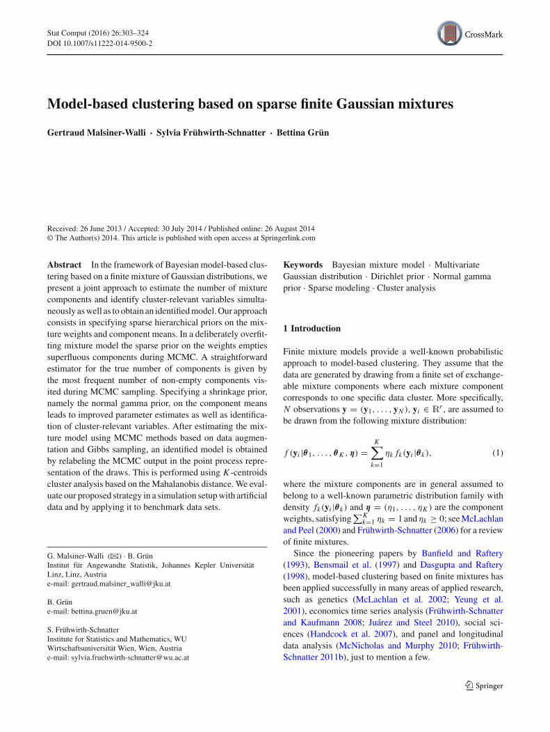
Stat Comput (2016) 26:303–324DOI 10.1007/s11222-014-9500-2

Model-based clustering based on sparse finite Gaussian mixtures

Gertraud Malsiner-Walli · Sylvia Frühwirth-Schnatter · Bettina Grün

Received: 26 June 2013 / Accepted: 30 July 2014 / Published online: 26 August 2014© The Author(s) 2014. This article is published with open access at Springerlink.com

Abstract In the framework of Bayesian model-based clus-tering based on a finite mixture of Gaussian distributions, wepresent a joint approach to estimate the number of mixturecomponents and identify cluster-relevant variables simulta-neously aswell as to obtain an identifiedmodel.Our approachconsists in specifying sparse hierarchical priors on the mix-ture weights and component means. In a deliberately overfit-ting mixture model the sparse prior on the weights emptiessuperfluous components during MCMC. A straightforwardestimator for the true number of components is given bythe most frequent number of non-empty components vis-ited during MCMC sampling. Specifying a shrinkage prior,namely the normal gamma prior, on the component meansleads to improved parameter estimates as well as identifica-tion of cluster-relevant variables. After estimating the mix-ture model using MCMC methods based on data augmen-tation and Gibbs sampling, an identified model is obtainedby relabeling the MCMC output in the point process repre-sentation of the draws. This is performed using K -centroidscluster analysis based on theMahalanobis distance. We eval-uate our proposed strategy in a simulation setupwith artificialdata and by applying it to benchmark data sets.

G. Malsiner-Walli (B) · B. GrünInstitut für Angewandte Statistik, Johannes Kepler UniversitätLinz, Linz, Austriae-mail: gertraud.malsiner_walli@jku.at

B. Grüne-mail: bettina.gruen@jku.at

S. Frühwirth-SchnatterInstitute for Statistics and Mathematics, WUWirtschaftsuniversität Wien, Wien, Austriae-mail: sylvia.fruehwirth-schnatter@wu.ac.at

Keywords Bayesian mixture model · MultivariateGaussian distribution · Dirichlet prior · Normal gammaprior · Sparse modeling · Cluster analysis

1 Introduction

Finite mixture models provide a well-known probabilisticapproach to model-based clustering. They assume that thedata are generated by drawing from a finite set of exchange-able mixture components where each mixture componentcorresponds to one specific data cluster. More specifically,N observations y = (y1, . . . , yN ), yi ∈ Rr , are assumed tobe drawn from the following mixture distribution:

f (yi |θ1, . . . , θK , η) =K∑

k=1

ηk fk(yi |θk), (1)

where the mixture components are in general assumed tobelong to a well-known parametric distribution family withdensity fk(yi |θk) and η = (η1, . . . , ηK ) are the componentweights, satisfying

∑Kk=1 ηk = 1 andηk ≥ 0; seeMcLachlan

and Peel (2000) and Frühwirth-Schnatter (2006) for a reviewof finite mixtures.

Since the pioneering papers by Banfield and Raftery(1993), Bensmail et al. (1997) and Dasgupta and Raftery(1998), model-based clustering based on finite mixtures hasbeen applied successfully in many areas of applied research,such as genetics (McLachlan et al. 2002; Yeung et al.2001), economics time series analysis (Frühwirth-Schnatterand Kaufmann 2008; Juárez and Steel 2010), social sci-ences (Handcock et al. 2007), and panel and longitudinaldata analysis (McNicholas and Murphy 2010; Frühwirth-Schnatter 2011b), just to mention a few.

123

304 Stat Comput (2016) 26:303–324

Despite this success and popularity of model-based clus-tering based on finite mixtures, several issues remain thatdeserve further investigation and are addressed in the presentpaper within a Bayesian framework. Above all, in applica-tions typically little knowledge is available on the specificnumber of data clusters we are looking for, and, as a conse-quence, the unknown number K of mixture components cor-responding to these data clusters needs to be estimated fromthe data. Tremendous research effort has been devoted to thisquestion, however, no uniquely best method has been iden-tified. Likelihood-based inference typically relies on modelchoice criteria such as BIC, approximate weight of evidence,or the integrated classification likelihood criterion to selectK , see e.g. Biernacki et al. (2000) for a comparison of differ-ent criteria. Bayesian approaches sometimes pursue a similarstrategy, often adding the DIC to the list of model choice cri-teria; see e.g. Celeux et al. (2006). However, methods thattreat K as an unknown parameter to be estimated jointlywith the component-specific parameters are preferable froma Bayesian viewpoint.

Within finite mixtures, a fully Bayesian approach towardselecting K is often based on reversible jump Markov chainMonte Carlo (RJMCMC), as introduced by Richardson andGreen (1997). RJMCMC creates a Markov chain that movesbetween finite mixtures with different number of compo-nents, based on carefully selected degenerate proposal den-sities which are difficult to design, in particular in higherdimensional mixtures, see e.g. Dellaportas and Papageor-giou (2006). Alternatively, the choice of K has been based onthe marginal likelihood p(y|K ), which has to be combinedwith a suitable prior p(K ) to obtain a valid posterior distri-bution p(K |y) over the number K of components (Nobile2004). However, also the computation of the marginal likeli-hood p(y|K ) turns out to be a challenging numerical problemin a finite mixture model even for moderate K (Frühwirth-Schnatter 2004).

A quite different approach of selecting the number K ofcomponents exists outside the framework of finite mixturemodels and relies on a nonparametric Bayesian approachbased on mixture models with countably infinite number ofcomponents. To derive a partition of the data, Molitor et al.(2010) and Liverani et al. (2013) define a Dirichlet processprior on the mixture weights and cluster the pairwise associ-ation matrix, which is obtained by aggregating over all parti-tions obtained during Markov chain Monte Carlo (MCMC)sampling, using partitioning around medoids (PAM; Kauf-man and Rousseeuw 1990). The optimal number of clustersis determined by maximizing an associated clustering score.

A second issue to be addressed concerns the selection ofcluster-relevant variables, as heterogeneity often is presentonly in a subset of the available variables. Since the inclusionof unnecessary variables might mask the cluster structure,statistical interest lies in identifying these cluster-relevant

variables. Several papers have suggested to solve the selec-tion of the number K of components and the identificationof cluster-relevant variables simultaneously. One way is torecast the choice both of K and the cluster-relevant variablesas a model selection problem. For instance, in the context ofmaximum likelihood estimation Raftery and Dean (2006),Maugis et al. (2009) and Dean and Raftery (2010) use agreedy search algorithm by comparing the various modelsthrough BIC. Penalized clustering approaches using the L1

norm to shrink cluster means together for variable selectionare considered in Pan and Shen (2007), with adaptations ofthe penalty term taking the group structure into account sug-gested in Wang and Zhu (2008) and Xie et al. (2008). Basedon a model using mode association Lee and Li (2012) pro-pose a variable selection algorithm using a forward searchfor maximizing an aggregated index of pairwise cluster sep-arability.

In the Bayesian framework, Tadesse et al. (2005) proposeRJMCMC techniques to move between mixture models withdifferent numbers of components while variable selection isaccomplished by stochastic search through the model space.Stingo et al. (2012) extend their approach in combinationwith Raftery and Dean (2006) to the discriminant analysisframework. Frühwirth-Schnatter (2011a) pursues a slightlydifferent approach by specifying a normal gamma prior onthe component means to shrink the cluster means for homo-geneous components, while model selection with respect toK is performed by calculating marginal likelihoods underthese shrinkage priors.

Variable selection in the context of infinite mixture mod-els has also been considered. Kim et al. (2006), for instance,combine stochastic search for cluster-relevant variables witha Dirichlet process prior on the mixture weights to estimatethe number of components. In a regression setting Chungand Dunson (2009) and Kundu and Dunson (2014) also usestochastic search variable selection methods in combinationwith nonparametric Bayesian estimation based on a probitstick-breaking process mixture or a Dirichlet process loca-tion mixture. Similarily, Yau and Holmes (2011) define aDirichlet process prior on the weights, however, they iden-tify cluster-relevant variables by using a double exponen-tial distribution as shrinkage prior on the component means.Lian (2010) uses Dirichlet process priors for simultaneousclustering and variable selection employing a base measureinducing shinkage on the cluster-specific covariate effects.

The main contribution of the present paper is to pro-pose the use of sparse finite mixture models as an alter-native to infinite mixtures in the context of model-basedclustering. While remaining within the framework of finitemixtures, sparse finite mixture models provide a semi-parametric Bayesian approach insofar as neither the num-ber of mixture components nor the cluster-relevant vari-ables are assumed to be known in advance. The basic

123

Stat Comput (2016) 26:303–324 305

idea of sparse finite mixture modeling is to deliberatelyspecify an overfitting finite mixture model with too manycomponents K and to assume heterogeneity for all avail-able variables apriori. Sparse solutions with regard to thenumber of mixture components and with regard to het-erogeneity of component locations are induced by speci-fying suitable shrinkage priors on, respectively, the mix-ture weights and the component means. This proposal leadsto a simple Bayesian framework where a straightforwardMCMC sampling procedure is applied to jointly estimatethe unknown number of mixture components, to deter-mine cluster-relevant variables, and to perform component-specific inference.

To obtain sparse solutions with regard to the number ofmixture components, an appropriate prior on the weight dis-tribution η = (η1, . . . , ηK ) has to be selected.We staywithinthe common framework by choosing a Dirichlet prior onη, however, the hyperparameters of this prior are selectedsuch that superfluous components are emptied automaticallyduring MCMC sampling. The choice of these hyperparame-ters is governed by the asymptotic results of Rousseau andMengersen (2011), who show that, asymptotically, an over-fitting mixture converges to the true mixture, if these hyper-parameters are smaller than d/2, where d is the dimensionof the component-specific parameter θk .

Sparse finitemixtures are related to infinitemixtures basedon a Dirichlet process prior, if a symmetric Dirichlet prior isemployed for η and the hyperparameter e0 is selected suchthat e0K converges to the concentration parameter of theDirichlet process as K goes to infinity. For finite K , sparsefinite mixtures provide a two-parameter alternative to theDirichlet process prior where, for instance, e0 can be heldfixed while K increases.

Following Ishwaran et al. (2001) and Nobile (2004), wederive the posterior distribution of the number of non-emptymixture components from the MCMC output. To estimatethe number of mixture components, we derive a point esti-mator from this distribution, typically, the posterior modewhich is equal to the most frequent number of non-emptycomponents visited during MCMC sampling. This approachconstitutes a simple and automatic strategy to estimate theunknown number of mixture components, without makinguse of model selection criteria, RJMCMC, or marginal like-lihoods.

Although sparse finite mixtures can be based on arbi-trary mixture components, investigation will be confined inthe present paper to sparse Gaussian mixtures where themixture components fk(yi |θk) in (1) arise from multivari-ate Gaussian densities with component-specific parametersθk = (μk,�k) consisting of the component meanμk and thevariance-covariance matrix �k , i.e.

fk(yi |θk) = fN (yi |μk,�k). (2)

To identify cluster-relevant variables within the frameworkof sparse Gaussian mixtures, we include all variables andassess their cluster-relevance by formulating a sparsity prioron the component means μk , rather than excluding vari-ables explicitly from the model as it is done by stochasticsearch. This strategy to identify cluster-relevant variableshas been applied previously by Yau and Holmes (2011) whodefine a Laplace prior as a shrinkage prior on the mixturecomponent means. To achieve more flexibility and to allowstronger shrinkage, we follow in the present paper Frühwirth-Schnatter (2011a) by using instead the normal gamma prioras a shrinkage prior on the mixture component means whichis a two-parameter generalization of the Laplace prior.

Specifying a sparse prior on the component means has inaddition the effect of allowing component means to be pulledtogether in dimensions where the data are homogeneous,yielding more precise estimates of the component means inevery dimension. Moreover, the dispersion of the estimatedcomponent means in different variables can be compared.In this way, a distinction between cluster-relevant variables,which are characterized by a high dispersion of the clusterlocations, and homogeneous variables, where cluster loca-tions are identical, is possible by visual inspection. For high-dimensional data, however, this approach might be cumber-some, as pointed out by a reviewer, and automatic tools foridentifying cluster-relevant variables using the posterior dis-tributions of the shrinkage parameters might need to be con-sidered.

Finally, in applied research it is often not only of interest toderive a partition of the data, but also to characterize the clus-ters by providing inferencewith respect to the cluster-specificparameters θk appearing in (1). The framework of finite mix-tures allows for identification of component-specific parame-ters, as soon as the label switching problem in an overfittingmixture model with empty components is solved. As sug-gested by Frühwirth-Schnatter (2001), we ensure balancedlabel switching during MCMC sampling by adding a ran-dom permutation step to the MCMC scheme. For relabelingthe draws in a post-processing procedure, a range of differentmethods has been proposed in the literature, see Sperrin etal. (2010) and Jasra et al. (2005) for an overview. However,most of these proposed relabeling methods become compu-tationally prohibitive for multivariate data with increasingdimensionality and a reasonable number of components.

Toobtain aunique labelingwe followFrühwirth-Schnatter(2011a), who suggests to cluster the draws in the pointprocess representation after having removed the drawswherethe number of non-empty components does not correspondto the estimated number of non-empty components and usingonly component-specific draws from non-empty compo-nents. Clustering the component-specific draws in the pointprocess representation reduces the dimensionality of the rela-beling problem, making this method feasible also for mul-

123

306 Stat Comput (2016) 26:303–324

tivariate data. For clustering the draws we use K -centroidscluster analysis (Leisch 2006) based on theMahalanobis dis-tance, which allows to fit also elliptical clusters and therebyconsiderably improves the clustering performance. The clus-ter assignments for the component-specific draws can be usedto obtain a unique labeling and an identified model, if in eachiteration each component-specific draw is assigned to a dif-ferent cluster.We suggest to use this proportion of drawswithunique assignment as a qualitative indicator of the suitabilityof the fitted mixture model for clustering.

The article is organized as follows. Section 2 describesthe proposed strategy for selecting the true number of mix-ture components and introduces the normal gamma prior onthe mixture component means. Section 3 provides detailson MCMC estimation and sheds more light on the rela-tion between shrinkage on the prior component means andweights. In Sect. 4 the strategy for solving the label switch-ing problem for an overfitting mixture model is presented.In Sect. 5 the performance of the proposed strategy is eval-uated in a simulation study and application of the proposedmethod is illustrated on two benchmark data sets. Section 6summarizes results and limitations of the proposed approachand discusses issues to be considered in future research.

2 Model specification

In a Bayesian approach, the model specification given inEqs. (1) and (2) is completed by specifying priors for allmodel parameters. As mentioned in the introduction, sparsefinite mixtures rely on specifying a prior on the mixtureweights η which helps in identifying the number of mix-ture components (see Sect. 2.1). To achieve identification ofcluster-relevant variables, a shrinkage prior on the compo-nent means μ1, . . . ,μK is chosen (see Sect. 2.2), while astandard hierarchical prior is chosen for the component vari-ances �1, . . . ,�K (see Sect. 2.3).

2.1 Identifying the number of mixture components

Following the usual approach,we assume that the prior on theweight distribution is a symmetric Dirichlet prior, i.e. η ∼Dir(e0, . . . , e0). However, since sparse finite mixtures arebased on choosing deliberately an overfitting mixture wherethe number of components K exceeds the true number K true,the hyperparameter e0 has to be selected carefully to enableshrinkage of the number of non-empty mixture componentstoward K true.

For an overfitting mixture model, it turns out that thehyperparameter e0 considerably influences the way the pos-terior distribution handles redundant mixture components.As observed by Frühwirth-Schnatter (2006, 2011a) in anexploratory manner, the posterior distribution of an overfit-

ting mixture model with K > K true might exhibit quitean irregular shape, since the likelihood mixes two possiblestrategies of handling superfluous components. For an over-fitting mixture model, high likelihood is assigned either tomixture components with weights close to 0 or to mixturecomponents with nearly identical component-specific para-meters. In both cases, several mixture model parameters arepoorly identified, such as the component-specific parametersof a nearly empty component in the first case, while only thesum of the weights of nearly identical mixture components,but not their individual values, is identified in the secondcase.

Rousseau and Mengersen (2011) investigate the asymp-totic behavior of the posterior distribution of an overfittingmixture model in a rigorous mathematical manner. Theyshow that the shape of the posterior distribution is largelydetermined by the size of the hyperparameter e0 of theDirich-let prior on the weights. In more detail, if the hyperparame-ter e0 < d/2, where d is the dimension of the component-specific parameter θk , then the posterior expectation of theweights asymptotically converges to zero for superfluouscomponents. On the other hand, if e0 > d/2, then the poste-rior density handles overfitting by defining at least two iden-tical components, each with non-negligible weight. In thesecond case, the posterior density is less stable than in thefirst case since the selection of the components that split mayvary. Therefore, Rousseau and Mengersen (2011) suggest toguide the posterior towards the first more stable case and to“compute the posterior distribution in a mixture model witha rather large number of components and a Dirichlet-typeprior on the weights with small parameters (...) and to checkfor small weights in the posterior distribution.” (p. 694). Fol-lowing these suggestions, our approach consists in purposelyspecifying an overfitting mixture model with K > K true

being a reasonable upper bound for the number of mixturecomponents. Simultaneously, we favor apriori values of e0small enough to allow emptying of superfluous components.

An important issue is how to select a specific value for e0 inan empirical application. The asymptotic results of Rousseauand Mengersen (2011) suggest that choosing e0 < d/2 hasthe effect of emptying all superfluous components, regard-less of the specific value, as the number of observations goesto infinity. However, in the case of a finite number of obser-vations, we found it necessary to select much smaller valuesfor e0.

We choose either a very small, but fixed Dirichlet para-meter e0, in particular in combination with the sparsity prioron the component means μk introduced in Sect. 2.2, as willbe discussed further in Sect. 3.2. Alternatively, to learn fromthe data how much sparsity is needed, we consider e0 to bean unknown parameter with a gamma hyperprior G(a, b).

To define the expectation of this prior, we follow Ishwaranet al. (2001) who recommend to choose e0 = α/K . In this

123

Stat Comput (2016) 26:303–324 307

case, the Dirichlet prior approximates a Dirichlet processprior with concentration parameter α as K becomes large,as already noted in the introduction. Since simulation stud-ies performed in Ishwaran et al. (2001) yield good approx-imations for α = 1 and K reasonable large, we match theexpectation E(e0) = 1/K obtained in this way:

e0 ∼ G(a, a · K ). (3)

The parameter a has to be selected carefully since it controlsthe variance 1/(aK 2) of e0. For our simulation studies andapplications,we set a = 10, aswe noted in simulation studies(not reported here) that values smaller than 10 allow largevalues for e0, and, as a consequence, superfluous componentswere not emptied during MCMC sampling.

For a sparse finite mixture, the posterior distribution willhandle redundant components by assigning to them vanish-ing weights and, as will be discussed in Sect. 3, superfluouscomponents are emptied during MCMC sampling. Regard-ing the selection of the number of components, we deviatefrom Rousseau and Mengersen (2011), because the strategyof separating between “true” and “superfluous” componentsbased on posterior size of the weights of the various com-ponents might fail in cases where a threshold for separatingbetween “large” or “small” weights is difficult to identify.

Following, instead, Nobile (2004) and Ishwaran et al.(2001) we derive the posterior distribution Pr(K0 =h|y), h = 1, . . . , K , of the number K0 of non-empty compo-nents from theMCMCoutput. I.e., for each iterationm of theMCMC sampling to be discussed in Sect. 3, we consider thenumber of non-empty components, i.e. components to whichobservations have been assigned for this particular sweep ofthe sampler,

K (m)0 = K −

K∑

k=1

I {N (m)k = 0}, (4)

where N (m)k is the number of observations allocated to com-

ponent k and I denotes the indicator function, and estimatethe posterior Pr(K0 = h|y) for each value h = 1, . . . , K ,by the corresponding relative frequency.

To estimate the number of mixture components, we derivea point estimator from this distribution. We typically usethe posterior mode estimator K0 which maximizes the (esti-mated) posterior distribution Pr(K0 = h|y) and is equal tothe most frequent number of non-empty components visitedduring MCMC sampling. The posterior mode estimator isoptimal under a 0/1 loss function which is indifferent to thedegree of overfitting K0. This appears particularly sensiblein the present context where adding very small, non-emptycomponents hardly changes the marginal likelihood. Thismakes the posterior distribution Pr(K0 = h|y) extremelyright-skewed and other point estimators such as the posteriormean extremely sensitive to prior choices, see Nobile (2004).

2.2 Identifying cluster-relevant variables

The usual prior on the mixture component means μk =(μk1, . . . , μkr )

′ is the independence prior,

μk ∼ N (b0,B0), k = 1, . . . , K , (5)

whereN (·) denotes themultivariate normal distribution. It iscommon to assume that all componentmeansμk are indepen-dent a priori, given data-dependent hyperparameters b0 andB0; see e.g. Richardson and Green (1997), Stephens (1997)and Frühwirth-Schnatter (2006). Subsequently, we call thisprior the standard prior and choose the median to defineb0 = median(y) and the range R j of the data in each dimen-sion j to define B0 = R0, where R0 = Diag(R2

1, . . . , R2r ).

Previous investigations in Yau and Holmes (2011) andFrühwirth-Schnatter (2011a) indicate that it is preferable toreplace the standard prior for the component means μk by ashrinkage prior, if it is expected that in some dimensions nocluster structure is present because all component means arehomogeneous. Shrinkage priors are well-known from vari-able selection in regression analysis where they are used toachieve sparse estimation of regression coefficients, see Pol-son and Scott (2010) and Armagan et al. (2011) for a recentreview.Shrinkagepriors are also very convenient fromacom-putational point of view, because they can be represented asa scale mixture of normals which makes it easy to implementMCMC sampling under these priors.

We apply in the following the normal gamma prior, forwhich the mixing distribution for the scale is specified by agammadistribution. The normal gammapriorwas introducedby Griffin and Brown (2010) for variable selection in regres-sion models and has been applied previously by Frühwirth-Schnatter (2011a) in the context of finite mixture distribu-tions. As opposed to the standard prior (5) which is basedon fixed hyperparameters b0 and B0, a hierarchical prior isintroduced, which places a normal prior on the prior meanb0 and a shrinkage prior on the prior variance matrix B0:

μk |�,b0 ∼ N (b0,B0), (6)

where

B0 = �R0�,

� = Diag(√

λ1, . . . ,√

λr ),

λ j ∼ G(ν1, ν2), j = 1, . . . , r,

b0 ∼ N (m0,M0).

In (6), a multivariate version of the normal gamma prior isemployed, where it is assumed that in each dimension j allcomponent means μ1 j , . . . , μK j follow a normal distribu-tion, where the variance depends on different scaling fac-tors λ j drawn from a gamma distribution with parameters ν1and ν2. The marginal prior for p(μ1 j , . . . , μK j |b0) can beexpressed in closed form as (see Frühwirth-Schnatter 2011a):

123

308 Stat Comput (2016) 26:303–324

Fig. 1 Normal gamma priorwith a variance of 1 for differentvalues of ν1, ν1 = 0.5 (blackdot-dashed line), ν1 = 1 (reddotted line), ν1 = 2 (bluelong-dashed line), and thestandard normal density (greensolid line), at zero (left-handside) and the tails (right-handside). (Color figure online)

−2 −1 0 1 2

0.0

0.2

0.4

0.6

0.8

1.0

μ

dens

ity

10 11 12 13 14 15

0e+

002e

−07

4e−

076e

−07

8e−

071e

−06

μ

dens

ity

π(μ1 j , · · · , μK j |b0)

= νν12

(2π)K/2�(ν1)2KpK (

√a jb j )

(b j

a j

)pK /2

, (7)

where

a j = 2ν2,

pK = ν1 − K/2,

b j =K∑

k=1

(μk j − b0 j )2/R2

j ,

and Kα(x) is themodifiedBessel function of the second kind.Furthermore, if the hyperparameters ν1 and ν2 are equal, thenin each dimension j the marginal variance of μk j is equal toR2j as for the standard prior.Yau and Holmes (2011) considered a closely related, spe-

cial case of prior (6) where ν1 = 1, which corresponds tothe double exponential or Laplace prior, also known as theBayesian Lasso (Park and Casella 2008). However, in thecontext of regression analysis, this specific prior has beenshown to be suboptimal in the sense that shrinkage to 0 istoo weak for insignificant coefficients, while a bias is intro-duced for large coefficients, see e.g. Polson and Scott (2010)and Armagan et al. (2011). The normal gamma prior intro-duced by Griffin and Brown (2010) is more flexible in thisrespect. Since the excess kurtosis is given by 3/ν1, the normalgamma prior has heavier tails than the Laplace distributionfor ν1 < 1, reducing the bias for large coefficients. At thesame time, it is more peaked than the Laplace distributionwhich leads to stronger shrinkage to 0 for insignificant coef-ficients. This can be seen in Fig. 1 where the normal gammaprior is plotted for ν1 = 0.5, 1, 2 and compared to the stan-dard normal distribution.

In the context of finite mixtures, the normal gamma priorintroduces exactly the flexibility we are seeking to identifycluster-relevant variables. To achieve this goal, the normalgamma prior is employed in (6) with value ν1 < 1. This

implies that λ j can assume values considerable smaller than1 in dimension j , which leads the prior distribution of μk j toconcentrate around the mean b0 j , pulling all the componentmeans μk j towards b0 j . This property becomes important indimensions where component densities are heavily overlap-ping or in the case of homogeneous variables, where actuallyno mixture structure is present and all observations are gen-erated by a single component only. In these cases, allowingthe prior variance to pull component means together yieldsmore precise estimates of the actually closely adjacent oreven identical component means.

In this way implicit variable selection is performed andvariableswhich are uninformative for the cluster structure areeffectively fit by a single component avoiding overfitting het-erogeneity and diminishing the masking effect of these vari-ables. Thus the same benefits regarding the fitted model areobtained as if the variables were excluded through a modelsearch procedure.

For cases where the variance of the prior for μk j , k =1, . . . , K , is shrunk to a small value, the mean b0 j of theprior becomes important. Thus, rather than assuming that b0is a fixed parameter as for the standard prior, we treat b0 asan unknown hyperparameter with its own prior distribution,see (6).

While variable selection is performed only implicitly withshrinkage priors in Bayesian estimation, explicit identifica-tion of the relevant clustering variables is possible a posteri-ori for the hierarchical shrinkage prior based on the normalgamma distribution. In the context of multivariate finite mix-tures, λ j can be interpreted as a local shrinkage factor indimension j which allows a priori that component means(μ1 j , . . . , μK j ) are pulled together and, at the same time, isflexible enough to be overruled by the data a posteriori, ifthe component means are actually different in dimension j .Hence, a visual inspection of theposterior distributions of thescaling factors λ j , j = 1, . . . , r , e.g. through box plots as inYau and Holmes (2011), reveals in which dimension j a high

123

Stat Comput (2016) 26:303–324 309

dispersion of the component means is present and where, onthe contrary, all component means are pulled together.

It remains to discuss the choice of the hyperparametersν1, ν2,m0 andM0 in (6). In the following simulation studiesand applications, the hyperparameters ν1 and ν2 are set to0.5 to allow considerable shrinkage of the prior variance ofthe component means. Furthermore, we specify an improperprior on b0, where m0 = median(y) and M−1

0 = 0.

2.3 Prior on the variance-covariance matrices

Finally, a prior on the variance-covariance matrices �k hasto be specified. Several papers, including Raftery and Dean(2006) and McNicholas and Murphy (2008), impose con-straints on the variance-covariance matrices to reduce thenumber of parameters which, however, implies that the cor-relation structure of the data needs to be modeled explicitly.

In contrast to these papers, we do not focus on model-ing sparse variance-covariance matrices, we rather modelthe matrices without constraints on their geometric shape.Following Stephens (1997) and Frühwirth-Schnatter (2006,p. 193), we assume the conjugate hierarchical prior �−1

k ∼W(c0,C0), C0 ∼ W(g0,G0), where W(·) denotes theWishart distribution. Regularization of variance-covariancematrices in order to avoid degenerate solutions is achievedthrough specification of the prior hyperparameter c0 bychoosing

c0 = 2.5 + r − 1

2,

g0 = 0.5 + r − 1

2,

G0 = 100g0c0

Diag(1/R21, . . . , 1/R

2r ),

see Frühwirth-Schnatter (2006, p. 192).

3 Bayesian estimation

To cluster N observations y = (y1, . . . , yN ), it is assumedthat the data are drawn from the mixture distribution definedin (1) and (2), and that each observation yi is generated byone specific component k.

The corresponding mixture likelihood derived from (1)and (2) is combined with the prior distributions introduced,respectively, for the weights η in Sect. 2.1, for the compo-nent meansμk in Sect. 2.2, and for�k in Sect. 2.3, assumingindependence between these components. The resulting pos-terior distribution does not have a closed form and MCMCsampling methods have to be employed, see Sect. 3.1.

The proposed strategy of estimating the number of compo-nents relies on the correct identification of non-empty com-ponents. In Sect. 3.2 we study inmore detail that prior depen-

dence between μk and η might be necessary to achieve thisgoal. In particular, we argue why stronger shrinkage of verysmall component weights ηk toward 0might be necessary forthe normal gamma prior (6) than for the standard prior (5),by choosing a very small value of e0.

3.1 MCMC sampling

Estimation of the sparse finite mixture model is performedthrough MCMC sampling based on data augmentationand Gibbs sampling (Diebolt and Robert 1994; Frühwirth-Schnatter 2006, chap. 3). To indicate the component fromwhich each observation stems, latent allocation variablesS = (S1, . . . , SN ) taking values in {1, . . . , K }N are intro-duced such that

f (yi |θ1, . . . , θK , Si = k) = fN (yi |μk,�k), (8)

and

Pr(Si = k|η) = ηk . (9)

As suggested by Frühwirth-Schnatter (2001), after eachiteration an additional random permutation step is added tothe MCMC scheme which randomly permutes the currentlabeling of the components. Random permutation ensuresthat the sampler explores all K ! modes of the full posteriordistribution and avoids that the sampler is trapped arounda single posterior mode, see also Geweke (2007). Withoutthe random permutation step, it has to be verified for eachfunctional of the parameters of interest, whether it is invariantto relabeling of the components. Only in this case, it does notmatter whether the random permutation step is performed.The detailed sampling scheme is provided in Appendix 1and most of the sampling steps are standard in finite mixturemodeling, with two exceptions.

The first non-standard step is the full conditional distri-bution p(λ j |μ1 j , . . . , μK j ,b0) of the shrinkage factor λ j .The combination of a gamma prior for λ j with the prod-uct of K normal likelihoods p(μk j |λ j , b0 j ), where the vari-ance depends on λ j , yields a generalized inverted Gaussiandistribution (GIG) as posterior distribution, see Frühwirth-Schnatter (2011a). Hence,

p(λ j |μ1 j , . . . , μK j ,b0) ∼ GIG(a j , b j , pK ),

where the parameters a j , b j , and pK are defined in (7).Furthermore, if the hyperparameter e0 of the Dirichlet

prior is random, a random walk Metropolis-Hastings stepis implemented to sample e0 from p(e0|η), where

p(e0|η) ∝ p(e0)�(Ke0)

�(e0)K

(K∏

k=1

ηk

)e0−1

, (10)

and p(e0) is equal to the hyperprior introduced in (3).

123

310 Stat Comput (2016) 26:303–324

3.2 On the relation between shrinkage in the weights and inthe component means

As common for finite mixtures, MCMC sampling alter-nates between a classification and a parameter simula-tion step, see Appendix 1. During classification, obser-vations are allocated to component k according to the(non-normalized) conditional probability ηk fN (yi |μk,�k),whereas the component-specific parameters μk,�k and theweight ηk are simulated conditional on the current classifi-cation S during parameter simulation. If no observation isallocated to component k during classification, then, sub-sequently, all component-specific parameters of this emptycomponent are sampled from the prior. In particular, the loca-tion μk of an empty component heavily depends on the priorlocation b0 and prior covariance matrix B0.

Under the standard prior (5), where

B0 = Diag(R21, . . . , R

2r ),

the location μk of an empty component is likely to be faraway from the data center b0, since in each dimension j with5 % probability the μk j will be further away from b0 j than2 · R j . As a consequence, fN (yi |μk,�k) is very small forany observation yi in the subsequent classification step andan empty component is likely to remain empty under thestandard prior.

In contrast, under the normal gamma prior (6), whereB0 = Diag(R2

1 ·λ1, . . . , R2r ·λr ), the scaling factor λ j shrinks

the prior variance ofμk j considerably, in particular in dimen-sions, where the component means are homogeneous. How-ever, the scaling factor λ j adjusts the prior variance alsoin cluster-relevant dimensions, since R2

j is generally muchlarger than the spread of the non-empty component meanswhich are typically allocated within the data range R j . Asa consequence, the location μk j of an empty component iseither close to the data center b0 j (in the case of homogeneousvariables) or close to the range spanned by the locations ofthe non-empty components (in the case of cluster-relevantvariables). In both cases, evaluating fN (yi |μk,�k) in thesubsequent classification step yields a non-negligible prob-ability and, as a consequence, observations are more likelyto be allocated to an empty component than in the standardprior case.

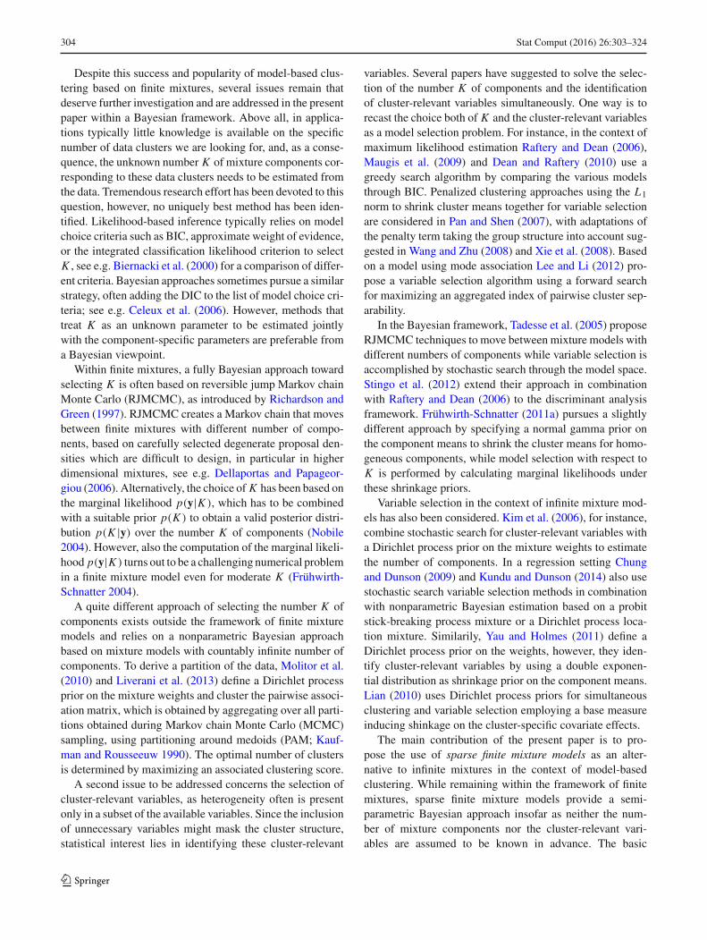
To illustrate the different allocation behavior of the stan-dard and the normal gamma prior in the presence of a super-fluous component more explicitly, we simulate N = 1,000observations from a bivariate two-component mixture modelwhere μ1 = (−2, 0)′, μ2 = (2, 0)′, �1 = �2 = I2, andη = (0.5, 0.5). We fit an overfitting mixture distributionwith K = 3 components, assuming that e0 ∼ G(10, 30).We skip the random permutation step, since the modes ofthe posterior distribution are well separated and the sampler

is trapped in the neighborhood of a single mode, yieldingimplicit identification.

In the top row of Fig. 2, posterior draws of all threecomponent means are displayed in a scatter plot both forthe standard (left-hand side) and the normal gamma prior(right-hand side). Under both priors, the posterior draws ofthe first two component means, displayed by triangle andcross points respectively, are concentrated around the truemeans μ1 = (−2, 0)′ and μ2 = (2, 0)′. However, the poste-rior draws of the mean of the third (superfluous) component,shown as circle points, are quite different, displaying a largedispersion over the plane under the standard prior and beinglocated either close to the two true component means or thedata center under the normal gamma prior. To illustrate theensuing effect on classification, we select a specific observa-tion yi , which location ismarked by a (blue) star in the scatterplots of the top, and determine for each MCMC sweep theprobability for yi to be allocated, respectively, to component1, 2 or 3. The corresponding box plots in the bottom row ofFig. 2 clearly indicate that the allocation probability for thethird (superfluous) component is considerably higher underthe normal gamma prior (plot on the right-hand side) thanunder the standard prior (plot on the left-hand side).

Since our strategy to estimate the number of mixture com-ponents relies on the number of non-empty components dur-ing MCMC sampling, we conclude from this investigationthat stronger shrinkage inηmight be necessary for the normalgamma prior (6) than for the standard prior (5). We compen-sate the tendency of the normal gamma prior to overestimatethe number of non-empty components, by encouraging verysmall prior weights ηk for empty components in order to keepthe conditional probability of an observation to be allocatedto an empty component during classification small. This isachieved by specifying a very small fixed hyperparameter e0in the Dirichlet prior, which is proportional to η

e0−1k . Thus,

the smaller e0, the smaller the weight of an empty componentk will be.

4 Identifying sparse finite mixtures

Identification of the finite mixture model requires handlingthe label switching problem caused by invariance of the rep-resentation (1) with respect to reordering the components:

f (yi |θ1, . . . , θK , η) =K∑

k=1

ηk fk(yi |θk)

=K∑

k=1

ηρ(k) fρ(k)(yi |θρ(k)),

where ρ is an arbitrary permutation of {1, . . . , K }. Theresulting multimodality and perfect symmetry of the pos-

123

Stat Comput (2016) 26:303–324 311

Fig. 2 Fitting a 3-componentnormal mixture to datagenerated by a 2-componentnormal mixture. Top row Scatterplots of the draws of theposterior component means μkunder the standard prior(left-hand side) and the normalgamma prior (right-hand side).Draws from component 1, 2,and 3 are displayed as greentriangles, red crosses, and greycircles, respectively. Bottom rowFor a single observation whichlocation is marked with a (blue)star in the scatter plots in thetop row, box plots of theconditional probabilities duringMCMC sampling to be assignedto component 1, 2 or 3 aredisplayed, under the standardprior (left-hand side) and normalgamma prior (right-hand side).MCMC is run for 1,000iterations, after discarding thefirst 1,000 draws. (Color figureonline)

−4 −2 0 2 4−

4−

20

24

μ1

μ 2

−4 −2 0 2 4

−4

−2

02

4

μ1

μ 2

1 2 3

0.0

0.2

0.4

0.6

0.8

1.0

components

cond

. pro

babi

lity

1 2 30.

00.

20.

40.

60.

81.

0

components

cond

. pro

babi

lity

terior distribution p(θ1, . . . , θK , η|y) for symmetric priorsmakes it difficult to perform component-specific inference.To solve the label switching problem arising in Bayesianmixture model estimation, it is necessary to post-processthe MCMC output to obtain a unique labeling. Many use-ful methods have been developed to force a unique labelingon draws from this posterior distribution when the numberof components is known (Celeux 1998; Celeux et al. 2000;Frühwirth-Schnatter 2001; Stephens 2000; Jasra et al. 2005;Yao and Lindsay 2009; Grün and Leisch 2009; Sperrin etal. 2010). However, most of these proposed relabeling meth-ods become computationally prohibitive formultivariate datawith increasing dimensionality. For instance, as explained in(Frühwirth-Schnatter, 2006, p. 96), Celeux (1998) proposesto use a K -means cluster algorithm to allocate the draws ofone iteration to one of K ! clusters, which initial centers aredetermined by the first 100 draws. The distance of the drawsto each of the K ! reference centers is used to determine thelabeling of the draws for this iteration. In general, most ofthe relabelingmethods use the complete vector of parameterswhich grows as a multiple of K even if they do not requireall K ! modes to be considered (see, for example Yao andLindsay 2009).

Following Frühwirth-Schnatter (2011a), we applyK -means clustering to the point process representation ofthe MCMC draws to identify a sparse finite mixture model,see Sect. 4.1. This allows to reduce the dimension of the prob-lem to the dimension of the component-specific parameters.As described in Sect. 4.2, we generalize this approach byreplacing K -means clustering based on the squared Euclid-ean distance by K -centroids cluster analysis based on theMahalanobis distance (Leisch 2006).

4.1 Clustering the MCMC output in the point processrepresentation

The point process representation of the MCMC draws intro-duced in Frühwirth-Schnatter (2006, Sect. 3.7.1) allows tostudy the posterior distribution of the component-specificparameters regardless of potential label switching, whichmakes it very useful for model identification. If the numberof mixture components matches the true number of com-ponents, then the posterior draws of the component-specificparameters θ

(m)1 , . . . , θ

(m)K cluster around the “true” points

θ true1 , . . . , θ trueK . To visualize the point process representa-tion of the posterior mixture distribution, projections of the

123

312 Stat Comput (2016) 26:303–324

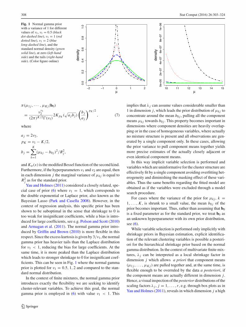
Fig. 3 Crabs data, K true = 4,K = 15, standard prior. Pointprocess representation ofposterior mean draws, μ(m)

k1

plotted against μ(m)k2 , across

k = 1, . . . , K . Left-hand sidedraws of all K = 15components. Right-hand sideonly draws from those M0

iterations where K (m)0 = 4 and

the components which werenon-empty

point process representation onto two-dimensional planescan be considered. These correspond to scatter plots of theMCMC draws (θ

(m)k j , θ

(m)

k j ′ ), for two dimensions j and j ′ andacross k = 1, . . . , K .

After clustering the draws in the point process representa-tion, a unique labeling is achieved for all those draws wherethe resulting classification is a permutation. By reorderingeach of these draws according to its classification, a (sub-set) of identified draws is obtained which can be used forcomponent-specific parameter inference.

Note that to reduce dimensionality, it is possible to clus-ter only a subset of parameters of the component-specificparameter vector and to apply the obtained classificationsequences to the entire parameter vector. In the present con-text of multivariate Gaussian mixtures, we only clustered theposterior component means and the obtained classificationsequence was then used to reorder and identify the othercomponent-specific parameters, namely covariance matricesand weights. This is also based on the assumption that theobtained clusters differ in the component means allowingclusters to be characterized by their means.

In the case of a sparse finite mixture model, where theprior on the weights favors small weights, many of the com-ponents will have small weights and no observation willbe assigned to these components in the classification step.Component means of all empty components are sampledfrom the prior and tend to confuse the cluster fit. There-fore, Frühwirth-Schnatter (2011a) suggests to remove alldraws from empty components before clustering. Addition-ally, after having estimated the number of non-empty com-ponents K0, all draws where the number of non-empty com-ponents is different from K0 are sampled conditional on a“wrong” model and are removed as well. The remainingdraws can be seen as samples from a mixture model withexactly K0 components. In Fig. 3 an example of the pointprocess representation of the MCMC draws is given. Afterhavingfitted a sparse finitemixturewith K = 15 components

to the Crabs data set described in Sect. 5.2, the left-hand sideshows the scatter plot of the MCMC draws (μ

(m)k1 , μ

(m)k2 ),

k = 1, . . . , K , from all components (including draws fromempty components). On the right-hand side, only draws fromthose M0 iterations are plotted where K0 = 4 and whichwere non-empty. In this case, the posterior distributions ofthe means of the four non-empty components can be clearlydistinguished. These draws are now clustered into K0 groups.The clusters naturally can be assumed to be of equal sizeand to have an approximate Gaussian distribution, thus sug-gesting the choice of K -means for clustering or, in orderto capture also non-spherical shapes or different volumes ofthe posterior distributions, the choice of K -centroids clusteranalysis where the distance is defined by a cluster-specificMahalanobis distance. The algorithm is explained in the fol-lowing subsection. The detailed scheme to identify a sparsefinite mixture model can be found in Appendix 2.

4.2 K -centroids clustering based on the Mahalanobisdistance

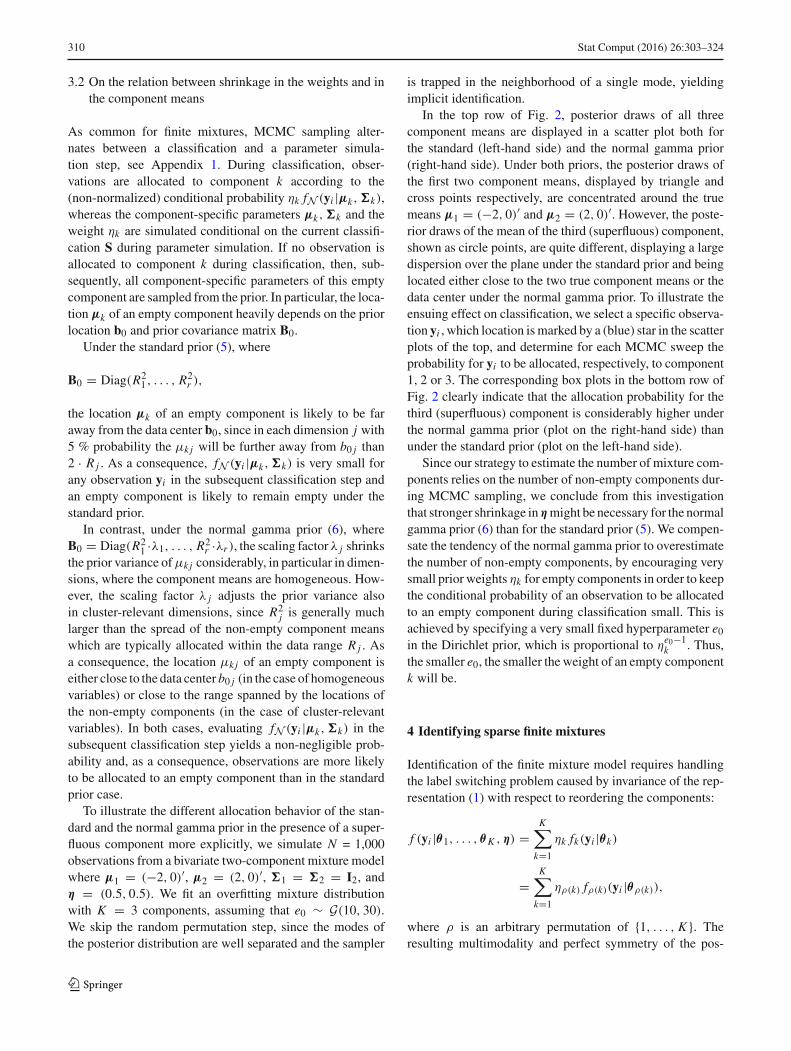
Defining the distance between a point and a centroid using theMahalanobis distance may considerably improve the clusterfit in the point process representation. As can be seen inFig. 4, where the clustering results for the Crabs data aredisplayed, if the posterior distributions have elliptical shape,clustering based on theMahalanobis distance is able to catchthe elongated, elliptical clusters whereas K -means based onthe squared Euclidean distance splits a single cluster intoseveral parts and at the same time combines these parts toone new artificial cluster.

For posterior draws of the component-specific parametervector x1, . . . , xN ∈ Rn and a fixed number of clusters K ,the K -centroids cluster problem based on the Mahalanobisdistance consists of finding a “good” set of centroids anddispersion matrices

CSK = {c1, . . . , cK ,S1, . . . ,SK }, (11)

123

Stat Comput (2016) 26:303–324 313

Fig. 4 Crabs data: Clusteringof the posterior mean draws ofthe plot on the right-hand side inFig. 3, through K -means(left-hand side) and K -centroidscluster analysis based on theMahalanobis distance(right-hand side)

where c1, . . . , cK are points in Rn and S1, . . . ,SK areinstances of the set of all positive definite matrices. “Good”means that using the assigned dispersion matrices S(xi ), thesum of all distances between objects xi and their assignedcentroids c(xi ) is minimized:

N∑

i=1

dS(xi )(xi , c(xi )) → minc1,...,cK ,S1,...,SK

, (12)

where {c(xi ),S(xi )} = argmin{ck ,Sk }∈CSK

dSk (xi , ck),

and the distance between an object xi and a centroid anda dispersion matrix (ck,Sk) is defined by the Mahalanobisdistance:

dSk (xi , ck) =√

(xi − ck)′S−1k (xi − ck). (13)

Since no closed form solution exists for the K -centroids clus-ter problem, an iterative estimation procedure is used. A pop-ular choice is thewell-known K -means algorithm, its generalform can be found in Leisch (2006). For theMahalanobis dis-tance (13), the K -centroids cluster algorithm is given by:

1. Start with a random set of initial centroids and variance-covariance matrices {ck,Sk}k=1,...,K .

2. Assign to each xi the nearest centroid ck where the dis-tance dSk (xi , ck) is defined by the Mahalanobis distance(13):

{c(xi ),S(xi )} = argmin{ck ,Sk }∈CSK

dSk (xi , ck)

3. Update the set of centroids and dispersion matrices{ck,Sk}k=1,...,K holding the cluster membership fixed:

c(new)k = mean

i :c(xi )=ck ,S(xi )=Sk({xi }),

S(new)k = var

i :c(xi )=ck ,S(xi )=Sk({xi })

4. Repeat steps 2 and 3 until convergence.

The algorithm is guaranteed to converge in a finite num-ber of iterations to a local optimum of the objective func-tion (12) (Leisch 2006). As starting values of the algo-rithm in step 1, the MAP estimates of the hyperparame-ters b1, . . . ,bK ,B1, . . . ,BK of the prior of the component-specific means are used.

5 Simulations and applications

5.1 Simulation study

In the following simulation study, the performance of theproposed strategy for selecting the unknown number of mix-ture components and identifying cluster-relevant variablesis illustrated for the case where the component densitiesare truly multivariate Gaussian. We use a mixture of fourmultivariate Gaussian distributions with component meansμ1 = (2,−2, 0, 0)′, μ2 = −μ1, μ3 = (2, 2, 0, 0)′, andμ4 = −μ3 and isotropic covariance matrices �k = I4,k = 1, . . . , 4, as data generating mechanism. Hence, thissimulation setup consists of two cluster-generating variablesin dimension 1 and 2 and two homogeneous variables indimension 3 and 4 and is chosen in order to study, whethercluster-relevant variables and homogeneous variables canbe distinguished. In Fig. 5, a randomly selected data set isshown, which was samples with equal weights. This figureindicates that, while in the scatter plot of the first two vari-ables four clusters are still visually discernible, the clustersare slightly overlapping in these dimensions indicating thatthe cluster membership of some observations is difficult toestimate. The other two variables are homogenous variablesand do not contain any cluster information, but render theclustering task more difficult.

As described in Sect. 2.1, we deliberately choose an over-fitting mixture with K components and base our estimate ofthe true number of mixture components on the frequency ofnon-empty components during MCMC sampling. We selectstrongly overfitting mixtures with K = 15 and K = 30,

123

314 Stat Comput (2016) 26:303–324

Fig. 5 Simulation setup withequal weights. Scatter plots ofdifferent variables for onerandomly selected data set

to assess robustness of the proposed strategy to choosingK , and investigate, if the number of non-empty componentsincreases as K increases. We simulate relatively large sam-ples of 1,000 observations to make it more difficult to reallyempty all superfluous components.

In addition, we consider two different weight distrib-utions, namely a mixture with equal weights, i.e. η =(0.25, 0.25, 0.25, 0.25), and a mixture with a very smallcomponent, where η = (0.02, 0.33, 0.33, 0.32), in order tostudy how sensitive our method is to different cluster sizes.For the second mixture, we investigate whether the smallcomponent survives or is emptied during MCMC samplingtogether with all superfluous components.

Prior distributions and the corresponding hyperparame-ters are specified as described in Sect. 2. The prior on theweight distribution defines a sparse finite mixture distribu-tion. We either use the gamma prior on e0 defined in (3) orchoose a very small, but fixed value for e0 as motivated bySect. 3.2. In addition, we compare the standard prior (5) forthe component means with the hierarchical shrinkage prior(6) based on the normal gamma distribution.

For each setting, ten data sets are generated, each con-sisting of 1,000 data points yi , and MCMC sampling is runfor each data set for M = 10,000 iterations after a burn-in of

2,000 draws. The starting classification of the observations isobtained by K -means. Estimation results are averaged overthe ten data sets and are reported in Tables 1 and 2 wheree0 provides the posterior median of e0 under the prior (3),whereas “e0 fixed” indicates that e0 was fixed at the reportedvalue. K0 is the posterior mode estimator of the true numberof non-empty components which is equal to 4. If the esti-mator K0 did not yield the same value for all data sets, thenthe number of data sets where K0 was the estimated numberof non-empty components is given in parentheses. M0 is theaverage number of iterations where exactly K0 componentswere non-empty.

For each data set, these draws are identified as describedin Sect. 4 using clustering in the point process representation.M0,ρ is the (average) rate among the M0 iterations where thecorresponding classifications assigned to the draws by theclustering procedure fail to be a permutation. Since in thesecases the labels 1, . . . , K0 cannot be assigned uniquely to theK0 components, these draws are discarded. For illustration,see the example in the Appendix 2. The non-permutation rateM0,ρ is ameasure for howwell-separated the posterior distri-butions of the component-specific parameters are in the pointprocess representation, with a value of 0 indicating perfectseparation, see Appendix 2 and Frühwirth-Schnatter (2011a)

123

Stat Comput (2016) 26:303–324 315

Table 1 Simulation setup with equal weights: results for different K under the standard prior (Sta), the normal gamma Prior (Ng), and when fittingan infinite mixture using the R package PReMiuM. Results are averaged over ten data sets

Prior K e0 e0 fixed K0 M0 M0,ρ MCR MSEμ

Sta 4 0.28 4 10000 0 0.049 0.167

15 0.05 4 9802 0 0.049 0.167

30 0.03 4 9742 0 0.048 0.168

Ng 4 0.28 4 10000 0 0.049 0.137

15 0.06 5(6) 2845 0.85 0.050 −30 0.03 5(5) 2541 0.93 0.050 −

Ng 4 0.01 4 10000 0 0.047 0.136

15 0.01 4 7465 0 0.048 0.137

30 0.01 4(8) 4971 0 0.048 0.136

30 0.001 4 9368 0 0.048 0.136

30 0.00001 4 9998 0 0.047 0.136

PReMiuM α Kest MCR MSEμ

0.66 4 0.047 0.231

Table 2 Simulation setup with unequal weights: results for different K under the standard prior (Sta), the normal gamma prior (Ng), and whenfitting an infinite mixture using the R package PReMiuM. Results are averaged over ten data sets

Prior K e0 e0 fixed K0 M0 M0,ρ MCR MSEμ

Sta 4 0.27 4 10000 0.00 0.038 1.670

15 0.05 4 9780 0.00 0.037 1.668

30 0.03 4 9728 0.00 0.038 1.663

Ng 4 0.01 4 10000 0.02 0.037 1.385

15 0.01 4 7517 0.02 0.038 1.314

30 0.01 4(9) 5221 0.00 0.037 1.279

30 0.001 4 9297 0.01 0.037 1.325

30 0.00001 4 9997 0.02 0.038 1.336

PReMiuM α Kest MCR MSEμ

0.65 4(9) 0.038 2.841

for more details. In the following component-specific infer-ence is based on the remaining drawswhere a unique labelingwas achieved.

Accuracy of the estimated mixture model is measuredby two additional criteria. Firstly, we consider the mis-classification rate (MCR) of the estimated classification.The estimated classification of the observations is obtainedby assigning each observation to the component where ithas been assigned to most often during MCMC samplingamong the draws where K0 components were non-emptyand which could be uniquely relabeled. The misclassifi-cation rate is measured by the number of misclassifiedobservations divided by all observations and should be assmall as possible. The labeling of the estimated classifi-cation is calculated by “optimally” matching true compo-

nents to the estimated mixture components obtaining in thisway the minimum misclassification rate over all possiblematches.

Secondly, whenever the true number of mixture compo-nents is selected for a data set, the mean squared error of theestimated mixture component means (MSEμ) based on theMahalanobis distance is determined as

MSEμ =K0∑

k=1

1

M0

M0∑

m=1

(μ(m)k −μtrue

k )′(�truek )−1(μ

(m)k −μtrue

k ),

(14)

where M0 = M0(1−M0,ρ) is the number of identified drawswith exactly K0 non-empty components. In Sects. 5.2 and5.3, where the true parameters μk and �k are unknown, the

123

316 Stat Comput (2016) 26:303–324

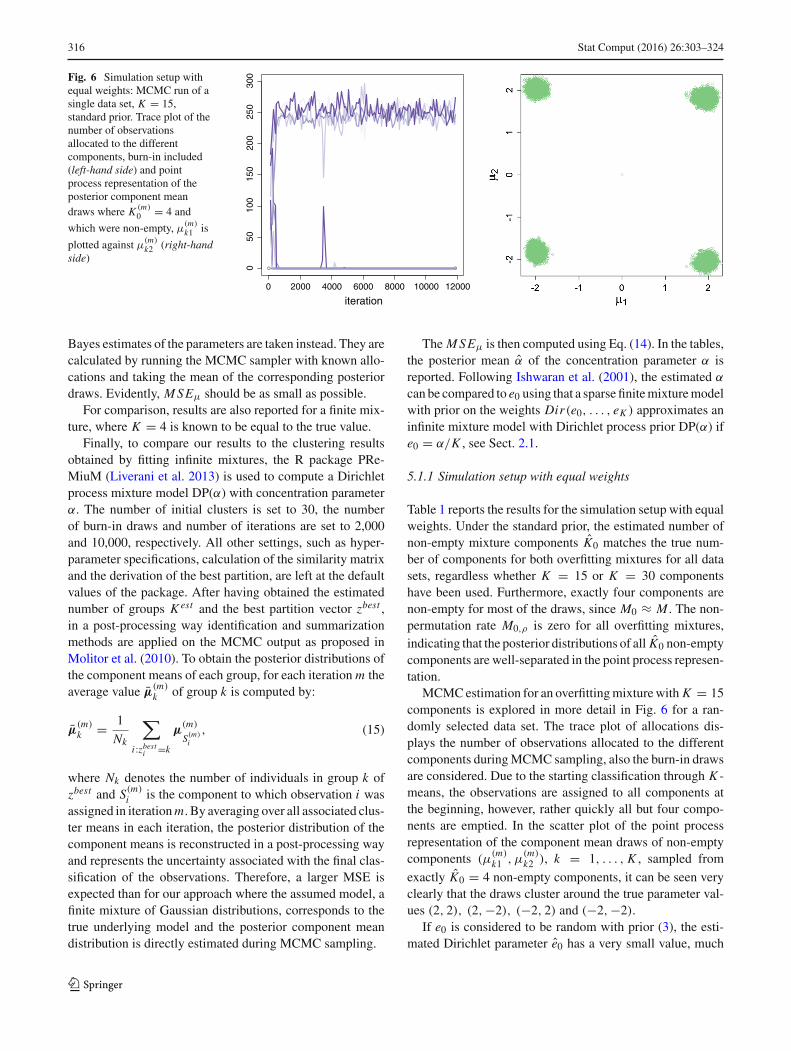
Fig. 6 Simulation setup withequal weights: MCMC run of asingle data set, K = 15,standard prior. Trace plot of thenumber of observationsallocated to the differentcomponents, burn-in included(left-hand side) and pointprocess representation of theposterior component meandraws where K (m)

0 = 4 and

which were non-empty, μ(m)k1 is

plotted against μ(m)k2 (right-hand

side)

0 2000 4000 6000 8000 10000 12000

050

100

150

200

250

300

iteration

Bayes estimates of the parameters are taken instead. They arecalculated by running the MCMC sampler with known allo-cations and taking the mean of the corresponding posteriordraws. Evidently, MSEμ should be as small as possible.

For comparison, results are also reported for a finite mix-ture, where K = 4 is known to be equal to the true value.

Finally, to compare our results to the clustering resultsobtained by fitting infinite mixtures, the R package PRe-MiuM (Liverani et al. 2013) is used to compute a Dirichletprocess mixture model DP(α) with concentration parameterα. The number of initial clusters is set to 30, the numberof burn-in draws and number of iterations are set to 2,000and 10,000, respectively. All other settings, such as hyper-parameter specifications, calculation of the similarity matrixand the derivation of the best partition, are left at the defaultvalues of the package. After having obtained the estimatednumber of groups Kest and the best partition vector zbest ,in a post-processing way identification and summarizationmethods are applied on the MCMC output as proposed inMolitor et al. (2010). To obtain the posterior distributions ofthe component means of each group, for each iterationm theaverage value μ

(m)k of group k is computed by:

μ(m)k = 1

Nk

∑

i :zbesti =k

μ(m)

S(m)i

, (15)

where Nk denotes the number of individuals in group k ofzbest and S(m)

i is the component to which observation i wasassigned in iterationm. By averaging over all associated clus-ter means in each iteration, the posterior distribution of thecomponent means is reconstructed in a post-processing wayand represents the uncertainty associated with the final clas-sification of the observations. Therefore, a larger MSE isexpected than for our approach where the assumed model, afinite mixture of Gaussian distributions, corresponds to thetrue underlying model and the posterior component meandistribution is directly estimated during MCMC sampling.

The MSEμ is then computed using Eq. (14). In the tables,the posterior mean α of the concentration parameter α isreported. Following Ishwaran et al. (2001), the estimated α

can be compared to e0 using that a sparse finitemixturemodelwith prior on the weights Dir(e0, . . . , eK ) approximates aninfinite mixture model with Dirichlet process prior DP(α) ife0 = α/K , see Sect. 2.1.

5.1.1 Simulation setup with equal weights

Table 1 reports the results for the simulation setup with equalweights. Under the standard prior, the estimated number ofnon-empty mixture components K0 matches the true num-ber of components for both overfitting mixtures for all datasets, regardless whether K = 15 or K = 30 componentshave been used. Furthermore, exactly four components arenon-empty for most of the draws, since M0 ≈ M . The non-permutation rate M0,ρ is zero for all overfitting mixtures,indicating that the posterior distributions of all K0 non-emptycomponents are well-separated in the point process represen-tation.

MCMCestimation for an overfittingmixturewith K = 15components is explored in more detail in Fig. 6 for a ran-domly selected data set. The trace plot of allocations dis-plays the number of observations allocated to the differentcomponents duringMCMC sampling, also the burn-in drawsare considered. Due to the starting classification through K -means, the observations are assigned to all components atthe beginning, however, rather quickly all but four compo-nents are emptied. In the scatter plot of the point processrepresentation of the component mean draws of non-emptycomponents (μ

(m)k1 , μ

(m)k2 ), k = 1, . . . , K , sampled from

exactly K0 = 4 non-empty components, it can be seen veryclearly that the draws cluster around the true parameter val-ues (2, 2), (2,−2), (−2, 2) and (−2,−2).

If e0 is considered to be random with prior (3), the esti-mated Dirichlet parameter e0 has a very small value, much

123

Stat Comput (2016) 26:303–324 317

smaller than the (asymptotic) upper boundgivenbyRousseauand Mengersen (2011), and decreases, as the number ofredundant components increases. This is true both for thestandard prior and the normal gamma prior. However, underthe normal gamma prior, the estimated number of non-emptycomponents K0 overfits the true number of mixture compo-nents for most of the data sets and increases with K . Forexample, if K = 15, the number of non-empty componentsis overestimated with K0 = 5 for 6 data sets. Also the highaverage non-permutation rate M0,ρ = 0.85 indicates thatthe selected model is overfitting. However, the MCR is nothigher than for K = 4, indicating that the fifth non-emptycomponent is a very small one.

Given the considerations in Sect. 3.2, we combine thenormal gamma prior with a sparse prior on the weight dis-tribution where e0 is set to a fixed very small value, e.g. to0.01 which is smaller than the 1% quantile of the posterior ofe0. For this combination of priors, superfluous componentsare emptied also under the normal gamma prior and the esti-mated number of non-empty components matches the truenumber of mixture components in most cases. For K = 30,e0 has to be chosen even smaller, namely equal to 0.001, toempty all superfluous components for all data sets. To inves-tigate the effect of an even smaller value of e0, we also sete0 = 10−5. Again, four groups are estimated. Thus evidentlyas long as the cluster information is strong small values ofe0 do not lead to underestimating the number of clusters ina data set. As a consequence, for the following simulations,we generally combine the normal gamma distribution witha sparse prior on the weight distribution where e0 is alwaysset to fixed, very small values.

Both for the standard prior (with e0 random) and the nor-mal gamma prior (with e0 fixed), the misclassification rateMCR and the mean-squared error MSEμ of the estimatedmodels have the same size, as if we had known the number ofmixture components in advance to be equal to K = 4. Thisoracle property of the sparse finite mixture approach is veryencouraging.

While the misclassification rate MCR is about the samefor both priors, interestingly, the MSEμ is considerablysmaller under the normal gamma prior (≈0.136) than underthe standard prior (≈0.167) for all K . This gain in efficiencyillustrates the merit of choosing a shrinkage prior on thecomponent-specific means.

As noted in Sect. 2.2, a further advantage of specifying anormal gamma prior for the component means, is the pos-sibility to explore the posterior distribution of the scalingfactor λ j . Therefore, visual inspection of the box plots of theposterior draws of λ j helps to distinguish between variables,where component distributions are well separated, and vari-ables, where component densities are strongly overlappingor even identical. The box plots of the posterior draws ofλ j displayed in Fig. 8 clearly indicate that only the first two

variables show a high dispersion of the component means,whereas for the two other dimensions the posterior distri-bution of λ j is strongly pulled toward zero indicating thatcomponent means are located close to each other and con-centrate at the same point.

If the data sets are clustered by fitting an infinite mix-ture model with the R package PReMiuM, similar clusteringresults are obtained. For all ten data sets four groups are esti-mated. The averaged estimated concentration parameter α is0.66. This indicates, that a sparse finite mixture model withK = 30 components and e0 ≈ 0.02 is a good approximationto a Dirichlet process DP(α) as α/K = 0.66/30 = 0.022.As expected, the MSEμ of the cluster means is considerablelarger (0.231) than for sparse finite mixtures, whereas themisclassification rate (0.047) is as for finite mixtures.

5.1.2 Simulation setup with unequal weights

To study if small non-empty components can be identifiedunder a sparse prior on the weights, the second simulationsetup uses the weight distribution η = (0.02, 0.33, 0.33,0.32) for data generation, where the first component gener-ates only 2 % of the data.

The simulation results are reported in Table 2. Regardlessof the number of specified components K , K0 = 4 non-empty components are identified under both priors. Again,for the normal gamma prior, the hyperparameter e0 of theDirichlet distribution has to be set to a very small value (0.001or even smaller) to empty all superfluous components in alldata sets.

While our estimator K0 is robust to the presence of avery small component, selecting the number of componentsby identifying ”large” weights, as has been suggested byRousseau and Mengersen (2011), is likely to miss the fourthsmall component. In the left-hand side plot of Fig. 7, the(unidentified) posterior weights sorted by size in each iter-ation are displayed for a single data set. The forth largestweight in each iteration is very small and there might beuncertaintywhether the forth component belongs to either thesuperfluous components or constitutes a non-empty compo-nent. However, by looking for non-empty components duringMCMC sampling as our approach does, the small componentcan be clearly identified since it is never emptied during thewhole MCMC run, as can be seen in the trace plot of alloca-tions in Fig. 7.

Again, both for the standard prior and the normal gammaprior, the misclassification rate MCR and the mean-squarederrorMSEμ of the estimatedmodels have the same size, as ifwe had known the number ofmixture components in advanceto be equal to K = 4. Again, the normal gamma prior domi-nates the standard prior, with the MSEμ being considerablysmaller under the normal gamma prior (≈ 1.385) than underthe standard prior (≈ 1.670) for all K . This illustrates once

123

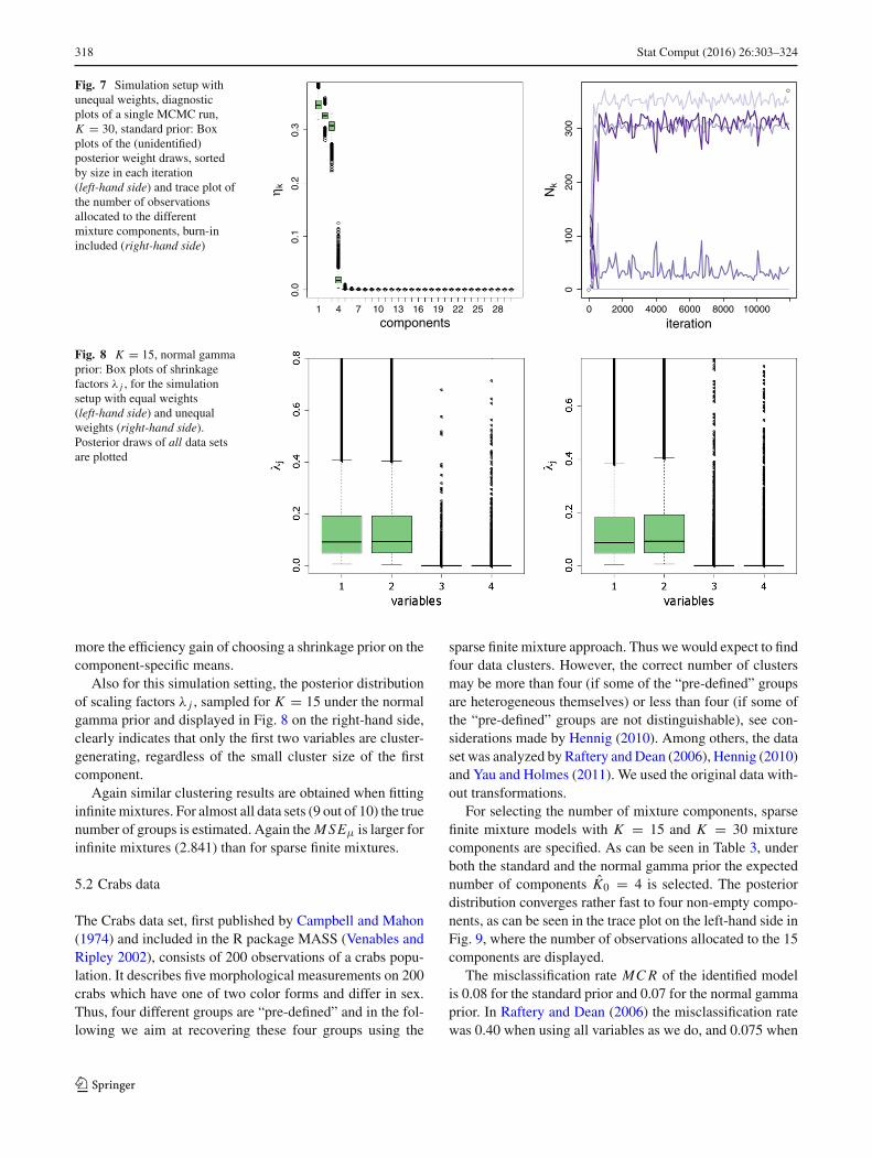
318 Stat Comput (2016) 26:303–324

Fig. 7 Simulation setup withunequal weights, diagnosticplots of a single MCMC run,K = 30, standard prior: Boxplots of the (unidentified)posterior weight draws, sortedby size in each iteration(left-hand side) and trace plot ofthe number of observationsallocated to the differentmixture components, burn-inincluded (right-hand side)

1 4 7 10 13 16 19 22 25 28

0.0

0.1

0.2

0.3

components

η k

0 2000 4000 6000 8000 10000

010

020

030

0

iteration

Nk

Fig. 8 K = 15, normal gammaprior: Box plots of shrinkagefactors λ j , for the simulationsetup with equal weights(left-hand side) and unequalweights (right-hand side).Posterior draws of all data setsare plotted

more the efficiency gain of choosing a shrinkage prior on thecomponent-specific means.

Also for this simulation setting, the posterior distributionof scaling factors λ j , sampled for K = 15 under the normalgamma prior and displayed in Fig. 8 on the right-hand side,clearly indicates that only the first two variables are cluster-generating, regardless of the small cluster size of the firstcomponent.

Again similar clustering results are obtained when fittinginfinitemixtures. For almost all data sets (9 out of 10) the truenumber of groups is estimated. Again the MSEμ is larger forinfinite mixtures (2.841) than for sparse finite mixtures.

5.2 Crabs data

The Crabs data set, first published by Campbell and Mahon(1974) and included in the R package MASS (Venables andRipley 2002), consists of 200 observations of a crabs popu-lation. It describes five morphological measurements on 200crabs which have one of two color forms and differ in sex.Thus, four different groups are “pre-defined” and in the fol-lowing we aim at recovering these four groups using the

sparse finite mixture approach. Thus we would expect to findfour data clusters. However, the correct number of clustersmay be more than four (if some of the “pre-defined” groupsare heterogeneous themselves) or less than four (if some ofthe “pre-defined” groups are not distinguishable), see con-siderations made by Hennig (2010). Among others, the dataset was analyzed by Raftery andDean (2006), Hennig (2010)and Yau and Holmes (2011). We used the original data with-out transformations.

For selecting the number of mixture components, sparsefinite mixture models with K = 15 and K = 30 mixturecomponents are specified. As can be seen in Table 3, underboth the standard and the normal gamma prior the expectednumber of components K0 = 4 is selected. The posteriordistribution converges rather fast to four non-empty compo-nents, as can be seen in the trace plot on the left-hand side inFig. 9, where the number of observations allocated to the 15components are displayed.

The misclassification rate MCR of the identified modelis 0.08 for the standard prior and 0.07 for the normal gammaprior. In Raftery and Dean (2006) the misclassification ratewas 0.40 when using all variables as we do, and 0.075 when

123

Stat Comput (2016) 26:303–324 319

Table 3 Crabs data: results for different K under the standard prior(Sta) and the normal gamma prior (Ng), and when fitting an infinitemixture using the R package PReMiuM. The MSEμ is calculated usingthe Mahalanobis distance based on Bayes estimates. M ′

0,ρ , MCR′, and

MSE ′μ are the results based on the clustering of the draws in the point

process representation through K -means instead of the K -centroidscluster analysis based on the Mahalanobis distance

Prior K e0 e0 fixed K0 M0 M0,ρ MCR MSEμ M ′0,ρ MCR′ MSE ′

μ

Sta 4 0.27 4 10, 000 0 0.08 0.80 0.27 0.08 3.67

15 0.05 4 10, 000 0 0.08 0.81 0.28 0.08 3.82

30 0.03 4 10, 000 0 0.08 0.80 0.29 0.08 3.42

Ng 4 0.01 4 10, 000 0 0.07 0.68 0.44 0.08 6.72

15 0.01 4 9, 938 0 0.07 0.67 0.46 0.08 8.19

30 0.01 4 9, 628 0 0.07 0.68 0.46 0.08 8.10

PReMiuM α Kest MCR MSEμ

0.67 3 0.28

Fig. 9 Crabs data, normalgamma prior, K = 15: Traceplot of the number ofobservations allocated to thedifferent components, burn-inincluded (left-hand side). Boxplots of the shrinkage factors λ jfor all five variables (right-handside)

0 2000 4000 6000 8000 10000

010

2030

4050

60

iteration

Nk

1 2 3 4 5

0.00

0.05

0.10

0.15

variables

λ j

excluding one variable. Again, there is a considerable reduc-tion in MSEμ under the normal gamma prior compared tothe standard prior. Box plots of the posterior draws of theshrinkage factor λ j in Fig. 9 reveal that all five variables arecluster-relevant which might be due to the high correlationbetween variables.

This specific case study also demonstrates the importanceof the refined procedure introduced in Sect. 4.2 to identify amixture by clustering the MCMC draws of the component-specific means in the point process representation. Cluster-ing using the squared Euclidean distance fails to capturethe geometry of the posterior mean distribution and leadsto a high non-permutation rate, denoted by M ′

0,ρ in Table 3.Clustering using K -centroids cluster analysis based on theMahalanobis distance, however, allows to capture the ellip-tical shapes of the posterior mean distribution properly, seeFig. 4, which in turn reduces the non-permutation rate M0,ρ

to 0. In this way, inference with respect to the component-specific parameters is considerably improved, as is evidentfrom comparingMSEμ andMSE ′

μ for both clusteringmeth-ods in Table 3.

By clustering the Crabs data using an infinite mixturemodel with initial settings as explained in Sect. 5.1, threegroups are estimated.

5.3 Iris data

The Iris data set (Anderson 1935; Fisher 1936) consists of50 samples from each of three species of Iris, namely Irissetosa, Iris virginica and Iris versicolor. Four features aremeasured for each sample, the length and width of the sepalsandpetals, respectively.Weaimat recovering the three under-lying classes using the sparse finite mixture approach andthus expect to find three data clusters, although, asmentionedalready for the Crabs data in Sect. 5.2, the true number ofclusters for a finite mixture of Gaussian distributions may bemore or less than three.

The results are reported in Table 4 by fitting sparse finitemixture models with 15 and 30 components, respectively.Values given in parentheses refer to the draws associatedwiththe number of non-empty components given in parenthesis incolumn K0. Under both priors, the expected number of com-

123

320 Stat Comput (2016) 26:303–324

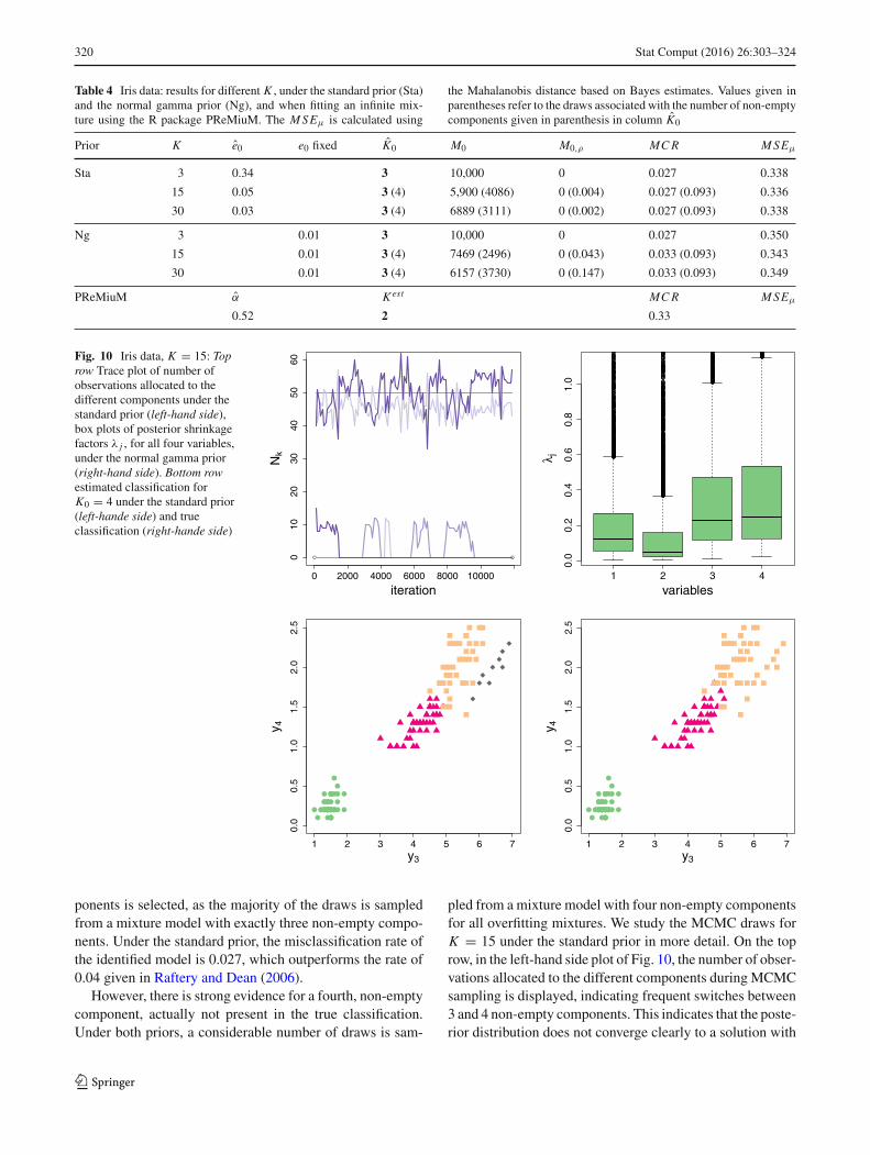
Table 4 Iris data: results for different K , under the standard prior (Sta)and the normal gamma prior (Ng), and when fitting an infinite mix-ture using the R package PReMiuM. The MSEμ is calculated using

the Mahalanobis distance based on Bayes estimates. Values given inparentheses refer to the draws associated with the number of non-emptycomponents given in parenthesis in column K0

Prior K e0 e0 fixed K0 M0 M0,ρ MCR MSEμ

Sta 3 0.34 3 10,000 0 0.027 0.338

15 0.05 3 (4) 5,900 (4086) 0 (0.004) 0.027 (0.093) 0.336

30 0.03 3 (4) 6889 (3111) 0 (0.002) 0.027 (0.093) 0.338

Ng 3 0.01 3 10,000 0 0.027 0.350

15 0.01 3 (4) 7469 (2496) 0 (0.043) 0.033 (0.093) 0.343

30 0.01 3 (4) 6157 (3730) 0 (0.147) 0.033 (0.093) 0.349

PReMiuM α Kest MCR MSEμ

0.52 2 0.33

Fig. 10 Iris data, K = 15: Toprow Trace plot of number ofobservations allocated to thedifferent components under thestandard prior (left-hand side),box plots of posterior shrinkagefactors λ j , for all four variables,under the normal gamma prior(right-hand side). Bottom rowestimated classification forK0 = 4 under the standard prior(left-hande side) and trueclassification (right-hande side)

0 2000 4000 6000 8000 10000

010

2030

4050

60

iteration

Nk

1 2 3 40.

00.

20.

40.

60.

81.

0

variables

λ j

1 2 3 4 5 6 7

0.0

0.5

1.0

1.5

2.0

2.5

y3

y 4

1 2 3 4 5 6 7

0.0

0.5

1.0

1.5

2.0

2.5

y3

y 4

ponents is selected, as the majority of the draws is sampledfrom a mixture model with exactly three non-empty compo-nents. Under the standard prior, the misclassification rate ofthe identified model is 0.027, which outperforms the rate of0.04 given in Raftery and Dean (2006).

However, there is strong evidence for a fourth, non-emptycomponent, actually not present in the true classification.Under both priors, a considerable number of draws is sam-

pled from a mixture model with four non-empty componentsfor all overfitting mixtures. We study the MCMC draws forK = 15 under the standard prior in more detail. On the toprow, in the left-hand side plot of Fig. 10, the number of obser-vations allocated to the different components during MCMCsampling is displayed, indicating frequent switches between3 and 4 non-empty components. This indicates that the poste-rior distribution does not converge clearly to a solution with

123

Stat Comput (2016) 26:303–324 321

three non-empty components and that a mixture model withK0 = 4 non-empty components has also considerable pos-terior probability. Moreover, the non-permutation rate M0,ρ

is small for K0 = 4 (0.004), indicating that the componentmeans are well separated. If further inference is based on thedraws with K0 = 4 non-empty components, the obtainedfour-cluster solution seems to be a reasonable solution. Thiscan be seen in Fig. 10 where scatter plots of 2 variables (petallength and petal width) under both the resulting classificationfor K0 = 4 and the true classification are displayed. Obser-vations of the fourth estimated component, displayed in darkgrey diamonds, constitute a rather isolated group.

Regarding the identification of cluster-relevant variables,box plots of the shrinkage factorsλ j displayed in Fig. 10 indi-cate that variable 2 (sepal width) is the most homogeneousvariable which coincides with results in Yau and Holmes(2011).

If the number of groups is estimated by specifying an infi-nite mixture model, only the two data clusters are identifiedindicating that the infinite mixture approach implemented inpackage PReMiuM with the default settings aims at identi-fying clearly separated clusters with minimum overlap.

6 Discussion

In the framework of Bayesian model-based clustering, wepropose a straightforward and simple strategy for simulta-neous estimation of the unknown number of mixture com-ponents, component-specific parameters, classification ofobservations, and identification of cluster-relevant variablesfor multivariate Gaussian mixtures. Our approach relieson specifying sparse priors on the mixture parameters andinvolves only standard MCMC methods.

Estimation of the unknown number of mixture compo-nents is based on sparse finite mixtures where a sparseprior on the weights empties superfluous components duringMCMC sampling and the number of true components canbe estimated from the number of non-empty components.An advantage of this strategy is that model selection can beperformed without computer-intensive calculations of mar-ginal likelihoods or designing sophisticated proposals withinRJMCMC. This approach works astonishingly well if thenumber of observations and the number of variables is nottoo large.

However, there are also limitations to the proposed strat-egy. First of all, we investigated our strategy under theassumption that the mixture components truly arise frommultivariate Gaussian distributions. In order to catch non-symmetrical cluster shapes or handle outliers it would also beinteresting to extend the approach to non-Gaussian compo-nent distributions, e.g. the t-distribution and the skew-normal

distribution (see Frühwirth-Schnatter and Pyne 2010; Leeand McLachlan 2014).

Wemay apply sparse finiteGaussianmixtures to data fromsuch skew or fat-tailedmixture distributions, however, in thiscase the posterior mixture distribution tends to fit more thanone Gaussian component to represent a single non-Gaussiancluster, in particular for an increasing number of observa-tions. As a consequence, the method is fitting Gaussian mix-tures in the sense of density estimation, where the numberof components is of no specific interest, and the estimatednumber of non-empty components no longer represents thenumber of distinct clusters. An important issue for furtherinvestigation is therefore how to combine mixture compo-nents, i.e. how to identify adjacent located components andmerge them into one larger cluster. Several recent papers haveconsidered the problem of merging Gaussian mixture com-ponents, see e.g. Li (2005), Baudry et al. (2010), and Hennig(2010).

To identify cluster-relevant variables, the standard priorfor the component means commonly applied for multivari-ate Gaussian mixtures is substituted by a hierarchical shrink-age prior based on the normal gamma prior. This prior tendsto fill superfluous components, since it becomes informa-tive during MCMC sampling and superfluous componentsare placed in reasonable locations. We found that the nor-mal gamma prior requires specification of a very sparseprior on the mixture weights, which is achieved by set-ting the hyperparameter e0 of the Dirichlet prior to a verysmall fixed value. Under this shrinkage prior, the true num-ber of components is recovered from overfitting finite mix-tures for simulated data. Additionally, under the normalgamma prior box plots of shrinkage factors allow visualidentification of cluster-relevant and homogeneous variables.Furthermore, component locations are estimated more pre-cisely under the normal gamma than under the standardprior.

A limitation of this strategy is that explicit identifica-tion of cluster-relevant variables is based on visual detec-tion in a post-processing step. In the presence of a hugenumber of variables, this strategy might be too cumber-some and an automatic approach might possibly be prefer-able. This could be developed similar to the automaticapproaches which are for example used for explicit variableselection in a regression setting when using the BayesianLasso.

Finally, we note a further limitation of the proposed strat-egy for high-dimensional data sets. When applying sparsefinitemixtures to high-dimensional data sets, Gibbs samplingwith data augmentation tends to get stuck in local modes, sothat superfluous components do not become empty duringsampling. An issue for further studies is therefore how toimprove mixing, i.e. to design well-mixing samplers, a prob-lem also mentioned in Yau and Holmes (2011).

123

322 Stat Comput (2016) 26:303–324

Acknowledgments This research was supported by the Austrian Sci-ence Fund (FWF): V170-N18.

OpenAccess This article is distributed under the terms of theCreativeCommons Attribution License which permits any use, distribution, andreproduction in any medium, provided the original author(s) and thesource are credited.

Appendix 1: Scheme for estimating using MCMC sam-pling

The sampling scheme iterates the following steps:

1. Parameter simulation conditional on the classificationS = (S1, . . . , SN ):

(a) Sample

η ∼ Dir(e1, . . . , eK ),

where

ek = e0 + Nk,

and Nk = #{i : Si = k} is the number of observationsassigned to component k.

(b) For k = 1, . . . , K : sample

�−1k ∼ W(ck,Ck),

where

ck = c0 + Nk/2,

Ck = C0 + 1

2

∑

i :Si=k

(yi − μk)(yi − μk)′.

(c) For k = 1, . . . , K : sample

μk ∼ N (bk,Bk),

where

Bk = (B−10 + Nk�

−1k )−1,

bk = Bk(B−10 b0 + �−1

k Nk yk),

and yk is the mean of the observations assigned by Sto component k.

2. Classification of each observation yi conditional onknowing μ,�, η:

(a) For i = 1, . . . , N : sample Si from

Pr(Si = k|yi ;μ,�, η) ∝ ηk fN (yi |μk,�k).

3. Sample hyperparameters:

(a) Sample

C0 ∼ W(g0 + Kc0,G0 +K∑

k=1

�−1k ).

(b) For a Dirichlet prior with random hyperparameter e0,sample e0 via a Metropolis-Hastings step from

p(e0|η) ∝ p(η|e0)p(e0),see Eq. (10).

Additionally, for the normal gamma prior:

(c) For j = 1, . . . , r , sample

λ j ∼ GIG(pK , a j , b j ),

where

pK = ν1 − K/2,

a j = 2ν2,

b j =K∑

k=1

(μk j − b0 j )2/R2

j .

(d) Sample

b0 ∼ N(1

K

K∑

k=1

μk; 1

KB0

),

where

B0 = Diag(R21λ1, . . . , R

2r λr ).

4. Randompermutation of the labeling: select randomly onepermutation ρ of K ! possible permutations of {1, . . . , K }and substitute:

η = ηρ(1,...,K ),

(μ1, . . . ,μK ) = (μρ(1), . . . ,μρ(K )),

(�1, . . . ,�K ) = (�ρ(1), . . . ,�ρ(K )),

S = ρ(S).

Appendix 2: Scheme for clustering in the point processrepresentation

After the MCMC run, a sparse finite mixture is identifiedby post-processing the MCMC draws through the followingsteps:

1. For each iteration m = 1, . . . , M of the MCMC run,determine the number of non-empty components K (m)

0according to Eq. (4).

2. Estimate the true number of mixture components byK0 = mode(K (m)

0 ), the value of the number of non-empty components occurring most often during MCMCsampling. Consider only the subsequence M0 of allMCMC iterations where the number of non-empty com-ponents is exactly equal to K0.

123

Stat Comput (2016) 26:303–324 323

3. For allM0 iterations, remove the draws from empty com-ponents.

4. Arrange the remaining draws of the different compo-nent means in a matrix with K0 · M0 rows and rcolumns. Cluster all K0 ·M0 draws into K0 clusters usingK -centroids cluster analysis (Leisch 2006)where the dis-tance between a point and a cluster centroid is determinedby the Mahalanobis distance. Details on the cluster algo-rithm are given in Sect. 4.2. The K -centroids clusteringalgorithm results in a classification indicating to whichclusters the component-specific parameters of each sin-gle draw belong.

5. For each iteration m, m = 1, . . . , M0, construct a classi-fication sequence ρ(m) of size K0 containing the classi-fications of each draw of iteration m.Form = 1, . . . , M0, checkwhether ρ(m) is a permutationof (1, . . . , K0). If not, remove the corresponding drawsfrom the MCMC subsample of size M0.The proportion of classification sequences of M0 notbeing a permutation is denoted by M0,ρ .

6. For the remainingM0(1−M0,ρ) draws, a unique labelingis achieved by resorting the draws according to the clas-sification sequences ρ(m). The resorted, identified drawscan be used for further component-specific parameterinference.

To illustrate step 5, consider for instance, that for K0 = 4,for iteration m a classification sequence ρ(m) = (1, 3, 4, 2)is obtained through the clustering procedure. That meansthat the draw of the first component was assigned to clus-ter one, the draw of the second component was assignedto cluster three and so on. In this case, the draws of thisiteration are assigned to different clusters, which allows torelabel these draws. However, if a classification sequenceρ(m) = (3, 1, 2, 1) is obtained, then draws sampled fromtwo different components are assigned to the same clusterand no relabeling can be performed. Thus these draws areremoved from further inference because no unique labelingcan be defined for this iteration.

As already observed by Frühwirth-Schnatter (2011a), allclassification sequences ρ(m), m = 1, . . . , M obtained instep 5 are expected to be permutations, if the point processrepresentation of the MCMC draws contains well-separatedsimulation clusters. If a small fraction of non-permutationsM0,ρ is present, the posterior draws corresponding to thenon-permutation sequences are removed from the M0 itera-tions. Only the subsequence of identified draws is used forfurther component-specific inference. However, a high frac-tion M0,ρ indicates that in the point process representationclusters are highly overlapping. This typically happens if theselected mixture model with K0 components is overfitting,see Frühwirth-Schnatter (2011a).

References

Anderson, E.: The Irises of the Gaspé Peninsula. Bull. Am. Iris Soc. 59,2–5 (1935)

Armagan, A., Dunson, D., Clyde, M.: Generalized beta mixtures ofGaussians. In: Shawe-Taylor, J., Zemel, R., Bartlett, P., Pereira, F.,Weinberger, K. (eds.) Advances in Neural Information ProcessingSystems (NIPS) 24, pp. 523–531, Curran Associates, Inc., (2011)

Banfield, J.D., Raftery, A.E.: Model-based Gaussian and non-Gaussianclustering. Biometrics 49, 803–821 (1993)

Baudry, J., Raftery, A.E., Celeux, G., Lo, K., Gottardo, R.: Combiningmixture components for clustering. J. Comput. Gr. Stat. 19, 332–353(2010)

Bensmail, H., Celeux, G., Raftery, A.E., Robert, C.P.: Inference inmodel-based cluster analysis. Stat. Comput. 7, 1–10 (1997)

Biernacki, C., Celeux, G., Govaert, G.: Assessing a mixture model forclusteringwith the integrated completed likelihood. IEEETrans. Pat-tern Anal. Mach. Intell. 22(7), 719–725 (2000)

Campbell, N., Mahon, R.: A multivariate study of variation in twospecies of rock crab of genus Leptograpsus. Austr. J. Zool. 22, 417–425 (1974)

Celeux, G.: Bayesian inference for mixture: the label switching prob-lem. In: Green, P.J., Rayne, R. (eds.) COMPSTAT 98, pp. 227–232.Physica, Heidelberg (1998)

Celeux, G., Hurn, M., Robert, C.P.: Computational and inferential dif-ficulties with mixture posterior distributions. J. Am. Stat. Assoc. 95,957–970 (2000)

Celeux, G., Forbes, F., Robert, C.P., Titterington, D.M.: Deviance infor-mation criteria for missing data models. Bayesian Anal. 1(4), 651–674 (2006)

Chung, Y., Dunson, D.: Nonparametric Bayes conditional distributionmodeling with variable selection. J. Am. Stat. Assoc. 104, 1646–1660 (2009)

Dasgupta, A., Raftery, A.E.: Detecting features in spatial pointprocesseswith clutter viamodel-based clustering. J.Am. Stat.Assoc.93(441), 294–302 (1998)

Dean, N., Raftery, A.E.: Latent class analysis variable selection. Ann.Inst. Stat. Math. 62, 11–35 (2010)

Dellaportas, P., Papageorgiou, I.: Multivariate mixtures of normals withunknown number of components. Stat. Comput. 16, 57–68 (2006)

Diebolt, J., Robert, C.P.: Estimation of finite mixture distributionsthrough Bayesian sampling. J. R. Stat. Soc. B 56, 363–375 (1994)

Fisher, R.: The use of multiple measurements in taxonomic problems.Ann. Eugenics 7(2), 179–188 (1936)

Frühwirth-Schnatter, S.: Markov chain Monte Carlo estimation of clas-sical and dynamic switching andmixturemodels. J. Am. Stat. Assoc.96(453), 194–209 (2001)

Frühwirth-Schnatter, S.: Estimating marginal likelihoods for mixtureand Markov switching models using bridge sampling techniques.Econ. J. 7, 143–167 (2004)

Frühwirth-Schnatter, S.: FiniteMixture andMarkov SwitchingModels.Springer-Verlag, New York (2006)

Frühwirth-Schnatter, S.: Label switching under model uncertainty. In:Mengerson, K., Robert, C., Titterington, D. (eds.) Mixtures: Estima-tion and Application, pp. 213–239. Wiley, New York (2011a)

Frühwirth-Schnatter, S.: Panel data analysis - a survey on model-basedclustering of time series. Adv. Data Anal. Classif. 5(4), 251–280(2011b)

Frühwirth-Schnatter, S., Kaufmann, S.: Model-based clustering of mul-tiple time series. J. Bus. Econ. Stat. 26(1), 78–89 (2008)

Frühwirth-Schnatter, S., Pyne, S.: Bayesian inference for finitemixturesof univariate and multivariate skew-normal and skew-t distributions.Biostatistics 11(2), 317–336 (2010)

Geweke, J.: Interpretation and inference in mixture models: simpleMCMC works. Comput. Stat. Data Anal. 51, 3529–3550 (2007)

123

324 Stat Comput (2016) 26:303–324

Griffin, J.E., Brown, P.J.: Inference with normal-gamma prior distribu-tions in regression problems. Bayesian Anal. 5(1), 171–188 (2010)

Grün, B., Leisch, F.: Dealing with label switching in mixture modelsunder genuine multimodality. J. Multivar. Anal. 100(5), 851–861(2009)

Handcock, M.S., Raftery, A.E., Tantrum, J.M.: Model-based clusteringfor social networks. J. R. Stat. Soc. A 170(2), 301–354 (2007)

Hennig, C.: Methods for merging Gaussian mixture components. Adv.Data Anal. Classif. 4, 3–34 (2010)

Ishwaran, H., James, L.F., Sun, J.: Bayesian model selection in finitemixtures by marginal density decompositions. J. Am. Stat. Assoc.96(456), 1316–1332 (2001)

Jasra, A., Holmes, C.C., Stephens, D.A.: Markov chain Monte Carlomethods and the label switching problem in Bayesian mixture mod-eling. Stat. Sci. 20(1), 50–67 (2005)

Juárez, M.A., Steel, M.F.J.: Model-based clustering of non-Gaussianpanel data based on skew-t distributions. J. Bus. Econ. Stat. 28(1),52–66 (2010)

Kaufman, L., Rousseeuw, P.J.: FindingGroups inData: An Introductionto Cluster Analysis. Wiley, New York (1990)

Kim, S., Tadesse, M.G., Vannucci, M.: Variable selection in clusteringvia Dirichlet process mixture models. Biometrika 93(4), 877–893(2006)

Kundu, S., Dunson, D.B.: Bayes variable selection in semiparametriclinear models. J. Am. Stat. Assoc. 109(505), 437–447 (2014)

Lee, H., Li, J.: Variable selection for clustering by separability basedon ridgelines. J. Comput. Gr. Stat. 21(2), 315–337 (2012)

Lee, S., McLachlan, G.J.: Finite mixtures of multivariate skew t-distributions: some recent and new results. Stat. Comput. 24(2), 181–202 (2014)

Leisch, F.: A toolbox for K -centroids cluster analysis. Comput. Stat.Data Anal. 51(2), 526–544 (2006)

Li, J.: Clustering based on a multi-layer mixture model. J. Comput. Gr.Stat. 14, 547–568 (2005)

Lian, H.: Sparse Bayesian hierarchical modeling of high-dimensionalclustering problems. J. Multivar. Anal. 101(7), 1728–1737 (2010)

Liverani, S., Hastie, D.I., Papathomas, M., Richardson, S.: PReMiuM:An R package for profile regression mixture models using Dirichletprocesses, arXiv preprint arXiv:1303.2836 (2013)

Maugis, C., Celeux, G., Martin-Magniette, M.L.: Variable selection forclustering with Gaussian mixture models. Biometrics 65(3), 701–709 (2009)

McLachlan, G.J., Peel, D.: FiniteMixtureModels.Wiley series in prob-ability and statistics. Wiley, New York (2000)

McLachlan, G.J., Bean, R.W., Peel, D.: A mixture-model basedapproach to the clustering of microarray expression data. Bioinfor-matics 18, 413–422 (2002)

McNicholas, P.D., Murphy, T.B.: Parsimonious Gaussian mixture mod-els. Stat. Comput 18(3), 285–296 (2008)

McNicholas, P.D., Murphy, T.B.: Model-based clustering of longitudi-nal data. Can. J. Stat. 38(1), 153–168 (2010)

Molitor, J., Papathomas, M., Jerrett, M., Richardson, S.: Bayesian pro-file regressionwith an application to the national survey of children’shealth. Biostatistics 11(3), 484–498 (2010)

Nobile, A.: On the posterior distribution of the number of componentsin a finite mixture. Ann. Stat. 32, 2044–2073 (2004)

Pan, W., Shen, X.: Penalized model-based clustering with applicationto variable selection. J. Mach. Learn. Res. 8, 1145–1164 (2007)

Park, T., Casella, G.: The Bayesian Lasso. J. Am. Stat. Assoc. 103(482),681–686 (2008)

Polson, N.G., Scott, J.G.: Shrink globally, act locally: sparse Bayesianregularization and prediction. In: Bernardo, J., Bayarri, M., Berger,J., Dawid, A., Heckerman, D., Smith, A., West, M. (eds.) BayesianStatistics, vol. 9, pp. 501–523. Oxford University Press, Oxford(2010)

Raftery, A.E., Dean, N.: Variable selection for model-based clustering.J. Am. Stat. Assoc. 101(473), 168–178 (2006)

Richardson, S., Green, P.J.: On Bayesian analysis of mixtures with anunknown number of components. J. R. Stat. Soc. B 59(4), 731–792(1997)

Rousseau, J., Mengersen, K.: Asymptotic behaviour of the posteriordistribution in overfitted mixture models. J. R. Stat. Soc. B 73(5),689–710 (2011)

Sperrin, M., Jaki, T., Wit, E.: Probabilistic relabelling strategies for thelabel switching problem in Bayesian mixture models. Stat. Comput.20(3), 357–366 (2010)

Stephens, M.: Bayesian methods for mixtures of normal distributions.Ph.D. thesis, University of Oxford (1997)

Stephens, M.: Dealing with label switching in mixture models. J. R.Stat. Soc. B 62, 795–809 (2000)

Stingo, F.C., Vannucci, M., Downey, G.: Bayesian wavelet-based curveclassification via discriminant analysis with Markov random treepriors. Statistica Sinica 22(2), 465 (2012)

Tadesse, M.G., Sha, N., Vanucci, M.: Bayesian variable selection inclustering high-dimensional data. J. Am. Stat. Assoc. 100(470), 602–617 (2005)

Venables, W.N., Ripley, B.D.: Modern Applied Statistics with S, 4thedn. Springer-Verlag, New York (2002)

Wang, S., Zhu, J.: Variable selection for model-based high-dimensionalclustering and its application to microarray data. Biometrics 64(2),440–448 (2008)

Xie, B., Pan, W., Shen, X.: Variable selection in penalized model-based clustering via regularization on grouped parameters. Biomet-rics 64(3), 921–930 (2008)

Yao, W., Lindsay, B.G.: Bayesian mixture labeling by highest posteriordensity. J. Am. Stat. Assoc. 104, 758–767 (2009)

Yau, C., Holmes, C.: Hierarchical Bayesian nonparametric mix-ture models for clustering with variable relevance determination.Bayesian Anal. 6(2), 329–352 (2011)

Yeung, K.Y., Fraley, C., Murua, A., Raftery, A.E., Ruzzo,W.L.: Model-based clustering and data transformations for gene expression data.Bioinformatics 17, 977–987 (2001)

123