Variational Inducing Kernels for Sparse Convolved MultipleOutput Gaussian Processes

Mauricio A. Alvarez alvarezm@cs.man.ac.ukSchool of Computer ScienceUniversity of ManchesterManchester, UK, M13 9PL

David Luengo luengod@ieee.orgDep. Teorıa de Senal y ComunicacionesUniversidad Carlos III de Madrid28911 Leganes, Spain

Michalis K. Titsias mtitsias@cs.man.ac.uk

Neil D. Lawrence neill@cs.man.ac.uk

School of Computer ScienceUniversity of ManchesterManchester, UK, M13 9PL

Abstract

Interest in multioutput kernel methods is increasing, whether under the guise of multitasklearning, multisensor networks or structured output data. From the Gaussian processperspective a multioutput Mercer kernel is a covariance function over correlated outputfunctions. One way of constructing such kernels is based on convolution processes (CP). Akey problem for this approach is efficient inference. Alvarez and Lawrence (2009) recentlypresented a sparse approximation for CPs that enabled efficient inference. In this paper,we extend this work in two directions: we introduce the concept of variational inducingfunctions to handle potential non-smooth functions involved in the kernel CP constructionand we consider an alternative approach to approximate inference based on variationalmethods, extending the work by Titsias (2009) to the multiple output case. We demonstrateour approaches on prediction of school marks, compiler performance and financial timeseries.

1. Introduction

Gaussian processes (GPs) are flexible non-parametric models which allow us to specify priordistributions and perform inference of functions. A limiting characteristic of GPs is the factthat the computational cost of inference is in general O(N3), N being the number of datapoints, with an associated storage requirement of O(N2). In recent years a lot of progress(Csato and Opper, 2001; Lawrence et al., 2003; Seeger et al., 2003; Snelson and Ghahramani,2006; Quinonero Candela and Rasmussen, 2005) has been made with approximations thatallow inference in O(K2N) (and associated storage of O(KN), where K is a user specified

1

arX

iv:0

912.

3268

v1 [

stat

.ML

] 1

6 D

ec 2

009

number. This has made GPs practical for a range of larger scale inference problems.In this paper we are specifically interested in developing priors over multiple functions.While such priors can be trivially specified by considering the functions to be independent,our focus is on priors which specify correlations between the functions. Most attempts toapply such priors so far (Teh et al., 2005; Osborne et al., 2008; Bonilla et al., 2008) havefocussed on what is known in the geostatistics community as “linear model of coregionaliza-tion” (LMC) (Journel and Huijbregts, 1978; Goovaerts, 1997). In these models the differentoutputs are assumed to be linear combinations of a set of one or more “latent functions” sothat the dth output of the function, fd (x) is given by

fd (x) =Q∑

q=1

ad,quq (x) , (1)

where uq (x) is one of Q latent functions that, weighted by {ad,q}Qq=1, sum to form each of theD outputs. GP priors are placed, independently, over each of the latent functions inducing acorrelated covariance function over {fd (x)}Dd=1. Approaches to multi-task learning arisingin the kernel community (see for example Evgeniou et al., 2005) can also be seen to beinstances of the LMC framework.We wish to go beyond the LMC framework, in particular, our focus is convolution pro-cesses (Higdon, 2002; Boyle and Frean, 2005). Using CPs for multi-output GPs was pro-posed by Higdon (2002) and introduced to the machine learning audience by Boyle andFrean (2005). Convolution processes allow the integration of prior information from phys-ical models, such as ordinary differential equations, into the covariance function. Alvarezet al. (2009), inspired by Gao et al. (2008), have demonstrated how first and second orderdifferential equations, as well as partial differential equations, can be accommodated in acovariance function. Their interpretation is that the set of latent functions are a set of latentforces, and they term the resulting models “latent force models”. The covariance functionsfor these models are derived through convolution processes (CPs). In the CP framework,output functions are generated by convolving Q latent processes {uq(x)}Qq=1 with kernelfunctions,1 Gd,q(x), associated to each output d and latent force q, so that we have

fd (x) =Q∑

q=1

∫ZGd,q (x− z)uq (z) dz. (2)

The LMC can be seen as a particular case of the CP, in which the kernel functions Gd,q(x)correspond to scaled Dirac δ-function Gd,q (x− z) = ad,qδ(x − z). In latent force modelsthe convolving kernel, Gd,r(·), is the Green’s function associated to a particular differentialequation.A practical problem associated with the CP framework is that in these models inferencehas computational complexity O(N3D3) and storage requirements O(N2D2). Recently,Alvarez and Lawrence (2009) introduced an efficient approximation for inference in thismulti-output GP model. The idea was to exploit a conditional independence assumptionover the output functions {fd (x)}Dd=1 given a finite number of observations of the latent

1. Not kernels in the Mercer sense, but kernels in the normal sense.

2

functions{{uq (xk)}Kk=1

}Q

q=1. This led to approximations that were very similar in spirit to

the PITC and FITC approximations of Snelson and Ghahramani (2006); Quinonero Candelaand Rasmussen (2005). In this paper we build on the work of Alvarez and Lawrence. Theirapproximation was inspired by the fact that if the latent functions are observed in theirentirety, the output functions are conditionally independent of one another (as can be seenin (2)). We extend the previous work presented in Alvarez and Lawrence (2009) in twoways. First, a problem with the FITC and PITC approximations can be their propensity tooverfit when inducing inputs are optimized. A solution to this problem was given in recentwork by Titsias (2009) who provides a sparse GP approximation that has an associatedvariational bound. In this paper we show how the ideas of Titsias can be extended tothe multiple output case. Second, we notice that if the locations of the inducing points,{xk}Kk=1, are close relative to the length scale of the latent function, the PITC approximationwill be accurate. However, if the length scale becomes small the approximation requiresvery many inducing points. In the worst case, the latent process could be white noise (assuggested by Higdon (2002) and implemented by Boyle and Frean (2005)). In this case theapproximation will fail completely. We further develop the variational approximation toallow us to work with rapidly fluctuating latent functions (including white noise). This isachieved by augmenting the output functions with one or more additional functions. Werefer to these additional outputs as the inducing functions. Our variational approximationis developed through the inducing functions. There are also smoothing kernels associatedwith the inducing functions. The quality of the variational approximation can be controlledboth through these inducing kernels and through the number and location of the inducinginputs.Our approximation allows us to consider latent force models with a larger number of states,D, and data points N . The use of inducing kernels also allows us to extend the induc-ing variable approximation of the latent force model framework to systems of stochasticdifferential equations (SDEs). In this paper we apply the variational inducing kernel ap-proximation to different real world datasets, including a multivariate financial time seriesexample.A similar idea to the inducing function one introduced in this paper, was simultaneouslyproposed by Lazaro-Gredilla and Figueiras-Vidal (2010). Lazaro-Gredilla and Figueiras-Vidal (2010) introduced the concept of inducing feature to improve performance over thepseudo-inputs approach of Snelson and Ghahramani (2006) in sparse GP models. Ouruse of inducing functions and inducing kernels is motivated by the necessity to deal withnon-smooth latent functions in the convolution processes model of multiple outputs.

2. Multiple Outputs Gaussian Processes

Let yd ∈ RN , where d = 1, . . . , D, be the observed data associated with the output functionyd(x). For simplicity, we assume that all the observations associated with different outputsare evaluated at the same inputs X (although this assumption is easily relaxed). We willoften use the stacked vector y = (y1, . . . ,yD) to collectively denote the data of all the out-puts. Each observed vector yd is assumed to be obtained by adding independent Gaussiannoise to a vector of function values fd so that the likelihood is p(yd|fd) = N (yd|fd, σ2

dI),

3

where fd is defined via (2). More precisely, the assumption in (2) is that a function valuefd(x) (the noise-free version of yd(x)) is generated from a common pool of Q independentlatent functions {uq(x)}Qq=1, each having a covariance function (Mercer kernel) given bykq (x,x′). Notice that the outputs share the same latent functions, but they also have theirown set of parameters ({αd,q}Qq=1, σ

2d) where αd,q are the parameters of the smoothing ker-

nel Gd,q(·). Because convolution is a linear operation, the covariance between any pair offunction values fd(x) and fd′(x′) is given by

kfd,fd′ (x,x′) = Cov[fd(x), fd′(x′)] =

Q∑q=1

∫ZGd,q(x− z)

∫ZGd′,q(x′ − z′)kq(z, z′)dzdz′.

This covariance function is used to define a fully-coupled GP prior p(f1, . . . , fD) over all thefunction values associated with the different outputs.The joint probability distribution of the multioutput GP model can be written as

p({yd, fd}Dd=1) =D∏

d=1

p(yd|fd)p(f1, . . . , fD).

The GP prior p(f1, . . . , fD) has a zero mean vector and a (ND)× (ND) covariance matrixKf ,f , where f = (f1, . . . , fD), which consists of N ×N blocks of the form Kfd,fd′ . Elementsof each block are given by kfd,fd′ (x,x

′) for all possible values of x. Each of such blocks iseither a cross-covariance or covariance matrix of pairs of outputs.Prediction using the above GP model, as well as the maximization of the marginal likelihoodp(y) = N(y|0,Kf ,f + Σ), where Σ = diag(σ2

1I, . . . , σ2DI), requires O(N3D3) time and

O(N2D2) storage which rapidly becomes infeasible even when only few hundreds of outputsand data are considered. Therefore approximate or sparse methods are needed in order tomake the above multioutput GP model practical.

3. PITC-like approximation for Multiple Outputs Gaussian Processes

Before we propose our variational sparse inference method for multioutput GP regressionin Section 4, we review the sparse method proposed by Alvarez and Lawrence (2009). Thismethod is based on a likelihood approximation. More precisely, each output function yd(x)is independent from the other output functions given the full-length of each latent functionuq(x). This means, that the likelihood of the data factorizes according to

p(y|u) =D∏

d=1

p(yd|u) =D∏

d=1

p(yd|fd),

with u = {uq}Qq=1 the set of latent functions. The sparse method in Alvarez and Lawrence(2009) makes use of this factorization by assuming that it remains valid even when weare only allowed to exploit the information provided by a finite set of function values,uq, instead of the full-length function uq(x) (which involves uncountably many points).Let uq, for q = 1, . . . , Q, be a K-dimensional vector of values from the function uq(x)which are evaluated at the inputs Z = {zk}Kk=1. These points are commonly referred to

4

as inducing inputs. The vector u = (u1, . . . ,uQ) denotes all these variables. The sparsemethod approximates the exact likelihood function p(y|u) with the likelihood

p(y|u) =D∏

d=1

p(yd|u) =D∏

d=1

N (yd|µfd|u,Σfd|u + σ2dI),

where µfd|u = Kfd,uK−1u,uu and Σfd|u = Kfd,fd −Kfd,uK−1

u,uKu,fd are the mean and covari-ance matrices of the conditional GP priors p(fd|u). The matrix Ku,u is a block diagonalcovariance matrix where the qth block Kuq ,uq is obtained by evaluating kq(z, z′) at theinducing inputs Z. Further, the matrix Kfd,u has entries defined by the cross-covariancefunction

Cov[fd(x), uq(z)] =∫ZGd,q(x− z′)kq(z′, z)dz′.

The variables u follow the GP prior p(u) = N(u|0,Ku,u) and can be integrated out to givethe following approximation to the exact marginal likelihood:

p(y|θ) = N (y|0,D + Kf ,uK−1u,uKu,f + Σ). (3)

Here, D is a block-diagonal matrix, where each block in the diagonal is given by Kfd,fd −Kfd,uK−1

u,uKu,fd for all d. This approximate marginal likelihood represents exactly eachdiagonal (output-specific) block Kfd,fd while each off diagonal (cross-output) block Kfd,fd′

is approximated by the Nystrom matrix Kfd,uK−1u,uKu,fd′ .

The above sparse method has a similar structure to the PITC approximation introducedfor single-output regression (Quinonero Candela and Rasmussen, 2005). Because of thissimilarity, Alvarez and Lawrence (2009) call their multioutput sparse approximation PITCas well. Two of the properties of this PITC approximation, which can be also its limitations,are:

1. It assumes that all latent functions in u are smooth.

2. It is based on a modification of the initial full GP model. This implies that theinducing inputs Z are extra kernel hyparameters in the modified GP model.

Because of point 1, the method is not applicable when the latent functions are white noiseprocesses. An important class of problems where we have to deal with white noise processesarise in linear SDEs where the above sparse method is currently not applicable there. Be-cause of 2, the maximization of the marginal likelihood in eq. (3) with respect to (Z,θ),where θ are model hyperparameters, may be prone to overfitting especially when the num-ber of variables in Z is large. Moreover, fitting a modified sparse GP model implies thatthe full GP model is not approximated in a systematic and rigorous way since there is nodistance or divergence between the two models that is minimizedIn the next section, we address point 1 above by introducing the concept of variationalinducing kernels that allow us to efficiently sparsify multioutput GP models having whitenoise latent functions. Further, these inducing kernels are incorporated into the variationalinference method of Titsias (2009) (thus addressing point 2) that treats the inducing inputsZ as well as other quantities associated with the inducing kernels as variational parame-ters. The whole variational approach provides us with a very flexible, robust to overfitting,approximation framework that overcomes the limitations of the PITC approximation.

5

4. Sparse variational approximation

In this section, we introduce the concept of variational inducing kernels (VIKs). VIKs giveus a way to define more general inducing variables that have larger approximation capacitythan the u inducing variables used earlier and importantly allow us to deal with white noiselatent functions. To motivate the idea, we first explain why the u variables can work whenthe latent functions are smooth and fail when these functions become white noises.In PITC, we assume each latent function uq(x) is smooth and we sparsify the GP modelthrough introducing, uq, inducing variables which are direct observations of the latentfunction, uq(x), at particular input points. Because of the latent function’s smoothness, theuq variables also carry information about other points in the function through the imposedprior over the latent function. So, having observed uq we can reduce the uncertainty of thewhole function.With the vector of inducing variables u, if chosen to be sufficiently large relative to thelength scales of the latent functions, we can efficiently represent the functions {uq(x)}Qq=1

and subsequently variables f which are just convolved versions of the latent functions.2

When the reconstruction of f from u is perfect, the conditional prior p(f |u) becomes a deltafunction and the sparse PITC approximation becomes exact. Figure 1(a) shows a cartoondescription of a summarization of uq(x) by uq.In contrast, when some of the latent functions are white noise processes the sparse ap-proximation will fail. If uq(z) is white noise3 it has a covariance function δ(z − z′). Suchprocesses naturally arise in the application of stochastic differential equations (see section7) and are the ultimate non-smooth processes where two values uq(z) and uq(z′) are uncor-related when z 6= z′. When we apply the sparse approximation a vector of “white-noise”inducing variables uq does not carry information about uq(z) at any input z that differsfrom all inducing inputs Z. In other words there is no additional information in the condi-tional prior p(uq(z)|uq) over the unconditional prior p(uq(z)). Figure 1(b) shows a pictorialrepresentation. The lack of structure makes it impossible to exploit the correlations in thestandard sparse methods like PITC.4

Our solution to this problem is the following. We will define a more powerful form ofinducing variable, one based not around the latent function at a point, but one given by theconvolution of the latent function with a smoothing kernel. More precisely, let us replaceeach inducing vector uq with the variables λq which are evaluated at the inputs Z and aredefined according to

λq(z) =∫Tq(z− v)uq(v)dv, (4)

where Tq(x) is a smoothing kernel (e.g. Gaussian) which we call the inducing kernel (IK).This kernel is not necessarily related to the model’s smoothing kernels. These newly definedinducing variables can carry information about uq(z) not only at a single input location but

2. This idea is like a “soft version” of the Nyquist-Shannon sampling theorem. If the latent functions werebandlimited, we could compute exact results given a high enough number of inducing points. In generalit won’t be bandlimited, but for smooth functions low frecuency components will dominate over highfrecuencies, which will quickly fade away.

3. Such a process can be thought as the “time derivative” of the Wiener process.4. Returning to our sampling theorem analogy, the white noise process has infinite bandwidth. It is therefore

impossible to represent it by observations at a few fixed inducing points.

6

(a) Latent function is smooth (b) Latent function is noise

uq(x) ! Tq(x) = !q(x)

(c) Generation of an inducing function

Figure 1: With a smooth latent function as in (a), we can use some inducing variables uq (red dots)from the complete latent process uq(x) (in black) to generate smoothed versions (for example theone in blue), with uncertainty described by p(uq|uq). However, with a white noise latent functionas in (b), choosing inducing variables uq (red dots) from the latent process (in black) does not giveus a clue about other points (for example the blue dots). In (c) the inducing function λq(x) acts asa surrogate for a smooth function. Indirectly, it contains information about the inducing points andit can be used in the computation of the lower bound. In this context, the symbol ∗ refers to theconvolution integral.

from the entire input space. Figure 1(c) shows how the inducing kernel generates theartificial construction λq(x), that shares some ligth over the, otherwise, obscure inducingpoints. We can even allow a separate IK for each inducing point, this is, if the set ofinducing points is Z = {zk}Kk=1, then

λq(zk) =∫Tq,k(zk − v)uq(v)dv,

with the advantage of associating to each inducing point zk its own set of adaptive pa-rameters in Tq,k. For the PITC approximation, this adds more hyperparameters to thelikelihood, perhaps leading to overfitting. However, in the variational approximation wedefine all these new parameters as variational parameters and therefore they do not causethe model to overfit. We use the notation λ to refer to the set of inducing functions {λq}Qq=1.

7

If uq(z) has a white noise 5 GP prior the covariance function for λq(x) is

Cov[λq(x), λq(x′)] =∫Tq(x− z)Tq(x′ − z)dz (5)

and the cross-covariance function between fd(x) and λq(x′) is

Cov[fd(x), λq(x′)] =∫Gd,q(x− z)Tq(x′ − z)dz. (6)

Notice that this cross-covariance function, unlike the case of u inducing variables, maintainsa weighted integration over the whole input space. This implies that a single inducingvariable λq(x) can properly propagate information from the full-length process uq(x) intothe set of outputs f .It is possible to combine the IKs defined above with the PITC approximation of Alvarezand Lawrence (2009), but in this paper our focus will be on applying them within thevariational framework of Titsias (2009). We therefore refer to the kernels as variationalinducing kernels (VIKs).

5. Variational inference for sparse multiple output Gaussian Processes.

We now extend the variational inference method of Titsias (2009) to deal with multipleoutputs and incorporate them into the VIK framework.We compactly write the joint probability model p({yd, fd}Dd=1) as p(y, f) = p(y|f)p(f).The first step of the variational method is to augment this model with inducing variables.For our purpose, suitable inducing variables are defined through VIKs. More precisely, letλ = (λ1, . . . ,λQ) be the whole vector of inducing variables where each λq is a K-dimensionalvector of values obtained according to eq. (4). The role of λq is to carry information aboutthe latent function uq(z). Each λq is evaluated at the inputs Z and has its own VIK, Tq(x),that depends on parameters θTq . We denote these parameters as Θ = {θTq}Qq=1.The λ variables augment the GP model according to

p(y, f ,λ) = p(y|f)p(f |λ)p(λ).

Here, p(λ) = N (λ|0,Kλ,λ) and Kλ,λ is a block diagonal matrix where each block Kλq ,λq inthe diagonal is obtained by evaluating the covariance function in eq. (5) at the inputs Z. Ad-ditionally, p(f |λ) = N (f |Kf ,λK−1

λ,λλ,Kf ,f−Kf ,λK−1λ,λKλ,f ) where the cross-covariance Kf ,λ

is computed through eq. (6). Because of the consistency condition∫p(f |λ)p(λ)dλ = p(f),

performing exact inference in the above augmented model is equivalent to performing exactinference in the initial GP model. Crucially, this holds for any values of the augmentationparameters (Z,Θ). This is the key property that allows us to turn these augmentationparameters into variational parameters by applying approximate sparse inference.Our method now follows exactly the lines of Titsias (2009) (in appendix A we present adetailed derivation of the bound based on the set of latent functions uq(x)). We introducethe variational distribution q(f ,λ) = p(f |λ)φ(λ), where p(f |λ) is the conditional GP prior

5. It is straightforward to generalize the method for rough latent functions that are not white noise or tocombine smooth latent functions with white noise.

8

defined earlier and φ(λ) is an arbitrary variational distribution. By minimizing the KLdivergence between q(f ,λ) and the true posterior p(f ,λ|y), we can compute the followingJensen’s lower bound on the true log marginal likelihood:

FV (Z,Θ) = logN(y|0,Kf ,λK−1

λ,λKλ,f + Σ)− 1

2tr(Σ−1K

),

where Σ is the covariance function associated with the additive noise process and K =Kf ,f − Kf ,λK−1

λ,λKλ,f . Note that this bound consists of two parts. The first part is thelog of a GP prior with the only difference that now the covariance matrix has a particularlow rank form. This form allows the inversion of the covariance matrix to take place inO(NDK2) time rather than O(N3D3). The second part can be seen as a penalization termthat regulates the estimation of the parameters. Notice also that only the diagonal of theexact covariance matrix Kf ,f needs to be computed. Overall, the computation of the boundcan be done efficiently in O(NDK2) time.The bound can be maximized with respect to all parameters of the covariance function;both model parameters and variational parameters. The variational parameters are theinducing inputs Z and the parameters θTq of each VIK which are rigorously selected so thatthe KL divergence is minimized. In fact each VIK is also a variational quantity and onecould try different forms of VIKs in order to choose the one that gives the best lower bound.The form of the bound is very similar to the projected process approximation, also known asDeterministic Training Conditional approximation (DTC) (Csato and Opper, 2001; Seegeret al., 2003; Rasmussen and Williams, 2006). However, the bound has an additional traceterm that penalizes the movement of inducing inputs away from the data. This termconverts the DTC approximation to a lower bound and prevents overfitting. In what follows,we refer to this approximation as DTCVAR, where the VAR suffix refers to the variationalframework.The predictive distribution of a vector of test points, y∗ given the training data can also befound to be

p (y∗|y,X,Z) = N (y∗|µy∗ ,Σy∗) ,

with µy∗ = Kf∗λA−1KλfΣ−1y and Σy∗ = Kf∗f∗ −Kf∗λ

(K−1

λλ −A−1)Kλf∗ + Σ∗ and A =

Kλ,λ + Kλ,fΣ−1Kf ,λ. Predictive means can be computed in O(NDK) whereas predictivevariances require O(NDK2) computation.

6. Experiments

We present results of applying the method proposed for two real-world datasets that willbe described in short. We compare the results obtained using PITC, the intrinsic coregion-alization model (ICM)6 employed in (Bonilla et al., 2008) and the method using variationalinducing kernels. For PITC we estimate the parameters through the maximization of theapproximated marginal likelihood of equation (3) using a scaled-conjugate gradient method.

6. The intrinsic coregionalization model is a particular case of the linear model of coregionalization withone latent function (Goovaerts, 1997). See equation (1) with Q = 1.

9

We use one latent function and both the covariance function of the latent process, kq(x,x′),and the kernel smoothing function, Gd,q(x), follow a Gaussian form, this is

k(x,x′) = N (x− x′|0,C),

where C is a diagonal matrix. For the DTCVAR approximations, we maximize the vari-ational bound FV . Optimization is also performed using scaled conjugate gradient. Weuse one white noise latent function and a corresponding inducing function. The inducingkernels and the model kernels follow the same Gaussian form as in the PITC case. Usingthis form for the covariance or kernel, all convolution integrals are solved analytically.

6.1 Exam score prediction

In this experiment the goal is to predict the exam score obtained by a particular studentbelonging to a particular school. The data comes from the Inner London Education Author-ity (ILEA).7 It consists of examination records from 139 secondary schools in years 1985,1986 and 1987. It is a random 50% sample with 15362 students. The input space consistsof features related to each student and features related to each school. From the multipleoutput point of view, each school represents one output and the exam score of each studenta particular instantiation of that output.We follow the same preprocessing steps employed in (Bonilla et al., 2008). The only featuresused are the student-dependent ones (year in which each student took the exam, gender,VR band and ethnic group), which are categorial variables. Each of them is transformed toa binary representation. For example, the possible values that the variable year of the examcan take are 1985, 1986 or 1987 and are represented as 100, 010 or 001. The transformation isalso applied to the variables gender (two binary variables), VR band (four binary variables)and ethnic group (eleven binary variables), ending up with an input space with dimension20. The categorial nature of data restricts the input space to 202 unique input featurevectors. However, two students represented by the same input vector x and belonging bothto the same school d, can obtain different exam scores. To reduce this noise in the data,we follow Bonilla et al. (2008) in taking the mean of the observations that, within a school,share the same input vector and use a simple heteroskedastic noise model in which thevariance for each of these means is divided by the number of observations used to computeit. The performance measure employed is the percentage of explained variance defined asthe total variance of the data minus the sum-squared error on the test set as a percentageof the total data variance. It can be seen as the percentage version of the coefficient ofdetermination between the test targets and the predictions. The performance measure iscomputed for ten repetitions with 75% of the data in the training set and 25% of the datain the test set.Figure 6.1 shows results using PITC, DTCVAR with one smoothing kernel and DTCVARwith as many inducing kernels as inducing points (DTCVARS in the figure). For 50 inducingpoints all three alternatives lead to approximately the same results. PITC keeps a relativelyconstant performance for all values of inducing points, while the DTCVAR approximationsincrease their performance as the number of inducing points increase. This is consistent with

7. Data is available at http://www.cmm.bristol.ac.uk/learning-training/multilevel-m-support/

datasets.shtml

10

the expected behaviour of the DTCVAR methods, since the trace term penalizes the modelfor a reduced number of inducing points. Notice that all the approximations outperformindependent GPs and the best result of the intrinsic coregionalization model presented in(Bonilla et al., 2008).

SM 5 SM 20 SM 50 ICM IND25

30

35

40

45

50

55

60

Pece

ntag

e of

exp

lain

ed v

aria

nce

Method

PITCDTCVARDTCVARS

Figure 2: Exam score prediction results for the school dataset. Results include the mean of thepercentage of explained variance of ten repetitions of the experiment, together with one standarddeviation. In the bottom, SM X stands for sparse method with X inducing points, DTCVAR refersto the DTC variational approximation with one smoothing kernel and DTCVARS to the sameapproximation using as many inducing kernels as inducing points. Results using the ICM modeland independent GPs (appearing as IND in the figure) have also been included.

6.2 Compiler prediction performance.

In this dataset the outputs correspond to the speed-up of 11 C programs after some trans-formation sequence has been applied to them. The speed-up is defined as the executiontime of the original program divided by the execution time of the transformed program.The input space consists of 13-dimensional binary feature vectors, where the presence of aone in these vectors indicates that the program has received that particular transformation.The dataset contains 88214 observations for each output and the same number of inputvectors. All the outputs share the same input space. Due to technical requirements, it isimportant that the prediction of the speed-up for the particular program is made using fewobservations in the training set. We compare our results to the ones presented in (Bonillaet al., 2008) and use N = 16, 32, 64 and 128 for the training set. The remaining 88214−Nobservations are used for testing, employing as performance measure the mean absolute

11

error. The experiment is repeated ten times and standard deviations are also reported. Weonly include results for the average performance over the 11 outputs.

Figure 3 shows the results of applying independent GPs (IND in the figure), the intrinsiccoregionalization model (ICM in the figure), PITC, DTCVAR with one inducing kernel(DTCVAR in the figure) and DTCVAR with as many inducing kernels as inducing points(DTCVARS in the figure). Since the training sets are small enough, we also include results ofapplying the GP generated using the full covariance matrix of the convolution construction(see FULL GP in the figure). We repeated the experiment for different values of K, butshow results only for K = N/2. Results for ICM and IND were obtained from (Bonilla et al.,2008). In general, the DTCVAR variants outperform the ICM method, and the independent

16 32 64 1280.02

0.04

0.06

0.08

0.1

0.12

Mea

n Ab

solu

te E

rror

Number of training points

INDICMPITCDTCVARDTCVARSFULL GP

Figure 3: Mean absolute error and standard deviation over ten repetitions of the compiler experimentas a function of the training points. IND stands for independent GPs, ICM stands for intrinsiccoregionalization model, DTCVAR refers to the DTCVAR approximation using one inducing kernel,DTCVARS refers to the DTCVAR approximation using as many inducing kernels as inducing pointsand FULL GP stands for the GP for the multiple outputs without any approximation.

GPs for N = 16, 32 and 64. In this case, using as many inducing kernels as inducingpoints improves in average the performance. All methods, including the independent GPsare better than PITC. The size of the test set encourages the application of the sparsemethods: for N = 128, making the prediction of the whole dataset using the full GP takesin average 22 minutes while the prediction with DTCVAR takes 0.65 minutes. Using moreinducing kernels improves the performance, but also makes the evaluation of the test setmore expensive. For DTCVARS, the evaluation takes in average 6.8 minutes. Time resultsare average results over the ten repetitions.

12

7. Stochastic Latent Force Models for Financial Data

The starting point of stochastic differential equations is a stochastic version of the equationof motion, which is called Langevin’s equation:

df(t)dt

= −Cf(t) + Su(t), (7)

where f(t) is the velocity of the particle, −Cf(t) is a systematic friction term, u(t) is arandom fluctuation external force, i.e. white noise, and S indicates the sensitivity of theouput to the random fluctuations. In the mathematical probability literature, the above iswritten more rigorously as df(t) = −Cf(t)dt+ SdW (t) where W (t) is the Wiener process(standard Brownian motion). Since u(t) is a Gaussian process and the equation is linear,f(t) must be also a Gaussian process which turns out to be the Ornstein-Uhlenbeck (OU)process.Here, we are interested in extending the Langevin equation to model multivariate timeseries. The way that the model in (7) is extended is by adding more output signals andmore external forces. The forces can be either smooth (systematic or drift-type) forces orwhite noise forces. Thus, we obtain

dfd(t)dt

= −Ddfd(t) +Q∑

q=1

Sd,quq(t), (8)

where fd(t) is the dth output signal. Each uq(t) can be either a smooth latent force that isassigned a GP prior with covariance function kq(t, t′) or a white noise force that has a GPprior with covariance function δ(t− t′). That is, we have a composition of Q latent forces,where Qs of them correspond to smooth latent forces and Qo correspond to white noiseprocesses. The intuition behind this combination of input forces is that the smooth partcan be used to represent medium/long term trends that cause a departure from the meanof the output processes, whereas the stochastic part is related to short term fluctuationsaround the mean. A model that employs Qs = 1 and Qo = 0 was proposed by Lawrenceet al. (2007) to describe protein transcription regulation in a single input motif (SIM) genenetwork.Solving the differential equation (8), we obtain

fd(t) = e−Ddtfd,0 +Q∑

q=1

Sd,q

∫ t

0e−Dd(t−z)uq(z)dz,

where fd,0 arises from the initial condition. This model now is a special case of the multiout-put regression model discussed in sections 1 and 2 where each output signal yd(t) = fd(t)+εhas a mean function e−Ddtfd,0 and each model kernel Gd,q(x) is equal to Sd,qe

−Dd(t−z). Theabove model can be also viewed as a stochastic latent force model (SLFM) following thework of Alvarez et al. (2009).

Latent market forces

The application considered is the inference of missing data in a multivariate financial dataset: the foreign exchange rate w.r.t. the dollar of 10 of the top international currencies

13

50 100 150 200 2500.75

0.8

0.85

0.9

0.95

1

1.05

1.1

1.15

(a) CAD: Real data and prediction

50 100 150 200 2507.8

8

8.2

8.4

8.6

8.8

9

9.2

9.4x 10

−3

(b) JPY: Real data and prediction

50 100 150 200 2500.7

0.75

0.8

0.85

0.9

0.95

(c) AUD: Real data and prediction

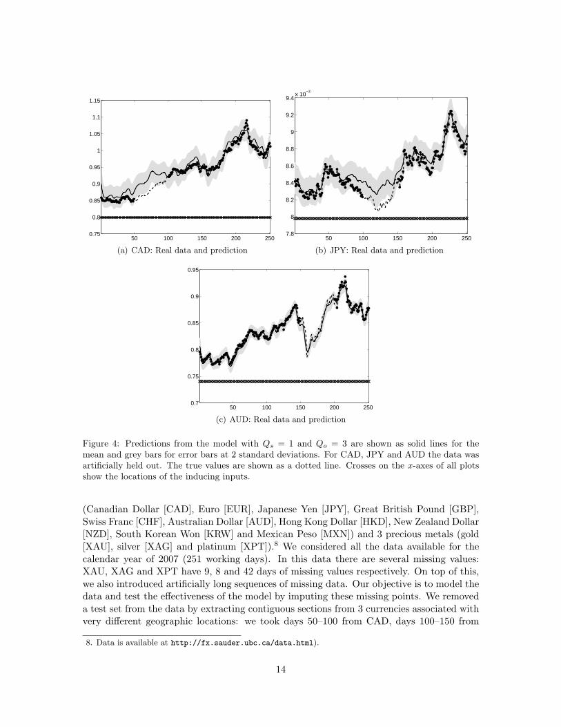
Figure 4: Predictions from the model with Qs = 1 and Qo = 3 are shown as solid lines for themean and grey bars for error bars at 2 standard deviations. For CAD, JPY and AUD the data wasartificially held out. The true values are shown as a dotted line. Crosses on the x-axes of all plotsshow the locations of the inducing inputs.

(Canadian Dollar [CAD], Euro [EUR], Japanese Yen [JPY], Great British Pound [GBP],Swiss Franc [CHF], Australian Dollar [AUD], Hong Kong Dollar [HKD], New Zealand Dollar[NZD], South Korean Won [KRW] and Mexican Peso [MXN]) and 3 precious metals (gold[XAU], silver [XAG] and platinum [XPT]).8 We considered all the data available for thecalendar year of 2007 (251 working days). In this data there are several missing values:XAU, XAG and XPT have 9, 8 and 42 days of missing values respectively. On top of this,we also introduced artificially long sequences of missing data. Our objective is to model thedata and test the effectiveness of the model by imputing these missing points. We removeda test set from the data by extracting contiguous sections from 3 currencies associated withvery different geographic locations: we took days 50–100 from CAD, days 100–150 from

8. Data is available at http://fx.sauder.ubc.ca/data.html).

14

JPY and days 150–200 from AUD. The remainder of the data comprised the training set,which consisted of 3051 points, with the test data containing 153 points. For preprocessingwe removed the mean from each output and scaled them so that they all had unit variance.It seems reasonable to suggest that the fluctuations of the 13 correlated financial time-seriesare driven by a smaller number of latent market forces. We therefore modelled the datawith up to six latent forces which could be noise or smooth GPs. The GP priors for thesmooth latent forces are assumed to have a squared exponential covariance function,

kq(t, t′) =1√2π`2q

exp(− (t− t′)2

2`2q

),

where the hyperparameter `q is known as the lengthscale.We present an example with Q = 4. For this value of Q, we consider all the possible combi-nations of Qo and Qs. The training was performed in all cases by maximizing the variationalbound using the scale conjugate gradient algorithm until convergence was achieved. Thebest performance in terms of achiving the highest value for FV was obtained for Qs = 1 andQo = 3. We compared against the LMC model for different values of the latent functionsin that framework. While our best model resulted in an standardized mean square errorof 0.2795, the best LMC (with Q=2) resulted in 0.3927. We plotted predictions from thelatent market force model to characterize the performance when filling in missing data.In figure 4 we show the output signals obtained using the model with the highest bound(Qs = 1 and Qo = 3) for CAD, JPY and AUD. Note that the model performs better atcapturing the deep drop in AUD than it does at capturing fluctuations in CAD and JPY.

8. Conclusions

We have presented a variational approach to sparse approximations in convolution pro-cesses. Our main focus was to provide efficient mechanisms for learning in multiple outputGaussian processes when the latent function is fluctuating rapidly. In order to do so, wehave introduced the concept of inducing function, which generalizes the idea of inducingpoint, traditionally employed in sparse GP methods. The approach extends the variationalapproximation of Titsias (2009) to the multiple output case. Using our approach we can per-form efficient inference on latent force models which are based around stochastic differentialequations, but also contain a smooth driving force. Our approximation is flexible enoughand has been shown to be applicable to a wide range of data sets, including high-dimensionalones.

Acknowledgements

The authors would like to thank Edwin Bonilla for his valuable feedback with respect to theexam score prediction example and the compiler dataset example. We also thank the authorsof Bonilla et al. (2008) who kindly made the compiler dataset available. DL has been partlyfinanced by Comunidad de Madrid (project PRO-MULTIDIS-CM, S-0505/TIC/0233), andby the Spanish government (CICYT project TEC2006-13514-C02-01 and researh grantJC2008-00219). MA and NL have been financed by a Google Research Award “Mecha-nistically Inspired Convolution Processes for Learning” and MA, NL and MT have been

15

financed by EPSRC Grant No EP/F005687/1 “Gaussian Processes for Systems Identifica-tion with Applications in Systems Biology”.

Appendix A. Variational Inducing Kernels

Recently, a method for variational sparse approximation for Gaussian processes learningwas introduced in Titsias (2009). In this appendix, we apply this methodology to a mul-tiple output Gaussian process where the outputs have been generated through a so calledconvolution process. For learning the parameters of the kernels involved, a lower bound forthe true marginal can be maximized. This lower bound has similar form to the marginallikelihood of the Deterministic Training Conditional (DTC) approximation plus an extraterm which involves a trace operation. The computational complexity grows as O(NDK2)where N is the number of data points per output, D is the number of outputs and K thenumber of inducing variables.

A.1 Computation of the lower bound

Given target data y and inputs X, the marginal likelihood of the original model is given byintegrating over the latent function9

p(y|X) =∫

up(y|u,X)p(u)du.

The prior over u is expressed as

p(u) =∫

λp(u|λ)p(λ)dλ.

The augmented joint model can then be expressed as

p (y, u,λ) = p(y|u)p(u|λ)p(λ).

With the inducing function λ, the marginal likelihood takes the form

p(y|X) =∫

u,λp(y|u,X)p(u|λ)p(λ)dλ du.

Using Jensen’s inequality, we use the following variational bound on the log likelihood,

FV (Z,Θ, φ(λ)) =∫

u,λq(u,λ) log

p(y|u,X)p(u|λ)p(λ)q(u,λ)

dλ du,

where we have introduced q(u,λ) as the variational approximation to the posterior. Fol-lowing Titsias (2009) we now specify that the variational approximation should be of theform

q(u,λ) = p(u|λ)φ(λ).

9. Strictly speaking, the distributions associated to u correspond to random signed measures, in particular,Gaussian measures.

16

We can write our bound as

FV (Z,Θ, φ(λ)) =∫

λφ(λ)

∫up(u|λ)

{log p(y|u) + log

p(λ)φ(λ)

}dudλ.

To compute this bound we first consider the integral

log T(λ,y) =∫

up(u|λ) log p(y|u)du.

Since this is simply the expectation of a Gaussian under a Gaussian we can compute theresult analytically as follows

log T(λ,y) =D∑

d=1

∫up(u|λ)

{−N

2log 2π − 1

2log |Σ| − 1

2tr[Σ−1

(ydy>d − 2ydf>d + fdf>d

)]}du.

We need to compute Eu|λ [fd] and Eu|λ[fdf>d

]. Eu|λ [fd] is a vector with elements

Eu|λ [fd(xn)] =Q∑

q=1

∫ZGd,q(xn − z′)Eu|λ[uq(z′)]dz′.

Assuming that the latent functions are independent GPs, Eu|λ[uq(z′)] = Euq |λq[uq(z′)] =

kuqλq(z′,Z)K−1λq ,λq

(Z,Z)λq. Then

Eu|λ [fd(xn)] =Q∑

q=1

kfdλq(xn,Z)K−1λqλq

(Z,Z)λq.

Eu|λ [fd] can be expressed as

Eu|λ [fd] = KfdλK−1λλλ = αd(X,λ) = αd.

On the other hand, Eu|λ[fdf>d

]is a matrix with elements

Eu|λ [fd(xn)fd(xm)] =Q∑

q=1

∫ZGd,q(xn − z)

∫ZGd,q(xm − z′)Eu|λ[uq(z)uq(z′)]dzdz′ + αd(xn)αd(xm).

With independent GPs the term Eu|λ[uq(z)uq(z′)] can be expressed as

Eu|λ[uq(z)uq(z′)] = kuquq(z, z′)− kuqλq(z,Z)K−1λqλq

(Z,Z)k>uqλq(z′,Z).

In this way

Eu|λ

[fdf>d

]= αdα

>d + Kfdfd −KfdλK−1

λλKλfd = αdα>d + Kdd,

with Kdd = Kfdfd −KfdλK−1λλKλfd .

17

The expression for log T(λ,y) is given as

log T(λ,y) = logN (y|α,Σ)− 12

D∑d=1

tr(Σ−1Kdd

).

The variational lower bound is now given as

FV (Z,Θ, φ) =∫

λφ(λ) log

{N (y|α,Σ) p(λ)φ(λ)

}dλ− 1

2

D∑d=1

tr(Σ−1Kdd

). (9)

A free form optimization over φ(λ) could now be performed, but it is far simpler to reverseJensen’s inequality on the first term, we then recover the value of the lower bound for opti-mized φ(λ) without ever having to explicitly optimise φ(λ). Reversing Jensen’s inequality,we have

FV (Z,Θ) = logN(y|0,KfλK−1

λλKλf + Σ)− 1

2

D∑d=1

tr(Σ−1Kdd

).

The form of φ(λ) which leads to this bound can be found as

φ(λ) ∝ N (y|α,Σ) p(λ)

= N(λ|Σλ|yK−1

λλKλfΣ−1y,Σλ|y)

= N(KλλA−1KλfΣ−1y,KλλA−1Kλλ

),

with Σλ|y =(K−1

λλ + K−1λλKλfΣ−1KfλK−1

λλ

)−1 = KλλA−1Kλλ and A = Kλλ+KλfΣ−1Kfλ.

A.2 Predictive distribution

The predictive distribution for a new test point given the training data is also required.This can be expressed as

p (y∗|y,X,Z) =∫

u,λp(y∗|u)q(u,λ)dλdu =

∫u,λ

p(y∗|u)p(u|λ)φ(λ)dλdu

=∫

up(y∗|u)

[∫λp(u|λ)φ(λ)dλ

]du.

Using the Gaussian form for the φ(λ) we can compute∫λp(u|λ)φ(λ)dλ =

∫λN (u|kuλK−1

λλλ, kuu − kuλK−1λλkλu)

×N(KλλA−1KλfΣ−1y,KλλA−1Kλλ

)dλ

= N(u|kuλA−1KλfΣ−1y, kuu − kuλ

(K−1

λλ −A−1)kλu

).

Which allows us to write the predictive distribution as

p (y∗|y,X,Z) =∫

uN (y∗|f∗,Σ∗)N

(u|µu|λ,Σu|λ

)du = N (y∗|µy∗ ,Σy∗)

with µy∗ = Kf∗λA−1KλfΣ−1y and Σy∗ = Kf∗f∗ −Kf∗λ

(K−1

λλ −A−1)Kλf∗ + Σ∗.

18

A.3 Optimisation of the Bound

Optimisation of the bound (with respect to the variational parameters and the parametersof the covariance functions) can be carried out through gradient based methods. We followthe notation of Brookes (2005) obtaining similar results to Lawrence (2007). This notationallows us to apply the chain rule for matrix derivation in a straight-forward manner. Theresulting gradients can then be combined with gradients of the covariance functions withrespect to their parameters to optimize the model.Let’s define G: = vec G, where vec is the vectorization operator over the matrix G. Fora function FV (Z) the equivalence between ∂FV (Z)

∂G and ∂FV (Z)∂G: is given through ∂FV (Z)

∂G: =((∂FV (Z)

∂G

):)>

. The log-likelihood function is given as

FV (Z,Θ) ∝ −12

log|Σ + KfλK−1λλKλf | −

12

tr[(

Σ + KfλK−1λλKλf

)−1yy>

]− 1

2tr(Σ−1K

),

where K = Kff −KfλK−1λλKλf . Using the matrix inversion lemma and its equivalent form

for determinants, the above expression can be written as

FV (Z,Θ) ∝12

log|Kλλ| −12

log|A| − 12

log|Σ| − 12

tr[Σ−1yy>

]+

12

tr[Σ−1KfλA−1KλfΣ−1yy>

]− 1

2tr(Σ−1K

),

up to a constant. We can find ∂FV (Z)∂θ and ∂FV (Z)

∂Z applying the chain rule to FV (Z,Θ)obtaining expressions for ∂FV (Z)

∂Kff, ∂FV (Z)

∂Kfλand ∂FV (Z)

∂Kλλand combining those with the relevant

derivatives of the covariances wrt Θ, Z and the parameters associated to the model kernels,

∂F∂G:

=[∂FA

∂A:∂A:∂G:

]δGK +

∂FG

∂G:, (10)

where the subindex in FE stands for those terms of F which depend on E, G is either Kff ,Kλf or Kλλ and δGK is zero if G is equal to Kff and one in other case. For conveniencewe have used F ≡ FV (Z,Θ). Next we present expressions for each partial derivative

∂A:∂Σ:

= −(Kλ,fΣ−1 ⊗Kλ,fΣ−1

),

∂FΣ

∂Σ:= −1

2((

Σ−1HΣ−1):)> +

12

((Σ−1K>Σ−1

):)>

∂A:∂Kλ,λ:

= I,∂A:∂Kλ,f :

=(Kλ,fΣ−1 ⊗ I

)+(I⊗Kλ,fΣ−1

)TA,

∂FKf ,f

∂Kf ,f := −1

2Σ−1:

∂FA

∂A:= −1

2(C:)> ,

∂FKλ,f

∂Kλ,f :=((

A−1Kλ,fΣ−1yy>Σ−1)

:)>

+((

K−1λ,λKλ,fΣ−1

):)>

,

∂FKλ,λ

∂Kλ,λ:=

12

((K−1

λ,λ

):)>− 1

2

((K−1

λ,λKλ,fΣ−1Kf ,λK−1λ,λ

):)>

,

where C = A−1 +A−1Kλ,fΣ−1yy>Σ−1Kf ,λA−1, H = Σ−yy>+Kf ,λA−1Kλ,fΣ−1yy>+(Kf ,λA−1Kλ,fΣ−1yy>

)> and TA is a vectorized transpose matrix (Brookes, 2005) and wehave not included its dimensions to keep the notation clearer. We can replace the above

19

expressions in (10) to find the corresponding derivatives, so

∂F∂Kf ,f :

= −12Σ−1:

We also have

∂F∂Kλ,f :

=− 12

(C:)>[(

Kλ,fΣ−1 ⊗ I)

+(I⊗Kλ,fΣ−1

)TA

]+((

A−1Kλ,fΣ−1yy>Σ−1)

:)>

+((

K−1λ,λKλ,fΣ−1

):)>

=((−CKλ,fΣ−1 + A−1Kλ,fΣ−1yy>Σ−1 + K−1

λ,λKλ,fΣ−1)

:)>

.

Finally, results for ∂F∂Kλ,f :

and ∂F∂Σ: are obtained as

∂F∂Kλ,λ:

=− 12

(C:)> +12

((K−1

λ,λ

):)>− 1

2

((K−1

λ,λKλ,fΣ−1Kf ,λK−1λ,λ

):)>

∂F∂Σ:

=12

((Σ−1

(K> −H

)Σ−1

):)>

+12

(C:)>(Kλ,fΣ−1 ⊗Kλ,fΣ−1

).

References

Mauricio Alvarez and Neil D. Lawrence. Sparse convolved Gaussian processes for multi-output regression. In NIPS, volume 21, pages 57–64. MIT Press, Cambridge, MA, 2009.

Mauricio Alvarez, David Luengo, and Neil D. Lawrence. Latent Force Models. In van Dykand Welling (2009), pages 9–16.

Christopher M. Bishop. Pattern Recognition and Machine Learning. Information Scienceand Statistics. Springer, 2006.

Edwin V. Bonilla, Kian Ming Chai, and Christopher K. I. Williams. Multi-task Gaussianprocess prediction. In John C. Platt, Daphne Koller, Yoram Singer, and Sam Roweis,editors, NIPS, volume 20, Cambridge, MA, 2008. MIT Press.

Phillip Boyle and Marcus Frean. Dependent Gaussian processes. In Lawrence Saul, YairWeiss, and Leon Bouttou, editors, NIPS, volume 17, pages 217–224, Cambridge, MA,2005. MIT Press.

Michael Brookes. The matrix reference manual. Available on-line., 2005. http://www.ee.ic.ac.uk/hp/staff/dmb/matrix/intro.html.

Lehel Csato and Manfred Opper. Sparse representation for Gaussian process models. InTodd K. Leen, Thomas G. Dietterich, and Volker Tresp, editors, NIPS, volume 13, pages444–450, Cambridge, MA, 2001. MIT Press.

Theodoros Evgeniou, Charles A. Micchelli, and Massimiliano Pontil. Learning multipletasks with kernel methods. Journal of Machine Learning Research, 6:615–637, 2005.

20

Pei Gao, Antti Honkela, Magnus Rattray, and Neil D. Lawrence. Gaussian process mod-elling of latent chemical species: Applications to inferring transcription factor activities.Bioinformatics, 24:i70–i75, 2008. doi: 10.1093/bioinformatics/btn278.

Pierre Goovaerts. Geostatistics For Natural Resources Evaluation. Oxford University Press,USA, 1997.

David M. Higdon. Space and space-time modelling using process convolutions. In C. An-derson, V. Barnett, P. Chatwin, and A. El-Shaarawi, editors, Quantitative methods forcurrent environmental issues, pages 37–56. Springer-Verlag, 2002.

Andre G. Journel and Charles J. Huijbregts. Mining Geostatistics. Academic Press, London,1978. ISBN 0-12391-050-1.

Neil D. Lawrence. Learning for larger datasets with the Gaussian process latent variablemodel. In Marina Meila and Xiaotong Shen, editors, AISTATS 11, San Juan, PuertoRico, 21-24 March 2007. Omnipress.

Neil D. Lawrence, Matthias Seeger, and Ralf Herbrich. Fast sparse Gaussian process meth-ods: The informative vector machine. In Sue Becker, Sebastian Thrun, and Klaus Ober-mayer, editors, NIPS, volume 15, pages 625–632, Cambridge, MA, 2003. MIT Press.

Neil D. Lawrence, Guido Sanguinetti, and Magnus Rattray. Modelling transcriptional reg-ulation using Gaussian processes. In Bernhard Scholkopf, John C. Platt, and ThomasHofmann, editors, NIPS, volume 19, pages 785–792. MIT Press, Cambridge, MA, 2007.

Miguel Lazaro-Gredilla and Anıbal Figueiras-Vidal. Inter-domain Gaussian processes forsparse inference using inducing features. In NIPS, volume 22, pages 1087–1095. MITPress, Cambridge, MA, 2010.

Michael A. Osborne, Alex Rogers, Sarvapali D. Ramchurn, Stephen J. Roberts, andNicholas R. Jennings. Towards real-time information processing of sensor network datausing computationally efficient multi-output Gaussian processes. In Proceedings of theInternational Conference on Information Processing in Sensor Networks (IPSN 2008),2008.

Joaquin Quinonero Candela and Carl Edward Rasmussen. A unifying view of sparse approx-imate Gaussian process regression. Journal of Machine Learning Research, 6:1939–1959,2005.

Carl Edward Rasmussen and Christopher K. I. Williams. Gaussian Processes for MachineLearning. MIT Press, Cambridge, MA, 2006. ISBN 0-262-18253-X.

Matthias Seeger, Christopher K. I. Williams, and Neil D. Lawrence. Fast forward selectionto speed up sparse Gaussian process regression. In Christopher M. Bishop and Brendan J.Frey, editors, Proceedings of the Ninth International Workshop on Artificial Intelligenceand Statistics, Key West, FL, 3–6 Jan 2003.

21

Edward Snelson and Zoubin Ghahramani. Sparse Gaussian processes using pseudo-inputs.In Yair Weiss, Bernhard Scholkopf, and John C. Platt, editors, NIPS, volume 18, Cam-bridge, MA, 2006. MIT Press.

Yee Whye Teh, Matthias Seeger, and Michael I. Jordan. Semiparametric latent factormodels. In Robert G. Cowell and Zoubin Ghahramani, editors, AISTATS 10, pages333–340, Barbados, 6-8 January 2005. Society for Artificial Intelligence and Statistics.

Michalis K. Titsias. Variational learning of inducing variables in sparse Gaussian processes.In van Dyk and Welling (2009), pages 567–574.

David van Dyk and Max Welling, editors. AISTATS, Clearwater Beach, Florida, 16-18April 2009. JMLR W&CP 5.

22