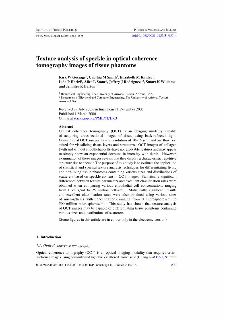
INSTITUTE OF PHYSICS PUBLISHING PHYSICS IN MEDICINE AND BIOLOGY

Phys. Med. Biol. 51 (2006) 1563–1575 doi:10.1088/0031-9155/51/6/014

Texture analysis of speckle in optical coherencetomography images of tissue phantoms

Kirk W Gossage1, Cynthia M Smith1, Elizabeth M Kanter1,Lida P Hariri1, Alice L Stone1, Jeffrey J Rodriguez1,2, Stuart K Williams1

and Jennifer K Barton1,2

1 Biomedical Engineering, The University of Arizona, Tucson, Arizona, USA2 Department of Electrical and Computer Engineering, The University of Arizona, Tucson,Arizona, USA

Received 29 July 2005, in final form 11 December 2005Published 1 March 2006Online at stacks.iop.org/PMB/51/1563

AbstractOptical coherence tomography (OCT) is an imaging modality capableof acquiring cross-sectional images of tissue using back-reflected light.Conventional OCT images have a resolution of 10–15 µm, and are thus bestsuited for visualizing tissue layers and structures. OCT images of collagen(with and without endothelial cells) have no resolvable features and may appearto simply show an exponential decrease in intensity with depth. However,examination of these images reveals that they display a characteristic repetitivestructure due to speckle.The purpose of this study is to evaluate the applicationof statistical and spectral texture analysis techniques for differentiating livingand non-living tissue phantoms containing various sizes and distributions ofscatterers based on speckle content in OCT images. Statistically significantdifferences between texture parameters and excellent classification rates wereobtained when comparing various endothelial cell concentrations rangingfrom 0 cells/ml to 25 million cells/ml. Statistically significant resultsand excellent classification rates were also obtained using various sizesof microspheres with concentrations ranging from 0 microspheres/ml to500 million microspheres/ml. This study has shown that texture analysisof OCT images may be capable of differentiating tissue phantoms containingvarious sizes and distributions of scatterers.

(Some figures in this article are in colour only in the electronic version)

1. Introduction

1.1. Optical coherence tomography

Optical coherence tomography (OCT) is an optical imaging modality that acquires cross-sectional images using near-infrared light backscattered from tissue (Huang et al 1991, Schmitt

0031-9155/06/061563+13$30.00 © 2006 IOP Publishing Ltd Printed in the UK 1563

1564 K W Gossage et al

1999). Standard resolution OCT systems have a typical axial resolution of 10–15 µm, andare therefore not suited for visualizing sub-cellular structures. Even in ultra-high resolution(2–5 µm) OCT systems, phase distortions in turbid media can limit resolution at depths greaterthan a few hundred microns. Therefore, identification of tissue type and pathology with OCTimages is generally based upon visualization of layers and multi-cellular structures within thesample.

1.2. Speckle in OCT images

The optical phenomenon known as speckle is well known and characterized for opticallyrough surfaces illuminated with coherent light. Recently, speckle in OCT images was studiedby Schmitt et al (1999). His paper defines two types of speckle that appear in OCT images.The first is due to interference from multiply scattered photons. This type of ‘chance’ speckleis typically a single pixel wide, random, and can therefore be reduced by averaging. Thesecond type of speckle results from interference of the wavefronts from multiple scattererswithin the OCT focal volume and is typically much larger. This ‘inherent’ larger speckleis constant from image to image at a given location. Speckle is often considered to be asource of noise due to its apparent degradation of image quality and visibility of boundaries.Several methods to reduce speckle in OCT images through hardware modifications and digitalimage post-processing have been published (Bashkansky and Reintjes 2000, Iftimia et al2003, Rogowska et al 2003). Results from one such hardware method, known as angularcompounding, can substantially increase image SNR and improve boundary detection byreducing speckle (Bashkansky and Reintjes 2000, Iftimia et al 2003). Adaptive filteringtechniques have also been shown to be useful for enhancing layer boundaries in cartilage byreducing the effects of speckle (Rogowska et al 2003). However, since ‘inherent’ speckle inOCT images is dependent upon the distribution of scatterers within the sample the specklepattern should differ between tissue types that have different scatterer distributions. Therefore,the possibility exists that speckle may provide a unique signature indicative of tissue type anddisease state.

1.3. Texture analysis

Texture in OCT images is a result of spatial deviations in intensity. If intensity valuesare viewed as elevations, then texture can be seen as a description of surface roughness(Oberholzer et al 1996). Texture analysis has been explored for many imaging modalities suchas ultrasound, MRI, CT, fluorescence microscopy and light microscopy, and used to assessimages from a variety of tissue types such as eyes (Thijssen et al 1991, Ursell et al 1998),prostate (Basset et al 1993), colon tissue (Atlamazoglou et al 2001) and chromatin in advancedprostate cancer tissue (Yogesan et al 1996). OCT offers a combination of minimally-invasiveimaging, micron scale resolution and millimetre depth of penetration unique among imagingmodalities. Texture analysis of speckle could extend OCT’s sensitivity to sub-resolutionchanges in tissue. Our previous work has demonstrated the feasibility of using texture analysisof speckle in OCT images for tissue classification (Gossage et al 2003). Excellent classificationresults were obtained during binary comparison of different tissue types (e.g. 97.9% correctclassification of mouse skin versus mouse fat) and good classification results were seen duringcomparison of normal and diseased tissue, even though the images showed no visible structurebeyond the speckle pattern (76.3% correct classification of normal versus diseased mouselung tissue). Texture analysis has the potential to assist in minimally-invasive detection anddiagnosis of diseases such as skin, oral and cervical cancer. This technique draws information

Texture analysis of speckle in optical coherence tomography images of tissue phantoms 1565

from changes in backscattered light that result from variation in size and concentration ofscatterers in tissues, therefore having the potential to identify early stage disease prior to tissuearchitecture changes.

Based upon these encouraging initial results, a more comprehensive study was undertakenusing well-controlled tissue phantoms. In this paper, we present the results of texture analysisof speckle in OCT images of living and non-living phantoms. We hypothesized that textureanalysis feature values and correct classification rates would vary in a regular fashion withchanges in the number and size of scatters in the phantoms.

2. Materials and methods

Two types of tissue phantoms were prepared and imaged in this study. The first consistedof various sizes and concentrations of silica microspheres suspended in gelatin. The secondcontained bovine aorta endothelial cells (BAEC) in gelled collagen.

2.1. Gelatin/microsphere tissue phantoms

Three different sizes of microspheres were used: 0.49 µm, 1.59 µm and 3.01 µm. These sizeswere chosen because they approximated the size range of cell nuclei and mitochondria, andwere well below the resolution of our OCT system. Silica microspheres were used becausetheir index of refraction (1.37) was similar to that of the cell nuclei. Each gelatin phantomcontained one of four concentrations (2.5, 25, 100, or 500 million/ml) of a single microspheresize. Plain gelatin was also imaged, for a total of 13 different gelatin phantoms.

The gelatin solution was made by mixing a 7.4 g packet of unflavoured gelatin with 290 mlof boiling water. An additional 65 ml of cold water was added to the solution once the gelatinhad completely dissolved. The gelatin solution was allowed to cool to room temperature (butnot set) before the microspheres were added and the mixture gently stirred. The mixture waspipetted into a standard 48 well plate to a thickness of 4–5 mm. Three to four gels weremade for each gelatin phantom type. The gels were covered with paraffin film, refrigeratedfor 40 min, then immediately removed and imaged. The index of refraction of gelatin wasmeasured using OCT, by dividing the measured optical pathlength of a calibrated cuvette filledwith gelatin by the known 1 mm physical pathlength. The attenuation coefficient (µt) of plaingelatin and gelatin/microsphere samples was estimated by measuring the signal obtained froma reflector at a known depth in the sample, relative to the signal measured using a distilledwater sample, and computed by Mie theory using the known size and index of refraction ofmicrospheres and index of refraction of gelatin (assuming no attenuation in the gelatin).

2.2. Collagen/BAEC tissue phantoms

A 3.5 mg ml−1 collagen I solution was obtained by combining three parts purified rat-tailcollagen I (4.7 mg ml−1; BD Biosciences, Bedford, MA) with one part 4X Dulbecco’sModified Eagle’s Medium. The solution was then brought to a pH of 7.0–7.4 by the additionof 1 M NaOH. Primary isolate bovine aortic endothelial cells (BAEC) passage 2–7 wereadded in concentrations of 2.5 or 25 million BAEC/ml collagen I. Including plain collagen,three different types of collagen phantoms were created. Individual gels (20 of each type)were created by pipetting the collagen/BAEC mixture into standard 48 well plates. The wellplate was then transferred to a 37 ◦C incubator with 5% CO2. After 15 min, the constructswere bathed in warm cell culture media. The collagen gels remained in the incubator untilimmediately before use. The concentration of BAEC were limited to 25 million because with

1566 K W Gossage et al

higher concentrations the cells assume a hyper-plastic behaviour and may not lengthen orproliferate as expected in vivo.

2.3. OCT system

The OCT system used in this study was similar to one described previously (Gossage et al 2003,Izatt et al 1997). The system was based on a single mode fibre-based Michelson interferometerand used a super luminescent diode light source with a 1300 nm centre wavelength, 60 nmbandwidth and a power of 800 µW (Superlum, Moscow, Russia). Light was carried tothe sample arm by a 9 µm core (SMF-28) fibre, collimated into a beam with an 8.1 mmdiameter and focused onto the sample with a 50 mm focal length lens. This gave the systeman approximate numerical aperture of 0.081. Light was also carried to the reference armthrough the same type of fibre. The reference arm optical pathlength was modulated using agalvo-mounted retroreflecting mirror. The reflected signal from the two arms combined andwas detected by a single element InGaAs detector (New Focus, San Jose, CA), coherentlydemodulated, and digitized by a 12-bit data acquisition (DAQ) board. The axial and lateralresolutions of the system in air were 15 and 14 µm, respectively. The integration time of thesystem was 0.14 ms/pixel and the noise floor of the system was measured to be—106 dB.

2.4. Imaging of the gels

All OCT images were 1 mm in optical depth by 1 mm in lateral extent and contained 512 ×512 pixels. Ten images were taken from each gel. 2 × 2 blocks of pixels were averagedto create images consisting of 256 × 256 pixels to reduce random detector noise and singlepixel speckle. The pixel size was thus 4 µm square, well below the resolution of the OCTsystem. The top of the image was positioned just beneath the air–gel interface. The interfacewas avoided because the strong signal from this large index of refraction mismatch woulddominate the signals of interest within the phantoms. All system settings (e.g. gain) remainedfixed during the entire imaging experiment. Image intensity values were scaled to an 8-bitgrey-level image and the scaled image was further processed to enhance speckle contrast andreduce the effects of system signal strength variations through a grey-scale transformationcommon to texture analysis studies known as histogram equalization. Ten 64 × 64 pixel‘regions’ were selected from each image. The evenly overlapping regions covered the entire1 mm lateral extent of the images (256 pixels), but only the depths between 0.25 mm and0.5 mm (64 pixels) which surrounded the focal depth. The regions were analysed using thetexture analysis described in the following section. Table 1 summarizes the gel types, numberof gels, number of images and number of regions analysed in this study.

2.5. Texture analysis

Two types of texture analysis features were extracted from OCT images of the tissue phantoms.The first type was obtained from spatial grey-level dependency matrices (SGLDMs), also calledco-occurrence matrices (Basset et al 1993, Atlamazoglou et al 2001, Yogesan et al 1996).A SGLDM is a spatial histogram of an image that quantifies the distribution of grey-scalevalues. SGLDMs were computed from the estimation of the second-order joint conditionalprobability density functions, sθ (i, j |d, θ ) (Rogowska et al 2003). Each sθ (i, j |d, θ ) was theprobability of a pixel with a grey-level value (i) being (d) pixels away from a pixel of grey-levelvalue (j) in the (θ ) direction. If the image contained Ng grey levels, then an Ng × Ng matrix,sθ (i, j |d, θ ), was created for each direction (θ ) for a given distance (d). In this study, the

Texture analysis of speckle in optical coherence tomography images of tissue phantoms 1567

Table 1. Numbers of gels, images and regions for each phantom type.

Phantom No of gels No of images No of regions

Gelatin/MicrospherePlain gelatin 4 40 4000.49 µm @ 2.5 million/ml 4 40 4000.49 µm @ 25 million/ml 4 40 4000.49 µm @ 100 million/ml 3 30 3000.49 µm @ 500 million/ml 3 30 3001.59 µm @ 2.5 million/ml 4 40 4001.59 µm @ 25 million/ml 4 40 4001.59 µm @ 100 million/ml 3 30 3001.59 µm @ 500 million/ml 3 30 3003.01 µm @ 2.5 million/ml 4 40 4003.01 µm @ 25 million/ml 4 40 4003.01 µm @ 100 million/ml 3 30 3003.01 µm @ 500 million/ml 3 30 300

Collagen/BAECPlain collagen 20 200 20002.5 million/ml 20 200 200025 million/ml 20 200 2000

direction took on four values, θ = 0◦, 45◦, 90◦ and 135◦, but distance was fixed at 1 pixel,so four SGLDMs were computed for each region. Five textural features were then calculatedfrom each SGLDM including energy, entropy, correlation, local homogeneity and inertia (alsocalled contrast), giving a total of 20 SGLDM features for each region. The SGLDM featuresfor a particular angle are calculated as follows:

Energy =L−1∑

i=0

L−1∑

j=0

[sθ (i, j |d)]2 (1)

Entropy =L−1∑

i=0

L−1∑

j=0

sθ (i, j |d) log(sθ (i, j |d)) (2)

Correlation =∑L−1

i=0

∑L−1j=0 (i − µx)(j − µy)sθ (i, j |d)

σxσy

(3)

Local-Homogeneity =L−1∑

i=0

L−1∑

j=0

1

1 + (i − j)2sθ (i, j |d) (4)

Inertia =L−1∑

i=0

L−1∑

j=0

(i − j)2sθ (i, j |d) (5)

where sθ(i, j |d) is the (i, j)th element of the SGLDM for distance d, L is the number of greylevels in the image, and where

µx =L−1∑

i=0

i

L−1∑

j=0

sθ (i, j |d) (6)

1568 K W Gossage et al

µy =L−1∑

i=0

j

L−1∑

j=0

sθ (i, j |d) (7)

σx =L−1∑

i=0

(i − µx)2

L−1∑

j=0

sθ (i, j |d) (8)

σy =L−1∑

i=0

(j − µy)2

L−1∑

j=0

sθ (i, j |d). (9)

The five features are different means of quantifying, in a single number, the distributionof grey-scale values within an image. The energy parameter is calculated by summing thesquare of each value in the SGLDM matrices. This gives high feature values to image regionsthat have only a small number of intensity distribution patterns. This parameter is largein homogeneous scenes because sθ (i, j |d, θ ) contains only a few but relatively high values.Entropy is computed by summing the multiplication of each sθ (i, j |d, θ ) value by the logof the sθ (i, j |d, θ ) value. This feature gives higher values to regions that contain a widevariety of intensity distributions. The amplification of small sθ (i, j |d, θ ) values, through thelog function, causes inhomogeneous images to have high entropy values. The correlationparameter quantifies the grey-level dependence within pixels relative to each other. Thisparameter is high in images with uniform grey-scale values. Local homogeneity gives ahigher weight to sθ (i, j |d, θ ) values with similar shaded pixels neighbouring one another.This is accomplished by scaling such that sθ (i, j |d, θ ) values nearer to the matrix diagonalreceive a proportionally higher weight than those values further from the diagonal. In otherwords, local homogeneity emphasizes images with lower contrast values. In contrast to localhomogeneity, inertia provides higher feature values to regions whose sθ (i, j |d, θ ) values arefar from the matrix diagonal. In other words, inertia provides higher weights to sθ (i, j |d, θ )values that represent image pixels with large intensity differences being in close proximity,i.e. regions of high contrast.

The second category of features was derived from the magnitude of the complex two-dimensional Fourier transform of the region. The 2D FFT of the tissue image was calculatedand the magnitude data stored in a matrix where the dc frequency component was representedby the origin of the axis in the frequency domain. The 2D FFT was then divided into fourconcentric square rings based on frequency (with the outermost ring representing the highestspatial frequency content), see figure 1. The magnitudes of the spatial frequencies in eachring were integrated and normalized to the total signal magnitude, such that each feature valuerepresented the percentage of signal within a certain range of spatial frequencies. Imagesthat contained large relatively homogeneous areas would have high values for FFT featuresassociated with lower spatial frequency rings. On the other hand, images with lots of smallerinhomogeneous areas would have higher values in the FFT features that corresponded to higherspatial frequency rings. The four spatial frequency parameters, together with the SGLDMfeatures, created a 24-element feature vector for each region.

2.6. Classification algorithm

A classification software program was developed based on a Round Robin (Leave-One-Out)algorithm patterned after Manly (Manly, 1997). The program uses a Mahalanobis distanceclassifier. Use of the Mahalanobis distance permitted the wide range of scales and distributionsof the SGLDM and FFT features to be normalized, so that those features could be used in

Texture analysis of speckle in optical coherence tomography images of tissue phantoms 1569

Figure 1. Diagram illustrating how the N × N 2D discrete Fourier transform space of an OCTimage was partitioned into four regions, each used to compute a texture feature. Fx and Fz arespatial frequencies in the lateral and axial dimensions, respectively.

combination to classify the phantoms. Because of the large size of the feature pool, an unequal-variance student t-test method was used to rank the features. Five classification schemeswere compared to determine which provided the highest correct classification rate. In mostclassification schemes, only seven features were used with the most significant differencesbetween the two phantoms being compared (the ‘top’ features). The schemes used: (1) onetexture feature from the top seven, (2) any two features from the top seven, (3) any threefeatures from the top seven, (4) any combination of one through seven features of the topseven and (5) any combination of three of all 24 features (ignoring t-test results).

An example classification experiment is illustrated as follows. A comparison of the plaingelatin and the gelatin/microsphere (0.49 µm@2.5 million/ml) phantoms involves evaluating400 regions for each phantom type. Using the second classification scheme listed above, thefirst of the 800 total regions was removed. The remaining 799 regions were used to determinewhich combination of two of the top seven features sorted the remaining 799 regions with thehighest correct classification rate. This feature pair was used to classify the ‘unknown’ regionto the group with the shortest Mahalanobis distance (Gossage et al 2003). The region wasthen placed back into the pool and the next of the 800 regions was removed and the processrepeated.

3. Results

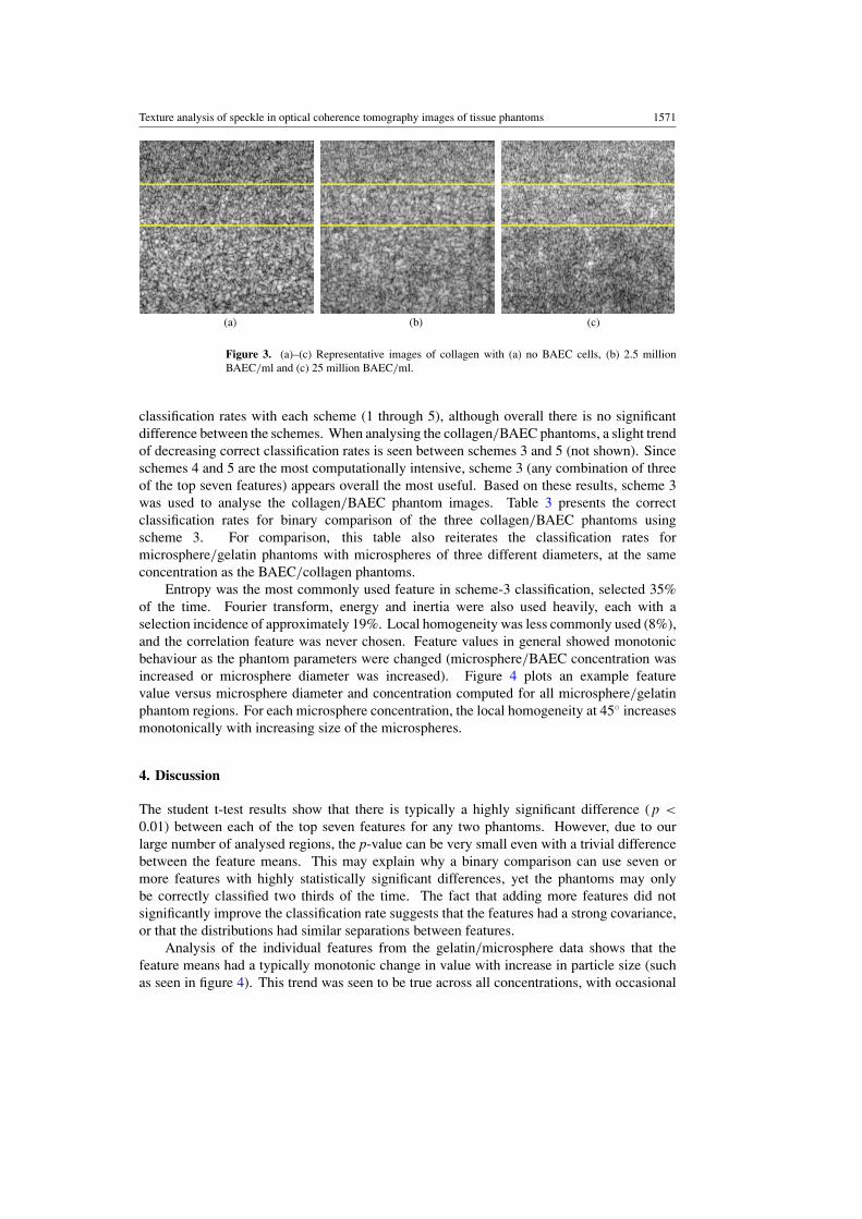
Figures 2(a)–(d) show representative images from four of the gelatin/microsphere phantoms((a), (b), (c) 500 million/ml concentration of 0.49 µm, 1.59 µm and 3.01 µm diametermicrospheres, respectively, and (d) plain gelatin). Figures 3(a)–(c) present representativeimages from the three collagen/BAEC phantoms ((a) no cells, (b) 2.5 million/ml BAECand (c) 25 million/ml BAEC). The horizontal lines delineate the portion of the image fromwhich the 64 × 64 pixel regions were selected. Overall, the images appear relatively free ofsingle pixel speckle and random noise. The images are dominated by multi-pixel speckle;as expected no image structures can be seen since the microspheres and cells are smallerthan the OCT system resolution. Differences in mean intensity, contrast and possibly speckle

1570 K W Gossage et al

(a) (b)

(c) (d)

Figure 2. (a)–(d) Representative images from gelatin/microsphere tissue phantoms.(a) 0.49 µm@500 million/ml, (b) 1.59 µm@500 million/ml, (c) 3.01 µm@500 million/mland (d) plain gelatin.

size can be seen. At lower concentrations of the largest microsphere diameter, occasionalbright dots were seen in the images (not shown) that may be a result of light backscatteredfrom isolated microspheres. For the samples containing 0.49 µm diameter microspheres at allconcentrations, and for all size microspheres at the lowest concentration (2.5 million/ml) theattenuation coefficient of the sample was very small and was dominated by µt of gelatin,0.027 mm−1. For samples containing 1.59 µm diameter microspheres, µt increased to0.34 mm−1 at the largest concentration (500 million/ml), and for samples containing3.01 µm diameter microspheres µt was 4.2 mm−1 at this concentration. Only in this lastcase—the largest diameter and highest concentration of microspheres—was attenuation withinthe 0.25 mm deep analysed region significant.

Table 2 lists the results of the five different classification schemes for all binarygelatin/microsphere tissue phantom comparisons. A slight trend is seen of increasing correct

Texture analysis of speckle in optical coherence tomography images of tissue phantoms 1571

(a) (b) (c)

Figure 3. (a)–(c) Representative images of collagen with (a) no BAEC cells, (b) 2.5 millionBAEC/ml and (c) 25 million BAEC/ml.

classification rates with each scheme (1 through 5), although overall there is no significantdifference between the schemes. When analysing the collagen/BAEC phantoms, a slight trendof decreasing correct classification rates is seen between schemes 3 and 5 (not shown). Sinceschemes 4 and 5 are the most computationally intensive, scheme 3 (any combination of threeof the top seven features) appears overall the most useful. Based on these results, scheme 3was used to analyse the collagen/BAEC phantom images. Table 3 presents the correctclassification rates for binary comparison of the three collagen/BAEC phantoms usingscheme 3. For comparison, this table also reiterates the classification rates formicrosphere/gelatin phantoms with microspheres of three different diameters, at the sameconcentration as the BAEC/collagen phantoms.

Entropy was the most commonly used feature in scheme-3 classification, selected 35%of the time. Fourier transform, energy and inertia were also used heavily, each with aselection incidence of approximately 19%. Local homogeneity was less commonly used (8%),and the correlation feature was never chosen. Feature values in general showed monotonicbehaviour as the phantom parameters were changed (microsphere/BAEC concentration wasincreased or microsphere diameter was increased). Figure 4 plots an example featurevalue versus microsphere diameter and concentration computed for all microsphere/gelatinphantom regions. For each microsphere concentration, the local homogeneity at 45◦ increasesmonotonically with increasing size of the microspheres.

4. Discussion

The student t-test results show that there is typically a highly significant difference ( p <

0.01) between each of the top seven features for any two phantoms. However, due to ourlarge number of analysed regions, the p-value can be very small even with a trivial differencebetween the feature means. This may explain why a binary comparison can use seven ormore features with highly statistically significant differences, yet the phantoms may onlybe correctly classified two thirds of the time. The fact that adding more features did notsignificantly improve the classification rate suggests that the features had a strong covariance,or that the distributions had similar separations between features.

Analysis of the individual features from the gelatin/microsphere data shows that thefeature means had a typically monotonic change in value with increase in particle size (suchas seen in figure 4). This trend was seen to be true across all concentrations, with occasional

1572 K W Gossage et al

Table 2. Classification results (% correct) for binary gelatin/microsphere gel comparisons. Thecolumn headings denote the type of classification scheme used. 7-1, 7-2 and 7-3: all possiblecombinations of 1, 2, or 3 of the top seven features, respectively. 7-ALL: all possible combinationsof any number of the top seven features. 24–3: all possible combinations of 3 of all 24 features.

Comparison 7-1 7-2 7-3 7-ALL 24-3

Plain versus 0.492.5 million/ml 61.3 65.1 67.3 66.3 65.125 million/ml 63.2 64.7 66.3 66.5 58.3100 million/ml 96.3 96.1 95.8 96.0 96.8500 million/ml 95.1 95.1 95.0 94.1 96.1

Plain versus 1.592.5 million/ml 64.2 68.2 69.6 69.0 70.325 million/ml 64.6 67.6 68.7 70.8 74.8100 million/ml 81.6 85.3 86.3 85.5 84.8500 million/ml 96.6 97.5 98.1 98.8 98.6

Plain versus 3.012.5 million/ml 71.6 71.3 70.0 70.0 73.125 million/ml 80.2 80.5 78.7 81.3 83.7100 million/ml 81.8 87.3 87.3 89.1 85.3500 million/ml 99.6 99.5 99.3 99.3 100.0

0.49 versus 1.592.5 million/ml 59.6 66.3 66.6 66.7 71.225 million/ml 69.6 73.8 72.8 72.8 79.4100 million/ml 89.1 89.1 89.2 90.0 90.6500 million/ml 91.0 92.0 94.1 94.1 92.0

0.49 versus 3.012.5 million/ml 78.0 77.0 77.6 78.0 76.325 million/ml 82.3 83.7 85.6 82.6 86.2100 million/ml 92.1 94.3 95.8 95.6 98.6500 million/ml 96. 96.6 97.5 98.6 100.0

1.59 versus 3.012.5 million/ml 67.3 68.0 65.3 67.8 70.725 million/ml 63.1 65.7 65.1 67.6 66.3100 million/ml 75.0 74.5 70.7 72.5 75.3500 million/ml 76.1 85.0 83.5 86.0 95.5

Table 3. Classification results (% correct) for binary comparison of BAEC/collagen phantoms andmicrosphere/gelatin phantoms with microspheres of various diameters at the same concentration.Classification based on the third (7-3) scheme.

Comparison BAEC 0.49 µm 1.59 µm 3.01 µm

Plain versus 2.5 million/ml 65.4 67.3 69.6 70.0Plain versus 25 million/ml 91.5 66.3 68.7 78.72.5 million/ml versus 25 million/ml 89.1 67.0 76.6 71.2

deviation in some features at the highest concentration and largest size of microsphere,potentially due to attenuation within the analysed region. A monotonic trend in featuremean is important because analogies may be drawn to the way that pathologists differentiate

Texture analysis of speckle in optical coherence tomography images of tissue phantoms 1573

Figure 4. Example computed feature (local homogeneity at 45◦) values as a function ofmicrosphere diameter and concentration in microsphere/gelatin phantoms.

normal from abnormal tissue types, by noting monotonic changes in the sizes and distributionsof cellular constituents.

In the microsphere/gelatin phantom data, there is a clear improvement in correctclassification of the size of the microspheres as the concentration of the microspheres increases(table 2). This result is expected because the more scatterers in a sample, the more likely therewill be multiple scatterers per volume element and thus speckle. Since our imaging systemhas a resolution volume of approximately 14 × 14 × 16 µm3, there are ∼319 million volumeelements per ml in the gels. If the only scatterers in these gels are microspheres, then onlygels with concentrations of 500 million/ml of microspheres will consistently contain speckle.However, images of plain gelatin still show speckle. Gelatin primarily consists of variousmolecular weight peptides of hydrolyzed collagen. These concentrated, yet extremely small,scatterers explain both gelatin’s near transparency and presence of speckle pattern in OCTimages. Modulation of the gelatin speckle pattern by light backscattered from one or moremicrospheres appears to cause differentiation of the set of texture features.

In the gelatin/microsphere phantoms, we also found that correct classification of theconcentration of microspheres improved as the size of the microspheres increased (data notshown). While all of the microsphere sizes chosen for this experiment were well below theresolution of the system, the larger microspheres could appear as bright spots in the images.We believe the ability to see these ‘structures’ improves the success of the classificationalgorithm. Also, by increasing the size of the microspheres, but keeping the concentrationconstant, the likelihood of having multiple scatterers per volume element increases, perhapscausing greater alterations in the speckle pattern.

The results from table 3 (BAEC/collagen suspensions) show interesting behaviour whencompared to the gelatin results. When looking at the results classifying plain collagen versus2.5 or 25 million cells per ml collagen, it can be seen that the collagen/BAEC experimentshad comparable or better results than the same concentration experiments performed withgelatin/microsphere phantoms. One explanation for this finding is that the collagen/BAECphantoms are much more complex than the gelatin/microsphere phantoms. The addition ofcells to a matrix introduces many more types and shapes of scattering structures (i.e. nucleus,cell walls, organelles) than does the addition of microspheres (which modelled the nucleus

1574 K W Gossage et al

or mitochondria as a homogeneous sphere). Logically, the classification results improve withan increase in concentration difference. Thus 25 million/ml versus plain did better than25 million/ml versus 2.5 million/ml, which in turn did better than 2.5 million/ml versusplain.

24 texture analysis features were computed for each region and the three features thatprovided the highest correct classification rate were selected by our software to classify eachunknown sample. Despite the empirical nature of our analysis, examination of the changes infeature values with an increase in scatterer size or concentration in the microsphere/gelatinphantoms reveals interesting trends in speckle parameters. A notable increase in localhomogeneity was observed as either scatterer concentration or size increased, conversely,a decrease was seen for inertia. This observation is in accordance with previous resultsfrom our group, which show that speckle contrast decreases as a function of the number ofscatterers (Tkaczyk et al 2002). Lowering of contrast may also explain changes in the FFTfeature values. A large increase in the value of the lowest frequency FFT feature occurred withincreasing scatterer size and concentration, whereas a decrease occurred for the second lowestFFT feature. The third and forth (the highest) FFT features contained only a small percentageof the total spatial frequency magnitude for any phantom. These results clearly indicate thatlow spatial frequency content increases with increase in scatterer size or concentration, whichwould be expected if image contrast decreased. The correlation feature value was similar forall phantoms and was never chosen by the classification program. The insensitivity of thisfeature may be due to the fact none of the images had regions of uniform grey-scale values(which would lead to high values of correlation). Entropy, which gives higher weight toimages with random or irregular patterns, was chosen most frequently for classification andappears to be the most useful texture parameter in these studies. This result coincides wellwith the random irregular nature of the speckle seen in the OCT images of the tissue phantoms.

5. Conclusion

Even though our OCT system does not have cellular resolution, texture analysis showspromise in being able to quantify cellularity in tissue. Since the speckle size is a functionof the resolution of the system, it may be possible to perform texture analysis of subcellularcomponents using ultrahigh resolution OCT systems. These experiments show that many ofthe texture features evaluated vary with both size and concentration of scatterers in a sample ina generally monotonic fashion (e.g., figure 4). The classification algorithm achieved good toexcellent results comparing biological and non-biological phantoms containing different sizesand concentrations of scatterers.

Despite being able to obtain promising classification results and seeing distinct trends withthis image analysis technique, texture analysis of OCT images has its limitations. One suchlimitation is the change in speckle size with depth relative to the focal point. Previous workillustrated that speckle size in OCT is a function of the OCT system resolution (Tkaczyk et al2002). Therefore, the lateral speckle size is a function of the spot size of the beam, variationsin which were minimized by using long depth of focus optics in the sample arm, and the axialspeckle size is a function of the coherence length of the light, which is influenced by scatteringand dispersion. Even in homogeneous samples of gelatin, the relative speckle size can be seento change with depth (see figure 2). This makes analysing inhomogeneous samples difficultbecause the changes in speckle based on tissue properties would need to be de-coupled fromthe speckle changes based on imaging depth. The focal point in our system was kept fixedwith respect to the surface of the sample and all regions analysed came from the same depthin the image so that depth effects on speckle would be minimized. Another concern with this

Texture analysis of speckle in optical coherence tomography images of tissue phantoms 1575

method is the effect of system parameters on speckle. As noted by others (Schmitt et al 1999),the speckle characteristics vary with system parameters such as light spectrum and systemnumerical aperture. This means that a very stable system is required to perform any real-timebased or repeated measurements. A solid plastic reference was used during the study. Imagesof the plastic were taken before each imaging session, and the speckle analysed, to ensure thatthe system parameters remained constant throughout the study. While texture analysis hasits limitations, it has potential to help characterize tissue type or health in samples that maycontain no apparent structural features in OCT images.

Acknowledgments

This work was partially supported by grants from The Whitaker Foundation and the NationalInstitutes of Health (CA83148).

References

Atlamazoglou V, Yova D, Kavavtzas N and Loukas S 2001 Texture analysis of fluorescence microscopic images ofcolonic tissue sections Med. Biol. Eng. Comput. 39 145–51

Bashkansky M and Reintjes J 2000 Statistics and reduction of speckle in optical coherence tomography Opt. Lett. 25545–7

Basset O, Sun Z, Mestas J L and Gimenez G 1993 Texture analysis of ultrasonic images of the prostate by means ofco-occurrence matrices Ultrasonic Imaging 15 218–37

Gossage K W, Tkaczyk T S, Rodriguez J J and Barton J K 2003 Texture analysis of optical coherence tomographyimages: feasibility for tissue classification J. Biomed. Opt. 8 570–5

Huang D, Swanson E A, Lin C P, Schuman J S, Stinson W G, Chang W, Hee M R, Flotte T, Gregory K,Puliafito C A and Fujimoto J G 1991 Optical coherence tomography Science 254 1178–81

Iftimia N, Bouma B E and Tearney G J 2003 Speckle reduction in optical coherence tomography by ‘path lengthencoded’ angular compounding J. Biomed. Opt. 8 260–3

Izatt J A, Kulkarni M D, Yazdanfar S, Barton J K and Welch A J 1997 In vivo bidirectional color Doppler flowimaging of picoliter blood volumes using optical coherence tomography Opt. Lett. 22 1439–41

Manly B F J 1997 Randomization, Bootstrap and Monte Carlo methods in biology (London: Chapman Hill)Oberholzer M, Ostrecher M, Christenm H and Bruhlmann M 1996 Methods in quantitative image analysis Histochem.

Cell. Biol. 105 333–55Rogowska J, Bryant C M and Brezinski M E 2003 Cartilage thickness measurements from optical coherence

tomography J. Opt. Soc. Am. A 20 357–67Schmitt J M 1999 Optical coherence tomography (OCT): a review IEEE J. Sel. Topics. Quant. Electron. 5 1205–15Schmitt J M, Xiang S H and Yung K M 1999 Speckle in optical coherence tomography J. Biomed. Opt. 4 95–105Thijssen J M, Verbeek A M, Romijn R L, deWolff-Rouendaal D and Oosterhius J A 1991 Echographic differentiation

of histological types of intraocular melanoma Ultrasound Med. Biol. 17 127–38Tkaczyk T S, Gossage K W and Barton J K 2002 Speckle image properties in optical coherence tomography Proc.

SPIE 4619 59–70Ursell P G, Spalton D J, Pande M V, Hollick E J, Barman S, Boyce J and Tilling K 1998 Relationship between

intraocular lens biomaterial and posterior capsule opacification J. Cataract. Refract. Surg. 24 352–60Yogesan K, Jorgensen T, Albergtsen F, Tveter K J and Danielsen H E 1996 Entropy-based texture analysis of

chromatin structure in advanced prostrate cancer Cytometry 24 268–76