
Methods for Detecting Unsolvable Planning Instances using ...
171
Linköping Studies in Science and Technology Dissertations, No. 1863 Methods for Detecting Unsolvable Planning Instances using Variable Projection Simon Ståhlberg Linköping University Department of Computer and Information Science Division for Software and Systems SE-581 83 Linköping, Sweden Linköping 2017
-
Upload
khangminh22 -
Category
Documents
-
view
0 -
download
0
Transcript of Methods for Detecting Unsolvable Planning Instances using ...

Linköping Studies in Science and TechnologyDissertations, No. 1863
Methods for DetectingUnsolvable Planning Instances
using Variable Projection
Simon Ståhlberg
Linköping UniversityDepartment of Computer and Information Science
Division for Software and SystemsSE-581 83 Linköping, Sweden
Linköping 2017

c© Simon Ståhlberg, 2017ISBN 978-91-7685-498-3ISSN 0345-7524URL http://urn.kb.se/resolve?urn=urn:nbn:se:liu:diva-139802/
Published articles have been reprinted with permission from therespective copyright holder.Typeset using LATEX
Printed by LiU-Tryck, Linköping 2017

AbstractIn this thesis we study automated planning, a branch of artificial intelli-gence, which deals with the construction of plans. A plan is typically anaction sequence that achieves some specific goal. In particular, we studyunsolvable planning instances, i.e. when there is no plan. Historically,this topic has been neglected by the planning community, and up to re-cently the International Planning Competition only evaluated plannerson solvable planning instances. For many applications we can know, forinstance by design, that there is a solution, but this cannot be a generalassumption. One example is penetration testing in computer security,where a system is considered safe if there is no plan for intrusion. Otherexamples are resource bounded planning instances that have insufficientresources to achieve the goal.
The main theme of this thesis is to use variable projection to proveunsolvability of planning instances. We implement and evaluate twoplanners: the first checks variable projections with the goal of findingan unsolvable projection, and the second builds a pattern collection toprovide dead-end detection. In addition to comparing these planners toexisting planners, we also utilise a large computer cluster to statisticallyassess whether they can be optimised further. On the benchmarks ofplanning instances that we used, it turns out that further improvementis likely to come from supplementary techniques rather than furtheroptimisation. We pursue this and enhanced variable projections withmutexes, which yields a very competitive planner. We also inspectwhether unsolvable variable projections tend to be composed of variablesthat play different roles, i.e. they are not ‘similar’. We devise a variablesimilarity measure to rate how similar two variables are, and statisticallyanalyse this. The measure can differentiate between unsolvable andsolvable planning instances quite well, and is integrated into our planners.We also define a binary version of the measure, namely, that two variablesare isomorphic if they behave in exactly the same way in some optimalsolution (extremely similar). With the help of isomorphic variables weidentify a computationally tractable class of planning instances thatmeet certain restrictions. There are several special cases of this classthat are of practical interest, and this result encompass them.
This work has been supported by the Theoretical Computer Sci-ence Laboratory, Department of Computer and Information Science,Linköping University, and in part by CUGS (the National GraduateSchool in Computer Science, Sweden).
i


Populärvetenskapligsammanfattning
I den här avhandlingen studerar vi automatisk planering, vilket är ettnyckelområde inom artificiell intelligens. Planering är att tänka innanman handlar för att uppnå ett specificerat mål. Motsatsen till detta äratt enbart handla reaktivt på vad som sker ögonblickligen. Planeringanvänder sig av kunskap om världen för att konstruera en plan för vadsom behöver göras, och i vilken ordning. Normalt tar vi inte hänsyn tillallt i den riktiga världen och gör en avgränsning. Denna avgränsningkallas oftast för domän, och tre exempel på mycket olika domäner ärlogistik, schemaläggning, och pussel som sudoku. För sudoku är dettill exempel onödigt att överväga dagens temperatur eftersom det intefinns någon koppling mellan de två, så inom denna värld har vi ingenkunskap om temperaturer. Med andra ord, inom planering studerar vihur man uppnår mål inom olika avgränsningar av verkligheten. Det ärviktigt att poängtera att det inte är ett fåtal domäner som vi studerar,trots allt, en artificiell intelligens måste, precis som en människa, kunnahantera många olika domäner och domäner som inte påträffats tidigare.
Den mest generella formen av automatisk planering är oavgörbar,vilket betyder att det inte finns en planerare som alltid kan konstruera(korrekta) planer. Det finns helt enkelt för många möjligheter vilket görvärlden ohanterbar. Därför är det vanligt att anta, bland annat, följandeförenklingar om världen: att vi känner till det nuvarande världstillståndettill fullo; att handlingar har exakt ett förutsägbart utfall; att handlingarutförs omedelbart; att inga handlingar kan utföras samtidigt; och attendast vi kan påverka världstillståndet. Med världstillståndet menar videt kollektiva tillstånd som alla ting i (den avgränsade) världen har. Detkan tyckas att dessa begränsningar är väldigt restriktiva, men det finns
iii

många exempel som uppfyller dessa krav, exempelvis, pusslen Rubikskub och sudoku. Det går också att använda denna typ av planeringför planeringsproblem som inte uppfyller kraven genom att se planernasom riktlinjer; om man vill besöka någon plats och behöver bestämmaen rutt är det i de flesta fall ointressant att överväga risken att fordonetgår sönder under färden, eller hur alla andra trafikanter kan tänkasbete sig – det är något som hanteras då. Trots alla restriktioner ärdenna typ av planering inte enkel, om man inte angriper planering påett klokt sätt så går det bara att konstruera planer för de allra enklasteplaneringsproblemen inom rimlig tid.
Nu när vi har beskrivit vad automatisk planering är, och vilkentyp av planering vi betraktar, är det dags att förklara vad avhand-lingen behandlar. En vanlig metodik för att utvärdera hur bra en nyplanerare fungerar är att låta den konstruera planer för en stor mängdplaneringsproblem. Vanligtvis är dessa planeringsproblem tagna frånplaneringstävlingen International Planning Competition, och de skaexemplifiera planeringsproblem från verkligheten. I denna avhandlingidentifierade vi en anomali: att alla dessa planeringsproblem var lös-bara! Det vill säga, för lösbara planeringsproblem så går det alltid attuppnå målet, och när man gav olösbara planeringsproblem till mångamoderna planerare så presterade de dåligt. Större delen av avhandlingenstuderar olösbara planeringsproblem och beskriver flertalet planeraresom presterar mycket bättre på sådana planeringsproblem. Stommeni våra planerare är variabelprojicering, vilket är en metod att förenklaplaneringsproblem på ett sådant sätt att olösbarhet behålls. Det villsäga, om variabelprojektionen av ett planeringsproblem är olösbar så ärplaneringsproblemet också olösbart. Denna egenskap utnyttjas i olikaavseenden av alla planerare i avhandlingen. Ett tillvägagångsätt är attsystematiskt variabelprojicera på alla möjliga vis för att undersöka omdet finns en olösbar variabelprojektion. Vår första planerare gör exaktdetta, och undersöker variabelprojektionerna som är enklast först. Vårandra planerare bygger sedan vidare på denna idé genom att ocksåutvinna kunskap ur de variabelprojektionerna som har undersökts. Bådaplanerarna presterar betydligt bättre än planerare som är optimeradeför lösbara planeringsproblem.
Utöver planerarna har vi också gjort en detaljerad statistisk analysav variabelprojicering, då det finns ett ofantligt antal sätt att förenklaplaneringsproblem. Denna analys togs fram med hjälp av ett stort be-räkningskluster, och med denna data kunde vi bekräfta att planerarnaanvände sig utav variabelprojicering på ett nära optimalt vis. Detta
iv

innebär att vidare förbättringar måste utnyttja ytterligare metoder, vil-ket är något vi också undersöker. Slutligen identifierar vi även en gruppav planeringsproblem som går att lösa snabbt. Dessa planeringsproblemhar en specifik struktur, vilket är av intresse i de fall en planerare stö-ter på ett planeringsproblem med denna struktur eftersom strukturenkan utnyttjas för att konstruera en plan snabbare, om det finns en.Strukturen av planeringsproblemen gav oss också insikt i varför vissavariabelprojektioner är olösbara och andra inte.
v


Acknowledgements
It has been quite an adventure. My supervisors, Peter Jonsson andChrister Bäckström, also supervised my master’s thesis and duringit Peter asked me if I was interested in a PhD programme. I hadnot considered it at the time and it piqued my interest. Thank you,Peter, for this opportunity that you gave me. When I embarked onthis adventure, I had a different understanding of the scope of it andmany of the intricacies of it took me by surprise. One aspect that Ifound especially challenging was academic writing, and I must thankmy advisors Peter Jonsson and Christer Bäckström for helping me withthis by pointing out many oddities in my writings.
I must also thank the other members of the laboratory of theor-etical computer science for providing and contributing to this uniqueexperience: Meysam Aghighi, who I also wrote a paper with; VictorLagerkvist; Hannes Uppman; and Biman Roy. It has been a pleasure.
Lastly, I want to thank my friends and family for their support andencouragement during this time.
Simon StåhlbergLinköping, August, 2017
vii


List of Publications
This thesis consists of results built up over the course of several years,and a large portion of it has been published previously. Specifically,this thesis contains results from the following publications:
• Christer Bäckström, Peter Jonsson, and Simon Ståhlberg. Fast de-tection of unsolvable planning instances using local consistency. InProceedings of the 6th International Symposium on CombinatorialSearch (SoCS ’13), pages 29–37, 2013.
• Meysam Aghighi, Peter Jonsson, and Simon Ståhlberg. Tractablecost-optimal planning over restricted polytree causal graphs. InProceedings of the 29th AAAI Conference on Artificial Intelligence(AAAI ’15), pages 3225–3231, 2015.
• Meysam Aghighi, Christer Bäckström, Peter Jonsson, and SimonStåhlberg. Refining complexity analyses in planning by exploitingthe exponential time hypothesis. Annals of Mathematics andArtificial Intelligence (AMAI), pages 157–175, 2016.
• Simon Ståhlberg. Tailoring pattern databases for unsolvable plan-ning instances. In Proceedings of the 27th International Conferenceon Automated Planning and Scheduling (ICAPS ’17), pages 274–282, 2017.
The author has also contributed to the following publication.
• Meysam Aghighi, Christer Bäckström, Peter Jonsson, and SimonStåhlberg. Analysing approximability and heuristics in planningusing the exponential-time hypothesis. In Proceedings of the 22ndEuropean Conference on Artificial Intelligence (ECAI ’16), pages184 – 192, 2016.
ix


Contents
Abstract i
Populärvetenskaplig sammanfattning iii
Acknowledgements vii
List of Publications ix
1 Introduction 11.1 Classical Planning . . . . . . . . . . . . . . . . . . . . . 31.2 Computational Complexity Theory . . . . . . . . . . . . 7
1.2.1 Asymptotic Complexity . . . . . . . . . . . . . . 81.2.2 Complexity Classes . . . . . . . . . . . . . . . . . 9
1.3 Contributions & Thesis Outline . . . . . . . . . . . . . . 10
I Preliminaries 15
2 Planning Formalism 172.1 States and Reachability . . . . . . . . . . . . . . . . . . 192.2 Variable Projection . . . . . . . . . . . . . . . . . . . . . 202.3 Graphs . . . . . . . . . . . . . . . . . . . . . . . . . . . . 212.4 Computational Problems . . . . . . . . . . . . . . . . . . 23
3 Solvable vs. Unsolvable Instances 253.1 Exponential Time Hypothesis . . . . . . . . . . . . . . . 263.2 Solvable vs. Unsolvable Instances . . . . . . . . . . . . . 27
xi

4 Planners & Benchmarks 314.1 Classical Planning Toolkit . . . . . . . . . . . . . . . . . 31
4.1.1 Search Algorithms . . . . . . . . . . . . . . . . . 324.1.2 Performance Comparison . . . . . . . . . . . . . 37
4.2 Benchmarks of Unsolvable Instances . . . . . . . . . . . 38
II Variable Projection 41
5 Consistency Checking 435.1 Definitions . . . . . . . . . . . . . . . . . . . . . . . . . . 435.2 Complexity Analysis . . . . . . . . . . . . . . . . . . . . 465.3 Statistical Analysis . . . . . . . . . . . . . . . . . . . . . 48
5.3.1 Unsolvable Projections . . . . . . . . . . . . . . . 495.3.2 Neighbour Projections . . . . . . . . . . . . . . . 505.3.3 Predecessor and Successor Projections . . . . . . 54
5.4 Experimental Analysis . . . . . . . . . . . . . . . . . . . 565.4.1 Planners . . . . . . . . . . . . . . . . . . . . . . . 585.4.2 Coverage . . . . . . . . . . . . . . . . . . . . . . 595.4.3 Discussion . . . . . . . . . . . . . . . . . . . . . . 61
6 Pattern Databases 636.1 Definitions . . . . . . . . . . . . . . . . . . . . . . . . . . 646.2 Methods . . . . . . . . . . . . . . . . . . . . . . . . . . . 656.3 Statistical Analysis . . . . . . . . . . . . . . . . . . . . . 66
6.3.1 Dead-end Detection . . . . . . . . . . . . . . . . 676.3.2 Unsolvable Projections . . . . . . . . . . . . . . . 71
6.4 Mutual Exclusions . . . . . . . . . . . . . . . . . . . . . 726.5 Experimental Evaluation . . . . . . . . . . . . . . . . . . 74
6.5.1 Planners . . . . . . . . . . . . . . . . . . . . . . . 756.5.2 Coverage . . . . . . . . . . . . . . . . . . . . . . 766.5.3 Discussion . . . . . . . . . . . . . . . . . . . . . . 79
III Polytree Causal Graphs & Variable Similarity 83
7 Tractable Classes 857.1 Preliminaries . . . . . . . . . . . . . . . . . . . . . . . . 867.2 Bounded Diameter . . . . . . . . . . . . . . . . . . . . . 87
7.2.1 Isomorphism . . . . . . . . . . . . . . . . . . . . 887.2.2 Defoliation of Polytrees . . . . . . . . . . . . . . 90
xii

7.2.3 The Algorithm . . . . . . . . . . . . . . . . . . . 957.2.4 Correctness . . . . . . . . . . . . . . . . . . . . . 977.2.5 Time Complexity . . . . . . . . . . . . . . . . . . 987.2.6 Discussion . . . . . . . . . . . . . . . . . . . . . . 100
7.3 Bounded Depth . . . . . . . . . . . . . . . . . . . . . . . 1027.3.1 Instance Splitting . . . . . . . . . . . . . . . . . . 1037.3.2 Algorithm . . . . . . . . . . . . . . . . . . . . . . 1087.3.3 Complexity . . . . . . . . . . . . . . . . . . . . . 1127.3.4 Soundness, Completeness & Optimality . . . . . 1147.3.5 Discussion . . . . . . . . . . . . . . . . . . . . . . 116
8 Variable Similarity 1198.1 Definitions . . . . . . . . . . . . . . . . . . . . . . . . . . 1208.2 Statistical Analysis . . . . . . . . . . . . . . . . . . . . . 1228.3 Improving Consistency Checking . . . . . . . . . . . . . 1228.4 Experimental Evaluation . . . . . . . . . . . . . . . . . . 1268.5 Discussion . . . . . . . . . . . . . . . . . . . . . . . . . . 129
IV Concluding Remarks 131
9 Concluding Remarks 133
Bibliography 139
xiii


Chapter One
Introduction
The contributions of this thesis are related to the area of automatedplanning, or simply planning, which is one of the main research areasof artificial intelligence (AI) and has been so since the beginning ofthe field. Before we go into detail of what planning is and what ourcontributions are, we give a concise overview of the role that planningplays in the broader context of AI. As the name AI suggests, a long-termgoal of the field is for some artifact to exhibit intelligent thought processor behaviour. Currently, the artifact is computers, but that mightchange with future inventions. The latter, however, is philosophicalby nature and there is a myriad of definitions of intelligence, whereevery definition has its own ambition. Four simple definitions are thatthe artifact should: think like humans; behave like humans; thinkrationally; or behave rationally. For example, robots were recentlyintroduced to the healthcare system to care for elderly, such as helpingthem stand, walk, or even alleviating loneliness [RMKB13]. In this casewe want robots to behave like humans, especially regarding alleviatingloneliness since a pure rational robot is unlikely to be suitable for humaninteraction (see Dautenhahn [Dau07] for a description of social rules forrobots). Additionally, Watson from IBM, originally built for Jeopardy![FBCc+10, Fer12], was recently specialised to diagnose cancer patients[FLB+13]. In this instance we want the system to think rationally andsuggest correct treatments.
Note that we have not formally defined what intelligence is, justthat an AI either imitates us or is rational. Both, at its core, dependon our subjective opinion (i.e. how do we define rational behaviour?).There is no formal definition of what intelligence is, and there is nolist of qualifications for when we have created something intelligent.One attempt to test when we have achieved our goal is the Turing testby Alan Turing in 1950 [Tur50]. The AI passes the test if a human
1

CHAPTER 1. INTRODUCTION
interrogator, after asking questions, cannot decide whether the responsesare from an AI or a human. The interrogator is in a different room thanthe AI since having a phyiscal body is not a requirement for intelligence.The total Turing test also includes a physical body. Again, Turing usedhuman-like behaviour as a measurement of intelligence. Many computerprograms, that are clearly not intelligent, frequently passes variantsof the Turing test. Hence, the test itself is widely criticised, but gaveinsights into what might be necessary to pass a thorough version. Topass a thorough version of the total Turing test, the AI might need tobe able to do at least the following.
• Knowledge representation. The AI might require knowledge aboutthe world to function, such as objects (doors and keys) and prop-erties (doors can be locked and unlocked), but also less tangiblethings like concepts, categories and relations (some keys lock andunlock doors).
• Automated reasoning. If the AI does not have complete knowledgeof the world, then she might need to use reasoning to derive furtherknowledge. One very active subarea of this field is automatedtheorem proving.
• Automated planning. The AI might need to perform actions in theworld to achieve its goal. Planning deals with the constructionof strategies, or action sequences, that achieves the goal. It isimportant to note that the plan is contructed ahead of time andthe AI has to consider expected and unexpected results. Thisthesis contributes to this area.
• Machine learning. If the AI does not have a complete understand-ing of the world, then it might sometimes fail. In this case, it isimportant for the AI to have the ability to learn.
• Natural language processing. In order to communicate with us,the AI needs to understand both written and spoken languages.Strictly speaking, natural language processing is not a necessityfor intelligence (this is also true for the capabilities beneath).
• Perception. The AI might need to take input from sensors, suchas cameras (computer vision), microphones, and so on, to extractknowledge about its surroundings.
2

1.1. CLASSICAL PLANNING
• Robotics. The AI might need to navigate and manipulate itssurroundings. Two subareas of this field are motion planningand path planning, which should not be confused with automatedplanning (a more general case).
A long-term goal is to develop a strong AI, which is a term reservedfor AIs that are able to do nearly all in the list. In contrast, a weak AIfocuses on a narrow task, and there are many such examples in the realworld. One example is the planning system part of the Deep Space Onespacecraft from NASA [JMM+00], which monitored the operation of thespacecraft and that its plans were executed – if not, then it diagnosedand repaired the plan. The planning system was necessary becausedirect control is unreasonable due to the communication delay. Anotherexample is the emerging technology of rescue robots, which are robotsused in disasters to search for and rescue people. Two examples ofdisasters are mining accidents and earthquakes, and in such situationsit might be dangerous for rescue personnel to undertake certain tasks,and it is appropriate to use robots. Furthermore, some robots are moreapt at surveying narrow spaces, and if they can navigate autonomouslythen personnel can be used more efficiently. The international Robo-Cup [KAK+97] competition has a league for rescue robots. Otherexamples are AIs for games such as chess and go, and AIs for thesegames have defeated world champions [Pan97, SHM+16, Orm16].
The field that this thesis expands on is automated planning, whichis unmistakably important to build many functional AIs. This intro-ductionary chapter is divided into three sections. Section 1.1 presentsthe planning problem that we study in high-level terms, and Section 1.2explains what computational complexity is. Finally, Section 1.3 outlinesand gives a summary of the results in this thesis.
1.1 Classical Planning
Within most areas of artificial intelligence, the notion of an intelligentagent is fundamental. An agent lives in a world, which she can perceiveand act in. The world consists of entities, such as doors, keys, andagents (we use the term variable instead of entity later on). At anyparticular point in time, every entity has a state and the state of theworld is the collective state of its entities. The agent can perform actionsin the world, such as opening a door. Of course, the aspiration is forthe world model to be as flexible as the real world, but we restrict the
3

CHAPTER 1. INTRODUCTION
world by imposing some assumptions on it. For instance, many differentworlds can be defined by assuming some of the following properties.
• Deterministic vs. stochastic. The outcome of every action ispredictable in a deterministic world.
• Discrete vs. continuous. The world is discrete if the set of possiblestates for every entity is discrete.
• Finite vs. infinite. The world is finite if the set of possible statesfor every entity is finite.
• Fully observable vs. partially observable. The world is fullyobservable if every agent can always perceive the state of everyentity.
• Static vs. dynamic. The world is static if only the actions ofagents can change the state of the world.
Clearly, there is no lack of assumptions to make about the real world.With respect to these properties, the classical world is the simplestpossible one: the number of states of the world is finite and discrete,every agent can fully observe it, and only the deterministic actions ofthe agents can change its state. It might seem like this problem is toosimple, are such worlds even encountered in the real world? Indeed,puzzles such as crosswords and Rubik’s Cube, as well as board gameslike chess and go, immediately meet these assumptions. Many taskssuch as plotting a route to drive can be viewed as a classical planningproblem; at a high-level we usually do not contemplate the risk of avehicle breakdown or other road users, and maps are easily translatedto some graph structure.
The planning problem deals with the construction of a plan, whichachieves a goal in a world for one or more agents. In addition to therestrictions discussed earlier, we also consider the following.
• If the initial state of the world is known.
• If actions have durations.
• If actions can be performed concurrently.
• If the goal is to reach some specific state, or to maximise somereward function.
• If there are several agents, and if they are co-operative.
4

1.1. CLASSICAL PLANNING
Joe
T KB
DL
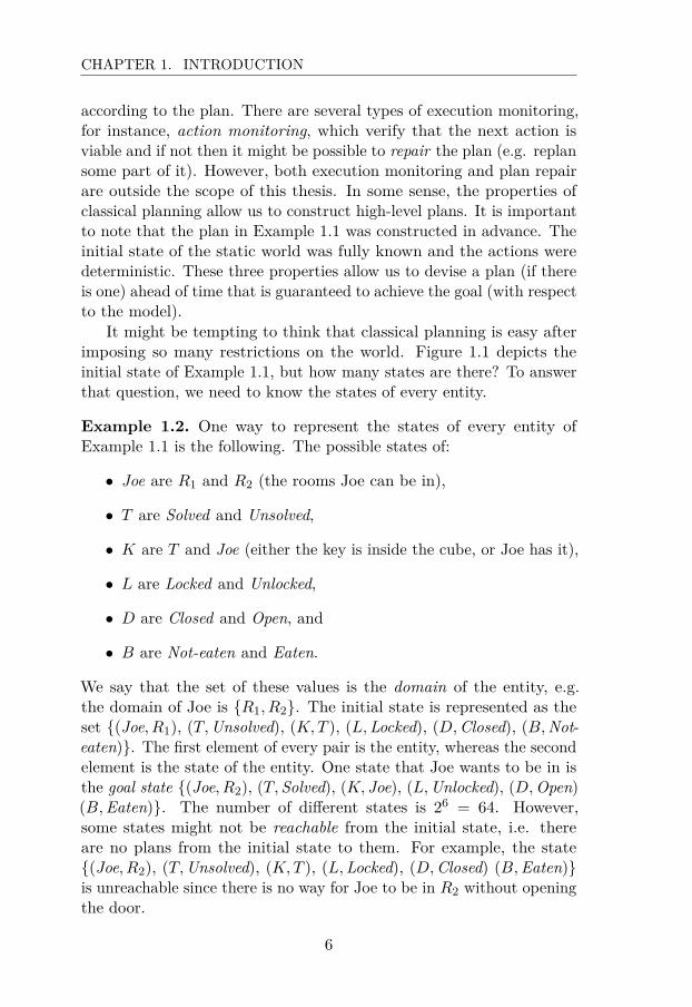
Figure 1.1: An illustration of the initial state of Example 1.1.
These properties are relevant to the agent(s) in the world and not theworld itself. The classical planning problem is the simplest problem. Inother words, the single agent lives in the classical world and knows theinitial state. Her actions have no duration and cannot be performedconcurrently. The goal is for the world to be in a specific state.
Example 1.1. Consider a world of two rooms R1 and R2, which areconnected by a locked door D. There is no window between the rooms.Joe lives in R1. He is a gorilla with a passion for consuming bananas.Sadly, he has not been able to enjoy his passion lately, but he has aplan. Joe noticed, by using his X-ray vision, that there is a bunch ofbananas B in R2. Specifically, musa acuminata – his favourite speciesof bananas. However, the door to R2 is locked, and the key K for thedoor is ‘hidden’ inside a toy T in his room. Arguably, it is not possibleto hide anything from Joe because of his awesome power. The toy isa Rubik’s Cube and he believes that the cube opens up when solved.Joe’s plan is simple: take T ; solve T ; grab K; unlock D with K; openD; enter R2; pick up B; and finally, munch on B.
Example 1.1 (together with Figure 1.1) is meant to illustrate aclassical planning problem, and in Chapter 2 we show how to formallymodel the example. The keen reader might have noticed that Joe isnot your typical gorilla: he is blessed with X-ray vision. This is aconsequence of Joe living in a classical world, which is fully observable.Joe’s plan is a high-level plan and there are many gaps that needs to befilled in. For instance, how to solve the Rubik’s Cube is left out, andhow to execute the plan in terms of motor control (robotics) is omitted.Such intricate details of a plan are often delegated to other systems tobe filled in.
If Joe’s plan does not succeed for some reason, then he has torevisit it. An execution monitoring agent checks if everything is going
5
CHAPTER 1. INTRODUCTION
according to the plan. There are several types of execution monitoring,for instance, action monitoring, which verify that the next action isviable and if not then it might be possible to repair the plan (e.g. replansome part of it). However, both execution monitoring and plan repairare outside the scope of this thesis. In some sense, the properties ofclassical planning allow us to construct high-level plans. It is importantto note that the plan in Example 1.1 was constructed in advance. Theinitial state of the static world was fully known and the actions weredeterministic. These three properties allow us to devise a plan (if thereis one) ahead of time that is guaranteed to achieve the goal (with respectto the model).
It might be tempting to think that classical planning is easy afterimposing so many restrictions on the world. Figure 1.1 depicts theinitial state of Example 1.1, but how many states are there? To answerthat question, we need to know the states of every entity.
Example 1.2. One way to represent the states of every entity ofExample 1.1 is the following. The possible states of:
• Joe are R1 and R2 (the rooms Joe can be in),
• T are Solved and Unsolved,
• K are T and Joe (either the key is inside the cube, or Joe has it),
• L are Locked and Unlocked,
• D are Closed and Open, and
• B are Not-eaten and Eaten.
We say that the set of these values is the domain of the entity, e.g.the domain of Joe is R1, R2. The initial state is represented as theset (Joe, R1), (T,Unsolved), (K,T ), (L,Locked), (D,Closed), (B,Not-eaten). The first element of every pair is the entity, whereas the secondelement is the state of the entity. One state that Joe wants to be in isthe goal state (Joe, R2), (T,Solved), (K, Joe), (L,Unlocked), (D,Open)(B,Eaten). The number of different states is 26 = 64. However,some states might not be reachable from the initial state, i.e. thereare no plans from the initial state to them. For example, the state(Joe, R2), (T,Unsolved), (K,T ), (L,Locked), (D,Closed) (B,Eaten)is unreachable since there is no way for Joe to be in R2 without openingthe door.
6

1.2. COMPUTATIONAL COMPLEXITY THEORY
The number of states of Example 1.2 is only 64, which might notsound like a lot. However, if we were to place an additional 260 bananasin R2, then the number of states would be greater than the number ofatoms in the observable universe.1 The reason for this absurd increasein the amount of states is that Joe can eat the bananas in very manydifferent orders. Every different combination of Eaten and Not-Eaten isan unique state. This effect is typically described as a combinatorialexplosion. Note that the same thing happens when we introduce irrelev-ant entities, for instance, suppose there are a lot of retractable pens onthe floor and Joe can extend the tip of each pen by clicking on top ofit. This also causes a combinatorial explosion of states. However, thepens are irrelevant for Joe’s plan. The problem is still easy for humanssince we are aware of the fact that there is no need to differentiatebetween the bananas, or that we can ignore the pens, but automatedplanners cannot differentiate. Of course, in the general case, we haveto differentiate between every entity and such problems would also beextremely difficult for humans. Much research in this field has beendevoted to how to deal with the combinatorial explosion of states. Inother words, even classical planning is computationally hard, which isthe theme of our next discussion.
1.2 Computational Complexity TheoryPlanning problems can differ vastly regarding computational complexity.The objective of computational complexity is to classify problems ac-cording to their inherent difficulty, and compare the difficulties to oneanother. We assume that the reader is already familiar with compu-tational complexity, and give a brief reminder. Consider the followingcomputational problem.
SATInstance: A boolean formula F on conjunctive normal form, i.e.F is a conjunction of clauses where each clause is a disjunction ofliterals.Question: Does F have a satisfying assignment?
We require, without loss of generality, that repeated clauses are notallowed and that no empty clauses appear. Note that the definitionof SAT instances implies that there are no unused variables, i.e. every
1The number of atoms in the observable universe is estimated to be 1080.
7

CHAPTER 1. INTRODUCTION
variable appears in at least one clause. The problem k-SAT, k ≥ 1, isthe SAT problem restricted to clauses containing at most k literals.
Example 1.3. The boolean formula (x∨y)∧(¬y∨¬z) has the satisfyingassignment x = T, y = T, z = F . The assignment of y does not matter.The formula is on conjunctive normal form.
The answer to the SAT problem for the boolean formula in Ex-ample 1.3 is ’yes’ since we have a satisfying assignment. An obviousalgorithm to find such an assignment is to systematically enumerateevery assigment, and check if any of them satisfies the boolean formula.Our main concerns are how efficient the algorithm is, and if there aremore efficient algorithms. We denote this particular algorithm as A forthe remainder of this section.
1.2.1 Asymptotic Complexity
Algorithm A answers the question of the SAT problem for a booleanformula F . Let n be the number of variables in F , and m be the lengthof F . Then the number of possible assignments for F is 2n. Given an as-signment, we can compute the next assignment in n steps. Furthermore,we can check whether an assignment satisfies F in roughly m steps.(The details of how we do this are left as an exercise.) Consequently,the number of steps of A is, in the worst case, roughly 2n · n ·m. Astep can be thought of as a machine instruction for a computer, or aconstant number of them, where the instruction takes constant time toexecute. In this case, the number of steps measure how much time thealgorithm require. Similarly, we can measure space, i.e. the memoryusage of the algorithm.
The analysis of algorithm A exemplify the intuition behind asymp-totic complexity: we ignore constant factors and terms and study howthe algorithm behave when the input size approach infinity. The ignoredfactors and terms are dominated by the remaining parts when the inputsize is sufficiently large. Formally, let f and g be two functions definedon some subset of the real numbers. Then we write f(x) = O(g(x)) ifand only if there is a positive constant c and a real number x0 suchthat f(x) ≤ c · g(x) for all x ≥ x0. Intuitively, the function f does notgrow faster than g for sufficiently large x. For example, the asymptoticcomplexity of A is 2n ·n ·m ≤ 2m ·m2 = O(2m ·m2) (n < m since everyvariable occurs at least once in F ).
8

1.2. COMPUTATIONAL COMPLEXITY THEORY
1.2.2 Complexity Classes
A complexity class is a set of problems of related complexity. We areespecially interested in the following classes.
• P: The set of problems that can be solved by an algorithmrunning in time O(nc), where c is a constant. When we say thatan algorithm is polynomial, then the problem it solves is in P.If a problem is in this class, then we consider it to be tractable(computationally feasible), and otherwise to be intractable. (Ifthis is a fair dichotomy is debatable.)
• NP: The set of problems that can be solved by a non-deter-ministic algorithm running in time O(nc), where c is a constant.A non-deterministic algorithm can be thought of as an algorithmthat, when confronted with a several options, is always able toguess the correct option. For instance, algorithm A has to checkevery assignment since we do not know which one is a satisfyingassignment, and if there is one. A non-deterministic version ofA consists of two phases: a non-deterministic phase and thena deterministic phase. The first phase guesses an answer andthe second phase verifies it. In this case, we would guess someassignment in the first phase, and then deterministically checkif it satisfies the formula in the second phase. Assuming thatevery guess was correct, A is in NP since both phases runs inpolynomial time. It is known that P ⊆ NP, but whether P 6= NPis a major open question. However, due to the amount of researchthat has been devoted to answering just that question throughoutmany decades, it is common to assume that P 6= NP.
• PSPACE: The set of problems that can be solved by an algorithmrunning in space O(nc), where c is a constant. It is knownthat NP ⊆ PSPACE, however if NP 6= PSPACE and P 6=PSPACE are also open questions.
As the reader might have noticed, there is a straightforward hierarchyof the complexity classes, but if a problem is, for instance, in PSPACEthen we do not know how hard it is (since P ⊆ PSPACE). Hence,hardness with respect to a complexity class means, informally, thatthe problem is at least as hard as the hardest problems in the class.For example, the SAT problem is in NP and is also NP-hard [GJ79,problem LO1]. Furthermore, if a problem is both inNP and isNP-hard
9

CHAPTER 1. INTRODUCTION
then we say that it is NP-complete (we use analogous definitions forother classes). Hardness can be formalised by using polynomial-timereductions, which translates, or reduces, one problem to another. Thereduction must be done in polynomial-time, and the answer for theformer problem is derived from the answer for the latter problem. If thelatter problem can be answered quickly, then so can the former sincethe reduction is done in polynomial-time. Hence, the latter problemis at least as hard as the former. If a problem is NP-hard then it iscommon to assume that there is no polynomial algorithm which solvesit (i.e. by assuming that P 6= NP). We refer the reader to the textbookby Papadimitriou [Pap94] for more information.
1.3 Contributions & Thesis Outline
There has been an impressive advancement in domain-independentplanning over the past decades. New and efficient planners haveentered the scene, for instance, Fast Forward [HN01], Fast Down-ward [Hel06a], Lama [RW10], and planners based on compilationinto SAT instances [RHN06]. Various ways to exploit the structure ofplanning instances have been proposed and integrated into existing plan-ners. Perhaps most importantly, a rich flora of heuristics has appeared,making many previously infeasible instances solvable with reasonableresources. See, for instance, Helmert et al. [HD09] for a survey andcomparison of the most popular heuristics. This development has largelybeen driven by the international planning competitions (IPC). However,in the long run one might question how healthy it is for a research areato focus so much effort on solving the particular problems choosen forthe competitions. This is a very natural question from a methodologicalpoint of view, and although it has not been raised as often as one mightexpect, it is not a new one, cf. Helmert [Hel06b].
One problem with the planning competitions so far is that allplanning instances have a solution, and the effect of this is that theplanners and methods used are getting increasingly faster at find-ing the solutions that we already know exist. It is important tonote that other similar competitions, such as the SAT competition(http://www.satcompetition.org) and the Constraint Solver Com-petition (http://cpai.ucc.ie), consider unsolvable instances togetherwith solvable instances. It is no secret that few planners exhibit anysimilar speed improvement for instances that have no solution. Formany applications we can know, e.g. by design, that there is a solu-
10

1.3. CONTRIBUTIONS & THESIS OUTLINE
tion, but this cannot be a general assumption. Obvious examples areplanning for error recovery and planning for systems that were notdesigned to always have a solution (old industrial plants that haveevolved over time is an archetypical example). Another example issupport systems where a human operator takes the planning decisionsand the planner is used to decide if there is a plan or not, or to attemptfinding errors in the human-made plan [GKS12]. System verificationhas an overlap with planning [ELV07], and proving that a forbiddenstate is unreachable corresponds to proving that there is no plan. Sim-ilarly, planning is used for penetration testing in computer security[BGHH05, SBH13, FNRS10, HGHB05], which is an area of emergingcommercial importance [SP12]. In penetration testing, a system isconsidered safe if there is no plan for intrusion. We finally note thatoversubscription planning (i.e. where not all goals can be satisfied sim-ultaneously and the objective is to maximise the number of satisfiedgoals) have been considered in the literature [Smi04].
Perhaps the most important contribution of our work is that wesparked interest in the anomaly explained above by implementing aplanner tailored towards unsolvable instances and demonstrated thatit outperformed state-of-the-art IPC planners on such instances. Thisexposed a weakness which needed to be addressed by the planningcommunity, and as a result a number of responses have been produced.The situation has improved significantly, and IPC has introduced anunsolvability track to encourage further research. The following public-ations are a few examples of recent methods for detecting unsolvableinstances. Hoffman et al. [HKT14] specialised the heuristic functionMerge & Shrink [HHH07] for detecting unsolvable instances. Steinmetzand Hoffmann [SH16] tailored the heuristic function hC for detectingdead-end states, and gave it the ability to learn from misclassificationsto improve itself. Lipovetzky et al. [LMG16] investigated the relationbetween traps and dead-ends, and devised a preprocessing algorithmfor computing them. Gnad et al. [GSJ+16] designed a method aroundpartial delete relexation, or red-black planning, to detect unsolvableplanning instances. Gnad et al. [GTSH17] exploited symmetries inthe planning instance to prune states during the search on its statetransition graph. This is far from a complete list, but it is clear itsparked an interest and that a lot of experimentation is taking place.It is worth noting that dead-end detection is not something new, butits relevance to unsolvable planning instances was not studied in-depth.Some contenders from the first unsolvability IPC are Aidos [SPS+16],
11

CHAPTER 1. INTRODUCTION
Django [GSH16], SymPA [Tor16], M+S and SimDominance [THK16];and they make use of the results in the publications above and more.We compare our planners to some of these contenders, and we outlineand describe our results next.
Part I: Introduction
In this part, we define the planning formalism that we use throughout thethesis (Chapter 2). We also motivate our work further by showing thatthere is no significant theoretical difference, with respect to complexity,between solvable and unsolvable instances (Chapter 3). Finally, we givea brief explanation of the inner workings of our planner (Section 4.1), anddiscuss the domains of unsolvable instances that we use (Section 4.2).
Part II: Variable Projection
This part describes two planners for unsolvable problems, both ofthem are based on variable projection, which is a technique to simplifyinstances. From now on, we use the more mathematical term variableinstead of entity, they are essentially synonyms. Variable projectionlets us project away variables from the instance, for example, if we wereto project away the lock in Example 1.1 then we can open the doorwithout the key. The key is still in the projected world, but it has nouse. A plan for the projected instance is: open the door; go to theother room; dine on the banana. Note that this plan is an incompleteand inapplicable plan for the original instance, and to complete it wecan add these actions: take the puzzle; solve the puzzle; grab the key;and unlock the door. In other words, variable projection lets us findpartial plans that are parts of a plan for the instance. The process ofcompleting a partial plan is also known as plan refinement; this is alsohow variable projection was used in the beginning [Kno94]. There is noguarantee that partial plans can be refined into a plan for the instance,however, if there is no partial plan at all for a projected instance thenthere is no plan for the original instance. This is a very importantproperty: we can prove that an instance is unsolvable by proving that asimpler instance, constructed by variable projection, is unsolvable. Thisfact is the cornerstone which our planners are based on.
The first planner, consistency checking, systematically enumeratesevery subset of variables and projects the instance onto it, and thenchecks whether the projection is unsolvable or not. If the projection isunsolvable, then the original instance must be unsolvable. Projections
12

1.3. CONTRIBUTIONS & THESIS OUTLINE
onto smaller subsets are faster to solve, so the method starts withprojecting onto every subset of size 1, then every subset of size 2, andso on, up to size k. Consistency checking for planning is often efficient,but at the cost of being incomplete, that is, it is infeasible to detectall unsolvable instances. Consistency checking also runs in polynomialtime for any fixed value of a parameter k, which can be used to trade offbetween efficiency and completeness. Consistency checking for planningis efficient if unsolvability can be proved with a reasonably small variablesubset, otherwise it quickly becomes too time-consuming because of thesheer number of possible projections.
The second planner is an adaptation of an existing heuristic functionfor solvable instances: pattern databases (PDB). More precisely, weadapt pattern collections. A pattern is the same as a projected instance,and we have a collection of different projected instances. Historically,PDBs have used variable projection for providing heuristic guidanceand, naturally, such PDBs perform badly when given an unsolvableinstance. We refocus PDBs to identify dead-end states – states fromwhich no goal state is reachable. Note that if the instance is unsolvable,then the initial state is a dead-end state. Hence, dead-end detection isa viable approach to identify unsolvable instances.
We evaluate both planners on 183 unsolvable planning instances over8 domains, matching our methods against some of the most commonlyused planners. A typical statistical analysis of some method studyinstance coverage and run-time, but we also carry out a much morein-depth statistical analysis by taking advantage of a large computercluster. One issue with the typical analysis is that the limitation of themethods is not clear. For example, if we have a PDB that performs wellon an instance, then we do not know if there is another PDB which wouldhave performed considerably better. With the help of the computercluster, we establish a distribution for every instance of its projections,of various properties. The distributions help us answer questions suchas ‘how optimal is our method with respect to its potential?’. Note thatwe are discussing the potential, or ‘upper bound’, of the method as awhole. In other words, to improve the potential of the method, we haveto complement it with additional techniques.
Part III: Polytree Causal Graphs & Variable Similarity
We take a detour from unsolvable instances and look at a specific classof instances, which gave us insights in which variable projections areof particular interest when trying to detect unsolvability. The class
13

CHAPTER 1. INTRODUCTION
consists of instances whose causal graph is a polytree. The causal graphof an instance is a directed graph of its variables, where an edge fromone variable to another means that the former can influence the latterthrough an action. We also restrict the domain size of the variables(entities) by a constant, and either the depth or the diameter of thecausal graph. The depth is a graph is the length of the longest simpledirected path, and the diameter is the longest simple undirected path.Similar classes has been studied previously, and some of them are specialcases of these classes.
The algorithm for one of the classes works by recursively breakingdown the instance into several smaller instances, which are then solvedindependently. A solution for the instance is then derived from thesolutions for the smaller instances. The foundation of the algorithmfor the other class is the notion of variable ismorphism. Essentially,two variables are isomorphic if one of them can be removed withoutaffecting solvability because the two ‘behave’ the same anyway. Goingback to Example 1.1, we mentioned that if we add 260 bananas thenwe get a combinatorial explosion, and we also mentioned that therewas no need to differentiate between them. One way to motivate thisis that the bananas are isomorphic. That is, we can remove all butone banana without affecting solvability. We show, by exploiting thisfeature, that the class defined in the previous paragraph is tractable,albeit the constants in the asymptotic complexity are large.
We follow up on this idea by defining a variable similarity measure,which scores the similarity of two variables between 0 and 1. Thesimilarity score of two isomorphic variables is always 1, however, itis possible for two non-isomorphic variables to also get the score 1.This is because it is infeasible to decide whether two variables areisomorphic in the general case, so we need an approximation. We thenshow empirically that the smallest unsolvable projections very oftenconsist of variables that pairwise score very low on the variable similaritymeasure. This is important since we now have a tool that can help usdecide whether to consider a variable projection. We use this measureto improve the planners in Part II. The tool is statistically analysedand the improvement is empirically evaluated.
Part IV: Conclusions
We conclude this thesis with a summary and discuss future researchdirections. The main topic is how to improve variable projection andthus the methods. We also mention some open research questions.
14

I
PART
Preliminaries
15


Chapter Two
Planning Formalism
In this chapter we present the planning formalism that is used in thisthesis and show some important properties, discuss how planners areimplemented in practice, and present the unsolvable instances that weevaluate our results on.
We use the extended simplified action structures (SAS+) [BN95]formalism, which uses multi-valued variables. This is the main differencebetween SAS+ and STRIPS, which use propositional atoms (binaryvariables). A SAS+ instance is a tuple Π = (V,A, I,G) where:
• V = v1, . . . , vn is the set of variables, and each variable is asso-ciated with a domain Dv. A partial state is a set s ⊆
⋃v∈V (v, d) :
d ∈ Dv where every variable in V occurs in at most one pair. Atotal state is a partial state where every variable in V occurs inexactly one pair. We also view partial states as partial functionsand use the corresponding notation, i.e. s[v] = d means that(v, d) ∈ s, and Domain(s) = v : (v, d) ∈ s denotes the domainof s.
• A is the set of actions. An action a = pre(a) → eff(a) con-sists of two partial states, a precondition pre(a) and an effecteff(a). An action a has a prevailcondition on a variable v if v ∈Domain(pre(a)) \Domain(eff(a)), i.e. there is a precondition butno effect on v.1 Furthermore, we do not allow pre(a)[v] = eff(a)[v]since the effect on v is then superfluous.
• I is the initial state, and it is a total state.
• G is the goal, and it is a partial state.1This is slightly non-standard, some formalisms define preconditions and prevail-
conditions of an action as distinct sets of pre(a). However, in the vast majority ofthis thesis we do not need to distinguish between the two.
17

CHAPTER 2. PLANNING FORMALISM
We write V (Π), A(Π), I(Π) and G(Π) for the set of variables, actions,the initial state and the goal of Π, respectively.
We say that a partial state s1 matches another partial state s2if s1 ⊆ s2. We define the composition of two partial states s1, s2 ass1 ⊕ s2 = s2 ∪ (v, s1[v]) : v ∈ Domain(s1) \Domain(s2). An action ais applicable in a total state s if pre(a) ⊆ s, and the result of applying ain s is the total state s⊕ eff(a).
Example 2.1. Recall Example 1.2. The way we represented the entities,i.e. the variables, followed the SAS+ formalism closely. Henceforth, wedenote the following instance as ΠJoe. The set of variables is V (ΠJoe) =Joe, T,K,L,D,B, where:
• DJoe = R1, R2 (the rooms Joe can be in),
• DT = Solved,Unsolved,
• DK = T, Joe (the key is either inside the cube, or Joe has it),
• DL = Locked,Unlocked,
• DD = Closed,Open, and
• DB = Not-eaten,Eaten.
The initial state is I(ΠJoe) = (Joe, R1), (T,Unsolved), (K,T ),(L,Locked), (D,Closed), (B,Not-eaten), and the goal is G(ΠJoe) =(B,Eaten) (Joe’s life goal is to devour B). The actions of ΠJoe arethe following.
• aSolve = (Joe, R1), (T,Unsolved) → (T,Solved),
• aGrabKey = (Joe, R1), (T,Solved), (K,T ) → (K, Joe),
• aUnlock = (K, Joe), (L,Locked), (D,Closed) → (L,Unlocked),
• aLock = (K, Joe), (L,Unlocked), (D,Closed) → (L,Locked),
• aOpen = (L,Unlocked), (D,Closed) → (D,Open),
• aClose = (D,Open) → (D,Closed),
• aR1→R2 = (D,Open), (Joe, R1) → (Joe, R2),
• aR2→R1 = (D,Open), (Joe, R2) → (Joe, R1),
• aIngest = (Joe, R2), (B,Not-eaten) → (B,Eaten),
18

2.1. STATES AND REACHABILITY
Note that the cube cannot be moved around (it is always in R1)and the same is true for B (it is always in R2). This is not a limitationof the SAS+ formalism, we simply wanted a more brief example. Forinstance, if the domain of B was R1, R2, Joe,Eaten, then we couldhave had actions to let Joe pick it up and put it down.
2.1 States and ReachabilityThe plan that Joe conceived in Example 1.1 was a linear plan, which isthe type of plans that we consider in this thesis. We are interested inwhether a state is reachable from the initial state, and whether a goalstate is reachable from another state. The following three definitionsdefine these nuances.
Definition 2.2. Let s0 and sn be two total states, and ω = 〈a1, . . . , an〉be sequence of actions. Then ω is a plan from s0 to sn if and only ifthere exists a sequence of intermediate total states 〈s1, . . . , sn−1〉 suchthat ai is applicable in si−1 and si is the result of applying ai in si−1for all 1 ≤ i ≤ n. The plan ω is also a solution with respect to a goal Gif G ⊆ sn, and the length of ω is |ω| = n.
A solution is optimal if there does not exists another a better solution,and with better we mean either shorter or lowest total cost (dependingon the context). When a solution is not optimal, it is suboptimal.The following definition is very important, especially for unsolvableinstances.
Definition 2.3. A state s is reachable with respect to an initial stateI if there is a plan from I to s. A state is unreachable with respect to Iif it is not reachable from I. A state s is a dead-end if there is no planfrom s to any goal state g, G ⊆ g, where G is the goal.
The state transition graph of an instance is an important structurefor finding solutions. The nodes of the graph are the total states of theinstance, and an edge from one state to another means that there is anapplicable action that takes us from the first state to the latter. A pathfrom the initial to a goal state in the graph represents a solution. Inother words, one way to solve instances is to use some search algorithmon the state transition graph.
Definition 2.4. Let Π be an instance. The set of every total stateof Π is TotalStates(Π) = (v1, d1), . . . , (vn, dn) : d1 ∈ Dv1 , . . . , dn ∈
19

CHAPTER 2. PLANNING FORMALISM
Dvn , n = |V (Π)|. The state transition graph of Π is the directed graphTG(Π) = (TotalStates(Π), E), where (s1, s2) ∈ E if and only if there isan action a ∈ A(Π) such that a is applicable in s1 and s2 is the resultof applying a in s1.Example 2.5. We noted in Example 1.2 that the number of totalstates of ΠJoe is 26 = 64, i.e. |TotalStates(ΠJoe)| = 64. The number ofgoal states is 32, but not all them are reachable. For example, the state(Joe, R2), (T,Unsolved), (K,T ), (L,Locked), (D,Closed), (B,Eaten)is unreachable since there is no way for Joe to enter R2 without solvingT . A plan and solution for ΠJoe is 〈aSolve, aGrabKey, aUnlock, aOpen,aR1→R2 , aIngest〉. This is not the only solution; after applying aOpen,Joe could aClose and aOpen again before applying the remainder of theplan. Of course, such a solution is suboptimal (there exists a bettersolution).
2.2 Variable ProjectionSome instances have enormous state transition graphs and are verydifficult to solve. When this is the case, it might help to relax, or abstract,the instance. Relaxation is a strategy which lets us approximate thesolution of an instance by solving an easier, related, instance. Thereare several ways to relax planning instances, and we focus on variableprojection. We define variable projection in the usual way [Hel04].Definition 2.6. Let Π = (V,A, I,G) be a SAS+ instance and letV ′ ⊆ V . The variable projection of a partial state s onto V ′ is definedas s|V ′ = (v, d) : (v, d) ∈ s, v ∈ V ′. The variable projection (or simplyprojection) of Π onto V ′ is Π|V ′ = (V ′, A|V ′ , I|V ′ , G|V ′), A|V ′ = a|V ′ :a ∈ A, eff(a|V ′) 6= ∅ where pre(a|V ′) = pre(a)|V ′ and eff(a|V ′) =eff(a)|V ′ .
Note that a variable projection cannot contain actions with an emptyeffect. It is safe to remove such actions since they cannot be part of anyoptimal solution, and nor do they affect solvability.Example 2.7. Suppose R2 in Example 1.1 contained an additional 260bananas and that Joe could not solve the Rubik’s Cube since it wasrigged. Then it does not matter if we consider that Joe only wants toeat 1 banana, or all 261 of them: the instance is unsolvable in bothcases. Hence, it makes sense for Joe to ignore, or project away, all butone banana since if he can devour one banana, then he can devour themall.
20

2.3. GRAPHS
The following theorem is central for this thesis.
Theorem 2.8. [Hel04] Let Π be a SAS+ planning instance, and V ′ ⊆V (Π). If Π|V ′ is unsolvable, then Π is unsolvable.
Proof. Assume that Π is solvable and Π|V ′ is unsolvable. Let ω =〈a1, . . . , an〉 be a solution for Π. Let ω′|V ′ = 〈a1|V ′ , a2|V ′ , . . . 〉 whereactions with empty effects have been removed. The actions in ω′ arein A|V ′ (per definition). The plan ω′ is applicable for Π|V ′ since ω isapplicable for Π. Furthermore, for every variable v ∈ V ′, v is assignedthe same values and in the same order. In other words, the final valuefor every v for ω′ is the same as for ω, thus ω′ is a solution for Π|V ′ .This contradicts that Π|V ′ is unsolvable.
Variable projection does not necessarily preserve unsolvability, asthe following example demonstrates. That is, if we ignore the ‘rigged’Rubik’s Cube, then the projection is solvable.
Example 2.9. Suppose we want to project ΠJoe (see Example 2.1)onto the variable set Joe,K, L,D,B, i.e. we project away the Rubik’sCube. The domain of every remaining variable is unaffected, but theactions aSolve and aGrabKey have changed and their projections are:
• aSolve|Joe,K,L,D,B = (Joe, R1) → , and
• aGrabKey|Joe,K,L,D,B = (Joe, R1), (K,T ) → (K, Joe).
Note that the effect of the first action is empty, i.e. applying it does notchange the world state. Clearly, we can remove such actions from theprojection. The precondition on T of the second action that required Tto be solved has been removed, and Joe can simply grab the key fromthe non-existing T (a side-effect of projection since there is no ‘correct’initial state for the key).
2.3 Graphs
The state transition graph is a victim of the combinatorial explosion,and it is often infeasible to represent it in memory. Hence, it is difficultto reason about the instance by using this graph explicitly. Thus, to geta bird’s-eye view of how the variables are interconnected it is commonto use the causal graph – an important tool that we frequently use.
21

CHAPTER 2. PLANNING FORMALISM
T
K L
D
B Joe
Figure 2.1: The causal graph of ΠJoe (see Example 2.1).
Definition 2.10. The causal graph CG(Π) of a SAS+ instance Π =(V,A, I,G) is the digraph (V,E) where an edge (v1, v2), such thatv1 6= v2, belongs to E if and only if there exists an action a ∈ A suchthat v2 ∈ Domain(eff(a)) and v1 ∈ Domain(pre(a)) ∪Domain(eff(a)).
Example 2.11. Figure 2.1 depicts the causal graph of ΠJoe. A mainpurpose of the causal graph is to highlight causal relationships betweenvariables. For example, an edge to B from Joe means that a change instate of B depends on the state of Joe. Indeed, B can only be eaten ifJoe is in the room.
It is common to define classes of planning instances by imposingrestrictions on the causal graph, and many tractable classes has beendefined with this approach. We take a much closer look at the causalgraph in Part III.
Yet another technique to describe dependencies is the domain trans-ition graph, which detail dependencies between the values of a domainof a variable.
Definition 2.12. The domain transition graph DTG(v) for a variablev ∈ V is the labelled digraph (Dv, E) where for every distinct d1, d2 ∈Dv, (d1, d2) ∈ E if and only if there exists an action a ∈ A such thatpre(a)[v] = d1 or v /∈ Domain(pre(a)), and eff(a)[v] = d2. The label ofan edge is a set of the prevailconditions of the actions that satisfy therequirement for the edge to exist (a set of sets).
Example 2.13. The domain transition graph (DTG) of a variable v il-lustrates how v can change its state. The DTG(B) of ΠJoe consists of twonodes and one edge: the nodes Not-eaten and Eaten, and an edge fromthe former to the latter with the label pre(aIngest) \ (B,Not-eaten).We remove non-prevailconditions since they are redundant with the
22

2.4. COMPUTATIONAL PROBLEMS
direction of the edge. There is no way for B to become Not-eaten onceeaten, so there is no edge in that direction.
In some sense, DTGs give a local overview of the planning instance.
2.4 Computational Problems
The SAS+ planning formalism presented so far have ignored the possib-ility that actions are not equal, i.e. that there is some kind of ‘cost’ ofapplying them. Suppose we want to model this logistics problem: wehave a truck, a number of packages and locations where the truck haveto deliver the packages to. If we ignore the time it takes for the truck todrive from one location to another, then a solution might be to drive tothe location furthest away without delivering any intermediate packages.Clearly, such solutions are suboptimal in practice and to remedy thiswe can incorporate driving time into the model. One approach is toassociate a cost with every action, and in the example the cost is thedriving time. In other words, in addition to an instance Π, we also givea cost function c : A(Π) → R. The cost of a plan ω = 〈a1, . . . , an〉 isc(ω) = c(a1) + · · ·+ c(an).
There are a number of computational problems in planning and thefollowing are the most common ones.
Plan Existence (PE)Instance: A SAS+ planning instance Π.Question: Is there a solution for Π?
Bounded Plan Existence (BPE)Instance: A SAS+ planning instance Π and a number b ∈ N.Question: Is there a solution ω for Π such that |ω| ≤ b?
Bounded Cost Plan Existence (BCPE)Instance: A SAS+ planning instance Π, a cost function c : A(Π)→N, and a number b ∈ N.Question: Is there a solution ω for Π such that c(ω) ≤ b?
These three problems are concerned with the existence of a solution,not the generation of one. In some cases, it is easier to verify theexistence of a solution than it is to generate one. Furthermore, theproblems are sorted in increasing difficulty: PE is easier than BPE sincethe latter is the optimisation version (if there is a ‘short’ solution);
23

CHAPTER 2. PLANNING FORMALISM
and BPE is easier than BCPE since the former is a special case of thelatter, i.e. let the cost of every action be 1. The following correspondingcomputational objectives require the generation of a solution.
Plan Generation (PG)Instance: A SAS+ planning instance Π.Objective: Generate a solution ω for Π, if one exists. Otherwise,answer ‘no’.
Bounded Plan Generation (BPG)Instance: A SAS+ planning instance Π and a number b ∈ N.Objective: Generate a solution ω for Π such that |ω| ≤ b, if oneexists. Otherwise, answer ‘no’.
Bounded Cost Plan Generation (BCPG)Instance: A SAS+ planning instance Π, a cost function c : A(Π)→N, and a number b ∈ N.Objective: Generate a solution ω for Π such that c(ω) ≤ b, if oneexists. Otherwise, answer ‘no’.
Of course, if we are able to generate a solution, then we can answerthe corresponding problem about its existence. If PG does not generatea solution, then no solution exists. However, if BPG or BCPG does notgenerate a solution then the instance can still be solvable, but a higherbound is required. We also consider the following problems.
Cost Optimal Plan Generation (COPG)Instance: A SAS+ planning instance Π and a cost function c :A(Π)→ N.Objective: Generate a solution ω for Π such that there is no othersolution ω′ for Π where c(ω′) < c(ω), if a solution exists. Otherwise,answer ‘no’.
Cost Optimal Plan Existence (COPE)Instance: A SAS+ planning instance Π and a cost function c :A(Π)→ N.Objective: Generate a cost c such that there is a solution ω for Πwhere c(ω) = c and there is no solution ω′ for Π where c(ω′) < c. IfΠ is unsolvable then c =∞. Otherwise, answer ‘no’.
The objective is to generate an optimal solution, or the cost of one,for the instance. The solutions generated when considering BPG andBCPG might not be optimal when the bound b is larger than the costof an optimal solution.
24

Chapter Three
Solvable vs. UnsolvableInstances
We mentioned earlier that we have identified an asymmetry betweenhow much attention solvable and unsolvable instances have gotten inthe literature, but is there a theoretical difference between the two?To prove that an instance is, in fact, solvable, we only have to give asolution for the instance. Furthermore, it is straightforward to verify thesolution: check if the first action is applicable, and if yes then apply itto the current state. Repeat this for the second action, and so on. If thefinal state is a goal state then the instance is solvable. In other words,the solution is a certificate that demonstrates solvability. In contrast, itmight be more tricky to provide a certificate for unsolvable instances.One certificate is the set of reachable states, and to verify it we needto: (1) check if the initial state is in it; (2) check if no goal state is init; and (3) check that the set of reachable states is closed under everyaction. Another possible certificate is the set of states that can reacha goal state. In this case, conditions (1) and (2) are flipped, i.e. theinitial state should not be in the set and every goal state should be. Thedescription so far might give the impression that it is computationallyeasier to verify solvability certificates, however, optimal solutions forsolvable instances can be of exponential length and thus expensive toverify. Eriksson, Röger and Helmert [ERH17] describes a family ofcertificates for unsolvability that can be efficiently verified, and oneimportant aspect of their certificates is a compact representation ofstates. Another possible certificate is a subset of variables such that theprojection onto it is unsolvable, and if the subset is sufficiently smallthen unsolvability can be verified efficiently. In this chapter we showthat there is no theoretical difference between solvable and unsolvableinstances.
25
CHAPTER 3. SOLVABLE VS. UNSOLVABLE INSTANCES
3.1 Exponential Time Hypothesis
The k-SAT problem is NP-complete when k ≥ 3 [GJ79, problem LO1],and there is no algorithm running in polynomial time if we assumeP 6= NP. However, there is a huge difference between the asymptoticcomplexity of O(2n) and O(20.386n) – a nuance which is not visible whenmerely studying complexity classes – but how small can the constantin the exponent be for k-SAT? A more precise characterisation of thecomplexity of k-SAT is possible by using the exponential time hypothesis(ETH) [IP01, IPZ01]. This hypothesis is a conjecture stated as follows.
Definition 3.1. For all constant integers k > 2, let sk be the infimumof all real numbers δ such that k-SAT can be solved in time O(2δn),where n is the number of variables of an instance. The exponential timehypothesis (ETH) is the conjecture that sk > 0 for all k > 2.
Informally, ETH says that satisfiability cannot be solved in subex-ponential time. One may equivalently define the ETH for the numberof clauses, i.e. replacing O(2δn) with O(2δm) in Definition 3.1, wherem is the number of clauses. It is known that the ETH with respectto the number of clauses holds if and only if the ETH with respect tothe number of variables holds [IPZ01]. Note that since the ETH refersto actual deterministic time bounds it is possible to swap the answer,i.e. if we could solve k-UNSAT in time O(f(n)) for some function f ,then we could also solve k-SAT in time O(f(n)). Hence, the ETH canequivalently be defined in terms of the k-UNSAT problem.
Since using the ETH offers more precision than polynomial reduc-tions between the usual complexity classes do, we will benefit from alsobeing more precise about how much a reduction blows up the instancesize, defining the following measure for this purpose.
Definition 3.2. Given a reduction ρ from some problem X to someproblem Y, we say that ρ has blow-up b, for some b > 0, if there existsan n > 0 such that ||ρ(I )|| ≤ ||I ||b for all instances I of X such that||I || ≥ n.
Clearly, every polynomial-time reduction has bounded blow-up.The following properties of 3-CNF formulae will be used in the
forthcoming proof. The bounds are straightforward to prove by recallingthat we require that F contains no repeated clauses, no empty clauses,and no unused variables.
26

3.2. SOLVABLE VS. UNSOLVABLE INSTANCES
Proposition 3.3. Let F be an arbitrary 3-CNF formula with n variablesand m clauses. Then one may assume that:
1. n ≤ 3m,
2. m ≤ 8n3,
3. ||F || ≤ 3m(1 + logn) and
4. ||F || ≤ 12m logm, for m ≥ 2.
The time complexity of a problem is usually defined as a function ofthe instance size, while the ETH is defined as a function of the numberof variables or clauses. This latter allows for a sharper characterizationbut it is not quite suitable for planning where the instance size is notnecessarily polynomial in the number of variables. We will instead usetime bounds on the form O(2nc), where n is the instance size.
Lemma 3.4. 3-SAT and 3-UNSAT cannot be solved in time O(2||F ||c)for any c < 1, unless the ETH is false.
Proof. Suppose 3-SAT can be solved in time O(2||F ||c) for some c < 1.We know from Proposition 3.3 that ||F || ≤ 12m logm, for m ≥ 2.Furthermore, 12m logm < m1+ε for all ε > 0 and large m. Chooseε = 1− c, which satisfies that ε > 0 since c < 1. It then follows from theassumption that 3-SAT can be solved in time O(2||F ||c) ⊆ O(2m(1+ε)c) =O(2md), where d = (1 + ε)c = (1 + ε)(1 − ε) < 1. This contradictsthe ETH since 2md grows slower than 2δm for all δ > 0. The case for3-UNSAT is analogous.
3.2 Solvable vs. Unsolvable InstancesIf we consider a tractable class of planning problems, then it is easyboth to find a solution and to find that there is no solution. On theother hand, if we are faced with an NP-hard class, then it cannot be thecase that all solvable instances are easy, and only some of the unsolvableinstances are hard, as the following result shows.
Theorem 3.5. Let A be a planning algorithm. Let C be a class ofSAS+ instances such that PE(C) is NP-hard and let ρ be a polynomial-time reduction from 3-SAT to PE(C) with blow-up b. If algorithm Acan generate a solution for each solvable instance in C in 2||Π||c stepsfor some c such that 0 < c < 1
b , then the ETH is not true.
27

CHAPTER 3. SOLVABLE VS. UNSOLVABLE INSTANCES
Note that the behaviour of A only needs to be correct for solvableinstances. For unsolvable instances, it may give incorrect answers ornot even terminate.
Proof. Suppose there is some algorithm A that can generate a solutionfor each solvable instance of C in 2||Π||c steps for some c such that0 < c < 1/b. Let F be an arbitrary 3-SAT instance and let ΠF = ρ(F )be the corresponding SAS+ instance. Simulate A on ΠF for 2||ΠF ||c
steps. If ΠF is solvable, then A will return a correct solution for ΠF ,since it has to be correct for all solvable instances. On the other hand,if ΠF is not solvable, then there are three possibilities:
1. A answers that ΠF has no solution,
2. A does not halt within 2||Π||c steps or
3. A returns an output string that is not a solution for ΠF .
Obviously, if A does not return any output string (cases 1 and 2),then ΠF has no solution. It remains to distinguish between a solvableinstance and case 3. This can be done by checking whether the outputstring returned by A is a solution for ΠF or not. The output string cancontain at most 2||ΠF ||c symbols, since A does not have time to producea longer output string, so there can be at most this many actions inthe string. Each step of a solution can be verified in time p(||ΠF ||) forsome fixed polynomial p. Hence, the output from A can be checked intime O(p(||ΠF ||) · 2||ΠF ||c). The construction of ΠF guarantees that Aoutputs a correct solution for ΠF if and only if F is satisfiable. Hence,we can check whether F is satisfiable or not in time
O(2||ΠF ||c+p(||ΠF ||)·2||ΠF ||c)⊆ O((1+p(||F ||b))·2(||F ||b)c)⊆ O(2||F ||bc+ε)
for all ε > 0. Furthermore, bc < 1, since c < 1/b, so we can choose εsuch that 0 < ε < 1− bc. However, then bc+ ε < 1, which contradictsthe ETH according to Lemma 3.4.
An immediate consequence of the proof of Theorem 3.5 is thefollowing.
Corollary 3.6. Let A be a planning algorithm and let C be a class ofSAS+ instances. If algorithm A can generate a plan for each solvableinstance in C in f(n) steps, then PE(C) can be solved in (p(n)+1) ·f(n)steps for some polynomial p that does not depend on C.
28

3.2. SOLVABLE VS. UNSOLVABLE INSTANCES
In other words, if A is a planner that can generate solutions for allsolvable instances in C, then there exists a planner A′ that is soundand complete for C and that has the same time complexity as A upto a polynomial factor. With this result in mind, one may speculatewhy planners apparently are better at analysing solvable instances thanunsolvable instances in empirical evaluations. One possible explanationis that the development of planners has to a large extent been spurredby the international planning competitions [LCO15]. However, thebackside of this development is that these competitions, and thusalso most planners, have been heavily focused on instances that areguaranteed to be solvable, that is, the planners and methods used aregetting increasingly faster at finding solutions but not on verifyingthat no solutions exist. Another possible explanation is that the testcases that have been used are not sufficiently large. Corollary 3.6 is anasymptotic result and a planner may very well not behave as expectedwhen given instances that are too small.
29


Chapter Four
Planners & Benchmarks
The methods proposed in this thesis are not implemented in any previ-ously existing planner, but are part of a planner that emerged from thiswork. Since we compare our implementations with other planners, weneed to discuss the most important details of our planner. The chapteris divided into two parts: implementation details of the planner and thebenchmarks that we use throughout the thesis to evaluate our proposedmethods.
4.1 Classical Planning Toolkit
Our planner, Classical Planning Toolkit (CPT), tackles the plan-ning problem the same way as most modern planners. Modern plannersoften solve planning instances by using some search algorithm in thestate transition graph of the instance. Almost all competitors that wecompare with are implemented in Fast Downward [Hel06a] (FD),which is why the implementation of CPT follows its implementationclosely. This is necessary; suppose our planner runs significantly fasterthan it, then we would like to know if the heuristic function is thereason for the measured difference and not some other implementationdetail. The main difference between CPT and FD is the programminglanguage that they are implemented in: CPT is implemented in C#,whilst FD is implemented in C++. In most cases, C++ is faster than C#by some factor, and we take a brief look at its performance later.
The motivation behind CPT is that the author wanted insight intothe design decisions behind modern planners. It should be straight-forward to implement the methods presented in this thesis in anotherplanner, such as FD. The programming language C# was chosen for itsgood balance between productivity and performance.
31

CHAPTER 4. PLANNERS & BENCHMARKS
4.1.1 Search Algorithms
Modern planners often search for a path from the initial state to a goalstate in the state transition graph of the instance. There is such apath if and only if the instance is solvable, and if such a path is foundthen it is trivial to derive a solution. The downside is that the size ofthe state transition graph is exponential in the number of variables, sofinding such a path, or deciding if one exists, is very computationallyexpensive. To deal with the combinational explosion, it is common touse informed search algorithms, such as A*, which are equipped withheuristic functions. When the search algorithm is informed then it canavoid states that either cannot lead to a goal state (a dead-end state);or lead to a costly solution. Therefore, it is able to reduce the numberof states that it needs to consider and is thus able to find a solutionmore quickly. However, whether this actually happens hinges on theheuristic function, which informs the search algorithm.
Heuristic Functions
In general, a heuristic function is a function that estimates how faraway a state is from solving the problem. In planning, a heuristicfunction often estimates the plan cost of reaching a goal state froma state. There may be a number of applicable actions for a state, allof which might lead to different states, and following up on some ofthem may have detrimental impact on performance if they are very faraway from solving the problem. Hence, an informed search algorithmexploits the heuristic function to avoid actions leading to such statesand thus produce a solution more quickly. Throughout this thesis, weare interested in heuristic functions that are:
• Admissible. A heuristic function is admissible if it never overes-timates the cost of reaching a goal state.
• Consistent. A heuristic function is consistent if its estimate isalways greater than or equal to the estimate for any of its adjacentstates, plus the cost of the action to that state.
These two properties are very important for the forthcoming searchalgorithm.
32

4.1. CLASSICAL PLANNING TOOLKIT
A* Search
The informed search algorithm A* [HNR68] is a widely used algorithmthroughout computer science, and unsurprisingly it is also regularlyused in AI. We briefly explain how this algorithm is used when solvingplanning instances, its properties and present some pseudocode.
Algorithm 4.1 contains pseudocode for an A* planner. The functionA* takes three arguments: the instance, a heuristic function, and a costfunction. Informally, the algorithm starts by generating the immediatelyreachable states of the initial node, and then use the heuristic functionto evaluate them. The states are put in a priority queue, and thepriority of a state is the cost it took to reach it plus the estimated costof reaching a goal state. The algorithm repeats this with the state thathas the currently lowest priority until a goal state has been found. Ifthe heuristic function is admissible and consistent, then the algorithm isguaranteed to find an optimal solution (if a solution exists at all). Sincethis thesis is concerned with solvability, the pseudocode in Algorithm 4.1does not construct a solution and simply outputs whether the instanceis solvable or not.
Depth-first & Breadth-first Search
Many of the details of A* are only useful for solvable instances: if thereis no solution then there is no point in considering the cost of actions,prioritising states in the open list, nor trying to estimate the distance tothe goal. The only exception to the last point is if the heuristic functioncan prove that some states are dead-ends (indicated by the heuristicvalue ∞). Hence, when dealing with an unsolvable instance, then asimple uninformed search algorithm should perform better. Two suchsearch algorithms are depth-first search [Tré82] (DFS) and breadth-firstsearch [Moo59] (BFS).
Pseudocode for a BFS planner is presented in Algorithm 4.2. Con-ceptually, the only difference between DFS and BFS is how Open isimplemented, and in BFS it is a queue (first in, first out) instead ofa stack (last in, first out). In practice, DFS should be implementedrecursively to achieve better memory efficiency. We mentioned earlierthat heuristic functions that can detect dead-ends are also useful forunsolvable instances, and to add that functionality to these two searchalgorithms then, just before Line 4 and 13, we evaluate I and s, respect-ively, with the heuristic function to decide whether s is added to Open(when the estimate is not ∞) or Closed (when the estimate is ∞). Of
33

CHAPTER 4. PLANNERS & BENCHMARKS
1 function A*(Π = (V,A, I,G), h : TotalStates(Π)→ R,c : A→ R)
2 if h(I) =∞ then3 return Unsolvable4 Let Open be a priority queue5 Let Closed be an empty set6 Add I to Open with priority 07 while |Open| > 0 do8 Let s be a state in Open with the lowest priority9 Let p be the priority of s in Open
10 Remove s from Open11 Add s to Closed12 if G ⊆ s then13 return Solvable14 forall a ∈ A : pre(a) ⊆ s do15 Let s′ = s⊕ eff(a)16 Let p′ = (p− h(s)) + c(a) + h(s′)17 if s′ 6∈ Closed then18 if s′ ∈ Open with priority p′′ then19 if p′ < p′′ then20 Remove s′ from Open21 Add s′ to Open with priority p′
22 else23 if h(s′) =∞ then24 Add s′ to Closed25 else26 Add s′ to Open with priority p′
27 return UnsolvableFigure 4.1: Pseudocode for the informed search algorithm A*in the context of SAS+ planning.
34

4.1. CLASSICAL PLANNING TOOLKIT
1 function BFS(Π = (V,A, I,G))2 Let Open be a first-in first-out queue3 Let Closed be an empty set4 Enqueue I to Open5 while |Open| > 0 do6 Dequeue s from Open7 if s 6∈ Closed then8 Add s to Closed9 if G ⊆ s then
10 return Solvable11 forall a ∈ A : pre(a) ⊆ s do12 Let s′ = s⊕ eff(a)13 Enqueue s′ to Open
14 return UnsolvableFigure 4.2: Pseudocode for the uninformed search algorithm breadth-first search in the context of SAS+ planning.
course, this only works if the heuristic function is admissible. So far, wehave been vague on intricate details such as how a state is represented,how we efficiently find all applicable actions, and how we get the statewith the lowest priority.
State Representation
In Chapter 2 we said that a partial state is a set of variable-valuepairs, where every variable occurs in at most one pair. Whilst this is aconvenient mathematical representation of a state, it is less suitable fora computer. For performance reasons, it is of outmost importance torepresent them well. After all, most of an instance consists of partialstates: the initial state, the goal, every state in the state transtiongraph, preconditions and effects. These two functions are central tohow CPT represents states:
• Let Vid : V → 0, . . . , |V | − 1 be a bijective function, and
• Let Dvid : Dv → 0, . . . , |Dv| − 1 be a bijective function.
A total state in CPT is represented as an array 〈n0, . . . , n|V |−1〉, where(Dv
id)−1(ni) is the value of the variable (Vid)−1(i) is the state. In other
35

CHAPTER 4. PLANNERS & BENCHMARKS
words, to construct a CPT total state s we allocate space for an arraya of size |V |, and for every variable v ∈ V we write Dv
id(s[v]) at positionVid(v) in a. For partial states, we use some unique natural numberu to represent that the variable, at the position in the array, is notdefined. i.e. there is no pair with that variable in the mathematicalrepresentation. For example, checking whether a precondition matchesa state is simply a matter of comparing whether the numbers at thesame position, that are not u, are equal. This representation is alot more memory efficient and cache friendly than the mathematicalrepresentation.
Open & Closed List
CPT stores one copy of every encountered state in a fixed-size blocklist (a list of fixed size arrays) with time O(1) for access/indexing (notto be confused with search) and amortised time O(1) for insert, in theworst case. Note that we never remove states, only add. To figureout exactly where in the block list a state is stored, we need someother data-structure to map states to indices, and we use a hash tablewhich uses the hashing function MurmurHash3 [App16]. The open listcontains indices for the block list instead of actual states. Furthermore,information such as whether the state is closed, if its a goal state, thebest known plan cost to it, its heuristic value, and so on, is storedtogether with the state in the block list.
The open list is different in the three search algorithms that wediscussed earlier. For DFS and BFS, how it should be implemented isstraightforward, however, for informed search algorithms it is less so,and is even an active research subject. A common explanation of A*is that the open list should be a heap (time Θ(1) to find a minimumelement, time Θ(logn) to remove or insert any element, in the worstcase), but the range of priorities for planning instances tends to berelatively narrow and heaps exploit this poorly. A more suitable data-structure is to use a hash table (with a good hash function, the expectedsearch and insert time is O(1)) where keys are priorities and values arelists of indices. To find an index to a state with a minimum priority,we iterate over the (relatively few) priorities, find the minimum, andthen pick some index in the associated list. To find out whether a stateis closed, we have to figure out its index in the block list (if it has one).This mapping is also done with the aforementioned hash table wherekeys are states and values are indices, so deciding whether we have seena state before should be fast.
36

4.1. CLASSICAL PLANNING TOOLKIT
Bottleneck Pegsol 3-SAT TPP6-2 30 65-15-1 05-02
CPT 25s 13s 112s 32sFD 37s 15s 62s 35s
Table 4.1: The total real time it took for CPT and FD to visit everyreachable state (rounded to closest full second), for 4 instances in 4different domains. The numbers below the domain name is the specificinstance in the benchmarks. Both planners were configured to use A*with a blind heuristic function.
Applicable Actions
It is common that only a few actions are applicable in any state, andtherefore iterating over the list of every action to check if it is applicableis wasteful. CPT generates a list of applicable actions the same way asFD does: by traversing a decision tree, where nodes are variables, thebranches are values, and leaf nodes are lists of actions. A path fromthe root to a leaf node determines which actions are in the list, morespecifically, the path must have assigned a single value, including theundefined value u, to every variable and they are the preconditions of theactions in the list. Thus, generating a list of applicable actions is simplya matter of traversing the decision tree, by chosing branches markedwith the value of the variable in the state and u (to get actions with noprecondition on the variable). We refer the reader to Helmert [Hel06a]for an in-depth explanation.
4.1.2 Performance Comparison
We also carried out a small performance comparison between CPTand FD, which is presented in Table 4.1. To make the comparisonfair, we gave the planners unsolvable instances and they use the sameconfiguration. The configuration is A* with a blind heuristic function(which returns 1 if the state is not a goal state, 0 otherwise). Notethat, the order in which the planners visit the reachable states does notmatter since the instances are unsolvable, so the benchmarks measureraw performance: time spent per state. Both planners were run on anIntel Core i7-6700K at 4.00 GHz with 32 GB RAM, and on Windows10. CPT ran using .NET Core, and FD was (natively) compiled usingMinGW64.
37

CHAPTER 4. PLANNERS & BENCHMARKS
The instances in Table 4.1 are explained in the next section. Theresults in Table 4.1 are surprising: CPT was able to beat FD in 3out of 4 instances. This is unexpected since C++ is normally a fasterlanguage than C#. One of the features of C# is that memory is managedwith the help of a garbage collector, which also runs on a differentthread. Thanks to managed memory, allocations and deallocations ofmemory are very fast, and these two are performance bottlenecks inCPT (and perhaps also in FD). Since the garbage collector runs on adifferent thread, the time spent managing memory is not included inthe measured time so CPT sometimes runs faster than FD. The reasonwhy CPT performs badly on 3-SAT is because of how it representsstates: it always allocate 16 bits of memory per binary variable, insteadof 1 bit. Consequently, memory operations such as copying states andapplying actions are slower. FD is more memory efficient when it comesto this, and for some instances CPT runs out of memory whilst FDdoes not.
Ultimately, the performance of CPT and FD is comparable, butraw performance is not imperative to begin with: a good heuristicfunction can easily improve these planners by an order of magnitude byreducing the number of states that they have to consider.
4.2 Benchmarks of Unsolvable Instances
Throughout this thesis, the following domains are repeatedly discussedand statistically analysed. The instances were provided by Hoffman etal. [HKT14], and we give a brief explanation of the domains in theportfolio:
• 3-SAT: We introduced k-SAT in Chapter 1.2, and unsolvableformulas are taken from the phase transition region. The phasetransition region is, intuitively, when there are not too few andnot too many clauses in a formula, and such formulas are regardedas being hard to solve [GW94].
• Bottleneck: n agents have to move to individual goals on a gridof tiles. However, when an agent moves to a tile then the tile isflipped, and agents can not move to a flipped tile. Instances areunsolvable since only n− 1 agents can fulfill their goal.
• Mystery: A fuel-restricted transportation domain where the namesof different types are obscured (e.g., locations are named foods).
38
4.2. BENCHMARKS OF UNSOLVABLE INSTANCES
The fuel is a property of every location, and there is not enoughfuel to achieve the goal.
• No mystery: Same as Mystery, but the names are not obfuscatedand the fuel is a property of every truck.
• Peg Solitaire (Pegsol): A tabletop game where, for these instances,the (impossible) goal is to have a single peg in the centre of theboard.
• Rovers: A power-restricted rover which has to complete its missionbefore it runs out of energy. Normally, the rover is able to rechargebut not in these instances, making them unsolvable.
• TPP: An agent is given a budget and can buy goods, drive betweenmarkets with different prices, and sell goods. The goal is to owna lot of goods, but its impossible to earn enough money to ownenough at the same time.
• Tiles: A sliding tiles puzzle where the initial state of the puzzle istaken from an unsolvable part of the state transition graph.
The results in this thesis are presented in chronological order and tomake the experiments tell a story, we do not compare the results withresults for planners that were developed later. Furthermore, we do notuse every benchmark in some experiments for the same reason.
There are more benchmarks available. However, some of the statist-ical analyses that we carried out were very computationally expensive(we used a large computer cluster), and the computations were per-formed before many of them were available. For this reason, we usesomewhat restricted set of benchmarks throughout this thesis. Thisdoes not change any conclusions.
39


II
PART
Variable Projection
41

Overview of Part II
In Chapter 2 we formally defined variable projection and gave someexamples. The larger part of this thesis studies variable projection withthe goal of using it to show unsolvability. Our first method is based onTheorem 2.8, which states that if a projection is unsolvable, then sois the original instance. Observe that Theorem 2.8 only works in onedirection, and there is no guarantee that there exists a proper subsetV ′ ⊂ V which proves unsolvability. Nevertheless, this theorem is thebasis for our first method, consistency checking, which is presented inChapter 5.
Chapter 6 strays away from the ambition of finding a single unsolv-able projection, and instead attempts to find projections that providegood dead-end detection. This is often easier in practice since we donot restrict ourselves to proving that a single state, i.e. the initial state,is a dead-end. The identified dead-ends are then used to combat thecombinatorial explosion when searching for a solution for the originalinstance.
42

Chapter Five
Consistency Checking
The forthcoming method for proving unsolvability, which is presentedin Section 5.1, balances completeness against efficiency through a para-meter k: the algorithm identifies more unsolvable instances but takesmore time for increasing values of k. The algorithm runs in polynomialtime with respect to the instance size, when k is fixed. In Section 5.2we analyse consistency checking formally with respect to computationalcomplexity, and in Section 5.3 we take a more hands-on approach andtry to solve every projection at the two lowest inconsistent levels, forevery benchmark, to get a picture of how viable consistency checkingis in practice. Finally, in Section 5.4 we compare its performance toplanners that existed when the method was published, on a subset ofthe benchmarks.
5.1 DefinitionsThe cornerstone of consistency checking is Theorem 2.8: if the projectionof an instance onto a subset of its variables is unsolvable, then theoriginal instance is also unsolvable. To show that an instance Π isunsolvable, it is thus sufficient to project the instance onto a singlesubset V ′ ⊆ V (Π) such that the projection Π|V ′ is unsolvable. This isa very powerful fact, but one that comes at a cost; deciding if such asubset exists is obviously as hard as deciding if Π is solvable. In orderto gain any efficiency at all from this idea, we must thus necessarilysettle for an incomplete method. Based on the assumption that therewill often exist a small subset of variables that suffices as a witness forunsolvability, the basic principle of our method is to check all subsetsof variables up to some predefined size k. Since, as we will see, manyplanners perform badly on unsolvable instances, an obvious use of thismethod is as a preprocessing step, attempting to decide if the instance
43

CHAPTER 5. CONSISTENCY CHECKING
is unsolvable before even invoking the planner to search for a solution.The parameter k can be used to balance time against coverage; a highervalue of k requires more time but also catches more unsolvable instances.
Definition 5.1. [BJS13] Let Π be a SAS+ instance and 1 ≤ k ≤ V (Π)be an integer. Then level k of Π is the set Π|V ′ : V ′ ⊆ V (Π), |V ′| = k.We say that a level is consistent if every projection in it is solvable, andinconsistent otherwise. A SAS+ instance Π is variable k-consistent foran integer k if level k of Π is consistent.
The two definitions are similar and the main difference is that wecan refer to a specific set of projections when talking about levels, whichis sometimes useful. We very often write k-(in)consistent instead ofvariable k-(in)consistent. We define the computational problem in thefollowing way.
Consistency CheckingInstance: A SAS+ instance Π and an integer 1 ≤ k ≤ |V (Π)|.Question: Is Π variable k-consistent?
Clearly, the number of subsets to check grows quickly with the valueof k. If there are n variables in total, then there are
(nk
)subsets of size
k, so checking consistency is usually only feasible for small values of k.If an instance is consistent for a particular k, then it is also consistentfor all k′ < k by definition, so if we have decided on a fixed k to checkconsistency for, it is sufficient to check all subsets exactly of size k. Inpractice, however, it may be desirable to make an iterative computationthat checks also all smaller sets in order of increasing size, since thealgorithm may often terminate early, for some set of smaller size thank. Similarly, if an instance is inconsistent for a particular k, then itis also inconsistent for all k′ > k. Furthermore, if we do not fix k inadvance, then we can check consistency for increasing values of k untilthe algorithm is stopped or hits a resource limit. The longer it runs,the greater the chance that it will detect that an unsolvable instance isunsolvable.
The straightforward iterative algorithm appears in Figure 5.1. Thetest in Line 4 can be performed by any complete and sound planner. Ofcourse, our implementation uses CPT and in this version of consistencychecking, CPT was configured to use depth-first search. The algorithmis reasonably efficient for small values of k, but it can easily be improvedby using well-known and obvious techniques. We will consider thefollowing two straightforward methods for filtering which subsets tocheck (Line 3).
44

5.1. DEFINITIONS
1 function ConsistencyCheck(Π, k)2 for i = 1 to k do3 forall V ′ ⊆ V (Π), |V ′| = i do4 if Π|V ′ is unsolvable then5 return k-inconsistent
6 return k-consistentFigure 5.1: The consistency checking method by Bäckström et al.[BJS13].
1. A projection without any goal variables is solved by the emptyplan, so it is sufficient to check projections containing at least onegoal variable.
2. A variable projection induces a subgraph of the causal graphwhich needs not be weakly connected even if the causal graph is.The components of the subgraph define independent subinstances,so if a projection to k variables induces more than one component,it suffices to check consistency for each component separately. Inthe incremental case we need not even do that; every componentthat is smaller than k must already have been checked in anearlier iteration, so it is not necessary to check consistency for theprojection at all.
As a further improvement, our implementation traverses the causalgraph to generate only those sets that are connected, thus avoidingto even consider the non-connected ones. Suppose we have a weaklyconnected component C of size k, then we can generate a weaklyconnected component C ′ of size k + 1 by adding a variable v 6∈ C suchthat (v, v′) or (v′, v) is an edge in the causal graph, where v′ ∈ C. This isdone for every possible v, not just one. If we do this for every componentof size k that satisfies (1) and (2), then we get every component ofsize k + 1 that satisfies (1) and (2). Of course, a component might begenerated several times and we must check if it has been generatedalready. The initial components are each individual goal variable.
45

CHAPTER 5. CONSISTENCY CHECKING
5.2 Complexity Analysis
We start by analysing Consistency Checking with standard complexitytheory and show that it can be decided in polynomial time for fixedintegers k.
Theorem 5.2. The problem Consistency Checking can be answered intime O(nk · d3k), for every k, where n is the number of variables and dis the maximum domain size.
Proof. Let 〈Π, k〉 be an instance of Consistency Checking of size n withm variables of maximum domain size d. Then m ≤ n and d ≤ n bythe standard assumption of reasonable encodings [GJ79]. There are(mk
)= m!
(m−k)!k! <(m−k)!mk
(m−k)!k! = 1k!m
k subsets of size k. Each projectedinstance has a state space with ≤ dk states, and checking if it is solvablecan be done by Dijkstra’s algorithm in O((dk)3) = O(d3k) time. We geta grand total of O(mkd3k) time, i.e. O(n4k) time, for checking variablek-consistency for Π.
Although k-consistency can be checked in polynomial time for everyfixed k, it is problematic that the degree of the polynomial grows withthe constant k. However, it could still be the case that we could solvethe problem in a way that does not scale as badly with the value of kby using some other algorithm.
A way to analyse that possibility is to use parameterised complexitytheory. We begin by defining the basic notions of parameterised com-plexity theory and refer to other sources [DF99, FG06] for an in-depthtreatment. A parameterised problem is a set of instances 〈I , k〉, whereI is the main part and k the parameter (usually a non-negative integer).The problem is fixed-parameter tractable (FPT) if there is an algorithmthat solves any instance 〈I , k〉 of size n in time f(k) · nc, where f isan arbitrary computable function and c is a constant independent ofboth n and k. Note that this expression is separable in the sense thatf(k) must not depend on n and the polynomial nc must not depend onk. FPT is the class of all fixed-parameter tractable decision problems.There are also various classes used to prove that problems are hard, eg.the class W[1].
Parameterised complexity offers a completeness theory, similar tothe theory of NP-completeness, that allows the accumulation of strongtheoretical evidence that some parameterised problems are not fixed-parameter tractable. This theory is based on a hierarchy of complexity
46

5.2. COMPLEXITY ANALYSIS
classesFPT ⊆W[1] ⊆W[2] ⊆W[3] ⊆ · · ·
where all inclusions are believed to be strict. Each class W[i] containsall parameterised decision problems that can be reduced to a certaincanonical parameterised problem under parameterised reductions. Aparameterised problem L reduces to a parameterised problem L′ if thereis a mapping R from instances of L to instances of L′ such that:
1. 〈I , k〉 is a Yes-instance of L if and only if 〈I ′, k′〉 = R(I , k) is aYes-instance of L′,
2. There is a computable function f and a constant c such that Rcan be computed in time O(f(k) · nc), where n denotes the sizeof 〈I , k〉, and
3. There is a computable function g such that k′ ≤ g(k).
Not much is known about the relationship between the parameterisedcomplexity classes and the standard ones, except that P ⊆ FPT.
If we could prove that Consistency Checking is in FPT, then wewould know that there is an algorithm that might still scale badly ink but not in the combination of k and n as the polynomial nk does.Unfortunately, if we consider k as a parameter there is little hope forsuch an algorithm, since the problem can be shown to be hard for theclass W[1].
Theorem 5.3. Consistency Checking is W[1]-hard when parameterisedby k.
Proof. We present a parameterised reduction from Independent Set,which is W[1]-hard [DF99], to Consistency Checking. Let (V,E) andk ≥ 0 denote an arbitrary instance of Independent Set and assumeV = v1, . . . , vn. Construct a planning instance Π = (W,A, I,G)as follows. Define the actions bji : (wi, s) → (wi, vj) and clmij :(eij , 0), (wi, vl), (wj , vm) → (eij , 1), and let
• W = w1, . . . , wk ∪ eij : 1 ≤ i < j ≤ k
• D(wi) = s, v1, . . . , vn, 1 ≤ i ≤ k
• D(eij) = 0, 1, 1 ≤ i < j ≤ k
• A = bji : 1 ≤ i ≤ k, 1 ≤ j ≤ n ∪ clmij : 1 ≤ i < j ≤ k, 1 ≤l,m ≤ n, l 6= m, (vl, vm) 6∈ E,
47

CHAPTER 5. CONSISTENCY CHECKING
• I = (wi, s) : 1 ≤ i ≤ k ∪ (eij , 0) : 1 ≤ i < j ≤ k
• G = (eij , 1) : 1 ≤ i < j ≤ k
To prove that this is indeed a parameterised reduction, we firstprove that Π has a solution if and only if G has an independent set ofsize k. Assume G contains an independent set v1, . . . , vk. Then, thefollowing is a valid solution for Π for some function f : [1, k] → [1, n]that tells how the bji actions select the k independent vertices from V :
bf(1)1 , . . . , b
f(k)k , c
f(1)f(1)11 , c
f(1)f(2)12 , ..., c
f(k−1)f(k)(k−1)k .
Assume instead that Π has a valid solution ω. Since all variableseij are set to 1 after the execution of ω, it follows that all variablesw1, . . . , wk are given distinct values. Additionally, these values (ifinterpreted as vertices in the original graph) form an independent set.Now note that |W | = k + k(k − 1) = k2 so Π has a solution if and onlyif Π is variable k2-consistent. Thus, it satisfies condition (1) and (3).To see that it satisfies condition (2), it is sufficient to note that thereduction can be performed in O(poly(k) · poly(|V | + |E|)) time: weintroduce k + k(k − 1) variables where each variables has a domain ofsize ≤ n+ 1 and we introduce less than k · n+ k2 · n2 actions.
Despite this negative result, Consistency Checking could still be inFPT for other parameters.
5.3 Statistical Analysis
When we introduced consistency checking, we said that it was based onthe assumption that there often exists a small subset of variables thatsuffices as a witness for unsolvability. The statistical analyses in thissection investigate precisely this assumption, and whether there oftenare similarities between such witnesses. The statistical data details howmany unsolvable projections there are, and if the unsolvable projectionsshare a significant number of variables. We also look into whetherunsolvable projections tend to form clusters with respect to how manyvariables they have in common, and it turns out that they do. InChapter 8 we take an even closer look at unsolvable projections and notonly consider how many variables they share, but also the structure oftheir domain transition graph and how they influence one another inthe causal graph.
48

5.3. STATISTICAL ANALYSIS
% of unsolvable projections # of instances
Domain (#) Avg. k Level k Level k + 1 Level k Level k + 1
3-SAT (30) 11 0.002 - 5 0Bottleneck (25) 4 1.425 3.755 20 20Mystery (9) 3.63 9.008 12.434 8 8No Mystery (25) 4.72 1.646 7.917 25 20Pegsol (24) 10.90 0.176 0.195 21 2Rovers (25) 4 0.002 0.005 3 3TPP (25) 4.2 0.039 0.152 5 4
Table 5.1: The average ratio between the number of unsolvable projec-tions and the total number of projections for the lowest inconsistentlevel k, and if possible level k+1, for every domain. However, it was notcomputationally feasible to solve every projection in both levels for everyinstance (especially 3-SAT). We also give the average lowest inconsistentlevel (avg. k). The last two columns detail for how many instances wewere able to do this. The Tiles domain is omitted since every projectionthat we considered was solvable, i.e. variable k-inconsistency can onlybe found for a large k.
The data used in the forthcoming analysis was collected by a singlecomputer, which solved a very large number of projections during thecourse of several months, starting with projections with the fewestvariables. Every projection had a weakly connected causal graph and atleast one goal variable. Of course, for most instances, there are simplytoo many projections to solve each and every one so the data is bynecessity incomplete.
5.3.1 Unsolvable Projections
We will now ask questions such as: What is the lowest value of k forwhich level k is inconsistent? What is the ratio between the numberof unsolvable projection and the total number of projections? Is thisratio higher at level k + 1? The ratio can decrease for higher levelssince we require projections to have a weakly connected causal graph.Table 5.1 presents data to answer these questions. The average ratiosbetween unsolvable and solvable projections in Table 5.1 are for thelowest inconsistent level k and the next level, k + 1. We observed thatthe ratios did not vary much between instances of the same domain.Unsurprisingly, the overall ratios are low at level k: 3-SAT and Rovershad the lowest average ratio of about 0.002%; Mystery had the highest
49

CHAPTER 5. CONSISTENCY CHECKING
average ratio of about 9%; and the average ratio (of the averages) overevery domain was about 1.76%. At level k + 1, the situation improvedsubstantially: Rovers had the lowest ratio with about 0.005% unsolvableprojections, which is almost 3 times more than the previous level; andthe highest ratio was about 12.43% for the Mystery domain. Theaverage ratio (of the averages) over every domain was 4.08% – slightlyhigher than 2 times the previous level. The outlier is Pegsol, whoseratio barely increased from level k to level k+ 1, and we will shed somelight on why this is the case later on.
The good news is that, for most domains, the ratio increases and lateron we will see that we can expect the ratio to increase at higher levels. Itis important to know how many unsolvable projections there are in orderto verify that the forthcoming histograms observe something interesting.For example, if the ratio of unsolvable and solvable ‘neighbours’ ishigher than the overall ratio of unsolvable and solvable projections, thenunsolvable projections tend to be ‘neighbours’.
5.3.2 Neighbour Projections
We conjecture that unsolvable projections tend to have a lot of variablesin common. Intuitively, the (impossible) dependencies between somevariables is why the instance is unsolvable, and unsolvable projectionsare able to isolate these dependencies.
Note
A histogram is a graphical representation of the frequency of thegiven data points, that is, the more frequent a data point is, thetaller its corresponding bar is. For instance, a tall bar at 0% meansthat many projections have around 0% unsolvable neighbours. Inthe upcoming histograms, we have aggregated the result for everyinstance in the same domain. For example, suppose Π1, Π2 andΠ3 are part of the same domain D, and the lowest inconsistentlevel for Πi is Li. Let U =
⋃3j=1Πj |V : Πj |V is an unsolvable
projection in level Lj. Then the data of the histogram is basedon U , e.g. the percentage of neighbours every projection in U has.We do this since presenting 183 histograms is impractical. Luckily,histograms for instances within the same domain tend to have asimilar distribution.
50

5.3. STATISTICAL ANALYSIS
Definition 5.4. Let Π|V1 and Π|V2 be projections that both have weaklyconnected causal graphs and contain at least one goal variable each.Then Π|V1 and Π|V2 are neighbours if |V1| = |V2| and |V1∩V2| = |V1|−1.
In other words, two neighbours share all but one variable and weexamine whether most unsolvable projections are also neighbours. Fig-ure 5.2 and 5.3 present histograms over how many unsolvable neighboursa projection have at the lowest inconsistent level k and the next level(k + 1), respectively. The difference between the two figures is thatFigure 5.2 is restricted to unsolvable projections, whilst Figure 5.3 isnot. The massive difference between these two figures implies thatunsolvable projections tend to have many variables in common. Forexample, unsolvable projections at level k for Pegsol has an average of14.2% unsolvable neighbours, whilst the same figure for all projectionsis 0.2%. In other words, an unsolvable projection is much more likelyto have unsolvable neighbours than a solvable projection. The averageratio (of the averages) between unsolvable and solvable neighbours forunsolvable projections was about 7.86% and 32.85% for level k andk+ 1, respectively. These ratios are significantly higher than the corres-ponding averages for all projections (0.17% and 1.3%). When the ratiosdiffer this significantly, then we are able to reason about how likely aprojection is to be solvable by looking at its neighbours: if we knowthat all of its neighbours are solvable, then the projection is very likelyto be solvable as well.
A natural follow-up question is what happens if we allow neighboursto differ in more than one variable.
Definition 5.5. A neighbourhood of unsolvable projections is the trans-itive closure of the neighbour relation on unsolvable neighbours.
In other words, every projection in the neighbourhood is unsolvable.Intuitively, a neighbourhood is a set of projections that have manyvariables in common. Table 5.2 details how many neighbourhoods thereare and how large they are. For every domain, except Pegsol, thenumber of neighbourhoods are very few and they can be quite large,especially at level k+ 1. The outlier is still Pegsol, where the histogramfor level k and level k + 1 are about the same, and they have aboutthe same average. For TPP, we note that, even though the unsolvableprojections at level k have 0% neighbours, there is on the average onlyone neighbourhood (of average size 1). The number of neighbourhoodscan go down from one level to another if they merge, and this happens
51
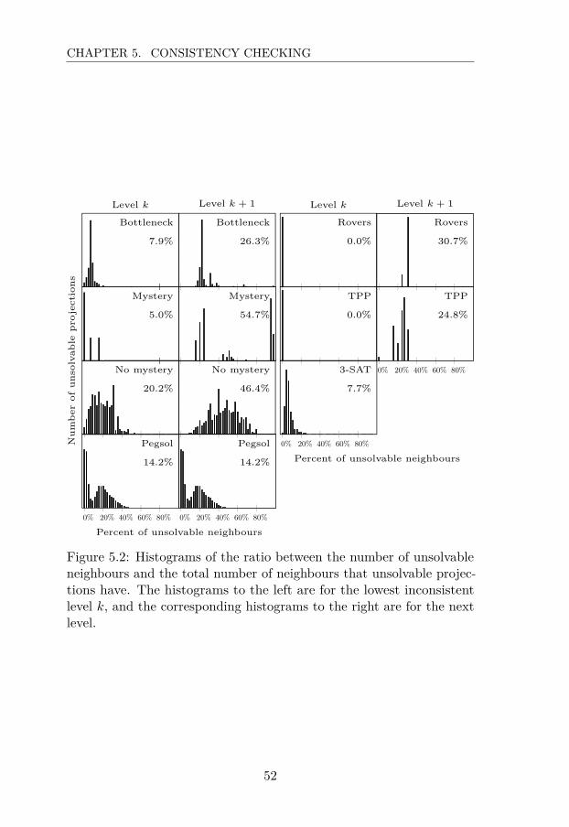
CHAPTER 5. CONSISTENCY CHECKING
Bottleneck
7.9%
Mystery
5.0%
No mystery
20.2%
0% 20% 40% 60% 80%
Pegsol
14.2%
Rovers
0.0%
TPP
0.0%
0% 20% 40% 60% 80%
3-SAT
7.7%
Bottleneck
26.3%
Mystery
54.7%
No mystery
46.4%
0% 20% 40% 60% 80%
Pegsol
14.2%
Rovers
30.7%
0% 20% 40% 60% 80%
TPP
24.8%
Level k Level k + 1 Level k Level k + 1
Percent of unsolvable neighbours
Percent of unsolvable neighbours
Numberofunso
lvable
pro
jections
Figure 5.2: Histograms of the ratio between the number of unsolvableneighbours and the total number of neighbours that unsolvable projec-tions have. The histograms to the left are for the lowest inconsistentlevel k, and the corresponding histograms to the right are for the nextlevel.
52
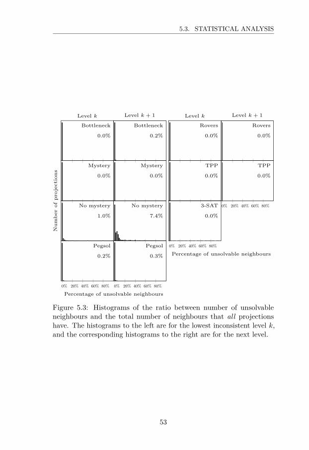
5.3. STATISTICAL ANALYSIS
Bottleneck
0.0%
Mystery
0.0%
No mystery
1.0%
0% 20% 40% 60% 80%
Pegsol
0.2%
Rovers
0.0%
TPP
0.0%
0% 20% 40% 60% 80%
3-SAT
0.0%
Bottleneck
0.2%
Mystery
0.0%
No mystery
7.4%
0% 20% 40% 60% 80%
Pegsol
0.3%
Rovers
0.0%
0% 20% 40% 60% 80%
TPP
0.0%
Percentage of unsolvable neighbours
Percentage of unsolvable neighbours
Numberofpro
jections
Level k Level k + 1 Level k Level k + 1
Figure 5.3: Histograms of the ratio between number of unsolvableneighbours and the total number of neighbours that all projectionshave. The histograms to the left are for the lowest inconsistent level k,and the corresponding histograms to the right are for the next level.
53

CHAPTER 5. CONSISTENCY CHECKING
if the neighbourhoods are similar and can be bridged by a commonunsolvable projection in the next level.
Considering that most domains have very few neighbourhoods, an-other natural question is if there are variables that always occur togetheror not at all in every unsolvable projection? We say that such variablesat some level are inseparable. The average number of inseperable pairsand triples is given in Table 5.3. For domains with very small neigh-bourhoods, the number of pairs and triples tends to be higher. Oneexplanation is that projections from different neighbourhoods are likelyto not have many variables in common, and since there are only fewprojections from the same neighbourhood, then the pair and triplesare likely to be inseparable. In general, it seems that as the averageneighbourhood size increases, the number of inseparable variable subsetsdecreases. If we could identify inseparable pairs and triples then wecould reduce the number of projections to check significantly, e.g. todecide if an instance Π is k-variable consistent we would normally haveto check
(|V (Π)|k
)projections, but if we know of an inseparable pair then
we only have to check(|V (Π)|k−1
)projections since we can treat the pair as
a single ‘variable’.
5.3.3 Predecessor and Successor Projections
Table 5.1 showed that the ratio between the number of unsolvableprojections and the total number of projections tends to increase fromone level to the next, and we take a closer look at this through the lensof predecessor, successor and minimal projections.
Definition 5.6. The projection Π|V1 is a predecessor to the projectionΠ|V2 if |V1| = |V2| − 1 and V1 ⊂ V2. Conversely, Π|V2 is a successor ofΠ|V1 . Furthermore, we require the causal graph of the instances to beweakly connected and the goal to be defined for at least one variable.
For the lowest inconsistent level k, every predecessor is solvable.Hence, the notion is only relevant for levels higher than k. Furthermore,an unsolvable projection is minimal if it has no unsolvable predecessors,e.g. all unsolvable projections at the lowest inconsistent level k areminimal. An unsolvable projection at level > k can be minimal, but ifit is not then it can be projected into one.
How many unsolvable predecessors that unsolvable projections tendto have is detailed in Figure 5.4, and on average they have about 27%unsolvable predecessors. The ratio for most domains is around that
54

5.3. STATISTICAL ANALYSIS
# of neighbourhoods Size of neighbourhoods
Domain Level k Level k + 1 Level k Level k + 1
3-SAT 1 - 213.8 -Bottleneck 2.35 1 33.53 2849.25Mystery 1 1 1.25 36.25No Mystery 1.12 1 17.5 223.9Pegsol 1474.95 1628 21.6 21.67Rovers 2.33 1 1 294TPP 1 1.5 1 30.5
Table 5.2: The average number of neighbourhoods and their averagesize for every domain, at the lowest inconsistent level k and at levelk+ 1. The average number of unsolvable projections per instance is theproduct of the number of neighbourhoods and their size.
# of inseparable pairs # of inseparable triples
Domain Level k Level k + 1 Level k Level k + 1
3-SAT 0 - 0 -Bottleneck 0.95 0.85 0.6 0.6Mystery 5.5 5.5 5.25 5.25No Mystery 2.36 1 1 0Pegsol 2.19 0 2 0Rovers 6 4.34 2.67 2.67TPP 7.4 3.5 7.2 1.5
Table 5.3: The average number of inseparable pairs and triples for everydomain, at the lowest inconsistent level k and at level k + 1.
55

CHAPTER 5. CONSISTENCY CHECKING
mark, and for Mystery it is a lot higher: 55.8%. The histograms arequite narrow for most domains, except for Mystery and No Mystery,which have quite a wide histogram. Pegsol is, again, the outlier and it isnot surprising considering how little the average size of neighbourhoodsincreased from level k to level k+1: since every successor of an unsolvableprojection is also unsolvable and the size of the neighbourhoods did notincrease, then there must be very few successors.
The number of unsolvable projections at level k + 1 that are alsominimal is given in Table 5.4, and for most domains there are very fewminimal unsolvable projections at level k + 1, i.e. nearly all unsolvableprojections appear to have propogated from some unsolvable predecessor.Yet again, Pegsol is the black sheep, who almost exclusively had minimalunsolvable projections, although, the previous observation explains thistoo (there must be very few unsolvable successors that are not filteredaway).
The main reason (excluding Pegsol, of course) for why the ratiobetween unsolvable and solvable projections increased is because unsolv-able projections give rise to unsolvable successors, i.e. they propagate tothe next level (and so on). Furthermore, successors of the same unsolv-able projection are also neighbours. This means that, for most domains,we can expect the density of unsolvable projections and neighbours toincrease strictly.
5.4 Experimental Analysis
A common way of evaluating methods on a large collection of bench-marks is to give the methods a time and space limit, and then counthow many they were able to solve within these limits. This is a bitdifferent from the original publication [BJS13], where we also measuredtheir runtime. The reason for this adjustment is that there were nobenchmarks of unsolvable instances, so these had to be constructedfrom scratch. Hence, we only had 11 benchmarks and were able to doa more detailed analysis per instance. However, at this point in timethere are many unsolvable instances available and we opted to use theminstead in the forthcoming analysis. As the reader will notice, we donot use every domain in the analysis, and we restrict the competition towhat was available then. We do this to demonstrate what the originalpublication [BJS13] demonstrated.
56

5.4. EXPERIMENTAL ANALYSIS
Bottleneck
20.3%
Mystery
55.8%
No mystery
24.5%
0% 20% 40% 60% 80%
Pegsol
0.0%
0% 20% 40% 60% 80%
Rovers
32.0%
0% 20% 40% 60% 80%
TPP
24.0%
Percentage of unsolvable predecessors
Numberofunso
lvable
pro
jections
Figure 5.4: Histograms for every domain over how many (in percent)unsolvable predecessors every unsolvable projection has, for one levelpast the lowest inconsistent level.
% of unsolvable projections that are minimal at level k + 1
Bottleneck 0.0Mystery 0.0No Mystery 31.9Pegsol 98.8Rovers 0.0TPP 1.5
Table 5.4: The percentage of unsolvable projections that are also minimalat lowest inconsistent level k + 1.
57

CHAPTER 5. CONSISTENCY CHECKING
5.4.1 Planners
Consistency checking (CC) used CPT to check projections, and CPTwas configured to use A∗ coupled with a pattern collection, whichconsisted of every pattern of size 3.1 (The terminology of patterndatabases is presented in Section 6.1.) Furthermore, since we are onlyinterested in Plan Existence, A∗ did not reprioritise states nor constructa plan. CC ran with both filters until it either found an unsolvableprojection or ran out resources. Note that, we do not exploit theobservations in Section 5.3 since they were not part of the originalmethod, but we will revisit this topic in Chapter 8, which presents someadditional improvements.
We compare consistency checking with a number of standard plan-ners that are optimised for Plan Generation:
• Fast Forward (FF) [HN01]. The planner was set to its standardconfiguration.
• Fast Downward (FD) [Hel06a]. This planner was tested intwo configurations, seq-sat-fdss-1 and seq-sat-fdss-2, referred to asFD1 and FD2, respectively.
• Lama [RW10]. This is yet another configuration of FD, seq-sat-lama-2011.
It is reasonable to assume that the heuristics of these planners willoften do more harm than good on unsolvable instances. There aresome methods that are primarily intended for planning that are reas-onable to use also for detecting unsolvable instances. We also evalu-ated A∗ coupled with the following admissible heuristic functions: (i.e.Cost Optimal Plan Generation)
• Blind. This heuristic function returns 1 if the state is not a goalstate, 0 otherwise. The blind heuristic will always be better thanany heuristic function that cannot detect dead-ends since it doesnot waste any resources.
• iPDB [HBH+07]. There are many approaches of constructingpattern collections, iPDB is one well-known way of doing so andis discussed in more detail in Section 6.1. We used the defaultsettings in FD, i.e. the maximum PDB size is 2 million and themaximum collection size is 20 million.
1The original paper used another configuration.
58

5.4. EXPERIMENTAL ANALYSIS
• hm [HG00]. This is a family of admissible heuristic functions. Fora given m ≥ 1, hm is the maximum cost of achieving any subsetof m goal atoms by regression, applying the same criterion alsoto all subgoals. CPT was configured to use depth-first search,which used hm for dead-end detection. If this state is identifiedas a dead-end, then the planner can backtrack early.
5.4.2 Coverage
All tests were run a computer with an Intel Xeon E5-2660 at 2.2 GHzCPU and 4 GB available RAM. All methods were given a time limit of30 minutes on each instance, and the empirical data for all methods islisted in Table 5.5.
The worst performing contender was blind search, which was ableto prove a mere 18 instances as unsolvable by exhaustively enumeratingevery reachable state and check if none is a goal state. In general, wecannot expect this to work since there often are too many states tostore in memory, thus this method serves as a baseline.
The planner configurations FF, FD1, FD2 and Lama outperformedblind search and were able to prove 19, 32, 34 and 23 instances as unsolv-able, respectively. It is worth noting that some of these configurationsconsist of several searches, and each search might use a different heuristicfunction. Regardless, they did not provide any meaningful improve-ment over blind search and were easily outperformed by the admissibleheuristics iPDB, h2 and h3, which were able to prove 48, 39, and 55instances as unsolvable. Overall, no method except for h3 could competewith CC and both identified a significant number of initial states asdead-ends (CC proves that an initial state is a dead-end by findingan unsolvable projection, and the heuristic function h3 proves this byproducing the value ∞). However, h3 is very expensive to compute andfor most instances, just evaluating the initial state can take up to halfa minute (if not more).
The best performing method was CC, which proved a total of 66instances as unsolvable. The most surprising observation was that iPDBidentified 17 TPP instances as unsolvable, but CC only identified 4,despite that both methods are based on variable projection. However,they identified the same initial states as dead-ends, i.e. iPDB madeuse of good dead-end detection to prune the reachable state transitiongraph.
59

CHAPTER 5. CONSISTENCY CHECKING
FD
hm
Dom
ain(#
)Blin
dF
FF
D1
FD2
Lam
aiPDB
h2
h3
CC
Bottle
neck
(25)
10(0)
19(0)
19(0)
19(0)
19(0)
18(18)
19(10)
20(20)
20(20)
Mystery
(9)
2(0)
0(0)
9(9)
9(9)
1(0)
4(3)
9(9)
9(9)
8(8)
Nomystery
(25)
0(0)
0(0)
0(0)
1(0)
0(0)
8(1)
3(0)
12(10)
25(25)
Rovers(25)
0(0)
0(0)
3(1)
3(1)
0(0)
1(1)
4(3)
8(8)
9(9)
TPP
(25)
6(0)
0(0)
1(0)
2(0)
3(0)
17(4)
4(1)
6(6)
4(4)
Total(109)
18(0)
19(0)
32(10)
34(10)
23(0)
48(27)
39(23)
55(53)
66(66)
Table5.5:
Coverag
eresults
forthemetho
dstested
onasubset
ofthebe
nchm
arks.The
figures
deno
teho
wman
yinstan
cest
hemetho
dswe
reab
leto
detect
asun
solvab
lewith
intheresource
boun
ds,a
ndthefig
ures
with
inpa
rentheses
deno
teho
wman
yinitial
states
wereidentifi
edas
dead
-end
s.
60

5.4. EXPERIMENTAL ANALYSIS
5.4.3 Discussion
The experiments were meant to illustrate a shortcoming of plannerstailored toward solvable instances. However, we have also convenientlyignored some domains that would highlight a weakness of CC, whichwe will discuss shortly. The configurations of the planners FF, FD andLama, were optimised for Plan Generation (PG), and one would assumesuch planners to be good at the corresponding problem Plan Existence(PE), however, this was obviously not the case since they just marginallyoutperformed blind search. The planner configurations for Cost OptimalPlan Generation (COPG), iPDB and hm, were more successful, despitetackling a tougher problem.
Consider the following two properties of heuristic functions, whereh is some heuristic function and h∗ is the perfect heuristic function.
1. Let s be a state. If h(s) =∞ then h∗(s) =∞.
2. For every state s, h(s) ≤ h∗(s).A heuristic function is safe if it fulfills property (1), and it is admissible ifit also fulfills (2). The heuristic functions of the planners were safe, andheuristic functions for PG need only to fulfill (1). However, it appearsthat admissible heuristic functions for COPG put more emphasis on(1) than non-admissible heuristic functions, despite (1) obviously beinguseful for both problems – a perplexing anomaly. After all, (2) is notimportant for unsolvable instances, thus there is no reason why safenon-admissible heuristic functions should perform worse than admissibleones.
There is a strong correlation between the instances that CC were ableto prove unsolvable and the data in Table 5.1. The lowest inconsistentlevel for the domains that CC performed well on is quite low, but it isalso low for the few instances of Rovers and TPP that the table had dataon. Recall that we used a lot more time to collect the data in Table 5.1,however, that did not help very much for Rovers and TPP. This exposesa weakness of CC, namely, that if there is no small unsolvable projectionthen spending more time is likely to be fruitless. This is especially clearin TPP, where iPDB was able to prove 17 instances as unsolvable andCC only 4. Note that the data in Table 5.1 in incomplete and it is likelythat for the remaining instances, the lowest inconsistent level is quitehigh. In Chapter 6 we will take a look at how to remedy this by takingadvantage of dead-ends identified whilst solving projections, using amore aggressive strategy, and by making projections more informativewith the help of mutexes.
61

CHAPTER 5. CONSISTENCY CHECKING
A much more extensive experimental analysis is presented in Sec-tion 6.5, where we use more benchmarks and also compare againstmethods developed since the original paper was published.
62
Chapter Six
Pattern Databases
A major drawback of consistency checking is that, when it does not findan unsolvable projection, then all the work is wasted since it does notsave any information about the solved projections. However, there isuseful information to store, namely, dead-end states. We remind thereader that no goal state is reachable from a dead-end state. A dead-endstate of a projection can match several states of the original instance,and all of them are dead-ends. Furthermore, all states reachable froma dead-end are also dead-ends. Consequently, dead-end detection canhave a significant impact on the performance of a planner. After all,the initial state of an unsolvable instance is a dead-end, and the planneris done if it can detect it as such.
A natural continuation of consistency checking is thus to solveprojections completely with regression search, and store all states thatnever got visited since they are dead-ends. If the initial state of aprojection was never visited then we have proven that the originalinstance is unsolvable. And when we have spent ample time on solvingprojections, then we turn our focus on the original instance and performa search that ignore states that match any stored dead-end state. Thisis one of the differences between the methods devised in this chapter andconsistency checking. A pitfall of consistency checking is how reluctantit is to check larger projections, and the second difference is that thedevised methods are a lot more eager to check larger projections.
In Section 6.1 we give a brief introduction to pattern databases [CS98]and present a strategy that we use to build them. We present the meth-ods that we analyse in Section 6.2 and carry out a detailed statisticalanalysis of them in Section 6.3, which is similar to the one we did forconsistency checking. For this statistical analysis, we took advantage ofa large computer cluster to determine a distribution for every instanceof how many dead-ends the projections have. These distributions are
63
CHAPTER 6. PATTERN DATABASES
then used in Section 6.3.1 to show that the proposed methods constructpattern collections that are amongst the best. In other words, to im-prove dead-end detection further would require additional techniques.We show in Section 6.3.2 that the two proposed methods differ in asignificant way: one method tends to find more unsolvable projectionsthan the other, which is important since an unsolvable projection im-plies that the instance is unsolvable. In Section 6.4, we show thatmutexes are useful for improving how many dead-ends patterns candetect. Finally, in Section 6.5 we run experiments and show that ourbest methods are competitive. The experiments also show that mutexeshave a considerable effect on many instances.
6.1 Definitions
We first give a brief introduction to pattern databases, and present onetechnique for constructing pattern collections. A pattern P ⊆ V (Π)is a subset of variables of an instance Π, and the lowest solution costof reaching a goal state in Π|P from each state s ∈ TotalStates(Π|P )is stored in a pattern database (PDB) hP . The database is used toefficiently provide an estimate of the real solution cost from some stateto a goal state. We write hP (s) to denote the cost associated with sin hP . A main problem with constructing a PDB is how to choosethe pattern, since PDBs are often vastly different with regard to howinformative they are (and there is an enormous amount of them). Apattern collection C consists of several patterns which, together, areused to provide a solution cost estimate: C(s) = maxhP (s) : P ∈ C.We are only interested in dead-end detection and for this purpose it issufficient to take the maximum, however, for an actual solution costestimate it might be beneficial to take the sum of a few, carefullyselected, PDBs.
A popular strategy to build a pattern collection is iPDB [HBH+07].The iPDB strategy uses hill-climbing search in the space of patterncollections, and we use a similar strategy. Hill-climbing search is anoptimisation technique which attempts to maximise some score functionby local search. In planning, the score function for solvable instancesis often the average cost in the PDB. The search starts with a patternof a single goal variable, and then attempts to find a better patternby repeatedly adding a single variable to it. There might be severalcandidates, and the candidate whose PDB scored best is selected. Thisprocedure is repeated until some condition is met. More precisely, for
64

6.2. METHODS
an instance Π, we use the following pattern selection strategy.
1. Let P = g where (g, d) ∈ G(Π), d ∈ Dg (i.e. g is a goal variable),and let b be a bound on the maximum PDB size. We also havesome function Score, where the input is a PDB and the output isa number;
2. Compute Score(hP∪v) for every v ∈ V (Π), where v /∈ P , v isweakly connected to some variable in P in the causal graph, and|Dv| ·
∏|Dv′ | : v′ ∈ P ≤ b.
3. If there are no candidates then return P ; and
4. Let P be the candidate with the highest score in step 2 and go tostep 2. If there are several candidates with the same score thenchoose one arbitrarily.
The resulting pattern is added to the pattern collection, and then westart yet another search (with another initial pattern, if there is one).This is repeated until either: the collection is sufficiently large; or if thelast 5 searches returned patterns that we have already seen before. Theimplementation tries to avoid candidates that were selected in previoussearches. For example, suppose there are two candidates C1 and C2,Score(C1) > Score(C2). If C1 was selected in a previous search but notC2, then C2 is selected. And if both were selected in previous searches,then C1 is selected. The purpose of this is to avoid selecting the samepattern several times when constructing a pattern collection.
6.2 Methods
We propose two methods for constructing pattern collections and bothmethods are based on hill-climbing search, and the only difference is thescore function. Before we define them, we give a definition of a centralconcept. Let Π be a planning instance. The function ξ(Π) generates aset of at most 20000 reachable states of Π by breadth-first search. Notethat, if Π is unsolvable then every state of ξ(Π) is a dead-end. Thefunction ξ is required to generate the same set every time for the sameinstance. The figure 20000 is somewhat arbitrary, and we discuss whyit is sufficiently large later on. Our methods are:
65

CHAPTER 6. PATTERN DATABASES
• HCDE(Π): A pattern collection is constructed for Π by hill-climbing search with the scoring function:
DE(hP ) = |s ∈ TotalStates(Π|P ) : hP (s) =∞||TotalStates(Π|P )|
which favours PDBs with a high percentage of dead-ends.
• HCSamples(Π): A pattern collection is constructed for Π by hill-climbing search with a scoring function that attempts to maximisethe number of different dead-end states that the pattern collectioncan detect. If two patterns are able to identify exactly the samestates as dead-ends, then we only need one of them. The overlapof a new pattern with the collection is approximated with thehelp of ξ(Π) in the following way. Let P be a pattern and let Cbe the current collection, then the scoring function is:
Samples(hP , C) = |s ∈ ξ(Π) : hP (s) =∞, C(s) 6=∞|
The function Samples outputs the number of dead-ends that C didnot detect as dead-ends, but hP did detect. Note that, ξ generatestates close to the initial state. Detecting dead-end states closeto the initial state is likely to prune away many reachable statesfrom the search space. Hence, Samples should favour patternsthat can detect many, previously undetected, dead-end states ofξ(Π). Furthermore, we resolve tiebreaks with DE(hP ) (and if westill have a tiebreak then the successor is chosen arbitrarily).
6.3 Statistical AnalysisWe present a detailed statistical analysis of how well pattern collec-tions constructed by the methods defined in Section 6.2 perform onbenchmarks. Roughly speaking, the analysis reveals the limit of patterncollections as a method for detecting dead-ends, and we attain this byletting a computer cluster1 generate PDBs using many years of CPU-time. The collected data lets us visualise the distribution of PDBs w.r.t.how many dead-ends they have – a crucial property for good dead-enddetection. We show that the methods perform comparably but thatHCDE tends to find more unsolvable projections, which is importantsince such projections prove that the instance is unsolvable.
1The processors were 8-core Intel Xeon E5-2660 at 2.2GHz, provided byNational Supercomputer Centre (NSC) at Linköping University. Website:https://www.nsc.liu.se/
66

6.3. STATISTICAL ANALYSIS
6.3.1 Dead-end Detection
A disadvantage of a typical experimental analysis, such as measuringcoverage, is the absence of a notion of optimality. For example, lethP be a PDB whose size is bounded by some integer b, and let s be adead-end state that hP cannot detect. Then we do not know if thereis another PDB, whose size is also bounded by b, that can detect s.An optimal pattern collection for the bound b would contain a PDBfor every dead-end that is detectable by a PDB whose size is boundedby b. Note that there might be dead-ends that an optimal patterncollection does not detect, for example, the initial state if there is noPDB of an unsolvable projection whose size is bounded by b. In thissection, we analyse how well the pattern collections constructed byHCDE and HCSamples are at detecting dead-ends, and whether spendingmore CPU-time would help. The latter is estimated by comparing howmany dead-ends they detect compared to pattern collections that wereconstructed by using years of CPU-time on a computer cluster. Thedead-ends that we use to compare them against are generated by ξ.
It is, of course, computationally infeasible to construct optimalpattern collections in general, and a more pragmatic approach is tospend an excessive amount of CPU-time instead. We used a computercluster to generate 20 million random PDBs for every instance Π wherethe size of every PDB is bounded by 500000, and we denote this set ofPDBs as P(Π). The pattern collection ϕ(Π) ⊆P(Π) consists of the1500 patterns with the highest percentage of dead-ends. We stress thateven though we generate 20 million PDBs, it is not a complete set ofPDBs for most instances, and it is possible for HCDE and HCSamplesto generate PDBs not in P(Π). The reason why we do not generatemore or larger PDBs is because of how computationally expensive itis. Of course, the same bound on PDB size was used by HCDE(Π) andHCSamples(Π) in the following analysis.
Figure 6.1 and 6.2 shows how HCDE and HCSamples perform againstϕ, where hill-climbing methods were given at most 20 minutes toconstruct a pattern collection. The pattern collections perform similarlyand in most domains they were able to detect as many dead-ends as ϕ.The exceptions are Pegsol and 3-SAT, which we examine more closelylater. In the other domains the ratio is close to 1, i.e. HCDE andHCSamples detected about as many dead-ends as ϕ. We observe theeffect of P(Π) being incomplete in 3-SAT, where HCDE and HCSamplesdetect many more dead-ends than ϕ. Typically, the frequency of dead-ends drop as the instance difficulty increase (roughly speaking, the
67

CHAPTER 6. PATTERN DATABASES
0
1
Bottleneck 90%
0
1
No mystery 91%
0
1
Pegsol
83%
0
1
Mystery 87%
0
1
Rovers 77%
01
3-SAT 28%
0
1
TPP 76%
Figure 6.1: Every point represents an instance Π and they are orderedaccording to increasing difficulty (left to right). The value of a pointis the ratio of the number of dead-ends identified by HCDE(Π) to thenumber of dead-ends detected by ϕ(Π) on the set ξ(Π). A point below 1means that the pattern collection identified fewer dead-ends than ϕ(Π),and the percentage is the average ratio of dead-ends that ϕ(Π) detectedof ξ(Π). No PDB detected any dead-end for Tiles.
68

6.3. STATISTICAL ANALYSIS
0
1
Bottleneck 90%
0
1
No mystery 91%
0
1
Pegsol
83%
0
1
Mystery 87%
0
1
Rovers 77%
01
3-SAT 28%
0
1
TPP 76%
Figure 6.2: Same as Figure 6.1 except that we used HCSamples.
69

CHAPTER 6. PATTERN DATABASES
0% 20% 40% 60% 80%
0.5%
0% 20% 40% 60% 80%
18.2%
0% 20% 40% 60% 80%
0.6%
Percent of dead-ends
No.
ofPD
Bs Pegsol (10) 3-SAT (22-5-2) 3-SAT (129-30-2)
Figure 6.3: Histograms of the percentage of dead-ends of the PDBs inP for 3 instances. The numbers within the parentheses denote specificinstances in the benchmark. The percentage in the upper right corneris the average percent of dead-ends across all PDBs of the instance.
difficulty of an instance is its state space size, or by the parameters usedto generate it), i.e. good patterns become more rare. Consider this: ϕwas given several weeks of CPU-time per instance to generate 20 millionPDBs and construct a pattern collection, whereas HCDE and HCSampleswere given a mere 20 minutes and they were still able to compete withϕ!
The two outliers are Pegsol and 3-SAT, but why is this? Figure 6.3shows the histograms of how many dead-ends the PDBs of P have for3 instances: a hard Pegsol instance, an easy 3-SAT instance and a hard3-SAT instance. The easier 3-SAT instance has a smaller state spacethan the harder one which means that the PDBs for the easy instanceare (relatively) a lot more informative than the PDBs for the hardinstance. To get a more meaningful distribution for the hard instancewe might have to consider larger PDBs or additional techniques (e.g.mutexes). The situation is different for Pegsol, where the distribution inFigure 6.3 is representative for every Pegsol instance, i.e. the PDBs arenot very informative. The distributions are even worse for smaller PDBs,i.e. no PDB has any dead-end. The methods HCDE and HCSamplesmight struggle when given these instances because their score functionscount dead-ends for smaller state space sizes but the score is almostalways 0. In other words, the search degrades to blind, uninformedsearch and is therefore unlikely to find the few patterns which are usefulfor dead-end detection.
70

6.3. STATISTICAL ANALYSIS
6.3.2 Unsolvable Projections
If we encounter an unsolvable projection at some point during theconstruction of a pattern collection then we can terminate early: weknow that the initial state is a dead-end and that the instance isunsolvable. Hence, unsolvable projections are very important. Theproposed methods differ in this regard; HCDE found a total of 1458unsolvable projections over all instances, whereas HCSamples only found499. To derive these figures, we did not terminate early, and everypattern collection contained at most 60 PDBs of unsolvable projections.However, this does not mean that HCDE finds a single unsolvableprojections faster, or more likely, than HCSamples. In this section, weinvestigate why HCDE finds more unsolvable projections than HCSamples,and whether the PDBs of unsolvable projections tend to have a lot ofdead-ends in addition to the initial state, i.e. if such PDBs are likely toget a high score by DE.
Note
We give a short example to illustrate how the figures in Table 6.1are computed. Suppose we have three instances Π1, Π2 and Π3 fromthe same domain D. For each instance Πi, 1 ≤ i ≤ 3 we compute100 PDBs, denoted hP1
i , . . . , hP100i . Then Hi is the histogram over
the ratios DE(hP1i ), . . . ,DE(hP100
i ).Suppose Πi|P1 , Πi|P2 and Πi|P3 are unsolvable, and are the only
unsolvable projections. Let r1i , r2
i and r3i be the percentile ranks
of the PDBs of these unsolvable projections in Hi. The percentilerank of a PDB is its relative position in a distribution, e.g. ifthe percentile rank of a PDB is 99 then 99% of the PDBs have asmaller or equal ratio of dead-ends. The figures in Table 6.1 arecomputed in the following way. Let ri = avgr1
i , r2i , r
3i . Then:
minri : 1 ≤ i ≤ 3 is the minimum-average; avgri : 1 ≤ i ≤ 3is the average-average; and maxri : 1 ≤ i ≤ 3 is the maximum-average. These figures are only for D.
Table 6.1 shows that PDBs of unsolvable projections tend to havea high percentile rank in the distribution of frequency of dead-ends,i.e. PDBs of unsolvable projections tend to have many dead-ends. Forexample, Figure 6.3 illustrates this distribution for 3 instances. Notethat a high percentile rank of a PDB for the Pegsol instance means thatthe PDB has around 10% dead-ends (i.e. a high percentile rank doesnot guarantee good dead-end detection but that it is amongst the best
71

CHAPTER 6. PATTERN DATABASES
Average percentile rank
Domain Minimum Average Maximum
3-SAT 98 98 99Bottleneck 49 67 93Mystery 51 75 99No mystery 96 97 99Pegsol 96 98 99Rovers 99 99 99TPP 99 99 99
Table 6.1: Minimum, average and the maximum average percentile rankof the ratio of dead-ends in the PDBs of the unsolvable projectionsin P(Π), for every instance Π. That is, for every instance of a do-main we take the average percentile rank of the unsolvable projections,and then we take the minimum, the average or the maximum (of theaforementioned average) over the entire domain.
for said purpose). For most domains, the percentile ranks are very high,around 98, which means that PDBs of unsolvable projections tend toscore high by DE. This partly explains why HCDE encounters far moreunsolvable projections than HCSamples: DE serves as a heuristic functionto find unsolvable projections. The two exceptions are Bottleneck andMystery, but their average percentile rank is higher than 50, i.e. theyhave more dead-ends than the average PDB.
6.4 Mutual Exclusions
A useful and well-known technique to improve the heuristic values of aPDB is to use mutexes: a mutex is a partial state which matches statesthat cannot be reached from the initial state. We generate mutexeswith the critical path heuristic hm [HG00]. More specifically, we letm = 2 or m = 3. In this section, we detail how many mutexes h2 and h3
identify and whether any of the mutexes can directly prove the instanceunsolvable. If a mutex does not infer unsolvability, then it can still havea tremendous effect on increasing the number of dead-ends in a PDB.
Definition 6.1. A partial state sm of a SAS+ instance Π is a mutualexclusion, or mutex, if and only if there is no state s reachable fromI(Π) such that sm ⊆ s.
72

6.4. MUTUAL EXCLUSIONS
Mutexes identified Goal is mutex
Domain (# instances) h2 h3 h2 h3
3-SAT (30) 42 38 554 0 0Bottleneck (25) 51 679 248 340 10 20Mystery (9) - - 9 9No mystery (25) 81 788 2 027 164 0 10Pegsol (24) 826 4 768 0 6Rovers (25) 19 431 234 424 3 8Tiles (20) 11 160 11 160 0 0TPP (25) 97 858 1 479 852 1 5
Table 6.2: The sum of mutexes identified for every domain. Mutexesare identified by either h2 or h3. The sum does not include mutexes forinstances whose goal matched a mutex (e.g. Mystery).
A common definition of mutex in the literature is that there is noreachable total state which contains more than one variable-value pairof a mutex, but we use a more general definition (for mutexes of size2, both definitions are identical). We get mutexes of size 2 and 3 fromh2 and h3, respectively. Ideally, for an unsolvable instance Π we wantto prove that some sm ⊆ G(Π) is a mutex (i.e. every goal state isunreachable), but it is obviously PSPACE-hard to do so. Hence, if weuse a polynomial-time algorithm to identify mutexes then the typicalcase is that the goal does not match any identified mutex.
To (naively) decide whether a partial state sm is a mutex for aninstance Π, we let sm be the goal and evaluate h2 on I(Π). Table 6.2details how many mutexes were found by h2 and h3, and how manyinstances were identified as unsolvable by a mutex. Every instance ofthe Mystery domain had a goal which matched a mutex as well as manyinstances of the Bottleneck domain. Mutexes from h2 immediatelyidentified 23 of 183 instances as unsolvable, whilst mutexes from h3
identified 58 instances as unsolvable. For every instance, it took lessthan 4 seconds for h2 to identify mutexes, and (except in a few cases)less than 5 minutes for h3.
The mutexes identified by h2 are also identified by h3, but they arein a different form. For example, suppose h2 identifies a mutex sm =(v1, d1), (v2, d2), then h3 will generate the mutexes sm ∪ (v3, d3) :v3 ∈ V \ v1, v2, d3 ∈ Dv3. Obviously, this set, collectively, identifiesthe same states as sm. In practice, we first generate mutexes by h2
since they are more general, and only add mutexes generated by h3 if
73

CHAPTER 6. PATTERN DATABASES
15.7%
0% 20% 40% 60% 80%
3.6%
Percent of dead-ends
Num
bero
fPD
Bs
3-SAT (22-5-4)
TPP (05-02)
84.2%
0% 20% 40% 60% 80%
88.4%
Percent of dead-ends
3-SAT (22-5-4)
TPP (05-02)
Figure 6.4: Histograms of the percent of dead-ends of the PDBs inP for two instances. The PDBs in the histograms to the left did notuse mutexes, whilst the PDBs in the histograms to the right did. Themutexes were generated by h3. No mutex matched any goal.
they are not matched by some more general mutex.If a solution for a projection visits a state that matches a mutex
then there is no corresponding solution for the original instance, andby avoiding such solutions we can generate PDBs with potentiallymore dead-ends. Figure 6.4 shows the impact of exploiting mutexeswhen generating PDBs for two instances, and the impact is a verysignificant increase in dead-ends: the average ratio of dead-ends forthe 3-SAT PDBs went from 15.7% to 84.2% and for the TPP PDBs itwent from 3.6% to 88.4%. Figure 6.4 consists of only two instances, butthe experiments in Section 6.5 show that many other instances benefitgreatly, too, from using mutexes.
6.5 Experimental Evaluation
In this section, we evaluate our methods on all benchmarks. The testswere run on a computer with an Intel Xeon E5-2660 at 2.2 GHz CPUand 4 GB available RAM, and every method were given 30 minutes forevery instance.
74
6.5. EXPERIMENTAL EVALUATION
6.5.1 Planners
This time we do not compare against configurations meant for solvableinstances (i.e. FF, Lama, and so on), and focuse on methods developedfor unsolvable instances. The methods we compare are:
• Blind. Same configuration as we used in Section 5.4.
• Two variants of the M&S heuristic that are optimised for dead-end detection [HKT14]. Hoffmann et al. [HKT14] gave threeconfigurations, and we present the two best ones: Mrg1 and Mrg2.
• Consistency Checking (CC). See Chapter 5 for details. We alsoevaluate the impact of using mutexes when solving projections,which were generated by h3.
• iPDB. This method is not designed for unsolvable instances, butserves as a baseline for our similar methods.
• HCBL. A pattern collection is constructed by hill-climbing searchwith the scoring function:
S(hP ) =∑hP (s):hP (s)6=∞,s∈TotalStates(Π|P )
|TotalStates(Π|P )|
This scoring function is useful for solvable instances, but not somuch for unsolvable. This method is very similar to iPDB and themain difference is that this method does not terminate the searchif the improvement is too small. The planner used a depth-firstsearch algorithm, and the pattern collection is used to detectdead-ends. Just like iPDB, this method also serves as a baseline.
• HCDE. The pattern collection is constructed as previously de-scribed, and is using the same planner as HCBL. We also evaluatedifferent PDB and pattern collection sizes, and how much PDBsbenefit from mutexes generated by h2 or h3. These paramet-ers are denoted as Cnm, where C is the pattern collection, n ≥max|TotalStates(Π|P )| : P ∈ C, m ≥
∑P∈C |TotalStates(Π|P )|,
and we write h2 or h3 to denote whether the mutexes were gener-ated by h2 or h3.
• DE-PDBs [PS16], which identifies dead-ends by systematicallyconstructing PDBs and then use them to prune the reachablestate space – very comparable to our method.
75

CHAPTER 6. PATTERN DATABASES
• Aidos [SPS+16], the winner of the first unsolvability IPC, whichconsists of an array of methods, and one of them is DE-PDBs.
• SymPA [Tor16], which performs bidirectional search in the originaland abstract state spaces.
6.5.2 Coverage
Coverage results are presented in Table 6.3, together with two differenttotals. The first total is the sum of coverage for all domains, whilst thesecond ignores the coverages of 3-SAT, Pegsol and Tiles. We motivatethe second total in the following way. Any heuristic function that isevaluated sufficiently fast will perform well on the excluded instancesbecause the blind heuristic function performs well. In other words, weare not measuring how good they are at dealing with the combinatorialexplosion. Note that blind search does not have full coverage for theexcluded domains, but no other method performed better (except forAidos in the 3-SAT domain). The domains excluded in second totalcoverage also coincide with the domains that we did not evaluatein Section 5.4, and a difference between the two totals is especiallynoticeable for consistency checking (CC): CC was not able to competewith Mrg1 in the first total (77 vs. 114), but could compete in thesecond total (66 vs. 65). This is because the lowest inconsistent level istoo high for CC even though it is possible to simply visit every reachablestate.
The M&S methods Mrg1 and Mrg2, just like CC, were tailoredtowards proving that the initial state is a dead-end; in this regard, Mrg1had the best performance with 114. The runner ups were C5M
60M withmutexes by h3 and Aidos, who showed 98 initial states as dead-ends(Aidos got coverage if any method detected the initial state as a dead-end). When the latter methods had to fall back to search, then theirtotal coverage was higher than Mrg1.
The best performing method w.r.t. total coverage was Aidos whichproved 170 (or 106) of 183 (or 109) instances as unsolvable – impressive!However, it is arguably not fair to compare a single method to acollection of methods. Hence, we focus our comparison to the mostsimilar method: DE-PDBs, which is also part of Aidos. Our bestperforming configuration was C5M
60M using mutexes generated by h3,which identified 147 (or 98) as unsolvable. DE-PDBs identified 132 (or83) instances as unsolvable, which is 15 less than ours. The differenceis explained by Mystery and Rovers, where our method had a much
76
6.5. EXPERIMENTAL EVALUATION
better coverage thanks to mutexes. When HCDE did not have accessto mutexes then its performance was comparable to DE-PDBs (137against 132), however, it was able to find more unsolvable projections(66 against 48). Increasing the maximum allowed PDB size had variedeffect, the total coverage dropped when it did not have any mutexes, andwent up slightly when it had mutexes. Note that, we did not increasethe maximum allowed pattern collection size. In other words, the totalmemory usage stayed the same and it was not utilised significantlybetter by increasing PDB size.
The reason why HCBL performs surprisingly well is because it stopsonce it finds an unsolvable projection, regardless of its score. This isespecially clear in the second total coverage, where 49 of 64 instanceswere proven as unsolvable by finding an unsolvable projection. No 3-SAT,Pegsol or Tile was proved as unsolvable by encountering an unsolvableprojection, and unsolvability was instead proven by exhaustive search.Note that iPDB performed significantly worse despite being similar toHCBL, and found only 27 unsolvable projections. The poor performanceof iPDB might be that it terminates its search too early since it doesnot see any significant heuristic improvement, and that this strategydoes not work well on unsolvable instances.
77

CHAPTER 6. PATTERN DATABASES
HC
BL
HC
DE
CC
C50
0k60M
C50
0k60M
C2.
75M
60M
C5M 60M
Dom
ain(#
)-
h3-
-h2
h3-
h2h3
-h2
h3
3-SA
T(30)
0(0)
0(0)
15(0)
15(5)
15(5)
15(5)
15(5)
15(5)
15(5)
15(5)
15(5)
15(5)
Bottle
neck
(25)
20(20)
20(20)
16(16)
21(19)
20(18)
21(20)
21(20)
20(19)
20(20)
20(20)
20(20)
20(20)
Mystery
(9)
8(8)
9(9)
6(6)
7(7)
9(9)
9(9)
6(6)
9(9)
9(9)
6(6)
9(9)
9(9)
Nomystery
(25)
25(25)
25(25)
20(12)
23(12)
23(12)
23(12)
23(14)
22(14)
23(14)
25(18)
25(18)
25(18)
Pegsol
(24)
0(0)
6(6)
24(0)
24(2)
24(7)
24(12)
24(5)
24(7)
24(12)
24(4)
24(9)
24(15)
Rovers(25)
9(9)
9(9)
11(11)
14(13)
17(17)
19(19)
10(10)
19(19)
21(21)
9(9)
19(18)
22(22)
Tile
s(20)
10(10)
10(10)
10(0)
10(0)
10(0)
10(0)
10(0)
10(0)
10(0)
10(0)
10(0)
10(0)
TPP
(25)
4(4)
6(6)
11(4)
23(8)
23(7)
23(10)
22(6)
22(5)
22(10)
22(5)
22(6)
22(9)
T otal(18
3)76
(76)
85(85)
113(49)
137(66)
141(75)
144(87)
131(66)
141(78)
144(91)
131(67)
144(85)
147(98)
Total*
(109
)66
(66)
69(69)
64(49)
88(59)
92(63)
95(70)
82(56)
92(66)
95(74)
82(58)
94(71)
98(78)
Dom
ain(#
)Blin
dMrg1
Mrg2
iPDB
h2h3
Aidos
DE-
PDBs
SymPA
3-SA
T(30)
15(0)
15(15)
13(13)
10(0)
10(0)
10(0)
30(0)
15(0)
10(9)
Bottle
neck
(25)
10(0)
5(5)
11(11)
18(18)
19(10)
20(20)
25(25)
19(12)
25(25)
Mystery
(9)
2(0)
6(6)
1(1)
4(3)
9(9)
9(9)
9(9)
6(6)
9(9)
Nomystery
(25)
0(0)
25(25)
25(25)
8(1)
3(0)
12(10)
25(14)
25(18)
25(19)
Pegsol
(24)
24(0)
24(24)
0(0)
16(0)
20(0)
16(6)
24(4)
24(0)
24(4)
Rovers(25)
0(0)
18(18)
18(18)
1(1)
4(3)
8(8)
22(22)
13(0)
23(4)
Tile
s(20)
10(0)
10(10)
10(10)
10(0)
10(0)
0(0)
10(0)
10(0)
10(0)
TPP
(25)
6(0)
11(11)
19(19)
17(4)
4(1)
6(6)
25(24)
20(3)
22(5)
T otal(18
3)67
(0)
114(114
)97
(97)
84(27)
79(23)
81(59)
170(98)
132(48)
148(75)
Total*
(109
)18
(0)
65(65)
74(74)
48(27)
39(23)
55(53)
106(94)
83(48)
104(62)
Table6.3:
Coverag
eresults
onthebe
nchm
arks.The
second
totalisthecoverage
ofeverydo
mainexcept
3-SA
T,Pe
gsol
andTile
s.The
figures
with
inpa
renthesesareho
wman
yinitial
states
werede
tected
asdead
-end
s.
78

6.5. EXPERIMENTAL EVALUATION
6.5.3 Discussion
An obvious critique against the statistical analysis done in Section 6.3is that PDBs with the most dead-ends are not necessarily the bestsince there is no guarantee that those will have the most impact whenpruning away reachable states. Suppose there exists a PDB with justone dead-end entry: the initial state. Obviously, there is no other PDBwith a greater pruning impact since the search finishes immediately.However, this PDB would get a very low score by the scoring functionDE (but selected if found), and thus thus claiming that there are veryfew better pattern collections might not be true. The following theoremshows that the described PDB cannot exist unless the initial state isthe only reachable state.
Theorem 6.2. Let Π be a SAS+ planning instance, and let Π|P , P ⊆V (Π) be an unsolvable projection. Then for every reachable state s ofΠ, hP (s) =∞.
Proof. Since Π|P is unsolvable, then hP (I(Π)|P ) = ∞. This meansthat every state s reachable from I(Π)|P is also hP (s) =∞ (otherwisehP was computed incorrectly). Suppose there is a reachable state s′of Π such that hP (s′|P ) 6=∞ (i.e. unreachable in Π|P ). The proof ofTheorem 2.8 essentially says that if a state is unreachable in a projection,then the matching states are unreachable in the original instance. This iseasily shown by changing the goal of the original instance to a reachablematching state, which would bring forth the situation where the originalinstance is solvable but not a projection; an obvious contradiction. Inother words, the assumption that s′ is unreachable is contradictive, thusevery reachable state of Π is detected as a dead-end by hP .
Theorem 6.2 is, perhaps, not surprising, but it explains a number ofobservations:
• PDBs of unsolvable projections can detect every reachable state asa dead-end, which means that we can expect PDBs of unsolvableprojections to contain many dead-end entries. This is backed upby the data in Table 6.1, except for Bottleneck and Mystery, forwhich the average percentile ranks are a fair bit below 99. This ispossible since there might be states that are both unreachable anddead-ends, i.e. the state transition graph consists of more than 2weakly connected components. Entries in a PDB for such states
79

CHAPTER 6. PATTERN DATABASES
are, of course, pointless, and perhaps the scoring function forHCDE should check whether the state associated with a dead-endentry is reachable in the projection to avoid giving such PDBs anunsuitable high score. This is not a problem for HCSamples sinceit evaluate PDBs on reachable states.
• Theorem 6.2 also reveals an important property of PDBs: let s bea state of the original instance that is detected as a dead-end bysome PDB, then the very same PDB detects every state reachablefrom s as a dead-end. This is trivially shown by replacing theinitial state of the instance with s, thus Theorem 6.2 is applicable.Perhaps, most PDBs with a high percentage of dead-ends identifieda state close to the initial state as a dead-end, and therefore also allsubsequent states. This might also explain why the Tiles domainis difficult: it is possible to undo actions (reversible actions), hence,proving that one reachable state is a dead-end also proves thatevery reachable state is a dead-end. Solvable projections with onlyreversible actions cannot contain any reachable dead-end statesince one would imply that every state is a dead-end, includinggoal states.
• Another possible critique against the statistical analysis in Sec-tion 6.3 is that we evaluated the methods on ‘only’ 20000 states,and that they were generated by using breadth-first search (in-stead of, for instance, depth-first search). We chose breadth-firstsearch since detecting dead-ends close to the initial state oftenleads to pruning a large part of the state transition graph. Ofcourse, there is no guarantee that this will happen. However,Theorem 6.2 says that if a PDB detects a dead-end state, thenall states reachable from it are detected as dead-ends by the verysame PDB. The problem with generating states using depth-firstsearch is that it can give a misleading score, e.g. when a singlePDB detects a large part of a search as dead-ends.
At this point, we have hopefully established that the scoring functionDE is a good way of measuring PDBs with respect to how well theyprune away reachable states, and that HCDE finds PDBs with very highscores (Chapter 6.3). Two concerns that we have not discussed yet are:we did not use all of the IPC instances to evaluate HCDE; and thatthe statistical analysis should have considered more and larger PDBs.Obviously, we believe that we would get a similar result, however, this
80
6.5. EXPERIMENTAL EVALUATION
kind of analysis is inherently computationally expensive and has to berestricted.
Based on the statistical analysis, we believe that there is littlepoint in spending more time to construct a better pattern collection.Furthermore, since the pattern collections are often very good, we believethat further improvement is likely to come from enhancing patterns withother techniques such as mutexes. We showed that mutexes generated byhm had a tremendous impact on the number of dead-ends in PDBs, andit would be interesting to compare different mutex generation methods.Another possibility of improving PDBs is to simplify the instance suchthat the simplified instance is solvable if and only if the original instanceis, e.g. redundant actions [HJ00] are actions that can be removed sincethey are replaceable by a sequence of other actions. DE-PDBs andHCDE without mutexes perform similarly, and a difference is the orderthey consider patterns. DE-PDBs is not as aggressive as HCDE since itconsiders patterns in the same way as consistency checking, perhapsthey differ significantly w.r.t. pattern collection construction time.
It is worth noting that solvable instances might also contain dead-ends and therefore the proposed methods might be useful for suchinstances, e.g. Sokoban [PRB14]. Pattern collections can easily betailored toward both heuristic guidance and dead-end detection; it issimply a matter of selecting different PDBs for either purpose. However,the cost is increased pattern collection construction time or increasedmemory usage. The latter might be addressed by compressing the PDBs[FKMH07].
81


III
PART
Polytree Causal Graphs &Variable Similarity
83

Overview of Part III
We now take a short intermission in our enterprise to prove unsolvability,and consider instances with polytree causal graphs. In Chapter 7, wereveal two computationally tractable classes of instances, which bothhave polytree causal graphs and meet some additional restrictions. Thenotion of variable isomorphism was pivotal for finding the first class,and intuitively two variables are isomorphic if they behave in the sameway in some optimal solution. If we know of an isomorphic pair, thenwe can remove one of the two variables without affecting solvability. Ifwe also want to preserve optimal solution cost, then the action costs forthe variables that we left intact need to be adjusted. We do preciselythis for instances with polytree causal graphs, and identify a number ofrestrictions for when such a strategy yields a polynomial time algorithm.In Chapter 8, we use a variant of variable isomorphism to analyseunsolvable projections. We also identify another related tractable classthrough the idea of instance splitting, which splits the instance such thatthe original instance is solvable if and only if the smaller correspondinginstances are. We construct a divide-and-conquer algorithm which runsin polynomial time when the instance meet certain restrictions.
We carried out an extensive statistical analysis of unsolvable pro-jections in Chapter 5.3 and noted that unsolvable projections tend tohave a significant number of variables in common. In Chapter 8 weask the question: why those variables? We postulate that unsolvableprojections tend to be composed of variables that play different roles, i.ethey are not ‘similar’. Isomorphic variables are, in some sense, extremelysimilar, and we devise a variable similarity measure to rate how similartwo variables are. We then perform a statistical analysis and show thatthe variable similarity measure can differentiate between unsolvable andsolvable projections quite well. This measure is then used to optimiseconsistency checking.
84

Chapter Seven
Tractable Classes
One approach for constructing heuristic functions is to: (1) find atractable (i.e. polynomial-time solvable) class of planning instances;(2) abstract the original instance to an instance in the tractable classand solve it; and (3) use the cost of the solution for the abstractinstance as a heuristic value (cf. Helmert [Hel04]; Helmert, Haslumand Hoffman [HHH07]; Katz and Domshlak [KD10]). An ongoingquest in the planning community is to identify as many and as generaltractable classes as possible, since having knowledge of these mightprove invaluable for constructing efficient planners [KD08a]. A commonapproach to the problem of identifying tractable instances is to imposerestrictions on the causal graph (cf., Brafman and Domshlak [BD03],Katz and Domshlak [KD07], or Giménez and Jonsson [GJ12]). In thischapter, we consider instances whose causal graphs are polytrees, i.e.acyclic graphs whose underlying undirected graphs are trees. PG isknown to be NP-hard for instances whose causal graph is a directed pathand having domain size ≥ 5 [GJ09]. This implies that such instancesmust be avoided when searching for tractable fragments. A naturalparameter when considering causal graphs is the diameter, that is,the length of the longest simple undirected path. Restrictions on thediameter have been used in previous work. For instance, Katz andDomshlak ([KD08b, KD10]) studied forks and inverted-forks while Katzand Keyder [KK12] studied hourglasses. In all these cases, the causalgraph is a polytree with diameter ≤ 2. Another parameter is the depth,namely, the length of the longest simple directed path. With this inmind, we use the following notation to define classes.
Definition 7.1. The classes P i,ok,d and −→P i,ok,d consist of instances that
are restricted in the following way: (1) the causal graph is a polytree;(2) the indegree of the causal graph is bounded by a fixed constant i;
85
CHAPTER 7. TRACTABLE CLASSES
(3) the outdegree of the causal graph is bounded by a fixed constant o;(4) for P i,ok,d the diameter is bounded by a fixed constant d, whilst for−→P i,ok,d the depth is bounded by a fixed constant d; (5) and the domain
size of every variable is bounded by k. We use the symbol ∞ to denotewhen the class is unrestricted in some regard.
Note that the only difference between the two classes is (4), i.e.whether we restrict the diameter or the depth of the causal graph. Thisis indicated by the line above the P; no arrow head indicates that werestrict the diameter (undirected path), and an arrow head indicatesthat we restrict the depth (directed path). Section 7.2 shows that theclass P∞,∞k,d is tractable, and Section 7.3 shows that −→P i,∞
k,d is tractable.In other words, the bound on the diameter is traded for a bound on thedepth and a bound on the indegree. Note that a bounded depth stillallows for an unbounded diameter.
7.1 Preliminaries
We briefly introduce and repeat some terminology that is used through-out this chapter. Consider a digraph P = (V,E). P is a polytree if it isacyclic and the underlying undirected graph is a tree. The diameter ofP is the longest shortest path in the underlying undirected graph, andthe depth of P is the longest shortest directed path in the underlyingdirected graph. A vertex v ∈ V is a leaf if the degree of v is exactly1. Furthermore, we say that v is an ingoing leaf if (v, w) ∈ E, and wesay that v is an outgoing leaf if (w, v) ∈ E, for some vertex w ∈ V . Avertex v ∈ V is critical if it is connected to at least one leaf, and atmost one non-leaf. The non-leaf connected to a critical vertex is itsparent.
Planning instances whose causal graph is a polytree only have unaryactions (a is unary if |Domain(eff(a))| = 1), otherwise a cycle wouldhave been introduced in the causal graph. We also define A†v = a ∈A : v ∈ Domain(pre(a)) and A†v = a ∈ A : v ∈ Domain(eff(a)).Additionally, the notation ‖x‖ denotes how many bits are required torepresent x with a reasonable encoding. For example, ‖Π‖ is how manybits we need to represent every variable (including its domain), everyaction, the initial state and the goal.
Lastly, we remind that the prevailconditions of an action a are thepreconditions that are still satisfied after applying the action, i.e. a hasa prevailcondition on v if v ∈ Domain(pre(a)) \Domain(eff(a)).
86

7.2. BOUNDED DIAMETER
aaaaaad
k 2 fix. const free2 COPG is in P COPG is in P* PG is NP-h.**
fix. const COPG is in P COPG is in P PG is NP-h.free PG is NP-h.*** PG is NP-h. PG is NP-h.
Table 7.1: The known results for P∞,∞k,d . The shaded cells are resultsthat can be derived from the neighbouring cells, and the results in boldare the new results. (* Katz and Keyder [KK12]. ** Domshlak andDinitz [DD01]. *** Giménez and Jonsson [GJ08].)
7.2 Bounded Diameter
The currently known results are presented in Table 7.1. We note thatsome of the previous work has used a slightly different set of restrictionsand is more general, but the results are still applicable to the restrictionsthat we consider. These results left an open case: what happens if boththe domain size and the diameter are bounded by arbitrary constants?We show that COPE is in P which immediately implies that COPG isin P, too. This follows from the fact that the length of our optimalsolutions are bounded by a polynomial in the instance size so we canuse prefix search for generating cost-optimal solutions given that wehave a polynomial time algorithm for COPE.
Let us compare our result with some other results for polytreecausal graphs. Brafman and Domshlak [BD03] gave a polynomial timealgorithm for instances with binary variables and where the causalgraph is a polytree such that the indegree of every vertex is bounded bya constant. Giménez and Jonsson [GJ12] later generalised this result bygiving an algorithm that, instead of restricting the indegree, restrictsthe number of prevailconditions. Note that a bound on the indegreeimplies a bound on the number of prevailconditions but not the otherway round. Our algorithm is a bit different: it allows not only binarydomains, but any domain size bounded by a constant and it allows theactions to have an unbounded number of prevailconditions. However,this flexibility comes at the expense of the diameter which must bebounded by a constant.
In this section, we devise an algorithm built on the notion of iso-morphic variables. Intuitively, two variables are isomorphic if thestructure of their domain transition graphs are isomorphic with regardto initial value, goal value, actions, prevailconditions, and so on. Inother words, the two variables will (or can) behave exactly the same in
87

CHAPTER 7. TRACTABLE CLASSES
every optimal solution, which allows us to combine them into a singlevariable. By combining isomorphic variables, we can gradually reducethe size of the initial instance, and this allows us to devise an algorithmthat runs in polynomial time.
7.2.1 Isomorphism
Identifying isomorphic variables is the keystone of our algorithm; infact, we will only need to take leaves into consideration. The basic ideais to look for isomorphic leaves that are connected to the same criticalvertex and remove them in a systematic way. The algorithm will removevariables such that the set of critical vertices changes. The next lemmaguarantees that we will not run out of critical vertices.
Lemma 7.2. Every tree consisting of at least three vertices has acritical vertex.
Proof. Let G = (V,E) be a tree, and since |V | ≥ 3 there exists a vertexv ∈ V that is not a leaf. Remove all of the leaves of G along with theirconnected edges, resulting in G′ = (V ′, E′). Since v is not a leaf of Gthen v ∈ V ′, i.e., |V ′| ≥ 1. Per definition, every leaf of G′ is a criticalvertex of G and there exists at least one leaf.
In graph-theoretic terms, two graphs (V,E), (V ′, E′) are said to beisomorphic if there exists a bijective function σ : V → V ′ such that(v, w) ∈ E if and only if (σ(v), σ(w)) ∈ E′. However, we obviously needto take more structure into consideration when considering isomorphismsbetween variables in planning instances. This implies that we need aslightly more involved definition.
Before we define isomorphism we need the following defintions. Letω = 〈a1, . . . , an〉 be a sequence of actions, then P(ω, v) = 〈pre(a1)[v],. . . , pre(an)[v]〉 denote the prevail- or preconditions ω has on the variablev. Also let S(ω, v) = 〈I[v], eff(a1)[v], . . . , eff(an)[v]〉 denote the valuesv visits. If either the prevail-, precondition or effect is undefined for vthen the result is u, which symbolises an undefined value.
Definition 7.3. Let Π = (V,A, I,G) ∈ P∞,∞k,d . Two leaves l1, l2 ∈CG(Π) that are connected to the critical vertex x are isomorphic if andonly if there exists a bijective function σ : Dl1 → Dl2 such that:
1. DTG(l1) is isomorphic to DTG(l2) by σ,
2. σ(I[l1]) = I[l2] and σ(G[l1]) = G[l2], where if both l1, l2 6∈Domain(G) then the equality is true,
88
7.2. BOUNDED DIAMETER
3. A†l1\A†l1= A†l2\A†l2 , and for every a ∈ A†l1\A†l1 , σ(pre(a)[l1])=pre(a)[l2],
4. For every edge (d, d′) ∈ DTG(l1) with label L1, (σ(d), σ(d′)) ∈DTG(l2) with label L2, L1 = L2, and the converse is true, and
5. For every d, d′ ∈ Dl1 , let ωl1 , ω′l1 be sequences of actions no longerthan |Dl1 | that take l1 from d to d′, and ωl2 , ω′l2 be sequences ofactions that take l2 from σ(d) to σ(d′) such that
• P(ωl1 , x) = P(ωl2 , x),• σ(S(ωl1 , l1)) = S(ωl2 , l2),• P(ω′l1 , x) = P(ω′l2 , x), and• σ(S(ω′l1 , l1)) = S(ω′l2 , l2).
Then R(c(ωl1), c(ω′l1)) = R(c(ωl2), c(ω′l2)), where: R(x, y) = −1 ifx < y; R(x, y) = 0 if x = y; and R(x, y) = 1 otherwise.
We note that the definition implicitly requires l1, l2 to be eitherboth in- or outgoing from x. Condition 3 requires every action withan effect on x to have the same prevailconditions on both l1, l2 (i.e.,both are ingoing leaves), and condition 4 requires the actions in theleaves to have the same prevailconditions on x (i.e., both are outgoingleaves). Condition 5 requires the costs of the actions for l1 and l2 tobe ‘compatible’ with each other, i.e., the best actions to use to get to aparticular value are the same no matter how x behaves.
We will now see that there are explicit bounds on the number ofnon-isomorphic leaves. Define In(x) and Out(x) to be the sets ofingoing and outgoing leaves of a critical vertex x, respectively. We givea proof for out-leaves; the proof for in-leaves can be done in a similarway.
Lemma 7.4. Every critical vertex x has at most
fO(m) = m(m+ 1)2(m+1)3 (((m+ 1)3 + 1)m!)
non-isomorphic outgoing leaves, where m = maxv∈x∪Out(x) |Dv|.
Proof. Let l ∈ Out(x). Every a ∈ A†l is of the form (x, α), (l, β) →(l, γ) or (x, α)→ (l, γ), which meansm·(m+1) possible preconditionsandm possible effects, thus |A†l| ≤ (m+1)3. A DTG consists of a subsetof these actions, hence, there are at most 2(m+1)3 different DTGs that l
89

CHAPTER 7. TRACTABLE CLASSES
can have. There are m options for an initial value and m+ 1 options fora goal value (including no goal value). Furthermore, there are at most(|A†l|+ 1)m different sequences of actions of length no longer than mand they can be sorted in at most (|A†l|+ 1)m! different ways, whichbrings us to the final value m(m+ 1)2(m+1)3 (((m+ 1)3 + 1)m!
).
Lemma 7.5. Every critical vertex x has at most fI(m) = fO(m)(m+1)qnon-isomorphic ingoing leaves, where q = |A†x| andm = maxv∈x∪In(x) |Dv|.
Proof. Since an ingoing leaf has no prevailconditions on other variables,the total number of different DTGs that it can have is less that or equalto fO(m) (see proof of Lemma 7.4). For each one of the q actions, everyingoing leaf can have either no precondition on, or one preconditionchosen from the m values. Hence, there are (m+ 1)q different ways toset preconditions on all ingoing leaves for the q actions that affect thecritical node.
7.2.2 Defoliation of Polytrees
After having identified isomorphic leaves in the causal graph, our al-gorithm will remove them. This will be accomplished with two methodswhere we combine isomorphic leaves and then take the product of theremaining leaves and their correpsonding critical vertex. The idea be-hind this is that the combination step removes sufficiently many leavesand, thanks to that, the new product vertices will have domain sizesthat grow in a controlled way. This method also guarantees that thenumber of vertices will decrease monotonically.
Definition 7.6. Let Π = (V,A, I,G) ∈ P∞,∞k,d be an instance, c be thecost function, and v1, v2 ∈ V, v1 6= v2 be two isomorphic variables (i.e.leaves) by a function σ such that both are connected to the same criticalvariable x ∈ V . The result of combining the two variables v1 and v2 isthe instance Π′ = (V ′, A′, I ′, G′) and cost function c′ where:
• V ′ = (V \ v1, v2) ∪ v3, where v3 6∈ V ,
• Dv3 = Dv1 ,
• Prevailconditions on x.Let λ(a1, a2) = pre(a1) → eff(a1), where v1 is replaced withv3 and the cost of the action is c(a1) + c(a2). Then A1 =λ(a1, a2) : a1 ∈ A†v1 , a2 ∈ A†v2 , σ(pre(a1)[v1]) = pre(a2)[v2],
90

7.2. BOUNDED DIAMETER
σ(eff(a1)[v1]) = eff(a2)[v2], pre(a1)[x] = pre(a2)[x], where weinterpret two undefined as equal,
• Prevailconditions on v1 and v2.Let λ(a) replace every occurance of v1 in a with v3. Then A2 =(v, d) ∈ pre(λ(a)) : v 6= v2 → eff(λ(a)) : a ∈ A†x, where everyaction keep its cost, i.e. c(a),
• A′ = (A \ (A†v1 ∪A†v2 ∪A†x)) ∪A1 ∪A2,
• I ′ = I|V \v1,v2 ∪ (v3, I[v1]), and
• G′ = G|V \v1,v2 ∪(v3, G[v1]) if v1 ∈ Domain(G) otherwise
Intuitively, we replace v2 by removing every occurrence of it and forevery action a affecting v1 we adjust c(a) to be the sum of the originalcost and the cost of corresponding action for v2. We can reuse v1, butfor clarity we use a new variable v3. From now on, we extend thebijective function σ to A†v1 such that for every a1 ∈ A†v1 , σ(a1) = a2 ∈A†v2 where σ(pre(a1)[v1]) = pre(a2)[v2], σ(eff(a1)[v1]) = eff(a2)[v2] andpre(a1)[x] = pre(a2)[x].
Theorem 7.7. The cost of an optimal solution does not change bycombining isomorphic variables.
Proof. Let Π = (V,A, I,G) ∈ P∞,∞k,d be an instance and c a cost function,let v1, v2 ∈ V be two isomorphic variables by a function σ, and let v3,Π′ be the resulting variable and instance by combining v1 and v2. Weshow that there is a correspondence between solutions of Π and Π′.
Let ω be an optimal solution for Π. Let x be the parent of v1 andv2. We note that ω might use ‘non-isomorphic’ sequences of actions forv1 and v2 to reach their respective goal value, but by Definition 7.3 itis easy to show that we can replace either sequence with an isomorphicsequence of actions which does not increase the total cost of the solution.We construct ω′ from ω in the following way: first, remove every actionin A†v2 from ω; second, replace every a ∈ ω ∩ A†v1 with λ(a, σ(a));finally, replace every a ∈ ω ∩A†x with the corresponding action a′ fromA2 of Definition 7.6. Since v1 and v2 are isomorphic it is straightforwardto show that ω′ is a solution for Π′ and using condition 5 of Definition7.3, they both have the same cost.
91

CHAPTER 7. TRACTABLE CLASSES
Note that the process is reversible. Let ω′ be a solution for Π′, thenwe can construct a solution ω for Π from ω′ in the following way: replaceevery a ∈ ω′ ∩A1 with a1 and a2 where a1 and a2 are isomorphic by σand a = λ(a1, a2); and replace every a′ ∈ ω′∩A2 with the correspondinga ∈ A†x (according to definition of A2 in Definition 7.3). The rest of theactions remain unchanged. Therefore, the cost of an optimal solutionfor Π and Π′ is the same.
By combining leaves (with a common critical vertex) we can achievethe bounds given by Lemmata 7.4 and 7.5. After doing so we willconstruct a new variable whose domain is the product of all the leavesand the critical vertex. The product of two variables is a variable whosedomain consists of possible states the two variables can be in, and anaction for one of the original variables are then instantiated to severalactions, one for each applicable ‘state’ in the domain of the new variable.The definition of product is very similar to synchronised product or themerge step from merge-and-shrink (M&S). The result from merge ofM&S ignores the dependencies between variables that have not beenmerged, while Definition 7.8 maintains these dependencies. In otherwords, taking the product of two variables by Definition 7.8 changesthe representation of the problem, but not the problem itself.
Definition 7.8. Let Π = (V,A, I,G) ∈ P∞,∞k,d , let c be a cost functionand let v1, v2 ∈ V . The product of v1 and v2 with respect to Π and c isthe instance Π′ = (V ′, A′, I ′, G′) and cost function c′:
• V ′ = (V \ v1, v2) ∪ v3
• Dv3 = d1, d2 : d1 ∈ Dv1 , d2 ∈ Dv2 ∪ g (assume Dv1 ∩Dv2 = ∅)
• A′ = A1 ∪A2 ∪A3 ∪A4 ∪Ag:
– The following allows the forthcoming definitions to be concise.
∆(s, v) =s[v] if v ∈ Domain(s)Dv otherwise
where s is a partial state and v is a variable.– Effect on v1:A1 = pre(a)|V \v1,v2 ∪ (v3, d1, d2) → (v3, eff(a)[v1],d2) : a ∈ A†v1 , d1 ∈ ∆(pre(a), v1), d2 ∈ ∆(pre(a), v2),and the cost of every new action is c(a),
92

7.2. BOUNDED DIAMETER
– Effect on v2:A2 is analogous to A1: swap v1 with v2 in the definition,
– Prevailconditions on v1 and/or v2:A3 = pre(a)|A\v1,v2 ∪ (v3, d1, d2) → eff(a) : a ∈(A†v1 ∪ A†v2) \ (A†v1 ∪ A†v2), and the cost of every newaction is c(a), d1 ∈ ∆(pre(a), v1), d2 ∈ ∆(pre(a), v2),
– No effect and no prevailcondition on both v1 and v2:A4 = a ∈ A\ (A†v1 ∪A†v2 ∪A†v1 ∪A†v2), and every actionkeep its cost.
– New goal actions:Ag = (v3, d1, d2) → (v3, g) : d1 ∈ ∆(G, v1), d2 ∈∆(G, v2), and the cost of every new goal action is 0.
• I ′ = (I|V \v1,v2 ∪ (v3, I[v1], I[v2])
• G′ = (G|V \v1,v2 ∪ (v3, g)
Basically, the domain of the new variable is the set product of thedomains of the first two variables, and a special value g for the goal.For every action in A(Π), we construct at most max|Dv1 |, |Dv2 |2 newactions, and an additional |Ag| for the goal variable.
Theorem 7.9. The cost of an optimal solution does not change bytaking the product of two variables.
Proof. We give a brief overview without going into fine points of Defin-ition 7.8. Let v1 and v2 be the variables of the product, and v3 theresulting variable.
(⇒) Let ω be an optimal solution for Π. Then we can construct asolution ω′ for Π′ by simply applying the rules in Definition 7.8. Forevery action a ∈ ω, iterating from start to end:
1. Action a has an effect on v1 or v2. Add the action in the rule tothe end of ω′. A single action might yield several actions, and inthis case we can ‘apply’ the current ω′ to figure out which one ofthe actions is applicable. It is guaranteed by construction thatone action is applicable.
2. Action a has a prevailcondition on v1 or v2. Add the action inthe rule to the end of ω′. Just like the previous case, the actionmight yield several actions and we can do the same to figure outwhich one we should use.
93

CHAPTER 7. TRACTABLE CLASSES
A B
C
1
2
3
X Y
(a) Before the product.
A B
C
1, X 1, Y
2, X 2, Y
3, X 3, Y
(b) After the product.
Figure 7.1: Circles are domain transition graphs, i.e. possible transitionsbetween two values in the domain of the variable. Lines between valuesdenote a precondition and an effect, and dashed lines to another linedenote prevailconditions. Figure 7.1a presents the original instance, andFigure 7.1b is the result of taking the product of the bottom and theright variable.
3. Action a neither an effect nor prevailcondition on v1 or v2. Addaction a to the end of ω′.
If v1 or v2 is in Domain(G) then we need to add the correspondingaction in Ag to the end of ω′. By construction, ω′ is a solution, thereplaced actions have the same cost and the cost of actions in Ag is 0.Therefore, c(ω) = c(ω′).
(⇐) Let ω′ be an optimal solution for Π′. It is straightforward tofigure out which action in A(Π) corresponds to an action a ∈ ω′. Foractions with an effect or prevailcondition on v1 or v2, we simply haveto find an action in A(Π) that yields a in the rule. If a ∈ Ag then weskip it. Otherwise, we keep a as is.
We illustrate the idea behind Definition 7.8 in Figure 7.1. Thedomain of the new variable is the cross product of each argument’sdomain; and the actions with a precondition or an effect on thesevariables are rewired to the new domain. The state transition graph
94

7.2. BOUNDED DIAMETER
before and after the product is essentially the same, with the exceptionthat a goal value might need to be introduced (the figure does notillustrate this). We also make the following simple observation.
Lemma 7.10. The product of n variables having domain size of atmost k results in a variable with domain size of at most (k + 1)n.
7.2.3 The Algorithm
We now present our algorithm, which can be found in Figure 7.2. Thesteps in the algorithm is roughly the following: (1) select a critical vertexx, (2) identify the isomorphic leaves of x, (3) combine the isomorphicleaves, and (4) take the product of the remaining leaves and the criticalvertex. The resulting instance has strictly fewer variables so this processmay be repeated in a recursive fashion. The algorithm terminates whenthere is two or fewer variables left, at which point the algorithm takesthe product of the variables and uses Dijkstra’s algorithm to computethe cost of an optimal solution.
Recall that, for a critical vertex x, the number of ingoing leaves forx is bounded by a function in |A†x|. We need a constant bound on thenumber of leaves so this poses a problem. In other words, we must finda way to construct a set Rx ⊆ A†x that contains every action used inan optimal solution and |Rx| is bounded by a constant. Then, we cansafely replace A†x with Rx. By knowing how many times a variablesneeds to change at most, we can construct the set Rx.
Theorem 7.11. Let Π ∈ P∞,∞k,d be an instance. The value of eachvariable in Π changes at most µ times in every optimal solution, where
µ = tt
..
.t
d timest = (k(k + 1))2
Proof. Let Changeω(v) be the number of times that the value of variablev changes in an optimal solution ω. We claim that Changeω(v) ≤ pk(k+1)p + k, where p = maxChangeω(v′) : (v, v′) ∈ CG(Π), and p = 0when there are no such variables v′. Each one of the v′ variables changesat most p times, so each one of them can only have p prevailconditionson v. Therefore, there are at most (k + 1)p different sequences ofprevailconditions on v. Variable v takes at most p different values ineach sequence of prevailconditions, and there are at most k changesbetween every two consecutive values (corresponding to a path in
95

CHAPTER 7. TRACTABLE CLASSES
DTG(v)). This brings the number of changes up to pk(k + 1)p. Finally,there are at most k actions needed to change the value of v to G[v] soChangeω(v) ≤ pk(k+1)p+k. By repeated use of this inequality and thefact that the diameter for CG(Π) is bounded by d, a straightforwardinduction proof shows that Changeω(v) ≤ µ.
Let RelevantActions(Π, c, x) where Π = (V,A, I,G), c : A→ Nand x ∈ V be a function that computes the set Rx (with the propertieswe mentioned earlier) for the critical vertex x. Let p be the parent of x(we assume there exists one, otherwise it is trivial). The function doesthe following:
1. Let Rx = ∅.
2. For every possible sequence of prevailconditions P = 〈d1, . . . , dn〉,di ∈ Dp∪u (the value u denotes an undefined prevailcondition),n ≤ µ compute the cheapest sequence ωx = 〈a1, . . . , an〉 such thatP(ωx, p) = P . The cost associated with ωx is the sum of c(ωx)and the cost of the cheapest possible action sequence for the leaveswith regard to the prevailconditions of ωx. The cheapest ωx canbe computed by simply trying all |A†x|µ combinations. he costof the cheapest possible action sequence for the leaves can becomputed in the following way:
(a) For every l ∈ In(x), ωx might have prevailconditions onl. To compute the cost of the cheapest path to the nextprevailcondition, or goal value, we simply try every path inDTG(l) no longer than |Dl|(µ+ 1).
(b) For every l ∈ Out(x), ωx does not have any prevailcon-ditions on l, but the other way around may happen. Tocompute the cost of the cheapest sequence of actions, wesimply try every sequence for l no longer than |Dl| such thatits prevailconditions can be satisfied by ωx.
We then set Rx to Rx ∪ a1, . . . , an.
3. Return Rx.
If there exists a solution for the original Π, then p has a sequence ofprevailconditions on x that is not longer than µ and we have computedthe cheapest sequence of actions for it. An optimal solution (if there isone) is preserved by replacing Ax with Rx, which we will prove later.
The other functions occurring in the algorithm are:
96

7.2. BOUNDED DIAMETER
• CriticalVertex(Π) returns a variable that is a critical vertexin CG(Π).
• CombineIsoVars takes the instance and a set of variables whichare either ingoing leaves or outgoing leaves in the causal graph,and checks if they are pairwise isomorphic, and combine them ifthey are.
• Product takes an instance and a set of variables and returns anew instance in which the variables in the second argument arereplaced by their product.
1 function BoundedDiameter(Π = (V,A, I,G), c : A→ N)2 if |V | ≤ 2 then3 return Product(Π, V )4 x = CriticalVertex(Π)5 (Vo,Π1) = CombineIsoVars(Π, Out(x))6 Rx = RelevantActions(Π1, c, x)7 Replace A with (A \Ax) ∪Rx8 (Vi,Π2) = CombineIsoVars(Π1, In(x))9 Π3 = Product(Π2, x ∪ Vo ∪ Vi)
10 return BoundedDiameter(Π3)Figure 7.2: The devised algorithm, which outputs a new instance witha single variable of constant size.
7.2.4 Correctness
We begin by proving that algorithm BoundedDiameter is correct.The groundwork has already been laid and the proofs are straightfoward.Firstly, we show that replacing actions with the ones computed byRelevantActions does not change the cost of optimal solutions.
Lemma 7.12. The cost of an optimal solution does not change byreplacing A with (A \A†x) ∪Rx.
Proof. Let Π = (V,A, I,G) ∈ P∞,∞k,d , c be a cost function, Π′ = (V, (A \A†x) ∪ Rx, I, G, c) and p the parent of x. Let Π have a solution ωand let α = ω ∩ A†x = 〈α1, . . . , αn〉, a = aini=1 and b = bini=1such that eff(αi)[x] = ai and pre(αi)[p] = bi. Rx contains enough
97

CHAPTER 7. TRACTABLE CLASSES
actions for a locally optimal solution over x ∪ In(x) ∪ Out(x) forany (a, b). So, there exists a plan ω with actions in (A \ A†x) ∪ Rxover x ∪ In(x) ∪ Out(x) with the same cost as the part of ω overx ∪ In(x) ∪Out(x). Let
ω′ = a ∈ ω : @v ∈ x ∪ In(x) ∪Out(x), v ∈ Domain(eff(a))
Now, since both ω′ and ω require x, p to take the values in a, b for theirexecution, they can be combined together into a solution for Π′ withthe same cost as ω.
We know that taking the product of two variables does not changethe cost of optimal solutions, and next we show that the output ofBoundedDiameter does neither.
Theorem 7.13. Let Π ∈ P∞,∞k,d be an instance. The cost of the optimalsolution for BoundedDiameter(Π) and Π is the same.
Proof. According to Lemma 7.2, CriticalVertex(Π) returns a criticalvertex x, which is connected to at least one leaf and the Productfunction reduces the number of variables by at least one. This meansthat the recursion stops after at most |V | steps. Using Theorems7.7, 7.9 and Lemma 7.12, the cost of the optimal solution for Π andBoundedDiameter(Π) are the same.
7.2.5 Time Complexity
We now turn our attention to the time complexity of algorithm Poly-tree. The main result is proven in Theorem 7.18 which builds onLemmata 7.14–7.17. We remind the reader that ||Π|| denotes the rep-resentational size of the instance Π.
Lemma 7.14. During the execution of BoundedDiameter(Π), everyv ∈ VΠ is the output of CriticalVertex at most once.
Proof. Assume that x ∈ V is the output of a CriticalVertex call.After Product(Π, x ∪ Vl), x is a leaf. Hence, it cannot be a criticalvertex anymore.
The fact that Rx contains at most µ actions for every pair (a, b)of sequences of length at most µ over Dx and Dp including undefined,results in |Rx| < µ2|Dx|µ(|Dp|+ 1)µ. After replacing A†x with Rx, wecan use Lemma 7.5 and the bound on |Rx| to derive a new bound on
98

7.2. BOUNDED DIAMETER
the number of non-isomorphic ingoing leaves. Note that for instancesin P∞,∞k,d , µ is a constant that only depends on k and d. Now letf(k) = (k + 1)fO(k)+fI(k)+1 (where fI and fO are the functions definedin Lemmata 7.4 and 7.5, respectively) and let fn = f fn−1 denote then-th iteration of f .
Lemma 7.15. Let y be the new variable created by Product(Π,x ∪ Vo ∪ Vi) (where Vo is the outgoing leaves connected to x andVi are the ingoing). Then |Dy| ≤ f(m) where m = max|Dv| : v ∈x, p ∪ Vo ∪ Vi and p is the parent of x.
Proof. This is straightforward according to Lemmata 7.4, 7.5, 7.10 andthe fact that fI and fO are strictly increasing.
We now show that the domain of the final variable is bounded by aconstant.
Lemma 7.16. |DBoundedDiameter(Π)| ≤ fd(k) for Π ∈ P∞,∞k,d .
Proof. Let v be the variable in BoundedDiameter(Π) and assume tothe contrary that |Dv| > fd(k). Going one step back and using Lemma7.15, either one of the multiplied vertices or the parent of v must havehad a domain size larger than fd−1(k). According to Lemma 7.14, vhas not been a critical vertex before so it has a domain size of at mostk. Therefore, there exists a vertex among the leaves or the parent of v,call it v1, such that |Dv1 | > fd−1(k). Again, going one step back, thereexists a vertex among the leaves or the parent of v1, call it v2, suchthat |Dv2 | > fd−2(k). Continuing this, we reach a vertex, vd, such that|Dvd| > k. Since the domain size of vd is greater than k, it cannot be a
variable in the original instance Π, so we must have another vertex, callit vd+1, that was either a leaf for vd or its parent if we go back again.This means that there is a path of length d+ 1 from v to vd+1 in thepolytree, but the causal graph for Π is supposed to be a tree with adiameter of d and we have a contradiction.
Since every variable’s domain is bounded by a constant during everystep of the algorithm, we can guarantee that RelevantActions runsin polynomial time.
Lemma 7.17. RelevantActions runs in polynomial time.
Proof. As a result of Lemma 7.16, the domain size of all variables isbounded by fd(k) throughout the algorithm. It is not hard to see thatthe algorithm runs in polynomial time by combining this fact with thefact that µ is a constant.
99

CHAPTER 7. TRACTABLE CLASSES
Finally, we show that the algorithm runs in polynomial time andthus the class is in P.
Theorem 7.18. COPE(P∞,∞k,d ) is in P.
Proof. Let Π = (V,A, I,G) ∈ P∞,∞k,d be an instance where c is the costfunction. The functions appearing in the algorithm run in polynomialtime. In particular, one may note CombineIsoVars runs in polynomialtime since Lemma 7.16 implies that the variable domains are of constantsize which implies that the isomorphism check can be performed inpolynomial time. Hence, according to Lemma 7.14, BoundedDia-meter(Π) runs in polynomial time, too. Finally, applying Dijkstra’salgorithm to the resulting DTG does not change the overall complexitydue to Lemma 7.16 and the fact that the action weights are boundedby a polynomial (that only depends on k and d) in ||Π||.
In order to use prefix search to construct an optimal solution for theoriginal instance Π we need an upper bound on the solution length thatis less than some polynomial p(||Π||). After running the algorithm on aninstance Π, we get a new instance Π′. Let ω be an optimal solution forΠ′. We know that the cost of an optimal solution for Π is c(ω), but wedo not have an upper bound on the length of it. Note that every actionin Π′ represents at most |V | actions in Π, where V is the variable set ofΠ, because the algorithm combines at most |V | variables. Furthermore,|ω| is bounded by fd(k). Hence, a loose polynomial upper bound onthe length of an optimal solution for Π is fd(k) · |V |.
7.2.6 Discussion
Exploiting Isomorphism
Consider the class of instances Θ having fork causal graphs and domainsize bounded by k. A directed graph (V,E) is a fork if there exists avertex r ∈ V such that every (u, v) ∈ E ⇔ u = r. Definition 7.3 tellsus when two leaves in V (Π) are isomorphic. Since the domain size isbounded by k, then the number of non-isomorphic leaves is boundedby a constant c. This bound can be exploited by variable projection inthe following way. As we have discussed extensively in Part II, if theprojection of Π onto V ′ ⊆ V (Π) is unsolvable, then so is Π. SupposeV ′ contains two isomorphic variables l1, l2. Clearly, removing l1 or l2from V ′ would not make the projection solvable. Thus, it is pointless ofto choose V ′ such that |V ′| > c+ 1 if one wants to check unsolvability.
100

7.2. BOUNDED DIAMETER
With this in mind, we can use the consistency checking algorithm forsolving PE(Θ): (1) enumerate all variable sets of size c, (2) for everysuch variable set project the instance onto it and solve it, (3) if it isunsolvable then report that the original instance is unsolvable, and(4) if all variable sets lead to solvable instances, then report that theinstance is solvable. We see that this procedure is a sound and completemethod for PE(Θ) and it trivially runs in polynomial time. In fact,this is the first example of a non-trivial class of planning instanceswhere consistency checking yields a polynomial-time algorithm that issimultaneously sound and complete.
This simple idea can, of course, be generalised. Up to now, wehave only discussed isomorphic leaves but it is possible to generalisethe definition to isomorphic subforks and more general substructures.While isomorphic variables would most likely be rare in practice, theobservation that projecting onto a set containing isomorphic variablesis pointless might hint that the inclusion of ‘similar’ variables shouldbe avoided. Consequently, it might be interesting to measure howsimilar two variables are. We speculate that choosing a set whosevariables are ‘dissimilar’ are the most useful for proving that an instanceis unsolvable. We investigate this idea in the context of consistencychecking in Chapter 8. We also speculate that this may, at leastpartially, explain why methods such as merge-and-shrink [HHH07] havebeen successful for identifying unsolvable instances [HKT14]. The waymerge-and-shrink choses variables to merge may somehow correlate totheir dissimilarity.
The Algorithm
Many polynomial-time algorithms for planning under polytree causalgraphs share a common problem: the degree of the polynomials are veryhigh, cf., Giménez and Jonsson [GJ12] and Katz and Keyder [KK12].The presented algorithm is, unfortunately, plagued with the very sameproblem. We believe that our algorithm can be vastly improved in atleast two different ways: (1) the upper bound on the number of timesa variable has to change is very pessimistic and (2) the isomorphismchecking procedure is based on blind exhaustive enumeration. However,such improvements do not change the idea of enumerating many differentpaths in the DTGs that our and the previously mentioned algorithmsare based upon. A completely new idea may be needed in order toobtain significantly lower complexity figures.
We observe that the high degree of the polynomial stems from
101

CHAPTER 7. TRACTABLE CLASSES
one single step, RelevantActions, which is needed because we allowcausal graphs with unbounded indegree. If the indegree is bounded by aconstant, then after merging isomorphic outgoing leaves, the number ofactions affecting the critical vertex is bounded by a constant. Hence, wecan skip RelevantActions and the time complexity of the algorithmis instead O(‖Π‖4), which is dramatically better. This might hintthat imposing a restriction on the indegree might be necessary to, forexample, construct efficient heuristics based on polytree causal graphs.Furthermore, Katz and Domshlak [KD09] implemented and evaluatedan admissible heuristic based on forks and inverted-forks, which theclass studied in this thesis generalises. To overcome the problem thattheir heuristic was computationally quite expensive, they precompiledvalues and stored them in a database. The very same idea may beuseful for a heuristic based on our class.
7.3 Bounded Depth
A more general restriction of diameter is depth. Whilst a boundeddiameter implies a bounded depth, the opposite is not true. In thissection we consider a bound on the depth instead of the diameter, andshow that −→P i,∞
k,d is tractable. That is, our algorithm requires a boundedindegree, which was not necessary for P∞,∞k,d . The algorithm presentedin this section is built on the notion of splitting an instance into severalindependent instances. It is obvious that when we have several weaklyconnected components in the causal graph, then we can project theoriginal instance onto each of them and solve them independently. Thesolutions for the projections can then be interleaved to construct asolution for the original instance. In other words, we fabricate weaklyconnected components in the causal graph by instance splitting, andthen use a divide-and-conquer strategy to construct a solution (if oneexists). As with most divide-and-conquer algorithms, it is desirable tohave subproblems of about equal size, and in our case this means thatthe weakly connected components should have about the same numberof variables.
Throughout this section, we will use the following assumption andnotation. We assume, without loss of generality, that there does notexist two actions a1, a2 such that pre(a1) = pre(a2) and eff(a1) = eff(a2),but c(a1) 6= c(a2). A weakly connected component is a subset of verticesthat induces a subgraph such that there is an undirected path betweenany two vertices. We use the notation wcc(G) where G is a graph to
102

7.3. BOUNDED DEPTH
denote the weakly connected components in G (i.e. is set of sets ofvertices).
7.3.1 Instance Splitting
A crucial part of the forthcoming algorithm is how to decide on avariable to split the instance in; this must be done with care to preventthat some weakly connected component in the causal graph consists ofthe majority of the variables.
Theorem 7.19. Let Π ∈ −→P∞,∞∞,∞ be a planning instance with variableset V . There exists a split variable v ∈ V which splits the causalgraph CG(Π) into weakly connected components C1, . . . , Cj such that|Ci| ≤ |V |/2 for all i, 1 ≤ i ≤ j.
We say that every variable with this property is a split variable. Theexistence of such a variable is guaranteed [Vyg11] and can be computedin polynomial time. For instance, one could simply try to remove eachvariable from the original instance and write down the size of the largestcomponent, and then return the variable that gave the smallest largestcomponent. This algorithm runs in time O(|V |3).
Once we have decided on a split variable, we split the instance.To do this we introduce a copy of the split variable into every newlyintroduced weakly connected component in the causal graph. Of course,this is insufficient since solutions for the projections onto these weaklyconnected components might use different actions for the copies, and tosynchronise them we decide on a specific action sequence beforehandthat every solution must use.
Definition 7.20. Let Π = (V,A, I,G) ∈ −→P∞,∞∞,∞ be a planning instance,v ∈ V be a variable, and S = 〈av1, . . . , avm〉 be a sequence of actions,where avn ∈ A†v for 1 ≤ n ≤ m. Removing v from CG(Π) results inj new weakly connected components, denoted C1, . . . , Cj . Splittingthe instance Π in variable v by S yields the instance Split(Π, S, v) =(V ′, A′, I ′, G′) where:
• V ′ = v1, . . . , vj ∪ V \ v, where v1, . . . , vj are new variables
• A′ =⋃ji=1a
vi1 , . . . , a
vim ∪
⋃a∈A λ(a), where avi
1 , . . . , avim are new
actions
• I ′ = (v1, 0), . . . , (vj , 0) ∪ I \ (v, I[v])
103

CHAPTER 7. TRACTABLE CLASSES
• G′ = (v1,m), . . . , (vj ,m) ∪G \ (v,G[v])
The domain of every variable vi ∈ v1, . . . , vj is 0, . . . ,m, the actionsaffecting it are avi
1 , . . . , avim, and the definition of every action avi
n , 1 ≤n ≤ m, 1 ≤ i ≤ j is:
• avin = (vi, n− 1) ∪ (v′, d′) ∈ pre(avn) : v′ ∈ Ci → (vi, n)
• c(avin ) = c(avn)
Note that for every i, the action avin only has preconditions on variables in
1 weakly connected component in the causal graph. However, collectively,they have the same preconditions as the original action. (It is safe to dothis since all newly introduced actions must be in every solution and inthe same order.) The idea of λ is to remap the prevailconditions on v tothe newly introduced variables. Let Ci be the component that containsthe variable that a has an effect on, then λ(a) is defined as follows.
λ(a) =
∅ if v ∈ Domain(eff(a))a if v 6∈ Domain(pre(a)) ∪Domain(eff(a))a1, . . . , ak otherwise
Where:
• C(S, v, d, I) =∑1 : s[v] = d, s ∈ eff(a) : a ∈ A ∪ I,
• N (〈av1, . . . , avm〉, l, v, d, I) =
0 if l = 1 and I[v] = d
nwhere l = C(〈av1, . . . , avn〉, v, d, I)and eff(avn)[v] = d, otherwise
• k = C(S, v,pre(a)[v], I), and
• al = (vi,N (S, l, v,pre(a)[v], I)) ∪ (v′, d′) ∈ pre(a) : v′ 6= v →eff(a), c(al) = c(a), for 1 ≤ l ≤ k.
The function C denotes how many times a value d ∈ Dv is visited bythe sequence S and the initial state. The function N gives the positionof the action in S that visits the given value for the l:th time.
Figure 7.3 illustrates various aspects of splitting: the need of apredefined action sequence for the split variable; introduction of copiesof the split variable and actions with prevailconditions on it; and thegoal of fabricating more weakly connected components in the causal
104

7.3. BOUNDED DEPTH
F T
F T
F T
(a) Before the split.
F T
F T
0 1 2 0 1 2
(b) After the split.
Figure 7.3: Circles are domain transition graphs. Lines between valuesdenote a precondition and an effect, and dashed lines to another linedenote prevailconditions. The initial instance consists of 3 binaryvariables. The instance was split in the middle variable by actions thatchanges the value from F to T , and back to F . The resulting instanceconsists of 4 variables, whereas two new variables are ternary; and thereare two actions that can change the value of the top variable, one foreach middle value that represent the old prevailcondition.
105

CHAPTER 7. TRACTABLE CLASSES
graph. Once we have split an instance and found solutions for eachindependent projection, we interleave them in the following way. Letω = 〈a1, . . . , an〉, ω′ = 〈a′1, . . . , a′m〉 be two sequences of actions, then ω9ω′ = 〈a1, . . . , an, a
′1, . . . , a
′m〉. To simplify our algorithm, interleave also
supports the special value ‘Unsolvable’: ω 9 Unsolvable = Unsolvable,or Unsolvable 9 ω′ = Unsolvable. In other words, if any argument is‘Unsolvable’, then so is the result.
Theorem 7.21. Let Π ∈ −→P∞,∞∞,∞ be a SAS+ instance with cost functionc. There exists a solution with total cost t for Π if and only if thereexists a solution with cost t+ c(S) · (|wcc(Split(Π, S, v))| − |wcc(Π)|) forSplit(Π, S, v) for every variable v ∈ V (Π) and some action sequence Swith effects only on v.
Proof. (⇒) Let ω = 〈a1, . . . , am〉 be a solution for Π such that c(ω) = t.Let S = 〈av1, . . . , avp〉 be every action in ω that are in A†v, in the sameorder. By Definition 7.20 the instance Split(Π, S, v) has replaced thevariable v by j = |wcc(Split(Π, S, v))| − |wcc(Π)| + 1 new variablesv1, . . . , vj and replaced every action that either had an effect or aprevailcondition on v with actions that has an effect or a prevailconditionon one of the variables that replaced v. In order to construct a solutionω′ for Split(Π, S, v), we can replace every action a in ω with a sequenceof actions:
• Action a has a prevailcondition on v:Let vi be the variable that replaced v in the weakly connectedcomponent that also contains the variable a has an effect on.Let l be the number of times pre(a)[v] is visited before a in ω.Then, replace a with the action a′ that has pre(a′)[v′] = l andeff(a) = eff(a′). This action exists since we based our split on ω.
• Action a has an effect on v:Let n be the number of actions with an effect on v in ω before a.Then, replace a with the introduced actions av1
n , . . . , avjn that has
the precondition pre(avin )[vi] = n and effect eff(avi
n )[vi] = n+ 1.
• Action a has no prevailcondition nor effect on v:Do not replace a, i.e. keep a.
We only replace actions that has an effect on v with several actions, onefor every introduced weakly connected component in the causal graph.The sequence S consists of such actions and thus c(ω′) = t+ (j− 1)c(S).
106

7.3. BOUNDED DEPTH
(⇐) Let ω be a solution for Split(Π, S, v) with cost t, where S =〈a1, . . . , am〉. Let j = |wcc(Split(Π, S, v))| − |wcc(Π)|+ 1 be the num-ber of variables introduced by the split. In other words, the weaklyconnected components C1, . . . , Cj were introduced by the split. Theremight be additional weakly connected components that were part of theoriginal instance, thus we do not need to consider them. Let ωi be thepart of ω that solves Π|Ci (i.e. every action that has an effect on anyvariable in Ci). Note that ω1 9 · · · 9 ωj is a solution for Split(Π, S, v)since every solution only affects the variables in its component andcan be interleaved in any way. Let avi
n , 1 ≤ n ≤ m, 1 ≤ i ≤ j be theactions that replaced an for vi. Another solution for Split(Π, S, v) is tointerleave ω1, . . . , ωj such that the actions av1
n , · · · , avjn are grouped up:
. . . , av11 , a
v21 , · · · , a
vj
1 , . . . , av1n , a
v2n , · · · , a
vjn . . . , av1
m , av2m , · · · , a
vjm , . . .
In other words, for every n, there are no other actions in between the ac-tions av1
n , · · · , avjn , but with other actions in between these subsequences.
To construct a solution ω′ for Π, we replace these subsequences, andactions with a prevailcondition on a new variable, with one action:• Subsequence av1
n , . . . , avjn :
Replace subsequence with action an.
• Subsequence a, where a has a prevailcondition on vi:Let ωi be the sequence that contains a, and let l be the number ofactions with an effect on vi before a in ωi. Then, replace a withthe action a′ that has c(a′) = c(a), eff(a) = eff(a′), and pre(a′) =pre(a|Ci) ∪ (v, eff(al)[v]) or pre(a) = pre(a|Ci) ∪ v = I[v] ifl = 0. This action exists per definition.
• Subsequence a, where a has no prevailcondition nor effecton any vi:Do not replace a, i.e. keep a.
We replace the actions that were introduced by the split with thecorresponding action that they replaced. Clearly,
c(ω′) = t− (j − 1)c(S)
The proof of Theorem 7.21 specifies how to construct a solution forthe original instance based on a solution for a split instance. There areno time-consuming steps and they can easily be performed in polynomialtime, and the algorithm we present next is very much inspired by thisproof.
107

CHAPTER 7. TRACTABLE CLASSES
7.3.2 Algorithm
The input to the algorithm is a planning instance Π ∈ −→P i,∞k,d , and the
idea of the algorithm is as follows: (1) compute a variable v to splitin; (2) compute an upper bound of how many times v might changevalue for any optimal solution; (3) for every possible sequence of actionsS that only affects v, we split Π in S, perform recursive calls, andconstruct a solution for Π; and (4) return the solution with the smallestcost. Furthermore, if Π only consists of 4 variables or less, then wesimply solve it directly with some optimal and complete planner.
Theorem 7.22. Let Π = (V,A, I,G) ∈ −→P∞,∞∞,∞ be a planning instance,and let c be a cost function. The maximum number of times v ∈ Vneeds to change value for any optimal solution is
Change(v) ≤ |Dv| · p · (|Dv|+ 1)p + |Dv|
wherep = maxChange(v′) : (v, v′) ∈ CG(Π)
If there is no variable v′ then p = 0.
Proof. In the case where there are not any outgoing variables, thenno other variable has any prevailconditions on v and we only have tofind the cheapest path to its goal value. The length of the cheapestpaths is obviously bounded by |Dv|. In this case, p = 0, which gives usChange(v) ≤ |Dv|.
In the case where there are outgoing variables, then p 6= 0 is themaximum number of times any variable with a prevailcondition on vhas to change. It is sufficient to only care about this number becausewe can always satisfy whatever prevailconditions other variables haveon v, as long as they change value fewer times. The idea is as follows:since all outgoing variables can only change at most p times then theycan only have p prevailconditions on v, in some ordering. There are(|Dv|+ 1)p unique orders to have prevailconditions on v, and for everyordering the variable follows a path in DTG(v) that visits the valuesin the ordering. The length of the ordering is p and between any twovalues the variable has to change value at most |Dv| times. Regardlessof how many outgoing variables v has, for every outgoing variable oneof the orderings must have satisfied all of its prevailconditions on v forthe optimal solution. After having done all this, the variable has toassume its goal value, which it can do in |Dv| variable changes.
108

7.3. BOUNDED DEPTH
Theorem 7.23. Let Π = (V,A, I,G) ∈ −→P∞,∞k,d be a planning instance,and let c be a cost function. Then, Change(v), v ∈ V is bounded bysome function, or constant, η = f(k, d).
Proof. Without loss of generality, assume that the domain size ofevery variable size is exactly k. Going back to the Theorem 7.22,and more specifically, the value of p: let O be the set of outgoingvariables from v, then the only possibility for two variables v1, v2 tohave Change(v1) > Change(v2) is if they have different values for pthemselves. One way this could happen is if there does not exists avariable that has a prevailcondition on v2, but there exists a variablethat has a prevailcondition on v1. Even if both of them do, at one pointduring the recursive chain that case must happen, which reflects in theirvalues of p. Hence, to determine what child to use to compute the valueof p, we simply take the variable that has a prevailcondition on v andhas the longest chain of children, grandchildren, and so on.
The definition of Change(v) is recursive, but since the longest dir-ected path is bounded, then so is the recursive depth. Furthermore,Change(v) only depend on k and d, and both are bounded by a constant,then Change(v) is bounded by some function f(k, d).
To make the complexity analysis of the forthcoming algorithm easier,we make sure that the recurrence relation in the algorithm conformsto the form that is required by the master theorem (Theorem 7.25).The problem with our explanation so far is that there is no obviousupper bound on the number of recursive calls since the degree for everyvariable in the causal graph is unbounded. One way to solve this is topass several components to each recursive call. A complication withthis is that we need to ensure that the total number of variables to therecursive calls decreases strictly. The algorithm in Figure 7.4 detailshow to divide, or distribute, the components between the two recursivecalls. The Divide function takes a set Components which containsdisjunct sets of variables, and the output is two sets A and B such thatA ∪B = C, A ∩B = ∅. The aim is to distribute the disjunct sets intotwo different sets as evenly as possible (with regard to the total numberof variables). The function Divide is a greedy; it starts with A = ∅,B = ∅, and for every set adds it to the set that currently contains thefewest variables.
Figure 7.5 presents the algorithm that computes the cost of anoptimal solution for instances in −→P i,∞
k,d . For clarity and conciseness, thealgorithm does not construct an optimal solution and instead compute
109

CHAPTER 7. TRACTABLE CLASSES
1 function Divide(Components)2 Let A = ∅3 Let B = ∅4 forall C ∈ Components do5 if NumVars(A) < NumVars(B) then6 Set A to A ∪ C7 else8 Set B to B ∪ C
9 return 〈A,B〉Figure 7.4: A greedy algorithm that distributes componentsbetween two sets. The algorithm considers one componentat a time, and adds it to the set which has the fewest totalnumber of variables.
the cost of one. In the proof of Theorem 7.21 we had access to avariable v and a sequence of actions S to split with, and we had asolution ω for Split(Π, S, v). Of course, in practice we do not haveaccess to these. Firstly, we have to select the variable v so that whenwe split the instance in it then no weakly connected component in thecausal graph is too big, and Theorem 7.19 discussed how to do this.Secondly, we also need a sequence of actions S for v, which is difficultsince the cost of the optimal solution for the splitted instance is affectedby the choice of S. In an actual implementation, we would most likelyneed a heuristic function to decide on a good S, but for the complexityanalysis we simply try all possible sequences S of length up to η. Sinceη is a constant and the number of actions is bounded by some constantκ = g(k, i), where k, d and i are constants, then the number of sequencesS that we need to try is bounded by
∑ηn=0 κ
n (i.e. a constant). Notethat, if we do not have a bounded number of actions, then we get anunbounded number of recursive calls. We then split the instance andperform recursive calls, and this is essentially our algorithm. There isone quirk though; if the weakly connected components are too smallthen we might introduce too many new variables, and to prevent thisthe base case of the algorithm is to solve weakly connected componentsof size 4 or less immedatiely by some optimal planner.
110

7.3. BOUNDED DEPTH
1 function Flatten(S)2 return e ∈ S′ : S′ ∈ S
3 function BoundedDepth(Π = 〈V,A, I,G〉 ∈ −→P i,∞k,d )
4 if V = ∅ then5 return 06 else if ∃C ∈ wcc(CG(Π)) : |C| ≥ |V |/2 then7 Let v be a split variable for Π where v ∈ C8 Let m = Change(v,CG(Π|C))9 Let t∗ =∞
10 forall paths S = 〈av1, . . . , avi 〉 of DTG(v) s.t. i ≤ m and Sfulfills the goal G[v] do
11 Let Π′ = Split(Π, S, v)12 Let
t =∑Planner(Π′|C) : C ∈ wcc(CG(Π′)), |C| ≤ 4
13 Let 〈A,B〉 = Divide(C ∈ wcc(CG(Π′)) : |C| > 4)14 Let tA = BoundedDepth(Π′|Flatten(A))15 Let tB = BoundedDepth(Π′|Flatten(B))16 Set t∗ to
min(t∗, (t+ tA + tB)− (|wcc(Π′)| − |wcc(Π)| − 1)c(S))17 return t∗
18 else19 Let 〈A,B〉 = Divide(wcc(Π))20 Let tA = BoundedDepth(Π|Flatten(A))21 Let tB = BoundedDepth(Π|Flatten(B))22 return tA + tB
Figure 7.5: Algorithm for computing the total cost of an optimal solutionfor Π ∈ −→P i,∞
k,d .
111

CHAPTER 7. TRACTABLE CLASSES
7.3.3 Complexity
Since we introduce variables when we split the instance, we need tomake sure that partitioning by the algorithm in Figure 7.4 is sufficientlyeven.
Theorem 7.24. Let Π be a planning instance with variable set V .Consider the function call BoundedDepth(Π), which consequentlycalls Divide. The output of Divide is two sets of components A andB such that |A| ≤ 9
10 |V | and |B| ≤910 |V |.
Proof. There are two calls to Divide in BoundedDepth, and we startwith the second one. For this call, there is no component C such that|C| ≥ |V |/2. Since every component C is of size |C| < |V |/2, then thedifference between A and B, with respect to number of variables, isat most |V |/2− 1 < |V |/2. Hence, A and B contain at most maxx :2x− 1 ≤ 1
2|V | =34 |V | variables, individually.
1
For the first call, there exists a component C such that |C| ≥ |V |/2,and we note that C is the only component of size |V |/2 or greater(otherwise the number of variables would exceed |V |). Splitting thelargest component yields at most |V |/5 components because componentsof size 4 or less are immediately solved. We also add one variable toevery new component, i.e. at most |V |/5 new variables. After splitting,every component has a size between 5 and |V |/2, and from the firstcase we can conclude that the number of variables in A and B containsis at most 3
4(|V |+ |V |/5) = 910 |V | variables, individually.
Before we present the proof for the asymptotic complexity of thealgorithm we introduce the master theorem.
Theorem 7.25. Master theorem [CLRS09]. Let a ≥ 1 and b > 1be constants, let f(n) be a function, and let T (n) be defined on thenonnegative integers by the recurrance
T (n) = aT (nb
) + f(n)
where nb is interpreted as either
⌊nb
⌋or⌈nb
⌉. Then T (n) has the following
asymptotic bounds:
1. If f(n) = O(nc) where c < logb a, then T (n) = Θ(nlogb a).1The largest possible size of a set such that it contains less than |V |/2 more
variables than the other set is solved by maximising x in x− (1− x) ≤ 12 . That is,
x · |V | is the largest possible size.
112
7.3. BOUNDED DEPTH
2. If f(n) = Θ(nlogb a), then T (n) = Θ(nlogb a logn).
3. If f(n) = Ω(nc) where c > logb a and af(nb ) ≤ kf(n) for someconstant k < 1 and all sufficiently large n, then T (n) = Θ(f(n)).
In the context of a recursive algorithm: n is the size of the problem;a is the number of subproblems in the recursion; nb is the (maximum)size of each subproblem; and f(n) is extra work done for every recursivecall, such as dividing and merging. Our algorithm is designed aroundthe master theorem, and next on the schedule is to apply it.
Theorem 7.26. The asymptotic complexity of the algorithm in Fig-ure 7.5 is Θ(|V (Π)|a) for instances Π ∈ −→P i,∞
k,d , where
a = log 109
2
k(k + 1)i∑
j=0
[kj(i
j
)]η
Proof. Let Π = (V,A, I,G) ∈ −→P i,∞k,d be a planning instance. Since we
are working with polytree causal graphs, then only variables with adegree > 1 are split variables and the degree of variables introduced bysplitting is 1 (i.e. they are never split variables). This means that asplit variable will never have a domain size > k (this is not necessarilytrue for the newly introduced variables). Let v′ be a split variable ofthe original instance, and v be a variable introduced by splitting in v′.Since DTG(v) is a simple path then it will change value exactly |Dv|−1times, thus |Dv| − 1 ≤ η (for the original instance). Hence, η is still avalid upper bound.
Observe that a bound on |A| depends on |V |, k and i: since thecausal graph is a polytree, then the actions are unary; every variable’sdomain size is bounded by k, so there are at most k different actionswith the same pre- and prevailconditions; and every action can have atmost i prevailconditions. Thus the number of actions with an effect ona specific variable is bounded by:
x = k(k + 1)i∑
j=0
[kj(i
j
)]
Hence, |A| is bounded by |V |x.Partial states are obviously bounded by a polynomial function that
only depends on |V | and k, that is, ‖I‖ and ‖G‖ are bounded by it.Since the all other components of Π, that is ‖A‖, ‖I‖, ‖G‖, are bounded
113

CHAPTER 7. TRACTABLE CLASSES
by a polynomial function that takes |V |, k, and i, then ‖Π‖ is alsobounded by some polynomial function that only depends on |V |, k andi. Note that k and i are fixed constants. Thus, we can use the mastertheorem on |V | instead of ‖Π‖.
Theorem 7.23 and Theorem 7.24 also provide an upper bound onthe number of recursive calls, and guarantee that the size of the inputto them is strictly smaller. More specifically, since the selected variablev can change at most η times, and there are at most x actions that hasan effect on v, then the number of action sequences is bounded by xη.For every such sequence we make two recursive calls, which gives us atotal of 2xη recursive calls.
The master theorem requires the recurrence to be of the formT (n) = aT (nb ) + f(n), which we have.
• n = |V | (size of the problem),
• a = 2xη (number of recursive calls),
• b = ( 910)−1 = 10
9 (size of subproblems, i.e. Theorem 7.24), and
• f(n) = O(n3).
Case (1) of the master theorem states that if f(n) = O(nc) wherec < logb a, then T (n) = Θ(nlogb a). The lowest sensible values fork and i are 2 and 0 (d = 0 implicitly), respectively, which impliesa ≥ 2 · (2 · 3)2 = 72. Since 3 < log 10
972 ≈ 40.59, then the asymptotic
complexity of the algorithm is Θ(|V |log 10
9a).
A brief note on f(n) in the proof. We have not shown that the workoutside of the recursive calls, that is, finding a split variable, splittingthe instance, and so on, can be done in O(n3). It is, however, obviousthat this can be done in polynomial time with a reasonable exponent,moreover, we have leeway for the exponent to be as large as 40.
7.3.4 Soundness, Completeness & Optimality
We now show soundness, completeness and optimality of the algorithmin Figure 7.5. The proofs are straightfoward and rely heavily on The-orem 7.21 and 7.22.
Theorem 7.27. Soundness.Let Π ∈ −→P∞,∞k,d , and c = BoundedDepth(Π). If c 6= ∞, then thereexists a solution for Π with cost c.
114

7.3. BOUNDED DEPTH
Proof. Let Π = (V,A, I,G) ∈ −→P∞,∞k,d . There are three cases in thealgorithm: (1) V = ∅; (2) there exists a component C ≥ |V |/2; (3)otherwise.
(1) Returns 0 since the goal is met in the initial state, i.e. G(Π) ⊆I(Π). This case only happens if the original instance does not have anyvariable.
(2) We have a split variable v, a sequence of actions S for v, andΠ′ = Split(Π, S, v). By construction (Definition 7.20), we can solve theprojections induced by the weakly connected components C1, . . . , Cj inCG(Π′) independently. According to Theorem 7.21 the total cost of anoptimal solution for Π′ is
∑ji=1 ci − |wcc(Split(Π, S, v)) \ wcc(Π)|c(S),
where ci is the cost of an optimal solution for Π′|Ci .(3) It is obvious that several projections induced by weakly connected
components in the causal graph can be (optimally) solved independentlyand that their solutions can be interleaved in any way to construct anoptimal solution.
Theorem 7.28. Completeness.Let Π ∈ −→P∞,∞k,d , and c = BoundedDepth(Π). Then c =∞ if and onlyif Π is unsolvable.
Proof. Let Π = (V,A, I,G) ∈ −→P∞,∞k,d . Suppose c = ∞ and that thereexists a solution ω for Π. We note that the algorithm has three cases:(1) V = ∅; (2) there exists a component C ≥ |V |/2; (3) otherwise. Oneof these cases must yield ∞ despite the existence of a solution.
(1) Returns 0 since the goal is met in the initial state, i.e. G(Π) ⊆I(Π). This contradicts the assumption.
(2) Theorem 7.21 says that there exists a sequence of actions S forevery v such that the instance Split(Π, S, v) is solvable if and only if Πis. Theorem 7.22 states that |S| ≤ η for some optimal solution, and thealgorithm enumerates all such sequences. Therefore the sequence willeventually be found and ∞ will not be returned. This contradicts theassumption.
(3) This case cannot yield ∞ since we can solve the projectionsinduced by weakly connected components in the causal graphs inde-pendently, and interleave their solutions in any way. We sum theircosts and no cost is ∞ unless the input instance is unsolvable. Thiscontradicts the assumption.
115
CHAPTER 7. TRACTABLE CLASSES
Theorem 7.29. Optimality.Let Π ∈ −→P∞,∞k,d , and c = BoundedDepth(Π). Then, there does notexists a solution for Π with cost c′ such that c′ < c.
Proof. Since the algorithm is complete (Theorem 7.28), we assumethat Π is solvable. In other words, there exists an optimal solutionfor Π with cost c′. Let c = BoundedDepth(Π), and assume c > c′.Then suboptimality must have been introduced in at least one of thethree cases: (1) V = ∅; (2) there exists a component C ≥ |V |/2;(3) otherwise.
(1) The algorithm always returns 0, which is the optimal cost forinstances with no variables. In other words, suboptimality cannot havebeen introduced in this case.
(2) Theorem 7.21 and 7.22 says that there is no longer sequence Swhich would yield a split with a smaller cost for Π (i.e. after compensat-ing for the additional costs). Since there exists a solution for Π with costc′ then a sequence S, |S| ≤ η can be extracted from it. Furthermore,the algorithm enumerates every sequence S′, |S′| ≤ η, computes thecost of Split(Π, S, v) and stores the cost of the cheapest split. However,since c > c′ it must never have encountered S – a contradiction.
(3) Since we can solve projections induced by weakly connectedcomponents in the causal graph independently, and optimally, to con-struct an optimal solution (or cost) for the original instance. Hence,suboptimality cannot have been introduced in this case.
7.3.5 Discussion
At the end of the proof for Theorem 7.26, we considered the lowestsensible values for the fixed constants k, i and d, and derived anunflattering exponent ≥ 40. This is probably a very pessimistic upperbound since it depends on Change is likely not a tight estimate. Ifthe goal is to find an optimal solution, then the algorithm must tryall possible action sequences to split with. However, if an suboptimalsolution is acceptable then it can stop after finding a split that has asolution. However, this does not change the complexity analysis, butit might perform well in practice. Furthermore, there are plenty ofexisting heuristic functions that could suggest action sequences to splitwith. Consider a solution ω for a variable projection that containsthe split variable. We can then extract an action sequence for a splitvariable from ω by removing actions that do not have an effect on thesplit variable. Of course, for every remaining action we need to find
116

7.3. BOUNDED DEPTH
an action in the original instance that projects to it. In other words,the co-operation of some abstraction method, or heuristic function, andthis algorithm could prove worthwhile to solve polytree instances.
Polytree causal graphs might not occur frequently in practice, al-though this does not mean that they are not useful. It is possible totransform causal graphs to polytrees by removing pre-, prevailcondi-tions and effects, but this also means that solutions are no longer validfor the original instance. However, such solutions can still be used toform a distance heuristic for the original instance. This strategy is alsoperformed by another causal graph heuristic [Hel04].
Another observation is that many parts of the algorithm can be usedfor other causal graph structures. A vertex in an undirected connectedgraph is an articulation point (or cut vertex) if and only if removing itdisconnects the graph. In order words, such vertices in a causal graphare split variables, even if the causal graph is not a polytree. It might berewarding to split the instance and use other means to solve projectionsinduced by the weakly connected components in the causal graph. Afterall, the state transition graph grows exponentially with the numberof variables, so if one is fortuitous and splits the variable with a goodaction sequence then the reward would be substantial.
117


Chapter Eight
Variable Similarity
The last topic in this thesis is variable similarity. This topic mightbe a bit controversial since there is no similar research, and becausewe analyse unsolvable projections with a very pragmatic approach. InChapter 7 we exploited the fact that when two variables are isomorphic(i.e. extremely ‘similar’), then we can aggregate them into one. This isnot uncommon; many theoretical results exploit similarities to deducewhen we can do something without ruining some purpose. For example,in M&S it is favourable to aggregate states with similar distances (orcosts) to the initial state and the goal states, and the purpose is tominimise the size of the abstract state space without sacrificing too muchinformation. Furthermore, when two states meet specific conditionsstates, they can be aggregated without affecting solvability with respectto subsequent merges. In some sense, the set of conditions denotes whentwo states are sufficiently similar to be exploited.
In this chapter we look into a much more general notion of similaritywhich might be useful despite the fact that we have no theoreticalunderstanding. The idea is to capture the cases above and other ones.Of course, the tool is not perfect but might function well in practice.More specifically, we devise a variable similarity measure that rates howsimilar two variables are on a scale (between 0 and 1). This measuretakes into account the domain transition graph of both variables andthe causal graph. Regarding the latter, we consider direct and indirectdependencies, and whether the indirect dependencies are also similar.In other words, two variables are similar if they have similar domaintransition graphs and if they have dependencies on similar variables.Consider an instance from some logistics domain; two trucks should beconsidered to be similar if they are able to visit the same areas andpick up the same packages. This is symbolised by having identical, orsimilar, domain transition graphs, and if they have arcs to the same
119
CHAPTER 8. VARIABLE SIMILARITY
variables in the causal graph then they, presumably, have actions toload and unload the same packages. We use the measure to analyseunsolvable variable projections and observe that they tend to consist ofdissimilar variables, more so than solvable projections.
8.1 DefinitionsAs we mentioned briefly earlier, the variable similarity measure takesinto account: (1) how similar the two domain transition graphs are and(2) how similar the adjacent variables in the causal graph are. In orderfor two variables to be considered similar, they must depend on similarvariables. The latter part is defined as a modification of SimRank[JW02], which is a general similarity measure. SimRank computesa similarity value for any domain with object-to-object relationships.Jeh and Widom [JW02] explain that SimRank, intuitively, considerstwo objects to be similar if they are referenced by similar objects, whichcoincides with our earlier discussion. Furthermore, many instancesencoded with the SAS+ formalism also capture the notion of objectsand relationships: the variables represent the objects, and the actionsrepresent the relationships. The input to SimRank is a graph, and inour case, an abstract overview of the instance and its dependencies isprovided by the causal graph. Our equations differ slightly from whatJeh and Widom [JW02] gave. We use their minimax variant, but welet s(v1, v2) take the average rather than the minimum in order to notignore either the in- or outgoing edges completely. The equations weuse are:
sIn(v1, v2) =C ·
∑v′
1∈In(v1) maxsIn(v′1, v′2) : v′2 ∈ In(v2)max(|In(v1)|, |In(v2)|)
sOut(v1, v2) =C ·
∑v′
1∈Out(v1) maxsOut(v′1, v′2) : v′2 ∈ Out(v2)max(|Out(v1)|, |Out(v2)|)
s(v1, v2) = sIn(v1, v2) + sOut(v1, v2)2
Where In(v1) = v2 : (v2, v1) ∈ CG(Π) and Out(v1) = v2 :(v1, v2) ∈ CG(Π), i.e., the neighbours that v is connected to with anin- and outgoing arc, respectively. If either In or Out returns an emptyset, then sIn(v1, v2) = 0 and sOut(v1, v2) = 0. Intuitively, how similar avariable v1 is to a variable v2 depend on if every adjacent variable ofv1 (in the causal graph) can be matched with a similar neighbour of
120
8.1. DEFINITIONS
v2, which is done recursively. We refer the reader to Jeh and Widomfor how to efficiently compute the value. The constant C is whatJeh and Widom called the decay factor, and its purpose is to let theclosest relationships have the most impact on the final similarity rating.We replace C with a function d(v1, v2) which allows us to influence thefinal similarity rating with regard to how similar the DTGs of the twovariables v1 and v2 are.
A natural choice of computing a similarity rating of two DTGs is tocompute the graph edit distance and divide it with some upper-boundof the edit distance. The graph edit distance is the smallest number ofoperations required to transform a graph to another, by using operationssuch as vertex insertion, vertex deletion, edge insertion, edge deletion,and so on. A naive upper-bound is to delete every vertex and edge,and then insert every vertex and edge in the goal graph. However,computing the graph edit distance is NP-hard [ZTW+09]. Instead, thesimilarity rating d(v1, v2) is computed in the following way:
1. For every pair of vertices d1, d2 in DTG(vi), compute the cheapestcost c from d1 to d2, and insert c into a sorted list li;
2. Compute the string edit distance (polynomial time) s for trans-forming l1 to l2 (symbol insertion, deletion and substitution);and
3. Return 1− (s/max|l1|, |l2|).
This method of computing a graph similarity rating is simple, butgiven two variables v1, v2 with isomorphic DTGs then d(v1, v2) = 1 (i.e.,s = 0).
We extend the function s to sets of variables, and take the pairwiseaverage:
s(V ) = 1(|V |2) ∑vi,vj∈V,i<j
s(vi, vj)
We take the pairwise average since, as discussed above, we want agood mix between variables that are depended on and depends onother variables. Taking, for example, the maximum, could be bad sincethere might be good combinations with two similar variables. Thenext problem is that s(V ) does not guarantee that the range of s(V ) isbetween 0 and 1, or that they are evenly distributed. Hence, to givea domain-independent threshold we need to normalise and adjust theratings produced by s. A straightforward way is to find the range of s,
121

CHAPTER 8. VARIABLE SIMILARITY
take the minimum min and the maximum max of it, and then adjustthe output:
s∗(V ) = s(V )−minmax−min
In the upcoming statistical analysis, the variable projection with themost similar variables is rated 1, and the projection with the leastsimilar variables is rated 0.
8.2 Statistical Analysis
In this statistical analysis we consider projections at the lowest incon-sistent level, i.e. there are no unsolvable projections with strictly fewervariables. The objective of this analysis is to find out whether the ‘core’of unsolvable projections tend to consist of dissimilar variables. Therisk of considering larger projections is that the core can be obscuredby all other variables. Furthermore, as we noted in Section 6.5.3, PDBsof unsolvable projections tend to contain many dead-end entries, thusthis analysis is relevant for PDBs too.
Figure 8.1 contains histograms of the similarity ratings for bothunsolvable projections, and all projections, for the lowest inconsistentlevel k. For most domains, the similarity measure partitions unsolvableand solvable projections surprisingly well; unsolvable projections tend tohave a very low similarity rating (close to 0%). This is very good newssince we can exploit this by checking projections with a low similarityrating. For 3-SAT and Pegsol, unsolvable projections tend to have alower similarity rating, however, the contrast is not as extreme. Everyprojection in the domain Tiles had the same similarity rating, thusthe measure was unable to differentiate between them. For level k + 1(Figure 8.2) the differences are not as distinct. One explanation is thatalmost all of them are successors of some unsolvable projection, and theadded (superfluous) variable is very often similar to the variables of theunsolvable predecessor(s).
8.3 Improving Consistency Checking
One obvious way to utilise the variable similarity measure is to filter outsolvable projections for consistency checking. A disadvantage of doingthis is that we can no longer guarantee k-consistency since we mightfilter out every unsolvable projection. If this happens then inconsistency
122

8.3. IMPROVING CONSISTENCY CHECKING
3-SAT
24.4%
Bottleneck
0.3%
Mystery
0.0%
0% 20% 40% 60% 80%
No mystery
0.0%
Pegsol
46.5%
Rovers
0.0%
TPP
0.0%
0% 20% 40% 60% 80%
Tiles
0.0%
3-SAT
59.1%
Bottleneck
24.7%
Mystery
26.8%
0% 20% 40% 60% 80%
No mystery
11.7%
Pegsol
60.1%
Rovers
16.1%
TPP
30.7%
0% 20% 40% 60% 80%
Tiles
0.0%
Unsolvable All Unsolvable All
Similarity values Similarity values
Numberofpro
jections
Figure 8.1: Histograms for every domain over the similarity ratingof projections for the lowest inconsistent level k. The histograms tothe left are restricted to unsolvable projections, and the correspondinghistograms to the right are not restricted.
123

CHAPTER 8. VARIABLE SIMILARITY
Bottleneck
0.6%
Mystery
12.6%
0% 20% 40% 60% 80%
No mystery
0.0%
Pegsol
55.4%
Rovers
6.0%
0% 20% 40% 60% 80%
TPP
1.0%
Bottleneck
33.1%
Mystery
33.2%
0% 20% 40% 60% 80%
No mystery
11.3%
Pegsol
60.0%
Rovers
18.6%
0% 20% 40% 60% 80%
TPP
30.3%
Unsolvable All Unsolvable All
Similarity values Similarity values
Numberofpro
jections
Figure 8.2: Histograms for every domain over the similarity rating ofprojections for one level above the lowest inconsistent level k, i.e. k + 1.The histograms to the left are restricted to unsolvable projections, andthe corresponding histograms to the right are not restricted.
124

8.3. IMPROVING CONSISTENCY CHECKING
must instead be found for a k′ > k. Based on the statistical analysis,this scenario seems unlikely.
In addition to the variable similarity measure, we also exploit ob-servations made in the statistical analysis for consistency checking, i.e.Section 5.3. Suppose we know the percentage p of unsolvable projectionsfor level k, and let u be the number of unsolvable projections that weaim to not filter out. Then we use the following conditions to decidewhether to check a projection Π|P for some instance Π:
1. if G(Π) is defined for some variable in P ,
2. if CG(Π|P ) is a weakly connected component,
3. if we have not checked up projections,
4. if the similarity rating of P is below the median rating for levelk (sort w.r.t. the rating, and only consider the most dissimilarhalf), and
5. if r ≥ (1 − c)1/u, where r ∈ [0, 1] is a random number from anuniform distribution, and c ∈ [0, 1] influences the probability thatthe current level is consistent.
Conditions (1) and (2) were used in the first version of consistencychecking, and are repeated to serve as a reminder. The statistical ana-lysis in Section 5.3 revealed how many unsolvable projections there are,even though they are scarce, they are not extremely rare. Furthermore,they tend to be less scarce at higher levels. Condition (3) exploits thisby generating a subset of level k, which contains u
p random projectionswith k variables; and the expected number of unsolvable projections inthis set is u. For example, if u = 10 and p = 0.0001 then we generate aset of 100000 random projections of size k. According to the statisticalanalysis, if there is not a single unsolvable projection in this set, then it isvery likely that Π is k-consistent. Condition (4) is fairly straightfoward:we ignore projections with similar variables. If every projection has anunique rating, then we filter out about half the projections (which mightseem cautious). Continuing on the previous example, we filter out about50000 of the randomly generated projections that we have reason tobelieve are solvable. Condition (5) exploits the fact that we only need tofind 1 unsolvable projection, and that there often are several unsolvableprojections. Suppose there are 10 unsolvable projections and we giveevery projection a 30% chance of being checked, then the probability ofnot checking any of the 10 unsolvable projections is (1− 0.3)10 ≈ 2.8%.
125

CHAPTER 8. VARIABLE SIMILARITY
In other words, 70% of all projections are filtered out, yet there is a97.2% chance that there still is an unsolvable projection to check. Inthe previous example, the final number of projections to check is about15000. Note that, in condition (5), we give the probability of filteringout every unsolvable projection.
Condition (3) and (5) are approximately the same, both filter outprojections blindly based on the given probabilities. The main dif-ference is that condition (3) establishes a set of projections for otherconditions to operate on. The implementation does not does not takeevery projection into account, it performs a breadth-first search with abounded branching factor (branches are selected randomly). This hope-fully avoids the potential problem of bias with respect to how frequentlyvariables are selected. Furthermore, since we know that unsolvable pro-jections do tend to cluster up, we want an ‘uneven’ search to increasethe likelyhood of finding a cluster. Recall that the pattern databasemethod HCDE had a tendency of finding the same cluster several timesbecause it selected similar branches in its search. Additionally, thisimplementation is often necessary since representing every projection ofsize k can make the method run out of memory, or time from generatingthem.
The variable similarity measure cannot improve our pattern databasemethods in any significant way since they already select amongst thebest patterns within the given restrictions for dead-end detection. Themeasure could be useful for guiding the initial part of the hill-climbingsearch since small PDBs might not contain any dead-end, thus thesuccessor is selected arbitrarily. When this happens, we can use themeasure as a fall back, and select a successor of dissimilar variables.
8.4 Experimental Evaluation
In this section, we evaluate different configurations of consistency check-ing on all benchmarks. We gave every configuration 30 minutes and4 GB of available memory for every instance. Every configurationuses a subset of the filters presented in Section 8.3, and the constantsare: c = 90%, p = 0.01%, u = 10. Since the frequency of unsolvableprojections tends to increase for higher levels, we do not aim to findinconsistency at the lowest possible level, but rather one above.
The coverage results are detailed in Table 8.1. Note that configur-ation 1, 2 is the configuration from Chapter 5. The figures withinparentheses are the average level inconsistencies were found at for the in-
126

8.4. EXPERIMENTAL EVALUATION
Domain (#) 1, 2 1, 2, 3 1, 2, 3, 4 1, 2, 3, 4, 5 1, 2, 3, 5
3-SAT (30) 0 (-) 1 (18.0) 5 (18.8) 5 (17.8) 5 (18.0)Bottleneck (25) 20 (1.0) 20 (1.0) 20 (1.0) 20 (1.0) 20 (1.0)Mystery (9) 9 (1.0) 9 (1.0) 9 (1.0) 9 (1.0) 9 (1.0)No mystery (25) 25 (3.6) 25 (3.6) 25 (3.6) 25 (3.7) 25 (3.7)Pegsol (24) 6 (1.0) 7 (3.6) 15 (13.1) 24 (16.5) 24 (16.5)Rovers (25) 9 (1.4) 9 (1.9) 10 (2.4) 11 (4.2) 12 (3.9)Tiles (20) 10 (8.0) 10 (8.0) 10 (8.0) 10 (8.0) 10 (8.0)TPP (25) 6 (1.0) 6 (1.0) 7 (1.7) 9 (4.1) 7 (2.0)
Total (183) 85 87 101 113 112Total* (109) 69 69 71 74 73
Table 8.1: Coverage results when using different filters. The figuresin the set denote which filters are used from the list in Section 8.3,and the figures within parentheses are the average level inconsistencieswere found at. Every configuration used mutexes generated by h3. Thesecond total excludes 3-SAT, Pegsol and Tiles.
stances they showed unsolvability, i.e. the average might differ betweenconfigurations that show unsolvability for different instances. Perhapsthe most surprising configuration is 1, 2, 3; restricting consistencychecking to check a fixed number of projections per level did not give asigificant increase in coverage. One would assume that giving up earlyon a level that has proven to either contain no or very few unsolvableprojections would be helpful, but 100000 projections per level mightstill be too many. For Pegsol instances, this configuration reached level16 (out of 33 levels), whilst 1, 2 reached level 8, before running out oftime. However, this improvement was obviously not enough to find anunsolvable projection.
The next configuration, 1, 2, 3, 4, performed a lot better. Mostnotably, it proved an additional 8 Pegsol and 4 3-SAT instances asunsolvable. Regarding the first domain, this configuration found un-solvable projections around level 20, but could not go any further sinceit ran out of time. The number of projections it checked per level wasaround 50000.
Out of these configurations, the best performing one was 1, 2, 3, 4, 5(i.e. every filter was used); the increase in coverage came mostly fromPegsol, and some from 3-SAT, Rovers and TPP. This configurationfound unsolvable projections between level 20 and 24 for most Pegsolinstances, and it checked around 10300 projections per level. When
127

CHAPTER 8. VARIABLE SIMILARITY
Domain (#) 1, 2, 3 1, 2, 3, 4 1, 2, 3, 4+ h3
3-SAT (30) 10 (37.1) 10 (34.2) 10 (33.8)Bottleneck (25) 12 (4.3) 18 (5.5) 20 (1.0)Mystery (9) 7 (4.1) 4 (4.3) 9 (1.0)No mystery (25) 24 (5.1) 25 (4.7) 25 (3.6)Pegsol (24) 20 (26.3) 21 (25.5) 21 (18.6)Rovers (25) 5 (9.8) 5 (11.8) 9 (2.7)Tiles (20) 10 (9.0) 10 (9.0) 10 (8.0)TPP (25) 4 (14.5) 11 (15.5) 11 (10.2)
Total (183) 92 104 115Total* (109) 52 63 74
Table 8.2: Coverage results for three configurations. The figures in theset denote which filters are used from the list in Section 8.3, and thefigures within parentheses are the average level inconsistencies werefound at. The third filter reduces to 100 and 100000 projections for1, 2, 3 and 1, 2, 3, 4, respectively, and the fourth filter reduces to100 projections. No configuration used mutexes unless stated otherwise.The second total excludes 3-SAT, Pegsol and Tiles.
filter 4 was removed from the best configuration, i.e. 1, 2, 3, 5, thensome coverage was lost for TPP since it ran out of time, but it gainedsome coverage in Rovers.
Consider the increase in the average level inconsistencies were foundat for Pegsol in Table 8.1. This increase does not stem from the methodsskipping many smaller unsolvable projections, but rather that the lowestinconsistent level was too high for some configurations. We also notea similar result for Rovers. Of course, the methods can fail to find anunsolvable projection at the lowest inconsistent level, but it is rare thatit does not find an unsolvable projection at the lowest inconsistent levelor the next level.
It is not obvious from Table 8.1 how useful the variable similaritymeasure is. Hence, in Table 8.2 we test two configurations and bothare limited to 100 projections. The configurations are 1, 2, 3 and1, 2, 3, 4, where the third filter reduces to 100 and 100000 projectionsfor respective configuration. The fourth filter, instead of halving, ensuresthat the 100 most dissimilar projections are left to be checked. We alsoincluded one configuration that uses mutexes so that we can comparethe figures with the ones in Table 8.1. The configuration with the
128

8.5. DISCUSSION
similarity filter performs overall better (104) than the configurationwithout it (92). The similarity filter works well on Bottleneck andTPP instances, but has an opposite effect on Mystery instances. Thehistograms for Mystery show that there are a fair amount of solvableinstances that are also very dissimilar, but this does not explain whyconfiguration 1, 2, 3 performs well on Mystery instances.
8.5 DiscussionLimiting the number of projections to check for every level appears tobe crucial for good performance. The statistical analysis throughoutthis thesis supports this since the frequency of unsolvable projectionsis not extremely low for the inspected instances. By exploiting thiswe increased the total coverage from 85 to 112 – 115, depending onconfiguration. In Section 6.5, the method that identified the most initialstates as dead-ends was Mrg1 with 114, or Aidos with 94 for the secondtotal, and one of the configurations barely beat Mrg1. Consistencychecking can be improved further by correctly identifying how manyprojections to consider per level, after all, we could detect 5 more 3-SATinstances by limiting to 100 projections per level.
Even though the variable similarity measure did not have an im-portant impact on the total coverage, it safely removed most solvableprojections and thus improved the running time significantly. Since themeasure is very fast to evaluate and it removed half of the projections tocheck per level, then it effectively halved the running time for sufficientlylarge instances. Nevertheless, it might be the case that the variablesimilarity measure can be exploited in different and better ways. Per-haps, by refining the variable measure we could provide a more distinctpartitioning between unsolvable and solvable projection. For example,we only take into account preconditions and effects indirectly via thecausal graph, and by considering them directly we might end up with abetter measure. It is important to note that the variable measure neverbackfired. In the worst observed case, Tiles, it simply gave the samesimilarity to every projection. In other words, it degraded elegantly: itgave no information, rather than misleading information. Of course,this may not be the case for every domain and has to be investigatedfurther.
129


IV
PART
Concluding Remarks
131


Chapter Nine
Concluding Remarks
This thesis is about to come to a conclusion, and it is time to summarisewhat we have learned. The theme of this thesis is unsolvable planninginstances – a facet of planning that has historically been neglected – andwe devised several methods for detecting unsolvable planning instancesusing variable projection. Furthermore, we scrutinised variable projec-tions statistically to outline various properties of projections, which areexploited in a range of ways.
The first method was consistency checking, which checks everyprojection with a certain number of variables. The method startswith projections with i = 1 variables, and if all such projections aresolvable then i is incremented by 1. This is repeated until either anunsolvable projection is found, or i is larger than some fixed constantk. As we noted in Chapter 8, it is essential to reduce the number ofprojections to check since there are simply too many of them. Supposewe want to check every projection with 10 variables of an instancewith 30 variables, then (if the undirected causal graph is a completegraph) we have to check about 30 million projections – an infeasibletask. If unsolvable projections are not exceedingly rare then afterchecking 1 million projections, it becomes questionable to check anymore projections. The statistical analysis revealed that even thoughunsolvable projections are uncommon at the lowest inconsistent level,there are still sufficiently many of them for proving unsolvability. Weexploited this by limiting the number of projections to consider perlevel, and it had an immense impact on the performance of the method.
A flaw of consistency checking is that if we never find an unsolv-able projection, then all of the computations are wasted. The secondmethod, pattern databases, mends this by storing every encountereddead-end state in a data structure, which is then used to prune the statetransition graph of the original instance. Of course, this could be added
133

CHAPTER 9. CONCLUDING REMARKS
to consistency checking but then we have to use a regression searchalgorithm and store them at the expense of time and space. However,it is often worthwhile to pay this price in practice. In Chapter 6 wedevised an opportunistic method which do what we just discussed. Byan extensive statistical analysis, we showed that this method foundvery good PDBs for the purpose of dead-end detection. We also showedthat PDBs of unsolvable projections tend to contain a lot of dead-endentries, which explained why the method also found many unsolvableprojections. Out of all of our proposed methods, this method had thebest performance with respect to total coverage.
We also explored polytree causal graphs, and unearthed some tract-able classes. The techniques used to find these classes gave inspirationto a variable similarity measure. This measure was able to distinguishbetween unsolvable and solvable projections fairly well, and was usedto optimise the running time of consistency checking.
Future Research Directions
We have already discussed a few research directions, and we extend onsome of these and also discuss some additional ones.
Refining Variable Projection
Variable projection is a fairly coarse abstraction method; every variablethat we add to a projection, at least doubles the size of its state transitiongraph. We demonstrated that variable projection can be refined withthe help of mutexes, which could turn previously solvable projectionsinto unsolvable ones. They could also increase the number of dead-endsin a projection. However, there might be other techniques that are alsouseful for variable projection.
Since we are only interested in (un)solvability, then it might bepossible to simplify an instance such that the instance is solvable if andonly if the simplified instance is. Hopefully, it is easier in practice toprove that the simplified instance is unsolvable. One such simplificationis to remove redundant actions [HJ00], which are actions that can bereplaced by a sequence of other actions. In other words, if a redundantaction is used in some solution, then we can construct another solutionwithout the redundant action. Thus, we can remove the redundantaction without affecting solvability. With respect to some projection, ifwe remove a redundant action then we potentially remove a transition in
134

its state transition graph. In the original instance, this does not matteras much since, per definition, there is another path to the target statebut this is not necessarily true for the projection. For example, if theredundant action has preconditions on a different set of variables thanthe sequence of actions it is redundant to, and the variable projectionwas not projected onto some of those variables, then the redundantaction can be applicable in states where the sequence of actions is not.Therefore, removing redundant actions might be helpful.
Refining the Variable Similarity Measure
The statistical analysis of the variable similarity measure is compelling:the similarity values of unsolvable projections were much closer to 0than the similarity values of all projections. In many domains, everyunsolvable projection got 0 as a score, or very close to it. However, thestatistical analysis is restricted to those instances where we could solveevery projection at the lowest inconsistent level. Furthermore, sincethere is little formal understanding of the variable similarity measure, itis difficult to get an understanding of the generality of the measure. Amore extensive analysis must be performed to see if the result holds, andif it does not then it can still useful: we can design a heuristic functionthat decides when it should be used. We suspect that the variablesimilarity measure works well on ‘natural’ domains, e.g. logistics, butless so on domains such as 3-SAT since it is not clear what every variablein the planning instance represents.
The variable similarity measure can be improved by taking intoaccount more information. For instance, at the moment it only considerspreconditions and effects indirectly via the causal graph. Furthermore,the way that we compute the similarity between two domain transitiongraphs is very crude, and there are many other ways of measuringgraph similarity. Hopefully, by improving these aspect of the measure,it can then partition between unsolvable and solvable projection moreaccurately.
Consistency Checking
Two approaches of improving consistency checking is by refining variableprojection – which we have discussed – and by improving the filters,which decides whether a projection should be checked. It is critical toreduce the number of projections to check and to do it in an ‘informative’fashion. At the moment, the informative filters that we have are: (1)
135

CHAPTER 9. CONCLUDING REMARKS
check if the projection has a goal variable; (2) check if causal graph ofthe projection is weakly connected; (3) check if the variable similarityvalue of the projection is sufficiently low. The first two are very simple,and the third one is somewhat difficult to exploit in its current state.Hopefully, by refining the variable similarity measure, we can set a muchmore aggressive threshold and improve the performance of consistencychecking even more.
Pattern Databases
The scoring function of HCDE counts the number of dead-ends, andwhen HCDE is in the scenario where the PDB of every successor containsno dead-ends, then it has to make an uninformative decision of whichone to choose as the successor. This is obviously bad, and one approachto decide tie-breaks is to use the variable similarity measure. Since themeasure considers structural information encoded in the causal graphand the domain transition graphs, then it can compute different scoresfor the successors. However, it is not clear whether this would leadto any improvement since HCDE already constructs very good patterncollections. The previous statement might not be true for all domains orfor other restrictions than what we used in the statistical analysis, andas such, a more extensive statistical analysis should be carried out. Ofcourse, we believe that we would get a similar results in most domains.
CEGAR
Variable projection is a fairly coarse abstraction method, and anothermethod which allows for a more fine grained control is cartesian ab-straction [SH13], and variable projection is a special case of it. Seippand Helmert [SH13] use cartesian abstraction in roughly the followingway: (1) find a solution for the abstract instance, if there is none thenthe original instance is unsolvable; (2) find a flaw in the solution byapplying it on the original instance, if there is none then we have founda solution for the original instance; (3) adjust the abstraction to re-solve the flaw; (4) if we are not satisfied with the current abstractionthen go to (1), otherwise we are done. In other words, this algorithm,also known as counterexample-guided cartesian abstraction refinement(CEGAR), disproves abstract solutions. Every abstract solution forunsolvable instances can be disproven, however, CEGAR appears to notwork well on unsolvable instances in practice (we got 74 out of 183 totalcoverage on the same machine and instances as our other experiments).
136
This might be because there are simply too many abstract solutionsto disprove, and disproving them one by one is too time consuming.In contrast to cartesian abstraction, the success of variable projectioncould be explained by being so coarse; it disproves a number of abstractsolutions in one go. We envision that CEGAR could be useful towardsthe end of both consistency checking and the PDB methods: once wehave identified a variable projection with a lot of dead-end states butwhich is solvable, there might be just a few abstract solutions to disproveand thus it might be appropriate to use CEGAR to find an unsolvableabstraction. In other words, if no unsolvable variable projection is found,then our best candidate could be used to jump-start CEGAR.
Additionally, PDBs could be used to help CEGAR decide howto resolve flaws by looking at the PDBs with many dead-ends. Forexample, suppose CEGAR constructs an abstract solution that visits adead-end state. CEGAR would, eventually, refine the abstraction suchthat the dead-end state is detected, but if it had access to dead-enddetection then it might be able to do so earlier by looking at the pattern.Alternatively, CEGAR could attempt to apply the abstract solutionon the original instance during its construction. That is, for everyaction added to the abstract solution, apply the latest action and, byusing some dead-end detection, check if the latest reached state is adead-end. However, this must be done with care since CEGAR mightbacktrack, i.e. we do not want to preemptively fix flaws. The benefit isthat CEGAR can avoid generating, and thus avoid disproving, abstractsolutions that other techniques has already disproved. Note that anydead-end detection technique for the original instance can be used.
Polytrees
We showed that P∞,∞k,d and −→P i,∞k,d are in P. Suppose our goal is to find
a more general and tractable class, then consider the following resultsfor the PG problem.
• P∞,∞2,∞ is NP-hard [GJ08], i.e. polytree causal graphs with binaryvariables;
•−→P 1,1
5,∞ is NP-hard [GJ09], that is, we cannot remove the boundon the diameter or depth; and
• P∞,∞∞,2 is NP-hard [DD01], namely, we cannot remove the boundon both the indegree and the domain size.
137
CHAPTER 9. CONCLUDING REMARKS
Two open questions are whether the problems −→P∞,∞k,d and −→P i,∞∞,d are
tractable. Note that the first problem generalises both of our results,whilst the second generalises the last result. It might be difficult toadapt our algorithms to unbounded domain sizes since tractabilityfollows from proving an upper bound on the number of times everyvariable has to change value. The derivation of the upper bound relyheavily on the maximum domain size, but is more flexible with respectto indegree. Hence, one way of showing that −→P∞,∞k,d is tractable could beto remove the dependency on the indegree when derivating said upperbound.
The polynomial time algorithm for −→P i,∞k,d is a divide-and-conquer
algorithm: it identifies a split variable in the causal graph, splits theinstance in it, and solves the subproblems independently. However, forthis to work, we have to decide on a sequence of actions S with effects onthe split variable. This strategy is not just applicable for polytree causalgraphs, in fact, we can do this for any causal graphs with articulationpoints (removing one disconnects the weakly connected component itis in). Note that every action with an effect on an articulation pointmust be unary. The problem is that it is difficult to decide on S. Onepossible approach of deciding on S is to use existing heuristic functionssince they often solve some relaxed problem under the hood, and thesolution might provide insight into which actions should be in S. If onedecides on an S successfully, then the reward is monumental since thesize of the state transition graph has, at least, been cut in half; and inthe best case (e.g. fork and inverted-fork causal graphs) the total sizeof each independent state transition graphs is O(|V | · |A| · k) where k isthe maximum domain size and |V | is the number of variables. Clearly,assuming |S| is not exponential in |V |, this is much better than O(k|V |).However, certain fork and inverted-forked causal graphs requires |S|to be exponential in |V |. Whilst the notion of instance splitting isvery intruiging, the concept is poorly understood and must be studiedfurther to assess the feasibility of it.
138

Bibliography
[ABJS16] Meysam Aghighi, Christer Bäckström, Peter Jonsson, andSimon Ståhlberg. Analysing approximability and heurist-ics in planning using the exponential-time hypothesis. InProceedings of the 22nd European Conference on ArtificialIntelligence (ECAI ’16), pages 184 – 192, 2016.
[ABJSb16] Meysam Aghighi, Christer Bäckström, Peter Jonsson, andSimon Ståhlberg. Refining complexity analyses in planningby exploiting the exponential time hypothesis. Annals ofMathematics and Artificial Intelligence (AMAI), pages 157–175, 2016.
[AJS15] Meysam Aghighi, Peter Jonsson, and Simon Ståhlberg.Tractable cost-optimal planning over restricted polytreecausal graphs. In Proceedings of the 29th AAAI Confer-ence on Artificial Intelligence (AAAI ’15), pages 3225–3231,2015.
[App16] Austin Appleby. Murmurhash. https://github.com/aappleby/smhasher/, January 2016.
[BD03] Ronen I. Brafman and Carmel Domshlak. Structure andcomplexity in planning with unary operators. Journal of Ar-tificial Intelligence Research (JAIR), pages 315–349, 2003.
[BGHH05] Mark Boddy, Johnathan Gohde, Thomas Haigh, and StevenHarp. Course of action generation for cyber security us-ing classical planning. In Proceedings of the 15th Interna-tional Conference on Automated Planning and Scheduling(ICAPS ’05), pages 12–21, 2005.
139
BIBLIOGRAPHY
[BJS13] Christer Bäckström, Peter Jonsson, and Simon Ståhlberg.Fast detection of unsolvable planning instances using localconsistency. In Proceedings of the 6th International Sym-posium on Combinatorial Search (SoCS ’13), pages 29–37,2013.
[BN95] Christer Bäckström and Bernhard Nebel. Complexityresults for SAS+ planning. Computational Intelligence,11(4):625–655, 1995.
[CLRS09] Thomas H. Cormen, Charles E. Leiserson, Ronald L. Rivest,and Clifford Stein. Introduction to Algorithms, Third Edi-tion. The MIT Press, 3rd edition, 2009.
[CS98] Joseph Culberson and Jonathan Schaeffer. Pattern data-bases. Computational Intelligence, 14(3):318–334, 1998.
[Dau07] Kerstin Dautenhahn. Socially intelligent robots: dimensionsof human-robot interaction. Philosophical Transactions ofthe Royal Society B: Biological Sciences, 362(1480):679–704,2007.
[DD01] Carmel Domshlak and Yefim Dinitz. Multi-agent off-linecoordination: Structure and complexity. In 6th EuropeanConference on Planning (ECP ’01), pages 34–43, 2001.
[DF99] Rodney Downey and Michael Fellows. Parameterized Com-plexity. Monographs in Computer Science. Springer, 1999.
[ELV07] Stefan Edelkamp, Stefan Leue, and Willem Visser, ed-itors. Directed Model Checking, 26.04. - 29.04.2006,volume 06172 of Dagstuhl Seminar Proceedings. Interna-tionales Begegnungs- und Forschungszentrum fuer Inform-atik (IBFI), Schloss Dagstuhl, Germany, 2007.
[ERH17] Salomé Eriksson, Gabriele Röger, and Malte Helmert. Un-solvability certificates for classical planning. In Proceedingsof the 27th International Conference on Automated Planningand Scheduling (ICAPS ’17), pages 88–97, 2017.
[FBCc+10] David Ferrucci, Eric Brown, Jennifer Chu-carroll, JamesFan, David Gondek, Aditya A. Kalyanpur, Adam Lally,J. William Murdock, Eric Nyberg, John Prager, Nico Sch-laefer, and Chris Welty. Articles building Watson: An
140
BIBLIOGRAPHY
overview of the DeepQA project. AI magazine, 31(3):59–79,2010.
[Fer12] David Ferrucci. Introduction to “This is Watson”. IBMJournal of Research and Development, 56(3):235–249, May2012.
[FG06] Jörg Flum and Martin Grohe. Parameterized ComplexityTheory. Texts in Theoretical Computer Science. An EATCSSeries. Springer, 2006.
[FKMH07] Ariel Felner, Richard E. Korf, Ram Meshulam, andRobert C. Holte. Compressed pattern databases. Journalof Artificial Intelligence (JAIR), 30:213–247, 2007.
[FLB+13] David Ferrucci, Anthony Levas, Sugato Bagchi, DavidGondek, and Erik Mueller. Watson: Beyond Jeopardy!Artificial Intelligence, 199-200(1):93–105, Jun 2013.
[FNRS10] Ariel Futoransky, Luciano Notarfrancesco, GerardoRicharte, and Carlos Sarraute. Building computer net-work attacks. Computing Research Repository (CoRR),abs/1006.1916, 2010.
[GJ79] Michael Garey and David Johnson. Computers and Intract-ability: A Guide to the Theory of NP-Completeness. W. H.Freeman, 1979.
[GJ08] Omer Giménez and Anders Jonsson. The complexity ofplanning problems with simple causal graphs. Journalof Artificial Intelligence Research (JAIR), pages 319–351,2008.
[GJ09] Omer Giménez and Anders Jonsson. Planning over chaincausal graphs for variables with domains of size 5 is NP-hard. Journal of Artificial Intelligence Research (JAIR),pages 675–706, 2009.
[GJ12] Omer Giménez and Anders Jonsson. The influence of k-dependence on the complexity of planning. Artificial Intel-ligence, 177-179:25–45, 2012.
[GKS12] Robert Goldman, Ugur Kuter, and Tony Schneider. Usingclassical planners for plan verification and counterexamplegeneration. AAAI Workshops, 2012.
141

BIBLIOGRAPHY
[GSH16] Daniel Gnad, Marcel Steinmetz, and Jörg Hoffmann.Django: Unchaining the power of red-black planning. FirstUnsolvability International Planning Competition, 2016.
[GSJ+16] Daniel Gnad, Marcel Steinmetz, Mathäus Jany, Jörg Hoff-mann, Ivan Serina, and Alfonso Gerevini. Partial deleterelaxation, unchained: On intractable red-black planningand its applications. In Proceedings of the 9th Annual Sym-posium on Combinatorial Search (SoCS ’16), pages 45–53,2016.
[GTSH17] Daniel Gnad, Álvaro Torralba, Alexander Shleyfman, andJörg Hoffmann. Symmetry breaking in star-topologydecoupled search. In Proceedings of the 27th Interna-tional Conference on Automated Planning and Scheduling(ICAPS ’17), pages 125–134, 2017.
[GW94] Ian Gent and Toby Walsh. The SAT phase transition. InProceedings of the 11th European Conference on ArtificialIntelligence (ECAI ’94), pages 105–109, 1994.
[HBH+07] Patrik Haslum, Adi Botea, Malte Helmert, Blai Bonet, andSven Koenig. Domain-independent construction of patterndatabase heuristics for cost-optimal planning. In Proceed-ings of the 22th AAAI Conference on Artificial Intelligence(AAAI ’07), pages 1007–1012, 2007.
[HD09] Malte Helmert and Carmel Domshlak. Landmarks, criticalpaths and abstractions: What’s the difference anyway?In Proceedings of the 19th International Conference onAutomated Planning and Scheduling (ICAPS ’09), pages162–169, 2009.
[Hel04] Malte Helmert. A planning heuristic based on causal graphanalysis. In Proceedings of the 14th International Conferenceon Automated Planning and Scheduling (ICAPS ’04), pages161–170, 2004.
[Hel06a] Malte Helmert. The Fast Downward planning system.Journal of Artificial Intelligence Research (JAIR), 26:191–246, 2006.
142

BIBLIOGRAPHY
[Hel06b] Malte Helmert. New complexity results for classical plan-ning benchmarks. In Proceedings of the 16th Interna-tional Conference on Automated Planning and Scheduling(ICAPS ’06), pages 52–61, 2006.
[HG00] Patrik Haslum and Héctor Geffner. Admissible heuristics foroptimal planning. In Proceedings of 5th International Con-ference on Artificial Intelligence Planning and Scheduling(AIPS ’00, pages 140–149, 2000.
[HGHB05] Steven Harp, Johnathan Gohde, Thomas Haigh, and MarkBoddy. Automated vulnerability analysis using AI planning.In AI Technologies for Homeland Security, Papers from the2005 AAAI Spring Symposium, Technical Report SS-05-01,Stanford, California, USA, March 21-23, 2005, pages 46–53,2005.
[HHH07] Malte Helmert, Patrik Haslum, and Jörg Hoffmann. Flex-ible abstraction heuristics for optimal sequential planning.In Proceedings of the 17th International Conference onAutomated Planning and Scheduling (ICAPS ’07), pages176–183, 2007.
[HJ00] Patrik Haslum and Peter Jonsson. Planning with reducedoperator sets. In Proceedings of 5th International Con-ference on Artificial Intelligence Planning and Scheduling(AIPS ’00), pages 150–158, 2000.
[HKT14] Jörg Hoffmann, Peter Kissmann, and Álvaro Torralba. “Dis-tance”? Who cares? Tailoring merge-and-shrink heuristicsto detect unsolvability. In Proceedings of the 21st EuropeanConference on Artificial Intelligence (ECAI ’14), pages 441–446, 2014.
[HN01] Jörg Hoffmann and Bernhard Nebel. The FF planning sys-tem: Fast plan generation through heuristic search. Journalof Artificial Intelligence Research (JAIR), 14:253–302, 2001.
[HNR68] Peter Hart, Nils Nilsson, and Bertram Raphael. A formalbasis for the heuristic determination of minimum cost paths.IEEE Transactions on Systems, Science, and Cybernetics,4(2):100–107, 1968.
143

BIBLIOGRAPHY
[IP01] Russell Impagliazzo and Ramamohan Paturi. On the com-plexity of k-SAT. Journal of Computer and System Sciences(JCSS), 62(2):367–375, 2001.
[IPZ01] Russell Impagliazzo, Ramamohan Paturi, and FrancisZane. Which problems have strongly exponential com-plexity? Journal of Computer and System Sciences (JCSS),63(4):512–530, 2001.
[JMM+00] Ari Jónsson, Paul Morris, Nicola Muscettola, Kanna Rajan,and Ben Smith. Planning in interplanetary space: Theoryand practice. In Proceedings of the 5th International Confer-ence on Artificial Intelligence Planning Systems (AIPS ’00),pages 177–186, 2000.
[JW02] Glen Jeh and Jennifer Widom. SimRank: A measure ofstructural-context similarity. In Proceedings of the 8th ACMSIGKDD International Conference on Knowledge Discoveryand Data Mining (KDD ’02), pages 538–543, 2002.
[KAK+97] Hiroaki Kitano, Minoru Asada, Yasuo Kuniyoshi, ItsukiNoda, and Eiichi Osawa. RoboCup: The robot world cupinitiative. In Proceedings of the First International Confer-ence on Autonomous Agents, pages 340–347, 1997.
[KD07] Michael Katz and Carmel Domshlak. Structural patternsof tractable sequentially-optimal planning. In 17th Interna-tional Conference on Automated Planning and Scheduling(ICAPS ’07), pages 200–207, 2007.
[KD08a] Michael Katz and Carmel Domshlak. New islands of tract-ability of cost-optimal planning. Journal of Artificial Intel-ligence Research (JAIR), 32(1):203–288, 2008.
[KD08b] Michael Katz and Carmel Domshlak. Structural pat-terns heuristics via fork decomposition. In 18th Interna-tional Conference on Automated Planning and Scheduling(ICAPS ’08), pages 182–189, 2008.
[KD09] Michael Katz and Carmel Domshlak. Structural-patterndatabases. In 19th International Conference on AutomatedPlanning and Scheduling (ICAPS ’09), pages 186–193, 2009.
144

BIBLIOGRAPHY
[KD10] Michael Katz and Carmel Domshlak. Implicit abstrac-tion heuristics. Journal of Artificial Intelligence Research(JAIR), 39:51–126, 2010.
[KK12] Michael Katz and Emil Keyder. Structural patterns beyondforks: Extending the complexity boundaries of classicalplanning. In 26th AAAI Conference on Artificial Intelli-gence (AAAI ’12), pages 1779–1785, 2012.
[Kno94] Craig Knoblock. Automatically generating abstractions forplanning. Artificial Intelligence, 68:243–302, 1994.
[LCO15] Carlos Linares López, Sergio Jiménez Celorrio, and Án-gel García Olaya. The deterministic part of the seventhinternational planning competition. Artificial Intelligence,223:82–119, 2015.
[LMG16] Nir Lipovetzky, Christian Muise, and Hector Geffner. Traps,invariants, and dead-ends. In Proceedings of the 26th Inter-national Conference on Automated Planning and Scheduling(ICAPS ’16), pages 211–215, 2016.
[Moo59] Edward Moore. The shortest path through a maze. InProceedings of the International Symposium on the Theoryof Switching, pages 285–292. Harvard University Press, 1959.
[Orm16] David Ormerod. AlphaGo defeats Lee Sedol 4-1 in GoogleDeepMind challenge match. https://gogameguru.com/alphago-defeats-lee-sedol-4-1/, March 2016.
[Pan97] Bruce Pandolfini. Kasparov and Deep Blue: The HistoricChess Match Between Man and Machine. Fireside ChessLibrary, 1997.
[Pap94] Christos H. Papadimitriou. Computational Complexity.Addison-Wesley, 1994.
[PRB14] André Grahl Pereira, Marcus Ritt, and Luciana S. Buriol.Solving sokoban optimally using pattern databases for dead-lock detection. In Encontro Nacional de Inteligência Artifi-cial e Computacional, pages 514–520, 2014.
[PS16] Florian Pommerening and Jendrik Seipp. Fast downwarddead-end pattern database. First Unsolvability InternationalPlanning Competition, 2016.
145

BIBLIOGRAPHY
[RHN06] Jussi Rintanen, Keijo Heljanko, and Ilkka Niemelä. Plan-ning as satisfiability: parallel plans and algorithms for plansearch. Artificial Intelligence, 170(12-13):1031–1080, 2006.
[RMKB13] Hayley Robinson, Bruce MacDonald, Ngaire Kerse, andElizabeth Broadbent. The psychosocial effects of a compan-ion robot: A randomized controlled trial. Journal of theAmerican Medical Directors Association, 14(9):661 – 667,2013.
[RW10] Silvia Richter and Matthias Westphal. The LAMA plan-ner: Guiding cost-based anytime planning with landmarks.Journal of Artificial Intelligence Research (JAIR), 39(1):127–177, September 2010.
[SBH13] Carlos Sarraute, Olivier Buffet, and Jörg Hoffmann. Pomdpsmake better hackers: Accounting for uncertainty in pen-etration testing. Computing Research Repository (CoRR),abs/1307.8182, 2013.
[SH13] Jendrik Seipp and Malte Helmert. Counterexample-guided cartesian abstraction refinement. In 23rd Inter-national Conference on Automated Planning and Scheduling(ICAPS ’13), pages 347–351, 2013.
[SH16] Marcel Steinmetz and Jörg Hoffmann. Towards clause-learning state space search: Learning to recognize dead-ends.In Proceedings of the 30th AAAI Conference on ArtificialIntelligence (AAAI ’16), pages 760–768, 2016.
[SHM+16] David Silver, Aja Huang, Chris Maddison, Arthur Guez,Laurent Sifre, George van den Driessche, Julian Sch-rittwieser, Ioannis Antonoglou, Veda Panneershelvam,Marc Lanctot, Sander Dieleman, Dominik Grewe, JohnNham, Nal Kalchbrenner, Ilya Sutskever, Timothy Lilli-crap, Madeleine Leach, Koray Kavukcuoglu, Thore Graepel,and Demis Hassabis. Mastering the game of go with deepneural networks and tree search. Nature, 529(7587):454–489,January 2016.
[Smi04] David Smith. Choosing objectives in over-subscription plan-ning. In Proceedings of the 14th International Conference
146

BIBLIOGRAPHY
on Automated Planning and Scheduling (ICAPS ’04), pages393–401, 2004.
[SP12] Carlos Sarraute and Ken Pickering. Encounters of the thirdkind between pentesting and automated planning. Invitedtalk at AAAI ’12 workshop Problem Solving Using ClassicalPlanners, 2012.
[SPS+16] Jendrik Seipp, Florian Pommerening, Silvan Sievers, MartinWehrle, Chris Fawcett, and Yusra Alkhazraji. Fast Down-ward Aidos. First Unsolvability International PlanningCompetition, 2016.
[Stå17] Simon Ståhlberg. Tailoring pattern databases for unsolv-able planning instances. In Proceedings of the 27th Interna-tional Conference on Automated Planning and Scheduling(ICAPS ’17), pages 274–282, 2017.
[THK16] Álvaro Torralba, Jörg Hoffmann, and Peter Kissmann. MS-Unsat and SimulationDominance: Merge-and-shrink anddominance pruning for proving unsolvability. First Unsolv-ability International Planning Competition, 2016.
[Tor16] Álvaro Torralba. SymPA: Symbolic perimeter abstractionsfor proving unsolvability. First Unsolvability InternationalPlanning Competition, 2016.
[Tré82] Charles Pierre Trémaux. French engineer of the telegraphin public conference. In École polytechnique of Paris, 1859–1882.
[Tur50] Alan Turing. Computing machinery and intelligence. Mind,59(236):433–460, 1950.
[Vyg11] Jens Vygen. Splitting trees at vertices. Discrete Mathemat-ics, 311(1):67–69, 2011.
[ZTW+09] Zhiping Zeng, Anthony K. H. Tung, Jianyong Wang, Jian-hua Feng, and Lizhu Zhou. Comparing stars: On approx-imating graph edit distance. In Proceedings of the VLDBEndowment, 2(1):25–36, August 2009.
147


Department of Computer and Information Science
Linköpings universitet
Dissertations
Linköping Studies in Science and Technology
Linköping Studies in Arts and Science Linköping Studies in Statistics
Linköping Studies in Information Science
Linköping Studies in Science and Technology
No 14 Anders Haraldsson: A Program Manipulation
System Based on Partial Evaluation, 1977, ISBN 91-
7372-144-1.
No 17 Bengt Magnhagen: Probability Based Verification of
Time Margins in Digital Designs, 1977, ISBN 91-7372-
157-3.
No 18 Mats Cedwall: Semantisk analys av process-
beskrivningar i naturligt språk, 1977, ISBN 91- 7372-
168-9.
No 22 Jaak Urmi: A Machine Independent LISP Compiler
and its Implications for Ideal Hardware, 1978, ISBN
91-7372-188-3.
No 33 Tore Risch: Compilation of Multiple File Queries in
a Meta-Database System 1978, ISBN 91- 7372-232-4.
No 51 Erland Jungert: Synthesizing Database Structures
from a User Oriented Data Model, 1980, ISBN 91-
7372-387-8.
No 54 Sture Hägglund: Contributions to the Development
of Methods and Tools for Interactive Design of
Applications Software, 1980, ISBN 91-7372-404-1.
No 55 Pär Emanuelson: Performance Enhancement in a
Well-Structured Pattern Matcher through Partial
Evaluation, 1980, ISBN 91-7372-403-3.
No 58 Bengt Johnsson, Bertil Andersson: The Human-
Computer Interface in Commercial Systems, 1981,
ISBN 91-7372-414-9.
No 69 H. Jan Komorowski: A Specification of an Abstract
Prolog Machine and its Application to Partial
Evaluation, 1981, ISBN 91-7372-479-3.
No 71 René Reboh: Knowledge Engineering Techniques
and Tools for Expert Systems, 1981, ISBN 91-7372-
489-0.
No 77 Östen Oskarsson: Mechanisms of Modifiability in
large Software Systems, 1982, ISBN 91- 7372-527-7.
No 94 Hans Lunell: Code Generator Writing Systems, 1983,
ISBN 91-7372-652-4.
No 97 Andrzej Lingas: Ad vances in Minimum Weight
Triangulation, 1983, ISBN 91-7372-660-5.
No 109 Peter Fritzson: Towards a Distributed Programming
Environment based on Incremental Compilation,
1984, ISBN 91-7372-801-2.
No 111 Erik Tengvald: The Design of Expert Planning
Systems. An Experimental Operations Planning
System for Turning, 1984, ISBN 91-7372- 805-5.
No 155 Christos Levcopoulos: Heuristics for Minimum
Decompositions of Polygons, 1987, ISBN 91-7870-
133-3.
No 165 James W. Goodwin: A Theory and System for Non-
Monotonic Reasoning, 1987, ISBN 91-7870-183-X.
No 170 Zebo Peng: A Formal Methodology for Automated
Synthesis of VLSI Systems, 1987, ISBN 91-7870-225-9.
No 174 Johan Fagerström: A Parad igm and System for
Design of Distributed Systems, 1988, ISBN 91-7870-
301-8.
No 192 Dimiter Driankov: Towards a Many Valued Logic of
Quantified Belief, 1988, ISBN 91-7870-374-3.
No 213 Lin Padgham: Non-Monotonic Inheritance for an
Object Oriented Knowledge Base, 1989, ISBN 91-
7870-485-5.
No 214 Tony Larsson: A Formal Hardware Description and
Verification Method , 1989, ISBN 91-7870-517-7.
No 221 Michael Reinfrank: Fundamentals and Logical
Foundations of Truth Maintenance, 1989, ISBN 91-
7870-546-0.
No 239 Jonas Löwgren: Knowledge-Based Design Support
and Discourse Management in User Interface
Management Systems, 1991, ISBN 91-7870-720-X.
No 244 Henrik Eriksson: Meta-Tool Support for Knowledge
Acquisition, 1991, ISBN 91-7870-746-3.
No 252 Peter Eklund: An Epistemic Approach to Interactive
Design in Multiple Inheritance Hierarchies, 1991,
ISBN 91-7870-784-6.
No 258 Patrick Doherty: NML3 - A Non-Monotonic
Formalism with Explicit Defaults, 1991, ISBN 91-
7870-816-8.
No 260 Nahid Shahmehri: Generalized Algorithmic
Debugging, 1991, ISBN 91-7870-828-1.
No 264 Nils Dahlbäck: Representation of Discourse-
Cognitive and Computational Aspects, 1992, ISBN
91-7870-850-8.
No 265 Ulf Nilsson: Abstract Interpretations and Abstract
Machines: Contributions to a Methodology for the
Implementation of Logic Programs, 1992, ISBN 91-
7870-858-3.
No 270 Ralph Rönnquist: Theory and Practice of Tense-
bound Object References, 1992, ISBN 91-7870-873-7.
No 273 Björn Fjellborg: Pipeline Extraction for VLSI Data
Path Synthesis, 1992, ISBN 91-7870-880-X.
No 276 Staffan Bonnier: A Formal Basis for Horn Clause
Logic with External Polymorphic Functions, 1992,
ISBN 91-7870-896-6.
No 277 Kristian Sandahl: Developing Knowledge Manage-
ment Systems with an Active Expert Methodology,
1992, ISBN 91-7870-897-4.
No 281 Christer Bäckström: Computational Complexity of
Reasoning about Plans, 1992, ISBN 91-7870-979-2.
No 292 Mats Wirén: Stud ies in Incremental Natural
Language Analysis, 1992, ISBN 91-7871-027-8.
No 297 Mariam Kamkar: Interprocedural Dynamic Slicing
with Applications to Debugging and Testing, 1993,
ISBN 91-7871-065-0.
No 302 Tingting Zhang: A Study in Diagnosis Using
Classification and Defaults, 1993, ISBN 91-7871-078-2
No 312 Arne Jönsson: Dialogue Management for Natural
Language Interfaces - An Empirical Approach, 1993,
ISBN 91-7871-110-X.
No 338 Simin Nadjm-Tehrani: Reactive Systems in Physical
Environments: Compositional Modelling and Frame-
work for Verification, 1994, ISBN 91-7871-237-8.
No 371 Bengt Savén: Business Models for Decision Support
and Learning. A Study of Discrete-Event
Manufacturing Simulation at Asea/ ABB 1968-1993,
1995, ISBN 91-7871-494-X.

No 375 Ulf Söderman: Conceptual Modelling of Mode
Switching Physical Systems, 1995, ISBN 91-7871-516-
4.
No 383 Andreas Kågedal: Exploiting Groundness in Logic
Programs, 1995, ISBN 91-7871-538-5.
No 396 George Fodor: Ontological Control, Description,
Identification and Recovery from Problematic
Control Situations, 1995, ISBN 91-7871-603-9.
No 413 Mikael Pettersson: Compiling Natural Semantics,
1995, ISBN 91-7871-641-1.
No 414 Xinli Gu: RT Level Testability Improvement by
Testability Analysis and Transformations, 1996, ISBN
91-7871-654-3.
No 416 Hua Shu: Distribu ted Default Reasoning, 1996, ISBN
91-7871-665-9.
No 429 Jaime Villegas: Simulation Supported Industrial
Training from an Organisational Learning
Perspective - Development and Evaluation of the
SSIT Method , 1996, ISBN 91-7871-700-0.
No 431 Peter Jonsson: Stud ies in Action Planning:
Algorithms and Complexity, 1996, ISBN 91-7871-704-
3.
No 437 Johan Boye: Directional Types in Logic
Programming, 1996, ISBN 91-7871-725-6.
No 439 Cecilia Sjöberg: Activities, Voices and Arenas:
Participatory Design in Practice, 1996, ISBN 91-7871-
728-0.
No 448 Patrick Lambrix: Part-Whole Reasoning in
Description Logics, 1996, ISBN 91-7871-820-1.
No 452 Kjell Orsborn: On Extensible and Object-Relational
Database Technology for Finite Element Analysis
Applications, 1996, ISBN 91-7871-827-9.
No 459 Olof Johansson: Development Environments for
Complex Product Models, 1996, ISBN 91-7871-855-4.
No 461 Lena Strömbäck: User-Defined Constructions in
Unification-Based Formalisms, 1997, ISBN 91-7871-
857-0.
No 462 Lars Degerstedt: Tabulation-based Logic Program-
ming: A Multi-Level View of Query Answering,
1996, ISBN 91-7871-858-9.
No 475 Fredrik Nilsson: Strategi och ekonomisk styrning -
En stud ie av hur ekonomiska styrsystem utformas
och används efter företagsförvärv, 1997, ISBN 91-
7871-914-3.
No 480 Mikael Lindvall: An Empirical Study of Require-
ments-Driven Impact Analysis in Object-Oriented
Software Evolution, 1997, ISBN 91-7871-927-5.
No 485 Göran Forslund: Opinion-Based Systems: The Coop-
erative Perspective on Knowledge-Based Decision
Support, 1997, ISBN 91-7871-938-0.
No 494 Martin Sköld: Active Database Management
Systems for Monitoring and Control, 1997, ISBN 91-
7219-002-7.
No 495 Hans Olsén: Automatic Verification of Petri Nets in
a CLP framework, 1997, ISBN 91-7219-011-6.
No 498 Thomas Drakengren: Algorithms and Complexity
for Temporal and Spatial Formalisms, 1997, ISBN 91-
7219-019-1.
No 502 Jakob Axelsson: Analysis and Synthesis of Heteroge-
neous Real-Time Systems, 1997, ISBN 91-7219-035-3.
No 503 Johan Ringström: Compiler Generation for Data-
Parallel Programming Languages from Two-Level
Semantics Specifications, 1997, ISBN 91-7219-045-0.
No 512 Anna Moberg: Närhet och d istans - Stud ier av kom-
munikationsmönster i satellitkontor och flexibla
kontor, 1997, ISBN 91-7219-119-8.
No 520 Mikael Ronström: Design and Modelling of a
Parallel Data Server for Telecom Applications, 1998,
ISBN 91-7219-169-4.
No 522 Niclas Ohlsson: Towards Effective Fault Prevention
- An Empirical Study in Software Engineering, 1998,
ISBN 91-7219-176-7.
No 526 Joachim Karlsson: A Systematic Approach for
Prioritizing Software Requirements, 1998, ISBN 91-
7219-184-8.
No 530 Henrik Nilsson: Declarative Debugging for Lazy
Functional Languages, 1998, ISBN 91-7219-197-x.
No 555 Jonas Hallberg: Timing Issues in High-Level Synthe-
sis, 1998, ISBN 91-7219-369-7.
No 561 Ling Lin: Management of 1-D Sequence Data - From
Discrete to Continuous, 1999, ISBN 91-7219-402-2.
No 563 Eva L Ragnemalm: Student Modelling based on Col-
laborative Dialogue with a Learning Companion,
1999, ISBN 91-7219-412-X.
No 567 Jörgen Lindström: Does Distance matter? On geo-
graphical d ispersion in organisations, 1999, ISBN 91-
7219-439-1.
No 582 Vanja Josifovski: Design, Implementation and
Evaluation of a Distribu ted Mediator System for
Data Integration, 1999, ISBN 91-7219-482-0.
No 589 Rita Kovordányi: Modeling and Simulating
Inhibitory Mechanisms in Mental Image
Reinterpretation - Towards Cooperative Human-
Computer Creativity, 1999, ISBN 91-7219-506-1.
No 592 Mikael Ericsson: Supporting the Use of Design
Knowledge - An Assessment of Commenting
Agents, 1999, ISBN 91-7219-532-0.
No 593 Lars Karlsson: Actions, Interactions and Narratives,
1999, ISBN 91-7219-534-7.
No 594 C. G. Mikael Johansson: Social and Organizational
Aspects of Requirements Engineering Methods - A
practice-oriented approach, 1999, ISBN 91-7219-541-
X.
No 595 Jörgen Hansson: Value-Driven Multi-Class Overload
Management in Real-Time Database Systems, 1999,
ISBN 91-7219-542-8.
No 596 Niklas Hallberg: Incorporating User Values in the
Design of Information Systems and Services in the
Public Sector: A Methods Approach, 1999, ISBN 91-
7219-543-6.
No 597 Vivian Vimarlund: An Economic Perspective on the
Analysis of Impacts of Information Technology:
From Case Stud ies in Health -Care towards General
Models and Theories, 1999, ISBN 91-7219-544-4.
No 598 Johan Jenvald: Methods and Tools in Computer-
Supported Taskforce Training, 1999, ISBN 91-7219-
547-9.
No 607 Magnus Merkel: Understanding and enhancing
translation by parallel text processing, 1999, ISBN 91-
7219-614-9.
No 611 Silvia Coradeschi: Anchoring symbols to sensory
data, 1999, ISBN 91-7219-623-8.
No 613 Man Lin: Analysis and Synthesis of Reactive
Systems: A Generic Layered Architecture
Perspective, 1999, ISBN 91-7219-630-0.
No 618 Jimmy Tjäder: Systemimplementering i praktiken -
En stud ie av logiker i fyra projekt, 1999, ISBN 91-
7219-657-2.
No 627 Vadim Engelson: Tools for Design, Interactive
Simulation, and Visualization of Object-Oriented
Models in Scientific Computing, 2000, ISBN 91-7219-
709-9.

No 637 Esa Falkenroth: Database Technology for Control
and Simulation, 2000, ISBN 91-7219-766-8.
No 639 Per-Arne Persson: Bringing Power and Knowledge
Together: Information Systems Design for Autonomy
and Control in Command Work, 2000, ISBN 91-7219-
796-X.
No 660 Erik Larsson: An Integrated System-Level Design for
Testability Methodology, 2000, ISBN 91-7219-890-7.
No 688 Marcus Bjäreland: Model-based Execution
Monitoring, 2001, ISBN 91-7373-016-5.
No 689 Joakim Gustafsson: Extending Temporal Action
Logic, 2001, ISBN 91-7373-017-3.
No 720 Carl-Johan Petri: Organizational Information Provi-
sion - Managing Mandatory and Discretionary Use
of Information Technology, 2001, ISBN -91-7373-126-
9.
No 724 Paul Scerri: Designing Agents for Systems with Ad -
justable Autonomy, 2001, ISBN 91 7373 207 9.
No 725 Tim Heyer: Semantic Inspection of Software
Artifacts: From Theory to Practice, 2001, ISBN 91
7373 208 7.
No 726 Pär Carlshamre: A Usability Perspective on Require-
ments Engineering - From Methodology to Product
Development, 2001, ISBN 91 7373 212 5.
No 732 Juha Takkinen: From Information Management to
Task Management in Electronic Mail, 2002, ISBN 91
7373 258 3.
No 745 Johan Åberg: Live Help Systems: An Approach to
Intelligent Help for Web Information Systems, 2002,
ISBN 91-7373-311-3.
No 746 Rego Granlund: Monitoring Distributed Teamwork
Training, 2002, ISBN 91-7373-312-1.
No 757 Henrik André-Jönsson: Indexing Strategies for Time
Series Data, 2002, ISBN 917373-346-6.
No 747 Anneli Hagdahl: Development of IT-supported
Interorganisational Collaboration - A Case Study in
the Swedish Public Sector, 2002, ISBN 91-7373-314-8.
No 749 Sofie Pilemalm: Information Technology for Non-
Profit Organisations - Extended Participatory Design
of an Information System for Trade Union Shop
Stewards, 2002, ISBN 91-7373-318-0.
No 765 Stefan Holmlid: Adapting users: Towards a theory
of use quality, 2002, ISBN 91-7373-397-0.
No 771 Magnus Morin: Multimedia Representations of Dis-
tributed Tactical Operations, 2002, ISBN 91-7373-421-
7.
No 772 Pawel Pietrzak: A Type-Based Framework for Locat-
ing Errors in Constraint Logic Programs, 2002, ISBN
91-7373-422-5.
No 758 Erik Berglund: Library Communication Among Pro-
grammers Worldwide, 2002, ISBN 91-7373-349-0.
No 774 Choong-ho Yi: Modelling Object-Oriented Dynamic
Systems Using a Logic-Based Framework, 2002, ISBN
91-7373-424-1.
No 779 Mathias Broxvall: A Study in the Computational
Complexity of Temporal Reasoning, 2002, ISBN 91-
7373-440-3.
No 793 Asmus Pandikow: A Generic Principle for Enabling
Interoperability of Structured and Object-Oriented
Analysis and Design Tools, 2002, ISBN 91-7373-479-9.
No 785 Lars Hult: Publika Informationstjänster. En stud ie av
den Internetbaserade encyklopedins bruksegenska-
per, 2003, ISBN 91-7373-461-6.
No 800 Lars Taxén: A Framework for the Coord ination of
Complex Systems´ Development, 2003, ISBN 91-
7373-604-X
No 808 Klas Gäre: Tre perspektiv på förväntningar och
förändringar i samband med införande av
informationssystem, 2003, ISBN 91-7373-618-X.
No 821 Mikael Kindborg: Concurrent Comics -
programming of social agents by child ren, 2003,
ISBN 91-7373-651-1.
No 823 Christina Ölvingson: On Development of
Information Systems with GIS Functionality in
Public Health Informatics: A Requirements
Engineering Approach, 2003, ISBN 91-7373-656-2.
No 828 Tobias Ritzau: Memory Efficient Hard Real-Time
Garbage Collection, 2003, ISBN 91-7373-666-X.
No 833 Paul Pop: Analysis and Synthesis of
Communication-Intensive Heterogeneous Real-Time
Systems, 2003, ISBN 91-7373-683-X.
No 852 Johan Moe: Observing the Dynamic Behaviour of
Large Distributed Systems to Improve Development
and Testing --- An Empirical Study in Software
Engineering, 2003, ISBN 91-7373-779-8.
No 867 Erik Herzog: An Approach to Systems Engineering
Tool Data Representation and Exchange, 2004, ISBN
91-7373-929-4.
No 872 Aseel Berglund: Augmenting the Remote Control:
Stud ies in Complex Information Navigation for
Digital TV, 2004, ISBN 91-7373-940-5.
No 869 Jo Skåmedal: Telecommuting’s Implications on
Travel and Travel Patterns, 2004, ISBN 91-7373-935-9.
No 870 Linda Askenäs: The Roles of IT - Stud ies of
Organising when Implementing and Using
Enterprise Systems, 2004, ISBN 91-7373-936-7.
No 874 Annika Flycht-Eriksson: Design and Use of Ontolo-
gies in Information-Provid ing Dialogue Systems,
2004, ISBN 91-7373-947-2.
No 873 Peter Bunus: Debugging Techniques for Equation-
Based Languages, 2004, ISBN 91-7373-941-3.
No 876 Jonas Mellin: Resource-Pred ictable and Efficient
Monitoring of Events, 2004, ISBN 91-7373-956-1.
No 883 Magnus Bång: Computing at the Speed of Paper:
Ubiquitous Computing Environments for Healthcare
Professionals, 2004, ISBN 91-7373-971-5
No 882 Robert Eklund: Disfluency in Swedish human-
human and human-machine travel booking d i-
alogues, 2004, ISBN 91-7373-966-9.
No 887 Anders Lindström: English and other Foreign
Linguistic Elements in Spoken Swedish. Stud ies of
Productive Processes and their Mod elling using
Finite-State Tools, 2004, ISBN 91-7373-981-2.
No 889 Zhiping Wang: Capacity-Constrained Production-in-
ventory systems - Modelling and Analysis in both a
trad itional and an e-business context, 2004, ISBN 91-
85295-08-6.
No 893 Pernilla Qvarfordt: Eyes on Multimodal Interaction,
2004, ISBN 91-85295-30-2.
No 910 Magnus Kald: In the Borderland between Strategy
and Management Control - Theoretical Framework
and Empirical Evidence, 2004, ISBN 91-85295-82-5.
No 918 Jonas Lundberg: Shaping Electronic News: Genre
Perspectives on Interaction Design, 2004, ISBN 91-
85297-14-3.
No 900 Mattias Arvola: Shades of use: The dynamics of
interaction design for sociable use, 2004, ISBN 91-
85295-42-6.
No 920 Luis Alejandro Cortés: Verification and Scheduling
Techniques for Real-Time Embedded Systems, 2004,
ISBN 91-85297-21-6.
No 929 Diana Szentivanyi: Performance Stud ies of Fault-
Tolerant Middleware, 2005, ISBN 91-85297-58-5.

No 933 Mikael Cäker: Management Accounting as
Constructing and Opposing Customer Focus: Three
Case Stud ies on Management Accounting and
Customer Relations, 2005, ISBN 91-85297-64-X.
No 937 Jonas Kvarnström: TALplanner and Other
Extensions to Temporal Action Logic, 2005, ISBN 91-
85297-75-5.
No 938 Bourhane Kadmiry: Fuzzy Gain-Scheduled Visual
Servoing for Unmanned Helicopter, 2005, ISBN 91-
85297-76-3.
No 945 Gert Jervan: Hybrid Built-In Self-Test and Test
Generation Techniques for Digital Systems, 2005,
ISBN: 91-85297-97-6.
No 946 Anders Arpteg: Intelligent Semi-Structured Informa-
tion Extraction, 2005, ISBN 91-85297-98-4.
No 947 Ola Angelsmark: Constructing Algorithms for Con-
straint Satisfaction and Related Problems - Methods
and Applications, 2005, ISBN 91-85297-99-2.
No 963 Calin Curescu: Utility-based Optimisation of
Resource Allocation for Wireless Networks, 2005,
ISBN 91-85457-07-8.
No 972 Björn Johansson: Joint Control in Dynamic
Situations, 2005, ISBN 91-85457-31-0.
No 974 Dan Lawesson: An Approach to Diagnosability
Analysis for Interacting Finite State Systems, 2005,
ISBN 91-85457-39-6.
No 979 Claudiu Duma: Security and Trust Mechanisms for
Groups in Distributed Services, 2005, ISBN 91-85457-
54-X.
No 983 Sorin Manolache: Analysis and Optimisation of
Real-Time Systems with Stochastic Behaviour, 2005,
ISBN 91-85457-60-4.
No 986 Yuxiao Zhao: Standard s-Based Application
Integration for Business-to-Business
Communications, 2005, ISBN 91-85457-66-3.
No 1004 Patrik Haslum: Admissible Heuristics for
Automated Planning, 2006, ISBN 91-85497-28-2.
No 1005 Aleksandra Tešanovic: Developing Reusable and
Reconfigurable Real-Time Software using Aspects
and Components, 2006, ISBN 91-85497-29-0.
No 1008 David Dinka: Role, Identity and Work: Extending
the design and development agenda, 2006, ISBN 91-
85497-42-8.
No 1009 Iakov Nakhimovski: Contributions to the Modeling
and Simulation of Mechanical Systems with Detailed
Contact Analysis, 2006, ISBN 91-85497-43-X.
No 1013 Wilhelm Dahllöf: Exact Algorithms for Exact
Satisfiability Problems, 2006, ISBN 91-85523-97-6.
No 1016 Levon Saldamli: PDEModelica - A High-Level Lan-
guage for Modeling with Partial Differential Equa-
tions, 2006, ISBN 91-85523-84-4.
No 1017 Daniel Karlsson: Verification of Component-based
Embedded System Designs, 2006, ISBN 91-85523-79-8
No 1018 Ioan Chisalita: Communication and Networking
Techniques for Traffic Safety Systems, 2006, ISBN 91-
85523-77-1.
No 1019 Tarja Susi: The Puzzle of Social Activity - The
Significance of Tools in Cognition and Cooperation,
2006, ISBN 91-85523-71-2.
No 1021 Andrzej Bednarski: Integrated Optimal Code Gener-
ation for Digital Signal Processors, 2006, ISBN 91-
85523-69-0.
No 1022 Peter Aronsson: Automatic Parallelization of Equa-
tion-Based Simulation Programs, 2006, ISBN 91-
85523-68-2.
No 1030 Robert Nilsson: A Mutation-based Framework for
Automated Testing of Timeliness, 2006, ISBN 91-
85523-35-6.
No 1034 Jon Edvardsson: Techniques for Automatic
Generation of Tests from Programs and
Specifications, 2006, ISBN 91-85523-31-3.
No 1035 Vaida Jakoniene: Integration of Biological Data,
2006, ISBN 91-85523-28-3.
No 1045 Genevieve Gorrell: Generalized Hebbian
Algorithms for Dimensionality Reduction in Natural
Language Processing, 2006, ISBN 91-85643-88-2.
No 1051 Yu-Hsing Huang: Having a New Pair of Glasses -
Applying Systemic Accident Models on Road Safety,
2006, ISBN 91-85643-64-5.
No 1054 Åsa Hedenskog: Perceive those things which cannot
be seen - A Cognitive Systems Engineering
perspective on requirements management, 2006,
ISBN 91-85643-57-2.
No 1061 Cécile Åberg: An Evaluation Platform for Semantic
Web Technology, 2007, ISBN 91-85643-31-9.
No 1073 Mats Grindal: Handling Combinatorial Explosion in
Software Testing, 2007, ISBN 978-91-85715-74-9.
No 1075 Almut Herzog: Usable Security Policies for Runtime
Environments, 2007, ISBN 978-91-85715-65-7.
No 1079 Magnus Wahlström: Algorithms, measures, and
upper bounds for Satisfiability and related problems,
2007, ISBN 978-91-85715-55-8.
No 1083 Jesper Andersson: Dynamic Software Architectures,
2007, ISBN 978-91-85715-46-6.
No 1086 Ulf Johansson: Obtaining Accurate and Compre-
hensible Data Mining Models - An Evolu tionary
Approach, 2007, ISBN 978-91-85715-34-3.
No 1089 Traian Pop: Analysis and Optimisation of
Distributed Embedded Systems with Heterogeneous
Scheduling Policies, 2007, ISBN 978-91-85715-27-5.
No 1091 Gustav Nordh: Complexity Dichotomies for CSP-
related Problems, 2007, ISBN 978-91-85715-20-6.
No 1106 Per Ola Kristensson: Discrete and Continuous Shape
Writing for Text Entry and Control, 2007, ISBN 978-
91-85831-77-7.
No 1110 He Tan: Aligning Biomedical Ontologies, 2007, ISBN
978-91-85831-56-2.
No 1112 Jessica Lindblom: Minding the body - Interacting so-
cially through embodied action, 2007, ISBN 978-91-
85831-48-7.
No 1113 Pontus Wärnestål: Dialogue Behavior Management
in Conversational Recommender Systems, 2007,
ISBN 978-91-85831-47-0.
No 1120 Thomas Gustafsson: Management of Real-Time
Data Consistency and Transient Overloads in
Embedded Systems, 2007, ISBN 978-91-85831-33-3.
No 1127 Alexandru Andrei: Energy Efficient and Pred ictable
Design of Real-time Embedded Systems, 2007, ISBN
978-91-85831-06-7.
No 1139 Per Wikberg: Eliciting Knowledge from Experts in
Modeling of Complex Systems: Managing Variation
and Interactions, 2007, ISBN 978-91-85895-66-3.
No 1143 Mehdi Amirijoo: QoS Control of Real-Time Data
Services under Uncertain Workload , 2007, ISBN 978-
91-85895-49-6.
No 1150 Sanny Syberfeldt: Optimistic Replication with For-
ward Conflict Resolution in Distributed Real-Time
Databases, 2007, ISBN 978-91-85895-27-4.
No 1155 Beatrice Alenljung: Envisioning a Future Decision
Support System for Requirements Engineering - A
Holistic and Human-centred Perspective, 2008, ISBN
978-91-85895-11-3.

No 1156 Artur Wilk: Types for XML with Application to
Xcerpt, 2008, ISBN 978-91-85895-08-3.
No 1183 Adrian Pop: Integrated Model-Driven Development
Environments for Equation-Based Object-Oriented
Languages, 2008, ISBN 978-91-7393-895-2.
No 1185 Jörgen Skågeby: Gifting Technologies -
Ethnographic Stud ies of End -users and Social Media
Sharing, 2008, ISBN 978-91-7393-892-1.
No 1187 Imad-Eldin Ali Abugessaisa: Analytical tools and
information-sharing methods supporting road safety
organizations, 2008, ISBN 978-91-7393-887-7.
No 1204 H. Joe Steinhauer: A Representation Scheme for De-
scription and Reconstruction of Object
Configurations Based on Qualitative Relations, 2008,
ISBN 978-91-7393-823-5.
No 1222 Anders Larsson: Test Optimization for Core-based
System-on-Chip, 2008, ISBN 978-91-7393-768-9.
No 1238 Andreas Borg: Processes and Models for Capacity
Requirements in Telecommunication Systems, 2009,
ISBN 978-91-7393-700-9.
No 1240 Fredrik Heintz: DyKnow: A Stream-Based Know-
ledge Processing Middleware Framework, 2009,
ISBN 978-91-7393-696-5.
No 1241 Birgitta Lindström: Testability of Dynamic Real-
Time Systems, 2009, ISBN 978-91-7393-695-8.
No 1244 Eva Blomqvist: Semi-automatic Ontology Construc-
tion based on Patterns, 2009, ISBN 978-91-7393-683-5.
No 1249 Rogier Woltjer: Functional Modeling of Constraint
Management in Aviation Safety and Command and
Control, 2009, ISBN 978-91-7393-659-0.
No 1260 Gianpaolo Conte: Vision-Based Localization and
Guidance for Unmanned Aerial Vehicles, 2009, ISBN
978-91-7393-603-3.
No 1262 AnnMarie Ericsson: Enabling Tool Support for For-
mal Analysis of ECA Rules, 2009, ISBN 978-91-7393-
598-2.
No 1266 Jiri Trnka: Exploring Tactical Command and
Control: A Role-Playing Simulation Approach, 2009,
ISBN 978-91-7393-571-5.
No 1268 Bahlol Rahimi: Supporting Collaborative Work
through ICT - How End-users Think of and Adopt
Integrated Health Information Systems, 2009, ISBN
978-91-7393-550-0.
No 1274 Fredrik Kuivinen: Algorithms and Hardness Results
for Some Valued CSPs, 2009, ISBN 978-91-7393-525-8.
No 1281 Gunnar Mathiason: Virtual Full Replication for
Scalable Distributed Real-Time Databases, 2009,
ISBN 978-91-7393-503-6.
No 1290 Viacheslav Izosimov: Scheduling and Optimization
of Fault-Tolerant Distribu ted Embedded Systems,
2009, ISBN 978-91-7393-482-4.
No 1294 Johan Thapper: Aspects of a Constraint
Optimisation Problem, 2010, ISBN 978-91-7393-464-0.
No 1306 Susanna Nilsson: Augmentation in the Wild : User
Centered Development and Evaluation of
Augmented Reality Applications, 2010, ISBN 978-91-
7393-416-9.
No 1313 Christer Thörn: On the Quality of Feature Models,
2010, ISBN 978-91-7393-394-0.
No 1321 Zhiyuan He: Temperature Aware and Defect-
Probability Driven Test Scheduling for System-on-
Chip, 2010, ISBN 978-91-7393-378-0.
No 1333 David Broman: Meta-Languages and Semantics for
Equation-Based Modeling and Simulation, 2010,
ISBN 978-91-7393-335-3.
No 1337 Alexander Siemers: Contributions to Modelling and
Visualisation of Multibody Systems Simulations with
Detailed Contact Analysis, 2010, ISBN 978-91-7393-
317-9.
No 1354 Mikael Asplund: Disconnected Discoveries:
Availability Stud ies in Partitioned Networks, 2010,
ISBN 978-91-7393-278-3.
No 1359 Jana Rambusch: Mind Games Extended:
Understanding Gameplay as Situated Activity, 2010,
ISBN 978-91-7393-252-3.
No 1373 Sonia Sangari: Head Movement Correlates to Focus
Assignment in Swedish, 2011, ISBN 978-91-7393-154-
0.
No 1374 Jan-Erik Källhammer: Using False Alarms when
Developing Automotive Active Safety Systems, 2011,
ISBN 978-91-7393-153-3.
No 1375 Mattias Eriksson: Integrated Code Generation, 2011,
ISBN 978-91-7393-147-2.
No 1381 Ola Leifler: Affordances and Constraints of
Intelligent Decision Support for Military Command
and Control --- Three Case Stud ies of Support
Systems, 2011, ISBN 978-91-7393-133-5.
No 1386 Soheil Samii: Quality-Driven Synthesis and
Optimization of Embedded Control Systems, 2011,
ISBN 978-91-7393-102-1.
No 1419 Erik Kuiper: Geographic Routing in Intermittently-
connected Mobile Ad Hoc Networks: Algorithms
and Performance Models, 2012, ISBN 978-91-7519-
981-8.
No 1451 Sara Stymne: Text Harmonization Strategies for
Phrase-Based Statistical Machine Translation, 2012,
ISBN 978-91-7519-887-3.
No 1455 Alberto Montebelli: Modeling the Role of Energy
Management in Embodied Cognition, 2012, ISBN
978-91-7519-882-8.
No 1465 Mohammad Saifullah: Biologically-Based Interactive
Neural Network Models for Visual Attention and
Object Recognition, 2012, ISBN 978-91-7519-838-5.
No 1490 Tomas Bengtsson: Testing and Logic Optimization
Techniques for Systems on Chip, 2012, ISBN 978-91-
7519-742-5.
No 1481 David Byers: Improving Software Security by
Preventing Known Vulnerabilities, 2012, ISBN 978-
91-7519-784-5.
No 1496 Tommy Färnqvist: Exploiting Structure in CSP-
related Problems, 2013, ISBN 978-91-7519-711-1.
No 1503 John Wilander: Contributions to Specification,
Implementation, and Execution of Secure Software,
2013, ISBN 978-91-7519-681-7.
No 1506 Magnus Ingmarsson: Creating and Enabling the
Useful Service Discovery Experience, 2013, ISBN 978-
91-7519-662-6.
No 1547 Wladimir Schamai: Model-Based Verification of
Dynamic System Behavior against Requirements:
Method , Language, and Tool, 2013, ISBN 978-91-
7519-505-6.
No 1551 Henrik Svensson: Simulations, 2013, ISBN 978-91-
7519-491-2.
No 1559 Sergiu Rafiliu: Stability of Adaptive Distribu ted
Real-Time Systems with Dynamic Resource
Management, 2013, ISBN 978-91-7519-471-4.
No 1581 Usman Dastgeer: Performance-aware Component
Composition for GPU-based Systems, 2014, ISBN
978-91-7519-383-0.
No 1602 Cai Li: Reinforcement Learning of Locomotion based
on Central Pattern Generators, 2014, ISBN 978-91-
7519-313-7.
No 1652 Roland Samlaus: An Integrated Development
Environment with Enhanced Domain -Specific

Interactive Model Validation, 2015, ISBN 978-91-
7519-090-7.
No 1663 Hannes Uppman: On Some Combinatorial
Optimization Problems: Algorithms and Complexity,
2015, ISBN 978-91-7519-072-3.
No 1664 Martin Sjölund: Tools and Methods for Analysis,
Debugging, and Performance Improvement of
Equation-Based Models, 2015, ISBN 978-91-7519-071-6.
No 1666 Kristian Stavåker: Contribu tions to Simulation of
Modelica Models on Data-Parallel Multi-Core
Architectures, 2015, ISBN 978-91-7519-068-6.
No 1680 Adrian Lifa: Hardware/ Software Codesign of
Embedded Systems with Reconfigurable and
Heterogeneous Platforms, 2015, ISBN 978-91-7519-040-
2.
No 1685 Bogdan Tanasa: Timing Analysis of Distributed
Embedded Systems with Stochastic Workload and
Reliability Constraints, 2015, ISBN 978-91-7519-022-8.
No 1691 Håkan Warnquist: Troubleshooting Trucks ---
Automated Planning and Diagnosis, 2015, ISBN 978-
91-7685-993-3.
No 1702 Nima Aghaee: Thermal Issues in Testing of
Advanced Systems on Chip, 2015, ISBN 978-91-7685-
949-0.
No 1715 Maria Vasilevskaya: Security in Embedded Systems:
A Model-Based Approach with Risk Metrics, 2015,
ISBN 978-91-7685-917-9.
No 1729 Ke Jiang: Security-Driven Design of Real-Time
Embedded System, 2016, ISBN 978-91-7685-884-4.
No 1733 Victor Lagerkvist: Strong Partial Clones and the
Complexity of Constraint Satisfaction Problems:
Limitations and Applications, 2016, ISBN 978-91-7685-
856-1.
No 1734 Chandan Roy: An Informed System Development
Approach to Tropical Cyclone Track and Intensity
Forecasting, 2016, ISBN 978-91-7685-854-7.
No 1746 Amir Aminifar: Analysis, Design, and Optimization
of Embedded Control Systems, 2016, ISBN 978-91-
7685-826-4.
No 1747 Ekhiotz Vergara: Energy Modelling and Fairness
for Efficient Mobile Communication , 2016, ISBN
978-91-7685-822-6.
No 1748 Dag Sonntag: Chain Graphs --- Interpretations,
Expressiveness and Learning Algorithms , 2016,
ISBN 978-91-7685-818-9.
No 1768 Anna Vapen: Web Authentication using Third -
Parties in Untrusted Environments , 2016, ISBN
978-91-7685-753-3.
No 1778 Magnus Jandinger: On a Need to Know Basis: A
Conceptual and Methodological Framework for
Modelling and Analysis of Information
Demand in an Enterprise Context , 2016, ISBN
978-91-7685-713-7.
No 1798 Rahul Hiran: Collaborative Network Security:
Targeting Wide-area Routing and Edge-
network Attacks, 2016, ISBN 978-91-7685-662-8.
No 1813 Nicolas Melot: Algorithms and Framework for
Energy Efficient Parallel Stream Computing on
Many-Core Architectures, 2016, ISBN 978-91-7685-
623-9.
No 1823 Amy Rankin: Making Sense of Adaptations:
Resilience in High-Risk Work, 2017, ISBN 978-91-
7685-596-6.
No 1831 Lisa Malmberg: Build ing Design Capability in
the Public Sector: Expand ing the Horizons of
Development, 2017, ISBN 978-91-7685-585-0.
No 1851 Marcus Bendtsen: Gated Bayesian Networks,
2017, ISBN 978-91-7685-525-6.
No 1852 Zlatan Dragisic: Completion of Ontologies and
Ontology Networks, 2017, ISBN 978-91-7685-522-5.
No 1854 Meysam Aghighi: Computational Complexity of
some Optimization Problems in Planning , 2017,
ISBN 978-91-7685-519-5.
No 1863 Simon Ståhlberg: Methods for Detecting
Unsolvable Planning Instances using Variable
Projection , 2017, ISBN 978-91-7685-498-3.
No 1879 Karl Hammar: Content Ontology Design
Patterns: Qualities, Methods, and Tools , 2017,
ISBN 978-91-7685-454-9.
Linköping Studies in Arts and Science
No 504 Ing-Marie Jonsson: Social and Emotional
Characteristics of Speech-based In-Vehicle
Information Systems: Impact on Attitude and
Driving Behaviour, 2009, ISBN 978-91-7393-478-7.
No 586 Fabian Segelström: Stakeholder Engagement for
Service Design: How service designers identify and
communicate insights, 2013, ISBN 978-91-7519-554-4.
No 618 Johan Blomkvist: Representing Future Situations of
Service: Prototyping in Service Design, 2014, ISBN
978-91-7519-343-4.
No 620 Marcus Mast: Human-Robot Interaction for Semi-
Autonomous Assistive Robots, 2014, ISBN 978-91-
7519-319-9.
No 677 Peter Berggren: Assessing Shared Strategic
Understanding, 2016, ISBN 978-91-7685-786-1.
No 695 Mattias Forsblad: Distribu ted cognition in home
environments: The prospective memory and
cognitive practices of older adults, 2016, ISBN 978-
91-7685-686-4.
Linköping Studies in Stat ist ics
No 9 Davood Shahsavani: Computer Experiments De-
signed to Explore and Approximate Complex Deter -
ministic Models, 2008, ISBN 978-91-7393-976-8.
No 10 Karl Wahlin: Roadmap for Trend Detection and As-
sessment of Data Quality, 2008, ISBN 978-91-7393-
792-4.
No 11 Oleg Sysoev: Monotonic regression for large
multivariate datasets, 2010, ISBN 978-91-7393-412-1.
No 13 Agné Burauskaite-Harju: Characterizing Temporal
Change and Inter-Site Correlations in Daily and Sub-
daily Precipitation Extremes, 2011, ISBN 978-91-7393-
110-6.
Linköping Studies in Informat ion Science
No 1 Karin Axelsson: Metodisk systemstrukturering- att
skapa samstämmighet mellan informationssystem-
arkitektur och verksamhet, 1998. ISBN-9172-19-296-8.
No 2 Stefan Cronholm: Metodverktyg och användbarhet -
en stud ie av datorstödd metod baserad
systemutveckling, 1998, ISBN-9172-19-299-2.
No 3 Anders Avdic: Användare och utvecklare - om
anveckling med kalkylprogram, 1999. ISBN-91-7219-
606-8.
No 4 Owen Eriksson: Kommunikationskvalitet hos infor-
mationssystem och affärsprocesser, 2000, ISBN 91-
7219-811-7.

No 5 Mikael Lind: Från system till process - kriterier för
processbestämning vid verksamhetsanalys, 2001,
ISBN 91-7373-067-X.
No 6 Ulf Melin: Koord ination och informationssystem i
företag och nätverk, 2002, ISBN 91-7373-278-8.
No 7 Pär J. Ågerfalk: Information Systems Actability - Un-
derstanding Information Technology as a Tool for
Business Action and Communication, 2003, ISBN 91-
7373-628-7.
No 8 Ulf Seigerroth: Att förstå och förändra system-
utvecklingsverksamheter - en taxonomi för
metau tveckling, 2003, ISBN91-7373-736-4.
No 9 Karin Hedström: Spår av datoriseringens värden ---
Effekter av IT i äld reomsorg, 2004, ISBN 91-7373-963-
4.
No 10 Ewa Braf: Knowledge Demanded for Action -
Stud ies on Knowledge Mediation in Organisations,
2004, ISBN 91-85295-47-7.
No 11 Fredrik Karlsson: Method Configuration method
and computerized tool support, 2005, ISBN 91-85297-
48-8.
No 12 Malin Nordström: Styrbar systemförvaltning - Att
organisera systemförvaltningsverksamhet med hjälp
av effektiva förvaltningsobjekt, 2005, ISBN 91-85297-
60-7.
No 13 Stefan Holgersson: Yrke: POLIS - Yrkeskunskap,
motivation, IT-system och andra förutsättningar för
polisarbete, 2005, ISBN 91-85299-43-X.
No 14 Benneth Christiansson, Marie-Therese
Christiansson: Mötet mellan process och komponent
- mot ett ramverk för en verksamhetsnära
kravspecifikation vid anskaffning av komponent-
baserade informationssystem, 2006, ISBN 91-85643-
22-X.