1

Integrated Airline Fleeting and Crew Pairing Decisions Rivi Sandhu (sandhu@uiuc.edu)

Diego Klabjan (klabjan@uiuc.edu) Department of Mechanical and Industrial Engineering

University of Illinois at Urbana-Champaign Urbana, IL

Abstract The tactical planning process of an airline is typically decomposed into several stages among which fleeting, aircraft routing, and crew pairing form the core. In such a decomposed and sequential approach the output of fleeting forms the input to aircraft routing and crew pairing. In turn, the output to aircraft routing is part of the input to crew pairing. Due to this decomposition, the resulting solution is often suboptimal. We propose a model that completely integrates the fleeting and crew pairing stages and it guarantees feasibility of plane-count feasible aircraft routings, but neglects aircraft maintenance constraints. We design two solution methodologies to solve the model. One is based on a combination of Lagrangian relaxation and column generation while the other one is a Benders decomposition approach. We conduct computational experiments for a variety of instances obtained from a major carrier.

1 Introduction Airline business processes related to tactical planning consist of schedule planning, fleeting, aircraft routing, and crew pairing (see e.g. Klabjan (2005)). In schedule planning, a set of flights with specific departure and arrival times is constructed. Next is fleeting, which assigns an equipment type or fleet (such as Airbus 320, Boeing 737-500, etc.) to each individual flight. The objective of the fleet assignment model (FAM) is to maximize profit subject to the number of available aircraft and other operational constraints. The problems that follow decompose based on the fleeting solution, i.e., there is a separate problem for every equipment type or fleet, or crew-compatible fleets. The aircraft rotation problem or aircraft routing is to find a set of generic aircraft routes that satisfy maintenance requirements without exceeding the number of available aircraft. The crew pairing optimization follows. In crew pairing a set of crew itineraries or pairings is constructed. The goal is to minimize the crew cost with each flight covered by exactly one pairing. A few weeks before the day of operations, the actual tail numbers or individual aircraft are assigned to each flight and monthly crew rosters or bidlines are assigned to every individual crew member. Throughout tactical planning, revenue management related processes match demand with supply, i.e., the number of available seats on the assigned equipment type.

At present in scholarly publications, only selected subsets of two of these problems are modeled and solved as a single integrated problem, e.g., fleeting and aircraft routing, and aircraft routing and crew pairing. In practice, all three models are solved sequentially and the output of one stage is the input to the next stage. Clearly, there is interdependency between the various stages. For example, the fleeting solution decomposes the problems that follow by equipment type or crew-compatible fleets. The aircraft rotation and crew pairing problems are then solved over a subset of flights pertaining to a single equipment type, or, in the case of crew pairing, to crew-compatible equipment types. This is due to the fact that each cockpit crew is qualified to fly a particular set of equipment types. But this dependency of crews on equipment types is not captured in fleeting. In the aircraft routing stage, decisions are made without considering the impact on the quality of the crew pairing

2

solution. The interaction between these two stages is in the fact that a crew can have a connection shorter than a predefined number of minutes only if it stays on the same aircraft. Solutions obtained by using this sequential methodology can therefore be suboptimal. Ideally all the tactical planning problems should be solved as a single large-scale problem.

We present an integrated approach for these three most important stages. While fleeting and crew pairing are captured completely, we neglect maintenance requirements in the aircraft routing component. We propose a model that simultaneously considers fleeting, the plane-count requirement in aircraft routing, and crew pairing. Pairings are modeled explicitly and the routing problem is captured by the plane-count constraints. When aircraft maintenance requirements are easily fulfilled due to the structure of the underlying flight network, our model completely integrates these three stages. We use two different solution methodologies to solve the integrated model. The first methodology entails solving the model by a combination of Lagrangian decomposition, Fisher (1985), and column generation, Barnhart et al. (1998b). Column generation is used to price out favorable pairings based on the Lagrangian multipliers. By using Lagrangian relaxation some constraints are penalized and are moved to the objective function. These penalties or multipliers are then used in pricing. The second solution methodology uses Benders decomposition, Benders (1962), on the model that relaxes integrality of pairing variables. The traditional FAM model along with Benders cuts from the crew pairing linear programming (LP) relaxation forms the restricted master problem (RMP). Based on the incumbent fleeting solution in each iteration, for each set of crew-compatible fleets we solve the crew pairing LP relaxation and add a Benders cut to the RMP. The main contributions of our work are as follows.

A novel model integrating fleeting, the plane-count constraints in aircraft routing, and crew pairing decisions. Fleeting and crew pairing aspects are accurately captured including fleet families (sets of crew-compatible fleets), the aircraft count, etc. The aircraft routing problem is captured via the concept of plane-count constraints, while the maintenance routing constraints are not explicitly modeled.

The application of solution methodologies to the problem specific nature of the model. We apply Benders decomposition, and a combination of Lagrangian relaxation and delayed column/pairing generation.

The use of a constrained shortest path algorithm in delayed column/pairing generation, where additional labels are required to capture different equipment types.

Substantial profit improvements obtained by our integrated approach. The integrated solutions on an average provide a 3% decrease in the overall planned cost, which amounts to tens of millions of dollars in annual savings.

We provide an overview of the optimization techniques used later in the manuscript in Section 2. In Section 3 we present a brief review of fleeting, aircraft routing, and crew pairing. We detail the integrated model in Section 4. In Section 5 we outline both solution methodologies. Finally, in Section 6 we present our computational experiments.

2 Delayed Column Generation, Lagrangian Relaxation, and Benders Decomposition

Large-scale linear programs are often solved by delayed column generation. In this algorithm, at every iteration, only a subset of columns is considered. In this context the problem with only a subset of columns is also called the restricted master problem. In every iteration of the algorithm, first the RMP is solved. Let π be the optimal dual vector, which for ease of discussion we assume it exists. Next the so-called subproblem or pricing problem is solved. In solving the subproblem we

identify a set S of columns with the lowest reduced cost with respect to π. If we cannot find a column with negative reduced cost, then we stop because π is an optimal dual solution to the original problem and together with the optimal primal solution to the RMP we have an optimal primal/dual pair. Otherwise, we append columns in S to the RMP and the entire procedure is iterated. After several iterations, when a large number of columns have been included in the RMP, columns with large reduced costs are removed from the RMP.

Usually the most computationally intensive step in delayed column generation is subproblem solving since it needs to scan many columns and typically it is a complex task to generate a single column. When columns correspond to constrained paths in a network, an efficient in practice algorithm known as the constrained shortest path algorithm is often employed, see e.g. Desaulniers et al. (1998). In this case, the task is to find the lowest cost s-t path (reduced cost in the delayed column generation framework) among all paths with certain feasibility properties or constraints.

We explain the algorithm by an example. Let us assume that we want to find a shortest path with respect to the reduced cost in a network subject to both the duration and the number of arcs in the selected path being below a given number. By duration we mean that every arc has an associated transit time and the duration of a path is the sum of transit times along the path. We introduce label vectors, which in this case have 3 coordinates, e.g., (k1,k2,k3). The first coordinate k1 corresponds to the reduced cost, the second coordinate k2 to the duration, and the last coordinate k3 to the number of arcs. With every node we associate a set of label vectors. For example, label vector (-45,134,4) at node i corresponds to source node s to node i path with reduced cost -45, duration 134, and 4 arcs. The constrained shortest path algorithm uses the same framework as standard shortest path algorithms. Suppose the algorithm selects node i for scanning. The constrained shortest path algorithm next scans all neighbors j of node i and all label vectors k at i. Each label vector k is updated or treated by traversing arc (i,j) and the updated label vector is appended to node j. In our example, the label update means that the new label vector has k3+1 as the third component, k2 plus the transit time of arc (i,j) as the second component, and k1 plus the “reduced cost” of arc (i,j) as the first component. The key observation is that under some realistic assumptions, label vectors that are dominated can be discarded. If we have two label vectors kk ~, at node j and kk ~

≤ component-wise, then the s-j path corresponding to k~ is not going to be part of the shortest path. The efficiency of the algorithm depends heavily on the frequency at which dominance occurs. Note that if there is no dominance, the algorithm simply enumerates all paths. It turns out that dominance occurs often in practice and therefore the algorithm is computationally efficient.

Lagrangian relaxation, see e.g. Fisher (1985), is a different widely used technique for solving large-scale integer programs. Suppose we can partition constraints into “easy” and “difficult” constraints. The concept behind this classification is that if the difficult constraints are removed, the resulting problem is easily solvable. In Lagrangian relaxation, difficult constraints get a linear penalty and are moved to the objective function. The resulting problem is called the Lagrangian relaxation and its objective value is a function of the penalties. Let us assume that we have a maximization problem. For any given values of penalties, the Lagrangian relaxation is computationally easy. Moreover, it always provides an upper bound on the optimal solution. The goal now is to find the best upper bound, i.e., to minimize the value of the Lagrangian relaxation over all possible penalties. This is the Lagrangian dual problem, which is a nonlinear convex optimization problem. In practice it can be solved by a variant of a subgradient algorithm. One drawback of this approach is that there is no guarantee to find feasible solutions. They have to be

3

4

constructed heuristically during the execution of the subgradient algorithm. The algorithm is very appealing because it is easy to implement and it can handle complex (difficult) side constraints.

Benders decomposition, see e.g. Benders (1962), is well suited for mixed-integer programs with linking integer variables. It requires that for any fixed value of integer variables, the resulting problem is a linear program, where the constraint matrix is often block diagonal. The algorithm at every iteration solves an RMP, which is a mixed-integer program with a single continuous variable that provides a bound on the optimal solution. Next we solve the linear program obtained from the original problem by fixing integer variables to the values from the RMP solution. The optimal dual vector to this linear program provides a Benders cut, which is added to the RMP and the procedure is repeated.

3 Traditional Models

3.1 The Fleet Assignment Model We assume that a daily flight schedule is given, i.e., every flight repeats every day of the week. The daily approximation is reasonable because for many carriers the majority of the flights have this property. In addition, a vast majority of research publications and airline practice focus on the daily problem.

Many airlines operate based on a hub-and-spoke flight network. Major airports where the activity is high are called hubs and the low activity airports, called spokes, are mostly served from hubs. Most flights either originate or terminate at hubs and there are only a few spoke to spoke flights. An alternative flight network is the spoke-to-spoke network. In such a network the flights are equally distributed throughout the network without the notion of hubs.

The fleeting problem is to find an assignment of equipment types or fleets to flights in a given flight schedule while maximizing profit, subject to assignment constraints (each flight must be assigned to a fleet), flow balance (every aircraft that lands must take off), and plane-count constraints (not to use more aircraft than there are available). The input is the flight schedule (obtained by the previous stage of schedule planning), the different equipment types, and the available number of aircraft for each equipment type. The objective function in FAM has two components – revenue and operating cost. The revenue is typically calculated based on the average fare for each leg. The operating cost consists of the costs associated by using a specific equipment type for a flight (fuel cost, landing fees, aircraft depreciation costs, etc.). Since the model uses the average fare for each leg to compute the revenue, such a model is also known as the leg-based fleet assignment model or traditional FAM.

We next describe the FAM model, which is an important component of our integrated model. We first explain the underlying network required for model description. Consider a station o. An activity or event represents either a landing or a take-off event. For the departure of flight l, let tl be the departure time. For the arrival of flight l, let tl be the arrival time plus the minimum aircraft turn time mt (typically around 30 minutes), called also the ready time. The ready-time-space network (RTN) has a node (o,s) for every station o and every activity s at this station. There is a flight arc between every departure and arrival event of the same flight. For every station o we order the activities based on tl, i.e. t1 ≤ t2 ≤ ··· ≤ tn, where n is the number of activities at the station (see the left figure in Figure 3). The network has a ground arc g = ((o,si), (o,si+1)) for i=1,2,..,n-1. In addition, there is a wraparound ground arc between the first and the last node of the time horizon. The wraparound arcs reflect the fact that the flight schedule repeats daily. Ground arcs are required to assist in tracking the number of aircraft on the ground, which leads to flow balance constraints. Let

G denote the set of all ground arcs. The ground arc time interval is the time between the two activities that define the ground arc.

The FAM related variables are the binary fleet assignment variables x and the ground arc variables z. For each flight arc l and each equipment type f, xfl is 1 if flight l is assigned to equipment type f. The nonnegative variable zgf counts the number of planes on the ground of equipment type f during the ground arc g time interval. Let MD be a fixed time, which corresponds to a time with low activity at most stations, e.g., 3 am. The FAM model reads

,0 binary,

)3(

)2(,0

)1(1

max

)()(

)()(

,

≥

∈≤+

∈∈=−−+

∈=

∑∑

∑∑

∑

∑

∈∈

∈∈

∈

zx

FfNzx

FfVvzxzx

Llx

xr

fWg

gfMl

fl

fvivIl

flfvovOl

fl

Fffl

fllf

fl

where

. leg tofleet assigning ofprofit :RTNin node from arc ground:)(contain which arcs ground ofset :

RTNin node toarc ground:)(fleet in aircraft ofnumber :RTNin nodes all ofset :at air in the flights ofset :

fleets all ofset :RTNin node from flights ofset :)(arcsflight all ofset :RTNin node toflights ofset :)(

lfrvvoMDW

vvifNVMDMFvvOLvvI

fl

f

The objective function maximizes the total profit of the assignment, which includes the overall revenue and the operating cost. Constraints (1) require that exactly one equipment type is assigned to each leg, (2) preserve the flow of aircraft (an aircraft that lands must take off), and (3) count the number of aircraft. The left-hand side of (3) captures all the aircraft that operate a flight at time MD and all the aircraft that are on the ground at time MD. Even though z variables should be by definition integer valued, due to the structure of the model, they can be relaxed to much simpler nonnegativity requirements. This traditional FAM model is described thoroughly in Hane et al. (1995).

Clarke et al. (1994) embed limited crew and maintenance considerations within FAM. An important extension is to capture multi-leg passenger itineraries in the revenue component, Kniker (1998), Jacobs et al. (1999), Barnhart et al. (2002a), Barnhart et al. (2002b). An extensive literature survey on fleeting models can be found in Klabjan (2005).

3.2 Aircraft Routing An aircraft route is a sequence of flights flown by the same aircraft. A routing or rotation is a set of aircraft routes, which partition all the flights in the schedule, i.e. each flight is assigned to a unique route. Regulatory agencies impose several rules regarding aircraft maintenance. In the U.S., the FAA imposes four types of maintenance checks. Three of them require a significant overhaul and are not captured in the aircraft routing problem because an aircraft is taken out of service for a long period

5

6

of time. The fourth requirement, so-called A-checks, must be performed every 3 to 4 days and typically have to be satisfied by a rotation. The aircraft routing problem consists of finding a maintenance feasible rotation (i.e., A-checks plus additional requirements imposed by individual airlines). It must also ensure that the rotation does not use more than the available number of aircraft, and clearly it must cover every flight exactly once. Sometimes the so-called big cycle constraint is imposed, which enforces equal aircraft wear by requiring each aircraft of a particular type f to operate in sequence each flight leg assigned to a type f aircraft. Because the fleeting solution decomposes the problem according to equipment types, the aircraft routing problem is solved for each fleet separately.

Because it is difficult to assign a cost to a given aircraft route, the problem is often treated only as a feasibility problem. There is a vast literature on the topic and we refer the reader to the survey work by Klabjan (2005) for more detailed information. The problem is often modeled as a set partitioning problem, where columns correspond to maintenance feasible sequences of flights linking two maintenance stations, Barnhart et al. (1998a), or as an Eulerian tour problem, which in turn leads to an asymmetric traveling salesman problem with side constraints, Clarke et al. (1997). A third formulation is based on multi-commodity flow approaches, Cordeau et al. (2000). We do not provide these formulations because they are not relevant to this work.

3.3 Crew Pairing The crew pairing problem is to find a subset of pairings or crew itineraries that partition all the flights in the network while minimizing the crew cost. The input to this stage is the fleeting and the aircraft routes obtained in the previous stages. Similarly to the aircraft routing problem, there is a separate crew pairing problem for each fleet family. A fleet family is a crew-compatible set of fleets, e.g., 737-100, 737-200, …, 737-900 all belong to the same fleet family. A pairing is a sequence of flights that satisfies several requirements. Clearly the destination station of a flight should be the same as the origin station of the next flight in the sequence. The origin station of the first flight should be the same as the destination station of the last flight in the sequence and it should be a crew base. A crew base is a designated station where crews are stationed. A pairing is composed of several duties, where a duty is a working day of a crew and is made up of a sequence of flights. A duty is subject to a number of regulatory and union rules. Some of the duty legality rules are the maximum and minimum sit connection times between two consecutive flights, the maximum flying and elapsed time in a duty, and many more. A crew can violate the minimum sit connection time, i.e., the time between two consecutive flights in a duty, only if the crew stays on the same aircraft. (This is the only reason that aircraft routing solutions are inputs to crew pairing.) Thus a crew can violate the minimum sit connection time only if it follows the plane turn. The plane turn is the physical event corresponding to an aircraft landing, taxing, parking at a gate, and then pushing of the gate for the next take off. The cost of a duty is often expressed as the maximum of three quantities: the flying time, a fraction of the elapsed time and the minimum guaranteed pay.

A pairing must also satisfy a large number of regulatory rules, such as the minimum and maximum rest time between two consecutive duties, the maximum elapsed time, an upper bound on the flying time, federal aviation rules, etc. The cost of a pairing is also typically expressed as the maximum of three terms: the sum of the duty costs, a fraction of the elapsed time and the minimum guaranteed pay. The problem is usually modeled as a set partitioning model. The decision variables yp are equal to 1 if pairing p is part of the solution, and 0 otherwise. The cost of a given pairing p is denoted by cp. The resulting model reads

.binary

)4(flight each for 1

min

p

Ppp

pp

p

y

ly

yc

l

=∑

∑

∈

We denote by the set of all pairings covering leg l. The side constraints, which are not given in (4), typically capture manpower requirements.

lP

The crew pairing problem is difficult to solve due to the following two reasons. The number of pairings and thus variables, is in the order of billions even for a medium-size fleet family of 200 flights. Also, the calculation of the cost of a pairing is very complex within dynamic generation of pairings, and a large number of complicated rules need to be taken into account while generating pairings. Due to the large number of variables, delayed column generation is employed. The pricing problem is traditionally solved as a constrained shortest path problem. Approaches based on finding the kth shortest path or depth-first search enumeration of pairings on a network have also been proposed. The underlying network, which is used to generate pairings, is detailed in Section 5.1.1. More details on the crew pairing problem and a survey of literature on crew scheduling is provided by Barnhart et al. (2003).

3.4 Crew Pairing with Plane-Count Klabjan et al. (2002) propose the following way to partially integrate aircraft routing and crew pairing. Instead of first obtaining aircraft routes and then crew pairings, they propose to reverse these two processes, i.e., first solving the crew pairing problem and then the aircraft routing problem.

In traditional crew pairing, pairings are generated based on the minimum sit connection time ms, unless the crew follows an aircraft turn. In the absence of maintenance constraints, Klabjan et al. (2002) show that to integrate aircraft rotation and crew pairing it suffices to add the so-called plane-count constraints to the set partitioning formulation (4) of the crew pairing problem. Suppose we consider pairings with the minimum sit time equal to mt. Pairings from a solution with a connection shorter than ms (but by definition larger than mt) imply a plane turn. We call such connections as forced turns. A set of forced turns can be extended into a plane-count feasible rotation if and only if the number of planes on the ground at any time imposed by the forced turns does not exceed the plane count obtained from the corresponding ground arc value in the FAM solution. Consider the following illustrative example. Assume that the FAM solution specifies that there are 2 planes of a selected fleet family on the ground at a time corresponding to a ground arc g. If the crew pairing solution uses 3 pairings with a forced turn that includes g, then the crew pairing solution implies 3 planes on the ground. This contradicts the plane count imposed by the FAM solution and in turn leads to an overall increase in the number of aircraft. Recall that a forced turn implies a plane turn.

The plane-count constraints forbid such occurrences. Let P be the set of all pairings covering any subset of legs in the flight schedule with the minimum sit connection time equal to mt. Let Pg’ be the set of pairings, which have a forced turn that includes g′ , and let be the number of times pairing includes . Note that in the daily problem, pairings wrap around in time (24 hours) and therefore a pairing can include a ground arc several times. Pairings including but not having a forced turn, i.e., those with the associated sit connection longer than mt, need not be considered because they have no effect on aircraft routing. The plane-count constraints from

gpa ′

gPp ′∈ g′g′

Klabjan et al. (2002) read

7

arc, ground gbya gPp

pgpg

′≤ ′∈

′∑′

where bg’ is the number of aircraft on the ground in the time interval defined by ground arc g′ . Note that in this section we assume that the fleeting has already been obtained and therefore the value bg’ is readily available from the fleeting solution. Example 1: Consider the following 8 flights. We assume that these are the only activities corresponding to the fleet family under consideration at this station.

Let the minimum plane turn time be 30 minutes and the minimum sit connection time be 45 minutes. A fleeting solution implies that there are no aircraft on the ground at 9:10 and there are 2 aircraft on the ground at 8:31. If the crew pairing solution contains a pairing connecting flight 1 to flight 4, a pairing connecting flight 2 to flight 5, and a pairing connecting flight 3 to flight 6, then the corresponding aircraft routes must use these connections because

the sit connections are shorter than 45 minutes. In turn, we have three aircraft on the ground at 8:31 and therefore one aircraft at 9:10, which implies that we have increased the plane count by 1. The underlying aircraft rotations will be plane-count infeasible.

In this case the corresponding plane-count constraint reads

∑∑∑∈∈

∈∈

∈∈

≤++

UUUUUU 654

3

654

2

654

1

.2

PPPpPp

p

PPPpPp

p

PPPpPp

p yyy

The first summation term on the left-hand side is over all pairings that cover leg 1 and either leg 4, or leg 5, or leg 6. We can similarly interpret the remaining two summation terms. This constraint clearly prevents the selection of the three pairings discussed earlier. For simplicity here we assume that each pairing in question includes the ground arc between 8:30 and 8:35 only once (otherwise the coefficients in front of y variables might not be 1).

If these constraints are added to the crew pairing problem (4), then the implied forced turns can always be extended into a plane-count feasible aircraft rotation. If maintenance feasibility is neglected, then the plane-count constraints are sufficient and necessary to guarantee that the resulting solution is feasible with respect to crew pairing and aircraft routing. If maintenance feasibility is easily achievable, which is the case for large hub-and-spoke flight networks, then this approach integrates the aircraft routing and the crew pairing problem.

3.5 Literature Review Some recent attempts have been made to integrate the various stages in airline planning. All of these attempts either only integrate two consecutive stages or they capture the crew pairing problem only at a very high level. Barnhart et al. (1998c) present a model that to some extent integrates FAM and crew pairing. They consider duties and not pairings in long-haul operations. The drawbacks of their model are that due to the large number of constraints, it is hard to solve, and in addition, pairings are approximated by duties. Barnhart et al. (1998a) propose a model for integrating FAM and the aircraft routing problem by using strings of flights. Desaulniers et al. (1997) present a model for the integration of FAM and time windows. Their model is a set partitioning model with side constraints. Rexing (1998) also presents a model that integrates FAM and time windows.

Cordeau et al. (2000) and Mercier et al. (2003) propose a model, which fully integrates the crew pairing and aircraft routing stages. They solve the model by a combination of branch-and-price and

8

9

Benders decomposition. Integration of aircraft routing and crew pairing is also discussed in Cohn and Barnhart (2003), where each feasible aircraft routing is modeled as a column. The approach by Klabjan et al. (2002) has already been described above.

Similar integration efforts have been undertaken in mass transit scheduling. Haase et al. (2001) present a model, which minimizes both the crew costs and the number of vehicles. They solve the underlying set partitioning model with side constraints using a branch-and-cut-and-price algorithm. Freling et al. (2003), Freling (1997), and Gaffi and Nonato (1999) propose models that integrate vehicle and crew scheduling in a single depot environment. The multiple-depot setting is discussed in Huisman et al. (2005). The solution methodology of Huisman et al. (2005) is similar to the one presented in this publication.

4 The Model

4.1 Approach The primary costs in airline operations are the operating costs from fleeting, which include the fuel cost and the crew cost. The integration of FAM and crew pairing stages could thus potentially yield much lower crew costs and better profitability. But an integration of only the fleeting and crew pairing stages implies that the crew pairing problem is solved prior to the aircraft routing problem. The solution obtained from such an integrated model could potentially cause the maintenance routing problem to be infeasible in terms of maintenance and the plane count. In our integrated model, we completely integrate the fleeting and crew pairing problems. To prevent infeasible routings with respect to plane count, we add additional constraints, similar to the plane-count constraints introduced in Section 3.4, which provide the necessary and sufficient conditions for the aircraft routing problem to be plane-count feasible. We do not ensure that the routings are maintenance feasible.

Because we simultaneously assign fleets and pairings, it no longer suffices to merely know which pairings are selected. We have to capture which fleet family a pairing is assigned to because all legs in a selected pairing must be assigned to the same fleet family. In addition, the plane-count constraints no longer have a fixed right hand side, because the number of aircraft on the ground depends on the assigned fleeting, and therefore is a decision variable.

4.2 Details We first discuss a complete integration of the crew pairing and fleeting problems. We integrate these models by enforcing that a pairing is assigned to a fleet family if and only if all the flights that constitute the pairing are assigned to the same fleet family. This implies assigning pairings to fleet families, which requires expanding the crew pairing variables. We then link the new crew pairing variables with the fleet assignment variables. For fleeting, we use the aforementioned variables and constraints from the traditional FAM model described by (1)-(3). In order to capture pairings within fleeting, we modify the pairing variables to yqp, where p is a pairing covering any subset of flights among all the flights in the schedule and q is a fleet family index. A pairing in this context might violate the minimum sit connection time, but this time must be larger than the minimum aircraft turn time. yqp is 1 if pairing p is assigned to fleet family q. There are two important differences in pairings considered here versus the pairings considered in traditional crew pairing models. The first one is that these pairings span all of the flights in the flight schedule and not only those flights assigned to a particular fleet family. Clearly we consider many more pairings. The second difference is in the fact that we allow pairings with the sit connection time less than the minimum sit time but still larger

than the minimum aircraft turn time. While this is not allowed in typical crew pairing models, we can consider all such possible connections because we do not know a priori which plane turns will be forced until we subsequently solve the aircraft routing problem. This follows from the discussions in Section 3.4.

The fleet-pairing linking constraints must model that a pairing p assigned to fleet family q covers flight l only if l is assigned to a fleet f (determined by the corresponding x variable) from fleet family q. It is important here to note that pairing assignment is done at the fleet family level (a fleet family is an input to the crew pairing problem), while leg and aircraft assignments are at the fleet level (fleets are modeled in the fleet assignment problem and the aircraft routing problem). For a given fleet family q let Sq be the set of all fleets in fleet family q and let Q be the set of all fleet families. Thus we have (recall that F is the set of all fleets) and these sets are disjoint. For

a fleet f let be the corresponding fleet family. By definition we have . We now detail the incorporation of the aircraft routing constraints into the integrated model.

UQq

qSF∈

=

Qfh ∈)( )( fhSf ∈

Recall the plane-count constraints arc. ground gbya g

Pppgp

g

′≤ ′∈

′∑′

In order to embed this into our integrated model, we have to observe that the ground arc value now corresponds to a decision variable and is not a fixed value. A technical difficulty is the fact that the RTN uses ready times whereas pairings are based on the actual arrival times. This requires deriving a ‘translation’ between the two networks. Another technical hurdle is the mapping between fleets and fleet families, which is overcome by modeling some constraints and summation terms with respect to fleets and others with respect to fleet families.

gb ′

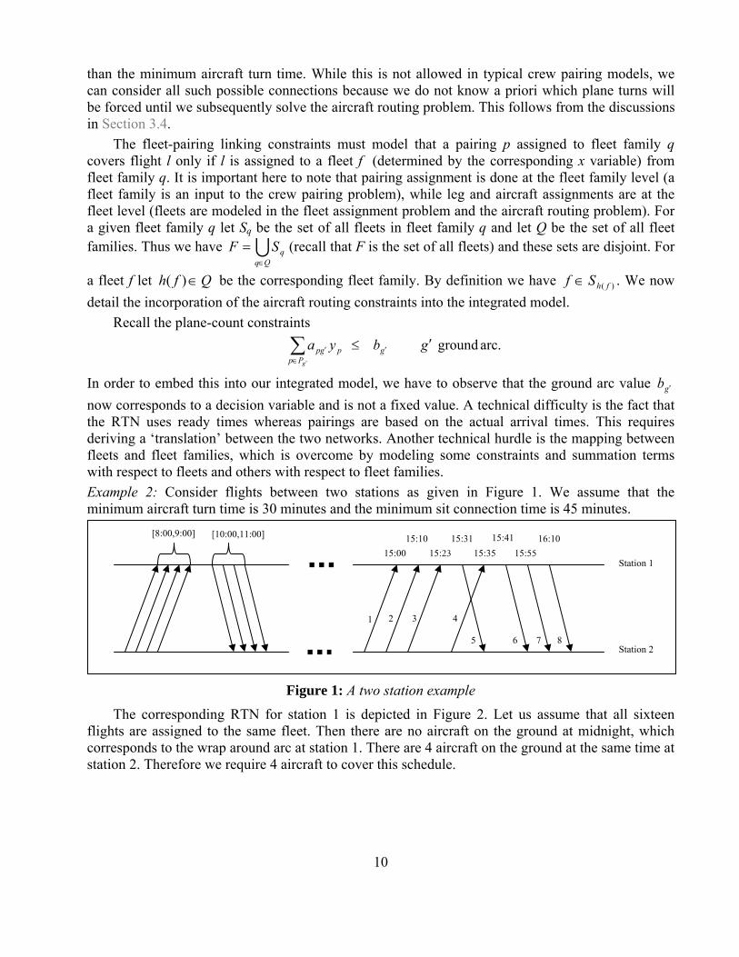
Example 2: Consider flights between two stations as given in Figure 1. We assume that the minimum aircraft turn time is 30 minutes and the minimum sit connection time is 45 minutes.

10

Figure 1: A two station example

The corresponding RTN for station 1 is depicted in Figure 2. Let us assume that all sixteen flights are assigned to the same fleet. Then there are no aircraft on the ground at midnight, which corresponds to the wrap around arc at station 1. There are 4 aircraft on the ground at the same time at station 2. Therefore we require 4 aircraft to cover this schedule.

8 7 6 5

4 3 2 1

[10:00,11:00] [8:00,9:00] 15:10 15:00 15:23

15:31 15:35

15:41 15:55

16:10

Station 1

Station 2

11

Figure 2: The ready-time-space network for station 1

Consider now the following pairings: p1={1,6,_},p2={2,7,_},p3={3,8,_},p4={4,5,_}, where the underscore can be replaced by any pair of connecting morning flights. Note that the last pairing has two overnight rests, one at each station. Assuming that the aircraft routes are yet to be determined, these pairings can be part of a solution, i.e. they are considered in the crew pairing model with plane count constraints. They imply 3 forced turns. If these pairings are in the solution, then the aircraft arriving with flight 4 is on the ground at station 1 at midnight. Therefore the plane count at station 1 is 1 and the plane count at station 2 is 4. All together we need 5 aircraft to cover the schedule in this case. If only 4 aircraft are available, then we need to impose a constraint, which prevents the selection of such a set of pairings.

Let the actual-time-space network (ATN) be defined in the same way as RTN except that for each arrival of flight l, tl is the actual arrival time la of leg l in ATN. The set of all ground arcs in ATN is denoted by G’ and the ground arcs are denoted by g’. Essential ground arcs are those ground arcs, which are defined by a departure followed by an arrival and they span a time period shorter than the minimum sit connection time. The plane-count constraints associated with non-essential ground arcs are redundant (for proof see Klabjan et al. (2002)). Let E(G’) ⊂ G’ be the set of essential ground arcs. Figure 3 details the difference between the RTN and ATN networks. When a flight arrives at a station, the arrowhead shows the actual arrival or ready time. For an outbound flight, the tail of the arc shows the actual departure time.

Figure 3: Comparison between RT

It remains to be seen how to convert the plane-count cowe have to link bg’ with the ground arc variables z. For each gground arc mg’ in RTN. Note that g’ is defined by the arrival o

4

gm ′ 6 7 8 5

1 2 3

arrival time ta

t1 t2 t3 t4

g

t RTN

g'

N and ATN

nstraints in’ ∈ E(G’), tf a leg l. Th

AT

g'

essential ground arc

to a hereis gr

N

non-essentialground arc

arrival time

m

ready time (t4 = ta + mt)

fleet-based setting, i.e. exists a corresponding ound arc mg’ is defined

by the ready time of leg l and an earlier activity. Let dep(g’) be the set of all flights that depart in the time interval [la , la + mt]. We replace the right hand side of the plane-count constraints by

,)()(

∑ ∑∈ ′∈

+′

q

gSf gdepl

flfm xz

where q is a fleet family. This expression states that the value of the ground arc corresponding to an arrival event of leg l in ATN is equal to the ground arc value of the same flight in RTN plus the number of departures in the set dep(g’). This correspondence between ground arc values in ATN and RTN is shown in Figure 4, and can be verified easily.

flights in dep(g')

l in RTN

mg' ready time

l in ATN

mt

g'

Example 2 (cont.): The ATN for s

Figure 5:

There is a single essential grocorresponding ground arc mg’ in departure times of legs 7 and 8 acount constraint reads 6ffm xz

g+

′

pp

which corresponds to all pairingground arc more than once).

Figure 4: Ground arc conversion

tation 1 is shown in Figure 5.

12

The actual-time-space network for station 1

und arc labeled by g ′ , which is defined by the arrival of leg 4. The RTN is shown in Figure 2. The ready time of leg 4 is between the nd therefore dep(g’)={6,7}. Thus the right-hand side of the plane-

for a fleet f. The corresponding left-hand side for fleet f is 7fx+

∑∑∑∈∈

∈∈

∈∈

++

UUUUUU 654

3

654

2

654

1PPPp

Ppfp

PPPpPp

fp

PPPP

fp yyy ,

s that include ground arc g ′ (assuming they do not include this

g ′ 85 6 7

1 2 3 4

If all flights are assigned to a single fleet and there are only 4 available aircraft, then . Pairings p1, p2, p3 appear on the left-hand side and therefore in this case the

constraint imposes that no more than 2 of these pairings can be selected. Recall that selecting all 3 of them yields a solution with 5 aircraft.

1,0 76 ===′ fffm xxz

g

The complete integrated model reads

0.z binary, binary,

)9(),()(

)8(,

)7(

)6(,0

)5(1

max

)()(

)(

)()(

)()(

,,

≥

∈′∈′+≤

∈∈=

∈≤+

∈∈=−−+

∈=

−

∑ ∑∑

∑

∑∑

∑∑

∑

∑∑

∈ ′∈′∈′

∈

∈∈

∈∈

∈

′

xy

QqGEgxzya

FfLlxy

FfNzx

FfVvzxzx

Llx

ycxr

q

g

l

Sf gdeplflfm

gPpqpgp

flPp

pfh

fWg

gfMl

fl

fvivIl

flfvovOl

fl

Fffl

fppf

pfllf

fl

The objective function captures the profit component from fleeting and the total crew cost; thus we capture the system wide revenue and cost. Constraints (5)-(7) are the standard FAM constraints, (8) ensures that a pairing is assigned to a fleet family if and only if all the legs in the pairing are assigned to the same fleet family, and (9) are the plane-count constraints.

Several extensions and enhancements can be easily incorporated. Next we mention a few of them.

• If aircraft turn times depend on the fleet (as is usually the case in practice), then all we have to do is to add dependency on f to g ′ and )(gdep ′ in (9). The corresponding RTN network needs to be adjusted accordingly.

• In practice, each fleet family uses only a subset of crew bases. This is very easy to accommodate by changing the summation range in (8).

• Suppose that in each fleet family q the number of available crews is in the range [lq,uq], thus limiting the manpower. This is easily captured by adding

Qquyl qp

qpq ∈≤≤ ∑

to the model. Other variations of the manpower constraints can be treated in a similar way.

5 Solution Methodologies The integrated model is too large to be solved by standard optimization software packages even for small instances. We propose two different methodologies. Our approach is to either decompose the problem into smaller problems, which can be easily solved, or to consider only a subset of pairings at a time.

13

14

We first sketch the latter, which is in spirit very similar to the one used by Huisman et al. (2005). We described in Section 2 the concept of delayed column generation for linear programs. This framework cannot be directly applied to our integrated model because we have integer variables and therefore the dual values are not available. The main idea is to obtain approximate dual values by means of Lagrangian relaxation, where the Lagrangian multipliers take the role of dual values, and as a consequence pairings are generated dynamically as needed.

In this approach we use the Lagrangian relaxation over a small subset of pairings to obtain Lagrangian multipliers. These multipliers are then used to price out new favorable pairings. Consider the integrated model over a small subset of pairings. Instead of solving it by a standard mixed-integer programming solver, which does not have a notion of dual values, we relax constraints (8) and (9) in the spirit of the Lagrangian relaxation. Thus we solve the resulting problem over a subset of pairings by using Lagrangian relaxation, which at the end returns Lagrangian multipliers (dual values) associated with (8) and (9). These values are next used to obtain (price out) favorable/useful new pairings. The notion of “usefulness” is defined based on the reduced cost with respect to the Lagrangian multipliers. These newly obtained pairings are then added to the set of already considered pairings and the entire procedure is iterated.

In the second approach the key observation is that the reduced problem with only constraints (5)-(7) is the traditional FAM model, which is relatively easy to solve. We first relax the integrality requirements on the pairing variables. The resulting problem can now be solved by Benders decomposition (see Section 2), wherein the crew pairing problem is solved as a linear program. The information from the dual of the LP is used to form Benders cuts, which are then added to the FAM model.

Another widely used solution methodology for solving large-scale mixed-integer programs is branch-and-price, see e.g. Barnhart et al. (1998b). We believe branch-and-price is not a suitable algorithm for solving our model since it requires too many pricing operations. As shown in Section 5.1.1, the pricing step of our model is computationally harder than the usual pricing subproblem for crew pairing and therefore its invocations must be limited. In our computational experiments, pricing is called at most 10 times in the Lagrangian relaxation with column generation algorithm. We believe that a branch-and-price type algorithm would require many more pricing operations and therefore it would produce excessive computational times. The appeal of Benders decomposition is that the cut generation procedure is decomposed with respect to the current fleeting and therefore it results in solving several standard crew pairing LP relaxations. The drawback is that the integrality of the pairing assignment variables is relaxed.

In Section 5.1 we describe the solution methodology using Lagrangian relaxation with column generation. A detailed discussion about column generation is postponed to Section 5.1.1. Section 5.2 details the solution methodology using Benders decomposition.

5.1 Lagrangian relaxation with column generation Traditionally, column generation is used along with the LP relaxations in the branch-and-price framework. We propose a column generation type approach combined with Lagrangian relaxation. First we approximate the model by changing the partitioning requirement (8) into covering constraints. We then relax constraints (8) and (9) and associate nonnegative Lagrangian multipliers λ with constraints (8) and µ with constraints (9). The Lagrangian relaxation of the restricted master problem reads

∑∑

∑ ∑ ∑ ∑∑ ∑∑∑ ∑∑

′−

+−−−+=∈

′∈ ∈ ∈∈

f gfmgfh

f qqp

g gPpqggp

Rp Sf plflpfl

g gdeplgfhfl

lfl

g

q

z

yacxr

'''

' ''

' ''

)(

)()()( )()(max),(

µ

µλµλµλφ

subject to FAM constraints (5),(6), and (7), where R is a small subset of pairings. Given pairing p and leg l in p we denote by the fact that pairing p covers or includes leg l.

pl ∈

The Lagrangian dual problem ),(min0,

µλφµλ ≥≥o

is solved by the subgradient algorithm. The obtained

Lagrangian multipliers λ and µ are then used to find new pairings, which are added to the set R in the RMP. The Lagrangian relaxation of the RMP is the traditional FAM model with a different objective function, which contains the Lagrangian multipliers. The solution methodology is next detailed step-wise. 1. Initialization: In this step we find initial pairings in R by applying the traditional sequential

approach. We first solve FAM and next we solve the crew pairing problem with the plane-count constraints by using the fleeting obtained from FAM. The pairings obtained in solving the crew pairing problem are used as the initial set of columns in the RMP. The initial set of columns and this initial fleeting are feasible to the integrated model because the generated pairings cover all the flights in the schedule and they do not violate the plane-count constraints.

2. Setting the lower bound: We add the initial set of columns obtained in step 1 to the RMP. The objective value (profit in the integrated model) of the initial solution, denoted by LB, is equal to the objective value of the Lagrangian dual over this initial set of columns. This follows directly from the fact that the LP relaxation of the RMP in this case yields an integer solution. LB is clearly a lower bound on the optimal value of the integrated model as well as of the initial Lagrangian dual problem.

3. Computing Lagrangian multipliers (major iteration): We use subgradient optimization to solve the Lagrangian dual problem with the current set of columns. We use the step updating heuristic proposed by Caprara et al. (1999). Next we briefly describe the formulas for calculation of the subgradients and the step sizes.

After changing the set partitioning constraints to set covering constraints, constraints (8) read

.,)( FfLlxy flPp

pfhl

∈∈≥∑∈

Let x, y be an optimal solution to the RMP. The subgradient vector s(λ) associated with a given λ is defined as

.,)( )(, FfLlyxslPp

pfhflfl ∈∈−= ∑∈

λ

Similarly, the subgradient vector s(µ) associated with a given µ is .),()(

)()(' QqGEgxzyas

qq

gSf gdepl

flSf

fmgPp

qpgpqg ∈′∈′−−= ∑ ∑∑∑∈ ′∈∈′∈

′ ′µ

Let k be the iteration count within the subgradient algorithm. The step size along s(λk), denoted by σk, is calculated as σk = θ(φ(λk,µk ) – LB)/|| s(λk) ||2, where θ > 0 is a parameter, which controls the step size along the subgradient direction. We change this parameter as required to increase or

15

decrease the step size. For example, if the objective value does not change for k consecutive iterations, we reduce θ by half. We replace s(λk) by s(µk) in the above formula and compute the step size τk along s(µk). Note that we deliberately do not use the same step size for λ and µ. The computational experiments have shown that such a choice yields better convergence.

Next we update the Lagrangian multipliers using the following formula λk+1 = max { λk + σk s(λk), 0 } µk+1 = max { µk + τk s(µk), 0 },

where the maximum is considered component-wise. We stop the subgradient algorithm either after a given number of iterations or if the norm of the subgradient becomes small.

4. Pricing: In this step we use the Lagrangian multipliers to price out favorable pairings using the constrained shortest path algorithm. Formally, we have to solve

(10) .minmin'

''

:⎟⎟

⎠

⎞

⎜⎜

⎝

⎛+− ∑∑∑

∈′

∈ ∈gq Ppg

qggpSf pl

flppqac µλ

This is detailed in Section 5.1.1. If λ and µ are viewed as dual prices, then (10) finds a column with the lowest reduced cost in the traditional sense. Let S be a small subset of pairings that either attain this minimum or are very close to it.

5. Loop: We first check the following termination criterion. − The above minimum (10) is nonnegative, i.e. no columns with negative reduced cost are

obtained. − If ),( µλφ does not change significantly for a given number of iterations.

− If a predefined maximum number of major iterations have been completed. If any of these termination criteria is satisfied, we go to step 6; otherwise, we add the obtained pairings S from step 4 to the RMP, i.e., we set , and we go to step 3. USRR ≡

6. Obtaining the final solution: The final solution is obtained by using the fleeting produced by the Lagrangian dual in the last iteration. We use this fleeting to obtain aircraft routes and crew pairings using the traditional approach.

As described earlier, after fleeting is solved, the problem decomposes by fleet family type. In the proposed integrated approach, the crew pairing problem for a given equipment type may be infeasible. This might happen either because we relax the partitioning constraints (8) to covering constraints or it might occur due to the nature of Lagrangian relaxation, i.e., a Lagrangian solution might not be feasible to the original problem. This was not observed in practice. Note that the traditional sequential approach suffers the same drawback. We believe that by using our integrated approach, which explicitly considers pairings and captures the dependency of pairings on fleet families, the likelihood of producing a crew infeasible fleet family is substantially lower. 5.1.1 Pricing Pricing is the problem of generating pairings with the lowest reduced cost. There are two approaches to finding pairings with the least reduced cost. The first one is by enumerating all pairings and the second, typically more efficient, and sometimes, the only practical one, is by using a variant of a shortest path algorithm. We use the latter approach to price out pairings based on (10). In this section, we first review the traditional constrained shortest path algorithm as it is applied to the crew

16

pairing problem. Additional details were given in Section 2. We then show how to tailor this algorithm to solve (10).

There are two types of networks that can be built to solve the pairing generation problem: a flight network or a duty period network. In the flight network each flight departure and arrival has an associated node in the network. A flight arc connects the departure node of a flight with the corresponding arrival node of the same flight. We add connection arcs between an arrival and a departure node at the same station subject to the constraints on the connection time. (It must either be a legal sit connection or a legal rest connection.) We augment the network by adding a source s and a sink t. We connect source s to every departure node originating at the crew base. Similarly, we connect all the arrival nodes at the crew base to sink t. If there is more than one crew base, we need to construct a separate network for each crew base. The duty period network is similar except that we replace the flight arcs by duty periods and connection arcs correspond to legal rest connections. Although we can capture more pairing feasibility rules in the duty period network (all duty rules are embedded by definition), the duty period network is much larger than the flight network. Because we deal with the daily problem and to avoid cyclic networks, we replicate each flight several times until the maximum elapsed time of pairings is reached. For example, if pairings cannot exceed 5 days, then the network has 5 copies of each flight, each one offset in time by a day. The resulting network captures all pairings and is acyclic. The expanded network also naturally embeds ground arcs. Each ground arc in the original network now has several copies.

It is clear that each pairing corresponds to an s-t path but an s-t path might violate pairing feasibility rules. In order to circumvent this, to find a favorable feasible pairing, the constrained shortest path algorithm must be employed (see Section 2 for details on constrained shortest path algorithms). In such an algorithm, a label is maintained for each feasibility rule and cost component. The latter are required if the cost of a pairing is nonlinear. Examples of labels are those corresponding to the maximum number of duties, the maximum elapsed time, the sum of the duty costs, etc. In addition, to capture the dual prices (in our case the Lagrangian multipliers), an additional label is required. Each s-i path is represented as a vector consisting of the values of all resources. Thus every node i contains a set of label vectors.

For the integrated approach pricing (10), we can reduce the problem to the constrained shortest path problem. Assume that to solve the traditional crew pairing pricing problem we require k labels and let the corresponding label vector at node i be denoted by u. Furthermore, assume that it encodes a path p (partial pairing) from s to i. Because the Lagrangian multipliers contribute to the calculation of the reduced cost (10), we need to augment the underlying network and incorporate these values. We have |Q| Lagrangian multipliers for each flight and each ground arc. Therefore we need to add |Q| new labels to the existing labels. Thus the number of required labels becomes k+|Q|. This clearly results into higher computing times; however, since the pricing step is not performed often (at most 10 times) this is acceptable.

The new label vector becomes ).,,,,(

::2

:1

||21

∑∑ ∑∑∑∑∑∑∑′′′ ∈′

′∈ ∈∈′

′∈ ∈∈′

′∈ ∈

+−+−+−=gQgg Ppg

gQSf pl

flPpg

gSf pl

flPpg

gSf pl

fluv µλµλµλ L

It is easy to see that if vv ≤ for two label vectors at the same node, then the path corresponding to v can be discarded and the corresponding label vector can be removed.

If the duty period network is used, then for each duty d we precompute ).,,,(

::2

:1

||21

∑∑ ∑∑∑∑∑∑∑′′′ ∈′

′∈ ∈∈′

′∈ ∈∈′

′∈ ∈

+−+−+−gQgg Pdg

gQSf dl

flPdg

gSf dl

flPdg

gSf dl

fl µλµλµλ L

17

These are then used as node weights in the network and the labels are updated upon scanning of duty d by adding this vector to the last |Q| coordinates of the label vector.

If the flight network is used, then the treatment is slightly different. For each flight arc l in the network we first form the vector ).,,,()(

||21

∑∑∑∈∈∈

−−−=QSf

flSf

flSf

fll λλλα L To handle ground arcs,

consider a connection arc ca corresponding to a sit connection between an arrival of a flight and a departure of a different flight. Let the notation cag ∈′ mean that ground arc is included in connection ca. Next we form the vector

g ′

).,,,()(::

2:

1 ∑∑∑∈′′′

′∈′′

′∈′′

′=cagg

gQcagg

gcagg

gca µµµβ L

An example is given in Figure 6, where the dotted lines show the actual flights, which constitute the essential ground arc. The solid lines are the flight arcs.

If we treat label vector v by scanning flight arc l, then the new label vector v is given by ),)(,,)(,)(,( 2211 QQkkk lvlvlvuv ααα +++= +++ L

where u is the treatment of the standard crew pairing resources. If we are scanning a connection arc ca that corresponds to a sit connection, then the updated label vector is given by

).)(,,)(,)(,( 2211 QQkkk lvlvlvuv βββ +++= +++ L

If the connection arc corresponds to an overnight connection, then we treat only u as in the standard crew pairing pricing procedure.

essential ground arcs

β(ca) = (µ1g', µ2g') + (µ1ĝ, µ2ĝ)

18

Figure 6: Connection arc weights for |Q| = 2, |S1|=1, |S2|=1

We remark that ground arcs are captured correctly. The contribution of ground arcs is , where are the ground arcs in the network without replications. In the network

with replications, this quantity becomes

∑∈

′

''

'

:g

Ppgqggpa µ g′

∑∈

gPpg

qg:

µ , where g’s are the ground arcs in the expanded

network. This shows that all coefficients in front of µ are 1.

α(s)=(-λ1s, -λ2s)

α(t)=(-λ1t, -λ2t)

flights s and t in the ATN network

In our computational experiments we solve (10) based on the duty period network. Even though this network is larger than the flight time network, it captures more pairing feasibility rules and thus requires a lower number of labels.

5.2 Benders Decomposition In this approach we relax the integrality of the pairing variables while maintaining the integrality of the fleet assignment variables. Clearly this yields a relaxation of the integrated model. By preserving the integrality of the fleet assignment variables, we do not relax the important revenue based decisions. In essence, we comply with the hierarchy of the current sequential decision making process.

The resulting model is now suited for the Benders decomposition approach (see Section 2 for more details). The RMP consists of the FAM constraints (5)-(7) and the Benders cuts. Given a solution to the RMP, i.e., a feasible fleeting, the subproblem then decomposes into the LP relaxations of the crew pairing problems with plane-count constraints. The subproblem is clearly decomposed by fleet family and this substantially reduces the computational burden. More precisely, in each iteration we solve the RMP and then use the underlying fleeting to solve the LP relaxations of the crew pairing problems with embedded plane-count constraints. By using the dual values of these LP relaxations, we add Benders cuts. If an LP relaxation is infeasible, then a Benders feasibility cut is added.

Next we elaborate on the most significant steps. For a given fleet family q, we define Lq as the subset of flights that have been assigned to fleet family q after solving the RMP, i.e., given fleeting decision variables x. The LP subproblem for fleet family q then reads

.0

)12()(

)11(1

min

)(

≥

′∈′≤

∈=

′′∈

′

∈

∑

∑

∑

p

qggPp

pgp

qPp

p

pp

p

y

GEgbya

Lly

yc

l

Here denotes the set of the essential ground arcs with respect to the flights in Lq and

is the ground arc value.

)( qGE ′

)()(

∑ ∑∈ ′∈

′ +=′

q

gSf gdepl

flmg xzb

Let the duals for (11) be represented by θ and the duals for (12) by Π, whenever the LP is feasible. If the LP is infeasible, let ),( βα be an extreme ray with

(13) ,0)(

>+ ′′∈′

′∈

∑∑ qgGEg

gLl

qlff

b βα

where α corresponds to (11) and β to (12). Let η represent the upper bound on the crew cost in the relaxed integrated model. We index the Benders cut by k, where k is the iteration count. The RMP at the beginning of a new iteration reads

19

.0 binary, ed,unrestrict

(15) 0

)14(

(7), and (6) (5), sconstraint FAM subject to

max

'

''

'

''

)(:

)()(:

)()(

,

≥

∈≤+⎥⎦

⎤⎢⎣

⎡+

∈≤∏+⎥⎦

⎤⎢⎣

⎡∏+

−

′

′

∑∑ ∑

∑∑∑∑ ∑

∑

′∈′

′∈′

zx

Jkzx

Kkzx

xr

kgkkkk

g

qmg

kqglf

l gdeplg

kqg

klq

ffm

g

kfhg

flf

l gdeplg

kfhg

klfh

fllf

fl

η

ββα

ηθ

η

Constraints (14) are the Benders cuts and (15) are the Benders feasibility cuts. Here qk denotes an infeasible LP subproblem at iteration k.

The entire solution methodology is described stepwise as follows. Unlike the first solution methodology, we do not need to generate an initial feasible solution in this case. 1. Solving the Restricted Master Problem: Solve the restricted master problem and obtain a

fleeting. 2. Decompose based on fleeting: Based on the solution of the RMP, for each fleet family we

generate legs and plane-count information. 3. Solve the crew pairing LP relaxations: For a given fleet family, we use the corresponding leg

and plane-count information obtained in step 2 to solve the LPs (11)-(12). Once the LPs have been solved, one of the following two cases arises: the solution is optimal for each fleet family or there is a fleet family that yields an infeasible subproblem.

4. Generate Benders cut: If all the subproblems are feasible, we obtain the duals θk and Πk for constraints (11) and (12), respectively, for the current iteration k. Use these duals to add a new Benders cut (14) and go to step 6.

5. Generate a feasibility cut: For each infeasible subproblem, we obtain an extreme ray satisfying (13). For each such infeasible fleet family, we add the corresponding feasibility cut (15) and go to step 6.

6. Iterate: If we reach the maximum number of iterations, we go to step 7. Otherwise we go to step 1.

7. Obtaining the final solution: We use the fleeting from the last iteration to generate aircraft routes and crew pairings using the traditional approach.

6 Computational Experiments We tested the integrated model on four data sets. Real world data from a major US carrier were used. The carrier has a dense hub-and-spoke network structure with five crew bases and 8 hubs. Crew feasibility rules and the cost function comply with the airline rules. For discretionary purposes, the real profit numbers are fudged but the presented numbers show correct proportions and magnitudes. Due to the lack of data, we do not use the manpower constraints. However, the minimum turn time is fleet dependent and each fleet family uses only a specific subset of crew bases. The computing environment consists of a cluster of 27 dual 900 MHz Itanium 2 processors running the Red Hat 7.3 operating system and the gcc 3.2 development environment. For solving small LPs and the fleeting integer programming models, we used CPLEX from ILOG Inc., version 8.1.

20

21

In order to make a fairer comparison between the proposed solution methodologies and the traditional sequential approach, in our implementation of the traditional sequential approach we have also modeled constraints to prevent crew double overnights. Crew double overnights occur when only very late night flights of a fleet family arrive at a station and only early morning flights of the same fleet family depart with no other activity during the day. If this is the case, then the crew must have an extra day of rest due to the insufficient rest time between the arriving flight and the next available departure. We add constraints to FAM using legal rest arcs and mid-day breakouts such that the obtained fleeting is more “crew friendly”, see Clarke et al. (1994) for details. These constraints discourage crew double overnights by encouraging mid-day flights. While now the fleeting profit might be lower, the crew cost would be hopefully lower as well. These constraints are added to FAM only in the implementation of the traditional sequential approach for benchmarking purposes and to initialize the Lagrangian approach. Because the integrated model completely captures the interaction between fleeting and crew pairing, these constraints are not added in the implementation of the solution methodologies for the integrated model.

Each crew pairing problem is solved by branch-and-price. The pricing problem (10) and the pricing of the crew pairing LP relaxations in the second approach are solved by using the parallel constrained shortest path algorithm, Klabjan (2003).

We control tractability in the following way. First FAM is solved over all fleet families and flights. Next we pick a subset of fleet families (this selection process is described below) and the corresponding flights. The integrated model is then solved by considering only this subset of fleet families and flights. We select the fleet families greedily with respect to the flight time credit, which is defined as the ratio: (crew cost - total flying time) / (total flying time). The flight time credit measures the maximum possible relative improvement in the crew cost. Note that the crew cost is always larger than or equal to the total flying time and therefore the flight time credit is always nonnegative. To summarize, we first solve the problem by using the traditional approach. This gives us the flight time credit for each fleet family. We next select a desirable number of fleet families with the largest flight time credit. These selected fleet families form the input to the integrated model. In other words, instead of considering all fleet families at once, to ensure tractability, we consider subsets of fleet families. The number of flights in each instance and the number of considered fleet families are given in Table 1. Cases 3 and 4 are not full fleet families, i.e., after obtaining a fleeting, we choose a subset of fleet families and then from each set of flights for a given fleet family we pick a subset of flights. They were generated as proof of concept instances. Cases 1 and 2 on the other hand consist of the entire set of flights for a subset of fleet families. The first case consists of a majority of flights because the carrier uses 6 fleet families.

In this section we present the computational results for the four test cases. We first discuss all the benefits and then give a more detailed analysis of some of the test cases.

The increase in profits obtained by using the integrated approach as opposed to the sequential one is shown in Table 1. The monetary unit is US dollars. Both approaches were stopped after approximately the same elapsed time, which is discussed later. Profit here is defined as the combined profit resulting from FAM and the crew pairing costs, i.e., for the integrated approach it corresponds to the objective value. In the last two columns, we show the increase in profit obtained by solving the integrated model by Lagrangian and Benders respectively. Except for case 4, the Lagrangian relaxation approach outperforms Benders decomposition. We stress that these are daily profit increases that produce on an average 50 million dollars of additional profit per year for this particular airline. In addition, we selected a subset of fleet families just once. By repeating the fleet selection process several times, additional profit can be obtained.

22

Test Case Increase in Profit ($)

Fleet Families

Flights Lagrangian Benders

Case 1 4 942 150,000 25,000 Case 2 2 524 160,000 150,000 Case 3 3 251 30,000 8,000 Case 4 2 205 22,000 33,000

Table 1: Profits

Table 2 details the breakdown of the profit by revenue, operating cost of the flights, and crew cost. The breakdown has been presented for both solution methodologies. (The abbreviation for Lagrangian is Lgr and for Benders is Bns.) All values are shown as percentage increase or decrease values with respect to the corresponding value obtained by using the traditional methodology. To ensure data confidentiality, we present only the range instead of the actual percentage increase or decrease. For example, for case 4 solved by the Lagrangian approach, the revenue is 0% to 2% lower with respect to the traditional approach. Most of the increased profit does not come from diminishing revenue in FAM but it comes from the reduced crew cost. The change in the operating cost is negligible. This is a desired property because for historical and cultural reasons, carriers are not willing to sacrifice too much on the revenue side (even though it could increase the total profit). The last column shows the increase in profit with respect to the traditional approach.

Revenue % Operating Cost % Crew Costs % Savings Lgr Bns Lgr Bns Lgr Bns Lgr Bns

Case1 [-0.1,0] [-0.5,0] [0,0.5] [-0.1,0] [-6, -4] [-3, -1] [2, 4] [0,0.5] Case2 [-1,0] [-1,0] [0,1] [0,1] [-11, -8] [-10, -8] [5,8] [4,7] Case3 [-1,0] [-1,0] [0,1] [0,1] [-6, -3] [-4, -1] [1,4] [0.4,1] Case4 [-2,0] [-1,0] [0,0.5] [-1,0] [-4, -2] [-7, -5] [1,4] [2,5]

Table 2: Breakdown of profit

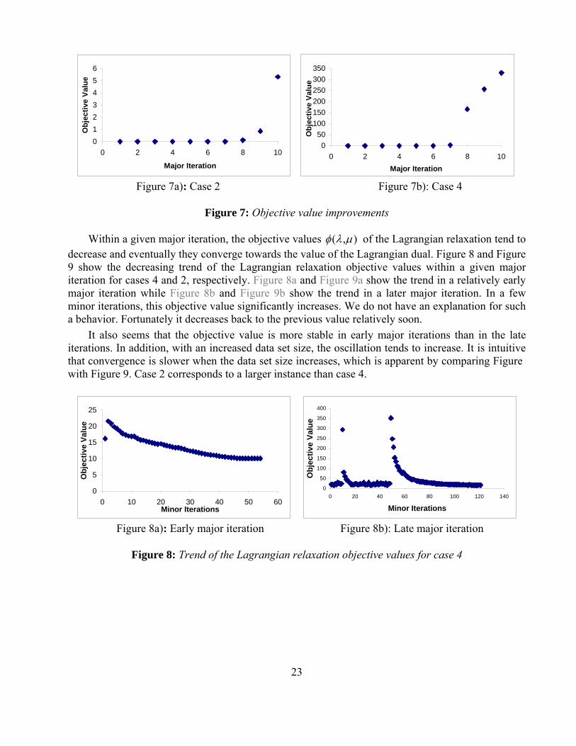
We next study in more details cases 2 and 4 when solved using the Lagrangian approach. Figure 7 shows the improvement in the objective value after every major iteration (steps 3-5 in the algorithm) for the two test cases. FigureT 7a shows the improvement for case 2 while Figure 7b shows the improvement for case 4. Obviously in the initial iterations the improvements are minimal and in subsequent iterations, the objective value increases substantially. It is obvious that based on this trend it might be beneficial to perform additional iterations.

0123456

0 2 4 6 8 10

Major Iteration

Obj

ectiv

e Va

lue

050

100150200250300350

0 2 4 6 8 10Major Iteration

Obj

ectiv

e Va

lue

Figure 7a): Case 2 Figure 7b): Case 4

Figure 7: Objective value improvements

Within a given major iteration, the objective values ),( µλφ of the Lagrangian relaxation tend to decrease and eventually they converge towards the value of the Lagrangian dual. Figure 8 and Figure 9 show the decreasing trend of the Lagrangian relaxation objective values within a given major iteration for cases 4 and 2, respectively. Figure 8a and Figure 9a show the trend in a relatively early major iteration while Figure 8b and Figure 9b show the trend in a later major iteration. In a few minor iterations, this objective value significantly increases. We do not have an explanation for such a behavior. Fortunately it decreases back to the previous value relatively soon.

It also seems that the objective value is more stable in early major iterations than in the late iterations. In addition, with an increased data set size, the oscillation tends to increase. It is intuitive that convergence is slower when the data set size increases, which is apparent by comparing Figure with Figure 9. Case 2 corresponds to a larger instance than case 4.

0

5

10

15

20

25

0 10 20 30 40 50 60Minor Iterations

Obj

ectiv

e Va

lue

0

50

100

150

200

250

300

350

400

0 20 40 60 80 100 120 140

Minor Iterations

Obj

ectiv

e Va

lue

Figure 8a): Early major iteration Figure 8b): Late major iteration

Figure 8: Trend of the Lagrangian relaxation objective values for case 4

23

0

100

200

300

400

500

600

0 50 100 150 200 250 300 350 400

Minor Iterations

Obj

ectiv

e Va

lue

0

100

200

300

400

500

600

700

800

0 50 100 150 200 250 300 350 400Minor Iterations

Obj

ectiv

e Va

lue

Figure 9a): Early major iteration Figure 9b): Late major iteration

Figure 9: Trend of the Lagrangian relaxation objective values for case 2

Now we focus on the Benders decomposition approach. In Benders decomposition the objective value is non-increasing across iterations. The trends for cases 2 and case 4 are shown in Figure 10. As we can see, due to degeneracy in the subproblems, the objective value can be constant for some iterations. We did not experiment with the core approach from Magnanti and Wong (1981), because it is a non-trivial task to find a core point.

382383383384384385385386386387387388

0 5 10 15 20 25 30Iteration

Obj

ectiv

e Va

lue

795

796

797798

799

800

801

802803

804

805

-1 1 3 5 7 9 11 13 15Iteration

Obj

ectiv

e Va

lue

Figure 10a): Case 2 Figure 10b): Case 4

Figure 10: Objective value in Benders decomposition

In order to get a sense on the quality of the Lagrangian approach, we created a small instance where it is possible to obtain an optimal solution. This instance has 74 legs and 2 fleets, which results in 73,514 total pairings. The resulting integrated model (5)-(9) has 402 rows and 147,286 variables. CPLEX is able to find an optimal solution in 35 seconds. We tested our Lagrangian approach and the traditional methodology. The results are summarized in Table 3. The top row shows the relative gap with respect to the optimal solution. It is encouraging to see that even for such a small instance with not many opportunities for improvement, the Lagrangian approach is less than 4% from the optimal solution. We believe this number to be even smaller for real-size problems. The remaining two rows of the table show the number of legs assigned to each fleet in the best solutions obtained for each approach.

24

25

Optimal Lagrangian Traditional Gap 0% 3.8% 14.3%

No. of legs in fleet 1 35 28 40 No. of legs in fleet 2 39 46 34

Table 3: Small test instance with 74 legs

The breakdown of computation times obtained by solving the integrated model using the Lagrangian approach is shown in Table 4. The units of measurement are listed in each column. The Lgr column shows the time taken to solve one subgradient iteration. The “average” column for each of the FAM, Lgr, and Pricing steps shows the average cumulative running time over all iterations. The percentile column for each of these steps shows the percentage of the total time that is spent in solving the step over all iterations. (We sum up the time taken for a given step in all minor and major iterations and calculate the % of the total time that can be attributed to the given step.) The last column shows the total time taken to solve a given data set using the integrated model.

Per Major Per Minor FAM Lgr Pricing Total Iteration Iteration Average % Average % Average %

(secs) (secs) (secs) (secs) (secs) (hrs) Case 1 12,250 35 25 71 33 90 1,300 11 34 Case 2 8,700 31 21 67 27 80 1,500 17 25 Case 3 6,600 50 37 70 49 89 600 9 19 Case 4 5,400 16 12 78 15 93 180 3 15

Table 4: Computation times for the Lagrangian approach

The running time for each major iteration increases significantly with an increasing number of legs. There is not a considerable increase in computational time with an increase in the number of fleet families as shown by cases 3 and 4. The subgradient optimization accounts for more than three-fourths of the time. The most intensive step is solving the RMP in each iteration and all other operations per iteration are negligible. The reason is in the slow convergence of the subgradient algorithm. It is surprising that the pricing step is not more computationally intensive. This could be primarily due to the employment of the parallel algorithm.

The computation times for Benders are shown in Table 5. The “average” column for the RMP and LP steps shows the absolute value of the average over all iterations. The “%” column shows the percentile of the total time that is spent in solving a step over all iterations. The last column gives the overall running time. The increase in the running time to solve the RMP is striking. The traditional FAM used in the Lagrangian approach takes less than 1 minute. On the other hand, after adding Benders cuts (we never add more than 30 of them), this running time increases to almost an hour.

26

RMP LP subproblem Total Time per

Iteration Average % Average % (mins) (mins) (mins) (hrs)

Case 1 124 60 48 59 48 29 Case 2 82 58 71 21 26 19 Case 3 66 57 88 7 11 15 Case 4 22 17 79 4 18 5

Table 5: Computation times of Benders decomposition

With an increase in the number of legs and fleet families, the computational time using the Benders approach increases. The distribution of time across RMP and LP shows a significant trend. For smaller test cases, the RMP takes about three-fourth of the total time to solve the problem. But with an increase in the size of the data set, the time taken to solve the LP subproblem increases significantly. For larger data sets, half of the total time is spent in solving the crew pairing LP relaxation.

7 Conclusions and Future Directions In solving the integrated model, the Lagrangian relaxation methodology on average outperforms the Benders decomposition algorithm. Only in test case 4 does the latter algorithm produce a slightly better result. Their behaviors in terms of the objective value improvements are complementary. The Benders algorithm makes substantial improvements in initial iterations and then it stalls due to the known phenomena of degeneracy. On the other hand, the Lagrangian methodology makes only minor improvements in early iterations and substantial improvements in later iterations. In early iterations Lagrangian multipliers are unstable. Once they stabilize, they reveal more accurate information, which results in significant gains. As a conclusion, if an improvement is desirable in a short amount of time, Benders decomposition should be used. If several hours of computing time are available, then Lagrangian relaxation should be used. Because this is a tactical planning problem, usually the latter condition holds. We find the Lagrangian relaxation approach more robust and practical.

Next we discuss some future directions. The convergence rate of the Lagrangian algorithm using subgradient optimization is very slow. The bundle method, see e.g. Lamarechal (1989), is known to have a better convergence rate as compared to the subgradient variants to solve Lagrangian relaxation. We see a potential improvement in the running time by using the bundle algorithm instead of the vanilla subgradient optimization.

On the algorithmic front, we plan to test an alternative algorithm, which is aligned with the existing one. We propose to directly solve the Lagrangian dual. In the current solution methodology, we consider only a subset of pairings in each iteration. We then generate columns and add them to the current subset. As opposed to this, in every subgradient or bundle iteration, we can price out all pairings to adjust the current iterate.

The revenue obtained from the current integrated model takes only the average fare per leg into account, i.e., fleeting is leg-based. The average fare for each leg is an approximation to the actual revenue due to the multi-leg passenger itineraries. Leg-based FAM solutions tend to be biased toward larger aircraft. This leads to the requirement of better revenue modeling practices. In origin-destination fleet assignment models (O-D FAM), Kniker (1998), Jacobs et al. (1999), Barnhart et al.

27

(2002a), Barnhart et al. (2002b), passenger revenues are modeled for each origin-destination itinerary rather than for each leg. The O-D FAM model is a combination of the leg-based FAM model and the passenger mix model. Given fixed seat capacity, the passenger mix model decides the number of passengers that should be booked on a given O-D itinerary.

To overcome this problem and to be consistent with yield management practices, we can integrate O-D FAM, crew pairing, and aircraft routing. O-D FAM can be solved using Benders decomposition. The newly formed integrated model can be solved along the same lines as the current integrated model. Unfortunately we believe this still might be out of reach in terms of tractability because the solution times for O-D fleeting are too high. An alternative might be to use clever high performance algorithms.

In our integrated model, although we present a complete integration of FAM and crew pairing problems, the integration with the aircraft routing model is only partial. Recall that our solution yields plane-count feasible aircraft routes but not necessarily maintenance-feasible routes. In addition, we do not capture the potential aircraft routing objective function. An integrated model, which fully integrates the aircraft routing model with FAM and the crew pairing model instead of just ensuring feasibility, is an interesting topic for future research.

8 Acknowledgments We would like to thank Michael Clarke from Sabre Inc. for providing the data and valuable discussions. We are indebted to Professor Karsten Shwan from the Georgia Institute of Technology, Atlanta, GA for allowing us to use his computing resources. Special thanks to Professor Eva Lee from the Georgia Institute of Technology, Atlanta, GA for assistance with CPLEX licenses. In addition, we are thankful to ILOG Inc. for providing the licenses.

9 References [1] Barnhart, C., Boland, N., Clarke, L., Johnson, E., Nemhauser, G., and Shenoi, R. (1998a). Flight

string models for aircraft, fleeting and routing. Transportation Science, 32, 208-220. [2] Barnhart, C., Johnson, E., Nemhauser, G., Savelsbergh, M. and Vance, P. (1998b). Branch-and-

Price: Column generation for solving huge integer programs. Operations Research, 46, 316-329. [3] Barnhart, C., Lu, F., and Shenoi, R. (1998c). Integrated airline schedule planning. In Yu, G.,

editor, Operations Research in the Airline Industry, 9, 384-403. Kluwer Academic Publishers. [4] Barnhart, C., Farahat, A., and Lohatepanont, M. (2002a). Airline fleet assignment: An enhanced

revenue model. Technical Report. Massachusetts Institute of Technology. [5] Barnhart, C., Kniker, T., and Lohatepanont, M. (2002b). Itinerary-Based airline fleet assignment,

Transportation Science, 36, 199-217. [6] Barnhart, C., Cohn, A., Johnson, E., Klabjan, D., Nemhauser, G. and Vance, P. (2003), Crew

scheduling. In Hall, R., editor, Handbook of Transportation Science, 517-560. Kluwer Scientific Publishers.

[7] Bélanger, N., Desaulniers, G., Desrosiers, J. and Soumis, F. (2005). Periodic airline fleet assignment with time windows, spacing constraints and time dependant revenues. In press in European Journal of Operational Research.

[8] Benders, J. (1962). Partitioning procedures for solving mixed-integer programming models. Numerische Mathematik, 4, 238-252.

28

[9] Caprara, A., Fischetti, M. and Toth, P. (1999). A heuristic algorithm for the set covering problem. Operations Research, 47, 730-743.

[10] Clarke, L., Hane, C., Johnson, E. and Nemhauser, G. (1994). Maintenance and crew considerations in fleet assignment. Transportation Science, 30, 249-260.

[11] Clarke, L., Johnson, E., Nemhauser, G., and Zhu, Z. (1997). The aircraft rotation problem. In Burkard, R.E., Ibaraki, T., and Queyranne, M., editors, Annals of OR: Mathematics of Industrial Systems II, 33-46. Baltzer Science Publishers.

[12] Cohn, A., and Barnhart, C. (2003). Improving crew scheduling by incorporating key maintenance routing decisions. Operations Research, 51, 387-396.

[13] Cordeau, J., Desrosiers, J., Soumis, F, and Stojković, G. (2000). Benders decomposition for simultaneous aircraft routing and crew scheduling. Transportation Science, 35, 375-388.

[14] Desaulniers, G., Desrosiers, J., Dumas Y., Solomon, M., and Soumi, F. (1997). Daily aircraft routing and scheduling. Management Science, 43, 841-855.

[15] Desaulniers, G., Desrosiers, J., Ioachim, I., Solomon, M., and Soumis, F. (1998). A unified framework for deterministic constrained vehicle routing and crew scheduling problems. In Crainic, T. and Laporte, G., editors, Fleet Management and Logistics, 57-93. Kluwer Publishing Company.

[16] Fisher, M. (1985). An applications oriented guide to Lagrangian relaxation. Interfaces, 15, 10-21.

[17] Freling, R. (1997). Models and techniques for integrating vehicle and crew scheduling. PhD thesis, Tinbergen Institute, Erasmus University Rotterdam.

[18] Freling, R., Huisman, D., and Wagelmans, A. (2003). Models and algorithms for integration of vehicle and crew scheduling. Journal of Scheduling, 6, 63-85.

[19] Gaffi, A., and Nonato, M. (1999). An integrated approach to extra-urban crew and vehicle scheduling. In Wilson, N.H.M., editor, Computer-Aided Transit Scheduling, 103-128. Springer-Verlag.

[20] Haase, K., Desaulniers, G., and Desrosiers, J. (2001). Simultaneous vehicle and crew scheduling in urban mass transit systems. Transportation Science, 35, 286-303.

[21] Hane, C., Barnhart, C., Johnson, E., Marsten, R., Nemhauser, G., and Sigismondi, G. (1995). The fleet assignment problem: Solving a large-scale integer program. Mathematical Programming, 70, 211-232.

[22] Huisman, D., Freling, R., and Wagelmans, A.P.M. (2005). Multiple-depot integrated vehicle and crew scheduling. Transportation Science, 39, 491-502.

[23] Jacobs, T., Johnson, E., and Smith, B. (1999). O&D FAM: Incorporating passenger flows into the fleeting process. In R. Darrow, editor, Thirty-Ninth Annual AGIFORS Symposium, New Orleans.

[24] Klabjan, D., Johnson, E., Nemhauser, G., Gelman, E., and Ramaswamy S. (2002). Airline crew scheduling with time windows and plane count constraints. Transportation Science, 36, 337-348.

[25] Klabjan, D. (2003). Parallel constrained shortest path. Presentation at ISMP 2003, Copenhagen, Denmark.

[26] Klabjan, D. (2005). Large-scale models in the airline industry. In Desaulniers, G., Desrosiers, J., and Solomon, M.M., editors, Column Generation, Kluwer Academic Publishers.

29

[27] Kniker, T. (1998). Itinerary-based airline fleet assignment. PhD thesis, Massachusetts Institute of Technology.

[28] Lamarechal, C. (1989). Nondifferentiable optimization. In Nemhauser, G.L., Rinnooy Kan, A.H.G., and Todd, M.J., editors, Handbooks in Operations Research and Management Science, Vol. 1, Optimization. North-Holland, 529–572.

[29] Magnanti, T., and Wong R. (1981). Accelerating Benders decomposition: Algorithmic enhancement and model selection criteria. Operations Research, 29, 464-484.

[30] Mercier, A., Cordeau, J.–F., and Soumis, F. (2003). A computational study of Benders decomposition for the integrated aircraft routing and crew scheduling problem. Computers & Operations Research, 32, 1451-1476.

[31] Rexing, B. (1998). Fleet assignment with time windows. Master’s thesis, Massachusetts Institute of Technology.