IEEE Transactions on Power Systems, Vol. 14, No. 1, February 1999 INTEGRATED RESOURCE PLANNING

USING SEGMENTATION METHOD BASED DYNAMIC PROGRAMMING

P. S. Neelakanta and M. H. Arsali Department of Electrical Engineering

Florida Atlantic University Boca Raton, Florida 3343, USA

ABSTRACT:

The state-of-the-art restructuring of industries is changing the fundamental nature of retail electricity business; and, as a result, the so-called Integrated Resource Planning (IRP) strategies are also undergoing modifications. Such modifications evolve from the relevant processes intended to minimize revenue requirements and maximize electrical system reliability vis-a'-vis capacity- additions (viewed as potential investments). IRP modifications also provide service-design bases meeting the customer needs towards profitability. This paper describes a procedure to determine optimal IRP to expand generation facilities of a power system over a stretched period of time. Relevant production-costing is based on the so- called segmentation method combined with an advanced dynamic programing technique which takes into account of the associated uncertainties in a cohesive and systematic manner. The primary advantage of this procedure is the ability to combine reliability constraints of the system along with the estimation@) on cost of production, via a fast and efficient algorithm. Due to reduced extent of state-descriptions involved in the relevant dynamic programing formulation, this procedure also allows a rapid calculation of the optimal plan envisaged commensurate with the set of input data assumed; Further, it allows the user to perform various risk and scenario analyses cohesively.

INTRODUCTION Integrated Resource Planning (IRP) is a contemporary approach to evolve strategies towards electric utility planning for future energy requirements [16]. The goal of IRP is to identify the resources or a set of mixed resources to meet the near and long- term consumer energy needs in an efficient and reliable manner at the lowest or reasonable cost outlays. The IRP strategies enable relevant cost analysis, optimizing its effectiveness, as well as they include the considerations as regard to the benefits of the entire supply- sideldemand-side options (as appropriate) and meeting the availability constraints. They also take into consideration the financial integrity, size and physical capability, as well as those factors of the utility company which have impact on the consumer, the environment, culture, community life styles, the State's economy, and upon the society as a whole. IRP is an open process and a public endeavor: The community, utility companies, and governmental agencies are provided with opportunities to participate in its development.

However, the state-of the-art deregulation and restructuring aspects of electric industry are changing the fundamental nature of retail electricity business, and would make a major impact on any IRP envisaged. With wholesale and potentials of retail access, electric utilities face competitive threats because customers are given alternatives. Hence, profitability and commercial risks have

PE-073-PWRS-0-05-1998 A paper recommended and approved by the IEEE Power System Planning and Implementation Committee of the IEEE Power Engineering Society for publication in the IEEE Transactions on Power Systems. Manuscript submitted October 3, 1998; made available for printing May 18, 1998.

375

become more important; as well as, the return on generation, transmission, and distribution investments has become rather less certain. As a result, companies are responding by establishing separate business units for generation, transmission, and distribution. Consequently, the concept of IRP itself is changing: Classically, at its inception, IRP evolved kom basic processes and considerations designed exclusively to minimize the revenue requirements and maximize the reliability of the electric system. Since then it has grown to a stage wherein one considers the capacity-additions as investments toward profitability, and places the service-design as a base to meet the customer needs.

The objective of IRP processing in the modern, state-of-the-art, competitive environment is, therefore, to retain the customers and meet their electricity-related needs by offering reliable and economical services, with due regard to deregulation, environmental, financial, regulatory and other considerations. This objective is accomplished in the IRP process by evaluating the extend to which the market power versus the supply-side and demand-side alternatives are equally poised. Relevant strategies should also incorporate an uncertainty to identify resource options which present the least-risk for changes in the various (assumed) operational parameters. IRP is, therefore, a dynamically evolving process which duly takes into account of any changes that may occur in the industry as well as in the regulatory strategies.

In short, the objective of IRP is to identify the best, (if not, optimal) overall plan that maximizes: 1) Overall satisfaction to all customers; and 2) risk-tolerance or ability to handle many (uncertain) future events, still remaining as a relatively "good" plan. These objectives also specify that the trade-offs between conflicting attributes should be evaluated and plans which minimize to the largest extent of all of such attributes evenly should be identified.

The optimization method presented in this paper is, hence, proposed to meet the above objectives with reference to both supply-side options as well as demand-side options. The appropriate methodology presented, therefore, is divided into three section as indicated bellow:

Resource optimization Dynamic programming Segmentation method of analysis and implementation technique

I. RESOURCE OPTIMIZATION There are several optimization methodologies which have been used for generation expansion planning in the past. These methods include; Decomposition Technique [4], Dynamic

0885-8950/99/$10.00 0 1998 IEEE

376

as the salvage value are presented in Appendix D.

11000 l2Oo0 I / 10000

9000 h $ 8000 1

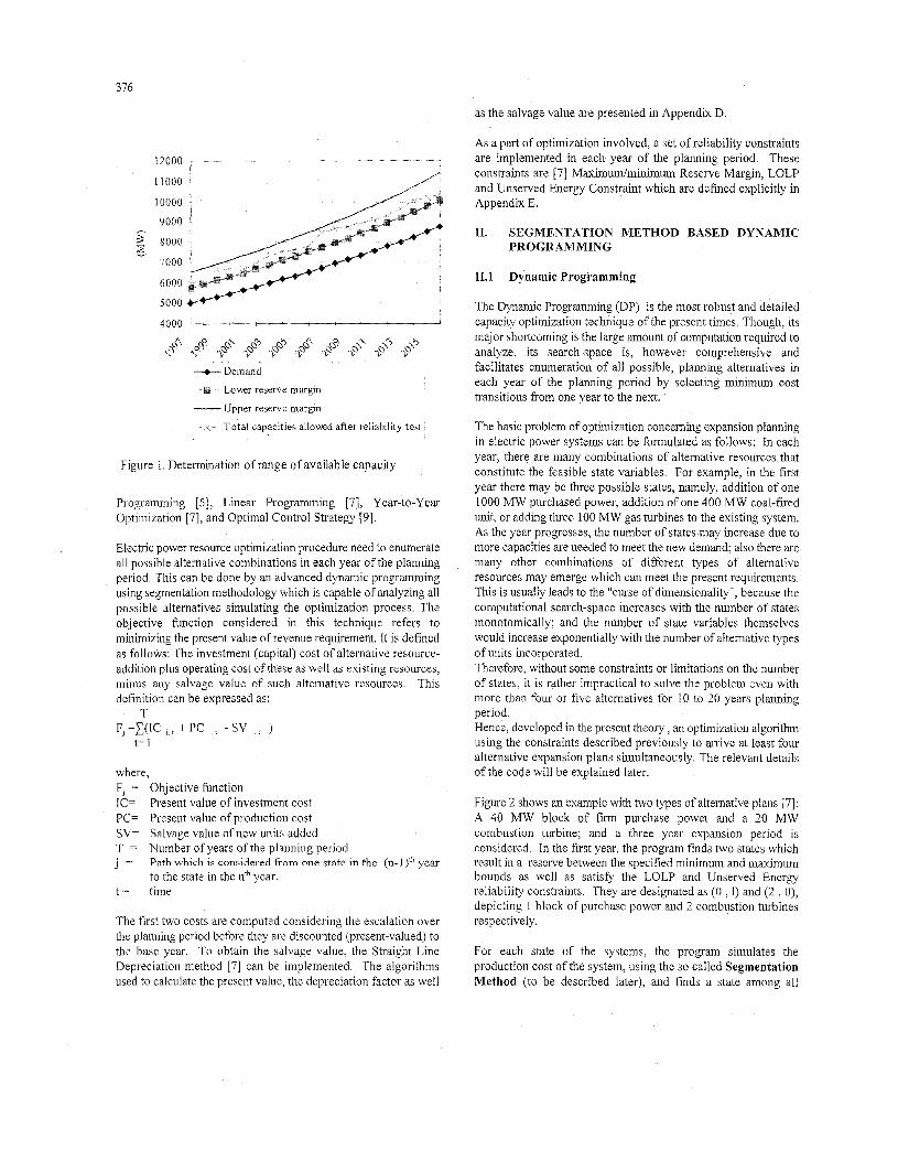
As a part of optimization involved, a set of reliability constraints are implemented in each year of the planning period. These constraints are [7] Maximudminimum Reserve Margin, LOLP and Unserved Energy Constraint which are defined explicitly in Appendix E.

11. SEGMENTATION METHOD BASED DYNAMIC PROGRAMMING

11.1 Dynamic Programming

4000

-+--Demand

- Upper reserve maran

< Total capacities allowrd after reliability test

Figure 1. Determination of range of available capacity

Programming [ 5 ] , Linear Programming [7], Year-to-Year Optimization [7], and Optimal Control Strategy [9].

Electric power resource optimization procedure need to enumerate all possible alternative combinations in each year of the planning period. This can be done by an advanced dynamic programming using segmentation methodology which is capable of analyzing all possible alternatives simulating the optimization process. The objective function considered in this technique refers to minimizing the present value of revenue requirement. It is defined as follows: The investment (capital) cost of alternative resource- addition plus operating cost of these as well as existing resources, minus any salvage value of such alternative resources. This definition can be expressed as:

T

t= 1 FJ =C(Ic J , t + pc J . f - sv j . f

where, F, = Objective function IC= Present value of investment cost PC= Present value of production cost SV= Salvage value of new units added T = Number of years of the planning period j = Path which is considered from one state in the (n- 1 )Ih year

to the state in the nth year. t = time

The first two costs are computed considering the escalation over the planning period before they are discounted (present-valued) to the base year. To obtain the salvage value, the Straight Line Depreciation method [7] can be implemented. The algorithms used to calculate the present value, the depreciation factor as well

The Dynamic Programming (DP) is the most robust and detailed capacity optimization technique of the present times. Though, its major shortcoming is the large amount of computation required to analyze, its search-space is, however comprehensive and facilitates enumeration of all possible, planning altematives in each year of the planning period by selecting minimum cost transitions from one year to the next.

The basic problem of optimization concerning expansion planning in electric power systems can be formulated as follows: In each year, there are many combinations of alternative resources that constitute the feasible state variables. For example, in the first year there may be three possible states, namely, addition of one 1000 MW purchased power, addition of one 400 MW coal-fired unit, or addmg three 100 MW gas turbines to the existing system, As the year progresses, the number of states may increase due to more capacities are needed to meet the new demand; also there are many other combinations of different types of alternative resources may emerge which can meet the present requirements. This is usually leads to the "curse of dimensionality", because the computational search-space increases with the number of states monotomically; and the number of state variables themselves would increase exponentially with the number of alternative types of units incorporated. Therefore, without some constraints or limitations on the number of states, it is rather impractical to solve the problem even with more than four or five altematives for 10 to 20 years planning period. Hence, developed in the present theory , an optimization algorithm using the constraints described previously to arrive at least four alternative expansion plans simultaneously. The relevant details of the code will be explained later

Figure 2 shows an example with two types of alternative plans [7]: A 40 MW block of firm purchase power and a 20 MW combustion turbine; and a three year expansion period IS

considered. In the first year, the program finds two states which result in a reserve between the specified minimum and maximum bounds as well as satisfy the LOLP and Unserved Energy reliability constraints. They are designated as ( 0 , 1) and (2 , 0), depicting 1 block of purchase power and 2 combustion turbines respectively.

For each state of the systems, the program simulates the production cost of the system, using the so called Segmentation Method (to be described later), and finds a state among all

377

the evolution of production costing models.

Unfortunately, no production costing model exists that has the descriptive accuracy, flexibility for alternative cases, nor has the ability to address all the relevant uncertainties in a contained

Y e a r 0 Y e a r 1 Y e a r 2 Y e a r 3

possible states the previous year which, when proceeding to the present state, does not necessitate a deletion of an alternative resource; as well as the state chosen results in a minimum cost incurred up to the present year. For the first year, the only feasible transition is from (0 , 0) and the minimum cost is confined to the cost incurred in the first year alone. This, so-called cost-to-date aspect represents present value of the total operating and production costs and the fixed charges and cumulated up to (inclusive 09 the present year. Thus, the state (0,l) requires a minimum of 76.3 million dollars to reach it from the initial value and the state (2,O) requires 80.0 million dollars to reach it from the initial states. The program then proceeds to the second year and finds four feasible states (O,3), (3,1), (4,l) and (5 ,O). Further, it simulates the production cost as follows: For each state, the program looks back one year and from the previous states [@,I) , (2,0)], a connectivity test is performed. Passing this test, enable the program to determine which of them can proceed to the present feasible states. For instance, (3,l) can emerge from both (0 , I ) and (2,O). Among these two feasible states, the program selects the minimum objective tinction cost at the same times remembering the transition from the prior state which yielded the minimum. This is called the "Backward Pointer" approach. For example, (3,l) has the minimum cost to date as 164.4 million dollars and the Backward Pointer shows by an arrow that (3,l) comes from (0,l). Considering the state (0,3) in the second year, it can come only from (0 , 1) since the connectivity test fails when applied to (0,l) from (0 , 2). The program proceeds in this manner till the last year. At that point, the minimum objective function cost for each state in the last year is calculated and then sorted to determine the "minimal" cost for all feasible transition. In the present example, (4,2) is the cheapest state in the last year and the minimum cost is 259 million dollars. To find the expansion schedules, it is only necessary to retrieve the Backward Pointer. Thus the optimal plan has the following sequence of states: ( 2 , 0 ), (4 , l), and (4 ,2). Subtracting one state from the following state gives the resource added each year. For example, in Figure 2, the optimal installation schedule is determined as indicated in Table 1.

Table 1. Optimal Installation Schedule of the Sample System considered for Dynamic Programming

Resource Addition YEAR 20 MW CT 40 MW Block Purchase Power 1 2 0 2 2 1 3 0 1

2.2. Segmentation Method

Any production cost evaluation has two objectives: The first one is the accuracy and the second one refers to estimating the costs under plausible alternative situations or scenarios. The first objective is obvious and limited only by the ability to understand, assemble, and process the information. The second objective is a little vague, but It has been the primary motivation that has influenced the development and application of new techniques in

E x a m p l e Candidate units A = 2 0 M W Combust ion turbine B = 40 M W B l o c k of purchase power

( 0 , l ) indicates 0 unit A , 1 unit B 7 6 3 indicates total c o s t at that s tage

Figure 2 Power Generation Expans lon viu D y n a m i c Programming

Figure 3. Daily load curve

manner. The generic art in production costing analysis is, therefore, the ability to compensate for the tunnel vision of the modeling capability.

Applying the sp-called segmentation method of analysis. in production costing analysis as described below is the simplest and

378

most accurate model for analyzing the supply resource altematives under various uncertainties which exist in the electric utilities' business of modern times.

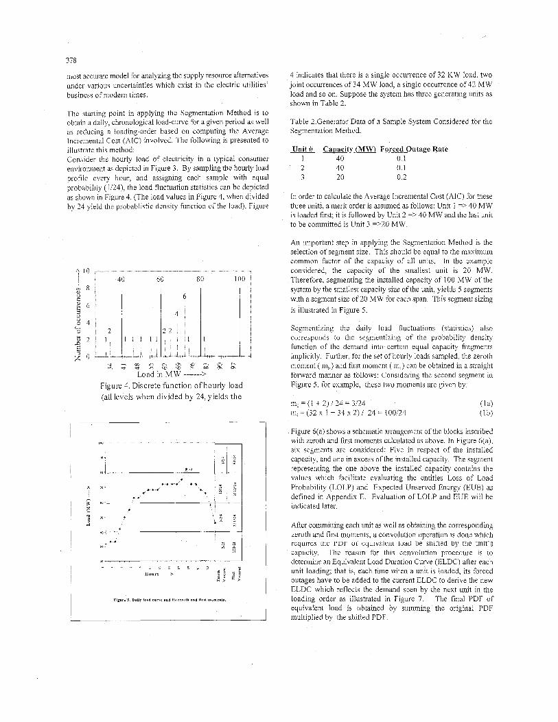
The starting point in applying the Segmentation Method is to obtain a daily, chronological load-curve for a given period as well as reducing a loading-order based on computing the Average Incremental Cost (AIC) involved. The following is presented to illustrate this method: Consider the hourly load of electricity in a typical consumer environment as depicted in Figure 3, By sampling the hourly load profile every hour, and assigning each sample with equal probability (l/24), the load fluctuation statistics can be depicted as shown in Figure 4. (The load values in Figure 4, when divided by 24 yield the probablistic density function of the load). Figure

40 60 80 100

b - ~ m n ~ m w m o r - r r i b Y r ' v ? i D i D r - c O O \ Q \

b a d in M W -------> Figure 4. Discrete function ofhourly load (all levels when divided by 24, yields the

4 indicates that there is a single occurrence of 32 KW load, two joint occurrences of 34 MW load, a single occurrence of 42 MW load and so on. Suppose the system has three generating units as shown in Table 2.

Table 2.Generator Data of a Sample System Considered for the Segmentation Method.

Unit # Capacity (MW) Forced Outage Rate 1 40 0.1 2 40 0.1 3 20 0.2

In order to calculate the Average Incremental Cost (AIC) for these three units, a merit order is assumed as follows: Unit 1 => 40 MW is loaded fust; it is followed by Unit 2 => 40 MW and the last unit to be committed is Unit 3 =>20 MW.

An important step in applying the Segmentation Method is the selection of segment size. This should be equal to the maximum common factor of the capacity of all units. In the example considered, the capacity of the smallest unit is 20 MW. Therefore, segmenting the installed capacity of 100 MW of the system by the smallest capacity size of the unit, yields 5 segments with a segment size of 20 MW for each span. This segment sizing is illustrated in Figure 5.

Segmentizing the daily load fluctuations (statistics) also corresponds to the segmentizing of the probability density function of the demand into certain equal capacity fragments implicitly. Further, for the set of hourly loads sampled, the zeroth moment ( m,) and fust moment ( m,) can be obtained in a straight forward manner as follows: Considering the second segment in Figure 5 , for example, these two moments are given by:

m, = (1 + 2) / 24 = 3124 m, = (32 x 1 + 34 x 2) / 24 = 100124

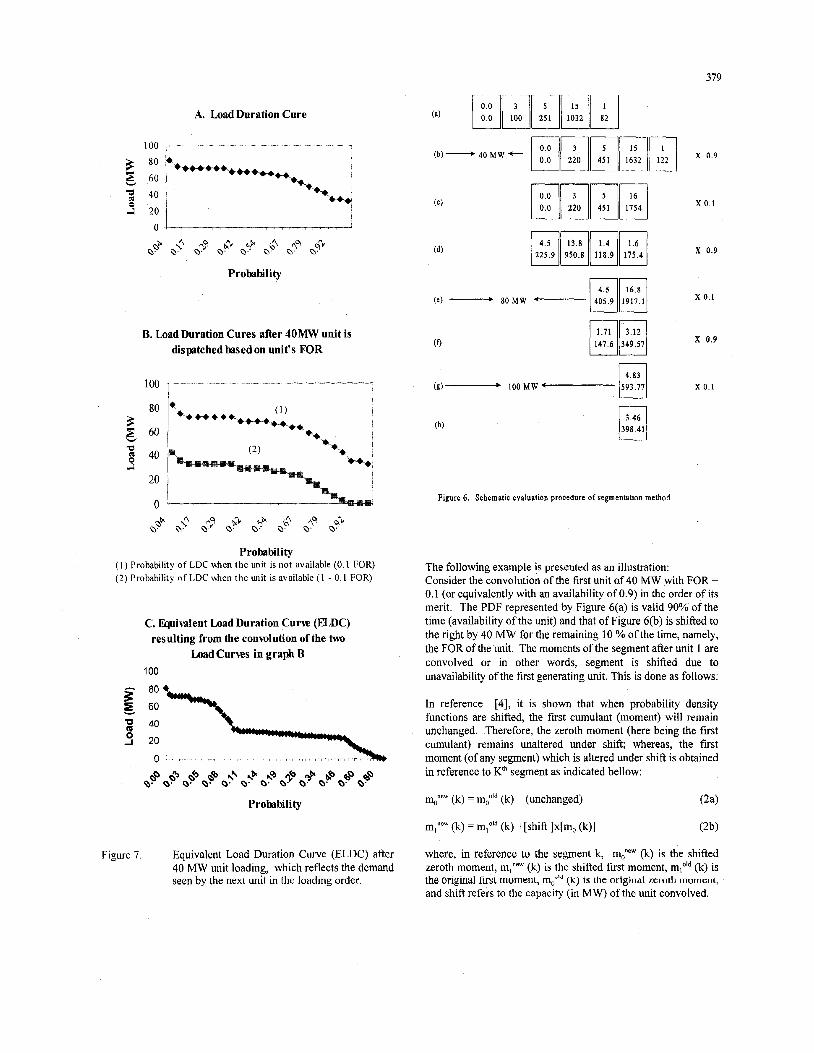
Figure 6(a) shows a schematic mangement of the blocks inscribed with zeroth and frst moments calculated as above. In Figure 6(a), six segments are considered: Five in respect of the installed capacity, and one in excess of the installed capacity. The segment representing the one above the installed capacity contains the values which facilitate evaluating the entities Loss of Load Probability (LOLP) and Expected Unserved Energy (EUE) as defined in Appendix E. Evaluation of LOLP and EUE will be indicated later.

After committing each unit as well as obtaining the corresponding zeroth and first moments, a convolution operation is done which requires the PDF of equivalent load be shined by tbe Unit's capacity. The reason for this convolution procedure is to determine an Equivalent Load Duration Curve (ELDC) after each unit loading; that is, each time when a unit is loaded, its forced outages have to be added to the current ELDC to derive the new ELDC which reflects the demand seen by the next unit in the loading order as illustrated in Figure 7. The final PDF of equivalent load is obtained by summing the original PDF multiplied by the shifted PDF.

379

A. Load Duration Cure

x 0.1

X 0 .9

Probability

x 0 . 1 (e) ____* 80MW

(0 ww 147.6 349.57 B. LoadDuration Cures after 40MW unit is

dispatched based on unit's FOR X 0 . 9

x 0.1 (g)- 100MW *

398.41 (h)

Figure 6 . Schematic ev:

U

id ation proce re a egmentation me

Probability ( 1 ) Probability of LDC when the unit is not available (0.1 FOR) (2) Probability of LDC when the unit is available ( 1 - 0.1 FOR)

The following example is presented as an illustration: Consider the convolution of the first unit of 40 MW with FOR = 0.1 (or equivalently with an availability of 0.9) in the order of its merit. The PDF represented by Figure 6(a) is valid 90% of the time (availability of the unit) and that of Figure 6(b) is shifted to the right by 40 MW for the remaining 10 % of the time, namely, the FOR of the unit. The moments of the segment after unit 1 are convolved or in other words, segment is shifted due to unavailability of the fvst generating unit. This is done as follows:

C. Equiwlent Load Duration C u m (ELDC) resulting from the conwlution of the two

Load Curves in graph B 100

s i .; 20

0

s i .; 20

0

In reference [4], it is shown that when probability density functions are shifted, the first cumulant (moment) will remain unchanged. Therefore, the zeroth moment (here being the first cumulant) remains unaltered under shift; whereas, the first moment (of any segment) which is altered under shift is obtained in reference to Kth segment as indicated bellow:

m T W (k) = m;ld (k) (unchanged) ( 2 4

mlnew (k) = m,"ld (k) +[shift ]x[mo (k)] (2b)

Figure 7. Equivalent Load Duration Curve (ELDC) after 40 MW unit loading, which reflects the demand seen by the next unit in the loading order.

where, in reference to the segment k, m T w (k) is the shifted zeroth moment, m,"ew (k) is the shifted first moment, mlold (k) is the origmal fust moment, mCid (k) is the original zeroth moment, and shift refers to the capacity (in MW) of the unit convolved.

380

In reference to the example under discussion, the original (unshifted) values of zeroth and first order moment of the second segment in Figure 6(bj, are m, = 3/24 and m, = 100124, respectively Hence, upon convolving, their (convolved) values are as follows:

m, = 3/24 (unchanged) m, = ( 100 + 40 x 3 )/24 = 220/24

It should be noticed here that all numbers in the block of Figure 6(bj are divided by 24 for normalization. Following the above procedure, the shifted moments for every segment in Figures 6(b) are calculated. Since one is interested in the first moment of unserved demand, that is, the first segment of the first moment lying to the right of the total generating capacity committed, it is not necessary to know the moments of the individual segments beyond the installed capacity. All the zeroth and first moments of the segment are added together after each generating capacity is included. In the example under discussion, the fourth segment of Figure 6 0 is equal to the sum of the shifted moment of segments 4 and 5 in Figure 6(b). In Figure 6(d), the moment of the final PDF of the equivalent load, after convolution o f unit 1 is obtained by multiplying each moment of the segment of Figure 6(a) by the availability of the machine (0.9) and also in reference to Figure 6 0 by the unavailability (FOR) ofthe machine (0. 1) and add them together. For example, the first segment of the zeroth and first moment in Figure 6(d) are:

mOfina' ( 1 ) = (5 x 0.9) + ( 0.0 x 0.1) = 4.5

mliinal ( I ) = (251 x 0.9) + (0.0 x 0.1) = 225.9

(4a?

(4b)

A general expression for Expected Unserved Energy (see Appendix E) per unit time can be written as follows [5]:

NS cu NS

j=s j=l j=s UD,, =Em, - (1 c , 1 x (E mo 1 ( 5 4

UE,, = T x UD,, (5b)

where, UD,, is the unserved energy per unit time after convolution of the unit, UE,, is the unserved energy after convolution of the unit, T is the time period (24 hours in this case), NS is the total number of segments, CU is the number of committed generating unit, and S is the number of committed segments corresponding to a generating unit From Figure 6(a), the initial Expected Unserved Energy per unit time is

UD, =Em, =(0+100+25 1+1032+82+0)/24=1465/24 6

J=1 M WHih (6a)

6 I 6

j=1 j=1 j=2 UD,,=Cm, - ccc, > x ( E m , > =

= (225.9 + 950.8 + 118.9 + 175.4)/24 - 40 x (4.5 + 13.8 + 1.4 + 1.6)/24 = 619 MWH (6ci

The general expression for the expected unit energy generation is given by:

The expected energy generation of unit 1 is, therefore,

E, = T (UD,-UD, ) E 24(1465-619)/24 = 846 MWH (7a)

or equivalently, E, = (UE, - U E , ) = ( 1 4 6 5 - 6 1 9 ) y846MWH (7b)

Unit 2 is committed next. This unit has a capacity C2 = 40 MW and FOR = 0 1. Figure 6(e) is obtained from Figure 6(d) by shifting the segment by 40 MW. Thus, the first shifted segment in Figure 6(e), is obtained in the similar manner as described earlier:

moneW = 4.5124 ( 8 4

mlneW = ( 225 9 + 40 x 4.5 )i 24 = 405.9 / 24 (8b)

The final segment shifted in Figure 6(e) combines the last three segments of Figure 6(d). The value in Figure 6(f) is obtained by multiplying all moments in each segment of Figure 6(d) by p =

0.9 and those of Figure 6(e) by q (FOR) = 0. 1 and added together. The segment below (40 + 40) = 80 MW of the committed capacity as explained earlier are not retained since they are not required in the calculation.

The unserved energy per unit time after convolution of the second unit is, from Figure 6(f), and Equation (5 ) , given by :

= (147.6 + 349.57)124 - (40 + 40) x (1.71 + 3.12)/24 = 110.77124 MWHih (9a)

Thus,

UE, = UD, x 24 = 110.77 MWH (9b)

The expected energy generation of Unit 2 is thus determined as:

E, = T(UD, - UD, ) 24(619- 110.77)/24 = 508.23 MWH Thus, UE, = UD, x 24 = 1465 MWH (6b)

The Unserved Energy per unit time after committing the 40 MW unit with FOR = 0.1 can be deducted kom Figure 6(d). It is equal to:

The last unit to be committed is a 20 MW unit with FOR = 0. 2. Figure 6(g) shows the effect of shifting the segment of Figure 6(f) by 20 MW. The only segment produced thereof is a combination of the two last segments of Figure 6(f). Multiplying all moments

381

Guidelines to Select the Segment Sue: The segment size should be equal to the maximum common factor of capacity of all units. Clearly, if the units are dissimilar, the segment size should be reduced to 1 MW. Such a reduction of segment size increases the number of segments spanning the installed capacity with corresponding increase in the computational requirements. However, as shown in Table C. 1 of Appendix C, this increase is tolerable vis-a'-vis the computational considerations. A coarse segment size if used to confine the search-space, the result obtained can, however, be only approximate.

2

3

in all segment of Figure 6(f) by p = 0.8 and those of Figure 6(g) by FOR=0.2 and adding the corresponding segments produce Figure 6(h). The unserved energy per unit time after committing this last unit is :

6 3 6

j=6 j=] J=6 UD3 = C m , - ( C C , ) x ( C m , > = ( 1 0 4

~398.41124 - (40+40+20) x 3.462/ 24 = 52.21124 MWHh

Thus,

UE, = UD, x24=52.21 MWH ( 1 Ob)

Hence, the expected energy generation of Unit 3 is given by:

E, =T(UD2 -UD3)=24(110.77-52.21)/ 24 = 58.56 MWH ( 1 0 ~ ) which is same as:

E, = (UE2 -UE3)=(l 10.77 - 52.2 1)=58.56 MWH ( 1 0 4

The total expected energy generation is hence determined as;

E,= (E,+E, +E3) = (846+508.23+58.56) = 1412.79 MWH(l1a)

The Energy Balance ( EB ) is given by: 508.23 $15.65 (508.23 x 40 15.65) = 7,954

58.56 $17.16 (58.56 x 20 17.16) =1,005

Total $28,199

EB = I465 - ( 1412.79 + 52.21 ) = 0 MWH (1 Ib)

where 1465 MWH corresponds to the system's total energy demand. The system LOLP is simply the zeroth moment in Figure 6(h) lying beyond the installed capacity or zeroth moment of Unserved Energy after convolving of all units. Thus,

LOLP = 3.462 124 = 0.14425 Yo (12)

In this paper, LOLP is expressed in percentage. Alternatively, to express this index as a ratio of time such as dayslyear, LOLE ( Loss Of Load Expectation) definition can be used. The following additional steps should be followed to find the LOLE: First, the LOLP percentage is changed to be a per unit value, and then it is multiplied by 365 or 8760: that is,

LOLE = LOLP X 365 (dayslyear ), if daily load-data is used (13a) or, LOLE = LOLP X 8760 (hours/year ), if hourly load-data is used (13b)

Therefore, in the present example,

LOLE = (0.144251100 per unit) x 365 = 0.5265 days1year (13c)

In this work, LOLP (expressed as a percentage) is used as a probablistic constraint. It is important to emphasis that the LOLP and Unserved Energies are finite values; and, there are no approximation made in the evaluation except for the hourly sampling of the load.

Production Costing Calculation: After expected energy generation for each unit in the merit-order is obtained, production costing calculation is done directly by multiplying the Average Incremental Cost (AIC) with expected energy generation of that unit. The following Table (Table 3) illustrates the calculation of production costing:

Table 3 Calculation of Production Cost

Loading Capacity Generation Total 1 o z p f 1 (MW) 1 (MWH) I *IC* 1 ProdUCtion ($/MWH) costs ($1

IRP strategies play a central role in determining the market share and profitability of electric utilities. The goal of IRP is to identify an optimal overall strategy which maximizes: 1). Satisfaction to all customers on overall basis; and, 2) risk-tolerance or ability to handle many uncertain future events while still remaining rela- tively a "good" plan. In the implantation of IRP, trade-offs between conflicting attributes are evaluated and plans which most evenly minimize all of them are identified. A general-purpose, universal optimization method does not exist since a single code cannot cope up with the gamut of diverse optimization problems which are invariably application-specific. Therefore, optimization techniques are oRen tailored to match the restricted goal function specified by the simulation model uniquely decided by the problem in hand. The optimization method presented in this paper refers to one such technique compatible for IRP strategies which duly accounts for supply side options as well as demand side option. The illustrative examples presented indicate the feasibility aspects of the proposed optimization approach

382

APPENDIX A

Size ( M W

200

CALCULATION OF AVERAGE INCREMENTAL COST ( a

Output (YO) Output Avg. Heat (MW) Rate

(BTUIK WH)

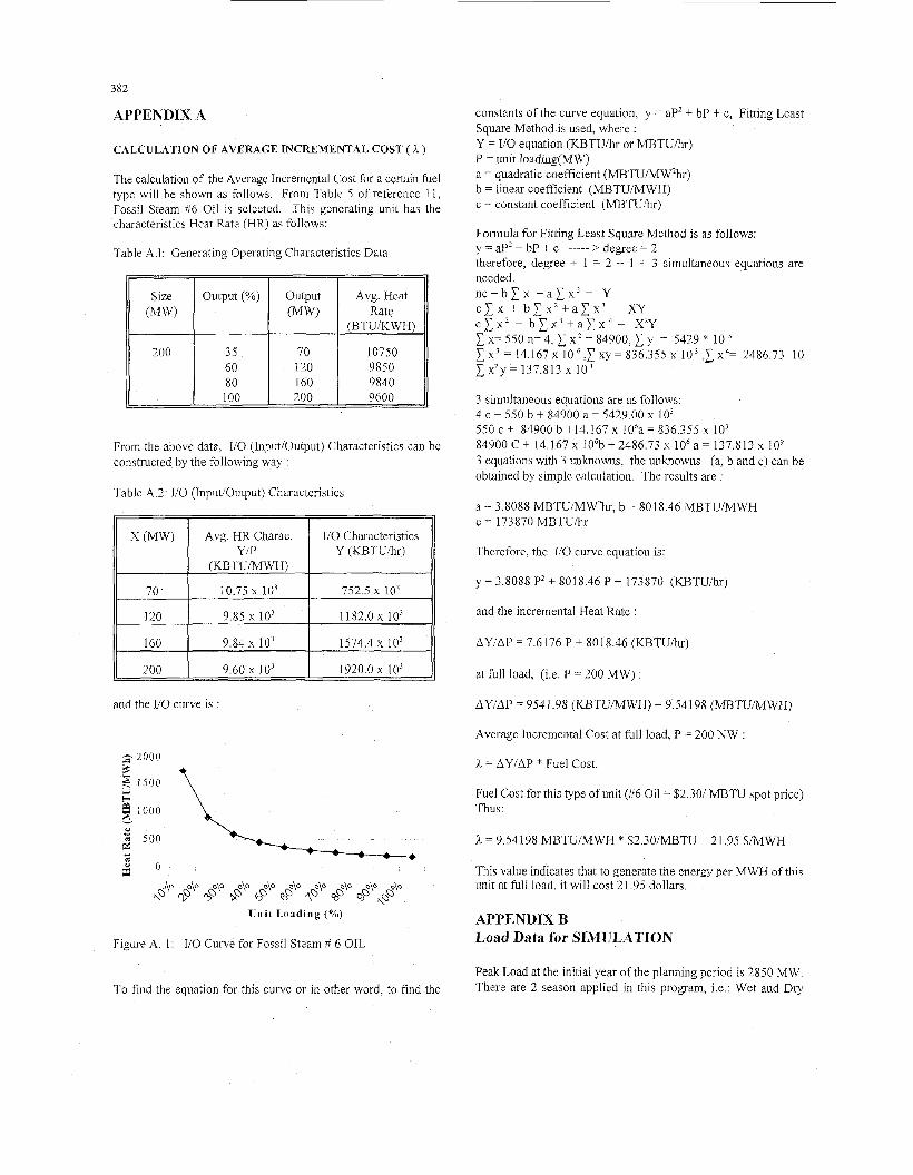
35 70 10750 60 120 9850 80 160 9840 100 200 9600

The calculation of the Average Incremental Cost for a certain fuel type will be shown as follows From Table 5 of reference 11, Fossil Steam #6 Oil is selected. This generating unit has the characteristics Heat Rate (HR) as follows:

X (MW)

Table A.l: Generating Operating Characteristics Data

I I I I

Avg. HR Charac. I10 Characteristics

(KBTUIMWH) YIP Y (KBTUh)

10.75 x lo3 752.5 x 103

From the above data, I/O (Input‘Output) Characteristics can be constructed by the following way :

160

200

Table A.2: I10 (InputIOutput) Characteristics

9.84 x io3

9.60 x io3

1574.4 x I O 3

1920.0 x 10’

and the I10 curve is

c 2000

$ 3 1500 7 b

1000 z_

Figure A. 1 : I10 Curve for Fossil Steam # 6 OIL

To find the equation for this curve or in other word, to find the

constants of the curve equation, y = aP2 + bP + c, Fitting Least Square Method is used, where : Y = I/O equation ( K B T U h or M B T U h ) P = unit loading(MW) a = quadratic coefficient (MBTU1MW’hr) b = linear coefficient (MBTU1MWH) c = constant coefficient (MBTUlhr)

Formula for Fitting Least Square Method is as follows: y = aP2 + bP + c ----- > degree = 2 therefore, degree + 1 = 2 + 1 = 3 simultaneous equations are needed n c + b C x + a C x Z = Y c z x + b C x 2 + a C x 3 = XY c z x ’ + b C x 3 + a C x 4 XzY x= 550 n= 4 , C x 2 = 84900, x3 = 14.167 x 10 ,I xy = 836.355 x I O 3 ,E x4= 2486.73 10 x2y = 137.813 x l o 3

y = 5429 * 10

3 simultaneous equations are as follows: 4 c + 550 b + 84900 a = 5429 00 x IO3 550 c + 84900 b +14.167 x 106a = 836.355 x lo3 84900 C + 14 167 x 106b + 2486.73 x lo6 a = 137.813 x lo9 3 equations with 3 unknowns, the unknowns (a, b and c) can be obtained by simple calculation The results are

a = 3.8088 MBTUIMW’hr, b = 8018.46 MBTUiMWH c = 173870 MBTUihr

Therefore, the I/O curve equation is:

y = 3.8088 P2 + 8018.46 P + 173870 (KBTUkr)

and the incremental Heat Rate :

AYIAP = 7.6 176 P + 801 8.46 (KBTUhr)

at full load, (Le. P = 200 MW) :

Average Incremental Cost at full load, P = 200 NW :

h = AYIAP * Fuel Cost.

Fuel Cost for this type of unit (#6 Oil = $2.301 MBTU spot price) Thus:

A = 9.54198 MBTUMWH * $2.30/MBTU = 21.95 $/MWH

This value indicates that to generate the energy per MWH of this unit at full load, it will cost 21.95 dollars.

APPENDIX B Load Data for SIMULATION

Peak Load at the initial year of the planning period is 2850 MW. There are 2 season applied in this program, i.e.: Wet and Dry

383

seasons. For Wet season, highest peak load occiirs in week 52 [ 1 11, i.e. 100% of 2850 MW = 2850 MW For Dry season, highest peak load occurs in week 23, i.e.

with the assumption, week one was taken as January (Table 1 of reference 11) Weekday peak was taken on Tuesday, i.e. 100% of weekly peak (Table 2 of reference 11) Weekend peak was taken on Saturday, Le. 77% of weekly peak

Table B. I . Hourly Peak Load Data ( Percent Of Daily Load )

90% of 2850 MW = 2565 MW

DRY SEASON WET SEASON WEEKDAY WEEKEND WEEKDAY WEEKEND

-- Hours YO I 64 2 60 3 58 4 56 5 56 6 58 7 64 8 76 9 87 I O 95 1 1 99 12 100 13 99 14 100

15 100 16 97 17 96 18 96 19 93 20 92 21 92 22 93 23 87 24 72

MW 1641 6 1539 1487 7 1436 4 1436 4 I487 6 1641 6 19494 2231 6 2436 8 2539 4 2565 2539 4

2565 2565 2488 1

2462 4 2462 4 2385 5 2359 8 2359 8 2385 5 2231 6 1846 8

9/. 74 70 66 65 64 62 62 66 81 86 91 93 93 92 91 91 92 94 95 95 100 93 88 80

- MW 1461.5 1382.5 1303.5 1283.8 1264 1224.5 1224.5 1303.5 1599.8 1698.5 1797.3 1836.8 1836.8 1817 1797.3 1797.3 1817 1856.5 1876.3 1876.3 1975.1 1836.8 1738 1580

- %

67 63 60 59 59 60 74 86 95 96 96 95 95 95 93 94 99 100 IO0 96 91 83 73 63

- MW 1909.5 1795.5 1710 1681.5 1681.5 1710 2109 245 1 2707.5 2736 2736 2707.5 2707.5 2707.5 2650.5 2679 2821.5 2850 2850 2136 2593.5 2365.5 2080.5 1795.5

- YO

78 72 68 66 64 65 66 70 80 88 90 91 90 88 87 87 91 IO0 99 97 94 92 87 81

- MW 1711 7 1580 1492 3 1448 4 1404 5 1426 4 1448 4 1536 2 1755 6 1931 2 1975 1

1997 1975 1

1931 2 I909 2 1997 1819 2194 5 2172 6 2128 7 2062 8 2018 9 1909 2 1777 5

APPENDIX C Expected Energy of Generations ( GWh ) for difference MW of Segment Size

Unit MW ---a 2 4 6 I O 20

I 30750692 30750692 30750692 30750692 307506

2 30750682 30750805 30750820 30750820 307508

3 3075 0977 3075 0692 3075 0663 3075 0677 3075 06

4 1257 9840 1257 9826 1257 9826 1257 9790 1257 98

5 1257 9954 1257 9982 1257 9968 1258 0032 1257 98

6 1257 9669 1257 9655 1257 9755 1257 9627 1257 97

7 1257 9726 1257 9783 1257 9783 1257 9854 1257 97 8 11824640 11824497 11824455 11824398 118203

Cont.

Unit MW ----> 2

9 2289.0083

10 483.0991

I 1 464.1327

12 406.3449

13 345.7417

14 593.4302

15 459.0435

16 109.5758

17 42.2228

18 10.5684

19 5.5677

20 3.0869

21 ,2154

22 ,1964

23 I 1929

24 ,1756

25 ,1656

26 ,2763

27 ,2554

28 ,2245

29 ,2002

Total Energy Gen.

Energy Demand

Unserved Energy

Energy Balance

System LOLP (%)

Prod. Cost (M$)

4

2289 0353

483 0962

464 0972

406 37 5

345 7353

593 4266

459 0648

109 5666

42 2204

10 5634

5 5697

3 0848

2150

1965

1928

1756

1657

2762

2553

2246

2002

20653

20654

13080

0008

0 43263

I80 6

6

2289.03 11

483.1076

464.0986

406.3605

345.7751

593.4181

459.0312

109.5651

42.22 12

10.5841

5.5637

3.0765

,2111

,2118

.1817

,1769

.I692

,2720

,2560

,2226

,1984

20653

20654

1.3080

,0008

0.43837

180.6

I O 20

2289 0325 2289 03

483 1062 483 10

464 0957 464 09

406 3605 406 49

345 7424 346 8 1

593 4281 593 17

4590500 458 12

109 5725 109 55

4242240 42 21

105682 1061

55676 551

3 0869 3 09

2154 21

1964 18

1929 19

1756 18

1656 16

2763 27

2554 25

2245 22

2002 19

20653 20653 20653

20654 20654 20654

13055 13080 130

0008 0008 00

041830 043263 0438

1806 1806 1806

CPU Time 00:23.02 00:11.32 00:06.51 00:05.13 00:04 Table C. 1. The Effect Of Changing The Segment Size

APPENDIX D PRESENT VALUE FACTOR

Figure D. 1. Present Worth Value

384

For Production Costing :PVPC- (1 + DISRT) -(" + ')

For Investment Cost: PVIC= (1 + DISRT)-'")

YBASE where: YBASE : DISRT : Discount Rate PC : Production Costing IC : Investment cost

NYR = YEAR -

Base Year for discounting

EUE (Expected Unserved Energy): Expected amount of energy which cannot be supplied per year owing to generating capacity deficiencies and / or shortages in basic energy supplies.

Installed Capacity: The total available capacity of all generations in the system

FOR ( Forced Outage Rate): The probability that the unit will not be available to serve a load in the future. FOR is defined as follows :

FOR = MTTR 1 (MTTF + MTTR)

MTTR = Mean Time To Repair MTTF = Mean Time to Failure

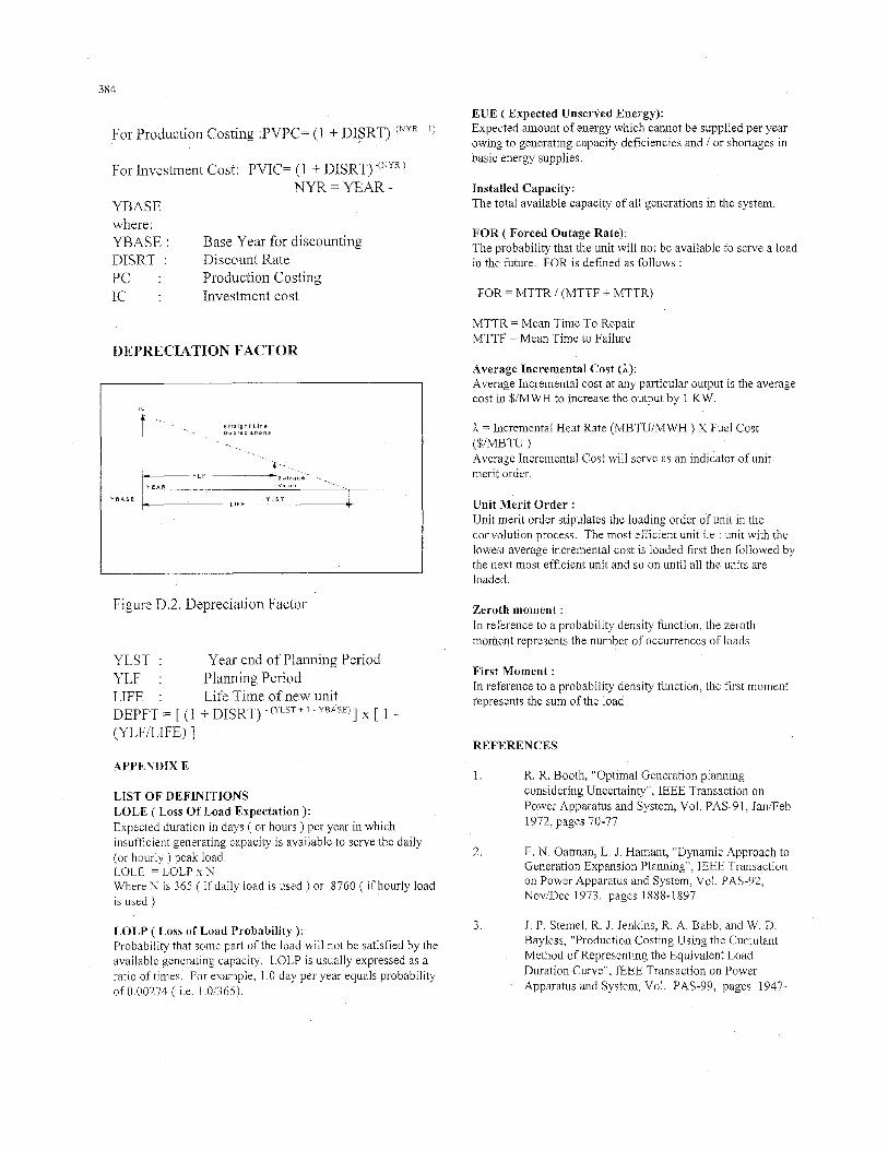
DEPRECIATION FACTOR

I C

S t r a i g h t L i n e D e p r e r i a t l u n s t

Figure D.2. Depreciation Factor

YLST : YLF : Planning Period LIFE : Life Time of new unit

(YLF/LIFE) ]

Year end of Planning Period

DEPFT = [ (1 + DISRT) (YLST * ' I x [ l -

APPENDIX E

LIST OF DEFINITIONS LOLE ( Loss Of Load Expectation ): Expected duration in days ( or hours ) per year in which insufficient generating capacity is available to serve the daily (or hourly ) peak load LOLE = LOLP x N Where N is 365 ( if daily load is used ) or 8760 ( if hourly load IS used )

LOLP ( Loss o f Load Probability ): Probability that some part of the load will not be satisfied by the available generating capacity. LOLP is usually expressed as a ratio of times. For example, 1 .O day per year equals probability of 0.00274 ( i.e. 1.01365).

Average Incremental Cost (A): Average Incremental cost at any particular output is the average cost in $ M W H to increase the output by 1 KW.

h = Incremental Heat Rate (MBTUIMWH ) X Fuel Cost ($/MBTU ) Average Incremental Cost will serve as an indicator of unit merit order.

Unit Merit Order : Unit merit order stipulates the loading order of unit in the convolution process. The most efficient unit i.e : unit with the lowest average incremental cost is loaded first then followed by the next most efficient unit and so on until all the units are loaded.

Zeroth moment : In reference to a probability density function, the zeroth moment represents the number of occurrences of loads

First Moment : In reference to a probability density function, the first moment represents the sum of the load

REFERENCE§

1. R. R. Booth, "Optimal Generation planning considering Uncertainty", IEEE Transaction on Power Apparatus and System, Vol. PAS-9 1 , Jan/Feb 1972, pages 70-77

2. E. N. Oatman, L. J. Hamant, "Dynamic Approach to Generation Expansion Planning", IEEE Transaction on Power Apparatus and System, Vol. PAS-92, NoviDec 1973, pages 1888-1897

3. J. P. Stemel, R. J. Jenkins, R. A. Babb, and W. D. Bayless, "Production Costing Using the Cumulant Method of Representing the Equivalent Load Duration Curve", IEEE Transaction on Power Apparatus and System, Vol. PAS-99, pages 1947-

385

17. Garrity, Thomas F., Wilkins, Daniel R., “Nuclear option for U S . electrical generating capacity additions utilizing boiling water reactor technology” IEEE Transactions on Energy Conversion v 8 n 2 Jun 1993. p 327-331

4.

5 .

6.

7.

8.

9.

IO.

11.

12.

13.

14.

15.

16.

1956, 1980

J. A. Bloom, “Long Range Generation Planning using Decomposition and Probabilistic Simulation”, IEEE Transaction on Power Apparatus and System, Vol. PAS-101, April 1982, pages 797-802

P. Sihombing and A. Affif, “Generation Expansion Planning using Cumulant Method”, IEEE Transaction on Power Apparatus and System, Vol. PAS-99, pages 1947-1956, 1985.

K. F. Schenk, R. B. Mirsa, S. Vassos, W. Wen, “New Method for the Evaluation of Expected Energy Generation and LOLP, IEEE Transactions on Power Apparatus and Systems, Vol. PAS-103, pages 294- 303, 1984

Electric Generation Expansion Analysis System, EPRI Report, El-256 1, Vol. 1 , 1982

Kendal and Stuart, “The Advanced Theory of Statistics”, Vol. 1, Macmillan Publishing Company Inc., NewYork, 1977

Expansion Planning for Electrical Generation System, A Guide Book IEAE. Vienna 1984.

Allen J. Wood and Bruce F. Wollenberg, “Power Generation Operation and Control”, John Willey and Sons. 1984.

IEEE Committee Report, “IEEE Reliability Test System” IEEE Transaction on Power Apparatus and Systems, Vol. PAS-98, pages 2047-2054, 1979.

Energy Information Administration, “The Changing Structure of the Electric Utility Industry”, DOE/EIA- 0562(96), December 1996.

Fukuyama, Yoshikazu, Chiang, Hsaio-Dong “Parallel genetic algorithm for generation expansion planning” IEEE Transactions on Power Systems v 11 n 2 May 1996. p 955- 961

Saraiva. J. Tome, Miranda, Vladimiro, Pinto, L.M.V.G., “Impact on some planning decisions From a fuzzy modeling of power systems” IEEE Transactions on Power Systems v 9 n 2 May 1994. p 819- 825

Tanabe, R., Yasuda, K., Yokoyama, R., Sasaki, H., “Flexible generation mix under multi objectives and uncertainties” IEEE Transactions on Power Systems v 8 n 2 May 1993. p 581- 586

Li, Wenyuan, Billinton, R., “Minimum cost assessment method for composite generation and transmission system expansion planning” IEEE Transactions on Power Systems v 8 n 2 May 1993. p 628- 635

Bibliographies:

Dr. P. S. Neelakanta, Perambur S. Neelakanta received his B. Eng degree from University of Madras, his M. Eng. degree from Indian Institute of Science(I.I.Sc., Bangalore, India (with Distinction) in 1968 and his Ph.D. degree from the Indian Institute of Technology (I.I.T.) Madras, India in 1975. He had been a faculty member in India, Malaysia, Singapore and the University of South Alabama, Mobile, Alabama, USA. He was also a Research Fellow at Technical University, Aachen, Germany and the Director of Research at RIT Research Corporation, Rochester, NY, USA. Currently, he is a Professor of Electrical Engineering at Florida Atlantic University, Boca Raton, Florida, USA.

Dr. Neelakanta has published extensively (over 125 papers) and his areas of research interest are: Electromagnetics, Stochastical Communication Theory, Radar, Neural Networks and Telecommunications. He has authored two books “Neural Networks Modeling” (with D. DeGroff as the co-author) and “Handbook of Electromagnetic Materials” both published by CRC Press.

Mohammad H. Arsali P.E. Mr. Arsali is a Professional Engineer and has more than 15 years of experience in the electric utility industry. He received his BSEE in 1980 and MSEE degrees in 1981 both f?om University of Alabama in Birmingham. He is currently an engineering consultant and also working toward his Ph.D. in Electrical Engineering at Florida Atlantic University. Prior to starting his consulting carrier in 1996, he worked for major investor-owned utilities (Georgia Power Company, Southern Company Services, and Florida Power & Light). His experience includes all aspects of power supply planning, retail and wholesale rate design, regulatory analysis, integrated resource planning, competitive bid evaluations, open access transmission filings, corporate modeling, contract development and negotiation for both generation and transmission, project management, and economic evaluation of regional power markets.