Multi-objective integrated production and distribution planning of perishable products

Int. J. Production Economics 138 (2012) 89–101

Contents lists available at SciVerse ScienceDirect

Int. J. Production Economics

0925-52

doi:10.1

n Corr

E-m

hans-ot

almada.

journal homepage: www.elsevier.com/locate/ijpe

Multi-objective integrated production and distribution planningof perishable products

P. Amorim a,n, H.-O. Gunther b, B. Almada-Lobo a

a DEIG, Faculty of Engineering, University of Porto, Rua Dr. Roberto Frias, s/n, 4600-001 Porto, Portugalb Department of Production Management, Technical University of Berlin, Strasse des 17. Juni 135, 10623 Berlin, Germany

a r t i c l e i n f o

Article history:

Received 24 January 2011

Accepted 5 March 2012Available online 12 March 2012

Keywords:

Perishability

Multi-objective

Production and distribution planning

73/$ - see front matter & 2012 Elsevier B.V. A

016/j.ijpe.2012.03.005

esponding author.

ail addresses: [email protected] (P. Amo

[email protected] (H.-O. Gunther),

[email protected] (B. Almada-Lobo).

a b s t r a c t

Integrated production and distribution planning have received a lot of attention throughout the years

and its economic advantages are well documented. However, for highly perishable products this

integrated approach has to include, further than the economic aspects, the intangible value of

freshness. We explore, through a multi-objective framework, the advantages of integrating these two

intertwined planning problems at an operational level. We formulate models for the case where

perishable goods have a fixed and a loose shelf-life (i.e. with and without a best-before-date). The

results show that the economic benefits derived from using an integrated approach are much

dependent on the freshness level of products delivered.

& 2012 Elsevier B.V. All rights reserved.

1. Introduction

Rapidly deteriorating perishable goods, such as fruits, vegeta-bles, yoghurt and fresh milk, have to take into account theperishability phenomenon even for the operational level ofproduction and distribution planning, which has a timespanranging from 1 week to 1 month. Usually these products startdeteriorating from the moment they are produced on. Therefore,without proper care, inventories may rapidly get spoiled beforetheir final use making the stakeholders incur on avoidable costs.The customers of these products are aware of the intense perish-ability they are subject to, and they attribute an intangible valueto the relative freshness of the goods (Tsiros and Heilman, 2005).To evaluate freshness customers rely on visual cues which maydiffer among the broad class of perishable products. Nahmias(1982) dichotomized deteriorating goods in two categoriesaccording to their shelf-life: (1) fixed lifetime: items’ lifetime ispre-specified and therefore the impact of the deteriorating factorsis taken into account when fixing it. In fact, the utility of theseitems may decrease during their lifetime, and when passing itslifetime, the item will perish completely and become of no value,e.g., milk, inventory in a blood bank, and yoghurt, etc. and(2) random lifetime: there is no specified lifetime for these items.The lifetime for these items is assumed as a random variable, andits probability distribution may take on various forms. Examples

ll rights reserved.

rim),

of items that keep deteriorating with some probability distribu-tion are electronic components, chemicals, and vegetables, etc.

When the shelf-life is fixed the most common visual cue thatcustomers rely on is the best-before-date (BBD). The BBD can bedefined as the end of the period, under any stated storageconditions, during which the product will remain fully market-able and retain any specific qualities for which tacit or expressclaims have been made. In this case, customers will adapt theirwillingness to pay for a product based on how far away the BBDis. On the other hand, when the expiry date of a product is notprinted and then the shelf-life is loose, customers have to rely ontheir senses or external sources of information to estimate theremaining shelf-life of the good. For example, if a banana hasblack spots or if flowers look wilted, then customers know thatthese products will be spoiled rather soon.

In the case of loose shelf-life, especially in the fresh food industry,manufacturers can make use of predictive microbiology to estimatethe shelf-life of these kinds of products based on external control-lable factors, such as humidity and temperature (Fu and Labuza,1993). To make concepts clearer, shelf-life is defined as the timeperiod for the product to become of no value for the customer due tothe lack of the tacit initial characteristics that the product issupposed to have. Thus, in our case, this period starts on the daythe product is produced. The determination of shelf-life as a functionof variable environmental conditions has been the focus of manyresearch activities in this field and a considerable number of reliablemodels exist, such as the Arrhenius model, the Davey model and thesquare-root model. These models take into account the knowledgeabout microbial growth in decaying food goods under differenttemperature and humidity conditions.

www.elsevier.com/locate/ijpe

www.elsevier.com/locate/ijpe

dx.doi.org/10.1016/j.ijpe.2012.03.005

mailto:[email protected]




dx.doi.org/10.1016/j.ijpe.2012.03.005

P. Amorim et al. / Int. J. Production Economics 138 (2012) 89–10190

Regarding production and distribution planning, many authorshave shown the economic advantages of using an integrateddecision model over a decoupled approach (Martin et al., 1993;Thomas and Griffin, 1996). These advantages are believed to beleveraged when the product suffers a rapid deterioration processand hence pushes towards a more integrated view of theseintertwined problems. For perishable goods the final productsinventory that is usually used to buffer and decouple these twoplanning decisions have to be questioned since customers distin-guish between different degrees of freshness and there is anactual risk of spoilage. In this work, we want to study thepotential advantages of using an integrated approach for opera-tional production and distribution planning of perishable goodscompared with a decoupled one. These advantages will beanalyzed through the economic and product freshness perspec-tive. We focus on highly perishable consumer goods industries,with a special emphasis on food processing, which have to copewith complex challenges, such as the integration of lot sizing andscheduling, the definition of setup families considering major andminor setup times and costs, and multiple non-identical produc-tion lines (Bilgen and Gunther, 2010). We are also interested inunderstanding if these potential advantages differ among the twodistinct perishable goods classes that we have mentioned before:with fixed shelf-life and with loose shelf-life. For both the cases,since we are interested in rapidly deteriorating goods, we con-sider a customer who prefers products with a higher freshnesslevel. To tackle explicitly this customer satisfaction issue weembedded our integrated operational production and distributionplanning problem in a multi-objective framework distinguishingtwo very different and conflicting objectives of the planner. Thefirst objective is concerned with minimizing the total costs overthe supply chain covering transportation, production, setup andspoilage costs. The second one aims at maximizing the freshnessof the products delivered to distribution centers and, therefore,maximize customers’ willingness to pay.

The remainder of the paper is organized as follows. The nextsection is devoted to the literature review of related topics. InSection 3, two integrated and two decoupled models are formu-lated for the multi-objective production and distribution planningof the perishable products problem. First we will focus onproducts with a fixed shelf-life and then with a loose one. InSection 4, an illustrative example to understand the impact of themodels is developed and analyzed. The paper is concluded inSection 5.

2. Literature review

Taking into account that perishability in supply chains hasreceived increased attention both in practice and in academicresearch it urges to continue the development of models thatincorporate explicitly this phenomenon (Ahumada and Villalobos,2009; Akkerman et al., 2010). Since in this section we only reviewliterature directly connected to our research and explore conceptsand strategies used to model this problem, readers are referred toKaraesmen et al. (2011) for an extensive review on papersmanaging perishable inventories. First we look into what hasbeen done in production and distribution modeling from adecoupled and integrated point of view with a special focus onperishability and consumer goods industries. Then, based on thispaper a discussion about the multi-objective approach used andsome other important modeling concepts follows. Hence, thecontribution of our work in this research field is clarified.

For tackling the operational production planning of perishablegoods, Marinelli et al. (2007) propose a solution approach for a realworld capacitated lot sizing and scheduling problem with parallel

machines and shared buffers, arising in a company producingyoghurt. The problem has been formulated as a hybrid continuoussetup and capacitated lot sizing problem. To solve this problem atwo-stage heuristic procedure based on the decomposition of theproblem into a lot sizing and a scheduling sub-problem has beendeveloped. This model accounted for perishability by using a make-to-order production strategy. With a similar approach, but focused onbatch processing, Neumann et al. (2002) decompose detailed produc-tion scheduling for batch production into batching and batchscheduling. The batching problem converts the primary requirementsfor products into individual batches, where the workload is to beminimized. They formulate the batching problem as a nonlinearmixed-integer program and transform it into a linear mixed-binaryprogram of moderate size. The batch scheduling problem allocatesthe batches to scarce resources such as processing units, workers, andintermediate storage facilities, where some regular objective functionlike the makespan is to be minimized. The batch scheduling problemis modeled as a resource-constrained project scheduling problem,which can be solved by a truncated branch-and-bound algorithm. Inthis work some intermediate perishable products cannot be storedeliminating the buffer between related activities. Pahl and Voß (2010)extend well-known discrete lot-sizing and scheduling models byincluding deterioration constraints. Also for the special case ofyoghurt production, Lutke Entrup et al. (2005) develop threemixed-integer linear programming models that integrate shelf-lifeissues into production planning and scheduling of the packagingstage. In this work product freshness is modeled as a linear functionhoping that retailers could pay the difference between differentdeterioration stages. Cai et al. (2008) develop a model and analgorithm for the production of seafood products. Due to a deadlineconstraint and the raw material perishability, the manufacturerdetermines three decisions: the product types to be produced; themachine time to be allocated for each product type; and the sequenceto process the products selected. It is interesting to notice that herethe perishability is focused on the raw materials.

Especially suited for lot-sizing and scheduling in the consumergoods industry, where natural sequences in sequencing productscan be found in order to minimize changeover time and to ensurequality standards, there is the concept of block planning. A blockrepresents a sequence, set a priori, of production orders ofvariable size, where each production order corresponds to aunique product type. Hence, each product type occurs at a givenposition in a block (Gunther et al., 2006). This concept will be veryuseful in reducing the complexity and augmenting the applic-ability of our models in the next section.

There are two papers worth of reference when modeling explicitlyrouting for perishable products. Osvald and Stirn (2008) develop aheuristic algorithm for the distribution of fresh vegetables in whichperishability represents a critical factor. The problem is formulated asa vehicle routing problem with time windows (VRPTW) and withtime-dependent travel times. The model considers the impact ofperishability as a part of the overall distribution costs. Hsu et al.(2007) consider the randomness of the perishable food deliveryprocess and construct a stochastic VRPTW model to obtain optimaldelivery routes, loads, fleet dispatching and departure times fordelivering perishable food from a distribution center. They take intoaccount inventory costs due to deterioration of perishable food andenergy costs for cold storage vehicles.

Regarding transportation in the consumer goods industry there isa significant trend in outsourcing this function to third party logisticsservice providers (3PL) (Lutke Entrup, 2005). This decision enablesconsumer goods manufacturers to move towards a more flexible coststructure and, hence, the manufacturer is able to choose generallybetween Less-than-truckload (LTL), where the shipper only pays aprice according to the capacity used, and full-truckload where theshipper pays a fixed cost per load (Gunther and Seiler, 2009). The

P. Amorim et al. / Int. J. Production Economics 138 (2012) 89–101 91

temperature of the transportation, in the case of perishable goods,especially food, has to be in accordance with the requirements of theperishable goods transported, for instance, chilled or frozen. In ourcase we will consider that all products have the same temperaturerequirements and hence can be grouped together in every shipment.

Looking at the literature on integrated production anddistribution models dealing with perishable products, Eksiogluand Mingzhou (2006) address a production and distributionplanning problem in a dynamic, two-stage supply chain. Theirmodel considers that the final product is perishable and has alimited shelf-life. Furthermore, strong assumptions are made,such as, unlimited capacity. They formulate this problem as anetwork flow problem with a fixed charge cost. Based on theeconomic order quantity, Yan et al. (2011) develop an integratedproduction–distribution model for a deteriorating item in a two-echelon supply chain. Their objective is to minimize the totalsystem cost. Some restrictions concerning perishability areimposed. For example, the supplier’s production batch size islimited to an integer multiple of the discrete delivery lot quantityto the buyer. In a more operational perspective, Chen et al. (2009)propose a nonlinear mathematical model to consider productionscheduling and vehicle routing with time windows for perishablefood products. The demand at retailers is assumed to be stochas-tic and perishable goods will deteriorate once they are produced.Thus, the revenue of the supplier is uncertain and depends on thevalue and the transaction quantity of perishable products whenthey are carried to retailers. The objective of this model is tomaximize the expected total profit of the supplier. The productionquantities, the time to start production and the vehicle routes aredetermined in the model iteratively through a decompositionprocedure. The solution algorithm is composed of the constrainedNelder–Mead method and a heuristic for the vehicle routing withtime windows. Recently, Rong et al. (2011) developed an MIPmodel where the quality of a single product is modeled throughouta multi-echelon supply chain. Their model uses the knowledge ofpredictive microbiology in forecasting shelf-life based on thetemperature of transportation and stocking. Their objective func-tion reflects this reality by taking into account the incrementalcooling costs necessary to achieve a longer shelf-life. This work hasa straight linkage to the models developed for the loose shelf-lifecase of this paper.

Based on this paper, when developing production and/or distribu-tion models applied to the type of perishable products treated in thiswork, a considerable number of different approaches could beconsidered. We can impose a make-to-order strategy for all productsso that it is likely that no products will spoil and they will bedelivered with good freshness standards. It is also possible to enforceconstraints on the number of periods that a product can stay in stockor just control the number of spoiled products and penalize it in theobjective function. A third way of taking into consideration products’perishability is by using differentiating holding costs depending onthe shelf-life. So items with a shorter shelf-life are given higherholding costs and items with a longer shelf-life are given lowerholding costs. Finally, from a customer value point of view, it ispossible to either attribute a value to the different degrees offreshness that a product has when delivered, or to assign a demandfunction that varies in function of items’ remaining shelf-life. Thisway we are explicitly controlling the perishability process since weknow for every delivered product the corresponding monetary valueof the remaining shelf-life and, therefore, we may focus on maximiz-ing profit. However, most of these alternatives imply an exhaustivedifferentiation of costs, freshness values and demand functionsamong products. This can be very inaccurate in the consumer goodsindustries that need to handle hundreds of stock keeping units. Thus,without demeriting these approaches, to tackle the perishabilityphenomenon in planning tasks, such as production and distribution,

it is necessary to employ another method to understand thecomplementary effects of supply chain costs and product perish-ability. In order to follow our goal of understanding the impact ofintegrating the analysis of production and distribution planning, bothin economic and in freshness terms, the use of a single objectivefunction would hinder the important trade-off between these twoconflicting objectives. Some authors have already given hints aboutthe importance of using a multi-objective framework to fully explorethe perishability phenomenon (e.g. Arbib et al., 1999; Lutke Entrup,2005). Nevertheless, to the best of our knowledge, this is the firstwork that addresses the integrated production and distributionplanning of perishable products in a multi-objective framework.

3. Problem statement and model formulations

The production and distribution planning problem consideredin this paper consists of a number of plants p¼ 1, . . . ,P havingdedicated lines which produce multiple perishable items with alimited capacity to be delivered to distribution centers. It isrelevant to understand the importance of the design choice ofhaving such a complex supply chain instead of just consideringone plant and multiple distribution centers. As said before, wefocus on perishable consumer goods industries which are knownfor demanding increasing flexibility in the supply chain planningprocesses. Thus, to consider a network of production plants whichcan add increased flexibility and reliability to hedge against thecomplex dynamics of such industries is crucial. Therefore,although we are tackling an operational level of decision makingfor these two planning tasks we assume a central organizationalunit that makes decisions which are followed directly at a locallevel. The length of the planning horizon for such planningproblem ranges from 1 week to 1 month.

All product variants k¼ 1, . . . ,K belonging to the same familyform a block. Therefore a product can only be assigned to oneblock. Blocks j¼ 1, . . . ,N are to be scheduled on l¼ 1, . . . ,L parallelproduction lines over a finite planning horizon consisting ofmacro-periods d¼ 1, . . . ,T with a given length. The schedulingtakes into account that the setup time and cost between blocks isdependent on the sequence of production (major setup). Thesequence of products in a block is set a priori due to naturalconstraints in this kind of industries. Hence, when changing theproduction between two products of the same block only a minorsetup is needed that is not dependent on the sequence, but onlyon the product to be produced.

In order to consider the initial stock that might be used to fulfilcurrent demand it is important to have an overview of the inventorybuilt up in each macro-period due to perishability concerns. Thelength of the horizon that needs to be considered is related to theproduct with the longest shelf-life. One shall consider an integermultiple X of past planning horizons that is enough to cover thelongest shelf-life, i.e. X ¼ dmax ~uk=Te, where ~uk is a conservativevalue for shelf-life of product k, hence t¼�XTþ1, . . . ,0;1, . . . ,T . LetT� ¼ f�XTþ1, . . . ,0g and T þ ¼ f1, . . . ,Tg, thus the domain of t isequivalent to ½T� ¼ T� [ T þ .

A macro-period is divided into a fixed number of non-over-lapping micro-periods with variable length. Since the productionlines can be scheduled independently, this is done for each lineseparately. Sld denotes the set of micro-periods s belonging tomacro-period d and production line l. All micro-periods are put inorder s¼ 1, . . . ,Sl, where Sl corresponds to the total number ofmicro-periods of line l. It is important to notice that each line isassigned to a plant. The length of a micro-period is a decisionvariable, expressed by the production of several products of oneblock in the respective micro-period on a line and by the time toset up the block in case it is necessary. A sequence of consecutive


micro-periods, where the same block is produced on the sameline, defines the size of a lot of a block through the quantity ofproducts produced during these micro-periods. Therefore, a lotmay aggregate several products from a given block and maycontinue over several micro and macro-periods. Moreover, a lot isindependent of the discrete time structure of the macro-periods.The number of micro-periods of each day defines the upper boundon the number of blocks to be produced daily on each line.

There is no inventory held at production plants. Thus, at theend of each day the production output is delivered to distributioncenters c¼ 1, . . . ,DC, which have an unlimited storage capacity.The delivery function is assured by a 3PL, and we assume that itcharges a flat rate per pallet transported between a plant and aDC. Moreover, it is assumed that the 3PL is able to cope withwhatever distribution planning was decided beforehand and,hence, there is no capacity restriction for transportation. This3PL takes care of all sorts of other decisions besides the quantitiesto be transported and it complies with the tightest recommenda-tions and regulations on transportation of perishable goods. Thedistances between production plants and distribution centers aresmall enough so that the product is delivered on the same day it isproduced. Therefore, the decrease of freshness during the trans-portation is considered to be negligible compared with thedecrease at the storage process. The small distance assumptionis quite realistic in supply chains of highly perishable goodswhere the distribution centers are not very far away from theproduction plants. However, this poses a limitation for theapplication of this model when this assumption is not verified.For our purposes these assumptions shall not pose a problemsince we are still considering directly the most important costdrivers for transportation services: distance, quantity and servicelevel. The demand for an item in a macro-period at a distributioncenter is assumed to be dynamic and deterministic.

The problem is to plan production and distribution so as tominimize total cost and maximize mean remaining shelf-life ofproducts at the distribution centers over a planning horizon.

In Fig. 1 a graphical interpretation of the problem dealt with inthis paper is presented. It represents the product flow from plants toDCs and the correspondent demand satisfaction. To understand thatthis is just a layer of the supply network a shadowed replication wasdrawn behind the main scheme. The figure depicts a weekly planninghorizon and the inventory that is carried linking the consecutiveplanning horizons. Special care was taken when representing the

B C C

A

21 3 4

1 73 822 5 1 29Demand perproduct

Plant(s)

DC(s)

Minor setup

t = 2t = 1

s =1 s =2

Fig. 1. Graphical interpretation

major setups showing that changing between different blocks triggerssetups that are dependent on the sequence and, on the other hand,minor setups are fixed for a given product to be produced (in this casethey are all equal).

In the remainder of this section two cases are formulated:(1) when the shelf-life is fixed beforehand, and (2) when theshelf-life is indirectly a decision variable influenced by theenvironmental setting. For each of these cases an integrated anda decoupled production and distribution planning model ispresented in order to compare the two different approachesafterwards. The environment variables considered for the looseshelf-life case are quite related to the fresh food industry. Hence,for the sake of correctness, we should consider that we arefocusing on this specific perishable industry. In a latter phasethe appropriated generalizations will be introduced.

Consider the following indices, parameters and decision vari-ables that are applicable to both studied cases:

Indices

l parallel production linesi,j blocksk productst,d,h,b macro-periods: tA ½T�; d,hAT þ ; bAT�

s micro-periodsc distribution centers (DCs)p production plants

Parameters

Lp set of lines at plant p

Klj set of products belonging to block j and line l

9Klj9 number of products belonging to block j and line l

Sld set of micro-periods s within macro-period d for line l

½dkdc� number of non-zero occurrences in the demand matrixCapld capacity (time) of production line l available in

macro-period d

alk capacity consumption (time) needed to produce oneunit of product k on line l

clk production costs of product k (per unit) on line l

mlj minimum lot-size (units) of block j if produced on line l

scblijðstblijÞ sequence dependent setup cost (time) for a change-over from block i to block j on line l

Spoiledinventory

A BB CC

4 3 74 266 7 8 9 4

Major setup

t = 3 t = 4 t = 5

A, B,...-Blocks

1, 2,...-Products

2

of the problem statement.


scplkðstplkÞ sequence-independent setup cost (time) for a change-over to product k on line l

fk cost associated with the spoilage of one unit of product k

in inventorytcpc cost for transporting one item from production plant p

to DC c

dkdc demand for product k in macro-period d at DC c (units)ylj0 equals 1, if line l is set up for block j at the beginning of

the planning horizon (0 otherwise)I�khc minimum inventory of product k to be held in macro-

period h at DC c (units)Rn

kbc stock of product k at the beginning of the planninghorizon that was produced in macro-period b at DC c

(units), 8bAT�

Decision variables

Bkdc quantity of stock of product k that spoils in macro-period d at DC c (units)

Rkdc quantity of stock of product k produced in macro-periodd to be used in the next planning horizon at DC c (units)

wktdc fraction of demand in macro-period d of product k

produced in macro-period t at DC c

qlks quantity of product k produced in micro-period s on linel (units)

plks setup state: plks¼1, if line l is set up for product k inmicro-period s (0 otherwise)

yljs setup state: yljs¼1, if line l is set up for block j in micro-period s (0 otherwise)

zlijs takes on 1, if a changeover from block i to block j takesplace on line l at the beginning of micro-period s

(0 otherwise)xkhpc quantity of product k produced in macro-period h

shipped from production plant p to DC c (units)

3.1. Case 1: fixed shelf-life

In the case where shelf-life is fixed, there is only need ofadding an extra parameter to the list already defined, namely

uk shelf-life duration of product k after completion of itsproduction (macro-periods)

When we have a fixed shelf-life it is possible to admit that thevariable wktdc is only instantiated for dZt4drtþuk to ensurethat demand fulfilled in period d is produced beforehand withunits that have not perished yet. Following the same reasoningvariable Rkdc is only instantiated for dZT�uk.

3.1.1. Integrated model

The integrated production and distribution planning of perish-able goods with fixed shelf-life (PDP-FSL) may be formulated as amulti-objective mixed-integer model: PDP-FSL

minXl,i,j,s

scblijzlijsþXl,k,s

ðscplkplksþclkqlksÞ

þX

k,h,p,c

tcpcxkhpcþXk,d,c

fkBkdc ð1Þ

maxX

k,t,d,c

tþuk�d

ukwktdc

!1

½dkdc�ð2Þ

subject to :X

kAKlj

plksryljs9Klj9 8l,s,j ð3Þ

qlksrCapld

alkplks 8l,k,d,sASld ð4Þ

Xi,j,sASld

stblijzlijsþX

k,sA Sld

ðstplkplksþalkqlksÞrCapld 8l,d ð5Þ

Xj

yljs ¼ 1 8l,s ð6Þ

XkAKlj

qlksZmljðyljs�ylj,s�1Þ 8l,j,s ð7Þ

zlijsZyli,s�1þyljs�1 8l,i,j,s ð8Þ

XlA Lp ,sA Slh

qlks ¼X

c

xkhpc 8k,h,p ð9Þ

Xp

xkhpc ¼X

d

wkhdcdkdcþRkhc 8k,h,c ð10Þ

Xd

wkbdcdkdc rRn

kbc 8k,c,b ð11Þ

Xt

wktdc ¼ 1 8k,d,c : dkdc 40; ð12Þ

Xt

wktdc ¼ 0 8k,d,c : dkdc ¼ 0; ð13Þ

I�khc rX

d4h,trh

wktdcdkdcþXdrh

Rkdc 8k,h,c ð14Þ

BkdcZRn

kbc�X

h

wkbhcdkhc8k,b,d¼ bþukþ1,c ð15Þ

Bkdc , Rkdc , wktdc , qlks, xkhpc , zlijsZ0;

plks, yljsAf0;1g ð16Þ

In the first objective (1) total costs are minimized, namely:production costs, transportation costs and spoilage costs. Theproduction costs include: sequence dependent setup costsbetween blocks (major setup), sequence independent setup costsof products (minor setup) and variable production line costs. Thisobjective function aggregates the measurable economic impor-tance throughout the considered supply chain.

In the second objective (2) the mean fractional remainingshelf-life of products to be delivered is maximized. Hence, theremaining shelf-life of a product is expressed by tþuk�d, where t

accounts for the completion date of the product, uk for the shelf-life of the product and d for the delivery date of such order. Thisquantity reflects the available time of product k at DC to satisfyretailers’ demand. Dividing this quantity by the initial shelf-lifewe obtain the fractional remaining shelf-life. Since we are con-cerned about multiple items with different shelf-lives, by doingthis operation we somehow normalize the impact of shelf-lifevariation among products. To obtain the mean fractional remain-ing shelf-life we need to divide the quantity relative to all ordersby the number of occurrences in the demand matrix ½dkdc�. Thiscardinality, for a given input set data, is constant and easilycomputed. It is important to note that this objective takes valuesbetween 0% and 100%. To further understand the behavior of suchobjective function let us now consider a scenario where a clientdemands two different products. One of the products is veryperishable (1 unit of time) and the other is subject to lowperishability (10 units of time). If, after producing and deliveringthem, the very perishable one has 2 days to be sold and the otherone has 5 days, they will contribute equally to this objectivefunction.


This multi-objective approach for modeling the integratedproduction and distribution planning for perishable goods hasan interesting aspect to consider regarding inventory costs. Whenmaximizing freshness in the second objective we are alreadytrying to minimize stocks since we will try to produce as late aspossible (note that tardiness is not allowed). Hence, if we had alsoincluded inventory costs in the first objective we would besomehow duplicating the inventory carrying cost effect. There isalso a reasoning that comes more from a practical point of view tojustify the disregarding of inventory carrying costs in operationalplanning of perishable goods. Let us consider the holding cost Ht

to carry one unit (palette) of inventory from one period t (day) toperiod tþ1. A fair assumption is that the holding cost consistsentirely of interest on money tied up in inventory. Hence, if i isthe annual interest rate and we consider periods as days (opera-tional planning) then Ht ¼ ick=365, where ck is the averageproduction cost of producing a palette of product k. Looking, forinstance, at the yoghurt production where to produce a pack of4�125 g cups would cost about h0:5 and a palette can hold 1056packs, then for a 5% interest rate, one would have a holding costper period of about h0:07 per pallet. This cost seems notsignificant enough compared with the costs of major and minorsetups, as well as when compared with the different variableproduction costs between lines.

Regarding the constraints that bound this model, constraints(3) and (4) ensure that a product of a given block can only beproduced if both the block and the product are set up. Further-more, with (6) just one block can be produced on a given line andin a given micro-period. Limited capacity in the lines is to bereduced by setup times between blocks, setup times betweenproducts and also by the time consumed in production (5).Constraint (7) introduces minimum lot-sizes for each block. Theconnection between setup states and changeover indicators forblocks is established by (8).

Constraint (9) ensures that total production in each macro-period at every production plant is to be distributed among thedifferent DCs. Moreover, this constraint links parallel productionlines together.

Products arriving from different production plants at a DC areused to meet future demand in the current planning horizon or toconstitute final stock to use in the next planning horizons, asstated by (10).

Constraint (11) ensures that the initial stock in each DC ofproducts produced before the actual planning horizon can bespent in the current planning horizon to fulfil demand. Never-theless, there is a special concern with perishability and thereforeonly products which have not perished are allowed to be used.Constraint (15) is used to calculate the quantity of perishedinventory.

Each day demand is to be met without backlogging withspecific production done until that day and with stock left fromthe past planning horizons (12). Eq. (13) is just needed to ensurethat production variables wktdc are zero when the demand at a DCin a period d is null.

In (14) minimum inventory levels for each product in stock areset per macro-period and per DC. In fact, with the formulationchosen there is no need to explicitly define an inventory decisionvariable. The stock of product k in a macro-period h is equal to theproduction done until macro-period h to be used in a futureperiod in the current planning horizon in addition to the produc-tion to stock until macro-period h for each DC. The definition ofthese bounds, made in an upper hierarchical decision level, isquite important both regarding consumer satisfaction and thequantity of spoiled products. Nevertheless, in terms of storagecapacity at the DCs probably this is not the most realistic andimportant setting for practitioners. For perishable consumer

products, the storage capacity per temperature zone, also knownas climate zone, is the most common. In this case, the storagespace is divided in zones according to the temperature require-ments of different products, for instance, chilled, frozen andambient (for a comprehensive discussion of this topic please referto Broekmeulen, 2001). However, in this work we are morefocused on the customer satisfaction at an operational level, andhence looking specifically at every product inventory level to besure that the demand variability, so common in the consumergoods industry, as well as seasonality is well taken into account.

Finally, (16) defines the domain of the decision variables.

3.1.2. Decoupled production and distribution model

A decoupled model is designed to mimic a two-stage proce-dure commonly found in industry due to practical organizationalreasons. In the first stage, the production quantities of products ineach production plant over the planning horizon, qlks, are deter-mined. Then in the second stage, the delivery quantities, xkhpc, arefound in function of product availability at each production plant.To allow an analytical comparison between the integrated anddecoupled approach the two formulations bellow (PP-FSL and DP-FSL) will need to fulfil the same production requirements as theintegrated approach. This will happen when in the integratedapproach one does not allow carrying stocks from one planninghorizon to the other. Therefore, production requirements are thesame as final demand requirements.

The production planning of perishable goods with fixed shelf-life (PP-FSL) may be formulated as a multi-objective mixed-integer model: PP-FSL

minXl,i,j,s

scblijzlijsþXl,k,s

ðscplkplksþclkqlksÞ ð17Þ

maxXk,h,d

hþuk�d

uk

Xc

wkhdc

!1

½dkdc�ð18Þ

subject to : ð3Þ2ð8ÞXl,sA Slh

qlksZ

Xd,c

wkhdcdkdc 8k,h ð19Þ

Xh,c

wkhdc ¼ 1 8k,d,cX

c

dkdc 40; ð20Þ

Xh,c

wkhdc ¼ 0 8k,d,cX

c

dkdc ¼ 0; ð21Þ

wkhdc , qlks, zlijsZ0; plks, yljsAf0;1g ð22Þ

In the objective function (17) the cost minimization onlyreflects production costs. The objective function (18) aims atmaximizing also the mean fractional remaining shelf-life ofproducts to be delivered. However, it considers an aggregationof demand by DC because when we are just planning productionit is not known which plant will serve a certain demand order at aDC. Furthermore, at this stage we cannot take directly intoaccount the possible initial stock at the DCs with a certainfreshness level.

Constraints (3)–(8) from the PDP-FSL model are to be includedin this one. Constraint (19) ensures that total production in eachmacro-period at every production plant is enough to cover theaggregated future demand, while constraints (20) and (21) havethe same meaning as (12) and (13), respectively, but on anaggregated level.

Given the production quantities, Q!¼ ðqlksÞl,k,s, from the

production sub-problem, the distribution planning of perishablegoods with fixed shelf-life (DP-FSL) may be formulated as a


multi-objective linear model: DP-FSL (Q!

)

minX

k,h,p,c

tcpcxkhpcþXk,d,c

fkBkdc ð23Þ

maxX

k,t,d,c

tþuk�d

ukwktdc

!1

½dkdc�ð24Þ

subject to : ð9Þ2ð15Þ

Bkdc , Rkd, wktdc , xkhpc Z0 ð25Þ

In the objective function (23), the cost minimization encom-passes transportation and spoilage costs. The objective function(24) aims at maximizing the mean fractional remaining shelf-lifeof products to be delivered at each DC.

Constraints (9)–(15) from the PDP-FSL model have the samemeaning as before.

3.2. Case 2: loose shelf-life

In the case where the shelf-life of the perishable products isnot fixed, for example, by a stamp tagging the BBD, but ratherdepends on different external factors (cf. Section 1), it is impor-tant to define several other indices, parameters and decisionvariables to model the production and distribution planning. Asdiscussed in Section 2, we will rely on the fact that manufacturerscan estimate the shelf-life of products throughout the supplychain based on external factors using the knowledge of predictivemicrobiology.

We will consider that the goods produced have the sametemperature requirements and hence the temperature control isdone per DC. This idea follows what has been said in relation totemperature transportation requirements and product groupingat distribution centers in Section 2.

Indices

r discrete temperatures allowed for storing productsrespecting legal requirements

Parameters

Drk fraction of shelf-life decrease of product k when spend-ing a macro-period in stock at temperature r

Yn

rbc temperature state selected in macro-period b at DC c,8bAT�

frc cost of keeping DC c at temperature r~uk conservative estimation of the shelf-life duration of

product k after completion of its production (macro-periods) based on the worst storage conditions

Decision variables

Yrdc temperature state: Yrdc¼1, if DC c is at temperature rin macro-period d (0 otherwise)

uþktdc fraction of remaining shelf-life of product k produced inmacro-period t for meeting demand in macro-period d

at DC c

u�ktdc fraction of violated shelf-life of product k produced inmacro-period t if it was meeting demand in macro-period d at DC c

uþktdc spoilage state: uþktdc¼1, if product k produced in macro-period t for meeting demand in macro-period d at DC c isnot spoiled (0 otherwise)

u�ktdc spoilage state: u�ktdc¼1, if product k produced in macro-period t for meeting demand in macro-period d at DC c isspoiled (0 otherwise)

Unlike the former case, in Case 2 it is not possible to bounddecision variable domains based on the precise shelf-life becauseshelf-life is itself, indirectly, a decision variable. The modeling ofthis case grasps this characteristic by making shelf-life dependenton the deterioration characteristics of the product itself expressedby Drk and on the environment (temperature) conditionsexpressed by Yrtc . Nevertheless, it is possible to limit the decisionvariables based on a conservative estimation of the product’sshelf-life ~uk. Hence for wktdc we have dZt4drtþ ~uk and Rkbc isonly instantiated for dZT� ~uk. The use of ~uk will be helpful tomodel the freshness objective in the decoupled production modeldealing with loose shelf-life (PP-LSL).

3.2.1. Integrated model

The integrated production and distribution planning of perish-able goods with loose shelf-life (PDP-LSL) may be formulated as amulti-objective mixed-integer nonlinear model: PDP-LSL

minXl,i,j,s

scblijzlijsþXl,k,s

ðscplkplksþclkqlksÞ

þX

k,h,p,c

tcpcxkhpcþXk,d,c

fkBkdcþXr,d,c

Yrdcfrc ð26Þ

maxX

k,t,d,c

uþktdcwktdc

!1

½dkdc�ð27Þ


Bkdc ZRn

kbcu�kbdc�Xhod

wkbhcdkhc8k,b,d,c ð28Þ

uþkhdcþu�khdc ¼ 1�Xd

t4h

XrYrtcDrk 8k,h,d,c ð29Þ

uþkbdcþu�kbdc ¼ 1�X0

t4b

XrYn

rtcDrk

�Xd

t ¼ 1

XrYrtcDrk 8k,b,d,c ð30Þ

u�ktdc Z�u�ktdcðd�tÞmaxr

Drk ð31Þ

uþktdc ruþktdc 8k,t,d,c ð32Þ

uþktdcþu�ktdc r1 8k,t,d,c ð33Þ

wktdc ruþktdc 8k,t,d,c ð34Þ

XrYrdc ¼ 1 8d,c ð35Þ

Bkdc , Rkd, wktdc , qlks, xkhpc , zlijs, uþkbdc Z0; u�kbdc r0;

plks, yljs, Yrtc , uþkbdc , u�kbdc Af0;1g ð36Þ

In objective function (26) production, transportation andspoilage costs are taken into account similarly to the case of fixedshelf-life. Beyond these costs, the energy cost of keeping the DCsat a certain temperature is also included. Objective function (27)aims at maximizing the mean fractional remaining shelf-life ofproducts to be delivered. In this case the remaining shelf-life of acertain quantity used to fulfil an order is explicitly expressed byuþktdc . Due to the uncertain nature of the shelf-life of each product,this second objective renders the multi-objective model nonlinear


and non-convex, contrarily to the former case (fixed shelf-life,)which did not have nonlinearities.

Concerning the constraints this problem is subject to, con-straints (3)–(14) are the same as in PDP-FSL and concern theproduction stage.

Constraint (28) is a nonlinear constraint used to calculate thequantity of perished inventory.

Constraints (29)–(33) define the whole set of possible fractionsof remaining, uþkbdc , and violated, u�kbdc , shelf-lives. Constraints (31)and (32) ensure that when a product perishes then u�ktdc takesvalue 1 and when a product has still some remaining shelf-lifethen uþktdc takes value 1, respectively. For the ‘‘big M’’ constraints(31), a tight value for ‘‘M’’ is given. It is calculated for everycombination of d,t,k after getting the maximum value of Drk for agiven k and then multiplying it by the difference between thedemand and the production day. Note that for (32) there is noneed to define the value of ‘‘M’’ since the constraint is alreadytight. Constraint (33) is used to ensure that a product eitherperishes or still has some freshness, since these are completelydisjoint physical states. Hence, constraints (29) and (30) definethe amount of remaining or violated fractional shelf-life forproducts produced in the current and in the last planning horizon,respectively. For each combination of k,h,d,c (k,b,d,c) either uþkhdc

(uþkbdc) takes a positive value if the deterioration process has notyet made the product spoiled or u�khdc (u�kbdc) takes a negativevalue representing the violation of the shelf-life. These values aredefined based on the product inner characteristics and on theprofile of temperature storage.

Constraint (34) makes sure that only products with someremaining shelf-life are used to satisfy demand and constraint(35) only lets one temperature to be chosen in each macro-periodfor each DC.

Finally, constraints (36) define the variable domains. We notethat u�kbdc r0.

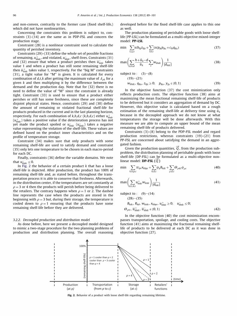
In Fig. 2 the behavior of a certain product k that has a looseshelf-life is depicted. After production, the product has 100% ofremaining shelf-life and, as stated before, throughout the trans-portation process it is able to conserve that freshness. Afterwards,in the distribution center, if the temperatures are set constantly atr¼ 3 or 4 then the products will perish before being delivered tothe retailers. The contrary happens when r¼ 1 or 2. The dashedline represents the case when the products are stored in thebeginning with r¼ 3 but, during their storage, the temperature iscooled down to r¼ 1 ensuring that the products have someremaining shelf-life before they are delivered.

3.2.2. Decoupled production and distribution model

As done before, here we present a decoupled model designedto mimic a two-stage procedure for the two planning problems ofproduction and distribution planning. The overall reasoning

Fig. 2. Behavior of a product with loose sh

developed before for the fixed shelf-life case applies to this oneas well.

The production planning of perishable goods with loose shelf-life (PP-LSL) can be formulated as a multi-objective mixed-integermodel: PP-LSL

minXl,i,j,s

scblijzlijsþXl,k,s

ðscplkplksþclkqlksÞ ð37Þ

maxXk,h,d

hþ ~uk�d~uk

Xc

wkhdc

!1

½dkdc�ð38Þ


ð19Þ2ð21Þ

wkhdc, qlks, zlijsZ0; plks, yljsAf0;1g ð39Þ

In the objective function (37) the cost minimization onlyreflects production costs. The objective function (38) aims atmaximizing the mean fractional remaining shelf-life of productsto be delivered but it considers an aggregation of demand by DC.However, this objective value is calculated based on a roughestimation of the remaining shelf-life at delivery time using ~uk

because in the decoupled approach we do not know at whattemperatures the storage will be done afterwards. With thismeasure we are able to compute an upper bound of the meanremaining shelf-life of products delivered.

Constraints (3)–(8) belong to the PDP-FSL model and regardproduction restrictions, whereas constraints (19)–(21) fromPP-FSL are concerned about satisfying the demand in an aggre-gated fashion.

Given the production quantities, Q!

, from the production sub-problem, the distribution planning of perishable goods with looseshelf-life (DP-FSL) can be formulated as a multi-objective non-linear model: DP-FSL (Q

!)

minX

k,h,p,c

tcpcxkhpcþXk,d,c

fkBkdcþXr,d,c

Yrdcfrc ð40Þ

maxX

k,t,d,c

uþktdcwktdc

!1

½dkdc�ð41Þ


ð28Þ2ð35Þ

Bkdc , Rkd, wktdc , xkhpc, uþkbdc Z0; u�kbdc r0;

Yrtc , uþkbdc , u�kbdc Af0;1g ð42Þ

In the objective function (40) the cost minimization encom-passes transportation, spoilage, and cooling costs. The objectivefunction (41) aims at maximizing the fractional remaining shelf-life of products to be delivered at each DC as it was done inobjective function (27).

elf-life regarding remaining lifetime.

Table 3Changeover times and costs data for illustrative example.

Block i Block j Line l stblij scblij

1 2 1 5 5


Constraints (9)–(14) and (28)–(35) belong to the PDP-FSL andPDP-LSL models, respectively. The first group is concerned aboutthe distribution function of perishable goods and the second oneabout the determination of the remaining shelf-life of productsdelivered.

1 4 1 10 10

1 2 2 2.5 2.5

1 3 2 5 5

1 4 2 7.5 7.5

2 1 1 10 10

2 4 1 7.5 7.5

2 1 2 7.5 7.5

2 3 2 2.5 2.5

2 4 2 5 5

3 1 2 10 10

3 2 2 7.5 7.5

3 4 2 2.5 2.5

4 1 1 15 15

4 2 1 12.5 12.5

4 1 2 12.5 12.5

4 2 2 10 10

4 3 2 7.5 7.5

Table 4Shelf-lives and decay rates for the different scenarios.

Scenario Temperatures Products

Fixed shelf-life Loose shelf-life

1 2 3 4 1 2 3 4

1 0.111 0.111 0.125 1.000

Base 2 9 9 8 1 0.100 0.100 0.111 0.500

3 0.091 0.091 0.100 0.333

1 0.500 0.333 0.500 1.000

High perish. 2 2 3 2 1 0.333 0.250 0.333 0.500

3 0.250 0.200 0.250 0.333

1 0.111 0.111 0.125 0.167

Low perish. 2 9 9 8 6 0.100 0.100 0.111 0.143

3 0.091 0.091 0.100 0.125

4. Illustrative example

To understand the trade-off present in the two models (fixedand loose shelf-life) regarding total costs and product freshness aswell as the differences between an integrated over a decoupledapproach for production and distribution planning an illustrativeexample was developed.

In this instance there are four products to be scheduled andproduced on two production lines that are located in twodifferent production plants. Each of these products belongs to adifferent block and therefore there is always sequence-dependentsetup time and cost to consider when changing from one productto another. Moreover, although the first line is able to produceevery product, the second one is not able to produce all of theproducts. The production lines are considered similar and, there-fore, variable production costs are neglected. The number ofmicro-periods per macro-period was set at the constant value offour allowing the production of all products in a macro-period.The capacity of each line is the same in all macro-periods andevery production plant (100 units). The planning horizon is 10days (macro-periods) and the shelf-life of products varies con-siderably among them, from highly perishable ones (1 day) toothers which can last throughout the entire planning horizon.Demand has to be satisfied in two different DCs and products canbe transported between any pair production plant–DC. Initial stockwas set to zero in both DCs. In case shelf-life is not fixed, there arethree different temperature levels possible to be chosen at each DCinfluencing its duration. Finally, a sensitivity analysis regardingthe perishability impact was conducted and different scenarioswhere shelf-lives and decay rates are varied were analyzed(Table 4). In Tables 1–3 the remainder data of the illustrativeexample is given.

The remainder of this section shows the results when solvingthe illustrative example for both cases: fixed and loose shelf-life.

Table 1Demand data for illustrative example.

DC Product Macro-period

1 2 3 4 5 6 7 8 9 10

1 1 0 40 0 0 0 0 0 0 48 0

2 1 0 0 40 0 0 0 0 0 0 48

1 2 30 30 0 0 0 40 48 36 36 0

2 2 40 30 30 0 0 0 0 48 36 36

1 3 10 0 10 0 0 10 12 12 0 12

2 3 10 0 10 0 0 10 12 12 0 12

1 4 10 20 30 0 0 0 0 12 24 36

2 4 0 10 20 30 36 0 12 0 0 24

Table 2Transportation and temperature related costs data for illustrative example.

DC Production plant Temperatures

1 2 1 2 3

1 0.03 0.1 2 2.5 3.25

2 0.15 0.05 1.75 2.25 3

To complement the explanations of the following sections abouthow the different problems were solved readers should refer toFig. 3.

4.1. Results case 1: fixed shelf-life

In this section results for the case where the shelf-life is fixedare presented. Since the models developed are either multi-objective mixed-integer or multi-objective linear it was possibleto obtain optimal solutions for this small instance with the help ofCPLEX. For the integrated approach, merely by aggregating bothobjectives with varying weights and solving the resulting single-objective model to optimality it was possible to determine avariety of solutions from which the Pareto-optimal front could beconstructed. On the other hand, to obtain the results for thedecoupled approach, in order to compare them with the ones ofthe integrated approach, a more complex method is needed. First,solutions on the Pareto-optimal front for the production sub-problem were determined. Afterwards, for each of the productionsolutions a new Pareto-optimal front was computed for thedistribution sub-problem. To compute the solution of the coupledproblem it is necessary to obtain the values for the two objectivesfor each pair of connected production–distribution solutions. Forthe first objective, concerning total costs, the summation of eachof the sub-problems’ first objective was considered. Then, for thesecond objective, concerning the mean remaining shelf-life of theproducts delivered, the retrieved value of the distribution sub-

Fig. 3. Matrix showing a visual representation of the solving strategies for each Case–Approach combination.

Fig. 4. Pareto-optimal fronts of the illustrative example when using an integrated

and a decoupled approach (Case 1).

Fig. 5. Relative importance regarding total cost of production and transportation

cost using an integrated approach (Case 1).


problem is the one that represents the coupled solution value. Infact, ultimately, it is the distribution planning that fixes theproduct delivery freshness. To obtain the integrated approachPareto-front we needed about 30 min CPU running time while forthe decoupled approach, since the problems are less complex, halfof the computational time was enough. The two left quadrants ofFig. 3 represent these solution procedures.

In Fig. 4 the Base scenario solutions of the Pareto-optimal frontsfor both the integrated and decoupled approach are presented.

It is rather clear from the comparison of the Pareto fronts thatthe integrated approach strongly dominates the decoupled one.Both curves have a similar behavior, which means that for thelower values of freshness just a small increase in costs fosterssignificantly the remaining shelf-life of delivered products. Never-theless, when we are approaching a strict Just-in-Time (JIT)accomplishment of the demand, touching very high freshnessstandards, the costs start to increase in a more important way.

Furthermore, it is interesting to notice that the savings in costswhen using an integrated approach over a decoupled one tend tofade when we aim at an increased freshness. This may beexplained by the fact that to achieve very high freshness stan-dards almost no inventory is allowed since we are working undera JIT policy, this will constrain so much the solution space that theintegrated and coupled solutions are rather the same.

Figs. 5 and 6 concern the relative importance of productionand transportation costs for both the integrated and thedecoupled approach in the Base scenario.

The relative importance of the costs in both approaches is ratherindependent of the freshness of the products delivered. Only whenapproaching a very high performance by delivering products with aremaining shelf-life around 100% it is possible to see that the twographs converge (with an increase of the % Production Costs). Whencomparing the two approaches, it seems that having a larger viewover the information in the supply chain (integrated approach), while


cost using a decoupled approach (Case 1).

Fig. 7. Total percentage saving when using an integrated approach over a

decoupled one for three scenarios (Case 1).

Fig. 8. Pareto-optimal fronts for the illustrative example when using an integrated

and a decoupled approach (Case 2).


taking operational decisions of production and distribution planning,leads to better overall costs by means of avoiding the greedy behaviorof locally optimizing production and then adjust distribution. Thedecoupled approach has to emphasize quite heavily the costs of thetransportation process in order to compensate the potential mistakesof the myopic production planning. The integrated approach increasesthe share of the production costs in the total costs in order to have aglobal decrease afterwards.

Finally, in Fig. 7 we perform a sensitivity analysis regarding theperishability settings. The percentage saving of using an inte-grated approach over a decoupled one is plotted for the threescenarios. In order to calculate the saving, both Pareto fronts(integrated and decouple approach) were estimated through asecond-order polynomial regression which has a good fit to theexperimental data with all R2 above 90%.

The potential savings of using an integrated approach over adecoupled one are rather considerable for the fixed-shelf-life caseand, independently of the scenario, the behavior over the remainingshelf-life is quite similar. For the scenario with highly perishableproducts the savings can ascend up to 42% when aiming at 70% ofremaining shelf-life.

When comparing the three scenarios it is observable that theadvantages of using an integrated approach are leveraged by thedegree of perishability the goods are subject to. In fact, when weare planning using a decoupled approach and the products aresubject to intense perishability, the myopic mistakes incurred inproduction planning will be hardly corrected by the distributionprocess because the buffer between those activities is reduced bythe small amount of time that goods can stay stored. Therefore,the advantages of using an integrated approach are boostedconsiderably for this scenario. On the other hand, when dealingwith products with low perishability the buffer enables thepossibility of correcting the potential production mistakes andthe integrated approach has less comparative advantage.

4.2. Results case 2: loose shelf-life

In this section we focus on the case where the shelf-life is loose.Since in this case there are models which are multi-objective mixed-integer nonlinear it was not straightforward to obtain directly anysolution with the help of exact methods as done before. Therefore, asimple hybrid genetic heuristic was developed to solve this problem.This heuristic bases itself on the fact that when fixing Yrtc the modelis no longer non-linear because the fractional remaining shelf-lifeuþktdc and also u�kbdc are then known.

Hence, a population of individuals representing the tempera-ture states, Yrtc , is randomly created ensuring feasibility. At eachgeneration these values are fed into CPLEX and optimal solutionsfor the single-objective model resulting from aggregating bothobjective functions with varying complementary random weightsare obtained. The population is then subject to simple cross-overand mutation operators. In the end all the individuals are rankedaccording to non-domination (Deb et al., 2000) and a Pareto frontis obtained. More details about this heuristic can be found inAmorim et al. (2011). The number of different combinations forYrdc is ðDC:TÞ9r9, where 9r9 stands for the cardinality of possibletemperatures. Therefore, for this small example, we would havealready 8000 possible solutions that would need to be evaluateduntil optimality could be achieved for each of the varyingweightings given to both objective functions. To obtain the resultsfor the decoupled approach this heuristic had to be inserted in thedistribution planning sub-problem in a scheme very close to theone used in the decoupled approach for fixed shelf-life (refer tothe right quadrants of Fig. 3). Before, the production planningsub-problem is solved with CPLEX since it has no nonlinearities.To unveil the near-optimal Pareto front of the integratedapproach we needed about 50 min CPU running time since thisproblem was considerably harder to solve than the one with fixedshelf-life. Once again to obtain the Pareto front for the decoupledapproach less computational effort is needed.

In Fig. 8 the results of the Pareto fronts for both the integratedand decoupled approach are presented. These solutions concernthe Base scenario.

As it happened with the results of Case 1 the Pareto frontrelated to the integrated approach strongly dominates the onecorresponding to the decoupled approach. It is interesting to notethat our simple heuristic was able to capture the non-convexitiesof both Pareto fronts. The other reasoning made before for Case 1regarding the behavior of the fronts also applies to this case.

As done before for Case 1, in Fig. 9 the results of the sensitivityanalysis to understand the effect of different perishability settingsare presented. The percentage saving of using an integratedapproach over a decoupled one is plotted for the three scenarios.


cost using a decoupled approach (Case 2).


Unlike Case 1 the savings are not as bold and the maximum savingascends to 20% for an average remaining shelf-life of about 65% in theBase scenario, which is still rather remarkable. Nevertheless, thebehavior of both saving curves (from Case 1 and Case 2) is verysimilar. The explanation for the difference in the amount of savingsbetween the fixed and loose shelf-life case may lie in the fact that forthe loose shelf-life case the distribution process has much morefreedom to influence both costs and especially product freshness.Hence, for the decoupled approach even after the production processhas fixed the production quantities, the distribution process is stillable to compensate potential mistakes through the decisions ontemperature of storage.

Looking at the differences between the three scenarios it isinteresting to notice that in this case the reasoning is not asstraightforward as in Case 1. Here, the two extreme scenarios havea similar behavior for different reasons. The scenario with productssubject to low perishability has a rather humble saving when usingan integrated approach for the same reasons as in Case 1. Hence, sincethe time buffer between production and distribution is rather largethe advantages of using an integrated approach are hindered. In thescenario having products with a high perishability the explanation forthe relative low saving is related to the possibility of correctingfreshness problems coming from a myopic production planning in thedecoupled approach through controlling the temperature of storagein the distribution planning. When products are highly perishable asmall decrease in the storage temperature will entail a strongpercentage augmentation of shelf-life. Hence, if in a product with7 days of shelf-life we are able to augment it to 8 days throughstoring it at cooler temperature, then the percentage increasing ofshelf-life is not very significant. But, if the product is highly perish-able, then an absolute increase of 1 day will reflect a strongpercentage increase. Therefore, the scenario with products subjectto intermediate perishability (Base scenario) is the one which gainsmore from an integrated approach.

5. Conclusions

In this paper, we have discussed the importance of integrating theanalysis for a production and distribution planning problem dealingwith perishable products. The logistic setting of our operationalproblem is multi-product, multi-plant, multi-DC and multi-period.We have developed models for two types of perishable products:with fixed shelf-life and with loose shelf-life, always taking intoaccount that customers attribute decreasing value to products whilethey are aging until they completely perish. The novel formulationsallow a comprehensive and realistic understanding of these inter-twined planning problems. Furthermore, the loose-shelf-life modelwas able to incorporate the possibility of dealing with the underlyinguncertainty of a random spoilage process with the help of predictivemicrobiology. To understand the impact of the integrated approach in

both the economic and the freshness perspective a multi-objectiveframework was used. Since the models for the loose shelf-life casewere not possible to solve with standard solvers, even for a smallexample, a simple heuristic was developed for these cases.

Computational results for an illustrative example show thatthe Pareto front of the integrated approach strongly dominatesthe Pareto front of the decoupled one for both classes of perish-able products. The economic savings that this coupled analysisentail is smoothed as we aim to deliver fresher products. Never-theless, in the fixed shelf-life case for a 70% mean remainingshelf-life of delivered products we may reach savings around 42%.The explanation regarding the fact that the gap between theintegrated and the decoupled approach tends to smooth for veryhigh freshness standards may be due to the reason that in thelatter case no inventory is allowed since we are working com-pletely under a JIT policy, turning the problem at hand soconstrained that the integrated and coupled solutions are ratherthe same. The multi-objective framework proved to be essentialto draw these multi-perspective conclusions.

This work should be perceived as an exploratory research inthis challenging field. Future work should focus on understandingthe impact of the integrated approach at the tactical planninglevel and how these potential benefits and awareness of the cost-freshness relationship can be applied in industrial environments.More in detail, it is important to go deeper into the freshnessobjective function and evaluate what other indicators besides themean value of the fractional remaining shelf-life can be modeledand what are the differences in the plans that they yield.

Acknowledgment

The first author appreciate the support of the FCT ProjectPTDC/EGE-GES/ 104443/2008 and the FCT Grant SFRH/BD/68808/2010.

References

Ahumada, O., Villalobos, J., 2009. Application of planning models in the agri-foodsupply chain: a review. European Journal of Operational Research 196, 1–20.

Akkerman, R., Farahani, P., Grunow, M., 2010. Quality, safety and sustainability infood distribution: a review of quantitative operations managementapproaches and challenges. OR Spectrum 32, 863–904.

Amorim, P., Antunes, C.H., Almada-Lobo, B., 2011. Multi-objective lot-sizing andscheduling dealing with perishability issues. Industrial & Engineering Chem-istry Research 50, 3371–3381.

Arbib, C., Pacciarelli, D., Smriglio, S., 1999. A three-dimensional matching modelfor perishable production scheduling. Discrete Applied Mathematics 92, 1–15.

Bilgen, B., Gunther, H.O., 2010. Integrated production and distribution planning inthe fast moving consumer goods industry: a block planning application. ORSpectrum 32, 927–955.

Broekmeulen, R., 2001. Modelling the Management of Distribution Centres.Lecture Notes in Business Information Processing. Woodhead Publishing Ltd.

Cai, X., Chen, J., Xiao, Y., Xu, X., 2008. Product selection, machine time allocation,and scheduling decisions for manufacturing perishable products subject to adeadline. Computers & Operations Research 35, 1671–1683.

Chen, H.K., Hsueh, C.F., Chang, M.S., 2009. Production scheduling and vehiclerouting with time windows for perishable food products. Computers &Operations Research 36, 2311–2319.

Deb, K., Agrawal, S., Pratap, A., Meyarivan, T., 2000. A Fast Elitist Non-dominated SortingGenetic Algorithm for Multi-objective Optimisation: NSGA-II. Springer-Verlag,London, UK.

Eksioglu, S.D., Mingzhou, J., 2006. Computational Science and Its Applications—ICCSA2006. Lecture Notes in Computer Science, vol. 3982. Springer, Berlin, Heidelberg.

Fu, B., Labuza, T., 1993. Shelf-life prediction: theory and application. Food Control4, 125–133.

Gunther, H.O., Grunow, M., Neuhaus, U., 2006. Realizing block planning conceptsin make-and-pack production using MILP modelling and SAP APO. Interna-tional Journal of Production Research 44, 3711–3726.

Gunther, H.O., Seiler, T., 2009. Operative transportation planning in consumergoods supply chains. Flexible Services and Manufacturing 21, 51–74.

Hsu, C.I., Hung, S., Li, H.C., 2007. Vehicle routing problem with time-windows forperishable food delivery. Journal of Food Engineering 80, 465–475.


Karaesmen, I.Z., Scheller-Wolf, A., Deniz, B., 2011. Managing perishable and aginginventories: review and future research directions. In: Kempf, K.G., Keskino-cak, P., Uzsoy, R., Hillier, F.S. (Eds.), Planning Production and Inventories in theExtended Enterprise, International Series in Operations Research & Manage-ment Science, vol. 151. Springer, US, pp. 393–436.

Lutke Entrup, M., 2005. Advanced planning in fresh food industries. Physica,Heidelberg.

Lutke Entrup, M., Gunther, H.O., Van Beek, P., Grunow, M., Seiler, T., 2005. Mixed-integer linear programming approaches to shelf-life-integrated planning andscheduling in yoghurt production. International Journal of ProductionResearch 43, 5071–5100.

Marinelli, F., Nenni, M.E., Sforza, A., 2007. Capacitated lot sizing and schedulingwith parallel machines and shared buffers: a case study in a packagingcompany. Annals of Operations Research 150, 177–192.

Martin, C., Dent, D., Eckhart, J., 1993. Integrated production, distribution, andinventory planning at Libbey–Owens–Ford. Interfaces 23, 68–78.

Nahmias, S., 1982. Perishable inventory theory: a review. Operational Research 30,680–708.

Neumann, K., Schwindt, C., Trautmann, N., 2002. Advanced production schedulingfor batch plants in process industries. OR Spectrum 24, 251–279.

Osvald, A., Stirn, L., 2008. A vehicle routing algorithm for the distribution of freshvegetables and similar perishable food. Journal of Food Engineering 85, 285–295.

Pahl, J., Voß, S., 2010. Advanced Manufacturing and Sustainable Logistics.Lecture Notes in Business Information Processing, vol. 46. Springer, Berlin,Heidelberg.

Rong, A., Akkerman, R., Grunow, M., 2011. An optimization approach for managingfresh food quality throughout the supply chain. International Journal ofProduction Economics 131, 421–429.

Thomas, D., Griffin, P., 1996. Coordinated supply chain management. EuropeanJournal of Operational Research 94, 1–15.

Tsiros, M., Heilman, C., 2005. The effect of expiration dates and perceived risk onpurchasing behavior in grocery store perishable categories. Journal of Marketing69, 114–129.

Yan, C., Banerjee, A., Yang, L., 2011. An integrated production–distribution modelfor a deteriorating inventory item. International Journal of Production Eco-nomics 133, 228–232.

Multi-objective integrated production and distribution planning of perishable products

Documents

Transcript of Multi-objective integrated production and distribution planning of perishable products