Retrieval of Spatial Join Pattern Instances from Sensor Networks∗†

Man Lung Yiu

Department of Computer Science

Aalborg University

DK-9220 Aalborg, Denmark

mly@cs.aau.dk

Nikos Mamoulis

Department of Computer Science

University of Hong Kong

Pokfulam Road, Hong Kong

nikos@cs.hku.hk

Spiridon Bakiras

Dept. of Math. and Comp. Science

John Jay College

City University of New York

sbakiras@jjay.cuny.edu

Abstract

We study the continuous evaluation of spatial join queries and extensions thereof, defined by

interesting combinations of sensor readings (events) that co-occur in a spatial neighborhood.

An example of such a pattern is “a high temperature reading in the vicinity of at least four high-

pressure readings”. We devise protocols for ‘in-network’ evaluation of this class of queries,

aiming at the minimization of power consumption. In addition, we develop cost models that

suggest the appropriateness of each protocol, based on various factors, including selectivity of

query elements, energy requirements for sensing, and network topology. Finally, we experi-

mentally compare the effectiveness of the proposed solutions on an experimental platform that

emulates real sensor networks.∗Work supported by grant HKU 7155/06E from Hong Kong RGC.†A preliminary version of this work appeared in [25], available athttp://www.cs.aau.dk/∼mly/ssdbm07senpat.pdf

1

1 Introduction

Advances in computer hardware have brought to availability small and relatively cheap devices

forming a powerful network that interacts and collects information from the environment, where it

is deployed [27]. Sensor networks have several applications, including environmental monitoring

[15, 13], control/maintenance of industrial infrastructure [1], military applications [20], structural

monitoring [17], etc. Recently, the problem of evaluating queries over a sensor network has at-

tracted significant research interest from the database community, leading to the development of

two research DBMS prototypes [24, 14]. These systems provide to the user an interface, via which

queries are expressed in adeclarativeway; the user needs not deal withhowqueries are evaluated.

Suitable extensions of SQL were proposed with clauses that consider the special features of sen-

sor networks. These features include the transient, on-demand nature of sampled data, extended

lifetime of continuous (non-transient) queries, sampling rate or compression of sensor readings,

event-triggered queries, etc.

The main focus of existing work on sensor networks has been the minimization of power consump-

tion at sensor nodes, during query evaluation. Sensors are usually battery-operated and they are

often deployed in hostile environments or rough terrains, where the network runs unsupervised for

long time intervals. Thus, power is of utmost importance, since it is directly related to the longevity

of the network. Previously studied topics include the energy-efficient retrieval of aggregations or

data summaries [13, 5, 3, 7, 6, 19], the derivation and maintenance of data models that describe

the data distribution [8, 4], and the optimal in-network placement of operators or filter predicates

on the sensed values [14, 2, 1, 22]. To our knowledge, there is no prior work for in-network evalu-

ation of queries thatspatially correlatemeasurements fromdifferentsensors. An example of such

a query (taken from [3]) is “generate a notification whenever two sensors within 5 yards from each

other simultaneously measure an abnormal temperature”. Aspatial pattern queryretrieves sets

of sensors (pairs in this example), whose readings qualify some selection predicates (e.g., abnor-

mal temperatures) and their locations qualify some pairwise distance predicates (e.g., within five

yards). Data analysts may be interested in the on-line identification of pattern instances that occur

2

rarely in the environments where sensors are deployed and may indicate exceptional events. For

instance, an unusually high temperature detected in the vicinity of multiple low-humidity readings

may indicate high chance of a fire break in the local area, where the pattern is detected. An-

other application of spatial pattern queries is the prediction of weather phenomena based on spatial

combinations of sensor readings.

A straightforward way to evaluate spatial pattern queries is to program the sensors to transmit

their readings together with their locations to a central basestation (via a routing tree [10, 14]),

where their spatial associations are validated. Although this approach is easy to implement, it may

waste more energy than necessary, as sensor readings that are not part of query results may be

sent all the way up to the root. Motivated by the lack of effective evaluation protocols for spatial

pattern queries, in this paper, we study this problem in depth, focusing on (i) filtering techniques

for readings that do not participate in the result, (ii) in-network computation of query results. We

propose optimized evaluation protocols for binary spatial joins and more complex query patterns

and compare them for different problem parameters. Our solutions are orthogonal to snapshot-

based schemes (e.g., [11]), which apply query evaluation only to a small (self-maintained) sample

of the network and to techniques that summarize sensor readings over long time intervals before

applying query evaluation on them (e.g., [6]). The contributions of this paper can be summarized

as follows:

• We identify the interesting class ofspatial pattern queries. We formally define them and

discuss how they can be expressed using the language extensions of [14].

• We propose energy-efficient protocols for in-network evaluation of spatial pattern queries.

In addition, we provide cost models which can be used by a query optimizer to determine a

suitable evaluation method based on query parameters and data statistics.

• We experimentally evaluate the effectiveness of the proposed techniques by tuning various

parameters, including query selectivity, network size, topology and density, sampling cost,

etc.

3

The remainder of the paper is organized as follows. Section 2 reviews related work. Section 3

formally defines spatial pattern queries. In Section 4, we describe in detail the proposed solutions,

and analyze their costs in Section 5. Section 6 discusses the evaluation of variants and extensions

of pattern queries, as well as advanced issues, like multiple query evaluation. Section 7 experimen-

tally demonstrates the applicability and efficiency of our techniques. Finally, Section 8 concludes

the paper.

2 Background and Related Work

The special characteristics of a sensor network compared to a generic wireless network are (i)

the limited resources of nodes (energy, communication range, network bandwidth and capacity),

(ii) unreliable communication with high packet loss rates and frequent node failures, and (iii)

unsupervised nature with nodes placed at hostile environments (e.g., remote areas, war fields, etc.).

Thus, query evaluation techniques for sensor networks aim at minimizing the energy cost, subject

to the constraints of the network (e.g., communication range, maximum data volume that can be

sent by a node at a cycle, etc.). Besides, sensor networks are inherently redundant (i.e., dense),

in order to keep the network connected after node failures and increase the reliability of sensed

information.

Query evaluation in sensor networks is performed in two steps [10, 24, 14]. Suppose that the query

should collect the readings from all sensors. The query is registered at a basestation, which is

connected to aroot noder. In the first step, the query is disseminated to the sensors, and a spanning

tree of the network, rooted atr is dynamically constructed. If a node receives the query for the

first time, it selects one of the senders as its parent in the tree and broadcasts the query. Otherwise,

the message is ignored. The resultingcommunication(or routing) tree is used to acquire sensor

readings related to the query, up to the basestation. Delivery of sensor readings (or query results) to

the root is performed in multiple phases. During a specific phase, a level of the treesendsand the

level above listens andreceivesinformation addressed for it. Finally, the root collects all readings

and sends them to the basestation.

4

Queries over sensor networks are usuallycontinuous, i.e., they remain active for a lengthy time

interval (e.g., minutes, hours). Otherwise, the cost for disseminating the query may not be com-

pensated. Frequent instantaneous queries are best processed if the network operates in a push-based

manner; sensors periodically and unconditionally collect measurements and route them to a bases-

tation, where queries are registered and evaluated as queries over streaming data. For example,

in the work of [9], efficient algorithms are developed for processing continuous constraint queries

at a centralized basestation, without considering communication cost in the underlying infrastruc-

ture (e.g., sensor network). In this paper, we exploit in-network evaluation techniques in order to

minimize power consumption of the sensor network for processing continuous queries. Next, we

review work on (continuous) query evaluation on sensor networks.

2.1 Aggregation and summarization

Madden et al. [13] proposed a simple, but powerful protocol for computing common aggregate

functions (e.g., count, sum, max, min). Each sensor combines the information received by its

children with its own measurement to derive and send data of constant size, capturing a partial

computation of the aggregate function. In [5], a multi-path algorithm for computing aggregates is

presented to reduce communication errors as multiple parents may hear and aggregate the infor-

mation broadcast by a single child. [16] proposes a hybrid method that combines the tree topology

of [13] with the ring network topology of [5]. Besides, [7] describes a method for pushing error

tolerance in network nodes, in order to avoid sending information if the aggregate is within some

error bound. The problem of redistributing the error tolerance among nodes in order to minimize

the overall error at dynamic environments is also studied. A similar approach was independently

proposed in [19]. To minimize network communication, [6] presents a methodology for in-network

compression of multiple (time-series) signals generated by sensors (e.g., one for temperature, one

for humidity, etc.). The rationale is that measurements observed at the same node are likely to

follow similar trends. Soheili et al. [21] focused on the processing of spatial aggregation query,

which derives the aggregate (e.g., average) of sensor values (e.g., temperatures) in a user-defined

spatial windowW . They developed a distributed and hierarchical structure on the sensor network

5

such that each node maintains the enclosing rectangle of its descendants in the routing tree. Energy

consumption reduction is achieved by keeping irrelevant nodes (for query processing ofW ) asleep.

2.2 Data models, snapshots, and filters

An alternative to continuously collecting and processing sensor data (which drains the network

energy resources), is to define and maintain simple data models (e.g., mixtures of Gaussians) for

the data distribution [8, 4]. These models, potentially combined with exact readings, provide

query answers with some approximation confidence. Besides, [11] describes a framework for

dynamically selecting and maintaining representatives in a redundant sensor network. The set of

representatives (snapshot) plays the role of a dynamic sample that can answer queries cheaply and

approximately.

Another class of problems is the distribution of filters or database operators in the routing tree of a

sensor network. [22] studies the optimal placement of query operators (e.g., selection predicates),

in order to minimize (i) the communication cost for information that does not end up in the query

result and (ii) the computational burden at lower tree levels (assuming that lower-level nodes have

reduced computational capabilities). [2] focuses on the assignment of operators that correlate mea-

surements from two (apriori defined) spatial regions. [26] examines a similar problem and applies

synopses of sensor values to eliminate unqualified readings that cannot lead to results. Assum-

ing that tuples originated from sensors in two different spatial regions, [18] develops solutions for

routing and joining those tuples in the sensor network. On the other hand, our problem searches

for rare spatial associations of (instantaneous) events, anywhere in the network map.

In another direction, [1] studies continuous joining a table of predicates (e.g., ‘humidity>50oC’)

with the sensed values. If the table is small enough to be stored at each node, it acts a filter that

prevents non-qualifying readings to be sent to the basestation. If the table cannot fit in a node’s

local memory, it is placed at neighboring nodes and the predicates are evaluated in a distributed

fashion. Yang et al. [23] examine continuous self-join processing on the tuples generated from the

sensor network; two tuples are joined together if they satisfy the join predicate and stay in the same

6

time window. In contrast to [1, 23], the queries we study do not simply consider sensor values;

they also have to satisfy a spatial pattern, which will be defined formally in the next section.

The closest work to ours is [12], which reports pairs of sensor events located within a given distance

range, and reduces communication cost by a distributed routing index. The sensors record past

events in their neighborhood which help to predict future occurrences of them at other locations of

the map. Messages are then routed based on these predictions. As the author suggests, the index is

appropriate for applications where events correspond to moving objects with well-estimated future

locations. Our focus, on the other hand is on arbitrary, instantaneous, ad-hoc events. In addition,

the methodology of [12] relies heavily on the regular grid networks and may not be applicable to

arbitrary network topologies.

3 Problem Formulation

Let SN be a network ofN sensors. Each sensors ∈ SN is associated with a spatiallocation1

s.loc, and can produce a sets.m of measurements (e.g., temperature, humidity, etc.) for the spatial

region around it (different sensors might produce different sets of readings, in general).

We adopt the framework described in Section 2, where users register continuous queries at a bases-

tation and a routing tree is created to acquire results (or readings that are processed at the base).

Each registered query is associated with: (i) alifetime(e.g., 2 hours), during which it is active and

continuously produces results from the sampled measurements, and (ii) anepoch duration(e.g.,

10 seconds), every which the network samples measurements. In other words, queries apply to

instances of the network at different timestamps (for every epoch).

A binary spatial patternquery identifies pairs of sensors, for which (i) the readings qualify some

particular selection predicates and (ii) the locations are no further than a particular distance from

each other. An example of such a query is “find pairs of sensors〈s1, s2〉, such thats1.temperature>50oC,

s2.humidity<40%, anddistance(s1, s2)<10m”. A generalized spatial pattern query (formally de-

1We assume that the locations of sensors are known to them. They could be constant and apriori defined (forstationary, manually placed sensors), or detected by GPS devices placed on the sensors.

7

.humidity<40%

v1.temperature>50

v3.humidity<40%v2

v5.humidity<40%v4.humidity<40%

dist(v1.loc,v2.loc<10) dist(v1.loc,v3.loc<10)

dist(v1.loc,v5.loc<10)dist(v1.loc,v4.loc<10)

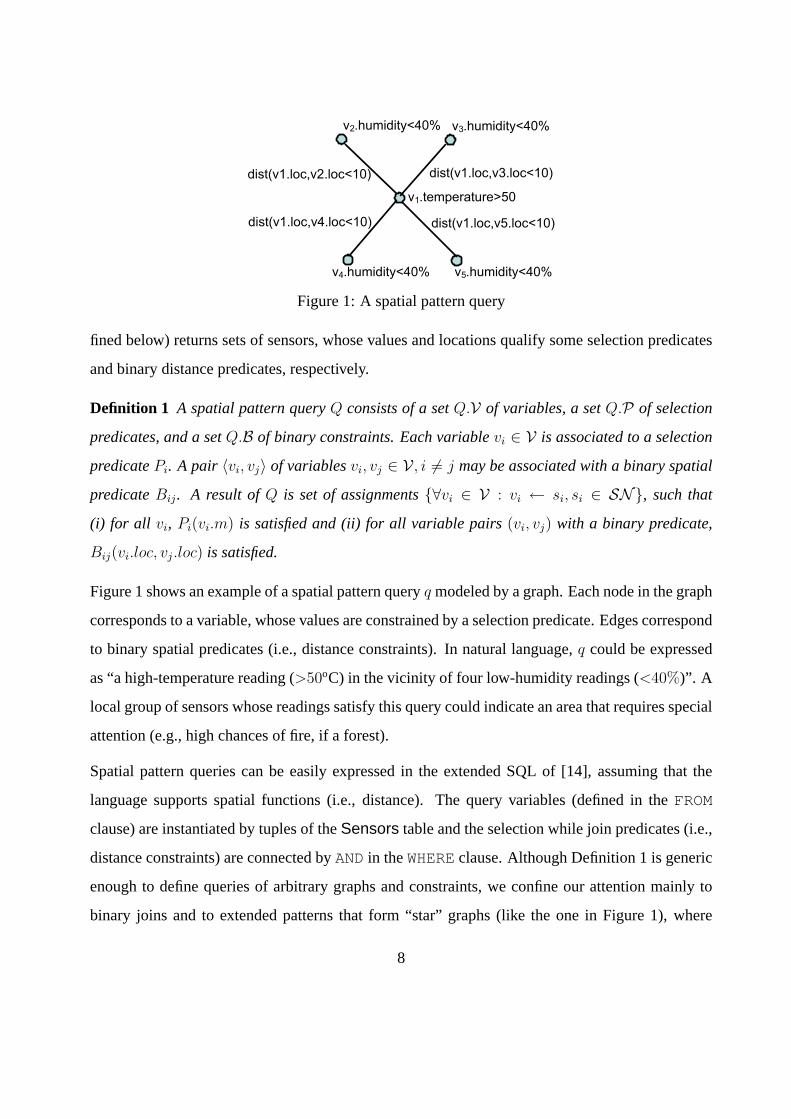
Figure 1: A spatial pattern query

fined below) returns sets of sensors, whose values and locations qualify some selection predicates

and binary distance predicates, respectively.

Definition 1 A spatial pattern queryQ consists of a setQ.V of variables, a setQ.P of selection

predicates, and a setQ.B of binary constraints. Each variablevi ∈ V is associated to a selection

predicatePi. A pair 〈vi, vj〉 of variablesvi, vj ∈ V , i 6= j may be associated with a binary spatial

predicateBij. A result ofQ is set of assignments{∀vi ∈ V : vi ← si, si ∈ SN}, such that

(i) for all vi, Pi(vi.m) is satisfied and (ii) for all variable pairs(vi, vj) with a binary predicate,

Bij(vi.loc, vj.loc) is satisfied.

Figure 1 shows an example of a spatial pattern queryq modeled by a graph. Each node in the graph

corresponds to a variable, whose values are constrained by a selection predicate. Edges correspond

to binary spatial predicates (i.e., distance constraints). In natural language,q could be expressed

as “a high-temperature reading (>50oC) in the vicinity of four low-humidity readings (<40%)”. A

local group of sensors whose readings satisfy this query could indicate an area that requires special

attention (e.g., high chances of fire, if a forest).

Spatial pattern queries can be easily expressed in the extended SQL of [14], assuming that the

language supports spatial functions (i.e., distance). The query variables (defined in theFROM

clause) are instantiated by tuples of theSensors table and the selection while join predicates (i.e.,

distance constraints) are connected byANDin theWHEREclause. Although Definition 1 is generic

enough to define queries of arbitrary graphs and constraints, we confine our attention mainly to

binary joins and to extended patterns that form “star” graphs (like the one in Figure 1), where

8

a centric feature (e.g., high temperature) is correlated to a number of other features (e.g., low

humidity) in its surrounding environment. Such patterns were shown important in spatial analysis

applications and are more intuitive than queries that combine variables in an arbitrary graph. The

centric feature models a point of interest (e.g., high fire risk area, expensive equipment) which

should trigger an alert whenever its local measurements and the conditions in the region around it

form an abnormal combination.

4 Proposed Methods

In this section, we explore the applicability of several methods for computing spatial pattern queries

in a sensor network. We divide the evaluating protocols in two classes. The class ofacquisitional

protocols collect sensor measurements via the communication tree and apply query evaluation at

the basestation. Filters are placed at nodes that generate or relay data to minimize the transferred

volume. The second class ofdistributedprotocols apply in-network query evaluation and send the

results to the basestation (again using the tree). We start by discussing the simple case of a binary

spatial join with distance constraint smaller than the communication range of the nodes. Then, we

extend the suggested protocols for more complex queries and multi-hop distance constraints.

4.1 Single-hop binary joins

We first focus on binary join patterns that are sensor pairs〈si, sj〉, such thatP1(si.m), P2(sj.m)

are satisfied, anddistance(si.loc, sj.loc) ≤ c, wherec is smaller than the radio communication

range2 between two nodes. For the ease of exposition, we denote a binary join query in our context

by the triplet〈P1, P2, c〉.

4.1.1 Brute-force acquisitional protocol

The straightforward way to evaluate the query is to program all sensors to sense the measurements

relative to selection predicatesP1 andP2, at every epoch, and send this information to the bases-

2Without loss of generality, we assume that all sensors have the same communication range. Our protocols andfiltering techniques can be easily adjusted for the generic case.

9

tation, which evaluates the spatial join locally. A simple optimization that reduces the number of

unnecessary values transmitted to the base is to “push-down” the selection predicates at the nodes

(as suggested in [14, 1]). In our example, temperature and humidity are sensed by all sensors but

only high temperature and low humidity values (i.e., those that qualify the selection predicates)

are sent to the base. In order to minimize the transferred data, we only transmit the location of

a qualifying node (or its identifier, if nodes have fixed locations) and two bits that indicate which

predicate(s) the node qualifies (e.g.,10 implies thatP1 is qualified, butP2 is not). Sensors are

synchronized such that only two consecutive levels of the tree are active at the same phase (while

the remaining nodes are sleeping), as discussed in Section 2. When a lower-level node senses and

transmits data (if not filtered byP1 or P2) to its parent, its parent listens, reads and combines its

readings with those of its children; the combined readings are then sent to the upper level during

the next phase. We denote this simple, but generic protocol by AQB (i.e., the first ‘acquisitional’

protocol).

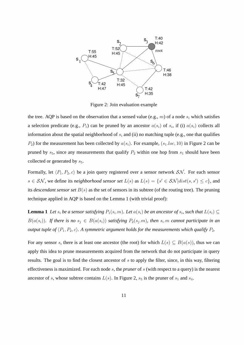
As an example, consider the sensor network depicted in Figure 2. Nodes within communication

range from each other are connected by edges. Solid edges denote the structure of the commu-

nication tree (rooted at nodes3). The values next to the nodes denote the (current) local tem-

perature (T) and humidity (H) conditions. LetP1=‘T>50’, P2=‘H<40’, and c equals the sensor

communication range (one hop). Nodess1 ands2 qualify P1, whereass6 ands7 qualify P2. The

only join result is〈s2, s6〉. In the first phase of the cycle,s1, s4, ands7 (level-3 nodes) sense

their values, apply the predicates ands1 sends(s1.loc, 10) (i.e., onlyP1 is satisfied) to its parent

(i.e., s5). Similarly, (s7.loc, 01) is sent tos6. In the second phase,(s2.loc, 10), (s1.loc, 10), and

{(s7.loc, 01), (s6.loc, 01)} are sent to the root, bys2, s5, ands6, respectively. Finally,s3 forwards

all these tuples to the base, where the join result is computed.

4.1.2 Pruner-based acquisitional protocol

Protocol AQB may send more information than necessary to the base, as many tuples (e.g.,(s1.loc, 10)

in Figure 2) are likely not to participate in the spatial join. In this section, we propose AQP, a pro-

tocol that improves upon AQB, by adding more sophisticated filters in the intermediate nodes of

10

1

23

4

5

6

7

rootT:55

H:45

T:42

H:47

T:32

H:45

T:42

H:35

T:46

H:38

T:52

H:45

T:40

H:42

s

s

s

s

s

s

s

Figure 2: Join evaluation example

the tree. AQP is based on the observation that a sensed value (e.g.,m) of a nodesi which satisfies

a selection predicate (e.g.,P1) can be pruned by an ancestora(si) of si, if (i) a(si) collects all

information about the spatial neighborhood ofsi and (ii) no matching tuple (e.g., one that qualifies

P2) for the measurement has been collected bya(si). For example,(s1.loc, 10) in Figure 2 can be

pruned bys5, since any measurements that qualifyP2 within one hop froms1 should have been

collected or generated bys5.

Formally, let〈P1, P2, c〉 be a join query registered over a sensor networkSN . For each sensor

s ∈ SN , we define itsneighborhood sensor setL(s) asL(s) = {s′ ∈ SN|dist(s, s′) ≤ c}, and

its descendant sensor setB(s) as the set of sensors in its subtree (of the routing tree). The pruning

technique applied in AQP is based on the Lemma 1 (with trivial proof):

Lemma 1 Letsi be a sensor satisfyingP1(si.m). Leta(si) be an ancestor ofsi, such thatL(si) ⊆B(a(si)). If there is nosj ∈ B(a(si)) satisfyingP2(sj.m), thensi.m cannot participate in an

output tuple of〈P1, P2, c〉. A symmetric argument holds for the measurements which qualifyP2.

For any sensors, there is at least one ancestor (the root) for whichL(s) ⊆ B(a(s)), thus we can

apply this idea to prune measurements acquired from the network that do not participate in query

results. The goal is to find the closest ancestor ofs to apply the filter, since, in this way, filtering

effectiveness is maximized. For each nodes, theprunerof s (with respect to a query) is the nearest

ancestor ofs, whose subtree containsL(s). In Figure 2,s5 is the pruner ofs1 ands4.

11

We design the following technique for determining pruners efficiently. It is applied only once while

the query is disseminated and the routing tree is constructed. When a sensor nodes broadcasts

the query, at the same time it collects ids/locations of its neighbors and determines|L(s)| (the

cardinality ofL(s)), which is then broadcasted to all nodes inL(s). Starting from the leaf nodes,

each sensors sends up the communication tree a table consisting of〈si, |L(si)|, 1〉 tuples for all

si ∈ L(s) plus a〈s, |L(s)|, 1〉 tuple for itself. Intermediate tree nodes merge the tables they receive

from their children by summing their counters (the last field of the tuples). The first node which,

after the aggregation, has a〈s, |L(s)|, |L(s)|〉 tuple becomes the pruner fors and does not forward

the tuple to its parent node.

After this process, each nodes keeps a list of itsprunees(i.e., nodes for whichs is the pruner).

The difference between our improved acquisitional protocol AQP and the baseline AQB is that, in

AQP, whenevers retrieves information from its subtree regarding the join query, for each prunee

that transmits a tupleτ qualifyingP1 (P2), s checks whether there is a matching tuple forP2 (P1)

in its acquired table, which also qualifies the distance predicate withτ . If there is no such tuple,

thenτ is pruned from the data sent to the parent ofs. AQP manages to filter early some node

readings (e.g.,(s1.loc, 10)) that do not qualify the join predicate.

4.1.3 Distributed evaluation

The class ofdistributedprotocols aim at computing query results locally around network nodes

and sending them to the basestation. Such a technique is expected to pay-off for low-selectivity3

joins, where many measurements that satisfy predicatesP1 or P2 do not qualify the join condition.

During the first stage of distributed evaluation, nodes that qualifyP1 andP2 communicate and

determine the join results. During the second stage, the routing tree is used to send the join results

to the base.

Initially, all nodes sense the measurements related toP1 andP2. If a nodesi qualifiesP1, it broad-

casts its location to its neighborhood. If a nodesj qualifiesP2, it listens for potential messages

3Low-selectivity joins output few results while high-selectivity joins produce many results.

12

from nodes that qualifyP1. For each received message,sj produces a join result. Nodes that

qualify neitherP1 norP2 remain asleep until the first stage terminates (they may have to wake and

forward join results, during the second stage). Note that the roles ofP1 andP2 could be inter-

changed; we denote by DS1 (DS2) the distributed protocol, where nodes qualifyingP1 (P2) send

messages and those qualifyingP2 (P1) receive them and compute join results. Intuitively, DS1

should be preferred to DS2 when nodes that qualifyP1 are fewer than those qualifyingP2, since

transmission is more expensive than listening and receiving [15].

As an example, consider again the network of Figure 2. In the first stage of the distributed protocol,

measurements are collected, and (i) nodess1 ands2 (qualifying P1) broadcast their locations, (ii)

nodess6 ands7 (qualifyingP2) listen for potential messages, (iii) nodess3, s4, ands5 stay asleep.

After nodes6 reads the transmission ofs2, the join result〈s2, s6〉 is formulated. This is the only

tuple that will be forwarded to the root at the second stage (result acquisition).

So far we have ignored the cost for sensing measurements at nodes, which is usually small com-

pared to communication costs. For some measurements, however, this cost may be significant [14].

For cases where sensing forP2 is significantly expensive, it might be beneficial to defer sensing

and instruct all nodes to listen forP1 messages. Only if a listener receives a message from aP1

node, it performs expensive sensing forP2 measurements. We denote this protocol by DS1′.

4.2 Complex join queries

We now consider more complex pattern queries, as described in Section 3. Queries correspond

to star graphs, where the center sensor node should satisfy selection predicatePC and there are

k border nodes that should qualifyPB within distancec from the center. A star pattern query is

simply denoted by a quadruple〈PC , PB, c, k〉. As in Section 4.1, we assume thatc is at most equal

to the radio range of the sensors.

Acquisitional protocols We can directly apply the brute-force acquisitional protocol AQB. Sen-

sor readings that qualifyPC or PB are unconditionally sent to the basestation, where the pattern is

evaluated. In addition, we can adapt protocol AQP as follows. A tuple qualifyingPC which has

13

been generated by a nodesi is filtered at nodepr(si) (pruner ofsi) if there are less thank tuples

that qualifyPB and reachpr(si) (otherwise, we know that there may be a query result that contains

the tuple). A tuple qualifyingPB, which has been generated by a nodesi is filtered atpr(si) if

there is no tuple satisfyingPC that reachespr(si) (i.e., similar to binary join queries).

Distributed protocols A simple way to extend the distributed protocols for complex queries is

to ask ‘border’ nodes (those qualifyingPB) broadcast their locations. At the same time ‘centric’

nodes (those qualifyingPC) listen for potential messages. If a centric nodesi, receives at least

k messages, we know that there is a query result centered atsi.4 The query result is sent to the

base station through the routing tree, at the second stage of the protocol. We denote this protocol

by DSB. An alternative protocol aims at minimizing the messages broadcast from border nodes;

presumably more sensors qualifyPB thanPC for the pattern query to have small selectivity and

correspond to an interesting, exceptional event. Protocol DSC asks nodes that qualifyPC (center

nodes) to send a message and nodes that qualifyPB (border nodes) to listen. If a border node

receives a message it sends a response with its location to its neighbors. Finally, center nodes

listen for messages and those that hear from at leastk nodes send the query result to the base.

4.3 Multi-hop queries

Distance constraints longer than the radio rangeh impose difficulties for distributed evaluation

protocols. Given a nodes, there is no bound for the number of hops required to find the nodes

within distancec (>h) from s. Nonetheless, for a relatively dense and uniform network, we could

set an approximate upper boundλ for this number. Letcoverage(c,λ) be the probability that two

sensor nodes within distancec are reachable withinλ hops. Figure 3 plots the coverage as a

function ofλ on a typical random network (with the default parameter values discussed in Section

7). For instance, for the curve of “c = 3h”, c is set to 3 times of the radio rangeh. Observe

that the coverage increases rapidly whenλ increases. In order to balance the coverage and energy

consumption, we suggest to setλ =⌈

c√

2h

⌉for multi-hop communication. We now discuss in more

4In fact, if si receivesm > k messages, we have multiple query results, one for each(mk

)combination of border

nodes. Nonetheless all these results can be compressed to a single tuple containingsi and all qualifying border nodes.

14

detail the protocols that can be applied for queries that involve multi-hop distances.

0

20

40

60

80

100

1 2 3 4 5 6 7 8

Accu

mu

lative

pe

rce

ntile

(%

)

Hops

c=2hc=3hc=4h

Figure 3: Coverage in multi-hop communication

Acquisitional protocols Since AQB does not apply any filtering or in-network evaluation, there

is no difference than the method described in Section 4.1 for multi-hop queries. For AQP, the only

difference is in the initialization of the query, at the stage when pruners are defined. Each node

needs to determine the number of itsλ-hop neighbors before sending it up the communication tree.

This process requires flooding a large number of messages and it is more expensive than the simple

1-hop communication. However, it is performed only once, during the initialization of the routing

tree and it is expected to pay off if the query has long lifetime.

Distributed protocols The distributed protocols described so far can be easily adapted for multi-

hop queries, at the expense of higher communication cost, since the whole network may need to

stay up in order to listen and relay potential messages, during the first stage (computation of query

results). Ifλ is large, the cost of flooding may be too high for distributed evaluation to pay-off. In

such cases, the acquisitional protocols are expected to dominate.

A bi-directional distributed protocol For queries that are simple binary joins, we can apply

a bi-directional distributed protocol (BD) in order to reduce message flooding during the first

(computation) stage. Instead of asking nodes that qualifyP1 to flood their locations up toλ hops

(which are then received by listeners that qualifyP2 and converted to query results), we ask all

15

nodes that qualify eitherP1 or P2 to send their locations and a pair of bits indicating the qualified

predicates (i.e., the information sent by nodes to the base according to AQB/AQP). However, the

flooding range is now reduced. Nodes that qualifyP1 send their messages up tox hops (x < λ)

and nodes that qualifyP2 up toλ − x hops.5 During this process all nodes of the network are up

in order to listen and relay messages. If a node receives a message from both aP1 node and aP2

node, it formulates and caches the join result. In the second stage of the algorithm, nodes send

the computed results up the tree to the basestation. Note that duplicate results could be computed,

since the same pair of messages may be received by the same node. For instance, consider a

query that seeks for high-temperature/low-humidity readings withinλ = 2 hops in the network of

Figure 2. When BD is applied, all nodes that sense either high temperature (>50) or low humidity

(<40) transmit their readings up to 1 hop (i.e.,x = 1, λ − x = 1). Both s5 ands6 then identify

〈s2, s7〉) as a result. Duplicate results are eliminated by merging operations at the second stage of

the protocol, when all results are sent up the communication tree.

An interesting problem is to pick a value ofx such that the communication cost is minimized. In

general,x can takeλ + 1 values (the extreme casesx = 0, x = λ correspond to the uni-directional

distributed protocols DS1 and DS2). Intuitively,x should be chosen to minimize the expected

expansion areaπ(Sel(P1) · x2 + Sel(P2) · (λ− x)2), whereSel(Pi) corresponds to the probability

that a node qualifiesPi (for i = {1, 2}). In other words, ifP1 has low selectivity (few nodes

qualify it) compared toP2, nodes that qualify it should transmit far and nodes that qualifyP2

should transmit close in order to minimize network traffic.

5 Cost Analysis

In this section, we analyze the costs of the proposed protocols. We assume that the basestation

maintains statistics about the sensed measurements. These statistics can be used to estimate the

selectivity of selection and/or join predicates. They could either be collected by sampling readings

from the whole network regularly, or by asking the sensors to compute and maintain local sum-

5A node that qualifies both predicates sends its message up tomax{x, λ− x} hops.

16

random grid ladder

Figure 4: Three network topologies

maries, which are consolidated and sent to the base periodically (as in [6]). To provide examples

throughout the analysis, we consider three network topologies, which simulate cases of randomly

or manually placed sensors.

Figure 4 shows graphically the RANDOM, GRID, and LADDER networks. RANDOM represents

the most common case with randomly deployed sensors, GRID network models the situation where

sensors are distributed regularly, and LADDER corresponds to the scenario where sensors are

placed along a road/track. In each network, the lines connect node pairs within 1-hop distance,

assuming that the radio range equals the distance between two consecutive nodes in a row of the

grid. The solid lines show potential routing trees, assuming that the root nodes are central to each

network.The GRID and LADDER topologies are also shown in Figure 4. Due to space constraints,

we confine our discussion to single-hop binary join queries.

Protocol AQB We start by analyzing the cost of protocol AQB, which is the simplest. Recall

that each nodes generates a tuple if it qualifies either ofP1 andP2. Let Sel(P1) andSel(P2)

be the selectivities of the two predicates (i.e., the probabilities to be satisfied). LetE be the

probability that a node generates a message. Assuming that the two predicates are independent,

E = 1−(1−Sel(P1))(1−Sel(P2)). Every node forwards tuples from itself and all its descendants

to its parent in the routing tree. Let|B(s)| be the number of nodes in the subtreeB(s) rooted at

nodes. Then,s has1− (1− E)|B(s)| probability to transmit and when it does, it sends|B(s)| · Emessages to its parent. LetC be the maximum number of tuples that can fit in a packet. The total

17

number of transmitted packets is expected to be:

TAQB =∑

s∈SN(1− (1− E)|B(s)|)

⌈ |B(s)| · EC

⌉(1)

The number of received packets by sensor nodes isRAQB = TAQB −⌈

N ·EC

⌉, since the root’s

packets are received by the base. After adding the costs for sampling two measurements per node,

we derive the following formula:

Cost(AQB) = CT TAQB + CRRAQB + N(CS1 + CS2) (2)

In Eq. 2,CT (CR) andCS1 (CS2) are the costs for transmitting (receiving) a packet and sensing

for P1 (P2). Note that we ignore the processing cost, which is insignificant (only few calculations

are performed at each node). We assume that|B(s)|, for eachs is known by the optimizer. For

random networks, this information can be forwarded to the base after query dissemination.

Protocol AQP Protocol AQP is similar to AQB, except that tuples may be filtered out at pruner

nodes. LetE1 be the probability that a node satisfiesP1 and no node within distancec from it

satisfiesP2. We can computeE1 if we know the average size of a neighborhood. Letc be the join

distance. In a random network, the expected number of nodes within distancec from a random

node (excluding itself) is given byρ = N · πc2/A, whereN is the number of nodes, andA is

the area of the workspace. Then,E1 = Sel(P1) · (1 − Sel(P2))ρ+1. Similarly, we can derive

E2 = Sel(P2) · (1 − Sel(P1))ρ+1. The probability that a node satisfying eitherP1 or P2 does not

participate in a join result isE1 +E2, since the two events are mutually exclusive (a node is within

distancec from itself). Thus, the probability that a generated tuple will be pruned isE1+E2

Eand this

will happen once it reaches the corresponding pruner node.

In order to estimate the cost of AQP, we need to know, for each nodes, the numberΦ(s) of nodess′

for which the prunerspr(s′) appear in the subtree rooted ats (i.e.,pr(s′) ∈ B(s)). The basestation

can deriveΦ(s) (similarly to the derivation of|B(s)|). For random topologies, during the process

18

of determining the prunees (see Section 4.1.2), nodes compute and forward this number to the

base. The expected number of nodes in a subtreeB(s) rooted ats not pruned by a pruner which is

also inB(s) is:

K(s) = |B(s)| − Φ(s) · E1 + E2

E(3)

The numberTAQP of transmitted packets during AQP can be estimated after replacing|B(s)| by

K(s) in Eq. 1. Finally, the cost of AQP becomes:

Cost(AQP) = CT TAQP + CRRAQP + N(CS1 + CS2) (4)

Distributed protocols Consider the distributed protocol DS1. In the first stage, nodes that qual-

ify P1 broadcast messages and nodes that qualifyP2 listen, potentially receive them, and formulate

query results. Thus,T 1DS1 = N · Sel(P1) packets are sent. In addition, there is a listening cost for

L1DS1 = N · Sel(P2) packets and a reading cost forR1

DS1 = (N · Sel(P2)) · (ρ · Sel(P1)) packets.

Thus the total cost of DS1 in the first stage (including sampling) is:

Cost1(DS1) = CT T 1DS1 + CLL1

DS1 + CRR1DS1 + N(CS1 + CS2) (5)

The corresponding cost of DS2 can be derived by swappingP1 andP2 in Eq. 5. Observe that the

reading costs of DS1 and DS2 are identical. Since transmitting a message is much more expensive

than listening6 (i.e., CT > CL), DS1 should be preferred to DS2 ifSel(P1) < Sel(P2) (and

vice-versa).

The second stage of all distributed protocols is similar to AQB; join results are sent up the routing

tree and no filtering is performed. Therefore, to compute the packet transmissionsT 2DS1 during the

second stage of DS1, it suffices to adjust Eq. 1, substitutingE by E ′; the expected query results

generated by a node.E ′ equalsSel(P2) · (ρ · Sel(P1)) (i.e., component ofR1DS1). In addition,

C becomesC ′, since the capacity of packets now changes (join results are transmitted instead of

6We employ low-power idle listening [15], where a node listens only for a short time interval for potential messages.See Table 1 for some typical operation costs.

19

single node locations, as in AQB/AQP). The reading costR2DS1, during the second stage is derived

by removing fromT 2DS1 the root’s transmissions. Overall, the cost of DS1 is given below:

Cost(DS1) = Cost1(DS1) + CT T 2DS1 + CRR2

DS1 (6)

We conclude the analysis by considering the cost of the protocol DS1′, which is described at the

end of Section 4.1.3. This protocol asks nodes that qualifyP1 to transmit messages andall nodes

in the network to listen and receive messages unconditionally. Only nodes that receive messages

sense and verifyP2. In this case,T 1DS1′ = T 1

DS1, but L1DS1′ = N andR1

DS1′ = N · (ρ · Sel(P1));

i.e., the listening and reading costs increase. On the other hand, the sampling cost is reduced to

SA1DS1′ = N(CS1 + (ρ · Sel(P1))CS2) and the overall cost of the first stage is:

Cost1(DS1′) = CT T 1DS1′ + CLL1

DS1′ + CRR1DS1′ + SA1

DS1′ (7)

By comparing the first-stage costs of DS1,DS2,DS1′, and DS2′ (i.e., the symmetric of DS1′), the

optimizer can determine the most appropriate distributed protocol based on the selectivities of the

predicates and the sampling costs.

6 Extensibility

In this section, we discuss extensions of spatial pattern queries and the issue of multiple query

processing.

6.1 Queries with temporal predicates

The queries that we have seen so far apply to a particular time-snapshot of the network (i.e., a single

epoch), looking for sensor combinations that qualify unary selections and binary spatial predicates.

Analysts may also be interested in patterns that includetemporalpredicates between sensor read-

ings. For example, consider thespatio-temporaljoin pattern query: “report cases, where a high

temperature is sensed at most 5 seconds after a nearby low-humidity reading”. In addition to the

20

spatial constraint (nearby), qualifying pairs of readings should also satisfy a temporal constraint.

Formally, Definition 1 of Section 3 can be enriched to include constraintsTij between pairs of

variables(vi, vj). The temporal constraint can be in the form of an interval (e.g.,[0, 5]) of the

allowed time differencevj.t− vi.t, wherev.t denotes the time instant the sensor value that instan-

tiates variablev was sampled. Note that the spatial-only queries we have seen so far in fact hide a

temporal constraint; in a qualifying combination of sensor readings, all readings should be taken

within the same epoch.

The acquisitional and distributed protocols discussed in Section 4 can easily be extended for han-

dling queries with temporal constraints. For AQB, we only need to maintain (at the basestation)

a window of recent readings (defined by the longest time difference between query variables). In

AQP, pruner nodes should keep track, for every prunees the last time a value that qualifiesP1

or P2 was last seen in their neighborhood. Based on this information, a reading froms can be

pruned, if we know that there is no tuple that can potentially join with it. Finally, in the distributed

protocols, the sensor nodes must keep in their memory a window of last sensed values qualifying

the ‘oldest’ predicate (e.g., low humidity in the example query above). Readings that qualify the

‘most recent’ predicate (e.g., high temperature) are broadcast and joined with the buffers of their

neighbors, where query results are computed and sent to the base.

6.2 Monitoring the validity of query results

There are cases, where query results remain valid for long time. For instance, once a high-

temperature/low-humidity combination is being detected, it could stay valid for a long period.

For such cases, continuously reporting the same result wastes resources. The only interesting in-

formation for long-lasting patterns is when they cease to be valid. Thus, an interesting problem

is to monitor the validity of query results, while minimizing energy consumption. The distributed

protocols are especially suitable for this purpose. As soon as a query result is identified by a node

s, all other participant nodes are notified (by a simple broadcast froms). At the same time,s

becomes responsible of notifying the basestation for the invalidation of the pattern at some future

time instant. While the values of the participant nodes satisfy the corresponding selections, the

21

result remains valid. If a nodesi violates its local selectionPi, it sends a message tos, which

notifies the base.

6.3 Multiple query optimization

Multiple query optimization is an important issue for sensor networks, due to the high evaluation

cost. For simplicity, assume that queries have a common routing tree. For extending protocol

AQB, we can apply the techniques of [1] that push down tables with all selection predicates that

appear in the patterns. A simple adaptation of AQP is to compute and use at every node a set

of prunees for each distance value which is a multiple of the radio range (i.e., one-hop prunees,

two-hop prunees, etc.). Tuples that qualify selections are enriched with a bitmap indicating the

set of queries for the selections of which they are valid. A pruner keeps track of the queries that

apply in each prunee list and uses it to potentially filter tuples, relevant to these queries. The

distributed protocols can be effective only when multiple queries share common predicates. On

the other hand, (as suggested in [14]), in-network distributed evaluation of multiple queries may

not be appropriate if their types and predicates vary greatly. A promising idea is to adopt a hybrid

approach, where common selection predicates and low-selectivity joins are pushed in the network

and expensive queries are left for evaluation at the basestation. In the future, we plan to study the

optimization of multiple spatial pattern queries extensively.

7 Experimental Evaluation

In this section, we evaluate the efficiency of the proposed protocols on an experimental platform

that simulates real sensor networks. Table 1 shows the components we consider when measuring

query cost (taken from [15]). In all (but one) experiments, the selection predicates are applied

on the cheapest to sense measurements, thus the sensing cost is negligible compared to commu-

nication/listening costs. We do not count the computational cost, since the operations involved

in our protocols are cheap filters or distance checks. The packet size (excluding the header) was

set to 30 bytes (typical for MICA motes [13]). Our protocols pack multiple events/messages in

one packet, before transmitting them. The acquisitional protocols use 18-bit messages (node-id

22

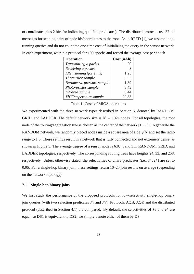
or coordinates plus 2 bits for indicating qualified predicates). The distributed protocols use 32-bit

messages for sending pairs of node ids/coordinates to the root. As in REED [1], we assume long-

running queries and do not count the one-time cost of initializing the query in the sensor network.

In each experiment, we run a protocol for 100 epochs and record the average cost per epoch.

Operation Cost (nAh)Transmitting a packet 20Receiving a packet 8Idle listening (for 1 ms) 1.25Thermistor sample 0.35Barometric pressure sample 1.39Photoresistor sample 3.43Infrared sample 9.44I2CTemperature sample 20.83

Table 1: Costs of MICA operations

We experimented with the three network types described in Section 5, denoted by RANDOM,

GRID, and LADDER. The default network size isN = 1024 nodes. For all topologies, the root

node of the routing/aggregation tree is chosen as the center of the network [13, 5]. To generate the

RANDOM network, we randomly placed nodes inside a square area of side√

N and set the radio

range to1.5. These settings result in a network that is fully connected and not extremely dense, as

shown in Figure 5. The average degree of a sensor node is 6.8, 4, and 3 in RANDOM, GRID, and

LADDER topologies, respectively. The corresponding routing trees have heights 24, 33, and 258,

respectively. Unless otherwise stated, the selectivities of unary predicates (i.e.,P1, P2) are set to

0.05. For a single-hop binary join, these settings return10–20 join results on average (depending

on the network topology).

7.1 Single-hop binary joins

We first study the performance of the proposed protocols for low-selectivity single-hop binary

join queries (with two selection predicatesP1 andP2). Protocols AQB, AQP, and the distributed

protocol (described in Section 4.1) are compared. By default, the selectivities ofP1 andP2 are

equal, so DS1 is equivalent to DS2; we simply denote either of them by DS.

23

(a) network (b) routing tree

Figure 5: RANDOM topology

Figures 6a to 6c show the averaged costs (with error bars) of the three protocols as a function

of the join selectivity. The join output size was controlled by tuningSel(P1) (=Sel(P2)). For

joins with few results, Protocol DS is more efficient than AQB and AQP because pruner nodes (in

AQP) are located several levels above their prunees and measurements that qualify the selections

participate in very few or no join results. In GRID, the effectiveness of AQP is low because pruner

nodes appear at high levels of the tree. On the other hand, in LADDER, pruning effectiveness is

maximized, since each node has its pruner only 1-2 hops away. As the join output size increases,

the energy consumption increases for all protocols, as more tuples are transferred to the base, but

the relative performance of DS compared to AQB/AQP decreases, as the number of join results

compared to the tuples that qualify eitherP1 or P2 increases. Eventually, DS becomes worse

than the acquisitional protocols, since all readings that qualify the selections participate join result

and the join output size well exceeds number of tuples that qualify either selection. Figure 6d

validates the accuracy of the cost models, presented in Section 5. We applied equations in Section

5 to estimate the costs of the protocols for each queryQ on the RANDOM network and averaged

the error|est(Q)−act(Q)|act(Q)

for all queries having the same join selectivity (est(Q) andact(Q) are the

estimated and actual costs, respectively). Observe that the error is quite low (less than 10%) and

decreases with the output size, since queries with more result have less randomness. We note that

24

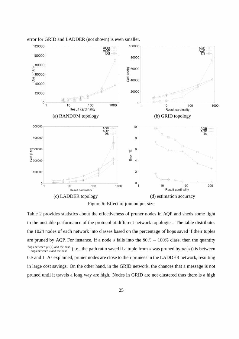
error for GRID and LADDER (not shown) is even smaller.

0

20000

40000

60000

80000

100000

120000

1 10 100 1000

Co

st (n

Ah

)

Result cardinality

AQBAQP

DS

0

20000

40000

60000

80000

100000

1 10 100 1000

Cost

(nA

h)

Result cardinality

AQBAQP

DS

(a) RANDOM topology (b) GRID topology

0

100000

200000

300000

400000

500000

1 10 100 1000

Co

st

(nA

h)

Result cardinality

AQBAQP

DS

0

2

4

6

8

10

1 10 100 1000

Err

or

(%)

Result cardinality

AQBAQP

DS

(c) LADDER topology (d) estimation accuracy

Figure 6: Effect of join output size

Table 2 provides statistics about the effectiveness of pruner nodes in AQP and sheds some light

to the unstable performance of the protocol at different network topologies. The table distributes

the 1024 nodes of each network into classes based on the percentage of hops saved if their tuples

are pruned by AQP. For instance, if a nodes falls into the80% − 100% class, then the quantityhops betweenpr(s) and the base

hops betweens and the base (i.e., the path ratio saved if a tuple froms was pruned bypr(s)) is between

0.8 and1. As explained, pruner nodes are close to their prunees in the LADDER network, resulting

in large cost savings. On the other hand, in the GRID network, the chances that a message is not

pruned until it travels a long way are high. Nodes in GRID are not clustered thus there is a high

25

probability that a neighborhood is split into different subtrees. The effectiveness of pruners in

RANDOM is in-between the two other topologies.

Ratio(%) RANDOM GRID LADDER80-100 414 179 99460-80 250 280 1640-60 165 243 920-40 105 190 50-20 90 132 0

Table 2: Number of nodes for each hops-saving class (protocol AQP)

Next, we verify the assertion that AQP and DS achieve better cost balancing than AQB among

different nodes. Figure 7 shows the average cost per node as a function of node’s level in the

routing tree, in the RANDOM and GRID topologies (the plot for the LADDER network is similar).

In general, sensor nodes at higher levels receive and forward more data so they have larger burden.

DS and AQP have better balancing, since they manage to eliminate tuples that do not participate

in join results early, either by computation of the exact join results (DS) or by filtering tuples at

pruner nodes (AQP).

0

20

40

60

80

100

0 5 10 15 20 25

Co

st p

er

no

de

(n

Ah

)

Sensor node level

AQBAQP

DS

0

10

20

30

40

50

60

70

80

1 4 7 10 13 16 19 22 25 28 31 34

Cost

per

node (

nA

h)

Sensor node level

AQBAQP

DS

(a) RANDOM topology (b) GRID topology

Figure 7: Cost balancing of sensor nodes

We also tested the effect of the network density to the relative performance of the protocols. We

gradually increased the communication range in the GRID and LADDER networks and measured

the costs of the three protocols. Figure 8 plots the average energy consumption as a function of

the average node degree in the two networks. In this experiment, we keepP1 andP2 constant and

26

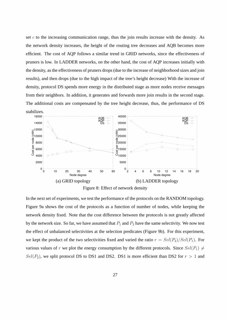
setc to the increasing communication range, thus the join results increase with the density. As

the network density increases, the height of the routing tree decreases and AQB becomes more

efficient. The cost of AQP follows a similar trend in GRID networks, since the effectiveness of

pruners is low. In LADDER networks, on the other hand, the cost of AQP increases initially with

the density, as the effectiveness of pruners drops (due to the increase of neighborhood sizes and join

results), and then drops (due to the high impact of the tree’s height decrease) With the increase of

density, protocol DS spends more energy in the distributed stage as more nodes receive messages

from their neighbors. In addition, it generates and forwards more join results in the second stage.

The additional costs are compensated by the tree height decrease, thus, the performance of DS

stabilizes.

0

2000

4000

6000

8000

10000

12000

14000

16000

0 10 20 30 40 50 60

Cost

per

node (

nA

h)

Node degree

AQBAQP

DS

0

5000

10000

15000

20000

25000

30000

35000

40000

2 4 6 8 10 12 14 16 18 20

Cost

per

node (

nA

h)

Node degree

AQBAQP

DS

(a) GRID topology (b) LADDER topology

Figure 8: Effect of network density

In the next set of experiments, we test the performance of the protocols on the RANDOM topology.

Figure 9a shows the cost of the protocols as a function of number of nodes, while keeping the

network density fixed. Note that the cost difference between the protocols is not greatly affected

by the network size. So far, we have assumed thatP1 andP2 have the same selectivity. We now test

the effect of unbalanced selectivities at the selection predicates (Figure 9b). For this experiment,

we kept the product of the two selectivities fixed and varied the ratior = Sel(P2)/Sel(P1). For

various values ofr we plot the energy consumption by the different protocols. SinceSel(P1) 6=Sel(P2), we split protocol DS to DS1 and DS2. DS1 is more efficient than DS2 forr > 1 and

27

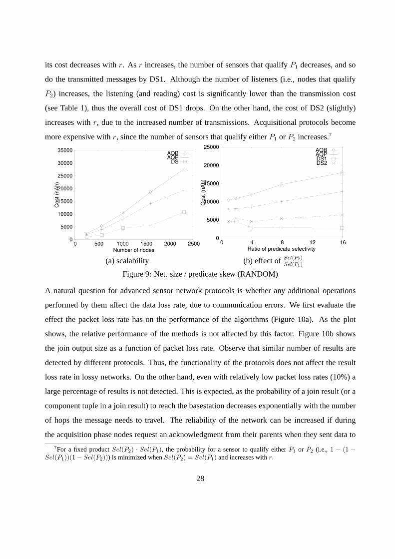
its cost decreases withr. As r increases, the number of sensors that qualifyP1 decreases, and so

do the transmitted messages by DS1. Although the number of listeners (i.e., nodes that qualify

P2) increases, the listening (and reading) cost is significantly lower than the transmission cost

(see Table 1), thus the overall cost of DS1 drops. On the other hand, the cost of DS2 (slightly)

increases withr, due to the increased number of transmissions. Acquisitional protocols become

more expensive withr, since the number of sensors that qualify eitherP1 or P2 increases.7

0

5000

10000

15000

20000

25000

30000

35000

0 500 1000 1500 2000 2500

Co

st (n

Ah

)

Number of nodes

AQBAQP

DS

0

5000

10000

15000

20000

25000

0 4 8 12 16

Co

st (n

Ah

)

Ratio of predicate selectivity

AQBAQPDS1DS2

(a) scalability (b) effect ofSel(P2)Sel(P1)

Figure 9: Net. size / predicate skew (RANDOM)

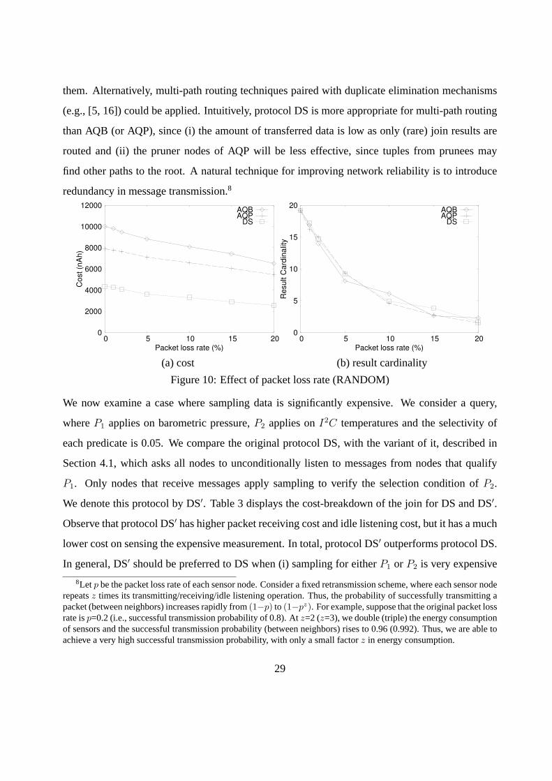
A natural question for advanced sensor network protocols is whether any additional operations

performed by them affect the data loss rate, due to communication errors. We first evaluate the

effect the packet loss rate has on the performance of the algorithms (Figure 10a). As the plot

shows, the relative performance of the methods is not affected by this factor. Figure 10b shows

the join output size as a function of packet loss rate. Observe that similar number of results are

detected by different protocols. Thus, the functionality of the protocols does not affect the result

loss rate in lossy networks. On the other hand, even with relatively low packet loss rates (10%) a

large percentage of results is not detected. This is expected, as the probability of a join result (or a

component tuple in a join result) to reach the basestation decreases exponentially with the number

of hops the message needs to travel. The reliability of the network can be increased if during

the acquisition phase nodes request an acknowledgment from their parents when they sent data to

7For a fixed productSel(P2) · Sel(P1), the probability for a sensor to qualify eitherP1 or P2 (i.e., 1 − (1 −Sel(P1))(1− Sel(P2))) is minimized whenSel(P2) = Sel(P1) and increases withr.

28

them. Alternatively, multi-path routing techniques paired with duplicate elimination mechanisms

(e.g., [5, 16]) could be applied. Intuitively, protocol DS is more appropriate for multi-path routing

than AQB (or AQP), since (i) the amount of transferred data is low as only (rare) join results are

routed and (ii) the pruner nodes of AQP will be less effective, since tuples from prunees may

find other paths to the root. A natural technique for improving network reliability is to introduce

redundancy in message transmission.8

0

2000

4000

6000

8000

10000

12000

0 5 10 15 20

Co

st (n

Ah

)

Packet loss rate (%)

AQBAQP

DS

0

5

10

15

20

0 5 10 15 20

Re

su

lt C

ard

ina

lity

Packet loss rate (%)

AQBAQP

DS

(a) cost (b) result cardinality

Figure 10: Effect of packet loss rate (RANDOM)

We now examine a case where sampling data is significantly expensive. We consider a query,

whereP1 applies on barometric pressure,P2 applies onI2C temperatures and the selectivity of

each predicate is 0.05. We compare the original protocol DS, with the variant of it, described in

Section 4.1, which asks all nodes to unconditionally listen to messages from nodes that qualify

P1. Only nodes that receive messages apply sampling to verify the selection condition ofP2.

We denote this protocol by DS′. Table 3 displays the cost-breakdown of the join for DS and DS′.

Observe that protocol DS′ has higher packet receiving cost and idle listening cost, but it has a much

lower cost on sensing the expensive measurement. In total, protocol DS′ outperforms protocol DS.

In general, DS′ should be preferred to DS when (i) sampling for eitherP1 or P2 is very expensive

8Let p be the packet loss rate of each sensor node. Consider a fixed retransmission scheme, where each sensor noderepeatsz times its transmitting/receiving/idle listening operation. Thus, the probability of successfully transmitting apacket (between neighbors) increases rapidly from(1−p) to (1−pz). For example, suppose that the original packet lossrate isp=0.2 (i.e., successful transmission probability of 0.8). Atz=2 (z=3), we double (triple) the energy consumptionof sensors and the successful transmission probability (between neighbors) rises to 0.96 (0.992). Thus, we are able toachieve a very high successful transmission probability, with only a small factorz in energy consumption.

29

and should not be performed unconditionally or (ii) eitherSel(P1) or Sel(P2) is close to 100%;

the majority of nodes qualify the predicate, so sensing should follow listening.

Average nodes / epochOperation Protocol DS Protocol DS′

Transmitting a packet 162.8 162.8Receiving a packet 126.6 461.9

Idle listening 49.9 1024Sensing barom. pressure 1024 1024

SensingI2C temp. 1024 16.2

Total cost (nAh) 27084.5 9992.0

Table 3: Cost breakdown for a query with expensive predicates (RANDOM)

7.2 Complex joins

In this section, we evaluate the effectiveness of the protocols described in Section 4.2 for spatial

pattern queries with variables forming a star graph topology. Figure 11 shows the cost of the

protocols as a function of number of border nodes, after fixing the selectivities of both predicates

PC and PB to 0.1. When the number of border nodes increases, only DSB and DSC achieve

significant cost reduction. For queries with many border nodes, very few results are generated and

the level-off costs of DSB and DSC indicate the cost of the distributed phase. DSB is slightly

cheaper than DSC, because DSC requires more nodes to transmit packets in the distributed phase.

The next experiment evaluates the protocols by varying the selectivities ofPC andPB. Figure

12a shows the cost of the protocols as a function ofPC ’s selectivity, with 3 border nodes and

Sel(PB) = 0.05. DSC has the best performance at very small values ofSel(PC). DSB starts

outperforming the other protocols asSel(PC) increases. Figure 12b shows the cost of the protocols

as a function ofSel(PB), for queries with 3 border nodes andSel(PC) = 0.05. The situation is

reversed in this case. DSB has the best performance at low values ofSel(PB), while DSC becomes

the best protocol as the number of border nodes increases.

30

0

5000

10000

15000

20000

2 3 4 5

Co

st (n

Ah

)

Number of border nodes

AQBAQPDSBDSC

Figure 11: Cost as a function of number of border nodes, RANDOM topology

0

5000

10000

15000

20000

25000

30000

0 0.05 0.1 0.15 0.2 0.25 0.3

Co

st (n

Ah

)

Center predicate selectivity

AQBAQPDSBDSC

0

5000

10000

15000

20000

25000

30000

0 0.05 0.1 0.15 0.2 0.25 0.3

Co

st (n

Ah

)

Border predicate selectivity

AQBAQPDSBDSC

(a) varyingSel(PC) (b) varyingSel(PB)

Figure 12: Effect of selectivity (RANDOM)

7.3 Multi-hop queries

We now study the performance of the protocols for multi-hop binary join queries. In protocol

BD, x is set toλ/2. Figure 13 plots the costs as a function of join distance, on all three network

topologies. In the RANDOM network, acquisitional protocols outperform distributed protocols for

join distances greater than one hop. The result for GRID topology is similar except that acquisi-

tional protocols start outperforming the distributed ones at a longer join distance. In the LADDER

network, although the distributed protocols perform better than AQB, protocol AQP maintains

the good performance it has at single-hop joins for multi-hop queries and greatly outperforms the

31

distributed methods. The effectiveness of pruners remains high due to the linearity of the topol-

ogy. Note that the bidirectional protocol (BD) does not have large performance difference than the

purely distributed protocol. It turns out that BD has high packet reading cost, since intermediate

nodes collect messages unconditionally. In addition, BD generates many duplicate join results

which increase the cost of transmitting them to the basestation. In summary, acquisitional proto-

cols are favorable for multi-hop queries, due to the extreme cost of flooding the selection results at

long ranges.

0

20000

40000

60000

80000

100000

1 2 3 4

Co

st (n

Ah

)

Join distance (hops)

AQBAQP

DSBD

0

10000

20000

30000

40000

50000

60000

70000

1 2 3 4

Cost

(nA

h)

Join distance (hops)

AQBAQP

DSBD

(a) RANDOM topology (b) GRID topology

0

10000

20000

30000

40000

50000

60000

1 2 3 4

Cost

(nA

h)

Join distance (hops)

AQBAQP

DSBD

(c) LADDER topology

Figure 13: Cost as a function of join distance

Finally, we verify the trade-off of disseminating continuous queries in a sensor network and apply-

ing in-network filtering or evaluation, as opposed to continuously and unconditionally acquiring

measurements, and evaluating queries at the basestation. Table 4 shows the costs of the various

32

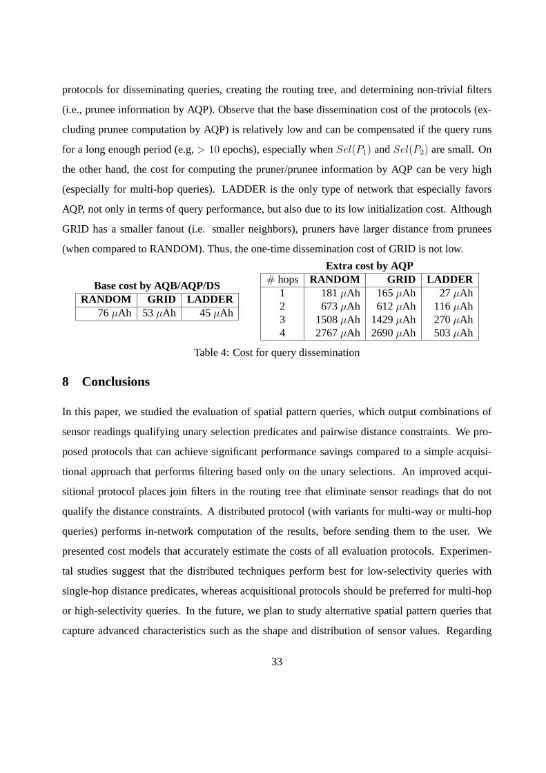
protocols for disseminating queries, creating the routing tree, and determining non-trivial filters

(i.e., prunee information by AQP). Observe that the base dissemination cost of the protocols (ex-

cluding prunee computation by AQP) is relatively low and can be compensated if the query runs

for a long enough period (e.g,> 10 epochs), especially whenSel(P1) andSel(P2) are small. On

the other hand, the cost for computing the pruner/prunee information by AQP can be very high

(especially for multi-hop queries). LADDER is the only type of network that especially favors

AQP, not only in terms of query performance, but also due to its low initialization cost. Although

GRID has a smaller fanout (i.e. smaller neighbors), pruners have larger distance from prunees

(when compared to RANDOM). Thus, the one-time dissemination cost of GRID is not low.

Base cost by AQB/AQP/DSRANDOM GRID LADDER

76µAh 53µAh 45µAh

Extra cost by AQP# hops RANDOM GRID LADDER

1 181µAh 165µAh 27µAh2 673µAh 612µAh 116µAh3 1508µAh 1429µAh 270µAh4 2767µAh 2690µAh 503µAh

Table 4: Cost for query dissemination

8 Conclusions

In this paper, we studied the evaluation of spatial pattern queries, which output combinations of

sensor readings qualifying unary selection predicates and pairwise distance constraints. We pro-

posed protocols that can achieve significant performance savings compared to a simple acquisi-

tional approach that performs filtering based only on the unary selections. An improved acqui-

sitional protocol places join filters in the routing tree that eliminate sensor readings that do not

qualify the distance constraints. A distributed protocol (with variants for multi-way or multi-hop

queries) performs in-network computation of the results, before sending them to the user. We

presented cost models that accurately estimate the costs of all evaluation protocols. Experimen-

tal studies suggest that the distributed techniques perform best for low-selectivity queries with

single-hop distance predicates, whereas acquisitional protocols should be preferred for multi-hop

or high-selectivity queries. In the future, we plan to study alternative spatial pattern queries that

capture advanced characteristics such as the shape and distribution of sensor values. Regarding

33

continuous query evaluation, we will continue to explore the approach in Section 6.2 for reducing

energy consumption by saving notifications of identical spatial patterns in consecutive epochs.

References

[1] D. J. Abadi, S. Madden, and W. Lindner. REED: Robust, Efficient Filtering and Event De-

tection in Sensor Networks. InProc. of VLDB, 2005.

[2] B. J. Bonfils and P. Bonnet. Adaptive and Decentralized Operator Placement for In-Network

Query Processing. InProc. of IPSN, 2003.

[3] P. Bonnet, J. Gehrke, and P. Seshadri. Towards Sensor Database Systems. InProc. of MDM,

2001.

[4] D. Chu, A. Deshpande, J. Hellerstein, and W. Hong. Approximate Data Collection in Sensor

Networks using Probabilistic Models. InProc. of ICDE, 2006.

[5] J. Considine, F. Li, G. Kollios, and J. W. Byers. Approximate Aggregation Techniques for

Sensor Databases. InProc. of ICDE, 2004.

[6] A. Deligiannakis, Y. Kotidis, and N. Roussopoulos. Compressing Historical Information in

Sensor Networks. InProc. of ACM SIGMOD, 2004.

[7] A. Deligiannakis, Y. Kotidis, and N. Roussopoulos. Hierarchical In-Network Data Aggrega-

tion with Quality Guarantees. InProc. of EDBT, 2004.

[8] A. Deshpande, C. Guestrin, S. Madden, J. M. Hellerstein, and W. Hong. Model-Driven Data

Acquisition in Sensor Networks. InProc. of VLDB, 2004.

[9] M. Hadjieleftheriou, N. Mamoulis, and Y. Tao. Continuous Constraint Query Evaluation for

Spatiotemporal Streams. InProc. of SSTD, 2007.

[10] C. Intanagonwiwat, R. Govindan, and D. Estrin. Directed Diffusion: A Scalable and Robust

Communication Paradigm for Sensor Networks. InProc. of MOBICOM, 2000.

34

[11] Y. Kotidis. Snapshot Queries: Towards Data-Centric Sensor Networks. InProc. of ICDE,

2005.

[12] Y. Kotidis. Processing Proximity Queries in Sensor Networks. InInternational Workshop on

Data Management for Sensor Networks, 2006.

[13] S. Madden, M. J. Franklin, J. M. Hellerstein, and W. Hong. TAG: A Tiny AGgregation

Service for Ad-Hoc Sensor Networks. InProc. of OSDI, 2002.

[14] S. Madden, M. J. Franklin, J. M. Hellerstein, and W. Hong. TinyDB: An Acquisitional Query

Processing System for Sensor Networks.ACM TODS, 30(1):122–173, 2005.

[15] A. Mainwaring, D. Culler, J. Polastre, R. Szewczyk, and J. Anderson. Wireless Sensor Net-

works for Habitat Monitoring. InProc. of WSNA, 2002.

[16] A. Manjhi, S. Nath, and P. B. Gibbons. Tributaries and Deltas: Efficient and Robust Aggre-

gation in Sensor Network Streams. InProc. of ACM SIGMOD, 2005.

[17] J. Paek, K. Chintalapudi, J. Cafferey, R. Govindan, and S. Masri. A Wireless Sensor Network

for Structural Health Monitoring: Performance and Experience. InProc. of the 2nd IEEE

Workshop on Embedded Networked Sensors, 2005.

[18] A. Pandit and H. Gupta. Communication-Efficient Implementation of Range-Joins in Sensor

Networks. InProc. of DASFAA, 2006.

[19] M. A. Sharaf, J. Beaver, A. Labrinidis, and P. K. Chrysanthis. Balancing Energy Efficiency

and Quality of Aggregate Data in Sensor Networks.VLDB J., 13(4):384–403, 2004.

[20] G. Simon, M. Maroti, A. Ledeczi, G. Balogh, B. Kusy, A. Nadas, G. Pap, J. Sallai, and

K. Frampton. Sensor network-based countersniper system. InProc. of SenSys, 2004.

[21] A. Soheili, V. Kalogeraki, and D. Gunopulos. Spatial Queries in Sensor Networks. InProc.

of ACM GIS, 2005.

35

[22] U. Srivastava, K. Munagala, and J. Widom. Operator Placement for In-Network Stream

Query Processing. InProc. of ACM PODS, 2005.

[23] Xiaoyan Yang and Hock-Beng Lim and M. TamerOzsu and Kian-Lee Tan. In-network Exe-

cution of Monitoring Queries in Sensor Networks. InProc. of ACM SIGMOD, 2007.

[24] Y. Yao and J. Gehrke. The Cougar Approach to In-network Query Processing in Sensor

Networks.SIGMOD Record, 31(3):9–18, 2002.

[25] M. L. Yiu, N. Mamoulis, and S. Bakiras. Retrieval of Spatial Join Pattern Instances from

Sensor Networks. InProc. of SSDBM, 2007.

[26] H. Yu, E.-P. Lim, and J. Zhang. On In-network Synopsis Join Processing for Sensor Net-

works. InMDM, 2006.

[27] F. Zhao and L. Guibas.Wireless Sensor Networks: An Information Processing Approach.

Elsevier/Morgan Kaufmann, 2004.

36