Measuring urban sprawl, coalescence, and dispersal: a case study of Pordenone, Italy

IntroductionLand-use change and urban sprawl are very much causes of many of the major human-induced environmental challenges affecting modern society, with most scholarshipagreeing that the changes are predominantly harmful to public services (Carruthersand Ulfarsson, 2003), public health (Ewing et al, 2003), and climate (Ewing et al, 2007).Yet exactly what constitutes urban sprawl is highly multidimensional and difficult toquantify (Ewing et al, 2002; Frenkel and Ashkenazi, 2008; Torrens, 2008), especiallywhen all of the causes and impacts are incorporated into the measures (Burchfieldet al, 2006; Ewing, 1994). Hasse and Lathrop (2003, page 160) noted that ` The litera-ture on sprawl, with a tinge of irony, is broadly dispersed and multifaceted. A variety ofdefinitions for sprawl have been put forth that describe sprawl.''

There has been considerable debate about the costs and consequences of sprawl,and even whether the net effect is positive or negative (Burchell et al, 1998; Ewing,1997; Glaeser and Kahn, 2003; Gordon and Wong, 1985; Hasse and Lathrop, 2003).Clearly sprawl is a component of urban expansion and a defining element is lowsettlement densities (Brueckner, 2002; Peiser, 1989). From the majority of points ofview the characteristics of modern urbanization are considered unsustainable; how-ever, new models of sustainable urban development are proposed which should help tomitigate the risks related to sprawl (Ewing, 1994).

Starting in the late 1970s, new urban planning theories arose in the US with abackground in urban visions and theoretical models inspired by the `European' city

Measuring urban sprawl, coalescence, and dispersal:a case study of Pordenone, Italy

Federico MartellozzoôDepartment of Geography, McGill University, 805 Sherbrooke Street West, Montreal, QuebecH3A 2K6, Canada; e-mail: [email protected]

Keith C ClarkeDepartment of Geography, 1832 Ellison Hall, University of California Santa Barbara,Santa Barbara, CA 93106-4060, USA; e-mail: [email protected] 25 July 2009; in revised form 23 April 2010

Environment and Planning B: Planning and Design 2011, volume 38, pages 1085 ^ 1104

Abstract. A critical challenge of global change is managing the uncontrolled spread of cities into theirsurrounding rural and other land. The phenomenon of urban `sprawl' is well known, but it remainscontroversial because there are no universal definitions about its etiology, nor of the causes andvariables related to it. The goal of this study is to depict the temporal trend of sprawl, so as toidentify a `sprawl signature' and its evolution for the Italian Province of Pordenone focusing exclu-sively on spatial dispersion features. Data were compiled from multitemporal remote sensing andused to delimit urban expansion over time. We aim to describe the spatiotemporal patterns associatedwith urban sprawl using the perspective of the cyclical urban growth theory and focusing on measuresthat can detect the degree of spatial dispersion during time related to sprawl both in past andprojected urban forms. Exactly how the spatiotemporal patterns of urban growth are identified iscrucial for urban planners, as knowledge of them allows more efficient calibration of policies tocontrol land-use change in order to satisfy specific needs of the population and prevent the risksand costs related to sprawl.

doi:10.1068/b36090

ô Current address: Department of Geography and Earth System Science Program, Room 705,7th Floor, Burnside Hall, McGill University, 805 Sherbrooke Street West, Montreal, QuebecH3A 2K6, Canada; e-mail: [email protected]

proposed by architect Leon Krier, and the `pattern language' theories of ChristopherAlexander. The origins of these approaches lie in European city elements as solutionsto North American urban problems of sprawl. Ironically, the case study we present inthis research concerns an area in northeastern Italy, considered by the EuropeanCommunity to be one of the most explicative examples of modern urban sprawl,even though it is not a big metropolis (Krier and Thadani, 2009). The new philosophy,later called New Urbanism, grew in the early 1980s as a reaction to the negative environ-mental and human consequences of sprawl. The goal was to use sustainable planning andarchitectural principles functioning together in order to create human-scale, walkablecommunities. The planned growth vision of New Urbanism takes into account issuessuch as sustainable development, reduced traffic congestion, public transportation, andaccess to parks and green areas, in contrast to the continuous outward expansionand development of urban areas with their constantly increasing need for automobiletransportation capacity. Instead, the role of quality of life became central.

The monitoring of land-cover transitions related to urban development over time isusually to find out the amount and location of land-use change for planning purposes.Nevertheless, the ability to anticipate a trend in urban sprawl behavior for a specificregion would give planners a useful tool to understand sprawl's long-term impact ona region, or even to take steps to prevent or retard it. Although various studies havebeen dedicated to the measurement and monitoring of urban growth, they have limita-tions in providing generalizations of the characteristics of urban sprawl. In this study,we choose to define urban sprawl purely cartometrically, that is by quantifying the shape,distribution, and spatial extent of built-up areas. Our approach follows Batty's conceptof form as a result of function (Batty and Kim, 1992), but instead of focusing ontheories of density and settlement size (Batty, 2002; 2008; Batty and Longley, 1994) oron demographic structure (Brueckner, 2002; Lowry, 1990), we focus on urban spatialform alone. Advantages of this approach are that it avoids the complexity of the sprawldefinitions, works across spatial scales, and is approachable with data from maps andgeographic information systems. Disadvantages are that it negates social and economicfactors, and ignores the body of theory on urban density and rank-size structure.

Our work is influenced by the general principles set forth by Dietzel et al (2005a;2005b) that urban sprawl is a phenomenon highly correlated to time, in that the growthof urban areas oscillates between coalescence and diffusion processes with sprawlgrowth behavior concentrated in the former. Thus, a priori, we expect both sprawl andregular urban expansion to be present in space and over time. This is in contrast tothe view that sprawl represents continued and sustained fragmentation (Irwin andBockstael, 2007). The measure we chose to follow is spatial entropy, a quantity thathas long been associated with the dissipative property of systems, including urban areasand systems (Batty, 1974; Batty and Longley, 1994; Herold et al, 2002; Yeh and Li, 2001).Entropy is apparently the only almost-universally shared spatial measurementconcept concerning urban sprawl (Torrens, 2008). We aim to depict the evolution ofthe spatial patterns of sprawl over time in order to identify a `sprawl evolutionsignature' for the region of interest, similar to Silva's concept of urban DNA (Silvaand Clarke, 2005).

The goals of this study were to: (1) map the dynamics of land-use change in a knownEuropean sprawling metropolis over time; (2) quantify the spatial form using measuresable to detect spatial dispersion, in order to test for evidence of the oscillation betweencoalescence and diffusion processes in urban growth, and so to test the hypothesis thatsprawl is contained in the latter phase only; and (3) to use a land-use-change model andthe same measures to test whether it is possible to use these measures prescriptively

1086 F Martellozzo, K C Clarke

to forecast sprawl, with the intent of possibly equipping planners with a further tool tosupport growth management strategies.

Urban sprawl as spatial dispersionTo be useful, a measure of sprawl must consider it a matter of degree. For instance,scattered development and polycentric or multinucleated urban development are verysimilar; hence the distinction between these two different trends of growth is elusiveand leads us to consider sprawl as a matter of resolution as well as scale (Batty, 2008).`At what number of centers polycentrism ceases and sprawl begins is not clear''(Gordon and Wong, 1985, page 662). Sprawl can also be analyzed across all its dimen-sions: density, land use, and time (Ewing, 1994; Pesier, 1989). In addition, sprawlmeasures should permit cross-comparison between cities, and so should avoid data-specific or reduction techniques, such as multiple regression (Frenkel and Ashkenazi,2008). Nevertheless, we chose to focus on the entropy of spatial form and its evolutionover time.

The concept of entropy, based in information theory, has been used to describe thecomplexity of sprawl patterns through space and time (Yeh and Li, 2001). Entropy hasorigins in thermodynamics, but is more broadly considered to be the level of disorga-nization of a system and hence also the amount of energy needed to reorganize thesystem. Since its formalization by Shannon (1948) as information theory, it has beenapplied in many different fields including physics, remote sensing, computer science,cartography, mathematics, and geography. Entropy measures for the analysis of spatialdistributions have been related to distances and density metrics, depending on thenature of the phenomenon (Novelli and Occelli, 1999). One of the most effectivesynthetic indices to describe entropy is Shannon's logarithmic function which hasbeen applied widely in urban geography because it is considered to be a robust metricfor detecting dispersion when applied with density measures (Peiser, 1989; Yeh and Li,2001). Batty (1974) defined the concept of spatial entropy and discovered the necessityof a coherent zoning system when analyzing spatial distribution and entropy overspace. Entropy is still of interest beyond specific case studies in urban growth detec-tion. It is used in modeling and classification techniques (Li and Huang, 2002) from amore theoretical point of view. Some studies convey modification and correction of theentropy formula in order to obtain a more meaningful tool to compare dispersion andcoalescence of spatial phenomena through space and time (Heikkila and Hu, 2006).

Entropy has been addressed as fundamental in studies of spatial pattern; hence it isa very good means for the investigation of diffusion or dispersal. The entropy measureis most likely to be affected by the oscillatory behavior between diffusion and coa-lescence anticipated in the work by Dietzel et al (2005a; 2005b). The fact that entropycan be considered from both a relative and an absolute perspective, and the fact that itcan be corrected for biases induced by scale, resolution, or the zoning system, alsomakes it a useful tool to investigate the diffusive and coalescent phases of urban growth.

In phased oscillation theory, urban growth over time follows a process in whichdispersed or isolated clusters form due to the influence of core areas (characterized byhigher density) on regions of lower density; this is followed by a coalescence phase,with a tendency for the clusters to grow together, clump, and form single entities.In urban growth scenarios no movement of clusters is possible, a cell once urban tendsto remain urban, so it is important to observe trends in the distribution of new clustersover time (Dietzel et al, 2005a). In many cases, the scatter and further growth ofsprawled zones takes place over long time spans, and so we seek to assimilate bothhistorical data and modeled future trends.

Measuring urban sprawl, coalescence, and dispersal 1087

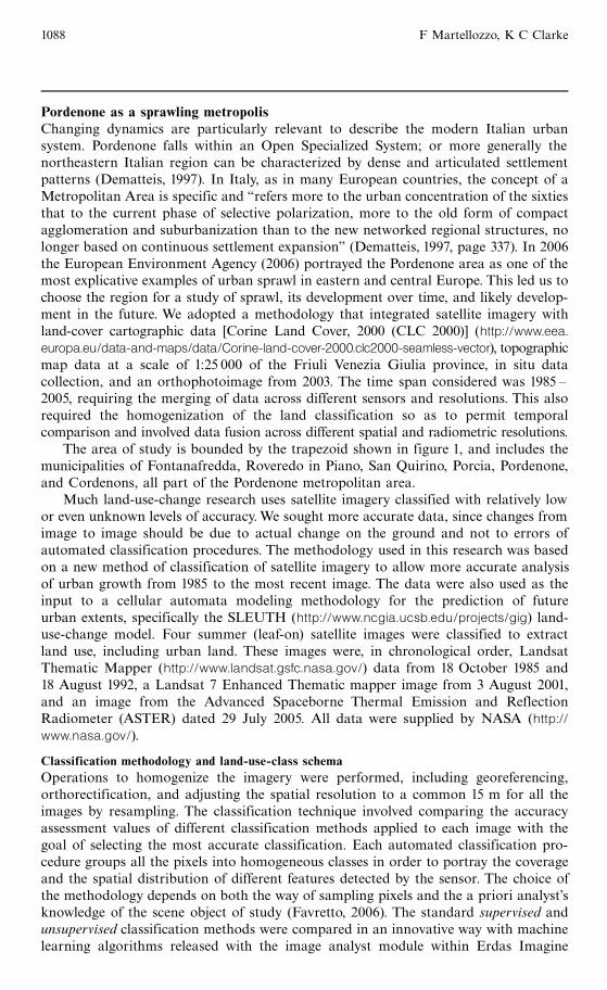
Pordenone as a sprawling metropolisChanging dynamics are particularly relevant to describe the modern Italian urbansystem. Pordenone falls within an Open Specialized System; or more generally thenortheastern Italian region can be characterized by dense and articulated settlementpatterns (Dematteis, 1997). In Italy, as in many European countries, the concept of aMetropolitan Area is specific and ` refers more to the urban concentration of the sixtiesthat to the current phase of selective polarization, more to the old form of compactagglomeration and suburbanization than to the new networked regional structures, nolonger based on continuous settlement expansion'' (Dematteis, 1997, page 337). In 2006the European Environment Agency (2006) portrayed the Pordenone area as one of themost explicative examples of urban sprawl in eastern and central Europe. This led us tochoose the region for a study of sprawl, its development over time, and likely develop-ment in the future. We adopted a methodology that integrated satellite imagery withland-cover cartographic data [Corine Land Cover, 2000 (CLC 2000)] (http://www.eea.europa.eu/data-and-maps/data/Corine-land-cover-2000.clc2000-seamless-vector), topographicmap data at a scale of 1:25 000 of the Friuli Venezia Giulia province, in situ datacollection, and an orthophotoimage from 2003. The time span considered was 1985 ^2005, requiring the merging of data across different sensors and resolutions. This alsorequired the homogenization of the land classification so as to permit temporalcomparison and involved data fusion across different spatial and radiometric resolutions.

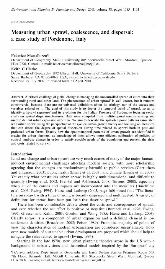
The area of study is bounded by the trapezoid shown in figure 1, and includes themunicipalities of Fontanafredda, Roveredo in Piano, San Quirino, Porcia, Pordenone,and Cordenons, all part of the Pordenone metropolitan area.

Much land-use-change research uses satellite imagery classified with relatively lowor even unknown levels of accuracy.We sought more accurate data, since changes fromimage to image should be due to actual change on the ground and not to errors ofautomated classification procedures. The methodology used in this research was basedon a new method of classification of satellite imagery to allow more accurate analysisof urban growth from 1985 to the most recent image. The data were also used as theinput to a cellular automata modeling methodology for the prediction of futureurban extents, specifically the SLEUTH (http://www.ncgia.ucsb.edu/projects/gig) land-use-change model. Four summer (leaf-on) satellite images were classified to extractland use, including urban land. These images were, in chronological order, LandsatThematic Mapper (http://www.landsat.gsfc.nasa.gov/) data from 18 October 1985 and18 August 1992, a Landsat 7 Enhanced Thematic mapper image from 3 August 2001,and an image from the Advanced Spaceborne Thermal Emission and ReflectionRadiometer (ASTER) dated 29 July 2005. All data were supplied by NASA (http://www.nasa.gov/).

Classification methodology and land-use-class schemaOperations to homogenize the imagery were performed, including georeferencing,orthorectification, and adjusting the spatial resolution to a common 15 m for all theimages by resampling. The classification technique involved comparing the accuracyassessment values of different classification methods applied to each image with thegoal of selecting the most accurate classification. Each automated classification pro-cedure groups all the pixels into homogeneous classes in order to portray the coverageand the spatial distribution of different features detected by the sensor. The choice ofthe methodology depends on both the way of sampling pixels and the a priori analyst'sknowledge of the scene object of study (Favretto, 2006). The standard supervised andunsupervised classification methods were compared in an innovative way with machinelearning algorithms released with the image analyst module within Erdas Imagine


software (http://www.erdas.com). The method looks at a pixel and determines the rulesof classification not only on the base of spectral properties of pixels but also on thecontext, the positional relation with neighboring pixels.

For an accuracy assessment, the image chosen for comparing the different classifi-cations results was the Landsat image from 2001; this image was classified using allthree methods (supervised, unsupervised, and machine learning). The classificationscheme chosen used a reduction of the CLC 2000 scheme into seven relevant classes(tables 1 and 2) (Favretto and Martellozzo, 2008).

The unsupervised classification was performed first; this method was very usefulfor exploratory analysis. Furthermore it helped us to understand the spectral differ-entiation within classes, even if the use of ground truth was minimal (Jensen, 1996). Theoutput was thematic maps where the number of classes is known but their meaningneeds to be interpreted. This method was applied several times before reduction into theseven CLC 2000 classes, in order to understand the land cover and to better define asignificant classification scheme. The algorithm used for the unsupervised classificationwas ISODATA (iterative self-organizing data analysis technique).

The second methodology applied was supervised classification; generally speaking thisautomatic procedure is more accurate than the unsupervised. In spite of this, it requiresmore analyst effort and a sufficient knowledge of the area of study. It requires the analyst

Figure 1. [In color online.] Area of interest with the name of the municipalities of the Pordenonemetropolitan area and geographic coordinates of the trapezoid that frames the area of interest.Source: false color image, ASTER 29 July 2005 (Advanced Spaceborne Thermal Emission andReflection Radiometer database, http://asterweb.jpl.nasa.gov/).


to define training areas that allow an algorithm to analyze and group pixels on the basis ofspectral similarities (Jensen, 1996). The supervised algorithm used maximum likelihood,where a statistical procedure assigns each pixel to the class that shows most spectralsimilarity. Ground-truth data came from field visits to the zones in question.

The third classification method applied was the machine learning (ML) approach.This method was inspired by a computing philosophy that develops algorithms that areadaptive to the data. A classification is applied, and then adjusted to maximize apreestablished performance criterion (Huang and Jensen, 1997). Successive adjust-ments improve the overall classification accuracy. The ML algorithm learns eachtime it receives feedback and then modifies a set of weights in order to achieve thebest results. This methodology generally gives improved results, but it is also timeconsuming and still requires more work to be done by analysts. The step-by-stepprocedure starts with preliminary information given to the algorithm that refines itselfwith subsequent corrections; actually ML methodologies produce a large amount ofdata but only the final results are useful (Huang and Jensen, 1997). In our case the MLfunctionalities distributed with the Image Analyst module within Erdas Imagine wereused. The accuracy for each classification method was assessed taking as a reference amosaic of an Orthoimage from 2003 and a Landsat image from 2002.

Accuracy assessment defines the degree of coherence of the classified image withthe ground truth. A large number of pixels are taken from the thematic image andcompared with a reference map of higher authority to see which and how many pixelswere classified correctly (Jensen, 1996). An error or confusion matrix is built for thiscomparison; the sampling strategy used to select pixels was stratified random sam-pling. The kappa statistic, a measure of overall accuracy, ranges from 0 to 1, wherevalues >0.7 are considered good to optimum correlation between the classified imageand the ground truth (Jensen, 1996) while values 4 0.4 identify a very low correlation.

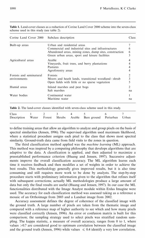
Table 1. Land-cover classes as a reduction of Corine Land Cover 2000 scheme into the seven-classscheme used in this study (see table 2).

Corine Land Cover 2000 Subclass description Class

Built-up areas Urban and residential areas 7Commercial and industrial sites and infrastructures 6Abandoned areas, mining zones, dump sites, construction 6Green urban areas, sport and leisure facilities 3

Agricultural areas Arable 4Vineyards, fruit trees, and berry plantations 4Pastures 4Agroforestry areas 4

Forests and seminatural Forests 2environments Moors and heath lands, transitional woodland ± shrub 3

Open fields with little or no sparse vegetation 5

Humid areas Inland marshes and peat bogs 2Salt marshes na

Water bodies Continental water 1Maritime water na

Table 2. The land-cover classes identified with seven-class scheme used in this study.

Class 1 2 3 4 5 6 7Description Water Forest Shrubs Arable Bare ground Periurban Urban


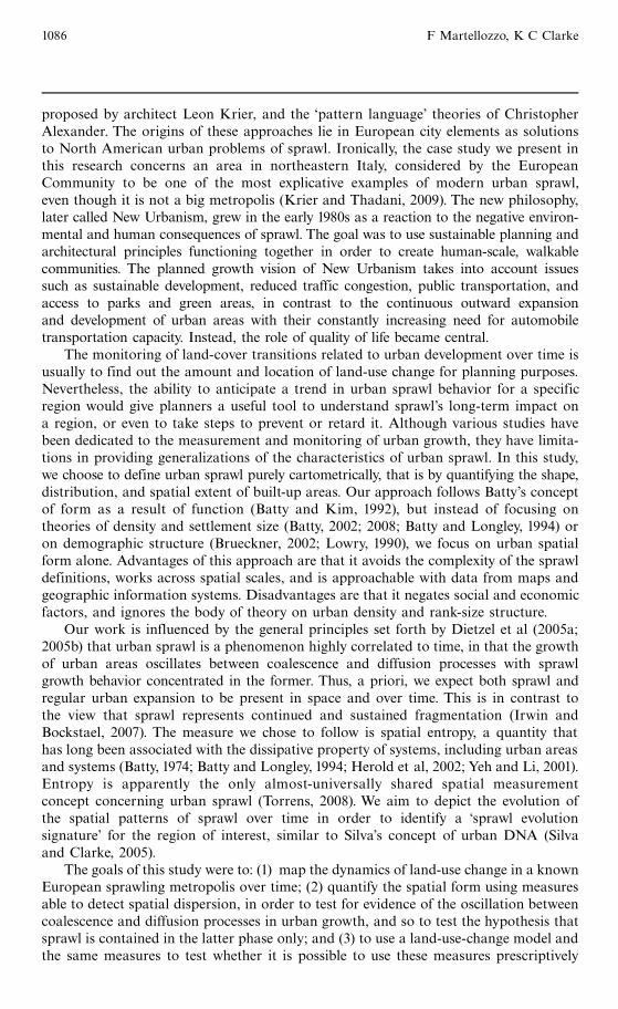
A comparison of the accuracy assessment from the Landsat 2001 image classified withthe three different classification methods (table 3) showed that the classification mostsuitable for the area of interest was the ML procedure, since both the kappa index andoverall accuracy show that ML classification is significantly better than the supervisedand unsupervised methods. The superior accuracy of the ML method is also easy tosee by visual inspection of the image (see figure 2).

Following comparison of the different classification methods based on the 2001Landsat image, the ML procedure was selected and applied to each image in thedataset as follows. First, training areas for each class were identified and from these

Table 3. Accuracy assessment for each classification method applied to the Landsat image from2001.

Reference Classification Producer's User's Overall Kappamap accuracy accuracy classification index

(%) (%) accuracy (%)

Orthophoto 2003� Unsupervised 71.43 55.56 60.00 0.5277Landsat 2002 ISODATA

Orthophoto 2003� Supervised 68.63 55.32 63.33 0.5706Landsat 2002 maximum

likelihood

Orthophoto 2003� machine 81.85 76.87 76.67 0.7246Landsat 2002 learning

Administrative boundaries

Water

Forest

Shrubs

Arable

Bare ground

Periurban

Urban(a)

(b)

(c) (d)

Figure 2. [In color online.] Detail of the Landsat 2001 image classified with the (a) unsupervised,(b) supervised, and (c) machine-learning methods; (d) shows the same portion of the image as itappears in the orthophoto image used as reference map for the accuracy assessment.


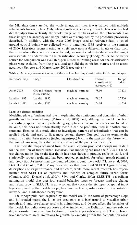
the ML algorithm classified the whole image, and then it was trained with multiplerefinements for each class. Only when a sufficient accuracy in each class was reacheddid the algorithm reclassify the whole image on the basis of all the refinements. Forthese images the accuracy and kappa index were computed by the procedure previouslydescribed. In addition, with the Aster 2005 image used as reference data, a set ofground control points were collected with a hand-held GPS receiver in the summerof 2006. Literature suggests using as a reference map a different image or data fromthat from which the classification is derived, because it could introduce bias that mightoverestimate or underestimate the classification accuracy (Foody, 2002). As no bettersource for comparison was available, pixels used as training areas for the classificationphase were excluded from the pixels used to build the confusion matrix and to assessaccuracy (Favretto and Martellozzo, 2008) (see table 4).

Land-use-change modelingModeling plays a fundamental role in explaining the spatiotemporal dynamics of urbangrowth and land-use change (Petrov et al, 2009). Yet, although a model has beensuccessfully applied in one particular geographical area and outcomes are found tobe valid, this does not automatically mean it can be profitably used in another envi-ronment. Even so, this study aims to investigate patterns of urbanization that can beapplied widely and used to fit a more general theory. Our goal was to examine thetrends in spatial form metrics (including entropy) both in the past and the future, withthe goal of assessing the value and consistency of the predictive measures.

The thematic maps obtained from the classifications produced enough useful datafor the creation of future urban scenarios. For modeling we used the SLEUTH land-use-change model due to the fact that it has been shown to produce realistic, valid, andstatistically robust results and has been applied extensively for urban-growth planningand prediction for more than one hundred cities around the world (Clarke et al, 2007;Dietzel and Clarke, 2007). Many prior studies that have used SLEUTH give thoroughdescriptions of its performance and structure, while more recent research has experi-mented with SLEUTH on patterns and theories of complex future urban forms(Candau, 2003; Dietzel et al, 2005b; Silva and Clarke, 2002). SLEUTH is a cellularautomaton model that uses four spatial-behavior types to forecast land-use changeand urban growth. SLEUTH is an acronym that covers the six types of spatial inputlayers required by the models: slope, land use, exclusion, urban extent, transportationnetwork, and a hill-shaded background.

The topographic data required by the model are in the form of percentage slopeand hill-shaded maps, the latter are used only as a background to visualize urbangrowth and land-use-change results in animations, and do not affect the behavior ofthe model. For calibration purposes and to implement the Deltatron land-use submo-del, a consistent land-use classification for two time periods is required. The exclusionlayer introduces areal limitations to growth by excluding from the computation areas

Table 4. Accuracy assessment report of the machine learning classification for dataset images.

Reference map Image Classification Overall Kappaclassification indexaccuracy (%)

Aster 2005 Ground control point machine learning 78.00 0.7408(GPS survey)

Landsat 1992 Landsat 1992 machine learning 78.57 0.7500

Landsat 1985 Landsat 1985 machine learning 77.14 0.7284


where urban growth is not possible, for example, water bodies. The user can also usea weights layer in order to establish a certain degree of `resistance' (Clarke, 2008)against growth, in an attempt to reduce or modify the urbanization rate due to legalrestriction, zoning, or differential suitability.

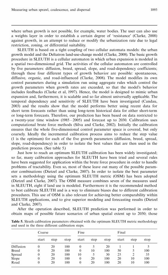
SLEUTH is based on a tight coupling of two cellular automata models: the urbangrowth model and the Deltatron land-use-change model (Clarke, 2008). The basic growthprocedure in SLEUTH is a cellular automaton in which urban expansion is modeled ina spatial two-dimensional grid. The activities of the cellular automaton are controlledby five parameters: diffusion, breed, spread, slope, and road-dependency coefficients;through these four different types of growth behavior are possible: spontaneous,diffusive, organic, and road-influenced (Clarke, 2008). The model modifies its owncontrol parameters during a simulation run using aggregate rules which control thegrowth parameters when growth rates are exceeded, so that the model's behaviorincludes feedbacks (Clarke et al, 1997). Hence, the model is designed to mimic urbanexpansion and, furthermore, it is scalable and so far almost universally applicable. Thetemporal dependency and sensitivity of SLEUTH have been investigated (Candau,2003) and the results show that the model performs better using recent data forshort term forecasts rather than using long-term historical data for either short-termor long-term forecasts. Therefore, our prediction has been based on data restricted toa twenty-year time window (1985 ^ 2005) and forecast up to 2030. Calibration usescomputational brute force methods (Silva and Clarke, 2002). Initially the calibrationensures that the whole five-dimensional control parameter space is covered, but onlycoarsely. Ideally the incremental calibration process aims to reduce the step value(1 is the optimum) for each of the five growth parameters (diffusion, breed, spread,slope, road-dependency) in order to isolate the best values that are then used in theprediction process. (See table 5.)

Just how to reach an optimum SLEUTH calibration has been widely investigated;so far, many calibration approaches for SLEUTH have been tried and several ruleshave been suggested for application within the brute force procedure in order to handleproblems of tractability. Even so, most of these leave out many of the possible param-eter combinations (Dietzel and Clarke, 2007). In order to isolate the best parametersets a methodology using the optimum SLEUTH metric (OSM) has been adopted(Dietzel and Clarke, 2007). The OSM measure combines seven of the measures usedin SLEUTH, eight if land use is modeled. Furthermore it is the recommended methodto best calibrate SLEUTH and is a way to eliminate biases due to different calibrationprocedures. This use of OSM is also relevant for achieving better comparability withinSLEUTH applications, and to give superior modeling and forecasting results (Dietzeland Clarke, 2007).

After the operation described, SLEUTH prediction was performed in order toobtain maps of possible future scenarios of urban spatial extent up to 2030; those

Table 5. Sleuth calibration parameters obtained with the optimum SLEUTH metric methodologyand used in the three different calibration steps.

Coarse Fine Final

start step stop start step stop start step stop

Diffusion 0 20 100 0 5 20 1 1 5Breed 0 20 100 0 10 100 50 5 100Spread 0 20 100 10 5 30 25 2 35Slope 0 20 100 0 20 100 20 10 100Road 0 20 100 0 20 100 20 10 100


results were then used with the classified historical maps to observe spatial form andentropy trends in urban patterns from 1985 to 2030 for a time span of almost half acentury. The model was capable of creating annual projections, unlike the data frompast years where only four time slices were available.

EntropyMany studies in geography, economics, or other social sciences have used the conceptof entropy to describe the dispersal of activities or phenomena in spatial settings(Hekkila and Hu, 2006). To state that a relation or a phenomenon shows spatialvariability implies that the observations are not spatially stationary at all times (Novelliand Occelli, 1999), hence spatiotemporal investigation of urban sprawl is justified. Oneway to look at urban sprawl is to consider the urban extent as a phenomenon spatiallydispersed across the territory or spatial extent and considered as the density of urbanland with respect to the total land area available, yielding a fundamental measure ofurban density:

fi �D act

iXki

D acti

, (1)

where D acti , the density of land development in the ith zone [equal to the amount of

actual land developed (built-up land)], is divided by the amount of land that isavailable for development (ie, excluding water bodies or nonconvertible land uses)for a total of k zones.

administrative boundary

class 1Ðwater

class 2Ðriparial trees

class 3Ðlow vegetation

class 4Ðcrops

class 5Ðbare ground

class 6Ðperiurban

class 7Ðurban

(b)

(c)

(e)(d)

(a)

1985

1992

20052001

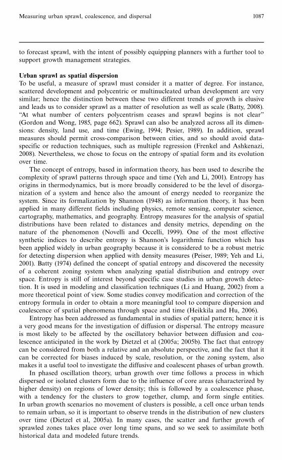
Figure 3. [In color online.] (a) Municipal boundaries of the study area used for the entropyzoning scheme, and (b) classified land cover for 1985; (c) 1992; (d) 2001, and (e) 2005.


The general entropy function is believed to have some limitations because itcontains bias when used for a wider period of time or for different areas. Even thoughour study focused only on a single area, we calculated Batty's entropy H because it iswidely considered to be more spatially oriented ` though Batty had clearly space inmind when he introduced equation (2)'' (Hekkila and Hu, 2006, page 853).

H � ÿXk

i

ln�

fiDi

�, (2)

where Di represents the discrete extent of the feature analyzed for the ith category, and,as before, fi is urban density.

Given that entropy can be usefully applied to investigate the spatial spread ofgeographical phenomena, we examined the differences among entropy at differenttimes (Ht�1 ÿHt ), as this change might indicate a change in the degree of dispersionof land (urban) development or urban sprawl (Yeh and Li, 2001). While looking atentropy the choice of an informative zoning system is very important. The zonesshould not be too numerous because this would overestimate the level of entropy(Hekkila and Hu, 2006), and entropy must be sufficiently accurate to convey theinformation on sprawl that we seek. We chose to use the municipal boundaries todivide the Pordenone metropolitan area into six zones (figure 3).

Results and discussionSLEUTH was calibrated for Pordenone and used to forecast urban expansion andland-use transitions up to 2050. The forecast period is probably too large, because itis well known that prediction results are more reliable when the forecast time span is aswide as or smaller than the time span of the input data used for calibration (Dietzeland Clarke, 2007). However, the calibration achieved OSM values close to 0.3. OSM isa composite of eight measures of goodness of fit from 0 to 1, multiplied together. Thesevalues were considered sufficient, and the values of coefficients used for the calibrationand their related OSMs are shown in table 6. These values were used in the finalcalibration to derive coefficient values to use for prediction (table 7).

We found that using standard SLEUTH forecasting parameters results in an over-estimate of growth. While SLEUTH applications usually assume that all areas thaturbanized in 90% of the Monte Carlo simulations are likely to become urban, insteadwe used 99%, a much higher level of confidence, and so fewer forecast urban areas. Wenoticed that land-use transitions and urban extents from the two confidence rates arealmost identical up to 2037 but, as might be expected, notable differences show up beyondthat time. Consequently, we used the more conservative definition of forecast growth.

Table 6. Ten best OSM results and coefficients.

Optimum CoefficientSLEUTH metric

diffusion breed spread slope road

0.30 10 83 86 44 550.28 8 83 86 44 570.27 11 83 86 42 540.27 11 83 86 44 570.27 11 83 86 44 570.26 10 83 86 44 540.26 11 83 86 44 530.26 11 83 86 42 570.26 11 83 86 43 55


Results show urban expansion in the area considered up to 2050 of more than 90%compared with 2005, implying that the urban area will double in less than half acentury (figure 4). The period 1985 ^ 2005 is known to have been characterized byincreasing sprawl. With geostatistical analysis and by visual inspection, we noticedthat the period 2005 ^ 20 is when most new urban clusters are generated, while2020 ^ 50 shows a predominance of coalescence between the clusters. Therefore, weexpected an increase in entropy around 2010 and a drop in entropy values whileapproaching 2050 (figure 5). Even so, the entropy trend shows that there is a breakpoint between 2005 and 2010 in which the slope of the curve changes dramatically, butthe drop that we expected was not found. This is the point when past data yield tomodel forecasts, so the change may be more abrupt than actual, yet the overall slowdown is apparent. This might be because the entropy value is strictly related to thetotal area of land available and depends on the zoning scheme chosen, or likewisebecause spatial entropy applied to spatially distributed data might be independent ofhow those geographical data are arranged in space.We note that `An entropy functioncan be applied to spatial data, but the entropy as such may be completely aspatial''(Karlstro« m and Ceccato, 2000, page 5).

The two-phase urban growth theory can help us to understand the entropy curvewe computed. In fact, the oscillation from a growth pushed by sprawl to a form ofgrowth influenced by coalescence it is not immediate but needs time to gradually shiftfrom one form to the other. Hence, we have to seek measures that can observe eitherthe level of dispersion or the degree of cohesion. Therefore, from this perspective,

Table 7. Coefficient change due to SLEUTH self-modification. The 2005 coefficients (rounded tointegers) were used for the prediction process. Forecast set was {12,100,100,5,59}.

Year Coefficient

diffusion breed spread slope road

1992 10.62 88.11 91.29 35.75 55.832001 11.61 96.36 99.84 15.29 57.872005 12.08 100 100 4.77 58.92

2005 2010 2020

2030 2040 2050

Figure 4. Output maps of SLEUTH forecast of urban area expansion up to 2050 (likelihood99%).


in order to investigate the distribution of urban spread, spatial autocorrelation mustbe reflected in the measure. Spatial autocorrelation is basically a comparison of twosets of similarities; similarities that can belong to either the attribute or the location(Goodchild, 1986). A measure of spatial autocorrelation can be intended as a descrip-tive index, focusing on patterns drawn by the way phenomena are spatially distributed.Even so ` at the same time the measure can be a causal process, measuring the degreeof influence exerted by something over its neighbors'' (Karlstro« m and Ceccato, 2000,page 6). The main aim of this study is to investigate urban sprawl and to suggest asimpler and easier means of observing its trend over time. We note that the mostshared concept about urban sprawl is that it involves the spread of urban areas intothe surrounding landscape. This concept is closely associated with the number ofdistinct and separate clusters in the study area and the average size of the clusters.It is reasonable to imagine a sprawled area as characterized by a large number of smalldisconnected urban land parcels (or pixels), while on the other hand an urban formcharacterized by a small number of urban cells that is large and connected leads to anurban growth pattern that follows cohesion principles. In other words, the degree towhich an urban system is previously clustered represents an initial condition thatpropagates into future patterns. Consequently, we calculated both the average cluster(of urban cells) size and the number of clusters and then normalized these measuresover the time span in order to have more comparable values (figure 6).

These data reveal a situation in which urban extent is continuously and graduallygrowing and the average cluster size also gradually grows. Yet the number of clustersinitially increases and then falls, curiously at almost the same time that Batty's entropytrend shows a change in slope (figure 5), in about 2009. These observations lead us tobelieve that the time of maximum sprawl in the Pordenone region is when the distancebetween curves 2 and 3 in figure 6 is largest; while when they cross, in about 2034, iswhen sprawl will eventually end in favor of the increased coalescence of urban areas.To better observe and depict the Pordenone urban growth trend we computed an indexthat summarizes the results and dynamics conveyed by the number of clusters and the

Batty's

spatialentropy

2.4

2.2

2.0

1.8

1.6

1.4

1.2

1.0

0.81985 1995 2005 2015 2025 2035 2045

1990 2000 2010 2020 2030 2040 2050

Figure 5. Batty's spatial entropy for 1985 ^ 2050.


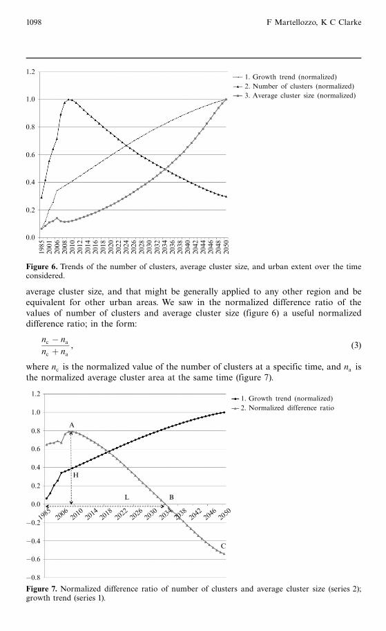
average cluster size, and that might be generally applied to any other region and beequivalent for other urban areas. We saw in the normalized difference ratio of thevalues of number of clusters and average cluster size (figure 6) a useful normalizeddifference ratio; in the form:

nc ÿ nanc � na

, (3)

where nc is the normalized value of the number of clusters at a specific time, and na isthe normalized average cluster area at the same time (figure 7).

1.2

1.0

0.8

0.6

0.4

0.2

0.0

1985

2001

2006

2008

2010

2012

2014

2016

2018

2020

2022

2024

2026

2028

2030

2032

2034

2036

2038

2040

2042

2044

2046

2048

2050

1. Growth trend (normalized)

2. Number of clusters (normalized)

3. Average cluster size (normalized)

Figure 6. Trends of the number of clusters, average cluster size, and urban extent over the timeconsidered.

1.2

1.0

0.8

0.6

0.4

0.2

0.0

ÿ0.2

ÿ0.4

ÿ0.6

ÿ0.8

1. Growth trend (normalized)

2. Normalized difference ratio

1985

2006

2010

2014

2018

2022

2026

2030

2034

2038

2042

2046

2050

A

H

L B

C

Figure 7. Normalized difference ratio of number of clusters and average cluster size (series 2);growth trend (series 1).


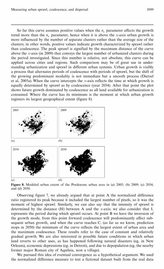
So far this curve assumes positive values when the nc parameter affects the growthtrend more than the na parameter, hence when it is above the x-axis urban growth ismore influenced by the number of separate clusters rather than the average size of theclusters; in other words, positive values indicate growth characterized by sprawl ratherthan coalescence. The peak sprawl is signified by the maximum distance of the curveabove the x-axis (in 2009) that conveys the largest number of urbanized clusters duringthe period investigated. Since this number is relative, not absolute, this curve can beapplied across cities and regions. Such comparison may be of great use in under-standing urbanization and sprawl in different urban systems. Urban growth is visiblya process that alternates periods of coalescence with periods of sprawl, but the shift ofthe growing predominant modality is not immediate but a smooth process (Dietzelet al, 2005a). When the curve intercepts the x-axis reflects the time at which growth isequally determined by sprawl as by coalescence (year 2034). After that point the plotshows future growth dominated by coalescence as all land available for urbanization isconsumed. Where the curve has its minimum is the moment at which urban growthregisters its largest geographical extent (figure 8).

Observing figure 7, we already argued that at point A the normalized differenceratio registered its peak because it included the largest number of pixels, so it was themoment of highest sprawl. Similarly, we can also say that the intensity of sprawl isdetermined by the distance (H) between A and the x-axis; we also consider that Lrepresents the period during which sprawl occurs. At point B we have the inversion ofthe growth mode, from this point forward coalescence will predominantly affect sub-sequent urban growth, and when the curve reaches C, (as far as we know, predictionstops in 2050) the minimum of the curve reflects the largest extent of urban area andthe maximum coalescence. These results refer to the case of constant and relativelygradual growth. We are also interested in possible future conditions in which urbanland reverts to other uses, as has happened following natural disasters (eg, in NewOrleans), economic depressions (eg, in Detroit), and due to depopulation (eg, the nearbyformer major Roman city of Aquileia, now a village).

We pursued this idea of eventual convergence as a hypothetical argument. We usedthe normalized difference measure to test a fictional dataset built from the real data

(a) (b)

(c) (d)

2005 2009

2034 2050

Figure 8. Modeled urban extent of the Pordenone urban area in (a) 2005; (b) 2009; (c) 2034;and (d) 2050.


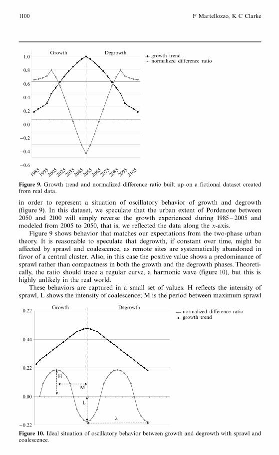
in order to represent a situation of oscillatory behavior of growth and degrowth(figure 9). In this dataset, we speculate that the urban extent of Pordenone between2050 and 2100 will simply reverse the growth experienced during 1985 ^ 2005 andmodeled from 2005 to 2050, that is, we reflected the data along the x-axis.

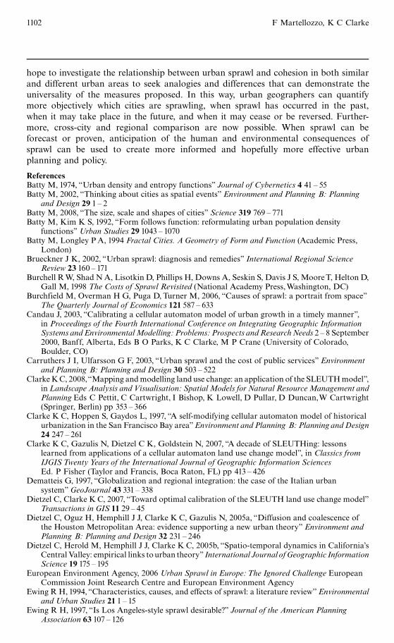
Figure 9 shows behavior that matches our expectations from the two-phase urbantheory. It is reasonable to speculate that degrowth, if constant over time, might beaffected by sprawl and coalescence, as remote sites are systematically abandoned infavor of a central cluster. Also, in this case the positive value shows a predominance ofsprawl rather than compactness in both the growth and the degrowth phases. Theoreti-cally, the ratio should trace a regular curve, a harmonic wave (figure 10), but this ishighly unlikely in the real world.

These behaviors are captured in a small set of values: H reflects the intensity ofsprawl, L shows the intensity of coalescence; M is the period between maximum sprawl

1.0

0.8

0.6

0.4

0.2

0.0

ÿ0.2

ÿ0.4

ÿ0.6

growth trendnormalized difference ratio

Growth Degrowth

1985199520052025203520452055

2105

2065207520852095

Figure 9. Growth trend and normalized difference ratio built up on a fictional dataset createdfrom real data.

Growth Degrowth0.22

0.44

0.22

0.00

ÿ0.22

normalized difference ratiogrowth trend

H

M

L

l

Figure 10. Ideal situation of oscillatory behavior between growth and degrowth with sprawl andcoalescence.


and highest compactness, and l determines the period during which the urban areapasses from its largest extent to its smallest.

Using the results presented allows us to describe the behavior of urban expansionover time and to focus on defining whether growth (or degrowth) will eventually beaffected by coalescence rather than spread. Both the growth trend and the normalizeddifference ratio can be used to classify growth in the two phases. To define furtherwhether an urban area is passing through a coalescence phase rather than sprawling wecomputed the simple ratio between the number of clusters and average cluster size(figure 11). From the results obtained by measurement and with SLEUTH, the Porde-none urban area faces the greatest amount of sprawl somewhere between 2005 and2010 (probably in 2009), after which the growth mode shifts from sprawl to coalescencesomewhere around 2034. The simple ratio in 2034 is forecast to be 7.81, which suggeststhat anything below that value would be indicative of coalescence, while on the otherhand everything above 7.81 should reflect sprawl. These assertions must be testedagainst known historical data, since the data for Pordenone cannot clarify completelythe relation between the number of clusters and average cluster size.

ConclusionSo far the observations we have made allow understanding of what kind of landcovertransitions occurred in the past and toward which future forms they could lead.Similarly the forecast modeling provides a longer time span on which to compareand analyze the modifications of the spatial form of the urban environment. Fromthe Italian Urban System Dynamics (Dematteis, 1997) we found evidence of thetendency of an urban node to first sprawl and then start cohesion in order to gainmore importance in the network. Hence, our investigation conducted with the aim ofdetecting the spatial dispersion of the system through entropy, which proved unsatis-factory as an aggregate measure of sprawl, led us to develop an approach based on thesame principles supported by evidence of the oscillatory behavior of urban growth setforth by Dietzel et al (2005a). We also tested the index with a hypothetical growth/degrowth trend. The authors are aware that a single case study cannot prove atheoretical framework; nevertheless, we believe the methodology and measures pre-sented are useful tools for urban planners and policy makers. In future research we

simple rationcna

� �80

70

60

50

40

30

20

10

0

1985

2001

2006

2008

2010

2012

2014

2016

2018

2020

2022

2024

2026

2028

2030

2032

2034

2036

2038

2040

2042

2044

2046

2048

2050

Figure 11. Simple ratio of number of clusters and average cluster size.


hope to investigate the relationship between urban sprawl and cohesion in both similarand different urban areas to seek analogies and differences that can demonstrate theuniversality of the measures proposed. In this way, urban geographers can quantifymore objectively which cities are sprawling, when sprawl has occurred in the past,when it may take place in the future, and when it may cease or be reversed. Further-more, cross-city and regional comparison are now possible. When sprawl can beforecast or proven, anticipation of the human and environmental consequences ofsprawl can be used to create more informed and hopefully more effective urbanplanning and policy.

ReferencesBatty M, 1974, ` Urban density and entropy functions'' Journal of Cybernetics 4 41 ^ 55Batty M, 2002, ``Thinking about cities as spatial events'' Environment and Planning B: Planning

and Design 29 1 ^ 2Batty M, 2008, ``The size, scale and shapes of cities'' Science 319 769 ^ 771Batty M, Kim K S, 1992, ` Form follows function: reformulating urban population density

functions'' Urban Studies 29 1043 ^ 1070Batty M, Longley P A, 1994 Fractal Cities. A Geometry of Form and Function (Academic Press,

London)Brueckner J K, 2002, ` Urban sprawl: diagnosis and remedies'' International Regional Science

Review 23 160 ^ 171Burchell RW, Shad NA, Lisotkin D, Phillips H, Downs A, Seskin S, Davis J S, MooreT, Helton D,

Gall M, 1998 The Costs of Sprawl Revisited (National Academy Press,Washington, DC)Burchfield M, Overman H G, Puga D, Turner M, 2006, ` Causes of sprawl: a portrait from space''

The Quarterly Journal of Economics 121 587 ^ 633Candau J, 2003, ` Calibrating a cellular automaton model of urban growth in a timely manner'',

in Proceedings of the Fourth International Conference on Integrating Geographic InformationSystems and EnvironmentalModelling: Problems: Prospects andResearchNeeds 2 ^ 8 September2000, Banff, Alberta, Eds B O Parks, K C Clarke, M P Crane (University of Colorado,Boulder, CO)

Carruthers J I, Ulfarsson G F, 2003, ` Urban sprawl and the cost of public services'' Environmentand Planning B: Planning and Design 30 503 ^ 522

ClarkeKC, 2008,` Mapping andmodelling land use change: an application of the SLEUTHmodel'',in Landscape Analysis and Visualisation: Spatial Models for Natural Resource Management andPlanning Eds C Pettit, C Cartwright, I Bishop, K Lowell, D Pullar, D Duncan,W Cartwright(Springer, Berlin) pp 353 ^ 366

Clarke K C, Hoppen S, Gaydos L, 1997, À self-modifying cellular automaton model of historicalurbanization in the San Francisco Bay area''Environment and Planning B: Planning and Design24 247 ^ 261

Clarke K C, Gazulis N, Dietzel C K, Goldstein N, 2007, À decade of SLEUTHing: lessonslearned from applications of a cellular automaton land use change model'', in Classics fromIJGIS TwentyYears of the International Journal of Geographic Information SciencesEd. P Fisher (Taylor and Francis, Boca Raton, FL) pp 413 ^ 426

Dematteis G, 1997, ` Globalization and regional integration: the case of the Italian urbansystem'' GeoJournal 43 331 ^ 338

Dietzel C, Clarke KC, 2007, ` Toward optimal calibration of the SLEUTH land use change model''Transactions in GIS 11 29 ^ 45

Dietzel C, Oguz H, Hemphill J J, Clarke K C, Gazulis N, 2005a, ` Diffusion and coalescence ofthe Houston Metropolitan Area: evidence supporting a new urban theory'' Environment andPlanning B: Planning and Design 32 231 ^ 246

Dietzel C, Herold M, Hemphill J J, Clarke K C, 2005b, ``Spatio-temporal dynamics in California'sCentral Valley: empirical links tourban theory'' International Journal ofGeographic InformationScience 19 175 ^ 195

European Environment Agency, 2006 Urban Sprawl in Europe: The Ignored Challenge EuropeanCommission Joint Research Centre and European Environment Agency

Ewing R H, 1994, ` Characteristics, causes, and effects of sprawl: a literature review''Environmentaland Urban Studies 21 1 ^ 15

Ewing R H, 1997, `Ìs Los Angeles-style sprawl desirable?'' Journal of the American PlanningAssociation 63 107 ^ 126


Ewing RH, Pendall R, Chen DDT, 2002Measuring Sprawl and its Impact Smart Growth America,Washington, DC

Ewing R, Schmid T, Killingsworth R, Zlot A, Raudenbush S, 2003, ` Relationship between urbansprawl and physical activity, obesity, and morbidity'', in Urban Ecology: An InternationalPerspective on the Interaction BetweenHumans andNatureEds J M Marzluff, E Schulenberger,W Endlicher, M Alberti, G Bradley, C Ryan, U Simon, C ZumBrunnen (Springer, NewYork)pp 567 ^ 582

Ewing R H, Bartholomew K,Winkelman S,Walters J, Chen D, 2007 Growing Cooler: Evidenceon Urban Development and Climate Change (Urban Land Institute,Washington, DC)

Favretto A, 2006 Strumenti per l'Analisi Geografica GIS e Telerilevamento (Patron, Bologna)Favretto A, Martellozzo F, 2008, ` Evoluzione della copertura del suolo in ambito urbano. Uno

studio preliminare per alcuni della Provincia di Pordenone (Friuli Venezia Giulia) attraversoimmagini tele rivelate di periodi diversi'', in Atti del VII Workshop ` Beni Ambientali eCulturali e GISöComunicare l'Ambiente'' [Land cover transitions in an urban environment.An introductory study of somemunicipalities of the Pordenone province (Friuli Venezia Giulia Îtaly) with time-series remote sensed images'', in Proceedings of theVIIWorkshopÈnvironmentaland Cultural Heritage and GISöCommunicating the Environment''], Trieste, 21 November(Patron, Bologna) pp 69 ^ 76

Foody G M, 2002, ` Status of land cover classification accuracy assessment''Remote Sensing ofEnvironment 80 185 ^ 201

Frenkel A, Ashkenazi M, 2008, ` Measuring urban sprawl: how can we deal with it?'' Environmentand Planning B: Planning and Design 35 56 ^ 79

Glaeser E L, Kahn M E, 2003, ` Sprawl and urban growth'', DP 2004, Harvard Institute ofEconomic Research, http://www.economics.harvard.edu/pub/hier/2003/HIER2004.pdf

Goodchild M F, 1986 Spatial Autocorrelation, Concepts and Techniques in Modern Geographyvolume 47 (GeoBooks, Norwich)

Gordon P,Wong H L, 1985, ` The costs of urban sprawl: some new evidence'' Environment andPlanning A 17 661 ^ 666

Hasse J E, Lathrop R G, 2003, ` Land resource impact indicators of urban sprawl''AppliedGeography 23 159 ^ 175

Heikkila E J, Hu L, 2006, Àdjusting spatial-entropy measures for scale and resolution effects''Environment and Planning B: Planning and Design 33 845 ^ 861

HeroldM, Scepan J, ClarkeKC, 2002, ` The use of remote sensing and landscape metrics to describestructures and changes in urban land uses'' Environment and Planning A 34 1443 ^ 1458

Huang X, Jensen R J, 1997, À machine-learning approach to automated knowledge-basebuilding for remote sensing image analysis with GIS data'' Photogrammetric Engineering andRemote Sensing 63 1185 ^ 1194

Irwin E G, Bockstael N E, 2007, ` The evolution of urban sprawl: evidence of spatial heterogeneityand increasing land fragmentation'' Proceedings of the National Academy of Sciences (PNAS)104(52) 20672 ^ 20677

Jensen R J, 1996 Introductory Digital Image Processing: A Remote Sensing Perspective 2nd edition(Prentice-Hall, Upper Saddle River, NJ)

Karlstro« m E, Ceccato V, 2000, À new information theoretical measure of global and local spatialassociation'' Papers of the European Regional Science Association Barcelona, 29 August ^1 September, Royal Institute of Technology, Stockholm, http://mpra.ub.uni-muenchen.de/6848/1/WRSA08.pdf

Krier L, Thadani D, 2009 The Architecture of Community (Island Press,Washington, DC)Li Z, Huang P, 2002, ` Quantitative measures for spatial information maps'' International

Journal of Geographic Information Science 16 699 ^ 709Lowry I S, 1990, ` World urbanization in perspective'', in Population and Development Review 16

Supplement: Resources, Environment, and Population: Present Knowledge, Future OptionsEds K Davis, M S Bernstam (Oxford University Press, NewYork) pp 148 ^ 176

Novelli E, Occelli S, 1999, ` Profili descrittivi di distribuzioni spaziali: alcune misure didiversificazione'' Cybergeo: European Journal of Geography, Syste© mes, Modelisation,Geostatistiques 108 http://cybergeo.revues.org/4930?lang=en

Peiser R B, 1989, ` Density and urban sprawl'' Land Economics 65(3) 193 ^ 204Petrov L O, Lavalle C, Kasanko M, 2009, ` Urban land use scenarios for a tourist region in

Europe: applying the MOLAND model to Algarve, Portugal'' Landscape and Urban Planning92 10 ^ 23


Shannon C E, 1948, `A mathematical theory of communication'' Bell System Technical Journal27 379 ^ 423; 623 ^ 656

Silva E, Clarke C K, 2002, ``Calibration of the SLEUTH urban growth model for Lisbon andPorto, Portugal'' Computers, Environments and Urban Systems 26 525 ^ 552

Silva E, Clarke K C, 2005, ``Complexity, emergence and cellular urban models: lessons learnedfrom applying SLEUTH to two Portuguese metropolitan areas'' European Planning Studies13 93 ^ 115

Torrens P M, 2008, `A toolkit for measuring sprawl''Applied Spatial Analysis 1 5 ^ 36Yeh A G, Li X, 2001, ` Measurement of urban sprawl in a rapidly growing region using entropy''

Photogrammatic Engineering and Remote Sensing 67 83 ^ 90

ß 2011 Pion Ltd and its Licensors


Conditions of use. This article may be downloaded from the E&P website for personal researchby members of subscribing organisations. This PDF may not be placed on any website (or otheronline distribution system) without permission of the publisher.

Measuring urban sprawl, coalescence, and dispersal: a case study of Pordenone, Italy

Documents

Transcript of Measuring urban sprawl, coalescence, and dispersal: a case study of Pordenone, Italy