1

Land consumption by urban sprawl - a new approach to deduce urban development scenarios from actors’ preferences Diana Reckien, Klaus Eisenack, Matthias K. B. Lüdeke

MANUSCRIPT

0B0BAbstract

A new modelling approach to urban sprawl dynamics is introduced which allows representing qualitative

knowledge on relations between moving actor populations and properties of locations. The results of this

Qualitative Attractiveness Migration (QuAM) Model are scenario-like sets of possible future developments of

the urban system, much in contrast to quantitative forecasts gained by traditional modelling approaches. QuAM-

models allow for the interaction between internal dynamics and external influences. The application of the new

approach is exemplified by the case of urban sprawl in Leipzig since 1990. It was possible to reproduce the

observed qualitative development and to calculate future scenarios. The scenario runs project a new wave of

middle class driven residential sprawl and suggest implications for sprawl reducing policy interventions.

Keywords: urban sprawl, land consumption, preferences, qualitative differential equations

Diana Reckien

Matthias K. B. Lüdeke ()

Potsdam Institute for Climate Impact Research

P.O. Box 601203

14412 Potsdam

Germany

e-mail: luedeke@pik-potsdam.de

Tel: +49 (0)331 288 2578

Fax: +49 (0)331 288 20709

Klaus Eisenack

Carl von Ossietzky University Oldenburg

Department of Economics and Statistics

26111 Oldenburg, Germany

2

1B1B1 Introduction

This paper aims to introduce a new modelling approach to urban sprawl which allows representing

qualitative knowledge on relations between properties of locations and moving actor populations. Such an

approach enables the formalization of interactions that are difficult to quantify, i.e. social and socio-economic

processes such as migration and the relation between actors and their environment.

A qualitative dynamic modelling approach can deal with a number of problems that are difficult to

answer with quantitative modelling. Variables can be measured on ordinal scale instead of real or ratio-scale,

which is often difficult, particularly when social and socio-economic processes are to be formalized [38];

relations are represented by large classes of functions, thereby avoiding specific and sometimes poorly justified

parameterisations; results are sequences of trend combinations forming qualitative instead of quantitative

trajectories, often forming a more adequate representation of our knowledge of the system; and the possibility of

branching in the qualitative trajectories allows for alternative future developments that are in accordance with the

model assumptions. Particularly the last feature bridges the gap between techniques which analyse future

development by alternative scenarios mainly based on plausibility [46] and unique quantitative trajectories based

on, e.g., systems of differential equations [1]. We could show the appropriateness of the dynamic qualitative

modeling approach for other socio-ecological systems with hardly quantifiable relations, e.g. in the realm of

sustainable agriculture [17, 43], fisheries management [16] and forest overexploitation [17].

In the urban sprawl model presented here the influence of environmental characteristics and other actors

on the households’ location attractiveness is described. Our qualitative modeling approach is well suited to

formalize the relation between different actor classes and between actors of the same class of moving

households, e.g. families with children, elderly people, young childless couples etc, through the actor classes’

impact on their environment and its characteristics. Changing quantities of certain household classes cause

dynamics and generate scenario-like, qualitative development paths of spatial migration due to their

interdependencies to other household classes. We show that this approach generates valuable information to

support policy and plan making in urban, suburban and potentially other environments.

We will illustratively describe the approach by way of an empirical example of migration dynamics of

suburban households in Leipzig/Germany. Our focus reflects the general trend in urban development in Western

city regions, which, at least since the II. World War was mostly centrifugal [48]. This process known as

suburbanisation or urban sprawl describes the extension of urban settlements beyond the original urban fringes,

mainly along major transport routes, incorporating low-density development and mono-functional land use (see,

for example, [24, 54]). Increasing living standards, spare time and modern transportation technology have

enabled private and economic actors to re-evaluate spatial characteristics in order to live and work in more

pleasant surroundings. Social and technological changes put more emphasis on the value of environmental

characteristics. Debate about the consequences of sprawl often results from the discrepancy between the positive

consequences for private entities willing to relocate to suburban regions and the negative consequences for the

environment, the community as a whole, the environment and the economy [39, 54]. Causes and consequences

are not seldom located in different spatial areas and scales. This spatial mismatch makes sprawl difficult to

manage [50].

Success in controlling urban sprawl is limited so far [26]. This leaves the impression that sprawl

processes are not fully understood yet. We assume that an important, even crucial, aspect has not received

adequate attention, which is the relations (in-)between migrating actors conditioning the location characteristics

of a place, and that this is - at least partially - due to the limited possibilities of traditional dynamic modelling to

represent the respective knowledge adequately. Our assumption is that household interactions are very important

in the suburban realm and therefore need to be incorporated in simulation tools of population development at the

urban fringe. Brueckner and Largey [7] empirically found that social interactions in the low-density, suburban

realm are stronger than in dense, urban environment. They thereby disproved the counter-argument, which has

3

long been advocated, e.g. by Putnam [45] and others. People are influenced by others; follow other actors’

choices and opinions. Therefore, the social composition of neighbourhoods is an important issue for residential

migration, as it is for economic actors, i.e. represented by the importance of synergy effects [25]. Thus, actors

contribute to the attractiveness of a region in multiple, mutual ways. Actor populations are a feature of an area

and this must be at least qualitatively included in both firms’ and residents’ evaluations of spatial attractiveness

[1]. By considering this, we strive to contribute to a more comprehensive understanding of urban sprawl. This is

the precondition for the development of successful regulation systems enabling a more dense urban development

which lessens the presently alarming trends of land consumption.

In the next section we shortly review established approaches to model urban dynamics that motivate the

introduction of qualitative attractiveness models. We then introduce the basic concepts underlying our approach

and the mathematical theory in the third and forth, the methodological sections. The fifth section presents an

example of Leipzig to illustrate the steps necessary to define the model, including the empirical base. The

application demonstrates the deductive abilities (and limitations) of the new approach, which are again discussed

in the final section.

2B2B2 Comparison of current methods and rationale for QuAM-models

There exist a variety of formal dynamic modelling approaches to urban development, each of them

emphasizing different facets of the complex phenomenology and variety of interacting mechanisms which

generate urban dynamics. Although not explicitly dealing with urban expansion a methodically paradigmatic

branch started with the checkerboard model of segregation by Schelling [52]. The basic idea is that the decision

to stay or to move is made in dependence on the (e.g., racial) composition of an actor's neighbourhood. In case of

moving, the composition of both, the old and the new neighbourhood is changed, thereby directly influencing the

appropriateness of these for other actors and possibly initializing new moves. This generates different

developments depending on the initial distribution in space, the size of the neighbourhood and the rule

describing an acceptable neighbourhood composition. Eventually these development paths lead to either large

scale spatial segregation or other patterns. Recent applications are shown in, e.g., Zhang [60] and Fossett and

Waren [20]. Characteristic for this approach is the emphasis on the immediate feedback of location decisions of

moving actors on the decisions of others, a property which is due to our research on urban sprawl a decisive

element in understanding the observed dynamics [42].

These segregation models set the stage for the introduction of cellular automata in describing land use

dynamics in general [55] and modelling of urban development in particular [10]. The checkerboard model can

already be understood as a cellular automaton, but in the latter the number of considered actors or land use types

was increased. More complex rules for the appropriateness of a neighbourhood were the result; more complex

neighbourhood structures and stochastic elements were introduced [58]. Such models are widely used for urban

growth simulations, albeit there is a large variation in the importance of the endogenous (rule-based) dynamics

compared to exogenous settings. The latter comprise, amongst others, pre-given aggregated growth rates for each

land use type to make the results compatible to the observed spatial-temporal development by constraining the

endogenous rule-based development. The uncertainty arising from mapping originally qualitative (e.g. ordinal

scale) relations on - to some extent arbitrarily chosen - quantitative representations is one important reason for

the necessity to introduce strong exogenous constraints for the endogenous dynamics into the models. The

modelling approach suggested in this paper addresses this problem, at least for up to intermediate spatial

differentiations.

Another actor oriented view including behavioural aspects of migration was introduced by Wolpert [59].

The very rough assumptions on the “appropriateness” of a neighbourhood as applied in the cellular automata are

investigated in detail. Examples are the studies on the relation of stated preferences for city sizes and locations

(as inferred from surveys) and trends in population distribution in the USA by Fuguitt and Zuiches [21] and

4

Brown et al. [6]. Although these approaches deal mainly with the reasons for migration (i.e. push- and pull

factors), some of the studies also indicate how migration feeds back on the properties of locations. One example

is Weichhart [57] who shows that the natural environment of a location is an important determinant of residential

preferences - a spatial property which is certainly strongly influenced by in-migration. Others, e.g. Filion et al.

[18] study location preferences in a dispersed Canadian agglomeration. They found a high harmonisation of the

residents’ preferences with the attributes of dispersion and inferred the future "entrenchment" of the present

urban structure. These findings support the chosen model structure which emphasizes the interaction between

different actor groups.

Geographical economics mainly consider land prices and transportation costs to explain location

decisions of economic actors in an equilibrium setting [56, 2]. In these theories the spatial concentration of

economic activities was postulated but only partly explained. By introducing economies of scale and

monopolistic competition, Krugman [32, 33] and Fujita and Mori [22] solved this theoretical problem in a non-

trivial way. This approach extends the elaborated apparatus of economic theory to spatial dynamics under the

standard premise of invariant actor preferences. By its very nature, this approach focuses on the economic

dimension of spatial structure without necessarily looking at feedback loops of transport costs and development.

Loops of cause-effect relations are the core hypothesis of systems dynamics models. They allow for

flexible inclusion of non-economic relations between actors by quantifying these with plausible mathematical

functions, and by computing transient dynamics far from equilibrium [19, 1]. These models were the first that

mathematically investigated the influence of complex and differentiated relations between actors and places on

the qualitative spatial dynamics of an urban region. Systems dynamics models include relations that have to be

quantified with plausible, albeit not always further justified mathematical functions. To give an example,

knowing that an urban region becomes less attractive for retailers with a decreasing fraction of residents needs to

be described by an explicit function (linear or exponential etc.) in systems dynamics models although this is

somehow arbitrary if only the direction of influence is known. This exemplifies the problems of measurement, of

quantifying qualitative characteristics and of uncertainty in determining model parameters of socio-economic

systems, which goes along with all quantitative modelling approaches.

Serious concerns have been expressed about the use of computer simulations of urban dynamics in

general, partly due to various epistemological and methodological objections. Concerns are related to the use of

large-scale quantitative models that are often claimed to be too general in purpose [9], and to the application of

models to examine (only) land-use changes [13]. Large models tend to become a black box, making them an

unsuitable tool for learning. Not all of the approaches outlined above are explicitly dynamic in time. Some of

them integrate social with economic processes. But, the complexity and contingency of social processes makes

deterministic predictions impossible. Further problems of modelling coupled socio-economic and bio-physical

systems relate to heterogeneous knowledge from different scientific disciplines and to uncertainties that cannot

be expressed by probabilities [15]. However, quantitative models are also known for their power in making

assumptions and definitions explicit and for systematically exploring their consequence by deductive reasoning

[53]. When this potential is to be used to understand urban development, the above objections need to be

considered carefully.

To overcome some of the above-mentioned shortcomings we introduce a new model class, the Qualitative

Attractiveness Migration models (QuAM-models). They follow the systems dynamics heritage and combine

them with a number of characteristics of the other approaches. Qualitative attractiveness models mathematically

treat the influence of actors on each other as relations, but in contrast to simulation models not as mathematical

functions. Only qualitative relations, increasing or decreasing influences between the systems variables, are

considered instead. Such a modelling approach allows a projection of the variables’ development into the future.

The mathematical concept of qualitative differential equations (QDEs), which was first introduced by Kuipers

[34], allows realizing this program by representing qualitative relations without choosing one quantitative

function arbitrarily. An interesting consequence of this "honest" representation of knowledge in the model is that

5

the resulting dynamics (that can be deduced in a mathematically sound way) differ from usual outcomes of

quantitative dynamic models: different possible developments may occur and they are rather described in terms

of trends and trend changes than in terms of explicit numbers. This is to some extent unusual for the description

of a driver for environmental damages but - according to our view - robust statements like "given policy

intervention X the present expansion trend will monotonically decrease and eventually reverse" are sometimes

preferable over exact quantitative projections which are based on a - sometimes intransparent - multitude of

assumptions.

3B3B3 Methodological Approach

We suggest an actors approach assuming that households are the central elements in the suburban

migration process. But also business entities, retail units etc. are actors that condition the location characteristics

of a place. If the location preferences of these actors are known, they can be modelled. This approach is related

to action space research (Aktionsraumforschung), in which the city is a production of the cumulative actions of

individuals [23]. Individuals do not only shape the city around them, they are also influenced by their own

cumulative developments and do not act independently [23]. In response to the postulated insufficient

consideration of the individual actors’ roles in shaping the environment and sprawl development [47] this

approach supposes a strong individual motivation.

In action space research, groups of individuals are of particular importance since only an agglomeration

of actions will change the structure and therefore the production of the city. For that reason we look at migrating

household classes and businesses within the suburban area, groups of actors with similar location preferences

and attributes. Homogeneity in preferences and attributes is assumed to lead to recursive dynamics via two

mechanisms: (1) Groups of similar location preferences might result in a similar imprint on the city’s

development, because they are looking for similar residential areas; (2) Similar social strati and living conditions

of households as well as economic attributes of business actors are assumed to leave a similar feedback on the

location characteristics. The combination of (1) and (2) can change the migration patterns and results in a

dynamic process.

The boundaries of the suburban area that is to be modeled are not necessarily administrative. We are

following a functional definition of space [31]. All neighborhoods with a remarkable number of new migrants

and a recent influx of defined homogenous groups of inhabitants are covered.

The underlying assumption that the presence of certain actor classes is changing the attractiveness of the

region generates dynamics. The influences of actor classes on the different location preferences (dimensions of

attractiveness) have to be specified. Attractiveness of a suburban region is used in an extended sense, closer to

the migration decision: it comprises the usual location properties and the affordability to move for the considered

actor class. In this notation a region which, e.g., does not offer affordable housing is not attractive for a specific

actor class, independent from other advantages. The attractiveness of a region for an actor class depends on three

aspects:

a. The fixed characteristics of the respective region, e.g. orography,

b. The presence of other actor classes, and

c. Policy influences.

Actor classes migrate along attractiveness gradients (move from a region of lower to a region of higher

attractiveness). Thereby, actors reduce their population in the region they leave and increase it in the region they

move. This migration may change the attractiveness of both regions for all actor classes with respect to

mechanism (b) and cause further changes in migration fluxes. Aspect (a) can be and (b) is endogenous to the

formal model (both can be altered by the actor class populations); (a) can also be and (c) is exogenous. The

model considers net migration of actor classes, i.e. some actors of the class may well move in the other direction;

the model describes the aggregated net fluxes under mean preference assumptions. The main ideas are similar to

established attractiveness models in urban dynamics (see, e.g. [1]) but QuAM-models differ in modelling

6

qualitative relationships between variables.

4B4B4 Qualitative Differential Equations (QDEs)

We formalize the relations sketched above with the mathematical theory of QDEs [34] which is based on

dynamical systems theory, i.e. the state of a system is related to its rate of change. In the realm of usual

quantitative modelling this is represented by differential or difference equations where explicit numerical

relations between the variables and their rates of change are needed. In contrast, QDEs deduce the time

development of the variables from a much weaker, namely a "qualitative" understanding of the interactions of

the system elements. This qualitative understanding can be characterized by the following:

1. Which elements are directly related? (e.g., A and B may be directly related)

2. What is the direction of the influences? (e.g., B may influence A)

3. Is it a strengthening or alleviating influence? (e.g., B may alleviate A)

4. Is it an influence on the variable or its rate of change? (e.g., B alleviates the change of A)

Levels 3 and 4 imply that it is possible to describe the elements A and B of the system by ordinal scale,

i.e. a "greater/less than" relation can be defined. At level 4 of the determination QDEs can be applied and

generate the time course of the variables by their trends and trend changes. As QDEs are a generalized system

analytic method, the boundaries of the system, its elements, their qualitative relations and exogenous drivers

have to be identified. In all cases where this can be done at least in parts the method is applicable. It was

originally developed and applied by Kuipers and his group in physics and human physiology [34]. Further

applications emerged, e.g. in finance [3], epidemiology [29], chemistry [30] and the automotive industry [51]. It

is increasingly used in ecology [28, 4, 61]. In sustainability science it was applied on smallholder agriculture in

developing countries [43], fisheries management [16] and urban dynamics [47, 35]. Here, it was the aim to

calculate possible future developments from the qualitative systems understanding, to choose desirable outcomes

from the developed set of possible futures, and to identify critical branching points that allow assessing policy

options with a positive influence on the development.

Tailored to attractiveness migration models, the formal base of QDEs is as follows. We divide the area

under consideration into a set of m regions, indexed by r=1, ..., m. It is assumed that there are n distinct actor

classes (different kinds of residents, retailers, etc), indexed by i=1,..., n, and that members of each actor class

assess the attractiveness of urban regions with homogeneous preferences. The population of actors of class i in region r (at a given point in time) is expressed by the variable Pri. The attractiveness of an actor of class i

assigned to the region r (at a given point in time) is denoted by Ari. This implicitly assumes that the

attractiveness can be expressed as a one-dimensional, aggregate quantity. We will see, however, that the method

does not require a measure of aggregate attractiveness on a rational scale. For the exposition it is yet clearer to take all variables as measurable with rational scale. The attractiveness Ari(Pr1, ..., Prn, Eri) depends on the

presence of other actor classes in the region r, and possibly on further influences Eri. As for attractiveness, Eri is

implicitly a variable that needs to be measured quantitatively. Eri may represent the influences from actors in

other regions, other urban areas, policy measures. Crucial is here, that Eri is exogenously set, while the dynamics

of the other variables evolve by endogenous rules. Population changes in time t assign to that region according to dPri/dt = fri (A1i, …, Ari,…,Ami), where fri is an increasing function in Ari and a decreasing function in all other

arguments determining the population change of class i in region r depending on the attractiveness of this region

in comparison to the other regions.

If all these variables, dependencies and functions were known quantitatively, this formulation would set

up a dynamic system that can straightforward be simulated with readily available software. However, as

discussed above, this is generally not the case for urban and socio-economic systems. Measuring attractiveness is

prone to diverse subtleties. We therefore restrict ourselves to characterise the effect of a changing number of the population of actor class i in region r (Pri) on the attractiveness of, e.g., actor j in the same region (Arj) only by

the direction of influence (e.g.: "the attractiveness of an urban region for retailers decreases with a decreasing

7

number of residents"). Mathematically, this amounts to taking only the signs of the partial derivatives srij=Ari/Prj, eri=Ari/Eri as given. These signs can be, for example, expressed as a causal loop diagram (see

Figure 1) or as a matrix (see Table 1). To obtain the signs techniques of quantitative as well as of qualitative data

collection (interviews, oral history, focus groups, Delphi groups) and data analysis (hermeneutics, discourse

analysis, grounded theory) can be applied (for the potential role of these techniques in the different stages of

model development and interpretation of model results see [37]). We will show an example in section 5. QDEs

will determine all possible population paths in time that are compatible with the qualitative statements made in

the form of the causal loop diagram or matrix. As a consequence of the limited information used, the resulting

dynamics cannot be characterised by quantitative rates of change (e.g., “500 middle income families with

children will move to the periphery during the next year”) but only by trend combinations and their change (e.g.,

“while the population of retired residents will continuously increase, the number of families with children in a

particular region will first increase and then decrease”).

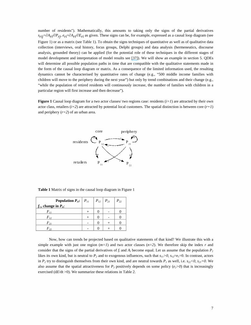
Figure 1 Causal loop diagram for a two actor classes/ two regions case: residents (i=1) are attracted by their own

actor class, retailers (i=2) are attracted by potential local customers. The spatial distinction is between core (r=1)

and periphery (r=2) of an urban area.

P11 P

22

P21

P12

++

++

--

-

-

core periphery

res idents

retailers

Table 1 Matrix of signs in the causal loop diagram in Figure 1

Population Pri:

fri, change in Pri:

P11 P12 P21 P22

F11 + 0 - 0

F12 + 0 - 0

F21 - 0 + 0

F22 - 0 + 0

Now, how can trends be projected based on qualitative statements of that kind? We illustrate this with a

simple example with just one region (m=1) and two actor classes (n=2). We therefore skip the index r and

consider that the signs of the partial derivatives of fi and Ai become equal. Let us assume that the population P1

likes its own kind, but is neutral to P2 and to exogenous influences, such that s11>0, s12=e1=0. In contrast, actors

in P2 try to distinguish themselves from their own kind, and are neutral towards P1 as well, i.e. s22<0, s21=0. We

also assume that the spatial attractiveness for P2 positively depends on some policy (e2>0) that is increasingly

exercised (dE/dt >0). We summarize these relations in Table 2.

8

Table 2 Matrix of signs for the one region example described in the text, including an exogenous policy

influence E

Population Pi:

fi - change in Pi:

P1 P2 E

f1 + 0 0

f2 0 - +

Now suppose that the region is currently in a situation with a trend combination where both populations

increase at the same time (dP1/dt, dP2/dt > 0). Is it possible that P1 or P2 will begin to decrease later? We first

consider a trend reversal for P1. Since the first derivative with respect to time is dP1/dt > 0, this is only possible

if the second derivate is d2P1/dt2 is negative. By the rules of calculus, differentiating yields

d2P1/dt2= f1/A1 (s11 dP1/dt + s12 dP2/dt + e1 dE/dt) = f1/A1 s11 dP1/dt.

Since all terms on the right hand side are positive, it is impossible that P1 becomes negative. This situation is

different for P2, where

d2P2/dt2= f2/A2 (s21 dP1/dt + s22 dP2/dt + e2 dE/dt)

= f2/A2 (s22 dP2/dt + e2 dE/dt).

Since the summands in the brackets have opposite signs, the overall sign of d2P1/dt2 is indeterminate, i.e.

depends on the absolute value of the coefficients. Since they are not explicitly known in the model, it must be

concluded that it is possible that P1 begins to decrease. This means that the system may change from a qualitative

state characterized by increasing P1 and P2 values into a state of increasing P1 and decreasing P2. This is the only

transition which is in accordance with the model assumptions. Figure 2 depicts this part of a qualitative

trajectory in symbols that are easy to grasp.

Figure 2 Qualitative trajectory as described in the text showing the only possible transition from the positive trend combination

possible transition

dP1 > 0

dt> 0

dP2

dt

dP1 > 0

dt< 0

dP2

dt

As mentioned before there is a further important feature of the method: Due to the qualitative

assumptions made in the model, it may happen that multiple different trend combinations follow in time.

Mapping all possible sequences of trend combinations can therefore result in “scenario trees”.

Making computations as above for a more complex model is cumbersome and bears the risk of errors.

There are cases where the calculus is not as simple. For that purpose, different software tools were developed

that take the list of variables, the signs of the partial derivatives and further qualitative constraints as input (e.g.

[34, 4]) and determine all possible trend combinations and sequences of trends automatically. For the purpose of

this paper, these program packages appeared to be unnecessarily comprehensive and a specific and fast version

with a simplified constraint satisfaction algorithm could be implemented based on the techniques developed in

[14, 36, 15].

In summary, setting up a qualitative attractiveness model involves the following steps:

9

1. Determine actor classes with homogeneous preferences and attributes.

2. Determine which actor classes contribute to or diminish the attractiveness for other actor classes or the

same class, and express this as a matrix of signs.

3. Compute all possible trend combinations and their sequence.

In the following, we present a real-world example and show what implications follow for urban policy and

plan making with respect to urban sprawl in Leipzig.

5B5B5 Application to urban sprawl in Leipzig

The analysis of sprawl in Leipzig is taken from an EU-project called URBS PANDENS [42]. The

identification of prominent actor classes, location preferences and attributes as well as feedbacks of the actor

class population on the properties of the location was achieved through expert interviews (urban researchers and

local experts). Other case studies that used qualitative attractiveness models based this information on household

surveys [47]. For the urban fringe of Leipzig four sprawl relevant actor classes (P1 - P4) have been identified in

the post-reunification period (approximately 1990 to 2005) on a level of aggregation which allows representing

the most important feedbacks:

1. Middle income households (P1)

2. High income households (P2)

3. Industries/businesses (P3)

4. Large retail/leisure centres (P4)

For all P1 - P4 seven potentially relevant dimensions of locational attractiveness have been identified (not

all dimensions apply to all actor classes):

Standard of flats (heating, bathroom, double-glazing windows etc.),

Price of accommodation (rents, prices of houses and premises),

Physical environment (density of settlement, proximity to natural landscape etc.),

Transport infrastructure (roads, train and bus lines),

Social aspects (social environment and image of the area),

Accessibility of large areas (e.g. for a shopping mall) and

Catchment area (number of customers able to visit a shopping mall and contributing to its profitability).

Attractiveness dimensions represent the preference for certain location characteristics. After their actor

class specific determination they are ordered (see Table 3, first column). In a following step, the influence of the

actor class populations on each dimension of attractiveness has to be discussed and determined (shown in Table

3, columns 2 - 5). Again, expert knowledge of the project participants and local researchers was used as basis,

which is documented in [42, 40, 12, 35]. Empirical investigations would be favoured and can be taken up at a

later stage to back up these postulated relations (cf. [47] for an extensive example based on a household survey).

10

Table 3 Attractiveness dimensions of the Leipzig suburbs for the four actor classes (P1 to P4) ordered according

to importance for each actor) and how they are influenced by actor population changes (- : negative; o: neutral;

+: positive influence).

A1 for Middle

income households

(P1)

P1 P2 P3 P4 Remarks:

Standard of flats o o o o Oversupply of new flats due to depreciation possibilities for

investors.

Price o - o o In general oversupply, but image gain drives prices upwards.

Phys. environment o o o o Still low density, relatively low aesthetical value of Leipzig’s

periphery.

Infrastructure o o o + Oversupply of traffic infrastructure due to meanwhile debated

“Ostförderung”. Shopping malls are welcomed.

Neighbourhood o + o o Image gain of the region by increasing high income household.

AGGR.EFFEKT o - o +

A2 for High income

households (P2)

P1 P2 P3 P4

Neighbourhood o + o o Image gain of the region by increasing high income household.

Phys. environment o o o o Still low density, relatively low aesthetical value of Leipzig’s

periphery.

Infrastructure o o o o Oversupply of traffic infrastructure due to meanwhile debated

“Ostförderung”. Shopping malls are not welcomed.

Price o - o o In general oversupply, but image gain drives prices upwards.

AGGR.EFFECT o + o o

A3 for Industries/

businesses (P3)

P1 P2 P3 P4

Accessibility of

Large areas

o o o o Competition of communes makes land being available.

Infrastructure o o + o Synergies of transport and other infrastructure.

AGGR.EFFECT o o + o

A4 for Large retail/

leisure centres (P4)

P1 P2 P3 P4

Catchment area o o o o Often include the whole agglomeration, not sprawl-relevant.

Accessibility of

Large areas

o o o o Competition of communes makes land being available.

Infrastructure o o + o They benefit from P3 with respect to, e.g., transport

infrastructure.

AGGR.EFFECT o o + o

Table 4 Resulting aggregated attractiveness matrix. Columns represent the influence of increasing Pi on the

attractiveness A of this region for each actor class j. Reading example, row 2: For actor class 1, an increase of the

population P2 would decrease the attractiveness while an increase in P4 would increase the attractiveness.

Changes in the population of P1 or P3 would not affect the attractiveness of the region to P1.

Population

Attractiveness

P1 P2 P3 P4

A1 o - o +

A2 o + o o

A3 o o + o

A4 o o + o

11

Already in the case of four actor classes a relatively complex net of relations is established, as Table 3

shows. It will be difficult to answer questions about the dynamics of actor classes by a short sequence of

computations on the paper. At this point qualitative dynamic modelling develops its strength. It enables the

mathematical deduction of time developments from a qualitative system’s analysis like the above. In Table 4, all

attractiveness dimensions and their dependence on changes in the actor populations are summarised. This matrix

is the main input into the qualitative dynamic modelling algorithm with respect to the endogenous interactions

and produces the following result (Figure 3).

Figure 3 Trend combinations in a qualitative trajectory according to the dynamics as specified in Table 4.

Reading the graphs: Ellipses denote qualitative states partitioned by the qualitative states of single actor classes.

Partitions in the ellipses stand for actor classes from P1 – left to P4 – right hand side of each ellipse. An upward

arrow stands for an increasing population trend, a downward arrow for decreasing populations, and a rhombus

for the possibility of either direction. Slim arrows show possible transitions from one qualitative state to the next

showing a development in time from left to right. The dynamic state of a region is changing, if at least one

defined trend of P1-4 is changing its sign.

The ellipses in Figure 3 show the computed scenarios for the temporal development of the Leipzig

suburbs by a sequence of qualitative states (the ellipses). These are very simple examples but they already show

the scenario character. Where two arrows start from the same node and end in another one, both paths are

possible. In Figure 3i) one can see that, if all actor classes but the retail parks persistently increase, either the

middle income households will decrease afterwards or the retails park become more numerous. With more actor

classes and stronger interactions between them a lot more complex trend combinations will appear.

Now a validation based on observations regarding qualitative states and existing trends can be performed.

Empirically, all actor classes were increasing in suburban Leipzig at the beginning of the time period modelled.

Such a qualitative state is only incorporated in the very right ellipse in Figure 3i) (a rhombus symbolises an

upward or downward trend). This state is - except for P1 - a stable one, i.e. no trend changes are expected for the

future, which has not been proven true for Leipzig after 2000. The expert study team concluded that during the

late 1990s’ and early years of this century the formerly strong increase of middle and high income households,

industry and retail parks in suburban Leipzig changed. A substantial number of residential households moved

back to the inner city [40, 12] while the number of business actors kept increasing. This is shown in Figure 4.

Passing from the beginning of the 1990s (state (1)) to the early 20th century (state (4)) is only possible by passing

over state (2) or (3) in Figure 4b).

12

Figure 4 a) Trend combinations for the Leipzig periphery as observed during the 1990s (left hand side state) and

the beginning of the year 2000 (right hand side state). b) As it is improbable that the trends of P1 and P2 changed

their sign exactly at the same time two different qualitative trajectories reproduce the observation.

The divergence between observation and model output demonstrates that an important influence must

have been forgotten in the model. There are two possible explanations: first, the aggregation of preferences (the

steps from Table 3 to Table 4) should form another matrix, or second, external influences are remarkably

important in directing household migration.

We investigated the first explanation by reconsidering the impacts of the high income households P2 on

the attractiveness for other residential households (column 3 in Table 3, effect of P2 on A1 and A2: price vs

neighborhood effect). When the influence signs of P2 on A1 and A2 are changed (successively individually and

combined), and new calculations are performed, results are as shown in Figure 5. It contains the observed state

(1) still as stable state with no future changes in trends under all possible aggregations of P2. All other relations

are strongly assumed to be correct as they refer to commonly agreed economic synergy effects, infrastructure

provision and fixed location characteristics.

Figure 5 Resulting trajectories after a) influence of P2 on A1 was changed to a positive sign and b) influence of

P2 on A1 was changed to neutral.

a)

b)

This clearly shows that a change of the aggregated attractiveness matrix does not generate new

trajectories. The first alternative can thus not reproduce the observed development, such that we next consider

the possibility of external influences. The continuous increase in the supply of attractive, renovated flats and

houses in the inner city changed the demand for suburban premises; an increase that was only made possible due

to the clarification of ownership relations and the displacement of fiscal stimulation from new buildings to the

restoration of old buildings [40, 44]. These external influences tend to reduce the difference in attractiveness

between inner city and periphery for the residential actor classes and thereby the net-attractiveness of suburbia;

important influences which have to be incorporated into the model.

13

In Table 5 the modified attractiveness matrix is shown. Besides the 4 columns P1 - P4 as shown in Tables

3 and 4, a fifth column is added for the external influence E. It represents the increasing renovation of inner city

accommodation after the solving of restitution claims in inner Leipzig [40] decreasing the attractiveness of the

suburban areas.

Table 5 Attractiveness matrix for suburban Leipzig including the additional external effect on the attractiveness

for the residential actor classes, represented by the "E-column". E is not dependent on Pi. It acts as a

continuously negative influence on A1 and A2, reflecting the effect discussed in the text.

Figure 6 Graph resulting from the attractiveness matrix of Table 5 (upper part). Lower part: observed trend

sequences

The respective output of the qualitative modelling algorithm is shown in Figure 6. The upper part gives

all transitions of trend combinations according to the matrix in Table 5. It contains a branch which incorporates

the observed state (1) (lower part of Figure 6) at the beginning of the 1990s and another (state (4)) at the

beginning of 2000. This proves that the system analysis is in accordance with the observed trajectory. The now

validated model can be used to discuss possible future developments.

Assuming that the exogenous influences persist, Figure 6 remains valid. It is again given in the upper part

of Figure 7 and unfolds in the lower.

Figure 7 Possible futures of suburban Leipzig as calculated by QuAM on basis of Table 5 (upper part of the

figure). The lower part: observed trends and future development.

Pop.; Time

Attractiveness

P1 P2 P3 P4

E

A1 o - o + -

A2 o + o o -

A3 o o + o o

A4 o o + o o

14

Starting with the state of decreasing residents (P1, P2) and increasing commercial actors (P3, P4)

(approximately the year 2000), the model predicts a possible trend reversal for the middle income households P1.

They may start to net-migrate to the suburbs again, even under increasing attractiveness of the inner city (state 5

in Figure 7). The present situation in Figure 7 represents the year 2005 (the time of the study). The qualitative

states to its right, (5) and (6), draw possible developments after that time. The model projects a positive trend of

business activities in the suburban area of Leipzig. High-income households are projected to constantly decrease

in numbers while middle-income households may constantly oscillate between increase and decrease.

In case the external influence considered in the last model run ceases, as it has by now in the year 2010, a

straight-forward analysis with the QDE algorithm reveals that the oscillation stops and the middle income

families constantly contribute to sprawl. As shown in Figure 3iii), the QuAM-run without external influence

clearly deduces that, next to the numbers of business actors and middle income households being continuously

increasing, the number of high income households simultaneously decrease in the suburbs of Leipzig.

6B6B6 Implications for anti-sprawl policy in Leipzig

To use the output of QuAM-models for policy recommendations the sequence of trends has to be

analysed. Our example demonstrates that the residential re-urbanisation in Leipzig starting in the late 1990’s [47]

can only be explained by the combination of mutual actor class interactions (i.e. the "free play of forces") and

external, regulating influences on the attractiveness difference between inner city and suburbs. The observed

development cannot be explained without an increasing supply of attractive flats and houses in the inner city (or

elsewhere outside the modelled region) resulting from the clarification of ownership and the displacement of

fiscal stimulation from new buildings to the restoration of old buildings. This is a strong hint that these political

measures were necessary for and successful with respect to residential re-urbanisation in Leipzig.

The future situation as generated by the model shows that the population of the middle income

households in the suburbs will increase again after the year 2005. This trend change - which is unfavourable with

respect to a compact city paradigm and other sustainability criteria - can occur independently from the

continuation of the above measures. It would generate middle class driven sprawl and a kind of gentrification of

the inner city (the latter being one reason of the former). It follows that, e.g., strategies which ensure reasonable

rents and land prices in the inner city are of great importance for a sustainable, anti-sprawl development of

Leipzig. The price is an important attractiveness dimension for the middle income households, as it is the social

environment (see Table 3). While it is assumed that this dimension is positively influenced by an increase of

high income households, other measures addressing the social character of neighbourhoods should be initiated.

Local policy and plan making would need to target their activities to the demand of the middle income

households in order to keep them from moving to the suburbs.

With respect to business and industry the model predicts further sprawl. Here the co-operation between

municipalities (including the city of Leipzig) becomes important in order to mitigate competition for investments

(and inhabitants) and to reduce land consumption. If a halt of economic activity in suburban Leipzig would be

favoured, a different matrix of signs needs to characterise the actors’ interdependencies. At the point considered,

it would need to be externally imposed.

7B7B7 Discussion

QuAM-models have proved to reproduce the qualitative suburban development in Leipzig, to be suitable

for this kind of sprawl analysis, and to support the generation of advice for constraining sprawl and thereby

extensive land consumption. The method has potentials and limitations, which we want to discuss in more detail

15

hereafter.

The results of the Leipzig example show that the observed urban development can neither be reproduced

by considering only endogenous, nor only exogenous influences. The link of natural, physical and social

properties of space as well as actor preferences, actor interdependencies, and their externally imposed changes

have to be considered jointly. These results may not hold for other examples, but the question is how they

compare, in principle, with results obtainable with other approaches, e.g., geographical economics. The latter is

strong in producing results of a general nature, but tailoring them to a particular case is empirically difficult and

considering social dynamics is at least uncommon. A systems dynamics model would be an established option to

jointly consider economic and social interactions. This has yet the difficulties to quantify those interactions and

to empirically measure preferences. One work-around is extensive parameter and sensitivity studies. They would

allow for outlining the mathematical functions and parameter sets that are consistent with the observed

development path. However, finding (even only) one set of parameters bears the risk of mistake and granting this

path as the only possible (see [27] for a discussion). Furthermore, producing a result as shown in Figure 7 would

require even more computations: a broad variety of parameterisations with only endogenous influences need to

be compared with a variety including exogenous influences. These problems also hold for cellular automata or

agent based models, since these approaches allow for large degrees of freedom. However, a QuAM-model

avoids these difficulties. It - formally – considers not only a single systems dynamics model, but jointly

computes with one simulation run the set of all models that are consistent with the assumptions made by the

signs in the aggregated attractiveness matrix.

This feature of QuAM-models is not miraculous at all, since the solution algorithm uses very general

deductive rules and only determines sequences of trends instead of quantitative time series. It can be shown

mathematically that the algorithm determines the qualitative “abstraction” of all quantitative models subsumed

by an aggregated attractiveness matrix simultaneously [34, 15]. However, the very generalizing power of the

method comes at a price. Qualitative input can only produce qualitative output. Results are not unique time

paths, but possible “branching” scenario trees that allow for alternative developments. Taking this view employs

the QuAM-model yet with additional features that are interesting for certain applications. Since a QuAM-model

formally subsumes a broad set of systems dynamics models, it generalizes from particular cases. Although the

concrete actor classes, their detailed preference relations and their quantitative populations may be numerically

different for other cities than Leipzig, they may in some cases be similar in the qualitative sense, i.e. they are

expressed by the same aggregated attractiveness matrix. In this case (being, of course, an empirical matter), we

would assume to observe similar patterns of urban development and similar ways to control urban sprawl with

planning instruments. The method can be used to determine a typology of urban development on an intermediate

level of generality (see [17], for a general discussion, and [42]).

Another feature, yet the other side of the same coin, is the robustness of the QuAM-model against

uncertainties. Determining the actor classes does not require exactly homogeneous preferences. It is only

necessary that all actors of one class are qualitatively homogeneous in the sense that they are attracted to or

repelled from the same actor classes and exogenous influences. This is of great advantage for difficulties with

respect to the parameterization of social cause-effect phenomena. In our example expert knowledge was used

and proved to be sufficient to derive the necessary information for the qualitative model. In other cases actor

classes and their preferences can be unearthed differently, e.g. by household surveys and clustering [47].

However, preferences do not need to be measured quantitatively, but only by signs. Population changes do not

need to be determined by change rates, but only by trends. The strength of QuAM-models is that powerful

systems dynamics methods are used even if only qualitative knowledge is available.

With respect to the application of QuAM-models to derive anti-sprawl policies and the above-mentioned

disadvantages of other approaches, the QuAM-model is not a black box and therefore an adequate tool for

learning in interdisciplinary research teams but also for decision makers which have to be confident in the model

results [49]. The scenario-like outputs of QDEs seem furthermore, at least to our knowledge about the

16

mechanisms driving urban developments, much more appropriate than the exact and unique quantitative

outcomes generated by traditional modelling.

Although these features hold great advantages, an application of the QuAM-model might also need

familiarization. The pace of sequences of qualitative states (time between ellipses) cannot be determined with the

approach. Resource management policies on the contrary have to obey to relatively fixed and pre-given steps in

time to deliver plans and assure its implementation. The application of QuAM-models for policy and plan

making needs constant monitoring and thinking in non-traditional ways of time.

Discussing the explanatory power of QuAM-models refers to validation. In the setting of this paper, a

qualitative model is refuted when it is not able to reproduce an observed (qualitative) time path of urban

development. However, if a model is not falsified, nothing is said about its validity. The mode of inference used

is thus one of abduction [41]: it derives one possible theory from a particular observation. Making a stronger

statement would require testing several competing theories and their explanation of observations (see [27]). For

QuAM-models this means to consider an even broader set of models (e.g. by variation in some signs), as

outlined for the Leipzig case. A more profound critique is that even without variation in signs, the set of

scenarios computed may be very general in the sense that very many branching points occur. In the extreme case

the qualitative model is so general that almost every future development is possible, which would prohibit

falsification. However, such a case would only show that the input - our knowledge of the system - is insufficient

to make any forecasts or to discriminate between assumptions on the base of observational data. This contrasts

precise quantitative simulations that derive logically stronger statements, being easier to falsify. In fact, usually

every quantitative model is falsified in the strict sense, since computed numbers nearly always differ from

measurements [8]. Yet, this does not necessary imply that the assumptions underlying the model are wrong. We

conclude that QuAM-models allow for more robustness to uncertainties in urban development than conventional

quantitative approaches. QuAM-models are logically weaker, but honest in the sense of a fair relation between

the informational requirements to set up a model and the strength of its output. In comparison to other methods

QuAM-models have complementary features.

8B8B8 Summary and Conclusion

In this paper we introduced and discussed the new QuAM modelling approach, which computes urban

sprawl in a scenario-like, but deductive and fully transparent way. Unlike well-established quantitative

approaches, QuAM-models allow for representing qualitative knowledge on relations between and within

moving actor populations and properties of locations. The approach is strong in formalizing relations that are

difficult to quantify, i.e. social processes such as migration and the relation between actors and their

environment.

The dynamics resulting from qualitative relations can be computed using qualitative differential equations

(QDEs). The strength of QDEs is that powerful mathematical system theoretical methods become available if

only qualitative knowledge of the interactions of the system’s elements is available. It offers the possibility to

represent qualitative relations, e.g. between actor classes and their location attractiveness, without choosing one

quantitative function arbitrarily.

An interesting consequence of this "honest" representation of knowledge in the model is that the resulting

dynamics (that can be deduced in a mathematically sound way) differs from usual outcomes of quantitative

dynamic models: different possible developments may occur and they are rather described in terms of trends and

trend changes than in terms of explicit numbers. This is of particular interest with respect to urban modelling

predicting possible futures. The scenario-like outputs of QuAM-models seem very appropriate for the

mechanisms that drive urban/suburban development.

17

We illustratively described the method by way of the suburban migration dynamics in Leipzig, Germany,

after the unification. Our example showed that the suburban actors’ development at that time was driven by both,

the imprint of the actor classes on the environment’s attractiveness and all other actors, and the depreciation and

tax incentives as well as restitution claims that characterised the East-German legal passage to a market

economy, respectively. We show that the interactions between social actors and their environment are strongly

conditioning the suburban location attractiveness and therefore opt for its inclusion in urban simulation models.

However, social interactions are not easy and “honestly” reproducible by quantitative modelling, which strongly

speaks for the QuAM method. Moreover, with QuAM-models important policy implications can be derived

concerning the abatement of sprawl around Leipzig in the future.

Acknowledgements

This study was funded in parts by the EU grand EVK4-2001-00052 and the BMBF grant 01LG0506E.

References

1. Allen P M, 1997 Cities and regions as self-organizing systems (Gordon and Breach Science Publishers,

UK)

2. Alonso W, 1964 Location and Land Use (Harvard University Press, Cambridge)

3. Benaroch M, Dhar V, 1995, “Controlling the complexity of investment decisions using qualitative

reasoning techniques” Decision Support Systems 15 115-131.

4. Bredeweg B, Salles P, 2003, “Qualitative Reasoning about Population and Community Ecology”

Artificial Intelligence 24 77-90.

5. Bredeweg B, 1992 Problem Solving Behaviour in GARP, Expertise in Qualitative Prediction of

Behaviour PhD Dissertation (University of Amsterdam, Amsterdam)

6. Brown D L, Fuguitt G V, Heaton T B, Waseem S, 1997, "Continuities in size of place preferences in the

United States, 1972-1992" Rural Sociology 62(4) 408-428

7. Brueckner J K, Largey A G, 2006, “Social interaction and urban sprawl” Journal of Urban Economics

64 18-34

8. Cartwright N, 1983 How the Laws of Physics Lie (Oxford University Press, Oxford)

9. Cecchini A, Rizzi P, 2001, “Is urban gaming simulation useful?” Simulation and Gaming 32(4) 507-521

10. Cheng J Q, Masser I, 2004, "Understanding spatial and temporal processes of urban growth: cellular

automata modelling" Environment and Planning B 31(2) 167-194

11. Cieslewicz D J, 2002, “The environmental impacts of sprawl” in Urban Sprawl – causes, consequences

and policy responses Eds G D Squires (The Urban Institute Press, Washington) pp 23-38

12. Couch C, Karecha J, Nuissl H, Rink D, 2005, "Decline and sprawl: An evolving type of urban

development - Observed in Liverpool and Leipzig" European Planning Studies 13(1) 117-136

13. Couclelis H, 2005, “Where has the future gone? Rethinking the role of integrated land-use models in

spatial planning” Environment & Planning A 37 1353-1371

14. Eisenack K, Petschel-Held G, 2002, “Graph Theoretical Analysis of Qualitative Models in

Sustainability Science” in Working Papers of 16th Workshop on Qualitative Reasoning, Eds N Agell, J

A Ortega (Edición Digial@tres, Sevilla) pp 53-60

15. Eisenack K, 2006 Model ensembles for natural resource management: extensions of qualitative

differential equations using graph theory and viability theory PhD Dissertation, Free University Berlin,

Berlin, http://www.diss.fu-berlin.de/2006/326

16. Eisenack K, Kropp J, Welsch H, 2006a, “A qualitative dynamical modelling approach to capital

accumulation in unregulated fisheries” Journal of Economic Dynamics and Control 30 2613-2636

17. Eisenack K, Lüdeke M, Kropp J, 2006b, “Construction of Archetypes as a Formal Method to Analyze

Social-Ecological Systems” in Proceedings of the Institutional Dimensions of Global Environmental

Change Synthesis Conference, http://www2.bren.ucsb.edu/~idgec/abstracts.php.

18. Filion P, Bunting T, Warriner K, 1999, "The entrenchment of urban dispersion: residential preferences

and location patterns in a dispersed city" Urban Studies 36(8) 1317-1347

19. Forrester J W, 1968 Urban Dynamics (MIT Press, Cambridge and London)

18

20. Fossett M, Waren W, 2005, "Overlooked implications of ethnic preferences for residential segregation

in agent-based models" Urban Studies 42(11) 1893-1917

21. Fuguitt G V, Zuiches J J, 1975, "Residential preferences and population distribution" Demography

12(3) 491-504

22. Fujita M, Mori T, 1997, "Structural stability and evolution of urban systems" Regional Science and

Urban Economics 27(4-5) 399-442

23. Gaebe W, 2004 Urbane Räume (Eugen Ulmer, Stuttgart)

24. Galster G, Hanson R, Ratcliffe M R, Wolman H, Coleman S, Freihage J, 2001, ”Wrestling sprawl to the

ground: defining and measuring an elusive concept“ Housing Policy Debate 12(4) 681-713

25. Gordon I R, McCann P, 2000, “Industrial cluster: complexes, agglomeration and/or social networks?”

Urban Studies 37(3) 513-532

26. Gordon P, Richardson H W, 2001, “The sprawl debate: let the markets plan” The Journal of Federalism

31(3) 131-149

27. Grimm V, Revilla E, Berger U, Jeltsch F, Mooij W M, Railsback S F, Thulke H-H, Weiner J, Wiegand

T, DeAngelis D L, 2005, “Pattern-Oriented Modeling of Agent-Based Complex Systems: Lessons from

Ecology” Science 310(5750) 987-991

28. Guerrin F, Dumas J, 2001, “Knowledge representation and qualitative simulation of salmon redd

functioning. Part I: qualitative modeling and simulation” Biosystems 59 75-84.

29. Heidtke K R, Schulze-Kremer S, 1998, “Design and implementation of a qualitative simulation model

of lambda phage infection” Bioinformatics 14 81-91

30. Juniora F N, Martin J A, 2000, “Heterogeneous control and qualitative supervision, application to a

distillation column” Engineering Applications of Articial Intelligence 13 179-197

31. Kilper H, Zibell B, 2005, “Stadt- und Regionalplanung” in Handbuch Sozialraum Ed. F Kessel,

Reutlinger C, Maurer S, Frey O (VS Verlag, Wiesbaden) pp 165-180

32. Krugman P, 1979, “Increasing returns, monopolistic competition and international trade” Journal of

International Economics 9 469-479

33. Krugman P, 1991 Geography and Trade (MIT Press, Cambridge MA)

34. Kuipers B, 1994 Qualitative Reasoning: Modelling and Simulation with Incomplete Knowledge (MIT

Press, Cambrigde and London)

35. Lüdeke M K B, Reckien D, Petschel-Held G, 2004, "Modellierung von Urban Sprawl am Beispiel von

Leipzig (Modelling urban sprawl exemplified for the case of Leipzig)" in Schrumpfung und Urban

Sprawl - Analytische und Planerische Problemstellungen Eds H Nuissl, D Rink (UFZ-

Diskussionspapiere 3/2004, Leipzig) pp 7-18

36. Lüdeke M K B, Reckien D, 2007, “Modelling urban sprawl: actors and mathematics” in Urban Sprawl

in Europe: landscapes, land-use change and policy Eds C Couch, L Leontidou, G Petschel-Held

(Blackwell, Oxford) pp 183-216

37. Luna-Reyes L F, Anderson D L, 2003, "Collecting and analyzing qualitative data for system dynamics:

methods and models" System Dynamics Review 19 271-296

38. Meen D, Meen G, 2003, “Social behaviour as a basis for modeling the urban housing market: A

review” Urban Studies 40(5-6) 917-935

39. Nuissl H, Couch C, 2007, “Lines of Defence: Policies for the Control of Urban Sprawl” in Urban

Sprawl in Europe: Landscapes, Land-Use Change & Policy Eds C Couch, L Leontidou, G Petschel-

Held (Blackwell, Oxford) pp 217-241

40. Nuissl H, Rink D, 2005, "The 'production' of urban sprawl in eastern Germany as a phenomenon of

post-socialist transformation" Cities 22(2) 123-134

41. Peirce CS, 1878: “Deduction, Induction and Hypothesis” Popular Science Monthly 13 470-482.

42. Petschel-Held G, 2005 Urban Sprawl: European Patterns, Environmental Degradation and Sustainable

Development (URBS PANDENS) Final Report of the EU-project EVK4-2001-00052, http://www.pik-

potsdam.de/urbs/projekt/DetailedReport.pdf

43. Petschel-Held G, Lüdeke M K B, 2001, "Integration of case studies on global change by means of

qualitative differential equations" Integrated Assessment 2 123-138

19

44. Pichler-Milanovic N, Gutry-Korycka M, Rink D, 2007, “Sprawl in the post-socialist city: the changing

economic and institutional context of central and eastern European cities” in Urban Sprawl in Europe:

landscapes, land-use change and policy Eds C Couch, L Leontidou, G Petschel-Held (Blackwell,

Oxford) pp 102-135

45. Putnam R D, 2000 Bowling Alone (Simon and Schuster, New York)

46. Raskin, P., T. Banuri, G. Gallopín, P. Gutman, A. Hammond, R. Kates, and R. Swart. 2002. Great

Transition: the Promise and Lure of the Times Ahead. Report of the Global Scenario Group.

Stockholm Environment Institute - Boston. 99 pp.

47. Reckien D, 2007 Intraregional migration in old industrialised regions– Qualitative Modelling of

household location decisions as an input to policy and plan making in Leipzig/Germany and

Wirral/Liverpool/UK, PIK Report 105, http://www.pik-potsdam.de/research/publications/pikreports

48. Reckien D, Karecha J, 2007, “Sprawl in European cities – the comparative background” in Urban

Sprawl in Europe: landscapes, land-use change and policy Eds C Couch, L Leontidou, G Petschel-Held

(Blackwell, Oxford) pp 39-67

49. Reckien D, Eisenack K, (2008): Urban Sprawl: Using a Game to Sensitize Stakeholders to the

Interdependencies Between Actors' Preferences, Simulation & Gaming 20 1-18

50. Reckien D, Martinez-Fernandez C, 2009, “Why do cities shrink?”, in press: European Planning

Studies.

51. Sachenbacher M, 2001, Automated qualitative abstraction and its application to automotive systems

PhD Dissertation, Technische Universiät München, München

52. Schelling T C, 1971, "Dynamic models of segregation" Journal of Mathematical Sociology 1 143-186

53. Snidal D, 2000, “Formal models of international politics” in Models, numbers, and cases: methods for

studying international relations Eds D F Sprinz, Y Wolinsky-Nahmias, (University of Michigan Press,

Ann Arbor) pp 227-264

54. Squires G D, 2002 Urban Sprawl - Causes, Consequences and Policy Response (The Urban Institute

Press, Washington D.C.)

55. Tobler W, 1979, "Cellular Geography" in Philosophy in Geography Eds S Gale, G Olson, (Reidel,

Dordrecht) pp 379-386

56. von Thünen J H, 1826 Der isolierte Staat in Beziehung auf Landwirtschaft und Nationalökononmie

(Hamburg) - English Translation by C M von Wartenberg, 1966 Thünen's Isolated State (Pergamon

Press, Oxford)

57. Weichhart P, 1983, "Assessment of the natural environment - a determinant of residential preferences?"

Urban Ecology 7 325-343

58. White R, Engelen G, 1993, "Cellular automata and fractal urban form: a cellular modelling approach to

the evolution of urban land use patterns" Environment and Planning A 25 1175-1199

59. Wolpert J, 1965, "Behavioral aspects of the decision to migrate" Papers of the Regional Science

Association 15 159-169.

60. Zhang J F, 2004, "A dynamic model of residential segregation" Journal of Mathematical Sociology

28(3) 147-170

61. Zitek A, Muhar S, Preiss S, Schmutz S, 2007, “The riverine landscape Kamp (Austria): an integrative

case study for qualitative modeling for sustainable development” in Working papers of the 21st

International Workshop on Qualitative Reasoning Ed. C Price (Aberystwyth University, Aberystwyth,

UK) pp 212-217