
urban sprawl in the state of missouri: current trends, driving ...
155
URBAN SPRAWL IN THE STATE OF MISSOURI: CURRENT TRENDS, DRIVING FORCES, AND PREDICTED GROWTH ON MISSOURI’S NATURAL LANDSCAPE ______________________________________________________________________ A Dissertation presented to the Facaulty of Forestry Department University of Missouri _____________________________________________________________________ In Partial Fulfillment of the Requirements for the Degree Doctor of Philosophy _____________________________________________________________________ By Bo ZHOU Dr. Hong S. He, Dissertation Supervisor December 2012
-
Upload
khangminh22 -
Category
Documents
-
view
0 -
download
0
Transcript of urban sprawl in the state of missouri: current trends, driving ...
URBAN SPRAWL IN THE STATE OF MISSOURI:
CURRENT TRENDS, DRIVING FORCES, AND
PREDICTED GROWTH ON MISSOURI’S NATURAL
LANDSCAPE
______________________________________________________________________
A Dissertation
presented to
the Facaulty of Forestry Department
University of Missouri
_____________________________________________________________________
In Partial Fulfillment
of the Requirements for the Degree
Doctor of Philosophy
_____________________________________________________________________
By
Bo ZHOU
Dr. Hong S. He, Dissertation Supervisor
December 2012

The undersigned, appointed by the dean of the graduate school, have examined the
dissertation entitled
URBAN SPRAWL IN THE STATE OF MISSOURI: CURRENT
TRENDS, DRIVING FORCES, AND PREDICTED GROWTH ON
MISSOURI’S NATURAL LANDSCAPE
Presented by Bo Zhou
A candidate for the degree of
Doctor of Philosophy
And hereby certify that, in their opinion, it is worthy of acceptance
Hong S. He
Professor
Department of Forestry
David R. Larsen
Professor
Department of Forestry
Francisco X. Aguilar
Assistant Professor
Department of Forestry
Cuizhen Wang
Associate Professor
Department of Geography
John Fresen
Assistant Teaching Professor
Department of Statistics

ii
ACKNOWLEGMENTS
This study was funded by the Missouri Department of Conservation, which also provided
Landsat imageries and road network GIS files covering the whole study area of Missouri.
The University of Missouri Department of Forestry faculty and staff were a valuable
resource of information and support. The GIS and Spatial Analysis Lab provided a
wonderful place to conduct my research and exchange ideas with my colleagues.
I would like to give a special acknowledgment to my advisor, Dr. Hong S. He for
his continuous support, knowledge, and feedback. I would also like to thank my
committee members, Dr. David R. Larsen, Dr. Francisco X. Aguilar, Dr Susan Wang and
Dr. John Fresen for their wonderful recommendations and remarks. Besides my
committee members, I would like to thank Dr. Jason A. Hubbart for his continuous
interest and support in my research not to mention his fabulous editing of the manuscript
of my second chapter. Outside the university, I would also like to thank Tim Nigh and
John H. Schulz with the Missouri Department of Conservation for their expertise and
support throughout the progress of my research.
My current colleagues and past alumni in the GIS and Spatial Analysis Lab have
been a tremendous part of my support both academically and psychologically. Thanks to
Zhenqian Lu and Jackie Schneiderman in my early stage of GIS learning. Thanks to Jian
Yang and Yangjian Zhang for their guidance in my overall direction of research. Thanks
to Erica Serna for always backing me up when I am not in a good mood. Thanks to Jacob
Fraser, Wenjuan Wang, Jeffrey Schneiderman, Chris Bobryk, Shannon Bobryk, Michael
Sunde, Qia Wang and Wenchi Jin for providing me an enjoyable environment to do
research in this lab.

iii
Finally, I would like to thank my parents for always believing me and supporting
me unconditionally. They gave me the name ‘Bo’ when I was born so that I know I am
destined to have a Ph. D. Degree when I grow up. It is my pleasure to accomplish my
dream on their behave.

iv
TABLE OF CONTENTS
ACKNOWLEGMENTS .................................................................................................................. ii
TABLE OF CONTENTS ................................................................................................................ iv
LIST OF FIGURES ....................................................................................................................... vii
LIST OF TABLES ........................................................................................................................... x
ABSTRACT .................................................................................................................................... xi
Introduction ...................................................................................................................................... 1
1. Research problem ................................................................................................................. 1
2. Objectives ............................................................................................................................ 3
3. Chapter outline ..................................................................................................................... 4
References .................................................................................................................................... 6
Chapter I. Mapping and analyzing change of impervious surface for two decades using multi-
temporal Landsat imagery in Missouri ............................................................................................ 7
Abstract ........................................................................................................................................ 7
1. Introduction .......................................................................................................................... 9
2. Approach and method ........................................................................................................ 12
2.1. Overview of impervious surface mapping approach ................................................. 12
2.2. Data source and preprocessing ................................................................................. 15
2.3. Procedure for mapping percent of impervious surface .............................................. 17
2.4. Accuracy assessment .................................................................................................. 19
2.5. Impervious surface growth analysis .......................................................................... 20
3. Results ................................................................................................................................ 21
3.1. Accuracy assessment .................................................................................................. 21
3.2. Statewide statistics of impervious surface growth ..................................................... 22
3.3. Spatial patterns of impervious surface growth .......................................................... 23
3.4. Sprawl affected area in relation to land cover, terrain, and road network ............... 24
3.5. Impervious surface growth in relation to LTA, watershed, and county boundaries .. 25
4. Discussion .......................................................................................................................... 27
4.1. Approach implications ............................................................................................... 27
4.2. Result implications ..................................................................................................... 30
4.3. Conclusions ................................................................................................................ 33
References .................................................................................................................................. 35
Tables ......................................................................................................................................... 41
Figures ....................................................................................................................................... 47
Chapter II. A pixel level approach of population estimation from Landsat derived impervious
surface and Census data for the state of Missouri .......................................................................... 54

v
Abstract ...................................................................................................................................... 54
1. Introduction ........................................................................................................................ 55
2. Method ............................................................................................................................... 61
2.1. Data............................................................................................................................ 61
2.2. Identify the best range of imperviousness for population mapping ........................... 63
2.3. Regression relationship between population and imperviousness ............................. 64
2.4. Estimating per pixel population ................................................................................. 70
3. Results ................................................................................................................................ 72
3.1. Results validation ....................................................................................................... 72
3.2. Pixel-based regression model .................................................................................... 73
3.3. Map results ................................................................................................................. 73
4. Discussion .......................................................................................................................... 75
4.1. Approach implications ............................................................................................... 75
4.2. Data implications ....................................................................................................... 76
4.3. Result implications ..................................................................................................... 77
5. Conclusions ........................................................................................................................ 78
References .................................................................................................................................. 80
Tables ......................................................................................................................................... 83
Figures ....................................................................................................................................... 86
Chapter III. A pixel-level approach of GIS simulation of urban growth from historical impervious
surface and population in Jackson County, Missouri .................................................................... 96
Abstract ...................................................................................................................................... 96
1. Introduction ........................................................................................................................ 97
2. Methodology .................................................................................................................... 102
2.1. Study area ................................................................................................................ 102
2.2. Data preparation ..................................................................................................... 103
2.3. Model design ............................................................................................................ 107
2.4. Model structure ........................................................................................................ 109
2.5. Model calibration ..................................................................................................... 111
2.6. Model simulation ..................................................................................................... 112
3. Results .............................................................................................................................. 113
3.1. Pattern of historical impervious surface growth ..................................................... 113
3.2. Model calibration ..................................................................................................... 114
3.3. Future impervious surface growth prediction ......................................................... 116
4. Discussion ........................................................................................................................ 117
5. Conclusion ....................................................................................................................... 120
References ................................................................................................................................ 122

vi
Tables ....................................................................................................................................... 126
Figures ..................................................................................................................................... 127
VITA ............................................................................................................................................ 142

vii
LIST OF FIGURES
Figure 1-1. The 2 m NAIP image overlapped with a validation block inside the study area.
Each outlined small box represents a 30 m by 30 m pixel corresponding to the Landsat pixel.
The numbers inside each box is corresponding to the digitized and measured PIS inside each
box. ......................................................................................................................................................... 47
Figure 1-2. Sub-pixel classifier (SPC) for percent of impervious surface (PIS) for the state of
Missouri: a portion of Springfield in (a) 1980; (b) 1990; (c) 2000; and Jefferson City in (d)
1980; (e) 1990; (f) 2000. ......................................................................................................................... 48
Figure 1-3. Sub-pixel classifier (SPC) for percent of impervious surface (PIS) for the state of
Missouri: a portion of Kansas City in (a) 1980; (b) 1990; (c) 2000 with A indicating leap frog,
B indicating low density development on urban fringe of Kansas City, and C indicating low
density development along the highway I-470; and a portion of St. Louis metro in (d) 1980; (e)
1990; (f) 2000 with A indicating development along highway I-70, B indicating infilling
pattern, and C indicating rural sprawl. .................................................................................................... 49
Figure 1-4. Impervious surface growth (ISG) in the state of Missouri versus density of road
networks for 1980s, and 1990s. .............................................................................................................. 50
Figure 1-5. Percent of Impervious surface growth (ISG) summarized by Land type association
(LTA) in the state of Missouri: a) 1980s; b) 1990s. ISG summarized by 10 digit watershed of
the state of Missouri: c) 1980s; d) 1990s. ............................................................................................... 51
Figure 1-6. Per capita share of impervious surface (PCIS) summarized by county for 1980,
1990 and 2000 in the state of Missouri. .................................................................................................. 52
Figure 1-7. Impervious surface growth (ISG) by county in hectare: (a) 1980s; (b) 1990s.
Percent change of per capita share of impervious surface (PCIS) by county: (c) 1980s; (d)
2000s. ...................................................................................................................................................... 53
Figure 2-1. Study area in Missouri, USA with preprocessed impervious surface data overlaid
with Census block boundaries. A small area is magnified to show details. ............................................ 86
Figure 2-2. Four different versions of preprocessed imperviousness: a) imperviousness with
road network removed; b) imperviousness with road network and values larger than 80%
removed; c) imperviousness with road network and values larger than 70% removed; d)
imperviousness with road network and values larger than 60% removed. ............................................. 87
Figure 2-3. GIS model diagram for attaching census population to each pixel inside based on
the assumption that uniform population for each impervious surface pixel. .......................................... 88
Figure 2-4. Census blocks classified into five categories based on population density with
percent of impervious surface as background. ........................................................................................ 89
Figure 2-5. Census blocks classified into five categories based on adjusted population density
with percent of impervious surface as background. ................................................................................ 90
Figure 2-6. The distributions of population against percent of impervious surface class in each
adjusted population density category based on the mean and standard deviation of population
in Table 1. ............................................................................................................................................... 91
Figure 2-7. Regression relationships between population and impervious surface for blocks of
different adjusted population density. ..................................................................................................... 92

viii
Figure 2-8. GIS model diagram for calculating population estimates based Census population
and percent of impervious surface plus four unique coefficients of γ, θ, κ, and λ derived from
Missouri, USA. ....................................................................................................................................... 93
Figure 2-9. Per-pixel population for Missouri, USA with four panels magnified for detail with
the open space indicating no population and darker color indicating more population. ......................... 94
Figure 2-10. Histogram of number of people per pixel for the whole state of Missouri, USA
excluding pixels with zero population. ................................................................................................... 95
Figure 3-1. Graphic illustration to show the derivation of core urban areas using impervious
surface generated binary urban and non-urban dataset. A morphological operation involving
dilation and erosion is used to delineate the core urbanized areas. The core urban derived
centroids are visibly better than the ones generated by Census designated place and urbanized
areas by Census definition. ................................................................................................................... 127
Figure 3-2. Overall model structure of the urban growth simulation model with a total of 6 sub-
modules illustrated. ............................................................................................................................... 128
Figure 3-3. Diagram of the transition probability module, all the predictor variables are
reclassified based on the statistical results generated from the multi-criteria evaluation of
historical impervious surface coupled with default or expert input weights excluding the non-
developable areas to generate the final transition probability surface output. ...................................... 129
Figure 3-4. Diagram of the urban growth simulation module, the generation of new impervious
surface pixels is based on an iteration loop controlled by the input of preset total growth. The
module is stopped by a Boolean logic once the designated growth total is met. The output can
be impervious surface density based on the location of new urban and historical density
distribution of impervious surface or simply the location of new urban growth. ................................. 130
Figure 3-5. Flowchart of overall model simulation of future urban growth. ........................................ 131
Figure 3-6. Output of distance analysis and terrain analysis module normalized predictor
variables: elevation, slope, distance to centroids, distance to road, distance to major road,
distance to water, distance to major water, distance to 1980 imperviousness and distance to
1990 imperviousness. ............................................................................................................................ 132
Figure 3-7. The frequencies of impervious surface growth summarized by normalized elevation
in 1980s and 1990s (A). The frequencies of impervious surface growth summarized by
normalized slope in the 1980s and 1990s (B). ...................................................................................... 133
Figure 3-8. The frequencies of impervious surface growth summarized by normalized distance
to growth centroids (A), major road (B), historical impervious surface (C), and major water (D)
in the 1980s and 1990s. ......................................................................................................................... 134
Figure 3-9. Reclassified transition probability surface values based on normalized elevation,
slope, distance to centroids, distance to major road, distance to major water and distance to
1980 impervious surface and multi-criteria evaluation derived statistical results. High values
are corresponding to high possibility to change from non-urban to urban based on historical
impervious surface growth in the 1980s. .............................................................................................. 135
Figure 3-10. Reclassified transition probability values based on normalized elevation, slope,
distance to centroids, distance to major road, distance to major water and distance to 1990
impervious surface and multi-criteria evaluation derived statistical results. High values are
corresponding to high possibility to change from non-urban to urban based on historical
impervious surface growth in the 1990s. .............................................................................................. 136
Figure 3-11. Total transition probability values for all developable pixels for the decade of
1980s and 1990s. High total values are corresponding to high possibility to change from non-

ix
urban to urban based on historical impervious surface growth in the 1980s and 1990s
correspondingly. ................................................................................................................................... 137
Figure 3-12. ROC curves for model simulation of impervious surface growth calibration in
1980s (upper) and 1990s (lower) for Jackson, Greene, and Boone Counties compared with
random growth of impervious surface. ................................................................................................. 138
Figure 3-13. Model simulation for future urban growth in the form of impervious surface
growth for Jackson County for 2010, 2020 and 2030 with historical impervious surface extent
of 2000 for reference and an inset to illustrate the exact location of the simulation in the spatial
context of Missouri. .............................................................................................................................. 139
Figure 3-14. Model simulation for future urban growth in the form of impervious surface
growth for Greene County for 2010, 2020 and 2030 with historical impervious surface extent
of 2000 for reference and an inset to illustrate the exact location of the simulation in the spatial
context of Missouri. .............................................................................................................................. 140
Figure 3-15. Model simulation for future urban growth in the form of impervious surface
growth for Boone County for 2010, 2020 and 2030 with historical impervious surface extent of
2000 for reference and an inset to illustrate the exact location of the simulation in the spatial
context of Missouri. .............................................................................................................................. 141

x
LIST OF TABLES
Table 1-1. Landsat imagery utilized for impervious surface mapping ................................................... 41
Table 1-2. Coefficients for conversion of Landsat 5 TM DN to Landsat 7 ETM+ DN .......................... 42
Table 1-3. Accuracy assessment ............................................................................................................. 43
Table 1-4. Impervious surface growth (ISG) and total area of pixels with ISG in hectare ..................... 44
Table 1-5. The amount of land affected by impervious surface growth (ISG) by land cover in
hectare ..................................................................................................................................................... 46
Table 2-1. Performance metrics of regression analysis versus dasymetric mapping , comparison
is made upon four different types of imperviousness datasets all of which have road network
imperviousness removed. ........................................................................................................................ 83
Table 2-2. Moran’s I values calculated for the census blocks population density classified
based on the five population density categories and the five adjusted population density
categories. ............................................................................................................................................... 84
Table 2-3. Average and standard deviation of population for the pixels classified by both
percent of impervious surfaces and adjusted population density (APD). Pixels with either zero
population or zero percent impervious surfaces are not included to reduce confusion between
the population and imperviousness relationship. .................................................................................... 85
Table 3-1. Model simulation validation for the decade of 1980s and 1990s presented as (%)
error. ...................................................................................................................................................... 126

xi
URBAN SPRAWL IN THE STATE OF MISSOURI:
CURRENT TRENDS, DRIVING FORCES, AND
FUTURE GROWTH ON MISSOURI’S NATURAL
LANDSCAPE
Bo Zhou
Dr. Hong S. He Dissertation Advisor
ABSTRACT
Human population growth and associated sprawl has rapidly converted open lands to
developed use and affected their distinctive ecological characteristics. Missouri reflects a
full range of sprawl characteristics that include large metropolitan centers, which led
growth in 1980s, and smaller metropolitan and rural areas, which led growth in 1990s. In
order to study the historical patterns of sprawl, there is a need to quantitatively and
geographically depict the extent and density of impervious surface for three time periods
of 1980, 1990, and 2000 for the entire state of Missouri. This research goes beyond the
usual hot spots of metropolitan areas to include rural landscapes where negative impact
was exerted to the ecosystem due to the low density development and larger affected
areas.
Mapped impervious surface is the best candidate of ancillary data for dasymetric
mapping of population in several comparison studies. The current research examines the
performances of dasymetric mapping of population with imperviousness as ancillary data
and regression analysis of population using imperviousness as a predictor. In the context
of this comparison, this research also examines the performance of imperviousness with

xii
road network removed versus imperviousness with road network and certain ranges of
values removed. The assessment of approach and ancillary data performance is done by
comparing estimated population for each block to the original Census block population.
Results from this work can be aggregated to any geographical unit (hydrologic
boundaries, administrative boundaries, etc.). More importantly, the aggregated
population information will be crucial in the modeling of future urban growth.
A pilot future urban growth study for the two decades of 1980s and 1990s was
done in Missouri. The historical urban growth of the two decades were analyzed then
coupled with various predictor variables to investigate the influence of each predictor
variables towards the process of urban growth. The knowledge learned from the process
is then used to build an urban growth simulation model that is GIS-based with open
framework for ease of management and improvement. The complexity of urban systems
is making the holistic modeling approach obsolete. Because it is impossible for one
omnipotent model to solve urban growth problems of different locations, in this research,
we decided to group those problems by different physical and mathematical process to
tackle them one by one. Correspondingly, we used multiple sub modules each responsible
for different processes related to urban growth. The structure of this model ensures each
individual module can be updated and improved, and more sub modules can be added.
Pixel level urban growth was simulated for year 2010, 2020 and 2030. This model
framework is developed with the ultimate goal of simulating urban growth for the entire
state of Missouri.

1
Introduction
1. Research problem
In the domain of land use policy, sprawl may be define as “low-density development on
the edges of cities and towns that is poorly planned, land consumptive, automobile
dependent and designed without regards to its surroundings” (Freilich, 2003). It is often
referred to as uncontrolled, scattered suburban development that increases traffic
problems, depletes local resources, and destroys open space (Peiser, 2001). For larger
metropolitan areas, urban sprawl tends to be relatively dense affecting a smaller area per
housing unit; but the number of housing unit also tends to be greater, thus increasing
local environmental impacts. In contrast, for mid-to small-size cities and towns, rural
sprawl often occurs at lower densities and affects much larger areas than doe’s urban
sprawl (Radeloff et al., 2004). In both cases, the effects of sprawl ripple through the
economic, fiscal, social, government tax revenues, and quantity and quality of public
services. Moreover, sprawl has cumulative ecological and environmental effects at large
scales (e.g. ecoregion), effects which may often occur over long period of time (e.g.
decades) before they are recognized (Mckinney, 2002; Liu et al., 2003). Such large scale
effects include land use change, degradation of soil, air and water quality, fragmentation
and loss of wildlife habitat, and ultimately the decline of the amenities and heritage
values that enhance the quality of life and bestow a sense of place on regions and
localities where people live (Knight et al., 1995; Theobald, 2001; Hansen et al., 2002). In
light of the negative effects of sprawl, understanding sprawl and its spatial and temporal

2
trends is essential to establish scientifically sound conservation policies, as well as to
raise the public awareness of the dark side of sprawl.
Situated in the heartland, Missouri reflects the full range of sprawl reality in the
U.S. The state has a mixture of large metropolitan centers, namely Kansas City and St.
Louis, and numerous small to mid size cities and towns, and vast rural agricultural, forest,
and prairie (Brookings Institution, 2002). Missouri has experienced shifting patterns of
population growth over the past decades. During the 1980s Kansas City and St. Louis
metro areas accounted for the largest share of growth in the state (57.5%), followed by
smaller metropolitan areas (23.6%) and rural areas (18.9%). In the 1990s the population
growth in the state’s rural areas has a share of (36.4%) versus smaller metropolitan area
(23.3%) and metropolitan areas (40.2%) (Brookings Institution, 2002). This increase of
rural population growth has been fueled by small metropolitan growth with four smaller
metropolitan areas (Springfield, Joplin, Columbia, and St. Joseph) emerged as the fastest
growing regions expanding their size into the rural areas at a rate of 18.3%.
Besides the shifting pattern of population growth, more recent urban growth,
sprawl, has the tendency to consume open land faster and occur more often on distinctive
or otherwise significant ecological land types (Johnson & Beale, 2002; Schnaiberg et al.,
2002, Barlett et al., 2000; Heimlich & Anderson, 2001). Thus, poses great threat to the
conservation of natural resources and environment.
At the same time of housing development spread out, other basic infrastructure
and service facilities such as transportation, commercial, and other developments also
spread out even though population growth is modest compared to the spread of urbanized
areas. To sum up, the dispersal of population in Missouri required the conversion of

3
435,400 acres of fields, farmland, forests, and green space to “urban” use in the decade of
80s and 90s combined. The growth is equivalent to 35% increase of the state’s urbanized
area, given the population growth of only 9.7% during the same period of time yielding
an actual decrease in population density which is a strong sign of unhealthy urban sprawl
(Brookings Institution, 2002). These urban growths occurred both at the fringe of urban
areas and in forested rural amenity areas including southern Missouri. In fact, this
phenomenon is not unique to the state of Missouri. Previous research have indicated this
phenomenon to be common in most of U.S. Midwest, and about one-third of the growth
in the form of housing growth occurred outside non-metropolitan areas in the Midwest
from 1940 to 2000 (Radeloff et al., 2005).
Urban sprawl is gaining more and more recognition from policy makers.
Although this phenomenon is much discussed though poorly defined, more often it is
studied qualitatively than quantitatively not even to mention spatially. The negative
effects of sprawl on the natural landscape are numerous, to name just a few: forest and
habitat fragmentation and destruction, increased pollution and reliance on fossil fuel,
decreased water quality and quantity. With such a problem so evident in the state of
Missouri, it is necessary to study and understand this phenomenon better in order to
balance economic development and urban land use growth. Such knowledge will ensure
the set up of a healthy public policy and better decision making for the better future of
Missouri.
2. Objectives
The objectives of my research are to (1) map the extent and density of impervious surface
for the state of Missouri for three time periods of 1980, 1990, and 2000, (2) develop a

4
mapping approach for per pixel population estimation for the entire state of Missouri, and
(3) develop and calibrate an urban growth simulation model based on historical urban
growth to predict future urban growth. These three objectives correspond to the
following three chapters in my dissertation.
3. Chapter outline
Chapter 1 presented a systematic approach to map impervious surface for 1980, 1990 and
2000. Accuracy of the impervious surface mapping is conducted by comparing the sub-
pixel classifier derived percent of impervious versus the ground-truth percent of
impervious surface derived with air photos. For the whole state of Missouri over three
time periods, the assessed RMSE is between 24.89 to 25.75%, SE is between 5.89 to
8.22%, and MAE is between 14.28 to 14.64%. Considering the size of the study area, the
obtained accuracy is satisfactory. Our results show that during 1980–2000, 129,853 ha of
land were converted to impervious surface. While sprawl was prominent on urban fringe
during 1980s with 23,674 ha of land converted to impervious surface, there was a
temporal shift in the rural landscapes in the 1990s with 48,079 ha of land converted to
impervious surface.
Chapter 2 presented a dasymetric and localized regression mapping approach to model
per pixel population by imperviousness per pixel and Census population at Census unit
level for the whole state of Missouri, USA. Unique relationships were discovered
between population and imperviousness at pixel level for each census block. These
relationships were used to assign the number of people to each individual pixel with the
presence of impervious surface at Census block level. The findings inferred from the
mapping result indicate that over 99% of the population pixels coincide with impervious

5
surface pixels have equal or less than six people. This mapping approach improves upon
previous approaches for given flexibility in using Census data of different geographical
levels and its insensitivity to the location and size of the study area. The mapping result
is an improvement over the uniform distribution of population defined and used by U.S.
Census. This approach also manages to map per pixel population for a large geographic
area at a resolution not achieved before.
Chapter 3 presented an open, rule-based, modulated, GIS model that was developed using
ModelBuilder in ArcGIS. Multiple independent variables are identified and analyzed as
the predictor variables of this model. Model calibration was done using MCE of
historical urban growth. A trial and error approach was used to derive weights for each
predictor variable in order for the simulated urban growth to be consistent spatially with
the actual urban growth. The calibrated model is used to simulate future urban growth
for 2010, 2020 and 2030 under the historical growth trend during the 1990s.

6
References
BARTLETT, J. G., MAGEEAN, D. M. & O'CONNOR, R. J. (2000) Residential
expansion as a continental threat to U.S. coastal ecosystems. Population and
Environment, 21, 429-468.
BROOKING, I. (2002) Growth in the heartland: challenges and opportunities for
Missouri. Washington, D.C., USA, Brookings Institution, Center on Urban and
Metropolitan Policy.
FREILICH, R. H. (2003) Smart growth in western metro areas. Natural Resources
Journal, 43, 687-702.
HANSEN, A. J., RASKER, R., MAXWELL, B., ROTELLA, J. J., JOHNSON, J. D.,
WRIGHT PARMENTER, A., LANGNER, U., COHEN, W. B., LAWRENCE, R.
L. & KRASKA, M. P. V. (2002) Ecological causes and consequences of
demographic change in the new west. BioScience, 52, 151-162.
HEIMLICH, R. E. & ANDERSON, W. D. (2001) Development at the urban fringe and
beyond: Impacts on agriculture and rural land. Development at the Urban Fringe
and Beyond: Impacts on Agriculture and Rural Land.
JOHNSON, K. M. & BEALE, C. L. (2002) Nonmetro recreation counties: Their
identification and rapid growth. Rural America, 17, 12-19.
KNIGHT, R. L., WALLACE, G. N. & RIEBSAME, W. E. (1995) Ranching the view:
Subdivisions versus agriculture. Conservation Biology, 9, 459-461.
LIU, J., DAILY, G. C., EHRLICHT, P. R. & LUCK, G. W. (2003) Effects of household
dynamics on resource consumption and biodiversity. Nature, 421, 530-533.
MCKINNEY, M. L. (2002) Urbanization, biodiversity, and conservation. BioScience, 52,
883-890.
PEISER, R. (2001) Decomposing urban sprawl. Town Planning Review, 72, 275-298.
RADELOFF, V. C., HAMMER, R. B. & STEWART, S. I. (2005) Rural and suburban
sprawl in the U.S. Midwest from 1940 to 2000 and its relation to forest
fragmentation. Conservation Biology, 19, 793-805.
SCHNAIBERG, J., RIERA, J., TURNER, M. G. & VOSS, P. R. (2002) Explaining
human settlement patterns in a recreational lake district: Vilas County, Wisconsin,
USA. Environmental Management, 30, 24-34.
THEOBALD, D. M. (2001) Land-use dynamics beyond the American urban fringe.
Geographical Review, 91, 544-564.

7
Chapter I. Mapping and analyzing change of impervious surface
for two decades using multi-temporal Landsat imagery in
Missouri
Abstract
Human population growth and associated sprawl has rapidly converted open lands to
developed use and affected their distinctive ecological characteristics. Missouri reflects a
full range of sprawl characteristics that include large metropolitan centers, which led
growth in 1980s, and smaller metropolitan and rural areas, which led growth in 1990s. In
order to study the historical patterns of sprawl, there is a need to quantitatively and
geographically depict the extent and density of impervious surface for three time periods
of 1980, 1990, and 2000 for the entire state of Missouri. We mapped impervious surface
using Sub-pixel ClassifierTM
, an add-on module of Erdas Imagine for the three time
periods, where impervious surface growth was derived as the subtraction of impervious
surface mapped from the different time periods. Accuracy assessment was performed by
comparing satellite derived impervious surface images with ground-truth acquired from
high resolution air photos. Results show that during 1980–2000, 129,853 ha of land were
converted to impervious surface. Sprawl was prominent on urban fringe (within the
urban boundaries) during 1980s with 23,674 ha of land converted to impervious surface
compared to 22,918 ha in 1990s. There was a temporal shift in the rural landscapes
(outside the urban boundaries) in the 1990s with 48,079 ha of land converted to
impervious surface compared to 35,180 ha in 1980s. Major findings based on analysis of
the impervious surface growth include: i) new growth of impervious surfaces are
concentrated on areas with 0.5 to 1.0 percent road cover; ii) most new growths are either

8
inside or close to urban watersheds; and iii) most new growths are either inside or close
to counties with metropolitan cities. This research goes beyond the usual hot spots of
metropolitan areas to include rural landscapes where negative impact was exerted to the
ecosystem due to the low density development and larger affected areas.
Keywords: Impervious surface growth; Sub-pixel classification; Urban and rural sprawl;
Missouri

9
1. Introduction
Sprawl can be defined as low-density development on the edge of cities and towns that
are poorly planned, land consumptive, automobile dependent and designed without
regards to its surroundings (Freilich, 2003). It is often referred to as uncontrolled,
scattered suburban development that increases traffic problems, depletes local resources,
and destroys open space (Peiser, 2001). Thus, by definition, most of the new growth can
be classified as sprawl (Esch et al., 2009). The effects of sprawl ripple through the
economic, fiscal, social/cultural, tax revenues, and quantity/quality of public services.
Moreover, sprawl may have cumulative effects that occur at a very large region (e.g.
ecoregion) and over a long period of time (e.g. decades) before they were recognized
(Mckinney, 2002; Liu et al., 2003). Such large scale effects include land use change,
degradation of soil, air and water quality, increased pollution, fragmentation and loss of
wildlife habitat, and ultimately the loss of ecological services that sustain local or
regional communities (Knight et al., 1995; Theobald, 2001; Hansen et al., 2002; Walker
and Salt, 2006).
Humans are the dominant factor causing ecosystem degradation, land use change,
pollution of streams, lakes and other surface waters, and depletion of natural resources.
Successful management of ecosystems altered by human intervention is best achieved
through cooperation between local communities, and state and federal agencies using
reliable information. This requires an understanding of the complex interactions between
hydrologic processes, climate, land use, water quality, ecology, and human
socioeconomic considerations. Furthermore, a general lack of analytical tools and
baseline information about urban and rural sprawl at state levels has lead to a serious lack

10
of progress identifying and prioritizing courses of action. It is therefore understandable
that intense debates are occurring in communities regarding the nature of sprawl, and
possible avenues for environmental amelioration (Law et al. 2008).
Situated in the mid-western portion of the United States, Missouri reflects a full
range of sprawl characteristics (Brookings Institution 2002) that include large
metropolitan centers (i.e., Kansas City, St. Louis) and numerous small to mid-size cities
and towns. Coupled with the spectrum of urban areas are vast landscapes of rural
agricultural, forest, and prairie environments (Nigh and Schroeder, 2002). Missouri has
experienced shifting patterns of population growth over the past decades. During the
1980s, Kansas City and St. Louis metro areas accounted for the largest share of growth in
the state (57.5%), followed by smaller metropolitan areas (23.6%) and rural areas (18.9%)
(Brookings Institution, 2002). In the 1990s, the population growth in the state’s rural
areas had a share of (36.4%) versus smaller metropolitan areas (23.3%) and large
metropolitan areas (40.2%) (Brookings Institution, 2002). This increase of rural
population growth has been fueled by small metropolitan growth with four smaller
metropolitan areas (Springfield, Joplin, Columbia, and St. Joseph) that emerged as the
fastest growing regions expanding their size into the surrounding rural areas (Brookings
Institution, 2002).
Human population growth and associated sprawl has rapidly converted open lands
to developed uses that consequently affected their distinctive ecological characteristics
(Johnson and Beale, 2002; Schnaiberg et al., 2002; Barlett et al., 2000; Heimlich and
Anderson, 2001). In Missouri, this low-density development converted >71,000 ha of
fields, farmland, forests, and green space to urban use during the 1980s and 1990s. This

11
type of growth was equivalent to a 35% increase of the state’s urbanized area, given the
population growth of only 9.7% during the same period of time (Brookings Institution,
2002). The low density growth is not unique to Missouri; For example, within the
Midwest, about one-third of housing growth occurred outside non-metropolitan areas
during 1940–2000 (Radeloff et al 2005). Other studies have found shifting trends of
sprawl from suburban to rural areas throughout United States (Fuguitt, 1985; Johnson and
Fuguitt, 2000).
Previous studies have identified various factors that were important in studying
sprawl. For example, Behan (2008) and Patman (2003) determined that proximity to
water and roads were highly correlated with sprawl. Also, there appears to be a close
relationship between sprawl and certain types of land use and land cover (LULC), where
LULC was used to predict new sprawl (Xian and Homer 2009). Radeloff et al. (2005)
reported that sprawl was not spatially homogeneous and certain eco-regions were more
inclined to experience sprawl than others. At the watershed scale, the amount of sprawl
can serve as an indicator of watershed health (Brabec et al., 2002; Arnold and Gibbons,
1996). Sprawl is also influenced by municipal or political entities which enact land use
regulations that ultimately affect lifestyle preferences of people within local jurisdictions
(Carruthers, 2003). The objectives of this research are: i) map the extent and density of
impervious surface for the state of Missouri for three time periods of 1980, 1990, and
2000, and ii) summarize the growth of impervious surfaces using various datasets with
different geographical boundaries, and iii) find out whether rural sprawl has become
more prominent than urban sprawl in the last two decades.

12
2. Approach and method
2.1. Overview of impervious surface mapping approach
Previous sprawl research has used housing density as an indicator for urban and rural
sprawl (Theobald 2001; Radeloff et al., 2005); however, there are limitations when using
census data to study sprawl. Census blocks were often too coarse and only updated at
decadal intervals, which is not timely for monitoring purposes (Harris and Longley, 2000;
Plane and Rogerson, 1994). Census block and block group boundaries change over time
and this complicates sprawl studies by introducing a spatial mismatch between
boundaries of different datasets (Hammer et al., 2004). Housing development also does
not reflect other forms of development such as infrastructure construction. The nonlinear
variation of the aggregated population density of urban areas as a function of total
population are due to different measurement scales (i.e. block group) and complicates
identification of urban sprawl in a uniform spatial context (Sutton, 2002).
Many studies have suggested that impervious surface is a reliable indicator of
urbanization because it is closely tied to urban and rural development (e.g., Arnold and
Gibbons, 1996; Powell et al., 2008). Impervious surface has distinct man-made features
and can be detected and quantified by remote sensing over time to reflect urban and rural
sprawl (Cronon 1991, Reisner 1993, Alberti et al. 2008, Anderson 2006). Other research
indicates that remote sensing technology was an effective tool to overcome the
limitations of census data with per-pixel classification (Chen, et al., 2000; Epstein et al.,
2002; Ji et al., 2001; Lo and Yang, 2002; Ward et al., 2000; Yeh and Li, 2001). However,
since virtually every pixel represents mixtures of different surface materials (e.g. concrete,

13
asphalt, metal, vegetation or water), numerous developments may be left undetected due
to the 30m resolution of satellite image (Raup, 1982; Theobald, 2001; Clapham, 2003).
In order to overcome such limitations, more recent studies have focused on
deriving and quantifying impervious surface at sub-pixel level using remotely sensed data
with on-the-ground verification. Civco and Hurd (1997) derived impervious surfaces at
sub-pixel level with artificial neural network processing. Carlson and Arthur (2000)
calculated percent of impervious surface per pixel using fractional vegetation derived
from scaled normalized difference vegetation index (NDVI). Yang et al. (2003) proposed
a General Classification and Regression Tree (CART) approach that used Landsat
satellite data derived Tasseled Cap transformed data. Bauer et al. (2007) used regression
analysis to estimate impervious surface area per pixel.
Another approach included a vegetation-impervious-soil model that
parameterized biophysical composition of urban environment (Ridd, 1995), which was
later improved by Wu and Murray (2003) and Lu and Weng (2006) using four end-
members: high-albedo and low-albedo, coupled with soil and vegetation extracted from
the image. The impervious surface was extracted by adding the high and low-albedo
fractions. However, confusion occurs among classification of dry soils that are mixed
with high-albedo fractions, water, building shadows, vegetation shadows, and dark
impervious surface materials which over-estimates the extent and density of impervious
surface. The over-estimated impervious surface was removed by expert rules developed
from sample plots using high spatial resolution aerial photos (Lu and Weng 2006). Most
recently, Weng and Lu (2009) used the concept of landscape in the whole study area as a
continuum by combining the benefits of Vegetation-Impervious Surface-Soil (VIS) and

14
Linear Spectral Mixture Analysis (LSMA) to better characterize and quantify the spatial
and temporal changes of the urban landscape.
The majority of previous research has focused on the concept of validation for
sub-pixel impervious surface mapping within small study areas, such as cities. The more
recent direction of research in impervious surface densities has focused on larger areas
with extents at state and country levels. For instance, Bauer et al. (2007) attempted to
assess changes in impervious surfaces at large spatial (the state of Minnesota) and
temporal (a decade between 1990 and 2000) scales. Haase et al. (2007) mapped
impervious surface for the state of Pennsylvania to predict water quality in 42 watersheds.
The National Land Cover Database (NLCD) project is another example of a large scale
study that provides impervious surface densities at sub-pixel levels for the entire country
for 1992 (Vogelmann et al., 2001b) and 2001 (Homer et al., 2002).
Although large scale impervious surface mapping have been implemented using
various approaches with success, the mapping procedures are complicated due to
inconsistent image quality and scale, where mixed pixels occurs over large geographical
areas. The pixel unmixing approach is very sensitive to the end-member derivation
process, which needs to be performed for each image individually (Lu and Weng 2006).
The regression approach is very sensitive to calibration sites which also require
individual image processing to ensure good mapping results (Bauer, 2007). Thus, in this
research, a more efficient approach is chosen. Sub-pixel ClassifierTM
(SPC), engineered
by Applied Analysis Inc., is an add-on module to Leica Geosystems’ Erdas Imagine
software, and was selected due to its applicability and automated signature derivation
capability. The classified pixel had percentage values of 0-20%, 20-30%, 30-40%, ~ 90-
15
100%, a total of 9 classes by default setting of the software, representing the percent of
impervious surface inside each pixel.
2.2. Data source and preprocessing
For impervious surface mapping, 30m Landsat TM and ETM+ imageries were acquired
from the U.S. Geological Survey (USGS) at decadal intervals (1980, 1990, and 2000)
(Table 1). A total of 45 images were collected where 15 images represented each date and
covered the entire state of Missouri. Images were selected based on the following criteria:
i) winter season images with leaf-off for maximum impervious exposure; ii) image
acquisition time (month and year) to be within a close range for minimum color
difference; and iii) low cloud coverage. Compromises were made when good quality
images were not available.
High spatial resolution air photos were collected to assist impervious surface
mapping and provide accuracy assessments. For 1980 and 1990 satellite images, 2m
resolution National High Altitude Photography (NHAP) black-and-white (B/W) and 1m
resolution National Aerial Photography Program (NAPP) B/W images were used for
error checking, respectively. The NHAP/NAPP archives were used because they are an
invaluable source of high quality, cloud free, quad-based photography that covers the
conterminous U.S. A total of 200 scenes were downloaded from USGS Global
Visualization Viewer (GloVis) and were selected based on error checking sampling
locations. Only NHAP and NAPP photos that were exclusively within the respective
years (1980 and 1990) were selected for more accurate error checking. For 2000’s
impervious surface mapping, a total of 115 2m Digital Ortho Quarter Quad tiles (DOQQs)
National Agriculture Imagery Program (NAIP) color photos were obtained from Missouri

16
Spatial Data Information Service (MSDIS). The selection of 2004 photos was due to the
high image quality and low cloud cover (Timothy Nigh, personal communication).
Standard procedures were followed for satellite image preprocessing, which
included: (a) navigation registration, (b) radiometric normalization, (c) relative
radiometric calibration (Jensen, 1996), (d) rectification and geo-referencing to the UTM
projection (NAD 83 datum, Zone 15 North). Navigation registration was performed by
acquiring coordinate values of the four corners of an image from associated metadata.
Radiometric normalization was performed for images because scenes were acquired by
different sensors. To correct for inconsistencies among different sensors, the digital
number (DN) of Landsat 5 TM was converted to a pseudo Landsat 7 ETM+ DN using
calibration coefficients derived by Vogelmann et al. (2001a) (Table 2). Relative
radiometric calibration was performed due to differences between image acquisition
conditions. One ETM+ image with good quality from 2000 was used as a reference
image. For all images overlapping with the reference images, pseudo-invariant features
(PIFs) were selected from inside the overlapped areas. Image normalization was
performed on those images using the PIF features. The normalized images were then
treated as new references. This process was repeated until all year 2000 images were
normalized. Images from the 1980 and 1990 used calibrated 2000 images of the
corresponding paths and rows as references to perform relative radiometric calibration.
Georeferencing was performed by selecting ground control points (GCPs) from
TIGER/Line data from the U.S. Census Bureau in 1992 and 2000. Due to the lack of
TIGER/Line data in the 1980, the 1992 data was used to georeference 1980 images.
Coordinate locations, mostly road intersections, were identified by overlaying

17
TIGER/Line data on top of Landsat images. Because the state of Missouri is relatively
flat, geometric correction was performed with 1st order polynomial and nearest neighbor
resampling methods. The root-mean-square (RMS) error of the georeferenced images
were less than 0.5 pixels (15 m). The processed images are then mosaiced and trimmed
by Missouri state boundary into three state images representing the time periods of 1980,
1990, and 2000. The preprocessing of air photos included only geometric correction,
which was performed with the same approach and projection properties used on Landsat
images.
2.3. Procedure for mapping percent of impervious surface
The mapping of impervious surface included a procedure specifically tailored for sub-
pixel classification, a procedure for signature derivation, and a procedure for material of
interest (MOI) classification. The first procedure is called preprocessing. Preprocessing
was automated by the software and prepares the images for sub-pixel classification. The
output of preprocessing is an .aasap file that is an associated file to the image. The
second procedure of signature derivation was conducted semi-automatically by manually
creating a training set using areas-of-interest (AOIs) to represent pixels with 100% pure
impervious surface. In cases where large man-made structures are available, this process
can be done directly with Landsat images. If large man-made structures are not available,
air photos were used together with Landsat images to better identify Landsat pixels with
pure impervious surface. Since most Landsat pixels are mixed with more than one type of
material, the identification of pure impervious surface pixel is difficult with Landsat
images alone. To overcome this difficulty, an output signature was created using the
training set together with the source image and the preprocessing file. During this process,

18
multiple signatures were derived representing different types of impervious surfaces
(light, medium, and dark) to accommodate for impervious surfaces that were of different
materials. In the last procedure of MOI classification, three different signatures were used
to classify light, medium and dark impervious surfaces separately. The three outputs were
combined together to form one final image that represents the total percent of impervious
surface for each pixel.
Classified impervious surface pixels were visually compared with high resolution
air photos of the same period to ensure consistency throughout the mapping process.
Based on visual interpretation, bare soils of different color were found to be mixed with
sub-pixel classified impervious surfaces. The best way to reduce the confusion of soil
with impervious surface is to use a soil mask. Since new developments usually occurred
within certain distances to road networks, buffers were created from TIGER/Line data
and used as a mask to reduce the error in rural areas (Esch et al. 2009). Because only
1992 and 2000 TIGER/Line data is available in good quality, 1992 TIGER/Line data was
used on both 1980 and 1990 Landsat images.
A series of buffer distances were compared by overlaying onto air photos and
90m was selected as the final buffer distance. Ninety meters was chosen because it
generated the best balance between covering most rural impervious surface and excluding
most bare soil confusion. Urban masks were also created by combining city boundaries of
all Missouri cities in 1994 (MSDIS, 2010). A buffer was generated with a distance of
900 m where most of the new growths of impervious surface from 2000 were within the
buffer distance. This urban mask was used to correct the confusion between impervious

19
surface and soil for the mapping results of year 2000. The original city boundaries were
used to reduce the soil confusion for mapping results of years 1980 and 1990.
2.4. Accuracy assessment
Accuracy assessment was performed by comparing impervious surface estimated from
sub-pixel classifier with ground-truth information from high resolution air photos that
covered state of Missouri. Although previous research on large area sample design
includes multi-level stratification and random sampling (Stehman et al., 2003; Wulder et
al. 2006), we found that the traditional geographic stratification does not work well due to
the uneven distribution of impervious surfaces in Missouri. Thus, a different sampling
approach based on population density was used with the rationale that impervious surface
usually coincides with human population (Lu et al. 2006). This design ensured no bias
toward pixels of different percent of impervious surface and greater number of samples
was allocated to places where more impervious surface was detected.
The actual sampling design was set up by dividing the state into five sub-regions:
high, medium high, medium, medium low and low population density. Forty random
points were generated in each sub-region and a total of 200 sampling points were used
statewide (Congalton, 1991). To ensure correct evaluation of mapping results, each
sample point was converted to pixel blocks of 3 by 3 with 30 m resolution pixel with a
total area of 8100 m2 (Fig. 1) (Xian and Homer, 2009). A total of 1800 pixels were used
in the accuracy assessment. Corresponding to the sampling blocks, air photos were used
as ground truth reference for assessing the accuracy of sub-pixel classifier. In each
sample block, total amount of impervious surface was measured. Percent of impervious
surface for the same block was then calculated by taking the total amount of impervious

20
surface and dividing by the total area of the block (900 m2) and rounded to the closest
10th
percentile to ensure the same format with the sub-pixel classifier output. The ground-
truth results were then compared with sub-pixel classifier mapped results. Three
statistical measures were used to describe the error: 1) RMSE (Eq. (1), 2) standard error
(SE) (Eq. (2), and 3) mean absolute error (MAE) (Eq. (3), and defined by the following
equations, respectively,
1
2 21
1
nRMSE P Pi i
in
(1)
1
1
nSE P Pi i
in
(2)
1
1
nMAE P Pi i
in
(3)
Where iP is the true PIS for pixel i, and iP is the SPC classified PIS for pixel i, and n is
the total number of pixels being assessed. Mean RMSE, SE and MAE were calculated for
all sample pixels.
2.5. Impervious surface growth analysis
Impervious surface growth (ISG) was determined through the subtraction of impervious
surfaces mapped from each date. ISG was used to describe urban and rural sprawl
because most of the growth in the last two decades fall within areas of very low density.
Urban sprawl was defined as growth inside corresponding urban mask whereas rural
sprawl was defined as growth outside the urban mask.
ISG was derived by subtracting the impervious surface maps of 1990 by 1980,
and 2000 by 1990. Binary maps were derived from the ISG maps where PIS=0 indicated

21
pixels with no ISG and PIS>0 indicated pixels with ISG. ISG maps were then used to
calculate the area of absolute impervious surface by multiplying the total number of
pixels in each PIS category of impervious surface with the PIS value. Resulting binary
maps geographically depict pixels affected by new growth of impervious surface and
with approximate area affected by sprawl.
Sixteen class LULC maps of 1993 and 2005 were acquired from Missouri Spatial
Data Information Service (MSDIS, 2010) and used in conjunction with impervious
surface binary maps of 1980s and 1990s to identify land cover that had been converted
due to sprawl. Spatial pattern of land cover affected by sprawl can be mapped by class
where total area of land cover affected by sprawl was estimated. To determine the effects
of sprawl on Missouri landscapes, land type association (LTA) derived from Missouri
ecological classification system (Nigh and Schroeder 2002) was used. Due to the
heterogeneity between sizes of LTAs, the ISG maps were weighted by LTA area and ISG.
Each LTA was then calculated as a percent increase. Similar analyses were conducted for
10-digit watershed and county boundaries to study the degree affected by impervious
surface growth at watershed and county levels, respectively.
3. Results
3.1. Accuracy assessment
To illustrate the accuracy of impervious surface mapping, average values of overall
RMSE, SE, and MAE were calculated for 1980, 1990 and 2000, respectively. The
averaged RMSE for the whole study area was approximately 25 percent, with a SE of 7%,
and MAE approximately 14 percent for all three time periods (Table 3). The mean values
for air photo-derived PIS (PIS-t) are consistently smaller than the mean values for

22
satellite image-derived PIS (PIS-m) for all three time periods, which indicates that the
sub-pixel classifier overestimates impervious surface by about 8% (Table 3). Results also
indicate that all statistical measures are very consistent over the three time periods.
Although the averaged RMSEs, SEs and MAEs are higher for three time periods than
previous research at smaller scales (Xian and Homer, 2009), the mapping accuracy is
acceptable considering the size of the study area.
3.2. Statewide statistics of impervious surface growth
Within the decade of 1980, a total of 58,855 ha of land were converted to impervious
surface, whereas the total affected area by sprawl was 131,202 ha. Among the
conversions, more land was consumed in rural areas representing about 60% of the total
converted land with an urban/rural ratio of 67.3%. Most impervious surface growth in
urban areas occurred as a mixture of (approximately 30% to 40%) of impervious surface
with other land cover classes, such as vegetation, bare soil, and water. Most impervious
surface growth in rural areas was characterized with 20% to 30% impervious surface
mixed with other land cover classes. Lower impervious surface percentages in rural areas
suggest that rural sprawl has lower density of development than urban sprawl (Table 4).
In the decade of 1990s, a total of 70,998 ha of land were converted to impervious
surface, whereas the total affected area was 160,377 ha. Among the conversions, about
68% of land was consumed in rural areas with an urban/rural ratio of 47.7%. Most
development in urban area occurs in 30% to 40% of impervious surface per pixel. For
rural areas, the most development occurs in 20% to 30% of impervious surface per pixel.
The greatest difference between impervious surface growth from the 1980s and 1990s
was the shift of sprawl from urban to rural areas, where more land was consumed in the

23
latter decade (Table 4). Further, high density developments were more likely to occur
within urban areas than in rural areas. This phenomenon was confirmed by the increasing
trend of urban/rural ratio in both 1980s and 1990s (Table 4).
The small area represented by impervious surface class of 0 to 10% and 10 to 20%
was caused by limitations of the sub-pixel classifier where pixels with less than 20% of
impervious surface cannot be identified. The abrupt increase of impervious surface
between 90 to 100% could be attributed to high density developments within urban areas
such as shopping centers, plazas, and parking lots or impervious structures (warehouses)
found within rural areas. Further, the three signatures approach used for mapping
impervious surface could also lead to a certain degree of overestimation.
3.3. Spatial patterns of impervious surface growth
Mapped impervious surfaces show diverse patterns across the state and multiple instances
of these patterns are described below; however, due to the large spatial extent of the state,
not all are listed. A uniform pattern occurred within residential blocks where
developments appeared homogenous within each block; however, this type of distribution
did not hold true across neighboring residential blocks. The uniform pattern was best
illustrated by the historical impervious surface growth found in the city of Springfield
where within block residential developments were similar in density and spatial
arrangement (Fig. 2a, b, and c). A radial pattern of urban sprawl existed where residential
developments illustrated growth trends that sprawled away from urban centers in various
directions and with various speed and density, which was less organized than the uniform
pattern seen within individual residential blocks. A good example was illustrated by
patterns found around Jefferson City, which has various residential densities scattering

24
around its vicinity over time (Fig. 2d, e, and f). Leapfrog development was prevalent
where new residences are constructed at various distances away from existing urban areas;
bypassing vacant locations nearby. A good example was illustrated by the city of Blue
Springs, which has a lower density development than Kansas City but higher density
development than leap frog development displayed along highway (I-470) (Fig. 3a-c). An
infill development pattern was prevalent where big undeveloped space was encompassed
by highways. A good example was illustrated by St. Charles which was in the St. Louis
metro area where the triangle formed by three sections of highways was filled with
developments in the last two decades (B and C on Fig. 3d-f). Finally, rural sprawl pattern
where developments were scattered in open space outside cities and towns and usually
occurred in a random fashion unlike urban sprawl. Thus, a specific example of rural
sprawl was not provided.
3.4. Sprawl affected area in relation to land cover, terrain, and road network
The most affected land cover types by sprawl in terms of total area were grassland and
cropland, where both land cover types were close to 1% being affected by impervious
surface growth in both decades (Table 5). Between the two type of forests evergreen
seemed to be much less affected by sprawl than deciduous in terms of total area, but
when we look at the per land cover class percentage the difference was not as pronounced
and it was very clear that both type of forests were affected to a similar degree in two
decades. There were also some significant developments happening close to water (Table
5) which suggests people’s preference on housing locations close to water body for
recreational purposes with the development intensity increased slightly during 1990s.

25
Histograms were generated for area of total sprawl and summarized by percent of
road cover. Histograms depicted the occurrence of sprawl within 0.2-3.5% range of
percent road cover (Fig. 4). Open land with less than 0.2% of road cover was not suitable
for sprawl because of travel limitations, whereas land with over 3.5% road cover has
already been filled with developments and has no space for further sprawl. The road
cover effect on sprawl was very similar for the last two decades where 80% was in a
range of 0.5 to 1.0 percent (Fig. 4). Sprawl in the 1990s was claiming more land than in
the 1980s in the same road density range.
3.5. Impervious surface growth in relation to LTA, watershed, and county boundaries
Results from analyzing impervious surface growth by LTA show a shifting pattern from
1980s to 1990s. In the 1980s, sprawl only affected LTAs that were close to large
metropolitan areas (i.e St. Louis and Kansas City). A shifting pattern was less apparent in
most LTAs within the Till Plains (TP) and Mississippi Basin (MB) ecological sections,
which were the state’s primary agricultural regions (Fig. 5a). Also, LTAs at the core of
Ozark Highlands (OZ) ecological section, the primary forest region of the state, were not
affected in 1980s (Fig. 5a). In 1990s, noticeable increases in impervious surface growth
were shown within LTAs of TP, MB, and OZ sections (Fig. 5b).
It was very obvious that in 1990s more LTAs were being affected by ISG (Fig.
5b). While most LTAs have experienced less than 1% ISG in both decades, only few
LTAs stand out to show that they were under constant pressure. The LTAs were St.
Charles Co. Prairie, Chesterfield Loess Woodland, Manchester Oak Savanna, Lower
Meramec Oak/Mixed Hardwood/Forest Hills, Jackson Co. Prairie, and, Platte River
Loess Prairie. Most of these LTAs were very close to St. Louis and Kansas City metro
26
regions. Despite the fact that ISG has started to affect more eco-regions during the 1990s,
the most dominant growth hotspots were still close to metropolitan cities. The LTAs
being affected most were predominantly nearby metros. The most vulnerable ecological
land type was identified as prairie, which may be attributed to economic or political
complexities when clearing forests for development.
The overall impervious surface growth patterns by watershed show that
watersheds adjacent to metropolitan area were mostly affected (Fig. 5c and d). More
watersheds were affected by ISG during 1990s than during the 1980s. The unique feature
illustrated by this result was that the watersheds close to the Lake of the Ozarks were
affected more by ISG during the decade of the 1980s than 1990s (A on Fig. 5c).
Sprawl was expressed in terms of change per capita share of impervious surface
(PCIS). The PCIS increases from 0.133 ha/person in 1980s, to 0.139 ha/person in 1990s,
and to 0.140 ha/person in 2000s at the state level. Although PCIS increased more in the
1980s than the 1990s, there was more ISG in the 1990s than the 1980s. The slight
increase of PCIS for 1990s was due to faster population increase in the 1990s. Most
counties have an increase in PCIS but the rate often varies (Fig. 6). A few counties show
slight decreases in PCIS with the exception of Stoddard County, which had a dramatic
decrease during 1980s.
The spatial pattern of impervious surface growth during the 1980s suggests that
counties with the highest ISG were those that have metropolitan or small metropolitan
cities inside or adjacent to the metropolitan counties (Fig. 7a). The counties with the
largest increase of PCIS were mostly rural counties which have very little or even no
increase in ISG. Such increases were due to loss of population in those rural counties (Fig.

27
7c). Among them, Worth, Mercer, and Pike counties have the highest loss of population;
thus highest increase in PCIS. Counties with a slight decrease in PCIS were usually
metropolitan counties or those nearby, which have some significant increase of ISG (Fig.
7a). In this case, the cause of decrease in PCIS was due to the increase of population.
Among them, Stoddard County has the highest increase of population. The spatial pattern
of ISG during the 1990s shows an expansion pattern of ISG. Many rural counties that do
not show ISG in the 1980s have significant ISG in 1990s (Fig. 7b). The other very
distinctive pattern was a collection of adjacent counties, which have significant decreases
in PCIS (Fig. 7d). These counties share the Lake of the Ozarks and were a hotspot that
attracted large population of retirees in the 1990s (Swanson, 1993).
4. Discussion
4.1. Approach implications
This paper shows that sub-pixel classifier was able to extract impervious surface at sub-
pixel level for Landsat images for the entire state of Missouri. Sub-pixel classification of
impervious surface provided more information than traditional land cover classification
by providing both spatially explicit distribution of impervious surface and accurate
quantification of impervious surface area at pixel level. Previous assessment of
impervious surface mapping has concluded that sub-pixel classifier only has a slight
disadvantage compared to other more complicated approaches, but it does have the
advantage of being spatially explicit. Impervious surface density is reported at a per
pixel level and is very useful for future impervious surface growth modeling (Civco,
2002).

28
In this research, three impervious surface signatures were used; however, there is
a potential issue of overestimation with this approach due to the overlap of impervious
surface classified by the three signatures. To resolve this issue, we experimented with
two solutions: i) reduce the classification tolerance of sub-pixel classifier so that few
pixels in the final image have density over 100%, and ii) increase the classification
tolerance of sub-pixel classifier and use only one medium impervious surface signature.
Results indicated that the first approach is superior, indicated by severe underestimation
of impervious surface in the second solution as compared to overestimation of
impervious surface in the first solution. Thus, the first solution was used in this research,
where we forced the remaining pixels with over 100% impervious surface density to
100%.
Sub-pixel classifier has difficulty distinguishing between impervious surfaces and
bare soil because of their innate similarity, which is compounded by the heterogeneity of
mixed pixels. There are several ways to address the confusion between impervious
surface and bare soil. The ideal approach is to use exposed soil maps as masks to reduce
the confusion with impervious surfaces. However, such datasets are not available for the
three time periods when impervious surfaces were mapped. Furthermore, it is not cost
effective to produce such datasets for such a large study area. A second effective
approach is to derive accurate urban boundaries from high resolution air photos (Yang et
al., 2003). This approach is not practical for the same reason as the first approach. A third
approach is to use multi-date imagery to minimize the effects of exposed soil confusion
(Yang et al. 2003), but additional errors could be introduced due to the amount of satellite
images used. Urban and road network masks were used in this research as a compromise

29
to the discussed approaches. Although drawbacks and confusions associated with this
approach exist inside the buffer zones, the accuracy assessment results suggest that the
mapping results are satisfactory.
Sub-pixel classifier is not effective in identifying pixels with less than 20% of
impervious surface, which is the range of impervious surface density that lakes and
streams are also sensitive to (Bauer et al., 2007). Impervious surface at this density range
have some impact on water quality. Thus, the mapping result of this research may not be
suitable for water quality studies in rural areas where the density of impervious surface
per pixel are generally very low. The sub-pixel resolution of 20% of a Landsat pixel
(around 180 m2) is sufficient in identifying new housing development and infrastructure
development associated with impervious surface.
Sub-pixel classifier has the ability to classify the state mosaic with a universal
signature to reduce human interaction and processing time. High quality images and good
preprocessing to develop high quality mosaic of the whole study area are necessary
components for modeling. In this study, an issue was discovered that there are
differences inside the mosaic caused by image acquisition time and condition. Since only
pure impervious surface pixels were used as PIFs for radiometric correction, vegetation
cover on images obtained during different time periods have different reflectance (color)
and texture (density). Water bodies also have different reflectance in different conditions
along with bare soils, which have different reflectance due to differences in moisture
content. When these materials mix with impervious surface over a large geographic area,
the mixed pixel problem becomes complicated. Previous impervious surface mapping
research mostly focused in metropolitan cities with only one or few frames of images
30
involved and theses issues were not pronounced (Lu and Weng, 2006; Wu and Murray,
2003). Even with one image frame, the classification results can become problematic if
the study uses images from different dates (Clapham, 2003). Such findings contributed to
the selection of sub-pixel classifier over other approaches that focus on the interactions
between different ground materials such as the V-I-S model (Ridd, 1995). The advantage
with Sub-pixel classifier is the ability to focus the material of interest, such as impervious
surface.
The temporal inconsistency between satellite imagery and air photos is a big
source of potential error in this research. It is very difficult to acquire images on the
desired date and time especially when dealing with large study areas. Previous research
suggests that this issue can be resolved by using estimated conditions on the desired date
based on available images for earlier or later dates (Foody, 2010). Such an approach
would only be accurate if the two dates were very close in order to assume no change or
that the change is linear and can be extrapolated or interpolated. Air photos have random
acquisition dates for accuracy assessment in 1980 and 1990, for the 2000 accuracy
assessment, the acquisition date of air photos is 2004. Thus, accuracy assessment
compromises were made based on the available air photos.
4.2. Result implications
The statewide assessment of impervious surface growth for 1980s and 1990s were
provided in this research. The amount of land converted to impervious surface and
estimates of the area of land affected by impervious surface growth was reported.
Compared to the number reported by the Brookings report (Brookings Institution, 2002),
the estimated total sprawl affected area in this research was larger although the area of

31
pure impervious surface was smaller. The cause of the difference was from the different
assessment approaches between the two studies. This approach used impervious surface
per pixel to calculate both impervious surface growth and total area affected. The
Brookings’ approach used zoning and planning data to estimate only total area affected
by impervious surface growth. The advantage of this approach is the ability to pick up
new developments that were not zoned or planned, which leads to a more complete
estimate of new developments for the last two decades.
Other advantages exhibited by the mapping results were the ability to estimate
affected areas and determining the spatial extent as a per pixel density estimate of
impervious surface. Such results can be overlaid with municipal, political, or natural units
such as LTA and watershed for more magnified causal-effect studies. For example, 74
water bodies in Missouri have been identified as impaired or limited for a variety of
beneficial uses as listed on the 2004/2006 303(d) list (MoDNR 2007). Using the amount
of impervious surface quantified in this study can be used to explore potential
correlations with water quality indicators for urban areas and subsequently, create more
focused management policies.
Our results also show that fundamental relationships exist between sprawl and
road infrastructure requirements for 1980s to 1990s. This suggests that people do not
move to areas with very high road cover (such as city center) or areas with very low road
cover. Thus, limiting sprawl by avoiding construction of road networks in the sprawl
prone range (e.g., 0.5-1.0%) should be considered as a way to control sprawl. Cervero
(2003) argued that the expansion of road networks will induce more sprawl and building
our way out of sprawl was not a guaranteed solution. More innovation approaches, such

32
as investing in public transportations such as light rail, or adopting in new urbanism
design to reduce automobile use should be considered with the ultimate goal of
increasing residential density and reducing sprawl (Handy, 2005).
Impervious surface impact analysis at the watershed level shows most of the
affected watersheds were either inside a city or close to a city where both population
density and impervious surface density were high. This was reinforced by the low per
capita impervious surface at metropolitan counties and contributed to the inevitable high
concentrations of water pollutants confirmed by previous research (Tu et al., 2007).
Policies devised for watershed protection should focus on reducing water quality
degradation (brabec, 2002) in urban watersheds. The focus of policy implementation
should not prevent development, but to avoid low density sprawl and reduce the possible
impact of sprawl on our natural resources. Possible solutions may include emphasizing
green development that incorporates watershed protection as priority goals. This type of
innovation can be accomplished by increasing development density in residential areas or
using more a scientific design that reduces the impact of runoff to surrounding waterways.
Other solutions may include encouraging redevelopment of brown-fields or limiting total
area of impervious surface construction to reduce the collective negative effects of
impervious surfaces at the concentrated urban watersheds (Berke et al., 2003).
Impervious surface impact analysis at county level provides a broad comparison
of all counties in Missouri. This type of distribution indicates very uneven area of
impervious surface growth throughout the state. This may be caused by the uneven
distribution of cities and associated socio-economic status within the state. Results
suggest that county wide or city wide sprawl management plans should be comprehensive

33
at broad scales, but rather more local, focused policies that reflect the needs of individual
counties and cities with the greatest sprawl record or those with the greatest sprawl
potential. For rural counties and small cites experiencing very little sprawl, implementing
any anti-sprawl policy may hurt local development and the economy (Anthony, 2004). To
prevent the fast consumption of flat open land for development at individual city levels,
policy tools should be implemented that include urban growth boundaries (UGB) and tax
or impact fees to contain sprawl (Brueckner, 2000).
4.3. Conclusions
Impervious surface for 1980, 1990 and 2000 were mapped in this research. Accuracy of
the impervious surface mapping is conducted by comparing the sub-pixel classifier
derived percent of impervious versus the ground-truth percent of impervious surface
derived with air photos. For the whole state of Missouri over three time periods, the
assessed RMSE is between 24.89 to 25.75%, SE is between 5.89 to 8.22%, and MAE is
between 14.28 to 14.64%. Considering the size of the study area, the obtained accuracy is
satisfactory. Our results show that during 1980–2000, 129,853 ha of land were converted
to impervious surface. While sprawl was prominent on urban fringe during 1980s with
23,674 ha of land converted to impervious surface, there was a temporal shift in the rural
landscapes in the 1990s with 48,079 ha of land converted to impervious surface. Future
research could focus on, but not limited to, 1) more efficient and accurate large scale
impervious surface mapping, 2) associating impervious surface with population data to
explore the correlation relationship (Lu et al., 2006, Zhou et al. in review) for cities of
various size, and 3) modeling efforts on prediction of possible future impervious surface
growth including spatial pattern and density. With the help of prediction models, the

34
effect of the aforementioned policy tools could be tested in the developing stage and
validated after the implementation stage.

35
References
ALBERTI, M. (2008) Advances in urban ecology: integrating humans and ecological
processes into urban ecosystems. New York, NY, USA, Springer Science.
ANDERSON, D. R. (2008) Model based inference in the life sciences: A primer on
evidence. Springer-Verlag. New York, NY.
ANTHONY, J. (2004) Do state growth management regulations reduce sprawl? Urban
Affairs Review, 39, 376-397.
ARNOLD JR, C. L. & GIBBONS, C. J. (1996) Impervious surface coverage: The
emergence of a key environmental indicator. Journal of the American Planning
Association, 62, 243-258.
BARTLETT, J. G., MAGEEAN, D. M. & O'CONNOR, R. J. (2000) Residential
expansion as a continental threat to U.S. coastal ecosystems. Population and
Environment, 21, 429-468.
BAUER, M. E., LOEFFELHOLZ, B. C. & WILSON, B. (2007) Estimating and mapping
impervious surface by regression analysis of Landsat imagery. IN WENG, Q. (Ed.)
Remote Sensing of Impervious Surface. Boca Raton, FL, CRC press.
BEHAN, K., MAOH, H. & KANAROGLOU, P. (2008) Smart growth strategies,
transportation and urban sprawl: Simulated futures for Hamilton, Ontario.
Canadian Geographer, 52, 291-308.
BERKE, P. R., MACDONALD, J., WHITE, N., HOLMES, M., LINE, D., OURY, K. &
RYZNAR, R. (2003) Greening development to protect watersheds: Does new
urbanism make a difference? Journal of the American Planning Association, 69,
397-413.
BRABEC, E., SCHULTE, S. & RICHARDS, P. L. (2002) Impervious surfaces and water
quality: A review of current literature and its implications for watershed planning.
Journal of Planning Literature, 16, 499-514.
BROOKINGS, I. (2002) Growth in the heartland: challenges and opportunities for
Missouri. Washington, D. C., USA, Brookings Insititution, Center on Urban and
Metropolitan Policy.
BRUECKNER, J. K. (2000) Urban sprawl: Diagnosis and remedies. International
Regional Science Review, 23, 160-171.
CARLSON, T. N. & TRACI ARTHUR, S. (2000) The impact of land use - Land cover
changes due to urbanization on surface microclimate and hydrology: A satellite
perspective. Global and Planetary Change, 25, 49-65.

36
CARRUTHERS, J. I. (2003) Growth at the fringe: The influence of political
fragmentation in United States metropolitan areas. Papers in Regional Science, 82,
475-499.
CERVERO, R. (2003) Road expansion, urban growth, and induced travel: A path
analysis. Journal of the American Planning Association, 69, 145-164.
CHEN, S., ZENG, S. & XIE, C. (2000) Remote sensing and GIS for urban growth
analysis in China. Photogrammetric Engineering and Remote Sensing, 66, 593-
598.
CIVCO, D. L., HURD, J. D., ARNOLD, C. L. & PRISLOE, S. (2002) Characterization
of suburban sprawl and forest fragmentation through remote sensing applications.
Proceedings, Annual Conference of the American Society for Photogrametry and
Remote Sensing (ASPRS). Washington, D.C.
CIVCO, D. L., HURD, J. D., ARNOLD JR, C. L. & PRISLOE, S. (1997) Impervious
surface mapping for the state of Connecticut. ASPRS 2001 Annual Convention.
Seattle, Washington.
CLAPHAM JR, W. B. (2003) Continuum-based classification of remotely sensed
imagery to describe urban sprawl on a watershed scale. Remote Sensing of
Environment, 86, 322-340.
CONGALTON, R. G. (1991) A review of assessing the accuracy of classifications of
remotely sensed data. Remote Sensing of Environment, 37, 35-46.
CRONON, W. (1991) Nature's metropolis: Chicago and the Great West.
EPSTEIN, J., PAYNE, K. & KRAMER, E. (2002) Techniques for mapping suburban
sprawl. Photogrammetric Engineering and Remote Sensing, 68, 913-918.
ESCH, T., HIMMLER, V., SCHORCHT, G., THIEL, M., WEHRMANN, T.,
BACHOFER, F., CONRAD, C., SCHMIDT, M. & DECH, S. (2009) Large-area
assessment of impervious surface based on integrated analysis of single-date
Landsat-7 images and geospatial vector data. Remote Sensing of Environment,
113, 1678-1690.
FOODY, G. M. (2010) Assessing the accuracy of land cover change with imperfect
ground reference data. Remote Sensing of Environment, 114, 2271-2285.
FREILICH, R. H. (2003) Smart growth in western metro areas. Natural Resources
Journal, 43, 687-702.

37
FUGUITT, G. V. (1985) The nonmetropolitan population turnaround. Annual review of
sociology, 11, 259-280.
HAASE, A. T., CUDABACK, C. N. & CARLSON, T. N. (2007) Development of the
watershed evaluation tool using remotely sensed data. Pennsylvania Geographer,
45, 3-20.
HAMMER, R. B., STEWART, S. I., WINKLER, R. L., RADELOFF, V. C. & VOSS, P.
R. (2004) Characterizing dynamic spatial and temporal residential density patterns
from 1940-1990 across the North Central United States. Landscape and Urban
Planning, 69, 183-199.
HANDY, S. (2005) Smart growth and the transportation-land use connection: What does
the research tell us? International Regional Science Review, 28, 146-167.
HANSEN, A. J., RASKER, R., MAXWELL, B., ROTELLA, J. J., JOHNSON, J. D.,
WRIGHT PARMENTER, A., LANGNER, U., COHEN, W. B., LAWRENCE, R.
L. & KRASKA, M. P. V. (2002) Ecological causes and consequences of
demographic change in the new west. BioScience, 52, 151-162.
HARRIS, R. & LONGLEY, P. (2000) Data-rich models of the urban environment: RS,
GIS and 'lifestyles'. GISRUK. York, England.
HEIMLICH, R. E. & ANDERSON, W. D. (2001) Development at the urban fringe and
beyond: Impacts on agriculture and rural land. Washington, D.C, Economic
Research Service, U.S. Department of Agriculture.
HOMER, C. G., HUANG, C., YANG, L. & WYLIE, B. K. (2002) Development of a
circa 2000 land cover database for the United States. Proceedings of the ASPRS
2002 Annual Convention. Washington, D. C.
JENSEN, J. R. (1996) Introductory digital image processing: a remote sensing
perspective. Second edition.
JI, C. Y., LIU, Q., SUN, D., WANG, S., LIN, P. & LI, X. (2001) Monitoring urban
expansion with remote sensing in China. International Journal of Remote Sensing,
22, 1441-1455.
JOHNSON, K. M. & BEALE, C. L. (2002) Nonmetro recreation counties: Their
identification and rapid growth. Rural America, 17, 12-19.
JOHNSON, K. M. & FUGUITT, G. V. (2000) Continuity and change in rural migration
patterns, 1950-1995. Rural Sociology, 65, 27-49.
KNIGHT, R. L., WALLACE, G. N. & RIEBSAME, W. E. (1995) Ranching the view:
Subdivisions versus agriculture. Conservation Biology, 9, 459-461.

38
LAW, N. L., FRALEY-MCNEAL, L., CAPPIELLA, K. & PITT, R. (2008) Monitoring
to demonstrate environmental results: guidance to develop local stormwater
monitoring studies using six example study designs. Ellicott City, MD USA,
Center for Watershed Protection.
LIU, J., DAILY, G. C., EHRLICHT, P. R. & LUCK, G. W. (2003) Effects of household
dynamics on resource consumption and biodiversity. Nature, 421, 530-533.
LO, C. P. & YANG, X. (2002) Drivers of land-use/land-cover changes and dynamic
modeling for the Atlanta, Georgia metropolitan area. Photogrammetric
Engineering and Remote Sensing, 68, 1073-1082.
LU, D. & WENG, Q. (2006) Use of impervious surface in urban land-use classification.
Remote Sensing of Environment, 102, 146-160.
LU, D., WENG, Q. & LI, G. (2006) Residential population estimation using a remote
sensing derived impervious surface approach. International Journal of Remote
Sensing, 27, 3553-3570.
MCKINNEY, M. L. (2002) Urbanization, biodiversity, and conservation. BioScience, 52,
883-890.
NIGH, T. A. & SCHROEDER, W. A. (2002) Atlas of Missouri ecoregions. Jefferson
City, Missouri, Missouri Conservation Commission.
PEISER, R. (2001) Decomposing urban sprawl. Town Planning Review, 72, 275-298.
PLANE, D. A. & ROGERSON, P. A. (1994) Migration: Analyzing the geographic
patterns. The Geographical Analysis of Population with Applications to Planning
and Business. New York, USA, John Wiley & Sons.
POWELL, S. L., COHEN, W. B., YANG, Z., PIERCE, J. D. & ALBERTI, M. (2008)
Quantification of impervious surface in the Snohomish Water Resources
Inventory Area of Western Washington from 1972-2006. Remote Sensing of
Environment, 112, 1895-1908.
RADELOFF, V. C., HAMMER, R. B. & STEWART, S. I. (2005) Rural and suburban
sprawl in the U.S. Midwest from 1940 to 2000 and its relation to forest
fragmentation. Conservation Biology, 19, 793-805.
RAUP, P. M. (1982) An agriculture critique of the national agricultural lands study. Land
Economics, 58, 260-274.
REISNER, M. (1993) Cadillac desert: The American west and its disappearing water,
New York, NY, Penguin USA (Paper), Revised Edition.

39
RIDD, M. K. (1995) Exploring a V-I-S (vegetation-impervious surface-soil) model for
urban ecosystem analysis through remote sensing: comparative anatomy for cities.
International Journal of Remote Sensing, 16, 2165-2185.
SCHNAIBERG, J., RIERA, J., TURNER, M. G. & VOSS, P. R. (2002) Explaining
human settlement patterns in a recreational lake district: Vilas County, Wisconsin,
USA. Environmental Management, 30, 24-34.
STEHMAN, S. V., WICKHAM, J. D., SMITH, J. H. & YANG, L. (2003) Thematic
accuracy of the 1992 National Land-Cover Data for the eastern United States:
Statistical methodology and regional results. Remote Sensing of Environment, 86,
500-516.
SUTTON, P. C. (2003) A scale-adjusted measure of "Urban Sprawl" using nighttime
satellite imagery. Remote Sensing of Environment, 86, 353-369.
THEOBALD, D. M. (2001) Land-use dynamics beyond the American urban fringe.
Geographical Review, 91, 544-564.
TU, J., XIA, Z. G., CLARKE, K. C. & FREI, A. (2007) Impact of urban sprawl on water
quality in eastern Massachusetts, USA. Environmental Management, 40, 183-200.
VOGELMANN, J. E., D., H., T., M., J., C. M., W., M. J. & H., B. (2001) Effects of
Landsat 5 Thematic Mapper and Landsat 7 Enhanced Thematic Mapper Plus
radiometric and geometric calibrations and corrections on landscape
characterization. Remote Sensing of Environment, 78, 55-70.
VOGELMANN, J. E., HOWARD, S. M., YANG, L., LARSON, C. R., WYLIE, B. K. &
VAN DRIEL, J. N. (2001) Completion of the 1990's National Land Cover Data
Set for the conterminous United States. Photogrammetric Engineering and
Remote Sensing, 67, 650-662.
WALKER, B. & SALT, D. (2006) Resilience thinking: sustaining ecosystems and people
in a changing world, Washington D. C., USA, Island Press.
WARD, D., PHINN, S. R. & MURRAY, A. T. (2000) Monitoring growth in rapidly
urbanizing areas using remotely sensed data. Professional Geographer, 52, 371-
386.
WENG, Q. & LU, D. (2009) Landscape as a continuum: An examination of the urban
landscape structures and dynamics of Indianapolis City, 1991-2000, by using
satellite images. International Journal of Remote Sensing, 30, 2547-2577.
WU, C. & MURRAY, A. T. (2003) Estimating impervious surface distribution by
spectral mixture analysis. Remote Sensing of Environment, 84, 493-505.

40
WULDER, M. A., FRANKLIN, S. E., WHITE, J. C., LINKE, J. & MAGNUSSEN, S.
(2006) An accuracy assessment framework for large-area land cover classification
products derived from medium-resolution satellite data. International Journal of
Remote Sensing, 27, 663-683.
XIAN, G. & HOMER, C. (2009) Monitoring urban land cover change by updating the
national land cover database impervious surface products. 2009 Joint Urban
Remote Sensing Event.
YANG, L., HUANG, C., HOMER, C. G., WYLIE, B. K. & COAN, M. J. (2003) An
approach for mapping large-area impervious surfaces: Synergistic use of Landsat-
7 ETM+ and high spatial resolution imagery. Canadian Journal of Remote
Sensing, 29, 230-240.
YEH, A. G. O. & LI, X. (2001) Measurement and monitoring of urban sprawl in a rapidly
growing region using entropy. Photogrammetric Engineering and Remote Sensing,
67, 83-90.
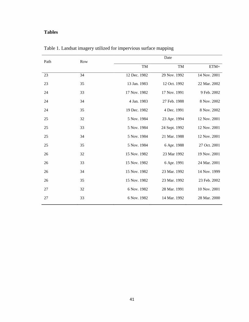
41
Tables
Table 1. Landsat imagery utilized for impervious surface mapping
Path Row Date
TM TM ETM+
23 34 12 Dec. 1982 29 Nov. 1992 14 Nov. 2001
23 35 13 Jan. 1983 12 Oct. 1992 22 Mar. 2002
24 33 17 Nov. 1982 17 Nov. 1991 9 Feb. 2002
24 34 4 Jan. 1983 27 Feb. 1988 8 Nov. 2002
24 35 19 Dec. 1982 4 Dec. 1991 8 Nov. 2002
25 32 5 Nov. 1984 23 Apr. 1994 12 Nov. 2001
25 33 5 Nov. 1984 24 Sept. 1992 12 Nov. 2001
25 34 5 Nov. 1984 21 Mar. 1988 12 Nov. 2001
25 35 5 Nov. 1984 6 Apr. 1988 27 Oct. 2001
26 32 15 Nov. 1982 23 Mar 1992 19 Nov. 2001
26 33 15 Nov. 1982 6 Apr. 1991 24 Mar. 2001
26 34 15 Nov. 1982 23 Mar. 1992 14 Nov. 1999
26 35 15 Nov. 1982 23 Mar. 1992 23 Feb. 2002
27 32 6 Nov. 1982 28 Mar. 1991 10 Nov. 2001
27 33 6 Nov. 1982 14 Mar. 1992 28 Mar. 2000
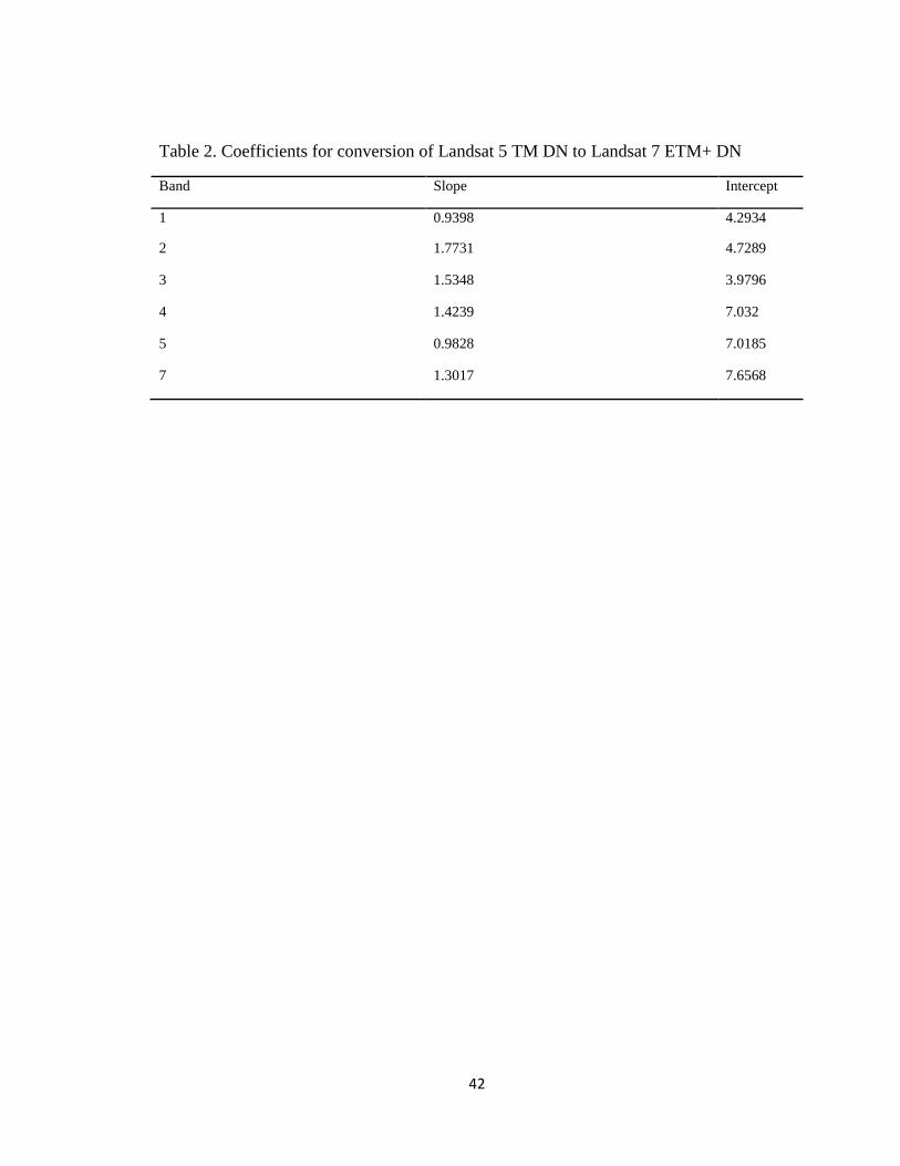
42
Table 2. Coefficients for conversion of Landsat 5 TM DN to Landsat 7 ETM+ DN
Band Slope Intercept
1 0.9398 4.2934
2 1.7731 4.7289
3 1.5348 3.9796
4 1.4239 7.032
5 0.9828 7.0185
7 1.3017 7.6568

43
Table 3. Accuracy assessment
Date Mean PIS-t Mean PIS-m RMSE SE MAE
1980 30 38 25.75 8.08 14.28
1990 31 40 25.57 8.22 14.48
2000 35 41 24.89 5.89 14.64
Mean PIS-t is the true percent of impervious surface measured from airphotos and
averaged for all the sampled pixels. Mean PIS-m is the SPC classified percent of
impervious surface averaged for all the sampled pixels. RMSE is root-mean squared error,
SE is systematic error, and MAE is mean absolute error.

44
Table 4. Impervious surface growth (ISG) and total area of pixels with ISG in hectare
PIS (%) Urban areas (ha) Rural areas (ha) Urban + Rural (ha) U/R
(%) Pure
mpervious
Pixels with
impervious
Pure
impervious
Pixels with
impervious
Pure
impervious
Pixels with
impervious
1980 - 1990
0-10 1 5 239 2,388 239 2,393 0.2
10-20 1 2 170 849 170 851 0.3
20-30 3,461 11,535 9,972 33,239 13,432 44,774 34.7
30-40 4,341 10,852 9,527 23,816 13,867 34,669 45.6
40-50 4,118 8,235 6,587 13,174 10,705 21,409 62.5
50-60 3,284 5,473 3,146 5,244 6,430 10,716 104.4
60-70 2,356 3,366 1,513 2,162 3,869 5,528 155.7
70-80 1,534 1,918 769 962 2,303 2,879 199.4
80-90 876 973 415 461 1,291 1,434 211.3
90-100 3,705 3,705 2,844 2,844 6,549 6,549 130.3
Total 23,675 46,064 35,181 85,138 58,855 131,202 67.3
1990 - 2000
0-10 1 4 258 2,584 259 2,588 0.2
10-20 1 2 175 877 176 879 0.2
20-30 3,675 12,249 13,206 44,020 16,881 56,269 27.8
30-40 4,287 10,718 13,421 33,551 17,708 44,269 31.9
40-50 3,744 7,488 9,295 18,590 13,039 26,078 40.3
50-60 2,931 4,885 4,559 7,597 7,489 12,482 64.3
60-70 2,023 2,890 2,002 2,860 4,025 5,750 101.0
70-80 1,231 1,539 850 1,062 2,081 2,601 144.9
80-90 686 763 404 448 1,090 1,211 170.1
90-100 4,340 4,340 3,911 3,911 8,251 8,251 111.0
Total 22,918 44,877 48,080 115,500 70,998 160,377 47.7
Urban and rural area was distinguished by the two urban boundaries for the state of
Missouri. Total areas of pixels with impervious surface growth were calculated by adding
up pixels that have impervious surface by the categories of PIS and converted to hectare.

45
Pure impervious surface area was calculated by the Pixels with impervious area
multiplied by the corresponding PIS, in this case 10% to 100% with 10% increment. The
column total was the sum of all 10 categories of PIS. U/R stands for urban ISG versus
rural ISG ratio and was calculated by urban and rural sprawl in each category of PIS as
well as the total value.

46
Table 5. The amount of land affected by impervious surface growth (ISG) by land cover
in hectare
Land cover 1980-1990 (%) 1990-2000 (%)
Grassland 69564 (1.0) 59673 (0.8)
Cropland 23229 (0.6) 40816 (1.0)
Deciduous forest 27728 (0.5) 26281 (0.4)
Open water 2251 (0.8) 2478 (0.9)
Barren or sparsely vegetated 579 (2.5) 1811 (7.9)
Evergreen forest 253 (0.1) 610 (0.2)
% in this table stands for percent of each class being affected compared to the total of that
class

47
Figures
Fig
ure
1. T
he
2 m
NA
IP i
mag
e over
lapp
ed w
ith a
val
idat
ion b
lock
insi
de
the
study a
rea.
Eac
h
outl
ined
sm
all
box r
epre
sents
a 3
0 m
by 3
0 m
pix
el c
orr
espondin
g t
o t
he
Lan
dsa
t pix
el. T
he
num
ber
s in
side
each
box i
s co
rres
pondin
g t
o t
he
dig
itiz
ed a
nd m
easu
red P
IS i
nsi
de
each
box.

48
Fig
ure
2. S
ub
-pix
el c
lass
ifie
r (S
PC
) fo
r per
cent
of
imper
vio
us
surf
ace
(PIS
) fo
r th
e st
ate
of
Mis
souri
: a
port
ion o
f S
pri
ngfi
eld i
n (
a) 1
980;
(b)
1990;
(c)
20
00;
and J
effe
rson C
ity i
n (
d)
1980;
(e)
1990;
(f)
20
00.

49
Fig
ure
3. S
ub
-pix
el c
lass
ifie
r (S
PC
) fo
r per
cent
of
imper
vio
us
surf
ace
(PIS
) fo
r th
e st
ate
of
Mis
souri
: a
port
ion o
f K
ansa
s C
ity i
n (
a) 1
980;
(b)
1990;
(c)
2000 w
ith A
in
dic
atin
g l
eap f
rog, B
indic
atin
g l
ow
den
sity
dev
elopm
ent
on u
rban
fri
ng
e of
Kan
sas
Cit
y, an
d C
indic
atin
g l
ow
den
sity
dev
elopm
ent
along t
he
hig
hw
ay I
-470;
and a
port
ion o
f S
t. L
ouis
met
ro i
n (
d)
1980;
(e)
1990;
(f)
2000 w
ith A
indic
atin
g d
evel
opm
ent
along h
ighw
ay I
-70, B
indic
atin
g i
nfi
llin
g p
atte
rn, an
d C
indic
atin
g r
ura
l sp
raw
l.

50
Fig
ure
4. Im
per
vio
us
surf
ace
gro
wth
(IS
G)
in t
he
stat
e of
Mis
souri
ver
sus
den
sity
of
road
net
wo
rks
for
1980s,
and 1
990s.

51
Figure 5. Percent of Impervious surface growth (ISG) summarized by Land type
association (LTA) in the state of Missouri: a) 1980s; b) 1990s. ISG summarized by 10
digit watershed of the state of Missouri: c) 1980s; d) 1990s.
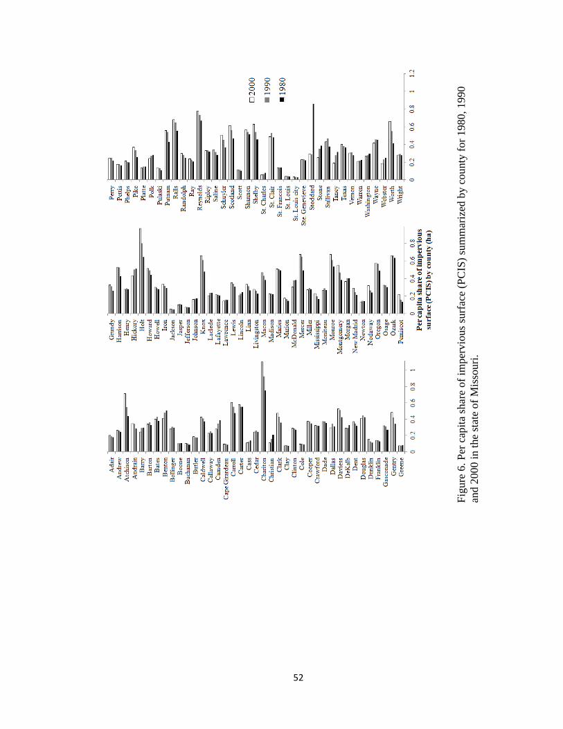
52
Fig
ure
6. P
er c
apit
a sh
are
of
imper
vio
us
surf
ace
(PC
IS)
sum
mar
ized
by c
ou
nty
for
1980, 1990
and 2
000 i
n t
he
stat
e of
Mis
souri
.

53
Figure 7. Impervious surface growth (ISG) by county in hectare: (a) 1980s; (b) 1990s.
Percent change of per capita share of impervious surface (PCIS) by county: (c) 1980s; (d)
2000s.

54
Chapter II. A pixel level approach of population estimation from
Landsat derived impervious surface and Census data for the state
of Missouri
Abstract
Land use and planning decisions, typically made at the municipal level, can be aided by
the use of high resolution population information. In this study pixel-level population
was derived for the state of Missouri using a combined approach that included dasymetric
mapping and regression analysis. The predictor variables used to map population
included Census population and imperviousness, which are strongly correlated. Mapping
accuracy was assessed by comparing mapped pixel-level population, aggregated by
Census block, with the corresponding Census block population. The level of accuracy
achieved in this research is comparable to other studies conducted in smaller study areas,
because its approach combined the benefits of both dasymetric mapping and regression
analysis. The resulting pixel-level population data exhibited a realistic spatial pattern that
was strongly correlated with the distribution of impervious surface. Results from this
work can be aggregated to any geographic unit (e.g. hydrologic boundaries,
administrative boundaries), thus making it possible to incorporate high resolution
population data in a variety of studies. The methodology developed in this study can also
be used to map pixel-level population in other statewide mapping efforts.
Keywords: Impervious surface; population; pixel-level; GIS

55
1. Introduction
The fast growing population and rapid expansion of urbanized area has huge impact on
natural resource conservation, environmental protection and economic growth. Most of
the urban sprawl occurred right on the edges of cities and towns in various speed, shape,
density and direction. Thus, it is crucial to have accurate spatial information of the extent
of urbanized area and population density for decision making in natural resource
management and environmental protection. Missouri is a Midwestern state containing a
mixture of highly urbanized metropolitan areas, mid-sized cities, rural communities, and
considerable agricultural and forested landscapes. During the 1980s, the Kansas City and
St. Louis metropolitan areas led the state in terms of population growth, while mid-sized
cities such as St. Joseph, Joplin, Columbia, and Springfield grew fastest in the 1990s
(Brookings Institution, 2002). Decentralized growth, or sprawl, can impair the ability of
local governments to provide essential services to the general public. Thus, planning at
municipal, county, watershed, regional, or statewide scales is critical to ensure that future
growth not only provides economic benefits but is accompanied by effective use of
natural resources (Verbesselt et al., 2010). For planners to make informed decision,
spatial information of urbanized area and population density are necessary at local,
regional and state level.
In U.S., decadal population information is usually disseminated at census block
level and subsequently aggregated to each ascending geographic census reporting unit
(e.g. block group, census tract, and county). Such polygon-based reporting units are
often insufficient in representing the true spatial distribution of population density inside
each unit because their population values are assumed to be uniformly distributed, thus

56
failing to account for within unit population variation (Moon and Farmer, 2001). An
additional shortcoming of census reporting units is that they are often arbitrary (i.e.
having irregular shape) especially in rural areas. Oftentimes, spatial datasets such as
hydrologic units and administrative boundaries have different areal units that may not
conform to census reporting units, rendering integrating census data with other spatial
data difficult. Moreover, when the boundaries and/or scale of data aggregation are
modified during the data integration process, the result of spatial data analysis will be
greatly affected which is commonly known as the modifiable areal unit problem (MAUP)
(Openshaw, 1983). Because of the problems with polygon-based population data, efforts
to map population as a continuous raster surface are being made (Langford and Unwin,
1994; Mennis, 2003). By modeling population as a continuous raster surface, the spatial
aggregation of population to any predefined boundaries will become a simple process of
addition, thus alleviating the MAUP problem.
Previous population modeling can be categorized into areal interpolation and
statistical modeling (Wu et al. 2005). Areal interpolation is the transformation of
geographic data from one set of boundaries to another. Areal interpolation can be further
divided into interpolation based on mathematical functions and ancillary information (Wu
et al., 2005). Mathematically based interpolation methods include areal based
repartitioning (Tobler 1979) and point based interpolation (Martin 1989). The benefit of
areal based repartitioning is the mass preserving, or pycnophylactic, property as coined
by Tobler (1979). Areal repartitioning is usually based upon areal weighting. This
approach requires the assumption that population is evenly distributed inside each census
reporting unit at which areal repartitioning is performed. Point based areal interpolation

57
was developed in part to solve the problem of assuming uniform population distribution
introduced by areal repartitioning. In point based interpolation, the population of each
census reporting unit is assigned to centroids, and distance based functions (e.g. inverse
distance weighting) are used to assign population to pixels (Martin, 1989). Unlike areal
based interpolation, point based interpolation assumes that population density decreases
away from the centroid. However, in many cases, centroids are not the population center
in a census reporting unit (Wu and Murray, 2005) and population decay functions are not
necessarily accurate in describing the actual spatial pattern of population (Martin, 1989).
Thus, both areal repartitioning and point-based interpolation are not ideal for precise
population modeling.
Areal interpolation based on ancillary information is usually known as dasymetric
mapping. The earliest reference to dasymetric mapping is the population map of
European Russia in 1992 by Russian cartographer Semenov Tian-Shansky (Mennis and
Hultgren, 2006). The origin of the method also explains the Russian heritage of the term
“dasymetric” (Wright, 1936). Modern cartography textbooks define a dasymetric map as
one that illustrates the statistical surface of data by partitioning space into zones
exhaustively which reflect the underlying statistical variation of the data (Dent, 1999;
Slocum et al., 2003; Mennis and Hultgren, 2006). The most widely used dasymetric
mapping variables are derived from remote sensing. Among all the ancillary datasets
used for dasymetric mapping of population, remote sensing derived variables such as
land use/land cover (LULC) data (Mennis, 2003) and statistics such as image spectral and
textural statistics (Harvey, 2002) are the most widely studied. The mathematical
relationship between population data and ancillary datasets can be derived using

58
regression analysis (Wu, 2007 and Mennis, 2003) to support population mapping. The
advantage of dasymetric mapping (e.g. LULC based) over areal interpolation is that it
assumes equal population density within the same LULC classes. However, dasymetric
mapping is not without flaws. For example, Langford et al. (1991) used dasymetric
mapping with LULC data to redistribute polygon-based population to raster cells based
on population density. Langford et al. (1991) later discovered that their approach
underestimated urban population while overestimating rural population, due to the fact
that it assumed equal population density for land use classes without differentiation for
location (e.g. urban vs rural). To address this shortcoming, Langford and Unwin (1994)
improved their previous work by classifying satellite images to residential and
nonresidential areas and assigning census reporting unit population only to residential
pixels inside each census reporting unit. The most recent application of dasymetric
mapping utilized address points as ancillary data (Zandbergen, 2011). However, this
application requires high resolution address point datasets which might not be readily
available.
Unlike areal interpolation, statistical modeling infers a regression relationship
between population and other physical and socioeconomic variables. There are two
advantages with statistical modeling: the first is the ability to include multiple variables
in the regression analysis. For instance, previous studies have used urban areas (Tobler,
1969), dwelling units (Lo, 1989), land use classes (Lo, 2003), physical and
socioeconomic characteristics such as slope and road density (Dobson, 2000), and
spectral features such as greenness and surface temperature (Li and Weng, 2005) as
predictor variables. The second advantage of statistical modeling is the ability to estimate

59
population without census population data as input, which makes it possible to estimate
population in regions without census data or to estimate intercensal population (Wu and
Murray, 2007). However, statistical modeling approaches may have disadvantages. For
instance, by including multiple predictor variables in the regression analysis, the model
can become overcomplicated and may result in problems of collinearity. Moreover, such
regression models do not use census population data as input, thus making it difficult to
transfer them to other study areas. Furthermore, the pycnophylactic property of areal
interpolation is not warranted even within the study area where the regression models are
developed. Thus, rescaling of the population mapping result is required (Wu and Murray,
2005).
The choice of ancillary datasets and predictor variables for dasymetric mapping
and statistical modeling is also very important. Recent researches suggest that
imperviousness derived from remotely sensed images can be a promising candidate for
dasymetric mapping (Wu and Murray, 2005; Morton and Yuan, 2009). Density,
distribution, areal extent, and temporal change of impervious surfaces, are representative
of anthropogenic effects in urban and rural areas (Arnold and Gibbons, 1996; Powell et
al., 2008). Impervious surfaces have distinct man-made features that can be detected and
quantified using remote sensing to reflect anthropogenic development over time (Cronon,
1991; Reisner, 1993; Alberti et al., 2008; Anderson, 2007). In residential areas
impervious surfaces are generally associated with housing, which is a strong indicator of
population (Theobald, 2001). Impervious surface also provides information on urban
morphology (Ji and Jensen, 1999), which can be used to evaluate zoning and planning

60
outcomes. Imperviousness and population are so strongly correlated that one can be used
to predict the other (Wu and Murray, 2005) (Chabaeva et al., 2004).
Wu and Murry (2005) used a cokriging method and spatial autocorrelation
between imperviousness and Census population to map pixel level population. Morton
and Yuan (2009) used regression analysis to derive a relationship between
imperviousness and population density to map population at the pixel level. In a
comparison study, Wu and Murray (2007) found that imperviousness estimated
population considerably better than both spectral radiance and LULC by achieving 7%
less relative error for the entire study area and 30–31% less mean average percentage
error at the Census block group level.
Despite recent successes of using imperviousness in population estimation, there
are still critical issues that need to be resolved. For example, a limitation of the
regression approach is that the relationship between population and imperviousness
developed in one study area is generally not applicable in another study area. Morton and
Yuan (2009) suggested that a single regression relationship is insufficient when the study
area contains both metropolitan and rural areas. The insufficiency is due to the varying
population density pattern that differs by region (Pozzi and Small, 2005). A limitation
with the cokriging approach is its assumption that the mapped population raster
resembles a continuous surface. In reality, however, population exists primarily in
developed areas which are represented by impervious surfaces. The spatial distribution
of population is not continuous, because urbanized areas such as commercial, industrial
and infrastructural areas have no population. Consequently, high density impervious
surfaces may have low or no population. Previous researches have shown that excluding
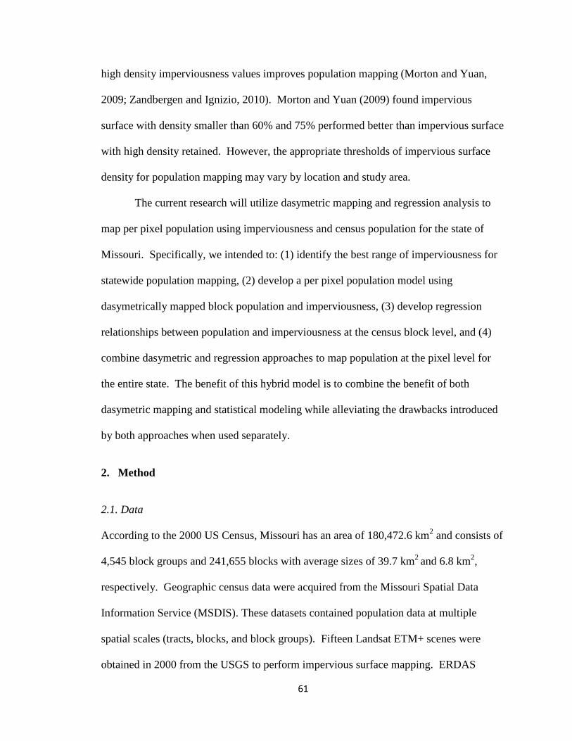
61
high density imperviousness values improves population mapping (Morton and Yuan,
2009; Zandbergen and Ignizio, 2010). Morton and Yuan (2009) found impervious
surface with density smaller than 60% and 75% performed better than impervious surface
with high density retained. However, the appropriate thresholds of impervious surface
density for population mapping may vary by location and study area.
The current research will utilize dasymetric mapping and regression analysis to
map per pixel population using imperviousness and census population for the state of
Missouri. Specifically, we intended to: (1) identify the best range of imperviousness for
statewide population mapping, (2) develop a per pixel population model using
dasymetrically mapped block population and imperviousness, (3) develop regression
relationships between population and imperviousness at the census block level, and (4)
combine dasymetric and regression approaches to map population at the pixel level for
the entire state. The benefit of this hybrid model is to combine the benefit of both
dasymetric mapping and statistical modeling while alleviating the drawbacks introduced
by both approaches when used separately.
2. Method
2.1. Data
According to the 2000 US Census, Missouri has an area of 180,472.6 km2 and consists of
4,545 block groups and 241,655 blocks with average sizes of 39.7 km2
and 6.8 km2,
respectively. Geographic census data were acquired from the Missouri Spatial Data
Information Service (MSDIS). These datasets contained population data at multiple
spatial scales (tracts, blocks, and block groups). Fifteen Landsat ETM+ scenes were
obtained in 2000 from the USGS to perform impervious surface mapping. ERDAS

62
IMAGINE’s Subpixel Classifier (SPC) was used to derive the per-pixel (30m resolution)
proportion of imperviousness for the entire state. The mapping of impervious surface
included a procedure specifically tailored for sub-pixel classification, a procedure for
signature derivation, and finally the procedure for material of interest classification. The
first procedure was automated by SPC software. The second procedure was conducted
semi-automatically using areas-of-interest (AOIs) derived to represent pixels with 100%
pure impervious surface. This procedure was assisted by overlaying aerial photos with
Landsat imageries to better identify Landsat pixels with impervious surface only. During
this process, multiple signatures were derived representing different type of impervious
surfaces: light, medium, and dark. The three different signatures were then used to
classify light, medium and dark impervious surfaces separately. The three outputs were
combined together to form one final image that represented the total percentage of
imperviousness for each pixel. The classification scheme for imperviousness consisted of
9 classes and preserved a 10% increment between classes, except from the 0 to 20%
range, which was classified as 0%. The difference in increment at the beginning of the
range was due to the limitation of the SPC software that materials covering less than 20%
of a pixel are unidentifiable. The remaining imperviousness values were classified with
10% increments as follows: 30%, 40%… 90%, and 100%. Since 20% of a pixel is
equivalent to 180 m2, the median and average floor area in new single-family houses are
183 m2 and 202 m
2 for the Midwest region of U.S. (U.S. Census, 2000). The floor areas
together with driveway will most likely have a footprint larger than 180 m2. Thus, such a
limitation of the software is not going to hurt the accurate mapping of population based
on impervious surface.

63
To avoid assigning population values where roads were present, vector based
TIGER/Line road network data (U.S. Census, 2000) was used to mask out coincident
impervious surface pixels (Morton and Yuan, 2009). The preprocessed imperviousness
per pixel data was then overlaid onto census block group boundaries to 1) illustrate the
distribution of impervious surface pixels, and 2) define spatial relationships between
census block group boundaries and impervious surface pixels for Missouri (Fig. 1).
2.2. Identify the best range of imperviousness for population mapping
Since the relationship between population and imperviousness varies by location, it was
necessary to identify the range of imperviousness most directly correlated with
population for the state of Missouri. We also want to gain a more comprehensive
understanding of the performance of various types of imperviousness in population
estimation accuracy. To accomplish this, four datasets with varying ranges of
imperviousness were prepared (Figure 2) to identify the most accurate candidate for
population mapping. First, total imperviousness was used to illustrate the overall spatial
pattern of impervious surface (Fig. 2A). Second, cells with imperviousness greater than
80 percent removed (Fig. 2B). Third, cells with imperviousness greater than 70 percent
removed (Fig. 2C). Fourth, cells with imperviousness greater than 60 percent removed
(Fig. 2D). The performance of each dataset was determined by using block group level
populations to estimate block level populations so that they could be directly compared
with Census block level population data. Since statewide accuracy assessments are
excessively time-consuming, subsets were taken from each of the four datasets in order to
determine the optimal threshold range of imperviousness for population mapping. We
randomly picked 1,500 out of the 4,545 block groups in the state of Missouri which

64
contained 21,145 blocks. After both dasymetric mapping and regression analysis were
applied to estimate block population based on the selected block group population and
the four types of imperviousness. The estimated values were compared with the known
block population. An error analysis was performed based on similar studies (Zandbergen
and Ignizio, 2010; Zandbergen, 2011). For each block, the following error metrics were
determined: (1) the number of people placed incorrectly determined by the sum of the
absolute values of the difference between estimated and known population counts for
each block, divided by two, (2) the median of the absolute value of the percent error for
each block group, using the known population for each block as the denominator, (3) the
R-squared value of the correlation between estimated and known population counts for
each block. These error metrics were determined for each of the approach and ancillary
datasets combination (Table 1). Based on Table 1, it is apparent that pixels with
imperviousness values greater than 70% removed performed the best across the board
regardless of the approach used. Between the two approaches, dasymetric mapping
performed consistently better than regression. Thus, it is appropriate to use dasymetric
approach using pixels with imperviousness values greater than 70% removed to estimate
block population from block group population in the state of Missouri. We have also
calculated the percent area of the removed impervious surface pixels which turned out to
be 0.27% of the total study area. Thus, the removal of imperviousness greater than 70%
will have very little impact on the final population mapping.
2.3. Regression relationship between population and imperviousness
The imperviousness raster with values greater than 70% removed was used to estimate
the total amount of impervious area for each block group and block. To redistribute the
65
population from block group to block, the total amount of imperviousness for each block
were used as weight factors to assign portions of the block group population to each
block. In order to further disseminate the block population to finer spatial units such as a
raster grid with resolution equivalent to the imperviousness raster, we need to study the
relationship between population and imperviousness at the pixel level. Since there is no
raster population data with resolution comparable to the imperviousness raster used in
this research, validating the mapping result is difficult. However, strong relationships
between imperviousness and population exist, and utilizing these relationships for
population assignment is warranted because the true spatial distribution of population is
not uniform. Since the relationship between imperviousness and population can vary
among Census blocks, multiple scenarios should be considered when mapping population
based on imperviousness. Common scenarios include: 1) Census block polygons
containing only single-family residential units, where the spatial distribution of
population coincides with each housing unit and is also spatially correlated with low
density impervious surface, 2) Census block polygons containing both single-family
residential units and apartment complexes, where the spatial distribution of population
coincides with both types of structures and is spatially correlated with low to medium
density impervious surface, 3) Census block polygons containing both residential and
commercial areas, where the spatial distribution of population coincides only with the
residential areas although the commercial areas might have higher density impervious
surface.
With the aforementioned scenarios in mind, three assumptions were made in order
to study the relationship between imperviousness and population. The first assumption
66
was that population was entirely associated with pixel level imperviousness (i.e. 0%
imperviousness corresponds to 0 population). The second assumption was that pixels
with low density impervious surfaces have low population. That is, pixels in rural areas
and low density residential neighborhoods with low densities of imperviousness will have
low population values. The third assumption was that high density imperviousness can
be associated with either low or high population values, a problem partially ameliorated
by removing imperviousness values greater than 70%. However, this approach does risk
excluding high density residential areas (e.g. high-rise) which contain large populations
and are typically located in large urban centers.
Based on the three assumptions, it is appropriate to assign population only to
pixels that spatially coincide with imperviousness greater than zero inside each census
block. This census block based average population per pixel can be used together with an
error term to model the actual population for each pixel. The average population for each
impervious surface pixel was determined from the following formula (Eq. [1]):
(1)
Where PPPi is population per pixel in block i, POPi is population for block i, Ni is the
number of impervious surface pixels in block i, and nij is the number of impervious
surface pixels with percent of impervious surface j, where j = 0, 20, 30… 100, in block i.
A GIS model was created to calculate the average population estimation (Fig. 3). The
following equation was used to quantify the actual population for each pixel inside block
i (Eq. [2]):
(2)

67
Where PPP*
ij is the actual population per pixel in block i with percent of impervious
surface j and εij as the error term with percent of impervious surface j in block i. Similar
to population for each pixel, percent of impervious surface for each pixel also has
estimation errors and was expressed using the following formula (Eq. [3]):
(3)
Where PIS*
j is the actual percent of impervious surface for pixels classified j percent of
impervious surface. Since both the predictor variable PIS*
j and dependent variable PPP*
ij
are modeled with an asymptotic value plus an error term. Thus, the regression problem
between PPP*
ij and PIS*
j per pixel for all blocks i or any subsets of all the blocks belong
to the errors–in–variables regression problem.
Before running the regression analysis between population and impervious
surface at the pixel level, it is necessary to solve the spatial autocorrelation problem
which violates the independence assumption in standard regression models (Wu et al.,
2006). Every city inside the state can be viewed at as a cluster of population. The best
way to resolve the spatial autocorrelation problem is to break the clusters into several
subsets by classifying them into various population density (PD) categories (Morton and
Yuan, 2009). In this study, however, clustering is not alleviated after classifying the
census blocks into five evenly distributed PD classes (Fig. 4). Thus, in this investigation,
a different density measurement of population called adjusted population density (APD)
was proposed. Instead of using the total area for each Census block, the total area of
impervious surface inside each Census block was used as the denominator in the density
measurement. The following equation was used to calculate the APD of the
corresponding Census block (Eq. [4]):
68
(4)
Where APDi is adjusted population density per square kilometer for block i, POPi is
population for block i, A is the area of each pixel (900 m2), PISj is percent of impervious
surface, and nij is the number of pixels for percent of impervious surface j in block i.
The APD was used because the traditional PD can introduce bias at the pixel scale,
particularly in rural areas. This is due to the fact that the majority of land cover in rural
Census blocks was classified as non-urban (i.e. forest, agriculture, pasture, bare soil, and
water), consequently diluting the PD for areas with population. Therefore using the
adjusted density equation helped to avoid underestimating the actual PD within areas that
were considered developed land within rural Census blocks.
To reduce the problem of spatial clustering of population, the blocks were
classified into five categories based on quantile rules using APD per square kilometer: (1)
low density (≤ 1500), (2) medium – low (1501 – 4000), (3) medium (4001 – 8000), (4)
medium – high (8001 – 13500), and (5) high (> 13500). The reclassified census blocks
significantly reduced spatial clustering compared to the classification based on PD (Fig.
5). Moran’s I statistics were also calculated to quantify the degree of clustering of
Census block level population. A Moran’s I value near +1.0 indicates clustering, a value
near -1.0 indicates dispersion, and a value close to zero indicates a random pattern. The
Moran’s I values were summarized for both the five PD categories as well as for the five
APD categories in Table 2. The overall Moran’s I for all the census blocks based on PD
is 0.153, indicating classifying census blocks based on APD instead of PD is more
effective in reducing spatial autocorrelation between census block PD.

69
The sample sizes for each adjusted population density categories were very large
(about 50,000 census blocks for each density category) and the estimation errors for all
population pixels summed to zero (Eq. [2]). That is, the sample size was large enough to
assume that the average of independent observations will be approximately normally
distributed, as described by the Central Limit Theorem (Billingsley, 1995). Thus, it is
reasonable to assume that the summarized mean population would be the same based on
either the actual population for each pixel PPP*
ij or the averaged population for each
pixel PPPi. For the sake of simplicity, PPPi values are summarized for each percent of
impervious surface category as well as for the five density categories of Census blocks
with mean and standard deviations (Table 3). Raster cells with population values equal
to zero can be associated with either zero percent impervious surface pixels (undeveloped)
or very high percent impervious surface pixels (industrial and commercial areas). Thus,
only non-zero population and impervious surface pixels are included in the analysis to
reduce confusion.
We plotted the distributions of population against imperviousness classes in each
APD category based on the mean and standard deviation of population in Table 3 (Fig. 6).
We noticed the mean values of population indicated by the hollowed dots have linear
increasing trends (Fig. 6). Thus, we ran regression analysis between sampled population
and percent of impervious surface based on the mean values for the five APD categories.
Accordingly, five regression lines are generated based on the five APD categories (Fig.
7). The R2 statistics were not reported with the regression equations because these
regression lines were based on mean population values for percent of impervious surface
categories instead of actual populations for each pixel.
70
The slopes of the five regression relationships follow an increasing trend with the
increase of APD (Fig. 7). Thus, it is reasonable to believe that the slope of the regression
relationship is correlated with the adjusted population density. In order to find out if such
an assumption is valid, the average adjusted population density is calculated for each
APD category. After comparing the five slopes of the regression relationships with the
average APD of each category, we were able to confirm the positive correlation.
2.4. Estimating per pixel population
A population mapping model can be established based on the regression relationships
derived between population and imperviousness together with the two correlation
relationships with APD. The first regression relationship takes the form (Eq. [5]):
(5)
Where POPIj is the population for pixel with density j in subset of Census blocks I,
coefficient αI is the slope of the regression relationship between population and percent of
impervious surface per pixel for subsets of Census blocks I, PISj is the percent of
impervious surface density. There is no intercept for this regression relationship due to
the assumption that zero population is associated with zero imperviousness. The
regression relationship between the slope of the first regression relationship and the
adjusted population density takes the form (Eq. [6]):
(6)
Where coefficient γ is the slope of this relationship between the slope of the first
regression relationship αI and APDI which is the adjusted population density for subset of
Census blocks I. Coefficient θ is the intercept of this relationship.

71
By substituting αI into the first regression relationship, the following equation results (Eq.
[7]):
(7)
Note that the subset of Census blocks I can be any subset of all Census blocks. Thus, i
may be substituted for I, which corresponds to the subset of each individual Census block
and gives the following equation (Eq. [8]):
(8)
The above equation is the regression relationship between populations and percent of
impervious surfaces at the pixel level where APDi is the dasymetric component (or
geographically weighted component) and PISj is the regression component. This
regression relationship may be applied to study areas of various sizes and in different
locations to calculate population per pixel based on any Census population units and the
percent of impervious surface information therein.
Unlike areal interpolation, this regression approach does not have the
pycnophylactic property. Thus, a rescaling approach is used to preserve the total number
of population for each Census polygon (Wu and Murray, 2005). The equation used for
rescaling takes the form (Eq. [9]):
(9)
Where POP*
ij is the rescaled mass preserved population for pixels with percent of
impervious surface j in Census polygon i, POPij is the population estimation obtained
through the regression equation (Eq. [8]), and POPi is the dasymetricly mapped
population for Census polygon i and , which is the sum of POPij for Census
polygon i.

72
A GIS model was developed to implement the aforementioned procedures and to
map populations at pixel level (Fig. 8). The required inputs for this GIS model include
the following: Census population, percent of impervious surface, and two regression
relationship coefficients: γ, θ, which are site specific and need to be derived for each
individual study area. To address the problem of associating high density imperviousness
with either high density or low density population, a procedure was added to remove
Census blocks that overlapped areas with high density impervious surface. For simplicity,
we assigned uniform population based on the estimated block population and the
presence of impervious surface pixels. It is not feasible to assess pixel level accuracy
because there was no accurate pre-existing population information available at the pixel
level for the state of Missouri.
3. Results
3.1. Results validation
The block population estimation based on block group population is summarized in Table
1. The best performance combination is dasymetric mapping using imperviousness with
road network data and pixels with imperviousness values less than 70%. The percent of
people placed incorrectly is 19.5% with a median absolute percent error of 27.7 and R-
squared value of 0.787 using the actual block population for comparison. This result is
consistent with previous research. If we subject the per pixel population estimation to the
block level population validation, the accuracy will be very similar to the best accuracy
reported in Table 1. However, without the availability of statewide population at pixel
level, we are not capable of reporting the pixel level population estimation accuracy.

73
3.2. Pixel-based regression model
This study has derived unique deterministic relationships for each census block based on
their adjusted population density. Thus, the errors are minimized in the modeling process.
The model used for the state of Missouri takes the following form (Eq. [10]):
(10)
Where POPij is the population per pixel in block i for percent of impervious density j.
This regression model was specifically derived for the state of Missouri. Thus, to
implement this approach in study areas other than Missouri, it is necessary to derive
model coefficients specific to the study area in question.
3.3. Map results
Due to the large extent of the study area, not all areas can be presented and described.
Figure 9 shows the mapped population density for each pixel in four panels representing
four different cities in Missouri. Results show the spatial distribution, actual location,
and spatial variations of population in detail unattainable with Census population data
alone (Fig. 9). For example, it is shown that residential neighborhoods in Springfield
have relatively uniform population densities within each neighborhood but large
variances among different neighborhoods. The downtown core areas are generally
without population (A on Springfield panel in Fig. 9). The railway hub is also without
population (B on Springfield panel in Fig. 9). In the park or forested area, there is low
and scattered population (C on Springfield panel in Fig. 9). The general population
distribution pattern outside the downtown core area is an increase followed by a decrease
in population radiating out from the city center.

74
The city of Columbia has a gradual trend in decreasing population radiating out
from the inner city. In the inner city of Columbia, there is a concentration of population
near the University Hospital Center (A on Columbia panel in Fig. 9). In the outer city of
Columbia, there exists a scattered pattern in spatial distribution of residential
neighborhood (B and C on Columbia panel in Fig. 9). Kansas City exhibits both the
patchy relationships of Springfield and the gradual decreasing trend of the city of
Columbia. Plus, there is many rural population scattering between Kansas City and the
leapfrog developments (A on Kansas City panel in Fig. 9). St. Louis, on the other hand,
is more uniform in distribution of population density in residential areas of various
densities. The core of downtown area (A on St. Louis panel in Fig. 9) as well as the
Forest Park area (B on St. Louis Panel in Fig. 9) is without any population. In general,
the per-pixel population map has a very similar spatial pattern to the imperviousness map,
which is due to the assumption that population will coincide with the presence of
impervious surface. Moreover, the map result ensures a reasonable estimate of
population density, which is highly correlated to impervious surface. The mapping
results also ensure that spatial allocation of population is consistent with block level
Census population data.
A histogram showing the frequency of pixel level population values for the entire
study area can be seen in Figure 10; pixels with no population values were not included
in the analysis. Results indicate that for pixels with population over 99% will contain 6
or less persons (Fig. 10).

75
4. Discussion
4.1. Approach implications
This approach avoided several problems at the data preprocessing stage encountered by
previous studies. For example, the cokriging approach (Wu and Murray, 2005) where
point population is necessary, assumptions must be made to convert U.S. Census
population data to point population data. In this study, block population was first
estimated by a well-established dasymetric mapping technique and then disseminated to
each pixel based on the presence of impervious surface, which is more accurate than
assigning the entire population to an arbitrary or geometrically derived point. Instead of
using a single linear regression relationship for the entire study area (Morton and Yuan,
2009), five initial regression relationships were derived between adjusted population
density and imperviousness per pixel, a concept unique to this research. Since the five
regression relationships derived from the five subsets of data were not spatially clustered,
it can be concluded that they were independent of one another. Thus, it was possible to
expand these regression relationships to ensure that each Census block has its own
regression relationship based on the locally calculated adjusted population density.
Another example is the approach by Wu and Murray (2005) where residential area was
derived with conventional image classification. This approach requires separate
procedures to derive residential area which might introduce more errors due to issues of
error propagation. Moreover, this type of approach might risk the exclusion of areas with
low density population (e.g. exurban areas and some high density urban centers). In this
study, the assignment of population to non-residential area is reduced by excluding areas
such as census blocks with no population, pixels with no impervious surface, and

76
impervious surface overlapped with all road networks. Last but not least, previous
studies generate continuous surfaces of population density (Wu and Murray, 2005). In
reality, population distribution is not always continuous over the landscape. Although
GIS masks were used to filter unrealistic population pixels, the use of masks after
assigning population to each pixel will reduce the total predicted population, thereby
requiring further adjustment (Wu and Murray, 2005).
There are two advantages associated with the methodology presented in this study.
First, this approach assumes a strong correlative relationship between imperviousness and
population at the pixel level. The strong relationships ensure the use of different
deterministic relationships tailored to each census unit. These relationships are then used
to map population at the pixel level rather than using a single universal regression model
for the entire study area (Morton and Yuan, 2009). By modeling population versus
impervious surface at each census block, population variation due to location is
considered and incorporated into the mapping model by introducing the local population
density measure of adjusted population density. The second advantage of using this
approach is only impervious surface mapped population is strongly associated with the
presence of impervious surface. This is different from interpolation models used in other
studies where population is assigned to the entire study area with varying densities (Wu
and Murray, 2005).
4.2. Data implications
There are three major limitations with the dataset used in this study. First, per pixel
population information is not available for error checking. The only population
information available was aggregated population for each Census block. For the same

77
reason, the relationship between imperviousness and population at the pixel level cannot
be established directly. Several assumptions have to be made in order to study the
relationship between population and imperviousness. Second, population in Missouri has
a high degree of spatial variability. Thus, it is necessary to analyze population at smaller
scales, such as by Census block or block group. Third, imperviousness, which is
obtained from subpixel classification of Landsat images, is subject to mapping accuracy
which can lead to error propagation in the population mapping process.
4.3. Result implications
We have presented a method for mapping statewide pixel level population that achieved
similar or better accuracy compared to previous population estimates based on Census
block group data (Wu and Murray, 2005 and 2007; Wu et al., 2005 and 2006; Morton and
Yuan, 2009; Zandbergen and Ignizio, 2010). More importantly, this study showed that it
was possible to map pixel level population for the entire state of Missouri. Using pixel
level population data has many advantages relative to U.S. Census population data. For
example, pixel based population data can be easily associated with all other spatial
datasets (e.g. watershed boundaries, ecological units, and elevation data), avoids
problems with boundary discrepancies caused by the irregular shape and size of Census
polygons, and can be easily plugged into raster based models with minimal adjustment.
Moreover, traditional estimations of population density only give a per area average of
population distribution, whereas pixel based population data provides a more detailed
illustration of the spatial distribution of population. The results of this study also confirm
Sutton’s (2009) theory regarding the population holding capacity (~ 6 persons/900 m2 in
this study) of a given area of impervious surface and establish a correlation between

78
imperviousness and population, thus suggesting that pixel based population estimates are
possible when predicated on coincident areas of imperviousness (Fig. 10). The
population estimation method presented here also makes it possible to infer population
based on imperviousness derived from remotely sensed imagery or model predictions
without relying on decadal Census population data (Fig. 10). Pixel based population data
is also useful in numerous ways, such as: location analyses for health-care centers and
public libraries, integration of demographic and socioeconomic characteristics for risk
and impact assessments, and emergency planning and management, consequence
assessment, mitigation planning, and implementation.
5. Conclusions
A dasymetric mapping with localized regression approach was presented here to model
per pixel population using per-pixel imperviousness and Census population at Census
unit level for the state of Missouri. Unique relationships were discovered between
population and imperviousness at the pixel level for each census block. These
relationships were used to assign Census block level population values to each pixel in
accordance with the presence of imperviousness. The findings inferred from the mapping
result indicated that over 99% of the pixel population values in Missouri contained
between one and six people. This population mapping approach improves upon previous
methods because it allows for the use of Census data at various scales (e.g. block, block
group, tract) and is insensitive to the size and location of the study area. The mapping
result is an improvement over the uniform distribution of population as defined by U.S.
Census geographic data. This approach also manages to map per pixel population for a
large geographic area at a high spatial resolution.
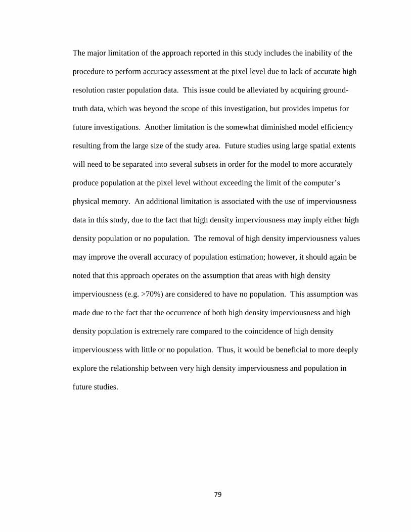
79
The major limitation of the approach reported in this study includes the inability of the
procedure to perform accuracy assessment at the pixel level due to lack of accurate high
resolution raster population data. This issue could be alleviated by acquiring ground-
truth data, which was beyond the scope of this investigation, but provides impetus for
future investigations. Another limitation is the somewhat diminished model efficiency
resulting from the large size of the study area. Future studies using large spatial extents
will need to be separated into several subsets in order for the model to more accurately
produce population at the pixel level without exceeding the limit of the computer’s
physical memory. An additional limitation is associated with the use of imperviousness
data in this study, due to the fact that high density imperviousness may imply either high
density population or no population. The removal of high density imperviousness values
may improve the overall accuracy of population estimation; however, it should again be
noted that this approach operates on the assumption that areas with high density
imperviousness (e.g. >70%) are considered to have no population. This assumption was
made due to the fact that the occurrence of both high density imperviousness and high
density population is extremely rare compared to the coincidence of high density
imperviousness with little or no population. Thus, it would be beneficial to more deeply
explore the relationship between very high density imperviousness and population in
future studies.

80
References
ALBERTI, M. (2008) Advances in urban ecology: integrating humans and ecological
processes into urban ecosystems. New York, NY, USA, Springer Science.
ANDERSON, D. R. (2008) Model based inference in the life sciences: A primer on
evidence. Springer-Verlag. New York, NY.
ARNOLD JR, C. L. & GIBBONS, C. J. (1996) Impervious surface coverage: The
emergence of a key environmental indicator. Journal of the American Planning
Association, 62, 243–258.
BILLINGSLEY, P. (1995) Probability and Measure, Wiley-Interscience.
BROOKING, I. (2002) Growth in the heartland: challenges and opportunities for
Missouri. Washington, D.C., USA, Brookings Institution, Center on Urban and
Metropolitan Policy.
CHABAEVA, A., CIVCO, D. L. & PRISLOE, S. (2004) Development of a population
density and land use based regression model to calculate the amount of
imperviousness. Denver, CO: Proceedings 2004 ASPRS Annual Convention.
CRONON, W. (1991) Nature's metropolis: Chicago and the Great West.
DOBSON, J. E., BRIGHT, E. A., COLEMAN, P. R., DURFEE, R. C. & WORLEY, B.
A. (2000) LandScan: A global population database for estimating populations at
risk. Photogrammetric Engineering and Remote Sensing, 66, 849-857.
EICHER, C. L. & BREWER, C. A. (2001) Dasymetric mapping and areal interpolation:
Implementation and evaluation. Cartography and Geographic Information Science,
28, 125–138.
HARVEY, J. T. (2002) Estimating census district populations from satellite imagery:
Some approaches and limitations. International Journal of Remote Sensing, 23,
2071-2095.
JI, M. & JENSEN, J. R. (1999) Effectiveness of subpixel analysis in detecting and
quantifying urban imperviousness from landsat thematic mapper imagery.
Geocarto International, 14, 31-39.
LANGFORD, M., MAGUIRE, D. J. & UNWIN, D. J. (1991) The areal interpolation
problem: estimating population using remote sensing in a GIS framework.
Handling geographical information, 55-77.
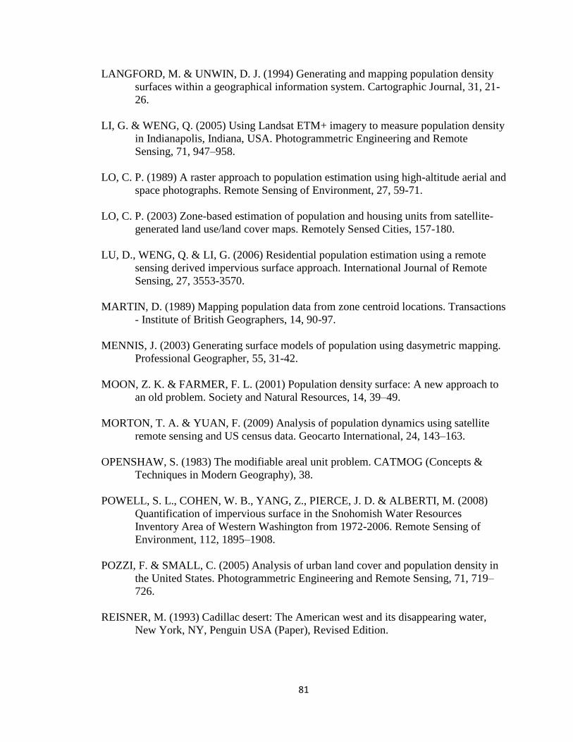
81
LANGFORD, M. & UNWIN, D. J. (1994) Generating and mapping population density
surfaces within a geographical information system. Cartographic Journal, 31, 21-
26.
LI, G. & WENG, Q. (2005) Using Landsat ETM+ imagery to measure population density
in Indianapolis, Indiana, USA. Photogrammetric Engineering and Remote
Sensing, 71, 947–958.
LO, C. P. (1989) A raster approach to population estimation using high-altitude aerial and
space photographs. Remote Sensing of Environment, 27, 59-71.
LO, C. P. (2003) Zone-based estimation of population and housing units from satellite-
generated land use/land cover maps. Remotely Sensed Cities, 157-180.
LU, D., WENG, Q. & LI, G. (2006) Residential population estimation using a remote
sensing derived impervious surface approach. International Journal of Remote
Sensing, 27, 3553-3570.
MARTIN, D. (1989) Mapping population data from zone centroid locations. Transactions
- Institute of British Geographers, 14, 90-97.
MENNIS, J. (2003) Generating surface models of population using dasymetric mapping.
Professional Geographer, 55, 31-42.
MOON, Z. K. & FARMER, F. L. (2001) Population density surface: A new approach to
an old problem. Society and Natural Resources, 14, 39–49.
MORTON, T. A. & YUAN, F. (2009) Analysis of population dynamics using satellite
remote sensing and US census data. Geocarto International, 24, 143–163.
OPENSHAW, S. (1983) The modifiable areal unit problem. CATMOG (Concepts &
Techniques in Modern Geography), 38.
POWELL, S. L., COHEN, W. B., YANG, Z., PIERCE, J. D. & ALBERTI, M. (2008)
Quantification of impervious surface in the Snohomish Water Resources
Inventory Area of Western Washington from 1972-2006. Remote Sensing of
Environment, 112, 1895–1908.
POZZI, F. & SMALL, C. (2005) Analysis of urban land cover and population density in
the United States. Photogrammetric Engineering and Remote Sensing, 71, 719–
726.
REISNER, M. (1993) Cadillac desert: The American west and its disappearing water,
New York, NY, Penguin USA (Paper), Revised Edition.

82
SATTERTHWAITE, D. (2005) "The scale of urban change worldwide 1950-2000 and its
underpinnings". Human Settlements Discussion Paper Series.
STEHMAN, S. V. & CZAPLEWSKI, R. L. (1998) Design and analysis for thematic map
accuracy assessment: Fundamental principles. Remote Sensing of Environment,
64, 331–344.
SUTTON, P. C., ANDERSON, S. J., ELVIDGE, C. D., TUTTLE, B. T. & GHOSH, T.
(2009) Paving the planet: Impervious surface as proxy measure of the human
ecological footprint. Progress in Physical Geography, 33, 510–527.
THEOBALD, D. M. (2001) Land-use dynamics beyond the American urban fringe.
Geographical Review, 91, 544–564.
TOBLER, W. R. (1969) Satellite confirmation of settlement size coefficients. Area, 1,
30-34.
TOBLER, W. R. (1979) Smooth pycnophylactic interpolation for geographical regions.
Journal of the American Statistical Association, 74, 519-530.
VERBESSELT, J., HYNDMAN, R., NEWNHAM, G. & CULVENOR, D. (2010)
Detecting trend and seasonal changes in satellite image time series. Remote
Sensing of Environment, 114, 106–115.
WU, C. & MURRAY, A. T. (2005) A cokriging method for estimating population
density in urban areas. Computers, Environment and Urban Systems, 29, 558–579.
WU, C. & MURRAY, A. T. (2007) Population estimation using landsat enhanced
thematic mapper imagery. Geographical Analysis, 39, 26–43.
WU, S. S., QIU, X. & WANG, L. (2005) Population estimation methods in GIS and
remote sensing: A review. GIScience and Remote Sensing, 42, 80-96.
WU, S. S., QIU, X. & WANG, L. (2006) Using semi-variance image texture statistics to
model population densities. Cartography and Geographic Information Science, 33,
127-140.
ZANDBERGEN, P. A. & IGNIZIO, D. A. (2010) Comparison of dasymetric mapping
techniques for small-area population estimates. Cartography and Geographic
Information Science, 37, 199-214.
ZANDBERGEN, P. A. (2011) Dasymetric Mapping Using High Resolution Address
Point Datasets. Transactions in GIS, 15, 5-27.

83
Tables
Table 1. Performance metrics of regression analysis versus dasymetric mapping,
comparison is made upon four different types of imperviousness datasets all of which
have road network imperviousness removed.
Imperviousness People Placed Incorrectly Median Abs. % Error R-squared
Count Percentage Rank
Regression
Imperviousness 1074783 29.8 4 35.1 0.470
Imperviousness < 80% 946892 26.2 2 34.8 0.599
Imperviousness < 70% 930774 25.8 1 35.9 0.641
Imperviousness < 60% 962284 26.7 3 38.7 0.628
Dasymetric
Imperviousness 820982 22.8 4 32.2 0.716
Imperviousness < 80% 728489 20.2 3 28.5 0.772
Imperviousness < 70% 703457 19.5 1 27.7 0.787
Imperviousness < 60% 709271 19.7 2 28.2 0.786

84
Table 2. Moran’s I values calculated for the census blocks population density classified
based on the five population density categories and the five adjusted population density
categories.
Moran’s I Population density categories Adjusted population density categories
Low 0.546 0.029
Med-Low 0.985 0.028
Medium 0.770 0.017
Med-Hi 0.743 0.019
High 0.497 0.021

85
Table 3. Average and standard deviation of population for the pixels classified by both
percent of impervious surfaces and adjusted population density (APD). Pixels with either
zero population or zero percent impervious surfaces are not included to reduce confusion
between the population and imperviousness relationship.
Imperviousness
Low APD Med-low APD Medium APD Med-Hi APD High APD
Mean STD Mean STD Mean STD Mean STD Mean STD
20 0.12 0.19 0.51 0.50 1.29 1.29 2.30 3.81 4.46 5.21
30 0.15 0.27 0.68 1.45 1.59 1.14 2.78 1.05 5.50 4.71
40 0.18 0.38 0.84 1.12 1.83 1.14 3.24 2.22 6.58 5.56
50 0.20 0.52 0.94 0.57 2.02 1.06 3.68 3.24 7.98 7.32
60 0.22 0.45 1.00 0.66 2.17 0.83 4.18 1.41 9.46 7.69
70 0.23 0.35 1.06 0.88 2.29 0.91 4.60 1.68 10.57 7.04
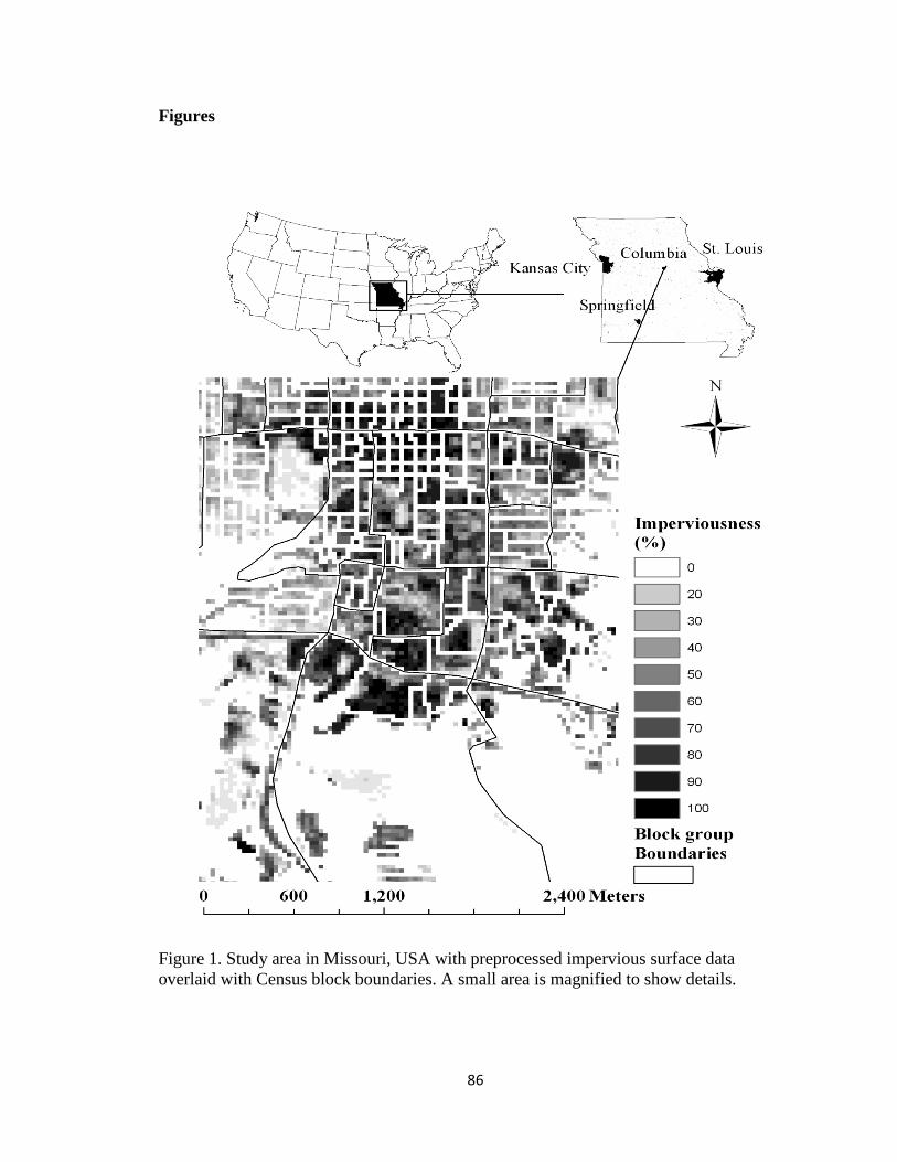
86
Figures
Figure 1. Study area in Missouri, USA with preprocessed impervious surface data
overlaid with Census block boundaries. A small area is magnified to show details.
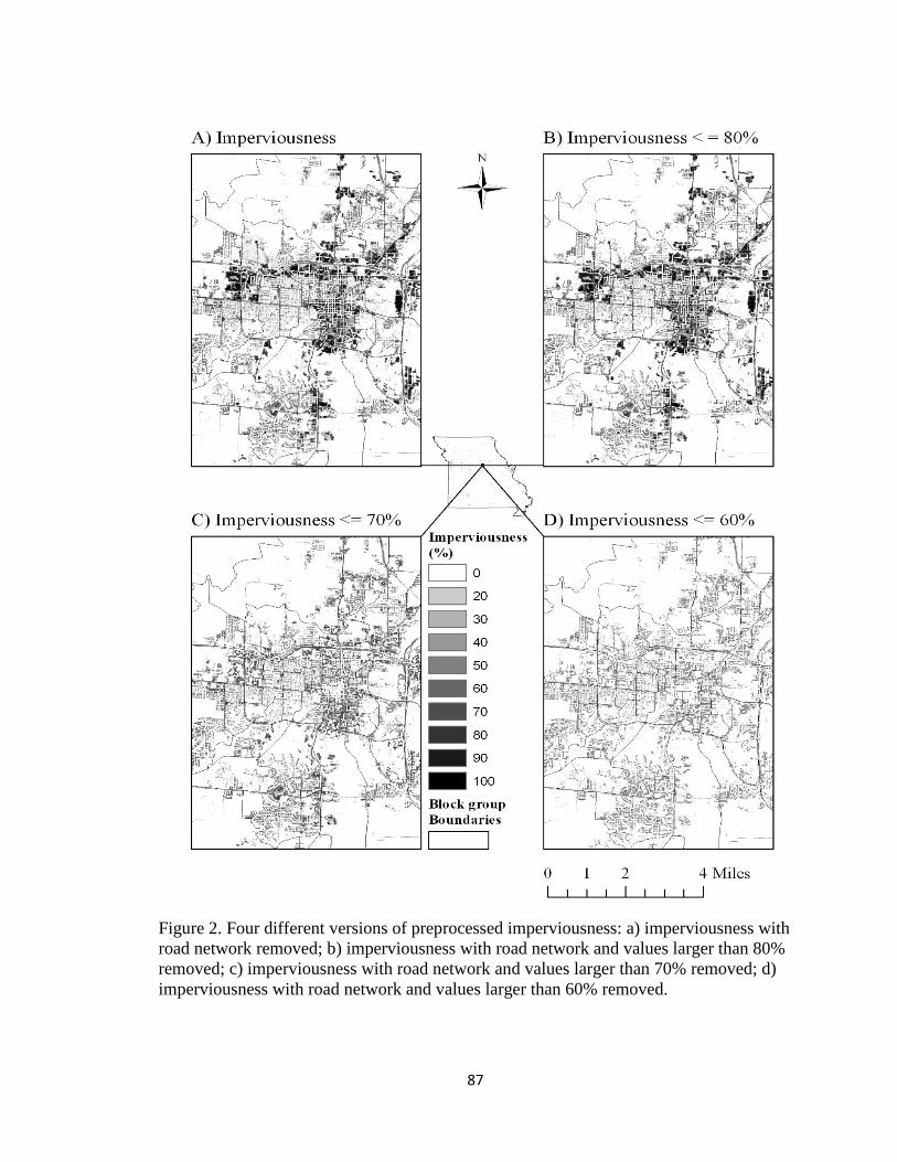
87
Figure 2. Four different versions of preprocessed imperviousness: a) imperviousness with
road network removed; b) imperviousness with road network and values larger than 80%
removed; c) imperviousness with road network and values larger than 70% removed; d)
imperviousness with road network and values larger than 60% removed.

88
Fig
ure
3. G
IS m
odel
dia
gra
m f
or
atta
chin
g c
ensu
s popula
tion t
o e
ach p
ixel
insi
de
bas
ed o
n t
he
assu
mpti
on
that
unif
orm
popula
tion f
or
each
im
per
vio
us
surf
ace
pix
el.
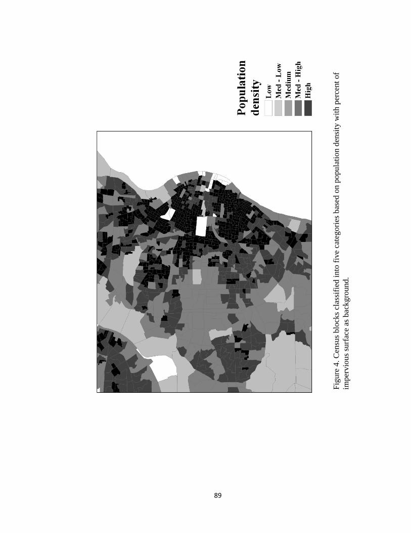
89
Fig
ure
4. C
ensu
s blo
cks
clas
sifi
ed i
nto
fiv
e ca
teg
ori
es b
ased
on p
opula
tio
n d
ensi
ty w
ith p
erce
nt
of
imper
vio
us
surf
ace
as b
ackgro
und.

90
Fig
ure
5. C
ensu
s blo
cks
clas
sifi
ed i
nto
fiv
e ca
teg
ori
es b
ased
on a
dju
sted
popula
tion d
ensi
ty w
ith
per
cent
of
imper
vio
us
surf
ace
as b
ackgro
und.

91
Figure 6. The distributions of population against percent of impervious surface class in
each adjusted population density category based on the mean and standard deviation of
population in Table 1.

92
Fig
ure
7. R
egre
ssio
n r
elat
ionsh
ips
bet
wee
n p
opula
tion a
nd i
mper
vio
us
surf
ace
for
blo
cks
of
dif
fere
nt
adju
sted
popula
tion d
ensi
ty.
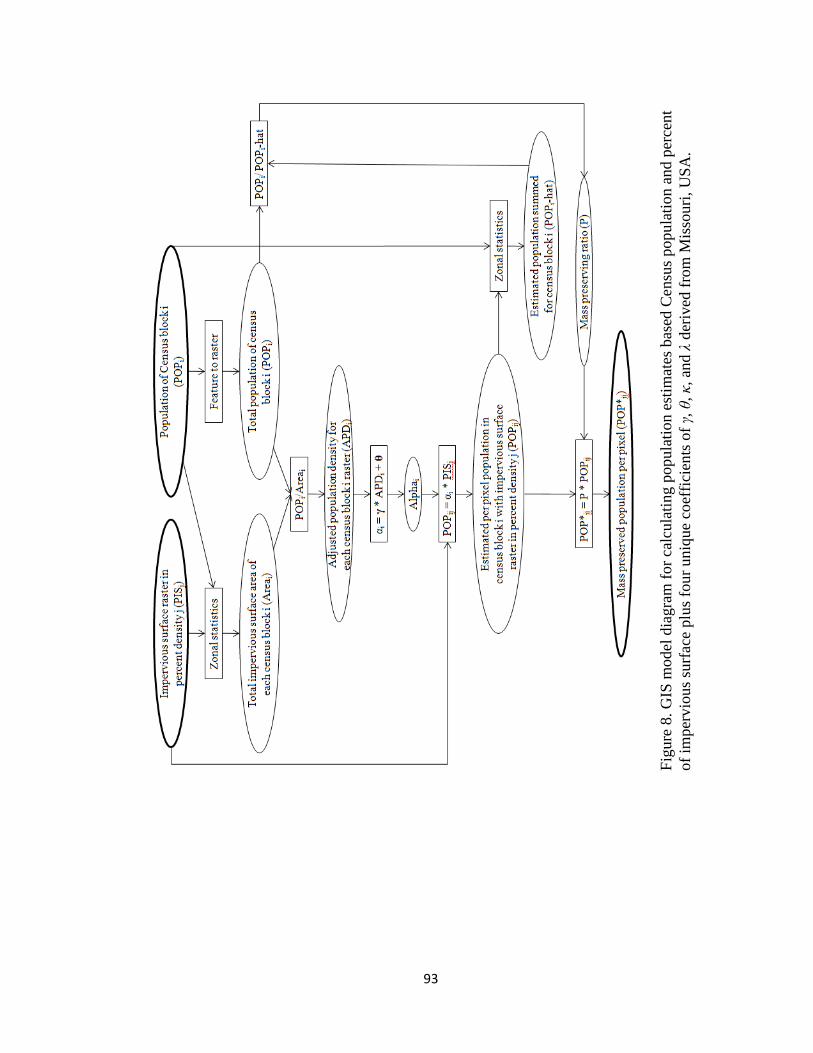
93
Fig
ure
8. G
IS m
odel
dia
gra
m f
or
calc
ula
ting p
opula
tion e
stim
ates
bas
ed C
ensu
s popula
tion a
nd p
erce
nt
of
imper
vio
us
surf
ace
plu
s fo
ur
uniq
ue
coef
fici
ents
of
γ, θ
, κ, an
d λ
der
ived
fro
m M
isso
uri
, U
SA
.

94
Figure 9. Per-pixel population for Missouri, USA with four panels magnified for detail
with the open space indicating no population and darker color indicating more population.
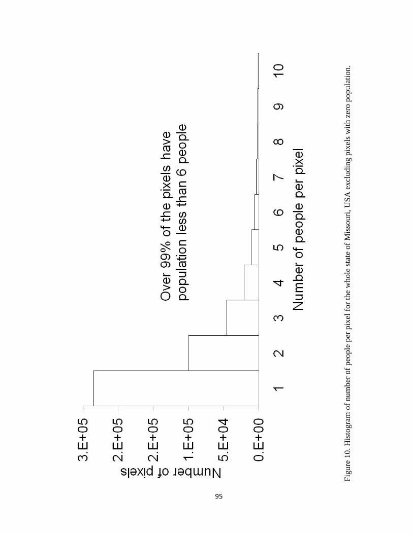
95
Fig
ure
10. H
isto
gra
m o
f num
ber
of
peo
ple
per
pix
el f
or
the
whole
sta
te o
f M
isso
uri
, U
SA
excl
udin
g p
ixel
s w
ith z
ero p
opula
tion.

96
Chapter III. A pixel-level approach of GIS simulation of urban
growth from historical impervious surface and population in
Jackson County, Missouri
Abstract
This research analyzes the historical urban growth for the two decades of 1980s and
1990s in three Missouri counties: Jackson, Greene and Boone. Historical urban growth
was coupled with various predictor variables to investigate their influences on urban
growth processes. The knowledge derived from the analysis was then used to design a
GIS-based urban growth model. A holistic modeling approach is often inadequate for
characterizing the complex nature of urban systems. To address this issue, a flexible
modeling approach was developed using modules to represent different components of
urban growth processes. The model’s structure ensured that each individual module
could be updated and modified independently, and allowed for the addition of new
modules. The model’s primary module for urban growth simulation was built using a
rule-based framework that incorporated multi-criteria evaluation (MCE). This module
was designed to be calibrated using historical urban growth in order to simulate future
urban growth which is represented by pixel level imperviousness. After analyzing
historical urban growth in the selected counties, the model was used to simulate pixel
level imperviousness for the years 2010, 2020 and 2030. The modeling framework
presented in this study is not reliant on long term historical datasets, and is thus
transferrable to other study areas.
Keywords: Impervious surface; urban growth simulation; GIS

97
1. Introduction
Urban development in the United States since the 1950s has been dominated by the shift
of residential, commercial, and industrial land uses to the urban fringe which stimulates
the conversion of rural landscape near major metropolitan areas into low-density
residential subdivisions together with strip commercial developments (Radeloff, 2005).
Situated in the Midwestern portion of the United States, Missouri reflects a full range of
urban and rural sprawl characteristics that include large metropolitan centers (Kansas
City, St. Louis) and numerous small to mid-sized cities and towns (Zhou et al., 2012).
The rapid pace, broad scope, and complex spatial dynamics of urban growth challenge
city planners, resource managers and decision makers to address the cumulative effect of
ecosystem degradation (Fang et al., 2005; Lathop et al., 2007). Common questions
researchers and decision-makers face are: How quickly will urbanization occur? What
will be the spatial extent and density of future urban growth? Unfortunately, there are no
definitive answers to these questions. Without the ability to simulate urban growth with
reasonable accuracy, developing future urban growth and land use policies is difficult.
By making robust urban growth predictions available to decision makers, they can better
understand the dynamics of urban systems to make informed policy decisions.
Land use change modeling and urban growth prediction dates back to 1950s,
however the utility of early models was limited. It was not until the advent of modern
computers in the 1990s and advances in geographic information systems (GIS) that urban
growth modeling was rigorously revived (Wegener 1994). During recent years, land use
change and urban growth models have become a very important tool for city planners,
economists, ecologists and resource managers to support decision making. There are two

98
approaches towards land use change studies. The first approach focuses on the specific
mechanisms that drive land use change and urban growth in a particular city or region.
The site specific approach often uses statistical methods such as logistic regression, with
coefficients derived for a given study area (Huang et al., 2009). In the second approach
transferrable land use change models that can be calibrated in a variety of study areas are
developed. Examples of transferrable land use change models include: Land Use Change
Analysis System (LUCAS) (Berry et al., 1996), Land Transformation Model (LTM)
(Pijanowski et al., 1997; Pijanowski et al., 2000, Pijanowski et al., 2002), Urban
SIMulation (UrbanSIM) (Waddell, 1998), Slope, Land use, Exclusion, Urban extent,
Transportation, Hillside (SLEUTH) model (Clarke and Gaydos, 1998), and California
Urban Future (CUF) (Landis 1995). While these approaches differ in terms of
transferability, both may contain aspects of certain widely used model algorithms such as:
multi-criteria evaluation (MCE) (Jiang and Eastman, 1999), cellular automata (Wu, 1996;
Clarke et al., 1997), and Markov Chain (Zhang, 2011).
Many land use change models emphasize on rigorous model calibration, are
heavily study area and data dependent, and may require deep mathematical and statistical
understanding in order to be used. Such a high technical threshold is impractical for city
planners, resource managers and decision makers to overcome. Thus, these approaches
are still mostly restricted to academia (Allen and Lu, 2003). The MCE approach, on the
other hand, is much easier to understand and implement; it simply evaluates the influence
of each predictor variable independently and assesses their impact on urban growth.
Predictor variables can then be weighted accordingly to predict future urban growth.

99
Such an approach can fit different study areas easily which ensures the transferability of
the model.
Each of the land use change models mentioned above has its own merits, but they
also have drawbacks that precluded their applicability in this research. The LUCAS
model is very desirable due to its modular structure and the fact it uses open source GIS
software (GRASS). The modular structure ensures that different physical processes
related to land use change and urban growth are modeled separately, thus making the
processes easier for users to understand. Another benefit of the modular structure is
expandability; new modules can be added as better understanding of the system is
achieved. However, LUCAS employs a patch-based simulation which is not realistic
compared to actual land use change and urban growth. The LTM model is GIS based and
relies on artificial neural network (ANN) routines and a MCE approach to identify
influential land use change factors and weight them accordingly. However, the demand
on specific datasets such as high-quality vantage points is difficult to acquire especially
for model applications in large areas (Agarwal, 2002). The UrbanSIM model excels in
the incorporation of public policies in the modeling process which considers the human
aspects, the behavior of policy makers, planners and the general public. However, this
model relies on vector-based datasets, which can be difficult to obtain for certain study
areas. The SLEUTH model is unique in that it captures urban patterns through the
application of four urban land use change types: spontaneous growth, new spreading
center growth, edge growth, and road-influenced growth. These four growth types are
applied sequentially during each growth cycle, and are controlled by the interactions of
five growth coefficients: dispersion, breed, spread, road gravity and slope. However,

100
SLEUTH lacks drivers of urban growth such as population and economic growth. The
CUF model utilizes population projections for new parcel allocation and incorporates
incentives for adjacent development by annexation. However, this model is also vector
based which has the similar drawbacks with census data such as change of boundaries
over time and the modifiable areal unit problem (Openshaw, 1983). Last but not least,
the aforementioned models use a black-box approach which prevents the user from
making changes to the model other than parameter modifications. Since decision makers
require higher model flexibility for practical application purposes, a more open model
framework is desired. Moreover, most land use change models cannot be executed on
standard GIS platforms (e.g. ArcGIS) which are widely used in academia, government,
and industry. Thus, it would be beneficial to develop land use change and urban growth
models that can be deployed on widely used geospatial platforms, such as ArcGIS.
When majority of the attention was paid to the test of different approach and land
use change model development, relatively less was done to polish the datasets used for
land use change and urban growth studies. One of the problems with model inputs is the
lack of consistent methodology to measure sprawl due to the differences in defining this
phenomenon (Batisani and Yarnal, 2009). This lack of understanding in the pattern and
processes of urban growth in a landscape is stemmed from the inconsistent definition of
urbanized areas (Tsai, 2005). Census bureau has four different definitions related to
urbanized areas: Census Designated Place, Consolidated City, Incorporated Place, and
Urbanized Areas. All of them are vector datasets delineating urbanized areas with
polygon based on different criteria. They are all representing cities with different spatial
extent for different research purpose. However, none of them is capable of describing the

101
spatial distribution and density of urbanized areas. A very important feature of urban
sprawl is the low density growth of residential areas. However, most urban models are
not capable of illustrating the density of growth. Without the density information, the
urban model is not getting detailed urbanization information as input. Thus, the outputs
of the urban models are going to be less useful for decision makers who are more
interested with the density rather than the extent of urban growth. In light of this problem,
a more consistent measure of urbanized area is necessary. Recently, impervious surface
derived from Landsat ETM+ imageries emerged to be a promising candidate. The
density, distribution, areal extent and temporal change of impervious surface, is
considered emblematic of human-related effects in both urban and rural areas (Arnold
and Gibbons, 1996; Powell et al., 2008). Impervious surface has distinct man-made
features and can be detected and quantified by remote sensing to reflect anthropogenic
development over time (Alberti et al., 2008, Zhou et al. 2012). Impervious surface also
provides information on urban morphology (Ji and Jensen, 1999) and urban morphology
information assists with evaluating outcomes of zoning and planning.
This research builds upon previous research to develop a new land use change and
urban growth model that is open, modulated, and GIS based. This model platform
utilizes pixels as basic modeling unit suitable for universal application in vastly different
areas. The driver identified in this model is population growth induced impervious
surface growth. Other predictor variables used are commonly available pixel based
datasets (e.g. elevation, slope, road network, and water body). There are four major
objectives in this research. The first objective is to build several GIS analysis modules
(terrain analysis, distance analysis, demand analysis, suitability analysis and urban

102
growth). The second objective is to study the relationship between the explanatory
drivers of urban growth with historical urban growth through MCE to determine the
influence of each explanatory driver. The third objective is to calibrate the urban growth
model using weights derived from MCE as well as human interaction until the simulated
historical growth is consistent with actual historical growth. The fourth objective is to
generate future urban growth with the calibrated model.
2. Methodology
2.1. Study area
This study utilized three counties: Jackson, Greene and Boone each contained a large
metropolitan, medium metropolitan and a small city respectively to proof the
effectiveness of the model on cities of various sizes. Jackson County encompasses the
majority of Kansas City metropolitan area in the Missouri part of the city. Jackson
County has a total area of 1595.77 km2, inside which Kansas City was ranked high
among the sprawl-threatened metropolitan areas in the United States (Ewing et al., 2002).
Jackson County has witnessed significant urban growth in the last few decades mostly
from the growth of Kansas City. Impervious surface has increase 6.99 km2 with an
impact area of 14.59 km2 in the 1980s and 18.53 km
2 with an impact area of 38.51 km
2 in
the 1990s (Zhou et al., 2012). In the mean time the total population for Jackson County
has decreased from 668,893 in 1980 to 633,151 in 1990 and recovered to 654,856 in 2000
(U.S. Census Bureau). As a very typical county of the state of Missouri, Jackson County
is generally characterized by rolling hills and open plains. Because of the
suburbanization, the county has experienced significant alteration of its natural landscape
into urban buildup in the form of impervious surface. Greene County encompassed the
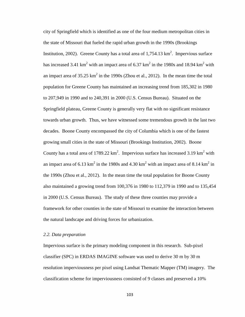
103
city of Springfield which is identified as one of the four medium metropolitan cities in
the state of Missouri that fueled the rapid urban growth in the 1990s (Brookings
Institution, 2002). Greene County has a total area of 1,754.13 km2. Impervious surface
has increased 3.41 km2 with an impact area of 6.37 km
2 in the 1980s and 18.94 km
2 with
an impact area of 35.25 km2 in the 1990s (Zhou et al., 2012). In the mean time the total
population for Greene County has maintained an increasing trend from 185,302 in 1980
to 207,949 in 1990 and to 240,391 in 2000 (U.S. Census Bureau). Situated on the
Springfield plateau, Greene County is generally very flat with no significant resistance
towards urban growth. Thus, we have witnessed some tremendous growth in the last two
decades. Boone County encompassed the city of Columbia which is one of the fastest
growing small cities in the state of Missouri (Brookings Institution, 2002). Boone
County has a total area of 1789.22 km2. Impervious surface has increased 3.19 km
2 with
an impact area of 6.13 km2 in the 1980s and 4.30 km
2 with an impact area of 8.14 km
2 in
the 1990s (Zhou et al., 2012). In the mean time the total population for Boone County
also maintained a growing trend from 100,376 in 1980 to 112,379 in 1990 and to 135,454
in 2000 (U.S. Census Bureau). The study of these three counties may provide a
framework for other counties in the state of Missouri to examine the interaction between
the natural landscape and driving forces for urbanization.
2.2. Data preparation
Impervious surface is the primary modeling component in this research. Sub-pixel
classifier (SPC) in ERDAS IMAGINE software was used to derive 30 m by 30 m
resolution imperviousness per pixel using Landsat Thematic Mapper (TM) imagery. The
classification scheme for imperviousness consisted of 9 classes and preserved a 10%

104
increment between classes except from the 0 to 20% range, where 0–20% was classified
as 0%, and 90 – 100%, which was classified as 100%. The difference in increment at the
beginning and end of the range was due to the software limitation of the SPC that it
cannot identify material covers less than 20% of a pixel. The remaining classes followed
10% increments where 20–30% classified as 30% up to 80–90% classified as 90%. Since
20% of a pixel is equivalent to 180 m2, most single family houses plus driveway will
have a footprint larger than 180 m2. Thus, such a limitation of the software is not going
to hurt the accurate mapping of population based on impervious surface. In a preliminary
research, imperviousness per pixel has been derived for the whole state of Missouri for
the year 1980, 1990 and 2000 (Zhou et al., 2012).
Beside the primary modeling unit, there are many predictor (independent)
variables. Since this research is precursor and foundation to a statewide study, the
availability of statewide dataset is a crucial criterion in choosing the candidates.
Considering the data availability and previous research, elevation, slope, waterbody, road
network, urban center and historical impervious surface growth are chosen as the
predictor variables in this research (Poelmans and Van Rompaey, 2009). More predictor
variables can be easily added as model input once available. Elevation data is obtained
from Missouri Spatial Data Information Service (MSDIS) in the format of 30m resolution
raster (hereafter referred to as ‘DEM’). Slope data is calculated from the elevation data
using Slope function in ArcGIS while retaining the same resolution (hereafter referred to
as ‘slope’). Waterbody is obtained from MSDIS as the overall hydrology combining
rivers, streams, lakes and ponds (hereafter referred to as ‘water’). An alternative

105
waterbody data is obtained by extracting major rivers from the hydrology dataset
(hereafter referred to as ‘major water’).
Road network data from 1992 and 2000 were obtained from U.S. Census website
in the topologically integrated geographic encoding and referencing (TIGER) road
centerline format. The TIGER road centerline data consist of polylines at a scale of
1:100,000 with codes for road types. Each road type can be assigned a weight in the
modeling process to imply their level of importance towards urban growth (Clarke and
Gaydos, 1998). However, due to the empirical nature of weights for different road types,
equal weights were used in one road network data (hereafter referred to as ‘road’). And
major roads were extracted as anther road network data to provide an alternative
(hereafter referred to as ‘major road’).
Urban center is a very important variable for urban modeling, which is used in
almost all urban modeling endeavors. However, it is by far the most difficult predictor
variable to obtain. Because it is not readily available and the entire collection of Census
defined urban boundaries are not satisfactory in generating urban centers for satellite
cities and leapfrog development surrounding metropolitans. Thus, a morphological
operation was used on impervious surface to achieve core urban areas through dilation
and erosion. The urban cores are then subject to a geometric mean center operation
which outputs the centroids of the urban core polygons which are used as a predictor
variable in this research (hereafter referred to as centroid). A graphic illustration is also
provided to show the derivation of core urban areas using impervious surface in the study
area of Jackson County (Fig. 1). To illustrate the superiority of urban core in terms of
centroids derivation, Census designated place (CDP), a very popular urban boundary

106
definition (Butzler et al., 2011), as well as Census designated urbanized area, another
common urban boundary definition, are included for comparison. Census designated
places (CDPs) are delineated for each decennial Census as the statistical counterparts of
incorporated places (U.S. Census Bureau). An urbanized area (UA) consists of densely
settled territory that contains 50,000 or more people (U.S. Census Bureau). According to
the definitions, both urban boundaries are defined based on population but with different
purposes. The urban boundaries derived by impervious surface are used in this research
because not only of its association with population, but also of its actual spatial
distribution and density that is geographically more accurate in defining the actual
urbanized area. Figure 1 also illustrates that the centroids generated by urban core are
located right in the middle of all sizable developments. On the other hand, centroids
derived by both Census designated place and urbanized area are either too numerous or
too clustered to show the actual growth center (Fig. 1).
Historical impervious surface growth is obtained by subtracting 1980
imperviousness by 1990 imperviousness and 1990 imperviousness by 2000
imperviousness. All the feature datasets are then converted to 30m by 30m resolution
raster through feature to raster tool in ArcGIS. The use of 30m by 30m resolution for all
the analysis dataset is on one hand determined by the resolution of satellite image derived
imperviousness and on the other hand the recent trend of using finer grids for urban
growth modeling and the availability of more powerful computers. Although previous
researches have outlined the benefit of different modeling units such as parcels (Landis,
1994). The benefit of using raster based modeling approach far outweighs the use of
parcels. For one thing, parcel data is not available for most States; another issue is parcel

107
boundaries may change overtime. Thus, more recent researches chose to use 30m by
30m raster as basic modeling unit (Deal and Schunk, 2004; Fang et al., 2005; Batisani
and Yarnal, 2009; Jokar Arsanjani et al., 2012). Moreover, raster data can be easily
aggregated to any geographical unit (hydrologic boundaries, administrative boundaries
and even parcels) allowing higher flexibility in model output utility.
Given the fact that not all predictor variables are created for this particular study,
data preprocessing is necessary to ensure they are spatially and temporally consistent.
Elevation, slope and waterbody do not change dramatically over time. Thus, no further
preprocessing is necessary. For source data collected in years other than the three
baseline years of 1980, 1990 and 2000, a linear interpolation is necessary to estimate the
values for the desired year provided the availability of multiple road network datasets
(Allen and Lu, 2003). However, since the TIGER data is in vector format, thus the
interpolation is not very convenient compounded by the reality that TIGER data prior to
1992 is not available. So imperfect data is still used in this research considering road
network is very important predictor variable for urban growth models.
2.3. Model design
The design principle is to build a simulation model instead of a forecasting model. The
simulation unit of the model is each county in the state of Missouri. In this pilot study,
only a few Counties are illustrated. The rationale to have county boundaries as the basic
modeling unit is that decision making is usually made at the political boundary level.
City boundaries are not used because a broader extent such as county provides the spatial
extent to which the urban area expands.

108
A rule-based model is used instead of the more popular logistic regression model,
because the latter relies entirely on historical data for calibration and simulation. For
example, the logistic regression approach is not capable of incorporating other factors,
new growth policies such as growth boundaries, which will have a bearing on the future
urban growth but are not responsible for the spatial pattern of historical urban growth. In
a rule-based model, these factors can be easily incorporated. Moreover, the effectiveness
of logistic regression approach is not very stable with a success rate ranging from less
than 30% to more than 90% depending on the study area (Allen and Lu, 2003). Another
very important feature of rule-based model is less computational intensive than a logistic
regression model. Thus, it will be more accessible to decision-makers who are less
familiar with the technical and statistical aspect of more complicated models such as
logistic regression, cellular automata or Markov Chain models. Finally, a rule-based
model is very easy and convenient to implement in the ModelBuilder environment of
ArcGIS.
This study used an open and modulated modeling approach, integrating several
individually developed modules to accomplish the urban growth simulation task at pixel
level. The rationale to take this specific approach is to make maintenance, update, and
expansion of simulation model easier than a holistic model. The justifications to use
multiple modules instead of a big model include: first, limited understanding of the urban
systems; second, individual processes related to urban growth may follow different
mathematical or physical processes that can be analyzed more effectively individually
(Landis, 1994); third, the modules can be easily modified and improved to meet future

109
needs, and new modules can be added to incorporate more aspect of urban systems upon
acquisition of new knowledge or expert input.
As shown in figure 2, the conceptual model framework involves five sub modules.
Distance Analysis Module calculates the Euclidean distance between all the undeveloped
pixels on the landscape against all distance based predictor variables (in raster format)
and then performs an overlay analysis between historical impervious surface growth and
distance based predictor variables. Terrain Analysis Module performs an overlay
analysis of historical impervious surface growth and its relationship to terrain based
predictor variable. Transition Probability Module combines together the output of
distance analysis and terrain analysis module to analyze the effect of various predictor
variables on historical urban growth. It then assigns weight to each predictor variable
and then combines them together to form the final raster transition probability surface
which contains the probability of each non-impervious surface pixels being converted to
impervious surface. Demand and Scenario Module determines the total urban growth
demand based on historical population growth as well as specified urban growth
scenarios. Urban Growth Simulation Module utilizes the output of transition probability
module and demand and scenarios module to simulate urban growth through calibration
and prediction. Calibration is done by comparing simulated historical growth with actual
historical growth. If the calibration failed to pass the ROC criteria, the transition
probability surface will be regenerated with different weights. Once the calibration is
passed, the same weights will be used to generate a new transition probability surface for
future urban growth prediction.
2.4. Model structure

110
Both distance and terrain analysis module will perform normalization to all the predictor
variables changing their value range to between 0 and 100 following the formula (Eq.
[2]):
N = INT[100(V - Vmin)/(Vmax - Vmin)] (1)
Where N is the normalized value, V is absolute value, Vmin is minimum value and Vmax is
maximum value and the function INT convert all decimal to integer. The purpose of
normalization is to ensure the model outputs of different study areas can be compared in
terms the underlying characteristics instead of the absolute values.
Transition probability module utilizes a rule-based modeling approach which uses
MCE derived statistical results to reclassify normalized predictor variables into transition
probability surface with higher value meaning more likely to transition into urbanized
pixel. The transition probability surfaces are then combined with weights determined by
expert inputs to determine the overall transition probability for the study area. The final
transition probability surface is then generated by applying a mask of unsuitable areas for
urbanization (Fig. 3).
Demand and scenario module utilizes different scenarios other than the default as
specified by historical trend. Growth scenarios are very important for simulation models
because the actual future urban growth is not predictable. But we could use different
scenarios for decision making purpose in order to prevent the fruition of undesirable
development outcomes. Growth scenarios could also be expressed as policy constraints,
growth rules, growth rates, or even to set up growth boundaries (Allen and Lu, 2003).
Different growth ratios will be used to determine the scenarios for future urban growth.
Growth ratio is also called sprawl index or sprawl scatter index and is defined as the ratio

111
of urban population growth versus urban area growth measured as the total
imperviousness growth. It can be defined using the following formula (Eq. [2]):
r = [(P1 – P0) / P0] / [(I1 – I0) / I0] (2)
Where r is the growth ratio; P0 is the starting population; P1 is the ending population; I0 is
the starting total imperviousness; and I1 is the ending total imperviousness. The
simulated total imperviousness growth is determined by the formula (Eq. [3]):
ΔI = I1 – I0 = I0(A1 – A0) / rA0 (3)
Different growth ratios were chosen to implement different growth scenarios for two
reasons. First, previous researches have indicated population growth to be the
fundamental driving force for future urban growth (Barlett et al., 2000; Heimlich and
Anderson, 2001; Johnson and Beale, 2002; Schnaiberg et al., 2002). Second, the
relationship between population and imperviousness has been researched in a precedent
study (Zhou et al., under reivew)
2.5. Model calibration
The calibration of the transition probability module is done by combining the output of
the Transition probability module and historical urban growth in a model simulation run
in the urban growth simulation module. The simulated historical urban growth is then
compared with the actual urban growth to evaluate the output of transition probability
module. There are quantification errors and locations errors for the simulated urban
growth pixels. Due to the design of this simulation model, quantification errors can be
ignored. So the accuracy assessment will focus on the location errors. The ROC method
will be used to assess the performance of the transition probability as compared to a
random decision surface (Pontius and Schneider, 2001). Two raster maps are needed to

112
calculate the ROC curve: (1) the suitability map that illustrate the relative likelihood of
each pixel undergoing a transition from undeveloped to developed, and (2) a map of
actual urban growth for the same timeframe of the simulation. The suitability map is the
most appropriate candidate to calculate a ROC curve, because it is the easiest to
understand that suitability map shows the priority in which pixels are selected to
transition from undeveloped to developed. The ROC curves work the best with binary
maps (i.e. developed and undeveloped). If more than two land-cover types are present,
then a ROC curve can be created for each land-cover type (i.e. one land-type versus the
rest). The first step in creating a ROC curve is to first slicing the suitability map into
several percentile groups. One common slicing scheme is to assign 10% of pixels for
each percentile group. Therefore, each of the 10 groups contains 10% of the pixels in the
study area. An increase in number of groups increases accuracy of estimated ROC, but
increases also the calculation complexity. If the evaluation result does not pass the
standard established by the user, the weight factor for each predictor variables need to be
changed. The default weights for each predictor variables are ones. It is preferable to
have expert input on the weight factors. However, in case expert inputs are not available,
a trial and error approach is used until the predetermined standard is reached. This
process can be done interactively by overlaying historical urban growth with each
predictor variable to find the ones with higher impact factor.
2.6. Model simulation
Urban growth simulation module serves two purposes: (1) for calibration runs, the
random component is deactivated in order to have the highest validation accuracy (Fig. 4);
(2) for simulation runs, the random component is turned on in order to capture the more

113
or less random aspect of the future urban growth. This module utilizes iterations to turn
undeveloped pixel into urbanized pixel. At the end of each model iteration the module
uses a Boolean logic to determine if more iteration is necessary based on the demand and
scenarios module output of total urban growth. This density of each impervious surface
pixel is determined by the historical relationship with elevation and slope. If only
location information is desired, the final output of this module can be reclassified into a
binary raster with 1 indicating urban and 0 indicating non-urban. Regardless of the
format, the final output of this module and the whole model can be used for land use
decision making, urban growth policy testing, public education of the negative effect of
urban sprawl and etc.
All of the modules described above are capable of processing raster datasets of
various resolutions. These modules were developed using ESRI’s ModelBuilder, an
ArcGIS application. In ModelBuilder, the model is represented by a flux diagram in a
graphic user interface that facilitates the creation, visualization, editing, and execution of
geoprocessing workflows which can be shared, modified and reused in different
geographic areas (Allen, 2011). A flowchart is presented here to illustrate all the major
procedures in a model simulation run (Fig. 5).
3. Results
3.1. Pattern of historical impervious surface growth
Figure 6 shows the distance analysis module and terrain analysis module output maps.
The impervious surface growths for two decades were compared against these maps to
generate the statistical results. The general pattern of impervious surface growth versus

114
terrain is similar between 1980s and 1990s (Fig. 7). More land was consumed in the
decade of 1990s compared to the 1980s. Moreover, impervious surface growth in the
1990s has consumed more high elevation land (Fig. 7A) as well as high slope land (Fig.
7B). Although a strong trend of slope resistance is preventing impervious surface growth
encroaching into even higher sloped areas (Fig. 7B). The peaks for impervious surface
growth occurred at similar ranges for both elevation (Fig. 7A) and slope (Fig. 7B).
Similarly, distance measures were analyzed using historical impervious surface growth.
The two distance measure of normalized distance to road and water are not used because
of their high density distribution which leads to the impervious surface growths
concentrated in a narrow band of values. Figure 8A has the most complicated trend of
distribution due to the spatially uneven distributed centroids. Figure 8B is very intuitive
in that it shows new urban growth are usually very close to the road network. In other
words, undeveloped pixels that are close to the major highways are more likely to turn
into developments. Figure 8C is even more extreme than 8B in that it shows majority of
developments are very close to the most recent developments. More explicitly speaking,
impervious surface increments in the 1980s are more closely related to the impervious
surface of 1980 and impervious surface increments in the 1990s are more closely related
to the impervious surface of 1990. Figure 8D is showing a slow but affirmative decrease
in development as distance to major water increases. In other words, although the
influence of water on impervious surface growth is not as immediate as historical
impervious surface or road network, the influence is still clear enough that it can’t be
ignored.
3.2. Model calibration

115
Based on the statistic results of figure 7 and 8, all of the predictor variables were
reclassified using the frequency of impervious surface growth. These reclassified
transition probability surfaces for the decade of 1980s (Fig. 9) and 1990s (Fig. 10) are
showing areas with high impervious surface growth in red and low growth area in green.
These transition probability surfaces are summed with default weight to generate the total
transition probability surfaces (Fig. 11). The default weights were chosen so that each
transition probability surfaces is exerting similar amount of influence towards the total
transition probability surface. Two total transition probability surfaces for the decades of
1980s and 1990s with historical impervious surface removed are produced for calibration
using Jackson County as example (Fig. 11). Similar steps were taken for both Greene
and Boone County with two more sets of total transition probability surfaces produced
for comparison purpose. For calibration purpose, the historical growth scenarios are used
for the decade of 1980s and 1990s to generate the suitability maps for three counties.
These suitability maps are compared with the actual urban growth for two decades in
these three counties to validate the effectiveness of the simulation model. Six ROC
curves are generated based on the simulated historical growth (Fig. 12). The areas under
the six ROC curves are ranged from 0.68 to 0.85 with a short span. In both decades, the
ROC has an increasing trend from large metropolitan county (Jackson) to medium
metropolitan county (Greene) to small city county (Boone) with the decade of 1990s’
ROC having slightly higher values (Fig. 12). Statistically, ROC above 50% is better than
random. Similar research has reported ROCs ranging from 65 to 70% in a different study
area (Pontius and Schneider, 2001) which proved the performance of the simulation

116
model satisfactory. Thus, the same approach can be applied to predict future urban
growth under the same scenario of historical urban growth.
3.3. Future impervious surface growth prediction
For large metropolitan area (Jackson County in this study), potential urban development
mostly circled around the leap-frog development from the satellite cities of Kansas City
metropolitan area with a high likelihood to merge with the core Kansas City urban area to
form an even bigger metro (Fig. 13). According to this simulation, the total population
for Jackson County will increase by 21,705 for every time step of 10 years with a net
growth of 65,115. The total population of Jackson County will reach 719,971 in the year
2030 based on historical population growth trend. Similarly, the urban growth for each
decade is measured at 18.53 km2 in terms of impervious surface growth with a potential
impact area of 38.51 km2. By 2030, the total urbanized area of Jackson County will reach
250 km2 in total impervious surface with a potential to impact about 500 km
2 of land
which is near a third of the total land area of Jackson County. If the growth rate
continues, the entire area of Jackson County will be developed in less than 250 years
considering areas that are not suitable for development. All of the above projections are
based on the same growth rate during the decade of 1990s. In light of the fact that urban
growth is considerably faster in the 1990s than the 1980s, a possible exponential growth
trend will consume the open land in Jackson County even faster.
In medium sized metropolitan cities (Greene County in this study), potential
urban development concentrated around the urban fringe of the city of Springfield and
along the major highways (Fig. 14). According to this simulation, the total population for
Greene County will increase by 32,442 for every time step of 10 years with a net growth

117
of 97,326. The total population of Greene County will reach 337,717 in the year 2030
based on historical population growth trend. Similarly, the urban growth for each decade
is measured at 18.60 km2 in terms of impervious surface growth with a potential impact
area of 35.20 km2. By 2030, the total urbanized area of Greene County will reach 160
km2 in total impervious surface with a potential to impact about 300 km
2 of land which is
near a sixth of the total land area of Greene County.
In small cities (Boone County), potential urban development concentrated mostly
in the northwest and west region and scattered around southwest, southeast and northeast
regions of the city of Columbia. Some rural urban growth can also be spotted in the
northeast and southeast corner as well as west side of Boone County (Fig. 15).
According to this simulation, the total population for Boone County will increase by
23,075 for every time step of 10 years with a net growth of 69,225. The total population
of Boone County will reach 204,679 in the year 2030 based on historical population
growth trend. Similarly, the urban growth for each decade is measured at 4.23 km2 in
terms of impervious surface growth with a potential impact area of 8.10 km2. By 2030,
the total urbanized area of Boone County will reach 55 km2 in total impervious surface
with a potential to impact about 100 km2 of land.
4. Discussion
The ultimate purpose of building a simulation model is to apply it towards decision
making. A useful urban growth simulation model should eventually be used by urban
planners and policy makers. The biggest reason that urban growth simulation models are
rarely used by policy makers and urban planners and only circulated in the field of
academia is because most models are too complicated to use. Take the very population

118
logistic regression approach as an example which was implemented in most urban growth
models, the derivation of model coefficients are too time-consuming and statistically
demanding. One misstep in the data collection or preprocessing stage will lead to the
coefficients that are against common sense and even ridiculous in certain cases. Distance
to urban centers, elevation, distance to roads and distance to streams are considered very
important predictor variable as a consensus among urban growth modelers. However, the
coefficients of these predictor variables, according to a recent research, are so small that
the effects of these predictor variables are negligible (Jokar Arsanjani et al., 2012).
Another very important reason to explain the unflattering popularity of urban growth
model is that most model frameworks focused more on model structure design but
neglected the importance of data preprocessing which might be more important than the
model structure. As illustrated in this research the derivation of growth centroids is a
very good example of outlining the procedures to prepare predictor variable s that are
more likely to generate more meaningful results.
It may be argued that a rule-based model is less scientific than a more rigorous
deterministic model with statistics derived coefficients. However, people like policy
makers and urban planners may have more “knowledge” of the urban systems than any
outgoing urban growth models. Plus, knowledge from the experts could be used to guide
smarter growth through a more environmental and ecological friendly way of urban
development (Freilich, 2003). Moreover, humans have the tendencies to not follow the
established common sense on building new urban areas. Thus, many new growths can
only be linked to personal preference rather than the rules deducted from predictor
variable evaluation. After all, humans are the underlying driving forces for all urban

119
growths and there is a certain stochastic components related to people’s preference and
decision making. Thus, a stochastic component is added to the urban growth simulation
module to at least partly explain the stochastic nature of individual’s decision making in
terms of urban growth preference.
This research establishes a solid framework for future urban growth research as
well as providing a preliminary tool for decision making in terms of future urban growth.
However, it still has constraints and limitations. The biggest limitation is the absence of
a macro-economic module that can better predict future population demographics by
inferencing the supporting capacity of local economy in order to more scientifically
calculate the fluctuation of population instead of using the historical trend. Another
limitation of this modeling approach is the inability to link growth scenarios to actual
growth policies. In this research, the historical development density is used in absence of
the knowledge of future growth density. Default scenarios could be used to give a range
of variability for decision making purpose. However, unless the physical meaning of
development density is defined, this issue will always be a limitation for urban growth
models. Other minor limitations include but are not limited to predictor variable
accuracy including spatial and temporal consistencies. The most important model input
in this research is the historical impervious surface which is derived by satellite image
and will subject to classification accuracy. Due to the time frame chosen by this research,
some predictor variables may not be available at certain fixed time steps. Either data
interpolation is used to alleviate the problem, or the less than perfect data will be used
when interpolation is not feasible.

120
Finally, it is very important to work with decision makers and urban planner such
as state and city agencies in charge of growth management to further develop this model
provided with their expertise stemmed from previous management experience on urban
growth. At the end of the day, a model has to be used to show its value. And only
through practical applications can a theoretical models be updated regularly and
improved.
5. Conclusion
In this research, an open, rule-based, modulated, GIS model was developed using
ModelBuilder in ArcGIS. Multiple independent variables are identified and analyzed as
the predictor variables of this model. Model calibration was done using MCE of
historical urban growth. A trial and error approach was used to derive weights for each
predictor variable in order for the simulated urban growth to be consistent spatially with
the actual urban growth. The calibrated model is used to simulate future urban growth
for 2010, 2020 and 2030 under the historical growth trend during the 1990s.
Urban growth simulation is a very complicated physical process that imposes a
huge challenge to researchers who are trying to model and simulate future urban growth.
With the help of a GIS model, the urban growth process can be quantified, analyzed and
replicated to simulate future urban growth. The model framework and analysis
workflows can have a huge impact on future urban growth management. Even under the
conservative historical growth trend, it is still projected that a third of the land area of
Jackson County will be developed by 2030. This model simulation result can be used to
education citizens the negative effects of low density urban growth through statistics
reporting and visual demonstration. More importantly, the simulated results can urge the

121
policy makers and urban planners to take a different route in urban growth management
before everything get out of control. It is very imperative for researchers and policy
makers to work together to link urban growth policies with actual model simulation
output in order to build a more practical model that can be used in real life application.

122
References
AGARWAL, C., GREEN, G. M., GROVE, J. M., EVANS, T. P. & SCHWEIK, C. M.
(2002) A review and assessment of land-use change models: Dynamics of space,
time, and human choice. A Review and Assessment of Land-Use Change Models:
Dynamics of Space, Time, and Human Choice.
ALBERTI, M. (2008) Advances in urban ecology: integrating humans and ecological
processes into urban ecosystems. New York, NY, USA, Springer Science.
ALLEN, D. W. (2011) Getting to Know ArcGIS ModelBuilder, ESRI Press.
ALLEN, J. & LU, K. (2003) Modeling and prediction of future urban growth in the
Charleston region of South Carolina: A GIS-based integrated approach. Ecology
and Society, 8.
ARNOLD JR, C. L. & GIBBONS, C. J. (1996) Impervious surface coverage: The
emergence of a key environmental indicator. Journal of the American Planning
Association, 62, 243–258.
BARTLETT, J. G., MAGEEAN, D. M. & O'CONNOR, R. J. (2000) Residential
expansion as a continental threat to U.S. coastal ecosystems. Population and
Environment, 21, 429-468.
BATISANI, N. & YARNAL, B. (2009) Urban expansion in Centre County, Pennsylvania:
Spatial dynamics and landscape transformations. Applied Geography, 29, 235-
249.
BERRY, M. W., HAZEN, B. C., MACINTYRE, R. L. & FLAMM, R. O. (1996) Lucas: a
system for modeling land-use change. IEEE computational science & engineering,
3, 24-35.
BROOKINGS, I. (2002) Growth in the heartland: challenges and opportunities for
Missouri. Washington, D. C., USA, Brookings Insititution, Center on Urban and
Metropolitan Policy.
BUTZLER, S. J., BREWER, C. A. & STROH, W. J. (2011) Establishing classification
and hierarchy in populated place labeling for multiscale mapping for the National
map. Cartography and Geographic Information Science, 38, 100-109.
CLARKE, K. C. & GAYDOS, L. J. (1998) Loose-coupling a cellular automaton model
and GIS: long-term urban growth prediction for San Francisco and
Washington/Baltimore. International Journal of Geographical Information
Science, 12, 699-714.

123
CLARKE, K. C., HOPPEN, S. & GAYDOS, L. (1997) A self-modifying cellular
automaton model of historical urbanization in the San Francisco Bay area.
Environment and Planning B: Planning and Design, 24, 247-261.
DEAL, B. & SCHUNK, D. (2004) Spatial dynamic modeling and urban land use
transformation: A simulation approach to assessing the costs of urban sprawl.
Ecological Economics, 51, 79-95.
EICHER, C. L. & BREWER, C. A. (2001) Dasymetric mapping and areal interpolation:
Implementation and evaluation. Cartography and Geographic Information Science,
28, 125-138.
EWING, R. (1994) Characteristics, causes, and effects of sprawl: A literature review.
Environmental and Urban Issues, 21, 1-15.
FANG, S., GERTNER, G. Z., SUN, Z. & ANDERSON, A. A. (2005) The impact of
interactions in spatial simulation of the dynamics of urban sprawl. Landscape and
Urban Planning, 73, 294-306.
FREILICH, R. H. (2003) Smart growth in western metro areas. Natural Resources
Journal, 43, 687-702.
HEIMLICH, R. E. & ANDERSON, W. D. (2001) Development at the urban fringe and
beyond: Impacts on agriculture and rural land. Development at the Urban Fringe
and Beyond: Impacts on Agriculture and Rural Land.
HUANG, B., ZHANG, L. & WU, B. (2009) Spatiotemporal analysis of rural-urban land
conversion. International Journal of Geographical Information Science, 23, 379-
398.
JI, M. & JENSEN, J. R. (1999) Effectiveness of subpixel analysis in detecting and
quantifying urban imperviousness from landsat thematic mapper imagery.
Geocarto International, 14, 31-39.
JIANG, H. & EASTMAN, J. R. (2000) Application of fuzzy measures in multi-criteria
evaluation in GIS. International Journal of Geographical Information Science, 14,
173-184.
JOHNSON, K. M. & BEALE, C. L. (2002) Nonmetro recreation counties: Their
identification and rapid growth. Rural America, 17, 12-19.
JOKAR ARSANJANI, J., HELBICH, M., KAINZ, W. & DARVISHI BOLOORANI, A.
(2012) Integration of logistic regression, Markov chain and cellular automata
models to simulate urban expansion. International Journal of Applied Earth
Observation and Geoinformation.
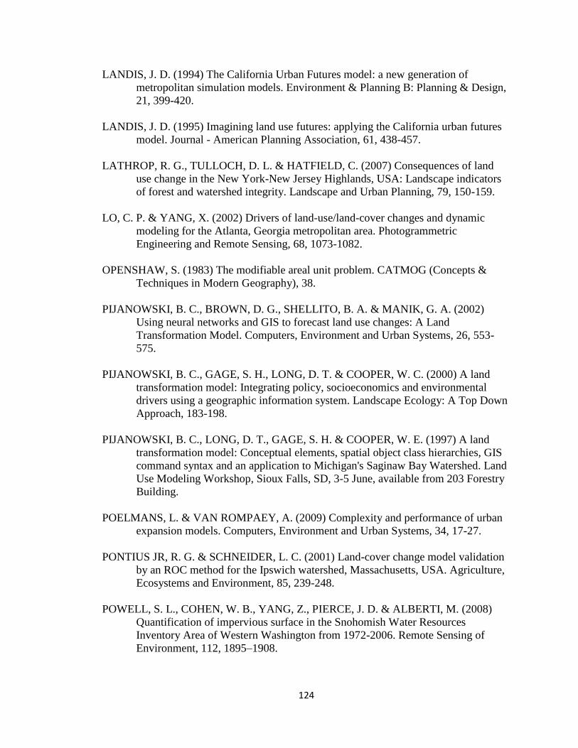
124
LANDIS, J. D. (1994) The California Urban Futures model: a new generation of
metropolitan simulation models. Environment & Planning B: Planning & Design,
21, 399-420.
LANDIS, J. D. (1995) Imagining land use futures: applying the California urban futures
model. Journal - American Planning Association, 61, 438-457.
LATHROP, R. G., TULLOCH, D. L. & HATFIELD, C. (2007) Consequences of land
use change in the New York-New Jersey Highlands, USA: Landscape indicators
of forest and watershed integrity. Landscape and Urban Planning, 79, 150-159.
LO, C. P. & YANG, X. (2002) Drivers of land-use/land-cover changes and dynamic
modeling for the Atlanta, Georgia metropolitan area. Photogrammetric
Engineering and Remote Sensing, 68, 1073-1082.
OPENSHAW, S. (1983) The modifiable areal unit problem. CATMOG (Concepts &
Techniques in Modern Geography), 38.
PIJANOWSKI, B. C., BROWN, D. G., SHELLITO, B. A. & MANIK, G. A. (2002)
Using neural networks and GIS to forecast land use changes: A Land
Transformation Model. Computers, Environment and Urban Systems, 26, 553-
575.
PIJANOWSKI, B. C., GAGE, S. H., LONG, D. T. & COOPER, W. C. (2000) A land
transformation model: Integrating policy, socioeconomics and environmental
drivers using a geographic information system. Landscape Ecology: A Top Down
Approach, 183-198.
PIJANOWSKI, B. C., LONG, D. T., GAGE, S. H. & COOPER, W. E. (1997) A land
transformation model: Conceptual elements, spatial object class hierarchies, GIS
command syntax and an application to Michigan's Saginaw Bay Watershed. Land
Use Modeling Workshop, Sioux Falls, SD, 3-5 June, available from 203 Forestry
Building.
POELMANS, L. & VAN ROMPAEY, A. (2009) Complexity and performance of urban
expansion models. Computers, Environment and Urban Systems, 34, 17-27.
PONTIUS JR, R. G. & SCHNEIDER, L. C. (2001) Land-cover change model validation
by an ROC method for the Ipswich watershed, Massachusetts, USA. Agriculture,
Ecosystems and Environment, 85, 239-248.
POWELL, S. L., COHEN, W. B., YANG, Z., PIERCE, J. D. & ALBERTI, M. (2008)
Quantification of impervious surface in the Snohomish Water Resources
Inventory Area of Western Washington from 1972-2006. Remote Sensing of
Environment, 112, 1895–1908.

125
RADELOFF, V. C., HAMMER, R. B. & STEWART, S. I. (2005) Rural and suburban
sprawl in the U.S. Midwest from 1940 to 2000 and its relation to forest
fragmentation. Conservation Biology, 19, 793-805.
SCHNAIBERG, J., RIERA, J., TURNER, M. G. & VOSS, P. R. (2002) Explaining
human settlement patterns in a recreational lake district: Vilas County, Wisconsin,
USA. Environmental Management, 30, 24-34.
TSAI, Y. H. (2005) Quantifying urban form: Compactness versus 'sprawl'. Urban Studies,
42, 141-161.
WADDELL, P. (1998) Oregon Prototype Metropolitan Land Use Model. Proceedings of
the Conference on Transportation, Land Use, and Air Quality.
WEGENER, M. (1994) Operational urban models: state of the art. Journal - American
Planning Association, 60, 17-29.
WU, F. (1996) A linguistic cellular automata simulation approach for sustainable land
development in a fast growing region. Computers, Environment and Urban
Systems, 20, 367-387.
YU, J., CHEN, Y., WU, J. & KHAN, S. (2011) Cellular automata-based spatial multi-
criteria land suitability simulation for irrigated agriculture. International Journal
of Geographical Information Science, 25, 131-148.
ZHANG, R., TANG, C., MA, S., YUAN, H., GAO, L. & FAN, W. (2011) Using Markov
chains to analyze changes in wetland trends in arid Yinchuan Plain, China.
Mathematical and Computer Modelling, 54, 924-930.
ZHOU, B., HE, H. S., NIGH, T. A. & SCHULZ, J. H. (2012) Mapping and analyzing
change of impervious surface for two decades using multi-temporal Landsat
imagery in Missouri. International Journal of Applied Earth Observation and
Geoinformation, 18, 195-206.

126
Tables
Table 1. Model simulation validation for the decade of 1980s and 1990s presented as (%)
error.
Model validation 1980s 1990s
Omission error
Low
Urban (simulated as non-urban) 57.55 51.23
Non-urban (simulated as urban) 0.95 2.75
Commission error
Urban (simulated as non-urban) 54.96 50.61
Non-urban (simulated as urban) 1.06 2.82
Overall error 1.97 5.27
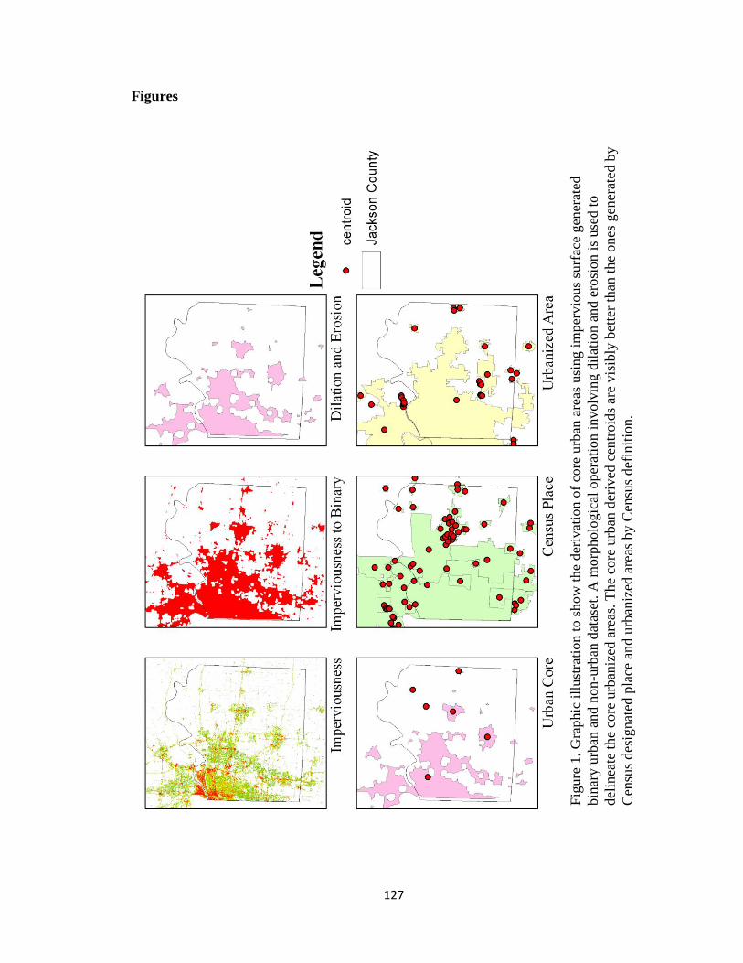
127
Figures
Fig
ure
1. G
raphic
ill
ust
rati
on t
o s
how
the
der
ivat
ion o
f co
re u
rban
are
as u
sing i
mper
vio
us
surf
ace
gen
erat
ed
bin
ary u
rban
and n
on
-urb
an d
atas
et. A
morp
holo
gic
al o
per
atio
n i
nvolv
ing d
ilat
ion a
nd e
rosi
on i
s use
d t
o
del
inea
te t
he
core
urb
aniz
ed a
reas
. T
he
core
urb
an d
eriv
ed c
entr
oid
s ar
e vis
ibly
bet
ter
than
the
ones
gen
erat
ed b
y
Cen
sus
des
ignat
ed p
lace
and u
rban
ized
are
as b
y C
ensu
s def
init
ion.

128
Fig
ure
2. O
ver
all
model
str
uct
ure
of
the
urb
an g
row
th s
imula
tion m
odel
wit
h a
tota
l of
6 s
ub
-module
s il
lust
rate
d.

129
Fig
ure
3. D
iagra
m o
f th
e tr
ansi
tion p
robab
ilit
y m
odule
, al
l th
e pre
dic
tor
var
iable
s ar
e re
clas
sifi
ed
bas
ed o
n t
he
stat
isti
cal
resu
lts
gen
erat
ed f
rom
the
mult
i-cr
iter
ia e
val
uat
ion o
f his
tori
cal
imper
vio
us
surf
ace
couple
d w
ith d
efau
lt o
r ex
per
t in
put
wei
ghts
excl
udin
g t
he
non
-dev
elopab
le a
reas
to g
ener
ate
the
final
tra
nsi
tion p
robab
ilit
y s
urf
ace
outp
ut.

130
Fig
ure
4. D
iagra
m o
f th
e urb
an g
row
th s
imula
tio
n m
odule
, th
e gen
erat
ion o
f new
im
per
vio
us
surf
ace
pix
els
is b
ased
on
an i
tera
tion l
oop c
ontr
oll
ed b
y t
he
input
of
pre
set
tota
l gro
wth
. T
he
module
is
stopped
by a
Boole
an l
ogic
once
th
e des
ignat
ed g
row
th t
ota
l is
met
. T
he
outp
ut
can b
e im
per
vio
us
surf
ace
den
sity
bas
ed o
n t
he
loca
tion o
f new
urb
an a
nd h
isto
rica
l den
sity
dis
trib
uti
on o
f im
per
vio
us
surf
ace
or
sim
ply
the
loca
tion o
f new
urb
an g
row
th.
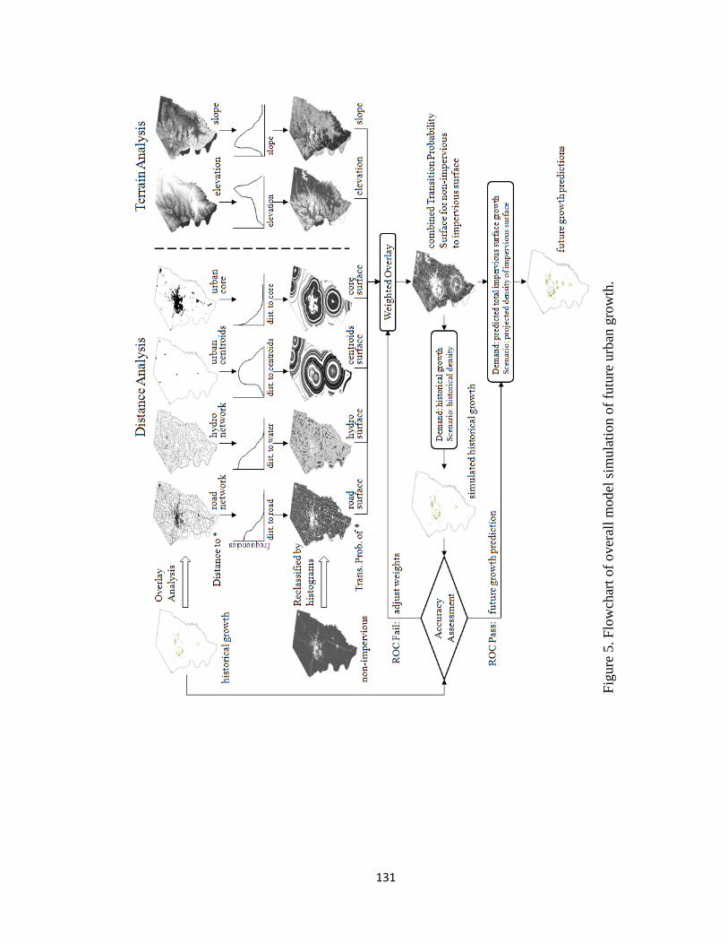
131
Fig
ure
5. F
low
char
t of
over
all
model
sim
ula
tion o
f fu
ture
urb
an g
row
th.
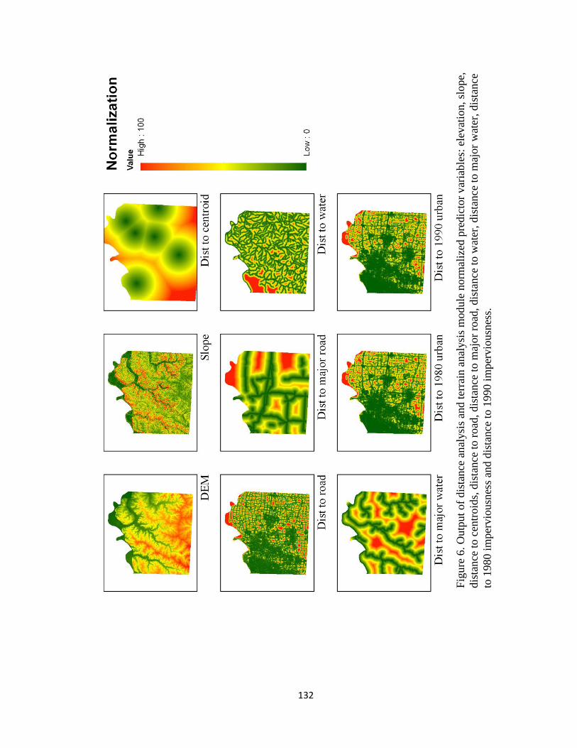
132
Fig
ure
6. O
utp
ut
of
dis
tance
an
alysi
s an
d t
erra
in a
nal
ysi
s m
od
ule
norm
aliz
ed p
redic
tor
var
iable
s: e
levat
ion, sl
ope,
dis
tance
to c
entr
oid
s, d
ista
nce
to r
oad
, dis
tance
to m
ajor
road
, dis
tance
to w
ater
, dis
tance
to m
ajor
wat
er, dis
tance
to 1
980 i
mper
vio
usn
ess
and d
ista
nce
to 1
990 i
mper
vio
usn
ess.

133
Fig
ure
7. T
he
freq
uen
cies
of
imper
vio
us
surf
ace
gro
wth
sum
mar
ized
by n
orm
aliz
ed e
lev
atio
n i
n 1
980s
and 1
990s
(A).
Th
e
freq
uen
cies
of
imper
vio
us
surf
ace
gro
wth
sum
mar
ized
by n
orm
aliz
ed s
lop
e in
the
1980s
and 1
990s
(B).
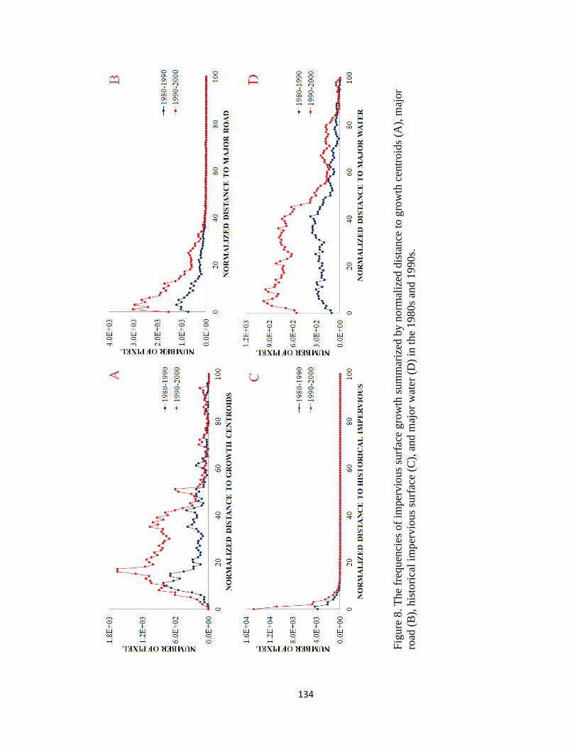
134
Fig
ure
8. T
he
freq
uen
cies
of
imper
vio
us
surf
ace
gro
wth
sum
mar
ized
by n
orm
aliz
ed d
ista
nce
to g
row
th c
entr
oid
s (A
), m
ajor
road
(B
), h
isto
rica
l im
per
vio
us
surf
ace
(C),
and m
ajor
wat
er (
D)
in t
he
198
0s
and 1
990s.
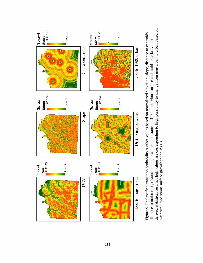
135
Fig
ure
9. R
ecla
ssif
ied t
ransi
tion p
robab
ilit
y s
urf
ace
val
ues
bas
ed o
n n
orm
aliz
ed e
lev
atio
n, sl
ope,
dis
tance
to c
entr
oid
s,
dis
tance
to m
ajor
road
, dis
tance
to m
ajor
wat
er a
nd d
ista
nce
to 1
980 i
mper
vio
us
surf
ace
and m
ult
i-cr
iter
ia e
val
uat
ion
der
ived
sta
tist
ical
res
ult
s. H
igh v
alues
are
corr
espo
ndin
g t
o h
igh p
oss
ibil
ity t
o c
han
ge
from
non
-urb
an t
o u
rban
bas
ed o
n
his
tori
cal
imper
vio
us
surf
ace
gro
wth
in t
he
1980
s.
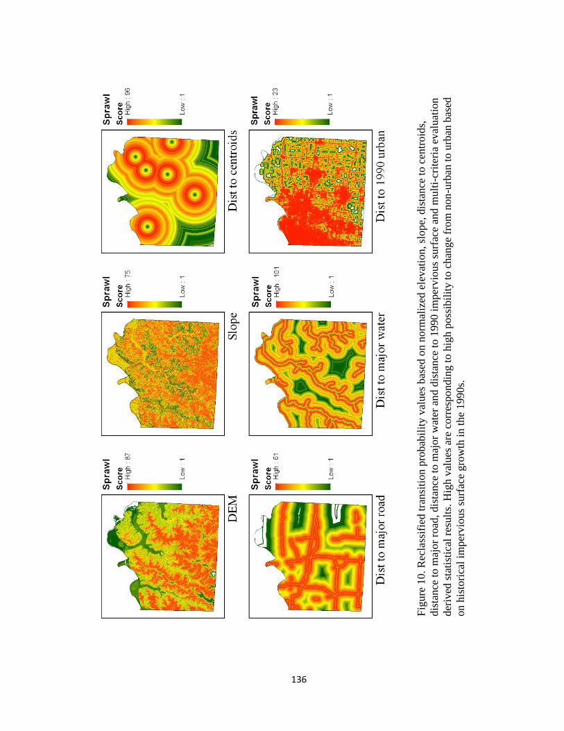
136
Fig
ure
10. R
ecla
ssif
ied t
ransi
tion p
robab
ilit
y v
alues
bas
ed o
n n
orm
aliz
ed e
levat
ion, sl
ope,
dis
tance
to c
entr
oid
s,
dis
tance
to m
ajor
road
, dis
tance
to m
ajor
wat
er a
nd d
ista
nce
to 1
990 i
mper
vio
us
surf
ace
and m
ult
i-cr
iter
ia e
val
uat
ion
der
ived
sta
tist
ical
res
ult
s. H
igh v
alues
are
corr
espo
ndin
g t
o h
igh p
oss
ibil
ity t
o c
han
ge
from
non
-urb
an t
o u
rban
bas
ed
on h
isto
rica
l im
per
vio
us
surf
ace
gro
wth
in t
he
199
0s.

137
Fig
ure
11. T
ota
l tr
ansi
tion p
robab
ilit
y v
alues
for
all
dev
elopab
le p
ixel
s fo
r th
e dec
ade
of
1980s
and 1
990s.
Hig
h t
ota
l
val
ues
are
corr
espondin
g t
o h
igh p
oss
ibil
ity t
o c
han
ge
from
non
-urb
an t
o u
rban
bas
ed o
n h
isto
rica
l im
per
vio
us
surf
ace
gro
wth
in t
he
1980s
and 1
990s
corr
espondin
gly
.

138
Figure 12. ROC curves for model simulation of impervious surface growth calibration in
1980s (upper) and 1990s (lower) for Jackson, Greene, and Boone Counties compared
with random growth of impervious surface.
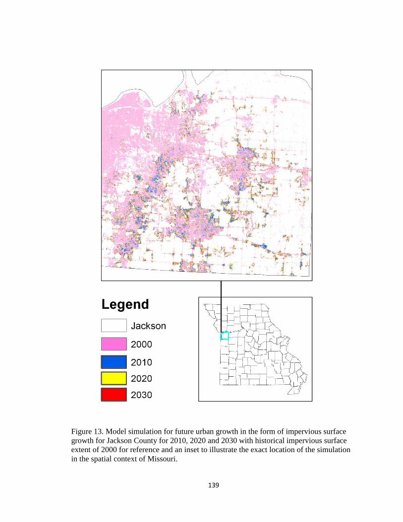
139
Figure 13. Model simulation for future urban growth in the form of impervious surface
growth for Jackson County for 2010, 2020 and 2030 with historical impervious surface
extent of 2000 for reference and an inset to illustrate the exact location of the simulation
in the spatial context of Missouri.
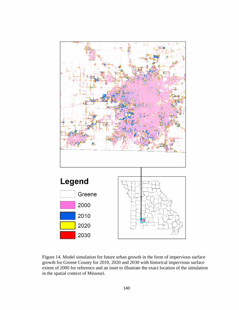
140
Figure 14. Model simulation for future urban growth in the form of impervious surface
growth for Greene County for 2010, 2020 and 2030 with historical impervious surface
extent of 2000 for reference and an inset to illustrate the exact location of the simulation
in the spatial context of Missouri.
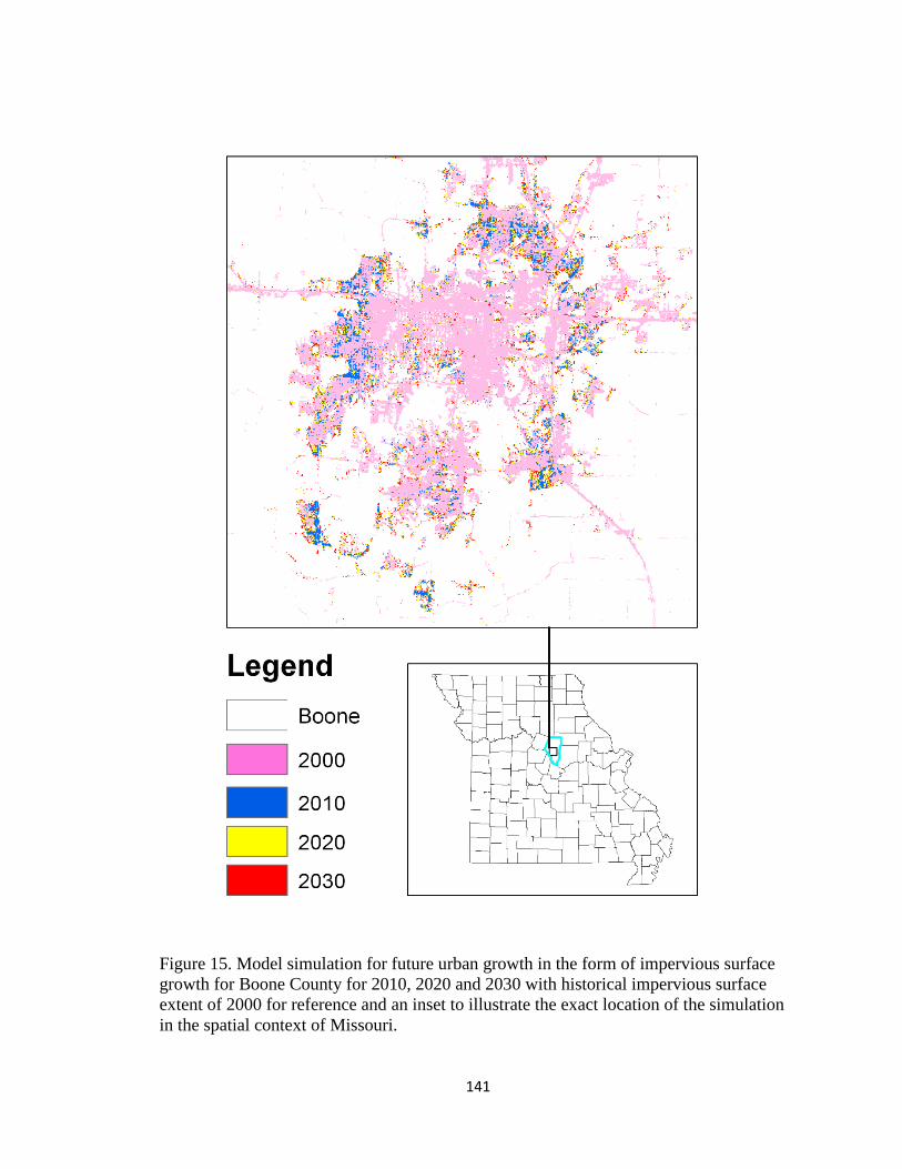
141
Figure 15. Model simulation for future urban growth in the form of impervious surface
growth for Boone County for 2010, 2020 and 2030 with historical impervious surface
extent of 2000 for reference and an inset to illustrate the exact location of the simulation
in the spatial context of Missouri.

142
VITA
Bo Zhou was born July 20th
, 1983 in Wuhan, China. After graduating with his
undergraduate degree in China, he came to the US to pursue graduate studies in the
University of Missouri. His seven years in the graduate school is very eventful and
productive. He has attended various academic conferences and presented in each. He
has published two peer reviewed papers and two more papers are under review. He
received the following degrees: a B.S. in Remote Sensing and Photogrammetry from
Wuhan University in Wuhan China (2005); a M.A. in Geography from University of
Missouri at Columbia, Missouri (2007); and a Ph.D. in Forestry from University of
Missouri at Columbia, Missouri (2012).