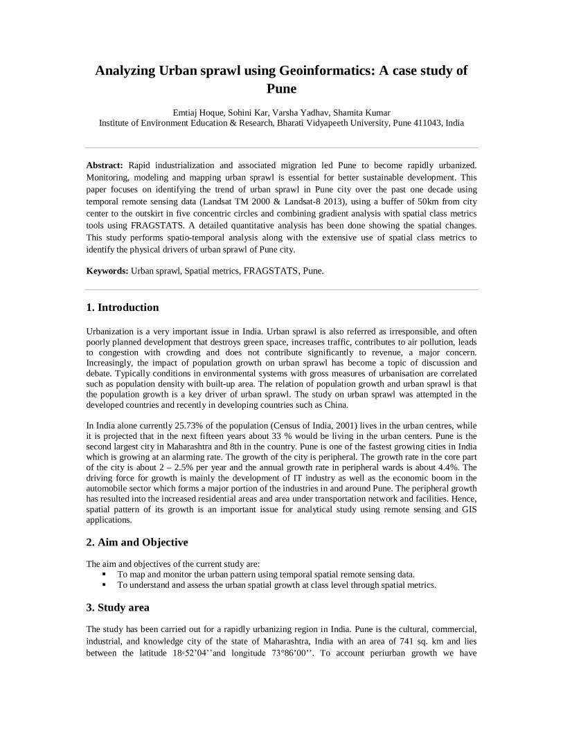
Analyzing Urban sprawl using Geoinformatics: A case study of Pune

Emtiaj Hoque, Sohini Kar, Varsha Yadhav, Shamita Kumar Institute of Environment Education & Research, Bharati Vidyapeeth University, Pune 411043, India

Abstract: Rapid industrialization and associated migration led Pune to become rapidly urbanized. Monitoring, modeling and mapping urban sprawl is essential for better sustainable development. This paper focuses on identifying the trend of urban sprawl in Pune city over the past one decade using temporal remote sensing data (Landsat TM 2000 & Landsat-8 2013), using a buffer of 50km from city center to the outskirt in five concentric circles and combining gradient analysis with spatial class metrics tools using FRAGSTATS. A detailed quantitative analysis has been done showing the spatial changes. This study performs spatio-temporal analysis along with the extensive use of spatial class metrics to identify the physical drivers of urban sprawl of Pune city.

Keywords: Urban sprawl, Spatial metrics, FRAGSTATS, Pune.

1. Introduction Urbanization is a very important issue in India. Urban sprawl is also referred as irresponsible, and often poorly planned development that destroys green space, increases traffic, contributes to air pollution, leads to congestion with crowding and does not contribute significantly to revenue, a major concern. Increasingly, the impact of population growth on urban sprawl has become a topic of discussion and debate. Typically conditions in environmental systems with gross measures of urbanisation are correlated such as population density with built-up area. The relation of population growth and urban sprawl is that the population growth is a key driver of urban sprawl. The study on urban sprawl was attempted in the developed countries and recently in developing countries such as China. In India alone currently 25.73% of the population (Census of India, 2001) lives in the urban centres, while it is projected that in the next fifteen years about 33 % would be living in the urban centers. Pune is the second largest city in Maharashtra and 8th in the country. Pune is one of the fastest growing cities in India which is growing at an alarming rate. The growth of the city is peripheral. The growth rate in the core part of the city is about 2 – 2.5% per year and the annual growth rate in peripheral wards is about 4.4%. The driving force for growth is mainly the development of IT industry as well as the economic boom in the automobile sector which forms a major portion of the industries in and around Pune. The peripheral growth has resulted into the increased residential areas and area under transportation network and facilities. Hence, spatial pattern of its growth is an important issue for analytical study using remote sensing and GIS applications. 2. Aim and Objective The aim and objectives of the current study are: To map and monitor the urban pattern using temporal spatial remote sensing data. To understand and assess the urban spatial growth at class level through spatial metrics.

3. Study area

The study has been carried out for a rapidly urbanizing region in India. Pune is the cultural, commercial, industrial, and knowledge city of the state of Maharashtra, India with an area of 741 sq. km and lies between the latitude 18◦52’04’’and longitude 73°86’00’’. To account periurban growth we have

considered 50km. circular buffer from the Pune administrative boundary by considering the City Business District (CBD) as center (Figure 1). The predominant land cover primarily consists of grassland, cropland, and bare land with forests, urban zones and scattered water bodies.

Pune district is among the highest in the state with over 57.39 lakh people living in cities according to the Census of India. Population is one of the main factor of the urban growth as well as migration from rural to urban areas. According to the Census of India 2001 and 2011, the actual population of Pune in 2001 was 7,232,555 which had an increase in urban growth to 9,429,408. The population growth per sq. km reduced from 30.73% in 2001 to 30.37% in 2011. The density per sq.km in 2001 was 462 which increased to 603 in 2011. This depicts that there has been a huge growth in a span of 10 years contributing to urban growth.

Invest in manufacturing, IT and overall growth in economic activity has led to an influx of people into Pune. Pune has established itself as the ‘Academic Corridor’ of India and is also the emerging InfoTech Hub. It is the place of huge IT investments. Hence migration due to employment opportunities as well as educational purpose has been major ‘pull factors’. Due to close proximity to the economic region of the country i.e Mumbai, rapid growing infrastructure and enchanting climate makes Pune a favorable place to settle. Urban sprawl is the scattering of new development of land use pattern causing loss of productive agricultural land, forest covers and other forms of greenery, loss in surface water bodies, depletion in ground water aquifers and increasing levels of air and water pollution causing environmental problems. The process of urbanization is affected by population growth and migration.

4. Data source and type Different remote sensing and GIS data from different sources has been used in this research. Landsat TM images of 2000 and Landsat 8 20113 were used to detect urban land cover change pattern of this study area. These images were obtained from the United States Geological Survey (USGS) website as standard product i.e. geometrically and radio metrically corrected. Most GIS data such as administrative boundaries, CBD, major roads are obtained from SOI maps. All dataset used in this study are geometrically referenced to the WGS 1984, UTM 43N projection system

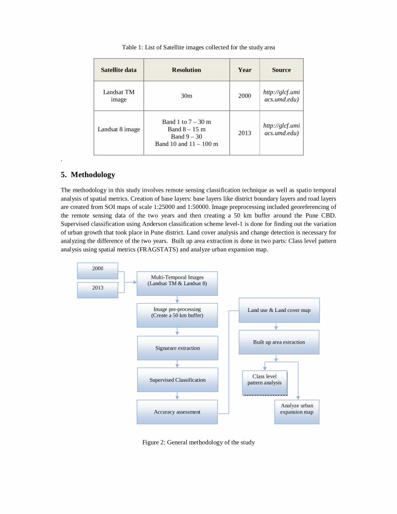
Table 1: List of Satellite images collected for the study area

Satellite data Resolution Year

Source

Landsat TM image 30m 2000

http://glcf.umiacs.umd.edu)

Landsat 8 image

Band 1 to 7 – 30 m

Band 8 – 15 m Band 9 – 30

Band 10 and 11 – 100 m

2013 http://glcf.umiacs.umd.edu)

.

5. Methodology

The methodology in this study involves remote sensing classification technique as well as spatio temporal analysis of spatial metrics. Creation of base layers: base layers like district boundary layers and road layers are created from SOI maps of scale 1:25000 and 1:50000. Image preprocessing included georeferencing of the remote sensing data of the two years and then creating a 50 km buffer around the Pune CBD. Supervised classification using Anderson classification scheme level-1 is done for finding out the variation of urban growth that took place in Pune district. Land cover analysis and change detection is necessary for analyzing the difference of the two years. Built up area extraction is done in two parts: Class level pattern analysis using spatial metrics (FRAGSTATS) and analyze urban expansion map.

Figure 2: General methodology of the study

2000

2013

Image pre-processing (Create a 50 km buffer)

Multi-Temporal Images (Landsat TM & Landsat 8)

Signature extraction

Supervised Classification

Accuracy assessment

Land use & Land cover map

Built up area extraction

Class level pattern analysis

Analyze urban expansion map

6. Results and Discussions 6.1. Land use analysis

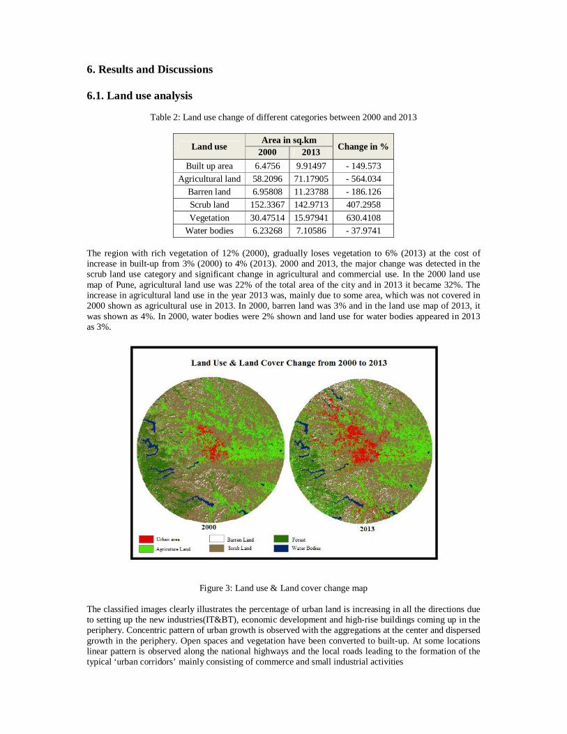
Table 2: Land use change of different categories between 2000 and 2013

Land use Area in sq.km

Change in % 2000 2013 Built up area 6.4756 9.91497 - 149.573

Agricultural land 58.2096 71.17905 - 564.034 Barren land 6.95808 11.23788 - 186.126 Scrub land 152.3367 142.9713 407.2958 Vegetation 30.47514 15.97941 630.4108

Water bodies 6.23268 7.10586 - 37.9741 The region with rich vegetation of 12% (2000), gradually loses vegetation to 6% (2013) at the cost of increase in built-up from 3% (2000) to 4% (2013). 2000 and 2013, the major change was detected in the scrub land use category and significant change in agricultural and commercial use. In the 2000 land use map of Pune, agricultural land use was 22% of the total area of the city and in 2013 it became 32%. The increase in agricultural land use in the year 2013 was, mainly due to some area, which was not covered in 2000 shown as agricultural use in 2013. In 2000, barren land was 3% and in the land use map of 2013, it was shown as 4%. In 2000, water bodies were 2% shown and land use for water bodies appeared in 2013 as 3%.

Figure 3: Land use & Land cover change map

The classified images clearly illustrates the percentage of urban land is increasing in all the directions due to setting up the new industries(IT&BT), economic development and high-rise buildings coming up in the periphery. Concentric pattern of urban growth is observed with the aggregations at the center and dispersed growth in the periphery. Open spaces and vegetation have been converted to built-up. At some locations linear pattern is observed along the national highways and the local roads leading to the formation of the typical ‘urban corridors’ mainly consisting of commerce and small industrial activities

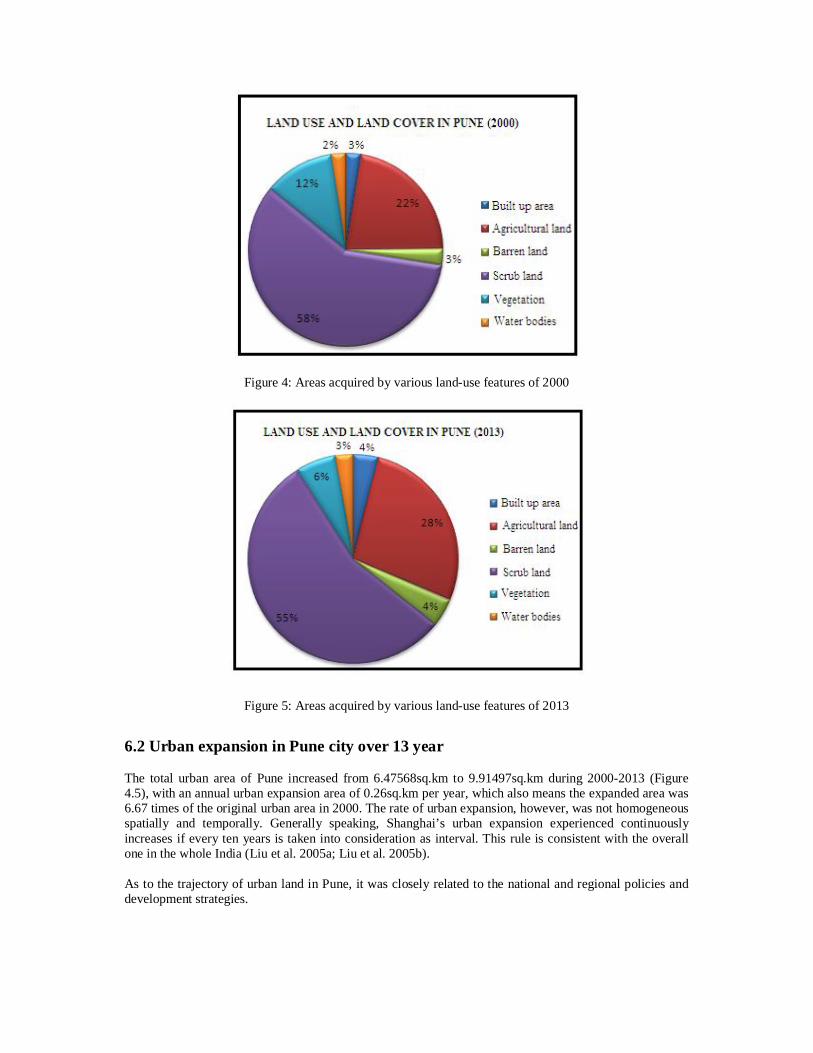
Figure 4: Areas acquired by various land-use features of 2000

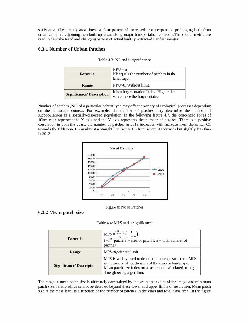
Figure 5: Areas acquired by various land-use features of 2013 6.2 Urban expansion in Pune city over 13 year The total urban area of Pune increased from 6.47568sq.km to 9.91497sq.km during 2000-2013 (Figure 4.5), with an annual urban expansion area of 0.26sq.km per year, which also means the expanded area was 6.67 times of the original urban area in 2000. The rate of urban expansion, however, was not homogeneous spatially and temporally. Generally speaking, Shanghai’s urban expansion experienced continuously increases if every ten years is taken into consideration as interval. This rule is consistent with the overall one in the whole India (Liu et al. 2005a; Liu et al. 2005b). As to the trajectory of urban land in Pune, it was closely related to the national and regional policies and development strategies.

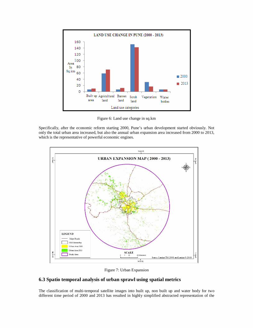
Figure 6: Land use change in sq.km

Specifically, after the economic reform starting 2000, Pune’s urban development started obviously. Not only the total urban area increased, but also the annual urban expansion area increased from 2000 to 2013, which is the representative of powerful economic engines.

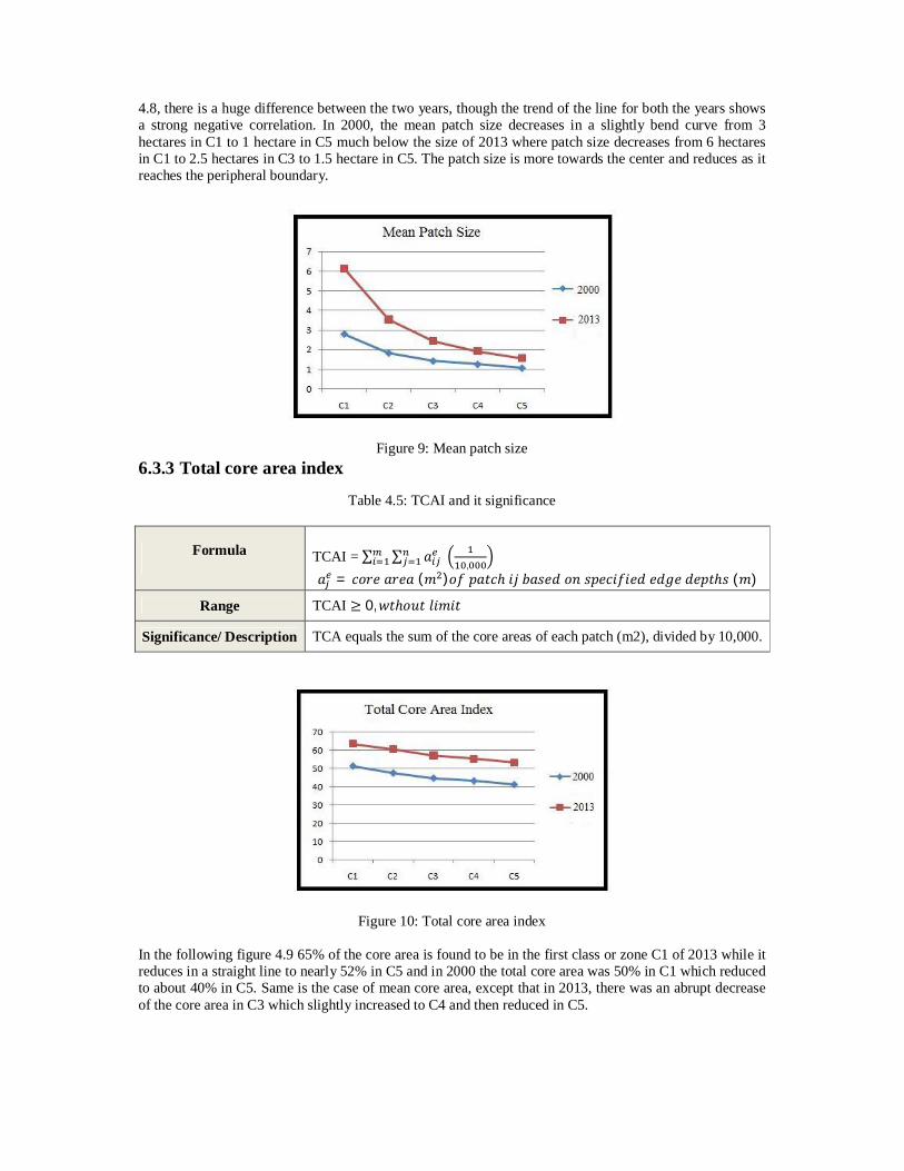
Figure 7: Urban Expansion

6.3 Spatio temporal analysis of urban sprawl using spatial metrics The classification of multi-temporal satellite images into built up, non built up and water body for two different time period of 2000 and 2013 has resulted in highly simplified abstracted representation of the

study area. These study area shows a clear pattern of increased urban expansion prolonging both from urban center to adjoining non-built up areas along major transportation corridors.The spatial metric are used to describe trend and changing pattern of actual built up extracted Landsat images. 6.3.1 Number of Urban Patches

Table 4.3: NP and it significance

Formula NPU = n NP equals the number of patches in the landscape.

Range NPU>0, Without limit.

Significance/ Description It is a fragmentation Index. Higher the value more the fragmentation

Number of patches (NP) of a particular habitat type may affect a variety of ecological processes depending on the landscape context. For example, the number of patches may determine the number of subpopulations in a spatially-dispersed population. In the following figure 4.7, the concentric zones of 10km each represent the X axis and the Y axis represents the number of patches. There is a positive correlation in both the years, the number of patches in 2013 increases with increase from the center C1 towards the fifth zone C5 in almost a straight line, while C3 from where it increases but slightly less than in 2013.

Figure 8: No of Patches 6.3.2 Mean patch size

Table 4.4: MPS and it significance

Formula

MPS =∑,

i =푖 patch; a = area of patch I; n = total number of patches

Range MPS>0,without limit

Significance/ Description

MPS is widely used to describe landscape structure. MPS is a measure of subdivision of the class or landscape. Mean patch size index on a raster map calculated, using a 4 neighboring algorithm.

The range in mean patch size is ultimately constrained by the grain and extent of the image and minimum patch size; relationships cannot be detected beyond these lower and upper limits of resolution. Mean patch size at the class level is a function of the number of patches in the class and total class area. In the figure

4.8, there is a huge difference between the two years, though the trend of the line for both the years shows a strong negative correlation. In 2000, the mean patch size decreases in a slightly bend curve from 3 hectares in C1 to 1 hectare in C5 much below the size of 2013 where patch size decreases from 6 hectares in C1 to 2.5 hectares in C3 to 1.5 hectare in C5. The patch size is more towards the center and reduces as it reaches the peripheral boundary.

Figure 9: Mean patch size 6.3.3 Total core area index

Table 4.5: TCAI and it significance

Formula

TCAI = ∑ ∑ 푎

,

푎 = 푐표푟푒 푎푟푒푎 (푚 )표푓 푝푎푡푐ℎ 푖푗 푏푎푠푒푑 표푛 푠푝푒푐푖푓푖푒푑 푒푑푔푒 푑푒푝푡ℎ푠 (푚)

Range TCAI ≥ 0,푤푡ℎ표푢푡 푙푖푚푖푡

Significance/ Description TCA equals the sum of the core areas of each patch (m2), divided by 10,000.

Figure 10: Total core area index

In the following figure 4.9 65% of the core area is found to be in the first class or zone C1 of 2013 while it reduces in a straight line to nearly 52% in C5 and in 2000 the total core area was 50% in C1 which reduced to about 40% in C5. Same is the case of mean core area, except that in 2013, there was an abrupt decrease of the core area in C3 which slightly increased to C4 and then reduced in C5.

6.3.4 Core area density

Table 4.6: CAD and it significance

Formula

CAD =

∑ (10,000)(100)

푛 = number of disjunct core areas in patch ij based on specified edge depth (m) A= total landscape area

Range CAD > 0, without limit.

Significance/ Description

CAD equals the sum of number of disjunct core areas contained within each patch of the corresponding patch type, divided by total landscape area (m2), multiplied by 10,000 and100.

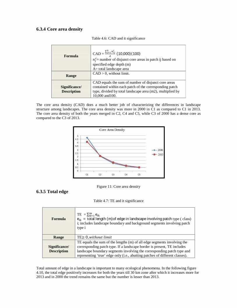
The core area density (CAD) does a much better job of characterizing the differences in landscape structure among landscapes. The core area density was more in 2000 in C1 as compared to C1 in 2013. The core area density of both the years merged in C2, C4 and C5, while C3 of 2000 has a dense core as compared to the C3 of 2013.

Figure 11: Core area density 6.3.5 Total edge

Table 4.7: TE and it significance

Formula

TE = ∑ e e = total length (m)of edge in landscape involving patch type ( class) i; includes landscape boundary and background segments involving patch type i

Range TE≥ 0,푤푖푡ℎ표푢푡 푙푖푚푖푡

Significance/ Description

TE equals the sum of the lengths (m) of all edge segments involving the corresponding patch type. If a landscape border is present, TE includes landscape boundary segments involving the corresponding patch type and representing ‘true’ edge only (i.e., abutting patches of different classes).

Total amount of edge in a landscape is important to many ecological phenomena. In the following figure 4.10, the total edge positively increases for both the years till 30 km zone after which it increases more for 2013 and in 2000 the trend remains the same but the number is lesser than 2013.

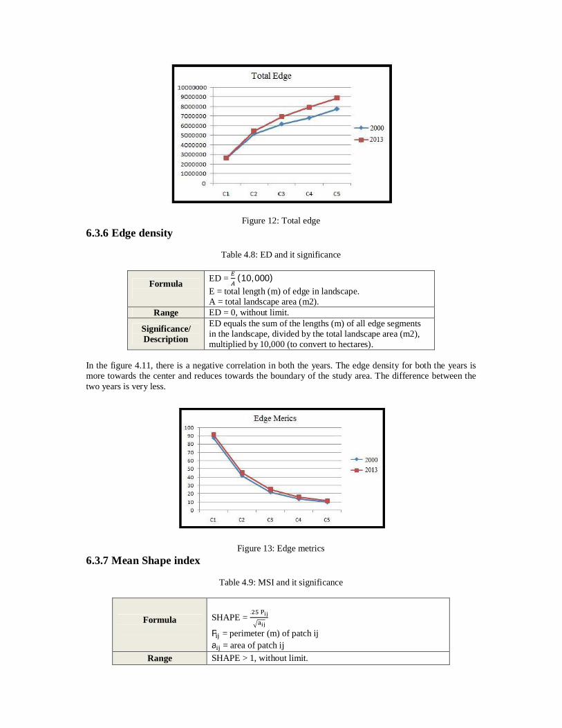
Figure 12: Total edge 6.3.6 Edge density

Table 4.8: ED and it significance

Formula

ED = (10, 000) E = total length (m) of edge in landscape. A = total landscape area (m2).

Range ED = 0, without limit.

Significance/ Description

ED equals the sum of the lengths (m) of all edge segments in the landscape, divided by the total landscape area (m2), multiplied by 10,000 (to convert to hectares).

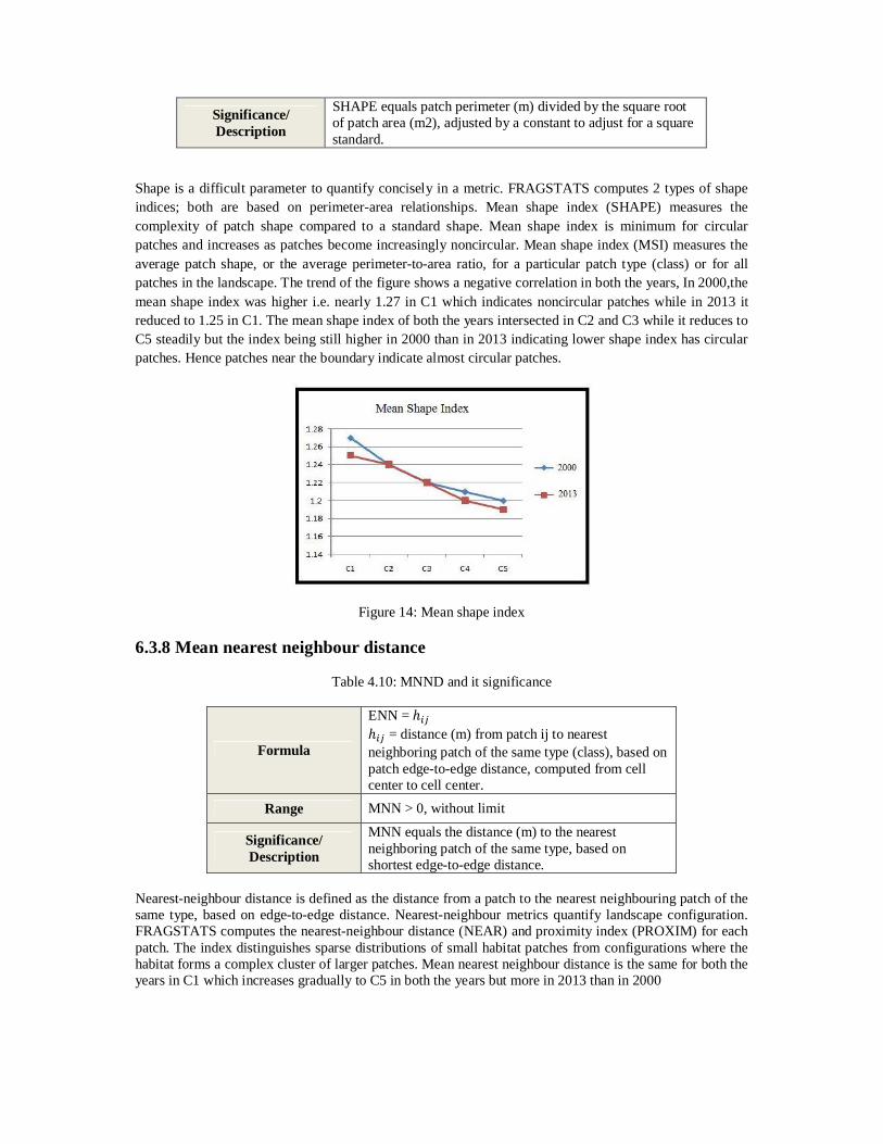
In the figure 4.11, there is a negative correlation in both the years. The edge density for both the years is more towards the center and reduces towards the boundary of the study area. The difference between the two years is very less.

Figure 13: Edge metrics 6.3.7 Mean Shape index

Table 4.9: MSI and it significance

Formula

SHAPE =

.

P = perimeter (m) of patch ij a = area of patch ij

Range SHAPE > 1, without limit.

Significance/ Description

SHAPE equals patch perimeter (m) divided by the square root of patch area (m2), adjusted by a constant to adjust for a square standard.

Shape is a difficult parameter to quantify concisely in a metric. FRAGSTATS computes 2 types of shape indices; both are based on perimeter-area relationships. Mean shape index (SHAPE) measures the complexity of patch shape compared to a standard shape. Mean shape index is minimum for circular patches and increases as patches become increasingly noncircular. Mean shape index (MSI) measures the average patch shape, or the average perimeter-to-area ratio, for a particular patch type (class) or for all patches in the landscape. The trend of the figure shows a negative correlation in both the years, In 2000,the mean shape index was higher i.e. nearly 1.27 in C1 which indicates noncircular patches while in 2013 it reduced to 1.25 in C1. The mean shape index of both the years intersected in C2 and C3 while it reduces to C5 steadily but the index being still higher in 2000 than in 2013 indicating lower shape index has circular patches. Hence patches near the boundary indicate almost circular patches.

Figure 14: Mean shape index

6.3.8 Mean nearest neighbour distance

Table 4.10: MNND and it significance

Formula

ENN = ℎ ℎ = distance (m) from patch ij to nearest neighboring patch of the same type (class), based on patch edge-to-edge distance, computed from cell center to cell center.

Range MNN > 0, without limit

Significance/ Description

MNN equals the distance (m) to the nearest neighboring patch of the same type, based on shortest edge-to-edge distance.

Nearest-neighbour distance is defined as the distance from a patch to the nearest neighbouring patch of the same type, based on edge-to-edge distance. Nearest-neighbour metrics quantify landscape configuration. FRAGSTATS computes the nearest-neighbour distance (NEAR) and proximity index (PROXIM) for each patch. The index distinguishes sparse distributions of small habitat patches from configurations where the habitat forms a complex cluster of larger patches. Mean nearest neighbour distance is the same for both the years in C1 which increases gradually to C5 in both the years but more in 2013 than in 2000

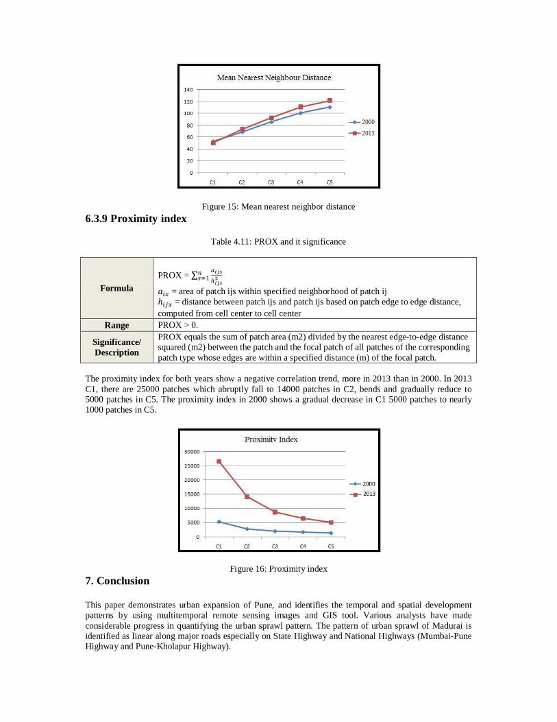
Figure 15: Mean nearest neighbor distance 6.3.9 Proximity index

Table 4.11: PROX and it significance

Formula

PROX = ∑

푎 = area of patch ijs within specified neighborhood of patch ij ℎ = distance between patch ijs and patch ijs based on patch edge to edge distance, computed from cell center to cell center

Range PROX > 0.

Significance/ Description

PROX equals the sum of patch area (m2) divided by the nearest edge-to-edge distance squared (m2) between the patch and the focal patch of all patches of the corresponding patch type whose edges are within a specified distance (m) of the focal patch.

The proximity index for both years show a negative correlation trend, more in 2013 than in 2000. In 2013 C1, there are 25000 patches which abruptly fall to 14000 patches in C2, bends and gradually reduce to 5000 patches in C5. The proximity index in 2000 shows a gradual decrease in C1 5000 patches to nearly 1000 patches in C5.

Figure 16: Proximity index 7. Conclusion This paper demonstrates urban expansion of Pune, and identifies the temporal and spatial development patterns by using multitemporal remote sensing images and GIS tool. Various analysts have made considerable progress in quantifying the urban sprawl pattern. The pattern of urban sprawl of Madurai is identified as linear along major roads especially on State Highway and National Highways (Mumbai-Pune Highway and Pune-Kholapur Highway).

The urban sprawl is one of the potential threats to sustainable development where urban planning with effective resource utilization and allocation of infrastructure initiatives are key concerns. Thus identification and analysis of the patterns of sprawl would help in effective landuse planning in urban area. It is important to study and understand the trend of urban sprawls, which ultimately focus for urban landscape planning and environmental management. 8. References

1. Angel, S., Parent, J., Civco, D., 2007. Urban sprawl metrics: an analysis of global urban expansion using GIS. In: Proceedings of ASPRS 2007 Annual Conference, Tampa, Florida May 7–11, URL: http://clear.uconn.edu/publications/research/ tech papers/Angel et al ASPRS2007.pdf. 2. Barredo, J.l., Demicheli, L., 2003. Urban sustainability in developing countries mega cities, modeling and predicting future urban growth in lagos. Cities 20 (5), 297–310. 3. Bharath H. Aithal, Bharath Settur, Durgappa Sanna D., and Ramachandra. T.V., 2012. Empirical patterns of the influence of Spatial Resolution of Remote Sensing Data on Landscape Metrics., International Journal of Engineering Research and Applications (IJERA), Vol. 2, Issue 3, May-Jun 2012, pp.767-775. 4. Bharath H. Aithal, Bharath Setturu, Sreekantha S, Sanna Durgappa D and T. V. Ramachandra, “Spatial patterns of urbanization in Mysore: Emerging Tier II City in Karnataka”., Proceedings of NRSC User Interaction Meet- 2012, 16th & 17th, February 2012, 2012b, Hyderabad. 5. Bhatta, B., 2009a. Analysis of urban growth pattern using remote sensing and GIS: a case study of Kolkata, India. International Journal of Remote Sensing 30 (18), 4733–4746. 6. Fan. F, Y.Wang, et.al., 2009, Evaluating the Temporal and Spatial Urban Expansion Patterns of Guangzhou from 1979 to 2003 by Remote Sensing and GIS Methods, “International Journal of Geographical Information Science”, Vol. 23(11), pp 1371–1388. 7. Herold, M., Goldstein, N.C., Clarke, K.C., ”The spatiotemporal form of urban growth: measurement, analysis and modelling” Remote Sens. Environ. 86, 2003, pp. 286–302. 8. J, and Masser, 2003, Urban growth pattern modeling: a case study of Wuhan city, PR China. “Landscape and Urban Planning”, Vol. 62, pp 199217. 9. McGarigal, K., Marks, B.J., 1995. FRAGSTATS: spatial pattern analysis program for quantifying landscape structure. USDA Forest Service General Technical Report PNW-351. 10. Saravanan.P, Ilangovan.P, Identification of Urban Sprawl Pattern for Madurai Region Using GIS, International Journal of Geomatics and Geoscience Volume 1, No 2, 2010 11. Sudhira.H.S, T.V. Ramachandra, K.S.Jagadish, 2004, Urban sprawl: metrics, dynamics and modelling using GIS, “International Journal of Applied Earth Observation and Geoinformation”, Vol. 5, pp 29–39. 12. Sulochana Shekhar. Changing Space of Pune – A GIS perspective GIS development Map World Form , Hyderabad , India. Paper Ref NO: MWF PN 116.