Measuring discrete feature dimensions in AFM images with Image SXM

Bickmore et al. Geological Materials Research v.1, n.5, p.1

Copyright ©1999 by the Mineralogical Society of America

Measuring Discrete Feature Dimensions in AFM Imageswith Image SXM

Barry R. Bickmore1, Eric Rufe1, Steve Barrett2, and Michael F. Hochella, Jr.1

1Department of Geological Sciences, 4044 Derring Hall, Virginia Polytechnic Institute and StateUniversity, Blacksburg, VA 24061 USA

2Surface Science Research Centre, University of Liverpool, Liverpool L69 3BX, UnitedKingdom

(Received August 2, 1999; Published November 23, 1999)

Abstract

A suite of macros for the freeware image analysis program, Image SXM, are described.These macros are designed to measure the perimeter, horizontal area, and volume of discretefeatures in AFM images, obtaining accurate and consistent estimates. Directions for using thesoftware and example applications are also given. Such tools allow one to perform tasks whichwould otherwise be extremely tedious or next to impossible. Examples include calculatingreaction rates from time-series images of reacting particles or etch pits with complex shapes, andclassifying objects based on their dimensions.

Keywords: Atomic Force Microscopy, image analysis, perimeter, area, volume, Image SXM

Introduction

In the past decade, a significant number of Earth scientists have successfully employedAtomic Force Microscopy (AFM) to characterize the surface morphology and reactivity ofminerals and other environmental particles (for reviews, see Nagy and Blum, 1994; Hochella,1995; Maurice and Lower, 1997). In this technique, the response of a scanned probe is translatedinto a digital, 3-dimensional map of a surface. Thus, the spatial dimensions of surface featuressuch as etch pits, as well as small particles deposited on a substrate (e.g. clays) can be measured.The ability of the Atomic Force Microscope to operate under fluids, including aqueous solutions,also allows for the real-time characterization of the rates at which such features and particlesgrow or dissolve. Some features, such as euhedral etch pits, are conveniently characterized usingthe standard analysis software that comes with AFM systems, but others have complicatedshapes, and require more sophisticated analysis.

Using its built-in macro language, we have customized the Image SXM image analysisenvironment to measure the perimeter, horizontal area, and volume of discrete surface featuresand particles in AFM images, obtaining accurate and consistent estimates. Image SXM (Barrett,1997) is a spin-off of the popular public domain NIH Image analysis software (Rasband andBright, 1995; Barrett et al., 1995; Liner, 1999), designed especially for the analysis of ScanningProbe Microscopy (SPM), Scanning Electron Microscopy (SEM), and Scanning AugerMicroscopy (SAM) images. With respect to SPM images, Image SXM is able to read 3-dimensional image files created by most commercial SPM software packages, and subject them



to various analysis routines. Two aspects of this program are especially convenient for themeasurement of irregularly-shaped features in AFM images. First, Image SXM allows the user toutilize rectangular, oval, polygonal, and freehand selection tools to define a region of interest(ROI) of any shape, thus excluding extraneous features. Second, it allows the user to createmacros to perform most of the functions of the program automatically, and perform calculations,in a specified sequence.

Users of this software will now be able to quickly obtain reliable measurements of discretefeatures in AFM images. Such tools allow one to perform tasks which would otherwise beextremely tedious or next to impossible. Examples include calculating reaction rates from time-series images of reacting particles or etch pits with complex shapes (Bosbach et al., 1999; Rufeand Hochella, 1999), and classifying biomolecules and other surface features based on theirdimensions (Chen et al., 1996; McMaster et al., 1996).

Algorithms

Perimeter and horizontal area

In order to estimate the perimeter or horizontal area of a discrete feature, the image must betransformed into binary format. That is, a certain height (or pixel intensity) level is chosen as thethreshold, and pixels on either side of the threshold are changed either to black or white,depending upon which side of the threshold they fall. The black areas are treated as particles, andthe area of each one can be determined by multiplying the number of pixels in the particle by ascaling factor. The perimeter of each particle may be calculated by adding 1 for each edge-touching pixel, and √2 for each corner-touching pixel, and then multiplying by a scaling factor(Russ, 1990, pp. 183-185; Russ, 1995, pp. 520-522).

The difficulty in perimeter and horizontal area calculations is deciding at which height levelto set the threshold, because, especially in the case of irregularly shaped features, the effect ofaltering the threshold even slightly can be drastic. In order to estimate consistent values fromfeature to feature and from image to image, one must decide upon some optimum threshold levelat which to make the measurements. Therefore, our Image SXM macros threshold the image at254 of the 256 possible gray levels (excluding white and black), and calculate the perimeter andarea of the particles in the selected area at each setting. The perimeter vs. threshold height curveis then subjected to a 3, 5, 7, or 9 point (user-defined) smoothing routine, and the derivative ofthe perimeter vs. threshold height curve is calculated at each height level from the smoothedcurve. The resulting derivative curve is essentially a map of image complexity vs. thresholdsetting. That is, perimeter values where the feature boundaries are the least complex will changethe least from threshold level to threshold level, and so will produce values near zero in thederivative curve (Russ, 1990, pp. 108-115). Optimum threshold levels are selected where theabsolute values of a string of 5 or more consecutive derivative points fall below a user-definedtolerance level.



Volume

The volume of a feature can easily be calculated by first defining a baseline height, and thenmultiplying the area of the selected ROI by the average pixel height (relative to the baselineheight) within the ROI (Russ, 1995, p. 541). This method of volume calculation implicitlyassumes that any noise in the image is distributed symmetrically about the true height values. Italso ignores effect of AFM tip geometry and other artifacts on the perceived volume, although auser could modify the macro code to account for such things for specific applications.

The volume calculation macros define the baseline height by first creating a histogram of thenumber of pixels at each height level within the ROI. The histogram is then subjected to a 5-point smoothing routine, after which the height level of the baseline is determined by identifyingthe maximum of the first large peak from the bottom (in the case of particles) or top (in the caseof pits). If there is a significant deviation from the overall baseline in an area within the ROI, asmaller peak in the histogram might interfere with the baseline determination. Therefore, the useris asked to define a minimum (particles) or maximum (pits) height level for the baseline toexclude such anomalies

Directions for use

Image SXM macros are stored in text files, and are loaded into the program by selecting the“Load Macros” command under the “Special” menu, and selecting the desired file. The macrosdescribed here are in a text file named “pavmacro.txt”. The following macros are included in thefile: 1) “Prepare Temp Window”, 2) “Particle Perim-Area”, 3) “Pit Perim-Area”, 4) “PlotParticle Perim”, 5) “Plot Particle Area”, 6) “Plot Particle P-Deriv”, 7) “Plot Pit Perim”, 8) “PlotPit Area”, 9) “Plot Pit P-Deriv”, 10) “Particle Volume”, 11) “Pit Volume”, and 12) “PlotSmoothed Histogram”. This section describes procedures which can be used to utilize thesemacros to measure discrete features in AFM images.

Image preparation

In preparation for measurement, an image must be subjected to three processes, all of whichcan be performed using Image SXM or any standard AFM software. First, images must besubjected to a flattening routine, a least-squares polynomial fit to remove unwanted features fromthe scan lines. This removes variations in the baseline height from scan to scan in an image.Second, if the image is tilted with respect to the x-y plane, a tilt correction routine must beapplied. Third, a median filter, which assigns each pixel the median height value of its immediateneighborhood (9 or 25 pixels) must be applied to reduce random noise. While operations such aslowpass filters may flatten out the edges of a feature and thus distort its shape, median filters donot, although some blurring does occur (Russ, 1990, pp. 46-48). Within Image SXM, flatteningand tilt correction routines may be found under the “Compensation” category in the “SPM”menu. [Note: It is best to hold the “Shift” key down before using the mouse to pull down the“SPM” menu and select the tilt correction routine. This causes the program to readjust the z-scaling so that objects in the image are not cut off by being moved above or below the original z-scale.] A 3x3 pixel median filter routine can be found under the “Rank Filters” category in the“Process” menu.



Measuring perimeter and area

In order to run macros in Image SXM, one must first choose the “Load Macros” functionunder the “Special” menu and then select the desired macro text file. The names of the macros inthe file then appear in the “Special” menu, and will run when selected.

To measure perimeter/area, one opens the desired image file and then creates a blanktemporary image window with dimensions identical to those of the image, by running the“Prepare Temp Window” macro. The image window is automatically brought to the front. Oneof the selection tools is then used to define a ROI around the feature of interest. The user thenruns either the “Particle Perim-Area” or “Pit Perim-Area” macro. The program then measures theperimeter and area of the feature at every height level.

After the perimeter/area calculations have been performed, the user is asked to providevalues for the smoothing degree; i.e. the number of points averaged to smooth the perimeter vs.height curve before calculating the derivative. Smoothing degrees of 3, 5, 7, or 9 may be used.The user is also prompted for a perimeter picking tolerance. For instance, a tolerance of 0.005(the default) means that only perimeter derivative values of 0±0.005 will be considered when thecomputer picks suitable height levels to measure perimeters and the corresponding areas. (Thedefault values for smoothing degree and tolerance of 7 and 0.005, respectively, usually workwell for reasonably simple features within images up to a few µm on a side. A lower smoothingdegree might be required if, for instance, the user would like the program to pick a larger numberof suitable height levels. A higher tolerance might be desirable if the horizontal area of the imageis very large, and hence the derivative reflecting even relatively small changes in the calculatedperimeter curve would also be correspondingly larger.) When the tolerance is entered, theprogram picks any suitable height levels at which to accurately estimate perimeter values, andthen prints the corresponding heights and perimeters in the"Info” window. The user is askedwhether the results should be saved, and if so the perimeter picks, as well as the area, perimeter,and perimeter derivative values at each height level are saved in a text file in a form easilyaccessible to a spreadsheet program for further analysis. Whether the file is saved or not, the userwill be asked whether the computer should recalculate the results, and if so, the user is promptedfor a new smoothing degree and perimeter picking tolerance, after which the derivative curve isrecalculated and new perimeter picks are made. The user then has the option of saving the newresults file.

In some cases the program will not pick any height levels at which to measure the perimeter,or will not pick any in the specific height region of interest to the user. In that case, theperimeter, area, and perimeter derivative data can be plotted vs. height level by running the “PlotParticle Perim”, “Plot Particle Area”, “Plot Particle P-Deriv”, “Plot Pit Perim”, “Plot Pit Area”,and “Plot Pit P-Deriv” macros. These take the data obtained by running the “Particle Perim-Area” or “Pit Perim-Area” macro and create an x-y plot in a separate window. One may obtainthe exact coordinates of any point on a plot by running the mouse cursor across the plot window.The x value of the cursor position, and the y value of the plot corresponding to that x value, aredisplayed in the “Info” window. The user can employ these plots to find the most suitableheights at which to measure perimeter and area by eye.



Often it is useful to obtain the perimeter and area of a feature in a time-series. For instance,the authors have used this software to analyze lateral etch pit growth and clay mineral dissolutionin time series of AFM images. Growth/dissolution rates can be measured and related to specificcomponents of the surface area (e.g. the area of step edges). Since the assigned height of thebaseline level in an image can vary somewhat due to noise, image drift, etc., it is not useful topick a height at which to measure the perimeter/area and then measure those values at the sameheight level throughout the series of images. Rather, it is better to pick a suitable height level tomake the measurements in the first image, note the specific feature of the perimeter vs. heightplot corresponding to that height level, and then find the same feature in the perimeter vs. heightplots in subsequent images to determine where to make the measurements.

Measuring volume

Volume measurements are made by selecting a ROI around the feature of interest, andrunning either the “Particle Volume” or “Pit Volume” macro. The user is then prompted todefine a minimum (particles) or maximum (pits) height level for the baseline. After this is done,the baseline level chosen by the computer and the calculated volume are displayed in the “Info”window. It is useful to then run the “Plot Smoothed Histogram” macro, which creates an x-y plotof the smoothed number of pixels vs. height histogram. Again, by running the mouse cursoracross the plot, the user can find the plotted value for the x value of the cursor position, which isdisplayed in the “Info” window. Using this plot, the user may determine whether the programestimated a reasonable value for the baseline height. If not, the volume macro may be run again,and a minimum or maximum baseline height may be entered to exclude a false result.

Examples

In this section, a few examples will be cited to illustrate both the usefulness of the softwaredescribed here, and the nature of the results that can be obtained therefrom.

Square pits

Figure 1a shows our first example, which is a synthetic AFM image, created with thedrawing and calibration tools included with Image SXM. The base level (i.e. the level above thepits) in this image is at 81 nm. In the center there are two concentric, square pits, the larger oneat 48 nm height and the smaller at 11 nm. The larger pit is 2.00 µm on a side, while the smaller is1.00 µm on a side. After drawing the pit pattern, we also used a macro to add random noise in anormal distribution about the original pixel values. In this case, the standard deviation of thenoise distribution about the original pixel values is 5% of the total z-range (black to white,100nm). The dashed line around the pits marks the selected ROI for our calculations. Figure 1bshows a histogram of the number of pixels in the ROI corresponding to each height level.

Since this is a synthetic image, the values one should expect to measure with the macros arealready known. When the “Pit Perim-Area” macro was run (smoothing degree = 7, tolerance =0.005), the program picked two height levels at which to measure perimeters and areas: 35.3 nmand 68.2 nm. Figure 2 shows plots of the perimeter, perimeter derivative, and area vs. thresholdheight obtained by running the plotting macros described above. The dashed lines in the figure



denote the height levels the program picked. These plots show that the program picked heightlevels for measurement near the upper edges of the pits, but where the perimeter (and area)values change very little. Figure 3 illustrates this principle even more clearly. Here a crosssection of the pits is shown, and again the dashed lines indicate the height levels picked. It isreadily seen that heights were chosen near the upper edges of the pits, but just below where thenoise in the image would complicate the measurements.

The program should be expected to measure perimeters and areas for the smaller pit in theneighborhood of 4 µm and 1 µm2, and indeed, the measured values were 3.97 µm and 1.00 µm2.The measured values for the larger pit, 8.02 µm and 4.00 µm2, are similarly in agreement withthe expected values, 8 µm and 4 µm2.

When the “Pit Volume” macro was run, it correctly picked the baseline level at 81 nm (seeFigure 4), and calculated a pit volume of 0.168 µm3. The expected value was 0.169 µm3. Thus,all of the measured values for perimeter, area, and volume are within 1% of the expected values.Certainly the more complicated shapes and imaging artifacts found in real AFM images woulddegrade the accuracy of these measurements, but this example serves to show that their mostlimiting factor is likely the quality of the data itself. That is, scanner drift, tip-sampleconvolution, and poor resolution of small features in an image would likely contribute more tothe measurement error than anything associated with the computerized image analysis routines.For a discussion of various perimeter, area, and volume calculation routines, see Russ (1990; pp.99-125, 181-191), and Russ (1995; pp. 507-522, 541-545).

Irregularly-shaped clay particle

Figure 5a is an AFM image of a montmorillonite clay particle fixed to a polyethyleneimine-coated mica substrate, taken under deionized water (see Bickmore et al., 1999). The image wassubjected to flattening and median filter routines to remove variations in scan line height andrandom noise, respectively. The baseline height of the image around the particle is ~2 nm, and itexhibits two distinct terraces at ~8 nm and ~14 nm.

When the “Particle Perim-Area” macro was run, the program picked two heights at which tomake measurements: 6.7 and 12.9 nm. Figures 5b and 5c show the binarized image, thresholdedat these height levels. Careful comparison of these with Figure 5a reveals that if one were totrace the outline of the particle for measurement by eye, the true perimeter and area of theparticle would likely be significantly overestimated. Figure 6 shows a cross-section of theparticle, with the height levels picked by the computer algorithm marked by dashed lines. Thisfigure illustrates the fact that the measurement routine picks height levels near the top of theterraces, to minimize the error associated with edge-broadening due to the pyramidal shape ofthe AFM probe tip, but just below where the rounded end of the probe tip, random noise, etc.,begin to complicate the image.

The experimental artifacts just mentioned are made apparent in Figure 6, and hence it alsoserves to illustrate potential sources of error in the volume calculations. Although we cannot becertain of the “true” value of the particle volume, an “expected” volume was approximated usingthe measured heights and areas of the terraces, and the “Particle Volume” macro was run.



Whereas a volume of 1.21 x 10-3 µm3 was expected, the routine calculated a volume of 1.35 x10-3 µm3, representing an error of ~12%. (The volume of the two small, white bumps on top ofthe particle in Figure 5a amounted to ~1 x 10-5 µm3, and was taken into account in thecalculation of the “expected” volume.) If errors of this magnitude are unacceptable, users maywish to customize this measurement routine (or create new routines) to account for artifactsspecific to their images. For instance, the following references describe methods to remove tip-sample interaction artifacts, which may add significantly to the measured volume (Keller, 1991;Keller and Franke, 1993; Bonnet et al., 1994; Markiewicz and Goh, 1994, 1995; Wilson et al.,1995; Villarrubia, 1997). A simple routine of this type has been incorporated into Image SXM(menu SPM/Images/Tip Locus Effect), and is described by Barrett et al. (1999). In this routinethe effect of a paraboloid tip with a user-defined radius of curvature is deconvoluted from thecaptured image. The image of the clay particle in Figure 5a was deconvoluted using this routine,assuming a radius of curvature of 30 nm for the tip. The calculated volume of the particle in thedeconvoluted image was 1.26 x 10-3 µm, representing an error of only ~4%.

Dissolving mica etch pit – time series

Figure 7 is an animation of a time series of AFM images of some etch pits on a phlogopitemica surface, that are dissolving in pH 2 HCl (see Rufe and Hochella, 1999). A ROI was selectedaround the largest pit in each of these images, and the “Pit Perim-Area” macro run. Figure 8consists of perimeter vs. threshold height plots for these images, in sequence from top to bottom.The dashed lines mark the threshold heights the computer program picked to measure perimeterand area values. This figure clearly shows that the baseline height of the image can changesignificantly in such a sequence, but the feature corresponding to the ideal measurement heightin each perimeter vs. threshold height plot is easily identified.

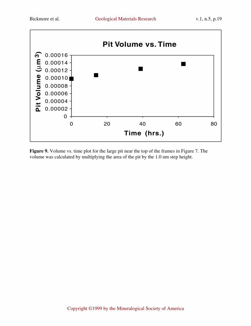
Figure 9 is a plot of the pit volume (calculated by multiplying the measured pit area by thestep height of 1.0 nm) vs. time. The lack of scatter in these data illustrates plainly the utility ofhaving measurement tools to estimate accurate and consistent values for discrete featuredimensions in AFM images. In addition, phlogopite mica is a 2:1 phyllosilicate, which is knownto dissolve inward from edge surfaces, rather than etching of the basal surfaces. The informationgained from subjecting images such as these to the analysis routines described here can be usedto obtain dissolution rates for these minerals, normalized to the reactive (edge) surface area. Infact, such information, obtained in a much more tedious fashion, has already been used in thisway (Rufe and Hochella, 1999; Bosbach et al., 1999).

Obtaining the software

Links for downloading the latest version of Image SXM and the macros described in thispaper from the World-Wide Web can be found at the following address:http://www.geocities.com/Athens/Parthenon/2671/Macros.html

http://www.geocities.com/Athens/Parthenon/2671/Macros.html



Acknowledgements

This work was funded by grants from the National Science Foundation (EAR-9527092,EAR-9628023) and the Petroleum Research Fund of the American Chemical Society (PRF31598-AC2, 34326-AC2). Additional funding was supplied by the National Science FoundationGraduate Fellowship Program and the American Federation of Mineralogical SocietiesScholarship Foundation. Christopher Daniel and Frank Spear provided helpful reviews of themanuscript. E.R. would also like to thank K. Rosso for programming instruction during the earlystages of this project.



References

Barrett, S.D., Leibsle, F.M., and Dipple, S.J. (1995) Customised image analysis made easy.Microscopy and Analysis, 47, 17-19.

Barrett, S.D. (1997) Image analysis and the internet. Scientific Data Management, 1, 18-25.Barrett, S.D., Bickmore, B.R., Rufe, E., Hochella, M.F., Jr., Torzo, G., and Cerolini, D. (1999)

The use of macros in AFM image analysis and image processing. Journal of ComputerAssisted Microscopy, submitted.

Bickmore, B.R., Bosbach, D., Hochella, M.F., Jr., and Charlet, L. (1999) Methods forperforming atomic force microscopy imaging of clay minerals in aqueous solutions. Claysand Clay Minerals, 47, 573-581.

Bonnet, N., Dongmo, S., Vautrot, P., and Troyon, M. (1994) A mathematical morphologyapproach to image formation and image restoration in scanning tunneling and atomic forcemicroscopies. Microscopy Microanalysis Microstructures, 5, 477-487.

Bosbach, D., Charlet, L., Bickmore, B.R., and Hochella, M.F., Jr. (1999) The dissolution ofhectorite: In-situ, real-time observations using Atomic Force Microscopy. AmericanMineralogist, in revision.

Chen X.Y., Davies M.C., Roberts C.J., Shakesheff K.M., Tendler S.J.B., Williams P.M. (1996)Dynamic surface events measured by simultaneous probe microscopy and surface plasmondetection. Analytical Chemistry, 68,1451-1455.

Hochella, M.F. Jr. (1995) Mineral surfaces: their characterization and their chemical, physicaland reactive nature. In D.J. Vaughan and R.A.D. Pattrick, Eds., Mineral Surfaces, p. 17-60.Chapman & Hall, London.

Keller, D.J. (1991) Reconstruction of STM and AFM images distorted by finite-sized tips.Surface Science, 253, 353-364.

Keller, D.J. and Franke, F.S. (1993) Envelope reconstruction of probe microscopy images.Surface Science, 294, 409-419.

Liner, C.L. (1999) Geophysics and NIH image. Computers and Geosciences, 25, 403-414.Markiewicz, P. and Goh, M.C. (1994) Atomic Force Microscopy probe tip visualization and

improvement of images using a simple deconvolution procedure. Langmuir, 10, 5-7.Markiewicz, P. and Goh, M.C. (1995) Simulation of Atomic Force Microscope tip-

sample/sample-tip reconstruction. Journal of Vacuum Science and Technology, B13, 1115-1118.

Maurice, P.A. and Lower, S.K. (1997) Using Atomic Force Microscopy to study soil mineralreactions. Advances in Agronomy, 62, 1-43.

McMaster T.J., Winfield M.O., Baker A.A., Karp A., Miles M.J., (1996) Chromosomeclassification by Atomic Force Microscopy volume measurement. Journal of VacuumScience and Technology, B14, 1438-1443.

Nagy, K.L. and Blum, A.E., Eds. (1994) Scanning Probe Microscopy of Clay Minerals, 239 p.The Clay Minerals Society, Boulder, CO.

Rasband, W.S. and Bright, D.S. (1995) NIH Image – A public domain image-processingprogram for the Macintosh. Microbeam Analysis, 4, 137-149.

Rufe, E. and Hochella, M.F., Jr. (1999) Quantitative assessment of reactive surface area ofphlogopite during acid dissolution. Science, 285, 874-876.

Russ, J.C. (1990) Computer-Assisted Microscopy: The Measurement and Analysis of Images,453 p. Plenum, New York.



Russ, J.C. (1995) The Image Processing Handbook, 2nd Ed., 674 p. CRC, London.Villarrubia, J.S. (1997) Algorithms for scanned probe microscope image simulation, surface

reconstruction, and tip estimation. Journal of Research of the National Institute of Standardsand Technology, 102, 425-455.

Wilson, D. L., Kump, K.S., Eppell, S.J., and Marchant, R.E. (1995) Morphological restoration ofAtomic-Force Microscopy images. Langmuir, 11, 265-272.



Figure 1. a) Synthetic 256 x 256 pixel AFM image of two concentric square pits, 1 µm and 2 µmon a side. The z-range of the image (white to black) is 100 nm, and the three terraces are locatedat 11, 48, and 81 nm. Random noise has been added to the image in a normal distribution aboutthe original pixel values. The dashed line indicates the ROI upon which the macro calculationswere performed. b) Histogram of the number of pixels within the ROI corresponding to eachgrey level. Both a) and b) are digital captures of windows in the Image SXM program, takenduring the measurement procedure.

a

b



Figure 2. a) Plot of perimeter vs. threshold height for the calculations performed on the ROI inFigure 1a. Dashed lines represent the threshold heights the program picked as ideal levels tomeasure perimeter and area. b) Plot of perimeter derivative vs. threshold height. c) Plot of areavs. threshold height. a), b), and c) are digital captures of windows in the Image SXM program,taken during the measurement procedure, with the dashed lines being added afterward.

a

b

c



Figure 3. The dashed line in a) denotes the area from which the data for the cross section of thesquare pits plotted in b) is taken. Both a) and b) are digital captures of windows in the ImageSXM program, taken during the measurement procedure, with the dashed lines in b) being addedafterward.

a

b



Figure 4. Plot of the same histogram as in Figure 1b, after being subjected to a five pointsmoothing routine. The “Pit Volume” macro generated the smoothed histogram, and used it tocalculate the “baseline” height (dashed line) from which to calculate the volume of the pits. Thisfigure is a digital captures of the data plot window in the Image SXM program, taken during themeasurement procedure, with the dashed line being added afterward.



Figure 5. a) 1.7 x 1.7 µm (256 x 256 pixel) AFM image of a montmorillonite clay particle underdeionized water. The particle has well-defined terraces at ~8 and ~14 nm height, with thebaseline at ~2 nm. The dashed line represents the ROI used for the measurement routines. b)Binarized version of a), thresholded at 6.7 nm, the first level picked by the perimeter/areameasurement routine. c) Thresholded at 12.9 nm, the second level picked. a), b), and c) aredigital captures of image windows in the Image SXM program, taken during the measurementprocedure.



Figure 6. The dashed line in a) denotes the area from which the data for the cross section of themontmorillonite clay particle plotted in b) is taken. The dashed lines in b) indicate the thresholdlevels at which the perimeter and area were measured. Both a) and b) are digital captures ofwindows in the Image SXM program, taken during the measurement procedure, with the dashedlines in b) being added afterward.

a

b



Figure 7. Animation of a sequence of four 880 nm x 880 nm (512 x 512 pixel) AFM images ofthe surface of a phlogopite mica crystal, taken under pH 2 HCl. The surface was pre-etched withHF, and the images were taken at 0 hrs., 14 hrs., 39 hrs., and 63 hrs. The perimeter and area ofthe large, 1 nm deep pit at the top of the image were measured through the sequence to determinethe volume change of the pit over time. Click on the frame to play the animation.

Fig07.html



Figure 8. Perimeter vs. threshold height plots for the large etch pit near the top of each of theframes in Figure 7. Dashed lines indicate the threshold height at which perimeter and area weremeasured. Clearly the baseline height of the images, and hence the “absolute” height of the idealmeasurement threshold vary from frame to frame, due to changing imaging conditions, imagedrift, etc. However, the flat terrace in the perimeter vs. threshold height plots, corresponding tothe edges of the pit, is clearly recognizable in each. a), b), c), and d) are digital captures of dataplot windows in the Image SXM program, taken during the measurement procedure, with thedashed lines being added afterward.

0 hrs.

14 hrs.

39 hrs.

63 hrs.



Figure 9. Volume vs. time plot for the large pit near the top of the frames in Figure 7. Thevolume was calculated by multiplying the area of the pit by the 1.0 nm step height.

0

0.00002

0.00004

0.00006

0.00008

0.00010

0.00012

0.00014

0.00016

Time (hrs.)

Pit

Vo

lum

e (

µm

)

3Pit Volume vs. Time

0 20 40 60 80

Measuring discrete feature dimensions in AFM images with Image SXM

Documents

Transcript of Measuring discrete feature dimensions in AFM images with Image SXM