Modeling reactive multiphase flow and transport of concentrated solutions
Upload
khangminh22Category
view
0download
0
THÈSE
Pour obtenir le grade de
DOCTEUR DE LA COMMUNAUTE UNIVERSITE
GRENOBLE ALPES
Spécialité : Matériaux, Mécanique, Génie Civil, Électrochimie Arrêté ministériel : 25 mai 2016
Présentée par
João Paulo COSAS FERNANDES
Thèse dirigée par Laurent GONON et codirigée par Vincent MAREAU préparée au sein du Laboratoire Systèmes Moléculaires et nanoMatériaux pour l'Energie et la Santé / Polymères Conducteurs Ioniques dans l'École Doctorale Ingénierie-Matériaux, Mécanique Énergétique, Environnement, Procédés, Production (I-MEP²)
Co-localisation AFM/Raman : Caractérisation de systèmes polymères multiphasés Thèse soutenue publiquement le 16 novembre 2017, devant le jury composé de :
DR Didier R. LONG Directeur adjoint Laboratoire Polymères et Matériaux Avancés LPMA de Lyon (UMR5268), CNRS – Président
Pr. Isabelle ROYAUD Département Science et Ingénierie des Matériaux et Métallurgie (SI2M) de l’Institut Jean Lamour (UMR 7198), Université de Lorraine - Rapporteur
Pr. Odile FICHET Co-directrice du Laboratoire de Physicochimie des Polymères et des Interfaces (EA2528), Université de Cergy Pontoise - Rapporteur
DR Deborah JONES Directrice associée de l’Institut Charles Gerhardt de Montpellier, CNRS - Membre
Delphine TAVERNIER-LOHR Responsable R&D Groupe Serge Ferrari, La Tour du Pin - Membre


Co-localized AFM/Raman characterization of multiphase
polymer systems
João Paulo Cosas Fernandes
This dissertation is submitted for the degree of Doctor of Philosophy
16 November 2017

i
Even Diamonds start as Coal
Just give it Time
The Fire feels Divine
- Incubus

ii

iii
Acknowledgements
First I would like to thank my thesis directors Laurent Gonon and Vincent Mareau,
for believing in me and giving me the means to fulfill my goals, inside the lab and outside
as well. Laurent was always pushing me to go beyond the expectations, always scientifically
rigorous and critical, but also a good listener to my ideas and opinions. Vincent is a master
of experimentation in the lab, with whom I learned a lot about putting ideas into practice.
Our scientific discussions have always been a challenge for me, but also made me go
further into any subject we worked on together. I hope the best for you !
To my friends from the lab, Ph.D. students, post-docs, senior researchers, professors,
staff... You were part of my daily life for the past 3 years and I thank you a lot for the good
times we spent together. Lucille, Katya, Natacha, Nicolas, Coraline, Tao, Rémi, Laurent,
Christopher, thank you for the daily laughs and for the great support until the very end !
Hakima, you are a great person, mother and researcher. You have always been there for me
when I needed answers, with your enthusiasm and kindness. Emilie, Charly and Joëlle,
thanks for being my support in the daily life of the lab, from experiments to the
bureaucracy of a foreign student, you were always very helpful and kind. Jojo, may you
continue to enlighten peoples’ life with your great sense of humor !
Outside the lab, I had the pleasure of meeting incredible people, each of one battling
to achieve their best selves. I thank the people that kindly welcomed me back in Grenoble,
Figueira, Julianny, Drieli and Marina, and all the BRAFITECs that came into my life and
made it more joyful. Volta, Lorena, Ebert, Contin, Raíssa, Juliana, Luciane, Thibault.. Thanks
for the shared moments. I thank the CrazyVosDent volleyball team for the two and a half
years of partnership, victories, defeats and apéros after each match. Les Ducs du Tranqui !
Certainly the best friends I had the pleasure of meeting and living together for the past 2
years. Tuxo and Xaxa, thanks for the good moments, discussions, laughs, travels and
snowboarding weekends. I am truly grateful for the daily support and I hope the best for
your future ! A special thanks to Julie Grande, for being by my side until the end, for caring
for my back’s health and for teaching me more than she can imagine.
I thank my family, my aunts, uncles and cousins, for the support you gave me at
each step of my education and for the warmest welcomes each time I come back home.
At last, but not least, I thank my parents Sonia and Mauricio. You have always been
there for me, you gave me all the conditions and opportunities to be who I am today. Even
when my decisions made me go so far away from home, you gave me strength. For you
both, I will keep trying my best. I love you.

iv

v
Contents
INTRODUCTION xiii
CHAPTER 1
MOTIVATION
PROLOGUE 1
1. Heterogeneous and multi-phase complex polymer materials 2
1.1. Polymer Blends 2
1.2. Multilayer Polymeric Materials 3
1.3. Fiber Reinforced Polymer Composites 6
1.3.1. Polymer Nanocomposites 8
1.4. Block-copolymers 10
2. Bulk vs Surface Properties 11
2.1. Characterization of both the Surface and Bulk of Polymer Materials 13
2.2. Sample Preparation Techniques for Bulk Direct Observations 14
3. Polymer membranes 15
4. Manuscript Structure 16
CHAPTER 2
Co-Localized AFM/Raman and Complementary Analyses
PROLOGUE 19
1. Fundamentals of Atomic Force Microscopy 20
1.1. Fundamentals of PeakForce Quantitative NanoMechanics (QNM) 21
1.2. System Calibration for Quantitative Nano-Mechanical Measurements 24
1.3. Nanomechanical Models for Quantitative Measurements 25
1.4. Absolute vs Relative Calibration Method 27
2. Fundamentals of Raman Spectroscopy 28
2.1. Raman Principle 28
2.2. Raman Mapping and Spatial Resolution 29
3. AFM-Confocal Raman Coupling 32
3.1. Commercially available AFM-Raman coupling systems 32
4. Sample Preparation Techniques 35
4.1. Cryo-Fracture 35
4.2. Cryo-Ultramicrotomy 36
Contents vi
vi
4.3. Focused Ion Beam (FIB) cross-sectioning 39
4.4. Summary Table of Sample Preparation Techniques 41
5. Complementary Analyses 43
5.1. Optical Microscopy (OM) 43
5.2. Electron Microscopies 43
5.2.1. Scanning Electron Microscopy (SEM) 44
5.2.2. Transmission and Scanning Transmission Electron Microscopy (TEM/STEM) 47
5.3. Fourier Transform Infrared Spectroscopy (FTIR) 49
5.4. Summary Table of Characterization Techniques 51
6. Conclusions of Chapter 2 53
6.1. Difficulties related to sample preparation by Cryo-Ultramicrotomy 53
6.2. Difficulties related to the co-localization of AFM/Raman analyses 53
7. Conclusions du Chapitre 2 en Français 54
7.1. Difficultés liées à la préparation des échantillons par Cryo-Ultramicrotomie 54
7.2. Difficultés liées à la co-localisation des analyses AFM/Raman 54
CHAPTER 3
Experimental Methods and Developments
PROLOGUE 57
1. Sample preparation by Cryo-Ultramicrotomy 57
1.1. Sectioning of injection molded specimens 58
1.2. Sectioning of polymer membranes 59
1.3. Cryo-ultramicrotomy parameters 59
1.4. Avoiding frost melting water-diffusion onto the sample’s surface 60
2. AFM/Raman Co-localization Setup 60
2.1. Atomic Force Microscope (AFM) 61
2.1.1. AFM Calibration Method 61
2.2. Raman Spectrometer 67
2.2.1. Raman Calibration Method 67
3. Co-localization Methods 68
3.1. Co-localization with the Co-localized Raman Microscope 68
3.2. Co-localization with the Regular Raman Microscope - Shuttle Stage 69
4. Complementary Analyses 71
4.1. Scanning Electron Microscopy (SEM) 71
4.2. Transmission and Scanning Transmission Electron Microscopy (TEM/STEM) 71

vii Contents
vii
4.3. µ-ATR-FTIR imaging 71
5. Conclusions of Chapter 3 73
6. Conclusions du Chapitre 3 en Français 74
CHAPTER 4
Compatibilization of Polymer Blends based on PA6/ABS
PROLOGUE 77
1. Theoretical Background and Motivation 78
1.1. Polyamide 6 (PA6) 78
1.2. Acrylonitrile-Butadiene-Styrene (ABS) 79
1.3. Mixing and compatibilization of polymer blends 80
1.4. Objectives of work 81
2. Study of compatibilization of PA6/ABS blends with SAN-MA 82
2.1. Materials used 82
2.2. Blending protocols 82
2.3. Phase identification of the reference sample by Raman and AFM analyses 83
2.4. Effect of blending protocol on morphology 85
2.5. Effect of the morphology on the rheological behavior 87
2.5.1. Discussions of the effect of blending protocol on morphology and rheological
properties 88
2.6. Effect of SAN-MA compatibilizer on PA6 structure 89
2.6.1. PA6 polymorphs quantification by Differential Scanning Calorimetry (DSC ) 90
2.6.2. Distribution of PA6 polymorphs studied by co-localized AFM-Raman analyses 91
2.6.3. Discussions of the effect of SAN-MA compatibilizer on PA6 structure 94
3. Conclusions of Chapter 4 95
3.1. Summary of conclusions of Chapter 4 96
4. Conclusions du Chapitre 4 en Français 97
4.1. Résumé des conclusions du Chapitre 4 en Français 98
CHAPTER 5
Hybrid Membranes for Fuel Cell
PROLOGUE 101
1. Theoretical Background and Motivation 102
1.1. Hydrogen Fuel Cells Fundamentals 102
1.2. Polymer Membrane Electrolytes 103
1.2.1. Sulfonated Polyether-etherketone (sPEEK) 104

Contents viii
viii
1.3. Sol-Gel method 105
1.4. Objectives of work 106
2. Study of hybrid membranes based on dimethoxysilane (SHDi) precursors 107
2.1. Materials used 107
2.2. Micro-scale distribution of the SG along the membrane’s cross-section 108
2.3. Impact of the processing steps on the hybrid membrane’s morphology 110
2.4. Impact of the processing steps on the hybrid membrane’s nanomechanical properties and
SG uptake 112
2.5. Insights on the SG condensation process thanks to the water trapped at the
ultramicrotomed surfaces 112
2.6. Morphological evolution over time 114
2.7. Nano-manipulation and nanomechanical characterization of growing crystals 115
2.7.1. Co-localized AFM/Raman analysis on the crystals 116
2.8. Morphological Analysis by Scanning Electron Microscopy (SEM) 117
2.9. Discussion of the characterization of hybrid membranes based on SHDi precursor 118
2.10. Complementary µ-ATR-FTIR analysis – Feasibility and preliminary results 120
2.11. Conclusions of the Study of Hybrid membranes based on SHDi precursor 122
3. Study of hybrid membranes based on trimethoxysilane (SHTriM) precursors 123
3.1. Materials used 123
3.2. Effect of the thermal treatments on the membrane’s morphology 124
3.2.1. Effect of the SG uptake on the morphology 125
3.3. Complementarity between AFM and SANS 126
3.3.1. Fundamentals of Small Angle Neutron Scattering 126
3.3.2. SANS experiments 127
3.4. Co-localized AFM/Raman cross-section analysis 129
3.5. Conclusions of the Study of Hybrid Membranes based on SHTriM precursors 131
4. Summary of Conclusions of Chapter 5 132
5. Résumé des Conclusions du Chapitre 5 en Français 134
CHAPTER 6
Copolymer Electrolytes for Lithium Batteries
PROLOGUE 137
1. Theoretical Background and Motivation 138
1.1. Lithium Batteries Fundamentals 138
1.2. Polymer Electrolytes based on PEO 139
1.3. Copolymers as Electrolytes 140

ix Contents
ix
1.4. Morphological Analysis of Polymer Electrolytes 142
1.5. Objectives of work 143
2. Study PS-PEO-PS copolymers doped with lithium salt 144
2.1. Materials used 144
2.2. Sample preparation for cross-section analysis 145
2.3. Morphological study of PS-PEO-PS copolymers 146
2.3.1. Effect of the Lithium salt on the morphology 146
2.4. Effect of reticulation on PS-PCi-PS copolymers morphologies 150
3. Study of “single ion” copolymer electrolyte 152
3.1. Material used 152
3.2. Morphology of PSTFSILi-PEO-PSTFSILi copolymer 153
3.3. Surface morphology and properties evolution with hydration degree 156
4. Conclusions of Chapter 6 161
4.1. Summary of Conclusions of Chapter 6 162
5. Conclusions du Chapitre 6 en Français 163
5.1. Résumé des Conclusions du Chapitre 6 en Français 164
CONCLUSIONS 166
ANNEXES 186
Annex 1. Annexes of Chapter 4: Compatibilization of compatibilized blends based on PA6/ABS
187
Annex 1.1 Blending procedure 187
Annex 1.2 Raman band assignment of the blend components 187
Annex 1.3 Rheological Measurements 189
Annex 1.4 Differential Scanning Calorimetry (DSC) 189
Annex 1.5 Fabrication and analysis of the reference PA6 polymorphs 189
Annex 1.6 Co-localized AFM-Raman analyses of the compatibilized blends 191
Annex 1.7 Raman analysis of characteristic PA6 γ-phase band at 960 cm-1 193
Annex 2. Annexes of Chapter 5: Hybrid Membranes for Fuel Cell 193
Annex 2.1 Fabrication process of the hybrid membranes based on SHDi precursor 193
Annex 2.2 Thermogravimetric Analysis (TGA) of hybrid membranes based on SHDi precursors
194
Annex 2.3 Raman assignment of the sPEEK and SG phase chemical signatures 194
Annex 2.4 Fabrication process of the hybrid membranes based on SHTriM precursor 196

Contents x
x
Annex 2.5 Effect of trapped water on the surface of Polyethylene terephthalate (PET)
membranes 196
List of Tables 201
List of Figures 202
BIBLIOGRAPHY 210

xi
Abbreviations ABS
Acrylonitrile-Butadiene-Styrene. ATR
Attenuated Total Reflection. ATR-FTIR
Attenuated Total Reflection Fourier
Transform Infrared Spectroscopy. BSE
Backscattered Electrons. D
Deflection. DMA
Dynamic Mechanical Analysis. DSC
Differential Scanning Calorimetry. E
Modulus. EDS
Energy Dispersive X-ray Spectroscopy. EELS
Electron Energy Loss Spectroscopy. EOC
Ethylene Octene Copolymer. EPDM
Ethylene Propylene Diene Terpolymer. F
Force. FIB
Focused Ion Beam. FT-IR
Fourier transform Infrared Spectroscopy. G’
Storage Modulus. GF
Glass Fiber. GFc
non-treated commercial glass fiber. GFf
Glass Fiber with film former. HDPE-g-MAH
Polyethylene-graft-Maleic Anhydride. HT
HydroThermal. iPP
isotactic Polypropylene.
IR
Infrared Spectroscopy.
k
Spring Constant. LB
Lithium Batteries. LDPE
Low Density Polyethylene. LEPMI
Laboratoire d’Electrochimie et de Physico-
chimie des Matériaux et des Interfaces. , LiTFSI
Lithium bis(trifluorosulfone)imide. LMP
Lithium Metal Polymer. MA
Maleic Anhydride. MEA
Membrane Electrode Assembly. MMA-MA
Methyl Methacrylate-Maleic Anhydride. MPP
Maleic anhydride grafted Polypropylene. ɳ*
Complex Viscosity NR
Natural Rubber. OM
Optical Microscopy OsO4
Osmium tetroxide PA6
Polyamide 6 PB
Polybutadiene.
PC
Polycarbonate.
Post-condensation. PCL
Poly-ε-caprolactone.
PEMFC
Proton Exchange Membrane Fuel Cells. PEMWE
Proton Exchange Membrane Water
Electrolyzer. PEO
Polyethylene Oxide. PET
Polyethylene terephthalate.

Abbreviations xii
xii
PLA
Polylactic acid. PLLA
Poly(L-lactic acid). PMMA
Poly(methyl methacrylate). POE
Polyolefin Elastomer. PP
Polypropylene. PS
Polystyrene.
PSTFSILi
Polystyrene-grafted-Lithium
bis(trifluorosulfone)imide. QNM
Quantitative NanoMechanics. R
Tip radius R-PA6
Recycled-Polyamide 6. RuO4
Ruthenium tetroxide. s.
SAN-MA
Styrene-Acrylonitrile grafted with Maleic
Anhydride. SANS
Small Angle Neutron Scattering. SAXS
Small Angle X-Ray Scattering. SBC
Styrene-Butadiene Copolymer.
SE
Secondary Electrons. SEM
Scanning Electron Microscopy. SG
Sol-Gel. SHDi
(3-mercaptopropyl)-methyldimethoxysilane. SHTriM
(3-mercaptopropyl)-trimethoxysilane. sPEEK
sulfonated Polyether-etherketone. , SPEs
Solid Polymer Electrolytes. STEM
Scanning Transmission Electron
Microscope. TEM
Transmission Electron Microscope.
Transmission Electron Microscopy. Tg
Glass Transition Temperature. TGA
Thermogravimetric Analysis. Tm
Melting Temperature UFSCar
Federal University of São Carlos. UHMWPE
Ultrahigh Molecular Weight Polyethylene V
Deflection Voltage WAXD
Wide Angle X-Ray Diffraction. WVP
Water Vapor Permeability XANES
X-ray Absorption Near Edge Structure. XPS
X-ray Photoelectron Spectroscopy. Z
Z-Position δ
Indentation υ
Poisson ratio

xiii
INTRODUCTION In this thesis, we present the development of an innovative approach for the characterization
of polymer systems, especially membranes, that couples co-localized Atomic Force Microscopy
(AFM) and Confocal Raman microspectroscopy with electron microscopies (STEM and SEM) and
other complementary techniques. We present here an experimental approach giving access to
topographic, nanomechanical and chemical co-localized analyses after cross-sectioning of polymer
membranes using cryo-ultramicrotomy without epoxy embedding. Obtaining co-localized
information is the key element to study the process-structure-properties relationship of a variety of
heterogeneous or multiphase polymer systems, like blends, nanocomposites, hybrids, multilayers
and aged materials. The project was carried out in the Laboratory of Molecular Systems and
Nanomaterials for Energy and Health (SyMMES), under the guidance of Laurent Gonon and
Vincent Mareau.
Our objective was to develop an experimental methodology of characterization capable of
providing multiples information at multiple scales, analyzing a single sample specially prepared to
be suitable for complementary analyses. A substantial effort was done in order to apply this strategy
to the characterization of thin polymer membranes (thickness below 100 µm). We demonstrated that
the co-localization of information is essential for the elucidation of the process-structure-properties
interplays, for various systems like compatibilized polymeric blends, hybrid polymer membranes for
Fuel Cell, and also copolymer electrolyte membranes for lithium batteries.
French Introduction
Dans cette thèse, nous présentons le développement d'une approche innovante pour la
caractérisation des systèmes polymères, en particulier des membranes, qui couple la Microscopie de
Force Atomique (AFM) avec la microspectroscopie confocale Raman avec des microscopes
électroniques (STEM et SEM) et d'autres techniques complémentaires. Nous présentons ici une
approche expérimentale donnant accès à des analyses topographiques, mécaniques et chimiques co-
localisées après coupe transversale des membranes polymères à l'aide de cryo-ultramicrotomie sans
enrobage d'époxy. L'obtention d'informations co-localisées est l'élément clé dans l'étude de la
relation structure-structure-structure d'une variété de systèmes polymères hétérogènes ou
polyphasés, tels que des mélanges, des nanocomposites, des hybrides, des multicouches et des
matériaux vieillis. Le projet a été réalisé dans le laboratoire des Systèmes Moléculaires et des
nanoMatériaux pour l'Energie et la Santé (SyMMES) sous la direction de Laurent Gonon et Vincent
Mareau.
Notre objectif était de développer une méthodologie de caractérisation expérimentale
capable de fournir des multiples informations sur plusieurs échelles, en analysant un échantillon
unique spécialement préparé pour être adapté aux analyses complémentaires. Des efforts
considérables ont été faits pour appliquer cette stratégie à la caractérisation de membranes
polymères fines (épaisseur inférieure à 100 μm). Nous avons démontré que la co-localisation de
l'information est essentielle pour l'élucidation des interactions mise en œuvre-structure-propriété,
pour divers systèmes tels que les mélanges de polymères compatibilisés, les membranes polymères
hybrides pour les piles à combustible et les membranes polymères pour les batteries au litthium.

xiv


CHAPTER 1
MOTIVATION

1 Chapter 1 – Motivation
1
PROLOGUE
This chapter will illustrate the complexity of different polymeric systems, such as polymer
blends, multilayers, (nano)-composites and copolymers. For each system, we will present studies
where the understanding of their intrinsic complex characteristics and interactions was important
and challenging for the development of new engineering solutions. We will see, among other
examples, how the morphology of immiscible polymer blends affects their mechanical properties,
and how their performances can be optimized; the effect of a compatibilization strategy on the
performance of polymer composites reinforced with glass fibers and its effect on the matrix
morphology, and finally the importance of the control of copolymer morphologies or crystalline
polymorphs on the functional properties of gas separation membranes.
The last part of this chapter will be focusing on the necessity to characterize both the surface
and the bulk of materials. For the sake of clarity, we will consider the term “bulk” as being a
synonym of “core”, i.e., relative to the interior of the volume or thickness of the material, excluding
the external surface. We will show that the proper characterization of the whole material (bulk +
surface) makes possible the understanding of degradation processes or the optimization of material
properties by tuning both bulk and surface morphologies and chemistries. Finally, a particular
attention will be given to thin polymeric materials like films and membranes, for which additional
technical challenges are associated to achieve co-localized information, and to separate bulk and
surface contributions.
French Prologue
Ce chapitre illustrera la complexité des différents systèmes polymères, tels que les mélanges
de polymères, les multicouches, les (nano)-composites et les copolymères. Pour chaque système,
nous présenterons des études où la compréhension de leurs caractéristiques et interactions
complexes intrinsèques était importante et difficile pour le développement de nouvelles solutions
d'ingénierie. Nous verrons, entre autres exemples, comment la morphologie des mélanges de
polymères immiscibles affecte leurs propriétés mécaniques et leur performance optimale; l'effet
d'une stratégie de compatibilité sur la performance des composites polymères renforcés avec des
fibres de verre et leurs effets sur la morphologie de la matrice, et enfin l'importance du contrôle des
morphologies du copolymère ou des polymorphes cristallins sur les propriétés fonctionnelles des
membranes de séparation des gaz.
La dernière partie de ce chapitre sera axée sur la nécessité de caractériser à la fois la surface
et l’intérieur des matériaux. Par souci de clarté, nous considérerons le terme «masse» comme
synonyme de «noyau», c'est-à-dire par rapport à l'intérieur du volume ou de l'épaisseur du matériau,
à l'exclusion de la surface externe. Nous montrerons que la caractérisation appropriée de tout le
matériau (masse + surface) permet de comprendre le processus de dégradation ou l'optimisation des
propriétés du matériau en accordant à la fois les morphologies et les chimies de masse et de surface.
Enfin, l'attention particulière sera accordée aux matériaux polymères minces comme les films et les
membranes, pour lesquels des défis techniques supplémentaires sont associés à la acquisition
d'informations co-localisées et à séparer les contributions de la masse et de la surface.
Chapter 1 – Motivation 2
2
1. Heterogeneous and multi-phase complex polymer materials
1.1. Polymer Blends
A polymer blend is a mixture of two or more polymers to create a new material with specific
physical properties.1 This strategy is widely used since the development of a polymer blend is less
time and money consuming than the synthesis of a new polymer for a specific application. However,
it requires a systematic study of the process-structure-properties relationships of the blend material.
Polymer blends are a typical example of how important the developed morphology is for the final
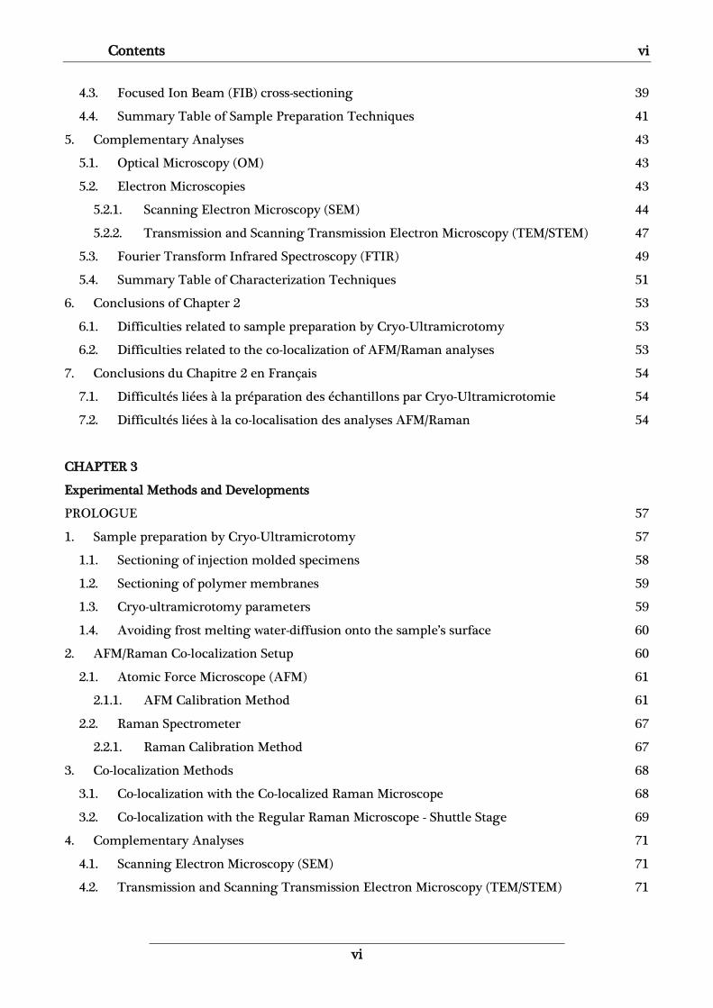
properties of the material. For entropic reasons, most polymers are immiscible2 and the blends show
a phase-segregated morphology, as illustrated in Figure 1.1. The properties of these phases separated
materials are roughly the average of the properties of each component alone. For example,
Ruckdäschel et al.3,4 have studied immiscible poly(2,6-dimethyl-1,4-phenylene ether) (PPE) and
poly(styrene-co-acrylonitrile) (SAN) blends. SAN is a rather rigid material with a modulus of 3.80 ±
0.12 GPa, presenting low deformation at rupture and fracture energy (2.93 ± 0.06 % and 27 ± 1
kJ/m2). Compared to SAN, PPE presents a lower modulus of 2.50 ± 0.09 GPa but much higher
deformation at rupture of 69.8 ± 39 % and fracture energy (710 ± 443 kJ/m2). The authors have
shown, for example, that for a 60/40 composition (wt%), a PPE/SAN blend verifies the rule of
averaged properties: a modulus of 3.08 ± 0.15 GPa, a deformation at rupture and fracture energy of
40.2 ± 24.5 % and 418 ± 252 kJ/m2 respectively. Transmission Electron Microscopy (TEM) image on
Figure 1.1 shows the continuous nature of the SAN (bright phase) while the PPE (dark phase) tends
to form particles. The proper control of the morphology, considering size and distribution of the
domains, interface interactions and adhesion between the components, is mandatory to obtain
improved synergic properties.
Material E (GPa) ε (%) W (kJ/m2)
PPE 2.50 ± 0.09 69.8 ± 39.0 710 ± 443
PPE/SAN 60/40 3.08 ± 0.15 40.2 ± 24.5 418 ± 252
SAN 3.80 ± 0.12 2.93 ± 0.06 27 ± 1
Figure 1.1. TEM micrograph of an immiscible PPE/SAN 60/40 wt% blend and table of mechanical properties of
PPE, SAN and 60/40 PPE/SAN blend.3,4
Improvement of modulus is only attained on polymer blends when the adhesion of the
materials at the interfaces is sufficient. If not the case, the incompatibility between the components
can lead to the formation of defects at the interface and therefore to brittle characteristics.3 One of
the most mature strategies to improve the miscibility of polymer blends is compatibilization.
Compatibilizing agents are chemically modified copolymers capable of interacting with one or both
components of the blend, acting like surfactants to modify the interfacial tension between phases,
improving the phases’ dispersion. The final morphology developed in the presence of these
compatibilizers corresponds to smaller droplets of the minority phase dispersed into the main
component. Ruckdäschel et al.3,4 have used this strategy to improve the miscibility of PPE/SAN
blends using compatibilizers based on polystyrene-polybutadiene-poly(methyl methacrylate)
triblock terpolymers (SBM). Figure 1.2 shows TEM images of the morphological evolution of the

3 Chapter 1 – Motivation
3
PPE/SAN blend with the increasing amount of SBM and the mechanical properties of each
composition. They observed that the addition of 5 wt% of SBM led to no significant morphological
change, but almost doubled the deformation at rupture and the fracture energy (from 40.2 ± 24.5 %
to 76.4 ± 14.6% and from 418 ± 252 kJ/m2 to 817 ± 156 kJ/m2, respectively). These improvements were
attributed to the presence of the compatibilizer at the interphase, confirmed by TEM by the
irregularly contrasted regions at the phases’ boundaries (Figure 1.2 (b)). Increasing SBM
compatibilizer’s ratio up to 10%, the morphology of the blend was modified, becoming co-
continuous, which improved the deformation at rupture and the fracture energy of the blend up to
97.9 ± 3.0% and 1022 ± 32 kJ/m2 respectively. On the other hand, the Young’s modulus keep on
dropping from 3.08 ± 0.09 GPa for the uncompatibilized blend to 3.01 ± 0.09 GPa for 5% SBM and
2.84 ± 0.07 GPa for 10% SBM. Further addition of SBM to 20 wt% turned back the morphology to a
dispersed PPE phase into a SAN matrix. However, the average droplet size of the PPE phase was
reduced in comparison to the previous compositions. The good deformation at rupture and the
fracture energy properties were maintained (96.8 ± 12.7% and 944 ± 127 kJ/m2) but it caused a more
pronounced drop of the modulus (2.57 ± 0.06 GPa).3,4 This example evidences the need to understand
the impact of the compatibilizer on both the morphology and the mechanical properties of the
compatibilized blends in order to optimize their resulting properties
Material E (GPa) ε (%) W (kJ/m2)
PPE/SAN 60/40
3.08 ± 0.15 40.2 ± 24.5 418 ± 252
+5 wt% SBM
3.01 ± 0.09 76.4 ± 14.6 817 ± 156
+10 wt% SBM
2.84 ± 0.07 97.9 ± 3.0 1022 ± 32
+20 wt% SBM
2.57 ± 0.06 96.8 ± 12.7 944 ± 127
Figure 1.2. TEM micrographs showing different morphologies developed for increasing amount of SBM
compatibilizer into PPE/SAN blends. The table presents the corresponding mechanical properties. 3,4
1.2. Multilayer Polymeric Materials
Another approach used to combine properties of different polymers in a material is to
produce multilayer films, with each layer consisting of a polymer with specific properties. These
materials are widely used in the food industry. To guarantee the integrity and safety of the food,
packaging films must have the following properties: strength (resistance to puncture, impact and
tear), sealing and preservation against moisture (barrier to the transmission of water vapor in or
out), oxygen (to reduce microbial activity), light (prevent light-induced changes in flavor or
nutritional quality) and chemicals (prevent the food from absorbing unwanted substances from the
environment). The use of a single material with all those properties is highly improbable. Hence the
development of multilayer materials is of prime importance.5,6 Figure 1.3 shows an example of
multilayer material which is mainly composed of an outer layer of Nylon, responsible for the
mechanical strength and scuff resistance, a layer of Ethylene vinyl alcohol (EVOH), which is an
excellent gas barrier, and a layer of Low Density Polyethylene (LDPE), an inert polymer good for

Chapter 1 – Motivation 4
4
food-contact. In order to ensure that the layers stick to each other, an adhesive layer called “tie layer”
is often used.
Figure 1.3. Example of multilayer polymer material composed of an outer layer of nylon, a gas barrier layer of
EVOH and the contact layer of LDPE intercalated with adhesive layers
Multilayer processing creates interfaces between different materials and the adhesion
between them is critical for the mechanical and barrier properties. To overcome this problem, it was
necessary to develop adhesives layers, or “tie layers”, which are used between each different
polymeric layer to enhance surface compatibility and to seal up any voids and defects. Common
adhesives used on multilayers are based on reactive polyurethane chemistry, i.e, the reaction of an
isocyanate with a hydroxyl group to form a urethane linkage. The isocyanate pre-polymer will
always contain a portion of free diisocyanate monomer, which is consumed within the adhesive layer
during the curing reaction. The major issue of this adhesive layer consists on the migration of
unreacted diisocyanate through the layers into the food, in which it can react with water, forming
amines. Some aromatic amines are potential carcinogens, thus, it is very important to study the
nature of the materials used as adhesives and the efficiency of the curing process, in order to ensure
the safety of the material for food application.5–9 However these investigations are challenging due
to the complexity of the final product and the low thickness of each phase.
For some other applications, the ability of selected additives to migrate through the layers
can also be used to improve the multilayer properties. For example, Gherardi and coworkers7
developed a procedure to incorporate antimicrobial agents in a multilayer material, based on a
commercial packaging with a polyurethane adhesive free of isocyanate. They have studied the
antimicrobial activity of the new films and the release of the active compounds. Mass spectrometric
results showed that the compounds were released from the adhesive layer, crossing the material and
reaching the food for antimicrobial action. On the other hand, the researchers claimed that a deeper
research was necessary to study the correlation between their release rates and the thickness,
chemical composition and structure of the adhesive layer. The characterization of the chemical
profile throughout the cross-section of the multilayer film, for example with spectroscopy
techniques, could have given insights on the specific layer limiting or controlling the release rate of
the antimicrobial agents. The challenge for this kind of sample is to be able to properly open the
membrane, if possible without an embedding, to avoid a chemical contamination of the material by
diffusion of the embedding medium.
The gas barrier properties, often required for multilayer polymer materials (not only for food
packaging), will depend on the nature of the gas and the properties of the polymers, such as the
degree of crystallinity, cross-linking, polymer chemistry, glass transition temperature (Tg). The gas
Gas Barrier layer
Product contact layer low leachable levels
Outer layer Strenght and scuff resistances
Adhesive layers

5 Chapter 1 – Motivation
5
barrier properties are highly affected by crystallization and orientation of the lamellae, as the chains
packing affects the free volume available for gas transportation.10–15 Cocca and coworkers16 have
studied the effect of crystal polymorphism on the mechanical and barrier properties of Poly(L-lactic
acid) (PLLA). They have shown how the degree of crystallinity (crystal fraction) and the nature of
the polymorph (α or α’) affected the Young’s modulus and elongation at break (Figure 1.4(a) and (b),
respectively). The authors discussed how the transition from the α’ to the α polymorph (higher chain
packing and interchain interaction for the α form) affected the mechanical properties of the
material, improving Young’ modulus but decreasing elongation at rupture. This transition from α’ to
α form corresponds also to the abrupt decrease of the water vapor permeability (WVP), shown on
Figure 1.4(d), with somehow the same degree of crystallinity (very small increase of the crystal
fraction). Correlation between optical microscopy and Wide Angle X-Ray Diffraction (WAXD)
analysis was used to estimate the polymorphic composition of the PLLA samples, however, no
quantitative determination was possible due to the very similar WAXD profiles of the two
polymorphs.16 This problem could be addressed by the co-localization of microscopies and
spectroscopy techniques, which could have provided direct morphological and chemical information
for the quantitative analysis of the nature of the phases in the samples.17 Furthermore, the analysis
of the distribution of polymorphs and the size of the crystallite in the samples could have explained
the drop on the elongation at break and WVP for samples with almost the same degree of
crystallinity (Figure 1.4 (c)).
(a) (b) (c)
Figure 1.4. Different properties of PLLA films as function of the degree of crystallinity: (a) Young's modulus,
(b) elongation at break and (c) permeability to water vapor (WVP). The crystal polymorphs are indicated for
each degree of crystallinity.16
Chapter 1 – Motivation 6
6
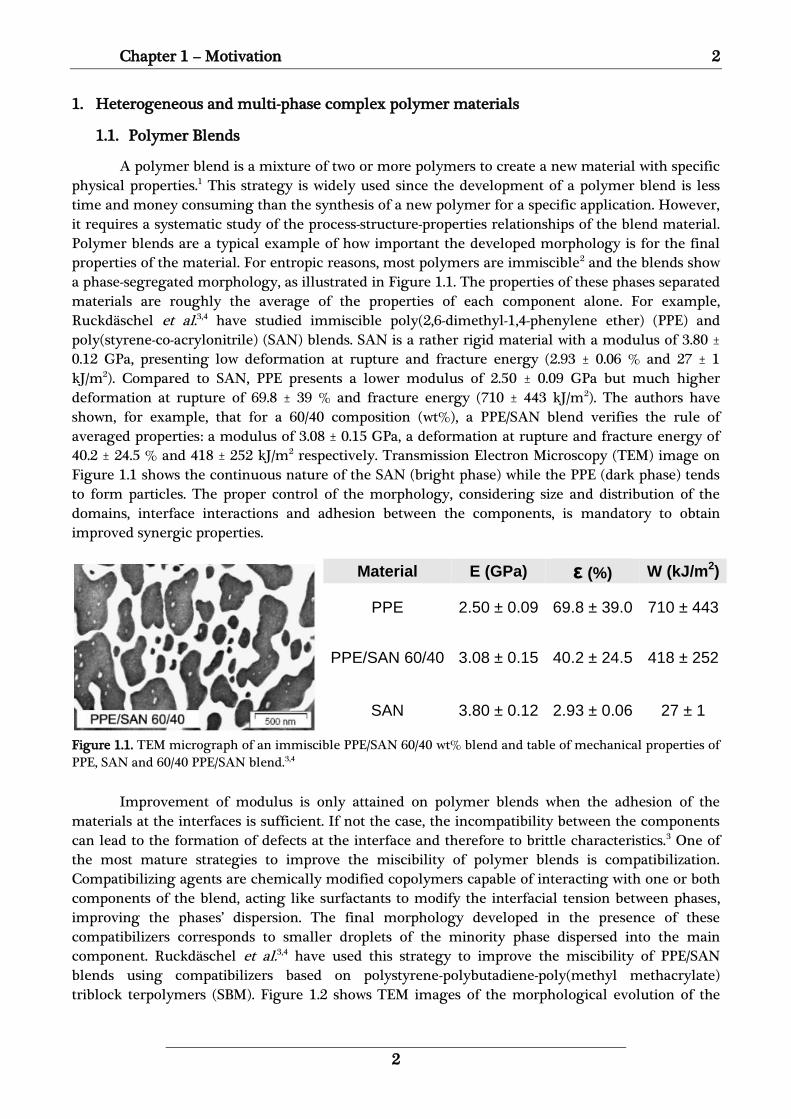
1.3. Fiber Reinforced Polymer Composites
A composite is a structured material that consists of two or more constituents which are
combined at a macroscopic level and are not soluble in each other.18 The matrix of the composite,
generally continuous, can be a metal, a ceramic, carbon or a polymer. Embedded inside the matrix,
the second constituent is the reinforcing phase, which can be of different natures (ceramic clays,
polymers/ natural fibers, inorganic fillers...) and have a variety of forms and shapes, such as fibers,
particles or flakes. The nature and shape of the secondary phase is mainly determined by the
application or the properties that one wants to improve.
The most common use of the polymer composite strategy is for the enhancement of
mechanical properties of the polymer itself. For this mean, fibers are generally used due to their
high aspect ratio, i.e., the ratio between their length and diameter (l/d). The performance of a
polymer/fiber composite will be determined by the interactions between the matrix and the
reinforcement. Indeed, the mechanical properties of the composite are mainly ensured by the fibers
and a good charge transfer from the matrix to the fibers is necessary to reach the best performances.
This load transfer is only effective if the fibers are well dispersed in the matrix and if the adhesion of
the matrix on the fiber is good. Therefore the quality of the interface can be problematic when
hydrophobic polymer matrices like Polyethylene are used with hydrophilic fibers like glass fibers for
example. The incompatibility between the components leads to poor wettability during processing,
creating discontinuities and voids at the interface, which are ineffective for load transfer and
actually act like stress-concentration points, hampering the mechanical performance of the
composite.
In order to improve and guarantee the interface bonding, a common strategy is based on the
chemical modification of the fiber’s surface using a sizing to improve their wettability by the matrix,
and the creation of chemical bonds between the fiber’s surface and the polymer matrix. For
example, a sizing containing a coupling agent is commonly applied on glass fibers. The most
common kind of coupling agents used are organometallic or organosilanes.19–23 Organosilane
precursors are molecules that contain two types of reactive functional groups (Figure 1.5): one
capable of forming chemical bonds with inorganic materials and one capable of interacting with
organic materials. The hydrolysis of the ethoxy or methoxy groups (O-X) in contact with water leads
to the formation of silanol groups, which engender the creation of oligomers by partial
condensation. The silanol dimers hydrogen bond to the surface of the fiber and then, through water
condensation, chemical bonds are created between the coupling agent and the surface of the glass
fibers. The reactive group R bore by the coupling agent (vinyl groups, epoxy, amino, mercapto, etc)
is available to physico-chemical interactions with the chain of the polymer matrix, improving
wettability, miscibility and forming chemical bonds or hydrogen bonds with polar matrices.
Figure 1.5. Scheme of reaction of hydrolysis and condensation of a silane coupling agent for surface
modification of fibers. R: vinyl groups, epoxy, amino, mercapto; X: methyl or ethyl groups.
7 Chapter 1 – Motivation
7
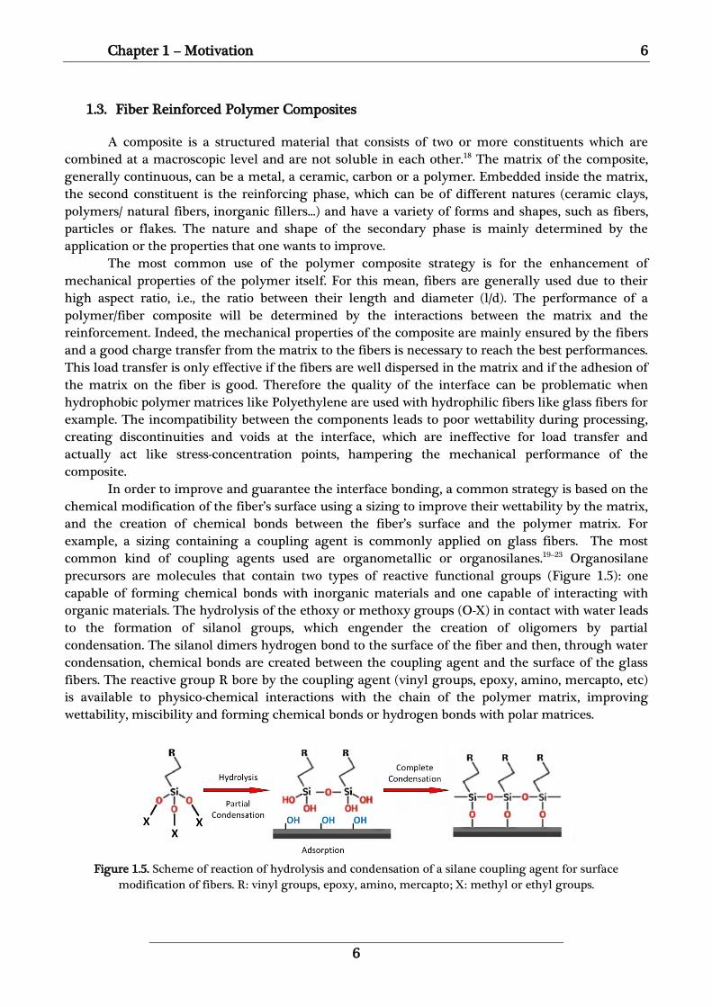
Other alternatives to the use of silane coupling agents have been developed with the use of
reactive copolymers like Maleic Anhydride grafted on polyolefines.24–26 For example, Guojun Luo et
al 24 studied a polypropylene/glass fiber (PP/GF) composites prepared by treating GF with a film
former (GFf) containing maleic anhydride grafted polypropylene (MPP) and a β-nucleating agent.
The interfacial adhesion and the crystal morphology between GF and PP were observed by scanning
electron microscopy (SEM) (shown on Figure 1.6) and the tensile and impact strength were
measured (Table 1.1). The composite prepared with the non-treated commercial fiber (GFc)
presented poor interfacial adhesion and a smooth GF surface was observed after debonding (Figure
1.6 (a)). This caused poor mechanical properties, i.e., no substantial improvement on tensile strength
(from 27.1 MPa for PP alone to 31.3 MPa for the composite) and especially the impact strength,
which dropped from 10.4 to 5.1 kJ/m2, as shown on Table 1.1. The interfacial adhesion was improved
by the presence of the coating film. SEM images showed a layer of remnant polymer on the surface
of the GFf after debonding (Figure 1.6(b)) and the tensile strength attained 61.8 MPa. With the
addition of 2 wt% MPP, the covering polymer layer on the GF surface appeared thicker and with a
roughen fracture surface. The fact that the impact strength attained 14.2 kJ/m2 (roughly the double
from the composite without MPP) evidenced the better adhesion interface. The authors verified that
when the content of MPP was increased to 3 wt% and 10 wt%, the interface microstructures appeared
nearly identical, with fibers completely covered (Figure 1.6 (c), (d) and (e)). On the other hand, the
tensile strength of the composites increased from 61.6 MPa (3 wt% MPP) to 67.3MPa (10 wt% MPP),
even though the interface microstructure was unchanged.
Figure 1.6. SEM micrographs representing the interfacial adhesion between GF and PP matrix for PP/GFc (a,
a1), PP/GFf (b, b1), PP/2MPP/GFf (c, c1), PP/3MPP/GFf (d, d1) PP/10MPP/GFf (e, e1). (a1), (b1), (c1), (d1) and (e1)
are enlarged areas marked by the dashed yellow squares in (a), (b), (c), (d) and (e) respectively. 24
Table 1.1. Tensile and Impact strength of the PP composites 24
To understand the impact of the GF coating film on the crystallization process, the
researchers monitored the isothermal crystallization by optical microscopy. On the one side, for
PP/GFc sample, PP crystals nucleated randomly and grew into large spherulites, as shown on Figure

Chapter 1 – Motivation 8
8
1.7(a). On the other side, in PP/GFf sample, nuclei were found concentrated near the surface of GFf,
and after 600 s a layer of oriented crystalline lamellae was found surrounding the GFf. A SEM image
of the etched fractured surface of this sample showed structures in the form of spikes grown
perpendicular to the fibers, which were attributed to β-transcrystals. The very good adhesion of these
crystals to the GFf surface (intimate contact between the two materials) is thus suspected to be
responsible for the efficient stress transfer between the PP matrix and the GF. Structural, chemical
and morphological analyses of these structures (by Confocal Raman for example) could have
provided an unambiguous attribution of the crystals nature. In addition, nano-mechanical
properties, such as adhesion and modulus profiles at the fiber-matrix interface could have been
accessed by AFM in order to characterize the quality, integrity and continuity of the interface.
(a) (b)
Figure 1.7. (a) Polarized optical micrographs during an isothermal PP crystallization at 135°C around a single
fiber (GFc or GFf) (b) SEM micrograph of the etched fracture surface for PP/2%MPP/GFf injection molded
sample. Adapted from 24
The impact of the coupling agent at the fiber-polymer interface has to be studied at a local
scale to be able to optimize the material’s performances. Therefore the development of
characterization methods that can provide direct probing of morphological, mechanical and
chemical properties of the polymer-fiber interface/interphase could accelerate the progress in the
field.
1.3.1. Polymer Nanocomposites
The complexity of composite materials increases when one of the fillers has at least one of its
dimensions in the nano-range, turning it into a nanocomposite material. Usually nanocomposite
materials have enhanced properties when compared to their non-nano composite equivalent.27–33
Inorganic additives, like calcium carbonate, glass beads, talc and clay for example, were often used
as fillers on polymer materials to reduce cost and enhance the mechanical properties, but the use of
the corresponding nano-fillers has given them a much more functional interest.
As for the reinforcement fibers, the interface between the nanoclay and the polymer is
determinant in the effectiveness of load transfer from the polymer matrix to nanofillers. As most
polymers are hydrophobic, they are not compatible with hydrophilic nanoclays for example. This
means that a simple mixing of the components would create agglomerates of nanoclay, which
would lose their nano-dimensions. An exfoliation of the nanoclay and their perfect embedding by
the polymer matrix is required to reach optimal performances. Figure 1.8 shows TEM images of an
β-crystals PP/GFc
PP/GFf

9 Chapter 1 – Motivation
9
agglomerated and an exfoliated nanocomposite.29 The exfoliation and uniform dispersion of
nanofillers in the polymer matrix can be achieved by means of surface modification of clays, like
grafting and chemical treatments, solution induced intercalation process, in situ polymerization and
melting process.27,29,34–37 Pramoda and coworkers38 studied how the mechanical and thermal
properties of polyamide 6/clay nanocomposite are influenced by the exfoliation degree of the clay
particles. They suggest that exfoliated nanocomposites exhibit higher onset temperature for
degradation than those with agglomerated clay particles. Chan et al.30 have used morphological
characterization to tune their fabrication process in order to produce uniformly-dispersed samples.
Thanks to the better dispersion, even when small amounts of nanoparticles from 1 to 10 wt% were
incorporated in the polymer matrix, a substantial improvement of mechanical properties was
achieved, e.g., up to 57% increase in Young’s Modulus using 7 wt% of nanoclay inside an epoxy
matrix. Improvements were also observed for exfoliated nanocomposites on their barrier properties,
chemical resistance, reduced solvent uptake and flame retardancy: the exfoliated nanofillers making
the diffusion pathway through the nanocomposite much more intricate.36,39–44 Therefore
nanocomposites require lower amounts of fillers than regular composites to reach comparable
performances.29
(a) (b)
Figure 1.8. SEM image characteristic of nanoclay morphology in a 95/5 wt% Polyamide6-Montmorillonite
nanocomposite: (a) agglomerated and (b) exfoliated.29
Inorganic nanoparticles can also have an impact on the crystallization of the polymer matrix
by acting as heterogeneous nucleation sites. Smith and Vasanthan45 have studied the effect of
nanoclay on the crystallization kinetics and spherulitic morphology of poly(trimethylene
terephthalate) (PTT)/nanoclay films. They have shown by polarized light microscopy (PLM) that the
addition of 10 wt% of nanoclay had great impact on the size and distribution of the spherulites, as
shown on Figure 1.9. The conformational changes induced were monitored by Infrared
spectroscopy, indicating that nanoclay accelerates the polymer chain conformational transition from
trans to gauche. Differences on crystallinity and/or on the crystal structure (polymorphism) have
been shown to greatly impact the mechanical and thermal properties of composites.45–51 The
association of optical microscopy with spectroscopy techniques could have directly provided not only
information about the conformational transition but also the distribution of the different
polymorphic crystals induced by the presence of the clay, by probing the chemical structure of each
crystal seen on the optical image.

Chapter 1 – Motivation 10
10
(a) (b)
Figure 1.9. PLM photographs of (a) neat PTT and (b) PTT nanocomposite with 10wt% of clay. Adapted from45
1.4. Block-copolymers
Block-copolymers, contrary to polymer blends, present covalent links between different
polymeric materials usually immiscible, which gives very specific properties due to the resulting
nanophase separation (self-assembly). The challenge on the development of these materials lies on
the precise control of the nanostructure morphology. This can be achieved by tuning the molecular
weight, monomer chemistry and processing temperatures, for example. When composed by two
immiscible blocks, nanodomains dimensions can range from 5 nm to more than 100 nm, and the
developed morphology can exhibit a big variety of symmetries, resulting into, for example,
lamellae, cylinders, bicontinuous gyroids and even body-centered cubic arrays of spheres, as
illustrated on Figure 1.10.52–54
(a) (b) (c) (d)
Lamellae
Hexagonal packed
cylinders
Bicontinuous gyroids
Cubic packed spheres
Figure 1.10. Example of copolymer morphologies: (a) lamellae (b) hexagonal packed cylinders (c)
bicontinuous gyroids and (d) cubic packed spheres. Adapted from 52–54
A good example of the impact of the copolymer morphology on its properties is given by
Zhuang et al.55 who studied for styrene-butadiene copolymer (SBC) membranes the impact of the
polystyrene/polybutadiene (PS/PB) ratios on both the gas separation (CO2/N2) performance and the
ageing properties. They have detected different nanophase-separated structures by AFM at the
surface of the copolymer membranes depending on the PS/PB ratios as illustrated on Figure 1.11.
Three different morphologies were obtained: cubic lattice spheres of PB in a continuous PS matrix (4
wt% PB), PS and PB lamellae parallel to the membrane surface (55 wt% PB) and cylinders of PS in a
continuous PB matrix (70 wt% PB). Crystalline regions inside the PS domain were observed in both
samples rich in PB, which affected the gas transport due to the stable and regular molecular

11 Chapter 1 – Motivation
11
structure of the PS domain. According to the authors, the synergism between the lamellar
morphology and the presence of α crystals in the PS phase increased the diffusion pathway for CO2
and simultaneously enhanced the CO2/N2 selectivity. A similar result was obtained for the
cylindrical structure, which presented γ crystals in the PS phase. The different spacing within the
crystal lattice restricts the N2 transport but do not significantly affect the CO2 permeability. This
leads to an even higher CO2/N2 selectivity for the PS30/PB70 membrane. Furthermore, the
researchers have shown that the cylindrical micro-structure of the PS30/PB70 membrane exhibited
high ageing resistance under operation conditions, due to the morphological stability of the
cylindrical micro-structure. The authors prepared these membranes by spin-coating, leading to a
membrane thickness of about 10 µm. For such thickness, the morphological analysis of the surface
by AFM might be insufficient for the correlation of properties with the morphology, i.e., the
development of the morphology through the membrane thickness may be considerably different
from what observed at the surface. A cross-section analysis (after cryo-ultramicrotomy for example)
would therefore be appropriate to get a deeper understanding of the obtained morphologies. In
addition, co-localized confocal Raman spectroscopy may offer a mapping of the PS α/γ crystals
distribution and ageing effects on the bulk of the membranes.
Figure 1.11. AFM topographic images on the membrane’s surface of (a) PS, (b) PS96/PB4, (c) PS45/PB55, (d)
PS30/PB70 and (e) PB. Adapted from 55
2. Bulk vs Surface Properties
As discussed on the previous sections, the properties of polymeric materials depend on their
nanostructure, the proper control of phase separation, the dispersion and distribution of charges and
the quality of interfaces, all of these parameters being potentially variable through the material
thickness. The resulting heterogeneities of properties can be induced by the processing methods, or
tailored intentionally to achieve specific distinct properties for the surface and the bulk. In addition,
after ageing, materials become generally heterogeneous in terms of chemistry, morphology and
mechanical properties, due to the inhomogeneous degradation process through the material
(surface/bulk).
Processing of thermoplastic polymers is mainly related to the application of shear to the
molten material at high temperature followed by high thermomechanical stresses due to the rapid
cooling of the material at the end of the process. Therefore, the thermomechanical history may not

Chapter 1 – Motivation 12
12
be homogeneous throughout the whole thickness of the material, inducing differences in the local
order of the polymer chains and the distribution of additives. This can result in different
morphologies in terms of molecular orientation, lamellar thickness, crystal structure, shape and
dimensions, crystallinity degree, orientation of the amorphous phase, dispersion state of a blended
polymer, length and orientation of reinforcing fibers and crystalline texture (skin-bulk structure),
since the kinetics and morphology of crystallization are intrinsically related to the flow and cooling
regimes.56 In injection molding, for example, the surface morphology is highly affected by the
thermomechanical stresses induced by the rapid cooling of the chains when in contact with the cold
mold and the orientation of the chains caused by shear stress. Liparoti and coworkers57 performed a
multiscale mechanical characterization of isotactic polypropylene (iPP) injection molded samples.
The developed morphologies were characterized by polarized optical microscopy and AFM, as shown
on Figure 1.12.
They revealed a complex multilayer morphology composed of globular elements, fibrils and
spherulites, from the surface to the bulk of the sample. The thickness of the different layers was
correlated to the injection molding conditions (packing pressures and mold temperatures). The
authors also evidenced a correlation between the local mechanical properties and the different
morphologies formed along the sample thickness. At the sample’s surface, the cooling rate is the
highest, which does not allow the crystallization of the macromolecules, therefore low modulus is
found. Further from the surface, as the cooling rate decreases, the macromolecules can align
themselves and, due to the stress induced by the flow, form compact structures characterized by
higher moduli in the shear layer. As the bulk of the material takes more time for cooling and is less
affected by the shear, the polymer chains have more time to crystallize, forming spherulites. Thus,
flow and thermomechanical stresses will cause a gradient of different morphologies from the
surface to the bulk.
Figure 1.12. Morphology profile through the material thickness detected by optical microscopy (central
micrograph) and by AFM height maps. The positions where the analyses were performed are indicated by
arrows pointing on the cross section optical micrograph.57
Important material properties such as optical, chemical, electrical and ionic transport can be
tuned by adjusting the material’s morphology or gradient of morphologies. For example, the
properties of polymeric materials used as membranes for filtration, or separation of gases and

13 Chapter 1 – Motivation
13
liquids, will depend on both the surface and the bulk properties. On the one hand, the selective
sorption of molecules on the membrane’s surface is controlled by the morphology, roughness and
chemical properties at the surface (hydrophilicity/hydrophobicity, chemical affinity, etc.) and on the
other hand, the diffusion of these absorbed molecules through the thickness of the material is
controlled by the bulk morphology, dispersion of charges, cross-linking degree, etc.58–63 Wei Zhang
and coworkers63 have studied the pervaporation performance of polymeric chitosan membranes by
simultaneously changing their surface and bulk structures. To adjust the degree of crystallinity of
the membrane’s bulk they tuned the pre-drying processing step (the shorter this step the lower the
degree of crystallinity of the bulk). A lower crystallinity implied that the transport of the permeation
molecules was faster, i.e., a membrane with a less compact structure exhibited a higher flux,
however it had a lower separation factor. In order to improve selectivity they functionalized the
membrane’s surface with maleic anhydride. After modifying both the bulk and the surface of the
membranes the authors improved by 400% the separation factor and by 60% the flux. They
concluded that the combination of bulk modification by pre-drying treatments and surface
functionalization was an effective method to simultaneously improve both the permeability and
permselectivity of polymeric membranes, but they claim that further research needs to be done in
order to understand the relationship between the membrane’s bulk characteristics and the
pervaporation process. The clear and direct characterization of both the membrane’s bulk and
surface remains therefore the main technical challenge to be solved.
Ageing is another source of surface/bulk heterogeneity. It results of complex physical and
chemical interactions, such as physical creep and relaxation, chemical degradation by oxidation,
chain scission and hydrolysis, induced from the operating conditions: high mechanical stresses,
mechanical and thermal cycling, attack by chemical agents or UV light exposition, for example.
These complex interactions affect the surface and the bulk of the material in different ways. For
example, during the thermal ageing of polymers, the bulk can be affected by structural and
morphological changes caused by temperature-induced transitions, while the surface is mainly
affected by thermo-oxidative degradation, which is limited to a thin surface layer up to a few tens of
micrometers, depending on the kinetic of oxidation of the material. The surface contamination of
the material by fuels, lubricants and chemicals can diffuse through the thickness of the material
over time. Reciprocally, additives such as plasticizers or stabilizers can migrate from the bulk to the
surface of the material over time. These diffusion processes and the chemical reactions involved in
the ageing mechanism are affected by the nature of the material (selective sorption of molecules on
the surface), the state of order and morphology in polymer blends, multilayers and composites, as
well as the nature, size and dispersion of charges, and porosity distribution. Thus, during ageing, a
gradient profile is formed inside the material. Therefore, the understanding of the mechanisms and
kinetics of diffusion and degradation from the surface to the bulk, and of the effects of
morphological and chemical changes on the material properties offer a chance to develop ageing
mitigation strategies.64,65
2.1. Characterization of both the Surface and Bulk of Polymer Materials
This section will focus on the experimental techniques classically used for chemical and
morphological characterization of both the surface and bulk of polymer materials.
The characterization techniques used for probing the chemical properties of surfaces are
based on vibrational spectroscopies and backscattered radiation. The most common vibrational
spectroscopies used are Fourier Transform Infrared Spectroscopy (FT-IR) and Raman spectroscopy.
These techniques use the frequency-dependent absorption or emission of radiation from chemical
bonds and structures, in order to identify and quantify components or chemical groups in the

Chapter 1 – Motivation 14
14
structure. For IR spectroscopy, Diffuse Reflectance FTIR (DRIFTS) and Specular Reflection FTIR are
used for the characterization of rough surfaces (powders) and smooth surfaces, respectively.
Attenuated Total Reflection Fourier Transform Infrared Spectroscopy (ATR-FTIR) is the most
popular technique for surface analysis due to the short penetration depth (~1 to 5 µm depending on
the crystal used and the wavenumber), allowing the characterization of a large area (~1 mm2) of the
top layer of the material. Raman spectroscopy is a complementary technique to IR spectroscopy,
because some vibration modes are inactive in IR and active in Raman, and vice-versa, allowing the
complete chemical characterization of the material. Energy Dispersive X-ray Spectroscopy (EDS or
EDX) is a technique based on the interaction of the material with an electron beam, and is used for
identifying, quantifying and mapping elements on the surface of the material. X-ray photoelectron
spectroscopy (XPS) has a lateral resolution from 1 mm to 10 µm, but a depth resolution of tens of
nanometer, being particularly suitable for elementary analysis of modified surfaces, such as plasma-
treated or oxidized surfaces, thin coatings or grafted polymers on the surface.
The characterization of the physical properties of the surface include the morphology,
topography, crystallization, microphase separation, as well as size, shape, distribution and orientation
of charges which can be analyzed by direct observation, e.g., using optical or electron microscopies.66
Optical Microscopy is a low-resolution (classical resolution roughly about 0,5-1 µm) and low-
magnification technique (from 2x up to ~2000x) used to provide a first look at the surface, due to its
easy sample preparation, low cost and simple principles of operation. Scanning Electron Microscopy
(SEM) is widely used for the characterization of surfaces with high magnification (up to 500000x)
and high resolution (5~10 nm) and can provide additional interesting information depending on the
interactions of the electron beam and the specimen used to obtain the image. Using separate
detectors for Backscattered Electrons (BSE/ sensitive to electronic density) and Secondary Electrons
(SE/ sensitive to surface topography), compositional and topographic images of the same area may
be produced. Finally, Atomic Force Microscopy (AFM) is an advanced technique for surface analysis
based on the interaction of a scanning probe with the sample’s surface. Three dimensional
topographic images are obtained, giving access to morphological measurements, including
roughness. The lateral resolution will depend mainly on the tip radius of the probe (typically ~5-10
nm). The substantial developments of the past years have enabled different modes of operation,
allowing probing the mechanical, thermal, electrical and magnetic properties of the material’s
surface with a high spatial resolution.
The characterization of the bulk properties is usually performed using techniques that probe
the material as a whole, averaging the response of the surface and the bulk. For example,
Differential Scanning Calorimetry (DSC) and Dynamic Mechanical Analysis (DMA) are used to
evaluate the thermomechanical behavior of the material, providing insights on phase transitions,
miscibility of components, crystallinity and degree of crosslinking. However in order to do a direct
observation and probe the bulk of the material (without surfaces), special techniques are required to
open the sample for optical/electron microscopies, AFM imaging (topography, mechanical, etc.) and
chemical mapping (Raman, µ-ATR-FTIR), which will be discussed in the next section.
2.2. Sample Preparation Techniques for Bulk Direct Observations
The most used and simple technique to access the bulk of a material is the cryo-fracture, in
which the polymer is cooled in liquid nitrogen (-196ºC), in order to induce afterward a brittle
fracture in the rigidified material at its glassy state. The sample is then installed or glued to a
support and the surface is imaged using a microscope (generally SEM). Although easy to prepare,
the surface is not always representative of the inner morphology of the membrane. The

15 Chapter 1 – Motivation
15
unpredictable brittle fracture creates irregular rough surface which can follow the material
heterogeneities, like particles or phases with different mechanical properties, making difficult to
understand the real morphology of the material. Other advanced techniques used to provide better
cross-sections are Cryo-Ultramicrotomy and Focused Ion Beam (FIB). Cryo-ultramicrotomy is based
on the use of a diamond knife operating at cryo temperature to cut ultrathin slices (down to 50 nm)
of the material’s surface with controlled cutting speed, angle and depth. FIB cross-sectioning uses a
high energy (~30 kV) ionic beam, typically gallium, of 10 nm to 1 µm in diameter to cut the sample
surface with controlled parameters. Both techniques can provide surfaced samples with very flat
surfaces and minimum artifacts for direct observation by Optical Microscopy, Scanning Electron
Microscopy (SEM), Atomic Force Microscopy (AFM) and can also provide thin sections (~50 nm) for
complementary morphological analysis using Transmission Electron Microscopy (TEM).67–69 An
advanced discussion of these sample preparation techniques will be presented on Chapter 2.
3. Polymer membranes
For polymer films/membranes, the need to distinguish the surface from the bulk of the
material becomes even more crucial than it can be for massive polymer products. Indeed the
properties gradients that can be found from the surface to the bulk of the membranes can develop at
length scales comparable with the membrane’s thickness. A polymer film is a continuous planar
material which is flexible and “free-standing”, with thickness ranging from a few hundreds to tenths
of micrometers, in opposition to ultrathin films (thickness at nanometer scale) coated on a
substrate.70 Polymer films can be made of a single material or multiphase systems (blends,
composites, multilayers) and are commonly used as barriers for separation of two mediums, like in
packaging, or electrical insulators for wires and cables. The term membrane is often used to
designate polymer films with specific functionalities of technological interest, i.e., it can be
considered as an interphase between two mediums acting as a selective barrier, responsible for the
regulation of gas transport, diffusion of liquids or ions between each side of the membrane.71 Due to
these functionalities, membranes are widely used for technical applications, such as desalination of
water through reverse osmosis, nanofiltration, dialysis, separation of molecules, liquids or gases, and
ion exchange electrolytes for fuel cells and electrolyzers. Due to their technological importance, this
section will focus on membranes rather than polymer films.
Membranes can be manufactured by a variety of processes, such as extrusion of the polymer
melt, hot pressing, polymerization on substrates and casting by solvent evaporation. Each method
induces different morphologies (orientation, asymmetries) on the surface and through the thickness
of the membrane, which can deeply affect their functional properties. Figure 1.13 represents the
different questions of interest on the surface and the bulk of polymer membranes. However,
distinguishing the chemical and physical contributions from the surface and the bulk on these low
thickness materials can be difficult due to the experimental issues on accessing, probing and
differentiating properties and morphologies.

Chapter 1 – Motivation 16
16
Figure 1.13. Schematic representation of the different properties to be characterized on the surface and the
bulk of membranes
For this purpose, the use of multiple characterization techniques is at the same time essential
and challenging, each technique imposing their own particularities in terms of cost, resolution,
sensitivity and dimensions of the probed area.72 Therefore, this thesis focused on the development of
new methodologies and strategies for sample preparation and characterization, allying
morphological, physical and chemical information, to contribute to the advance study of the
process-structure-properties relationships of a variety of heterogeneous or multiphase polymeric
systems, especially when processed into membranes.
4. Manuscript Structure
This manuscript will be composed by the following chapters:
Chapter 2: Co-localized AFM/Raman and Complementary Analyses
In the second chapter, we will present an introduction to the fundamentals of each technique
used to study complex polymer systems. Special attention will be given to AFM and Confocal
Raman spectroscopy, being the techniques chosen to be the basis of our multiscale characterization
approach for co-localized chemical, nanomechanical and morphological analysis. The techniques
most suitable for sample preparation will be presented, as well as the specific technical challenges
associated to the characterization of polymer membranes.
Chapter 3: Experimental Methods and Developments
The third chapter will be focused on the methodology used and experimental developments
done for sample preparation by cryo-ultramicrotomy, as well for the co-localized AFM/Raman
analyses and complementary techniques (SEM, STEM and µ-ATR-FTIR). A specific technique of co-
localization has been developed in order to ensure the acquisition of physical, morphological and
chemical data on the same area.
Chapter 4: Compatibilization of Polymer Blends based on PA6/ABS
The co-localized methodology will be used to study the compatibilization of PA6/ABS
polymer blends. The interest, accuracy and complementarity of co-localized AFM and Raman
analysis will be demonstrated by elucidating the effect of the compatibilizer and blending protocol
on the blend’s morphology and on the PA6 crystallization’s polymorphism (α and γ phase amount
and distribution in the blends).

17 Chapter 1 – Motivation
17
Chapter 5: Hybrid Membranes for Fuel Cell
This chapter will be dedicated to the study done on alternative membranes for Fuel Cell
operation, based on the hybridization of a sulfonated polyether-etherketone (sPEEK) membrane with
an active network by sol-gel chemistry. Thanks to the technical developments specific for membrane
characterization presented on Chapter 3, we will demonstrate the impact of each step of fabrication
on the membrane’s morphology, nanomechanical properties and stability over time of two different
hybrid membranes.
Chapter 6: Copolymer Electrolytes for Lithium Batteries
At last, chapter 6 will focus on the study of the bulk morphology of new Lithium batteries
electrolytes made of Polyethylene Oxide (PEO) based copolymers with different structures.
Challenges lay in sample preparation due to the high hydrophilicity of the materials, which implied
special development for proper sample characterization without modification induced by water
adsorption. The effect of the copolymer structure on the morphologies will be shown by AFM and
compared to previously done Small Angle X-Ray Scattering (SAXS) experiments, providing a clear
morphological determination and evaluation of nanomechanical properties.

CHAPTER 2
Co-Localized AFM/Raman and
Complementary Analyses

19 Chapter 1 – Motivation
19
PROLOGUE
Complementary characterization techniques must be used for the complete understanding of
the process-structure-properties relationship of materials and this implies a full knowledge of the
physical, morphological and chemical properties through the material thickness. Our strategy is
based on the co-localization of morphological, nanomechanical and chemical information acquired
from AFM/Raman but also by complementary techniques like Optical Microscopy, Electron
Microscopies ( Scanning Electron Microscopy (SEM) and Scanning Transmission Electron
Microscopy (STEM)) and finally by micro-Infrared Spectroscopy (-ATR-FTIR).
In this chapter, the fundamentals of AFM and Raman micro-spectroscopy will be presented
and the accessed information, resolution and limitations of each will be discussed in order to define
the best way to perform efficient co-localized analyses. As a key step is the sample preparation, the
techniques giving access to the bulk of the material as Cryo-fracture, Cryo-ultramicrotomy and
Focused Ion Beam milling will be described. A brief introduction to each technique will be
presented, discussing the methods, limitations and potential artifacts.
French Prologue
Une compréhension complète de la relation mise en œuvre-structure-propriétés d’un
matériau implique une connaissance approfondie de ses propriétés physiques, morphologiques et
chimiques dans tout son volume et implique donc l’utilisation de techniques complémentaires. La
stratégie développée est basée sur la co-localisation des informations morphologiques, nano-
mécaniques et chimiques acquises par AFM et par Raman, mais aussi par des techniques
complémentaires comme la microscopie (optique, électronique à balayage (SEM) et à transmission
(STEM)) ou la spectroscopie micro-infrarouge (-ATR-FTIR).
Dans ce chapitre, les fondements de la micro-spectroscopie AFM et Raman seront présentés
et les informations acquises, la résolution et les limites de chaque technique seront discutées afin de
définir la stratégie la plus efficace pour réaliser des analyses co-localisées de la même zone d’intérêt.
Une étape clé étant la préparation d’échantillon, les différentes techniques permettant d’ouvrir le
matériau telles que Cryo-fracture, Cryo-ultramicrotomie et découpe par un faisceau d’ions (FIB)
seront présentées. Une brève introduction à chaque technique sera présentée, en discutant les
méthodes, les limites et les artefacts potentiels.

Chapter 2 – Co-Localized AFM/Raman and Complementary Analyses 20
20
1. Fundamentals of Atomic Force Microscopy
AFM is a high-resolution method based on the use of a very sharp probe installed on a
cantilever to scan the sample surface. A laser beam is constantly reflected from the top of the
cantilever towards a position-sensitive photodetector, which detects the deflection of the cantilever
and calculates its Z position (Figure 2.1). In contact mode, for example, an electronic feedback loop
is used to keep the cantilever deflection constant during scanning, i.e., the feedback adjusts the
height of the probe support along the Z axis so that the deflection is kept constant to a user-defined
value (setpoint). In this situation, the feedback output equals the sample surface topography to
within a small error. The image is then built by scanning the sample’s surface line by line at a
constant frequency rate using a xyz piezoelectric scanner. Thanks to this scanning probe microscopy
(SPM) imaging technique, the resolution is not limited by diffraction, but depends on the size and
shape of the probe, generally a tip radius of curvature of less than 5 nm is used for accurate surface
analysis.
Figure 2.1. Basic setup for AFM analysis showing the reflection of the laser on the cantilever surface towards
the photodetector. Adapted from 73
Since the introduction of the Atomic Force Microscopy by Binning in 198674, a substantial
development of the system capabilities has been done. Different modes of tip-sample interaction can
be used to image the sample. The most basic one is the Contact Mode, in which a piezoelectric
ceramic raises or lowers the cantilever in order to maintain a constant deflection (cantilever motion
on the Z direction) and therefore a constant contact force, as it scans the imaged area.75,76 In order to
overcome the drawbacks of the Contact Mode, like the high lateral friction forces, researchers have
developed the Tapping Mode in 1993. In Tapping operating mode in air, a piezoelectric ceramic
installed in the tip holder makes the cantilever oscillates a little bit below its resonance frequency.
The tip oscillates vertically and touches or "taps" the sample’s surface at a constant frequency during
the scan. Due to the intermittent contact with the sample, the lateral friction forces between the tip
and the material are minimized, thus minimizing damage to the sample and improving the
durability of the probe. The feedback loop adjusts the height of the scanner to keep a constant
oscillation amplitude of the cantilever (setpoint), therefore, topographic information are collected.77
The mechanical interactions between the probe and each component of the material can engender a
shift between the phase of the imposed oscillation by the piezoelectric ceramic and the phase
measured by the photodiode. Especially for adhesive and viscoelastic samples, it allows the
formation of a “phase image” consisting of an overlap of properties (modulus, adhesion, etc.). In
2008 an operation mode called Harmonix was released, allowing the reconstruction of the force-
distance curves from the lateral deflection signal, and the extraction of quantitative mechanical

21 Chapter 1 – Motivation
21
data. However, it required special asymmetric probes and the operation and interpretation of the
results was difficult. To overcome these difficulties, the PeakForce QNM (Quantitative
NanoMechanics) mode was introduced in 2012, with a relatively simple operation process possible to
use with any kind of probes. An oscillation of the cantilever in the Z-direction at 2 kHz is imposed by
the piezoelectric scanner, which also controls the xyz displacements. 2 kHz is a much lower
frequency than the resonant frequency of typical probes (50 – 300 kHz). This mode of operation
allows for acquiring force-distance curves in real time (2000 per second), as well as their analysis,
meaning the simultaneous mapping of mechanical information like Young’s modulus, adhesion,
deformation and dissipation along with the classical topography image. These mapping therefore
have the same nanometric lateral resolution as the topography image.78,79 The fundamentals of
PeakForce QNM will be presented in the next section.
1.1. Fundamentals of PeakForce Quantitative NanoMechanics (QNM)
The PeakForce QNM is based on the control of the cantilever deflection. A feedback-loop
imposes a setpoint to the maximal value of the deflection, and therefore the maximum force applied
on the sample, called the Peak Force. In order to understand how the imaging control is done, one
should first analyze the dynamics of the tip-sample interaction. Figure 2.2 represents the Z position
of the cantilever (dashed line) over time as the piezoelectric system approaches the tip, touches the
surface and retracts to the original position. At the same time, the deflection of the cantilever is
followed on the approach and withdraw motions, represented by the blue and red lines respectively.
From point A to point B, the figure represents the approach of the cantilever. As the tip gets closer to
the sample, attractive forces (Van der Waals force, dipole-dipole interactions and electrostatic forces)
overcome the cantilever stiffness and pull the tip over the surface (point B), causing a downward
deflection of the cantilever called the “snap-on”. The tip stays in contact with the surface and the
deflection increases until the Z position of the modulation reaches its bottom limit position
(maximum deflection) at point C. While the probe is retracted from the surface, the deflection
decreases accordingly. Adhesion interactions, usually capillary meniscus between tip and surface
prevent the probe from retracting from the surface, causing a downwards deflection, characterized
by a minimum peak on the curve (point D). Finally, the cantilever deflection goes back to zero when
the adhesion forces are overcame, and then damped oscillations are usually observed for low spring
constant cantilevers (not represented here) up to the zero deflection position (point E).

Chapter 2 – Co-Localized AFM/Raman and Complementary Analyses 22
22
(a)
(b)
Figure 2.2. (a) Schematic representation of the tip-sample interaction dynamics79 (b) Force-distance curve
obtained from the tip-surface contact with the approach in blue and the retraction in red. Different mechanical
properties are extracted from the curves: Modulus from the slope of the linear part, Adhesion from the
minimum force of the retraction curve, Deformation calculated from the distance in separation from the point
of contact to the maximum load on the approach curve, and Dissipation of energy as the area between the
approach and retraction curves (yellow area).
From the determination of the cantilever spring constant, one can transform the previous
diagram of the deflection as a function of time (Figure 2.2(a)) on a force-distance curve, as shown on
Figure 2.2(b). When scanning the sample surface, the tip oscillates in the Z-direction with a
frequency of 2 kHz (2000 force-distance curves per second). A minimum of 2 force-distance curves is
necessarily averaged for each pixel of the image. For typical 512 x 512 pixels images, 2048 force-
distance curves are needed to achieve the 512 + 512 pixels of each line (trace and retrace). Therefore
the maximum scan frequency is then 0.977 Hz for such a resolution. The change in Z-position used
as the distance between the tip and the sample must be corrected considering the deflection of the
cantilever. The corrected distance, called separation, is then calculated by subtracting the cantilever
deflection from the Z-position. The real-time analysis of half a million force-distance curves per
image allows the acquisition of mechanical mappings: modulus (from the slope of the linear part of
the retracting curve), adhesion (minimum force of the retracting curve), deformation (calculated
from the distance in separation from the point where the force is zero to the maximum load on the
approach curve) and energy dissipation (area between approach and retraction curves).
Figure 2.3 shows an example of the application of the technique to a polylactic acid
(PLA)/natural rubber (NR) blend by Martínez-Tong and coworkers.80 Topography, elastic modulus
and adhesion maps were obtained simultaneously, revealing the morphology of the blend on an
area of 5x5 µm2 (Figure 2.3 (a), (b) and (c), respectively). The PLA matrix appeared with a Young’s
modulus of about 2.4 GPa and an adhesion close to zero. NR appeared like droplets with diameters
ranging from 50 to 1000 nm, a mean modulus value of 12 MPa and high adhesion (near 20 nN).
This was attributed to the rubbery characteristic of NR (Tg = -73ºC) in comparison to that of PLA
(Tg = 58 ºC).

23 Chapter 1 – Motivation
23
(a) Topography (b) Modulus (c) Adhesion
Figure 2.3. 5x5 µm2 AFM PF-QNM images of (a) topography, (b) Young’s modulus and (c) adhesion force
presented with their corresponding profiles, along the dashed line indicated in the corresponding image.
Adapted from 80 As another example, Dong Wang and coworkers81 were interested on the morphology of
blends based on polyolefin elastomer (POE)/polyamide (PA6) compatibilized with POE grafted
maleic anhydride (POE-g-MA). They have used nanomechanical mappings to reveal morphological
differences on the distribution of the PA6 domains dispersed in the POE matrix and the POE/PA6
interface of the blends. Figure 2.4 (a) shows characteristic image of a non-compatibilized blend with
droplets of PA6 of high modulus (2.5GPa – purple on the image) with sizes ranging from 2 to 4 µm,
dispersed in the low modulus POE matrix (23.5 MPa/red). The compatibilized blend (Figure 2.4 (b))
presented a homogeneous and fine dispersion of the PA6 phase with sizes of less than 1 µm. Figure
2.4 (c) and (d) show the mapping of the mechanical properties at the interface of the
uncompatibilized and compatibilized blends, respectively. The uncompatibilized interface appears
with a neat phase separation, whereas the compatibilized interface is much rougher, due to the
increased interdiffusion of the phases. Other recent studies probing nanomechanical properties of
compatibilized blends and hybrid films can be found in the literature.82–84
(a) (b)
(c) (d)
Figure 2.4. AFM modulus images of (a) uncompatibilized POE/PA6 and (b) reactive compatibilized POE-g-
MA/PA6 blends. Interfacial roughening observed with nanomechanical mapping: (c) POE/PA6 and (d) POE-g-
MA/PA6 blends.
Chapter 2 – Co-Localized AFM/Raman and Complementary Analyses 24
24
1.2. System Calibration for Quantitative Nano-Mechanical Measurements
To measure quantitative mechanical properties one needs to control the calibration
procedure, as well as the operating conditions. First of all, calibration should take into account
mainly three aspects:
Cantilever/Photodetector’s deflection sensitivity;
Cantilever’s spring constant;
Dimensions and shape of the tip.
The deflection sensitivity of the cantilever/photodetector provides a relationship between
cantilever deflection (nm) and the potential change across the photodetector (V), which is the main
parameter used for feedback control. This parameter depends on the properties of the probe, the
laser alignment and the quality of the laser reflection on the cantilever. The deflection sensitivity is
often measured by doing an indentation ramp on a hard sample like sapphire or fused silica (non-
deformable). The downward motion of the probe on the sapphire’s surface is recorded (Z-direction)
and directly correlated to the potential change of the photodetector, since there is no sample
deformation.
The spring constant of the cantilever can be determined by different methods, the usual one
being the measurement of the Thermal Tune noise and the Sader methods. An interlaboratory study
evidenced that the determination of the cantilever’s spring constant is a crucial step, as the simple
use of the nominal spring constant given by the manufacturer can result into errors up to 125%.85
The Thermal Tune noise method is based on the acquisition of the thermal amplitude fluctuations
versus frequency from which the spring constant of the cantilever can be calculated. The Sader
method extracts the cantilever spring constant in the fundamental resonance mode from the
dimensions of the cantilever as well as its resonant frequency, the density of the surrounding
medium (usually air), and the local Reynolds’ number. This method has been shown to work well for
cantilevers with a rectangular section, over a wide range of spring constants. However, precise
measurements of the cantilever dimensions, fluid density and the fluid Reynolds’ number are
essential for this model, and therefore limit its practical use. Therefore, the Thermal Tune method is
used, as this procedure is universal (independent of the material and geometry of the cantilever and
of the environment) and less time consuming. This method is considered to have a better accuracy
than the Sader method, with error of less than 8%.86–89
The accurate evaluation of the tip shape and size is also very important, since the tip-sample
contact area defines the mechanical stresses imposed on the material (therefore on the cantilever)
affecting the mechanical measurements. This can be achieved by direct observation of the tip shape
by SEM (Figure 2.5 (a)) or even by blind tip reconstruction techniques, i.e., deconvolution of the tip
geometry from a topographic image of a rough sample (Figure 2.5(b)).90–92 Indeed, when imaging a
rough sample with very sharp features, the image shows the tip geometry (the sharpest feature takes
an image of the biggest one). However, imaging rough samples can cause tip abrasion, loss of
resolution and therefore the true tip dimensions remain unknown, as they evolve during the
calibration step.

25 Chapter 1 – Motivation
25
(a) (b)
Figure 2.5. (a) SEM micrographs showing the direct measurement of the cantilever and tip dimensions (b)
Blind tip reconstruction for evaluation of tip shape. 90,92
1.3. Nanomechanical Models for Quantitative Measurements
Among the nanomechanical models used for quantitative measurements, the most common
in the literature are the Hertz, Derjaguin-Muller-Toporov (DMT), Sneddon and Johnson-Kendall-
Roberts (JKR) ’s models.91,93,94 Each model has its own particularities (Figure 2.6) and can be more
suitable for the study of different polymer systems (glassy or rubbery). The Hertz model describes
the indentation of spherical indenter (the probe tip) on an elastic surface. This model is appropriate
when the indentation depth is significantly less than the radius of curvature of the probe. The
Sneddon model considers a conical indenter and is more suitable when the indentation depth
exceeds the radius of curvature of the probe. Like the Hertz model, Sneddon model neglects the
adhesion forces between the tip and the sample, hence, it can only be applied when the sample
exhibits adhesion forces much smaller than the load force.95,96 The DMT and JKR models are a
modification of the Hertz model that take into account the adhesive forces outside and inside the
contact area between the tip and the surface, respectively.

Chapter 2 – Co-Localized AFM/Raman and Complementary Analyses 26
26
Indenter Models
Spherical Hertz
𝐹 = 4
3
𝐸
(1 − 𝜐2)√𝑅𝛿
32
DMT
𝐹 = 4
3
𝐸
(1−𝜐2)√𝑅𝛿
3
2 − 2𝜋𝑅𝛾
JKR
𝐹 =9
3
𝐸
(1−𝜐2)√𝑅𝛿
3
2𝛥𝛾
Conical Sneddon
𝐹 =2
𝜋
𝐸
(1 − 𝜐2)tan 𝛼 𝛿2
Figure 2.6. Schematic representation of two different kinds of indenters and the mechanical models used to
describe the tip-sample interaction. F is the applied force (from force curve), E is the Young’s modulus (fit
parameter), υ is Poisson’s ratio (typically 0.2-0.5 for polymer materials), R is the radius of curvature of the
indenter (tip), δ is indentation depth, γ the work of adhesion and α is the half angle of the indenter.96,97
It is still a difficult task to get quantitative mechanical properties at the nanoscale. Modulus
measurements with AFM are based on a surface analysis and dependent on the theoretical models
used for calculation. The measured modulus is then the average of thousands of measurements on
the probed surface. Macroscopic modulus measurements however are based on a volumetric
measurement, not only the surface, which means it can be influenced by the morphology of the
phases, properties of the interphases and imperfections inside the material.98
Dokukin et al.99 estimated the Young’s modulus of polymers using different nanomechanical
models and tip shapes for comparison with macroscopic measurement done by Dynamic Mechanical
Analysis (DMA). Table 2.1 presents the results of the measured modulus of Polyurethane (PU) and
Polystyrene (PS) samples. They showed that, by AFM, there can be an overestimation of the Young’s
modulus by an order of 2.5 to 3.5 compared to the macroscopic modulus measured by DMA. It is
commonly assumed that the AFM modulus measurements are done within the linearity limits of the
stress-strain relation, however, the use of extreme sharp probes can lead to high stresses that exceed
the linearity limits, which causes plastic deformation and bias to the results. Dokukin used dull
probes with tip radius of more than 200 nm and different nanomechanical models (depending on
the sample) to achieve a better agreement with the macroscopic value of Young’s modulus, with a
rather high resolution up to 50 nm. However, the use of dull probes is more likely to produce
topographic artifacts.

27 Chapter 1 – Motivation
27
Table 2.1. Comparison of PU and PS modulus measured with different techniques and nanomechanical
models99
EPU EPS Contact
Diameter Depth
(GPa) (GPa) (nm) (nm)
Macro DMA 0.63 ± 0.15 2.68 ± 0.23 ~5x10⁶ n/a
Nanoindenter 0.91 ± 0.02 <3.4 >8000 >300
AFM PeakForce QNM (Sharp probe, DMT model) 2.2 ± 0.3 3.7 ± 0.6 5-10 1-3
AFM PeakForce QNM (Dull probe, DMT model) 0.66 ± 0.07 1.6 ± 0.4 35-70 2-10
AFM PeakForce QNM (Dull probe, JKR model) 0.98 ± 0.22 2.7 ± 0.5 ~50 ~3
1.4. Absolute vs Relative Calibration Method
Different methods have been used to achieve reliable calibration for AFM mechanical
measurements, which can be divided in two: the Absolute Calibration and the Relative Calibration.
The Absolute Calibration Method requires the correct determination of the tip radius
corresponding to the indentation depth used when imaging the sample (either by direct observation
or by tip reconstruction). The tip radius is then used on nanomechanical models to calculate the
Young’s Modulus of the material. The Absolute Method is time consuming and rather difficult to
implement due to the tip evaluation. The tip shape is rarely an ideal sphere, which leads to errors in
the measurements. Furthermore, there may be lateral and buckling movements of the AFM tip
which engenders shear forces that are not taken into account by nanomechanical models.97
The alternative approach used is the Relative Calibration Method, which relies on the use of
a standard sample with known modulus to estimate the tip radius corresponding to a certain
deformation depth. This method avoids the need to determine the exact shape of the tip by the
estimation of an “effective” tip radius used to correct the measured modulus on a reference sample,
avoiding errors in the measurement of the tip radius and considering the effective tip-surface area of
contact. This method is less time consuming but implies a careful control on the deformation depth
while probing the sample, to keep it identical to the one used during the calibration step.
In conclusion, the power of AFM relies on its high lateral resolution (~5-10 nm), very high
vertical resolution (better than 1 nm), the possibility to operate in air or in liquid, the possibility to
measure any type of materials (conductive and non-conductive), and finally AFM is a non-
destructive technique (surface deformation of few nanometers). For conventional surface analysis,
the sample does not need any special treatment and it can be characterized in its pristine state. To
access to the bulk properties of the materials, fracturing or sectioning are necessary, taking great
care to preserve the original morphology and produce a flat surface. Indeed, excessively rough
surfaces can engender artifacts, since the topographic and mechanical information derived from the
tip-sample interaction are greatly affected by the topology of the material.99 Techniques for sample
preparation will be discussed later on this chapter.

Chapter 2 – Co-Localized AFM/Raman and Complementary Analyses 28
28
2. Fundamentals of Raman Spectroscopy
2.1. Raman Principle
In Raman spectroscopy, the sample is irradiated with light from a laser source and
consequently the molecules are excited from their ground state to an unstable virtual state.
Immediately after excitation, the molecules return to either their original vibration level (elastic
Rayleigh scattering) or to other energy levels, as illustrated on Figure 2.7. The difference in energy
between the elastically scattered photons and the Raman shifted photons is caused by the excitation
(Stokes Raman scattering) or annihilation (Anti-Stokes Raman scattering) of a specific molecular
vibration.
Figure 2.7. Energy level diagram showing the states involved in Raman signal
The intensity of the Raman emission comes from changes in the polarization of vibrations,
thus, symmetric or nonpolar vibrations are strongly active in Raman. Generally, Raman active bands
tend to be weak or inactive in Infrared spectroscopy (IR), and vice versa, both techniques are
therefore very complementary. The vibrational frequency of functional groups scatter the radiation
at characteristic frequencies, giving therefore a fingerprint for the type and coordination of the
molecules involved in the scattering process. Figure 2.8 (a) shows an example of a characteristic
Raman spectrum of Polystyrene. These specific interactions allow for qualitative and quantitative
analyses of the material’s composition, such as its chemistry (the structural units, type and degree of
branching, end groups and additives), conformation order (physical arrangement of the polymer
chain), its state of order (crystalline, mesomorphous and amorphous phases) and orientation (type
and degree of polymer chain and side group alignment in anisotropic materials), as summarized on
Figure 2.8 (b).100–103
(a) (b)
Figure 2.8. (a) Raman spectrum of Polystyrene (b) schematic representation of different chemical and
structural information issued from the interpretation of Raman spectra.

29 Chapter 1 – Motivation
29
2.2. Raman Mapping and Spatial Resolution
To obtain local information on the material chemistry/composition, Raman analysis must be
performed in confocal mode.
The basic Confocal Raman setup is composed by a laser source, objective lenses, filters,
confocal aperture, slit, grating monochromators and a CCD detector, as illustrated on Figure 2.9.
Grating monochromators and the slit width determine the spectral resolution of a spectrometer. The
more grooves per millimeter, the better is the dispersion, and the greater is the resolution.
Shortening the slit width can also improve the spectral resolution, at the cost of signal intensity loss
and increasing analysis time.104
Figure 2.9. Schematic representation of a Confocal Raman spectrometer. Adapted from 104,105
An example of Raman mapping is given by the work of Luckachan and Mittal, who
characterized the crystallinity variations and phase distribution in polymer blends based on poly-L-
lactide (PLA), poly-ε-caprolactone (PCL) and thermoplastic starch (TPS).106 Carbonyl carbon bands
centred at 1768 and 1723 cm−1 correspond to crystalline bands of PLA and PCL respectively. Figure
2.10 shows the chemical mappings of an area of 25x25 µm2 from the binary PLA/PCL blends and a
ternary PLA50/TPS30/PCL20 blend. The binary blend (Figure 2.10(a)) presented small domains of PLA
phase confined between large clusters of PCL phase. The analysis of the Raman spectra indicated
that the PLA was in an amorphous state, which was confirmed by X-ray diffraction. The addition of
TPS (Figure 2.10 (b)) improved the dispersion of both PLA and PCL components and resulted in
enhanced crystallinity of PLA. The study demonstrated the potential of Raman mapping to evaluate
the phase distribution and crystallinity of individual components in polymer blends. The co-
localization of this chemical information with nanomechanical information from AFM could, on the
one hand, provide the study of the blends morphology with a better resolution (nanometric for AFM
rather than micrometric for Raman) and, on the other hand, allow the acquisition of complementary
nanomechanical properties of the polymer phases to study the interface between the components.

Chapter 2 – Co-Localized AFM/Raman and Complementary Analyses 30
30
(a) (b)
Figure 2.10. Raman mapping images of (b) PLA/PCL binary blend and (b) PLA50/TPS30/PCL20 ternary blend
plotted from the combination of intensity maps of the bands centered at 1768 cm−1 (PLA) and 1723 cm−1
(PCL).106
To analyze the internal chemical structure and composition through the thickness of the
material, mainly two approaches can be used with Raman microscopy. The first is the depth
profiling of the sample with the confocal microscopy mode and the second involves real sample
sectioning.
For the first approach, the scattered light from the illuminated spot is collected and
collimated by the same objective and focused in a detector, passing through a pinhole aperture, as
illustrated in Figure 2.11(a), where only light from a selected spot C can reach the detector, while the
emitted radiation from spots A and B are excluded. The limited aperture improves the lateral and
axial spatial resolution of the microscope, allowing nondestructive depth profiling, i.e., the confocal
microscope focus is moved incrementally deeper into the sample to act like a depth selector. Figure
2.11 (b) is an example of depth profiling on a Polyethylene terephthalate (PET) sample coated with a
15 µm layer of Polyethylene (PE). Spectra were taken from 10 µm away from the surface to 20 µm
deep in the material.
(a) (b)
Figure 2.11. (a) Schematic representation of the confocal aperture used for depth profiling (b) Confocal depth
profiling scan through a 15 µm coating of PE on PET. Adapted from 107,108

31 Chapter 1 – Motivation
31
The combination of the high chemical sensitivity of Raman spectroscopy with the spatial
resolution of confocal microscopy is currently said to be able to provide information from very
small sample volumes, down to 1 µm3, depending on the wavelength used (better resolution for
shorter wavelengths). But great care must be taken when obtaining Raman confocal depth profiles,
lateral lines and maps, since artifacts can be created by the fact that the focused laser beam
generates an extended illumination volume within the sample. The contribution of out-of-focus
sample regions has been shown to be very pronounced when doing confocal Raman depth profiles
in polymers, causing miscalculations of phase thickness and misinterpretation of chemical
composition due to data superposition. As illustrated on Figure 2.11 (b), Neil J. Everall has shown
that when probing a 15 µm PE coating on a PET substrate by depth profiling, PET signal could be
detected even 10 µm away from the surface.107,109
The second approach to perform analyses through the thickness is to mechanically open the
material perpendicular to the surface and then do a confocal Raman mapping of the exposed
section, by lateral scanning rather than depth profiling. However, even for this approach, out-of-
focus effects can be a problem, as signals from materials outside of the intended focus can
contribute to the collected light. Everall showed that when moving the laser laterally from the
PET/PE interface towards the PE/air interface (Figure 2.12 (a)), the PET signal fell monotonically, as
expected, but when the laser focus was positioned 1 µm outside the PE layer, in the air (yellow
spectrum), the PE signal almost disappeared but the PET signal increased by an order of magnitude,
the global intensity dropping again when moving away from the layer. He explained this
phenomenon by the excitation of waveguide modes by the focused photons, observed for systems
with a coating layer (15 µm in this case), which induces diffraction at the coating/air interface
(illustrated on Figure 2.12 (b)). The author concluded that the interpretation of data when focusing
near a surface, either in depth profiling or lateral scanning, is difficult, especially when working with
multilayers or coated materials.108
(a) (b)
Figure 2.12. (a) Lateral scan on the cross-section of PET/PE laminate showing spectra at each distance from the
PET/PE interface (b) schematic representation of the effect of the excited waveguide modes which increase the
observed PET signals outside the sample. 108
Therefore, despite the artifact observed for multilayer samples even for lateral scanning, the
method of mechanically sectioning the material is still considered to be more accurate than the
depth profiling. Naturally, sample preparation is more time consuming and requires special tools
and knowledge, in order to preserve the internal structure for reliable chemical analysis.109 This
issue will be discussed in Section 4 dedicated to sample preparation techniques.
In addition, limitations of Raman spectroscopy lie on the fact that some materials fluoresce
under light irradiation, which can mask the Raman bands. To decrease fluorescence, two solutions
are often used: illuminating the sample for a certain time before the spectra acquisition in order to

Chapter 2 – Co-Localized AFM/Raman and Complementary Analyses 32
32
quench the fluorescence, and/or to use monochromatic laser source with higher wavelength, which
however degrades the resolution. Moreover, the focused monochromatic laser beam may cause local
heating and/or photodecomposition of sensible samples, requiring the use of low power (filters).
Finally the collection of data from such a small volume (~1 µm3) can be difficult when probing a
rough surface, causing loss of focus during imaging. This problem may be addressed by the use of
auto-focus system to automatically find and correct potential drifts. However, use of auto-focus
considerably increases the acquisition time for mappings.
3. AFM-Confocal Raman Coupling
Studies of the chemical composition and structure of polymers used in a variety of
applications have been done using Raman spectroscopy. This goes from composites for engineering,
nanocomposites, polymer blends, to membranes for electrodialysis and fuel cell application as
examples among others.110–113 It has been reported as well in the literature the capabilities of the
technique on the study of chemical and structural changes induced by ageing effects, with very
localized information.114–117 Nanocomposites and polymer blends have also been studied by AFM,
demonstrating its capacity for the identification of the different phases thanks to morphological and
mechanical characterization at nanoscale.118–123 The independent studies already done show that
these techniques, if used together in a co-localized way, have a huge potential in the characterization
and development of new materials, as they provide qualitative and quantitative complementary
information in high resolution to understand the process-structure-properties interplays. Some
authors have already tried to couple AFM and Raman information for surface and bulk
analyses.124,125 Roigé and coworkers125 have performed non co-localized AFM and Raman
spectroscopy measurements during heating of thin films for organic photovoltaics (OPVs) and were
able to characterize different crystallization transitions at the surface (probed with AFM) and at the
bulk (probed by depth profiling with Raman). Based on each of the analysis done separately, the
authors supposed that there may be morphological and/or molecular mobility gradient along the
film thickness. A direct observation and co-localized AFM/Raman analysis of the material’s bulk
would clear any doubts about morphological profiles on the cross-section.
Different strategies are proposed in order to combine AFM and Raman microscopes. This
combination can be done using two separate instruments or with a dedicated instrument.
3.1. Commercially available AFM-Raman coupling systems
One example of combination of separate instruments is the setup proposed by Bruker and
Horiba Jobin Yvon, leading companies on the production of AFM and Raman instruments,
respectively. The setup is composed of a Dimension Icon AFM with a modified LabRam Confocal
Raman Spectrometer equipped with two microscopes, as shown on Figure 2.13 (a). One in a classic
configuration for Raman analysis and another one installed laterally and specially dedicated for
AFM-Raman co-localized analysis. The two systems are coupled by using the AFM stage to move the
sample from below the AFM head to below the Raman objective (Figure 2.13 (b) and (c)). First, the
AFM analysis is done, then the co-localization is achieved by the motorized stage and finally the
Raman analysis is performed. The setup is designed to permit co-localization of data and at the same
time to ensure the high performance of both systems. Each instrument can also be used
independently and simultaneously for conventional AFM and Raman analyses.

33 Chapter 1 – Motivation
33
(a)
(b)
(c)
Figure 2.13. (a) Bruker/Horiba Jobin Yvon AFM-Raman setup composed of (1) AFM Dimension Icon; (2)
Modified Raman LabRam HR; (3) Motorized stage from Icon equipped with a second piezoelectric stage
controlled by LabRam for Raman mapping. Co-localization strategy is shown by images (b) with the sample
below the AFM head and (c) with the sample below the Raman objective.126
The strategy of combining both AFM and Raman analyses in a single instrument is
illustrated by the setup proposed by Witec (Figure 2.14(a)). A special designed AFM head is installed
on the objective turret of the microscope, as shown in Figure 2.14 (b). The system allows the
switching between the imaging techniques by the turn of the objective turret without moving the
sample (Figure 2.14 (c)), which permits the co-localization of morphological and chemical data from
nanometric to micrometric scale. As for the previous setup shown, each of the measurements is
done separately and co-localized by simply turning the turret, which guaranties the accuracy of the
co-localization. On the other hand, the setup does not allow independent and simultaneous AFM and
Raman analyses. In addition the AFM performances are lower than with a dedicated AFM.
(a)
(b)
(c)
Figure 2.14. (a) Witec setup allying AFM-Raman in a single instrument. (b) AFM head installed on the
objective turret (c) Co-localization strategy based on the turning of the objective turret to switch between AFM
and Raman analyses.
The last example of a dedicated combination of AFM and Raman in a single instrument is
given by the strategy of Tip Enhanced Raman Spectroscopy (TERS). The instrument proposed by
Horiba Jobin Yvon takes advantage that the incident laser generates a strong electromagnetic field
at the apex of the tip (metal coated), which acts like an antenna to enhance the Raman signal of the
molecules near the tip by a factor of 1014-15, overcoming the diffraction limit of conventional Raman
spectroscopy. The spatial resolution of such measurement depends upon the tip itself, which has

Chapter 2 – Co-Localized AFM/Raman and Complementary Analyses 34
34
dimensions typically <50 nm, thus TERS would similarly have a spatial resolution of <50 nm.
Topographic and chemical information can be then acquired in high resolution. The technique can
be used for transparent (transmission mode) and opaque samples (reflection mode), as illustrated on
Figure 2.15 (a) and (b). The company states that the achievement of high spatial resolution (<50 nm)
results is not guaranteed, and cannot be expected for every possible sample. Actually, to achieve the
TERS enhancements, it is important to control the spectral response of the metallic tip to match the
excitation light frequency. The main challenges on the fabrication of TERS probes are: (i)
manufacturing reproducible probes with high enhancement factors and high resolution imaging
capabilities; (ii) probe lifetime and (iii) probe mass production not involving complicated and poorly
reproducible manual procedures. Therefore, due to the lack of reproducibility, the control of the
plasmon resonance at the probe apex is still a challenge in TERS developments.127
(a) (b)
Figure 2.15. Schematic representation of Tip-Enhanced Raman Spectroscopy in two configurations: (a)
transmission for transparent samples and (b) reflection for opaque samples. Adapted from 127
The combination of both techniques in a single instrument can be advantageous for the
accuracy of the co-localization of morphological and chemical analyses. The TERS technique could
provide the best resolution to the analysis, but the poorly reproducible probes remain as the main
limiting factor for nano-Raman to become a routine characterization technique. The system using
the turning turret for switching between techniques can certainly provide a fast and precise co-
localization of information, but does not allow the individual and simultaneous operation of both
instruments and have lower performances than dedicated instruments. Therefore, the combination
of two separate instruments dedicated for AFM and Raman analyses, respectively, seems to be the
most advantageous, benefiting of the best performance of each instrument, as well as an increased
productivity as both instruments can also be used simultaneously.
However, when combining an AFM and a Raman, it is important to preserve the
performances of each instrument, which requires a good management of the mechanical noises
caused by vibrations, cooling fans, thermal drifts, etc., which can strongly affect the quality of
repositioning of the co-localized analysis.
The success of the co-localized analysis highly depends on the quality of the sample
preparation. Next section will therefore be dedicated to the discussion of the sample preparation
techniques used to open samples in order to go beyond the surface.

35 Chapter 1 – Motivation
35
4. Sample Preparation Techniques
Direct observation and probing of the material’s bulk requires a proper sample preparation
technique, capable of providing a sample compatible with the AFM/Raman analysis requirements
(size, shape, thickness, surface conditions, etc.) and if possible representative of the whole material
(surface plus bulk). The process of opening a material can involve mechanical and chemical stresses,
inherent to the technique used. Artifacts can rarely be avoided, but they must be minimized by the
proper choice and control of the sample preparation method.
In this section we will compare the sample preparation techniques providing access to the
cross-section of the material, especially of thin membranes (20-300 µm) : Cryo-fracture, Cryo-
ultramicrotomy and Focused Ion Beam (FIB). The techniques were chosen to be compatible with co-
localized AFM/Raman and any complementary techniques, such as Electron Microscopies
(SEM/STEM). The three techniques will be briefly described, and their compliance with the
following requirements will be discussed:
Access to the complete cross-section of the material (from the surface to the bulk)
No mechanical, thermal, chemical, structural or morphological (hydration,
oxidation…) modification during preparation
4.1. Cryo-Fracture
The Cryo-fracture is a technique to open polymeric materials by a brittle fracture at low
temperature. To achieve a brittle fracture the polymer needs to be below its glass transition
temperature, therefore it is generally covered with liquid nitrogen (-196ºC) before being fractured
with tweezers, as schematically represented in Figure 2.16. The brittle fracture path is unpredictable
and usually follows the structural details/defects of the sample, such as spherulites in
semicrystalline polymers, phase boundaries and interfaces in polymer blends and composites, or any
heterogeneity where the local mechanical properties are different, inducing a preferable pathway for
crack propagation. This creates a rough surface, not always representative of the initial morphology
of the material. Nevertheless, it can reveal the size, shape and distribution of phases.
Figure 2.16. Schematic representation of the cryo-fracture procedure on a polymer membrane
Especially for AFM and Raman analyses, the technique has another serious drawback as it
can induce artifacts due to the achieved surface roughness. The AFM tip is very sensitive to
topography variations and artifacts can appear due to the convolution of the tip shape with the
topological objects. As illustrated in Figure 2.17, the measured surface will always be a combination
of the shape of the tip and the real surface of the sample.128,129 Therefore, the mechanical properties
probed by the tip on the rough surface will present artifacts due to the constant change on the
contact point (surface and position of the point of the tip on contact with the sample), which

Chapter 2 – Co-Localized AFM/Raman and Complementary Analyses 36
36
generates apparent modulus inhomogeneities. Figure 2.17 (b) and (c) show an example of artifacts
induced by topography on the modulus measurement of a poly(methyl methacrylate) (PMMA)
sample. Although PMMA is amorphous and homogeneous, the image shows a nodular surface and
great modulus inhomogeneities. One can see that there is a correlation between the height and the
modulus images, which suggests that the nodular morphology is possibly due to convolution
artifacts, affecting not only the topography but the measured modulus as well.99,129
In addition, a wide rough surface as produced by cryo-fracture would not allow the probing
of the entire thickness of the material by AFM, since variations of the order of several microns in the
Z direction can occur in a matter of few microns laterally. Such abrupt variations cannot be handled
by the tip. The rough surface can also be a problem for the Raman analysis, since it can cause loss of
focus from one point to another when mapping the sample. This may be addressed by the use of an
autofocus system, but it increases the acquisition time considerably and it is not easy for the system
to automatically detect properly the sample’s surface.
(a) (b)
(c)
Figure 2.17. (a) Schematic representation of tip convolution when probing a rough sample and the differences
on the contact point (b) AFM Topography image of a PMMA sample and (c) correspondent AFM Modulus
image of the sample showing modulus heterogeneities artifacts induced by sample roughness. Adapted
from129
At last, another important concern when working with nitrogen cooled materials is the fact
that ambient air always contains humidity, which leads to frost deposition on the material’s very cold
surface.130 The melting of the ice crystals during warming up to the room temperature can result in
morphological changes or even dissolution of the material when working with hydrophilic samples.
Thus, it is very important to control the process to avoid morphological modification due to the
material swelling or solubilization, in the presence of liquid water.
4.2. Cryo-Ultramicrotomy
Cryo-ultramicrotomy is an advanced but usual technique for preparation of thin sections
(thickness ~50 nm) for TEM/STEM analysis but can also be used for the production of very flat
surfaces for microscopic analysis. The principle of the cryo-ultramicrotome is illustrated on Figure
2.18. A sample is installed in a sample holder, which is moved towards a knife with a given distance
and speed in a cyclic motion, the whole system being in cryo temperatures (usually down to -120ºC).
When the sample goes downward, in contact with the knife, a thin section is cut. Its thickness
depends on the cutting depth defined by the forward motion (difference from A to B on Figure 2.18),
the cutting angle defined by the inclination of the knife, the type of knife (glass or diamond) and

37 Chapter 1 – Motivation
37
also the mechanical properties of the material sectioned. The best results are obtained with diamond
knives due to their hardness. The flat surfaces of the block after ultramicrotomy can be studied by
means of AFM/Raman and the sections produced can be collected on copper grids (Figure 2.18 (b)
and (c)) for further TEM/STEM analysis.
(a) (b) (c)
Figure 2.18. Schematic representation of Cryo-Ultramicrotomy operation showing: (a) motion of the sample
holder during sectioning and (b) the collection of thin sections on a copper grid.131 (c) Optical microscopy
image of a 200 mesh grid with thin transparent samples highlighted by the red circles.67
The cryo-ultramicrotome setup allows the control of the temperature and cutting conditions
(cutting speed, depth and angle) in order to optimize the process for the preparation according to the
sample’s properties. Figure 2.19 (a) shows AFM topographic images of a 5x5µm2 area of a cryo-
fractured Poly(lactic acid) sample (A) and a cryo-ultramicrotomed one (B) and their respective
profiles. As expected, Martínez-Tong and coworkers80 showed that the surface of the cryo-
ultramicrotomed sample was extremely flat, with roughness of about 10 nm, despite some cutting
lines caused by small scratches on the diamond knife, while the surface of the cryo-fractured sample
was much rougher. Figure 2.19 (b) and (c) are AFM phase-contrast images (tapping mode) from the
work of Tanem et al.132, which shows how the optimization of the cutting conditions such as
temperature and speed, can improve the quality of the obtained surface and therefore of the
morphological analysis of heterophasic PP copolymers (PP/Rubber/PE). The non-optimized sample
(Figure 2.19 (b)) appears with both matrix and soft rubbery phase heavily deformed. After
optimization of the parameters (Figure 2.19 (c)), the interface between the matrix and the rubber
phase appears much clearer. Inside the rubbery phase, there are crystalline inclusions, which by
itself present islands of soft materials, an information that could not be accessed on the non-
optimized sample.
Cryo-utramicrotomy therefore appears as a better cutting technique than Cryo-fracture for
AFM and Raman co-localized analyses. However in both cases, the frost deposition on the surface of
the material when warming up to the room temperature can be source of artifacts and therefore
must be limited and/or suppressed for water sensitive samples.

Chapter 2 – Co-Localized AFM/Raman and Complementary Analyses 38
38
(a) (b)
(c)
Figure 2.19. (a) Comparison of the surface roughness of an area of 5x5 µm2 obtained by cryo-fracture and cryo-
ultramicrotomy of a polyurethane sample. Example of an area of 2x2 µm2 a (b) non-optimized and an (c)
optimized (cutting temperature and speed) surface of a cryo-ultramicrotomed sample of a heterophasic
polypropylene copolymer sample. Adapted from 80,132
The cryo-ultramicrotomy strategy is usually done on a fragment of the sample mounted or
glued to a holder. For thin samples like polymer membranes, which are flexible and cannot be
directly glued on the sample holder, a previous step of embedding in a resin is usual. Typical resins
are based on epoxy, polyester or methacrylate polymers which are crosslinked by UV radiation or
heat, as illustrated on Figure 2.20.
Figure 2.20. Schematic representation of the embedding procedure for sectioning of thin materials
The limitations of the embedding technique lie on the interactions between the sample and
the resin. Differences on the hardness of the embedding medium and the sample can impose
difficulties during the cryo-sectioning (uneven cutting), thus the cross-linking must be well
controlled in order to obtain a resin with mechanical properties similar to the sample’s ones.
Furthermore, the resin used should not chemically interact with the sample or diffuse into it, which
could create chemical “pollutant” profiles through its thickness, a critical point when working with
thin polymer membranes. The temperature or UV radiation used for polymerization of the resins
can also change the sample’s morphology and chemistry.130 Thus, for the application of the cryo-
ultramicrotomy technique to thin polymer membranes, an alternative strategy must be developed to
avoid using embedding medium. We have used a specially designed sample holder that acts like a
vice to hold the sample perpendicular to the knife during sectioning. Details will be given in
Chapter 3.

39 Chapter 1 – Motivation
39
4.3. Focused Ion Beam (FIB) cross-sectioning
The operation of the FIB instrument resembles the one of a Scanning Electron Microscope
(SEM), but instead of a focused electron beam to image the sample, the FIB uses a focused ion beam
capable of imaging, sputtering (surface solid erosion) or milling the sample. The ion beam, usually
gallium, is accelerated with energy between 4 and 50 keV. If used in low current (~1 pA) it is capable
of providing high resolution imaging (up to 5 nm) and at high current (~40 nA) it can be used for
precise ion milling, with nanometric resolution. Some systems ally electron and ion beams in a
single instrument (presented schematically on Figure 2.21) to enable SEM imaging during FIB cross-
sectioning, and also compositional analysis with energy dispersive systems (EDS, based on the
detection and measurement of X-rays).131,133 For the preparation of cross-sections, the milling is done
in multiple steps, first roughly removing material and then smoothly milling using finer beams at
each time. Then the sample is tilted and the polished sidewall can be imaged. Cross-sections with
depth of a few micrometers and width of 10-15 µm are prepared in a matter of minutes. The
technique can also be used (when no other simpler techniques are available) for the preparation of
thin sections for TEM analysis, by milling both sides of the area of interest.134
(a) (b)
Figure 2.21. Schematic representation of a FIB instrument composed by an electron and an ionic beam. (a)
Sample is perpendicular to the electron beam for imaging and (b) the sample is tilted for milling with the
ionic beam. Adapted from 135
An example of FIB cross-sectioning is presented on Figure 2.22, showing an image of a graft-
copolymer of deproteinized natural rubber and polystyrene (DPNR-graft-PS) prepared by Fukuhara
and coworkers.136 The authors were capable of preparing a very smooth surface throughout several
microns of the cross-section, revealing the morphology of the material, with bright domains
characteristic of PS and dark domains (OsO4 stained) of DPNR. This example shows that the
technique is suitable for the preparation of cross-sections from blocs, but it can also be adapted for
the opening of thin membrane cross-sections for co-localized AFM-Raman analysis, however the
opened surface might not be very large (few micrometers).

Chapter 2 – Co-Localized AFM/Raman and Complementary Analyses 40
40
(a) (b)
Figure 2.22. (a) FIB milling of the cross-section of a DPNR-graft-PS copolymer (b) Inset showing details of the
microstructure, PS appearing in bright domains and DPNR in dark.
The greatest limitation of the technique for the preparation of polymer cross-sections is the
heating effect induced by the ion beam on the material, which can melt or be partly altered (thermo-
chemical degradation or modification of its crosslinked density/morphology). For example,
Polymers known to be sensitive to electron beam damage, such as PMMA, undergo degradation
during FIB milling. 80 Bassim and coworkers have studied the effects of electron and ion beam
irradiation on the chemistry of polyacrylamide.137 Figure 2.23 shows an X-ray absorption near edge
structure (XANES) spectrum of a ultramicrotomed sample with an intense amide peak (C)
characteristic of the polymer, and spectra of FIB-prepared samples showing two additional peaks
corresponding to nitrile (−C≡N) and imine (C=N−C). According to the authors, the amide functions
are transformed into these other species by the departure of hydrogen atoms or hydroxyl groups. In
addition, they have shown that these damages can be amplified by the Ga+ ions generated during
FIB-preparation. For example, Russell J. Bailey et al.135 have shown, by phase contrast AFM
mappings, local changes in the elastic modulus of polycarbonate surfaces parallel to a FIB section at
varying beam energies. They observed an increase on the elastic modulus of the polymer due to the
implantation of Ga+ ions in the material’s surface.
Figure 2.23. XANES spectra showing the effect of electron and ion beam on the chemical structure of a
polyacrylamide. Adapted from 137
Different approaches have been proposed to improve the FIB technology to allow a damage
free preparation for polymeric samples, which involve the use of in situ low-energy Ga+ ions (500 eV
to 2 keV) or low-energy Ar+ ions (500 eV to 2.5 keV) at the final milling, or even performing the
procedure in cryogenic temperatures.137 The use of low-energy milling could be a more appropriate
technique than embedding and cryo-ultramicrotomy for water sensitive samples, since there is no
possibility of frost deposition on the opened sample surface, but the effect of Ga+ ions implantation
in the surface can impact the AFM nanomechanical measurements.

41 Chapter 1 – Motivation
41
4.4. Summary Table of Sample Preparation Techniques
The advantages and limitations of each sample preparation technique are summarized on Table 2.2.
Table 2.2. Summary table of advantages and limitations of the sample preparation methods
Technique Advantages Limitations
Cryo-Fracture Easy sample preparation
High surface roughness not
suitable for AFM/Raman analysis
Not fully representative of
materials morphology
Risk of frost deposition and
therefore of liquid water trapped
on the opened surface which can
induce surface modifications
Cryo-Ultramicrotomy
Surface representative of the
inner morphology
Low roughness of the opened
surface suitable for AFM/Raman
analysis
Possibility for thin sections
collection for additional
TEM/STEM analyses
Risk of chemical contamination
by embedding medium for thin
samples
Risk of frost deposition and
therefore of liquid water on the
opened surface
Focused Ion Beam
(FIB)
Surface representative of the
inner morphology
Low roughness of the opened
surface suitable for AFM/Raman
analysis
Possibility of thin sections
collection for additional
TEM/STEM analyses
Expensive and time consuming
technique, not readily available
everywhere
Not possible to prepare large
surfaces for AFM exploration
Electron and Ionic Beam damage
can cause chemical and structural
changes

Chapter 2 – Co-Localized AFM/Raman and Complementary Analyses 42
42
Cryo-fracture, although an easy and non-expansive sample preparation method, do not
comply with the requirements of surface quality and representability of the original material
morphology for further analysis. The rough surface induces measurement artifacts and jeopardizes
co-localized AFM/Raman analysis. Cryo-ultramicrotomy and cryo-FIB are both capable of opening
materials for bulk analysis and they can provide thin sections for morphological and chemical
analysis with TEM/STEM. However, cryo-ultramicrotomy is a much faster process, much cheaper,
and able to open much larger surfaces. FIB is therefore usually reserved to impossible or hard to cut
samples. The association of techniques can be useful for a better understanding of the polymer
structure, allowing the recognition of artifacts that could result in image misinterpretations.
However, some limitations still must be addressed for the complete compliance with the
requirements.
The FIB electron and ion beam interaction with the material will always be a potential source
of damage and artifacts to polymeric materials. These effects are difficult to evaluate and control,
and require constant verification by complementary chemical analyses. Cryo-ultramicrotomy has
been shown as a technique suitable for opening polymers, but the use of embedding for preparation
of thin materials needs to be addressed, once there can be chemical reactions and/or diffusion of the
embedding media through the thickness of the polymer. Another important issue is the possibility
of frost deposition and subsequent water melt on the opened surface, which could engender
chemical and morphological changes.
In conclusion, Cryo-Ultramicrotomy appears as the most promising sample preparation
technique for a multiscale and multi characterization approach allowing the combination of co-
localized techniques like AFM-Raman setup on the opened surface, as well as Optical and Electron
Microscopies (SEM/STEM) for complementary analyses on the opened surface and the ultrathin
sections collected. An introduction to the fundamentals of these complementary techniques will be
presented in the next section.

43 Chapter 1 – Motivation
43
5. Complementary Analyses
5.1. Optical Microscopy (OM)
OM is based on the illumination of the sample with a light source and the collection of the
reflected or transmitted light by a system of lenses to form a magnified image of an object. OM
provides a rapid overview of the general appearance of a relative large area of the sample with a
resolution beyond the limit of the human eye, with magnifications range from 2x to 2000x. For
routine analysis, the resolution is of the order of 1 µm but can be pushed to less than 0.5 µm
depending on the nature of the sample probed, the objective lens and the wavelength of the light.71
Sample preparation for OM analysis is simple and no radiation damage occurs during the
observation. For these reasons, the use of OM is considered to be a good starting point on the
characterization of the morphology of the material or to identify interesting zones for further
analyses with other techniques.
In reflection mode, a contrast can be obtained from small differences in the refractive index
between dispersed phases, making possible the qualitative and quantitative analysis for
morphological characterization (size, shape, orientation, distribution and dispersion of phases,
porosity and surface roughness). Several examples from the literature allied OM with different
techniques, such as electron microscopies138–140 and AFM57,141 for morphological analyses and even
Raman spectroscopy for chemical analysis.142 Thin materials can be observed in transmission mode
for quantitative measurement of refractive indices and birefringence. Furthermore, limited chemical
information can also be achieved by the assessment of birefringence changes on optically
anisotropic samples, as well as color changes occurring during chemical ageing, degradation and
crystallization which can be recorded in real time for kinetics studies.143
The disadvantages of the technique are related to the limited resolution and the decreasing
depth of field with the increasing magnification. The depth of field is the thickness of the sample
that appears focused in the image. If the sample is rough due to the sample preparation technique
applied, at magnifications of 1000x and higher, it becomes impossible to focus all the surface
features at the same time. This problem can basically be solved with the preparation of a flat surface
of the material71,72, or by the use of specific microscopes equipped with Extended Focal Image (EFI)
mode that collect a series of images at different depths, thus obtaining a clear final 2D image over a
height greater than that of a conventional optical system. One example is the Opto-digital
Microscope DSX500 from Olympus.144
5.2. Electron Microscopies
The use of a high voltage electron beam instead of light is of prime importance to overcome
the limited resolution of OM. The Rayleigh criterion for the diffraction limit to resolution is given
by the equation θ=1.22 𝜆
𝐷 , where θ is the angle the objects are separated by, λ is the wavelength of
light and D is aperture diameter. It states that two objects are just resolvable when the center of the
diffraction pattern of one is directly over the first minimum of the diffraction pattern of the other.
Practically this usually means that the resolution in microscopy is limited to about ½ of the
wavelength of the illumination source used. The photons used in OM have wavelengths between 400
and 700 nm, electrons, however, present wavelengths of much less than 1 nm (2.5 pm at 200 keV)
which can give a sub-nanometric resolution.71 Electron microscopes can be divided in: Scanning
Electron Microscope (SEM), for surface analysis of massive samples, Transmission Electron
Microscope (TEM) and Scanning Transmission Electron Microscope (STEM), for bulk analysis of

Chapter 2 – Co-Localized AFM/Raman and Complementary Analyses 44
44
ultrathin sections. These microscopes are operated in vacuum, in reflection or transmission mode,
with acceleration voltage from <5kV to 300kV. Furthermore, SEM has a depth of field close to 1 µm
which is significantly larger than what is achieved with OM.145,146 In addition to topographic
information (for SEM), these techniques can provide complementary chemical information based on
the different interactions of the electron beam with the material, which can emit low-energy
electrons, X-rays, optical photons, etc. The detection of these different emissions is useful for
chemical and crystallographic analysis at high resolution.100 A brief description of the fundamentals
of the techniques will be discussed.
5.2.1. Scanning Electron Microscopy (SEM)
Scanning Electron Microscopy (SEM) is a technique that provides information essentially
from the surface of the material, i.e., a few micrometers thick layer, by detecting the electrons
emitted after interaction with the primary electron beam. Due to the great depth of field of the
technique (~1 µm), images have a three dimensional appearance, even when rough samples are
imaged in magnifications of 1000x.100,145 For polymers, and non-conductive materials in general, a
gold or carbon coating is necessary to avoid charge build up, which distorts the images and can
damage the sample’s surface.
Images can be formed by collecting different signals emitted from the sample, each of them
carrying complementary information. The three most important signals from the specimen are
backscattered electrons (BSE), secondary electrons (SE), and X-rays. Figure 2.24 illustrates the
interaction volume of the electron beam with the sample and the region from which each signal
originates.
Figure 2.24. (a) Schematic representation of the interaction volume of the primary beam with the material
showing the regions where the different signals come from.

45 Chapter 1 – Motivation
45
BSE are formed when the electrons from the beam are scattered by the collision with the
atomic nuclei in the sample. Some of the scattered electrons lose their energy and are reflected back
from the sample surface, from a depth of 10 nm to more than 1 µm depending on the sample and
the beam voltage applied. This energy loss is linked to the atomic number of the material, which
means that these electrons give strong compositional contrast in multiphase materials. The lateral
resolution of a BSE image can range from 50 to 200 nm, because of the high energy (> 50 eV) and
the wide area from which the electrons are ejected. Thus this mode is mainly used to collect images
based on atomic distribution. Sample preparation for observation with SEM-BSE is generally simple
but since polymers have low atomic number and the scattering of electrons is weak (giving poor
contrast), the technique requires the use of staining agents composed by high molecular weight
elements, such as osmium tetroxide (OsO4) and ruthenium tetroxide (RuO4) for contrast
enhancement.
SE are low energy electrons (< 50 eV) that interacted with the superficial layers of the
material’s surface, and are emitted from a depth of 2 to 10 nm. SE are greatly influenced by the
topography of the sample, i.e., if the beam falls on a tilted surface or onto a peak, more of the
interaction volume is near to the surface, so more SE will be produced. Therefore steep surfaces and
edges tend to be brighter than flat surfaces, valleys or pits, which results in images with a well-
defined, three-dimensional appearance. As SE come from an area defined by the beam size, they give
very high resolution topographic images (down to about 1 nm). Finally, characteristic X-rays are
emitted when the incident electrons are capable of exciting electrons from the nuclei into high
energy states, which release energy into X-ray form when decaying back to the low energy state.
Each kind of atom has a unique X-ray signature, characteristic of its atomic number, allowing the
characterization of the chemical composition of the sample. Energy Dispersive X-ray Spectroscopy
(EDS) and Electron Energy Loss Spectroscopy (EELS) are techniques that use this signal for
elemental analysis (for elements of atomic number Z > 10). However, characteristic X-rays come
from depth of 1 to 7 µm, which limits the lateral resolution to several microns.66,145
The general spatial resolution depends on the region from which the signal comes from,
varying from 1 nm to few micrometers. The interaction volume will depend on the nature of the
material being probed and the energy of the primary beam. Low atomic number materials scatter
less the electrons from the incident beam, which increases the size of the interaction volume.
Increasing the energy of the electron beam has the same effect. Radiation damage can occur if the
energy is sufficiently high, causing changes in the structure of polymers, mass and crystallinity loss,
dimensional changes and image distortion. Figure 2.25 is an example from the literature showing
the effect of a 20 keV electron beam on a poly(methyl methacrylate) sample.145 Images from (1) to
(7) are relative to the application of different etching times to gradually remove the irradiated
material, i.e., highly affected material been etched first and less affected material further, revealing
an affected zone up to more than 5 µm in depth. Generally, low accelerating voltages and low beam
currents are required to avoid radiation damage, under the cost of resolution. Modern SEM systems
with a field emission gun can be operated at low beam voltage with high resolution, which reduces
the need for metal or carbon coating on the polymer surface.

Chapter 2 – Co-Localized AFM/Raman and Complementary Analyses 46
46
Figure 2.25. Example of damage caused by a 20keV electron beam on a polymer sample. Images from (1) to
(7) are relative to different etching times applied on the sample to gradually remove the irradiated material
and to reveal the damage. Adapted from 145
An example of the sensitivity of secondary electrons to small topographic features is given
by the work of Ming Jin and coworkers147, who studied the morphology of ultrahigh molecular
weight polyethylene (UHMWPE) and isotactic polypropylene (iPP) blends moulded via micro-
injection. Figure 2.26 show SEM-SE images of the morphology of the skin, subskin and core of cryo-
ultramicrotomed and then etched injection molded samples. The skin layer (Figure 2.26 (a)) is
dominated by abundant shish-kebabs along the flow direction (indicated by the yellow arrow), but a
large number of β–cylindrulites appear in the subskin region (Figure 2.26(b)). In the core of the
material (Figure 2.26(c)) several oriented bundle-like β crystals were observed aside from randomly
distributed β spherulites. The researchers claimed that this study was the first to discover oriented
bundle-like β modification in the micro-injected molded parts.
(a) (b) (c)
Figure 2.26. SEM micrographs of a PP/UHMWPE blend: (a) skin layer showing shish-kebab structures; (b)
subskin layer showing β–cylindrulites and (c) core layer showing bundle-like β crystals. The yellow arrow
represents the flow direction.147
Uthaipan et al.148 used SEM in BSE mode to study the morphologies of ternary blends
composed of ethylene propylene diene terpolymer (EPDM), ethylene octene copolymer (EOC) and
Polypropylene (PP). The specimens devoted to SEM observation were prepared by cryo-fracture in
liquid nitrogen, to form a fresh cross-section surface. The rubber phase was stained with ruthenium
tetroxide (RuO4) vapor to increase the phase contrast in BSE mode. SEM-BSE images on Figure 2.27
show that when the EOC content was increased, the particle size of the dispersed elastomer phases
decreased, and coalescence of these dispersed domains was hindered, i.e., the EOC acted as an
efficient compatibilizing agent at the EPDM/PP interfaces.

47 Chapter 1 – Motivation
47
(a) (b)
(c) (d)
Figure 2.27. SEM-BSE images of elastomer phases in PP matrix with different weight compositions:
(a)EPDM40/EOC10/PP50, (b) EPDM30/EOC20/PP50, (c) EPDM20/EOC30/PP50, (d) EPDM10/EOC40/PP50. 148
5.2.2. Transmission and Scanning Transmission Electron Microscopy (TEM/STEM)
TEM is operated in transmission mode, which means that the electron beam needs to pass
through the thickness of the sample. For that, high accelerating voltages are used, typically 40-120
kV and very thin specimen layers are studied, with thicknesses of the order of 50-150 nm. The
detectors collect the electrons scattered by the nuclei of the material. To avoid the scattering of the
electrons by air, this technique demands operation in high vacuum.71
Sample preparation is a key step for TEM characterization. For bulk sample, thin sections
(~50-150 nm) are usually obtained by Cryo-ultramicrotomy or recently by FIB (for hard samples).
Like for SEM-BSE, the technique generally requires additional staining steps with osmium tetroxide
(OsO4) and ruthenium tetroxide (RuO4) for contrast enhancement. Image contrast is then achieved
from the distribution of the staining elements in the material, i.e., regions with high concentration of
the heavier element will scatter more electrons, appearing darker on the image.100
Yongjin Li and a coworker149 studied the morphologies of poly(phenylene oxide)/polyamide
6 (PPO/PA6) blend nanocomposites with organoclay. Sections were stained with OsO4 for contrast
enhancement of the PA6. Figure 2.28 shows TEM images of the composites, PPO appearing as light
gray domains and PA6 as dark gray with dark lines inside, relative to the organoclay. The authors
observed that the exfoliated clay was located only in the PA6 phase (Figure 2.28 (b)), which they
were able to correlate to rheological measurements. They concluded that the selective localization of
the exfoliated clay in the PA increased the viscosity of PA6 and impeded the coalescence of the PPO
phase. Therefore, the average diameter of the dispersed PPO domains decreased significantly when a
small amount of clay was added (1 to 5 %wt).

Chapter 2 – Co-Localized AFM/Raman and Complementary Analyses 48
48
(a) (b)
Figure 2.28. TEM micrographs of PPO/PA6 nanocomposites at low magnification (a) showing small domains
of PPO phase (light gray) in PA6 phase (dark gray) and at higher magnification (b) showing dark lines inside
the PA6 phase relative to the organoclay.149
A STEM microscope is a combination of a TEM and a SEM. The detectors collect the
transmitted electrons scattered by the sample, but the electron beam scans the sample line by line,
as in SEM. Advantages of STEM over TEM involve the increase on the thickness of the probed
samples (up to a few microns thick at 200 keV, compared to only about 0.5 micron for a TEM at the
same energy), the possibility of simultaneously display images using different modes (Bright Field,
High Angle Annular Dark Field, Z-contrast), and it can supply more information than the traditional
TEM system, like chemical and structural analyses. STEM can collect SE and BSE images in the
same way as a standard SEM, allowing to correlate surface information (from SE) with bulk
information from the STEM modes, while it offers higher resolution than the SEM system due to the
higher accelerating voltages in STEM.66,150 Chemical analysis from EDS and EELS can be obtained at
high resolution (0.1 nm in a dedicated high performance STEM system), allowing the identification
of local elemental composition.
Heinzl and coworkers151 have used a STEM equipped with EDS to study silica reinforced
polybenzimidazole membranes. Figure 2.29 (a) show elemental maps (C, O and Si) of the material
where it could be seen that the elements Si and O dominated in the bright silica particles. Figure
2.29 (b) shows EDS line scan measurements of the SiO2 particles, in which a homogeneous elemental
composition was observed, free of any kind of contamination, such as enrichment of other elements
like P or K (present at the reagents during membrane preparation) at the interface between the
particles and the polymer matrix. This example illustrates the power of elemental analysis in high
resolution, which could be of interest for the analysis of the interface of chemically modified
nanofillers in nanocomposites and hybrid materials.

49 Chapter 1 – Motivation
49
(a) (b)
Figure 2.29. (a) STEM image of silica reinforced polybenzimidazole membranes with elemental maps for the
elements C, O and Si displayed as insets. (b) EDS scan line of a silica particle showing the corresponding
elemental distribution.151
The major problem with the use of electron microscopy for characterization is the beam-
sensitive nature of polymeric materials. The stationary high-energy beam can result in severe
radiation damage, causing chemical changes, mass transport, destruction of crystallinity,
heating/etching and formation of holes in the thin section. All these changes make the image
interpretation difficult during analysis, demanding the preparation of replicate samples, which is
time consuming. However, it is a direct complementary technique to AFM for morphological
characterization.
5.3. Fourier Transform Infrared Spectroscopy (FTIR)
The Infrared spectroscopy technique is based on the absorption of radiation in the infrared
frequency range, typically at the mid-IR-region wavenumber from 400 to 4000 cm-1, due to the
molecular vibrations of the functional groups contained in the polymer chain.152 For the vibration to
be detectable in the IR spectra, the absorption must result in a change of dipole moment of the
chemical group. Chemical groups with strong dipole moments at the ground state will display
strong IR absorptions.101 On the other hand, certain vibrational modes in symmetric molecules do
not show up in IR spectra, due to the absence of dipole moment variation.71 The vibrational patterns
recorded as a function of the wavenumber are characteristic of the internal structure of the material,
providing a fingerprint of its molecular structure and composition, allowing the measurement of
crystallinity, tacticity and molecular strain.71
The acquisition of the vibrational behavior of polymers is usually done in two modes of
operation: transmission through the material thickness or attenuated total reflection (ATR) of IR
radiation at the surface. Infrared spectroscopy in transmission mode is often used for analysis of thin
polymer films from 10 to 30 µm thick, due to the high absorption of the materials. In ATR mode, as
illustrated on Figure 2.30, the polymer material is put in contact with a crystal (typically diamond
or germanium), in which the beam of infrared light is directed at a certain angle. The infrared will
reflect inside the crystal and evanescent waves will penetrate into the surface of the sample, typically
from 0.5 to 5 µm depending on the angle of incidence, wavelength of the infrared beam and the type
of crystal used.152 The technique requires a good contact between the sample surface and the crystal
for the analysis, which implies the application of a certain pressure that as a drawback is capable of
causing damages to the surface.

Chapter 2 – Co-Localized AFM/Raman and Complementary Analyses 50
50
Figure 2.30. Schematic representation of the IR spectroscopy in ATR mode
Attenuated total reflection (ATR) has also been combined with a microscope to carry out
ATR microspectroscopy. Researchers claim to have attained spatial resolution from 12 down to 2
µm, using a micro-ATR FT-IR objective with germanium crystal.153–156 Cheng and coworkers157 have
used this technique to study the compatibilization of ultra-high molecular weight poly-ethylene
UHMWPE/Recycled-Polyamide 6 (R-PA6) blends with polyethylene-graft-maleic anhydride (HDPE-
g-MAH). As show on Figure 2.31, they were able to map the distribution of the components on an
area of 300x300 µm2 with resolution down to ~2 µm. Figure 2.31 (a) shows the distribution of R-PA6
in an uncompatibilized UHMWPE/R-PA6 blend with the pink areas relative to R-PA6 domains
(obtained using a FTIR spectrum of R-PA6) and the blue areas are for UHMWPE, clearly indicating
that these two polymers are incompatible. Figure 2.31 (b) shows the phase distribution of a
compatibilized blend with UHMWPE domains with a typical size of 5-40 µm disperses in the R-PA6
phase. Author concluded that adding 8%wt of HDPE-g-MAH to the immiscible UHMWPE/R-PA6
blends significantly improves their miscibility.
(a) (b)
Figure 2.31. Micro ATR-FTIR mappings with dimension of 300x300µm2 representing the distribution of R-PA6
in different UHMWPE/R-PA6 blends. (a) uncompatibilized blend and (b) compatibilized blend with HDPE-g-
MAH. Maps were obtained using a FTIR spectrum of R-PA6 as uniquely representative FTIR imaging
recognition results.157
Like for conventional ATR-FTIR spectroscopy, µ-ATR-FTIR requires good contact of the
crystal with the sample, which may cause sample damage. The operation must be done several times
for the acquisition of a cross-section or a mapping in a large area, which increases the risk of surface
damage and transfer of material from one point to another.157,158 This is critical when probing the
cross-section of thin materials, since the high stress imposed can break the sample and make the
analysis impossible.

51 Chapter 1 – Motivation
51
5.4. Summary Table of Characterization Techniques
A summary table of all the characterization techniques is presented below, with the
resolution, information acquired and limitations of each technique.
Table 2.3. Summary table of techniques used for morphological and chemical characterization of polymers
Technique Sample
Preparation Resolution Information Limits
Atomic Force
Microscopy
(AFM)
No sample
preparation needed
for surface analysis
5-20 nm
Topography - 3D
images
Nano-Mechanical
information
Difficult sample
preparation for a cross
section analysis of a
bulk material
Confocal Raman
Spectroscopy
Flat surface required
to avoid auto-focus
system
(time consuming)
Spatial
resolution down
to 1 µm
Chemical/structural
information
Surface and bulk
analysis
Slow acquisition for
polymers
Beam damage for
sensible samples
Optical
Microscopy
(OM)
No sample
preparation needed Micrometric
Rapid view of large
area
Low magnification
Decreasing depth of
field with increasing
magnification
Scanning
Electron
Microscopy
(SEM)
Conductive coating
for non- conducting
samples
1 nm
High depth of
field
Topography with
3D appearance
Chemical Contrast
(BSE)
Low beam damage
High Vacuum
Operation
Transmission
Electron
Microscopy
(TEM)
Thin sections must be
prepared
Staining for contrast
enhancement
< 1 nm
Morphology based
on chemical
contrast
High beam damage
High Vacuum
Operation
Scanning
Transmission
Electron
Microscopy
(STEM)
Thin sections must be
prepared
Staining for contrast
enhancement
< 1 nm
High depth of
field (SE mode)
Morphology
Chemical analysis
(EDS)
High beam damage
High Vacuum
Operation
µ-ATR-FTIR No sample
preparation needed
for surface analysis
Spatial
resolution down
to 2 µm
Chemical/structural
information
Difficult sample
preparation for bulk
analysis
Surface damage on
contact

Chapter 2 – Co-Localized AFM/Raman and Complementary Analyses 52
52
Our main objective is to ally complementary techniques capable of providing the best
insights into the morphology, mechanical properties and chemical profiles of polymeric materials.
The co-localization of information is highly desired for direct correlation between process-structure-
properties and morphology. For that, one important issue is the ability to successively characterize
the sample with different techniques without any or with very limited sample damage.
The use of Cryo-ultramicrotomy as the sample preparation technique allows for multiple
complementary analyses. Electron Microscopies techniques such as SEM and STEM can provide
high resolution morphological and chemical analysis complementary to AFM/Raman. To limit any
damage on the sample, the analyses must be done in a specific order. OM and AFM, as non-
destructive techniques, should be done first. Then, the morphological/nanomechanical information
acquired can be co-localized with Raman structural and chemical information by mapping the same
area probed by AFM. Punctual Raman analysis can also be done in zones not probed by the AFM.
These analyses must be done prior to SEM analysis, as SEM is more destructive for the sample,
therefore, being done as the final step of characterization to provide additional morphological
analysis with chemical contrast (SE/BSE). In parallel, the thin sections collected during Cryo-
ultramicrotomy can be used for complementary bulk analysis for STEM. For complementary
chemical analyses, FTIR is able to provide high quality quantitative and qualitative chemical
information, but the µ-ATR-FTIR technique implies the application of pressure on the surface of the
material, which is also source of sample damage. The use of µ-ATR-FTIR as complementary
technique requires a dedicated sample and special developments to allow the probing of a
membrane cross-section. The schematic representation of the characterization strategy is presented
on Figure 2.32.
This strategy will make possible quantitative structural/morphological analyses, such as
spatial distribution of phases and chemical species, their concentration (or abundance), morphology
of the components, mechanical properties and statistical analyses, at scales from tens of nanometers
to tens of microns to establish the process-structure-properties relationship of complex polymeric
materials.
Figure 2.32. Characterization strategy
53 Chapter 1 – Motivation
53
6. Conclusions of Chapter 2
We discussed in this chapter the best strategies for the characterization of the surface and
bulk morphology, mechanical properties and chemical composition of polymeric materials. We have
described morphological, nanomechanical and chemical characterization techniques: AFM, Raman
spectroscopy, Optical Microscopy, SEM, TEM/STEM and µ-ATR-FTIR. The sample preparation
appear as a key step to combined these different characterization techniques, Cryo-ultramicrotomy
being the most promissing to properly open the material. From the especificities of each technique,
we could define the characterization strategy used in this study. However, some limitations must still
be adressed to obtain a surface entirely characteristic of the bulk of the material and to collect co-
localized AFM/Raman information without any positioning error:
6.1. Difficulties related to sample preparation by Cryo-Ultramicrotomy
In order to produce a well-suited sample for co-localized AFM/Raman analysis, especially for
thin polymeric membranes, specific strategies for the following issues must be developed:
A strategy for the cutting of polymeric thin membranes without embedding to suppress
any chemical contamination
The limitation and/or suppression of frost deposition on the sample surface when
warming up to the room temperature in order to avoid any morphological modification
due to the sample swelling or solubilizing (water sensitive samples).
A strategy for the preparation of polymeric thin membranes for µ-ATR-FTIR cross-
section analysis
6.2. Difficulties related to the co-localization of AFM/Raman analyses
Even after a suitable sample preparation, more technical difficulties need to be overcome for
a proper co-localization of AFM/Raman information. We have chosen to combine two of the best
commercially available instruments but not specifically designed for co-localized analysis.
Therefore, noise from mechanical vibrations and operation of the Raman spectrometer can result in
instabilities in the feedback loop of the AFM when they are operated simultaneously. Temperature
changes in the room will result in the AFM/Raman stage drift, which make it very tough to keep the
tip (AFM)/focus (Raman) in the selected field-of-view. Solutions for the following issues must be
developed:
Control of mechanical vibrations and thermal drifts for proper co-localization
Development of strategies for precise repositioning of the sample
The strategies and developments done in order to address the difficulties in preparing the
sample and co-localizing AFM/Raman information will be presented in the next chapter.

Chapter 2 – Co-Localized AFM/Raman and Complementary Analyses 54
54
7. Conclusions du Chapitre 2 en Français
Nous avons discuté dans ce chapitre des meilleures stratégies pour la caractérisation de la
morphologie, des propriétés mécaniques et de la composition chimique de la surface et du volume
des matériaux polymères. Nous avons décrit les techniques de caractérisation morphologique,
nanomécanique et chimique: AFM, spectroscopie Raman, Microscopie optique, SEM, TEM/STEM et
μ-ATR-FTIR. La préparation de l'échantillon apparaît comme une étape clé pour combiner ces
différentes techniques de caractérisation, la Cryo-ultramicrotomie étant la plus prometteuse pour
ouvrir correctement le matériau. Cependant, certaines limitations doivent encore être résolues pour
obtenir une surface réellement caractéristique de l’intérieur du matériau et garantir une parfaite
colocalisation des informations obtenues par AFM et Raman:
7.1. Difficultés liées à la préparation des échantillons par Cryo-Ultramicrotomie
Afin de produire un échantillon bien adapté pour les analyses co-localisées AFM/Raman mais
aussi TEM/STEM, IR, et ce notamment dans le cas de membranes polymères de faible épaisseur, la
technique de préparation des échantillons par cryo-ultramicrotomie doit être adaptée pour
permettre:
La découpe de l’échantillon sans un enrobage pour éviter toute contamination chimique
La limitation et/ou la suppression du dépôt de givre sur la surface de l'échantillon afin
d'éviter une modification de la surface du matériau par l’eau condensée lors du
réchauffement de l’échantillon (échantillons sensibles à l'eau)
La préparation d’une surface compatible pour l’analyse μ-ATR-FTIR de la section ouverte.
7.2. Difficultés liées à la co-localisation des analyses AFM/Raman
Même après une préparation d'échantillon appropriée, des difficultés techniques
supplémentaires doivent être surmontées pour une parfaite co-localisation des informations
AFM/Raman. Le bruit provenant des vibrations mécaniques (notamment celles dues au
fonctionnement du spectromètre Raman) peut induire des instabilités non compensables par la
boucle d’asservissement de l’AFM. . De même ; tout changement de température dans la pièce ou
d’un des deux instruments peut conduire à la dérive spatiale de l’échantillon, ce qui rend donc
problématique toute analyse Raman (perte de focus). Des solutions pour les problèmes suivants
doivent être développées :
Suppression des vibrations mécaniques et limitation des dérives thermiques
Développement de stratégies pour un repositionnement précis de l'échantillon
Les stratégies et les développements effectués afin de résoudre les difficultés de préparation de
l'échantillon et de co-localisation des informations AFM/Raman seront présentés dans le prochain
chapitre.

55 Chapter 1 – Motivation
55

CHAPTER 3
Experimental Methods
and Developments
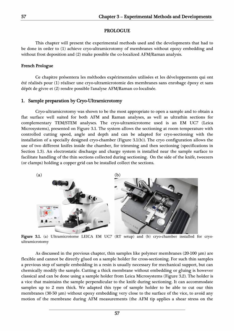
57 Chapter 3 – Experimental Methods and Developments
57
PROLOGUE
This chapter will present the experimental methods used and the developments that had to
be done in order to (1) achieve cryo-ultramicrotomy of membranes without epoxy embedding and
without frost deposition and (2) make possible the co-localized AFM/Raman analysis.
French Prologue
Ce chapitre présentera les méthodes expérimentales utilisées et les développements qui ont
été réalisés pour (1) réaliser une cryo-ultramicrotomie des membranes sans enrobage époxy et sans
dépôt de givre et (2) rendre possible l'analyse AFM/Raman co-localisée.
1. Sample preparation by Cryo-Ultramicrotomy
Cryo-ultramicrotomy was shown to be the most appropriate to open a sample and to obtain a
flat surface well suited for both AFM and Raman analyses, as well as ultrathin sections for
complementary TEM/STEM analyses. The cryo-ultramicrotome used is an EM UC7 (Leica
Microsystems), presented on Figure 3.1. The system allows the sectioning at room temperature with
controlled cutting speed, angle and depth and can be adapted for cryo-sectioning with the
installation of a specially designed cryo-chamber (Figure 3.1(b)). The cryo configuration allows the
use of two different knifes inside the chamber, for trimming and then sectioning (specifications in
Section 1.3). An electrostatic discharge and charge system is installed near the sample surface to
facilitate handling of the thin sections collected during sectioning. On the side of the knife, tweezers
(or clamps) holding a copper grid can be installed collect the sections.
(a) (b)
Figure 3.1. (a) Ultramicrotome LEICA EM UC7 (RT setup) and (b) cryo-chamber installed for cryo-
ultramicrotomy
As discussed in the previous chapter, thin samples like polymer membranes (20-100 µm) are
flexible and cannot be directly glued on a sample holder for cross-sectioning. For such thin samples
a previous step of sample embedding in a resin is usually necessary for mechanical support, but can
chemically modify the sample. Cutting a thick membrane without embedding or gluing is however
classical and can be done using a sample holder from Leica Microsystems (Figure 3.2). The holder is
a vice that maintains the sample perpendicular to the knife during sectioning. It can accommodate
samples up to 2 mm thick. We adapted this type of sample holder to be able to cut our thin
membranes (30-50 µm) without epoxy embedding very close to the surface of the vice, to avoid any
motion of the membrane during AFM measurements (the AFM tip applies a shear stress on the

Chapter 3 – Experimental Methods and Developments 58
58
sample even with PFQNM mode). As a rule of the thumb the sample should not hang out of the vice
more than the value of its thickness. For 30 µm thick membranes it implies cutting at 30 µm from
the vice’s surface, therefore the vice was trimmed and polished to minimize the risk of collision with
the diamond knife. The same holder was used to study all the samples: thin and thick membranes, as
well as slices from injection molded specimens. The preparation of each kind of sample is presented
in the next sections.
(a) (b)
Figure 3.2. Sample holder used to cut thick membranes (a) classical and (b) modified to minimize the risk of
collision when cutting thin membranes close to the surface of the holder.
1.1. Sectioning of injection molded specimens
Sections about 1 mm thick were cut with a scroll-saw from the center part of standard
injection molded specimens. Then the sections were cut as a triangle with a scalpel and installed in
the sample holder, as shown schematically on Figure 3.3 (a). In cryo-ultramicrotomy, the block was
first trimmed with the trimmer knife in a trapezoidal shape (Figure 3.3 (b)) and then surfaced
perpendicular to the injection direction, first with the trimmer, then with the diamond knife, for
perfect surfacing and thin sections’ collection on copper grids (Lacey Carbon Support Film 400
mesh).
(a) (b)
Figure 3.3. (a) Schematic representation of sample preparation from standard injection molded specimens (b)
Optical micrograph of the trapezoidal shape trimmed at the top of the triangular section, before
cryosectionning.
Cutting direction
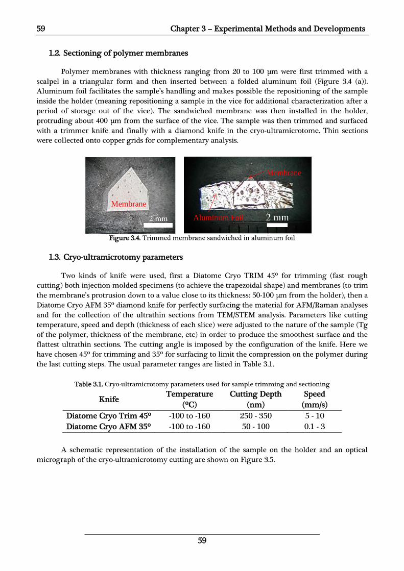
59 Chapter 3 – Experimental Methods and Developments
59
1.2. Sectioning of polymer membranes
Polymer membranes with thickness ranging from 20 to 100 µm were first trimmed with a
scalpel in a triangular form and then inserted between a folded aluminum foil (Figure 3.4 (a)).
Aluminum foil facilitates the sample’s handling and makes possible the repositioning of the sample
inside the holder (meaning repositioning a sample in the vice for additional characterization after a
period of storage out of the vice). The sandwiched membrane was then installed in the holder,
protruding about 400 µm from the surface of the vice. The sample was then trimmed and surfaced
with a trimmer knife and finally with a diamond knife in the cryo-ultramicrotome. Thin sections
were collected onto copper grids for complementary analysis.
Figure 3.4. Trimmed membrane sandwiched in aluminum foil
1.3. Cryo-ultramicrotomy parameters
Two kinds of knife were used, first a Diatome Cryo TRIM 45º for trimming (fast rough
cutting) both injection molded specimens (to achieve the trapezoidal shape) and membranes (to trim
the membrane’s protrusion down to a value close to its thickness: 50-100 µm from the holder), then a
Diatome Cryo AFM 35º diamond knife for perfectly surfacing the material for AFM/Raman analyses
and for the collection of the ultrathin sections from TEM/STEM analysis. Parameters like cutting
temperature, speed and depth (thickness of each slice) were adjusted to the nature of the sample (Tg
of the polymer, thickness of the membrane, etc) in order to produce the smoothest surface and the
flattest ultrathin sections. The cutting angle is imposed by the configuration of the knife. Here we
have chosen 45º for trimming and 35º for surfacing to limit the compression on the polymer during
the last cutting steps. The usual parameter ranges are listed in Table 3.1.
Table 3.1. Cryo-ultramicrotomy parameters used for sample trimming and sectioning
Knife Temperature
(ºC)
Cutting Depth
(nm)
Speed
(mm/s)
Diatome Cryo Trim 45º -100 to -160 250 - 350 5 - 10
Diatome Cryo AFM 35º -100 to -160 50 - 100 0.1 - 3
A schematic representation of the installation of the sample on the holder and an optical
micrograph of the cryo-ultramicrotomy cutting are shown on Figure 3.5.
Aluminum Foil
Membrane
Membrane

Chapter 3 – Experimental Methods and Developments 60
60
(a) (b)
Figure 3.5. (a) Schematic representation of the cryo-ultramicrotomy procedure of a polymeric membrane (b)
Optical micrograph of the cryo-ultramicrotomy cutting of a thick membrane without embedding
1.4. Avoiding frost melting water-diffusion onto the sample’s surface
As discussed in the last chapter, when working with liquid nitrogen cooled materials the
presence of humidity in the ambient air is of prime concern, as it gets trapped on cold surfaces
(condensation then crystallization) and the subsequent melting of the ice crystals observed during
warming-up can seriously impact the sample. In order to limit these effects, we have developed a
process to work in a fully controlled environment under a constant flux of dry nitrogen to avoid any
contact of the sample (either holded by the vice, or sections collected on a copper grid) with the
humid air.
2. AFM/Raman Co-localization Setup
For the co-localization of AFM and Raman analyses, as explained in the previous chapter, we
used a Bruker Dimension Icon AFM microscope co-localized with a Horiba Jobin Yvon LabRam HR
Raman spectrometer (Figure 3.6). Each of the two instruments is considered as state of the art. This
commercial co-localization system was supposed to allow the co-localization of information and also
independent and simultaneous conventional AFM and Raman analyses. However, substantial
developments had to be done in order to make it possible. Noise from mechanical vibrations and
operation of the Raman spectrometer affected the AFM measurements when both instruments were
operated simultaneously, thus a specially designed active piezoelectric table had to be installed
under the AFM. Both AFM and Raman microscopes are also installed on an active anti-vibration air
table, to filter mechanical vibrations transmitted by the floor. Temperature variations (day/night,
despite air conditioning) in the room resulted in a thermal drift of the sample when characterized by
the Raman (sample’s stage belonging to the AFM). An attempt to limit the thermal drift, consisted
to replace the feet of the Raman spectrometer originally made of aluminum by Invar feet (a
nickel/iron alloy with low thermal expansion coefficient), however with limited success (for co-
localization no longer than 30 minutes), which explains the development of a shuttle stage to solve
this issue (details in section 3.2)
Sample
Knife
Sections
Grid

61 Chapter 3 – Experimental Methods and Developments
61
Figure 3.6. Co-localizated AFM/Raman setup installed at the laboratory SyMMES
2.1. Atomic Force Microscope (AFM)
The AFM used is a Nanoscope Dimension Icon microscope controlled by the software
Nanoscope V, and equipped with the Peak Force QNM mode (PFQNM). AFM measurements were
made under ambient conditions (room temperature and relative humidity of about 50%) with a
standard cantilever holder for operation in air. For topography measurements, low spring constant
(k) cantilevers were used with k ranging from 0.2-0.4 N/m (Bruker ScanAsyst-Air probes) and tip
radius of about 10 nm. For nanomechanical analysis using PFQNM, cantilevers with spring constant
of about 40 N/m were used (Bruker RTESPA or OTESPA probes), which are suitable for the modulus
range of the polymeric materials studied. The tip was oscillated in the z-direction (travel distance of
150 nm) at 2 kHz (therefore 2000 force-distance curves recorded per second) while scanning the
sample line by line at a maximum scan rate of 0.977 Hz, (~9 minutes/image). Images were taken
with a resolution of 512x512 pixels. With 2 force-distance curves averaged per pixel), each image
corresponds to about half a million force-distance curves. AFM images were analyzed using
Nanoscope Analysis version 1.7.
2.1.1. AFM Calibration Method
As discussed in Chapter 2, the tip shape is not an ideal sphere and can change due to the
mechanical abrasion during calibration and analysis. Thus, the precise determination of the tip
radius before calibration is not representative of its real shape when probing the material besides
that it is considered as an ideal sphere by the nanomechanical models. In order to avoid these
drawbacks, the tip radius was determined by a Relative Calibration method using a dedicated
reference samples kit provided by Bruker (Model: PFQNM-SMPKIT-12m). The kit provides different
samples with known modulus for cantilever calibration.
Theoretical Part
First, using a nanomechanical model we will mathematically deduce the main parameters
controlling the measurement of the Young’s modulus of the material and the measurements that
should be done in reference samples in order to allow further quantitative analysis
Active
anti-vibration
air table
Aluminum feet
(changed)
Active
piezoeletric
table

Chapter 3 – Experimental Methods and Developments 62
62
Considering the Hertzian model on Equation 3.3, the loading force (F) is given by the
reduced Modulus (E*), indentation depth (δ), Poisson ratio (υ) and the tip radius (R).
3.1
The reduced modulus is defined using Equation 3.2, where υprobe and υsample are the Poisson’s
ratio of the probe and the sample, and Eprobe and Esample are the modulus of the probe and the sample.
3.2
Assuming that Eprobe >> Esample, (since Eprobe ~70GPa for silicon) one can neglect the probe
contribution and consider the simplification of Equation 3.1, with Esample and υsample simply as E and υ
(Equation 3.3).
3.3
The sample Modulus (E) can be then expressed in terms of the applied loading force (F),
indentation depth (δ), Poisson ratio (υ) and the tip radius (R) as in Equation 3.4.
3.4
The indentation depth (δ) can be calculated from the subtraction of the deflection (D) from
the Z-position (Z). The deflection (D) is by itself calculated from the Sensitivity (S) and the deflection
voltage (V) (Equation 3.5). The loading force (F) is related to the spring constant (k) of the
cantilever by the deflection (D) as shown in Equation 3.6. Thus, the modulus E can be expressed by
Equation 3.7.
3.5
3.6
3.7
Assuming the analysis of two different materials, the ratio between their moduli is given by:
3.8
If the same cantilever is used to probe both materials (k1=k2) and the same deflection voltage
(V) is applied when imaging each sample individually, the maximum loading force (Peak Force) is
the same on both materials. The Z-position (Z) to impose the same deflection voltage depends on the
mechanical properties of each material. The modulus ratio is equal to:
𝑭 = 𝟒
𝟑 𝑬∗ √𝑹 𝜹
𝟑𝟐
𝟏
𝑬∗= (
𝟏 − 𝝊𝒑𝒓𝒐𝒃𝒆𝟐
𝑬𝒑𝒓𝒐𝒃𝒆) + (
𝟏 − 𝝊𝒔𝒂𝒎𝒑𝒍𝒆𝟐
𝑬𝒔𝒂𝒎𝒑𝒍𝒆)
𝑭 = 𝟒
𝟑
𝑬
(𝟏 − 𝝊𝟐) √𝑹 𝜹
𝟑𝟐
𝑬 = 𝟑
𝟒
𝑭
√𝑹 𝜹 𝟑𝟐
(𝟏 − 𝝊𝟐)
𝜹 = (𝒁 − 𝑫) = (𝒁 − 𝑺. 𝑽)
𝑭 = 𝒌. 𝑺. 𝑽
𝑬 = 𝟑
𝟒 𝒌 . 𝑺 . 𝑽
√𝑹 𝜹 𝟑𝟐
(𝟏 − 𝝊𝟐)
𝑬𝟏
𝑬𝟐=
(𝟏 − 𝝊𝟏𝟐)
(𝟏 − 𝝊𝟐𝟐)
𝒌𝟏. 𝑺𝟏. 𝑽𝟏
𝒌𝟐. 𝑺𝟐. 𝑽𝟐 √
𝑹𝟐
𝑹𝟏 (
𝜹𝟐
𝜹𝟏)
𝟑𝟐

63 Chapter 3 – Experimental Methods and Developments
63
3.9
This means that the modulus ratio will be determined by the value of the deflection
sensitivity and the indentation ratio of each phase. If the deflection sensitivity (S) is correct, the
indentation ratio (𝜹𝟐
𝜹𝟏) is correct and hence the modulus ratio (
𝑬𝟏
𝑬𝟐) is correct.
To achieve quantitative force measurements, the rigidity of the cantilever can be measured
with the Thermal Tune method. As the procedure of the Thermal Tune method depends on the
Deflection Sensitivity, the importance of the proper measurement of the Deflection Sensitivity is
evidenced one more time.
Finally, the tip radius must be adjusted according to a certain indentation on a reference
sample, to take into account the effective tip-sample area of contact. This can be done by considering
the application of Equation 3.9 to compare the measured modulus (Emeasured) on the reference sample
using the Thermal Tuned spring constant (kThermal Tuned), with the expected value for its modulus
(Ereference) that should be measured with the actual tip radius, that we call Restimated. Since υ, kThermal Tuned,
S, Z and V are the same, Equation 3.9 can be written as:
3.10
or
3.11
From Equation 3.11, one can estimate the tip radius for an applied indentation on a chosen
reference sample (Equation 3.12). The same indentation should be applied to the unknown sample in
order to have a good agreement with the modulus calibration. In practice, the system does not show
the indentation depth (the real material’s deformation under the tip) in real time, but a calculated
deformation from the force-distance curves within a certain fitting region. The displayed
deformation is slightly lower than the real deformation because the default Deformation Fit Region
is 85% of the full deformation. Therefore, deformation shown by the software is different from
sample indentation but has close correlation and it is the parameter used in real time to ensure the
agreement with the calibration.
3.12
The developed procedure is composed of different steps: Adjustment of laser alignment and
feedback loop, determination of the Deflection Sensitivity, cantilever’s Spring Constant and Tip
Radius. The procedure is done as follows:
𝑬𝟏
𝑬𝟐=
(𝟏 − 𝝊𝟏𝟐)
(𝟏 − 𝝊𝟐𝟐)
√𝑹𝟐
𝑹𝟏 (
𝜹𝟐
𝜹𝟏)
𝟑𝟐
= 𝑨. (𝒁𝟐 − 𝑺. 𝑽
𝒁𝟏 − 𝑺. 𝑽)
𝟑𝟐
𝑬𝒎𝒆𝒂𝒔𝒖𝒓𝒆𝒅
𝑬𝒓𝒆𝒇𝒆𝒓𝒆𝒏𝒄𝒆=
(𝟏 − 𝝊𝟐)
(𝟏 − 𝝊𝟐) 𝒌𝒕𝒉𝒆𝒓𝒎𝒂𝒍 𝒕𝒖𝒏𝒆𝒅. 𝑺. 𝑽
𝒌𝒕𝒉𝒆𝒓𝒎𝒂𝒍 𝒕𝒖𝒏𝒆𝒅. 𝑺. 𝑽 √
𝑹𝒏𝒐𝒎𝒊𝒏𝒂𝒍
𝑹𝒆𝒔𝒕𝒊𝒎𝒂𝒕𝒆𝒅 (
(𝒁 − 𝑺. 𝑽)
(𝒁 − 𝑺. 𝑽))
𝟑𝟐
𝑬𝒎𝒆𝒂𝒔𝒖𝒓𝒆𝒅
𝑬𝒓𝒆𝒇𝒆𝒓𝒆𝒏𝒄𝒆= √
𝑹𝒏𝒐𝒎𝒊𝒏𝒂𝒍
𝑹𝒆𝒔𝒕𝒊𝒎𝒂𝒕𝒆𝒅
𝑹𝒆𝒔𝒕𝒊𝒎𝒂𝒕𝒆𝒅 = 𝑹𝒏𝒐𝒎𝒊𝒏𝒂𝒍 (𝑬𝒎𝒆𝒂𝒔𝒖𝒓𝒆𝒅
𝑬𝒓𝒆𝒇𝒆𝒓𝒆𝒏𝒄𝒆)
𝟐

Chapter 3 – Experimental Methods and Developments 64
64
Laser Alignment and Feedback Loop
After installation of the cantilever on the AFM head, the laser alignment was adjusted using
the knobs and centered on the photodiode detector in order to have the maximum reflection signal.
The first reference sample used for calibration of the system is the sapphire. After engagement on
the sample’s surface, one needs to adjust the feedback look using the Sync Distance parameter. The
Sync Distance is the distance between the start point of an extend-retract cycle and the point of peak
force, used by the system to control the feedback loop and the maximum applied force on the
sample. Using a deflection-time representation, as illustrated on Figure 3.7 (a), the Sync Distance can
also be understood as the time in which the minimum Z position of the cantilever is attained, which
implies the maximum deflection of the cantilever (PeakForce). Figure 3.7 (b) show force-distance
curves with three possible situations where the Sync Distance is too early (or too short) (b)-1, i.e., the
feedback force will be read before the actual maximum applied force; the correct position (b)-2, in
which the feedback measurement is done on the maximum applied load and thus both extend and
retract curves are aligned; and finally when it is too late (or too long) (b)-3, in which the feedback is
taken on the retract curve, thus after the actual maximum force was applied. The Sync Distance is
adjusted by imaging the sapphire sample allowing the proper control of the feedback and
calculation of the mechanical properties from the force-distance curves.
(a) (b)
1
2
3
Figure 3.7. a) Schematic representation of the tip trajectory and deflection signal in function of time. In this
representation, the Sync Distance parameter represents the time correspondent to the maximum deflection
(Peak Force). (b) Images of the proper adjustment of the Sync Distance. 1) Sync too early; 2) Correct Sync
Distance and 3) Sync too late.
Determination of the Deflection Sensitivity
The nominal values of tip radius (Rnominal) and spring constant (knominal) provided by the
manufacturer were entered in the system for the preliminary measurement and evaluation of the
Deflection Sensitivity.
The Deflection Sensitivity was first measured doing a deflection-distance curve (Ramp Mode)
on the standard sapphire sample. The sapphire is a rigid material, thus no deformation is induced by
the tip on its hard surface. An example of the deflection-distance curve on the sapphire surface is
given on Figure 3.8. The deflection sensitivity is then measured on the linear part of the curve, as
illustrated on Figure 3.8. This parameter highly depends on the cantilever used and the laser
reflectivity on the cantilever’s surface which can be enhanced by reflective coatings on its back.
Thus, the deflection sensitivity must be measured for each cantilever before analysis of a sample.
Back to imaging mode, the Sync Distance is readjusted using the same force used for the deflection-
Sync Distance

65 Chapter 3 – Experimental Methods and Developments
65
distance curve and the Deflection Sensitivity is updated in order to take into account the
perturbations of the oscillatory and scanning movements of the tip.
Figure 3.8. Deflection-distance curve on the sapphire sample showing the limits for deflection sensitivity
determination.
Considering the sensibility range of the cantilevers used in this study, the deflection
sensitivity was then validated using the standard Polystyrene-Low Density Polyethylene (PS-LDPE)
sample provided by Bruker. The modulus of the Polystyrene is 2.7 GPa and the one of LDPE is 0.1
GPa, which gives a modulus ratio of 27, or equivalent to 1.431 in log scale. In this case, the deflection
voltage (V), the spring constant (k) and the deflection sensitivity (S) are equal for both phases, since
they are probed at the same time. This means that if the ΔLogE measured is equal to 1.431, then the
deflection sensitivity is correct, in accordance with Equation 3.9 as illustrated on Figure 3.9. If not
verified, the laser alignment was readjusted to optimize the signal and a new measurement of the
deflection sensitivity on the sapphire sample was performed.
(a) (b)
Figure 3.9. (a) AFM Log Modulus image of PS-LDPE standard sample. PS appearing in white yellow and LDPE
in dark brown. (b) Log Modulus section corresponding to the line on the image showing a log difference of
about 1.4 between both phases.
Determination of Spring Constant and Tip Radius Estimation
The actual spring constant (kthermal tune) of the cantilever was then determined using the
Thermal Tune method. The advantage of using the standard PS-LDPE sample at the previous step of
deflection sensitivity validation is that one can use the same sample for tip radius estimation,
depending on the modulus range of the sample of interest to be measured further. The Young’s
modulus (Emeasured) of one of the reference sample phases (PS or LDPE) was measured using the
nominal tip radius (Rnominal), imposing deformation depths from 2 nm to 10 nm at the phase of
interest, to operate within the limits of the DMT model (as presented on Chapter 2) used by
Nanoscope Software to calculate the mechanical properties from the force-distance curves. With
these measurements, one can now estimate the actual tip radius for an imposed deformation on the
ΔLogE ~1.4

Chapter 3 – Experimental Methods and Developments 66
66
chosen standard sample phase (PS or LDPE) using Equation 3.12, presented here once again for the
sake of convenience:
3.12
The tip radius (Restimated) is then corrected in the software, which gives now the proper value
(2.7 GPa for the PS or 0.1 GPa for the LDPE) for a certain imposed deformation on the chosen
reference. Samples are then imaged with a peakforce setpoint inducing a similar deformation depth
as the one used for calibration.
It is important to notice that while imaging the PS-LDPE sample, once the tip radius is
estimated based on one of the standard sample phases (PS or LDPE) the modulus measured for the
other phase on the image is either under or overestimated depending on the cantilever chosen, since
the deformation imposed on both phases can be very different, hence, the tip-sample area of contact.
This bias of the PFQNM cannot be avoided and should be taken into account when probing
multiphase samples with great modulus difference.
Different cantilever types are used for different ranges of sample modulus, i.e., a single
cantilever cannot have a good sensitivity for materials with a too big modulus difference.
Nevertheless, according to the Young’s modulus range of the samples of interest, this procedure can
be adapted for different cantilever types (higher or lower rigidity) by adapting different references
samples (two materials with different known modulus to validate the cantilever’s deflection
sensitivity).
A summary of the presented procedure is presented on Figure 3.10.
Figure 3.10. Algorithm of the calibration procedure
𝑹𝒆𝒔𝒕𝒊𝒎𝒂𝒕𝒆𝒅 = 𝑹𝒏𝒐𝒎𝒊𝒏𝒂𝒍 (𝑬𝒎𝒆𝒂𝒔𝒖𝒓𝒆𝒅
𝑬𝒓𝒆𝒇𝒆𝒓𝒆𝒏𝒄𝒆)
𝟐

67 Chapter 3 – Experimental Methods and Developments
67
2.2. Raman Spectrometer
Confocal Raman spectroscopy was performed in backscattering mode using a LabRam HR
(Laser He Ne-632,8nm-17mW), with a 100x long working distance objective and an X, Y micro-
motorized stage. Data were treated using LabSpec Software version 6.3.40. The typical analyzed
range was from 400 to 3400cm-1 with a grating of 600 gr/mm, a hole of 200 µm and a slit of 100 µm,
to guarantee confocal configuration and spectral resolution. The typical acquisition time was 10
seconds per accumulation with 2 to 4 accumulations per spectrum. To avoid photothermal polymer
degradation by the laser beam, a neutral density filter of 25 or 50% was used.
2.2.1. Raman Calibration Method
Raman calibration for chemical analysis was done following the procedure proposed by
Horiba-Jobin Yvon. The spectrometer must be calibrated considering three parameters: Zero Order,
Sinus Arm and Laser Confocality.
Zero order is the term used to define when the grating within the spectrometer behaves like
a mirror, reflecting incoming light rather than refracting it into several wavelengths. It must be
calibrated for each grating used (600 or 1800 gr/mm, in our case). After selecting a grating, the
spectrograph is moved to the zero order position. Using the 100x objective, a real time display of 1 s
and a ND Filter of 1% the acquisition is started. An intense peak near 0 nm is seen. The Offset Shift
parameter was corrected to shift the peak back at 0 nm (from yellow to blue line), as illustrated on
Figure 3.11.
Figure 3.11. Offset shift correction of the Zero Order
After the start point for the grating has been set, the movement of the grating relative to the
wavelength of the diffracted light must be calibrated. This movement is induced by a so called sinus
arm, driven by stepping motor. Any deformation of the sinus arm during the movement of the
grating will induce shifts in the wavelengths of Raman light on the CCD detector.
Focusing on a Silicon sample with the 100x objective, the acquisition window was centered to
the position of the Si band (520 cm-1). Using a real time display of 1 s, the Coeff parameter was
adjusted in order to center the strong Si band to its reference position (520,7 cm-1 from the red to the
green line) as shown on Figure 3.12 (a). Changing the Coeff parameter will adjust the grating
position taking into account the deformation of the sinus arm.
The Laser Confocality is then evaluated, i.e., the laser power provided in confocal
configuration is compared to the total power emitted. The Silicon standard sample was focused with
the 100x objective and a spectrum relative to the Si peak at 520 cm-1 was acquired with an acquisition
time of 1 second, ND filter of 100% and confocal configuration, i.e., with a slit of 100 µm and a hole
of 200 µm. The hole was then changed to 1000 µm and a new spectrum was acquired. The intensity

Chapter 3 – Experimental Methods and Developments 68
68
ratio between the confocal configuration (200 µm hole) and the reference spectrum (1000 µm hole)
must be superior to 50% (meaning that still half of the light comes through the pinhole). An
example is given on Figure 3.12 (b), where the intensity on confocal configuration (blue line)
corresponds to 51.8% of the reference intensity (green line). If the ratio is lower than 50%, then the
laser’s confocality is not good and the internal confocal optical parts of the system must be
realigned.
(a) (b)
Figure 3.12. (a) Calibration of the sinus bar position by the correction of the Si peak at 520 cm-1 (b) Evaluation
of the confocality by the ratio of intensities measured with a hole of 200 and 1000 µm, here a ratio of 51.8%
was found.
3. Co-localization Methods
Two strategies have been developed in order to obtain good AFM/Raman co-localization data,
depending on the intensity of the Raman response of the investigated material. The Raman
spectrometer is equipped with two confocal microscopes. The one facing the AFM is dedicated to co-
localized AFM-Raman experiments and will be called the co-localized Raman microscope. The
second one, which is positioned with direct access in front of the user (standard position for LabRam
HR), will be called the regular Raman microscope (Figure 3.13).
Figure 3.13. Co-localizated AFM/Raman setup. The red arrows show the Co-localized Raman Microscope
installed in front of the AFM and the Regular Raman Microscope positioned with direct access in front of the
user
3.1. Co-localization with the Co-localized Raman Microscope
For samples with intense Raman response, the co-localization is done using the co-localized
Raman microscope. During the co-localization process, the AFM motorized stage is simply used to
move the sample from the AFM to the co-localized Raman microscope, and reciprocally, as
illustrated on Figure 3.14. First the sample is visualized optically with the co-localized Raman
microscope, which has a much better resolution than the AFM optical microscope, to select the area
of interest, then, the sample is moved with the motorized stage from the Raman objective to the
Co-localized
Raman
Microscope Regular
Raman
Microscope

69 Chapter 3 – Experimental Methods and Developments
69
AFM tip for AFM imaging. Finally the sample is moved back to the co-localized Raman microscope
for Raman mapping. The Raman analysis is done after the AFM analysis because the Raman laser
heating is potentially destructive for the sample, in particular for organic materials.
This approach is suitable for fast mappings, with acquisition times below 30 minutes. Indeed,
during this time scale, the thermal drift of the co-localized setup (sample on the AFM stage drifting
below the co-localized Raman microscope) is negligible and does not affect the measurements. Long
time scale thermal drift occurs mainly due to the dilatation/contraction of the table-top (lateral
thermal drift) and of the Raman feet (vertical thermal drift), due to the day/night temperature
variations of the room (despite air-conditioning), because the sample when observed by the Raman is
on the AFM stage and not attached to the Raman. For short acquisition times, the co-localization
error induced by the displacement from the AFM to Raman or Raman to AFM is only of about 3 µm
and in most of the cases this error of registration can be corrected by scanning, on the AFM, a larger
surface than the co-localized final area, and identifying registration points in both AFM and Raman
images.
(a) (b)
Figure 3.14. (a) Stage below AFM head for topographic/nanomechanical analysis and (b) below the co-localized
Raman microscope for chemical analysis
3.2. Co-localization with the Regular Raman Microscope - Shuttle Stage
In general, polymers respond weakly to Raman and due to their thermal sensitivity, low laser
power must be used, which increases the acquisition time substantially. For example, the acquisition
time of a Raman mapping with dimensions of 10x10 µm2 and a step of 0.5 µm between each point
(20 lines of 20 points = 400 points) can be up to 10 hours. In this case, a lateral thermal drift as small
as few µm’s during the analysis is already too large, causing mapping distortion. A vertical thermal
drift even smaller can result in a complete loss of focus and therefore of the Raman signal. To
address this problem, we have to use the Regular Raman Microscope, which is not affected by
thermal drifts since in this case the sample is on the Raman’s stage which cannot drift. To co-localize
de AFM and Raman images in these conditions, a specific strategy has been developed using a
shuttle stage between both instruments. This transfer shuttle allows transferring the sample from
the AFM stage to the regular Raman microscope stage, and vice versa, without losing the area of
interest. Two docks for the shuttle stage were fixed, one on the AFM stage, the other on the Regular
Raman Microscope stage. These docks receive and magnetically maintain the shuttle stage in
position. The shuttle stage itself has a magnet to maintain the sample during transfer and imaging
but also two targets glued on its surface (Figure 3.15 (a)). These two targets are required for the

Chapter 3 – Experimental Methods and Developments 70
70
triangulation of the area of interest making possible a perfect repositioning (error of about 3 µm in
both x and y directions). This method takes into account any angle shift existing when docking the
shuttle stage for analysis, as illustrated on Figure 3.15 (b).
(a) (b)
Figure 3.15. ((a) Shuttle stage design showing the dock to be installed on both AFM and Raman and the shuttle
stage itself with both targets and the sample area. (b) Illustration of the shuttle stage strategy.
This shuttle stage strategy has the advantage that both instruments can be used
simultaneously even when doing co-localized analyses, since the sample is not on the AFM stage
during the Raman mapping (or the reverse). However it is naturally a time consuming process
compared to the co-localization using the co-localized Raman microscope (targets localization,
calculations using an excel spreadsheet to find the final x and y coordinates of the area of interest).
In addition with the shuttle stage strategy, both the AFM and Raman motorized stages need to be
calibrated exactly the same way. As it is impossible a correction factor needs to be applied to the x
and y translations to obtain the same displacements for both stages from the targets to the sample.
The precision of the correction factor is critical when the displacements are big. Finally, due to the
height of the sample in the holder, about 10 mm higher than the level of the targets, there is a risk
of collision of the AFM head with the holder during the process.
These issues can be addressed if the sample is installed in a vice holder which has targets
printed on its surface. These targets should be near the sample and if possible at the same focal
plane. We have therefore milled targets with micrometric dimensions on the surface of the holders
with Focused Ion Beam (FIB), as shown on Figure 3.16. Since the distance to be travelled from the
targets to the sample is way less important and the sample is practically at the same topographic
level as the targets (50 to 100 µm above, instead of millimeters), the co-localization procedure
becomes much faster, more accurate (the precision of the co-localization is improved to less than 3
µm) and without any risk of collision between the AFM tip and the sample.
(a)
(b)
Figure 3.16. (a) SEM image of the Micro-Targets milled by FIB on the surface of the sample holder (b) Detail
of one micro-target.

71 Chapter 3 – Experimental Methods and Developments
71
4. Complementary Analyses
4.1. Scanning Electron Microscopy (SEM)
Ultramicrotomed surfaces of hybrid membranes samples were analyzed with a scanning
electron microscope Zeiss Ultra 55 (INAC, Grenoble, France) with a FEG source (Schottky type)
operated at 0.8 keV (with a resolution of 1.7 nm) in Secondary Electron (SE) mode (with an In-Lens
detector for the topographic images) and at 1.5 kV in Backscattered Electron (BSE) mode for
complementary chemical contrast images. In the case of the hybrid membranes, it was possible to
avoid the use of gold or carbon coating in order to preserve the original topography of the samples
using low voltage to prevent charge build-up at the sample’s surface.
4.2. Transmission and Scanning Transmission Electron Microscopy (TEM/STEM)
Morphologies of the Polyamide 6/Acrylonitrile-butadiene-styrene (PA6/ABS) blends were
analyzed by TEM using a Magellan 400L scanning transmission electron microscope (LCE, São
Carlos, Brazil) operating in transmission mode. A two-step selective staining technique was used to
generate the phase contrast. The sections were first exposed to osmium tetroxide vapor (OsO4) for
15h and then to ruthenium tetroxide vapor (RuO4) for 2h to respectively stain the PB and SAN
phases.
For the hybrid membranes, the thin sections were analyzed with a scanning transmission
eletron microscope HITACHI S-5500 (INAC, Grenoble, France) with a cold-FEG source operated at
15 keV in Bright Field mode to provide complementary high-resolution (< 1nm) morphological
information. No staining step was necessary due to the strong natural contrast between the sPEEK
and the sol-gel phase.
4.3. µ-ATR-FTIR imaging
ATR-FTIR imaging measurements were carried out on a Thermo Scientific Nicolet iN 10MX
equipped with a liquid nitrogen cooled focal plane array detector (FPA) and a removable
Germanium micro-ATR crystal (Refractive index, n=4). The Germanium conical tip and the linear
array detector allow mapping over an area of 100x25 µm2, with the effective pixel size of 6.25x6.25
µm2. Each measurement consists of at least 240 spectra co-added at 8 cm−1 spectral resolution and
has been rationed against a background spectrum which was measured prior to each new sample
measurement.
Imaging with the Ge crystal for µ-ATR-FTIR implies that the micro crystal must be brought
into intimate contact with the surface, applying a sufficient contact force. The Ge crystal has a
diameter of 350 µm which is about 10 times larger than the thickness of our polymer membranes
(~30 µm thick). This means that for a membrane cross-section analysis, a membrane standing out of
the vice holder is exposed to a high stress during analysis which generally results into membrane’s
bending or breaking making cross-section analysis impossible. Therefore, the membrane needs a
mechanical reinforcement to withstand the pressure of the ATR crystal. Rather than using epoxy
embedding (to avoid chemical contamination and/or diffusion of the embedding resin into the
polymer), we have used a polymeric backing made of an inert polymer (PP). The membrane was
sandwiched between two reinforcement sheets and aluminum foil (for handling), as shown on
Figure 3.17, then installed on the vice holders for cryo-ultramicrotomy. The schematic
representation of the µ-ATR-FTIR imaging is presented on Figure 3.18.

Chapter 3 – Experimental Methods and Developments 72
72
(a) (b)
Figure 3.17. (a) Polymeric membrane sample sandwiched between aluminum foil and PP sheets on side view
(b) Top view of the sandwiched sample
(a) (b) (c)
Figure 3.18. Schematic representation of µ-ATR-FTIR imaging. (a) Field of view of the detector and contact
area of the crystal. (b) Germanium conical tip on sample. (c) Mapping of a large area of the sample with
multiple steps
Aluminum foil
PP backing
Polymer
membrane

73 Chapter 3 – Experimental Methods and Developments
73
5. Conclusions of Chapter 3
We have developed different characterization strategies making possible the co-localization
of information from AFM and Raman microscopes. For that, Cryo-Ultramicrotomy was adapted to
give access to the cross-section (surface + bulk) of the material without the use of embedding,
avoiding chemical contamination. A strategy using dry nitrogen was also developed to avoid frost
deposition after cryo-ultramicrotomy, to protect water sensitive samples. The cryo-ultramicrotomed
samples have a perfectly flat surface suitable for co-localized AFM/Raman analysis, SEM and µ-ATR-
FTIR, and the cutting also provides ultrathin sections for complementary Transmission Electron
Microscopy analyses.
Different co-localization strategies were developed depending on the Raman intensity
response of the samples. For samples that respond intensely to Raman, the AFM motorized stage is
simply used to move the sample from the AFM to the co-localized Raman microscope, and
reciprocally. This approach is suitable for fast mappings, with acquisition times below 30 minutes.
For polymer samples that respond weakly to Raman, a strategy using a shuttle stage between both
instruments was developed, allowing transferring the sample from the AFM stage to the regular
Raman microscope stage, and vice versa, without losing the area of interest and allowing long time
acquisition mappings, up to more than 10 hours. Furthermore, it has the advantage that both
instruments can be used simultaneously even when doing co-localized analyses. The co-localization
precision was improved to less than 3 µm thanks to the association of the shuttle stage strategy with
milled targets on the surface of the vice holders, limiting the repositioning displacement (in X, Y
and also Z direction).
The calibration methodology for AFM nanomechanical analysis was developed based on the
mathematically deduction of the main parameters controlling the measurement of the Young’s
modulus of the material, using a theoretical nanomechanical model (Hertzian). The presented
procedure can be adapted for different cantilever types and using different reference samples,
considering the Young’s modulus range of the samples of interest.
The developed methodologies for AFM/Raman co-localized analyses were published in the
International Journal of Polymer Analysis and Characterization. The paper entitled “AFM-Raman
Co-localization Setup: Advanced Characterization Technique for Polymers” exemplifies the co-
localization strategy by the study of hybrid membranes for fuel cell application.159

Chapter 3 – Experimental Methods and Developments 74
74
6. Conclusions du Chapitre 3 en Français
Nous avons développé différentes stratégies de caractérisation permettant la co-localisation
de l'information des microscopes AFM et Raman. Pour cela, la Cryo-Ultramicrotomie a été adapté
pour donner accès à la section transversale (surface + intérieur) du matériau sans enrobage (pas de
contamination chimique, impact thermique ou mécanique). Une stratégie utilisant de l'azote sec a
également été développée pour éviter l'effet de dépôt de givre sur des échantillons sensibles à l'eau.
Les échantillons cryo-ultramicrotomés ont une surface parfaitement plane adaptée à l'analyse
AFM/Raman co-localisée, SEM et μ-ATR-FTIR, et la procédure de coupe fournit également des
sections ultra-fines pour des analyses complémentaires de microscopie électronique de transmission.
La précision de co-localisation a été améliorée grâce à la stratégie de la plate-forme navette à l'aide
de cibles à la surface des porteurs, ce qui limite le déplacement pour le repositionnement (en X, Y et
Z).
Différentes stratégies de co-localisation ont été développées en fonction de l'intensité de la
réponse Raman des échantillons. Pour les échantillons qui répondent intensément au Raman, la
platine motorisé de l’AFM est simplement utilisé pour déplacer l'échantillon de l'AFM vers le
microscope Raman co-localisé et réciproquement. Cette approche convient aux mappings rapides,
avec des temps d'acquisition inférieurs à 30 minutes. Pour les échantillons de polymères qui
répondent faiblement à Raman, une stratégie utilisant une navette entre les deux instruments a été
développée, permettant de transférer l'échantillon de la platine AFM à celle du microscope Raman
régulier, et vice versa, sans perdre la zone d'intérêt et permettant l’acquisition des mappings de
longue durée, jusqu'à plus de 10 heures. En outre, il est avantageux que les deux instruments
puissent être utilisés simultanément même lorsqu'ils effectuent des analyses co-localisées. La
précision de la co-localisation a été améliorée à moins de 3 μm grâce à l'association de la stratégie de
la navette avec des cibles gravées à la surface des portes-échantillons, limitant le déplacement de
repositionnement (en X, Y et Z également).
Les méthodologies développées pour les analyses co-localisées AFM/Raman ont été publiées
au journal International Journal of Polymer Analysis and Characterization. L'article intitulé «AFM-
Raman Co-localization Setup: Advanced Characterization Technique for Polymers», illustre la
stratégie de co-localisation par l'étude des membranes hybrides pour piles à combustible.159

75 Chapter 3 – Experimental Methods and Developments
75
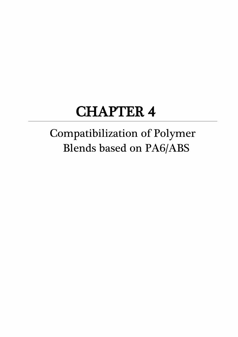
CHAPTER 4
Compatibilization of Polymer
Blends based on PA6/ABS

77 Chapter 4 – Compatibilization of Polymer Blends based on PA6/ABS
77
PROLOGUE
In this chapter, we will present the morphological and chemical analysis of polymer blends
based on Polyamide 6 (PA6) and Acrylonitrile-Butadiene-Styrene (ABS) copolymer, compatibilized
with a Styrene-Acrylonitrile grafted with Maleic Anhydride (SAN-MA). The blends were prepared on
the Department of Materials Engineer at the Federal University of São Carlos (DEMa-UFSCar/São
Carlos, Brazil).
We will present here a brief introduction to the materials used (PA6 and ABS) and the
fundamentals of blend compatibilization. Then, we will present the study of the blends using the co-
localized AFM/Raman setup, first applied on a non compatibilized PA6/ABS blend and second on
compatibilized systems with SAN-MA copolymer. The study of the non-compatibilized blend allowed
for the optimization of the co-localization procedure and for the proper assignment of the phases
using both AFM and Raman techniques. The study of the compatibilized blends was first interested
on the effect of the blending protocol on the development of the morphology of the blends. We were
able to show by complementary AFM and STEM analyses that the addition of the SAN-MA
copolymer in different steps of the blending can develop different final morphologies, which have
an impact on their rheological properties. Finally, we were interested on the fundamental aspects of
the PA6 polymorphs (α and γ) distribution in the materials. Using co-localized AFM/Raman
analyses, we have shown that the presence of the compatibilizer favors the formation of the γ
polymorphs and its amount and distribution depends on the blending protocols.
French Prologue
Dans ce chapitre, nous présenterons l'analyse morphologique et chimique des mélanges de
polymères à base de Polyamide 6 (PA6) et de copolymère Acrylonitrile-Butadiène-Styrène (ABS),
compatibilisé avec un Styrène-Acrylonitrile greffé avec de l'Anhydride Maléique (SAN-MA). Les
mélanges ont été préparés au Département d'Ingénierie des Matériaux à l'Université Fédérale de São
Carlos (DEMa-UFSCar / São Carlos, Brésil).
Nous présenterons ici une brève introduction aux matériaux utilisés (PA6 et ABS) et les
fondements de la compatibilization des mélanges polymères. Ensuite, nous allons présenter l'étude
des mélanges à l'aide du système de co-localisation AFM/Raman, d'abord appliquée sur un mélange
PA6/ABS non compatibilisé et deuxièmement sur des systèmes compatibilisés avec un copolymère
SAN-MA. L'étude du mélange non compatibilisé a permis d'optimiser la procédure de co-localisation
et d'affecter correctement les phases en utilisant les techniques AFM et Raman. L'étude des
mélanges compatibilisés s'intéresse d'abord à l'effet du protocole de mélange sur le développement
de la morphologie des mélanges. Nous avons pu montrer par des analyses complémentaires AFM et
STEM que l'addition du copolymère SAN-MA à différentes étapes du mélange peut développer
différentes morphologies finales, qui ont un impact sur leurs propriétés rhéologiques. Enfin, nous
nous intéressions aux aspects fondamentaux de la distribution des polymorphes PA6 (α et γ) dans
ces matériaux. À l'aide d'analyses AFM/Raman co-localisées, nous avons montré que la présence du
compatibilisant favorise la formation des polymorphes γ et que sa quantité et sa distribution
dépendent des protocoles de mélange.

Chapter 4 – Compatibilization of Polymer Blends based on PA6/ABS 78
78
1. Theoretical Background and Motivation
1.1. Polyamide 6 (PA6)
Polyamides (or Nylons) are characterized by the presence of an amide (-COONH-) in the
backbone chain.160 The polyamide produced from ε-caprolactam is called Polyamide 6, once it have
six carbon atoms derived from the lactam, as shown on Figure 4.1.
Figure 4.1. Polyamide 6 structure
The olefin sequences on the PA6 structure are non-polar and flexible at room temperature.
The amide groups, however are very polar, being capable of attracting the neighboring chains to
form hydrogen bonds between them.161 The symmetry and regularity of the backbone chain allied to
the hydrogen bonds make the PA6 a semi-crystalline thermoplastic with high crystallinity, which
control its physical and mechanical properties.
In general, the polyamides were considered as the first engineering polymers, since they
have very attractive features for engineering applications.161 Indeed, polyamide 6 has high toughness
above its glass transition temperature (Tg ~50ºC), high rigidity, good chemical resistance to
hydrocarbons and good resistance to abrasion due to inherent low-friction properties. Its crystalline
melting temperature is ~220ºC, beyond which it presents a very low melt viscosity, which allows the
injection molding of parts with complex forms such as micro-gears. Its high rigidity, chemical and
heat resistance make the PA6 a good substitute for low strength metals like for example in
components in the engine compartment of vehicles. Additionally its high polarity favors the
interaction of the polymer chains with the polar surface of organophilic clays, making possible the
production of nanocomposites based on polymer/clay systems.38,51,162
Due to their polar nature, polyamides tend to absorb moisture from their surroundings, until
certain equilibrium is reached, which can have a negative effect on dimensional stability. The
increasing moisture content can impact the materials properties, increasing the impact resistance
and flexibility, however, it decreases the polyamide strength and stiffness below the glass transition
temperature (<50-80 ºC). The extent of moisture content is dependent on temperature, crystallinity
and thickness of the product, being critical when it occurs on the pellets before processing. To
prevent negative effects of moisture absorption during service a preconditioning drying step is often
adopted before extrusion/injection of the molded part. But the most important downside of the
material is related to its notch-sensitive behavior below its glass transition temperature compared to
other polymers. Figure 4.2 shows the impact strength of notched samples of commonly used plastics
such as Acrylonitrile-Butadiene-Styrene (ABS), Polystyrene (PS) and Polycarbonate (PC). The
Polyamide 6 (Nylon 6 in the figure) appears with an impact strength 8 times lower than
Polycarbonate (PC).163

79 Chapter 4 – Compatibilization of Polymer Blends based on PA6/ABS
79
Figure 4.2. Impact strength (notched izod) of different polymeric materials163
This brittle behavior shows that the material is very sensitive to crack propagation. Therefore
its impact resistance is poor and it tends to fail in a brittle manner at low temperaures.164 One
strategy to mitigate this mechanical behavior is to introduce rubber particles to improve the
mechanism of energy absorption and crack propagation. The addition of low modulus materials
decreases notch-sensitivity, increasing toughness at low temperatures. Examples from the literature
used a series of different polymers, such as natural rubber, ethylene propylene diene rubber (EPDM),
polybutadiene (PB) and copolymers, like Styrene–Ethylene/Butylene–Styrene block copolymer
(SEBS) and Acrylonitrile-Butadiene-Styrene (ABS).165–167 In this work, we will focus on the blending of
PA6 with ABS.
1.2. Acrylonitrile-Butadiene-Styrene (ABS)
ABS were originally made by blending a lightly crosslinked natural rubber (NBR) into a
Styrene-Acrylonitrile (SAN) copolymer. Nowadays such materials are commonly made by
polymerizing styrene and acrylonitrile around polybutadiene in a polybutadiene latex, forming
polybutadiene molecules grafted with SAN (PB-g-SAN). The resultant material is then blended with
styrene-acrylonitrile (SAN). The chemical structures of the components and an example of the
microstructure are presented on Figure 4.3. As illustrated on the TEM image of Figure 4.3 (b), the
morphology is complex. The PB rubber particles (dark on the image) appear uniformly dispersed in
the fragile matrix of SAN (white), which is also present in sub-inclusions inside the PB particles. PB-
g-SAN lies on the interphase between the SAN matrix and the dispersed PB, being responsible for
anchoring both phases and thus allowing PB to increase the final tenacity of the material.168
(a) (b)
Polyacrylonitrile Polybutadiene Polystyrene
Figure 4.3. (a) Structures of the ABS components: Polyacrylonitrile, polybutadiene and polystyrene. (b) TEM
image showing the morphology of a ABS (SAN65.9/PB-g-SAN34.1 w/w with 44%wt PB content in PB-g-SAN).
The rubber particles (PB) appear in dark and the SAN matrix in white, which is also present in sub-inclusions
inside the rubber particles. The scale bar represents 200 nm. Adapted from169

Chapter 4 – Compatibilization of Polymer Blends based on PA6/ABS 80
80
The SAN phase usually comprises more than 70% of the ABS total composition. On the one
hand, the amount and molecular weight of the SAN are the principle variables controlling the
properties of the matrix. If increased, the strength and rigidity of the ABS increases. On the other
hand, the increasing amount of rubber controls the impact resistance of the material. However, as
the rubber content increases, the strength, hardness, heat resistance and rigidity of the ABS decrease.
Finally, the properties of the material are highly affected by the size and distribution of the dispersed
phase, the cross-linking density of PB, copolymer composition and amount of PB-g-SAN. In general,
ABS is a hard tough material with good resistance to impact even at low temperatures.
By blending ABS with other polymers it is possible to extend the range of use and a variety of
properties, such as heat distortion temperature, impact strength, flame retardancy, processing
conditions and weatherability.168
1.3. Mixing and compatibilization of polymer blends
Blends can be obtained by mechanical mixing in the molten state. In this technique, two or
more resins are blended in mixing equipment, typically double screw extruders or internal mixers.
Additionally it is possible to incorporate fillers, reinforcements and additives. The blending process
involves high temperatures (above the softening/melting temperature of the components) and high
shear, promoting the homogenization and dispersion of the constituents of the polymer blend.
Under the action of the shearing force, the dispersed elements are elongated and broken down, as
illustrated on Figure 4.4. Size reduction of the dispersed domains continues till the total force of the
particle equals the surface tension which is responsible for particle coalescence. The competitive
process between breaking down (size reduction) and particle coalescence (surface tension
minimization) is always present in unstable polymeric heterophase systems. For low content of
dispersed phase, the equilibrium radius of the particles depends on its surface tension, the shearing
forces applied and the viscosity difference between the continuous and the dispersed phases. When
the viscosities of the two components are similar, the mechanical shear can be effectively transferred
to the mixture to enforce a good dispersion of the phases. Blends with a greater disparity in the
components melt viscosity show larger domains, but it decreases with the increasing shearing forces
and low surface tensions.170,171 In conclusion, the lower the melt viscosity difference between the two
constituents of the mixture, the better the dispersion.
Figure 4.4. Schematic representations of particle break down under a shearing stress field and coalescence.
Adapted from 170
In order to reduce the competitive process of particle coalescence in unstable heterophase
systems, proper formulations can be developed to control the morphology and characteristics of
polymer blend. To reduce the surface tension and improve miscibility, compatibilization can be
achieved by chemical or physical means. Physical compatibilization lies on the use of copolymers
bearing different blocks, each one compatible with one of the components of the blend. The physical
entanglements of the chains of each polymer with the correspondent block of the compatibilizer
engender a reduction of the interfacial tension between the phases and inhibit the coalescence
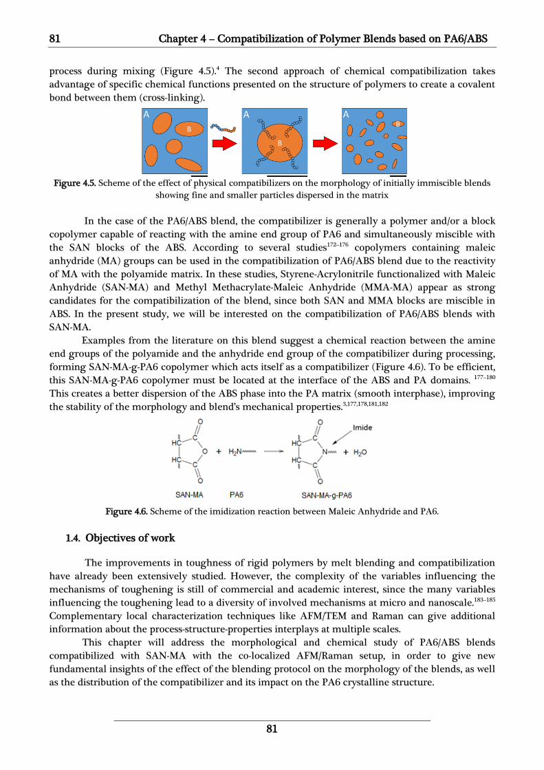
81 Chapter 4 – Compatibilization of Polymer Blends based on PA6/ABS
81
process during mixing (Figure 4.5).4 The second approach of chemical compatibilization takes
advantage of specific chemical functions presented on the structure of polymers to create a covalent
bond between them (cross-linking).
Figure 4.5. Scheme of the effect of physical compatibilizers on the morphology of initially immiscible blends
showing fine and smaller particles dispersed in the matrix
In the case of the PA6/ABS blend, the compatibilizer is generally a polymer and/or a block
copolymer capable of reacting with the amine end group of PA6 and simultaneously miscible with
the SAN blocks of the ABS. According to several studies172–176 copolymers containing maleic
anhydride (MA) groups can be used in the compatibilization of PA6/ABS blend due to the reactivity
of MA with the polyamide matrix. In these studies, Styrene-Acrylonitrile functionalized with Maleic
Anhydride (SAN-MA) and Methyl Methacrylate-Maleic Anhydride (MMA-MA) appear as strong
candidates for the compatibilization of the blend, since both SAN and MMA blocks are miscible in
ABS. In the present study, we will be interested on the compatibilization of PA6/ABS blends with
SAN-MA.
Examples from the literature on this blend suggest a chemical reaction between the amine
end groups of the polyamide and the anhydride end group of the compatibilizer during processing,
forming SAN-MA-g-PA6 copolymer which acts itself as a compatibilizer (Figure 4.6). To be efficient,
this SAN-MA-g-PA6 copolymer must be located at the interface of the ABS and PA domains. 177–180
This creates a better dispersion of the ABS phase into the PA matrix (smooth interphase), improving
the stability of the morphology and blend’s mechanical properties.3,177,178,181,182
Figure 4.6. Scheme of the imidization reaction between Maleic Anhydride and PA6.
1.4. Objectives of work
The improvements in toughness of rigid polymers by melt blending and compatibilization
have already been extensively studied. However, the complexity of the variables influencing the
mechanisms of toughening is still of commercial and academic interest, since the many variables
influencing the toughening lead to a diversity of involved mechanisms at micro and nanoscale.183–185
Complementary local characterization techniques like AFM/TEM and Raman can give additional
information about the process-structure-properties interplays at multiple scales.
This chapter will address the morphological and chemical study of PA6/ABS blends
compatibilized with SAN-MA with the co-localized AFM/Raman setup, in order to give new
fundamental insights of the effect of the blending protocol on the morphology of the blends, as well
as the distribution of the compatibilizer and its impact on the PA6 crystalline structure.

Chapter 4 – Compatibilization of Polymer Blends based on PA6/ABS 82
82
2. Study of compatibilization of PA6/ABS blends with SAN-MA
The study of the compatibilization of PA6/ABS blends is an ongoing publication entitled
“New insights on the compatibilization of PA6/ABS blends: A co-localized AFM-Raman study”
submitted to the journal “Polymer” on November 2017 and will be presented in an adapted format.
In this work, we will first be interested on using the co-localized AFM-Raman analyses to
characterize a reference PA6/ABS blend, in order to properly assign the chemical and
nanomechanical signatures of each component of the blend. The study of the compatibilized blends
will focus in two aspects. First, the effect of the blending protocols on the morphology of the
compatibilized blends will be studied by complementary AFM and TEM analyses, to be correlated
with their rheological properties. Finally, we will be interested on the fundamental aspects of the
effects of the compatibilizer and the blending protocol on the amount and distribution of the PA6
polymorphic phases, as revealed by co-localized AFM-Raman analysis.
2.1. Materials used
PA6 commercially known as B300 and supplied by Polyform (density 1.13 g/cm3, MFI 2.9
g.10 min-1 at 230ºC and 2.16 kg) was used as the matrix phase. ABS commercialized as Cycolac Resin
EX58 (52.8 wt % butadiene, 12.4 wt % acrylonitrile, and 34.6 wt % styrene) was kindly provided by
SABIC and used as the dispersed phase. The SAN-MA with a composition of 65.7 wt% styrene 33 wt%
acrylonitrile and 1.3 wt% maleic anhydride was provided by D.R. Paul from the University of Texas
at Austin. The repeat unit of each polymer is reported on Figure 4.7.
(a) (b) (c)
Polyamide 6
Polyacrylonitrile, Polybutadiene, Polystyrene Polyacrylonitrile, Polystyrene, Maleic Anhydride
Figure 4.7. Chemical structures of (a) PA6 and (b) components of ABS copolymer and (c) components of SAN-
MA copolymer
2.2. Blending protocols
The polymeric blends were prepared at the Federal University of São Carlos (UFSCar, Brazil).
Details of the blending procedure are presented on Annex 1.1. Four blends were prepared:
1. PA6+ABS (reference material): the two polymers were blended in a single extrusion step.
2. (PA6/ABS/SAN-MA): the three polymers were blended in a single extrusion step.
3. (ABS/SAN-MA)+PA6: ABS and SAN-MA were preblended in a first extrusion step.
Subsequently the obtained product was blended with PA6 in a second extrusion step.
4. (PA6/SAN-MA)+ABS: PA6 and SAN-MA were preblended in a first extrusion step.
Subsequently the obtained product was blended with ABS in a second extrusion step.
The composition of the binary reference blend and the compatibilized blends were fixed
respectively at 60/40 wt % (PA6/ABS) and 57.5/37.5/5 wt % (PA6/ABS/SAN-MA). The materials
obtained by extrusion were quenched in water, granulated, dried and injection molded at 245 ºC,
into standard specimens for mechanical and thermomechanical analysis. For each formulation,

83 Chapter 4 – Compatibilization of Polymer Blends based on PA6/ABS
83
sections about 1 mm thick were cut (scroll-saw) from the center part of standard injection molded
specimens then cryo-ultramicrotomed as described on Chapter 3.
2.3. Phase identification of the reference sample by Raman and AFM analyses
A co-localized AFM-Raman spectroscopy analysis of the reference PA6+ABS sample was done
in order to correlate the topography of the phases to their assigned chemical signature and then to
their mechanical properties. First, a rapid AFM image of the sample was acquired to identify
interesting zones for further co-localization with Raman, since the polymer phases could not be seen
by optical microscopy. Figure 4.8 (a) shows the AFM topographic image of a 20x20 µm2 area. Despite
the low roughness of the image due to the sample preparation (cryo-ultramicrotomy), two different
phases can be seen. One phase appears as large domains (more than 10 µm in length) with high
roughness (Ra=27.5 nm) inside the other phase which shows a lower roughness (Ra = 11 nm). It is
important to outline that the analyzed surface issued from cryo-ultramicrotomy is flat. Therefore
any topographical contrast results from the differences of penetration depth of the AFM tip in the
sample, thus from the modulus contrast between each component, i.e., the component with lower
modulus appears lower on topography due to the deeper tip indentation depth.
The colocalized Raman mapping corresponding to the sample area highlighted by a red
square on Figure 4.8 (a) is composed of 441 Raman spectra (area of 10x10 µm2 with 0.5µm steps).
From this mapping file we produced four analysis mappings, Figure 4.8 (b) to (e), based on the
integration of the vibration bands of respectively the PA6 matrix (NH vibration band at 3300 cm-1
(area between 3250 and 3350 cm-1 relative to the baseline)), the Polybutadiene (PB) (integration of
the C=C vibration of PB at ~1660 cm-1 (1657-1680cm-1)), the Polyacrylonitrile (PAN) (integration of
the CN vibration of PAN at ~2240 cm-1 (2200-2280cm-1)) and the Polystyrene (PS) (integration of the
aromatic CH vibration of PS at ~3055cm-1 (3020-3120cm-1)) of the ABS phase. The complete
assignment of the Raman bands of each component is presented in Annex 1.2. On Figure 4.8(b), the
bright area on the Raman map (area rich in PA6) corresponds to the AFM image low topography
and low roughness matrix. Consequently, the mappings related to the ABS phase observation
(Figure 4.8 (c), (d) and (e)) have inverted contrasts (high intensity where Figure 3(b) shows a low one,
and a low intensity where Figure 4.8 (b) shows a high one), highlighting the PA6/ABS phase
separation. One can see that the PA6 Raman signal never decreases to zero on Figure 4.8(b), even
inside the ABS domains. It is important to notice that the AFM analysis is based on a surface analysis
(depth of penetration of the AFM tip of few nm to tens of nm as function of the material rigidity),
while the Raman spectra has a deeper spatial response (depth probed of about 1 µm due to confocal
configuration used) which explains why the PA6 signal is never zero, indicating that the PA6 matrix
can be detected below an ABS domain observed at the sample surface by AFM. Furthermore, the
limited lateral resolution of the confocal Raman micro spectroscopy of about 1 µm in every
direction, explains the much better image resolution obtained by AFM (lateral resolution of few
nm).

Chapter 4 – Compatibilization of Polymer Blends based on PA6/ABS 84
84
ABS
(a) AFM Height Image (b) Mapping PA6 (c) Mapping PB
(d) Mapping PAN (e) Mapping PS
Figure 4.8. AFM-Raman co-localized analysis of sample PA6+ABS (a) AFM Image; Colocalized Raman
mapping relative to: (b) Polyamide 6 (3230-3350cm-1) (c) Polybutadiene (1657-1680cm-1) (d) Acrylonitrile
(2200-2280cm-1) and (e) Polystyrene (3020-3120cm-1)
AFM images of the reference sample PA6+ABS with dimensions of 5x5µm2 were acquired
with PeakForce QNM mode on a reduced surface to look in detail at the morphology of the ABS/PA
interface (Figure 4.9). Both topography and modulus images (Figure 4.9 (a) and (b)) show 3 phases:
The first one in depression on the topographic image (black domains) due to its low modulus (the
tip goes deeper in the material), a second one, stiffer with a high modulus which appears as a
dominant phase on the topographic image due to the limited penetration of the tip in the material
and a third one with an intermediate modulus/height. Once again, after cryo-ultramicrotomy the
surface is flat, therefore any topographical contrast results from the modulus contrast between each
component. Correlating the previous Raman chemical maps and the physical properties of each
phase one can postulate that the stiffer phase corresponds to the PS and PAN blocks of the ABS
domains (in agreement with the calibration performed on the PS standard, and expected due to the
low amount of acrylonitrile: 12% of this phase) and the soft domains correspond to the PB of ABS,
which are surrounded by a continuous PA6 phase. As expected, deformation and adhesion images
(Figure 4.9 (c) and (d)) clearly highlight the high deformation and adhesion observed for the small
spherical domains detected inside the stiffer phase.
(a) (b) (c) (d)
Figure 4.9. Complementary AFM 5x5µm2 images of a PA6+ABS blend: (a) Topography (b) Modulus (c) Deformation (d)
Adhesion

85 Chapter 4 – Compatibilization of Polymer Blends based on PA6/ABS
85
The calibration of the AFM tip allows for measuring the Young’s Modulus of each phase,
which gives about 1.68 GPa for the PA6 matrix, and about 2.60 GPa for the stiffer PS-PAN phase
which include soft PB domains with a Young’s modulus of 0.45 GPa. The thermal properties of each
component, their modulus measurements and values from the literature are reported on Table 4.1.
We remark that the measurements done with the PeakForce QNM mode are coherent with the
general trend of the typical bulk modulus of the polymers for the PA6 and PS-PAN domains.
However, one can observe that the PB phase with a measured Young’s modulus of 0.45GPa is
somewhat stiffer than what expected from the literature (0.01 GPa). This discrepancy can originate
from the contribution of the stiffer PS-PAN, since the PB phase is confined into a PS-PAN phase. In
addition, the relative calibration takes into account an estimation of the tip radius used to probe the
PS in the standard PS/LDPE sample. Since the deformation applied to the PB domains is higher than
the one used for calibration (>10 nm rather than 2 nm), the effective tip radius in contact with this
phase is underestimated and therefore the measured modulus is overestimated. Nevertheless, the
complementary and co-localized AFM-Raman analyses allowed for the complete assignment of the
phases by their chemical signatures and nano-mechanical properties.
Table 4.1. Mechanical and thermal properties of each component of the blend186,187
Emeasured Eliterature Tg Tm
Sample (GPa) (GPa) (ºC) (ºC)
Polybutadiene 0.45 0.002 – 0.01 -28 126-156
Polyamide 6 1.68 1.1 – 3.2 70 215-225
Polystyrene - 2.7 – 3.4 100 -
Polyacrylonitrile - 3.1 – 3.8 97 320
Poly(Styrene-Acrylonitrile) 2,60 2.8 – 4.0 100 -
2.4. Effect of blending protocol on morphology
We will now be interested on the effect of the compatibilizer on the general morphology of
the blend and further on the effect of the blending protocol on the final morphology.
As previously observed, a PA6+ABS blend appears very heterogeneous with a well defined
interface between each phase due to the low compatibility of ABS with PA6. Figure 4.10 shows 15x15
µm2 AFM modulus images of the reference sample PA6+ABS (Figure 4.10 (a)) and a compatibilized
blend (PA6/ABS/SAN-MA) (Figure 4.10(b)).
The non-compatibilized blend PA6+ABS (Figure 4.10(a)) presents ABS domains (high
modulus-yellow) with more than 10 µm in length surrounding PB spheres with an average diameter
of 265±148 nm. The compatibilized blend presented in Figure 4.10(b), however, appears with
dispersed ABS domains with average lateral dimensions of 1.1±0.4 µm surrounding PB spheres with
a slightly lower average diameter of 233±130 nm. Furthermore, the number of PB spheres per ABS
domain decreases significantly with the addition of a compatibilizer in the blend. These reductions
are attributed to the ability of SAN-MA to promote steric stabilization of ABS, suppressing the
coalescence phenomena.188,189

Chapter 4 – Compatibilization of Polymer Blends based on PA6/ABS 86
86
(a)
(b)
Figure 4.10. AFM 15x15 µm2 Modulus images of (a) reference sample PA6+ABS and (b) compatibilized sample
(PA6/ABS/SAN-MA)
One can now look at the impact of the processing conditions on the final morphology of the
blends. The effect of the different blending protocols is shown in details on AFM and TEM images of
Figure 4.11. Figure 4.11(a) and (b) show, respectively, 10x10 µm2 AFM modulus images and TEM
images of samples 1-(PA6/ABS/SAN-MA), 2-(ABS/SAN-MA)+PA6 and 3-(PA6/SAN-MA)+ABS.
Regardless the blending protocol employed it is easily observed that, compared to PA6+ABS,
the simple incorporation of SAN-MA leads to a significant reduction in the ABS domain size for all
the ternary blends. Notwithstanding, the impact of the blending protocol should be studied in detail,
since different morphology and very slight changes in the average size and distribution of the
domains can result in different mechanical properties or in the brittle-tough transition of the
blend.190 One can see on Figure 4.11 (a) that the stiffer phase of the ABS, brighter on the image,
related to PS-PAN blocks, is always present surrounding the PB phase (dark), as indicated by the red
arrows. It should be noticed that some of the PB spheres appear brighter than expected on the
images. Indeed, the high indentation depth imposed on the PB phase can be sufficient to probe the
stiffer phase under it, especially if the PB phase is thin. Sample (PA6/ABS/SAN-MA) on Figure
4.11(a)-1 shows well-distributed and dispersed domains of ABS phase with a mean size of 1.1±0.4µm
in length and PB particles with average diameter of 230±130 nm. The respective TEM image on
Figure 4.11 (b)-1 makes clear that the sample exhibits a particle-in-matrix morphology, i.e., spherical
domains of ABS dispersed in PA6. Sample (ABS/SAN-MA)+PA6 (Figure 4.11(a)-2 and (b)-2) presents
ABS clusters that can have more than 2 µm in length (mean diameter of 1.5±0.8µm), with more PB
spheres per ABS cluster when compared to the other samples, although the average PB spheres
diameter was the same of the previous sample: 230±130 nm. The different chemical contrast
obtained on the TEM image of a larger area (Figure 4.11 (b)-2) reveals interconnected ABS domains,
resulting in an almost co-continuous structure. Finally, sample (PA6/SAN-MA)+ABS on Figure
4.11(a)-3 and (b)-3 also exhibit particle-in-matrix morphology, with dispersed ABS domains with an
average diameter of 1.2±0.5 µm and PB spheres with 230±130 nm. However, one can see
heterogeneous areas of low modulus on (PA6/SAN-MA)+ABS, where the distribution was not
effective (surrounded by a red dashed line on Figure 4.11 (a)-3), probably PA6 with less SAN-MA.
The lack of compatibilizer can affect the dispersion of the ABS domains neighboring this area.
Indeed, ABS domains appear larger than far from the low modulus area, the red arrow indicating an
ABS domain with more than 3 µm in length in comparison to domains with about 1 µm at the
surrounding areas. The blending protocol has a clear effect on the morphology of the blends,
inducing the formation of particle-in-matrix morphologies (samples (PA6/ABS/SAN-MA) and
(PA6/SAN-MA)+ABS) or almost co-continuous morphologies (sample (ABS/SAN-MA)+PA6).
Furthermore, the size of the ABS domains depends on the morphology, i.e., smaller ABS domains
(~1.1µm) being formed in the particle-in-matrix rather than aggregates reaching more than 2 µm
when the almost co-continuous morphology is obtained.

87 Chapter 4 – Compatibilization of Polymer Blends based on PA6/ABS
87
One can observe that the combination of AFM and TEM allows a fine identification of the
morphology and phases distribution, using mechanical and chemical contrasts. On the one hand,
TEM is very effective to reveal the general morphology of the samples and, on the other hand, AFM
allows a more precise investigation of the phase surrounding the PB spheres, which is possible by
TEM only for specific system and with time-taking and careful staining procedure. The use of AFM
gives additional nanomechanical information to clarify the distribution of the SAN blocks at the
nanoscale, providing a very effective method to reveal subtle changes in the PA6/ABS interface.
(PA6/ABS/SAN-MA) (ABS/SAN-MA)+PA6 (PA6/SAN-MA)+ABS
(a)-1 (a)-2 (a)-3
Mo
du
lus
(b)-1 (b)-2 (b)-3
TE
M
Figure 4.11. (a) AFM 10x10µm2 Modulus images, (b) TEM images. Samples: 1-(PA6/ABS/SAN-MA); 2-
(ABS/SAN-MA)+PA6 and 3-(PA6/SAN-MA)+ABS;
2.5. Effect of the morphology on the rheological behavior
In general, the rheological behavior of multiphase systems can be closely related to the
resulting morphologies and structural properties. The influence of SAN-MA compatibilizer and the
different blending protocols on the rheological properties are shown on Figure 4.12 (details on the
rheological measurements are shown in Annex 1.3). One can observe on Figure 4.12(a) that the
simple addition of SAN-MA does not have a significant effect on the complex viscosity (ɳ*) of
PA6+ABS system since sample (PA6/ABS/SAN-MA) exhibit a very similar response compared to the
binary blend. In contrast, a significant impact on the rheological properties can be observed if SAN-
MA is first added to the ABS phase prior to the blending with PA6, however no effect is observed if
SAN-MA is first added to the PA6 phase prior to the blending with ABS. Indeed, especially at low
frequencies, (ABS/SAN-MA)+PA6 exhibited a significant increase in melt viscosity compared to the
other samples. According to Jafari et al.191 this effect can be attributed to the increase of the flow
resistance due to the extra tensions resulted from the higher anchoring effect of the almost co-
continuous morphology of the (ABS/SAN-MA)+PA6, as already observed in Figure 4.11. A similar
behavior can be observed for the storage modulus (G’ on Figure 4.12 (b)) and loss modulus (G” on
Figure 4.12 (c)) which are slightly higher for (ABS/SAN-MA)+PA6 than what was observed for the
other compatibilized blends, and can also be related to its almost co-continuous morphology.191,192
Both samples (PA6/ABS/SAN-MA) and (PA6/SAN-MA)+ABS presented similar rheological behaviors

Chapter 4 – Compatibilization of Polymer Blends based on PA6/ABS 88
88
due to their particle-in-matrix morphology. In Figure 4.12(b), one can notice the modest beginning
of a plateau on PA6+ABS curve at low frequencies. According to Solomon et al.193, the apparent
plateau is accordant to the response of a viscoelastic solid or a viscoelastic fluid with high relaxation
time. In the case of sample PA6+ABS, the presence of large and heterogeneous ABS domains might
be hampering morphological rearrangements, thus, increasing its relaxation time at lower
frequencies. Nonetheless, since the incorporation of SAN-MA is the responsible for the better phase
dispersion, such plateau is not observed in the ternary blends.
(a) (b) (c)
Figure 4.12. Rheological behavior of (PA6/ABS) and ternary blends. (a) Complex viscosity; (b) Storage modulus
(G’) and (c) Loss modulus (G”).
2.5.1. Discussions of the effect of blending protocol on morphology and rheological
properties
One can now analyze the impact of the blending protocol on the morphology and phase
distribution of the compatibilized polymer blends. The different blending protocols aim at the
optimization of the interactions between the compatibilizers and the components of the blends, the
compatibilizer being effective if located at the PA6/ABS interface. Blending SAN-MA with PA6 in a
first step should favor the chemical interaction between the anhydride groups of SAN-MA with the
amine end groups of the polyamide, then, the physical interaction with the ABS would be achieved
in a second step of extrusion. On the other hand, blending the SAN-MA with ABS should favor the
physical entanglement of the compatibilizer with the PS-PAN blocks of the ABS prior to the
chemical reaction with PA6. Morphological differences due to blending protocol effect were
previously reported by Castro et al.194 for a very similar system and explored by the viscosity ratio
approach. It is well-established that maleic anhydride-based copolymers can chemically react with
amine groups of PA6, increasing its viscosity. Analogously to Castro et al.194, when (PA6/SAN-
MA)+ABS protocol is used, the formation of PA6-g-SAN-MA is favored during the first extrusion step
and the grafted-copolymer shows higher viscosity values compared to neat polyamide. Once the
viscosity of ABS is also higher than PA6, it is expected that the viscosity ratio of PA6-g-SAN-MA/ABS
is closer to unity compared to the respective PA6/ABS pair. With the viscosity ratio of the
components at least closer to unit, a finer break-up of dispersed phase would be expected.195 Indeed,
AFM and TEM analyses (Figure 4.11), confirmed the particle-in-matrix morphology. However, AFM
analysis for the (PA6/SAN-MA)+ABS showed areas of lower modulus, probably PA6 without
compatibilizer, surrounded by larger ABS domains (Figure 4.11 (a)-3) which are characteristic of a
local lack of compatibilizer and were not seen for the 2 other blending protocols. We hypothesize
that, considering that the SAN-MA reacted with the amine end groups and was diluted on the
majority phase of the blend (PA6=57.5 wt%) prior to the blending with the minority phase

89 Chapter 4 – Compatibilization of Polymer Blends based on PA6/ABS
89
(ABS=37.5/5 wt%), the local amount and mobility of the compatibilizer available for interaction
during the second extrusion may be limited by dilution, which can locally hamper the effectiveness
of the compatibilization creating heterogeneous areas where the compatibilization of the ABS phase
was less effective. When (ABS/SAN-MA)+PA6 protocol is employed, the compatibilizer is expected to
be preferentially located in the ABS phase. In this case, the dilution of the compatibilizer in the ABS
is done in a more selective way, once the compatibilizer SAN-MA doesn’t interact with the PB, which
corresponds to about 50% of the ABS phase. The physical entanglement between SAN-MA and the S-
AN moieties of the ABS phase is favored. During the second extrusion with the majority phase PA6,
one should expect that the availability of the compatibilizer at the interface for chemical reaction of
the Maleic Anhydride with PA6 is better and not affected by a deleterious dilution effect. For this
blend, however, the formation of an almost co-continuous morphology was evidenced by AFM, TEM
and rheological analyses. One can suppose that the viscosity ratio of PA6 to ABS might be close to
the volumetric ratio, which according to Paul & Barlow model196 is the main criterion to obtain a co-
continuous morphology. Since there are “in-situ” graft reactions occurring during the blending steps,
the viscosity ratio quantification is not trivial. Nevertheless, the co-continuous morphology can also
be related to the presence of compatibilizer preferentially at the interface, which lowers the
interfacial tension and, according to Pötschke197, leads to broader composition ranges of co-
continuous morphologies. Finally, in (PA6/ABS/SAN-MA) an intermediate situation was observed,
favoring at the same time the interactions between the SAN-MA with both S-AN moieties (physical
entanglement) and PA6 (chemical reaction), consequently improving miscibility. TEM and AFM
confirmed the particle-in-matrix structure, with finely distributed ABS domains presenting a
diameter of about 1 µm and no heterogeneous areas of PA6 without compatibilizer.
A schematic representation of the developed morphologies from the different blending
protocols is presented on Figure 4.13.
Figure 4.13. Schematic representation of the AFM/TEM analyses and results.
2.6. Effect of SAN-MA compatibilizer on PA6 structure
Raman spectroscopy can be useful for identification and evaluation of phase distribution in
blends by probing their intrinsic chemical signature. In addition, this technique makes possible the
acquisition of complementary and valuable structural information.198 In this part of the study, the
effect of the compatibilizer and of the blending protocol on the amount PA6 polymorphic crystalline
phases will be first quantified by DSC and then its distribution will be characterized by co-localized
AFM-Raman analysis. This advanced characterization will bring new insights on the impact of the
compatibilizer and of the blending protocol onto the blend’s morphology and properties.
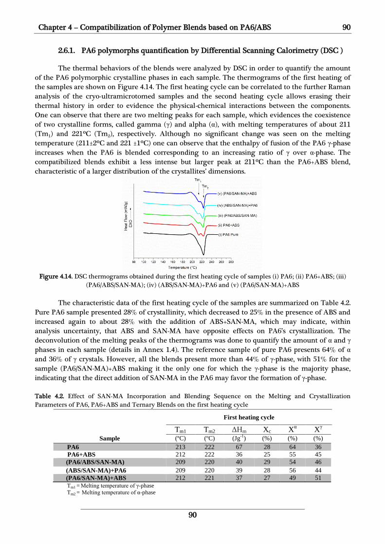
Chapter 4 – Compatibilization of Polymer Blends based on PA6/ABS 90
90
2.6.1. PA6 polymorphs quantification by Differential Scanning Calorimetry (DSC )
The thermal behaviors of the blends were analyzed by DSC in order to quantify the amount
of the PA6 polymorphic crystalline phases in each sample. The thermograms of the first heating of
the samples are shown on Figure 4.14. The first heating cycle can be correlated to the further Raman
analysis of the cryo-ultramicrotomed samples and the second heating cycle allows erasing their
thermal history in order to evidence the physical-chemical interactions between the components.
One can observe that there are two melting peaks for each sample, which evidences the coexistence
of two crystalline forms, called gamma (γ) and alpha (α), with melting temperatures of about 211
(Tm1) and 221ºC (Tm2), respectively. Although no significant change was seen on the melting
temperature (211±2ºC and 221 ±1ºC) one can observe that the enthalpy of fusion of the PA6 γ-phase
increases when the PA6 is blended corresponding to an increasing ratio of γ over α-phase. The
compatibilized blends exhibit a less intense but larger peak at 211ºC than the PA6+ABS blend,
characteristic of a larger distribution of the crystallites’ dimensions.
Figure 4.14. DSC thermograms obtained during the first heating cycle of samples (i) PA6; (ii) PA6+ABS; (iii)
(PA6/ABS/SAN-MA); (iv) (ABS/SAN-MA)+PA6 and (v) (PA6/SAN-MA)+ABS
The characteristic data of the first heating cycle of the samples are summarized on Table 4.2.
Pure PA6 sample presented 28% of crystallinity, which decreased to 25% in the presence of ABS and
increased again to about 28% with the addition of ABS+SAN-MA, which may indicate, within
analysis uncertainty, that ABS and SAN-MA have opposite effects on PA6’s crystallization. The
deconvolution of the melting peaks of the thermograms was done to quantify the amount of α and γ
phases in each sample (details in Annex 1.4). The reference sample of pure PA6 presents 64% of α
and 36% of γ crystals. However, all the blends present more than 44% of γ-phase, with 51% for the
sample (PA6/SAN-MA)+ABS making it the only one for which the γ-phase is the majority phase,
indicating that the direct addition of SAN-MA in the PA6 may favor the formation of γ-phase.
Table 4.2. Effect of SAN-MA Incorporation and Blending Sequence on the Melting and Crystallization
Parameters of PA6, PA6+ABS and Ternary Blends on the first heating cycle
First heating cycle
Tm1 Tm2 ΔHm Xc Xα
Xγ
Sample (ºC) (ºC) (Jg-1
) (%) (%) (%)
PA6 213 222 67 28 64 36
PA6+ABS 212 222 36 25 55 45
(PA6/ABS/SAN-MA) 209 220 40 29 54 46
(ABS/SAN-MA)+PA6 209 220 39 28 56 44
(PA6/SAN-MA)+ABS 212 221 37 27 49 51
Tm1 = Melting temperature of γ-phase
Tm2 = Melting temperature of α-phase

91 Chapter 4 – Compatibilization of Polymer Blends based on PA6/ABS
91
The second heating cycle (Figure 4.15/Table 4.3) allowed comparing the thermal properties
of the samples after erasing their thermal history (identical and controlled cooling conditions after
the melting step). First one can observe that the crystallization that took place in the DSC (during
the cooling step) reached higher crystallization ratio for all the samples but lower γ over α-phase
ratios, which certainly comes from a difference of crystallization temperature. This question will not
be studied extensively here. Like for the first heating cycle, the addition of ABS decreased the PA6
crystallinity (from 41% for pure PA6 down to 36% for PA6+ABS, and increased the amount of γ-
phase of 20% (from 15 to 18%), almost similar to the 25% increase observed during the first heating
cycle (from 36 to 45%). If the addition of SAN-MA compatibilizer had no significant impact on the
material crystallinity index (±2%), its impact on the polymorphic phases amount is confirmed, all
the compatibilized blends presenting higher content of γ-phase than the non-compatibilized one.
One can observe that the ratio of γ-phase increases significantly from 18% for the binary blend to
32% for the (PA6/SAN-MA)+ABS formulation. These results indicate that the γ-phase is favored
when SAN-MA is added to the blend, especially when it is done directly to the PA6 phase,
confirming what was observed during the first heating cycle.
Figure 4.15. DSC thermograms obtained during the second heating cycle of samples (i) PA6; (ii) PA6+ABS; (iii)
(PA6/ABS/SAN-MA); (iv) (ABS/SAN-MA)+PA6 and (v) (PA6/SAN-MA)+ABS
Table 4.3. Effect of SAN-MA Incorporation and Blending Sequence on the Melting and Crystallization
Parameters of PA6, PA6+ABS and Ternary Blends on the cooling and second heating cycle.
Cooling Second heating cycle
Tc ΔHc Tm1 Tm2 ΔHm Xc X
α X
γ
Sample (ºC) (Jg-1
) (ºC) (ºC) (Jg-1
) (%) (%) (%)
PA6 190 90 212 220 99 41 85 15
PA6+ABS 189 48 212 219 52 36 82 18
(PA6/ABS/SAN-MA) 188 45 212 220 47 34 77 23
(ABS/SAN-MA)+PA6 188 49 213 220 49 36 77 23
(PA6/SAN-MA)+ABS 188 48 213 220 53 38 68 32 Tc =
Crystallization temperature Tm1 = Melting temperature of γ-phase
ΔHc = Crystallization enthalpy Tm2 = Melting temperature of α-phase
2.6.2. Distribution of PA6 polymorphs studied by co-localized AFM-Raman analyses
We will now be interested on the distribution of the PA6 polymorphic phases in the blends by
co-localized AFM-Raman analysis. First, one must properly assign the Raman response of the α and γ
phases. In order to do so PA6 samples in different crystallographic forms were prepared: one
amorphous and two crystalline samples. Sample Alpha presented only α crystals and sample

Chapter 4 – Compatibilization of Polymer Blends based on PA6/ABS 92
92
Gamma only γ crystals. DSC and X-Ray diffraction (DRX) were performed to characterize their
structure and crystallinity index. Details are given in Annex 1.5.
Figure 4.16 presents the characteristic Raman spectra of the α, γ and amorphous phases. The
peak at 1125 cm-1 corresponds to the C-C symmetric vibrations for trans conformation of the
backbone, the signature of the monoclinic α-phase of PA6, while the 1080 cm-1 peak is attributed to
the C-C vibration of gauche conformation, signature of the hexagonal γ-phase.198–200 One can see that
the γ-phase has also a characteristic peak at 960 cm-1 (CO-NH) but due to its low intensity, it was not
used for phase identification. The amorphous phase presents both 1080 and 1125 cm-1, characteristic
of gauche and trans conformations, globally with low intensity and no preferable conformation. The
increase of crystallinity in each of the crystalline forms engenders the prevalence of one band
relative to the other. Thus, it is possible to quantify the presence of each phase by the characteristic
intensity ratio of the bands at 1080 and 1125cm-1 (I1080/I1125).
Figure 4.16. Typical Raman spectra of Polyamide alpha, gamma and amorphous phases.
Table 4.4 reports the I1080/I1125 Raman ratio calculated from the literature201 and
experimentally from at least 10 different spectra. The amorphous samples presented an I1080/I1125
ratio of about 1.40. Increasing the overall amount of α-phase naturally decreased the I1080/I1125 ratio
down to about 0.33 for sample Alpha. Contrarily, the I1080/I1125 ratio increased to about 2.0 with the
increase of γ-phase for sample Gamma. Since the Raman intensity characteristic of one phase is
proportional to its content in the material102,202, the differences between the experimentally
calculated values and the literature are related to different samples’ crystallinities. It is expected that
areas of the compatibilized blends with high crystallinity of γ-phase would have I1080/I1125 ratio of
about 2.5 or above if locally the material crystallinity is higher than the crystallinity of the
polyamides used as references. Reversely, a locally higher content of α, amorphous or a mixture of
phases should decrease this ratio.102,202 Details are presented in Annex 1.5.
Table 4.4. Characteristic band intensity ratios from literature and calculated experimentally.
I1080/I1125
Amorphous
Alpha (α) Gamma (γ)
Literature201
- 0.42 2.5
Experimental 1.40 0.33 2.0

93 Chapter 4 – Compatibilization of Polymer Blends based on PA6/ABS
93
Figure 4.17 (a)-1 3 are Raman mappings relative to the PB phase (integration between 1657-
1680 cm-1) overlapped on binary AFM modulus images (PB spheres shown in black) of the
compatibilized samples: 1-(PA6/ABS/SAN-MA), 2-(ABS/SAN-MA)+PA6 and 3-(PA6/SAN-MA)+ABS.
Individual Raman mappings and corresponding AFM images were shown in Annex 1.6. Due to the
micrometric resolution of the Raman, the PB spheres included in the ABS phase cannot be
individually distinguished, but zones with higher concentration of PB spheres are visible on the
Raman mappings. The AFM/Raman co-localization is confirmed by the good correlation between the
PB Raman mappings and the PB clusters seen by AFM. It is worth reminding that the AFM is based
on a surface analysis, while the Raman probes a depth of about 1 µm, being able to detected ABS
domains below the sample surface probed by AFM. These Raman mappings were analyzed to display
the I1080/I1125 ratio for each sample (Figure 4.17 (b) 1 to 3).
Sample (PA6/ABS/SAN-MA) presents areas with I1080/I1125 ratio values around 2.5 (green areas
on Figure 4.17(b)-1) which characterize a high amount of PA6 in γ form (I1080/I1125 > 2 VS I1080/I1125 ~
1.4 for the amorphous phase), homogenously distributed in the sample. Sample (ABS/SAN-MA)+PA6
on Figure 4.17(b)-2 presents equivalent ratio values (~2.5/green) but a different distribution. Areas
with a higher γ concentration appear in green, especially over the richer PB areas (corresponding to
the ABS domains), and lower I1080/I1125 ratio appear in orange/red, which can be related to a mixture
of α, amorphous and γ phase. The differentiation between α and the amorphous phase contribution
was attempted using the γ-phase characteristic peak at 960 cm-1 however, a clear conclusion could
not be obtained (details in Annex 1.6). Notwithstanding, the subtraction of a spectrum with low
I1080/I1125 ratio from one with a high ratio revealed only peaks relative to the PA6 in γ-phase (shown in
Annex 1.6), which confirms that the areas with high I1080/I1125 ratio present more γ-phase than the low
ratio zones, but it is not possible to affirm if these low ratio zones are composed of mixtures of phases
or amorphous zones. Finally, sample (PA6/SAN-MA)+ABS presents I1080/I1125 ratio values around 2.5
and higher (blue areas on Figure 4.17(b)-3), which is an indication of a high content of γ-phase in the
PA6, not only over the ABS domains. This result is in accordance with the previous DSC analysis of
this sample, i.e., when SAN-MA is added directly to the PA6 the γ-phase is favored.
(PA6/ABS/SAN-MA) (ABS/SAN-MA)+PA6 (PA6/SAN-MA)+ABS
(a)-1 (a)-2 (a)-3
Superposition
of PB map on
Binary AFM
Image
(b)-1 (b)-2 (b)-3
Ratio I1080/I1125
Figure 4.17. (a) Superposition of PB Raman mapping (band integration between 1657-1680 cm-1) on the binary
AFM Modulus image, showing the PB phase in black. The higher the amount of PB, the brighter is the pixel.
(b) Ratio of the peak intensities I1080/I1125 for : 1-(PA6/ABS/SAN-MA); 2- (ABS/SAN-MA)+PA6 and 3-(PA6/SAN-
MA)+ABS.

Chapter 4 – Compatibilization of Polymer Blends based on PA6/ABS 94
94
The I1080/I1125 Raman ratio can also give an insight on the local crystallinity of the probed
areas. The mean values of the I1080/I1125 ratio for samples (PA6/ABS/SAN-MA), (ABS/SAN-MA)+PA6
and (PA6/SAN-MA)+ABS were 2.2±0.2, 2.2±0.3 and 2.6±0.3, respectively. This shows that the first two
samples, despite a different phase distribution, have a similar crystallinity index for the mapped
areas, while the mapped area of the last sample (PA6/SAN-MA)+ABS has a higher crystallinity index.
Previous DSC analysis also showed samples (PA6/ABS/SAN-MA) and (ABS/SAN-MA)+PA6 with
similar crystallinities and about 45% of γ-phase, while sample (PA6/SAN-MA)+ABS presented 51% of
γ-phase. These results indicate that the blending protocols have an effect on the distribution of the
PA6 polymorphic phases in the blend, i.e., when the blending protocol leads to the concentration of
the compatibilizer near the ABS domains, a higher content of γ-phase at the interface of these
domains is seen. Similarly, when the compatibilizer is add in the PA6, higher content of γ-phase can
be found in PA6 zones, not necessarily near the ABS domains.
2.6.3. Discussions of the effect of SAN-MA compatibilizer on PA6 structure
The DSC and co-localized AFM-Raman analyses presented on Figure 4.14 and 4.17,
respectively, illustrates the impact of the compatibilizer and the blending protocols on the PA6
polymorphic phases’ amount and distribution. DSC analyses have shown that the addition of SAN-
MA directly in the PA6 favors the γ-phase. Raman mappings are in accordance with the previous
DSC analyses, which showed samples (ABS/SAN-MA)+PA6 and (PA6/SAN-MA)+ABS with similar
amount of γ-phase (~45%) and sample (PA6/SAN-MA)+ABS with more γ-phase than the others (51%).
One can consider the mapped areas as representative of the materials and deduce that the
distribution of the PA6’s polymorphic phases is directly related to the compatibilizer preferred
location induced by the blending protocol.
Sample (PA6/ABS/SAN-MA), presented a homogeneous distribution of PA6 γ-phase with no
preferred locations (Figure 4.17 (b)-1). Sample (ABS/SAN-MA)+PA6, with a similar amount of γ-
phase, showed a heterogeneous distribution of γ-phase (Figure 4.17 (b)-2), presenting high content
of γ-phase over the ABS domains, where the compatibilizer is preferentially located due to the
blending protocol. Finally, sample (PA6/SAN-MA)+ABS (Figure 4.17 (b)-3) presented a higher mean
value of the I1080/I1125 ratio, related to the higher crystallinity of the probed area, and an
heterogeneous distribution, with high I1080/I1125 ratio observed at areas even far from the ABS
domains. In this case, the mixing protocol suggests that the compatibilizer is concentrated in the
PA6, which leads to the formation of a higher content of γ-phase. This behavior can be attributed to
disturbances in the homogeneous nucleation process of PA6 due to the compatibilizer presence,
which limits the polymer chain mobility, favoring the crystallization of the less stable γ-phase.198,203
Disturbances on the crystallization of PA6 have already been reported for composites and
compatibilized blends194,199,204, but this work is the first to report the influence of the blending
protocol on the distribution of the PA6’s polymorphic phases in the blend.
A schematic representation of the different PA6 polymorphic phases’ amount and
distribution developed from the different blending protocols is presented on Figure 4.18.

95 Chapter 4 – Compatibilization of Polymer Blends based on PA6/ABS
95
Figure 4.18. Schematic representation of the analyses and results.
3. Conclusions of Chapter 4
The co-localized AFM/Raman analyses done on the binary and compatibilized PA6/ABS
blend exemplify the power of this technique for morphological, nanomechanical and chemical
characterization of polymer blends. Based on the chemical information collected by Raman and the
nanomechanical information issued from AFM a clear phase attribution was performed. Atomic
Force Microscopy allied to Transmission Electron Microscopy allowed the characterization of the
effect of different blending protocols on the morphology of the blends, as well as the dispersion and
distribution of the sub-phases of the ABS at nanometric scale. It has been shown that the addition of
the compatibilizer on the ABS phase prior to the PA6 phase induces the formation of an almost co-
continuous morphology, rather than a particle-in-matrix morphology when the compatibilizer is
added prior in the PA6 or in a single extrusion step. The morphological analysis helped the
interpretation of the rheological measurements. The almost co-continuous morphology exhibited a
significant increase in melt viscosity, especially at low frequencies, and its rheological properties (G’
and G”) were higher than what was observed for the samples with particle-in-matrix morphology,
attributed to the increase of the flow resistance due to the extra tensions resulted from the higher
anchoring effect of the almost co-continuous morphology.
The coupling of AFM with Raman spectroscopy provided new fundamental insights on the
effect of the compatibilizer on the Polyamide crystalline structure. Raman analyses of the
distribution of the different polyamide polymorphs (α, γ and amorphous) showed good correlation
with DSC analyses, allowing the interpretation of the effects of the compatibilizer on the structure of
the Polyamide matrix. It was shown that the compatibilizer influences the crystallization of the
Polyamide, favoring the formation of the less stable γ polymorphic phase. Furthermore, the
distribution of the γ-phase in the blend depends on the blending protocol due to the different
preferred locations of the compatibilizer induced by the process. High amount of γ-phase is present
near the ABS domains when the compatibilizer is blended with ABS prior to PA6. Contrarily, high
amounts of γ-phase are seen inside the PA6 phase when the compatibilizer is blended with PA6 prior

Chapter 4 – Compatibilization of Polymer Blends based on PA6/ABS 96
96
to ABS. Finally, a homogeneous distribution of γ-phase is acquired when the components are
blended in a single step.
We verify that for all the different blending protocol used, the general morphology of the
compatibilized blends, i.e., the distribution and sizes of ABS domains, was improved when compared
to the reference PA6+ABS sample. However, we have shown that the presence of the compatibilizer
and the blending protocol can have an impact on the amount and distribution of the different
polymorphic phases of the polyamide. Further research must be performed to correlate this
fundamental knowledge to the functional properties of the material, for example mechanical
strength, impact resistance and heat distortion temperature.
In addition to the fundamental knowledge of the morphology of these specific polymer
blends, the developed strategy allying morphological and chemical characterization by AFM, SEM
and Raman spectroscopy on cryo-ultramicrotomed samples opens new possibilities for a better
understanding of the micro and nanoscale behavior of the compatibilization interplays in polymer
blends and composites, i.e., to design and tailor their functional properties from the nanoscale.
3.1. Summary of conclusions of Chapter 4
The complete assignment of the components of the blends was achieved using their chemical
signatures and nano-mechanical properties
The morphology of the blends, as revealed by AFM and TEM, depend on the blending protocol:
(PA6+ABS+SAN-MA): particle-in-matrix morphology
(ABS+SAN-MA)+PA6: almost co-continuous morphology
(PA6+SAN-MA)+ABS: particle-in-matrix morphology
The developed morphologies have different rheological properties.
The almost co-continuous morphology presented higher storage modulus (G’) and loss modulus (G’’)
than the particle-in-matrix one, due to the higher anchoring effect
DSC and Raman analysis show that SAN-MA compatibilizer favors the formation of the γ polymorph,
especially when the SAN-MA is added directly in contact with PA6
Co-localized AFM/Raman analyses show that the distribution of the γ polymorph depends on the
blending protocol:
SAN-MA prior on ABS phase: γ polymorph near the ABS domains – heterogeneous distribution
SAN-MA directly on PA6: high content of γ far from ABS domains – heterogeneous distribution
SAN-MA blended simultaneously with PA6/ABS: γ polymorph homogeneously distributed

97 Chapter 4 – Compatibilization of Polymer Blends based on PA6/ABS
97
4. Conclusions du Chapitre 4 en Français
Les analyses co-localisées AFM/Raman effectuées sur les mélanges PA6/ABS binaire et
compatibilisés illustrent la puissance de cette technique pour la caractérisation morphologique,
nanomécanique et chimique des mélanges polymères. Sur la base des informations chimiques
recueillies par Raman et des informations nanomécaniques issues de l'AFM, une attribution de phase
claire a été effectuée. La microscopie de force atomique alliée à la microscopie électronique de
transmission a permis de caractériser l'effet de différents protocoles de mélange sur la morphologie
des mélanges, ainsi que la dispersion et la distribution des sous-phases de l'ABS à l'échelle
nanométrique. Il a été démontré que l'addition du compatibilisant sur la phase ABS avant la phase
PA6 induit la formation d'une morphologie presque co-continue, plutôt qu'une morphologie des
particules dans matrice lorsque le compatibilisant est ajouté avant la PA6 ou dans une seule étape
d'extrusion. L'analyse morphologique a contribué à l'interprétation des mesures rhéologiques. La
morphologie presque co-continue a présenté une augmentation significative de la viscosité à l'état
fondu, en particulier à basse fréquence. Ses propriétés rhéologiques (G'et G") étaient supérieures à
celles observées pour les échantillons à morphologie particule dans matrice, attribuée à
l'augmentation de la résistance à l'écoulement due aux tensions supplémentaires issues de l'effet
d'ancrage plus élevé de la morphologie presque co-continue.
Le couplage AFM-Raman a fourni de nouvelles connaissances fondamentales sur l'effet du
compatibilisant sur la structure cristalline de la polyamide. Les analyses Raman de la distribution
des différents polymorphes de la PA6 (α, γ et amorphe) ont montré une bonne corrélation avec les
analyses DSC, ce qui permet d'interpréter les effets de l'agent compatibilisant sur la structure de la
matrice de polyamide. Il a été démontré que le compatibilisant influence la cristallisation de la
polyamide, favorisant la formation de la phase polymorphe γ moins stable. En plus, la distribution de
la phase γ dans le mélange dépend du protocole de mélange en raison des différentes distributions
du compatibilisant induit par le processus. Une quantité élevée de phase γ est présente près des
domaines ABS lorsque le compatibilisant est mélangé avec de l'ABS avant la PA6. Au contraire, des
quantités élevées de phase γ sont observées à l'intérieur de la phase PA6 lorsque le compatibilisant
est mélangé avec la PA6 avant l'ABS. Finalement, une distribution homogène de la phase γ est
acquise lorsque les composants sont mélangés en une seule étape.
Nous vérifions que, malgré le protocole de mélange utilisé, la morphologie générale des
mélanges, c'est-à-dire la distribution et la taille des domaines ABS, a été améliorée par rapport à
l'échantillon PA6+ABS de référence. Cependant, nous avons montré que la présence du
compatibilisant et du protocole de mélange peut avoir un impact sur la quantité et la répartition des
différentes phases polymorphes de la polyamide. D'autres recherches doivent être effectuées pour
corréler ces connaissances fondamentales aux propriétés fonctionnelles du matériau (par exemple
résistance mécanique, résistance aux chocs et température de distorsion thermique).
En plus des connaissances fondamentales de la morphologie de ces mélanges de polymères,
la stratégie développée alliant la caractérisation morphologique et chimique par spectroscopie AFM,
SEM et Raman sur des échantillons cryo-ultramicrotomés ouvre de nouvelles possibilités pour une
meilleure compréhension du comportement micro et nanométrique de la compatibilisation dans les
mélanges de polymères et composites, c'est-à-dire pour concevoir et adapter leurs propriétés
fonctionnelles à partir de la l’échelle nanometrique.

Chapter 4 – Compatibilization of Polymer Blends based on PA6/ABS 98
98
4.1. Résumé des conclusions du Chapitre 4 en Français
L'analyse co-localisée AFM/Raman a permis l'affectation complète des composants des mélanges en
utilisant leurs signatures chimiques et leurs propriétés nano-mécaniques
La morphologie des mélanges, telle que révélée par AFM et TEM, dépend du protocole de mélange:
(PA6+ABS+SAN-MA): morphologie des particules dans matrice
(ABS+SAN-MA)+PA6: morphologie presque co-continue
(PA6+SAN-MA)+ABS: morphologie des particules dans matrice
Les morphologies développées ont des propriétés rhéologiques différentes.
La morphologie presque co-continue a présenté un module de stockage (G') et un module de perte (G'')
plus élevés que le type de particules dans la matrice, en raison de l'effet d'ancrage plus élevé
Les analyses DSC et Raman montrent que le compatibilisant SAN-MA favorise la formation du
polymorphe γ, surtout lorsque le SAN-MA est ajouté directement en contact avec la PA6
Les analyses co-localisées AFM/Raman montrent que la distribution du polymorphe γ dépend du
protocole de mélange:
SAN-MA avant la phase ABS: polymorphe γ près des domaines ABS - distribution hétérogène
SAN-MA ajouté sur PA6: contenu élevé de γ loin des domaines ABS - distribution hétérogène
SAN-MA mélangé simultanément avec PA6 / ABS: polymorphe γ réparti de manière homogène

99 Chapter 4 – Compatibilization of Polymer Blends based on PA6/ABS
99

CHAPTER 5
Hybrid Membranes
for Fuel Cell

101 Chapter 5 – Hybrid Membranes for Fuel Cells
101
PROLOGUE
In this chapter, we will present the study of alternative membranes for Fuel Cell operation,
based on the hybridization of a sulfonated polyether-etherketone (sPEEK) membrane with an active
network by sol-gel chemistry. The membranes were prepared at the laboratory SyMMES (Grenoble,
France) as part of the thesis works of Isabel Zamanillo López and Natacha Huynh.
We will present here a brief introduction to the Fuel Cell technology and the fundamentals
of solid polymer electrolytes and sol-gel reactions. Then, we will present the fabrication of hybrid
membranes based on two different sol-gel precursors. The study of hybrid membranes based on (3-
mercaptopropyl)-methyldimethoxysilane (SHDi) precursors allowed for the understanding of the
effect of each step of fabrication on the membrane’s morphology, nanomechanical properties and
stability over time. The second study, hybrid membranes based on (3-mercaptopropyl)-
trimethoxysilane (SHTriM) focused on the effect of the varying amount of sol-gel phase on the
morphology of the hybrid membranes. Furthermore, direct observation of the morphology by AFM
allowed to orient the selection of an appropriate fitting model for SANS interpretation, giving
complementary structural information about the SG phase and the sPEEK matrix. Finally, we stress
out that the complete morphological and chemical characterization of the membranes was only
possible thanks to the use of cryo-ultramicrotomy allied to co-localized AFM/Raman setup and
complementary characterization techniques, which contributions will be outlined.
French Prologue
Dans ce chapitre, nous présenterons l'étude de membranes alternatives pour pile à
combustible, basée sur l'hybridation d'une membrane de polyéther-éthercétone sulfonée (sPEEK)
avec un réseau actif par chimie sol-gel. Les membranes ont été préparées au laboratoire SyMMES
(Grenoble, France) dans le cadre des travaux de thèse d'Isabel Zamanillo López et Natacha Huynh.
Nous allons vous présenter ici une brève introduction à la technologie des piles à
combustible et les fondamentaux des électrolytes polymères solides et des réactions sol-gel. Ensuite,
nous présenterons la fabrication de membranes hybrides à base de deux précurseurs sol-gel
différents. L'étude de membranes hybrides à base du précurseur (3-mercaptopropyl)-
méthyldiméthoxysilane (SHDi) a permis de comprendre l'effet de chaque étape de fabrication sur la
morphologie de la membrane, ses propriétés nanomécaniques et sa stabilité au cours du temps. La
seconde étude portant sur des membranes hybrides à base de (3-mercaptopropyl)-triméthoxysilane
(SHTriM) a montré l'effet de la quantité croissante de phase sol-gel sur la morphologie des
membranes hybrides. Par ailleurs, l'observation directe de la morphologie par AFM a permis
d'orienter la sélection d'un modèle d'ajustement (fit) approprié pour l'interprétation des analyses
SANS, en fournissant des informations structurelles complémentaires sur la phase SG et la matrice
sPEEK. Finalement, nous soulignons que la caractérisation fine de la morphologie et de la chimie
des membranes n'a été possible qu'avec l'utilisation de la cryo-ultramicrotomie alliée à la co-
localisation AFM/Raman et à des techniques de caractérisation complémentaires, dont les
contributions seront soulignées.

Chapter 5 – Hybrid Membranes for Fuel Cell 102
102
1. Theoretical Background and Motivation
1.1. Hydrogen Fuel Cells Fundamentals
Renewable energy sources as solar and wind, which are weather dependent, are intermittent
by nature. Thanks to the Proton Exchange Membrane Water Electrolyzer (PEMWE) hydrogen
technologies offer a chemical storage solution to smooth intermittent electricity production. This
chemical energy remains available to be later restored in the form of electricity by proton Exchange
Membrane Fuel Cells (PEMFC). The PEMWE/PEMFC couple is therefore a solution for sustainable
development if renewable hydrogen is used. In general, PEMFC can also be used as a power source
in a variety of applications, such as transport, portable, stationary and emergency backup power
applications. In this study, we will be particularly interested in PEMFCs that use hydrogen fuel, a
promising system for zero CO2 and pollutant emission.
PEMFC is composed of a Membrane Electrode Assembly (MEA) which includes gas diffusion
layers, the catalyst layers (electrodes) and the proton exchange membrane used as electrolyte, as
illustrated on Figure 5.1. During operation, hydrogen molecules adsorb on the anode catalysts (left),
and protons and electrons are formed by the resulting electrochemical reaction (oxidation). The
electrons flow through the external circuit, delivering electrical energy (lighting lamp) and finally
reduce oxygen into oxygen ions at the cathode (right). Protons meanwhile migrate through the
electrolyte membrane and react with these oxygen ions, forming water as a byproduct.205
Figure 5.1. Operating principle of a fuel cell. Adapted from 205
The electrochemical reactions are: oxidation of hydrogen at the anode (Equation 5.1) and
reduction of oxygen at the cathode (Equation 5.2).
5.1
5.2
𝟐 𝑯𝟐 → 𝟒𝑯+ + 𝟒𝒆−
𝑶𝟐 + 𝟒𝑯+ + 𝟒𝒆− → 𝟐 𝑯𝟐𝑶

103 Chapter 5 – Hybrid Membranes for Fuel Cells
103
The role of the polymer membrane electrolyte is to transport the protons generated at the
anode to the cathode to allow the oxygen reduction’s reaction to take place. For effective Fuel Cell
operation, the membrane must be highly proton conducting, but should not conduct electrons,
avoiding short circuit, and sufficiently gas-tight to avoid gas crossover (resulting in hot-spots and
destruction).206
To ensure the perennial emergence of this technology, the membrane must allow the
PEMFC operation at high temperature (100-150°C) and therefore low relative humidity (10-50%).
Researchers have focused on the development of PEMFCs operating at high temperatures (> 100 °C)
because it has been proved that operating above 100°C increases the speed of electrochemical
reactions, decreases the sensitivity of the catalyst to carbon monoxide (responsible for “poisoning” of
the MEA) and simplifies the cooling system and water management.207,208
In Fuel Cell devices, certain stresses or constraints lead to accelerated materials ageing. For
example, membrane mechanical failure is accelerated by the swelling (due to hydration) and
shrinkage (dehydration) that occurs at each start/stop operation. Membranes showing little or no
change in dimension at different water contents will extend MEA lifetime.209 The membrane also
has to withstand chemical degradation due to attack by radicals and other reactive species. MEA
degradation often manifests itself as a gradual decay in fuel cell performance followed by a sudden
catastrophic failure of the cell due to gas crossover through tears in the membrane. The ability of
the membrane to resist to the mechanical stresses and chemical attack is the limiting factor in the
lifetime of PEMFC.210 For practical applications, the membrane’s lifetime must exceed 8000h and
50000h respectively for PEMFC transport and stationary applications.206,211,212 The role of proton
conducting membrane is therefore central in the operation of the cell.
1.2. Polymer Membrane Electrolytes
The chemical functions conferring the proton conductivity to the solid polymer electrolyte
(also called ionomer) are acid functions, most often of the sulfonic type -SO3H. The ion exchange
capacity of the polymer corresponds to the amount of ionic sites relative to the polymer mass, which
is directly related to the proton conductivity of the membrane and consequently to the performance
of the Fuel Cell. Notwithstanding, as already state above, due to the complexity of the factors
contributing to membrane degradation, other properties are important to assure the long term
reliability and performance of the device, such as low gas permeation (H2 and O2), good mechanical
strength, no electronic conductivity, electrochemical resistance and chemical stability. According to
Jones et al. 210, no single property can be used as a stand-alone metric for membrane durability.
There are basically two families of polymers used in PEMFC: fluorinated and non-fluorinated
polymers. Perfluorinated membranes are the ones that currently offer the most satisfaction both in
terms of performance and durability. To date, Nafion® is the most widely accepted as a reference
membrane due to its excellent functional and electrochemical properties up to 80°C. Its structure
consists of a perfluorinated hydrophobic skeleton with pendant chains terminated by sulfonic acid
groups -SO3H (Figure 5.2). The perfluorinated polymer has been chosen for its excellent proton
conductivity, arising from a very good hydrophilic/hydrophobic nanophase separation, as well as for
its electronic insulating properties and very good chemical stability. In the presence of water, there
is a differential swelling of the hydrophobic and hydrophilic phases and the appearance of channels
(hydrophilic zones) allowing the transport of the protons. However, the thermomechanical
relaxation of Nafion® occurs around 100 °C, which imposes a maximum operating temperature of
the order of 80° C, representing a direct limit to the application of Nafion® to high temperature
PEMFCs.213 In addition, the decrease of Nafion’s proton conductivity above 80ºC, associated with low
relative humidity, along with high membrane’s cost (>500 €/m2), which represents more than 80% of

Chapter 5 – Hybrid Membranes for Fuel Cell 104
104
the cost of the MEA stack, make difficult its use in a PEMFC for a low cost passenger electric car.206
A competitive cost can only be reached with improved performance or with the development of
alternative membranes.214,215
Figure 5.2. Nafion® structure
Non-fluorinated membranes, mainly polyaromatic polymers, represent an alternative to
Nafion®, being less expensive and with suitable thermomechanical properties for higher operating
temperatures (>100 °C).207 However, they are more sensitive to the chemical degradation and
therefore their lifetime is generally lower than that of perfluorinated membranes, e.g., from
hundreds up to few thousands hours of operation against more than 20000 h for Nafion at 80ºC.216
One of the solutions to overcome these problems is to develop alternative non-fluorinated aromatic
composite membranes with improved chemical stability.
1.2.1. Sulfonated Polyether-etherketone (sPEEK)
In this work, we have used sPEEK membranes as an alternative to Nafion®. Its structure is
presented on Figure 5.3. sPEEK has better mechanical strength, better thermal stability and is less
expensive than Nafion®. However, it is less chemically stable in operating conditions under the
attack of H2O2 (a byproduct resulting from incomplete electrochemical reactions and gas
crossover).217
Figure 5.3. (a) sPEEK structure (X=0.4)
The hydrophobic/hydrophilic phase separation, essential to the good conductivity of the
membranes, is much more pronounced in Nafion® than in sPEEK. In the polyaromatic membrane,
the polymer backbone is less hydrophobic and less flexible, due to the presence of aromatic groups,
than for a perfluorinated one. Thus, the ionic channels are narrower and branched with many "dead
ends" (unconnected channels). In addition, the -SO3H functions are less acidic than in Nafion® which
results in a less labile proton.218 All these factors reduce the ionic conductivity.211
New solutions for these problems are based on the synthesis of new polymer architectures
(new polymers, interpenetrating polymer networks, 3D structures by reticulation, etc.) or
modification of the existing membranes. Mendil-Jakani et al.219 have shown that hydrothermal
treatments above 60ºC had strong impact on quality of the hydrophilic/hydrophobic interfaces,
water uptake, and conductivity. Thermally treated membranes presented a nano-phase separation in

105 Chapter 5 – Hybrid Membranes for Fuel Cells
105
liquid water even at room temperature, which is not observed for pristine sPEEK membrane. Portale
et al.220 have shown that high proton conductivities of about 100 mS/cm, which is equivalent to the
conductivity of a native Nafion® membrane in liquid water at room temperature, can be reached on
swelled sPEEK membranes in temperatures of about 70ºC. However, for temperatures above 87 °C,
irreversible swelling occurs and the membrane mechanical properties degrade rapidly, resulting in a
rapid drop of the proton conductivity. Influences of membrane fabrication steps have also been
shown by Fichet et al.221,222 on Semi-Interpenetrating Polymer Networks (semi-IPNs) combining a
fluorinated network with sPEEK, showing that the drying time can induce a decrease of the water
uptake and conductivity due to its effect on the hydrophilic/hydrophobic nano-separation.
Another way is the addition of an inorganic phase to promote better mechanical properties,
to enhance the proton conductivity (addition of a mineral acid) or to improve water retention at high
temperatures. If the use of inert reinforcements generally reduces the proton conductivity, it results
in greater mechanical properties, limiting dimensional changes. The introduction of inorganic oxide
and solid acid components (metal oxides, zeolites, metal hydrogen phosphates and heteropolyacids)
can lead to an improvement in the proton conductivity under low RH.209 The preparation methods
for inorganic–organic membranes include on the one hand the in situ precipitation of inorganic
particles in functionalized polymer solutions or in pre-cast ionomer membranes, and on the other
hand the formation of interpenetrating inorganic and organic networks.218 Other strategies reported
by extensive reviews by Jones and Rozière223,224, Alberti and Casciola225 and Savadogo226 include
polymer blending, partial cross-linking and organic–organic composite membranes, but up to now,
these modifications did not lead to expected improvements and often generated a critical loss of
proton conduction.221 However, mechanical reinforcement to prevent mechanical failure from
wet/dry humidity cycling may be insufficient210,211, and these strategies do not systematically take
into account the required enhancement of the chemical resistance of the membrane. The
introduction of stabilizing units to increase the membrane’s chemical stability at high temperature
can be achieved with the fabrication of hybrid membranes with tailored sol-gel precursors. This
strategy simultaneously provides mechanical reinforcement and chemical stabilization, which is a
powerful approach to overcome the aforementioned limitations.227–231
1.3. Sol-Gel method
To create a hybrid material, the in-situ formation of an inorganic network can be achieved
by soft chemistry-based processes, from molecular, colloidal or polymeric precursors that are
formed at low temperatures and pressures. The sol-gel method is one of the most used for the
preparation of hybrid materials for its versatility and low processing temperature. It involves the
preparation of a stable suspension of colloidal (nanometric) solid particles (sol) from metal
alkoxides or inorganic salts, which is converted by the hydrolysis and polycondensation of the
precursors into a three-dimensionally continuous solid network supporting a continuous liquid
phase (gel). The gelation of the sol-gel system can be engendered by covalent links, entanglement of
chains, van der Waals forces or hydrogen bonds, depending on the precursor’s chemistry.232,233 The
precursors are well tailored molecules able to condensate into a multidimensional structure with
completely different properties.234 An example of well-known sol-gel process is based on silane
precursors. Silane precursors have a generic structure of R4-nSi-OXn, with n ranging from 1 to 4 and
where R is an organic group, and the Si-OX bond is able to hydrolyze into silanol groups (Si-OH)
which will them condensate into Si-O-Si bonds. The condensation degree reached by the molecules
will depend on the amount of hydrolysable bonds, forming dimers, linear chains or three-
dimensional networks. Figure 5.4 below shows a schematic example of the hydrolysis and
condensation of a siloxane precursor bearing two hydrolysable groups (-OX) on its structure. Since

Chapter 5 – Hybrid Membranes for Fuel Cell 106
106
the hydrolysis and condensation reactions occur simultaneously, competing with each other, the
control of the condensation degree will depend on the careful control of different process
parameters, such as temperature, pH, concentration of precursors and agitation.
Figure 5.4. Representation of hydrolysis and condensation of a generic precursor molecule
In addition to the combination of the different properties of inorganic (hardness, chemical,
thermal stability) and organic materials (toughness, elasticity, low density), specially tailored
functional molecules (-R) can be introduced into the inorganic phase, allowing new possibilities to
create multifunctional materials.
1.4. Objectives of work
Fuel Cells still require significant lifetime enhancement and cost reductions if they are to
compete with established technologies. The challenge in developing high performance membranes
is achieving the required mechanical strength and durability especially at elevated temperatures.210
The sol-gel method appears as a powerful approach to simultaneously improve the mechanical
strength and chemical resistance of the polymer electrolyte. The process parameters are critical to
define the properties and morphology of the final membrane, as are thermal post-treatments used
for conditioning and optimizing the functional properties of the membranes (proton conductivity,
membrane swelling and thermomechanical strength).211,218,221,235 Therefore, it is of prime importance
to qualify the impact of each step of fabrication on the physical and chemical properties of the
hybrid membrane. However, this imposes difficulties on the access to the bulk of the polymer
membrane for direct observation of the morphology and probing its chemical properties.
This chapter will be focused on the morphological and chemical characterization of
alternative membranes based on sPEEK with two different SG precursors bearing active groups for
chemical stabilization. Cryo-ultramicrotomed samples were prepared for co-localized AFM/Raman
analyses, as well as complementary Electron Microscopy (STEM) and µ-ATR-FTIR to study the
process-structure-properties interplays of membranes fabrication.

107 Chapter 5 – Hybrid Membranes for Fuel Cells
107
2. Study of hybrid membranes based on dimethoxysilane (SHDi) precursors
We will first be interested on the study of a class of hybrid membranes based on (3-
mercaptopropyl)-methyldimethoxysilane precursors, produced during the thesis of Isabel Zamanillo
López. This work entitled “Co-localized AFM-Raman: A powerful tool to optimize the Sol-Gel
chemistry of Hybrid Polymer Membranes for Fuel Cell” was submitted to the journal Polymer on
September 2017 and will be presented here in an adapted format.
2.1. Materials used
Sulfonated poly(ether ether ketone) (sPEEK) commercial membranes purchased from Fumatech®
(E-750) with an ionic exchange capacity (IEC) of 1.33 meq.g-1(milli molar SO3H per gram of
polymer) were used as host membranes for the preparation of hybrid membranes by Sol-Gel (SG)
chemistry.
SG precursor: (3-mercaptopropyl)-methyldimethoxysilane (SHDi) (Figure 5.5), was purchased
from Sigma Aldrich. This precursor satisfies the requirements to obtain a reactive hybrid membrane,
i.e., the hydrolysis of the alkoxy groups leads to the formation of alkoxy groups and their
condensation to the formation of an inorganic SG phase (Figure 5.5) with a linear chemical structure
bearing mercaptopropyl organofunctional groups. Therefore, the SG phase allows introducing into
the host sPEEK membrane the antioxidant thiol group to improve the lifetime of the sPEEK phase.
Figure 5.5. Sol-Gel phase formation by hydrolysis and condensation of SG precursor
The hybrid membranes collected and characterized after the different stages of fabrication are
illustrated on Figure 5.6 and summarized in Table 5.1. The commercial sPEEK membrane is first
nanostructured to be transformed in a host membrane (Step 1), then the SG precursors are
impregnated inside the membrane (Step 2), the linear SG structure forming a 3D network phase into
the host sPEEK membrane and finally two thermal treatments are done: one to improve the extent
of condensation (Step 3 - Post-condensation/PC) and the other to improve the proton conductivity of
the hybrid membrane (Step 4 – HydroThermal/HT). The details of the membranes fabrication
process are presented in Annex 2.1. The SG phase uptake was determined by Thermogravimetric
Analysis (TGA) according to Equation 5.3 taking into account the SiO2 weight residue at 700°C and
the weight of dry hybrid membrane at 200°C (a temperature corresponding to the complete water
desorption). Details of the procedure are described in Annex 2.2. To characterize the inner
morphology of the hybrid membranes, they were properly opened by cry-ultramicrotomy as
described in Chapter 3.

Chapter 5 – Hybrid Membranes for Fuel Cell 108
108
5.3
Where M SiO2 = 60.08 g/mol and MSG = Molar Mass of the SG repeat unit of the condensed
SG phase from SHDi precursor = 134.32 g/mol.
Figure 5.6. Schema of the different steps of fabrication of the hybrid membranes
Table 5.1 Sample and fabrication step
Sample Step of fabrication
Hyb-I Hybrid Membrane after impregnation/condensation
Hyb-PC Post-Condensed Hybrid Membrane in 6.3 %RH at 74ºC for 72 hours
Hyb-PC-HT Post-Condensed and Hydrothermally Treated (80°C/72h) Hybrid Membrane
2.2. Micro-scale distribution of the SG along the membrane’s cross-section
The micro-scale morphology of the final hybrid membrane (post-condensed and
hydrothermally treated) Hyb-PC-HT was studied in order to get a first idea of the SG/sPEEK phases
distribution. Figure 5.7 (a) shows an optical photography of the cryo-ultramicrotomed cross-section
of the membrane taken with the optical microscope of the AFM. The cryo-ultramicrotomy
procedure provided samples with very low roughness, and with minimum topography artifacts,
despite some vertical lines caused by small scratches on the diamond knife.
The Young’s modulus AFM image presented on Figure 5.7(b) corresponds to the first 10 µm
of the left side of the membrane’s cross-section (illustrated by a red square on the optical image).
First, one can see that at this scale the membrane’s morphology is almost homogeneous (brown and
yellow colors mixed) except for the first micrometers (between one and two micrometers) near the
outer surface where the presence of a skin with a higher modulus is detected (yellower color).
The modulus of the host sPEEK and the SG phases taken separately were measured by AFM
at 1.85 and 0.3 GPa respectively, which gives yellow (higher modulus) and brown (lower modulus)
colors with the chosen color scale. Therefore, the presence of the higher modulus skin could be
attributed either to a partial crosslinking of the SG phase (oxidation of the SH groups leading to SS
covalent bonds due to their high O2 sensitivity) and therefore an increase of the Young modulus, or
a depletion of the low modulus SG phase at the surface, potentially due to the washing step required
after impregnation/condensation of the SG precursors to avoid the formation of a pure SG layer at
the membrane’s surfaces, or maybe due to the sPEEK host membrane morphology giving less space
for the SG phase at the membrane’s surface.
%𝑆𝐺 =
𝑚 𝑆𝑖𝑂2 𝑟𝑒𝑠𝑖𝑑𝑢𝑒 𝑎𝑡 700°𝐶𝑀𝑆𝑖𝑂2
× 𝑀𝑆𝐺
𝑚 ℎ𝑦𝑏𝑟𝑖𝑑 𝑚𝑒𝑚𝑏𝑟𝑎𝑛𝑒 𝑎𝑡 200°𝐶 − (𝑚 𝑆𝑖𝑂2 𝑟𝑒𝑠𝑖𝑑𝑢𝑒 𝑎𝑡 700°𝐶
𝑀𝑆𝑖𝑂2× 𝑀𝑆𝐺 )
× 100%

109 Chapter 5 – Hybrid Membranes for Fuel Cells
109
Colocalized Raman analysis was performed both on the membrane’s bulk and skin to give
additional information to interpret the AFM image. The complete Raman assignment of the bands
relative to the sPEEK and the SG phase is shown in Annex 2.3. Figure 5.7(c) shows 2 spectra, one
acquired on the membrane’s skin (blue colors associated to the blue cross on the AFM image) and
one acquired on the bulk (green color/green cross). Both spectra show 2 distinct peaks between 2700
and 3200cm-1. The peak centered at ~3080 cm-1 is assigned to the contribution of the CH groups of
the aromatic ring of the sPEEK. The peak centered at ~2900 cm-1 refers to the aliphatic –CH
vibrations of the SG phase. From this assignment, we clearly observe that the SG uptake is not
homogeneous inside the membrane. The spectra collected on the skin (blue) shows a much lower
ratio of SG vs. sPEEK than the spectra of the bulk (green). The co-localized Raman information give
us the proof that the higher modulus skin of the hybrid membrane observed by AFM corresponds to
a depleted layer where the SG concentration is lower, either because the sPEEK host membrane
accepts a lower SG uptake on its skin (due to higher crystallization ratio for example), or due to SG
partial removal from the sPEEK host during the washing step.
(a) (b) (c)
Figure 5.7. (a) Optical Image of the cryo-ultramicrotomed surface of sample Hyb-PC-HT; (b) AFM modulus
image of the first 10µm of the cross-section from the left of the outer surface (corresponding to the red square
drawn over (a)); (c) Co-localized Raman analysis of the membrane’s skin (blue cross) and bulk (green cross).
The distribution of the SG phase inside the membrane was determined by the ratio between
the area of the peak assigned to the SG (between 2785 and 3015cm-1) and the area of the peak
assigned to the sPEEK contribution (between 3020 and 3120cm-1) after normalizing the Raman
spectra relative to the sPEEK, as shown on Figure 5.8 (a). The SG phase distribution across the
membrane is presented on Figure 5.8 (b). One can observe that the SG uptake at the outer surfaces
of the membrane is lower than in the bulk (roughly divided by two) and that the depletion is limited
to the first micrometers on both sides, confirming the AFM observation. The SG depleted skin’s
thickness was measured by AFM to be between 1 and 2µm and about 3µm by Raman analysis. This
discrepancy arises from the lower lateral resolution of the Raman vs. AFM. As observed on Figure
5.8 (b), the SG content of the membrane’s skins is equivalent on both sides, however the cross-section
analysis revealed a slow decrease of the SG uptake when going from the left to the right of the cross-
section. One can suspect a difference of accessibility of the SG precursors’ for each side of the
membrane, with for example temporary contact between one side of the membrane and the surface
of the reactor during the impregnation step. A stronger agitation of the reactive medium should
therefore be applied to improve that point.

Chapter 5 – Hybrid Membranes for Fuel Cell 110
110
(a) (b)
Figure 5.8. (a) Membrane’s skin and bulk normalized spectra (normalization relative to the CH-band intensity
of sPEEK at 3080 cm-1) (b) Relative SG phase uptake inside the Hyb-PC-HT membrane’s cross-section (area
ratio between the band between 2785 and 3015cm-1 and the band between 3020 and 3120cm-1; membrane
thickness: 35 µm)
2.3. Impact of the processing steps on the hybrid membrane’s morphology
The nanoscale morphology of the hybrid membranes after each step of the fabrication
process (Hyb-I, Hyb-PC and Hyb-PC-HT) was imaged by AFM and STEM, in order to study the
impact of the different treatments (PC and HT) on the distribution of phases and their mechanical
properties. The AFM height images of the 3 membranes presented on Figure 5.9 (a), (d) and (g) do
not allow distinguishing clearly the phase’s morphologies. The microstructure of the hybrid
membranes is much better revealed by the different Young’s modulus of each phase, with the
modulus images shown on Figure 5.9 (b), (e) and (h). The calibration of the AFM tip allows the
determination of the Young’s Modulus of each phase, which gives 1.85 GPa for the sPEEK and a
range from 0.5 to 1.0 GPa for the Sol-Gel depending on the membrane history (to be discussed
further), which appears as brown dark domains of about 40-100 nm dispersed on the membrane
structure. Complementary STEM images shown on Figure 5.9 (c), (f) and (i) were taken in Bright
Field mode on the thin sections collected during the cryo-ultramicrotomy preparation of each
sample (details given in Chapter 3). One can observe very contrasted images. Indeed, the sPEEK and
the SG interact differently with the electron beam due to the presence of silicon atoms (higher
atomic number) in the SG structure, thus a chemical contrast is observed without the need for
sample staining. The SG phase appears darker in the image, since it scatters more electrons than the
sPEEK phase. The STEM images confirm the distribution of the SG phase inside the membranes and
shows that even inside the sPEEK phase there are nanometric domains of SG (dark spots) which are
difficult to visualize on the AFM modulus image.
It should be noticed that the AFM Modulus image of Figure 5.9 (b) relative to the membrane
analyzed after the impregnation/condensation step (Hyb-I), shows larger domains of SG phase when
compared to the complementary STEM image on Figure 5.9 (c). This can be explained by the fact
that the STEM analysis is done in transmission and the volume of the section is analyzed (about 100
nm thick). Therefore one can visualize the sPEEK phase inside the SG domains, which is not the case
when probing the mechanical properties of the cross-section surface by AFM (only the first nm are
analyzed). Bright round shapes can be seen on the STEM image of Figure 5.9 (c), which are related to
damages on the section due to a long exposure of the sample to the electron beam (small holes
through the section). Comparing the sample Hyb-I (before thermal PC treatment) with the post-

111 Chapter 5 – Hybrid Membranes for Fuel Cells
111
condensed sample Hyb-PC, both modulus (Figure 5.9 (b) and (e)) and STEM (Figure 5.9 (c) and (f))
images show an improvement of the phase separation, the size of the SG domains decreases with the
smallest ones disappearing. This results evidence the impact of the condensation and densification of
the SG phase after the post-condensation treatment at 74ºC for 24h (condensation of residual Si-OH
groups into Si-O-Si bonds). On the other hand, comparing Figure 5.9 (f) and (i) one can see that the
hydrothermal treatment (HT) applied on sample Hyb-PC did not have a strong impact on the
morphology (distribution of each phase remaining unaffected).
Height Modulus STEM
(a) (b) (c)
Hyb
-I
(d) (e) (f)
Hyb
-PC
(g) (h) (i)
Hyb
-PC
-HT
Figure 5.9. Hybrid membranes’ structure at different stages of the fabrication process revealed by AFM and
STEM. Sample Hyb-I: (a - AFM Height; b - AFM Modulus and c- STEM); Sample Hyb-PC: (d - AFM Height; e -
AFM Modulus and f – STEM); and sample Hyb-PC-HT: (g - AFM Height; h - AFM Modulus and i – STEM).

Chapter 5 – Hybrid Membranes for Fuel Cell 112
112
2.4. Impact of the processing steps on the hybrid membrane’s nanomechanical
properties and SG uptake
The evolution of the modulus of the Sol-Gel phase was recorded after each fabrication step
(Table 5.2). Sample Hyb-I presented a SG phase with a modulus of about 0.5 GPa. However, we found
a modulus of 0.3 GPa for a pure SG phase (analyzed alone and free of mechanical stresses). This
discrepancy can originate from the contribution of the stiffer sPEEK phase, since the SG phase is
surrounded by the sPEEK phase in hybrid membranes. After the post-condensation treatment, the
SG phase in sample Hyb-PC presented a modulus of 0.7 GPa. Finally the hydrothermally treated
sample Hyb-PC-HT had a SG phase with a modulus of 1.0 GPa. The clear increase of the Young
modulus of the SG phase along with the successive treatments confirms the effects of these post
treatments on improving the SG phase condensation and densification.
Thermogravimetric Analysis (TGA) was done in order to follow the hybrid membrane
composition after each step, giving additional information. Details of the procedure used are shown
in Annex 2.2. Results are shown on Table 5.2. Sample Hyb-I presents 240% of SG phase uptake after
impregnation. One can observe that the SG phase uptake of the hybrid membrane is unchanged
after the post condensation treatment (240% Hyb-PC) whereas it drops to 115% after the
hydrothermal treatment (Hyb-PC-HT). Therefore we understand that the increase on the Young
modulus of the SG phase from sample Hyb-I to Hyb-PC is related to the improvement of the SG
condensation (no significant change of the SG uptake in the hybrid membrane), whereas the
observed increase of modulus after the hydrothermal treatment (from 0.7 for Hyp-PC to 1.0 GPa for
Hyb-PC-HT) could be related to the elution of oligomers (SG phase uptake drops from 240 to 115%)
that were acting as plasticizers of the SG phase.
Table 5.2 Modulus of each phase of the hybrid membranes (AFM measurement) and SG phase uptake (TGA)
Sample sPEEK Modulus (GPa) SG Modulus (GPa) %SG
Hyb-I 1.85 0.5 240
Hyb-PC 1.85 0.7 240
Hyb-PC-HT 1.85 1.0 115
2.5. Insights on the SG condensation process thanks to the water trapped at the
ultramicrotomed surfaces
Images of freshly cryo-cut samples (cut at -120ºC, imaged at RT) of hybrid membranes at
different stages of the fabrication process were obtained by Optical Microscopy (OM), using the 100x
long objective of the Raman Microscope, and are presented on Figure 5.10. These optical images can
give the first insights on the mechanical stability behavior of the membranes during the cryo-
ultramicrotomy process. The three samples endured the process with no cracks or tearing. However,
despite the good quality of the cryo-cuts, dark stains were observed on the cross-section of Hyb-I
(Figure 5.10 (a)) and Hyb-PC (Figure 5.10 (b)), but not on the cross-section of Hyb-PC-HT (Figure
5.10 (c)). We found that these stains were, caused by the presence of liquid water issued from the
melting of ice crystals (deposited on the sample’s surface during the cutting process) when the
sample warms back to room temperature. To be noticed: the same samples ultramicrotomed at
room temperature (RT) did not present such dark stains (confirming that it was due to the water
condensation after the cryo process and not from the sample itself). However, due to the low glass
transition temperature of the SG phase the quality of the RT-ultramicrotomed surface was very poor
(surface deformation due to shearing forces).

113 Chapter 5 – Hybrid Membranes for Fuel Cells
113
(a) Hyb-I (b) Hyb-PC (c) Hyb-PC-HT
Figure 5.10. Optical microphotographs evidencing both the quality of the cryo-ultramicrotomed membranes
cross-sections of hybrid membrane at each step of the fabrication process: (a) after impregnation/condensation
(Hyb-I membrane); (b) after post-condensation step (Hyb-PC membrane) and (c) after hydrothermal treatment
(Hyb-PC-HT membrane), and the presence of water droplets for (a) and (b).
At the time we cryo-ultramicrotomed these samples, it was not possible to avoid the
formation of water droplets on the cutted surfaces. However this originally unwanted phenomenon
turned out to reveal very important information about the condensation extent of the SG phase.
AFM images (Figure 5.11) acquired with PeakForce QNM confirm the presence of liquid on the cryo-
ultramicrotomed surface of the membrane Hyb-I and Hyb-PC. Figure 5.11 (a) to (d) relative to the
Hyb-I membrane confirm the presence of droplets on the cross-section. Indeed, the droplets appear
on the images as areas with lower Young’s Modulus (dark brown) and higher Adhesion and
Deformation (yellow/white) than the polymer matrix (yellow on the Modulus image and brown on
Adhesion/Deformation). The post-condensed sample Hyb-PC opened surface on the other hand
seems to have been locally swollen by water, with the affected zones having a less defined contour
with, however, like for the droplets observed for Hyb-I membrane, a higher topography, lower
modulus and higher adhesion than the matrix, as shown on Figure 5.11 (e) to (h). Finally, as already
observed by optical microscopy (AFM results not shown), no water or surface modification induced
by water diffusion was detected by AFM on the cryo-ultramicrotomed surface of the post condensed
and hydrothermally treated membrane (Hyb-PC-HT).

Chapter 5 – Hybrid Membranes for Fuel Cell 114
114
Height Modulus Adhesion Deformation
(a) (b) (c) (d)
Hyb
-I
(e) (f) (g) (h)
Hyb
-PC
Figure 5.11. AFM images confirm the presence of water droplets on the cross-section of sample Hyb-I from (a)
to (d); and a zone swollen by water on sample Hyb-PC from (e) to (h)
2.6. Morphological evolution over time
We have followed the evolution of the water droplets areas of Hyb-I membranes over time,
expecting a fast drying of the absorbed water. Figure 5.12 presents the Height and Adhesion AFM
images of sample Hyb-I chronologically taken up to 90 days after sample preparation. Instead of the
expected drying of the water droplets, we observed the appearance of small objects inside the water
droplets about 15 days after cryo-ultramicrotomy, which can be seen on the adhesion image of
Figure 5.12(b) as small dark dots of low adhesion (red arrow) inside the water droplets (high
adhesion areas). Figure 5.12 (c) presents the same area (red circle) analyzed 15 days later (30 days
after cutting). The growth of the objects over time is evidenced by the increasing size of the dark
dots inside the liquid zones, from 100 nm to 250 nm for the object followed here by the red arrow.
Three months after cutting, it was noticed that the undefined objects observed on the cross-section of
the Hyb-I membrane had evolved into well-defined crystals, always located inside the water droplets,
as shown on Figure 5.12(d) (zoomed inset). It should be noticed that over the same length of time
(after cutting) the post-condensed sample Hyb-PC presented no sign of any crystal growth inside the
water swollen areas presented on Figure 5.11. In addition, pure sPEEK membrane did not show
neither water droplets remaining at the surface of the cryo-ultramicrotomed membrane nor any
objects growing subsequently at its surface.

115 Chapter 5 – Hybrid Membranes for Fuel Cells
115
Figure 5.12. AFM Height and Adhesion images of the cryo-ultramicrotomed surface of Hyb-I membrane taken
just after cutting (a), 15 days after cutting (b), 30 days after cutting (c) and 90 days after cutting (d). The red
arrows highlight the growth of non-adhesive objects inside de water droplets. The zoomed inset on image (d)
evidences the regular shape of the growing objects.
As the host sPEEK membrane does not contain any water soluble species (at room
temperature) one can suspect that these crystallites originate from species migrating from the SG
phase (before the post-condensation treatment). In order to confirm this hypothesis a chemical
analysis of the observed growing objects was necessary.
2.7. Nano-manipulation and nanomechanical characterization of growing crystals
The nanodimensions of the growing objects made it impossible to do direct Raman analysis,
since the confocal Raman with a volume resolution of about 1µm3 could not discriminate the signal
of nano-objects only present at the very surface of the sample. We had to pile them up in order to
analyze their chemistry and to do so we used the AFM tip as a nano-broom to gather the particles
from a large area of 20x20µm2 (Figure 5.13(a)) to achieve a concentration compatible with the
Raman analysis. This nano-manipulation successfully produced a pack of particles of about 5 µm in
the x and y directions and more than 200 nm in the z direction, as shown by AFM on Figure 5.13 (b).
(a)
(b)
Figure 5.13. AFM Height images of the cryo-ultramicrotomed Hyb-I membrane before (a) and after nano-
sweeping the growing objects (b).
(a) Freshly after cut (b) 15 days after cut (c) 30 days after cut (d) 90 days after cut
Hei
gh
t
A
dh
seio
n

Chapter 5 – Hybrid Membranes for Fuel Cell 116
116
The topography image presented on Figure 5.14(a) evidences the very regular rhombus
shape of the particles inside the pack (red arrow), characteristic of crystalline materials. As a
confirmation, the crystals were observed to have higher modulus (about 4.8 GPa) than the polymer
matrix (1.85 GPa) as illustrated by the modulus image of Figure 5.14 (b). The crystals also present a
lower adhesion (about 5nN) than the surrounding liquid (about 100 nN) and the polymer matrix
(about 40 nN), and a lower deformation (about 3 nm) than the surrounding liquid (about 30 nm) and
the polymer matrix (about 8 nm), as observed respectively on the adhesion and deformation images
of Figure 5.14(c) and (d).
(a) Height (b) Modulus
(c) Adhesion (d) Deformation
Figure 5.14. AFM images of the pack of particles (a) Topography, (b) Modulus, (c) Deformation and (d)
Adhesion
2.7.1. Co-localized AFM/Raman analysis on the crystals
A 10x10 µm Raman mapping (400 to 3250 cm-1 range) co-localized with the AFM-scanned
area of Figure 5.14 was recorded in order to do a chemical analysis of the crystals. The same Raman
bands were observed everywhere on the mapping, however, the pack of particles showed a much
stronger SG/sPEEK ratio (area of the peaks between 2785 and 3015 cm-1 - assigned to the SG
structure - divided by the area of the peak found between 3020 and 3120 cm-1 - assigned to the sPEEK
structure) than the surrounding membrane’s cross-section surface. The co-localized Raman mapping
of this ratio is shown on Figure 5.15(b). We therefore found that the crystals have the same chemical
signature as the SG phase, and this result confirms the hypothesis that these crystals originate from
the migration and crystallization of species chemically similar to the SG precursors.

117 Chapter 5 – Hybrid Membranes for Fuel Cells
117
(a) (b)
Figure 5.15. (a) Pack of growing objects piled-up by the AFM tip on sample Hyb-I (b) Raman mapping of the
ratio SG/sPEEK
2.8. Morphological Analysis by Scanning Electron Microscopy (SEM)
SEM imaging is potentially more destructive for the samples, since the electron beam and
the high vaccum can cause irreversible changes on the sample’s surface. Therefore, it has been
performed as the final step of characterization to provide additional morphological analysis with
chemical contrast.
SEM images of samples Hyb-I and Hyb-PC were acquired in two different modes of operation
collecting respectively the “Secondary Electrons” (SE) and the “Back-Scattered Electrons” (BSE).
Details of each mode were given in Chapter 2, section 5.2.1. Figure 5.16 (a) shows the topography (SE
image) of a pack of particles evidencing the regular rhombus shape of the crystals (red arrow). It has
been observed that the liquid phase (already observed by optical and atomic force microscopies)
evaporates under the heat of the electron beam, leaving empty spaces between crystals, as can be
seen on the red-circled zone of Figure 5.16 (a). Heat buildup of the sample under the electron beam,
generally considered as a drawback of the technique, finds here its usefulness. On the BSE image
shown on Figure 5.16 (b) for the same sample area as Figure 5.16 (a), three different contrasts were
observed, the membrane’s surface (darker areas), the crystals (brighter areas) and an intermediate
brightness area surrounding (not systematically) the crystals. This intermediate phase not always
observed surrounding the crystals is attributed to the remaining liquid or to the surface where the
liquid was before its evaporation under electron beam. As the SG precursor contains silicon atoms
(higher atomic number: 14 for silicon versus 8 for oxygen and 6 for carbon) the brighter the area on
the BSE image the more it contains silicon and therefore SG or SG precursors. This observation
corroborates the Raman observation: the crystals originate from the migration and crystallization of
species chemically similar to the SG precursors. It also evidences that the liquids zones are rich on
non-condensed SG precursors/oligomers that reduce its evaporation rate.
The swollen zones (already observed by optical and atomic force microscopies) of sample
Hyb-PC were also imaged by SEM and are shown on Figure 5.16 (c) SE mode and (d) BSE mode.
Only a slight topographic contrast is observed on Figure 5.16 (c) with the swollen zones being
smoother than the rest of the cross-section, however a higher contrast is evidenced by the BSE mode
on Figure 5.16 (d). This contrast highlights the higher concentration of non-condensed SG
precursors/oligomers inside the swollen zone. One can also see that the image’s brightness is slightly
higher at the center of the swollen zone than on its periphery, probably because of the progressive
evaporation of the liquid droplet during the 90 days preceding the SEM observation.

Chapter 5 – Hybrid Membranes for Fuel Cell 118
118
SE BSE
(a) (b)
Hy
b-I
(c) (d)
Hy
b-P
C
Figure 5.16. SEM images taken 90 days after cryo-ultramicrotomy of the cross-section of sample Hyb-I (a – SE
mode; b – BSE mode) and of sample Hyb-PC (c – SE mode; d – BSE mode).
2.9. Discussion of the characterization of hybrid membranes based on SHDi precursor
The results presented above have demonstrated that by impregnating a SG precursor’s
solution into a commercial sPEEK membrane we obtained, after a multi-step process, hybrid
membranes. We were also able to follow the evolution of the morphology, chemical composition
and physical properties of the membranes after each of these steps by co-localized AFM-Raman and
complementary SEM analysis as discussed below.
After the impregnation/condensation step (sample Hyb-I) the membrane presented a high
SG phase uptake of 240% determined by TGA (Table 5.4), which evidences the effectiveness of the
impregnation process. The phase distribution (between the SG and sPEEK phases) was analyzed by
AFM and STEM (Figure 5.9(b) and (c)), making possible the measurement of the young modulus of
each phase: 1.85 GPa for the sPEEK matrix and 0.5 GPa for the SG phase. The SG phase found in the
hybrid membrane appears stiffer than the corresponding free (condensed out of the membrane) SG
phase (0.5 versus 0.3 GPa). This observation can be explained by three factors: 1) a different
condensation degree of the SG prepared outside and inside the membrane, 2) the confinement, as
the SG is surrounded by the sPEEK matrix, and 3) the presence of nanodomains of sPEEK inside the
SG phase, making this later stiffer. Indeed the high-resolution STEM images have shown that SG
and sPEEK phases are not pure and contain nanodomains of the other phase.
The cross sections of Hyb-I and Hyb-PC membranes were found to have drops of liquid at
their surface after cryo-ultramicrotomy, which were not the case for Hyb-PC-HT cross-sections, as
illustrated by Figure 5.21. Understanding the origin of this observation gave us valuable additional
information. We found that in a general manner it was the ice deposition on the cold freshly opened
cross-section issued from cryo-ultramicrotomy, and its melting when warming up from cryo to
ambient temperature, that was at the origin of the liquid found at the surface of the cross-sections
(no such liquid was observed after Ultramicrotomy performed at room temperature). However, if

119 Chapter 5 – Hybrid Membranes for Fuel Cells
119
for the Hyb-PC-HT cross-sections this water evaporates fast from the cross-section, it was not the case
for the Hyb-I and Hyb-PC cross-sections. The ulterior crystallization phenomenon observed in the
liquid found at the surface of Hyb-I cross-sections (Figure 5.12) and the understanding that the
observed crystals had a chemical composition similar to the SG phase thanks to a co-localized AFM-
Raman analysis (Figure 5.15), led us to the diagnosis presented now. When the cryo-ultramicrotomed
surfaced cross-section is taken out of the cryo-environment, the air humidity forms ice crystal on the
opened surface, and as the temperature rises, ice melts. If no soluble species are present in the
membrane, then the water evaporates leaving no traces. However if soluble species can diffuse to the
water, the water is then trapped at the cross-section surface for a much longer time. Then, the
trapped water allows for the swelling of the sPEEK phase, and the dissolution and migration of
additional hydrophilic chemical species to the membrane surface. As sPEEK was re-acidified and
rinsed before impregnation, we observed no trapped water for pure sPEEK membranes. The
hydrophilic chemical species were then understood to come from the SG phase and to be
uncondensed or partially-condensed SG precursors, as confirmed by the co-localized AFM-Raman
analysis (Figure 5.15). After a certain time the concentration of these water-soluble species in the
liquid phase reaches a critical point and we observed the nucleation of crystals in the liquid. The
crystallization process lowers the concentration of the water species in the liquid, and after a certain
time length the hybrid membrane stops releasing soluble species, i.e., diffusion takes place only in a
limited swollen volume of the membrane below each water droplets, this limited volume not being
an infinite reservoir. Then the evaporation of the water becomes possible. From these observations
we understand that even though the hybrid membrane contains a high amount of SG, the
condensation process was not yet completed after the impregnation step, making a post-
condensation step mandatory.
As expected, the thermal treatment of post-condensation had no impact on the weight ratio
of SG in the membrane (240% by TGA for Hyb-PC, identical to the one found for Hyb-I). However
one can observe on the AFM and STEM images of Figure 5.9(c) and (f) a densification of the SG
domains. The Young modulus of the SG phase increases from 0.5 to 0.7 GPa and the size of the SG
domains decreases, with the smallest ones disappearing, as a consequence of the PC step. In addition,
the effect of the water condensed at the membrane’s surface after cryo-ultramicrotomy provides
here again useful information. If the Hyb-PC membrane shows traces of droplets of condensed water
on its cross-section (optical contrast observed on Figure 5.21, higher topography and adhesion
observed on Figure 5.11), this sample shows no trace of crystal nucleation, contrarily to the non-
treated Hyb-I membrane. We can therefore understand that water soluble species are still released
from the SG phase (which explains the trapped water droplets at the surface of the membrane cross-
section) but these species either reach a lower concentration on the water, or are not able to
crystallize due to a higher molecular weight for example). Figure 5.16 (d) confirms the presence of
non-condensed SG precursors/oligomers in the water-swollen areas of the membrane, which appear
brighter in BSE mode (higher concentration of silicon containing species).
Finally after the last step (HT) which consists on a 72h hydrothermal treatment at 80°C, we
observed no trace of condensed water at the membrane’s surface after cryo-ultramicrotomy, which
imply the absence of water soluble species in the hybrid membrane, which are essential to reduce
the rate of evaporation of water). This demonstrates that these species still observed after the PC step
were washed away during the HT step. This elution should be, at least in part, responsible for the SG
uptake decreasing from 240% to 115% (TGA results Table 2). If the morphology of the SG phase
distribution seems unmodified by the HT step (when comparing Hyb-PC and Hyb-PC-HT on Figure
5.9), an increase of the SG modulus was observed from 0.7 to 1.0 GPa (Table 2). This modulus
increase can be related to the elution of species that previously acted as plasticizers of the SG phase.
It should be noted that the elution of the water-soluble species from the SG phase is critical in order

Chapter 5 – Hybrid Membranes for Fuel Cell 120
120
to avoid their elution during the Fuel Cell operation, which could affect the device’s efficiency.
Further research must be performed to evaluate the performance of the membrane during FC
operation.
2.10. Complementary µ-ATR-FTIR analysis – Feasibility and preliminary results
µ-ATR-FTIR is a complementary technique which allows following the evolution of the SG
phase condensation or effects of oxidative degradation, by the identification of chemical signatures
that are undetectable or have low intensity by Raman, such as the Si-O-Si bonds presented in the SG
structure and carboxylic groups.
Figure 5.17 (a) shows an example of µ-ATR-FTIR imaging of the intensity of the Si-O-Si band
on the cross-section of membrane Hyb-I, superposed to the optical image. It is worth reminding that
the µ-ATR-FTIR analysis uses a germanium (Ge) crystal with a tip diameter of 350 µm, which is
about 10 times larger than our polymer membranes (~30 µm thick). Therefore, to be cut using the
cryo-ultramicrotome, the membranes were sandwiched between PP sheets (200 µm each) for
mechanical reinforcement as described on Chapter 3. The image shows basically three different
zones: the PP backing appearing in dark blue, due to the absence of Si-O-Si bands on its structure, the
edges of the membrane appearing in light blue and the bulk of the membrane with an essentially
green color. Figure 5.17(b) shows the FTIR spectrum of sample Hyb-I (after
impregnation/condensation) in the middle of membrane’s cross-section. Among the bands of
interest, the bands of Si-O-Si network (1080 cm-1) and the SG precursors (CH2, CH3 and O-CH3 near
2900 cm-1) can give insights on the degree of condensation of the SG phase trough the cross-section
and after the post-condensation step, i.e., the decrease of -CH3 and -O-CH3 bands (the CH2 groups not
participating on the hydrolysis/condensation) with the increase of the Si-O-Si band. In addition, this
technique allows to detect any trace of material oxidation due to the strong absorption of the C=O
(~1700 cm-1) of the species formed.
(a) (b)
Figure 5.17. (a) Example of µ-ATR-FTIR imaging of sample Hyb-I (30 µm) sandwiched between two PP sheets
(~200 µm each). The mapping is relative to the peak at 1080 cm-1 (Si-O-Si), red meaning high intensity of the
band and blue zero intensity. (b) FTIR spectrum of sample Hyb-I (after impregnation/condensation) in the
middle of membrane’s cross-section.
The lower intensity of the Si-O-Si bands at the edges (thickness of ~6 µm) might be related to
the depleted SG skin revealed by co-localized AFM/Raman analysis, or to a lower degree of
condensation at the outer surface compared to the bulk. The former hypothesis was refuted by the
analysis of the ratio between the area of the Si-O-Si band (1080 cm-1) relative to the area of the
aliphatic CH groups (~2900 cm-1), which presented a constant ratio (I1080/I2900~2) throughout the
thickness of the membrane (not shown). Therefore, the low intensity of the Si-O-Si band seen at the

121 Chapter 5 – Hybrid Membranes for Fuel Cells
121
outer surface is related to the depleted SG skin. We remark that this zone appears much larger than
in AFM/Raman analyses due to the lower resolution of the µ-ATR-FTIR.
In order to evaluate the effectiveness of the post-condensation treatment on the hybrid
membranes, sample Hyb-I and Hyb-PC were analyzed. To outline the chemical modification induced
by this thermal treatment, spectra from the center of each membrane were acquired for comparison.
Figure 5.18 show the subtraction of Hyb-I from Hyb-PC spectra. The spectral difference shows a
decrease of the bands at 2900, 1460 and 1025 cm-1. These bands can be related to methanol (CH3-OH
– from OMNIC Nicolet Sampler Library), as shown on Figure 5.18 for comparison. Methanol
elimination (by vaporization due to the thermal treatment applied) is a signature of an additional
hydrolysis and condensation processes occurring during the post-condensation thermal treatment.
One should expect an increase of the of Si-O-Si bonds (~1080cm-1), but the methanol elimination
masks the increase of Si-O-Si IR band. Nevertheless, we can conclude that the post-condensation
treatment increases the SG condensation degree. Furthermore, no bands relative to the C=O groups
(~1700 cm-1) were identified in both samples, which is a sign that no oxidation of the material
occurred during the fabrication process.
Figure 5.18. Subtraction of Hyb-I from Hyb-PC spectra (red line) showing the decrease of the bands at 2900,
1460 and 1025 cm-1 and reference methanol spectrum (blue).

Chapter 5 – Hybrid Membranes for Fuel Cell 122
122
2.11. Conclusions of the Study of Hybrid membranes based on SHDi precursor
In this study, we were interested on the morphological evolution of the hybrid membranes
with the different fabrication steps. We revealed the formation of a depleted skin layer (lower SG
concentration) about one micrometer thick on both sides of the membrane whereas the SG phase
concentration is almost constant through the rest of the membrane thickness. A stronger agitation
of the reactive medium is proposed to obtain a constant SG concentration inside the membrane,
however the origin of the depleted skins has still to be understood (heterogeneous sPEEK host
membrane morphology, or impact of the washing step). Complementary optical microscopy, AFM,
and SEM of the hybrid membranes cross-sections after cryo-ultramicrotomy have shown the
diffusion of water-soluble species from the SG phase of Hyb-I and Hyb-PC membranes into the
atmospheric water condensed at the cross-section surface. The crystallization of these species only
observed for Hyb-I membrane, gave us an insight on their higher concentration and/or lower
molecular weight before the PC step. We used the AFM tip to nano-manipulate the crystals to obtain
a pile making possible a co-localized AFM-Raman analysis to find that the crystals were chemically
similar to the SG precursors.
The quantitative nano-mechanical data collected by AFM revealed a densification of the SG
phase through the fabrication process (with a Young modulus increasing from 0.5 to 0.7 from Hyb-I
to Hyb-PC and then 1.0 GPa from Hyb-PC to Hyb-PC-HT). The first increase was attributed to an
improved condensation of the SG phase and the second modulus increase to the elution of the water-
soluble species (not fully condensed species originally acting as plasticizers) during the final
hydrothermal treatment.
Finally, µ-ATR-FTIR imaging on the cross-section of hybrid membranes was achieved,
revealing methanol elimination during the post-condensation thermal treatment, which is a
signature of the hydrolysis and condensation processes. Therefore, the post-condensation treatment
increases the SG condensation degree.

123 Chapter 5 – Hybrid Membranes for Fuel Cells
123
3. Study of hybrid membranes based on trimethoxysilane (SHTriM) precursors
We will now present the study of another class of hybrid membranes based on a different
kind of precursor issued from the Ph.D. thesis of Natacha Huynh in the laboratory SyMMES
(Grenoble, France). In this part of the study, we will focus on the effect of the different chemistry
and amount of the precursor on the membranes’ morphologies. Furthermore, the complementarity
between the morphological AFM analyses and Small Angle Neutron Scattering (SANS) data from N.
Huynh’s work will be presented.
3.1. Materials used
The Sol-Gel (SG) precursor used in this part of the study was a (3-mercaptopropyl)-
trimethoxysilane (SHTriM), purchased from Sigma Aldrich. Its chemical structure and the first step
of hydrolysis and condensation are shown in Figure 5.19. Rather than linear chains, this precursor
should allow the formation of tridimensional chemical structures within the sPEEK host membrane.
Figure 5.19. SHTriM sol-gel precursor structure before and after a first step of hydrolysis and condensation
The different hybrid membranes collected and characterized after the each stage of fabrication
are summarized in Table 5.3. The details about the membranes fabrication process are presented in
Annex 2.4. Membranes are denoted Hybrid_X, with X being the theoretical targeted SG uptake after
impregnation. Rather than using TGA like for the SHDi membranes, the actual SG uptake after
impregnation (%SGw) was determined by weighting the membranes before and after hybridization,
then using Equation 5.4, where msPEEK is the mass of the nanostructured host membrane and mhyb is
the mass of the hybrid membrane after impregnation. The different membranes were cut in cryo-
ultramicrotomy as described on Chapter 3.
5.4
Table 5.3 Samples, step of fabrication and SG content determined by weighting
Sample Step of Fabrication %SGw
Hybrid_10
Hybrid Membrane after impregnation/condensation
10.3
Hybrid_10_PC
Post-Condensed in 10 %RH at 80ºC for 24 hours
10.5
Hybrid_10_PC_HT
Post-Condensed and Hydrothermally Treated (80°C/72h)
5.1
Hybrid_20_PC_HT 19.3
Hybrid_30_PC_HT 29.5
%𝑺𝑮𝒘 = 𝒎𝒉𝒚𝒃 − 𝒎𝒔𝑷𝑬𝑬𝑲
𝒎𝒔𝑷𝑬𝑬𝑲

Chapter 5 – Hybrid Membranes for Fuel Cell 124
124
3.2. Effect of the thermal treatments on the membrane’s morphology
The morphology of samples Hybrid_10, Hybrid_10_PC and Hybrid_10_PC_HT are shown on
Figure 5.20, which is a “composition” of the three AFM modulus images, corresponding to the first
10 µm of the left side of the membranes’ cross-sections. The SHTriM based membranes’
morphologies are almost homogeneous through their thicknesses, with the SG phase appearing as
round shape domains of low modulus (brown color) distributed into the sPEEK matrix (yellow
color), except for the first 500 nm near the outer surface, where the skin with less SG phase (fewer
darker spots) is observed once again (surrounded by the red dashed lines). These SHTriM
membranes seem to present non connected domains of SG, distributed in the sPEEK matrix. This
comes from the fact that these membranes have a much lower SG uptake than the SHDi
membranes presented before in this chapter (10 vs 240%SG).
Sample Hybrid_10 and Hybrid_10_PC have the same SG uptake after impregnation (10.3 and
10.5% respectively) but sample Hybrid_10_PC_HT presented only 5.1%. One could think that this loss
of 50% of SG phase is an effect of the thermal treatment, however, the three samples are issued from
three different batches and sample Hyb_10_PC_HT already presented less SG from the first step of
impregnation (~7%), due to issues during impregnation (non-homogeneous distribution of the
precursors in the impregnation bath). Thus, we can consider that there is a small elution effect
(within the measurement incertitude) due to the hydrothermal treatment (HT), but not 50%.
Visually, the morphology of sample Hybrid_10_PC_HT seems to present smaller SG domains than
Hybrid_10 and Hybrid_10_PC. Indeed, the size of the SG domains was found to be 85±24 nm, 87±27
nm and 78±18 nm respectively for Hybrid_10, Hybrid_10_PC and Hybrid_10_PC_HT. The difference
in the size of the SG domains of sample Hybrid_10_PC_HT seems to be mainly related to its smaller
SG uptake, rather than an effect of the thermal treatments, which should be confirmed with the
further studies of membranes with different SG uptakes.
Figure 5.20. Composition of three AFM modulus images of the first 10 µm of the left side of the membranes’
cross-sections.
Differently from the SHDi hybrid membranes, no trapped water or elution of the water-soluble
species from uncondensed or partially-condensed SG precursors was seen on the cryo-
ultramicrotomed membranes’ surfaces over time. Indeed, the developments on the fabrication based
on the work with the SHDi hybrid membranes (optimization of treatment temperatures and times)
guaranteed a better condensation of the SG phase, which decreases its hydrophilicity. Furthermore,
the different chemistry of the precursors allows for the formation of three dimensional structures
rather than linear chains, which hampers the mobility of low molecular weight oligomers or
partially condensed precursors.

125 Chapter 5 – Hybrid Membranes for Fuel Cells
125
3.2.1. Effect of the SG uptake on the morphology
Figure 5.21 shows AFM modulus images (5x5 and 1x1µm2) of samples Hybrid_10_PC_HT,
Hybrid_20_PC_HT and Hybrid_30_PC_HT, which present 5.1, 19.3 and 29.5% of SG uptake
respectively. From the 5x5 µm2 images (Figure 5.21 (a) to (c)) the mean diameter of SG domains was
measured: 78±18 nm, 110±48 nm and 135±63 nm, respectively for samples Hybrid_10_PC_HT,
Hybrid_20_PC_HT and Hybrid_30_PC_HT. As expected, the mean diameter of the SG phase increased
with its increasing uptake. The mean SG phase diameter (DAFM), the sPEEK and SG modulus
measured on the 1x1 µm2 images (Figure 5.21 (d) to (f)) are presented on Table 5.4. The SG phase
appeared with about 0.89 GPa and the sPEEK phase with about 1.85 GPa. The lower difference
between the SG phase modulus and the sPEEK modulus presented on sample Hybrid_10_PC_HT (1
GPa and 1.85 GPa) can originate from the contribution of the stiffer sPEEK phase confining the
smaller SG domains.
Hybrid_10_PC_HT Hybrid_20_PC_HT Hybrid_30_PC_HT
(a) (b) (c)
(d) (e) (f)
5.1%SGw 19.3%SGw 29.5%SGw
Figure 5.21. AFM modulus images of samples (a) Hybrid_10_PC_HT (b) Hybrid_20_PC_HT and (c)
Hybrid_30_PC_HT
Table 5.4 Modulus of each phase of the hybrid membranes (AFM) and percentage of SG phase (TGA)
Sample %SGw DAFM (nm) sPEEK Modulus (GPa) SG Modulus (GPa)
Hybrid_10_PC_HT 5.1 78±18 1.85 1.00
Hybrid_20_PC_HT 19.3 110±48 1.89 0.88
Hybrid_30_PC_HT 29.5 135±63 1.85 0.85

Chapter 5 – Hybrid Membranes for Fuel Cell 126
126
3.3. Complementarity between AFM and SANS
SANS experiments were done as part of the thesis of Natacha Huynh (SyMMES, Grenoble,
France). AFM analyses of the membranes’ morphology were of prime importance for the
interpretation of the SANS data. To illustrate this, we will first present a brief introduction to the
fundamentals of SANS and then the SANS results will be presented with a focus on the
complementarity with AFM analysis.
3.3.1. Fundamentals of Small Angle Neutron Scattering
A SANS experiment consists in irradiating a sample with a monochromatic neutron beam
and measuring the scattered intensity as a function of the scattering vector q defined as �⃗� = �⃗⃗�𝑓 − �⃗⃗�𝑖
where ki=2/ and 𝑞 =4𝜋
𝜆𝑠𝑖𝑛 are the norm of the wave vector and the norm of the scattering
vector respectively with 2 the scattering angle (Figure 5.22).
(a) (b)
Figure 5.22. (a) Schematic setup of SANS experiments. (b) Principle of scattering and definition of scattering
vector q. Interferences between two spherical waves scattered by two atoms separated by r in real space.236
SANS is a technique that enables to probe the 3-D structure of materials in the range of 1 to
300 nm and provides statistically averaged information on a sample volume of about 1 mm3. For
condensed and dispersed particles consisting of homogeneous isotropic scattering centers, this
scattered intensity contains quantitative information on their size, volume, shape (form factor P(q)),
interaction (structure factor S(q)). For 𝑛 centrosymmetric particles of volume (V), the intensity is
given by Equation 5.5237 :
5.5
where ² is the contrast factor ( is the difference of scattering length density between two
phases).
The specific properties of neutrons (possibility of tuning the scattering intensity by using the
isotopic substitution, e.g. contrast variation method) allow extracting selectively the structural
information of one phase from a multiphase system that cannot be obtained by other experimental
techniques (contrast matching principle). The principle of the contrast matching is shown on Figure
5.23. In a pure two phases system, when the scattering length density () of one of the phase
corresponds to the scattering length density value of the solvent (solvent) then the scattering signal
vanishes. As a consequence, the scattering signal of the other phase can be extracted. For more
details, the interested reader can refer to the literature.237
𝑰(𝑸) =𝒏
𝑽𝒗𝟐𝟐. 𝑷(𝑸). 𝑺(𝑸)

127 Chapter 5 – Hybrid Membranes for Fuel Cells
127
Figure 5.23. Contrast matching principle
3.3.2. SANS experiments
SANS measurements were carried out on the D22 spectrometer at the high flux reactor
Institut Laue Langevin (ILL – Grenoble, France) on samples Hybrid_20_PC_HT and
Hybrid_30_PC_HT. Figure 5.24 shows the SANS spectra of sample Hybrid_20_PC_HT, equilibrated in
two different ratio of the H 2O-D2O mixture, allowing to match either the sPEEK phase signal or the
sol-gel phase signal, i.e., in a 50%-50% and 83.5%-16.5% H2O-D2O mixture respectively.
Figure 5.24. SANS spectra of the sPEEK (blue, obtained for 83.5%-16.5% H2O-D2O) and Sol-Gel (purple,
obtained for 50%-50% H2O-D2O) phases obtained by selective phase matching with contrast variation method.
The incoming wavelength was λ=6 Å. Sample-detector distances of 2.8 m and 17.6 m were used to cover the
extended range of momentum transfer 0.003 < Q < 0.4 Å-1, allowing to probe sizes and correlations in the
range of 2-300 nm.
The SANS profile of the sPEEK phase (blue) displays a well-defined peak located at q~0.1 Å-1.
This peak is called the ionomer peak, which is the fingerprint of a well-defined nano-segregated
morphology, i.e., the hydrophilic/hydrophobic nanophase separation of sPEEK, as described in the
literature.219,238,239 It can therefore be concluded that the sol-gel process has allowed preserving the
nano-segregated morphology of the host sPEEK membrane. A similar result have was obtained on
SAXS analyses of Nafion®/silicate hybrids by Wilkes et al 240, which have shown that the original
phase separated morphology of unfilled Nafion® persists despite the insertion of the sol-gel- derived
silicon oxide phase.
The SANS profile of the sol-gel phase displays two main structural features (low-q signal
which seems to follow sphere scattering, i.e., constant intensity scaling as q-0, followed by a Porod’s

Chapter 5 – Hybrid Membranes for Fuel Cell 128
128
behavior (intensity decays as q-4), and a bump at intermediate scattering range) at two different
length scales which indicates that the sol-gel phase is a hierarchically organized system.
At this stage, it is worth reminding that the structural information that can be obtained from
SANS profiles analysis are model-dependent and that a scattering profile (Fourier space) can
correspond to several structural organization in the real space. In order to select the appropriate
fitting model, it is therefore of prime importance to cross-correlate, on the one hand, structural
information to chemical information of the material and, on the other hand, to other morphological
information extracted from direct observation with techniques such as AFM and SEM. The
organization of the sol-gel phase into spherical-shaped domains of diameter (DSG-AFM) in the range of
80-150 nm has been evidenced by the direct AFM observations (Figure 5.21). These findings have
allowed to orient the selection of an appropriate fitting model for SANS, the so-called Beaucage
model.241 It models hierarchically organized structures, in the present case, elementary spherical
aggregates organized into larger spheres (see the sketches in Figure 5.24).
The characteristic dimensions measured from AFM and SANS analyses are presented on
Table 5.5 for comparison. The mean diameter of the SG aggregates measured by SANS (DSG-SANS) for
sample Hybrid_20_PC_PT was 154 nm, in reasonable accordance with the average diameter
measured with AFM (DSG-AFM = 110±48 nm). Sample Hybrid_30_PC_PT presented DSG-SANS of 173 nm
and DSG-AFM of 135±63 nm. It is important to notice that while the AFM analysis was done in the dry
state, the SANS experiments were carried out in hydrated membranes. Although the SG phase is
able to slightly swell in the presence of water, the differences observed between AFM and SANS
results cannot be explained by the different swelling state. Indeed, SANS measurements done with
dry membranes showed similar results (data not shown) as compared to the hydrated one. Therefore,
the differences in large sphere diameter observed between the AFM and SANS measurements result
mainly from the different averaging procedures of each analysis. The AFM probes a very local area
of the sample, while SANS provides statistically averaged information on a sample volume of about
1 mm3. Nevertheless, the measurements can be considered as in very good agreement, given the
standard deviations of the AFM analyses and the fitting procedure used in SANS. Furthermore, both
techniques evidence that the diameter of the SG aggregates increase with the increasing SG content,
from a mean of 110 to 135 nm by AFM and from 154 to 173 nm by SANS, when going from 20 to
30% of SG.
Besides the diameter of the SG aggregates (DSG-SANS), SANS can also give two complementary
information not probed by AFM. The first one is the size of the elementary SG particles (dSG-SANS).
Both samples presented dSG-SANS of ~9 nm besides the increase on the aggregate diameter DSG-SANS
with the increasing SG uptake, which is an expected result. The second complementary information
is the inter-domain distance between the hydrophobic and hydrophilic phases of the sPEEK (diono). As
the SANS experiments were carried out in hydrated membranes, the typical
hydrophilic/hydrophobic nanophase separation can be revealed only by SANS. The inter-domain
distances diono measured from the ionomer peaks qiono (corresponding Bragg spacing diono=2/qino)
were 6.3 nm for sample Hydrid_20_PC_HT and 4.8 nm for sample Hybrid_30_PC_HT. This can be an
indication that the presence of the SG phase limits the swelling of the host sPEEK membrane,
probably because of the tridimensional SG’s chemical structure.
Table 5.5 AFM and SANS measurements of the hybrid membranes
Sample %SGw AFM SANS
DSG-AFM (nm) DSG-SANS (nm) dSG-SANS (nm) diono (nm)
Hybrid_20_PC_HT 19.3 110±48 154 8.8 6.3
Hybrid_30_PC_HT 29.5 135±63 173 9.0 4.8

129 Chapter 5 – Hybrid Membranes for Fuel Cells
129
3.4. Co-localized AFM/Raman cross-section analysis
The distribution of the SG phase inside the membrane was determined with Raman by the
ratio between the area of the peak assigned to the SG (between 2800 and 3015cm-1) and sPEEK
contributions (between 3020 and 3130cm-1), hereby called RSG/sPEEK. The SG phase distributions across
the membranes are presented on Figure 5.25, with the respective AFM modulus images of the first
10 µm of the left side of the cross-section of the samples Hybrid_10_PC_HT, Hybrid_20_PC_HT and
Hybrid_30_PC_HT. As expected, the amount of SG at the outer surfaces on both sides of the
membranes is lower than in the bulk (depleted SG skin visualized by AFM). The SG depleted skin’s
thickness was measured by AFM to be of about 500 nm and about 1 µm by Raman analysis, due to
the lower lateral resolution of the Raman vs. AFM. The Raman ratio RSG/sPEEK is rather constant in the
bulk of the membranes, an improvement when compared to the cross-section analysis of the SHDi
based membrane (Figure 5.8), maybe due to the use of a stronger agitation of the reactive medium.
One can see that the average ratio value inside the membrane depends on the SG uptake, which is
expected.
(b)
(c)
(d)
5.1%SGw 19.3%SGw 29.5%SGw
Figure 5.25. (a) Relative amount of SG phase through the membranes’ cross-sections (area ratio between the
bands between 2800 and 3020 cm-1 and the band between 3020 and 3130cm-1) for samples presenting different
SG uptakes. Membranes’ thicknesses were normalized. (b) to (d) present AFM modulus images of the first 10
µm of the left side of the membranes’ cross-sections (a) Hybrid_10_PC_HT (b) Hybrid_20_PC_HT and (c)
Hybrid_30_PC_HT. Red dashed lines surround the SG depleted zone at the outer surface.
The average relative SG uptake measured by Raman (�̅�SG/sPEEK) taken from the mean values
through the cross section of the membranes (not considering the edges) was traced following the SG
uptake determined by weighting (%SGw) for membranes varying from 5 to 30%SGw (Figure 5.26).
This data treatment is possible thanks to the homogeneous distribution of the SG phase inside the
membrane, except for the edges, which was not the case for the SHDi membranes. The analysis of a
(a)

Chapter 5 – Hybrid Membranes for Fuel Cell 130
130
pure sPEEK membrane was also done to take into consideration any contribution from its structure
on the CH range (2800 to 3015cm-1) and from the background noise, as illustrated on Figure 5.26 (a).
As can be seen on the experimental data (green points) on Figure 5.26 (b), �̅�SG/sPEEK increases linearly
with the increasing %SGw. The corrected data by subtraction of the sPEEK mean value from the
hybrid membranes ones give a linear correlation (red points) departing from zero, as expected for a
membrane presenting no SG phase. Thus, it is possible to determine an equation to correlate �̅�SG/sPEEK
and %SGw (Equation 5.6) from experimental data.
(a) (b)
Figure 5.26. (a) Example of spectra on the cross-section of sPEEK and hybrid membranes with %SGw varying
from 5 to 30% (b) Mean relative uptake of SG phase (�̅�𝑺𝑮𝒔𝑷𝑬𝑬𝑲⁄ ) as a function of the SG uptake measured by
weighting (%SGw). Experimental points are shown in green and the corrected points from the subtraction of
the sPEEK spectra are shown in red.
5.6
Using Equation 5.6 we are able to calculate the SG uptake of membranes based on the
SHTriM precursor using their Raman signature. Therefore, confocal Raman analysis by depth
profiling of fresh made membranes can provide non-destructive rapid confirmation if the targeted
SG uptake was attained, requiring no sample preparation. Furthermore, this Raman quantitative
analysis will be of interest on further studies of ageing and degradation of the membranes after Fuel
Cell operation allowing the quantification of any oxidation or loss of SG phase.
�̅�𝑺𝑮𝒔𝑷𝑬𝑬𝑲⁄ = 𝟎. 𝟎𝟏𝟗 × %𝑺𝑮 + 𝟎. 𝟏𝟖𝟏𝟗

131 Chapter 5 – Hybrid Membranes for Fuel Cells
131
3.5. Conclusions of the Study of Hybrid Membranes based on SHTriM precursors
The hybrid membranes based on SHTriM precursors were studied by following the
morphological evolution with the different elaboration steps and with the increasing SG phase
uptake. Differently from the SHDi hybrid membranes, no trapped water or elution of the water-
soluble species from uncondensed or partially-condensed SG precursors was seen on the cryo-
ultramicrotomed membranes’ surfaces over time, mostly due to the different chemistry of the
precursors that allow the formation of tridimensional structures instead of linear chains and the
optimization of the membrane fabrication procedure after the study of the SHDi membranes.
AFM analysis of the cryo-ultramicrotomed membranes revealed the morphology of the
membranes on their cross-sections, with the presence of the depleted SG skin at the outer surface
and a good distribution of the SG in the bulk. It is important to notice that these membranes were
not rinsed after the impregnation procedure, and nevertheless, the depleted SG skin is present.
Apparently, simply taking off the membrane from the precursors/water/ethanol mixture solution is
already sufficient to prevent the formation of a SG coat at the outer surface of the membrane
making not necessary the rinsing step. One can see that the size of the depleted zones of the samples
at each step of fabrication is mainly constant, which could be an indication that this skin is not
produced by the process, but is rather related to the sPEEK morphology. The depletion of SG at the
outer surfaces therefore should come from the host sPEEK membranes’ morphology, which
accommodates less SG phase at the membrane’s outer surface. A higher crystallinity index of the
sPEEK near the outer surface could explain the lack of free volume for the SG phase. Therefore, we
propose as future work the evaluation of the local crystallinity of the sPEEK phase by Raman on
these SG depleted zones and in the bulk. It has been shown in literature that Raman carbonyl band
(C=O) of PEEK depends on crystallinity, the C=O stretching mode observed at 1651 cm-1 in
amorphous PEEK and at 1644 cm-1 in crystalline PEEK.242,243 Ellis et al 244 have also shown that the
band at 1596 cm-1 increases relative to that at 1607 cm-1 (both related to C=C strech) with increasing
crystallinity. Other Raman spectroscopy studies and reviews available can help answering this
question.102,245
AFM analysis also revealed the growth of the SG domains diameter with the increasing SG
uptake, from 78±48nm for a membrane with 5.1% of SG uptake up to 135±63 nm for 29.5% SG
uptake. The sizes of the SG domains were mainly related the SG uptake and not affected by the
thermal treatments. AFM also allowed for the quantitative nano-mechanical analysis of the
components: the sPEEK phase appearing with a modulus of about 1.8 GPa and the SHTriM based SG
phase with a modulus of about 0.9 GPa. The SG domains appear as isolated clusters and do not seem
to have a link between them at the studied scale. However, it is possible that there are silicon oxide
bridges between them. It is worth remembering that the SG precursors impregnate into a network of
channels in the membrane before hydrolysis and condensation. Mauritz et al 229,231,240 have studied
hybrid membranes based on Nafion® and the sol-gel process, in which they concluded that although
the inorganic phase was to be found predominantly as isolated clusters, some of these were linked by
silicon oxide bridges, presumed to be formed in the later stages of reaction. In order to address this
hypothesis, we have prepared samples for 3D reconstruction by FIB/SEM serial sections. The
experiments are currently under work in collaboration with the laboratory LEMMA (Grenoble,
France).
The round shape of the SG domains observed by AFM directed the choice of the fitting
model used for the SANS analysis. SANS data showed that the SG phase presents a hierarchically
organized system, composed of elementary particles (dSG-SANS ~9nm) which aggregate into the round
shape domains seen by AFM. SANS could give more complementary information: the inter-domain
distance between the hydrophobic and hydrophilic phases of sPEEK (diono). It has been shown that

Chapter 5 – Hybrid Membranes for Fuel Cell 132
132
despite the presence of SG phase, the hybrid membrane conserves the hydrophobic/hydrophilic
nanophase separation of the host sPEEK. However,t the increasing SG uptake limits the swelling of
the host sPEEK membrane (dino decreasing from 6.3 to 4.8 nm when going from 19.3 to 29.5%SGw),
which can be related to the possible links between the clusters, forming a 3D network SG phase. The
combination of AFM and SANS techniques was shown to give valuable information for the
comprehension of the hybrid membranes’ structures.
The chemical homogeneity of the membranes on their cross-section was evaluated by co-
localized AFM/Raman analysis, and it was found to be improved when compared to the previously
studied SHDi based membrane, due to an optimization of the impregnation conditions. A linear
correlation between the Raman signal and the SG uptake was observed, allowing the determination
of an equation to quantify the SG uptake directly from Raman data. These experiments confirm that
a quantitative Raman analysis of the SG content of the membranes can be done, even for very low
SG uptakes down to <5%. Finally, it provides a new tool for quantitative analysis of SG uptake for
further studies of ageing and degradation of the membranes after Fuel Cell operation.
4. Summary of Conclusions of Chapter 5
In this chapter we presented the study of the bulk morphology of alternative hybrid
membranes for Fuel Cell based on a sPEEK host membrane and two different Sol-Gel precursors. We
need to stress that the fine characterization of the membranes was only possible thanks to the
association of cryo-ultramicrotomy (providing very flat cross-sections without topographic artifact,
parallel to the Raman objective, and also ultrathin sections for STEM) with co-localized AFM-Raman
and complementary STEM, SEM, SANS and µ-ATR-FTIR analyses. Each of the complementary
techniques provided important information for the comprehension of the hybrid membranes’
characteristics and optimization of their fabrication process. Below are presented a summary of the
conclusions of this chapter sorted out for each technique:
AFM:
Direct observation of the bulk hybrid membranes morphologies was
achieved thanks to the mechanical contrast of the phases (Modulus,
Adhesion, Deformation)
Modulus images revealed a high modulus skin at the outer surface
Nanomechanical analysis revealed the evolution of the SG phase (SHDi)
with the fabrication steps and the adhesion images revealed the elution and
crystallization of water-soluble species from membranes at the early stages
of fabrication
Nano-manipulation of crystals allowed for co-localized AFM/Raman analysis
Direct observation of the shape of the SG domains (SHTriM) guided the
choice of the fitting model for SANS
133 Chapter 5 – Hybrid Membranes for Fuel Cells
133
Raman: Punctual chemical analysis on skin and bulk allowed the conclusion that the
high modulus skin observed by AFM is a depleted SG zone
The SG distribution was evaluated at the cross-section, revealing a slow
decrease of SG content from one side to the other for SHDi, which was
improved for SHTriM
Co-localized chemical information with AFM revealed the nature of the
eluted species and crystals, i.e., partially condensed molecules of the
precursor
Quantitative chemical analysis was done to correlate Raman response to
%SG uptake, which will allow the evaluation of SG uptake changes in aged
hybrids
STEM: Direct observation of the bulk morphology with high resolution (<1 nm) by
the chemical contrast revealed sPEEK phase even inside the SG domains
The technique opens the possibility of doing high resolution elemental
analysis by EDS/EELS
SEM: Direct observation of the bulk hybrid membranes morphologies using
topography and chemical contrast (SE/BSE) confirmed the presence of non-
condensed SG precursors/oligomers in the water-swollen areas of the
membranes in the early stages of fabrication
µ-ATR-FTIR: Chemical analysis at the bulk of the membranes allowed revealing methanol
elimination as a signature of an additional hydrolysis and condensation
processes occurring during the post-condensation thermal treatment
SANS: Contrast matching allowed extracting structural information selectively of
each phase, which cannot be obtained by other experimental techniques
Spectra indicated that the SHTriM SG phase is hierarchically organized, i.e.,
elementary particles forming the round shape aggregates seen by AFM
The hydrophobic/hydrophilic nanophase separation of sPEEK was revealed
even at the presence of SG by the presence of the ionomer peak
The inter-domain distance diono decreases with the increasing SG uptake due
to the SG 3D structure that limits the sPEEK swelling
We would like to stress out that the diffusion of water-soluble species into atmospheric water
condensed at the cross-section surface of membranes have also been seen in a different system based
on Polyethylene Terephthalate (PET) membranes (presented in Annex 2.5). However, due to the
highly porous nature of the PET membranes, we were not capable of performing the nano-
manipulation of the observed crystals for proper chemical assignment and identification.
Nevertheless, the phenomenon is another evidence that hydrophilic species can migrate from the
bulk of polymer materials to the water trapped at the cryo-ultramicrotomed surface.
Our next objective it to use the same characterization strategy to quantify the physical and
chemical modifications induced into SG/sPEEK hybrid membranes during fuel cell operation in
order to understand the structure/functional properties/durability relationship of these hybrid

Chapter 5 – Hybrid Membranes for Fuel Cell 134
134
systems. Indeed, in a general manner, in-depth studies of ageing under realistic operation conditions
are still needed to enable further materials improvements toward the targeted performances.
5. Résumé des Conclusions du Chapitre 5 en Français
Dans ce chapitre, nous avons présenté l'étude de la morphologie de membranes hybrides
alternatives pour pile à combustible à base d'une membrane hôte sPEEK et de deux précurseurs Sol-
Gel différents. Nous devons souligner que l'inspection fine des membranes n'a été possible que grâce
à l'association de la cryo-ultramicrotomie (fournissant des sections transversales très plates sans
artifact topographique, parallèlement à l'objectif Raman, et des sections ultra-fines pour STEM) avec
une co-localisation AFM-Raman et analyses complémentaires comme STEM, SEM, SANS et μ-ATR-
FTIR. Chacune des techniques complémentaires a fourni des informations importantes pour la
compréhension des caractéristiques des membranes hybrides et l'optimisation de leur processus de
fabrication. Ci-dessous nous présentons un résumé des conclusions de ce chapitre pour chaque
technique:
AFM:
L'observation directe des morphologies de l’intérieur des membranes
hybrides a été réalisée par le comportement mécanique des phases (module,
adhésion, déformation)
Les images de module ont révélé une morphologie avec un module élevé à
la surface extérieure
L'analyse nanomécanique a permis de suivre l'évolution de la phase SG des
membranes hybrides SHDi avec les étapes de fabrication et les images
d’adhésion ont révélé l'élution et la cristallisation des espèces hydrosolubles
à partir des membranes aux premières étapes de fabrication
La nano-manipulation des cristaux a permis l’analyse co-localisée AFM/
Raman
L'observation directe de la forme des domaines SG des membranes hybrides
SHTriM a guidé le choix du modèle de montage pour SANS
Raman: L'analyse chimique ponctuelle de la surface extérieur et dans le volume a
permis de conclure que la peau de module élevé observée par l'AFM est une
zone appauvrit en SG
La distribution SG a été évaluée à travers la coupe transversale, révélant une
diminution lente de la teneur en SG d'un côté à l'autre pour les membranes
SHDi, ce qui a été amélioré pour les membranes SHTriM
Les informations chimiques co-localisées avec AFM ont révélé la nature des
espèces élués et des cristaux, c'est-à-dire des molécules partiellement
condensées du précurseur
Une analyse chimique quantitative a été effectuée pour corréler la réponse
Raman vs %SGw, ce qui va permettre une évaluation des changements de la
prise en SG dans les hybrides après vieillissement

135 Chapter 5 – Hybrid Membranes for Fuel Cells
135
STEM: L'observation directe de la morphologie en haute résolution (<1 nm) par le
contraste chimique a révélé la phase sPEEK même à l'intérieur des domaines
SG (SHDi)
La technique ouvre la possibilité d'effectuer une analyse élémentaire haute
résolution par EDS/EELS
SEM: L'observation directe des morphologies de l’intérieure des membranes
hybrides utilisant la topographie et le contraste chimique (SE/BSE) a
confirmé la présence de précurseurs/oligomères SG non condensés dans les
zones gonflées par l'eau des membranes dans les premières étapes de
fabrication
µ-ATR-FTIR: L'analyse chimique de l’intérieur des membranes a permis de révéler
l'élimination du méthanol en tant que signature d’un processus d’hydrolyse
et condensation supplémentaire intervenant lors du traitement thermique de
post-condensation
SANS: La variation de contraste permet d'extraire sélectivement les informations
structurelles de chaque phase, qui ne peut pas être obtenue par d'autres
techniques expérimentales
Les spectres ont indiqué que la phase SG (SHTriM) est hiérarchiquement
organisée, c'est-à-dire des particules élémentaires formant les agrégats de
forme ronde vus par AFM
La séparation des nano-phases hydrophobe/hydrophile du sPEEK a été
révélée même en présence de SG par la présence d’un pic d'ionomère
La distance inter-domaine (diono) diminue avec l'augmentation de la prise en
SG grâce à la structure SG 3D qui limite le gonflement du sPEEK
Nous souhaitons souligner que la diffusion d'espèces hydrosolubles dans l'eau atmosphérique
condensée à la surface des membranes coupée par cryo-ultramicrotomie a également été observée
dans un système différent basé sur les membranes de polyéthylène téréphtalate (PET) (présenté à
l'Annexe 2.5). Cependant, en raison de la nature hautement poreuse des membranes PET, nous
n'étions pas en mesure d'effectuer la nano-manipulation des cristaux pour une identification
chimique appropriées. Néanmoins, le phénomène est une autre preuve que les espèces hydrophiles
peuvent migrer de la masse de matériaux polymères vers l'eau piégée sur la surface cryo-
ultramicrotomée.
Notre prochain objectif est d'utiliser la même stratégie de caractérisation pour quantifier les
modifications physiques et chimiques induites dans les membranes hybrides SG/sPEEK pendant
l'opération de la pile à combustible afin de comprendre la relation structure-propriétés-durabilité de
ces systèmes hybrides. En effet, d'une manière générale, des études approfondies du vieillissement
dans des conditions de fonctionnement réalistes sont encore nécessaires pour permettre d'améliorer
les matériaux vers les performances ciblées.

CHAPTER 6
Copolymer Electrolytes
for Lithium Batteries

137 Chapter 6 – Copolymer Electrolytes for Lithium Batteries
137
PROLOGUE
In this chapter, we will present the morphological analysis of polymer electrolyte
membranes for Lithium Batteries (LB). Samples were prepared in the laboratory “Laboratoire
d’Electrochimie et de Physico-chimie des Matériaux et des Interfaces” (LEPMI/Grenoble, France), as
part of the thesis work of Adrien Lassagne, and also the thesis work of Bérengère Pelletier at the
Institut de Chimie Radicalaire (UMR 7273/ Marseille, France). We will present here a brief
introduction to LB technology fundamentals and the use of polymer electrolytes, especially block
copolymers based on Polyethylene Oxide (PEO), as solid electrolytes. Then, we will discuss the
technological developments that had to be done for sample preparation, due to the high sensitivity
of the samples to water. Finally, we will show the results of the study of three different kinds of
electrolyte copolymers based on PEO. The first systems are based on PS-PEO-PS copolymers with the
addition of lithium salt. The effect of the salt on the morphology of the copolymers will be
evaluated by Atomic Force Microscopy and the revealed morphology compared to previously done
by Small Angle X-Ray Diffraction (SAXS) analyses. The second study will be the interested on the
morphological changes induced by the modification of the PEO block by cross-linking and the
increasing amount of PS block. Finally, the morphological analysis of a “single-ion” copolymer
(PSTFSILi-PEO-PSTFSILi) will be presented.
French Prologue
Dans ce chapitre, nous présenterons l'analyse morphologique de membranes d'électrolyte
polymère pour les batteries au lithium (LB). Ces membranes ont été préparées au Laboratoire
d’Electrochimie et de Physico-chimie des Matériaux et des Interfaces” (LEPMI/Grenoble, France),
dans le cadre du travail de thèse d'Adrien LASSAGNE, ainsi celui de Bérengère PELLETIER à
l’Institut de Chimie Radicalaire (UMR 7273 / Marseille, France). Dans une première partie, nous
rappellerons le principe de la technologie LB, le rôle de l’électrolyte polymère situé au cœur du
dispositif et pourquoi les copolymères à blocs à base d'oxyde de polyéthylène (PEO), peuvent être
utilisés comme électrolytes solides. Ensuite, nous discuterons des développements technologiques
qui doivent être faits pour la préparation des échantillons, en raison de la grande sensibilité des
échantillons à l'eau. Enfin, nous montrerons les résultats de l'étude des trois types différents de
copolymères d'électrolyte à base de PEO. Les premiers systèmes sont basés sur des copolymères PS-
PEO-PS avec addition de sel de lithium. L'effet du sel sur la morphologie des copolymères sera
évalué par la Microscopie de Force Atomique et la morphologie révélée sera comparé aux analyses
de Diffraction de Rayons-X à Petit Angle (SAXS) précédemment réalisées. La deuxième étude sera
intéressé par les changements morphologiques induits par la modification du bloc PEO par
réticulation et la quantité croissante de bloc PS. Finalement, l'analyse morphologique d'un
copolymère "mono-ion" (PSTFSILi-PEO-PSTFSILi) sera présentée.

Chapter 6 – Copolymer Electrolytes for Lithium Batteries 138
138
1. Theoretical Background and Motivation
1.1. Lithium Batteries Fundamentals
Electrochemical generators are systems consisting of two electrodes (positive and negative)
separated by an electrolyte, for converting chemical energy into electrical energy. The positive and
negative electrodes are often referred as cathode (where the reduction takes place) and anode
(oxidation), respectively. The electrolyte is a substance that produces an ionic conducting solution
when dissolved in a polar solvent. Electrochemical reactions are carried out at the
electrode/electrolyte interfaces allowing the direct conversion of chemical energy into electrical
energy. If these reactions are reversible, then this is referred to as a secondary electrochemical
generator or as an electrical accumulator. They induce an electron circulation in an external circuit,
which generates electrical work. The electrolyte must be an electronic insulator and stable over a
wide electrochemical window. Lithium metal was chosen as a negative electrode material because of
its light weight and its high reducing power among all the alkali metals, with a theoretical mass
capacity of 3860 Ah.kg-1. Furthermore, lithium is a good electronic conductor, which allows it to be
directly used as a current collector, representing a significant weight gain. The principle of operation
of a lithium metal battery is shown on Figure 6.1.
Figure 6.1. Principle of operation of a lithium metal battery. During the discharging process, lithium ions
migrate through the electrolyte system, ion-conducting medium, and separator membrane, from anode to
cathode (left image),while the transport direction is reversed during the charging process (right image).246
The main problem with rechargeable lithium metal technologies working with liquid
electrolytes occurs during charging. During this step, lithium in Li+ form is reduced to lithium metal
on the lithium electrode, forming a concentration gradient at high current density. This deposition
does not occur homogeneously247,248 thus forming dendrites (Figure 6.2). These dendrites can grow
until reach the other electrode, creating a short-circuit that can cause the dendrite to melt by
overheating and can ignite the electrolyte.249 Because of these safety problems, the
commercialization of the first lithium metal batteries was stopped in 1989. Since safety is a major
issue, an increasing number of researchers are focusing on solid electrolytes, in particular trying to
increase the conductivities at low temperature in order to reduce the operating temperatures.

139 Chapter 6 – Copolymer Electrolytes for Lithium Batteries
139
Figure 6.2. SEM image of Lithium dendrites at the Lithium Metal Electrode’s surface.250
To address the growth of the dendrites, the replacement of the liquid electrolyte with a solid
polymer electrolyte has been proposed because the dendritic lithium growth is mechanically limited
by the solid medium.251,252 This technology is called Lithium Metal Polymer (LMP). In an LMP
system, a lithium salt is dissolved in a polymer matrix without the presence of a liquid solvent.
In order to meet the specifications of the LMP technology, the polymer electrolyte must have
a sufficient ionic conductivity and mechanical strength. If the ionic conductivity is not sufficient, the
resistance between the electrodes will be too great and it will be impossible to charge or discharge
the battery. The mechanical strength is important to mechanically block the growth of the dendrites.
Newman et al.252 suggest the use of electrolytes with a shear modulus greater than 1 GPa. Both ionic
conductivity and mechanical strength can be controlled by the nature of the polymers, their
composition and developed morphology.
1.2. Polymer Electrolytes based on PEO
Polyethylene Oxide (PEO) is a semi-crystalline polymer with a melting temperature (Tm)
around 60 °C. It is able to solvate Li+ ions by means of the ether function of its repeating unit (Figure
6.3), which interact with the Li+ cations to form a sphere of solvation, responsible for the good
dissociation of the salts.253 They are then transmitted from one chain to another. This mechanism
occurs only in the amorphous zones of the polymer. However, because of its high crystallinity, the
ionic conductivity of PEO based electrolytes below their Tm is insufficient, thus the material must be
used above its melting temperature. PEO low glass transition temperature (Tg= -60ºC) ensures a
high mobility of the chains when PEO is amorphous, which facilitates ion transport.254
Figure 6.3. Polyethylene oxide (PEO) structure
LMP systems therefore use some of the stored energy to keep the PEO melted (usually
between 80 ºC and 90ºC), which is why it is oriented towards applications with a large amount of
energy such as electric vehicles or stationary storage. To lower the operating temperature, the
melting temperature of the PEO must be lowered. This can be achieved by the introduction of
defects within the molecular chain, breaking the regularity of the PEO and hindering its
crystallization. However, PEO completely loses its mechanical strength at its amorphous state.

Chapter 6 – Copolymer Electrolytes for Lithium Batteries 140
140
Therefore, copolymerization of PEO with rigid polymers, such as Polystyrene (PS), has been a
strategy to ally the advantages of PEO (high conductivity) to new properties (PS higher mechanical
strength) by controlling the copolymer composition.
1.3. Copolymers as Electrolytes
Block copolymers have many advantages because their properties are adjustable, depending
on the chemical nature of the blocks, their size, the resulting morphology, etc. As it is well
established, the phase nanoseparation is driven by the affinity of the different blocks, which is
characteristic of the Flory-Huggins parameter (χ), depending on the nature of the polymers, the
temperature and the number of units (N). The resulting micro-phase separation of the blocks is
generated by the minimization of the interfacial energy which depends on the surface to volume
ratio. A schematic phase diagram is presented on Figure 6.4. Starting from 100% vol of polymer A
up to 50% vol of polymer B, firstly, spheres of polymer B are obtained in a matrix of polymer A, then
cylinders organized in hexagons, then gyroids and finally a lamellar structure. Knowing the phase
diagram, it is theoretically possible to choose the volume fractions in order to achieve the desired
morphologies.
Figure 6.4. Theoretical phase diagram of a triblock copolymer. Schematic examples of morphologies are
given. L: lamellar, C: cylindrical, S: spheres and G: gyroids. N is the degree of polymerization of the diblocks
formed by snipping the triblocks in half. Adapted from 255
Typically, co-continuous morphologies, developed from lamellar and gyroid structures,
should guarantee the best compromise between conductivity and mechanical strength, thanks to
better percolation of the phases.256 The simplest method for achieving controlled structures is
solvent evaporation. In the case of a preparation of the electrolyte by solvent-casting, the rate of
evaporation of the solvent affects the structure and orientation of the morphology. Nevertheless, this
only works properly for very thin films (<10 µm). The thickness of the solid electrolyte for Li
Batteries varies from 10 to more than 100 µm, which can induce the formation of morphological
heterogeneities throughout its thickness.
The conductivity is also affected by the morphology of the ionic conducting phase, which
should be continuous through the thickness of the electrolyte and provide the shortest possible
travel distance (tortuosity ) for the ions. The tortuosity depends directly on the volume fractions of
each phase and on the morphology of the copolymer. The conductivities, as a function of the inverse
of the tortuosity (1/) are presented on Figure 6.5 for three copolymers (PEO-PS) with different
morphologies and along two perpendicular axes. The gyroids geometries should induce a good
conductivity whatever the alignment of the phases while the conductivity of lamellar and cylindrical
geometries are extremely dependent on the orientation of the domains.

141 Chapter 6 – Copolymer Electrolytes for Lithium Batteries
141
Figure 6.5. Conductivity of different morphologies and measurement directions. Adapted from 257
In order to reduce the operating temperature of LMP-type batteries, researchers investigate a
wide variety of solid copolymer electrolytes and lithium salts. Figure 6.6 shows the most frequently
used lithium salts in polymer based electrolytes.258,259 The PEO is the block which in the presence of a
lithium salt ensures the conductivity of the electrolyte. PMMA and PS can be used as a second block
of the copolymer, breaking the regularity of the PEO chain and hampering its general
crystallization. They also act as mechanical reinforcement blocks, making the electrolyte harder
than lithium dendrites and thus preventing dendrites from reaching the positive electrode to short-
circuit the battery. It has been shown that PS-PEO-PS triblock copolymers with a PEO central block
of 35000 g.mol-1 were very good candidates for the lithium metal battery’s industrial scale-up.260
(a) (b) (c)
Figure 6.6. Examples of Lithium salts for lithium batteries: (a) lithium trifluoromethanesulfonate (LiTf
“Triflate”) (b) lithium bis(fluorosulfonyl)imide (LiFSI) (c) lithium bis(fluoromalonato)borate (LiDFOB).
Adapted from258,259
Another approach is the use of the "single-ion" copolymers, which satisfies different
expectations from traditional electrolytes. In these materials, the lithium salt is directly grafted onto
the polymer chain, as illustrated on Figure 6.7 for different single-ion copolymers from the
literature.261–263 The direct consequence is the absence of concentration gradient of Lithium in the
thickness of the electrolyte. As already mentioned, this concentration gradient at high current
density is responsible for the nucleation of dendrites of lithium. This strategy would therefore make
it possible to develop new solid electrolytes that could annihilate the nucleation of the dendrites. In
PEO-Polyanion block copolymers, the Polyanion block acts as mechanical reinforcement, but also as
an ion reservoir, without risk of salt precipitation.

Chapter 6 – Copolymer Electrolytes for Lithium Batteries 142
142
(a) (b) (c)
Figure 6.7. Examples of single-ion copolymers. (a) Li [PSTFSILi-g-MPEGA] (b) PS-b-P(MALi-co-OEGMA) and
(c) poly(LiMTFSI)-b-PEO-b-poly(LiMTFSI). More details in 261–263
1.4. Morphological Analysis of Polymer Electrolytes
The morphological analyses of these copolymers reported in the literature are usually
performed using Small Angle X-Ray Scattering (SAXS), Electron Microscopies (TEM/STEM) and
AFM.
SAXS is a non-destructive technique particularly well suited for the determination of the
nano-structure of block copolymers. In a SAXS instrument a monochromatic beam of X-rays is
brought to a sample from which some of the X-rays (wavelength 0.1 to 0.2 nm) scatter and are
recorded at very low angles (typically 0.1-10º). This angular range contains information about the
shape and size of macromolecular domains, characteristic distances of partially ordered materials.
SAXS is capable of giving structural information of domains between 5 and 25 nm, and the repeat
distances in partially ordered systems of up to 150 nm.264 An example of a spectrum obtained in
SAXS for a PEO-PS diblock copolymer synthesized by anionic polymerization is given in Figure 6.8.
Figure 6.8. Example of SAXS spectrum of a PS-PEO diblock copolymer. Mn PS= 9200 g.mol-1 and Mn PEO=
8700g.mol-1.265
The relative position of the correlation peaks corresponds to the reflections on the planes of
the different structures, which allows the identification of the block copolymer’s morphology. The
periodicity of the domain (d0) can also be calculated from the value of the diffusion vector of the
first-order peak (q*) by the equation: d0 = 2 π/q*. From Figure 6.8, L. Zhu et al 265 determined that the
relative position of the peaks indicate a lamellar morphology and the first-order scattering peak
corresponds to a d0 of 18.7 nm.

143 Chapter 6 – Copolymer Electrolytes for Lithium Batteries
143
Pelletier et al.266 have used TEM analyses on ultramicrotomed sections from thin films
obtained by solvent casting to study the morphology of PS-PEO-PS copolymers by direct observation.
An example is given on Figure 6.9 (a) for a copolymer with a volumetric fraction of PEO (fPEO) of
0.27. The sample was stained with ruthenium (PEO phase) to enhance the contrast between PS and
PEO phases. Since the sample was composed mostly of PS, the PEO phase appears narrow, and the
inter-domain distance measured was about 41 nm.
They have also done AFM analysis on the surface of thin films prepared by spin coating from
the same copolymer. AFM phase image on Figure 6.9 (b) shows the presence of the two domains due
to the viscoelasticity difference between PS and PEO phases. A "labyrintic" surface organization was
observed. Given the composition of sample (fPEO = 0.27), the bright color domains correspond to the
PS and the darkest to the PEO, the inter-domain distance being 45 nm.
(a)
(b)
Figure 6.9. (a) TEM image (2x2 µm2) and (b) AFM phase image (1x1µm2) of a PS-PEO-PS copolymer with
composition fPEO = 0.27. 266
The block copolymers morphology is impacted by the substrate but also by the rate of
solvent evaporation (impact on the kinetics of the microphases-separation). Therefore, the
orientation of the phase separated structure with respect to the surface can change by varying the
thickness of the sample during annealing, the nature and roughness of the substrate or the rate of
solvent evaporation.267 Therefore data obtained by SAXS or TEM from solvent casted membranes
(after cryo-ultramicrotomy sectioning for TEM) can be different from data obtained by AFM on spin-
coated samples.
1.5. Objectives of work
Despite the advances in the use of block copolymers, research still needs to be made to
improve the performance of LMP batteries in terms of safety, autonomy and performance. In order
to achieve this objective, it is essential to understand the functioning of Solid Polymer Electrolytes
(SPEs) based on triblock copolymers and to establish correlations between the composition, the
nanostructure, the mechanical properties and the ionic conductivity. The direct morphological
characterization of thick films of these copolymers is still a challenge to be addressed. Furthermore,
the addition of salt to the copolymer substantially increases its hydrophilicity, which makes difficult
the sample preparation for direct observation.
In this context, this chapter will address the morphological study of a series of triblock PS--
PEO--PS doped with a lithium salt and PSTFSILi--PEO--PSTFSILi copolymers, using cryo-
ultramicrotomy to open the material for direct observation of the bulk membrane morphology
using Atomic Force Microscopy.

Chapter 6 – Copolymer Electrolytes for Lithium Batteries 144
144
2. Study PS-PEO-PS copolymers doped with lithium salt
2.1. Materials used
The copolymers used in this study were provided by the laboratory LEPMI. The structure of each
copolymer system is presented on Figure 6.10. Figure 6.10(a) shows the structure of the PS-PEO-PS
copolymer. PEO based copolymers with a modified block (Figure 6.10(b)) are denoted PCi. These
synthesis were carried out with different PEOs, denoted PC18 (MnPEO=18000gmol-1) and PC22
(MnPEO=22000gmol-1) resulting in polymers having a special unit X distributed in a controlled
manner throughout the chain. To enhance the conductivity of the polymer systems, lithium salt
bis(trifluorosulfone)imide (LiTFSI) was mixed to the copolymers (Figure 6.10(c)).
(a) (b) (c)
Figure 6.10. Structures of (a) PS-PEO-PS, (b) PS-PCi –PS(i=18 or 22) and (c) lithium bis(trifluorosulfone)imide
(LiTFSI)
The main objective of modifying the PEO is to reduce both its crystallinity and its melting
temperature, and thus to form polymer electrolytes with a good conductivity at low temperature. In
addition the X unit in the structure of the copolymer allows the cross-linking of the PEO domains.
The X unit therefore impacts the morphology, mechanical properties and conductivity of the
copolymer. The cross-linking reaction is schematically presented on Figure 6.11.
Figure 6.11. Schematic cross-linking reaction of PS-PCi-PS (i=18 or 22)

145 Chapter 6 – Copolymer Electrolytes for Lithium Batteries
145
The compositions of the PS-PEO-PS or PS-PCi-PS copolymers and their calorimetric properties
are summarized on Table 6.1. The calorimetric properties of the copolymers were determined by
DSC by Lassagne and Pelletier.266,268 For the calculation of the crystallinity index (Xc) of the samples,
the melting enthalpy ΔHm was weighted by the amount of sample and its composition. Thus, Xc
corresponds only to the crystallinity of the PEO block, since the PS blocks are not able to crystallize.
Table 6.1. Composition and thermal properties of the copolymers studied.266,268
Ref.Sample Copolymer Cross-linked
LiTFSI %wt Bloc PS
fPEO
(vol)
Mn
(block PEO)
g.mol-1
Mn
(blocks PS)
g.mol-1
Mn
Copolymer g.mol
-1
Tm
°C
Xc
%
SPEOS PS-PEO-PS No No 32.6 0.65 35000 16900 51900 50 36
SPEOS+LiTFSI PS-PEO-PS No Yes 32.6 0.65 35000 16900 51900 38 22
SPC18S PS-PC18-PS No Yes 23 0.78 18000 5346 23346 25 20
SPC18S_X PS-PC18-PS Yes Yes 30 0.72 18000 7714 25714 18 20
SPC22S_X PS-PC22-PS Yes Yes 22 0.79 22000 6241 28241 25 30 X = Cross-linked
2.2. Sample preparation for cross-section analysis
Samples of copolymer membranes were cryo-ultramicrotomed secured in a vice as shown in
Chapter 3, without the need of epoxy embedding.
These membranes are highly sensitive to water due to the presence of LiTFSI salt. Even a low
content of water (relative humidity) can modify the surface morphology. In order to address this
problem, a specially designed device was developed in our laboratory to avoid frost
deposition/melting on the cryo-ultramicrotomed surface and on the ultrathin sections collected
when warming back to room temperature. Figure 6.12 (a) shows optical microscopy images of the
cryo-ultramicrotomed surface obtained after no specific water control out of the cryo-
ultramicrotome: the membrane’s surface appears very rough and deformed. This is an indication
that morphological modifications occurred after cutting. Indeed, big spherulites can be observed at
the surface of the membrane due to the plasticization effect of the water. Figure 6.12 (a) also shows
a thin section collected on a copper grid, completely solubilized by the condensed water. Figure 6.12
(b), on the other hand, shows both the intact membrane’s surface and the intact thin section
collected on a copper grid. We succeeded protecting the membrane’s morphology from atmospheric
water, avoiding any morphological changes.

Chapter 6 – Copolymer Electrolytes for Lithium Batteries 146
146
No water control With water control
(a) (b)
Membrane’s Surface
Membrane’s Surface
Thin section
Thin section
Figure 6.12. Optical photographs of the membrane’s surface and thin sections on copper grid in different
conditions: (a) affected surface and solubilized thin section after cryo-ultramicrotomy without control of frost
deposition and (b) intact surface and thin section collected after optimized cryo-ultramicrotomy with water-
control.
The cryo-ultramicrotomed membrane’s surface was used from AFM analysis of the bulk
morphology and correlated with SAXS experiments previously done by the laboratory LEPMI. To be
noticed, we had not enough time to do TEM/STEM characterization of the collected thin sections.
These complementary characterizations are proposed as future work.
2.3. Morphological study of PS-PEO-PS copolymers
2.3.1. Effect of the Lithium salt on the morphology
We will be first characterizing the morphology of samples SPEOS and SPEOS+LiTFSI, which
present high molecular weight (Mncopolymer = 51900 gmol-1) and the opportunity to understand the
impact of the addition of lithium salt on the polymer morphology.
AFM images using the Peak Force QNM mode were acquired under ambient conditions at
room temperature and a relative humidity of about 50%. 10x10 µm2 area AFM height and modulus
images of the copolymer membrane SPEOS (no salt) are shown on Figure 6.13 (a) and (b)
respectively. One can see that the topography presents a series of vertical lines (not an AFM or
cutting artifact), parallel to each other and to the outer surface (left of the image), and small round
features with a higher topography distributed on the surface. It is important to remember that after
cryo-ultramicrotomy any topographical contrast results from the differences of penetration depth of
the AFM tip into the sample (since the cryo-ultramicrotomed surface if flat by definition, except if
the surface gets polluted or deformed after the procedure). Meaning that, here, the topography
reveals a modulus contrast: the component with lower modulus appears lower on topography due to
the deeper tip indentation depth. One can notice that despite the higher topography of the small
round features distributed on the surface, they appear with low modulus (black dots on the modulus
image), meaning that their topography was developed after the cryo-ultramicrotomy procedure
(otherwise low modulus area are naturally depressed by the tip and not protruding from the
Membrane Membrane
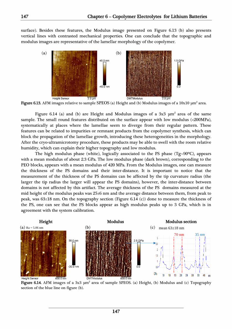
147 Chapter 6 – Copolymer Electrolytes for Lithium Batteries
147
surface). Besides these features, the Modulus image presented on Figure 6.13 (b) also presents
vertical lines with contrasted mechanical properties. One can conclude that the topographic and
modulus images are representative of the lamellar morphology of the copolymer.
(a)
(b)
Figure 6.13. AFM images relative to sample SPEOS (a) Height and (b) Modulus images of a 10x10 µm2 area.
Figure 6.14 (a) and (b) are Height and Modulus images of a 3x3 µm2 area of the same
sample. The small round features distributed on the surface appear with low modulus (<200MPa),
systematically at places where the lamellae seem to diverge from their regular pattern. These
features can be related to impurities or remnant products from the copolymer synthesis, which can
block the propagation of the lamellae growth, introducing these heterogeneities in the morphology.
After the cryo-ultramicrotomy procedure, these products may be able to swell with the room relative
humidity, which can explain their higher topography and low modulus.
The high modulus phase (white), logically associated to the PS phase (Tg~90ºC), appears
with a mean modulus of about 2.3 GPa. The low modulus phase (dark brown), corresponding to the
PEO blocks, appears with a mean modulus of 420 MPa. From the Modulus images, one can measure
the thickness of the PS domains and their inter-distance. It is important to notice that the
measurement of the thickness of the PS domains can be affected by the tip curvature radius (the
larger the tip radius the larger will appear the PS domains), however, the inter-distance between
domains is not affected by this artifact. The average thickness of the PS domains measured at the
mid height of the modulus peaks was 25±6 nm and the average distance between them, from peak to
peak, was 63±18 nm. On the topography section (Figure 6.14 (c)) done to measure the thickness of
the PS, one can see that the PS blocks appear as high modulus peaks up to 3 GPa, which is in
agreement with the system calibration.
Height Modulus Modulus section
(a) Ra = 5.06 nm (b) (c)
Figure 6.14. AFM images of a 3x3 µm2 area of sample SPEOS. (a) Height, (b) Modulus and (c) Topography
section of the blue line on figure (b).
35 nm
mean 63±18 nm
70 nm

Chapter 6 – Copolymer Electrolytes for Lithium Batteries 148
148
Topography images of the copolymer membrane with lithium salt SPEOS+LiTFSI are
presented on Figure 6.15 (a) and (d) (dimension of 3x3 µm2 and 1x1 µm2, respectively). On the
modulus images shown on Figure 6.15 (b) and (e), the microstructure of the copolymer is revealed
by the different Young’s modulus of each phase. The low modulus phase (dark brown) with a mean
modulus of 200 MPa is related to the low crystallinity PEO phase containing LiTFSI salt, which is
lower than the PEO phase without salt (mean modulus of 420 MPa). The high modulus phase
(white), related to the PS (Tg~90ºC), appears with a modulus up to 2.1 GPa (mean value of 1.28GPa).
The microstructure revealed on Figure 6.15 (b) is essentially lamellar, but the presence of the salt in
the structure clearly affects the long range order of the self-assembly. The lamellae appear with
shorter length and more spaced along the membrane. The thickness of the PS domains was
measured at the mid height of the modulus peaks and a mean value of 35±7 nm was obtained. The
average distance from peak to peak (dPS) was 88±56 nm (as shown on the modulus section analysis of
Figure 6.15 (c)). It is important to take into account that lamellae with different angular orientations
can show (as an artifact) larger inter-domain distances, which explains the high standard deviation of
these measurements. Modulus section analyses inside the dark brown phase (example given on
Figure 6.15 (f)) also revealed some regular features with modulus up to 370 MPa and spaced of 31±4
nm from each other (dPEO), probably related to the presence of 22.6% of crystalline PEO. The
characteristic distances measured are schematically represented on Figure 6.16.
Height Modulus Modulus section
(a) Ra = 5.7 nm (b) (c)
(d) Ra = 2.72 nm (e) (f)
Figure 6.15. Copolymer SPEOS+LiTFSI morphology revealed by Height and Modulus AFM images. (a) Height
and (b) Modulus of a 3x3 µm2 area; (c) represents the section of the red line on figure (b). (d) Height and (e)
Modulus of a 1x1 µm2 area; (f) represents the section of the blue line on figure (e).
70 nm => mean 88±56 nm
31 nm => mean 31±4 nm

149 Chapter 6 – Copolymer Electrolytes for Lithium Batteries
149
Figure 6.16. Schematic representation of the measured distances: the PS domain thickness, the distance
between PS domains (dPS) and the distance between PEO lamellae (dPEO).
Using SAXS experiments, Pelletier266 was able to determine the morphology of PS-PEO-PS
copolymers with a PEO volume fraction (fPEO) of at the range of 0.38 to 0.48, appearing with lamellar
morphology. However, Pelletier claims that it was impossible to determine the global morphology
for sample SPEOS and SPEOS+LiTFSI (fPEO= 0.65). Samples with high PEO content do not show well-
defined structures by SAXS appearing typically with a very broad peak of low intensity.269 Due to the
absence of higher order scattering peaks, on the basis of SAXS patterns alone, the morphology
cannot be clearly defined. Apparently the electronic contrast between the PEO and the PS blocks is
not enough to allow the long range morphological analysis by SAXS. Nevertheless, an estimation of
the characteristic inter domain distance (d0) of 31.5 nm was done by SAXS. Since this measurement
was issued from a low intensity and broad peak, it should be considered with caution. The SAXS and
AFM results are summarized on Table 6.2. Although SAXS could not provide the global morphology
of the sample, the observation of a lamellar morphology by AFM is in agreement with the
theoretical morphology determined for a copolymer with fPEO=0.65.
Table 6.2. Theoretical morphology, SAXS and AFM results for sample SPEOS and SPEOS+LiTFSI 266
Sample Copolymer fPEO
(vol) Theoretical Morphology
SAXS Morphology
d0SAXS
nm
AFM Morphology
dPEO AFM
nm
dPS AFM
nm SPEOS PS-PEO-PS 0.65 lamellar - 33 lamellar - 63±18
SPEOS+LiTFSI PS-PEO-PS 0.65 lamellar - 31.5 lamellar 31±4 88±56
Height and Modulus images corresponding to the first 10 µm of the left side of the
SPEOS+LiTFSI membrane’s cross-section are shown on Figure 6.17 (a) and (b). Figure 6.17 (b) reveals
highly oriented lamellae perpendicular to the membrane’s surface, probably induced during the
membrane’s manufacturing.267 The same trend was seen on the other side of the membrane’s cross-
section (not shown). The average thickness of the PS domains was 28±5 nm, which is lower than at
the bulk (35±7 nm) but the mean length of 413±132 nm is almost the double than what measured in
the bulk of the membrane (223±76 nm), as highlighted by the inset image on Figure 6.17 (b).
However, the average distance between the PS domains was 95±53 nm, similar to the previous 88±56
nm measured in the bulk.

Chapter 6 – Copolymer Electrolytes for Lithium Batteries 150
150
(a) Height (b) Modulus
Figure 6.17. AFM Height (a) and Modulus (b) images of a 10x10 µm2 area of the sample SPEOS+LiTFSI
from the surface to the bulk showing highly oriented lamellae perpendicular to the membrane’s surface (left).
The zoomed inset on (b) shows the lamellae on an area of 3x3 µm2.
2.4. Effect of reticulation on PS-PCi-PS copolymers morphologies
The next analyses are relative to samples SPC18S, SPC18S_X and SPC22S_X in order to evaluate
the effect of cross-linking on mechanical properties and nanophase separation. Figure 6.18 shows the
topographic and modulus AFM images of samples SPC18S, SPC18S_X and SPC22S_X. No regular
structure was seen for the analyzed samples. Indeed, the measurements have been done at room
temperature (T~23ºC), which is very close to the determined Tm of the samples: 25, 18.4 and 25.2ºC,
respectively for SPC18S, SPC18S_X and SPC22S_X. Thus, samples are essentially in an amorphous state.
The mechanical strength of the sample is basically assured by the rigid PS blocks at room
temperature.
Sample SPC18S (22%PS) appears with low roughness and a homogeneous modulus
distribution (mean modulus of 158 MPa), with no clear phase separation. Comparing sample SPC18S
with sample SPC18S_X (Figure 6.18 (b)) which has a higher fraction of PS (30%) the effect of a higher
content of PS and the cross-linking can be evidenced. In Sample SPC18S_X (Figure 6.18 (b)) a better
phase separation is seen, with elongated nodules seen on topography appearing with high modulus
(up to 1.2 GPa) on the modulus image (Figure 6.18 (e)). The presence of round or elongated features
is in accordance with the theoretical morphology for a copolymer with an fPEO~0.75, which can
present spheres or cylinders. These features are probably related to the PS blocks of the copolymers,
since the higher Tg of the PS blocks (about 70ºC for a block with 2850 g.mol-1)270 make them appear
at the glassy state. An average distance between the PS domains (dPS) was measured, giving 78±38
nm from peak to peak on the modulus image. The cross-linking has also an effect on the mean
modulus of the probed area, increasing from 158 MPa to 379 MPa. The mean value of the dark
brown phase (amorphous cross-linked PEO with salt) was about 220 MPa, higher than the mean
value of 158 MPa measured for sample SPC18S.
Sample SPC22S_X ((Figure 6.18 (c)) is also cross-linked but has longer blocks of PEO
(MnPEO=22000 gmol-1), i.e., the molar weight between each cross-links (Mc) is bigger. One can see by
the topographic and modulus images ((Figure 6.18 (c) and (f)) that the elongated high modulus
nodulus are more distant from each other (average distance of 96±38 nm). The mean modulus
dropped to about 164 MPa, the PEO (dark brown) appearing with a mean modulus of 110 MPa and
the PS phase (bright) with 360 MPa (up to 500 MPa). This drop is probably related to the presence of
longer chains of PEO between the cross-linkers. A summary of the above measurements are
presented on Table 6.3.

151 Chapter 6 – Copolymer Electrolytes for Lithium Batteries
151
SPC18S SPC18S_X SPC22S_X
(a) (b) (c)
Hei
gh
t
(d) (e) (f)
Mod
ulu
s
Figure 6.18. AFM Height of the copolymer systems: (a) SPC18S, (b) SPC18S_X and (c) SPC22S_X and the
corresponding Modulus images (d) (e) and (f). Images are 1x1µm2.
It is important to consider the lengths of the polymer chains when analyzing the measured
distances. The maximum physically possible length of the polymer, called contour length (L),
corresponds to the fully extended polymer chain. This defines the maximum distance between the
different blocks. In order to minimize its free energy, the polymer chain reduces the distance
between its two free ends, maximizing its entropy. Consequently, the effective distance between the
two ends is way less than the contour length when free of mechanical stresses. Considering the
shortest PEO blocks of the analyzed copolymers with Mn=18000 gmol-1, the contour length is
estimated to be of the order of 200 nm. The contour length for a PS block with Mn=3500 gmol-1 is of
the order of 14 nm. The inter-domains distance from the center of a PS domain to another PS
domain would be given by half the length of a PS block plus the PEO length plus half the other PS
block length (1/2PS+ PEO+1/2PS = ~214 nm). The maximum distances measured (~134 nm) are still
under this value. Even if we consider that the glassy PS blocks could stretch the flexible amorphous
PEO blocks to their maximum extension, the measured distances are still realistic, since they are
always inferior to the sum of the contour lengths of the blocks.
Table 6.3. AFM PeakForce QNM analysis of samples SPC18S, SPC18S_X and SPC22S_X
Sample Copolymer %wt Bloc PS
fPEO
(vol)
Mn
(Block PEO)
g.mol-1
Mn
(Blocks PS)
g.mol-1
EPEO MPa
EPS
MPa Emean
MPa dPS
AFM
nm
SPC18S PS-PC18-PS 23 0.78 18000 5346 - - 158 -
SPC18S_X PS-PC18-PS 30 0.72 18000 7714 220 800 379 76±38
SPC22S_X PS-PC22-PS 22 0.79 22000 6241 110 360 164 96±38

Chapter 6 – Copolymer Electrolytes for Lithium Batteries 152
152
Lassagne268 tested the effect of cross-linking on the Young modulus at 40ºC for samples with
composition of fPEO=0.79 (MnPEO = 23000 gmol-1, MnPS = 6250 gmol-1). For these samples with 21%vol
PS he could see an increase of modulus from 0.15 MPa to 3.3 MPa at 40ºC. As expected, the cross-
linking of the central block of a structured material had a significant impact on its mechanical
behavior.
Moreover, SAXS analysis of these materials (Table 6.4) showed that they exhibited a certain
phase separation, but the morphology could not be determined. The second order peak was broad
and had low intensity, meaning a large dispersion. From the first order peak, Lassagne estimated
inter-domain distances of the samples. The distance was slightly enlarged for sample SPC22S_X due
to the higher molecular weight of the PEO block, the characteristic distance (d0) increasing from 20
for sample SPC18S to 32 nm. Differences between AFM and SAXS measurements can originate from
the local measurements obtained by AFM versus the statistical measurements obtained from SAXS
(here from low intensity and broad peaks). Nevertheless, the inter-distances measured by both
techniques have the same order of magnitude.
Table 6.4. SAXS results for samples SPC18S, SPC18S_X and SPC22S_X 268
Sample Copolymer %wt PS
fPEO
(vol) Morphology
d0
nm
SPC18S PS-PC18-PS 23 0.78 not determined 20 SPC18S_X PS-PC18-PS 30 0.72 -- -- SPC22S_X PS-PC22-PS 22 0.79 not determined 32
3. Study of “single ion” copolymer electrolyte
3.1. Material used
The structure of the “single-ion” copolymers studied is presented on Figure 6.19. The
composition of the copolymer and its thermal properties determined by DSC by Lassagne are
presented on Table 6.5.
Figure 6.19. Structure of the PSTFSILI-PEO-PSTFSILI copolymer
Table 6.5. Composition of the PSTFSILi-PEO-PSTFSILi copolymer
Copolymer %wt Bloc
PSTFSILi
fPEO
(vol)
%vol PSTFSILi OE/Li 25
Mn
(PEO)
g.mol-1
Mn
(PS)
g.mol-1
Mn
Copolymer g.mol
-1
Tg
°C
Tm
°C
Xc
%
PSTFSILi-PEO- PSTFSILi 23.5 0.81 23.75 35000 10752 45752 1.7 62.4 42.9
Samples were prepared for AFM analysis of the cross-section by cryo-ultramicrotomy with
the same methodology described for the PS-PEO-PS copolymers at Section 2.2.

153 Chapter 6 – Copolymer Electrolytes for Lithium Batteries
153
3.2. Morphology of PSTFSILi-PEO-PSTFSILi copolymer
The PeakForce QNM analysis of a 3x3 µm2 area of the sample is shown on Figure 6.20. One
can see by the topography and modulus images (Figure 6.20 (a) and (b)) a lamellar morphology. The
mean thickness of the lamellae was 22±9 nm and the average distance measured between them was
27±10 nm. The proper assignment of the phases can be done based on the work of Lassagne.
(a) Height (b) Modulus
Figure 6.20. AFM (a) Height and (b) Modulus images of a 1x1 µm2 area of sample PSTFSILi-PEO-PSTFSILi.
Lassagne has shown that the miscibility of this system is improved by the presence of the salt
grafted on the structure. Indeed, he could show that certain compositions of the copolymer (< 20%wt
of PS) presented one single glass transition temperature (Tg), characteristic of miscible systems. For
low concentration of PSTFSILi, the PSTFSILi blocks are completely miscible inside the amorphous
PEO phase. Increasing the content of PSTFSILi will promote a certain phase separation, but with an
interphase with a constant composition near 50/50w (determined by the evolution of the Tg with
fPEO). The schematic representation is shown on Figure 6.21. SAXS experiments showed that the
nano-phase separation was only present below the melting temperature of the PEO phase. Thus, the
clear phase separation present at room temperature is engendered by the crystallization of PEO
(PEO rejecting PSTFSILi out of crystalline lamellae). Indeed, this sample presented 42.9% of
crystallinity and a melting temperature of 62.4ºC. From these results, we can conclude the proper
assignment of the phases seen by AFM: High modulus phase is the crystalline PEO and the low
modulus phase is the amorphous PEO mixed with PSTFSILi.
Figure 6.21. Schematic representation of the evolution of the morphology with the composition of single-ion
copolymers at room temperature. Adapted from 268

Chapter 6 – Copolymer Electrolytes for Lithium Batteries 154
154
Figure 6.22 (a) to (d) are relative to the PeakForce QNM analysis of a 1x1 µm2 area. As
indicated by the red arrows, the lamellae, relative to the crystalline PEO, appear with high modulus
(bright yellow), with a mean value of 800 MPa, low adhesion (dark brown/ 7 nN) and low
deformation (dark brown/ 3 nm). The blue arrows indicate the mixture of amorphous PEO and
PSTFSILi phases, appearing with a lower modulus (brown/ ~380 MPa), high adhesion (bright yellow/
12 nN) and high deformation (yellow/ 6 nm).
(a) Height (b) Modulus (c) Adhesion (d) Deformation
Figure 6.22. AFM images of a 1x1 µm2 area of sample PSTFSILi-PEO-PSTFSILi. (a) Height, (b) Modulus, (c)
Adhesion and (d) Deformation. Red arrow points on a crystalline PEO lamella and blue arrow on the
amorphous phase composed of amorphous PEO blended with PSTFSILi.
The lamellar morphology observed at room temperature by AFM is in total agreement with
the morphology determined by SAXS (Table 6.6) for a copolymer with the same composition by
Lassagne and Louise Frenck.268,271 The inter-domain distance measured by SAXS was 25 nm, which is
in very good agreement with the 27±10 nm measured by AFM.
Table 6.6. SAXS results for the “single-ion” sample and inter-lamellar distance measured by AFM
Copolymer %wt
Block PS fPEO
(vol) Morphology
d0SAXS
nm dAFM
nm
PSTFSILi-PEO- PSTFSILi 23.50 0.81 lamellar 25 27±10
Tensile tests at 40ºC of both systems are shown on Figure 6.23 (a). The higher crystallinity,
with the PEO lamellar morphology can explain the higher mechanical properties observed for the
PSTFSILi-PEO-PSTFSILi systems in comparison to the doped PS-PEO-PS ones. However, the presence
of crystalline PEO limits the conductivity of the sample below the PEO melting temperature. Figure
6.23 (b) shows the evolution of the conductivity with temperature. One can see that for sample
PSTFSI_81 (fPEO=0.81/blue line) the conductivity is very low at temperatures near 40ºC, but increases
considerably above 55ºC. Indeed, the ionic conductivity only increases when the melting of the PEO
crystalline domains gives sufficient mobility to the PEO chains.

155 Chapter 6 – Copolymer Electrolytes for Lithium Batteries
155
(a) (b)
Figure 6.23. (a) Tensile test at 40ºC of a PSTFSILi-PEO-PSTFSILi and a PS-PEO-PS copolymer. (b) Evolution of
conductivity of PSTFSILi-PEO-PSTFSILi copolymer as a function of temperature. 260
Probing the surface of a larger area, it was possible to reveal the presence of grains of self-
assembled domains. Figure 6.24 (a) shows the topography of a 3x3 µm2 area, in which is possible to
perceive slightly depressed topography boundaries in between adjacent zones. These boundaries
appear clearer on the corresponding Error Channel image (Figure 6.24 (b)). Figure 6.24 (c)
highlights the grain boundaries with dashed red lines as guides to the eyes.
(a) Height (b) Error Channel (c) Error Channel
Figure 6.24. AFM images of a 3x3 µm2 area of the sample TF1514. (a) Height, (b) and (c) Error Channel. The
dashed red lines added on image (c) highlight the grain boundaries.
These grains affect the ionic conductivity of electrolytes based on block copolymers. When
the lithium ions move between the electrodes, the ionic conductivity can take place in two ways:
intra–grain and inter-grain transport. Considering the intra-grain transport the key factors are the
number of dimensions of the conductive pathway (two dimensions for a lamellar structure or 3D for
a cylindrical or gyroid structure) and the orientation of the domains. For example, in a 2D lamellar
system (Figure 6.25), only a fraction of the domains contribute positively to the transport of ions,
which also depends on the orientation of the lamellae.272,273 If the non-conductive block (red) is
perpendicular to the arrival of the lithium ions, the transport will be stopped and consequently the
conductivity will be zero (Figure 6.25 (c)).

Chapter 6 – Copolymer Electrolytes for Lithium Batteries 156
156
(a) (b) (c)
Figure 6.25. Schematic representation of the effect of domain orientation on the ionic transport for a lamellar
morphology. The red domain representing the non-conductive phase and the blue domain the conductive
phase.246
Considering the inter-grain transport, the overall ionic conductivity of the electrolytes will be
lowered by the bending of the conductive channels (Figure 6.26 (b) ), by reducing their size between
two grains or completely stopped if the orientation of the adjacent grain is in a perpendicular
orientation (Figure 6.26 (c)).274
(a) (b)
Conduction lowered
(c)
No conduction
Figure 6.26. (a) Schematic representation of an electrolyte based on a block copolymer showing the
discontinuity of the domains. Non-conductive domains are in red, the conductive domains in blue and grain
boundaries in black. (b) Decrease in conductivity due to the presence of channel bending. (c) Absence of
conduction due to the perpendicular orientation of two grains.275
Thus, the AFM images evidence that besides the presence of crystallinity, the presence of
grain boundaries of self-assembled domains may limit the ionic conductivity.
3.3. Surface morphology and properties evolution with hydration degree
We have used a low spring constant AFM tip (k~0.4N/m) to probe the very top surface of the
sample. In this case, only qualitative mechanical analysis is achieved. Figure 6.27 shows AFM
complementary images of a 3x3 µm2 area of the “single-ion” sample. It is possible to notice four
domains (the larger one being surrounded by a red dashed line) with different mechanical
properties than the rest of the scanned area. These domains present high modulus (white on Figure
6.27 (b)) but at the same time high adhesion and high deformation (white on Figure 6.27 (c) and (d)).
A lamellar structure can be observed on the deformation image. This is an unexpected and
contradictory behavior, since a material with high modulus usually appears with low deformation.
We assume that this contradiction may be caused by AFM measurement artifacts, since a strong
adhesion can result in erroneous modulus and deformation calculation276–282. According to Ebenstein
et al.282 when the adhesion dominate the tip-sample interactions, nanomechanical models like
Herztian and DMT can underestimate the contact area and the effective load experienced by the
sample, resulting in an overestimation of the sample modulus. This can explain why the modulus

157 Chapter 6 – Copolymer Electrolytes for Lithium Batteries
157
measurement of is so high in the high adhesion domains. Still according to Ebenstein et al.282
another possible source of uncertainty may lie in the assumption that the jump-to-contact point
observed in the force-distance curves represents initial contact between the tip and the sample.
Attractive surface forces can cause an early jump-to-contact, leading to overestimation of
deformation from the force-distance curves.
(a) Height (b) Modulus (c) Adhesion (d) Deformation
Figure 6.27. AFM images of a 3x3 µm2 area of the “single-ion” sample PSTFSILi-PEO-PSTFSILi. (a) Height, (b)
Modulus, (c) Adhesion and (d) Deformation. The red dashed line delimits a grain with different behavior
compared to the others.
Keeping in mind the possible artifact observed by AFM, we can analyze the AFM images
obtained. Figure 6.28 shows the deformation image with a relative scale. The lamellae inside the
domain appear with a lower relative deformation (about 0.2 nm/black on the image) than the
lamellae out of the domain (about 0.68 nm/brown). However, the phase excluded from the PEO
lamellae appears with higher deformation (about 1.54 nm/white) than for the equivalent phase on
the adjacent grains (about 1.18 nm/yellow), but with higher modulus and adhesion, as shown
previously on Figure 6.27. This can be the sign that the lamellae inside these particular domains are
directly exposed to the air (and to the AFM tip) while the rest of the sample present a soft top layer
giving a slightly higher deformation above the lamellae. We observed by AFM the progressive
disappearance of the high modulus, high adhesion and high deformation domains, when the
originally dry sample equilibrates with the relative humidity of the room. Figure 6.29 shows AFM
Adhesion images of a 10x10 µm2 area of the “single-ion” sample with the evolution of two different
domains. One can see that the high adhesion zones shrink over time until their complete
disappearance after about 8 hours. The diameter of the high adhesion domain pointed by the red
arrow decreased linearly over time at a rate of about 275 nm per hour. The sample was subsequently
dried at room temperature under nitrogen flux for 2 days and the phenomenon could be observed
again. We therefore assume that the soft top layer that grows at the surface of the sample is
composed of adsorbed water and amorphous PEO mixed with PSTFSILi.

Chapter 6 – Copolymer Electrolytes for Lithium Batteries 158
158
Figure 6.28. AFM deformation image of a 3x3 µm2 area of the “single-ion” sample PSTFSILi-PEO-PSTFSILi.
Red arrows indicate the mean values of deformation of the lamellae inside the domain and on the adjacent
grains. Blue arrows indicate the mean values of the mixture PEO+PSTFSILi inside the domain and on the
adjacent grains.
(a) t=0 Dry state
(b) t = 3.5 hours (c) t = 7.2 hours Equilibrated with room RH
Figure 6.29. AFM adhesion images of a 10x10 µm area showing the evolution of the high adhesion grains with
time. (a) Initial state, t=0; (b) after 3.5 hours and (c) after 7.2 hours.
To explain the presence of a much stronger adhesion on the amorphous PEO mixed with
PSTFSILi surrounding the crystalline PEO lamellae inside of the dry domains, we propose the
following interpretation: in the dry state the CF3 groups of PSTFSILi block can strongly interact with
the AFM tip, whereas this specific interaction is absent when the sample is hydrated through water
adsorption from the air. Houston et al.283 have shown that a self-assembled monolayer film
terminated by CF3 end group presented an increase in adhesion by almost a factor of 4 compared to
CH3 end groups, as measured by interfacial force microscope (IFM) for the interaction between the
films and a tungsten tip. This interpretation of the AFM measurements can lead to a schematic
representation of the sample’s surface, presented on Figure 6.30.

159 Chapter 6 – Copolymer Electrolytes for Lithium Batteries
159
(a) (b)
Figure 6.30. Schematic representation of the surface properties of the “single-ion” sample PSTFSILi-PEO-
PSTFSILi. (a) Side view and (b) Top view
As evidenced by Figure 6.29, the hydration degree (equilibrium with room RH) of the sample
can change the mechanical behavior of the surface of these domains. One hypothesis is that when
the crystalline PEO at the surface equilibrates with the room relative humidity, part of its
crystallinity is broken and the mixture of amorphous PEO and PSTFSILi blocks is hydrated. The
hydrophobic CF3 groups turn away from the hydrated surface, decreasing adhesion. This change in
crystalline order takes place from the edges to the interior of the domains because, in general,
polymers at the edges of crystalline domains can relax more easily, once they have fewer neighbors
and hence experience fewer constraints. Consequently, they can reduce their number of chain folds
much faster than molecules inside the domains.267 This causes the gradual increase of hydration of
the amorphous PEO and PSTFSILi blocks mixture, decreasing the local adhesion (no more CF3
groups at the surface). This hypothesis is schematically presented on Figure 6.31.
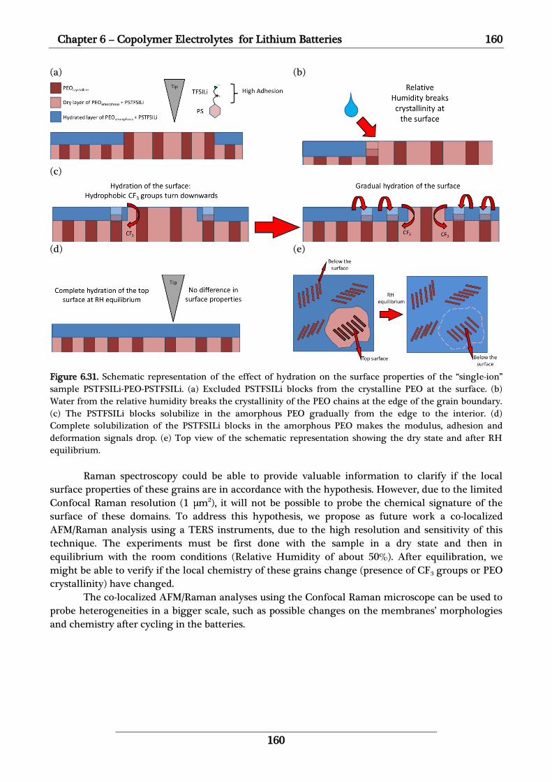
Chapter 6 – Copolymer Electrolytes for Lithium Batteries 160
160
(a) (b)
(c)
(d) (e)
Figure 6.31. Schematic representation of the effect of hydration on the surface properties of the “single-ion”
sample PSTFSILi-PEO-PSTFSILi. (a) Excluded PSTFSILi blocks from the crystalline PEO at the surface. (b)
Water from the relative humidity breaks the crystallinity of the PEO chains at the edge of the grain boundary.
(c) The PSTFSILi blocks solubilize in the amorphous PEO gradually from the edge to the interior. (d)
Complete solubilization of the PSTFSILi blocks in the amorphous PEO makes the modulus, adhesion and
deformation signals drop. (e) Top view of the schematic representation showing the dry state and after RH
equilibrium.
Raman spectroscopy could be able to provide valuable information to clarify if the local
surface properties of these grains are in accordance with the hypothesis. However, due to the limited
Confocal Raman resolution (1 µm2), it will not be possible to probe the chemical signature of the
surface of these domains. To address this hypothesis, we propose as future work a co-localized
AFM/Raman analysis using a TERS instruments, due to the high resolution and sensitivity of this
technique. The experiments must be first done with the sample in a dry state and then in
equilibrium with the room conditions (Relative Humidity of about 50%). After equilibration, we
might be able to verify if the local chemistry of these grains change (presence of CF3 groups or PEO
crystallinity) have changed.
The co-localized AFM/Raman analyses using the Confocal Raman microscope can be used to
probe heterogeneities in a bigger scale, such as possible changes on the membranes’ morphologies
and chemistry after cycling in the batteries.

161 Chapter 6 – Copolymer Electrolytes for Lithium Batteries
161
4. Conclusions of Chapter 6
The objective of this study was to reveal the bulk morphology of new Lithium batteries
electrolytes made of PEO based copolymers with different structures.
An innovative strategy had to be developed for sample preparation of these materials by
cryo-ultramicrotomy due to the high sensibility of these copolymers to water. Thanks to the
achieved developments we were able to obtain suitable samples for AFM analysis (cryo-
ultramicrotomed surface of the membrane) and also ultra-thin sections for complementary Electron
Microscopy analysis (TEM/STEM). This developed technique is robust and should be used for sample
preparation for further studies on all kinds of samples, avoiding contact with water and any
hydration effect.
Morphological analyses were done by AFM with the PeakForce QNM mode on PS-PEO-PS
copolymers with different compositions and doped with lithium salt. Images of the non-doped
copolymer showed a very regular lamellar structure, except for some localized heterogeneities
where apparently remnant products of the synthesis could break the regularity of the morphology.
The effect of the LiTFSI salt in the morphology of the electrolytes could be evidenced, with the
partial breakdown of the lamellar morphology regularity. Furthermore, we observed an orientation
of the lamellae perpendicular to the membrane’s surface, probably related to the processing of the
electrolyte, which can have an impact on the conductivity. The inter-domain distances could be
measured directly from the modulus images, by the nanomechanical differences between the
phases. The morphologies revealed by AFM could provide a clear morphological determination
when the SAXS was not conclusive.
Samples with modified PEO blocks were analyzed. The impact of the PEO block cross-linking
was evaluated by the nanomechanical properties of the different phases. We could verify the general
trend of increasing modulus with the cross-linking degree and PS content of the samples, in
accordance with macroscopic tensile tests previously done with similar samples. The increase on the
spacing between the phases with the increasing length of the PEO block and the consequentially
drop of modulus was also observed.
The study of a “single ion” copolymer revealed a different phase separation morphology, in
which lamellar stacks of crystalline PEO are surrounded by a mixture of amorphous PEO mixed
with the PSTFSILi block. The presence of grain boundaries of self-assembled domains was evidenced
in the thickness of the material. Domains with contradictory surface nanomechanical properties
(simultaneously high modulus, adhesion and deformation) were identified and the origins of this
unexpected behavior were discussed. Nevertheless, the nanomechanical properties of these domains
were followed over time and we could verify their evolution until the equilibrium with the room
relative humidity. A hypothesis to explain this phenomenon is the presence of CF3 groups from the
PSTFSILi blocks, in the dry state, that can strongly interact with the tip. These interactions gradually
decrease with the hydration degree of the surface through water adsorption from the air.
Complementary high resolution chemical analysis by TERS is proposed as future work in order to
address this hypothesis.

Chapter 6 – Copolymer Electrolytes for Lithium Batteries 162
162
4.1. Summary of Conclusions of Chapter 6
Sample preparation by cryo-ultramicrotomy was achieved for highly water sensitive samples, avoiding
any morphological/structural changes due to the melting of ice issued from frost deposition
The addition of salt in the morphology of PS-PEO-PS copolymers induces a partial breakdown of the
lamellar regularity as evidenced by AFM modulus images of the bulk of the membranes
The lamellae near the outer surface of the PS-PEO-PS membranes are longer and perpendicular to the
surface when compared to the lamellae in the bulk, probably related to the processing method of the
electrode
The inter-domain distances could be measured directly from the AFM modulus images, by the
nanomechanical differences between the phases, complementing SAXS analyses
The direct observation of the morphologies by AFM could provide a clear morphological
determination when the SAXS was not conclusive.
Nanomechanical measurements of modified PS-PEO-PS was achieved, revealing an increasing
modulus with the cross-linking degree and PS content of the samples
The morphology of the “single-ion” copolymer was revealed by AFM modulus images and its
interpretation was possible thanks to complementary SAXS analyses
There are grain boundaries of self-assembled domains in the thickness of the “single-ion” copolymer
The surface nanomechanical properties of self-assembled domains change over time until equilibrium
with the room relative humidity
Hypothesis: The strong interactions of CF3 groups from the PSTFSILi blocks with the AFM tip may
decrease with the hydration degree, causing the modification of the nanomechanical properties.
Analysis by TERS is proposed as future work in order to address this hypothesis

163 Chapter 6 – Copolymer Electrolytes for Lithium Batteries
163
5. Conclusions du Chapitre 6 en Français
L'objectif de cette étude était de révéler la morphologie de nouvelles électrolytes à piles au
lithium constituées de copolymères à base de PEO avec différentes structures.
Une stratégie innovante devait être développée pour la préparation des échantillons de ces
matériaux par cryo-ultramicrotomie en raison de la grande sensibilité de ces copolymères à l'eau.
Grâce aux développements réalisés, nous avons pu obtenir des échantillons appropriés pour l'analyse
AFM (surface cryo-ultramicrotomée de la membrane) et aussi des sections minces pour une analyse
complémentaire de microscopie électronique (TEM / STEM).
Des analyses morphologiques ont été effectuées par AFM avec le mode PeakForce QNM sur
des copolymères PS-PEO-PS avec différentes compositions et dopés avec du sel de lithium. Les
images du copolymère non dopé ont montré une structure lamellaire très régulière, à l'exception de
certaines hétérogénéités localisées où les produits apparemment restants de la synthèse pourraient
rompre la régularité de la morphologie. L'effet du sel LiTFSI dans la morphologie des électrolytes
pourrait être mis en évidence, avec la rupture partielle de la régularité de la morphologie lamellaire.
En outre, nous avons observé une orientation des lamelles perpendiculaires à la surface de la
membrane, probablement liée au traitement de l'électrolyte, ce qui peut avoir une incidence sur la
conductivité. Les distances inter-domaines peuvent être mesurées directement à partir des images de
module, par les différences nanomécaniques entre les phases. Les morphologies révélées par l'AFM
pourraient donner une détermination morphologique claire lorsque la SAXS n'était pas concluante
Les échantillons avec blocs PEO modifiés ont également été analysés. L'impact de la
réticulation du bloc PEO a été évalué par les propriétés nanomécaniques des différentes phases.
Nous pourrions vérifier la tendance générale de l'augmentation du module avec le degré de
réticulation et la teneur en PS des échantillons, conformément à des essais de traction
macroscopiques précédemment réalisés avec des échantillons similaires. L'augmentation de
l'espacement entre les phases avec la longueur croissante du bloc PEO et conséquemment une chute
de module ont été également observés.
L'étude d'un copolymère "mono-ion" a révélé une morphologie de séparation de phase
différente, dans laquelle des piles lamellaires de PEO cristallin sont entourées d'un mélange de PEO
amorphe mélangé avec le bloc PSTFSILi. La présence de limites de grain des domaines auto-
assemblés a été mise en évidence dans l'épaisseur du matériau. Des domaines ayant des propriétés
nanomécaniques de surface contradictoires (simultanément, module élevé, adhérence et
déformation) ont été identifiés et les origines de ces comportements inattendus ont été discutées.
Néanmoins, les propriétés nanomécaniques de ces domaines ont été suivies au fil du temps et nous
pourrions vérifier leur évolution jusqu'à l'équilibre avec l'humidité relative de la pièce. Une
hypothèse pour expliquer ce phénomène est la présence de groupes CF3 sur les blocs PSTFSILi, qui
peuvent fortement interagir avec la pointe, à l'état sec. Ces interactions diminuent progressivement
avec le degré d'hydratation de la surface par adsorption d'eau de l'air. Une analyse chimique
complémentaire de haute résolution par TERS est proposée comme un travail futur afin de répondre
à cette hypothèse.

Chapter 6 – Copolymer Electrolytes for Lithium Batteries 164
164
5.1. Résumé des Conclusions du Chapitre 6 en Français
La préparation d'échantillons par cryo-ultramicrotomie a été obtenue pour des échantillons fortement
sensibles à l'eau, évitant tout changement morphologique/structurel dû à la fonte de la glace issue du
dépôt de givre au cours de la préparation de l’échantillon
L'addition de sel de Lithium dans la morphologie des copolymères PS-PEO-PS induit une rupture
partielle de la régularité lamellaire, comme en témoignent les images AFM de module
Les lamelles près de la surface extérieure des membranes PS-PEO-PS sont plus longues et
perpendiculaires à la surface par rapport aux lamelles dans le volume de la membrane,
probablement liées au procédé de mise en forme de l'électrode
Les distances inter-domaines peuvent être mesurées directement à partir des images AFM de module,
par les différences nanomécaniques entre les phases, complétant les analyses SAXS
L'observation directe des morphologies par AFM a pu fournir une détermination morphologique claire
lorsque le SAXS n'était pas concluant.
Les mesures nanomécaniques du PS-PEO-PS modifié ont été réalisées, révélant un module croissant
avec le degré de réticulation et la teneur en PS des échantillons
La morphologie du copolymère "single-ion" a été révélée par des images AFM de module et son
interprétation était possible grâce à des analyses SAXS complémentaires
Il existe des limites de grain des domaines auto-assemblés dans l'épaisseur du copolymère "single-ion"
Les propriétés nanomécaniques de surface des domaines auto-assemblés changent avec le temps
jusqu'à l'équilibre avec l'humidité relative de la pièce
Les fortes interactions des groupes CF3 des blocs PSTFSILi avec la pointe AFM peuvent diminuer avec
le degré d'hydratation, provoquant la modification des propriétés nanomécaniques de surface.
L'analyse par TERS est proposée comme un travail futur afin de répondre à cette hypothèse

165 Chapter 6 – Copolymer Electrolytes for Lithium Batteries
165

CONCLUSIONS

167 Conclusions
167
GENERAL CONCLUSIONS
The complex polymeric systems’ deep understanding is important and challenging for the
development of new engineering solutions. In order to elucidate the process-structure-properties-
durability interplays, co-localization of chemical, physical and morphological information is
essential. Although challenging, it should bring direct and uncontroversial answers. The surface of a
material is not always representative of its bulk properties, for example when considering the
distribution of charges, morphology profiles and effects of ageing. Therefore, the characterization of
both the surface and the bulk is of prime importance to design more efficient materials, making
possible the optimization of fabrication processes, the characterization of the achieved properties and
the understanding of degradation/ageing. This dual characterization becomes even more critical for
thin polymeric materials (<100 µm) such as films and membranes, which can present accentuated
properties profiles throughout their thickness. The surface and bulk contributions on the final
properties can therefore be very distinct and critical for the materials performances, but it implies
technical challenges to access and distinguish surface and bulk contributions.
The main objective of this thesis was to develop an experimental methodology of
characterization capable of providing quantitative structural/morphological analyses, such as spatial
distribution of phases, concentration (or abundance) of chemical species, nanomechanical
properties, identification of specimens and statistical analyses (average domains sizes and inter-
domain distances), at scales from tens of nanometers to tens of microns. At the center of our
characterization strategy, we aimed the co-localization of morphological, nanomechanical and
chemical information using a special setup combining Atomic Force Microscopy and Confocal
Raman spectroscopy. The challenge was to achieve a precise repositioning of the sample under each
microscope. Indeed, we have chosen to combine two of the best commercially available instruments
but not specifically designed for co-localized analysis.
Substantial improvements had to be performed to allow the co-localization of AFM/Raman
information:
A specially designed active piezoelectric table had to be installed under the AFM to supress
the noise from mechanical vibrations and operation of the Raman spectrometer;
To limit the effects of thermal drift caused by temperature variations in the room, we
replaced the feet of the Raman spectrometer to an alloy with low thermal expansion
coefficient.

Conclusions 168
168
Finally, two different strategies were developped for co-localization (using the two Raman
microscopes) depending on the sample’s Raman response intensity. For samples that respond
intensely to Raman, the AFM motorized stage is simply used to move the sample from the AFM to
the Co-localized Raman microscope, and reciprocally. For polymers, which respond weakly to
Raman, mapping acquisition time can be up to 10 hours (with dimensions of 10x10 µm2
corresponding to 441 points). In this case, a lateral thermal drift as small as few µm’s over several
hours, makes mapping impossible due to distortions during the analysis. This is critical when using
the Co-localized Raman Microscope, since the sample is placed on the AFM’s stage and is thus
subjected to the thermal drifts existing between both instruments. Therefore, a specific strategy was
developed using a shuttle stage that allows transferring the sample between the AFM and the
Regular Raman Microscope,
allowing mappings with unlimited
acquisition times. To limit the
repositioning displacement (in X,
Y and also Z direction), we have
milled targets on the surface of the
sample holders, which improved
the co-localization precision (error
of less than 3 µm in both x and y
directions). Such a small error can
then usually be corrected when
superposing AFM and Raman
images.
The optimization of the system setup was essential, but not sufficient for proper co-localized
characterization. A proper sample preparation was necessary in order to achieve the best
performances with each instrument, i.e., sensitivity and spatial resolutions. At the same time, it must
comply with sample quality requirements for characterization such as: access to the complete cross-
section of the material (from the surface to the bulk) and no mechanical, thermal, chemical,
structural or morphological modification during preparation. Cryo-ultramicrotomy was chosen as
the best sample preparation method for our strategy, providing a suitable sample for both AFM and
Raman analyses (low roughness, surface parallel to the sample holder) and preserving the intrinsic
properties of the sample. Furthermore, the technique opens the possibility of multiple
complementary analyses by Electron Microscopies (SEM, TEM and STEM) or µ-ATR-FTIR for
example.
Several technical limitations had to be addressed in order to make the sample preparation by
Cryo-Ultramicrotomy possible. Among them, we highlight:
The adaptation of a specific sample holder to allow for the preparation of thin membranes
without embedding, suppressing any chemical modification (reaction/diffusion of the
embedding medium);
For water sensitive samples, a strategy was developed for suppression of frost deposition on
the sample’s surface when warming up to room temperature in order to avoid any
morphological modification due to the sample swelling or solubilization;
The use of inert polymer backings as mechanical reinforcements to achieve µ-ATR-FTIR
cross-section analysis of thin membranes.

169 Conclusions
169
During this Ph.D. work, three different polymer systems were studied: 1) blends based on
Polyamide 6 (PA6) and Acrylonitrile-Butadiene-Styrene (ABS), compatibilized with a Styrene-
Acrylonitrile grafted with Maleic Anhydride (SAN-MA) additive; 2) hybrid membranes for PEMFC
application based on a sulfonated polyetheretherketone (sPEEK) and an active network prepared by
sol-gel chemistry; and 3) block copolymers electrolyte based on PS-PEO-PS for lithium battery
application.
1) Compatibilization of Polymer Blends based on PA6/ABS
The first study, presented in Chapter 4, was focused on the impact of the compatibilizer and
the mixing protocols on the morphology of an immiscible PA6/ABS blend. The main results are:
The association of the AFM nanomechanical
properties and the Raman chemical analysis can
provide unambiguous identification of the
components of the studied system. The
nanomechanical analysis of the immiscible
PA6/ABS blend was in agreement with the
literature.
The addition of the SAN-MA copolymer at different
steps of the blending can develop different final
morphologies (particle-in-matrix or almost co-
continuous), impacting the rheology of the melted
blends and therefore the dispersion and distribution
of the sub-phases of the ABS at nanometric scale.
The presence of the compatibilizer favors the formation of the γ crystalline phase, which
amount and distribution depend on the blending protocols.
2) Hybrid Membranes for Fuel Cell
The second study, presented in Chapter 5, was focused on the fabrication of hybrid
membranes for Fuel Cell based on two different sol-gel precursors. The main goal of this study was
to qualify the impact of each step of the fabrication process (impregnation/condensation and
thermal treatments) on the membranes’ physical, nanomechanical and chemical properties, as well
as their stability over time, using co-localized AFM/Raman and complementary analyses.
The morphology of different membranes was revealed by the mechanical properties of the
different phases. Quantitative nanomechanical and chemical analyses were achieved;

Conclusions 170
170
The formation of a depleted skin layer (lower SG
concentration) about one micrometer thick was
observed on both sides of the membranes whereas
the SG phase concentration was almost constant
through the rest of the membrane thickness;
Membranes on the early steps of fabrication exhibited on
their cross-sectioned surface the diffusion and
crystallization of water-soluble species from the SG phase
into the atmospheric water condensed during the sample
preparation.
Complementary Electron Microscopy analyses by
SEM and STEM on the cryo-ultramicrotomed surfaces and
the ultrathin sections collected also gave valuable
information for the comprehension of the morphology and
the process of diffusion and crystallization of the non-
condensed SG precursors/oligomers.
We have also adapted cryo-ultramicrotomy for complementary µ-ATR-FTIR imaging of the
cross-section of the hybrid membranes, which gave additional information about the membrane’s
processing:
The post-condensation treatment increases the SG
condensation degree evidenced by methanol
elimination during this fabrication step.
Finally, we have allied morphological AFM analysis with another complementary technique,
Small Angle Neutron Scattering (SANS), to go further into the comprehension of the material’s
structure. The morphology observed by AFM directed the choice of the fitting model used for the
SANS analysis, which showed that:
The SG phase presents a hierarchically organized
system, composed of elementary particles which
aggregate into round shape domains;
The mean diameter of the SG aggregates measured by
AFM (DSG-AFM) and by SANS (DSG-SANS) are in reasonable
accordance considering the different averaging
procedures. Both analyses confirm the increasing
diameter of the SG domains with the SG uptake.

171 Conclusions
171
3) Copolymer Electrolytes for Lithium Batteries
The third study, presented in Chapter 6, focused on the morphological study of a series of
triblock copolymers, used as polymer electrolytes in Lithium Metal Polymer (LMP) batteries. The
addition of Lithium salt to the copolymer substantially increases its ionic conductivity but also its
hydrophilicity, which makes difficult the sample preparation by cryo-ultramicrotomy for direct
observation. The main developments were:
An innovative strategy was developed for the cryo-ultramicrotomy procedure due to the
material’s high sensibility to water allowing obtaining suitable samples for AFM analysis (on
the cryo-ultramicrotomed surface of the membrane) and also ultrathin sections for
complementary Electron Microscopy analysis (TEM/STEM) avoiding their water-
solubilization.
The three systems studied were based on PS-PEO-PS copolymers with Lithium salt or in
“single-ion” form. The study focused on the nanomechanical and morphological analysis by AFM
and its correlation with SAXS measurements. The main conclusions are the following:
The nanomechanical differences between the
phases allowed morphological determination
of the copolymers and measurement of the
inter-domain distances. A good correlation
with previously SAXS measurements was
achieved;
Quantitative nanomechanical
measurements allowed following the
evolution of the materials according to
their chemical structure: effect of cross-
linking and increasing length of PS and
PEO blocks;
The surface nanomechanical properties
evolution from the dry state to the
equilibrium with the room relative
humidity was evidenced.

Conclusions 172
172
Achievement of the Co-localization Strategy to study multiphase systems
For each of the three studies presented in this thesis, the AFM/Raman co-localization and the
multi-technique strategy developed were useful for the acquisition of valuable information that
could not be accessed by other means. This strategy can be applied to the study of a variety of
different materials and can provide the following information:
1) Identification of phases
The association of the AFM nanomechanical properties and the Raman chemical analysis
can provide unambiguous identification of the components of the studied system.
2) Distribution of phases (and additives)
The analysis of the phase’s distribution on the material can be done by the direct association
of AFM with Electron microscopies (SEM/STEM/TEM) data. This information can be correlated to
fabrication processes, presence of additives and thermal treatments. Raman spectroscopy can
provide additional information by probing the chemical signature of polymorphic phases or
additives in the material, which cannot always be probed directly by nanomechanical properties.
3) From morphology to structural analysis
The nanomechanical differences between phases allow for direct observation of the
nanostructure, measurement of inter-domain distances and correlation with analysis by
complementary techniques such as SAXS and SANS, in order to go further into the comprehension
of the material’s structure. X-rays and Neutrons scattering techniques can provide additional
information not probed by the nanomechanical differences evidenced by AFM. The association of
these techniques allows for the complete morphological/structural comprehension of the material
from nano to macroscopic scale, as exemplified by the characterization of the “single-ion”
copolymers, for which the previous SAXS studies allowed the proper interpretation of the AFM
images.
4) Co-localized quantitative nanomechanical and chemical analyses to follow the material
The developed strategy allows the chemical analysis of the cross-section of the material in
order to qualify the impact of each step of fabrication on its physical, nanomechanical and chemical
properties, as well as their stability over time. AFM nanomechanical measurements and Raman
chemical analysis can be used qualitatively and quantitatively on the study of modifications in the
chemical structure by cross-linking, additives, chemical treatments, annealing and ageing of
polymeric materials. Complementary µ-ATR-FTIR imaging on the cross-section of thin polymer
membranes can also provide complementary information to Raman spectroscopy, revealing effects
of undesired oxidation and chemical evolution after chemical/thermal treatments. The association of
both techniques can be useful to optimize processes and identify degradation mechanisms to
mitigate ageing effects.
5) Study of dynamic processes
Changes in morphology, nanomechanical and chemical properties of the samples can be
followed in real time under different stimuli, such as humidity variations, addition of additives,
temperature or processes such as crystallization. In this case, the kinetics of the phenomenon must
be compatible with the frame-rate of the AFM images to be followed over time. The same kind of
experiments can be performed under the Raman spectrometer by following specific bands related to
functionalized groups, polymorphs or overall crystallinity under controlled conditions, for example,
from zero humidity (under dry nitrogen flux) until 100% relative humidity. Raman spectroscopy is
capable of acquiring spectra in less than a second in order to probe changes occurring in real time,
being limited by the range of analysis and mainly by the intensity of the sample’s Raman response.

173 Conclusions
173
Perspectives
The potential for improving the amount of information that can be accessed using the AFM-
Raman co-localized strategy lies on the capabilities of the different AFM modes of operation and
complementary techniques. The main perspectives of work are listed as following:
1) Utilization of complementary AFM modes
Atomic Force Microscopy can probe a variety of properties of materials depending on the
operation methods. Probing properties such as current, conductance, surface potential, and
capacitance are increasingly important in a number of applications including research on
semiconductors, solar cells and batteries, conductive polymers and nanoelectronics. Localized
thermal analysis can also be of interest on the study of the effects of ageing in the material. Among
the modes of operation we highlight three modes that can be used in addition to PeakForce QNM in
order to help the comprehension of the process-structure-properties interplays and enlarge the range
of studied materials:
Conductive AFM (C-AFM):
In this mode, a bias voltage is applied between tip and sample, allowing for simultaneously
measurement of material’s topography and the electric current flow at the contact point of
the tip with the sample’s surface. This technique can
be useful for identifying and characterizing
conductive pathways in polymer composites and
electrolytes. These capabilities may be of interest on
the imaging of ion conductivity of the hybrid
membranes for Fuel Cell and copolymer
electrolytes for lithium batteries in their cross-
section rather than the surface, as well as
nanocomposites containing carbon nanotubes and
piezoelectric materials.284–288
Kelvin probe force microscopy (KPFM):
This mode images the surface potential distribution of a sample without direct electrical tip-
sample contact. Applications include imaging the Kelvin potential or work function of a
surface and measuring applied voltage differences between conductors. This mode can be
associated with Peak Force (PeakForce KPFM™) in order to acquire simultaneously, highly
correlated nanoscale topography, electrical and mechanical property mapping over a wide
range of samples, such as organic (semi)conducting materials for thin film transistors,
organic blends for photovoltaics and
electrode materials, which can present
surface potential variations under
light/dark conditions attributed to
changes in physical and chemical
properties including particle size,
phase of the surface layer and
nanocrystalline deposits.289,290

Conclusions 174
174
Nano Thermal Analysis (Nano-TA):
This mode enables high resolution thermal characterization with a spatial resolution of
about 100 nm to correlate morphologic information to the local thermal properties of a
material. Rather than a sample-averaged response as given by conventional thermal
methods, such as differential scanning calorimetry (DSC),
thermomechanical analysis (TMA), and dynamic mechanical
analysis (DMA), Nano-TA can provide information on localized
components/defects and profiles of thermal properties on the
cross-section of coatings, films and membranes.291–295
The association of these different modes of operation with the nanomechanical properties
given by the PeakForce QNM mode and chemical analysis by Raman can therefore be of interest to
study a variety of polymeric materials.
2) Electron Microscopy modes and characterization of water-sensitive samples
Electron microscopy techniques such as SEM, TEM and STEM open a wide range of
possibilities in terms of complementary characterization with the AFM-Raman co-localized strategy.
Energy Dispersive X-ray Spectroscopy (EDS) and Electron Energy Loss Spectroscopy (EELS) are
useful techniques for elemental analysis (atomic number Z > 10) and can be of interest for the
analysis of the interface of chemically modified nanofillers in nanocomposites and hybrid materials.
The developments achieved during the study of polymer electrolytes for Lithium batteries
open new possibilities for the characterization of water-sensitive samples. The morphological studies
by TEM/STEM on thin sections collected by cryo-ultramicrotomy are still to be done and will impose
challenges on the control of the imaging parameters to avoid electron beam damage.
3) Studies of ageing
The developed strategy allying nanomechanical characterization by AFM with qualitative
and quantitative chemical characterization by Raman spectroscopy and µ-ATR-FTIR imaging is a
powerful tool for the study of aged materials and degradation processes. Considering the hybrid
membranes for Fuel Cell, our next objective it to use this analysis strategy to quantify the physical
and chemical modifications induced into SG/sPEEK hybrid membranes after realistic Fuel Cell
operation. The same strategy can be applied to the study of copolymers for Lithium batteries after
cycling in order to first understand the chemical/structural changes induced by ageing and then to
optimize the structure and design ageing mitigation strategies.
4) Correlation of microstructural analysis with final properties
Finally, further research must be performed to correlate the fundamental microstructural
knowledge of the materials to their functional properties. In the case of the compatibilized PA6/ABS
blends, for example, the effect of the different morphologies and distribution of phases should have
an impact on the mechanical strength, impact resistance and heat distortion temperature of the
blends, which is still to be studied. In the same context, the effects of different SG precursors, their
amount and distribution in the hybrid membranes must be correlated to their proton conductivity,
swelling behavior and mechanical properties in order to adjust the fabrication process to obtain
membranes with optimum performances.

175 Conclusions
175
The work presented in this thesis has been valorized to the scientific community as follows:
Publications
▪ “AFM-Raman Co-localization Setup: Advanced Characterization Technique for
Polymers” accepted for publication in the “International Journal of Polymer Analysis
and Characterization” in September 2017
▪ “Co-localized AFM-Raman: A powerful tool to optimize the Sol-Gel chemistry of Hybrid
Polymer Membranes for Fuel Cell” accepted for publication in “Polymers” in January
2018
▪ “New insights on the compatibilization of PA6/ABS blends: A co-localized AFM-Raman
study” submitted to “Polymers” in November 2017
Presentations
▪ Oral presentation at the European Materials Research Society (E-MRS) 2017 Fall Meeting –
Warsaw, Poland - 2017
Title: Co-localized AFM-Raman on cryo-ultramicrotomed membrane cross-sections: A
powerful tool to Optimize Hybrid PEM for Fuel Cell
▪ Poster presentation at the International Conference on Advanced Energy Materials (AEM) –
Guildford, England - 2017
Title: Stabilized hybrid membranes for long-lived fuel cell. Presented by Natacha Huynh
▪ Oral presentation at the 32nd International Conference of the Polymer Processing Society
(PPS) – Lyon, France – 2016
Title: A new process to convert proton exchange membranes into high performances and
reliable hybrid membranes for fuel cell
▪ Poster presentation at the 32nd International Conference of the Polymer Processing Society
(PPS) – Lyon, France - 2016
Title: AFM-Raman Co-localization setup: Advanced characterization technique for polymers
▪ Poster presentation at the 4th International Soft Matter Conference (ISMC) – Grenoble,
France - 2016
Title: Advanced multitechnique characterization strategy: Cryo-ultramicrotomy allied with
AFM-Raman and Electron Microscopy
▪ Oral presentation at the 44th Colloque National du Groupe Français des Polymères (GFP) –
Belvaux, Luxembourg - 2015
Title: Co-localized AFM-Raman setup: a powerful tool to combine multi-technique and
multiscale characterizations of polymer membranes
▪ Poster presentation at the 44th Colloque National du Groupe Français des Polymères (GFP) –-
Belvaux, Luxembourg 2015
Title: AFM-Raman and Electron Microscopies: Complementarities for polymer membrane
characterization using cryo-ultramicrotomed cross-sections
▪ Poster presentation at the European Polymer Conference (EUPOC) – Gargnano, Italy - 2015
Title: Co-localized AFM-Raman setup: a powerful tool to study PEMFC membrane
stabilization by active nano-networks
Honours
and
awards
▪ Award of Best Poster Contribution at the European Polymer Conference (EUPOC) -
2015

Conclusions 176
176
CONCLUSIONS GENERALES EN FRANÇAIS
L’étude avancée de systèmes polymères complexes comme les mélanges compatibilisés,
nanocomposites, copolymères à bloc, etc. est cruciale pour le développement de nouvelles solutions
d'ingénierie. Afin d'élucider les relations « mise en œuvre-structure-propriétés-durabilité » de ces
systèmes, la co-localisation d’informations chimique, physique et morphologique devient essentielle
pour obtenir des réponses fiables. La surface d'un matériau n'est pas toujours représentative de ses
propriétés globales, particulièrement en ce qui concerne la distribution des charges, les profils
morphologiques et les effets de vieillissement. Par conséquent, la caractérisation de la surface et de
l’intérieur des matériaux est également d'une importance primordiale pour concevoir des matériaux
plus efficaces, permettant l'optimisation des processus de fabrication, la caractérisation des
propriétés obtenues et la compréhension des processus de vieillissement. Cette double
caractérisation devient encore plus critique pour les matériaux polymères minces (<100 μm) tels que
les films et les membranes, qui peuvent présenter des variations de propriétés importantes dans leur
épaisseur. Les contributions de la surface et du cœur sur les propriétés finales peuvent donc être très
distinctes et critiques pour les performances des matériaux, mais leur caractérisation implique des
difficultés techniques afin de distinguer les contributions de la surface et du cœur.
L'objectif principal de cette thèse était de développer une méthodologie expérimentale de
caractérisation capable de fournir des analyses structurelles/morphologiques quantitatives telles que
la répartition spatiale des phases et leur analyse statistique (moyenne des tailles de domaines et des
distances inter-domaine), l’identification et la mesure des concentrations des espèces chimiques,
l’analyse des propriétés nanomécaniques, tout cela à des échelles de dizaines de nanomètres à des
dizaines de microns. Au centre de notre stratégie de caractérisation, nous avons visé la co-
localisation des informations morphologiques, nanomécaniques et chimiques par le couplage de la
Microscopie de Force Atomique (AFM) et de la Microspectroscopie Confocale Raman. Le défi était
de réaliser un repositionnement précis de l'échantillon sous chaque microscope. En effet, nous avons
choisi de combiner deux des meilleurs instruments disponibles dans le marché mais pas
spécifiquement conçus pour une analyse co-localisée.

177 Conclusions
177
Des améliorations substantielles ont dû être effectuées pour permettre la co-localisation des
informations AFM/Raman:
o Une table piézoélectrique active spécialement conçue a été installée sous l'AFM pour
supprimer le bruit des vibrations mécaniques et du fonctionnement du spectromètre Raman;
o Pour limiter les effets de la dérive thermique causée par les variations de température dans
la pièce, nous avons remplacé les pieds du spectromètre Raman.
Finalement, deux stratégies différentes ont été développées pour la co-localisation (utilisant
chacun des deux microscopes Raman) en fonction de l'intensité de réponse Raman de l'échantillon.
Pour les échantillons qui répondent intensément au Raman, la platine motorisée AFM est
simplement utilisée pour déplacer l'échantillon de l'AFM vers le microscope Raman co-localisé, et
réciproquement. Pour les polymères, qui répondent faiblement au Raman, le temps d'acquisition des
mappings peut atteindre jusqu'à plus de 10
heures (avec des dimensions de 10x10 μm2
correspondant à 441 points). Dans ce cas, une
dérive thermique latérale aussi faible que
quelques μm sur plusieurs heures, rend la
cartographie impossible en raison de
distorsions au cours de l'analyse. Ceci est
problématique lors de l'utilisation du
Microscope Raman Co-localisé, puisque
l'échantillon est placé sur la platine AFM et est
donc soumis aux dérives thermiques existant
entre les deux instruments. Par conséquent,
une stratégie spécifique a été développée à l'aide d'une navette qui permet de transférer l'échantillon
entre l'AFM et le Microscope Raman classique, permettant des mappings avec des temps
d'acquisition illimités. Pour limiter le déplacement de repositionnement (en X, Y et aussi en
direction Z), nous avons gravé des cibles sur la surface des supports d'échantillons, ce qui a amélioré
la précision de la co-localisation (erreur inférieure à 3 μm dans les directions x et y). Une erreur
aussi faible peut alors être corrigée lors de la superposition d'images AFM et Raman.
L'optimisation de la configuration du système était essentielle, mais pas suffisante pour une
caractérisation co-localisée efficace. Une préparation d'échantillon appropriée était nécessaire pour
atteindre les performances ultimes de chaque instrument en termes de sensibilité et de résolution
spatiale. La préparation d’échantillons devait aussi respecter les exigences de qualité de l'échantillon
pour une caractérisation propre telles que: l'accès à la section transversale complète du matériau (de
la surface au cœur) et aucune modification mécanique, thermique, chimique, structurelle ou
morphologique lors de la préparation. La Cryo-ultramicrotomie sans enrobage a été choisie comme
la meilleure méthode de préparation d'échantillon pour notre stratégie, fournissant un échantillon
approprié pour les analyses AFM et Raman (faible rugosité et surface parallèle au support
d'échantillon), en préservant les propriétés intrinsèques de l'échantillon. Par ailleurs, la technique
ouvre la possibilité de multiples analyses complémentaires par microscopie électronique (SEM, TEM
et STEM) ou par μ-ATR-FTIR par exemple.

Conclusions 178
178
Plusieurs limitations techniques ont dû être dépassées afin de rendre possible la préparation
d’échantillon par Cryo-Ultramicrotomy. Parmi celles-ci, nous soulignons:
L'adaptation d'un support d'échantillon spécifique pour permettre la préparation de
membranes minces sans enrobage, en supprimant toute modification chimique (réaction/
diffusion de la résine d’enrobage);
Pour les échantillons sensibles à l'eau, une stratégie a été développée pour la suppression du
dépôt de givre sur la surface de l'échantillon lors du réchauffement jusqu'à la température
ambiante afin d'éviter toute modification morphologique due au gonflement ou à la
solubilisation de l'échantillon;
L'utilisation de renforts mécaniques inertes (polymères) pour obtenir une analyse μ-ATR-
FTIR de la coupe transversale de membranes minces.
La stratégie développée a été appliquée à trois systèmes polymères différents: 1) des
mélanges polyamide 6 (PA6) / acrylonitrile-butadiène-styrène (ABS), compatibilisés avec un styrène-
acrylonitrile greffé anhydride maléique (SAN-MA); 2) de membranes hybrides constituées d’une
matrice polymère de type polyétheréthercétone sulfoné (sPEEK) et d’une phase inorganique
chimiquement active préparée par chimie Sol-Gel (SG); 3) des copolymères à bloc de type PS-PEO-PS
utilisés comme électrolytes pour les batteries lithium.
1) Compatibilisation des mélanges de polymères à base de PA6 /ABS
La première étude, présentée au chapitre 4, a porté sur l'impact du compatibilisant et des
protocoles de mélange sur la morphologie d'un mélange PA6/ABS non miscible. Les principaux
résultats sont les suivants:
L'association des propriétés nanomécaniques obtenues
par AFM et l'analyse chimique Raman a pu fournir
une identification sans ambiguïté des composants du
système étudié. L'analyse nanomécanique du
mélange PA6/ABS immiscible était en accord avec la
littérature ;
L'ajout du copolymère SAN-MA à différentes étapes du
mélange peut développer différentes morphologies
finales (particules dans matrice ou presque co-
continues), ce qui affecte la rhéologie des mélanges
fondus et donc la dispersion et la distribution des sous-
phases de l'ABS à l'échelle nanométrique ;
La présence du compatibilisant favorise la formation de la phase cristalline γ, dont la
quantité et la distribution dépendent des protocoles de mélange.

179 Conclusions
179
2) Membranes hybrides pour pile à combustible
La deuxième étude, présentée au chapitre 5, a porté sur la fabrication de membranes
hybrides pour pile à combustible à base de deux précurseurs sol-gel différents. L'objectif principal de
cette étude était de qualifier l'impact de chaque étape du processus de fabrication
(imprégnation/condensation et traitements thermiques) sur les propriétés physiques,
nanomécaniques et chimiques des membranes, ainsi que leur stabilité au fil du temps, en utilisant la
co-localisation AFM/Raman et des analyses complémentaires.
La morphologie des différentes membranes a été révélée par les propriétés mécaniques des
différentes phases. Des analyses nanomécaniques et chimiques quantitatives ont été
réalisées;
La formation d'une couche appauvrie (concentration
SG inférieure) d'environ un micromètre d'épaisseur
des deux côtés des membranes a été observée, alors
que la concentration en phase SG était presque
constante dans le reste de l'épaisseur de la
membrane;
Des membranes après les premières étapes de fabrication
ont montré sur la surface de leur coupe transversale la
diffusion et la cristallisation d'espèces hydrosolubles de la
phase SG dans l'eau condensée après la coupe de
l'échantillon.
Des analyses complémentaires de microscopie
électronique par SEM et STEM sur les surfaces cryo-
ultramicrotomées et les sections ultra-fines collectées ont
également fourni des informations précieuses pour la
compréhension du processus de diffusion et cristallisation
des précurseurs/oligomères SG non condensés, et de la
morphologie des membranes en général.

Conclusions 180
180
Nous avons également adapté la cryo-ultramicrotomie pour l'imagerie μ-ATR-FTIR de la
coupe transversale des membranes hybrides:
Le traitement de post-condensation augmente le
degré de condensation de la phase SG. Cela a été mis
en évidence par l'élimination du méthanol au cours
de cette étape de fabrication.
Finalement, nous avons allié l'analyse morphologique par AFM avec une autre technique
complémentaire, la diffusion des neutrons à petit angle (SANS), pour aller plus loin dans la
compréhension de la structure du matériau. La morphologie observée par AFM a orienté le choix du
modèle utilisé pour l’ajustement des données SANS, qui ont montré que:
La phase SG présente un système hiérarchiquement
organisé, composé de particules élémentaires qui
s'accumulent dans des domaines de formes arrondis;
Le diamètre moyen des agrégats SG mesurés par
AFM (DSG-AFM) et par SANS (DSG-SANS) est
raisonnablement concordant, en considérant les
différentes procédures de calcul de la moyenne. Les
deux analyses confirment le diamètre croissant des
domaines SG avec la teneur en SG.
3) Électrolytes copolymères à bloc pour batteries lithium
La troisième étude, présentée au chapitre 6, a porté sur l'étude morphologique d'une série de
copolymères tribloc, utilisés comme électrolytes polymères dans des batteries lithium (LMP).
L'addition de sel de lithium au copolymère augmente considérablement sa conductivité ionique
mais aussi son hydrophilie, ce qui rend difficile la préparation de l'échantillon par cryo-
ultramicrotomie pour une observation directe. Les principaux développements ont été les suivants:
Une stratégie innovante a été développée pour la procédure de cryo-ultramicrotomie en
raison de la haute sensibilité du matériau à l'eau, permettant d'obtenir des échantillons
appropriés pour l'analyse AFM (sur la surface cryo-ultramicrotomée de la membrane) et
aussi des sections ultra-fines pour l'analyse complémentaire en microscopie électronique
(TEM/STEM) évitant leur solubilisation dans l'eau.
Les trois systèmes étudiés étaient basés sur des copolymères PS-PEO-PS avec du sel de
lithium ou sous forme "single-ion". L'étude a porté sur l'analyse nanomécanique et morphologique
par AFM et sa corrélation avec les mesures SAXS. Les principales conclusions sont les suivantes:
Les différences nanomécaniques entre les phases
ont permis l’analyse morphologique des
copolymères et la mesure des distances entre
domaines. Une bonne corrélation avec les mesures
précédentes de SAXS a été obtenue;

181 Conclusions
181
Des mesures nanomécaniques quantitatives ont
permis de suivre l'évolution des matériaux selon
leur structure chimique: effet de réticulation et
augmentation de la longueur des blocs PS et PEO;
L'évolution des propriétés nanomécaniques de
surface de l'état sec jusqu’à l'équilibre avec
l'humidité relative de la pièce a été mise en
évidence.
Les apports de la Stratégie de Co-localisation pour l'étude de systèmes multiphasés
Pour chacune des trois études présentées dans cette thèse, la co-localisation AFM/Raman et la
stratégie multi-technique développée ont été utiles pour l'acquisition d'informations précieuses qui
n'aurait pas pu être accessibles par d'autres moyens. Cette stratégie peut être appliquée à l'étude
d'une variété de matériaux différents et peut fournir les informations suivantes:
1) Identification des phases
L'association des propriétés nanomécaniques AFM et l'analyse chimique de Raman peuvent
fournir une identification sans ambiguïté des composants du système étudié.
2) Distribution des phases (et des additifs)
L'analyse de la distribution des phases dans le matériau peut être effectuée par l'association
directe de l'AFM avec les microscopies électroniques (SEM/STEM/TEM). Cette information peut être
corrélée aux processus de fabrication, à la présence d'additifs et à des traitements thermiques. La
spectroscopie Raman peut fournir des informations supplémentaires en sondant la signature
chimique des phases polymorphes ou des additifs dans le matériau, ce qui ne peut pas toujours être
sondés directement par contraste nanomécanique ou chimique (staining).
3) De la morphologie à l'analyse structurelle
Les différences nanomécaniques entre les phases permettent une observation directe de la
nanostructure, la mesure des distances entre domaines et la corrélation avec l'analyse par des
techniques complémentaires telles que SAXS et SANS, afin d'approfondir la compréhension de la
structure du matériau. Les techniques de diffusion des rayons X et des neutrons peuvent fournir des
informations supplémentaires non sondées par les différences nanomécaniques mises en évidence
par AFM. L'association de ces techniques permet la compréhension morphologique/structurelle
complète du matériau de l'échelle nano à l'échelle macroscopique, comme en témoigne la
caractérisation des copolymères "single-ion", pour lesquels les études SAXS précédentes ont permis
une interprétation correcte des images AFM.

Conclusions 182
182
4) Analyses nanomécanique et chimique quantitative pour suivre l’évolution du matériau
La stratégie développée permet l'analyse chimique de la coupe transversale du matériau afin
de qualifier l'impact de chaque étape de fabrication sur ses propriétés physiques, nanomécaniques et
chimiques, ainsi que leur stabilité au fil du temps. Les mesures nanomécaniques obtenues par AFM
et l'analyse chimique quantitative par Raman peuvent être utilisées qualitativement et
quantitativement sur l'étude de tout changement lié à l'évolution de la structure, à l'oxydation ou
aux pertes des composants par des traitements thermiques et le vieillissement des matériaux
polymères. L’analyse par μ-ATR-FTIR sur la coupe transversale de membranes polymères peut
également fournir des informations complémentaires à la spectroscopie Raman, révélant les effets
de l'oxydation indésirable et l'évolution chimique après des traitements chimiques/thermiques.
L'association des deux techniques peut être utile pour optimiser les processus et identifier les
mécanismes de dégradation pour atténuer les effets du vieillissement.
5) Étude des processus dynamiques
Les changements morphologiques et des propriétés nanomécaniques et chimiques des
échantillons peuvent être suivis en temps réel pour différents stimuli, tels que les variations
d'humidité, l’ajout d'additifs, variation de la température ou des processus tels que la cristallisation.
Dans ce cas, la cinétique du phénomène à suivre au fil du temps doit être compatible avec la vitesse
d’imagerie de l’AFM. Le même type d'expériences peut être effectué sous le spectromètre Raman en
suivant des bandes spécifiques liées à des groupes fonctionnalisés, des polymorphes ou une
cristallinité globale dans des conditions contrôlées, par exemple d’une humidité allant de 0 (sous
flux d'azote sec) à 100% d'humidité relative. La spectroscopie Raman est capable d'acquérir des
spectres en moins d'une seconde afin de sonder les changements en temps réel, en étant limité par la
gamme d'analyse et principalement par l'intensité de la réponse Raman de l'échantillon.
Perspectives
Le potentiel d'amélioration de la quantité d'informations auxquelles on peut accéder en
utilisant la stratégie co-localisée AFM-Raman repose sur les capacités des différents modes de
fonctionnement AFM et des techniques complémentaires. Les principales perspectives du travail
sont les suivantes:
1) Utilisation des modes AFM complémentaires
La Microscopie de Force Atomique peut sonder une variété de propriétés de matériaux selon
les méthodes d'opération. Les propriétés telles que le courant, la conductance, le potentiel de surface
et la capacité sont de plus en plus importantes dans un certain nombre d'applications, y compris la
recherche sur les semi-conducteurs, les cellules solaires et les batteries, les polymères conducteurs et
la nanoélectronique. L'analyse thermique localisée peut également être utile pour étudier les effets
du vieillissement dans les matériaux. Parmi les modes de fonctionnement pertinents, nous mettons
en évidence trois modes qui peuvent être utilisés en plus du PeakForce QNM afin d'aider à la
compréhension des relations « mise en œuvre-structure-propriétés-durabilité » et élargir la gamme
de matériaux étudiés:

183 Conclusions
183
Conductive AFM (C-AFM):
Dans ce mode, une tension de polarisation est appliquée entre la pointe et l'échantillon, ce
qui permet de mesurer simultanément la topographie du matériau et le flux de courant
électrique au point de contact de la pointe avec la surface de l'échantillon. Cette technique
peut être utile pour identifier et caractériser les
chemins de conduction dans les composites
polymères et les électrolytes (conductivité
ionique des membranes hybrides pour PEMFC,
des copolymères utilisés comme électrolytes pour
les batteries lithium, ainsi que les
nanocomposites contenant des nanotubes de
carbone et des matériaux piézoélectriques). 284–288
Microscopie à sonde de Kelvin (KPFM):
Ce mode représente la répartition du
potentiel de surface d'un échantillon
sans contact direct de la pointe avec
l'échantillon. Les applications
comprennent l'imagerie du potentiel
de Kelvin ou la fonction de travail
d'une surface et la mesure des
différences de tension appliquées
entre les conducteurs. Ce mode peut être associé au Peak Force (PeakForce KPFM ™) afin
d'acquérir simultanément la topographie à l'échelle nanométrique et la cartographie des
propriétés électriques et mécaniques pour une large gamme d'échantillons, tels que des
matériaux organiques semi-conducteurs pour transistors à couche mince, mélanges
organiques pour le photovoltaïque et les matériaux d'électrode, qui peuvent présenter des
variations de potentiel de surface dans des conditions de lumière/obscurité attribuées à des
changements dans les propriétés physiques et chimiques, y compris la taille des particules, la
phase de la couche superficielle et les dépôts nanocristallins. 289,290
Nano analyse thermique (Nano-TA):
Ce mode permet une caractérisation thermique à haute résolution avec une résolution
spatiale d'environ 100 nm pour corréler l'information morphologique aux propriétés
thermiques locales d'un matériau. Plutôt qu'une réponse moyenne de l'échantillon donnée
par des méthodes thermiques conventionnelles, telles que la
calorimétrie différentielle à balayage (DSC), l'analyse
thermomécanique (TMA) et l'analyse mécanique dynamique
(DMA), la Nano-TA peut fournir des informations locales sur les
composants/défauts et les profils de propriétés thermiques sur la
coupe transversale de revêtements, films et membranes. 291–295
L'association de ces différents modes de fonctionnement avec les propriétés nanomécaniques
fournies par le mode PeakForce QNM et l'analyse chimique par Raman peuvent donc permettre
l'étude d’une large gamme de matériaux polymères.

Conclusions 184
184
2) Modes de microscopie électronique et caractérisation d’échantillons sensibles à l'eau
Les techniques de microscopie électronique telles que SEM, TEM et STEM ouvrent une large
gamme de possibilités en termes de caractérisation complémentaire à la stratégie de co-localisation
AFM-Raman. La spectroscopie de rayons X à dispersion d’énergie (EDS) et la spectroscopie de perte
d'énergie (EELS) sont des techniques utiles pour l'analyse élémentaire (numéro atomique Z>10) et
peuvent être intéressantes pour l'analyse de l'interface des nano charges chimiquement modifiés
dans les nanocomposites et les matériaux hybrides.
Les développements réalisés au cours de l'étude des électrolytes polymères pour les batteries
lithium ouvrent de nouvelles possibilités pour la caractérisation des échantillons sensibles à l'eau.
Les études morphologiques par TEM/STEM sur des sections minces collectées par cryo-
ultramicrotomie restent à faire et imposeront des défis sur le contrôle des paramètres d'imagerie
pour éviter l’endommagement des échantillons par le faisceau d'électrons.
3) Études du vieillissement des matériaux
La stratégie développée alliant la caractérisation nanomécanique par AFM avec une
caractérisation chimique qualitative et quantitative par spectroscopie Raman et l'imagerie μ-ATR-
FTIR est un outil puissant pour l'étude des matériaux vieillis et des processus de dégradation. Pour
les membranes hybrides pour PEMFC, notre prochain objectif est d'utiliser cette stratégie d'analyse
pour quantifier les modifications physiques et chimiques induites dans les membranes hybrides
SG/sPEEK après leur test (vieillissement) sur un banc de pile. La même stratégie peut être appliquée
à l'étude des copolymères pour les batteries au lithium après le cyclage afin de comprendre d'abord
les changements chimiques/structurels induits par le vieillissement, puis d'optimiser la structure et
de concevoir des stratégies de stabilisation.
4) Corrélation de l'analyse microstructurale avec les propriétés fonctionnelles
Enfin, d'autres recherches doivent être effectuées pour corréler les connaissances
microstructurales fondamentales des matériaux et leurs propriétés fonctionnelles. Dans le cas des
mélanges compatibilisés PA6/ABS, par exemple, l'effet des différentes morphologies et de la
distribution des phases devrait avoir une incidence sur la résistance mécanique, la résistance aux
chocs et la température de distorsion thermique des mélanges, ce qui doit encore être étudié. Dans le
même contexte, les effets de différents précurseurs de SG, leur quantité et leur distribution dans les
membranes hybrides doivent être corrélés à leur conductivité protonique, au comportement de
gonflement et aux propriétés mécaniques afin d'ajuster le processus de fabrication pour obtenir des
membranes présentant des performances optimales.

185 Conclusions
185

ANNEXES
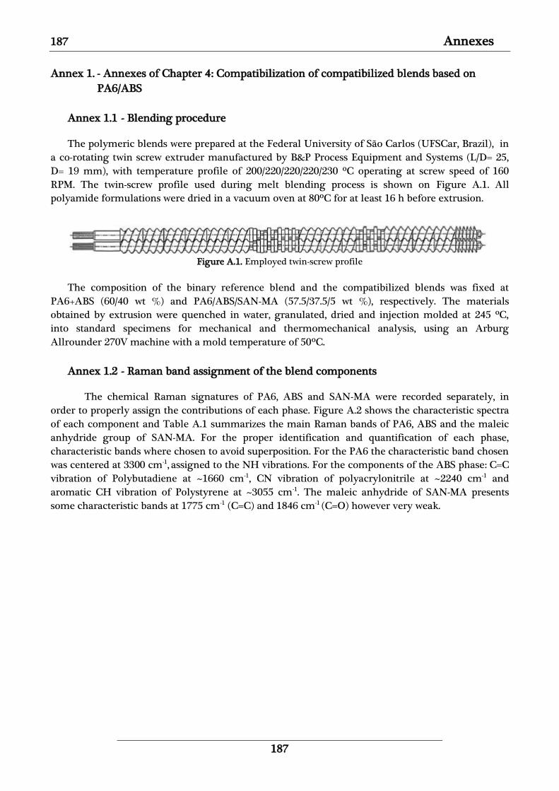
187 Annexes
187
Annex 1. - Annexes of Chapter 4: Compatibilization of compatibilized blends based on
PA6/ABS
Annex 1.1 - Blending procedure
The polymeric blends were prepared at the Federal University of São Carlos (UFSCar, Brazil), in
a co-rotating twin screw extruder manufactured by B&P Process Equipment and Systems (L/D= 25,
D= 19 mm), with temperature profile of 200/220/220/220/230 ºC operating at screw speed of 160
RPM. The twin-screw profile used during melt blending process is shown on Figure A.1. All
polyamide formulations were dried in a vacuum oven at 80ºC for at least 16 h before extrusion.
Figure A.1. Employed twin-screw profile
The composition of the binary reference blend and the compatibilized blends was fixed at
PA6+ABS (60/40 wt %) and PA6/ABS/SAN-MA (57.5/37.5/5 wt %), respectively. The materials
obtained by extrusion were quenched in water, granulated, dried and injection molded at 245 ºC,
into standard specimens for mechanical and thermomechanical analysis, using an Arburg
Allrounder 270V machine with a mold temperature of 50ºC.
Annex 1.2 - Raman band assignment of the blend components
The chemical Raman signatures of PA6, ABS and SAN-MA were recorded separately, in
order to properly assign the contributions of each phase. Figure A.2 shows the characteristic spectra
of each component and Table A.1 summarizes the main Raman bands of PA6, ABS and the maleic
anhydride group of SAN-MA. For the proper identification and quantification of each phase,
characteristic bands where chosen to avoid superposition. For the PA6 the characteristic band chosen
was centered at 3300 cm-1, assigned to the NH vibrations. For the components of the ABS phase: C=C
vibration of Polybutadiene at ~1660 cm-1, CN vibration of polyacrylonitrile at ~2240 cm-1 and
aromatic CH vibration of Polystyrene at ~3055 cm-1. The maleic anhydride of SAN-MA presents
some characteristic bands at 1775 cm-1 (C=C) and 1846 cm-1 (C=O) however very weak.

Annexes 188
188
Figure A.2. Raman spectra of ABS, PA6, and SAN-MA and identified with an arrow the characteristic bands
used for identification. PA6 at 3300cm-1 (NH), PB at 1660 cm-1 (C=C), PAN at 2240 cm-1 (CN), PS at 3055 cm-1
(aromatic CH) and MA at 1775 cm-1 (C=O)
Table A.1 Raman spectra of the components and assignment of the Raman bands 160,199,296–298
PA6 ABS
MA Assignment PAN PB PS
928m CO-NH
1000vs Aromatic ring
1030m Aromatic ring
1065m υ(C-O)
1060-1225m υ(C-C)
1264m υ(C-O), υ(C-COO)
1440s 1440m 1440m 1440m CH2 bending
1580w Aromatic Ring
1600m Aromatic Ring
1635s Amide-I
1650sh υ(C=C) cis
1667m υ(C=C) trans
1775vw υ (C=O)
1846vw υ (C=O)
2238s Nitrile
2882vs 2880m 2880m υ(CH2)
2901vs 2900s 2900s υ(CH2)
2958vs υ(CH2)
3055s Aromatic ring
3300m υ(N-H)
vs: very strong; s: strong; m: medium; w: weak; vw: very weak; sh: shoulder; υ: stretching

189 Annexes
189
Annex 1.3 - Rheological Measurements
Viscoelastic behaviors of polymeric blends were evaluated on a parallel-plate Advanced
Rheometric Expansion System (ARES) rheometer (DEMa, São Carlos, Brazil). Samples were
compression molded into 1 mm thickness disk-shape specimens at 245ºC. Frequency sweep tests
from 500 to 0.1 rad were carried out in oscillatory shear and strain of 5% at 245ºC under dry
nitrogen atmosphere. Each rheological measurement was performed within the materials’ linear
viscoelastic region.
Annex 1.4 - Differential Scanning Calorimetry (DSC)
Melting and crystallization temperatures and the corresponding enthalpies of the PA6/ABS
blends were determined by differential scanning calorimetry (DSC) using a TA Instruments Q20
apparatus. These analyses were performed on samples cut from the center part of the injection
molded specimens. Prior to analysis, samples were dried 24 hours under a nitrogen flux in order to
avoid any moisture artifacts on the thermograms.299 A heat-cool-heat program was used from 30 to
250°C with a heating/cooling rate of 10°C.min-1. Crystallization temperatures (Tc) and enthalpies
(ΔHc) were obtained from the cooling cycle; melting temperatures (Tm) and enthalpies (ΔHf) were
obtained from the first and second heating cycle and the degree of crystallization (Xc) was calculated
according to Eq. A.1:
𝑋𝑐 = ΔH𝑓
ΔH𝑓0(𝑃𝐴6)
× 1
𝑤𝑃𝐴6× 100 A.1
Where ΔHf is the enthalpy of fusion obtained by DSC; ΔH𝑓0(𝑃𝐴6) = 240 𝐽𝑔−1 is the enthalpy of
fusion of 100% crystalline PA6 and wPA6 is the weight fraction of PA6 in the blends.300
The enthalpy of fusion of α and γ phases was determined by Karl-Heinz Illers300 as 241 Jg-1 for the
α-phase and 239 Jg-1 for γ-phase. Since the difference is small, the mean value of 240 Jg-1 was used for
quantification of both phases by deconvolution of the melting peak. The determination of the
baseline used to calculate the crystallinity index of each sample was done using the procedure
described in the literature299, in order to take into account any effects of residual moisture (dried
samples under a nitrogen flux), silent crystallization and stress relaxations.
Annex 1.5 - Fabrication and analysis of the reference PA6 polymorphs
In order to obtain raw data on the polymorphs’ Raman chemical signature, PA6 samples in
different crystallographic forms were prepared: an amorphous sample was obtained by quenching in
liquid nitrogen a PA6 sample from the melt (250ºC), and crystalline samples exhibiting α and γ
phases were obtained by isothermal crystallization (from the melt at 250°C) at 180ºC and 80ºC
respectively. X-Ray Diffraction analysis of the references samples was performed for the
identification of PA6 samples presenting a single polymorph (α, γ or amorphous) in order to allow
the assignment of the Raman spectra to each PA6 polymorph. The X-Ray diffraction patterns in
Figure A.3(a) show that each of the reference samples presents only one single polymorph of PA6
crystal, as described in the literature.243,301,302 DSC analysis showed that the γ sample presented less
than 5% of crystallinity and two α samples presented 33 and 19% of crystallinity (labelled 33%C and
19%C). The determination of the crystallinity index by DSC requires special care for polyamides
(due to moisture absorption, silent crystallization and stress relaxation) and it becomes more
difficult for low crystallinity samples.299 Raman spectra were then acquired on preferential zones

Annexes 190
190
where the crystallinity was higher, detected by polarized optical microscopy (for γ sample). Figure
A.3(b)) presents the characteristic Raman spectra of the α, γ and amorphous phases. The C-C
stretching region of the PA6 Raman spectra is composed of three primary peaks at 1060, 1080, and
1125 cm-1. The peaks at 1060 and 1125 cm-1 are characteristic of the C-C symmetric vibrations for
trans conformation of the backbone, the signature of the monoclinic α-phase of PA6, while the 1080
cm-1 peak is attributed to the C-C vibration of gauche conformation, signature of the hexagonal γ-
phase.198–200 One can see that the γ-phase has also a characteristic peak that appears at 960 cm-1 and
which, although not very intense, could be used for phase identification. The amorphous phase
presents both 1080 and 1125 cm-1, characteristic of gauche and trans conformations, globally with
low intensity and no preferable conformation. The increase of crystallinity in each of the crystalline
forms engenders the prevalence of one band relative to the other. Thus, it is possible to quantify the
presence of each phase by the characteristic intensity ratio of the bands at 1080 and 1125cm-1
(I1080/I1125).
(a)
(b)
Figure A.3. (a) X-Ray Diffraction of Polyamide 6 in different forms. (i) Alpha form, (ii) Gamma and (iii)
Amorphous; and (b) respective Raman spectra of each phase
Table A.2 reports the I1080/I1125 Raman ratio from the literature and experimentally calculated
from at least 10 different spectra, as well as samples’ crystallinity index estimated by DSC. The
amorphous samples presented an I1080/I1125 ratio of 1.41±0.05. Increasing the amount of α-phase
(19%C) decreased the I1080/I1125 ratio down to 0.43±0.04 and an increase on its crystallinity (33%C)
decreased even more the ratio down to 0.33±0.01. The low standard variations of the measurements
confirm the homogeneity of these samples. Contrarily, the I1080/I1125 ratio increased to 2.0±0.4 with
the increase of γ-phase. Despite efforts, a gamma sample with higher crystallinity could not be
obtained by isothermal crystallization. Nevertheless, one can expect that the I1080/I1125 ratio will
increase with γ-phase’s crystallinity. In conclusion, the higher the crystallinity of γ-phase detected,
the higher the I1080/I1125 ratio. Inversely, the ratio decreases with the increasing crystallinity of α-
phase. Since the Raman intensity characteristic of one phase is proportional to its content in the
material, the differences between the experimentally calculated values and the literature are related
to different samples’ crystallinities (no information on the crystallinity index available from
literature data).

191 Annexes
191
Table A.2. Characteristic band intensity ratios from literature and calculated experimentally from at least 10
Raman spectra in an area of 10x10 µm2. The overall crystallinity index on the sample is presented in brackets
I1080/I1125
Amorphous
Alpha (α) Gamma (γ)
Literature201
- 0.42 2.5
Experimental 1.41±0.05 [< 5%C] 0.33±0.01 [33%C] 2.0±0.4 [< 5%C]*
0.43±0.04 [19%C]
* Raman spectra acquired where the crystallinity was higher, detected by polarized optical microscopy
Annex 1.6 - Co-localized AFM-Raman analyses of the compatibilized blends
Co-localized AFM-Raman analyses were done in order to evaluate the impact of the blending
protocol on the compatibilization (phases’ distribution, structure) and the co-localization precision.
Raman mappings presented in Figure A.4 are relative to the chemical distribution of each
component in the blends co-localized with AFM images in a 10x10 µm2 area (Figure A.4 (a)-1 to 3)
corresponding to 1-(PA6/ABS/SAN-MA), 2-(ABS/SAN-MA)+PA6 and 3-(PA6/SAN-MA)+ABS). Figure
A.4(b)-1 to (b)-3 present the PA6 matrix signal, which appears homogeneous on the mapped area of
the three samples contrary to what was observed for the reference PA6+ABS sample (Figure 4.8).
Figure A.4 (c)-1 to (c)-3 are relative to the Polybutadiene. Due to the micrometric resolution of the
Raman, the PB spheres included in the ABS phase cannot be individually distinguished, but zones
with higher concentration of PB spheres are clearly visible on the Raman mappings. Based on these
mappings, the areas corresponding to higher concentration of PB domains were highlighted by a red
border and superposed on a binarization of the AFM modulus images as shown on Figure A.4 (f)-1 to
(f)-3. The binary AFM modulus images show the PB spheres in black to be used as guides for the co-
localization. The AFM/Raman co-localization efficiency is confirmed by the good correlation
between the PB Raman mappings and the PB clusters highlighted by AFM. The Raman maps
showing the distribution of the PS and PAN phases (Figure A.4 (d) and (e), respectively) reveal the
presence of these components all over the samples, whatever the blending protocol, i.e., the signal is
never zero (scale limits were chosen in order to enhance contrast for correlation with the ABS
clusters). In contrast, the reference sample PA6+ABS (Figure A.4 (d) and (e)), exhibited a clear phase
separation between PA6 and PS/PAN (the signal relative to PS and PAN is zero inside Polyamide
areas). This fact also evidences the improvement on the PA6/ABS miscibility due to the addition of a
SAN-MA compatibilizer. The mapped area of the sample (ABS/SAN-MA)+PA6 presented higher
Raman signal of PB, PAN and PS than the other samples (brighter zones on the image). This is
related to the bigger size and thickness of the ABS domains and its almost co-continuous
morphology, in accordance the previous AFM and TEM images of Figure 4.11.

Annexes 192
192
(PA6/ABS/SAN-MA) (ABS/SAN-MA)+PA6 (PA6/SAN-MA)+ABS (a)-1 (a)-2 (a)-3
AF
M
Image
(b)-1 (b)-2 (b)-3
Map
pin
g P
A6
(32
30
-335
0cm
-1)
(c)-1 (c)-2 (c)-3
Map
pin
g P
B
(16
57
-168
0cm
-1)
(d)-1 (d)-2 (d)-3
Map
pin
g P
AN
(2
200
-228
0cm
-1)
(e)-1 (e)-2 (e)-3
Map
pin
g P
S
(30
20
-312
0cm
-1)
(f)-1 (f)-2 (f)-3
AF
M B
inary
Mod
ulu
s Im
age
Figure A.4. AFM-Raman co-localized analysis of samples 1- (PA6/ABS/SAN-MA), 2- (ABS/SAN-MA)+PA6 and 3-(PA6/SAN-
MA)+PA6. (a) AFM Image; Raman mapping area relative to: (b) Polyamide 6 (c) Polybutadiene (d) Acrylonitrile and (e)
Polystyrene; (f) AFM Binary Modulus image. PB domains were highlighted by a red border on the images (c) to (f).

193 Annexes
193
Annex 1.7 - Raman analysis of characteristic PA6 γ-phase band at 960 cm-1
An attempt to distinguish between the α and the amorphous phases was performed using the γ-
phase characteristic peak at 960 cm-1 and the peak at 920 cm-1 (CO-NH), to calculate a new ratio
I920/I960 capable of revealing the contribution of the α-phase. The higher the crystallinity of α-phase
detected, the higher the I920/I960 ratio (I920/I960 ). Inversely, the ratio decreases with the increasing
amount of amorphous phase (I920/I960 ~1). This means that if one compare this ratio with the I1080/I1125
ratio it would be possible to distinguish if the zones of lower I1080/I1125 ratio (~1.5) are mixtures of α+γ
or amorphous zones. However, a clear conclusion was difficult to provide for these blends, due to the
low intensity of this peak and the presence of high intensity peaks related to the PS phase at 1000
and 1030 cm-1, as one can observe on Figure A.5(a). This increases the uncertainty on the
deconvolution of the peak at 960 cm-1 for further analysis. Figure A.5(b) shows the result of a
subtraction of a spectrum with low I1080/I1125 ratio from one with a high ratio. One can see that the
remaining peaks are all relative to the Polyamide 6 in γ-phase, which confirms that areas with high
I1080/I1125 ratio present more γ-phase than the low ratio zones. However, it is not possible to affirm if
these low ratio zones are composed of mixtures of α+γ or amorphous zones.
(a) (b)
Figure A.5. (a) Typical spectra of areas with high, intermediary and low ratio I1080/I1125; (b) Spectra of the
subtraction of the low I1080/I1125 ratio spectrum from the a high ratio I1080/I1125 spectrum
Annex 2. - Annexes of Chapter 5: Hybrid Membranes for Fuel Cell
Annex 2.1 - Fabrication process of the hybrid membranes based on SHDi precursor
The fabrication of the hybrid membranes based on SHDi precursor was done as part of the
Ph.D. thesis of Isabel Zamanillo López at the laboratory SyMMES/Grenoble. The steps were done as
follows:
Step 1: From a pristine to a host sPEEK membrane
Prior to the impregnation of the host sPEEK membrane with the SG precursor, the host
membrane was prepared as followed. The pristine sPEEK membranes were re-acidified in a 1M
sulfuric acid solution at room temperature for 4 hours and triple rinsed with pure water. Then a
hydrothermal treatment (liquid water at 80ºC for 72h) was applied on the re-acidified membrane in
order to improve the nano-phase separation between hydrophilic and hydrophobic domains. This
hydrothermal treatment allows improving the membrane’s proton conductivity to make it
comparable with the benchmark Nafion.303 Finally this host sPEEK membrane was conditioned in 50-

Annexes 194
194
50vol% methanol-water mixture, the solvent composition used for the SG
impregnation/condensation step.
Step 2: Sol-Gel impregnation/condensation into a host sPEEK membrane
A 0.2 M SG precursor solution in a 50/50 water/ethanol mixture at pH 4.5 (addition of acetic acid)
was prepared. 2 hours were needed to obtain a homogenous solution, after what the host sPEEK
membrane was immersed into this solution during 4 days (at room temperature). Then the
membrane was removed, rinsed with pure water to avoid the formation of a SG coating on the outer
surface (potential loss of proton conductivity and problems of compatibility with the electrodes in
fuel cell), and then dried under vacuum conditions at room temperature.
Step 3: Post-Condensation (PC) of the SG phase to improve its extent of condensation
The hybrid membrane was thermally post-condensed at 74ºC and 6.3%RH for 72 hours.
Step 4: A HydroThermal (HT) treatment to improve the proton conductivity of the hybrid
membrane
A hydrothermal treatment (liquid water at 80ºC for 72 hours) was applied to the hybrid
membrane in order to improve its proton conductivity, and eventually remove any uncondensed SG
precursors or entrapped oligomers.
Annex 2.2 - Thermogravimetric Analysis (TGA) of hybrid membranes based on SHDi
precursors
The SG uptake of the hybrid membrane was determined by thermogravimetric analysis
(TGA 92-12 from Setaram Instrumentation, with a resolution of 1 µg). Samples were heated at
10ºC/min from room temperature up to 700ºC under O2 flow to ensure a complete degradation of
the organic phase. The SG uptake was determined according to Equation A.2 taking into account the
SiO2 weight residue at 700°C and the weight of dry hybrid membrane at 200°C (a temperature
corresponding to the complete water desorption).
%𝑆𝐺 =
𝑚 𝑆𝑖𝑂2 𝑟𝑒𝑠𝑖𝑑𝑢𝑒 𝑎𝑡 700°𝐶
𝑀𝑆𝑖𝑂2×𝑀𝑆𝐺
𝑚 ℎ𝑦𝑏𝑟𝑖𝑑 𝑚𝑒𝑚𝑏𝑟𝑎𝑛𝑒 𝑎𝑡 200°𝐶−(𝑚 𝑆𝑖𝑂2 𝑟𝑒𝑠𝑖𝑑𝑢𝑒 𝑎𝑡 700°𝐶
𝑀𝑆𝑖𝑂2×𝑀𝑆𝐺)
× 100%
A.2
Where M SiO2 = 60.08 g/mol and MSG = Molar Mass of the SG repeat unit of the condensed
SG phase from SHDi precursor = 134.32 g/mol.
Annex 2.3 - Raman assignment of the sPEEK and SG phase chemical signatures
The chemical Raman signatures of each component of the hybrid membranes were recorded
separately, in order to properly assign the contributions of each phase. Figure A.6 below shows the
typical spectra of the host sPEEK membrane and a hydrolyzed and condensed precursor, here called
polySHDi, from 400 to 3250 cm-1. The assignment of each peak is listed on Table A.3. The
differentiation of both phases can be easily done from 2400 to 3250 cm-1 once the peak centered at
~3070 cm-1 is assigned as to the contribution of the CH units of the aromatic ring presented on the
sPEEK structure, and the peak centered at ~2900 cm-1 refers to the –CH2 /–CH3 vibrations presented
on the Sol-Gel structure, as well as the peak at ~2580 cm-1 which is related to the thiol (-SH)

195 Annexes
195
functions. The presence of a peak at ~507 cm-1 can indicate the presence of di-sulfide (-S-S-) functions
issued from an oxidation of thiol units.
Figure A.6. Raman spectra of pure sPEEK and condensed SG precursor (polySHDi)
Table A.3. Observed Raman shifts (cm-1), band intensities and assignments for the polymers244,304–306
sPEEK polySHDi Assignment
507 m υ(S-S)
648 m υ(S-C)
746 m υ(S-C)
810 m ω(CH)
863 w CH2 rock trans
1002 w υ(C-C) trans
1010 w Ring stretching mode or δC-H
1039 w CH2 rock trans
1147 vs δ(C-CO-C) stretching mode
1233 w CH2 twist
1206 w υφ-O
1254 w CH2 twist
1280 w Ring mode
1301 w CH2 twist
1308 w Ring mode
1337 w CH2 twist
1409 m δ(CH2)/δ(CH3)
1414 w υ-CO- / υC-O-C
1429 m δ(CH2)/δ(CH3)
1499 w υC=C Ring stretches
1596 vs υC=C Ring stretches
1606 vs υC=C Ring stretches
1645 m υC=O
2571 s υS-H
2798 w υ(CH2)
2882 sh υ(CH2)
2901 s υ(CH2)
2958 m υ(CH3)/υ(CH2)
3070 m υC-H aromatic ring
vs: very strong; s: strong; m: medium; w: weak; sh: shoulder; υ: stretching; δ: bending; ω: wagging

Annexes 196
196
Annex 2.4 - Fabrication process of the hybrid membranes based on SHTriM precursor
The fabrication of the membranes was done as part of Ph.D. thesis of Natacha Huynh at the
laboratory SyMMES. The steps were done as follows:
Step 1: From a pristine to a host sPEEK membrane
Prior to the impregnation of the host sPEEK membrane with the SG precursor, the host
membrane was prepared following the previous procedure described at Annex 2.1.
Step 2: Sol-Gel impregnation/condensation into a host sPEEK membrane
A 0.1 M SG precursor solution in a 64/36 water/ethanol mixture at pH 4 (addition of acetic acid)
was prepared. After a complete SG precursor’s dissolution (2 hours), the host sPEEK membranes
were immersed in different volumes of this solution, in order to vary the SG uptake, for 40 hours at
30ºC. Then the membranes were removed and dried under nitrogen flux at room temperature.
Step 3: Post-Condensation (PC) of the SG phase to improve its extent of condensation
The hybrid membrane was thermally cured at 80ºC and 10%RH for 24 hours to increase the
hydrolysis/condensation of the SG precursors/oligomers into the host membrane.
Step 4: HydroThermal (HT) treatment to improve the proton conductivity of the hybrid
membrane.
A hydrothermal treatment (liquid water at 80ºC for 72 hours) was applied to the hybrid
membrane in order to improve its proton conductivity, and eventually remove any uncondensed SG
precursors or entrapped oligomers.
Annex 2.5 - Effect of trapped water on the surface of Polyethylene terephthalate (PET)
membranes
Polyethylene terephthalate (PET) membranes were provided by an industrial partner. In
order to produce porous membranes, samples were irradiated using the track-etching technique. The
structure of PET is presented in Figure A.7 and a summary of the studied samples is presented in
Table A. 4. Samples of PET membranes with a thickness of about 30 µm were trimmed and cryo-
ultramicrotomed using the procedure described on Chapter 3.
Figure A.7. PET structure
Table A. 4. PET samples and fabrication step
Sample Step of fabrication
PET-Pristine Pristine PET membrane
PET-Porous Porous PET membrane after irradiation

197 Annexes
197
Figure A.8 shows topographic images (10x10 µm2) collected on the PET membrane surface
(non cryo-ultramicrotomed). Sample PET-Pristine shows a rather flat surface while the holes with a
diameter of about 1 µm formed by irradiation are clearly visible on the PET-Porous membrane.
(a) (b)
Figure A.8. AFM topographic images of a 10x10 µm2 area of the external surface (non ultramicrotomed) of
samples (a) PET-Pristine and (b) PET-Porous
Figure A.9 shows optical images of the cryo-ultramicrotomed surfaces of samples. PET-
Pristine presents a very flat surface, despite some vertical lines caused by scratches on the knife and
some dust on the surface. PET-Porous, however, presents a very rough surface after cryo-
ultramicrotomy due to the presence of the pores, which makes difficult AFM imaging of large areas
and hampers the access to the complete cross-section of the membrane. Nevertheless, there are still
suitable limited areas for analysis.
(a) (b)
Figure A.9. Optical image of samples (a) PET-Pristine and (b) PET-Porous after cryo-ultramicrotomy
Figure A.10 shows the AFM topographic images of the cryo-ultramicrotomed surface of the
samples. One can see on sample PET-Porous Figure A.10(b) that the cryo-ultramicrotomy procedure
evenly cuts the pores, which appear as elongated features with very low topography (black on the
image). On the center of the image (Figure A.10(c)), we observed the presence of small objects
appearing with higher topography, some of them concentrated in a round shaped zone. As the
objects should have been cut by the diamond knife during ultramicrotomy, these objects necessarily
appeared after the sample preparation procedure, probably due to water trapped on the surface after
warming to the room temperature (at this time, no specific procedure was developed to avoid the
deposition of ice crystal on the sample surface at the end of the cryo-ultramicrotomy step). Sample
PET-Pristine, however, did not present any objects or signs of water trapped on its surface (Figure
A.10 (a)).

Annexes 198
198
(a) (b) (c)
Figure A.10. AFM topography images of a 10x10µm2 area of samples (a) PET-Pristine and (b) PET-Porous. (c)
Inset relative to a 5x5µm2 area showing objects on the surface of sample PET-Porous
As for the hybrid membranes, we have followed the evolution of these objects on the surface
over time. Figure A.11 shows the topography of the samples 7 and 20 days after cutting. We could
see that the high topography round shape shrank after 20 days and at the same time showed a
decrease on adhesion (not shown). The objects inside it get unified at the center of the zone. Some of
the objects have also grown in size, from 121 to 184 nm (as indicated by the red arrows on the
image), and others with a small size disappeared (red circle on the image). The disappearance of the
high topography zones with time is an evidence of water evaporation. The disappearance of the
small size objects and the growth of others may indicate that the small ones have been consumed by
the growth of the bigger ones, forming crystals with polygonal shapes. Due to the nanodimensions
of the crystals, it was not possible to do direct Raman analysis (volume resolution of about 1µm3).
We have tried to use the AFM to pile up the nano-crystals to achieve a compatible size with the
Raman resolution, as we have done with the hybrid membranes based on SHDi SG phase. However,
the very rough surface of the porous sample made it difficult to move a reasonable amount of
crystals from a large surface for analysis.
(a) 7 days after cut (b) 20 days after cut
Figure A.11. AFM topography images of a 2x2 µm2 area of sample PET-Porous (a) after cryo-ultramicrotomy
and (b) 20 days after the procedure
Therefore, SEM analyses at the same area of sample PET-Porous probed by AFM have been
performed to collect additional information (Figure A.12). SEM was used in two different modes of
operation collecting respectively the “Secondary Electrons” (SE) and the “Back-Scattered Electrons”
(BSE). Figure A.12 (b) shows the SE-SEM image of the surface. One can see the crystals almost
systematically close to a small hole on the surface, probably small channels that allowed the
migration of low molecular weight molecules, which fed the growth of the crystals until the
evaporation of water. However, these small holes are not seen by AFM, maybe hidden by the crystals
above it, or remaining water. It is possible that when the sample was put in the SEM microscope, the

199 Annexes
199
water trapped in these channels was expelled during the equilibration of the sample in vacuum,
dislocating the crystal from the top of the hole. On the BSE image (Figure A.12 (c)) corresponding to
the same area shown on Figure A.12 (b), one can observe three different contrasts: the membrane’s
surface (gray areas), the crystals (brighter areas) and darker area corresponding to the pores with a
deeper topography (BSE is not sensitive to low topography variations). The brighter BSE signal of the
crystals indicates that they scatter more electrons than the surrounding materials, maybe because of
their higher crystallinity density.
We can hypothesize that the irradiation used to make the membrane porous induces chain
scissions and the formation of PET oligomers. PET oligomers are probably hydro-soluble due to the
formation of oxidized groups. In the presence of water, they can solubilize and migrate to the
surface. The water evaporation is slowed by the presence of the dissolved oligomers, favoring the
migration of other species to the surface. Once the concentration of these oligomers attains a critical
point, crystallization can occur.
As expected, SEM analysis of sample PET-Pristine (Figure A.13) showed no crystals on the
surface, even several days after cryo-ultramicrotomy. It is clear that the irradiation is responsible for
the creation of water-soluble low molecular weight species that can diffuse from the membrane
when in contact with water.
AFM SE BSE
(a) (b) (c)
Figure A.12. Co-localized AFM/SEM analysis of sample PET-Porous: (a) AFM topography image of a 10x10 µm2
area; (b) SEM-SE image of the area delimited by the red line and (c) correspondent SEM-BSE image of the
same area.
Figure A.13. SEM-SE image of sample PET-Pristine showing no crystal on the surface after cryo-
ultramicrotomy

Annexes 200
200
In order to provide chemical evidence of the elution of these species on water, samples of
PET-Pristine and PET-Porous were soaked in water from 1 month and the soaking waters issued from
these natural ageing were analyzed by Raman spectroscopy. Figure A.14 shows the Raman spectra
from the water collected from sample PET-Porous and PET-Pristine, and the chemical signature of
the Polyethylene bag containing the water. Although no difference can be seen from the PE bag and
the water issued from sample PET-Pristine, one can see the apparition of new Raman bands at 875,
1000, 1610 and 3067 cm-1 in the water used for sample PET-Porous. These bands can be related to the
elution of PET oligomers from the irradiated sample.
Figure A.14. Raman spectra of samples PET-Pristine, PET-Porous and the PE bag showing the apparition of
new Raman bands at 875, 1000, 1610 and 3067 cm-1 in the water used for sample PET-Porous.
Even though the direct identification and chemical assignment of the crystals by Raman
spectroscopy could not have been done, their presence and growth is one more evidence that water
trapped on the surface of cryo-ultramicrotomed samples (if a specific methodology is not applied to
avoid frost deposition) can engender the elution of water soluble molecules from the bulk to the
opened surface. Their further crystallization after water evaporation is possible, depending on their
chemical structure.

List of Tables
Table 1.1. Tensile and Impact strength of the PP composites 23 7 Table 2.1. Comparison of PU and PS modulus measured with different techniques and nanomechanical
models98 27 Table 2.2. Summary table of advantages and limitations of the sample preparation methods 41 Table 2.3. Summary table of techniques used for morphological and chemical characterization of polymers 51 Table 3.1. Cryo-ultramicrotomy parameters used for sample trimming and sectioning 59 Table 4.1. Mechanical and thermal properties of each component of the blend184,185 85 Table 4.2. Effect of SAN-MA Incorporation and Blending Sequence on the Melting and Crystallization
Parameters of PA6, PA6+ABS and Ternary Blends on the first heating cycle 90 Table 4.3. Effect of SAN-MA Incorporation and Blending Sequence on the Melting and Crystallization
Parameters of PA6, PA6+ABS and Ternary Blends on the cooling and second heating cycle. 91 Table 4.4. Characteristic band intensity ratios from literature and calculated experimentally. 92 Table 5.1 Sample and fabrication step 108 Table 5.2 Modulus of each phase of the hybrid membranes (AFM measurement) and SG phase uptake (TGA) 112 Table 5.3 Samples, step of fabrication and SG content determined by weighting 123 Table 5.4 Modulus of each phase of the hybrid membranes (AFM) and percentage of SG phase (TGA) 125 Table 5.5 AFM and SANS measurements of the hybrid membranes 128 Table 6.1. Composition and thermal properties of the copolymers studied.262,264 145 Table 6.2. Theoretical morphology, SAXS and AFM results for sample SPEOS and SPEOS+LiTFSI 262 149 Table 6.3. AFM PeakForce QNM analysis of samples SPC18S, SPC18S_X and SPC22S_X 151 Table 6.4. SAXS results for samples SPC18S, SPC18S_X and SPC22S_X 264 152 Table 6.5. Composition of the PSTFSILi-PEO-PSTFSILi copolymer 152 Table 6.6. SAXS results for the “single-ion” sample and inter-lamellar distance measured by AFM 154

List of Figures Figure 1.1. TEM micrograph of an immiscible PPE/SAN 60/40 wt% blend and table of mechanical properties of
PPE, SAN and 60/40 PPE/SAN blend.3,4 2
Figure 1.2. TEM micrographs showing different morphologies developed for increasing amount of SBM
compatibilizer into PPE/SAN blends. The table presents the corresponding mechanical properties. 3,4 3
Figure 1.3. Example of multilayer polymer material composed of an outer layer of nylon, a gas barrier layer of
EVOH and the contact layer of LDPE intercalated with adhesive layers 4
Figure 1.4. Different properties of PLLA films as function of the degree of crystallinity: (a) Young's modulus,
(b) elongation at break and (c) permeability to water vapor (WVP). The crystal polymorphs are indicated
for each degree of crystallinity.16 5
Figure 1.5. Scheme of reaction of hydrolysis and condensation of a silane coupling agent for surface
modification of fibers. R: vinyl groups, epoxy, amino, mercapto; X: methyl or ethyl groups. 6
Figure 1.6. SEM micrographs representing the interfacial adhesion between GF and PP matrix for PP/GFc (a,
a1), PP/GFf (b, b1), PP/2MPP/GFf (c, c1), PP/3MPP/GFf (d, d1) PP/10MPP/GFf (e, e1). (a1), (b1), (c1), (d1)
and (e1) are enlarged areas marked by the dashed yellow squares in (a), (b), (c), (d) and (e) respectively. 24
7
Figure 1.7. (a) Polarized optical micrographs during an isothermal PP crystallization at 135°C around a single
fiber (GFc or GFf) (b) SEM micrograph of the etched fracture surface for PP/2%MPP/GFf injection
molded sample. Adapted from 24 8
Figure 1.8. SEM image characteristic of nanoclay morphology in a 95/5 wt% Polyamide6-Montmorillonite
nanocomposite: (a) agglomerated and (b) exfoliated.29 9
Figure 1.9. PLM photographs of (a) neat PTT and (b) PTT nanocomposite with 10wt% of clay. Adapted from45
10
Figure 1.10. Example of copolymer morphologies: (a) lamellae (b) hexagonal packed cylinders (c)
bicontinuous gyroids and (d) cubic packed spheres. Adapted from 52–54 10
Figure 1.11. AFM topographic images on the membrane’s surface of (a) PS, (b) PS96/PB4, (c) PS45/PB55, (d)
PS30/PB70 and (e) PB. Adapted from 55 11
Figure 1.12. Morphology profile through the material thickness detected by optical microscopy (central
micrograph) and by AFM height maps. The positions where the analyses were performed are indicated
by arrows pointing on the cross section optical micrograph.57 12
Figure 1.13. Schematic representation of the different properties to be characterized on the surface and the
bulk of membranes 16
Figure 2.1. Basic setup for AFM analysis showing the reflection of the laser on the cantilever surface towards
the photodetector. Adapted from 73 20
Figure 2.2. (a) Schematic representation of the tip-sample interaction dynamics79 (b) Force-distance curve
obtained from the tip-surface contact with the approach in blue and the retraction in red. Different
mechanical properties are extracted from the curves: Modulus from the slope of the linear part,
Adhesion from the minimum force of the retraction curve, Deformation calculated from the distance in
separation from the point of contact to the maximum load on the approach curve, and Dissipation of
energy as the area between the approach and retraction curves (yellow area). 22
Figure 2.3. 5x5 µm2 AFM PF-QNM images of (a) topography, (b) Young’s modulus and (c) adhesion force
presented with their corresponding profiles, along the dashed line indicated in the corresponding image.
Adapted from 80 23
Figure 2.4. AFM modulus images of (a) uncompatibilized POE/PA6 and (b) reactive compatibilized POE-g-
MA/PA6 blends. Interfacial roughening observed with nanomechanical mapping: (c) POE/PA6 and (d)
POE-g-MA/PA6 blends. 23
Figure 2.5. (a) SEM micrographs showing the direct measurement of the cantilever and tip dimensions (b)
Blind tip reconstruction for evaluation of tip shape. 90,92 25

203 List of Figures
203
Figure 2.6. Schematic representation of two different kinds of indenters and the mechanical models used to
describe the tip-sample interaction. F is the applied force (from force curve), E is the Young’s modulus (fit
parameter), υ is Poisson’s ratio (typically 0.2-0.5 for polymer materials), R is the radius of curvature of the
indenter (tip), δ is indentation depth, γ the work of adhesion and α is the half angle of the indenter.96,97 26
Figure 2.7. Energy level diagram showing the states involved in Raman signal 28
Figure 2.8. (a) Raman spectrum of Polystyrene (b) schematic representation of different chemical and
structural information issued from the interpretation of Raman spectra. 28
Figure 2.9. Schematic representation of a Confocal Raman spectrometer. Adapted from 104,105 29
Figure 2.10. Raman mapping images of (b) PLA/PCL binary blend and (b) PLA50/TPS30/PCL20 ternary blend
plotted from the combination of intensity maps of the bands centered at 1768 cm−1 (PLA) and 1723 cm−1
(PCL).106 30
Figure 2.11. (a) Schematic representation of the confocal aperture used for depth profiling (b) Confocal depth
profiling scan through a 15 µm coating of PE on PET. Adapted from 107,108 30
Figure 2.12. (a) Lateral scan on the cross-section of PET/PE laminate showing spectra at each distance from the
PET/PE interface (b) schematic representation of the effect of the excited waveguide modes which
increase the observed PET signals outside the sample. 108 31
Figure 2.13. (a) Bruker/Horiba Jobin Yvon AFM-Raman setup composed of (1) AFM Dimension Icon; (2)
Modified Raman LabRam HR; (3) Motorized stage from Icon equipped with a second piezoelectric stage
controlled by LabRam for Raman mapping. Co-localization strategy is shown by images (b) with the
sample below the AFM head and (c) with the sample below the Raman objective.126 33
Figure 2.14. (a) Witec setup allying AFM-Raman in a single instrument. (b) AFM head installed on the
objective turret (c) Co-localization strategy based on the turning of the objective turret to switch between
AFM and Raman analyses. 33
Figure 2.15. Schematic representation of Tip-Enhanced Raman Spectroscopy in two configurations: (a)
transmission for transparent samples and (b) reflection for opaque samples. Adapted from 127 34
Figure 2.16. Schematic representation of the cryo-fracture procedure on a polymer membrane 35
Figure 2.17. (a) Schematic representation of tip convolution when probing a rough sample and the differences
on the contact point (b) AFM Topography image of a PMMA sample and (c) correspondent AFM
Modulus image of the sample showing modulus heterogeneities artifacts induced by sample roughness.
Adapted from129 36
Figure 2.18. Schematic representation of Cryo-Ultramicrotomy operation showing: (a) motion of the sample
holder during sectioning and (b) the collection of thin sections on a copper grid.131 (c) Optical microscopy
image of a 200 mesh grid with thin transparent samples highlighted by the red circles.67 37
Figure 2.19. (a) Comparison of the surface roughness of an area of 5x5 µm2 obtained by cryo-fracture and cryo-
ultramicrotomy of a polyurethane sample. Example of an area of 2x2 µm2 a (b) non-optimized and an (c)
optimized (cutting temperature and speed) surface of a cryo-ultramicrotomed sample of a heterophasic
polypropylene copolymer sample. Adapted from 80,132 38
Figure 2.20. Schematic representation of the embedding procedure for sectioning of thin materials 38
Figure 2.21. Schematic representation of a FIB instrument composed by an electron and an ionic beam. (a)
Sample is perpendicular to the electron beam for imaging and (b) the sample is tilted for milling with
the ionic beam. Adapted from 135 39
Figure 2.22. (a) FIB milling of the cross-section of a DPNR-graft-PS copolymer (b) Inset showing details of the
microstructure, PS appearing in bright domains and DPNR in dark. 40
Figure 2.23. XANES spectra showing the effect of electron and ion beam on the chemical structure of a
polyacrylamide. Adapted from 137 40
Figure 2.24. (a) Schematic representation of the interaction volume of the primary beam with the material
showing the regions where the different signals come from. 44
Figure 2.25. Example of damage caused by a 20keV electron beam on a polymer sample. Images from (1) to
(7) are relative to different etching times applied on the sample to gradually remove the irradiated
material and to reveal the damage. Adapted from 145 46

List of Figures 204
204
Figure 2.26. SEM micrographs of a PP/UHMWPE blend: (a) skin layer showing shish-kebab structures; (b)
subskin layer showing β–cylindrulites and (c) core layer showing bundle-like β crystals. The yellow arrow
represents the flow direction.147 46
Figure 2.27. SEM-BSE images of elastomer phases in PP matrix with different weight compositions:
(a)EPDM40/EOC10/PP50, (b) EPDM30/EOC20/PP50, (c) EPDM20/EOC30/PP50, (d) EPDM10/EOC40/PP50. 148 47
Figure 2.28. TEM micrographs of PPO/PA6 nanocomposites at low magnification (a) showing small domains
of PPO phase (light gray) in PA6 phase (dark gray) and at higher magnification (b) showing dark lines
inside the PA6 phase relative to the organoclay.149 48
Figure 2.29. (a) STEM image of silica reinforced polybenzimidazole membranes with elemental maps for the
elements C, O and Si displayed as insets. (b) EDS scan line of a silica particle showing the corresponding
elemental distribution.151 49
Figure 2.30. Schematic representation of the IR spectroscopy in ATR mode 50
Figure 2.31. Micro ATR-FTIR mappings with dimension of 300x300µm2 representing the distribution of R-PA6
in different UHMWPE/R-PA6 blends. (a) uncompatibilized blend and (b) compatibilized blend with
HDPE-g-MAH. Maps were obtained using a FTIR spectrum of R-PA6 as uniquely representative FTIR
imaging recognition results.157 50
Figure 2.32. Characterization strategy 52
Figure 3.1. (a) Ultramicrotome LEICA EM UC7 (RT setup) and (b) cryo-chamber installed for cryo-
ultramicrotomy 57
Figure 3.2. Sample holder used to cut thick membranes (a) classical and (b) modified to minimize the risk of
collision when cutting thin membranes close to the surface of the holder. 58
Figure 3.3. (a) Schematic representation of sample preparation from standard injection molded specimens (b)
Optical micrograph of the trapezoidal shape trimmed at the top of the triangular section, before
cryosectionning. 58
Figure 3.4. Trimmed membrane sandwiched in aluminum foil 59
Figure 3.5. (a) Schematic representation of the cryo-ultramicrotomy procedure of a polymeric membrane (b)
Optical micrograph of the cryo-ultramicrotomy cutting of a thick membrane without embedding 60
Figure 3.6. Co-localizated AFM/Raman setup installed at the laboratory SyMMES 61
Figure 3.7. a) Schematic representation of the tip trajectory and deflection signal in function of time. In this
representation, the Sync Distance parameter represents the time correspondent to the maximum
deflection (Peak Force). (b) Images of the proper adjustment of the Sync Distance. 1) Sync too early; 2)
Correct Sync Distance and 3) Sync too late. 64
Figure 3.8. Deflection-distance curve on the sapphire sample showing the limits for deflection sensitivity
determination. 65
Figure 3.9. (a) AFM Log Modulus image of PS-LDPE standard sample. PS appearing in white yellow and LDPE
in dark brown. (b) Log Modulus section corresponding to the line on the image showing a log difference
of about 1.4 between both phases. 65
Figure 3.10. Algorithm of the calibration procedure 66
Figure 3.11. Offset shift correction of the Zero Order 67
Figure 3.12. (a) Calibration of the sinus bar position by the correction of the Si peak at 520 cm-1 (b) Evaluation
of the confocality by the ratio of intensities measured with a hole of 200 and 1000 µm, here a ratio of
51.8% was found. 68
Figure 3.13. Co-localizated AFM/Raman setup. The red arrows show the Co-localized Raman Microscope
installed in front of the AFM and the Regular Raman Microscope positioned with direct access in front of
the user 68
Figure 3.14. (a) Stage below AFM head for topographic/nanomechanical analysis and (b) below the co-localized
Raman microscope for chemical analysis 69
Figure 3.15. ((a) Shuttle stage design showing the dock to be installed on both AFM and Raman and the shuttle
stage itself with both targets and the sample area. (b) Illustration of the shuttle stage strategy. 70
Figure 3.16. (a) SEM image of the Micro-Targets milled by FIB on the surface of the sample holder (b) Detail
of one micro-target. 70

205 List of Figures
205
Figure 3.17. (a) Polymeric membrane sample sandwiched between aluminum foil and PP sheets on side view
(b) Top view of the sandwiched sample 72
Figure 3.18. Schematic representation of µ-ATR-FTIR imaging. (a) Field of view of the detector and contact
area of the crystal. (b) Germanium conical tip on sample. (c) Mapping of a large area of the sample with
multiple steps 72
Figure 4.1. Polyamide 6 structure 78
Figure 4.2. Impact strength (notched izod) of different polymeric materials163 79
Figure 4.3. (a) Structures of the ABS components: Polyacrylonitrile, polybutadiene and polystyrene. (b) TEM
image showing the morphology of a ABS (SAN65.9/PB-g-SAN34.1 w/w with 44%wt PB content in PB-g-
SAN). The rubber particles (PB) appear in dark and the SAN matrix in white, which is also present in sub-
inclusions inside the rubber particles. The scale bar represents 200 nm. Adapted from169 79
Figure 4.4. Schematic representations of particle break down under a shearing stress field and coalescence.
Adapted from 170 80
Figure 4.5. Scheme of the effect of physical compatibilizers on the morphology of initially immiscible blends
showing fine and smaller particles dispersed in the matrix 81
Figure 4.6. Scheme of the imidization reaction between Maleic Anhydride and PA6. 81
Figure 4.7. Chemical structures of (a) PA6 and (b) components of ABS copolymer and (c) components of SAN-
MA copolymer 82
Figure 4.8. AFM-Raman co-localized analysis of sample PA6+ABS (a) AFM Image; Colocalized Raman
mapping relative to: (b) Polyamide 6 (3230-3350cm-1) (c) Polybutadiene (1657-1680cm-1) (d) Acrylonitrile
(2200-2280cm-1) and (e) Polystyrene (3020-3120cm-1) 84
Figure 4.9. Complementary AFM 5x5µm2 images of a PA6+ABS blend: (a) Topography (b) Modulus (c)
Deformation (d) Adhesion 84
Figure 4.10. AFM 15x15 µm2 Modulus images of (a) reference sample PA6+ABS and (b) compatibilized sample
(PA6/ABS/SAN-MA) 86
Figure 4.11. (a) AFM 10x10µm2 Modulus images, (b) TEM images. Samples: 1-(PA6/ABS/SAN-MA); 2-
(ABS/SAN-MA)+PA6 and 3-(PA6/SAN-MA)+ABS; 87
Figure 4.12. Rheological behavior of (PA6/ABS) and ternary blends. (a) Complex viscosity; (b) Storage modulus
(G’) and (c) Loss modulus (G”). 88
Figure 4.13. Schematic representation of the AFM/TEM analyses and results. 89
Figure 4.14. DSC thermograms obtained during the first heating cycle of samples (i) PA6; (ii) PA6+ABS; (iii)
(PA6/ABS/SAN-MA); (iv) (ABS/SAN-MA)+PA6 and (v) (PA6/SAN-MA)+ABS 90
Figure 4.15. DSC thermograms obtained during the second heating cycle of samples (i) PA6; (ii) PA6+ABS; (iii)
(PA6/ABS/SAN-MA); (iv) (ABS/SAN-MA)+PA6 and (v) (PA6/SAN-MA)+ABS 91
Figure 4.16. Typical Raman spectra of Polyamide alpha, gamma and amorphous phases. 92
Figure 4.17. (a) Superposition of PB Raman mapping (band integration between 1657-1680 cm-1) on the binary
AFM Modulus image, showing the PB phase in black. The higher the amount of PB, the brighter is the
pixel. (b) Ratio of the peak intensities I1080/I1125 for : 1-(PA6/ABS/SAN-MA); 2- (ABS/SAN-MA)+PA6 and 3-
(PA6/SAN-MA)+ABS. 93
Figure 4.18. Schematic representation of the analyses and results. 95
Figure 5.1. Operating principle of a fuel cell. Adapted from 205 102
Figure 5.2. Nafion® structure 104
Figure 5.3. (a) sPEEK structure (X=0.4) 104
Figure 5.4. Representation of hydrolysis and condensation of a generic precursor molecule 106
Figure 5.5. Sol-Gel phase formation by hydrolysis and condensation of SG precursor 107
Figure 5.6. Schema of the different steps of fabrication of the hybrid membranes 108
Figure 5.7. (a) Optical Image of the cryo-ultramicrotomed surface of sample Hyb-PC-HT; (b) AFM modulus
image of the first 10µm of the cross-section from the left of the outer surface (corresponding to the red
square drawn over (a)); (c) Co-localized Raman analysis of the membrane’s skin (blue cross) and bulk
(green cross). 109
Figure 5.8. (a) Membrane’s skin and bulk normalized spectra (normalization relative to the CH-band intensity
of sPEEK at 3080 cm-1) (b) Relative SG phase uptake inside the Hyb-PC-HT membrane’s cross-section

List of Figures 206
206
(area ratio between the band between 2785 and 3015cm-1 and the band between 3020 and 3120cm-1;
membrane thickness: 35 µm) 110
Figure 5.9. Hybrid membranes’ structure at different stages of the fabrication process revealed by AFM and
STEM. Sample Hyb-I: (a - AFM Height; b - AFM Modulus and c- STEM); Sample Hyb-PC: (d - AFM
Height; e - AFM Modulus and f – STEM); and sample Hyb-PC-HT: (g - AFM Height; h - AFM Modulus
and i – STEM). 111
Figure 5.10. Optical microphotographs evidencing both the quality of the cryo-ultramicrotomed membranes
cross-sections of hybrid membrane at each step of the fabrication process: (a) after
impregnation/condensation (Hyb-I membrane); (b) after post-condensation step (Hyb-PC membrane) and
(c) after hydrothermal treatment (Hyb-PC-HT membrane), and the presence of water droplets for (a) and
(b). 113
Figure 5.11. AFM images confirm the presence of water droplets on the cross-section of sample Hyb-I from (a)
to (d); and a zone swollen by water on sample Hyb-PC from (e) to (h) 114
Figure 5.12. AFM Height and Adhesion images of the cryo-ultramicrotomed surface of Hyb-I membrane taken
just after cutting (a), 15 days after cutting (b), 30 days after cutting (c) and 90 days after cutting (d). The
red arrows highlight the growth of non-adhesive objects inside de water droplets. The zoomed inset on
image (d) evidences the regular shape of the growing objects. 115
Figure 5.13. AFM Height images of the cryo-ultramicrotomed Hyb-I membrane before (a) and after nano-
sweeping the growing objects (b). 115
Figure 5.14. AFM images of the pack of particles (a) Topography, (b) Modulus, (c) Deformation and (d)
Adhesion 116
Figure 5.15. (a) Pack of growing objects piled-up by the AFM tip on sample Hyb-I (b) Raman mapping of the
ratio SG/sPEEK 117
Figure 5.16. SEM images taken 90 days after cryo-ultramicrotomy of the cross-section of sample Hyb-I (a – SE
mode; b – BSE mode) and of sample Hyb-PC (c – SE mode; d – BSE mode). 118
Figure 5.17. (a) Example of µ-ATR-FTIR imaging of sample Hyb-I (30 µm) sandwiched between two PP sheets
(~200 µm each). The mapping is relative to the peak at 1080 cm-1 (Si-O-Si), red meaning high intensity of
the band and blue zero intensity. (b) FTIR spectrum of sample Hyb-I (after impregnation/condensation)
in the middle of membrane’s cross-section. 120
Figure 5.18. Subtraction of Hyb-I from Hyb-PC spectra (red line) showing the decrease of the bands at 2900,
1460 and 1025 cm-1 and reference methanol spectrum (blue). 121
Figure 5.19. SHTriM sol-gel precursor structure before and after a first step of hydrolysis and condensation 123
Figure 5.20. Composition of three AFM modulus images of the first 10 µm of the left side of the membranes’
cross-sections. 124
Figure 5.21. AFM modulus images of samples (a) Hybrid_10_PC_HT (b) Hybrid_20_PC_HT and (c)
Hybrid_30_PC_HT 125
Figure 5.22. (a) Schematic setup of SANS experiments. (b) Principle of scattering and definition of scattering
vector q. Interferences between two spherical waves scattered by two atoms separated by r in real space.236
126
Figure 5.23. Contrast matching principle 127
Figure 5.24. SANS spectra of the sPEEK (blue, obtained for 83.5%-16.5% H2O-D2O) and Sol-Gel (purple,
obtained for 50%-50% H2O-D2O) phases obtained by selective phase matching with contrast variation
method. The incoming wavelength was λ=6 Å. Sample-detector distances of 2.8 m and 17.6 m were used
to cover the extended range of momentum transfer 0.003 < Q < 0.4 Å-1, allowing to probe sizes and
correlations in the range of 2-300 nm. 127
Figure 5.25. (a) Relative amount of SG phase through the membranes’ cross-sections (area ratio between the
bands between 2800 and 3020 cm-1 and the band between 3020 and 3130cm-1) for samples presenting
different SG uptakes. Membranes’ thicknesses were normalized. (b) to (d) present AFM modulus images
of the first 10 µm of the left side of the membranes’ cross-sections (a) Hybrid_10_PC_HT (b)
Hybrid_20_PC_HT and (c) Hybrid_30_PC_HT. Red dashed lines surround the SG depleted zone at the
outer surface. 129

207 List of Figures
207
Figure 5.26. (a) Example of spectra on the cross-section of sPEEK and hybrid membranes with %SGw varying
from 5 to 30% (b) Mean relative uptake of SG phase (𝑅𝑆𝐺𝑠𝑃𝐸𝐸𝐾) as a function of the SG uptake
measured by weighting (%SGw). Experimental points are shown in green and the corrected points from
the subtraction of the sPEEK spectra are shown in red. 130
Figure 6.1. Principle of operation of a lithium metal battery. During the discharging process, lithium ions
migrate through the electrolyte system, ion-conducting medium, and separator membrane, from anode
to cathode (left image),while the transport direction is reversed during the charging process (right
image).246 138
Figure 6.2. SEM image of Lithium dendrites at the Lithium Metal Electrode’s surface.250 139
Figure 6.3. Polyethylene oxide (PEO) structure 139
Figure 6.4. Theoretical phase diagram of a triblock copolymer. Schematic examples of morphologies are given.
L: lamellar, C: cylindrical, S: spheres and G: gyroids. N is the degree of polymerization of the diblocks
formed by snipping the triblocks in half. Adapted from 255 140
Figure 6.5. Conductivity of different morphologies and measurement directions. Adapted from 257 141
Figure 6.6. Examples of Lithium salts for lithium batteries: (a) lithium trifluoromethanesulfonate (LiTf
“Triflate”) (b) lithium bis(fluorosulfonyl)imide (LiFSI) (c) lithium bis(fluoromalonato)borate (LiDFOB).
Adapted from258,259 141
Figure 6.7. Examples of single-ion copolymers. (a) Li [PSTFSILi-g-MPEGA] (b) PS-b-P(MALi-co-OEGMA) and
(c) poly(LiMTFSI)-b-PEO-b-poly(LiMTFSI). More details in 261–263 142
Figure 6.8. Example of SAXS spectrum of a PS-PEO diblock copolymer. Mn PS= 9200 g.mol-1 and Mn PEO=
8700g.mol-1.265 142
Figure 6.9. (a) TEM image (2x2 µm2) and (b) AFM phase image (1x1µm2) of a PS-PEO-PS copolymer with
composition fPEO = 0.27. 266 143
Figure 6.10. Structures of (a) PS-PEO-PS, (b) PS-PCi –PS(i=18 or 22) and (c) lithium bis(trifluorosulfone)imide
(LiTFSI) 144
Figure 6.11. Schematic cross-linking reaction of PS-PCi-PS (i=18 or 22) 144
Figure 6.12. Optical photographs of the membrane’s surface and thin sections on copper grid in different
conditions: (a) affected surface and solubilized thin section after cryo-ultramicrotomy without control of
frost deposition and (b) intact surface and thin section collected after optimized cryo-ultramicrotomy
with water-control. 146
Figure 6.13. AFM images relative to sample SPEOS (a) Height and (b) Modulus images of a 10x10 µm2 area.
147
Figure 6.14. AFM images of a 3x3 µm2 area of sample SPEOS. (a) Height, (b) Modulus and (c) Topography
section of the blue line on figure (b). 147
Figure 6.15. Copolymer SPEOS+LiTFSI morphology revealed by Height and Modulus AFM images. (a) Height
and (b) Modulus of a 3x3 µm2 area; (c) represents the section of the red line on figure (b). (d) Height and
(e) Modulus of a 1x1 µm2 area; (f) represents the section of the blue line on figure (e). 148
Figure 6.16. Schematic representation of the measured distances: the PS domain thickness, the distance
between PS domains (dPS) and the distance between PEO lamellae (dPEO). 149
Figure 6.17. AFM Height (a) and Modulus (b) images of a 10x10 µm2 area of the sample SPEOS+LiTFSI from
the surface to the bulk showing highly oriented lamellae perpendicular to the membrane’s surface (left).
The zoomed inset on (b) shows the lamellae on an area of 3x3 µm2. 150
Figure 6.18. AFM Height of the copolymer systems: (a) SPC18S, (b) SPC18S_X and (c) SPC22S_X and the
corresponding Modulus images (d) (e) and (f). Images are 1x1µm2. 151
Figure 6.19. Structure of the PSTFSILI-PEO-PSTFSILI copolymer 152
Figure 6.20. AFM (a) Height and (b) Modulus images of a 1x1 µm2 area of sample PSTFSILi-PEO-PSTFSILi. 153
Figure 6.21. Schematic representation of the evolution of the morphology with the composition of single-ion
copolymers at room temperature. Adapted from 268 153
Figure 6.22. AFM images of a 1x1 µm2 area of sample PSTFSILi-PEO-PSTFSILi. (a) Height, (b) Modulus, (c)
Adhesion and (d) Deformation. Red arrow points on a crystalline PEO lamella and blue arrow on the
amorphous phase composed of amorphous PEO blended with PSTFSILi. 154

List of Figures 208
208
Figure 6.23. (a) Tensile test at 40ºC of a PSTFSILi-PEO-PSTFSILi and a PS-PEO-PS copolymer. (b) Evolution of
conductivity of PSTFSILi-PEO-PSTFSILi copolymer as a function of temperature. 260 155
Figure 6.24. AFM images of a 3x3 µm2 area of the sample TF1514. (a) Height, (b) and (c) Error Channel. The
dashed red lines added on image (c) highlight the grain boundaries. 155
Figure 6.25. Schematic representation of the effect of domain orientation on the ionic transport for a lamellar
morphology. The red domain representing the non-conductive phase and the blue domain the
conductive phase.246 156
Figure 6.26. (a) Schematic representation of an electrolyte based on a block copolymer showing the
discontinuity of the domains. Non-conductive domains are in red, the conductive domains in blue and
grain boundaries in black. (b) Decrease in conductivity due to the presence of channel bending. (c)
Absence of conduction due to the perpendicular orientation of two grains.275 156
Figure 6.27. AFM images of a 3x3 µm2 area of the “single-ion” sample PSTFSILi-PEO-PSTFSILi. (a) Height, (b)
Modulus, (c) Adhesion and (d) Deformation. The red dashed line delimits a grain with different behavior
compared to the others. 157
Figure 6.28. AFM deformation image of a 3x3 µm2 area of the “single-ion” sample PSTFSILi-PEO-PSTFSILi.
Red arrows indicate the mean values of deformation of the lamellae inside the domain and on the
adjacent grains. Blue arrows indicate the mean values of the mixture PEO+PSTFSILi inside the domain
and on the adjacent grains. 158
Figure 6.29. AFM adhesion images of a 10x10 µm area showing the evolution of the high adhesion grains with
time. (a) Initial state, t=0; (b) after 3.5 hours and (c) after 7.2 hours. 158
Figure 6.30. Schematic representation of the surface properties of the “single-ion” sample PSTFSILi-PEO-
PSTFSILi. (a) Side view and (b) Top view 159
Figure 6.31. Schematic representation of the effect of hydration on the surface properties of the “single-ion”
sample PSTFSILi-PEO-PSTFSILi. (a) Excluded PSTFSILi blocks from the crystalline PEO at the surface.
(b) Water from the relative humidity breaks the crystallinity of the PEO chains at the edge of the grain
boundary. (c) The PSTFSILi blocks solubilize in the amorphous PEO gradually from the edge to the
interior. (d) Complete solubilization of the PSTFSILi blocks in the amorphous PEO makes the modulus,
adhesion and deformation signals drop. (e) Top view of the schematic representation showing the dry
state and after RH equilibrium. 160

209 List of Figures
209

BIBLIOGRAPHY

211 Bibliography
211
(1) Parameswaranpillai, J.; Thomas, S.; Grohens, Y. Polymer Blends: State of the Art, New Challenges, and
Opportunities. In Characterization of Polymer Blends: Miscibility, Morphology and Interfaces; Thomas, S.,
Grohens, Y., Jyotishkumar, P., Eds.; Wiley-VCH Verlag GmbH & Co. KGaA, 2015; pp 1–6.
(2) Coleman, M. M.; Graf, J. F.; Painter, P. Specific Interactions and the Miscibility of Polymer Blends. Technomic 1991,
20.
(3) Ruckda, H.; Abetz, V.; Mu, A. H. E. Toughening of Immiscible PPE/SAN Blends by Triblock Terpolymers. Polymer
(Guildf). 2007, 48, 2700–2719 DOI: 10.1016/j.polymer.2007.03.005.
(4) Sandler, J. K. W.; Altsta, V.; Schmalz, H.; Abetz, V.; Mu, A. H. E. Compatibilisation of PPE / SAN Blends by Triblock
Terpolymers : Correlation between Block Terpolymer Composition , Morphology and Properties. 2006, 47, 2772–
2790 DOI: 10.1016/j.polymer.2006.02.064.
(5) Dixon, J. Packaging Materials 9. Multilayer Packaging for Food and Beverages; 2011.
(6) Kim, J. K.; Thomas, S.; Saha, P. Multicomponent Polymeric Materials; Kim, J. K., Thomas, S., Saha, P., Eds.;
Springer, 2016.
(7) Gherardi, R.; Becerril, R.; Nerin, C.; Bosetti, O. Development of a Multilayer Antimicrobial Packaging Material for
Tomato Puree Using an Innovative Technology. LWT - Food Sci. Technol. 2016, 72, 361–367 DOI:
10.1016/j.lwt.2016.04.063.
(8) Sidwell, J. A. Food Contact Polymeric Materials; iSmithers Rapra Publishing, 1992.
(9) Langhe, D.; Ponting, M. Manufacturing and Novel Applications of Multilayer Polymer Films; William Andrew,
2016.
(10) Ren, X.; Ren, J.; Deng, M. Poly ( Amide-6-B-Ethylene Oxide ) Membranes for Sour Gas Separation. Sep. Purif.
Technol. 2012, 89, 1–8 DOI: 10.1016/j.seppur.2012.01.004.
(11) Shieh, J.; Shung, T. Cellulose Nitrate-Based Multilayer Composite Membranes for Gas Separation. 2000, 166, 259–
269.
(12) Peter, J.; Peinemann, K. Multilayer Composite Membranes for Gas Separation Based on Crosslinked PTMSP Gutter
Layer and Partially Crosslinked Matrimid ® 5218 Selective Layer. 2009, 340, 62–72 DOI:
10.1016/j.memsci.2009.05.009.
(13) Bazzarelli, F.; Bernardo, P.; Tasselli, F.; Clarizia, G.; Dzyubenko, V. G.; Vdovin, P.; Jansen, J. C. Multilayer Composite
SBS Membranes for Pervaporation and Gas Separation. Sep. Purif. Technol. 2011, 80 (3), 635–642 DOI:
10.1016/j.seppur.2011.06.025.
(14) Gezgin, Z.; Lee, T. C.; Huang, Q. Nanoscale Properties of Biopolymer Multilayers. Food Hydrocoll. 2017, 63, 209–
218 DOI: 10.1016/j.foodhyd.2016.08.040.
(15) Cavallo, D.; Goossens, H.; Meijer, H. E. H. Co-Extruded Multilayer Polymer Films for Photonic Applications. In
Organic and Hybrid Photonic Crystals; Comoretto, Da., Ed.; Springer International Publishing Switzerland, 2015;
pp 145–166.
(16) Cocca, M.; Laura, M.; Lorenzo, D.; Malinconico, M.; Frezza, V. Influence of Crystal Polymorphism on Mechanical
and Barrier Properties of Poly (L-Lactic Acid). Eur. Polym. J. 2011, 47 (5), 1073–1080 DOI:
10.1016/j.eurpolymj.2011.02.009.
(17) Wunderlich, B.; Grebowicz, J. Thermotropic Mesophases and Mesophase Transitions of Linear, Flexible
Macromolecules. Adv. Polym. Sci. 1984, 60/61, 1–59 DOI: 10.1007/3-540-12994-4_1.
(18) Kaw, A. K. Mechanics of Composite Materials; CRC Taylor and Francis Group, 2006.
(19) Zheng, N.; He, J.; Zhao, D.; Huang, Y.; Gao, J.; Mai, Y. Improvement of Atomic Oxygen Erosion Resistance of
Carbon Fiber and Carbon Fiber / Epoxy Composite Interface with a Silane Coupling Agent. JMADE 2016, 109, 171–
178 DOI: 10.1016/j.matdes.2016.07.004.
(20) Xie, Y.; Hill, C. a. S.; Xiao, Z.; Militz, H.; Mai, C. Silane Coupling Agents Used for Natural Fiber/polymer
Composites: A Review. Compos. Part A Appl. Sci. Manuf. 2010, 41 (7), 806–819 DOI:
10.1016/j.compositesa.2010.03.005.
(21) Cui, H.; Kessler, M. R. Pultruded Glass Fiber / Bio-Based Polymer : Interface Tailoring with Silane Coupling Agent.
Compos. Part A 2014, 65, 83–90 DOI: 10.1016/j.compositesa.2014.05.021.
(22) Abdelmouleh, M.; Boufi, S.; Belgacem, M.; Dufresne, a. Short Natural-Fibre Reinforced Polyethylene and Natural
Rubber Composites: Effect of Silane Coupling Agents and Fibres Loading. Compos. Sci. Technol. 2007, 67 (7–8),
1627–1639 DOI: 10.1016/j.compscitech.2006.07.003.
(23) Castellano, M.; Gandini, A.; Fabbri, P.; Belgacem, M. N. Modification of Cellulose Fibres with Organosilanes : Under
What Conditions Does Coupling Occur ? 2004, 273, 505–511 DOI: 10.1016/j.jcis.2003.09.044.
(24) Luo, G.; Li, W.; Liang, W.; Liu, G.; Ma, Y.; Niu, Y. Coupling Effects of Glass Fiber Treatment and Matrix
Modification on the Interfacial Microstructures and the Enhanced Mechanical Properties of Glass
Fiber/polypropylene Composites. Compos. Part B 2017, 111, 190–199 DOI: 10.1016/j.compositesb.2016.12.016.
(25) El-Sabbagh, A. Effect of Coupling Agent on Natural Fibre in Natural Fibre/polypropylene Composites on

Bibliography 212
212
Mechanical and Thermal Behaviour. Compos. Part B 2014, 57, 126–135 DOI: 10.1016/j.compositesb.2013.09.047.
(26) Liu, Y.; Zhang, X.; Song, C.; Zhang, Y.; Fang, Y.; Yang, B.; Wang, X. An Effective Surface Modification of Carbon
Fiber for Improving the Interfacial Adhesion of Polypropylene Composites. Mater. Des. 2015, 88, 810–819 DOI:
10.1016/j.matdes.2015.09.100.
(27) Chawla, K. K. Composite Materials.
(28) Ra, A.; Merah, N.; Boukhili, R.; Al-qadhi, M. Impact Resistance of Hybrid Glass Fiber Reinforced Epoxy/nanoclay
Composite. Polym. Test. 2017, 57, 1–11 DOI: 10.1016/j.polymertesting.2016.11.005.
(29) Tjong, S. C. Structural and Mechanical Properties of Polymer Nanocomposites. Mater. Sci. Eng. R 2006, 53
(August), 73–197 DOI: 10.1016/j.mser.2006.06.001.
(30) Chan, M.; Lau, K.; Wong, T.; Ho, M.; Hui, D. Mechanism of Reinforcement in a Nanoclay/polymer Composite.
Compos. Part B 2011, 42, 1708–1712 DOI: 10.1016/j.compositesb.2011.03.011.
(31) Sancaktar, E.; Kuznicki, J. Nanocomposite Adhesives: Mechanical Behavior with Nanoclay. Int. J. Adhes. Adhes.
2011, 31 (5), 286–300 DOI: 10.1016/j.ijadhadh.2010.09.006.
(32) Opelt, C. V; Becker, D.; Lepienski, C. M.; Coelho, L. A. F. Reinforcement and Toughening Mechanisms in Polymer
Nanocomposites E Carbon Nanotubes and Aluminum Oxide. Compos. Part B 2015, 75, 119–126 DOI:
10.1016/j.compositesb.2015.01.019.
(33) Chen, J.; Yan, N. Mechanical Properties and Dimensional Stability of Organo-Nanoclay Modified Biofiber Polymer
Composites. Compos. Part B 2013, 47, 248–254 DOI: 10.1016/j.compositesb.2012.11.015.
(34) Liu, D.; Pourrahimi, A. M.; Olsson, R. T.; Hedenqvist, M. S.; Gedde, U. W. Influence of Nanoparticle Surface
Treatment on Particle Dispersion and Interfacial Adhesion in Low-Density Polyethylene/aluminium Oxide
Nanocomposites. Eur. Polym. J. 2015, 66, 67–77 DOI: 10.1016/j.eurpolymj.2015.01.046.
(35) Chan, M.; Lau, K.; Wong, T. T.; Cardona, F. Interfacial Bonding Characteristic of Nanoclay/polymer Composites.
Appl. Surf. Sci. 2011, 258 (2), 860–864 DOI: 10.1016/j.apsusc.2011.09.016.
(36) Ammar, A.; Elzatahry, A.; Al-maadeed, M.; Alenizi, A. M.; Huq, A. F.; Karim, A. Nanoclay Compatibilization of
Phase Separated Polysulfone/polyimide Films for Oxygen Barrier. Appl. Clay Sci. 2017, 137, 123–134 DOI:
10.1016/j.clay.2016.12.012.
(37) Müller, C. M. O.; Borges, J.; Yamashita, F. Composites of Thermoplastic Starch and Nanoclays Produced by
Extrusion and Thermopressing. Carbohydr. Polym. 2012, 89 (2), 504–510 DOI: 10.1016/j.carbpol.2012.03.035.
(38) Pramoda, K. P.; Liu, T.; Liu, Z.; He, C.; Sue, H. Thermal Degradation Behavior of Polyamide 6/clay Nanocomposites.
Polym. Degrad. Stab. 2003, 81, 47–56 DOI: 10.1016/S0141-3910(03)00061-2.
(39) Lebaron, P. C.; Wang, Z.; Pinnavaia, T. J. Polymer-Layered Silicate Nanocomposites: An Overview. Appl. Clay Sci.
1999, 15, 11–29.
(40) Tan, B.; Thomas, N. L. A Review of the Water Barrier Properties of Polymer/clay and Polymer/graphene
Nanocomposites. J. Memb. Sci. 2016, 514, 595–612 DOI: 10.1016/j.memsci.2016.05.026.
(41) Wu, Q.; Li, M.; Gu, Y.; Li, Y.; Zhang, Z. Nano-Analysis on the Structure and Chemical Composition of the
Interphase Region in Carbon Fiber Composite. Compos. Part A 2014, 56, 143–149 DOI:
10.1016/j.compositesa.2013.10.003.
(42) Wang, M.; Wang, Z.; Li, N.; Liao, J.; Zhao, S.; Wang, J.; Wang, S. Relationship between Polymer-Filler Interfaces in
Separation Layers and Gas Transport Properties of Mixed Matrix Composite Membranes. J. Memb. Sci. 2015, 495,
252–268 DOI: 10.1016/j.memsci.2015.08.019.
(43) Jeddi, J.; Yousefzade, O.; Babaei, A.; Ghanbar, S.; Rostami, A. Morphology, Microstructure and Rheological
Properties of SAN (Styrene-Acrylonitrile)/ EPDM (Ethylene-Propylene-Diene Monomer) Nanocomposites:
Investigating the Role of Organoclay Type and Order of Mixing. Mater. Chem. Phys. 2017, 187, 191–202 DOI:
10.1016/j.matchemphys.2016.12.001.
(44) Musse Branco, C.; Sharma, S.; Madalena, M.; Forte, D. C.; Steinberger-wilckens, R. New Approaches towards Novel
Composite and Multilayer Membranes for Intermediate Temperature-Polymer Electrolyte Fuel Cells and Direct
Methanol Fuel Cells. J. Power Sources 2016, 316 (x), 139–159 DOI: 10.1016/j.jpowsour.2016.03.052.
(45) Smith, L.; Vasanthan, N. Effect of Clay on Melt Crystallization, Crystallization Kinetics and Spherulitic Morphology
of Poly(trimethylene Terephthalate) Nanocomposites. Thermochim. Acta 2015, 617, 152–162 DOI:
10.1016/j.tca.2015.08.035.
(46) Cuthbert, O.; Sinha, S.; Bandyopadhyay, J.; Wesley-smith, J.; Mohammad, N. Morphology, Thermal Properties and
Crystallization Kinetics of Ternary Blends of the Polylactide and Starch Biopolymers and Nanoclay: The Role of
Nanoclay Hydrophobicity. Polymer (Guildf). 2015, 71, 82–92 DOI: 10.1016/j.polymer.2015.06.058.
(47) As, L.; Hassan, S.; Ali, H.; Häussler, L.; Wagenknecht, U.; Heinrich, G. Non-Isothermal Crystallization Behavior of
PLA/LLDPE/nanoclay Hybrid: Synergistic Role of LLDPE and Clay. Thermochim. Acta 2013, 565, 102–113 DOI:
10.1016/j.tca.2013.04.016.
(48) Lai, S.; Li, H.-C.; Liao, Y.-C. Properties and Preparation of Compatibilized Nylon 6 nanocomposites/ABS Blends: Part
II - Physical and Thermal Properties. Eur. Polym. J. 2007, 43, 1660–1671 DOI: 10.1016/j.eurpolymj.2007.02.009.

213 Bibliography
213
(49) Pramoda, K. P.; Mohamed, A.; Phang, I. Y.; Liu, T. Crystal Transformation and Thermomechanical Properties of
Poly(vinylidene Fluoride)/clay Nanocomposites. Polym. Int. 2005, 54 (November 2004), 226–232 DOI:
10.1002/pi.1692.
(50) Phang, I. Y.; Pramoda, K. P.; Liu, T.; He, C. Crystallization and Melting Behavior of Polyester/clay Nanocomposites.
Polym. Int. 2004, 53 (November 2003), 1282–1289 DOI: 10.1002/pi.1513.
(51) Liu, T. X.; Liu, Z. H.; Ma, K. X.; Shen, L.; Zeng, K. Y.; He, C. B. Morphology, Thermal and Mechanical Behavior of
Polyamide 6/layered-Silicate Nanocomposites. Compos. Sci. Technol. 2003, 63, 331–337.
(52) Lodge, T. P. Block Copolymers: Past Successes and Future Challenges. Macromol. Chem. Phys. 2003, 204, 265–273.
(53) Abetz, V.; Simon, P. F. W. Phase Behaviour and Morphologies of Block Copolymers. In Block Copolymers I; Abetz,
V., Ed.; Springer Berlin Heidelberg, 2005; pp 125–212.
(54) Ruzette, A.-V.; Leibler, L. Block Copolymers in Tomorrow’s Plastics. Nat. Mater. 2005, 4, 19–31.
(55) Zhuang, G.; Wey, M.; Tseng, H. Effect of Copolymer Microphase-Separated Structures on the Gas Separation
Performance and Aging Properties of SBC-Derived Membranes. J. Memb. Sci. 2017, 529, 63–71 DOI:
10.1016/j.memsci.2017.01.060.
(56) Pantani, R.; Coccorullo, I.; Speranza, V.; Titomanlio, G. Modeling of Morphology Evolution in the Injection
Molding Process of Thermoplastic Polymers. Prog. Polym. Sci. 2005, 30, 1185–1222 DOI:
10.1016/j.progpolymsci.2005.09.001.
(57) Liparoti, S.; Sorrentino, A.; Speranza, V.; Titomanlio, G. Multiscale Mechanical Characterization of iPP Injection
Molded Samples. Eur. Polym. J. 2017, 90 (March), 79–91 DOI: 10.1016/j.eurpolymj.2017.03.010.
(58) Karimi, H.; Bajestani, M. B.; Mousavi, S. A.; Garakani, R. M. Polyamide Membrane Surface and Bulk Modification
Using Humid Environment as a New Heat Curing Medium. J. Memb. Sci. 2017, 523 (September 2016), 129–137
DOI: 10.1016/j.memsci.2016.09.042.
(59) Ameli, A.; Kazemi, Y.; Wang, S.; Park, C. B.; Pötschke, P. Process-Microstructure-Electrical Conductivity
Relationships in Injection-Molded Polypropylene/carbon Nanotube Nanocomposite Foams. Compos. Part A 2017,
96, 28–36 DOI: 10.1016/j.compositesa.2017.02.012.
(60) Ghosh, S.; Viana, J. C.; Reis, R. L.; Mano, J. F. Oriented Morphology and Enhanced Mechanical Properties of Poly (L-
Lactic Acid) from Shear Controlled Orientation in Injection Molding. Mater. Sci. Eng. A 2008, 490, 81–89 DOI:
10.1016/j.msea.2008.01.003.
(61) Fujiyama, M. Morphology-Mechanical Property Relationships in Injection Molding. In Polyproylene An A-Z
reference; Karger-Kocsis, J., Ed.; Springer Netherlands, 1999; pp 519–526.
(62) Li, Q.; Pan, X.; Hou, C.; Jin, Y.; Dai, H.; Wang, H. Exploring the Dependence of Bulk Properties on Surface
Chemistries and Microstructures of Commercially Composite RO Membranes by Novel Characterization
Approaches. Desalination 2012, 292, 9–18 DOI: 10.1016/j.desal.2012.02.005.
(63) Zhang, W.; Yu, Z.; Qian, Q.; Zhang, Z.; Wang, X. Improving the Pervaporation Performance of the Glutaraldehyde
Crosslinked Chitosan Membrane by Simultaneously Changing Its Surface and Bulk Structure. J. Memb. Sci. 2010,
348, 213–223 DOI: 10.1016/j.memsci.2009.11.003.
(64) Paci, B.; Generosi, A.; Bailo, D.; Albertini, V. R.; Bettignies, R. De. Discriminating Bulk, Surface and Interface Aging
Effects in Polymer-Based Active Materials for Efficient Photovoltaic Devices. Chem. Phys. Lett. 2010, 494 (1–3), 69–
74 DOI: 10.1016/j.cplett.2010.05.076.
(65) Eibl, S. Comparison of Surface and Bulk Analytical Techniques for the Distinct Quantification of a Moderate
Thermal Pre-Load on a Carbon Fibre Reinforced Plastic Material. Polym. Degrad. Stab. 2017, 135, 31–42.
(66) Techniques for Membrane Surface Characterization. In Surface Engineering of Polymer Membranes; Springer
Berlin Heidelberg, 2009; pp 5–63.
(67) Corazza, M.; Simonsen, S. B.; Gnaegi, H.; Thydén, K. T. S.; Krebs, F. C.; Gevorgyan, S. A. Comparison of
Ultramicrotomy and Focused-Ion-Beam for the Preparation of TEM and STEM Cross Section of Organic Solar
Cells. Appl. Surf. Sci. 2016, 389, 462–468 DOI: 10.1016/j.apsusc.2016.07.096.
(68) Shi, H.; Shi, D.; Wang, X.; Yin, L.; Yin, J.; Mai, Y. A Facile Route for Preparing Stable Co-Continuous Morphology of
LLDPE/PA6 Blends with Low PA6 Content. Polymer (Guildf). 2010, 51, 4958–4968 DOI:
10.1016/j.polymer.2010.08.023.
(69) Munroe, P. R. The Application of Focused Ion Beam Microscopy in the Material Sciences. Mater. Charact. 2009, 60
(1), 2–13 DOI: 10.1016/j.matchar.2008.11.014.
(70) Schmitz, P.; Janocha, S. Films. In Ullmann’s Polymers and Plastics: Products and Processes; Wiley-VCH Verlag
GmbH & Co. KGaA, 2012; pp 650–676.
(71) Sawyer, L. C.; Grubb, D. T. Polymer Microscopy, 2nd editio.; Springer-Science+Business Media, B.V., 1996.
(72) Bernstein, R.; Kaufman, Y.; Freger, V. Membrane Characterization. In Encyclopedia of Membrane Science and
Technology; Hoek, E. M. V., Tarabara, V. V., Eds.; John Wiley & Sons, Inc., 2013; pp 1–41.
(73) Kaemmer, S. B. Introduction to Bruker’s ScanAsyst and PeakForce Tapping AFM Technology. In Application note
#133; Bruker Nano Surfaces Division, 2011; pp 1–12.

Bibliography 214
214
(74) Binnig, G.; Quate, C. F. Atomic Force Microscope. Phys. Rev. Lett. 1986, 56, 930–933 DOI:
10.1103/PhysRevLett.56.930.
(75) Rivoal, J.; Frétigny, C. Microscopie À Force Atomique (AFM). Techniques de l’Ingénieur. 2005, p 22.
(76) Coulon, G. Imagerie de Surface de Polymères: Microscopie À Force Atomique. Doss. Tech. l’Ingénieur 2012.
(77) Chatterjee, S.; Gadad, S. S.; Kundu, T. K. Atomic Force Microscopy A Tool to Unveil the Mystery of Biological
Systems. Resonance 2010, No. July, 622–642.
(78) Vancso, J.; Schon, P.; Duvigneau, J. What’s New in Atomic Force Microscopy of Polymers ? An Update. Microsc.
Anal. 2009, 23, 5–11.
(79) Pittenger, B.; Erina, N.; Su, C. Quantitative Mechanical Property Mapping at the Nanoscale with PeakForce QNM.
In App. Note 128; 2012; p 12.
(80) Martinez-Tong, D. E.; Najar, A. S.; Soccio, M.; Nogales, A.; Bitinis, N.; Lopez-Manchado, M. A.; Ezquerra, T. A.
Quantitative Mapping of Mechanical Properties in Polylactic Acid/natural Rubber/organoclay Bionanocomposites
as Revealed by Nanoindentation with Atomic Force Microscopy. Compos. Sci. Technol. 2014, 104, 34–39 DOI: DOI
10.1016/j.compscitech.2014.08.030.
(81) Wang, D.; Fujinami, S.; Liu, H.; Nakajima, K.; Nishi, T. Investigation of Reactive Polymer - Polymer Interface Using
Nanomechanical Mapping. Macromolecules 2010, 7, 5521–5523 DOI: 10.1021/ma100799s.
(82) Megevand, B.; Pruvost, S.; Lins, L. C.; Livi, S.; Gerard, J.-F.; Duchet-Rumeau, J. Probing Nanomechanical Properties
with AFM to Understand the Structure and Behavior of Polymer Blends Compatibilized with Ionic Liquids. RSC
Adv. 2016, 6, 96421–96430 DOI: 10.1039/C6RA18492H.
(83) Smolyakov, G.; Pruvost, S.; Cardoso, L.; Alonso, B.; Belamie, E.; Duchet-Rumeau, J. AFM PeakForce QNM Mode:
Evidencing Nanometre-Scale Mechanical Properties of Chitin-Silica Hybrid Nanocomposites. Carbohydr. Polym.
2016, 151, 373–380 DOI: 10.1016/j.carbpol.2016.05.042.
(84) Smolyakov, G.; Pruvost, S.; Cardoso, L.; Alonso, B.; Belamie, E.; Duchet-Rumeau, J. PeakForce QNM AFM Study of
Chitin-Silica Hybrid Films. Carbohydr. Polym. 2017, 166, 139–145 DOI: 10.1016/j.carbpol.2017.02.075.
(85) te Riet, J.; Katan, A. J.; Rankl, C.; Stahl, S. W.; van Buul, A. M.; Phang, I. Y.; Gomez-Casado, A.; Schön, P.; Gerritsen,
J. W.; Cambi, A.; Rowan, A. E.; Vancso, G. J.; Jonkheijm, P.; Huskens, J.; Oosterkamp, T. H.; Gaub, H.; Hinterdorfer,
P.; Figdor, C. G.; Speller, S. Interlaboratory Round Robin on Cantilever Calibration for AFM Force Spectroscopy.
Ultramicroscopy 2011, 111, 1659–1669 DOI: 10.1016/j.ultramic.2011.09.012.
(86) Emerson, R. J.; Camesano, T. a. On the Importance of Precise Calibration Techniques for an Atomic Force
Microscope. Ultramicroscopy 2006, 106 (4–5), 413–422 DOI: 10.1016/j.ultramic.2005.11.008.
(87) Kim, M. S.; Choi, J. H.; Kim, J. H.; Park, Y. K. Accurate Determination of Spring Constant of Atomic Force
Microscope Cantilevers and Comparison with Other Methods. Measurement 2010, 43, 520–526 DOI:
10.1016/j.measurement.2009.12.020.
(88) Georgakaki, D.; Mitridis, S.; Sapalidis, A. A.; Mathioulakis, E.; Polatoglou, H. M. Calibration of Tapping AFM
Cantilevers and Uncertainty Estimation: Comparison between Different Methods. Meas. J. Int. Meas. Confed. 2013
DOI: 10.1016/j.measurement.2013.08.010.
(89) Ohler, B. Practical Advice on the Determination of Cantilever Spring Constants. Veeco Instruments Inc 2007, pp 1–
12.
(90) Flater, E. E.; Zacharakis-Jutz, G. E.; Dumba, B. G.; White, I. A.; Clifford, C. A. Towards Easy and Reliable AFM Tip
Shape Determination Using Blind Tip Reconstruction. Ultramicroscopy 2014, 146, 130–143 DOI:
10.1016/j.ultramic.2013.06.022.
(91) Kopycinska-Müller, M.; Geiss, R. H.; Hurley, D. C. Contact Mechanics and Tip Shape in AFM-Based
Nanomechanical Measurements. Ultramicroscopy 2006 DOI: 10.1016/j.ultramic.2005.12.006.
(92) Sikora, A. Quantitative Normal Force Measurements by Means of Atomic Force Microscopy Towards the Accurate
and Easy Spring Constant Determination. Nanosci. Nanometrology 2016, 2 (1), 8–29 DOI:
10.11648/j.nsnm.20160201.12.
(93) Lin, D. C.; Horkay, F. Nanomechanics of Polymer Gels and Biological Tissues: A Critical Review of Analytical
Approaches in the Hertzian Regime and beyond. Soft Matter 2008, 4 (4), 669 DOI: 10.1039/b714637j.
(94) Derjaguin, B. V; Muller, V. M.; Toporov, Y. U. P. Effect of Contact Deformation on the Adhesion of Particles. J.
Colloid Interface Sci. 1975, 52 (3), 105–108 DOI: 10.1016/0021-9797(75)90018-1.
(95) Sweers, K. K. M.; Bennink, M. L.; Subramaniam, V. Nanomechanical Properties of Single Amyloid Fibrils. J. Phys.
Condens. Matter 2012, 24, 12 DOI: 10.1088/0953-8984/24/24/243101.
(96) Cappella, B. Mechanical Properties of Polymers Measured through AFM Force-Distance Curves; Alig, I., Pasch, H.,
Schönherr, H., Eds.; Springer International Publishing Switzerland, 2016.
(97) Young, T. J.; Monclus, M. A.; Burnett, T. L.; Broughton, W. R.; Ogin, S. L.; Smith, P. A. The Use of the PeakForce
Quantitative Nanomechanical Mapping AFM-Based Method for High-Resolution Young’s Modulus Measurement
of Polymers. Meas. Sci. Technol. 2011, 22 (12), 125703 DOI: 10.1088/0957-0233/22/12/125703.
(98) Schön, P.; Bagdi, K.; Molnár, K.; Markus, P.; Pukánszky, B.; Julius Vancso, G. Quantitative Mapping of Elastic

215 Bibliography
215
Moduli at the Nanoscale in Phase Separated Polyurethanes by AFM. Eur. Polym. J. 2011, 47 (4), 692–698 DOI:
10.1016/j.eurpolymj.2010.09.029.
(99) Dokukin, M. E.; Sokolov, I. Quantitative Mapping of the Elastic Modulus of Soft Materials with HarmoniX and
Peak Force QNM AFM Modes. Langmuir 2012, 28 (46), 16060–16071 DOI: 10.1021/la302706b.
(100) Hunt, B. J.; James, M. I. Polymer Characterization; Springer Netherlands, 1993.
(101) Kennedy, J. P. Introduction to Polymer Spectroscopy; Springer Berlin Heidelberg, 1984.
(102) Stuart, B. H. Polymer Crystallinity Studied Using Raman Spectroscopy. Vib. Spectrosc. 1996, 10, 79–87.
(103) Schmidt, U.; Hild, S.; Ibach, W.; Hollricher, O. Characterization of Thin Polymer Films on the Nanometer Scale
with Confocal Raman AFM. Macromol. Symp. 2005, 230, 133–143 DOI: 10.1002/masy.200551152.
(104) Ferraro, J. R.; Nakamoto, K.; Brown, C. W. Introductory Raman Spectroscopy; Elsevier, 2003.
(105) Fenn, M. B.; Xanthopoulos, P.; Pyrgiotakis, G.; Grobmyer, S. R.; Pardalos, P. M.; Hench, L. L. Raman Spectroscopy
for Clinical Oncology. Adv. Opt. Technol. 2011, 20 DOI: 10.1155/2011/213783.
(106) Luckachan, G. E.; Mittal, V. Evaluation of Crystallinity Variation and Phase Dispersion in Polymer Blends and
Nanocomposites by Raman Mapping. J. Polym. Res. 2015, 22, 1–12 DOI: 10.1007/s10965-015-0878-0.
(107) Everall, N. The Influence of out-of-Focus Sample Regions on the Surface Specificity of Confocal Raman
Microscopy. Applied spectroscopy. 2008, pp 591–598.
(108) Everall, N. J. Confocal Raman Microscopy: Common Errors and Artefacts. Analyst 2010, 135 (10), 2512–2522 DOI:
10.1039/c0an00371a.
(109) Everall, N. J. Confocal Raman Microscopy: Why the Depth Resolution and Spatial Accuracy Can Be Much Worse
than You Think. Applied Spectroscopy. 2000, pp 1515–1520.
(110) Washer, G.; Brooks, T.; Saulsberry, R. Characterization of Kevlar Using Raman Spectroscopy. J. Mater. Civ. Eng.
2009, 21, 226–234 DOI: 10.1061/(ASCE)0899-1561(2009)21:5(226).
(111) Scipioni, R.; Gazzoli, D.; Teocoli, F.; Palumbo, O.; Paolone, A.; Ibris, N.; Brutti, S.; Navarra, M. A. Preparation and
Characterization of Nanocomposite Polymer Membranes Containing Functionalized SnO2 Additives. Membranes
(Basel). 2014, 4, 123–142 DOI: 10.3390/membranes4010123.
(112) Das, R. S.; Agrawal, Y. K. Raman Spectroscopy: Recent Advancements, Techniques and Applications. Vib. Spectrosc.
2011, 57, 163–176 DOI: 10.1016/j.vibspec.2011.08.003.
(113) López-Garcia, U.; Antaño-López, R.; Orozco, G.; Chapman, T.; Castaneda, F. Characterization of Electrodialysis
Membranes by Electrochemical Impedance Spectroscopy at Low Polarization and by Raman Spectroscopy. Sep.
Purif. Yechnology 2009, 68, 375–381 DOI: 10.1016/j.seppur.2009.06.012.
(114) Radice, S.; Oldani, C.; Merlo, L.; Rocchia, M. Aquivion PerfluoroSulfonic Acid Ionomer Membranes : A Micro-
Raman Spectroscopic Study of Ageing. Polym. Degrad. Stab. 2013, 98 (6), 1138–1143 DOI:
10.1016/j.polymdegradstab.2013.03.015.
(115) Mattsson, B.; Ericson, H.; Torell, L. M.; Sundholm, F. Degradation of a Fuel Cell Membrane as Revealed by Micro-
Raman Spectroscopy. Electrochim. Acta 2000, 45, 1405–1408.
(116) Peike, C.; Kaltenbach, T.; Weiss, K. A.; Koehl, M. Indoor vs. Outdoor Aging - Polymer Degradation in PV Modules
Investigated by Raman Spectroscopy. In Proceedings of SPIE; Dhere, N. G., Wohlgemuth, J. H., Eds.; Spie-Int Soc
Optical Engineering: Bellingham, 2012; Vol. 8472.
(117) X. S. Liu; A. S. Vaughan; G. Chen. A Raman Spectrocopy Study of Bulk and Surface Ageing Phenomena in
Polyethylene. Annu. Rep. Conf. Electr. Insul. Dielectr. Phenom. 2003, 145–148.
(118) Foster, B. New Atomic Force Microscopy (AFM) Approaches Life Sciences Gently, Quantitatively, and
Correlatively. Am. Lab. 2012, 44 (4), 24–28.
(119) Wang, M.; Peng, Z. Investigation of the Nano-Mechanical Properties and Surface Topographies of Wear Particles
and Human Knee Cartilages. Wear 2015, 324–325, 74–79 DOI: 10.1016/j.triboint.2013.05.005.
(120) Panaitescu, D. M.; Frone, A. N.; Nicolae, C. Micro- and Nano-Mechanical Characterization of Polyamide 11 and Its
Composites Containing Cellulose Nanofibers. Eur. Polym. J. 2013, 49 (12), 3857–3866 DOI:
10.1016/j.eurpolymj.2013.09.031.
(121) Panaitescu, D. M.; Vuluga, Z.; Radovici, C.; Nicolae, C. Morphological Investigation of PP/nanosilica Composites
Containing SEBS. Polym. Test. 2012, 31 (2), 355–365 DOI: 10.1016/j.polymertesting.2011.12.010.
(122) Johnson, D.; Hilal, N. Characterisation and Quantification of Membrane Surface Properties Using Atomic Force
Microscopy: A Comprehensive Review. Desalination 2015, 356, 149–164 DOI: 10.1016/j.desal.2014.08.019.
(123) Panaitescu, D. M.; Frone, A. N.; Spataru, I. C. Effect of Nanosilica on the Morphology of Polyethylene Investigated
by AFM. Compos. Sci. Technol. 2013, 74, 131–138 DOI: 10.1016/j.compscitech.2012.10.001.
(124) Khulbe, K. C.; Matsuura, T. Characterization of Synthetic Membranes by Raman Spectroscopy , Electron Spin
Resonance , and Atomic Force Microscopy ; a Review. Polymer (Guildf). 2000, 41, 1917–1935.
(125) Roigé, A.; Campoy-quiles, M.; Ossó, J. O.; Alonso, M. I.; Vega, L. F.; Garriga, M. Surface vs Bulk Phase Transitions in
Semiconducting Polymer Films for OPV and OLED Applications. Synth. Met. 2012, 161 (23–24), 2570–2574 DOI:
10.1016/j.synthmet.2011.09.031.
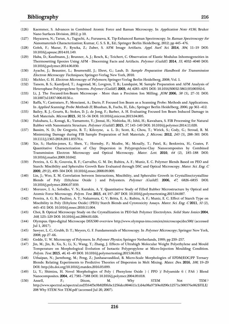
Bibliography 216
216
(126) Kaemmer, S. Advances in Combined Atomic Force and Raman Microscopy. In Application Note #136; Bruker
Nano Surfaces Division, 2012; p 10.
(127) Hayazawa, N.; Tarun, A.; Taguchi, A.; Furusawa, K. Tip-Enhanced Raman Spectroscopy. In Raman Spectroscopy for
Nanomaterials Characterization; Kumar, C. S. S. R., Ed.; Springer Berlin Heidelberg, 2012; pp 445–476.
(128) Gołek, F.; Mazur, P.; Ryszka, Z.; Zuber, S. AFM Image Artifacts. Appl. Surf. Sci. 2014, 304, 11–19 DOI:
10.1016/j.apsusc.2014.01.149.
(129) Haba, D.; Kaufmann, J.; Brunner, A. J.; Resch, K.; Teichert, C. Observation of Elastic Modulus Inhomogeneities in
Thermosetting Epoxies Using AFM - Discerning Facts and Artifacts. Polymer (Guildf). 2014, 55, 4032–4040 DOI:
10.1016/j.polymer.2014.06.030.
(130) Ayache, J.; Beaunier, L.; Boumendil, J.; Ehret, G.; Laub, D. Sample Preparation Handbook for Transmission
Electron Microscopy Techniques; Springer-Verlag New York, 2010.
(131) Michler, G. H. Electron Microscopy of Polymers; Springer-Verlag Berlin Heidelberg, 2008; Vol. 1.
(132) Tanem, B. S.; Kamfjord, T.; Augestad, M.; Lovgren, T. B.; Lundquist, M. Sample Preparation and AFM Analysis of
Heterophase Polypropylene Systems. Polymer (Guildf). 2003, 44, 4283–4291 DOI: 10.1016/S0032-3861(03)00392-6.
(133) Li, J. The Focused-Ion-Beam Microscope - More than a Precision Ion Milling. JOM 2006, 58 (3), 27–31 DOI:
10.1007/s11837-006-0156-z.
(134) Raffa, V.; Castrataro, P.; Menciassi, A.; Dario, P. Focused Ion Beam as a Scanning Probe: Methods and Applications.
In Applied Scanning Probe Methods II; Bhushan, B., Fuchs, H., Eds.; Springer Berlin Heidelberg, 2006; pp 361–412.
(135) Bailey, R. J.; Geurts, R.; Stokes, D. J.; de Jong, F.; Barber, A. H. Evaluating Focused Ion Beam Induced Damage in
Soft Materials. Micron 2013, 50, 51–56 DOI: 10.1016/j.micron.2013.04.005.
(136) Fukuhara, L.; Kosugi, K.; Yamamoto, Y.; Jinnai, H.; Nishioka, H.; Ishii, H.; Kawahara, S. FIB Processing for Natural
Rubber with Nanomatrix Structure. Polymer (Guildf). 2015, 57, 143–149 DOI: 10.1016/j.polymer.2014.11.020.
(137) Bassim, N. D.; De Gregorio, B. T.; Kilcoyne, a. L. D.; Scott, K.; Chou, T.; Wirick, S.; Cody, G.; Stroud, R. M.
Minimizing Damage during FIB Sample Preparation of Soft Materials. J. Microsc. 2012, 245 (3), 288–301 DOI:
10.1111/j.1365-2818.2011.03570.x.
(138) Xie, S.; Harkin-jones, E.; Shen, Y.; Hornsby, P.; Mcafee, M.; Mcnally, T.; Patel, R.; Benkreira, H.; Coates, P.
Quantitative Characterization of Clay Dispersion in Polypropylene-Clay Nanocomposites by Combined
Transmission Electron Microscopy and Optical Microscopy. Mater. Lett. 2010, 64 (2), 185–188 DOI:
10.1016/j.matlet.2009.10.042.
(139) Pereira, A. G. B.; Gouveia, R. F.; Carvalho, G. M. De; Rubira, A. F.; Muniz, E. C. Polymer Blends Based on PEO and
Starch: Miscibility and Spherulite Growth Rate Evaluated through DSC and Optical Microscopy. Mater. Sci. Eng. C
2009, 29 (2), 499–504 DOI: 10.1016/j.msec.2008.09.009.
(140) Lin, J.; Woo, E. M. Correlation between Interactions, Miscibility, and Spherulite Growth in Crystalline/crystalline
Blends of Poly (Ethylene Oxide ) and Polyesters. Polymer (Guildf). 2006, 47, 6826–6835 DOI:
10.1016/j.polymer.2006.07.039.
(141) Morozov, I. A.; Solodko, V. N.; Kurakin, A. Y. Quantitative Study of Filled Rubber Microstructure by Optical and
Atomic Force Microscopy. Polym. Test. 2015, 44, 197–207 DOI: 10.1016/j.polymertesting.2015.04.007.
(142) Pereira, A. G. B.; Paulino, A. T.; Nakamura, C. V; Britta, E. A.; Rubira, A. F.; Muniz, E. C. Effect of Starch Type on
Miscibility in Poly (Ethylene Oxide) (PEO)/ Starch Blends and Cytotoxicity Assays. Mater. Sci. Eng. C 2011, 31 (2),
443–451 DOI: 10.1016/j.msec.2010.11.004.
(143) Choi, B. Optical Microscopy Study on the Crystallization in PEO-Salt Polymer Electrolytes. Solid State Ionics 2004,
168, 123–129 DOI: 10.1016/j.ssi.2004.01.026.
(144) Olympus. Opto-digital Microscope DSX500 overview http://www.olympus-ims.com/en/microscope/dsx500/ (accessed
Jul 1, 2017).
(145) Sawyer, L. C.; Grubb, D. T.; Meyers, G. F. Fundamentals of Microscopy. In Polymer Microscopy; Springer New York,
2008; pp 27–66.
(146) Gedde, U. W. Microscopy of Polymers. In Polymer Physics; Springer Netherlands, 1999; pp 239–257.
(147) Jin, M.; Jin, B.; Xu, X.; Li, X.; Wang, T.; Zhang, J. Effects of Ultrahigh Molecular Weight Polyethylene and Mould
Temperature on Morphological Evolution of Isotactic Polypropylene at Micro-Injection Moulding Condition.
Polym. Test. 2015, 46, 41–49 DOI: 10.1016/j.polymertesting.2015.06.018.
(148) Uthaipan, N.; Jarnthong, M.; Peng, Z.; Junhasavasdikul, B. Micro-Scale Morphologies of EPDM/EOC/PP Ternary
Blends: Relating Experiments to Predictive Theories of Dispersion in Melt Mixing. Mater. Des. 2016, 100, 19–29
DOI: http://dx.doi.org/10.1016/j.matdes.2016.03.099.
(149) Li, Y.; Shimizu, H. Novel Morphologies of Poly ( Phenylene Oxide ) ( PPO )/ Polyamide 6 ( PA6 ) Blend
Nanocomposites. 2004, 45, 7381–7388 DOI: 10.1016/j.polymer.2004.09.018.
(150) Ansell, P.; Dixon, M. Why STEM Not TEM ?
http://www.spectral.se/spectral.nsf/f164f3e9b82f0febc1256dcc004611c1/d4a98a973f4e0290c12571e300376e06/$FILE/
208 Why STEM Not TEM.pdf (accessed Jul 20, 2007).

217 Bibliography
217
(151) Heinzl, C.; Ossiander, T.; Gleich, S.; Scheu, C. Transmission Electron Microscopy Study of Silica Reinforced
Polybenzimidazole Membranes. J. Memb. Sci. 2015, 478, 65–74 DOI: 10.1016/j.memsci.2014.12.051.
(152) Koenig, J. L. Fourier Transform Infrared Spectroscopy of Polymers. In Spectroscopy: NMR, Fluorescence, FT-IR.
Advances in Polymer Science; Springer Berlin Heidelberg, 1993; pp 87–154.
(153) Chan, K. L. A.; Govada, L.; Bill, R. M.; Chayen, N. E.; Kazarian, S. G. Attenuated Total Reflection-FT-IR
Spectroscopic Imaging of Protein Crystallization. Anal. Chem. 2009, 81 (10), 3769–3775 DOI: 10.1021/ac900455y.
(154) Chan, K. L. A.; Hammond, S. V; Kazarian, S. G. Applications of Attenuated Total Reflection Infrared Spectroscopic
Imaging to Pharmaceutical Formulations. Anal. Chem. 2003, 75 (9), 2140–2146 DOI: 10.1021/ac026456b.
(155) Glassford, S. E.; Govada, L.; Chayen, N. E.; Byrne, B.; Kazarian, S. G.; Crystal, G. Micro ATR FTIR Imaging of
Hanging Drop Protein Crystallisation. Vib. Spectrosc. 2012, 63, 492–498 DOI: 10.1016/j.vibspec.2012.07.011.
(156) Kazarian, S. G.; Chan, K. L. A. FTIR Imaging of Polymeric Materials under High-Pressure Carbon Dioxide.
Macromolecules 2004, 37, 579–584 DOI: 10.1021/ma035420y.
(157) Cheng, J.; Yang, X.; Dong, L.; Yuan, Z.; Wang, W.; Wu, S.; Chen, S.; Zheng, G.; Zhang, W.; Zhang, D.; Wang, H.
Effective Nondestructive Evaluations on UHMWPE / Recycled-PA6 Blends Using FTIR Imaging and Dynamic
Mechanical Analysis. Polym. Test. 2017, 59, 371–376 DOI: 10.1016/j.polymertesting.2017.02.021.
(158) Nagle, D. J.; George, G. A.; Rintoul, L.; Fredericks, P. M. Use of Micro-ATR/FTIR Imaging to Study Heterogeneous
Polymer Oxidation by Direct Solvent Casting onto the ATR IRE. Vib. Spectrosc. 2010, 53, 24–27 DOI:
10.1016/j.vibspec.2010.01.018.
(159) Fernandes, J. P. C.; Mareau, V. H.; Gonon, L. AFM-Raman Co-Localization Setup: Advanced Characterization
Technique for Polymers. Int. J. Polym. Anal. Charact. 2017, 1–7 DOI: 10.1080/1023666X.2017.1391740.
(160) Lobo, H.; Bonilla, J. W. Handbook of Plastic Analysis; Marcel Dekker, Inc., 2003.
(161) Bashford, D. Thermoplastics; Springer Netherlands, 1997.
(162) Gallego, R.; García-Lopez, D.; Merino, J. C.; Pastor, J. M. The Effect of Montmorillonite and Compatibilizer
Quantities on Stiffness and Toughness of Polyamide Nanoblends a JC Merino a , B and JM Pastor a , B. Polym. Int.
2010, 59, 472–478 DOI: 10.1002/pi.2724.
(163) PolymerTechnnology & Services LLC. Brochure. 2013, p 12.
(164) Tanrattanakul, V.; Sungthong, N.; Raksa, P. Rubber Toughening of Nylon 6 with Epoxidized Natural Rubber.
Polym. Test. 2008, 27, 794–800 DOI: 10.1016/j.polymertesting.2008.05.013.
(165) Burgish, G.; Paternoster, M.; Peduto, N.; Saraceno, A. Toughness Enhancement of Polyamide 6 Modified with
Different Type of Rubber:the Influence of Internal Rubber Cavitation. J. Appl. Polym. Sci. 1997, 66, 777–787.
(166) Wang, C.; Su, J. X.; Li, J.; Yang, H.; Zhang, Q.; Du, R. N.; Fu, Q. Phase Morphology and Toughening Mechanism of
Polyamide 6/EPDM-G-MA Blends Obtained via Dynamic Packing Injection Molding. Polymer (Guildf). 2006, 47,
3197–3206.
(167) Jr., E. C.; Kopacak, U.; Goncalves, M. C.; S.P. Nunes. In Situ Compatibilization of Polyamide 6/natural Rubber
Blends with Maleic Anhydride. Polymer (Guildf). 2000, 41, 5929–5935.
(168) Whelan, T.; Goff, J. Injection Molding of Thermoplastics Materials; Whelan, T., Goff, J., Eds.; Van Nostrand
Reinhold, 1990.
(169) Zhang, N.; Bao, X. X.; Tan, Z. Y.; Sun, S. L.; Zhou, C.; Yang, H. D.; Zhang, H. X. Morphology and Mechanical
Properties of ABS Blends Prepared from Emulsion-Polymerized PB-G-SAN Impact Modifier with AIBN as Initiator.
J. Appl. Polym. Sci. 2007, 105, 1237–1243 DOI: 10.1002/app.
(170) Kryszewski, M.; Galeski, A.; Martuscelli, E. Polymer Blends Processing, Morphology and Properties. Vol 2;
Kryszewski, M., Galeski, A., Martuscelli, E., Eds.; Springer Science+Business Media, LLC, 1984.
(171) Utracki, L. A.; Shi, H. Development of Polymer Blend Morphology During Compounding in a Twin-Screw
Extruder. Part I: Droplet Dispersion and Coalescence-A Review. Polym. Eng. Sci. 1992, 32 (24), 1824–1833.
(172) Singh, H.; Gupta, N. K. Evolution of Properties in ABS/PA6 Blends Compatibilized by Fixed Weight Ratio SAGMA
Copolymer. J. Polym. Res. 2011, 18 (6), 1365–1377.
(173) Jafari, S. H.; Ptschke, P.; Stephan, M.; Pompe, G.; Warth, H.; Alberts, H. Thermal Behavior and Morphology of
Polyamide 6 Based Multicomponent Blends. J. Appl. Polym. Sci. 2002, 84 (14), 2753–2759 DOI: 10.1002/app.10570.
(174) Kudva, R. A.; Keskkula, H.; Paul, D. R. Compatibilization of Nylon 6/ABS Blendsusing Glycidyl
Methacrylate/methyl Methacrylate Copolymers. Polymer (Guildf). 1998, 39 (12), 2447–2460 DOI: 10.1016/S0032-
3861(97)00583-1.
(175) As’habi, L.; Jafari, S. H.; Khonakdar, H. A.; Baghaei, B. Morphological, Rheological and Thermal Studies in Melt
Processed Compatibilized PA6/ABS/clay Nanocomposites. J. Polym. Res. 2011, 18, 197–205.
(176) Sundararajs, U.; Macosko, C. W. Drop Breakup and Coalescence in Polymer Blends : The Effects of Concentration
and Compatibilization. Macromolecules 1995, 28, 2647–2657.
(177) Al-Malaika, S. Reactive Modifiers for Polymers, 1st ed.; Al-Malaika, S., Ed.; Blackie Academic & Professional, 1997.
(178) Zhou, X.; Zhang, P.; Jiang, X.; Rao, G. Influence of Maleic Anhydride Grafted Polypropylene on the Miscibility of
Polypropylene / Polyamide-6 Blends Using ATR-FTIR Mapping. Vib. Spectrosc. 2009, 49, 17–21 DOI:

Bibliography 218
218
10.1016/j.vibspec.2008.04.004.
(179) Majumdar, B.; Keskkula, H.; Pault, D. R. Effect of the Nature of the Polyamide on the Properties and Morphology
of Compatibilized Nylon/acrylonitrile-Butadiene-Styrene Blends. Polymer (Guildf). 1994, 35 (25), 5468–5477.
(180) Ishak, Z. A. M.; Chow, W. S.; Takeichi, T. Influence of SEBS-G-MA on Morphology, Mechanical, and Thermal
Properties of PA6/PP/organoclay Nanocomposites. Eur. Polym. J. 2008, 44, 1023–1039 DOI:
10.1016/j.eurpolymj.2008.01.019.
(181) Chiang, C.; Chang, F. Polymer Blends of Polyamide-6 (PA6) and Poly (Phenylene Oxide) (PPO) Compatibilized by
Styrene-Maleic Anhydride (SMA) Copolymer. Polymer (Guildf). 1997, 38 (19), 4807–4817.
(182) Visakh, P. M.; Thomas, S.; Chandra, A. K.; Mathew, A. P. Advances in Elastomers I - Blends and Interpenetrating
Networks; Visakh, P. M., Thomas, S., Chandra, A. K., Mathew, A. P., Eds.; Springer, 2013.
(183) Evans, A. G.; Ahmad, Z. B.; Gilbert, D. G.; Beaumont, P. W. R. Mechanisms of Toughening in Rubber Toughened
Polymers. Acta Metall. 1986, 34 (1), 79–87.
(184) Quaresimin, M.; Schulte, K.; Zappalorto, M.; Chandrasekaran, S. Toughening Mechanisms in Polymer
Nanocomposites: From Experiments to Modelling. Compos. Sci. Technol. 2016, 123, 187–204 DOI:
10.1016/j.compscitech.2015.11.027.
(185) Argon, A. S.; Cohen, R. E. Toughenability of Polymers. Polymer (Guildf). 2003, 44, 6013–6032 DOI: 10.1016/S0032-
3861(03)00546-9.
(186) Contents, S.; Class, P. Polymer Data Handbook; Oxford University Press, 1999.
(187) Shen, L.; Yee, I.; Liu, T. Nanoindentation Studies on Polymorphism of Nylon 6. Polym. Test. 2006, 25, 249–253 DOI:
10.1016/j.polymertesting.2005.09.019.
(188) Wildes, G.; Keskkula, H.; Paul, D. R. Morphology of PC/SAN Blends: Effect of Reactive Compatibilization, SAN
Concentration, Processing, and Viscosity Ratio. J. Polym. Sci. Part B Polym. Phys. 1999, 37, 71–82.
(189) Lyu, S. P.; Jones, T. D.; Bates, F. S.; Macosko, C. W. Role of Block Copolymers on Suppression of Droplet
Coalescence. Macromolecules 2002, 35, 7845–7855 DOI: 10.1021/ma020754t.
(190) Boudenne, A.; Ibos, L.; Candau, Y.; Thomas, S. Handbook of Multiphase Polymer Systems; John Wiley & Sons, 2011.
(191) Jafari, S. H.; Stephan, M.; Warth, H.; Alberts, H. Multicomponent Blends Based on Polyamide 6 and Styrenic
Polymers: Morphology and Melt Rheology. Polymer (Guildf). 2002, 43, 6985–6992.
(192) Mojarrad, A.; Jahani, Y.; Barikani, M. Investigation on the Correlation Between Rheology and Morphology of PA6 /
ABS Blends Using Ethylene Acrylate Terpolymer as Compatibilizer. J. Appl. Polym. Sci. 2011, 120, 2173–2182 DOI:
10.1002/app.
(193) Solomon, M. J.; Almusallam, A. S.; Seefeldt, K. F.; Somwangthanaroj, A.; Varadan, P. Rheology of
Polypropylene/Clay Hybrid Materials. Macromolecules 2001, 34, 1864–1872.
(194) Castro, L. D. .; Oliveira, A. D.; Kersch, M.; Altstädt, V.; Pessan, L. A. Effects of Mixing Protocol on Morphology and
Properties of PA6 / ABS Blends Compatibilized with MMA-MA. J. Appl. Polym. Sci. 2016, 43612, 1–8 DOI:
10.1002/app.43612.
(195) Kim, B. K.; Lee, Y. M.; Jeong, H. M. Physical Properties of ABS/SMA/nylon-6 Ternary Blends: Effect of Blending
Sequence. Polymer (Guildf). 1993, 34 (10), 2075–2080.
(196) Paul, D. R.; Barlow, J. W. Polymer Blends (or Alloys). J. Macromelecular Sci. Part C 1980, 18 (1), 109–168 DOI:
dx.doi.org/10.1080/00222358008080917 PLEASE.
(197) Pötschke, P.; Paul, D. R. Formation of Co-Continuous Structures in Melt-Mixed Immiscible Polymer Blends. J.
Macromol. Sci. Part C 2003, 43 (1), 87–141 DOI: 10.1081/MC-120018022.
(198) Fornes, T. D.; Paul, D. R. Crystallization Behavior of Nylon 6 Nanocomposites. Polymer (Guildf). 2003, 44, 3945–
3961 DOI: 10.1016/S0032-3861(03)00344-6.
(199) Liu, S.; Zhang, C.; Proniewicz, E.; Proniewicz, L. M.; Kim, Y.; Liu, J.; Zhao, Y.; Xu, Y.; Wu, J. Crystalline Transition
and Morphology Variation of Polyamide 6/CaCl2 Composite during the Decomplexation Process. Spectrochim.
Acta Part A Mol. Biomol. Spectrosc. 2013, 115, 783–788 DOI: 10.1016/j.saa.2013.06.056.
(200) Stephens, J. S.; Chase, D. B.; Rabolt, J. F. Effect of the Electrospinning Process on Polymer Crystallization Chain
Conformation in Nylon-6 and Nylon-12. Macromolecules 2004, 37, 877–881.
(201) Ferreiro, V.; Depecker, C.; Laureyns, J.; Coulon, G. Structures and Morphologies of Cast and Plastically Strained
Polyamide 6 Films as Evidenced by Confocal Raman Microspectroscopy and Atomic Force Microscopy. Polymer
(Guildf). 2004, 45, 6013–6026 DOI: 10.1016/j.polymer.2004.06.018.
(202) Zhong, L.; Ren, X.; Yang, S.; Chen, E.; Sun, C.; Stroeks, A.; Yang, T. Lamellar Orientation of Polyamide 6 Thin Film
Crystallization on Solid Substrates. Polymer (Guildf). 2014, 55, 4332–4340.
(203) Kolesov, I.; Mileva, D.; Androsch, R.; Schick, C. Structure Formation of Polyamide 6 from the Glassy State by Fast
Scanning Chip Calorimetry. Polymer (Guildf). 2011, 52, 5156–5165 DOI: 10.1016/j.polymer.2011.09.007.
(204) Roeder, J.; Oliveira, R. V. B.; Gonc, M. C.; Soldi, V.; Pires, A. T. N. Polypropylene/polyamide-6 Blends: Influence of
Compatibilizing Agent on Interface Domains. Polym. Test. 2002, 21, 815–821.
(205) Heinzel, A. Fuel Cells and Hydrogen Technology. In Technology Guide; Bullinger, H.-J., Ed.; Springer, Berlin,

219 Bibliography
219
Heidelberg, 2009; pp 368–373.
(206) Lamy, C.; Jones, D. J.; Coutanceau, C.; Brault, P.; Martemianov, S. Do Not Forget the Electrochemical
Characteristics of the Membrane Electrode Assembly When Designing a Proton Exchange Membrane Fuel Cell
Stack. Electrochim. Acta 2011, 56 (28), 10406–10423 DOI: 10.1016/j.electacta.2011.05.098.
(207) Zhang, J.; Xie., Z.; Zhang, J.; Tang, Y.; Song, C.; Navessin, T.; Shi, Z.; Song, D.; Wang, H.; Wilkinson, D. P.; Liu, Z.-S.;
Holdcroft, S. High Temperature PEM Fuel Cells. J. Power Sources 2006, 160 (2), 872–891 DOI:
https://doi.org/10.1016/j.jpowsour.2006.05.034.
(208) Schmidt, T. J.; Gasteigerand, H. A.; Behm, R. J. Rotating Disk Electrode Measurements on the CO Tolerance of a
High-Surface Area Pt/Vulcan Carbon Fuel Cell Catalyst. J. Electrochem. Soc. 1999, 146 (4), 1296–1304 DOI: DOI:
10.1149/1.1391761.
(209) Sood, R.; Cavaliere, S.; Jones, D. J.; Rozière, J. Electrospun Nanofibre Composite Polymer Electrolyte Fuel Cell and
Electrolysis Membranes. Nano Energy 2016, 26, 729–745 DOI: 10.1016/j.nanoen.2016.06.027.
(210) Subianto, S.; Pica, M.; Casciola, M.; Cojocaru, P.; Merlo, L.; Hards, G.; Jones, D. J. Physical and Chemical
Modification Routes Leading to Improved Mechanical Properties of Perfluorosulfonic Acid Membranes for PEM
Fuel Cells. J. Power Sources 2013, 233, 216–230 DOI: 10.1016/j.jpowsour.2012.12.121.
(211) Jones, D. J.; Rozière, J. Advances in the Development of Inorganic – Organic Membranes for Fuel Cell Applications.
Adv. Polym. Sci. 2008, 215 (July), 219–264 DOI: 10.1007/12_2008_150.
(212) 2015 ANNUAL REPORT of The Hydrogen and Fuel Cell Technical Advisory Committee; 2016.
(213) Adjemian, K. T.; Dominey, R.; Krishnan, L.; Ota, H.; Majsztrik, P.; Zhang, T.; Mann, J.; Kirby, B.; Gatto, L.; Velo-
Simpson, M.; Leahy, J.; Srinivasan, S.; Benziger, J. B.; Bocarsly, andAndrew B. Function and Characterization of
Metal Oxide-Naflon Composite Membranes for Elevated-Temperature H2/O2 PEM Fuel Cells. Chem. Mater. 2006,
18 (9), 2238–2248 DOI: 10.1021/cm051781b.
(214) Chandan, A.; Hattenberger, M.; El-kharouf, A.; Du, S.; Dhir, A.; Self, V.; Pollet, B. G.; Ingram, A.; Bujalski, W. High
Temperature (HT) Polymer Electrolyte Membrane Fuel Cells (PEMFC) - A Review. J. Power Sources 2013, 231,
264–278 DOI: 10.1016/j.jpowsour.2012.11.126.
(215) Wu, J.; Yuan, X. Z.; Martin, J. J.; Wang, H.; Zhang, J.; Shen, J.; Wu, S.; Merida, W. A Review of PEM Fuel Cell
Durability: Degradation Mechanisms and Mitigation Strategies. J. Power Sources 2008, 184, 104–119 DOI:
10.1016/j.jpowsour.2008.06.006.
(216) Borup, R.; Meyers, J.; Pivovar, B.; Kim, Y. S.; Mukundan, R.; Garland, N.; Myers, D.; Wilson, M.; Garzon, F.; Wood, D.;
Zelenay, P.; More, K.; Stroh, K.; Zawodzinski, T.; Boncella, J.; McGrath, J. E.; Inaba, M.; Miyatake, K.; Hori, M.; Ota,
K.; Ogumi, Z.; Miyata, S.; Nishikata, A.; Siroma, Z.; Uchimoto, Y.; Yasuda, K.; Kimijima, K.-I.; Iwashita, N. Scientific
Aspects of Polymer Electrolyte Fuel Cell Durability and Degradation. Chem. Rev. 2007, 107 (10), 3904–3951 DOI:
10.1021/cr050182l.
(217) Kreuer, K. D.; Schuster, M.; Obliers, B.; Diat, O.; Traub, U.; Fuchs, A.; Klock, U.; Paddison, S. J.; Maier, J. Short-Side-
Chain Proton Conducting Perfluorosulfonic Acid Ionomers: Why They Perform Better in PEM Fuel Cells. J. Power
Sources 2008, 178 (2), 499–509 DOI: https://doi.org/10.1016/j.jpowsour.2007.11.011.
(218) Kreuer, K. D. On the Development of Proton Conducting Polymer Membranes for Hydrogen and Methanol Fuel
Cells. 2001, 185, 29–39.
(219) Mendil-Jakani, H.; López, I. Z.; Mareau, V. H.; Gonon, L. Optimization of Hydrophilic/hydrophobic Phase Separation
in sPEEK Membranes by Hydrothermal Treatments. Phys. Chem. Chem. Phys. 2017, 19, 16013–16022 DOI:
10.1039/C7CP00087A.
(220) Portale, G.; Carbone, A.; Martinelli, A.; Passalacqua, E. Microstructure, State of Water and Proton Conductivity of
Sulfonated Poly(ether Ether Ketone). Solid State Ionics 2013, 252 (0), 62–67 DOI:
https://doi.org/10.1016/j.ssi.2013.08.031.
(221) Delhorbe, V.; Cailleteau, C.; Chikh, L.; Guillermo, A.; Gebel, G.; Morin, A.; Fichet, O. Influence of the Membrane
Treatment on Structure and Properties of Sulfonated Poly(etheretherketone) Semi-Interpenetrating Polymer
Network. J. Memb. Sci. 2013, 427, 283–292 DOI: 10.1016/j.memsci.2012.10.001.
(222) Chikh, L.; Delhorbe, V.; Fichet, O. (Semi-)Interpenetrating Polymer Networks as Fuel Cell Membranes. J. Memb.
Sci. 2011, 368 (1–2), 1–17 DOI: 10.1016/j.memsci.2010.11.020.
(223) Jones, D. J.; Rozière, J. V.3: Fuel Cell Technology and Applications. In Handbook of Fuel Cells–Fundamentals,
Technology and Applications; Vielstich, W., Lamm, A., Gasteiger, H., Eds.; Wiley, 2003; p 447.
(224) Rozière, J.; Jones, D. J. No Title. In Proceedings of the 1st European PEFC Forum; Büchi, F., Scherer, G., Wokaun, A.,
Eds.; Lucerne, 2001; p 145.
(225) Alberti, G.; Casciola, M. Composite Membranes for Medium-Temperature PEM Fuel Cells. Annu. Rev. Mater. Res.
2003, 33, 129–154 DOI: https://doi.org/10.1146/annurev.matsci.33.022702.154702.
(226) Savadogo, O. Emerging Membranes for Electrochemical Systems Part II. High Temperature Composite
Membranes Forpolymer Electrolyte Fuel Cell (PEFC) Applications. J. Power Sources 2004, 127 (1–2), 135–161 DOI:
10.1016/j.jpowsour.2003.09.043.

Bibliography 220
220
(227) Aparicio, M.; Lecoq, E.; Castro, Y.; Duran, A. Proton Conducting Organic/Inorganic Sol-Gel Membranes Produced
from Phenyltriethoxysilane and 3-Methacryloxypropyl Trimethoxysilane. J. Sol-Gel Sci. Technol. 2005, 34, 233–239.
(228) Deng, Q.; Moore, R. B.; Mauritz, K. A. Novel Nafion/ORMOSIL Hybrids via in Situ Sol-Gel Reactions. 1. Probe of
ORMOSIL Phase Nanostructures by Infrared Spectroscopy. Chem. Mater. 1995, 7, 2259–2268.
(229) Mauritz, K. A.; Hassan, M. K. Nanophase Separated Perfluorinated Ionomers as Sol-Gel Polymerization Templates
for Functional Inorganic Oxide Nanoparticles. Polym. Rev. 2007, 47, 543–565 DOI: 10.1080/15583720701638393.
(230) Colicchio, I.; Demco, D. E.; Baias, M.; Keul, H.; Moeller, M. Influence of the Silica Content in SPEEK-Silica
Membranes Prepared from the Sol-Gel Process of Polyethoxysiloxane : Morphology and Proton Mobility. J. Memb.
Sci. 2009, 337, 125–135 DOI: 10.1016/j.memsci.2009.03.037.
(231) Mauritz, K. A. Organic-Inorganic Hybrid Materials: Perfluorinated Ionomers as Sol-Gel Polymerization Templates
for Inorganic Alkoxides. Mater. Sci. Eng. C 1998, 6, 121–133.
(232) Schubert, U. Chemistry and Fundamentals of the Sol-Gel Process. In The Sol-Gel Handbook: Synthesis,
Characterization and Applications. Volume 2; Levy, D., Zayat, M., Eds.; John Wiley & Sons, 2015; p 1616.
(233) Brinker, C. J.; Scherer, G. W. Sol-Gel Science: The Physics and Chemistry of Sol-Gel Processing; Academic Press,
Inc, 1990.
(234) Hüsing, N.; Hartmann, S. Inorganic-Organic Hybrid Porous Materials. In Organic-Inorganic Hybrid
Nanomaterials; Kalia, S., Haldorai, Y., Eds.; Springer International Publishing, 2015; pp 143–185.
(235) Delhorbe, V.; Cailleteau, C.; Chikh, L.; Guillermo, A.; Gebel, G.; Morin, A.; Fichet, O. Influence of the Membrane
Treatment on Structure and Properties of Sulfonated Poly (Etheretherketone) Semi-Interpenetrating Polymer
Network. J. Memb. Sci. 2013, 427, 283–292 DOI: 10.1016/j.memsci.2012.10.001.
(236) Cousin, F. Small Angle Neutron Scattering. EPJ Web Conf. 2015, 104, 1–49 DOI:
https://doi.org/10.1051/epjconf/201510401004.
(237) Zemb, T.; Lindner, P. Neutron, X-Rays and Light. Scattering Methods Applied to Soft Condensed Matter, 1st ed.;
Zemb, T., Lindner, P., Eds.; North Holland, 2002.
(238) Online, V. A.; Lopez, I. Z.; Legrand, P. M.; Mareau, V. H.; Gonon, L. A New Interpretation of SAXS Peaks in
Sulfonated Poly(ether Ether Ketone) (sPEEK) Membranes for Fuel Cells †. 2014, 11228–11235 DOI:
10.1039/c4cp00710g.
(239) Gebel, G. Structure of Membranes for Fuel Cells: SANS and SAXS Analyses of Sulfonated PEEK Membranes and
Solutions. Macromolecules 2013, 46, 6057–6066.
(240) Mauritz, K. A.; Stefanithis, D.; Davis, S. V; Scheetz, R. W.; Pope, R. K.; Wilkes, G. L.; Huang, H.-H. Microstructural
Evolution of a Silicon Oxide Phase in a Perfluorosulfonic Acid Lonomer by an In Situ Sol-Gel Reaction. J. Appl.
Polym. Sci. 1995, 55, 181–190.
(241) Beaucage, G. Combined Small-Angle Scattering for Characterization of Hierarchically Structured Polymer Systems
over Nano-to-Micron Meter: Part II Theory. Polym. Sci. A Compr. Ref. 2012, 2, 399–409 DOI: 10.1016/B978-0-444-
53349-4.00032-7.
(242) Stuart, B. H. A Fourier Transform Raman Spectroscopy Study of the Crystallisation Behaviour of a Poly (Ether
Ether Ketone)/ Poly (Ether Sulphone) Blend. Spectrochim. Acta Part A 1997, 53 (1997), 107–110.
(243) Everall, N. J.; Chalmers, J. M.; Ferwerda, R.; van der Maas, J. H.; Hendra, P. J. Measurement of Poly (Aryl Ether
Ether Ketone) Crystallinity in Isotropic and Uniaxial Samples Using Fourier Transform-Raman Spectroscopy: A
Comparison of Univariate and Partial Least-Squares Calibrations. J. Raman Spectrosc. 1994, 25 (June 1993), 43–51.
(244) Ellis, G.; Naffakh, M.; Marco, C.; Hendra, P. J. Fourier Transform Raman Spectroscopy in the Study of
Technological Polymers Part 1: Poly (Aryl Ether Ketones ), Their Composites and Blends. 1997, 1425 (97).
(245) Maddams, W. F. A Review of Fourier-Transform Raman Spectroscopic Studies on Polymers. Spectrochim. Acta
1994, 50A, 1967–1986.
(246) Young, W.-S.; Kuan, W.-F.; Epps, T. H. Block Copolymer Electrolytes for Rechargeable Lithium Batteries. J. Polym.
Sci. Part B Polym. Phys. 2014, 52 (1), 1–16.
(247) I. Yoshimatsu, T. Hirai, J. Y. Lithium Electrode Morphology during Cycling in Lithium Cells. J. Electrochem. Soc.
1988, 135, 2422–2427.
(248) Koch, V. R.; Young, J. H. The Stability of the Secondary Lithium Electrode in Tetrahydrofuran-Based Electrolytes. J.
Electrochem. Soc. 1979, 125, 1371–1377.
(249) M. Rosso, C. Brissot, A. Teyssot, M. Dollé, L. Sannier, J.M. Tarascon, R. Bouchet, S. L. Dendrite Short-Circuit and
Fuse Effect on Li/polymer/Li Cells. Electrochim. Acta 2006, 51 (25), 5334–5340.
(250) Dollé, M.; Sannier, L.; Beaudoin, B.; Trentin, M.; Tarascon, J. M. Live Scanning Electron Microscope Observations of
Dendritic Growth in Lithium/polymer Cells. Electrochem. Solid - State Lett. 2002, 5, 286–289.
(251) F. Croce, G.B. Appetecchi, L. Persi, B. S. Nanocomposite Polymer Electrolytes for Lithium Batteries. Nature 1998,
394, 456–458.
(252) Monroe, C.; Newman, J. The Impact of Elastic Deformation on Deposition Kinetics at Lithium/Polymer Interfaces.
J. Electrochem. Soc. 2005, 152, 396–404.

221 Bibliography
221
(253) Johansson, P. First Principles Modelling of Amorphous Polymer Electrolytes: Li+-PEO, Li+-PEI, and Li+-PES
Complexes. Polym. 2001, 42, 4367–4373.
(254) D. Devaux, R. Bouchet, D. Glé, R. D. Mechanism of Ion Transport in PEO/LiTFSI Complexes: Effect of
Temperature, Molecular Weight and End Groups. Solid State Ionics 2012, 227, 119–127.
(255) Matsen, M. W. Effect of Architecture on the Phase Behavior of AB-Type Block Copolymer Melts. Macromolecules
2012, 45 (4), 2161–2165 DOI: 10.1021/ma202782s.
(256) S.B. Darling. Directing the Self-Assembly of Block Copolymers. Prog. Polym. Sci. 2007, 32, 1152–1204.
(257) Young, W.-S.; Epps, T. H. Ionic Conductivities of Block Copolymer Electrolytes with Various Conducting Pathways:
Sample Preparation and Processing Considerations. Macromolecules 2012, 45, 4689–4697.
(258) Younesi, R.; Veith, G. M.; Johansson, P.; Edström, K.; Vegge, T. Lithium Salts for Advanced Lithium Batteries: Li–
metal, Li–O2, and Li–S. Energy Environ. Sci. 2015, 8 (7), 1905–1922 DOI: 10.1039/C5EE01215E.
(259) Burjanadze, M.; Karatas, Y.; Kaskhedikar, N.; Kogel, L. M.; Kloss, S.; Gentschev, A.-C.; Hiller, M. M.; Müller, R. a.;
Stolina, R.; Vettikuzha, P.; Wiemhöfer, H.-D. Salt-in-Polymer Electrolytes for Lithium Ion Batteries Based on
Organo-Functionalized Polyphosphazenes and Polysiloxanes. Zeitschrift für Phys. Chemie 2010, 224 (10–12), 1439–
1473 DOI: 10.1524/zpch.2010.0046.
(260) Bouchet, R.; Maria, S.; Meziane, R.; Aboulaich, A.; Lienafa, L.; Bonnet, J.; Phan, T. N. T.; Bertin, D.; Gigmes, D.;
Devaux, D.; Denoyel, R.; Armand, M. Efficient Electrolytes for Lithium-Metal Batteries. Nat. Mater. 2013, 12, 1–6.
(261) Feng, S.; Shi, D.; Liu, F.; Zheng, L.; Nie, J.; Feng, W. Single Lithium-Ion Conducting Polymer Electrolytes Based on
Poly [(4-Styrenesulfonyl)(trifluoromethanesulfonyl ) Imide ] Anions. Electrochim. Acta 2013, 93, 254–263 DOI:
10.1016/j.electacta.2013.01.119.
(262) Rolland, J.; Poggi, E.; Vlad, A.; Gohy, J.-F. Single-Ion Diblock Copolymers for Solid-State Polymer Electrolytes.
Polymer (Guildf). 2015, 68, 344–352 DOI: 10.1016/j.polymer.2015.04.056.
(263) Porcarelli, L.; Aboudzadeh, M. A.; Rubatat, L.; Nair, J. R.; Shaplov, A. S.; Gerbaldi, C.; Mecerreyes, D. Single-Ion
Triblock Copolymer Electrolytes Based on Poly(ethylene Oxide) and Methacrylic Sulfonamide Blocks for Lithium
Metal Batteries. J. Power Sources 2017, 364, 191–199 DOI: 10.1016/j.jpowsour.2017.08.023.
(264) Glatter, O.; Kratky, O. Small Angle X-Ray Scattering; London: Academic Press Inc. Ltd., 1982.
(265) Zhu, L.; Cheng, S. Z. D.; Calhoun, B.; Ge, Q.; Quirk, R. P.; Thomas, E. L.; Hsiao, B. S.; Yeh, F.; Lotz, B. Phase
Structures and Morphologies Determined by Self-Organization, Vitrification, and Crystallization: Confined
Crystallization in an Ordered Lamellar Phase of PEO-B-PS Diblock Copolymer. Polymer (Guildf). 2001, 42, 5829–
5839.
(266) Pelletier, B. Caractérisation Approfondie de Copolymères Triblocs PS-B-POE-B-PS Utilisés En Tant qu’Electrolytes
Polymères Solides Pour Les Batteries Lithium-Métal-Polymère, 2015.
(267) Yang, P.; Yu, X.; Han, Y. Transition between Crystallization and Microphase Separation in PS-B-PEO Thin Film
Influenced by Solvent Vapor Selectivity. Polymer (Guildf). 2010, 51 (21), 4948–4957 DOI:
10.1016/j.polymer.2010.08.025.
(268) Lassagne, A. Synthèse et Caractérisation de Nouveaux Électrolytes Copolymères Pour Batteries Lithium Métal
Polymère, 2017.
(269) Bouchet, R.; Phan, T. N. T.; Beaudoin, E.; Devaux, D.; Davidson, P.; Bertin, D.; Denoyel, R. Charge Transport in
Nanostructured PS-PEO-PS Triblock Copolymer Electrolytes. Macromolecules 2014, 47, 2659–2665.
(270) Claudy, P.; Létoffé, J. M.; Camberlain, Y.; Pascault, J. P. Glass Transition of Polystyrene versus Molecular Weight.
Polym. Bull. 1983, 9 (4–5), 208–215 DOI: 10.1007/BF00283709.
(271) Frenck, L. Study of a Buffer Layer Based on Block Copolymer Electrolytes , between the Lithium Metal and a
Ceramic Electrolyte for Aqueous Lithium-Air Battery Study of a Buffer Layer Based on Block Copolymer
Electrolytes , between the Lithium Metal and a Ceramic Ele, 2017.
(272) Singh, M.; Odusanya, G.; Wilmes, G. M.; Eitouni, H. B.; Gomez, E. D.; Patel, A. J.; Chen, V. L.; Park, M. J.; Fragouli, P.;
Iatrou, H.; Hadjichristidis, N.; Cookson, D.; Balsara, N. P. Effect of Molecular Weight on the Mechanical and
Electrical Properties of Block Copolymer Electrolytes. Macromolecules 2007, 40 (13), 4578–4585 DOI:
doi:10.1021/ma0629541.
(273) Sax, J.; Ottino, J. M. Modeling of Transport of Small Molecules in Polymer Blends: Application of Effective Medium
Theory. Polym. Eng. Sci. 1983, 23 (3), 165–176.
(274) Jinnai, H.; Yasuda, K.; Nishi, T. Three-Dimensional Observations of Grain Boundary Morphologies in a Cylinder-
Forming Block Copolymer. Macromol. Symp. 2006, 245–246 (1), 170–174.
(275) Chintapalli, M.; Chen, X. C.; Thelen, J. L.; Teran, A. A.; Wang, X.; Garetz, B. A.; Balsara, N. P. Effect of Grain Size on
the Ionic Conductivity of a Block Copolymer Electrolyte. Macromolecules 2014.
(276) Noort, S. J. T. Van; Werf, K. Van Der; Grooth, B. G. De; Hulst, N. F. Van; Greve, J. Height Anomalies in Tapping
Mode Atomic Force Microscopy in Air Caused by Adhesion. Ultramicroscopy 1997, 69, 117–127.
(277) Dubourg, F.; Aime, J. P. Role of the Adhesion between a Nanotip and a Soft Material in Tapping Mode AFM. Surf.
Sci. 2000, 466, 137–143.

Bibliography 222
222
(278) Carrillo, F.; Gupta, S.; Balooch, M.; Marshall, S. J.; Marshall, G. W.; Pruitt, L.; Puttlitz, C. M. Nanoindentation of
Polydimethylsiloxane Elastomers: Effect of Crosslinking, Work of Adhesion, and Fluid Environment on Elastic
Modulus. J. Mater. Res. 2017, 20 (10), 2820–2830 DOI: 10.1557/JMR.2005.0354.
(279) Kaufman, J. D.; Klapperich, C. M. Surface Detection Errors Cause Overestimation of the Modulus in
Nanoindentation on Soft Materials. J. Mech. Behav. Biomed. Mater. 2009, 2 (4), 312–317 DOI:
10.1016/j.jmbbm.2008.08.004.
(280) Gupta, S.; Carrillo, F.; Li, C.; Pruitt, L.; Puttlitz, C. Adhesive Forces Significantly Affect Elastic Modulus
Determination of Soft Polymeric Materials in Nanoindentation. Mater. Lett. 2007, 61, 448–451 DOI:
10.1016/j.matlet.2006.04.078.
(281) Dinte, B. P.; Watson, G. S.; Dobson, J. F.; Myhra, S. Artefacts in Non-Contact Mode Force Microscopy: The Role of
Adsorbed Moisture. Ultramicroscopy 1996, 63, 115–124.
(282) Ebenstein, D. M.; Wahl, K. J. A Comparison of JKR-Based Methods to Analyze Quasi-Static and Dynamic
Indentation Force Curves. J. Colloid Interface Sci. 2006, 298, 652–662 DOI: 10.1016/j.jcis.2005.12.062.
(283) Houston, J. E.; Doelling, C. M.; Vanderlick, T. K.; Hu, Y.; Scoles, G.; Wenzl, I.; Lee, T. R. Comparative Study of the
Adhesion, Friction, and Mechanical Properties of CF3- and CH3-Terminated Alkanethiol Monolayers. Langmuir
2005, 21 (9), 3926–3932 DOI: 10.1021/la046901t.
(284) Hiesgen, R.; Helmly, S.; Morawietz, T.; Yuan, X.-Z.; Wang, H.; Friedrich, K. A. Atomic Force Microscopy Studies of
Conductive Nanostructures in Solid Polymer Electrolytes. Electrochim. Acta 2013, 110, 292–305 DOI:
10.1016/j.electacta.2013.04.147.
(285) Morawietz, T.; Handl, M.; Oldani, C.; Friedrich, K. A.; Hiesgen, R. Quantitative in Situ Analysis of Ionomer
Structure in Fuel Cell Catalytic Layers. ACS Appl. Mater. Interfaces 2016, 8 (40), 27044–27054 DOI:
10.1021/acsami.6b07188.
(286) Kiss-Pataki, B.; Tiusanen, J.; Dobrik, G.; Vértesy, Z.; Horváth, Z. E. Visualization of the Conductive Paths in Injection
Moulded MWNT/polycarbonate Nanocomposites by Conductive AFM. Composites Science and Technology. 2014,
pp 102–109.
(287) Hiesgen, R.; Aleksandrova, E.; Meichsner, G.; Wehl, I.; Roduner, E.; Friedrich, K. A. High-Resolution Imaging of
Ion Conductivity of Nafion® Membranes with Electrochemical Atomic Force Microscopy. Electrochim. Acta 2009,
55 (2), 423–429 DOI: 10.1016/j.electacta.2009.05.049.
(288) Takimoto, N.; Takamuku, S.; Abe, M.; Ohira, A.; Lee, H.-S.; McGrath, J. E. Conductive Area Ratio of Multiblock
Copolymer Electrolyte Membranes Evaluated by E-AFM and Its Impact on Fuel Cell Performance. J. Power
Sources 2009, 194 (2), 662–667 DOI: 10.1016/j.jpowsour.2009.06.045.
(289) Nagpure, S. C.; Bhushan, B.; Babu, S. S. Surface Potential Measurement of Aged Li-Ion Batteries Using Kelvin Probe
Microscopy. J. Power Sources 2011, 196 (3), 1508–1512 DOI: 10.1016/j.jpowsour.2010.08.031.
(290) Musumeci, C.; Liscio, A.; Palermo, V.; Samorì, P. Electronic Characterization of Supramolecular Materials at the
Nanoscale by Conductive Atomic Force and Kelvin Probe Force Microscopies. Mater. Today 2014, 17 (10), 504–517
DOI: 10.1016/j.mattod.2014.05.010.
(291) Timofeeva, M.; Bolshakov, A.; Tovee, P. D.; Zeze, D. A.; Dubrovskii, V. G.; Kolosov, O. V. Scanning Thermal
Microscopy with Heat Conductive Nanowire Probes. Ultramicroscopy 2016, 162, 42–51 DOI:
10.1016/j.ultramic.2015.12.006.
(292) Juszczyk, J.; Kaźmierczak-Bałata, A.; Firek, P.; Bodzenta, J. Measuring Thermal Conductivity of Thin Films by
Scanning Thermal Microscopy Combined with Thermal Spreading Resistance Analysis. Ultramicroscopy 2017,
175, 81–86 DOI: 10.1016/j.ultramic.2017.01.012.
(293) Dai, X.; Moffat, J. G.; Wood, J.; Reading, M. Thermal Scanning Probe Microscopy in the Development of
Pharmaceuticals. Adv. Drug Deliv. Rev. 2012, 64 (5), 449–460 DOI: 10.1016/j.addr.2011.07.008.
(294) Nakamoto, K.; Urasaki, T.; Hondo, S.; Murahashi, N.; Yonemochi, E.; Terada, K. Evaluation of the Crystalline and
Amorphous States of Drug Products by Nanothermal Analysis and Raman Imaging. J. Pharm. Biomed. Anal. 2013,
75, 105–111 DOI: 10.1016/j.jpba.2012.11.020.
(295) Dawson, A.; Rides, M.; Maxwell, A. S.; Cuenat, A.; Samano, A. R. Scanning Thermal Microscopy Techniques for
Polymeric Thin Films Using Temperature Contrast Mode to Measure Thermal Diffusivity and a Novel Approach
in Conductivity Contrast Mode to the Mapping of Thermally Conductive Particles. Polym. Test. 2015, 41 (1), 198–
208 DOI: 10.1016/j.polymertesting.2014.11.008.
(296) Guilment, J.; Bokobza, L. Determination of Polybutadiene Microstructures and Styrene-Butadiene Copolymers
Composition by Vibrational Techniques Combined with Chemometric Treatment. Vib. Spectrosc. 2001, 26, 133–
149.
(297) Stuart, B. H. A Fourier Transform Raman Study of Water Sorption by Nylon 6. Polym. Bull. 1994, 33, 681–686.
(298) Menchaca, C.; Manoun, B.; Martínez-Barrera, G.; Castaño, V. M.; López-Valdivia, H. In Situ High-Temperature
Raman Study of Crystalline Nylon 6,12 Fibers Gamma-Irradiated in Argon Atmosphere. J. Phys. Chem. Solids
2006, 67, 2111–2118 DOI: 10.1016/j.jpcs.2006.05.017.

223 Bibliography
223
(299) Khanna, Y. P.; Kuhn, W. P. Measurement of Crystalline Index in Nylons by DSC : Complexities and
Recommendations. J. Polym. Sci. Part B Polym. Phys. 1997, 35, 2219–2231.
(300) Illers, K.-H. Polymorphie, Kristallinitat Und Schmelzwarme von Poly(c-Caprolactam), 2*). Makromol. Chem. 1978,
179, 497–507.
(301) Kolesov, I.; Androsch, R. The Rigid Amorphous Fraction of Cold-Crystallized Polyamide 6. Polymer (Guildf). 2012,
53 (21), 4770–4777 DOI: 10.1016/j.polymer.2012.08.017.
(302) Heuvel, H. M.; Huisman, R.; Lind, K. C. J. B. Quantitative Information from X-Ray Diffraction of Nylon-6 Yarns . I .
Development of a Model for the Analytical Description of Equatorial X-Ray Profiles. J. Polym. Sci. 1976, 14, 921–
940.
(303) Mendil-Jakani, H.; Zamanillo Lopez, I.; Legrand, P. M.; Mareau, V. H.; Gonon, L. A New Interpretation of SAXS
Peaks in Sulfonated Poly(ether Ether Ketone) (sPEEK) Membranes for Fuel Cells. Phys. Chem. Chem. Phys. 2014,
16, 11228–11235 DOI: 10.1039/c4cp00710g.
(304) Thompson, W. R.; Cai, M.; Ho, M.; Pemberton, J. E. Hydrolysis and Condensation of Self-Assembled Monolayers of
(3-Mercaptopropyl) Trimethoxysilane on Ag and Au Surfaces. Langmui 1997, 13 (8), 2291–2302.
(305) Smith, E.; Dent, G. Modern Raman Spectroscopy – A Practical Approach; Wiley, 2005.
(306) Products, R.; Note, T. Characteristic Raman Vibrational Frequencies of Organic Groups. 1991, No. 1103, 1–2.

Summary The comprehension of the intrinsic characteristics and interactions found in complex polymeric systems is
important and challenging for the development of new engineering solutions. In order to elucidate the
process-structure-properties interplays, the co-localization of different information becomes essential, to obtain
reliable answers. The characterization of both the surface and the bulk of materials is also of prime
importance, especially for thin polymeric materials (<100 µm) such as membranes, which can present
contrasted properties profiles throughout their thickness. To do so, the material must be properly opened with
no structural, chemical and morphological modifications. Therefore, the main objective of this thesis was to
develop an experimental methodology of characterization allying the co-localization of morphological,
nanomechanical and chemical information using a special setup combining Atomic Force Microscopy and
Confocal Raman Microspectroscopy to study cross-sections of cryo-ultramicrotomed samples.
We applied the developed strategy to three different polymer systems: 1) blends of Polyamide 6 (PA6) and
Acrylonitrile-Butadiene-Styrene (ABS), compatibilized with a Styrene-Acrylonitrile grafted with Maleic
Anhydride (SAN-MA); 2) hybrid membranes of sulfonated polyether-etherketone (sPEEK) with active networks
prepared by Sol-Gel (SG) chemistry; 3) block copolymers based on PS-PEO-PS used as polymer electrolyte
membranes. The first study was focused on the impact of the compatibilizer and the mixing protocols on the
morphology of an immiscible PA6/ABS blend. Co-localized AFM/Raman established that the addition of the
SAN-MA copolymer, at different steps of the blending, favors the formation of the PA6 γ polymorph with
amounts and distribution depending on the blending protocols. The different resulting morphologies were
found to impact the blends’ rheological properties. The second study focused on the fabrication of hybrid
sPEEK/SG membranes for Fuel Cell based on two different SG precursors. The main goal of this study was to
qualify the impact of each step of fabrication on the membranes’ physical, nanomechanical and chemical
properties, as well as their stability over time. Quantitative nano-mechanical (AFM) and chemical analysis
(Raman) of the SG phase revealed its evolution throughout the fabrication process, confirming the efficiency
of the applied thermal treatments. For membranes based on (3-mercaptopropyl)-trimethoxysilane SG
precursor, it has been shown that the SG phase presents a hierarchically organized system, composed of
elementary particles which aggregate into the round shape domains. The presence of SG phase inside the
membrane (AFM/Raman) conserves the hydrophobic/hydrophilic nanophase separation of the host sPEEK, but
the increasing SG uptake limits the swelling of the host membrane, which can affect its proton conductivity.
Finally, the third study was focused on the morphological analysis of a series of triblock copolymers, used as
polymer electrolytes in batteries. Their nanomechanical heterogeneities allowed the measurement of the
inter-domain distances between the PS and PEO phases directly from the AFM images which were correlated
to Small Angle X-Ray Scattering (SAXS) measurements. It has been shown that the material’s surface
nanomechanical properties evolve from the dry state to the equilibrium with the room relative humidity.
To summarize, the development of the characterization methodology allying co-localized AFM/Raman
with multiple complementary techniques allowed for the study of different complex polymeric systems for a
variety of applications. In each of the three studies of this thesis, the co-localization and multi-technique
strategy provided valuable information that could not be accessed by other means. This could only be possible
by the adaptation of cryo-ultramicrotomy for sample preparation, especially for thin polymer membranes and
water sensitive samples.
Keywords: AFM, Raman, co-localization,cryo-ultramicrotomy, polymer membrane, Electron Microscopy,

Résumé L’étude avancée de systèmes polymères complexes (mélanges compatibilisés, nanocomposites,
copolymères à bloc, etc) est cruciale pour le développement de nouvelles solutions d'ingénierie. Afin d'élucider
les relations mise en œuvre-structure-propriétés-durabilité de ces systèmes, la co-localisation d’informations
chimique, physique et morphologique devient essentielle pour obtenir des réponses fiables. La caractérisation
de la surface et de l’intérieur des matériaux est également d'une importance primordiale, en particulier pour
les matériaux polymères minces (<100 μm) tels que les membranes, qui peuvent présenter des profils de
propriétés contrastés entre les surfaces et le coeur. Ces profils de propriétés peuvent être induits par le procédé
de mise en œuvre, la chimie du matériau ou son vieillissement. Pour cela, le matériau doit être correctement
ouvert sans modification structurelle, chimique ou morphologique. Par conséquent, l'objectif principal de cette
thèse a été de développer une méthodologie expérimentale de caractérisation alliant la co-localisation des
informations morphologiques, nanomécaniques et chimiques obtenues par le couplage de la Microscopie de
Force Atomique (AFM) et la Microspectroscopie Confocale Raman et d’une technique de préparation des
coupes transversales par cryo-ultramicrotomie.
La stratégie développée a été appliquée à trois systèmes polymères différents: 1) des mélanges
polyamide 6 (PA6) / acrylonitrile-butadiène-styrène (ABS), compatibilisés avec un styrène-acrylonitrile greffé
anhydride maléique (SAN-MA); 2) de membranes hybrides constituées d’une matrice polymère de type
polyétheréthercétone sulfoné (sPEEK) et d’une phase inorganique chimiquement active préparée par chimie
Sol-Gel (SG); 3) des copolymères à bloc de type PS-PEO-PS utilisés comme électrolytes pour les batteries
lithium. L’étude morphologique du mélange PA/ABS a montré que l'addition d’un copolymère SAN-MA
améliore significativement la dispersion de la phase ABS dans la matrice PA et, en fonction du protocole
appliqué, modifie la morphologie du mélange et la structure cristalline de la phase PA (teneur/distribution des
phases -). Les modifications morphologiques observées ont ensuite été corrélées aux propriétés rhéologiques
des mélanges. L’étude des membranes hybrides sPEEK/SG avait pour objectif de comprendre l’impact des
étapes clés d’élaboration de ces membranes sur la morphologie des mélanges, la distribution de la phase SG
dans la matrice sPEEK et sa densité de réticulation et le précurseur utilisé: (3-mercaptopropyl)-
methyldimethoxysilane (SHDi) et (3-mercaptopropyl)-triméthoxysilane (SHTriM). L'efficacité des traitements
thermiques appliqués aux différentes étapes du processus de fabrication des membranes SHDi a été
démontrée. Pour les membranes basées sur le précurseur SHTriM, il a été démontré que la phase SG présente
un système hiérarchiquement organisé, avec des domaines sphériques composés de particules élémentaires
plus petites. L’inclusion d'une phase SG à l'intérieur de la membrane sPEEK ne perturbe pas la nanoséparation
hydrophobe/hydrophile de la matrice, mais limite son gonflement. Enfin, une 'analyse morphologique a
été réalisée sur une série de copolymères à bloc utilisés comme électrolytes polymères dans les batteries
lithium. Le contraste nanomécanique des différentes phases a permis de mesurer les distances inter-domaine
entre les phases PS et PEO par AFM et une bonne corrélation a été obtenu avec des résultats de diffusion de
rayons X aux petits angles (SAXS). Il a été démontré que les propriétés nanomécaniques de surface du
matériau évoluent avec son hydratation (humidité relative de la pièce).
Dans chacune des trois études présentées dans cette thèse, la stratégie de co-localisation et a fourni des
informations précieuses inaccessibles autrement. Cela ne fut possible qu'après une mise en œuvre spécifique
de la cryo-ultramicrotomie pour la coupe de membranes fines et d’échantillons sensibles à l'eau.
Mots-clés: AFM, Raman, co-localisation, cryo-ultramicrotomie, membrane, microscopie électronique,

Copyright © 2022 FDOKUMEN