Orifice Meter Multiphase Wet Gas Flow Performance - NFOGM
27
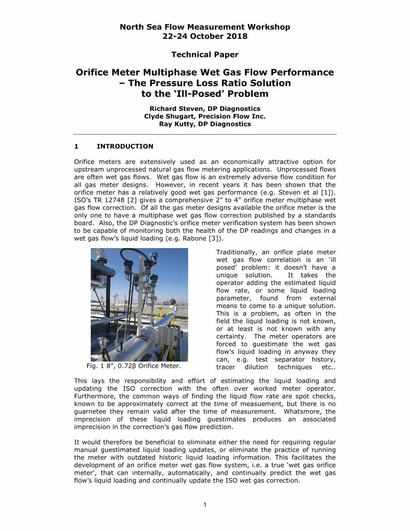
North Sea Flow Measurement Workshop 22-24 October 2018 Technical Paper 1 Orifice Meter Multiphase Wet Gas Flow Performance – The Pressure Loss Ratio Solution to the ‘Ill-Posed’ Problem Richard Steven, DP Diagnostics Clyde Shugart, Precision Flow Inc. Ray Kutty, DP Diagnostics 1 INTRODUCTION Orifice meters are extensively used as an economically attractive option for upstream unprocessed natural gas flow metering applications. Unprocessed flows are often wet gas flows. Wet gas flow is an extremely adverse flow condition for all gas meter designs. However, in recent years it has been shown that the orifice meter has a relatively good wet gas performance (e.g. Steven et al [1]). ISO’s TR 12748 [2] gives a comprehensive 2” to 4” orifice meter multiphase wet gas flow correction. Of all the gas meter designs available the orifice meter is the only one to have a multiphase wet gas flow correction published by a standards board. Also, the DP Diagnostic’s orifice meter verification system has been shown to be capable of monitoring both the health of the DP readings and changes in a wet gas flow’s liquid loading (e.g. Rabone [3]). Fig. 1 8”, 0.72β Orifice Meter. Traditionally, an orifice plate meter wet gas flow correlation is an ‘ill posed’ problem: it doesn’t have a unique solution. It takes the operator adding the estimated liquid flow rate, or some liquid loading parameter, found from external means to come to a unique solution. This is a problem, as often in the field the liquid loading is not known, or at least is not known with any certainty. The meter operators are forced to guestimate the wet gas flow’s liquid loading in anyway they can, e.g. test separator history, tracer dilution techniques etc.. This lays the responsibility and effort of estimating the liquid loading and updating the ISO correction with the often over worked meter operator. Furthermore, the common ways of finding the liquid flow rate are spot checks, known to be approximately correct at the time of measuement, but there is no guarnetee they remain valid after the time of measurement. Whatsmore, the imprecision of these liquid loading guestimates produces an associated imprecision in the correction’s gas flow prediction. It would therefore be beneficial to eliminate either the need for requiring regular manual guestimated liquid loading updates, or eliminate the practice of running the meter with outdated historic liquid loading information. This facilitates the development of an orifice meter wet gas flow system, i.e. a true ‘wet gas orifice meter’, that can internally, automatically, and continually predict the wet gas flow’s liquid loading and continually update the ISO wet gas correction.
-
Upload
khangminh22 -
Category
Documents
-
view
0 -
download
0
Transcript of Orifice Meter Multiphase Wet Gas Flow Performance - NFOGM
North Sea Flow Measurement Workshop 22-24 October 2018
Technical Paper
1
Orifice Meter Multiphase Wet Gas Flow Performance – The Pressure Loss Ratio Solution
to the ‘Ill-Posed’ Problem
Richard Steven, DP Diagnostics Clyde Shugart, Precision Flow Inc.
Ray Kutty, DP Diagnostics
1 INTRODUCTION Orifice meters are extensively used as an economically attractive option for upstream unprocessed natural gas flow metering applications. Unprocessed flows are often wet gas flows. Wet gas flow is an extremely adverse flow condition for all gas meter designs. However, in recent years it has been shown that the orifice meter has a relatively good wet gas performance (e.g. Steven et al [1]). ISO’s TR 12748 [2] gives a comprehensive 2” to 4” orifice meter multiphase wet gas flow correction. Of all the gas meter designs available the orifice meter is the only one to have a multiphase wet gas flow correction published by a standards board. Also, the DP Diagnostic’s orifice meter verification system has been shown to be capable of monitoring both the health of the DP readings and changes in a wet gas flow’s liquid loading (e.g. Rabone [3]).
Fig. 1 8”, 0.72β Orifice Meter.
Traditionally, an orifice plate meter wet gas flow correlation is an ‘ill posed’ problem: it doesn’t have a unique solution. It takes the operator adding the estimated liquid flow rate, or some liquid loading parameter, found from external means to come to a unique solution. This is a problem, as often in the field the liquid loading is not known, or at least is not known with any certainty. The meter operators are forced to guestimate the wet gas flow’s liquid loading in anyway they can, e.g. test separator history, tracer dilution techniques etc..
This lays the responsibility and effort of estimating the liquid loading and updating the ISO correction with the often over worked meter operator. Furthermore, the common ways of finding the liquid flow rate are spot checks, known to be approximately correct at the time of measuement, but there is no guarnetee they remain valid after the time of measurement. Whatsmore, the imprecision of these liquid loading guestimates produces an associated imprecision in the correction’s gas flow prediction. It would therefore be beneficial to eliminate either the need for requiring regular manual guestimated liquid loading updates, or eliminate the practice of running the meter with outdated historic liquid loading information. This facilitates the development of an orifice meter wet gas flow system, i.e. a true ‘wet gas orifice meter’, that can internally, automatically, and continually predict the wet gas flow’s liquid loading and continually update the ISO wet gas correction.

North Sea Flow Measurement Workshop 22-24 October 2018
Technical Paper
2
Industry has slowly been moving towards such a wet gas orifice meter design. A methodology that could achieve such a feat has long been applied with the Venturi meter. A wet gas flow’s liquid loading can be predicted via its relationship with the Venturi meter’s measureable Pressure Loss Ratio, ‘PLR’ (see de Leeuw [4]). Some in industry have periodically discussed adopting this method for orifice meters, e.g. a CEESI Joint Industry Project (JIP) in the early 2000’s. Steven (e.g. [1, 5] and Reader-Harris [6, 7] have semi-independently conducted research, but overall progress has been slow. In 2012 ISO 11583 [6] published an orifice meter PLR vs. liquid loading equation set. This was based on very limited 4” orifice meter wet gas flow data published by the CEESI JIP in 2007 [5]. The technical principle is sound, but it is now known that there are some limitations, restrictions, and indeed flaws to this equation set. These include:
a biased PLR dry gas baseline calculation,
limits to the upper beta range, β ≤ 0.68 (due to ISO’s lack of data),
applicability to gas with liquid hydrocarbon only, and not gas with liquid hydrocarbon and / or water (due to ISO’s lack of data), and,
limitations in some other parameter ranges (due in part to ISO’s lack of data and in part to some physical limitations inherent to the technique.)
This paper discusses multiple orifice meter data sets where DP Diagnostics have altered, rectified, and improved the ISO liquid loading prediction calculations, and turned this concept into a practical wet gas orifice meter product. 2 WET GAS FLOW PARAMETER DEFINITIONS A wet gas flow is defined to be any two-phase (liquid and gas) flow where the liquid loading Lockhart-Martinelli parameter (XLM) is less or equal to 0.3, i.e. XLM≤0.3. This definition covers any combination of gaseous and liquid components, i.e. the liquid can be a liquid hydrocarbon (LHC), water or a mix of LHC and water. The Lockhart-Martinelli parameter (equation 1) is a non-dimensional expression of the relative amount of total liquid with the gas flow. Note that mg and ml are the gas and liquid mass flow rates respectively (where ml is the sum of the liquid component flow), and g & l are the gas and liquid densities respectively.
l
g
g
lLM m
mX
--- (1)
glg
g
ggDA
mFr
1 ---- (2)
The gas to liquid density ratio (DR = ρg/ρl) is a non-dimensional expression of pressure. The gas densiometric Froude numbers (Frg), shown as equation 2, is a non-dimensional expression of the gas flow rate, where g is the gravitational constant, D is the meter inlet diameter, and A is the meter inlet area. With one single liquid component a wet gas has one liquid density. With multiphase wet gas flow there is two liquid densities (water and LHC). The “water to liquid mass ratio” (or ‘WLR’) is here defined as the ratio of the water to

North Sea Flow Measurement Workshop 22-24 October 2018
Technical Paper
3
total liquid mass flow rates. The WLR is shown as equation 3, where mw and mlhc represent the mass flow rates of water and liquid hydrocarbon respectively.
lhcw
w
mm
mWLR ..
.
--- (3)
It is common reasonable engineering assumption to consider the liquid components of a wet gas flow homogenously mixed. The homogenous liquid phase density (ρl,hom) is calculated by equation 4, where ρLHC and ρw are the liquid hydrocarbon and water densities respectively. Steven et al [8] discusses the WLR and average liquid density calculations if there is also chemical inhibitor.
WLRWLR wlhc
hlwl
1hom,
--- (4)
Most wet gas flow conditions produce a positive bias in the orifice meter gas flow rate prediction. This bias is called an over-reading (‘OR’), see equation 5. Wet gas usually produces a differential pressure (ΔPwg) greater than if the gas phase of the wet gas flow flowed alone (ΔPg). The result is an erroneous, or ‘apparent’ gas mass flow rate prediction (mg,apparent). This over-reading ratio is often described as a percentage (see equation 6). Correction of this over-reading is the basis for orifice meter ‘wet gas corrections’.
g
tp
g
Apparentg
P
P
m
mOR
.
.
--- (5)
%100*1%100*1%.
.
g
tp
g
Apparentg
P
P
m
mOR --- (6)
3 STANDARD ORIFICE METERS AND WET GAS FLOW PERFORMANCE ISO TR 12748 [2] states a horizontally installed orifice meter wet gas flow correction. The equation set is reproduced here as equation set 7 through 13. Table 1 shows the range of this correction’s applicability. Figure 2 reproduces the ISO massed orifice meter wet gas flow data set of >2000 data points, from multiple owners, recorded independently and periodicaly over two decades, at two institutions, using three test facilities, using multiple orifice meters of paddle, single and dual chamber flange tap design. For a known liquid flow rate this ISO correction predicts the gas flow to 2% uncertainty at 95% confidence. A limitation of this data set, and hence the ISO orifice meter wet gas correction, is that it covers 2” thru 4” orifice meters only. Use at larger meter diameters is therefore an extrpolation of the correlation. In 2015 CEESI (Steven [9]) released two 8”, 0.68β orifice meter wet gas data sets showing that extrapolating this ISO correlation to 8” orifice meters increases the gas flow prediction uncertainty (for a known liquid flow) to 3%. In 2016/17 a Precision Flow 8” dual chamber orifice meter (shown in Figure 1) was tested at CEESI in multiphase wet gas flow. A 0.721β plate was used. Table 2 shows the data set range. This data set extrapolates the correlation in terms of meter size

North Sea Flow Measurement Workshop 22-24 October 2018
Technical Paper
4
and beta. Figure 3 reproduces the 2015 NSFMW CEESI graph (Steven [9]) with the new Precision Flow data superimposed on that data set. Even with the higher beta the ISO correlation predicts the gas flow to < 3% uncertainty.
Fig 2. ISO Orifice Meter Multiphase Wet Gas Data Set
With & Without ISO Correction for Known Liquid Flow Rate.
2
,
..
1 LMLM
apparentgg
XCX
mm
--- (7)
n
g
l
n
l
gC
hom,
hom,
--- (8)
WLRFr
transitiong *2.05.1 -- (9)
WLRA exp*1.04.0# -- (10)
2
,
#
2
1
transitiong
stratFr
An -- (11)
stratnn for transitiongg FrFr , -- (12)
2
#
2
1
gFr
An for transitiongg FrFr , -- (13)
Note that Frg then 21n

North Sea Flow Measurement Workshop 22-24 October 2018
Technical Paper
5
Parameter Range Pressure (P) 6.7 < P (Bar) < 78.9
Gas to liquid DR 0.0066 < DR< 0.11 Frg range 0.22 to 7.25
WLR 0 ≤ WLR ≤ 1 XLM < 0.35
Inside full bore diameter 2” thru 4” Beta (Diameter Ratio) 0.2433 ≤ β ≤ 0.7298 Gas / Liquid phases Natural gas / LHC / Water
Table 1. ISO TR 12748 Orifice Meter Wet Gas Flow Correction Factor Range.
Fig 3. All 8” Orifice Meter Multiphase Wet Gas Data
With & Without ISO Correction Applied.
Parameter Range Abs. Pressure 35 < Pressure (Bar) <75.2
Gas to liquid density ratio 0.027 < DR < 0.085 Frg range 0.5 < Frg < 3.6
WLR 0 < WLR < 1 XLM 0 ≤ XLM < 0.07
Inside full bore diameter 7.625” Beta (Diameter Ratio) 0.721
Gas / Liquid phase Gas / LHC / Water Table 2. Precision Flow Multiphase Wet Gas Flow Data Set Flow Range.
4 GAS METER DIAGNOSTIC SYSTEMS AND WET GAS FLOW All gas meter designs have significant over-readings when applied to wet gas flows (e.g. see Figure 18, in Section 6). Some gas meters, e.g. ultasonic, Coriolis, and orifice meters have diagnostic suites that can potentially identify the presence wet gas flow, and therefore when the (uncorrected) gas flow prediction is probably biased. This has been discussed in several conference papers, e.g. Stoof [10] for ultrasonic meters, Hollingsworth [11] and Steven [12] for Coriolis meters, and Steven [9] for ultrasonic and orifice meters.

North Sea Flow Measurement Workshop 22-24 October 2018
Technical Paper
6
Fig 4. Schematic of a Coriolis Meter Drive Gain Diagnostic Reaction to Wet Gas.
Fig 5. Schematic Ultrasonic Meter Profile Factor & Symmetry Reaction to Wet Gas.
Fig 6. Schematic of an Orifice Meter PLR vs XLM Wet Gas Relationship.
North Sea Flow Measurement Workshop 22-24 October 2018
Technical Paper
7
Figures 4, 5, and 6 show respective schematics of Coriolis meter drive gain, ultrasonic meter profile factor and symmetry, and orifice meter PLR parameter relationships with Lockhart Martinelli parameter. These schematics represent original data shown by Steven in [12], [9], and [1] respectively. Each of these gas meter designs have multiple diagnostic parameters within their respective diagnostic suites that could potentially identify wet gas flow. Figures 4, 5, and 6 serves only as examples. However, gas meter diagnostics do not solve the problem of wet gas metering. They only sometimes show there is a problem. They do not predict the wet gas liquid loading. Furthermore, even when the liquid loading is somehow known, a relaible wet gas correction is still required to find the true gas (and liquid) flow rates. Some gas meter manufacturers only advocate using the diagnostic system to indicate when the gas is wet. However, all gas meter diagnostic suites have a finite sensitivity to different problems. For any gas meter design’s diagnostic system there is always a small finite liquid loading before the warning threshold is crossed. And a small finite liquid loading produces a corresponding finite gas flow prediction bias, already in existence when the diagnostic warning is triggered. For example: In 2015 Stoof [10] said tha a specific ultrasonic meter “… uses standard diagnostic parameters such as Speed of Sound and Turbulence in order to identify a potential presence of wet gas with LVF of typically >0.5%. This is typically the amount of LVF where significant over-reading of a meter starts.” Note that LVF is ‘Liquid Volume Fraction’ and is a liquid loading parameter. That is this ultrasonic meter’s diagnostics have a sensitivity threshold to wet gas of LVF > 0.5%. There is no guidance offered on what course of action to take if and when the diagnostic suite does identify wet gas flow. Furthermore, it is implied that when there is an un-noticed wet gas flow of LVF ≤0.5% there is no ‘significant’ associated gas flow prediction bias. But, ‘significant’ over-reading is a subjective term: Consider a wet natural gas flow at 15 Bar(a) and 288K. At these conditions a 0.5% LVF is a XLM of about 0.0466. Steven [15] shows at these conditions various ultrasonic meter design’s wet gas flow over-readings can be between 0% and +10%. Figure 18 shows one ultrasonic meter having an over-reading at this diagnostic wet gas sensitivity threshold up to +10%. Some would consider an unnoticed ultrasonic meter gas flow prediction bias of +10% significant. For the special case of intermittent wet gas flow, i.e. a gas flow that only periodically becomes wet, Hollingsworth [11]) promotes a specific use of a gas meter diagnostic system. If and when the diagnostic system shows a potential problem in a flow known to be periodically wet, the system is then programmed to treat the gas flow prediction as biased. While the diagnostic system continues to indicate a problem the gas flow prediction is held at the last value read before the onset of the diagnostic alarm, i.e. the last ‘trustworthy’ gas flow prediction. That is, it is assumed that the present wet gas flow has the same gas flow rate as prior to the gas becoming wet. When the diagnostic warning dissipates the live gas flow prediction resumes. In this way any liquid induced gas flow prediction bias is hoped to be avoided. As long as the various underlying assumptions are valid this approach is valid. However, this methodology does contain several big assumptions which may or may not be valid in any given field application. In order for this methodology to work the following list of assumptions must hold true:

North Sea Flow Measurement Workshop 22-24 October 2018
Technical Paper
8
1. the flow is only intermittently wet, so that a dry gas flow rate can be set,
2. the diagnostic parameter shift is caused specifically by wet gas and not another unrelated malfunction source,
3. the diagnostic parameter is sensitive enough to indicate wet gas flow before significant bias has been induced in the gas flow prediction,
4. the wet gas flow has the same gas flow rate as the preceeding dry gas flow.
However, for many intermittent wet natural gas flows, there is no guarantee or physical basis to assume that the wet gas flow’s gas flow rate is the same quantity as when the flow was previously dry. Also, this method cannot be employed in continuous wet gas flow. Regradless of whether the gas meter diagnostic suite is used to simply alert the user to the presence of wet gas flow, or to assume that the last gas flow rate metered without a diagnostic alarm is still the true gas flow rate, these methods are clearly limited in their capability. In these scenarios the users are effectively left with two chocies. They can do nothing but passively wait and hope for the problem (i.e. the liquid) to go away. Or they can actively react to the presence of wet gas flow by trying to predict the liquid loading from an independent means, and if it exists, then apply some wet gas correction. It is therefore advantageous for a gas meter to not only be able to identify wet gas flow, but also be capable of real time estimation of the liquid loading, the associated over-reading, and the actual gas flow rate. The following now describes how an orifice meter can achieve this. 5 ORIFICE METER’S AND ISO TR 11583’s XLM = f(PLR) EQUATION A gas meter with a diagnostic suite that may sense the presence of wet gas and thereby indicate a problem, and / or has a wet gas correction algorithm that requires manual input of the liquid quantity, is still just inherently a gas meter. Although useful, these ‘bells and whistles’ do not a wet gas meter make. A definition for a basic wet gas meter is a system that can take primary signals from sensors internal to that metering system only, and apply them to suitable algorithms to show the gas is wet, quantify the liquid loading, and predict the actual gas flow rate of that wet gas flow. To achieve this there must be at least one parameter derivable from the meter’s primary signals that has a reproducible, and therefore mathematically predictable relationship with the liquid loading across a wide range of wet gas flow conditions. Amongst gas meters, only DP meter systems have been shown to have such parameters. The examples of the Coriolis meter drive gain and ultrasonic meter diagnostic parameters sketched in Figures 4 and 5 show some trending with liquid loading. However, there is considerable scatter in real data sets. So far such Corilois and ultrasonic meter parameters are only used to show general trending. In 1997 the Royal Dutch Shell engineer de Leeuw [13] discussed Venturi meters in wet gas flow applications. De Leeuw proposed a (third) pressure tap be placed downstream of the meter so that the permanent pressure loss ‘PPL’ (ΔPPPL) could be read along with the traditional DP (ΔPt). De Leeuw stated:

North Sea Flow Measurement Workshop 22-24 October 2018
Technical Paper
9
“The potential for the pressure loss measurement is to use it as a means to determine the liquid content of the flow, from which the over-reading factor can be determined. In essence this could form a simple two phase meter”. This concept converts a stand alone DP meter into a wet gas meter design ‘for the masses and not just the classes’. For the specific case of Venturi meters with the specific scenario of wet gas flow, de Leeuw discussed using the Pressure Loss Ratio (‘PLR’), i.e. the ratio of the PPL and traditional DPs (PLR = ΔPPPL / ΔPt), to quantify a wet gas flow’s liquid loading. However, in order to find the XLM=f(PLR) relationship de Leeuw stated “additional experiments might be required”. This seminal insight led to twenty years of various commercial ‘wet gas‘ Venturi meters applying this principle. Venturi meters are only one meter design within a general group called the Differential Pressure (‘DP’) meters. Other DP meters, including the orifice meter, operate according to the same physical principles. Hence, orifice meters could also be expected to have a PLR=f(XLM) relationship. In circa 1998 a CEESI run JIP (that included de Leeuw’s team at Shell) was planning to investigate the wet gas performance of various gas meters. The JIP members decided then that all DP meters to be wet gas flow tested (including orifice meters) should have both the traditional and PPL DPs read. Figure 7 shows a schematic of an orifice meter with a 3rd pressure tap located 6D downstream of the plate, and two DP transmitters reading the traditional DP (ΔPt) and PPL (ΔPPPL) respectively. Figures 1 and 7 show an orifice meter with this arrangement. Technically, for flange tap orifice meters, due to the upstream tap being in such close proximity to the plate there is a slight PPL and PLR bias, but that is not important at this juncture. This orifice meter geometry effectively reads a value that can be labelled a Pressure Loss Ratio (‘PLR’).
Fig 7. Schematic Sketch of an Orifice Meter with a Downstream Pressure Tap
and PPL DP (ΔPPPL) and Traditional (ΔPt) DP Being Read. The 2007 CEESI JIP data release [5] showed 4”, 0.34β, 0.4β, 0.5β and 0.68β orifice meter wet gas flow data. For ≥0.5β there was a mathematically derivable relationship between the PLR and XLM. Although it was not part of the original CEESI JIP report, this data release gave examples of an orifice meter wet gas correction coupled with rudimentry sample XLM=f(PLR) data fits. Figure 8 reproduces one sample graph of this data. An ISO TC30 working group subsequently fitted this JIP ≥ 0.5β wet gas orifice meter XLM vs. PLR data and published the results in TR 11583 [6]. The ISO TR 11583 XLM = f(PLR) fit is reproduced here as equation set 14 through 16.

North Sea Flow Measurement Workshop 22-24 October 2018
Technical Paper
10
Fig 8. Sample JIP 4”, 0.5β Oifice Meter PLR vs. XLM Data.
Limits of use in addition to the limits of the wet gas correlation are the beta range 0.5 ≤ β ≤ 0.68, i.e. the JIP 4” data used by ISO, the XLM limit expressed as equation 17, and the maximum DR limit expressed as equation 18. The dry gas orifice meter PLRdry value is the Urner theoretical value published in ISO 5167-2 [14], where Cd and β represents the orifice meter discharge coefficient (calculatable by the RHG equation, also given in ISO 5167-2) and orifice beta respectively. The wet gas flow PLRwet is that read from the meter in service. Equation 16 is the XLM prediction which is a function of orifice meter beta (β), the wet gas flow’s DR, and ‘Y’, i.e. the difference in the read wet (PLRwet) and dry (PLRdry) baseline PLR.
224
224
11
11
dd
dddry
CC
CCPLR
(14)
drywet PLRPLRY (15)
92.0
9.4
41.6DR
YX LM
(16)
46.045.0 DRXLM (17)
09.021.0 DR (18)
The XLM limit of applicability (i.e. equation 17) is largely due to the limits of the small data set used to create the correlation rather than any known physical limitations in the technique. Figure 9 shows diagramatical representation of this ISO TR 11583 density ratio limitation.

North Sea Flow Measurement Workshop 22-24 October 2018
Technical Paper
11
Fig 9. ISO TR 11583 XLM =f(PLR) Maximum XLM vs. DR.
The stated DR limit of applicability of the ISO TR 11583 XLM = f(PLR) data fit (i.e. equation 18) is represented by Figure 10. Whereas these authors consider equation 17 and it’s corresponding Figure 9 to be practical and defensible with the data set ISO used, the authors consider the limits of equation 18 (see Figure 10) rather conservative. For example, equation 18 states that for a 0.5β the ISO XLM prediction is only valid for DR ≤0.015. However, the ISO TR 11583 data set’s minimum DR was 0.014, meaning it is not practically possible to apply this algorithm to 0.5β orifice meters without extrapolating the DR parameter.
Fig 10. ISO TR 11583 XLM = f(PLR) Maximum Density Ratio (XLM) vs. Beta (β).
Figure 8 shows JIP data where a quantifyable XLM = f(PLR) relationship is still plausible at higher DR values, e.g. a DR of 0.052, albeit at increasing scatter. The XLM prediction at higher DR values has higher uncertainty due in part to more data scatter, but the resulting gas flow prediction has an associated uncertainty still of industrial practical use. It is perhaps prudent as this juncture to discuss the sensitivity of this ISO orifice meter algorithm to the DP signal uncertainties, the associated PLR uncertainty, the corresponding XLM prediction uncertainty, and finally the associated OR prediction uncertainty.

North Sea Flow Measurement Workshop 22-24 October 2018
Technical Paper
12
The single phase orifice meter uses the square root of the traditional DP (√ΔPt) to predict the gas flow rate. Hence, a 1% ΔPt reading uncertainty produces an associated ½% flow prediction uncertainty component. A 1% DP uncertainty is rather large for the modern digital DP transmitters on the market, most will give significantly lower uncertainties across wide DP ranges. Therefore DP reading uncertainties are not usually a significant issue to modern single phase orifice meter operators. However, for the case of wet gas flow, the ratio of the PPL and traditional DP readings (ΔPPPL/ΔPt) gives the PLR used to predict XLM. If both DP transmitters were to have a large 1% ΔP uncertainty then the associated root sum square PLR uncertainty is √2%. Equation 19 shows the sensivity of the ISO XLM prediction to the PLR value.
92.0
9.4
41.6DR
dPLR
dX LM
(19)
In the following example, let us assume that the ISO TR 11583 equation set is precisley correct. Consider a wet gas with a XLM of 0.071, a DR of 0.04, a Frg of 2.5, and a WLR of 0% flowing through a 0.65β orifice meter. The ISO PLRdry prediction for a discharge coefficient of 0.603 is approximately 0.574. Say the read wet gas PLR is 0.6, making the Y value 0.026. The ISO equation 16 then predicts a XLM of 0.071, as required. Now, let us account for the real world DP reading uncertainties. Equation 19 shows that in this case the local gradient (i.e. sensitivity) of the XLM prediction to the PLR input is 2.74. PLR uncert PLR dry Read PLR wet Y XLM OR OR%
0% 0.574 0.600 0.026 0.071 1.097 9.71 +√2% 0.574 0.608 0.034 0.094 1.128 12.80 -√2% 0.574 0.592 0.018 0.048 1.066 6.59
Table 3. DP Readings with 1% Uncertainty Effect of ISO TR 11583 Calculations. PLR uncert PLR dry Read PLR wet Y XLM OR OR%
0% 0.574 0.600 0.026 0.071 1.097 9.71 +1/√2% 0.574 0.604 0.030 0.083 1.113 11.26 -1/√2% 0.574 0.596 0.022 0.060 1.082 8.15
Table 4. DP Readings with ½ % Uncertainty Effect of ISO TR 11583 Calculations. Consider the scenarios of the DP readings having maximum uncertaities of 1% (see Table 3) and 0.5% (see Table 4). The effect of these two DP uncertainties on the read PLR values and associated XLM predictions cause the over reading of 9.7% to be predicted as between +12.8% and 6.6% (i.e. 9.7%±3.1%) and +11.3% and 8.2% (i.e. 9.7%±1.6%) respectively. As a check on the veracity of the calculation, note that Table 3 shows the DP uncertainty of +1% causing a PLR difference of 0.608-0.06=0.08, and a corresponding XLM difference of 0.094-0.071=0.023, which gives a ratio of 0.23/0.08=2.74 as required by equation 19. Note that halfing the DP uncertainty from 1% to ½% causes the uncertainty of the OR% prediction to approximately half from 3.1% to 1.6%, i.e. there is a linear relationship between DP reading uncertainty and %OR prediction. Whereas the relatively large uncertainties involved in real world wet gas metering means that this examples uncertainties are only moderate, the uncertainty of the DP reading in wet gas is ceratinly more critical than it is with dry gas flow applications. Thankfully, modern digital DP transmitters give low uncertainties across reasonable DP ranges, it is possible to expand the DP range by stacking DP transmitters of different ranges, and the DP Diagnostics’s verification system has

North Sea Flow Measurement Workshop 22-24 October 2018
Technical Paper
13
an excellent DP reading integrity check that proves the quality of the DP readings. However, the general rule of instrumentation of course holds, the larger the signal being read, and the closer to the instruments upper range limit the signal is, the more accurate the systems output will be. That is, as the DPs go up, the wet gas orifice meter’s ability to measure wet gas flow via the PLR gets better. Once, the PLR has been predicted as accurately as practically possible, the effect of the resulting XLM prediction uncertainty is also important. Considering equations 5 and 7, we can say the orifice meter wet gas flow over-reading is expressed by equation 20. Hence, the local sensitivity, i.e. the gradient of OR vs. XLM, is given by equation 21.
21 LMLM XCXOR (20)
212
2
LMLM
LM
LM XCX
CX
dX
dOR
(21)
Equation 21 indicates that the OR prediction (i.e. gas flow prediction correction) is not overly sensitive to XLM. For example, let us consider the case of a wet gas flow with a XLM of 0.05, a DR of 0.07, a Frg of 3, and a WLR of 0%. The resulting Chisholm parameter ‘C’ (see equation 8) is 2.6 and the corresponding over-reading ‘OR’ is 1.064, or +6.4%. Hence, at a XLM of 0.05 the local gradient (equation 21) is a modest value of 1.27. A severe to moderate percentage XLM error produces a moderate to modest associated OR prediction bias. That is, the correction is quite forgiving to biases in XLM prediction. Say at these conditions we predict a XLM value of not 0.05, but 0.08 instead. This is a +60% XLM bias. The associated OR prediction jumps from 1.064 (or 6.4%), to 1.102 (or 10.2%). Note that the ratio of the OR difference (1.102-1.064 = 0.0378) and the XLM difference (0.08-0.05 = 0.03) is 0.0378/0.03 = 1.26 (i.e. approximately the local gradient at a XLM value of 0.05 as calculated by equation 21). So, a +60% XLM bias produces <+4% gas flow prediction bias. Moderate XLM prediction bias is absorbed well in the wet gas correction algorithm. Therefore, a practical commercial wet gas orifice meter XLM =f(PLR) fit can operate across a larger DR range, and absorb a larger uncertainty in the associated XLM prediction, than implied by the natural caution of ISO. The ISO TR 11583 Lockhart Martinelli parameter prediction method is an initial data fit that promotes the concept. It is not meant to be the last word on the matter. It has several limitations due to the limited information available at the time of publication. Limiting factors include:
The TR 11583 orifice meter over-reading correction uses an earlier version than that later published by TR 12748 (i.e. equation set 7 thru 13 here), i.e. it is only applicable to gas with LHC, and not gas with LHC and water.
The orifice meter ISO 5167-2 theoretical dry gas PLR baseline has since been shown to have a significant bias at β>0.55, i.e. in the beta range orifice meter PLR is sensitive to XLM.
The ISO TR 11583 orifice meter XLM = f(PLR) relationship was only proven against gas with LHC, not multiphase wet gas flow data
The data available to the ISO TC30 technical committee limited the range of XLM that could be predicted by TR 11583. The ISO TR 11583 orifice
North Sea Flow Measurement Workshop 22-24 October 2018
Technical Paper
14
meter XLM = f(PLR) relationship is only valid for 2” ≤ inlet diameter ≤ 4”, and 0.5 ≤ β ≤ 0.68.
ISO TR 11583 text does not offer any wet gas flow metering system diagnostic capability or redundant sub-systems.
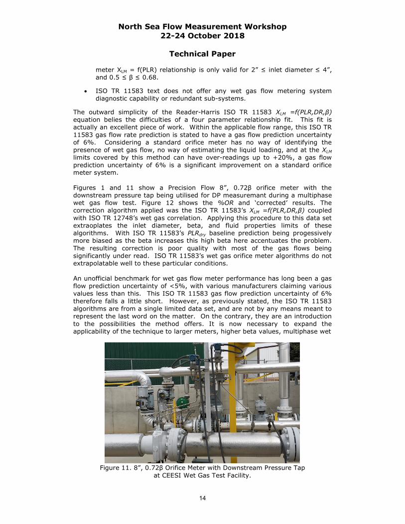
The outward simplicity of the Reader-Harris ISO TR 11583 XLM =f(PLR,DR,β) equation belies the difficulties of a four parameter relationship fit. This fit is actually an excellent piece of work. Within the applicable flow range, this ISO TR 11583 gas flow rate prediction is stated to have a gas flow prediction uncertainty of 6%. Considering a standard orifice meter has no way of identifying the presence of wet gas flow, no way of estimating the liquid loading, and at the XLM limits covered by this method can have over-readings up to +20%, a gas flow prediction uncertainty of 6% is a significant improvement on a standard orifice meter system. Figures 1 and 11 show a Precision Flow 8”, 0.72β orifice meter with the downstream pressure tap being utilised for DP measuremant during a multiphase wet gas flow test. Figure 12 shows the %OR and ‘corrected’ results. The correction algorithm applied was the ISO TR 11583’s XLM =f(PLR,DR,β) coupled with ISO TR 12748’s wet gas correlation. Applying this procedure to this data set extraoplates the inlet diameter, beta, and fluid properties limits of these algorithms. With ISO TR 11583’s PLRdry baseline prediction being progessively more biased as the beta increases this high beta here accentuates the problem. The resulting correction is poor quality with most of the gas flows being significantly under read. ISO TR 11583’s wet gas orifice meter algorithms do not extrapolatable well to these particular conditions. An unofficial benchmark for wet gas flow meter performance has long been a gas flow prediction uncertainty of <5%, with various manufacturers claiming various values less than this. This ISO TR 11583 gas flow prediction uncertainty of 6% therefore falls a little short. However, as previously stated, the ISO TR 11583 algorithms are from a single limited data set, and are not by any means meant to represent the last word on the matter. On the contrary, they are an introduction to the possibilities the method offers. It is now necessary to expand the applicability of the technique to larger meters, higher beta values, multiphase wet
Figure 11. 8”, 0.72β Orifice Meter with Downstream Pressure Tap
at CEESI Wet Gas Test Facility.

North Sea Flow Measurement Workshop 22-24 October 2018
Technical Paper
15
Fig 12. 8”, 0.721β Orifice Meter Wet Gas Data.
gas flows, and wider XLM and DR ranges, while reducing the gas flow prediction uncertainty to <5%. Also, any sub-system redundancy and diagnostic capabilities should be well received. 6 ORIFICE METER’S AND A COMMERCIAL XLM = f(PLR) EQUATION
DP Diagnostics has access to four wet gas orifice meter data sets with PPL data. These are 1) a Precision Flow 8”, 0.72β multiphase wet gas orifice meter data set, 2) the publicly released 1999-2002 JIP 4”, 0.5β two-phase wet gas orifice meter data set [5], 3) the CEESI 4”, 0.5β two-phase wet gas orifice meter data set long disclosed and discussed at gas meter schools, and 4) a blinded 3rd party 4”, 0.6β multiphase wet gas orifice meter data set. DP Diagnostics has created its own commercial wet gas orifice meter algorithm from this data. This technique is public domain. There is no IP associated with such a technique – hence the principles inclusion in an ISO technical report. Anybody is free to gather appropriate orifice meter wet gas data and produce an algorithm based on the XLM = f(PLR, β, DR) relationships. Hence, any disclosed algorithm can be copied by any 3rd parties, and therefore out of necessity DP Diagnostics considers their algorithm confidential. However, DP Diagnostics does optionally use the ISO TR 12748 multiphase wet gas correlation, DP Diagnostics PLRdry =f(β) and XLM = f(PLR, β, DR) data fits (see equation set 22 thru 24). However, DP Diagnostics also applies their orifice meter diagnostic system’s pattern recognition system to assure wet gas flow is identified. Only when this system identifies wet gas is the wet gas algorithm applied. The ISO method assumes every and any change in PLR is due to wet gas flow condition changes. It isn’t. This is a weaknes in the ISO methodology that DP Diagnostics has overcome.

North Sea Flow Measurement Workshop 22-24 October 2018
Technical Paper
16
fPLR fitdry , (22)
fitdrywet PLRPLRY , (23)
DRYfX LM ,, (24)
Table 5 shows the DP Diagnostics wet gas orifice meter algorithm range. The use of a much larger and wider range data set shows that much (but not all) of the limitations of ISO TR 11583 are due to limited data and not physical constraints. However, there are some limits due to physical constraints, e.g no β≤0.5, no DR > 0.1, and no XLM > 0.2.
Parameter Range DR range 0.01 < DR < 0.1 Frg range 0.5 < Frg < 5.2
WLR 0 < WLR < 1 XLM XLM < 0.2
Inside full bore diameter 2” ≤ Inlet diameter ≤ 8” Beta (Diameter Ratio) 0.5 ≤ β ≤ 0.75
Gas / Liquid phase Gas / LHC / Water Table 5. DP Diagnostics XLM vs. PLR Wet Gas Flow Data Set Flow Range.
The bias induced on the PLRdry prediction by the use of the ISO 5167-2 [14] Urner theoretical baseline was first publicly discussed in 2012 by Steven [15]. In 2016, Reader-Harris [16] suggested a theoretical calculation to correct this ISO orifice meter PLR equation bias. DP Diagnostics presently chooses to use a PLR = f(β) data fit from proven multiple data sets.
Fig 13. All 8”, 0.72β Orifice Meter Multiphase Wet Gas Flow Data .

North Sea Flow Measurement Workshop 22-24 October 2018
Technical Paper
17
Figure 13 shows all the 8”, 0.72β multiphase wet gas orifice meter data. This shows both the uncorrected OR and the result of applying the DP Diagnostics wet gas orifice meter algorithm, i.e. equation set 7 thru 13 coupled with the DP Diagnostics XLM = f(PLR, β, DR) data fit. This is the same raw data as ‘corrected’ by the ISO TR 11583 algorithm in Figure 12. The bias has been largely removed. Across the wet gas flow range the standard orifice meter has a OR (i.e. a gas flow prediction bias) of up to +10%. Applying the new wet gas orifice meter algorithm produces a gas flow prediction with 2.5% uncertainty to 95% confidence. The precise gas flow prediction uncertainty of this wet gas orifice meter is wet gas flow range dependent. Figure 14 shows the data for gas with water only. In that case the gas flow prediction uncertainty is <2% to 95% confidence. Although the liquid loading range in this particular data set is restricted to XLM < 0.07 (i.e. about ¼ of the range insustry considers wet gas) the majority of gas meters inadvertently used with wet natural gas flows operate in this liquid loading range.
Fig 14. 8”, 0.72β Orifice Meter Gas with Water Wet Gas Flow Data.
Fig 15. All 8”, 0.72β Orifice Meter Wet Gas Flow Data – Liquid Flow Rate
Predictions by Cross Referenceing DP Diagnostics Gas Flow and XLM Predictions.

North Sea Flow Measurement Workshop 22-24 October 2018
Technical Paper
18
Once a wet gas flow’s gas flow and Lockhart Martinelli parameter have both been predicted there is naturally an associatted total liquid flow rate prediction. This is predicted by rearranging equation 1 to produce equation 25, where mg and XLM are the predicted values.
DR
Xmm LMg
l (25)
As with all instruments and metrology, the smaller a measurand becomes the more difficult it becomes to measure it at a low percentage uncertainty. This wet gas orifice meter naturally has the same challenge. As such, there is little value in stating a wet gas meters liquid flow rate prediction uncertainties. The wet gas orifice meter’s liquid flow prediction is an informative trending indicator, and not a stated liquid flow ‘measurement’. This is an exact analogy with gas Coriolis meter denity outputs. Figure 15 shows all the 8”, 0.72β orifice meter total liquid flow prediction vs. the reference values. The liquid flow prediction trends with the reference and gives an indication of the approximate liquid mass flow rate. Figure 16 shows the ISO compliant 4”, 0.5β dual chamber orifice plate meter with a 6D downstream pressure port installed in the CEESI wet gas flow test facility. This meter was used to collect both the public JIP data (1999-2002) and the later independent CEESI wet gas data disclosed at the US gas meter schools. Figure 17 shows all wet gas data available to DP Diagnostics in term of the orifice meter over-reading and wet gas orifice meter gas flow prediction results obtained by the above wet gas orifice meter algorithm. Table 5 shows the range of these combined wet gas data sets.
Fig 16. 1 4”, 0.5β Orifice Meter.
The massed data shows the ‘wet gas orifice meter’ algorithm with a gas flow prediction uncertainty of 4% at 95% confidence. As shown in Figure 14 some individual data sets over certain ranges can have smaller uncertainties. Most gas meter operating procedures treat wet gas flow as an abnormal operating condition. They have reactive solutions for when wet gas flow is identified. However, this wet gas orifice meter operating procedure treats both dry and wet gas flows as normal operational conditions. This is a proactive approach to the wet gas flow metering.
There is very limited public data on the wet gas flow performance of different gas meter designs. There is therefore very little comparision data for the wet gas flow performance of different gas meter designs. Steven [9, 12] published 4” ultrasonic meter and 3” Coriolis meter wet gas data sets with standard orifice meter performance comparisons. Figure 18 superimposes the published 3” Coriolis meter and 4” ultrasonic meter wet gas data onto the 4” standard orifice meter and wet gas orifice meter data. The standard orifice meter and ultrasonic

North Sea Flow Measurement Workshop 22-24 October 2018
Technical Paper
19
Fig 17. All Available Wet Gas Orifice Meter Data.
Fig 18. 3” Gas Coriolis Meter, 4” Gas Ultrasonic Meter, 4” Gas Orifice Meter, and
the 4” Wet Gas Orifice Meter Data Superimposed on One Graph. meter have very similar wet gas performance. At a XLM of 0.2 they have an %OR up to +20%, while the 3” gas Corilois meter has a %OR of about +55%. The ‘wet gas orifice meter’, i.e. the orifice meter with the 6D downstream tap and the wet gas algorithms has a gas flow uncertainty of 3.5%. 7 WET GAS ORIFICE METER VERIFICATION AND SYSTEM REDUNDANCY The DP Diagnostics orifice meter verification system is described in multiple papers (e.g. Skelton [17]). A short review is given in the Appendix. When the gas is dry, and the meter is fully sevicable, the diagnostics results plotted on

North Sea Flow Measurement Workshop 22-24 October 2018
Technical Paper
20
the display are all inside the box (see Fig A2). As the gas gets wetter, i.e. the XLM and %OR increase, the points move away from the origin and the box. While the DP integrity check (x4,0) is unaffected by wet gas flow, (x1,y1) moves progressively into the 1st quadrant, while (x2,y2) and (x3,y3) both move progressively into the 3rd quadrant. Figure 19 shows the diagnostic response of an 8”, 0.72β orifice meter with wet gas flow at DR 0.014, Frg of 1.4 and WLR 0%. The diagnostics have identified there is a problem, the pattern is indicative of
Fig 19. 8” Orifice Meter Diagnostic
Wet Gas Flow Response. wet gas flow, and the increase and decrease of XLM can be tracked. However, the diagnostics offer more than just XLM monitoring, it can also be used to offer gas flow prediction redundancy.
Fig 20. 8”, 0.72β Orifice Meter Diagnostic’s y1, y2, and y3 Wet Gas Response
for DR 0.059 , WLR 0%, Frg 1.2. If PLR is sensitive to XLM, then PRR and RPR must also be sensitive to XLM. Figure 20 shows the 8”, 0.72β orifice meter diagnostic system’s PLR based y1, PRR based y2, and RPR based y3 diagnostic parameters vs. XLM. Clearly y1 (i.e. PLR) is sensitive to XLM, as required by the Section 6 XLM=f(PLR) relationship. Figure 20 also shows that y2 (i.e. PRR) and y3 (i.e. RPR) are also sensitive to XLM, and in fact slightly more sensitive, i.e. a slightly steeper (opposite sign) gradient. Hence, we can also derive XLM=f(PRR) and XLM=f(RPR). Furthermore, PRR and RPR use ΔPr, i.e. the smallest of these three orifice meter DPs. Any absolute shift in the DP values is largest in percentage terms with this smallest value, hence PRR and RPR are slightly more sensitivitive to XLM than PLR. However, in practice this slight advantage is negated by slightly higher ΔPr reading uncertainty (due to the smaller value). Nevertheless, the reading of the 3rd DP opens up two patent

North Sea Flow Measurement Workshop 22-24 October 2018
Technical Paper
21
pending backup, redundant, extra methods of predicting XLM. With all three DPs read the system has direct measurements of the PLR (ΔPPPL/ΔPt), the PRR (ΔPr/ΔPt), and the RPR (ΔPr/ΔPPPL). Giving the PRR and RPR parameters equivalent data fits to equation 24 produces corresponding XLM predictions for PRR and RPR as shown by equation 26 and 27 respectively.
XLM =f(Y,β,DR) = f(PLR) (24)
XLM = f(PRR) (26) XLM = f(RPR) (27)
Fig 21. 8”, 0.72β Wet Gas Orifice Meter with Three DP Ratio XLM Predictions
Supplied to Correction Factor Equation Set 7 Through 13.
Fig 22. 4”, 0.5β Wet Gas Orifice Meter with Three DP Ratio XLM Predictions
Supplied to Correction Factor Equation Set 7 Through 13.

North Sea Flow Measurement Workshop 22-24 October 2018
Technical Paper
22
DP Diagnostics have created such equation 26 and 27 data fits for their wet gas orifice meter system. Figures 21 and 22 show the results of applying these these back up systems to 8”, 0.72β and a 4”, 0.5β wet gas orifice meters. Reading the three DPs produces three ways of predicting the XLM and hence three ways of pedicting the gas flow rate. The resulting gas flow prediction is of the same order as the main XLM = f(PLRread) method. That is, these back up methods are practically very useful. If any one DP transmitter is lost - to saturation, drift, electrical failure etc., a relatively common problem with wet gas flow - the wet gas orifice meter continue to be serviceable via the remaining two DP transmitters. Note, with the diagnostic ability to infer any DP from the other two (see equation A1) this includes losing the main traditional DP reading. The traditional DP can be inferred from the other two DP readings, and XLM can be found via equation 27, meaning the full wet gas algorithm still remains available. This is a feature that does not exist in the basic ISO TR 11583 discussion. Worked Example: Let us consider the 8”, 0.72β wet gas orifice meter data set. At a DR of 0.0755, a Frg of 2.6, a WLRm of 37.3%, and XLM of 0.067 the corresponding OR% was 8.1%. The DPs read correctly are a ΔPt of 43.5 kPa, a ΔPr of 20.6 kPa, and a ΔPPPL of 23.0 kPa. The apparent gas mass flow rate is 25 kg/s. In this example the read PLR is 0.528 and the corresponding XLM prediction is 0.057. The orifice meter wet gas correlation shown as equation set 7 through 13 then predicts a gas flow rate of 22.8 kg/s. That is +1.2% from the data’s reference gas flow of 23.1 kg/s. That is, the standard orifice meter has a gas flow bias of +8.1% while the wet gas orifice meter has a gas bias of +1.2%. Let us now assume there is a DP reading problem. Consider the case of the traditional DP transmitter being spanned such that the maximum DP is 40 kPa (162”WC). The wet gas flow conditions are creating a DP larger than the instruments upper range limit, i.e. the DP transmitter is ‘saturated’. Wet gas flow causes significant higher DPs than if the gas flow alone, and hence this example is a one of the most common problems faced by users of orifice meters in wet gas flow applications. In this example the PLR read is not the correct value of 23kPa/43.5kPa =0.528, but 23kPa/40kPa =0.575. The resulting erroneous XLM prediction is 0.197 producing an associated gas flow rate prediction of 20.1 kg/s, i.e. a -12% gas flow rate prediction bias. This is an under-reading of 2.7 kg/s (i.e. 11.2 MMSCFD). Without diagnostics this problem would not be identified by means of any automated meter warning, and may well go un-noticed.
Fig 23. 8”, 0.72β Orifice Meter Wet Gas Flow Diagnostics Results For Correctly Read DPs (Left Hand Plot) and Over-Ranged DPt Transmitter (Right Hand Plot).
Figure 23 shows the diagnostic results for this example. The left hand side plot is the correctly operating meter with the wet gas flow. In this plot the DP integrity

North Sea Flow Measurement Workshop 22-24 October 2018
Technical Paper
23
check x4 shows the DPs are read correctly. The rest of the pattern is typical indicator of wet gas flow. (Note the standard ISO TR 11583 methodology just assumes any change in PLR is due to the presence of wet gas.) The right hand plot shows the diagnostic result when the traditional DP is saturated. In this plot the DP integrity check x4 shows the DPs are read incorrectly. The DP reading problem is now identified. At this point the meter operator now knows (via the diagnostics result) that the DP readings are not trustworthy. A cursory look at the three DP transmitters and their respective upper range limit will identify that the traditional DP transmitter is saturated (i.e. over ranged). As there are three DP readings, the removal of the traditional DP leaves the recovered and PPL DP readings. These now allow the correct traditional DP to be inferred via equation A1. The resulting ΔPt is 43.63kPa. Therefore, the apparent gas mass flow rate can still be correctly predicted via this inferred traditional DP. To operate as a wet gas orifice meter the XLM still needs to be predicted by the system (i.e. not keypad entered by the operator). The traditional DP is off-line, and the ISO method of using PLR is therefore also off-line. But with the DP Diagnostics three DP system we know the correct RPR (via the recovered and PPL DP readings) is 20.64kPa/22.98kPa =0.898, and hence we apply equation 27. (Alternatively, the inferred ΔPt allows PLR or PRR to be used.) The resulting XLM prediction of 0.0538, which along with the inferred traditional DP, now gives a gas mass flow rate prediction of 23.2 kg/s, which is +1.6% from the reference value. Hence, we can predict the actual gas mass flow rate as 23.2 kg/s, which instead of the ISO methodologies unnoticed -12% bias, is a gas flow prediction at <2% from the refernce result, and <0.5% from a serviceable ΔPt transmitter methodology. 9 CONCLUSIONS Orifice meters are very good wet gas flow meters. This statement will seem counter-intuitive to some. For many years a significant portion of flow meter subject specialists (including these authors), and vendors of competing meter designs, assumed and claimed standard gas orifice meters would have a relatively poor wet gas flow performance. It seemed intuitive that this would be the case. The orifice meter operates on simple principles while wet gas flow metering appears to be a highly complex challenge. But this position was largely based on intuition, not data. There used to be little data collated and analysed, so intuition was really all that industry had to go on. But now there is plenty data. Domingos [18] says a frequently heard objection to experimental evidence threatening to over-turn established dogma is “Data can’t replace human intuition”. In fact, it’s the other way around: human intuition can’t replace data. Intuition is what you use when you don’t know the facts, and since you often don’t intuition is often precious. But when the evidence is before you, why deny it? If you want to be tomorrows authority ride the data, don’t fight it. Massed data sets from different test facilities, using various paddle plate and dual chamber orifice meter designs by different manufacturers, researched by different groups, over many years, shows a remarkable (and unexpected) reproducibility. The resulting ISO TR 12748 publication shows the most advanced multiphase wet gas flow correlation of any gas meter. Across the wet gas range, i.e. XLM ≤0.3, for a known liquid loading, it predicts the gas flow to 2% uncertainty at 95% confidence.

North Sea Flow Measurement Workshop 22-24 October 2018
Technical Paper
24
The requirement to know the liquid loading from an external source is the Achilles heel of most generic gas meters with a wet gas correlation. Without that external liquid loading knowledge any such gas meter wet gas correlation is an ill-posed problem, i.e. there is no unique solution to the algorithm, there are two unknowns and one equation. Although the orifice meter has the most comprehensive multiphase wet gas correlation of all gas meter designs, if the liquid loading isn’t known then the standard orifice meter with a wet gas correlation is still just a gas meter. However, the orifice meter has a rare ability amongst simple gas meters to internally predict the liquid loading. The use of the downstream pressure port to read the PLR allows the XLM = f(PLR) relationship to be utilised. This internal prediction of the liquid loading makes the wet gas orifice meter algorithm a well posed problem, i.e. solveable with a unique solution. This thereby turns the system into a bonafide ‘wet gas orifice meter’, i.e. a meter that directly predicts the gas flow and liquid loading with no end user liquid loading keypad entry required. The crucial XLM =f(PLR) relationship is not heresay, or the unsubstantiated claims of vendors. On the contrary, both independepnt neutral test facilities NEL (e.g. Reader-Harris [7]), and CEESI, in conjunction with end users BP and ConocoPhillips (e.g. Steven et al [1, 8]) have independently discussed the existence of this relationship. So well understood is the direct reproducible physical link between the readable PLR and the liquid loading that ISO TR 11583 has published a XLM = f(PLR) relationship, albeit for a very limited orifice meter geometry and wet gas flow condition range. The limitations of this ISO equation set is partially only due to lack of data. DP Diagnostics has gathered together a wider ranging geometry and wet gas orifice meter data set, and developed their own alternative XLM =f(PLR) expression with correspondingly wider applicability. The resulting orifice meter system is a true wet gas meter. This DP Diagnostics wet gas orifice meter is designed for deliberate continuous use in wet gas flow applications. The presence of liquid with the gas is not an abnormal or adverse flow condition to this system, but rather a normal operating condition. There is no wet gas ‘correction’ per se. Rather, by the intrinsic nature of the combined wet gas correlation and liquid loading estimate method, a wet gas flow calculation algorithm is produced that predicts both the wet gas flow’s gas flow and liquid loading. The additional use of the orifice meter diagnostics IP gives the wet gas orifice meter user some system verifciation capability. Unlike the ISO methodology, the use of diagnostics gives a DP reading integrity check. Unlike the ISO method, this meter will not mistake DP reading problems with actual physical shifts in PLR and liquid loading. Furthermore, the diagnostics allows an easy visual way to monitor changes in wet gas liquid loading. Finally, this systems additional reading of the recovered DP gives three different DP ratios instead of ISO’s one. Each of these three DP ratios (and not just the singular PLR discussed by ISO) has a physical reproducible realtionship with the liquid loading. Hence, unlike the limiting ISO methodology, the DP Diagnostics wet gas orifice meter has redundant systems, and can continue to operate if any one of the system’s DP transmitters fails. When it comes to wet gas flow metering the orifice meter is a surprising diamond in the rough. Many orifice meters are used by default with wet gas flow, as most marginal field opeartors use basic gas meters out of economic necessity. Nevertheless, few would have claimed the orifice meter was particularly good at wet gas metering. However, irrefutable independent evidence, in the form of

North Sea Flow Measurement Workshop 22-24 October 2018
Technical Paper
25
massed data sets, has now led ISO to publish remarkable orifice meter wet gas equations quantifying the orifice meters wet gas performance. This ISO publication is not the last word on the issue, but rather the opening of R&D on a general principle. DP Diagnostics has now developed the concept further and created a wet gas orifice meter system that, for wider wet gas flow and orifice meter geometry ranges, can predict the gas flow to <4% uncertainty, and for some wet gas flow conditions <2.5% uncertainty without knowledge of the liquid flow being required. 10 REFERENCES [1] Steven R. et al “Horizontally Installed Orifice Plate Meter Response To Wet
Gas Flows”, North Sea Flow Measurement Workshop, Norway 2011. [2] ISO TR 12748: 2105 “Natural Gas – Wet Gas Flow Operations in Natural
Gas Operations” [3] Rabone J. “DP Meter Verification System - Operator Field Results and
Practical Use”, North Sea Flow Measurement Workshop, Norway 2017. [4] De Leeuw. R, "Liquid Correction of Venturi Meter Readings in Wet Gas
Flow", North Sea Flow Measurement Workshop, Norway, Oct 1997. [5] Steven R. “CEESI 1999-2002 Joint Industry Project Wet Gas Flow Meter
Data Release”, Estes Park, Colorado, USA, 2007. [6] ISO TR 11583: 2102 “Measurement of Wet Gas Flow by Means of Pressure
Differential Devices Inserted in Circular Cross-Section Conduits.” [7] Reader-Harris M. “Testing ISO/TR 11583 Outside It’s Range of Applicability:
Areas for Possible Improvement” European Flow Measurement Workshop, Netherlands, 2017.
[8] Steven R. et al “Expanded Knowledge On Orifice Meter Response To Wet
Gas Flows”, North Sea Flow Measurement Workshop, UK, Oct 2014. [9] Steven R. et al “Comparisons of Ultrasonic and Differential Pressure Meter
Responses to Wet Natural Gas Flow”, North Sea Flow Measurement Workshop, Norway, 2015.
[10] Stoof S. et al. ”Realizing a Class 1 Ultrasonic Gas Meter without HP
Calibration – An Innovative Approach as Contribution to an Economic Upstream Metering Solution”, North Sea Flow Measurement Workshop, Norway, 2015.
[11] Hollingsworth J. “A Method for Identifying and Reducing Errors in Wet Gas
Measurement with Coriolis Meters”, North Sea Flow Measurement Workshop, Norway, 2017.
[12] Steven R. et al “Coriolis Meters & Wet Gas Service” KL, Malaysia, SE Asia Hydrocarbon Flow Measurement Conference, March 2017 [13] De Leeuw R., “Liquid Correction of Venturi Meter Readings in Wet Gas
Flow”, North Sea Flow Measurement Workshop, Norway, 1997.

North Sea Flow Measurement Workshop 22-24 October 2018
Technical Paper
26
[14] International Standard Organisation, “Measurement of Fluid Flow by Means of Pressure Differential Devices, Inserted in Circular Cross Section Conduits Running full –Part 2”, No. 5167-2, 2003.
[15] Steven R. et al “Differential Pressure Meters – A Cabinet of Curiosities (and Some Alternative Views on Accepted DP Meter Axioms)”, North Sea Flow Measurement Workshop, St Andrews, UK, 2012. [16] Reader Harris M. “Diagnostics And Orifice Plates: Experimental Work”, North Sea Flow Measurement Workshop, UK, 2016. [17] Skelton M. et al “Diagnostics for Large High Volume Flow Orifice Plate Meters”, North Sea Flow Measurement Workshop, St. Andrews, UK, 2010. [18] Domingos P. “The Master Algorithm”, Page 39, Published by Basic Books, ISBN 978-0-465-09427-1. Appendix The technical details of the DP Diagnostics orifice meter diagnostics system are explained in multiple papers (e.g. Skelton et al [17]). The following is a short review.
Fig A1. Schematic of Orifice Meter, Istrumentation, and Pressure Fluctuation Plot. Figure A1 shows a sketch of an orifice meter with a 6D downstream presure tap and its associated pressure field. Three DPs are read from these three pressure taps, i.e. the traditional (ΔPt), PPL (ΔPPPL), and recovered DP (ΔPr). The relationship of these DPs is shown in Fig A1 and equation A1. This equation gives a powerful check on the integrity of the read DPs. Equation A1 holds true regardless of the flow being dry or wet gas. If we denote the actual percentage difference between the read (ΔPt) and inferred traditional DP (ΔPt,inf = ΔPr +ΔPPPL) as δ%, and the acceptable difference (i.e. unceratinty) of the DP sum as θ%, then an acceptable set of DP readings are within -1 ≤ δ%/θ% ≤ +1. DP Summation: ΔPt =ΔPr + ΔPPPL, uncertainty ± θ% --- (A1)
Traditional flow calculation: mt =f(ΔPt), uncertainty ± x% --- (A2)
Expansion flow calculation: mr =f(ΔPr), uncertainty ± y% --- (A3)
PPL flow calculation: mPPL =f(ΔPPPL), uncertainty ± z% --- (A4)
PLR calculation: PLR = ΔPPPL/ΔPt uncertainty ± a% --- (A5)
PRR calculation: PRR = ΔPr/ΔPt uncertainty ± b% --- (A6)
RPR calculation: RPR = ΔPr/ΔPPPL uncertainty ± a% --- (A7)

North Sea Flow Measurement Workshop 22-24 October 2018
Technical Paper
27
Each of the three DPs can individually meter the gas flow. Equations A2, A3, and A4 indicate this, where mt, mr, and mPPL denote the traditional, expansion, and PPL gas mass flow predictions. The uncertainties of these traditional, expansion, and PPL meters are denoted as x%, y%, and z% respectively. These flow predictions can be inter-compared. The difference between the PPL and traditional meters is denoted ψ%. The root sum square of their allowable difference is denoted as φ% (=√(x2+z2)). Normal operation therefore gives -1≤ ψ%/φ% ≤+1. The difference between the expansion and traditional meters is denoted λ%. The root sum square of their allowable difference is denoted as ξ% (=√(x2+y2)). Normal operation therefore gives -1 ≤ λ%/ξ% ≤ +1. The difference between the expansion and PPL meters is denoted Х%. The root sum square of their allowable difference is denoted as ν% (=√(y2+z2)). Normal operation therefore gives -1 ≤ Х%/ν% ≤ +1. Reading three DPs produces three DP ratios, i.e. the ‘PLR’ (see equation A5), the PRR (see equation A6), the RPR (see equation A7). Orifice meters have a reproducible PLR. DP Diagnostics predict the DP Ratios from data fits. These DP ratio predictions have uncertainties PLR±a%, PRR±b%, and RPR±c% respectively. The difference between the read and predicted DP ratios are α%, γ%, and η% for the PLR, PRR, and RPR parameters respectively. Hence, normal operation is indicated by -1 ≤ α%/a% ≤ +1 for the PLR, -1 ≤ γ%/b% ≤ +1 for the PRR, and -1 ≤ η%/c% ≤ +1 for the RPR. These seven diagnostic results can be shown on the operator interface as plots on a graph. That is, we can plot the following four co-ordinates to represent the seven diagnostic checks: (ψ%/φ%,α%/a%), (λ%/ξ%,γ%/b%), (Х%/ν%, η%/c%) and (δ%/θ%,0).
Fig A2. Normalized Diagnostic Box (NDB) with diagnostic results
For simplicity we can refer to these points as (x1,y1), (x2,y2), (x3,y3) & (x4,0). A Normalised Diagnostics Box (or ‘NDB’) of corner coordinates (1,1), (1,-1), (-1,-1) & (-1,1) can be plotted on the same graph, see Figure A2. This is the standard user interface of the diagnostic system. All four diagnostic points inside (a green border) NDB indicate a serviceable DP meter with single phase flow.
One or more point/s outside (a red) NDB indicates a possible meter system problem. Different problems can produce different diagnostic patterns.