mathematics

Article

On Little’s Formula in Multiphase Queues

Saulius Minkevicius 1 , Igor Katin 1 , Joana Katina 2,* and Irina Vinogradova-Zinkevic 3

�����������������

Citation: Minkevicius, S.; Katin, I.;

Katina, J.; Vinogradova-Zinkevic, I.

On Little’s Formula in Multiphase

Queues. Mathematics 2021, 9, 2282.

https://doi.org/10.3390/

math9182282

Academic Editors: Frank Werner, Lev

Klebanov and Christophe Chesneau

Received: 28 June 2021

Accepted: 13 September 2021

Published: 16 September 2021

Publisher’s Note: MDPI stays neutral

with regard to jurisdictional claims in

published maps and institutional affil-

iations.

Copyright: © 2021 by the authors.

Licensee MDPI, Basel, Switzerland.

This article is an open access article

distributed under the terms and

conditions of the Creative Commons

Attribution (CC BY) license (https://

creativecommons.org/licenses/by/

4.0/).

1 Institute of Data Science and Digital Technologies, Vilnius University, Akademijos st. 4,LT-08412 Vilnius, Lithuania; saulius.minkevicius@mif.vu.lt (S.M.); igor.katin@mif.vu.lt (I.K.)

2 Institute of Computer Science, Vilnius University, Didlaukio st. 47, LT-08303 Vilnius, Lithuania3 Department of Information Technologies, Vilnius Gediminas Technical University, Sauletekio al. 11,

LT-10223 Vilnius, Lithuania; irina.vinogradova-zinkevic@vilniustech.lt* Correspondence: joana.katina@mif.vu.lt

Abstract: The structure of this work in the field of queuing theory consists of two stages. The firststage presents Little’s Law in Multiphase Systems (MSs). To obtain this result, the Strong Law ofLarge Numbers (SLLN)-type theorems for the most important MS probability characteristics (i.e.,queue length of jobs and virtual waiting time of a job) are proven. The next stage of the work is toverify the result obtained in the first stage.

Keywords: multiphase systems; heavy traffic; Little’s formula

1. Introduction

Interest in the field of multiphase queueing systems has been stimulated by thetheoretical values of the results, as well as by their possible applications in informationand computing systems, communication networks, and automated technological pro-cesses. The investigation methods of single phase queueing systems are provided in [1–3].The asymptotic analysis of queueing systems in heavy traffic models are of special inter-est (see, for example, in [4–7]). The papers [8,9] describe the research start of diffusionapproximation relative to queueing networks. Intermediate models—multiphase queue-ing systems—are considered rarer due to serious technical difficulties (see, for example,book [10]).

In this paper, we present a survey of articles issued between 2010 and 2021 that inves-tigate heavy traffic networks. In [11], a multiclass queueing system was investigated—weconsider a heterogeneous queueing system to consist of one large pool of identical servers.The arriving customers belong to one of several classes, which determines the servicetimes in the distributional sense. In [12], a class of multiclass networks was analyzed—aclass of stochastic processes known as semi-martingale reflecting Brownian motions isoften used to approximate the dynamics of heavily loaded queuing networks. In [13],a model of approximation of resource sharing games was developed. In [14], the problemof scheduling in queueing networks was analyzed. In [15], a model of parallel multiclassqueues was investigated. The model of input queued switch operation was analyzed in [16].In [17], the stationary distribution was investigated. The authors justified the steady-statediffusion approximation of a generalized Jackson network in heavy traffic. Their approachinvolves the so-called limit interchange argument, which has since become a popular tooland has been employed by many others who study diffusion approximations. A survey ofstochastic network analysis was presented in [18]. In [19], MapTask scheduling in heavytraffic optimality is analyzed. In [20], the authors investigate the departure process inopen queuing networks. The delay process is analyzed in [21]. Motivated by the strin-gent requirements on delay performance in data center networks, the authors study aconnection-level model for bandwidth sharing among data transfer flows, where file sizeshave phase-type distributions and proportionally fair bandwidth allocation is used. In [22],universal bounds are investigated. In [23], the load balancing policy problem in heavy

Mathematics 2021, 9, 2282. https://doi.org/10.3390/math9182282 https://www.mdpi.com/journal/mathematics

Mathematics 2021, 9, 2282 2 of 14

traffic was developed. In [24], the MaxWeight 23 scheduling algorithm is considered. Ourpaper on SLLN in MS is one of the first works in this area.

The study of generalized networks can be traced back to their namesake [25,26],who considered networks with inputs and exponential service times and showed that theinvariant probability for the process has a simple product form. The foregoing assumptionson the arrival streams and service times were made to greatly simplify the analysis of thesenetworks. Relaxing these assumptions was the subject of the work by Borovkov [27], wherea model similar to Markovian network is considered. The finite buffer case is treated inKonstantopoulos and Walrand [28], and general point process arrival streams and generalservice processes are considered for networks without feedback [29].

We will next present some definitions in the theory of metric spaces (see, for exam-ple, [30]). Let C be a metric space consisting of real continuous functions in [0, 1] with auniform metric of the following.

ρ(m, n) = sup0≤s≤1

|m(s)− n(s)|, m, n ∈ C.

Let D be a space of all real-valued right-continuous functions in [0,1] having left limitsand endowed with the Skorokhod topology, induced by the metric d (under which D iscomplete and separable). Moreover, note that d(m, n) ≤ ρ(m, n) for m, n ∈ D. In this paper,we constantly use an analog of the theorem on converging together (see, for example, [30]).

Suppose ε > 0 and Mk, Nk, M ∈ D. If Pr(

limk→∞

d(Mk, M) > ε

)= 0

and Pr(

limk→∞

d(Mk, Nk) > ε

)= 0, then Pr

(limk→∞

d(Nk, M) > ε

)= 0.

(1)

There is one service device in each phase of the MS; the service discipline is FCFS (i.e.,first come, first served). Service time distribution and the incoming flow of jobs to the firstphase of the MS are both common. We investigate here an x-phase MS (i.e., when a job isserved in the ith phase of MS, it proceeds to the i + 1 phase of MS, and it leaves MS after thejob has been served in the x-phase of MS). Let us denote the time of arrival of the kth job bytk. The service time of the kth job in the ith phase of MS is denoted by S(i)

k ; Zk = tk+1 − tk.

Let us introduce mutually independent renewal processes mi(t) = {maxx

x∑

j=1S(i)

j ≤ t},

e(t) = {maxx

x∑

j=1Zj ≤ t} (number of jobs that arrive at MS until the time moment t).

Next, we denote the number of jobs by σi(t) after service departure from the ith phaseof MS until the time t; the queue length of jobs by Qi(t) in the ith phase of MS at the timemoment t; ui(t) = ∑i

j=1 Qj(t), i = 1, 2, . . . , x, and t > 0.

Let inter-arrival (Zk) at MS and service times (S(i)k ) in each phase of MS for i =

1, 2, . . . , x be mutually independent and identically distributed random variables.Define αi = (ES(i)

k )−1, α0 = (EZk)−1, βi = α0 − αi, β0 = 0, mi(t) = e(t) − mi(t),

i = 1, 2, . . . , x, t > 0.Suppose the following condition to be satisfied α0 > α1 > · · · > αx > 0. Then, the

following is the case.βx > βx−1 > · · · β1 > 0. (2)

2. SLLN for the Queue Length of Jobs in MS

One of the main results of this paper is a theorem on SLLN for the summary length ofjobs in MS.

Theorem 1 (SLLN for the summary length of jobs in MS). If conditions (2) are fulfilled, thenthe following is the case.

Mathematics 2021, 9, 2282 3 of 14

(V1(s)

s;

V2(s)s

; . . . ;Vx(s)

s

)⇒ (β1; β2; . . . ; βx).

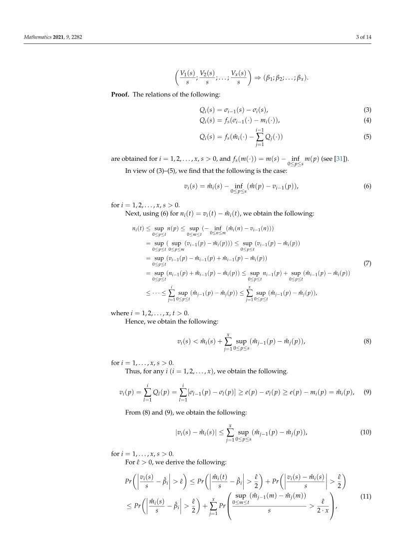
Proof. The relations of the following:

Qi(s) = σi−1(s)− σi(s), (3)

Qi(s) = fs(σi−1(·)−mi(·)), (4)

Qi(s) = fs(mi(·)−i−1

∑j=1

Qj(·)) (5)

are obtained for i = 1, 2, . . . , x, s > 0, and fs(m(·)) = m(s)− inf0≤p≤s

m(p) (see [31]).

In view of (3)–(5), we find that the following is the case:

vi(s) = mi(s)− inf0≤p≤s

(m(p)− vi−1(p)), (6)

for i = 1, 2, . . . , x, s > 0.Next, using (6) for ni(t) = vi(t)− mi(t), we obtain the following:

ni(t) ≤ sup0≤p≤t

n(p) ≤ sup0≤m≤t

(− inf0≤n≤m

(mi(n)− vi−1(n)))

= sup0≤p≤t

( sup0≤p≤m

(vi−1(p)− mi(p))) ≤ sup0≤p≤t

(vi−1(p)− mi(p))

= sup0≤p≤t

(vi−1(p)− mi−1(p) + mi−1(p)− mi(p))

= sup0≤p≤t

(ni−1(p) + mi−1(p)− mi(p)) ≤ sup0≤p≤t

ni−1(p) + sup0≤p≤t

(mi−1(p)− mi(p))

≤ · · · ≤i

∑j=1

sup0≤p≤t

(mj−1(p)− mj(p)) ≤x

∑j=1

sup0≤p≤t

(mj−1(p)− mj(p)),

(7)

where i = 1, 2, . . . , x, t > 0.Hence, we obtain the following:

vi(s) < mi(s) +x

∑j=1

sup0≤p≤s

(mj−1(p)− mj(p)), (8)

for i = 1, . . . , x, s > 0.Thus, for any i (i = 1, 2, . . . , x), we obtain the following.

vi(p) =i

∑l=1

Ql(p) =i

∑l=1

[σl−1(p)− σl(p)] ≥ e(p)− σl(p) ≥ e(p)−mi(p) = mi(p), (9)

From (8) and (9), we obtain the following:

|vi(s)− mi(s)| ≤x

∑j=1

sup0≤p≤s

(mj−1(p)− mj(p)), (10)

for i = 1, . . . , x, s > 0.For ε > 0, we derive the following:

Pr(∣∣∣∣vi(s)

s− βi

∣∣∣∣ > ε

)≤ Pr

(∣∣∣∣ mi(t)s− βi

∣∣∣∣ > ε

2

)+ Pr

(∣∣∣∣vi(s)− mi(s)s

∣∣∣∣ > ε

2

)

≤ Pr(∣∣∣∣ mi(s)

s− βi

∣∣∣∣ > ε

2

)+

x

∑j=1

Pr

sup0≤m≤t

(mj−1(m)− mj(m))

s>

ε

2 · x

,(11)

Mathematics 2021, 9, 2282 4 of 14

where i = 1, . . . , x, s > 0.Note that sup

0≤m≤s(mi−1(m)− mi(m))/s ≥ 0 for i = 1, . . . , x. In addition, note that the

following is the case:

lims→∞

mi−1(s)− mi(s)s

= βi−1 − βi < 0 (12)

almost everywhere for i = 1, . . . , x (see [31]). Thus, similarly as in [31], we prove that thesecond item in (11) also tends to zero.

Thus, we obtain that for ε > 0, the following is the case.

lims→∞

Pr(∣∣∣∣vi(s)

s− βi

∣∣∣∣ > ε

)= 0, i = 1, . . . , x. (13)

Using the convergence together theorem (see, for example, [30] and (13)), we completethe proof of the theorem.

The theorem on SLLN for the queue length of jobs is proved similarly as Theorem 1.

Theorem 2 (SLLN for the queue length of jobs in MS). If conditions (2) are fulfilled, then thefollowing is the case.

(Q1(s)

s;

Q2(s)s

; . . . ;Qx(s)

s

)⇒ (β1; β2 − β1; . . . ; βx − βx−1).

Proof. Using (13), we derive the following:∣∣∣∣Qi(s)s− (βi − βi−1)

∣∣∣∣ ≤ ∣∣∣∣vi(s)s− βi

∣∣∣∣+ ∣∣∣∣vi−1(s)s− βi−1

∣∣∣∣, (14)

where i = 1, . . . , x, s > 0.Using the convergence together theorem (see, for example, [30] and (14)), we complete

the proof of the theorem.

3. SLLN for the Virtual Waiting Time of a Job in MS

In this section, we present the proof of Little’s formula in MS. The main tools inproving this fact are SLLN for the queue length of jobs and the virtual length of a job in MS.

Definitions of the random variables tk, Zk, S(i)k , e(t), and mi(t) for i = 1, 2, . . . , x are

the same as in the proof of Theorems 1 and 2. Let us define βi = ES(i)k , β0 = EZk, and

αi =βi

βi−1− 1 for i = 1, 2, . . . , x. Assume that condition (2) is fulfilled. Therefore, αi > 0

for i = 1, . . . , x.In addition, let us define Vi(t) as a virtual waiting time of a job in the ith phase of MS

at time t. Denote Si(s) as the time, that is, the summary service of jobs arriving at the ithphase of MS until time t for i = 1, . . . , x and s > 0.

Note that Si(s) = ∑σi−1(t)j=1 S(i)

j for i = 1, . . . , x and s > 0.

Moreover, let ni(s) = Si(s)− s, fs(n(· )

)= n(s)− inf

0≤m≤sn(m), ni(s) = ∑

mi−1(s)j=1 S(i)

j −s, m0(s) = e(s) for i = 1, . . . , x, s > 0.

If Si(0) = Vi(0) = 0, then the following is the case (see [1], p. 41).

Vi(s) = fs(ni(· )) for i = 1, . . . , x and s > 0

Thus, we prove a theorem about SLLN for the virtual waiting time of a job in MS.

Theorem 3 (SLLN for the virtual waiting time of a job in MS). If conditions (2) are fulfilled,then the following is the case.

Mathematics 2021, 9, 2282 5 of 14

(V1(s)

s;

V2(s)s

; . . . ;Vx(s)

s

)⇒ (α1; α2; . . . ; αx).

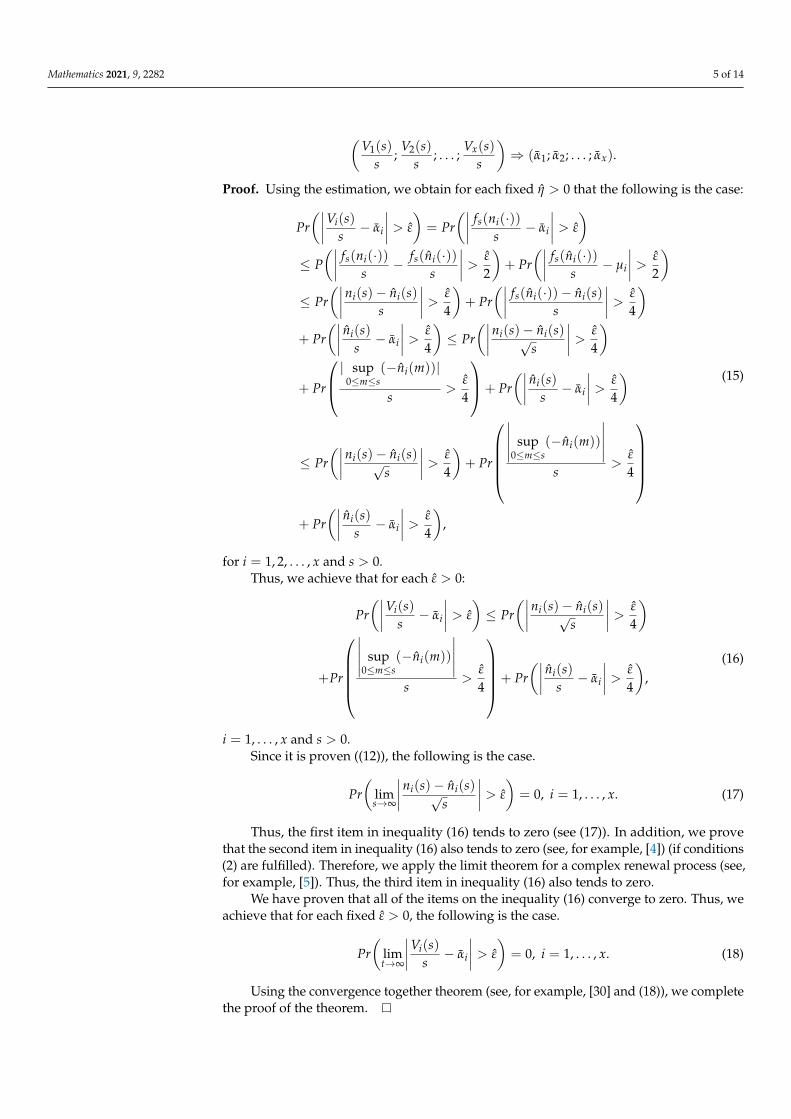
Proof. Using the estimation, we obtain for each fixed η > 0 that the following is the case:

Pr(∣∣∣∣Vi(s)

s− αi

∣∣∣∣ > ε

)= Pr

(∣∣∣∣ fs(ni(·))s

− αi

∣∣∣∣ > ε

)≤ P

(∣∣∣∣ fs(ni(·))s

− fs(ni(·))s

∣∣∣∣ > ε

2

)+ Pr

(∣∣∣∣ fs(ni(·))s

− µi

∣∣∣∣ > ε

2

)≤ Pr

(∣∣∣∣ni(s)− ni(s)s

∣∣∣∣ > ε

4

)+ Pr

(∣∣∣∣ fs(ni(·))− ni(s)s

∣∣∣∣ > ε

4

)+ Pr

(∣∣∣∣ ni(s)s− αi

∣∣∣∣ > ε

4

)≤ Pr

(∣∣∣∣ni(s)− ni(s)√s

∣∣∣∣ > ε

4

)

+ Pr

| sup0≤m≤s

(−ni(m))|

s>

ε

4

+ Pr(∣∣∣∣ ni(s)

s− αi

∣∣∣∣ > ε

4

)

≤ Pr(∣∣∣∣ni(s)− ni(s)√

s

∣∣∣∣ > ε

4

)+ Pr

∣∣∣∣∣ sup0≤m≤s

(−ni(m))

∣∣∣∣∣s

>ε

4

+ Pr

(∣∣∣∣ ni(s)s− αi

∣∣∣∣ > ε

4

),

(15)

for i = 1, 2, . . . , x and s > 0.Thus, we achieve that for each ε > 0:

Pr(∣∣∣∣Vi(s)

s− αi

∣∣∣∣ > ε

)≤ Pr

(∣∣∣∣ni(s)− ni(s)√s

∣∣∣∣ > ε

4

)

+Pr

∣∣∣∣∣ sup0≤m≤s

(−ni(m))

∣∣∣∣∣s

>ε

4

+ Pr(∣∣∣∣ ni(s)

s− αi

∣∣∣∣ > ε

4

),

(16)

i = 1, . . . , x and s > 0.Since it is proven ((12)), the following is the case.

Pr(

lims→∞

∣∣∣∣ni(s)− ni(s)√s

∣∣∣∣ > ε

)= 0, i = 1, . . . , x. (17)

Thus, the first item in inequality (16) tends to zero (see (17)). In addition, we provethat the second item in inequality (16) also tends to zero (see, for example, [4]) (if conditions(2) are fulfilled). Therefore, we apply the limit theorem for a complex renewal process (see,for example, [5]). Thus, the third item in inequality (16) also tends to zero.

We have proven that all of the items on the inequality (16) converge to zero. Thus, weachieve that for each fixed ε > 0, the following is the case.

Pr(

limt→∞

∣∣∣∣Vi(s)s− αi

∣∣∣∣ > ε

)= 0, i = 1, . . . , x. (18)

Using the convergence together theorem (see, for example, [30] and (18)), we completethe proof of the theorem.

Mathematics 2021, 9, 2282 6 of 14

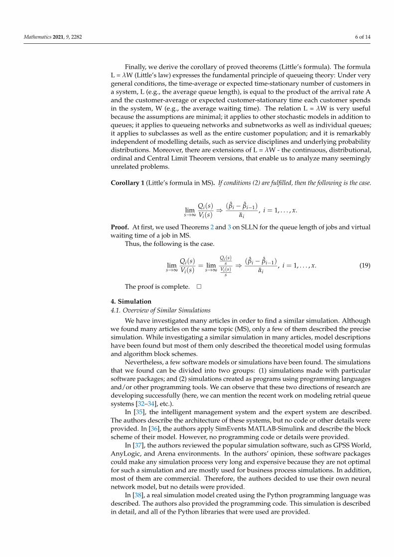
Finally, we derive the corollary of proved theorems (Little’s formula). The formulaL = λW (Little’s law) expresses the fundamental principle of queueing theory: Under verygeneral conditions, the time-average or expected time-stationary number of customers ina system, L (e.g., the average queue length), is equal to the product of the arrival rate Aand the customer-average or expected customer-stationary time each customer spendsin the system, W (e.g., the average waiting time). The relation L = λW is very usefulbecause the assumptions are minimal; it applies to other stochastic models in addition toqueues; it applies to queueing networks and subnetworks as well as individual queues;it applies to subclasses as well as the entire customer population; and it is remarkablyindependent of modelling details, such as service disciplines and underlying probabilitydistributions. Moreover, there are extensions of L = λW - the continuous, distributional,ordinal and Central Limit Theorem versions, that enable us to analyze many seeminglyunrelated problems.

Corollary 1 (Little’s formula in MS). If conditions (2) are fulfilled, then the following is the case.

lims→∞

Qi(s)Vi(s)

⇒ (βi − βi−1)

αi, i = 1, . . . , x.

Proof. At first, we used Theorems 2 and 3 on SLLN for the queue length of jobs and virtualwaiting time of a job in MS.

Thus, the following is the case.

lims→∞

Qi(s)Vi(s)

= lims→∞

Qi(s)s

Vi(s)s

⇒ (βi − βi−1)

αi, i = 1, . . . , x. (19)

The proof is complete.

4. Simulation4.1. Overview of Similar Simulations

We have investigated many articles in order to find a similar simulation. Althoughwe found many articles on the same topic (MS), only a few of them described the precisesimulation. While investigating a similar simulation in many articles, model descriptionshave been found but most of them only described the theoretical model using formulasand algorithm block schemes.

Nevertheless, a few software models or simulations have been found. The simulationsthat we found can be divided into two groups: (1) simulations made with particularsoftware packages; and (2) simulations created as programs using programming languagesand/or other programming tools. We can observe that these two directions of research aredeveloping successfully (here, we can mention the recent work on modeling retrial queuesystems [32–34], etc.).

In [35], the intelligent management system and the expert system are described.The authors describe the architecture of these systems, but no code or other details wereprovided. In [36], the authors apply SimEvents MATLAB-Simulink and describe the blockscheme of their model. However, no programming code or details were provided.

In [37], the authors reviewed the popular simulation software, such as GPSS World,AnyLogic, and Arena environments. In the authors’ opinion, these software packagescould make any simulation process very long and expensive because they are not optimalfor such a simulation and are mostly used for business process simulations. In addition,most of them are commercial. Therefore, the authors decided to use their own neuralnetwork model, but no details were provided.

In [38], a real simulation model created using the Python programming language wasdescribed. The authors also provided the programming code. This simulation is describedin detail, and all of the Python libraries that were used are provided.

Mathematics 2021, 9, 2282 7 of 14

After this review, some conclusions can be drawn:

1. Commercial models do not meet the requirement to make MS simulations. In addition,they are usually expensive.

2. None of the provided models meets the requirement to make all of the necessarysimulations and experiments.

Consequently, we decided to create our own model that fits all of the requirements,can run on one computer and any operating system, and works in multi-threading mode.

4.2. Simulator

To implement the experiment, a Multiphase Queueing System (MS) simulator wascreated. The Python programming language (version 3.6.9) and its multiprocessing pro-gramming library were used. The simulator runs on any operating system that supports thePython programming language. The main new features of this simulator are the following:

• Real asynchronous processes that are not dependent on each other;• Possibility to stop simulation at a particular time and not only when all clients are

served (as [38]);• Possibility to measure any moment of time:

– Client enters MS tk (and also Zk = tk+1 − tk – time between two clients’ arrival);– Waiting time Vi of each client in every queue;– Service time S(i)k of client k in the ith service of the queue;– Amount of clients Qi(t) in each queue after time t (when the process stopped

after time t);

• Client proceeds to the consumer process not only after it pass all services (as [38]) butalso immediately if MS stopped after the specified time t;

• All of the values to be measured are stored in synchronized variables for eliminatingtheir undefined states (some issues could appear because of the operating system, thePython programming language, or hardware errors);

• Each service really stops after all of the clients pass away or after the specified time t;• Clients enters the consumer process from any place of MS if it stops after the specified

time t. For example, a client cannot pass all of the services or could even be in awaiting queue for one of the services;

• All of the calculations are performed, and only then is MS stopped or when all theclients pass through or after the specified time ends.

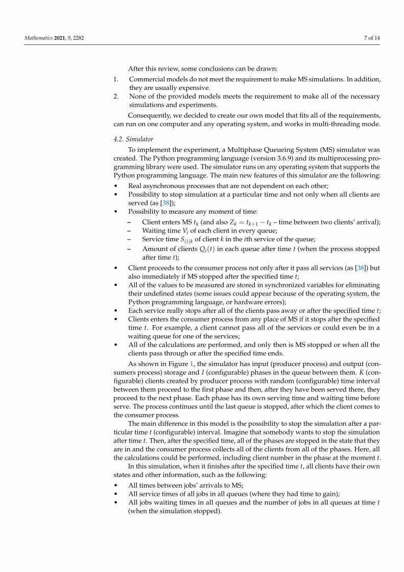
As shown in Figure 1, the simulator has input (producer process) and output (con-sumers process) storage and I (configurable) phases in the queue between them. K (con-figurable) clients created by producer process with random (configurable) time intervalbetween them proceed to the first phase and then, after they have been served there, theyproceed to the next phase. Each phase has its own serving time and waiting time beforeserve. The process continues until the last queue is stopped, after which the client comes tothe consumer process.

The main difference in this model is the possibility to stop the simulation after a par-ticular time t (configurable) interval. Imagine that somebody wants to stop the simulationafter time t. Then, after the specified time, all of the phases are stopped in the state that theyare in and the consumer process collects all of the clients from all of the phases. Here, allthe calculations could be performed, including client number in the phase at the moment t.

In this simulation, when it finishes after the specified time t, all clients have their ownstates and other information, such as the following:

• All times between jobs’ arrivals to MS;• All service times of all jobs in all queues (where they had time to gain);• All jobs waiting times in all queues and the number of jobs in all queues at time t

(when the simulation stopped).

Mathematics 2021, 9, 2282 8 of 14

Figure 1. Algorithm of the simulation model.

All of the measurable parameters of the model are listed in Table 1.

Table 1. Model parameters.

Parameter Description

tk Client’s k arrival to MS timeVi Client’s waiting time before service in the ith phaseSi Client’s service time in the ith phaseQi Clients amount in the ith phase at the moment t

After the model stops, the consumer process performs all of the computations for thevalues listed in Table 2.

Table 2. Computational parameters of the model.

Parameter Description

E(Vi) Estimated waiting time before service in the ith phaseE(Si) Estimated service time in the ith phaseQi/t Clients amount in the queue i at time t, divided by tZk+1 Estimated time between two clients entering MSE(Z) Estimated time between clients on entering MS

4.3. Experiment

The experiment results were obtained using this simulation with thefollowing parameters:

• Time interval of 15 s (measurements were made each second from 1 to 15);• Five phases in MS;

Mathematics 2021, 9, 2282 9 of 14

• 100,000 clients received from the producer.

During the experiment, the MS system was stopped at each second, and all of thecalculations were made. In each phase, the following is the case:

• Q1–Q5—numbers of clients in all five phases divided by t;• E(V1)–E(V5)—estimated waiting times in each phase are calculated and divided by t;• Q1/V1–Q5/V5 ratios for each phase are calculated.

The list of hardware and software used in the experiment is provided in Table 3.

Table 3. Hardware and software used in the experiment.

OS Linux Mint, Linux PC 5.4.0-62-generic #70-UbuntuSMP Tue Jan 12 12:45:47 UTC 2021 ×86_64 ×86_64×86_64 GNU/Linux

Python programminglanguage

Python 3.6.9 (default, 18 April 2020, 01:56:04)[GCC 8.4.0] on Linux

Python libraries multiprocessing, time, random, numpy, sys, asyncio,matplotlib, pylab, matplotlib.pyplot, math, ctypes

IDE Visual Studio Code

Processor Intel(R) Core(TM) i7-8700 CPU @ 3.20 GHz

Memory 32747MB (17387MB used)

Storage ATA Samsung SSD 860

Video adapter NVIDIA GeForce GTX 1080 Ti/PCIe/SSE2

The results of calculation ratios Q1/V1, Q2/V2, Q3/V3, Q4/V4, and Q5/V5 in 1–15 ssimulations are provided in Table 4.

Table 4. Results of ratio calculation.

t, s Q1/V1 Q2/V2 Q3/V3 Q4/V4 Q5/V5

1 0 0 0 0 02 15,783.208889 7713.886687 10,173.894957 8327.816417 4849.4445533 16,158.595911 24,539.397682 3903.148301 12,644.343116 7150.6217674 7150.621767 14,994.150418 4764.470185 9563.342329 9489.5306625 16,618.375117 11,304.161697 24,609.465659 11,133.676329 7467.4627896 16,349.095476 16,200.135701 10,906.525734 21,445.316714 7687.6437077 16,540.717478 10,413.616874 17,795.190157 11,758.146436 9688.6446388 17,363.635526 11,608.885913 13,812.022670 14,145.828118 8471.5495749 19,027.493286 15,717.070406 19,310.638918 13,772.830493 14,585.09710310 17,339.523710 11,679.801550 14,368.463078 12,014.946867 10,045.98569511 20,742.679577 23,891.867419 15,796.962250 17,233.303617 18,584.62015812 17,426.702838 84,383.182448 12,677.306401 11,978.191479 8637.41632313 19,019.020194 16,494.458220 21,366.420617 20,901.589822 26,116.32841014 0 0 0 0 015 0 0 0 0 0

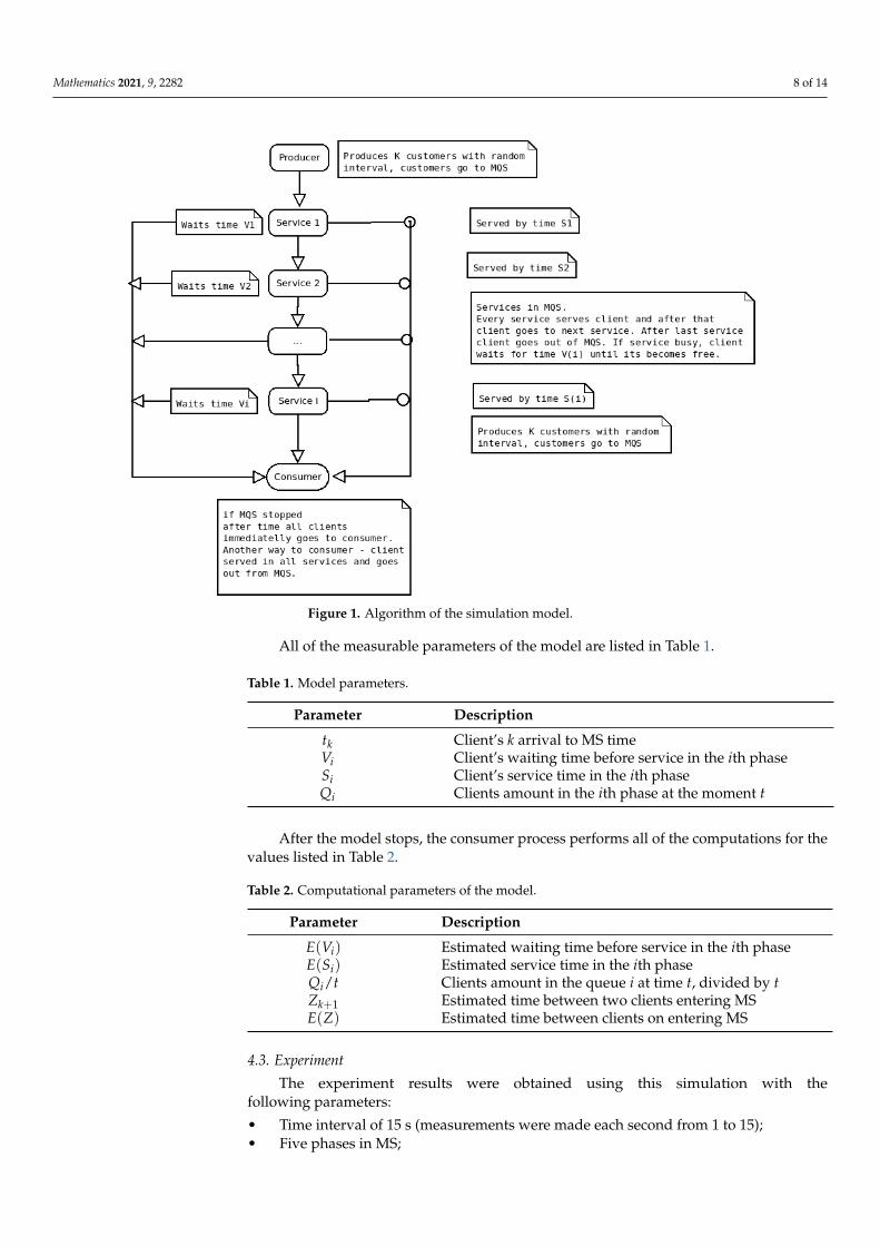
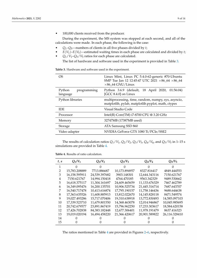
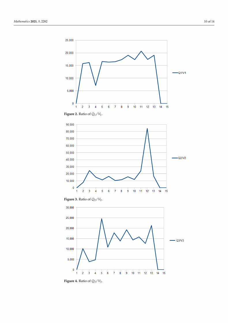
The ratios mentioned in Table 4 are provided in Figures 2–6, respectively.

Mathematics 2021, 9, 2282 10 of 14

Figure 2. Ratio of Q1/V1.

Figure 3. Ratio of Q2/V2.

Figure 4. Ratio of Q3/V3.

Mathematics 2021, 9, 2282 11 of 14

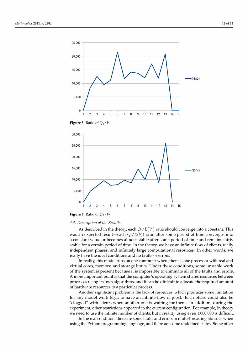
Figure 5. Ratio of Q4/V4.

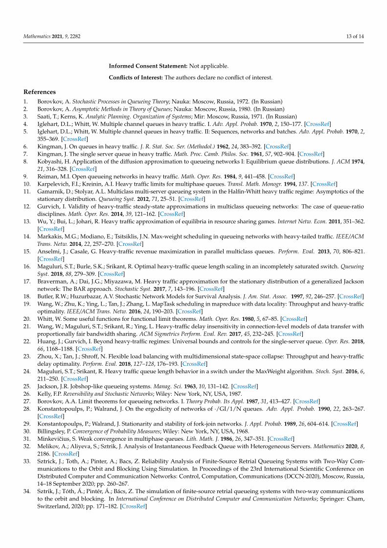
Figure 6. Ratio of Q5/V5.

4.4. Description of the Results

As described in the theory, each Qi/E(Vi) ratio should converge into a constant. Thiswas an expected result—each Qi/E(Vi) ratio after some period of time converges intoa constant value or becomes almost stable after some period of time and remains fairlystable for a certain period of time. In the theory, we have an infinite flow of clients, reallyindependent phases, and infinitely large computational resources. In other words, wereally have the ideal conditions and no faults or errors.

In reality, this model runs on one computer where there is one processor with real andvirtual cores, memory, and storage limits. Under these conditions, some unstable workof the system is present because it is impossible to eliminate all of the faults and errors.A more important point is that the computer’s operating system shares resources betweenprocesses using its own algorithms, and it can be difficult to allocate the required amountof hardware resources to a particular process.

Another significant problem is the lack of resources, which produces some limitationfor any model work (e.g., to have an infinite flow of jobs). Each phase could also be“clogged” with clients when another one is waiting for them. In addition, during theexperiment, other restrictions appeared in the current configuration. For example, in theorywe need to use the infinite number of clients, but in reality using even 1,000,000 is difficult.

In the real condition, there are some faults and errors in multi-threading libraries whenusing the Python programming language, and there are some undefined states. Some other

Mathematics 2021, 9, 2282 12 of 14

mistakes could appear due to the calculation accuracy and time measurement becauseapproximations are used. The lack of resources especially affects measurements of timebecause the system could lag.

The most expected result is to find a stable interval for every phase where the equilib-rium of model load and theoretical conditions are satisfied and to create the experimentwhere all listed theorems could be checked. A stable time interval should be found for eachratio, in this interval the ratio of Qj/E(Vj) should be the same or very similar.

All of the calculation results for each ratio are listed above. In every chart of each ratio,we can observe the state and the time when the ratio becomes stable or changes a little.Each phase becomes a stable state at a different time period. This could happen because ofdifferent times of the critical load and also because of no load for each phase.

For example, the first ratio Q1/E(V1) becomes stable after 2 s (4 s value is an issue)and remains stable until 13 s. The second ratio is more stable from 3 to 11 s, the thirdfrom 6 to 12, the fourth from 7 to 12, and the fifth is more stable at the beginning but lessstable at the end. It is difficult to find a stable period for the fifth (or last) phase because itbecomes clogged after all of the other phases are empty or almost empty. When a largeflow of clients arrives, the period of stability should begin, but the phase becomes emptyvery soon. In addition, for this configuration, all clients pass MS at the 14th second, and allphases become empty.

This experiment result shows that each phase has its own stability period; thus, it couldbe considered that the ratio of Qj/E(Vj) converges to a constant, as proved in the theory.

Corollary 2 (Validation of Little’s formula in MS). At this stage of the work, we confirm thatthe results of the first stage are correct.

5. Concluding Remarks

• We observe that the heavy traffic condition used in the proof of the theorems on SLLNis fundamental. Abandoning this condition makes the proof of the theorems verycomplicated. In the future, it would be interesting to examine the situation underlight traffic.

• By using another method to prove theorems and normalizing boundary processesdifferently than compared to SLLN (e.g., probability limit theorems or the law of theiterated logarithm—but this is implicated only in the single-phase case, and there isno research in the multiphase case), Little’s law becomes the successful process orbecomes its law of the iterated logarithm analog. With SLLN, the boundary process isconstant—this process can be modeled.

• The theoretical results cannot be directly verified by modeling them, which is evi-denced by the modeling block diagram. Modeling has its own explicit specifics; thus,a comprehensive review of the literature in this area was required.

• The ideas of the modeling part are related to the often cited work [38]. In this work,for the first time, the modern possibilities of the Python programming language wereapplied in order to model the queuing system. Continuing this topic, the Pythonconcept was used to test the theoretical results of the first stage.

• The first and second parts of this paper deal with similar but completely separatesubject areas. As much as possible, efforts were made to bring them closer togetherand to present them as a single study.

Author Contributions: Conceptualization, S.M. and I.K.; methodology, S.M.; software, I.K.; valida-tion, J.K. and I.V.-Z.; formal analysis, S.M. and I.K.; investigation, I.K.; resources, I.K.; data curation,J.K. and I.V.-Z.; writing—original draft preparation, S.M.; writing—review and editing, J.K. andI.V.-Z.; visualization, J.K.; supervision, S.M. and I.K.; project administration, J.K. and I.V.-Z. Allauthors have read and agreed to the published version of the manuscript.

Funding: This research received no external funding.

Institutional Review Board Statement: Not applicable.

Mathematics 2021, 9, 2282 13 of 14

Informed Consent Statement: Not applicable.

Conflicts of Interest: The authors declare no conflict of interest.

References1. Borovkov, A. Stochastic Processes in Queueing Theory; Nauka: Moscow, Russia, 1972. (In Russian)2. Borovkov, A. Asymptotic Methods in Theory of Queues; Nauka: Moscow, Russia, 1980. (In Russian)3. Saati, T.; Kerns, K. Analytic Planning. Organization of Systems; Mir: Moscow, Russia, 1971. (In Russian)4. Iglehart, D.L.; Whitt, W. Multiple channel queues in heavy traffic. I. Adv. Appl. Probab. 1970, 2, 150–177. [CrossRef]5. Iglehart, D.L.; Whitt, W. Multiple channel queues in heavy traffic. II: Sequences, networks and batches. Adv. Appl. Probab. 1970, 2,

355–369. [CrossRef]6. Kingman, J. On queues in heavy traffic. J. R. Stat. Soc. Ser. (Methodol.) 1962, 24, 383–392. [CrossRef]7. Kingman, J. The single server queue in heavy traffic. Math. Proc. Camb. Philos. Soc. 1961, 57, 902–904. [CrossRef]8. Kobyashi, H. Application of the diffusion approximation to queueing networks I: Equilibrium queue distributions. J. ACM 1974,

21, 316–328. [CrossRef]9. Reiman, M.I. Open queueing networks in heavy traffic. Math. Oper. Res. 1984, 9, 441–458. [CrossRef]10. Karpelevich, F.I.; Kreinin, A.I. Heavy traffic limits for multiphase queues. Transl. Math. Monogr. 1994, 137. [CrossRef]11. Gamarnik, D.; Stolyar, A.L. Multiclass multi-server queueing system in the Halfin-Whitt heavy traffic regime: Asymptotics of the

stationary distribution. Queueing Syst. 2012, 71, 25–51. [CrossRef]12. Gurvich, I. Validity of heavy-traffic steady-state approximations in multiclass queueing networks: The case of queue-ratio

disciplines. Math. Oper. Res. 2014, 39, 121–162. [CrossRef]13. Wu, Y.; Bui, L.; Johari, R. Heavy traffic approximation of equilibria in resource sharing games. Internet Netw. Econ. 2011, 351–362.

[CrossRef]14. Markakis, M.G.; Modiano, E.; Tsitsiklis, J.N. Max-weight scheduling in queueing networks with heavy-tailed traffic. IEEE/ACM

Trans. Netw. 2014, 22, 257–270. [CrossRef]15. Anselmi, J.; Casale, G. Heavy-traffic revenue maximization in parallel multiclass queues. Perform. Eval. 2013, 70, 806–821.

[CrossRef]16. Maguluri, S.T.; Burle, S.K.; Srikant, R. Optimal heavy-traffic queue length scaling in an incompletely saturated switch. Queueing

Syst. 2018, 88, 279–309. [CrossRef]17. Braverman, A.; Dai, J.G.; Miyazawa, M. Heavy traffic approximation for the stationary distribution of a generalized Jackson

network: The BAR approach. Stochastic Syst. 2017, 7, 143–196. [CrossRef]18. Butler, R.W.; Huzurbazar, A.V. Stochastic Network Models for Survival Analysis. J. Am. Stat. Assoc. 1997, 92, 246–257. [CrossRef]19. Wang, W.; Zhu, K.; Ying, L.; Tan, J.; Zhang, L. MapTask scheduling in mapreduce with data locality: Throughput and heavy-traffic

optimality. IEEE/ACM Trans. Netw. 2016, 24, 190–203. [CrossRef]20. Whitt, W. Some useful functions for functional limit theorems. Math. Oper. Res. 1980, 5, 67–85. [CrossRef]21. Wang, W.; Maguluri, S.T.; Srikant, R.; Ying, L. Heavy-traffic delay insensitivity in connection-level models of data transfer with

proportionally fair bandwidth sharing. ACM Sigmetrics Perform. Eval. Rev. 2017, 45, 232–245. [CrossRef]22. Huang, J.; Gurvich, I. Beyond heavy-traffic regimes: Universal bounds and controls for the single-server queue. Oper. Res. 2018,

66, 1168–1188. [CrossRef]23. Zhou, X.; Tan, J.; Shroff, N. Flexible load balancing with multidimensional state-space collapse: Throughput and heavy-traffic

delay optimality. Perform. Eval. 2018, 127–128, 176–193. [CrossRef]24. Maguluri, S.T.; Srikant, R. Heavy traffic queue length behavior in a switch under the MaxWeight algorithm. Stoch. Syst. 2016, 6,

211–250. [CrossRef]25. Jackson, J.R. Jobshop-like queueing systems. Manag. Sci. 1963, 10, 131–142. [CrossRef]26. Kelly, F.P. Reversibility and Stochastic Networks; Wiley: New York, NY, USA, 1987.27. Borovkov, A.A. Limit theorems for queueing networks. I. Theory Probab. Its Appl. 1987, 31, 413–427. [CrossRef]28. Konstantopoulps, P.; Walrand, J. On the ergodicity of networks of ·/GI/1/N queues. Adv. Appl. Probab. 1990, 22, 263–267.

[CrossRef]29. Konstantopoulps, P.; Walrand, J. Stationarity and stability of fork-join networks. J. Appl. Probab. 1989, 26, 604–614. [CrossRef]30. Billingsley, P. Convergence of Probability Measures; Wiley: New York, NY, USA, 1968.31. Minkevicius, S. Weak convergence in multiphase queues. Lith. Math. J. 1986, 26, 347–351. [CrossRef]32. Melikov, A.; Aliyeva, S.; Sztrik, J. Analysis of Instantaneous Feedback Queue with Heterogeneous Servers. Mathematics 2020, 8,

2186. [CrossRef]33. Sztrick, J.; Toth, A.; Pinter, A.; Bacs, Z. Reliability Analysis of Finite-Source Retrial Queueing Systems with Two-Way Com-

munications to the Orbit and Blocking Using Simulation. In Proceedings of the 23rd International Scientific Conference onDistributed Computer and Communication Networks: Control, Computation, Communications (DCCN-2020), Moscow, Russia,14–18 September 2020; pp. 260–267.

34. Sztrik, J.; Tóth, Á.; Pintér, Á.; Bács, Z. The simulation of finite-source retrial queueing systems with two-way communicationsto the orbit and blocking. In International Conference on Distributed Computer and Communication Networks; Springer: Cham,Switzerland, 2020; pp. 171–182. [CrossRef]

Mathematics 2021, 9, 2282 14 of 14

35. Bychkov, I.V.; Kazakov, A.L.; Lempert, A.A.; Bukharov, D.S.; Stolbov, A.B. An intelligent management system for the developmentof a regional transport logistics infrastructure. Autom. Remote Control 2016, 77, 332–343. [CrossRef]

36. Harahap, E.; Darmawan, D.; Fajar, Y.; Ceha, R.; Rachmiatie, A. Modeling and simulation of queue waiting time at traffic lightintersection. J. Phys. Conf. Ser. 2019, 1188, 012001. [CrossRef]

37. Gorbunova, A.V.; Vishnevsky, V.M.; Larionov, A.A. Evaluation of the end-to-end delay of a multiphase queuing system usingartificial neural networks. In International Conference on Distributed Computer and Communication Networks; Lecture Notes inComputer Science; Springer: Cham, Switzerland, 2020; pp. 631–642. [CrossRef]

38. Dolgopolovas, V.; Dagiene, V.; Minkevicius, S.; Sakalauskas, L. Python for scientific computing education: Modeling of queueingsystems. Sci. Program. 2014, 22, 37–51. [CrossRef]