Mathematical Modelling and Analysis Publisher: Taylor&Francis and VGTU

Volume 22 Number 1, January 2017, 78–94 http://www.tandfonline.com/TMMA

https://doi.org/10.3846/13926292.2017.1269025 ISSN: 1392-6292

c©Vilnius Gediminas Technical University, 2017 eISSN: 1648-3510

Modelling the Photovoltaic Output Power usingthe Differential Polynomial Network andEvolutionary Fuzzy Rules∗

Ladislav Zjavkab, Pavel Kromera,b, Stanislav Misakc andVaclav Snasela,b

aDep. of Computer Science, FEECS, VSB - Technical University of OstravabIT4innovations National Supercomputing Center, VSB - TechnicalUniversity of OstravacENET Centre, VSB - Technical University of Ostrava

17. listopadu 15/2172 Ostrava, Czech Republic

E-mail(corresp.): ladislav.zjavka@vsb.cz

E-mail: pavel.kromer@vsb.cz

E-mail: stanislav.misak@vsb.cz

E-mail: vaclav.snasel@vsb.cz

Received December 1, 2016; revised December 23, 2016; published online January 5, 2017

Abstract. The unstable production of renewable energy sources, which is difficultto model using conventional computational techniques, may be predicted to advantageby means of biologically inspired soft-computing methods. The photovoltaic outputpower is primarily dependent on the solar direct or global radiation, which short-termnumerical forecasts are possible to apply for daily power predictions. The study com-pares two methods, which can successfully model dynamic fluctuant variances of thesolar irradiance and corresponding output power time-series. Differential polynomialnetwork is a new neural network class, which defines and substitutes for the generalpartial differential equation to model an unknown system function. Its total output iscomposed from selected neurons, i.e. relative polynomial substitution terms, formedin all network layers of a multi-layer structure. The proposed derivative polynomialregression using relative dimensionless fraction units, formed according to the Simi-larity analysis, can describe and generalize data relations on a wider range of valuesthan defined by the training interval when using standard soft-computing composingtechniques that apply only absolute data. 1-variable time-series observations are pos-sible to model by time derivatives of a converted ordinary differential equation, solvedanalogously with partial derivative substitution terms of several time-point variables.

∗ This work was supported by The Ministry of Education, Youth and Sports from theNational Programme of Sustainability (NPU II) project “IT4Innovations excellence inscience - LQ1602”, by project LO1404 “Sustainable Development of Centre ENET”, VSB-Technical University of Ostrava, student’s projects SGS SP2016/177 and SP2016/175, andCzech Science Foundation project no. GJ16-25694Y.

Modelling the Photovoltaic Output Power 79

Keywords: photovoltaic output power, solar irradiation, differential polynomial neural

network, evolution fuzzy rules.

AMS Subject Classification: 68T05; 92B20.

1 Introduction

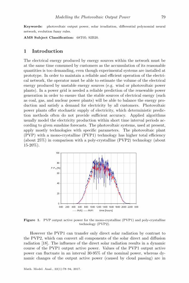
The electrical energy produced by energy sources within the network must beat the same time consumed by customers as the accumulation of its reasonablequantities is too demanding, even though experimental systems are installed atprototype. In order to maintain a reliable and efficient operation of the electri-cal network, the operator must be able to estimate the volume of the electricalenergy produced by unstable energy sources (e.g. wind or photovoltaic powerplants). In a power grid is needed a reliable prediction of the renewable powergeneration in order to ensure that the stable sources of electrical energy (suchas coal, gas, and nuclear power plants) will be able to balance the energy pro-duction and satisfy a demand for electricity by all customers. Photovoltaicpower plants offer stochastic supply of electricity, which deterministic predic-tion methods often do not provide sufficient accuracy. Applied algorithmsusually model the electricity production within short time interval periods ac-cording to given sunshine forecasts. The photovoltaic systems, used at present,apply mostly technologies with specific parameters. The photovoltaic plant(PVP) with a mono-crystalline (PVP1) technology has higher total efficiency(about 25%) in comparison with a poly-crystalline (PVP2) technology (about15-20%).

Figure 1. PVP output active power for the mono-crystalline (PVP1) and poly-crystallinetechnology (PVP2).

However the PVP1 can transfer only direct solar radiation by contrast tothe PVP2, which can convert all components of the solar direct and diffusionradiation [18]. The influence of the direct solar radiation results in a dynamiccourse of the PVP1 output active power. Values of the PVP1 output activepower can fluctuate in an interval 30-95% of the nominal power, whereas dy-namic changes of the output active power (caused by cloud passing) are in

Math. Model. Anal., 22(1):78–94, 2017.

80 L. Zjavka, P. Kromer, S. Misak and V. Snasel

units of minutes in this specific case. The maximal value of the output activepower of the PVP2 is not so high (about 85% of a nominal value) however thedynamic changes are smaller and this system is more stable. The character-istics are necessary to respect in prediction models. The analysis (Figure 1)characterizes a typical day during July 2011 with changeable cloudiness for thenominal power 1MWp.

Figure 2. The power curve of PVP with monocrystalline technology (PVP1) andpolycrystalline technology (PVP2).

Power curves can characterize the two above mentioned PVPs (Figure 2),where the PVP1 is a photovoltaic system placed on a tracker and the PVP2 is asystem with a stabile construction. The power curve shows a dependence of theoutput active power on the solar radiation (Figure 2). The PVP1 power curve(placed on the tracker) has higher values of the hysteresis, which is caused bythe different output power for eastern and western sun. Therefore it is possibleto obtain the different output power for the same values of the solar radiationwhereas output power values are higher for azimuth corresponding of easternsun. The PVP2 hysteresis power curve is flatter by a virtue of the stabileplacing and poly-crystalline technology. The power curves were created forsame day as in the previous case (Figure 1).

Prediction models must respect all the above mentioned specifications of thePVP parameters. Developed prediction techniques for the PVP production,based on the optimization for specific areas, can use fuzzy sets and logic [4],neural networks [23], statistical short-term forecasting [11], non-linear functionrelations [25] or Gaussian equations [26]. The study compares two differenttypes of daily prediction models: the general differential equation solutions ofpolynomial networks and symbolic tree expressions of evolutional fuzzy rules(of a searched function), tested at a 14-day period. The applied time-seriesdata contain only information about the solar radiation intensity related tocorresponding power output values in a location of the facility. No other ad-ditional relevant data (e.g. relative humidity, pressure, visibility) were consid-ered, which might significantly impact the presented models results. Each ofthe two methods applies a different approach to the training data, either dailyupdated or long-term invariant models. The paper is organized as follows:

Modelling the Photovoltaic Output Power 81

Section 2 and Section 3 present the principles of both the compared methods,Section 4 contains experimental results first using real solar irradiation data(for testing both model types) and then numerical forecast data (for real dailypredictions), and Section 5 and Section 6 resume evaluations and implications.

2 General partial differential equation decomposition andsubstitution

2.1 General differential equation composition models

A lot of physical or natural systems, which is not possible to model using aunique explicit function, can be described to advantage by means of differentialequations solved using neural networks [27], genetic programming [6, 10, 12]based on trajectory methods [22], wave series [3, 8] and other. The generalpartial differential equation (DE) (2.1), which selective exact form is not knownin advance (for a specific system model), can generally describe a system ofrelated variables with sum derivative terms. The searched function u, whichis possible to calculate as a sum of the derivative terms (+ bias) (2.1) may beexpressed in the form of sum series, consisting of convergent series arisen frompartial derivative terms (2.2) of 2 input variables.

a+ bu+

n∑i=1

ci∂u

∂xi+

n∑i=1

n∑j=1

dij∂2u

∂xi∂xj+ . . . = 0, (2.1)

a, b, ~c(d11, dc12, . . .) – parameters, ~x(x1, x2, . . . , xn) – vector of n input vari-

ables, u(~x) – searched function u =∞∑k=1

uk, uk – partial separable functions of

u: (∑ ∂uk∂x1

,∑ ∂uk

∂x2,∑ ∂2uk

∂x21,∑ ∂2uk

∂x1∂x2,∑ ∂2uk

∂x22

). (2.2)

Volterra functional series, a discrete analogue of which is the Kolmogorov-Gabor polynomial (2.3), express general connections between input and outputvariables. This polynomial can approximate any stationary random sequenceof observations and can be computed by either adaptive methods or a systemof Gaussian normal equations. Group Method of Data Handling (GMDH),created by a Ukrainian scientist Aleksey Ivakhnenko in 1968, when the back-propagation technique was not known yet [13], decomposes the complexity ofa system or process (2.3) into many simpler relationships each described bya low order 2-variable polynomial processing function (2.4) of a single neuron(node). The GMDH evolves progressively a polynomial neural network (PNN)multi-layer structure towards the output layer, adding layers one after one insuccessive steps calculating the actual last layer coefficients and selecting itsoptimal neurons. It defines an optimal structure of a complex system modelidentifying non-linear relations between input and output variables [20].

Y = a0 +

n∑i=1

aixi +

n∑i=1

n∑j=1

aijxixj +

n∑i=1

n∑j=1

n∑k=1

aijkxixjxk + . . . , (2.3)

Math. Model. Anal., 22(1):78–94, 2017.

82 L. Zjavka, P. Kromer, S. Misak and V. Snasel

A(a1, a2, . . . , an) – vector of parameters, X(x1, x2, . . . , xn) – vector of n inputvariables.

Differential polynomial neural network (D-PNN) is a new neural networktype, which extends the basic complete GMDH PNN structure to form sumseries of relative combination derivation terms, which together define and sub-stitute for the selective general partial differential equation (DE) of a multi-variable function searched model based on data observations. This derivativeseries model is differs from simple upright computational techniques, which cancompose a searched function from a collection of operators and terminals of adefined set to form symbolic tree-like structural expressions.

y = a0 + a1x1 + a2xj + a3xixj + a4x2i + a5x

2j . (2.4)

The similarity theory is based on the hypothesis functional relationships existamong the non-dimensional parameters, which can describe a physical system.The Buckingham π theorem removes extraneous information from a problemby forming dimensionless groups of variables and is the fundamental of dimen-sional analysis. It states if the Equation (2.5) is the only relationship among theqi’s and if it holds for any arbitrary choice of the units in which q1, q2, . . . , qnare measured, then it can be written in the form using π1, π2, . . . , πm as in-dependent dimensionless products of the qi’s (7). If k is the minimal numberof principal quantities necessary to express the dimensions of the q’s, thenm = n− k [24].

Φ(q1, q2, . . . , qn) = 0, Φ(π1, π2, . . . , πn) = 0, (2.5)

where π1, π2, . . . , πm are independent dimensionless products of the q’s. Themethod of integral analogues provides an essential principle for the partialderivative terms (2.2) polynomial substitution. It is a part of the similaritydimensional analysis, which applies various formal adaptations of a DE (or dataobservations) to form dimensionless characteristic groups of variables [7], thusthe original mathematical operators and symbols in a DE are replaced by theratio of corresponding variables. The derivatives are replaced by their integralanalogues, i.e. derivative operators are removed and replaced by analogue orproportion signs in equations. The complete input polynomials (of a uniformdegree) replace the partial searched functions uk of derivative terms (2.2), whilethe reduced combination polynomials of denominators represent the derivativeversatile parts (2.9). If the u(x1, x2, . . . , xn) function of the partial DE (2.1) isdefined around a point A(a1, a2, . . . , an), its partial derivation in respect of ximay be considered 1-variable function g(xi) (2.6).[

∂u

∂xi

]A

=∂u(A)

∂xi

= limxi→ai

u(a1, . . . , ai−1, xi, ai+1, . . . , an)− u(a1, . . . , ai−1, ai, ai+1, . . . , an)

xi − ai

= limxi→ai

g(xi)− g(ai)

xi − ai. (2.6)

Modelling the Photovoltaic Output Power 83

If the partial DE involves u(~x) function derivatives with respect only to time tvariable, which the independent variables x1, x2, . . . , xn depends on, the equa-tion (2.6) is possible to express in (2.7).[

du(t, x1, . . . , xn)

dt

]t=ta

= limt→ta

u(t, a1, . . . , an)− u(ta, a1, . . . , an)

t− ta,

dx = xi − ai = t− ta = dt. (2.7)

If only one independent variable x occurs in the function u, the equation (2.7)becomes the form (2.8).[

du(t, x)

dt

]t=ta

= limt→ta

u(t, a)− u(ta, a)

t− ta. (2.8)

On this assumption the general partial DE (2.1), which describes 1-variabletime-series, might be converted into an ordinary DE with only time derivatives.The variables x1, x2, . . . , xn of the u function are observations in various timet, so partial derivatives (2.1) turns into derivatives in respect of the only timet variable. The input vector ~x variables depend only on time t so the searchedfunction u is replaced by f(~x) time observations. Combinations of the partialDE term denominators (2.1) project themselves into partial numerator f(~x)functions in the ordinary DE

a+ bf +

n∑i=1

cidf(xi)

dt+

n∑i=1

n∑j=1

dijdf(xi, xj)

dt+ . . .+

n∑i=1

ccidf2(xi)

dt2+ . . . = 0,

where f(~x) – function of independent time observations x(x1, x2, . . . , xn). Thisequation is formed and solved analogous to the general partial DE (2.1) bymeans of partial derivative terms substitutions using combinations of severaltime-point variables.

Figure 3. 2-variable combination block consists of basic (/) and composite terms (CT) -neurons.

Blocks (nodes) of the D-PNN (Figure 3) form simple neurons, one for eachfractional polynomial derivative combination, so each neuron represents a sub-

Math. Model. Anal., 22(1):78–94, 2017.

84 L. Zjavka, P. Kromer, S. Misak and V. Snasel

stitution DE term (2.9) (2.10) (2.11)

y1 =∂f(x1, x2)

∂x1= w1

(a0 + a1x1 + a2x2 + a3x1x2 + a4x21 + a5x

22)

12

1.5(b0 + b1x1), (2.9)

y3 =∂2f(x1, x2)

∂2x2= w3

a0 + a1x1 + a2x2 + a3x1x2 + a4x21 + a5x

22

2.7(b0 + b1x2 + b2x22), (2.10)

y5 =∂2f(x1, x2)

∂x1∂x2= w5

a0 + a1x1 + a2x2 + a3x1x2 + a4x21 + a5x

22

2.3(b0 + b1x11 + b2x12 + b3x11x12). (2.11)

Each block contains a single output polynomial (2.4), without derivativepart. Neurons do not affect the block output but can be directly included inthe total network output sum of a DE solution. Each block has 1 and neuron2 vectors of adjustable parameters ~a and ~a,~b respectively. The numerator rootfunction decreases a combination degree of the input polynomial (2.9), in orderto get the dimensionless values [7].

The GMDH polynomial (2.4) is applied in the block outputs and neuronfractions as it proves generally to yield best results besides being easy to use.Each block includes 5 simple substitution neurons of the 2nd order partial DE(2.12) of a searched 2-variable partial u function model, formed with respectto 2 single x1, x2 (2.9), 2 squared x21, x

22 (2.10) and 1 combination x1x2 (2.11)

derivative variables, which correspond exactly to the GMDH polynomial vari-ables. This DE type is preferably used to describe natural and physical systemsnon-linearities.

F

(x1, x2, u,

∂u

∂x1,∂u

∂x2,∂2u

∂x21,

∂2u

∂x1∂x2,∂2u

∂x22

)= 0, (2.12)

where F (x1, x2, u, p, q, r, s, t) is a function of 8 variables.

2.2 Differential polynomial neural network

Multi-layer D-PNN forms composite functions (Figure 4). The previous layerblocks produce internal functions, which substitute for the next hidden layerinput variables of neuron and block polynomials in external functions. Compos-ite DE terms, i.e. composite function derivatives in respect of the variables ofprevious layers, are calculated according to the partial derivation rules (2.13),(2.14) by products of the external and internal function partial derivatives.

F (x1, x2, . . . , xn) = f(y1, y2, . . . , ym) = f(Φ1(X), Φ2(X), . . . , Φm(X)), (2.13)

∂F

∂xk=

m∑i=1

∂f(y1, y2, . . . , ym)

∂yi· ∂Φi(X)

∂xk, k = 1, . . . , n. (2.14)

The blocks of the 2nd and following hidden layers produce extended neurons -composite terms (CT), which substitute for the composite function derivativesin respect of the output and input variables of the back connected previouslayer blocks, e.g. the 1st block of the 3rd layer (Figure 4) can form linear CT

Modelling the Photovoltaic Output Power 85

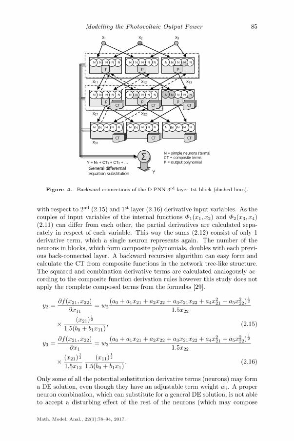
Figure 4. Backward connections of the D-PNN 3rd layer 1st block (dashed lines).

with respect to 2nd (2.15) and 1st layer (2.16) derivative input variables. As thecouples of input variables of the internal functions Φ1(x1, x2) and Φ2(x3, x4)(2.11) can differ from each other, the partial derivatives are calculated sepa-rately in respect of each variable. This way the sums (2.12) consist of only 1derivative term, which a single neuron represents again. The number of theneurons in blocks, which form composite polynomials, doubles with each previ-ous back-connected layer. A backward recursive algorithm can easy form andcalculate the CT from composite functions in the network tree-like structure.The squared and combination derivative terms are calculated analogously ac-cording to the composite function derivation rules however this study does notapply the complete composed terms from the formulas [29].

y2 =∂f(x21, x22)

∂x11= w2

(a0 + a1x21 + a2x22 + a3x21x22 + a4x221 + a5x

222)

12

1.5x22

× (x21)12

1.5(b0 + b1x11), (2.15)

y3 =∂f(x21, x22)

∂x1= w3

(a0 + a1x21 + a2x22 + a3x21x22 + a4x221 + a5x

222)

12

1.5x22

× (x21)12

1.5x12

(x11)12

1.5(b0 + b1x1). (2.16)

Only some of all the potential substitution derivative terms (neurons) may forma DE solution, even though they have an adjustable term weight wi. A properneuron combination, which can substitute for a general DE solution, is not ableto accept a disturbing effect of the rest of the neurons (which may compose

Math. Model. Anal., 22(1):78–94, 2017.

86 L. Zjavka, P. Kromer, S. Misak and V. Snasel

other solutions) in the parameter optimization. The D-PNN total output Y is

calculated as the arithmetic mean of all active neuron outputs Y = 1k

∑ki=1 yi,

so as to prevent a changeable number of selected active neurons (of a combi-nation) from influencing its value. Here k is the number of active neurons (DEterms). The selection of a fit neuron combination is the principal part of theDE composition and may apply the binary particle swarm optimization in theinitial composing phase, rather than a standard genetic algorithm as the chainlengths (number of neurons) may differ in each individual solution. Parametersof polynomials are adjusted by means of the gradient steepest descent (GSD)method, supplied with sufficient random mutations to prevent from trapping toa local error minima [29]. The GSD parameter updates result from the partialderivatives of the polynomial substitution DE terms with respect to the singleparameters ~a,~b [20] analogous to the standard neural network error calculation.

3 Evolutionary fuzzy rules

Fuzzy classification is an umbrella term for different methods capable of ef-ficient soft classification of data. In contrast to its crisp counterpart, fuzzyclassification provides a more sensitive tools for data analysis [4]. Fuzzy deci-sion trees and fuzzy if-then rules are prime examples of efficient, transparent,and intelligible fuzzy classifiers and value estimators [4].

The need for interpretable and linguistically comprehensible classificationand regression tools is widely recognized [9,28]. It is also well-known that bio-inspired and evolutionary methods possess the ability to learn and optimizevarious types of fuzzy systems [9] and data mining models [2]. Evolutionaryfuzzy rules (FR) [16, 17] are simple yet powerful classification and regressioninstruments based on the merger of fuzzy information retrieval (IR) and geneticprogramming.

Fuzzy information retrieval uses extended Boolean queries that consist ofsearch terms, operators, and weights, and evaluates them against an internalrepresentation (index) of a collection of documents. It is based on the fuzzy settheory and fuzzy logic that facilitate flexible and accurate search [21]. Evolu-tionary fuzzy rules use similar basic concepts, data structures, and operations,and apply them to general data processing tasks such as classification, predic-tion, and so forth. Here, the concepts of information retrieval are employedto interpret data and to define the classification or regression models. Sym-bolic rules of such models are then evolved using genetic programming [1, 15],a generic, problem-independent meta-heuristic machine learning algorithm.

The data processed by a fuzzy rule is a real valued matrix. Each row ofthe matrix corresponds to a single data record interpreted as a fuzzy set offeatures. Such a general, real valued matrix D with m rows (data records)and n columns (data attributes, features) can be mapped to an IR index thatdescribes a collection of objects.

A fuzzy rule takes the form of a weighted symbolic expression roughly cor-responding to an extended Boolean query in the fuzzy IR analogy. The ruleconsists of weighted feature names and weighted aggregation operators. Theevaluation of such an expression assigns to each data record a real value from

Modelling the Photovoltaic Output Power 87

the range [0, 1]. Such valuation can be interpreted as an ordering, labeling, ora fuzzy set induced on the data records.

The fuzzy rule is a symbolic expression that can be parsed into a treestructure consisting of nodes and leafs. There are three types of leafs (a.k.a.terminal nodes)

a) Feature node which represents the name of a feature (a search term in the IRanalogy). It specifies a requirement for a particular feature in the currentlyprocessed data record.

b) Past feature node which defines a requirement on certain feature in a previ-ous data record. The index of the previous data record (current - 1, current- 2, etc.) is a parameter of the node.

c) Past output node which puts the requirement on a previous output of thepredictor. The index of the previous output (current - 1, current - 2, etc.)is a parameter of the node.

A fuzzy rule can be expressed using a simple infix notation

feature1:0.5 and:0.4 (feature2[1]:0.3 or:0.1 ([1]:0.1 and:0.2 [2]:0.3)),

where feature1:0.5 is a feature node, feature2[1]:0.3 is a past feature node,and [1]:0.5 is a past output node. Different node types can be used whendealing with different data sets. For example, the past feature node and pastoutput node are useful for the analysis of time series and data sets where theordering of the records matters. But their usage is pointless for the analysisof regular data sets. The feature node is the basic building block of classifiersand predictors developed for arbitrary data. An example is given in Figure 5.

Figure 5. An example of a fuzzy rule.

The evaluation of a node, f:a, with value f ∈ [0, 1] and weight a ∈ [0, 1], isperformed using a threshold interpretation of the retrieval status value (RSV)concept known from fuzzy information retrieval [5]

g(f, a) =

{P (a)f/a, f < a,

P (a) +Q(a)(f − a)/(1− a), f ≥ a,

where P (a) = (1 + a)/2 and Q(a) = (1− a2)/4 are coefficients used to fine-tunethe threshold curve.

Math. Model. Anal., 22(1):78–94, 2017.

88 L. Zjavka, P. Kromer, S. Misak and V. Snasel

Typical evolutionary fuzzy rules support and, or, not, prod, and sum oper-ator nodes. However, more general or domain specific operators can be used aswell. Both nodes and leafs are weighted to soften the criteria they represent.The operators and, or, not, prod, and sum are evaluated using fuzzy set oper-ations. In this study, the standard t-norm and s-norm are used to implementand and or operators, respectively

t(x, y) = min(x, y), s(x, y) = max(x, y),

operator not is evaluated using the standard fuzzy complement c(x) = 1 − xand prod and sum operators, respectively, using the product t-norm and itsdual s-norm, bounded sum

tprod(x, y) = xy, ssum(x, y) = a+ b− ab.

However, other classes of complement, intersection, and union models [14, 19]can be used as well.

A fuzzy rule is a simple version of a general fuzzy rule-based system thatconsists of a single expression describing soft requirements on data records interms of their features. In evolutionary fuzzy rules, this expression is evolved us-ing genetic programming [1]. The tree structures, corresponding to the parsedfuzzy rules, are developed by an iterative application of crossover, mutation,and selection operators in order to find an accurate model of the training data.

The general process of rule evolution is used for data-driven search forcustom classifiers or predictors. Different data sets may by characterized bydifferent properties and different hidden structure, and the adaptability of ge-netic programming is essential for the evolution of problem-specific fuzzy rules.On the other hand, the stochastic nature of genetic programming introducesprobabilistic elements into the process of rule evolution.

The evolutionary fuzzy rules, although machine-generated, retain the un-derstandable structure and ease of interpretation inherited from the extendedBoolean search expressions, and allow a soft classification/regression withoutthe complexity and computational costs of full-featured fuzzy rule-based sys-tems [16].

4 Real data experiments

The above two methods prediction models were verified on the database ofmeasured values (output active power, solar radiation) for PVP1 with mono-crystalline technology and nominal power 1MWp. The volumes of electricalenergy produced by the PVP and values of the solar radiation in the samelocation were recorded in 10 minute intervals between November 2010 andApril 2011. The complete data set for the evolutionary fuzzy rules applicationwas divided into two halves. The first part (i.e. for about 3 months) was usedas the training data and the second part as the testing set.

The D-PNN was trained in other way, updating its DE models per diem(Figure 6). It was trained with time-series of last 1 up to 4 days to form thefollowing day power model, which is possible to test a day before the traininginterval in real-time.

Modelling the Photovoltaic Output Power 89

Figure 6. The daily updated (D-PNN) and completely trained (Fuzzy-rules) models.

Figure 7. RMSE: Day 0. D-PNN = 0.00833, Fuzzy = 0.00987 - back-time check D-PNNmodel computed from the Day 1. Day 3. D-PNN = 0.05433, Fuzzy = 0.09243.

Figure 7 shows this back-computed model of day 0, trained with the follow-ing day 1. The average number of the applied derivative neurons (substitutionDE terms) in the total network sum output was around 60 and it can a fewvary as per a model solution.

Figure 8. 14-day PVP power average testing RMSE of normalized data D-PNN =0.0212, Fuzzy = 0.0364.

Figure 8 shows the root mean squared error (RMSE), calculated on thetesting normalized data, in each of 14 modelled successive days. Both methodsmanaged to estimate the PVP active power quite well for some days and lessaccurately for several other days (day 3. and day 10.).

Each Figure 7 – 10 show a day time-window with non-zero output power(i.e. solar radiation). The average testing error is around 1-2% of a dailyoutput active power peak, which is a satisfactory result, considering that only1-variable time-series of the solar radiation intensity were available. Both theapplied methods provide mostly similar results but the responses to some daysinput patterns differ fairly as the computing paradigms do. However the D-PNN models, based on the up-dated time ordinary DE solutions, appear anybetter. The presented models applied only 3 input time-series of the solar

Math. Model. Anal., 22(1):78–94, 2017.

90 L. Zjavka, P. Kromer, S. Misak and V. Snasel

Figure 9. RMSE: Day 5. D-PNN = 0.02837, Fuzzy = 0.05832. Day 7. D-PNN =0.00650, Fuzzy = 0.014978.

irradiance to estimate the PVP active power, corresponding to the end-time(3rd) variable.

Figure 10. RMSE: Day 9. D-PNN = 0.00450, Fuzzy = 0.03458. Day 10. D-PNN =0.07857, Fuzzy = 0.14127.

The D-PNN (more successful method) was chosen to predict the daily PVP2output power using 24-hour “Aladin” forecasts of the solar irradiance, whichaccuracy primarily influences the power model estimations (Figure 11), testedon real actual data only in the previous experiments.

Figure 11. 14-day average prediction RMSE of the PVP power: D-PNN = 134.98 andsolar irradiance: Aladin = 146.43 from 13.6.2011 to 26.6.2011 in Starojicska Lhota (Czech

rep.).

The short-term “Aladin” numerical forecast model refines the global FrenchARPEGE model on a middle-scale target area using a more detailed time andspatial resolution of the interpolation. The forecast model, calculated for fol-lowing 48-hours at 0:00 CET in the nodal point 17.9132/49.5860 (the closed toStarojicska Lhota, Czech rep.), can predict the direct and diffusion (together

Modelling the Photovoltaic Output Power 91

Figure 12. RMSE: Day 1. D-PNN = 99.09, Aladin = 115.91. Day 2. D-PNN =137.21, Aladin = 190.99.

Figure 13. RMSE: Day 5. D-PNN = 162.16, Aladin = 151.87. Day 7. D-PNN =170.82, Aladin = 180.41.

global) solar radiation, which sum enter the PVP2 power prediction modelsusing 2nd data set (Figure 12 – Figure 14). The D-PNN model, trained withhourly averaged real time-series (in respect of hourly forecasts) of several previ-ous days, applies the “Aladin” irradiance prognoses, which inaccuracies it maypartly compensate in some cases (Figure 13). An extended D-PNN model,based on a partial DE solution, using weather surface observations of severalprevious days (in several surrounding locations) combined with complete 24-hour forecasts (of the relative humidity, static pressure, etc.), might improvethe daily solar irradiance and consequent PVP power predictions (Figure 12,Day 2).

5 Discussion

The D-PNN models, based on ordinary differential equation solutions, provedto provide more accurate PVP power estimations than the presented fuzzy rulealgorithm. The daily updated D-PNN model merits become evident in the real24-hour PVP2 power prediction using global solar irradiance forecasts of thenumerical weather prediction model “Aladin”. D-PNN models are updatedwith only some few last day time-series, thus the latest derivative changesprojected themselves into a DE solution, which utilizes less but up to datedata samples. Analogous daily trained recurrent neural network (RNN) modelsprovide very similar results [30]. On the other hand if the weather conditionschange suddenly, overnight from the training to testing day(s), the D-PNN

Math. Model. Anal., 22(1):78–94, 2017.

92 L. Zjavka, P. Kromer, S. Misak and V. Snasel

Figure 14. RMSE: Day 9. D-PNN = 72.11, Aladin = 94.55. Day 10. D-PNN =143.28, Aladin = 80.68.

model can also show itself out of truth enough (day 10. in Figure 10) howeverthese cases are less frequent. As a result if a sizable (fixed) testing error ofthe D-PNN daily power estimations (in the last not trained day verification) isexceeded, there should be applied the alternative fuzzy (or ANN) completelytrained prediction model, which results from much varied long-term trainingconditions and accordingly comprises considerable features of far more datasamples.

6 Conclusions

The PVP1 power supplies are very unstable as a result of the applied technologyand dynamic changes in the solar radiation intensity, which influences also themore stable PVP2 power generation. To eliminate the rapid power changes aregulation system is used by the network operator to stable the operation. Thekey is mainly to estimate the power generation from these sources for certainshort time (day ahead) future intervals. Two different types of the neuro andfuzzy-computing methods were tested at the 14-day data period. The evolutionfuzzy rule algorithm applies genetic programming techniques with the principlesof fuzzy information retrieval. Its training data set included one half of thecomplete data at disposal. D-PNN was trained only with time-series of severallast days, updating its DE model per diem. Its relative data computing allowapply more varied training and testing data intervals of the daily time-series.The presented fuzzy model needs apply a larger training data set to eliminatethis handicap, as the absolute data values may differ considerably from day today (day 9. and 10. in Figure 10). For this reason some days testing errorsmay quite intensify (day 3. in Figure 7, day 7. in Figure 9 and day 9. inFigure 10), which applies also for completely trained ANN power models [23].

References

[1] M. Affenzeller, S. Wagner, S. Winkler and A. Beham. Genetic Algorithms andGenetic Programming: Modern Concepts and Practical Applications. Chapmanand Hall/CRC, 2009. ISBN 1584886293, 9781584886297.

[2] J. Bacardit and X. Llora. Large-scale data mining using genetics-based ma-chine learning. Wiley Interdisciplinary Reviews: Data Mining and KnowledgeDiscovery, 3(1):37–61, 2013. https://doi.org/10.1002/widm.1078.

Modelling the Photovoltaic Output Power 93

[3] C. Bai. Exact solutions for nonlinear partial differential equa-tion: a new approach. Physics Letters A, 288(3-4):191–195, 2001.https://doi.org/10.1016/S0375-9601(01)00522-9.

[4] J.C. Bezdek, J. Keller, R. Krisnapuram and N.R. Pal. Fuzzy Models and Algo-rithms for Pattern Recognition and Image Processing (The Handbooks of FuzzySets). Springer-Verlag New York, Inc., Secaucus, NY, USA, 2005.

[5] G. Bordogna and G. Pasi. Modeling vagueness in information retrieval. InLectures on information retrieval, pp. 207–241. Springer-Verlag New York, Inc.New York, NY, USA, 2001.

[6] H. Cao, L. Kang, Y. Chen and J. Yu. Evolutionary model-ing of systems of ordinary differential equations with genetic program-ming. Genetic Programming and Evolvable Machines, 1(4):309–337, 2000.https://doi.org/10.1023/A:1010013106294.

[7] K.L. Chan and W. Y. Chau. Mathematical theory of reduction of physicalparameters and similarity analysis. International Journal of Theoretical Physics,18(11):835–844, 1979. https://doi.org/10.1007/BF00670461.

[8] J.M. Chaquet and E.J. Carmona. Solving differential equations with Fourierseries and evolution strategies. Applied Soft Computing, 12(9):3051–3062, 2012.https://doi.org/10.1016/j.asoc.2012.05.014.

[9] O. Cordon. A historical review of evolutionary learning methods for Mamdani-type fuzzy rule-based systems: Designing interpretable genetic fuzzy sys-tems. International Journal of Approximate Reasoning, 52(6):894–913, 2011.https://doi.org/10.1016/j.ijar.2011.03.004.

[10] T.W. Cornforth and H. Lipson. Inference of hidden variables in systems of differ-ential equations with genetic programming. In Genetic Programming and Evolv-able Machines, pp. 155–190. Springer, 2013. https://doi.org/10.1007/s10710-012-9175-4.

[11] L.A. Fernandez-Jimenez, A. Munoz-Jimenez, A. Falces, M. Mendoza-Villena,E. Garcia-Garrido, P.M. Lara-Santillan, E. Zorzano-Alba and P.J. Zorzano-Santamaria. Short-term power forecasting system for photovoltaic plants. Re-newable Energy, 44(C):311–317, 2012.

[12] H. Iba. Inference of differential equation models by genetic programming.Information Sciences: an International Journal, 178(23):4453–4468, 2008.https://doi.org/10.1016/j.ins.2008.07.029.

[13] A.G. Ivakhnenko. Polynomial theory of complex systems. IEEETransactions on Systems, Man and Cybernetics, 1(4):364–378, 1971.https://doi.org/10.1109/TSMC.1971.4308320.

[14] G.J. Klir and B. Yuan. Fuzzy Sets and Fuzzy Logic: Theory and Applications.Prentice Hall, INc. Upper Saddle River, NY, USA, 1995.

[15] J.R. Koza. Genetic Programming: On the Programming of Computers by Meansof Natural Selection. MIT Press, Cambridge, MA, USA, 1992.

[16] P. Kromer, S. J. Owais, J. Platos and V. Snasel. Towards new di-rections of data mining by evolutionary fuzzy rules and symbolic regres-sion. Computers & Mathematics with Applications, 66(2):190–200, 2013.https://doi.org/10.1016/j.camwa.2013.02.017.

[17] P. Kromer, J. Platos, V. Snasel and A. Abraham. Fuzzy classifi-cation by evolutionary algorithms. In Systems, Man, and Cybernet-ics (SMC), 2011 IEEE International Conference on, pp. 313–318, 2011.https://doi.org/10.1109/ICSMC.2011.6083684.

Math. Model. Anal., 22(1):78–94, 2017.

94 L. Zjavka, P. Kromer, S. Misak and V. Snasel

[18] P. Mastny, J. Drapela, S. Misak, J. Machacek, M. Ptacek, L. Radil, T. Bartosıkand T. Pavelka. Renewables sources of electric energy. CVUT,, Praha, 2011.

[19] P. Musilek, R. Guanlao and G. Barreiro. Genetic programming of fuzzy ag-gregation operations. Journal of Intelligent & Fuzzy Systems, 16(2):107–118,2005.

[20] N.Y. Nikolaev and H. Iba. Polynomial harmonic GMDH learning net-works for time series modeling. Neural Networks, 16(10):1527–1540, 2003.https://doi.org/10.1016/S0893-6080(03)00188-6.

[21] G. Pasi. Fuzzy sets in information retrieval: State of the art and research trends.In Humberto Bustince, Francisco Herrera and Javier Montero(Eds.), Fuzzy Setsand Their Extensions: Representation, Aggregation and Models, volume 220 ofStudies in Fuzziness and Soft Computing, pp. 517–535. Springer Berlin Heidel-berg, 2008. https://doi.org/10.1007/978-3-540-73723-0 26.

[22] P. Perona, A. Porporato and L. Ridolfi. On the trajectory method for the re-construction of differential equations from time series. Nonlinear Dynamics,23:13–33, 2000. https://doi.org/10.1023/A:1008335507636.

[23] L. Prokop, S. Misak, T. Novosad, P. Kromer, J. Platos and V. Snasel. Photo-voltaic power plant output estimation by neural networks and fuzzy inference. InIntelligent Data Engineering and Automated Learning, Proceedings of the 13thInternational Conference, Natal, Brazil, August 29 − 31, 2012., pp. 810–817,2012.

[24] D. Randall. Dimensional Analysis, Scale Analysis, and Similarity Theories.2012.

[25] C.R. Sanchez Reinoso, M. Cutrera, M. Battioni, D.H. Milone and R.H. Buitrago.Photovoltaic generation model as a function of weather variables using ar-tificial intelligence techniques. International Journal of Hydrogen Energy,37(19):14781–14785, 2012.

[26] Y. Su, L.-Ch. Chan, L. Shu and K.-L. Tsui. Real-time prediction models foroutput power and efficiency of grid-connected solar photovoltaic systems. AppliedEnergy, 93:319–326, 2012. https://doi.org/10.1016/j.apenergy.2011.12.052.

[27] I.G. Tsoulos, D. Gavrilis and E. Glavas. Solving differential equations withconstructed neural networks. Neurocomputing, 72(10-12):2385–2391, 2009.https://doi.org/10.1016/j.neucom.2008.12.004.

[28] L.-X. Wang and J.M. Mendel. Generating fuzzy rules by learning from examples.IEEE Transactions on Systems, Man and Cybernetics, 22(6):1414–1427, 1992.https://doi.org/10.1109/21.199466.

[29] L. Zjavka and V. Snasel. Constructing ordinary sum differential equa-tions using polynomial networks. Information Sciences, 281:462–477, 2014.https://doi.org/10.1016/j.ins.2014.05.036.

[30] L. Zjavka and V. Snasel. Power output models of Ordinary Differential Equa-tions by Polynomial and Recurrent Neural Networks, volume 237 of Advances inIntelligent Systems and Computing, pp. 1–11. Springer International Publishing,Cham, 2014. https://doi.org/10.1007/978-3-319-01781-5 1.