Motion planning in RobotManipulators: An AI-based approach

by

Rachit SapraRoll No: 30EE12A12006

Submitted in Partial Fulfilment of the Requirements

for the Degree of Master of Technology in

Mechatronics of Academy of Scientific and Innovative Research (AcSIR)

CSIR-Central Mechanical Engineering ResearchInstitute

Durgapur

July 2014

CERTIFICATE

This is to certify that the thesis titled “Motion Planning in Robot Manipulators:an AI-based approach” submitted in partial fulfillment of the requirements for theaward of degree of Master of Technology in Mechatronics of Academy of Scientificand Innovative Research, is an authentic record of the work carried out by me underthe supervision of Dr. S. Majumder at CSIR-Central Mechanical Engineering ResearchInstitute, Durgapur.

The work presented in this thesis has not been submitted to any other University/Institute for the award of any degree.

15 July 2014 Rachit Sapra

It is certified that the above statement by the candidate is correct to the best of myknowledge and belief.

15 July 2014 Dr. S. MajumderChief ScientistCSIR-CMERI

Surface Robotics Laboratory

To Neerav and Vedakshi

ACKNOWLEDGEMENTS

It gives me extreme pleasure in upbringing the project and thesis for fulfillment of ‘Mas-ter of Technology’ in Mechatronics at Council of Scientific and Industrial Research-Central Mechanical Engineering Research Institute Durgapur, West Bengal, India. Iexpress sincere thanks to Director,CSIR-CMERI & DG CSIR for giving the opportu-nity to pursue my master’s programme with AcSIR. I am also grateful to Prof. S.N.Shome, Dean, School of Mechatronics for his continuous support and valuable sugges-tions.

I would like to express sincerest thanks to my project guide Dr. S. Majumder whoprovided me with infinite freedom and facilities to pursue my research. He always en-couraged us to think laterally and this thesis is the outcome of his encouragement. I alsothank Ms. S. Datta for her critical feedback on my research work. She has always beensupportive to us.

I would also like to express profused thanks to the colleagues in Surface Robotics lab,especially Anjan, Nalin, Sukanta, Arijit, Imtiaz, Shantanu, Subhro and Manvi for mak-ing me feel like a part of the lab.

I would like to thank my friend Michael who motivated me to join the Surface Roboticslab. Without him, I would be doing my thesis work somewhere else and would never re-alise my love for Artificial Intelligence. I am also grateful to my friends Anand Agrawal,Pratik Raje, Bijo Sebastian and Shatadal Ghosh who believed in my potential to carryout good research.

It would be unfair not to acknowledge my only brother Ankit Sapra and my sister-in-law Archana Bansal Sapra. Listening to their voices in times of homesickness providedme the stability to continue my work. Last but not the least, I would like to dedicatethis thesis to my parents who are and will be the prime source of inspiration to me. Thestruggles they pulled together made me who I am right now.

ABSTRACT

The purpose of Motion planning in Robot Manipulators is to enable the robot to movefrom one location to the other without colliding with any obstacles in its neighbour-hood. In order to perform motion planning successfully, one needs to find solutions tothe following modules: Forward kinematics, Inverse Kinematics, Workspace 7→ Con-

figuration space transformation and path planning. In this thesis, we try to find AI

(Artificial Intelligence) based solutions, wherever possible to solve these modules.

We propose an Inverse Kinematics solver that applies the concept of Sampling Im-portance Resampling (SIR) on the forward kinematics model to generate solutions tothe inverse problem. The uniqueness of the approach is that, unlike most numericalsolutions to the Inverse Kinematics problem, the proposed approach finds multiple so-lutions to the problem, which is desirable. Simulation results on a 6-DOF(Degree ofFreedom) Puma-like manipulator show that the proposed approach detects multiple so-lutions which are in close proximity to the closed-form solutions. Other advantagesof the proposed approach are: it is immune to singularity issues, does not require anyinitial estimate and is thus free from local minima issues.Next, we propose an approach for the explicit transformation of workspace obstaclesinto configuration space obstacles. For computational efficiency, we generate only theboundaries of the obstacle using some results from set theory. Simulations on a 2-DOFplanar manipulator show that various convex and non-convex obstacles in workspacecan be represented into their configuration space equivalent using the proposed ap-proach. It is also discussed how an implicit representation of configuration space obsta-cles is possible using machine learning.We also propose a path planner that tries to establish Line Of Sight (LOS) between thecurrent state and the goal state. The advantage of the proposed approach is that it iscomputationally cheap. Moreover, it exhibits a high degree of parallelism which is ab-sent in most modern-day path planners.After reading this thesis, the reader will be able to experience robotics from an ArtificialIntelligence perspective. The reader will also witness that some problems in roboticsneed to be looked from an entirely new perspective that utilizes learning.

Keywords : Motion planning, forward kinematics, workspace, configuration space,

sampling importance resampling, inverse kinematics, machine learning, degree of free-

dom

Contents

1 INTRODUCTION 11.1 Overview . . . . . . . . . . . . . . . . . . . . . . . . . . . . . . . . . 11.2 Research Statement . . . . . . . . . . . . . . . . . . . . . . . . . . . . 31.3 Who will benefit from the research . . . . . . . . . . . . . . . . . . . . 4

1.3.1 Scientific Contributions . . . . . . . . . . . . . . . . . . . . . 41.3.2 Applicable Contributions . . . . . . . . . . . . . . . . . . . . . 4

1.4 Organization of the thesis . . . . . . . . . . . . . . . . . . . . . . . . . 5

2 ROBOT KINEMATICS 62.1 Overview . . . . . . . . . . . . . . . . . . . . . . . . . . . . . . . . . 6

2.1.1 Mobility . . . . . . . . . . . . . . . . . . . . . . . . . . . . . 72.1.2 Forward Kinematics . . . . . . . . . . . . . . . . . . . . . . . 72.1.3 Inverse Kinematics . . . . . . . . . . . . . . . . . . . . . . . . 8

2.2 Rigid body motion . . . . . . . . . . . . . . . . . . . . . . . . . . . . 92.2.1 Special Orthogonal group [SO(3)] . . . . . . . . . . . . . . . . 112.2.2 Euler angles . . . . . . . . . . . . . . . . . . . . . . . . . . . . 122.2.3 Roll-Pitch-Yaw . . . . . . . . . . . . . . . . . . . . . . . . . . 172.2.4 Quaternions . . . . . . . . . . . . . . . . . . . . . . . . . . . . 182.2.5 Homogenous transformations . . . . . . . . . . . . . . . . . . 19

2.3 Forward Kinematics of Open chains . . . . . . . . . . . . . . . . . . . 202.3.1 Denavit-Hartenberg Representation (D-H representation) . . . . 22

3 BAYESIAN FILTERS 253.1 Introduction . . . . . . . . . . . . . . . . . . . . . . . . . . . . . . . . 253.2 Bayes’ Rule . . . . . . . . . . . . . . . . . . . . . . . . . . . . . . . . 253.3 Belief Distributions . . . . . . . . . . . . . . . . . . . . . . . . . . . . 263.4 Bayes Filters . . . . . . . . . . . . . . . . . . . . . . . . . . . . . . . 263.5 Parametric Bayes Filter . . . . . . . . . . . . . . . . . . . . . . . . . . 273.6 Non-parametric Filters . . . . . . . . . . . . . . . . . . . . . . . . . . 27

3.6.1 Histogram Filter . . . . . . . . . . . . . . . . . . . . . . . . . 283.6.2 Decomposition techniques . . . . . . . . . . . . . . . . . . . . 29

3.6.3 Particle Filter . . . . . . . . . . . . . . . . . . . . . . . . . . . 293.7 Summary . . . . . . . . . . . . . . . . . . . . . . . . . . . . . . . . . 32

4 INVERSE KINEMATICS - The previous and the Proposed 344.1 Introduction . . . . . . . . . . . . . . . . . . . . . . . . . . . . . . . . 344.2 Previous work . . . . . . . . . . . . . . . . . . . . . . . . . . . . . . . 35

4.2.1 What we propose for IK solution . . . . . . . . . . . . . . . . . 374.3 Proposed Approach . . . . . . . . . . . . . . . . . . . . . . . . . . . . 374.4 Implementation . . . . . . . . . . . . . . . . . . . . . . . . . . . . . . 41

4.4.1 ABB IRB 120 . . . . . . . . . . . . . . . . . . . . . . . . . . . 434.5 Results and Discussions . . . . . . . . . . . . . . . . . . . . . . . . . . 47

4.5.1 Findings . . . . . . . . . . . . . . . . . . . . . . . . . . . . . 474.5.2 Parameter selection . . . . . . . . . . . . . . . . . . . . . . . . 474.5.3 Uncertainty of solution . . . . . . . . . . . . . . . . . . . . . . 48

4.6 Assessment of the proposed approach . . . . . . . . . . . . . . . . . . 484.7 Future work . . . . . . . . . . . . . . . . . . . . . . . . . . . . . . . . 494.8 Summary . . . . . . . . . . . . . . . . . . . . . . . . . . . . . . . . . 51

5 CONFIGURATION SPACE - An explicit representation 535.1 Introduction . . . . . . . . . . . . . . . . . . . . . . . . . . . . . . . . 535.2 Configuration Space . . . . . . . . . . . . . . . . . . . . . . . . . . . . 54

5.2.1 Properties of C-space Transforms . . . . . . . . . . . . . . . . 555.3 Proposed Primitive . . . . . . . . . . . . . . . . . . . . . . . . . . . . 57

5.3.1 Case 1 . . . . . . . . . . . . . . . . . . . . . . . . . . . . . . . 575.3.2 Case 2 . . . . . . . . . . . . . . . . . . . . . . . . . . . . . . . 595.3.3 Case 3 . . . . . . . . . . . . . . . . . . . . . . . . . . . . . . . 595.3.4 Line obstacle . . . . . . . . . . . . . . . . . . . . . . . . . . . 60

5.4 Explicit Construction of C-space Obstacles . . . . . . . . . . . . . . . 615.5 Implementation aspects . . . . . . . . . . . . . . . . . . . . . . . . . . 645.6 Future Work . . . . . . . . . . . . . . . . . . . . . . . . . . . . . . . . 665.7 Summary . . . . . . . . . . . . . . . . . . . . . . . . . . . . . . . . . 68

6 MOTION PLANNING - The previous and the proposed 696.1 Introduction . . . . . . . . . . . . . . . . . . . . . . . . . . . . . . . . 69

6.1.1 Properties of Motion planning algorithm . . . . . . . . . . . . . 696.2 Motion planning Literature . . . . . . . . . . . . . . . . . . . . . . . . 70

6.2.1 Graph or Tree Search algorithms . . . . . . . . . . . . . . . . . 706.2.2 Sampling-based Algorithms . . . . . . . . . . . . . . . . . . . 736.2.3 Artificial Potential fields based path planners . . . . . . . . . . 77

6.3 Comments on various path planners . . . . . . . . . . . . . . . . . . . 78

6.3.1 Tree search algorithms . . . . . . . . . . . . . . . . . . . . . . 786.3.2 Sampling-based approaches . . . . . . . . . . . . . . . . . . . 786.3.3 Artificial-potential field based approaches . . . . . . . . . . . . 80

6.4 Proposed Path planner . . . . . . . . . . . . . . . . . . . . . . . . . . 806.4.1 Implementation on a stationary global map . . . . . . . . . . . 866.4.2 Discussions . . . . . . . . . . . . . . . . . . . . . . . . . . . . 886.4.3 Advantages of the proposed planner . . . . . . . . . . . . . . . 936.4.4 Shortcomings of the LOS planner . . . . . . . . . . . . . . . . 936.4.5 Conclusions . . . . . . . . . . . . . . . . . . . . . . . . . . . . 94

6.5 Summary . . . . . . . . . . . . . . . . . . . . . . . . . . . . . . . . . 95

7 MOTION PLANNING ON A 2-DOF MANIPULATOR 967.1 The Task . . . . . . . . . . . . . . . . . . . . . . . . . . . . . . . . . . 967.2 What we have . . . . . . . . . . . . . . . . . . . . . . . . . . . . . . . 967.3 The Integration . . . . . . . . . . . . . . . . . . . . . . . . . . . . . . 977.4 Implementation issues . . . . . . . . . . . . . . . . . . . . . . . . . . 1007.5 Summary . . . . . . . . . . . . . . . . . . . . . . . . . . . . . . . . . 101

8 CONCLUSION 1028.1 Summary of the Thesis . . . . . . . . . . . . . . . . . . . . . . . . . . 1028.2 My contributions . . . . . . . . . . . . . . . . . . . . . . . . . . . . . 1038.3 My perspective . . . . . . . . . . . . . . . . . . . . . . . . . . . . . . 103

8.3.1 On Inverse Kinematics . . . . . . . . . . . . . . . . . . . . . . 1038.3.2 On Configuration spaces . . . . . . . . . . . . . . . . . . . . . 1048.3.3 On Path Planning . . . . . . . . . . . . . . . . . . . . . . . . . 105

Bibliography 105

List of Publications 110

List of Figures

2.1 A two-link robot manipulator . . . . . . . . . . . . . . . . . . . . . . . 62.2 A four bar Linkage . . . . . . . . . . . . . . . . . . . . . . . . . . . . 72.3 Two link manipulator showing the end effector position . . . . . . . . . 72.4 A 6 DOF manipulator . . . . . . . . . . . . . . . . . . . . . . . . . . . 82.5 A two-link manipulator showing two solutions to Inverse kinematics . . 92.6 A rigid body in space with body frame at ~p from the fixed frame . . . . 102.7 A vector~v expressed in {a} and {b} frames . . . . . . . . . . . . . . . 122.8 Wrist mechanism . . . . . . . . . . . . . . . . . . . . . . . . . . . . . 132.9 Wrist mechanism with β = 900 . . . . . . . . . . . . . . . . . . . . . . 152.10 Wrist mechanism for ZYZ Euler angles . . . . . . . . . . . . . . . . . . 162.11 Vector~v rotated along the fixed reference frame axes . . . . . . . . . . 172.12 A three DOF planar manipulator with its frames. . . . . . . . . . . . . 212.13 Link frame assignment to define DH convention . . . . . . . . . . . . . 23

3.1 (a) Target density f , (b) Samples are drawn from g instead of f , and (c)Samples for f are obtained by multiplying each sample with its impor-tance weight. . . . . . . . . . . . . . . . . . . . . . . . . . . . . . . . 31

4.1 Figure illustrates different techniques used by both persons for liftingdifferent weights . . . . . . . . . . . . . . . . . . . . . . . . . . . . . 35

4.2 Figure shows how Attempt 1 works for a 2D joint space . . . . . . . . . 404.3 Figure shows how Attempt 2 works for a 2D joint space . . . . . . . . . 414.4 Flowchart of the proposed approach . . . . . . . . . . . . . . . . . . . 424.5 On left is the ABB-IRB 120 and on right are its dimensions . . . . . . . 434.6 Reference frames for all joint axes of ABB IRB 120 . . . . . . . . . . . 444.7 D-H table for ABB IRB-120 . . . . . . . . . . . . . . . . . . . . . . . 444.8 A screenshot of the simulator RoKiSim . . . . . . . . . . . . . . . . . 454.9 Uncertainty of finding solutions v/s number of iterations . . . . . . . . 484.10 Working procedure of improved IK solver that uses SIR and gradient-

descent . . . . . . . . . . . . . . . . . . . . . . . . . . . . . . . . . . 50

ii

5.1 (a) Two-link manipulator. (b) Toral Configuration space of this 2 DOFmanipulator. (c) Flattened version of the toroidal C-space . . . . . . . . 55

5.2 Illustration of point translation property . . . . . . . . . . . . . . . . . 575.3 Point obstacle at a distance d from the origin of base frame of the two-

link manipulator. . . . . . . . . . . . . . . . . . . . . . . . . . . . . . 585.4 (a) Workspace of manipulator with a point obstacle at d > l1, and (b)

Corresponding C-space. . . . . . . . . . . . . . . . . . . . . . . . . . . 585.5 (a) Workspace of manipulator with a point obstacle on x-axis at d <= l1,

and (b) Corresponding C-space. . . . . . . . . . . . . . . . . . . . . . 595.6 (a) Workspace of manipulator with point obstacle not on x-axis, and (b)

Corresponding C-space. . . . . . . . . . . . . . . . . . . . . . . . . . . 605.7 (a) Manipulator workspace containing a line obstacle, and (b) Corre-

sponding C-space. . . . . . . . . . . . . . . . . . . . . . . . . . . . . . 615.8 (a) Manipulator workspace containing a triangular obstacle, and (b) cor-

responding C-space. . . . . . . . . . . . . . . . . . . . . . . . . . . . . 625.9 (a) Manipulator workspace containing a triangular obstacle nearer to

origin, and (b) corresponding C-space. . . . . . . . . . . . . . . . . . . 625.10 (a) Manipulator workspace containing a rectangular obstacle, and (b)

corresponding C-space. . . . . . . . . . . . . . . . . . . . . . . . . . . 635.11 (a) Manipulator workspace containing a non-convex obstacle, and (b)

corresponding C-space. . . . . . . . . . . . . . . . . . . . . . . . . . . 635.12 (a) Manipulator workspace containing 5 arbitrary obstacles, and (b) cor-

responding C-space. . . . . . . . . . . . . . . . . . . . . . . . . . . . . 655.13 (a) Manipulator workspace containing a line obstacle, (b) C-space show-

ing only the obstacle boundary, and (c) C-space showing the completeobstacle. . . . . . . . . . . . . . . . . . . . . . . . . . . . . . . . . . . 67

6.1 Example of a roadmap for a 2-dimensional state space. The empty cir-cles signify nodes of the roadmap while the grey portions are the obsta-cles . . . . . . . . . . . . . . . . . . . . . . . . . . . . . . . . . . . . 74

6.2 Merging of two EST trees. The configuration q ∈ Tstart is unable toconnect to r ∈ Tgoal but can connect to s ∈ Tgoal . . . . . . . . . . . . . 75

6.3 Merging of two RRT trees. . . . . . . . . . . . . . . . . . . . . . . . . 776.4 A∗ in action. Blue color depicts the region explored by the algorithm. . . 796.5 Figure shows the LOS connection being obstructed by an obstacle . . . 816.6 Figure shows the LOS line being rotated until it is clear of obstacles. . . 826.7 Red color depicts the incremental path traced by the algorithm. . . . . . 836.8 Figure shows LOS between current state and goal state being hindered

due to obstacle . . . . . . . . . . . . . . . . . . . . . . . . . . . . . . 84

iii

6.9 Figure shows the total path traced by the algorithm. . . . . . . . . . . . 856.10 Path traced by the algorithm (in red color) . . . . . . . . . . . . . . . . 876.11 Path traced by the algorithm when start-goal distance is larger . . . . . 876.12 Path traced by the algorithm when the line joining start and goal has

negative slope . . . . . . . . . . . . . . . . . . . . . . . . . . . . . . . 886.13 Path traced by the algorithm (in red color) . . . . . . . . . . . . . . . . 896.14 Path traced by the algorithm (in red color) . . . . . . . . . . . . . . . . 896.15 Path traced by the algorithm (in red color) for various obstacles . . . . . 906.16 Algorithm does not find path through the region between two lines at

the bottom . . . . . . . . . . . . . . . . . . . . . . . . . . . . . . . . 906.17 Path traced by the algorithm (in red color) for a complex obstacle . . . . 916.18 Path traced by the algorithm (in red color) . . . . . . . . . . . . . . . . 916.19 Path traced by the algorithm for a global map having narrow free space. 926.20 Path traced by the algorithm (in red color) . . . . . . . . . . . . . . . . 926.21 Algorithm fails to generate a path that joins the start and the goal . . . . 936.22 Navy blue color depicts the region explored by the algorithm . . . . . . 94

7.1 A Graphical User Interface showing the workspace of a 2 DOF ma-nipulator, its equivalent C-space representation, and path planning inC-space using the A∗ algorithm . . . . . . . . . . . . . . . . . . . . . . 97

7.2 GUI showing A∗ path planning . . . . . . . . . . . . . . . . . . . . . . 987.3 GUI showing A∗ path planning . . . . . . . . . . . . . . . . . . . . . . 997.4 GUI showing A∗ path planning . . . . . . . . . . . . . . . . . . . . . . 997.5 figure shows the problem of infering the position in real world . . . . . 100

8.1 (a) A header goal by a footballer, (b) A header goal by another foot-baller, (c) A bicycle kick by a footballer, and (d) A bicycle kick byanother footballer . . . . . . . . . . . . . . . . . . . . . . . . . . . . . 104

iv

List of Tables

4.1 Comparison of various numerical strategies with the proposed approach 52

v

List of Algorithms

1 Algorithm for Bayes filter . . . . . . . . . . . . . . . . . . . . . . . . . 262 Algorithm: SIR particle filter . . . . . . . . . . . . . . . . . . . . . . . 323 Tree Search Algorithm . . . . . . . . . . . . . . . . . . . . . . . . . . 714 Pseudocode for the proposed LOS planner . . . . . . . . . . . . . . . . 86

vi

Chapter 1

INTRODUCTION

1.1 Overview

Humans toy with the space around them effortlessly. It seems extremely easy for us tolift a water bottle from the table, pour some water into a glass placed nearby, put the capback to the bottle, and place the bottle back to the table. We never consciously analyzehow our hands perform those tasks with such ease. It is with Robotics that we cameto realise how tough it is to merely replicate the same motion planning ability that ourhands possess. It took many years of research just to replicate satisfactorily the samebehavior into robotic arms.Needless to say, we have come too far into realizing the dream of Artificial Intelligence

(AI) singularity [35], and though the robotics and AI community should be happy aboutit, there is a pitfall. We still do not know the mechanism by which a human brain comesup with various behaviors in different situations. Due to the lack of this knowledge,researchers try to replicate humans only on the basis of their behavior rather than on thebasis of what caused them to exhibit such behavior. It is due to this reason that we haveinnumerous approaches and methods to quantify different human behaviors. Researchis going on in the field of neuro-science to unravel the secrets of human brain, but forthe time being, we have to be content with replicating only the behavior of humans.This thesis concentrates on replicating the collision-free motion planning ability of hu-mans. In order to replicate this behavior, we must first ask ourselves the followingquestions:

1. By what amount should each joint of our arm move (rotate / translate) in orderto reach a particular location? Is there a definite mapping between the locationto be reached and the amount by which each joint should be moved to attain thatlocation?

2. Is this a one-to-one mapping? In other words, does there exist only one set ofjoint movements through which we can reach a particular location?

1

3. If not, how do humans decide which set of movements would be best for a partic-ular situation?

4. We have many links in each arm. So, how do we encode information about whereeach of these links lies in space at any instant? Is this information related to thevalues of joint movements too?

5. How do humans ensure no part of their arm is in collision with any obstacle whileperforming any task with their hands?

6. What criteria do humans adopt to plan paths from one location to the other?

7. If there are multiple collision-free paths to reach a location, which path to choose?

In robotics, we answer these questions in the following way : The answer to the firstquestion is yes. There is such a mapping and it’s called the Inverse Kinematics map-

ping. The answer to the second question is no. The Inverse Kinematics mapping isnot one-to-one. The answer to the third question depends on the situation. It has beenanswered for different situations by various approaches but no single approach has yetbeen devised in literature to answer this question generically. The answer to the fourthquestion is the forward kinematics mapping. The answer to the fifth question was at firstcomputationally expensive in robotics literature. This is because each point on each linkof a robot arm needs to be checked for collision at all times. Later, some researchers in-troduced the Configuration spaces (derived from Lagrangian Mechanics) into robotics.In configuration space, the whole robot reduces to a point and thus, collisions need tobe detected only for one point. As for the sixth question, various criteria are adopted toplan paths in robotics, depending on the complexity of the planning problem. However,all criteria have one thing common: all of them have a bias towards goal location. Theanswer to the seventh question is the notion of optimality. Most planners choose a paththat results in minimum energy /minimum execution time. Such a path is also called anoptimal path.Throughout this thesis, we try to answer all these questions in detail using existingmethods, and wherever needed, we come out with newer approaches.

2

1.2 Research Statement

From the previous section, we understood that in order to perform motion planning inrobot manipulators, problems like Forward Kinematics, Inverse Kinematics, Configu-ration Space generation and Path Planning need to be addressed. The following listdescribes which of the mentioned problems require further investigation.

• Forward Kinematics is a straightforward problem due to a one-to-one mapping.The existing literature is fit to solve this problem.

• Inverse Kinematics problem is not easy to solve due to its one-to-many mapping.Moreover, it requires solving the non-transcendental equations. Existing methodsthat find all solutions to the problem are not generalized, while those that aregeneralized are iterative and thus slower. Moreover, most iterative methods donot yield all solutions in reasonable time.

• Configuration space has its roots in mechanics and topology. It also depends onthe Inverse Kinematics solution. If an approach can be established that finds allsolutions to the Inverse Kinematics problem, the Configuration space representa-tion will also be a straightforward task.

• Some path planners focus on optimality (minimum energy) and completeness,but trade off with computational resources. Others focus on maintaining com-putational tractability but are not optimal. No single planner is thus complete,efficient and optimal.

From the above list, it can be observed that Inverse Kinematics and path planning prob-lem (though having wide literature) require further investigation.We propose an Inverse Kinematics solver in this thesis that uses the concept of Sampling

Importance Resampling to generate multiple solutions to the problem. It is reliable,complete , efficient and does not require an initial estimate. Since the configurationspace representation demands mutliple solutions to the Inverse Kinematics problem,the proposed approach solves the problem of configuration space representation too. Apath-planner that tries to establish Line Of Sight (LOS) between the current location andthe goal location is also proposed in this thesis. It is online, fast, intuitive and exhibitshigh degree of parallelism. However, it is not optimal.Now that all the problems in the above list have been explored into sufficient depth, wecan perform motion planning in robot manipulators easily.Having done all this, we would like to convey a message to the reader. Since we haven’tyet uncovered the secrets of human brain, we do not know the most appropriate way tosolve any of the above issues. Thus, in general, most problems in robotics can be solvedusing multiple techniques. There is no unique solution. Some techniques might stand

3

out in a particular situation while some others might stand out in a different situation.The user must therefore analyse what he expects from the solution of a given problemand should apply techniques accordingly.

1.3 Who will benefit from the research

After reading this thesis, young researchers in the field of robotics will get insightsabout some traditional practices in robotics and the voids inherent in these practises.This thesis also provides the readers with an understanding of how these voids can befilled to a certain extent using the approaches proposed by us.

1.3.1 Scientific Contributions

A new robust Inverse Kinematics solver is presented in this thesis which, unlike mostnumerical solutions, generates multiple solutions to the problem, which is desirable.This approach can be used by the robotics community to solve inverse kinematics prob-lem for any serial manipulator.A new approach for motion planning has been discussed which is faster than the state-of-the-art motion planners. The proposed approach is intuitive but lacks a mathematicalbasis and is therefore not guaranteed to work in all situations. It can however be com-bined with existing approaches to yield a complete motion planner that is faster than thestate-of-the-art planners. Such a planner, though not optimal can still be deployed forpath planning in robot manipulators due to its online and fast planning virtues.

1.3.2 Applicable Contributions

Inverse Kinematics and Motion planning are both essential in the fields of robotics,computer graphics and gaming community. Thus, approaches presented in this thesiscan be applied to these fields. Particularly, the inverse kinematics solver describedin this thesis can be used in games to reduce erratic discontinuities in the motion ofarticulated structures.

4

1.4 Organization of the thesis

This thesis has been organized as follows:

• Unit 2 discusses the basics of robot kinematics. It describes how to represent theposition and orientation of a body in space. The Forward Kinematics mapping isalso discussed.

• Unit 3 discusses Bayes filters. In particular, particle filter is described in detailbecause it will be used in the proposed Inverse Kinematics solver. It is also de-scribed why we choose particle filter and not some other Bayes filter for solvingthe Inverse Kinematics problem.

• Unit 4 discusses the Inverse kinematics problem in detail. Initially, some im-portant previous work from the existing literature is described. We then analyzethe shortcomings of these approaches. Next, we propose an approach for InverseKinematics that uses the concept of Sampling Importance Resampling particle

filter to generate multiple solutions to the problem. The proposed approach isshown to work for a 6 Degree of Freedom robot arm. Finally, a comparison of theproposed approach with the existing approaches is described.

• Unit 5 discusses how to represent obstacles in the robot task space to obstacles inthe configuration space. An explicit representation of configuration space obsta-cles for a 2 Degree of Freedom robot arm is the theme of this unit.

• Unit 6 describes the path planning strategies available in literature. The voids inthe existing path planners are briefly discussed. Next, we propose a path plannerthat tries to establish Line Of Sight (LOS) with the goal location. The merits anddemerits of the proposed planner are also described.

• In unit 7, we just assemble the modules discussed so far. A Graphical User In-terface illustrates how paths are first planned in configuration space and then re-flected into the robot’s physical space (task space).

• Unit 8 presents the summary of the thesis. It also presents our contributions andour perspective about the problems discussed in this thesis.

5

Chapter 2

ROBOT KINEMATICS

2.1 Overview

A robot manipulator consists of many rigid bodies connected together with joints. Asimple robot manipulator is shown in figure 1. A typical robot consists of joints, links,and an end effector. Just like a human hand, an end effector is required for the robot toperform tasks. The end effector is sometimes referred as a gripper or a hand. As in 2.1,robot manipulators are essentially open chain[41].

Figure 2.1: A two-link robot manipulator

Now, a fundamental question arises: how does this robot move? It moves by rotating(or translating) the joints and usually, we have motors attached to the joints (In somerobots, the motor is placed away from the joints and hence the joints are driven usingbelts or gears but we will not deal with those complexities for now). The robot shownin figure 2.1 has two joints (revolute), two links, and an end effector. Most robots areusually equipped with sensors (joint encoders) which tell us the readings of joint anglevalues.

6

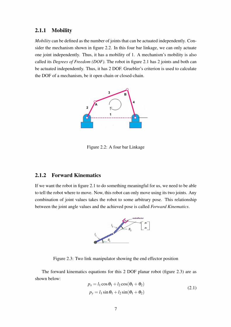
2.1.1 Mobility

Mobility can be defined as the number of joints that can be actuated independently. Con-sider the mechanism shown in figure 2.2. In this four bar linkage, we can only actuateone joint independently. Thus, it has a mobility of 1. A mechanism’s mobility is alsocalled its Degrees of Freedom (DOF). The robot in figure 2.1 has 2 joints and both canbe actuated independently. Thus, it has 2 DOF. Gruebler’s criterion is used to calculatethe DOF of a mechanism, be it open chain or closed-chain.

Figure 2.2: A four bar Linkage

2.1.2 Forward Kinematics

If we want the robot in figure 2.1 to do something meaningful for us, we need to be ableto tell the robot where to move. Now, this robot can only move using its two joints. Anycombination of joint values takes the robot to some arbitrary pose. This relationshipbetween the joint angle values and the achieved pose is called Forward Kinematics.

Figure 2.3: Two link manipulator showing the end effector position

The forward kinematics equations for this 2 DOF planar robot (figure 2.3) are asshown below:

px = l1 cosθ1 + l2 cos(θ1 +θ2)

py = l1 sinθ1 + l2 sin(θ1 +θ2)(2.1)

7

In other words, (θ1,θ2) 7→ (px, py) is essentially the forward kinematic mapping.The robot discussed here was just a 2 DOF robot. Let’s look at a more realistic robotthat has 6 DOF (figure 2.4). In this case, the forward kinematics mapping will looksomething of this sort: (θ1,θ2,θ3,θ4,θ5,θ6) 7→ (px, py, pz). However, only the knowl-edge of position isn’t enough. Orientation needs to be obtained as well in order tocompletely describe any object. Position and orientation are sometimes jointly referredto as pose. The actual forward kinematic mapping for this manipulator is as follows:(θ1,θ2,θ3,θ4,θ5,θ6) 7→ (p,o) where p = [px, py, pz]

T and o being the orientation of theend effector with respect to a reference frame.Another question that may arise at this stage is: How to describe the orientation of thisrobot? More specifically, how to describe the orientation of any rigid body in space?This question will be answered in detail in the subsequent section on rigid body trans-formations but for now, it must be remembered that there exist methods using whichwe can describe the orientation of rigid bodies. Thus, once the position and orientationhave been defined for any set of joint angle values, the forward kinematics problem issolved.

Figure 2.4: A 6 DOF manipulator

2.1.3 Inverse Kinematics

The Inverse Kinematics problem is the opposite of forward kinematics. Specifically, theInverse kinematics problem is: ”Given the position and orientation of the end-effectorof the manipulator, calculate all possible sets of joint angles which could be used toattain this given position and orientation [11].” Thus, (p,o) 7→ (θ1,θ2,θ3, .........,θn) is

8

an Inverse kinematics mapping. It might seem that this is just the inverse problem offorward kinematics and can be solved without much ado. But the problem is that in-verse kinematics does not have a one-to-one mapping. There can be multiple sets ofjoint values that yield the same pose. As can be seen in figure 2.5, there are two ways toreach the point (px, py). The two configurations are termed elbow-up and elbow-down

configurations.

Figure 2.5: A two-link manipulator showing two solutions to Inverse kinematics

The fact that Inverse kinematics problem has multiple solutions offers both advantagesand disadvantages. The advantage being that there could be multiple ways of manipu-lating any object. Thus, if one of the ways is blocked, an object can still be manipulatedusing other sets of joint values. The disadvantage is on programmer’s part because hehas to first generate multiple solutions to the inverse problem and then choose the bestsolution for a particular situation. The latter is particularly difficult since almost similarsituations can also have different manipulation schemes. Subsequent sections will coverrigid body motion, forward kinematics and inverse kinematics in detail.

2.2 Rigid body motion

Consider a body shown in figure 2.6. We want to describe the pose of this body. Anatural way is to define the body frame {b} with respect to a fixed space frame {s}.Let’s start by describing the position and orientation of the body frame with respect tothe fixed frame.Position- The position vector ~p can be described in terms of fixed frame {s} as:

~p = p1X + p2Y + p3Z (2.2)

p1, p2, p3 being the coordinates of the position vector ~p.Orientation- Orientation of a body can be expressed by forming a relationship betweenthe fixed frame {s} and body frame {b}. The following equations depict a relationship

9

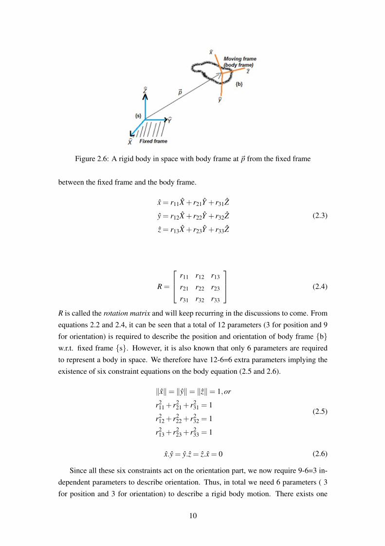
Figure 2.6: A rigid body in space with body frame at ~p from the fixed frame

between the fixed frame and the body frame.

x = r11X + r21Y + r31Z

y = r12X + r22Y + r32Z

z = r13X + r23Y + r33Z

(2.3)

R =

r11 r12 r13

r21 r22 r23

r31 r32 r33

(2.4)

R is called the rotation matrix and will keep recurring in the discussions to come. Fromequations 2.2 and 2.4, it can be seen that a total of 12 parameters (3 for position and 9for orientation) is required to describe the position and orientation of body frame {b}w.r.t. fixed frame {s}. However, it is also known that only 6 parameters are requiredto represent a body in space. We therefore have 12-6=6 extra parameters implying theexistence of six constraint equations on the body equation (2.5 and 2.6).

‖x‖= ‖y‖= ‖z‖= 1,or

r211 + r2

21 + r231 = 1

r212 + r2

22 + r232 = 1

r213 + r2

23 + r233 = 1

(2.5)

x.y = y.z = z.x = 0 (2.6)

Since all these six constraints act on the orientation part, we now require 9-6=3 in-dependent parameters to describe orientation. Thus, in total we need 6 parameters ( 3for position and 3 for orientation) to describe a rigid body motion. There exists one

10

more constraint that hasn’t yet been accounted for. It’s the type of coordinate frame tochoose: right-handed frame or left-handed frame. Although this constraint does not af-fect the number of independent parameters, it needs to be specified because the rotationmatrices arising from the two frames have different properties.

I f M =

1 1 1a b c

1 1 1

where M ∈ℜ3×3 (2.7)

, then it is known that det M = aT (b× c). Applying this to the rotation matrix in 2.4,we get:

det R = xT (y× z) (2.8)

where x = [r11 r21 r31]T , y = [r12 r22 r32]

T , z = [r13 r23 r33]T . Since (y× z) = x for

a right-handed coordinate system, equation 2.8 results in det R = xT .x = 1. For theleft-handed frame, since (y× z) =−x, thus det R = xT .− x =−1All the seven constraints for a right-handed coordinate frame can now be rewritten as:

RT .R = I and det R =+1 (2.9)

2.2.1 Special Orthogonal group [SO(3)]

The special orthogonal group (SO(3)) is the set of all rotation matrices that satisfy equa-tion 2.9. Alternatively, SO(3) = {R ∈ℜ3×3|RT R = I and det R =+1}. The next sub-section discusses the properties of SO(3); no proofs have been provided for the sake ofsimplicity but the readers can refer to [27] for proofs.

Properties of SO(3)

• R−1 = RT

• If R1,R2 ∈ SO(3), then R1.R2 ∈ SO(3)

• If x ∈ℜ3, then ‖Rx|= ‖x‖

• If there are three distinct coordinate frames {a}, {b}, and {c}, then Rac = RabRbc

• RabRba = I, meaning that Rab is the inverse of Rba.

• If there are two coordinate frames {a} and {b} in space (figure 2.7), then the vec-tor~v can be expressed in terms of both the coordinate frames as:

11

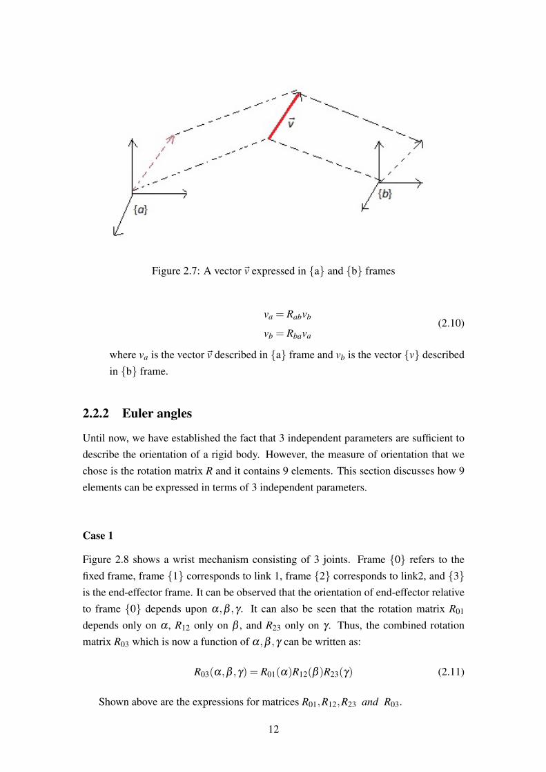
Figure 2.7: A vector~v expressed in {a} and {b} frames

va = Rabvb

vb = Rbava(2.10)

where va is the vector~v described in {a} frame and vb is the vector {v} describedin {b} frame.

2.2.2 Euler angles

Until now, we have established the fact that 3 independent parameters are sufficient todescribe the orientation of a rigid body. However, the measure of orientation that wechose is the rotation matrix R and it contains 9 elements. This section discusses how 9elements can be expressed in terms of 3 independent parameters.

Case 1

Figure 2.8 shows a wrist mechanism consisting of 3 joints. Frame {0} refers to thefixed frame, frame {1} corresponds to link 1, frame {2} corresponds to link2, and {3}is the end-effector frame. It can be observed that the orientation of end-effector relativeto frame {0} depends upon α,β ,γ . It can also be seen that the rotation matrix R01

depends only on α , R12 only on β , and R23 only on γ . Thus, the combined rotationmatrix R03 which is now a function of α,β ,γ can be written as:

R03(α,β ,γ) = R01(α)R12(β )R23(γ) (2.11)

Shown above are the expressions for matrices R01,R12,R23 and R03.

12

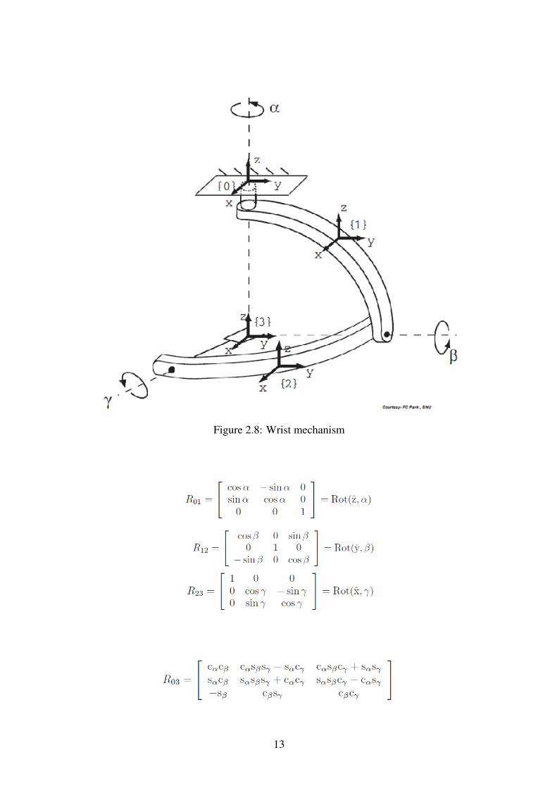
Figure 2.8: Wrist mechanism

13

At this stage, a question arises: Given some arbitrary rotation matrix R ∈ SO(3),does there exist any angle set (α,β ,γ) such that R = R03(α,β ,γ). The answer to thisquestion can be found using a brute-force strategy. From the above expressions, wecan find the values of angles as given in equations 2.12, 2.13 and 2.14. Clearly, thedenominator of equation 2.12 can assume two values, a positive and a negative. If weconsider only a positive denominator, then in accordance with tan arguments, β canassume values only in the range [−π

2 , π

2 ]. Similarly, α and γ can attain values in therange [0,2π]. The angles (α,β ,γ) just described are more commonly referred to asZYX Euler Angles. The reason why they are called ZY X Euler angles is due to thefollowing interpretations:

• Since α rotates along z axis of frame {0}, β along y axis of frame {1}, and γ

along x axis of frame{2},

• and the sequence of rotations is first along Z, then along Y , and finally along X .

tanβ =

(sinβ

cosβ

)or β = tan−1

(sinβ

cosβ

)

⇒ β = tan−1

−r31√r2

11 + r221

(2.12)

Similarly, α = tan−1(

r21

r11

)(2.13)

γ = tan−1(

r32

r33

)(2.14)

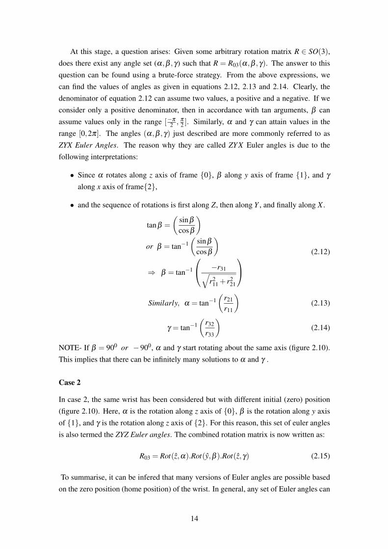
NOTE- If β = 900 or −900, α and γ start rotating about the same axis (figure 2.10).This implies that there can be infinitely many solutions to α and γ .

Case 2

In case 2, the same wrist has been considered but with different initial (zero) position(figure 2.10). Here, α is the rotation along z axis of {0}, β is the rotation along y axisof {1}, and γ is the rotation along z axis of {2}. For this reason, this set of euler anglesis also termed the ZYZ Euler angles. The combined rotation matrix is now written as:

R03 = Rot(z,α).Rot(y,β ).Rot(z,γ) (2.15)

To summarise, it can be infered that many versions of Euler angles are possible basedon the zero position (home position) of the wrist. In general, any set of Euler angles can

14

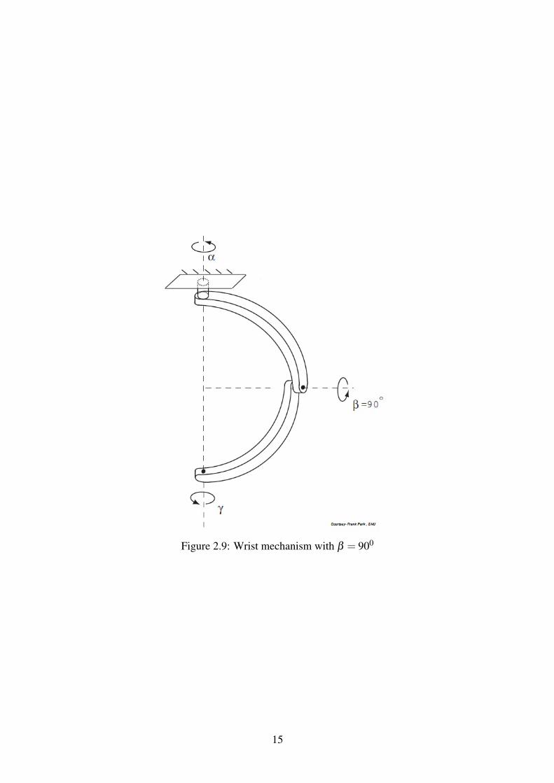
Figure 2.9: Wrist mechanism with β = 900

15

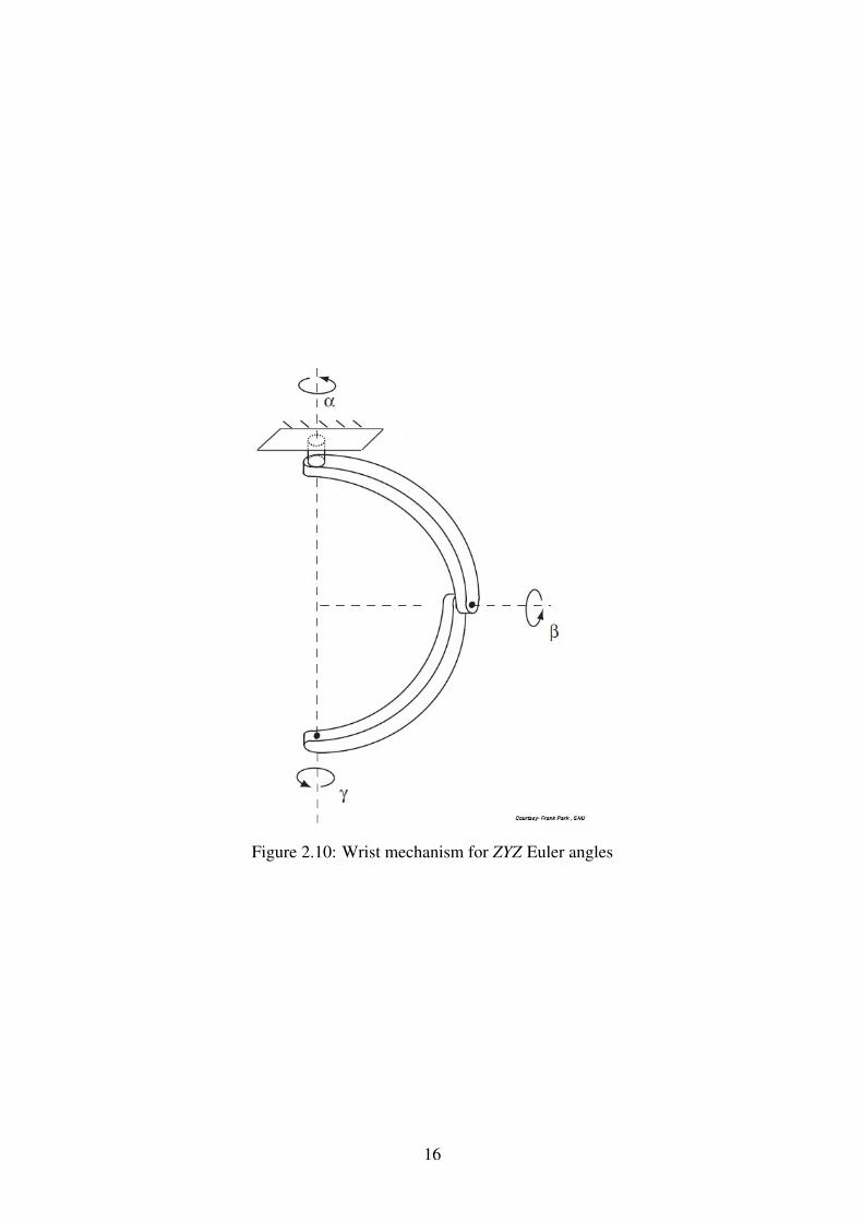
Figure 2.10: Wrist mechanism for ZYZ Euler angles

16

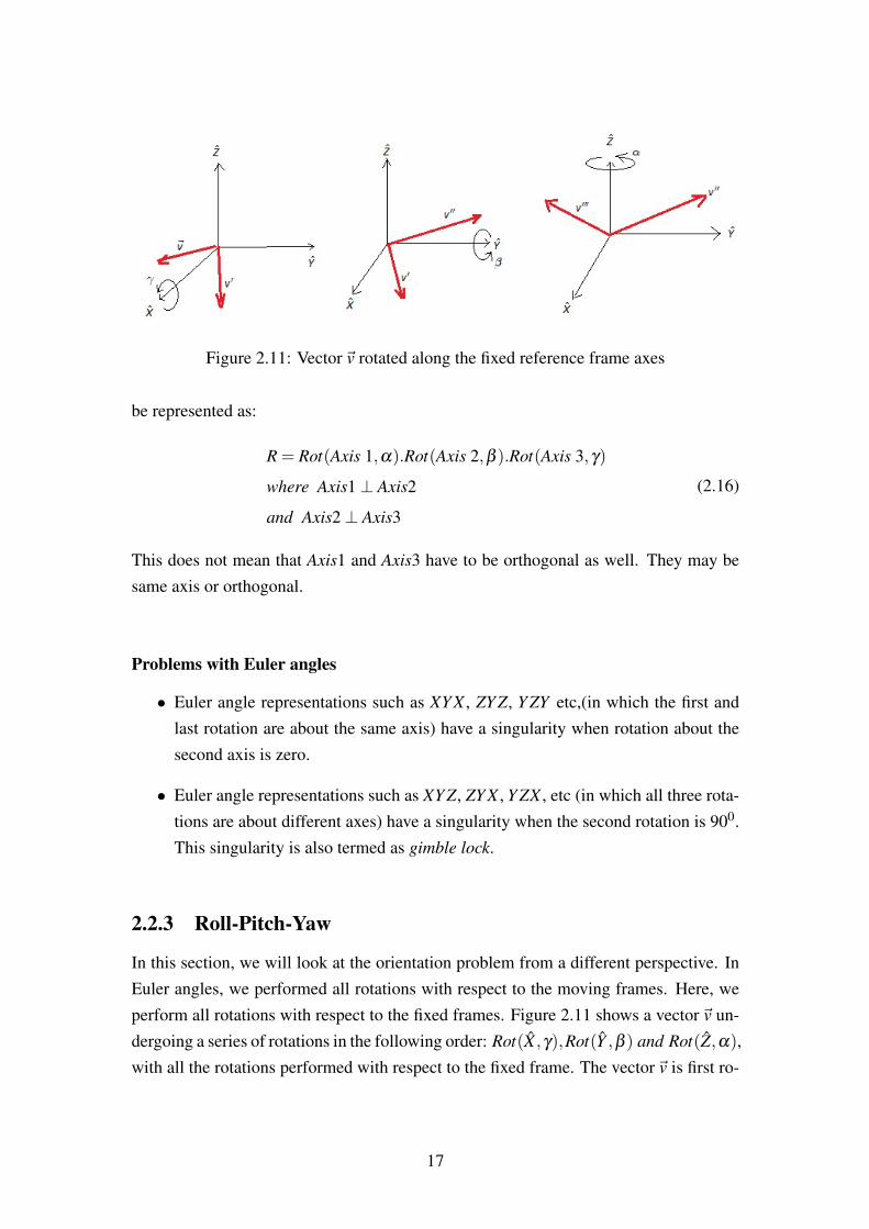
Figure 2.11: Vector~v rotated along the fixed reference frame axes

be represented as:

R = Rot(Axis 1,α).Rot(Axis 2,β ).Rot(Axis 3,γ)

where Axis1⊥ Axis2

and Axis2⊥ Axis3

(2.16)

This does not mean that Axis1 and Axis3 have to be orthogonal as well. They may besame axis or orthogonal.

Problems with Euler angles

• Euler angle representations such as XY X , ZY Z, Y ZY etc,(in which the first andlast rotation are about the same axis) have a singularity when rotation about thesecond axis is zero.

• Euler angle representations such as XY Z, ZY X , Y ZX , etc (in which all three rota-tions are about different axes) have a singularity when the second rotation is 900.This singularity is also termed as gimble lock.

2.2.3 Roll-Pitch-Yaw

In this section, we will look at the orientation problem from a different perspective. InEuler angles, we performed all rotations with respect to the moving frames. Here, weperform all rotations with respect to the fixed frames. Figure 2.11 shows a vector~v un-dergoing a series of rotations in the following order: Rot(X ,γ),Rot(Y ,β ) and Rot(Z,α),with all the rotations performed with respect to the fixed frame. The vector~v is first ro-

17

tated about X by amount γ . The new vector v′ can be written as:

v′ =

1 0 00 cosγ −sinγ

0 sinγ cosγ

v (2.17)

The vector v′ is then rotated by an amount β about Y . The new vector v′′ is:

v′′ =

cosβ 0 sinβ

0 1 0−sinβ 0 cosβ

v′ (2.18)

The vector v” is then rotated about Z by an amount α . The resulting vector v′′′ is thus:

v′′′ =

cosα −sinα 0sinα cosα 0

0 0 1

v′′ (2.19)

From equations 2.17,2.18 and 2.19, v′′′=Rot(Z,α).Rot(Y ,β ).Rot(X ,γ).v′,which meansthat the rotation matrix R = Rot(Z,α).Rot(Y ,β ).Rot(X ,γ). This matrix is similar to therotation matrix in ZYX Euler angles. Thus, the same product of rotations admits twodifferent physical interpretations:

• As a sequence of rotations with respect to the moving frame, as in Euler angles.

• As a sequence of rotations with respect to the fixed frame, as in Roll-pitch-yawrepresentation.

2.2.4 Quaternions

Another representation of orientation is the Euler parameters, also known as a unit

quaternion. In terms of an equivalent axis K = [kx ky kz]T and the equivalent angle θ ,

the Euler parameters are written as:

q0 = cos(θ

2)

q1 = kx sin(θ

2)

q2 = ky sin(θ

2)

q3 = kz sin(θ

2)

(2.20)

Also,q2

0 +q21 +q2

2 +q23 = 1 (2.21)

18

The rotation matrix can then be written in terms of the unit quaternion components as:

R =

q20 +q2

1−q22−q2

3 2(q1q2−q0q3) 2(q1q3 +q0q2)

2(q1q2 +q0q3) q20−q2

1 +q22−q2

3 2(q2q3−q0q1)

2(q1q3−q0q2) 2(q2q3 +q0q1) q20−q2

1−q22 +q2

3

(2.22)

An advantage with quaternion representation is that it does not suffer from the issuesof singularity unlike Euler angles. However, they are not used as much as Euler an-gles because it is hard to visualize quaternions. Even engineers find it hard to visualizequaternions, let alone physicians or doctors.

2.2.5 Homogenous transformations

So far, we discussed how to describe the position and orientation of a body in spaceusing the position vector ~p and the Rotation matrix R respectively. Efforts would be re-duced if somehow, we could generate a single compact representation for both positionand orientation. The Homogenous Transformation matrix serves as that package. It is a4×4 matrix represented as

T =

[R p

O 1

]Here, R ∈ℜ3×3, p ∈ℜ3×1, and O = [0 0 0]The transformation matrix T ∈ SE(3), the Special Euclidean group. The Special Eu-clidean group is also called the ”group of rigid body motions” and is defined as :

SE(3) =

{[R p

O 1

]∈ℜ

4×4|R ∈ SO(3) and p ∈ℜ3

}(2.23)

Properties of Special Euclidean group

This section discusses the properties of special euclidean group without delving into theproofs of these.

• If T1,T2 ∈ SE(3), then T1T2 ∈ SE(3)

• T−1 =

[RT −RT p

O 1

]∈ SE(3)

• Tac = TabTbc

19

• TabTba = I, meaning that Tab is the inverse of Tba

• If x and y are two position vectors, then ‖T x−Ty‖= ‖x− y‖

Similar to the rotation matrix, the same sequence of transformations renders two differ-ent physical interpretations; one being the sequence of transformations with respect tothe moving frame and the other being the sequence of transformations with respect tothe fixed frame.

2.3 Forward Kinematics of Open chains

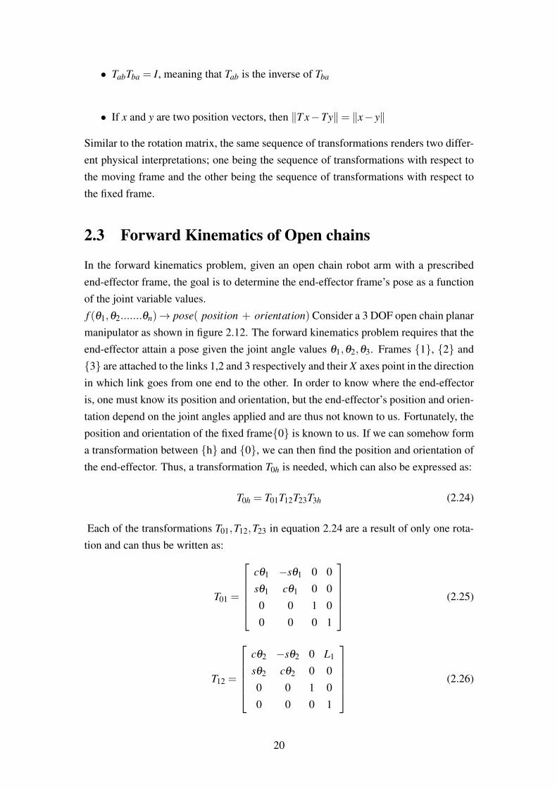
In the forward kinematics problem, given an open chain robot arm with a prescribedend-effector frame, the goal is to determine the end-effector frame’s pose as a functionof the joint variable values.f (θ1,θ2.......θn)→ pose( position + orientation) Consider a 3 DOF open chain planarmanipulator as shown in figure 2.12. The forward kinematics problem requires that theend-effector attain a pose given the joint angle values θ1,θ2,θ3. Frames {1}, {2} and{3} are attached to the links 1,2 and 3 respectively and their X axes point in the directionin which link goes from one end to the other. In order to know where the end-effectoris, one must know its position and orientation, but the end-effector’s position and orien-tation depend on the joint angles applied and are thus not known to us. Fortunately, theposition and orientation of the fixed frame{0} is known to us. If we can somehow forma transformation between {h} and {0}, we can then find the position and orientation ofthe end-effector. Thus, a transformation T0h is needed, which can also be expressed as:

T0h = T01T12T23T3h (2.24)

Each of the transformations T01,T12,T23 in equation 2.24 are a result of only one rota-tion and can thus be written as:

T01 =

cθ1 −sθ1 0 0sθ1 cθ1 0 00 0 1 00 0 0 1

(2.25)

T12 =

cθ2 −sθ2 0 L1

sθ2 cθ2 0 00 0 1 00 0 0 1

(2.26)

20

Figure 2.12: A three DOF planar manipulator with its frames.

21

T23 =

cθ3 −sθ3 0 L2

sθ3 cθ3 0 00 0 1 00 0 0 1

(2.27)

T3h does not depend on any joints and is thus constant (equation2.28).

T3h =

1 0 0 L3

0 1 0 00 0 1 00 0 0 1

(2.28)

Multipying all these, we can obtain T0h which is the transformation between the fixedframe and the hand frame. Remember that this is just a transformation between ref-erence frames. Thus, a point at ~x from the base frame will be at T0h~x from the handframe. Another thing to observe is that the transformation matrix T0h is a function ofjoint angles and with change in joint angles, the transformation values change.Since the approach we used to derive the transformation T0h lacks generality, a specificconvention is needed to ensure coherence among the research community. The nextsubsection provides that generic convention.

2.3.1 Denavit-Hartenberg Representation (D-H representation)

The basic idea underlying the Denavit-Hartenberg approach to forward kinematics is toattach reference frames to each link of the open chain, and to derive the forward kine-matics based on knowledge of the relative displacements between adjacent link frames.Figure 2.13 shows three joints i− 1, i and i+ 1. We draw a common perpendicular tothe two consecutive joint axes. Frame {a} has z component parallel to the joint axis i

and is slid along the common perpendicular. The new frame along the joint axis i iscalled {b}. Frame {b} is now shifted along the joint axis i to frame {c}. Frame {c} isnot the same as frame {i}. So a transformation exists between {c} and {i}. Followingare the two rules that are followed before defining the D-H notation.

• All zi are aligned to the joint axes i.

• All xi are aligned along the common normal between i and i+1 joint axes.

As in figure 2.13, four parameters viz. αi−1,ai−1,di,θi are needed to describe the trans-formation Ti,i−1. These parameters are called the Denavit-Hartenberg or D-H parame-ters [22]. They have been defined as follows:

• The link twist αi−1 is the angle from zi−1 to zi, measured about ˆxi−1.

22

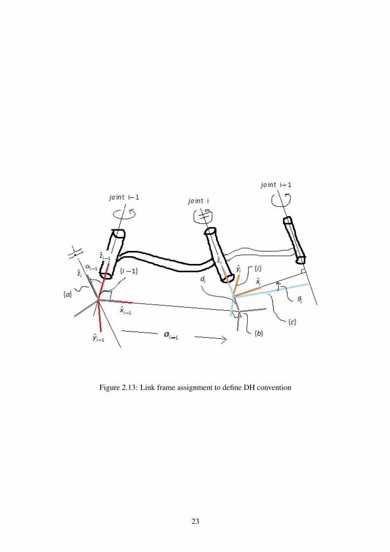
Figure 2.13: Link frame assignment to define DH convention

23

• The length of the mutually perpendicular line, denoted by the scalar ai−1 is calledthe link length.

• Link offset di is the distance from the intersection of xi−1 and zi to the link i frameorigin. (positive direction defined along zi)

• Joint angle θi is the angle from xi−1 to xi, measured about the zi axis in the right-hand sense.

Are four parameters sufficient to define any transformation?

We discussed in the preceding sections that a minimum of six parameters are requiredto represent any transformation in space. However, the D-H convention requires only 4parameters to describe any transformation. So where is the catch? Is there somethingwrong with D-H convention ? or, is the fact that minimum 6 parameters are required torepresent any transformation incorrect? All these are valid questions and the answer toall of them is: Neither is the D-H convention wrong, nor is our previous understandingof the transformations incorrect. The difference of 2 (6-4) parameters arises because inprevious discussions, we assigned all frames arbitrarily while in D-H convention, frameassignment follows a specific set of rules and this results in the reduction of parameters.In short, we put 2 constraints during the frame assignment process thus requiring only4 parameters per transformation.

What if the two joint axes are parallel?

What will be the perpendicular line along which xi−1 will be assigned since there existinfinitely many lines that are perpendicular to two parallel lines? The answer to it variesfrom person to person. In genral, the line most convenient to the user is considered.Before we conclude the chapter, we define few terms that will be used throughout therest of this document.

• Joint space : The position of all links of a manipulator of n DOF can be specifiedwith a set of n joint variables. This set is often refered to as the n×1 joint vector.The space of all such joint vectors is the joint space.

• Workspace or taskspace - Workspace of a robot manipulator is the volume ofspace spanned by the robot end-effector.

• Cartesian space- The term cartesian space is used when position is measuredalong orthogonal axes and orientation is measured according to any conventionsdiscussed before. Cartesian space is sometimes referred to as operational space.

24

Chapter 3

BAYESIAN FILTERS

3.1 Introduction

In this unit, generic Bayes filter along with its tractable variants have been discussed.In particular, we will discuss non-parametric versions of Bayes filter due to the fact thatnon-parametric filters do not assume any structure of the state space. This virtue will beapplied in the Inverse Kinematics problem in the next unit.

3.2 Bayes’ Rule

Bayes rule is of utmost importance in the field of probabilistic robotics. Let’s go on ashort detour to understand the Bayes rule intuitively. Suppose we observe a car accidentC where the driver A collides into a stop sign. What is the probability that the driver A

was overspeeding? In this scenario, what we can observe is the event C, but if we wantto know what caused such an event, the Bayes rule comes into the picture. Bayes ruleis stated mathematically as follows:

P(A|C) =P(C|A).P(A)

P(B),

A→ cause

C→ e f f ect

P(A|C)→ posterior

P(C|A)→ likelihood

P(A)→ Prior

P(B)→ marginal likelihood

(3.1)

25

3.3 Belief Distributions

A key concept in probabilistic robotics is that of a belief (posterior) [53]. A belief re-flects the robot’s internal knowledge about the state of the environment. Often, it is thecase that state cannot be measured directly. Instead, the robot has to infer its state fromthe data. Thus, in robotics, true state is distinguished from its belief.In robotics, beliefs are often represented using conditional probability distributions. Aposterior distribution assigns a probability to each possible hypothesis with regards tothe true state. Belief distributions are nothing but posterior probabilities over state vari-ables conditioned on the available data. We will denote the posterior over a state xtbypost(xt).

post(xt) = p(xt |z1:t ,u1:t) (3.2)

This posterior is the probability distribution over the state xt at time t, conditioned onall previous measurements z1:t and all past controls u1:t . It is assumed that the belief istaken after the measurement at time t, zt has been recorded. Sometimes, it is also usefulto calculate posteriors before the measurement zt has been recorded. Such a posterior isreferred to as prediction and is denoted as follows:

¯post(xt) = p(xt |z1:t−1,u1:t) (3.3)

The reason why it is called as prediction is quite apparent. Based on the previous data,3.3 predicts the state x at time t. Calculating post(xt) from ¯post(xt) is called correction

or measurement update.

3.4 Bayes Filters

Bayes filters are used to calculate the beliefs from measurement z and input u data. Ta-ble 1 depicts a single step of the Bayes filter algorithm.

Algorithm 1 Algorithm for Bayes filterAlgorithm Bayes Filter(post(xt−1,ut ,zt)):for all xt do

¯post(xt) =∫

p(xt |ut ,xt−1)post(xt−1)dxpost(xt) = η p(zt |xt) ¯post(xt)

end forreturn post(xt)

In Line 3, η is used as a normalizer because the posterior obtained by multiplying¯post(xt) and the probability of occurence of zt is not yet a probability. This normalizer

26

is used to make the sum equal 1. Line 2 is called prediction step. Line 3 is called mea-

surement update step.

Bayes filter is recursive, meaning that the posterior post(xt) is derived using the in-formation from post(xt−1) which in turn is derived using post(xt−2) and so on. Thisimplies that the Bayes filter makes Markov assumption which specifies that the state isa complete summary of the past. To compute the posterior recursively, the bayes algo-rithm thus requires the initial belief at time t = 0. If post(x0) is known with certainty,a point mass probability distribution is assigned to x0 while if post(x0) is totally un-known, a uniform distribution is assigned to x0.Bayes filter is not a practical algorithm. So, probabilistic algorithms use tractable ap-proximations to execute Bayes filter on a digital computer. It must be noted here thatno unique answer exists for any robotics application. It all depends on the user and thesystem.

3.5 Parametric Bayes Filter

Although the parametric variants of Bayes filter are unimportant to us, it seems worth-while to understand them superficially.Gaussian filters constitute the earliest tractable version of the Bayes filter and are byfar the most popular family of filters to date. All gaussian techniques have a commontheme that the structure of a state space can be represented by multivariate normal dis-tributions. The structure of state space is characterized by two sets of parameters: themean µ and the covariance Σ. The Kalman Filter [28] which is linear and gaussianwas invented in the 1950s by Rudolph Kalman and is by far the most used filter (alongwith its variants) in robotics.Using a Gaussian to represent the posterior has significant implications. Firstly, theGaussians are unimodal, meaning they only have one maximum. This prevents it frombeing used in problems where multiple hypothesis exist. However, such a unimodalrepresentation is characteristic of many tracking problems in robotics, in which the pos-terior is focused around the true state with small uncertainty.

3.6 Non-parametric Filters

Non-parametric filters are an alternative to the Gaussian techniques. They do not assumethe posterior to be of any fixed functional form, like in Gaussians. Instead, posteriors areapproximated using a finite number of values, each of which corresponds approximatelyto a region in state space. The quality of approximation is thus dependent on the number

27

of parameters used to represent the posterior. As the number of parameters tends toinfinity, the approximation tends to converge to the true posterior. In this section, we willdiscuss two non-parametric filters relevant to the context of this thesis: the Histogramfilter and the Particle filter. Both these filters can approximate complex multimodalbeliefs. For this reason, both these methods are often resorted to the problem of robotglobal localization.

3.6.1 Histogram Filter

Histogram filters [54] decompose the state space into finite regions and represent eachregion by a single probability value. When applied to discrete spaces, they are knownas discrete Bayes Filters.

range(Xt) = x1,t ∪ x2,t ∪ x3,t ........∪ xk,t (3.4)

As shown in 3.4, range(Xt) denotes the state space of a variable X at any time t, i.e. X

can assume any value in this space at time t. Each xk,t is a partition of the state spacein such a way that xi,t ∩ xk,t = φ for i 6= k. A straightforward decomposition of the statespace can be a multi-dimensional grid, and the granularity of decomposition defines theaccuracy and computational efficiency of the filter. A fine granularity ensures lowererrors of approximation but at the cost of higher computational complexity.

It must be noted that the Discrete Bayes filter carries no further information within eachregion. It only represents each region by a probability value. If the state space is trulydiscrete, the conditional probabilities p(xk,t |ut ,xi,t−1) and p(zt |xk,t) are well-defined butin continuous state spaces, p(xk,t |ut ,xi,t−1) and p(zt |xk,t) are defined over all states. Thedensities for each region are thus obtained by replacing xk,t by a representative of thisregion, which is in most instances the mean of each region xk,t .

xk,t = |xk,t |−1∫

xk,t

xtdxt (3.5)

One can then simply replace :

p(zt |xk,t)≈ p(zt |xk,t)

p(xk,t |ut ,xi,t−1)≈η p(xk,t |ut , xi,t−1)

|xk,t |(3.6)

We can now modify algorithm 1 by using equation 3.6 to obtain a Histogram filter im-plementation.

28

3.6.2 Decomposition techniques

Decomposition of continuous state spaces is done in two ways: static and dynamic.Static strategies perform a fixed decomposition that is known beforehand, irrespectiveof the shape of the posterior to be approximated. Dynamic techniques are adaptive innature, implying that the decomposition varies with the shape of the posterior. Statictechniques are much easier to implement but due to the lack of adaptivity, they arecomputationally inefficient. As will be seen in the next unit, we will use decomposi-tion techniques to improve the localization process. Since we do not know how muchspeedup the dynamic techniques may provide for our Inverse Kinematics problem , wewill be relying on the static decomposition techniques.

3.6.3 Particle Filter

The particle filter [50] [52] is an alternative nonparametric implementation of the Bayesfilter. Instead of describing the required probability density in a functional form (pdf ),it is represented approximately as a set of random samples in the state space. As thenumber of samples tends to infinity, this becomes an exact equivalent to the functionalform. These random samples are the particles of the filter which are propagated andupdated according to the dynamics and measurement models. Unlike the Kalman filter,this approach is not restricted by linear Gaussian assumptions and is thus able to en-capsulate more complex and nonlinear modelling issues. The two main variants of theparticle filter, Importance Sampling [42] and Sampling Importance Resampling (SIR)

[48] are presented.

Importance Sampling

The objective of importance sampling is to sample the distribution in the region of “im-portance” to achieve computational efficiency. This is of utmost importance especiallyfor the high dimensional space where data are usually sparse, and the region of interestwhere target lies is relatively small in the whole data space. The idea of importancesampling is to choose a proposal distribution q(x) in place of the true probability dis-

tribution p(x), which is hard to sample.

The underlying mathematical concept is simple. Consider a statistical problem thatestimates the integral:

I =∫

f (x)p(x)dx, (3.7)

29

f (x) being an integrable function.Since p(x) is hard to sample from, we rewrite the equation 3.7 in terms of q(x) as:

∫f (x)p(x)dx =

∫f (x)

p(x)q(x)

q(x)dx (3.8)

Importance sampling uses a number of independent samples (say Np ) drawn from q(x)

to obtain a weighted sum to approximate f as in equation 3.9.

f =1

Np

Np

∑i=1

W (xi) f (xi) (3.9)

Here, W (xi) =p(x)q(xi)

are called the importance weights. To ensure that ∑Npi=1W (xi) = 1,

importance weights are normalized and equation 3.9 transforms to:

f =1

Np∑

Npi=1W (xi) f (xi)

1Np

∑Npj=1W (x j)

f =Np

∑i=1

W (xi) f (xi)

(3.10)

Here, W (xi) =W (xi)

∑Npj=1 W (x j)

are the normalized importance weights.

Equation 3.10 suggests that the approximation depends on two things: the strength ofsample f (xi), and the importance weight corresponding to that sample.

• If q(.) is close to p(.), and the strength of that sample is high, a very high proba-bility is assigned to that sample.

• If q(.) is close to p(.) and the strength of that sample is low, a moderate probabilityis assigned to that sample.

• If q(.) is not close to p(.) and the strength of that sample is high, a low probabilityis assigned to that sample.

• If q(.) is not close to p(.) and the strength of that sample is low, a very lowprobability is assigned to that sample.

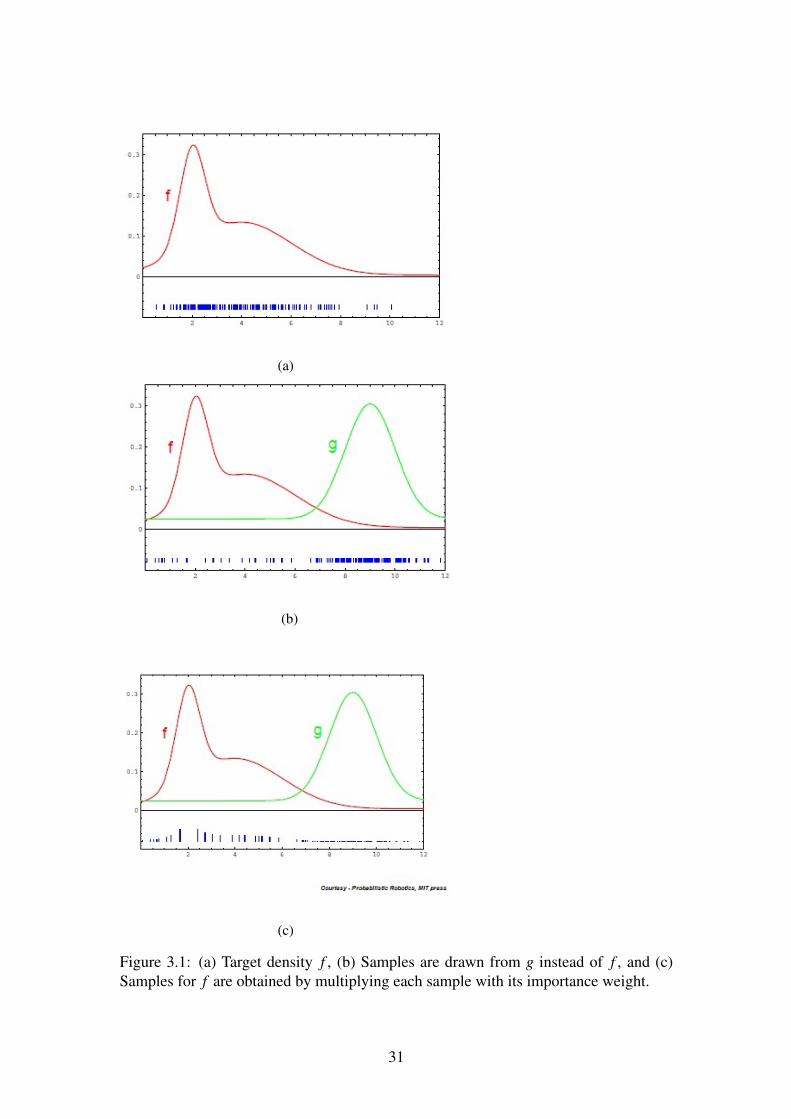
Thus, samples (or particles) with higher importance weights yield true probabilitiesmaking the approximation a good one. An illustration of importance sampling from[53] is given in figure 3.1. However, many samples though useless because of theirnegligible contributions are propagated in future iterations of filtering. This leads tocomputational inefficiency.

30

(a)

(b)

(c)

Figure 3.1: (a) Target density f , (b) Samples are drawn from g instead of f , and (c)Samples for f are obtained by multiplying each sample with its importance weight.

31

Sampling Importance Resampling

SIR is motivated from Bootstrap and jack knife techniques [15]. The intuition of boot-strapping is to evaluate the properties of an estimator through empirical cumulative

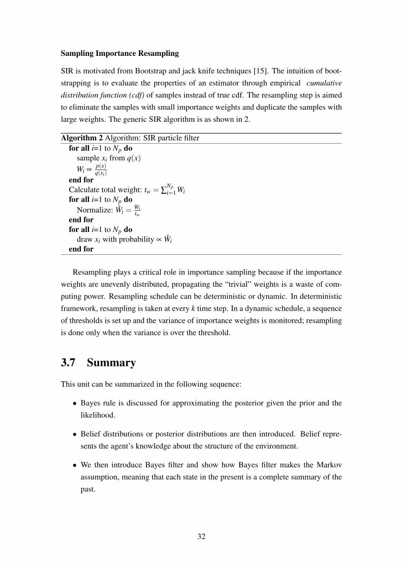
distribution function (cdf) of samples instead of true cdf. The resampling step is aimedto eliminate the samples with small importance weights and duplicate the samples withlarge weights. The generic SIR algorithm is as shown in 2.

Algorithm 2 Algorithm: SIR particle filterfor all i=1 to Np do

sample xi from q(x)Wi ∝

p(x)q(xi)

end forCalculate total weight: tw = ∑

Npi=1Wi

for all i=1 to Np doNormalize: Wi =

Witw

end forfor all i=1 to Np do

draw xi with probability ∝ Wiend for

Resampling plays a critical role in importance sampling because if the importanceweights are unevenly distributed, propagating the “trivial” weights is a waste of com-puting power. Resampling schedule can be deterministic or dynamic. In deterministicframework, resampling is taken at every k time step. In a dynamic schedule, a sequenceof thresholds is set up and the variance of importance weights is monitored; resamplingis done only when the variance is over the threshold.

3.7 Summary

This unit can be summarized in the following sequence:

• Bayes rule is discussed for approximating the posterior given the prior and thelikelihood.

• Belief distributions or posterior distributions are then introduced. Belief repre-sents the agent’s knowledge about the structure of the environment.

• We then introduce Bayes filter and show how Bayes filter makes the Markovassumption, meaning that each state in the present is a complete summary of thepast.

32

• It is then argued that the Bayes filter in its original form is intractable and there-fore, variants of bayes filter are introduced to enable implementation on a digitalcomputer.

• The Gaussian variants, like Kalman filter make assumptions about the structureor distribution of the state space and represent the state space using a fixed para-metric model. The advantage is that problems, such as tracking can be solvedwith very low approximation errors. The disadvantage being that most roboticsproblems cannot be solved by assuming a unimodal parametric state space.

• The Non-parametric filters , viz. the Histogram filter and the Particle filter arethen discussed.

• The histrogram filters are non-parametric and can approximate multimodal dis-tributions. They divide the state space in a number of regions and then assign asingle probability value to each region. The granularity of region division definesthe level of approximation of the distribution.

• The particle filter is also a non-parametric variant of Bayes filter. It approximatescomplex multimodal distributions using a set of random state samples. As thenumber of particles increases, the approximation gets better but computationalcost increases.

• Two versions of particle filter, Importance sampling and Sampling ImportanceResampling (SIR) are discussed and it is shown how SIR algorithm saves a sig-nificant amount of computation by incorporating the Resampling part.

33

Chapter 4

INVERSE KINEMATICS - Theprevious and the Proposed

4.1 Introduction

In unit 2, it was discussed why the Inverse Kinematics (IK) problem is not an easy one.Following are the issues that need to be resolved in order to solve the IK problem:

• Existence or non-existence of solutions - An IK algorithm must be able to dif-ferentiate unsolvable instances from the solvable ones. If a solution exists, thealgorithm must be able to generate it while if the desired pose lies outside theworkspace, the algorithm should be able to detect it as an unsolvable instance.

• Multiple solutions- An IK algorithm should be able to generate all possible solu-tions to attain the desired pose.

• Choice of solution- This is not entirely the job of an IK algorithm to decide whichsolution to choose from the set of solutions because the choice of solution dependson the situation. In different situations, even humans move their hands differentlyas shown in figure 4.1. The boy on the left side of figure tries to lift the weightusing a different technique than the one lifting dumbbells on the right. The choiceof solution depends on the situation at hand and a single IK algorithm may notchoose an optimal solution in all situations. This is rather a learning issue.

Method of solution: The primary goal of any IK problem solver is to find all possi-ble solutions, if they exist, and choose the best solution. The criteria upon which to callany solution “best” varies for different applications, but a reasonable choice is to pickthe solution closest to the current configuration. The IK solution strategies can broadlybe divided into two classes: Closed form solutions and Numerical solutions. Numeri-cal solutions due to their iterative nature are slower compared to closed form solutions.

34

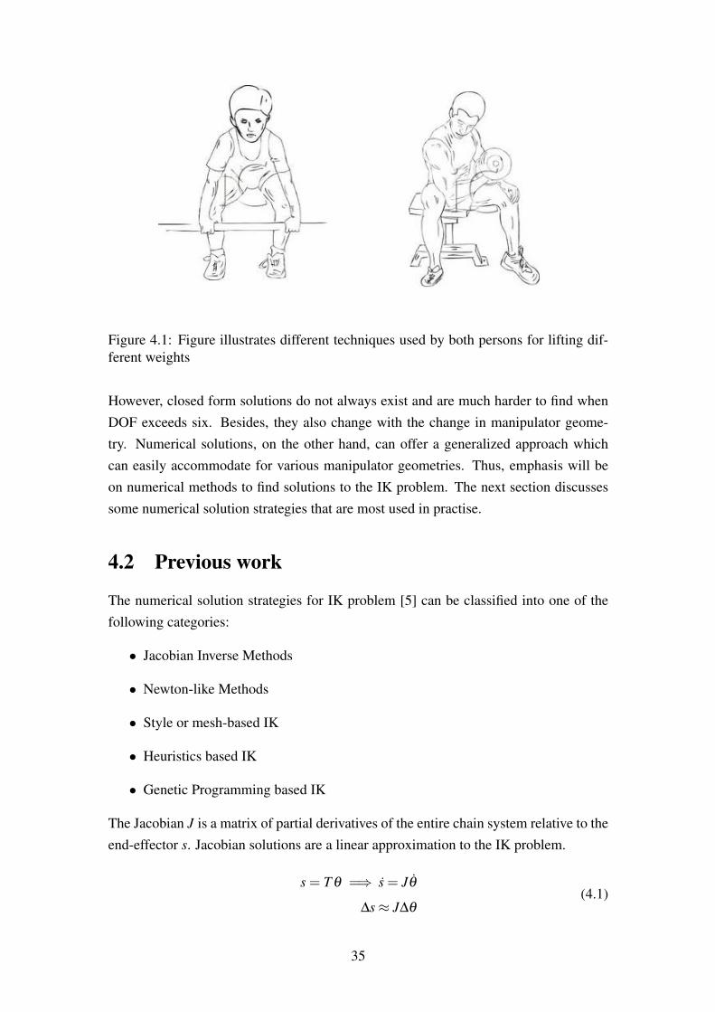
Figure 4.1: Figure illustrates different techniques used by both persons for lifting dif-ferent weights

However, closed form solutions do not always exist and are much harder to find whenDOF exceeds six. Besides, they also change with the change in manipulator geome-try. Numerical solutions, on the other hand, can offer a generalized approach whichcan easily accommodate for various manipulator geometries. Thus, emphasis will beon numerical methods to find solutions to the IK problem. The next section discussessome numerical solution strategies that are most used in practise.

4.2 Previous work

The numerical solution strategies for IK problem [5] can be classified into one of thefollowing categories:

• Jacobian Inverse Methods

• Newton-like Methods

• Style or mesh-based IK

• Heuristics based IK

• Genetic Programming based IK

The Jacobian J is a matrix of partial derivatives of the entire chain system relative to theend-effector s. Jacobian solutions are a linear approximation to the IK problem.

s = T θ =⇒ s = Jθ

∆s≈ J∆θ(4.1)

35

The idea is to choose ∆θ such that ∆s is approximately equal to e, the desired end-effector pose. Thus, the forward problem is e = J∆θ and the inverse problem is ∆θ =

J−1e. In cases where J is non-invertible, this method fails and Least-squares solutionsare resorted to find ∆θ .A number of methods have been proposed to find Jacobian inverse. Pseudo-inverse

[6] is a popular approach to find the best possible solution in the least squares sense.The main advantage of it is that it is defined for all matrices, including those whichare non-square or not of full row rank. However, it performs poorly near singularities.Singularities are those points of the workspace where J is non-invertible. Singularitiesare of two kinds: Workspace boundary singularities and Workspace interior singulari-

ties. As an alternative, the Jacobian Transpose [57] method uses transpose of Jacobianinstead of inverse, the problem being that transpose is not the same as inverse. Singular

Value Decomposition (SVD) is a powerful tool for obtaining pseudo-inverse, but it iscomputationally intensive. Damped Least Squares (DLS)[55] method works using op-timization. Instead of finding ∆θ that gives the best solution to e = J∆θ , it finds ∆θ

that minimizes –‖J∆θ − e‖2 +λ‖∆θ‖2,

λ ∈ℜ

(4.2)

Like all optimization problems, λ should be large enough but if it is too large, con-vergence rate is greatly reduced. Pseudo-inverse DLS works better than both DLS andpseudo-inverse. Selectively Damped Least Squares (SDLS) [8] performs better thanother Jacobian inversion methods discussed so far. It adjusts the damping factor sep-arately for each singular vector of Jacobian SVD based on the difficulty of reachingthe target. However, it is computationally intensive. Feedback Inverse Kinematics [47]solves IK problem from a control perspective by minimizing the difference betweendemanded and actual Cartesian velocities.Newton-based methods rely on a second-order Taylor series expansion of the form-

f (x+σ) = f (x)+ |∆ f (x)|T σ +σT H f (x)σ

2,

H f (x) is the Hessian matrix(4.3)

However, the calculation of Hessian matrix is complex, thereby resulting in high com-putational cost per iteration. Several approaches have been proposed which use anapproximation of the Hessian matrix based on a function gradient value [16]. Thesemethods demand a close initial estimate. Therefore, a proper step-size control is neces-sary to avoid divergence due to a poor initial estimate. One advantage, though, is thatthese do not suffer from singularities.Style or Mesh-based [20] solutions are based on a learned model of human poses. The

36

advantage is that the speed of posing task is a function of model parameters rather thanof manipulator geometry. The drawback is that these solutions require an off-line train-ing. Besides, the results are totally dependent on the training data set.Heuristics based solutions are widely used to solve IK problem. One of the most pop-ular methods is the Cyclic Coordinate Descent (CCD) [56]. It attempts to minimizeposition and orientation errors by transforming each joint variable, one at a time. Itoffers high speed and ease of implementation. However, it produces motion with erraticdiscontinuities. Triangulation [43] method is a non-iterative approach. It uses cosinerule to calculate each joint angle starting at the root of kinematic chain moving towardsthe end-effector. By virtue of being non-iterative, it is reasonably fast, but when con-straints are applied, this algorithm often fails even if there is a solution.Genetic Algorithms (GAs) [18] have also been employed for the solution of IK prob-lem [46]. It was observed that GAs could find solutions to the IK problem even forvery complex robot geometries. Despite this advantage, GAs are not widely used tosolve the IK problem because of their sluggishness. Even an approximate solution isn’tguaranteed in reasonable time limit.

4.2.1 What we propose for IK solution

The numerical solution proposed in this thesis differs considerably from the methodsdiscussed above, which are for the most part based on inversion/optimization/seriesexpansion/learning based. The proposed approach applies SIR (Sampling Importance

Resampling) particle filter on the forward model to obtain solutions to the IK problem.The advantages of this method are manifold –

• Particle filter can represent multimodal posterior, resulting in multiple solutionsto the IK problem; something that lacks in many other numerical methods.

• There is no need of numerical inversion, thus the method is immune to singulari-ties.

• There is no problem of local minima or convergence rate.

• There is no need of an initial estimate.

• Implementing the particle filters is simple.

4.3 Proposed Approach

The proposed Inverse Kinematics solver is described in the following sequence-

• Defining Inverse Kinematics as a filter problem.

37

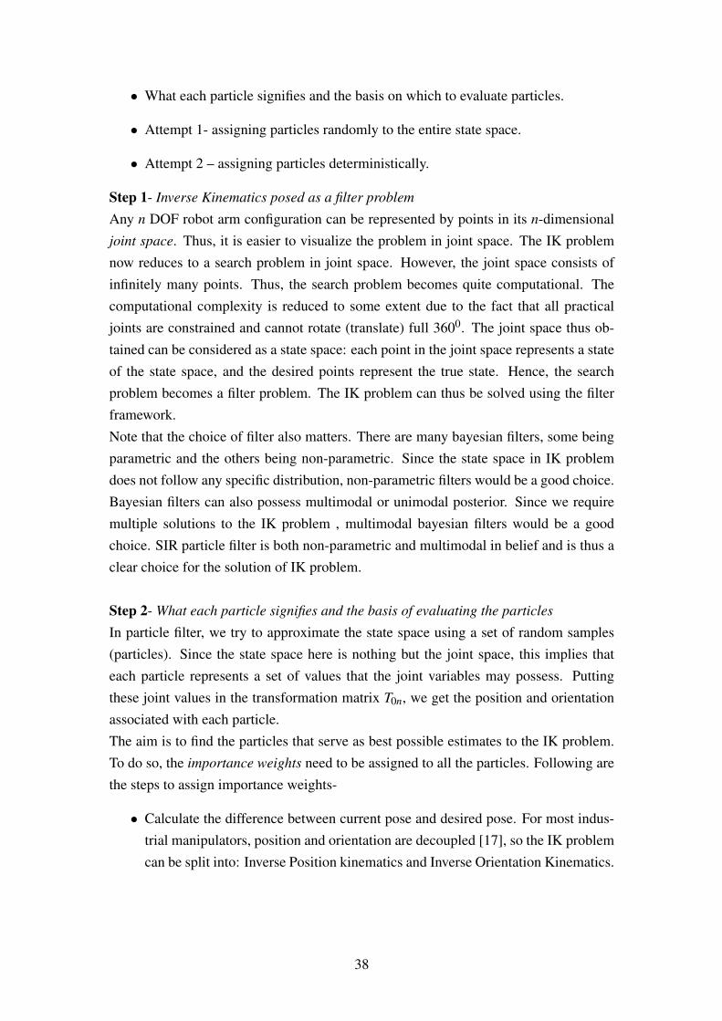
• What each particle signifies and the basis on which to evaluate particles.

• Attempt 1- assigning particles randomly to the entire state space.

• Attempt 2 – assigning particles deterministically.

Step 1- Inverse Kinematics posed as a filter problem

Any n DOF robot arm configuration can be represented by points in its n-dimensionaljoint space. Thus, it is easier to visualize the problem in joint space. The IK problemnow reduces to a search problem in joint space. However, the joint space consists ofinfinitely many points. Thus, the search problem becomes quite computational. Thecomputational complexity is reduced to some extent due to the fact that all practicaljoints are constrained and cannot rotate (translate) full 3600. The joint space thus ob-tained can be considered as a state space: each point in the joint space represents a stateof the state space, and the desired points represent the true state. Hence, the searchproblem becomes a filter problem. The IK problem can thus be solved using the filterframework.Note that the choice of filter also matters. There are many bayesian filters, some beingparametric and the others being non-parametric. Since the state space in IK problemdoes not follow any specific distribution, non-parametric filters would be a good choice.Bayesian filters can also possess multimodal or unimodal posterior. Since we requiremultiple solutions to the IK problem , multimodal bayesian filters would be a goodchoice. SIR particle filter is both non-parametric and multimodal in belief and is thus aclear choice for the solution of IK problem.

Step 2- What each particle signifies and the basis of evaluating the particles

In particle filter, we try to approximate the state space using a set of random samples(particles). Since the state space here is nothing but the joint space, this implies thateach particle represents a set of values that the joint variables may possess. Puttingthese joint values in the transformation matrix T0n, we get the position and orientationassociated with each particle.The aim is to find the particles that serve as best possible estimates to the IK problem.To do so, the importance weights need to be assigned to all the particles. Following arethe steps to assign importance weights-

• Calculate the difference between current pose and desired pose. For most indus-trial manipulators, position and orientation are decoupled [17], so the IK problemcan be split into: Inverse Position kinematics and Inverse Orientation Kinematics.

38

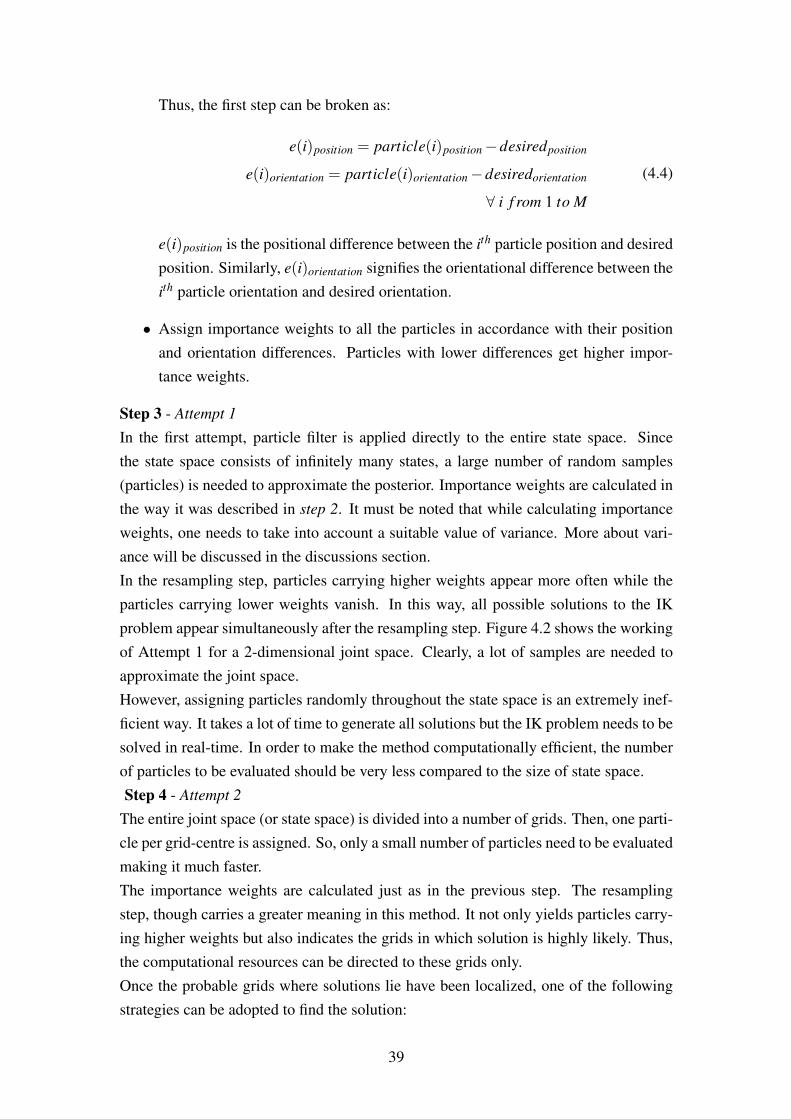
Thus, the first step can be broken as:

e(i)position = particle(i)position−desiredposition

e(i)orientation = particle(i)orientation−desiredorientation

∀ i f rom 1 to M

(4.4)

e(i)position is the positional difference between the ith particle position and desiredposition. Similarly, e(i)orientation signifies the orientational difference between theith particle orientation and desired orientation.

• Assign importance weights to all the particles in accordance with their positionand orientation differences. Particles with lower differences get higher impor-tance weights.

Step 3 - Attempt 1

In the first attempt, particle filter is applied directly to the entire state space. Sincethe state space consists of infinitely many states, a large number of random samples(particles) is needed to approximate the posterior. Importance weights are calculated inthe way it was described in step 2. It must be noted that while calculating importanceweights, one needs to take into account a suitable value of variance. More about vari-ance will be discussed in the discussions section.In the resampling step, particles carrying higher weights appear more often while theparticles carrying lower weights vanish. In this way, all possible solutions to the IKproblem appear simultaneously after the resampling step. Figure 4.2 shows the workingof Attempt 1 for a 2-dimensional joint space. Clearly, a lot of samples are needed toapproximate the joint space.However, assigning particles randomly throughout the state space is an extremely inef-ficient way. It takes a lot of time to generate all solutions but the IK problem needs to besolved in real-time. In order to make the method computationally efficient, the numberof particles to be evaluated should be very less compared to the size of state space.Step 4 - Attempt 2

The entire joint space (or state space) is divided into a number of grids. Then, one parti-cle per grid-centre is assigned. So, only a small number of particles need to be evaluatedmaking it much faster.The importance weights are calculated just as in the previous step. The resamplingstep, though carries a greater meaning in this method. It not only yields particles carry-ing higher weights but also indicates the grids in which solution is highly likely. Thus,the computational resources can be directed to these grids only.Once the probable grids where solutions lie have been localized, one of the followingstrategies can be adopted to find the solution:

39

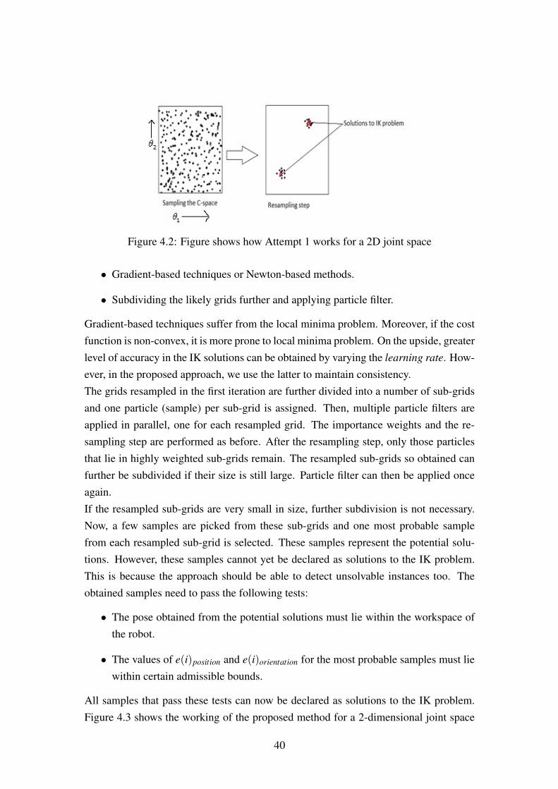
Figure 4.2: Figure shows how Attempt 1 works for a 2D joint space

• Gradient-based techniques or Newton-based methods.

• Subdividing the likely grids further and applying particle filter.

Gradient-based techniques suffer from the local minima problem. Moreover, if the costfunction is non-convex, it is more prone to local minima problem. On the upside, greaterlevel of accuracy in the IK solutions can be obtained by varying the learning rate. How-ever, in the proposed approach, we use the latter to maintain consistency.The grids resampled in the first iteration are further divided into a number of sub-gridsand one particle (sample) per sub-grid is assigned. Then, multiple particle filters areapplied in parallel, one for each resampled grid. The importance weights and the re-sampling step are performed as before. After the resampling step, only those particlesthat lie in highly weighted sub-grids remain. The resampled sub-grids so obtained canfurther be subdivided if their size is still large. Particle filter can then be applied onceagain.If the resampled sub-grids are very small in size, further subdivision is not necessary.Now, a few samples are picked from these sub-grids and one most probable samplefrom each resampled sub-grid is selected. These samples represent the potential solu-tions. However, these samples cannot yet be declared as solutions to the IK problem.This is because the approach should be able to detect unsolvable instances too. Theobtained samples need to pass the following tests:

• The pose obtained from the potential solutions must lie within the workspace ofthe robot.

• The values of e(i)position and e(i)orientation for the most probable samples must liewithin certain admissible bounds.

All samples that pass these tests can now be declared as solutions to the IK problem.Figure 4.3 shows the working of the proposed method for a 2-dimensional joint space

40

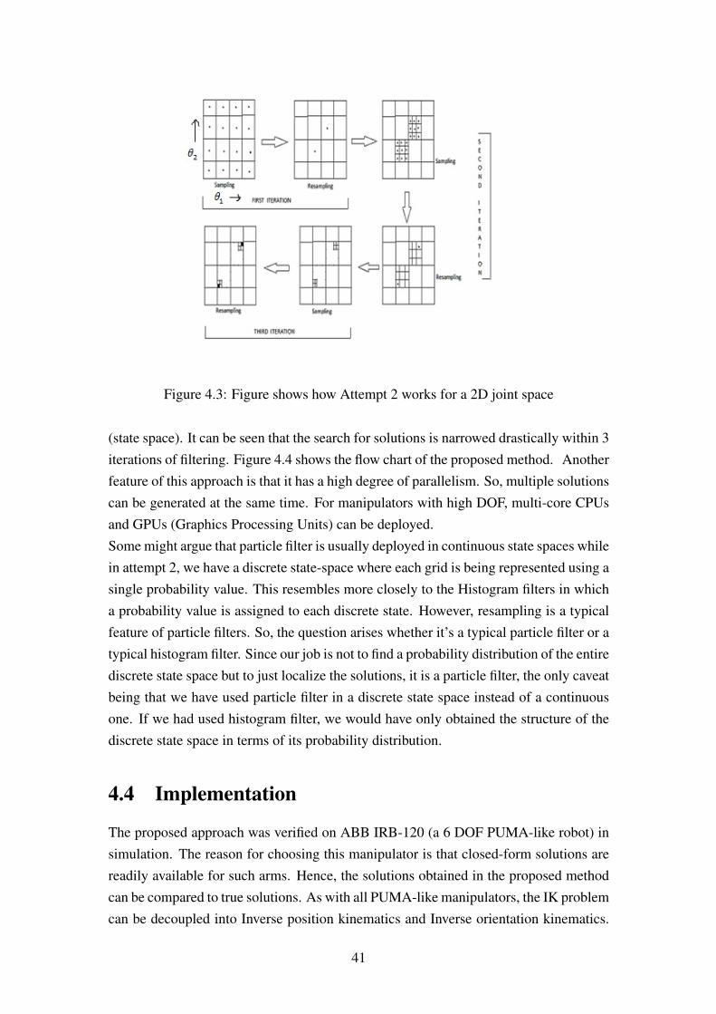
Figure 4.3: Figure shows how Attempt 2 works for a 2D joint space

(state space). It can be seen that the search for solutions is narrowed drastically within 3iterations of filtering. Figure 4.4 shows the flow chart of the proposed method. Anotherfeature of this approach is that it has a high degree of parallelism. So, multiple solutionscan be generated at the same time. For manipulators with high DOF, multi-core CPUsand GPUs (Graphics Processing Units) can be deployed.Some might argue that particle filter is usually deployed in continuous state spaces whilein attempt 2, we have a discrete state-space where each grid is being represented using asingle probability value. This resembles more closely to the Histogram filters in whicha probability value is assigned to each discrete state. However, resampling is a typicalfeature of particle filters. So, the question arises whether it’s a typical particle filter or atypical histogram filter. Since our job is not to find a probability distribution of the entirediscrete state space but to just localize the solutions, it is a particle filter, the only caveatbeing that we have used particle filter in a discrete state space instead of a continuousone. If we had used histogram filter, we would have only obtained the structure of thediscrete state space in terms of its probability distribution.

4.4 Implementation

The proposed approach was verified on ABB IRB-120 (a 6 DOF PUMA-like robot) insimulation. The reason for choosing this manipulator is that closed-form solutions arereadily available for such arms. Hence, the solutions obtained in the proposed methodcan be compared to true solutions. As with all PUMA-like manipulators, the IK problemcan be decoupled into Inverse position kinematics and Inverse orientation kinematics.

41

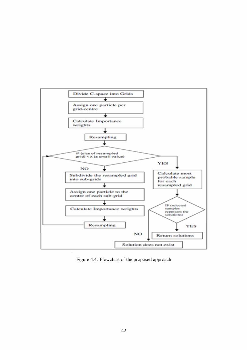
Figure 4.4: Flowchart of the proposed approach

42

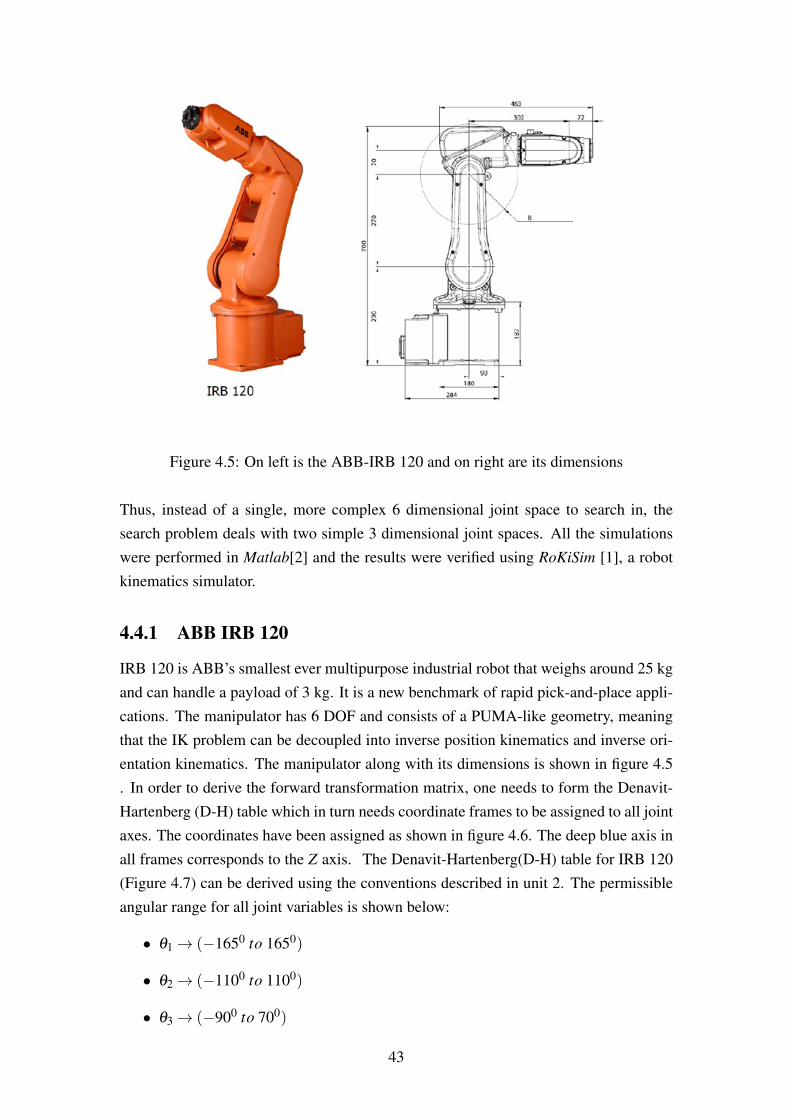
Figure 4.5: On left is the ABB-IRB 120 and on right are its dimensions

Thus, instead of a single, more complex 6 dimensional joint space to search in, thesearch problem deals with two simple 3 dimensional joint spaces. All the simulationswere performed in Matlab[2] and the results were verified using RoKiSim [1], a robotkinematics simulator.

4.4.1 ABB IRB 120

IRB 120 is ABB’s smallest ever multipurpose industrial robot that weighs around 25 kgand can handle a payload of 3 kg. It is a new benchmark of rapid pick-and-place appli-cations. The manipulator has 6 DOF and consists of a PUMA-like geometry, meaningthat the IK problem can be decoupled into inverse position kinematics and inverse ori-entation kinematics. The manipulator along with its dimensions is shown in figure 4.5. In order to derive the forward transformation matrix, one needs to form the Denavit-Hartenberg (D-H) table which in turn needs coordinate frames to be assigned to all jointaxes. The coordinates have been assigned as shown in figure 4.6. The deep blue axis inall frames corresponds to the Z axis. The Denavit-Hartenberg(D-H) table for IRB 120(Figure 4.7) can be derived using the conventions described in unit 2. The permissibleangular range for all joint variables is shown below:

• θ1→ (−1650 to 1650)

• θ2→ (−1100 to 1100)

• θ3→ (−900 to 700)

43

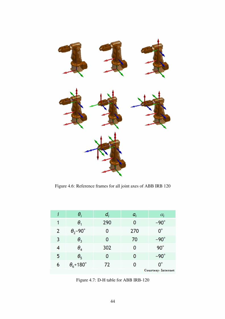
Figure 4.6: Reference frames for all joint axes of ABB IRB 120

Figure 4.7: D-H table for ABB IRB-120

44

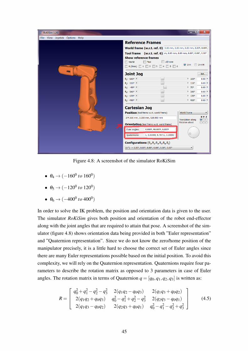
Figure 4.8: A screenshot of the simulator RoKiSim

• θ4→ (−1600 to 1600)

• θ5→ (−1200 to 1200)

• θ6→ (−4000 to 4000)

In order to solve the IK problem, the position and orientation data is given to the user.The simulator RoKiSim gives both position and orientation of the robot end-effectoralong with the joint angles that are required to attain that pose. A screenshot of the sim-ulator (figure 4.8) shows orientation data being provided in both ”Euler representation”and ”Quaternion representation”. Since we do not know the zero/home position of themanipulator precisely, it is a little hard to choose the correct set of Euler angles sincethere are many Euler representations possible based on the initial position. To avoid thiscomplexity, we will rely on the Quaternion representation. Quaternions require four pa-rameters to describe the rotation matrix as opposed to 3 parameters in case of Eulerangles. The rotation matrix in terms of Quaternion q = [q0,q1,q2,q3] is written as:

R =

q20 +q2

1−q22−q2

3 2(q1q2−q0q3) 2(q1q3 +q0q2)

2(q1q2 +q0q3) q20−q2

1 +q22−q2

3 2(q2q3−q0q1)

2(q1q3−q0q2) 2(q2q3 +q0q1) q20−q2

1−q22 +q2

3

(4.5)

45

Next, using the D-H table, we find the total Transformation Matrix in terms of jointvariables θ1......θ6. Since position and orientation are decoupled, the first three jointvariables starting from the base frame, viz. θ1,θ2 and θ3 define the position and vari-ables θ4,θ5,θ6 define the orientation. Using the final transformation matrix, the positionvector p = [px, py, pz] can be related to joint variables θ1,θ2 and θ3 using equation 4.6.

px = 70cθ1sθ23 +270cθ1sθ2 +302cθ1cθ23 +72R(1,3)

py = 70sθ1sθ23 +270sθ1sθ2 +302sθ1cθ23 +72R(2,3)

pz =−302sθ23 +70cθ23 +270cθ2 +290+72R(3,3),

where θi j = θi +θ j

(4.6)

Since p and R are known to us, we can solve for the unknown joint variables using theSIR particle filter. Following are the steps that we performed in order to obtain solutionsto the first three joint variables of IK problem:

• Divide the joint subspace θ1 - θ2 - θ3 into grids as described in attempt 2 of thepreceding section.

• Sample the subspace θ1- θ2- θ3 as described in attempt 2 of the preceding section.

• Now,each particle has some value of θ1, θ2, θ3. Placing these angle values inequation 4.6, we obtain the position vector for that sample. Each sample thus hasa position vector associated with it.

• For each sample, the difference between sample position and desired positionis computed as described in equation4.4. Particles with lower differences gethigher importance weights. Such an inverse relationship between differences andweights can be obtained by using either negative exponentials or reciprocal func-tions.

• Resampling takes place and particles (samples) that had higher importance weightsreappear (Survival of the fittest).

• Rest follows as described in 4.4.

A similar procedure is adopted to compute the remaining three joint variables of themanipulator.

46

4.5 Results and Discussions

4.5.1 Findings

Example 1- For the position vector [81.666 mm, 207.636 mm, 270.773 mm] and ori-entation quaternion [0.62060, -0.61902, -0.17694, 0.44761], the simulator RoKiSim

showed joint variable values of [50, 20, 60, 90, 100, 120]. When the proposed methodwas run in MATLAB, it showed joint variable values of [50, 20, 60, 90, 100, 120],which is exactly the same as the closed-form solution.Example 2- For the position vector [102.493 mm, 290.556 mm, 144.405 mm] and ori-entation quaternion [0.36924, -0.63286, -0.58466, 0.34833], the simulator RoKiSimshowed joint variable values of [59.99, 50, 29.51, 59.32, 66, 100.89]. The joint variablevalues obtained through proposed approach were [60, 50, 29, 59, 66, 101]. Notice thatthere is a difference of less than 0.520 between the obtained joint variable values and thetrue joint variable values. This difference might look small but for a large link length, itresults in a substantial positional error.Example 3- In this example, a singular configuration is chosen to evaluate the per-formance of the proposed method. For the position vector [191.380 mm, 331.481

mm, 235.287 mm] and orientation quaternion [0.12966, -0.83640, -0.48290, -0.22458],RoKiSim showed joint variable values of [60, 30, 30, 60, 0, 120]. Since θ5 =0, therobot arm has lost a DOF. The solutions obtained from the proposed method are: [60,

30, 30, 114, 0, 66] ; [ 60, 30, 30, 81, 0, 99] ; [ 60, 30, 30, 32, 0, 148] ; [60, 30, 30, 60,

0, 120] and [ 60, 30, 30, 18, 0, 162], and many more. Clearly, the proposed approachtries to find a family of solutions for which (θ4 + θ6 = 180) which is what we wouldexpect from a good IK solver.

4.5.2 Parameter selection

In order to implement the proposed method, joint space needs to be divided into a num-ber of grids. A good way of doing so is to divide each dimension of the joint spaceseparately. Consider n as the number of parts in which each dimension of joint space isdivided. So the 3 dimensional joint spaces for inverse position and inverse orientationproblems get divided into n3 grids each. Further, n may vary for different iterations.The selection of n is very crucial to the efficiency of the proposed method. The largerthe value of n, the more the number of particles (=n3) that need to be evaluated. Hence,a large value of n is undesirable since that will result in more computation per iteration.On the other hand, if n is too small, time required per iteration will be less but morenumber of iterations will be required. To solve the IK problem for ABB IRB-120, n = 6was chosen in the first iteration,n = 4 in the second iteration, and n = 2 in the third

47

Figure 4.9: Uncertainty of finding solutions v/s number of iterations

iteration. Thus, 216, 64 and 8 particles were evaluated in the first, second and thirditeration respectively. However, if n = 16 was chosen in the first iteration, the efficiencywould be reduced drastically since 4096 (=163) particles would then need to be evalu-ated. Thus, n needs to be chosen carefully.

4.5.3 Uncertainty of solution

Figure 4.9 shows the uncertainty in the solution of IK problem. Initially, the solution is100% uncertain since there is no clue where the solution might lie. After the first iter-ation, the solution lies within 10−3% uncertainty. After the second iteration, a 10−7%uncertainty is reported. After the third iteration, a 10−9% uncertainty is reported. Itmust be noted that there isn’t a huge variation in the percentage uncertainty from thesecond iteration to the third iteration, implying a satisfactory convergence. So, the com-putational resources need not be wasted on another iteration of filtering.

4.6 Assessment of the proposed approach

The proposed approach is assessed based on the following criteria:

• Reliability - The approach is able to find a solution, if one exists. Moreover, it candetect unsolvable instances too.

48

• Completeness - Since particle filter is used in the proposed approach, multiplesolutions are easily generated. Thus the proposed method offers completeness.

• Stability – Since no inversion techniques are used in the proposed approach, thealgorithm works equally well near degenerate configurations. Thus, it is stable.

• Generality - Since it is a numerical method, it can be applicable to a wide varietyof robot geometries. Thus, it is a generalized method.

• Efficiency- The proposed method is computationally efficient and can be appliedto manipulators with DOF exceeding six. However, it is slower compared to someexisting numerical solutions.

It is clear that the proposed approach can generate multiple solutions to the IK problem.However, which solution to choose from amongst the generated solutions hasn’t beendiscussed in the proposed approach. As was explained at the start of the chapter, thechoice of solution varies from situation to situation. In general, a reasonable choice isto pick the solution closest to the current configuration. This problem can be solvedwithout much ado using appropriate minimization techniques.Table 4.1 shows a comparison of some of the numerical strategies discussed in section2.2 along with the proposed approach.

4.7 Future work

A new IK solver has been proposed in this thesis that uses the concept of SIR particlefilter to determine all possible sets of joint angles. The proposed approach has beenshown to possess many advantages. However, this approach has a disadvantage due tothe fact that the solutions we obtain are coarse. In the simulations we performed onABB-IRB 120, the solutions returned by the proposed approach were present in integerform. A 0.50 maximum deviation from the true angular value can thus be observed. A0.50 deviation can result in a 1.745 cm (0.5*(π/180)*200) positional difference for a200 cm link. A deviation close to 2 cm is unacceptable for the robots deployed in Man-ufacturing and Automobile sectors. Thus, there exists the scope of further improvementin the developed IK solver.

One way of solving this problem of coarse solutions is to use the SIR algorithm onlyto localize the grids that contain the solutions. Once we know the grids where solutionsmight lie, we have close initial estimates with us. We can then use Gradient descenttechnique to obtain solutions to the joint variables since a small learning rate in gradientdescent will result in highly accurate solutions. The question that arises here is: Whatshould be the Cost function for the gradient descent algorithm? The answer is simple:

49

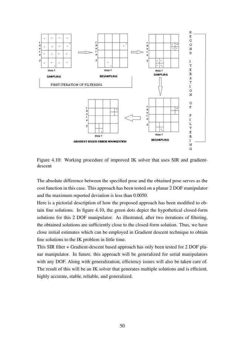
Figure 4.10: Working procedure of improved IK solver that uses SIR and gradient-descent

The absolute difference between the specified pose and the obtained pose serves as thecost function in this case. This approach has been tested on a planar 2 DOF manipulatorand the maximum reported deviation is less than 0.0050.Here is a pictorial description of how the proposed approach has been modified to ob-tain fine solutions. In figure 4.10, the green dots depict the hypothetical closed-formsolutions for this 2 DOF manipulator. As illustrated, after two iterations of filtering,the obtained solutions are sufficiently close to the closed-form solution. Thus, we haveclose initial estimates which can be employed in Gradient descent technique to obtainfine solutions to the IK problem in little time.This SIR filter + Gradient-descent based approach has only been tested for 2 DOF pla-nar manipulator. In future, this approach will be generalized for serial manipulatorswith any DOF. Along with generalization, efficiency issues will also be taken care of.The result of this will be an IK solver that generates multiple solutions and is efficient,highly accurate, stable, reliable, and generalized.

50

4.8 Summary

In this chapter, the problem of Inverse Kinematics (IK) in robot manipulators has beendiscussed. Various numerical methods that are used to solve the IK problem have beendescribed in brief. Jacobian-based methods perform poorly near singularities. Newton-based methods require an initial estimate. Optimization-based methods work well butgenerate only one solution to the problem. Heuristics-based methods, particularly theCyclic Coordinate Descent (CCD) are fast, efficient and the most used. However, theyproduce motion with erratic discontinuities. Genetic programming based methods gen-erate multiple solutions but are sluggish in nature.The proposed IK solver utilizes Sampling Importance Resampling (SIR) to generatemultiple solutions. Since no inversion technique is involved, the method works equallywell near singularities. Moreover, the method does not need any initial estimate to gen-erate solutions. However, no emphasis has been laid on how to pick a solution fromamongst the generated solutions. A reasonable choice is to pick the solution closest tothe current configuration, which requires solving a fairly simple minimization problem.On close observation, it seems that since the proposed approach needs a forward kine-matics model for inverse problem calculation, this approach may well be classified un-der heuristics-based solution strategies.

51

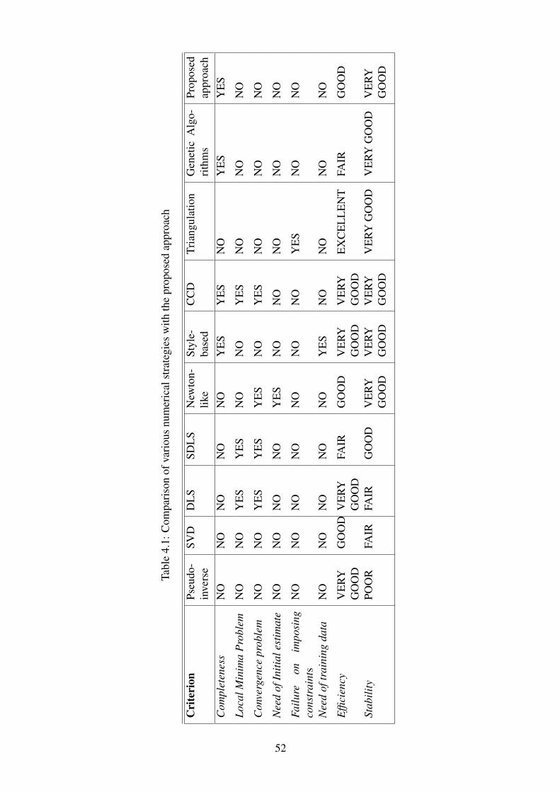
Tabl

e4.

1:C

ompa

riso

nof

vari

ous

num

eric

alst

rate

gies

with

the

prop

osed

appr

oach

Cri

teri

onPs

eudo

-in

vers

eSV

DD

LS

SDL

SN

ewto

n-lik

eSt

yle-

base

dC

CD

Tria

ngul

atio

nG

enet

icA

lgo-

rith

ms

Prop

osed

appr

oach

Com

plet

enes

sN

ON

ON

ON

ON

OY

ES

YE

SN

OY

ES

YE

S

Loca

lMin

ima

Pro

blem

NO

NO

YE

SY

ES

NO

NO

YE

SN

ON

ON

O

Con

verg

ence

prob

lem

NO

NO

YE

SY

ES

YE

SN

OY

ES

NO

NO

NO

Nee

dof

Initi

ales

timat

eN

ON

ON

ON

OY

ES

NO

NO

NO

NO

NO

Failu

reon

impo

sing

cons

trai

nts

NO

NO

NO

NO

NO

NO

NO

YE

SN

ON

O

Nee

dof

trai

ning

data

NO

NO

NO

NO

NO

YE

SN

ON

ON

ON

O

Effi

cien

cyV

ERY

GO

OD

GO

OD

VE

RYG

OO

DFA

IRG

OO

DV

ERY

GO

OD

VE

RYG

OO

DE

XC

EL

LE

NT

FAIR

GO

OD

Stab

ility

POO

RFA

IRFA

IRG

OO

DV

ERY

GO

OD

VE

RYG

OO

DV

ERY

GO

OD

VE

RYG

OO

DV

ERY

GO

OD

VE

RYG

OO

D

52

Chapter 5

CONFIGURATION SPACE - Anexplicit representation

5.1 Introduction

Collision-free motion planning in robotics aims to find a path that is free from all obsta-cles. In order to create a collision-free motion planner, one must be able to specify thelocation of every point on the robot. In other words, to ensure that no point on the robotis in collision with obstacles, one needs to know the location of all points on the robot.

While specifying the location of all points on the robot, the following questions mayarise: What is the best way to specify the location of all points on the robot? Is thereany definite representation for this purpose? Will this representation help to simplifythe motion planning problem? How can one take into account all the obstacles in theworld while planning motion?

Lozano-Perez [40] introduced the concept of configuration space (an approach derivedfrom Lagrangian mechanics) to answer these questions. To understand configurationspace, one must first know what the term configuration means in robotics. The config-uration of a robot specifies the location of every point on the robot. The Configurationspace, or C-space of a robot thus represents the space of all such configurations that therobot may possess. A configuration is thus a point in this abstract C-space. The dimen-sion of a C-space is equal to the number of degrees of freedom (DOF) of the robot [40].

In order to detect collisions, we now need to specify just a point in C-space (as opposedto all points on a robot in the world) and detect whether it is collision-free. The conceptof C-space is thus a powerful abstraction in the context of motion planning. Motionplanning can now be viewed as searching for obstacle-free paths in C-space. For this

53

purpose, obstacles in the real world need to be transformed to obstacles in C-space.However, this transformation is complicated due to the unusual topological structure ofC-spaces.

The transformation from workspace1 to C-space may not be explicitly constructed. Itis because explicit representation is both time and memory consuming. Some planningapproaches detect collisions along proposed paths without pre-computing C-space [32][24]. Others assume the existence of a C-space and then devise paths that search inthe free-regions of C-space although the C-space is not explicitly constructed [9] [13].The third category of planning schemes uses an explicit representation of C-space toorganize free regions into a graph which is then searched for feasible paths. An explicitrepresentation is also needed at times to ensure completeness of a motion planning al-gorithm. It is also better for the sake of visualization to represent C-space explicitly. Anexplicit construction of C-space is therefore the main theme of this paper.

In this unit, we discuss an approach to transform obstacles in the world into C-spaceobstacles for a 2 DOF R-R planar manipulator. A single primitive is defined to gen-erate C-space transforms for various convex and non-convex obstacles. Since the pre-computation of C-space transform for an entire obstacle is computationally expensive,we generate only the boundaries of C-space obstacle by utilizing the properties of C-space transforms. The proposed approach can be generalized, with some modifications,to generate explicit C-space representations for robots with higher DOF. The next sec-tion discusses the basics of C-space and the properties of C-space transforms relevantto the context of this paper.

5.2 Configuration Space

Basics of Configuration space for the 2 DOF R-R planar manipulator: It was de-scribed in the previous section that the dimension of C-space is equal to the DOF of sys-tem. In other words, the mobility of a robot is the dimension of the C-space. Since themanipulator considered here has mobility in its two revolute joints, the two joint vari-ables constitute the two dimensions of C-space. The two revolute joints are assumed tobe unconstrained, meaning that they can rotate full 3600. Since 00 and 3600 are equiv-alent, θ1 = 0 curve and theta1 = 360 curve are attached together to ensure topologicalconsistency. Similarly, θ2 = 0 curve and θ2 = 360 curve are attached together. This is

1Workspace of a manipulator is that volume of space which the manipulator’s end-effector can reach[11]. However, collision might occur anywhere within the outer boundary of workspace. Thus, only theouter envelope is of importance to us and we will therefore use the word workspace in this paper to referto the volume of space inside the outer boundary of workspace.

54

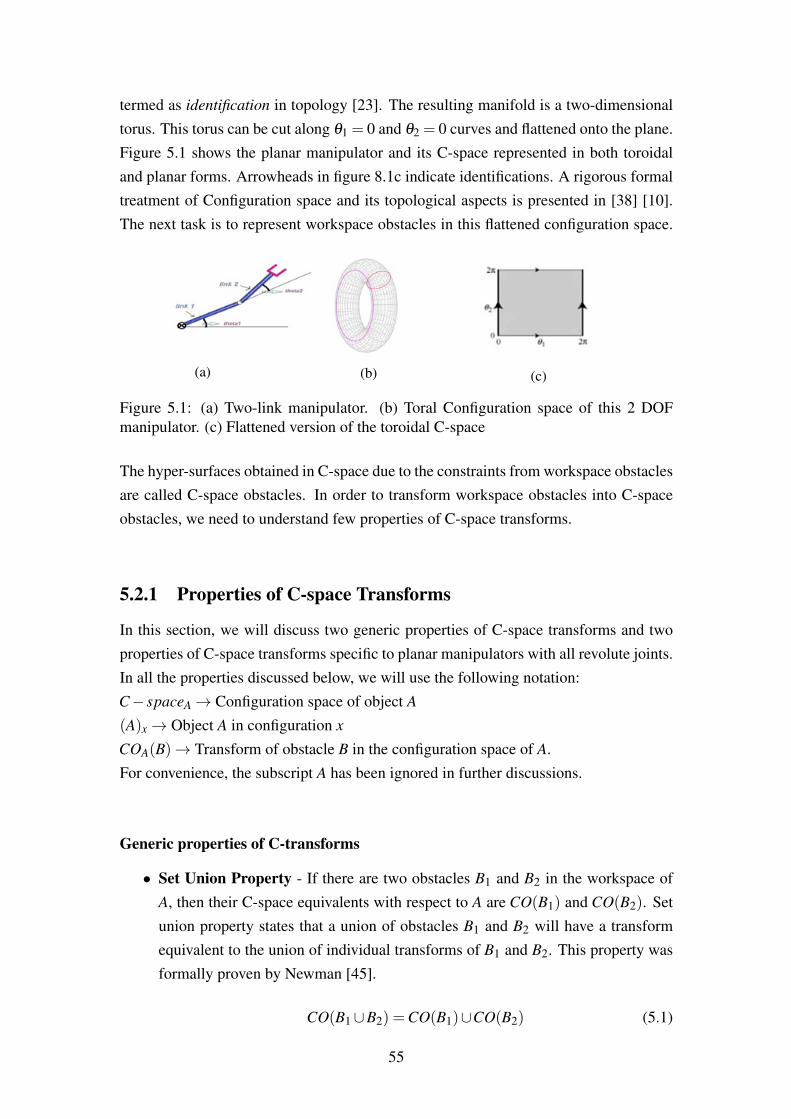
termed as identification in topology [23]. The resulting manifold is a two-dimensionaltorus. This torus can be cut along θ1 = 0 and θ2 = 0 curves and flattened onto the plane.Figure 5.1 shows the planar manipulator and its C-space represented in both toroidaland planar forms. Arrowheads in figure 8.1c indicate identifications. A rigorous formaltreatment of Configuration space and its topological aspects is presented in [38] [10].The next task is to represent workspace obstacles in this flattened configuration space.

(a) (b) (c)

Figure 5.1: (a) Two-link manipulator. (b) Toral Configuration space of this 2 DOFmanipulator. (c) Flattened version of the toroidal C-space

The hyper-surfaces obtained in C-space due to the constraints from workspace obstaclesare called C-space obstacles. In order to transform workspace obstacles into C-spaceobstacles, we need to understand few properties of C-space transforms.

5.2.1 Properties of C-space Transforms

In this section, we will discuss two generic properties of C-space transforms and twoproperties of C-space transforms specific to planar manipulators with all revolute joints.In all the properties discussed below, we will use the following notation:C− spaceA→ Configuration space of object A

(A)x→ Object A in configuration x

COA(B)→ Transform of obstacle B in the configuration space of A.For convenience, the subscript A has been ignored in further discussions.

Generic properties of C-transforms

• Set Union Property - If there are two obstacles B1 and B2 in the workspace ofA, then their C-space equivalents with respect to A are CO(B1) and CO(B2). Setunion property states that a union of obstacles B1 and B2 will have a transformequivalent to the union of individual transforms of B1 and B2. This property wasformally proven by Newman [45].

CO(B1∪B2) =CO(B1)∪CO(B2) (5.1)

55

This property has an important implication. A line can be considered as a unionof all points lying on it. Thus, the C-space transform of a line is the union oftransforms of all points on that line. Another implication is that if we have C-space transforms for some simple convex obstacles, we can obtain transforms fornon-convex obstacles.

• Set Containment property - This property is as follows:

I f B1 ⊇ B2,

then CO(B1)⊇CO(B2)(5.2)

This property states that an obstacle enclosed in a larger obstacle has a transformwhich is fully enclosed in the transform of the larger obstacle. An important im-plication of this property is that we can avoid transforming the entire obstacle justby transforming the boundary of that obstacle. This can save a lot of computation.

Properties of C-space transforms specific to planar manipulators

These properties apply only to manipulators that have all revolute joints with paralleljoint axes.

• Point Translation property - A point p in workspace has a transform CO(p) thatyields its C-space equivalent. If this point is rotated about an axis z (the axis beingnormal to the plane in which manipulator works) by an angle θ , the transformgets translated by amount θ in C-space. For a 2 DOF planar R-R manipulator, thetranslation occurs along the θ1 axis of C-space.

CO(rot(p, z,θ) =CO(p)⊕ (θ ,0) (5.3)

A simple illustration is shown in figure 5.2. Clearly, the transform gets shifted byan amount θ along θ1 axis. Note that this is just a hypothetical illustration. TheC-space transform of a point is actually different than the one shown.

• Set Translation property - This is a generalization of the point translation prop-erty and described as follows. If any workspace obstacle is rotated by an angle θ ,this means that each point of that obstacle is rotated by θ . By point translationproperty, the transform of each point gets translated by an amount θ in C-space.By set union property, the transform of this rotated obstacle is the union of trans-forms of all the rotated points. The property is stated below:

CO{S(rot(θ)}=CO(p1(θ))∪CO(p2(θ))∪ ............∪CO(pn(θ)) (5.4)

56

Figure 5.2: Illustration of point translation property

Here, S is the set corresponding to the obstacle and p1, p2, ...., pn are points (ele-ments of obstacle set S) on the obstacle.

A more detailed and illustrative description of these properties is presented in [44]. Withan understanding of these properties, we now move ahead to construct Configurationspaces. The next section describes the primitive used to construct C-space obstacles.

5.3 Proposed Primitive

The primitive we will use is a line obstacle inclined at an arbitrary angle with respectto the X-axis of the base frame. To understand C-space transforms for line obstacles,we need to understand C-space transforms for point obstacles because line is composedof points. Figure 5.3 shows a point obstacle at a distance d (Euclidean distance) fromthe base of manipulator. In order to compute its transform, we need to know whetherthe point can only be in collision with link 2 of the manipulator or with both links. Asimple way to know it is: if d > l1, the point will only collide with link 2 (also termedas link 2 obstacle). If d <= l1, the point will collide with both links (also termed as link1 and link 2 obstacle).

5.3.1 Case 1

If a point (along x-axis) is a link 2 obstacle and lies on the X-axis of the manipulatorbase frame, we need to find all configurations of the manipulator that lead to link 2colliding with the point. This implies that we need to find combinations of θ1 and θ2

that result in collision with the point. We use cosine law to calculate θ1 and θ2 for all

57

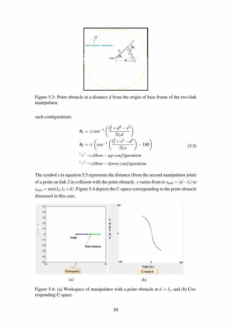
Figure 5.3: Point obstacle at a distance d from the origin of base frame of the two-linkmanipulator.

such configurations.

θ1 =±cos−1(

l21 +d2− s2

2l1d

)θ2 =±

(cos−1

(l21 + s2−d2

2l1s

)−180

)′+′→ elbow−up con f iguration′−′→ elbow−down con f iguration

(5.5)

The symbol s in equation 5.5 represents the distance (from the second manipulator joint)of a point on link 2 in collision with the point obstacle. s varies from to smin = |d− l1| tosmax =min(l2, l1+d) .Figure 5.4 depicts the C-space corresponding to the point obstaclediscussed in this case.

(a) (b)

Figure 5.4: (a) Workspace of manipulator with a point obstacle at d > l1, and (b) Cor-responding C-space.

58

5.3.2 Case 2

If a point (along x-axis) is both link 1 and link 2 obstacle, configurations correspondingto link 2 colliding with the point can be found as in Case 1. However, when link 1 is incollision, θ1 = 0 irrespective of the values of θ2, i.e. θ2 can have all values from -180 to180. Figure 5.5 shows the C-space obtained for this case.

(a) (b)

Figure 5.5: (a) Workspace of manipulator with a point obstacle on x-axis at d <= l1,and (b) Corresponding C-space.

5.3.3 Case 3

If the point obstacle is no longer on the x-axis, we need to find the angle (with respect tox-axis) by which the vector corresponding to this point got rotated. If the point obstacleis situated at coordinate (x’,y’) , the angle θtrans with respect to x-axis is:

θtrans = tan−1(

y′

x′

)(5.6)

We now compute θ1 and θ2 as described in case 1 or case 2, based on the distance d.The only difference being that we use the point translation property by adding θtrans toθ1.It can be observed from figure 5.6 that the C-space hypersurface corresponding to thepoint obstacle has been translated along θ1 axis. The point translation property has thusenabled us to find transforms for point obstacles placed anywhere in the workspace.

59

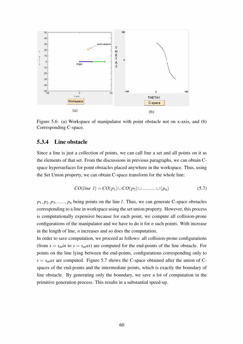
(a) (b)

Figure 5.6: (a) Workspace of manipulator with point obstacle not on x-axis, and (b)Corresponding C-space.

5.3.4 Line obstacle

Since a line is just a collection of points, we can call line a set and all points on it asthe elements of that set. From the discussions in previous paragraphs, we can obtain C-space hypersurfaces for point obstacles placed anywhere in the workspace. Thus, usingthe Set Union property, we can obtain C-space transform for the whole line:

CO(line l) =CO(p1)∪CO(p2)∪ ..........∪ (pn) (5.7)

p1, p2, p3, ......, pn being points on the line l. Thus, we can generate C-space obstaclescorresponding to a line in workspace using the set union property. However, this processis computationally expensive because for each point, we compute all collision-proneconfigurations of the manipulator and we have to do it for n such points. With increasein the length of line, n increases and so does the computation.In order to save computation, we proceed as follows: all collision-prone configurations(from s = smin to s = smax) are computed for the end-points of the line obstacle. Forpoints on the line lying between the end-points, configurations corresponding only tos = smax are computed. Figure 5.7 shows the C-space obtained after the union of C-spaces of the end-points and the intermediate points, which is exactly the boundary ofline obstacle. By generating only the boundary, we save a lot of computation in theprimitive generation process. This results in a substantial speed-up.

60

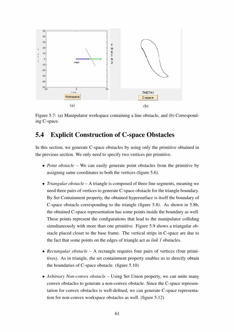
(a) (b)

Figure 5.7: (a) Manipulator workspace containing a line obstacle, and (b) Correspond-ing C-space.

5.4 Explicit Construction of C-space Obstacles

In this section, we generate C-space obstacles by using only the primitive obtained inthe previous section. We only need to specify two vertices per primitive.

• Point obstacle – We can easily generate point obstacles from the primitive byassigning same coordinates to both the vertices (figure 5.6).

• Triangular obstacle – A triangle is composed of three line segments, meaning weneed three pairs of vertices to generate C-space obstacle for the triangle boundary.By Set Containment property, the obtained hypersurface is itself the boundary ofC-space obstacle corresponding to the triangle (figure 5.8). As shown in 5.8b,the obtained C-space representation has some points inside the boundary as well.These points represent the configurations that lead to the manipulator collidingsimultaneously with more than one primitive. Figure 5.9 shows a triangular ob-stacle placed closer to the base frame. The vertical strips in C-space are due tothe fact that some points on the edges of triangle act as link 1 obstacles.

• Rectangular obstacle – A rectangle requires four pairs of vertices (four primi-tives). As in triangle, the set containment property enables us to directly obtainthe boundaries of C-space obstacle. (figure 5.10)

• Arbitrary Non-convex obstacle – Using Set Union property, we can unite manyconvex obstacles to generate a non-convex obstacle. Since the C-space represen-tation for convex obstacles is well-defined, we can generate C-space representa-tion for non-convex workspace obstacles as well. (figure 5.12)

61

(a) (b)

Figure 5.8: (a) Manipulator workspace containing a triangular obstacle, and (b) corre-sponding C-space.

(a) (b)

Figure 5.9: (a) Manipulator workspace containing a triangular obstacle nearer to origin,and (b) corresponding C-space.

62

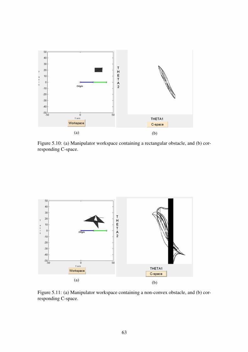
(a) (b)

Figure 5.10: (a) Manipulator workspace containing a rectangular obstacle, and (b) cor-responding C-space.

(a) (b)

Figure 5.11: (a) Manipulator workspace containing a non-convex obstacle, and (b) cor-responding C-space.

63

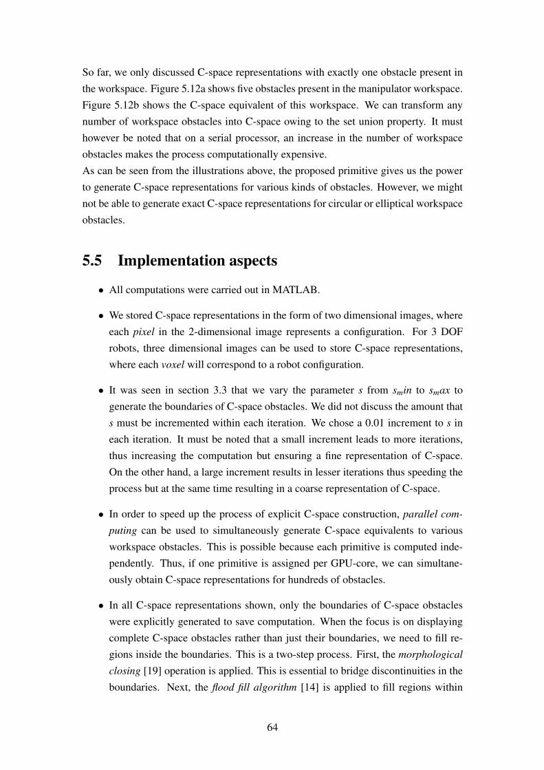
So far, we only discussed C-space representations with exactly one obstacle present inthe workspace. Figure 5.12a shows five obstacles present in the manipulator workspace.Figure 5.12b shows the C-space equivalent of this workspace. We can transform anynumber of workspace obstacles into C-space owing to the set union property. It musthowever be noted that on a serial processor, an increase in the number of workspaceobstacles makes the process computationally expensive.As can be seen from the illustrations above, the proposed primitive gives us the powerto generate C-space representations for various kinds of obstacles. However, we mightnot be able to generate exact C-space representations for circular or elliptical workspaceobstacles.

5.5 Implementation aspects

• All computations were carried out in MATLAB.

• We stored C-space representations in the form of two dimensional images, whereeach pixel in the 2-dimensional image represents a configuration. For 3 DOFrobots, three dimensional images can be used to store C-space representations,where each voxel will correspond to a robot configuration.

• It was seen in section 3.3 that we vary the parameter s from smin to smax togenerate the boundaries of C-space obstacles. We did not discuss the amount thats must be incremented within each iteration. We chose a 0.01 increment to s ineach iteration. It must be noted that a small increment leads to more iterations,thus increasing the computation but ensuring a fine representation of C-space.On the other hand, a large increment results in lesser iterations thus speeding theprocess but at the same time resulting in a coarse representation of C-space.

• In order to speed up the process of explicit C-space construction, parallel com-

puting can be used to simultaneously generate C-space equivalents to variousworkspace obstacles. This is possible because each primitive is computed inde-pendently. Thus, if one primitive is assigned per GPU-core, we can simultane-ously obtain C-space representations for hundreds of obstacles.

• In all C-space representations shown, only the boundaries of C-space obstacleswere explicitly generated to save computation. When the focus is on displayingcomplete C-space obstacles rather than just their boundaries, we need to fill re-gions inside the boundaries. This is a two-step process. First, the morphological

closing [19] operation is applied. This is essential to bridge discontinuities in theboundaries. Next, the flood fill algorithm [14] is applied to fill regions within

64

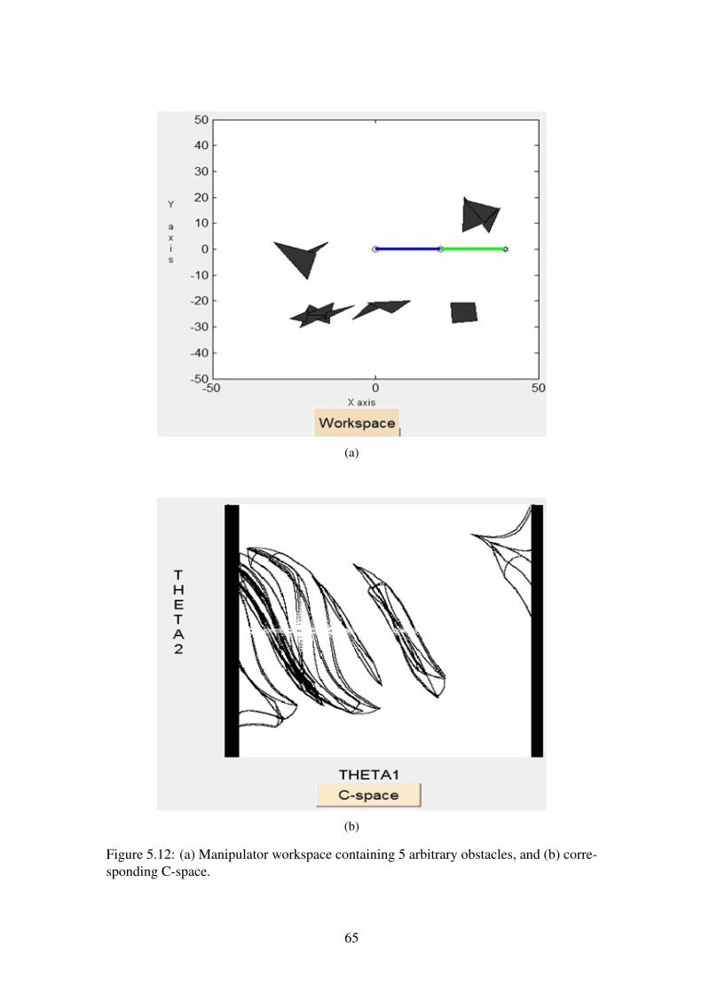
(a)

(b)

Figure 5.12: (a) Manipulator workspace containing 5 arbitrary obstacles, and (b) corre-sponding C-space.

65

the boundaries. Figure 5.13 shows the C-space representations before and afterapplying above steps.

• In this paper, it was assumed that both revolute joints of the 2-DOF manipulatorare free to rotate full 3600 and hence we were able to use identifications. Inpractice, revolute joints are constrained and identifications cannot be applied totheir C-space. This implies that C-space does not have wrap-around features inpractice.

• While computing C-space, it was assumed that the two links of the 2-DOF manip-ulator have no thickness. In practice, links have finite thickness. To ensure thatthe effect of thickness is appropriately apparent in the C-space representation,morphological dilation [19] of C-space obstacles can be performed. However, noattempt has been made in this paper to find a mathematical relationship betweenthe amount of dilation to be performed and the links’ thickness.

• The proposed approach can be generalized for all kinds of serial manipulatorsif the following issues are appropriately handled: The first being that point andset translation properties are inapplicable to manipulators in which the joint axesare not parallel, and the second being that cosine law cannot be used directly forrobots with DOF greater than 2. The former can be resolved since the set unionproperty and set containment property still hold for all kinds of robots. The lattercan be resolved if instead of cosine law, we use the Inverse Kinematics solverdeveloped by Majumder et al [51] to obtain solutions to the joint variables.

5.6 Future Work

This unit stresses on the theme of explicit C-space representation. The problem is that anexplicit C-space representation is neither computationally efficient nor always tractable.It can be infered, without doubt, from the contents of this unit why explicit represen-tations are computationally inefficient. However, nothing in regard to the feasibility

aspects has yet been elaborated.While pixels are used to display two-dimensional C-spaces and voxels to display three-dimensional C-spaces, it is much harder to display C-spaces with more than three di-mensions on a computer. For such reasons as tractability and efficiency, an implicitrepresentation of C-space has been a recurrent theme in the motion planning literature.An implicit representation can be achieved by incorporating learning [3] into the C-space. This will save computation and yield a functional form for generating C-spacehypersurfaces. The idea is as follows:

66

(a)

(b) (c)

Figure 5.13: (a) Manipulator workspace containing a line obstacle, (b) C-space showingonly the obstacle boundary, and (c) C-space showing the complete obstacle.

67

• Take a simple robot manipulator for which explicit representation is available.

• Then, for a point obstacle, compute the C-space representation.

• Take different locations of point obstacle and compute C-space representation foreach of them.

• Thus, we obtain a large number of <obstacle location, C-space shape> pairswhich serve as the training data for our learning algorithm.

• Based on the training data, we now try to find a function that can generalize bestfor all training points.

• This function that represents the relationship between obstacle location and C-space shape provides a generalized implicit representation of the C-space.

• The issue is that this is not a straightforward problem since we need to find thefunction of a function.Explanation- We know that there exists a functional relationship between the ob-ject location and equivalent C-space representation. For instance, a particularobstacle location might yield a quadratic relation between the object location andthe C-space representation. For another obstacle location, the relation might beeither quadratic but with changed coefficients or a cubic relation. Thus, we needto be able to learn a function that predicts the right function for each obstaclelocation.

Research is being done to pursue this idea and in future, we hope to be able to buildsuch an implicit representation for C-spaces. Such a representation also seems intuitivesince initially, even a child explores the space around him to eventually learn his ownstructure.

5.7 Summary

This chapter presents the utility of Configuration space approach in the context of robotmotion planning. We then go on to describe few essential properties of configurationspace transforms and how these properties can be used to generate a computationallyefficient primitive. This primitive is then used to generate C-space hypersurfaces cor-responding to various convex and non-convex obstacles. A few aspects related to thestorage, efficiency and applicability are then presented. Finally, it is discussed how theproposed approach can be modified to obtain C-space representations for robot manip-ulators with higher DOF. The need of an implicit C-space representation has also beenemphasized with a possible approach to obtain such a representation.

68

Chapter 6

MOTION PLANNING - The previousand the proposed

6.1 Introduction

Robot motion planning is one of the most sought-after domains in robotics and has ahighly diverse literature. Control theory, Electromagnetic Field theory, Artificial In-

telligence, Data Science, Probability, graph-theory and many other streams have con-tributed to the motion planning literature. The reason for such a diversity is that planningis closely related to problem-solving. Even the most standard textbook in Artificial Intel-ligence by Russell and Norvig [49] defines planning and problem-solving in such a waythat both seem identical. This is one of the reasons why problem-solving techniques inall the streams mentioned above have been applied to motion planning problems.The task of a robot motion planning algorithm is to find a path between two locationssuch that no point on the robot collides with any obstacle during the execution of thatpath. The problem becomes somewhat tougher for Robot manipulators than for a smallwheeled robot. This is because manipulators have n links and therefore, the devisedplanner must ensure that none of the links collides with any obstacle throughout thecourse of that plan. We therefore perform motion planning in Configuration spaceswhere the planner only needs to devise point-to-point paths that are free from obstacles.

6.1.1 Properties of Motion planning algorithm

• Completeness - A planner is termed complete if it finds a path when one existsand declares failure in finite time when no path exists. It is often computationallyintractable to ensure completeness of a motion planner. Thus, weaker notions ofcompleteness exist.

69

– Resolution completeness - If a path exists at a given resolution of discretiza-tion (granularity), the planner will find it.

– Probabilistic completeness - The probability of finding a path converges to1 as time tends to ∞.

• Optimality - A planner is termed optimal if it finds a path that has minimum pathlength/minimum energy consumption/ takes minimum execution time.

• Offline / Online planner -A motion planner is termed offline if it constructs theplan in advance, based on a known model of the environment, and then the planis given to an executor.A motion planner is termed online if it incrementally constructs the plan whilethe agent is executing. Often, online and offline planners cannot be distinguishedwhen the offline algorithm hands off the plans very quickly to the executor.

The next section briefly describes some important motion planning algorithms.

6.2 Motion planning Literature

It is almost impossible to describe the entire motion planning literature even briefly.However, we have made an attempt to describe some seminal researches in the field ofmotion planning. We will focus only on three frameworks for motion planning thoughthere exist many others worthy of description.

• Graph-based search algorithms

• Sampling-based algorithms

• Artificial Potential Fields based algorithms

6.2.1 Graph or Tree Search algorithms

A search problem consists of:

• State space - The state space is an abstraction of the real world relevant to thesearch problem.

• Successor function - measures how the state-space evolves in response to ouractions.

• Start and Goal state

70

Algorithm 3 Tree Search Algorithmfunction tree search (problem,strategy) returns solution/failureloop doif no candidates for expansion, return failure

expand a leaf node according to strategyif node contains goal state, return ”success” and solution sequenceelse expand node and add resulting nodes to the search treeend

A generic tree search algorithm is presented in 3. The fundamental task is to determinewhat strategy to adopt for any given problem. Based on the strategies to be adopted, weclassify tree-search algorithms into Uninformed search and Informed search. Followingare the key uninformed searches that we’ll briefly see.

• Depth-first search (DFS) -

– Strategy- expand deepest node first.

– Implementation- Fringe is LIFO stack.

– Time Complexity - O(bm) , where b is the number of successors at each depthand m being the number of tiers (total depth).

– Completeness - If m is a finite value, we eventually get a solution, so it’scomplete as long as there are no cycles in the world.

– Optimality - No, it just finds the ”leftmost” solution first.

• Breadth First Search -

– Strategy- expand shallowest node first.

– Implementation- Fringe is FIFO queue.

– Time Complexity - O(bs) , where b is the number of successors at each depthand s being the depth of shallowest solution.

– Completeness - If s is a finite value, this implies a solution exists, so it’scomplete.

– Optimality - Yes, but only if all paths have the same cost.

• Uniform Cost search -

– Strategy- Expand cheapest node first.

– Implementation- Fringe is a priority queue.

– Time Complexity - O(bt) , where b is the number of successors at each depthand t being the effective depth in terms of cost as well as path.

71

– Completeness - Yes, if the solution lies at a finite effective depth.

– Optimality - Yes, since it returns the least cost path only.

– Comments - Uniform Cost search is exactly like Breadth First search whenall path costs are equal.

Informed Search

- In informed search, we inject information about where the goals might be so that wehave to explore less. To reveal some information about where the goals might be, weuse a function named heuristic.A heuristic is a function that estimates how close a state is to the goal state. Everykind of problem has its own heurisitic function. For instance, all pathing problems haveheuristics in the form of Manhattan distance, Euclidean distance, etc.. Here, we showtwo common informed search algorithms.

• Greedy Search -

– Strategy- Expand the node that seems closest.

– Heuristic- Estimate of distance to nearest goal for each state (Manhattan orEuclidean distance).

– Common case - BFS(Best First Search) or greedy search takes you straightto the goal. This goal may not be the right goal.

– Worst Case - it’s a badly guided DFS which may end up exploring a lot ofnodes before it gets to the goal. This is attributed to the heuristics. If theheuristics are not designed well, BFS fails miserably.

– Optimality- Not guaranteed.

– Completeness - yes.

• A∗ search -

– Strategy- Based on the combination of Uniform Cost Search and Greedysearch. Uniform cost search is slow and steady while greedy search triesto go towards the goal asap. Combining the two will yield a search that isneither as expansive as UCS nor as unreliable as BFS.

f (n) = g(n)+h(n)

g(n) = backward cost(UCS)

h(n) = f orward cost(BFS)

(6.1)

– Completeness - Complete.

72

– Optimality - Optimal in all instances.

– Comments - The A∗ algorithm devised by Nils Nilsson finds applications inall kinds of planning problems and is the most used algorithm for planningpurposes till date. It is deployed in Google Self driving cars.

Permissible Heuristics- An appropriate heuristic function is essential for ensuring theoptimality of the A∗ algorithm. A poor heuristics is bound to yield inoptimal perfor-mance. A thumb rule to remember while devising heuristic functions is: Estimatedforward cost ≤ Actual Cost

6.2.2 Sampling-based Algorithms

The key idea behind sampling-based algorithms is to avoid an explicit construction ofConfiguration space obstacles, and instead perform a search that probes the C-spacewith a sampling scheme. The task of probing this C-space is essentially performed us-ing a collision detection module. We will not be discussing how this collision detectionmodule works because the prime focus is on planning and not collision-detection. How-ever, it must be noted that the philosophy of avoiding an explicit construction of C-spaceobstacles has enabled the researchers and practitioners to solve complex planning prob-lems that would otherwise be impossible to solve using an explicit C-space construction.The notion of probabilistic completeness is used in these algortihms, implying that withenough samples, these algorithms converge to a solution with probability 1.The state space for motion planning is the C-space. In robotics, the state space is un-countably infinite, yet a sampling-based algorithm tries to find a solution using a verysmall fraction of samples compared to the size of the state space. A question may strikethe curious mind: How can an algorithm offer completeness by merely using a finitenumber of samples in an uncountably infinite C-space? It turns out that the answer tothis question lies in the way we sample the entire state space.There are two kinds of sampling-based motion planners: single query planners and mul-

tiquery planners. In single-query planners, a single < start, goal> pair is specified andthe planner finds the sequence of samples to traverse. In a multi-query planner, a set of< start, goal> pairs is specified and the planner has to find paths for all of them quickly.Probabilistic Roadmaps (PRM) are the most deployed multiquery planners at presentwhile Rapidly exploring Random Trees (RRT) and Expansive Spaces Trees (EST) arethe most deployed single-query planners at present. A brief discussion of each of themfollows.

73

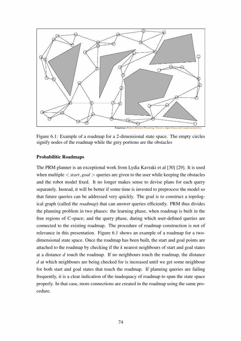
Figure 6.1: Example of a roadmap for a 2-dimensional state space. The empty circlessignify nodes of the roadmap while the grey portions are the obstacles

Probabilitic Roadmaps

The PRM planner is an exceptional work from Lydia Kavraki et al [30] [29]. It is usedwhen multiple < start,goal > queries are given to the user while keeping the obstaclesand the robot model fixed. It no longer makes sense to devise plans for each queryseparately. Instead, it will be better if some time is invested to preprocess the model sothat future queries can be addressed very quickly. The goal is to construct a topolog-ical graph (called the roadmap) that can answer queries efficiently. PRM thus dividesthe planning problem in two phases: the learning phase, when roadmap is built in thefree regions of C-space; and the query phase, during which user-defined queries areconnected to the existing roadmap. The procedure of roadmap construction is not ofrelevance in this presentation. Figure 6.1 shows an example of a roadmap for a two-dimensional state space. Once the roadmap has been built, the start and goal points areattached to the roadmap by checking if the k nearest neighbours of start and goal statesat a distance d touch the roadmap. If no neighbours touch the roadmap, the distanced at which neighbours are being checked for is increased until we get some neighbourfor both start and goal states that touch the roadmap. If planning queries are failingfrequently, it is a clear indication of the inadequacy of roadmap to span the state spaceproperly. In that case, more connections are created in the roadmap using the same pro-cedure.

74

Figure 6.2: Merging of two EST trees. The configuration q ∈ Tstart is unable to connectto r ∈ Tgoal but can connect to s ∈ Tgoal

Expansive Spaces Trees (EST)

ESTs were developed by [25] [26]. The developers of the algorithm did not use thisacronym in their publications but it got along in the literature and has been called sosince then. The following steps explain how ESTs work:

• Choose a configuration q from the tree T .

• Sample a random configuration qrand from the neighbourhood of q.

• If the connection between q and qrand bears no obstacles, qrand is added to thevertices of T and (q,qrand) is added to the edges of T .

• The process is repeated until a specified number of configurations have beenadded to T .

• We build 2 such trees, one originating from the start state, named Tstart and theother from the goal state named Tgoal .

• The two trees are merged by connecting some configuration qa ∈ Tstart to someconfiguration qb ∈ Tgoal (figure 6.2).

75

Rapidly-exploring Random Trees

RRTs are the best sampling-based single query planners available in the motion plan-ning literature. They were proposed by Stephen LaValle [34] [37] [36]. The RRTs havebeen proven to be probabilistically complete. The following steps demonstrate howRRTs work.

• Suppose T is one of the trees rooted at Tstart or Tgoal .

• At each iteration, a random configuration qrand is sampled from the free regionsof the state space.

• The configuration, qnear in tree T nearest to qrand is found.

• An attempt is made to progress from qnear to qrand .

• Thus, we move a finite distance step from qnear towards qrand .

• This new configuration qnew if collision free is added to the vertices of T and theedge (qnear,qnew) is added to the edges of T .

• We build two such trees, one from the start state and the other from the goal state.

• A random configuration qgrand is generated.

• One of the trees is then extended toward this random configuration and thus a newconfiguration qgnew results.

• Then, the node closest to qgnew in the other tree is extended towards qgnew .

• If a connection is established, the planner terminates with success, otherwise theprocess is repeated (figure 6.3).

A key feature of sampling-based approaches is their randomness. Randomness is anexcellent tool for exploration but in situations where planners are given short time tocompute the right sequence of actions, some amount of bias towards the goal is prefer-able. This ensures that the algorithm still has enough to explore but is goal-oriented too.However, it must be noted that too much bias will cause the algorithm to get trapped inlocal minima just as in Randomized potential fields [7].

76

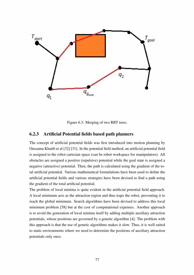
Figure 6.3: Merging of two RRT trees.

6.2.3 Artificial Potential fields based path planners

The concept of artificial potential fields was first introduced into motion planning byOussama Khatib et al [32] [31]. In the potential field method, an artificial potential fieldis assigned to the robot cartesian space (can be robot workspace for manipulators). Allobstacles are assigned a positive (repulsive) potential while the goal state is assigned anegative (attractive) potential. Then, the path is calculated using the gradient of the to-tal artificial potential. Various mathematical formulations have been used to define theartificial potential fields and various strategies have been devised to find a path usingthe gradient of the total artificial potential.The problem of local minima is quite evident in the artificial potential field approach.A local minimum acts as the attraction region and thus traps the robot, preventing it toreach the global minimum. Search algorithms have been devised to address this localminimum problem [58] but at the cost of computational expenses. Another approachis to avoid the generation of local minima itself by adding multiple auxiliary attractionpotentials, whose positions are governed by a genetic algorithm [4]. The problem withthis approach is that the use of genetic algorithms makes it slow. Thus, it is well suitedto static environments where we need to determine the positions of auxiliary attractionpotentials only once.

77

6.3 Comments on various path planners

In this section, we discuss what lacks in all the types of path planners described above.

6.3.1 Tree search algorithms

Graph based search or tree-based search algorithms like A∗ and Uniform Cost search

are complete and optimal. However, on close observation, we found the followingshortcomings with them.

• Even the best tree search, the A∗ algorithm has a blind behavior. Alternatively,when the heuristics is just goal-oriented, even the tree nodes close to the obstaclesare expanded (figure 6.4), meaning the algorithm cannot foresee what lies aheadand is somewhat blind . This behavior can be attributed to the serial nature of theprocessors and the algorithm need not be blamed for this. However, a parallellyworking algorithm would have foreseen the possibility of an obstacle in the veryfirst step and we would not be needing to expand nodes in that direction.

• There is no mechanism that allows the algorithm not to expand in the immediateneighbourhood of a branch that has already been closed from further expansion.This results in a huge waste of computation. If coarse granularity is chosen tosave computation, the algorithm is unable to traverse through narrow passages.

• Most tree search algorithms are offline. Every time a slight variation in the mapoccurs, the algorithm needs to replan. The D∗ lite [33] and Anytime dynamic A∗

[39] algorithms are somewhat online in that they do not entirely replan when themap changes; they just keep the path obtained before the map changed and planfrom there on in the new map.

6.3.2 Sampling-based approaches

Sampling-based approaches are seminal and work well even for complex motion plan-ning problems. However, they have their basis as randomness. By intuition, one mayargue that this may not be the way humans plan their motions. Humans do not followentirely different paths for the same conceptual situation. Einstein also said once that”God does not play Dice”. This does not mean sampling-based approaches are a badchoice for motion planning; it’s just that they are not intelligent as per Alan Turing’sdefinition of Intelligent systems.

78

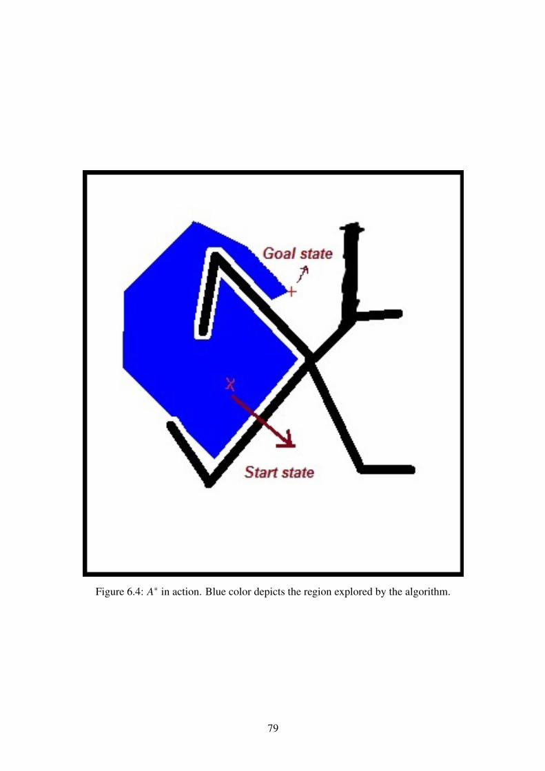
Figure 6.4: A∗ in action. Blue color depicts the region explored by the algorithm.

79

6.3.3 Artificial-potential field based approaches

Artificial potential field based approaches are very fast and have a strong mathematicalbasis. They can be used as online planners but the very existence of local minima makesthem a bad choice in situations where we have a lot of obstacles.

From this discussion above, we would like to have an algorithm that has the follow-ing properties:

• It should be an online algorithm.

• It should not waste too much computation due to its ”blindness”.

• It should work on a parallel computer and thus be able to foresee obstacles.

• It should seem intuitive.

• It should be an intelligent algorithm.

While the ”intelligence” aspect is hard to incorporate, the other aspects can be ad-dressed. The next section describes a path planner proposed by us.

6.4 Proposed Path planner

We propose a planner that tries to establish LOS(Line Of Sight ) between the currentstate the robot is in and the goal state. The planner requires an updated global map atall times. Following are the steps in which the proposed planner plans its motion:

• Step 1- It tries to establish a line connection between the goal state and the startstate (figure 6.5)

• Step 2 -If Line of Sight cannot be established, it rotates the line joining the cur-rent state and the goal state by an angle and checks if the rotated line is clear ofobstacles . If not, the line is rotated again until it is clear of obstacles (figure 6.6).The direction of rotation is determined by the position of start state and the goalstate.

• Step 3 - Once a free path is established, the planner proceeds along the rotatedline by a small arbitrary distance d (figure 6.7).

• Step 4 - After moving along the rotated line by distance d, we try to establishLOS between the current state and the goal state (figure 6.8).

80

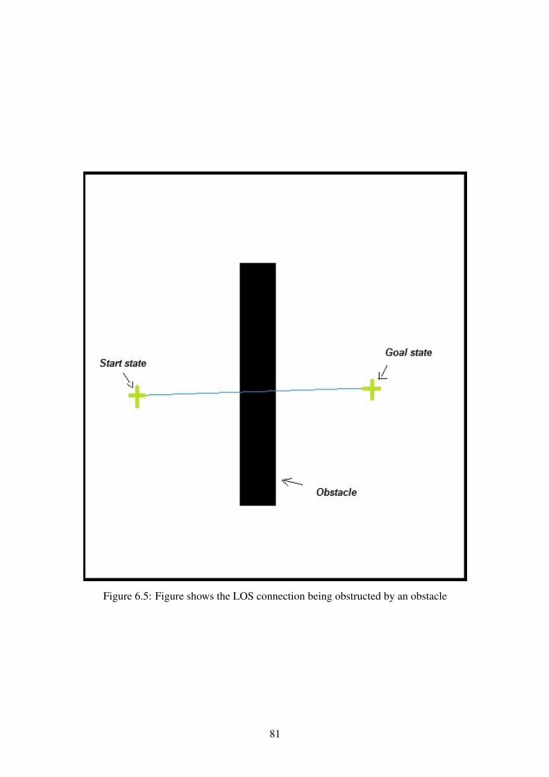
Figure 6.5: Figure shows the LOS connection being obstructed by an obstacle

81

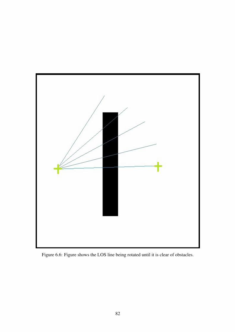
Figure 6.6: Figure shows the LOS line being rotated until it is clear of obstacles.

82

Figure 6.7: Red color depicts the incremental path traced by the algorithm.

83

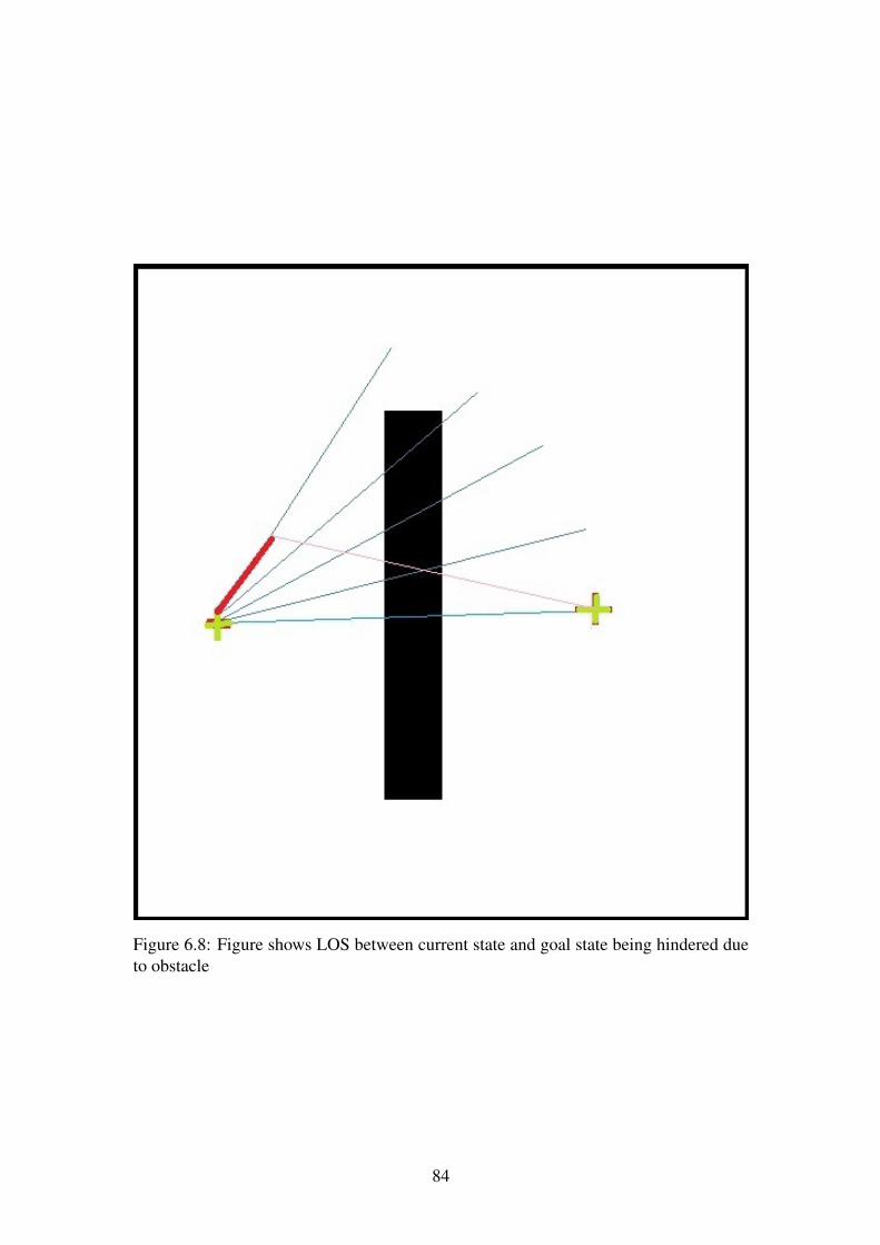
Figure 6.8: Figure shows LOS between current state and goal state being hindered dueto obstacle

84

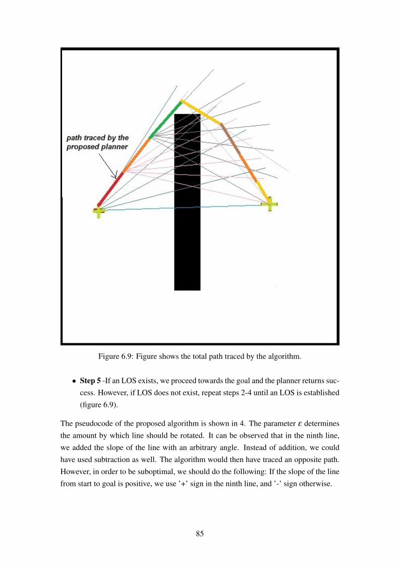
Figure 6.9: Figure shows the total path traced by the algorithm.

• Step 5 -If an LOS exists, we proceed towards the goal and the planner returns suc-cess. However, if LOS does not exist, repeat steps 2-4 until an LOS is established(figure 6.9).

The pseudocode of the proposed algorithm is shown in 4. The parameter ε determinesthe amount by which line should be rotated. It can be observed that in the ninth line,we added the slope of the line with an arbitrary angle. Instead of addition, we couldhave used subtraction as well. The algorithm would then have traced an opposite path.However, in order to be suboptimal, we should do the following: If the slope of the linefrom start to goal is positive, we use ’+’ sign in the ninth line, and ’-’ sign otherwise.

85

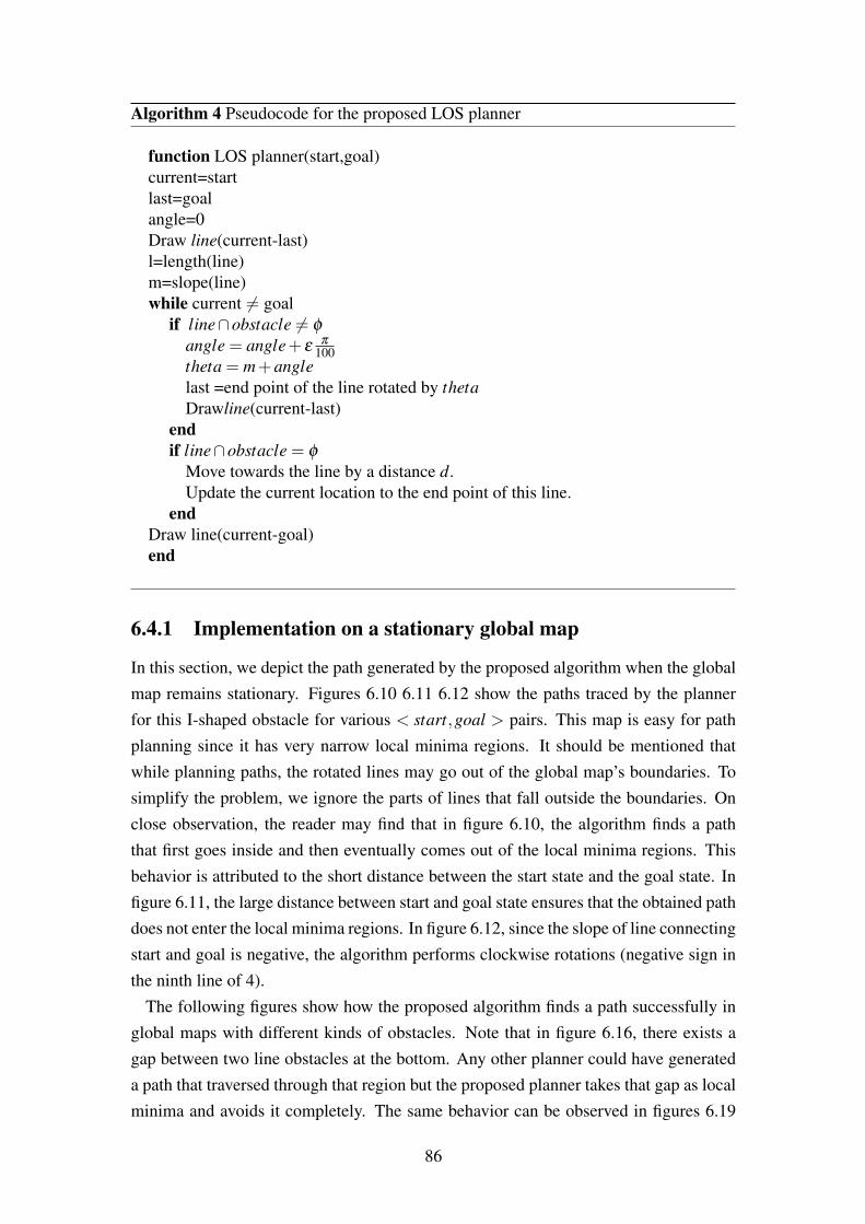
Algorithm 4 Pseudocode for the proposed LOS planner

function LOS planner(start,goal)current=startlast=goalangle=0Draw line(current-last)l=length(line)m=slope(line)while current 6= goal

if line∩obstacle 6= φ

angle = angle+ επ

100theta = m+anglelast =end point of the line rotated by thetaDrawline(current-last)

endif line∩obstacle = φ

Move towards the line by a distance d.Update the current location to the end point of this line.

endDraw line(current-goal)end

6.4.1 Implementation on a stationary global map

In this section, we depict the path generated by the proposed algorithm when the globalmap remains stationary. Figures 6.10 6.11 6.12 show the paths traced by the plannerfor this I-shaped obstacle for various < start,goal > pairs. This map is easy for pathplanning since it has very narrow local minima regions. It should be mentioned thatwhile planning paths, the rotated lines may go out of the global map’s boundaries. Tosimplify the problem, we ignore the parts of lines that fall outside the boundaries. Onclose observation, the reader may find that in figure 6.10, the algorithm finds a paththat first goes inside and then eventually comes out of the local minima regions. Thisbehavior is attributed to the short distance between the start state and the goal state. Infigure 6.11, the large distance between start and goal state ensures that the obtained pathdoes not enter the local minima regions. In figure 6.12, since the slope of line connectingstart and goal is negative, the algorithm performs clockwise rotations (negative sign inthe ninth line of 4).

The following figures show how the proposed algorithm finds a path successfully inglobal maps with different kinds of obstacles. Note that in figure 6.16, there exists agap between two line obstacles at the bottom. Any other planner could have generateda path that traversed through that region but the proposed planner takes that gap as localminima and avoids it completely. The same behavior can be observed in figures 6.19

86

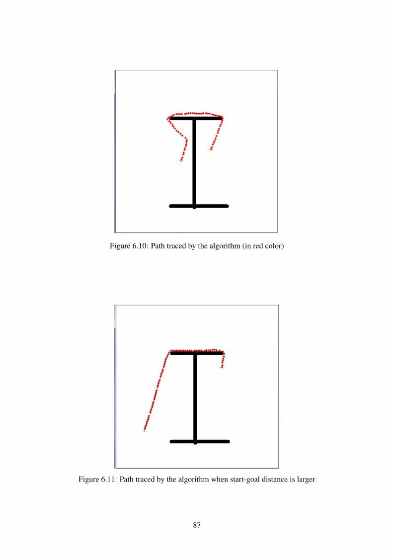
Figure 6.10: Path traced by the algorithm (in red color)

Figure 6.11: Path traced by the algorithm when start-goal distance is larger

87

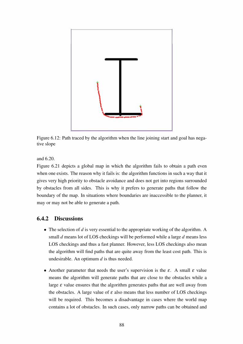
Figure 6.12: Path traced by the algorithm when the line joining start and goal has nega-tive slope

and 6.20.Figure 6.21 depicts a global map in which the algorithm fails to obtain a path evenwhen one exists. The reason why it fails is: the algorithm functions in such a way that itgives very high priority to obstacle avoidance and does not get into regions surroundedby obstacles from all sides. This is why it prefers to generate paths that follow theboundary of the map. In situations where boundaries are inaccessible to the planner, itmay or may not be able to generate a path.

6.4.2 Discussions

• The selection of d is very essential to the appropriate working of the algorithm. Asmall d means lot of LOS checkings will be performed while a large d means lessLOS checkings and thus a fast planner. However, less LOS checkings also meanthe algorithm will find paths that are quite away from the least cost path. This isundesirable. An optimum d is thus needed.

• Another parameter that needs the user’s supervision is the ε . A small ε valuemeans the algorithm will generate paths that are close to the obstacles while alarge ε value ensures that the algorithm generates paths that are well away fromthe obstacles. A large value of ε also means that less number of LOS checkingswill be required. This becomes a disadvantage in cases where the world mapcontains a lot of obstacles. In such cases, only narrow paths can be obtained and

88

Figure 6.13: Path traced by the algorithm (in red color)

Figure 6.14: Path traced by the algorithm (in red color)

89

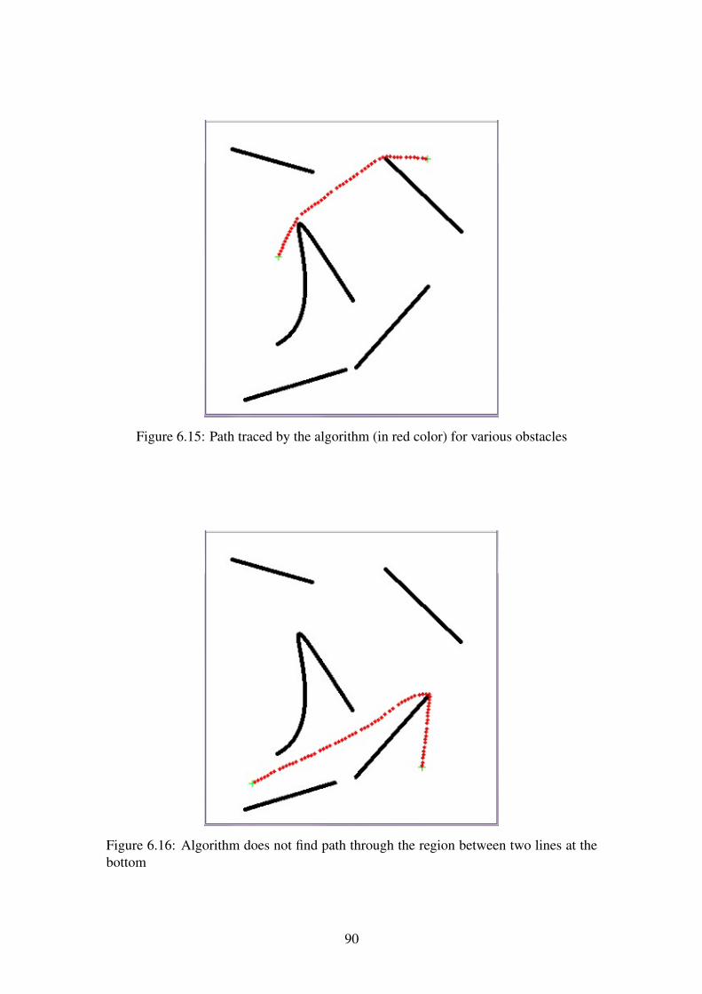
Figure 6.15: Path traced by the algorithm (in red color) for various obstacles

Figure 6.16: Algorithm does not find path through the region between two lines at thebottom

90

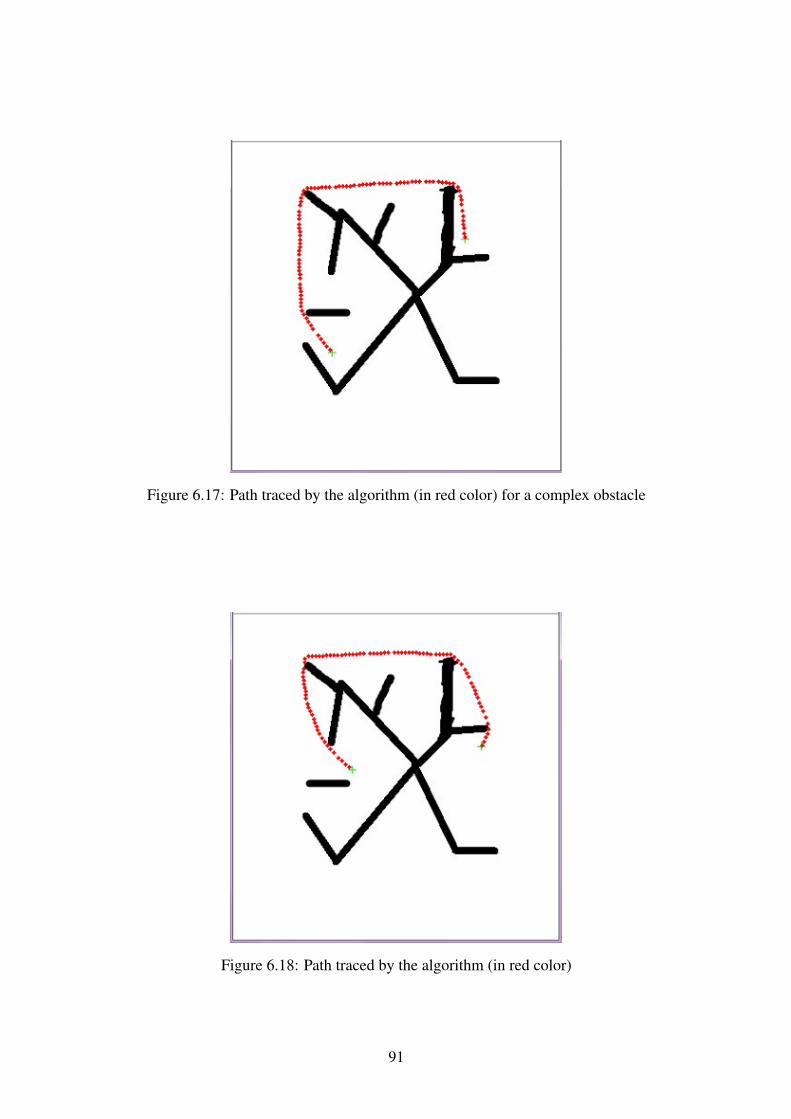
Figure 6.17: Path traced by the algorithm (in red color) for a complex obstacle

Figure 6.18: Path traced by the algorithm (in red color)

91

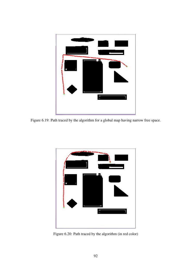
Figure 6.19: Path traced by the algorithm for a global map having narrow free space.

Figure 6.20: Path traced by the algorithm (in red color)

92

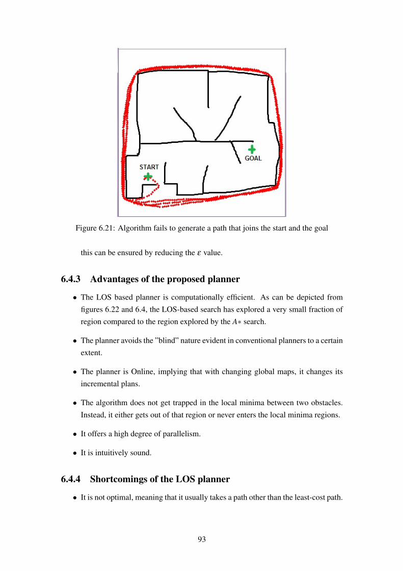
Figure 6.21: Algorithm fails to generate a path that joins the start and the goal

this can be ensured by reducing the ε value.

6.4.3 Advantages of the proposed planner

• The LOS based planner is computationally efficient. As can be depicted fromfigures 6.22 and 6.4, the LOS-based search has explored a very small fraction ofregion compared to the region explored by the A∗ search.

• The planner avoids the ”blind” nature evident in conventional planners to a certainextent.

• The planner is Online, implying that with changing global maps, it changes itsincremental plans.

• The algorithm does not get trapped in the local minima between two obstacles.Instead, it either gets out of that region or never enters the local minima regions.

• It offers a high degree of parallelism.

• It is intuitively sound.

6.4.4 Shortcomings of the LOS planner

• It is not optimal, meaning that it usually takes a path other than the least-cost path.

93

Figure 6.22: Navy blue color depicts the region explored by the algorithm

• It is not complete, meaning it sometimes fails to find solution even when oneexists.

• It lacks a mathematical basis.

6.4.5 Conclusions

Though the proposed LOS planner is fast, efficient and exhibits parallelism, it does notstand out on the key properties such as completeness and optimality. In case of mobilerobot motion planning, optimality needs to be ensured otherwise the mobile robot mightend up taking a much longer route and might thus lose all its energy before reachingthe goal. However, in case of path planning in robot manipulators, optimality is notthe necessary criteria. Instead, online and fast planning is the primary requisite. Themanipulator may end up taking a longer route but that won’t matter much because themanipulator has a limited workspace and the time difference between optimal path anda longer path won’t be much. Thus, the proposed LOS planner can be applied to pathplanning in robot manipulators. However, the proposed planner does not guaranteecompleteness either. Thus, research needs to be done to make the proposed plannercomplete. This will atleast ensure its applicability for path planning in robot manipula-tors. As for optimality, this intuition of searching for a Line of Sight path contradictswith the optimality guarantees. Thus, the proposed planner should almost never be usedfor path planning in mobile robots.We will use the A∗ search to plan paths in C-space. There are two reasons behind that.First, the proposed planner does not offer completeness. Secondly, we have an explicitrepresentation of C-space available to us and Sampling-based approaches are thus notneeded.

94

6.5 Summary

In this unit, we first discussed tree-based searches. Initially, uninformed searches werediscussed. Breadth first search, depth-first first search and uniform cost search are someimportant uniformed searches. All uninformed searches proved to be computationallyexpensive. Thus, some information about the planning problem is injected into theplanner using a heuristic function. Greedy search works only on the basis of heuristics.Thus, it often leads to the (wrong) goal although it is very speedy. The pathbreakingA∗ search uses the properties of both greedy search and the uniform cost search. Uni-form cost search resembles exploration while the greedy search resembles exploitation.Thus, the A∗ search utilizes the combination of both and is thus the most used plannertill date.The sampling-based approaches are then discussed. They are deployed due to two rea-sons: they are faster than conventional tree search algorithms, and their applicationcan avoid an explicit C-space representation. For multiple queries, the ProbabilisticRoadmap (PRM) algortihm is used. For single queries, Expansive Spaces trees (ESTs)and Rapidly-exploring Random Trees (RRTs) are used, RRT being the most widely usedsampling-based algorithm for motion planning.Next, we propose a planner that tries to establish Line of Sight (LOS) with the goalat all times. As long as LOS is not available, it keeps searching for one. We showedhow it was computationally inexpensive, less ”blind”, devoid of local minima problemand had a high degree of parallelism. However, we also observed that it did not offercompleteness and optimality.

95

Chapter 7

MOTION PLANNING ON A 2-DOFMANIPULATOR

7.1 The Task

The prime task is to plan obstacle-free motion for robot manipulators. This task canbe decomposed into the following modules based on the sequence in which one willencounter them:

• In order to plan paths, one must first know the values of joint variables requiredto reach a particular position and orientation. (Inverse Kinematics problem)

• In order to avoid obstacles, one must plan paths in C-space since each point in C-space represents a robot’s configuration. Thus, the planning problem will reduceto planning paths from one point in C-space to another point in C-space.

• Once the C-space has been constructed, one then needs to devise a planner thatplans paths from one point to the other.

7.2 What we have

• We have with us an Inverse Kinematics solver that uses SIR particle filter. Thiswill ensure we have the values of joint variables for the initial and the final posi-tions. (Unit 4)

• We have an explicit C-space representation that we obtained using a line primi-tive. (Unit 5)

• We have the A∗ algorithm with us that plans paths optimal in C-space. Thosepaths may not be optimal in workspace. (Unit 6)

96

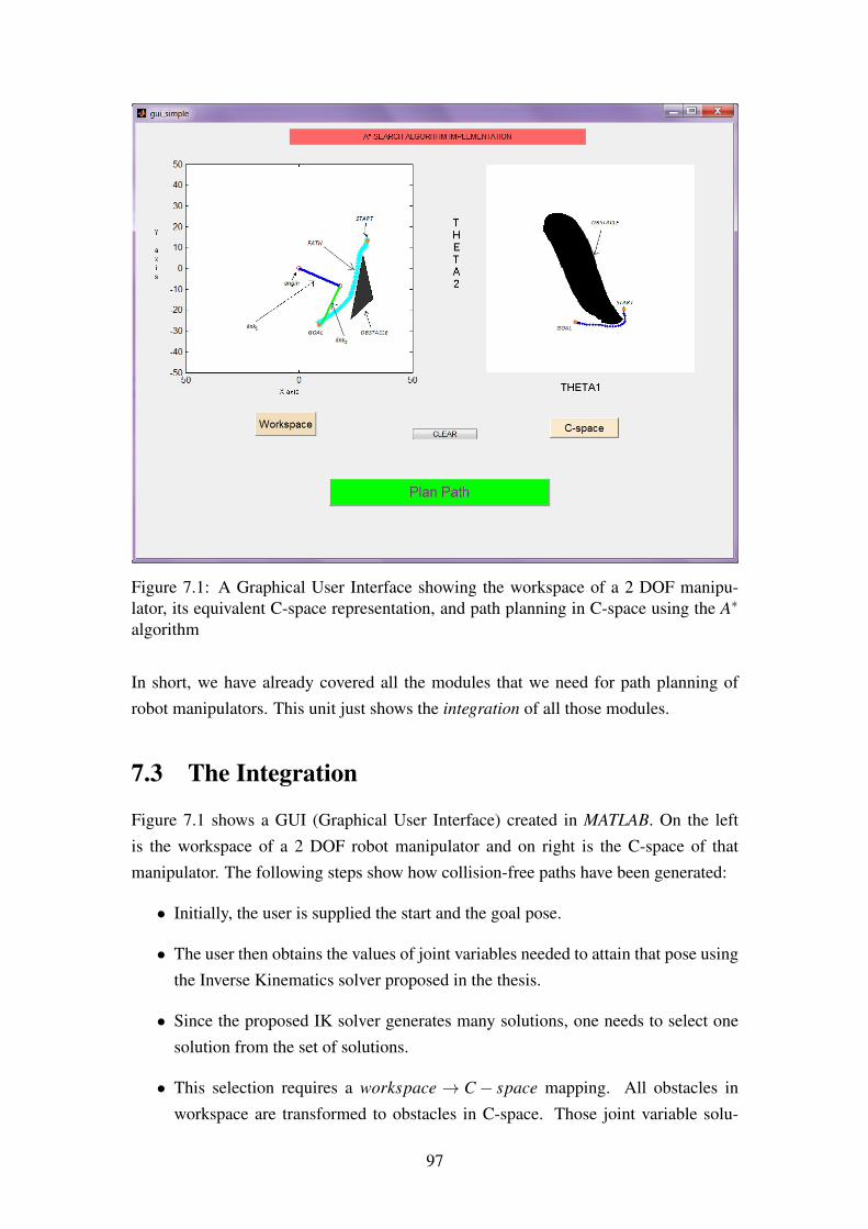
Figure 7.1: A Graphical User Interface showing the workspace of a 2 DOF manipu-lator, its equivalent C-space representation, and path planning in C-space using the A∗

algorithm

In short, we have already covered all the modules that we need for path planning ofrobot manipulators. This unit just shows the integration of all those modules.

7.3 The Integration

Figure 7.1 shows a GUI (Graphical User Interface) created in MATLAB. On the leftis the workspace of a 2 DOF robot manipulator and on right is the C-space of thatmanipulator. The following steps show how collision-free paths have been generated:

• Initially, the user is supplied the start and the goal pose.

• The user then obtains the values of joint variables needed to attain that pose usingthe Inverse Kinematics solver proposed in the thesis.

• Since the proposed IK solver generates many solutions, one needs to select onesolution from the set of solutions.

• This selection requires a workspace → C− space mapping. All obstacles inworkspace are transformed to obstacles in C-space. Those joint variable solu-

97

Figure 7.2: GUI showing A∗ path planning

tions that lie in the C-space obstacle region are rejected and the solution that liesin the free C-space region is selected for both start and goal positions.

• Once the start and goal positions have been selected in the C-space, the A∗ searchalgorithm finds the path between the start and the goal.

• So far, the path has been found in C-space. Each node in the C-space path containsinformation about the angle pair < θ1,θ2 >.

• Each < θ1,θ2 > pair yields a position described in cartseian space (Forward Kine-matics). Thus, a reverse mapping between C-space path→ workspace path canbe established.

• Note that this reverse mapping doesn’t mean that an optimal path in C-space willyield an optimal path in workspace.

Figure 7.2, 7.3 and 7.4 show path planning using A∗ search for various < start,goal >

pairs. It can be seen from figure 7.3 that the path planned in C-space is optimal whilethe corresponding workspace path is not optimal at all.

98

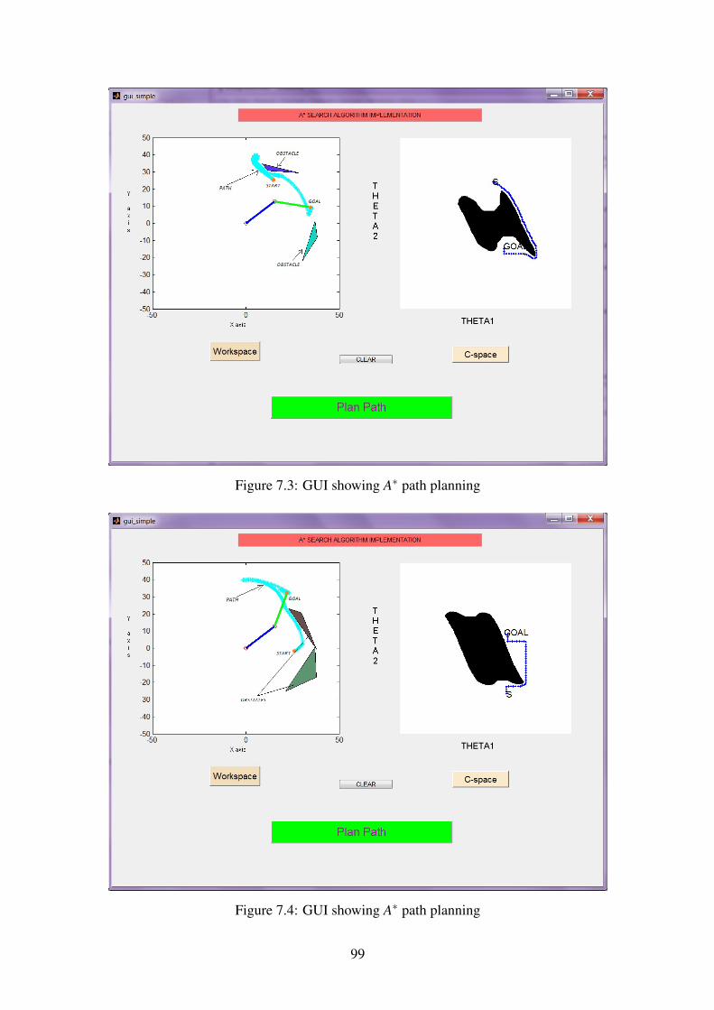
Figure 7.3: GUI showing A∗ path planning

Figure 7.4: GUI showing A∗ path planning

99

Figure 7.5: figure shows the problem of infering the position in real world

7.4 Implementation issues

The GUI created here is just a simulation of path planning. In real implementation, onemay face the following issues:

• In the simulation described, we know in advance the position of all obstacles.However, in real implementation, we do not have the position of obstacles knownbeforehand. Instead, we need to infer the position of obstacles from the sensordata available to us. In general, a camera is used to obtain position. However, theposition obtained by the camera is the representation of the obstacle described incamera frame coordinates while we have always represented position with respectto the manipulator’s fixed frame. Thus, a transformation from camera frame tothe manipulator’s fixed frame is needed. The problem is depicted in figure 7.5.We need the following transformations: Tcamera,obstacle and Tbase,camera.

• In the GUI created in this unit, the position of all the obstacles was identified usingtheir vertices (corners). In practise, one needs to detect corners of an obstacleusing some image processing technique. The most common technique for thispurpose is the Harris corner detection algorithm [12] [21].

• In practise, the links will not be of zero width. Thus, one will need to find a rela-tionship between the width of links and the amount by which C-space obstaclesshould be inflated.

100

7.5 Summary

In this unit, we integrated all the modules we described in the preceding units to even-tually obtain a path planner for robot manipulators. A GUI has been created for a 2DOF planar manipulator. GUI shows the workspace of manipulator and its C-space. Italso depicts how path is being planned first in C-space and then in workspace. Finally,some issues relating to the implementation of such a path planner in real world havebeen discussed.

101

Chapter 8

CONCLUSION

8.1 Summary of the Thesis

This thesis concerns itself with path planning in robot manipulators. In order to planpaths for manipulators, one needs to be able to carry information among workspace,joint space and Configuration space (C-space).

• Joint variables corresponding to the desired pose are specified in joint space.

• Start and goal pose (position and orientation) are specified in the workspace.Moreover, robot manipulators are usually controlled in joint space.

• Path planning is usually performed in C-spaces.

It is clear that we need to establish mappings between these spaces in order to be ableto perform motion planning.

• The mapping joint space 7→ workspace is the forward kinematics mapping and isdescribed in Unit 2.

• The mapping workspace 7→ joint space is the Inverse Kinematics mapping and isdescribed in Unit 4. This mapping is of particular interest since robots are usuallycontrolled in joint space. Moreover, it is not a one-to-one mapping making it hardfor the user to detect all solutions and even harder to choose a solution from thesolution set.

• Path planning in workspace suffers from expensive collision detection since thecollision detection algorithm has to check if any part on any link of the robot is incollision with any obstacle. The mapping workspace 7→ C-space is thus essentialin order to be able to plan collision-free paths. The fact that a robot is just apoint in the C-space makes path planning very easy. This workspace 7→ C-space

mapping is described in Unit 5.

102

• Paths are planned in C-space and unit 6 helps us decide which planner to be usedfor a particular situation. Tree-search or graph-search algorithms are preferredwhen an explicit representation of C-space obstacles is feasible and efficient.Sampling-based algorithms are used when it is almost impossible to representC-space obstacles explicitly.

• The C-space 7→ workspace is again like a forward kinematics mapping. Eachpoint on C-space when transformed to workspace yields the pose. Unit 7 showshow paths created in C-space can be reflected into workspace/task space usingthis transformation.

8.2 My contributions

• An Inverse Kinematics solver that uses the concept of Sampling Importance Re-sampling has been proposed in this thesis. This solver is reliable, complete, stableand generic. Work is in progress to make the solver computationally efficient sothat IK solutions can be computed in real-time.

• An approach for the explicit construction of C-space obstacles has been proposedin this thesis. The proposed approach is simple and computationally efficient.

• A path planner that tries to establish Line Of Sight (LOS) between the currentstate and the goal state has been proposed in this thesis. The proposed planner iscomputationally efficient, avoids local minima problem, exhibits high degree ofparallelism and is intuitionally sound.

8.3 My perspective

8.3.1 On Inverse Kinematics

In unit 4, three key issues in IK problem were listed: the existence or non-existence of

solutions, Multiple solutions and Choice of solution. While the first two issues havebeen addressed in the proposed IK solver, the third one, which is the most essential onehas not yet been addressed.Numerous approaches exist to address the first two issues, while no single approachthat addresses the third issue completely, exists as of now. This is because there doesnot exist a unique answer on which solution to choose. If we observe human behavior,we can infer that different humans choose different solutions in the same situation, thusgiving rise to somewhat distinct outcomes. Figures 8.1a ,8.1b ,8.1c and 8.1d showfootballers choosing different actions when they recieve the ball at the same height.

103

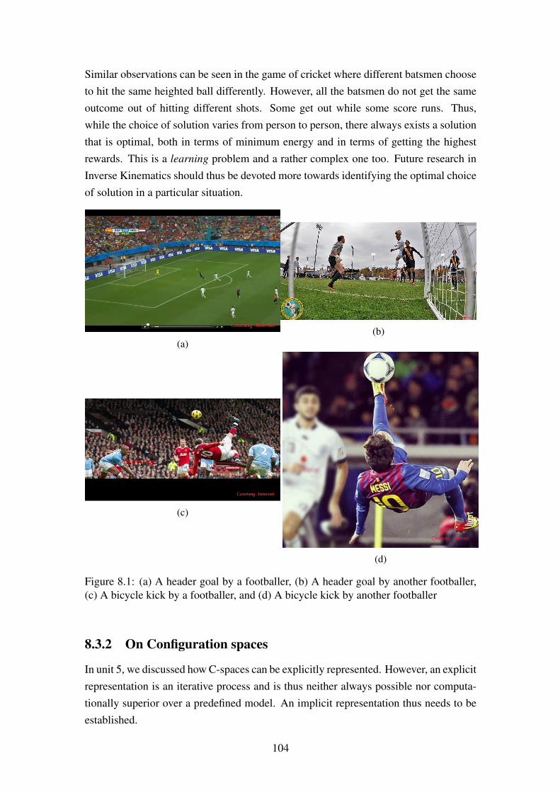
Similar observations can be seen in the game of cricket where different batsmen chooseto hit the same heighted ball differently. However, all the batsmen do not get the sameoutcome out of hitting different shots. Some get out while some score runs. Thus,while the choice of solution varies from person to person, there always exists a solutionthat is optimal, both in terms of minimum energy and in terms of getting the highestrewards. This is a learning problem and a rather complex one too. Future research inInverse Kinematics should thus be devoted more towards identifying the optimal choiceof solution in a particular situation.

(a)(b)

(c)

(d)

Figure 8.1: (a) A header goal by a footballer, (b) A header goal by another footballer,(c) A bicycle kick by a footballer, and (d) A bicycle kick by another footballer

8.3.2 On Configuration spaces

In unit 5, we discussed how C-spaces can be explicitly represented. However, an explicitrepresentation is an iterative process and is thus neither always possible nor computa-tionally superior over a predefined model. An implicit representation thus needs to beestablished.

104

If we look at a 3-4 month child, we can observe that it tries to manipulate its surround-ings. By doing so, it actually tries to infer its own structure over time. For the nextfew months, the kid is unable to plan collision-free trajectories but with time, it learnsits own structure almost completely and can now perform complex manipulation taskswith ease. A similar learning philosophy should be applied to C-spaces. It can be donein the following way: Initially, the robot constructs explicit representations for variousC-space obstacles. With enough training data, the robot then learns a generalized func-tional representation between any object in workspace and its corresponding C-spaceequivalent. If C-space structure is learnt in this way, it will be an interesting and intu-itive finding.

8.3.3 On Path Planning

In unit 6, we discussed a number of path planners available in literature. It can be arguedthat planning and learning are not entirely different. Whereas planning problems aim atcoming out with a sequence of actions for a particular problem, learning problems tellus what action to choose if the agent gets into a particular state. Planning combined withlearning can be an excellent solution to motion planning. It is because although mostplanners compute the entire sequence of actions beforehand, they do not encode anyinformation in the plan about what to do if the agent drifts from the specified plan. Thus,whenever the agent drifts from the specified plan, learning might come to aid and bringthe agent back to the specified plan. If no learning is incorporated, the planner mighthave to replan again and again if the agent takes actions stochastically. Replanning isthus unnecessary if learning is incorporated into the system .Thus, a learning + planning

approach is the ultimate solution to motion planning.

105

Bibliography

[1] RoKiSim 1.62 robot kinematics simulator. http://www.parallemic.org/

RoKiSim.html.

[2] Mathworks matlab. http://www.mathworks.in/products/matlab/.

[3] John Robert Anderson, Ryszard S Michalski, Ryszard Stanisław Michalski,Jaime Guillermo Carbonell, and Tom Michael Mitchell. Machine learning: An

artificial intelligence approach, volume 2. Morgan Kaufmann, 1986.

[4] F Arambula Cosıo and Padilla Castaneda. Autonomous robot navigation usingadaptive potential fields. Mathematical and computer modelling, 40(9):1141–1156, 2004.

[5] Andreas Aristidou and Joan Lasenby. Inverse kinematics: a review of existingtechniques and introduction of a new fast iterative solver. 2009.

[6] Joao Carlos Alves Barata and Mahir Saleh Hussein. The moore–penrose pseu-doinverse: A tutorial review of the theory. Brazilian Journal of Physics, 42(1-2):146–165, 2012.

[7] Jerome Barraquand and Jean-Claude Latombe. Robot motion planning: A dis-tributed representation approach. The International Journal of Robotics Research,10(6):628–649, 1991.

[8] Samuel R Buss and Jin-Su Kim. Selectively damped least squares for inversekinematics. journal of graphics, gpu, and game tools, 10(3):37–49, 2005.

[9] John Canny. Collision detection for moving polyhedra. Pattern Analysis and

Machine Intelligence, IEEE Transactions on, (2):200–209, 1986.

[10] Howie M Choset. Principles of robot motion: theory, algorithms, and implemen-

tation. MIT press, 2005.

[11] John J Craig. Introduction to robotics, volume 7. Addison-Wesley Reading, MA,1989.

106

[12] Konstantinos G Derpanis. The harris corner detector. York University, 2004.

[13] Bruce R Donald. A search algorithm for motion planning with six degrees offreedom. Artificial Intelligence, 31(3):295–353, 1987.

[14] Edward R Dougherty. An introduction to morphological image processing. Tuto-

rial texts in optical engineering, 1992.

[15] Bradley Efron and B Efron. The jackknife, the bootstrap and other resampling

plans, volume 38. SIAM, 1982.

[16] Roger Fletcher. Practical methods of optimization. John Wiley & Sons, 2013.

[17] King Sun Fu, Ralph Gonzalez, and CS George Lee. Robotics: Control Sensing

Vision and Intelligence. Tata McGraw-Hill Education, 1987.

[18] David Edward Goldberg et al. Genetic algorithms in search, optimization, and

machine learning, volume 412. Addison-wesley Reading Menlo Park, 1989.

[19] Rafael C Gonzalez, Richard Eugene Woods, and Steven L Eddins. Digital image

processing using MATLAB. Pearson Education India, 2004.

[20] Keith Grochow, Steven L Martin, Aaron Hertzmann, and Zoran Popovic. Style-based inverse kinematics. In ACM Transactions on Graphics (TOG), volume 23,pages 522–531. ACM, 2004.

[21] Chris Harris and Mike Stephens. A combined corner and edge detector. In Alvey

vision conference, volume 15, page 50. Manchester, UK, 1988.

[22] Richard S Hartenberg and Jacques Denavit. Kinematic synthesis of linkages.McGraw-Hill New York, 1964.

[23] Allen Hatcher. Algebraic topology. Tsinghua University Press, 2002.

[24] Martin Herman. Fast, three-dimensional, collision-free motion planning. InRobotics and Automation. Proceedings. 1986 IEEE International Conference on,volume 3, pages 1056–1063. IEEE, 1986.

[25] David Hsu. Randomized single-query motion planning in expansive spaces. PhDthesis, Stanford University, 2000.

[26] David Hsu, Robert Kindel, Jean-Claude Latombe, and Stephen Rock. Randomizedkinodynamic motion planning with moving obstacles. The International Journal

of Robotics Research, 21(3):233–255, 2002.

[27] Reza N Jazar. Theory of applied robotics. Springer, 2010.

107

[28] Rudolph Emil Kalman. A new approach to linear filtering and prediction prob-lems. Journal of basic Engineering, 82(1):35–45, 1960.

[29] Lydia E Kavraki and Jean-Claude Latombe. Probabilistic roadmaps for robot pathplanning. 1998.

[30] Lydia E Kavraki, Petr Svestka, J-C Latombe, and Mark H Overmars. Probabilisticroadmaps for path planning in high-dimensional configuration spaces. Robotics

and Automation, IEEE Transactions on, 12(4):566–580, 1996.

[31] Oussama Khatib. The potential field approach and operational space formulationin robot control. In Adaptive and Learning Systems, pages 367–377. Springer,1986.

[32] Oussama Khatib. Real-time obstacle avoidance for manipulators and mobilerobots. The international journal of robotics research, 5(1):90–98, 1986.

[33] Sven Koenig and Maxim Likhachev. D* lite. In AAAI/IAAI, pages 476–483, 2002.

[34] James J Kuffner and Steven M LaValle. Rrt-connect: An efficient approach tosingle-query path planning. In Robotics and Automation, 2000. Proceedings.

ICRA’00. IEEE International Conference on, volume 2, pages 995–1001. IEEE,2000.

[35] Ray Kurzweil. The singularity is near: When humans transcend biology. Penguin,2005.

[36] Steven M LaValle. Rapidly-exploring random trees a new tool for path planning.1998.

[37] Steven M LaValle and James J Kuffner. Randomized kinodynamic planning. The

International Journal of Robotics Research, 20(5):378–400, 2001.

[38] Steven Michael LaValle. Planning algorithms. Cambridge university press, 2006.

[39] Maxim Likhachev, David I Ferguson, Geoffrey J Gordon, Anthony Stentz, andSebastian Thrun. Anytime dynamic a*: An anytime, replanning algorithm. InICAPS, pages 262–271, 2005.

[40] Tomas Lozano-Perez. Spatial planning: A configuration space approach. Com-

puters, IEEE Transactions on, 100(2):108–120, 1983.

[41] Asok Kumar Mallik, Amitabha Ghosh, and Gunter Dittrich. Kinematic analysis

and synthesis of mechanisms. CRC Press, 1994.

108

[42] Andrew W Marshall. The use of multi-stage sampling schemes in monte carlocomputations. Technical report, DTIC Document, 1954.

[43] R Muller-Cajar and R Mukundan. Triangualation-a new algorithm for inversekinematics. 2007.

[44] Wyatt S Newman and Michael S Branicky. Real-time configuration space trans-forms for obstacle avoidance. The International Journal of Robotics Research,10(6):650–667, 1991.

[45] Wyatt Seybert Newman. High-speed robot control in complex environments. PhDthesis, Massachusetts Institute of Technology, 1987.

[46] Joey K Parker, Ahmad R Khoogar, and David E Goldberg. Inverse kinematics ofredundant robots using genetic algorithms. In Robotics and Automation, 1989.

Proceedings., 1989 IEEE International Conference on, pages 271–276. IEEE,1989.

[47] Alexandre N Pechev. Inverse kinematics without matrix inversion. In Robotics and

Automation, 2008. ICRA 2008. IEEE International Conference on, pages 2005–2012. IEEE, 2008.

[48] Donald B Rubin. Multiple imputation for nonresponse in surveys, volume 307.John Wiley & Sons, 2009.

[49] Stuart Russell, Peter Norvig, and Artificial Intelligence. A modern approach. Ar-

tificial Intelligence. Prentice-Hall, Egnlewood Cliffs, 25, 1995.

[50] M Sanjeev Arulampalam, Simon Maskell, Neil Gordon, and Tim Clapp. A tuto-rial on particle filters for online nonlinear/non-gaussian bayesian tracking. Signal

Processing, IEEE Transactions on, 50(2):174–188, 2002.

[51] Rachit Sapra, Michael Mathew, and S Majumder. A solution to inverse kinemat-ics problem using the concept of sampling importance resampling. In Advanced

Computing & Communication Technologies (ACCT), 2014 Fourth International

Conference on, pages 471–477. IEEE, 2014.

[52] Sebastian Thrun. Particle filters in robotics. In Proceedings of the Eighteenth

conference on Uncertainty in artificial intelligence, pages 511–518. Morgan Kauf-mann Publishers Inc., 2002.

[53] Sebastian Thrun, Wolfram Burgard, and Dieter Fox. Probabilistic robotics. MITpress, 2005.

109

[54] Sebastian Thrun, Dieter Fox, Wolfram Burgard, and Frank Dellaert. Robust montecarlo localization for mobile robots. Artificial intelligence, 128(1):99–141, 2001.

[55] Charles W Wampler. Manipulator inverse kinematic solutions based on vectorformulations and damped least-squares methods. Systems, Man and Cybernetics,

IEEE Transactions on, 16(1):93–101, 1986.

[56] L-CT Wang and Chih Cheng Chen. A combined optimization method for solv-ing the inverse kinematics problems of mechanical manipulators. Robotics and

Automation, IEEE Transactions on, 7(4):489–499, 1991.

[57] William A. Wolovich and H. Elliott. A computational technique for inverse kine-matics. 1984.

[58] Xiaoping Yun and Ko-Cheng Tan. A wall-following method for escaping localminima in potential field based motion planning. In Advanced Robotics, 1997.

ICAR’97. Proceedings., 8th International Conference on, pages 421–426. IEEE,1997.

110

List of Publications

Rachit Sapra, Michael Mathew, and S Majumder. A solution to inverse kinematics prob-lem using the concept of sampling importance resampling. In Advanced Computing &Communication Technologies (ACCT), 2014 Fourth International Conference on, pages471–477. IEEE, 2014.

Rachit Sapra, Michael Mathew, and S Majumder. Efficient Computation of Configu-ration space transforms for Collision-free motion planning. In International Conferenceon Control, Instrumentation, Communication & Computational Technologies,ICCICCT. IEEE, 2014.

Michael Mathew, Rachit Sapra and S Majumder. A Learning Based Approach to SelfModeling Robots.In International Conference on Control, Instrumentation, Communi-cation & Computational Technologies,ICCICCT . IEEE, 2014.

111