MASTER'S THESIS - DiVA portal

MASTER'S THESIS

GNSS Antenna Comparison for BistaticApplications

Johan Norberg

Master of Science in Engineering TechnologySpace Engineering

Luleå University of TechnologyDepartment of Computer Science, Electrical and Space Engineering

LULEÅ UNIVERSITY OF TECHNOLOGY UNIVERSITY OF COLORADO

GNSS Antenna Comparison

for Bistatic Applications

Johan Norberg

2011-04-28

2

Abstract Global Navigation Satellite System (GNSS) signals are gaining more and more traction as a passive

bistatic radar source for remote sensor measurements. Measurements of soil moisture and ocean

surface roughness can be flagged as two examples.

Two of the main collection approaches for these measurements are: (a) to use a base station on the

ground; or (b) airborne equipment onboard an aircraft. The aircraft approach requires a dual

receiver with two antennas, one upward looking (direct signal) and one downward looking (reflected

signal), and the GNSS satellite is the transmitter. A ground base station however can work with only

one antenna and a single receiver.

This paper focuses on the first approach, data collected using the base station method and, in

particular, the role that the antenna and its design has on the measurements at the base station. It

will discuss how different antennas, with different beam patterns, impacts the received reflected

signal that is used for the bistatic applications. The particular application of interest in this case is as

a dual snow depth sensor and soil moisture sensor. The analysis is done by examining the signal to

noise ratio of the received GPS satellite signal over the period of a complete pass of the satellite.

Multiple measurements are taken, varying parameters such as antenna height and surface moisture

to assess the performance of the antennas for such bistatic applications.

A GPS/GNSS antenna design made for a high precision ground station is designed to suppress

reflected signals, especially those signals that are reflected from the ground and incident upon the

antenna from below. This is controlled by the pattern of the lobes and by minimizing the left hand

circular polarized signal, since the GNSS signals is broadcast with a right hand circular polarization

and a change of polarization occurs when the signal is reflected. How successful the reflected signals

are suppressed depends on the surface it reflects upon as well as the polarization design of the

antenna. Such features are not desirable when the GPS receiver is being utilized as a snow depth/soil

moisture sensor. Instead, the combination of the direct and reflected signals contains the desired

information.

As a result, a basic, low cost, compact antenna capable of receiving both the direct and the reflected

signal was designed for this application. Three Monopole antennas were developed, one for each

band (L1, L2 and L5) with the L2 and later on the L5 holding the most interest, for some testing to

see how the measurements change relative to a survey grade antenna. The goal for these antennas

was to be an (inexpensive and effective) alternative for a snow depth measuring system and also a

low cost substitute to other bistatic applications, such as soil moisture measurements systems.

The measurement were recorded both in raw RF data to process later on with a software defined

radio (SDR) in MATLAB and with Trimble’s NetR8 receiver. The commercial receiver from Trimble

also provided a converter to give its measured data as a RINEX file, which could be parsed out in

MATLAB.

The two interested component of the data that was to be calculate was signal to noise ratio (SNR)

and the elevation angle of the satellite. This was done to be able to compare the different set of

measurement, both a look between different antennas and then of the different heights of the

Monopole antenna, to conclude what impact the multipath has on the different scenarios.

3

The main objective is to observe the fluctuation of the SNR for the different elevation angles. That is

to say, to observe the constructive and destructive interference the multipath has on the signal. The

multipath profile is heavily dependent on the height of the antenna above the surface as well as the

antenna site including the moist level or reflectivity of the ground.

The test site of the data collection was on a high roof at the University of Colorado (urban area) that

had a top layer of small stones and a drainage system to avoid water build-up.

The result indicated that the higher the antenna is placed the weaker the influence of the multipath,

while a wet surface will increase the influence compared to a dry surface. As expected, the

Monopole antenna that has wide beams and ignores the polarization of the signal is much more

open to multipath. The advantage of that is the constructive and destructive interference comes out

much distinctly but that in itself put some new demands on the receiver, especially in the phase of a

destructive interference on low elevation angle that may drop the SNR value below the receiver

threshold. However, the best result was observed when the satellite is at a high elevation angle.

Under these circumstances the commercial antenna is best on suppressing the multipath, while the

Monopole picks up a nice pattern of the constructive and destructive interference, this becomes

even more clear when the surface is wet.

4

Preface This paper was done in accords for a Master Thesis at Luleå University of Technology for the

duration of one semester, in collaboration with University of Colorado.

With the increasing interest and broader application for Bistatic radar solutions an investigation was

prompt, for the impact of the antenna and software chooses for just such application. To that end, a

design of a low price antenna alternative and a SDR was developed for comparison and evaluation.

The SDR was constructed on an existing framework of L1 signal but was special redesign to process

only L2C. Although the preliminary result was promising, an issue arise with the Phase Loop Lock

(PLL) tracking when both the CM and the CL code were implemented. That was never resolved

during the time frame of the project, but a likely reason is the L2C quarter cycle problem (induced

phase shifts).

The antenna part of the project went smoothly, however some urban RF interference occurred

during some data collection, but that could be alleviated with an extra cavity filter near the antenna.

A special acknowledgment and thanks goes out to Dennis Akos (mentor) and to Kristine Larson at

CU, for their insight and expertise. Also great gratuity to CU for usage of equipment and facilities and

to all the people in Boulder that welcomed me warmly. Without all of you, this thesis would not

have been possible.

5

Table of Contents Abstract ................................................................................................................................................... 2

Preface .................................................................................................................................................... 4

Table of Contests Figures ........................................................................................................................ 6

1 Introduction .................................................................................................................................... 7

2 Theory ............................................................................................................................................. 9

2.1 Antenna ................................................................................................................................... 9

2.2 L2C compare to L1 .................................................................................................................. 9

2.3 Bistatic measuring ................................................................................................................. 10

2.4 SDR ........................................................................................................................................ 12

2.4.1 C/No Estimate ............................................................................................................... 12

3 Experiment .................................................................................................................................... 14

3.1 Antenna comparison ............................................................................................................. 14

3.2 NetR8 .................................................................................................................................... 21

3.2.1 Height and water .......................................................................................................... 21

3.3 SDR ........................................................................................................................................ 27

3.3.1 40min data set of PRN 15.............................................................................................. 27

4 Results ........................................................................................................................................... 29

4.1 Antenna comparison ............................................................................................................. 29

4.2 NetR8 .................................................................................................................................... 29

4.3 SDR ........................................................................................................................................ 29

5 Conclusions ................................................................................................................................... 30

6 Future Work .................................................................................................................................. 31

7 Reference ...................................................................................................................................... 32

6

Table of Contests Figures Figure 1: A typical pinwheel antenna ..................................................................................................... 7

Figure 2: A Monopole antenna (L2) ........................................................................................................ 8

Figure 3: Overview of CM and CL code construction ............................................................................ 10

Figure 4: Geometry of the GNSS signal at the receiving antenna ........................................................ 11

Figure 5: Observed and Modeled GPS SNR Snow Data ........................................................................ 11

Figure 6: L2 Monopole antenna with pre. Amp, with simulated gain pattern (without pre. Amp) ..... 14

Figure 7: Standing wave ration above the reflection coefficient for the L2 Monopole antenna ......... 15

Figure 8: The complex impedance and phase for the L2 Monopole antenna ...................................... 15

Figure 9: Frequency sweep for the L2 Monopole antenna ................................................................... 16

Figure 10: Smith chart for the L2 Monopole antenna .......................................................................... 17

Figure 11: Novatel Pinwheel antenna(Left) and Antcom L1L2L5 antenna(Right) ................................ 17

Figure 12: Sky plot of PRN 07 and position of the antenna .................................................................. 18

Figure 13: L1 (C/A-code) Measurement from PRN 07 .......................................................................... 18

Figure 14: L2C (CM+CL-code) Measurement from PRN 07 ................................................................... 19

Figure 15: Sky plot of PRN 17 and position of the antenna .................................................................. 19

Figure 16: L1 (C/A-code) Measurement from PRN 17 .......................................................................... 20

Figure 17: L2C (CM+CL-code) Measurement from PRN 17 ................................................................... 20

Figure 18: Trimble NetR8 Receiver ....................................................................................................... 21

Figure 19: Position of the antenna for the height comparison ............................................................ 22

Figure 20: PRN 07 at 48,5in above surface, dry .................................................................................... 22


Figure 22: PRN 07 at 54in above surface, dry ....................................................................................... 23

Figure 23: PRN 31 at 54in above surface, dry ....................................................................................... 24



Figure 26: PRN 07 at 48,5in above surface, wet ................................................................................... 25

Figure 27: PRN 31 at 48,5in above surface, wet ................................................................................... 26

Figure 28: 40min data set from PRN15, NetR8 ..................................................................................... 27

Figure 29: 40min data set of PRN15, SDR(CM+CL-code) ...................................................................... 28

7

1 Introduction Using Global Navigation Satellite Systems (GNSS) signals as bistatic radar transmission for remote

sensor measurement is gaining more and more traction, especially for applications such as soil

moisture measurement, snow depth and ocean surface roughness. Some of the main collection

method for those applications is by a base station on the ground or from the use of aircraft and

satellite altimetry. Where the base station on the ground normally only uses one antenna the

aircraft and satellite collection method utilise a dual receiver for one downward looking antenna and

one upward looking antenna. The focus in this paper are going to be on the data collected from the

base station method and take up the part that the antenna has for the base station and investigate

the impact it has on the reflected signal which is used for the bistatic applications.

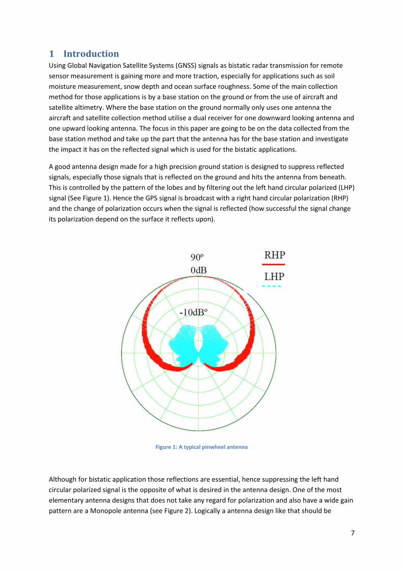
A good antenna design made for a high precision ground station is designed to suppress reflected

signals, especially those signals that is reflected on the ground and hits the antenna from beneath.

This is controlled by the pattern of the lobes and by filtering out the left hand circular polarized (LHP)

signal (See Figure 1). Hence the GPS signal is broadcast with a right hand circular polarization (RHP)

and the change of polarization occurs when the signal is reflected (how successful the signal change

its polarization depend on the surface it reflects upon).

Figure 1: A typical pinwheel antenna

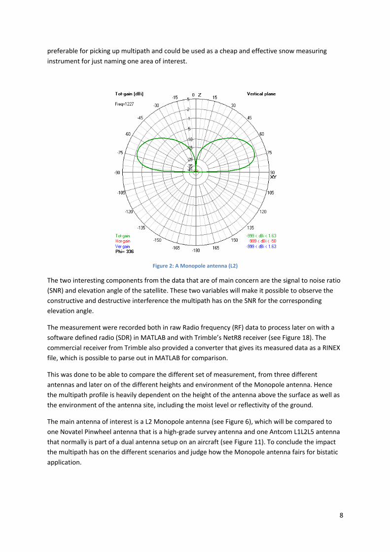
Although for bistatic application those reflections are essential, hence suppressing the left hand

circular polarized signal is the opposite of what is desired in the antenna design. One of the most

elementary antenna designs that does not take any regard for polarization and also have a wide gain

pattern are a Monopole antenna (see Figure 2). Logically a antenna design like that should be

8

preferable for picking up multipath and could be used as a cheap and effective snow measuring

instrument for just naming one area of interest.

Figure 2: A Monopole antenna (L2)

The two interesting components from the data that are of main concern are the signal to noise ratio

(SNR) and elevation angle of the satellite. These two variables will make it possible to observe the

constructive and destructive interference the multipath has on the SNR for the corresponding

elevation angle.

The measurement were recorded both in raw Radio frequency (RF) data to process later on with a

software defined radio (SDR) in MATLAB and with Trimble’s NetR8 receiver (see Figure 18). The

commercial receiver from Trimble also provided a converter that gives its measured data as a RINEX

file, which is possible to parse out in MATLAB for comparison.

This was done to be able to compare the different set of measurement, from three different

antennas and later on of the different heights and environment of the Monopole antenna. Hence

the multipath profile is heavily dependent on the height of the antenna above the surface as well as

the environment of the antenna site, including the moist level or reflectivity of the ground.

The main antenna of interest is a L2 Monopole antenna (see Figure 6), which will be compared to

one Novatel Pinwheel antenna that is a high-grade survey antenna and one Antcom L1L2L5 antenna

that normally is part of a dual antenna setup on an aircraft (see Figure 11). To conclude the impact

the multipath has on the different scenarios and judge how the Monopole antenna fairs for bistatic

application.

9

2 Theory

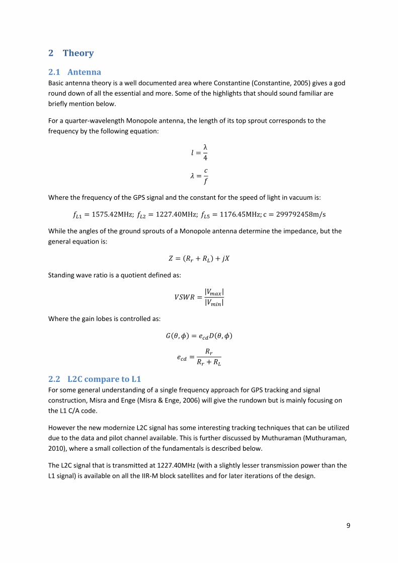
2.1 Antenna Basic antenna theory is a well documented area where Constantine (Constantine, 2005) gives a god

round down of all the essential and more. Some of the highlights that should sound familiar are

briefly mention below.

For a quarter-wavelength Monopole antenna, the length of its top sprout corresponds to the

frequency by the following equation:

Where the frequency of the GPS signal and the constant for the speed of light in vacuum is:

While the angles of the ground sprouts of a Monopole antenna determine the impedance, but the

general equation is:

Standing wave ratio is a quotient defined as:

Where the gain lobes is controlled as:

2.2 L2C compare to L1 For some general understanding of a single frequency approach for GPS tracking and signal

construction, Misra and Enge (Misra & Enge, 2006) will give the rundown but is mainly focusing on

the L1 C/A code.

However the new modernize L2C signal has some interesting tracking techniques that can be utilized

due to the data and pilot channel available. This is further discussed by Muthuraman (Muthuraman,

2010), where a small collection of the fundamentals is described below.

The L2C signal that is transmitted at 1227.40MHz (with a slightly lesser transmission power than the

L1 signal) is available on all the IIR-M block satellites and for later iterations of the design.

10

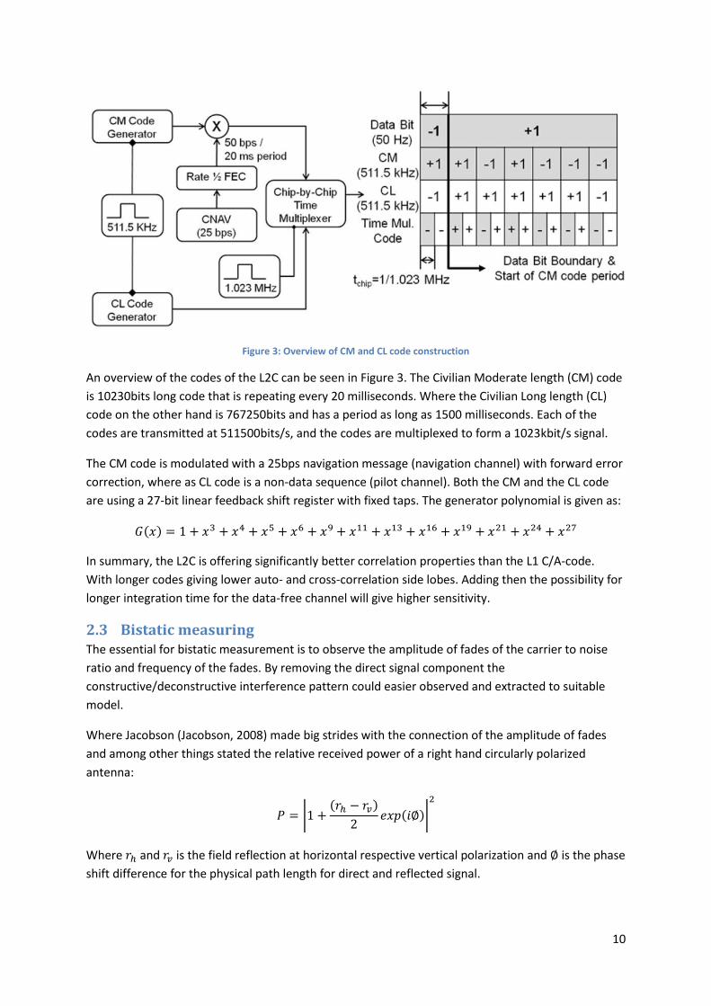
Figure 3: Overview of CM and CL code construction

An overview of the codes of the L2C can be seen in Figure 3. The Civilian Moderate length (CM) code

is 10230bits long code that is repeating every 20 milliseconds. Where the Civilian Long length (CL)

code on the other hand is 767250bits and has a period as long as 1500 milliseconds. Each of the

codes are transmitted at 511500bits/s, and the codes are multiplexed to form a 1023kbit/s signal.

The CM code is modulated with a 25bps navigation message (navigation channel) with forward error

correction, where as CL code is a non-data sequence (pilot channel). Both the CM and the CL code

are using a 27-bit linear feedback shift register with fixed taps. The generator polynomial is given as:

In summary, the L2C is offering significantly better correlation properties than the L1 C/A-code.

With longer codes giving lower auto- and cross-correlation side lobes. Adding then the possibility for

longer integration time for the data-free channel will give higher sensitivity.

2.3 Bistatic measuring The essential for bistatic measurement is to observe the amplitude of fades of the carrier to noise

ratio and frequency of the fades. By removing the direct signal component the

constructive/deconstructive interference pattern could easier observed and extracted to suitable

model.

Where Jacobson (Jacobson, 2008) made big strides with the connection of the amplitude of fades

and among other things stated the relative received power of a right hand circularly polarized

antenna:

Where and is the field reflection at horizontal respective vertical polarization and is the phase

shift difference for the physical path length for direct and reflected signal.

11

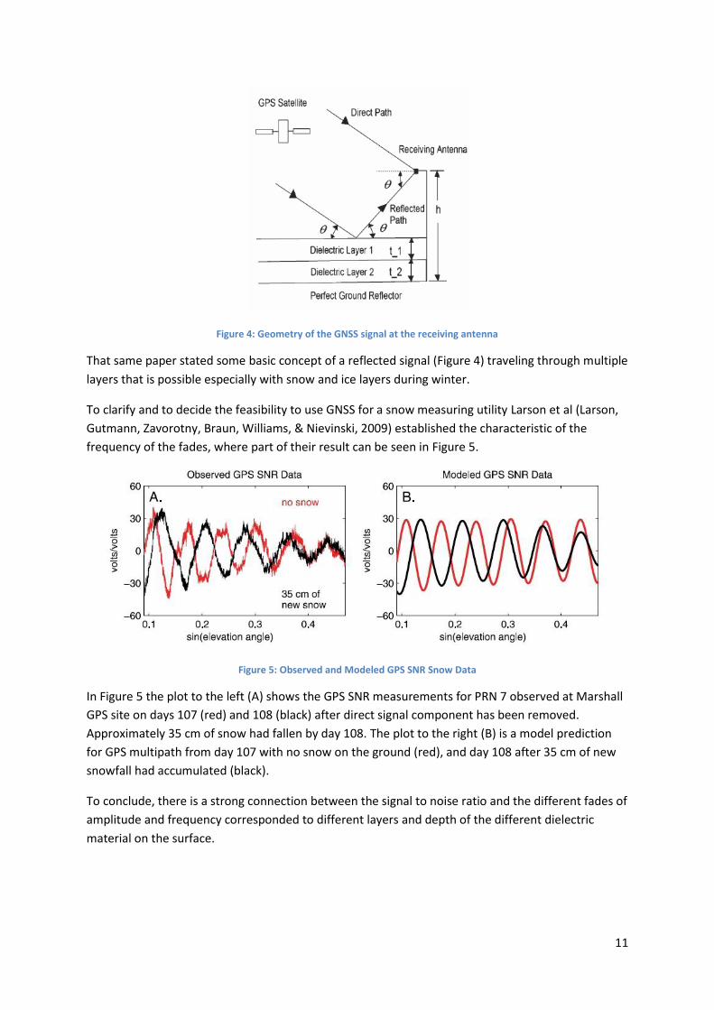
Figure 4: Geometry of the GNSS signal at the receiving antenna

That same paper stated some basic concept of a reflected signal (Figure 4) traveling through multiple

layers that is possible especially with snow and ice layers during winter.

To clarify and to decide the feasibility to use GNSS for a snow measuring utility Larson et al (Larson,

Gutmann, Zavorotny, Braun, Williams, & Nievinski, 2009) established the characteristic of the

frequency of the fades, where part of their result can be seen in Figure 5.

Figure 5: Observed and Modeled GPS SNR Snow Data

In Figure 5 the plot to the left (A) shows the GPS SNR measurements for PRN 7 observed at Marshall

GPS site on days 107 (red) and 108 (black) after direct signal component has been removed.

Approximately 35 cm of snow had fallen by day 108. The plot to the right (B) is a model prediction

for GPS multipath from day 107 with no snow on the ground (red), and day 108 after 35 cm of new

snowfall had accumulated (black).

To conclude, there is a strong connection between the signal to noise ratio and the different fades of

amplitude and frequency corresponded to different layers and depth of the different dielectric

material on the surface.

12

2.4 SDR An SDR code has many advantages compare to a commercial in the box solution. Mainly the

customisation and flexibility of the post processing, but requires some heavy computation.

2.4.1 C/No Estimate

A fundamental way to determining the status of the GNSS tracking and controlling a receiver is to

have a good estimate of the carrier to noise ratio (C/No).

However each carrier to noise algorithms differences itself in computational complexity, phase noise

and other variables depending on the algorithm used. A comparison between different algorithms

was made by Falletti et al (Falletti, Pini, & Presti, 2010). Where the three C/No estimators that is of

main interest is the Power Ratio Method (PRM), Variance Summing Method (VSM) and Moments

Method (MOM).

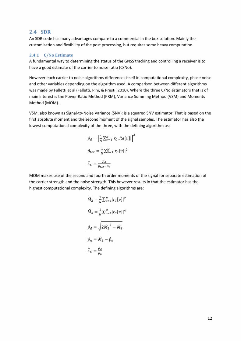
VSM, also known as Signal-to-Noise Variance (SNV): is a squared SNV estimator. That is based on the

first absolute moment and the second moment of the signal samples. The estimator has also the

lowest computational complexity of the three, with the defining algorithm as:

MOM makes use of the second and fourth order moments of the signal for separate estimation of

the carrier strength and the noise strength. This however results in that the estimator has the

highest computational complexity. The defining algorithms are:

13

The PRM, also known as Narrowband-wideband Power Ratio (NWPR) and is the only algorithm that

estimates C/No directly, VSM and MOM only estimates the SNR which can be converted to C/No due

to it sample the “observable”, hence is fairly well used. The PRM estimator is placing in-between the

other two estimators when it comes to computational complexity, with the following algorithms:

,

14

3 Experiment The three parts/stages experiment was design to clarify and give a preliminary indication of the

differences and impact that the choice of antenna and receiver has on bistatic applications.

As a first step, it is important to make an antenna comparison with exactly identical equipment,

observing the same GPS satellite on three succeeding days (one day for each antenna) with similar

weather. This will give a clear first impression and clarification of the impact that the beam pattern

has on the received signal.

For the second stage a NetR8 receiver, high graded surface receiver, is used as a reference for

bringing forward the impact of the environment has on the measured data depending where the

antenna is setup. Whether the antenna is mounted high or low under dry or wet surface will all

affect the performance of the antenna and the equipment.

As a last and third stage, an SDR receiver is implemented for its fully flexible and excellent post

processing option. Adding a newly develop software with increasing support for the “new” L2 signal

which primary result shall then be put in comparison with the data from NetR8 receiver.

3.1 Antenna comparison The performance of the self-design Monopole antenna will be directly compared to the Novatel

Pinwheel antenna (high graded ground station antenna) and an Antcom L1L2L5 antenna (airplane

model antenna).

First step is to take a closer look on the simulated result from the Monopole antenna using a

freeware named: 4nec2. The simulation will have an ideal ground plane and does not factor in a

polarization.

Figure 6: L2 Monopole antenna with pre. Amp, with simulated gain pattern (without pre. Amp)

15

To the left side in Figure 6 we can see the end product of the L2 antenna with DC-block, preamplifier

and cable converter to an N-male contact. While to the right we have the simulated gain pattern in

the vertical plane, hence you can superimpose the gain pattern directly on the antenna. By doing

that it stands clear that have it mounted horizontal should be preferable for bistatic application,

hence that will give one lobe covering the direct signal and the other aiming for the ground for the

reflected signal.

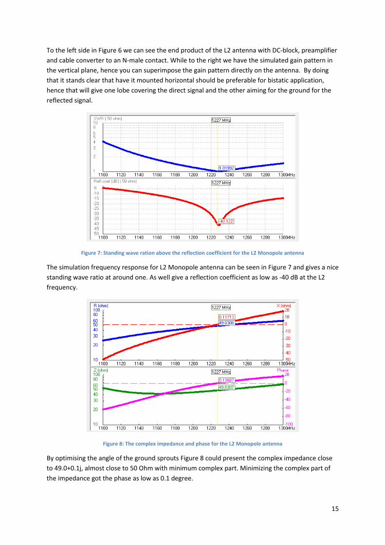
Figure 7: Standing wave ration above the reflection coefficient for the L2 Monopole antenna

The simulation frequency response for L2 Monopole antenna can be seen in Figure 7 and gives a nice

standing wave ratio at around one. As well give a reflection coefficient as low as -40 dB at the L2

frequency.

Figure 8: The complex impedance and phase for the L2 Monopole antenna

By optimising the angle of the ground sprouts Figure 8 could present the complex impedance close

to 49.0+0.1j, almost close to 50 Ohm with minimum complex part. Minimizing the complex part of

the impedance got the phase as low as 0.1 degree.

16

So over all the simulation indicates that the Monopole antenna will be nicely tuned to the L2

frequency.

When the L2 Monopole antenna is put through its paces in a test chamber, connected to a network

analyser it produce the following graphs.

Figure 9: Frequency sweep for the L2 Monopole antenna

From a frequency sweep of the antenna, Figure 9 could be produces with a network analyser that

indicate a primarily reflection coefficient as low as -54 dB for L2 frequency. However the reflection

coefficient changes heavily dependent on the surroundings. For best result one should be in an open

space with no reflective surfaces nearby, or as in this case in a testing camber with absorbing

material on the walls.

After the successful frequency sweep of the antenna the network analyser was set to Smith chart for

the final tuning of the angle of the ground sprout. That manages to get the Impedance around 50

Ohm where the imaginary part is just a fraction, see Figure 10. After the tuning process the

reflection coefficient was double checked to see that the antenna still had a nice frequency response

to the L2 frequency.

17

Figure 10: Smith chart for the L2 Monopole antenna

That keeps the testing chamber result in line on all of the essential parameters that was established

in the simulation.

Next step in the process is to collect some GPS data for a direct comparison, all data will be recorded

by the NetR8 and to will later be parser in MATLAB.

Figure 11: Novatel Pinwheel antenna(Left) and Antcom L1L2L5 antenna(Right)

All three antennas mounted on a tripod on three subsequent days to track the same GPS satellites

for carrier to noise comparison.

Of all the GPS satellite that was visible during the time of data collection, there were two that was

selected for they compensated each other’s ground track and both reach a high elevation angle. PRN

07 could be seen from NW to SE while PRN 17 covered SW to E. Note that the Monopole antenna

was placed in a horizontal position with the antenna sprout in the direction to SE.

18

Figure 12: Sky plot of PRN 07 and position of the antenna

The location of the antenna (University of Colorado, Engineering Building in Boulder) and sky trace

plot of the first satellite of interest (PRN 07) are illustrated in Figure 12.

Figure 13: L1 (C/A-code) Measurement from PRN 07

Three L1 C/No traces from PRN 07 can be seen in Figure 13, which was taken over three subsequent

days. The pinwheel is stable (except as PRN 07 set), note that the pinwheel have an offset by +10dB.

The Antcom (an offset by +5dB) exhibits a nice constructive and destructive interference pattern

during rise but level out before some interference when it set. The Monopole has deeper fades but

appears sporadic especially during the time when the satellite start to set.

19

Figure 14: L2C (CM+CL-code) Measurement from PRN 07

The corresponding L2 C/No traces that were recorded simultaneous as the L1 data from PRN 07 can

be seen in Figure 14. Where the Pinwheel antenna exhibits an overall stable trace that can be seen

with an offset of +10dB. The Antcom exhibits a nice constructive and destructive interference

pattern during the satellite rises and is seen with an offset of +5dB. The Monopole antenna has

deeper fades but still appears sporadic especially during when setting, but overall an improvement

from the L1 trace. The benefit of using the L2 signal compare to the L1 signal indicates smoother

traces with stronger characteristic for the constructive and destructive fluctuations.

Figure 15: Sky plot of PRN 17 and position of the antenna

The sky plot of the second satellite of interest (PRN 17) can be seen in Figure 15 as the antenna has

the same position as previously. Hence the data was collected simultaneously as the data of PRN 07.

The ground trace of the satellite overlaps the gain lobes of the Monopole antenna nicely.

20

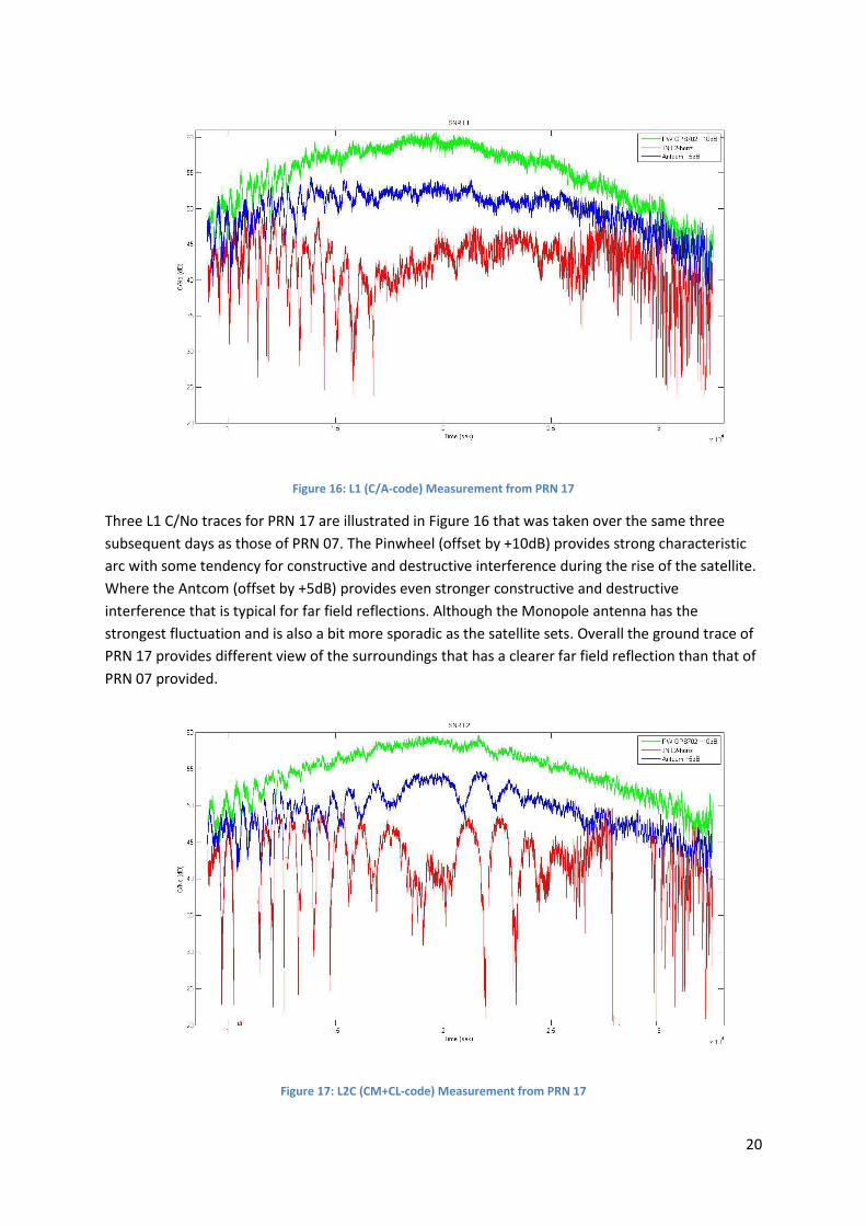
Figure 16: L1 (C/A-code) Measurement from PRN 17

Three L1 C/No traces for PRN 17 are illustrated in Figure 16 that was taken over the same three

subsequent days as those of PRN 07. The Pinwheel (offset by +10dB) provides strong characteristic

arc with some tendency for constructive and destructive interference during the rise of the satellite.

Where the Antcom (offset by +5dB) provides even stronger constructive and destructive

interference that is typical for far field reflections. Although the Monopole antenna has the

strongest fluctuation and is also a bit more sporadic as the satellite sets. Overall the ground trace of

PRN 17 provides different view of the surroundings that has a clearer far field reflection than that of

PRN 07 provided.

Figure 17: L2C (CM+CL-code) Measurement from PRN 17

21

The corresponding L2 C/No traces that were recorded simultaneous as the L1 data from PRN 17 can

be seen in Figure 17. The Pinwheel (offset by +10dB) provides a strong characteristic arc with some

small tendency for constructive and destructive interference during the rise. The Antcom (offset by

+5dB) continues to show a nice far field reflection pattern during rise but also tends to have a

limited left hand circular polarized rejection even on high evaluation angles compare to the

Pinwheel. The Monopole has the desired stronger fades and continues to be sporadic as the satellite

sets. The receiver tends to drop the trace when the fades becomes too strong as the occasionally

occurs with the Monopole antenna. In summary, more clarity for the desired fluctuations than the

L1 signal on PRN 17 and both signals on PRN 07.

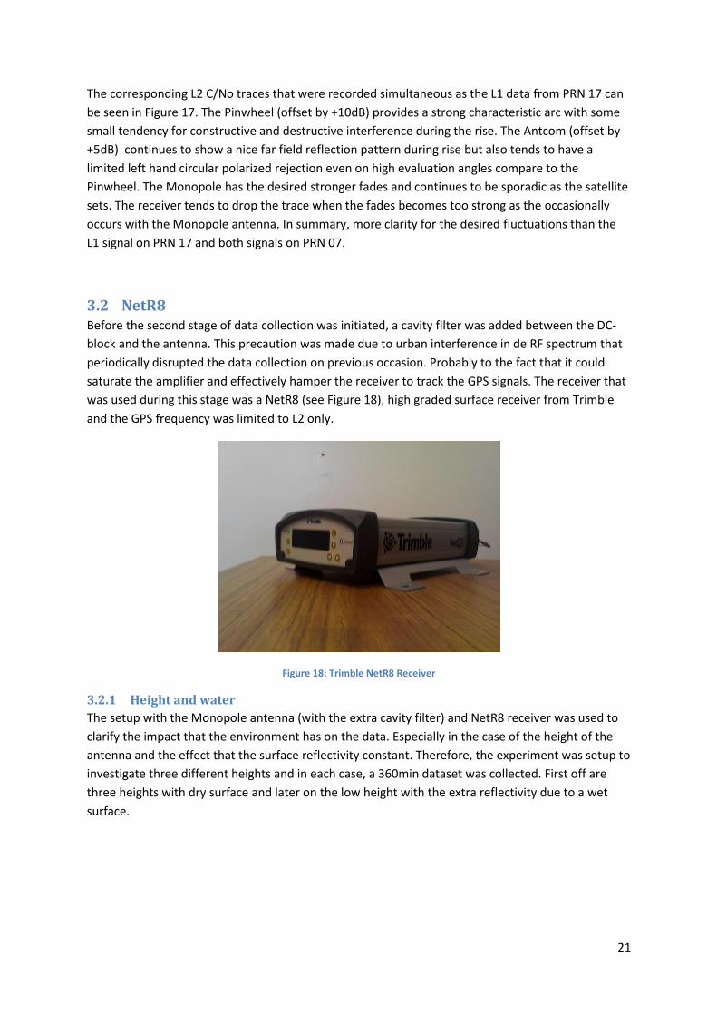
3.2 NetR8 Before the second stage of data collection was initiated, a cavity filter was added between the DC-

block and the antenna. This precaution was made due to urban interference in de RF spectrum that

periodically disrupted the data collection on previous occasion. Probably to the fact that it could

saturate the amplifier and effectively hamper the receiver to track the GPS signals. The receiver that

was used during this stage was a NetR8 (see Figure 18), high graded surface receiver from Trimble

and the GPS frequency was limited to L2 only.

Figure 18: Trimble NetR8 Receiver

3.2.1 Height and water

The setup with the Monopole antenna (with the extra cavity filter) and NetR8 receiver was used to

clarify the impact that the environment has on the data. Especially in the case of the height of the

antenna and the effect that the surface reflectivity constant. Therefore, the experiment was setup to

investigate three different heights and in each case, a 360min dataset was collected. First off are

three heights with dry surface and later on the low height with the extra reflectivity due to a wet

surface.

22

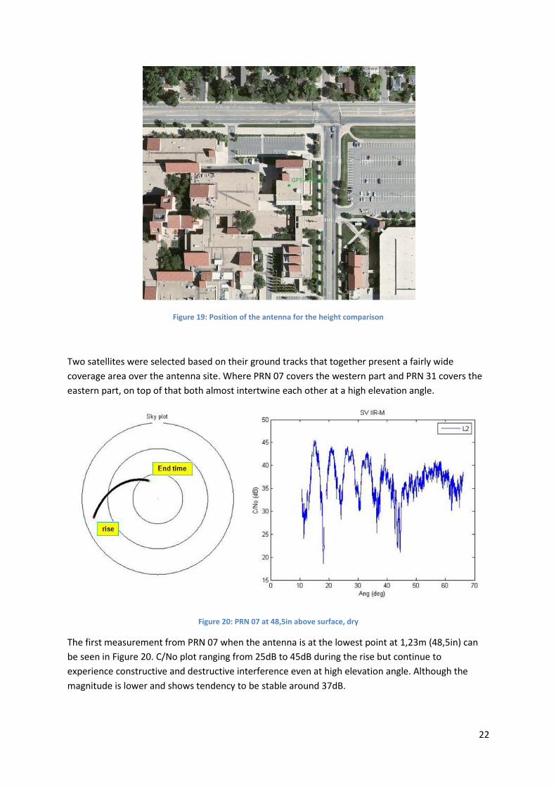
Figure 19: Position of the antenna for the height comparison

Two satellites were selected based on their ground tracks that together present a fairly wide

coverage area over the antenna site. Where PRN 07 covers the western part and PRN 31 covers the

eastern part, on top of that both almost intertwine each other at a high elevation angle.

Figure 20: PRN 07 at 48,5in above surface, dry

The first measurement from PRN 07 when the antenna is at the lowest point at 1,23m (48,5in) can

be seen in Figure 20. C/No plot ranging from 25dB to 45dB during the rise but continue to

experience constructive and destructive interference even at high elevation angle. Although the

magnitude is lower and shows tendency to be stable around 37dB.

23


During the same measurement the PRN 31 C/No plot with the antenna at 1,23m (48,5in) can be seen

in Figure 21. Overall a performance increase from PRN 07, with higher C/No value with deeper fades

ranging from 48dB as low as 22dB.

Figure 22: PRN 07 at 54in above surface, dry

As the height is increased for the second measurement, PRN 07 C/No plot show similar pattern as in

the lower height. However at a small height increase to 1,37m (54in) produce the C/No plot shown

in Figure 22 that have more signal drops during the rise of the satellite and during the higher angles

is less affected by reflected signal.

24

Figure 23: PRN 31 at 54in above surface, dry

PRN 31 does not seem so to be effected with the increase of the height to 1,37m (54in) as PRN 07

but even so, a slight performance decrease is noted in the C/No that can be seen in Figure 23. With

an increase tendency for dropping the signal.


PRN 07 C/No trace continues to deteriorate as the height it increase to 1,61m (63,5in) as can be seen

in Figure 24. The loss of performance is generally focused in the constructive and destructive

interference pattern and the increase of signal dropout even on high angle.

25


Still PRN 31 C/No values seem rather unaffected with the increase of the height, now at 1,61m

(63,5in) the C/No plot can be seen in Figure 25. It still has a signal dropout but the effect does not

seem to increase in frequency as the height of the antenna gets higher.

After three measurement on three different height the antenna was lowered to 1,23m (48,5in) and

on a rainy an adjacently day when the ground was saturated from rainfall. The following data was

recorded.

Figure 26: PRN 07 at 48,5in above surface, wet

During that adjacently day of rainfall the PRN 07 C/No values can be seen in Figure 26. The C/No

values ranging from as low 21dB up to 47dB and generally seem to get a hefty boost. Overall the

constructive and destructive interference pattern comes out nicely, even at the high elevation angle

without heavy signal loses.

26

Figure 27: PRN 31 at 48,5in above surface, wet

During the same measurement the PRN 31 C/No plot with the antenna at 1,23m (48,5in) can be seen

in Figure 27. An overall performance increase from PRN 07, with higher C/No value with deeper

fades ranging from 50dB as low as 21dB. Although some single drops is present.

27

3.3 SDR An SDR receiver has many advantages compare to a commercial in the box solution. Mainly the

customisation and flexibility of the post processing which could be use to optimise for the end users

need.

The previous version used in this report have only partially supported the L2C signal, however to

fully utilise the signal both the CM and CL code should be exploited for maximum effect.

3.3.1 40min data set of PRN 15

To estimate the progress of the SDR a small 40min data set was recorded and PRN 15 was singled

out to be processed. The same segment of data was also processed with the NetR8 for reference.

Figure 28: 40min data set from PRN15, NetR8

The converted RINEX file that was retrieved from the NetR8 receiver log can be seen in Figure 28.

The C/No value follows a clear constructive/deconstructive interference pattern. However under its

constraints of the sensitivity software it drops the trace every time at the lower end of the fades.

28

Figure 29: 40min data set of PRN15, SDR(CM+CL-code)

The corresponding data that was processed with the SDR can be seen in Figure 29. MATLAB SDR

processing shows the same C/No profile as the one from the NetR8, however it fails to lock on the

exact phase which hamper the SDR to keep a stable track on the satellite.

One explanation could be that it may have crept in an error in the merging process when the CM and

CL code was match together. However a far more likely explanation is that of the L2C quarter cycle

problem that was mentioned by Wübbena et al (Wübbena, Schmitz, & Bagge, 2009).

29

4 Results

4.1 Antenna comparison The benefits of using the L2 signal compared to the L1 are made clear in the simple antenna

comparison. The signals of all three antennas indicate smoother traces with stronger characteristic

for the constructive and destructive fluctuations when using the L2 signal. However, the Antcom

seems to have limited left hand circular polarized rejection. Although that antenna was constructed

for an airplane to collect the direct signal and have the airplane body as is ground plane, so

presumably the antenna will not accumulate that many left hand circular polarized signal compare

to ground base antennas on normal use.

Nevertheless, the Monopole antenna gives better multipath performance on high elevation angle

where the reflection point is closing up on the antenna.

In summary, the Monopole antenna is more open for the desired fluctuations that are characteristic

of the constructive and destructive interference. Although during the intense fades of the signal new

demands are placed on the receiver and its threshold level need to be optimised. Therefore, the

overall usage of a more openly designed antenna should give more clarity for bistatic application.

4.2 NetR8 The main reason for the differences in the two GPS satellites can be found by looking at Figure 19.

Where PRN 07 covers the area to the west that contains mostly structures, rooftops and obstacles at

roughly the same height as the antenna. PRN 31 that covers the east part have on the other hand

more open space (including a parking lot). This leads to that the far field reflections have a greater

impact to the data collected from PRN 07 than that of PRN 31.

In summary, the result indicated that the higher the antenna is placed the weaker is the influence of

the multipath, while a wet surface will increase the influence of the constructive and destructive

interference pattern compare to a dry surface.

4.3 SDR The SDR for the L2C code is under development and further improvement is needed to be applied.

But in summary the first preliminary results is promising.

30

5 Conclusions The result indicated that the higher the antenna is placed the weaker the influence of the multipath

is, while a wet surface will increase the influence compare to a dry. As expected the Monopole

antenna that has wide beams and ignores the polarization of the signal is much more open to

multipath. The advantage of that is the constructive and destructive interference comes out much

more distinctly but that in itself put some new demands on the receiver, especially in the phase of a

destructive interference on low elevation angle that may drop the SNR value below the receiver

threshold. Nevertheless, the best result was observed when the satellite is at a high elevation angle

where the reflection point is closing up on the antenna. There the other antenna is best on

suppressing the multipath, the Monopole picks up a nice pattern of the constructive and destructive

interference that only becomes clearer when the surface is wet.

31

6 Future Work Dual patch: Assess a dual patch antenna design, one with an upward and one downward looking

antenna that will take into account of the polarization of the signal. i.e. the downward looking

should be LHP and the upward looking should have a RHP affiliation. By then taking both antennas

received signal into one input for data collection should give a compact and fairly robust system.

Especially considering that both the antennas signals should together give an almost fully spherical

view where each half would be optimise for the direct respectively the reflected signal.

L2C – Sensitivity: Get the SDR code work correctly with both CM and CL tracking, solve phase

lock/data bit issues. In addition, more C/No estimators could be added for comparison etc.

Real time: A Real time L2C GPS SDR receiver should be implemented after the above issues have

been corrected and accounted for. This will enable a direct over view of the GPS signal being tracked

and give direct feedback to the user. It is also a desired attribute for the end user.

L5: Including GIOVE (Galileo In-Orbit Validation Element) measurements in the SDR implemented

and take advantage of the L5 characteristic with significantly better correlation properties. Higher

chipping rate means sharper autocorrelation peak. Longer codes give lower auto- and cross-

correlation side lobes. Longer integration time for the data-free channel means higher sensitivity.

32

7 Reference Constantine, B. (2005). Antenna Theory: Analysis And Design (3rd Edition ed.). Tempe, USA: Arizona

State University.

Falletti, E., Pini, M., & Presti, L. L. (2010, January/February). Are C/No Algorithms Equivalent in All

Situations? (G. Gibbons, Ed.) Inside GNSS , 5, pp. 20-27.

Jacobson, M. D. (2008, July). Dielectric-Covered Ground Reflectors in GPS Multipath Reception—

Theory and Measurement. IEEE GEOSCIENCE AND REMOTE SENSING LETTERS , 5, pp. 396-399.

Larson, K. M., Gutmann, E. D., Zavorotny, V. U., Braun, J. J., Williams, M. W., & Nievinski, F. G. (2009,

September 11). Can we measure Snow depth with GPS receivers? Geophysical Research Letters , 36.

Misra, P., & Enge, P. (2006). GLOBAL POSITIONING SYSTEM: Signals, Measurements, and

Performance (Second Edition ed.). Lincoln, Massachusetts, USA: Ganga-Jamuna Press.

Muthuraman, K. (2010). Tracking Techniques for GNSS Data/Pilot Signals. Geomatics Engineering.

Calgary: University Of Calgary.

Wübbena, G., Schmitz, M., & Bagge, A. (2009). Some Thoughts on Satellite Induced Phase Shifts aka

“the L2C Quarter Cycle Problem” and the Impact on RINEX and RTCM. Garbsen, Germany: Geo++,

Gesellschaft für satellitengestützte geodätische und navigatorische Technologien mbH.

MASTER'S THESIS - DiVA portal

Documents

Transcript of MASTER'S THESIS - DiVA portal