Machine Learning - دانشگاه فردوسی مشهد

زشبکه‌های‌باور‌بِی(هساختار، پارامتر ها و استنتاج از شبک)

ماشین‌یادگیری(Machine Learning)

دانشگاه‌فردوسی‌مشهد‌دانشکده‌مهندسی‌

رضا‌منصفی

4بخش

بحث‌در‌این‌گفتار‌مورد‌مطالب‌

احتمالی معرفی مدل های گرافی 1.

وابستگی و استقالل های شرطی بین متغیر های تصادفی2.

شبکه بیزیادگیری ساختار 3.

شبکه بیزیادگیری پارامتر های 4.

و انجام عملشبکه بیز استنتاج از 5.

قانون بیزطبقه بندی توسط 6.

(Naive Bayes)شبکه بیز ساده یادگیری و استنتاج 7.

2021اُكتبر 26شنبه، سه2دانشگاه فردوسی-دانشکده مهندسی -رضا منصفی -يادگيری ماشين

26-Oct-21 4

( Naïve Bayes Classifier)بیز ساده طبقه بند -7

Naïve)براساس قضیه بیز ساده كه احتمالی ساده طبقه بند های:طبقه بند بیز ساده Bayes) باویژگی هابین(سادگی-:به معنی)قویاستقاللفرض هایاستفاده

( NB)سادهبیزیادگیر:روش های بیزیناز یکی از روش های یادگیری بسیار كاربردیNaïveطبقه بند) Bayes)

-:برخی از حوزه ها عملکرد آن قابل مقایسه بادر Neural)عصبیشبکه( 1 Network )وDecision)تصمیم درختیادگیری( 2 Tree Learning)

توسطxهر مثال یادگیری كه بیز ساده برای اِعمال طبقه بند :چگونههدفتابعصفات توصیف شده، به طوری كه از مقادیر عطفی f(x)محدود مجموعهازمقدارهربتواندC باشدداشته را

(سادگی-:به معنی)قوی استقالل

P(

م لو

مع|

ولجه

م)

ن سی

پ=

P(

ل هو

جم

|م

لومع

)ی

مایت ن

سدر

=

Pل)

هوج

(من

شیپی

=

Pم)

لومع

)ه

واگ

=

A set of 14 training examples of the target concept Play Tennis, where each day is

described by the attributes 1) Outlook, 2) Temperature, 3) Humidity, and 4) Wind26-Oct-21

7

Day Outlook Temperature Humidity Wind Play Tennis

D1 Sunny Hot High Weak No

D2 Sunny Hot High Strong No

D3 Overcast Hot High Weak Yes

D4 Rain Mild High Weak Yes

D5 Rain Cool Normal Weak Yes

D6 Rain Cool Normal Strong No

D7 Overcast Cool Normal Strong Yes

D8 Sunny Mild High Weak No

D9 Sunny Cool Normal Weak Yes

D10 Rain Mild Normal Weak Yes

D11 Sunny Mild Normal Strong Yes

D12 Overcast Mild High Strong Yes

D13 Overcast Hot Normal Weak Yes

D14 Rain Mild High Strong No

بیز ساده برای مسئله یادگیری مفهوم طبقه بند بکارگیری ، تصمیمدرخت شبیه به یادگیری :كاربرد(ببردتنیس بازی لذت آلتو بتواند از آقای كه تخمین روزهایی )

مثال

نری

ه تاد

سوع

ناز

یها

ند ه ب

بقط

بیز،

با

ضفر

اللتق

اسن

بیام

تمی ه

ژگوی

)اx)

HumidityOutlook

Play

Tennis

Temperature Wind8

Note: To calculate VNB it requires 10 probabilities that can be estimated from the

training data.

Note: First, the probabilities of the

different target values can

easily be estimated based on

their frequencies over the

14 training examples

P(Play Tennis | X)

Classify: Use the Naive Bayes classifier and the training data from the table

to classify the following novel instance

P(Play Tennis | Outlook = sunny, Temperature = cool, Humidity = high, Wind = strong)

Task: Is to predict the target value (yes or no) of the target concept

PlayTennis for this new instance

Instantiating to fit the current task, the target value VNB

is given by

Note: In the final expression that xi has been instantiated using the

particular attribute values of the new instance

26-Oct-21 9

?

26-Oct-2110

P P(P)

Yes 9/14 = 0.64

No 5/14 = 0.36

O P P(O | P)

Sunny Yes 2/9 = 0.22

Sunny No 3/5 = 0.60

Overcast Yes 4/9 = 0.44

Overcast No 0/5 = 0.0

Rain Yes 3/9 = 0.33

Rain No 2/5 = 0.40

T P P(T | P)

Hot Yes 2/9 = 0.22

Hot No 2/5 = 0.40

Mild Yes 4/9 = 0.44

Mild No 2/5 = 0.40

Cool Yes 3/9 = 0.33

Cool No 1/5 = 0.20

H P P(H | P)

High Yes 3/9 = 0.33

High No 4/5 = 0.80

Normal Yes 6/9 = 0.66

Normal No 1/5 = 0.20

W P P(W | P)

Strong Yes 3/9 = 0.33

Strong No 3/5 = 0.60

Weak Yes 6/9 = 0.66

Weak No 2/5 = 0.40

Outlook

Play

Tennis

Temperature Humidity Wind

P(P1ayTennis = yes) = 9/14 = 0.64

P(P1ayTennis = no) = 5/14 = 0.36

Estimate: Similarly, the conditional probabilities. For example, those for

Wind = strong are

P(Wind = strong | PlayTennis = yes) = 3/9 = 0.33

P(Wind = strong | PlayTennis = no) = 3/5 = 0.60

Calculate VNB: Using these probability estimates and similar estimates for the remaining attribute values, calculate VNB according as follows

(now omitting attribute names for brevity)

P(yes) P(sunny | yes) P(cool | yes) P(high | yes) P(strong | yes) =

0.64 * 0.22 * 0.33 * 0.33 * 0.33 = 0.0053

P(no) P(sunny | no) P(cool | no) P(high | no) P(strong | no) =

0.36 * 0.6 * 0.2 * 0.8 * 0.6 = 0.0206

Result: The Naive Bayes classifier assigns the target value PlayTennis = no

to this new instance, based on the probability estimates learned from the training data

Normalizing: The above quantities to sum to one we can calculate the conditional probability that the target value is no, given the observed attribute values

Result: This probability is 0.0206 / (0.0206 + 0.0053) = 0.795 = %79.526-Oct-21 11

Overcast, Cool, High, Strong

C1 = yes 9/14 * 4/9 * 3/9 * 3/9 * 3/9 = 0.01 100%

C2 = no 5/14 * 0/5 * 1/5 * 4/5 * 3/5 = 0.00 0%

C1 = P(yes) * P(Overcast | yes) * P(Cool | yes) * P(High| yes) * P(Strong | yes)

C2 = P(no) * P(Overcast | no) * P(Cool | no) * P(High| no) * P(Strong | no)

بیشینهروشبهپارامتر هاتخمیندلیلبه:توجه

Maximum)درست نمایی Likelihood)احتمال

نمی باشدمنطقیكهصفرتنیسبازیانجام

26-Oct-21 13

?P(Play Tennis | Outlook = Overcast, Temperature = cool, Humidity = high, Wind = strong)

? , Cool , High , Strong

P P(P)

Yes 12/20

No 8/20

O P P(O | P)

Sunny Yes 3/12

Sunny No 4/8

Overcast Yes 5/12

Overcast No 1/8

Rain Yes 4/12

Rain No 3/8

T P P(T | P)

Hot Yes 3/12

Hot No 3/8

Mild Yes 5/12

Mild No 3/8

Cool Yes 4/12

Cool No 2/8

H P P(H|P)

High Yes 4/11

High No 5/7

Normal Yes 7/11

Normal No 2/7

W P P(W|P)

Strong Yes 4/11

Strong No 4/7

Weak Yes 7/11

Weak No 3/7

C1 = Yes 12/20 * 4/12 * 4/11 * 4/11 = 0.026 40%

C2 = No 8/20 * 2/8 * 5/7 * 4/7 = 0.040 60%

احتمال هامحاسبهآن وقتوOمتغیرحذفابتدا

14

? P(Play Tennis | Outlook = ?, Temperature = cool, Humidity = high, Wind = strong)

The ClassifierThe Bayes Naive classifier selects the most likely classification VNB given the attribute

values a1 , a2 , …… an.

This results in:

We generally estimate P(ai | vj) using m-estimates:

where:

n = the number of training examples for which v = vj

nc = number of examples for which v = vj and a = ai

p = a priori estimate for P(ai | vj)

m = the equivalent sample size

Car theft Example: Attributes are 1) Color , 2) Type , 3) Origin, and

the subject, stolen can be either 1) yes or 2) no.

Training example: We want to classify a Red Domestic SUV.

Note: There is no example of a Red Domestic SUV in our data set.

Note: Looking back at equation

we can see how to compute this.

We need to calculate the probabilities

26-Oct-21 15

26-Oct-21 17

Yes: No:

Red: Red:

n = 5 n = 5

n_c = 3 n_c = 2

p = 0.5 p = 0.5

m = 3 m = 3

SUV: SUV:

n = 5 n = 5

n_c = 1 n_c = 3

p = 0.5 p = 0.5

m = 3 m = 3

Domestic: Domestic:

n = 5 n = 5

n_c = 2 n_c = 3

p = 0.5 p = 0.5

m = 3 m = 3

Looking at P(Red | Yes), we have 5 cases where vj = Yes , and in 3 of those cases ai = Red.

So for P(Red | Yes), n = 5 and nc = 3.

Note that all attribute are binary (two possible values).

We are assuming no other information so, p = 1 / (number-of-attribute-values) = 0.5 for all of

our attributes.

Our m value is arbitrary,

(We will use m = 3) but consistent for all attributes.

Now we simply apply equation (3) using the precomputed values of n , nc, p, and m.

We have P(Yes) = 0.5 and P(No) = 0.5,

so we can apply equation.

For v = Yes, we have

P(Yes) * P(Red | Yes) * P(SUV | Yes) * P(Domestic | Yes) = 0.5 * 0.56 * 0.31 * 0.43 = 0.037

and for v = No, we have

P(No) * P(Red | No) * P(SUV | No) * P(Domestic | No) = 0.5 * 0.43 * 0.56 * 0.56 = 0.069

Since 0:069 > 0:037, our example gets classified as ’NO’

26-Oct-21 18

26-Oct-21 19

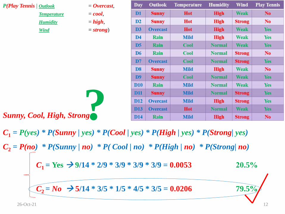
Underflow Prevention

Multiplying lots of probabilities, which are between 0 and 1 by definition, can result in

floating-point underflow.

Since log(xy) = log(x) + log(y), it is better to perform all computations by summing

logs of probabilities rather than multiplying probabilities.

Class with highest final un-normalized log probability score is still the most probable.

positionsi

jijCc

NB cxPcPc )|(log)(logargmaxj

TANطبقه بند (Tree Augmented Naïve Bayes)

. کندمیاستفادهخودساختاربه عنوان(باشدداشتهمی توانددیگربینازوالدیکتنهاویژگیهر)درختیکاز

Naïveبهنسبتباالتریکارآییویژگی هابیناستقاللفرضنداشتندلیلبهطبقه بنداین Bayesدارد

.داردنیازمحاسباتانجامویادگیریبرایبیش تریزماندرختیساختاریادگیریدلیلبهاما

.اددافزایشراویژگی هربرایمجازوالد هایتعدادمی توانکلیبه طور

K-Dependence Bayesian Classifier (k-DBC):kاستویژگیهربرایمجازوالد هایتعدادبیان گر.

Naïveطبقه بند:مثال Bayes0یک-DBCو

DBC-1یکTANطبقه بند

.می باشد26-Oct-21 20

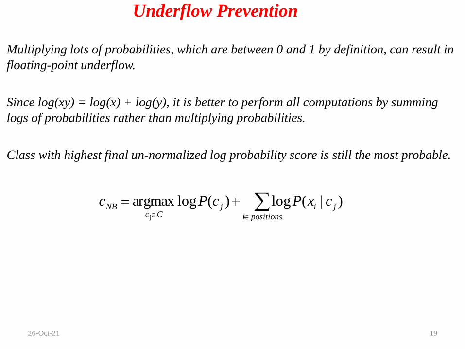
Bayesian Learning

Bayesian reasoning provides a probabilistic approach to inference.

It is based on the assumption that the quantities of interest are governed by

probability distributions and that optimal decisions can be made by reasoning

about these probabilities together with observed data.

It is important to machine learning because it provides a quantitative approach

to weighing the evidence supporting alternative hypotheses.

Bayesian reasoning provides the basis for learning algorithms that directly

manipulate probabilities, as well as a framework for analyzing the operation of

other algorithms that do not explicitly manipulate probabilities.

2021اُكتبر 26شنبه، سه 21-دانشکده مهندسی -رضا منصفی -يادگيری ماشين

دانشگاه فردوسی مشهد

Bayes Theorem

Goal: In machine learning often interest is in determining the best hypothesis

from some space H, given the observed training data D.

Define: The best hypothesis is that to demand the most probable hypothesis, given

the data D plus any initial knowledge about the prior probabilities of the

various hypotheses in H.

Bayes theorem: Provides a direct method for calculating such probabilities.

Provides a way to calculate the probability of a hypothesis based on its prior

probability P(h), the probabilities of observing various data given the

hypothesis P(D | h), and the observed data itself P(D).

P(h): The initial probability that hypothesis h holds, before we have observed the

training data.

P(h) called the prior probability of h and may reflect any background

knowledge we have about the chance that h is a correct hypothesis.

2021اُكتبر 26شنبه، سه 22

Note: If no such prior knowledge, then simply assign the same prior

probability to each candidate hypothesis.

P(D): P(D) to denote the prior probability that training data D will be

observed (i.e., the probability of D given no knowledge about which

hypothesis holds).

P(D | h): P(D | h) to denote the probability of observing data D given some

world in which hypothesis h holds.

P(x | y): P(x | y) to denote the probability of x given y.

P (h | D): In machine learning problems are interested in the probability

P (h | D) that h holds given the observed training data D. P (h | D)

is called the posterior probability of h, because it reflects our

confidence that h holds after have seen the training data D.

Note: The posterior probability P(h | D) reflects the influence of the

training data D, in contrast to the prior probability P(h), which is

independent of D.2021اُكتبر 26شنبه، سه23

دانشگاه فردوسی مشهد-دانشکده مهندسی -رضا منصفی -يادگيری ماشين

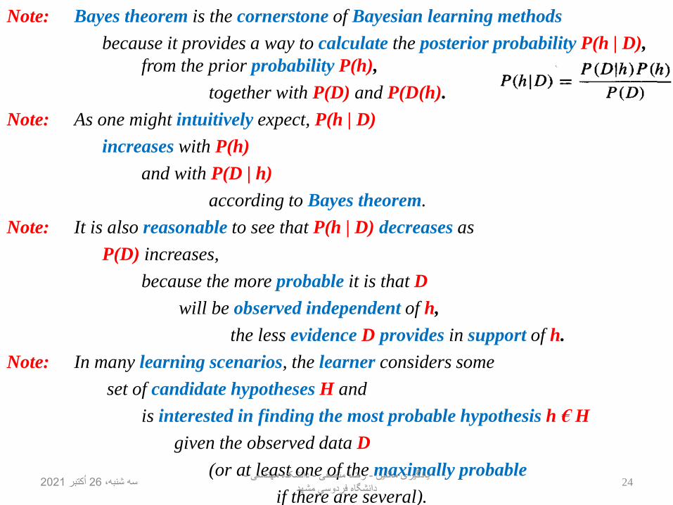
Note: Bayes theorem is the cornerstone of Bayesian learning methods

because it provides a way to calculate the posterior probability P(h | D),

from the prior probability P(h),

together with P(D) and P(D(h).

Note: As one might intuitively expect, P(h | D)

increases with P(h)

and with P(D | h)

according to Bayes theorem.

Note: It is also reasonable to see that P(h | D) decreases as

P(D) increases,

because the more probable it is that D

will be observed independent of h,

the less evidence D provides in support of h.

Note: In many learning scenarios, the learner considers some

set of candidate hypotheses H and

is interested in finding the most probable hypothesis h € H

given the observed data D

(or at least one of the maximally probable

if there are several). 2021اُكتبر 26شنبه، سه 24

-دانشکده مهندسی -رضا منصفی -يادگيری ماشين


MAP : Any such maximally probable hypothesis is called a

maximum a posteriori (MAP) hypothesis.

Note: Can determine the MAP hypotheses by using Bayes theorem

to calculate the posterior probability of

each candidate hypothesis.

MAP: More precisely, we will say that hMAP is

a MAP hypothesis provided


Note: The final step above we dropped the term P(D)

because it is a constant

independent of h.



Note: In some cases, we will assume that every hypothesis in H is equally probable

a priori (P(hi) = P(hj)

for all hi and hj in H).

Note: Need only consider the term

P(D | h) to find the most probable hypothesis.

P(D | h): P(D | h) is often called the likelihood

of the data D given h,

and any hypothesis that

maximizes P(D | h) is called a

Maximum Likelihood (ML)

hypothesis, hML.

Note: In order to make clear the connection to

machine learning problems, we

introduced Bayes theorem above by

referring to the data D as training examples of

some target function and referring to

H as the space of candidate target functions.

2021اُكتبر 26شنبه، سه 26-دانشکده مهندسی -رضا منصفی -يادگيری ماشين


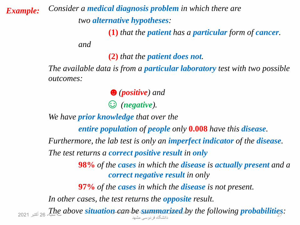
Example: Consider a medical diagnosis problem in which there are

two alternative hypotheses:

(1) that the patient has a particular form of cancer.

and

(2) that the patient does not.

The available data is from a particular laboratory test with two possible

outcomes:

☻(positive) and

☺ (negative).

We have prior knowledge that over the

entire population of people only 0.008 have this disease.

Furthermore, the lab test is only an imperfect indicator of the disease.

The test returns a correct positive result in only

98% of the cases in which the disease is actually present and a

correct negative result in only

97% of the cases in which the disease is not present.

In other cases, the test returns the opposite result.

The above situation can be summarized by the following probabilities:2021اُكتبر 26شنبه، سه 27



P(☻ | Cancer) P( Cancer) = 0.98 * 0.08 = 0.0078

P(☻ | ¬Cancer) P(¬Cancer) = 0.03 * 0.992 = 0.0298


P(Cancer) = 0.08 P(¬Cancer) = 0,992

P(☻ | Cancer) = 0.98 P(☺ | Cancer) = 0.02

P(☻ | ¬Cancer) = 0.03 P(☺ | ¬Cancer) = 0.97

Suppose we now observe a new patient for whom

the lab test returns a positive result.

Should we diagnose the patient as having cancer or not?

The maximum a posteriori hypothesis can be found using

Thus, hMAP = ¬Cancer.

The exact posterior probabilities can also be determined

by normalizing the above quantities so that they sum to 1.

P(Cancer |☻ ) = (0.0078) / (0.0078 + 0.298) = 0.21

This step is warranted because Bayes theorem states that the

posterior probabilities are just

the above quantities

divided by the probability of the data, P(☻)-دانشکده مهندسی -رضا منصفی -يادگيری ماشين


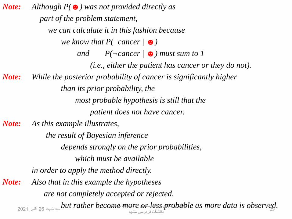
Note: Although P(☻) was not provided directly as

part of the problem statement,

we can calculate it in this fashion because

we know that P( cancer | ☻)

and P(¬cancer | ☻) must sum to 1

(i.e., either the patient has cancer or they do not).

Note: While the posterior probability of cancer is significantly higher

than its prior probability, the

most probable hypothesis is still that the

patient does not have cancer.

Note: As this example illustrates,

the result of Bayesian inference

depends strongly on the prior probabilities,

which must be available

in order to apply the method directly.

Note: Also that in this example the hypotheses

are not completely accepted or rejected,

but rather become more or less probable as more data is observed.2021اُكتبر 26شنبه، سه 29



2021اُكتبر 26شنبه، سه-دانشکده مهندسی -رضا منصفی -يادگيری ماشين

دانشگاه فردوسی مشهد30

Estimation: Two terms based on the training data.

Note: Easy to estimate each of the P(vj) simply by counting the frequency

with which each target value vj occurs in the training data.

Important Note: Estimating the different P (al , a2 , ….an | vj) terms in this fashion is

not feasible unless we have a very, very large set of training data.

Problem: The number of these terms is equal to the number of

possible instances times the number of possible target values.

How: Need to see every instance in the instance space many times in order

to obtain reliable estimates.

26-Oct-2131

N.B classifier: Is based on the simplifying assumption that the attribute values

are conditionally independent given the target value.

How: The assumption is that given the target value of the instance,

the probability of observing the conjunction al , a2 , ….an

is just the product of the probabilities for the individual attributes:

Naive Bayes classifier:

The approach used by the naive Bayes classifier.

VNB = the target value output by the Naive Bayes classifier.

Note: In NB classifier the number of distinct P(ai | vj) terms that must

be estimated from the training data is just the number of distinct

attribute values times the number of distinct target values

a much smaller number than if we were to estimate the

P(a1, a2 . . . an | vj) terms as first contemplated.

26-Oct-2132

Summarize: The Naive Bayes learning method involves a learning step

in which the various P(vj) and P(ai | vj) terms are estimated,

based on their frequencies over the training data!!!!!!

Learned Hypothesis: The set of these estimates corresponds to the learned

hypothesis.

Classification: This hypothesis is then used to classify each new instance

by applying the rule

Note: Whenever the naive Bayes assumption of conditional independence is

satisfied, this naive Bayes classification VNB is identical to the MAP

classification.

Note: One interesting difference between the Naive Bayes learning method and

other learning methods we have considered is that there is no explicit search

through the space of possible hypotheses (in this case, the space of possible

hypotheses is the space of possible values that can be assigned to the

various P(vj) and P(ai | vj) terms).

Note: Instead, the hypothesis is formed without searching, simply by counting the

frequency of various data combinations within the training examples.

26-Oct-21 33

Machine Learning - دانشگاه فردوسی مشهد

Documents

Transcript of Machine Learning - دانشگاه فردوسی مشهد