Reliable Machine Learning in Feedback Systems
203
Reliable Machine Learning in Feedback Systems Sarah Dean Electrical Engineering and Computer Sciences University of California, Berkeley Technical Report No. UCB/EECS-2021-170 http://www2.eecs.berkeley.edu/Pubs/TechRpts/2021/EECS-2021-170.html August 3, 2021
-
Upload
khangminh22 -
Category
Documents
-
view
1 -
download
0
Transcript of Reliable Machine Learning in Feedback Systems

Reliable Machine Learning in Feedback Systems
Sarah Dean
Electrical Engineering and Computer SciencesUniversity of California, Berkeley
Technical Report No. UCB/EECS-2021-170
http://www2.eecs.berkeley.edu/Pubs/TechRpts/2021/EECS-2021-170.html
August 3, 2021

Copyright © 2021, by the author(s).All rights reserved.
Permission to make digital or hard copies of all or part of this work forpersonal or classroom use is granted without fee provided that copies arenot made or distributed for profit or commercial advantage and that copiesbear this notice and the full citation on the first page. To copy otherwise, torepublish, to post on servers or to redistribute to lists, requires prior specificpermission.

Reliable Machine Learning in Feedback Systems
by
Sarah Ankaret Anderson Dean
A dissertation submitted in partial satisfaction of the
requirements for the degree of
Doctor of Philosophy
in
Electrical Engineering and Computer Sciences
in the
Graduate Division
of the
University of California, Berkeley
Committee in charge:
Professor Benjamin Recht, Chair
Professor Francesco Borrelli
Associate Professor Moritz Hardt
Summer 2021

Reliable Machine Learning in Feedback Systems
Copyright 2021
by
Sarah Ankaret Anderson Dean

1
Abstract
Reliable Machine Learning in Feedback Systems
by
Sarah Ankaret Anderson Dean
Doctor of Philosophy in Electrical Engineering and Computer Sciences
University of California, Berkeley
Professor Benjamin Recht, Chair
Machine learning is a promising tool for processing complex information, but it remains an
unreliable tool for control and decision making. Applying techniques developed for static
datasets to realworldproblems requires grapplingwith the effects of feedback and systems
that change over time. In these settings, classic statistical and algorithmic guarantees do
not always hold. How do we anticipate the dynamical behavior of machine learning
systems before we deploy them? Towards the goal of ensuring reliable behavior, this
thesis takes steps towards developing an understanding of the trade-offs and limitations
that arise in feedback settings.
In Part I, we focus on the application of machine learning to automatic feedback control.
Inspired by physical autonomous systems, we attempt to build a theoretical foundation
for the data-driven design of optimal controllers. We focus on systems governed by linear
dynamics with unknown components that must be characterized from data. We study
unknown dynamics in the setting of the Linear Quadratic Regulator (LQR), a classical
optimal control problem, and show that a procedure of least-squares estimation followed
by robust control design guarantees safety and bounded sub-optimality. Inspired by the
use of cameras in robotics, we also study a setting in which the controller must act on
the basis of complex observations, where a subset of the state is encoded by an unknown
nonlinear and potentially high dimensional sensor. We propose using a perception map,
which acts as an approximate inverse, and show that the resulting perception-control loop
has favorable properties, so long as either a) the controller is robustly designed to account
for perception errors or b) the perception map is learned from sufficiently dense data.
In Part II, we shift our attention to algorithmic decision making systems, where machine
learning models are used in feedback with people. Due to the difficulties of measure-
ment, limited predictability, and the indeterminacy of translating human values into
mathematical objectives, we eschew the framework of optimal control. Instead, our goal
is to articulate the impacts of simple decision rules under one-step feedback models. We

2
first consider consequential decisions, inspired by the example of lending in the presence
of credit score. Under a simple model of impact, we show that several group fairness
constraints, proposed to mitigate inequality, may harm the groups they aim to protect.
In fact, fairness criteria can be viewed as a special case of a broader framework for de-
signing decision policies that trade off between private and public objectives, in which
notions of impact and wellbeing can be encoded directly. Finally, we turn to the setting of
recommendation systems, which make selections from a wide array of choices based on
personalized relevance predictions. We develop a novel perspective based on reachability
that quantifies agency and access. While empirical audits show that models optimized
for accuracy may limit reachability, theoretical results show that this is not due to an in-
herent trade-off, suggesting a path forward. Broadly, this work attempts to re-imagine the
goals of predictive models ubiquitous in machine learning, moving towards new design
principles that prioritize human values.

i
To my family.

ii
Contents
Contents ii
1 Introduction 11.1 Data-Driven Optimal Control . . . . . . . . . . . . . . . . . . . . . . . . . . . 3
1.2 Feedback in Social-Digital Systems . . . . . . . . . . . . . . . . . . . . . . . . 4
I Data-Driven Optimal Control 7
2 System Level Analysis and Synthesis 82.1 Introduction . . . . . . . . . . . . . . . . . . . . . . . . . . . . . . . . . . . . . 8
2.2 From Linear Controllers to System Responses . . . . . . . . . . . . . . . . . . 8
2.3 Optimal Linear Control . . . . . . . . . . . . . . . . . . . . . . . . . . . . . . . 13
2.4 System Level Synthesis . . . . . . . . . . . . . . . . . . . . . . . . . . . . . . . 16
2.5 Finite Dimensional Approximations . . . . . . . . . . . . . . . . . . . . . . . 20
3 Learning to Control the Linear Quadratic Regulator 233.1 Introduction . . . . . . . . . . . . . . . . . . . . . . . . . . . . . . . . . . . . . 23
3.2 System Identification through Least-Squares . . . . . . . . . . . . . . . . . . 29
3.3 Robust Synthesis . . . . . . . . . . . . . . . . . . . . . . . . . . . . . . . . . . 37
3.4 Sub-Optimality Guarantees . . . . . . . . . . . . . . . . . . . . . . . . . . . . 43
3.5 Numerical Experiments . . . . . . . . . . . . . . . . . . . . . . . . . . . . . . . 48
3.6 Conclusion and Open Problems . . . . . . . . . . . . . . . . . . . . . . . . . . 53
3.7 Omitted Proofs . . . . . . . . . . . . . . . . . . . . . . . . . . . . . . . . . . . 56
4 Perception-Based Control for Complex Observations 624.1 Introduction . . . . . . . . . . . . . . . . . . . . . . . . . . . . . . . . . . . . . 62
4.2 Bounded Errors via Robust Generalization . . . . . . . . . . . . . . . . . . . . 66
4.3 Robust Perception-Based Control . . . . . . . . . . . . . . . . . . . . . . . . . 70
4.4 Bounded Errors via Uniform Convergence . . . . . . . . . . . . . . . . . . . . 74
4.5 Certainty Equivalent Perception-Based Control . . . . . . . . . . . . . . . . . 79
4.6 Experiments . . . . . . . . . . . . . . . . . . . . . . . . . . . . . . . . . . . . . 80

iii
4.7 Conclusion and Open Problems . . . . . . . . . . . . . . . . . . . . . . . . . . 86
4.8 Omitted Proofs . . . . . . . . . . . . . . . . . . . . . . . . . . . . . . . . . . . 88
II Feedback in Social-Digital Systems 97
5 Fairness and Wellbeing in Consequential Decisions 985.1 Introduction . . . . . . . . . . . . . . . . . . . . . . . . . . . . . . . . . . . . . 98
5.2 Delayed Impact of Fair Decisions . . . . . . . . . . . . . . . . . . . . . . . . . 102
5.3 Impact-Aware Decisions . . . . . . . . . . . . . . . . . . . . . . . . . . . . . . 107
5.4 Optimality of Threshold Policies . . . . . . . . . . . . . . . . . . . . . . . . . 113
5.5 Main Characterization Results . . . . . . . . . . . . . . . . . . . . . . . . . . . 116
5.6 Simulations . . . . . . . . . . . . . . . . . . . . . . . . . . . . . . . . . . . . . . 121
5.7 Conclusion and Discussion . . . . . . . . . . . . . . . . . . . . . . . . . . . . . 125
5.8 Omitted Proofs . . . . . . . . . . . . . . . . . . . . . . . . . . . . . . . . . . . 126
6 Reachability in Recommender Systems 1356.1 Introduction . . . . . . . . . . . . . . . . . . . . . . . . . . . . . . . . . . . . . 135
6.2 Recommenders and Reachability . . . . . . . . . . . . . . . . . . . . . . . . . 138
6.3 Computation via Convex Optimization . . . . . . . . . . . . . . . . . . . . . . 142
6.4 Impact of Preference Model Geometry . . . . . . . . . . . . . . . . . . . . . . 147
6.5 Audit Demonstration . . . . . . . . . . . . . . . . . . . . . . . . . . . . . . . . 152
6.6 Conclusion and Open Problems . . . . . . . . . . . . . . . . . . . . . . . . . . 158
6.7 Additional Experimental Details . . . . . . . . . . . . . . . . . . . . . . . . . 160
Bibliography 170

iv
Acknowledgments
I received a huge amount of support from my collaborators, mentors, family, friends,
and the broader UC Berkeley community during my PhD work. It has been wonderful to
be surrounded by so many great people, and I have thoroughly enjoyed the time I have
spent in this beautiful place.
It’s hard to say what my PhD research would have looked like without the guidance
of my advisor Benjamin Recht. When I began my graduate career, I wasn’t sure exactly
where I wanted to focus, and Ben showed me that I didn’t have to. Ben modeled for
me a research agenda with a wide breadth and encouraged me to follow my curiousity
while maintaining a unified rigorous perspective. Whether the topic is robust control,
recommendation systems, or computational microscopy, Ben offers wisdom, relevant
references, and abundant hot takes.
There are many others whose mentorship has been invaluable to my success. Moritz
Hardt introduced me to the world of “fair” machine learning, and taught me how to
think critically and with technical clarity about the deployment of machine learning in
social contexts. During our many joint group meetings with the MPC lab, Francesco
Borrelli challenged me to articulate the goals of my work relative to traditional controls
perspectives. When Nikolai Matni joined Ben’s group as a post-doc, he patiently taught
us about something called System Level Synthesis, a framework which has proven to be
literally fundamental to much of the work in this thesis. My education in control theory
was rounded out by the perspectives ofMurat Arcak, AndrewPackard, andClaire Tomlin.
Special thanks to Moritz, Francesco, and Claire for serving on my quals and dissertation
committee, and to Shirley, Ria, Jon, and Kosta for smoothing out bureaucratic bumps and
making sure my compute needs were met.
Perhaps the most wonderful thing about my time as a PhD student has been all my
truly excellent collaborators, who helped to shape the work presented in this dissertation.
It has been a pleasure to formulate andwork through problems of data-driven controlwith
Horia Mania, Nik, Stephen Tu, and Vickie Ye. I deeply enjoyed thinking about fairness
and wellbeing with Lydia Liu, Esther Rolf, and Max Simchowitz, and I’m thankful for the
wisdom of Joshua Blumenstock and Daniel Björkegren, who helped to ground us in the
perspective of welfare economics. I am indebted to everyone at Canopy, especially Brian
Whitman and Sarah Rich, for introducing me to the rich problem space of recommender
systems in an inspiring real-world setting. Working through reachability with Mihaela
Curmei helped immensely with clarifying my thoughts on these ideas.
I have been fortunate to work with many others. My collaborations with Andrew
Taylor, Ryan Cosner, Victor Doronbantu, Aaron Ames, and Yisong Yue brought me into
the world of nonlinear control. Ugo Rosolia taught me about receding horizon control,
including how to race a car autonomously. I would never have gottenmy hands dirty with
hardware without Aurelia Guy or Rohan Sinha, who, along with Vickie, turned a dream
of racing-from-pixels into a reality. I’m grateful to Deirdre Quillen for entertaining my
fascinationwith ice skating robots. The best research code I’vewrittenwas in collaboration

v
with Mihaela, Wenshuo Guo, Karl Krauth, and Alex Zhao. Zack Phillips and Laura
Waller taught me how to think about optimization within the context of a larger system,
a perspective which carries over into the rest of my work. Co-organizing GEESE with
McKane Andrus, Roel Dobbe, Nitin Kohli, and Tom Gilbert, Nate Lambert, and Tom
Zick expanded my horizons, and our many conversations changed the way I think about
technology. The entire Modest Yachts slack has been a source of entertainment and
information and it would be remiss not to mention Yasaman Bahri, Ross Boczar, Orianna
DeMasi, Sara Fridovich-Keil, Eric Jonas, John Miller, Juanky Perdomo, Becca Roelofs,
Ludwig Schmidt, Vaishaal Shankar, and Shivaram Venkataraman.
Finally, crucial to my happiness and success are my friends, whose support has been
a constant since our days at Scotia-Glenville schools and on Penn’s campus; my partner
Pavlo Manovi, who I am lucky to share a life with; and my family, who made me who I
am today.

1
Chapter 1
Introduction
Manymodern digital systems—fromautomotive vehicles to socialmedia platforms—have
unprecedented abilities tomeasure, store, and process data. Optimism about the potential
to benefit from this data is driven by parallel progress in machine learning, where huge
datasets and vast computational power have led to advances in complex tasks like image
recognition and machine translation. However, many applications go beyond processing
complex information to acting on the basis of it—moving from classifying, categorizing,
and translating to making decisions and taking actions. Applying techniques developed
for static datasets to real world problems requires grappling with the effects of feedback
and systems that change over time. In these settings, classic statistical and algorithmic
guarantees do not always hold. Even rigorously evaluating performance can be difficult.
How do we anticipate the behavior of machine learning systems before we deploy them?
Can we design them to ensure good outcomes? What are the fundamental limitations
and trade-offs?
In this thesis, we develop principled techniques for a variety of dynamical settings,
towards a vision of reliablemachine learning. Thiswork draws on tools and concepts from
control theory, which has a long history of formulating guarantees about the behavior
of dynamical systems, optimization, which provides a language to articulate goals and
tradeoffs, and of course machine learning, which uses data to understand and act on the
world. Machine learning models are designed to make accurate predictions, whether
about the trajectory of an autonomous vehicle, the likelihood of a loan repayment, or the
level of engagement with a news article. Traditionally concieved of in the framework of
static supervised learning, these models become part of a dynamical system as soon as
they are used to take actions that affect the environment (Figure 1.1). Whether the context
is steering an autonomous vehicle, approving a loan, or recommending a piece of content,
incorporating the learned model into policy gives rise to a feedback loop.
There are problems associated with the use of static models in dynamic environments.
Whether due to distribution shift, partial observability, or error accumulation, their pre-
dictive abilities may fail in feedback settings. Supervised learning is usually designed
to guaranteed good average case performance, but a lane detector that works well on

CHAPTER 1. INTRODUCTION 2
predictionobservation model
training data
policy
action
predictionobservation model
training data
Figure 1.1: Though machine learning models are often trained with a static supervised
learning framing in mind (left), when deployed, they become part of a feedback loop
(right).
average may still misclassify a particular image and cause a crash. Furthermore, the sta-
tistical correlations exploited to make accurate predictions may in fact contain biases or
other harmful patterns that we wish to avoid propagating. Considering an applicant’s
zip code in a lending decision may be statistically optimal, but lead to practices of redlin-
ing. Recommending videos with objectionable content might increase engagement, but
at a detriment to the viewer’s mental health. Contending with these challenges requires
thinking carefully about how machine learning models are used, and designing policies
that ensure desirable outcomes and are robust to errors.
In the following chapters, we consider several settings, broadly categorized into two
parts: data-driven optimal control and feedback in social-digital systems. In Part I,
we show how to combine machine learning and robust control to design data-driven
policies with non-asymptotic performance and safety guarantees. Chapter 2 reviews a
framework that enables policy analysis and synthesis for systemswith uncertain dynamics
and measurement errors. In Chapter 3, we consider the setting of a linear system with
unknown dynamics and study the sample complexity of a classic optimal control problem
with safety constraints. In Chapter 4, we look instead to challenges presented by complex
sensing modalities and develop guarantees for perception-based control. Turning from
the dynamics of physical systems to impact in social ones, in Part II, we consider learning
algorithms that interact with people. In Chapter 5, we characterize the relationship
between fairness andwellbeing in consequential decisionmaking. We focus on the setting
of content recommendation in Chapter 6, and develop a method for characterizing user
agency in interactive systems. In the remainder of this chapter, we introduce andmotivate
the settings for the chapters to follow.

CHAPTER 1. INTRODUCTION 3
1.1 Data-Driven Optimal ControlHaving surpassedhumanperformance in video games [MKS+15] andGo [SHM+16], there
has been a renewed interest in applying machine learning techniques to planning and
control. In particular, there has been a considerable amount of effort in developing new
techniques for continuous control where an autonomous system interacts with a physical
environment [DCHSA16; LFDA16]. Despite some impressive results in domains like
manipulation [ABC+20], recent years have seen both driver and pedestrian fatalities due
to malfunctions in automated vehicle control systems [Boa17; Boa20; Nat17]. Contending
with errors arising from learned models is different from traditional notions of process
andmeasurement noise. How canwe ensure that our newdata-driven automated systems
are safe and robust?
In Part I of this thesis, we attempt to build a foundation for the theoretical understand-
ing of how machine learning interfaces with control by analyzing simple optimal control
problems. We develop baselines delineating the possible control performance achievable
given a fixed amount of data collected from a system with an unknown component. The
standard optimal control problem aims to find a control sequence that minimizes a given
cost. We assume a dynamical systemwith state GC ∈ R= can be acted on by a control DC ∈ R<and obeys the dynamics
GC+1 = 5C(GC , DC , FC) (1.1.1)
where FC is the process noise. The control action is allowed to depend on observations
HC ∈ R3 of the system state, which may be partial and imperfect: HC = 6C(GC , EC) where ECis the measurement noise. Optimal control then seeks to minimize
minimize 2(G0, D0, G1, . . . , G)−1, D)−1, G))subject to GC+1 = 5C(GC , DC , FC)
HC = 6C(GC , EC). (1.1.2)
Here, 2(·) denotes a cost function which depends on the trajectory, and the input DC is
allowed to depend on all previous measurements and actions. In this generality, prob-
lem (1.1.2) encapsulates many of the problems considered in the reinforcement learning
literature. It is also a difficult problem to solve generally, but for restricted settings, classic
approaches in control theory offer tractable solutions when the dynamics and measure-
ment models are known.
We study this problem when components of it are unknown and must be estimated
from data. Even in the case of linear dynamics, it is challenging to reason about the
effects of machine learning errors on the evolution of an uncertain system. Chapter 2
covers background on linear systems and controllers that is crucial to our investigations.
It presents an overview of System Level Synthesis, a recently developed framework for
optimal control that allows us to handle uncertainty in a transparent and analytically
tractable manner.

CHAPTER 1. INTRODUCTION 4
In Chapter 3, we study howmachine learning interfaceswith control when the dynam-
ics of the system are unknown and the state can be observed exactly. We analyze one of
the most well-studied problems in classical optimal control, the Linear Quadratic Regulator(LQR). In this setting, the system to be controlled obeys linear dynamics, and we wish
to minimize some quadratic function of the system state and control action. We further
investigate tradeoffs with safety by considering the additional requirement that both the
state and input satisfy linear constraints. This problem has been studied for decades in
control. The unconstrained version has a simple, closed form solution on the infinite
time horizon and an efficient, dynamic programming solution on finite time horizons.
The constrained version has received much attention within the Model Predictive Control
(MPC) community. By combining linear regression with robust control, we bound the
number of samples necessary to guarantee safety and performance.
In Chapter 4, we turn to a setting inspired by the fact that incorporating rich, perceptual
sensing modalities such as cameras remains a major challenge in controlling complex
autonomous systems. We focus on the practical scenario where the underlying dynamics
of a system are well understood, and it is the interaction with a complex sensor that is
the limiting factor. Specifically, we consider controlling a known linear dynamical system
for which partial state information can only be extracted from nonlinear and potentially
high dimensional observations. Our approach is to design a virtual sensor by learning a
perception map, i.e., a map from complex observations to a subset of the state. Showing
that errors in the perception map do not accumulate and lead to instability requires
generalization guarantees stronger than are typical in machine learning. We show that
either robust control or sufficiently dense data can guarantee the closed-loop stability and
performance of such a vision based control system.
1.2 Feedback in Social-Digital SystemsFrom credit scores to video recommendations, manymachine learning systems that inter-
act with people have a temporal feedback component, reshaping a population over time.
Lending practices, for example, can shift the distribution of debt and wealth in the popu-
lation. Job advertisements allocate opportunity. Video recommendations shape interests.
Machine learning algorithms used in these contexts are mostly trained to optimize a sin-
gle metric of performance. The decisions made by such algorithms can have unintended
adverse side effects: profit-maximizing loans can have detrimental effects on borrowers
[ST19] and fake news can undermine democratic institutions [Per17].
However, it is difficult to explicitly model or plan around the dynamical interactions
between populations and algorithms. Unlike in physical systems, there are difficulties
of measurement, limited predictability [SLK+20], and the indeterminacy of translating
human values into mathematical objectives. Actions are usually discrete: an acceptance
or a rejection, choosing a particular piece of content to recommend. Rather than attempt
to design a policy that optimizes a questionable objective subject to incorrect dynamical

CHAPTER 1. INTRODUCTION 5
models, our goal is to develop a framework for articulating the impacts of simple decision
rules. We therefore investigate methods for quantifying and incorporating considerations
of impact without using the full framing of optimal control. This work attempts to re-
imagine the goals of predictive models ubiquitous in machine learning, moving towards
new design principles that prioritize human values.
Chapter 5 focuses on consequential decision making. From medical diagnosis and
criminal justice to financial loans and humanitarian aid, consequential decisions increas-
ingly rely on data-driven algorithms. Existing scholarship on fairness in automated
decision making criticizes unconstrained machine learning for its potential to harm his-
torically underrepresented or disadvantaged groups in the population [Exe16; BS16].
Consequently, a variety of fairness criteria have been proposed as constraints on standard
learning objectives. Even though these constraints are clearly intended to protect the dis-
advantaged group by an appeal to intuition, a rigorous argument to that effect is often
lacking. In Chapter 5, we contextualize group fairness criteria by characterizing their
delayed impact. By framing the problem in terms of a temporal measure of wellbeing,
we see that static criteria alone cannot ensure favorable outcomes. We then consider
an alternate framework: dual optimization of institutional (e.g. profit) and individual
(e.g. welfare) objectives directly. Decisions constrained to obey fairness criteria can be
equivalently viewed through the dual objective lens by defining welfare in a particular
group-dependent way. This insight, arising from the equivalence between constrained
and regularized optimization, shows that fairness constraints can be viewed as a special
case of balancing multiple objectives.
Chapter 6 focuses on recommendation systems, which offer a distinct set of challenges.
Through recommendation systems, personalized preference models mediate access to
many types of information on the internet. Aiming to surface content that will be con-
sumed, enjoyed, and highly rated, these models are primarily designed to accurately
predict individuals’ preferences. The focus on improving model accuracy favors systems
in which human behavior becomes as predictable as possible—effects which have been
implicated in unintended consequences like polarization or radicalization. In Chapter 6,
we attempt to formalize some of the values at stake by considering notions of user control
and access. We investigate reachability as a way to characterize user agency in interactive
systems. We develop a metric that is computationally tractable and can be used to audit
dynamical properties of a recommender system prior to deployment. Our experimental
results show that accurate predictive models, when used to sort information, can un-
intentionally make portions of the content library inaccessible. Our theoretical results
show that there is no inherent trade-off, suggesting that it is possible to design learning
algorithms which provide agency while maintaining accuracy.
Ultimately, the integration of data-driven automation into important domains requires
us to understand and guarantee properties like safety, equity, agency, and wellbeing. This
is a challenge in dynamic and uncertain systems. The work presented in Part I takes a
step towards building a theoretical foundation for what it takes to guarantee safety in
data-driven optimal control. There is a further challenge in formally defining important

CHAPTER 1. INTRODUCTION 6
properties as tractable technical specifications. This is especially true for qualitative and
contextual concepts like agency and wellbeing. The work presented in Part II takes a step
towards evaluating proposed technical formalisms and articulating new ones. Progress
along both of these thrusts is necessary to enable reliable machine learning in feedback
systems.

7
Part I
Data-Driven Optimal Control

8
Chapter 2
System Level Analysis and Synthesis
2.1 IntroductionIt is difficult to reason about the trajectory of uncertain dynamical systems. One source
of uncertainty is noise: process noise perturbs the evolution of the system, measurement
noise corrupts measurements of the system state. Another source of uncertainty arises
when the dynamics or measurement models are not fully known. The behavior of the
system depends on not only on the values of the unknown components, be they noise
processes or models, but on the control inputs. Designing control laws that are safe and
stable requires accounting for all possible trajectories of an uncertain system.
Of course, control theoryhas longdealtwith these challenges. Theproblemof feedback
control is to mitigate the perturbation of process noise based on measurements of the
system state, noisy though they may be. The field of robust control has developed an
abundance of design methods for systems with uncertain dynamics and measurement
models. Despite this rich history, classical methods do not readily offer an accounting for
how the magnitude of the uncertainty degrades the optimality of the controller, or how
much uncertainty is tolerable when needing to keep a system safe.
In this section, we review a recently developed framework for linear control synthesis
that allows us to grapple with uncertainty in a transparent and analytically tractable
manner. The machinery that we review plays an important role in Chapters 3 and 4. This
chapter uses material first presented in papers coauthored with Horia Mania, Nikolai
Matni, BenjaminRecht, StephenTu, andVickieYe [DMMRT20; DTMR19; DMRY20; DR21].
2.2 From Linear Controllers to System ResponsesThe evolution of a linear system is determined by its initial condition G0 and the dynamics
equation
GC+1 = �GC + �DC + FC (2.2.1)

CHAPTER 2. SYSTEM LEVEL ANALYSIS AND SYNTHESIS 9
where � ∈ R=×= and � ∈ R=×< are the state transition matrices, DC ∈ R< is the control input,
and FC ∈ R= is the process noise, also called the disturbance. The process noise is often
assumed to be stochastic, zero mean, and independent over time. It can alternatively be
modeled as bounded and adversarial; both can be handled in a straightforward manner.
Measurements, or system outputs, take the form
HC = �GC + EC (2.2.2)
where � ∈ R3×= is the measurement matrix and EC ∈ R3 is the measurement noise. As
before, this noise process is often assumed to be stochastic, but bounded and adversarial
models can be handled as well.
We now show that when linear systems are in feedback with linear controllers, the
trajectory can be written as a linear function of the process and measurement noise.
State FeedbackA state feedback controller relies on perfect measurements of the system state. As a moti-
vating example, a static state feedback control policy , i.e., let DC = GC . Then, the closed
loop map from the disturbance process (F0, F1, . . . ) to the state GC and control input DC at
time C is given by
GC = (� + � )CG0 +∑C−1
:=0(� + � ):−1FC−: ,
DC = (� + � )CG0 +∑C−1
:=0 (� + � ):−1FC−: .
(2.2.3)
This follows by substituting the static control policy and unrolling the recursion in (2.2.1).
Letting F−1 = G0, ΦG(:) := (� + � ):−1, and ΦD(:) := (� + � ):−1
, we can rewrite (2.2.3)
as [GCDC
]=
C+1∑:=1
[ΦG(:)ΦD(:)
]FC−: , (2.2.4)
where (ΦG(:),ΦD(:)) are called the closed-loop system response elements induced by the static
controller . For any stable closed-loop system, i.e. the spectral radius �(�+ � ) < 1, the
matrix powers decay,
lim
C→∞(� + � )C = 0 .
Therefore, as long as stabilizes the system (�, �), the system response elements are well
defined on infinite horizons.
Though more difficult to write in closed-form, a similar argument can be made for
any controller which is a linear function of the state and its history. Therefore, the
expression (2.2.4) is valid for any linear dynamic controller. Though we conventionally
think of the control policy as a functionmapping states to input, whenever such amapping
is linear, both the control input and the state can be written as linear functions of the

CHAPTER 2. SYSTEM LEVEL ANALYSIS AND SYNTHESIS 10
disturbance signal (FC)C≥0. This immediately makes transparent the effect of the process
noise on the system trajectories.
With such an identification, the linear dynamics require that the system response
variables (ΦG(:),ΦD(:))must obey the constraints
ΦG(1) = � , ΦG(: + 1) = �ΦG(:) + �ΦD(:) , ∀: ≥ 1 . (2.2.5)
As we describe in detail in Section 2.4, these constraints are in fact both necessary and
sufficient. Therefore, designing linear controllers is equivalent to designing system re-
sponses to noise. This is useful because the state feedback parameterization generally
leads to non-convex expressions. Inspecting (2.2.3), it is clear that convex expressions
of GC and DC will be non-convex in . On the other hand, since the relation in (2.2.4) is
linear, convex constraints on state and input translate to convex constraints on the system
response elements.
Output FeedbackAn output feedback controller must compute control inputs on the basis of measurements.
Whenever this controller is a linear function of themeasurements, it is also a linear function
of the states and measurement noise variables. Therefore, like in the state feedback case,
it will be possible to view the closed-loop system in terms of linear system response
variables. The main difference is that there are two sources of noise driving the system,
and therefore four system response variables of interest.
As an illustrative example, consider the classic Luenberger observer combined with a
static feedback policy. The observer uses measurements to update a state estimate
GC+1 = �GC + �DC + !(HC − �GC) , (2.2.6)
where ! is the static gain matrix and G0 is the initial estimate. The static controller is
DC = GC . By defining the auxiliary state variable 4C = GC − GC the closed-loop dynamics
can be written as [GC+1
4C+1
]=
[� + � �
0 � − !�
] [GC4C
]+
[� 0
0 !
] [F:
E:
].
Therefore, we can unroll the recursion in a similar manner to the state feedback case
and write the trajectory in terms of a convolution with the system response variables[GCDC
]=
C+1∑:=1
[ΦGF(:) ΦGE(:)ΦDF(:) ΦDE(:)
] [FC−:EC−:
]. (2.2.7)
As long as the controller and observer are both stable, i.e. �(�+� ) < 1 and �(�−!�) < 1,
the system response elements are well-defined on infinite horizons.

CHAPTER 2. SYSTEM LEVEL ANALYSIS AND SYNTHESIS 11
The expression (2.2.7) holds for any controller that is a linear function of the history of
system outputs. Therefore, for linear output feedback control, the trajectory can bewritten
as a linear function of the process and measurement noise. This makes transparent the
effect of these two noise processes on the system trajectories.
The dynamics and measurement model require that the system responses obey the
constraints
ΦGF(1) = � ,[ΦGF(: + 1) ΦGE(: + 1)
]= �
[ΦGF(:) ΦGE(:)
]+ �
[ΦDF(:) ΦDE(:)
],[
ΦGF(: + 1)ΦDF(: + 1)
]=
[ΦGF(:)ΦDF(:)
]� +
[ΦGE(: + 1)ΦDE(: + 1)
]� . (2.2.8)
As in the state feedback case, these constraints are in fact both necessary and sufficient.
Therefore, designing linear controllers is equivalent to designing system responses, and
because the relation in (2.2.7) is linear, convex constraints on state and input translate to
convex constraints on the system response elements.
Signals and Transfer FunctionsTo make guarantees about the behavior of systems on arbitrarily long time horizons, it
is necessary to reason about their infinitely long trajectories (G0, G1, . . . ). As the previous
subsections illustrate, these trajectories are the result of a convolution between system
response variables and noise signals. It is therefore pertinent to develop notation and
machinery for dealing with these objects.
First, for notational convenience, we turn to themore compact representation of transferfunctions. The signal (G0, G1, . . . ) that results from the convolution between the operator
(Φ(1),Φ(2), . . . ) and the signal (F−1, F0, F1, . . . ) is written as
x = Φw .
One way to obtain this representation is by definition. We can directly define the
notation of signals x = (G0, G1, . . . ) and linear operators Φ = (Φ(1),Φ(2), . . . ). Then, definethe multiplication operation between these objects to correspond to a linear convolution,
so that
x = Φw ⇐⇒ GC =
C+1∑:=1
Φ(:)FC−: ∀C ≥ 0 .
An alternative is to take a I-transform and work in the frequency domain. The fre-
quency domain variable I can informally be thought of as a time-shift operator act-
ing on signals, i.e., I(GC , GC+1, . . . ) = (GC+1, GC+2, . . . ). We define Φ(I) = ∑∞C=1
I−CΦ(C),x(I) = ∑∞
C=0I−CGC and similarly for w(I). By manipulating summations and polynomials,
we have
x(I) =( ∞∑:=1
I−:Φ(:)) ( ∞∑
:=−1
I−:F:
)=
∞∑C=0
C+1∑:=1
I−CΦ(:)FC−: ,

CHAPTER 2. SYSTEM LEVEL ANALYSIS AND SYNTHESIS 12
as desired. The argument I of the transfer function and signals is often dropped. This
representation is common in the controls literature.
Finally, it can be convenient to alternatively represent these objects as semi-infinite
vectors and block Toeplitz matrices. Here, we define
x =G0
G1
...
, Φ =
Φ(0) 0 0 . . .
Φ(1) Φ(0) 0 . . .
Φ(2) Φ(1) Φ(0)...
.... . .
.Then the convolution follows by matrix-vector multiplication. This representation makes
some properties evident by analogy to matrices. It can also be useful for implementation
and computation when considering finite horizons or truncations of signals and system
responses.
The three representations above are in some sense equivalent (see, e.g. the introductory
chapters of the textbook by Dahleh and Diaz-Bobillo [DD94]). In the remainder of this
chapter, Chapter 3, and Chapter 4, we use letters such as G and � to denote vectors and
matrices, and boldface letters such as x and G to denote infinite horizon signals and linear
convolution operators. We write G0:C = (G0, G1, . . . , GC) for the history of signal x up to time
C. For a function GC ↦→ 5C(GC), we write f(x) to denote the signal
(5C(GC)
)∞C=0
. We will denote
the Cth element as G[C] = �(C) and x[C] = GC . We will also denote �[C : 1] as the block row
vector of system response elements of G
�[C : 1] =[�(C) . . . �(1)
],
and similarly for �[1 : C] with indices reversed. Linear dynamic controllers can also be
written in this notation, i.e. u = Ky. We use the shorthand DC = K(H0:C) to indicate the
dependence between inputs and measurements at the Cth time step.
Under this notation, we have for state and output feedback respectively,[xu
]=
[ΦxΦu
]w or
[xu
]=
[Φxw ΦxvΦuw Φuv
] [wv
]. (2.2.9)
The affine realizability constraints can be rewritten for state feedback as[I� − � −�
] [ΦxΦu
]= � ,
and for output feedback as[I� − � −�
] [Φxw ΦxvΦuw Φuv
]=
[� 0
],
[Φxw ΦxvΦuw Φuv
] [I� − �−�
]=
[�
0
].

CHAPTER 2. SYSTEM LEVEL ANALYSIS AND SYNTHESIS 13
This follows from (2.2.5) and (2.2.7). I can also been derived from writing the linear
dynamics in signal notation and then rearranging the expressions,
Ix = �x + �u +w, y = �x + v .
We finish this discussion by introducing norms and normed spaces on signals and
transfer functions. For a thorough introduction to the functional analysis commonly used
in control theory, see the text by Zhou, Doyle, and Glover [ZDG96]. As is standard, we
let ‖G‖? denote the ℓ?-norm of a vector G. For a matrix ", we let ‖"‖? denote its ℓ? → ℓ?operator norm. We will consider the ℋ2, ℋ∞, and ℒ1 norms, which are infinite horizon
analogs of the Frobenius, spectral, and ℓ∞→ ℓ∞ operator norms of a matrix, respectively:
‖G‖ℋ2=
√√ ∞∑:=0
‖�(:)‖2�, ‖G‖ℋ∞ = sup
‖w‖2=1
‖Gw‖2, ‖G‖ℒ1= sup
‖w‖∞=1
‖Gw‖∞ .
As theℋ∞ and ℒ1 norms are induced norms, they satisfy the sub-multiplicative property
‖GH‖ ≤ ‖G‖‖H‖. Theℋ2 norm satisfies
‖GH‖ℋ2≤ ‖G‖ℋ∞ ‖H‖ℋ2
.
We remark that it is also possible to define the ℋ∞ system norm in terms of the power
norm [YG14], defined as ‖x‖?>F := (lim)→∞ 1
)
∑):=0‖G: ‖2
2)1/2.
In this thesis,we restrict our attention to the function spaceℛℋ∞, consistingofdiscrete-time stable matrix-valued transfer functions. We use
1
Iℛℋ∞ to denote the set of transfer
functions G such that IG ∈ ℛℋ∞. A linear time-invariant transfer function is stable if
and only if it is exponentially stable. Therefore, we further define for positive values �
and � ∈ [0, 1)
ℛℋ∞(�, �) :=
{G =
∞∑:=0
�(:)I−: | ‖�(:)‖2 ≤ ��: , : = 0, 1, 2, ...}. (2.2.10)
This set contains transfer functions that satisfy a specified decay rate in the spectral norm
of their impulse response elements.
2.3 Optimal Linear ControlWe now turn to optimal control. While the previous section developed machinery use-
ful for understanding the general behavior of linear systems in feedback with linear
controllers, this section focuses on the design of linear controllers. Putting aside our
discussion of system responses for now, we introduce optimal control problems written

CHAPTER 2. SYSTEM LEVEL ANALYSIS AND SYNTHESIS 14
in terms of state and control signals. In particular we consider
minimizeK 2(x, u)subject to GC+1 = �GC + �DC + FC
HC = �GC + ECDC = K(H0:C),
(2.3.1)
for GC the state, DC the control input, FC the process noise, EC the measurement noise, K a
linear time-invariant operator, and 2(x, u) a suitable cost function.Control design depends on how the disturbance w and measurement error v are
modeled, as well as performance objectives. Table 2.1 summarizes several common cost
functions that arise from different system desiderata and different classes of disturbances
and measurement errors ��� := (w, v). By modeling the disturbance and sensor noise as
being drawn from different signal spaces, and by choosing correspondingly suitable cost
functions, we can incorporate practical performance, safety, and robustness considerations
into the design process. We now review prominent examples of optimal control problems
that we revisit in Chapters 3 and 4.
Example 2.1 (Linear Quadratic Regulator). Suppose that the cost function is given by
2(x, u) = Ew
[lim
)→∞
1
)
)∑C=0
G>C &GC + D>C 'DC
],
for some specified positive definite matrices & and ' and FCi.i.d.∼ N(0, �). Further suppose
that the controller is given full information about the system, i.e. � = � and EC = 0 such
that the measurement model collapses to HC = GC . Then the optimal control problem
reduces to the familiar Linear Quadratic Regulator (LQR) problem
minimize EF
[lim
)→∞
1
)
)∑C=0
G>C &GC + D>C 'DC
]subject to GC+1 = �GC + �DC + FC .
(2.3.2)
For stabilizable (�, �), and detectable (�, &), this problem has a closed-form stabilizing
controller based on the solution of the discrete algebraic Riccati equation (DARE) [ZDG96].
This optimal control policy is linear, and given by
DLQR
C = −(�>%� + ')−1�>%�GC =: LQRGC , (2.3.3)
where % is the positive-definite solution to the DARE defined by (�, �, &, ').
Example 2.2 (Linear Quadratic Gaussian Control). Suppose that we have the same setup
as the previous example, but that now the measurement is instead given by HC = �GC + EC

CHAPTER 2. SYSTEM LEVEL ANALYSIS AND SYNTHESIS 15
for some � such that the pair (�, �) is detectable, and that ECi.i.d.∼ N(0, �). Then the optimal
control problem reduces to the Linear Quadratic Gaussian (LQG) control problem, the
solution to which is:
DLQG
C = LQRGC , (2.3.4)
where GC is the Kalman filter estimate of the state at time C. The steady state update rule
for this estimate also linear, and is given by
GC+1 = �GC + �DC + !LQG(HC+1 − �(�GC + �DC)) ,
for filter gain !LQG = −%�>(�%�> + �)−1where % is the solution to the DARE defined
by (�>, �>, � , �). This optimal output feedback controller satisfies the separation principle,meaning that the optimal controller LQR is computed independently of the optimal
estimator gain !LQG.
The LQR and LQG problems best model sensor noise, aggregate behavior, and natural
processes arising from statical-mechanical systems. The robust version of these problems
considers instead the worst-case quadratic cost for ℓ2 or power-norm bounded noise. This
is theℋ∞ optimal control problem, which has a rich history [ZDG96].
In our final example, we consider robustness in the sense of worst-case deviations
and ℓ∞ bounded noise. In particular, the ℒ1 control problem [DP87] minimizes the cost
function
2(x, u) = sup
w,vC≥0
&1/2GC'1/2DC
∞
for FC and EC such that ‖FC ‖∞ ≤ 1, ‖EC ‖∞ ≤ 1 for all :. The optimal controller does not
obey the separation principle, and as such, there is no clear notion of an estimated state.
This formulation best accommodates real-time safety constraints and actuator saturation,
which we motivate in the following example.
Example 2.3 (Reference Tracking). Consider a reference tracking problem where it is
known that both the distances between waypoints and sensor errors are instantaneously
ℓ∞ bounded, and we want to ensure that the system remains within a bounded distance
of the waypoints. Denoting the system state as ��� and the waypoint sequence as r, the costfunction is
2(���, u) = sup
‖AC+1−AC ‖∞≤1,‖EC ‖∞≤1,C≥0
&1/2(�C − AC)'1/2DC
∞.
If we specify costs by & = diag(1/12
G,8) and ' = diag(1/12
D,8), then as long as the optimal
cost is less than 1, we can guarantee bounded tracking error |�8 ,C− A8 ,: | ≤ 1G,8 and actuation
|D8 ,C | ≤ 1D,8 for all possible realizations of the waypoint and sensor error processes. Con-
sidering the one-step lookahead case, we can define an augmented state, i.e. GC := [�C ; AC],

CHAPTER 2. SYSTEM LEVEL ANALYSIS AND SYNTHESIS 16
Name Disturbance class Cost function Use cases
LQR/ℋ2
E[���] = 0,
E[���4] < ∞, �C i.i.d.E�
[lim
)→∞
)∑C=0
1
)G>C &GC + D>C 'DC
]Sensor noise,
aggregate behavior,
natural processes
ℋ∞‖���‖?>F ≤ 1,
or ‖���‖2 ≤ 1
sup
‖���‖?>F≤1
lim
)→∞
1
)
)∑C=0
G>C &GC + D>C 'DC ,
or sup
‖���‖2≤1
∞∑C=0
G>C &GC + D>C 'DC
Modeling error,
energy/power
constraints
ℒ1 ‖���‖∞ ≤ 1 sup
‖���‖∞≤1,C≥0
&1/2GC'1/2DC
∞
Real-time safety
constraints, actuator
saturation/limits
Table 2.1: Different noise model classes induce different cost functions, and can be used
to model different phenomenon, or combinations thereof. See texts by Zhou, Doyle, and
Glover [ZDG96] and Dahleh and Pearson [DP87] for more details.
and model waypoints as bounded disturbances, i.e. FC := AC+1 − AC . A similar formulation
exists for any )-step lookahead of the reference trajectory.
We can then formulate the following ℒ1 optimal control problem,
minimize sup‖�‖∞≤1,C≥0
&1/2GC'1/2DC
∞
subject to GC+1 = �GC + �DC + �FC ,HC = �GC + EC ,
(2.3.5)
where
� =
[� 0
0 �
], � =
[�
0
], � =
[� 0
], � =
[0
�
], &1/2 =
[&1/2 −&1/2] .
2.4 System Level SynthesisWe now formally discuss the System Level Synthesis (SLS) framework, which shows that
optimal control problems can be equivalently cast in terms of system response variables.
To motivate the state feedback case, consider an arbitrary transfer function K denoting
the map from state to control action, u = Kx. Then the closed-loop transfer matrices from
the process noise w to the state x and control action u satisfy[xu
]=
[(I� − � − �K)−1
K(I� − � − �K)−1
]w. (2.4.1)
This expression is non-convex in K, posing a problem for efficiently solving optimal
control problems. Therefore, we turn to an alternate parametrization. The following

CHAPTER 2. SYSTEM LEVEL ANALYSIS AND SYNTHESIS 17
theorem parameterizes the set of stable closed-loop transfer matrices that are achievable
by some stabilizing controller K.
Theorem 2.4.1 (state feedback Parameterization [WMD19]). The following are true:
• The affine subspace defined by[I� − � −�
] [ΦxΦu
]= � , Φx,Φu ∈
1
Iℛℋ∞ (2.4.2)
parameterizes all system responses (2.4.1) from w to (x, u), achievable by an internallystabilizing state feedback controller K.
• For any transfer matrices (Φx,Φu) satisfying (2.4.2), the controller K = ΦuΦ−1
x is internallystabilizing and achieves the desired system response (2.4.1).
In the output feedback case, for u = Ky, closed-loop transfer matrices from the process
w and measurement noise v to the state x and control action u satisfy[xu
]=
[(I� − � − �K�)−1 (I� − � − �K�)−1�K
K�(I� − � − �K)−1 K�(I� − � − �K�)−1�K
] [wv
]. (2.4.3)
Again, this expression is non-convex in K, so we turn to the system level parametrization.
Theorem 2.4.2 (output feedback Parameterization [WMD19]). The following are true:
• The affine subspace defined by Φxw,Φxv,Φuw ∈ 1
Iℛℋ∞, Φuv ∈ ℛℋ∞,[I� − � −�
] [Φxw ΦxvΦuw Φuv
]=
[� 0
],
[Φxw ΦxvΦuw Φuv
] [I� − �−�
]=
[�
0
](2.4.4)
parameterizes all system responses (2.4.3) from (w, v) to (x, u), achievable by an internallystabilizing state feedback controller K.
• For any transfer matrices (Φxw,Φxv,Φuw,Φuv) satisfying (2.4.2), the controller K = Φuv −ΦuwΦ−1
xwΦxv is internally stabilizing and achieves the desired system response (2.4.3).
Theorem 2.4.1 and 2.4.2 make formal the intuition that linear controllers are equivalent
to systemresponses constrained to lie in an affine space. As a result, optimizationproblems
over stabilizing linear controllers can be reparameterized into optimization problems over
system response variables. We will sometimes denote that a system response Φ satisfies
the realizability constraints in (2.4.2) or (2.4.4) as Φ ∈ A, where A denotes affine space
defined by (�, �) or (�, �, �) depending on the context. Theorem 2.4.1 and 2.4.2 also
describe how to recover the control law from the system responses. This controller can be
implemented via a state-space realization [AM17] or as an interconnection of the system
response elements [WMD19].

CHAPTER 2. SYSTEM LEVEL ANALYSIS AND SYNTHESIS 18
Control Costs as System NormsIn this SLS framework, many control costs (including those in Table 2.1) can be written
as system norms. We first consider the ℋ∞ and ℒ1 costs, which can be written in signal
notation as
2(x, u) = sup
‖w‖≤�F‖v‖≤�E
[&1/2x'1/2u
] ,where �F and �E respectively bound the norms of w and v and we allow ‖ · ‖ to represent
the ℓ2/power norm or ℓ∞ norm and associated induced norm. Then by substituting the
identity (2.2.9), the cost can be written as
sup
‖w‖≤�F‖v‖≤�4
[&1/2
'1/2
] [Φxw ΦxvΦuw Φuv
] [wv
] = [&1/2
'1/2
] [Φxw ΦxvΦuw Φuv
] [�F�
�E�
] .For LQR and LQG control, the control objective is equivalent to a system ℋ2 norm, a
fact that we now derive. From the expression (2.2.7), we have that
G>C &GC =C+1∑:=1
C+1∑ℓ=1
[FC−:EC−:
]> [ΦGF(:)>ΦGE(:)>
]&
[ΦGF(ℓ ) ΦGE(ℓ )
] [FC−ℓEC−ℓ
]. (2.4.5)
Then as long as the process and measurement noise are zero mean, independent from
each other and across time, and have variances �2
F and �2
E respectively,
E[G>C &GC
]=
C+1∑:=1
Tr( [�FΦGF(:)>�EΦGE(:)>
]&
[�FΦGF(:) �EΦGE(:)
] ).
A similar expression holds for the input term. We can then write
lim
)→∞
1
)
)∑C=1
E[G>C &GC + D>C 'DC
]=
∞∑C=1
Tr( [�FΦGF(C)>�EΦGE(C)>
]&
[�FΦGF(C) �EΦGE(C)
] )+ Tr
( [�FΦDF(C)>�EΦDE(C)>
]&
[�FΦDF(C) �EΦDE(C)
] )=
∞∑C=1
[& 1
2 0
0 '1
2
] [ΦGF(C) ΦGE(C)ΦDF(C) ΦDE(C)
] [�F� 0
0 �E�
] 2
�
=
[& 1
2 0
0 '1
2
] [Φxw ΦxvΦuw Φuv
] [�F� 0
0 �E�
] 2
ℋ2
.

CHAPTER 2. SYSTEM LEVEL ANALYSIS AND SYNTHESIS 19
This derivation requires only fairly general assumptions about the noise processes.
However, using system response variables implicitly assumes a linear (possibly dynamic)
controller. Thus, the equivalence between the ℋ2 norm and the LQR/LQG cost only
holds under this restricted policy class. The optimal controller is in fact a linear dynamic
controller a) in the state feedback case and b) when the noise processes are Gaussian (as
in Example 2.1 and 2.2). However, the optimal filtering procedure for more general noise
processes will not be a Kalman filter, and it may not be linear [Ber95].
Robustness to Unknown DynamicsSo far we have seen that System Level Synthesis provides a convenient parametrization
that makes transparent the effects of noise signals and allows for convex optimization.
Neither of these properties is entirely unique to SLS, and other approaches to control
synthesis are possible. However, a major benefit is in how SLS handles misspecification
in the dynamics model. In this section, we show how uncertainty in the dynamics can be
handled in a transparent manner. This allows for the computation of robust controllers
that stabilize all systems within an uncertainty set.
Althoughclassicmethods exist for computing robust controllers [Fer97; Pag95; SAPT02;
WP95], they typically require solving non-convex optimization problems, and it is not
readily obvious how to extract interpretable measures of controller performance as a
function of the size of the uncertainty. By lifting the system description into a higher di-
mensional space, SLS makes it tractable to reason analytically about uncertain dynamics.
The robust variant of Theorem 2.4.1 traces the effects of misspecification.
Theorem 2.4.3 (Robust Stability [MWA17]). Let Φx and Φu be two transfer matrices in 1
Iℛℋ∞such that [
I� − � −�] [
ΦxΦu
]= � + ∆. (2.4.6)
Then the controller K = ΦuΦ−1
x stabilizes the system described by (�, �) if and only if (� + ∆)−1 ∈ℛℋ∞. Furthermore, the resulting system response is given by[
xu
]=
[ΦxΦu
](� + ∆)−1w. (2.4.7)
Corollary 2.4.4. Under the assumptions of Theorem 2.4.3, if ‖∆‖ < 1 for any induced norm ‖ · ‖,then the controller K = ΦuΦ−1
x stabilizes the system described by (�, �).The proof of the corollary follows immediately from the small gain theorem.
To see why these results are useful, suppose that some estimate (�, �) is used for
synthesis. Then,[I� − � −�
] [ΦxΦu
]= � ⇐⇒
[I� − � −�
] [ΦxΦu
]= � +
[� − � � − �
] [ΦxΦu
].

CHAPTER 2. SYSTEM LEVEL ANALYSIS AND SYNTHESIS 20
Therefore Theorem 2.4.3 allows us to write a closed-form expression for the trajectory of
the uncertain system in terms of the designed response (Φx,Φu), and uncertainties � − �and � − �.
A similar result holds for output feedback controllers which makes transparent the
effect of uncertainty in the measurement matrix � (see e.g. work by Boczar, Matni, and
Recht [BMR18]).
2.5 Finite Dimensional ApproximationsThe System Level Synthesis framework introduced in Section 2.4 shows that optimal
control problems like (2.3.1) can be cast in terms of system response variables. However,
system responses are semi-infinite, so it is not clear how to solve the resulting optimization
problem efficiently. An elementary approach to reducing the semi-infinite program to a
finite dimensional one is to only optimize over the first ! elements of the transfer functions,
effectively taking a finite impulse response (FIR) approximation. Since these are stable
maps, we expect the effects of such an approximation to be negligible as long as the
optimization horizon ! is chosen to be sufficiently large. Later in this section, we show
that this is indeed the case.
Wefirst outlinehowtheoptimizationvariables andconstraints admitfinite-dimensional
representations. To derive the finite expressions, it is useful to consider the (truncated)
Toeplitz matrix representation of the transfer functions. The FIR approximation optimizes
over ((ΦG(C),ΦD(C))!C=1in the state feedback case and ((ΦGF(C),ΦDF(C),ΦGE(C),ΦDE(C))!C=1
in
the output feedback case. The affine realizability constraints reduce to a finite number
of linear equality constraints in the form of (2.2.5) or (2.2.8). The ℋ2 norm can be cast
as a second order cone constraint. The ℋ∞ norm can be reduced to a compact SDP as
in Theorem 5.8 of Dumitrescu [Dum07], described explicitly for SLS in Appendix G.3
of Dean et al. [DMMRT18]. The ℒ1 norm becomes an ℓ∞ → ℓ∞ operator norm on the
horizontal concatenation of system response elements, Φ[! : 1]. Finally, the controller
given by K = ΦuΦ−1
x or K = Φuv − ΦuwΦ−1
xwΦxv can be written in an equivalent state-space
realization (� , � , � , � ) via Theorems 2 and 3 of Anderson and Matni [AM17].
In the interest of clarity, for the remainder of this thesis we will present the infinite
horizon version of the optimization problems, with the understanding that finite horizon
approximations are necessary in practice. The sub-optimality results presented in Chap-
ters 3 and 4 hold up to constant factors for these approximations. We now make precise
that for sufficiently long horizons !, the effects of the approximation are negligible.

CHAPTER 2. SYSTEM LEVEL ANALYSIS AND SYNTHESIS 21
Sub-optimality of Finite ApproximationConsider a general state feedback optimal control problem cast in system response vari-
ables:
minimize
[&1/2
'1/2
] [ΦxΦu
] subject to
[I� − � −�
] [ΦxΦu
]= � ,
Φx,Φu ∈ 1
Iℛℋ∞
(2.5.1)
where ‖·‖ is any induced norm. We define cost(K) to be the norm of the system response
generated by applying the controller K = Φ−1
u Φx to the systemwith linear dynamics (�, �).The finite approximation to this problem optimizes over only the first ! impulse re-
sponse elements:
min
0≤�<1
min
Φx ,Φu ,+
1
1 − �
[&1/2
'1/2
] [ΦxΦu
] subject to
[I� − � −�
] [ΦxΦu
]= � + I−!+,
Φx =∑!C=1
I−CΦG(C), Φu =∑!C=1
I−CΦD(C) ,‖+ ‖ ≤ � .
(2.5.2)
The slack term + accounts for the error introduced by truncating the infinite response
transfer functions. This allows us to optimize over controllers that don’t necessarily force
the system to have a finite impulse response. We remark that it is possible to enforce that
the system is FIR by setting + = 0 and � = 0; the problem remains feasible whenever
(�, �) is controllable and ! is large enough. While that makes for a cruder approximation,
it avoids the additional complexity of searching over the scalar variables �.Intuitively, if the truncated tail captured by + is sufficiently small, then the finite
approximation has near optimal performance. The next result formalizes this intuition.
It shows that the cost penalty incurred decays exponentially in the horizon ! over which
the approximation is taken.
Theorem 2.5.1. Let K★ = Φ★u(Φ★
x )−1 be the controller resulting from the optimal control prob-lem (2.5.1) and suppose that Φ★
x ∈ ℛℋ∞(�★, �★). Let K! = Φ!u(Φ!
x )−1 be controller resultingfrom the finite approximation (2.5.2). Then for any 0 < � < 1, as long as
! ≥ log(2�★/�)/log(1/�★) + 1 ,
the relative sub-optimality of the finite approximation is bounded by �
cost(K!) − cost(K★)cost(K★) ≤ � .

CHAPTER 2. SYSTEM LEVEL ANALYSIS AND SYNTHESIS 22
Proof. First, notice that since the affine realizability constraint is not exactly met, by the
robustness result in Theorem 2.4.3
cost (K!) = [&1/2
'1/2
] [Φ!
xΦ!
u
](� + I−!+!)−1
.The expression can be further simplified using the properties of induced norms,
cost (K!) ≤ [&1/2
'1/2
] [Φ!
xΦ!
u
] 1
1 − ‖+!‖≤
[&1/2
'1/2
] [Φ!
xΦ!
u
] 1
1 − �!,
where the final inequality holds due to the inequality constraint ‖+ ‖ ≤ �.Next, we construct a feasible solution to (2.5.2):
Φx =
!∑C=1
I−CΦ★G (C), Φu =
!∑C=1
I−CΦ★D(C), + = −Φ★
G (! + 1), � = �★�!+1
★ . (2.5.3)
Because (Φ★x ,Φ★
u) is a solution to the original optimal control problem, the infinite system
response satisfies the affine realizability constraint for (�, �). It is straightforward to check
that the under the definition of + , the truncated affine constraints are satisfied as well.
We also have that ‖+ ‖ = ‖Φ★G (! + 1)‖ ≤ �★�!+1
★ = � by the definition of �★ and �★. By the
assumption on ! and �, �★�!+1
★ < 1.
Then by the optimality of (Φ!x ,Φ!
u, �!),
1
1 − �!
[&1/2
'1/2
] [Φ!
xΦ!
u
] ≤ 1
1 − �
[&1/2
'1/2
] [ΦxΦu
] .Notice that Φx = Φ★
x +∑∞C=!+1
I−CΦ★G (C) and Φu = Φ★
u +∑∞C=!+1
I−CΦ★D(C). Therefore, by
triangle inequality, [&1/2
'1/2
] [ΦxΦu
] ≤ [&1/2
'1/2
] [Φ★
xΦ★
u
] .Combining this chain of inequalities,
cost(K!) ≤ 1
1 − � ★ �!+1
★
cost
(K★) ≤ (
1 + 2� ★ �!+1
★
)cost
(K★) .
where the final inequality holds by the observation that1
1−G ≤ 1 + 2G whenever G ≤ 1/2,which is implied by the assumption on �.
A nearly identical result also holds for the ℋ2 norm, where in the finite problem, the
constraint on + is in terms of the ℓ2 → ℓ2 operator norm. Similar results hold when the
optimal control problem has additional constraints so long as care is taken to incorporate
the variable+ into them analogously. Finally, it is possible to generalize this to the output
feedback case, though the analogous truncated synthesis problem will search over two
auxiliary variables.

23
Chapter 3
Learning to Control the Linear QuadraticRegulator
3.1 IntroductionIn this chapter, we attempt to build a foundation for the theoretical understanding of
how machine learning interfaces with control by analyzing one of the most well-studied
problems in classical optimal control, the Linear Quadratic Regulator (LQR). This chapter
uses material first presented in papers coauthored with Horia Mania, Nikolai Matni,
Benjamin Recht, and Stephen Tu [DTMR19; DMMRT20; DMMRT18].
We assume that the system to be controlled obeys linear dynamics, and we wish to
minimize some quadratic function of the system state and control action. The optimal
control problem can be written as
minimize E[
1
)
∑)C=1
G>C &GC + D>C−1'DC−1
]subject to GC+1 = �GC + �DC + FC
. (3.1.1)
In what follows, we will be concerned with the infinite time horizon variant of the LQR
problem where we let the time horizon ) go to infinity. When the dynamics are known,
this problem has a celebrated closed form solution based on the solution of matrix Riccati
equations [ZDG96].
We will further consider the constrained version of the LQR problem, in which the
system state and control actions are linearly constrained. Wedefine the polytopic constraint
sets:
X := {G : �GG ≤ 1G}, U := {D : �DD ≤ 1D} . (3.1.2)
The incorporation of such constraints can ensure system safety (by avoiding unsafe re-
gions of the state space) and reliability (by preventing controller saturation). This richer
modeling comes at a cost: the constrained LQR problem does not have a simple closed
form solution. Nevertheless, by restricting the policy class to linear controllers, we will
develop a framework in which the problem becomes tractable.

CHAPTER 3. LEARNING TO CONTROL LQR 24
We analyze the LQR problem when the dynamics of the system are unknown, and we
can measure the system’s response to varied inputs. We will assume that we can conduct
experiments of the following form: given some initial state G0, we can evolve the dynamics
for ) time steps using any control sequence (D0, . . . , D)−1), measuring the resulting output
(G1, . . . , G)). Is it possible to keep the system safe using only the data collected?
We propose a method that couples our uncertainty in estimation with the control
design. Our main approach uses the following framework of Coarse-ID control to solve the
problem of LQR with unknown dynamics:
1. Use supervised learning to learn a coarse model of the dynamical system to be
controlled. We refer to the system estimate as the nominal system.
2. Build probabilistic guarantees about the distance between the nominal system and
the true, unknown dynamics.
3. Solve a robust optimization problem over controllers that optimizes performance of
the nominal system while penalizing signals with respect to the estimated uncer-
tainty, ensuring safe and robust execution.
For a sufficient amount of data, this approach is guaranteed to return a control policy with
small relative cost which guarantees the safety and asymptotic stability of the closed-loop
system. Though simple to state, the analysis of this procedure will take the remainder of
the chapter: Section 3.2 focus on the estimation in the second step, Section 3.3 develops a
method for synthesizing robust controllers in the third step, and Section 3.4 provides end-
to-end performance guarantees. We present numerical experiments demonstrating the
capability of this procedure in Section 3.5, and offer concluding remarks and an accounting
of open problems in Section 3.6.
Problem SettingWe fix an underlying linear dynamical system with full state observation,
GC+1 = �GC + �DC + FC , (3.1.3)
where we have initial condition G0 ∈ R= , sequence of inputs (D0, D1, . . . ) ⊆ R< , and dis-
turbance process (F0, F1, . . . ) ⊆ R= . We consider the expected infinite horizon quadratic
cost for the system (�, �) in feedback with a linear controller K:
�(�, �,K)2 :=1
�2
F
lim
)→∞
1
)
)−1∑C=0
EF[G>C &GC + D>C 'DC] .
We assume that the disturbance process is generated by any distribution which satisfies
E[FC] = 0, E[FCF>C ] = �2
F�, and independence across time, i.e., FC ⊥ F; for C ≠ :. Note that

CHAPTER 3. LEARNING TO CONTROL LQR 25
any distribution satisfying these constraints induces the same expected quadratic cost, so
it is unnecessary to specify a specific distribution. We further assume that the disturbance
is norm bounded so that it satisfies ‖FC ‖∞ ≤ AF for all : ≥ 0. This assumption makes it
possible to reason about constraints on the system state and control input on infinite time
horizons. We require that the constraints (3.1.2) are satisfied for any possible disturbance
sequence.
Putting the cost and the constraints together, the optimal control problem that acts as
our baseline is:
minimizeK �(�, �,K)subject to G0 fixed, DC = K(G0:C) ,
GC+1 = �GC + �DC + FC ,�GGC ≤ 1G , �DDC ≤ 1D ∀C ,∀{FC : ‖FC ‖∞ ≤ AF} .
(3.1.4)
Above, we search over linear dynamic stabilizing feedback controllers for (�, �) of theform u = Kx. This is made possible by the system level synthesis framework described in
the previous chapter.
As will we show, the optimal control problem given in (3.1.4) is a convex, but infinite-
dimensional problem. It is an idealized baseline to compare our actual solutions to;
our sub-optimality guarantees will be with respect to the optimal cost achieved by this
problem. It is a relevant baseline, since it optimizes for average case performance but
ensures safety for the worst-case behavior, consistent with literature on Model Predictive
Control (MPC) [MSR05; OJM08]. We remark that an alternative to (3.1.4) is to replace the
worst case constraints with probabilistic chance constraints [FGS16]. We do not workwith
chance constraints because they are generally difficult to directly enforce on an infinite
horizon; arguments around recursive feasibility using robust invariant sets are common
in the literature to deal with this issue. When the system is unconstrained, i.e. when
X = R= andU = R< , this baseline is the widely-studied classical LQR problem.
Related WorkWe first describe related work in the estimation of unknown linear systems and then turn to
connections in the literature on robust control with uncertain models and the satisfaction ofsafety constraints. We then end this review with a discussion of recent works that directly
address the LQR problem and related variants.
Estimation of unknown linear systems. Estimation of unknown linear dynamical sys-
tems has a long history in the system identification subfield of control theory. Classical
results focus on asymptotic guarantees and/or frequency domain methods [Lju99; CG00;
HJN91; Gol98]. Ourgoal is to analyze the optimality of controllers constructed fromafinite
amount of data, so we focus on non-asymptotic guarantees for state space identification.
Early results on non-asymptotic rates for parameter identification featured conservative

CHAPTER 3. LEARNING TO CONTROL LQR 26
bounds exponential in the system degree [CW02; VK08]. In the past decade, the first
polynomial time guarantees were presented in terms of predictive output performance
of the model [PIM10; HMR18]. Recently, Hazan, Singh, and Zhang [HSZ17] and Hazan
et al. [HLSZZ18] proposed a novel spectral filtering algorithm and showed that one can
compete in a regret setting in terms of prediction error. It is not clear how such prediction
error bounds can be used in a downstream robust synthesis procedure or converted into
a sub-optimality result.
In parallel to the system identification community, identification of auto-regressive
time series models is a widely studied topic in the statistics literature [BJRL15; GZ01;
KM17; MSS17; MR10]. Many of these works studied generalization for data which is not
independent over time, extending the standard learning theory guarantees. At the crux
of these arguments lie various mixing assumptions [Yu94], which limits the analysis to
stable dynamical systems. Furthermore, results from this line of research suggest that
systems with smaller mixing time (i.e. systems that are more stable) are easier to identify
(i.e. take less samples). This does not align with our empirical testing, which suggests
that identification benefits from more easily excitable systems.
Our results rely on recent work by Simchowitz et al. [SMTJR18] who take a step
towards reconciling this issue for stable systems. Since the work presented in this chapter
was published, there has been a renewed interest in providing finite data guarantees for
classic system identification procedures. For partially observed linear systems, Oymak
andOzay [OO19] andSarkar, Rakhlin, andDahleh [SRD21] present non-asymptotic results
for a Ho-Kalman-like procedure and Simchowitz, Boczar, and Recht [SBR19] propose a
semi-parametric least squares method that is consistent for marginally stable systems. In
the state observation setting, Sarkar andRakhlin [SR19] show that least-squares estimation
is consistent for a restricted class of unstable systems. Developing consistent estimators
for arbitrary unstable systems remains an open problem.
Robust controller design. For end-to-end guarantees, parameter estimation is only half
the picture. It is necessary to ensure that the computed controller guarantees stability and
performance for the entire family of systemmodels described by a nominal estimate and a
set of unknown but boundedmodel errors. This problem has a rich history in the controls
community. Whenmodeling errors are arbitrarynormbounded linear time-invariant (LTI)
operators in feedback with the nominal plant, traditional small gain theorems and robust
synthesis techniques exactly solve the problem [DD94; ZDG96]. For more structured
errors, there are sophisticated techniques based on structured singular values like �-synthesis [Doy82; FTD91; PD93; YND91] or integral quadratic constraints (IQCs) [MR97].
While theoretically appealing andmuch less conservative, the resulting synthesismethods
are both computationally intractable (although effective heuristics do exist) and difficult
to interpret analytically.
In order to bound the degradation in performance of controlling an uncertain system
in terms of the size of the perturbations affecting it, we leverage a novel parameterization

CHAPTER 3. LEARNING TO CONTROL LQR 27
of robustly stabilizing controllers based on the SLS framework [WMD19] that is reviewed
in Chapter 2. Originally developed to allow for scaling optimal and robust controller
synthesis techniques to large-scale systems, the SLS framework can be viewed as a gener-
alization of the celebrated Youla parameterization [YJB76]. We use SLS because it allows
us to account for model uncertainty in a transparent and analytically tractable way.
Since the work presented in this chapter was published, there has been a renewed
interest in robust synthesis procedures for the types of uncertainty sets that result from
estimation [US18; UFSH19; US20].
Safety constraints. Thedesign of controllers that guarantee robust constraint satisfaction
has long been considered in the context of model predictive control [BM99], including
methods that model uncertainty in the dynamics directly [KBM96], or model it as an
enlarge disturbance process [MSR05; GKM06]. These traditional works do not usually
consider identifying the unknown dynamics. Strategies for incorporating safety with
estimation of thedynamics include experiment-design inspired costs [LRH11], decoupling
learning from constraint satisfaction [AGST13], and set-membership methods rather than
parameter estimation [TFSM14; LAC17]. Due to the receding horizon nature of model
predictive controllers, this literature relies on set invariance theory for infinite horizon
guarantees [Bla99]. In this chapter, we consider the infinite horizon problem directly, and
therefore we do not require computation of invariant sets.
Themachine-learning community has begun to consider safety in reinforcement learn-
ing, where much work positions itself as ensuring safety for arbitrary dynamical systems
in lieu of providing statistical guarantees [BS15; BTSK17; DDV+18; CNDG18]. One line
of work proposes methods for modifying potentially unsafe inputs generated by arbitrary
reinforcement learning algorithms, building on ideas from robust MPC [WZ18; KBTK18].
Despite good empirical results, it remains to show whether the modified inputs success-
fully excite the system, allowing for a statistical learning rate. Most similar to our work
is that of Lu et al. [LZBRS17], who propose a method to allow excitation on top of a safe
controller, but consider only finite-time safety and require non-convex optimization to
obtain formal guarantees. Later follow-up work by Ahmadi et al. [ACST21] guarantees
safety and excitation on the basis of planning over one and two step horizons.
PAC learning and reinforcement learning. There is a body of work that focuses on
the unconstrained LQR problem from the perspective of probably-approximately-correct
(PAC) and reinforcement learning. In terms of end-to-end guarantee, our work is most
comparable to that of Fiechter [Fie97], who analyzes an identify-then-control scheme
similar to the one we propose. There are several key differences. First, our probabilistic
bounds on identification aremuch sharper, sincewe leveragemoremodern tools fromhigh
dimensional statistics. Second, Fiechter implicitly assumes that the estimated controller
induces a closed-loop that is not only stable but also contractive. While this is a very
strongassumption, contractive closed-loopassumptions are actuallypervasive throughout

CHAPTER 3. LEARNING TO CONTROL LQR 28
the early literature, as we describe below. Finally, Fiechter proposes to directly solve
the discounted LQR problem with the identified model, and takes a certainty equivalentapproach to controller synthesis, which does not take into account any uncertainty. This is
problematic for two reasons: the optimal solution to the discounted LQR problem does not
guarantee stabilization (see e.g. [PBND17]) and even if the optimal solution does stabilize
the underlying system, the certainty equivalent controller may not. Our experiments
demonstrate this behavior.
There is a body of related efforts in RL and online learning. In a seminal work,
Abbasi-Yadkori and Szepesvári [AS11] propose to use the optimism in the face of uncer-
tainty (OFU) principle for the LQR problem, by maintaining confidence ellipsoids on the
true parameter, and using the controller which, in feedback, minimizes the cost objective
the most among all systems in the confidence ellipsoid. They show that the regret of
this approach scales as O(√)), where O(·) hides problem dependent constants and poly-
logarithmic factors. However, the method is computationally intractable, and the analysis
makes the very strong assumption that the optimal closed-loop systems are contractive
for every �, � in the confidence ellipsoid. The regret bound is improved by Ibrahimi,
Javanmard, and Roy [IJR12] under additional sparsity constraints on the dynamics. More
recently, Cohen, Koren, and Mansour [CKM19] and Abeille and Lazaric [AL20] propose
computationally tractable approximations to the OFU principle based on semidefinite
programming and Lagrangian relaxation, respectively. They improve the analysis, relax-
ing some of the more restrictive assumptions, and show that the approximate methods
achieve the same regret scaling.
An alternative online approach is to use Thompson sampling [RVKOW18] for ex-
ploration. This method has been shown to achieve O(√)) regret for one dimensional
systems [AL17; AL18] or within a Bayesian framework of expected regret [OGJ17]. These
works also make the same restrictive assumption that the optimal closed-loop systems
are uniformly contractive over some known set. Recent work shows that a naive &-greedyexploration scheme in combination with the certainty equivalent controller achieves opti-
mal regret [MTR19; SF20]. In fact, the regret of this scheme does not depend directly on
the state dimension; Perdomo et al. [PSAB21] show that rather than requiring consistent
parameter recovery, the performance of certainty equivalent control scales with the pre-
diction error of the estimates. The success of the certainty equivalent controller in online
settings hinges on large enough horizons ) to guarantee small enough estimation errors.
In our framework, we construct controllers with stability and performance guarantees
even in moderate error regimes.
Many of the aforementioned works assume enough knowledge to construct an initial
stabilization controller. In recent work, Treven et al. [TCMK21] propose a data-driven
method for constructing a controller for potentially unstable systems under a Bayesian
prior.
Since the work presented in this chapter was published, additional variants of the
LQR problem have been investigated, including the partially observed setting [TMP20;

CHAPTER 3. LEARNING TO CONTROL LQR 29
LAHA20] and non-stochastic noise models [ABHKS19; HD19]. There has also been a
resurgence of interest in model-free methods, which do not rely on estimating the dynam-
ics model directly. Fazel et al. [FGKM18] show that randomized search algorithms similar
to policy gradient can learn the optimal controller with a polynomial number samples.
These ideas have also been applied to continuous time settings [MZSJ21]. Approaches
based on characterizing the value function and & function are also popular: Yang et al.
[YCHW19] study the actor critic algorithm and Krauth, Tu, and Recht [KTR19] investigate
least square temporal differences and policy improvement. Tu and Recht [TR19] present
a class of dynamics models for which there is a gap in the sample complexity of model
free and model based methods, suggesting that model based methods, such as the one
investigated here, aremore efficient, at least when it is known that the dynamics are linear.
3.2 System Identification through Least-SquaresTo estimate a coarse model of the unknown system dynamics, we turn to the simple
method of linear least squares. By running experiments in which the system starts at G0
and the dynamics evolvewith a given input, we can record the resulting state observations.
The set of inputs and outputs from each such experiment will be called a rollout, and the
resulting dataset is {(GC , DC) : 0 ≤ C ≤ )}. Therefore, we can estimate the systemdynamics
by
(�, �) ∈ arg min
(�,�)
)−1∑C=0
1
2
‖�GC + �DC − GC+1‖22. (3.2.1)
For the Coarse-ID control setting, a good estimate of error is just as important as the
estimate of the dynamics. Statistical theory allows us to quantify the error of the least
squares estimator. First, we present an illustrative theoretical analysis of the error in a
simplified setting. Then, we present results that apply in full generality.
Least Squares Estimation as a RandomMatrix ProblemWebegin by explicitly writing the form of the least squares estimator. First, fixing notation
to simplify the presentation, let Θ :=[� �
]> ∈ R(=+<)×= and let IC :=
[GCDC
]∈ R=+< . Then
the system dynamics can be rewritten, for all C ≥ 0,
G>C+1= I>C Θ + F>C .

CHAPTER 3. LEARNING TO CONTROL LQR 30
Then in a rollout, we will collect
-) :=
G>
1
G>2
...
G>)
, /) :=
I>
0
I>1
...
I>)−1
, ,) :=
F>
0
F>1
...
F>)−1
. (3.2.2)
The system dynamics give the identity
-) = /)Θ +,) .
The least squares estimator for Θ is (assuming for now invertibility of />)/)),
Θ = (/>)/))−1/>)-) = Θ + (/
>)/))
−1/>),) . (3.2.3)
Then the estimation error is given by
� := Θ − Θ = (/>)/))−1/>),) . (3.2.4)
The magnitude of this error is the quantity of interest in determining confidence sets
around estimates (�, �). However, since,) and /) are not independent, this estimator
is difficult to analyze using standard methods. We therefore begin with a simplified
procedure using Gaussian noise injection and system resets to recover an independent
data estimator in the following subsection. After that, we consider estimation from
dependent data collected during closed-loop system operation, and present results that
rely on recently developed statistical results for linear system estimation.
Simplified Gaussian SettingTo sidestep issues of data dependence, we suppose the ability to reset the system to
G0 = 0 and perform multiple system rollouts. Having the ability to reset the system to a
state independent of past observations is important for this analysis, and it could also be
Algorithm 1 Estimation of linear dynamics with independent data
1: for ℓ from 1 to # do2: G
(ℓ )0= 0
3: for C from 0 to ) − 1 do4: G
(ℓ )C+1
= �G(ℓ )C + �D
(ℓ )C + F
(ℓ )C with F
(ℓ )C
i.i.d.∼ N(0, �2
F�=) and D(ℓ )C
i.i.d.∼ N(0, �2
D�<).5: end for6: end for7: (�, �) ∈ arg min(�,�)
∑#ℓ=1
1
2‖�G(ℓ )
)−1+ �D(ℓ )
)−1− G(ℓ )
)‖2
2

CHAPTER 3. LEARNING TO CONTROL LQR 31
practically important for potentially unstable systems. We excite the systemwithGaussian
noise for # rollouts, each of length ). The resulting dataset is {(G(ℓ )C , D(ℓ )C ) : 1 ≤ ℓ ≤ #, 0 ≤
C ≤ )}, where C indexes the time in one rollout and ℓ indexes independent rollouts.
We now show the statistical rate for the least squares estimator which uses just the last
sample of each trajectory: (G(ℓ )), G(ℓ ))−1
, D(ℓ ))−1). This estimation procedure is made precise in
Algorithm 1. Our analysis ideas are analogous to those used to prove statistical rates for
standard linear regression, and they leverage tools in non-asymptotic analysis of random
matrices.
The fact that this strategy results in independent data can be seen by defining the
estimator matrix directly. The previous estimator (3.2.3) is amended to rely on -# =[G(1))
G(2))
. . . G(#))
]>, /# , and ,# , which are similarly defined. The matrices in the
estimator thus contain independent rows. To see this, define the matrices
�) =[�)−2� �)−3� . . . �
]and �) =
[�)−2 �)−3 . . . �=
]. (3.2.5)
We can unroll the system dynamics and see that
G)−1 = �)
D0
D1
...
D)−2
+ �)F0
F1
...
F)−2
. (3.2.6)
Using Gaussian excitation, DC ∼ N(0, �2
D�<) and assuming Gaussian process noise FC ∼N(0, �2
F�=) gives [G)−1
D)−1
]∼ N
(0,
[�2
D�)�>)+ �2
F�)�>)
0
0 �2
D�<
] ). (3.2.7)
Since �)�>)� 0, as long as both �D , �F are positive, this is a non-degenerate distribution.
Therefore, bounding the estimation error can be achieved via proving a result on the
error in randomdesign linear regressionwithvector valuedobservations. First, wepresent
a standard lemma which bounds the spectral norm of the product of two independent
Gaussian matrices.
Lemma 3.2.1. Fix a � ∈ (0, 1) and # ≥ 2 log(1/�). Let 5: ∈ R< , 6: ∈ R= be independentrandom vectors 5: ∼ N(0,Σ 5 ) and 6: ∼ N(0,Σ6) for 1 ≤ : ≤ # . With probability at least 1− �, #∑
:=1
5: 6>:
2
≤ 4‖Σ 5 ‖1/22‖Σ6 ‖1/2
2
√#(< + =) log(9/�) .
Lemma 3.2.1 shows that if - is =1 × # with i.i.d. N(0, 1) entries and . is # × =2 with
i.i.d. N(0, 1) entries, and - and . are independent, then with probability at least 1− � we

CHAPTER 3. LEARNING TO CONTROL LQR 32
have
‖-.‖2 ≤ 4
√#(=1 + =2) log(9/�) .
Next, we state a standard non-asymptotic bound on the minimum singular value of a
standard Wishart matrix (see e.g. Corollary 5.35 of [Ver10]).
Lemma 3.2.2. Let - ∈ R#×= have i.i.d. N(0, 1) entries. With probability at least 1 − �,√�min(->-) ≥
√# −√= −
√2 log(1/�) .
We combine the previous lemmas into a statement on the error of random design
regression.
Lemma 3.2.3. Let I1, ..., I# ∈ R= be i.i.d. from N(0,Σ) with Σ invertible. Let /> :=[I1 ... I#
]. Let , ∈ R#×? with each entry i.i.d. N(0, �2
F) and independent of /. Let� := (/>/)†/>, , and suppose that
# ≥ 8= + 16 log(2/�) . (3.2.8)
For any fixed matrix &, we have with probability at least 1 − �,
‖&�‖2 ≤ 16�F ‖&Σ−1/2‖2
√(= + ?) log(18/�)
#.
Proof. First, observe that / is equal in distribution to -Σ1/2, where - ∈ R#×= has i.i.d.
N(0, 1) entries. By Lemma 3.2.2, with probability at least 1 − �/2,√�min(->-) ≥
√# −√= −
√2 log(2/�) ≥
√#/2 .
The last inequality uses (3.2.8) combined with the inequality (0 + 1)2 ≤ 2(02 + 12). Fur-
thermore, by Lemma 3.2.1 and (3.2.8), with probability at least 1 − �/2,
‖->, ‖2 ≤ 4�F
√#(= + ?) log(18/�) .
Let ℰ denote the event which is the intersection of the two previous events. By a union
bound, P(ℰ) ≥ 1− �. We continue the rest of the proof assuming the event ℰ holds. Since
->- is invertible,
&� = &(/>/)†/>, = &(Σ1/2->-Σ1/2)†Σ1/2->, = &Σ−1/2(->-)−1->, .
Taking operator norms on both sides,
‖&�‖2 ≤ ‖&Σ−1/2‖2‖(->-)−1‖2‖->, ‖2 = ‖&Σ−1/2‖2‖->, ‖2
�min(->-).

CHAPTER 3. LEARNING TO CONTROL LQR 33
Combining the inequalities above,
‖->, ‖2�min(->-)
≤ 16�F
√(= + ?) log(18/�)
#.
The result now follows.
This lemma, in combination with the error decomposition in 3.2.4, allows us to show
a bound on the estimation errors.
Proposition 3.2.4. Assume we collect data from the linear, time-invariant system initialized atG0 = 0, using inputs DC
i.i.d.∼ N(0, �2
D�<) for C = 0, . . . , ) − 1, with ) ≥ 2. Suppose that the processnoise is FC
i.i.d.∼ N(0, �2
F�=) and that
# ≥ 8(= + <) + 16 log(4/�) .
Then, with probability at least 1− �, the least squares estimator using only the final sample of eachtrajectory satisfies both the inequality
‖� − �‖2 ≤16�F√
�min(�2
D�)�>)+ �2
F�)�>))
√(= + 2<) log(36/�)
#, (3.2.9)
and the inequality
‖� − �‖2 ≤16�F�D
√(= + 2<) log(36/�)
#. (3.2.10)
Proof. Consider the least squares estimation error (3.2.4) with modified single-sample-
per-rollout matrices. Recall that rows of the design matrix /# are distributed as indepen-
dent normals, as in (3.2.7). Then applying Lemma 3.2.3 with &� =[�= 0
]so that &��
extracts only the estimate for �, we conclude that with probability at least 1 − �/2, theexpression (3.2.9) holds as long as # ≥ 8(=+<)+16 log(4/�). Now applying Lemma 3.2.3
under the same condition on # with &� =[0 �<
], we have with probability at least
1−�/2, that the expression in (3.2.10) holds. The result follows by application of the union
bound.
There are several interesting points to make about the guarantees offered by Proposi-
tion 3.2.4. First, there are =(= +<) parameters to learn and our bound states that we need
$(= + <) measurements, each measurement providing = values. Hence, this appears to
be an optimal dependence with respect to the parameters = and <. Second, this propo-
sition illustrates that not all linear systems are equally easy to estimate. The matrices
�)�>)and �)�
>)are finite time controllability Gramians for the control and noise inputs,
respectively. These are standard objects in control: each eigenvalue/vector pair of such

CHAPTER 3. LEARNING TO CONTROL LQR 34
a Gramian characterizes how much input energy is required to move the system in that
particular direction of the state-space. Therefore �min(�2
D�)�>)+ �2
F�)�>)) quantifies the
least controllable, and hence most difficult to excite and estimate, mode of the system.
This property is captured nicely in our bound, which indicates that for systems for which
all modes are easily excitable (i.e., all modes of the system amplify the applied inputs and
disturbances), the identification task becomes easier.
Estimation in Closed-LoopWhile the bound in Proposition 3.2.4 provides interpretable insights, the procedure in
Algorithm 1 may not be practically possible. Injecting Gaussian noise into a system will
likely cause violations of state and input constraints. Instead, is necessary to simultane-
ously excite and regulate the system. We propose to learn by additively injecting bounded
noise to the control inputs computed by a safe controller. In what follows, we describe
how a controller that guarantees that the closed-loop system remains within the specified
constraint set can also ensure that enough noise is injected into the system to obtain a
statistical guarantee on learning.
We bound the errors of the least squares estimator when the system is controlled by
u = Kx + ��� , (3.2.11)
where each ��� = (�0, �1, . . . ) is stochastic, independent across time, and ℓ∞-bounded with
‖�C ‖∞ ≤ A�.The bulk of the proof for the statistical rate comes from a general theorem regarding
linear-response time series data from Simchowitz et al. [SMTJR18]. We assume that w and
��� are both zero-mean sequenceswith independent coordinates and finite fourthmoments,
assumptions which are quickly verified for common distributions such as uniform on a
compact interval or over a discrete set of points. Before stating the main estimation result,
we introduce the notation: 0 . 1 (resp. 0 & 1) denotes that there exists an absolute
constant � > 0 such that 0 ≤ �1 (resp. 0 ≥ �1).
Theorem 3.2.5. Fix a failure probability � ∈ (0, 1). Suppose the disturbance (FC)C≥0 and theexcitation (�C)C≥0 are zero-mean sequences with independent coordinates and
EFC [FC(8)2] = �2
F , EFC [F:(8)4] . �4
F , E�C [�C(8)2] = �2
� , E�C [�C(8)4] . �4
� .
Assume for simplicity that �� ≤ �F , and that the stabilizing controller K in (3.2.11) achieves aSLS response Φx ∈ 1
Iℛℋ∞(�G , �),Φu ∈ 1
Iℛℋ∞(�D , �). Let �2
:= =�2
G + 3�2
D . Then as long asthe trajectory length ) satisfies the condition:
) & (= + <) log
(<�2
D
�+ �2
F
�2
�
�2�2
D�2
�(1 − �2)
(1 + ‖�‖2
2+‖G0‖2
2
�2
F)
) ), (3.2.12)

CHAPTER 3. LEARNING TO CONTROL LQR 35
we have the following bound on the least-squares estimation errors that holds with probability atleast 1 − �,
max{‖Δ�‖2, ‖Δ�‖2} .�F�D��
√= + <)
√log
(<�D
�+ �F
��
��D� �(1 − �2)
(1 + ‖�‖2 +
‖G0‖2�F√)
)).
Wemake several observations about the guarantee offered by Theorem 3.2.5. First, we
emphasize that this result relies on K being a stabilizing controller, unlike in the indepen-
dent data case. This closed-loop stability assumption is pervasive in the literature on least
squares estimation from linear time series. Like Proposition 3.2.4, there appears to be an
optimal dependence with respect to the parameters = and <. Though the dependence
on problem parameters is somewhat less transparent than in the independent data case,
there are two main insights to be had. First, the bound on estimation errors decreases
with the size of the excitation, and increases with the size of the process noise, illustrating
an inverse dependence on the signal-to-noise ratio. Second, the bound increases propor-
tionally to �D , a constant which bounds the gain from disturbance to control inputs under
the stabilizing controller K. This indicates that when the closed-loop system has larger
transients, the dynamics matrices are easier to estimate.
We remark on the interpretation of statistical learning bounds. A priori guarantees,
like the one presented here, depend on quantities related to the underlying true sys-
tem. Statistical bounds in terms of data-dependent quantities can also be worked out;
however, modern methods like bootstrapping generally provide tighter statistical guar-
antees [Efr92]. Though a priori guarantees like this one are not directly useful when the
system is unknown, they yield insights about qualities of systems that make them easier
or harder to estimate.
We now turn to the proof of Theorem 3.2.5, which hinges on a result on the estimation
of linear response time-series by Simchowitz et al. [SMTJR18]. We thus present that result
in the context of our problem. Recall that Θ> = [�, �], Θ> = [�, �], and IC = [G>C , H>C ]>.We denote the filtration ℱC = �(G0, �0, F0 . . . , �C−1, FC−1, �C). It is clear that the process
(IC)C≥0 is (ℱC)C≥0-adapted. The process (IC)C≥0 is said to satisfy the (:, �, �)-block martingalesmall-ball (BMSB) condition if for any 9 ≥ 0 and E ∈ R=+< , one has that
1
:
:∑8=1
P(|〈E, I 9+8〉| ≥ �
)≥ � almost surely.
This condition is used for characterizing the size of the minimum eigenvalue of the
covariance matrix
∑)−1
C=0ICI>C . A larger � guarantees a larger lower bound of the minimum
eigenvalue. In the context of our problem the result by Simchowitz et al. [SMTJR18]
translates as follows.

CHAPTER 3. LEARNING TO CONTROL LQR 36
Theorem 3.2.6 (Simchowitz et al. [SMTJR18]). Fix � ∈ (0, 1). For every ), :, �, and � suchthat {IC}C≥0 satisfies the (:, �, �)-BMSB and⌊
)
:
⌋&= + <�2
log
(1 +
∑)−1
C=0Tr(EICI>C )
:b)/:c�2�2�
),
the estimate Θ defined in (3.2.1) satisfies the following statistical rate
P©«‖Θ − Θ‖2 > O(1)�F��
√√√= + <:b)/:c log
(1 +
∑)−1
C=0Tr(EICI>C )
:b)/:c�2�2�
)ª®¬ ≤ �.
Therefore, in order to apply this result, there are two necessary ingredients. The first is
:, �, and � such that (IC)C≥0 satisfies the (:, �, �)-BMSB condition. The second is an upper
bound on the trace of the covariance of IC . Before addressing these two issues directly, we
begin with a simple small-ball result for random variables with finite fourth moments.
Lemma 3.2.7. Let - ∈ R be a zero-mean random variable with finite fourth moment, whichsatisfies the conditions
E[-4] ≤ �(E[-2])2 .Let 0 ∈ R be a fixed scalar and � ∈ (0, 1). We have that
P{|0 + - | ≥√�E[-2]} ≥ (1 − �)2/max{4, 3�} .
Wedefer the proof, and proofs of the following lemmas, to Section 3.7. The next lemma
addresses the BMSB condition.
Lemma 3.2.8. Let G0 be any initial state in R= and let (DC)C≥0 be the sequence of inputs generatedaccording to (3.2.11), and assume �� ≤ �F . Then, the process IC = [G>C , D>C ]> satisfies the(
1,��
2�D,
1
� · �F
)BMSB condition,
where � is an absolute constant, and �F = max1≤8≤3 E[F4
8]/(E[F2
8])2. In particular, we can take
� = 192.
The next lemma provides an upper bound on the trace of the covariance of IC .
Lemma 3.2.9. Let �� ≤ �F . Then, the process (IC)C≥0 satisfies)−1∑C=0
Tr(EICI
>C
)≤ �2
�<) + �2
F
�2�2
)
(1 − �2)
(1 + ‖�‖2 +
‖G0‖22
�2
F)
).
The estimation result in Theorem 3.2.5 follows from Theorem 3.2.6, Lemma 3.2.8,
Lemma 3.2.9, and simple algebra.

CHAPTER 3. LEARNING TO CONTROL LQR 37
3.3 Robust Synthesis
With estimates of the system (�, �) and operator norm error bounds (�� , ��) in hand,
we now turn to control design. We will make use of tools from System Level Synthesis
introduced in Chapter 2. Using the SLS framework, as opposed to traditional techniques
from robust control, allows us to (a) compute robust and constraint-satisfying controllers
using semidefinite programming, and (b) provide sub-optimality guarantees in terms of
the size of the uncertainties on our system estimates.
In this section, we first show how to represent the LQR problem in the SLS framework.
Then, we return to the problem setting of model estimates with error bounds to develop
a robust synthesis procedure.
System Level Approach to LQRBefore proceeding, wemust formulate the LQR problem in terms of the system responses.
As developed in the previous chapter, the LQR cost can be equivalentlywritten as a system
ℋ2 norm weighted by the cost matrices & and '.
�(�, �,K)2 = [& 1
2 0
0 '1
2
] [ΦxΦu
] 2
ℋ2
(3.3.1)
where Φx and Φu satisfy the constraint
[I� − � −�
] [ΦxΦu
]= �.
It remains to reformulate the inequality constraints. First, making use of the identity
GC = ΦG(C + 1)G0 +∑C:=1
ΦG(:)FC−: we can write the robust constraint as
�GΦG(C + 1)G0 + max
(FC)C≥0
�G
C∑:=1
ΦG(:)FC−: ≤ 1G .
Then considering elements in the second term with each 9 indexing the rows of �G ,
max
(FC)C≥0
�>G,9
C∑:=1
ΦG(:)FC−: =C∑:=1
max
‖F‖∞≤AF�>G,9ΦG(:)F
=
C∑:=1
AF ‖�>G,9ΦG(:)‖1 = AF ‖�>G,9ΦG[C : 1]‖1 .
We can perform similar manipulations with the input constraints. This inspires the
definition of the vector valued constraint functions
�G(Φx; C)9 := �>G,9ΦG(C + 1)G0 + AF ‖�>G,9ΦG[C : 1]‖1 ,�D(Φu; C)9 := �>D,9ΦD(C + 1)G0 + AF ‖�>D,9ΦD[C : 1]‖1 ,

CHAPTER 3. LEARNING TO CONTROL LQR 38
with 9 indexing the rows of �G and �D and entries of �G and �D .
Thus, the worst-case polytopic constraints on state and input become closed-form
polytopic constraints on the system response: �G(Φx; :) ≤ 1G and �D(Φu; :) ≤ 1D . The
appearance of the row-wise ℓ1 norm over the multiplication of the the system response
elements with the constraint matrix can be understood as an analog to the ℓ∞ → ℓ∞operator norm, mediated by the shape of the polytope. In the next section when we
introduce robustness to unknown dynamics, the ℒ1 system norm will come into play
for similar reasons. It is also possible to consider worst-case constraints for disturbances
from arbitrary bounded convex sets. Chen and Anderson [CA19] show that in the SLS
framework, the representation of such worst-case constraints remains convex.
Combining the re-parametrized cost and the constraints, we have the following convex
optimization problem over system response variables:
min
Φx ,Φu∈ 1
Iℛℋ∞
[&1/2
'1/2
] [ΦxΦu
] ℋ2
(3.3.2)
s.t.[I� − � −�
] [ΦxΦu
]= � ,
�G(Φx; C) ≤ 1G , �D(Φu; C) ≤ 1D ∀ C ≥ 1 .
By the state feedback parameterization result Theorem 2.4.1, the SLS parametrization
encompasses all internally stabilizing state feedback controllers acting on the true system
(�, �) [WMD19]. Therefore, the equivalence between (3.3.2) and (3.1.4) follows by the
consistency between the parameterizations.
Robust LQR Synthesis
We return to the problem setting where estimates (�, �) of a true system (�, �) satisfy
‖Δ�‖2 ≤ �� , ‖Δ�‖2 ≤ ��
whereΔ� := �−� andΔ� := �−�. In light of this, it is natural to pose the following robust
variant of the LQR optimal control problem (3.1.4), which computes a robustly stabilizing
and constraint-satisfying controller. The controller seeks to minimize performance and
guarantee safety of the system in theworst case, given the (high-probability) norm bounds
on the perturbations Δ� and Δ�:
minimize sup
‖Δ�‖2≤��‖Δ�‖2≤��
lim)→∞ 1
)
∑)C=1E
[G>C &GC + D>C−1
'DC−1
]subject to GC+1 = (� + Δ�)GC + (� + Δ�)DC + FC ,
�GGC ≤ 1G , �DDC ≤ 1D ∀C ,∀{FC : ‖FC ‖∞ ≤ AF} ,∀{(Δ� ,Δ�) : ‖Δ�‖2 ≤ �� , ‖Δ�‖2 ≤ ��}.
(3.3.3)

CHAPTER 3. LEARNING TO CONTROL LQR 39
Towards developing a tractable formulation, we make use of the ability for SLS to
trace the effects of unknown dynamics on closed-loop behavior. The following lemma
describes the behavior of the true system in terms of the estimated system. It also presents
a condition under which which any controller K that stabilizes (�, �) also stabilizes the
true system (�, �).
Lemma 3.3.1. Let the controller K stabilize (�, �) and (Φx,Φu) be its corresponding systemresponse on system (�, �). Let
∆ :=[Δ� Δ�
] [ΦxΦu
]. (3.3.4)
Then if K stabilizes (�, �), it results in the following system trajectory
x = Φx(� + ∆)−1w, u = Φu(� + ∆)−1w . (3.3.5)
Therefore, it achieves the following LQR cost
�(�, �,K) = [& 1
2 0
0 '1
2
] [ΦxΦu
] (� + ∆
)−1
ℋ2
. (3.3.6)
A sufficient condition for K to stabilize (�, �) is that ‖∆‖ℋ∞ < 1.
Proof. Follows immediately from Theorems 2.4.1, 2.4.3 and Corollary 2.4.4 by noting that
for system responses (Φx,Φu) satisfying[I� − � −�
] [ΦxΦu
]= � ,
it holds that [I� − � −�
] [ΦxΦu
]= � + ∆
for ∆ as defined in equation (3.3.4).
We therefore recast the robust LQR problem (3.3.3) in the following equivalent form
minimize sup
‖Δ�‖2≤��‖Δ�‖2≤��
[& 1
2 0
0 '1
2
] [ΦxΦu
] (� + ∆
)−1
ℋ2
subject to
[I� − � −�
] [ΦxΦu
]= � , Φx,Φu ∈ 1
Iℛℋ∞,
�G(Φx(� + ∆)−1; C) ≤ 1G , �D(Φu(� + ∆)−1
; C) ≤ 1D ∀ C ≥ 1,
∆ =[Δ� Δ�
] [ΦxΦu
].
(3.3.7)

CHAPTER 3. LEARNING TO CONTROL LQR 40
This robust control problem is one subject to real parametric uncertainty, a class of prob-
lems known to be computationally intractable even in the absence of state and input
constraints [BYDM94]. Although effective computational heuristics (e.g., DK iteration
[ZDG96]) exist for unconstrained LQR, the performance of the resulting controller on the
true system is difficult to characterize analytically in terms of the size of the perturbations.
To circumvent this issue and to deal with safety constraints, we take a slightly conser-
vative approach. We find an upper-bound to the cost �(�, �,K) and develop sufficient
conditions for constraint satisfaction that depend only on the norm of the uncertainties
Δ� and Δ�. First, note that if ‖∆‖ℋ∞ < 1, we can write
�(�, �,K) ≤ ‖(� + ∆)−1‖ℋ∞ �(�, �,K) ≤1
1 − ‖∆‖ℋ∞�(�, �,K). (3.3.8)
Because �(�, �,K) captures the performance of the controller K on the nominal system
(�, �), it is not subject to any uncertainty.
Next, we derive a sufficient condition for the state and input constraints. Notice that
as long as the inverse exists,
Φx(� + ∆)−1 = Φx
(� − ∆(� + ∆)−1
)= Φx − Φx∆(� + ∆)−1 .
Therefore, each state constraint (indexed by 9) is satisfied at time C as long as
1G,9 ≥ max
w�>G,9(Φxw)[C] − �>G,9(Φx∆(� + ∆)−1w)[C] .
The first term reduces to �G(Φx; C) as above. We resort to a sufficient condition to bound
the second term,
|�>G,9(Φx∆(� + ∆)−1w)[C]| ≤ ‖�>G,9ΦG[C + 1 : 1]‖1‖∆(� + ∆)−1w‖∞≤ ‖�>G,9ΦG[C + 1 : 1]‖1‖∆‖ℒ1
‖(� + ∆)−1‖ℒ1‖w‖∞
≤ ‖�>G,9ΦG[C + 1 : 1]‖1‖∆‖ℒ1
1 − ‖∆‖ℒ1
max(AF , ‖G0‖∞)
The first inequality is generalized Cauchy-Schwarz and the second holds by the sub-
multiplicative property of the operator norm. A similar computation can be performed for
input constraints. Recently work by Chen et al. [CWMPM20] shows that the conservatism
of these robust constraint sets with respect to the initial condition G0 can be ameliorated at
the expense of increase complexity in the resulting synthesis procedure. Their approach
results in an optimization problem requiring a search over an additional scalar parameter.

CHAPTER 3. LEARNING TO CONTROL LQR 41
It therefore remains to compute a tractable bound for ‖∆‖ℋ∞ and ‖∆‖ℒ1. Define ��,∞
and ��,∞ to be ℓ∞ bounds on the estimates,
‖Δ�‖∞ ≤ ��,∞, ‖Δ�‖2 ≤ ��,∞ .
Then we have the following fact.
Proposition 3.3.2. For ∆ as defined in (3.3.4)
‖∆‖ℋ∞ ≤√
2
[��Φx��Φu
] ℋ∞
, ‖∆‖ℒ1≤ 2
[��,∞Φx��,∞Φu
] ℒ1
. (3.3.9)
Proof. Note that for any block matrix of the form
["1 "2
], we have ["1 "2
] 2≤
(‖"1‖22 + ‖"2‖22
)1/2
. (3.3.10)
To verify this assertion, note that ["1 "2
] 2
2= �max("1"
∗1+"2"
∗2) ≤ �max("1"
∗1) + �max("2"
∗2) = ‖"1‖22 + ‖"2‖22 .
With (3.3.10) in hand, we have [Δ� Δ�] [
ΦxΦu
] ℋ∞
=
[ 1
���
1
���
] [��Φx��Φu
] ℋ∞
≤ [ 1
���
1
���
] 2
[��Φx��Φu
] ℋ∞≤√
2
[��Φx��Φu
] ℋ∞
.
Noting that the matrix ℓ∞→ ℓ∞ operator norm is the maximum ℓ1 norm of a row, ["1 "2
] ∞ ≤ ‖"1‖∞ + ‖"2‖∞ . (3.3.11)
The ℒ1 bound follows similarly.
Applying Proposition 3.3.2 in conjunction with the bound (3.3.8), we arrive at the
following upper bound to the cost function of the robust LQR problem (3.3.3), which is
independent of the perturbations (Δ� ,Δ�):
sup
‖Δ�‖2≤��‖Δ�‖2≤��
�(�, �,K) ≤ �(�, �,K)
1 −√
2
[��Φx��Φu
] ℋ∞
. (3.3.12)

CHAPTER 3. LEARNING TO CONTROL LQR 42
We remark that the bound (3.3.12) is of interest independent of the synthesis procedure for
K. For example, it can be applied to static controllers, including the optimal unconstrained
LQR controller K computed using the nominal system (�, �).Motivated by this bound and the sufficient conditions for constraint satisfaction, we
introduce the auxiliary variables 0 ≤ �, � < 1 anddefine the following robust optimization
problem:
�(�, �) := min
Φx ,Φu∈ 1
Iℛℋ∞
1
1 − � �(�, �,K) (3.3.13)
s.t.[I� − � −�
] [ΦxΦu
]= � ,
√2
[��Φx��Φu
] ℋ∞≤ �, 2
[��,∞Φx��,∞Φu
] ℒ1
≤ �,
��G(Φx; C) ≤ 1G , ��
D(Φu; C) ≤ 1D ∀ C ≥ 1 .
The vector valued robust constraint functions are defined at each index 9 as
��G(Φx; C)9 := �G(Φx; C)9 +
�1 − � max(AF , ‖G0‖∞)‖�>G,9ΦG[C + 1 : 1]‖1 ,
and similarly for ��D(Φu; C)9 .
Theorem 3.3.3. For a system with true dynamics (�, �) and estimates (�, �) satisfying ‖� −�‖2 ≤ �� and ‖� − �‖2 ≤ ��, then any controller designed from a feasible solution to the robustcontrol problem (3.3.13) for any 0 ≤ �, � < 1 will stabilize the true system. Furthermore, the stateand input constraints will be satisfied.
In this problem, � determines the increase in the ℋ2 cost due to the dynamics uncer-
tainty, while � determines the increase in the state and input values with respect to the
constraints. Bothvalues canbeviewedasboundinganenlargenoiseprocess w = (�+∆)−1wdriving the system. Viewing the effects of the errors in the dynamicsmodel as an enlarged
noise signal allows us to make connections to the MPC literature, where the additive dis-
turbance approximation is common. This literature often considers the enlarged noise
process FC = FC + Δ�GC + Δ�DC , or equivalently w = w + Δ�x + Δ�u. Then the norm
‖w‖∞ can be bounded using the state and input constraint sets. This strategy is overly
conservative for large constraint sets because this bound degrades as the constraint sets
increase in size. On the other hand, our approach does not depend on the constraint set.
However, it is affected by the size of the initial condition. Further comparison between
the two approaches is presented in the Appendix of [DTMR19].
The robust synthesis problem (3.3.13) is convex, albeit infinite dimensional. As dis-
cussed in Section 2.5, a simple finite impulse response truncation yields a finite dimen-
sional problemwith similar guarantees. Even if the solution is approximated, as long as it

CHAPTER 3. LEARNING TO CONTROL LQR 43
is feasible, the resulting controller will be stabilizing and guarantee constraint satisfaction.
As we show in the next section, for sufficiently small estimation error bounds �� and ��,we can further bound the sub-optimality of the performance achieved by our robustly
stabilizing controller relative to that achieved by the optimal LQR controller.
3.4 Sub-Optimality GuaranteesWe now return to analyzing the Coarse-ID control framework. How much is control
performance degraded by uncertainties about the dynamics? In this section, we derive a
sub-optimality boundwhich answers this question for the LQRproblem. For this purpose,
we consider the addition of an outer minimization over the auxiliary variables:
min
0≤�<1
0≤�<1
�(�, �) .(3.4.1)
The existence of state and input constraints results in increased complexity, both in the
sub-optimality argument and in the optimization problem above. We therefore begin by
outlining the argument in the unconstrained case. After, we present the full result and
remark on the adjustments necessary when state and input constraints are present.
Unconstrained LQRWhen the problem is unconstrained, i.e. when X = R= andU = R< , the variable � does
not play a role. Therefore (3.4.1) can be efficiently optimized considering just one auxiliary
variable:
min
�∈[0,1)min
Φx ,Φu∈ 1
Iℛℋ∞
1
1 − � �(�, �,K) (3.4.2)
s.t.[I� − � −�
] [ΦxΦu
]= � ,
√2
[��Φx��Φu
] ℋ∞≤ �
The objective is jointly quasi-convex in (�,Φx,Φu). Hence, as a function of � alone the
objective is quasi-convex, and furthermore is smooth in the feasible domain. Therefore,
the outer optimizationwith respect to � can effectively be solvedwithmethods like golden
section search. The inner optimization is a convexproblem, though an infinite dimensional
one.
For sufficiently small estimation error bounds �� and ��, we can bound the sub-
optimality of the performance achieved by our robustly stabilizing controller relative to
that achieved by the optimal LQR controller. Denote the solution to the true optimal
control problem as (Φ★x ,Φ★
u), then define K★ = Φ★uΦ★
x−1
and �★ = �(�★, �★,K★). In the
unconstrained setting, the optimal controller is static, and can thus also be written as ★.

CHAPTER 3. LEARNING TO CONTROL LQR 44
We use the notationℜ" = (I� −")−1
for the transfer function induced by the closed-loop
matrix ".
Proposition 3.4.1. Let �★ denote the minimal LQR cost achievable by any controller for thedynamical system with transition matrices (�, �), and let ★ denote the optimal contoller. Let(�, �) be estimates of the transition matrices such that ‖Δ�‖2 ≤ ��, ‖Δ�‖2 ≤ ��. Then, if K issynthesized via (3.4.2), the relative error in the LQR cost is
�(�, �,K) − �★�★
≤ 5(�� + ��‖ ★‖2)‖ℜ�+� ★‖ℋ∞ , (3.4.3)
as long as (�� + ��‖ ★‖2)‖ℜ�+� ★‖ℋ∞ ≤ 1/5.This result offers a guarantee on the performance of the robust controller regardless of
the estimation procedure used to estimate the transitionmatrices. Togetherwith our result
on system identification, Proposition 3.4.1 yields a sample complexity upper bound on
the performance of the robust SLS controller K when (�, �) are not known; we later make
this guarantee precise. The rest of the section is dedicated to proving Proposition 3.4.1.
Recall that ★ is the optimal LQR static state feedback matrix for the true dynamics
(�, �), and let ∆ := − [Δ� + Δ� ★]ℜ�+� ★. We begin with a technical result.
Lemma 3.4.2. Define � := (��+ ��‖ ★‖2)‖ℜ�+� ★‖ℋ∞ , and suppose that � < (1+√
2)−1. Then(�0, ΦG , ΦD) is a feasible solution of (3.4.2), where
�0 =
√2�
1 − � , ΦG = ℜ�+� ★(� + ∆)−1, ΦD = ★ℜ�+� ★(� + ∆)−1. (3.4.4)
Proof. Note that ‖∆‖ℋ∞ ≤ (�� + ��‖ ★‖2)‖ℜ�+� ★‖ℋ∞ = � < 1. Then by construction
ΦG , ΦD ∈ 1
Iℛℋ∞. Therefore, we are left to check three conditions:
�0 < 1,
[I� − � −�
] [ΦG
ΦD
]= � , and
[��ΦG
��ΦD
] ℋ∞≤√
2�1 − � . (3.4.5)
The first two conditions follow by simple algebraic computations. For the final condition, [��ΦG
��ΦD
] ℋ∞
=√
2
[ ��ℜ�+� ★�� ★ℜ�+� ★
](� + ∆)−1
ℋ∞
≤√
2‖(� + ∆)−1‖ℋ∞ [ ��ℜ�+� ★�� ★ℜ�+� ★
] ℋ∞
≤√
2
1 − ‖∆‖ℋ∞
[ ����� ★
]ℜ�+� ★
ℋ∞
≤√
2(�� + ��‖ ★‖2)‖ℜ�+� ★‖ℋ∞1 − ‖∆‖ℋ∞
≤√
2�1 − � .

CHAPTER 3. LEARNING TO CONTROL LQR 45
With the feasible solution in hand, we turn to the proof of the sub-optimality result.
Proof of Proposition 3.4.1. Let (�★,Φ★G ,Φ★
D) be an optimal solution to problem (3.4.2) and
let K = Φ★u(Φ★
G )−1. We can then write
�(�, �,K) ≤ 1
1 − ‖∆‖ℋ∞�(�, �,K) ≤ 1
1 − �★�(�, �,K),
where the first inequality follows from the bound (3.3.8), and the second follows from
the fact that ‖∆‖ℋ∞ ≤ �★ due to Proposition 3.3.2 and the constraint in optimization
problem (3.4.2).
FromLemma3.4.2weknow that (�0, ΦG , ΦD)defined in equation (3.4.4) is also a feasible
solution. Therefore, because ★ = ΦDΦ−1
G , we have by optimality,
1
1 − �★�(�, �,K) ≤ 1
1 − �0
�(�, �, ★) ≤�(�, �, ★)
(1 − �0)(1 − ‖∆‖ℋ∞)=
�★
(1 − �0)(1 − ‖∆‖ℋ∞),
where the second inequality follows by the argument used to derive (3.3.8) with the
true and estimated transition matrices switched. Recall that ‖∆‖ℋ∞ ≤ � and that �0 =√2�/(1 + �). Therefore
�(�, �,K) − �★�★
≤ 1
1 − (1 +√
2)�− 1 =
(1 +√
2)�1 − (1 +
√2)�≤ 5� ,
where the last inequality follows because � < 1/5 < 1/(2 + 2
√2). The conclusion follows.
Constrained LQRWe now return to the LQR problem with state and input constraints. In this section, we
present a general result and outline the necessary changes to the sub-optimality argument.
Proofs are deferred to Section 3.7.
Recall the robust control synthesis problem which minimizes �(�, �) given in (3.3.13)
over 0 ≤ �, � < 1. This outer minimization can be achieved by searching over the box
[0, 1) × [0, 1). It is possible to reduce the computational complexity by minimizing over
only a single variable: max(�, �). The sub-optimality bound would retain the same flavor,
but the norm distinctions between cost and constraints would be less clear.
Before we can present a bound on the sub-optimality of robust controllers synthesized
using estimated dynamics, there is some care to be taken relating to the constraints. In
the previous subsection, our sub-optimality proof hinged on the construction of a feasible
solution to the optimization problem. However, because the robust problem tightens the
state and input constraints, constructing this feasible solution is more delicate.

CHAPTER 3. LEARNING TO CONTROL LQR 46
Therefore, we define a constraint-tightened version of the optimal controller. Define
� =
[��Φ★x
��Φ★u
] ℋ∞
, �∞ =
[��,∞Φ★x
��,∞Φ★u
] ℒ1
.
Then the doubly robust constraint functions are defined at each index 9 as
��G(Φx; C)9 = �>G,9Φ(C + 1)G0 +
AF
1 − 2�∞‖�>G,9ΦG[C : 1]‖1
+ 4�∞max(AF , ‖G0‖∞)1 − 4�∞
‖�>G,9ΦG[C + 1 : 1]‖1 ,
and similarly for ��D(Φu; C). These doubly robust constraints take the form of the robust
constraints with � = 4�∞ and an enlarged noise process where AF is replaced byAF
1−2�∞.
Then the optimal robustly constrained controller is defined as
(Φ2x,Φ2
u) ∈ argmin
Φx ,Φu∈ 1
Iℛℋ∞
[&1/2
'1/2
] [ΦxΦu
] ℋ2
(3.4.6)
s.t.[I� − � −�
] [ΦxΦu
]= � , [��Φx
��Φu
] ℋ∞≤ �,
[��,∞Φx��,∞Φu
] ℒ1
≤ �∞,
��G(Φx; C) ≤ 1G , ��
D(Φu; C) ≤ 1D ∀ C ≥ 1 .
with K2 = Φ2u(Φ2
x)−1. This optimization problem designs a controller which satisfies more
stringent state and input constraints than the optimal controller, without increasing the
norms of the system response (as controlled by � and �∞). The relative robustness cost gapis defined as
"� =�(�, �,K2) − �(�, �,K★)
�(�, �,K★). (3.4.7)
Nowwe are ready to state a bound on the sub-optimality of robust controllers synthesized
on estimated dynamics.
Theorem 3.4.3. Suppose that the robust optimal constrained controller problem (3.4.6) is feasible.As long as � ≤ 1
4
√2
and �∞ ≤ 1
4, the cost achieved by K = ΦuΦ−1
x synthesized from the minimizersof (3.4.1) satisfies
�(�, �, K) − �★�★
≤ 4
√2(1 +"�)
[��Φ★x
��Φ★u
] ℋ∞+"� .

CHAPTER 3. LEARNING TO CONTROL LQR 47
This result is stated in terms of quantities depending only on the true unknown system
It therefore highlights properties that make systems easier or harder to robustly control.
We see that the bound grows with the ℋ∞ norm of the closed-loop responses Φ★x and
Φ★u. It also grows with the robustness cost gap "�. This cost gap is be difficult to
characterize analytically; in general, it requires checking the boundaries of the robust
polytopic constraints. Once errors �� and �� are small enough that the optimal system
response (Φ★x ,Φ★
u) satisfies the doubly robust constraints, we will have zero cost gap,
"� = 0. If the optimal controller saturates its constraints, then the cost gap will be
nonzero for any nonzero estimation errors. In Section 3.5, we numerically characterize
this optimality gap for a double integrator example (Figure 3.5).
As in the unconstrained case, proving Theorem 3.4.3 relies on the construction of a
feasible solution to (3.3.13), which we present in the following lemma.
Lemma 3.4.4. Under the conditions of Theorem 3.4.3, we have that the following is a feasiblesolution to (3.4.1)
Φx = Φ2x(� − ∆)−1, Φu = Φ2
u(� − ∆)−1, � =
√2�
1 −√
2�, � =
2�∞1 − 2�∞
.
where the (Φ2x,Φ2
u) is defined as in (3.4.6) and we define ∆ := −[Δ� Δ�
] [Φ2
xΦ2
u
].
The proof of Theorem 3.4.3 follows a similar argument to the proof of Proposition 3.4.1
above, except that there is an extra step to account for the difference between the optimal
solution (Φ★x ,Φ★
u) and the robustly constrained one (Φ2x,Φ2
u). This step gives rise to the
term "� that appears in the bound.
End-to-End GuaranteesWe now combine our estimation and synthesis results to provide end-to-end guarantees
on the Coarse-ID control framework. We begin with the first step: data collection. By
designing the controller used during data collection (3.2.11) with the robust synthesis
procedure, it is possible to guarantee safety during the estimation process. We therefore
have a computationally tractable algorithm which returns a controller that (a) guarantees
the closed-loop system remains within the specified constraint set and (b) ensures that
enough noise can be injected into the system to obtain a statistical guarantee on learning.
To proceed, define an expanded noise process FC = ��C + FC . Then synthesize K0
according to (3.3.13) with initial system estimates (�0, �0), initial dynamics uncertainties
(�0
�, �0
�) and (�0
�,∞, �0
�,∞), noise bound AF replaced with
A�‖�‖∞ + AF ≤ A�(‖�0‖∞ + �0
�,∞) + AF ,

CHAPTER 3. LEARNING TO CONTROL LQR 48
and input constraints 1D,9 replaced with 1D,9 − A�‖�D,9 ‖1. As long as the synthesis problem
is feasible, the control law u = K0x + ��� stabilizes the true system, satisfies state and input
constraints, and allows for learning at the rate given in Theorem 3.2.5.
Finally, we connect the sub-optimality result to the statistical learning bound for an
end-to-end sample complexity bound on the constrained LQR problem. Define
num = <�D +�F��
��D� (1 − �2)
(1 + ‖�‖2 +
‖G0‖2�F√)
).
Further define ") to be the value of "� when the definition determined by (3.4.6) has
values set as
� = �
[Φ★x
Φ★u
] ℋ∞
, �∞ = �√= + <
[Φ★x
Φ★u
] ℒ1
, � &�F�D��
√= + <)
√log(num/�) .
Corollary 3.4.5. Under the assumptions of Theorem 3.2.5, for a trajectory of length
) & (= + <) log (num/�) �2
F�2
D
�2
�
max
{(= + <)
[Φ★x
Φ★u
] 2
ℒ1
,
[Φ★x
Φ★u
] 2
ℋ∞
}, (3.4.8)
the cost achieved by K = Φu(Φx)−1 synthesized from (3.3.13) on the least-squares estimates �, �satisfies with probability at least 1 − �,
�(�, �, K) − �★�★
.�F�D��
√= + <)(1 +"))
[Φ★x
Φ★u
] ℋ∞
√log (num/�) +") .
Proof Sketch. This result follows by combining the statistical guarantee in Theorem 3.2.5
with the sub-optimality bound in Theorem 3.4.3. Note that we use the naïve bound
��,∞ ≤√=�� and similarly ��,∞ ≤
√<��; this results in an extra factor of (= + <)
appearing in (3.4.8) and in the definition of ") .
Our final result depends both on the true system and the initial system estimates by
way of the data collecting controller, which affects constants �G , �D , and �. The largest
possible excitation covariance �� also depends on the initial system estimates through the
feasibility of the robust control problem. There is a trade-off here: for fast estimation,
larger excitation �� and transients �D are beneficial. However, the safety constraints
will preclude these values from being too large. The constraints also have an effect on
sub-optimality through ") .
3.5 Numerical ExperimentsWe demonstrate the utility of our framework and illustrate our results on estimation,
controller synthesis, and LQR performance with numerical experiments of the end-to-
end Coarse-ID control scheme.

CHAPTER 3. LEARNING TO CONTROL LQR 49
Unconstrained LQRThe least squares estimation procedure (3.2.1) is carried out on a simulated system in
Python. The synthesis and performance experiments are run in MATLAB. We make
use of the YALMIP package for prototyping convex optimization [Löf04] and use the
MOSEK solver under an academic license [ApS15]. In particular, when using the FIR
approximation described in Section 2.5, we find it effective to make use of YALMIP’s
dualize function, which considerably reduces the computation time.
We focus experiments on a particular example system. Consider the LQR problem
instance specified by
� =
1.01 0.01 0
0.01 1.01 0.01
0 0.01 1.01
, � = � , & = 10−3� , ' = � . (3.5.1)
The dynamics correspond to a marginally unstable graph Laplacian system where
adjacent nodes are weakly connected, each node receives direct input, and input size
is penalized relatively more than state. Dynamics described by graph Laplacians arise
naturally in consensus and distributed averaging problems. For this system, we collect
data using inputs with variance �2
D = 1 and noise with variance �2
F = 1. The rollout length
is fixed to ) = 6, and the number of rollouts used in the estimation is varied. The system
estimates are constructed with all collected data rather than just the final time step.
We synthesize robust controllerswith twodifferent approaches: the FIR approximation
with filters of length ! = 32 and slack variable + set to 0, and a common Lyapunov
(CL) relaxation of the static synthesis problem described in [DMMRT20]. Once the FIR
responses (ΦG(C))!C=1and (ΦD(C))!C=1
are found, we represent the dynamic controller K =
ΦuΦ−1
x by finding an equivalent state-space realization (� , � , � , � ) via Theorem 2
of [AM17]. In what follows, we compare the performance of these controllers with the
nominal LQR controller (the solution to (3.1.1) with � and � as model parameters), and
explore the trade-off between robustness, complexity, and performance.
The relative performance of the nominal controller is compared with robustly syn-
thesized controllers in Figure 3.1. For both robust synthesis procedures, two controllers
are compared: one using the true errors on � and �, and the other using the bootstrap
estimates of the errors (as described in [DMMRT20]). The robust static controller gen-
erated via the common Lyapunov approximation performs slightly worse than the more
complex FIR controller, but it still achieves reasonable control performance. Moreover,
the conservative bootstrap estimates also result in worse control performance, but the
degradation of performance is again modest.
Furthermore, the experiments show that the nominal controller often outperforms
the robust controllers when it is stabilizing. On the other hand, the nominal controller is
not guaranteed to stabilize the true system, and as shown in Figure 3.1, it only does so
in roughly 80 of the 100 instances after # = 60 rollouts. It is also important to note a

CHAPTER 3. LEARNING TO CONTROL LQR 50
distinction between stabilization for nominal and robust controllers. When the nominal
controller is not stabilizing, there is no indication or warning (though sufficient conditions
for stability can be checked using our result in Corollary 3.3.1 or structured singular value
methods [QBR+95]). On the other hand, the robust synthesis procedure will return as
infeasible, giving a warning by default that the uncertainties are too high.
Figure 3.2 explores the trade-off between performance and complexity for the compu-
tational approximations, both for FIR truncation and the common Lyapunov relaxation.
We examine the trade-off both in terms of the bound on the LQR cost (given by the value
of the objective) as well as the actual achieved value. It is interesting that for smaller
numbers of rollouts (and therefore larger uncertainties), the benefit of using more com-
plex FIR models is negligible, both in terms of the actual costs and the upper bound. This
trend makes sense: as uncertainties decrease to zero, the best robust controller should
approach the nominal controller, which is associated with infinite impulse response (IIR)
transfer functions. Furthermore, for the experiments presented here, FIR length of ! = 32
seems to be sufficient to characterize the performance of the robust synthesis procedure
in (3.4.2). Additionally, we note that static controllers are able to achieve costs of a similar
magnitude.
The SLS framework guarantees a stabilizing controller for the true system provided
that the computational approximations are feasible for any value of � between 0 and 1, as
long as the system errors (�� , ��) are upper bounds on the true errors. Figure 3.3 displays
the controller performance for robust synthesis when � is set to 0.999. Simply ensuring a
stable model and neglecting to optimize the nominal cost yields controllers that perform
nearly an order of magnitude better than those where we search for the optimal value of
�. This observation aligns with common practice in robust control: constraints ensuring
stability are only active when the cost tries to drive the system up against a safety limit.
We cannot provide end-to-end sample complexity guarantees for this method and leave
such bounds as an enticing challenge for future work.
Constrained LQRWe now turn to a constrained LQR problem. In this case, we consider true dynamics are
given by a double integrator
GC+1 =
[1 0.1
0 1
]GC +
[0
1
]DC + FC .
Because the double integrator is under-actuated (having fewer control inputs than states),
it is a challenging control task when safety constraints must be satisfied. We consider
constraints that require states to be bounded between −8 and 8, and inputs to be bounded
in between−4 and 4. The process noise is uniformly distributed on [−0.1, 0.1]×[−0.1, 0.1].Our initial estimate comes from a randomly generated initial perturbation of the true
system with ��,∞ = ��,∞ = 0.1. Safe controllers are generated with finite truncation

CHAPTER 3. LEARNING TO CONTROL LQR 51
(a) LQR Cost Suboptimality
0 20 40 60 80 100number of rollouts
10−1
100
101
102
rela
tive
LQ
Rco
stsu
bopt
imal
ity
CL bootstrapFIR bootstrapCL trueFIR truenominal
(b) Frequency of Finding Stabilizing Controller
0 20 40 60 80 100number of rollouts
0.0
0.2
0.4
0.6
0.8
1.0
freq
uenc
yof
stab
ility
FIR trueCL trueFIR bootstrapCL bootstrapnominal
Figure 3.1: The performance of controllers synthesized on the results of 100 identification experi-
ments is plotted against the number of rollouts. Controllers are synthesized nominally, using FIR
truncation, and using the common Lyapunov (CL) relaxation. In (a), the median sub-optimality
of nominal and robustly synthesized controllers are compared, with shaded regions displaying
quartiles, which go off to infinity in the case that a stabilizing controller was not found. In (b), the
frequency that the synthesis methods found stabilizing controllers.
(a) LQR Cost Suboptimality Bound
0 20 40 60 80 100number of rollouts
100
101
102
rela
tive
LQ
Rco
stsu
bopt
imal
itybo
und
CLFIR 4FIR 8FIR 32FIR 96
(b) LQR Cost Suboptimality
0 20 40 60 80 100number of rollouts
100
101
102
rela
tive
LQ
Rco
stsu
bopt
imal
ity
CLFIR 4FIR 8FIR 32FIR 96
Figure 3.2: The performance of controllers synthesized with varying FIR filter lengths on the
results of 10 of the identification experiments using true errors. The median sub-optimality of
robustly synthesized controllers does not appear to change for FIR lengths greater than 32, and the
common Lyapunov (CL) synthesis tracks the performance in both upper bound and actual cost.

CHAPTER 3. LEARNING TO CONTROL LQR 52
LQR Cost Sub-optimality
0 20 40 60 80 100number of rollouts
10−1
100
101
102
rela
tive
LQ
Rco
stsu
bopt
imal
ity
CL bootstrapFIR bootstrapCL trueFIR truenominal
Figure 3.3: The performance of controllers synthesized on the results of 100 identification exper-
iments is plotted against the number of rollouts. The plot compares the median sub-optimality of
nominal controllers with fixed-� robustly synthesized controllers (� = 0.999).
−5 0 5x1
−5
0
5
x2
(a) Learning Trajectories and Input
−5 0 5x1
−5
0
5
x2
(b) Trajectories and Input
0 50 100time
−505
inpu
t
0 20time
−505
inpu
t
Figure 3.4: Safe learning trajectories synthesized with coarse initial estimates (a), then
robust execution with reduced model errors (b).
length ! = 15, and for larger initial conditions, the system is warm-started with a finite-
time robust controller with horizon 20 to reduce the initial condition.
Figure 3.4 displays safe trajectories and input sequences for several example initial
conditions. Figure 3.4a plots trajectories that we use for learning: the controller both
regulates and excites the system (�C is uniform on [−0.5, 0.5]), and is robust to initial
uncertainties. Figure 3.4b demonstrates an ability to operate closer to the constraints
when there is less uncertainty: in this case, there is no input excitation (�C = 0) and the
system estimates are better specified (�∞ = 0.001), so larger initial conditions are feasible.

CHAPTER 3. LEARNING TO CONTROL LQR 53
103 104 105
number of datapoints
10−3
10−2
erro
rs
(a) Estimation ErrorsεA,∞
εB,∞
10−1
1/rx
0.5
1.0
1.5
2.0
2.5
σ u
(b) Safety vs. Explorationε∞=0.1ε∞=0.075ε∞=0.05ε∞=0.025
0.00 0.02 0.04errors
0.000
0.005
0.010
0.015
0.020
0.025
0.030
rela
tive
optim
ality
gap
(c) Robust Optimal Cost Suboptimality Gap
Figure 3.5: Over time, estimation errors decrease (a). As safety requirements increase,
the maximum feasible excitation decreases (b). The robust cost sub-optimality gap "�
displays an abrupt transition from feasibility to near-optimality with error size (c).
Figure 3.5a displays the decreasing estimation errors over time, demonstrating learn-
ing. Shaded areas represent quartiles over 400 trials. Figure 3.5b displays the trade-off
between safety and exploration by showing the largest value of A� for which the robust
synthesis is feasible, given constraint sets of the form
X = {G | ‖G‖∞ ≤ AG} .
We leave G0 = 0 and examine a variety of sizes of estimation error in the dynamics. As
the uncertainties in the dynamics decrease, higher levels of both safety and exploration
are achievable. Finally, Figure 3.5c shows the value of the relative robust sub-optimality
gap "� for the given example. We see a sharp transition from infeasibility for � ≥ 0.05
to near-optimality for � ≤ 0.03. This indicates that the gap may be most significant as a
feasibility condition for our sub-optimality guarantees to hold.
3.6 Conclusion and Open ProblemsCoarse-ID control is a straightforward approach to merging non-asymptotic methods
from system identification with contemporary approaches to robust control. Indeed,
many of the principles of Coarse-ID control were well established in the 90s [CG00;
CN93; HJN91], but fusing together an end-to-end result required contemporary analysis
of random matrices and a new system level perspective on controller synthesis. Another
benefit of our SLS approach is that it handles constraints on the state and input in a
straightforwardmanner, allowing for the design of linear controllers that guarantee safety
during and after data collection. Our results can be extended in a variety of directions,

CHAPTER 3. LEARNING TO CONTROL LQR 54
and we close this chapter with a discussion of some of the short-comings of our approach
and of several open questions.
Is it possible to reduce the conservatism? We use a very coarse characterization of the
uncertainty to bound the quantity ∆ to yield a tractable optimization problem. In fact, the
only property we use about the error between our nominal system and the true system is
that the maps
G ↦→ (� − �)G and D ↦→ (� − �)Dare contractions. Stronger bounds that account for the fact that these are static linear op-
erators could be engineered, for example, using the theory of IQCs [MR97]. Alternatively,
incorporating known problem structure, like sparsity, could allow us to characterize the
uncertainty ∆ with more precision than just a norm bound. Such tighter bounds could
yield considerably less conservative control schemes in both theory and practice.
Furthermore, our numerical experiments suggest that optimizing a nominal cost sub-
ject to robust stability constraints, as opposed to directly optimizing the cost upper bound,
leads to better empirical performance. Is this a phenomenological observation specific to
the systems used in our experiments, or is there a deeper principle at play?
Follow-up work on the unconstrained LQR problem suggests that the conservatism
in robust control is detrimental once enough data has been collected. For small enough
estimation errors �, Riccati perturbation theory can guarantee that the sub-optimality of
the nominal controller scales as O(�2) [MTR19]. Our robust synthesis, on the other hand,
guarantees a scaling of O(�). This is advantageous when errors are moderate to large,
meaning that robust control is more valuable in low data regimes, as suggested by our
numerical experiments. A similar understanding of this trade-off does not yet exist for
systems that are required to satisfy safety constraints on the states and inputs.
What is the most efficient way to collect data? It would be of interest to determine
system identification algorithms that are tuned to particular control tasks. In the Coarse-
ID control approach, the estimation and control are completely decoupled. However, it
may be beneficial to inform the identification algorithm about the desired cost, resulting in
improved sample complexity. One direction would be to connect this work to experiment
design literature, perhaps by replacing the objective in the synthesis problem (3.3.13)
with an exploration inspired cost function for the data collecting controller K0. Recent
investigation byWagenmaker, Simchowitz, and Jamieson [WSJ21] along this line suggests
that the certainty equivalent controller is in some sense optimal for the unconstrained
LQR problem. However, we know of no such work on the constrained LQR problem.
Analternativeway to reasonaboutdata collection is the throughexploration-exploitation
trade-offs studied in the setting of online learning. Casting LQR in this setting, one seeks
to minimize cost at all times, including during learning. Recent work has shown that a
simple &-greedy extension of the certainty equivalent controller achieves optimal scaling

CHAPTER 3. LEARNING TO CONTROL LQR 55
for unconstrained LQR [MTR19; SF20]. Developing an online algorithm for constrained
LQR would require an analysis of recursive feasibility, to understand the transition that
occurs when controllers are updated based on refined system estimates. It would also
likely require a finer analysis on the performance loss characterized by by the constraints
cost gap "�.
Can we quantify the difficulty of constraints? The nature of the unconstrained and
constrained LQR problems are vastly different. While the optimal policy for uncon-
strained LQR is a static linear controller that can be efficiently computed, the optimal
policy in the presence of constraints is piecewise affine and suffers from the curse of di-
mensionality [BMDP02]. Our results develop sub-optimality guarantees with respect to
linear baselines; it would be interesting to characterize the performance gap between the
optimal linear and nonlinear controllers.
We suspect that the nature of exploration is different for constrained problems as
well. While certainty equivalent control is efficient in the online setting [MTR19; SF20],
achieving a regret bounded by O(√)), it is unlikely that such an approach would be
valid when constraint satisfaction is required. Follow up work extending our robust
Coarse-ID control framework to the online setting results in a regret bounded by O()2/3)for unconstrained LQR [DMMRT18]. Robustness is necessary to guarantee constraint
satisfaction. Is it possible to achieve O(√)) regret for constrained LQR?
To answer such questions, it is necessary to find lower bounds for constrained control
problemswhen themodel is unknown. Such boundswould offer a reasonable benchmark
for how well one could ever expect to do.
Can these tools be extended to nonlinear control? Even when the underlying system
is linear, when state and input constraints are present, the optimal control strategy is
nonlinear. For example, inModel PredictiveControl (MPC), controller synthesis problems
are approximately solved on finite time horizons, one step is taken, and then this process
is repeated [BBM17]. MPC is an effective solution which substitutes fast optimization
solvers for clever, complex control design. The Coarse-ID paradigm has been successfully
extended to MPC [CWMPM20], although for finite-time control problems, many other
methods for incorporating robustness are possible [BZTB20; BRSB21].
Providing sample complexity results like the ones presented here is challenging for
nonlinear control. Once the controller is nonlinear, the closed-loop system obeys non-
linear dynamics, and therefore many of the properties that enabled our sub-optimality
analysis no longer apply. Recent work by Ho [Ho20] extends the SLS framework to non-
linear dynamics, which could be a promising way forward. However, even when the
dynamics are fully known, optimality guarantees are scarce in nonlinear control due to
the nonconvex nature of the problem. It may thus be more fruitful to turn away from
optimality towards goals like ensuring stability and safety [SRSSP20; TDD+20].

CHAPTER 3. LEARNING TO CONTROL LQR 56
3.7 Omitted Proofs
Estimation ProofsProof of Lemma 3.2.7. Recall that we want to show
P{|0 + - | ≥√�E[-2]} ≥ (1 − �)2/max{4, 3�} .
for - ∈ R zero-mean with E[-4] ≤ �(E[-2])2, 0 a fixed scalar, and and � ∈ (0, 1).First, we note thatwe can assume 0 ≥ 0without loss of generality, sincewe can perform
a change of variables- ← −-. We have thatE[(0+-)4] = 04+602E[-2]+40E[-3]+E[-4].Therefore, by the Paley-Zygmund inequality and Young’s inequality, we have that
P{|0 + - | ≥√�E[-2]} ≥ P{|0 + - | ≥
√�E[(0 + -)2]}
= P{(0 + -)2 ≥ �E[(0 + -)2]}
≥ (1 − �)2 (E[(0 + -)2])2
E[(0 + -)4]
= (1 − �)2 04 + 202E[-2] + (E[-2])204 + 802E[-2] + 3E[-4] .
Now define the function 5 (0) for 0 ≥ 0 as
5 (0) =04 + 202� + �2
04 + 802� + 3�.
Clearly 5 (0) = �2/(3�) and 5 (∞) = 1. Since by Jensen’s inequality we know that �2 ≤ �,this means 5 (0) < 5 (∞). On the other hand,
3
305 (0) =
40(02 + �
) (�
(302 − 4�
)+ 3�
)(04 + 802� + 3�
)2
.
Assume that � ≠ 0 (otherwise the claim is trivially true). The only critical points of the
function 5 on non-negative reals is at 0 = 0 and 0 =
√4�2−3�
3� if 4�2 ≥ 3�. If 4�2 < 3�, then
0 = 0 is the only critical point of 5 , so 5 (0) ≥ 5 (0) = �2/(3�) ≥ 1/(3�). On the other hand,
if 4�2 ≥ 3� holds, Some algebra yields that
5 (√(4�2 − 3�)/(3�)) =
7�2 − 3�
16�2 − 3�≥ inf
�∈[3,4]
7 − �16 − � = 1/4 .
The inequality above holds since 3� ∈ [3�2, 4�2]. Hence,
5 (0) ≥ min{1/4, 1/(3�)} = 1/max{4, 3�} .

CHAPTER 3. LEARNING TO CONTROL LQR 57
Proof of Lemma 3.2.8. Recall that we want to show that IC = [G>C , D>C ]> satisfies the(1,
��
2�D,
1
� · �F
)BMSB condition.
For all C ≥ 1, denote
�C = DC − �C −ΦD(1)FC−1
= ΦD(C + 1)G0 +C−2∑:=0
ΦD(C − :)(��: + F:) +ΦD(1)��C−1.
Therefore, we have [GC+1
DC+1
]=
[�GC + �DC
�C+1
]︸ ︷︷ ︸
�I,C
+[�= 0
ΦD(1) �<
]︸ ︷︷ ︸
"I
[FC�C+1
].
Notice that � =[F>C �>
C+1
]> ∈ R=+< is a random vector with a finite fourth moment and
each coordinate �8 is independent and zero-mean. Then for any @ ∈ R=+< , by Rosenthal’s
inequality, we have that E[|〈@, �〉|4] ≤ � · ��E[|〈@, �〉|2]2 for an absolute constant—we can
take � = 4 (see e.g. [IS02]).
We now apply Lemma 3.2.7 with 0 = 〈E, �I,C〉, - = 〈">I E, �〉, � = 4��, and � = 1/2.Then, for any fixed E ∈ R=+< ,
P�
(|〈E, �I,C +"I�〉| ≥
√�min("IΣ�"
>I )/2
)≥ 1
� · ��.
Recall that we denote IC = [G>C , D>C ]> and define
ΣI :=
[�2
F�= �2
FΦD(1)>�2
FΦD(1) �2
FΦD(1)ΦD(1)> + �2
��<
].
Then we can write the expression as
P(|〈E, IC〉| ≥
√�min(ΣI)
)≥ 1
� · ��.
Since ΦD ∈ 1
Iℛℋ∞(�D , �) we have ‖ΦD(1)‖ ≤ �D . Then, by a simple argument based
on a Schur complement it follows that
�min(ΣI) ≥ �2
� min
(1
2
,�2
F
2�2
F�2
D + �2
�
).
The conclusion follows since �D ≥ 1.

CHAPTER 3. LEARNING TO CONTROL LQR 58
Proof of Lemma 3.2.9. Recall that wewant to bound the covariance
∑)−1
C=0Tr
(EICI
>C
). Note
that
EICI>C =
[ΦG(C + 1)ΦD(C + 1)
]G0G>0
[ΦG(C + 1)ΦD(C + 1)
]>+
[0 0
0 �2
��<
]+
C−1∑:=0
[ΦG(C − :)ΦD(C − :)
](�2
���> + �2
F�=)[ΦG(C − :)ΦD(C − :)
].
Since for all : ≥ 1 we have ‖ΦG(:)‖ ≤ �G�: and ‖ΦD(:)‖ ≤ �D�: , we obtain
TrEICI>C ≤ <�2
� + (=�2
G + <�2
D)(�2C+2‖G0‖2
2+ (�2
F + �2
�‖�‖2)C∑:=1
�2:
).
Therefore, we get that
)−1∑C=0
TrEICI>C ≤ <�2
�) +�2)
1 − �2
(=�2
G + <�2
D)(�2
F + �2
�‖�‖2) +�2
1 − �2
(=�2
G + <�2
D)‖G0‖22,
and the conclusion follows by simple algebra.
Sub-optimality ProofsProof of Lemma 3.4.4. The proposed feasible solution is
Φx = Φ2x(� − ∆)−1, Φu = Φ2
u(� − ∆)−1, � =
√2�
1 −√
2�, � =
2�∞1 − 2�∞
,
where ∆ = −[Δ� Δ�
] [Φ2
xΦ2
u
]. First, notice that ‖∆‖ℋ∞ ≤
√2� < 1 and ‖∆‖ℒ1
≤ 2�∞ < 1
by Proposition 3.3.2 and the assumptions on � and �∞. Then by construction, Φx and Φusatisfy the equality constraints.
Checking theℋ∞ norm constraint,
√2
[��Φx��Φu
] ℋ∞
=√
2
[��Φ2x
��Φ2x
](� − ∆)−1
ℋ∞≤√
2�1
1 − ‖∆‖ℋ∞≤√
2�
1 −√
2�= � .
Similarly, for the ℒ1 norm constraint,
2
[��,∞Φx��,∞Φu
] ℒ1
≤ 2�∞1
1 − ‖∆‖ℒ1
≤ 2�∞1 − 2�∞
= � .

CHAPTER 3. LEARNING TO CONTROL LQR 59
Then it remains to show that the tightened state and input constraints are satisfied.
For compactness we will write 20 = max(1, 1
AF‖G0‖∞). Recall that the robust constraint
functions have the form
��G(Φx; C)9 = �>G,9ΦG(C + 1)G0 + AF ‖�>G,9ΦG[C : 1]‖1 +
�AF20
1 − � ‖�>G,9ΦG[C + 1 : 1]‖1 .
We have that ΦG = Φ2x + Φ2
x∆(� − ∆)−1. Define the frequency response elements of
∆(�−∆)−1by�(C) and the notation�(1 : C) to be the vertical concatenation of�(1), . . . , �(C)
in a matrix and
ToepC(�) :=
�(1)...
. . .
�(C) . . . �(1)
.Then, by manipulating system response variables, we can show that
Φ(C) = Φ2G(C) +Φ2G[C : 1]�(1 : C) , Φ[C : 1] = Φ2G[C : 1] +Φ2G[C : 1]ToepC(�) .
Before considering the constraint functions, we show a general fact for any vector E,
‖E>Toep:(�)‖1 ≤2�∞
1 − 2�∞‖E‖1 . (3.7.1)
This is true by the following manipulations:
‖E>Toep:(�)‖1 = ‖Toep:(�)>E‖1 ≤ ‖Toep:(�)>‖1‖E‖1 = ‖Toep:(�)‖∞‖E‖1
≤ ‖∆(1 − ∆)−1‖ℒ1‖E‖1 ≤
2�∞1 − 2�∞
‖E‖1 .
Above, we make use of the fact that the ℓ1 and ℓ∞ norms are duals, and therefore ‖�‖∞ =‖�>‖1. The second inequality holds because Toep:(�) is a truncation of the semi-infinite
Toeplitz matrix associated with the operator ∆(1 − ∆)−1. The final decomposition is valid
because ‖∆‖ℒ1≤ 2�∞ < 1.
Now we are ready to consider the state constraint indexed by 9 and C,
��G(Φx; C)9 = �>G,9(Φ2G(C + 1) +Φ2G[C + 1 : 1]�(1 : C + 1))G0
+ AF ‖�>G,9Φ2G[C : 1](� + ToepC(�))‖1
+ �1 − � AF20‖�>G,9Φ2G[C + 1 : 1](� + ToepC+1
(�))‖1 .
Considering each term individually,
�>G,9(Φ2G(C + 1) +Φ2G[C + 1 : 1]�(1 : C + 1))G0
= �>G,9Φ2G(C + 1)G0 + �>G,9Φ2G[C + 1 : 1]�(1 : C + 1)G0 .

CHAPTER 3. LEARNING TO CONTROL LQR 60
Then defining �1 to contain an identity in the first block and zeros elsewhere,
�>G,9Φ2G[C + 1 : 1]�(1 : C + 1)G0 ≤ ‖�>G,9Φ2G[C + 1 : 1]ToepC+1
(�)�1‖1‖G0‖∞
≤ ‖�>G,9Φ2G[C + 1 : 1]‖12�∞
1 − 2�∞‖G0‖∞ .
The first inequality is Hölder’s inequality and the second by (3.7.1). Next, the second term:
AF ‖�>G,9Φ2G[C : 1](� + Toep:(�))‖1 ≤ AF1
1 − 2�∞‖�>G,9Φ2G[C : 1]‖1 .
Finally, the last term,
�1 − � AF20‖�>G,9Φ2G[C + 1 : 1](� + ToepC+1
(�))‖1 ≤2�∞
1 − 4�∞AF20
1
1 − 2�∞‖�>G,9Φ2G[C + 1 : 1]‖1
where we use (3.7.1) and plug in the definition of �:
�1 − � =
2�∞
(1 − 2�∞)(1 − 2�∞1−2�∞
)=
2�∞1 − 4�∞
.
The resulting sum is
��G(ΦG ; C)9 ≤ �>G,9Φ2G(C + 1)G0 +
AF
1 − 2�∞‖�>G,9Φ2G[C : 1]‖1
+(
2�∞1 − 2�∞
‖G0‖∞ +2�∞
1 − 4�∞
20AF
1 − 2�∞
)‖�>G,9Φ2G[C + 1 : 1]‖1 .
Then considering constants around the final term,
2�∞1 − 2�∞
‖G0‖∞ +2�∞
1 − 4�∞
20AF
1 − 2�∞≤ 1
1 − 2�∞
(2�∞ +
2�∞1 − 4�∞
)20AF =
4�∞1 − 4�∞
20AF .
Thus, we see that ��G(Φx; C)9 ≤ ��
G(Φ2x; C)9 ≤ 1 9 due to the constraints on Φ2
x. A similar
computation with the input constraints shows the same result. Therefore, the proposed
solution is feasible.
Proof of Theorem 3.4.3. Using (3.3.8) along with the bound in Proposition 3.3.2 and the
constraints in optimization problem (3.4.1),
�(�, �, K) ≤ 1
1 − � �(�, �, K) .

CHAPTER 3. LEARNING TO CONTROL LQR 61
Next, we connect the optimal system response to the estimated system using the feasible
solution to the robust optimization problem, constructed in Lemma 3.4.4:
1
1 − � �(�, �, K) ≤1
1 − � �(�, �,K2) .
This is true because (K, �) is the optimal solution to (3.4.1), so objective function with
feasible (ΦDΦ−1
G = K2 , �) is an upper bound. Then we have
�(�, �, K) ≤ 1
1 − � �(�, �,K2)
≤ 1
1 − �1
1 − ‖∆‖2�(�★, �★,K2)
≤ 1
1 −√
2�
1−√
2�
1
1 −√
2�(1 +")�(�★, �★,K★)
≤(1 + 4
√2�(1 +") +"
)�(�★, �★,K★) .
The second inequality follows follows by the argument used to derive (3.3.8) with the roles
of the nominal and true systems switched. The final follows from bounding ‖∆‖2 by√
2�and noticing that
G1−G ≤ 2G for 0 ≤ G ≤ 1
2, where we set G = 2
√2�. Finally, we note that
� =
[ �����K★
]Φ★G
ℋ∞≤ (�� + ��‖K★‖ℋ∞)‖Φ★
G ‖ℋ∞ .

62
Chapter 4
Perception-Based Control for ComplexObservations
4.1 IntroductionIn this chapter, we examine the problem of using perceptual information in feedback con-
trol loops. Whereas the previous chapter was devoted to proving safety and performance
guarantees for learning-based controllers applied to systemswith unknown dynamics, we
now focus on the practical scenario where the underlying dynamics of a system are well
understood, and it is instead the interaction with a perceptual sensor that is the limiting
factor. This chapter usesmaterial first presented in papers coauthoredwithNikolaiMatni,
Benjamin Recht, and Vickie Ye [DMRY20; DR21].
We consider controlling a known linear dynamical system for which partial state
information can only be extracted from high dimensional observations. Our approach is
to design a virtual sensor by learning a perception map, i.e., a map from high dimensional
observations to a subset of the state, and crucially to quantify its errors. The analysis
of this approach combines contemporary techniques from statistical learning theory and
robust control. To characterize the closed-loop behavior, it is necessary to bound the errors
of the perception map pointwise to guarantee robustness. We consider two settings in
which pointwise bounds can be derived: robust and certainty equivalent.
In the robust setting, we show that under suitable smoothness assumptions, bounded
errors can be guaranteed within a neighborhood of the training data. This model of
uncertainty allows us to synthesize a robust controller that ensures that the system does
not deviate too far from states visited during training. Our main result shows that the
perception and robust control loop is able to robustly generalize under adversarial noise
models. In the certainty equivalent setting, we analyze a non-parametric approach to
learning the perception map. Under a dynamically feasible dense sampling scheme and
stochastic noise, the learned map converges uniformly. This allows us to show that
certainty equivalent control, which treats the perception map as if it is true, has bounded
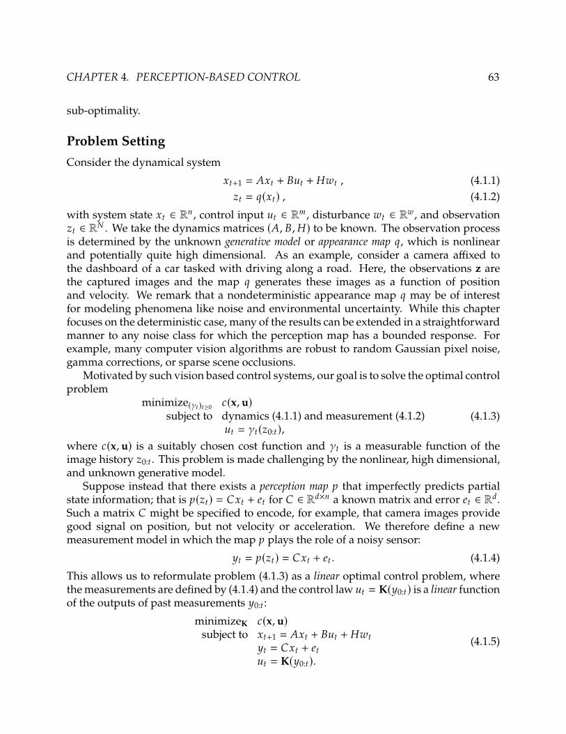
CHAPTER 4. PERCEPTION-BASED CONTROL 63
sub-optimality.
Problem SettingConsider the dynamical system
GC+1 = �GC + �DC + �FC , (4.1.1)
IC = @(GC) , (4.1.2)
with system state GC ∈ R= , control input DC ∈ R< , disturbance FC ∈ RF , and observation
IC ∈ R# . We take the dynamics matrices (�, �, �) to be known. The observation process
is determined by the unknown generative model or appearance map @, which is nonlinear
and potentially quite high dimensional. As an example, consider a camera affixed to
the dashboard of a car tasked with driving along a road. Here, the observations z are
the captured images and the map @ generates these images as a function of position
and velocity. We remark that a nondeterministic appearance map @ may be of interest
for modeling phenomena like noise and environmental uncertainty. While this chapter
focuses on the deterministic case, many of the results can be extended in a straightforward
manner to any noise class for which the perception map has a bounded response. For
example, many computer vision algorithms are robust to random Gaussian pixel noise,
gamma corrections, or sparse scene occlusions.
Motivated by such vision based control systems, our goal is to solve the optimal control
problem
minimize(�C)C≥02(x, u)
subject to dynamics (4.1.1) and measurement (4.1.2)
DC = �C(I0:C),(4.1.3)
where 2(x, u) is a suitably chosen cost function and �C is a measurable function of the
image history I0:C . This problem is made challenging by the nonlinear, high dimensional,
and unknown generative model.
Suppose instead that there exists a perception map ? that imperfectly predicts partial
state information; that is ?(IC) = �GC + 4C for � ∈ R3×= a known matrix and error 4C ∈ R3.Such a matrix � might be specified to encode, for example, that camera images provide
good signal on position, but not velocity or acceleration. We therefore define a new
measurement model in which the map ? plays the role of a noisy sensor:
HC = ?(IC) = �GC + 4C . (4.1.4)
This allows us to reformulate problem (4.1.3) as a linear optimal control problem, where
themeasurements are defined by (4.1.4) and the control law DC = K(H0:C) is a linear functionof the outputs of past measurements H0:C :
minimizeK 2(x, u)subject to GC+1 = �GC + �DC + �FC
HC = �GC + 4CDC = K(H0:C).
(4.1.5)

CHAPTER 4. PERCEPTION-BASED CONTROL 64
camera
perception controller
perception errors
idealized system and perception x
<latexit sha1_base64="butjOCTCphwFmdoCmokPtPNKqoI=">AAAB9XicbVDLSgMxFL1TX7W+qi7dBIvgqsxUQZdFNy4r2Ae0Y8lk0jY0kwxJRi1D/8ONC0Xc+i/u/Bsz7Sy09UDI4Zx7yckJYs60cd1vp7Cyura+UdwsbW3v7O6V9w9aWiaK0CaRXKpOgDXlTNCmYYbTTqwojgJO28H4OvPbD1RpJsWdmcTUj/BQsAEj2FjpvhdIHupJZK/0adovV9yqOwNaJl5OKpCj0S9/9UJJkogKQzjWuuu5sfFTrAwjnE5LvUTTGJMxHtKupQJHVPvpLPUUnVglRAOp7BEGzdTfGymOdBbNTkbYjPSil4n/ed3EDC79lIk4MVSQ+UODhCMjUVYBCpmixPCJJZgoZrMiMsIKE2OLKtkSvMUvL5NWreqdVWu355X6VV5HEY7gGE7Bgwuoww00oAkEFDzDK7w5j86L8+58zEcLTr5zCH/gfP4AVJqTDQ==</latexit>
x<latexit sha1_base64="butjOCTCphwFmdoCmokPtPNKqoI=">AAAB9XicbVDLSgMxFL1TX7W+qi7dBIvgqsxUQZdFNy4r2Ae0Y8lk0jY0kwxJRi1D/8ONC0Xc+i/u/Bsz7Sy09UDI4Zx7yckJYs60cd1vp7Cyura+UdwsbW3v7O6V9w9aWiaK0CaRXKpOgDXlTNCmYYbTTqwojgJO28H4OvPbD1RpJsWdmcTUj/BQsAEj2FjpvhdIHupJZK/0adovV9yqOwNaJl5OKpCj0S9/9UJJkogKQzjWuuu5sfFTrAwjnE5LvUTTGJMxHtKupQJHVPvpLPUUnVglRAOp7BEGzdTfGymOdBbNTkbYjPSil4n/ed3EDC79lIk4MVSQ+UODhCMjUVYBCpmixPCJJZgoZrMiMsIKE2OLKtkSvMUvL5NWreqdVWu355X6VV5HEY7gGE7Bgwuoww00oAkEFDzDK7w5j86L8+58zEcLTr5zCH/gfP4AVJqTDQ==</latexit>
u<latexit sha1_base64="N1CBxeDehIkKwyTBxQP4awmeNoo=">AAAB9XicbVDLSgMxFL3js9ZX1aWbYBFclZkq6LLoxmUF+4B2LJlMpg3NJEOSUcrQ/3DjQhG3/os7/8ZMOwttPRByOOdecnKChDNtXPfbWVldW9/YLG2Vt3d29/YrB4dtLVNFaItILlU3wJpyJmjLMMNpN1EUxwGnnWB8k/udR6o0k+LeTBLqx3goWMQINlZ66AeSh3oS2ytLp4NK1a25M6Bl4hWkCgWag8pXP5QkjakwhGOte56bGD/DyjDC6bTcTzVNMBnjIe1ZKnBMtZ/NUk/RqVVCFElljzBopv7eyHCs82h2MsZmpBe9XPzP66UmuvIzJpLUUEHmD0UpR0aivAIUMkWJ4RNLMFHMZkVkhBUmxhZVtiV4i19eJu16zTuv1e8uqo3roo4SHMMJnIEHl9CAW2hCCwgoeIZXeHOenBfn3fmYj644xc4R/IHz+QNQC5MK</latexit>
u<latexit sha1_base64="N1CBxeDehIkKwyTBxQP4awmeNoo=">AAAB9XicbVDLSgMxFL3js9ZX1aWbYBFclZkq6LLoxmUF+4B2LJlMpg3NJEOSUcrQ/3DjQhG3/os7/8ZMOwttPRByOOdecnKChDNtXPfbWVldW9/YLG2Vt3d29/YrB4dtLVNFaItILlU3wJpyJmjLMMNpN1EUxwGnnWB8k/udR6o0k+LeTBLqx3goWMQINlZ66AeSh3oS2ytLp4NK1a25M6Bl4hWkCgWag8pXP5QkjakwhGOte56bGD/DyjDC6bTcTzVNMBnjIe1ZKnBMtZ/NUk/RqVVCFElljzBopv7eyHCs82h2MsZmpBe9XPzP66UmuvIzJpLUUEHmD0UpR0aivAIUMkWJ4RNLMFHMZkVkhBUmxhZVtiV4i19eJu16zTuv1e8uqo3roo4SHMMJnIEHl9CAW2hCCwgoeIZXeHOenBfn3fmYj644xc4R/IHz+QNQC5MK</latexit>
w<latexit sha1_base64="sZ1ZbwUPvZ/SniHKOlVTgU72ST4=">AAAB9XicbVDLSgMxFL1TX7W+qi7dBIvgqsxUQZdFNy4r2Ae0Y8lk0jY0kwxJxlKG/ocbF4q49V/c+Tdm2llo64GQwzn3kpMTxJxp47rfTmFtfWNzq7hd2tnd2z8oHx61tEwUoU0iuVSdAGvKmaBNwwynnVhRHAWctoPxbea3n6jSTIoHM42pH+GhYANGsLHSYy+QPNTTyF7pZNYvV9yqOwdaJV5OKpCj0S9/9UJJkogKQzjWuuu5sfFTrAwjnM5KvUTTGJMxHtKupQJHVPvpPPUMnVklRAOp7BEGzdXfGymOdBbNTkbYjPSyl4n/ed3EDK79lIk4MVSQxUODhCMjUVYBCpmixPCpJZgoZrMiMsIKE2OLKtkSvOUvr5JWrepdVGv3l5X6TV5HEU7gFM7Bgyuowx00oAkEFDzDK7w5E+fFeXc+FqMFJ985hj9wPn8AUxWTDA==</latexit>
w<latexit sha1_base64="sZ1ZbwUPvZ/SniHKOlVTgU72ST4=">AAAB9XicbVDLSgMxFL1TX7W+qi7dBIvgqsxUQZdFNy4r2Ae0Y8lk0jY0kwxJxlKG/ocbF4q49V/c+Tdm2llo64GQwzn3kpMTxJxp47rfTmFtfWNzq7hd2tnd2z8oHx61tEwUoU0iuVSdAGvKmaBNwwynnVhRHAWctoPxbea3n6jSTIoHM42pH+GhYANGsLHSYy+QPNTTyF7pZNYvV9yqOwdaJV5OKpCj0S9/9UJJkogKQzjWuuu5sfFTrAwjnM5KvUTTGJMxHtKupQJHVPvpPPUMnVklRAOp7BEGzdXfGymOdBbNTkbYjPSyl4n/ed3EDK79lIk4MVSQxUODhCMjUVYBCpmixPCpJZgoZrMiMsIKE2OLKtkSvOUvr5JWrepdVGv3l5X6TV5HEU7gFM7Bgyuowx00oAkEFDzDK7w5E+fFeXc+FqMFJ985hj9wPn8AUxWTDA==</latexit>
e<latexit sha1_base64="wZvbKNFJx9khKR1QLuSGuTIgBT8=">AAAB9XicbVDLSgMxFM34rPVVdekmWARXZaYKuiy6cVnBPqAdSyZzpw3NJEOSUcrQ/3DjQhG3/os7/8ZMOwttPRByOOdecnKChDNtXPfbWVldW9/YLG2Vt3d29/YrB4dtLVNFoUUll6obEA2cCWgZZjh0EwUkDjh0gvFN7nceQWkmxb2ZJODHZChYxCgxVnroB5KHehLbK4PpoFJ1a+4MeJl4BamiAs1B5asfSprGIAzlROue5ybGz4gyjHKYlvuphoTQMRlCz1JBYtB+Nks9xadWCXEklT3C4Jn6eyMjsc6j2cmYmJFe9HLxP6+XmujKz5hIUgOCzh+KUo6NxHkFOGQKqOETSwhVzGbFdEQUocYWVbYleItfXibtes07r9XvLqqN66KOEjpGJ+gMeegSNdAtaqIWokihZ/SK3pwn58V5dz7moytOsXOE/sD5/AE3u5L6</latexit>
z<latexit sha1_base64="c82gP32MmAPddn6IZKsm/pse8jY=">AAAB9XicbVDLSgMxFL1TX7W+qi7dBIvgqsxUQZdFNy4r2Ae0Y8lk0jY0kwxJRqlD/8ONC0Xc+i/u/Bsz7Sy09UDI4Zx7yckJYs60cd1vp7Cyura+UdwsbW3v7O6V9w9aWiaK0CaRXKpOgDXlTNCmYYbTTqwojgJO28H4OvPbD1RpJsWdmcTUj/BQsAEj2FjpvhdIHupJZK/0adovV9yqOwNaJl5OKpCj0S9/9UJJkogKQzjWuuu5sfFTrAwjnE5LvUTTGJMxHtKupQJHVPvpLPUUnVglRAOp7BEGzdTfGymOdBbNTkbYjPSil4n/ed3EDC79lIk4MVSQ+UODhCMjUVYBCpmixPCJJZgoZrMiMsIKE2OLKtkSvMUvL5NWreqdVWu355X6VV5HEY7gGE7Bgwuoww00oAkEFDzDK7w5j86L8+58zEcLTr5zCH/gfP4AV6STDw==</latexit>
y<latexit sha1_base64="2A7DuJCvpRVdVAiUcdT84g18VK8=">AAAB9XicbVDLSgMxFL3js9ZX1aWbYBFclZkq6LLoxmUF+4B2LJlMpg3NJEOSUcrQ/3DjQhG3/os7/8ZMOwttPRByOOdecnKChDNtXPfbWVldW9/YLG2Vt3d29/YrB4dtLVNFaItILlU3wJpyJmjLMMNpN1EUxwGnnWB8k/udR6o0k+LeTBLqx3goWMQINlZ66AeSh3oS2yubTAeVqltzZ0DLxCtIFQo0B5WvfihJGlNhCMda9zw3MX6GlWGE02m5n2qaYDLGQ9qzVOCYaj+bpZ6iU6uEKJLKHmHQTP29keFY59HsZIzNSC96ufif10tNdOVnTCSpoYLMH4pSjoxEeQUoZIoSwyeWYKKYzYrICCtMjC2qbEvwFr+8TNr1mndeq99dVBvXRR0lOIYTOAMPLqEBt9CEFhBQ8Ayv8OY8OS/Ou/MxH11xip0j+APn8wdWH5MO</latexit>
y<latexit sha1_base64="2A7DuJCvpRVdVAiUcdT84g18VK8=">AAAB9XicbVDLSgMxFL3js9ZX1aWbYBFclZkq6LLoxmUF+4B2LJlMpg3NJEOSUcrQ/3DjQhG3/os7/8ZMOwttPRByOOdecnKChDNtXPfbWVldW9/YLG2Vt3d29/YrB4dtLVNFaItILlU3wJpyJmjLMMNpN1EUxwGnnWB8k/udR6o0k+LeTBLqx3goWMQINlZ66AeSh3oS2yubTAeVqltzZ0DLxCtIFQo0B5WvfihJGlNhCMda9zw3MX6GlWGE02m5n2qaYDLGQ9qzVOCYaj+bpZ6iU6uEKJLKHmHQTP29keFY59HsZIzNSC96ufif10tNdOVnTCSpoYLMH4pSjoxEeQUoZIoSwyeWYKKYzYrICCtMjC2qbEvwFr+8TNr1mndeq99dVBvXRR0lOIYTOAMPLqEBt9CEFhBQ8Ayv8OY8OS/Ou/MxH11xip0j+APn8wdWH5MO</latexit>
K<latexit sha1_base64="tD88yrkV+7bzZ6nNjOx+spkLbjY=">AAAB9XicbVDLSgMxFL1TX7W+qi7dBIvgqsxUQZdFN4KbCvYB7VgymbQNzSRDklHK0P9w40IRt/6LO//GTDsLbT0QcjjnXnJygpgzbVz32ymsrK6tbxQ3S1vbO7t75f2DlpaJIrRJJJeqE2BNORO0aZjhtBMriqOA03Ywvs789iNVmklxbyYx9SM8FGzACDZWeugFkod6EtkrvZ32yxW36s6AlomXkwrkaPTLX71QkiSiwhCOte56bmz8FCvDCKfTUi/RNMZkjIe0a6nAEdV+Oks9RSdWCdFAKnuEQTP190aKI51Fs5MRNiO96GXif143MYNLP2UiTgwVZP7QIOHISJRVgEKmKDF8YgkmitmsiIywwsTYokq2BG/xy8ukVat6Z9Xa3XmlfpXXUYQjOIZT8OAC6nADDWgCAQXP8ApvzpPz4rw7H/PRgpPvHMIfOJ8/EDmS4A==</latexit>
K<latexit sha1_base64="tD88yrkV+7bzZ6nNjOx+spkLbjY=">AAAB9XicbVDLSgMxFL1TX7W+qi7dBIvgqsxUQZdFN4KbCvYB7VgymbQNzSRDklHK0P9w40IRt/6LO//GTDsLbT0QcjjnXnJygpgzbVz32ymsrK6tbxQ3S1vbO7t75f2DlpaJIrRJJJeqE2BNORO0aZjhtBMriqOA03Ywvs789iNVmklxbyYx9SM8FGzACDZWeugFkod6EtkrvZ32yxW36s6AlomXkwrkaPTLX71QkiSiwhCOte56bmz8FCvDCKfTUi/RNMZkjIe0a6nAEdV+Oks9RSdWCdFAKnuEQTP190aKI51Fs5MRNiO96GXif143MYNLP2UiTgwVZP7QIOHISJRVgEKmKDF8YgkmitmsiIywwsTYokq2BG/xy8ukVat6Z9Xa3XmlfpXXUYQjOIZT8OAC6nADDWgCAQXP8ApvzpPz4rw7H/PRgpPvHMIfOJ8/EDmS4A==</latexit>
car and environment
Figure 4.1: (Left) A diagram of the proposed perception-based control pipeline. (Right)
The conceptual rearrangement of the closed-loop system permitted through our percep-
tion error characterization.
As illustrated in Figure 4.1, guarantees of performance, safety, and robustness require
designing a controller which suitably responds to system disturbance and sensor error.
For linear optimal control problems, a variety of cost functions and noise models have
well understood solutions; recall those reviewed in Chapter 2. Perhaps the most well
known is the combination of Kalman filtering with static state feedback, which arises as
the solution to the linear quadratic Gaussian (LQG) problem. However, the perception
errors edonot necessarily obey assumptions aboutmeasurement noisemade in traditional
optimal control, and must be handled carefully.
In what follows, we overload the norm ‖·‖ so that it applies equally to elements GC ,
signals x, and linear operators Φ. For any element norm, we define the signal and linear
operator norms as
‖x‖ = sup
C≥0
‖GC ‖ , ‖Φ‖ = sup
‖w‖≤1
‖Φw‖
We primarily focus on the triple (‖G: ‖∞, ‖x‖∞, ‖Φ‖ℒ1), though many of our results could
be extended.
Related WorkVision based estimation, planning, and control. There is a rich body of work, spanning
several research communities, that integrates complex sensing modalities into estimation,
planning, and control loops. The robotics community has focused mainly on integrating
camera measurements with inertial odometry via an Extended Kalman Filter (EKF) [JS11;
KS11; HKBR14]. Similar approaches have also been used as part of Simultaneous Local-
ization andMapping (SLAM) algorithms in both ground [LSB+15] and aerial [LAWCS13]
vehicles. We note that these works focus solely on the estimation component, and do
not consider downstream use of the state estimate in control loops. In contrast, work
by Loianno et al. [LBMK16], Tang, Wüest, and Kumar [TWK18], and Lin et al. [LGQ+18]

CHAPTER 4. PERCEPTION-BASED CONTROL 65
demonstrate techniques that use camera measurements to aid inertial position estimates
in order to enable aggressive control maneuvers in unmanned aerial vehicles.
Themachine learning community has taken amore data-driven approach. The earliest
such example is likely [Pom89], in which a 3-layer neural-network is trained to infer road
direction from images. Modern approaches to vision based planning, typically relying
on deep neural networks, include learning maps from image to trail direction [GGC+15],
learningQ-functions for indoornavigationusing 3DCADimages [SL17], andusing images
to specify waypoints for indoor robotic navigation [BTGMT20]. Moving from planning to
low-level control, end-to-end learning for vision based control has been achieved through
imitation learning from training data generated via human [BDD+16] and model predic-
tive control [PCS+18]. The resulting policies map raw image data directly to low-level
control tasks. Codevilla et al. [CMLKD18] propose a method for mapping high level
navigational commands, images, and other sensor measurements to control actions via
imitation learning. Similarly, Williams et al. [WDGRT18] map image and inertial data to
a cost landscape, which is then optimized via a path integral based sampling algorithm.
More closely related to our approach is from work by Lambert et al. [LSRLB18], where
a deep neural network is used to learn a map from image to system state—we note that
such a perception module is naturally incorporated into our proposed pipeline. To the
best of our knowledge, none of the aforementioned results provide safety or performance
guarantees.
The observation of a linear system through a static nonlinearity is classically studied
in the controls community as aWeiner systemmodel [ST17]. While there are identification
results for Weiner systems, they apply only to single-input-single-output systems, and
often require assumptions that do not apply to the motivation of cameras [Has87; Wig94;
Gre97; TS14]. More flexible identification schemes have been proposed [LB01; SK16], but
they lack theoretical guarantees. Furthermore, these approaches focus on identifying the
full forward model, rather than an inverse model as we do here.
Learning, robustness, and control. There is much related and recent work at the in-
tersection of learning and control theory. Similar in spirit is a line of work on the
Linear Quadratic Regulator which focuses on issues of system identification and sub-
optimality [DMMRT20; DMMRT18; AS11]. This style of sample complexity analysis has
allowed for illuminating comparisons between model based and model free policy learn-
ing approaches [TR19; ALS19]. Mania, Tu, and Recht [MTR19] and Simchowitz and
Foster [SF20] show that the simple strategy of model based certainty equivalent control is
efficient, though the argument is specialized to linear dynamics and quadratic cost. For
nonlinear systems, analyses of learning often focus on ensuring safety over identification
or sub-optimality [TDLYA19; BTSK17; WZ18; COMB19], and rely on underlying smooth-
ness for their guarantees [LSCAY20; NLS+20]. An exception is a recent result by Mania,
Jordan, and Recht [MJR20] which presents finite sample guarantees for parametric non-
linear system identification.

CHAPTER 4. PERCEPTION-BASED CONTROL 66
While the majority of work on learning for control focuses on settings with full state
observation, output feedback is receiving growing attention for linear systems [SBR19;
SSH20] and for safety-critical systems [LCT20]. Recent work in closely related problem
settings includes Mhammedi et al. [MFS+20], who develop sample complexity guaran-
tees for LQR with nonlinear observations and [MHKL20], who leverage representation
learning in Block MDPs. However, neither address issues of stability due to their focus
on finite horizon problems.
Our theoretical contributions in the robust setting are similar in spirit to those of the
online learning community, in that we provide generalization guarantees under adver-
sarial noise models [AHMS13; AHM15; KM16; HK01; YP18; ABHKS19]. The statistical
analysis used in the certainty equivalent setting focuses on nonparametric pointwise er-
ror bounds over a compact set. Distinct from mean-error generalization arguments most
common in learning theory, our analysis is directly related to classical statistical results
on uniform convergence [Dev78; Lie89; Han08].
4.2 Bounded Errors via Robust GeneralizationWhile it is typical in the machine learning community to consider mean error general-
ization bounds, we show in the following example that it is necessary to quantify the
uncertainty pointwise to guarantee robustness. This motivating example shows how er-
rorswithin sets of vanishingly smallmeasure can cause systems to exit bounded regions of
well-characterized perception and lead to instability. For a simple setting, we construct a
disturbance sequence that leads to instability, illustrating that feedback control objectives
require very strong function approximation error bounds.
Example 4.1. Consider a one dimensional linear system that is open-loopunstable (|0 | > 1)
with an arbitrary linear controller and adversarial disturbances:
GC+1 = 0GC + DC + FC , DC =
C∑:=0
: GC−: .
Further suppose that the perception map has been characterized within the bounded
interval [−Γ, Γ] and is imperfect only around the point G ∈ [−Γ, Γ]:
G = ?(@(G)) ={
0 |G | ≥ Γ or G = G
G otherwise
.
Then consider the disturbance sequence F0 = G − (0 + 0)G0, F1 = Γ − 0G − 1G0, and
FC = 0 for all C ≥ 2. The perception error at G causes the unstable system trajectory
|GC | = |0C−1G | → ∞ as C →∞ .
Furthermore, by carefully choosing G0 and G, it is possible to construct scenarios where
this instability occurs for disturbances of arbitrarily small norm.

CHAPTER 4. PERCEPTION-BASED CONTROL 67
Data-dependent perception errorIn this section, we consider a general class of perception maps and introduce a procedure
to estimate regions for which a the perception map can be used safely during operation.
We first suppose access to initial training data S = {(G8 , I8)})8=1, used to learn a perception
map via any of the wide variety of traditional supervised methods. We then estimate safe
regions around the training data, under an assumption of slope boundedness.
Definition 4.1 (Slope boundedness). A fuction 5 is locally (-slope bounded for a radius
� around G0 if for G ∈ ��(G0), ‖ 5 (G) − 5 (G0)‖ ≤ (‖G − G0‖, where the ball ��(G0) ={G : ‖G − G0‖ ≤ �}.
This allows us to characterize how quickly the learned perception map degrades as we
move away from the initial training data. We will describe the regions of the state space
within which the sensing is reliable using a safe set which approximates sub-level sets
of the error function 4(G) = ?(@(G)) − �G. We make this precise in the following lemma,
defining a safe set which is valid under an assumption that the error function is locally
slope bounded around training data.
Lemma 4.2.1 (Closeness implies generalization). Suppose that the error function ? ◦ @ − � islocally (-slope bounded with a radius of � around training data points. Define the safe set
X� =⋃
(G8 ,I8)∈S{G ∈ ��(G8) : ‖?(I8) − �G8 ‖ + (‖G − G8 ‖ ≤ �} .
(4.2.1)
Then for any (G, I) with G ∈ X�, the perception error is bounded: ‖?(I) − �G‖ ≤ �.
Proof. The proof follows by a simple argument. For training data point (G8 , I8) such that
G8 ∈ ��(G),
‖?(I) − �G‖ = ‖?(@(G)) − �G − (?(@(G8)) − �G8) + ?(@(G8)) − �G8 ‖≤ (‖G − G8 ‖ + ‖?(@(G8)) − �G8 ‖ .
The second line follows from the assumptionabout local slopeboundedness. Thenbecause
G ∈ ��(G8), by the definition of X�, we have
‖?(I) − �G‖ ≤ (‖G − G8 ‖ + ‖?(@(G8)) − �G8 ‖ ≤ � .
The safe set X� is defined in terms of a bound on the slope of the error function lo-
cally around the training data. Deriving the slope boundedness of the error function
relies on the learned perception map as well as the underlying generative model. It is
possible to also estimate a bound on ( using an additional dataset composed of samples
around each training data point [DMRY20]. However, the validity of this estimate will
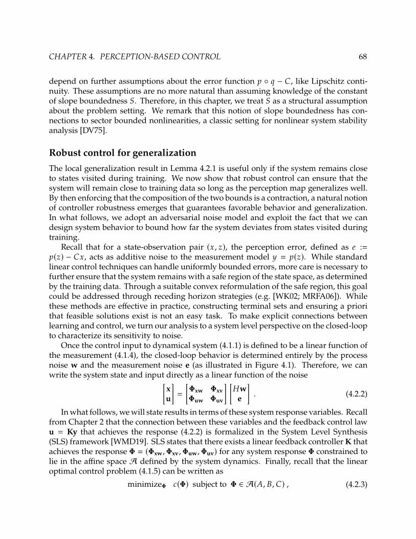
CHAPTER 4. PERCEPTION-BASED CONTROL 68
depend on further assumptions about the error function ? ◦ @ − �, like Lipschitz conti-
nuity. These assumptions are no more natural than assuming knowledge of the constant
of slope boundedness (. Therefore, in this chapter, we treat ( as a structural assumption
about the problem setting. We remark that this notion of slope boundedness has con-
nections to sector bounded nonlinearities, a classic setting for nonlinear system stability
analysis [DV75].
Robust control for generalizationThe local generalization result in Lemma 4.2.1 is useful only if the system remains close
to states visited during training. We now show that robust control can ensure that the
system will remain close to training data so long as the perception map generalizes well.
By then enforcing that the composition of the two bounds is a contraction, a natural notion
of controller robustness emerges that guarantees favorable behavior and generalization.
In what follows, we adopt an adversarial noise model and exploit the fact that we can
design system behavior to bound how far the system deviates from states visited during
training.
Recall that for a state-observation pair (G, I), the perception error, defined as 4 :=
?(I) − �G, acts as additive noise to the measurement model H = ?(I). While standard
linear control techniques can handle uniformly bounded errors, more care is necessary to
further ensure that the system remains with a safe region of the state space, as determined
by the training data. Through a suitable convex reformulation of the safe region, this goal
could be addressed through receding horizon strategies (e.g. [WK02; MRFA06]). While
these methods are effective in practice, constructing terminal sets and ensuring a priori
that feasible solutions exist is not an easy task. To make explicit connections between
learning and control, we turn our analysis to a system level perspective on the closed-loop
to characterize its sensitivity to noise.
Once the control input to dynamical system (4.1.1) is defined to be a linear function of
the measurement (4.1.4), the closed-loop behavior is determined entirely by the process
noise w and the measurement noise e (as illustrated in Figure 4.1). Therefore, we can
write the system state and input directly as a linear function of the noise[xu
]=
[Φxw ΦxvΦuw Φuv
] [�w
e
]. (4.2.2)
Inwhat follows, wewill state results in terms of these system response variables. Recall
from Chapter 2 that the connection between these variables and the feedback control law
u = Ky that achieves the response (4.2.2) is formalized in the System Level Synthesis
(SLS) framework [WMD19]. SLS states that there exists a linear feedback controller K that
achieves the response Φ = (Φxw,Φxv,Φuw,Φuv) for any system response Φ constrained to
lie in the affine space A defined by the system dynamics. Finally, recall that the linear
optimal control problem (4.1.5) can be written as
minimizeΦ 2(Φ) subject to Φ ∈ A(�, �, �) , (4.2.3)

CHAPTER 4. PERCEPTION-BASED CONTROL 69
where the cost function 2 is redefined to operate on system responses. Section 2.4 presents
examples of control costs that can be written as system norms.
In what follows, we specialize controller design concerns to our perception-based
setting, and develop further conditions on the closed-loop response Φ to incorporate into
the synthesis problem.
Lemma 4.2.2 (Generalization implies closeness). For a perception map ? with errors e =
?(z)−�x, let the system responses (Φxw,Φxv,Φuw,Φuv) lie in the affine space defined by dynamics(�, �, �), and let K be the associated controller. Then the state trajectory x achieved by the controllaw u = K?(z) and driven by noise process w, satisfies, for any target trajectory x,
‖x − x‖ ≤ ‖x − x‖ + ‖Φxv‖‖e‖. (4.2.4)
where we define the nominal closeness ‖x − x‖ = ‖Φxw�w − x‖ to be the deviation from thetarget trajectory in the absence of measurement errors.
Proof. Notice that over the course of a trajectory, wehave systemoutputs y = ?(z) = �x+e.Then recalling that the system responses are defined such that x = Φxw�w + Φxve, we
have that
‖x − x‖ = ‖Φxw�w + Φxve − x‖ ≤ ‖Φxw�w − x‖ + ‖Φxv‖‖e‖ .
Letting x represent a trajectory of training data, the terms in bound (4.2.4) capture
different generalization properties. The first is small if we plan to visit states during
operation that are similar to those seen during training. The second term is a measure of
the robustness of the closed-loop system to the error e.We are now in a position to state the main result on robust generalization and stability,
which shows that under an additional robustness condition, Lemmas 4.2.1 and 4.2.2
combine to define a control invariant set around the training data within which the
perception errors, and consequently the performance, are bounded.
Theorem 4.2.3. Let the assumptions of Lemmas 4.2.1 and 4.2.2 hold and, for simplicity of presen-tation, suppose that the training error is bounded: ‖?(I8) − �G8 ‖ ≤ �S for all (G8 , I8) ∈ S. Definethe signal xS to have elements populated by states in the training dataset S. Then as long as
‖Φxv‖ ≤1 − 1
� ‖x − xS‖( + �S
�
, (4.2.5)
the perception errors remain bounded
‖?(z) − �x‖ ≤ ‖x − xS‖ + �S1 − (‖Φxv‖
=: �, (4.2.6)
and the closed-loop trajectory lies within X�.

CHAPTER 4. PERCEPTION-BASED CONTROL 70
Proof. Recall that as in the proof of Lemma 4.2.1, as long as GC ∈ ��(G8C ) for all C and some
G8C ∈ S,
‖4C ‖ ≤ (‖GC − G8C ‖ + ‖48C ‖ =⇒ ‖e‖ = max
C‖4C ‖ ≤ (‖x − xS‖ + ‖eS‖ , (4.2.7)
where we define the data signal xS = (G8C )C≥0 and error signal eS = (48C )C≥0 corresponding
to (GC)C≥0.
By assumption, ‖eS‖ ≤ �S . Substituting this expression into the result of Lemma 4.2.2,
we see that as long as ‖GC − G8C ‖ ≤ � for all C,
‖x − xS‖ ≤ ‖x − xS‖ + ‖Φxv‖((‖x − xS‖ + ‖eS‖) ⇐⇒ ‖x − xS‖ ≤‖x − xS‖ + �S‖Φxv‖
1 − (‖Φxv‖.
Next, to ensure that the the radius � is bounded, first note that by the definition of the ℓ∞norm, maxC ‖GC − G8C ‖ ≤ � if and only if ‖x − xS‖ ≤ �. A sufficient condition for this is
given by
‖x − xS‖ + �S‖Φxv‖1 − (‖Φxv‖
≤ � ⇐⇒ ‖Φxv‖ ≤1 − 1
� ‖x − xS‖( + �S
�
,
and thus we arrive at the robustness condition. This validates the the bound on ‖x − xS‖,which we now use to bound ‖e‖, starting with (4.2.7) and rearranging,
‖e‖ ≤ ‖x − xS‖ + �S1 − (‖Φxv‖
.
Theorem 4.2.3 shows that the bound (4.2.5) should be used during controller synthesis
to ensure generalization. Feasibility of the synthesis problem depends on the controlla-
bility and observability of the system (�, �, �), which impose limits on how small ‖Φxv‖can be made to be, and on the planned deviation from training data as captured by the
quantity ‖x − xS‖. In the following section, we show how to simplify this term for a
reference tracking problem.
4.3 Robust Perception-Based Control
Reference TrackingWe consider a reference tracking problemwith the goal of ensuring that the system tracks
a series of arbitrary waypoints that are sequentially revealed. Recall from Example 2.3
that the reference tracking objective is given by:
2(���, u) = sup
‖AC+1−AC ‖≤Δref,
C≥0
&1/2(�C − AC)'1/2DC
,

CHAPTER 4. PERCEPTION-BASED CONTROL 71
for a reference signal AC and a linear system with state �C such that
�C+1 = ��C + �DC .
We suppose that observations are generated as IC = @(�C) and that the perception map
?(IC) = ��C + 4C satisfies the slope-bounded assumption.
Further recall that we can reformulate the problem by defining the state as the concate-
nation with the next waypoint, GC := [�C ; AC], the disturbance as the change in reference,
FC := AC+1 − AC , and
� =
[� 0
0 �
], � =
[�
0
], � =
[� 0
], � =
[0
�
], &1/2 =
[&1/2 −&1/2] .
Under this formulation, the optimal control problem has the same form as (4.1.5) and can
therefore be written in terms of system response variables as in (4.2.3) with the cost 2(Φ)given by a weighted ℒ1 system norm.
Robust SynthesisWe now show how to simplify the term ‖x − xS‖ in the case of waypoint tracking. The
expression allows us to propose a robust control synthesis problem.
Proposition 4.3.1. Consider reference tracking problem and suppose that for all C = 0, 1, . . . , thereference trajectory has bounded differences ‖AC+1 − AC ‖ ≤ Δref and is within a ball of radius �ref
from the training data:min
�8∈S‖AC − �8 ‖ ≤ �ref ∀ C ≥ 0 .
Then, the closed-loop deviation from training data is bounded by:
‖x − xS‖ ≤ Δref‖[� −�
]Φxw�‖ + �ref .
Proof. Because the appearance and perception maps depend on the augmented state GConly through �C , the errors do not depend the reference signal AC . We can arbitrarily define
the second element of lifted training data so that
‖x − xS‖ = ‖��� − ���S‖ ≤ ‖��� − r‖ + ‖r − ���S‖ .
Therefore, noting that ��� − r =[� −�
]x,
‖x − xS‖ ≤ ‖[� −�
]Φxww‖ + ‖r − ���S‖
≤ Δref‖[� −�
]Φxw‖ + �ref .

CHAPTER 4. PERCEPTION-BASED CONTROL 72
Using the expression in Proposition 4.3.1 it is possible to add the robustness condition
from Theorem 4.2.5 to a control synthesis problem as a constraint on the norm of system
response variables (( + �S
�
)‖Φxv‖ +
Δref
�‖[� −�
]Φxw�‖ +
�ref
�≤ 1 .
This constraint immediately implies a trade-off between the size of different parts of the
system response: Φxv, which is the closed-loop response tomeasurements, andΦxw, which
is the response to waypoints. Because the system responses must lie in an affine space,
they cannot both become arbitrarily small. Therefore, the synthesis problem must trade
off between sensitivity to measurement errors and tracking fidelity. These trade-offs are
mediated by the quality of the perception map, the ambition of the control task, and the
comprehensiveness of the training data. High quality perception maps will have small
training error �S , small slope bound (, and large radius � within which the slope bound
holds. Ambitious control tasks will design for large jumps between waypoints Δref. Large
deviations from training data �ref will be required for more ambitious control tasks or less
comprehensive training datasets. Therefore, the higher quality the perception map and
the more comprehensive the training data, the more ambitious the control tasks that are
possible.
This robustness constraint is enough to guarantee a finite cost, but it does not guarantee
a small cost. To achieve this, we incorporate the constraint alongwith the perception error
bound from Theorem 4.2.5 to arrive at the following robust synthesis procedure:
minimizeΦ,�>0
[&1/2
'1/2
] [Φxw ΦxvΦuw Φuv
] [Δref�
��
] subject to Φ ∈ A(�, �, �),
(( + �S� )‖Φxv‖ + Δ
ref
� ‖[� 0
]Φxw�‖ + �
ref
� ≤ 1
Δref‖[� 0
]Φxw�‖ + �ref + �S ≤ �(1 − (‖Φxv‖) .
This can be formulated into a convex program for fixed �. There is some lower limit
�0 for which � < �0 will be infeasible. In the limit as � grows large, the cost is increasing
in �. Therefore, the full problem can be approximately solved via one-dimensional search
over a bounded range of values.
Necessity of RobustnessRobust control is notoriously conservative, and our main result in Theorem 4.2.3 relies
heavily on small gain-like arguments. Can the conservatism inherent in this approach
be generally reduced? In this section, we answer in the negative by describing a class of
examples for which the robustness condition in Theorem 4.2.3 is necessary. For simplicity,
we specialize to the goal of regulating a system to the origin, rather than an arbitrary

CHAPTER 4. PERCEPTION-BASED CONTROL 73
waypoint tracking problem. Let I0 = @(0) and assume that (0, I0) is in the training set and
that the perception map is perfect at the origin: ?(I0) = 0.
We consider the following optimal control problem
minimizeΦ 2(Φ) subject to Φ ∈ A(�, �, �), ‖Φxv‖ ≤ .
and define Φ as a minimizing argument in the absence of the inequality constraint. For
simplicity, we consider only systems in which the closed-loop is strictly proper and has a
state-space realization.
To avoid notational collisions while discussing frequency domain quantities, we use �as the frequency domain variable (rather than I, as introduced in Chapter 2).
Proposition 4.3.2. Suppose that the frequency response at � = 1 satisfies
‖Φxv‖ℒ1= ‖Φxv(1)‖∞→∞ .
Then there exists a differentiable error function with slope bound ( such that the origin G = 0 is anasymptotically stable equilibrium if and only if < 1
( .
Proof. Sufficiency follows from our main analysis, or alternatively from a simple applica-
tion of the small gain theorem. We therefore focus on showing necessity, which follows
by construction. We use a combination of classic nonlinear instability arguments with
properties of real stability radii.
Recall that HC = �GC + (?(@(GC)) − �GC). Define �C to represent the internal state of the
controller. Then we can write the closed-loop behavior of the system, ignoring the effect
of process noise because it does not affect the stability analysis, as the following nonlinear
recursion: [GC+1
�C+1
]= �CL
[GC�C
]+ �CL4(GC) .
Suppose that the error function 4(G) = ?(@(G)) − �G is differentiable at G = 0 with
derivative �. Then the stability of the origin depends on the linearized closed-loop system
�CL(�) := �CL + �CL��CL where �CL = [� 0] picks out the relevant component of the
closed-loop state. If any eigenvalues of �CL(�) lie outside of the unit disk, then G = 0 is
not an asymptotically stable equilibrium.
Switching gears, we return to the system response variables to construct � that results
in a lack of stability. We set ( = 1/‖Φxv‖ and notice that if ≥ 1
( , then Φ is also the solution
to the constrained problem. By assumption, ‖Φxv‖ℒ1= ‖Φxv(1)‖∞→∞. Thus, there exist
real F, E such that E>Φxv(1)F = ‖Φxv‖ℒ1. We set � = (FE>.
We now argue that for this choice of �, �CL(�) has an eigenvalue on the unit disk. Recall
that the frequency response Φxv(�) = �CL(�� − �CL)−1�CL, so
Φxv(1) = �CL(� − �CL)−1�CL

CHAPTER 4. PERCEPTION-BASED CONTROL 74
This makes the connection between Φxv(1) and the matrices making up �CL(�). Then by
a classic result for stability radii (e.g. Remark 4.2 and Corollary 4.5 in Hinrichsen and
Pritchard [HP90]), �CL((FE>) has an eigenvalue on the unit disk. Thus, for any error
function with derivative � = (FE> at zero, the robust condition is necessary as well as
sufficient. One such error function is simply 4(G) = �G.
We now present a simple example in which this condition is satisfied, and construct
the corresponding error function which results in an unstable system.
Example 4.2. Consider the double integrator
GC+1 =
[1 3C
0 1
]GC +
[0
1
]DC , HC = ?(IC) = GC + 4(GC) , (4.3.1)
and the control law resulting from the ℋ2 optimal control problem with identity weight
matrices along with the robustness constraint ‖Φxv‖ ≤ . Notice that the solution to
the unconstrained problem would be the familiar LQG combination of Kalman filtering
and static feedback on the estimated state. We denote the optimal unconstrained system
response by Φ.
Consider an error function with slope bounded by ( = 1/‖Φxv‖ and derivative at G = 0
equal to
� =
[−1/‖Φxv‖ 0
−1/‖Φxv‖ 0
],
Calculations confirm that theℒ1 norm satisfies the relevant property. Therefore, the origin
is not a stable fixed point if the synthesis constraint ≥ 1
( .
4.4 Bounded Errors via Uniform ConvergenceWe now turn instead to perception maps learned via nonparametric regression, and
show how sufficiently dense data implies uniformly bounded errors. We make several
further assumptions to the problem setting introduced in Section 4.1. First, we assume
that (�, �, �) is output controllable, meaning that for any initial condition G0 ∈ R= and
arbitrary H ∈ R3, there exists a sequence of inputs D0, . . . , D=−1 that, when applied to the
noiseless system, ensure �G= = H. We also assume that for each C, the process noise FCis zero mean, bounded by �F , and independent across time. Next, we assume that that
observations depend on the state only through �G, so that
IC = @(�GC) .
The matrix � therefore determines the state subspace that affects the observation, which
we will refer to as the measurement subspace. This emulates a natural setting in which
observations from the system (e.g. camera images) are complex but encode a subset of the

CHAPTER 4. PERCEPTION-BASED CONTROL 75
state (e.g. position). We further assume that @ is continuous and that there is a continuous
inverse function ?★ : R# → R3 with ?★(@(H)) = H. For the example of a dashboard
mounted camera, such an inverse exists whenever each camera pose corresponds to a
unique image, which is a reasonable assumption in sufficiently feature rich environments.
We pose a learning problem focused on the unknown inverse function ?★. We suppose
that during the training phase, there is an additional system output,
Htrain
C = �GC + EC (4.4.1)
where for each C, the noise EC is zero mean and has independent entries bounded by
�E . This assumption corresponds to using a simple but noisy sensor for characterizing
the complex sensor. The noisy system output will both supervise the learning problem
and allow for the execution of a sampling scheme where the system is driven to sample
particular parts of the state space.
We suppose that the control cost 2 is given by the system ℒ1 norm. Notice that due to
its noisiness, using the training sensor would be suboptimal compared using transformed
observations.
Nonparametric RegressionSince uniform error bounds are necessary for robust guarantees, we now introduce a
method to learn perception maps with such bounds. For simplicity of analysis and
exposition, we focus on Nadarya-Watson estimators. We expect that our insights will
generalize to more complex techniques, and we demonstrate similarities with additional
regressors in simulation experiments presented in Section 4.6.
The Nadarya-Watson regression estimators with training data {(IC , Htrain
C )})C=0
, band-
width � ∈ R+, and metric 3I : R# × R# → R+ have the form
?(I) =)∑C=0
��(IC , I)B)(I)
Htrain
C , B)(I) =)∑C=0
�� (IC , I) , �� (IC , I) = �(3I(IC ,I)
�
), (4.4.2)
with ?(I) = 0 when B)(I) = 0 and � : R+→ [0, 1] is a kernel function. We assume that the
kernel function is Lipschitz with parameter !� and that �(D) = 0 for D > 1, and define the
quantity +� =∫R?+�
(‖H‖∞
)3H.
Thus, predictions are made by computing a weighted average over the labels Htrain
Cof training data points whose corresponding observations IC are close to the current
observation, asmeasured by themetric 3I . We assume the functions @ and ?★ are Lipschitz
continuous with respect to 3I , i.e. for some !@ and !?
3I(@(H), @(H′)) ≤ !@ ‖H − H′‖ , ‖?★(I) − ?★(I′)‖ ≤ !?3I(I, I′) . (4.4.3)
While our final sub-optimality results depend on !@ and !? , the perception map and
synthesized controller do not need direct knowledge of these parameters.

CHAPTER 4. PERCEPTION-BASED CONTROL 76
For an arbitrary I with B)(I) ≠ 0, the prediction error can be decomposed as
‖?(I) − ?★(I)‖ ≤ )∑C=0
��(IC , I)B)(I)
(�GC − �G) + )∑
C=0
��(IC , I)B)(I)
EC
. (4.4.4)
The first term is the approximation error due to finite sampling, even in the absence of
noisy labels. This term can be bounded using the continuity of the true perception map
?★. The second term is the error due to measurement noise. We use this decomposition
to state a pointwise error bound, which can be used to provide tight data-dependent
estimates on error.
Lemma 4.4.1. For a learned perception map of the form (4.4.2) with training data as in (4.4.1)
collected during closed-loop operation of a system with appearance map satisfying (4.4.3), we havewith probability at least 1 − � that for a fixed I with B)(I) ≠ 0,
‖?(I) − ?★(I)‖ ≤ �!? +�E√B)(I)
√log
(32
√B)(I)/�
). (4.4.5)
We present the proof of this result in the Section 4.8.
The expression illustrates that there is a tension between having a small bandwidth �and ensuring that the coverage term B)(I) is large. Notice thatmost of the quantities in this
upper bound can be readily computed from the training data; only !? , which quantifies
the continuity of themap from observation to state, is difficult tomeasure. We remark that
while useful for building intuition, the result in Lemma 4.4.1 is only directly applicable
for bounding error at a finite number of points. Since our main results handle stability
over infinite horizons, they rely on a modified bound introduced in Section 4.8 which is
closely tied to continuity properties of the estimated perception map ? and the sampling
scheme we propose in the next section.
Dense SamplingWe now propose a method for collecting training data and show a uniform, sample-
independent bound on perception errors under the proposed scheme. This strategy relies
on the structure imposed by the continuous and bijective map @, which ensures that
driving the system along a dense trajectory in the measurement subspace corresponds to
collecting dense samples from the space of possible observations. In what follows, we
provide a method for driving the system along such a trajectory.
Weassume that during training, the systemstate can be reset according to adistribution
D0 whichhas has support boundedby �0. Wedonot assume that these states are observed.
Between resets, an affine control law drives the system to evenly sample the measurement
subspace with a combination of a stabilizing output feedback controller and affine inputs:
DC = Ktrain(Htrain
0:C ) + Dref
C . (4.4.6)

CHAPTER 4. PERCEPTION-BASED CONTROL 77
Algorithm 2 Uniform Sampling with Resets
1: Input systemmatrices � and �, stabilizing controller Ktrain and corresponding system
response Φtrain
xw , sampling radius Γ, target dataset size ).
2: for ℓ from 1 to ) do3: reset G0,ℓ ∼ D0 and sample Href
ℓ∼ Unif(�Γ(03))
4: design inputs Dref
0:=−1,ℓ:= (�Φtrain
xw �)[1 : =]†Href
ℓ
5: for : from 0 to = − 1 do6: apply D:,ℓ = Ktrain(Htrain
0::,C) + Dref
:,ℓ
7: end for8: end for9: Return uniformly sampled training data {(I=,ℓ , Htrain
=,ℓ)})ℓ=1
=: {(IC , Htrain
C )})C=1
The stabilizing feedback controller prevents the accumulation of errors resulting from the
process noise and the unobserved reset state. Recalling the SLS machinery developed
in Chapter 2, the closed-loop trajectories resulting from this controller can be written
as linear functions of the reference input Dref
C and the noise FC , EC in terms of the system
responsevariables
(Φtrain
xw ,Φtrain
xv ,Φtrain
uw ,Φtrain
uv), so longasK is stabilizing. Defining F−1 = G0
and FC = �FC + �Dref
C for C ≥ 0, we can write the trajectory of the system through the
measurement subspace as
�x = �Φtrain
xw w + �Φtrain
xv vBecause the feedback control law K is chosen such that the closed-loop system is stable,
the system response variables decay. We therefore assume that for some " ≥ 1 and
0 ≤ � < 1, the projection of the system response elements into the measurement subspace
satisfies the decay condition
�Φtrain
xw , �Φtrain
xv ∈ ℛℋ∞(", �) . (4.4.7)
We are then free to design Dref
C to ensure even sampling. Since the triple (�, �, �) isoutput controllable, these reference inputs can drive the system to any statewithin = steps.
Algorithm 2 leverages this fact to construct control sequences which drive the system to
points uniformly sampled from the measurement subspace. The use of system resets
ensures independent samples; we note that since the closed-loop system is stable, such a
“reset” can approximately be achieved by waiting long enough with zero control input.
As a result of the unobserved reset states, process noise, and the noisy sensor, the
states visited while executing Algorithm 2 do not exactly follow the desired uniform
distribution. They can be decomposed into two terms:
�G=,ℓ =
=∑:=1
�ΦGF(:)�Dref
=−:,ℓ︸ ︷︷ ︸Href
ℓ
+�ΦGF(= + 1)G0 +=∑:=1
�ΦGF(:)�F=−:,ℓ + �ΦG=(:)E=−:,ℓ︸ ︷︷ ︸�ℓ

CHAPTER 4. PERCEPTION-BASED CONTROL 78
where Href
ℓis uniformly sampled from �Γ(03), and the noise variable �ℓ is bounded:
‖�ℓ ‖ ≤ ‖�ΦGF(ℓ + 1)‖‖G0‖ +=∑ℓ=1
‖�ΦGF(ℓ )‖‖�F=−ℓ ‖ + ‖�ΦG=(ℓ )‖‖E=−ℓ ‖
≤ "(�0�
=+1 + (�F + �E)=∑ℓ=1
�ℓ)≤ "max{�0, �F , �E}
1 − � .
The following lemma shows that uniform samples corrupted with independent and
bounded noise ensure dense sampling of the measurement subspace. In particular, the
lemma provides a high probability lower bound on the coverage B)(I).
Lemma 4.4.2. Suppose training data satisfying (4.4.1) is collected by the sampling scheme inAlgorithm 2 with radius Γ ≥ Γ + "max{�0 ,�F ,�E}
1−� + �!@
and a stabilizing controller whose systemresponse variables satisfy (4.4.7). If the appearance map satisfies continuity properties (4.4.3), thenfor all I observed from a state G satisfying ‖�G‖∞ ≤ Γ,
B)(I) ≥1
2
√)+�
(�
Γ!@
) 32
with probability at least 1 − � as long as ) ≥ 8+−1
� log(1/�)(Γ!?!2
@)3�−3.
We use this coverage property of the training data and the error decomposition pre-
sented in (4.4.4) to show our main uniform convergence result.
Theorem 4.4.3. Suppose training data satisfying (4.4.1) is collected by the sampling scheme inAlgorithm 2 with radius Γ =
√2Γ and a stabilizing controller whose system response variables
satisfy (4.4.7). If the appearance map satisfies continuity properties (4.4.3), then as long as the stateremains within the set {G | ‖�G‖ ≤ Γ}, the Nadarya-Watson regressor (4.4.2) will have boundedperception error for every observation I:
‖?(I) − ?★(I)‖ ≤�!? +�E
)1
4
(!@√
2Γ
�
) 34(√3 log ()2/�) + 1
)(4.4.8)
with probability at least 1 − � as long as � ≤ !@((√
2 − 1)Γ −"max{�0, �F , �E}(1 − �)−1) and
) ≥ max
{83+−1
� (√
2!?!2
@)3(Γ/�)3 log()2/�), +−1
3
� (24!�!?)4
3!33
@ (Γ/�)3+4
3
}.
Proofs are presented in Section 4.8.

CHAPTER 4. PERCEPTION-BASED CONTROL 79
4.5 Certainty Equivalent Perception-Based ControlThe previous section shows that nonparametric regression can be successful for learning
the perception map within a bounded region of the state space. We now show how to
translate these bounded errors into closed-loop performance guarantees.
Suppose that we apply a linear controller to our perception estimates,
u = �(z) = K?(z) . (4.5.1)
This is the certainty equivalent controller, which treats the learned perception map as
if it is true. We will compare this controller with �★(z) = K?★(z), the result of perfect
perception. We suppose that ‖�x‖ is bounded by Γmax(Φ) under the optimal control law
for all possible disturbance signals.
Proposition 4.5.1. Let (Φxw,Φxv,Φuw,Φuv) denote the system responses induced by the controllerK, and let 2(�★) denote the cost associated with the policy �★(z) = K?★(z). Then for a perceptioncomponent with error bounded by �? within the set {G | ‖�G‖∞ ≤ Γ}, the sub-optimality of thecertainty equivalent controller (4.5.1) is bounded by
2(�) − 2(�★) ≤ �?
[&1/2Φxv'1/2Φuv
] .as long as the sampled region is large enough and the errors are small enough, �? ≤ Γ−Γmax(Φ)
‖�Φxv‖ .
Proof. The main difference between the certainty equivalent and optimal closed-loop
systems is the measurement noise signal. For the certainty equivalent closed-loop, we
have the perception errors e. For the optimal closed-loop, there is no measurement noise.
Therefore, we write the cost:
2(�) = sup
w
[&1/2
'1/2
] [Φxw ΦxvΦuw Φuv
] [�w
e
] ≤ sup
w
[&1/2
'1/2
] [Φxw ΦxvΦuw Φuv
] [�w
0
] + [&1/2
'1/2
] [ΦxvΦuv
]e
≤ 2(�★) + sup
w
[&1/2
'1/2
] [ΦxvΦuv
]e
≤ 2(�★) + [&1/2
'1/2
] [ΦxvΦuv
] · sup
w‖?(z) − ?★(z)‖
Recall the uniform error bound on the learned perception map. As long as ‖�x‖ ≤ Γ,we can guarantee that ‖?(z) − ?★(z)‖ ≤ �? . Notice that we have
‖�x‖ ≤ sup
w‖�Φxw�w + �Φxve‖ ≤ Γmax(Φ) + �? ‖�Φxv‖ ,
by the definition of Γmax(Φ). Therefore, the result follows as long as �? ≤ Γ−Γmax(Φ)‖�Φxv‖ .

CHAPTER 4. PERCEPTION-BASED CONTROL 80
Thus, the optimal closed-loop system’s sensitivity to measurement noise is closely
related to the sub-optimality. We now state our main result. The proof is presented in
Section 4.8.
Corollary 4.5.2. Suppose that training data satisfying (4.4.1) is collected with a stabilizingcontroller whose system response variables satisfy (4.4.7) according to Algorithm 2 with Γ =
2Γmax(Φ) ≥ max{1, "max{�0 ,�F ,�E}1−� } from a system with appearance map satisfying (4.4.3), and
that the Nadarya-Watson regressor (4.4.2) uses bandwidth � chosen to minimize the upper boundin (4.4.8). Then the overall sub-optimality of the certainty equivalent controller (4.5.1) is boundedby
2(�) − 2(�★) ≤ 4!@!?Γmax(Φ)(432�4
E
)
) 1
3+4
[&1/2Φxv'1/2Φuv
] √log()2/�) (4.5.2)
with probability greater than 1− � for large enough ) ≥ 432�4
E
(10!@!? ‖�Φxv‖
√log()2/�)
)3+4
.
4.6 ExperimentsTo illustrate our results and to probe their limits, we perform experiments in three sim-
ulated environments: a synthetic example, a simplified unmanned aerial vehicle (UAV)
with a downward facing camera, and an autonomous driving example with a dashboard
mounted camera. The latter two settings make use of complex graphics simulation. Code
necessary for reproducing experiments is available at:
• https://github.com/modestyachts/robust-control-from-vision• https://github.com/modestyachts/certainty_equiv_perception_controlIn all cases, system dynamics are defined using a hovercraft model, where positions
along east-west and north-south axes evolve independently according to double integrator
dynamics. The hovercraft model is specified by
� =
1 0.1 0 0
0 1 0 0
0 0 1 0.1
0 0 0 1
, � =
0 0
1 0
0 0
0 1
, � =
[1 0 0 0
0 0 1 0
], (4.6.1)
so that G(1) and G(3) respectively represent position along east and north axes, while G(2)
and G(4) represent the corresponding velocities.

CHAPTER 4. PERCEPTION-BASED CONTROL 81
(a) (b)
Figure 4.2: In (a), visual inputs {IC} for the synthetic (left) and CARLA (right) examples.
In (b), the nominal trajectory the synthetic circle (left) and simulated vehicle (right) are
driven to follow.
Robust ControllersWe begin with an evaluation of robust control methods. Here, we compare a synthetic ex-
ample to a complex autonomous driving example. The synthetic example uses generated
64×64pixel images of amoving blurrywhite circle on a black background; the complex ex-
ample uses 800× 600 pixel dashboard camera images of a vehicle in the CARLA simulator
platform [DRCLK]. Figure 4.2(a) shows representative images seen by the controllers.
Training andvalidation trajectories are generatedbydriving the systemwith anoptimal
state feedback controller (i.e. where measurement y = x) to track a desired reference
trajectory r+���, where r is a nominal reference, and ��� is a random norm bounded random
perturbation satisfying ‖�C ‖ ≤ 0.1.
We consider three different perception maps: a linear map for the synthetic example
and both visual odometry and a convolutional neural net for the CARLA example. For
the CNN, we collect a dense set of training examples around the reference to train the
model. We use the approach proposed by Coates and Ng [CN12] to learn a convolutional
representation of each image: each resized and scaled image is passed through a single
convolutional, ReLU activation, and max pooling layer. We then fit a linear map of
these learned image features to position and heading of the camera pose. We require
approximately 30, 000 training points. During operation, pixel-data I is passed through
the CNN, and the position estimates H are used by the controller. We note that other more
sophisticated architectures for feature extraction would also be reasonable to use in our
control framework; we find that this one is conceptually simple and sufficient for tracking
around our fixed reference.
To perform visual odometry, we first collect images from known poses around the
desired reference trajectory. We then use ORB SLAM [MMT15] to build a global map of
visual features and adatabase of reference imageswith knownposes. This is the “training”
phase. We use one trajectory of 200 points; the reference database is approximately this
size. During operation, an image I is matched with an image I8 in the database. The
re-projection error between the matched features in I8 with known pose G8 and their
corresponding features in I is then minimized to generate a pose estimate. For more
details on standard visual odometry methods, see [SF11]. We highlight that modern

CHAPTER 4. PERCEPTION-BASED CONTROL 82
0.00 0.05 0.10‖x− xd‖∞
0.0
0.2
0.4
‖p(z
)−
x‖∞
(a)
0.2 0.4 0.6 0.8 1.00
1
(b)
0.0 0.5 1.0 1.50
1
(c)
0 50 100 150time steps
0.0
2.5
‖x−
r‖∞
0 50 100 1500
10
0 50 100 1500
50
LQG robust LQG nominal L1 robust L1 nominal
Figure 4.3: (top) Test perception error ‖?(I)−�G‖ vs. distance to the nearest training point‖G − G8 ‖; and (bottom) median tracking error for 200 rollouts using the (a) linear map on
synthetic images, (b) SLAM and (c) CNN on CARLA dashboard images. Error bars show
upper and lower quartiles.
visual SLAM algorithms incorporate sophisticated filtering and optimization techniques
for localization in previously unseen environments with complex dynamics; we use a
simplified algorithm under this training and testing paradigm in order to better isolate
the data dependence.
We then estimate safe regions for all threemaps. In the toppanels of Figure 4.3we show
the error profiles as a function of distance to the nearest training point for the linear (left),
SLAM (middle), and CNN (right) maps. We see that these data-dependent localization
schemes exhibit the local slope bounded property posited in Section 4.2.
We compare robust synthesis to the behavior of nominal controllers that do not take into
account the nonlinearity in themeasurementmodel. In particular, we compare the perfor-
mance of naively synthesized LQG and ℒ1 optimal controllers with controllers designed
with the robustness condition (4.2.5). To make the synthesis computationally tractable,
we take a finite approximation, restricting the system responses (Φxw,Φxv,Φuw,Φuv) tobe finite impulse response (FIR) transfer matrices of length ) = 200, i.e., we enforce that
Φ()) = 0. We then solve the resulting optimization problem with MOSEK under an
academic license [ApS19]. For further details on formulating control synthesis problems,
refer to Chapter 2.
The bottom panels of Figure 4.3 show that the robustly synthesized controllers remain
within a bounded neighborhood around the training data. On the other hand, the nominal
controllers drive the system away from the training data, leading to a failure of the
perception and control loop. We note that although visual odometry may not satisfy
smoothness assumptions when the feature detection and matching fails, we nevertheless
observe safe system behavior, suggesting that using our robust controller, no such failures
occur.

CHAPTER 4. PERCEPTION-BASED CONTROL 83
(a) UAV sampling
25 0 25x position (m)
50
0
50
y po
sitio
n (m
)
(b) Example observations (c) Car sampling
x position (m)
200
20
y pos
ition (
m)
20
020
angl
e (d
egre
es)
100
0
100
Figure 4.4: Coverage of training data for (a) UAV and (c) autonomous driving settings. In
(b), example observations taken from positions indicated by yellow stars.
Certainty Equivalent ControlWenow turn to an evaluation of certainty equivalent control. We compare theUAVand car
environments. In both cases, observations are 300×400 pixel RGB images generated using
the CARLA simulator [DRCLK]. For the UAV setting, we fix the height and orientation
of the camera so that it faces downward from an elevation of 40m. For the autonomous
driving setting, the height is fixed to ground level and the orientation is determined by
the car’s velocity. Figure 4.4b shows example observations.
For the UAV, the rendered image depends only on the position, with a scale factor of
20 to convert into meters in CARLA coordinates. For the car example, observations are
determined as a function of vehicle pose, and thus additionally depend on the heading
angle. We defined the heading to be arctan(G(4)/G(2)), so the rendered image depends on
the position as well as velocity state variables. For the driving setting, the scale factor is
11.
We construct training trajectories by applying a static reference tracking controller to
trace circles of varying radius. For the training phase, the noisy sensor as gives rise to
measurements Htrain
C = �GC+EC where EC is generated by clipping aGaussianwith standard
deviation 0.01 between −1 and 1. We use the static reference tracking controller:
DC = (GC − �†Href
C ),where the state estimate is computed as in (2.2.6). The feedback parameter is generated
as the optimal LQR controller when costs are specified as & = �>� and ' = � while
the estimation parameter ! is generated as the optimal infinite horizon Kalman filter for
process noise with covariance, = � and measurement noise with covariance + = 0.1 · �.We use the periodic reference
Href
C =[0C sin(2�C/100) 0C cos(2�C/100)
]>, 0C = 1.75 + 0.125 (bC/100c mod 4)
which traces circles counterclockwise, ranging in radius from 1.75 to 2.25, or 35-45m
for the UAV and 19.25-24.75m for the car. We collect training data for 0 ≤ C ≤ ) =

CHAPTER 4. PERCEPTION-BASED CONTROL 84
(a) Perception errors over region
50 0 5050
0
50NW
50 0 5050
0
50KRR
50 0 5050
0
50VO
50 0 5050
0
50SLAM
100
102
(b) Perception errors
NW KRR VO SLAM
100
102
104
inner errorsouter errors
Figure 4.5: In (a), heatmaps illustrate perception errors. In (b), median and 99th percentile
errorswithin the inner (37-42m radius) and outer (25-55m radius, excluding inner) regions
of training data.
2, 000. Figure 4.4a and 4.4c display the positions from which training observations and
measurements are collected. Notice that for the car, this strategy results in a sparsely
sampled measurement subspace.
We consider four types of perception predictors:
• Nadarya-Watson (NW): The estimated position is computed based on training data
as in (4.4.2) where 3I(I, IC) = ‖I − IC ‖2 is the ℓ2 distance on raw pixels. The only
hyperparameter is the bandwidth �.
We investigated a few additional metrics based on ℓ2 distance between transformedpixels, but did not observe any benefits. The transformations we considered were:
pretrained Resnet-18 features,1 Gaussian blur,2 and edge detection-type filters.3
• Kernel Ridge Regression (KRR): The estimated position is computed as
?(I) =[(Htrain
0)> . . . (Htrain
))>
](�� + )−1
[:(I0, I) . . . :(I) , I)
]>where the kernel matrix is defined from the training data with 8 9 = :(I8 , I 9) andwe use the radial basis function kernel, :(I, I′) = 4− ‖I−I
′‖22 . The hyperparameters
are regularization � and spread .
• Visual Odometry (VO): This structured method relies on a database of training
images with known poses, which we construct using ORB-SLAM [MMT15], and
calibrate to the world frame using position measurements {Htrain
C } which determine
scale and orientation. We use only the first 200 training data points to initialize this
database.
New observations I are matched with an image IC in the training data based on
“bag of words” image descriptor comparison. Then, the camera pose is estimated
1https://github.com/christiansafka/img2vec2https://scikit-image.org/docs/stable/api/skimage.filters.html#skimage.filters.
gaussian3https://scikit-image.org/docs/stable/api/skimage.filters.html

CHAPTER 4. PERCEPTION-BASED CONTROL 85
to minimize the re-projection error between matched features in I and IC , and from
this we extract the position estimate ?(I).
• Simultaneous Localization and Mapping (SLAM): This structured method pro-
ceeds very similarly to the VO method described above, with two key differences.
First, all new observations I are added to the database along with training images.
Second, pose estimates are initialized based on the previous frame, resulting in a
temporal component. We implement this method by running ORB-SLAM online.
These additional methods allow for comparison with a classical nonparametric approach,
a classical computer vision approach, and a non-static state-of-the-art approach.
We evaluate the learned perception maps on a grid of 2, 500 points, with −2.5 ≤G(1), G(3) ≤ 2.5. For the car, we set the angle of the grid points as arctan(−G(1)/G(3)) tomimic counter-clockwise driving, which results in a best-case evaluation of the learned
perception components. For SLAM evaluation, the ordering of each evaluated point mat-
ters. We visit the grid points by scanning vertically, alternating upwards and downwards
traversal. ForNWandKRR,we choose hyperparameters which result in low errorswithin
the region covered by training samples. In the UAV setting, we used � = 25, 000, = 10−9,
and � = 0.111. In the car setting, we used � = 16666.67.
The resulting errors are displayed for the UAV in Figure 4.5a and for the car in Fig-
ure 4.6a. The error heat maps are relatively similar for the three static regressors, with
small errors within the training data coverage and larger errors outside of it. Though VO
has very small errors at many points, its heat map looks much noisier. The large errors
come from failures of feature matching within a database of key frames from the training
data; in contrast, NWandKRRpredictions are closely related to ℓ2 distance between pixels,
leading to smoother errors. Because SLAM performs mapping online, it can leverage the
unlabeled evaluation data to build out good perception away from training samples. In
the UAV setting, SLAM has high errors only due to a tall building obstructing the camera
view, visible in Figure 4.4b. Similarly, in the driving setting, a wall and a statue obstruct
the view in the locations that SLAM exhibits large errors. Figure 4.5b and 4.6b summarize
the evaluations by plotting the median and 99th percentile errors in the inner region of
training coverage compared with the outer region.Finally, we evaluate the closed-loop performance of the predictors by using them for a
reference tracking task. We consider reference trajectories of the form
Href
C =[0 sin(2�:/100) 2 cos(2�:/100)
]>(4.6.2)
and a static reference tracking controller which has the same parameters as the one used
to collect training data.
We first examine how changes to the reference trajectory lead to failures in Figure 4.7.
For the UAV setting, NW with dense sampling is sufficient to allow for good tracking of
the reference with 0 = 1.9, but tracking fails when trying to track a reference outside the
sampled region with 0 = 1.6. As the reference signal drives the system into a sparsely

CHAPTER 4. PERCEPTION-BASED CONTROL 86
(a) Perception errors over region
25 0 25
25
0
25NW
25 0 25
25
0
25VO
25 0 25
25
0
25SLAM
100
102
(b) Perception errors
NW VO SLAM
100
102
104
inner errorsouter errors
Figure 4.6: In (a), heatmaps illustrate perception errors. In (b), median and 99th percentile
errors within the inner (20.35-23.1m radius) and outer (13.75-30.25m radius, excluding
inner) regions of training data.
sampled region, errors increase until eventually the UAV exits the region covered by
training data. Once this occurs, the system loses stability due to the perception failure.
Despite briefly regaining perception, the system does not recover.
The autonomous driving setting illustrates failure modes that arise for nonparametric
predictors when training data is not dense. The trajectories in Figure 4.8 show that
even though the reference is contained within the well-sampled region (0 = 1.9), NW
experiences failures due to neglecting to densely sample with respect to angle. Errors
cause the system to deviate from the reference, and eventually the system exits the region
covered by training data, losing stability due to the perception failure. SLAM does not
have this problem.
4.7 Conclusion and Open ProblemsThough standard practice is to treat the output of a perception module as an ordinary
signal, this may only be justifiable in high-data and low-error settings. We have demon-
strated both in theory and experimentally that accounting for the inherent uncertainty of
perception-based sensors can improve the performance of the resulting control loop. We
200 100 0x position
0
50
y po
sitio
n
successfailure
0 10 20 30 40timesteps
50
0
50
posi
tion
xy
Figure 4.7: Two different reference trajectories for the UAV with NW perception lead to a
success and a failure. Left, reference and actual trajectories. Right, predicted (solid) and
actual (dashed) positions for the failed tracking example.

CHAPTER 4. PERCEPTION-BASED CONTROL 87
75 50 25 0 25x position
20
0
20
y po
sitio
n
referenceSLAMNW
0 10 20 30 40 50timesteps
50
0
posi
tion
xy
Figure 4.8: Two different predictors lead to a success and a failure of reference tracking for
the car. Left, reference and actual trajectories for NW and SLAM. Right, predicted (solid)
and actual (dashed) positions for NW.
developed a sample complexity bound for the case that the perception map is learned via
nonparametric regression, and showed that using it in a control loop without accounting
for its errors is valid for sufficiently dense training data. Our result depends exponen-
tially on the dimension of the measurement space, highlighting that closed-loop stability
requires onerous learning guarantees. The setting we consider incorporates both a lack of
direct state observation and nonlinearity, making it relevant to modern robotic systems.
We hope that future work will continue to probe this problem setting to rigorously
explore relevant trade-offs. One direction for future work is to contend with the sampling
burden by collecting data in a more goal-oriented manner, perhaps with respect to a
target task or the continuity of the observation map. It is also of interest to consider
extensions which do not rely on the supervision of a noisy sensor or make clearer use of
the structure induced by the dynamics on the observations. One path forwardwould be to
assume that the training labels were the result of a state estimation process. Making closer
connections with modern computer vision methods like SLAM could lead to insights
about unsupervised and semi-supervised learning, particularly when data has known
structure. Another direction is to relax the assumption that the dynamics are known a
priori, making use of recent results for linear system identification.
We further hope to highlight the challenges involved in adapting learning-theoretic
notions of generalization to the setting of controller synthesis. First note that if we collect
data using one controller, and then use this data to build a new controller, there will be
a distribution shift in the observations seen between the two controllers. Any statistical
generalization bounds on performance must necessarily account for this shift. Second,
from a more practical standpoint, most generalization bounds require knowing instance
specific quantities governing properties of the class of functions we use to fit a predictor.
Hence, they will include constants that are not measurable in practice. This issue can
perhaps be mitigated using some sort of bootstrap technique for post-hoc validation.
However, we note that the sort of bounds we aim to bootstrap are worst case, not average
case. Indeed, the bootstrap typically does not even provide a consistent estimate of the
maximumof independent randomvariables, see for instance [BF81], andCh 9.3 in [Che11].
Other measures such as conditional value at risk require billions of samples to guarantee
five 9s of reliability [RU+00]. We highlight these issues only to point out that adapting

CHAPTER 4. PERCEPTION-BASED CONTROL 88
statistical generalization to robust control is an active area with many open challenges to
be considered in future work.
4.8 Omitted ProofsIn this section, we provide proofs and intermediate lemmas. To begin, recall the pointwise
error bound presented in Lemma 4.4.1. Its proof relies on the following concentration
result, which allows us to handle training data collected from the closed-loop system.
Care is needed because DC depends on H0:C , and a result, IC = 6(GC) will depend on
previous noise variables E: for : < C.
Lemma 4.8.1 (adapted fromCorollary 1 in [APS11]). Let (ℱC)C≥0 be a filtration, let (+C)C≥0 be areal-valued stochastic process adapted to (ℱC), and let (,C)C≥1 be a real-valued martingale differenceprocess adapted to (ℱC). Assume that,C | ℱC−1 is conditionally sub-Gaussian with parameter �.Then for all ) ≥ 0, with probability 1 − �,
)∑:=1
+C,C
2
2
≤ 2�2
log
©«√∑)
C=1+2
C
�
ª®®¬(1 +
)∑C=1
+2
C
).
Proof of Lemma 4.4.1. Recall that the error can be bounded by an approximation term
and a noise term:
‖?(I) − ?★(I)‖ = )∑C=0
��(IC , I)B)(I)
(�GC + EC) − �G
≤ )∑C=0
��(IC , I)B)(I)
(�GC − �G) + )∑
C=0
��(IC , I)B)(I)
EC
.The approximation error is bounded by the weighted average value of ‖�GC − �G‖ for
points in the training set that are close to the current observation. Using the continuity of
the map ? from observations to labels, we have that
��(IC , I) > 0 =⇒ 3I(IC , I) ≤ � =⇒ ‖�GC − �G‖ ≤ �!? .
This provides an upper bound on the average.
Turning to the measurement error term, we begin by noting that
%
( )∑C=0
��(IC , I)B)(I)
EC
≥ B) ≤ 3∑8=1
%
(1
B)(I)
��� )∑C=0
��(IC , I)EC ,8��� ≥ B) . (4.8.1)

CHAPTER 4. PERCEPTION-BASED CONTROL 89
We then apply Lemma 4.8.1 with ℱC = G0:C , +C = ��(IC , I), and,C = EC ,8 . Note that EC ,8 is
�E/2 sub-Gaussian due to the fact that it is bounded. Therefore, with probability at least
1 − �/32,
1
B)(I)
��� )∑C=0
��(IC , I)EC ,8��� ≤ �E
2B)(I)
√√√√√2 log
©«32
�
√√√)∑:=0
��(IC , I)2ª®¬ (1 +
)∑:=0
��(IC , I)2)
(a)
≤ �E2
√2 log
(32
�
√B)(I)
) √1 + B)(I)B)(I)
(b)
≤ �E
√√√log
(32
√B)(I)/�
)B)(I)
,
where (a) holds since �� ≤ 1, and (b) since B)(I) ≥ 1 implies that
√1+B) (I)B) (I) ≤
√2
B) (I) . Then
with probability 1 − �,
)∑C=0
��(IC − I)B)(I)
EC
≤ �E
√√√log
(32
√B)(I)/�
)B)(I)
. (4.8.2)
Since Lemma 4.4.1 is only useful for bounding errors for a finite collection of points,
we now prove a similar bound that holds over all points. While it is possible to use the
following result in a data-driven way (with I8 = IC and � = )), we will use it primarily
for our data independent bound.
Lemma 4.8.2. Consider the setting of Lemma 4.4.1. Let {I8}�8=1be any arbitrary set of observations
with B)(I8) ≠ 0. Then for all I, the learned perception map has bounded errors with probability atleast 1 − �:
‖?(I) − ?★(I)‖ ≤�!? +min
8
�E√B)(I8)
√log
(32�
√B)(I8)/�
)+ 2�E)
B)(I8)!�
�3I(I, I8) . (4.8.3)
Proof. To derive a statement which holds for uncountably many points, we adapt the
proof of Lemma 4.4.1. Previously, we used the fact that the error can be bounded by an
approximation term and a noise term. Now, we additionally consider a continuity term

CHAPTER 4. PERCEPTION-BASED CONTROL 90
so that for any 1 ≤ 8 ≤ �,
‖?(I) − ?★(I)‖ ≤ )∑C=0
��(IC , I)B)(I)
(�GC − �G) + )∑
C=0
��(IC , I8)B)(I8)
EC
+
)∑C=0
��(IC , I)B)(I)
EC −��(IC , I8)B)(I8)
EC
≤ �!? +
�E√B)(I8)
√log
(32�
√B)(I8)/�
)+
)∑C=0
��(IC , I)B)(I)
EC −��(IC , I8)B)(I8)
EC
.The final line holds for all I8 with probability at least 1 − � · �/�, following the logic of
the proof of Lemma 4.4.1 along with a union bound. Now, consider the third term and
the boundedness of the noise: )∑C=0
��(IC , I)B)(I)
EC −��(IC , I8)B)(I8)
EC
≤ �E
)∑C=0
�����(IC , I)B)(I)
−��(IC , I8)B)(I8)
��� .Using the fact that each term in the expression is nonnegative,�����(IC , I)
B)(I)−��(IC , I8)B)(I8)
��� = 1
B)(I8)
��� B)(I8)B)(I)
��(IC , I) − ��(IC , I8)���
≤ 1
B)(I8)(����(IC , I) − ��(IC , I8)�� + ��� B) (I8)B) (I) − 1
�����(IC , I))Using the smoothness of the kernel, we have that
|��(IC , I) − ��(IC , I8)| =���� (
3I(IC ,I)�
)− �
(3I(IC ,I8)
�
) ��� ≤ !���� 3I(IC ,I)−3I(IC ,I8)�
��� ≤ !��3I(I, I8)
where the final inequality uses the fact that 3I is a metric. Additionally, we have that���1 − B) (I8)B) (I)
��� = 1
B)(I)|B)(I) − B)(I8)|
≤ 1
B)(I)
)∑C=0
|��(IC , I) − ��(IC , I8)|
≤ 1
B)(I)!�
�)3I(I, I8)

CHAPTER 4. PERCEPTION-BASED CONTROL 91
Therefore,
)∑C=0
�����(IC , I)B)(I)
−��(IC , I8)B)(I8)
��� ≤ )∑C=0
1
B)(I8)
(!�
�+ 1
B)(I)!�
�)��(IC , I8)
)3I(I, I)
=1
B)(I8)
()!�
�+
∑)C=0
��(IC , I)B)(I)
!�
�)
)3I(I, I8)
=2)
B)(I8)!�
�3I(I, I8)
The result follows.
Proof of Lemma 4.4.2. We begin by establishing some properties of the training data gen-
erated by Algorithm 2.
ℎ(IC) = ℎ(I=,ℓ ) = �G=,ℓ
=
=∑:=1
�ΦGF(:)�Dref
=−:,ℓ + �ΦGF(= + 1)G0 +=∑:=1
�ΦGF(:)�F=−:,ℓ + �ΦG=(:)�=−:,ℓ
=[�ΦGF(1)� . . . �ΦGF(=)
]�
[�ΦGF(1)� . . . �ΦGF(=)�
]†Href
ℓ + �ℓ= Href
ℓ + �ℓ
where in the second line, we use the fact that (�, �, �) is output controllable. In this
expression, Href
ℓis sampled by Algorithm 2 uniformly from {H | ‖H‖ ≤ Γ} and
‖�ℓ ‖ ≤ ‖�ΦGF(ℓ + 1)‖‖G0‖ +=∑ℓ=1
‖�ΦGF(ℓ )‖‖�F=−ℓ ‖ + ‖�ΦG=(ℓ )‖‖E=−ℓ ‖
≤ "(�0�
=+1 + (�F + �E)=∑ℓ=1
�ℓ)≤ "�
1 − � .
where we let � = max{�0, �F , �E}Now, we reason about the density of the training data over the measurement sub-
space. Above, we see that �G=,ℓ = �GC are generated as the sum of two indepen-
dent random variables. The first is a uniform random variable which has density
5Unif(H) = (2Γ)−31{‖H‖ ≤ Γ}. The second is a bounded random variable, so the sup-
port of its density 5�(H) is contained within the set {‖H‖ ≤ "�1−� }.

CHAPTER 4. PERCEPTION-BASED CONTROL 92
We now upper and lower bound the density of each �GC , which we denote as 5 .
5 (H) =∫ ∞
−∞(2Γ)−31{‖D‖ ≤ Γ} 5�(D − H)3D
= (2Γ)−3∫‖D+H‖≤Γ
5�(D)3D
≤ (2Γ)−3 .
5 (H) = (2Γ)−3∫‖D+H‖≤Γ
5�(D)3D
≥ (2Γ)−31{‖H‖ ≤ Γ − "�1−� }
∫‖D‖≤ "�
1−�
5�(D)3D
= (2Γ)−31{‖H‖ ≤ Γ − "�1−� } .
The inequality follows bynoting that {‖D‖ ≤ "�1−� } ⊆ {‖D+H‖ ≤ Γ}whenever ‖H‖ ≤ Γ−"�
1−� .
We now turn our attention to finding a lower bound on B)(I) =∑)C=1
��(I, @(�GC)).We will use Bennett’s inequality [Ben62], which requires computing the expectation and
second moment of each ��(I, @(�GC)). We begin by lower bounding the expected value.
E�GC [��(I, @(�GC))] =∫
(3I(@(H),@(D))
�
)5 (?★(D))3D
(a)
≥ (2Γ)−3∫{‖D‖≤Γ−"�
1−� }�
(3I(I,@(D))
�
)3D
(b)
≥ (2Γ)−3∫{‖D‖≤Γ−"�
1−� }�
(!@ ‖?★(I)−D‖
�
)3D
(c)
= (2Γ)−3∫
�(!@ ‖?★(I)−D‖
�
)3D
(d)
=�3
(2Γ!@)3
∫� (‖D‖) 3D
(e)
=
(�
2Γ!@
)323+�
where (a) follows by the lower bound on 5 (H), (b) follows by the smoothness of 6, (c) holds
as long as ‖?★(I)‖ ≤ Γ − "�1−� −
�!@
which is guaranteed for ‖?★(I)‖ ≤ Γ by assumption, (d)
is a result of a change of variables, and (e) follows by the assumption on �. Turning to the

CHAPTER 4. PERCEPTION-BASED CONTROL 93
second moment,
E�GC [��(I, @(�GC))2] =∫
�(3I(@(H),@(D))
�
)2
5 (?★(D))3D
(a)
≤ (2Γ)−3∫
�(3I(I,@(D))
�
)2
3D
(b)
≤ (2Γ)−3∫
�(‖?★(I)−D‖
!?�
)3D
(c)
=
(�!?
2Γ
)3 ∫� (‖D‖) 3D =
(�!?
Γ
)3+�
where (a) follows by the upper bound on 5 (H), (b) follows by the smoothness of ?★ and
the fact that � ∈ [0, 1], and (c) by a change of variables.
We now bound the deviation
%
(B)(I) ≤ )
(�
Γ!@
)3+� − �
)= %
()∑C=1
((�
Γ!@
)3+� − ��(I, IC)
)≥ �
)(a)
≤ %()∑C=1
E[��(I, IC)] − ��(I, IC) ≥ �
)(b)
≤ 4−�2/(2)( �!?Γ)3+�)
where (a) follows by our lower bound on the expectation and (b) follows by a one-side
version of Bennet’s inequality for nonnegative random variables, which uses the fact that
��(I, IC) ⊥ ��(I, I:) for : ≠ C.Therefore, with probability at least 1 − �,
B)(I) ≥ )+�
(�
Γ!@
)3−
√2+�) log(1/�)
(�!?
Γ
) 32
≥ 1
2
√)+�
(�
Γ!@
) 32
,
where the second inequality holds under the assumption that ) ≥ 8+−1
� log(1/�)(Γ!?!
2
@
�
)3.
Wearenowready to showthemain result by combiningLemma4.8.2withLemma4.4.2.

CHAPTER 4. PERCEPTION-BASED CONTROL 94
Proof of Theorem 4.4.3. Webegin by specifying the set of {I8} to be used in the application
of Lemma 4.8.2. By selecting I8 = @(H8) for {H8}�8=1defined as an � grid of {H | ‖H‖ ≤ Γ},
we have that for any I, min8 3I(I, I8) ≤ min8 !? ‖?★(I) − H8 ‖ ≤ !?�. Then notice that an �
grid requires � ≥ (2Γ/�)3 points, or rearranging, that � ≤ 2Γ�−1/3. Therefore, we have
that with probability at least 1 − �/2
‖?(I) − ?★(I)‖ ≤�!? +�E√B)(I8★)
√log
(232�
√)/�
)+ 4�E
)
B)(I8★)!�
�!?Γ�
−1/3 , (4.8.4)
where 8★ is the index of the closest element of {I8}�8=1to I.
Next, we use Lemma 4.4.2 to show that each B)(I8★) is bounded below. First, notice
that for Γ =√
2Γ the condition in Lemma 4.4.2 is met by the assumption that � ≤ !@((√
2−1)Γ− "�
1−� ). Therefore for any 1 ≤ 8 ≤ �, with probability at least 1−� · �/(2�), as long as
) ≥ 8+−1
� log(2�/�)(Γ!?!
2
@
�
)3,
B)(I8) ≥1
2
√)+�
(�
Γ!@
) 32
=: B)�32 . (4.8.5)
We can therefore select � to balance terms, with
�1/3 =4)!�!?Γ
√B)�
3+4
4
=4
√2)3/4!�!?Γ
3+4
4 !34
@
+1/4� �
3+4
4
. (4.8.6)
For this choice of �, we have by union bound that with probability at least 1 − �,
‖?(I) − ?★(I)‖ ≤�!? +�E√B)�
3/4
(√log
(232�
√)/�
)+ 1
). (4.8.7)
Bounding the logarithmic term,
log
(232�
√)/�
)= 3log
©«232/3 ©«4
√2)3/4!�!?Γ
3+4
4 !34
@
+1/4� �
3+4
4
ª®¬)1/23/�1/3ª®¬≤ 3log
(24+
− 1
4
� !�!?!34
@
(Γ�
) 3+4
4
)33+2
43 /� 1
3
)≤ 3log
()2/�
).
where the first inequality follows because 32/3 ≤ 3/√
2 and the final inequality follows
due to the assumption that (24!�!?)4
3+− 1
3
�
(Γ�
) 3+4
3
!33
@ ≤ ).

CHAPTER 4. PERCEPTION-BASED CONTROL 95
The result follows. It only remains to note that the condition on ) in Lemma 4.4.2 is
satisfied due to the assumption that
) ≥ 8+−1
� 3 log()2/�)(Γ!?!
2
@
�
)3by noting that log(2�/�) ≤ log(232�
√)/�) ≤ 3 log()2/�).
Proof of Corollary 4.5.2. To show this result, we combine the expressions inTheorem4.4.3
and Proposition 4.5.1 for a carefully chosen value of �. To balance the terms, we set
(recalling that Γ =√
2Γ = 2Γmax(Φ))
�(3+4)/4 =31/2�E!?√B)=
√231/2�E(2Γmax(Φ)!@)
34
!?()+�)1
4
Returning to the unsimplified bound (4.8.7), this choice of � results in
‖?(I) − ?★(I)‖ ≤(2Γmax(Φ)!@!?)33+4
(432�4
E
)
) 1
3+4
(√1
3log
(232�
√)/�
)+ 1√
3+ 1
). (4.8.8)
We begin by simplifying the first term. Note that since ?★ ◦ @ is an identity map, !?!@ ≥ 1,
so (2Γmax(Φ)!@!?)33+4 ≤ 2Γmax(Φ)!@!? since Γmax(Φ) ≥ 1/2 by assumption.
Next, considering the the logarithmic term:
log
(232�
√)/�
)= 3log
©«232/3 ©«4)!�!?(2Γmax(Φ))√B)
31/2�E!?√B)
ª®¬)1/23/�1/3ª®¬= 3log
(232/3−1/2
(8!�!
2
?Γmax(Φ)�E
))1+1/23/�1/3
)≤ 3log
(3 · 8!�!2
?Γmax(Φ)�−1
E )3/2/�1/3
)≤ 3log
()2/�
)where the first inequality follows because 32/3−1/2 ≤ 1.5 and the final inequality is true as
long as (24!�!2
?Γmax(Φ)�−1
E )2 ≤ ). Further simplifying,√1
3log
(232�
√)/�
)+ 1√
3+ 1 ≤
√log ()2/�) + 1√
3+ 1 ≤ 2
√log ()2/�) .

CHAPTER 4. PERCEPTION-BASED CONTROL 96
The resulting error bound is
‖?(I) − ?★(I)‖ ≤ 4!@!?Γmax(Φ)(432�4
)
) 1
3+4√
log()2/�) =: �? . (4.8.9)
Then the result follows by Proposition 4.5.1 as long as ) ≥ max{)1, )2, )3, )4}, where
we ensure that the simplification in the logarithm above is valid with
)1 = (24!�!2
?Γmax(Φ)�−1
E )2,
we ensure that � ≤ !@((2 −√
2)Γmax(Φ) − "�1−� ) (Theorem 4.4.3) with
)2 =(43�2
E)2(2Γmax(Φ))3!4
@
+�((2 −√
2)Γmax(Φ) −" �1−� )3+4!4
?
,
we ensure ) ≥ 8+−1
� log(2�/�)(Γ!?!
2
@
�
)3(the usage of Lemma 4.4.2 in Theorem 4.4.3) with
)3 = +�
(8(!@!?)33 log()2/�)
) 3+4
4
(!@!?Γmax(Φ)√
231/2�E
)3,
and finally we ensure that �? ≤ (√
2−1)Γmax(Φ)‖�Φxv‖ (Proposition 4.5.1) with
)4 = 432�4
E
(10!@!? ‖�Φxv‖
√log()2/�)
)3+4
.
For large enough values of ), )4 will dominate.

97
Part II
Feedback in Social-Digital Systems
98
Chapter 5
Fairness and Wellbeing in ConsequentialDecisions
5.1 IntroductionIn this chapter, we turn our attention from the continuous control of linear systems
to making consequential decisions about individuals. We formally examine the impactof these decisions on populations, and ask whether fairness criteria promote the long-
term well-being of disadvantaged groups as measured in terms of a temporal variable
of interest. Going beyond the standard classification setting, we introduce a one-step
feedback model of decision making that exposes how decisions change the underlying
population over time. We further consider welfare-aware machine learning as an inherently
multi-objective problem that requires explicitly balancing decision outcomes against the
primary objective. This chapter uses material first presented in papers coauthored with
Daniel Björkegren, Joshua Blumenstock, Moritz Hardt, Lydia T. Liu, Esther Rolf, and Max
Simchowitz [LDRSH18; RSD+20].
Our running example is a hypothetical lending scenario. There are two groups in the
population with features described by a summary statistic, such as a credit score, whose
distribution differs between the two groups. The bank can choose thresholds for each
group at which loans are offered. While group-dependent thresholds may face legal
challenges [RY06], they are generally inevitable for some of the criteria we examine. The
impact of a lending decision has multiple facets. A default event not only diminishes
profit for the bank, it also worsens the financial situation of the borrower as reflected in
a subsequent decline in credit score. A successful lending outcome leads to profit for the
bank and also to an increase in credit score for the borrower.
When thinking of one of the two groups as disadvantaged, it makes sense to ask what
lending policies (choices of thresholds) lead to an expected improvement in the score
distribution within that group. An unconstrained bank would maximize profit, choosing
thresholds that meet a break-even point above which it is profitable to give out loans. One

CHAPTER 5. FAIRNESS AND WELLBEING IN CONSEQUENTIAL DECISIONS 99
frequently proposed fairness criterion, sometimes called demographic parity, requires
the bank to lend to both groups at an equal rate [e.g. CKP09; ZVRG17]. Subject to this
requirement the bank would continue to maximize profit to the extent possible. Another
criterion, originally called equality of opportunity, equalizes the true positive rates between
the two groups, thus requiring the bank to lend in both groups at an equal rate among
individuals who repay their loan [HPS16]. Other criteria are natural, but for clarity we
restrict our attention to these three.
We further study a natural class of selection policies that balance multiple objectives
(e.g., private profit and public welfare). We show that this class of score-based policies
has a natural connection to classifiers constrained to satisfy demographic parity and its
&-fair analog [EJJ+19].
Related WorkA growing literature highlights the inability of any one fairness definition to solve more
general concerns of social equity [CG18]. The impossibility of satisfying all desirable
criteria [KMR17; Cho17] and the unintended consequences of enforcing parity constraints
based on sensitive attributes [KNRW18] indicate that existing approaches to fairness in
machine learning are not a panacea for these adverse effects. Recent work byHu andChen
[HC20] contend that while social welfare is of primary concern in many applications,
common fairness constraints may be at odds with the relevant notion of welfare.
A line of recent work considers long term outcomes in settings inspired by education
and the labor market [HC18a; MOS19; LWH+20]. The equilibrium analysis of the dynam-
ics arising from repeated decisions and adaptions allows for specific conclusions relating
fairness criteria to long term outcomes. This style of analysis is reminiscent of economic
arguments for affirmative action [FV92], setting which has also been extensively studied
in the social sciences [see e.g., KBSW85; KDK06]. Complementary to this type of domain
specific analysis, our framework is general: by focusing on a single decision, we avoid the
need to model dynamics.
Ensign et al. [EFNSV18] consider feedback loops in predictive policing, where the
police more heavily monitor high crime neighborhoods, thus further increasing the mea-
sured number of crimes in those neighborhoods. While the work addresses an important
temporal phenomenon using the theory of urns, it is rather different from our one-step
feedback model both conceptually and technically. A growing literature on fairness in the
“bandits” setting of learning [see JKMR16, et sequelae] deals with online decision making
that ought not to be confused with our one-step feedback setting. Fuster et al. [FGRW17]
consider the problem of fairness in credit markets from a different perspective. Their
goal is to study the effect of machine learning on interest rates in different groups at an
equilibrium, under a static model without feedback. Ultimately, we advocate for a view
towards long term outcomes and the design of decision policies that prioritize impact
from the outset.

CHAPTER 5. FAIRNESS AND WELLBEING IN CONSEQUENTIAL DECISIONS 100
The definition and measurement of welfare is an important and complex problem
that has received considerable attention in the social science literature [cf. Dea80; Dea16;
SSF09]. There, a standard approach is to sum up individual measures of welfare, to obtain
an aggregate measure of societal welfare. The separability assumption (independent
individual scores) is a standard simplifying assumption [e.g. Flo14] that appears in the
foundational work of Pigou [Pig20], as well as Burk [Bur38], Samuelson [Sam47], Arrow
[Arr63] and Sen [Sen73]. However, alternative forms of social welfare functions exist [e.g.
CO96] and may be of interest for future work.
Problem SettingWe consider two groups A and B, which comprise a 6A and 6B = 1− 6A fraction of the total
population, and an institution which makes a binary decision for each individual in each
group, called selection. Individuals in each group are assigned scores in X := [�], and the
scores for group j ∈ {A,B} are distributed according Dj ∈ Simplex�−1
. The institution
selects a policy � := (�A ,�B) ∈ [0, 1]2� , where �j(G) corresponds to the probability the
institution selects an individual in group j with score G. One should think of a score as an
abstract quantity which summarizes how well an individual is suited to being selected;
examples are provided at the end of this section.
We assume that the institution is utility-maximizing, but may impose certain con-
straints to ensure that the policy � is fair, in a sense described in Section 5.2. We assume
that there exists a function u : X → R, such that the institution’s expected utility for a
policy � is given by
U(�) = E[u(G)] = ∑j∈{A,B} 6j
∑G∈X �j(G)Dj(G)u(G). (5.1.1)
Institutions will design policies which maximizeU , subject to fairness constraints.
Novel to this work, we focus on the effect of the selection policy � on the groups A and
B. We quantify these outcomes in terms of an average effect that a policy �j has on group j.Formally, for a function �(G) : X → R, we define the average change of the mean score �jfor group j
Δ�j(�) := Ej[�(G)] =∑G∈XDj(G)�j(G)�(G) . (5.1.2)
We remark that many of our results also go through if Δ�j(�) simply refers to an abstract
change in well-being, not necessarily a change in the mean score. Furthermore, it is
possible tomodify the definition of�j(�) such that it directly considers outcomes of those
who are not selected.1 Lastly, we assume that the success of an individual is independent
1If we consider functions �1(G) : X → R and �0(G) : X → R to represent the average effect of
selection and non-selection respectively, then Δ�j(�) :=∑G∈XDj(G)
(�j(G)�1(G) + (1 − �j(G))�0(G)
). This
model corresponds to replacing �(G) in the original outcome definition with �1(G) − �0(G), and adding
a offset
∑G∈XDj(G)�0(G). Under the assumption that �1(G) − �0(G) increases in G, this model gives rise
to outcomes curves resembling those in Figure 5.1 up to vertical translation. All presented results hold
unchanged under the further assumption that Δ�(�MaxUtil) ≥ 0.

CHAPTER 5. FAIRNESS AND WELLBEING IN CONSEQUENTIAL DECISIONS 101
of their group given the score; that is, the score summarizes all relevant information about
the success event, so there exists a function 1 : X → [0, 1] such that individuals of score G
succeed with probability 1(G).We now introduce the specific domain of credit scores as a running example in the
rest of the chapter, after which we present two more examples showing the general
applicability of our formulation to many domains.
Example 5.1 (Credit scores). In the setting of loans, scores G ∈ [�] represent credit scores,and the bank serves as the institution. The bank chooses to grant or refuse loans to
individuals according to a policy�. Both bank and personal utilities are given as functions
of loan repayment, and therefore depend on the success probabilities 1(G), representingthe probability that any individual with credit score G can repay a loan within a fixed time
frame. The expected utility to the bank is given by the expected return from a loan, which
can bemodeled as an affine function of 1(G): u(G) = D+1(G)+D−(1−1(G)), where D+ denotesthe profit when loans are repaid and D− the loss when they are defaulted on. Individual
outcomes of being granted a loan are based on whether or not an individual repays the
loan, and a simple model for �(G)may also be affine in 1(G): �(G) = 2+1(G) + 2−(1− 1(G)),modified accordingly at boundary states. The constant 2+ denotes the gain in credit score
if loans are repaid and 2− is the score penalty in case of default.
Example 5.2 (Advertising). A second illustrative example is given by the case of advertis-
ing agencies making decisions about which groups to target. An individual with product
interest score G responds positively to an ad with probability 1(G). The ad agency expe-
riences utility u(G) related to click-through rates, which increases with 1(G). Individualswho see the ad but are uninterested may react negatively (becoming less interested in
the product), and �(G) encodes the interest change. If the product is a positive good
like education or employment opportunities, interest can correspond to well-being. Thus
the advertising agency’s incentives to only show ads to individuals with extremely high
interest may leave behind groups whose interest is lower on average. A related historical
example occurred in advertisements for computers in the 1980s, where male consumers
were targeted over female consumers, arguably contributing to the current gender gap in
computing.
Example 5.3 (College Admissions). The scenario of college admissions or scholarship
allotments can also be considered within our framework. Colleges may select certain
applicants for acceptance according to a score G, which could be thought encode a “college
preparedness” measure. The students who are admitted might “succeed” (this could be
interpreted as graduating, graduating with honors, finding a job placement, etc.) with
some probability 1(G) depending on their preparedness. The college might experience a
utility u(G) corresponding to alumnidonations, or positive ratingwhena student succeeds;
they might also show a drop in rating or a loss of invested scholarship money when a
student is unsuccessful. The student’s success in college will affect their later success,
which could be modeled generally by �(G). In this scenario, it is challenging to ensure

CHAPTER 5. FAIRNESS AND WELLBEING IN CONSEQUENTIAL DECISIONS 102
that a single summary statistic G captures enough information about a student; it may be
more appropriate to consider G as a vector as well as more complex forms of 1(G).
While a variety of applications are modeled faithfully within our framework, there
are limitations to the accuracy with which real-life phenomenon can be measured by
strictly binary decisions and success probabilities. Such binary rules are necessary for the
definition and execution of existing fairness criteria, (see Sec. 5.2) and as we will see, even
modeling these facets of decision making as binary allows for complex and interesting
behavior.
5.2 Delayed Impact of Fair Decisions
The Outcome CurveWe now introduce important outcome regimes, stated in terms of the change in average
group score. Apolicy (�A ,�B) is said to cause active harm to group j if�j(�j) < 0, stagnationif �j(�j) = 0, and improvement if �j(�j) > 0. Under our model, MaxUtil policies can be
chosen in a standard fashion which applies the same threshold policy �MaxUtil for bothgroups, and is agnostic to the distributionsDA andDB. Hence, if we define
Δ�MaxUtilj := Δ�j(�MaxUtil) (5.2.1)
we say that a policy causes relative harm to group j if Δ�j(�j) < Δ�MaxUtilj , and relativeimprovement if Δ�j(�j) > Δ�MaxUtilj . In particular, we focus on these outcomes for a dis-
advantaged group, and consider whether imposing a fairness constraint improves their
outcomes relative to the MaxUtil strategy. From this point forward, we take A to be
disadvantaged group.
Figure 5.1 displays the important outcome regimes in terms of selection rates
�j :=
∑G∈XDj(G)�j(G) .
This succinct characterization is possiblewhen considering decision rules based on (possi-
bly randomized) score thresholding, inwhich all individualswith scores above a threshold
are selected. In Section 5.4, we justify the restriction to such threshold policies by showing it
preserves optimality. We further show that the outcome curve is concave, thus implying
that it takes the shape depicted in Figure 5.1. To explicitly connect selection rates to de-
cision policies, we define the rate function AD(�j) which returns the proportion of group
j selected by the policy. We show that this function is invertible for a suitable class of
threshold policies, and in fact the outcome curve is precisely the graph of the map from
selection rate to outcome � ↦→ Δ�A(A−1
DA(�)). Next, we define the values of � that mark
boundaries of the outcome regions.

CHAPTER 5. FAIRNESS AND WELLBEING IN CONSEQUENTIAL DECISIONS 103
Active HarmRelative HarmRelative Improvement
Selection Rate0 1*
OUTCOME CURVE
(a)
Selection Rate0 1
(b)
Selection Rate0 1
(c)
Figure 5.1: The above figure shows the outcome curve. The horizontal axis represents the
selection rate for the population; the vertical axis represents the mean change in score. (a)
depicts the full spectrum of outcome regimes, and colors indicate regions of active harm,
relative harm, and no harm. In (b): a group that has much potential for gain, in (c): a
group that has no potential for gain.
Definition 5.1 (Selection rates of interest). Given the disadvantaged groupA, the following
selection rates are of interest in distinguishing between qualitatively different classes of
outcomes (Figure 5.1). We define:
• �MaxUtil as the selection rate for A under MaxUtil
• �0 as the harm threshold, such that Δ�A(A−1
DA(�0)) = 0
• �∗ as the selection rate such that Δ�A is maximized
• � as theoutcome-complement of theMaxUtil selection rate,Δ�A(A−1
DA(�)) = Δ�A(A−1
DA(�MaxUtil))
with � > �MaxUtil
Decision Rules and Fairness CriteriaWe will consider policies that maximize the institution’s total expected utility, potentially
subject to a constraint: � ∈ C ⊂ [0, 1]2� which enforces some notion of “fairness”. For-
mally, the institution selects�★ ∈ argmax U(�) s.t.� ∈ C. We consider the three following
constraints:
Definition 5.2 (Fairness criteria). Themaximum utility (MaxUtil) policy corresponds to the
null-constraint C = [0, 1]2� , so that the institution is free to focus solely on utility.

CHAPTER 5. FAIRNESS AND WELLBEING IN CONSEQUENTIAL DECISIONS 104
The demographic parity (DemParity) policy results in equal selection rates between both
groups. Formally, the constraint is C = {(�A ,�B) :
∑G∈XDA(G)�A =
∑G∈XDB(G)�B} .
The equal opportunity (EqOpt) policy results in equal true positive rates (TPR) between
both group, where TPR is defined as
TPRj(�) :=
∑G∈XDj(G)1(G)�(G)∑G∈XDj(G)1(G)
.
EqOpt ensures that the conditional probability of selection given that the individual will
be successful is independent of the population, formally enforced by the constraint
C = {(�A ,�B) : TPRA(�A) = TPRB(�B)} .
Just as the expectedoutcome� canbe expressed in termsof selection rate for threshold
policies, so can the total utility U . In the unconstrained cause, U varies independently
over the selection rates for group A and B; however, in the presence of fairness constraints
the selection rate for one group determines the allowable selection rate for the other. The
selection rates must be equal for DemParity, but for EqOptwe can define a transfer function,�(A→B)
, which for every loan rate � in group A gives the loan rate in group B that has the
same true positive rate. Therefore, when considering threshold policies, decision rules
amount tomaximizing functions of single parameters. This idea is expressed in Figure 5.2,
and underpins the results to follow.
In order to clearly characterize the outcome of applying fairness constraints, we make
the following assumption.
Assumption 5.1 (Institution utilities). The institution’s individual utility function is morestringent than the expected score changes, u(G) > 0 =⇒ �(G) > 0. (For the linear form presentedin Example 5.1, D−D+ <
2−2+
is necessary and sufficient.)
This simplifying assumption quantifies the intuitive notion that institutions take a
greater risk by accepting than the individual does by applying. For example, in the credit
setting, a bank loses the amount loaned in the case of a default, but makes only interest in
case of a payback. Using Assumption 5.1, we can restrict the position of MaxUtil on the
outcome curve in the following sense.
Proposition 5.2.1 (MaxUtil does not cause active harm). Under Assumption 5.1,
0 ≤ Δ�MaxUtil ≤ Δ�∗ .
We defer the proof to Section 5.8, and the proofs of all subsequent results presented in
this section. The following results are corollaries to theorems presented in Section 5.5.
Prospects and Pitfalls of Fairness CriteriaWe begin by characterizing general settings under which fairness criteria act to improve
outcomes over unconstrained MaxUtil strategies. For this result, we will assume that

CHAPTER 5. FAIRNESS AND WELLBEING IN CONSEQUENTIAL DECISIONS 105
01
Selection Rate
MUDPEO
01
Figure 5.2: Both outcomes Δ� and institution utilities U can be plotted as a function of
selection rate for one group. The maxima of the utility curves determine the selection
rates resulting from various decision rules.
group A is disadvantaged in the sense that the MaxUtil acceptance rate for B is large
compared to relevant acceptance rates for A.
Corollary 5.2.2 (Fairness Criteria can cause Relative Improvement). (a) Under the assump-tion that �MaxUtilA < � and �MaxUtilB > �MaxUtilA , there exist population proportions 60 < 61 < 1 suchthat, for all 6A ∈ [60, 61], DemParity causes relative improvement, i.e. �MaxUtilA < �DemParityA < �.
(b) Under the assumption that there exist �MaxUtilA < � < �′ < � such that �MaxUtilB >
�(A→B)(�), �(A→B)(�′), there exist population proportions 62 < 63 < 1 such that, for all 6A ∈[62, 63], EqOpt causes relative improvement, i.e. �MaxUtilA < �EqOptA < �.
This result gives the conditions under whichwe can guarantee the existence of settings
in which fairness criteria cause improvement relative to MaxUtil. Relying on machinery
proved in Section 5.5, the result follows from comparing the position of optima on the
utility curve to the outcome curve. Figure 5.2 displays a illustrative example of both
the outcome curve and the institutions’ utility U as a function of the selection rates in
group A. In the utility function (5.1.1), the contributions of each group are weighted by
their population proportions 6j, and thus the resulting selection rates are sensitive to these
proportions.
As we see in the remainder of this section, fairness criteria can achieve nearly any
position along the outcome curve under the right conditions. This fact comes from the
potential mismatch between the outcomes, controlled by�, and the institution’s utilityU ,
controlled by u.

CHAPTER 5. FAIRNESS AND WELLBEING IN CONSEQUENTIAL DECISIONS 106
The next result implies that DemParity can be bad for long termwell-being of the disad-
vantaged group by being over-eager, under the mild assumption that Δ�A(�MaxUtilB ) < 0:
Corollary 5.2.3 (DemParity can cause harm by being over-eager). Fix a selection rate �.Assume that �MaxUtilB > � > �MaxUtilA . Then, there exists a population proportion 60 such that,for all 6A ∈ [0, 60], �DemParityA > �. In particular, when � = �0, DemParity causes active harm,and when � = �, DemParity causes relative harm.
The assumption�A(�MaxUtilB ) < 0 implies that a policywhich selects individuals from
group A at the selection rate that MaxUtilwould have used for group B necessarily lowers
average score in A. This is one natural notion of disadvantaged group A’s ‘disadvantage’relative to group B. In this case, DemParity penalizes the scores of group A even more
than a naive MaxUtil policy, as long as group proportion 6A is small enough. Again, small
6A is another notion of group disadvantage.
Using credit scores as an example, Corollary 5.2.3 tells us that an overly aggressive
fairness criterion will give too many loans to individuals in a disadvantaged group who
cannot pay them back, hurting the group’s credit scores on average. In the following
theorem, we show that an analogous result holds for EqOpt.
Corollary 5.2.4 (EqOpt can causeharmbybeingover-eager). Suppose that �MaxUtilB > �(A→B)(�)and � > �MaxUtilA . Then, there exists a population proportion 60 such that, for all 6A ∈ [0, 60],�EqOptA > �. In particular, when � = �0, EqOpt causes active harm, and when � = �, EqOptcauses relative harm.
We remark that in Corollary 5.2.4, we rely on the transfer function, �(A→B), which for
every loan rate � in group A gives the loan rate in group B that has the same true positive
rate. Notice that if �(A→B)were the identity function, Corollary 5.2.3 and Corollary 5.2.4
would be exactly the same. Indeed, our framework (detailed in Section 5.5) unifies the
analyses for a large class of fairness constraints that includes DemParity and EqOpt as
specific cases, and allows us to derive results about impact on�using general techniques.
Fairness Under Measurement ErrorNext, consider the implications of an institution with imperfect knowledge of scores.
Under a simple model in which the estimate of an individual’s score - ∼ D is prone to
errors 4(-) such that - + 4(-) =: - ∼ D. Constraining the error to be negative results
in the setting that scores are systematically underestimated. In this setting, it is equivalent
to consider the CDF of underestimated distribution D to be dominated by the CDF true
distribution D, that is
∑G≥2 D(G) ≤
∑G≥2D(G) for all 2 ∈ [�]. Then we can compare the
institution’s behavior under this estimation to its behavior under the truth.
Proposition 5.2.5 (Underestimation causes under-selection). Fix the distribution of B asDBand let � be the acceptance rate of A when the institution makes the decision using perfect knowledge

CHAPTER 5. FAIRNESS AND WELLBEING IN CONSEQUENTIAL DECISIONS 107
of the distribution DA. Denote � as the acceptance rate when the group is instead taken as DA.Then �MaxUtilA > �MaxUtilA and �DemParityA > �DemParityA . If the errors are further such that the trueTPR dominates the estimated TPR, it is also true that �EqOptA > �EqOptA .
Because fairness criteria encourage a higher selection rate for disadvantaged groups
(Corollary 5.2.2), systematic underestimation widens the regime of their applicability.
Furthermore, since the estimated MaxUtil policy under-loans, the region for relative im-
provement in the outcome curve (Figure 5.1) is larger, corresponding to more regimes
under which fairness criteria can yield favorable outcomes. Thus the potential for mea-
surement error should be a factor when motivating these criteria.
5.3 Impact-Aware Decisions
Outcome-Based AlternativeWe have seen how fairness criteria may actively harm disadvantaged groups. It is thus
natural to consider a modified decision rule which involves the explicit maximization of
Δ�A. In this case, imagine that the institution’s primary goal is to aid the disadvantaged
group, subject to a limited profit loss compared to the maximum possible expected profit
UMaxUtil. The corresponding problem is as follows.
max
�AΔ�A(�A) s.t. UMaxUtilA −UA(�) < � . (5.3.1)
Unlike the fairness constrained objective, this objective no longer depends on group B and
instead depends on our model of the mean score change in group A, Δ�A.
Proposition 5.3.1 (Outcome-based solution). In the above setting, the optimal policy �A is athreshold policy with selection rate � = min{�∗, �max}, where �∗ is the outcome-optimal loan rateand �max is the maximum loan rate under the bank’s “budget”.
The above formulation’s advantage over fairness constraints is that it directly opti-
mizes the outcome of A and can be approximately implemented given reasonable ability
to predict outcomes. Importantly, this objective shifts the focus to outcome modeling,
highlighting the importance of domain specific knowledge.
Welfare-Aware DecisionsWe now briefly describe and examine a framework to more explicitly consider tradeoffs
between the profit gained by an institution and the impact of decisions on a population.
We will see that fairness constraints are a special case within this broader framework.
Consider two simultaneous objectives: tomaximize theprivate return, generically referred
to as profit; and to improve a measure of wellbeing (such as social welfare or user health),
referred to as welfare.

CHAPTER 5. FAIRNESS AND WELLBEING IN CONSEQUENTIAL DECISIONS 108
0.0 0.1 0.2 0.3 0.4profit utility Up
0.0
0.1
0.2
0.3
0.4
wel
fare
util
ity U
w
−2 0 2profit score fp
−3
−2
−1
0
1
2
3
wel
fare
sco
re f w
α= 0.1
−2 0 2profit score fp
−3
−2
−1
0
1
2
3
wel
fare
sco
re f w
α = 0.5
−2 0 2profit score fp
−3
−2
−1
0
1
2
3
wel
fare
sco
re f w
α = 0.9
Figure 5.3: Illustration of a Pareto curve (bottom left) and the decision boundaries induced
by three different trade-off parameters . Colored (darker in gray scale) points indicate
selected individuals.
This framework eschews the perspective based on groups, and instead associates to
each individual a value ? representing the expected profit to be garnered from approving
this individual and F encoding the change in welfare. The profit score ? generalizes the
individual utility u(G) and the welfare score F generalizes the change in wellbeing �(G).Rather than relying on an underlying score G, we suppose that ? and F can be defined
within a population arbitrarily, so that their values can vary independently. The profit and
welfare objectives are thus expectations over the joint distribution of (?, F). We generalize
the notation ofU(�) and Δ�(�) toUP(�) andUW(�) to be explicit about this framing.
Given two objectives, one can no longer define a unique optimal policy �. Instead,
we focus on policies � which are Pareto-optimal [Par06], in the sense that they are not
strictly dominated by any alternative policy, i.e. there is no �′ such that both UP and
UW are strictly larger under �′. For a general set of policy classes, it is equivalent to
consider policies that maximize a weighted combination of both objectives. We can thus
parametrize the Pareto-optimal policies by ∈ [0, 1]:
Definition 5.3 (Pareto-optimal policies). An -Pareto-optimal policy (for ∈ [0, 1]) satis-fies:
�★ ∈ argmax U (�),U (�) := (1 − )UP(�) + UW(�).
In the definition above, the maximization of � is taken over the class of randomized
policies. This weighted optimization is analogous in some sense to the outcome-based
alternative described in the previous subsection. Supposing that the profit and welfare
scores are exactly known, the expected weighted contribution from accepted individuals
is (1 − )? + F. Therefore, one can show [RSD+20] that the optimal policy is given by a
threshold policy on this composite. We will write this Pareto-optimal policy as
�★ (?, F) = 1{(1 − )? + F ≥ 0}. (5.3.2)

CHAPTER 5. FAIRNESS AND WELLBEING IN CONSEQUENTIAL DECISIONS 109
Note that in general, some care should be taken to define a suitably randomized threshold
policy when the score distributions are discrete. Section 5.4 makes this precise. In the
remained of this section, we will suppose taht the score distributions are continuous to
simplify the exposition.
Though they are all Pareto-optimal, the policies �★ induce different trade-offs between
the two objectives. The parameter determines this trade-off, tracing the Pareto frontier:
P := {(UP(�★ ),UW(�★ )) : ∈ [0, 1]}
Figure 5.3 plots an example of this curve (bottom-left panel) and the corresponding deci-
sion rules for three points along it. Wenote the concave shape of this curve, amanifestation
of diminishing marginal returns: as a decision policy forgoes profit to increase total welfare,
less welfare is gained for the same amount of profit forgone.
Rather than a fairness constraint, the weight directly encodes the importance of a
secondary objective concerned with social welfare. Notice that the larger the value of ,the more emphasis placed on the welfare objective, and the higher the achieved value of
UW. This framework rests heavily on the impact or welfare model which determines the
scoresF. Rolf et al. [RSD+20] examine the implications when thewelfare and profit scores
are not perfectly known.
Fairness as WelfareThough itmay seem that theweighted optimization of profit andwelfare in this framework
is completely distinct from our previous discussions of policies constrained to be fair, we
now demonstrate that fairness can be represented as a special case. In particular, we show
that profit maximization with group fairness constraints corresponds to multi-objective
optimization over profit and welfare for an induced definition of welfare. This connection
illustrates that fairness constraints are, in some sense, a special case of a broader definition
of welfare-aware machine learning.
We begin with a general connection that applies to a wide class of constrained utility
maximization problems. Consider a population partitioned into subgroups j ∈ Ω and
a classifier which has access to the profit score ? of each individual. In this case, the
policies decompose over groups such that � = (�j)j∈Ω. The fairness-constrained problem
maximizesUP(�) subject to a fairness constraint.
For a large class of fairness criteria including DemParity and EqOpt, we can restrict
our attention to threshold policies �j(?) = 1{? ≥ Cj} where Cj are group-dependent thresh-olds. Notice that the unconstrained solution would simply be �MaxUtil(?) = 1{? ≥ 0} forall groups. For this reason, we consider groups with Cj < 0 as comparatively disadvan-taged (since their threshold increases in the absence of fairness constraints) and Cj > 0 as
advantaged.In this setting, there exist fixed welfare scores F such that a multi-objective framework
would arrive at the same solution policy for any population.

CHAPTER 5. FAIRNESS AND WELLBEING IN CONSEQUENTIAL DECISIONS 110
Proposition 5.3.2. Any fairness-constrained threshold policy giving rise to thresholds (C★j )j∈Ω isequivalent to a set of -Pareto policies for ∈ (0, 1) in (5.3.2) with welfare scores fixed within eachgroup and defined as
Fj = −1 −
C★j .
In particular, Fj and C★j have opposite signs for all settings of ∈ (0, 1), and any relative scalebetween them achieved by some choice of .
Proof. The equivalence follows by comparing the policies
� (F, ?) = 1{ F + (1 − )? ≥ 0} and �fair,j(?) = 1{? ≥ C★j } .
Restricting the choice to a fixed score within each group yields the expression
Fj = −1 −
C★j =: −2C★j .
Thus we have that Fj ∝ −C∗j for all j. Further, notice that for any 2 > 0 there exists some
∈ (0, 1) achieving that 2 with = 1
1+2 .
Notice that disadvantaged groups (with negative thresholds) are assigned a positive
welfare weight, while advantaged groups (with positive thresholds) are assigned a neg-
ative welfare weight. This highlights a particular interpretation of fairness constraints as
assigning a social value to individuals of a group which is disadvantaged.
Tradeoffs Between Fairness and ProfitWhile the result presented above is valid for a wide class of policies, it does not shed light
on the trade-off between profit and fairness. We now consider soft fairness constraints,
restricting our attention to two groups under DemParity for simplicity:
�&fair∈ argmax
�=(�A ,�B)�=(�A ,�B)
UP(�) (5.3.3)
s.t. Ej[�j(?)] = �j j ∈ {A,B}, |�A − �B | ≤ &
where Ej is the expectation taken over all members of group j. We note that with addi-
tional mild assumptions, our arguments extend naturally to other criteria, including equal
opportunity.
We now show how this inexact fairness setting can be modeled equivalently by the
multi-objective framework. Recall that we assume that the distribution of the profit score
? has continuous support within these populations. This is a departure from the previous

CHAPTER 5. FAIRNESS AND WELLBEING IN CONSEQUENTIAL DECISIONS 111
setting, but it simplifies the argument considerably. The following proposition shows
that the that solution to the constrained profit maximization problem (5.3.3) changes
monotonically with the fairness parameter &. Its proof is deferred to Section 5.8.
Proposition 5.3.3. Suppose that the unconstrained selection rate in group A is less than or equalto the unconstrained selection rate in group B. Then the policy �&
fair= (�&
A ,�&B) that optimizes
eq. (5.3.3) is equivalent to randomized group-dependent threshold policies with thresholds C&A andC&B satisfying the following:
• C&A ≤ 0 for all & ≥ 0 and C&A is increasing in & ,
• C&B ≥ 0 for all & ≥ 0 and C&B is decreasing in & .
Notice that the unconstrained selection rate in group A being less than the uncon-
strained selection rate in group B is equivalent to A being disadvantaged compared with
B. Thuswe see that as & increases, the group-dependent optimal thresholds shrink toward
the unconstrained profit maximizing solution, where CA = CB = 0. We present the proof of
this result in the next section.
We define the map &A(?) := & s.t. C&A = ? for ? ∈ [C0A , 0]. Proposition 5.3.3 implies that
&A(?) is increasing in ?.
Theorem 5.3.4. Under the conditions of Proposition 5.3.3, the family of policies�&fair
parametrizedby & corresponds to a family of -Pareto policies for a fixed choice of group-dependent welfareweightings. In particular, denoting the associated thresholds as C&A and C&B and defining for eachindividual in A with profit score ?,
FA =
{− ?
C&A(?)B
C0A ≤ ? ≤ 0
0 otherwise
and for all individuals in B,
FB =
{−1 0 ≤ ? ≤ C0B0 otherwise
,
then for each �&fair
there exists an equivalent (&)-Pareto policy � (&) where the trade-off parameter (&) decreases in &.
Proof. By Proposition 5.3.3, the policy �&is equivalent to a threshold policy with group
dependent thresholds denoted C&A and C&B. The group dependent threshold policy 1{? ≥ C&j }is equivalent to an -Pareto optimal policy (for some definition of welfare score F) if and
only if for all values of ?:
1{? ≥ C&j } = 1{ (&)F + (1 − (&))? ≥ 0} .

CHAPTER 5. FAIRNESS AND WELLBEING IN CONSEQUENTIAL DECISIONS 112
It is sufficient to restrict our attention to welfare scores F that depend on profit score
and group membership, which we denote as F?
j . Starting with group B, we have that for
0 ≤ ? ≤ C0B, F?
B = −1, so
� (&) = 1{− (&) + (1 − (&))? ≥ 0} = 1{? ≥ (&)1 − (&) } .
Thus, equivalence is achieved for this case if (&)
1− (&) = C&B, or equivalently,
(&) =C&B
1 + C&B. (5.3.4)
We will use this definition for (&)moving forward, and verify that the proposed welfare
score definitions work.
We now turn to group A in the case that C0A ≤ ? ≤ 0. We have F?
A =?
C&A(?)B
, so
� (&) = 1{−C&B
C&A(?)B
?
1 + C&B+
?
1 + C&B≥ 0} .
Because 1 + C&B ≥ 0 and ? ≤ 0, the indicator will be one if and only if C&B ≥ C&A(?)B .
By Proposition 5.3.3, this is true if and only if & ≤ &A(?), which is true if any only if
C&A ≤ C&A(?)A = ?. This is exactly the condition for �&
fair,A, as desired.
Then finally we consider the remaining cases. In the case that ? ≤ C0A in A or ? ≤ 0 in
B, we have that �&fair,j = 0 for all & by Proposition 5.3.3. Then as desired, 0+ (1− (&))? ≤ 0
in this case. In the case that ? ≥ 0 in A or ? ≥ C0B in B, we have that �&fair,j = 1 for all &. Then
as desired, 0 + (1 − (&))? ≥ 0 in this case.
Finally, we remark on the form of (&) in (5.3.4). By proposition 5.3.3, C&B ≥ 0 and is
decreasing in &, so (&) is decreasing in &.
Note that the presented construction of induced welfare scores is not unique. In fact,
simply switching the roles of A and B in the proof verifies the alternate definitions,
FA =
{1 C0A ≤ ? ≤ 0
0 otherwise
, FB =
{− ?
C&B(?)A
0 ≤ ? ≤ C0B0 otherwise
, (5.3.5)
in which case we define &B(?) to be the value of & such that ? = C&B. This construction
generalizes in a straightforward manner to multiple groups, where functions similar to
&B(?)would be defined for each group.
Theorem 5.3.4 shows that it is possible to define fixed welfare scores such that the
family of inexact fair policies parametrized by any & ≥ 0 in (5.3.3) corresponds to a family

CHAPTER 5. FAIRNESS AND WELLBEING IN CONSEQUENTIAL DECISIONS 113
of Pareto-optimal policies parametrized by (&). The group-dependent welfare scores
are such that F ≥ 0 for all individuals in the disadvantaged group and F ≤ 0 in the
advantaged group. Furthermore, the induced trade-off parameter (&) increases as &decreases.
Fairness constraints can be seen as encoding implicit group-dependent welfare scores
for individuals, where members of disadvantaged groups are assigned positive welfare
scores and members of advantaged groups assigned negative scores. This correspon-
dence is related to the analysis of welfare scores in Hu and Chen [HC18b], however, our
perspective focuses on trade-offs between welfare and profit objectives, in contrast to pure
welfare maximization. It is also related to the analysis by Kasy and Abebe [KA21], who
use this perspective to argue that fairness criteria suffer from limitations. While some
applications may directly call for statistical parity as a criterion, our results emphasize the
inevitability of fairness constraints as trade-offs between multiple objectives, and frames
these trade-offs explicitly in terms of welfare measures.
5.4 Optimality of Threshold PoliciesNow, wemove towards statements of the main theorems underlying the results presented
in Section 5.2. We begin by establishing notation which we shall use throughout. Recall
that ◦ denotes the Hadamard product between vectors. We identify functions mapping
X → Rwith vectors in R� . We also define the group-wise utilities
Uj(�j) :=
∑G∈XDj(G)�j(G)u(G) , (5.4.1)
so that for � = (�A ,�B),U(�) := 6AUA(�A) + 6BUB(�B).First, we formally describe threshold policies, and rigorously justify why we may
always assume without loss of generality that the institution adopts policies of this form.
Definition 5.4 (Threshold selection policy). A single group selection policy � ∈ [0, 1]� is
called a threshold policy if it has the form of a randomized threshold on score:
�2,� =
1, G > 2
�, G = 2
0, G < 2
, for some 2 ∈ [�] and � ∈ (0, 1] . (5.4.2)
As a technicality, if nomembers of a population have a given score G ∈ X, there may be
multiple threshold policies which yield equivalent selection rates for a given population.
To avoid redundancy, we introduce the notation �j �Dj �′j to mean that the set of scores
on which �j and �′j differ has probability 0 under Dj. For any distribution Dj, �Dj is an
equivalence relation. Moreover, if �j �Dj �′j , then �j and �′j both provide the same utility
for the institution, induce the same outcomes for individuals in group j, and have the

CHAPTER 5. FAIRNESS AND WELLBEING IN CONSEQUENTIAL DECISIONS 114
same selection and true positive rates. Hence, if (�A ,�B) is an optimal solution to any of
MaxUtil, EqOpt, or DemParity, so is any (�′A ,�′B) for which �A �DA �
′A and �B �DB �
′B.
For threshold policies in particular, their equivalence class under �Dj is uniquely
determined by the selection rate function,
ADj(�j) :=
∑G∈XDj(G)�j(G) , (5.4.3)
which denotes the fraction of group j which is selected. Remark that the inverse A−1
Dj(�j) is
an equivalence class rather than a single policy. However,Dj◦ A−1
Dj(�j) is well defined, since
Dj◦�j = Dj◦�′j for any two policies in the same equivalence class. All quantities of interest
will only depend on policies �j through Dj ◦ �j, it does not matter which representative
of A−1
Dj(�j) we pick. One choice is the set of all threshold policies �2,� such that, � = 1 if
Dj(2) = 0 andDj(2 − 1) > 0 if � = 1 and 2 > 1.
It turns out the policies which arise in this away are always optimal in the sense that,
for a given loan rate �j, the threshold policy A−1
Dj(�j) is the (essentially unique) policy which
maximizes both the institution’s utility and the utility of the group. We have the following
result:
Proposition 5.4.1 (Threshold policies are preferable). Suppose that u(G) and �(G) are strictlyincreasing in G. Given any loaning policy �j for population with distribution Dj, then the policy�thresh
j := A−1
Dj(ADj(�j)) ∈ Tthresh(Dj) satisfies
Δ�j(�thresh
j ) ≥ Δ�j(�j) andUj(�thresh
j ) ≥ Uj(�j) . (5.4.4)
Moreover, both inequalities hold with equality if and only if �j �Dj �thresh
j .
The map �j ↦→ A−1
Dj(ADj(�j)) can be thought of transforming an arbitrary policy �j into
a threshold policy with the same selection rate. In this language, the above proposition
states that this map never reduces institution utility or individual outcomes. We can also
show that optimal MaxUtil and DemParity policies are threshold policies, as well as all
EqOpt policies under an additional assumption:
Proposition 5.4.2 (Existence of optimal threshold policies under fairness constraints).Suppose that u(G) is strictly increasing in G. Then all optimal MaxUtil policies (�A ,�B) satisfy�j �Dj A
−1
Dj
(ADj(�j)
)for j ∈ {A,B}. The same holds for all optimal DemParity policies, and if in
addition u(G)/1(G) is increasing, the same is true for all optimal EqOpt policies.
To prove Proposition 5.4.1, we invoke the following general lemma which is proved
using standard convex analysis arguments (in Section 5.8):

CHAPTER 5. FAIRNESS AND WELLBEING IN CONSEQUENTIAL DECISIONS 115
Lemma 5.4.3. Let v ∈ R� , and let w ∈ R�>0, and suppose either that v(G) is increasing in
G, and v(G)/w(G) is increasing or, ∀G ∈ X , w(G) = 0. Let D ∈ Simplex�−1 and fix C ∈
[0,∑G∈XD(G) ·w(G)]. Then any
�∗ ∈ arg max
�∈[0,1]�〈v ◦ D ,�〉 s.t. 〈D ◦w ,�〉 = C (5.4.5)
satisfies �∗ �D A−1
D (AD(�∗)). Moreover, at least one threshold policy maximizer �∗ exists.
Proof of Proposition 5.4.1. Wewill first prove Proposition 5.4.1 for the functionUj. Given
our nominal policy �j, let � 9 = ADj(�j). We now apply Lemma 5.4.3 with v(G) = u(G) andw(G) = 1. For this choice of v and w, 〈v ,�〉 = Uj(�) and that 〈D9 ◦w ,� = ADj(�). Then,if �j ∈ arg max�Uj(�) s.t. ADj(�) = �j, Lemma 5.4.5 implies that �j �Dj A
−1
Dj(ADj(�j)).
On the other hand, assume that �j �Dj A−1
Dj
(ADj(�j)
). We show that A−1
Dj(ADj(�j)) is a
maximizer; which will imply that �j is a maximizer since �j �Dj A−1
Dj(ADj(�j)) implies that
Uj(�j) = �j �Dj A−1
Dj(ADj(�j)). By Lemma 5.4.3 there exists a maximizer �∗j , which means
that �∗j = A−1
Dj(ADj(�∗j )). Since �∗j is feasible, we must have ADj(�∗j ) = ADj(�j), and thus
�∗j = A−1
Dj(ADj(�j)), as needed. The same argument follows verbatim if we instead choose
v(G) = �(G), and compute 〈v ,�〉 = Δ�j(�).
We now argue Proposition 5.4.2 for MaxUtil, as it is a straightforward application of
Lemma 5.4.3. We will prove Proposition 5.4.2 for DemParity and EqOpt separately in
Section 5.5.
Proof of Proposition 5.4.2 for MaxUtil. MaxUtil follows from lemma 5.4.3 with v(G) =u(G), and C = 0 and w = 0.
Quantiles and Concavity of the Outcome CurveTo further our analysis, we now introduce left and right quantile functions, allowing us
to specify thresholds in terms of both selection rate and score cutoffs.
Definition 5.5 (Upper quantile function). Define Q to be the upper quantile function
corresponding toD, i.e.
Qj(�) = argmax{2 :
�∑G=2
Dj(G) > �} and Q+j (�) := argmax{2 :
�∑G=2
Dj(G) ≥ �} . (5.4.6)
Crucially Q(�) is continuous from the right, and Q+(�) is continuous from the left.
Further, Q(·) and Q+(·) allow us to compute derivatives of key functions, like the mapping
from selection rate � to the group outcome associatedwith a policy of that rate,Δ�(A−1
� (�)).

CHAPTER 5. FAIRNESS AND WELLBEING IN CONSEQUENTIAL DECISIONS 116
Because we takeD to have discrete support, all functions in this work are piecewise linear,so we shall need to distinguish between the left and right derivatives, defined as follows
%− 5 (G) := lim
C→0−
5 (G + C) − 5 (G)C
and %+ 5 (H) := lim
C→0+
5 (H + C) − 5 (H)C
. (5.4.7)
For 5 supported on [0, 1], we say that 5 is left- (resp. right-) differentiable if %− 5 (G) existsfor all G ∈ (0, 1] (resp. %+ 5 (H) exists for all H ∈ [0, 1)). We now state the fundamental
derivative computation which underpins the results to follow:
Lemma 5.4.4. Let eG denote the vector such that eG(G) = 1, and eG(G′) = 0 for G′ ≠ G. ThenDj ◦ A−1
Dj(�) : [0, 1] → [0, 1]� is continuous, and has left and right derivatives
%+(Dj ◦ A−1
Dj(�)
)= e
Q(�) and %−(Dj ◦ A−1
Dj(�)
)= e
Q+(�) . (5.4.8)
We defer the proof to Section 5.8. Moreover, Lemma 5.4.4 implies that the outcome
curve is concave under the assumption that �(G) is monotone:
Proposition 5.4.5. Let D be a distribution over � states. Then � ↦→ Δ�(A−1
D (�)) is concave. Infact, if w(G) is any non-decreasing map from X → R, � ↦→ 〈w , A−1
D (�)〉 is concave.
Proof. Recall that a univariate function 5 is concave (and finite) on [0, 1] if and only (a) 5
is left- and right-differentiable, (b) for all G ∈ (0, 1), %− 5 (G) ≥ %+ 5 (G) and (c) for any G > H,
%− 5 (G) ≤ %+ 5 (H).Observe that Δ�(A−1
D (�)) = 〈�,D ◦ A−1
D (�)〉. By Lemma 5.4.4, D ◦ A−1
D (�) has right andleft derivatives e
Q(�) and eQ+(�). Hence, we have that
%+Δ�(�B) = �(Q(�B)) and %−Δ�(�B) = �(Q+(�B)) . (5.4.9)
Using the fact that �(G) is monotone, and that Q ≤ Q+, we see that %+Δ�( 5 −1
D (�B)) ≤%−Δ�( 5 −1
D (�B)), and that %Δ�( 5 −1
D (�B)) and %+Δ�( 5 −1
D (�B)) are non-increasing, from which
it follows that Δ�( 5 −1
D (�B)) is concave. The general concavity result holds by replacing
�(G)with w(G).
5.5 Main Characterization ResultsWe are now ready to present and prove theorems that characterize the selection rates
under fairness constraints, namely DemParity and EqOpt. These characterizations are
crucial for proving the results in Section 5.2. We also show that these computations
generalize readily to other linear constraints.

CHAPTER 5. FAIRNESS AND WELLBEING IN CONSEQUENTIAL DECISIONS 117
0.0 0.2 0.4 0.6 0.8 1.0
group A selection rate
0.0
0.2
0.4
0.6
0.8
1.0
grou
pB
sele
ctio
nra
te
Utility Contour Plot
� �
� � � �
Figure 5.4: Considering the utility as a function of selection rates, fairness constraints
correspond to restricting the optimization to one-dimensional curves. The DemParity(DP) constraint is a straight line with slope 1, while the EqOpt (EO) constraint is a curve
given by the graph of the transfer function�(A→B). The derivatives considered throughout
Section 5.5 are taken with respect to the selection rate �A (horizontal axis); projecting the
EO and DP constraint curves to the horizontal axis recovers concave utility curves such
as those shown in the lower panel of Figure 5.2 (where MaxUtil in is represented by a
horizontal line through the MU optimal solution).
A Characterization Theorem for DemParityIn this section, we provide a theorem that gives an explicit characterization for the range
of selection rates �A for A when the bank loans according to DemParity. Observe that the
DemParity objective corresponds to solving the following linear program:
max
�=(�A ,�B)∈[0,1]2�U(�) s.t. 〈DA ,�A〉 = 〈DB,�B〉 .
Let us introduce the auxiliary variable � := 〈DA ,�A〉 = 〈DB,�B〉 corresponding to the
selection rate which is held constant across groups, so that all feasible solutions lie on the
green DP line in Figure 5.4. We can then express the following equivalent linear program:
max
�=(�A ,�B)∈[0,1]2� ,�∈[0,1]
U(�) s.t. � = 〈Dj,�j〉, j ∈ {A,B} .
This is equivalent because, for a given �, Proposition 5.4.2 says that the utility maximizing
policies are of the form �j = A−1
Dj(�). We now prove this:
Proof of Proposition 5.4.2 for DemParity. Noting that ADj(�j) = 〈Dj,�j〉, we see that, by
Lemma 5.4.3, under the special case where v(G) = u(G) andw(G) = 1, the optimal solution

CHAPTER 5. FAIRNESS AND WELLBEING IN CONSEQUENTIAL DECISIONS 118
(�∗A(�),�∗B(�)) for fixed ADA(�A) = ADB(�B) = � can be chosen to coincidewith the threshold
policies. Optimizing over �, the global optimal must coincide with thresholds.
Hence, any optimal policy is equivalent to the threshold policy � = (A−1
DA(�), A−1
DB(�)),
where � solves the following optimization:
max
�∈[0,1]U
((A−1
DA(�), A−1
DB(�)
)). (5.5.1)
We shall show that the above expression is in fact a concave function in �, and hence the set
of optimal selection rates can be characterized by first order conditions. This is presented
formally in the following theorem:
Theorem 5.5.1 (Selection rates for DemParity). The set of optimal selection rates �∗ satisfy-ing (5.5.1) forms a continuous interval [�−DemParity, �+DemParity], such that for any � ∈ [0, 1], wehave
� < �−DemParity if 6Au(QA(�)
)+ 6Bu
(QB(�)
)> 0 ,
� > �+DemParity if 6Au(Q+A(�)
)+ 6Bu
(Q+B(�)
)< 0 .
Proof. Note that we can write
U((A−1
DA(�), A−1
DB(�)
))= 6A〈u ,DA ◦ A−1
DA(�)〉 + 6B〈u ,DB ◦ A−1
DB(�)〉 .
Sinceu(G) is non-decreasing in G, Proposition5.4.5 implies that � ↦→ U((A−1
DA(�), A−1
DB(�)
))is concave in �. Hence, all optimal selection rates �∗ lie in an interval [�−, �+]. To further
characterize this interval, let us us compute left- and right-derivatives.
%+U((A−1
DA(�), A−1
DB(�)
))= %+6A〈u ,DA ◦ A−1
DA(�)〉 + %+6B〈u ,DB ◦ A−1
DB(�)〉
= 6A〈u , %+(DA ◦ A−1
DA(�)
)〉 + 6B〈u , %+
(DB ◦ A−1
DB(�)
)〉
Lemma 5.4.4= 6A〈u , eQA(�)〉 + 6B〈u , eQB(�)〉= 6Au(QA(�)) + 6Bu(QB(�)) .
The same argument shows that
%−U((A−1
DA(�), A−1
DB(�))) = 6Au(Q+A(�)) + 6Bu(Q+B(�)).
By concavity of U((A−1
DA(�), A−1
DB(�)
)), a positive right derivative at � implies that � < �∗
for all �∗ satisfying (5.5.1), and similarly, a negative left derivative at � implies that � > �∗
for all �∗ satisfying (5.5.1).

CHAPTER 5. FAIRNESS AND WELLBEING IN CONSEQUENTIAL DECISIONS 119
With a result of the above form, we can now easily prove statements such as that in
Corollary 5.2.3 (see Section 5.8 for proofs), by fixing a selection rate of interest (e.g. �0)
and inverting the inequalities in Theorem 5.5.1 to find the exact population proportions
under which, for example, DemParity results in a higher selection rate than �0.
EqOpt and General ConstraintsNext, we will provide a theorem that gives an explicit characterization for the range of
selection rates �A for A when the bank loans according to EqOpt. Observe that the EqOptobjective corresponds to solving the following linear program:
max
�=(�A ,�B)∈[0,1]2�U(�) s.t. 〈wA ◦ DA ,�A〉 = 〈wB ◦ DB,�B〉 , (5.5.2)
where w j =1
〈1,Dj〉 . This problem is similar to the demographic parity optimization
in (5.5.1), except for the fact that the constraint includes the weights. Whereas we pa-
rameterized demographic parity solutions in terms of the acceptance rate � in equa-
tion (5.5.1), we will parameterize equation (5.5.2) in terms of the true positive rate (TPR),
C := 〈wA ◦ DA ,�A〉. Thus, (5.5.2) becomes
max
C∈[0,Cmax]max
(�A ,�B)∈[0,1]2�
∑9∈{A,B}
6jUj(�j) s.t. 〈w j ◦ Dj,�j〉 = C , j ∈ {A,B} , (5.5.3)
where Cmax = minj∈{A,B}{〈Dj,w j〉} is the largest possible TPR. The magenta EO curve in
Figure 5.4 illustrates that feasible solutions to this optimization problem lie on a curve
parametrized by C. Note that the objective function decouples for j ∈ {A,B} for the inner
optimization problem,
max
�j∈[0,1]�
∑9∈{A,B}
6jUj(�j) s.t. 〈w j ◦ Dj,�j〉 = C . (5.5.4)
We will now show that all optimal solutions for this inner optimization problem are Dj-a.e. equal to a threshold policy, and thus can be written as A−1
Dj(�j), depending only on the
resulting selection rate.
Proof of Proposition 5.4.2 for EqOpt. We apply Lemma 5.4.3 to the inner optimization
in (5.5.4) with v(G) = u(G) and w(G) = 1(G)〈1,Dj〉 . The claim follows from the assumption that
u(G)/1(G) is increasing by optimizing over C.
This selection rate �j is uniquely determined by the TPR C:
Lemma 5.5.2. Suppose that w(G) > 0 for all G. Then the function
)j ,w j(�) := 〈A−1
Dj(�),Dj ◦w j〉
is a bijection from [0, 1] to [0, 〈Dj,w〉].

CHAPTER 5. FAIRNESS AND WELLBEING IN CONSEQUENTIAL DECISIONS 120
Hence, for any C ∈ [0, Cmax], the mapping from TPR to acceptance rate, )−1
j ,w j(C), is well
defined and any solution to (5.5.4) is Dj-a.e. equal to the policy A−1
Dj()−1
j ,w j(C)). Thus (5.5.3)reduces to
max
C∈[0,Cmax]
∑9∈{A,B}
6jUj
(A−1
Dj
()−1
j ,w j(C)))
. (5.5.5)
The above expression parametrizes the optimization problem in terms of a single
variable. We shall show that the above expression is in fact a concave function in C, and
hence the set of optimal selection rates can be characterized by first order conditions. This
is presented formally in the following theorem:
Theorem 5.5.3 (Selection rates for EqOpt). The set of optimal selection rates �∗ for group Asatsifying (5.5.3) forms a continuous interval [�−EqOpt, �+EqOpt], such that for any � ∈ [0, 1], we have
� < �−EqOpt if 6Au(QA(�))wA(QA(�))
+ 6Bu(QB(�(A→B)
w (�)))wB(QB(�(A→B)
w (�)))> 0 ,
� > �+EqOpt if 6Au(Q+A(�))wA(Q+A(�))
+ 6Bu(Q+B(�
(A→B)w (�)))
wB(Q+B(�(A→B)w (�)))
< 0 .
Here, �(A→B)w (�) := )−1
B,wB()−1
A,wA(�)) denotes the (well-defined) map from selection rates �A for A
to the selection rate �B for B such that the policies �∗A := A−1
DA(�A) and �∗B := A−1
DB(�B) satisfy the
constraint in (5.5.2).
Proof. Starting with the equivalent problem in (5.5.5), we use the concavity result of
Lemma 5.8.2. Because the objective function is the positive weighted sum of two concave
functions, it is also concave. Hence, all optimal true positive rates C∗ lie in an interval
[C−, C+]. To further characterize [C−, C+], we can compute left- and right-derivatives, again
using the result of Lemma 5.8.2.
%+∑
9∈{A,B}6jUj
(A−1
Dj()−1
j ,w j(C)))= 6A%+UA
(A−1
DA()−1
A ,wA(C)))+ 6A%+UA
(A−1
DA()−1
A ,wA(C)))
= 6Au(QA()−1
A ,wA(C)))wA(QA()−1
A ,wA(C)))+ 6B
u(QB()−1
B ,wB(C)))wB(QB()−1
B ,wB(C)))
The same argument shows that
%−∑
9∈{A,B}6jUj
(A−1
Dj()−1
j ,w j(C)))= 6A
u(Q+A()−1
A ,wA(C))wA(Q+A()
−1
A ,wA(C)))+ 6B
u(Q+B()−1
B ,wB(C)))wB(Q+B()
−1
B ,wB(C))).

CHAPTER 5. FAIRNESS AND WELLBEING IN CONSEQUENTIAL DECISIONS 121
By concavity, a positive right derivative at C implies that C < C∗ for all C∗ satisfying (5.5.5),
and similarly, a negative left derivative at C implies that C > C∗ for all C∗ satisfying (5.5.5).
Finally, by Lemma 5.5.2, this interval in C uniquely characterizes an interval of accep-
tance rates. Thus we translate directly into a statement about the selection rates � for
group A by seeing that )−1
A ,wA(C) = � and )−1
B ,wB(C) = �(A→B)w (�).
Lastly, we remark that the results derived in this section go through verbatim for any
linear constraint of the form 〈w ,DA◦�A〉 = 〈w ,DB◦�B〉, as long as u(G)/w(G) is increasingin G, and w(G) > 0.
5.6 SimulationsWe examine the outcomes induced by fairness constraints in the context of FICO scores for
two race groups. FICO scores are a proprietary classifier widely used in the United States
to predict credit worthiness. Our FICO data is based on a sample of 301,536 TransUnion
TransRisk scores from 2003 [US 07], preprocessed by Hardt, Price, and Srebro [HPS16].
These scores, corresponding to G in our model, range from 300 to 850 and are meant to
predict credit risk. Empirical data labeled by race allows us to estimate the distributions
Dj, where j represents race, which is restricted to two values: Black and White non-
Hispanic (labeled “White" in figures). In this dataset 12% of the population is Black while
88% is White.
Individuals were labeled as defaulted if they failed to pay a debt for at least 90 days
on at least one account in the ensuing 18-24 month period; we use this data to estimate
the success probability given score, 1j(G), which we allow to vary by group to match the
empirical data (see Figure 5.5). Our outcome curve framework allows for this relaxation;
however, this discrepancy can also be attributed to group-dependent mis-measurement
of score, and adjusting the scores accordingly would allow for a single 1(G). We use
the success probabilities to define the affine utility and score change functions defined in
Example 5.1. We model individual penalties as a score drop of 2− = −150 in the case of a
default, and in increase of 2+ = 75 in the case of successful repayment.
Delayed Impact of Fairness CriteriaIn Figure 5.6, we display the empirical CDFs along with selection rates resulting from
different loaning strategies for two different settings of bank utilities. In the case that the
bank experiences a loss/profit ratio ofD−D+= −10, no fairness criteria surpass the active
harm rate �0; however, in the case ofD−D+= −4, DemParity over-loans, in line with the
statement in Corollary 5.2.3.
These results are further examined in Figure 5.7, which displays the normalized out-
come curves and the utility curves for both the Black and the White group. To plot the
MaxUtil utility curves, the group that is not on display has selection rate fixed at �MaxUtil.

CHAPTER 5. FAIRNESS AND WELLBEING IN CONSEQUENTIAL DECISIONS 122
300 400 500 600 700 8000.0
0.2
0.4
0.6
0.8
1.0
blackwhite
0.0 0.2 0.4 0.6 0.8 1.00.0
0.2
0.4
0.6
0.8
1.0
score CDF
repa
ypr
obab
ility
Groups
Repay Probability by Group
Figure 5.5: The empirical payback rates as a function of credit score and CDF for both
groups from the TransUnion TransRisk dataset.
300 400 500 600 700 8000.0
0.2
0.4
0.6
0.8
1.0 Pro�t/Loss Ratio: 1/4
300 400 500 600 700 8000.0
0.2
0.4
0.6
0.8
1.0Pro�t/Loss Ratio: 1/10
Loaning Decisions
fract
ion
ofgr
oup
abov
e
score score
BlackWhite
harmMU DPEO
Groups
Criteria
Figure 5.6: The empirical CDFs of both groups are plotted along with the decision thresh-
olds resulting from MaxUtil, DemParity, and EqOpt for a model with bank utilities set to
(a)D−D+= −4 and (b)
D−D+= −10. The threshold for active harm is displayed; in (a) DemParity
causes active harm while in (b) it does not. EqOpt and MaxUtil never cause active harm.

CHAPTER 5. FAIRNESS AND WELLBEING IN CONSEQUENTIAL DECISIONS 123
In this figure, the top panel corresponds to the average change in credit scores for each
group under different loaning rates �; the bottom panels shows the corresponding totalutility U (summed over both groups and weighted by group population sizes) for the
bank.
Figure 5.7 highlights that the position of the utility optima in the lower panel deter-
mines the loan (selection) rates. In this specific instance, the utility and change ratios are
fairly close,D−D+= −4, and
2−2+= −2, meaning that the bank’s profit motivations align with
individual outcomes to some extent. Here, we can see that EqOpt loans much closer to
optimal than DemParity.Although one might hope for decisions made under fairness constraints to positively
affect the Black group, we observe the opposite behavior. The MaxUtil policy (solid
orange line) and the EqOpt policy result in similar expected credit score change for the
Black group. However, DemParity (dashed green line) causes a negative expected credit
score change in the Black group, corresponding to active harm. For the White group, the
bank utility curve has almost the same shape under the fairness criteria as it does under
MaxUtil, the main difference being that fairness criteria lowers the total expected profit
from this group.
This behavior stems from a discrepancy in the outcome and profit curves for each
population. While incentives for the bank and positive results for individuals are some-
what aligned for the majority group, under fairness constraints, they are more heavily
misaligned in the minority group, as seen in graphs (left) in Figure 5.7. We remark that
in other settings where the unconstrained profit maximization is misaligned with individ-
ual outcomes (e.g., whenD−D+= −10), fairness criteria may perform more favorably for
the minority group by pulling the utility curve into a shape consistent with the outcome
curve.
Connections to WelfareWe demonstrate the induced welfare scores in the context of a credit lending scenario. In
this context, we define the profit score as the expected gain from lending to an individual,
? = D+ · 1 + D− · (1 − 1) ,
where 1 is the individual’s probability of repayment and we set D+ = 1 and D− = −4. The
empirical cumulative density functions are displayed in Figure 5.8a.
We solve the relaxed fairness problem (5.3.3) using a two dimensional grid over thresh-
olds. Figure 5.8b shows the thresholds (C&A , C&B) for various values of &. As predicted by
Proposition 5.3.3, they are generally shrinking in magnitude towards ? = 0, and the
threshold is negative for the Black group and positive for the White group. Due to the
discrete support of the empirical distributions, the monotonicity of these thresholds is not
perfect.
Lastly, we use these threshold values to compute induced welfare scores using the
construction given in Theorem 5.3.4. Figure 5.8c shows how welfare scores are assigned

CHAPTER 5. FAIRNESS AND WELLBEING IN CONSEQUENTIAL DECISIONS 124
0.0 0.2 0.4 0.6 0.8 1.0
-60
-40
-20
0
20
40
scor
ech
ange
Black
0.0 0.2 0.4 0.6 0.8 1.0
-60
-40
-20
0
20
40White
0.0 0.2 0.4 0.6 0.8 1.0
selection rate-1.00
-0.75
-0.50
-0.25
0.00
0.25
0.50
0.75
1.00
profi
t
0.0 0.2 0.4 0.6 0.8 1.0
selection rate-1.00
-0.75
-0.50
-0.25
0.00
0.25
0.50
0.75
1.00MUDPEO
Outcome Curves
Utility CurvesBlack White
Figure 5.7: The outcome and utility curves are plotted for both groups against the group
selection rates. The relative positions of the utility maxima determine the position of the
decision rule thresholds. We holdD−D+= −4 as fixed.
−4 −2 0profit score
0.0
0.5
1.0
CDF
blackwhite
(a)
0.0 0.2 0.4ε-fairness
−3
−2
−1
0
prof
it sc
ore
thre
shol
d
blackwhite
(b)
−4 −2 0expected profit
0
2
4
6
8
indu
ced
welfa
re sc
ore
WhiteBlack
(c)
0.0 0.2 0.4ε-fairness
0.35
0.40
0.45
expe
cted
ave
rage
pro
fit
0.0
0.1
0.2
0.3
α(ε)
(d)
Figure 5.8: Empirical example of how trade-offs between profit and fairness in lending
can be equivalently encoded by amulti-objective framework. In (a), cumulative density of
profit scores groupby race,where 88%of thepopulation isWhitewhile 12% is Black. In (b),
thresholds for &-fair policies. As & increases, the magnitude of the thresholds decrease.
In (c), distribution of profit and induced welfare scores. Marker size corresponds to
population sizes. In (d), the fairness parameter & determines the profit trade-off and
corresponds to the welfare weight .

CHAPTER 5. FAIRNESS AND WELLBEING IN CONSEQUENTIAL DECISIONS 125
depending on group and on profit score. The fact that only some individuals have nonzero
welfare scores highlights the limitations of fairness criteria to affect only individualswithin
a bounded interval of themax profit solution. Individualswith sufficiently low repayment
probabilities will never be considered by “fair” policies. Figure 5.8d shows the welfare
weight (&), which is generally decreasing in &, though not monotonically.
5.7 Conclusion and DiscussionWe focus on the impact of a selection policy over a single epoch. The motivation is that
the designer of a system usually has an understanding of the time horizon after which
the system is evaluated and possibly redesigned. Formally, nothing prevents us from
repeatedly applying our model and tracing changes over multiple epochs. Indeed, follow
up work by D’Amour et al. [DSA+20] analyzes the equilibrium behavior of the model
we propose. In reality, however, it is plausible that over greater time periods, economic
background variables might dominate the effect of selection.
In this chapter, we advocate for a view toward long-term outcomes in the discussion of
“fair” machine learning. We argue that without a careful model of delayed outcomes, we
cannot foresee the impact a fairness criterion would have if enforced as a constraint on a
classification system. However, if such an accurate outcome model is available, we show
that there aremore direct ways to optimize for positive outcomes than via existing fairness
criteria. The extent to which such a solution could form the basis of successful regulation
depends on the accuracy of the available outcomemodel. We further draw connections to
a more general framework, in which the simultaneous optimization of profit and welfare
are considered. This allows us to more broadly frame the goals of decisions, illustrating
how to design policies that prioritize the social impact of an algorithmic decision from the
outset, rather than as an afterthought.
A pertinent question is whether our model of outcomes is rich enough to faithfully
capture realistic phenomena. By focusing on the impact that selection has on individuals
at a given score, wemodel the effects for those not selected as zero-mean. For example, not
getting a loan in ourmodel has no negative effect on the credit score of an individual. This
does not mean that wrongful rejection (i.e., a false negative) has no visible manifestation
in our model. If a classifier has a higher false negative rate in one group than in another,
we expect the classifier to increase the disparity between the two groups (under natural
assumptions). In other words, in our outcome-based model, the harm of denied opportu-
nity manifests as growing disparity between the groups. The cost of a false negative could
also be incorporated directly into the outcome-based model by a simple modification (see
Footnote 1). This may be fitting in some applications where the immediate impact of a
false negative to the individual is not zero-mean, but significantly reduces their future
success probability.
In essence, the formalismwepropose requires us to understand the two-variable causal
mechanism that translates decisions to outcomes. This can be seen as relaxing the require-

CHAPTER 5. FAIRNESS AND WELLBEING IN CONSEQUENTIAL DECISIONS 126
ments compared with recent work on avoiding discrimination through causal reasoning
that often required stronger assumptions [KLRS17; NS18; KRP+17]. In particular, these
works required knowledge of how sensitive attributes (such as gender, race, or proxies
thereof) causally relate to various other variables in the data. Our model avoids the del-
icate modeling step involving the sensitive attribute, and instead focuses on an arguably
more tangible economic mechanism. Nonetheless, depending on the application, such an
understanding might necessitate greater domain knowledge and additional research into
the specifics of the application. This is consistent with much scholarship that points to
the context-sensitive nature of fairness in machine learning.
5.8 Omitted Proofs
Proofs of Main ResultsWe remark that the proofs in this section rely crucially on the characterizations of the
optimal fairness-constrained policies developed in Section 5.5. We first define the notion
of CDF domination, which is referred to in a few of the proofs. Intuitively, it means that
for any score, the fraction of group B above this is higher than that for group A. It is
realistic to assume this if we keep with our convention that group A is the disadvantaged
group relative to group B.
Definition 5.6 (CDFdomination). DA is said to be dominated byDB if∀0 ≥ 1,∑G>0DA(G) <∑
G>0DB(G). We denote this asDA ≺ DB.
Frequently, we shall use the following lemma:
Lemma 5.8.1. Suppose that DA ≺ DB. Then, for all � > 0, it holds that QA(�) ≤ QB(�) andu(QA(�)) ≤ u(QA(�))
Proof. The fact that QA(�) ≤ QB(�) follows directly from the definition of monotonicty of
u implies that u(QA(�)) ≤ u(QB(�)).
Proof of Proposition 5.2.1. The MaxUtil policy for group j solves the optimization
max
�j∈[0,1]�Uj(�j) = max
�j∈[0,1]Uj(A−1
Dj(�j)) .
Computing left and right derivatives of this objective yields
%+Uj(A−1
Dj(�j)) = u(Qj(�)), %−Uj(A−1
Dj(�j)) = u(Q+j (�)) .
By concavity, solutions �∗ satisfy
� < �∗ if u(Qj(�)) > 0 ,
� > �∗ if u(Q+j (�)) < 0 .(5.8.1)

CHAPTER 5. FAIRNESS AND WELLBEING IN CONSEQUENTIAL DECISIONS 127
Therefore, we conclude that the MaxUtil policy loans only to scores G s.t. u(G) > 0, which
implies �(G) > 0 for all scores loaned to. Therefore we must have that 0 ≤ Δ�MaxUtil. Bydefinition Δ�MaxUtil ≤ Δ�∗.
Proof of Corollary 5.2.2. We begin with proving part (a), which gives conditions under
which DemParity cases relative improvement. Recall that � is the largest selection rate for
which Δ�(�) = Δ�(�MaxUtilA ). First, we derive a condition which bounds the selection rate
�DemParityA from below. Fix an acceptance rate � such that �MaxUtilA < � < min{�MaxUtilB , �}.By Theorem 5.5.1, we have that DemParity selects to group A with rate higher than � as
long as
6A ≤ 61 :=1
1 − u(QA(�))u(QB(�))
.
By (5.8.1) and the monotonicity of u, u(QA(�)) < 0 and u(QB(�)) > 0, so 0 < 61 < 1.
Next, we derive a condition which bounds the selection rate �DemParityA from above.
First, consider the case that �MaxUtilB < �, and fix �′ such that �MaxUtilB < �′ < �. Then
DemParity selects group A at a rate �A < �′ for any proportion 6A. This follows from
applying Theorem 5.5.1 since we have that u(Q+A(�′)) < 0 and u(Q+B(�′)) < 0 by (5.8.1) and
the monotonicity of u.Instead, in the case that �MaxUtilB > �, fix �′ such that � < �′ < �MaxUtilB . Then DemParity
selects group A at a rate less than �′ as long as
6A ≥ 60 :=1
1 − u(Q+A(�′))u(Q+B(�′))
.
By (5.8.1) and the monotonicity of u, 0 < 60 < 61. Thus for 6A ∈ [60, 61], the DemParityselection rate for group A is bounded between � and �′, and thus DemParity results in
relative improvement.
Next, we prove part (b), which gives conditions under which EqOpt cases relative
improvement. First, we derive a condition which bounds the selection rate �EqOptA from
below. Fix an acceptance rate � such that �MaxUtilA < � and �MaxUtilB > �(A→B)(�). By
Theorem 5.5.3, EqOpt selects group A at a rate higher than � as long as
6A > 63 :=1
1 − 1
� ·1(QB(�(A→B)(�)))u(QB(�(A→B)(�)))
u(QA(�))1(QA(�))
.
By (5.8.1) and the monotonicity of u, u(QA(�)) < 0 and u(QB(�(A→B)(�))) > 0, so 63 > 0.
Next, we derive a condition which bounds the selection rate �EqOptA from above. First,
consider the case that there exists �′ such that �′ < � and �MaxUtilB < �(A→B)(�′) . Then
EqOpt selects group A at a rate less than this �′ for any 6A. This follows from Theorem 5.5.3

CHAPTER 5. FAIRNESS AND WELLBEING IN CONSEQUENTIAL DECISIONS 128
sincewehave that u(Q+A(�′)) < 0 and u(Q+B(�(A→B)(�′))) < 0 by (5.8.1) and themonotonicity
of u.In the other case, fix �′ such that � < �′ < � and �MaxUtilB > �(A→B)(�′). ByTheorem5.5.3,
EqOpt selects group A at a rate lower than �′ as long as
6A > 62 :=1
1 − 1
� ·1(Q+B(�(A→B)(�′)))u(Q+B(�(A→B)(�′)))
u(Q+A(�′))1(Q+A(�′))
.
By (5.8.1) and the monotonicity of u, 0 < 62 < 63. Thus for 6A ∈ [62, 63], the EqOptselection rate for group A is bounded between � and �′, and thus EqOpt results in relative
improvement.
Proof of Corollary 5.2.3. Recall our assumption that � > �MaxUtilA and �MaxUtilB > �. As
argued in the above proof of Corollary 5.2.2, by (5.8.1) and the monotonicity of u,u(QA(�)) < 0 and u(QB(�)) > 0. ApplyingTheorem5.5.1, DemParity selects at a higher rate
than � for any population proportion 6A ≤ 60, where 60 = 1/(1 − u(QA(�))u(QB(�))) ∈ (0, 1). In par-
ticular, if � = �0, which we defined as the harm threshold (i.e. Δ�A(A−1
DA(�0)) = 0 and Δ�A
is decreasing at �0), then by the concavity of Δ�A, we have that Δ�A(A−1
DA(�DemParityA )) < 0,
that is, DemParity causes active harm.
Proof of Corollary 5.2.4. By Theorem 5.5.3, EqOpt selects at a higher rate than � for any
population proportion 6A ≤ 60, where 60 = 1/(1 − 1
� ·1(QB(�(A→B)(�)))u(QB(�(A→B)(�)))
u(QA(�))1(QA(�)) ). Using our
assumptions �MaxUtilB > �(A→B)(�) and � > �MaxUtilA , we have that u(QB(�(A→B)(�))) > 0
and u(QA(�)) < 0, by (5.8.1) and the monotonicity of u. This verifies that 60 ∈ (0, 1). In
particular, if � = �0, then by the concavity of Δ�A, we have that Δ�A(A−1
DA(�EqOptA )) < 0, that
is, EqOpt causes active harm.
Proof of Proposition 5.2.5. Denote the upper quantile function under D as Q. Since
D ≺ D, we have Q(�) ≤ Q(�). The conclusion follows for MaxUtil and DemParity fromTheorem 5.5.1 by the monotonicity of u.
If we have that TPRA(�) > TPRA(�) ∀�, that is, the true TPR dominates estimated TPR,
then by the monotonicity of u(G)/1(G) and Theorem 5.5.3, we have that the conclusion
follows for EqOpt.
Proof of Proposition 5.3.1. ByProposition5.4.5, �∗ = argmax� Δ�A(�) exists and isunique.
�max = max{� ∈ [�MaxUtilA , 1] :U(�MaxUtilA ) − UA(�) ≤ �} exists and is unique, by the conti-
nuity of Δ�A and Proposition 5.4.5. Either �∗ is feasible, or �∗ > �max.

CHAPTER 5. FAIRNESS AND WELLBEING IN CONSEQUENTIAL DECISIONS 129
Characterization of Fairness SolutionsDerivative computation for EqOpt. In this section, we prove Lemma 5.5.2. Wewill prove
Lemma 5.5.2 in tandem with the following derivative computation which we applied in
the proof of Theorem 5.5.3.
Lemma 5.8.2. The function
Uj(C;w j) :=Uj
(A−1
Dj
()−1
j ,w j(C)))
is concave in C and has left and right derivatives
%+Uj(C;w j) =u(Qj()−1
j ,w j(C)))w j(Qj()−1
j ,w j(C)))and %−Uj(C;w j) =
u(Q+j ()−1
j ,w j(C)))w j(Q+j ()−1
j ,w j(C))).
Proof of Lemmas 5.5.2 and 5.8.2. Consider a � ∈ [0, 1]. Then, Dj ◦ A−1
Dj(�) is continuous
and left and right differentiable by Lemma 5.4.4, and its left and right derivatives are
indicator vectors eQj(�) and e
Q+j (�), respectively. Consequently, � ↦→ 〈w j,Dj ◦ A−1
Dj(�)〉 has
left and right derivatives w j(Q(�)) and w j(Q+(�)), respectively; both of which are both
strictly positive by the assumption w(G) > 0. Hence, )j ,w j(�) = 〈w j,Dj ◦ A−1
Dj(�)〉 is strictly
increasing in �, and so the map is injective. It is also surjective because � = 0 induces the
policy �j = 0 and � = 1 induces the policy �j = 1 (up to Dj-measure zero). Hence, )j ,w j(�)is an order preserving bijection with left- and right-derivatives, and we can compute the
left and right derivatives of its inverse as follows:
%+)−1
j ,w j(C) =1
%+)j ,w j(�)���=)−1
j ,wj (C)=
1
w j(Qj()−1
j ,w j(C))),
and similarly, %−)−1
j ,w j(C) =1
w j(Q+()−1
j ,wj (C))). Then we can compute that
%+Uj(ADj()−1
j ,w j(C))) = %+U(ADj(�))���=)−1
j ,wj (C))· %+)j ,w j(sup(C))
=u(Qj()−1
j ,w j(C)))w j(Qj()−1
j ,w j(C))).
and similarly %−Uj(ADj()j ,w j(C))) =U(Q+j ()−1
j ,wj (C)))w j(Q+j ()−1
j ,wj (C))). One can verify that for all C1 < C2, one
has that %+Uj(ADj()−1
j ,w j(C1))) ≥ %−Uj(ADj()−1
j ,w j(C2))), and that for all C, %+Uj(ADj()−1
j ,w j(C))) ≤%−Uj(ADj()−1
j ,w j(C))). These facts establish that the mapping C ↦→ Uj(ADj()−1
j ,w j(C))) is concave.

CHAPTER 5. FAIRNESS AND WELLBEING IN CONSEQUENTIAL DECISIONS 130
Optimality of Threshold PoliciesProof of Lemma 5.4.3. Given � ∈ [0, 1]� , we define the normal cone at � as NC(�) :=
ConicalHull{z : � + z ∈ [0, 1]�}. We can describe NC(�) explicitly as:
NC(�) := {z ∈ R� : z 8 ≤ 0 if �8 = 0, z 8 ≥ 0 if �8 = 1} .
Immediately from the above definition, we have the following useful identity, which is
that for any vector g ∈ R� ,
〈g , z〉 ≤ 0 ∀z ∈ NC(�), if and only if ∀G ∈ X ,
�(G) = 0 g(G) < 0
�(G) = 1 g(G) > 0
�(G) ∈ [0, 1] g(G) = 0
. (5.8.2)
Now consider the optimization problem (5.4.5). By the first order KKT conditions, we
know that for any optimizer �∗ of the above objective, there exists some � ∈ R such that,
for all z ∈ NC(�∗)
〈z, v ◦ D + �D ◦w〉 ≤ 0 .
By (5.8.2), we must have that
�∗(G) =
0 D(G)(v(G) + �w(G)) < 0
1 D(G)(v(G) + �w(G)) > 0
∈ [0, 1] D(G)(v(G) + �w(G)) = 0
.
Now �∗(G) is not necessarily a threshold policy. To conclude the theorem, it suffices to
exhibit a threshold policy �∗ such that �∗(G) �D �∗. (Note that �∗(G) will also be feasible
for the constraint, and have the same objective value; hence �∗ will be optimal as well.)
Given �∗ and �, let 2∗ = min{2 ∈ X : v(G) + �w(G) ≥ 0}. If either (a) w(G) = 0 for
all G ∈ X and v(G) is strictly increasing or (b) v(G)/w(G) is strictly increasing, then the
modified policy
�∗(G) =
0 G < 2∗�∗(G) G = 2∗1 G > 2∗
,
is a threshold policy, and�∗(G) �D �∗. Moreover, 〈w , �∗〉 = 〈w , �∗〉 and 〈D , �∗〉 = 〈D , �∗〉,which implies that �∗ is an optimal policy for the objective in Lemma 5.4.3.
Proof of Lemma 5.4.4 . We shall prove
%+(Dj ◦ A−1
Dj(�)
)= e
Qj(�) , (5.8.3)

CHAPTER 5. FAIRNESS AND WELLBEING IN CONSEQUENTIAL DECISIONS 131
where the derivative is with respect to �. The computation of the left-derivative is anal-
ogous. Since we are concerned with right-derivatives, we shall take � ∈ [0, 1). Since
Dj ◦ A−1
Dj(�) does not depend on the choice of representative for A−1
Dj, we can choose a can-
nonical representation for A−1
Dj. The threshold policy�
Qj(�),�(�) has acceptance rate �, where
we define
�+ =�∑
G=Qj(�)D(G) and �− =
�∑G=Qj(�)+1
D(G) , (5.8.4)
�(�) =� − �−�+ − �−
. (5.8.5)
Note then that for each G, �Qj(�),�(�)(G) is piece-wise linear, and thus admits left and right
derivatives. We first claim that
∀G ∈ X \ {Qj(�)}, %+�Qj(�),�(�)(G) = 0 . (5.8.6)
To see this, note that Qj(�) is right continuous, so for all & sufficiently small, Qj(� + &) =Qj(�). Hence, for all & sufficiently small and all G ≠ Q(�), we have �
Qj(�+&),�(�+&)(G) =�
Qj(�+&),�(�+&)(G), as needed. Thus, Equation (5.8.6) implies that %+Dj ◦ A−1
Dj(�) is supported
on G = Qj(�), and hence
%+Dj ◦ A−1
Dj(�) = %+Dj(G)�Qj(�),�(�)(G)
��G=Qj(�) · eQj(�) .
To conclude, we must show that %+Dj(G)�Qj(�),�(�)(G)��G=Qj(�) = 1. To show this, we have
1 = %+(�)= %+(ADj(�Qj(�),�(�))) since ADj(�Qj(�),�(�)) = � ∀� ∈ [0, 1)
= %+
(∑G∈XD(G) · �
Qj(�),�(�)(G))
= %+D(G) · �Qj(�),�(�)(G)��G=Qj(�) , as needed.
Connections to WelfareWe begin with the definition of important quantities. Recall that demographic parity
constrains the selection rates of policies. Further recall that the rate function for each
group Aj(�). Because we focus on threshold policies, with some abuse of notation, we will
write Aj(C) := Aj(1{? ≥ C}). This function is monotonic in the threshold C, and therefore
its inverse maps acceptance rates to thresholds which achieve that rate, i.e. A−1
j (�) = Cj.

CHAPTER 5. FAIRNESS AND WELLBEING IN CONSEQUENTIAL DECISIONS 132
Define 5A(�) and 5B(�) to be components of the objective function in (5.3.3) due to each
group, that is,
5j(�) = 6jUj(A−1
j (�)) .
By Proposition 5.4.5, the functions 5j are concave. Therefore, the combined objective
function is concave in each argument,
UP(�A , �B) =∑
j∈{A,B}5j(�j) . (5.8.7)
We restrict our attention to the case that ? has continuous support. In this case, the
functions 5j are differentiable.
Lemma 5.8.3. If the distribution of exact profit scores for groups A and B are such that thatmaximum profit selection rates �MaxUtilA = AA(0) and �MaxUtilB = AB(0) and AA(0) ≤ AA(0), then forany & ≥ 0, the selection rates �& maximizing the optimization problem (5.3.3) under demographicparity satisfy the following:
�MaxUtilA ≤ �&A ≤ �&B ≤ �MaxUtilB .
Proof of Proposition 5.8.3. First, we argue that �&A ≤ �MaxUtilB . If it were that �&A > �MaxUtilB ,
then the alternate solution �A = �MaxUtilB and �B = �MaxUtilB would be feasible for (5.3.3) and
achieve a higher objective value by the concavity of (5.8.7).
Next we show that �&B ≤ �MaxUtilB . Assume for the sake of contradiction that �&B >�MaxUtilB . Then since �&A ≤ �MaxUtilB , setting �B = �MaxUtilB achieves higher objective value
without increasing |�B−�&A |, and thus would be feasible for (5.3.3). By a similar argument,
�&A ≥ �MaxUtilA .
Lastly, we show that for any optimal selection rates, �&A ≤ �&B for all & ≥ 0. Suppose for
the sake of contradiction that �&A > �&B. In this case, we can equivalently write that
�MaxUtilB − �&B > �MaxUtilB − �&A and/or �&A − �MaxUtilA > �&B − �
MaxUtilA .
In either case, setting �&A = �&B would be a feasible solution which would achieve a higher
objective function value, by the concavity of (5.8.7). This contradicts the assumption that
�&A > �&B, and thus it must be that �&A ≤ �&B.
Lemma 5.8.4. Under the conditions of Lemma 5.8.3, the maximizer (�&A , �&B) of the &-demographic
parity constrained problem in (5.3.3) is either satisfied with the maximum profit selection rates(�MaxUtilA , �MaxUtilB ), or �&B − �
&A = & (or the two conditions coincide).
Proof of Lemma 5.8.4. Suppose that the MaxUtil selection rates are not feasible. If it were
that |�&A − �&B | = � < & then we could construct an alternative solution using the remaining
& − � slack in the constraint. This would achieve a higher objective function value, since
the functions 5j are concave. Therefore, |�&A − �&B | = &. Furthermore, by Lemma 5.8.3, we
have that |�&A − �&B | = �&B − �
&A .

CHAPTER 5. FAIRNESS AND WELLBEING IN CONSEQUENTIAL DECISIONS 133
This result implies that the complexity of the maximization (5.3.3) can be reduced to a
single variable search:
�★ = argmax
�5A(�) + 5B(� + &), �&
fair= (1{? ≥ A−1
j (�★)}, 1{? ≥ A−1
j (�★ + &}}) (5.8.8)
This expression holds when |�MaxUtilA − �MaxUtilB | > &, and otherwise the solution is given
by (�MaxUtilA , �MaxUtilB ) .
Lemma 5.8.5. Under the conditions of Lemma 5.8.3, as & ≥ 0 decreases, the group-dependentselection rates �&A and �&B become closer to the profit maximizing selection rates for each group. Thatis, the functions |�&A − �
MaxUtilA | and |�&B − �
MaxUtilB | are both increasing in &.
Proof of Lemma 5.8.5. We show that for any &′ ≥ & ≥ 0, it must be that |�&j − �MaxUtilj | ≤|�&′j −�MaxUtilj |. First, we remark that if |�MaxUtilA −�MaxUtilB | ≤ & or if & ≤ |�MaxUtilA −�MaxUtilB | ≤&′, the claim holds by application of Lemma 5.8.3.
Otherwise, let the &-demographic parity constrained solution be optimized by (�, �+&)and the &′-demographic parity constrained solution be optimized by (�′, �′ + &′). This isvalid by Lemma5.8.4. Equivalently, � ∈ argmax{ 5A(�)+ 5B(�+&)} and �′ ∈ argmax{ 5A(�′)+5B(�′ + &′)}. Since 5A and 5B are concave and differentiable,
5 ′A(�) + 5′B(� + &) = 0 and 5 ′A(�
′) + 5 ′B(�′ + &′) = 0 .
Assume for sake of contradiction that � < �′ and recall that by Lemma 5.8.3 we further
have �′ > � ≥ �MaxUtilA , so by the concavity of 5A,
5A(�) ≥ 5A(�′) and 5 ′A(�′) ≤ 5 ′A(�) .
Analogously, we must have that �MaxUtilB ≥ �′ + &′ > � + &, so that
5B(�′ + &′) ≥ 5B(� + &) and 5 ′B(�′ + &′) ≥ 5 ′B(� + &) .
Using the equations above, we have that
5 ′B(� + &) = − 5′A(�)
≤ − 5 ′A(�′)
= 5 ′B(�′ + &′)
Since 5B is concave and thus its derivative is decreasing, this statement implies that �+ & ≥�′ + &′, which is a contradiction. Thus, it must be that � ≥ �′, i.e. �&A ≥ �&
′A . With an
analogous proof by contradiction, one can show that �&′
B ≥ �&B.Combining these two inequalities in Lemma 5.8.3 completes the proof of Lemma 5.8.5.

CHAPTER 5. FAIRNESS AND WELLBEING IN CONSEQUENTIAL DECISIONS 134
Proof of Proposition 5.3.3. The proof makes use of Proposition 5.8.3 and Lemma 5.8.5.
First, we show that C&A ≤ 0 for all & ≥ 0. This is a consequence of Lemma 5.8.3,
which shows that �&A ≥ �MaxUtilA . Since AA is a decreasing function (and thus, A−1
A is also a
decreasing function), this implies that
C&A = A−1
A (�&A) ≤ A
−1
A (�MaxUtilA ) = 0
A similar argument holds to show that C&B ≥ 0 for all & ≥ 0.
Now we show that C&A is increasing in & and C&B is decreasing in & to show that both
are shrinking toward 0 as & increases. Since Cj = A−1
j (�) is decreasing in �, Lemma 5.8.5
implies that the functions |C&A | = |C&A − C
MaxUtilA | and |C&B | = |C
&�− CMaxUtilB | are also decreasing
in & toward the max profit thresholds of CMaxUtilA = CMaxUtilB = 0. Since C&A ≤ 0 and C&B ≥ 0 for
all & ≥ 0, this concludes the proof of Proposition 5.3.3.

135
Chapter 6
Reachability in Recommender Systems
6.1 IntroductionIn this chapter, we consider the setting of recommendation systems. Rather than a single
consequential decision, these systems make algorithmic selections from an overabun-
dance of choices and characterized by their interactivity. This chapter uses material
first presented in papers coauthored with Mihaela Curmei, Benjamin Recht, and Sarah
Rich [DRR20; CDR21].
Recommendation systems influence the way information is presented to individuals
for a wide variety of domains including music, videos, dating, shopping, and advertising.
On one hand, the near-ubiquitous practice of filtering content by predicted preferences
makes the digital information overload possible for individuals to navigate. By exploiting
the patterns in ratings or consumption across users, preference predictions are useful in
surfacing relevant and interesting content. On the other hand, this personalized curation
is a potential mechanism for social segmentation and polarization. The exploited patterns
across users may in fact encode undesirable biases which become self-reinforcing when
used in feedback to make recommendations.
Recent empiricalwork shows that personalization on the Internet has a limited effect on
political polarization [FGR16], and in fact it can increase the diversity of content consumed
by individuals [NHHTK14]. However, these observations follow by comparison to non-
personalized baselines of cable news orwell knownpublishers. In a digitalworldwhere all
content is algorithmically sorted by default, how do we articulate the trade-offs involved?
In the past year, YouTube has come under fire for promoting disturbing children’s content
and working as an engine of radicalization [Tuf18; Nic18; Bri17]. This comes after a push
on algorithm development towards the goal of reaching 1 billion hours of watchtime per
day; over 70% of views now come from the recommended videos [Sol18].
The Youtube controversy is an illustrative example of potential pitfalls when putting
large scale machine learning-based systems in feedback with people, and highlights the
importance of creating analytical tools to anticipate and prevent undesirable behavior.

CHAPTER 6. REACHABILITY IN RECOMMENDER SYSTEMS 136
Such tools should seek to quantify the degree to which a recommender system will meet
the information needs of its users or of society as a whole, where these “information
needs” must be carefully defined to include notions like relevance, coverage, and di-
versity. An important approach involves the empirical evaluation of these metrics by
simulating recommendations made by models once they are trained [ETA+18]. In this
chapter, we develop a complementary approach which differs in two major ways: First,
we investigate properties of the predictive model analytically, making it possible to un-
derstand underlying mechanisms. Second, our evaluation considers a range of possible
user behaviors rather than a static snapshot.
Drawing conclusions about the likely effects of recommendations involves treating
humans as a component within the system, and the validity of these conclusions hinges
onmodeling humanbehavior. Wepropose an alternative evaluation that favors the agency
of individuals over the limited perspective offered by behavioral predictions. Our main
focus is on questions of possibility and access: to what extent can someone be pigeonholed
by their viewing history? What videos may they never see, even after a drastic change in
viewing behavior? And how might a recommender system encode biases in a way that
effectively limits the available library of content?
This perspective brings user agency into the center, prioritizing the the ability for
models to be as adaptable as they are accurate, able to accommodate arbitrary changes
in the interests of individuals. We adopt an interventional lens, which considers arbitrary
and strategic user actions. This chapter develops a notion of reachability, which measures
the ability of an individual to influence a recommender model to select a certain piece of
content. Reachability provides an upper bound on the ability of individuals to discover
specific content, thus isolating unavoidable biases within preference models from those
due to user behavior. While there are many system-level or post-hoc approaches to
incorporating user feedback, we focus directly on themachine learningmodel that powers
recommendations.
Weuse reachability to define ofmetricswhich capture the possible outcomes of a round
of system interactions, including the availability of content and discovery possibilities for
individuals. In Section 6.3, we show that they can be computed by solving a convex
optimization problem for a class of relevant recommenders. In Section 6.4, we draw
connections between the stochastic and deterministic settings. This perspective allows us
to describe the relationship between agency and stochasticity and further to argue that
there is not an inherent trade-off between reachability and model accuracy. Finally, we
present an audit of recommendation systems using a variety of datasets and preference
models. We explore how design decisions influence reachability and the extent to which
biases in the training datasets are propagated.
Related WorkMuch work on recommender systems focuses on the accuracy of the model. This en-
codes an implicit assumption that the primary information needs of users or society are

CHAPTER 6. REACHABILITY IN RECOMMENDER SYSTEMS 137
historical data
Recommender
Observational
Recommender
behaviourmodel
Closed-Loop historical data
Recommenderpossible
behaviours
Interventionalhistorical
data
Figure 6.1: Conceptual framings of recommendation systems consider user behaviors to
varying degrees. In this chapter we focus on evaluating interventional properties.
described by predictive performance. The recommender systems literature has long pro-
posed a variety of other metrics for evaluation, including notions of novelty, serendipity,
diversity, and coverage [HKTR04; VC11]. Alternative metrics are useful both for diagnos-
ing biases and as objectives for post-hoc mitigating techniques such as calibration [Ste18]
and re-ranking [SJ18]. There is also a long history of measuring and mitigating bias in
recommendation systems [CDW+20]. Empirical investigations have found evidence of
popularity and demographic bias in domains including movies, music, books, and ho-
tels [AMBM19; ETA+18; ETKMK18; JLKJ15]. A inherent limitation of these approaches
is that they focus on observational bias induced by preference models, i.e. examining the
result of a single round of recommendations without considering individuals’ behav-
iors. While certainly useful, they fall short of providing further understanding into the
interactive nature of recommendation systems.
The behavior of recommendation systems over time and in closed-loop is still an
open area of study. It is difficult to definitively link anecdotal evidence of radicaliza-
tion [ROWAM20; FCF20] to proprietary recommendation algorithms. Empirical studies
of human behavior find mixed results on the relationship between recommendation and
content diversity [NHHTK14; FGR16]. Simulation studies [CSE18; YHT+21; KDZ+20]
and theoretical investigations [DGL13] shed light on phenomena in simplified settings,
showing how homogenization, popularity bias, performance, and polarization depend
on assumed user behavior models. Even ensuring accuracy in sequential dynamic set-
tings requires contending with closed-loop behaviors. Recommendation algorithmsmust
mitigate biased sampling in order to learn underlying user preference models, using
causal inference based techniques [SSSCJ16; YCX+18] or by balancing exploitation and
exploration [KBKTC15; MGP15]. Reinforcement Learning algorithms contend with these
challenges while considering a longer time horizon [CBC+19; IJW+19], implicitly using
data to exploit user behavior.
Our work eschews behavior models in favor of an interventional framing which consid-
ers a variety of possible user actions (Figure 6.1). Giving users control over their recom-
mendations has been found to have positive effects, while reducing agency has negative
effects [HXK+15; LLZ+21]. Most similar to our work is a handful of papers focusing on
decision systems through the lens of the agency of individuals. This chapter extends the
notion of recourse proposed by Ustun, Spangher, and Liu [USL19] to multiclass classifica-

CHAPTER 6. REACHABILITY IN RECOMMENDER SYSTEMS 138
Updated predicted scores
Goal itemHistorical data
Score update
B: Learned preference score model
Selection probabilities
Selection policy
User action
Original predicted scores
A: User action model C: Stochastic selection rule
Figure 6.2: We audit recommender systems under a user action model (A), which rep-
resents possibilities for system interaction; a learned preference model (B), which scores
items based on data and updates based on interactions; and a stochastic selection rule (C),
which selects the next recommendation.
tion settings and specializes to concerns most relevant for information retrieval systems.
Recourse in consequential decision making focuses on binary decisions, where users seek
to change negative classification through modifications to their features. [KBSV20]. This
work has connections to concepts in explainability and transparency via the idea of coun-terfactual explanations [Rus19;WMR17], which provide statements of the form: if a user had
features -, then they would have been assigned alternate outcome .. Work in strategic
manipulation studies nearly the same problemwith the goal of creating a decision system
that is robust to malicious changes in features [HMPW16; MMDH19].
Applying these ideas to recommender systems is complex because while they can be
viewed as classifiers or decision systems, there are as many outcomes as pieces of content.
Computing precise action sets for recourse for every user-item pair is unrealistic; we
don’t expect a user to even become aware of the majority of items. Instead, we consider
the “reachability” of items by users, drawing philosophically from the fields of formal
verification and dynamical system analysis [BCHT17; OF06].
6.2 Recommenders and Reachability
Stochastic Recommender SettingWe consider systems composed of = individuals as well as a collection of < pieces of
content. For consistencywith the recommender systems literature, we refer to individuals
as users, pieces of content as items, and expressed preferences as ratings. Wewill denote a
rating by user D of item 8 as AD8 ∈ ℛ, whereℛ ⊆ Rdenotes the space of valueswhich ratings
can take. For example, ratings corresponding to the percentage of a video watched would
have ℛ = [0, 1] while discrete star ratings would have ℛ = {1, 2, 3, 4, 5}. The number of
observed ratings will generally be much smaller than the total number of possible ratings,
and we denote by ΩD ⊆ {1, . . . , <} the set of items seen by the user D. The goal of
a recommendation system is to understand the preferences of users and recommend
relevant content.

CHAPTER 6. REACHABILITY IN RECOMMENDER SYSTEMS 139
In this work, we focus on the common setting in which recommenders are the compo-
sition of a scoring function ) with selection rule � (Figure 6.2). The scoring function models
the preferences of users. It is constructed based on historical data (e.g. observed ratings,
user/item features) and returns a score for each user and item pair. For a given user D
and item 8, we denote BD8 ∈ R to be the associated score, and for user D we will denote by
sD ∈ R< the vector of scores for all items. A common example of a scoring function is a
machine learning model which predicts future ratings based on historical data.
We will focus on the way that scores are updated after a round of user interaction. For
example, if a user consumes and rates several new items, the recommender system should
update the scores in response. Therefore, we define the score function as an update rule
which takes as its argument the user action. The new score vector is s+D = )D(a), where
a ∈ AD represents actions taken by user D andAD represents the set of all possible actions.
Thus )D encodes the historical data, the preferencemodel class, and the update algorithm.
The action spaceAD represents possibilities for system interaction, encoding for example
limitations due to user interface design. We define the form of the score update function
and discuss the action space in more detail in Section 6.3.
The selection rule� is a policywhich, for given user D and scores sD , selects one ormore
items from a set of specified target itemsΩCD ⊆ {1, . . . , <} as the next recommendation. The
simplest selection rule is a top-1 policy, which is a deterministic rule that selects the item
with the highest score for each user. A simple stochastic rule is the &-greedy policy which
with probability 1 − & selects the top scoring item and with probability & chooses uni-
formly from the remaining items. Many additional approaches to recommendation can
be viewed as the composition of a score function with a selection policy. This setting also
encompasses implicit feedback scenarios, where clicks or other behaviors are defined as or
aggregated into “ratings.” Many recommendation algorithms, even those not specifically
motivated by regression, include an intermediate score prediction step, e.g. point-wise
approaches to ranking. Further assumptions in Section 6.3 will not capture the full com-
plexity of other techniques such as pairwise ranking and slate-based recommendations.
We leave such extensions to future work.
In this work, we are primarily interested in stochastic policies which select items
according to a probability distribution on the scores sD parametrized by a exploration
parameter. Policies of this form are often used to balance exploration and exploration in
online or sequential learning settings. A stochastic selection rule recommends an item 8
according to P(�(sD ,ΩC
D) = 8), which is 0 for all non-target items 8 ∉ ΩC
D . For example,
to select among items that have not yet been seen by the user, the target items are set as
ΩCD = Ωc
D (recalling that ΩD denotes the set of items seen by the user D). Deterministic
policies are a special case of stochastic policies, with a degenerate distribution.
Stochastic policies have been proposed in the recommender system literature to im-
prove diversity [CPNB15] or efficiently explore in a sequential setting [KBKTC15]. By
balancing exploitation of items with high predicted ratings against explorations of items
with lower predictions, preferences can be estimated so that future predicted ratings
are more accurate. However, our work decidedly does not take a perspective based on
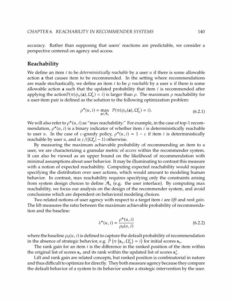
CHAPTER 6. REACHABILITY IN RECOMMENDER SYSTEMS 140
accuracy. Rather than supposing that users’ reactions are predictable, we consider a
perspective centered on agency and access.
ReachabilityWe define an item 8 to be deterministically reachable by a user D if there is some allowable
action a that causes item to be recommended. In the setting where recommendations
are made stochastically, we define an item 8 to be � reachable by a user D if there is some
allowable action a such that the updated probability that item 8 is recommended after
applying the actionP(�()D(a),ΩCD) = 8) is larger than �. The maximum � reachability for
a user-item pair is defined as the solution to the following optimization problem:
�★(D, 8) = max
a∈AD
%(�()D(a),ΩCD) = 8). (6.2.1)
Wewill also refer to �★(D, 8) as “max reachability.” For example, in the case of top-1 recom-
mendation, �★(D, 8) is a binary indicator of whether item 8 is deterministically reachable
to user D. In the case of �-greedy policy, �★(D, 8) = 1 − � if item 8 is deterministically
reachable by user D, and is �/(|ΩCD | − 1) otherwise.
By measuring the maximum achievable probability of recommending an item to a
user, we are characterizing a granular metric of access within the recommender system.
It can also be viewed as an upper bound on the likelihood of recommendation with
minimal assumptions about user behavior. It may be illuminating to contrast this measure
with a notion of expected reachability. Computing expected reachability would require
specifying the distribution over user actions, which would amount to modeling human
behavior. In contrast, max reachability requires specifying only the constraints arising
from system design choices to define AD (e.g. the user interface). By computing max
reachability, we focus our analysis on the design of the recommender system, and avoid
conclusions which are dependent on behavioral modeling choices.
Two related notions of user agency with respect to a target item 8 are lift and rank gain.The lift measures the ratio between the maximum achievable probability of recommenda-
tion and the baseline:
�★(D, 8) =�★(D, 8)�0(D, 8)
(6.2.2)
where the baseline �0(D, 8) is defined to capture the default probability of recommendation
in the absence of strategic behavior, e.g. %(�
(sD ,ΩC
D
)= 8
)for initial scores sD .
The rank gain for an item 8 is the difference in the ranked position of the item within
the original list of scores sD and its rank within the updated list of scores s+D .Lift and rank gain are related concepts, but ranked position is combinatorial in nature
and thusdifficult to optimize fordirectly. Theybothmeasure agencybecause they compare
the default behavior of a system to its behavior under a strategic intervention by the user.

CHAPTER 6. REACHABILITY IN RECOMMENDER SYSTEMS 141
Given that recommenders are designed with personalization in mind, we view the ability
of users to influence the model in a positive light. This is in contrast to much recent work
in robust machine literature where strategic manipulation is undesirable.
Diagnosing System LimitationsThe analysis of stochastic reachability can be used to audit recommender systems and
diagnose systemic biases from an interventional perspective (Figure 6.1). Unlike studies
of observational bias, these analyses take into account system interactivity. Unlike studies
of closed-loop bias, there is no dependence on a behaviormodel. Becausemax reachability
considers the best case over possible actions, it isolates structural biases from those caused
in part by user behavior.
Max reachability is a metric defined for each user-item pair, and disparities across
users and items can be detected through aggregations. Aggregating over target items
gives insight into a user’s ability to discover content, thus detecting users who have been
“pigeonholed” by the algorithm. Aggregations over users can be used to compare how
the system makes items available for recommendation.
We define the following user- and item-based aggregations:
�D =
∑8∈ΩC
D
1{�D8 > �C}|ΩC
D |, �8 =
∑D �D81{8 ∈ ΩC
D}∑D 1{8 ∈ ΩC
D} (6.2.3)
The discovery �D is the proportion of target items that have a high chance of being
recommended, as determined by the threshold �C . A natural threshold is the better-than-
uniform threshold, �C = 1/|ΩCD |, recalling that ΩC
D is the set of target items. When �D8 =�0(D, 8), baseline discovery counts the number of items that will be recommended with
better-than-uniform probability and is determined by the spread of the recommendation
distribution. For deterministic top-1 recommendation, we have that �D = 1. When
�D8 = �★(D, 8), discovery counts the number of items that a user could be recommended
with better-than-uniform probability in the best case. In the deterministic case, this is the
proportion of target items deterministically reachable by the user. Lowbest-case discovery
means that the recommender system inherently limits user access to content.
The item availability�8 is the average likelihood of recommendation over all userswho
have item 8 as a target. It can be thought of as the chance that a uniformly selected user
will be recommended item 8. When �D8 = �0(D, 8), the baseline availability measures the
prevalence of the item in the recommendations. When �D8 = �★(D, 8), availabilitymeasures
the prevalence of an item in the best case. For deterministic top-1 recommendation, it is
the proportion of eligible users who can reach the item. Low best-case availability means
that the recommender system inherently limits the distribution of a given item.

CHAPTER 6. REACHABILITY IN RECOMMENDER SYSTEMS 142
Observed scores Predicted scores
History edits Future edits
Goal item
User action
Figure 6.3: User action space: The shade represents the magnitude of historical (purple)
or predicted (green) rating. The action items are marked with diagonal lines; they can be
strategically modified to maximize the recommendation probability of the goal item (star).
The value of the user action is shaded in blue.
6.3 Computation via Convex Optimization
Affine RecommendationIn this section, we consider a restricted class of recommender systems for which the max
reachability problem can be efficiently solved via convex optimization.
User action model. We suppose that users interact with the system through expressed
preferences, and thus actions are updates to the vector rD ∈ ℛ< , a sparse vector of observedratings. For each user, the action model is based on distinguishing between action and
immutable items.
Let ΩAD denote the set of items for which the ratings can be strategically modified by
the user D. Then the action set AD = ℛ |ΩAD | corresponds to changing or setting the value
of these ratings. Figure 6.3 provides an illustration. The action set should be defined to
correspond to the interface through which a user interacts with the recommender system.
For example, it could correspond to a display panel of “previously viewed” or “up next”
items.
The updated rating vector r+D ∈ ℛ< is equal to rD at the indices corresponding to
immutable items and equal to the action a at the action items. Note the partition into action
and immutable is distinct from earlier partition of items into observed and unobserved;
action items can be both seen (history edits) and unseen (future reactions), as illustrated in
Figure 6.2A. For the reachabilityproblem,wewill consider a set of target itemsΩCD that does
not intersect with the action itemsΩAD . Depending on the specifics of the recommendation

CHAPTER 6. REACHABILITY IN RECOMMENDER SYSTEMS 143
setting, we may also require that it does not intersect with the previously rated items ΩD .
We remark that additional user or item features used for scoring and thus recom-
mendations could be incorporated into this framework as either mutable or immutable
features. The only computational difficulty arises when mutable features are discrete or
categorical.
Recommender model. The recommender model is composed of a scoring function )and a selection function �, which we now specify. We consider affine score update functionswhere for each user, scores are determined by an affine function of the action: s+D = )D(a) =�Da + cD where �D ∈ R<×|Ω
AD | and cD ∈ R< are model parameters determined in part by
historical data. Such a scoringmodel arises from a variety of preference models, as shown
in the examples later in this section.
Wenow turn to the selection component of the recommender,which translates the score
sD into a probability distribution over target items. The stochastic policy we consider is:
Definition 6.1 (Soft-max selection). For 8 ∈ ΩCD , the probability of item selection is given
by
%(��(sD ,ΩCD) = 8) =
4�BD8∑9∈ΩC
D4�BD9
.
This form of stochastic policy samples an item according to a Boltzmann distribution
defined by the predicted scores (Figure 6.2C). Distributions of this form are common in
machine learning applications, and are known as Boltzmann sampling in reinforcement
learning or online learning settings [WXLGC17; CGLN17].
Convex OptimizationWe now show that under affine score update models and soft-max selection rules, the
maximum stochastic reachability problem can be solved by an equivalent convex problem.
First notice that for a soft-max selection rule with parameter �, we have that
log
(%(��(sD ,ΩC
D) = 8))= �BD8 − LSE
9∈ΩCD
(�BD9
)where LSE is the log-sum-exp function.
Maximizing stochastic reachability is equivalent tominimizing its negative log-likelihood.
Letting bD8 ∈ R|ΩAD | denote the 8th row of the action matrix �D and substituting the form
of the score update rule, we have the equivalent optimization problem:
min
a∈AD
LSE
9∈ΩCD
(�(b>D9a + 2D9)
)− �(b>D8a + 2D8) (6.3.1)
If the optimal value to (6.3.1) is �★(D, 8), then the optimal value for (6.2.1) is given by
�★(D, 8) = 4−�★(D,8).

CHAPTER 6. REACHABILITY IN RECOMMENDER SYSTEMS 144
The objective in (6.3.1) is convex because log-sum-exp is a convex function, affine
functions are convex, and the composition of a convex and an affine function is convex.
Therefore, whenever the action space AD is convex, so is the optimization problem. The
size of the decision variable scales with the dimension of the action, while the objective
function relies on a matrix-vector product of size |ΩCD | × |AD |. Being able to solve the
maximum reachability problem quickly is of interest, since auditing an entire system
requires computing �★ for many user and item pairs.
In particular, the optimization problem (6.3.1) can be solved as an optimization over
the exponential cone:
min
C ,a,uC − �(b>D8a + 2D8)
s.t. a ∈ AD ,∑9∈ΩC
D
D9 ≤ 1,(D9 , 1, �(b>D9a + 2D9) − C
)∈ K4G? ∀ 9 ∈ ΩC
D
(6.3.2)
ExamplesWe review examples of common preferencemodels and show how the score updates have
an affine form.
Example 6.1 (MF-SGD). Matrix factorization models compute scores as rating predictions
so that ( = %&>, where % ∈ R=×3 and & ∈ R<×3 are respectively user and item factors for
some latent dimension 3. They are learned via the optimization
min
%,&
=∑D−1
∑8∈ΩD
‖p>Dq8 − AD8 ‖22.
Under a stochastic gradient descent minimization scheme with step size , the one-step
update rule for a user factor is
p+D = pD − ∑8∈ΩAD
(q8q>8 pD − q8AD8) ,
Notice that this expression is affine in the action items. Therefore, we have an affine score
function:
)D(a) = &p+D = &(pD − &>A&ApD − &>Aa
)where we define &A = &ΩAD
∈ R|ΩAD |×3. Therefore,
�D = − &&>A , cD = &(pD − &>A&ApD
).

CHAPTER 6. REACHABILITY IN RECOMMENDER SYSTEMS 145
Example 6.2 (Item-KNN). Neighborhood models compute scores as rating predictions by
a weighted average, with:
BD8 =
∑9∈N8 F8 9AD9∑9∈N8 |F8 9 |
where F8 9 are weights representing similarities between items and N8 is a set of indices
of previously rated items in the neighborhood of item 8. Regardless of the details of how
these parameters are computed, the predicted scores are a linear function of observed
scores: sD =,rD .Therefore, the score updates take the form
)D(a) =,r+D = ,rD︸︷︷︸cD
+,�ΩAD︸ ︷︷ ︸�D
a
where �ΩAD selects rows of, corresponding to action items.
Example 6.3 (SLIM and EASE). For both SLIM [NK11] and EASE [Ste19], scores are
computed as
BD8 = w>8 rDfor w8 the row vectors of a weight matrix, . For SLIM, the sparse weights are computed
as
min
,
1
2
‖' − ', ‖2� +�
2
‖, ‖2� + �‖, ‖1s.t., ≥ 0, diag(,) = 0
For EASE, the weights are computed as
min
,
1
2
‖' − ', ‖2� + �‖, ‖2
�
s.t. diag(,) = 0
In both cases, the score updates take the form
)D(a) = ,rD︸︷︷︸cD
+,�ΩAD︸ ︷︷ ︸�D
a .
In all these examples, the action matrices can be decomposed into two terms. The first
is a term that depends only on the preference model (e.g. item factors & or weights,),
while the second is further dependent on the user action model (e.g. action item factors
&A or action selector �ΩAD ).
For simplicity of presentation, the examples above leave out model bias terms, which
are common in practice. Incorporating these model biases changes only the definition
of the affine term in the score update expression. We now present the full action model
derivation with biases.

CHAPTER 6. REACHABILITY IN RECOMMENDER SYSTEMS 146
Example 6.4 (BiasedMF-SGD). Biasedmatrix factorizationmodels [KB15] compute scores
as rating predictions with
BD8 = p>Dq8 + 5D + 68 + �% ∈ R=×3 and & ∈ R<×3 are respectively user and item factors for some latent dimension
3, f ∈ R= and g ∈ R< are respectively user and item biases, and � ∈ R is a global bias.
The parameters are learned via the regularized optimization
min
%,&,f,g,�
1
2
=∑D=1
∑8∈ΩD
‖p>Dq8 + 5D + 68 + � − AD8 ‖22+ �
2
‖%‖2� +�2
‖&‖2� .
Under a stochastic gradient descent minimization scheme [Kor08] with step size , theone-step update rule for a user factor is
p+D = pD − ∑8∈ΩAD
(q8q>8 pD + q8( 5D + 68 + �) − q8AD8) − �pD .
User bias terms can be updated in a similar manner, but because the user bias is equal
across items, it does not impact the selection of items.
Notice that this expression is affine in themutable ratings. Therefore, we have an affine
score function:
)D(a) = &p+D = &((1 − �)pD − &>A(&ApD + gA + (� + 5D)1) + &>Aa
)where we define &A = &ΩAD
∈ R|ΩAD |×3 and gA = gΩAD ∈ R|ΩAD |. Therefore,
�D = &&>A , cD = &((1 + �)pD − &>A(&ApD + gA + (� + 5D)1)
).
Example 6.5 (Biased MF-ALS). Rather than a stochastic gradient descent minimization
scheme,wemay insteadupdate themodelwith analternating least-squares strategy [ZWSP08].
In this case, the update rule is
p+D = arg min
p
∑8∈ΩAD ∩ΩD
‖p>q8 + 5D + 68 + � − AD8 ‖22+ �‖p‖2
2
= (&>D&D + ��)−1(&>rD +&>A(gA + (� + 5D)1) +&>Aa)
where we define &D = &ΩAD ∩ΩD. Similar to in the SGD setting, this is an affine expression,
and therefore we end up with the affine score parameters
�D = &(&>D&D + ��)−1&>A , cD = &(&>D&D + ��)−1(&>rD +&>A(gA + (� + 5D)1)) .

CHAPTER 6. REACHABILITY IN RECOMMENDER SYSTEMS 147
Example 6.6 (Biased Item-KNN). Biased neighborhoodmodels [DK11] compute scores as
rating predictions by a weighted average, with
BD8 = � + 5D + 68 +∑9∈N8 F8 9(AD9 − � − 5D − 68)∑
9∈N8 |F8 9 |
where F8 9 are weights representing similarities between items,N8 is a set of indices which
are in the neighborhood of item 8, and f, g, � are bias terms. Regardless of the details
of how these parameters are computed, the predicted scores are an affine function of
observed scores:
sD =,rD −,(g + (� + 5D)1) + g + (� + 5D)1where we can define
,8 9 =
{ F8 9∑9∈N8 |F8 9 |
9 ∈ N80 otherwise
Therefore, the score updates take the form
)D(a) =,(rD − g + (� + 5D)1) + g + (� + 5D)1)︸ ︷︷ ︸cD
+,�ΩAD︸ ︷︷ ︸�D
a .
6.4 Impact of Preference Model GeometryIn this section,we explore the connectionbetween stochastic anddeterministic reachability
to illustrate how both randomness and agency contribute to discovery as defined by the
max reachability metric. We make connections between agency and model geometry
for matrix factorization models. This allows us to argue by example that it is possible
to design preference models that guarantee deterministic reachability, and that doing so
does not induce accuracy trade-offs.
Connection to Deterministic RecommendationWe now explore how the softmax style selection rule is a relaxation of top-1 recom-
mendation. For larger values of �, the selection rule distribution becomes closer to the
deterministic top-1 rule. This also means that the stochastic reachability problem can be
viewed as a relaxation of the top-1 reachability problem.
In stochastic settings it is relevant to inquire the extent to which randomness impacts
discovery and availability. In the deterministic setting, the reachability of an item to a user
is closely tied to agency—the ability of a user to influence their outcomes. The addition
of randomness induces exploration, but not in a way that is controllable by users. In
the following result, we show how this trade-off manifests in the max reachability metric
itself.

CHAPTER 6. REACHABILITY IN RECOMMENDER SYSTEMS 148
Proposition 6.4.1. Consider the stochastic reachability problem for a �-softmax selection rule as� → ∞. Then if an item 8 ∈ ΩC
D is top-1 reachable by user D, �★(D, 8) → 1. In the opposite casethat item 8 is not top-1 reachable, we have that �★(D, 8) → 0.
Proof. Define
��(a) = LSE
9∈ΩCD
(�)D9(a)
)− �)D8(a)
and see that �D8(a) = 4−��(a). Then we see that
lim
�→∞1
���(a) = max
9∈ΩCD
()D9(a)
)− )D8(a)
yields a top-1 expression. If an item 8 is top-1 reachable for user D, then there is some
a such that the above expression is equal to zero. Therefore, as � → ∞, �★ → 0, hence
�★ → 1. In the opposite case when an item is not top-1 reachable we have that �★ → ∞,
hence �★→ 0.
This connection yields insight into the relationship betweenmax reachability, random-
ness, and agency in stochastic recommender systems. For itemswhich are top-1 reachable,
larger values of � result in larger �★, and in fact the largest possible max reachability is
attained as � → ∞, i.e. there is no randomness. On the other hand, if � is too large, then
items which are not top-1 reachable will have small �★. There is some optimal finite � ≥ 0
that maximizes �★ for top-1 unreachable items. Therefore, we see a delicate balance when
it comes to ensuring access with randomness.
Viewed in another light, this result says that for a fixed � � 1, deterministic top-1
reachability ensures that �★ will be close to 1. We now explore this perspective. Special-
izing to affine score update models, we now highlight how parameters of the preference
and action models play a role in determining max reachability.
Recall the definition of the convex hull.
Definition 6.2 (Convex hull). The convex hull of a set of vectorsV = {v8}=8=1is defined as
conv (V) ={
=∑8=1
F8v8 | w ∈ R=+,=∑8=1
F8 = 1
}.
A point v9 ∈ V is a vertex of the convex hull if
v9 ∉ conv
(V \ {v9}
).
Proposition 6.4.2. Consider the stochastic reachability problem for a �-softmax selection rule andaffine score update model with action vectors {bD9}<9=1
. Fix an 8 ∈ ΩCD . If bD8 is a vertex on the
convex hull of {bD9} 9∈ΩCDand actions are real-valued, then �★
D8→ 1 as � → ∞ and the item 8 is
top-1 reachable.

CHAPTER 6. REACHABILITY IN RECOMMENDER SYSTEMS 149
Proof. We begin by showing that if bD8 is a vertex on the convex hull of ℬ = {bD9} 9∈ΩCD,
then item 8 is top-1 reachable.
Item 8 is top-1 reachable if there exists some a ∈ R|ΩAD | such that b>D8
a + 2D8 ≥ b>D9
a + 2D9for all 9 ≠ 8. Therefore, top-1 reachability is equivalent to the feasibility of the following
linear program
min 0>a
s.t. �D8a ≥ fD8
where �D8 has rows given by bD8 − bD9 and fD8 has entries given by 2D9 − 2D8 for all 9 ∈ ΩCD
with 9 ≠ 8. Feasibility of this linear program is equivalent to boundedness of its dual:
max f>D8�s.t. �>D8� = 0, � ≥ 0.
We now show that if bD8 is a vertex on the convex hull of ℬ, then the dual is bounded
because the only feasible solution is � = 0. To see why, notice that
�>D8� = 0 ⇐⇒ bD8∑9∈ΩC
D9≠8
� 9 =∑9∈ΩC
D9≠8
� 9bD9 .
If this expression is true for some � ≠ 0, then we can write
bD8 =∑9∈ΩC
D9≠8
F 9bD9 , F 9 =� 9∑9∈ΩC
D9≠8
� 9=⇒ bD8 ∈ conv (ℬ \ {bD8}) .
This is a contradiction, and therefore it must be that � = 0 and therefore the dual is
bounded and item 8 is top-1 reachable.
To finish the proof, we appeal to Proposition 6.4.1 to argue that since item 8 is top-1
reachable, then �★D8→ 1 as �→∞.
This result highlights how the geometry of the score model determines when it is
preferable for the system to haveminimal exploration, from the perspective of reachability.
Latent Geometry in MF ModelsWe now restrict our attention to top-1 recommendation policies with score models based
onmatrix factorization, as in Example 6.1. This allows for a re-interpretation of our results
so far in terms of the latent space of item and user factors. The action vectors specialized
to the matrix factorization case are given as, for each 8 ∈ {1, . . . , <}
bD8 = − &Aq8 .

CHAPTER 6. REACHABILITY IN RECOMMENDER SYSTEMS 150
Figure 6.4: Left: Items in Latent Space. Right: Availability of Items to a User. An example
of item factors (indicted by colored points) in 3 = 2. In (a), the top-1 item regions are
indicated by color. The teal item is unavailable. In (b), reachability for a user who has
seen the blue and the green items (now in gray) with the blue item’s rating fixed. The
black line indicates how the user’s representation can change depending on their rating
of the green item. The red region indicates the constraining effect of requiring bounded
and integer-valued ratings, which affect the reachability of the yellow item.
The geometry of the action vectors is thus determined by the geometry of the item factors
and the set of action items. These two can be decomposed by re-interpreting the score
update model, described in Example 6.1, as consisting of two steps:
1. Update the user factor, depending on &A and actions a.
2. Recompute scores, depending on the target item factors {q9 | 9 ∈ ΩCD}.
With this interpretation in mind, we can define the item-region for item 8 as
S8 = {p | q>8 p > q>9 p ∀ 9 ≠ 8 ∈ ΩCD}
If a user’s latent vector lies within this set, then the user will be recommended item 8.
We can therefore interpret reachability as the search for an action a that brings the user’s
updated latent vector p+D into the item region S8 . There are thus two potential barriers
to reachability: first, the region S8 could be empty; second, the action space may not be
rich enough to allow for full movement. The first stems from the geometry of the learned
preference model parameters, while the second from user interface design. This idea is
illustrated in Figure 6.4 for a toy example with latent dimension 3 = 2.
User cold-start. Reachability yields a novel perspective on how to incorporate new users
into a recommender system. The user cold-start problem is the challenge of selecting items
to show a user who enters a system with no rating history from which to predict their
preferences. This is a major issue with collaboratively filtered recommendations, and
systems often rely on incorporating extraneous information [SPUP02]. These strategies

CHAPTER 6. REACHABILITY IN RECOMMENDER SYSTEMS 151
focus onpresenting itemswhich aremost likely to be rated highly or to bemost informative
about user preferences [BLR17].
The idea of reachability offers an alternative point of view. Rather than evaluating a
potential “onboarding set” only for its contribution to model accuracy, we can choose a
set which additionally ensures that many types of items are reachable. We can evaluate
an onboarding set by the geometry of the action vectors in latent space. Inspired by
Proposition 6.4.2, in the case of matrix factorization, we should check for any candidate
set of action items ΩAD , what proportion of the elements {&Aq9 | 9 ∈ ΩCD} are vertices
on the convex hull. Due to computational difficulties, we primarily propose this be used
to distinguish between candidate onboarding sets, based on the ways these sets provide
user agency. We leave to future work the task of generating candidate sets based on these
reachability properties.
Reachability Without Sacrificing AccuracyWe now consider whether geometric properties of the preference model relevant to reach-
ability are predetermined by the goal of accurate prediction. Is there a tension between
ensuring reachability and accuracy? We answer in the negative by presenting a construc-
tion for the case of matrix factorization models. Our result shows that the item and user
factors (% and &) can be slightly altered such that all items become top-1 reachable at no
loss of predictive accuracy. The construction expands the latent dimension of the user
and item factors by one and relies on a notion of sufficient richness for action items.
Definition 6.3 (Rich actions). For a set of item factors {q9}<9=1, let � = max9 ‖q9 ‖2. Then a
set of action items ΩAD ⊆ {1, . . . , <} is sufficiently rich if the vertical concatenation of their
item factors and norms is full rank:
rank
( [q>8
√�2 − ‖q8 ‖2
2
]8∈ΩAD
)= 3 + 1 .
Notice that this can only be true if |ΩAD | ≥ 3 + 1.
Proposition 6.4.3. Consider theMFmodel with user factors% ∈ R=×3 and item factors& ∈ R<×3.Further consider any user D with a sufficiently rich set of at least 3+1 action items and real-valuedactions. Then there exist % ∈ R=×3+1 and & ∈ R<×3+1 such that %&> = %&> and under thismodel, all target items 8 ∈ ΩC
D are top-1 reachable.
Proof. Let � be themaximum row norm of& and define v ∈ R< such that E2
8= �2−‖q8 ‖2
2.
Then we construct modified item and user factors as
& =[& v
], % =
[% 0
].
Therefore, we have that %&> = %&>.

CHAPTER 6. REACHABILITY IN RECOMMENDER SYSTEMS 152
Then notice that by construction, each row of & has norm �, so each q8 is on the
boundary of an ℓ2 ball in R3+1. As a result, each q8 is a vertex on the convex hull of {q9}=9=1
as long as all q9 are unique.For an arbitrary user D, the score model parameters are given by bD8 = − &Aq8 . We
show by contradiction that as long as the action items are sufficiently rich, each bD8 is avertex on the convex hull of {bD9}=9=1
. Supposing this is not the case for an arbitrary 8,
bD8 ==∑9=1
9≠8
F 9bD9 ⇐⇒ &Aq8 ==∑9=1
9≠8
F 9&Aq8 =⇒ q8 ==∑9=1
9≠8
F 9q8
where the final implication follows because the fact that &A is full rank (due to richness)
implies that &>A&A is invertible. This is a contradiction, and thereforewehave that each bD8must be a vertex on the convex hull of {bD9}=9=1
. Finally, we appeal to Proposition 6.4.2.
The existence of such a construction demonstrates that there is not an unavoidable
trade-off between accuracy and reachability in recommender systems.
6.5 Audit Demonstration
Experimental SetupCode is available at www.github.com/modestyachts/stochastic-rec-reachability.
Datasets. We evaluate max � reachability in settings based on three popular recommen-
dation datasets: MovieLens 1M (ML-1M) [HK15], LastFM 360K [Cel10] and MIcrosoft
News Dataset (MIND) [WQC+20]. ML-1M is a dataset of 1 through 5 explicit ratings
of movies, containing over one million recorded ratings; we do not perform any ad-
ditional preprocessing. LastFM is an impliciGangnamt rating dataset containing the
number of times a user has listened to songs of an artist. We used the version of
the LastFM dataset preprocessed by Shakespeare et al. [SPGC20]. For computational
tractability, we select a random subset of 10% of users and 10% artists and define ratings
as AD8 = log(#listens(D, 8)+1) to ensure that rating matrices are well conditioned. MIND is
an implicit rating dataset containing clicks and impressions data. We use a subset of 50K
users and 40K news articles spanning 17 categories and 247 subcategories. We transform
news level click data into subcategory level aggregation and define the rating associated
with a user-subcategory pair as a function of the number of times that the user clicked
on news from that subcategory: AD8 = log(#clicks(D, 8) + 1). Table 6.1 provides summary
statistics and Section 6.7 contains further details about the datasets and preprocessing
steps.

CHAPTER 6. REACHABILITY IN RECOMMENDER SYSTEMS 153
Table 6.1: Audit datasets
Data set ML 1M LastFM 360K MIND
Users 6040 13698 50000
Items 3706 20109 247
Ratings 1000209 178388 670773
Density (%) 4.47% 0.065% 5.54%
LibFM rmse 0.716 1.122 0.318
KNN rmse 0.756 1.868 -
Preference models. We consider two preference models: one based on matrix factor-
ization (MF) as well as a neighborhood based model (KNN). We use the LibFM SGD
implementation [Ren12] for the MF model and use the item-based k-nearest neighbors
model implemented by Krauth et al. [KDZ+20]. For each dataset and recommender
model we perform hyper-parameter tuning using a 10%-90% test-train split. We report
test performance in Table 6.1. See Section 6.7 for details about tuning. Prior to performing
the audit, we retrain the recommender models with the full dataset.
Reachability experiments. We solve the conic program (6.3.2) using theMOSEK Python
API under an academic license [ApS19]. To compute reachability, it is further necessary
to specify additional elements of the recommendation pipeline: the user action model,
the set of target items, and the soft-max selection parameter.
We consider three types of user action spaces: History Edits, Future Edits, andNext K in
which users can strategically modify the ratings associated to randomly chosen items
from their history, randomly chosen unobserved items, or the top- items according to
the baseline scores of the preference model. For each of the action spaces we consider a
range of values. We further constrain actions to lie in an interval corresponding to the
rating range, using [1, 5] for movies and [0, 10] for music and news.
In the case of movies (ML-1M) we consider target items to be all items that are neither
seen nor action items. In the case of music and news recommendations (LastFM &
MIND), the target items are all the items with the exception of action items. This reflects
an assumption thatmusic created by a given artist or newswithin a particular subcategory
can be consumed repeatedly, while movies are viewed once.
For each dataset and recommendation pipeline, we compute max reachability for soft-
max selection rules parametrized by a range of � values. Due to the computational burden
of large densematrices, we computemetrics for a subset of users and target items sampled
uniformly at random. For details about runtime, see Section 6.7.

CHAPTER 6. REACHABILITY IN RECOMMENDER SYSTEMS 154
−20 −15 −10 −5 0log(ρ?)
0
1000
2000
3000
4000
Cou
nt
ρ? histogramUniform
ρ? = 0.05
0.1 0.2 0.3ρ?
0
20
40
60
80
Cou
nt
ρ? ≥0.05
β
1
2
4
0 2 4 6log(λ?)
0
1000
2000
3000
4000
5000
6000
Cou
nt
Lift histogram
Figure 6.5: Left: Histogram of log max reachability values for � = [1, 2, 4]. Black dotted
line denotes �★ for uniformly random recommender. Center: Histogram of �★ > 0.05 (red
dotted line). Right: Histogram of log-lifts. Reachability evaluated on ML-1M for = 5
Random Future action space and a LibFM model.
10−5 10−4 10−3 10−2 10−1
Baseline ρ
10−5
10−4
10−3
10−2
10−1
ρ?
β = 1
Action items
20
10
5
10−32 10−22 10−12 10−7 10−2
Baseline ρ
10−27
10−23
10−19
10−15
10−11
10−7
10−3
ρ?
β = 10
No improvement
Figure 6.6: Log scale scatterplot of �★ values against baseline � for ∈ [5, 10, 20]. Col-
ors indicate action space size . We compare low (left) and high (right) stochasticity.
Reachability evaluated on ML-1M for Random Future action space and a LibFM model.

CHAPTER 6. REACHABILITY IN RECOMMENDER SYSTEMS 155
Impact of Recommender PipelineWe begin by examining the role of recommender pipeline components: stochasticity
of item selection, user action models, and choice of preference model. All presented
experiments in this section use the ML-1M dataset.
These experiments show that more stochastic recommendations correspond to higher
average max reachability values, whereas more deterministic recommenders have a more
disparate impact, with a small number of items achieving higher �★. We also see that
the impact of the user action space differs depending on the preference model. For
neighborhood based preference models, strategic manipulations to the history are most
effective at maximizing reachability, whereas manipulations of the items most likely to be
recommended next are ineffective.
Role of stochasticity. We investigate the role of the � parameter in the item selection
policy. Figure 6.5 illustrates the relationship between the stochasticity of the selection
policy and max reachability. There are significantly more target items with better than
random reachability for low values of �. However, higher values of � yield more items
with high reachability potential (> 5% likelihood of recommendation). These items are
typically items that are top-1 or close to top-1 reachable. While lower � values provide
better reachability on average and higher � values provide better reachability at the “top”,
higher � uniformly out-performs lower � values in terms of the lift metric. This suggests
that larger � corresponds tomore user agency, since the relative effect of strategic behavior
is larger. However, note that for very large values of �, high lift values are not so much
the effect of improved reachability as they are due to very low baseline recommendation
probabilities.
Role of user actionmodel. Wenowconsider different action space sizes. In Figure 6.6we
plot max reachability for target items of a particular user over varying levels of selection
rule stochasticity and varying action space sizes. Larger action spaces correspond to
improved item reachability for all values of �. However, increases in the number of action
items have a more pronounced effect for larger � values.
While increasing the size of the action space uniformly improves reachability, the same
cannot be said about the type of action space. For each user, we compute the average lift
over target items as a metric for user agency in a recommender (Figure 6.7). For LibFM,
the choice of action space does not strongly impact the average user lift, though Next Kdisplays more variance across users than the other two. However, for Item KNN, there is
a stark difference between Next K and and random action spaces.
Role of preferencemodel. As Figure 6.7 illustrates, a systemusing LibFMprovidesmore
agency on average than one using KNN. We now consider how this relates to properties
of the preference models. First, consider the fact that for LibFM, there is higher variance
among user-level average lifts observed for Next K action space compared with random

CHAPTER 6. REACHABILITY IN RECOMMENDER SYSTEMS 156
1.0 2.0β
100
101
102
103
104
105A
vera
geλ?
Average user lift: LibFMNext K
Random future
Random history
1.0 2.0β
Ave
rageλ?
Average user lift: KNNNext K
Random future
Random history
Figure 6.7: The distribution of average lifts (a notion of agency) over users. Colors indicate
different user action spaces for LibFM (left) and KNN (right) on ML-1M.
action spaces. This can be understood as resulting from the user-specific nature of Next Krecommended items. On the other hand, random action spaces are user independent, so
it is not surprising that there is less variation across users.
In a neighborhood-based model users have leverage to increase the � reachability only
for target items in the neighborhood of action items. In the case of KNN, the next items
up for recommendation are in close geometrical proximity to each other. This limits the
opportunity for discovery of more distant items for Next K action space. On the other
hand, the action items are more uniformly over space of item ratings in random action
models, thus contributing to much higher opportunities for discovery. Additionally, we
see that History Edits displays higher average lift values than Future Edits. We posit that
this is due to the fact that editing items from the history leads to a larger ratio of strategic
to non-strategic items.
Bias in Movie, Music, and News RecommendationWe further compare aggregated stochastic reachability against properties of user and
items to investigate bias. We aggregate baseline and max reachability to compute user-
level metrics of discovery and item-level metrics of availability. The audit demonstrates
popularity bias for items with respect to baseline availability. This bias persists in the best
case for neighborhood based recommenders and is thus unavoidable, whereas it could be
mitigated for MF recommenders. User discovery aggregation reveals inconclusive results
with weak correlations between the length of users’ experience and their ability to access
content.
Popularity bias. In Figure 6.8, we plot the baseline and best case item availability (as
in (6.2.3)) to investigate popularity bias. We consider popularity defined by the average
rating of an item in a dataset. Another possible definition of popularity is rating frequency,

CHAPTER 6. REACHABILITY IN RECOMMENDER SYSTEMS 157
(1.0, 2.82] (2.82, 3.33] (3.33, 3.74] (3.74, 5.0]
Average item rating
10−7
10−6
10−5
10−4
10−3
10−2
10−1
100A
vera
geit
emρ
LibFM Availabilitybaseline
max
(1.0, 2.82] (2.82, 3.33] (3.33, 3.74] (3.74, 5.0]
Average item rating
10−7
10−6
10−5
10−4
10−3
10−2
10−1
100
Ave
rage
item
ρ
KNN Availabilitybaseline
max
Figure 6.8: Comparison of baseline and best case availability of content, across four
popularity categories for LibFM (left) and KNN (right) preference models. Reachability
evaluated on ML-1M for Next 10 action space with � = 2.
but for this definition we did not observe any discernible bias. For both LibFM and
KNN models, the baseline availability displays a correlation with item popularity, with
Spearman’s rank-order correlations of AB = 0.87 and AB = 0.95. This suggests that as
recommendations are made and consumed, more popular items will be recommended at
disproportionate rates.
Furthermore, the best case availability for KNN displays a similar trend (AB = 0.94),
indicating that the propagation of popularity bias can occur independent of user behavior.
This does not hold for LibFM, where the best case availability is less clearly correlated
with popularity (AB = 0.57). The lack of correlation for best case availability holds in the
additional settings of music artist and news recommendation with the LibFMmodel (Fig-
ure 6.9). Our audit does not reveal an unavoidable systemic bias for LibFM recommender,
meaning that any biases observed in deployment are due in part to user behavior. In
contrast, we see a systematic bias for the KNN recommender, meaning that regardless of
user actions, the popularity bias will propagate.
Experience bias. To consider the opportunities for discovery provided to users, we
perform user level aggregations of max reachability values as in (6.2.3). We investigate
experience bias by considering how the discovery metric changes as a function of the
number of different items a user has consumed so far, i.e. their experience. Figure 6.10
illustrates that experience is weakly correlated with baseline discovery for movie recom-
mendation (AB = 0.48), but not so much for news recommendation (AB = 0.05). The best
case discovery is much higher, meaning that users have the opportunity to discover many
of their target items. However, the weak correlation with experience remains for best case
discovery of movies (AB = 0.53).

CHAPTER 6. REACHABILITY IN RECOMMENDER SYSTEMS 158
(0.69, 3.31] (3.31, 4.15] (4.15, 4.81] (4.81, 9.62]
Average item rating
10−7
10−6
10−5
10−4
10−3
10−2
10−1
100A
vera
geit
emρ
LastFM Availabilitybaseline
max
0.69 (0.69, 0.71] (0.71, 0.79] (0.79, 1.37]
Average item rating
10−3
10−2
10−2
10−2
10−1
10−0
100
Ave
rage
item
ρ
MIND Availabilitybaseline
max
Figure 6.9: Comparison of baseline and best case availability of content for four popularity
categories for LastFM (left) and MIND (right) with Next 10 actions, LibFM model, and
� = 2.
(20, 44] (44, 96] (96, 208] (208, 2314]
Number of total ratings
0
20
40
60
80
100
%it
ems
wit
hab
ove
ran
dom
ρ? ML-1M Discovery
baseline
max
(1, 6] (6, 11] (11, 18] (18, 88]
Number of total ratings
%it
ems
wit
hab
ove
ran
dom
ρ? MIND Discoverybaseline
max
Figure 6.10: Comparison of baseline and best case fraction of items with better than
random �★, grouped across four levels of user history length. Reachability evaluated on
ML-1M (left) and MIND (right) for Next 10 action space, � = 2, and LibFM model.
6.6 Conclusion and Open ProblemsIn this chapter, we consider the effects of using predicted user preferences to recommend
content, a practice prevalent throughout the digital world today. By defining reachability
for deterministic and stochastic recommenders, we provide a way to evaluate the impact
of using these predictive models to mediate the discovery of content. In applying this
lens to linear preference models, we see several interesting phenomena. The first is
simple but worth stating: good predictive models, when used to moderate information,
can unintentionally make portions of the content library inaccessible to users. This is
illustrated in practice in our study of the MovieLens, LastFM, and MIND datasets. Our
experiments illustrate the impact of system design choices and historical data on the

CHAPTER 6. REACHABILITY IN RECOMMENDER SYSTEMS 159
availability of content and users’ opportunities for discovery, highlighting instances in
which popularity bias is inevitable regardless of user behavior.
To some extent, the differences in the availability of items are related to their un-
popularity within training data. Popularity bias is a well known phenomenon in which
systems fail to personalize [Ste11], and instead over-recommend the most popular pieces
of content. Empirical work shows connections between popularity bias and undesirable
demographic biases, including the under-recommendation of female authors [ETKMK18].
YouTube was long known to have a popularity bias problem (known as the “Gangnam
Style Problem”), until the recommendations began optimizing for predicted “watch time”
over “number of views.” Their new model has been criticized for its radicalization and
political polarization [Tuf18; Nic18]. The choice of prediction target can have a large effect
on the types of content users can or are likely to discover, motivating the use of analytic
tools like the ones proposed here to reason about these trade-offs before deployment.
While the reachability criteriaproposed in thiswork forman important basis for reason-
ing about the availability of content within a recommender system, they do not guarantee
less biased behavior on their own. Because our audits primarily consider the feasibility,
we can only confirm possible outcomes rather than distinguish between probable ones.
This can illuminate limitations inherent in recommender systems for organizing and pro-
moting content. Consequently, a reachability audit can lead to actionable insights: system
designers can assess potential biases before releasing algorithmic updates into produc-
tion. Moreover, as reachability depends on the choice of action space, such system-level
insights might motivate user interface design: for example, a sidebar encouraging users
to re-rate items from their history. However, reachability alone will not fix problems
of filter bubbles or toxic content. There is an important distinction between technically
providing reachability and the likelihood that people will actually avail themselves of it.
With these limitations in mind, wemention several ways to extend the ideas presented
in this work:
• Generative theory of reachability. Analyzing connections between training data
and the reachability properties of the resulting model would to give context to
empirical work showing how biases can be reproduces in the way items are recom-
mended [ETKMK18; ETA+18].
• Extended class of preferencemodels. Manymodels for rating predictions do not fall
into the linear class described here, especially those that incorporate implicit feed-
back or perform different online update strategies for users. Not all simple models
are linear—for example, subset based recommendations offer greater scrutability
and thus user agency by design [BRA19].
• Extended class of selection rules. Slate-based and top-# recommendation is com-
mon, but it is computationally difficult to evaluate the reachability properties of
these selection rules. One avenue for addressing more generic recommender poli-

CHAPTER 6. REACHABILITY IN RECOMMENDER SYSTEMS 160
cies might be an approach based on sampling, which could apply to even black-box
recommender evaluation.
• Reachability by design. Our result on the lack of trade-off between accuracy and
reachability is encouraging. Minimum one-step reachability conditions could be ef-
ficiently incorporated into learning algorithms for preference models. Alternatively,
post-processing approaches to the recommender policy � could work with existing
models to modify their reachability properties. For example, Steck [Ste18] proposed
a method to ensure that the distribution of recommendations over genres remains
the same despite model predictions.
• Interaction over longhorizons. Directly consideringmultiple rounds of interactions
between users and recommendation systems would shed light on how these models
evolve over time. This is a path towardsunderstandingphenomena like filter bubbles
and polarization.
We highlight that the reachability lens presents a contrasting view to the popular line
of work on robustness in machine learning. When human behaviors are the subject of
classification and prediction, building “robustness” into a system may be at odds with
ensuring agency. Because the goal of recommendation is personalization more than
generalization, it would be appropriate to consider robust access over robust accuracy.
This calls for questioning the current normative stance and critically examining system
desiderata in light of usage context.
More broadly, we emphasize the importance of auditing systems with learning-based
components in ways that directly consider the models’ behavior when put into feedback
with humans. In the field of formal verification, making guarantees about the behavior
of complex dynamical systems over time has a long history. There are many existing
tools [ABDM00], though they are generally specialized to the case of physical systems
and suffer from the curse of dimensionality. We accentuate the abundance of opportunity
for developing novel approximations and strategies for evaluating large scale machine
learning systems.
6.7 Additional Experimental Details
Detailed Data DescriptionMovieLens1M. ML-1Mdatasetwasdownloaded fromGroupLens1 via theRecLab [KDZ+20]
interface2. It contains 1 through 5 rating data of 6040 users for 3706 movies. There are
a total of 1000209 ratings (4.47% rating density). The original data is accompanied by
additional user attributes such as age, gender, occupation and zip code. Our experiments
1https://grouplens.org/datasets/movielens/1m/2https://github.com/berkeley-reclab/RecLab

CHAPTER 6. REACHABILITY IN RECOMMENDER SYSTEMS 161
1 2 3 4 5
Rating
0
50000
100000
150000
200000
250000
Cou
nt
Rating histogram
User genderMale
Female
2.0 2.5 3.0 3.5 4.0 4.5 5.0
Mean rating
0
100
200
300
400
500
600
Nu
m.
use
rs
Average user rating
0 100 200 300 400 500
Num. items
0200400600800
10001200
Nu
m.
use
rs
User history length
1 2 3 4 5
Mean rating
0
100
200
300
400
Nu
m.
item
Average item rating
0 200 400 600 800 1000 1200 1400 1600
Num. users
0
250
500
750
1000
1250
1500
Nu
m.
item
s
Item popularity
Figure 6.11: Descriptive statistics for theMovieLens 1Mdataset split by user gender (28.3%
female). The mean ratings of both users and items are roughly normally distributed while
user’s history length and item popularity display power law distributions.
didn’t indicate observable biases across these attributes. We later show user discovery
results split by gender.
Figure 6.11 illustrates descriptive statistics for the ML-1M dataset.
LastFM 360K. The LastFM 360K dataset preprocessed3 by Shakespeare et al. [SPGC20]
was loaded via the RecLab interface. It contains data on the number of times users have
listened to various artists. We select a random subset of 10% users and a random subset of
10% items yielding 13698 users, 20109 items and 178388 ratings (0.056% rating density).
The item ratings are not explicitly expressed by users as in the MovieLens case. For a
user D and an artist 8 we define implicit ratings AD8 = log(#listens(D, 8) + 1). This data is
accompanied by artist gender, an item attribute.
Figure 6.12 illustrates descriptive statistics for the LastFM dataset.
MIcrosoft News Dataset (MIND). MIND is a recently published impression dataset
collected from logs of the Microsoft News website 4. We downloaded the MIND-smalldataset5, which contains behavior log data for 50000 randomly sampled users. There are
42416 unique news articles, spanning 17 categories and 247 subcategories. We aggregate
user interactions at the subcategory level and consider the problem of news subcategory
recommendation. The implicit rating of a user D for subcategory 8 is defined as: AD8 =
log(#clicks(D, 8) + 1). The resulting aggregated dataset contains 670773 ratings (5.54%
rating density).
Figure 6.13 illustrates descriptive statistics for the MIND dataset.
3https://zenodo.org/record/3964506#.XyE5N0FKg5n4https://microsoftnews.msn.com/5https://msnews.github.io/

CHAPTER 6. REACHABILITY IN RECOMMENDER SYSTEMS 162
0 2 4 6 8
Rating
0
5000
10000
15000
20000
25000
30000
35000
40000
Cou
nt
Rating histogram
Artist genderMale
Female
Mixed
1 2 3 4 5 6 7 8
Mean rating
0
200
400
600
800
1000
Nu
m.
use
rs
Average user rating
0 5 10 15 20 25 30
Num. artists
0
250
500
750
1000
1250
1500
Nu
m.
use
rs
User history length
0 1 2 3 4 5 6 7
Mean rating
0
250
500
750
1000
1250
Nu
m.
arti
sts
Average artist rating
2 4 6 8 10 12
Num. users
0
1000
2000
3000
Nu
m.
arti
sts
Artist popularity
Figure 6.12: Descriptive statistics for the LastFM dataset split by artist gender (over 54% of
artists have unknown gender, 36% are male, 6.5% are female and 3.5% are mixed gender).
Unlike ML 1M, for the LastFM dataset the user history lengths are normally distributed
around a mean of around 12 artists.
1 2 3 4 5
Rating
101
103
105
Cou
nt
Rating histogram
Has clicks
No clicks
new
ssp
orts
finan
cefo
odan
dd
rin
klif
esty
letr
avel
hea
lth
vid
eoau
tos
wea
ther tv
mu
sic
ente
rtai
nm
ent
mov
ies
kid
sm
idd
leea
stga
mes
Category
0
5000
10000
Nu
m.
new
sar
ticl
es
0.8 1.0 1.2 1.4
Mean rating
0
2000
4000
6000
Nu
m.
use
rs
Average user rating
0 10 20 30 40 50
Num. subcategories
0
2000
4000
6000
Nu
m.
use
rs
User history length
0.7 0.8 0.9 1.0 1.1 1.2
Mean rating
0
25
50
75
100
Nu
m.
sub
-cat
egor
ies
Average sub-category rating
0 25 50 75 100 125 150 175 200
Num. users
0
10
20
30
40
Nu
m.
sub
-cat
egor
ies
Sub-category popularity
Figure 6.13: Descriptive statistics for the MIND dataset: The orange bars correspond to
either user or items that have been displayed but have not clicked/ have not been clicked
on. Unlike ML 1M and LastFM, the MIND ratings have strongly skewed distribution,
with most user-subcategory ratings corresponding to users clicking on a small number of
articles from the sub-category. There is a long tail of higher ratings that corresponds to
most popular subcategories. The leftmost plot illustrates the unequal distribution of news
articles across categories. The same qualitative behavior holds for sub-categories.

CHAPTER 6. REACHABILITY IN RECOMMENDER SYSTEMS 163
Table 6.2: Tuning results
LibFM
Dataset LR Reg. Test RMSE Run time (s)
ML 1M 0.0112 0.0681 0.716 2.76 ± 0.32
LastFM 0.0478 0.2278 1.122 0.78 ± 0.13
MIND 0.09 0.0373 0.318 3.23 ± 0.37
KNN
Dataset Neigh. size Shrinkage Test RMSE Run time (s)
ML 1M 100 22.22 0.756 0.34 ± 0.07
Model TuningFor each dataset and recommender model we perform grid search for progressively finer
meshes over the tunable hyper-parameters of the recommender. We use recommenders
implemented by the RecLab library. For each dataset and recommender we evaluate
hyperparameters on a 10% split of test data. The best hyper-parameters for each setting
are presented in Table 6.2.
LibFM. We performed hyper-parameter tuning to find suitable learning rate and regu-
larization parameter for each dataset. Following [DBCJ21] we consider lr ∈ (0.001, 0.5)as the range of hyper-parameters for the learning rate and reg ∈ (10
−5, 100) for the regu-
larization parameter. In all experimental settings we follow the setup of [RZK19] and use
64 latent dimensions and train with SGD for 128 iterations.
KNN. Weperformhyperparameter tuningwith respect to neighborhood size and shrink-
age parameter. Following [DBCJ21] we consider the range (5, 1000) for the neighborhoodsize and (0, 1000) for the shrinkage parameter. We tune KNN only for the ML-1M dataset.
Experimental Infrastructure and Computational ComplexityAll experiments were performed on a 64 bit desktop machine equipped with 20 CPUs
(Intel(R) Core(TM) i9-7900X CPU @ 3.30GHz) and a 62 GiB RAM. Average run times for
training an instance of each recommender can be found in Table 6.2.
Experimental Setup for Computing ReachabilityThe parameters �D and cD are computed for each user based on the recommendermodel as
described in the examples in Section 6.3. For the LibFMmodel, we consider user updates

CHAPTER 6. REACHABILITY IN RECOMMENDER SYSTEMS 164
with = 0.1 and � = 0. Average run times for computing reachability of a user-item pair
in various settings can be found in Table 6.3.
ML 1M. We compute max stochastic reachability for the LibFM and KNN preference
model. We consider three types of user action spaces: History Edits, Future Edits, andNextK in which users can strategically modify the ratings associated to randomly chosen
items from their history, randomly chosen items from that they have not yet seen, or the
top- unseen items according to the baseline scores of the preference model. For each of
the action spaces we consider ∈ {5, 10, 20}.We perform reachability experiments on a random 3% subset of users (176). For each
choice of preference model, action space type and action space size we sample for each
user 500 random items that have not been previously rated and are not action items.
For each user-item pair we compute reachability for a range of stochasticity parameters
� ∈ {1, 2, 4, 10}. Note that across all experimental settings we compute reachability for
the same subset of users, but different subsets of randomly selected target items.
We use theML 1Mdataset to primarily gain insights in the role that preferencemodels,
item selection stochasticity and strategic action spaces play in determining the maximum
achievable degree of stochastic reachability in a recommender system.
LastFM. We run reachability experiment for LibFM recommender with Next K = 10action model and stochasticity parameter � = 2. We compute �★ values for 100 randomly
sampled users and 500 randomly sampled items from the set of non-action items (target
items can include previously seen items). Unlike the ML 1M dataset, the set of target
items is shared among all users.
MIND. We run reachability experiments for LibFM recommender with Next K = 10action model and stochasticity parameter � = 2. We compute reachability for all items
and users.
Reachability run times. In Table 6.3 we present the average clock time for computing
reachability for a user-item pair in the settings described above. Due to internal represen-
tation of action spaces as matrices the runtime dependence on the dimension of the action
space is fairly modest. We do not observe significant run time differences between dif-
ferent types of action spaces. We further add multiprocessing functionality to parallelize
reachability computations over multiple target items.
Detailed Results: Impact of Recommender DesignWe present further insights in the experimental settings studied in Section 6.5. For ML-
1M, we replicate the log scale scatter plots of �★ against baseline � for all the action spaces
(Next K, Random Future, Random History), the full range of � ∈ {1, 2, 4, 10} and the two

CHAPTER 6. REACHABILITY IN RECOMMENDER SYSTEMS 165
Table 6.3: Reachability run times (in seconds).
Num. actions ML 1M (LibFM) ML 1M (KNN) LastFM MIND
K = 5 0.82 ± 0.04 9.8 ± 3.4 - -
K = 10 0.87 ± 0.04 10.2 ± 6.1 4.91 ± 0.32 0.44 ± 0.01
K= 20 0.91 ± 0.05 11.4 ± 6.8 - -
10−5 10−4 10−3 10−2 10−1
Baseline ρ
10−4
10−3
10−2
10−1
ρ?
Next K: β = 1
Action items
20
10
5
10−6 10−4 10−2 10−1
Baseline ρ
10−5
10−4
10−3
10−2
10−1
ρ?
Next K: β = 2
No improvement
10−11 10−9 10−7 10−5 10−3 10−1
Baseline ρ
10−9
10−7
10−5
10−3
10−1
ρ?
Next K: β = 4
10−26 10−22 10−18 10−14 10−10 10−6 10−2
Baseline ρ
10−23
10−20
10−17
10−14
10−11
10−8
10−5
10−2
ρ?
Next K: β = 10
10−5 10−4 10−3 10−2 10−1
Baseline ρ
10−5
10−4
10−3
10−2
10−1
ρ?
Random Future: β = 1
Action items
20
10
5
10−8 10−6 10−4 10−3 10−2 10−1
Baseline ρ
10−7
10−6
10−5
10−4
10−3
10−2
10−1
ρ?
Random Future: β = 2
No improvement
10−13 10−11 10−9 10−7 10−5 10−3 10−1
Baseline ρ
10−11
10−9
10−7
10−5
10−3
10−1
ρ?
Random Future: β = 4
10−32 10−27 10−22 10−17 10−12 10−7 10−2
Baseline ρ
10−27
10−23
10−19
10−15
10−11
10−7
10−3
ρ?
Random Future: β = 10
10−5 10−4 10−3 10−2 10−1
Baseline ρ
10−4
10−3
10−2
10−1
ρ?
Random History: β = 1
Action items
20
10
5
10−7 10−5 10−3 10−2 10−1
Baseline ρ
10−5
10−4
10−3
10−2
10−1
ρ?
Random History: β = 2
No improvement
10−11 10−9 10−7 10−5 10−3 10−1
Baseline ρ
10−8
10−7
10−6
10−5
10−4
10−3
10−2
10−1
ρ?
Random History: β = 4
10−2810−2410−2010−1610−12 10−8 10−4 100
Baseline ρ
10−17
10−14
10−11
10−8
10−5
10−2
ρ?
Random History: β = 10
Figure 6.14: Log scale scatter plots of �★ against baseline � evaluated for the LibFM
preference model.
preference models: LibFM (Figure 6.14) and KNN (Figure 6.15). We observe that for both
KNN and LibFM, random history edits can lead to higher �★ values. We posit that this
increased agency is partly due to the fact that when editing items from the history a
user edits a larger fraction of total ratings compared to editing future items.
Themost striking feature of KNN reachability results is the strong correlation between
baseline � and �★. The correlations between baseline and max probability of recommen-
dation is less strong in the case of LibFM. These insights are corroborated by Figure 6.16
which compares the average LibFM and KNN user lifts for different choices of action
space, action size K, stochasticity parameter �.

CHAPTER 6. REACHABILITY IN RECOMMENDER SYSTEMS 166
10−4 10−3
Baseline ρ
10−4
10−3
ρ?
Next K: β = 1
Action items
20
10
5
10−6 10−4 10−2
Baseline ρ
10−6
10−5
10−4
10−3
10−2
ρ?
Next K: β = 2
No improvement
10−10 10−8 10−6 10−4 10−2
Baseline ρ
10−10
10−8
10−6
10−4
10−2
ρ?
Next K: β = 4
10−25 10−21 10−17 10−13 10−9 10−5 10−1
Baseline ρ
10−25
10−21
10−17
10−13
10−9
10−5
10−1
ρ?
Next K: β = 10
10−5 10−4 10−3 10−2
Baseline ρ
10−5
10−4
10−3
10−2
ρ?
Random Future: β = 1
Action items
20
10
5
10−7 10−5 10−3 10−2 10−1
Baseline ρ
10−7
10−6
10−5
10−4
10−3
10−2
10−1
ρ?
Random Future: β = 2
No improvement
10−12 10−10 10−8 10−6 10−4 10−2
Baseline ρ
10−12
10−10
10−8
10−6
10−4
10−2
ρ?
Random Future: β = 4
10−3010−2610−2210−1810−1410−1010−6 10−2
Baseline ρ
10−29
10−25
10−21
10−17
10−13
10−9
10−5
10−1
ρ?
Random Future: β = 10
10−5 10−4 10−3 10−2 10−1
Baseline ρ
10−4
10−3
10−2
10−1
ρ?
Random History: β = 1
Action items
20
10
5
10−8 10−6 10−4 10−3 10−2 10−1
Baseline ρ
10−6
10−5
10−4
10−3
10−2
10−1
ρ?
Random History: β = 2
No improvement
10−1510−1310−11 10−9 10−7 10−5 10−3 10−1
Baseline ρ
10−10
10−8
10−6
10−4
10−2ρ?
Random History: β = 4
10−3610−3110−2610−2110−1610−1110−6 10−1
Baseline ρ
10−26
10−22
10−18
10−14
10−10
10−6
10−2
ρ?
Random History: β = 10
Figure 6.15: Log scale scatter plots of �★ against baseline � evaluated for the KNN prefer-
ence model.
Detailed Results: BiasWe present further results on the settings studied in Section 6.5. We replicate the popu-
larity bias results on ML-1M for different action spaces and plot the results in Figure 6.17.
We see that the availability bias for KNN is dependent on the action space, with RandomHistory displaying no or little correlation between popularity and max availability. This is
not surprising given the results in Figure 6.7.
To systematically study the popularity bias, we compute the Spearman rank-order
correlation coefficient to measure the presence of a monotonic relationship between pop-
ularity (as measured by average rating) and availability (either in the baseline or max
case). We also compute the correlation between the popularity and the prevalence in the
dataset, as measured by number of ratings.
The impact of user action spaces is displayed in Figure 6.18, which plots the correlation
between popularity and max availability for different action spaces. For comparison, the
correlation between popularity and baseline availability is just over 0.8 for all of these
settings6, while the correlation with dataset prevalence is 0.346. Table 6.4 shows these
correlation values across datasets for a fixed action model. In all cases with the LibFM
6Due to variation in baseline actions, the baseline availability is not exactly the same.

CHAPTER 6. REACHABILITY IN RECOMMENDER SYSTEMS 167
1.0 2.0 4.0β
100
102
104
106
108
1010
Ave
rageλ?
LibFM: K = 5Next K
Random future
Random history
1.0 2.0 4.0β
Ave
rageλ?
LibFM: K = 10Next K
Random future
Random history
1.0 2.0 4.0β
Ave
rageλ?
LibFM: K = 20Next K
Random future
Random history
1.0 2.0 4.0β
100
102
104
106
108
1010
Ave
rageλ?
KNN: K = 5Next K
Random future
Random history
1.0 2.0 4.0β
Ave
rageλ?
KNN: K = 10Next K
Random future
Random history
1.0 2.0 4.0β
Ave
rageλ?
KNN: K = 20Next K
Random future
Random history
Figure 6.16: Side by side comparison of average user lifts for LibFM (top row)and
KNN(bottom row).
(1.0, 2.82] (2.82, 3.33] (3.33, 3.74] (3.74, 5.0]
Average item rating
10−7
10−6
10−5
10−4
10−3
10−2
10−1
100
Ave
rage
item
ρ
LibFM Random futurebaseline
max
(1.0, 2.82] (2.82, 3.33] (3.33, 3.74] (3.74, 5.0]
Average item rating
10−7
10−6
10−5
10−4
10−3
10−2
10−1
100
Ave
rage
item
ρ
KNN Random futurebaseline
max
(1.0, 2.82] (2.82, 3.33] (3.33, 3.74] (3.74, 5.0]
Average item rating
10−7
10−6
10−5
10−4
10−3
10−2
10−1
100
Ave
rage
item
ρ
LibFM Random historybaseline
max
(1.0, 2.82] (2.82, 3.33] (3.33, 3.74] (3.74, 5.0]
Average item rating
10−7
10−6
10−5
10−4
10−3
10−2
10−1
100
Ave
rage
item
ρ
KNN Random historybaseline
max
Figure 6.17: Side by side comparison of baseline and best-case availability of content,
across fourpopularity categories. From left to right: LibFMpreferencemodelwithRandomFuture, KNNpreferencemodelwithRandom Future, LibFMpreferencemodelwithRandomHistory, KNN preference model with Random History. Reachability evaluated on ML-1M
for with = 10 and � = 2.

CHAPTER 6. REACHABILITY IN RECOMMENDER SYSTEMS 168
Next K Random history Random future
Action space
0.0
0.2
0.4
0.6
0.8
1.0
Max
Ava
il.C
orre
lati
on
LibFM
K
5
10
20
Next K Random history Random future
Action space
Max
Ava
il.C
orre
lati
on
KNN
K
5
10
20
Figure 6.18: Comparison of Spearman’s correlation between item popularity and max
availability for different action spaces and models. Reachability evaluated on ML-1M
with � = 2.
Table 6.4: Spearman’s correlation with popularity for Next K with = 10 and � = 2.
corr. with corr. with corr. with
dataset model dataset prevalence baseline availability max availability
ml-1m libfm 0.346280 0.827492 0.501316
ml-1m knn 0.346280 0.949581 0.942986
mind libfm 0.863992 0.825251 0.435212
lastfm libfm 0.133318 0.671101 0.145949
model, the pattern that popularity is less correlated with max availability than baseline
availability holds; however, the correlation with dataset prevalence varies.
To investigate experience bias, we similarly compute the Spearman rank-order cor-
relation coefficient to measure the presence of a monotonic relationship between user
experience (as measured by number of items rated) and discovery (either in the baseline
or max case). We observe correlation values of varying sign across datasets and models,
and none are particularly strong (Table 6.5).
Finally, we investigate gender bias. We compare discovery across user gender for ML-
1M and availability across artist gender for LastFM (Figure 6.19). We do not observe any
trends in either baseline or max values.
CHAPTER 6. REACHABILITY IN RECOMMENDER SYSTEMS 169
Table 6.5: Spearman’s correlation with experience for Next K with = 10 and � = 2.
corr. with corr. with
dataset model baseline discovery max discovery
ml-1m libfm 0.475777 0.530359
ml-1m knn 0.206556 -0.031929
mind libfm 0.050961 0.112558
lastfm libfm -0.084130 -0.089226
F M
User gender
0
20
40
60
80
100
%of
item
sw
ith
abov
era
nd
omρ?
ML-1M Discovery: Next kbaseline
max
F M
User gender
%of
item
sw
ith
abov
era
nd
omρ?
ML-1M Discovery: Random futurebaseline
max
F M
User gender
%of
item
sw
ith
abov
era
nd
omρ?
ML-1M Discovery: Random historybaseline
max
Female Male Mixed
Artist gender
10−7
10−6
10−5
10−4
10−3
10−2
10−1
100
Ave
rage
item
ρ
LastFM Availabilitybaseline
max
Figure 6.19: Side by side comparison of baseline and maximum discovery across user
gender (left 3 panels) and availability across artist gender (rightmost panel). Reachability
evaluated on ML-1M and LastFMwith LibFMmodel, = 10, different action spaces, and
� = 2.

170
Bibliography
[ABC+20] OpenAI:Marcin Andrychowicz, Bowen Baker, Maciek Chociej, Rafal Joze-
fowicz, Bob McGrew, Jakub Pachocki, Arthur Petron, Matthias Plappert,
GlennPowell, AlexRay, et al. “Learningdexterous in-handmanipulation”.
In: The International Journal of Robotics Research 39.1 (2020).[ABDM00] Eugene Asarin, Olivier Bournez, Thao Dang, and Oded Maler. “Approxi-
mate reachability analysis of piecewise-linear dynamical systems”. In: In-ternational Workshop on Hybrid Systems: Computation and Control. Springer.2000.
[ABHKS19] Naman Agarwal, Brian Bullins, Elad Hazan, Sham Kakade, and Karan
Singh. “Online control with adversarial disturbances”. In: InternationalConference on Machine Learning. PMLR. 2019.
[ACST21] Amir Ali Ahmadi, Abraar Chaudhry, Vikas Sindhwani, and Stephen Tu.
“Safely Learning Dynamical Systems from Short Trajectories”. In: Learningfor Dynamics and Control. PMLR. 2021.
[AGST13] Anil Aswani, Humberto Gonzalez, S Shankar Sastry, and Claire Tomlin.
“Provably Safe and Robust Learning-BasedModel Predictive Control”. In:
Automatica 49.5 (2013).[AHM15] Oren Anava, Elad Hazan, and Shie Mannor. “Online learning for adver-
saries with memory: price of past mistakes”. In: Advances in Neural Infor-mation Processing Systems. 2015.
[AHMS13] Oren Anava, Elad Hazan, Shie Mannor, and Ohad Shamir. “Online learn-
ing for time series prediction”. In: Conference on Learning Theory. PMLR.
2013.
[AL17] Marc Abeille and Alessandro Lazaric. “Thompson Sampling for Linear-
Quadratic Control Problems”. In: International Conference on Artificial Intel-ligence and Statistics. PMLR. 2017.
[AL18] MarcAbeille andAlessandroLazaric. “Improved regret bounds for thomp-
son sampling in linear quadratic control problems”. In: International Con-ference on Machine Learning. PMLR. 2018.

BIBLIOGRAPHY 171
[AL20] Marc Abeille and Alessandro Lazaric. “Efficient optimistic exploration
in linear-quadratic regulators via lagrangian relaxation”. In: InternationalConference on Machine Learning. PMLR. 2020.
[ALS19] Yasin Abbasi-Yadkori, Nevena Lazic, and Csaba Szepesvári. “Model-Free
Linear Quadratic Control via Reduction to Expert Prediction”. In: Interna-tional Conference on Artificial Intelligence and Statistics. PMLR. 2019.
[AM17] James Anderson and Nikolai Matni. “Structured state space realizations
for SLS distributed controllers”. In: Allerton Conference on Communication,Control, and Computing. IEEE. 2017.
[AMBM19] Himan Abdollahpouri, Masoud Mansoury, Robin Burke, and Bamshad
Mobasher. “The impact of popularity bias on fairness and calibration in
recommendation”. In: arXiv preprint arXiv:1910.05755 (2019).[APS11] Yasin Abbasi-Yadkori, Dávid Pál, and Csaba Szepesvári. “Online Least
Squares Estimation with Self-Normalized Processes: An Application to
Bandit Problems”. In: arXiv preprint arXiv:1102.2670 (2011).[ApS15] MOSEKApS. The MOSEK optimization toolbox for MATLAB manual. Version
8.1 (Revision 25). 2015. url: http://docs.mosek.com/8.1/toolbox/index.html.
[ApS19] MOSEK ApS. MOSEK Optimizer API for Python Release 9.0.88. 2019. url:
https://docs.mosek.com/9.0/pythonapi.pdf.
[Arr63] Kenneth Joseph Arrow. Social Choice and Individual Values. 12. Yale Univer-sity Press, 1963.
[AS11] YasinAbbasi-Yadkori andCsaba Szepesvári. “Regret Bounds for theAdap-
tive Control of Linear Quadratic Systems”. In: Conference on Learning The-ory. PMLR. 2011.
[BBM17] Francesco Borrelli, Alberto Bemporad, andManfredMorari. Predictive con-trol for linear and hybrid systems. NewYork, NY, USA: CambridgeUniversity
Press, 2017.
[BCHT17] Somil Bansal, Mo Chen, Sylvia Herbert, and Claire J Tomlin. “Hamilton-
Jacobi reachability: A brief overview and recent advances”. In: Conferenceon Decision and Control. IEEE. 2017.
[BDD+16] MariuszBojarski,DavideDelTesta,DanielDworakowski, BernhardFirner,
Beat Flepp, Prasoon Goyal, Lawrence D Jackel, Mathew Monfort, Urs
Muller, Jiakai Zhang, et al. “End to end learning for self-driving cars”.
In: arXiv preprint arXiv:1604.07316 (2016).[Ben62] George Bennett. “Probability inequalities for the sum of independent ran-
dom variables”. In: Journal of the American Statistical Association 57.297
(1962).

BIBLIOGRAPHY 172
[Ber95] Dimitri P Bertsekas. Dynamic programming and optimal control. Vol. 1. 3.Athena scientific Belmont, MA, 1995. Chap. 5.
[BF81] Peter J Bickel and David A Freedman. “Some asymptotic theory for the
bootstrap”. In: The annals of statistics 9.6 (1981).[BJRL15] George EP Box, GwilymM Jenkins, GregoryCReinsel, andGretaMLjung.
Time series analysis: forecasting and control. John Wiley & Sons, 2015.
[Bla99] Franco Blanchini. “Set Invariance in Control”. In: Automatica 35.11 (1999).[BLR17] Sampoorna Biswas, Laks VS Lakshmanan, and Senjuti Basu Ray. “Com-
bating the cold start user problem in model based collaborative filtering”.
In: arXiv preprint arXiv:1703.00397 (2017).
[BM99] Alberto Bemporad and Manfred Morari. “Robust Model Predictive Con-
trol: A Survey”. In: Robustness in identification and control. Springer, 1999,pp. 207–226.
[BMDP02] Alberto Bemporad, Manfred Morari, Vivek Dua, and Efstratios N Pis-
tikopoulos. “The explicit linear quadratic regulator for constrained sys-
tems”. In: Automatica 38.1 (2002).[BMR18] Ross Boczar,NikolaiMatni, andBenjaminRecht. “Finite-data performance
guarantees for the output-feedback control of an unknown system”. In:
Conference on Decision and Control. IEEE. 2018.[Boa17] National Transportation Safety Board. Collision Between a Car Operating
With Automated Vehicle Control Systems and a Tractor-Semitrailer Truck NearWilliston, Florida, May 7, 2016. Tech. rep. NTSB/HAR-17/02. Washington,
DC, 2017.
[Boa20] National Transportation Safety Board.Collision Between a Sport Utility Vehi-cle Operating With Partial Driving Automation and a Crash Attenuator Moun-tain View, California, March 23, 2018. Tech. rep. NTSB/HAR-20/01. Wash-
ington, DC, 2020.
[BRA19] Krisztian Balog, Filip Radlinski, and Shushan Arakelyan. “Transparent,
scrutable and explainable usermodels for personalized recommendation”.
In: Conference on Research and Development in Information Retrieval. ACMSIGIR. 2019.
[Bri17] James Bridle. “Something is wrong on the internet”. In: Medium (Nov.
2017). url: https://medium.com/@jamesbridle/something-is-wrong-on-the-internet-c39c471271d2.
[BRSB21] Monimoy Bujarbaruah, Ugo Rosolia, Yvonne R Stürz, and Francesco Bor-
relli. “A Simple Robust MPC for Linear Systems with Parametric and
Additive Uncertainty”. In: arXiv preprint arXiv:2103.12351 (2021).

BIBLIOGRAPHY 173
[BS15] Felix Berkenkamp and Angela P. Schoellig. “Safe and Robust Learning
Control with Gaussian Processes”. In: European Control Conference (ECC).2015.
[BS16] Solon Barocas and Andrew D. Selbst. “Big Data’s Disparate Impact”. In:
California Law Review 104 (2016).
[BTGMT20] Somil Bansal, Varun Tolani, Saurabh Gupta, Jitendra Malik, and Claire
Tomlin. “Combining optimal control and learning for visual navigation in
novel environments”. In: Conference on Robot Learning. PMLR. 2020.
[BTSK17] FelixBerkenkamp,MatteoTurchetta,Angela Schoellig, andAndreasKrause.
“SafeModel-basedReinforcementLearningwith StabilityGuarantees”. In:
Neural Information Processing Systems. 2017.[Bur38] Abram Burk. “A reformulation of certain aspects of welfare economics”.
In: The Quarterly Journal of Economics 52.2 (1938). Publisher: MIT Press.
[BYDM94] Richard P Braatz, Peter M Young, John C Doyle, and Manfred Morari.
“Computational complexity of � calculation”. In: IEEE Transactions on Au-tomatic Control 39.5 (1994).
[BZTB20] Monimoy Bujarbaruah, Xiaojing Zhang,Marko Tanaskovic, and Francesco
Borrelli. “Adaptive Stochastic MPC Under Time-Varying Uncertainty”. In:
IEEE Transactions on Automatic Control 66.6 (2020).[CA19] Yuxiao Chen and James Anderson. “System level synthesis with state and
input constraints”. In: Conference on Decision and Control. IEEE. 2019.[CBC+19] Minmin Chen, Alex Beutel, Paul Covington, Sagar Jain, Francois Belletti,
and Ed H Chi. “Top-k off-policy correction for a REINFORCE recom-
mender system”. In: Conference on Web Search and Data Mining. 2019.[CDR21] Mihaela Curmei, Sarah Dean, and Benjamin Recht. “Quantifying Avail-
ability and Discovery in Recommender Systems via Stochastic Reachabil-
ity”. In: International Conference on Machine Learning. PMLR. 2021. eprint:
arXiv:2107.00833.
[CDW+20] Jiawei Chen, Hande Dong, Xiang Wang, Fuli Feng, Meng Wang, and Xi-
angnan He. “Bias and Debias in Recommender System: A Survey and
Future Directions”. In: arXiv preprint arXiv:2010.03240 (2020).[Cel10] Oscar Celma. “Music recommendation”. In:Music recommendation and dis-
covery. Springer, 2010, pp. 43–85.[CG00] Jie Chen and Guoxiang Gu. Control-Oriented System Identification: An ℋ∞
Approach. Wiley, 2000.
[CG18] Sam Corbett-Davies and Sharad Goel. “The measure and mismeasure of
fairness: A critical review of fair machine learning”. In: arXiv preprintarXiv:1808.00023 (2018).

BIBLIOGRAPHY 174
[CGLN17] Nicolò Cesa-Bianchi, Claudio Gentile, Gabor Lugosi, and Gergely Neu.
“Boltzmann Exploration Done Right”. In: Advances in Neural InformationProcessing Systems. Vol. 30. 2017.
[Che11] Michael R Chernick. Bootstrap methods: A guide for practitioners and re-searchers. Vol. 619. John Wiley & Sons, 2011.
[Cho17] Alexandra Chouldechova. “Fair predictionwith disparate impact: A study
of bias in recidivism prediction instruments”. In: Big data 5.2 (2017).[CKM19] AlonCohen,TomerKoren, andYishayMansour. “LearningLinear-Quadratic
Regulators Efficiently with only
√) Regret”. In: International Conference on
Machine Learning. PMLR. 2019.
[CKP09] Toon Calders, Faisal Kamiran, and Mykola Pechenizkiy. “Building Classi-
fiers with Independency Constraints”. In: International Conference on DataMining Workshops. IEEE. 2009.
[CMLKD18] Felipe Codevilla, Matthias Miiller, Antonio López, Vladlen Koltun, and
Alexey Dosovitskiy. “End-to-end driving via conditional imitation learn-
ing”. In: International Conference on Robotics and Automation. IEEE. 2018.[CN12] Adam Coates and Andrew Y Ng. “Learning feature representations with
k-means”. In:Neural networks: Tricks of the trade. Springer, 2012, pp. 561–580.[CN93] Jie Chen and Carl NNett. “The Caratheodory-Fejer problem and�∞ iden-
tification: a time domain approach”. In: Conference on Decision and Control.IEEE. 1993.
[CNDG18] Yinlam Chow, Ofir Nachum, Edgar Duenez-Guzman, and Mohammad
Ghavamzadeh. “ALyapunov-basedApproach toSafeReinforcementLearn-
ing”. In: arXiv preprint arXiv:1805.07708 (2018).[CO96] Andrew E Clark and Andrew J Oswald. “Satisfaction and comparison
income”. In: Journal of public economics 61.3 (1996).[COMB19] Richard Cheng, Gábor Orosz, Richard M. Murray, and Joel W. Burdick.
“End-to-End Safe Reinforcement Learning through Barrier Functions for
Safety-Critical Continuous Control Tasks”. In: Conference on Artificial Intel-ligence. AAAI. 2019.
[CPNB15] Fabian Christoffel, Bibek Paudel, Chris Newell, and Abraham Bernstein.
“Blockbusters andwallflowers: Accurate, diverse, and scalable recommen-
dationswith randomwalks”. In:Conference on Recommender Systems. ACM.
2015.
[CSE18] Allison JB Chaney, Brandon M Stewart, and Barbara E Engelhardt. “How
algorithmic confounding in recommendation systems increases homo-
geneity and decreases utility”. In: Conference on Recommender Systems.ACM. 2018.

BIBLIOGRAPHY 175
[CW02] Marco C Campi and ErikWeyer. “Finite sample properties of system iden-
tification methods”. In: IEEE Transactions on Automatic Control 47.8 (2002).[CWMPM20] Shaoru Chen, Han Wang, Manfred Morari, Victor M Preciado, and Niko-
lai Matni. “Robust closed-loop model predictive control via system level
synthesis”. In: Conference on Decision and Control. IEEE. 2020.[DBCJ21] Maurizio Ferrari Dacrema, Simone Boglio, Paolo Cremonesi, and Dietmar
Jannach. “A troubling analysis of reproducibility and progress in rec-
ommender systems research”. In: Transactions on Information Systems 39.2(2021).
[DCHSA16] Yan Duan, Xi Chen, Rein Houthooft, John Schulman, and Pieter Abbeel.
“Benchmarking deep reinforcement learning for continuous control”. In:
International Conference on Machine Learning. PMLR. 2016.
[DD94] Munther A Dahleh and Ignacio J Diaz-Bobillo. Control of uncertain systems:a linear programming approach. Upper Saddle River, NJ, USA: Prentice-Hall,
Inc., 1994.
[DDV+18] Gal Dalal, Krishnamurthy Dvijotham, Matej Vecerik, Todd Hester, Cos-
min Paduraru, and Yuval Tassa. “Safe Exploration in Continuous Action
Spaces”. In: arXiv preprint arXiv:1801.08757 (2018).
[Dea16] Angus Deaton. “Measuring and understanding behavior, welfare, and
poverty”. In: American Economic Review 106.6 (2016).
[Dea80] Angus Deaton. The measurement of welfare: Theory and practical guidelines.English. World Bank, Development Research Center, 1980.
[Dev78] Luc P Devroye. “The uniform convergence of the nadaraya-watson regres-
sion function estimate”. In: Canadian Journal of Statistics 6.2 (1978).[DGL13] Pranav Dandekar, Ashish Goel, and David Lee. “Biased assimilation, ho-
mophily, and the dynamics of polarization”. In: Proceedings of the NationalAcademy of Sciences. 2013.
[DK11] Christian Desrosiers and George Karypis. “A comprehensive survey of
neighborhood-based recommendationmethods”. In: Recommender systemshandbook (2011).
[DMMRT18] SarahDean, HoriaMania, NikolaiMatni, Benjamin Recht, and Stephen Tu.
“Regret bounds for robust adaptive control of the linear quadratic regu-
lator”. In: Advances in Neural Information Processing Systems. 2018. eprint:arXiv:1805.09388.
[DMMRT20] SarahDean, HoriaMania, NikolaiMatni, Benjamin Recht, and Stephen Tu.
“On the sample complexity of the linear quadratic regulator”. In: Founda-tions of Computational Mathematics 20.4 (2020). eprint: arXiv:1710.01688.

BIBLIOGRAPHY 176
[DMRY20] Sarah Dean, Nikolai Matni, Benjamin Recht, and Vickie Ye. “Robust guar-
antees for perception-based control”. In: Learning for Dynamics and Control.PMLR. 2020. eprint: arXiv:1907.03680.
[Doy82] John Doyle. “Analysis of feedback systemswith structured uncertainties”.
In: IEEE Proceedings D - Control Theory and Applications 129.6 (1982).[DP87] M. Dahleh and J. Pearson. “ℓ 1
-optimal feedback controllers for MIMO
discrete-time systems”. In: IEEETransactions onAutomatic Control 32.4 (Apr.
1987).
[DR21] Sarah Dean and Benjamin Recht. “Certainty equivalent perception-based
control”. In: Learning for Dynamics and Control. PMLR. 2021. eprint: arXiv:2008.12332.
[DRCLK] Alexey Dosovitskiy, Germán Ros, Felipe Codevilla, Antonio M. López,
and Vladlen Koltun. “CARLA: An Open Urban Driving Simulator”. In:
Conference on Robot Learning. PMLR. eprint: arXiv:1711.03938.
[DRR20] Sarah Dean, Sarah Rich, and Benjamin Recht. “Recommendations and
user agency: the reachability of collaboratively-filtered information”. In:
Conference on Fairness, Accountability, and Transparency. ACM. 2020. eprint:
arXiv:1912.10068.
[DSA+20] Alexander D’Amour, Hansa Srinivasan, James Atwood, Pallavi Baljekar,
D Sculley, and Yoni Halpern. “Fairness is not static: deeper understanding
of long term fairness via simulation studies”. In: Conference on Fairness,Accountability, and Transparency. ACM. 2020.
[DTMR19] SarahDean, Stephen Tu,NikolaiMatni, and Benjamin Recht. “Safely learn-
ing to control the constrained linear quadratic regulator”. In: AmericanControl Conference. IEEE. 2019. eprint: arXiv:1809.10121.
[Dum07] Bogdan Dumitrescu. Positive trigonometric polynomials and signal processingapplications. Vol. 103. Springer Science & Business Media, 2007.
[DV75] Charles A Desoer and Mathukumalli Vidyasagar. Feedback systems: input-output properties. Vol. 55. Siam, 1975.
[EFNSV18] Danielle Ensign, Sorelle A Friedler, Scott Nevlle, Carlos Scheidegger, and
Suresh Venkatasubramanian. “Runaway Feedback Loops in Predictive
Policing”. In:Conference on Fairness, Accountability and Transparency. Vol. 81.2018.
[Efr92] Bradley Efron. “Bootstrap methods: another look at the jackknife”. In:
Breakthroughs in statistics. Springer, 1992, pp. 569–593.

BIBLIOGRAPHY 177
[EJJ+19] Hadi Elzayn, Shahin Jabbari, Christopher Jung,Michael Kearns, SethNeel,
Aaron Roth, and Zachary Schutzman. “Fair algorithms for learning in
allocation problems”. In: Conference on Fairness, Accountability, and Trans-parency. ACM. 2019.
[ETA+18] Michael D Ekstrand, Mucun Tian, Ion Madrazo Azpiazu, Jennifer D Ek-
strand, Oghenemaro Anuyah, David McNeill, and Maria Soledad Pera.
“All the cool kids, how do they fit in?: Popularity and demographic biases
in recommender evaluation and effectiveness”. In: Conference on Fairness,Accountability and Transparency. ACM. 2018.
[ETKMK18] MichaelDEkstrand,MucunTian,MohammedR ImranKazi,HodaMehrpouyan,
and Daniel Kluver. “Exploring author gender in book rating and recom-
mendation”. In: Conference on Recommender Systems. ACM. 2018.
[Exe16] Executive Office of the President. Big data: A report on algorithmic systems,opportunity, and civil rights. Tech. rep. White House, May 2016.
[FCF20] Marc Faddoul, GuillaumeChaslot, andHanyFarid. “ALongitudinalAnal-
ysis of YouTube’s Promotion of Conspiracy Videos”. In: arXiv preprintarXiv:2003.03318 (2020).
[Fer97] E. Feron. “Analysis of Robustℋ2 Performance Using Multiplier Theory”.
In: SIAM Journal on Control and Optimization 35.1 (1997).
[FGKM18] Maryam Fazel, Rong Ge, Sham Kakade, and Mehran Mesbahi. “Global
Convergence of Policy Gradient Methods for the Linear Quadratic Reg-
ulator”. In: International Conference on Machine Learning. Vol. 80. PMLR.
2018.
[FGR16] Seth Flaxman, Sharad Goel, and Justin M Rao. “Filter bubbles, echo cham-
bers, and online news consumption”. In: Public opinion quarterly 80.S1
(2016).
[FGRW17] Andreas Fuster, Paul Goldsmith-Pinkham, Tarun Ramadorai, and Ansgar
Walther. “PredictablyUnequal? The Effects ofMachine Learning onCredit
Markets”. In: SSRN (2017).
[FGS16] Marcello Farina, Luca Giulioni, and Riccardo Scattolini. “Stochastic Linear
Model Predictive Control with Chance Constraints–a Review”. In: Journalof Process Control 44 (2016).
[Fie97] Claude-Nicolas Fiechter. “PAC Adaptive Control of Linear Systems”. In:
Conference on Computational Learning Theory. ACM. 1997.
[Flo14] Massimo Florio.Applied welfare economics: Cost-benefit analysis of projects andpolicies. Routledge, 2014.

BIBLIOGRAPHY 178
[FTD91] M. K. H. Fan, A. L. Tits, and J. C. Doyle. “Robustness in the presence of
mixed parametric uncertainty and unmodeled dynamics”. In: IEEE Trans-actions on Automatic Control 36.1 (1991).
[FV92] DeanPFoster andRakeshVVohra. “Aneconomic argument for affirmative
action”. In: Rationality and Society 4.2 (1992).[GGC+15] Alessandro Giusti, Jérôme Guzzi, Dan C Cireşan, Fang-Lin He, Juan P
Rodríguez, Flavio Fontana, Matthias Faessler, Christian Forster, Jürgen
Schmidhuber, Gianni Di Caro, et al. “A machine learning approach to
visual perception of forest trails for mobile robots”. In: IEEE Robotics andAutomation Letters 1.2 (2015).
[GKM06] Paul J Goulart, Eric C Kerrigan, and Jan M Maciejowski. “Optimization
over State Feedback Policies for Robust Control with Constraints”. In:
Automatica 42.4 (2006).[Gol98] A. Goldenshluger. “Nonparametric estimation of transfer functions: rates
of convergence and adaptation”. In: IEEE Transactions on Information Theory44.2 (Mar. 1998).
[Gre97] Włodzimierz Greblicki. “Nonparametric approach toWiener system iden-
tification”. In: IEEE Transactions on Circuits and Systems I: Fundamental The-ory and Applications 44.6 (1997).
[GZ01] Alexander Goldenshluger and Assaf Zeevi. “Nonasymptotic bounds for
autoregressive time series modeling”. In: The Annals of Statistics 29.2 (Apr.
2001).
[Han08] Bruce E Hansen. “Uniform convergence rates for kernel estimation with
dependent data”. In: Econometric Theory 24.3 (2008).[Has87] Z Hasiewicz. “Identification of a linear system observed through zero-
memory non-linearity”. In: International Journal of Systems Science 18.9
(1987).
[HC18a] Lily Hu and Yiling Chen. “A Short-term Intervention for Long-term Fair-
ness in the Labor Market”. In: The World Wide Web Conference. 2018.[HC18b] Lily Hu and Yiling Chen. “Welfare and Distributional Impacts of Fair
Classification”. In:Workshop on Fairness, Accountability, and Transparency inMachine Learning. 2018.
[HC20] Lily Hu and Yiling Chen. “Fair Classification and Social Welfare”. In:
Conference on Fairness, Accountability, and Transparency. ACM. 2020.
[HD19] Dimitar Ho and John C Doyle. “Robust model-free learning and control
without prior knowledge”. In: 2019 IEEE 58th Conference on Decision andControl. IEEE. 2019.

BIBLIOGRAPHY 179
[HJN91] A. J. Helmicki, C. A. Jacobson, and C. N. Nett. “Control oriented sys-
tem identification: a worst-case/deterministic approach inℋ∞”. In: IEEETransactions on Automatic Control 36.10 (Oct. 1991).
[HK01] Babak Hassibi and Thomas Kaliath. “H-∞ bounds for least-squares esti-
mators”. In: IEEE Transactions on Automatic Control 46.2 (2001).[HK15] F Maxwell Harper and Joseph A Konstan. “The MovieLens datasets: His-
tory and context”. In: ACM transactions on interactive intelligent systems 5.4(2015).
[HKBR14] Joel AHesch, Dimitrios GKottas, Sean L Bowman, and Stergios I Roumeli-
otis. “Camera-IMU-based localization: Observability analysis and consis-
tency improvement”. In: The International Journal of Robotics Research 33.1
(2014).
[HKTR04] JonathanHerlocker, JosephKonstan, LorenTerveen, and JohnRiedl. “Eval-
uating collaborative filtering recommender systems”. In: Ransactions onInformation Systems 22.1 (2004).
[HLSZZ18] Elad Hazan, Holden Lee, Karan Singh, Cyril Zhang, and Yi Zhang. “Spec-
tral filtering for general linear dynamical systems”. In: Advances in NeuralInformation Processing Systems. 2018.
[HMPW16] MoritzHardt, NimrodMegiddo, Christos Papadimitriou, andMaryWoot-
ters. “Strategic classification”. In: Conference on Innovations in TheoreticalComputer Science. 2016.
[HMR18] Moritz Hardt, Tengyu Ma, and Benjamin Recht. “Gradient descent learns
linear dynamical systems”. In: The Journal of Machine Learning Research 19.1(2018).
[Ho20] DimitarHo. “A system level approach to discrete-timenonlinear systems”.
In: American Control Conference. IEEE. 2020.[HP90] Diederich Hinrichsen and Anthony J Pritchard. “Real and complex stabil-
ity radii: a survey”. In: Control of uncertain systems. Springer, 1990, pp. 119–162.
[HPS16] Moritz Hardt, Eric Price, and Nati Srebro. “Equality of Opportunity in Su-
pervised Learning”. In: Advances in Neural Information Processing Systems.2016.
[HSZ17] Elad Hazan, Karan Singh, and Cyril Zhang. “Learning linear dynamical
systems via spectral filtering”. In:Advances in Neural Information ProcessingSystems. 2017.
[HXK+15] F Maxwell Harper, Funing Xu, Harmanpreet Kaur, Kyle Condiff, Shuo
Chang, and Loren Terveen. “Putting users in control of their recommen-
dations”. In: Conference on Recommender Systems. ACM. 2015.

BIBLIOGRAPHY 180
[IJR12] Morteza Ibrahimi, Adel Javanmard, and Benjamin V. Roy. “Efficient Rein-
forcement Learning for High Dimensional Linear Quadratic Systems”. In:
Advances in Neural Information Processing Systems. 2012.[IJW+19] Eugene Ie, Vihan Jain, Jing Wang, Sanmit Narvekar, Ritesh Agarwal, Rui
Wu, Heng-Tze Cheng, Tushar Chandra, and Craig Boutilier. “SlateQ: A
Tractable Decomposition for Reinforcement Learning with Recommenda-
tion Sets”. In: International Joint Conference on Artificial Intelligence. 2019.[IS02] R. Ibragimov and S. Sharakhmetov. “The Exact Constant in the Rosenthal
Inequality for RandomVariables withMean Zero”. In: Theory of Probability& Its Applications 46.1 (2002).
[JKMR16] Matthew Joseph, Michael Kearns, Jamie HMorgenstern, and Aaron Roth.
“Fairness in Learning: Classic and Contextual Bandits”. In: Advances inNeural Information Processing Systems. 2016.
[JLKJ15] Dietmar Jannach, Lukas Lerche, Iman Kamehkhosh, and Michael Jugo-
vac. “What recommenders recommend: an analysis of recommendation
biases and possible countermeasures”. In: User Modeling and User-AdaptedInteraction 25.5 (2015).
[JS11] Eagle S Jones and Stefano Soatto. “Visual-inertial navigation,mapping and
localization: A scalable real-time causal approach”. In: The InternationalJournal of Robotics Research 30.4 (2011).
[KA21] Maximilian Kasy and Rediet Abebe. “Fairness, equality, and power in
algorithmic decision-making”. In: Conference on Fairness, Accountability,and Transparency. 2021.
[KB15] Yehuda Koren and Robert Bell. “Advances in collaborative filtering”. In:
Recommender systems handbook (2015).[KBKTC15] Jaya Kawale, Hung H Bui, Branislav Kveton, Long Tran-Thanh, and San-
jay Chawla. “Efficient thompson sampling for online matrix-factorization
recommendation”. In: Advances in Neural Information Processing Systems.2015.
[KBM96] MayureshVKothare,VenkataramananBalakrishnan, andManfredMorari.
“Robust Constrained Model Predictive Control Using Linear Matrix In-
equalities”. In: Automatica 32.10 (1996).[KBSV20] Amir-HosseinKarimi,GillesBarthe, BernhardSchölkopf, and IsabelValera.
“A survey of algorithmic recourse: definitions, formulations, solutions,
and prospects”. In: arXiv preprint arXiv:2010.04050 (2020).[KBSW85] Stephen N. Keith, Robert M. Bell, August G. Swanson, and Albert P.
Williams. “Effects of Affirmative Action in Medical Schools”. In:New Eng-land Journal of Medicine 313.24 (1985).

BIBLIOGRAPHY 181
[KBTK18] Torsten Koller, Felix Berkenkamp, Matteo Turchetta, and Andreas Krause.
“Learning-based model predictive control for safe exploration”. In: Con-ference on Decision and Control. IEEE. 2018.
[KDK06] Alexandra Kalev, Frank Dobbin, and Erin Kelly. “Best Practices or Best
Guesses? Assessing the Efficacy of Corporate Affirmative Action and Di-
versity Policies”. In: American Sociological Review 71.4 (2006).
[KDZ+20] Karl Krauth, SarahDean, Alex Zhao,WenshuoGuo,Mihaela Curmei, Ben-
jamin Recht, andMichael I Jordan. “Do OfflineMetrics Predict Online Per-
formance in Recommender Systems?” In: arXiv preprint arXiv:2011.07931(2020).
[KLRS17] Matt J. Kusner, Joshua R. Loftus, Chris Russell, and Ricardo Silva. “Coun-
terfactual Fairness”. In: Advances in Neural Information Processing Systems.2017.
[KM16] Vitaly Kuznetsov and Mehryar Mohri. “Time series prediction and online
learning”. In: Conference on Learning Theory. PMLR. 2016.
[KM17] Vitaly Kuznetsov and Mehryar Mohri. “Generalization bounds for non-
stationary mixing processes”. In:Machine Learning 106.1 (Jan. 2017).[KMR17] JonM. Kleinberg, SendhilMullainathan, andManish Raghavan. “Inherent
Trade-Offs in the Fair Determination of Risk Scores”. In: Conference onInnovations in Theoretical Computer Science (2017).
[KNRW18] Michael Kearns, Seth Neel, Aaron Roth, and Zhiwei Steven Wu. “Pre-
venting Fairness Gerrymandering: Auditing and Learning for Subgroup
Fairness”. In: International Conference on Machine Learning. PMLR. 2018.
[Kor08] Yehuda Koren. “Factorizationmeets the neighborhood: amultifaceted col-
laborative filtering model”. In: Conference on Knowledge Discovery and Datamining. 2008.
[KRP+17] Niki Kilbertus, Mateo Rojas-Carulla, Giambattista Parascandolo, Moritz
Hardt, Dominik Janzing, and Bernhard Schölkopf. “Avoiding Discrimina-
tion through Causal Reasoning”. In:Advances in Neural Information Process-ing Systems. 2017.
[KS11] Jonathan Kelly and Gaurav S Sukhatme. “Visual-inertial sensor fusion:
Localization, mapping and sensor-to-sensor self-calibration”. In: The Inter-national Journal of Robotics Research 30.1 (2011).
[KTR19] Karl Krauth, Stephen Tu, and Benjamin Recht. “Finite-time Analysis of
Approximate Policy Iteration for the Linear Quadratic Regulator”. In: Ad-vances in Neural Information Processing Systems 32 (2019).

BIBLIOGRAPHY 182
[LAC17] Matthias Lorenzen, Frank Allgöwer, and Mark Cannon. “Adaptive Model
Predictive Control with Robust Constraint Satisfaction”. In: IFAC Proceed-ings Volumes 50.1 (2017).
[LAHA20] Sahin Lale, Kamyar Azizzadenesheli, Babak Hassibi, and Anima Anand-
kumar. “LogarithmicRegret Bound inPartiallyObservable LinearDynam-
ical Systems”. In:Advances in Neural Information Processing Systems. Vol. 33.2020. eprint: arXiv:2003.11227.
[LAWCS13] Simon Lynen, Markus W Achtelik, Stephan Weiss, Margarita Chli, and
Roland Siegwart. “A robust and modular multi-sensor fusion approach
applied to mav navigation”. In: 2013 IEEE/RSJ international conference onintelligent robots and systems. IEEE. 2013.
[LB01] Seth L Lacy andDennis S Bernstein. “Subspace identification for nonlinear
systems that are linear in unmeasured states”. In: Conference on Decisionand Control. Vol. 4. IEEE. 2001.
[LBMK16] Giuseppe Loianno, Chris Brunner, GaryMcGrath, and Vijay Kumar. “Esti-
mation, control, and planning for aggressive flight with a small quadrotor
with a single camera and IMU”. In: IEEE Robotics and Automation Letters2.2 (2016).
[LCT20] Forrest Laine, Chiu-Yuan Chiu, and Claire Tomlin. “Eyes-Closed Safety
Kernels: Safety for Autonomous Systems Under Loss of Observability”.
In: Robotics: Science and Systems (2020).[LDRSH18] Lydia T Liu, Sarah Dean, Esther Rolf, Max Simchowitz, andMoritz Hardt.
“Delayed impact of fair machine learning”. In: International Conference onMachine Learning. PMLR. 2018. eprint: arXiv:1803.04383.
[LFDA16] Sergey Levine, Chelsea Finn, Trevor Darrell, and Pieter Abbeel. “End-to-
end Training of Deep Visuomotor Policies”. In: Journal of Machine LearningResearch 17.1 (Jan. 2016).
[LGQ+18] Yi Lin, Fei Gao, TongQin,Wenliang Gao, Tianbo Liu,WilliamWu, Zhenfei
Yang, and Shaojie Shen. “Autonomous aerial navigation using monocular
visual-inertial fusion”. In: Journal of Field Robotics 35.1 (2018).[Lie89] Hannelore Liero. “Strong uniform consistency of nonparametric regres-
sion function estimates”. In: Probability theory and related fields 82.4 (1989).[Lju99] Lennart Ljung. System Identification: Theory for theUser. Upper Saddle River,
NJ, USA: Prentice-Hall, Inc., 1999.
[LLZ+21] Kai Lukoff, Ulrik Lyngs, Himanshu Zade, J Vera Liao, James Choi, Kaiyue
Fan, Sean A Munson, and Alexis Hiniker. “How the Design of YouTube
Influences User Sense of Agency”. In: Conference on Human Factors in Com-puting Systems. 2021.

BIBLIOGRAPHY 183
[Löf04] J. Löfberg. “YALMIP : A toolbox for modeling and optimization in MAT-
LAB”. In: IEEE International Symposium on Computer Aided Control SystemDesign. 2004.
[LRH11] Christian A Larsson, Cristian R Rojas, and Håkan Hjalmarsson. “MPC
Oriented Experiment Design”. In: IFAC Proceedings Volumes 44.1 (2011).[LSB+15] Simon Lynen, Torsten Sattler, Michael Bosse, Joel AHesch,Marc Pollefeys,
and Roland Siegwart. “Get Out of My Lab: Large-scale, Real-Time Visual-
Inertial Localization.” In: Robotics: Science and Systems. 2015.[LSCAY20] Anqi Liu, Guanya Shi, Soon-Jo Chung, Anima Anandkumar, and Yisong
Yue. “Robust regression for safe exploration in control”. In: Learning forDynamics and Control. PMLR. 2020.
[LSRLB18] Alexander Lambert, Amirreza Shaban, Amit Raj, Zhen Liu, and Byron
Boots. “Deep forward and inverse perceptual models for tracking and
prediction”. In: International Conference on Robotics and Automation. IEEE.2018.
[LWH+20] Lydia T. Liu, Ashia Wilson, Nika Haghtalab, Adam Tauman Kalai, Chris-
tian Borgs, and Jennifer Chayes. “The Disparate Equilibria of Algorithmic
Decision Making when Individuals Invest Rationally”. In: Conference onFairness, Accountability, and Transparency. ACM. 2020.
[LZBRS17] Tyler Lu, Martin Zinkevich, Craig Boutilier, Binz Roy, and Dale Schuur-
mans. “Safe Exploration for Identifying Linear Systems via Robust Opti-
mization”. In: arXiv preprint arXiv:1711.11165 (2017).[MFS+20] Zakaria Mhammedi, Dylan J Foster, Max Simchowitz, Dipendra Misra,
Wen Sun, AkshayKrishnamurthy, Alexander Rakhlin, and John Langford.
“Learning the Linear Quadratic Regulator fromNonlinear Observations”.
In: Advances in Neural Information Processing Systems 33 (2020).[MGP15] Jérémie Mary, Romaric Gaudel, and Philippe Preux. “Bandits and recom-
mender systems”. In: International Workshop onMachine Learning, Optimiza-tion and Big Data. Springer. 2015.
[MHKL20] Dipendra Misra, Mikael Henaff, Akshay Krishnamurthy, and John Lang-
ford. “Kinematic state abstraction and provably efficient rich-observation
reinforcement learning”. In: International conference on machine learning.PMLR. 2020.
[MJR20] Horia Mania, Michael I. Jordan, and Benjamin Recht. “Active Learning
for Nonlinear System Identification with Guarantees”. In: arXiv preprintarXiv:2006.10277 (2020).
[MKS+15] VolodymyrMnih et al. “Human-level control through deep reinforcement
learning”. In: Nature 518 (Feb. 2015).

BIBLIOGRAPHY 184
[MMDH19] Smitha Milli, John Miller, Anca D Dragan, and Moritz Hardt. “The social
cost of strategic classification”. In:Conference on Fairness, Accountability, andTransparency. ACM. 2019.
[MMT15] Raúl Mur-Artal, J. M. M. Montiel, and Juan D. Tardós. “ORB-SLAM: a
Versatile and Accurate Monocular SLAM System”. In: IEEE Transactionson Robotics 31.5 (2015).
[MOS19] Hussein Mouzannar, Mesrob I Ohannessian, and Nathan Srebro. “From
fair decision making to social equality”. In: Conference on Fairness, Account-ability, and Transparency. ACM. 2019.
[MR10] Mehryar Mohri and Afshin Rostamizadeh. “Stability Bounds for Station-
ary )-mixing and �-mixing Processes”. In: Journal of Machine LearningResearch 11 (Mar. 2010).
[MR97] A. Megretski and A. Rantzer. “System analysis via integral quadratic con-
straints”. In: IEEE Transactions on Automatic Control 42.6 (June 1997).[MRFA06] David QMayne, SV Raković, Rolf Findeisen, and FrankAllgöwer. “Robust
output feedback model predictive control of constrained linear systems”.
In: Automatica 42.7 (2006).[MSR05] David Q Mayne, Maria M Seron, and SV Rakovic. “Robust Model Predic-
tive Control of Constrained Linear Systems with Bounded Disturbances”.
In: Automatica 41.2 (2005).[MSS17] Daniel J. McDonald, Cosma Rohilla Shalizi, and Mark Schervish. “Non-
parametric Risk Bounds for Time-series Forecasting”. In: Journal ofMachineLearning Research 18.1 (Jan. 2017).
[MTR19] Horia Mania, Stephen Tu, and Benjamin Recht. “Certainty Equivalence is
Efficient for Linear Quadratic Control”. In: Advances in Neural InformationProcessing Systems. 2019.
[MWA17] N. Matni, Y. Wang, and J. Anderson. “Scalable system level synthesis for
virtually localizable systems”. In: Conference on Decision and Control. IEEE.2017.
[MZSJ21] Hesameddin Mohammadi, Armin Zare, Mahdi Soltanolkotabi, and Mi-
hailo R Jovanovic. “Convergence and sample complexity of gradientmeth-
ods for themodel-free linear quadratic regulator problem”. In: IEEE Trans-actions on Automatic Control (2021).
[Nat17] NationalTransportationSafetyBoard.PreliminaryReportHighwayHWY18MH010.https://www.ntsb.gov/investigations/AccidentReports/Reports/HWY18MH010-prelim.pdf. Online; accessed 14 July 2021. 2017.

BIBLIOGRAPHY 185
[NHHTK14] Tien T Nguyen, Pik-Mai Hui, F Maxwell Harper, Loren Terveen, and
Joseph A Konstan. “Exploring the filter bubble: the effect of using recom-
mender systems on content diversity”. In: The World Wide Web Conference.2014.
[Nic18] Jack Nicas. “How YouTube Drives People to the Internet’s Darkest Cor-
ners”. In: The Wall Street Journal (Feb. 2018). url: https://www.wsj.com/articles/how- youtube- drives- viewers- to- the- internets-darkest-corners-1518020478.
[NK11] Xia Ning and George Karypis. “Slim: Sparse linear methods for top-n
recommender systems”. In: 2011 IEEE 11th International Conference on DataMining. IEEE. 2011.
[NLS+20] Yashwanth Kumar Nakka, Anqi Liu, Guanya Shi, Anima Anandkumar,
YisongYue, and Soon-Jo Chung. “Chance-constrained trajectory optimiza-
tion for safe exploration and learning of nonlinear systems”. In: IEEERobotics and Automation Letters 6.2 (2020).
[NS18] RaziehNabi and Ilya Shpitser. “Fair inference on outcomes”. In:Conferenceon Artificial Intelligence. Vol. 32. 1. AAAI. 2018.
[OF06] Stanley Osher and Ronald Fedkiw. Level set methods and dynamic implicitsurfaces. Vol. 153. Springer Science & Business Media, 2006.
[OGJ17] Y. Ouyang, M. Gagrani, and R. Jain. “Control of unknown linear systems
with Thompson sampling”. In: 2017 55th Annual Allerton Conference onCommunication, Control, and Computing (Allerton). 2017.
[OJM08] Frauke Oldewurtel, Colin N Jones, and Manfred Morari. “A Tractable
Approximation of Chance Constrained Stochastic MPC Based on Affine
Disturbance Feedback”. In: Conference on Decision and Control. IEEE. 2008.[OO19] Samet Oymak and Necmiye Ozay. “Non-asymptotic identification of lti
systems from a single trajectory”. In: American Control Conference. IEEE.2019.
[Pag95] Franco Paganini. “Necessary and sufficient conditions for robust ℋ2 per-
formance”. In: Conference on Decision and Control. Vol. 2. IEEE. 1995.[Par06] Vilfredo Pareto.Manuale di economia politica. Vol. 13. Societa Editrice, 1906.[PBND17] R. Postoyan, L. Buşoniu, D. Nešić, and J. Daafouz. “Stability Analysis of
Discrete-Time Infinite-Horizon Optimal Control With Discounted Cost”.
In: IEEE Transactions on Automatic Control 62.6 (June 2017).[PCS+18] Yunpeng Pan, Ching-An Cheng, Kamil Saigol, Keuntaek Lee, Xinyan Yan,
Evangelos Theodorou, and Byron Boots. “Agile autonomous driving us-
ing end-to-end deep imitation learning”. In: Robotics: Science and Systems(2018).

BIBLIOGRAPHY 186
[PD93] AndrewPackardand JohnDoyle. “The complex structured singular value”.
In: Automatica 29.1 (1993).[Per17] Nathaniel Persily. “The 2016 US Election: Can democracy survive the in-
ternet?” In: Journal of democracy 28.2 (2017).
[Pig20] A. C. Pigou. The economics of welfare. English. Macmillan London, 1920.
[PIM10] José Pereira, Morteza Ibrahimi, and Andrea Montanari. “Learning net-
works of stochastic differential equations”. In: Advances in Neural Informa-tion Processing Systems. 2010.
[Pom89] Dean A Pomerleau. “Alvinn: An autonomous land vehicle in a neural
network”. In: Advances in Neural Information Processing Systems. 1989.[PSAB21] Juan C Perdomo, Max Simchowitz, Alekh Agarwal, and Peter Bartlett.
“Towards a Dimension-Free Understanding of Adaptive Linear Control”.
In: arXiv preprint arXiv:2103.10620 (2021).[QBR+95] Li Qiu, B. Bernhardsson, A. Rantzer, E.J. Davison, P.M. Young, and J.C.
Doyle. “A formula for computation of the real stability radius”. In: Auto-matica 31.6 (1995).
[Ren12] Steffen Rendle. “FactorizationMachineswith libFM”. In:ACMTrans. Intell.Syst. Technol. 3.3 (May 2012). issn: 2157-6904.
[ROWAM20] Manoel Horta Ribeiro, Raphael Ottoni, Robert West, Virgílio AF Almeida,
andWagnerMeira Jr. “Auditing radicalization pathways on YouTube”. In:
Conference on Fairness, Accountability, and Transparency. ACM. 2020.
[RSD+20] Esther Rolf, Max Simchowitz, Sarah Dean, Lydia T Liu, Daniel Björkegren,
Moritz Hardt, and Joshua Blumenstock. “Balancing competing objectives
with noisy data: Score-based classifiers for welfare-aware machine learn-
ing”. In: International Conference on Machine Learning. PMLR. 2020.
[RU+00] RTyrrell Rockafellar, StanislavUryasev, et al. “Optimization of conditional
value-at-risk”. In: Journal of risk 2 (2000).[Rus19] Chris Russell. “Efficient search for diverse coherent explanations”. In:Con-
ference on Fairness, Accountability, and Transparency. ACM. 2019.
[RVKOW18] Daniel J. Russo, Benjamin Van Roy, Abbas Kazerouni, Ian Osband, and
Zheng Wen. “A Tutorial on Thompson Sampling”. In: Foundations andTrends on Machine Learning 11.1 (July 2018).
[RY06] Stephen Ross and John Yinger. The Color of Credit: Mortgage Discrimination,Research Methodology, and Fair-Lending Enforcement. Cambridge: MIT Press,
2006.
[RZK19] Steffen Rendle, Li Zhang, and Yehuda Koren. “On the difficulty of eval-
uating baselines: A study on recommender systems”. In: arXiv preprintarXiv:1905.01395 (2019).

BIBLIOGRAPHY 187
[Sam47] Paul A. Samuelson. Foundations of Economic Analysis. Harvard University
Press, 1947.
[SAPT02] M. Sznaier, T. Amishima, P.A. Parrilo, and J. Tierno. “A convex approach
to robustℋ2 performance analysis”. In: Automatica 38.6 (2002).[SBR19] Max Simchowitz, Ross Boczar, and Benjamin Recht. “Learning linear dy-
namical systems with semi-parametric least squares”. In: Conference onLearning Theory. PMLR. 2019.
[Sen73] Amartya Sen. “Behaviour and the Concept of Preference”. In: Economica40.159 (1973).
[SF11] Davide Scaramuzza and Friedrich Fraundorfer. “Visual odometry [tuto-
rial]”. In: IEEE robotics & automation magazine 18.4 (2011).[SF20] MaxSimchowitz andDylanFoster. “Naive exploration is optimal for online
LQR”. In: International Conference on Machine Learning. PMLR. 2020.
[SHM+16] David Silver et al. “Mastering the game of Go with deep neural networks
and tree search”. In: Nature 529 (Jan. 2016).[SJ18] Ashudeep Singh and Thorsten Joachims. “Fairness of exposure in rank-
ings”. In: Conference on Knowledge Discovery &DataMining. ACM SIGKDD.
2018.
[SK16] Houda Salhi and SamiraKamoun. “Combinedparameter and state estima-
tion algorithms for multivariable nonlinear systems using MIMO Wiener
models”. In: Journal of Control Science and Engineering 2016 (2016).[SL17] Fereshteh Sadeghi and Sergey Levine. “CAD2RL: Real Single-Image Flight
Without a Single Real Image”. In: Robotics: Science and Systems XIII, Mas-sachusetts Institute of Technology, Cambridge, Massachusetts, USA, July 12-16,2017. 2017.
[SLK+20] Matthew J Salganik, Ian Lundberg, Alexander T Kindel, Caitlin E Ahearn,
Khaled Al-Ghoneim, Abdullah Almaatouq, Drew M Altschul, Jennie E
Brand, Nicole Bohme Carnegie, Ryan James Compton, et al. “Measuring
the predictability of life outcomes with a scientific mass collaboration”. In:
Proceedings of the National Academy of Sciences 117.15 (2020).[SMTJR18] Max Simchowitz, Horia Mania, Stephen Tu, Michael I. Jordan, and Ben-
jamin Recht. “Learning Without Mixing: Towards A Sharp Analysis of
Linear System Identification”. In: Conference on Learning Theory. Vol. 75.PMLR. 2018.
[Sol18] Joan E. Solsman. “YouTube’s AI is the puppet master over most of what
you watch”. In: CNET (Jan. 10, 2018). url: https://www.cnet.com/news/youtube-ces-2018-neal-mohan/ (visited on 08/18/2019).

BIBLIOGRAPHY 188
[SPGC20] Dougal Shakespeare, Lorenzo Porcaro, Emilia Gómez, and Carlos Castillo.
“ExploringArtistGenderBias inMusicRecommendation”. In: arXiv preprintarXiv:2009.01715 (2020).
[SPUP02] Andrew I Schein, Alexandrin Popescul, Lyle H Ungar, and David M Pen-
nock. “Methods and metrics for cold-start recommendations”. In: Con-ference on Research and Development in Information Retrieval. ACM SIGIR.
2002.
[SR19] Tuhin Sarkar and Alexander Rakhlin. “Near optimal finite time identifica-
tion of arbitrary linear dynamical systems”. In: International Conference onMachine Learning. PMLR. 2019.
[SRD21] Tuhin Sarkar, Alexander Rakhlin, and Munther A Dahleh. “Finite Time
LTI System Identification.” In: J. Mach. Learn. Res. 22 (2021).[SRSSP20] Sumeet Singh, Spencer M Richards, Vikas Sindhwani, Jean-Jacques E Slo-
tine, and Marco Pavone. “Learning stabilizable nonlinear dynamics with
contraction-based regularization”. In: The International Journal of RoboticsResearch (2020).
[SSF09] Joseph Stiglitz, Amartya Sen, and Jean-Paul Fitoussi. “The measurement
of economic performance and social progress revisited”. In: Reflections andoverview. Commission on the measurement of economic performance and socialprogress, Paris (2009).
[SSH20] Max Simchowitz, Karan Singh, and Elad Hazan. “Improper learning for
non-stochastic control”. In: Conference on Learning Theory. PMLR. 2020.
[SSSCJ16] Tobias Schnabel, Adith Swaminathan, Ashudeep Singh, Navin Chandak,
andThorsten Joachims. “Recommendations as treatments:Debiasing learn-
ing andevaluation”. In: International Conference onMachine Learning. PMLR.
2016.
[ST17] Maarten Schoukens and Koen Tiels. “Identification of block-oriented non-
linear systems starting from linear approximations: A survey”. In: Auto-matica 85 (2017).
[ST19] PaigeMarta Skiba and JeremyTobacman. “Dopayday loans causebankruptcy?”
In: The Journal of Law and Economics 62.3 (2019).[Ste11] Harald Steck. “Item popularity and recommendation accuracy”. In: Con-
ference on Recommender Systems. ACM. 2011.
[Ste18] Harald Steck. “Calibrated recommendations”. In: Conference on Recom-mender Systems. ACM. 2018.
[Ste19] Harald Steck. “Embarrassingly shallow autoencoders for sparse data”. In:
The World Wide Web Conference. 2019.

BIBLIOGRAPHY 189
[TCMK21] LenartTreven, SebastianCuri,MojmírMutný, andAndreasKrause. “Learn-
ing Stabilizing Controllers for Unstable Linear Quadratic Regulators from
a Single Trajectory”. In: Learning for Dynamics and Control. PMLR. 2021.
[TDD+20] Andrew J Taylor, Victor DDorobantu, SarahDean, Benjamin Recht, Yisong
Yue, and Aaron D Ames. “Towards robust data-driven control synthe-
sis for nonlinear systems with actuation uncertainty”. In: arXiv preprintarXiv:2011.10730 (2020).
[TDLYA19] Andrew J Taylor, Victor D Dorobantu, Hoang M Le, Yisong Yue, and
Aaron D Ames. “Episodic learning with control lyapunov functions for
uncertain robotic systems”. In: 2019 IEEE/RSJ International Conference onIntelligent Robots and Systems (IROS). IEEE. 2019.
[TFSM14] Marko Tanaskovic, Lorenzo Fagiano, Roy Smith, and Manfred Morari.
“Adaptive Receding Horizon Control for Constrained MIMO Systems”.
In: Automatica 50.12 (2014).[TMP20] Anastasios Tsiamis, NikolaiMatni, andGeorge Pappas. “Sample complex-
ity of kalman filtering for unknown systems”. In: Learning for Dynamics andControl. PMLR. 2020.
[TR19] Stephen Tu and Benjamin Recht. “The gap between model-based and
model-freemethodson the linearquadratic regulator:Anasymptotic view-
point”. In: Conference on Learning Theory. PMLR. 2019.
[TS14] Koen Tiels and Johan Schoukens. “Wiener system identification with gen-
eralized orthonormal basis functions”. In: Automatica 50.12 (2014).[Tuf18] Zeynep Tufekci. “YouTube, the Great Radicalizer”. In: The New York Times
(Mar. 2018). url: https://www.nytimes.com/2018/03/10/opinion/sunday/youtube-politics-radical.html.
[TWK18] Sarah Tang, Valentin Wüest, and Vijay Kumar. “Aggressive flight with
suspended payloads using vision-based control”. In: IEEE Robotics andAutomation Letters 3.2 (2018).
[UFSH19] Jack Umenberger, Mina Ferizbegovic, Thomas B Schön, and Håkan Hjal-
marsson. “Robust exploration in linear quadratic reinforcement learning”.
In: vol. 32. 2019.
[US 07] US Federal Reserve. Report to the congress on credit scoring and its effects onthe availability and affordability of credit. 2007.
[US18] Jack Umenberger and Thomas B Schön. “Learning convex bounds for lin-
ear quadratic control policy synthesis”. In: Advances in Neural InformationProcessing Systems. 2018.
[US20] JackUmenberger andThomasBSchön. “Optimistic robust linear quadratic
dual control”. In: Learning for Dynamics and Control. PMLR. 2020.

BIBLIOGRAPHY 190
[USL19] Berk Ustun, Alexander Spangher, and Yang Liu. “Actionable recourse in
linear classification”. In: Conference on Fairness, Accountability, and Trans-parency. ACM. 2019.
[VC11] Saúl Vargas and Pablo Castells. “Rank and Relevance in Novelty and Di-
versity Metrics for Recommender Systems”. In: Conference on RecommenderSystems. ACM. Chicago, Illinois, USA: Association for ComputingMachin-
ery, 2011.
[Ver10] RomanVershynin. “Introduction to thenon-asymptotic analysis of random
matrices”. In: arXiv preprint arXiv:1011.3027 (2010).
[VK08] M. Vidyasagar and Rajeeva L. Karandikar. “A learning theory approach to
system identification and stochastic adaptive control”. In: Journal of ProcessControl 18.3 (2008).
[WDGRT18] GradyWilliams, Paul Drews, Brian Goldfain, James M Rehg, and Evange-
los A Theodorou. “Information-Theoretic Model Predictive Control: The-
ory and Applications to Autonomous Driving”. In: IEEE Transactions onRobotics 34.6 (2018).
[Wig94] Torbjörn Wigren. “Convergence analysis of recursive identification algo-
rithms based on the nonlinear Wiener model”. In: IEEE Transactions onAutomatic Control 39.11 (1994).
[WK02] ZhaoyangWan andMayuresh V Kothare. “Robust output feedbackmodel
predictive control using off-line linear matrix inequalities”. In: Journal ofProcess Control 12.7 (2002).
[WMD19] Y. Wang, N. Matni, and J. C. Doyle. “A System Level Approach to Con-
troller Synthesis”. In: IEEE Transactions on Automatic Control (2019).[WMR17] Sandra Wachter, Brent Mittelstadt, and Chris Russell. “Counterfactual ex-
planations without opening the black box: Automated decisions and the
GDPR”. In: Harvard Journal of Law & Technology 31.2 (2017).[WP95] F. Wu and A. Packard. “Optimal LQG performance of linear uncertain
systemsusing state-feedback”. In:AmericanControl Conference. Vol. 6. IEEE.1995.
[WQC+20] Fangzhao Wu, Ying Qiao, Jiun-Hung Chen, Chuhan Wu, Tao Qi, Jianxun
Lian, Danyang Liu, Xing Xie, Jianfeng Gao, Winnie Wu, et al. “Mind: A
large-scale dataset for news recommendation”. In: Annual Meeting of theAssociation for Computational Linguistics. 2020.
[WSJ21] AndrewWagenmaker,MaxSimchowitz, andKevin Jamieson. “Task-Optimal
Exploration inLinearDynamical Systems”. In: arXiv preprint arXiv:2102.05214(2021).

BIBLIOGRAPHY 191
[WXLGC17] ZengWei, Jun Xu, Yanyan Lan, Jiafeng Guo, and Xueqi Cheng. “Reinforce-
ment learning to rank with Markov decision process”. In: Conference onResearch and Development in Information Retrieval. ACM SIGIR. 2017.
[WZ18] KimPWabersich andMelanieNZeilinger. “Linearmodel predictive safety
certification for learning-based control”. In:Conference on Decision and Con-trol. IEEE. 2018.
[YCHW19] Zhuoran Yang, Yongxin Chen, Mingyi Hong, and Zhaoran Wang. “Prov-
ably global convergence of actor-critic: a case for linear quadratic regulator
with ergodic cost”. In: Advances in Neural Information Processing Systems.2019.
[YCX+18] Longqi Yang, Yin Cui, Yuan Xuan, Chenyang Wang, Serge Belongie, and
Deborah Estrin. “Unbiased offline recommender evaluation for missing-
not-at-random implicit feedback”. In: Conference on Recommender Systems.ACM. 2018.
[YG14] Seungil You and Ather Gattami. “H infinity analysis revisited”. In: arXivpreprint arXiv:1412.6160 (2014).
[YHT+21] Sirui Yao, Yoni Halpern, Nithum Thain, Xuezhi Wang, Kang Lee, Flavien
Prost, Ed H Chi, Jilin Chen, and Alex Beutel. “Measuring Recommender
System Effects with Simulated Users”. In: arXiv preprint arXiv:2101.04526(2021).
[YJB76] D. Youla, H. Jabr, and J. Bongiorno. “Modern Wiener-Hopf design of
optimal controllers–Part II: The multivariable case”. In: IEEE Transactionson Automatic Control 21.3 (June 1976).
[YND91] P.M. Young,M. P. Newlin, and J. C. Doyle. “� analysis with real parametric
uncertainty”. In: Conference on Decision and Control. Vol. 2. IEEE. 1991.[YP18] Sholeh Yasini and Kristiaan Pelckmans. “Worst-Case Prediction Perfor-
mance Analysis of the Kalman Filter”. In: IEEE Transactions on AutomaticControl 63.6 (2018).
[Yu94] BinYu. “Rates ofConvergence forEmpirical Processes of StationaryMixing
Sequences”. In: The Annals of Probability 22.1 (1994).
[ZDG96] Kemin Zhou, John C. Doyle, and Keith Glover. Robust and Optimal Control.Upper Saddle River, NJ, USA: Prentice-Hall, Inc., 1996.
[ZVRG17] Muhammad Bilal Zafar, Isabel Valera, Manuel Gomez Rogriguez, and
Krishna P. Gummadi. “Fairness Constraints: Mechanisms for Fair Classi-
fication”. In: International Conference on Artificial Intelligence and Statistics.PMLR. 2017.

BIBLIOGRAPHY 192
[ZWSP08] YunhongZhou,DennisWilkinson,Robert Schreiber, andRongPan. “Large-
scale parallel collaborative filtering for the netflix prize”. In: Internationalconference on algorithmic applications in management. Springer. 2008.