Lecture Notes – Part II: General Problem Solving - KWARC
113
1 Artificial Intelligence 1 Winter Semester 2021/22 – Lecture Notes – Part II: General Problem Solving Prof. Dr. Michael Kohlhase Professur für Wissensrepräsentation und -verarbeitung Informatik, FAU Erlangen-Nürnberg [email protected] January 28, 2022
-
Upload
khangminh22 -
Category
Documents
-
view
0 -
download
0
Transcript of Lecture Notes – Part II: General Problem Solving - KWARC
1
Artificial Intelligence 1Winter Semester 2021/22
– Lecture Notes –Part II: General Problem Solving
Prof. Dr. Michael Kohlhase
Professur für Wissensrepräsentation und -verarbeitungInformatik, FAU Erlangen-Nürnberg
January 28, 2022

2
This document contains Part II of the course notes for the course “Artificial Intelligence 1” heldat FAU Erlangen-Nürnberg in the Winter Semesters 2017/18 ff.
This part introduces search-based methods for general problem solving using atomic and fac-tored representations of states.
Concretely, we discuss the basic techniques of search-based symbolic AI. First in the shape ofclassical and heuristic search and adversarial search paradigms. Then in constraint propagation,where we see the first instances of inference-based methods.
Other parts of the lecture notes can be found at http://kwarc.info/teaching/AI/notes-*.pdf.
Syllabus WS21/22:Note that the video sections carry link, you can just click them to get to the first video and thengot to the next video via the FAU.tv interface.
Also: You can subscribe to this schedule at https://www.studon.fau.de/studon/calendar.php?client_id=StudOn&token=223af71cd80ac98552e0714dc1fde1cb.
# date topics Notes Video R&N1 Oct. 19 Admin, lecture format 1/2 1.1-2.12 Oct. 20 What is AI? AI exists! 3.1-1 3.1-3 1.3/43 Oct. 26 AI attacks, strong/narrow AI, KWARC topics 3.3-6 3.4-7 26.1/24 Oct. 27 PROLOG 4 4 9.4.3-55 Nov. 2 Complexity, Agents, Environments 5, 6.1/2 5, 6.1/2 2.1-36 Nov. 3 Agent Types, Rationality 6.3-6.6 6.3-6 2.4/57 Nov. 9 Problem solving, Tree Search 7.1-3 7.1-3 3.1-38 Nov. 10 Uninformed search 7.4 7.4/5 3.49 Nov. 16 Informed (Heuristic) Search 7.5 7.6-9 3.510 Nov. 17 Local search, Kalah 7.6 7.10-12 4.1/211 Nov. 23 Games, minimax 8.1/2 8.1-3 5.1/212 Nov. 24 Evaluation functions, alphabeta-search 8.3/4 8.4/5 5.313 Nov. 30 MCTS, alphago, 8.5-7 8.5-814 Dec. 1. CSP, Waltz Algorithm 9.1-3 9.1-4 6.115 Dec. 7. CSP as Search, Inference/Propagation 9.4-10.2 9.4-10.2 6.2/316 Dec. 8 CSP: Arc consistency, Cutsets, local search 10.3-8 10.3-9 6.417 Dec. 14 Propositional Logic 11.1/2 11.1-4 7.1-418 Dec. 15 Formal Systems, Propositional Calculi 11.3/4 11.5-819 Dec. 20 Propositional Automated Theorem Proving 11.5-7 11.9-14 7.520 Dec. 21 SAT Solvers, DPLL, clause learning 12 12 7.621 Jan. 11 First Order Syntax/Semantics, ND1 13 13 8.1-322 Jan. 12 Free Variable Tableaux, Unification, Prolog as
Resolution14 14 9.2-4
23 Jan. 18 Knowledge Representation, Semantic Network-s/Web
15.1 15.1-4 12
24 Jan. 19 Description Logics, ALC 15.2-3.1 15.5-825 Jan. 25 ALC Inference, Semantic Web Technology 15.3.2-.4 15.9-1226 Jan 26. Intro to Planning, STRIPS 16.1-3 16.1-3 10.1/227 Feb. 1 POP, PDDL, Planning Complexity/Algorithms 16.4-7 16.4-7 10.328 Feb. 2 Relaxing in Planning, Planning/Acting in the
Real World17 17 11.1
29 Feb. 8 Belief-State Search/Planning without observa-tions
18.1-5 18.1-5 11.2
30 Feb. 9 Planning with Observations/ AI-1 Conclusion 18.7/8,19 18.7/8 11.3
Contents
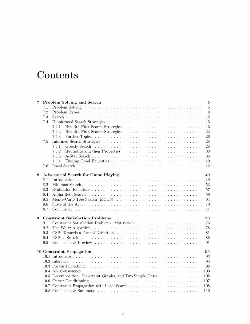
7 Problem Solving and Search 57.1 Problem Solving . . . . . . . . . . . . . . . . . . . . . . . . . . . . . . . . . . . . . 57.2 Problem Types . . . . . . . . . . . . . . . . . . . . . . . . . . . . . . . . . . . . . . 97.3 Search . . . . . . . . . . . . . . . . . . . . . . . . . . . . . . . . . . . . . . . . . . . 127.4 Uninformed Search Strategies . . . . . . . . . . . . . . . . . . . . . . . . . . . . . . 15
7.4.1 Breadth-First Search Strategies . . . . . . . . . . . . . . . . . . . . . . . . . 167.4.2 Breadth-First Search Strategies . . . . . . . . . . . . . . . . . . . . . . . . . 227.4.3 Further Topics . . . . . . . . . . . . . . . . . . . . . . . . . . . . . . . . . . 26
7.5 Informed Search Strategies . . . . . . . . . . . . . . . . . . . . . . . . . . . . . . . 287.5.1 Greedy Search . . . . . . . . . . . . . . . . . . . . . . . . . . . . . . . . . . 287.5.2 Heuristics and their Properties . . . . . . . . . . . . . . . . . . . . . . . . . 337.5.3 A-Star Search . . . . . . . . . . . . . . . . . . . . . . . . . . . . . . . . . . . 357.5.4 Finding Good Heuristics . . . . . . . . . . . . . . . . . . . . . . . . . . . . . 40
7.6 Local Search . . . . . . . . . . . . . . . . . . . . . . . . . . . . . . . . . . . . . . . 42
8 Adversarial Search for Game Playing 498.1 Introduction . . . . . . . . . . . . . . . . . . . . . . . . . . . . . . . . . . . . . . . . 498.2 Minimax Search . . . . . . . . . . . . . . . . . . . . . . . . . . . . . . . . . . . . . . 538.3 Evaluation Functions . . . . . . . . . . . . . . . . . . . . . . . . . . . . . . . . . . . 578.4 Alpha-Beta Search . . . . . . . . . . . . . . . . . . . . . . . . . . . . . . . . . . . . 598.5 Monte-Carlo Tree Search (MCTS) . . . . . . . . . . . . . . . . . . . . . . . . . . . 648.6 State of the Art . . . . . . . . . . . . . . . . . . . . . . . . . . . . . . . . . . . . . . 708.7 Conclusion . . . . . . . . . . . . . . . . . . . . . . . . . . . . . . . . . . . . . . . . 71
9 Constraint Satisfaction Problems 739.1 Constraint Satisfaction Problems: Motivation . . . . . . . . . . . . . . . . . . . . . 739.2 The Waltz Algorithm . . . . . . . . . . . . . . . . . . . . . . . . . . . . . . . . . . . 789.3 CSP: Towards a Formal Definition . . . . . . . . . . . . . . . . . . . . . . . . . . . 819.4 CSP as Search . . . . . . . . . . . . . . . . . . . . . . . . . . . . . . . . . . . . . . 869.5 Conclusion & Preview . . . . . . . . . . . . . . . . . . . . . . . . . . . . . . . . . . 91
10 Constraint Propagation 9310.1 Introduction . . . . . . . . . . . . . . . . . . . . . . . . . . . . . . . . . . . . . . . . 9310.2 Inference . . . . . . . . . . . . . . . . . . . . . . . . . . . . . . . . . . . . . . . . . . 9510.3 Forward Checking . . . . . . . . . . . . . . . . . . . . . . . . . . . . . . . . . . . . 9810.4 Arc Consistency . . . . . . . . . . . . . . . . . . . . . . . . . . . . . . . . . . . . . 10010.5 Decomposition: Constraint Graphs, and Two Simple Cases . . . . . . . . . . . . . 10510.6 Cutset Conditioning . . . . . . . . . . . . . . . . . . . . . . . . . . . . . . . . . . . 10710.7 Constraint Propagation with Local Search . . . . . . . . . . . . . . . . . . . . . . . 10810.8 Conclusion & Summary . . . . . . . . . . . . . . . . . . . . . . . . . . . . . . . . . 110
3

4 CONTENTS
Chapter 7
Problem Solving and Search
In this Chapter, we will look at a class of algorithms called search algorithm. These arealgorithms that help in quite general situations, where there is a precisely described problem, thatneeds to be solved. Hence the name “General Problem Solving” for the area.
7.1 Problem SolvingA Video Nugget covering this Section can be found at https://fau.tv/clip/id/21927.
Before we come to the search algorithms themselves, we need to get a grip on the types of problemsthemselves and how we can represent them, and on what the variuous types entail for the problemsolving process.
The first step is to classify the problem solving process by the amount of knowledge we haveavailable. It makes a difference, whether we know all the factors involved in the problem beforewe actually are in the situation. In this case, we can solve the problem in the abstract, i.e. makea plan before we actually enter the situation (i.e. offline), and then when the problem arises, onlyexecute the plan. If we do not have complete knowledge, then we can only make partial plans, andhave to be in the situation to obtain new knowledge (e.g. by observing the effects of our actions orthe actions of others). As this is much more difficult we will restrict ourselves to offline problemsolving.
Problem Solving: Introduction
� Recap: Agents perceive the environment and compute an action.
� In other words: Agents continually solve “the problem of what to do next”.
� AI Goal: Find algorithms that help solving problems in general.
� Idea: If we can describe/represent problems in a standardized way, we may have achance to find general algorithms.
� Concretely: We will use the following two concepts to describe problems
� States: A set of possible situations in our problem domain (= environments)
� Actions: that get us from one state to another. (= agents)
5
6 CHAPTER 7. PROBLEM SOLVING AND SEARCH
A sequence of actions is a solution, if it brings us from an initial state to a goalstate. Problem solving computes solutions from problem formulations.
Definition 7.1.1. In offline problem solving an agent computing an actionsequence based complete knowledge of the environment.
Remark 7.1.2. Offline problem solving only works in fully observable, determin-istic, static, and episodic environments.
Definition 7.1.3. In online problem solving an agent computes one action ata time based on incoming perceptions.
���� This Semester: we largely restrict ourselves to offline problem solving. (easier)
©:MichaelKohlhase 91
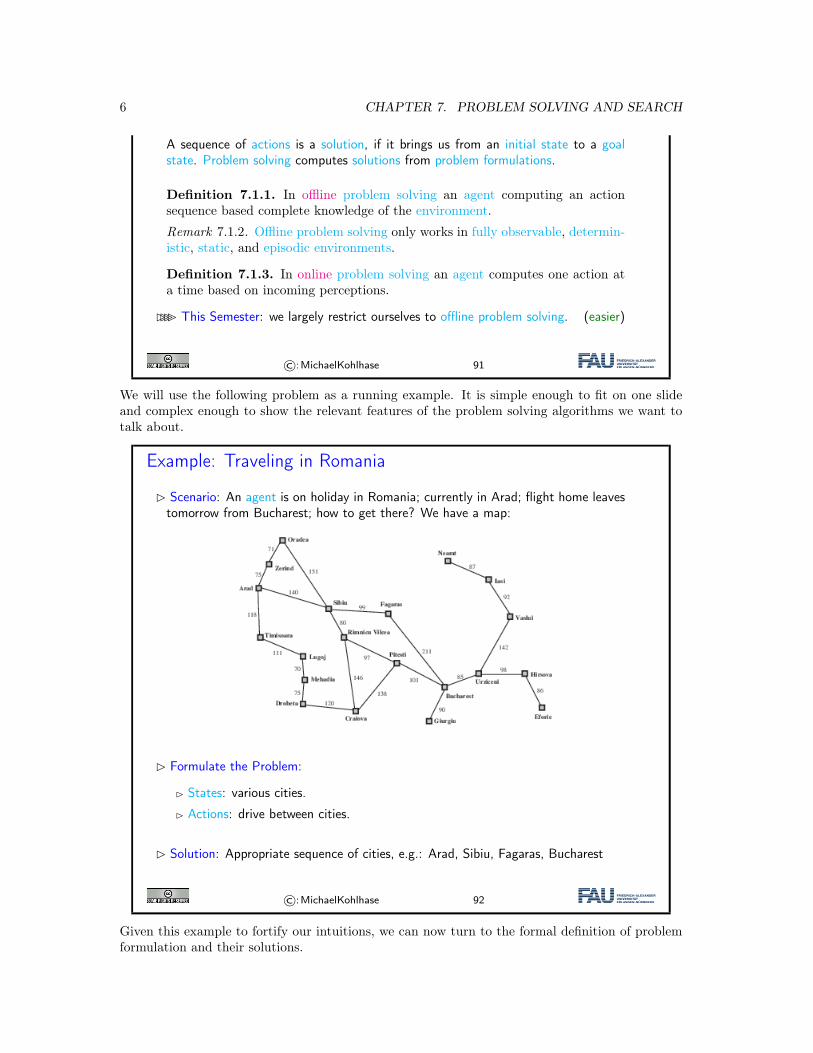
We will use the following problem as a running example. It is simple enough to fit on one slideand complex enough to show the relevant features of the problem solving algorithms we want totalk about.
Example: Traveling in Romania
� Scenario: An agent is on holiday in Romania; currently in Arad; flight home leavestomorrow from Bucharest; how to get there? We have a map:
� Formulate the Problem:
� States: various cities.
� Actions: drive between cities.
� Solution: Appropriate sequence of cities, e.g.: Arad, Sibiu, Fagaras, Bucharest
©:MichaelKohlhase 92
Given this example to fortify our intuitions, we can now turn to the formal definition of problemformulation and their solutions.
7.1. PROBLEM SOLVING 7
Problem Formulation
Definition 7.1.4. A problem formulation models a situation using states andactions at an appropriate level of abstraction.(do not model things like “put onmy left sock”, etc.)
� it describes the initial state (we are in Arad)
� it also limits the objectives by specifying goal states. (excludes, e.g. to stayanother couple of weeks.)
A solution is a sequence of actions that leads from the initial state to a goalstate.
Problem solving computes solutions from problem formulations.
� Finding the right level of abstraction and the required (not more!) information isoften the key to success.
©:MichaelKohlhase 93
The Math of Problem Formulation: Search Problems
Definition 7.1.5. A search problem Π:=⟨S,A,T ,I,G⟩ consists of a set S ofstates, a set A of actions, and a transition model T : A×S→P(S) that assignsto any action a∈A and state s∈S a set of successor states.
Certain states in S are designated as goal states (G⊆S) and initial states I⊆S.
Definition 7.1.6. We say that an action a∈A is applicable in a state s∈S, iffT (a,s) = ∅. We call Ta : S→P(S) with Ta(s):=T (a,s) the result relation for aand TA:=
⋃a∈ATa the result relation of Π.
Definition 7.1.7. A solution for a search problem ⟨S,A,T ,I,G⟩ consists of asequence of actions a1, . . . ,an such that for all i<1<n
� ai is applicable to state si−1, where s0∈I,
� si∈Tai(si−1), and sn∈G.
� Idea: A solution bring us from I to a goal state.
Definition 7.1.8. Often we add a cost function c : A→R+0 that associates a
step cost c(a) to an action a∈A. The cost of a solution is the sum of the stepcosts of its actions.
©:MichaelKohlhase 94
Observation: The problem of problems from Definition 7.1.5 is essentially a “black-box” descriptionthat provides the functionality needed to construct the state space. We will come back to this inslide 96.
Remark 7.1.9. Note that search problems formalize problem formulations by making many of theimplicit constraints explicit.We will now specialize Definition 7.1.5 to deterministic, fully observable environments, i.e. envi-ronments where actions only have one – assured – outcome state.
8 CHAPTER 7. PROBLEM SOLVING AND SEARCH
� Search Problems in deterministic, fully observable Envs
� This semester, we will restrict ourselves to search problems, where(extend in AI-II)
� |T (a,s)|≤1 for the transition models and ( ⇝deterministic environment)
� I = {s0} ( ⇝fully observable environment)
Definition 7.1.10. Then Ta induces partial function Sa : S→S whose domainis the set of states where a is applicable: S(s):=s′ if Ta = {s′} and undefinedotherwise.
We call Sa the successor function for a and Sa(s) the successor state of s.SA:=
⋃a∈ASa the successor relation of P.
Definition 7.1.11. The predicate that tests for goal states is called a goal test.
©:MichaelKohlhase 95
�� Blackbox/Declarative Problem Descriptions
� Observation: ⟨S,A,T ,I,G⟩ from Definition 7.1.5 is essentially a blackbox descrip-tion (think programmingAPI)
� provides the functionality needed to construct a state space.
� gives the algorithm no information about the problem
Definition 7.1.12. A declarative description (also called whitebox description)describes the problem itself ; problem description language
Example 7.1.13. The STRIPS language describes planning problems in termsof
� a set P of Boolean variables (propositions)
� a set I⊆P of propositions true in the initial state
� a set G⊆P , where state s⊆P is a goal if G⊆s
� a set a of actions, each a∈A with precondition prea, add list adda, and deletelist dela: a is applicable, if prea⊆s, result state is s∪adda\dela
� a function c that maps all actions a to their cost c(a).
Observation 7.1.14. Declarative descriptions are strictly more powerful thanblackbox descriptions: they induce blackbox descriptions, but also allow to ana-lyze/simplify the problem.
�� We will come back to this later ; planning.
©:MichaelKohlhase 96
1EdN:1
1EdNote: mark up strips and create appropriate references
7.2. PROBLEM TYPES 9
7.2 Problem TypesNote that this definition is very general, it applies to many many problems. So we will try tocharacterize these by difficulty.
A Video Nugget covering this Section can be found at https://fau.tv/clip/id/21928.
Problem types
� Single-state problem
� observable (at least the initial state)
� deterministic (i.e. the successor of each state is determined)
� static (states do not change other than by our own actions)
� discrete (a countable number of states)
Multiple-state problem:
� � initial state not/partially observable (multiple initial states?)
� deterministic, static, discrete
Contingency problem:
� � non-deterministic (solution can branch, depending on contingencies)
� unknown state space (like a baby, agent has to learn about states and actions)
©:MichaelKohlhase 97
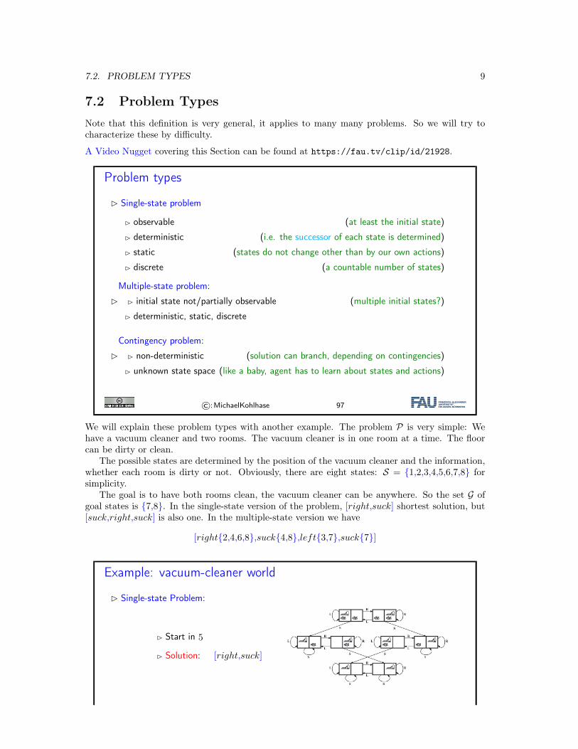
We will explain these problem types with another example. The problem P is very simple: Wehave a vacuum cleaner and two rooms. The vacuum cleaner is in one room at a time. The floorcan be dirty or clean.
The possible states are determined by the position of the vacuum cleaner and the information,whether each room is dirty or not. Obviously, there are eight states: S = {1,2,3,4,5,6,7,8} forsimplicity.
The goal is to have both rooms clean, the vacuum cleaner can be anywhere. So the set G ofgoal states is {7,8}. In the single-state version of the problem, [right,suck] shortest solution, but[suck,right,suck] is also one. In the multiple-state version we have
[right{2,4,6,8},suck{4,8},left{3,7},suck{7}]
Example: vacuum-cleaner world
� Single-state Problem:
� Start in 5
� Solution: [right,suck]
10 CHAPTER 7. PROBLEM SOLVING AND SEARCH
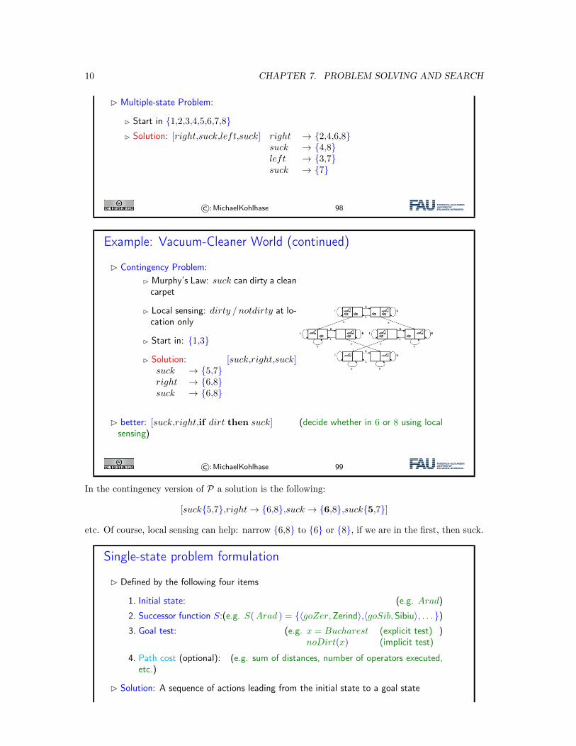
� Multiple-state Problem:
� Start in {1,2,3,4,5,6,7,8}� Solution: [right,suck,left,suck] right → {2,4,6,8}
suck → {4,8}left → {3,7}suck → {7}
©:MichaelKohlhase 98
Example: Vacuum-Cleaner World (continued)
� Contingency Problem:� Murphy’s Law: suck can dirty a clean
carpet
� Local sensing: dirty / notdirty at lo-cation only
� Start in: {1,3}
� Solution: [suck,right,suck]suck → {5,7}right → {6,8}suck → {6,8}
� better: [suck,right,if dirt then suck] (decide whether in 6 or 8 using localsensing)
©:MichaelKohlhase 99
In the contingency version of P a solution is the following:
[suck{5,7},right → {6,8},suck → {6,8},suck{5,7}]
etc. Of course, local sensing can help: narrow {6,8} to {6} or {8}, if we are in the first, then suck.
Single-state problem formulation
� Defined by the following four items
1. Initial state: (e.g. Arad)
2. Successor function S:(e.g. S(Arad ) = {⟨goZer,Zerind⟩,⟨goSib,Sibiu⟩, . . . })3. Goal test: (e.g. x = Bucharest (explicit test)
noDirt(x) (implicit test))
4. Path cost (optional): (e.g. sum of distances, number of operators executed,etc.)
� Solution: A sequence of actions leading from the initial state to a goal state
7.2. PROBLEM TYPES 11
©:MichaelKohlhase 100
“Path cost”: There may be more than one solution and we might want to have the “best” one ina certain sense.
Selecting a state space
� Abstraction: Real world is absurdly complexState space must be abstracted for problem solving
� (Abstract) state: Set of real states
� (Abstract) operator: Complex combination of real actions
� Example: Arad → Zerind represents complex set of possible routes
� (Abstract) solution: Set of real paths that are solutions in the real world
©:MichaelKohlhase 101
“State”: e.g., we don’t care about tourist attractions found in the cities along the way. But this isproblem dependent. In a different problem it may well be appropriate to include such informationin the notion of state.
“Realizability”: one could also say that the abstraction must be sound wrt. reality.
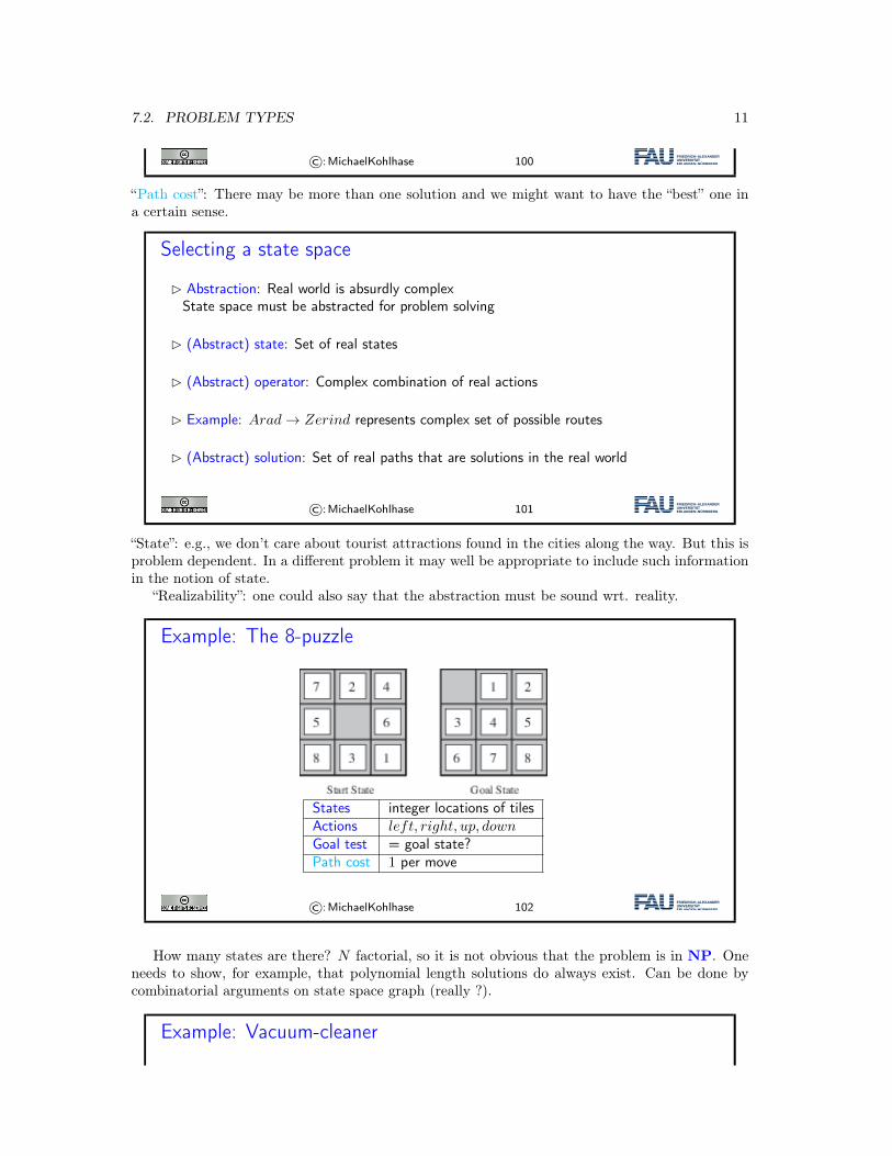
Example: The 8-puzzle
States integer locations of tilesActions left, right, up, downGoal test = goal state?Path cost 1 per move
©:MichaelKohlhase 102
How many states are there? N factorial, so it is not obvious that the problem is in NP. Oneneeds to show, for example, that polynomial length solutions do always exist. Can be done bycombinatorial arguments on state space graph (really ?).
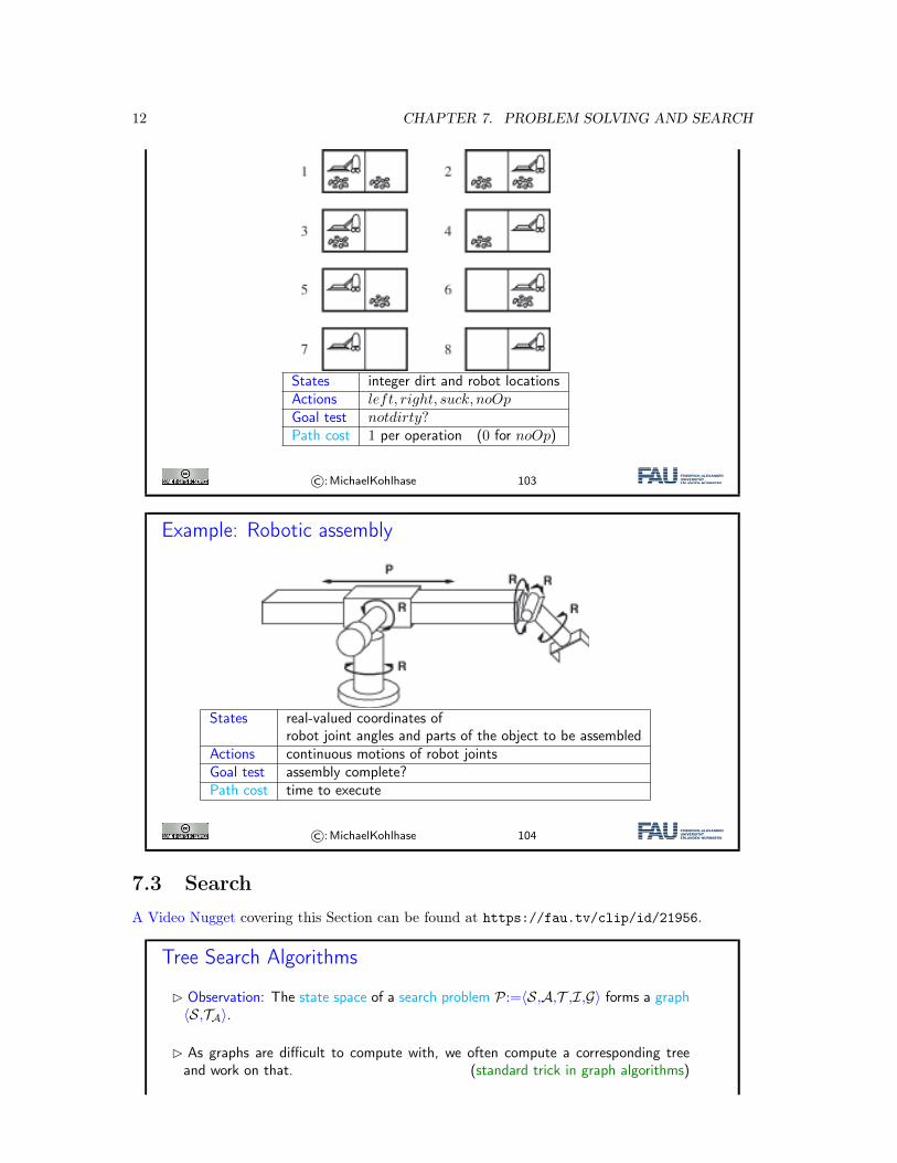
Example: Vacuum-cleaner
12 CHAPTER 7. PROBLEM SOLVING AND SEARCH
States integer dirt and robot locationsActions left, right, suck, noOpGoal test notdirty?Path cost 1 per operation (0 for noOp)
©:MichaelKohlhase 103
Example: Robotic assembly
States real-valued coordinates ofrobot joint angles and parts of the object to be assembled
Actions continuous motions of robot jointsGoal test assembly complete?Path cost time to execute
©:MichaelKohlhase 104
7.3 SearchA Video Nugget covering this Section can be found at https://fau.tv/clip/id/21956.
Tree Search Algorithms
� Observation: The state space of a search problem P:=⟨S,A,T ,I,G⟩ forms a graph⟨S,TA⟩.
� As graphs are difficult to compute with, we often compute a corresponding treeand work on that. (standard trick in graph algorithms)
7.3. SEARCH 13
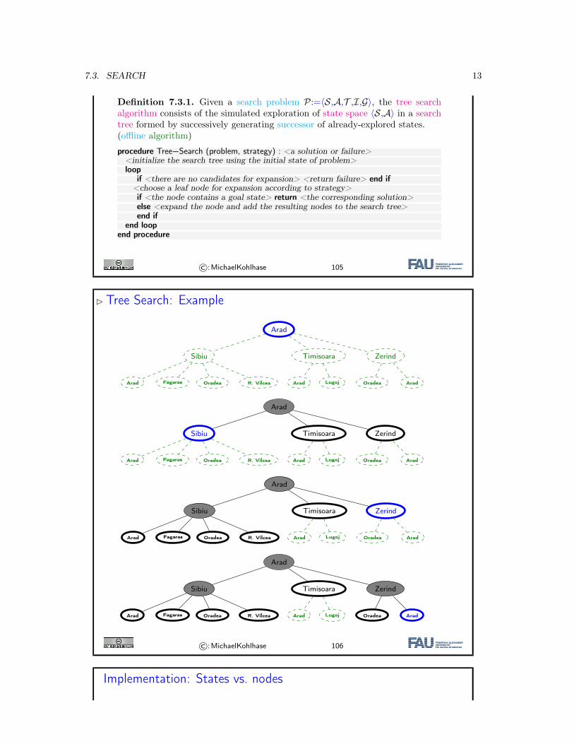
Definition 7.3.1. Given a search problem P:=⟨S,A,T ,I,G⟩, the tree searchalgorithm consists of the simulated exploration of state space ⟨S,A⟩ in a searchtree formed by successively generating successor of already-explored states.(offline algorithm)
procedure Tree−Search (problem, strategy) : <a solution or failure><initialize the search tree using the initial state of problem>loop
if <there are no candidates for expansion> <return failure> end if<choose a leaf node for expansion according to strategy>if <the node contains a goal state> return <the corresponding solution>else <expand the node and add the resulting nodes to the search tree>end if
end loopend procedure
©:MichaelKohlhase 105
� Tree Search: Example
Arad
Sibiu Timisoara Zerind
Arad Fagaras Oradea R. Vilcea Arad Lugoj Oradea Arad
Arad
Sibiu Timisoara Zerind
Arad Fagaras Oradea R. Vilcea Arad Lugoj Oradea Arad
Arad
Sibiu Timisoara Zerind
Arad Fagaras Oradea R. Vilcea Arad Lugoj Oradea Arad
Arad
Sibiu Timisoara Zerind
Arad Fagaras Oradea R. Vilcea Arad Lugoj Oradea Arad
©:MichaelKohlhase 106
Implementation: States vs. nodes
14 CHAPTER 7. PROBLEM SOLVING AND SEARCH
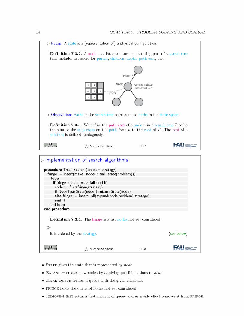
� Recap: A state is a (representation of) a physical configuration.
Definition 7.3.2. A node is a data structure constituting part of a search treethat includes accessors for parent, children, depth, path cost, etc.
� Observation: Paths in the search tree correspond to paths in the state space.
Definition 7.3.3. We define the path cost of a node n in a search tree T to bethe sum of the step costs on the path from n to the root of T . The cost of asolution is defined analogously.
©:MichaelKohlhase 107
� Implementation of search algorithms
procedure Tree_Search (problem,strategy)fringe := insert(make_node(initial_state(problem)))
loopif fringe <is empty> fail end ifnode := first(fringe,strategy)if NodeTest(State(node)) return State(node)else fringe := insert_all(expand(node,problem),strategy)end if
end loopend procedure
Definition 7.3.4. The fringe is a list nodes not yet considered.
��It is ordered by the strategy. (see below)
©:MichaelKohlhase 108
• State gives the state that is represented by node
• Expand = creates new nodes by applying possible actions to node
• Make-Queue creates a queue with the given elements.
• fringe holds the queue of nodes not yet considered.
• Remove-First returns first element of queue and as a side effect removes it from fringe.
7.4. UNINFORMED SEARCH STRATEGIES 15
• State gives the state that is represented by node.
• Expand applies all operators of the problem to the current node and yields a set of newnodes.
• Insert inserts an element into the current fringe queue. This can change the behavior ofthe search.
• Insert-All Perform Insert on set of elements.
Search strategies
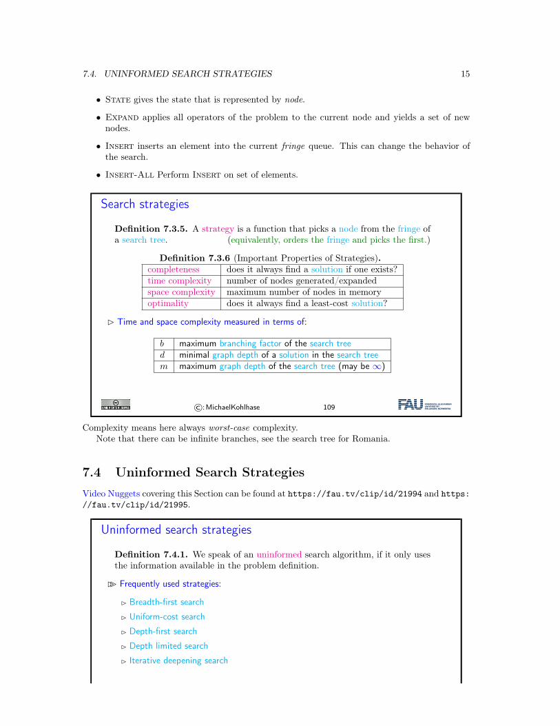
Definition 7.3.5. A strategy is a function that picks a node from the fringe ofa search tree. (equivalently, orders the fringe and picks the first.)
Definition 7.3.6 (Important Properties of Strategies).completeness does it always find a solution if one exists?time complexity number of nodes generated/expandedspace complexity maximum number of nodes in memoryoptimality does it always find a least-cost solution?
� Time and space complexity measured in terms of:
b maximum branching factor of the search treed minimal graph depth of a solution in the search treem maximum graph depth of the search tree (may be ∞)
©:MichaelKohlhase 109
Complexity means here always worst-case complexity.Note that there can be infinite branches, see the search tree for Romania.
7.4 Uninformed Search StrategiesVideo Nuggets covering this Section can be found at https://fau.tv/clip/id/21994 and https://fau.tv/clip/id/21995.
Uninformed search strategies
Definition 7.4.1. We speak of an uninformed search algorithm, if it only usesthe information available in the problem definition.
�� Frequently used strategies:
� Breadth-first search
� Uniform-cost search
� Depth-first search
� Depth limited search
� Iterative deepening search
16 CHAPTER 7. PROBLEM SOLVING AND SEARCH
©:MichaelKohlhase 110
The opposite of uninformed search is informed or heuristic search. In the example, one could add,for instance, to prefer cities that lie in the general direction of the goal (here SE).
Uninformed search is important, because many problems do not allow to extract good heuris-tics.
7.4.1 Breadth-First Search Strategies
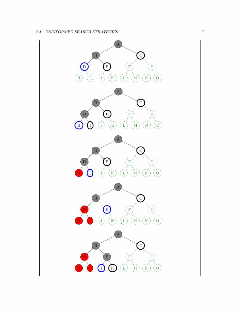
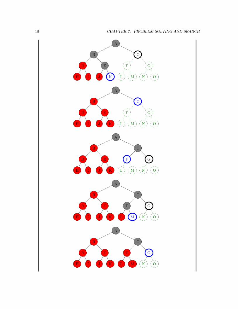
Depth-first Search
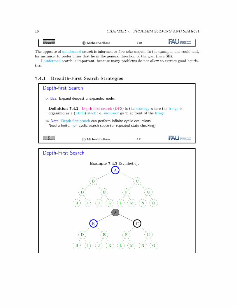
� Idea: Expand deepest unexpanded node.
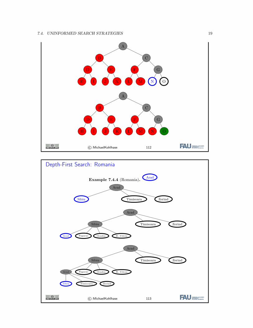
Definition 7.4.2. Depth-first search (DFS) is the strategy where the fringe isorganized as a (LIFO) stack i.e. successor go in at front of the fringe.
�� Note: Depth-first search can perform infinite cyclic excursionsNeed a finite, non-cyclic search space (or repeated-state checking)
©:MichaelKohlhase 111
Depth-First Search
Example 7.4.3 (Synthetic).
A
B C
D E F G
H I J K L M N O
A
B C
D E F G
H I J K L M N O
7.4. UNINFORMED SEARCH STRATEGIES 17
A
B C
D E F G
H I J K L M N O
A
B C
D E F G
H I J K L M N O
A
B C
D E F G
H I J K L M N O
A
B C
D E F G
H I J K L M N O
A
B C
D E F G
H I J K L M N O
18 CHAPTER 7. PROBLEM SOLVING AND SEARCH
A
B C
D E F G
H I J K L M N O
A
B C
D E F G
H I J K L M N O
A
B C
D E F G
H I J K L M N O
A
B C
D E F G
H I J K L M N O
A
B C
D E F G
H I J K L M N O
7.4. UNINFORMED SEARCH STRATEGIES 19
A
B C
D E F G
H I J K L M N O
A
B C
D E F G
H I J K L M N O
©:MichaelKohlhase 112
Depth-First Search: Romania
Example 7.4.4 (Romania). Arad
Arad
Sibiu Timisoara Zerind
Arad
Sibiu Timisoara Zerind
Arad Fagaras Oradea R. Vilcea
Arad
Sibiu Timisoara Zerind
Arad Fagaras Oradea R. Vilcea
Sibiu Timisoara Zerind
©:MichaelKohlhase 113
20 CHAPTER 7. PROBLEM SOLVING AND SEARCH
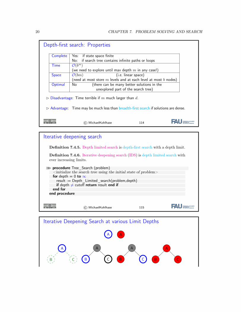
Depth-first search: Properties
Complete Yes: if state space finiteNo: if search tree contains infinite paths or loops
Time O(bm)(we need to explore until max depth m in any case!)
Space O(bm) (i.e. linear space)(need at most store m levels and at each level at most b nodes)
Optimal No (there can be many better solutions in theunexplored part of the search tree)
� Disadvantage: Time terrible if m much larger than d.
� Advantage: Time may be much less than breadth-first search if solutions are dense.
©:MichaelKohlhase 114
Iterative deepening search
Definition 7.4.5. Depth limited search is depth-first search with a depth limit.
Definition 7.4.6. Iterative deepening search (IDS) is depth limited search withever increasing limits.
��� procedure Tree_Search (problem)<initialize the search tree using the initial state of problem>for depth = 0 to ∞
result := Depth_Limited_search(problem,depth)if depth = cutoff return result end if
end forend procedure
©:MichaelKohlhase 115
Iterative Deepening Search at various Limit Depths
A A
A
B C
A
B C
A
B C
A
B C
7.4. UNINFORMED SEARCH STRATEGIES 21
A
B C
D E F G
A
B C
D E F G
A
B C
D E F G
A
B C
D E F G
A
B C
D E F G
A
B C
D E F G
A
B C
D E F G
A
B C
D E F G
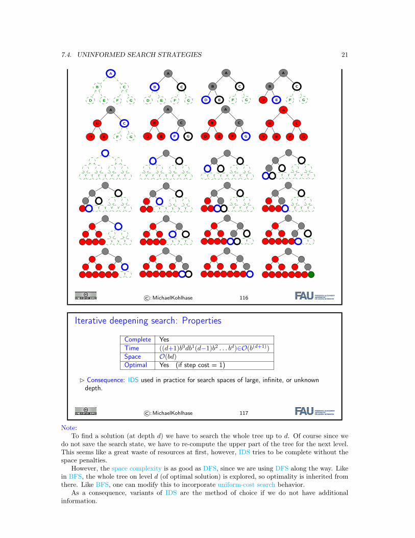
©:MichaelKohlhase 116
Iterative deepening search: Properties
Complete YesTime ((d+1)b0db1(d−1)b2 . . . bd)∈O(b(d+1))Space O(bd)Optimal Yes (if step cost = 1)
� Consequence: IDS used in practice for search spaces of large, infinite, or unknowndepth.
©:MichaelKohlhase 117
Note:To find a solution (at depth d) we have to search the whole tree up to d. Of course since we
do not save the search state, we have to re-compute the upper part of the tree for the next level.This seems like a great waste of resources at first, however, IDS tries to be complete without thespace penalties.
However, the space complexity is as good as DFS, since we are using DFS along the way. Likein BFS, the whole tree on level d (of optimal solution) is explored, so optimality is inherited fromthere. Like BFS, one can modify this to incorporate uniform-cost search behavior.
As a consequence, variants of IDS are the method of choice if we do not have additionalinformation.
22 CHAPTER 7. PROBLEM SOLVING AND SEARCH
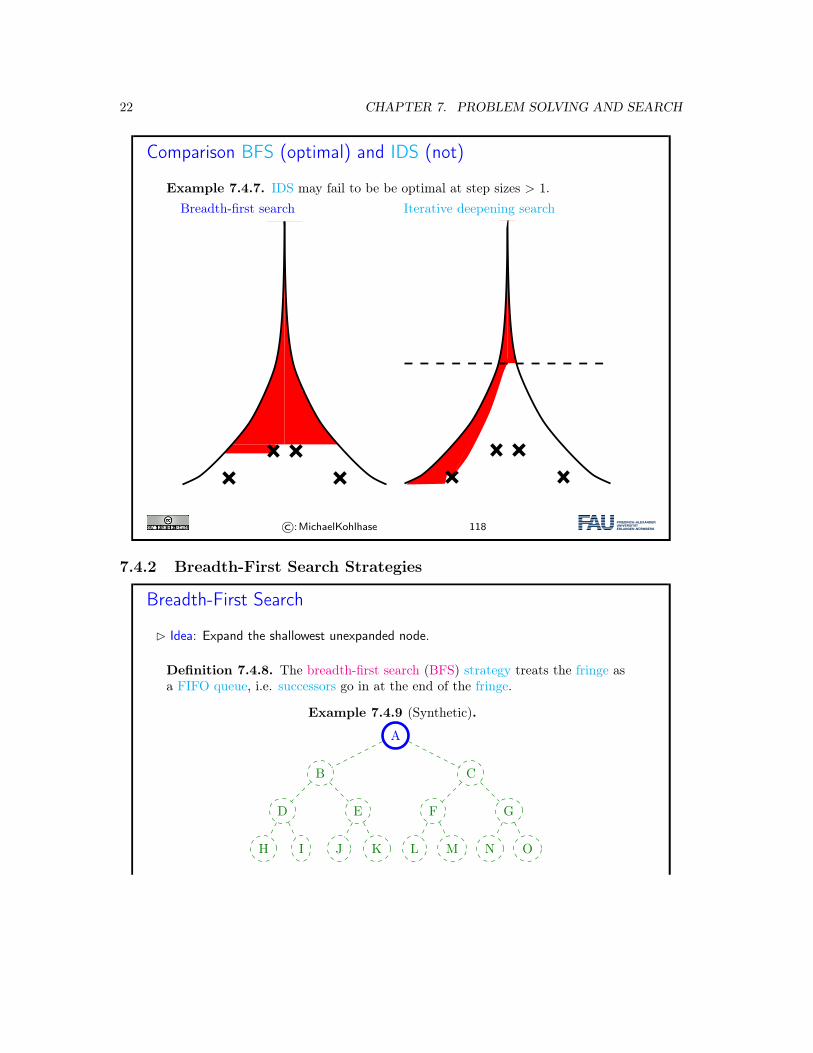
Comparison BFS (optimal) and IDS (not)
Example 7.4.7. IDS may fail to be be optimal at step sizes > 1.Breadth-first search Iterative deepening search
Comparison
Breadth-first search Iterative deepening search
Kohlhase: Künstliche Intelligenz 1 150 July 5, 2018
Comparison
Breadth-first search Iterative deepening search
Kohlhase: Künstliche Intelligenz 1 150 July 5, 2018
©:MichaelKohlhase 118
7.4.2 Breadth-First Search Strategies
Breadth-First Search
� Idea: Expand the shallowest unexpanded node.
Definition 7.4.8. The breadth-first search (BFS) strategy treats the fringe asa FIFO queue, i.e. successors go in at the end of the fringe.
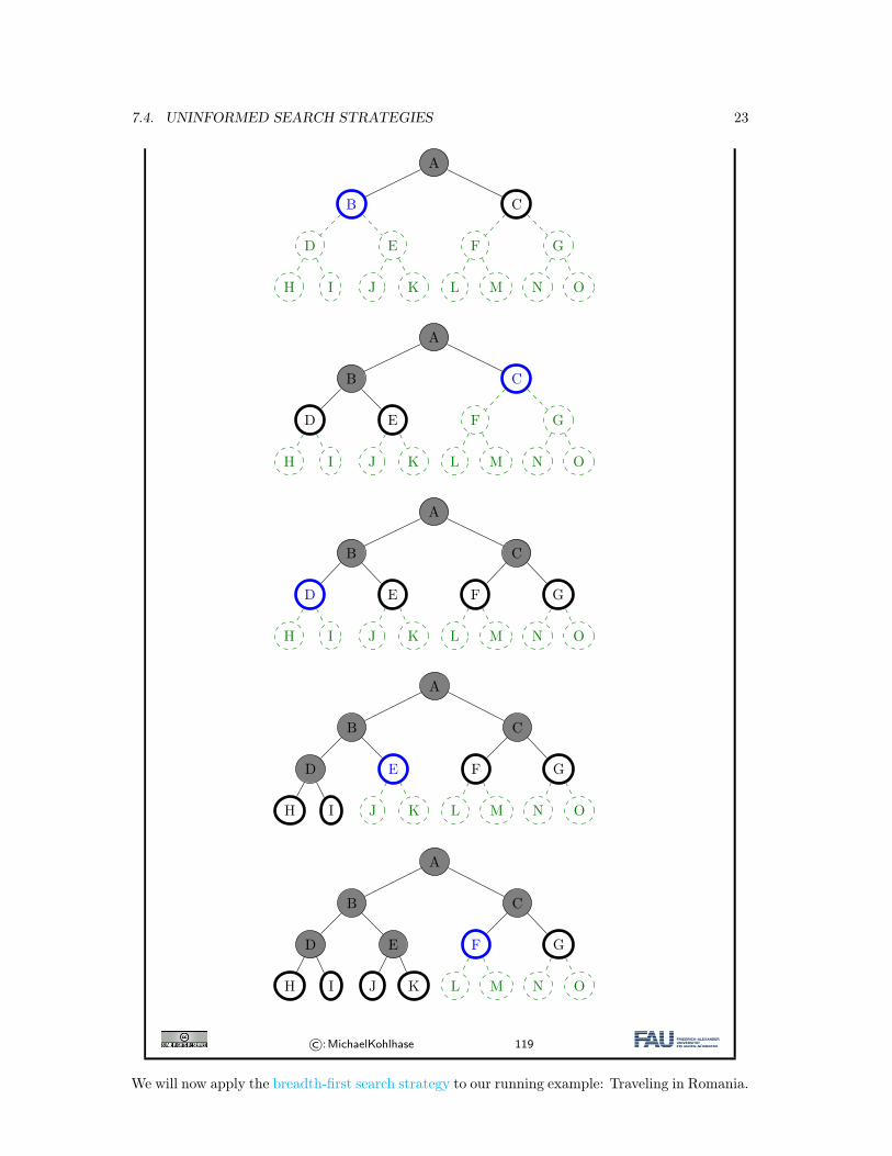
Example 7.4.9 (Synthetic).
A
B C
D E F G
H I J K L M N O
7.4. UNINFORMED SEARCH STRATEGIES 23
A
B C
D E F G
H I J K L M N O
A
B C
D E F G
H I J K L M N O
A
B C
D E F G
H I J K L M N O
A
B C
D E F G
H I J K L M N O
A
B C
D E F G
H I J K L M N O
©:MichaelKohlhase 119
We will now apply the breadth-first search strategy to our running example: Traveling in Romania.
24 CHAPTER 7. PROBLEM SOLVING AND SEARCH
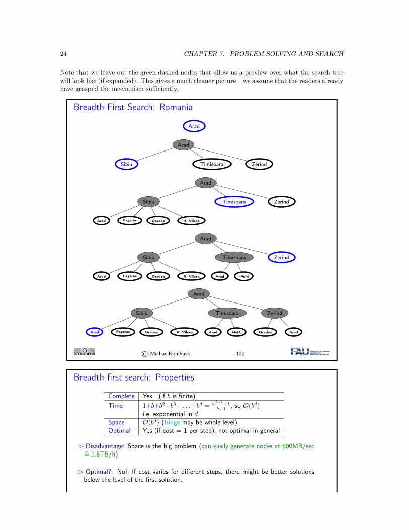
Note that we leave out the green dashed nodes that allow us a preview over what the search treewill look like (if expanded). This gives a much cleaner picture – we assume that the readers alreadyhave grasped the mechanism sufficiently.
Breadth-First Search: Romania
Arad
Arad
Sibiu Timisoara Zerind
Arad
Sibiu Timisoara Zerind
Arad Fagaras Oradea R. Vilcea
Arad
Sibiu Timisoara Zerind
Arad Fagaras Oradea R. Vilcea Arad Lugoj
Arad
Sibiu Timisoara Zerind
Arad Fagaras Oradea R. Vilcea Arad Lugoj Oradea Arad
©:MichaelKohlhase 120
Breadth-first search: Properties
Complete Yes (if b is finite)Time 1+b+b2+b3+ . . .+bd = bd−1−1
b−1 , so O(bd)
i.e. exponential in dSpace O(bd) (fringe may be whole level)Optimal Yes (if cost = 1 per step), not optimal in general
� Disadvantage: Space is the big problem (can easily generate nodes at 500MB/sec= 1.8TB/h)
� Optimal?: No! If cost varies for different steps, there might be better solutionsbelow the level of the first solution.
7.4. UNINFORMED SEARCH STRATEGIES 25
� An alternative is to generate all solutions and then pick an optimal one. This worksonly, if m is finite.
©:MichaelKohlhase 121
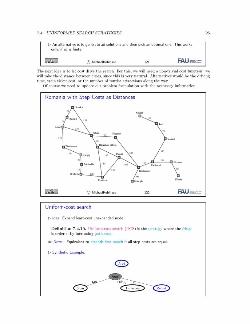
The next idea is to let cost drive the search. For this, we will need a non-trivial cost function: wewill take the distance between cities, since this is very natural. Alternatives would be the drivingtime, train ticket cost, or the number of tourist attractions along the way.
Of course we need to update our problem formulation with the necessary information.
Romania with Step Costs as Distances
©:MichaelKohlhase 122
Uniform-cost search
� Idea: Expand least-cost unexpanded node
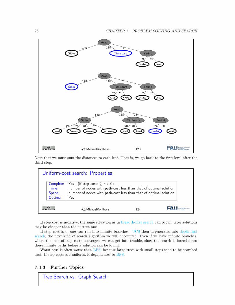
Definition 7.4.10. Uniform-cost search (UCS) is the strategy where the fringeis ordered by increasing path cost.
�� Note: Equivalent to breadth-first search if all step costs are equal.
� Synthetic Example:
Arad
Arad
Sibiu
140
Timisoara
118
Zerind
75
26 CHAPTER 7. PROBLEM SOLVING AND SEARCH
Arad
Sibiu
140
Timisoara
118
Zerind
75
Oradea
71
Arad
75
Arad
Sibiu
140
Timisoara
118
Zerind
75
Arad
118
Lugoj
111
Oradea
71
Arad
75
Arad
Sibiu
140
Timisoara
118
Zerind
75
Arad
140
Fagaras
99
Oradea
151
R. Vilcea
80
Arad
118
Lugoj
111
Oradea
71
Arad
75
©:MichaelKohlhase 123
Note that we must sum the distances to each leaf. That is, we go back to the first level after thethird step.
Uniform-cost search: Properties
Complete Yes (if step costs ≥ ϵ > 0)Time number of nodes with path-cost less than that of optimal solutionSpace number of nodes with path-cost less than that of optimal solutionOptimal Yes
©:MichaelKohlhase 124
If step cost is negative, the same situation as in breadth-first search can occur: later solutionsmay be cheaper than the current one.
If step cost is 0, one can run into infinite branches. UCS then degenerates into depth-firstsearch, the next kind of search algorithm we will encounter. Even if we have infinite branches,where the sum of step costs converges, we can get into trouble, since the search is forced downthese infinite paths before a solution can be found.
Worst case is often worse than BFS, because large trees with small steps tend to be searchedfirst. If step costs are uniform, it degenerates to BFS.
7.4.3 Further Topics
Tree Search vs. Graph Search
7.4. UNINFORMED SEARCH STRATEGIES 27
� We have only covered tree search algorithms.
� Nobody uses these in practice ⇝states duplicated in nodes are a huge problem forefficiency.
Definition 7.4.11. A graph search algorithm is a variant of a tree search al-gorithm that prunes nodes whose state has already been considered (duplicatepruning), essentially using a DAG data structure.
Observation 7.4.12. Tree search is memory-intensive – it has to store thefringe – so keeping a list of “explored states” does not lose much.
��� Graph versions of all the tree search algorithms considered here exist, but are moredifficult to understand (and to prove properties about).
� The (time complexity) properties are largely stable under duplicate pruning.
Definition 7.4.13. We speak of a search algorithm, when we do not want todistinguish whether it is a tree or graph search algorithm. (differenceconsidered in implementation detail)
©:MichaelKohlhase 125
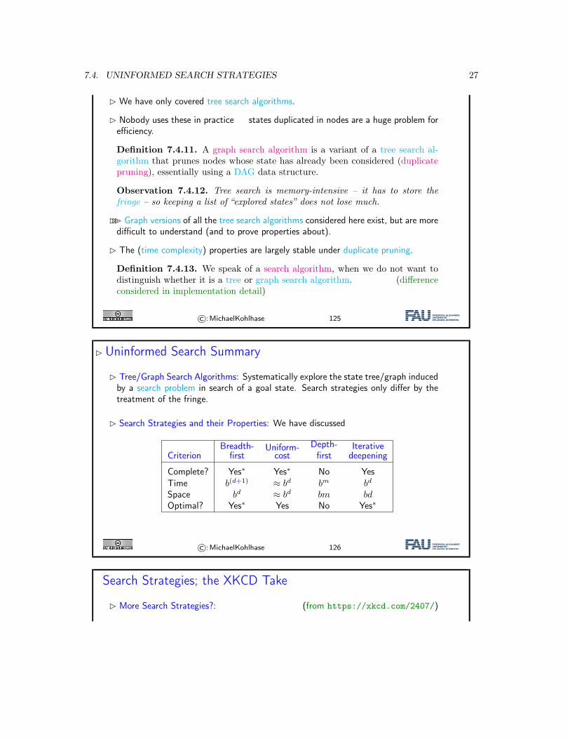
� Uninformed Search Summary
� Tree/Graph Search Algorithms: Systematically explore the state tree/graph inducedby a search problem in search of a goal state. Search strategies only differ by thetreatment of the fringe.
� Search Strategies and their Properties: We have discussed
CriterionBreadth-
firstUniform-
costDepth-first
Iterativedeepening
Complete? Yes∗ Yes∗ No YesTime b(d+1) ≈ bd bm bd
Space bd ≈ bd bm bdOptimal? Yes∗ Yes No Yes∗
©:MichaelKohlhase 126
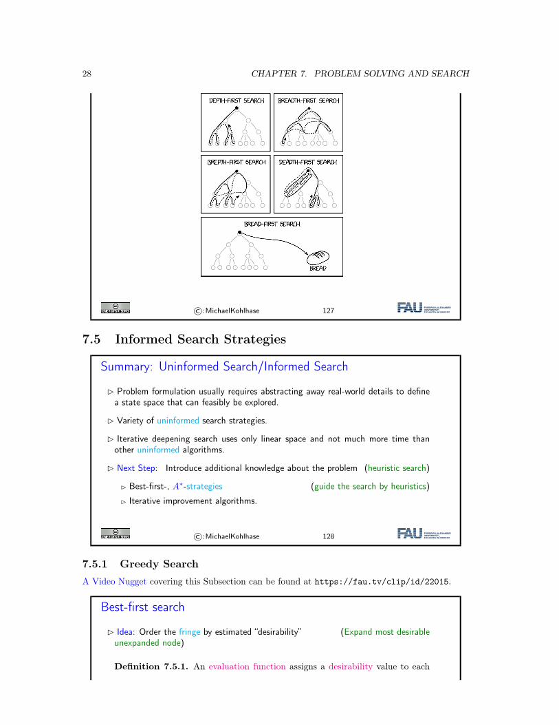
Search Strategies; the XKCD Take
� More Search Strategies?: (from https://xkcd.com/2407/)
28 CHAPTER 7. PROBLEM SOLVING AND SEARCH
©:MichaelKohlhase 127
7.5 Informed Search Strategies
Summary: Uninformed Search/Informed Search
� Problem formulation usually requires abstracting away real-world details to definea state space that can feasibly be explored.
� Variety of uninformed search strategies.
� Iterative deepening search uses only linear space and not much more time thanother uninformed algorithms.
� Next Step: Introduce additional knowledge about the problem (heuristic search)
� Best-first-, A∗-strategies (guide the search by heuristics)
� Iterative improvement algorithms.
©:MichaelKohlhase 128
7.5.1 Greedy SearchA Video Nugget covering this Subsection can be found at https://fau.tv/clip/id/22015.
Best-first search
� Idea: Order the fringe by estimated “desirability” (Expand most desirableunexpanded node)
Definition 7.5.1. An evaluation function assigns a desirability value to each
7.5. INFORMED SEARCH STRATEGIES 29
node of the search tree.
�� Note: A evaluation function is not part of the search problem, but must be addedexternally.
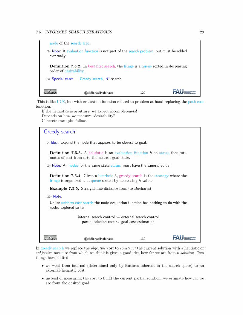
Definition 7.5.2. In best first search, the fringe is a queue sorted in decreasingorder of desirability.
�� Special cases: Greedy search, A∗-search
©:MichaelKohlhase 129
This is like UCS, but with evaluation function related to problem at hand replacing the path costfunction.
If the heuristics is arbitrary, we expect incompleteness!Depends on how we measure “desirability”.Concrete examples follow.
Greedy search
� Idea: Expand the node that appears to be closest to goal.
Definition 7.5.3. A heuristic is an evaluation function h on states that esti-mates of cost from n to the nearest goal state.
�� Note: All nodes for the same state states, must have the same h-value!
Definition 7.5.4. Given a heuristic h, greedy search is the strategy where thefringe is organized as a queue sorted by decreasing h-value.
Example 7.5.5. Straight-line distance from/to Bucharest.
��� Note:
Unlike uniform-cost search the node evaluation function has nothing to do with thenodes explored so far
internal search control ; external search controlpartial solution cost ; goal cost estimation
©:MichaelKohlhase 130
In greedy search we replace the objective cost to construct the current solution with a heuristic orsubjective measure from which we think it gives a good idea how far we are from a solution. Twothings have shifted:
• we went from internal (determined only by features inherent in the search space) to anexternal/heuristic cost
• instead of measuring the cost to build the current partial solution, we estimate how far weare from the desired goal
30 CHAPTER 7. PROBLEM SOLVING AND SEARCH
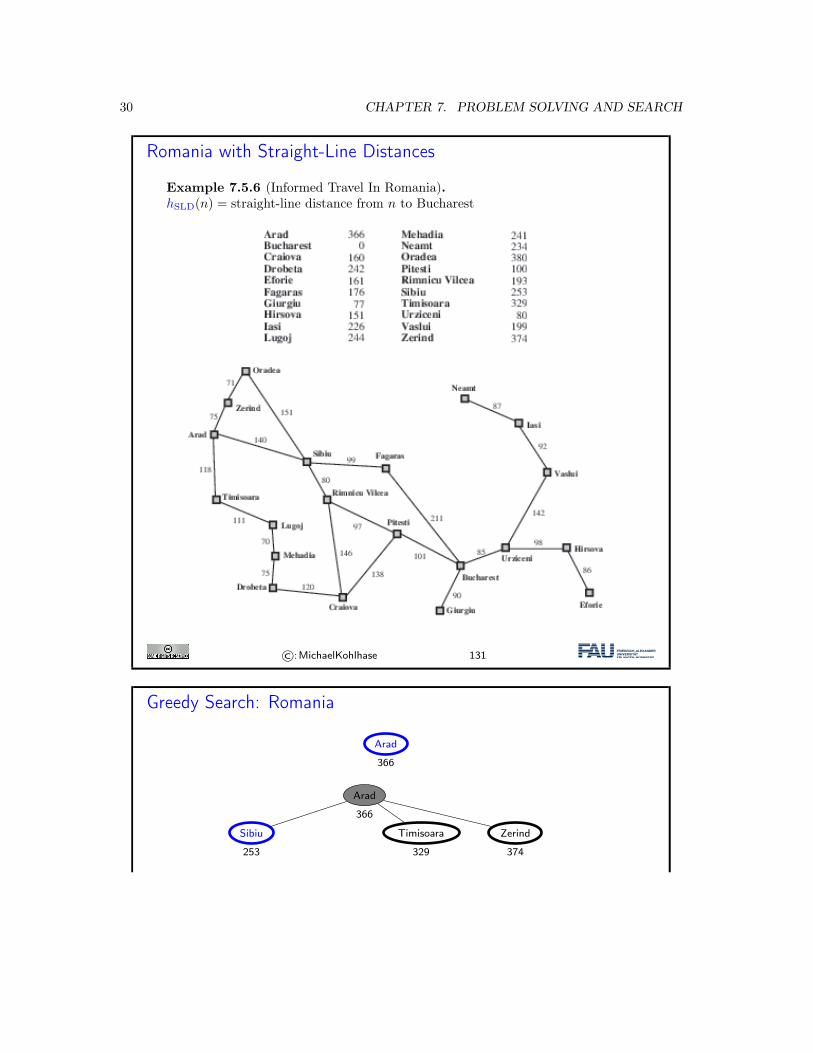
Romania with Straight-Line Distances
Example 7.5.6 (Informed Travel In Romania).hSLD(n) = straight-line distance from n to Bucharest
©:MichaelKohlhase 131
Greedy Search: Romania
Arad
366
Arad
366
Sibiu
253
Timisoara
329
Zerind
374
7.5. INFORMED SEARCH STRATEGIES 31
Arad
366
Sibiu
253
Timisoara
329
Zerind
374
Arad
366
Fagaras
176
Oradea
380
R. Vilcea
193
Arad
366
Sibiu
253
Timisoara
329
Zerind
374
Arad
366
Fagaras
176
Oradea
380
R. Vilcea
193
Sibiu
253
Bucharest
0
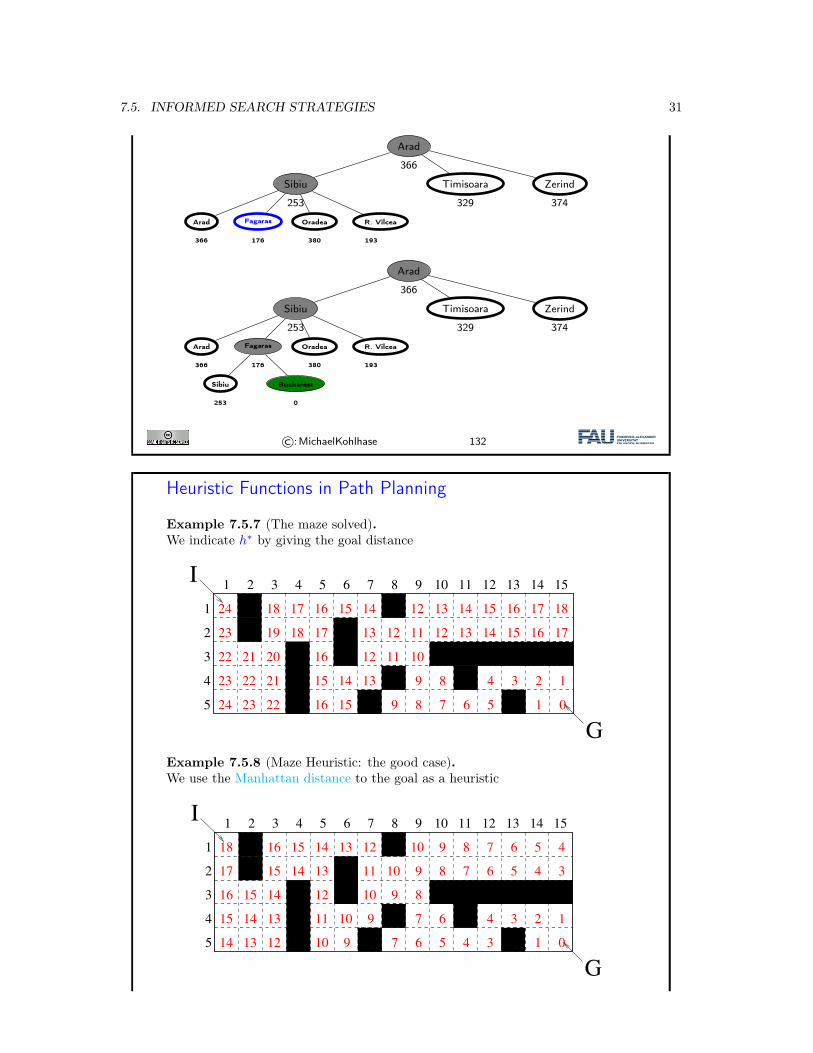
©:MichaelKohlhase 132
Heuristic Functions in Path Planning
Example 7.5.7 (The maze solved).We indicate h∗ by giving the goal distance
Heuristic Functions in Path Planning
I Example 4.4 (The maze solved).We indicate h⇤ by giving the goal distance
1 2 3 4 5 6 7 8 9 10 11 12 13 14 15
1
2
3
4
5
I
G
9
89 7
8
6 5
4 3 2 1
01
1011
11
12
12
12
12
13
13
13
13
14 14
14
14
15 15
15
15
15
16
16
16
16
1617
17 17
17
18
18
18
19
20
21
2122
22
22
23
23
2324
24
I Example 4.5 (Maze Heuristic: the good case).We use the Manhattan distance to the goal as a heuristic
I Example 4.6 (Maze Heuristic: the bad case).We use the Manhattan distance to the goal as a heuristic again
Kohlhase: Künstliche Intelligenz 1 160 July 5, 2018
Example 7.5.8 (Maze Heuristic: the good case).We use the Manhattan distance to the goal as a heuristic
Heuristic Functions in Path Planning
I Example 4.4 (The maze solved).We indicate h⇤ by giving the goal distance
I Example 4.5 (Maze Heuristic: the good case).We use the Manhattan distance to the goal as a heuristic
1 2 3 4 5 6 7 8 9 10 11 12 13 14 15
1
2
3
4
5
I
G
14 13 12
131415
16
17
18
15 14
15
16 15
14 13
14 13 12
11 10
1012
11
10
10
9
9
9 8
9
8 7 6 5 4
345678
7
67 5
6
4 3
4 3 2 1
01
910
I Example 4.6 (Maze Heuristic: the bad case).We use the Manhattan distance to the goal as a heuristic again
Kohlhase: Künstliche Intelligenz 1 160 July 5, 2018
32 CHAPTER 7. PROBLEM SOLVING AND SEARCH
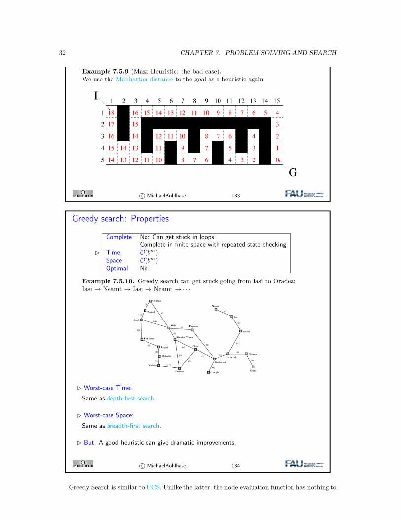
Example 7.5.9 (Maze Heuristic: the bad case).We use the Manhattan distance to the goal as a heuristic again
Heuristic Functions in Path Planning
I Example 4.4 (The maze solved).We indicate h⇤ by giving the goal distance
I Example 4.5 (Maze Heuristic: the good case).We use the Manhattan distance to the goal as a heuristic
I Example 4.6 (Maze Heuristic: the bad case).We use the Manhattan distance to the goal as a heuristic again
1 2 3 4 5 6 7 8 9 10 11 12 13 14 15
1
2
3
4
5
I
G
14 13 12
131415
16
17
18
15 14
15
16 15
14 13
14 13 12
10
1012
11
10
10
9
9
9 8
9
8 7 6 5 4
345678
7
67 5
6
4 3
4 3 2 1
01
91017
16
13
12
12
11
11
11
8
8
7 6 5
5
4 3
2
2
11
Kohlhase: Künstliche Intelligenz 1 160 July 5, 2018
©:MichaelKohlhase 133
Greedy search: Properties
�
Complete No: Can get stuck in loopsComplete in finite space with repeated-state checking
Time O(bm)Space O(bm)Optimal No
Example 7.5.10. Greedy search can get stuck going from Iasi to Oradea:Iasi → Neamt → Iasi → Neamt → · · ·
� Worst-case Time:
Same as depth-first search.
� Worst-case Space:
Same as breadth-first search.
� But: A good heuristic can give dramatic improvements.
©:MichaelKohlhase 134
Greedy Search is similar to UCS. Unlike the latter, the node evaluation function has nothing to
7.5. INFORMED SEARCH STRATEGIES 33
do with the nodes explored so far. This can prevent nodes from being enumerated systematicallyas they are in UCS and BFS.
For completeness, we need repeated state checking as the example shows. This enforces com-plete enumeration of state space (provided that it is finite), and thus gives us completeness.
Note that nothing prevents from all nodes being searched in worst case; e.g. if the heuristicfunction gives us the same (low) estimate on all nodes except where the heuristic mis-estimatesthe distance to be high. So in the worst case, greedy search is even worse than BFS, where d(depth of first solution) replaces m.
The search procedure cannot be optimal, since actual cost of solution is not considered.For both, completeness and optimality, therefore, it is necessary to take the actual cost of
partial solutions, i.e. the path cost, into account. This way, paths that are known to be expensiveare avoided.
7.5.2 Heuristics and their PropertiesA Video Nugget covering this Subsection can be found at https://fau.tv/clip/id/22019.
Heuristic Functions
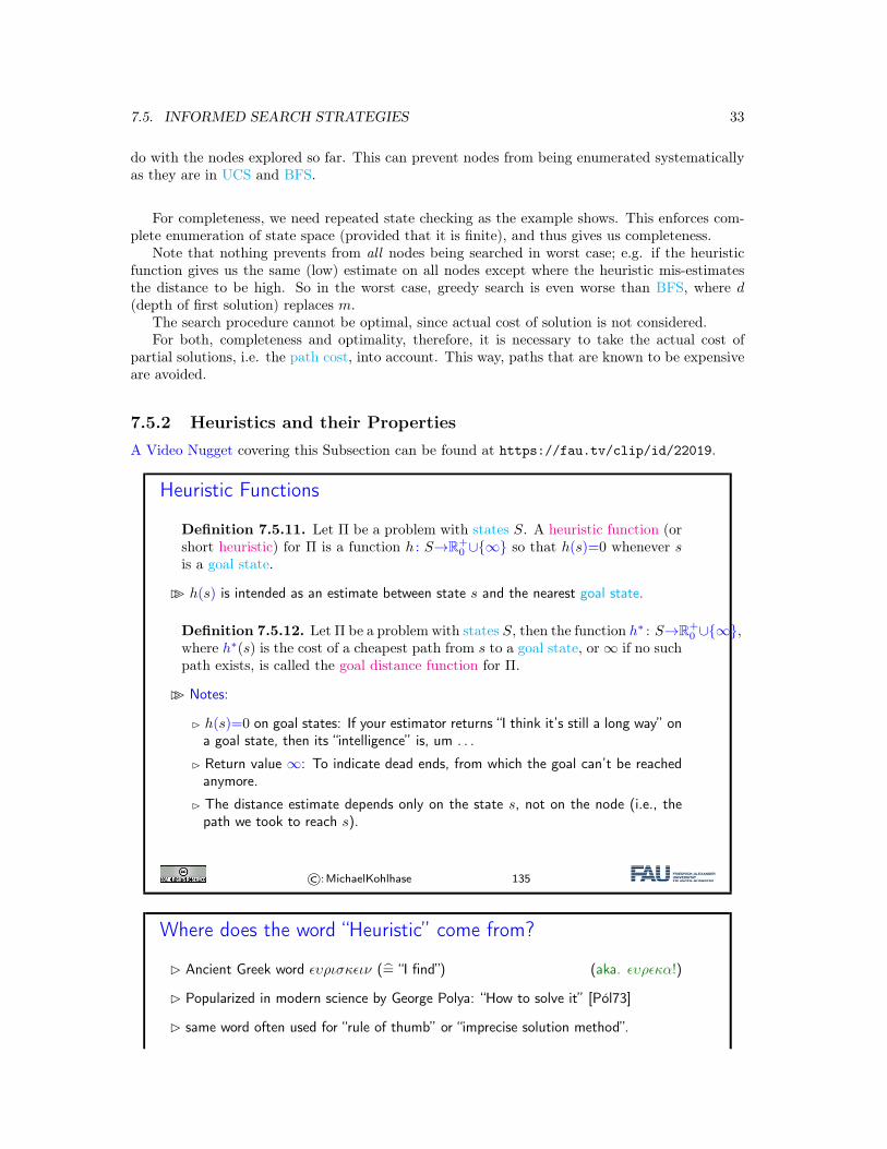
Definition 7.5.11. Let Π be a problem with states S. A heuristic function (orshort heuristic) for Π is a function h : S→R+
0 ∪{∞} so that h(s)=0 whenever sis a goal state.
�� h(s) is intended as an estimate between state s and the nearest goal state.
Definition 7.5.12. Let Π be a problem with states S, then the function h∗ : S→R+0 ∪{∞},
where h∗(s) is the cost of a cheapest path from s to a goal state, or ∞ if no suchpath exists, is called the goal distance function for Π.
�� Notes:
� h(s)=0 on goal states: If your estimator returns “I think it’s still a long way” ona goal state, then its “intelligence” is, um . . .
� Return value ∞: To indicate dead ends, from which the goal can’t be reachedanymore.
� The distance estimate depends only on the state s, not on the node (i.e., thepath we took to reach s).
©:MichaelKohlhase 135
Where does the word “Heuristic” come from?
� Ancient Greek word ϵυρισκϵιν (= “I find”) (aka. ϵυρϵκα!)
� Popularized in modern science by George Polya: “How to solve it” [Pól73]
� same word often used for “rule of thumb” or “imprecise solution method”.
34 CHAPTER 7. PROBLEM SOLVING AND SEARCH
©:MichaelKohlhase 136
Heuristic Functions: The Eternal Trade-Off
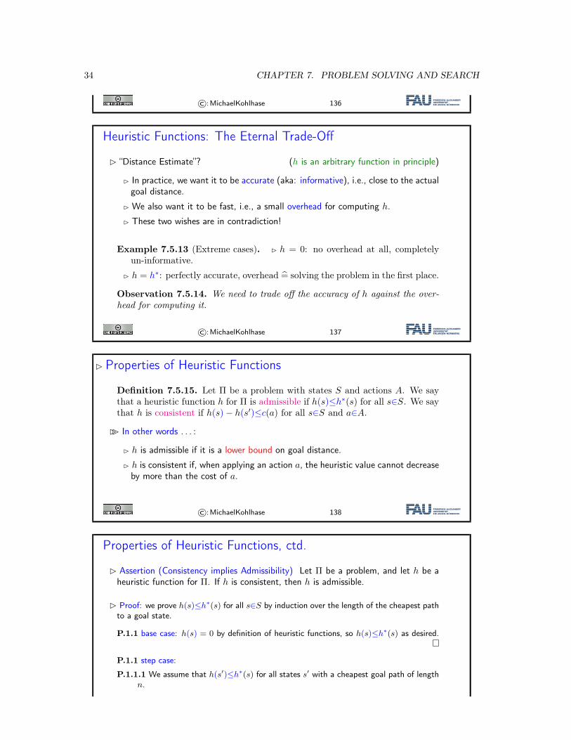
� “Distance Estimate”? (h is an arbitrary function in principle)
� In practice, we want it to be accurate (aka: informative), i.e., close to the actualgoal distance.
� We also want it to be fast, i.e., a small overhead for computing h.
� These two wishes are in contradiction!
Example 7.5.13 (Extreme cases). � h = 0: no overhead at all, completelyun-informative.
� h = h∗: perfectly accurate, overhead = solving the problem in the first place.
Observation 7.5.14. We need to trade off the accuracy of h against the over-head for computing it.
©:MichaelKohlhase 137
� Properties of Heuristic Functions
Definition 7.5.15. Let Π be a problem with states S and actions A. We saythat a heuristic function h for Π is admissible if h(s)≤h∗(s) for all s∈S. We saythat h is consistent if h(s)− h(s′)≤c(a) for all s∈S and a∈A.
�� In other words . . . :
� h is admissible if it is a lower bound on goal distance.
� h is consistent if, when applying an action a, the heuristic value cannot decreaseby more than the cost of a.
©:MichaelKohlhase 138
Properties of Heuristic Functions, ctd.
� Assertion (Consistency implies Admissibility) Let Π be a problem, and let h be aheuristic function for Π. If h is consistent, then h is admissible.
� Proof: we prove h(s)≤h∗(s) for all s∈S by induction over the length of the cheapest pathto a goal state.
P.1.1 base case: h(s) = 0 by definition of heuristic functions, so h(s)≤h∗(s) as desired.
P.1.1 step case:
P.1.1.1 We assume that h(s′)≤h∗(s) for all states s′ with a cheapest goal path of lengthn.
7.5. INFORMED SEARCH STRATEGIES 35
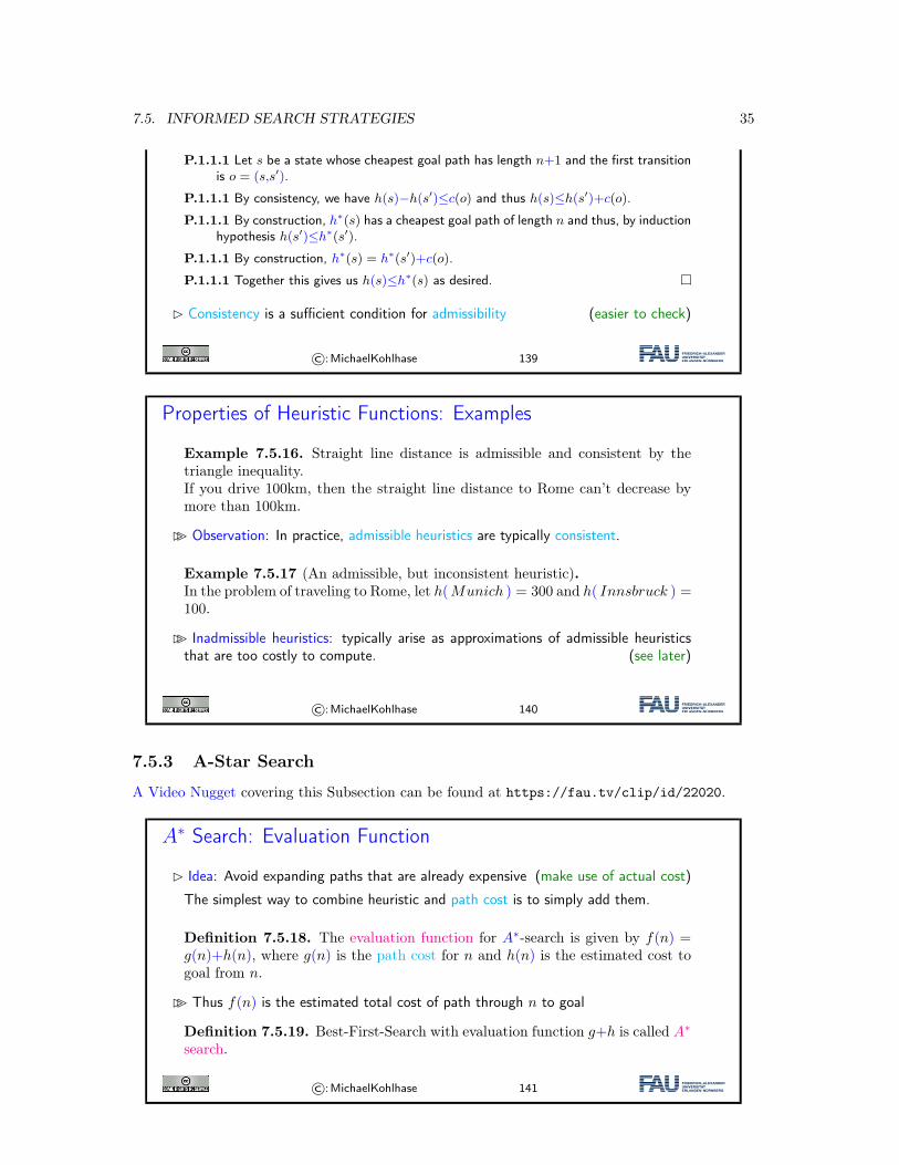
P.1.1.1 Let s be a state whose cheapest goal path has length n+1 and the first transitionis o = (s,s′).
P.1.1.1 By consistency, we have h(s)−h(s′)≤c(o) and thus h(s)≤h(s′)+c(o).
P.1.1.1 By construction, h∗(s) has a cheapest goal path of length n and thus, by inductionhypothesis h(s′)≤h∗(s′).
P.1.1.1 By construction, h∗(s) = h∗(s′)+c(o).
P.1.1.1 Together this gives us h(s)≤h∗(s) as desired.
� Consistency is a sufficient condition for admissibility (easier to check)
©:MichaelKohlhase 139
Properties of Heuristic Functions: Examples
Example 7.5.16. Straight line distance is admissible and consistent by thetriangle inequality.If you drive 100km, then the straight line distance to Rome can’t decrease bymore than 100km.
�� Observation: In practice, admissible heuristics are typically consistent.
Example 7.5.17 (An admissible, but inconsistent heuristic).In the problem of traveling to Rome, let h(Munich ) = 300 and h( Innsbruck ) =100.
�� Inadmissible heuristics: typically arise as approximations of admissible heuristicsthat are too costly to compute. (see later)
©:MichaelKohlhase 140
7.5.3 A-Star Search
A Video Nugget covering this Subsection can be found at https://fau.tv/clip/id/22020.
A∗ Search: Evaluation Function
� Idea: Avoid expanding paths that are already expensive (make use of actual cost)
The simplest way to combine heuristic and path cost is to simply add them.
Definition 7.5.18. The evaluation function for A∗-search is given by f(n) =g(n)+h(n), where g(n) is the path cost for n and h(n) is the estimated cost togoal from n.
�� Thus f(n) is the estimated total cost of path through n to goal
Definition 7.5.19. Best-First-Search with evaluation function g+h is called A∗
search.
©:MichaelKohlhase 141
36 CHAPTER 7. PROBLEM SOLVING AND SEARCH
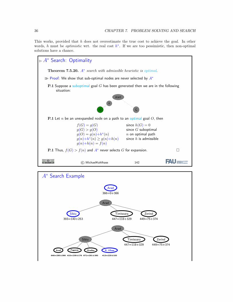
This works, provided that h does not overestimate the true cost to achieve the goal. In otherwords, h must be optimistic wrt. the real cost h∗. If we are too pessimistic, then non-optimalsolutions have a chance.
�A∗ Search: Optimality
Theorem 7.5.20. A∗ search with admissible heuristic is optimal.
�� Proof: We show that sub-optimal nodes are never selected by A∗
P.1 Suppose a suboptimal goal G has been generated then we are in the followingsituation:
start
n
O G
P.1 Let n be an unexpanded node on a path to an optimal goal O, then
f(G) = g(G) since h(G) = 0g(G) > g(O) since G suboptimalg(O) = g(n)+h∗(n) n on optimal pathg(n)+h∗(n) ≥ g(n)+h(n) since h is admissibleg(n)+h(n) = f(n)
P.1 Thus, f(G) > f(n) and A∗ never selects G for expansion.
©:MichaelKohlhase 142
A∗ Search Example
Arad
366=0+366
Arad
Sibiu
393=140+253
Timisoara
447=118+329
Zerind
449=75+374
Arad
Sibiu Timisoara
447=118+329
Zerind
449=75+374
Arad
646=280+366
Fagaras
415=239+176
Oradea
671=291+380
R. Vilcea
413=220+193
7.5. INFORMED SEARCH STRATEGIES 37
Arad
Sibiu Timisoara
447=118+329
Zerind
449=75+374
Arad
646=280+366
Fagaras
415=239+176
Oradea
671=291+380
R. Vilcea
Craiova
526=366+160
Pitesti
417=317+100
Sibiu
553=300+253
Arad
Sibiu Timisoara
447=118+329
Zerind
449=75+374
Arad
646=280+366
Fagaras Oradea
671=291+380
R. Vilcea
Craiova
526=366+160
Pitesti
417=317+100
Sibiu
553=300+253
Sibiu
591=338+253
Bucharest
450=450+0
Arad
Sibiu Timisoara
447=118+329
Zerind
449=75+374
Arad
646=280+366
Fagaras Oradea
671=291+380
R. Vilcea
Craiova
526=366+160
Pitesti Sibiu
553=300+253
Sibiu
591=338+253
Bucharest
450=450+0
Bucharest
418=418+0
Craiova
615=455+160
Sibiu
607=414+193
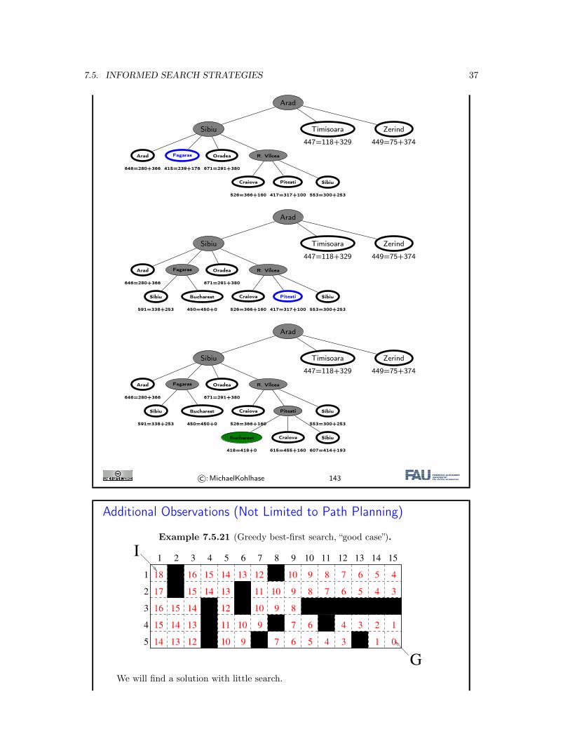
©:MichaelKohlhase 143
Additional Observations (Not Limited to Path Planning)
Example 7.5.21 (Greedy best-first search, “good case”).
Heuristic Functions in Path Planning
I Example 4.4 (The maze solved).We indicate h⇤ by giving the goal distance
I Example 4.5 (Maze Heuristic: the good case).We use the Manhattan distance to the goal as a heuristic
1 2 3 4 5 6 7 8 9 10 11 12 13 14 15
1
2
3
4
5
I
G
14 13 12
131415
16
17
18
15 14
15
16 15
14 13
14 13 12
11 10
1012
11
10
10
9
9
9 8
9
8 7 6 5 4
345678
7
67 5
6
4 3
4 3 2 1
01
910
I Example 4.6 (Maze Heuristic: the bad case).We use the Manhattan distance to the goal as a heuristic again
Kohlhase: Künstliche Intelligenz 1 160 July 5, 2018
We will find a solution with little search.
38 CHAPTER 7. PROBLEM SOLVING AND SEARCH
©:MichaelKohlhase 144
Additional Observations (Not Limited to Path Planning)
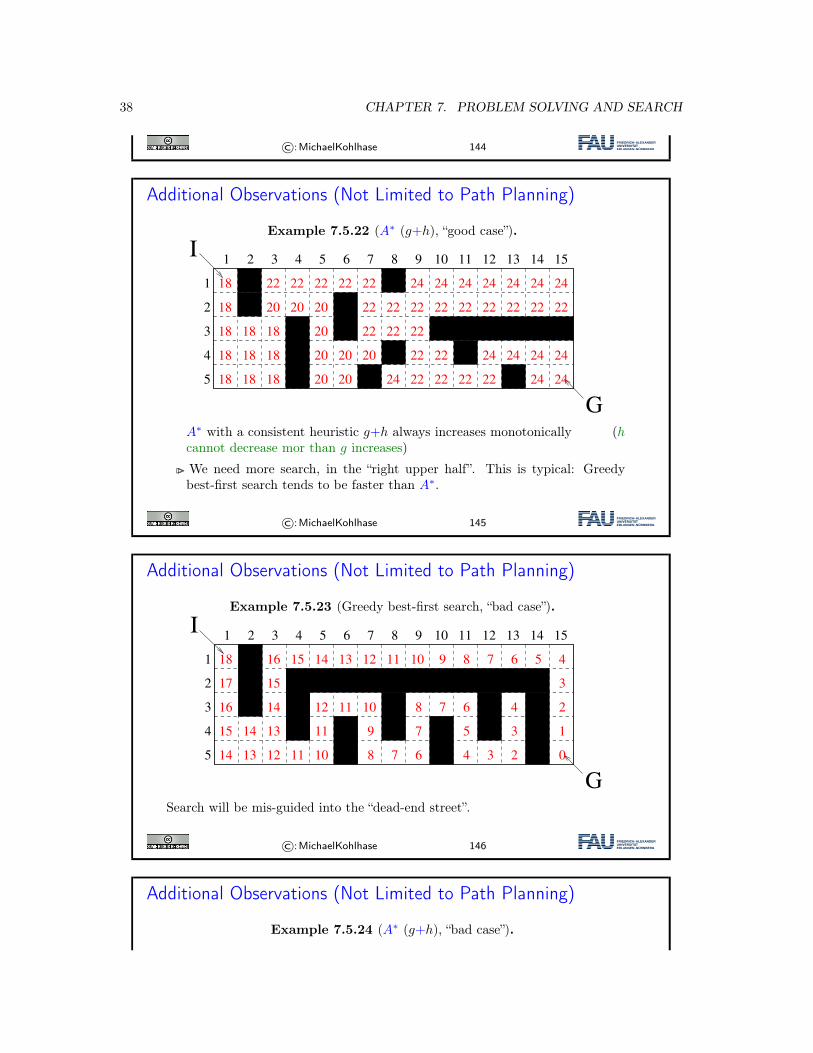
Example 7.5.22 (A∗ (g+h), “good case”).
Additional Observations (Not Limited to Path Planning) II
I Example 4.21 (A⇤ (g + h), “good case”).
1 2 3 4 5 6 7 8 9 10 11 12 13 14 15
1
2
3
4
5
I
G
18
18
18
18
18 18 18
18 18
18 18
20 20 20
20
20
20 20
20 20
22 22 22 22 22
22
22 22 22
22 22 22 22 22 22 22 22
22
22
22
22 22 22
24
24
24 24 24
2424
24 24 24 24 24 24 24
I A⇤ with a consistent heuristic g + h always increases monotonically (h cannotdecrease mor than g increases)
I We need more search, in the “right upper half”. This is typical: Greedy best-firstsearch tends to be faster than A⇤.
Kohlhase: Künstliche Intelligenz 1 177 July 5, 2018
A∗ with a consistent heuristic g+h always increases monotonically (hcannot decrease mor than g increases)
�� We need more search, in the “right upper half”. This is typical: Greedybest-first search tends to be faster than A∗.
©:MichaelKohlhase 145
Additional Observations (Not Limited to Path Planning)
Example 7.5.23 (Greedy best-first search, “bad case”).
Heuristic Functions in Path Planning
I Example 4.4 (The maze solved).We indicate h⇤ by giving the goal distance
I Example 4.5 (Maze Heuristic: the good case).We use the Manhattan distance to the goal as a heuristic
I Example 4.6 (Maze Heuristic: the bad case).We use the Manhattan distance to the goal as a heuristic again
1 2 3 4 5 6 7 8 9 10 11 12 13 14 15
1
2
3
4
5
I
G
14 13 12
131415
16
17
18
15 14
15
16 15
14 13
14 13 12
10
1012
11
10
10
9
9
9 8
9
8 7 6 5 4
345678
7
67 5
6
4 3
4 3 2 1
01
91017
16
13
12
12
11
11
11
8
8
7 6 5
5
4 3
2
2
11
Kohlhase: Künstliche Intelligenz 1 160 July 5, 2018Search will be mis-guided into the “dead-end street”.
©:MichaelKohlhase 146
Additional Observations (Not Limited to Path Planning)
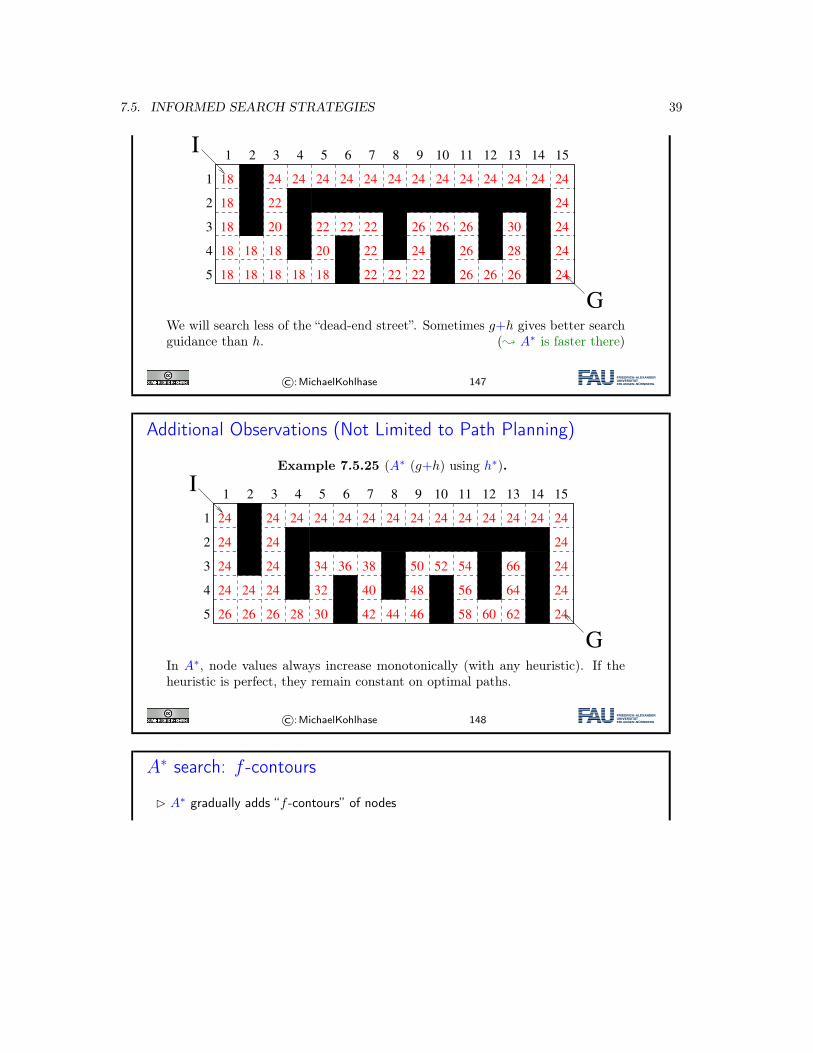
Example 7.5.24 (A∗ (g+h), “bad case”).
7.5. INFORMED SEARCH STRATEGIES 39Additional Observations (Not Limited to Path Planning) IV
I Example 4.23 (A⇤ (g + h), “bad case”).
1 2 3 4 5 6 7 8 9 10 11 12 13 14 15
1
2
3
4
5
I
G
18 18 18
181818
18
18
18
15 20
22
24 24
14 13
24 24 24
10
2222
20
18
10
9
9
9 45678
5
6 4 2
1
2417
16
13
12
12
24
22
18
8
5 3
11
22
22 22 22
24
26 26 26
26
26 26 26
28
30
24
24
24
24
242424242424
We will search less of the “dead-end street”. Sometimes g + h gives bettersearch guidance than h. (; A⇤ is faster there)
Kohlhase: Künstliche Intelligenz 1 179 July 5, 2018
We will search less of the “dead-end street”. Sometimes g+h gives better searchguidance than h. (; A∗ is faster there)
©:MichaelKohlhase 147
Additional Observations (Not Limited to Path Planning)
Example 7.5.25 (A∗ (g+h) using h∗).
Additional Observations (Not Limited to Path Planning) V
I Example 4.24 (A⇤ (g + h) using h⇤).
1 2 3 4 5 6 7 8 9 10 11 12 13 14 15
1
2
3
4
5
I
G
15
14 13 10
10
9
9
9 45678
5
6 4 2
1
17
16
13
12
12
8
5 3
11
24
24
24
24
24242424242424242424242424
24
24
242424
24
24
24
26 26 26 28 30
32
34 36 38
40
42 44 46
48
50 52 54
56
58 60 62
64
66
In A⇤, node values always increase monotonically (with any heuristic). If theheuristic is perfect, they remain constant on optimal paths.
Kohlhase: Künstliche Intelligenz 1 180 July 5, 2018
In A∗, node values always increase monotonically (with any heuristic). If theheuristic is perfect, they remain constant on optimal paths.
©:MichaelKohlhase 148
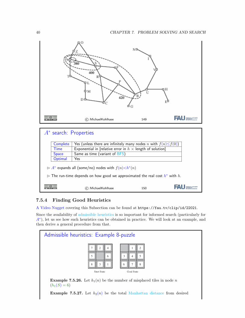
A∗ search: f -contours
� A∗ gradually adds “f -contours” of nodes
40 CHAPTER 7. PROBLEM SOLVING AND SEARCH
©:MichaelKohlhase 149
A∗ search: Properties
Complete Yes (unless there are infinitely many nodes n with f(n)≤f(0))Time Exponential in [relative error in h × length of solution]Space Same as time (variant of BFS)Optimal Yes
� A∗ expands all (some/no) nodes with f(n)<h∗(n)
� The run-time depends on how good we approximated the real cost h∗ with h.
©:MichaelKohlhase 150
7.5.4 Finding Good HeuristicsA Video Nugget covering this Subsection can be found at https://fau.tv/clip/id/22021.
Since the availability of admissible heuristics is so important for informed search (particularly forA∗), let us see how such heuristics can be obtained in practice. We will look at an example, andthen derive a general procedure from that.
Admissible heuristics: Example 8-puzzle
Example 7.5.26. Let h1(n) be the number of misplaced tiles in node n(h1(S) = 6)
Example 7.5.27. Let h2(n) be the total Manhattan distance from desired
7.5. INFORMED SEARCH STRATEGIES 41
location of each tile. (h2(S) = 2+0+3+1+0+1+3+4 = 14)
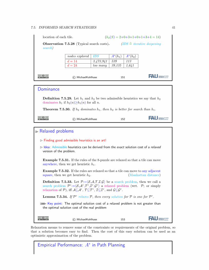
Observation 7.5.28 (Typical search costs). (IDS = iterative deepeningsearch)
nodes explored IDS A∗(h1) A∗(h2)
d = 14 3,473,941 539 113d = 24 too many 39,135 1,641
©:MichaelKohlhase 151
Dominance
Definition 7.5.29. Let h1 and h2 be two admissible heuristics we say that h2
dominates h1 if h2(n)≥h1(n) for all n.
Theorem 7.5.30. If h2 dominates h1, then h2 is better for search than h1.
©:MichaelKohlhase 152
�� Relaxed problems
� Finding good admissible heuristics is an art!
� Idea: Admissible heuristics can be derived from the exact solution cost of a relaxedversion of the problem.
Example 7.5.31. If the rules of the 8-puzzle are relaxed so that a tile can moveanywhere, then we get heuristic h1.
Example 7.5.32. If the rules are relaxed so that a tile can move to any adjacentsquare, then we get heuristic h2. (Manhattan distance)
Definition 7.5.33. Let P:=⟨S,A,T ,I,G⟩ be a search problem, then we call asearch problem Pr:=⟨S,Ar,T r,Ir,Gr⟩ a relaxed problem (wrt. P; or simplyrelaxation of P), iff A⊆Ar, T ⊆T r, I⊆Ir, and G⊆Gr.
Lemma 7.5.34. If Pr relaxes P, then every solution for P is one for Pr.
����� Key point: The optimal solution cost of a relaxed problem is not greater thanthe optimal solution cost of the real problem
©:MichaelKohlhase 153
Relaxation means to remove some of the constraints or requirements of the original problem, sothat a solution becomes easy to find. Then the cost of this easy solution can be used as anoptimistic approximation of the problem.
Empirical Performance: A∗ in Path Planning
42 CHAPTER 7. PROBLEM SOLVING AND SEARCH
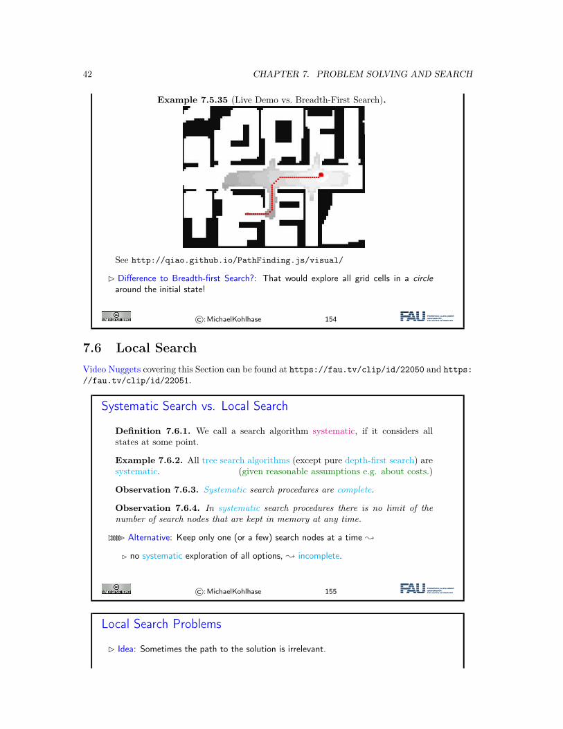
Example 7.5.35 (Live Demo vs. Breadth-First Search).
See http://qiao.github.io/PathFinding.js/visual/
� Difference to Breadth-first Search?: That would explore all grid cells in a circlearound the initial state!
©:MichaelKohlhase 154
7.6 Local SearchVideo Nuggets covering this Section can be found at https://fau.tv/clip/id/22050 and https://fau.tv/clip/id/22051.
Systematic Search vs. Local Search
Definition 7.6.1. We call a search algorithm systematic, if it considers allstates at some point.
Example 7.6.2. All tree search algorithms (except pure depth-first search) aresystematic. (given reasonable assumptions e.g. about costs.)
Observation 7.6.3. Systematic search procedures are complete.
Observation 7.6.4. In systematic search procedures there is no limit of thenumber of search nodes that are kept in memory at any time.
����� Alternative: Keep only one (or a few) search nodes at a time ;
� no systematic exploration of all options, ; incomplete.
©:MichaelKohlhase 155
Local Search Problems
� Idea: Sometimes the path to the solution is irrelevant.
7.6. LOCAL SEARCH 43
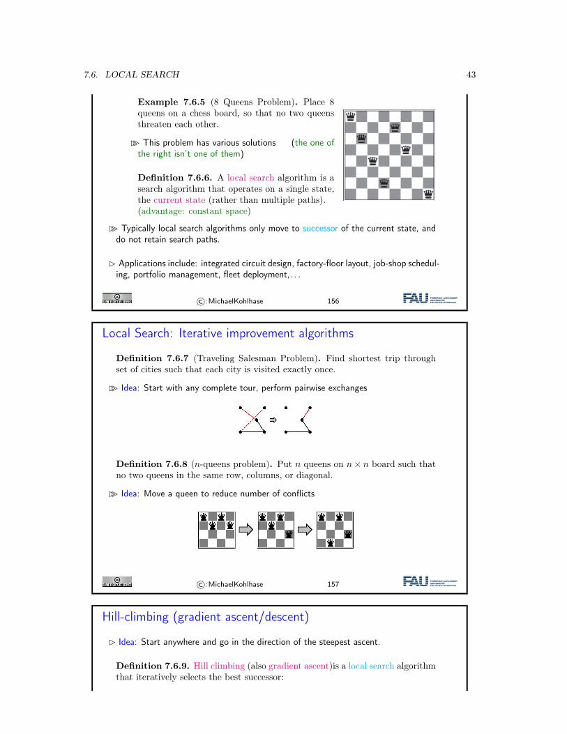
Example 7.6.5 (8 Queens Problem). Place 8queens on a chess board, so that no two queensthreaten each other.
�� This problem has various solutions (the one ofthe right isn’t one of them)
Definition 7.6.6. A local search algorithm is asearch algorithm that operates on a single state,the current state (rather than multiple paths).(advantage: constant space)
�� Typically local search algorithms only move to successor of the current state, anddo not retain search paths.
� Applications include: integrated circuit design, factory-floor layout, job-shop schedul-ing, portfolio management, fleet deployment,. . .
©:MichaelKohlhase 156
Local Search: Iterative improvement algorithms
Definition 7.6.7 (Traveling Salesman Problem). Find shortest trip throughset of cities such that each city is visited exactly once.
�� Idea: Start with any complete tour, perform pairwise exchanges
Local Search: Iterative improvement algorithms
I Definition 5.7 (Traveling Salesman Problem). Find shortest trip through setof cities such that each city is visited exactly once.
I Idea: Start with any complete tour, perform pairwise exchanges
I Definition 5.8 (n-queens problem). Put n queens on n ⇥ n board such thatno two queens in the same row, columns, or diagonal.
I Idea: Move a queen to reduce number of conflicts
Kohlhase: Künstliche Intelligenz 1 189 July 5, 2018
Definition 7.6.8 (n-queens problem). Put n queens on n× n board such thatno two queens in the same row, columns, or diagonal.
�� Idea: Move a queen to reduce number of conflicts
Local Search: Iterative improvement algorithms
I Definition 5.7 (Traveling Salesman Problem). Find shortest trip through setof cities such that each city is visited exactly once.
I Idea: Start with any complete tour, perform pairwise exchanges
I Definition 5.8 (n-queens problem). Put n queens on n ⇥ n board such thatno two queens in the same row, columns, or diagonal.
I Idea: Move a queen to reduce number of conflicts
Kohlhase: Künstliche Intelligenz 1 189 July 5, 2018©:MichaelKohlhase 157
Hill-climbing (gradient ascent/descent)
� Idea: Start anywhere and go in the direction of the steepest ascent.
Definition 7.6.9. Hill climbing (also gradient ascent)is a local search algorithmthat iteratively selects the best successor:
44 CHAPTER 7. PROBLEM SOLVING AND SEARCH
procedure Hill−Climbing (problem) /∗ a state that is a local minimum ∗/local current, neighbor /∗ nodes ∗/current := Make−Node(Initial−State[problem])loop
neighbor := <a highest−valued successor of current>if Value[neighbor] < Value[current] return [current] end ifcurrent := neighbor
end loopend procedure
�� Intuition:
Like best first search without memory.
� Works, if solutions are dense and local maxima can be escaped.
©:MichaelKohlhase 158
In order to understand the procedure on a more intuitive level, let us consider the followingscenario: We are in a dark landscape (or we are blind), and we want to find the highest hill. Thesearch procedure above tells us to start our search anywhere, and for every step first feel around,and then take a step into the direction with the steepest ascent. If we reach a place, where thenext step would take us down, we are finished.
Of course, this will only get us into local maxima, and has no guarantee of getting us intoglobal ones (remember, we are blind). The solution to this problem is to re-start the search atrandom (we do not have any information) places, and hope that one of the random jumps will getus to a slope that leads to a global maximum.
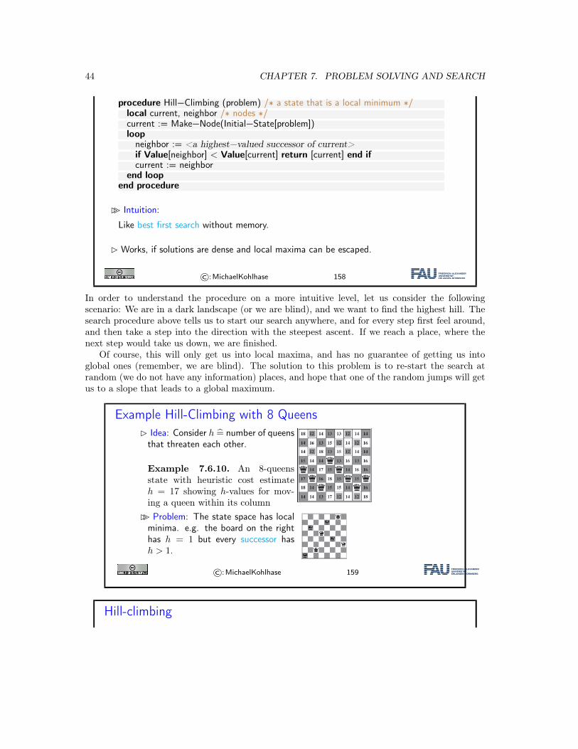
Example Hill-Climbing with 8 Queens� Idea: Consider h = number of queens
that threaten each other.
Example 7.6.10. An 8-queensstate with heuristic cost estimateh = 17 showing h-values for mov-ing a queen within its column
�� Problem: The state space has localminima. e.g. the board on the righthas h = 1 but every successor hash > 1.
©:MichaelKohlhase 159
Hill-climbing
7.6. LOCAL SEARCH 45
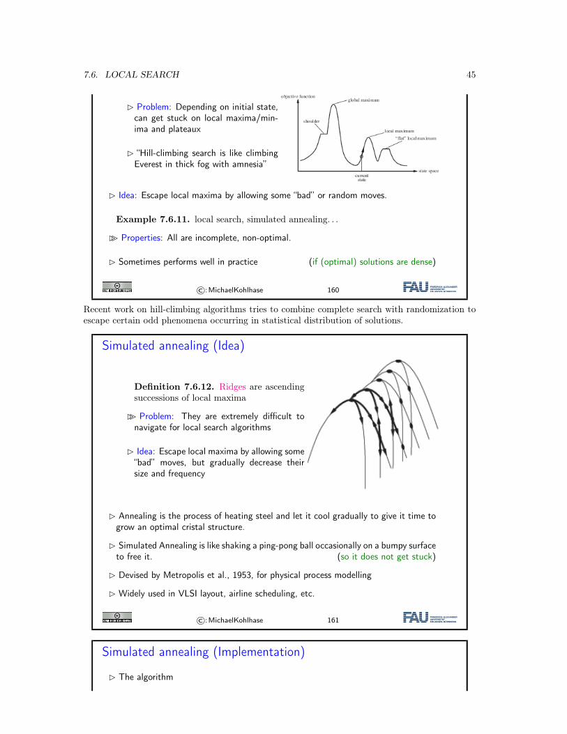
� Problem: Depending on initial state,can get stuck on local maxima/min-ima and plateaux
� “Hill-climbing search is like climbingEverest in thick fog with amnesia”
� Idea: Escape local maxima by allowing some “bad” or random moves.
Example 7.6.11. local search, simulated annealing. . .
�� Properties: All are incomplete, non-optimal.
� Sometimes performs well in practice (if (optimal) solutions are dense)
©:MichaelKohlhase 160
Recent work on hill-climbing algorithms tries to combine complete search with randomization toescape certain odd phenomena occurring in statistical distribution of solutions.
Simulated annealing (Idea)
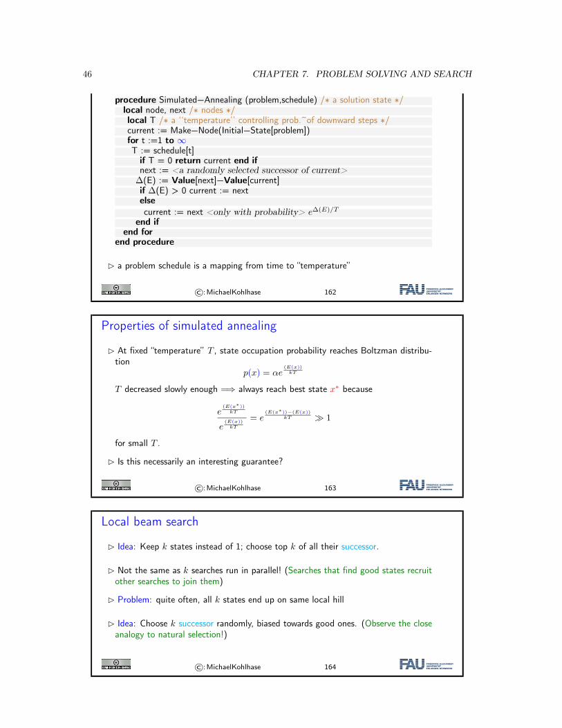
Definition 7.6.12. Ridges are ascendingsuccessions of local maxima
�� Problem: They are extremely difficult tonavigate for local search algorithms
� Idea: Escape local maxima by allowing some“bad” moves, but gradually decrease theirsize and frequency
� Annealing is the process of heating steel and let it cool gradually to give it time togrow an optimal cristal structure.
� Simulated Annealing is like shaking a ping-pong ball occasionally on a bumpy surfaceto free it. (so it does not get stuck)
� Devised by Metropolis et al., 1953, for physical process modelling
� Widely used in VLSI layout, airline scheduling, etc.
©:MichaelKohlhase 161
Simulated annealing (Implementation)
� The algorithm
46 CHAPTER 7. PROBLEM SOLVING AND SEARCH
procedure Simulated−Annealing (problem,schedule) /∗ a solution state ∗/local node, next /∗ nodes ∗/local T /∗ a ‘‘temperature’’ controlling prob.~of downward steps ∗/current := Make−Node(Initial−State[problem])for t :=1 to ∞T := schedule[t]
if T = 0 return current end ifnext := <a randomly selected successor of current>∆(E) := Value[next]−Value[current]if ∆(E) > 0 current := nextelsecurrent := next <only with probability> e∆(E)/T
end ifend for
end procedure
� a problem schedule is a mapping from time to “temperature”
©:MichaelKohlhase 162
Properties of simulated annealing
� At fixed “temperature” T , state occupation probability reaches Boltzman distribu-tion
p(x) = αe(E(x))
kT
T decreased slowly enough =⇒ always reach best state x∗ because
e(E(x∗))
kT
e(E(x))
kT
= e(E(x∗))−(E(x))
kT ≫ 1
for small T .
� Is this necessarily an interesting guarantee?
©:MichaelKohlhase 163
Local beam search
� Idea: Keep k states instead of 1; choose top k of all their successor.
� Not the same as k searches run in parallel! (Searches that find good states recruitother searches to join them)
� Problem: quite often, all k states end up on same local hill
� Idea: Choose k successor randomly, biased towards good ones. (Observe the closeanalogy to natural selection!)
©:MichaelKohlhase 164
7.6. LOCAL SEARCH 47
Genetic algorithms (very briefly)
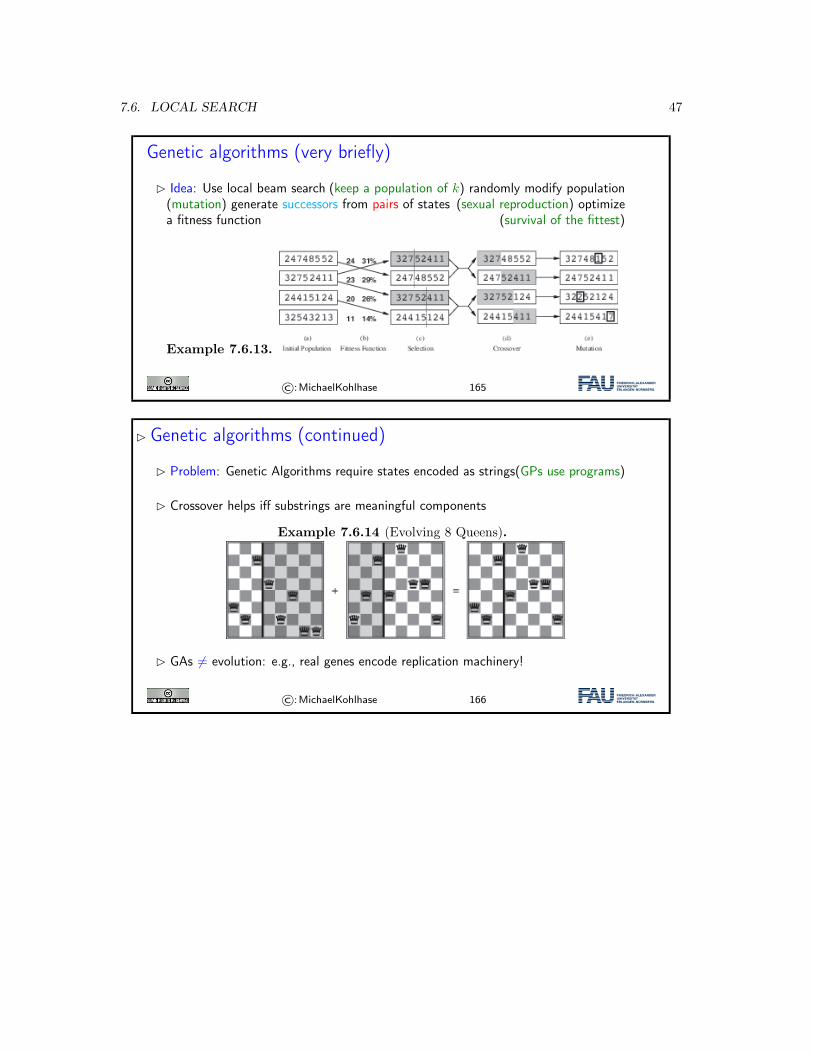
� Idea: Use local beam search (keep a population of k) randomly modify population(mutation) generate successors from pairs of states (sexual reproduction) optimizea fitness function (survival of the fittest)
Example 7.6.13.
©:MichaelKohlhase 165
� Genetic algorithms (continued)
� Problem: Genetic Algorithms require states encoded as strings(GPs use programs)
� Crossover helps iff substrings are meaningful components
Example 7.6.14 (Evolving 8 Queens).
� GAs = evolution: e.g., real genes encode replication machinery!
©:MichaelKohlhase 166

48 CHAPTER 7. PROBLEM SOLVING AND SEARCH
Chapter 8
Adversarial Search for Game Playing
A Video Nugget covering this Chapter can be found at https://fau.tv/clip/id/22079.
8.1 IntroductionVideo Nuggets covering this Section can be found at https://fau.tv/clip/id/22060 and https://fau.tv/clip/id/22061.
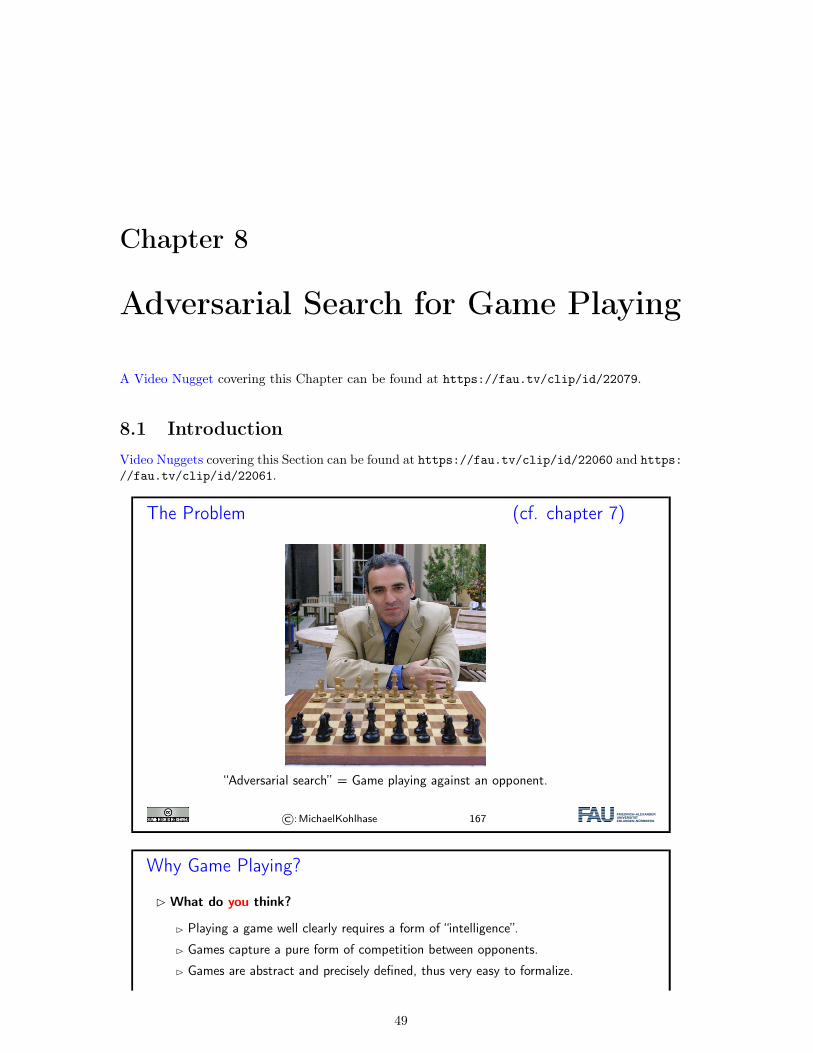
The Problem (cf. chapter 7)
“Adversarial search” = Game playing against an opponent.
©:MichaelKohlhase 167
Why Game Playing?
� What do you think?
� Playing a game well clearly requires a form of “intelligence”.
� Games capture a pure form of competition between opponents.
� Games are abstract and precisely defined, thus very easy to formalize.
49
50 CHAPTER 8. ADVERSARIAL SEARCH FOR GAME PLAYING
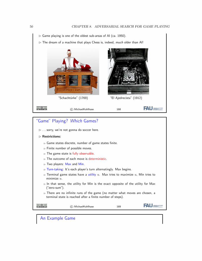
� Game playing is one of the oldest sub-areas of AI (ca. 1950).
� The dream of a machine that plays Chess is, indeed, much older than AI!
“Schachtürke” (1769) “El Ajedrecista” (1912)
©:MichaelKohlhase 168
“Game” Playing? Which Games?
� . . . sorry, we’re not gonna do soccer here.
� Restrictions:
� Game states discrete, number of game states finite.
� Finite number of possible moves.
� The game state is fully observable.
� The outcome of each move is deterministic.
� Two players: Max and Min.
� Turn-taking: It’s each player’s turn alternatingly. Max begins.
� Terminal game states have a utility u. Max tries to maximize u, Min tries tominimize u.
� In that sense, the utility for Min is the exact opposite of the utility for Max(“zero-sum”).
� There are no infinite runs of the game (no matter what moves are chosen, aterminal state is reached after a finite number of steps).
©:MichaelKohlhase 169
An Example Game
8.1. INTRODUCTION 51
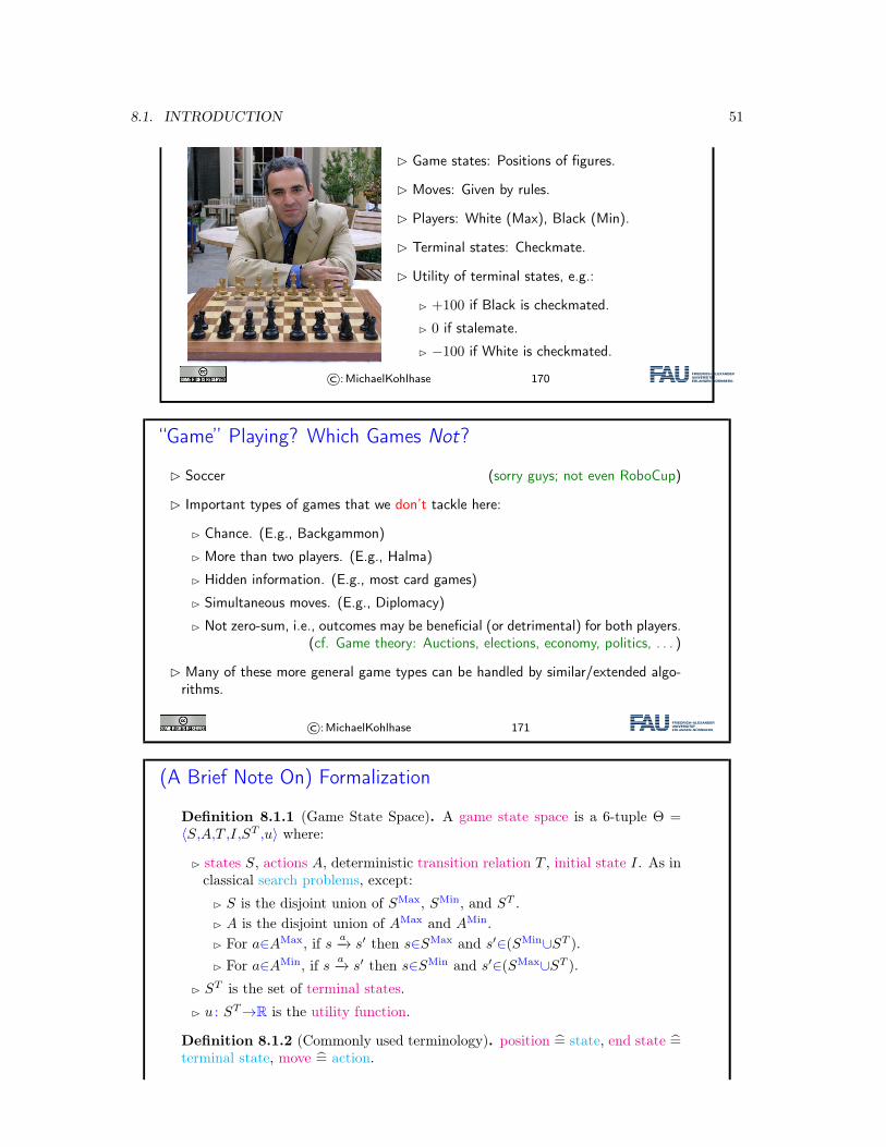
� Game states: Positions of figures.
� Moves: Given by rules.
� Players: White (Max), Black (Min).
� Terminal states: Checkmate.
� Utility of terminal states, e.g.:
� +100 if Black is checkmated.
� 0 if stalemate.
� −100 if White is checkmated.
©:MichaelKohlhase 170
“Game” Playing? Which Games Not?
� Soccer (sorry guys; not even RoboCup)
� Important types of games that we don’t tackle here:
� Chance. (E.g., Backgammon)
� More than two players. (E.g., Halma)
� Hidden information. (E.g., most card games)
� Simultaneous moves. (E.g., Diplomacy)
� Not zero-sum, i.e., outcomes may be beneficial (or detrimental) for both players.(cf. Game theory: Auctions, elections, economy, politics, . . . )
� Many of these more general game types can be handled by similar/extended algo-rithms.
©:MichaelKohlhase 171
(A Brief Note On) Formalization
Definition 8.1.1 (Game State Space). A game state space is a 6-tuple Θ =⟨S,A,T ,I,ST ,u⟩ where:
� states S, actions A, deterministic transition relation T , initial state I. As inclassical search problems, except:
� S is the disjoint union of SMax, SMin, and ST .� A is the disjoint union of AMax and AMin.� For a∈AMax, if s a−→ s′ then s∈SMax and s′∈(SMin∪ST ).� For a∈AMin, if s a−→ s′ then s∈SMin and s′∈(SMax∪ST ).
� ST is the set of terminal states.
� u : ST→R is the utility function.
Definition 8.1.2 (Commonly used terminology). position = state, end state =terminal state, move = action.
52 CHAPTER 8. ADVERSARIAL SEARCH FOR GAME PLAYING
�� A round of the game – one move Max, one move Min – is often referred to as a“move”, and individual actions as “half-moves”. We don’t do that here.
©:MichaelKohlhase 172
Why Games are Hard to Solve: I
� What is a “solution” here?
Definition 8.1.3. Let Θ be a game state space, and let X∈{Max,Min}. Astrategy for X is a function σX : SX→AX so that a is applicable to s wheneverσX(s) = a.
�� We don’t know how the opponent will react, and need to prepare for all possibilities.
Definition 8.1.4. A strategy is optimal if it yields the best possible utility forX assuming perfect opponent play (not formalized here).
�� In (almost) all games, computing a strategy is infeasible. Instead, compute thenext move “on demand”, given the current game state.
©:MichaelKohlhase 173
Why Games are hard to solve II
� Number of reachable states in Chess: 1040.
� Number of reachable states in Go: 10100.
� It’s worse even: Our algorithms here look at search trees (game trees), no duplicatechecking. Chess: 35100≃10154. Go: 200300≃10690.
©:MichaelKohlhase 174
How To Describe a Game State Space?
� Like for classical search problems, there are three possible ways to describe a game:blackbox/API description, declarative description, explicit game state space.
� Question: Which ones do humans use?
� Explicit ≈ Hand over a book with all 1040 moves in Chess.
� Blackbox ≈ Give possible Chess moves on demand but don’t say how they aregenerated.
� Answer: Declarative!With “game description language” = natural language.
©:MichaelKohlhase 175
8.2. MINIMAX SEARCH 53
Specialized vs. General Game Playing
� And which game descriptions do computers use?
� Explicit: Only in illustrations.
� Blackbox/API: Assumed description in (This Chapter)
� Method of choice for all those game players out there in the market (Chesscomputers, video game opponents, you name it).
� Programs designed for, and specialized to, a particular game.� Human knowledge is key: evaluation functions (see later), opening databases
(Chess!!), end databases.
� Declarative: General Game Playing, active area of research in AI.
� Generic Game Description Language (GDL), based on logic.� Solvers are given only “the rules of the game”, no other knowledge/input
whatsoever (cf. chapter 7).� Regular academic competitions since 2005.
©:MichaelKohlhase 176
Our Agenda for This Chapter
� Minimax Search: How to compute an optimal strategy?
� Minimax is the canonical (and easiest to understand) algorithm for solvinggames, i.e., computing an optimal strategy.
� Evaluation Functions: But what if we don’t have the time/memory to solve theentire game?
� Given limited time, the best we can do is look ahead as far as we can. Evaluationfunctions tell us how to evaluate the leaf states at the cut-off.
� Alpha-Beta Search: How to prune unnecessary parts of the tree?
� Often, we can detect early on that a particular action choice cannot be part ofthe optimal strategy. We can then stop considering this part of the game tree.
� State of the Art: What is the state of affairs, for prominent games, of computergame playing vs. human experts?
� Just FYI (not part of the technical content of this course).
©:MichaelKohlhase 177
8.2 Minimax SearchA Video Nugget covering this Section can be found at https://fau.tv/clip/id/22061.
“Minimax”?
54 CHAPTER 8. ADVERSARIAL SEARCH FOR GAME PLAYING
� We want to compute an optimal strategy for player “Max”.
� In other words: “We are Max, and our opponent is Min.”
Recall:
� � We compute the strategy offline, before the game begins. During the game,whenever it’s our turn, we just lookup the corresponding action.
� Max attempts to maximize the utility u(s) of the terminal state that will bereached during play.
� Min attempts to minimize u(s).
� So what?
� The computation alternates between minimization and maximization ; hence“minimax”.
©:MichaelKohlhase 178
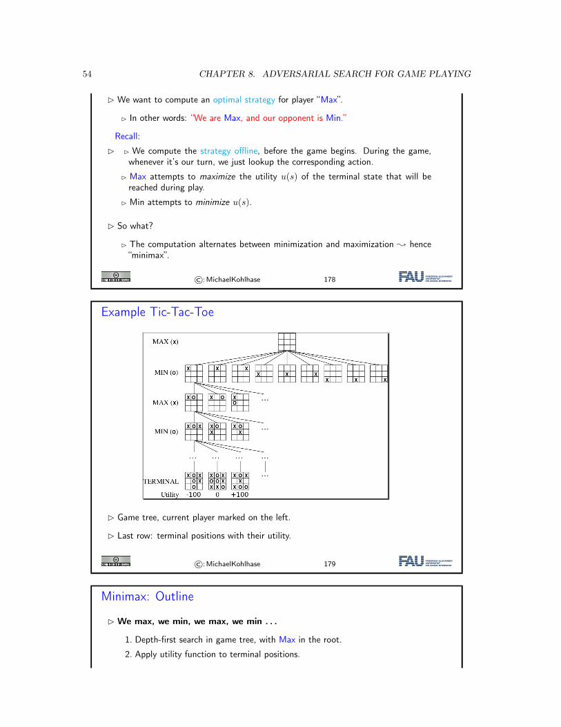
Example Tic-Tac-Toe
� Game tree, current player marked on the left.
� Last row: terminal positions with their utility.
©:MichaelKohlhase 179
Minimax: Outline
� We max, we min, we max, we min . . .
1. Depth-first search in game tree, with Max in the root.
2. Apply utility function to terminal positions.
8.2. MINIMAX SEARCH 55
3. Bottom-up for each inner node n in the tree, compute the utility u(n) of n asfollows:
� If it’s Max’s turn: Set u(n) to the maximum of the utilities of n’s successornodes.
� If it’s Min’s turn: Set u(n) to the minimum of the utilities of n’s successornodes.
4. Selecting a move for Max at the root: Choose one move that leads to asuccessor node with maximal utility.
©:MichaelKohlhase 180
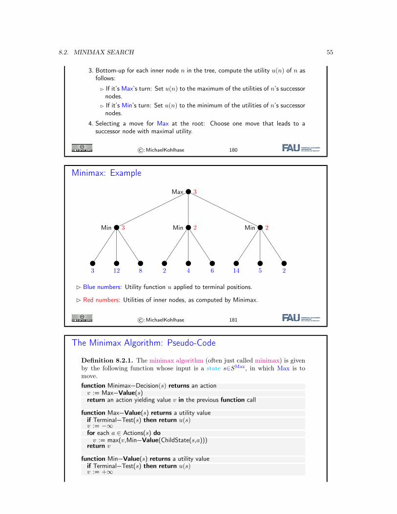
Minimax: Example
Max 3
Min 3
3 12 8
Min 2
2 4 6
Min 2
14 5 2
� Blue numbers: Utility function u applied to terminal positions.
� Red numbers: Utilities of inner nodes, as computed by Minimax.
©:MichaelKohlhase 181
The Minimax Algorithm: Pseudo-Code
Definition 8.2.1. The minimax algorithm (often just called minimax) is givenby the following function whose input is a state s∈SMax, in which Max is tomove.function Minimax−Decision(s) returns an actionv := Max−Value(s)return an action yielding value v in the previous function call
function Max−Value(s) returns a utility valueif Terminal−Test(s) then return u(s)v := −∞for each a ∈ Actions(s) dov := max(v,Min−Value(ChildState(s,a)))
return v
function Min−Value(s) returns a utility valueif Terminal−Test(s) then return u(s)v := +∞
56 CHAPTER 8. ADVERSARIAL SEARCH FOR GAME PLAYING
for each a ∈ Actions(s) dov := min(v,Max−Value(ChildState(s,a)))
return v
©:MichaelKohlhase 182
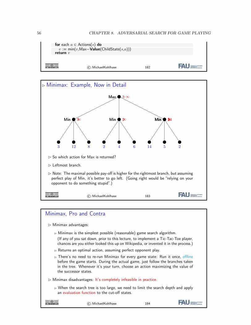
� Minimax: Example, Now in Detail
Max −∞Max 3
Min ∞Min 3
3 12 8
Min ∞Min 2
2 4 6
Min ∞Min 14Min 5Min 2
14 5 2
� So which action for Max is returned?
� Leftmost branch.
� Note: The maximal possible pay-off is higher for the rightmost branch, but assumingperfect play of Min, it’s better to go left. (Going right would be “relying on youropponent to do something stupid”.)
©:MichaelKohlhase 183
Minimax, Pro and Contra
� Minimax advantages:
� Minimax is the simplest possible (reasonable) game search algorithm.(If any of you sat down, prior to this lecture, to implement a Tic-Tac-Toe player,chances are you either looked this up on Wikipedia, or invented it in the process.)
� Returns an optimal action, assuming perfect opponent play.
� There’s no need to re-run Minimax for every game state: Run it once, offlinebefore the game starts. During the actual game, just follow the branches takenin the tree. Whenever it’s your turn, choose an action maximizing the value ofthe successor states.
� Minimax disadvantages: It’s completely infeasible in practice.
� When the search tree is too large, we need to limit the search depth and applyan evaluation function to the cut-off states.
©:MichaelKohlhase 184
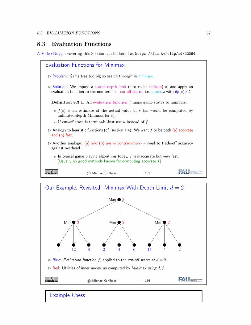
8.3. EVALUATION FUNCTIONS 57
8.3 Evaluation FunctionsA Video Nugget covering this Section can be found at https://fau.tv/clip/id/22064.
Evaluation Functions for Minimax
� Problem: Game tree too big so search through in minimax.
� Solution: We impose a search depth limit (also called horizon) d, and apply anevaluation function to the non-terminal cut off states, i.e. states s with dp(s)>d.
Definition 8.3.1. An evaluation function f maps game states to numbers:
� f(s) is an estimate of the actual value of s (as would be computed byunlimited-depth Minimax for s).
� If cut-off state is terminal: Just use u instead of f .
� Analogy to heuristic functions (cf. section 7.4): We want f to be both (a) accurateand (b) fast.
� Another analogy: (a) and (b) are in contradiction ; need to trade-off accuracyagainst overhead.
� In typical game playing algorithms today, f is inaccurate but very fast.(Usually no good methods known for computing accurate f)
©:MichaelKohlhase 185
Our Example, Revisited: Minimax With Depth Limit d = 2
Max 3
Min 3
3 12 8
Min 2
2 4 6
Min 2
14 5 2
� Blue: Evaluation function f , applied to the cut-off states at d = 2.
� Red: Utilities of inner nodes, as computed by Minimax using d, f .
©:MichaelKohlhase 186
Example Chess
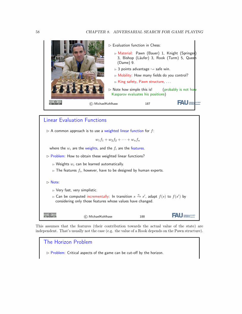
58 CHAPTER 8. ADVERSARIAL SEARCH FOR GAME PLAYING
� Evaluation function in Chess:
� Material: Pawn (Bauer) 1, Knight (Springer)3, Bishop (Läufer) 3, Rook (Turm) 5, Queen(Dame) 9.
� 3 points advantage ; safe win.
� Mobility: How many fields do you control?
� King safety, Pawn structure, . . .
� Note how simple this is! (probably is not howKasparov evaluates his positions)
©:MichaelKohlhase 187
Linear Evaluation Functions
� A common approach is to use a weighted linear function for f :
w1f1 + w2f2 + · · ·+ wnfn
where the wi are the weights, and the fi are the features.
� Problem: How to obtain these weighted linear functions?
� Weights wi can be learned automatically.
� The features fi, however, have to be designed by human experts.
� Note:
� Very fast, very simplistic.
� Can be computed incrementally: In transition sa−→ s′, adapt f(s) to f(s′) by
considering only those features whose values have changed.
©:MichaelKohlhase 188
This assumes that the features (their contribution towards the actual value of the state) areindependent. That’s usually not the case (e.g. the value of a Rook depends on the Pawn structure).
The Horizon Problem
� Problem: Critical aspects of the game can be cut-off by the horizon.
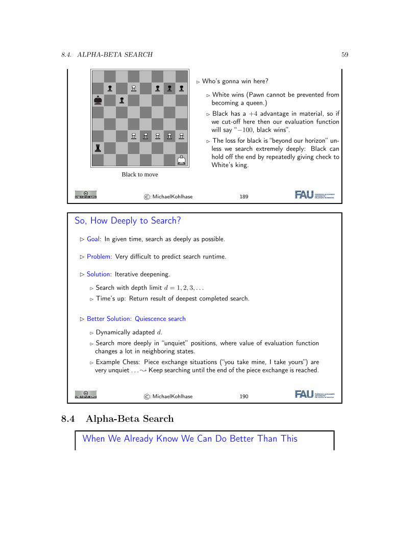
8.4. ALPHA-BETA SEARCH 59
Black to move
� Who’s gonna win here?
� White wins (Pawn cannot be prevented frombecoming a queen.)
� Black has a +4 advantage in material, so ifwe cut-off here then our evaluation functionwill say “−100, black wins”.
� The loss for black is “beyond our horizon” un-less we search extremely deeply: Black canhold off the end by repeatedly giving check toWhite’s king.
©:MichaelKohlhase 189
So, How Deeply to Search?
� Goal: In given time, search as deeply as possible.
� Problem: Very difficult to predict search runtime.
� Solution: Iterative deepening.
� Search with depth limit d = 1, 2, 3, . . .
� Time’s up: Return result of deepest completed search.
� Better Solution: Quiescence search
� Dynamically adapted d.
� Search more deeply in “unquiet” positions, where value of evaluation functionchanges a lot in neighboring states.
� Example Chess: Piece exchange situations (“you take mine, I take yours”) arevery unquiet . . .; Keep searching until the end of the piece exchange is reached.
©:MichaelKohlhase 190
8.4 Alpha-Beta Search
When We Already Know We Can Do Better Than This
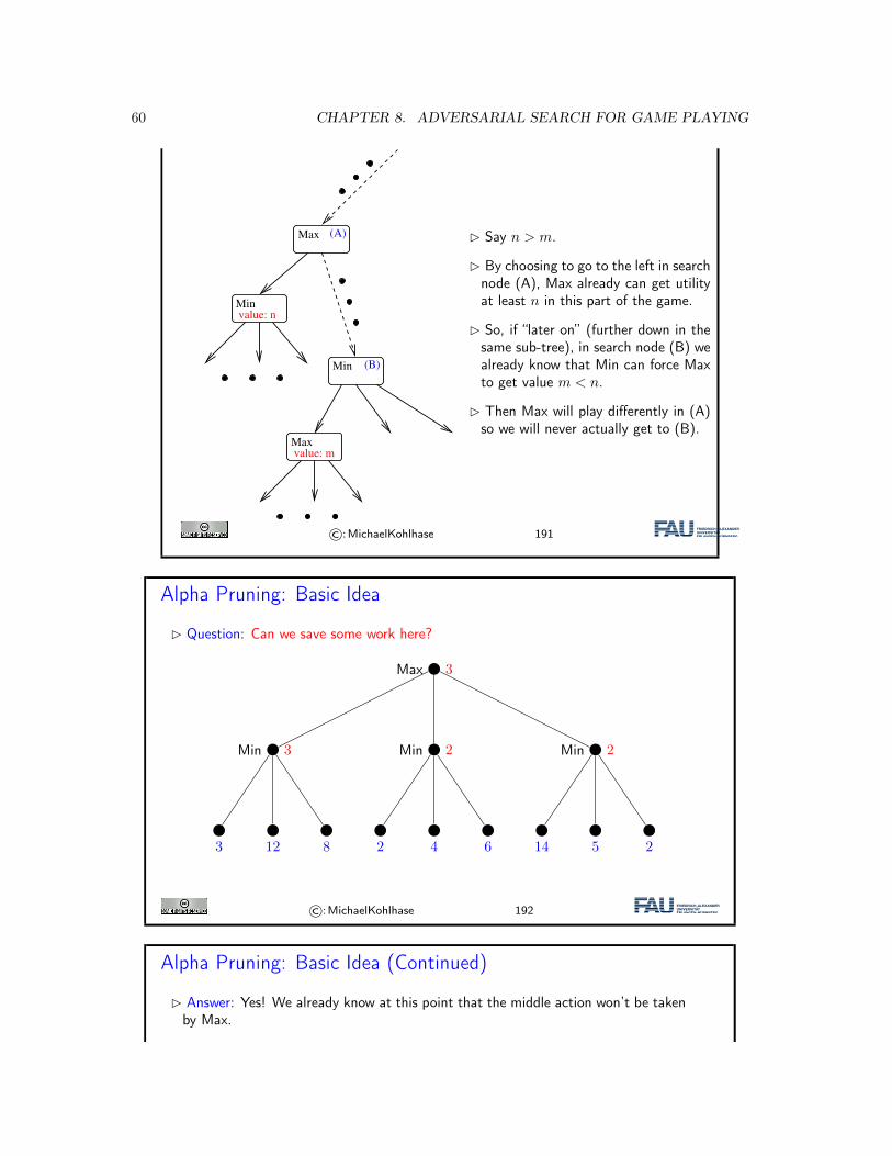
60 CHAPTER 8. ADVERSARIAL SEARCH FOR GAME PLAYING
Max (A)
Maxvalue: m
Minvalue: n
Min (B)
� Say n > m.
� By choosing to go to the left in searchnode (A), Max already can get utilityat least n in this part of the game.
� So, if “later on” (further down in thesame sub-tree), in search node (B) wealready know that Min can force Maxto get value m < n.
� Then Max will play differently in (A)so we will never actually get to (B).
©:MichaelKohlhase 191
Alpha Pruning: Basic Idea
� Question: Can we save some work here?
Max 3
Min 3
3 12 8
Min 2
2 4 6
Min 2
14 5 2
©:MichaelKohlhase 192
Alpha Pruning: Basic Idea (Continued)
� Answer: Yes! We already know at this point that the middle action won’t be takenby Max.
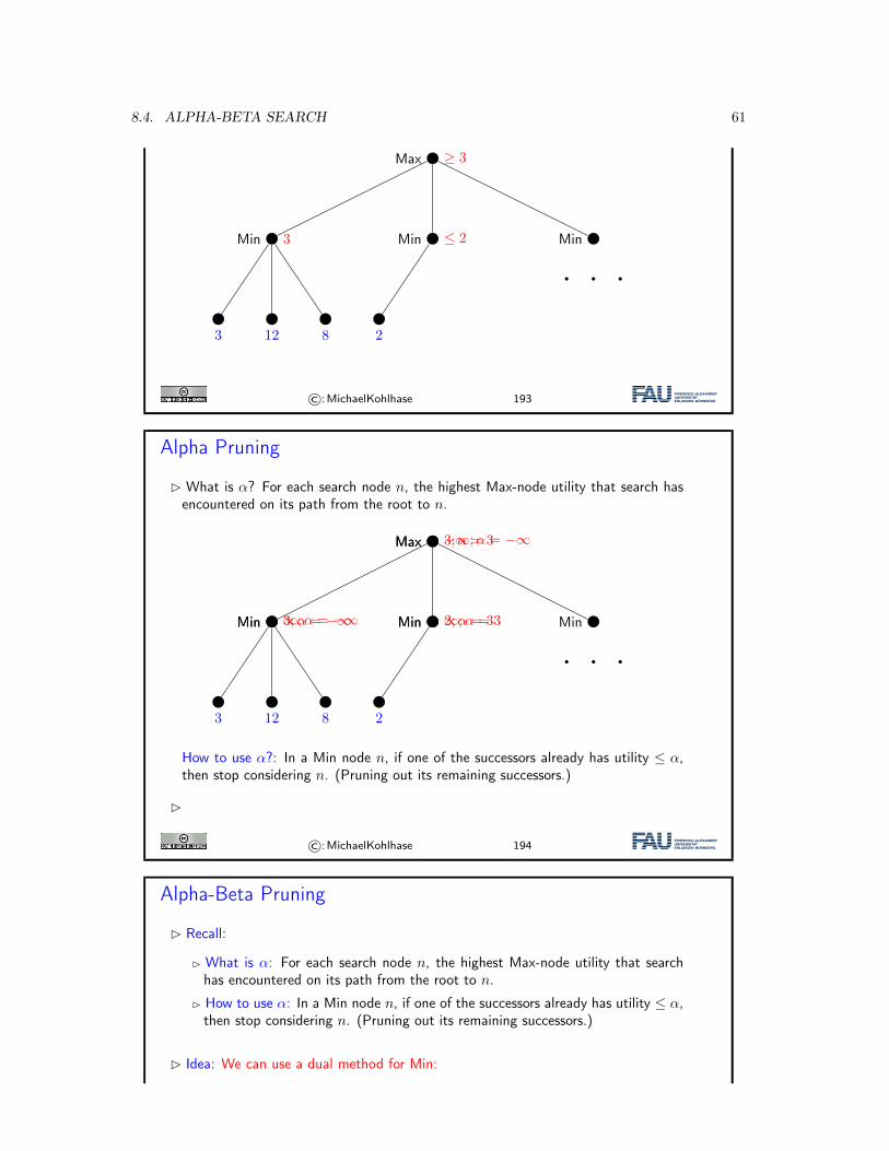
8.4. ALPHA-BETA SEARCH 61
Max ≥ 3
Min 3
3 12 8
Min ≤ 2
2
Min
©:MichaelKohlhase 193
Alpha Pruning
� What is α? For each search node n, the highest Max-node utility that search hasencountered on its path from the root to n.
Max −∞;α = −∞Max 3;α = 3
Min ∞;α = −∞Min 3;α = −∞
3 12 8
Min ∞;α = 3Min 2;α = 3
2
Min
How to use α?: In a Min node n, if one of the successors already has utility ≤ α,then stop considering n. (Pruning out its remaining successors.)
�
©:MichaelKohlhase 194
Alpha-Beta Pruning
� Recall:
� What is α: For each search node n, the highest Max-node utility that searchhas encountered on its path from the root to n.
� How to use α: In a Min node n, if one of the successors already has utility ≤ α,then stop considering n. (Pruning out its remaining successors.)
� Idea: We can use a dual method for Min:
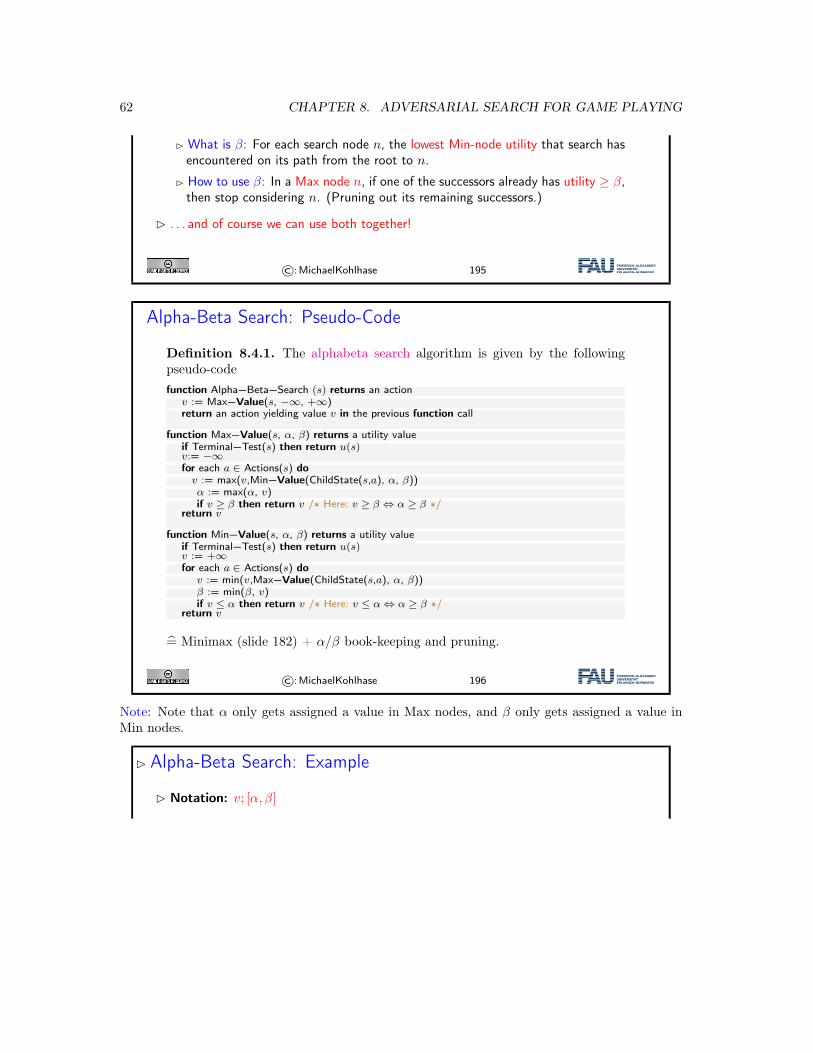
62 CHAPTER 8. ADVERSARIAL SEARCH FOR GAME PLAYING
� What is β: For each search node n, the lowest Min-node utility that search hasencountered on its path from the root to n.
� How to use β: In a Max node n, if one of the successors already has utility ≥ β,then stop considering n. (Pruning out its remaining successors.)
� . . . and of course we can use both together!
©:MichaelKohlhase 195
Alpha-Beta Search: Pseudo-Code
Definition 8.4.1. The alphabeta search algorithm is given by the followingpseudo-codefunction Alpha−Beta−Search (s) returns an action
v := Max−Value(s, −∞, +∞)return an action yielding value v in the previous function call
function Max−Value(s, α, β) returns a utility valueif Terminal−Test(s) then return u(s)v:= −∞for each a ∈ Actions(s) dov := max(v,Min−Value(ChildState(s,a), α, β))α := max(α, v)if v ≥ β then return v /∗ Here: v ≥ β ⇔ α ≥ β ∗/
return v
function Min−Value(s, α, β) returns a utility valueif Terminal−Test(s) then return u(s)v := +∞for each a ∈ Actions(s) do
v := min(v,Max−Value(ChildState(s,a), α, β))β := min(β, v)if v ≤ α then return v /∗ Here: v ≤ α ⇔ α ≥ β ∗/
return v
= Minimax (slide 182) + α/β book-keeping and pruning.
©:MichaelKohlhase 196
Note: Note that α only gets assigned a value in Max nodes, and β only gets assigned a value inMin nodes.
� Alpha-Beta Search: Example
� Notation: v; [α, β]
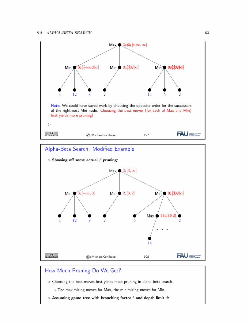
8.4. ALPHA-BETA SEARCH 63
Max −∞; [−∞,∞]Max 3; [3,∞]
Min ∞; [−∞,∞]Min 3; [−∞, 3]
3 12 8
Min ∞; [3,∞]Min 2; [3, 2]
2
Min ∞; [3,∞]Min 14; [3, 14]Min 5; [3, 5]Min 2; [3, 2]
14 5 2
Note: We could have saved work by choosing the opposite order for the successorsof the rightmost Min node. Choosing the best moves (for each of Max and Min)first yields more pruning!
�
©:MichaelKohlhase 197
Alpha-Beta Search: Modified Example
� Showing off some actual β pruning:
Max 3; [3,∞]
Min 3; [−∞, 3]
3 12 8
Min 2; [3, 2]
2
Min ∞; [3,∞]Min 5; [3, 5]Min 2; [3, 2]
5Max −∞; [3, 5]Max 14; [14, 5]
14
2
©:MichaelKohlhase 198
How Much Pruning Do We Get?
� Choosing the best moves first yields most pruning in alpha-beta search.
� The maximizing moves for Max, the minimizing moves for Min.
� Assuming game tree with branching factor b and depth limit d:
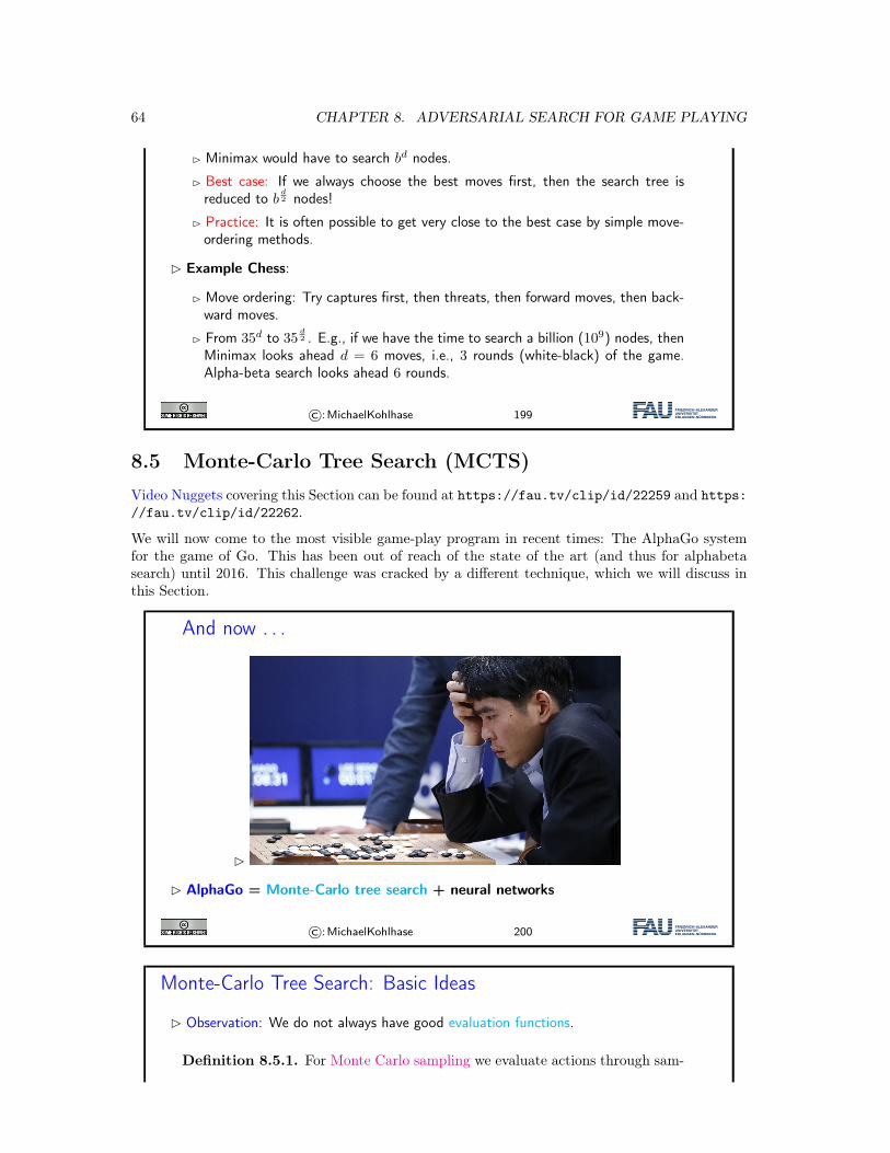
64 CHAPTER 8. ADVERSARIAL SEARCH FOR GAME PLAYING
� Minimax would have to search bd nodes.
� Best case: If we always choose the best moves first, then the search tree isreduced to b
d2 nodes!
� Practice: It is often possible to get very close to the best case by simple move-ordering methods.
� Example Chess:
� Move ordering: Try captures first, then threats, then forward moves, then back-ward moves.
� From 35d to 35d2 . E.g., if we have the time to search a billion (109) nodes, then
Minimax looks ahead d = 6 moves, i.e., 3 rounds (white-black) of the game.Alpha-beta search looks ahead 6 rounds.
©:MichaelKohlhase 199
8.5 Monte-Carlo Tree Search (MCTS)Video Nuggets covering this Section can be found at https://fau.tv/clip/id/22259 and https://fau.tv/clip/id/22262.
We will now come to the most visible game-play program in recent times: The AlphaGo systemfor the game of Go. This has been out of reach of the state of the art (and thus for alphabetasearch) until 2016. This challenge was cracked by a different technique, which we will discuss inthis Section.
And now . . .
�
� AlphaGo = Monte-Carlo tree search + neural networks
©:MichaelKohlhase 200
Monte-Carlo Tree Search: Basic Ideas
� Observation: We do not always have good evaluation functions.
Definition 8.5.1. For Monte Carlo sampling we evaluate actions through sam-
8.5. MONTE-CARLO TREE SEARCH (MCTS) 65
pling.
� When deciding which action to take on game state s:
while time not up doselect action a applicable to srun a random sample from a until terminal state t
return an a for s with maximal average u(t)
Definition 8.5.2. For the Monte-Carlo tree search algorithm (MCTS) we main-tain a search tree T , the MCTS tree.
while time not up doapply actions within T to select a leaf state s′
select action a′ applicable to s′, run random sample from a′
add s′ to T , update averages etc.return an a for s with maximal average u(t)When executing a, keep the part of T below a.
�� Compared to alphabeta search: no exhaustive enumeration.
� Pro: runtime & memory.
� Contra: need good guidance how to “select” and “sample”.
©:MichaelKohlhase 201
This looks only at a fraction of the search tree, so it is crucial to have good guidance where to go,i.e. which part of the search tree to look at.
Monte-Carlo Sampling: Illustration of Sampling
� Idea: Sample the search tree keeping track of the average utilities.
Example 8.5.3 (Single-player, for simplicity). (with adversary, distinguishmax/min nodes)
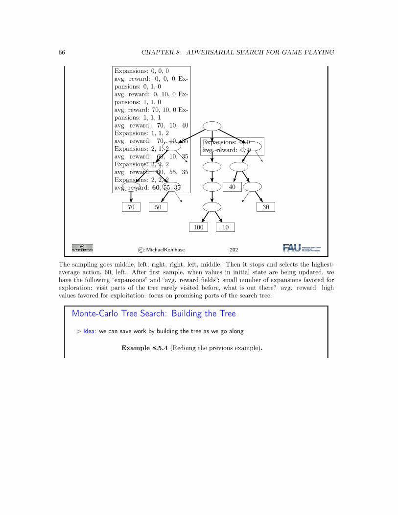
66 CHAPTER 8. ADVERSARIAL SEARCH FOR GAME PLAYING
40
70 50 30
100 10
Expansions: 0, 0, 0avg. reward: 0, 0, 0 Ex-pansions: 0, 1, 0avg. reward: 0, 10, 0 Ex-pansions: 1, 1, 0avg. reward: 70, 10, 0 Ex-pansions: 1, 1, 1avg. reward: 70, 10, 40Expansions: 1, 1, 2avg. reward: 70, 10, 35Expansions: 2, 1, 2avg. reward: 60, 10, 35Expansions: 2, 2, 2avg. reward: 60, 55, 35Expansions: 2, 2, 2avg. reward: 60, 55, 35
Expansions: 0, 0avg. reward: 0, 0
©:MichaelKohlhase 202
The sampling goes middle, left, right, right, left, middle. Then it stops and selects the highest-average action, 60, left. After first sample, when values in initial state are being updated, wehave the following “expansions” and “avg. reward fields”: small number of expansions favored forexploration: visit parts of the tree rarely visited before, what is out there? avg. reward: highvalues favored for exploitation: focus on promising parts of the search tree.
Monte-Carlo Tree Search: Building the Tree
� Idea: we can save work by building the tree as we go along
Example 8.5.4 (Redoing the previous example).
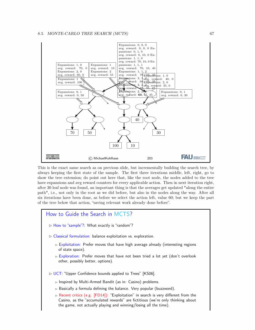
8.5. MONTE-CARLO TREE SEARCH (MCTS) 67
40
70 50 30
100 10
Expansions: 0, 0, 0avg. reward: 0, 0, 0 Ex-pansions: 0, 1, 0avg. reward: 0, 10, 0 Ex-pansions: 1, 1, 0avg. reward: 70, 10, 0 Ex-pansions: 1, 1, 1avg. reward: 70, 10, 40Expansions: 1, 1, 2avg. reward: 70, 10, 35Expansions: 2, 1, 2avg. reward: 60, 10, 35Expansions: 2, 2, 2avg. reward: 60, 55, 35Expansions: 2, 2, 2avg. reward: 60, 55, 35
Expansions: 1, 0avg. reward: 70, 0Expansions: 2, 0avg. reward: 60, 0
Expansions: 1avg. reward: 10Expansions: 2avg. reward: 55 Expansions: 1, 0
avg. reward: 40, 0Expansions: 2, 0avg. reward: 35, 0
Expansions: 0, 1avg. reward: 0, 50
Expansions: 1avg. reward: 100
Expansions: 0, 1avg. reward: 0, 30
©:MichaelKohlhase 203
This is the exact same search as on previous slide, but incrementally building the search tree, byalways keeping the first state of the sample. The first three iterations middle, left, right, go toshow the tree extension; do point out here that, like the root node, the nodes added to the treehave expansions and avg reward counters for every applicable action. Then in next iteration right,after 30 leaf node was found, an important thing is that the averages get updated *along the entirepath*, i.e., not only in the root as we did before, but also in the nodes along the way. After allsix iterations have been done, as before we select the action left, value 60; but we keep the partof the tree below that action, “saving relevant work already done before”.
How to Guide the Search in MCTS?
� How to “sample”?: What exactly is “random”?
� Classical formulation: balance exploitation vs. exploration.
� Exploitation: Prefer moves that have high average already (interesting regionsof state space).
� Exploration: Prefer moves that have not been tried a lot yet (don’t overlookother, possibly better, options).
� UCT: “Upper Confidence bounds applied to Trees” [KS06].
� Inspired by Multi-Armed Bandit (as in: Casino) problems.
� Basically a formula defining the balance. Very popular (buzzword).
� Recent critics (e.g. [FD14]): “Exploitation” in search is very different from theCasino, as the “accumulated rewards” are fictitious (we’re only thinking aboutthe game, not actually playing and winning/losing all the time).
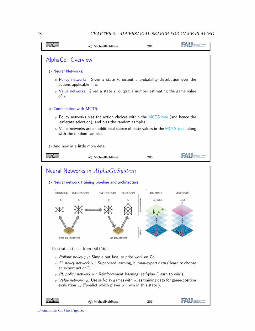
68 CHAPTER 8. ADVERSARIAL SEARCH FOR GAME PLAYING
©:MichaelKohlhase 204
AlphaGo: Overview
� Neural Networks:
� Policy networks: Given a state s, output a probability distribution over theactions applicable in s.
� Value networks: Given a state s, output a number estimating the game valueof s.
� Combination with MCTS:
� Policy networks bias the action choices within the MCTS tree (and hence theleaf-state selection), and bias the random samples.
� Value networks are an additional source of state values in the MCTS tree, alongwith the random samples.
� And now in a little more detail
©:MichaelKohlhase 205
Neural Networks in AlphaGoSystem
� Neural network training pipeline and architecture:
2 8 J A N U A R Y 2 0 1 6 | V O L 5 2 9 | N A T U R E | 4 8 5
ARTICLE RESEARCH
sampled state-action pairs (s, a), using stochastic gradient ascent to maximize the likelihood of the human move a selected in state s
∆σσ
∝∂ ( | )
∂σp a slog
We trained a 13-layer policy network, which we call the SL policy network, from 30 million positions from the KGS Go Server. The net-work predicted expert moves on a held out test set with an accuracy of 57.0% using all input features, and 55.7% using only raw board posi-tion and move history as inputs, compared to the state-of-the-art from other research groups of 44.4% at date of submission24 (full results in Extended Data Table 3). Small improvements in accuracy led to large improvements in playing strength (Fig. 2a); larger networks achieve better accuracy but are slower to evaluate during search. We also trained a faster but less accurate rollout policy pπ(a|s), using a linear softmax of small pattern features (see Extended Data Table 4) with weights π; this achieved an accuracy of 24.2%, using just 2 μs to select an action, rather than 3 ms for the policy network.
Reinforcement learning of policy networksThe second stage of the training pipeline aims at improving the policy network by policy gradient reinforcement learning (RL)25,26. The RL policy network pρ is identical in structure to the SL policy network,
and its weights ρ are initialized to the same values, ρ = σ. We play games between the current policy network pρ and a randomly selected previous iteration of the policy network. Randomizing from a pool of opponents in this way stabilizes training by preventing overfitting to the current policy. We use a reward function r(s) that is zero for all non-terminal time steps t < T. The outcome zt = ± r(sT) is the termi-nal reward at the end of the game from the perspective of the current player at time step t: +1 for winning and −1 for losing. Weights are then updated at each time step t by stochastic gradient ascent in the direction that maximizes expected outcome25
∆ρρ
∝∂ ( | )
∂ρp a s
zlog t t
t
We evaluated the performance of the RL policy network in game play, sampling each move ~ (⋅| )ρa p st t from its output probability distribution over actions. When played head-to-head, the RL policy network won more than 80% of games against the SL policy network. We also tested against the strongest open-source Go program, Pachi14, a sophisticated Monte Carlo search program, ranked at 2 amateur dan on KGS, that executes 100,000 simulations per move. Using no search at all, the RL policy network won 85% of games against Pachi. In com-parison, the previous state-of-the-art, based only on supervised
Figure 1 | Neural network training pipeline and architecture. a, A fast rollout policy pπ and supervised learning (SL) policy network pσ are trained to predict human expert moves in a data set of positions. A reinforcement learning (RL) policy network pρ is initialized to the SL policy network, and is then improved by policy gradient learning to maximize the outcome (that is, winning more games) against previous versions of the policy network. A new data set is generated by playing games of self-play with the RL policy network. Finally, a value network vθ is trained by regression to predict the expected outcome (that is, whether
the current player wins) in positions from the self-play data set. b, Schematic representation of the neural network architecture used in AlphaGo. The policy network takes a representation of the board position s as its input, passes it through many convolutional layers with parameters σ (SL policy network) or ρ (RL policy network), and outputs a probability distribution ( | )σp a s or ( | )ρp a s over legal moves a, represented by a probability map over the board. The value network similarly uses many convolutional layers with parameters θ, but outputs a scalar value vθ(s′) that predicts the expected outcome in position s′.
Reg
ress
ion
Cla
ssi�
catio
nClassi�cation
Self Play
Policy gradient
a b
Human expert positions Self-play positions
Neural netw
orkD
ata
Rollout policy
p p p (a⎪s) (s′)p
SL policy network RL policy network Value network Policy network Value network
s s′
Figure 2 | Strength and accuracy of policy and value networks. a, Plot showing the playing strength of policy networks as a function of their training accuracy. Policy networks with 128, 192, 256 and 384 convolutional filters per layer were evaluated periodically during training; the plot shows the winning rate of AlphaGo using that policy network against the match version of AlphaGo. b, Comparison of evaluation accuracy between the value network and rollouts with different policies.
Positions and outcomes were sampled from human expert games. Each position was evaluated by a single forward pass of the value network vθ, or by the mean outcome of 100 rollouts, played out using either uniform random rollouts, the fast rollout policy pπ, the SL policy network pσ or the RL policy network pρ. The mean squared error between the predicted value and the actual game outcome is plotted against the stage of the game (how many moves had been played in the given position).
15 45 75 105 135 165 195 225 255 >285Move number
0.10
0.15
0.20
0.25
0.30
0.35
0.40
0.45
0.50
Mea
n sq
uare
d e
rror
on e
xper
t ga
mes
Uniform random rollout policyFast rollout policyValue networkSL policy networkRL policy network
50 51 52 53 54 55 56 57 58 59
Training accuracy on KGS dataset (%)
0
10
20
30
40
50
60
70128 �lters192 �lters256 �lters384 �lters
Alp
haG
o w
in r
ate
(%)
a b
© 2016 Macmillan Publishers Limited. All rights reserved
Illustration taken from [Sil+16] .
� Rollout policy pπ: Simple but fast, ≈ prior work on Go.� SL policy network pσ: Supervised learning, human-expert data (“learn to choose
an expert action”).� RL policy network pρ: Reinforcement learning, self-play (“learn to win”).� Value network vθ: Use self-play games with pρ as training data for game-position
evaluation vθ (“predict which player will win in this state”).
©:MichaelKohlhase 206
Comments on the Figure:
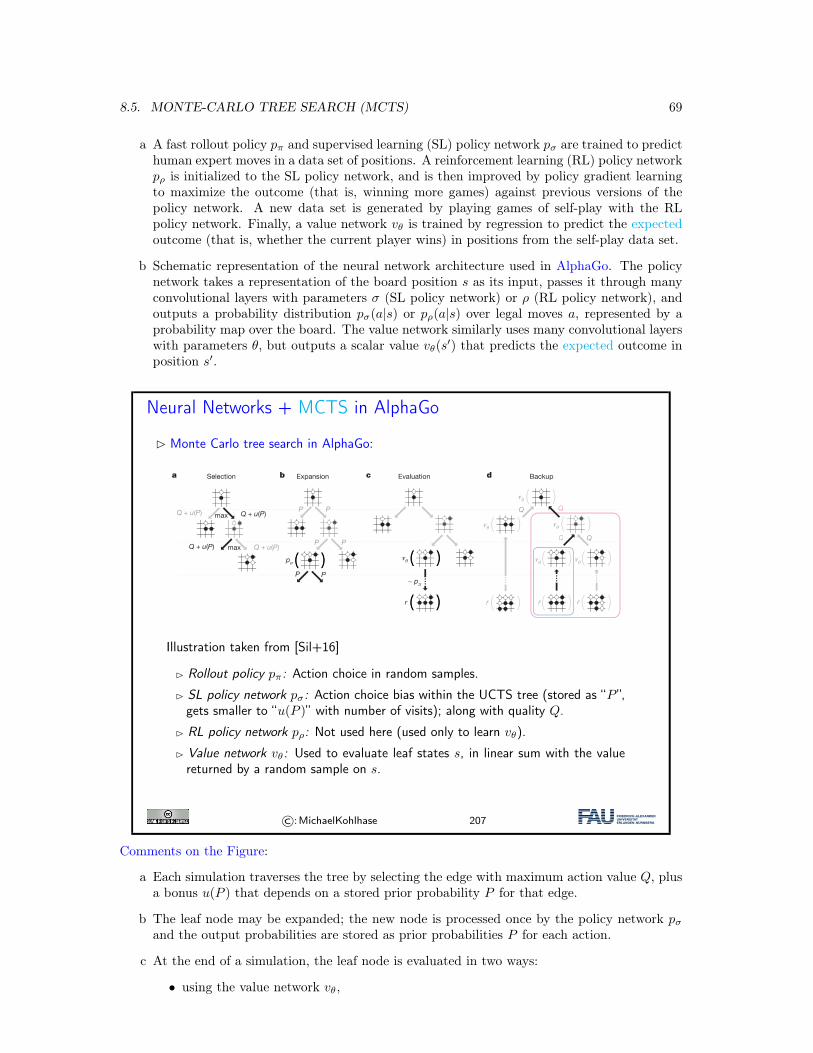
8.5. MONTE-CARLO TREE SEARCH (MCTS) 69
a A fast rollout policy pπ and supervised learning (SL) policy network pσ are trained to predicthuman expert moves in a data set of positions. A reinforcement learning (RL) policy networkpρ is initialized to the SL policy network, and is then improved by policy gradient learningto maximize the outcome (that is, winning more games) against previous versions of thepolicy network. A new data set is generated by playing games of self-play with the RLpolicy network. Finally, a value network vθ is trained by regression to predict the expectedoutcome (that is, whether the current player wins) in positions from the self-play data set.
b Schematic representation of the neural network architecture used in AlphaGo. The policynetwork takes a representation of the board position s as its input, passes it through manyconvolutional layers with parameters σ (SL policy network) or ρ (RL policy network), andoutputs a probability distribution pσ(a|s) or pρ(a|s) over legal moves a, represented by aprobability map over the board. The value network similarly uses many convolutional layerswith parameters θ, but outputs a scalar value vθ(s
′) that predicts the expected outcome inposition s′.
Neural Networks + MCTS in AlphaGo
� Monte Carlo tree search in AlphaGo:
4 8 6 | N A T U R E | V O L 5 2 9 | 2 8 J A N U A R Y 2 0 1 6
ARTICLERESEARCH
learning of convolutional networks, won 11% of games against Pachi23 and 12% against a slightly weaker program, Fuego24.
Reinforcement learning of value networksThe final stage of the training pipeline focuses on position evaluation, estimating a value function vp(s) that predicts the outcome from posi-tion s of games played by using policy p for both players28–30
E( )= | = ~…v s z s s a p[ , ]pt t t T
Ideally, we would like to know the optimal value function under perfect play v*(s); in practice, we instead estimate the value function
ρv p for our strongest policy, using the RL policy network pρ. We approx-imate the value function using a value network vθ(s) with weights θ,
⁎( )≈ ( )≈ ( )θ ρv s v s v sp . This neural network has a similar architecture to the policy network, but outputs a single prediction instead of a prob-ability distribution. We train the weights of the value network by regres-sion on state-outcome pairs (s, z), using stochastic gradient descent to minimize the mean squared error (MSE) between the predicted value vθ(s), and the corresponding outcome z
∆θθ
∝∂ ( )∂( − ( ))θ
θv s
z v s
The naive approach of predicting game outcomes from data con-sisting of complete games leads to overfitting. The problem is that successive positions are strongly correlated, differing by just one stone, but the regression target is shared for the entire game. When trained on the KGS data set in this way, the value network memorized the game outcomes rather than generalizing to new positions, achieving a minimum MSE of 0.37 on the test set, compared to 0.19 on the training set. To mitigate this problem, we generated a new self-play data set consisting of 30 million distinct positions, each sampled from a sepa-rate game. Each game was played between the RL policy network and itself until the game terminated. Training on this data set led to MSEs of 0.226 and 0.234 on the training and test set respectively, indicating minimal overfitting. Figure 2b shows the position evaluation accuracy of the value network, compared to Monte Carlo rollouts using the fast rollout policy pπ; the value function was consistently more accurate. A single evaluation of vθ(s) also approached the accuracy of Monte Carlo rollouts using the RL policy network pρ, but using 15,000 times less computation.
Searching with policy and value networksAlphaGo combines the policy and value networks in an MCTS algo-rithm (Fig. 3) that selects actions by lookahead search. Each edge
(s, a) of the search tree stores an action value Q(s, a), visit count N(s, a), and prior probability P(s, a). The tree is traversed by simulation (that is, descending the tree in complete games without backup), starting from the root state. At each time step t of each simulation, an action at is selected from state st
= ( ( )+ ( ))a Q s a u s aargmax , ,ta
t t
so as to maximize action value plus a bonus
( )∝( )+ ( )
u s aP s a
N s a,
,1 ,
that is proportional to the prior probability but decays with repeated visits to encourage exploration. When the traversal reaches a leaf node sL at step L, the leaf node may be expanded. The leaf position sL is processed just once by the SL policy network pσ. The output prob-abilities are stored as prior probabilities P for each legal action a, ( )= ( | )σP s a p a s, . The leaf node is evaluated in two very different ways:
first, by the value network vθ(sL); and second, by the outcome zL of a random rollout played out until terminal step T using the fast rollout policy pπ; these evaluations are combined, using a mixing parameter λ, into a leaf evaluation V(sL)
λ λ( )= ( − ) ( )+θV s v s z1L L L
At the end of simulation, the action values and visit counts of all traversed edges are updated. Each edge accumulates the visit count and mean evaluation of all simulations passing through that edge
∑
∑
( )= ( )
( )=( )
( ) ( )
=
=
N s a s a i
Q s aN s a
s a i V s
, 1 , ,
, 1,
1 , ,
i
n
i
n
Li
1
1
where sLi is the leaf node from the ith simulation, and 1(s, a, i) indicates
whether an edge (s, a) was traversed during the ith simulation. Once the search is complete, the algorithm chooses the most visited move from the root position.
It is worth noting that the SL policy network pσ performed better in AlphaGo than the stronger RL policy network pρ, presumably because humans select a diverse beam of promising moves, whereas RL opti-mizes for the single best move. However, the value function ( )≈ ( )θ ρv s v sp derived from the stronger RL policy network performed
Figure 3 | Monte Carlo tree search in AlphaGo. a, Each simulation traverses the tree by selecting the edge with maximum action value Q, plus a bonus u(P) that depends on a stored prior probability P for that edge. b, The leaf node may be expanded; the new node is processed once by the policy network pσ and the output probabilities are stored as prior probabilities P for each action. c, At the end of a simulation, the leaf node
is evaluated in two ways: using the value network vθ; and by running a rollout to the end of the game with the fast rollout policy pπ, then computing the winner with function r. d, Action values Q are updated to track the mean value of all evaluations r(·) and vθ(·) in the subtree below that action.
Selectiona b c dExpansion Evaluation Backup
p
p
Q + u(P)
Q + u(P)Q + u(P)
Q + u(P)
P P
P P
Q
Q
Q
rr r r
P
max
max
P
© 2016 Macmillan Publishers Limited. All rights reserved
Illustration taken from [Sil+16]
� Rollout policy pπ: Action choice in random samples.
� SL policy network pσ: Action choice bias within the UCTS tree (stored as “P ”,gets smaller to “u(P )” with number of visits); along with quality Q.
� RL policy network pρ: Not used here (used only to learn vθ).
� Value network vθ: Used to evaluate leaf states s, in linear sum with the valuereturned by a random sample on s.
©:MichaelKohlhase 207
Comments on the Figure:
a Each simulation traverses the tree by selecting the edge with maximum action value Q, plusa bonus u(P ) that depends on a stored prior probability P for that edge.
b The leaf node may be expanded; the new node is processed once by the policy network pσand the output probabilities are stored as prior probabilities P for each action.
c At the end of a simulation, the leaf node is evaluated in two ways:
• using the value network vθ,
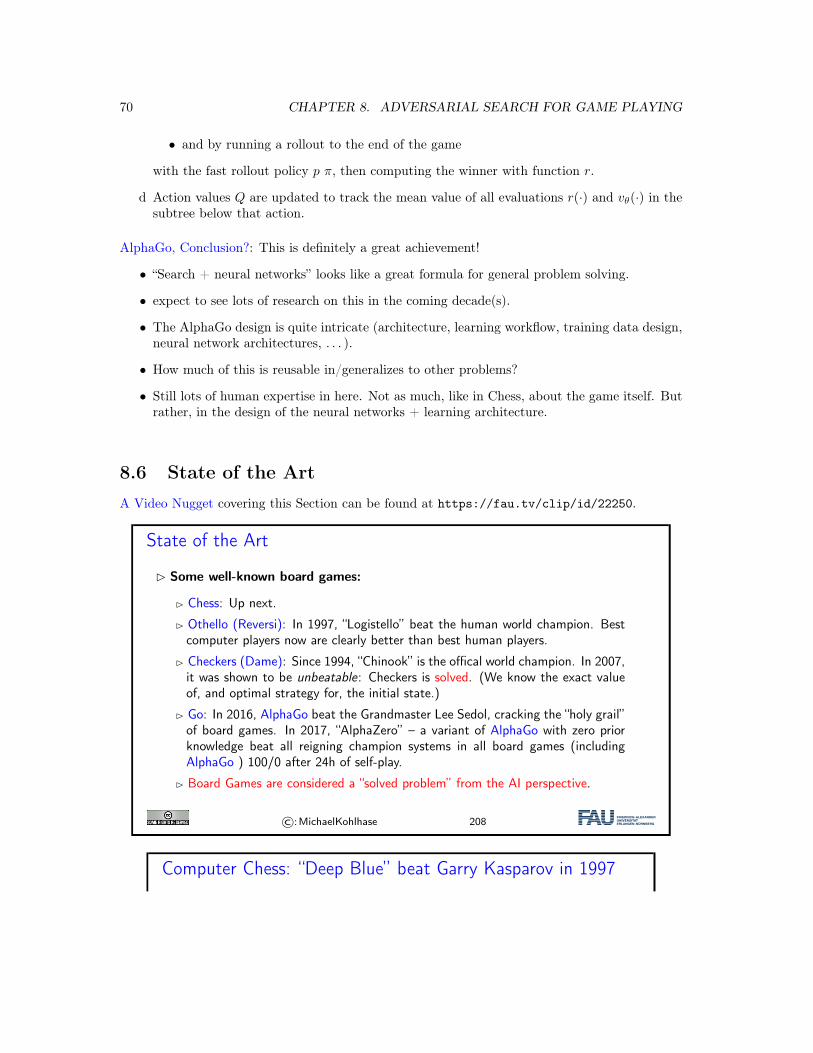
70 CHAPTER 8. ADVERSARIAL SEARCH FOR GAME PLAYING
• and by running a rollout to the end of the game
with the fast rollout policy p π, then computing the winner with function r.
d Action values Q are updated to track the mean value of all evaluations r(·) and vθ(·) in thesubtree below that action.
AlphaGo, Conclusion?: This is definitely a great achievement!
• “Search + neural networks” looks like a great formula for general problem solving.
• expect to see lots of research on this in the coming decade(s).
• The AlphaGo design is quite intricate (architecture, learning workflow, training data design,neural network architectures, . . . ).
• How much of this is reusable in/generalizes to other problems?
• Still lots of human expertise in here. Not as much, like in Chess, about the game itself. Butrather, in the design of the neural networks + learning architecture.
8.6 State of the ArtA Video Nugget covering this Section can be found at https://fau.tv/clip/id/22250.
State of the Art
� Some well-known board games:
� Chess: Up next.
� Othello (Reversi): In 1997, “Logistello” beat the human world champion. Bestcomputer players now are clearly better than best human players.
� Checkers (Dame): Since 1994, “Chinook” is the offical world champion. In 2007,it was shown to be unbeatable: Checkers is solved. (We know the exact valueof, and optimal strategy for, the initial state.)
� Go: In 2016, AlphaGo beat the Grandmaster Lee Sedol, cracking the “holy grail”of board games. In 2017, “AlphaZero” – a variant of AlphaGo with zero priorknowledge beat all reigning champion systems in all board games (includingAlphaGo ) 100/0 after 24h of self-play.
� Board Games are considered a “solved problem” from the AI perspective.
©:MichaelKohlhase 208
Computer Chess: “Deep Blue” beat Garry Kasparov in 1997
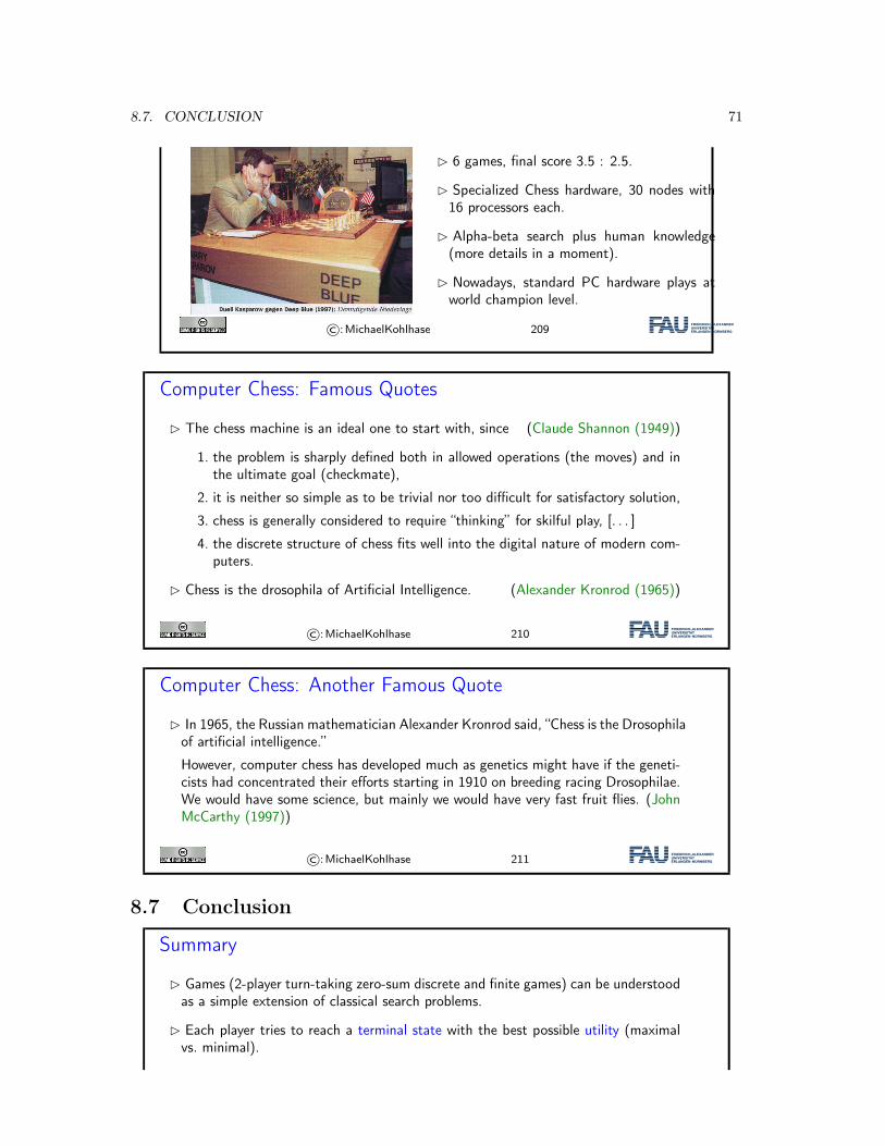
8.7. CONCLUSION 71
� 6 games, final score 3.5 : 2.5.
� Specialized Chess hardware, 30 nodes with16 processors each.
� Alpha-beta search plus human knowledge(more details in a moment).
� Nowadays, standard PC hardware plays atworld champion level.
©:MichaelKohlhase 209
Computer Chess: Famous Quotes
� The chess machine is an ideal one to start with, since (Claude Shannon (1949))
1. the problem is sharply defined both in allowed operations (the moves) and inthe ultimate goal (checkmate),
2. it is neither so simple as to be trivial nor too difficult for satisfactory solution,
3. chess is generally considered to require “thinking” for skilful play, [. . . ]
4. the discrete structure of chess fits well into the digital nature of modern com-puters.
� Chess is the drosophila of Artificial Intelligence. (Alexander Kronrod (1965))
©:MichaelKohlhase 210
Computer Chess: Another Famous Quote
� In 1965, the Russian mathematician Alexander Kronrod said, “Chess is the Drosophilaof artificial intelligence.”
However, computer chess has developed much as genetics might have if the geneti-cists had concentrated their efforts starting in 1910 on breeding racing Drosophilae.We would have some science, but mainly we would have very fast fruit flies. (JohnMcCarthy (1997))
©:MichaelKohlhase 211
8.7 Conclusion
Summary
� Games (2-player turn-taking zero-sum discrete and finite games) can be understoodas a simple extension of classical search problems.
� Each player tries to reach a terminal state with the best possible utility (maximalvs. minimal).
72 CHAPTER 8. ADVERSARIAL SEARCH FOR GAME PLAYING
� Minimax searches the game depth-first, max’ing and min’ing at the respective turnsof each player. It yields perfect play, but takes time O(bd) where b is the branchingfactor and d the search depth.
� Except in trivial games (Tic-Tac-Toe), Minimax needs a depth limit and apply anevaluation function to estimate the value of the cut-off states.
� Alpha-beta search remembers the best values achieved for each player elsewhere inthe tree already, and prunes out sub-trees that won’t be reached in the game.
� Monte-Carlo tree search (MCTS) samples game branches, and averages the find-ings. AlphaGo controls this using neural networks: evaluation function (“valuenetwork”), and action filter (“policy network”).
©:MichaelKohlhase 212
Suggested Reading:
• Chapter 5: Adversarial Search, Sections 5.1 – 5.4 [RN09].
– Section 5.1 corresponds to my “Introduction”, Section 5.2 corresponds to my “MinimaxSearch”, Section 5.3 corresponds to my “Alpha-Beta Search”. I have tried to add someadditional clarifying illustrations. RN gives many complementary explanations, nice asadditional background reading.
– Section 5.4 corresponds to my “Evaluation Functions”, but discusses additional aspectsrelating to narrowing the search and look-up from opening/termination databases. Niceas additional background reading.
– I suppose a discussion of MCTS and AlphaGo will be added to the next edition . . .
Chapter 9
Constraint Satisfaction Problems
In the last chapters we have studied methods for “general problem”, i.e. such that are applicableto all problems that are expressible in terms of states and “actions”. It is crucial to realize thatthese states were atomic, which makes the algorithms employed (search algorithms) relativelysimple and generic, but does not let them exploit the any knowledge we might have about theinternal structure of states.
In this Chapter, we will look into algorithms that do just that by progressing to factored statesrepresentations. We will see that this allows for algorithms that are many orders of magnitudemore efficient than search algorithms.
To give an intuition for factored states representations we, we present some motivational exam-ples in and go into detail of the Waltz algorithm, which gave rise to the main ideas of constraintsatisfaction algorithms in . define constraint satisfaction problems formally and use that todevelop a class of backtracking/search based algorithms. The main contribution of the factoredstates representations is that we can formulate advanced search heuristics that guide search basedon the structure of the states.
9.1 Constraint Satisfaction Problems: MotivationA Video Nugget covering this Section can be found at https://fau.tv/clip/id/22251.
A (Constraint Satisfaction) Problem
Example 9.1.1 (Tournament Schedule). Who’s going to play against who,when and where?
73
74 CHAPTER 9. CONSTRAINT SATISFACTION PROBLEMS
©:MichaelKohlhase 213
Constraint satisfaction problems (CSPs)
� Standard search problem: state is a “black box”—any old data structure that sup-ports goal test, eval, successor
Definition 9.1.2. A constraint satisfaction problem (CSP) is a search problem,where the states are given by a finite set V :={X1, . . . ,Xn} of variables anddomains {Dv|v∈V } and the goal test is a set of constraints specifying allowablecombinations of values for subsets of variables.
Definition 9.1.3. A CSP is satisfiable, iff it has a solution – a function fromvariables v to elements of their domains Dv that satisfy all constraints.
Remark 9.1.4. We are using factored representation for world states now.
���� Simple example of a formal representation language
� Allows useful general-purpose algorithms with more power than standard tree searchalgorithm.
©:MichaelKohlhase 214
Another Constraint Satisfaction Problem
Example 9.1.5 (SuDoKu). Fill the cells with row/column/block-unique digits
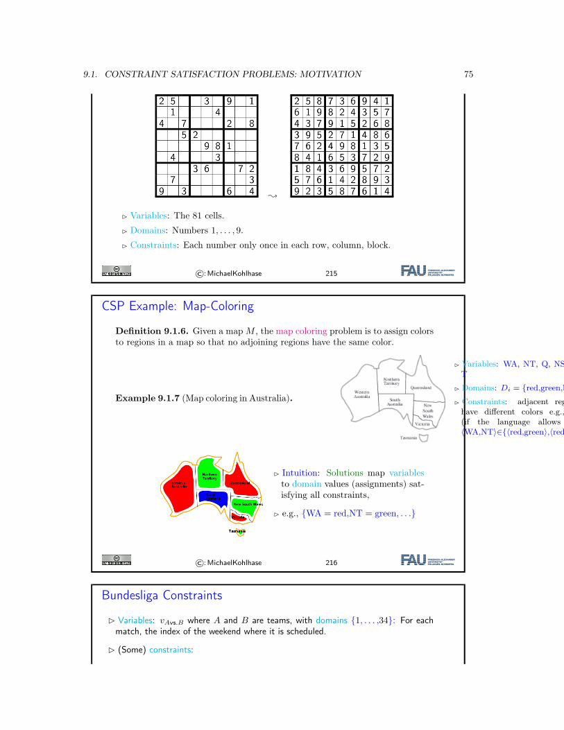
9.1. CONSTRAINT SATISFACTION PROBLEMS: MOTIVATION 75
;
� Variables: The 81 cells.
� Domains: Numbers 1, . . . , 9.
� Constraints: Each number only once in each row, column, block.
©:MichaelKohlhase 215
CSP Example: Map-Coloring
Definition 9.1.6. Given a map M , the map coloring problem is to assign colorsto regions in a map so that no adjoining regions have the same color.
Example 9.1.7 (Map coloring in Australia).
� Variables: WA, NT, Q, NSW, V, SA,T
� Domains: Di = {red,green,blue}� Constraints: adjacent regions must
have different colors e.g., WA=NT(if the language allows this), or⟨WA,NT⟩∈{⟨red,green⟩,⟨red,blue⟩,⟨green,red⟩, . . . }
� Intuition: Solutions map variablesto domain values (assignments) sat-isfying all constraints,
� e.g., {WA = red,NT = green, . . .}
©:MichaelKohlhase 216
Bundesliga Constraints
� Variables: vAvs.B where A and B are teams, with domains {1, . . . ,34}: For eachmatch, the index of the weekend where it is scheduled.
� (Some) constraints:
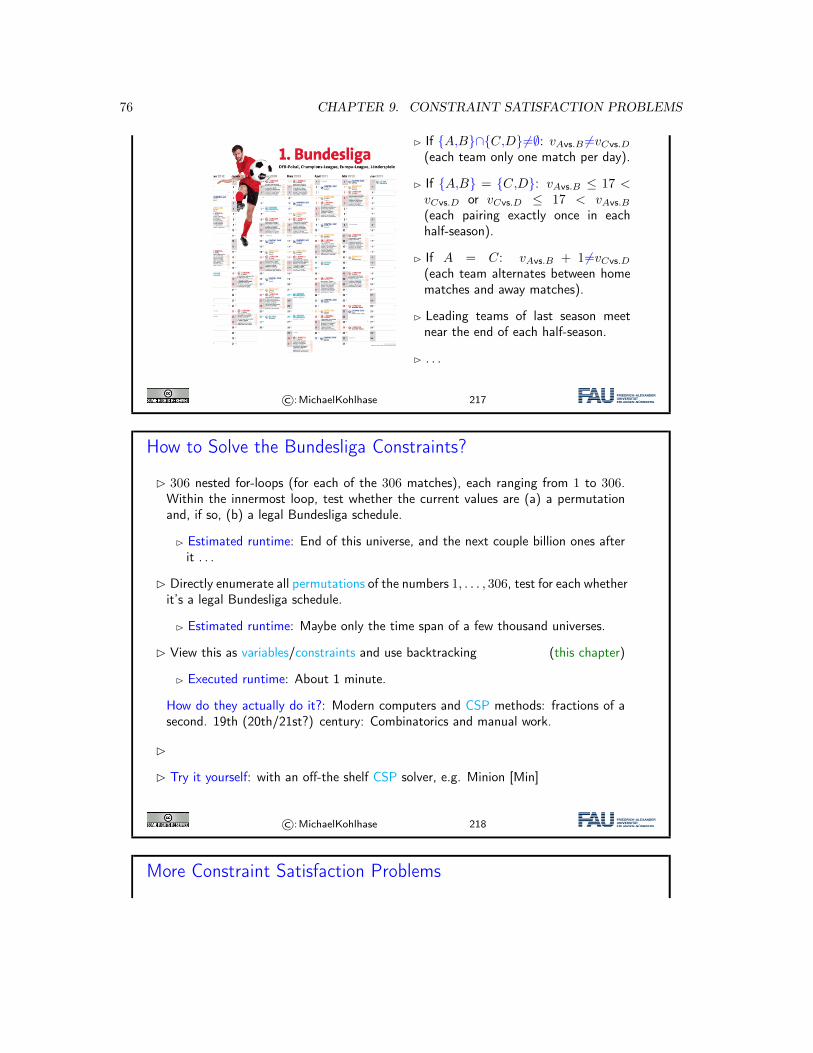
76 CHAPTER 9. CONSTRAINT SATISFACTION PROBLEMS
� If {A,B}∩{C,D}=∅: vAvs.B =vCvs.D(each team only one match per day).
� If {A,B} = {C,D}: vAvs.B ≤ 17 <vCvs.D or vCvs.D ≤ 17 < vAvs.B(each pairing exactly once in eachhalf-season).
� If A = C: vAvs.B + 1 =vCvs.D(each team alternates between homematches and away matches).
� Leading teams of last season meetnear the end of each half-season.
� . . .
©:MichaelKohlhase 217
How to Solve the Bundesliga Constraints?
� 306 nested for-loops (for each of the 306 matches), each ranging from 1 to 306.Within the innermost loop, test whether the current values are (a) a permutationand, if so, (b) a legal Bundesliga schedule.
� Estimated runtime: End of this universe, and the next couple billion ones afterit . . .
� Directly enumerate all permutations of the numbers 1, . . . , 306, test for each whetherit’s a legal Bundesliga schedule.
� Estimated runtime: Maybe only the time span of a few thousand universes.
� View this as variables/constraints and use backtracking (this chapter)
� Executed runtime: About 1 minute.
How do they actually do it?: Modern computers and CSP methods: fractions of asecond. 19th (20th/21st?) century: Combinatorics and manual work.
�
� Try it yourself: with an off-the shelf CSP solver, e.g. Minion [Min]
©:MichaelKohlhase 218
More Constraint Satisfaction Problems
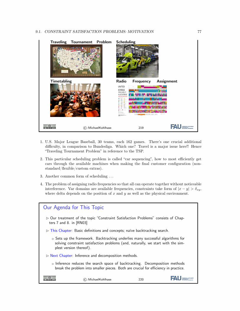
9.1. CONSTRAINT SATISFACTION PROBLEMS: MOTIVATION 77
Traveling Tournament Problem Scheduling
Timetabling Radio Frequency Assignment
©:MichaelKohlhase 219
1. U.S. Major League Baseball, 30 teams, each 162 games. There’s one crucial additionaldifficulty, in comparison to Bundesliga. Which one? Travel is a major issue here!! Hence“Traveling Tournament Problem” in reference to the TSP.
2. This particular scheduling problem is called “car sequencing”, how to most efficiently getcars through the available machines when making the final customer configuration (non-standard/flexible/custom extras).
3. Another common form of scheduling . . .
4. The problem of assigning radio frequencies so that all can operate together without noticeableinterference. Var domains are available frequencies, constraints take form of |x − y| > δxy,where delta depends on the position of x and y as well as the physical environment.
Our Agenda for This Topic
� Our treatment of the topic “Constraint Satisfaction Problems” consists of Chap-ters 7 and 8. in [RN03]
� This Chapter: Basic definitions and concepts; naïve backtracking search.
� Sets up the framework. Backtracking underlies many successful algorithms forsolving constraint satisfaction problems (and, naturally, we start with the sim-plest version thereof).
� Next Chapter: Inference and decomposition methods.
� Inference reduces the search space of backtracking. Decomposition methodsbreak the problem into smaller pieces. Both are crucial for efficiency in practice.
©:MichaelKohlhase 220
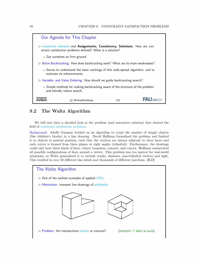
78 CHAPTER 9. CONSTRAINT SATISFACTION PROBLEMS
Our Agenda for This Chapter
� Constraint networks and Assignments, Consistency, Solutions: How are con-straint satisfaction problems defined? What is a solution?
� Get ourselves on firm ground.
� Naïve Backtracking: How does backtracking work? What are its main weaknesses?
� Serves to understand the basic workings of this wide-spread algorithm, and tomotivate its enhancements.
� Variable- and Value Ordering: How should we guide backtracking search?
� Simple methods for making backtracking aware of the structure of the problem,and thereby reduce search.
©:MichaelKohlhase 221
9.2 The Waltz Algorithm
We will now have a detailed look at the problem (and innovative solution) that started thefield of constraint satisfaction problems.
Background: Adolfo Guzman worked on an algorithm to count the number of simple objects(like children’s blocks) in a line drawing. David Huffman formalized the problem and limitedit to objects in general position, such that the vertices are always adjacent to three faces andeach vertex is formed from three planes at right angles (trihedral). Furthermore, the drawingscould only have three kinds of lines: object boundary, concave, and convex. Huffman enumeratedall possible configurations of lines around a vertex. This problem was too narrow for real-worldsituations, so Waltz generalized it to include cracks, shadows, non-trihedral vertices and light.This resulted in over 50 different line labels and thousands of different junctions. [ILD]
The Waltz Algorithm
� One of the earliest examples of applied CSPs
� Motivation: interpret line drawings of polyhedra
� Problem: Are intersections convex or concave? (interpret = label as such)
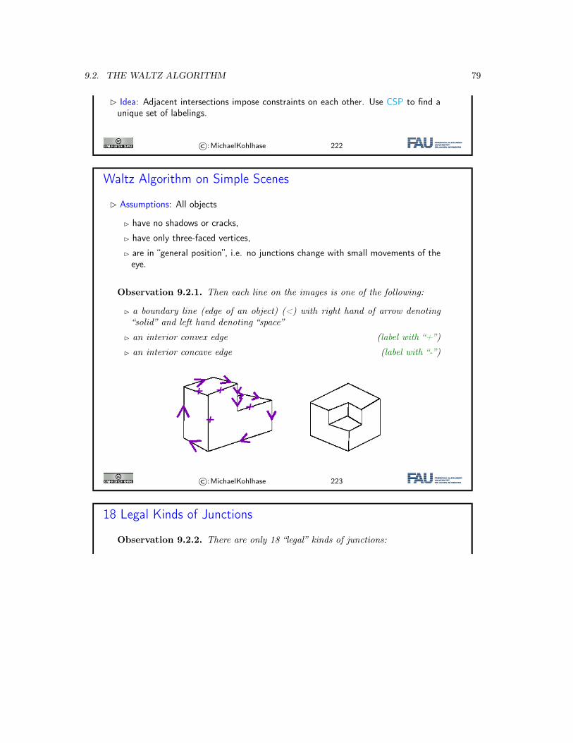
9.2. THE WALTZ ALGORITHM 79
� Idea: Adjacent intersections impose constraints on each other. Use CSP to find aunique set of labelings.
©:MichaelKohlhase 222
Waltz Algorithm on Simple Scenes
� Assumptions: All objects
� have no shadows or cracks,
� have only three-faced vertices,
� are in “general position”, i.e. no junctions change with small movements of theeye.
Observation 9.2.1. Then each line on the images is one of the following:
� a boundary line (edge of an object) (<) with right hand of arrow denoting“solid” and left hand denoting “space”
� an interior convex edge (label with “+”)
� an interior concave edge (label with “-”)
©:MichaelKohlhase 223
18 Legal Kinds of Junctions
Observation 9.2.2. There are only 18 “legal” kinds of junctions:
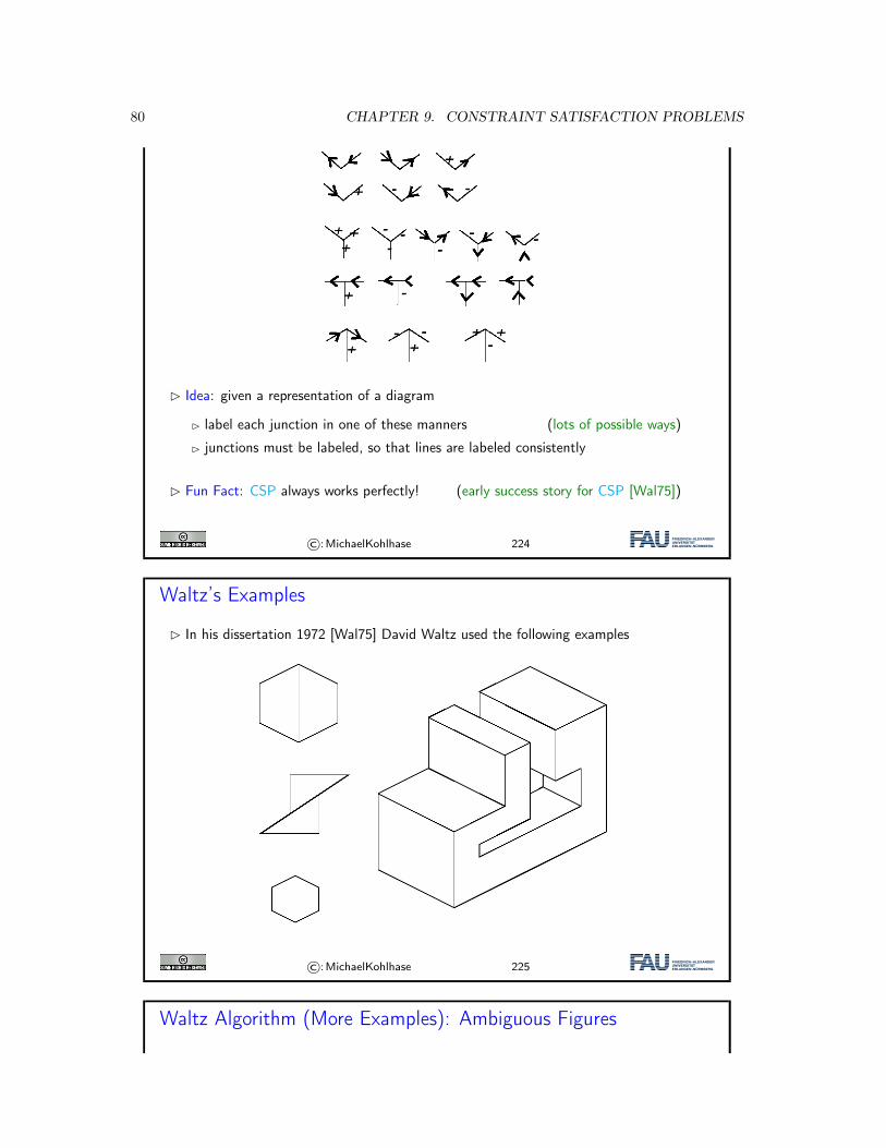
80 CHAPTER 9. CONSTRAINT SATISFACTION PROBLEMS
� Idea: given a representation of a diagram
� label each junction in one of these manners (lots of possible ways)
� junctions must be labeled, so that lines are labeled consistently
� Fun Fact: CSP always works perfectly! (early success story for CSP [Wal75])
©:MichaelKohlhase 224
Waltz’s Examples
� In his dissertation 1972 [Wal75] David Waltz used the following examples
©:MichaelKohlhase 225
Waltz Algorithm (More Examples): Ambiguous Figures
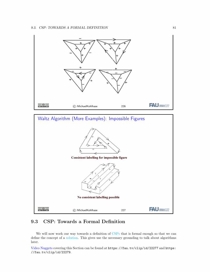
9.3. CSP: TOWARDS A FORMAL DEFINITION 81
©:MichaelKohlhase 226
Waltz Algorithm (More Examples): Impossible Figures
©:MichaelKohlhase 227
9.3 CSP: Towards a Formal Definition
We will now work our way towards a definition of CSPs that is formal enough so that we candefine the concept of a solution. This gives use the necessary grounding to talk about algorithmslater.
Video Nuggets covering this Section can be found at https://fau.tv/clip/id/22277 and https://fau.tv/clip/id/22279.
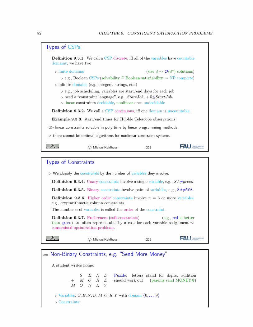
82 CHAPTER 9. CONSTRAINT SATISFACTION PROBLEMS
Types of CSPs
Definition 9.3.1. We call a CSP discrete, iff all of the variables have countabledomains; we have two
� finite domains (size d ; O(dn) solutions)
� e.g., Boolean CSPs (solvability = Boolean satisfiability ; NP complete)
� infinite domains (e.g. integers, strings, etc.)
� e.g., job scheduling, variables are start/end days for each job� need a “constraint language”, e.g., StartJob1 + 5≤StartJob3
� linear constraints decidable, nonlinear ones undecidable
Definition 9.3.2. We call a CSP continuous, iff one domain is uncountable.
Example 9.3.3. start/end times for Hubble Telescope observations
��� linear constraints solvable in poly time by linear programming methods
� there cannot be optimal algorithms for nonlinear constraint systems
©:MichaelKohlhase 228
Types of Constraints
� We classify the constraints by the number of variables they involve.
Definition 9.3.4. Unary constraints involve a single variable, e.g., SA=green.
Definition 9.3.5. Binary constraints involve pairs of variables, e.g., SA =WA.
Definition 9.3.6. Higher order constraints involve n = 3 or more variables,e.g., cryptarithmetic column constraints.
The number n of variables is called the order of the constraint.
Definition 9.3.7. Preferences (soft constraints) (e.g., red is betterthan green) are often representable by a cost for each variable assignment ;constrained optimization problems.
©:MichaelKohlhase 229
���� Non-Binary Constraints, e.g. “Send More Money”
A student writes home:
S E N D+ M O R EM O N E Y
Puzzle: letters stand for digits, additionshould work out (parents send MONEY€)
� Variables: S,E,N,D,M,O,R, Y with domain {0, . . . ,9}� Constraints:
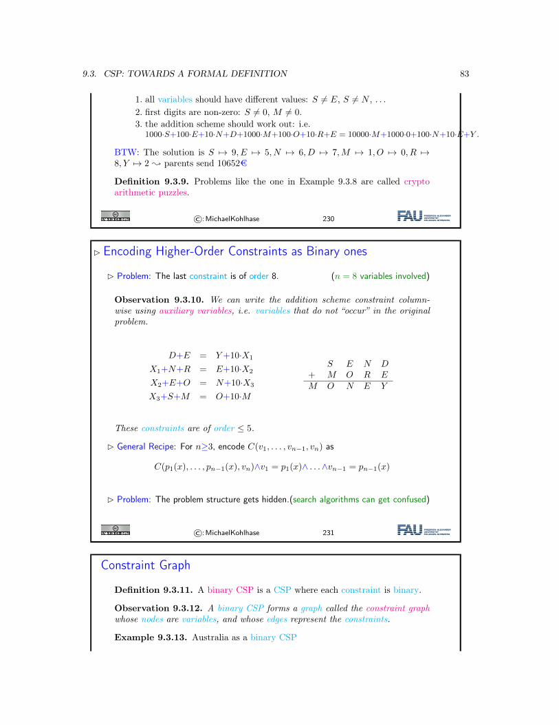
9.3. CSP: TOWARDS A FORMAL DEFINITION 83
1. all variables should have different values: S = E, S = N , . . .2. first digits are non-zero: S = 0, M = 0.3. the addition scheme should work out: i.e.
1000·S+100·E+10·N+D+1000·M+100·O+10·R+E = 10000·M+1000·0+100·N+10·E+Y .
BTW: The solution is S 7→ 9, E 7→ 5, N 7→ 6, D 7→ 7,M 7→ 1, O 7→ 0, R 7→8, Y 7→ 2 ; parents send 10652€
Definition 9.3.9. Problems like the one in Example 9.3.8 are called cryptoarithmetic puzzles.
©:MichaelKohlhase 230
� Encoding Higher-Order Constraints as Binary ones
� Problem: The last constraint is of order 8. (n = 8 variables involved)
Observation 9.3.10. We can write the addition scheme constraint column-wise using auxiliary variables, i.e. variables that do not “occur” in the originalproblem.
D+E = Y+10·X1
X1+N+R = E+10·X2
X2+E+O = N+10·X3
X3+S+M = O+10·M
S E N D+ M O R EM O N E Y
These constraints are of order ≤ 5.
� General Recipe: For n≥3, encode C(v1, . . . , vn−1, vn) as
C(p1(x), . . . , pn−1(x), vn)∧v1 = p1(x)∧ . . .∧vn−1 = pn−1(x)
� Problem: The problem structure gets hidden.(search algorithms can get confused)
©:MichaelKohlhase 231
Constraint Graph
Definition 9.3.11. A binary CSP is a CSP where each constraint is binary.
Observation 9.3.12. A binary CSP forms a graph called the constraint graphwhose nodes are variables, and whose edges represent the constraints.
Example 9.3.13. Australia as a binary CSP
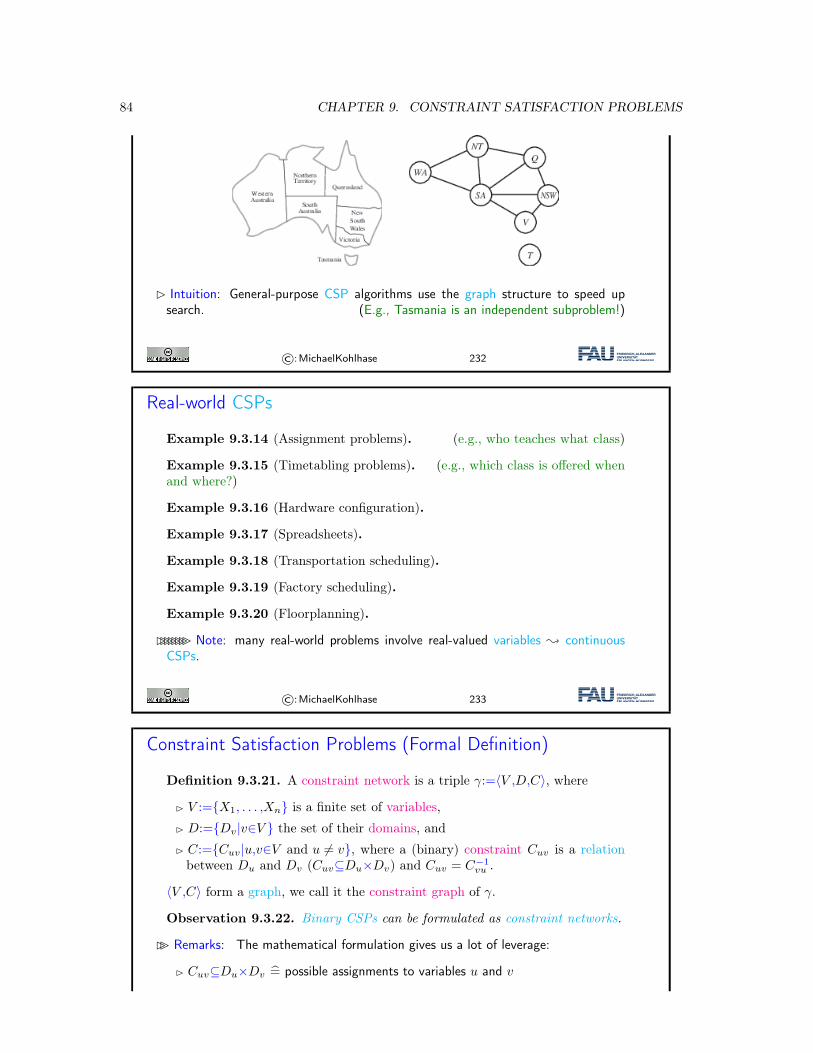
84 CHAPTER 9. CONSTRAINT SATISFACTION PROBLEMS
� Intuition: General-purpose CSP algorithms use the graph structure to speed upsearch. (E.g., Tasmania is an independent subproblem!)
©:MichaelKohlhase 232
Real-world CSPs
Example 9.3.14 (Assignment problems). (e.g., who teaches what class)
Example 9.3.15 (Timetabling problems). (e.g., which class is offered whenand where?)
Example 9.3.16 (Hardware configuration).
Example 9.3.17 (Spreadsheets).
Example 9.3.18 (Transportation scheduling).
Example 9.3.19 (Factory scheduling).
Example 9.3.20 (Floorplanning).
�������� Note: many real-world problems involve real-valued variables ; continuousCSPs.
©:MichaelKohlhase 233
Constraint Satisfaction Problems (Formal Definition)
Definition 9.3.21. A constraint network is a triple γ:=⟨V ,D,C⟩, where
� V :={X1, . . . ,Xn} is a finite set of variables,
� D:={Dv|v∈V } the set of their domains, and
� C:={Cuv|u,v∈V and u = v}, where a (binary) constraint Cuv is a relationbetween Du and Dv (Cuv⊆Du×Dv) and Cuv = C−1
vu .
⟨V ,C⟩ form a graph, we call it the constraint graph of γ.
Observation 9.3.22. Binary CSPs can be formulated as constraint networks.
�� Remarks: The mathematical formulation gives us a lot of leverage:
� Cuv⊆Du×Dv = possible assignments to variables u and v
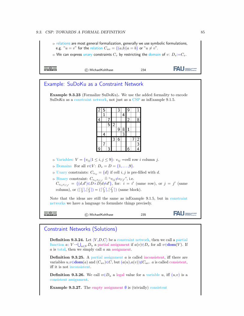
9.3. CSP: TOWARDS A FORMAL DEFINITION 85
� relations are most general formalization, generally we use symbolic formulations,e.g. “u = v” for the relation Cuv = {(a,b)|a = b} or “u = v”.
� We can express unary constraints Cv by restricting the domain of v: Dv:=Cv.
©:MichaelKohlhase 234
Example: SuDoKu as a Constraint Network
Example 9.3.23 (Formalize SuDoKu). We use the added formality to encodeSuDoKu as a constraint network, not just as a CSP as inExample 9.1.5.
� Variables: V = {vij |1 ≤ i, j ≤ 9}: vij =cell row i column j.
� Domains For all v∈V : Dv = D = {1, . . . ,9}.� Unary constraints: Cvij = {d} if cell i, j is pre-filled with d.
� Binary constraint: Cvijvi′j′ = “vij =vi′j′ ”, i.e.Cvijvi′j′ = {(d,d′)∈D×D|d=d′}, for: i = i′ (same row), or j = j′ (samecolumn), or (⌈ i
3⌉,⌈j3⌉) = (⌈ i′
3 ⌉,⌈j′
3 ⌉) (same block).
Note that the ideas are still the same as inExample 9.1.5, but in constraintnetworks we have a language to formulate things precisely.
©:MichaelKohlhase 235
Constraint Networks (Solutions)
Definition 9.3.24. Let ⟨V ,D,C⟩ be a constraint network, then we call a partialfunction a : V⇀
⋃u∈V Du a partial assignment if a(v)∈Dv for all v∈dom(V ). If
a is total, then we simply call a an assignment.
Definition 9.3.25. A partial assignment a is called inconsistent, iff there arevariables u,v∈dom(a) and (Cuv)∈C, but (a(u),a(v)) ∈Cuv. a is called consistent,iff it is not inconsistent.
Definition 9.3.26. We call v∈Du a legal value for a variable u, iff (u,v) is aconsistent assignment.
Example 9.3.27. The empty assignment ∅ is (trivially) consistent
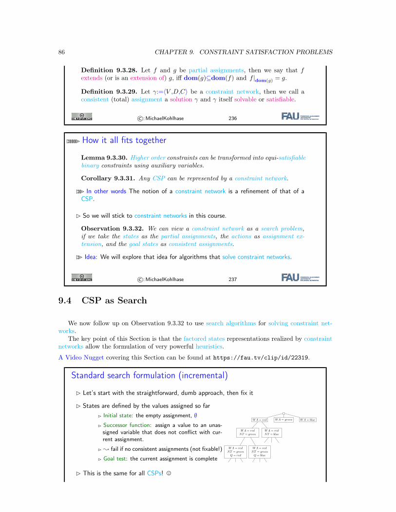
86 CHAPTER 9. CONSTRAINT SATISFACTION PROBLEMS
Definition 9.3.28. Let f and g be partial assignments, then we say that fextends (or is an extension of) g, iff dom(g)⊆dom(f) and f |dom(g) = g.
Definition 9.3.29. Let γ:=⟨V ,D,C⟩ be a constraint network, then we call aconsistent (total) assignment a solution γ and γ itself solvable or satisfiable.
©:MichaelKohlhase 236
������ How it all fits together
Lemma 9.3.30. Higher order constraints can be transformed into equi-satisfiablebinary constraints using auxiliary variables.
Corollary 9.3.31. Any CSP can be represented by a constraint network.
��� In other words The notion of a constraint network is a refinement of that of aCSP.
� So we will stick to constraint networks in this course.
Observation 9.3.32. We can view a constraint network as a search problem,if we take the states as the partial assignments, the actions as assignment ex-tension, and the goal states as consistent assignments.
�� Idea: We will explore that idea for algorithms that solve constraint networks.
©:MichaelKohlhase 237
9.4 CSP as Search
We now follow up on Observation 9.3.32 to use search algorithms for solving constraint net-works.
The key point of this Section is that the factored states representations realized by constraintnetworks allow the formulation of very powerful heuristics.
A Video Nugget covering this Section can be found at https://fau.tv/clip/id/22319.
Standard search formulation (incremental)
� Let’s start with the straightforward, dumb approach, then fix it
� States are defined by the values assigned so far� Initial state: the empty assignment, ∅� Successor function: assign a value to an unas-
signed variable that does not conflict with cur-rent assignment.
� ; fail if no consistent assignments (not fixable!)
� Goal test: the current assignment is complete
WA = red WA = green WA = blue
WA = redNT = green
WA = redNT = blue
WA = redNT = greenQ = red
WA = redNT = greenQ = blue
� This is the same for all CSPs! ,
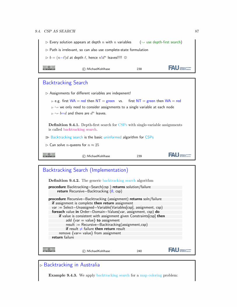
9.4. CSP AS SEARCH 87
� Every solution appears at depth n with n variables (; use depth-first search)
� Path is irrelevant, so can also use complete-state formulation
� b = (n−ℓ)d at depth ℓ, hence n!dn leaves!!!! /
©:MichaelKohlhase 238
Backtracking Search
� Assignments for different variables are indepenent!
� e.g. first WA = red then NT = green vs. first NT = green then WA = red
� ; we only need to consider assignments to a single variable at each node
� ; b=d and there are dn leaves.
Definition 9.4.1. Depth-first search for CSPs with single-variable assignmentsis called backtracking search.
�� Backtracking search is the basic uninformed algorithm for CSPs
� Can solve n-queens for n ≈ 25
©:MichaelKohlhase 239
Backtracking Search (Implementation)
Definition 9.4.2. The generic backtracking search algorithm
procedure Backtracking−Search(csp ) returns solution/failurereturn Recursive−Backtracking (∅, csp)
procedure Recursive−Backtracking (assignment) returns soln/failureif assignment is complete then return assignmentvar := Select−Unassigned−Variable(Variables[csp], assignment, csp)foreach value in Order−Domain−Values(var, assignment, csp) do
if value is consistent with assignment given Constraints[csp] thenadd {var = value} to assignmentresult := Recursive−Backtracking(assignment,csp)if result = failure then return result
remove {var= value} from assignmentreturn failure
©:MichaelKohlhase 240
� Backtracking in Australia
Example 9.4.3. We apply backtracking search for a map coloring problem:
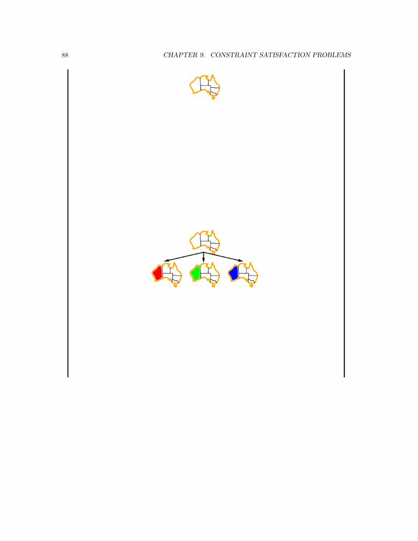
88 CHAPTER 9. CONSTRAINT SATISFACTION PROBLEMS
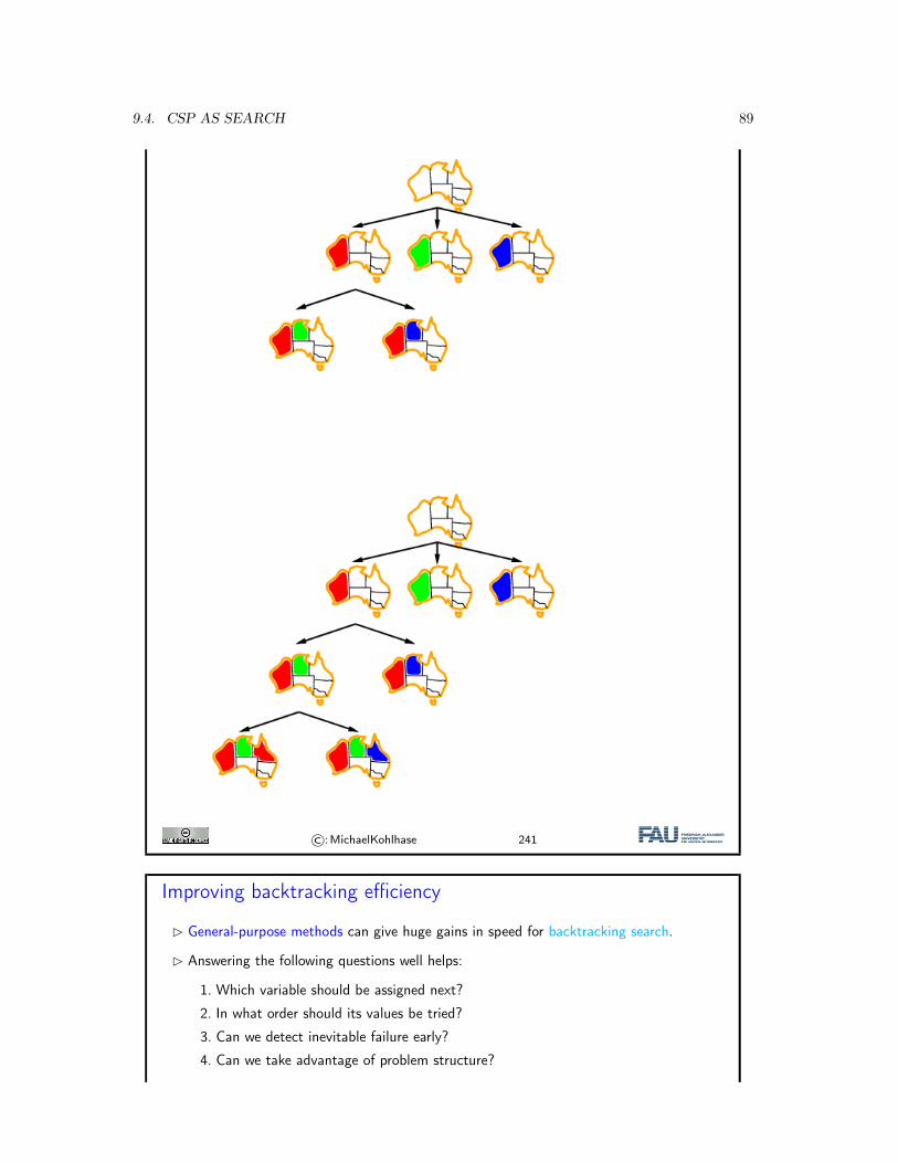
9.4. CSP AS SEARCH 89
©:MichaelKohlhase 241
Improving backtracking efficiency
� General-purpose methods can give huge gains in speed for backtracking search.
� Answering the following questions well helps:
1. Which variable should be assigned next?
2. In what order should its values be tried?
3. Can we detect inevitable failure early?
4. Can we take advantage of problem structure?
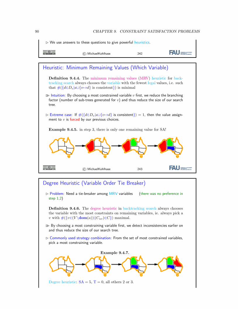
90 CHAPTER 9. CONSTRAINT SATISFACTION PROBLEMS
� We use answers to these questions to give powerful heuristics.
©:MichaelKohlhase 242
Heuristic: Minimum Remaining Values (Which Variable)
Definition 9.4.4. The minimum remaining values (MRV) heuristic for back-tracking search always chooses the variable with the fewest legal values, i.e. suchthat #({d∈Dv|a∪{v 7→d} is consistent}) is minimal
�� Intuition: By choosing a most constrained variable v first, we reduce the branchingfactor (number of sub-trees generated for v) and thus reduce the size of our searchtree.
� Extreme case: If #({d∈Dv|a∪{v 7→d} is consistent}) = 1, then the value assign-ment to v is forced by our previous choices.
Example 9.4.5. in step 3, there is only one remaining value for SA!
©:MichaelKohlhase 243
Degree Heuristic (Variable Order Tie Breaker)
� Problem: Need a tie-breaker among MRV variables (there was no preference instep 1,2)
Definition 9.4.6. The degree heuristic in backtracking search always choosesthe variable with the most constraints on remaining variables, ie. always pick av with #({v∈(V \dom(a))|(Cuv)∈C}) maximal.
�� By choosing a most constraining variable first, we detect inconsistencies earlier onand thus reduce the size of our search tree.
� Commonly used strategy combination: From the set of most constrained variables,pick a most constraining variable.
Example 9.4.7.
Degree heuristic: SA = 5, T = 0, all others 2 or 3.
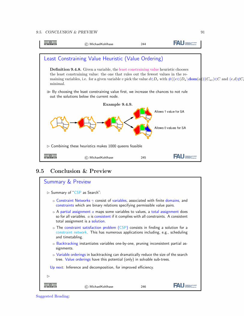
9.5. CONCLUSION & PREVIEW 91
©:MichaelKohlhase 244
Least Constraining Value Heuristic (Value Ordering)
Definition 9.4.8. Given a variable, the least constraining value heuristic choosesthe least constraining value: the one that rules out the fewest values in the re-maining variables, i.e. for a given variable v pick the value d∈Dv with #({e∈(Du\dom(a))|(Cuv)∈C and (e,d)∈Cuv})minimal.
�� By choosing the least constraining value first, we increase the chances to not ruleout the solutions below the current node.
Example 9.4.9.
� Combining these heuristics makes 1000 queens feasible
©:MichaelKohlhase 245
9.5 Conclusion & Preview
Summary & Preview
� Summary of “CSP as Search”:
� Constraint Networks γ consist of variables, associated with finite domains, andconstraints which are binary relations specifying permissible value pairs.
� A partial assignment a maps some variables to values, a total assignment doesso for all variables. a is consistent if it complies with all constraints. A consistenttotal assignment is a solution.
� The constraint satisfaction problem (CSP) consists in finding a solution for aconstraint network. This has numerous applications including, e.g., schedulingand timetabling.
� Backtracking instantiates variables one-by-one, pruning inconsistent partial as-signments.
� Variable orderings in backtracking can dramatically reduce the size of the searchtree. Value orderings have this potential (only) in solvable sub-trees.
Up next: Inference and decomposition, for improved efficiency.
�
©:MichaelKohlhase 246
Suggested Reading:
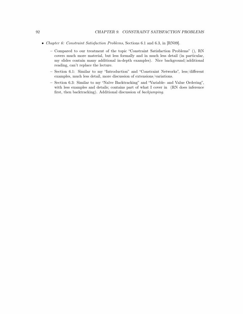
92 CHAPTER 9. CONSTRAINT SATISFACTION PROBLEMS
• Chapter 6: Constraint Satisfaction Problems, Sections 6.1 and 6.3, in [RN09].
– Compared to our treatment of the topic “Constraint Satisfaction Problems” (), RNcovers much more material, but less formally and in much less detail (in particular,my slides contain many additional in-depth examples). Nice background/additionalreading, can’t replace the lecture.
– Section 6.1: Similar to my “Introduction” and “Constraint Networks”, less/differentexamples, much less detail, more discussion of extensions/variations.
– Section 6.3: Similar to my “Naïve Backtracking” and “Variable- and Value Ordering”,with less examples and details; contains part of what I cover in (RN does inferencefirst, then backtracking). Additional discussion of backjumping.
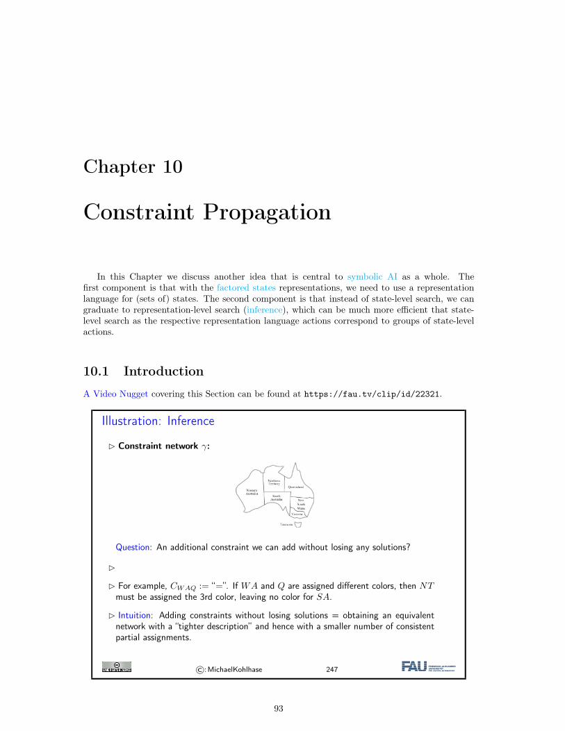
Chapter 10
Constraint Propagation
In this Chapter we discuss another idea that is central to symbolic AI as a whole. Thefirst component is that with the factored states representations, we need to use a representationlanguage for (sets of) states. The second component is that instead of state-level search, we cangraduate to representation-level search (inference), which can be much more efficient that state-level search as the respective representation language actions correspond to groups of state-levelactions.
10.1 Introduction
A Video Nugget covering this Section can be found at https://fau.tv/clip/id/22321.
Illustration: Inference
� Constraint network γ:
Question: An additional constraint we can add without losing any solutions?
�
� For example, CWAQ := “=”. If WA and Q are assigned different colors, then NTmust be assigned the 3rd color, leaving no color for SA.
� Intuition: Adding constraints without losing solutions = obtaining an equivalentnetwork with a “tighter description” and hence with a smaller number of consistentpartial assignments.
©:MichaelKohlhase 247
93
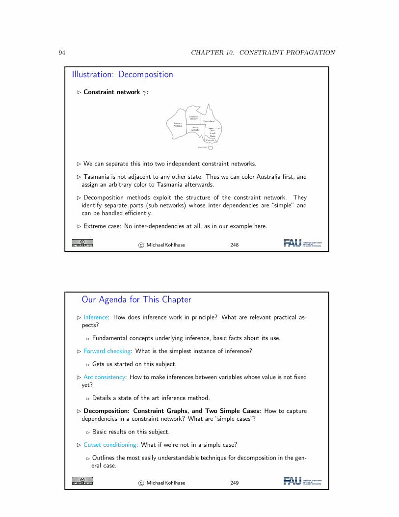
94 CHAPTER 10. CONSTRAINT PROPAGATION
Illustration: Decomposition
� Constraint network γ:
� We can separate this into two independent constraint networks.
� Tasmania is not adjacent to any other state. Thus we can color Australia first, andassign an arbitrary color to Tasmania afterwards.
� Decomposition methods exploit the structure of the constraint network. Theyidentify separate parts (sub-networks) whose inter-dependencies are “simple” andcan be handled efficiently.
� Extreme case: No inter-dependencies at all, as in our example here.
©:MichaelKohlhase 248
Our Agenda for This Chapter
� Inference: How does inference work in principle? What are relevant practical as-pects?
� Fundamental concepts underlying inference, basic facts about its use.
� Forward checking: What is the simplest instance of inference?
� Gets us started on this subject.
� Arc consistency: How to make inferences between variables whose value is not fixedyet?
� Details a state of the art inference method.
� Decomposition: Constraint Graphs, and Two Simple Cases: How to capturedependencies in a constraint network? What are “simple cases”?
� Basic results on this subject.
� Cutset conditioning: What if we’re not in a simple case?
� Outlines the most easily understandable technique for decomposition in the gen-eral case.
©:MichaelKohlhase 249
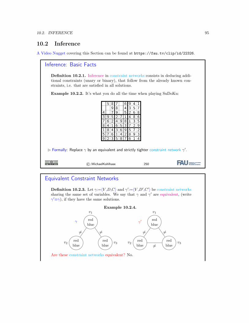
10.2. INFERENCE 95
10.2 InferenceA Video Nugget covering this Section can be found at https://fau.tv/clip/id/22326.
Inference: Basic Facts
Definition 10.2.1. Inference in constraint networks consists in deducing addi-tional constraints (unary or binary), that follow from the already known con-straints, i.e. that are satisfied in all solutions.
Example 10.2.2. It’s what you do all the time when playing SuDoKu:
� Formally: Replace γ by an equivalent and strictly tighter constraint network γ′.
©:MichaelKohlhase 250
Equivalent Constraint Networks
Definition 10.2.3. Let γ:=⟨V ,D,C⟩ and γ′:=⟨V ,D′,C ′⟩ be constraint networkssharing the same set of variables. We say that γ and γ′ are equivalent, (writeγ′≡γ), if they have the same solutions.
Example 10.2.4.
γ redblue
v1
redblue
v2redblue
v3
= =
γ′ redblue
v1
redblue
v2redblue
v3
= =
=
Are these constraint networks equivalent? No.
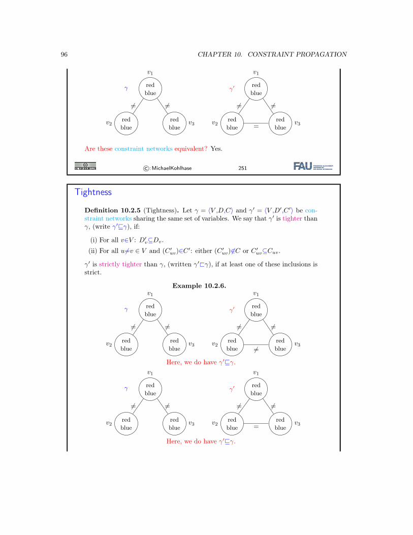
96 CHAPTER 10. CONSTRAINT PROPAGATION
γ redblue
v1
redblue
v2redblue
v3
= =
γ′ redblue
v1
redblue
v2redblue
v3
= =
=
Are these constraint networks equivalent? Yes.
©:MichaelKohlhase 251
Tightness
Definition 10.2.5 (Tightness). Let γ = ⟨V ,D,C⟩ and γ′ = ⟨V ,D′,C ′⟩ be con-straint networks sharing the same set of variables. We say that γ′ is tighter thanγ, (write γ′⊑γ), if:
(i) For all v∈V : D′v⊆Dv.
(ii) For all u=v ∈ V and (C ′uv)∈C ′: either (C ′
uv) ∈C or C ′uv⊆Cuv.
γ′ is strictly tighter than γ, (written γ′<γ), if at least one of these inclusions isstrict.
Example 10.2.6.
γ redblue
v1
redblue
v2redblue
v3
= =
γ′ redblue
v1
redblue
v2redblue
v3
= =
=Here, we do have γ′⊑γ.
γ redblue
v1
redblue
v2redblue
v3
= =
γ′ redblue
v1
redblue
v2redblue
v3
= =
=
Here, we do have γ′⊑γ.
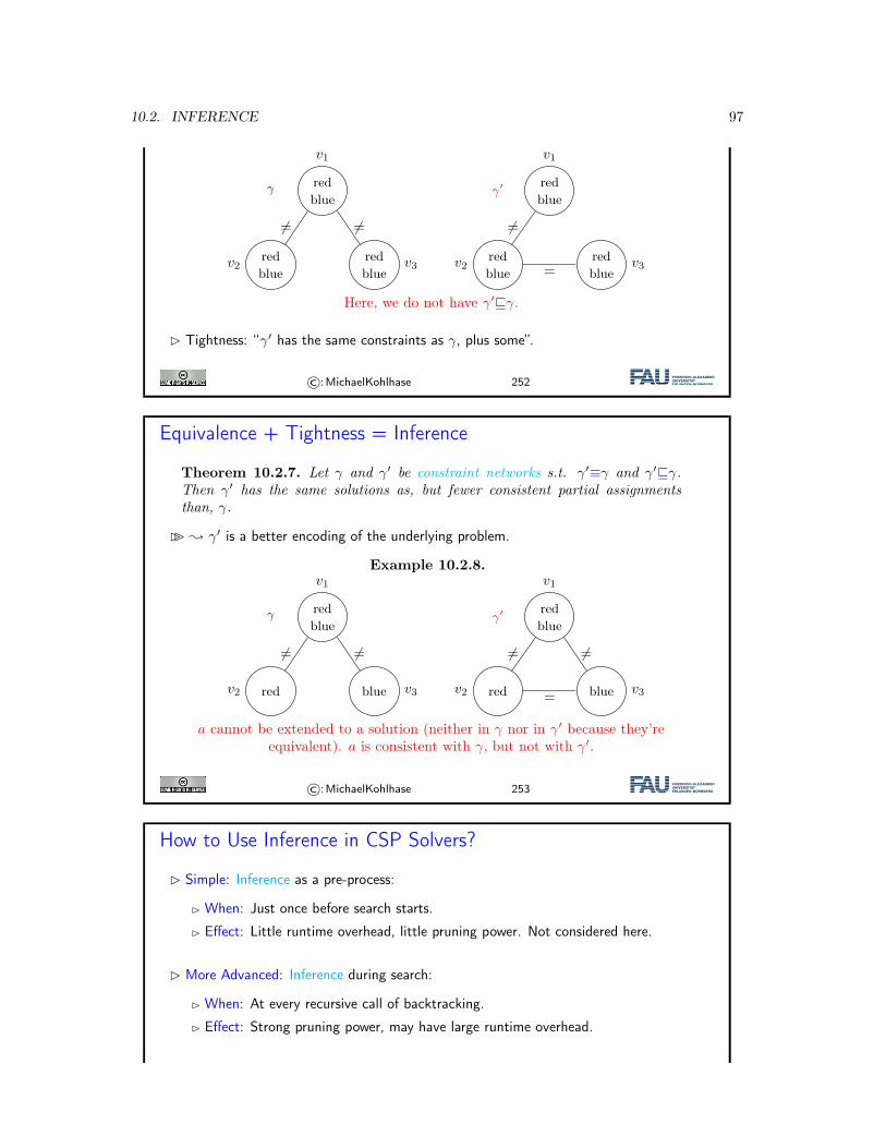
10.2. INFERENCE 97
γ redblue
v1
redblue
v2redblue
v3
= =
γ′ redblue
v1
redblue
v2redblue
v3
=
=
Here, we do not have γ′⊑γ.
� Tightness: “γ′ has the same constraints as γ, plus some”.
©:MichaelKohlhase 252
Equivalence + Tightness = Inference
Theorem 10.2.7. Let γ and γ′ be constraint networks s.t. γ′≡γ and γ′⊑γ.Then γ′ has the same solutions as, but fewer consistent partial assignmentsthan, γ.
�� ; γ′ is a better encoding of the underlying problem.
Example 10.2.8.
γ redblue
v1
redv2 blue v3
= =
γ′ redblue
v1
redv2 blue v3
= =
=
a cannot be extended to a solution (neither in γ nor in γ′ because they’reequivalent). a is consistent with γ, but not with γ′.
©:MichaelKohlhase 253
How to Use Inference in CSP Solvers?
� Simple: Inference as a pre-process:
� When: Just once before search starts.
� Effect: Little runtime overhead, little pruning power. Not considered here.
� More Advanced: Inference during search:
� When: At every recursive call of backtracking.
� Effect: Strong pruning power, may have large runtime overhead.
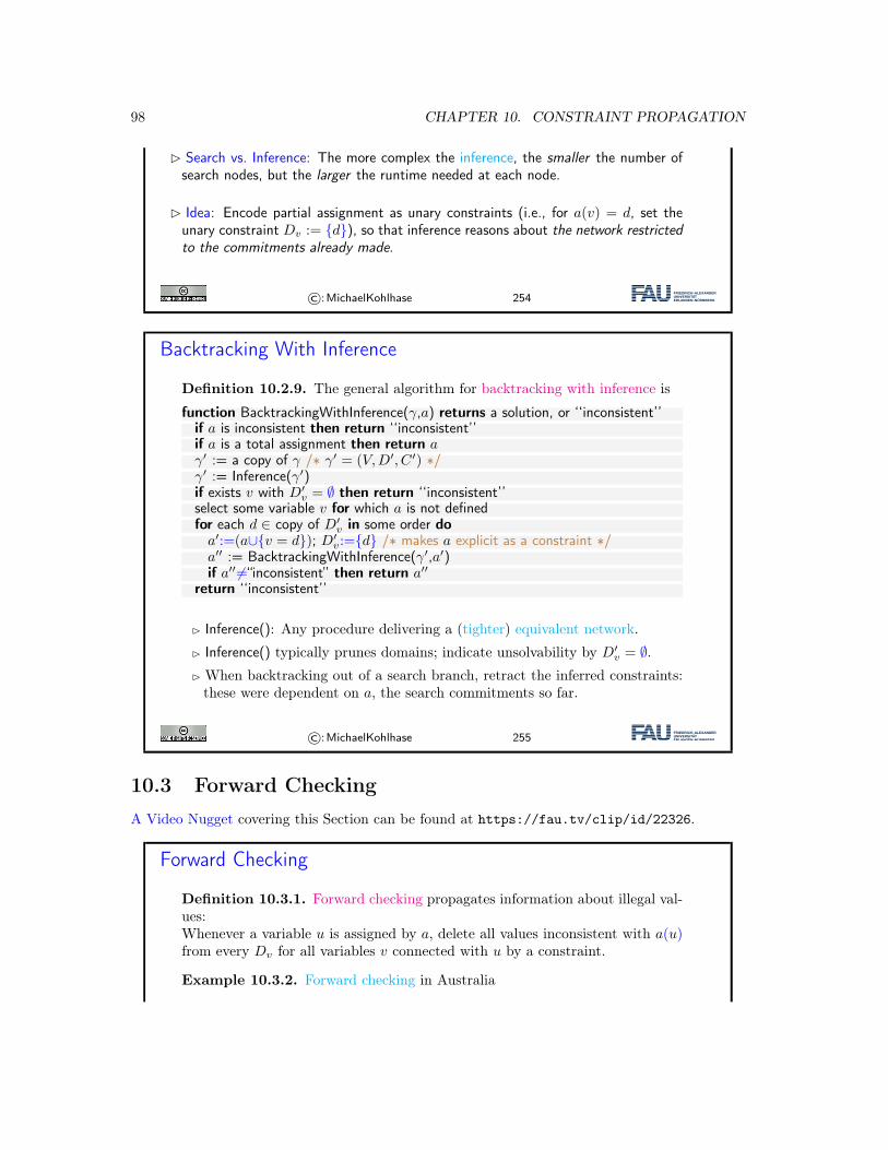
98 CHAPTER 10. CONSTRAINT PROPAGATION
� Search vs. Inference: The more complex the inference, the smaller the number ofsearch nodes, but the larger the runtime needed at each node.
� Idea: Encode partial assignment as unary constraints (i.e., for a(v) = d, set theunary constraint Dv := {d}), so that inference reasons about the network restrictedto the commitments already made.
©:MichaelKohlhase 254
Backtracking With Inference
Definition 10.2.9. The general algorithm for backtracking with inference is
function BacktrackingWithInference(γ,a) returns a solution, or ‘‘inconsistent’’if a is inconsistent then return ‘‘inconsistent’’if a is a total assignment then return aγ′ := a copy of γ /∗ γ′ = (V,D′, C ′) ∗/γ′ := Inference(γ′)if exists v with D′
v = ∅ then return ‘‘inconsistent’’select some variable v for which a is not definedfor each d ∈ copy of D′
v in some order doa′:=(a∪{v = d}); D′
v:={d} /∗ makes a explicit as a constraint ∗/a′′ := BacktrackingWithInference(γ′,a′)if a′′ =“inconsistent” then return a′′
return ‘‘inconsistent’’
� Inference(): Any procedure delivering a (tighter) equivalent network.
� Inference() typically prunes domains; indicate unsolvability by D′v = ∅.
� When backtracking out of a search branch, retract the inferred constraints:these were dependent on a, the search commitments so far.
©:MichaelKohlhase 255
10.3 Forward CheckingA Video Nugget covering this Section can be found at https://fau.tv/clip/id/22326.
Forward Checking
Definition 10.3.1. Forward checking propagates information about illegal val-ues:Whenever a variable u is assigned by a, delete all values inconsistent with a(u)from every Dv for all variables v connected with u by a constraint.
Example 10.3.2. Forward checking in Australia
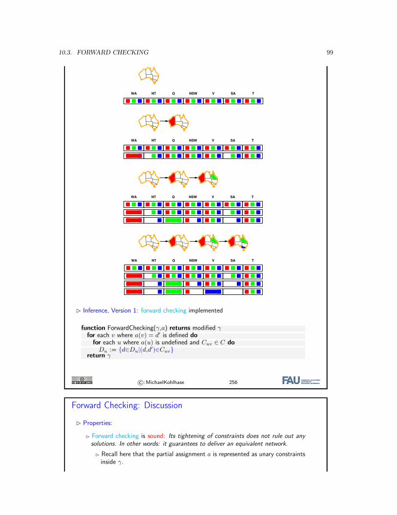
10.3. FORWARD CHECKING 99
Forward Checking
I Inference, version 1: Forward Checkingfunction ForwardChecking(�,a) returns modified �
for each v where a(v) = d 0 is defined dofor each u where a(u) is undefined and Cuv 2 C do
Du := {d 2 Du | (d , d 0) 2 Cuv}return �
I Example 3.1.
WA NT Q NSW V SA T
Kohlhase: Künstliche Intelligenz 1 295 July 5, 2018
� Inference, Version 1: forward checking implemented
function ForwardChecking(γ,a) returns modified γfor each v where a(v) = d′ is defined do
for each u where a(u) is undefined and Cuv ∈ C doDu := {d∈Du|(d,d′)∈Cuv}
return γ
©:MichaelKohlhase 256
Forward Checking: Discussion
� Properties:
� Forward checking is sound: Its tightening of constraints does not rule out anysolutions. In other words: it guarantees to deliver an equivalent network.
� Recall here that the partial assignment a is represented as unary constraintsinside γ.
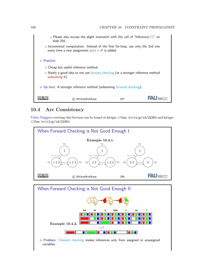
100 CHAPTER 10. CONSTRAINT PROPAGATION
� Please also excuse the slight mismatch with the call of “Inference(γ′)” onslide 255.
� Incremental computation: Instead of the first for-loop, use only the 2nd oneevery time a new assignment a(v) = d′ is added.
� Practice:
� Cheap but useful inference method.
� Rarely a good idea to not use forward checking (or a stronger inference methodsubsuming it).
� Up next: A stronger inference method (subsuming forward checking).
©:MichaelKohlhase 257
10.4 Arc ConsistencyVideo Nuggets covering this Section can be found at https://fau.tv/clip/id/22350 and https://fau.tv/clip/id/22351.
When Forward Checking is Not Good Enough I
Example 10.4.1.
1
v1
1 2 3v2 1 2 3 v3
v1 < v2
v2 < v3
1
v1
2 3v2 1 2 3 v3
v1 < v2
v2 < v3
1
v1
2 3v2 3 v3
v1 < v2
v2 < v3
©:MichaelKohlhase 258
When Forward Checking is Not Good Enough II
Example 10.4.2.
Forward Checking
I Inference, version 1: Forward Checkingfunction ForwardChecking(�,a) returns modified �
for each v where a(v) = d 0 is defined dofor each u where a(u) is undefined and Cuv 2 C do
Du := {d 2 Du | (d , d 0) 2 Cuv}return �
I Example 3.1.
WA NT Q NSW V SA T
Kohlhase: Künstliche Intelligenz 1 295 July 5, 2018
;?
When Forward Checking is Not Good Enough
1
v1
1 2 3v2 1 2 3 v3
v1 < v2
v2 < v3
1
v1
2 3v2 1 2 3 v3
v1 < v2
v2 < v3
1
v1
2 3v2 3 v3
v1 < v2
v2 < v3
WA NT Q NSW V SA T
;?
Forward checking makes inferences only “from assigned to unassigned” variables.Kohlhase: Künstliche Intelligenz 1 297 July 5, 2018
� Problem: Forward checking makes inferences only from assigned to unassignedvariables.
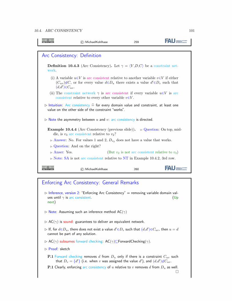
10.4. ARC CONSISTENCY 101
©:MichaelKohlhase 259
Arc Consistency: Definition
Definition 10.4.3 (Arc Consistency). Let γ = ⟨V ,D,C⟩ be a constraint net-work.
(i) A variable u∈V is arc consistent relative to another variable v∈V if either(Cuv) ∈C, or for every value d∈Du there exists a value d′∈Dv such that(d,d′)∈Cuv.
(ii) The constraint network γ is arc consistent if every variable u∈V is arcconsistent relative to every other variable v∈V .
� Intuition: Arc consistency = for every domain value and constraint, at least onevalue on the other side of the constraint “works”.
� Note the asymmetry between u and v: arc consistency is directed.
Example 10.4.4 (Arc Consistency (previous slide)). � Question: On top, mid-dle, is v3 arc consistent relative to v2?
� Answer: No. For values 1 and 2, Dv2 does not have a value that works.
� Question: And on the right?
� Anser: Yes. (But v2 is not arc consistent relative to v3)
� Note: SA is not arc consistent relative to NT in Example 10.4.2, 3rd row.
©:MichaelKohlhase 260
Enforcing Arc Consistency: General Remarks
� Inference, version 2: “Enforcing Arc Consistency” = removing variable domain val-ues until γ is arc consistent. (Upnext)
� Note: Assuming such an inference method AC(γ)
� AC(γ) is sound: guarantees to deliver an equivalent network.
� If, for d∈Du, there does not exist a value d′∈Dv such that (d,d′)∈Cuv, then u = dcannot be part of any solution.
� AC(γ) subsumes forward checking: AC(γ)⊑ForwardChecking(γ).
� Proof: sketch
P.1 Forward checking removes d from Du only if there is a constraint Cuv suchthat Dv = {d′} (i.e. when v was assigned the value d′), and (d,d′)∈Cuv.
P.1 Clearly, enforcing arc consistency of u relative to v removes d from Du as well.
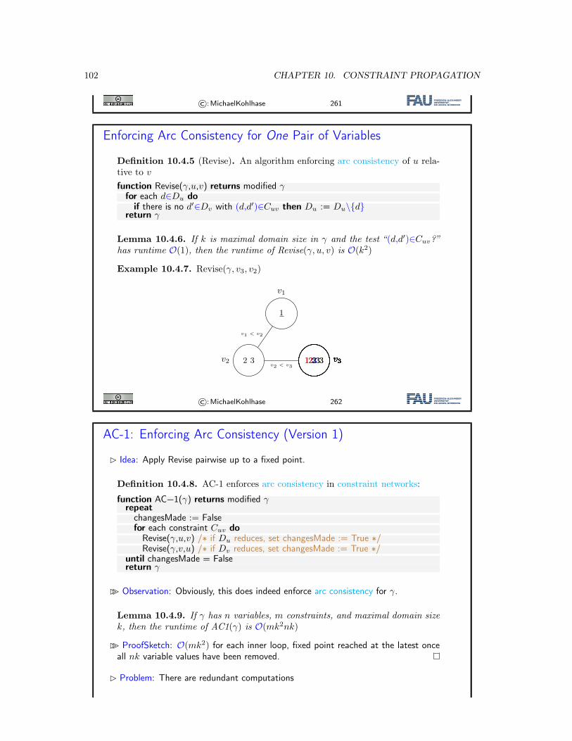
102 CHAPTER 10. CONSTRAINT PROPAGATION
©:MichaelKohlhase 261
Enforcing Arc Consistency for One Pair of Variables
Definition 10.4.5 (Revise). An algorithm enforcing arc consistency of u rela-tive to v
function Revise(γ,u,v) returns modified γfor each d∈Du do
if there is no d′∈Dv with (d,d′)∈Cuv then Du := Du\{d}return γ
Lemma 10.4.6. If k is maximal domain size in γ and the test “(d,d′)∈Cuv?”has runtime O(1), then the runtime of Revise(γ, u, v) is O(k2)
Example 10.4.7. Revise(γ, v3, v2)
1
v1
2 3v2 1 2 3 v31 2 3 v32 3 v32 3 v33 v33 v3
v1 < v2
v2 < v3
©:MichaelKohlhase 262
AC-1: Enforcing Arc Consistency (Version 1)
� Idea: Apply Revise pairwise up to a fixed point.
Definition 10.4.8. AC-1 enforces arc consistency in constraint networks:
function AC−1(γ) returns modified γrepeat
changesMade := Falsefor each constraint Cuv do
Revise(γ,u,v) /∗ if Du reduces, set changesMade := True ∗/Revise(γ,v,u) /∗ if Dv reduces, set changesMade := True ∗/
until changesMade = Falsereturn γ
�� Observation: Obviously, this does indeed enforce arc consistency for γ.
Lemma 10.4.9. If γ has n variables, m constraints, and maximal domain sizek, then the runtime of AC1(γ) is O(mk2nk)
�� ProofSketch: O(mk2) for each inner loop, fixed point reached at the latest onceall nk variable values have been removed.
� Problem: There are redundant computations
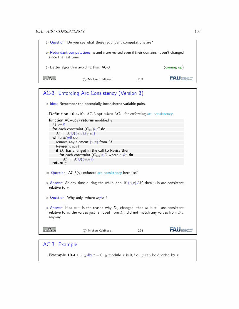
10.4. ARC CONSISTENCY 103
� Question: Do you see what these redundant computations are?
� Redundant computations: u and v are revised even if their domains haven’t changedsince the last time.
� Better algorithm avoiding this: AC-3 (coming up)
©:MichaelKohlhase 263
AC-3: Enforcing Arc Consistency (Version 3)
� Idea: Remember the potentially inconsistent variable pairs.
Definition 10.4.10. AC-3 optimizes AC-1 for enforcing arc consistency.
function AC−3(γ) returns modified γM := ∅for each constraint (Cuv)∈C doM := M∪{(u,v),(v,u)}
while M =∅ doremove any element (u,v) from MRevise(γ, u, v)if Du has changed in the call to Revise then
for each constraint (Cwu)∈C where w =v doM := M∪{(w,u)}
return γ
�� Question: AC-3(γ) enforces arc consistency because?
� Answer: At any time during the while-loop, if (u,v)∈M then u is arc consistentrelative to v.
� Question: Why only “where w =v”?
� Answer: If w = v is the reason why Du changed, then w is still arc consistentrelative to u: the values just removed from Du did not match any values from Dw
anyway.
©:MichaelKohlhase 264
AC-3: Example
Example 10.4.11. y divx = 0: y modulo x is 0, i.e., y can be divided by x
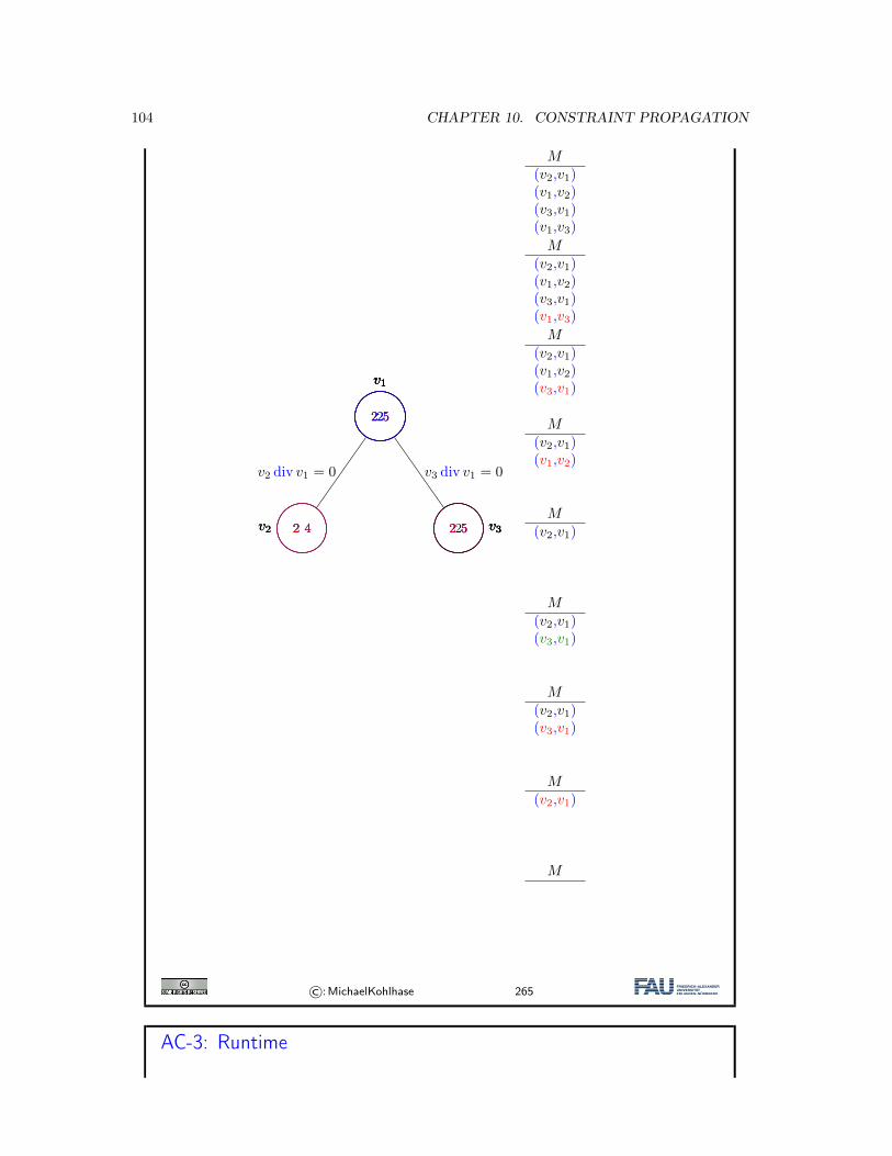
104 CHAPTER 10. CONSTRAINT PROPAGATION
2 5
v1
2 5
v1
2 5
v1
2
v1
2
v1
2 4v2 2 4v2 2 4v2 2 5 v32 5 v32 5 v32 v3
v2 div v1 = 0 v3 div v1 = 0
M(v2,v1)(v1,v2)(v3,v1)(v1,v3)
M(v2,v1)(v1,v2)(v3,v1)(v1,v3)
M(v2,v1)(v1,v2)(v3,v1)
M(v2,v1)(v1,v2)
M(v2,v1)
M(v2,v1)(v3,v1)
M(v2,v1)(v3,v1)
M(v2,v1)
M
©:MichaelKohlhase 265
AC-3: Runtime
10.5. DECOMPOSITION: CONSTRAINT GRAPHS, AND TWO SIMPLE CASES 105
Theorem 10.4.12 (Runtime of AC-3). Let γ = ⟨V ,D,C⟩ be a constraint net-work with m constraints, and maximal domain size k. Then AC-3(γ) runs intime O(mk3).
�� Proof: by counting how often Revise is called.
P.1 Each call to Revise(γ, u, v) takes time O(k2) so it suffices to prove that at mostO(mk) of these calls are made.
P.1 The number of calls to Revise(γ, u, v) is the number of iterations of the while-loop, which is at most the number of insertions into M .
P.1 Consider any constraint Cuv.
P.1 Two variable pairs corresponding to Cuv are inserted in the for-loop. In thewhile loop, if a pair corresponding to Cuv is inserted into M , then
P.1 beforehand the domain of either u or v was reduced, which happens at most2k times.
P.1 Thus we have O(k) insertions per constraint, and O(mk) insertions overall, asdesired.
©:MichaelKohlhase 266
10.5 Decomposition: Constraint Graphs, and Two SimpleCases
A Video Nugget covering this Section can be found at https://fau.tv/clip/id/22353.
Reminder: The Big Picture
� Say γ is a constraint network with n variables and maximal domain size k.
� kn total assignments must be tested in the worst case to solve γ
Inference: One method to try to avoid/ameliorate this explosion in practice.
� � Often, from an assignment to some variables, we can easily make inferencesregarding other variables.
Decomposition: Another method to avoid/ameliorate this explosion in practice.
� � Often, we can exploit the structure of a network to decompose it into smallerparts that are easier to solve.
� Question: What is “structure”, and how to “decompose”?
©:MichaelKohlhase 267
“Decomposition” 1.0: Disconnected Constraint Graphs
Theorem 10.5.1 (Disconnected Constraint Graphs). Let γ = ⟨V ,D,C⟩ be aconstraint network. Let ai be a solution to each connected component Vi of theconstraint graph of γ. Then a:=
⋃iai is a solution to γ.
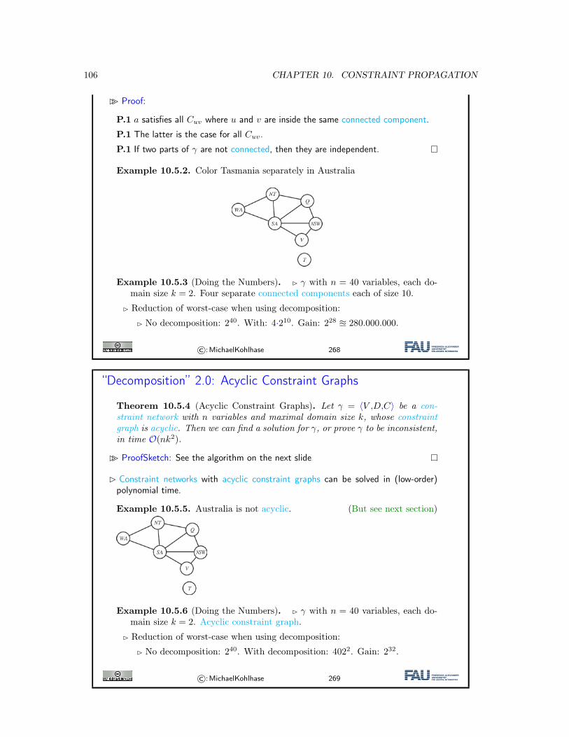
106 CHAPTER 10. CONSTRAINT PROPAGATION
�� Proof:
P.1 a satisfies all Cuv where u and v are inside the same connected component.
P.1 The latter is the case for all Cuv.
P.1 If two parts of γ are not connected, then they are independent.
Example 10.5.2. Color Tasmania separately in Australia
Example 10.5.3 (Doing the Numbers). � γ with n = 40 variables, each do-main size k = 2. Four separate connected components each of size 10.
� Reduction of worst-case when using decomposition:
� No decomposition: 240. With: 4·210. Gain: 228 ≊ 280.000.000.
©:MichaelKohlhase 268
“Decomposition” 2.0: Acyclic Constraint Graphs
Theorem 10.5.4 (Acyclic Constraint Graphs). Let γ = ⟨V ,D,C⟩ be a con-straint network with n variables and maximal domain size k, whose constraintgraph is acyclic. Then we can find a solution for γ, or prove γ to be inconsistent,in time O(nk2).
�� ProofSketch: See the algorithm on the next slide
� Constraint networks with acyclic constraint graphs can be solved in (low-order)polynomial time.
Example 10.5.5. Australia is not acyclic. (But see next section)
Example 10.5.6 (Doing the Numbers). � γ with n = 40 variables, each do-main size k = 2. Acyclic constraint graph.
� Reduction of worst-case when using decomposition:
� No decomposition: 240. With decomposition: 4022. Gain: 232.
©:MichaelKohlhase 269
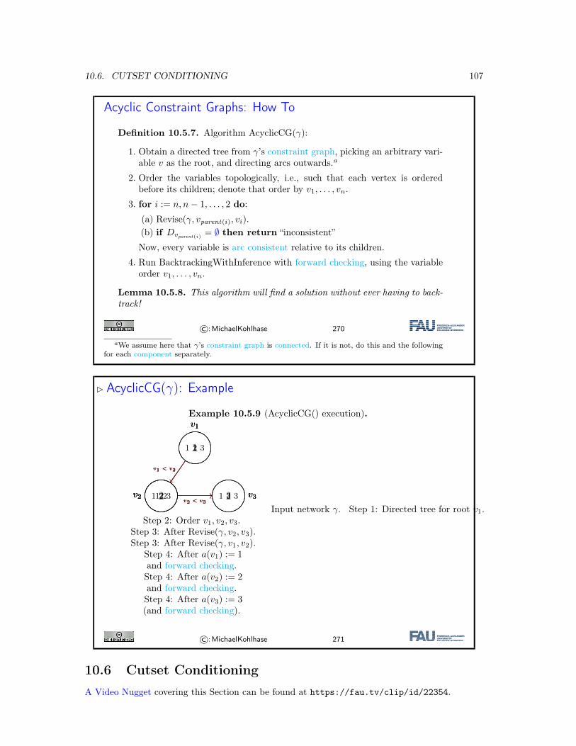
10.6. CUTSET CONDITIONING 107
Acyclic Constraint Graphs: How To
Definition 10.5.7. Algorithm AcyclicCG(γ):
1. Obtain a directed tree from γ’s constraint graph, picking an arbitrary vari-able v as the root, and directing arcs outwards.a
2. Order the variables topologically, i.e., such that each vertex is orderedbefore its children; denote that order by v1, . . . , vn.
3. for i := n, n− 1, . . . , 2 do:
(a) Revise(γ, vparent(i), vi).(b) if Dvparent(i) = ∅ then return “inconsistent”
Now, every variable is arc consistent relative to its children.
4. Run BacktrackingWithInference with forward checking, using the variableorder v1, . . . , vn.
Lemma 10.5.8. This algorithm will find a solution without ever having to back-track!
©:MichaelKohlhase 270
aWe assume here that γ’s constraint graph is connected. If it is not, do this and the followingfor each component separately.
� AcyclicCG(γ): Example
Example 10.5.9 (AcyclicCG() execution).
1 2 3
v1
1
v1
1
v1
1 2 3v2 1 2v2 2v2 2v2 1 2 3 v33 v33 v3
v1 < v2v1 < v2v1 < v2
v2 < v3v2 < v3v2 < v3
Input network γ. Step 1: Directed tree for root v1.Step 2: Order v1, v2, v3.
Step 3: After Revise(γ, v2, v3).Step 3: After Revise(γ, v1, v2).
Step 4: After a(v1) := 1and forward checking.Step 4: After a(v2) := 2and forward checking.Step 4: After a(v3) := 3(and forward checking).
©:MichaelKohlhase 271
10.6 Cutset ConditioningA Video Nugget covering this Section can be found at https://fau.tv/clip/id/22354.
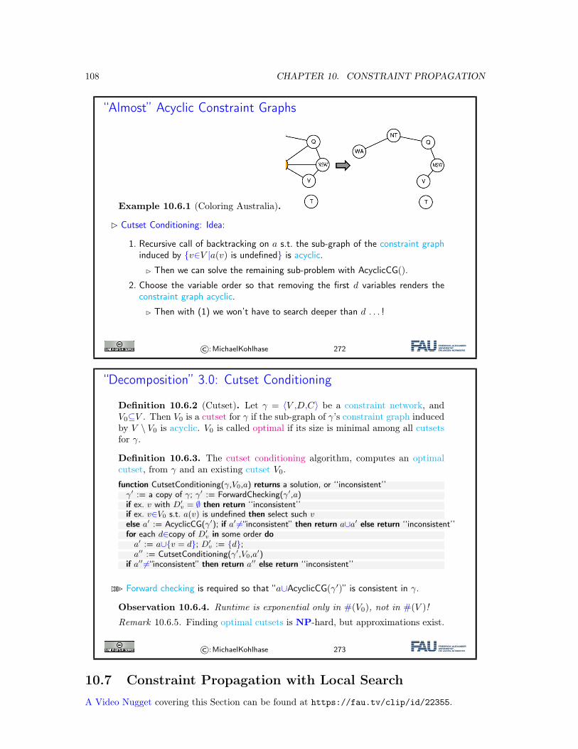
108 CHAPTER 10. CONSTRAINT PROPAGATION
“Almost” Acyclic Constraint Graphs
Example 10.6.1 (Coloring Australia).
� Cutset Conditioning: Idea:
1. Recursive call of backtracking on a s.t. the sub-graph of the constraint graphinduced by {v∈V |a(v) is undefined} is acyclic.
� Then we can solve the remaining sub-problem with AcyclicCG().
2. Choose the variable order so that removing the first d variables renders theconstraint graph acyclic.
� Then with (1) we won’t have to search deeper than d . . . !
©:MichaelKohlhase 272
“Decomposition” 3.0: Cutset Conditioning
Definition 10.6.2 (Cutset). Let γ = ⟨V ,D,C⟩ be a constraint network, andV0⊆V . Then V0 is a cutset for γ if the sub-graph of γ’s constraint graph inducedby V \ V0 is acyclic. V0 is called optimal if its size is minimal among all cutsetsfor γ.
Definition 10.6.3. The cutset conditioning algorithm, computes an optimalcutset, from γ and an existing cutset V0.function CutsetConditioning(γ,V0,a) returns a solution, or ‘‘inconsistent’’γ′ := a copy of γ; γ′ := ForwardChecking(γ′,a)if ex. v with D′
v = ∅ then return ‘‘inconsistent’’if ex. v∈V0 s.t. a(v) is undefined then select such velse a′ := AcyclicCG(γ′); if a′ =“inconsistent” then return a∪a′ else return ‘‘inconsistent’’for each d∈copy of D′
v in some order doa′ := a∪{v = d}; D′
v := {d};a′′ := CutsetConditioning(γ′,V0,a′)
if a′′ =“inconsistent” then return a′′ else return ‘‘inconsistent’’
��� Forward checking is required so that “a∪AcyclicCG(γ′)” is consistent in γ.
Observation 10.6.4. Runtime is exponential only in #(V0), not in #(V )!
Remark 10.6.5. Finding optimal cutsets is NP-hard, but approximations exist.
©:MichaelKohlhase 273
10.7 Constraint Propagation with Local SearchA Video Nugget covering this Section can be found at https://fau.tv/clip/id/22355.
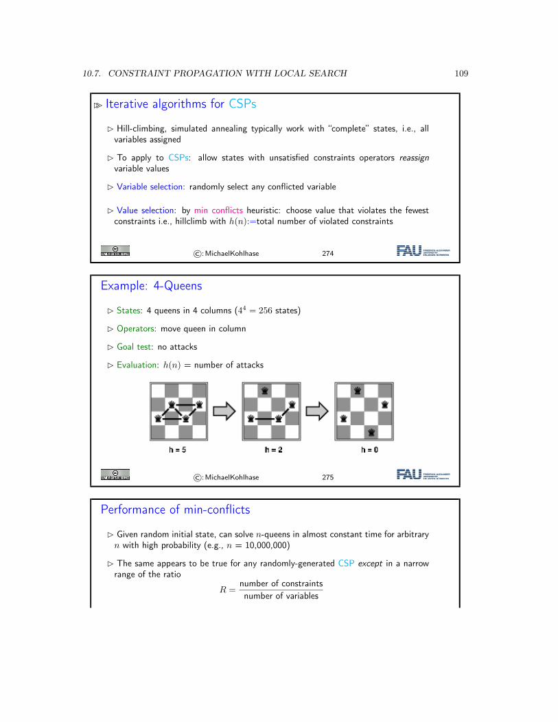
10.7. CONSTRAINT PROPAGATION WITH LOCAL SEARCH 109
�� Iterative algorithms for CSPs
� Hill-climbing, simulated annealing typically work with “complete” states, i.e., allvariables assigned
� To apply to CSPs: allow states with unsatisfied constraints operators reassignvariable values
� Variable selection: randomly select any conflicted variable
� Value selection: by min conflicts heuristic: choose value that violates the fewestconstraints i.e., hillclimb with h(n):=total number of violated constraints
©:MichaelKohlhase 274
Example: 4-Queens
� States: 4 queens in 4 columns (44 = 256 states)
� Operators: move queen in column
� Goal test: no attacks
� Evaluation: h(n) = number of attacks
©:MichaelKohlhase 275
Performance of min-conflicts
� Given random initial state, can solve n-queens in almost constant time for arbitraryn with high probability (e.g., n = 10,000,000)
� The same appears to be true for any randomly-generated CSP except in a narrowrange of the ratio
R =number of constraintsnumber of variables
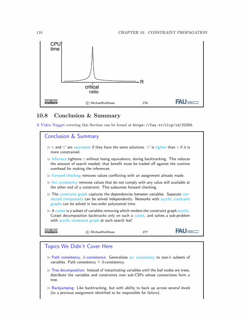
110 CHAPTER 10. CONSTRAINT PROPAGATION
©:MichaelKohlhase 276
10.8 Conclusion & SummaryA Video Nugget covering this Section can be found at https://fau.tv/clip/id/22356.
Conclusion & Summary
� γ and γ′ are equivalent if they have the same solutions. γ′ is tighter than γ if it ismore constrained.
� Inference tightens γ without losing equivalence, during backtracking. This reducesthe amount of search needed; that benefit must be traded off against the runtimeoverhead for making the inferences.
� Forward checking removes values conflicting with an assignment already made.
� Arc consistency removes values that do not comply with any value still available atthe other end of a constraint. This subsumes forward checking.
� The constraint graph captures the dependencies between variables. Separate con-nected components can be solved independently. Networks with acyclic constraintgraphs can be solved in low-order polynomial time.
� A cutset is a subset of variables removing which renders the constraint graph acyclic.Cutset decomposition backtracks only on such a cutset, and solves a sub-problemwith acyclic constraint graph at each search leaf.
©:MichaelKohlhase 277
Topics We Didn’t Cover Here
� Path consistency, k-consistence: Generalizes arc consistency to size-k subsets ofvariables. Path consistency = 3-consistency.
� Tree decomposition: Instead of instantiating variables until the leaf nodes are trees,distribute the variables and constraints over sub-CSPs whose connections form atree.
� Backjumping: Like backtracking, but with ability to back up across several levels(to a previous assignment identified to be responsible for failure).
10.8. CONCLUSION & SUMMARY 111
� No-Good Learning: Inferring additional constraints based on information gatheredduring backtracking.
� Local search: In space of total (but not necessarily consistent) assignments. (E.g.,8-Queens in chapter 7)
� Tractable CSP: Classes of CSPs that can be solved in polynomial time.
� Global Constraints: Constraints over many/all variables, with associated specializedinference methods.
� Constraint Optimization Problems (COP): Utility function over solutions, need anoptimal one.
©:MichaelKohlhase 278
Suggested Reading:
• Chapter 6: Constraint Satisfaction Problems in [RN09], in particular Sections 6.2, 6.3.2, and6.5.
– Compared to our treatment of the topic “Constraint Satisfaction Problems” (), RNcovers much more material, but less formally and in much less detail (in particular,my slides contain many additional in-depth examples). Nice background/additionalreading, can’t replace the lecture.
– Section 6.3.2: Somewhat comparable to my “Inference” (except that equivalence andtightness are not made explicit in RN) together with “Forward Checking”.
– Section 6.2: Similar to my “Arc Consistency”, less/different examples, much less detail,additional discussion of path consistency and global constraints.
– Section 6.5: Similar to my “Decomposition: Constraint Graphs, and Two Simple Cases”and “Cutset Conditioning”, less/different examples, much less detail, additional discus-sion of tree decomposition.

112 CHAPTER 10. CONSTRAINT PROPAGATION
Bibliography
[FD14] Zohar Feldman and Carmel Domshlak. “Simple Regret Optimization in Online Planningfor Markov Decision Processes”. In: Journal of Artificial Intelligence Research 51 (2014),pp. 165–205.
[ILD] 7. Constraints: Interpreting Line Drawings. url: https://www.youtube.com/watch?v=l-tzjenXrvI&t=2037s (visited on 11/19/2019).
[KS06] Levente Kocsis and Csaba Szepesvári. “Bandit Based Monte-Carlo Planning”. In: Pro-ceedings of the 17th European Conference on Machine Learning (ECML 2006). Ed.by Johannes Fürnkranz, Tobias Scheffer, and Myra Spiliopoulou. Vol. 4212. LNCS.Springer-Verlag, 2006, pp. 282–293.
[Min] Minion - Constraint Modelling. System Web page at http://constraintmodelling.org/minion/. url: http://constraintmodelling.org/minion/.
[Pól73] George Pólya. How to Solve it. A New Aspect of Mathematical Method. Princeton Uni-versity Press, 1973.
[RN03] Stuart J. Russell and Peter Norvig. Artificial Intelligence: A Modern Approach. 2nd ed.Pearso n Education, 2003. isbn: 0137903952.
[RN09] Stuart Russell and Peter Norvig. Artificial Intelligence: A Modern Approach. 3rd. Pren-tice Hall Press, 2009. isbn: 0136042597, 9780136042594.
[Sil+16] David Silver et al. “Mastering the Game of Go with Deep Neural Networks and TreeSearch”. In: Nature 529 (2016), pp. 484–503. url: http://www.nature.com/nature/journal/v529/n7587/full/nature16961.html.
[Wal75] David Waltz. “Understanding Line Drawings of Scenes with Shadows”. In: The Psychol-ogy of Computer Vision. Ed. by P. H. Winston. McGraw-Hill, 1975, pp. 1–19.
113