Inverse Design of Soft Robotic Actuators using Nonlinear ...

Inverse Design of Soft Robotic Actuators using NonlinearFinite Element Modeling

A THESIS

SUBMITTED TO THE FACULTY OF THE GRADUATE SCHOOL

OF THE UNIVERSITY OF MINNESOTA

BY

Mark David Gilbertson

IN PARTIAL FULFILLMENT OF THE REQUIREMENTS

FOR THE DEGREE OF

DOCTOR OF PHILISOPHY

Timothy M. Kowalewski, PhD

James D. Van de Ven, PhD

November, 2019

c© Mark David Gilbertson 2019

ALL RIGHTS RESERVED

Acknowledgements

The author would like to thank his adviser’s Timothy Kowalewski, PhD and James Van de Ven,

PhD for their mentorship and guidance during my PhD. The author would like to thank current

and former members of the Medical Devices and Robotics lab as well as the Mechanical En-

ergy and Power Systems lab including Trevor Stephens, Gillian McDonald, Chaitanya Awasthi,

Gabriel Korinek, Rod Doctker, John O’Neill, Anna French, Darrin Beekman, Jason Kelly, Steve

Thomalla, Anthony Knutsen, Alex Yudell, Rebecca Smith, Mark Brown, and many others for

their help and support during my time at the University of Minnesota. The author would like to

thank the graduate students John Huss and Corey Cruttenden for their friendship and help over

the past several years. The author would also like to thank the committee members William

Durfee, Phd, Julianna Abel, and Emmanuel Detournay, PhD. Additionally, the author would

like to thank Max Donath, PhD for his mentorship. The author would also like to acknowl-

edge John Gardner and Chris Hogan, PhD for their help in navigating the PhD process. The

author would like to thank the University of Minnesota Graduate School Interdisciplinary Doc-

toral Fellowship, the MnDRIVE Robotics, Sensors, and Advanced Manufacturing initiative, and

the NSF EFRI C3 SoRo for their financial support. The author acknowledges the Minnesota

Supercomputing Institute (MSI) at the University of Minnesota for providing resources that

contributed to the research results reported within this paper. URL: http://www.msi.umn.edu

i

Dedication

To my family.

ii

Abstract

The field of soft robotics has empowered robots to maneuver, traverse, and complete tasks

where traditional rigid robots fall short. These robots are able to bend continuously and conform

to their environments which makes their designs inherently safe. This makes soft robots a

suitable candidate for use in medical devices. This thesis explores an inverse soft robot design

algorithm, with possible future applications to a soft catheter robot.

Soft robot techniques were used to create a large scale prototype of a hydraulically powered,

serial, soft catheter robot. The locomotion section of this robot consisted of three fiber reinforced

elastomeric enclosures (FREE) actuators connected by passive valves. When controlled properly,

the locomotion section was able to ‘inchworm’ through a tube, thus demonstrating the feasibility

of a serially controlled catheter.

Although the FREE actuators were able to produce locomotion in the tube, the limitation

of realizable actuator shapes severely hampered the robot’s performance. This limitation moti-

vated the need for a generalized design tool where the user could dictate the desired actuator

shapes. To accomplish the additional design freedom, an inverse problem was explored. First,

a mathematical description of cylindrical actuator shapes was developed. Allowing a user to

create arbitrary actuator shapes that deformed from an initial state to a final state. Next, a

nonlinear inverse Finite Element Modeling optimization algorithm was developed to reconstruct

the material properties when the boundary conditions and internal pressure were known.

The inverse algorithm was tested on three cylindrical actuator motions. The first was a

ballooning actuator which expanded uniformly in every direction. The second was a bending

actuator capable of rotation constrained to a single plane. The third was a twisting actuator

that rotated along its axis in a nearly pure shear translation, transforming a pressure input into

out of plane motion. The material properties of all three actuator motions were successfully

reconstructed with the developed inverse algorithm. The reconstructed twisting actuator was

then 3D printed with a multi-material polyjet 3D printer and experimentally shown to match

the twist of both the ground truth design and simulated results. This provided some initial

validation of the inverse algorithm.

iii

Contents

Acknowledgements i

Dedication ii

Abstract iii

List of Tables v

List of Figures vi

1 Introduction 1

1.1 Motivation . . . . . . . . . . . . . . . . . . . . . . . . . . . . . . . . . . . . . . . 3

1.2 Thesis Overview and Specific Contributions . . . . . . . . . . . . . . . . . . . . . 6

2 Background 8

2.1 Background on Soft Robots . . . . . . . . . . . . . . . . . . . . . . . . . . . . . . 8

2.1.1 Fiber-Reinforced Elastomers . . . . . . . . . . . . . . . . . . . . . . . . . 10

2.1.2 Bellowed Soft Actuators . . . . . . . . . . . . . . . . . . . . . . . . . . . . 15

2.1.3 Fabrication of Soft Robotics . . . . . . . . . . . . . . . . . . . . . . . . . . 15

2.1.4 Soft Robotics in Medical Applications . . . . . . . . . . . . . . . . . . . . 21

2.2 Mathematical Preliminaries . . . . . . . . . . . . . . . . . . . . . . . . . . . . . . 22

2.2.1 Vector Norms . . . . . . . . . . . . . . . . . . . . . . . . . . . . . . . . . . 22

2.2.2 Optimization Algorithms . . . . . . . . . . . . . . . . . . . . . . . . . . . 23

2.3 Background on Continuum Mechanics . . . . . . . . . . . . . . . . . . . . . . . . 25

2.3.1 Kinematics of Deformation . . . . . . . . . . . . . . . . . . . . . . . . . . 25

iv

2.3.2 Physical Laws Defining Continuum Mechanics . . . . . . . . . . . . . . . 26

2.3.3 Constitutive Laws . . . . . . . . . . . . . . . . . . . . . . . . . . . . . . . 27

2.4 Background on Finite Element Modeling (FEM) . . . . . . . . . . . . . . . . . . 27

2.4.1 Tensor & Vector Math . . . . . . . . . . . . . . . . . . . . . . . . . . . . . 28

2.4.2 Stress & Strain . . . . . . . . . . . . . . . . . . . . . . . . . . . . . . . . . 29

2.4.3 Strain . . . . . . . . . . . . . . . . . . . . . . . . . . . . . . . . . . . . . . 33

2.4.4 Finite Element for 3D Hexahedron Elements . . . . . . . . . . . . . . . . 33

2.5 Background on Material Property Estimation . . . . . . . . . . . . . . . . . . . . 39

2.5.1 Elastography . . . . . . . . . . . . . . . . . . . . . . . . . . . . . . . . . . 39

2.5.2 Parameter Estimation . . . . . . . . . . . . . . . . . . . . . . . . . . . . . 42

3 Soft Robot Design for Traversing a Tube-Like environments 44

3.1 Serially actuated locomotion for soft robots in tube-like environments . . . . . . 45

3.1.1 Methods . . . . . . . . . . . . . . . . . . . . . . . . . . . . . . . . . . . . . 46

3.1.2 Results . . . . . . . . . . . . . . . . . . . . . . . . . . . . . . . . . . . . . 57

3.1.3 Discussion . . . . . . . . . . . . . . . . . . . . . . . . . . . . . . . . . . . . 63

3.1.4 Conclusion . . . . . . . . . . . . . . . . . . . . . . . . . . . . . . . . . . . 64

3.1.5 Specific Contributions . . . . . . . . . . . . . . . . . . . . . . . . . . . . . 65

3.2 Soft Passive Conical Valves for Serial Actuation . . . . . . . . . . . . . . . . . . . 65

3.2.1 Motivation . . . . . . . . . . . . . . . . . . . . . . . . . . . . . . . . . . . 65

3.2.2 Methods . . . . . . . . . . . . . . . . . . . . . . . . . . . . . . . . . . . . . 66

3.2.3 Results . . . . . . . . . . . . . . . . . . . . . . . . . . . . . . . . . . . . . 67

3.2.4 Conclusions . . . . . . . . . . . . . . . . . . . . . . . . . . . . . . . . . . . 68

3.2.5 Specific Contributions . . . . . . . . . . . . . . . . . . . . . . . . . . . . . 69

3.3 Force Analysis and Modeling of Soft Bending Actuator . . . . . . . . . . . . . . . 69

3.3.1 Abstract . . . . . . . . . . . . . . . . . . . . . . . . . . . . . . . . . . . . . 69

3.3.2 Introduction . . . . . . . . . . . . . . . . . . . . . . . . . . . . . . . . . . 70

3.3.3 Methods . . . . . . . . . . . . . . . . . . . . . . . . . . . . . . . . . . . . . 70

3.3.4 Results . . . . . . . . . . . . . . . . . . . . . . . . . . . . . . . . . . . . . 77

3.3.5 Discussion . . . . . . . . . . . . . . . . . . . . . . . . . . . . . . . . . . . . 84

3.3.6 Conclusion . . . . . . . . . . . . . . . . . . . . . . . . . . . . . . . . . . . 85

3.4 Chapter Summary . . . . . . . . . . . . . . . . . . . . . . . . . . . . . . . . . . . 86

v

4 Actuator Shape Generation 88

4.1 Actuator Centerline Creation . . . . . . . . . . . . . . . . . . . . . . . . . . . . . 88

4.2 Actuator Centerline . . . . . . . . . . . . . . . . . . . . . . . . . . . . . . . . . . 89

4.2.1 Initial Actuator Centerline . . . . . . . . . . . . . . . . . . . . . . . . . . 89

4.2.2 Final Actuator Centerline . . . . . . . . . . . . . . . . . . . . . . . . . . . 90

4.2.3 Actuator Centerline . . . . . . . . . . . . . . . . . . . . . . . . . . . . . . 91

4.3 Frame Definition . . . . . . . . . . . . . . . . . . . . . . . . . . . . . . . . . . . . 91

4.3.1 Frenet-Serret Formulae . . . . . . . . . . . . . . . . . . . . . . . . . . . . 91

4.3.2 Parallel Transport Formulae . . . . . . . . . . . . . . . . . . . . . . . . . . 92

4.3.3 Frame Evaluation . . . . . . . . . . . . . . . . . . . . . . . . . . . . . . . 92

4.4 Surface Creation . . . . . . . . . . . . . . . . . . . . . . . . . . . . . . . . . . . . 94

4.5 Volume Creation . . . . . . . . . . . . . . . . . . . . . . . . . . . . . . . . . . . . 95

4.6 Results . . . . . . . . . . . . . . . . . . . . . . . . . . . . . . . . . . . . . . . . . . 96

4.7 Summary . . . . . . . . . . . . . . . . . . . . . . . . . . . . . . . . . . . . . . . . 100

4.8 Contributions . . . . . . . . . . . . . . . . . . . . . . . . . . . . . . . . . . . . . . 101

5 Soft Robot Fabrication Using 3D Printers 102

5.1 Material Categorization . . . . . . . . . . . . . . . . . . . . . . . . . . . . . . . . 102

5.2 3D Printing Soft Robots . . . . . . . . . . . . . . . . . . . . . . . . . . . . . . . . 107

5.3 Summary . . . . . . . . . . . . . . . . . . . . . . . . . . . . . . . . . . . . . . . . 113

6 Inverse Finite Element Modeling for Soft Robots 114

6.1 Inverse Reconstruction Algorithm . . . . . . . . . . . . . . . . . . . . . . . . . . . 119

6.1.1 Displacement Penalty fU (E) . . . . . . . . . . . . . . . . . . . . . . . . . 120

6.1.2 Strain Penalty fε(E) . . . . . . . . . . . . . . . . . . . . . . . . . . . . . . 121

6.1.3 Similarity Objective . . . . . . . . . . . . . . . . . . . . . . . . . . . . . . 122

6.1.4 Sensitivity Matrix . . . . . . . . . . . . . . . . . . . . . . . . . . . . . . . 124

6.1.5 Options for the Inverse Algorithm . . . . . . . . . . . . . . . . . . . . . . 127

6.1.6 Node Reduction . . . . . . . . . . . . . . . . . . . . . . . . . . . . . . . . 128

6.2 Filtering or Dithering Algorithm to a Finite Set of Materials . . . . . . . . . . . 128

6.3 Implementation into MATLAB/Abaqus . . . . . . . . . . . . . . . . . . . . . . . 131

6.4 Inverse Design Algorithm Verification . . . . . . . . . . . . . . . . . . . . . . . . 134

vi

6.5 Case Study of a Realizable Twisting Actuator . . . . . . . . . . . . . . . . . . . . 143

6.5.1 Experimental Setup for Twisting Actuator . . . . . . . . . . . . . . . . . 146

6.6 Inverse Design Discussion . . . . . . . . . . . . . . . . . . . . . . . . . . . . . . . 150

6.7 Inverse Design Conclusions . . . . . . . . . . . . . . . . . . . . . . . . . . . . . . 153

7 Conclusions 154

Bibliography 157

Appendix A. Appendix A 166

A.1 Stress Strain Curves . . . . . . . . . . . . . . . . . . . . . . . . . . . . . . . . . . 166

Appendix B. Biosketch 173

vii

List of Tables

2.1 Tensor Operations . . . . . . . . . . . . . . . . . . . . . . . . . . . . . . . . . . . 29

3.1 Task-Specific Design Parameters . . . . . . . . . . . . . . . . . . . . . . . . . . . 53

3.2 Actuator Wrap Angles . . . . . . . . . . . . . . . . . . . . . . . . . . . . . . . . . 57

3.3 Pressure Volume Plot . . . . . . . . . . . . . . . . . . . . . . . . . . . . . . . . . 58

3.4 Valve Resistance . . . . . . . . . . . . . . . . . . . . . . . . . . . . . . . . . . . . 60

3.5 Results of Valve Experiment . . . . . . . . . . . . . . . . . . . . . . . . . . . . . . 68

3.6 Soft Bender Actuator . . . . . . . . . . . . . . . . . . . . . . . . . . . . . . . . . 71

5.1 Material Properties . . . . . . . . . . . . . . . . . . . . . . . . . . . . . . . . . . . 103

6.1 MATLAB Parameters for fmincon . . . . . . . . . . . . . . . . . . . . . . . . . . 134

viii

List of Figures

1.1 Proposed Soft Robot . . . . . . . . . . . . . . . . . . . . . . . . . . . . . . . . . . 2

1.2 Spiraling Actuator Designs . . . . . . . . . . . . . . . . . . . . . . . . . . . . . . 2

1.3 Ischemic Stroke . . . . . . . . . . . . . . . . . . . . . . . . . . . . . . . . . . . . . 4

1.4 Functional Independence . . . . . . . . . . . . . . . . . . . . . . . . . . . . . . . . 5

2.1 Robot Classification . . . . . . . . . . . . . . . . . . . . . . . . . . . . . . . . . . 9

2.2 Young’s Modulus Plot . . . . . . . . . . . . . . . . . . . . . . . . . . . . . . . . . 10

2.3 McKibben Actuator . . . . . . . . . . . . . . . . . . . . . . . . . . . . . . . . . . 11

2.4 FREE Actuator . . . . . . . . . . . . . . . . . . . . . . . . . . . . . . . . . . . . . 13

2.5 Spiraling FREE Actuator . . . . . . . . . . . . . . . . . . . . . . . . . . . . . . . 13

2.6 Arm Orthosis . . . . . . . . . . . . . . . . . . . . . . . . . . . . . . . . . . . . . . 14

2.7 3D Silicone Printer . . . . . . . . . . . . . . . . . . . . . . . . . . . . . . . . . . . 17

2.8 3D Printed Actuators . . . . . . . . . . . . . . . . . . . . . . . . . . . . . . . . . 18

2.9 UV-curable 3D Printer . . . . . . . . . . . . . . . . . . . . . . . . . . . . . . . . . 19

2.10 Stratasys J750 PolyJet 3D Printer . . . . . . . . . . . . . . . . . . . . . . . . . . 20

2.11 ACEO IMAGINE 3D Printer . . . . . . . . . . . . . . . . . . . . . . . . . . . . . 21

2.12 4D Printer . . . . . . . . . . . . . . . . . . . . . . . . . . . . . . . . . . . . . . . . 21

2.13 Cartesian Coordinate System . . . . . . . . . . . . . . . . . . . . . . . . . . . . . 28

2.14 Traction Forces . . . . . . . . . . . . . . . . . . . . . . . . . . . . . . . . . . . . . 30

2.15 Stress Components . . . . . . . . . . . . . . . . . . . . . . . . . . . . . . . . . . . 31

2.16 Shape Functions . . . . . . . . . . . . . . . . . . . . . . . . . . . . . . . . . . . . 36

2.17 Elastography Outline . . . . . . . . . . . . . . . . . . . . . . . . . . . . . . . . . . 40

2.18 Elastography Results . . . . . . . . . . . . . . . . . . . . . . . . . . . . . . . . . . 42

3.1 Proposed Soft Robot . . . . . . . . . . . . . . . . . . . . . . . . . . . . . . . . . . 45

ix

3.2 Soft Robot Illustration . . . . . . . . . . . . . . . . . . . . . . . . . . . . . . . . . 46

3.3 Ideal Actuation and Timing Events . . . . . . . . . . . . . . . . . . . . . . . . . . 47

3.4 Robot Hydraulics Model . . . . . . . . . . . . . . . . . . . . . . . . . . . . . . . . 48

3.5 FREE Actuator . . . . . . . . . . . . . . . . . . . . . . . . . . . . . . . . . . . . . 50

3.6 FREE in a Tube . . . . . . . . . . . . . . . . . . . . . . . . . . . . . . . . . . . . 51

3.7 Hydraulic Circuit Test Bench . . . . . . . . . . . . . . . . . . . . . . . . . . . . . 54

3.8 Fiber Wrapping Lathe . . . . . . . . . . . . . . . . . . . . . . . . . . . . . . . . . 54

3.9 Manufactured Passive Valve . . . . . . . . . . . . . . . . . . . . . . . . . . . . . . 56

3.10 Nonlinear-spring-loaded Accumulator Plot . . . . . . . . . . . . . . . . . . . . . . 58

3.11 Objective Function . . . . . . . . . . . . . . . . . . . . . . . . . . . . . . . . . . . 59

3.12 Flow Restrictor Testing . . . . . . . . . . . . . . . . . . . . . . . . . . . . . . . . 59

3.13 Optimized Volumetric Response . . . . . . . . . . . . . . . . . . . . . . . . . . . . 60

3.14 Soft Robot Locomotion Cycle . . . . . . . . . . . . . . . . . . . . . . . . . . . . . 62

3.15 Soft Robot Locomoting . . . . . . . . . . . . . . . . . . . . . . . . . . . . . . . . 63

3.16 Experimental Actuator Timing . . . . . . . . . . . . . . . . . . . . . . . . . . . . 63

3.17 Valve Diagram . . . . . . . . . . . . . . . . . . . . . . . . . . . . . . . . . . . . . 66

3.18 Conical Valve Mold . . . . . . . . . . . . . . . . . . . . . . . . . . . . . . . . . . . 67

3.19 Hydraulic Pump Setup . . . . . . . . . . . . . . . . . . . . . . . . . . . . . . . . . 67

3.20 Cracking Pressure Contour Plot . . . . . . . . . . . . . . . . . . . . . . . . . . . . 68

3.21 Dimensioned Bender Actuator . . . . . . . . . . . . . . . . . . . . . . . . . . . . . 71

3.22 Electro-Hydraulic Circuit . . . . . . . . . . . . . . . . . . . . . . . . . . . . . . . 72

3.23 Bender Test Apparatus . . . . . . . . . . . . . . . . . . . . . . . . . . . . . . . . 73

3.24 Bender Loading Conditions . . . . . . . . . . . . . . . . . . . . . . . . . . . . . . 74

3.25 Test Signals . . . . . . . . . . . . . . . . . . . . . . . . . . . . . . . . . . . . . . . 75

3.26 Quasi-Static Ramp Response . . . . . . . . . . . . . . . . . . . . . . . . . . . . . 78

3.27 Multi-level Staircase Response . . . . . . . . . . . . . . . . . . . . . . . . . . . . 78

3.28 Dynamic Chirp Response . . . . . . . . . . . . . . . . . . . . . . . . . . . . . . . 79

3.29 Bender Cumulative RMSE Plot Unconstrained . . . . . . . . . . . . . . . . . . . 80

3.30 Bender RMSE Values . . . . . . . . . . . . . . . . . . . . . . . . . . . . . . . . . 81

3.31 Bender Cumulative RMSE Plot Constrained . . . . . . . . . . . . . . . . . . . . . 82

3.32 Bender RMSE Plot Varying Parameters Constrained . . . . . . . . . . . . . . . . 83

x

3.33 Force Model Fit . . . . . . . . . . . . . . . . . . . . . . . . . . . . . . . . . . . . . 84

4.1 MRI Scan . . . . . . . . . . . . . . . . . . . . . . . . . . . . . . . . . . . . . . . . 89

4.2 Frenet-Serret . . . . . . . . . . . . . . . . . . . . . . . . . . . . . . . . . . . . . . 92

4.3 Soft Robot Cross Section . . . . . . . . . . . . . . . . . . . . . . . . . . . . . . . 95

4.4 Soft Robots in Renal Artery . . . . . . . . . . . . . . . . . . . . . . . . . . . . . . 96

4.5 Frame Comparison . . . . . . . . . . . . . . . . . . . . . . . . . . . . . . . . . . . 98

4.6 Twisting Actuator Design . . . . . . . . . . . . . . . . . . . . . . . . . . . . . . . 99

4.7 Actuator Design Visualization Tool . . . . . . . . . . . . . . . . . . . . . . . . . . 100

5.1 MTS Load Frame . . . . . . . . . . . . . . . . . . . . . . . . . . . . . . . . . . . . 104

5.2 Stress-strain curve for Stratasys Materials . . . . . . . . . . . . . . . . . . . . . . 105

5.3 Stress-strain curve for Stratasys FLX9740 . . . . . . . . . . . . . . . . . . . . . . 106

5.4 Stress-strain curve for multiple Stratasys FLX9785 dogbones . . . . . . . . . . . 107

5.5 GrabCAD Print . . . . . . . . . . . . . . . . . . . . . . . . . . . . . . . . . . . . . 109

5.6 Twisting Actuator . . . . . . . . . . . . . . . . . . . . . . . . . . . . . . . . . . . 110

5.7 Individual STL Files . . . . . . . . . . . . . . . . . . . . . . . . . . . . . . . . . . 111

5.8 STL Assembly . . . . . . . . . . . . . . . . . . . . . . . . . . . . . . . . . . . . . 112

6.1 Long-term vision of Inverse Algorithm . . . . . . . . . . . . . . . . . . . . . . . . 115

6.2 Actuator Motions . . . . . . . . . . . . . . . . . . . . . . . . . . . . . . . . . . . . 116

6.3 Inverse Algorithm Outline . . . . . . . . . . . . . . . . . . . . . . . . . . . . . . . 118

6.4 Inverse Algorithm Steps . . . . . . . . . . . . . . . . . . . . . . . . . . . . . . . . 119

6.5 Unwrapped Cylinder . . . . . . . . . . . . . . . . . . . . . . . . . . . . . . . . . . 123

6.6 Incremental FEM . . . . . . . . . . . . . . . . . . . . . . . . . . . . . . . . . . . . 125

6.7 Dithering a Stiffness Mapping . . . . . . . . . . . . . . . . . . . . . . . . . . . . . 131

6.8 Desired Actuator Motions . . . . . . . . . . . . . . . . . . . . . . . . . . . . . . . 135

6.9 Balloon Reconstruction Residual . . . . . . . . . . . . . . . . . . . . . . . . . . . 136

6.10 Balloon Reconstruction Geometry . . . . . . . . . . . . . . . . . . . . . . . . . . 137

6.11 Bending Actuator Residual . . . . . . . . . . . . . . . . . . . . . . . . . . . . . . 138

6.12 Bending Actuator Geometry . . . . . . . . . . . . . . . . . . . . . . . . . . . . . . 139

6.13 Twisting Actuator Dimensions . . . . . . . . . . . . . . . . . . . . . . . . . . . . 140

6.14 Twisting Actuator Residual . . . . . . . . . . . . . . . . . . . . . . . . . . . . . . 141

6.15 Twisting Actuator Geometry . . . . . . . . . . . . . . . . . . . . . . . . . . . . . 142

xi

6.16 Realizable Twisting Actuator Residual . . . . . . . . . . . . . . . . . . . . . . . . 144

6.17 Realizable Twisting Actuator Geometry . . . . . . . . . . . . . . . . . . . . . . . 145

6.18 Twisting Actuator Error Plots . . . . . . . . . . . . . . . . . . . . . . . . . . . . 146

6.19 Twisting Actuator Experimental Overview . . . . . . . . . . . . . . . . . . . . . . 147

6.20 Twisting Actuator Experimental Setup . . . . . . . . . . . . . . . . . . . . . . . . 147

6.21 Twisting Actuator Experiment . . . . . . . . . . . . . . . . . . . . . . . . . . . . 148

6.22 Twisting Actuator Twist as a Function of Pressure . . . . . . . . . . . . . . . . . 150

A.1 Stress-strain Data for Stratasys Agilus30 . . . . . . . . . . . . . . . . . . . . . . . 167

A.2 Stress-strain Data for Stratasys FLX9750 . . . . . . . . . . . . . . . . . . . . . . 168





xii

Chapter 1

Introduction

The field of soft robotics has empowered robots to maneuver, traverse, and complete tasks

where traditional rigid robots fall short [1]. These robots bend continuously and conform to

their environments, making their designs inherently safe. This makes soft robots a suitable

candidate for use in medical devices. In this thesis, the feasibility of a soft catheter robot will

be explored, and an inverse design algorithm to make soft robotic actuators was developed.

Soft robot techniques will be explored to create a large scale prototype of a hydraulically pow-

ered, serial, soft catheter robot. The design of the robot is shown in Figure 1.1. The locomotion

section consisted of three fiber reinforced elastomeric enclosures (FREE) actuators connected by

passive valves. When controlled properly the locomotion section was able to ‘inchworm’ through

a tube. The dynamics of a bending actuator were developed for use as a potential end-effector.

The demonstrated ability to locomote through a tube and the development of the dynamics for

a potential end-effector showed feasibility of a serially controlled catheter.

1

2

Figure 1.1: The proposed soft robot navigating through a tube. The robot consists of a tethered

base, three segments for locomotion, each containing a valve and an actuator, and an end-effector

made up of a bending and twisting actuators as well as a theranostic tip.

Although the FREE actuators were able to produce locomotion in the tube, the limitation

of realizable actuator shapes severely hampered the robot’s performance. Figure 1.2 shows the

optimal FREE spiraling actuator next to the desired tighter pitched spiral that is unrealized

with the FREEs. This limitation motivated the need for a generalized design tool where the

user could dictate the desired actuator shapes. To accomplish this additional design freedom, an

inverse problem was explored. First, a mathematical description of cylindrical actuator shapes

was developed. This allowed a user to create arbitrary actuator shapes that deform from an

initial state to a final state. Next, a nonlinear inverse FEM optimization algorithm was developed

to reconstruct the material properties when the BCs and internal pressure were known.

Figure 1.2: Top is the optimal FREE actuator designed for traversing a tube. Bottom is the

desired spiraling actuator which cannot be realized with FREEs.

The inverse algorithm was tested on three cylindrical actuator motions. The first was a

ballooning actuator, which expanded uniformly in every direction. The second was a bending

actuator, capable of rotation constrained to a single plane. The third was a twisting actuator

3

that rotated along its axis in a nearly pure shear translation, transforming a pressure input into

out-of-plane motion. The material properties of all three actuator motions were successfully

reconstructed with the developed inverse algorithm, thus showing the validity of the algorithm.

The reconstructed twisting actuator was then 3D printed with a Stratasys J750 and experimen-

tally shown to match the twist of both the ground truth design and simulated results.

1.1 Motivation

Traditional robots use rigid joints and links. While these robots can be very precise, they are

not always ideal for every situation. Soft robots, on the other hand, are inherently safer, as

they can conform to their environments and are limited in their ability to generate force. These

features make soft robots a great choice for medical industry, where safety is a top priority.

The motivation for this work is to make medical procedures safer by developing medical

devices that are inherently safe. A study in 2002 found that the average American experiences

9.2 surgical procedures over their lifetime [2]. In 2000, a landmark book came out in which it

was estimated that 98,000 people die in any given year from medical errors, with 32,000 of these

fatalities coming from errors during surgery [3]. The title of the book To Err Is Human is not

blaming the medical industry, but instead pointing out that all humans make errors and the

medical field is no exception [3]. Since 2000, new hospital regulations have been implemented

to reduce errors.

Not only is there an alarming number of preventable fatalities from surgical errors, but there

are numerous cases where no surgical options are even available. There are some patients with

heart anatomy too tortuous for a catheter intervention; these patients are currently deemed

“no-option” patients with the current medical technologies. Additionally, ischemic stroke, a

blockage which restricts blood flow in an artery going to the brain (Figure 1.3), totals more

than 200,000 cases annually in the US [4]. For patients that encounter an ischemic stroke, an

endovascular mechanical thrombectomy (mechanical removal of blockage) should be performed

within 7 hours, of the onset of symptoms to increase the likelihood of functional independence

of the patient to 64% [5]. If intervention is performed sooner than 7 hours the rate of functional

independence increases as shown in Figure 1.4. In Minnesota, there are 12 comprehensive stroke

centers that are able to perform the endovascular mechanical thrombectomy procedure [6]. If

a stroke victim is unable to reach one of these comprehensive stroke centers their level of care

4

will decrease. Due to these motivating factors, my research has explored developing new soft

robotics technology with a long-term vision of creating an autonomous, inherently safe, soft

catheter robot is that is able to traverse to the stroke location given a medical scan and remove

the clot. By working towards a device like this, we believe that we can reduce the time between

the stroke and the intervention by dispersing a soft robotic device capable of removing stroke

to more hospitals. This research make strides towards the feasibility of such a device.

Figure 1.3: An image depicting an ischemic stroke, where blood flow in an artery is blocked in

the brain [4].

5

Figure 1.4: The functional independence of stroke patients where percentage of patients with

functional independence at 90 days is plotted against time of arrival in the emergency department

[5].

6

1.2 Thesis Overview and Specific Contributions

This thesis consists of 7 chapters. The chapters and specific contributions from those chapters

are as follows:

• Chapter 1: Introduction - This chapter provides the motivation for the research and

provides an outline of its structure.

• Chapter 2: Background - This chapter outlines prior research on soft robotics, contin-

uum mechanics, finite element analysis, elastography, etc.

• Chapter 3: Soft Robot Design for Traversing a Tube-Like environments

– Experimentally showed that a hydraulic soft robot works to traverse tube. The soft

robot was designed with:

1. Only passive components with no moving parts.

2. Serially actuation (i.e. requires only one power source).

3. A geometry that avoids blocking flow while maintaining high contact area for

anchoring force (i.e. a spiral actuator). This includes experimental validation.

– Design of asymmetrical, conical, cracking pressure valves with an empirical design

table for use in serially actuated soft robots.

– Developed a force model of a bending actuator in a constrained and unconstrained

position using force and pressure data.

• Chapter 4: Actuator Shape Generation

– Generalized framework for describing soft robot kinematics from an intial to final

actuator shapes where:

1. A continuous robot centerline function can be constructed when given desired

(x, y, z) centerline points.

2. A method for describing actuator frames around the centerline.

3. A method to describe the actuator surface and volume where a varying radius and

shear can be applied to any point of the geometry and material incompressibility

constraint can be held from the initial to final geometry.

7

4. A design tool that allows user to view the initial/final actuator shapes as well as

the deformation and strain of a single voxel/element that the user can select.

• Chapter 5: Soft Robot Fabrication Using 3D Printers

– Determined constitutive laws and neo-Hookean fits for the stretchable materials that

Stratasys produces.

– An automated process that takes a cylindrical geometry and stiffness matrix and

creates a unique STL file for each material in the robot design. The files can then be

directly opened and printed on a Stratasys J750.

• Chapter 6: Inverse Finite Element Modeling for Soft Robots

– Created a nonlinear inverse FEM optimization algorithm to reconstruct the mate-

rial properties of cylindrical geometries when given the deformation, pressure, and

boundary conditions.

1. Sensitivity matrices on deformation and strain were derived to reconstruct ma-

terial properties within a multi-objective optimization.

2. A procedure to seed the initial material properties given the deformation and

pressure.

3. The algorithm was able to reconstruct three actuator motions (ballooning, bend-

ing, twisting) when the ground truth deformation was known.

4. The twisting actuator was 3D printed and it was shown that the reconstructed

actuator and ground truth actuator were comparable.

• Chapter 7: Conclusions - This chapter ties all of the research in the thesis together and

discusses how these technologies steer towards the long-term vision of a catheter robot.

Chapter 2

Background

This chapter provides background for the following chapters in this thesis. First a primer on

Soft Robots is discussed. Next, mathematical preliminaries are discussed which are used in

the Continuum Mechanics and Finite Element Background. The Continuum Mechanics section

provides a high level background on some equations that are used in the Finite Element Mod-

eling background and in Chapter 6. The Finite Element Modeling (FEM) section provides the

derivation for nonlinear FEM which is needed for Chapter 6. Finally, a background on material

property estimation is discussed. This section discusses a few methods that have been used to

determine material properties when given the load, deformation, and boundary condition.

2.1 Background on Soft Robots

Soft robots are constructed out of soft-elastomeric materials and deform continuously with

infinite degrees of freedom often times allowing them to mimic biology [7]. These robots are a

subset of hyper-redundant and continuum robots as shown in Figure 2.1 [7]. They are made out

of soft-elastomeric material which are normally within similar rigidities to natural organisms

(skin, tissue) which have Young’s modulus in range of 104 − 109 Pa as shown in Figure 2.2 [1].

The deformability and rigidity of soft robots allow them to actuate in constrained or confined

workspaces [8, 9]. These robots vary greatly in size from capillary robots (2mm in diameter) to

elephant trunck robots [10] and often mimic biological motion.

Soft robotic designers often draw inspiration from biology. Soft actuators often resemble

8

9

hysdrostatic skeletons, muscular hydrostats , or soft active plant structures [7]. Some examples of

muscular hydrostats are elephant trunks, octoupus arms, and mammal tongues. Plants use fiber

reinforcement, which allows them to change orientation using internal water pressure. Sunflowers

are a great example of this phenomena as they rotate throughout the day to maximize sunlight

exposure. Earthworms, octopus, and caterpillar are other common examples of soft robots.

Soft robots are generally actuated by dielectrics, cables, shape memory alloys (SMA), or

fluids. Dielectric elastomer actuators (DEA) use electroactive polymers which deform in the

presence of an electric field [11, 12, 13]. Tendons or cables have been employed to create tension

yielding actuation as performed by an octopus-inspired manipulator [14]. SMAs have been used

to create earthworm-inspired robots that are able to actuate while experiencing harsh external

force disturbances [15]. Fluid power driven actuators are a commonly used actuation method for

soft robots. Chambers or bellows are inflated with either pneumatics or hydraulics to produce

actuation. Fluid power robots can be classified into two categories fiber-reinforced and fiber-

less. Fiber-reinforced actuators utilize a single bellow and strategically placed fibers to add local

rigidity to specific location allowing for specified actuation modes (twisting, bending, spirals,

extending) [16, 17, 18, 19]. Fiber-less actuators consists of bellows with unique geometries and

fluidic chambers which allow for actuation [20].

Figure 2.1: Robot classification by materials used and degrees of freedom. Image from [7].

10

Figure 2.2: Chart showing various materials and their corresponding Young’s Modulus. Soft

Robots are typically in the 104−109 Pa and are typically constructed out of rubber and silicones.

Image from [1].

2.1.1 Fiber-Reinforced Elastomers

A large branch of soft robotics research consists of fiber-reinforced actuators and is explored

further in Chapter 3. These actuators generally consist of an elastomeric tube wrapped in

fibers or mesh to produce displacement and forces. This oldest brand of actuator originated

in the 1950s with the McKibben actuator [23]. McKibben actuators consists of a tube with

equal and opposite wrap angles. These actuators go by many names: pneumatic air muscles

(PAMs), artificial muscles, hydraulic artificial muscles (HAM). Although the McKibben actuator

was developed in the 1950s and further developed in the 1980s, it did not gain much research

attention until 1996 when Chou et al. developed a fundamental method for designing McKibben

actuators [19]. Their initial study created a simple model which mapped input pressure to output

force based on the wrap angle. This method achieved accuracies within 15% and was a simple

model to implement. Since then more in depth models for McKibben actuators have been

constructed. Some of these models include adding material properties while others have focused

on characterizing frictional forces in addition to material properties [18, 24]. Additionally,

McKibben’s have undergone dynamic modeling and controllers have developed to create robots

from several sections [25, 26]. Finite element modeling (FEM) has been introduced to robots

consisting of McKibben actuators [27, 28]. The FEM simulations have opened up opportunites

to break away from equal and opposite fiber wrappings of McKibbens and move towards two

pattern fiber weaves and varying fiber angles [29, 30, 31].

Trivedi et al. developed a geometrically exact McKibben actuator model [32]. This model

takes into account large deformations and hyperelastic material laws. The major assumption

11

in this model is that the fibers are inextensible which leads to eq. 2.1. The prinicple of virtual

work and neo-Hookean material law are then applied to solve for input pressure as a function

of λ1.

λ21cos

2(α) + λ22sin

2(α) = 1, α ∈ (0,π

2) (2.1)

where:

λ1 = stretch in the axial direction of the tube.

λ2 = stretch in the radial direction of the tube.

α = wrap angle on the tube.

Figure 2.3: Pertient dimension of a McKibben actuator. Note that α = −β Image from [33].

The field of McKibben actuator has matured in greatly in the last decade. The current

research in on these actuators is on control schemes [21], scaling [22], & interactions with an

environment. Other more recent work as focused on breaking the equal and opposite wrap angle

constraint of the McKibben actuator allowing for various motions.

Fiber-Reinforced Enclosed Elastomers (FREEs) Fiber-Reinforced Enclosed Elastomers

(FREE) utilize a soft elastomeric tube encased with two or three fibers of varying orientation

[34],[35],[36],[37]. By breaking the equal and opposite fiber restraint new motions can be cre-

ated. When two or three fibers of different wrap angles are added onto the cylindrical body screw

motion, spirals, bending, and extension can be created. The FREE model focuses on creating

kinematic models which map an internal volume to an output position. This model does have

several assumptions mainly being: (1) input fluid incompressibility and constant pressure, (2)

fiber inextensibility, (3) perfect cylinders for the initial and final geometry, (4) material effects

of the elastomer are neglected [37]. Even with these assumptions accuracies within 10-15% have

been found for spiraling actuators [35].

12

The FREE model picks up with Trivedi’s inextensibility assumption described in eq. 2.1. In

the FREE model, two or three wrap angles are varied, (α, β, γ), which allows for various motions

other than the extension or contraction of McKibben actuators. The derivation of the FREE

model relies on fiber in-extensibility, much like eq. 2.1, resulting in the geometric relation in eq.

2.2-2.4.

λ21c

2α + λ2

2c2α(θ + δ

θ) = 1 (2.2)

λ21c

2β + λ2

2c2β(ζ + δ

ζ) = 1 (2.3)

λ21c

2γ + λ2

2c2γ(ψ + δ

ψ) = 1 (2.4)

θ =Ltan(α)

r, ζ =

Ltan(β)

r, ψ =

Ltan(γ)

r

where cα = cos(α), and sα = sin(α). And, λ2 is the radial stretch parameter. δ is the

axial twist.

The axial twist, δ, can be solved as functions of the axial stretch parameter, λ1. This is done

by substituting eq. 2.2 into eq. 2.3, resulting in eq. 2.5 and eq. 2.6, respectively.

λ2 =

α|α|cβ

√1− c2αλ2

1 −β|β|cα

√1− c2βλ2

1

sα−β(2.5)

δ =L

r

β|β|sα

√1− λ2

1c2β −

α|α|sβ

√1− λ2

1c2α

α|α|cβ

√1− λ2

1c2α −

β|β|cα

√1− λ2

1c2β

(2.6)

The volume coefficient, V , is used to obtain a solution for λ1 and is also an input to the

system. V can be expressed in terms of stretch parameters (eq. 2.7).

V = λ1λ22 (2.7)

To solve for λ1, Newton Raphson’s method can be applied to eq. 2.5 and eq. 2.7 with an

initial condition of λ1 = 1 [36]. For spiral actuators consisting of three separate fiber angles, the

helix radius, R (eq. 2.8), is defined as the radius of the spirals. The helix radius, R, as well as

the helix angle, φ (eq. 2.9), are depicted in Fig. 2.5 and their derivation can be found in [35].

13

Figure 2.4: Two three wrap angle FREE actuators with relevant parameters labeled. (a) is

shown in the initial reference configuration while (b) is shown in the deformed in the pressurized,

deformed configuration [35].

Figure 2.5: A spiraling FREE actuator where the dotted black line indicates the centerline

of the cannula. The blue indicates the initial reference actuator while the green indicates the

pressurized deformed actuator. A few of the pertinent parameters for a spiraling actuator are

labeled on the figure.

R =ρ

1 +(

(δ+ψ)ρL

)2 (2.8)

φ = arctan((δ + ψ)ρ

L) (2.9)

The FREE model has several potential applications. One application is pipe inspection

or catheter procedures which are discussed in Chapter 3. Other applications are mechanical

structures like trusses, hexapod robots, pipe robots, or even rehabilitation devices as seen in

Figure 2.6 [38, 34]. One downside to the FREE model is the limitation of the deformed actuator

workspace. The actuators are limited to low strains (< 30%) due to the inextensible fibers.

Due to this restriction spiral actuators are not able to anchor into pipes with a much larger

diameter of the actuator with substantially loss in overall length. This is acceptable in certain

applications, but creates a design limitation in others.

14

Figure 2.6: [A] An arm orthosis device using FREE actuators. [B] An assortment of spiraling

three wrap angle FREE actuators developed by Bishop-Moser et al. [34].

15

2.1.2 Bellowed Soft Actuators

Another common class of fluidic soft robots are bellowed actuators. Instead of using fiber in-

extensibility to produce motion, several bellows reside within actuator. When certain bellows

are inflated different motions can be created. Suzumori et al. has developed flexible microac-

tuator (FMA) consisting of several bellows with each bellow having an independent pressure

line. When the FMA is inflated properly these actuators are able to produce up to 7 DOF and

can also be miniaturized down to 1 mm [39]. This group has also worked on two way bending

actuators which are 1 mm in diameter and able to pick up fragile fish eggs without breaking

them [40]. The molds for the FMAs are constructed through stereolithography and are accurate

down to 10 µm. A major downside to this method is the requirement of separate pressure lines

to each bellow. As you start to scale down the robot and maneuver within a confined area these

added lines become problematic.

2.1.3 Fabrication of Soft Robotics

Soft robots are typically fabricated in one of two ways: casting, or 3D printing. Casting soft

robots invloves making a mold of the desired part, preparing an elastomer, pouring the elastomer

into the mold, & allowing the elastomer to cure in the mold. This is the most common method

of soft robot creation and allows quick prototyping with the use of 3D printed molds. In recent

years 3D printing innovations have expanded into printing elastomer materials. This has opened

up a new avenue for realizing soft robotic designs.

The Wyss Institute and BioDesign Laboratory from Harvard University have made steps in

soft robotics research, and were a founding contributor to the Soft Robotics Toolkit, an open

source soft robotic development plan [41, 42]. The site contains videos and instructions on

how to design and fabricate several soft robotic systems. One such actuator utilizes a strain

limiting layer (fiberglass or ribbon) to aide in the bending motion [17]. Additionally, they have

tutorials on building PneuNets bending actuators [20], fiber-reinforced actuators, pneumatic

artificial muscles, SDM fingers, dielectric elastomer actuators, and combustion-driven actuator.

This site has since expanded from the work at Harvard and now includes research from several

Universities.

16

Additive Manufacturing of Flexible Materials

In the past decade Additive Manufacturing has taken major strides on incorporating flexible

materials into 3D printers. These flexible materials vary greatly in chemical makeup and material

properties, mainly durometer, stretchability, & hysteresis.

The simplest method of printing elastomeric materials is to replace an existing 3D printer’s

nozzle with a syringe full of silicone. This method has previously been used in the Medical

Robotics and Devices Lab to extrude stretchable electronics circuits [43]. Further work in this

field has been conducted by the McApline Research Group, they have successfully modified

existing printers to print function circuits on moving anatomy by extruding out an elastomeric

material with silver flakes for conductivity [44].

A printer made by the mLab Robotics at Oregon State University retrofitted a 3D printer

base and used a dynamic mixer as shown in Figure 2.7 to print DragonSkin 10A very fast

(Smooth-On, Macungie, PA) silicone [45]. To make the silicone printable a thickening agent,

Thi-Vex (Smooth-On, Macungie, PA), was added. Additionally, colored pigments were added to

part A and part B to view the mixing ability of the dynamic mixer. The results from this printer

can be seen in Figure 2.8, where three common actuators from the soft robotics toolkit were

printed. These actuators were then compared to their molded counterparts with comparable

results.

17

Figure 2.7: 3D silicone printer developed by mLab Robotics at Oregon State University. Left is

the 3D printer base, middle is the dynamic mixer silicone extruder, right is the syringe pump

to drive the silicone.

18

Figure 2.8: Three actuators that were printed with Dragon 10 very fast. These actuators showed

comparable results with their molded counterparts.

The Francis Group at the University of Minnesota modified a commercially available printer

with a UV curable elastomer print head [46]. With this print head they were able to out dogbones

and the University of Minnesota logo to around the size of a quarter as shown in Figure 2.9.

19

Figure 2.9: UV-curable 3D printer developed by the Francis Lab at the University of Minnesota.

(b) Two 3D prints are shown as well as a (c) magnified image of the print.

In addition to the advances from the research realm the commercial industry has made

strides in the printing of flexible materials with tunable chemistries. The current commercially

available printers offer a discrete set of materials that they can print and only offer materials

from 30A-90A durometer. However, these printers offer high resolution with voxel sizes less than

1mm.

The Stratasys J750 is one of the most sophisticated printers currently on the market (Figure

2.10). This printer uses PolyJet and voxel printing technologies to create parts with spatially

varying material properties [47]. To create flexible parts Stratasys’ proprietary flexible material

Agilus 30 can be printed or mixed with Vero material. The result is a flexible material that can

stretch between 200% - 60% with corresponding shore Hardness of 30A-85A. The voxel print

20

technology allows for sub-millimeter voxel size.

Figure 2.10: Stratasys J750 PolyJet 3D Printer [47].

Recently, a commercial 3D silicone printer has come to market. This printer was built by

Wacker Chemie AG and is called the ACEO IMAGINE. The IMAGINE prints the same basic

formulation of silicones that you can purchase from Wacker Chemie AG, but allows you to print

them by changing the reinforcing filler, cross linkers and additional cure catalysts. In order to

reduce the pot life of the material a UV light is used. Once the print is completed the part is

placed in a vaccuum at 200C for four hours to complete the curing process. The IMAGINE

printer can print three silicone materials with shore hardness of 20A, 40A, 60A and a maximum

stretch between 800% − 200%, respectively [48]. Figure 2.11 shows a sample silicone printed

part where two silicones were printed simultaneously. The downside to this printer at present

date is the 1.2mm minimum voxel size and that the multi-material version of the printer only

exists in companies German facility.

21

Figure 2.11: Part made on the ACEO IMAGINE printer. The part part consists of two silicones

being printed simultaneously [48].

Another advent in AM is adding continuous fibers to a silicone printer for reinforcement [49].

Three parts that were printed out with continuous fibers are shown in Figure 2.12. Adding a

continuous fiber to the printing process is still in the early research phases, but shows promise

for creating fiber-reinforced actuators.

Figure 2.12: Three parts made on a 4D printer where continuous fibers as the part was printed

[49].

2.1.4 Soft Robotics in Medical Applications

Due to their inherently safe nature and conformability, soft robots provide a numerous use

cases in the medical field. One such application Ventricle Assist Device (VAD). Instead of a

22

using a pump outside the heart a soft cardiac compression sleeve surrounds the heart to aide in

beat-to-beat heart pumping [50]. This device utilizes three fiber reinforced actuators, when the

actuators are pressurized they squeeze the ventricle which increases the pressure in the ventricle.

This pressure increase aides the pumping ability of the heart resulting in an increased ejection

fraction [51]. The soft VAD device is an extremely invasive device as it requires the robot to

be in full contact around the heart. Additionally, silicone materials struggle with fatigue life

and would need to be able to operate for 10 years to compete with other VAD devices on the

market. As such, the soft VAD is still in a research and development state. Further testing and

design refinements are needed before the device is used on humans.

Colonoscopy tools are an common focus for soft robots in medical devices. Chen et al. have

designed a silicone-rubber colonoscopy tool with three bellows which produces bending at the

tip [52]. The benefit of designing colonoscopy tools is that scaling is not an issue, the soft robots

can be larger than 10mm which makes fabricating devices in a lab much easier. Another benefit

of working on colonoscopy tools is that flow can be stopped temporarily without harming the

patient.

Research has also been performed on soft steerable catheter. Ikuta et al. created a device

consisting of two bending actuation connected in series to a bandpass valve which was powered

by a pressure line [53, 54, 55]. The steerable catheter has successfully been manufactured to

3 mm, but performs sub-optimally. Another limitation of this robot is that the two actuators

only bend which limits and slows the locomotion.

2.2 Mathematical Preliminaries

The focuses is now changed from soft robots and moved to background on mathematical prelim-

inaries that is needed for the inverse design algorithm in Chapter 6. First, three vector norms

are discussed, and then two optimization routines.

2.2.1 Vector Norms

In this subsection we will define three common norms as well as the pros and cons to each norm.

23

One Norm ||v||1

The one-norm or L1 norm is defined as the sum of the absolute values of its components as

outlined in eq. 2.10.

||v||1 =

n∑i=1

|vi| (2.10)

Two Norm ||v||2

The two-norm or L2 is also norm as the least-squares norm and is defined as the square root of

the sum of squares as outlined in eq. 2.11.

||v||2 =

√√√√ n∑i=1

v2i (2.11)

Infinity Norm ||v||∞

The ∞-norm or L∞ is defined as the maximum of the absolute values of its components as

outlined in eq. 2.12

||v||∞ = max|vi| : i = 1, 2, 3, ..., n (2.12)

There are a few major differences between between the 1-norm and 2-norm. The first is that

values less than one in the vector v contribute more to the 1-norm than the 2-norm. Likewise,

values greater than 1 contribute more to the 2-norm than the 1-norm. Therefore, if we prefer

to have a few larger errors when there are mostly smaller errors we will use the 1-norm. If we

desire to evaluate few large errors and a large amount of small errors we will use the 2-norm.

In other words if we care more about error outliers we should use the 1-norm and if we want to

avoid error outliers and have a bunch of small errors we should use the 2-norm.

2.2.2 Optimization Algorithms

Optimization is used in Chapters 3 and 6. Optimization is the process of determining the func-

tion inputs, x, which minimize or maximize a mathematical function, f(x). There are two main

24

cases of optimization 1) unconstrained, 2) constrained. The unconstrained optimization allows

for the determination of function inputs in the range of [-Inf, Inf]. Constrained optimization

can utilize a bounding function as well as a set range of inputs to determine the best solution

in the given search area. The simplest optimization method is the grid search or brute force

search. This method requires you to loop through every parameter variable. The grid search

is only feasible for small problems since the dimensionality of the problem scales exponentially

as the the number of states increases. Smarter optimization techniques have been developed,

which search along a direction and then change directions depending on the derivative of f(x).

Newton-Raphson

The Newton-Raphson (NR) method is a numerical root finding algorithm. The derivative of the

objective function is taken and used to aide in updating the states until the roots are determined.

The update for the NR method is described by eq. 2.13.

xn+1 = xn −f(xn)

f ′(xn)(2.13)

The derivative f ′(x) is crucial to the use of the NR method. If an analytical solution is

unattainable then convergence suffers. Additionally, for consistent convergence the assumptions

made in the proof of quadratic convergence must hold. Since f ′(x) is difficult to compute at each

step n, a modified NR approach was developed. The modified method updates f ′(x) instead of

recomputing the derivative at each time step. This can dramatically speed up the optimization

for large problems [56]. Some other search methods that are gradient based search and line

search algorithms [56]. All of these algorithms use some sort of variant of f ′(x) to determine

the roots.

Sequential Quadratic Programming (SQP)

SQP is a method for constrained nonlinear optimization that utilizes an iterative approach.

This method requires that the objective function and constraints can be twice continuously

differentiable [57]. The method can solve problems with equality or hard constraints as long as

they are small or medium sized. This method does not require the conditions to be met at the

end of every iteration allowing for a quicker solution [58].

25

2.3 Background on Continuum Mechanics

Continuum Mechanics deals with the behavior of a body that is treated as a mass instead of

discrete particles, such as classical mechanics. Continuum Mechanics is built upon character-

izing the kinematics of deformation from physical laws governing the deformation. The base

formulation for linear Continuum Mechanics occurred between 1687 to 1788 with Augustin-Louis

Cauchy and George Green receiving the bulk of the credit [59].

2.3.1 Kinematics of Deformation

A deformation from a reference body coordinate system X to a deformed coordinate system x

is described by the deformation mapping ϕ. The deformation mapping must be one-to-one in

order to satisfy the condition that particles cannot be created or destroyed. In other words a

single particle cannot have two particles mapped to the same spot and a single particle cannot

be mapped to two different spots.

x = ϕ(X) (2.14)

The deformation mapping describes a particle movement but does not define the shape

change of that particle. To describe the shape change, which could be strains, the deformation

gradient is defined. The deformation gradient is a second-order tensor which describes the

change from the reference to body coordinate by eq. 2.15

F =∂x

∂X(2.15)

Volume changes can be viewed with the symmetric right Cauchy-Green deformation tensor

(eq. 2.16) and strains can be viewed with the left Cauchy-Green tensor (eq. 2.17).

C = FTF (2.16)

B = FFT (2.17)

26

The material Jacobian, J , is described as the determinant of the deformation matrix. When

the value is one the particle is deemed incompressible.

J = det(F) (2.18)

In order for the deformation mapping to be invertible it must satisfy the inverse function

theorem [60] and the global invertibility conditions. The global invertibility condition is met

when Ψ is continuously differentiable and the material Jacobian is not zero. If both are true

then a proper one-to-one mapping is met.

With these deformation measures defined we can define the Lagrangian strain, ε, which

measures the change in length for the shape.

ε =1

2(FTF− I) (2.19)

2.3.2 Physical Laws Defining Continuum Mechanics

With a mapping and kinematics defined, the loads and mechanical conservation and balance

need to be resolved. This is accomplished by generalizing the laws of mechanics:

1. Conservation of Mass

2. Balance of Linear Momentum

3. Balance of Angular Momentum

4. Thermal Equilibrium

5. Conservation of Energy

6. Second Law of Thermodynamics

To solve for the balance equations, constitutive laws are needed to defined & a Finite Element

scheme is used to create the equilibrium of the boundary problems created.

27

2.3.3 Constitutive Laws

In order to create a relationship between stress and strain, constitutive laws are used. The

simplest constitutive law is Hooke’s Law which relates stress and strain through the Young’s

Modulus E. If larger strains are expected, hyperelastic constitutive laws can be applied to a

material.

Three of the most common hyperelastic constitutive laws are Neo-Hookean (eq. 2.20),

Mooney-Rivlin (eq. 2.22), and Ogden [61, 62]. The Neo-Hookean constitutive law is just a

first order Mooney-Rivlin, and is the primary choice if the model fits stress-strain data due

to its single parameter simplicity. The 2nd order Mooney-Rivlin is used when a Neo-Hookean

is insufficient. If extremely large deformation is expected the Ogden model does the best at

at capturing the material nonlinearity. Since the development of several hyperelastic constitu-

tive laws there have been studies comparing the various material constitutive laws on different

materials. One such study took a rubber and tissue sample and compared them to several

hyperelastic models. The result from this study was that Yeoh and Ogden constitutive models

most accurately predicated the stress-strain curve for rubber and tissue [63].

W = c1(I1 − 3) (2.20)

W = c1(I1 − 3) + c2(I2 − 3) (2.21)

W (λ1, λ2, λ3) =

N∑ρ=1

µραρ

(λαρ1 + λ

αρ2 + λ

αρ3 − 3) (2.22)

Where the c∗ indicates material constants.

2.4 Background on Finite Element Modeling (FEM)

Finite Element Modeling is a method to solve engineering problems, as well as, problems formu-

lated using Continuum Mechanics. A mathematical representation of an engineering problem

using differential equations is constructed and those equations are solved numerically. This nu-

merical method converts the problem into a system of algebraic expressions and uses Variational

28

of methods to minimize a defined error function over its domain. The method can be used for

a wide variety of problems whether that is solid mechanics, fluid dynamics, heat transfer, or

electromagnetism. Before we begin formulating a Finite Element model we must properly define

notation and the mathematical functions that will be used.

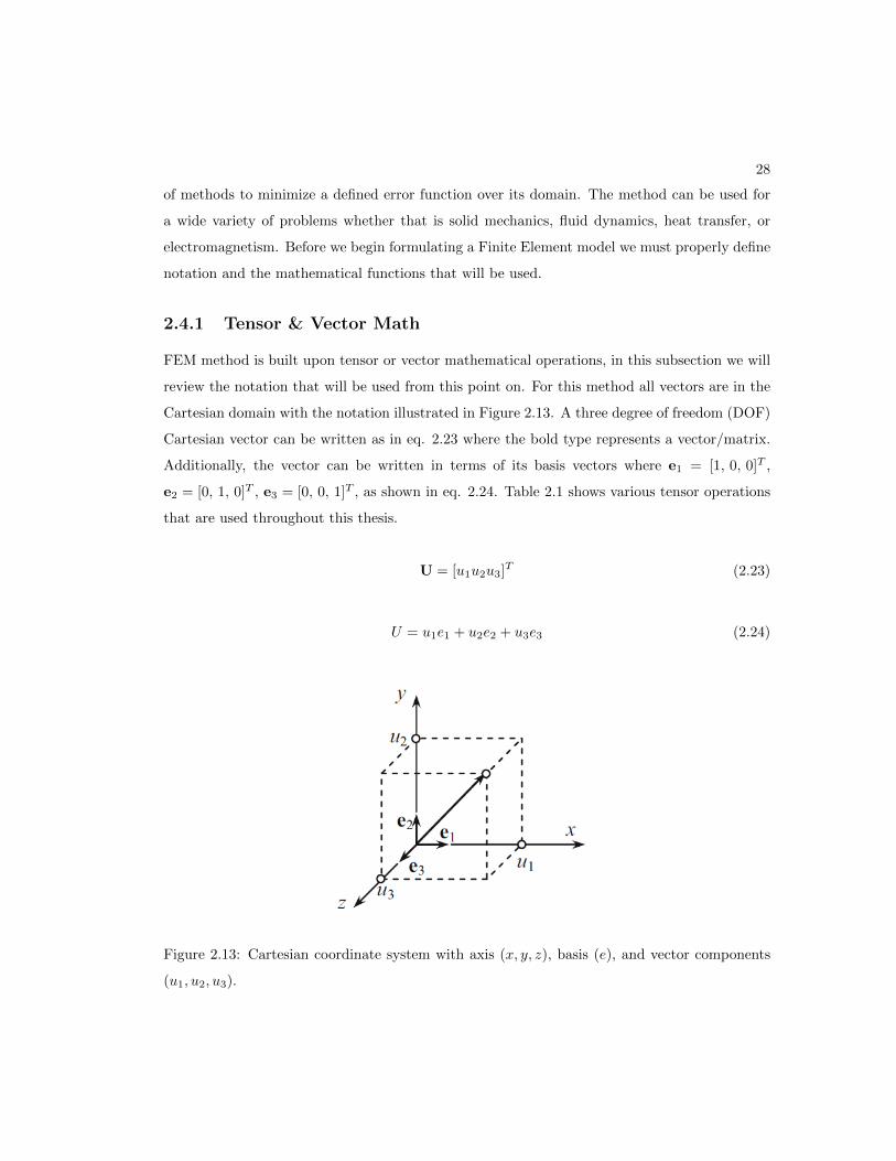
2.4.1 Tensor & Vector Math

FEM method is built upon tensor or vector mathematical operations, in this subsection we will

review the notation that will be used from this point on. For this method all vectors are in the

Cartesian domain with the notation illustrated in Figure 2.13. A three degree of freedom (DOF)

Cartesian vector can be written as in eq. 2.23 where the bold type represents a vector/matrix.

Additionally, the vector can be written in terms of its basis vectors where e1 = [1, 0, 0]T ,

e2 = [0, 1, 0]T , e3 = [0, 0, 1]T , as shown in eq. 2.24. Table 2.1 shows various tensor operations

that are used throughout this thesis.

U = [u1u2u3]T (2.23)

U = u1e1 + u2e2 + u3e3 (2.24)

Figure 2.13: Cartesian coordinate system with axis (x, y, z), basis (e), and vector components

(u1, u2, u3).

29

Table 2.1: Tensor operations with their matrix alternatives.

Tensor notation Tensor component notation Matrix notation

c = ab c = aibi c = aT b

A = a⊗ b Aij = aibj A = abT

b = Aa bi = Aijaj b = Aa

b = aA bj = aiAij c = aTA

2.4.2 Stress & Strain

The linear definition for stress and strain was developed by Robert Hooke [64]. In his defini-

tion stress was described as a force over an area and strain was described as change in length

over original length for one dimension. Later on a generalized Hooke’s law was created which

described stress in a three dimensional body.

The second order stress tensor is shown by eq. 2.25, the stress tensor has six degrees of

freedom and can be described by a 6x1 vector using Voigt notation as shown in eq. 2.25.

σ =

σ11 σ12 σ13

σ21 σ22 σ23

σ31 σ32 σ33

(2.25)

Stress Classification Surface Tractions describe an applied force per unit area. Consider

the specimen undergoing a surface force in Figure 2.14. The tensile forces F causes a surface

traction on the cross section of the specimen. This can be visualized when you take a cut of the

specimen and break down the force into pressure by looking at a small area ∆A using eq. 2.26.

Where t(n) is the surface traction and n represents the direction of the force.

30

Figure 2.14: Specimen undergoing multiple surface forces. The traction force is represented by

T (n) which is referred to as t(n) in this document [65].

t(n) = lim∆A→0

∆F

∆A(2.26)

The traction force can be broken down into its coordinate directions as shown in eq. 2.27.

If we consider (1) to be a traction acting in the 1-direction on the 12-plane then t1 is the

normal stress, and t2 and t3 are the shear stresses. This is akin to the standard stress definition

of σ11 being a normal stress to a force in the 1-direction while σ12 and σ13 are the shear

directions. Similarly, if the force is acting in 2-direction the normal component is σ22 and the

shear components are σ23 and σ21. Likewise for the 3-direction σ33 is the normal stress and

shear components are σ31 and σ32.

t(n) = t1e1 + t2e2 + t3e3 (2.27)

The normal and shear stresses can best be described by looking at a cube as shown in Figure

2.15. The cube is only used as a representation and holds all geometries as ∆V goes to zero.

31

Figure 2.15: Stress components acting on a unit cube [66].

Since there are only six DOF, the nine components of stress need to be reduced. If we

look at an infinitesimally small cube as shown in Figure 2.15 we can see that in order to reach

equilibrium symmetry must be applied. If the infinitesimally small cube is in equilibrium then

the shear stress σ12 must be equal to σ21 in order to prevent an imbalance in the moment.

This must also hold for the shear stress in the other two directions resulting in the symmetry

constraints of in eq. 2.30.

σ12 = σ21 (2.28)

σ23 = σ32 (2.29)

σ13 = σ31 (2.30)

When the symmetry constraints are added to the stress tensor in eq. 2.25 a reduced stress

tensor is created.

σ =

σ11 σ12 σ13

σ12 σ22 σ23

σ13 σ23 σ33

(2.31)

Eq. 2.31 can now be fully represented by six DOF and can be written in a 6 × 1 vector, this

32

is also known as Voigt notation.

σ =

σ11

σ22

σ33

σ12

σ23

σ13

(2.32)

Hydrostatic & Deviatoric Stresses The hydrostatic and deviatoric stresses can be found

from eq. 2.31. The hydrostatic stress or mean stress commonly relates to volume changes and

is found by eq. 2.33.

p =1

3tr(σ) =

1

3σii =

1

3(σ11 + σ22 + σ33) (2.33)

The deviatoric stress relates to the surface changes and is found by subtracting the hydro-

static stress from eq. 2.31.

s = σ − pI =

σ11 − p σ12 σ13

σ12 σ22 − p σ23

σ13 σ23 σ33 − p

(2.34)

Principle Stresses & Stress Invariants The principle stress is the maximum stress acting

on a given part in the three normal directions. These stresses are indicated by σ1, σ2, & σ3

and is written in such a way that σ1 >= σ2 >= σ3. The principle stress is determined when

the surface normal and surface traction are in the same direction. This can be represented in

eq. 2.35 where σn is the normal stress which also represents the eigenvalue and n represents the

direction of the stress and the eigenvector. Rearranging eq. 2.35 allows for the solution of σn.

σ · n = σnn (2.35)

(σ − σnI) · n = 0 (2.36)

33

Since n must hold the unity constraint, eq. 2.36 can be solved for with a determinant.

s = σ − pI =

∥∥∥∥∥∥∥∥∥σ11 − σn σ12 σ13

σ12 σ22 − σn σ23

σ13 σ23 σ33 − σn

∥∥∥∥∥∥∥∥∥ = 0 (2.37)

The 3x3 determinant in eq. 2.37 results in a cubic polynomial in the form of eq. 2.38 where

I1, I2, & I3 are the stress invariants. The stress invariants are found by solving for eq. 2.38 and

can be expressed by eq. 2.40-2.42.

σ3n − I1σ2

n + I2σn − I3 = 0 (2.38)

I1 = σii = σ11 + σ22 + σ33 (2.39)

I2 = σ11σ22 + σ22σ33 + σ33σ11 − σ212 − σ2

13 − σ223 (2.40)

I3 = |σ| = σ11σ22σ33 − σ11σ223 − σ22σ

213 − σ33σ

212 + 2σ12σ13σ23 (2.41)

(2.42)

2.4.3 Strain

Strain occurs when a force is subjected to an object causing the object to deform. The mea-

surement of this deformation into a unitless number is called strain. Unlike stress, strain can be

defined by several methods so it is important to create clear notation for which strain definition

is being used.

2.4.4 Finite Element for 3D Hexahedron Elements

We begin creating the finite element model by formulating the mathematical model with the

minimum total potential energy. The total energy in the elastic system is the stored energy

from strain, Πint subtracted by the external energy from the external forces Πext as described

by eq. 2.43. If we use a constitutive law’s strain energy function W (E) and add in body and

traction forces we can expand out eq. 2.44.

34

Π(u) = Πint(u)−Πext(u) (2.43)

Π(u) =

∫∫∫V0

W (ε)dΩ−∫∫∫

V0

uT fbdΩ−∫

Γ0

uT tdΓ (2.44)

Where,

Ω is the surface.

fb is the body force (gravitional force if included).

t is the surface traction forces.

Γ is the boundary which the surface forces act on.

ε is the Lagrangian strain in eq. 2.19.

A perturbation method is used to find a virtual displacement and solve eq. 2.44 at the

minimum energy. If we perturb the displacement field in the direction u and by the magnitude

τ then we can express the perturbation by eq. 2.45.

uτ = u+ τ u (2.45)

The first order variation of the potential energy is taken in the direction of u as τ tends

towards zero.

Π(u, u) = limτ=0

d

dτΠ(u+ τ u) (2.46)

Next we evaluate the minimum potential energy equation (eq. 2.44) with the first variation

(eq. 2.46).

Π(u, u) =

∫∫∫V0

S(ε) : εdΩ−∫∫∫

V0

uT fbdΩ−∫

Γ0

uT tdγ = 0 (2.47)

Where S(ε) the second Piola-Kirchoff Stress is defined as:

S(ε) =∂W (ε)

∂ε(2.48)

35

In eq. 2.47 we can see a linear relationship between the work done by the applied loads and

displacements u. Eq. 2.47 can be broken down into a load form and energy form. The load form

contains the body and surface forces as expressed by eq. 2.49 while the energy form contains

the internal energy being built up in the body as dictated by the constitutive law as the part

deforms as shown in eq. 2.50.

l((u)) =

∫∫∫V0

uT fbdΩ +

∫Γ0

uT tdΓ (2.49)

a(u, u) =

∫∫∫V0

S(u) : ε(u, (u))dV (2.50)

As seen from eq. 2.50 the energy form is nonlinear and a linearization scheme is needed to

readily solve eq. 2.47.

Linearization and Formation of the Tangent Stiffness Matrix

Since eq. 2.47 cannot easily be solved due to its non-linearity, an iterative approach using

Newton-Raphson (NR) method can be used to obtain a solution with a defined residual R. The

updated eq. 2.47 is rewritten with the residual R.

R = a(u, u)− l(u) (2.51)

The NR method uses the Jacobian of the residual in each iteration. Where the Jacobian is

the derivative of the force-displacement curve at the given iteration point.

To implement the NR method we need to linearize eq. 2.51. Since l(u) is independent from

u it does not need linearization. The energy form a(u, u) is a function of u and we linearize 2.50.

L[a(u, u)] =

∫∫∫V0

[∆S : ¯ε+ S : ∆¯ε]dV (2.52)

Where,

∆S is the stress increment.

∆¯ε is the increment of strain variation.

36

When a material constitutive law is linearized we can derive the stress increment as:

∆S =∂S

∂ε: ∆E = D : ∆ε (2.53)

If we substitute the stress increment (eq. 2.53) and the Lagrangian Strain (eq. 2.19) into

the linearized energy form (eq. 2.52) and we can form the tangent stiffness matrix.

L[a(u, u)] =

∫∫∫V0

[¯εD : ∆ε+ S : ∆¯ε]dV (2.54)

Shape Functions

Shape functions are used to transform the part coordinates (x, y, z) into a reference coordinate

system which ranges from -1 to 1 in the ξ = (ξ, η, κ) as shown in Figure 2.16. This reference

coordinate system is created to ease the integration of the eq. 2.54.

Figure 2.16: Coordinate transformation for a hexahedron elements from the part coordinate

(x, y, z) into a reference coordinate system ranging from -1 to 1 in the ξ = (ξ, η, κ).

To convert between the two coordinate systems we use shape functions. For a hexahedron

element the shape functions are defined as:

Ni =1

8(1 + ξξi)(1 + ηηi)(1 + κκi) (2.55)

Where (ξi, ηi, κi) denote the natural coordinates of either [−1 1].

The element displacement and location can be expressed by eq. 2.56 and eq. 2.57, respec-

tively.

37

u(ξ) =

Ne∑i=1

ui (2.56)

X(ξ) =

Ne∑i=1

Xi (2.57)

Solving for Finite Element

The variation of the Lagrangian strain ε can be written in eq. 2.58 where u is the variation

of the displacement vector, and BN is the nonlinear strain-displacement matrix. The strain-

displacement matrix relates strain and displacement with the deformation gradient, F , and the

derivative of the shape functions. Each node of the element can be described by eq. 2.59 they

can be combined to form the strain-displacement for the entire element as written in eq. 2.60.

ε = BN u (2.58)

BNI =

N1,IF11 N1,IF21 N1,IF31

N1,IF12 N1,IF22 N1,IF32

N1,IF13 N1,IF23 N1,IF33

N1,IF12 +N2,IF11 N1,IF22 +N2,IF21 N1,IF32 +N2,IF31



(2.59)

BN =(BN1

BN2... BN8

)(2.60)

If we substitute eq. 2.58 into eq. 2.54 then we can form the structural and internal energy

forms described by eq. 2.61 & eq. 2.63.

∫∫∫V0

[εD : ∆ε]dV =

∫∫∫V0

[BTNDBN ]dV (2.61)

38

∫∫∫V0

[S : ∆¯ε]dV (2.62)

=

∫∫∫V0

[BTGΣBG]dV (2.63)

Where BG provides a linear relationship between stress and strain described by eq. 2.64 and

eq. 2.64. The Σ is a block representation of the internal stress described by eq. 2.66.

BGI =

N1,1 0 0

N1,2 0 0

N1,3 0 0

0 N2,1 0

0 N2,2 0

0 N2,3 0

0 0 N3,1

0 0 N3,2

0 0 N3,3

(2.64)

BGI =(BG1

BG2BG3

BG4BG5

BG6BG7

BG8

)(2.65)

BGI = diag(S S ... S

)(2.66)

The tangent stiffness matrix can then be defined by recombining eq. 2.61 and eq. 2.63 to

form eq. 2.67

K =

∫∫∫V0

[BTNDBN + BT

GΣBG]dV (2.67)

The Potential Energy residual in eq. 2.51 can be rewritten and then used to find the dis-

placements as a linear equation as described by eq. 2.68.

K∆U = fext − fint (2.68)

39

Causes of Nonlinearities

There are several causes of nonlinearities that arise in mechanics problems. The first are geo-

metric nonlinearities which occur when the deformations are large and ε(x) = du(x)dx does not

represent the deformation. The second are material nonlinearities, which occurs with nonlinear

constitutive laws, elasto-plastic materials, or viscoelastic materials. The third nonlinearities are

kinematic which occur when contact of two linear materials cause a nonlinear force-displacement

curve. The fourrh nonlinearities are Force. Force nonlinearities occurs with inflation due to a

fluid. The pressure always stays normal so more deformed areas will experience more force.

FEM Programs

There are several commercial Finite Element Programs. Abaqus is a commercial finite element

program which can solve nonlinear finite element problems. Scripting can also be used in Abaqus

to expediate the creation of FEM models. Similar to Abaqus is Ansys which is another fully

integrated finite element solver. A couple of other solvers are Comsol and FEBio. Comsol is an

easy to use FEM program, but does not have as many capabilities as Abaqus or Ansys. FEBio

is a finite element program developed at the University of Utah. This program specializes in

solving tissue mechanics problems and can be used to solve for large deformations.

2.5 Background on Material Property Estimation

2.5.1 Elastography

The goal behind Elastography is to detect tumors from healthy cells by differences in stiffness.

This is done by estimating the spatial elastic properties of 2D soft tissues through medical strain

images. The medical strain images are collected by applying a small quasi-static compression

load on the tissue and using RF A-lines to estimate the local axial motions by means of a

correlation technique before and after the compression [67]. The axial motions can then be used

to construct a strain field and create medical strain image.

Elastography can be broken down into two main approaches. The first approach takes in

a strain medical image and directly converts the image to a Young’s modulus using Hooke’s

law [68]. For 2D strain maps, the Elastography method can reliably reconstruct a tissue’s

Young’s Modulus when the internal forces are known. This is only feasible in a few cases and

40

will not work in most tissue or engineering estimation problems. The second method involves

reconstruction of the Young’s Modulus by creating an inverse problem using the finite element

framework [67, 68, 69, 70].

In order to reconstruct the tissue stiffness, an inverse problem is created. To begin the

inverse problem the external forces, displacements, and geometry must be known. A mesh of

the 2D geometry is created and a Poisson ratio is set to 0.49. Next, an iterative approach is

used as outlined with a flowchart Figure 2.17. The basic outline of the Elastography process is

to define all the inputs, make a guess of elasticity distributions, determine the deformation with

the current properties, and then update the properties with a Jacobian of displacement with

respect to material properties until a residual is met.

Figure 2.17: Flowchart of the Elastography reconstruction algorithm from [67].

41

To smooth the Elasticity reconstruction and reject measurement noise a filter can be used.

One method is to post filter using a spatial low pass filter over all the elements [67, 68]. The

results of the post filter can be seen in Figure 2.18 Alternatively, a second objective can be added

into the material update which penalizes differences in neighboring elements [69, 71]. More

recent work has focused on reducing the number of known points that are needed. Moriata et

al. developed a method where the update only utilizes observed nodes and ignores nodes that

were not observed [72]. The Elastography method can successfully reconstructs the Young’s

Modulus for 2D problems as shown in Figure 2.18. The research for this method have not

focused heavily on large deformations, 3D geometry, or nonlinear material laws.

42

Figure 2.18: Elastography algorithm applied with a post filtering processes. Sub-image A-C

shows an increase in the filter weight [68].

2.5.2 Parameter Estimation

In addition to Elastography, several other papers have come out on solving the inverse problem

to determine material properties. One such paper reconstructed a neo-Hookean material of a

uniform flat circular membrane when an axisymmetric and nonaxisymmetric finite inflations are

applied [73]. Another study aimed to reconstruct the Young’s Modulus of 3D objects using an

inverse Finite Element approach when the displacement contained a large degree of noise [74].

Fachinotti et al. created a large deformation inverse finite element model where the anisotropic

43

Young’s modulus in the x, y, & z were reconstructed [75]. This method was applied to a turbine

and the three Young’s modulus were reconstructed. While these methods are able to solve their

specific problems, they are unable to reconstruct material properties where large deformations

and hyperelastic constitutive laws are needed.

Chapter 3

Soft Robot Design for Traversing

a Tube-Like environments

This chapter consists of an IEEE Robotics and Automation Letters (Section 3.1) as well as a

conference paper submitted to ASME Design of Medical Devices Conference (Section 3.2), and

ASME Dynamic Systems and Control Conference (Section 3.3).

This chapter covers various soft robotic design techniques in the aim of building a soft robot

that is able to navigate tubes or blood vessels as shown in Figure 3.1. First, the design of

an underactuated hydraulically powered soft robot that can traverse a pipe is designed and

experimentally tested. Next, a study is performed to evaluate the design space of passive

conical valves. Finally, a bending actuator is modeled for its force outputs in a constrained and

unconstrained environment.

44

45

Figure 3.1: The proposed soft robot navigating through a tube. The robot consists of a tethered

base; three segments for locomotion described in Section 3.1, each containing a valve and an

actuator; and an end-effector made up of a bending (Section 3.3) and twisting actuators as well

as a theranostic tip.

3.1 Serially actuated locomotion for soft robots in tube-

like environments

The goal of this soft robot is to successfully traverse a tube. Since the longterm vision of the

design is to create a medical catheter, it is imperative that the design be scalable and that blood

flow around the robot is not stopped. This section will discuss the design and actuation method

of the three locomotion segments (Spiral, Extender, Spiral) as shown in Figure 3.1. Previous

work has focused on the serial control using complex valves, which can be difficult to scale and

result in slower locomotion. However, in this chapter we aim to close the existing gap in current

soft robots by producing a serially actuated, soft robot using passive valves while simultaneously

allowing flow throughout locomotion in tube-like environments.

The novel contribution of this section is a generalizable method for designing soft robots to

locomote through a specific tube geometry that simultaneously: (1) uses only passive compo-

nents with no moving parts (i.e. simple orifice valves, unlike [76]), (2) is serially actuated (i.e.

requires only one power source, unlike [31]), and (3) utilizes a geometry that avoids blocking flow

while maintaining high contact area for anchoring force (i.e. a spiral actuator unlike a balloon

[31] or bending actuator [53]). This includes experimental validation.

The layout of this work is as follows. First, in subsection “Overall Design”, we discuss the

design of the robot based on ideal and theoretical models. In subsection “Model Components”,

46

we discuss the modeling of the actuators and valves which make up the robotic segments. Ob-

jectives will be set for the actuators and valves such that optimal robot locomotion is achieved.

In subsection “Physical Realization and Targeted Task”, the task of the robot is specified in-

cluding the desired geometry, pressures, and dynamic response. In sections “Actuator Design

and Construction” and “Valve Design and Construction”, we present the necessary actuator and

valve designs needed to achieve the task, respectively. The chapter concludes with a discussion

of the experimental results and future work.

3.1.1 Methods

Overall Design

Ideal Robot Design The goal of this chapter was to produce a design method for a soft robot

capable of traversing a cannula through serial actuation as shown in Figure 3.2. The proposed

robot consisted of three segments, each including an actuator and a valve. The first and third

segments contained spiral actuators to anchor into the cannular wall, while the second segment

utilized an extending actuator to produce locomotion. A spiral geometry was chosen to allow

locomotion to occur while also making the robot adaptable to environments where flow through

the cannula must be maintained (e.g. vasculature procedures, pipe inspection).

Figure 3.2: Soft robot locomoting through a cannula. The robot consists of a tethered base and

three segments, each containing a valve and an actuator. The spiral shapes prevent blockage of

fluid flow. The cap represents the end effector.

The serial combination of the multiple segments and the control of the flow into each actuator

with the valves provided the rationale for the ideal locomotion sequence represented by the events

labeled in Figure 3.3. Within the ideal sequence, the robot starts in its nominal unactuated state

(Figure 3.3 event A), then the first segment actuates, forming a spiral and anchoring into the

wall of the cannula (Figure 3.3 event B). While the first actuator remains anchored, the second

47

segment actuates, causing extension along the cannula (Figure 3.3 event C). This is followed by

the actuation of the third segment (Figure 3.3 event D). To move the robot along the cannula,

the actuators are deflated in the same order of actuation (Figure 3.3 events E-G). This sequence

is repeated until the robot reaches its destination.

Figure 3.3: (a) Ideal actuation and timing events of the soft robot actuators. (b) Volume

response of each actuator corresponding to the ideal actuation events (Events labeled A-G).

48

The ideal timing of each actuator is shown in Figure 3.3(b), where each timing event corre-

sponds to a state in Figure 3.3(a). The volume-time relationship is crucial because the volume

of liquid within each actuator directly translates to the pose of that actuator. There are two

important volumes for the actuators. The first is the contact volume, Vc, which is the volume

at which the spiral actuators (Act 1, Act 3 ) make contact with the cannula wall. The second

important volume is the final volume, Vf , which represents fully anchored spirals for Act 1 and

Act 3, and a fully extended actuator for Act 2.

Theoretical System Model For the purpose of modeling the pressures and volumes within

the system, the valves were modeled as flow restricting orifices, and the actuators were modeled

as nonlinear-spring-loaded hydraulic accumulators (Figure 3.4).

Figure 3.4: Theoretical model showing each segment modeled as a flow restrictor and an accu-

mulator.

The robot was driven by a pressure source. The resulting volume change for each segment

was described by the following system of differential equations for the flow rates:

V1 = fvalve1(u, PAct1)− fvalve2(PAct1 , PAct2)

V2 = fvalve2(PAct1 , PAct2)− fvalve3(PAct2 , PAct3)

V3 = fvalve3(PAct2 , PAct3)

(3.1)

where u is the pressure input, fvalvei describes the flow through a restricted orifice, and PActi is

an equation to describe the behavior of the pressure in the ith accumulator based on its material

properties.

49

Model Components

Actuator (Accumulator) Model The actuator was modeled as a nonlinear-spring-loaded

accumulator. The volume coefficient, V , was the independent variable defined as the ratio of

final actuator volume to initial actuator volume (eq. 3.2) and the internal pressure, P , was the

dependent variable.

V =VfVi

(3.2)

A polynomial function (eq. 3.3) modeled the nonlinear-spring-loaded accumulator where

the coefficients, cn, could be estimated using least squares from pressure-volume data for each

actuator. The polynomial order, nf , was increased until a residual, res (eq. 3.6), less than 2.5%

was reached.

PActi =

nf∑n=1

cn ˆ(V )n

(3.3)

for nf such that e < 2.5% where

ˆ(V ) = V − 1 (3.4)

e = |res(n)− res(n− 1)|/res(n− 1) (3.5)

res =

[ tf∑t=0

(P − [V ... V n][c1 ... cn]T )2

]1/2

(3.6)

The following assumptions were made: the loading on the rubber in the nonlinear-spring-

loaded accumulator was time invariant, exhibited no creep, hysteresis effects were negated [56],

and that derivations from such assumptions resulted in negligible error.

Valve (Flow Restrictor) Model The flow restrictors were modeled using the orifice equation

(eq. 3.7), which described fluid flow through a restricted orifice and was governed by the valve

coefficient, Ki (eq. 3.8), and pressure drop, ∆P [77].

fvalve = Kisgn(∆P )√|∆P | (3.7)

50

The valve coefficient, as determined by the orifice equation, was defined as:

Ki = CdAorfi

√2

ρf(3.8)

where Cd is the discharge coefficient is set for turbulent flow equaling 0.62, Aorfi is the cross-

sectional orifice area, ρf is the density of the fluid equal to 997.45 [kg m−3] (at 23C), and i

indicates the valve index. Although the orifice equation is a steady state model, we assumed

this model holds true throughout actuation of the robot.

Physical Realization and Targeted Task

Task To illustrate our general methodology, the specified task for the robot design was to

locomote through a cannula (D = 19mm) using a combination of segments that occluded the

cannula by less than 50% and experienced pressures under 200 kPa. The timing of the actuation

needed to follow Figure 3.3. This meant that Act 1 must anchor before extension of Act 2

contributed to locomotion. Additionally, Act 2 must be near its final volume before Act 3

anchored. This prevents Act 2 from buckling or wasting motion.

Actuator Design and Construction

Actuator Design To achieve the desired area occlusion ratio, the actuators inner radius was

chosen as r=5mm with 0.8mm thickness, resulting in an area occlusion ratio of 37%.

To achieve the actuator shapes shown in Figs. 3.2 and 3.3, FREE actuators were used.

FREE actuators utilize two or three varying wrap angles α, β, γ, as shown in Figure 2.4, to

create spiral or extending actuators [16],[35]. The derivation of the FREE model relied on fiber

inextensibility resulting in the geometric relations in eqs. 3.9-3.11. The following derivation of

eqs. 3.9-3.16 are attributed to and detailed in [16]-[37].

Figure 3.5: FREE wrap angles and stretch parameters from Bishop-Moser et al. [35].

51

λ21c

2α + λ2

2s2α(θ + δ

θ) = 1 (3.9)

λ21c

2β + λ2

2s2β(ζ + δ

ζ) = 1 (3.10)

λ21c

2γ + λ2

2s2γ(ψ + δ

ψ) = 1 (3.11)

θ =Ltan(α)

r, ζ =

Ltan(β)

r, ψ =

Ltan(γ)

r

where cα = cos(α), sα = sin(α), and L represents the overall length of the actuator.

The radial stretch parameter, λ2, and axial twist, δ, were solved as functions of the axial

stretch parameter, λ1. This was done by substituting eq. 3.9 into eq. 3.10, resulting in eq. 3.12

and eq. 3.13, respectively.

λ2 =

α|α|cβ

√1− c2αλ2

1 −β|β|cα

√1− c2βλ2

1

sα−β(3.12)

δ =L

r

β|β|sα

√1− λ2

1c2β −

α|α|sβ

√1− λ2

1c2α

α|α|cβ

√1− λ2

1c2α −

β|β|cα

√1− λ2

1c2β

(3.13)

The volume coefficient, V , was used to obtain a solution for λ1 and was also an input to the

system. V can be expressed in terms of stretch parameters:

V = λ1λ22 (3.14)

To solve for λ1, the Newton Raphson method was applied to eqs. 3.12 and 3.14 with an

initial condition of λ1 = 1 [36]. For spiral actuators consisting of three separate fiber angles,

the helix radius, R (eq. 3.15), was defined as the radius of the spirals. The helix radius as well

as the helix angle, φ (eq. 3.16), are depicted in Figure 3.6 and their derivation can be found in

[35].

Figure 3.6: Pertinent dimensions for a FREE spiral within a tube.

52

R =ρ

1 +(

(δ+ψ)ρL

)2 (3.15)

φ = arctan((δ + ψ)ρ

L) (3.16)

where ρ is provided in [35].

To demonstrate our generalizable method, we target actuators capable of forming the desired

spiral in Figure 3.2 as dictated by a specific task (i.e. traversing a D = 19mm diameter tube).

This informed the specific design criteria, which were fed into a cost function. The first constraint

was to set the volume coefficient to V = 1.30 which was used for both spirals and the extending

actuator. A V = 1.30 was chosen because it is large enough to produce the desired R and stable

enough to obtain solutions before geometric lock (e.g. see [16]). For the actuator to successfully

traverse a tube, R must be greater than or equal to D/2 (Figure 2.5). The selection for this

desired helix radius, R, was D/2. This assumed traction forces large enough to anchor the

actuator in the cannula since the spiral was able to compress twice the radius of the actuator

on the cannular wall. Next, we aimed to maintain constant overall axial length of the spiral

actuator in the x-direction, λx, as shown by eq. 3.17. A constant value was chosen as it reduces

slip between the cannula and actuator between contacting and anchoring.

λx = λ1Lcos(φ)√cos−2(φ)− 1 (3.17)

The final objective of the cost function was to minimize the axial twist, δ, of the actuator

(i.e. δ = 0) to minimize shear on the tube wall and maximize the efficiency of the robot. A

simple grid search with a constant step size of 1.0 was performed over all α, β, γ permutations

and the linear quadratic cost function (eq. 3.18) was evaluated with the design parameters in

Table 3.1. The α, β, γ values that minimized cost were taken to be the optimal fiber wrap

angles. The value for r was chosen based on the off-the-shelf latex tubing used to manufacture

the actuators.

53

Table 3.1: Task-Specific Design Parameters for D = 19mm

r L R λx δ

5mm 300mm D/2 1.0 0.0

minimizeΦ

ΦTQΦ

subject to α, β, γ ∈ [−90, 90]

(3.18)

where

Φ = [R−R, λx − λx, δ − δ] (3.19)

Q = I3x3 (3.20)

The second actuator was an extending McKibben actuator that was specified to consist of

equal but opposite fiber wrappings greater than 54.7. The goal of the second actuator was to

extend without buckling. The wrap angles of the extending actuator were determined through

an empirical study, which examined the relationship between wrap angle, actuator buckling, and

actuator extension. The volume coefficient for this actuator was the same as the spiral design,

V = 1.30.

To identify the parameters in eq. 3.3 for the kinematic actuator model using a pressure

input, an experiment was performed. The nonlinear-spring-loaded accumulator model shown in

eq. 3.3 was applied. Since the system was filled with water, we assumed incompressibility. The

relationship between PActi and V were found experimentally by inputting a sine wave on volume

using the characterization hydraulic test bench shown in Figure 3.7. The test bench recorded

the volume coefficient, V , and actuator pressure, P , at 100 Hz. Eq. 3.3 was then applied to

determine the number of coefficients and their respective values with least squares.

54

Figure 3.7: Closed hydraulic circuit test bench: A) linear actuator B) LVDT C) cylinder piston

rod D) stroke cylinder E) tubing leading to the FREE actuator.

Actuator Construction

The FREE actuators were constructed by turning fibers onto a latex tube (Kent Elastomer

Products, Inc.) as shown in Figure 3.8. A dipping process was used to secure the wrapped

fibers in place. Each wrapped actuator was dipped three times into a 50/50 distilled water-latex

(TAP Plastics Premium Liquid Latex Rubber) mixture with a two hour cure time between dips.

The stretchability of the latex tubing allowed for sufficient motion of the actuators while

keeping pressures under the task specification of 200 kPa.

Figure 3.8: Computer-controlled lathe modified to wrap fibers at desired α, β, γ wrap angles

onto a latex tubing.

Valve Design and Construction

Valve Design To create a model for the soft robot, eqs. 3.3 and 3.7 were substituted into eq.

3.1 to create the dynamic equations shown in eq. 3.21. The input pressure, u, was selected to

be a pressure square wave between 0 and 83 kPa (12 psi) with a two second period.

V1 = K1

√u− P1

′−K2

√P1 − P2

′

V2 = K2

√P1 − P2

′−K3

√P2 − P3

′

V3 = K3

√P2 − P3

′

(3.21)

55

Optimization of the resulting model (eq. 3.21) was performed with the design parameters

being the valve coefficients, Ki, of the valves. The optimization had two objectives. The first

was to maximize the volume change of Act2 while Act1 was anchored into the cannula, tB , and

before Act3 had contacted the cannula, tC , during the inflation phases, Vfwd (eq. 3.22). The

second goal was to maximize the volume change of Act2 between Act1 releasing contact from

the cannula, tE , and Act3 unanchoring, tF , during the deflation, Vrev (eq. 3.23). Vfwd and Vrev

were then combined into a single objective function which aimed to maximize their value while

keeping their volume changes the same (eq. 3.24). See Figure 3.3 for event time labels tB , tC ,

etc.

Vfwd = VAct2(tB)− VAct2(tC) (3.22)

Vrev = VAct2(tE)− VAct2(tF ) (3.23)

maximizeK2,K3

Jvol = [V 2fwd V 2

rev][c1 c2]T − c3|Vfwd − Vrev|2

subject to K2,K3 = [0,K1]

(3.24)

where ci = 1 for i = 1, 2, 3.

The robot response to the chosen input was simulated using MATLAB and Simulink. The

simulation utilized the nonlinear-spring-loaded accumulator model, PActi (eq. 3.3), and the

orifice equation, fvalve (eq. 3.7), to simulate the robot model in eq. 3.1. A square wave with

an amplitude of 83 kPa gauge pressure and frequency of 0.5 Hz was used as the input. The

pressure was chosen based on the material characteristics of the actuator. The frequency was

chosen because it was intuitive for human users and is on the order of a resting heart rate, thus

avoiding subjecting anatomy to foreign frequency content. The contact and anchoring volume

coefficients were defined as 1.13 and 1.30 as dictated by the actuator design.

To ensure that Act 1 actuated as quickly as possible, the cross-sectional orifice area, Aorf1 ,

was set to its maximum value dictated by the valve geometry. This maximized the valve coef-

ficient through valve 1. The simulation performed a grid search over K2 and K3 for values less

than or equal to K1 using a constant step size of 5.0x10−7m2. An optimal value for K1 was not

incorporated into the objective function because valve 1 was made to allow as much flow into

Act 1 as possible, making K1 the largest possible value determined by the valve’s cross-sectional

56

area. Eq. 3.24 was then evaluated and the K2, K3 combination which maximized Jvol was taken

as the optimal dynamic response.

Valve Construction The desired valves were constructed by placing flexible tubing within

a barbed fitting, inserting a set screw into the fitting wall, then setting the tubing with cast

polyurethane (TAP Plastics, One-to-One Polyurethane Casting Resin) (Figure 3.9). The set

screw allowed for adjustments in the flow restrictor opening, changing the effective Ki.

Figure 3.9: A manufactured passive valve. The process used to manufacture valves is as follows:

begin with a barbed fitting compatible with actuator size; insert set screw into the fitting wall;

back out set screw and insert flexible tubing; fill empty space with polyurethane resin.

To match the flow restrictor with the Ki’s found by the simulation, the characterization

hydraulic test bench (Figure 3.22) was used with the flow restrictor placed between two pressure

sensors. A cascading set of steps on voltage were inputted to the linear actuator, while the

pressure drop, ∆P , and piston position were recorded. The data was then filtered with a 4th

order Butterworth filter with a cutoff frequency of 10 Hz. Next, the data was segmented for

each voltage and transients were removed by attributing the data collected during the first third

of the stroke length to acceleration and evaluating the remaining data from the last two thirds

of the stroke length. The flow rate was then calculated using a noise robust differentiation [78]

based on the segmented piston position. Least squares was then applied to determine the Ki

term of the flow restrictor. If the Ki found using the test bench was above (or below) the desired

Ki, the set screw on the flow restrictor was tightened (or loosened). This process was repeated

until the target Ki from the simulation was achieved within 2%.

57

Robot Locomoting Through a Tube

Once all the valves were tuned and the actuators were built, each segment was assembled and

combined to form the robot. The locomotion hydraulic test bench was connected to the robot

and used as a pressure source. A 0.5 Hz square wave input with an amplitude of 83 kPa was

implemented with the locomotion hydraulic test bench. The robot was then placed in a cannula

of diameter D = 19mm and the segments were inflated and deflated to produce locomotion. A

panel of reviewers (N = 6) identified key timing events over 5.5 cycles of locomotion recorded

at 24fps 1080P (Cannon EOS Rebel T6).

3.1.2 Results

Actuator (Accumulator) Models and Design Outputs

The α, β, γ wrap angles which optimized cost objectives specified by the design tasks and

extender empirical study are shown in Table 3.2.

Table 3.2: Actuator Wrap Angles

α β γ

Spiral 72 −72 −14

Extender 80 −80 –∗

∗wrap angle not used.

Figure 3.10 shows the experimental results from the nonlinear-spring-loaded accumulator

experiment for a single spiral actuator. The same protocol was repeated for the other two

actuators and the resulting coefficients are listed in Table 3.3. However, the pressure volume

relationship for each actuator followed similar curves and values.

58

Figure 3.10: Nonlinear-spring-loaded accumulator relationship shown with a hysteresis loop for

actuator 1.

Table 3.3: Pressure Volume Relationship found with eq. 3.3.

c1 c2 c3 c4

PAct1 1.60 5.92 −11.14 7.18

PAct2 0.44 6.64 −8.79 4.28

PAct3 −0.28 10.61 −12.39 5.06

Valve Results

The simulation produced an objective function showing the values of Jvol (eq. 3.24) for each

combination of Ki’s in the grid search (Figure 3.11).

59

Figure 3.11: Objective function of grid search performed over Ki values, where the black dot

represents the maximum of eq. 3.24.

The values of Ki correlating to the maximum of the objective function were matched ex-

perimentally. The experimental change in pressure versus flow data for each flow restrictor was

compared to the optimal pressure versus flow data. An example of the experimental response

versus optimal response can be seen in Figure 3.12. The final values for both the optimal and

experimental Ki values are shown in Table 3.4.

Figure 3.12: Flow restrictor testing and models shown for valve 3 (transparency for steady state

data set to 15%; transient data excluded).

60

Table 3.4: Valve Resistance

Ki [m3Pa−1/2s−1] Valve 1 Valve 2 Valve 3

Optimal 1.64x10−6 3.05x10−7 4.30x10−8

Fit –∗ 3.02x10−7 4.26x10−8

Error –∗ −1.04% −0.84%

∗determined by max cross section.

After finding the optimal Ki values using the objective function shown in Figure 3.11, the val-

ues were entered into the simulation to produce the optimized volumetric response (Figure 3.13)

where Vfwd and Vrev both took 140ms. Due to the different polynomial constants describing

each accumulator, the final volume coefficients vary.

Figure 3.13: Optimized volumetric response for half an actuation period. States corresponding

to Figure 3.3 (a,b) are shown, with the extender volume objective (eq. 3.24) highlighted in bold

for Act 2. (Vi = 1.00, Vc = 1.12, Va = 1.30); (Event timings: tA = 0.00s, tB = 0.03s, tC = 0.17s,

tD = 1.00s, tE = 1.02s, tF = 1.16s, tG = 2.00s).

61

Soft Robot Modeling

The soft robot successfully traversed the cannula as shown in Fig 3.14. The robot locomoted

27 ± 4mm for each actuation cycle, which is within the deviation of the predicted locomotion

of 28mm. Figure 3.15 shows the robot locomoting through the cannula at different time steps,

allowing one to view the traversal. For both Figure 3.14 and Figure 3.15, a 5mm by 5mm grid

can be seen in the background. The images were cropped and the image was shrunk to 35% of

its original size in the horizontal direction. Additionally, the median timing of actuation was

within the measurement resolution of the prescribed timing as shown in Figure 3.16.

62

Figure 3.14: Soft robot at each event (Labeled A-G) in a cannula for a full cycle of 2 seconds.

(Compare with Figure 3.3) The grid markings in this figure and Figure 3.15 are 5mm by 5mm,

the image was cropped and the horizontally shrunk by 35%.

63

Figure 3.15: Soft robot locomotion through a cannula at different time steps. The images were

captured at full anchoring, Event D (See Figure 3.3a and Figure 3.14).

Figure 3.16: Experimental actuator timing for the forward, (tC − tB), and reverse, (tF − tE),

direction. Results found with (N = 6) independent reviewers timing all events for (N = 37) and

(N = 31). The dotted black measurement lines represent the discrete measurement resolution

with a video being recorded at 24 frames per second. Notches represent range in significant

difference in median at p = 0.05.

3.1.3 Discussion

We successfully used methodology proposed in [35] to provide ideal wrap angles for each actuator

in our robot (Table 3.2). The spiral actuator closely met the objectives described in Table 3.1.

64

The actuator pressure-volume relationship (Figure 3.10) was nonlinear and exhibited some rate-

independent hysteresis. This deviated from our assumptions, but not substantially relative to

the full pressure-volume range.

The optimization of the extension volume implies useful forward traversal locomotion. In

general, the last orifice (K3) has greater impedance than (K2) meaning that optimal tuning is

more sensitive to changes in (K3) than (K2).

The resulting optimization (Figure 3.13) shows that well over 50% of the extension volume

change results in extension as well as roughly equal and useful expansion and retraction stages.

One thing to note is that Act 3 always has a volume coefficient greater than one. This is due to

the system reaching a cyclic steady state response and Act 3 not being able to fully deflate. It is

worth noting that all three actuators have different coefficients (see Table 3.3) and different final

volumes (Vf/Vi > 1.3 in Figure 3.13) because the dipping processes was not fully repeatable

resulting in slightly different wall thicknesses.

The use of the orifice equation (eq. 3.7) to model the valves was mostly justified as seen in

Figure 3.12 with the exclusion of most transient data.

The experiment showed that the proposed design methodology succeeded at a) creating

shapes and sequences proposed in Figs. 3.2 and 3.3, b) achieved the timing suggested in Figure

3.3(b) and c) resulted in overall locomotion that was serially actuated and, by design, avoided

full occlusion of the cannula cross section thus allowing fluid flow. The actuator timing, when

accounting for measurement resolution, proved quite accurate since the mean timing for the

forward and reverse direction fell within one frame of the specified timing. Errors in the timing

could be attributed to the effect of external loading due to the contact and anchoring in the

cannula. The effect on the system’s dynamics can be seen in Figure 3.16. During inflation, the

actuator is fighting the reaction force generated due to contacting the cannula, thus extending

the time period of Vfwd. Conversely, the time period of Vrev is shorter due to the reaction

force assist the deflation gets from contact with the cannula. Our model neglected this contact

interaction, however, the resulting deviation was minimal (i.e. did not prevent locomotion).

3.1.4 Conclusion

We presented and experimentally verified a design methodology to realize task-specific, serially

actuated soft robots to traverse tube-like environments without causing full occlusion of the

65

tubular cross section. While we demonstrated this work for a specific case, it is generalizable

to other applications and environments. Such methodology can benefit multiple applications

including pipe inspection and medical catheter robots.

Currently, the methodology does not include sensing and navigation control, but instead

focuses on locomotion only. Consequently, the soft robot could locomote through bends, but

would need an additional degree of freedom to choose a particular path upon coming to a

junction.

The work presented has room for advancement. A study of occlusion ratio and pressure drop

in pipe flow will need to be evaluated. A traction model predicting the slip between the spiral

and cannula wall and effects on inflation as well as buckling or out plane motion of the extender

could be developed to greatly improve the accuracy of the predicated locomotion. Additionally,

the optimization can expand to include actuation frequency and actuator stiffness to tune robot

designs for different environments and actuator timing.

3.1.5 Specific Contributions

This research was performed with Gillian McDonald. Gillian McDonald developed the Simulink

model for optimizing valve coefficients, as well as the manufacturing method for the passive

valves. My contributions to section 3.1 was the development of a fiber wrapping lathe, the

FREE model optimization, and the experimental work.

3.2 Soft Passive Conical Valves for Serial Actuation

3.2.1 Motivation

Although much research has been performed in soft robotics, less attention has been paid to

the hydraulic valves used. Napp et al. have developed a passive bandpass valve that consists of

two moving diaphragms [76]. Unlike previous works, the valve proposed in this section consists

of a single diaphragm. The valve acts like a two-way check valve. Low pressure differentials

are blocked out while pressures above the cracking pressure are able to flow through the valve

wall, allowing each segment to fill up to a desired pressure. This section contributes a design of

asymmetrical cracking pressure valves with an empirical design table in an aim to achieve the

locomotion proposed in Figure 3.3. The design is built at a larger scale, but could be scalable

66

to catheter dimensions.

3.2.2 Methods

The design draws inspiration from the mitral valve which consists of three flaps which form a

cone. To create bi-directionality, the flaps were removed allowing the cone to invert on itself.

The inversion of the cone created asymmetric cracking pressures which was the desired design

parameters. The cracking pressure was defined as the pressure that first generated noticeable

flow through the valve. This was determined manually by measuring the pressure when water

first cracked through the valve. The valves created in Figure 3.17 show the design and flow path

for the forward and reverse flow directions.

Figure 3.17: Valve diagram showing the thickness and angle of the valve as well as the forward

and reverse flow directions.

The valves were created through a silicone molding process. A two part mold was 3D printed

(Objet260 Connex, Stratasys Inc.), which contained six varying cone angles from 0 − 50 as

shown in Figure 3.18. A 3/8” diameter bushing with a 3/8-16 UNC hole was placed into the

mold and served as the outer casing for the silicone valve. To mold the valve within the body, 8A

durometer silicone (TAP Platinum Silicone, TAP Plastics) was injected into each valve casing

and the mold was degassed. The top half of the mold was placed and a set of adjustable parallels

was used to set the thickness of the valves.

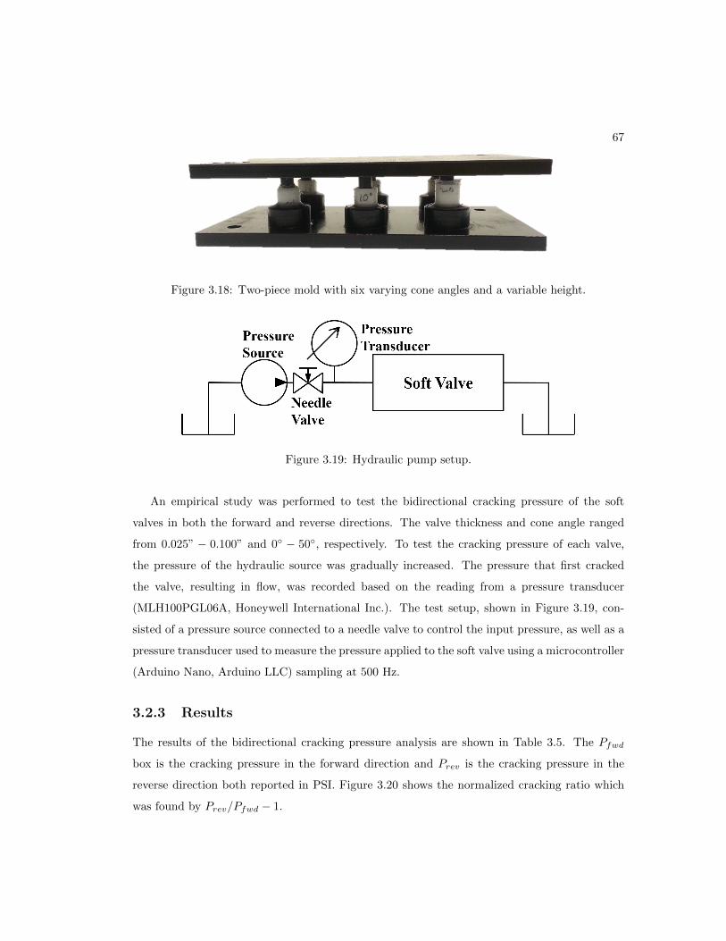
67

Figure 3.18: Two-piece mold with six varying cone angles and a variable height.

Figure 3.19: Hydraulic pump setup.

An empirical study was performed to test the bidirectional cracking pressure of the soft

valves in both the forward and reverse directions. The valve thickness and cone angle ranged

from 0.025” − 0.100” and 0 − 50, respectively. To test the cracking pressure of each valve,

the pressure of the hydraulic source was gradually increased. The pressure that first cracked

the valve, resulting in flow, was recorded based on the reading from a pressure transducer

(MLH100PGL06A, Honeywell International Inc.). The test setup, shown in Figure 3.19, con-

sisted of a pressure source connected to a needle valve to control the input pressure, as well as a

pressure transducer used to measure the pressure applied to the soft valve using a microcontroller

(Arduino Nano, Arduino LLC) sampling at 500 Hz.

3.2.3 Results

The results of the bidirectional cracking pressure analysis are shown in Table 3.5. The Pfwd

box is the cracking pressure in the forward direction and Prev is the cracking pressure in the

reverse direction both reported in PSI. Figure 3.20 shows the normalized cracking ratio which

was found by Prev/Pfwd − 1.

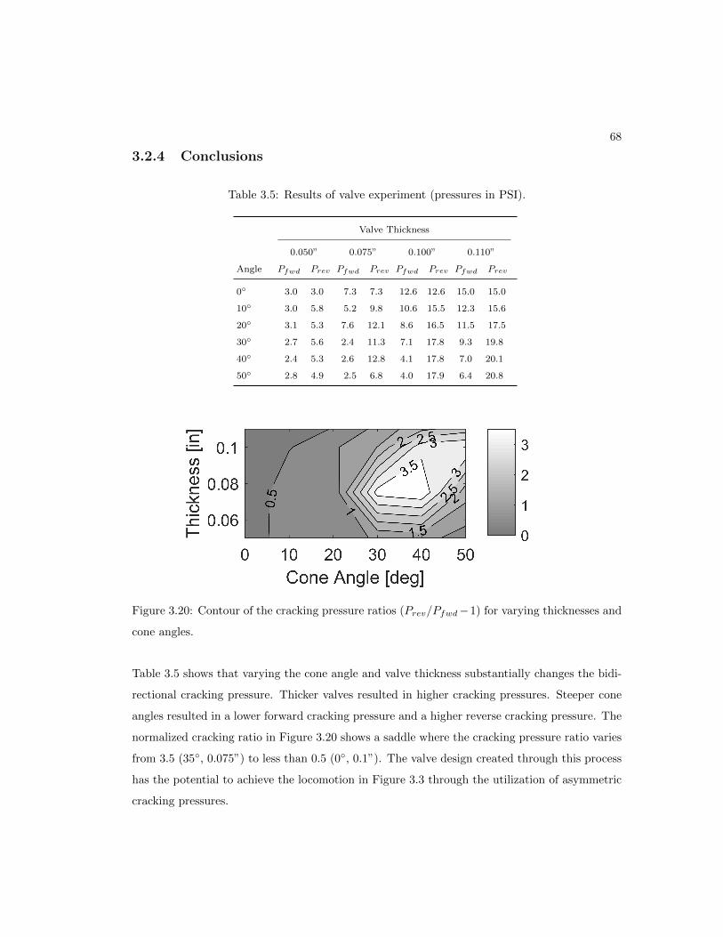
68

3.2.4 Conclusions

Table 3.5: Results of valve experiment (pressures in PSI).

Valve Thickness

0.050” 0.075” 0.100” 0.110”

Angle Pfwd Prev Pfwd Prev Pfwd Prev Pfwd Prev

0 3.0 3.0 7.3 7.3 12.6 12.6 15.0 15.0

10 3.0 5.8 5.2 9.8 10.6 15.5 12.3 15.6

20 3.1 5.3 7.6 12.1 8.6 16.5 11.5 17.5

30 2.7 5.6 2.4 11.3 7.1 17.8 9.3 19.8

40 2.4 5.3 2.6 12.8 4.1 17.8 7.0 20.1

50 2.8 4.9 2.5 6.8 4.0 17.9 6.4 20.8

Figure 3.20: Contour of the cracking pressure ratios (Prev/Pfwd−1) for varying thicknesses and

cone angles.

Table 3.5 shows that varying the cone angle and valve thickness substantially changes the bidi-

rectional cracking pressure. Thicker valves resulted in higher cracking pressures. Steeper cone

angles resulted in a lower forward cracking pressure and a higher reverse cracking pressure. The

normalized cracking ratio in Figure 3.20 shows a saddle where the cracking pressure ratio varies

from 3.5 (35, 0.075”) to less than 0.5 (0, 0.1”). The valve design created through this process

has the potential to achieve the locomotion in Figure 3.3 through the utilization of asymmetric

cracking pressures.

69

The tests were subject to several sources of error, mainly in the recording of the cracking

pressure since a manual detection of initial flow through the valve was used. Additionally,

various valves cracked with varying flow rates, which made it difficult to obtain a true and

definite cracking pressure. The normalized cracking ratio was developed to reduce the error in

the cracking pressure method by examining the relationship between the forward and reverse

cracking pressures for each valve. The results provide a promising design approach that could

be scalable for soft actuator valves. Additionally, these valves may be able to lengthen the filling

times in Figure 3.13 by the creation of unsymmetrical soft valves.

The results provide an alternative valve choice for a serially actuated soft robot. In addition

to the orifice valves described in Section 3.1, cone valves could be added to the robot simulation

to further optimize the actuator timing in accordance to Figure 3.3.

3.2.5 Specific Contributions

My contributions to section 3.2 was with the design of the conical actuators, running the ex-

periments, and developing the results. Gillian McDonald helped with the design of the conical

valves and the created the mold in Figure 3.18.

3.3 Force Analysis and Modeling of Soft Bending Actuator

3.3.1 Abstract

Soft robotic actuators may provide the means to develop a soft robotic catheter, enabling safer

and more effective transcatheter procedures. In many clinical applications, device contact force

affects the quality of diagnostic or the degree of therapy delivered. Therefore precise end effector

force control will be a requirement for the soft robotic catheter. In this study a bending soft

actuator system was fabricated, and the relationship between volume input and end effector

contact force is examined. Static and dynamic system identification were conducted under two

different loading conditions loosely related to actuation in a blood vessel. The experimental data

from these tests led to the creation of a non-linear system model. A reduced term model was

developed using a Root Mean Square Error (RMSE) method in order to observe the importance

of system dynamics and nonlinearities. A different system model was designed for each loading

condition. These two reduced models matched with experimental result, but differed in model

70

terms and parameters, suggesting that either loading condition identification or end effector

closed-loop sensing will be needed for accurate contact force control of a soft robotic actuator

in an intravascular environment.

3.3.2 Introduction

In this study, a soft bender actuator is hydraulically powered via water instead of clinically

incompatible pneumatic power, and a new force model is proposed and empirically evaluated.

This model relates input volume to output force at the end effector under two clinically motivated

loading conditions.

3.3.3 Methods

Soft Robot Design and Fabrication

The soft robotic bending actuator was designed and fabricated using the methods listed in the

Soft Robotic Toolkit [79]. The semicircular bending actuator is capable of providing higher

bending force than a circular cross section at a given pressure, which provides more efficient

force transmission at the tip. The main body of the bender was made from an addition cure

silicone rubber (Dragon Skin R© 00-30A, Smooth-On Inc.). This silicone was poured into a custom

mold made from a 3D printer (Replicator 5th Generation, MakerBot LLC) in combination with

a half round aluminum rod cut to size. The mold also included groove feature indentations

along the circumferential surface to hold the radial strain limiting layer. Once the silicone body

of the bender actuator had cured, strain limiting layers were added. A ribbon (Berwick Offray

LLC) was used as the axial strain limiting layer and adhered to the flat surface of the bender

with silicone rubber adhesive (Sil-Poxy R©, Smooth-On Inc.). The radial strain limiting layer was

created by wrapping fishing line (20-lb Berkley R© FireLine R©, Pure Fishing, Inc.) in the grooves

of the bender. This formed two equally opposing helices with a mesh density to prevent bulging.

To create a seal, one end of the bender was dip molded and the other attached to a standard

National Pipe Thread barbed fitting. The soft bender actuator is shown in Figure 3.21 and the

dimensions of the actuator are listed in Table 3.6. These dimension were chosen to aid prototype

development.

71

Table 3.6: Dimensions of Soft Bender Actuator

Inner Diameter Wall Thickness Length Wrap Angle

12.7mm 2mm 170mm ±80

Figure 3.21: Soft actuator with labeled dimensions

Electro-Hydraulic System and Test Setup

Electro-Hydraulic System Using water as the hydraulic fluid, a hybrid hydraulic and elec-

trical system was built to drive the soft actuator. The electro-hydraulic circuit was comprised

of a linear actuator (4-in, 25-lb Thrust Linear Actuator ServoCity, Robotzone, LLC) connected

to a hydraulic cylinder (1-1/16” cylinder - 2” stroke, Bimba Manufacturing Company). The

linear actuator was controlled via a motor driver chip (TBG549PG, Toshiba) connected to an

Arduino microprocessor (Arduino Nano, Arduino LLC). By controlling the linear actuator, and

subsequently the position of the hydraulic piston, the volume within the bender actuator could

be modulated. A linear variable differential transformer, (LVDT) (LD630-100, OMEGA En-

gineering Inc.) was attached to the linear actuator in order to precisely measure the position

of the cylinder piston which was used to calculate volume flow into the bender. A pressure

transducer (MLH100PGL06A, Honeywell International Inc.) was connected at the distal end of

the hydraulic circuit, just above the bender actuator, in order to monitor the pressure within

the soft robotic segment. The electro-hydraulic experimental setup can be seen in Figure 3.22.

72

Figure 3.22: Electro-hydraulic circuit: (a) linear actuator, (b) stroke cylinder, (c) cylinder piston

rod, (d) a LVDT, and (e) tubing leading to the bender.

Test Apparatus A test apparatus was assembled in order to provide: (1) a solid base upon

which to mount the bender and (2) an environment in which to measure the force applied by

the bender in the appropriate loading configurations.

The test frame and base functionality of the test apparatus was built from a modified 3D

printer (CubeX, 3D Systems, Inc). A custom aluminum adapter enabled the bender to mount

to the carriage of the 3D printer. In order to measure the force applied by the distal tip of

the bender, a load cell (3132, Phidgets Inc.) connected to a 24-bit analog to digital converter

(AD7730, Analog Devices) was mounted to the tray of the modified 3D printer. The test

apparatus can be seen in Figure 3.23, including the test frame, the load cell, and the bender

actuator.

73

Figure 3.23: The test apparatus comprising (a) the soft robotic bender actuator, (b) the gantry

carriage of a modified 3D printer, (c) the load cell to measure the contact force of the bender,

and (d) the modified 3D printer tray.

The contact force applied by the bender actuator was measured under two different loading

conditions as shown in Figure 3.24. These two loading conditions were selected to mimic the

environment a soft robotic catheter might encounter in the vasculature.

The unconstrained configuration allows the bender arch to stretch laterally when reacting to

the force experienced at the distal tip. An example of this condition in the anatomy is the bender

operating in larger vasculature or even a chamber of the heart such that the distal tip contacts

one side of the anatomy wall without the bender body arch contacting the opposite wall. For

applications in a more constricting vascular environment, the constrained configuration adds a

roller joint halfway up the length of the actuator to simulate the bender arch contacting the

74

opposite side of the vascular wall.

Figure 3.24: Unconstrained and constrained loading conditions.

System Identification and Characterization

To identify a system model that maps input volume to output force at the distal tip of the soft

actuator, two open loop evaluations were performed: (1) the static system response test and (2)

the dynamic system response test.

In these tests, a pulse-width modulated (PWM) voltage was sent to the electro-hydraulic

linear actuator to control the volume of the soft actuator. The LVDT recorded the piston

displacement which was used to derive a volume measurement. The pressure and force at the

distal tip of the soft actuator were recorded via the pressure transducer and load cell respectively,

at a rate of 83Hz.

Static System Response The static response was characterized by two tests: a ramp and

staircase response. The single level quasi-static ramp analysis was performed in order to un-

derstand the one-to-one relationship between force and input volume. The amplitude of PWM

voltage was increased by 47mV every 8s, as shown in Figure 3.25(a), until a pressure of 101.3kPa

had been reached in the soft actuator.

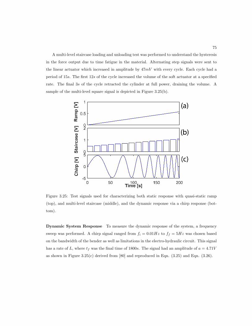
75

A multi-level staircase loading and unloading test was performed to understand the hysteresis

in the force output due to time fatigue in the material. Alternating step signals were sent to

the linear actuator which increased in amplitude by 47mV with every cycle. Each cycle had a

period of 15s. The first 12s of the cycle increased the volume of the soft actuator at a specified

rate. The final 3s of the cycle retracted the cylinder at full power, draining the volume. A

sample of the multi-level square signal is depicted in Figure 3.25(b).

Figure 3.25: Test signals used for characterizing both static response with quasi-static ramp

(top), and multi-level staircase (middle), and the dynamic response via a chirp response (bot-

tom).

Dynamic System Response To measure the dynamic response of the system, a frequency

sweep was performed. A chirp signal ranged from fi = 0.01Hz to ff = 5Hz was chosen based

on the bandwidth of the bender as well as limitations in the electro-hydraulic circuit. This signal

has a rate of L, where tf was the final time of 1800s. The signal had an amplitude of a = 4.71V

as shown in Figure 3.25(c) derived from [80] and reproduced in Eqn. (3.25) and Eqn. (3.26).

76

s(t) = a sin 2πfiL[exp (t/L)− 1] (3.25)

L =tf

log(fffi

)(3.26)

Given the physical characteristics of the bender actuator system, a nonlinear spring-mass-

damper system was chosen as the model structure. The spring component of the model corre-

sponds to the elasticity of the silicone body of the bender. The inertial mass of the system is

primarily represented in the mass of the fluid. The damping effects possibly originate from the

non-linear viscoelastic properties of the elastomer.

The curves from the two static tests informed the selection of the nonlinear terms (x3,x2) and

their derivatives in the model. This resulted in the model structure shown in Eqn. (3.27-3.29),

where F is the bender force exerted on the distal tip, X are the model terms which correspond

to the volume (x) and its derivatives Eqn. (3.28), and Φ are the model parameters Eqn. (3.29).

The constant term was used to eliminate any pre-loading of the actuator on the load cell. A

‘grey box’ system identification process was then applied to the soft actuator data to solve for

the model parameters, Φ [81]. Using non-negative least squares, the unknown parameters, Φ,

were estimated as shown in Eqn. (3.30), where Fm is the force measured by the loadcell [82].

F = XΦ (3.27)

X = [x3 x2 x x3 x2 x x3 x2 x 1] (3.28)

Φ = [C1 ... Cn]T (3.29)

minΦ‖XΦ− Fm‖22 where Φ > 0 (3.30)

The contribution and relative importance of individual terms to the overall accuracy of the

model was also investigated. A single term indexed by (p) was dropped from Eqn. (3.28)

and the parameters were recomputed using Eqn. (3.30). The percent change in accuracy was

subsequently recorded. The root mean squared error (RMSE) and the cumulative RMSE were

evaluated using Eqn. (3.32) and Eqn. (3.33), respectively, and were used as a metric to evaluate

the fit of the model. The difference of cumulative RMSE was found via Eqn. (3.34), where

∅ corresponds to a model with no model terms removed and p represents a model with the

p-th term removed from the analysis, both as a function of time (t). Then the results of Eqn.

77

(3.34) were plotted, and the variables with the most significant impact remained in the model.

Conversely, variables that showed no perceptible difference in cumulative error when removed

or added to the model were used to explore relative importance. For example, if a dynamic

term indicated by a time derivative was important, it should indicate a significant change in

cumulative error if removed from the least squares fit.

F (t) = Fm(t)−X(t)Φ (3.31)

RMSE =( tf∑i=ti

F (t)2)0.5

(3.32)

RMSEcum(t) =( t∑i=0

F (i)2)0.5

(3.33)

RMSEdiff (t, p) = RMSEcum(t, p)−RMSEcum(t, ∅) (3.34)

To establish the optimal model that maximizes efficiency while minimizing model complexity,

relative reductions in RMSE were investigated. This was performed by increasing the number

of model terms monotonically from 1 to 6 with all possible permutation of model terms in

each increment and including constant term in each iteration. The minimum RMSE in each

increment was computed in order to determine convergence in the model. A threshold of 1%

decrease in total RMSE for increase in model term was adopted as a criteria for selecting the

optimal model.

3.3.4 Results

The output of the quasi-static ramp test shown in Figure 3.26 provides a static map of the contact

force output of the bender as a function of the fluid volume input. An intuitive relationship

is observed. With increased fluid volume in the actuator, the cavity pressure increases. This

pressure results in a stronger bend that is translated into contact force at the actuator tip.

This test also shows the constrained loading condition produces larger forces, as the roller joint

directs more of the bending actuation into the load cell, producing larger contact forces at the

distal tip.

78

Figure 3.26: Quasi-static ramp response

The multi-level staircase response investigates energy storage of the soft actuator during the

expansion and contraction stages of the cycle. Figure 3.27 shows how the energy, represented

by the area within the curves, is stored throughout the actuation cycle.

The dynamic chirp signal was used to develop the system models and to understand the

behavior of the soft actuator under different frequency inputs. The observed response of the

dynamic chirp test is shown in Figure 3.28

Figure 3.27: Multi-level staircase response

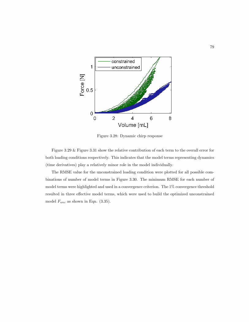
79

Figure 3.28: Dynamic chirp response

Figure 3.29 & Figure 3.31 show the relative contribution of each term to the overall error for

both loading conditions respectively. This indicates that the model terms representing dynamics

(time derivatives) play a relatively minor role in the model individually.

The RMSE value for the unconstrained loading condition were plotted for all possible com-

binations of number of model terms in Figure 3.30. The minimum RMSE for each number of

model terms were highlighted and used in a convergence criterion. The 1% convergence threshold

resulted in three effective model terms, which were used to build the optimized unconstrained

model Func as shown in Eqn. (3.35).

80

Figure 3.29: The cumulative RMSE difference of the unconstrained model, in respect to all

terms, when a single parameter is dropped from the analysis.

81

Figure 3.30: The RMSE values resulting from combination of different number of model terms

for the unconstrained conditions

Func =(x2 x3 x2 1

)

4.73× 10−7[Nm−6s4]

7.88× 10−4[Nm−9]

3.47× 10−3[Nm−6]

1.22× 10−2[N ]

(3.35)

In the constrained loading conditions the RMSE method was applied to find the maximum

number of model terms which influenced the force with a 1% convergence as shown in Figure

3.32. The minimum RMSE resulted in one effective model term x3. The simplified constrained

system model for the force, (Fcon), is shown in Eqn. (3.36).

82

Figure 3.31: The cumulative RMSE difference of the constrained model, with respect to all

terms, when a single parameter is dropped from the analysis.

Fcon =(x3 1

)6.52× 10−4[Nm−9]

2.42× 10−3[N ]

(3.36)

83

Figure 3.32: The RMSE values resulting from combination of different number of model terms

for the constrained conditions

The reduced term models (Func and Fcon) were compared to the experimental data in order

to verify the accuracy of the model. Figure 3.33 indicates that the reduced models are consistent

with the experimental results well.

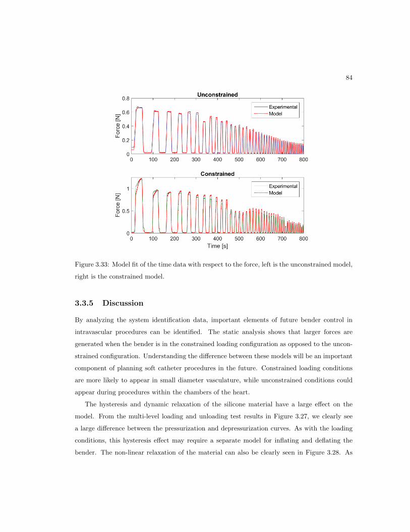
84

Figure 3.33: Model fit of the time data with respect to the force, left is the unconstrained model,

right is the constrained model.

3.3.5 Discussion

By analyzing the system identification data, important elements of future bender control in

intravascular procedures can be identified. The static analysis shows that larger forces are

generated when the bender is in the constrained loading configuration as opposed to the uncon-

strained configuration. Understanding the difference between these models will be an important

component of planning soft catheter procedures in the future. Constrained loading conditions

are more likely to appear in small diameter vasculature, while unconstrained conditions could

appear during procedures within the chambers of the heart.

The hysteresis and dynamic relaxation of the silicone material have a large effect on the

model. From the multi-level loading and unloading test results in Figure 3.27, we clearly see

a large difference between the pressurization and depressurization curves. As with the loading

conditions, this hysteresis effect may require a separate model for inflating and deflating the

bender. The non-linear relaxation of the material can also be clearly seen in Figure 3.28. As

85

the test progressed, the same volume input resulted in less contact force. These test results may

also indicate that end effector sensing feedback may be the best way to provide accurate control

of the soft actuator end effector in the context of an intravascular procedure.

Chirp signals were used to identify the system model. The original system has nine effective

model terms and the contribution of each model term towards system output varies. The less

influential model terms have been removed to develop a reduced system model for better analysis.

In the unconstrained force model (Func) the model terms x3, x, x3, x2, x and x were removed,

while x3, x2, x, x3, x2, x, x2 and x were removed in the constrained force model (Fcon). In these

force models the distal tip of the actuator is in contact with the load cell, which may negate some

damping effects from the inertial mass of the elastomer. This also accounts for the constant

preload term in Equation 3.35 and 3.36. The two system models (Func) and (Fcon) are not

identical in form and vary significantly in different loading conditions. Notably, a dynamic term

(x2) appears in (Func) but not in (Fcon). This may be due to the unconstrained case having

a lower overall stiffness and thereby allowing a interial fluid forces to be more apparent. In

either case, the reduced models (Eqn. 3.36 and 3.35) in concert with the observations of relative

influence of individual variables (Figure 3.30 and 3.32) indicate that dynamics play a negligible

role in this actuators performance, particularly when compared to the nonlinear stiffness.

The inability of a single model to predict bender contact force for a variety of loading

conditions will complicate attempts to control the soft actuator. This investigation suggests that

the system will either need to select from a variety of models based on the loading configuration,

or simply have accurate force sensing at the distal tip to incorporate successful control. Either

way, robust and intravascular compatible sensing modalities will be required for force control

applications within the surgical suite.

3.3.6 Conclusion

This work provides an initial investigation of the soft actuator output force system in order to

evaluate the potential of soft actuators to serve as catheter robots. Intravascular diagnostics

and therapy delivery are often sensitive to the degree of device contact force, therefore a soft

catheter robot must have contact force control at the end effector. Static and dynamic system

identification tests were performed on a bender actuator in two different loading conditions, and

reduced models were successfully developed and empirically confirmed for the dynamic output

86

contact force as a function of input volume.

The non-linearities of the soft actuator material presented hysteresis effects on the inflation

and deflation cycle, as well as contributed to the stress relaxation of the bender over time. These

characterizations will need to be addressed in the future control of the bender. It was also shown

that the bender dynamics appeared to play a minimal role, especially compared to nonlinear

stiffness.

The reduced models developed by the RMSE method closely matched the experimental

results. The system models for the two different loading conditions varied in both the significant

terms and the parameter values. From these results, it is inferred that modeling a more complete

set of loading conditions will result in a wide number of different models. Therefore, to accurately

predict the force output, the loading conditions must either be known or the system must have

accurate contact force feedback.

Implementing force control is an important step for soft robotic catheter clinically relevancy.

While the results from this work are encouraging, future work is needed to successfully apply

force control on a soft bender actuator. Proper loading conditions need to be identified in order

to select the most accurate model. Despite such challenges, soft actuators show potential to be

used in soft catheter robot due to their inherent compliance and biocompatibility.

3.4 Chapter Summary

In this chapter several design techniques for soft robots were developed. A soft robot design

was proposed that was able to locomote through a tube with three segments (spiral, extension,

spiral), the control of the flow was studied, and a bending actuator was modeled for use as

an end-effector. The proposed locomotion architecture was able to create locomotion, but the

design space of the FREE actuators was only able to realize actuators that were long and slender

to meet our design criteria for anchoring. This created a need to increase the design space for

spiraling actuators such that they can achieve tighter spirals, thus reducing their length.

In addition to the actuator design, a hydraulic circuit was created for powering soft robotic

locomotion. Orifice valves were also created and optimized to produce forward locomotion.

Conical valves were then empirically evaluated as they could provide anisotropic behavior during

the inflation and deflation of the actuator timing.

The designed proposed in this chapter provides a framework for creating a soft robot that

87

is scalable and able to traverse tubes. Further research is needed to refine the model, model

the spiral traction forces on the tube wall, resolves any issues with scaling, and to expand the

design space of the soft actuators (Chapter 6). Even with the further research needs, the design

was able to locomote through a tube and is feasible for a soft robotic catheter.

Chapter 4

Actuator Shape Generation

The previous Chapter 3 discussed the design of soft robotic actuators using fiber-reinforced

methods. Fiber-reinforced actuators are limited by the motions that they can produce, thus

limiting their design space. To circumvent the limited design space, this chapter introduces

a method for generating soft robotic actuator shapes. The chapter outlines a process where

an initial and final actuator shape can be defined by a user. The actuator geometry is then

mathematically described such that the initial and final actuator shapes can be arbitrated by

the joint parameter, q. For uses in the medical field, a patient’s MRI scan can be used to dictate

a unique actuator to fit their anatomy.

The first section will discuss the construction of spline through 3D space whether that be

a specific tube or a patient anatomy. The second section will discuss two methods for creating

actuator frames along the centerline. The third section will use the centerlines and frames to

create an initial and final actuator surface. The fourth section will outline the procedure for

transforming the actuator surfaces into a volume for incompressible materials (i.e. rubbers,

silicones, polyurethanes).

4.1 Actuator Centerline Creation

This section outlines the method for defining the initial and final actuator centerline functions.

While any curve could be a potential actuator centerline, we show this method being applied to

a medical scan of the renal artery.

88

89

4.2 Actuator Centerline

4.2.1 Initial Actuator Centerline

To demonstrate the process of creating an arbitrary centerline we will use medical scans and

extract out the centerlines of blood vessels. To start the process a medical image is imported

in the Vascular Modeling Toolkit Lab (VMTKLab). VMTKLab is a program for the 3D re-

construction, geometric analysis, mesh generation and surface data analysis for image-based

modeling of blood vessels. Once the medical scan is imported a thresholding and segmentation

procedure were performed and a 3D model was created as shown in Figure 4.1. Next, a center-

line command was used and a data file was created with the Cartesian points for the centerline

of the scan.

Figure 4.1: a) MRI scan data of patient anatomy. b) 3D model, where the actuator is designed

for the renal artery (boxed region).

The centerline data file was loaded into MATLAB and fit with a cubic spline followed by a

polynomial fitting as a function of the parametric variable for length, w. This resulted in a 3D

parametric centerline with coefficients β and order N=5 as written in eq. 4.1.

cα(w) =

N∑i=0

βiwi (4.1)

rα =

N∑i=0

γiwi (4.2)

The cubic spline and polynomial fit were also applied to the anatomical radius data, resulting

in eq. 4.2, with coefficients γ. Eqs. 4.1-4.2 yield a continuously differentiable basis for an

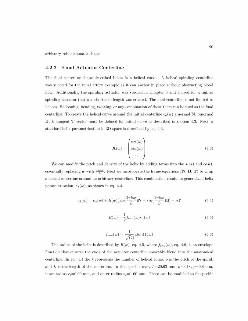
90

arbitrary robot actuator shape.

4.2.2 Final Actuator Centerline

The final centerline shape described below is a helical curve. A helical spiraling centerline

was selected for the renal artery example as it can anchor in place without obstructing blood

flow. Additionally, the spiraling actuator was studied in Chapter 3 and a need for a tighter

spiraling actuator that was shorter in length was created. The final centerline is not limited to

helices. Ballooning, bending, twisting, or any combination of those them can be used as the final

centerline. To create the helical curve around the initial centerline ca(w) a normal N, binormal

B, & tangent T vector must be defined for initial curve as described in section 4.3. Next, a

standard helix parametrisation in 3D space is described by eq. 4.3.

X(w) =

cos(w)

sin(w)

w

(4.3)

We can modify the pitch and density of the helix by adding terms into the sin() and cos(),

essentially replacing w with 2πkwL . Next we incorporate the frame equations (N, B, T) to wrap

a helical centerline around an arbitrary centerline. This combination results in generalized helix

parametrisation, cf (w), as shown in eq. 4.4.

cf (w) = cα(w) +R(w)[cos(2πkw

L)N + sin(

2πkw

L)B] + ρT (4.4)

R(w) =1

2fenv(w)rα(w) (4.5)

fenv(w) =1√(2)

atan(15w) (4.6)

The radius of the helix is described by R(w), eq. 4.5, where fenv(w), eq. 4.6, is an envelope

function that ensures the ends of the actuator centerline smoothly blend into the anatomical

centerline. In eq. 4.4 the k represents the number of helical turns, ρ is the pitch of the spiral,

and L is the length of the centerline. In this specific case, L=20.63 mm, k=3.18, ρ=0.8 mm,

inner radius ri=0.99 mm, and outer radius ro=1.00 mm. These can be modified to fit specific

91

design criterions, such as occlusion ratio, actuator contact area with anatomy, or a combination

of other objectives.

4.2.3 Actuator Centerline

With the initial and final actuator centerlines described by eq. 4.1 and eq. 4.4 an equation

to arbitrate between the two centerlines as a function of the joint parameter q is needed. A

linear convex weighting function is used, when q = 0 the actuator centerline follows the initial

centerline, when q = 1 the actuator centerline is the final centerline. For values of q between

0 and 1 the shape arbitrates linearly between the two desired configurations. The actuator

centerline as a function of q is described by eq. 4.7

c(w, q) = (1− q)cα(w) + qcf (w) (4.7)

4.3 Frame Definition

The next step is to calculate the frames of the centerline equations. The frame consists of

3 basis vectors, first a tangent vector T which is the slope of c(w, q), and then two normal

coordinate vectors (N1, N2) which produce a perpendicular frame to T. Both Frenet-Serret

and Parallel Transport Formulae are compared for their ability to describe the coordinate frame,[T, N1, N2

]as a function of the length parameter w.

4.3.1 Frenet-Serret Formulae

We begin assigning the coordinate frames along the centerline (eq. 4.7) which is parameterized

by w and q. These frames are defined using Frenet-Serret method by computing the tangent,

T, normal, N, and binormal, B, vectors along the centerline ca(w) [83].

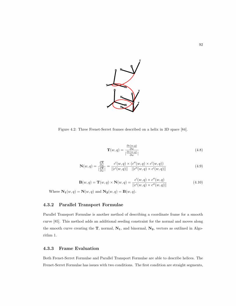
92

Figure 4.2: Three Frenet-Serret frames described on a helix in 3D space [84].

T(w, q) =∂c(w,q)∂w

|∂c(w,q)∂w |(4.8)

N(w, q) =∂T∂w

|∂T∂w |=

c′(w, q)× (c′′(w, q)× c′(w, q))||c′(w, q)|| ||c′′(w, q)× c′(w, q)||

(4.9)

B(w, q) = T(w, q)×N(w, q) =c′(w, q)× c′′(w, q)||c′(w, q)× c′′(w, q)||

(4.10)

Where N1(w, q) = N(w, q) and N2(w, q) = B(w, q).

4.3.2 Parallel Transport Formulae

Parallel Transport Formulae is another method of describing a coordinate frame for a smooth

curve [85]. This method adds an additional seeding constraint for the normal and moves along

the smooth curve creating the T, normal, N1, and binormal, N2, vectors as outlined in Algo-

rithm 1.

4.3.3 Frame Evaluation

Both Frenet-Serret Formulae and Parallel Transport Formulae are able to describe helices. The

Frenet-Serret Formulae has issues with two conditions. The first condition are straight segments,

93

Algorithm 1 Parallel Transport Frames [85]

1: procedure [T, N1, N2] = Parallel Transport(c(w, q))

2: T← ∂c(w, q)/∂w

3: n← length(w)

4: for i← 0 to n− 1 do

5: P← T(i)×T(i+ 1)

6: if ||P|| == 0 then

7: N1(i+ 1)← N1(i)

8: else

9: P← P/||P||

10: θ ← arccos( T(i) •T(i+ 1))

11: N1(i+ 1)← rotate(P, θ)N1(i)

12: end if

13: N2(i+ 1)← cross(T(i+ 1),N1(i+ 1)

)/||cross

(T(i+ 1),N1(i+ 1)

)||

14: end for

15: end procedure

94

in a straight segments T is zero, this causes N to become ill-defined, causing an undefined frame.

The second condition are points of inflection. Figure 4.5 shows centerline with an inflection point.

When the inflection point is reached N1 rotates 180 degrees, this will cause the actuator body

to intersect itself which is not feasible. Parallel Transport Formulae is not limited by inflection

points or straight portions as seen in Figure 4.5.

4.4 Surface Creation

The next step is to create the surface of the actuator body by wrapping a surface around

the centerline c(w, q) (eq. 4.4). To define the actuator three parametric variables are chosen

from the cylindrical coordinate basis resulting in X = [u, v, w], where u represents the radius

which could change as a function of length or circumferential position, v = [0 2π] represents

the direction of the θ wrap, and w = [0 L] is the length along the centerline. The frames are

then evaluated with either Frenet-Serret Formulae or Parallel Transport Formulae, resulting in[T(w, q), N1(w, q), N2(w, q)

]. The actuator body is then created as a function of parametric

variables X as written in eq. 7.

Φ(X, q) = c(w, q) +R(u, v, w)

[N1(w, q)cos

(v + γ(u, v, w, q)

)+ N2(w, q)sin

(v + γ(u, v, w, q)

)](4.11)

Where, R(u, v, w, q) is the instantaneous radius of the of the actuator that can change due

to thickness, circumferential position, length, or the joint variable as described by eq. 4.12.

γ(u, v, w, q) is the instantaneous twist or shear of the of the actuator that can change due to

thickness, circumferential position, length, or the joint variable as described by eq. 4.13.

R(u, v, w, q) = (1− q)Rinit(u, v, w) + qRfinal(u, v, w) (4.12)

γ(u, v, w, q) = (1− q)γinit(u, v, w) + qγfinal(u, v, w) (4.13)

95

4.5 Volume Creation

To create the volume from the surface we can modify the radius input u = [ri ro] in eq. 4.11.

Additionally, to enforce the material incompressibility constraint we can modify eq. 4.11 to

include a function f(u) which modifies the local thickness of the actuator body at each point as

shown in Figure 4.3.

Figure 4.3: The cross section of the soft robot is displayed in its initial underformed cylindrical

state and its deformed spiral state. The initial design focuses on creating a design over [v, w]

and does not directly account for u. The function f(u) was created to modifiy the thickness to

enforce incompressibility. The thickness adjusted by f(u) is shown by the red dashed line.

To enforce material incompressibility of the design, we use the deformation gradient F as

calculated by eq. 4.14 with the reference basis being in cylindrical coordinates, X, and the

deformed basis being in Cartesian coordinates, Φ(X) [56]. If the determinant of deformation

gradient is sufficiently close to one, we consider the design incompressible.

When solving eq. 4.15 for incompressibility, a first order differential equation is produced in

terms of f(u). If we assume that f(u) takes the form in eq. 4.16, we can solve for α0 and α1 at

every spatial location X.

F =

[∂Φ(X)

∂u

1

u

∂Φ(X)

∂v

∂Φ(X)

∂w

](4.14)

ε = |det(F )− 1| < 10−6 (4.15)

f(u) = α0 + α1u (4.16)

96

The combination of the incompressibility constrain eq. 4.16 into eq. 4.11 results in the

actautor body function of eq. 4.17.

Φ(X, q) = c(w, q) +(R(u, v, w)9f(u)

)[N1(w, q)cos

(v + γ(u, v, w, q)

)+ N2(w, q)sin

(v + γ(u, v, w, q)

)](4.17)

4.6 Results

To test the shape generation we perform a case study on a medical scan from a renal artery.

The renal artery centerline and mesh are shown in Fig. 4.4. Additionally, Fig. 4.4 contains the

soft robot’s centerline and final computational design that were developed with Frenet-Serret

Formulae. The incompressibility constraint was numerically satisfied in eq. 4.16 with all ε less

than 106 over the whole range of X = [u, v, w], 2000 spatial locations in all.

Figure 4.4: The medical scan from Figure 4.1 was segmented and two actuator designs were

created for the renal artery. The top image shows a ballooning actuator which fits the outer

wall of the renal artery. The bottom image is patient specific spiral actuator design that conforms

to the curvature inside the renal artery.

97

Several other actuator surfaces were created as well. Figure 4.5 shows an actuator that

arbitrates from a straight line to curve with an inflection point. The inflection points & a

straight line can both be handled with the Parallel Transport Formulae. Figure 4.6 shows a

twisting actuators which changes radius as a function of v & w as well as a shearing component

as a function of v.

98

Figure 4.5: [A] The frame algorithms for Frenet-Serret Formulae (FS) & Parallel Transport

Formulae are applied a curve that has a straight portion and experiences an inflection point. [B]

When Frenet-Serret Formulae is applied to the curves most of the frames cannot be constructed

as indicated by the red circle. [C] Subsequently, a surface cannot be created using Frenet-Serret

Formulae. [D] When Parallel Transport Formulae is applied the frames in the initial and final

centerline are reconstructable as shown by the green arrows. [E] A surface can then be wrapped

around the centerlines to produce an actuator shape. This actuator shape shows an actuator

radius which changes as a function of the length. (Figure courtesy of Chaitanya Awasthi)

99

Figure 4.6: A twisting actuator which has a radius that changes as a function of v & w can be

constructed with the method outlined in this chapter.

An actuator design visualization tool was created as shown in Figure 4.7. Once the user

selected the inputs required by eq. 4.17 an actuator body was created in the initial and final

states. A mesh was also created using 8-node hexahedron elements. Any element or voxel can

then be queried. The bottom two plots show the deformations and strains of a specified element

in the initial and final state.

100

Figure 4.7: An actuator design visualization tool was created. Once the user selected the inputs

required by eq. 4.17 an actuator body was plotted in the initial and final configurations. A

specific element or voxel could then be queried (dark blue) and the deformations and strains of

that element in the initial and final state could be looked at.

4.7 Summary

The shape generation method produced parametric soft robot actuator designs. The design

method was applied to a medical scan of a renal artery. A patient specific spiraling actuator

was designed that ensured volumetric incompressibility. The shape generation method can be

generalized to any shape that a polynomial centerline can be fit to. It is also capable of creating

a hexahedron mesh that can be used in FEM or to create a 3D print file. Although this is

just a kinematic model, the blueprint for possible design shapes are much greater than that of

101

fiber-reinforced actuators.

4.8 Contributions

Portions of the work presented in this chapter were published in the Hamlyn Symposium on

Medical Robotics with co-authors of Chaitanya Awasthi and Gillian McDonald. Gillian per-

formed the work in VMTKLab. Chaitanya helped with the development of the centerlines

and formulated the Parallel Transport Formulae. I worked with Chaitanya on the centerline

development, formulated the Frenet-Serret Formulae, surface, and volume equations.

Chapter 5

Soft Robot Fabrication Using 3D

Printers

In this chapter a method for printing cylindrical actuators on 3D printers is described. First,

dogbones were created and a neo-Hookean constitutive law was fit to stretchable 3D print-

able materials. The neo-Hookean fits were used when realizing printable actuator designs from

Chapter 6. Next, an automated process was developed which uses the cylindrical initial actuator

shape from Chapter 4 and the stiffness mapping from Chapter 6 to create STL files for each

independent material. These STL files can then be directly opened and printed on the Stratasys

J750.

5.1 Material Categorization

In order to create physical actuators, material properties will be needed. A material database of

some common silicones, polyurethanes, and Stratasys material properties were found. Tensile

tests were performed on a variety of elastomeric materials as shown in Table 5.1 using an MTS

load frame. Dogbone specimens where the length was > 10 times the thickness or width were

placed into the load frame as specified in [64]. Fig 5.1 shows a dogbone specimen loaded into

the MTS load frame in both the undeformed and a deformed state. A quasi-static loading test

was then ran on the load frame where a ramp on displacement was applied until the part broke.

102

103

A csv file was then created which provided the raw stress and strain data. The next step, was

to determine the constitutive law that fit data whether that be a Hooke’s law, Mooney-Rivlin,

or Neo-Hookean law. A least squares approach was used to determine the coefficients of the fit

with the constitutive law outlined in eq. 2.20.

The material models used, assume no material hysteresis. This is deemed acceptable as the

goal of the Chapter 6 is actuate from an initial to final shape once. For future development a

study on modeling hysteresis will need to be applied.

Table 5.1: Material Properties

Material Shore Hardness Max. Elongation Tensile Strength [MPa] Neo-Hookean c1 [MPa]

Dragon SkinR© 10 10A 1000% 475 psi –

PolyTek 74-20 20A > 1060% 217 –

PolyTek 74-29 30A > 1600% 281 –

PolyTek 74-44 45A > 2422% 462 –

Stratasys Agilus 30 30A > 220% 2.75 0.20

Stratasys FLX9740 40A > 120% 1.5 0.22

Stratasys FLX9750 50A > 105% 2.5 0.29

Stratasys FLX9760 60A > 80% 3.25 0.41

Stratasys FLX9770 70A > 70% 4.25 0.73

Stratasys FLX9785 85A > 60% 6.0 1.89

Stratasys FLX9795 95A > 40% 9.25 19.8

Figure 5.2 shows stress-strain curves for the seven stretchable materials that can be printed

on the Stratasys J750. From this figure it can be seen that these seven properties span a large

range of stiffness. Figure 5.3 shows the stress-strain curve and neo-Hookean fit for FLX9740.

The neo-Hookean fit holds up until 100% strain for FLX9740. The stress-strain fits for the other

six Stratasys materials are shown in Appendix A. One issue with the Stratasys materials are the

part to part variability as shown in Figure 5.4. Four dogbone samples were tested and a large

variance of material properties were exhibited. This causes issues when fitting a neo-Hookean

model as it will only track one of the samples well. This could lead to realized parts that behave

slightly different than the predicted simulations.

104

Figure 5.1: MTS Load Frame with a dogbone specimen secured into the jaws. The left image

shows the undeformed geometry and the right image shows the deformed geometry. Later

dogbones utilized a longer geometry with a greater aspect ratio.

105

Figure 5.2: Stress-strain data for the Stratasys materials that can be printed out on the Stratasys

J750 located in the Medical Devices Center at the University of Minnesota.

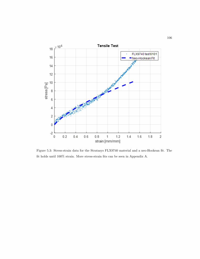
106

Figure 5.3: Stress-strain data for the Stratasys FLX9740 material and a neo-Hookean fit. The

fit holds until 100% strain. More stress-strain fits can be seen in Appendix A.

107

Figure 5.4: Stress-strain data for four dogbones printed with Stratasys FLX9785. It can be seen

that there is variance from dogbone to dogbone.

5.2 3D Printing Soft Robots

The actuator designs that are being created require more than one material so a multi-material

printer is needed. There were three options for realizing these soft robotic actuators with 3D

printers. The first option was to use the Stratasys J750, the second option was to use the ACEO

IMAGINE 100, & the third option was to build our own printer. Building a multi-material 3D

printer was deemed out of the scope of this thesis, but is currently being pursued within the

Medical Devices Lab, Francis Group, & Ellison Research Group at the University of Minnesota.

108

The second option was the ACEO IMAGINE 100, this printer is able to print three durometers

of silicones with elongation between 200%-600%. The major drawback to this printer was that

the multi-material printer was only located in their German facility, & the estimated three week

lead time was deemed too long. That left the Stratasys J750, which was located in the Medical

Devices Center at the University of Minnesota. The Stratasys J750 was able to print seven

stretchable materials as shown in Table 5.1, while these materials are not as stretchable as the

ACEO IMAGINE materials they are still stretchable enough to create some actuator designs.

To print out a part on the Stratasys J750 a CAD file is required. Once a CAD file is created

the part is imported into GrabCAD Print. GrabCAD Print is a software program released by

Stratasys to position the part to the bed, select materials, & create the print job. Figure 5.5

shows four twisting actuators on the print bed of a Stratasys J750 within GrabCAD Print. The

materials are assigned by selecting an individual STL file and selecting the material choice that

matches the name of the selected STL file. The next two subsections cover the actuator design

that will be used in Chapter 6 and expressed mathematically in Chapter 4, as well as, a method

for generating the cad file of the geometry.

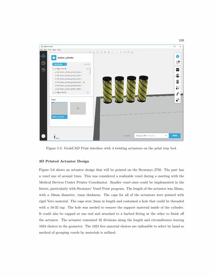
109

Figure 5.5: GrabCAD Print interface with 4 twisting actuators on the print tray bed.

3D Printed Actuator Design

Figure 5.6 shows an actuator design that will be printed on the Stratasys J750. The part has

a voxel size of around 1mm. This was considered a realizable voxel during a meeting with the

Medical Devices Center Printer Coordinator. Smaller voxel sizes could be implemented in the

future, particularly with Stratasys’ Voxel Print program. The length of the actuator was 32mm,

with a 10mm diameter, 1mm thickness. The caps for all of the actuators were printed with

rigid Vero material. The caps were 2mm in length and contained a hole that could be threaded

with a 10-32 tap. The hole was needed to remove the support material inside of the cylinder.

It could also be capped at one end and attached to a barbed fitting at the other to finish off

the actuator. The actuator contained 32 divisions along the length and circumference leaving

1024 choices in the geometry. The 1024 free material choices are unfeasible to select by hand so

method of grouping voxels by materials is utilized.

110

Figure 5.6: Twisting actuator design with a diameter of 10mm, length of 32mm, and thickness

of 1mm. Each voxel has a size of 1mm and the actuator consists of 32 divisions along the length

and 32 divisions around the circumference. The grey portions will be made out of Agilus 30,

the black portions will be FLX9785, and the red and blue portions will printed with Vero.

Generation of STL files for Cylindrical Actutaors

Since it is unfeasible to select all 1024 voxels and assign them the correct material an automated

material selection program was needed. The programmed worked by grouping the 1024 voxels

into the seven material groups. Each unique material groups was turned into an independent

STL file as shown in Figure 5.7. All the STL files could then be assembled (Figure 5.8) and were

loaded into GrabCAD Print as an assembly resulting in the actuators in Figure 5.5. Algorithm

2 outlines the process of creating individual STL files.

Algorithm 2 STL creation of cylindrical geometries

1: procedure Espatial = create STL(E,mesh(nodes,elements))

2: Eunique ← Determine the unique materials in the stiffness map

3: for i← 1 : length(Eunique) do

4: Ecell(i)←find(Eunique(i) == E)

5: crete stl file out of elements in Ecell(i)

6: end for

7: end procedure

111

Figure 5.7: Individual STL files.

112

Figure 5.8: Assembly of the individual STL files.

113

5.3 Summary

In this chapter a method for printing soft robotic actuators on a Stratasys J750 was developed.

First material properties for the seven material were determined by 3D printing dogbone samples,

testing them on a MTS load frame, and fitting a neo-Hookean constitutive law. Then a method

was outlined which was able to automate the material choice selection given a stiffness mapping

and cylindrical geometry. This method could easily be expanded to non-cylindrical geometries

if a mesh and stiffness map are given.

Chapter 6

Inverse Finite Element Modeling

for Soft Robots

In this chapter a method for reconstructing the spatial material properties of cylindrical actu-

ators using a nonlinear inverse FEM optimization routine, when given the initial/final actuator

geometry, BCs, and input pressure is derived. Figure 6.1 offers the long-term vision of the in-

verse material reconstruction process. By developing a process to reconstruct material spatially

varying material properties, progress will be made towards building a soft robotic catheter. To

begin the reconstruction process, the initial, undeformed actuator shape, as well as the final

actuator shape at a desired pressure are defined. Figure 6.1 shows the creation of a spiraling

actuator specific to a medical scan of an aortic branch. The initial shape for this actuator fol-

lows the curve of the patient’s anatomy while the desired final shape shows a helix capable of

anchoring within the anatomy. The deformation from the initial to final shape is described by

Φ(X, q) (Chapter 4). The deformation and strain are then determined from Φ(X, 1)− Φ(X, 0),

and the inverse FEM algorithm can run to deduce the material properties needed to actuate

from the initial to final shape for a desired input pressure. Once the material properties have

been reconstructed, a region of the actuator can be magnified to view a super-voxel. This super-

voxel is comprised of distinct material properties that can reconstruct the anisotropic behavior

required by the deformation. If the geometry is magnified even further, the voxel, which shows

a single material property that could be 3D printed can be seen. The actuator shapes in Figure

114

115

6.1 are not reconstructed in this thesis, however, this chapter does develop and inverse algorithm

to reconstruct actuator shapes, and validates the algorithm on three motions that occur in a

spiraling actuator (ballooning, bending, & twisting).

Figure 6.1: Long-term vision of the of the inverse FEM method that this thesis makes strides

towards. The left two images are the initial and final actuator shapes that were dictated by

the patients anatomy and constructed using the method outlined in Chapter 4. Given the two

shapes, BCs, and the input pressure, material properties could be reconstructed to achieve the

desired deformation. A zoomed in view of the actuator body shows a super-voxel which is made

up of several 3D printed materials. Zooming in further results in a voxel which is a printable

material.

The three actuator motions discussed in this chapter all use initial cylindrical actuator shape

in the form of Figure 6.2. The radius r, thickness t, actuator length L, and number of voxels

Eij are all variable. Each voxel’s unique material property can either be a Hooke’s law material

or Neo-Hookean material. The term E is used to describe the material property constant for

either Young’s Modulus or Hooke’s Law.

116

Figure 6.2: Actuator motions that will be solved for with the inverse algorithm.

When solving any inverse problem many issues arise in order to obtain a ‘good’ solution. A

few important topics in nonlinear inverse problems are:

1) existence

2) uniqueness

3) continuity

If all three of the above topics are true then the problem is said to be well poised, if one

or more of the statements does not hold the problem is ill-posed and a regularization scheme

is needed [67]. When a plausible displacement field is chosen (existence) and the loading and

boundary conditions are known a unique problem is created that is continuously dependent on

the material property.

The goal of this chapter is to create a nonlinear inverse FEM algorithm that can reconstruct

the material properties E spatially for the cylinder as shown in Figure 6.2. The method centers

around the 2-norm between desired and actual displacement as shown in eq. 6.1 and eq. 6.2

. The material properties are updated through gradient approach, where a cost function was

117

created to update ∆E until the deformation criteria is met. An approach similar to that of

tissue Elastography [67], [69] was developed.

minimize Φ(E)

subject to Elo < E < Ehi

(6.1)

Φ(E) =1

2

∥∥U−U(E)∥∥

2(6.2)

Where the objective function Φ(E) is described by one half the two norm of the displacements

with the current iteration, k, of displacement, U , and the desired displacement U .

A flowchart of the inverse reconstruction algorithm can be seen in Figure 6.3. First the user

needs to select the actuator that they are attempting to reconstruct by defining the inputs.

Figure 6.4 step 1 shows the initial and final actuator shapes determined by the user, and step 2

shows the application of the mesh of the geometry, the boundary conditions, and chosen desired

pressure of the actuator in its final shape. Once the design inputs are selected, an initial guess of

material properties needs to be found. The initial guess of material properties is determined using

the U and P in a Hooke’s law equation. This simple approximation generally produces the rough

structure of material that needs to be stiff or soft but is off on its magnitude. Figure 6.4, step

3 shows the result of the seeding algorithm, the darker shades of blue represent stiffer materials

and the lighter colors represent softer materials. Once the initial seed has been completed,

material properties are refined through the optimization routine. The forward FEM problem is

ran to calculate the displacements between the initial and desired actuator shapes, Uk. If the

shape reconstructed from the material properties is not similar enough to the desired shape,

the material properties, ∆E, are updated using sensitivity matrices on strain and deformation.

These matrices relate every spatial displacement and strain to every material property. Figure

6.4, step 4 shows the optimization algorithm in two steps k. When the optimization meets the

convergence requirements, a mapping of material properties needed to reconstruct the desired

actuator shape as indicated in Figure 6.4, step 5 is produced.

118

Figure 6.3: Inverse algorithm outline.

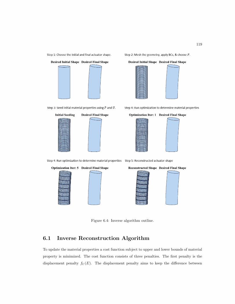
119

Figure 6.4: Inverse algorithm outline.

6.1 Inverse Reconstruction Algorithm

To update the material properties a cost function subject to upper and lower bounds of material

property is minimized. The cost function consists of three penalties. The first penalty is the

displacement penalty fU (E). The displacement penalty aims to keep the difference between

120

the desired and actual deformation to a minimum. The second penalty aims to minimize the

difference between desired and actual strain for each voxel, which is deemed the strain penalty,

fε(E). The third penalty is a similarity penalty, f∂(E). The similarity penalty penalizes changes

in neighboring voxel material properties. The material update equation can be seen in eq. 6.3

and eq. 6.4.

minimize∆E

w1fU (E) + w2fε(E) + w3f∂(E)

subject to Elo < Ek + ∆E < Ehi

(6.3)

Ek+1 = Ek + ∆E (6.4)

6.1.1 Displacement Penalty fU(E)

The displacement penalty deals with minimizing the difference between actual and desired dis-

placements. The penalty term is created by taking the derivative of eq. 6.2 with respect to E.

First eq. 6.2 is expanded into its matrix form. The expanded form of the 2-norm in eq. 6.5 is

nonlinear, so it is linearized.

Φ(E) =1

2(U(E)−U)T (U(E)−U) (6.5)

The linearization is performed by taking the derivative of eq. 6.5 with respect to the material

E and setting it equal to zero. A 2nd order Taylor Series expansion is utilized and centered

around the current iteration value of Ek described by eq. 6.7.

∂Φ(E)

∂E=∂Φ(Ek)

∂E+∂2Φ(Ek)

∂2E∆E = 0 (6.6)

Where the term ∆E is defined as ∆E = E−Ek.

The right hand side of eq. 6.6 is determined by taking the first derivative of eq. 6.5 with

respect to E and evaluating at Ek.

∂Φ(Ek)

∂E= Sk(U−Uk(Ek)) = 0 (6.7)

121

Where S is the displacement sensitivity matrix which describes the contribution of each

spatial displacement to every material voxel. The displacement sensitivity matrix was found by

taking the derivative of the current displacement with respect to the current material properties

as described by eq. 6.8. The detailed derivation for the sensitivity matrix is shown in subsection

6.1.4.

Sk =∂Uk(Ek)

∂E(6.8)

The second order term of eq. 6.6 is found by taking the derivative of eq. 6.7:

∂2Φ(Ek)

∂2E=

∂

∂ESk(U(Ek)−U) = STk Sk (6.9)

Substituting the first and second derivative term of the Taylor Series polynomial, (eq. 6.9

and eq. 6.7) into eq. 6.6 results in a relationship between the displacement sensitivity and

material change as described by eq. 6.10.

Sk(Uk(E)−U) + STk Sk∆E = 0 (6.10)

Eq. 6.10 is then used as the fU (E) penalty term in eq. 6.3 as shown by eq. 6.11.

fU (E) =∥∥Sk(Uk(E)−U) + STk Sk∆E

∥∥2

(6.11)

6.1.2 Strain Penalty fε(E)

The strain penalty deals with minimizing the difference between actual and desired strain for

the three normal and three shear strains. To minimize the strain difference the derivative of the

Lagrangian strain eq. 2.19 with respect to the material property is needed. The strain residual

that will be minimized is described by eq. 6.13.

Φε =1

2

∥∥ε− εk(E)∥∥

2(6.12)

=1

2

(ε− εk(E)

)T (ε− εk(E)

)(6.13)

122

Next, the derivative of eq. 6.13 with respect to the material property, E, is taken. A second

order Taylor Series polynomial is utilized for this derivation (eq. 6.14).

fε(E) =∂Φε(E)

∂E=∂Φε(Ek)

∂E+∂2Φε(Ek)

∂2E∆E = 0 (6.14)

Solving for the first order term results in eq. 6.15

∂Φε(Ek)

∂E= STεk

(ε− εk

)(6.15)

Where Sε is the strain sensitivity matrix which relates the strain of each voxel to every

spatial material property described by eq. 6.16 and described in more detail in subsection 6.1.4.

Sε =∂ε(Ek)

∂E(6.16)

The second order term of the Taylor series polynomial is described by eq. 6.17.

∂2Φε(Ek)

∂2E= STε Sε (6.17)

The penalty term fε(E) can then be reconstructed by substituting eq. 6.15 and eq. 6.15 into

eq. 6.14 resulting in the strain penalty term described by eq. 6.18.

fε(E) =∥∥STεk(ε− εk)+ STε Sε∆E

∥∥2

(6.18)

6.1.3 Similarity Objective

The strain, and displacement objective penalties alone may cause neighboring voxel properties

to have a very large variance or for there to exist neighborhoods of ‘runaway’ material properties.

The large variance in material properties is often beneficial as a neighboring between stiff and soft

creates motion. On the otherhand, when there are small variances in similar material properties

issues begin to arise. If the displacement residual is not close to the stopping criterion then a

few material parameters may locally runaway causing an increase in residual. By filtering the

123

soft and hard components with a band-stop style filter convergence could be found quicker and

more robustly.

The similarity objective, f∂(E), aims to smooth similar neighboring properties while allowing

for stark changes in neighboring properties. To implement the filtering process, the cylindrical

surface is unwrapped into cylindrical coordinates as shown in Figure 6.5. This mapping creates

an ‘image’ of material properties representing the neighboring voxels or elements. The difference

in both the θ and L direction are taken. This expresses the differences in neighboring cells.

Since stiff and soft material properties are desired, differences greater than 0.3(Ehi − Elo) are

left untouched. This allows for the smoothing of similar properties while encouraging difference

between stiff and soft properties. The thresholded derivatives of the stiffness mapping with

respect to L and θ are then summed together and a L2 norm is used to determine the penalty

for the difference. The resulting similarity objective is described by eq. 6.19 and Algorithm 3.

f∂(E) =

∥∥∥∥|∂Espatial

∂L|+ |∂Espatial

∂θ|∥∥∥∥

2

(6.19)

Where,

Espatial is the spatial material property seen in Figure 6.5.

Figure 6.5: Unwrapping of the cylindrical mesh so it fits into a 2D array.

124

Algorithm 3 Similarity Objective where a band-stop filter is applied to Espatial

1: procedure Espatial = similarity objective(Espatial, dEthresh )

2: dEθ ← ∂Espatial∂θ

3: dEL ← ∂Espatial∂L

4: dEθ ← dEθ > dEthresh

5: dEL ← dEL > dEthresh

6: f∂(E)← ||dEθ + dEL||27: end procedure

6.1.4 Sensitivity Matrix

The sensitivity matrices describe the contribution of displacement or strain from every element

on the cylindrical body.

Displacement Sensitivity Matrix

The displacement sensitivity matrix is determined with the incremental form of FEM. The

incremental form in eq. 6.20 is derived in Chapter 2 and Figure 6.6 shows a force displacement

plot of the incremental form.

Kk∆Uk + Fint − Fext = Rk (6.20)

Where,

Kk is the linearized tangent stiffness at the given step k.

∆uk is the displacement for the step k, Uk+1 −Uk.

Fint is the internal force from previous solutions to eq. 6.20.

Fext is the external force

Rk is the residual when solving for the displacement ∆uk.

125

Figure 6.6: Applying the force incrementally within FEM [64].

The final force and displacement is found when k = n. This is found by expanding Fint from

eq. 6.20 into eq. 6.21.

K1U1 + K2(U2 −U1) + · · ·+ Kn(Un −Un−1)− Fext = Rk (6.21)

In order to construct the sensitivity matrix the derivative of eq. 6.21 must be taken with

respect to the material property as dictated by eq. 6.8. When taking this derivative it can be

seen that Fext and Rk do not have any dependence on Ej and their derivatives are zero.

126

∂K1

∂EjU1 + K1

∂U1

∂Ej

+∂K2

∂Ej(U2 −U1) + K2(

∂U2

∂Ej− ∂U1

∂Ej)

+ · · ·

+∂Kn

∂Ej(Un −Un−1) + Kn(

∂Un

∂Ej− ∂Un−1

∂Ej)

(6.22)

The terms of the derivative in eq. 6.22 can then be grouped as shown in eq. 6.24.

∂K1

∂Ej(U1 −U0) +

∂K2

∂Ej(U2 −U1) + · · ·+ ∂Kn

∂Ej(Un −Un−1)

+∂U1

∂Ej(K1 −K2) +

∂U2

∂Ej(K2 −K3) + · · ·+ ∂Un

∂Ej(Kn−1 −Kn)

+Kn∂Un

∂Ej= 0

(6.23)

In eq. 6.23 a pattern arises, so a series formulation relating to ∂UN

∂Ejcan be solved for as

shown in eq. 6.24.

S =∂UN

∂E= −K−1

N

[N∑i=1

∂Ki

∂Ej(Ui −Ui−1) +

N−1∑i=1

(Ki −Ki+1)∂Ui

∂Ej

](6.24)

The derivative of the stiffness matrix with respect to each elements material property, ∂Ki

∂Ej,

is found by differentiating the local stiffness matrices of each element and mapping the differen-

tiated values into the global space. This differentiation could simply be found by dividing the

local element material property from the local element stiffness matrix. This was operation was

performed for all the pressure steps, and S in eq. 6.24 was constructed.

Solving for the Strain Sensitivity Matrix

The strain sensitivity is the derivative of the strain at each element with respect to each material

parameter described by eq. 6.16. The strain sensitivity matrix if found in a similar manner to

that of the displacement sensitivity matrix. If a relationship between displacement and strain

is utilized then Sε can be formulated. The derivation of the FEM in Chapter 2 is used. The

strain-displacement matrix relates the displacements and strains through B. Eq. 2.58 provides

127

a linearized relationship between displacement and strain. The derivative of eq. 2.58 is then be

taken to yield the strain sensitivity matrix shown by eq. 6.25.

∂ε(Ek)

∂E=

∂

∂EBU = B

∂U

∂E= BS (6.25)

Inverting the stiffness matrix

In order to invert the stiffness matrix in eq. 6.24 a regularization scheme is needed to reduce

the condition number. The simplest regularization scheme is to add an identity matrix to the

stiffness matrix resulting in eq. 6.26.

Kk = Kk + λI (6.26)

The value of λ has a large effect on the convergence of the optimization as well as condition

number of Kk. If λ is high then the condition number becomes low and the pseudo inverse

can be found. However, this leads to inaccuracy of the stiffness matrix and causes issues with

convergence. If the λ parameter is too low (lowest tested that works 10−3) then least squares

cannot be used as the condition number is > 1020. Other solution methods can be used by

they are slower and convergences is not guaranteed. The value of λ is determined through an

iterative process where its value is increased by an order of magnitude until a condition number

< 1012 is achieved.

6.1.5 Options for the Inverse Algorithm

Grouping Elements

Grouping elements aims to reduce the number of independent material voxels by grouping them

together. Grouping elements has two main uses. The first, is when a finer mesh than printable

voxel size is needed in order to solve the FEM problem (i.e. high deformation when the elements

become highly distorted). In this case, neighboring elements will be grouped together to make a

voxel that is large enough to print. The second case, is when a the user knows the structure of

the stiffness mapping and wants to converge to the values of the material parameters to reach

convergence.

128

To perform the element grouping the columns of the sensitivity matrix, which represents each

element material properties, can be grouped. The element groups are indicated by ψi where the

indice i represents each individual group of M groups.

Sgroup =

M∑i=1

S(:, ψi) (6.27)

Eq. 6.27 can then be set to S and used in eq. 6.24.

6.1.6 Node Reduction

Node reduction allows the user to choose which nodes to use in the optimization. In cylindrical

geometries, this would allow the user to ignore the caps or even the inner surface. The nodes

are reduced by removing rows of the sensitivity matrix as described by eq. 6.28.

Snode =

M∑i=1

S(ξi, :) (6.28)

Where i ranges from one to the number of reduced nodes M , and ξ is the nodes that are not

reduced.

6.2 Filtering or Dithering Algorithm to a Finite Set of

Materials

The result of the inverse optimization algorithm is a continuous stiffness mapping ranging be-

tween Elo and Ehi. A continuous stiffness mapping is an acceptable solution in simulation, but

is not realizable with currently available manufacturing methods. An algorithm is needed to

discretize the continuous stiffness mapping to a finite set of attainable material properties.

Binning Materials

A second method of performing this discretization is a binning algorithm. The continuous

stiffness mapping is binned using the discrete set of material properties as shown in Algorithm

4.

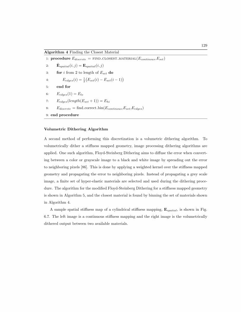
129

Algorithm 4 Finding the Closest Material

1: procedure Ediscrete = find closest material(Econtinous,Eset)

2: Espatial(i, j) = Espatial(i, j)

3: for i from 2 to length of Eset do

4: Eedges(i) = 12

(Eset(i)− Eset(i− 1)

)5: end for

6: Eedges(1) = Elo

7: Eedges(length(Eset + 1)) = Ehi

8: Ediscrete = find correct bin(Econtinous,Eset,Eedges)

9: end procedure

Volumetric Dithering Algorithm

A second method of performing this discretization is a volumetric dithering algorithm. To

volumetrically dither a stiffness mapped geometry, image processing dithering algorithms are

applied. One such algorithm, Floyd-Steinberg Dithering aims to diffuse the error when convert-

ing between a color or grayscale image to a black and white image by spreading out the error

to neighboring pixels [86]. This is done by applying a weighted kernel over the stiffness mapped

geometry and propagating the error to neighboring pixels. Instead of propagating a grey scale

image, a finite set of hyper-elastic materials are selected and used during the dithering proce-

dure. The algorithm for the modified Floyd-Steinberg Dithering for a stiffness mapped geometry

is shown in Algorithm 5, and the closest material is found by binning the set of materials shown

in Algorithm 4.

A sample spatial stiffness map of a cylindrical stiffness mapping, Espatial, is shown in Fig.

6.7. The left image is a continuous stiffness mapping and the right image is the volumetrically

dithered output between two available materials.

130

Algorithm 5 Modified Floyd-Steinberg Dithering

1: procedure dither(Espatial)

2: Espatial(i, j) = Espatial(i, j)

3: for i from top to bottom of length do

4: for j from left to right of θ do

5: Eij = find closest material(Espatial(i, j),Eset)

6: Espatial(i, j) = Eij

7: δE = Espatial(i, j)− Eij8: Espatial(i, j + 1) = Espatial(i, j + 1) + 7

16δE

9: Espatial(i+ 1, j − 1) = Espatial(i+ 1, j − 1) + 316δE

10: Espatial(i+ 1, j) = Espatial(i+ 1, j) + 516δE

11: Espatial(i+ 1, j + 1) = Espatial(i+ 1, j + 1) + 116δE

12: end for

13: end for

14: end procedure

∗Constants derived for globally minimized error via Floyd-Steinberg dithering algorithm.

131

Figure 6.7: Dithering of an first order continuous stiffness mapping to a binary material dithered

mapping. Left shows a continuous stiffness mapped geometry and the right image shows the

actuator after it has undergone a binary material dithering operation.

6.3 Implementation into MATLAB/Abaqus

The inverse optimization flowchart of Figure 6.3 in Algorithm 6 was implemented in MATLAB.

During the implementation MATLAB was used to call Abaqus to solve for displacements and

generated stiffness matrices for each FEM iteration. The Minnesota Super Computing Institute

(MSI) was used to run this program through a linux session using a NICE client.

The first step of this method is for the user to select the geometry, the deformation, applied

pressure, and boundary conditions. The geometries explored in this thesis are either a cube or

cylinder. Both geometries are meshed using 8-node hexahedron elements. The desired deforma-

tion U is simply found by subtracting the desired node location by the initial node location. The

applied pressure is applied to the internal surfaces on the cylindrical geometry and the selected

faces for the cube as dictated by the user.

The second step of the procedure is to seed the material parameters, Ek, using the desired

displacement and applied load. Hooke’s Law is used to seed the geometry. The strains of each

element can be calculated by applying eq. 2.58 to U . The stress is calculated using thick walled

pressure equations eq. 6.29. If a neo-Hookean model is selected as the constitutive law, the

Young’s Modulus from Hooke’s law can be divided by six to obtain an approximation for the

neo-Hookean material constant as described in [64, 32].

132

Algorithm 6 Inverse Finite Element Algorithm

1: procedure Espatial = inverse FEM(BCs,U ,Geometry(X,mesh),P )

2: Seed the material parameters Ek using U and the the load P

3: while Shapes have not met residual & less than max iteration do

4: Create Abaqus input file with the selected inputs BCs, Geometry, P , & Ek

5: Call Abaqus to get U and K

6: if∥∥U−U

∥∥2> Utol then

7: Create sensitivity matrices from eq. 6.24 & eq. 6.25

8: Calculate the material update ∆E by minimizing eq. 6.3.

9: Update Ek+1 using c.

10: Increment k.

11: end if

12: end while

13: end procedure

σa =−Pr2

o

r2o − r2

i

σc =−Pr2

o

r2o − r2

i

+r2i P

r2o − r2

i

σr =−Pr2

o

r2o − r2

i

− r2i P

r2o − r2

i

(6.29)

An iterative processes is then started to incrementally update Ek by ∆E. This update

occurs until either a specified residual, Utol is met by evaluating eq. 6.2, or a maximum number

of iterations occurs. To evaluate whether the stopping criteria has been met the deformation

with Ek is found with FEM. A MATLAB script was created which automatically generates

an Abaqus input file when the inputs stated above are specified. In addition to the algorithm

inputs, several parameters can be modified for better performance in Abaqus. The pressure

load can be applied in steps as shown in Fig. 6.6. The addition of the load steps allow for the

stiffness matrices to be extracted at each allowing for a more accurate sensitivity matrix. The

pressure steps all range from 0-1 and have a max step of 0.2 and a minimum step of 1e-5. To

determine the displacements in a timely manner a Quasi-Newton solution technique is deployed

and parallel computing is utilized. Since all of the simulations require large deformations the

large deformation solver is turned on in Abaqus. This adds the current deformation, streses,

etc. into the simulation as derived in the FEM section of Chapter 2. The method developed

is centered around using C3D8RH elements which are 8-node hexahedron elements formulated

133

with reduced integration to prevent shear locking. The user has a choice of either a Young’s

Modulus material or neo-Hookean material throughout the inverse process.

MATLAB needs to call Abaqus in order to run the simulation. A batch file is created in

MATLAB. When the batch file is ran an instance of Abaqus is opened on MSI and the job is

ran. When Abaqus is running there are temporary files created, by monitoring the existence

of the *.lck it can be determined whether or not the job is still running. Once the *.lck file

is deleted, the log file is checked for convergence. If errors occurred the inverse algorithm is

aborted, if convergence was met, the algorithm proceeds.

Once the Abaqus simulation had successfully converged, the data generated from Abaqus

needed to be imported to MATLAB. The Abaqus2matlab library was used to transfer the

deformed geometry from each step into MATLAB [87]. The residual between desired and current

displacement was then found. If the residual was greater than Utol the algorithm proceeded to

update ∆E. The next step, was to create the displacement and strain sensitivity matrices

described by eq. 6.24 and eq. 6.25. The first step in constructing the displacement sensitivity

matrix was to import the local stiffness matrices. An Abaqus input file was configured to

output the local stiffness matrices to a *.mtx file for each element. The *.mtx was formatted

in a lower triangular format and a MATLAB function was created to successfully import all of

these matrices. Once the local stiffness matrices for each step were imported the global stiffness

matrix for each step was reconstructed as a sparse matrix for efficiency. With the displacements,

local stiffness matrices, and global stiffness matrices eq. 6.24 was evaluated. In order to take

the inverse of K an identity matrix multiplied by a scalar was added to K to reduce to condition

number as outlined in subsection 6.1.4. During the computation of eq. 6.24 both sparse and

parallel for-loops were utilized to solve in a reasonable amount of time. The strain sensitivity is

determined by calculating eq. 6.25, where the B was calculated by eq. 2.59.

With the sensitivity matrix determined the user is allowed to group elements or reduce nodes

as described in subsections 6.1.5 and 6.1.6, respectively.

With the final modifications to the sensitivity matrices complete, the material properties can

be updated. To calculate eq. 6.4 the constrained optimization solver in MATLAB fmincon was

used. Since the cylindrical or cube inverse problems are not large scale the Sequential Quadratic

Programming method was selected. This solver satisfies the bounds at all iterations and can

recover from NaN and Inf results. The settings for fmincon are shown in Table 6.1. The weights

134

Table 6.1: MATLAB fmincon settings used to calculate ∆E.

Algorithm Max. Fcn. Eval. Optimality Tol. Step Tol. Max Iter. Diff. Min. Change

SQP 1e5 1e-6 1e-4 3e2 0.01

w1, w2, and w3 are all defined by the user and are generally modified based on the deformation.

For out of plane motions the displacements dominate which means w1 needs to be larger than

w2 and w3. When shear is involved the weight w2 associated with strain penalty is the most

important as it contains the three shear strain terms. Meanwhile, the displacement penalty deals

with Cartesian positions and is unable to reconstruct shearing. The weight w3 is associated to

the similarity penalty which is more of a practicality constraint. This weight is always small in

comparison to w1 or w2 and only acts to keep tame or smooth the material update.

Several options can be chosen before eq. 6.3 is evaluated. One of these options is to use

K-means clustering to bin the output of ∆E to a finite number of outputs. This is useful in

the first few iterations as it is a faster method of getting closer to reconstructed solution. Other

options are applying a binning operation as described by Algorithm 4 or the dithering algorithm

described by Algorithm 5. Once these options are chosen eq. 6.3 is evaluated, k is incremented

and the next loop iteration begins.

6.4 Inverse Design Algorithm Verification

To validate the nonlinear inverse FEM reconstruction algorithm (Algorithm 6), three actuator

motions were reconstructed: ballooning, bending, & twisting as shown in Figure 6.8. The

three motions are shown in level of difficulty with the ballooning actuator being the easiest

and twisting being the most difficult motion to achieve. All three motions were validated when

the ideal material properties were known. In other words, the desired stiffness mapping was

known, but the algorithm did not have access to the desired stiffness mapping. The algorithm

only had access to the deformation from the known stiffness mapping, the input pressure, and

boundary conditions. A neo-Hookean material was used for all three motions since it shows

the more difficult use case. All three actuators were designed to be short in length (6r to L)

and thick walled r < 10t. This was chosen to reduce the computational time of the MATLAB

implementation and to have an actuator that was feasible and affordable to 3D print on the

135

Stratasys J750. The verifying actuator shapes all classified as thick wall pressure vessel cases

as the radius is less than ten times the thickness. Additionally, these actuators were short in

the length compared to their diameter 3x length to diameter. The short actuator allowed

for fewer elements and reasonable simulation times (< 24hr). All of the cylinder geometries

are constructed with trilinear 8-node hexahedron elements and an internal pressure, and fixed

boundary condition on the bottom cap are applied to the geometry. Ballooning, bending, &

twisting provide basic motions that can be used in several robotic applications. If all three

motions can be reconstructed, then the proposed inverse algorithm is be deemed as a feasible

method for designing soft robots.

Figure 6.8: Actuator motions (A. ballooning, B. bending, C. twisting) that will be focus for

validating the inverse algorithm. The solid lines indicate the deformed geometry while the

dashed line shows the initial geometry.

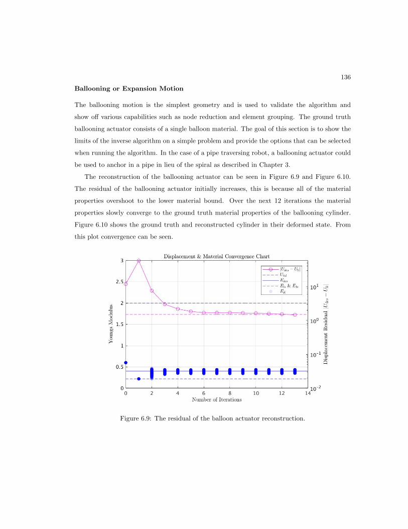
136

Ballooning or Expansion Motion

The ballooning motion is the simplest geometry and is used to validate the algorithm and

show off various capabilities such as node reduction and element grouping. The ground truth

ballooning actuator consists of a single balloon material. The goal of this section is to show the

limits of the inverse algorithm on a simple problem and provide the options that can be selected

when running the algorithm. In the case of a pipe traversing robot, a ballooning actuator could

be used to anchor in a pipe in lieu of the spiral as described in Chapter 3.

The reconstruction of the ballooning actuator can be seen in Figure 6.9 and Figure 6.10.

The residual of the ballooning actuator initially increases, this is because all of the material

properties overshoot to the lower material bound. Over the next 12 iterations the material

properties slowly converge to the ground truth material properties of the ballooning cylinder.

Figure 6.10 shows the ground truth and reconstructed cylinder in their deformed state. From

this plot convergence can be seen.

Figure 6.9: The residual of the balloon actuator reconstruction.

137

Figure 6.10: The geometry of the balloon reconstruction. The left image is the ground truth

actuator and the right image is the reconstructed actuator.

Bending Motion

The second motion is bending, this motion consists of the actuator bending in a single plane

such as the XY-plane described by Figure 6.8B. The ground truth bending actuator consists of

a stiff bottom portion of the cylinder along the length and several radial rings, the remainder of

actuator consists of soft materials. When an internal pressure is applied the soft materials will

stretch at a much higher rate than the stiff material resulting in bending. A bending actuator

138

was selected as it produces an out of plane motion that needs to be reconstructed. Additionally,

a bending actuator was evaluated in Section 3.3, and could be used as part of the end-effector

as shown in Figure 3.2. The weights for this actuator were w1 = 2, w2 = 0, and w3 = 1. Since

the motion was out of plane, the displacement penalty was the most important and received the

highest weight. The displacement penalty often causes runaway material parameters when used

alone so the similarity penalty was added in to smooth out each material update.

The reconstruction of the ballooning actuator can be seen in Figure 6.11 and Figure 6.12.

The initial seeding was able to extract out the location of the soft-stiff components. Only three

iterations were then needed to reconstruct this geometry as the initial guess was close to the

actual solution. Figure 6.12 shows the ground truth and reconstructed cylinder in their deformed

state. From this plot the convergence can be seen on the actuator bodies.

Figure 6.11: The residual of the bending actuator reconstruction.

139

Figure 6.12: The geometry of the balloon reconstruction. The left image is the ground truth

actuator and the right image is the reconstructed actuator.

Twisting Motion

The third motion is a twisting actuator, which will rotate about the neutral axis of the cylinder

as shown in Figure 6.8B. The twisting motion is the most difficult of the three motions to

reconstruct, as a normal input pressure needs to be transformed into shear strains. The ground

truth twisting actuator is shown in Figure 6.13. The actuator consists of a wrap of stiff material

at a desired ‘wrap angle’ similar to that of FREE actuators. When the actuator is inflated the

stiff ’wrap‘ will not deform much relative to the soft portion causing the actuator to twist. A

twisting actuator was selected for its anisotropic behavior during its deformation. Additionally, a

twisting actuator is a primitive motion that could later be combined with the other two motions

to produce more complex actuator motions. Another reason for the twisting actuator is that

it is shown in Figure 3.2 as the second component of the end-effector. The weights for this

actuator were w1 = 0, w2 = 1, and w3 = 0. Since the motion required mostly shear strain the

140

shear penalty was the most important. It was also determined that the shear penalty produced

changes in material properties that were fairly tamed and displacement and similarity penalties

were not needed.

Figure 6.13: Twisting actuator design with a diameter of 10mm, length of 32mm, and thickness

of 1mm. Each voxel has a size of 1mm and the actuator consists of 32 divisions along the length

and 32 divisions around the circumference. The grey portions will be made out of Agilus 30,

the black portions will be FLX9785, and the red and blue portions will printed with Vero.

The reconstruction of the twisting actuator can be seen in Figure 6.14 and Figure 6.15. The

residual and material properties of a continuous twisting actuator are plotted. From the plot,

it is shown that the residual falls quickly for the first four iterations and then hones in on the

material properties in the last three iterations until the stopping criterion is met. The first four

iterations the material properties were thresholded into two categories, this reduces the overall

number iterations needed and allows for the honing in of material properties to happen much

faster. The transparent blue dots indicate the 1024 material choices during the simulation.

Figure 6.15 shows the ground truth and reconstructed cylinder in their deformed state. From

this plot convergence can be seen.

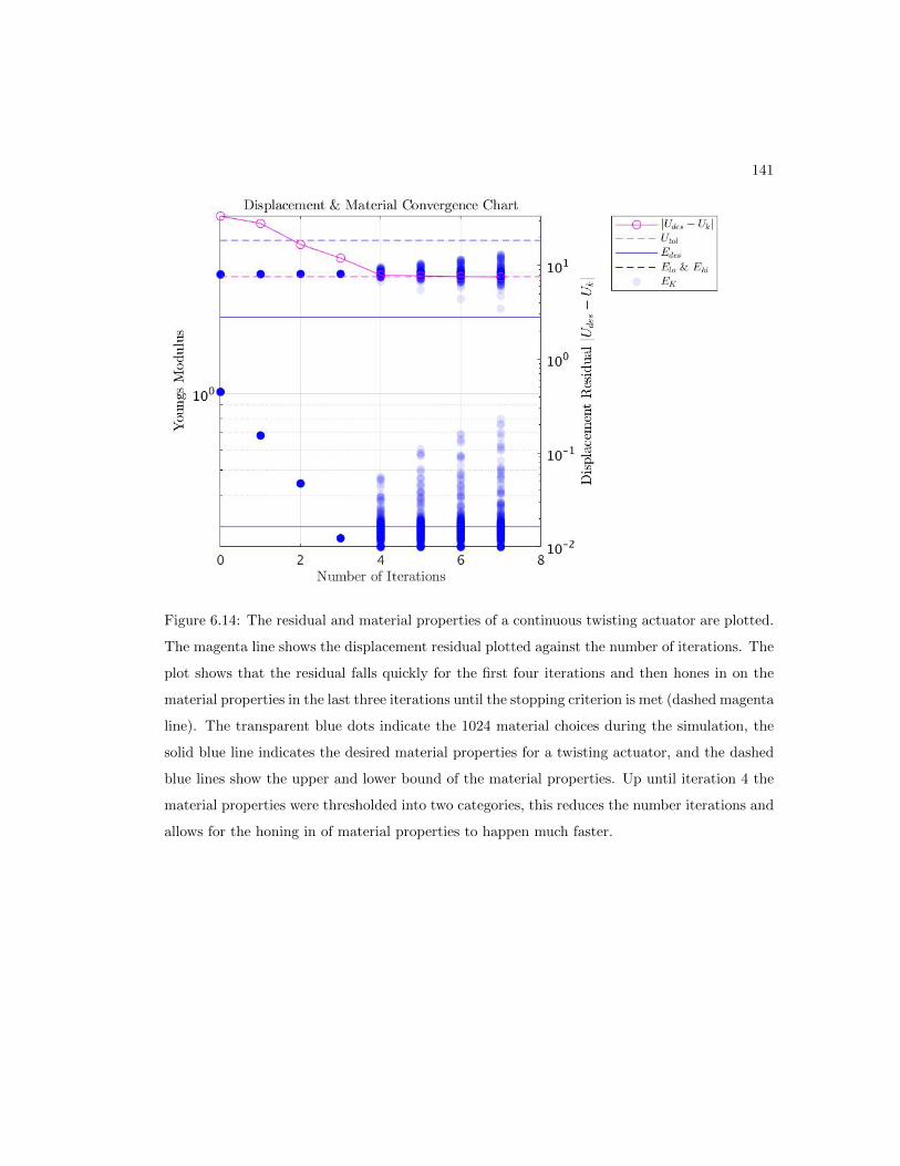
141

Figure 6.14: The residual and material properties of a continuous twisting actuator are plotted.

The magenta line shows the displacement residual plotted against the number of iterations. The

plot shows that the residual falls quickly for the first four iterations and then hones in on the

material properties in the last three iterations until the stopping criterion is met (dashed magenta

line). The transparent blue dots indicate the 1024 material choices during the simulation, the

solid blue line indicates the desired material properties for a twisting actuator, and the dashed

blue lines show the upper and lower bound of the material properties. Up until iteration 4 the

material properties were thresholded into two categories, this reduces the number iterations and

allows for the honing in of material properties to happen much faster.

142

Figure 6.15: The ground truth twisting actuator is shown on the left. The right image shows

the reconstructed twisting actuator geometry.

143

6.5 Case Study of a Realizable Twisting Actuator

The validating case studies all produced a continuous stiffness mapping which is unrealizable

with the Stratasys J750. This section will reconstruct the twisting actuator described above

when only the seven printable materials of the Stratasys J750 are available. Since the inverse

algorithm produces a continuous material stiffness between the low and high constraints. The

binning algorithm described by Algorithm 4 was applied to the continuous stiffness map in

order to create the best approximation of available materials. The Floyd-Steinberg dithering

(Algorithm 5) produced diverging results as the error shedding does not work with 1mm voxels

sizes. The Floyd-Stenberg dithering algorithm would have worked better with a reduced voxel

size as the error shedding would not have pushed material properties as far spatially.

The reconstruction of the discrete twisting actuator can be seen in Figure 6.16 and Figure

6.17. Figure 6.18 shows the error from material property, displacement, and strain. From

Figure 6.18 it can be seen that the material property error is minimal and only had some large

effects at the cap interfaces. This is expected as the cap causes smaller differences in each

voxels strain. The displacement error slowly increases with length. This is due to small strain

errors propagating the error of displacement. This displacement error was all < 0.3mm and

was deemed acceptable for the size of the geometry. The strain error was small throughout the

geometry. The largest errors in strain were associated to the boundary conditions at the caps.

144

Figure 6.16: The residual of a reconstructed twisting actuator.

145

Figure 6.17: Reconstructed twisting actuator geometry that was be printed on the Stratasys

J750.

146

Figure 6.18: Three error plots were created. The left plot shows error in the neo-Hookean

material property, the middle plot shows the error in displacement, the right plot shows the

error in the strain.

6.5.1 Experimental Setup for Twisting Actuator

The schematic of the experimental setup is outlined in Figure 6.19. The actuator is connected

to an air pump and pressure sensor which allowed for a slow increase in the pressure until the

desired pressure is reached. To measure the deformation, a Microsoft Lifecam is placed above

the actuator and a Google pixel was used for the side view. The LED was used to time sync

the two cameras. Figure 6.20 shows an image of the experimental setup.

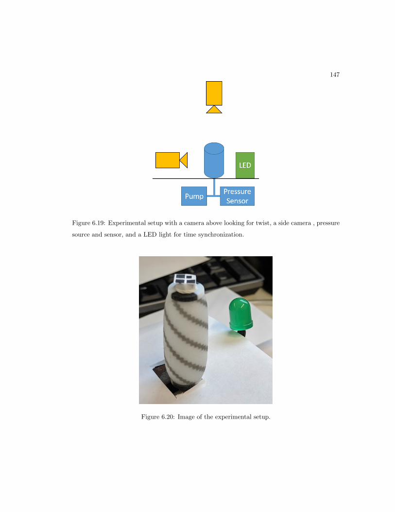
147

Figure 6.19: Experimental setup with a camera above looking for twist, a side camera , pressure

source and sensor, and a LED light for time synchronization.

Figure 6.20: Image of the experimental setup.

148

Determining the Rotation Angle

Computer vision was used to extract out the rotation angle of the twister actuator. The camera

was positioned above the actuator as shown in Figure 6.19. A qr marker was glued to the top of

the actuator and oriented such that it was in the center of the overhead cameras view as shown

in Figure 6.20. The goal of the vision algorithm was to determine the centroids of qr marker and

then determine the angle between the centroids to get actuator twist as shown in Figure 6.21.

The centroids were found by applying a Gaussian filter, thresholding the image, searching for

connected blobs, and then calculating the three centroids. The correct blobs were determined

by looking for blobs of similar area and aspect ratios. Once the centroids were determined an

atan2 function was used to calculate the angle.

Figure 6.21: A twisting actuator experiment where the three markers on the qr code are detected

and used to determine the twist angle.

Experimental Results

Figure 6.22 compares the twist of the reconstructed actuator with the ground truth actuator for

both the Abaqus simulation and experiment. From the figure it can be seen that both simulated

149

actuator’s twist closely match each other. It can also been seen that the experimental twist

closely follows the simulated twist and that the twist nearly matches around the point of failure

for the actuator. The difference in the simulated and experimentally most likely arises from

the fit of the neo-Hookean model. In Chapter 5, Figure 5.4 a stress strain curves for Stratasys

FLX9785 are shown. It can be seen that the material properties have variances within the print,

which likely accounts for the small difference in Figure 6.22.

150

Figure 6.22: Experimental and simulated twisting actuator where the pressure is plotted against

the twist. The blue indicates the ground truth actuator while the red indicates the reconstructed

actuator. The circles represent the simulated results and the dots indicate the experimental

results. An image of the ground truth twisting actuator is shown on the left of the plot.

6.6 Inverse Design Discussion

There are several discussion topics that arose when creating an inverse algorithm. The first

discussion point is on the options that the user is given when setting up the solver and algorithm.

151

The user can choose to group elements together as well as reduce the number of nodes. The

element grouping is useful for increasing the mesh density while keeping the number of individual

material properties constant. This gives the user the option to solve for higher deformation while

being limited by the voxel size that the 3D printer is able to print. Reducing the number of nodes

allows the user to determine some actuator locations that they do not care about. For instance,

the location of the internal surface is not always important. The nodes from the internal surface

could then be removed from the sensitivity matrix and not used when updating the material

properties. This allows for more ease of use from the user as only the important points need to

be defined. Future work should study how many nodes can be removed while reconstructing the

shape. Thus far it has been determined that the material properties can be reconstructed when

the nodes associated to the internal surface were removed. Additionally, a weighting scheme

could be implemented which prioritizes the motion of some nodes in comparison of others. Both

of these changes could help a user who only cares about a few specific locations of the actuator

and does not want to define the deformation of the entire actuator body.

The second discussion point is the assignment of weights. For instance the strain objective

incorporated all six DOF, however, this objective could not be used alone to reconstruct out of

plane motion as in the bending case. This was due to the fishing rod effect, if a fishing rod was

discretized into smaller pieces and there was a small amount of error in each piece. That sum

of errors would cause the tip position of the fishing rod to be in a different Cartesian position

than the desired position. This kept the need for an explicit penalty on Cartesian displacements

in addition to only strains. The similarity penalty was more of a practical engineering con-

straint and was always used in conjunction with the displacement penalty to prevent runaway

parameters and to smooth the spatial material parameters.

A third discussion point is the initial seeding which had a major affect on whether or not

the material properties would converge. A simple Hooke’s Law approximation was good enough

to provide the distribution of stiff and soft materials for the three actuators tested. If a pure

shearing actuator was desired, the seeding algorithm would choose a single material property

for all voxels, thus defeating the algorithm. To determine the seed for a pure shearing actuator

weighting or diffusion or dithering algorithm could be used. Since there is intuition of the

stiffness-structure needed to create twisting actuator, that stiffness mapping could be used as the

initial seeding. Alternatively, the twisting actuator structure could be used to shift some nodal

152

location of the actuator body to create an actuator more similar to the determined twisting

actuator. By utilizing the knowledge of the stiffness mappings found in Section 6.4 several

seeding options could arise.

A fourth discussion point is on the dithering or binning algorithms which were needed to

create a realizable stiffness matrix. Two algorithms were looked at. The first was a Floyd-

Steinberg dithering algorithm. For the twisting actuator, the Floyd-Steinberg dithering caused

divergence. This was most likely due to the relatively small mesh size (32x32), the shedding

of error to the neighboring voxel pushed stiff materials to far spatially away from the ideal

location. If a higher mesh density was used the Floyd-Steinberg dithering may have resulted

in convergence and has potential to perform better than the binning algorithm. The binning

algorithm used simply discretized the materials by setting the continuous material properties

to the closest discrete material properties. This worked for the twisting actuator resulted in

convergence. Future work should exploit the error shedding feature of the Floyd-Steinberg

dithering with the sensitivity matrices allowing for mechanics based error shedding approach

from voxel to voxel. Alternatively, a discrete optimization program could be developed where

only the material properties in the set can be used.

The fifth discussion point is centered on convergence. Since the inverse algorithm relies on

first solving a forward FEM problem for displacements, a force-displacement curve is created.

This curve is non-linear and when a change in material properties occurs the shape of the curve

can change substantially. This can cause material properties to overshoot or overcompensate.

When the next iteration occurs, the sensitivity matrices tries to pull the runaway properties

back. During this process neighboring tame material properties begin to follow the runaway

property due to the contribution of displacement of the runaway nodes. This causes errors in

the algorithm leading to a lack of convergence. One method to overcome this issue to seed

smartly. Another method to overcome runaway material properties would be to apply weights

on material properties based on strain error or displacement error. If the errors are high those

nodes should be given less weight in the sensitivity matrix. This would act similar to the

node reduction section. Another reason for the inability to reconstruct material properties is

the strain. Currently the strain was only taken at the center of the element. If the strain at

the edges of the element are not similar to the center, then a nonlinear strain has occurred

in the element. A higher mesh density should be used such that the desired strain is linear

153

throughout the element. The neighboring elements can then be grouped together to create a

voxel of a desired size. One major caveat to increasing mesh density is increasing the time of

the reconstruction algorithm.

6.7 Inverse Design Conclusions

A nonlinear inverse FEM optimization method was developed. This method updated material

properties with sensitivity matrices on displacement and strain. To validate the algorithm, three

actuator motions were successfully reconstructed. The first motion was a ballooning actuator,

which expanded uniformly in every direction. The second motion was a bending actuator,

capable of rotation constrained to a single plane. The third motion was a twisting actuator that

rotated along its axis in a nearly pure shear translation, transforming a pressure input into out

of plane motion.

To show that the inverse algorithm could produce a manufacturable design, a twisting ac-

tuator was reconstructed with a finite set of materials available on the Stratasys J750. The

ground truth and reconstructed twisting actuators were then realized by creating STL files of

the geometry, creating a print file, and executing the print file on Stratasys J750. The twist of

the ground truth and reconstructed actuator were compared with the simulation and experiment

to be comparable. This further validated the inverse algorithm. This algorithm worked well on

the three actuators that were tested. Future work, is needed to build a more robust algorithm

that is able to reconstruct the spiraling shape in Chapter 4.

Chapter 7

Conclusions

The field of soft robotics has empowered robots to maneuver, traverse, and complete tasks where

traditional rigid robots fall short. These robots are able to bend continuously and conform to

their environments, making their designs inherently safe. This makes soft robots a suitable

candidate for use in medical devices. In this thesis, contributions were made towards realizing a

soft catheter robot. A large scale protoype was built and an inverse soft robot design algorithm

was created.

First, a hydraulically soft robot was designed and experimentally shown to locomote through

a tube with three segments. The soft robot was designed with:

1. Only passive components with no moving parts.

2. Serially actuation (i.e. requires only one power source).

3. A geometry that avoids blocking flow while maintaining high contact area for anchoring

force (i.e. a spiral actuator). This includes experimental validation.

The three actuators needed for locomotion were spiral, extender, & spiral, were designed as

FREE actuators and optimized to meet a set of design requirements. These actuators were con-

trolled with passive valves which were optimized to ensure correct actuator timing. A potential

bending actuator was then modeled for use as an end-effector on the soft robot. A force model

of a bending actuator in a constrained and unconstrained position using force and pressure data

was developed. A study was also performed on asymmetrical, conical, cracking pressure valves

154

155

with an empirical design table for use in serially actuated soft robots being produced. The soft

robot designed and experimentally validated in Chapter 3, furthers the field of soft robots by

creating a serially actuated soft robot that is scalable, able to traverse tubes, and provides a

pathway for a soft catheter robot. However, the design space of the FREE actuators was only

able to realize actuators that were long and slender, motivating the need for an inverse FEM

design algorithm.

The first step of the inverse design method was the creation of the desired initial and final

actuator shapes. A generalized framework for describing soft robot kinematics from an initial

to final actuator was developed. Where:

1. A continuous robot centerline function can be constructed when given desired (x, y, z)

centerline points.

2. A method for describing actuator frames around the centerline.

3. A method to describe the actuator surface and volume where a varying radius and shear

can be applied to any point of the geometry and material incompressibility constraint can

be held from the initial to final geometry.

4. A design tool that allows user to view the initial/final actuator shapes as well as the

deformation and strain of a single voxel/element that the user can select.

The shape generation framework was then applied to a medical scan of a renal artery, where a

patient specific spiraling actuator was fit to an arterial branch of the scan.

Next, a nonlinear inverse FEM optimization algorithm to reconstruct the material properties

of cylindrical geometries when given the deformation, pressure, and boundary conditions was

created. This method reconstructed material properties by:

1. Deriving sensitivity matrices on deformation and strain to reconstruct material properties

within a multi-objective optimization.

2. Developing a procedure to seed the initial material properties given the deformation and

pressure.

The algorithm was successfully validated by reconstructing three actuator motions. The first

motion was a ballooning actuator, the second motion was a bending actuator, and the third

motion was a twisting actuator.

156

To show that the inverse algorithm could produce a manufacturable design, a twisting actu-

ator was reconstructed with a finite set of materials available on the Stratasys J750. To create

a realizable design:

1. Neo-Hookean fits for the stretchable materials that Stratasys produces were determined.

2. An automated process that takes a cylindrical geometry and stiffness matrix and creates

a unique STL file for each material in the robot design. The files can then be directly

opened and printed on a Stratasys J750.

The ground truth and reconstructed twisting actuators were then realized on Stratasys J750.

The twist of the ground truth and reconstructed actuator were compared with the simulation

and experiment, and the results were found to be comparable. This further validated the inverse

algorithm.

The work in this thesis provides the first steps towards realizing a soft catheter robot. Future

work will focus on refining the algorithms and models outlined in this thesis.

Bibliography

[1] Daniela Rus and Michael T Tolley. Design, fabrication and control of soft robots. Nature,

521(7553):467–475, May 2015.

[2] Peter Lee, S Regenbogen, and AA Gawande. How many surgical procedures will americans

experience in an average lifetime?: Evidence from three states. In 55th Annual Meeting,

2008.

[3] Molla S Donaldson, Janet M Corrigan, Linda T Kohn, et al. To err is human: building a

safer health system, volume 6. National Academies Press, 2000.

[4] The internet stroke center.

[5] Jeffrey L Saver, Mayank Goyal, AAD Van der Lugt, Bijoy K Menon, Charles BLM Majoie,

Diederik W Dippel, Bruce C Campbell, Raul G Nogueira, Andrew M Demchuk, Alejandro

Tomasello, et al. Time to treatment with endovascular thrombectomy and outcomes from

ischemic stroke: a meta-analysis. Jama, 316(12):1279–1289, 2016.

[6] MN Department of Health. Minnesota stroke system designated hospitals.

[7] Deepak Trivedi, Christopher D Rahn, William M Kier, and Ian D Walker. Soft robotics:

Biological inspiration, state of the art, and future research. Applied Bionics and Biome-

chanics, 5(3):99–117, 2008.

[8] Andrew D Marchese, Russ Tedrake, and Daniela Rus. Dynamics and trajectory optimiza-

tion for a soft spatial fluidic elastomer manipulator. The International Journal of Robotics

Research, page 0278364915587926, 2015.

157

158

[9] Andrew D Marchese and Daniela Rus. Design, kinematics, and control of a soft spa-

tial fluidic elastomer manipulator. The International Journal of Robotics Research, page

0278364915587925, 2015.

[10] Jungwook Paek, Inho Cho, and Jaeyoun Kim. Microrobotic tentacles with spiral bending

capability based on shape-engineered elastomeric microtubes. Scientific reports, 5, 2015.

[11] Wilhelm Conrad Rontgen. Ueber die durch electricitat bewirkten form-und volu-

menanderungen von dielectrischen korpern. Annalen der Physik, 247(13):771–786, 1880.

[12] Ron Pelrine, Roy Kornbluh, Qibing Pei, and Jose Joseph. High-speed electrically actuated

elastomers with strain greater than 100%. Science, 287(5454):836–839, 2000.

[13] Federico Carpi, Danilo De Rossi, Roy Kornbluh, Ronald Edward Pelrine, and Peter

Sommer-Larsen. Dielectric elastomers as electromechanical transducers: Fundamentals,

materials, devices, models and applications of an emerging electroactive polymer technol-

ogy. Elsevier, 2011.

[14] Marcello Calisti, Michele Giorelli, Guy Levy, Barbara Mazzolai, B Hochner, Cecilia Laschi,

and Paolo Dario. An octopus-bioinspired solution to movement and manipulation for soft

robots. Bioinspiration & biomimetics, 6(3):036002, 2011.

[15] S. Seok, C. D. Onal, K. J. Cho, R. J. Wood, D. Rus, and S. Kim. Meshworm: A peristaltic

soft robot with antagonistic nickel titanium coil actuators. IEEE/ASME Transactions on

Mechatronics, 18(5):1485–1497, Oct 2013.

[16] J. Bishop-Moser and S. Kota. Design and modeling of generalized fiber-reinforced pneumatic

soft actuators. IEEE Trans. Robot., 31(3):536–545, June 2015.

[17] Panagiotis Polygerinos, Zheng Wang, Johannes TB Overvelde, Kevin C Galloway, Robert J

Wood, Katia Bertoldi, and Conor J Walsh. Modeling of soft fiber-reinforced bending actu-

ators. 2015.

[18] Larry D Peel. Fabrication and mechanics of fiber-reinforced elastomers. PhD thesis,

Brigham Young University, 1998.

[19] Ching-Ping Chou and B. Hannaford. Measurement and modeling of mckibben pneumatic

artificial muscles. IEEE Trans. Robot. Autom., 12(1):90–102, Feb 1996.

159

[20] Bobak Mosadegh, Panagiotis Polygerinos, Christoph Keplinger, Sophia Wennstedt,

Robert F Shepherd, Unmukt Gupta, Jongmin Shim, Katia Bertoldi, Conor J Walsh, and

George M Whitesides. Pneumatic networks for soft robotics that actuate rapidly. Advanced

Functional Materials, 24(15):2163–2170, 2014.

[21] Michael De Volder, AJM Moers, and Dominiek Reynaerts. Fabrication and control of

miniature mckibben actuators. Sensors and Actuators A: Physical, 166(1):111–116, 2011.

[22] Steven D Thomalla and James D Van de Ven. Modeling and implementation of the mck-

ibben actuator in hydraulic systems. IEEE Transactions on Robotics, 34(6):1593–1602,

2018.

[23] G. Andrikopoulos, G. Nikolakopoulos, and S. Manesis. A survey on applications of pneu-

matic artificial muscles. Proc. Mediterranean Conf. Control Autom., pages 1439–1446, June

2011.

[24] Omotayo F Ewumi. Experimentally characterized embedded McKibben muscles as a nastic

material for biomedical applications. PhD thesis, Texas A&M University, 2007.

[25] Rongjie Kang, David T Branson, Tianjiang Zheng, Emanuele Guglielmino, and Darwin G

Caldwell. Design, modeling and control of a pneumatically actuated manipulator inspired

by biological continuum structures. Bioinspiration & biomimetics, 8(3):036008, 2013.

[26] Richard Quint van der Linde. Design, analysis, and control of a low power joint for walking

robots, by phasic activation of mckibben muscles. IEEE Transactions on Robotics and

Automation, 15 (4), 1999.

[27] Philip Moseley, Juan Manuel Florez, Harshal Arun Sonar, Gunjan Agarwal, William Curtin,

and Jamie Paik. Modeling, design, and development of soft pneumatic actuators with finite

element method. Advanced Engineering Materials, 2015.

[28] Jun-ya Nagase, Shuichi Wakimoto, Toshiyuki Satoh, Norihiko Saga, and Koichi Suzumori.

Design of a variable-stiffness robotic hand using pneumatic soft rubber actuators. Smart

Materials and Structures, 20(10):105015, 2011.

160

[29] Ili Najaa Aimi Mohd Nordin, AAM Faudzi, MRM Razif, E Natarajan, S Wakimoto, and

K Suzumori. Simulations of two patterns fiber weaves reinforced in rubber actuator. Jurnal

Teknologi, 69(3), 2014.

[30] AhmadAthif M Faudzi, M Rusydi M Razif, Ili Najaa Aimi M Nordin, K Suzumori, S Waki-

moto, and D Hirooka. Development of bending soft actuator with different braided angles.

In Advanced Intelligent Mechatronics (AIM), 2012 IEEE/ASME International Conference

on, pages 1093–1098. IEEE, 2012.

[31] Fionnuala Connolly, Panagiotis Polygerinos, Conor J Walsh, and Katia Bertoldi. Mechan-

ical programming of soft actuators by varying fiber angle. Soft Robot., 2(1):26–32, Mar

2015.

[32] Deepak Trivedi, Amir Lotfi, and Christopher D Rahn. Geometrically exact models for soft

robotic manipulators. Robotics, IEEE Transactions on, 24(4):773–780, 2008.

[33] Joshua Bishop-Moser, Girish Krishnan, Charles Kim, and Sridhar Kota. Design of soft

robotic actuators using fluid-filled fiber-reinforced elastomeric enclosures in parallel combi-

nations. In Intelligent Robots and Systems (IROS), 2012 IEEE/RSJ International Confer-

ence on, pages 4264–4269. IEEE, 2012.

[34] Joshua L Bishop-Moser. Design of Generalized Fiber-reinforced Elasto-fluidic Systems. PhD

thesis, University of Michigan, 2014.

[35] J. Bishop-Moser and S. Kota. Towards snake-like soft robots: Design of fluidic fiber-

reinforced elastomeric helical manipulators. Proc. IEEE/RSJ Int. Conf. Intell. Robots and

Syst. (IROS), pages 5021–5026, Nov 2013.

[36] Girish Krishnan. Kinematics of a new class of smart actuators for soft robots based on

generalized pneumatic artificial muscles. Proc. IEEE/RSJ Int. Conf. Intell. Robots and

Syst. (IROS), pages 587–592, Sept 2014.

[37] Girish Krishnan, Joshua Bishop-Moser, Charles Kim, and Sridhar Kota. Evaluating mo-

bility behavior of fluid filled fiber-reinforced elastomeric enclosures. Proc. ASME Int. Des.

Eng. Tech. Conf., pages 1089–1099, Aug 2012.

161

[38] Jonathan B Hopkins, Jordan Rivera, Charles Kim, and Girish Krishnan. Synthesis and

analysis of soft parallel robots comprised of active constraints. Journal of Mechanisms and

Robotics, 7(1):011002, 2015.

[39] Koichi Suzumori, Shoichi Iikura, and Hirohisa Tanaka. Development of flexible microac-

tuator and its applications to robotic mechanisms. In Robotics and Automation, 1991.

Proceedings., 1991 IEEE International Conference on, pages 1622–1627. IEEE, 1991.

[40] S. Wakimoto, K. Ogura, K. Suzumori, and Y. Nishioka. Miniature soft hand with curling

rubber pneumatic actuators. In Robotics and Automation, 2009. ICRA ’09. IEEE Inter-

national Conference on, pages 556–561, May 2009.

[41] Filip Ilievski, Aaron D Mazzeo, Robert F Shepherd, Xin Chen, and George M Whitesides.

Soft robotics for chemists. Angewandte Chemie, 123(8):1930–1935, 2011.

[42] Soft robotic toolkit.

[43] Sachin Bijadi. Feasibility of Additive Manufacturing Method for Developing Stretchable and

Flexible Embedded Circuits. PhD thesis, Citeseer, 2014.

[44] Zhijie Zhu, Shuang-Zhuang Guo, Tessa Hirdler, Cindy Eide, Xiaoxiao Fan, Jakub Tolar,

and Michael C McAlpine. 3d printed functional and biological materials on moving freeform

surfaces. Advanced Materials, 30(23):1707495, 2018.

[45] Osman Dogan Yirmibesoglu, John Morrow, Stephanie Walker, Walker Gosrich, Reece Aidan

Canizares, Hansung Kim, Uranbileg Daalkhaijav, Chloe Fleming, Callie Branyan, and Yigit

Menguc. Direct 3d printing of silicone elastomer soft robots and their performance compar-

ison with molded counterparts. In IEEE-RAS International Conference on Soft Robotics

(ROBOSOFT), 2018.

[46] Rui Ding, Yuyang Du, Rebecca B Goncalves, Lorraine F Francis, and Theresa M Reineke.

Sustainable near uv-curable acrylates based on natural phenolics for stereolithography 3d

printing. Polymer Chemistry, 10(9):1067–1077, 2019.

[47] Stratasys. J750 digital anatomy 3d printer.

[48] Wacker Chemie AG. Aceo. Wacker Chemie AG.

162

[49] Qingrui Wang, Xiaoyong Tian, Lan Huang, Dichen Li, Andrei V Malakhov, and Alexan-

der N Polilov. Programmable morphing composites with embedded continuous fibers by 4d

printing. Materials & Design, 155:404–413, 2018.

[50] Ellen T Roche, Robert Wohlfarth, Johannes TB Overvelde, Nikolay V Vasilyev, Frank A

Pigula, David J Mooney, Katia Bertoldi, and Conor J Walsh. A bioinspired soft actuated

material. Advanced Materials, 26(8):1200–1206, 2014.

[51] Steven C Obiajulu, Ellen T Roche, Frank A Pigula, and Conor J Walsh. Soft pneumatic

artificial muscles with low threshold pressures for a cardiac compression device. In ASME

2013 International Design Engineering Technical Conferences and Computers and Infor-

mation in Engineering Conference, pages V06AT07A009–V06AT07A009. American Society

of Mechanical Engineers, 2013.

[52] Gang Chen, Minh Tu Pham, and Tanneguy Redarce. Development and kinematic analysis

of a silicone-rubber bending tip for colonoscopy. In Intelligent Robots and Systems, 2006

IEEE/RSJ International Conference on, pages 168–173. IEEE, 2006.

[53] K. Ikuta, H. Ichikawa, K. Suzuki, and D. Yajima. Multi-degree of freedom hydraulic pressure

driven safety active catheter. Proc. IEEE Int. Conf. Robot. Autom. (ICRA), pages 4161–

4166, May 2006.

[54] K. Ikuta, M. Matsuda, D. Yajima, and Y. Ota. Precise bending angle control of hydraulic

active catheter by pressure pulse drive. Proc. IEEE Int. Conf. Robot. Autom. (ICRA),

pages 5588–5593, May 2010.

[55] K. Ikuta, Y. Matsuda, D. Yajima, and Y. Ota. Pressure pulse drive: A control method

for the precise bending of hydraulic active catheters. IEEE/ASME Trans. Mechatron.,

17(5):876–883, Oct 2012.

[56] Ellad B Tadmor, Ronald E Miller, and Ryan S Elliott. Continuum mechanics and thermo-

dynamics: from fundamental concepts to governing equations. Cambridge University Press,

2012.

[57] Paul T Boggs and Jon W Tolle. Sequential quadratic programming. Acta numerica, 4:1–51,

1995.

163

[58] Inc. The MathWorks. Matlab.

[59] Robert W Soutas-Little. History of continuum mechanics. Continuum Mechanics-Volume

I, page 80, 2011.

[60] Richard S Hamilton. The inverse function theorem of nash and moser. American Mathe-

matical Society, 7(1):65–122, 1982.

[61] M Mooney. A theory of large elastic deformation. Journal of applied physics, 11(9):582–592,

1940.

[62] RW Ogden. Large deformation isotropic elasticity-on the correlation of theory and experi-

ment for incompressible rubberlike solids. Proceedings of the Royal Society of London. A.

Mathematical and Physical Sciences, 326(1567):565–584, 1972.

[63] PALS Martins, RM Natal Jorge, and AJM Ferreira. A comparative study of several material

models for prediction of hyperelastic properties: Application to silicone-rubber and soft

tissues. Strain, 42(3):135–147, 2006.

[64] Nam-Ho Kim. Introduction to nonlinear finite element analysis. Springer Science & Business

Media, 2014.

[65] Bob McGinty. Continuum Mechanics. 2012.

[66] Wikipedia. Tensor.

[67] F. Kallel and M. Bertrand. Tissue elasticity reconstruction using linear perturbation

method. IEEE Transactions on Medical Imaging, 15(3):299–313, June 1996.

[68] MM Doyley, PM Meaney, and JC Bamber. Evaluation of an iterative reconstruction method

for quantitative elastography. Physics in Medicine & Biology, 45(6):1521, 2000.

[69] Assad A Oberai, Nachiket H Gokhale, and Gonzalo R Feijoo. Solution of inverse problems

in elasticity imaging using the adjoint method. Inverse problems, 19(2):297, 2003.

[70] Assad A Oberai, Nachiket H Gokhale, Marvin M Doyley, and Jeffrey C Bamber. Evaluation

of the adjoint equation based algorithm for elasticity imaging. Physics in Medicine &

Biology, 49(13):2955, 2004.

164

[71] Shyamal Guchhait and Biswanath Banerjee. Constitutive error based material parameter

estimation procedure for hyperelastic material. Computer Methods in Applied Mechanics

and Engineering, 297:455–475, 2015.

[72] M. Morita, M. Nakao, and T. Matsuda. Elastic modulus estimation based on local dis-

placement observation of elastic body. In 2017 39th Annual International Conference of

the IEEE Engineering in Medicine and Biology Society (EMBC), pages 2138–2141, July

2017.

[73] SK Kyriacou, AD Shah, and JD Humphrey. Inverse finite element characterization of

nonlinear hyperelastic membranes. Journal of Applied Mechanics, 64(2):257–262, 1997.

[74] Markus Becker and Matthias Teschner. Robust and efficient estimation of elasticity param-

eters using the linear finite element method. In SimVis, pages 15–28, 2007.

[75] Vıctor D Fachinotti, Alberto Cardona, and Philippe Jetteur. Finite element modelling

of inverse design problems in large deformations anisotropic hyperelasticity. International

Journal for Numerical Methods in Engineering, 74(6):894–910, 2008.

[76] Nils Napp, Brandon Araki, Michael T Tolley, Radhika Nagpal, and Robert J Wood. Simple

passive valves for addressable pneumatic actuation. Proc. IEEE Int. Conf. Robot. Autom.

(ICRA), pages 1440–1445, May 2014.

[77] John S Cundiff. Fluid power circuits and controls: fundamentals and applications. CRC

Press, 2001.

[78] Pavel Holoborodko. Smooth noise robust differentiators.

http://www.holoborodko.com/pavel/numerical-methods/numerical-derivative/smooth-

low-noise-differentiators/, 2008.

[79] K. C. Galloway and Panagiotis Polygerinos. Soft robotics toolkit.

[80] Antonın Novak, Laurent Simon, Frantisek Kadlec, and Pierrick Lotton. Nonlinear system

identification using exponential swept-sine signal. Instrumentation and Measurement, IEEE

Transactions on, 59(8):2220–2229, 2010.

165

[81] Jonas Sjoberg, Qinghua Zhang, Lennart Ljung, Albert Benveniste, Bernard Delyon, Pierre-

Yves Glorennec, Hakan Hjalmarsson, and Anatoli Juditsky. Nonlinear black-box modeling

in system identification: a unified overview. Automatica, 31(12):1691–1724, 1995.

[82] Charles L Lawson and RJ Hanson. Solving least squares problems prentice-hall. Englewood

Cliffs, NJ, 1974.

[83] F Frenet. Sur les courbes a double courbure. Journal de mathematiques pures et appliquees,

pages 437–447, 1852.

[84] Wikipedia. Frenet serret formulas. Wikipedia.

[85] Shoshichi Kobayashi and Katsumi Nomizu. Foundations of differential geometry, volume 1.

New York, 1963.

[86] RW Floyd and L Steinberg. An adaptive algorithm for spatial grey scale. Proceedings of

the Society of Information Display, 1976.

[87] George Papazafeiropoulos, Miguel Muniz-Calvente, and Emilio Martınez-Paneda.

Abaqus2matlab: a suitable tool for finite element post-processing. Advances in Engineering

Software, 105:9–16, 2017.

Appendix A

Appendix A

A.1 Stress Strain Curves

Contains the stress strain curves for various materials.

166

167

Figure A.1: Stress-strain data for the Stratasys Agilus30 material and a neo-Hookean fit.

168

Figure A.2: Stress-strain data for the Stratasys FLX9750 material and a neo-Hookean fit.

169


170


171

Figure A.5: Stress-strain data for the Stratasys FLX9785 material.

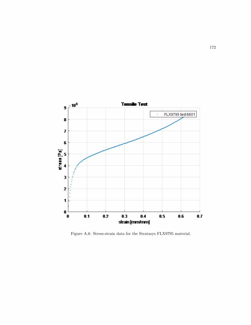
172

Figure A.6: Stress-strain data for the Stratasys FLX9795 material.

Appendix B

Biosketch

Mark is a PhD candidate in Mechanical Engineering at the University of Minnesota. He is a

member of both Medical Robotics & Devices Lab and the Mechanical Energy & Power Systems

Lab, & is co-advised by Professors Timothy M. Kowalewski and James D. Van de Ven. His

research has focused on developing soft robot technologies that can be applied to medical devices.

He has published both conference and letters papers, and was able to present his research at the

International Conference on Robotics and Automation in Singapore. Mark was also a recipient

of the University of Minnesota Interdisciplinary Doctoral Fellowship. During Mark’s graduate

career he was a teaching assistant for design, controls, and robotics courses. He developed and

implemented a 10 week robotics lab with a 6-DOF manipulator robot.

Prior to graduate school, Mark received his Bachelors in Mechanical Energy at the Uni-

versity of Minnesota. During his undergraduate degree, Mark founded and was president for

Copter Club, which was a club that built drones of different sizes. He has also held two intern-

ships. The first internship was at Graco Inc. in Minneapolis, where he performed testing on a

diaphragm pump and developed a spring loaded ball check valve. The second internship was

at Seagate. Mark created a computer vision algorithm to detect contaminants on disk drive

fixtures. Polarized images of the fixtures were taken, and the number and size of contaminants

were classified to quantify a cleaning method. He also performed a design of experiments to

study the effectiveness of cleaning disk drive fixtures with snow CO2.

173

Inverse Design of Soft Robotic Actuators using Nonlinear ...

Documents

Transcript of Inverse Design of Soft Robotic Actuators using Nonlinear ...