INTERLINKAGES AMONG SOUTH EAST ASIAN STOCK MARKETS (A Comparison Between Pre- and Post-1997-Crisis Periods)1

Aamir Rafique Hashmi• and Liu Xingyun

Department of Economics

National University of Singapore 10 Kent Ridge Crescent

Singapore 119260

Abstract

This paper examines inter-linkages among South East Asian (SEA), Tokyo

(TK) and New York (NY) stock market returns before and after the Asian

currency crisis using simple correlations, Granger causality tests and VAR

models. We find that inter-linkages among SEA markets have increased after

the emergence of crisis. The New York market affects the SEA markets but is

not affected by them. Tokyo market seems to be isolated from the region.

Singapore stock market appears to dominate other markets in the region and

its effect on them is even greater than that of New York. All five SEA markets

affect one another and their effects are transmitted within two days in most of

the cases.

Key words: Stock Market Integration; South-East Asian Stock Markets

JEL classification: F15; G15

1 Presented at a conference sponsored by Journal of International Money and Finance and the

University of Rome Tor Vergata, in Rome, December 5-7, 2001. • Corresponding author at email: ecsarh@nus.edu.sg or phone: (65) 874-3960.

- - 1

1. INTRODUCTION

Studies of market integration suggest that international stock markets have become

increasingly integrated in recent years2. Although this evidence is not undisputed,3 we can

safely comment that most of the recent studies find equity markets to be inter-linked. These

linkages can be attributed to the deregulation of international financial markets, shift to

floating exchange rates, advancement of communication system and information technology,

lower cost of transactions, and the development of new financial instruments and techniques.

There are a few interesting conclusions that emerge from the studies on stock market

integration. Some studies have found that New York market is the global leader and markets

in almost every part of the world are affected by it4. It has also been documented that

excluding New York, the other markets tend to have stronger relations with geographically

closer markets than with the remote ones. Saying the same thing in different words, intra-

continental linkages are stronger than inter-continental linkages5. Another finding is that

linkages are variable over time and generally major events (like 1973 and 1979 oil price

shocks, end of the Bretton Woods system, abolition of exchange controls in UK in late 1970s,

1987 stock market crash, 1991 Gulf) affect the linkages significantly.6 This last conclusion is

our motivation to study the effect of 1997 financial crisis on inter-linkages among SEA

markets. There are studies that concentrate on linkages among Asian markets7 but none has

attempted to study the effects of 1997 crisis on linkages.

2 The studies that provide evidence that markets are integrated and/or their degree of integration has been changing (mostly increasing) over time include, among many others, Ammer and May (1996), Arshanapalli and Doukas (1993), Bracker et al (1999), Eun and Shim (1989), Kasa (1992), Leachman and Fransic (1995), Longin and Solnik (1995) Rangvid (2001) and Taylor and Tonks (1989). For a comprehensive bibliography of studies on international stock market linkages see Roca (2000) pp.148-171. 3 See King (1994) and Baekaert and Harvey (1995). 4 Cheung and Mak (1992), Eun and Shim (1989), Koch and Koch (1993), Pesonen (1999) and Soydemir (2000) are just a few examples of such studies. 5 See, for example, Hilliard (1979) and Dekker et al (2001). 6 See, for example, Ammer and Mei (1996), Arshanapalli and Doukas (1993), Leachman and Fransic (1995) and Taylor and Tonks (1989). 7 Examples include Pan et al (1999), Dekker et al (2001) and Siklos and Ng (2001).

- - 2

In the course of our study we try to answer the following questions for both pre- and post-

crisis periods: are the SEA stock markets interlinked? How are the two largest markets of the

world are related to SEA markets? Which market appears to be the most influential in the

region? How much of the movements in one stock market can be explained by innovations in

other markets? How rapidly are the stock price movements in one market transmitted to

other markets?

In attempting to answer the above questions, analysis of correlations (and correlograms) and

Granger causality tests are conducted to examine the co-movements among the pair-wise

stock prices and returns. In addition, we also estimate vector-autoregressive models for both

pre- and post-crisis periods. The seven stock markets included in this study are New York

(NY), Tokyo (TK), Singapore (SG), Kuala Lumpur (KL), Bangkok (BK), Jakarta (JK), and

Manila (MN). Last five of these markets represent almost the entire South East region of Asia

The organization of the rest of the paper is as follows: Section 2 discusses the methodology

and data used. The empirical results are presented in Section 3 and Section 4 provides a

summary and conclusions of this study.

2. DATA AND METHODOLOGY

2.1 Data

The time series used in this study are daily stock market indexes at closing time, in terms of

local currencies. The stock indexes used are S&P 500 Composite, Nikkei 225 Stock Average,

Singapore Straits Times Index, Kuala Lumpur Composite, Bangkok S. E. T., Jakarta S. E.

Composite and Philippines S. E. Composite. The data cover a time period from 03/01/1994 to

29/12/2000, which is divided into two sub-periods. First sub-period has been named the pre-

- - 3

crisis period and covers from 03/01/1994 to 31/07/1997. The second sub-period has been

named the post-crisis period and covers from 01/08/1997 to 29/12/2000.

These stock market indices are transformed into continuously compounded daily rates of

return, defined as:

it

it

it PPR 1lnln −−=

where itP is stock price index series of market i. None of the data on stock prices that we use

have dividends reinvested. However, on a daily basis, dividends are relatively unimportant.

Changes in stock prices over short period are mainly affected by the arrival of information.

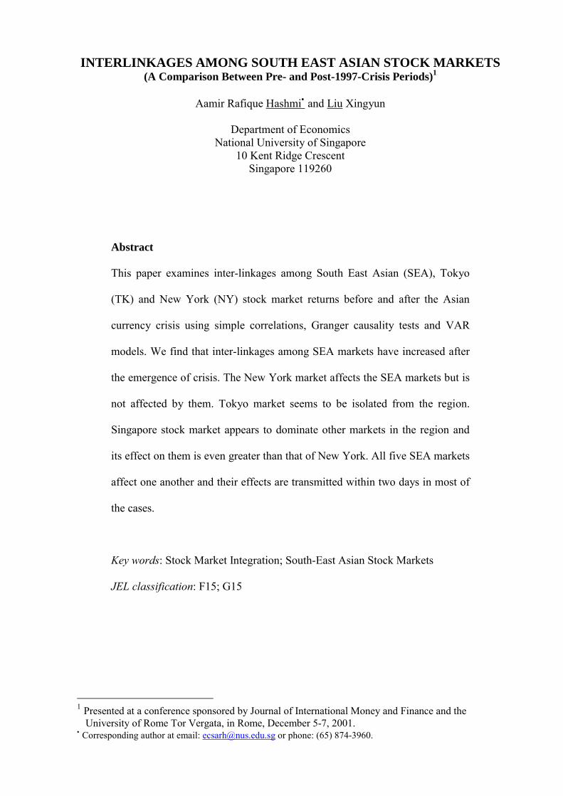
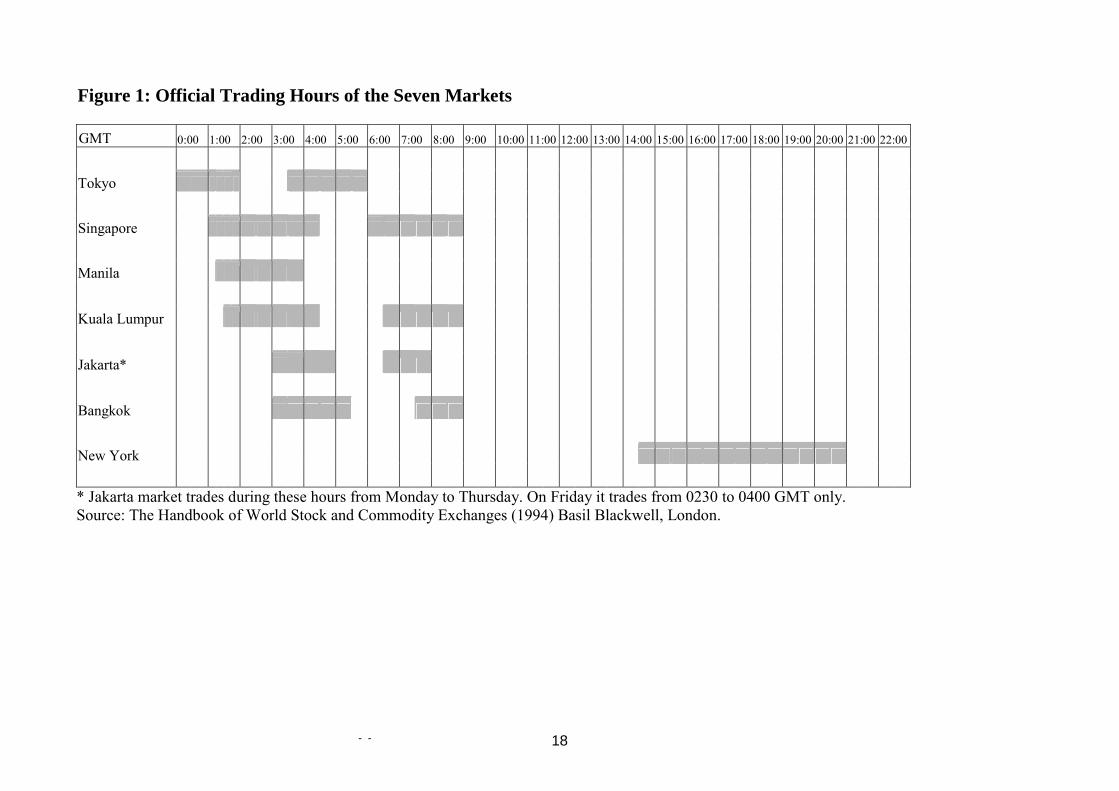
All these markets (except the New York) operate in similar time zones and there is a lot of

overlapping in their trading hours. Figure 1 plots the official trading hours for all seven

markets in our sample. As we are working with daily returns, we can treat the six markets

other than the New York as operating synchronously, although the closing price in Manila

may not be able to capture the effects of afternoon news from other markets operating in the

same time zone. The different opening and closing hours become more important when we

work with higher frequency data. In this study, however, our focus is on daily data so we

ignore the minor differences in opening and closing of markets in the SEA region. New York

is in a different time zone and opens when all these markets have closed. Due to this reason,

when we study the linkages from New York to other markets we should use the last day

returns in New York and current returns in other markets. However, when we study the

linkages from other markets to New York, we must consider the current returns for both.

2.2 Correlations and Cross-Correlograms

Simple correlations of daily returns reveal the link between the rates of change in the indices.

We also study the cross correlograms (up to 36 lags) between all pairs of the seven markets.

- - 4

We compute the correlation matrices for both pre- and post-crisis periods and then test their

equality using the Box-M statistic. It can be defined as [see Meric and Meric (1989)]:

( ) ( ) ( )

−+−×

+

−++

−+

−

+

−+−= −−~

122

~1

112121

2

ln1ln12

11

11

116

1321 RRnRRnnnnnk

kkM

where

k = number of variable in correlation matrix

ni = number of observations used to compute the ith correlation matrix

Ri = the ith correlation matrix

( ) ( )2

11

21

2211~

−+−+−

=nn

RnRnR

M follows a χ2 distribution with k(k+1)/2 degrees of freedom.

2.3 Granger Causality Test

Correlation does not necessarily imply causation in any economic sense. It is not unusual to

find that high correlations may simply be the result of spurious relationship and thus not of

much use. To address the question that whether some variable causes others, Granger (1969)

proposed a test to see how much of the current x can be explained by past values of x and

then to see whether adding lagged values of y can improve the explanation8. In a bivariate

VAR describing x and y, y does not Granger-cause x if the coefficient matrices jΦ are lower

triangular for all j:

+

++

+

+

=

−

−

−

−

−

−

t

t

pt

ptpp

p

t

t

t

t

t

t

yx

yx

yx

cc

yx

2

1)(

22)(

21

)(11

2

2)2(

22)2(

21

)2(11

1

1)1(

22)1(

21

)1(11

2

1 0...

00εε

φφφ

φφφ

φφφ

where j is the number of lag and j=1,2,�p.

To implement this test, we assume a particular autoregressive lag length p and estimate

tptpttptpttt uyyyxxxcx +++++++++= −−−−−− βββααα LL 221122111

8 For details, see Hamilton (1994).

- - 5

by OLS. We then conduct an F test of the null hypothesis

0: 210 ==== pH βββ L

2.4 The VAR Model

The popular time series technique of VAR is due to the seminal work of Sim (1980). It is

used to study the dynamic interrelations between n different variables. Many studies of stock

markets have used VAR models to study inter-linkages.9 The VAR model for n markets can

be expressed as:

t

m

sstst eRACR ++= ∑

=−

1

(1)

where Rt is a n × 1 column vector of daily rates of return of the n stock markets, C and As are,

respectively, n × 1 and n × n matrices of coefficients, m is the lag length, and et is a n × 1

column vector of error terms. The ijth component of As measures the direct effect that a

change in the return to the jth market will have on the return of the ith market in s period.

Since the coefficients in equation (1) contain complicated cross-equation feedbacks and are

difficult to describe intuitively, it is better to analyze the model�s reaction to typical random

shocks. By successive substitutions of the right-hand side of equation (1), we can obtain a

moving average representation as follow:

∑=

−+=x

sstst eBCR

0' (2)

Where each Bs is an n × n matrix. The Bij,s are called the impulse response functions, which

show the response of the ith market in s-period after a unit random shock in the jth market,

other things remaining constant. The decomposition of variance ( 2,

2, sisijB α∑ ) can reveal

how much variance of market i is determined by the innovations of market j in the s period. 9 Few examples include Ammer and Mei (1996), Chaudhary (1994), Eun and Shim (1989), King et al (1994), Rapach (2001), Roca (1999), Soydemir (2000) and Yuce and Mugan (2000).

- - 6

3. EMPIRICAL RESULTS

3.1 Preliminary Findings and Correlation Matrices

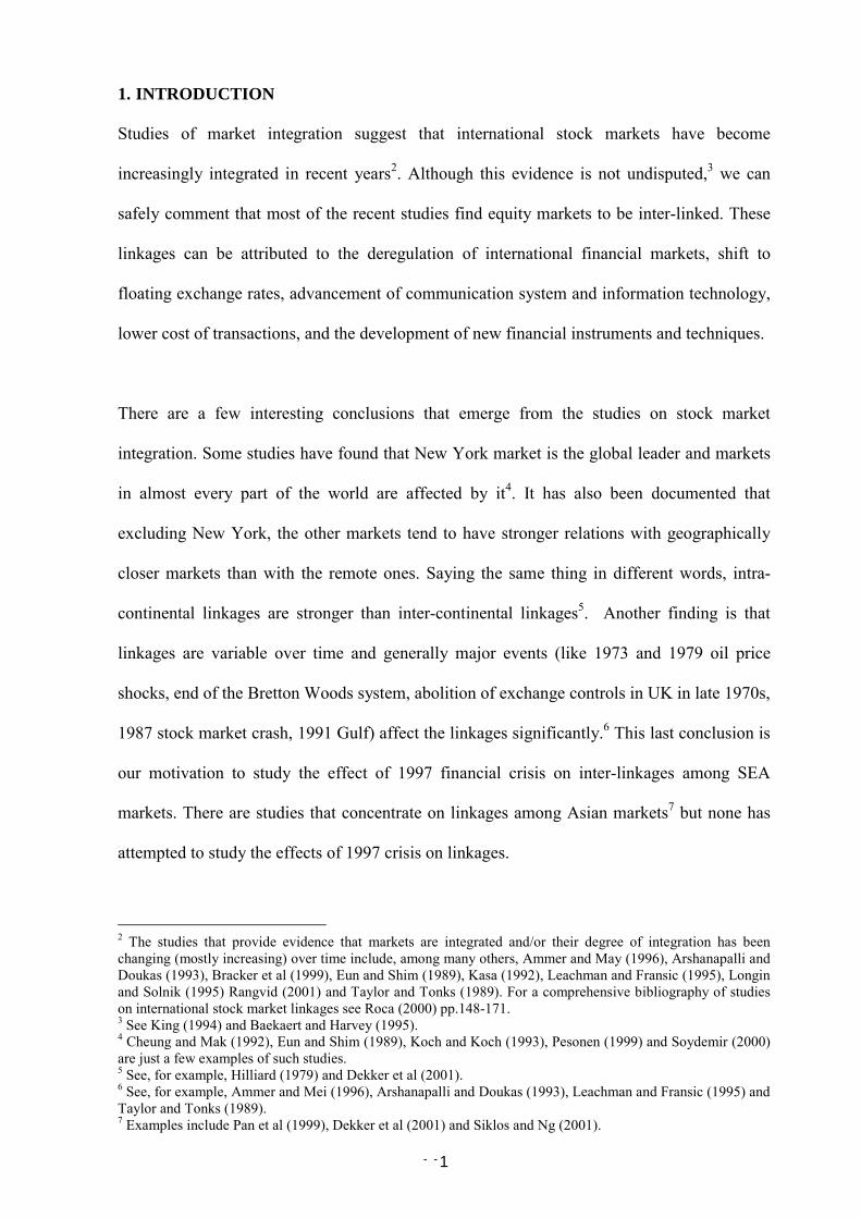
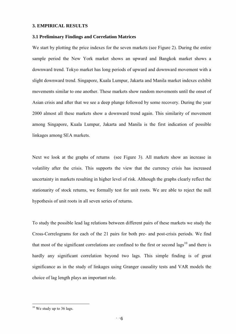
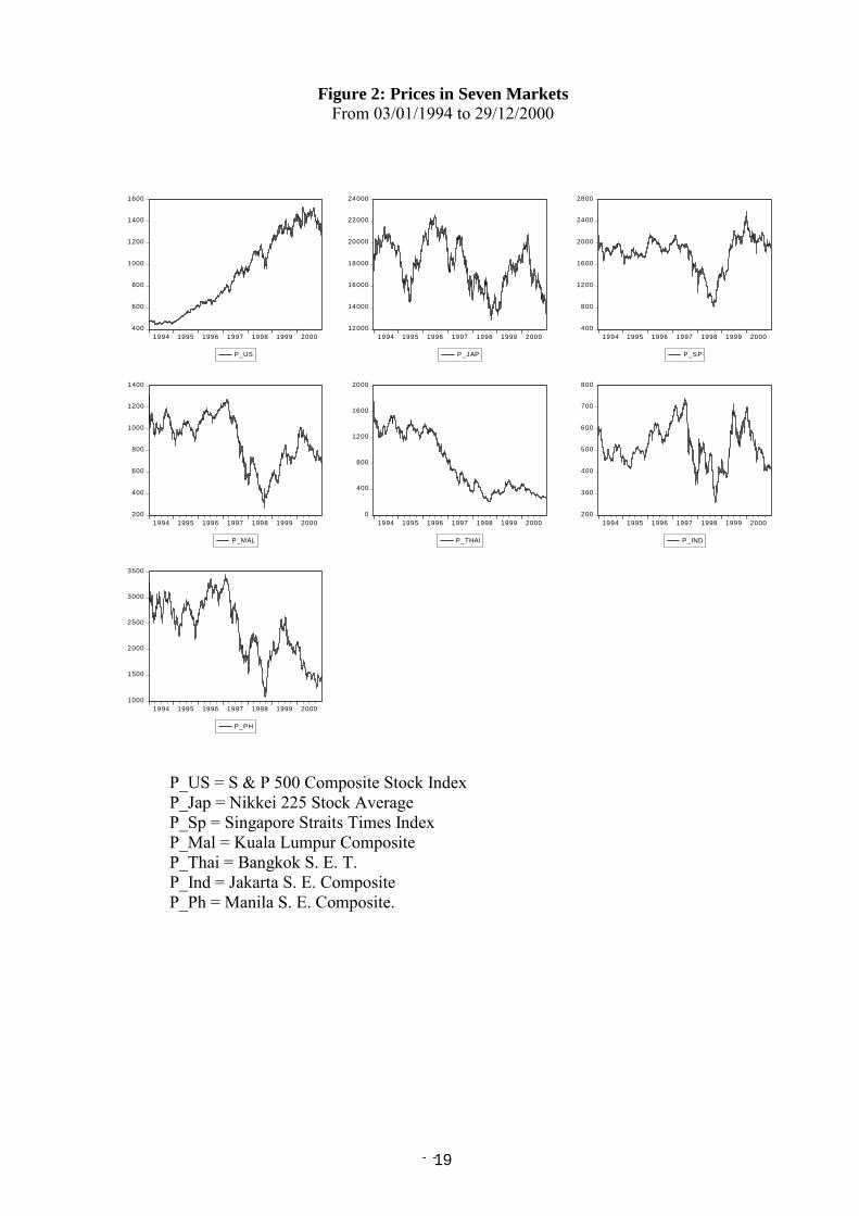
We start by plotting the price indexes for the seven markets (see Figure 2). During the entire

sample period the New York market shows an upward and Bangkok market shows a

downward trend. Tokyo market has long periods of upward and downward movement with a

slight downward trend. Singapore, Kuala Lumpur, Jakarta and Manila market indexes exhibit

movements similar to one another. These markets show random movements until the onset of

Asian crisis and after that we see a deep plunge followed by some recovery. During the year

2000 almost all these markets show a downward trend again. This similarity of movement

among Singapore, Kuala Lumpur, Jakarta and Manila is the first indication of possible

linkages among SEA markets.

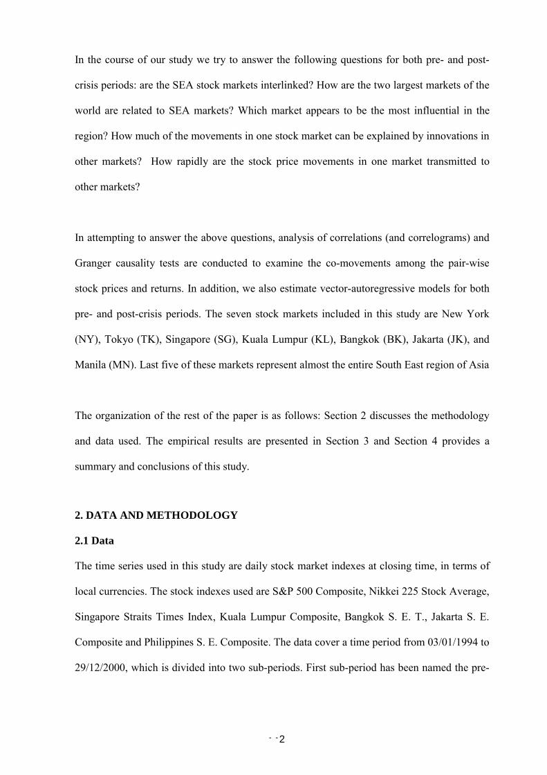
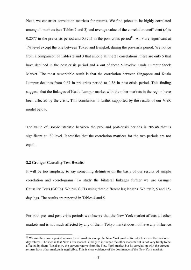
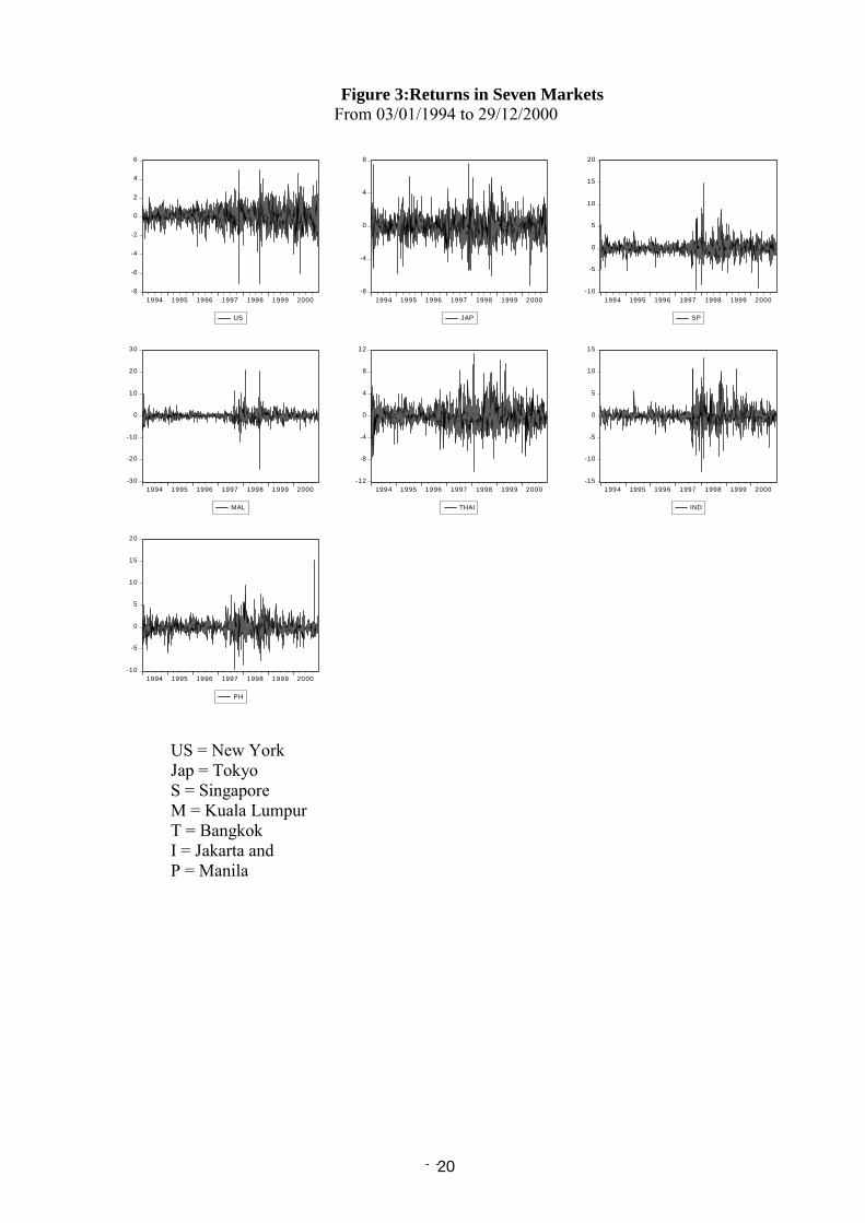
Next we look at the graphs of returns (see Figure 3). All markets show an increase in

volatility after the crisis. This supports the view that the currency crisis has increased

uncertainty in markets resulting in higher level of risk. Although the graphs clearly reflect the

stationarity of stock returns, we formally test for unit roots. We are able to reject the null

hypothesis of unit roots in all seven series of returns.

To study the possible lead lag relations between different pairs of these markets we study the

Cross-Correlograms for each of the 21 pairs for both pre- and post-crisis periods. We find

that most of the significant correlations are confined to the first or second lags10 and there is

hardly any significant correlation beyond two lags. This simple finding is of great

significance as in the study of linkages using Granger causality tests and VAR models the

choice of lag length plays an important role.

10 We study up to 36 lags.

- - 7

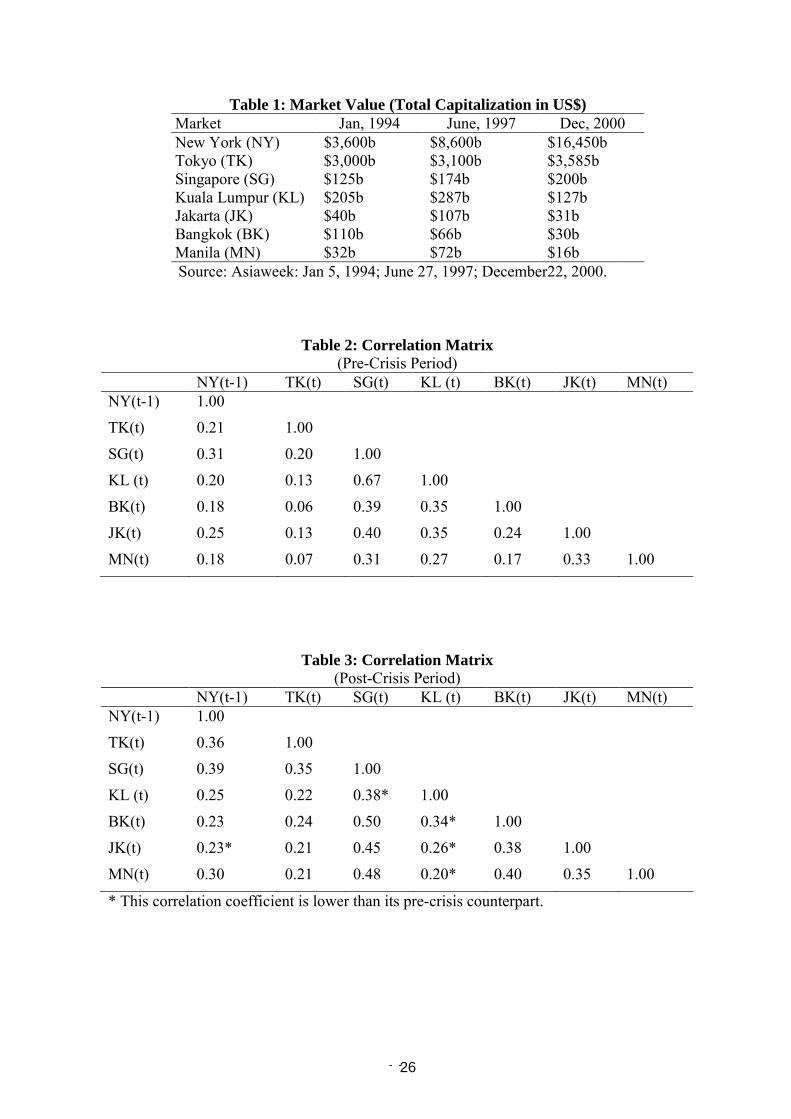
Next, we construct correlation matrices for returns. We find prices to be highly correlated

among all markets (see Tables 2 and 3) and average value of the correlation coefficient (r) is

0.2577 in the pre-crisis period and 0.3205 in the post-crisis period11. All r are significant at

1% level except the one between Tokyo and Bangkok during the pre-crisis period. We notice

from a comparison of Tables 2 and 3 that among all the 21 correlations, there are only 5 that

have declined in the post crisis period and 4 out of these 5 involve Kuala Lumpur Stock

Market. The most remarkable result is that the correlation between Singapore and Kuala

Lumpur declines from 0.67 in pre-crisis period to 0.38 in post-crisis period. This finding

suggests that the linkages of Kuala Lumpur market with the other markets in the region have

been affected by the crisis. This conclusion is further supported by the results of our VAR

model below.

The value of Box-M statistic between the pre- and post-crisis periods is 205.48 that is

significant at 1% level. It testifies that the correlation matrices for the two periods are not

equal.

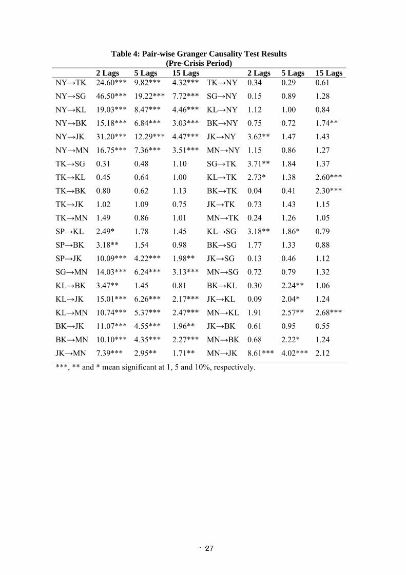
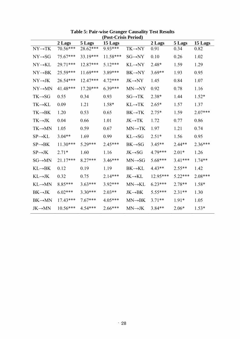
3.2 Granger Causality Test Results

It will be too simplistic to say something definitive on the basis of our results of simple

correlation and correlograms. To study the bilateral linkages further we use Granger

Causality Tests (GCTs). We run GCTs using three different lag lengths. We try 2, 5 and 15-

day lags. The results are reported in Tables 4 and 5.

For both pre- and post-crisis periods we observe that the New York market affects all other

markets and is not much affected by any of them. Tokyo market does not have any influence

11 We use the current period returns for all markets except the New York market for which we use the previous day returns. The idea is that New York market is likely to influence the other markets but is not very likely to be affected by them. We also try the current returns from the New York market but its correlation with the current returns from other markets is negligible. This is clear evidence of the dominance of the New York market.

- - 8

on the SEA regional markets and is not much affected by any market other than the New

York.

The pair-wise linkages between different SEA markets are very interesting. Singapore affects

all other four SEA markets before the crisis and is affected only by Kuala Lumpur. In the

post-crisis period, however, it is affected by all of them. This implies an increase in inter-

linkages among SEA markets after the crisis. The Kuala Lumpur market had a strong effect

on other four SEA markets before the crisis and was only affected by Singapore in the pre-

crisis period. After the crisis, it affects only Singapore and Manila but is affected by all four.

The Bangkok market provides a good example of increase in linkages after the crisis. We

notice that in the pre-crisis period it was only affected by Singapore and Kuala Lumpur

markets and it affected Jakarta and Manila. After the crisis, it was not being affected by

Kuala Lumpur any more but Manila and Jakarta were affecting it. The effects of Bangkok

market after the crisis are very significant and involved New York and Tokyo in addition to

all four SEA markets. Before the crisis, Jakarta was affected by all four and it affected only

Manila. After the crisis it was still affected by all (except KL) and was affecting all four.

Manila was affected by all four before and after the crisis. It affected only Jakarta before the

crisis but was affecting all four after it.

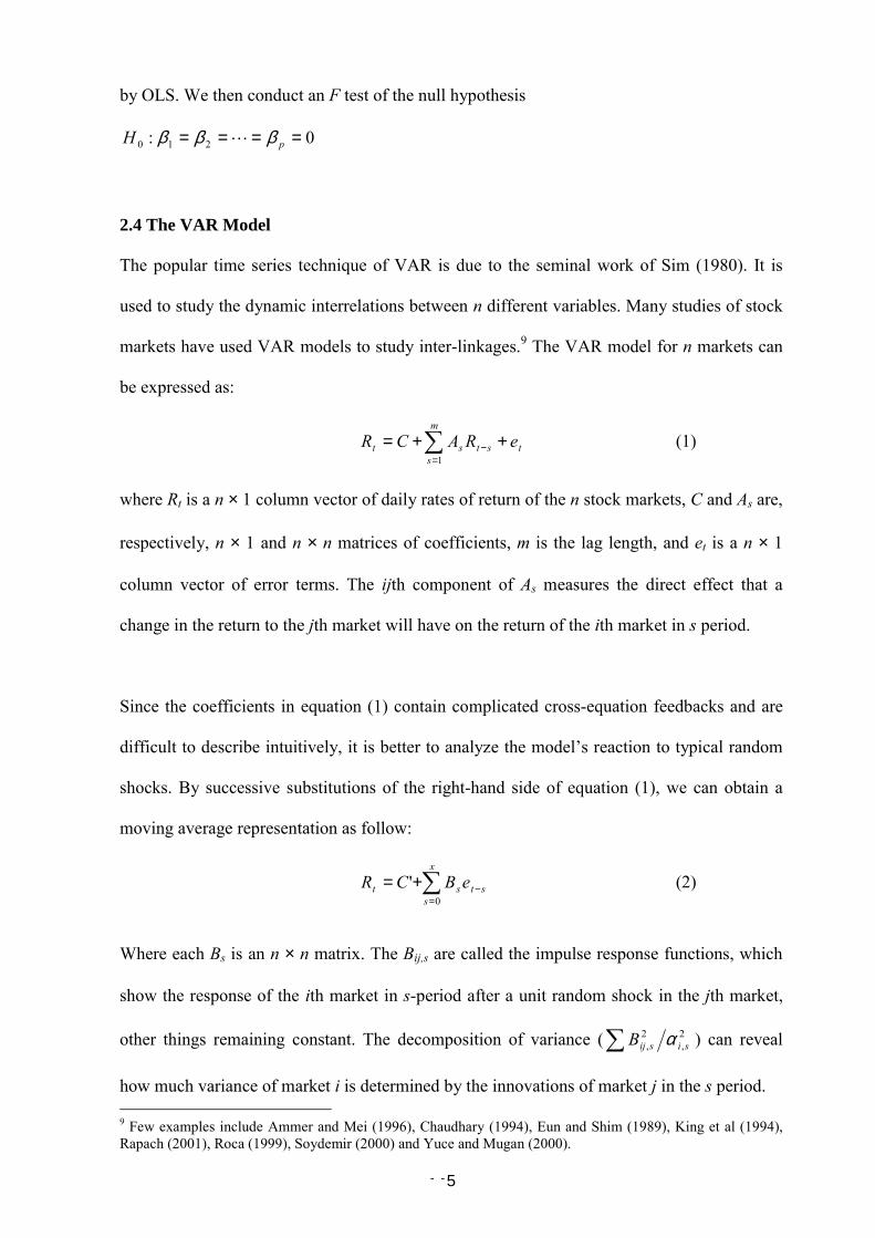
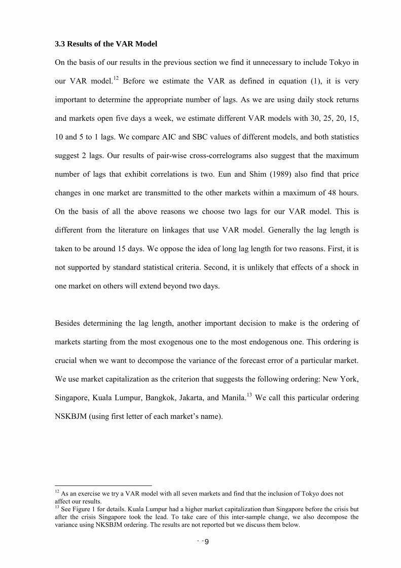
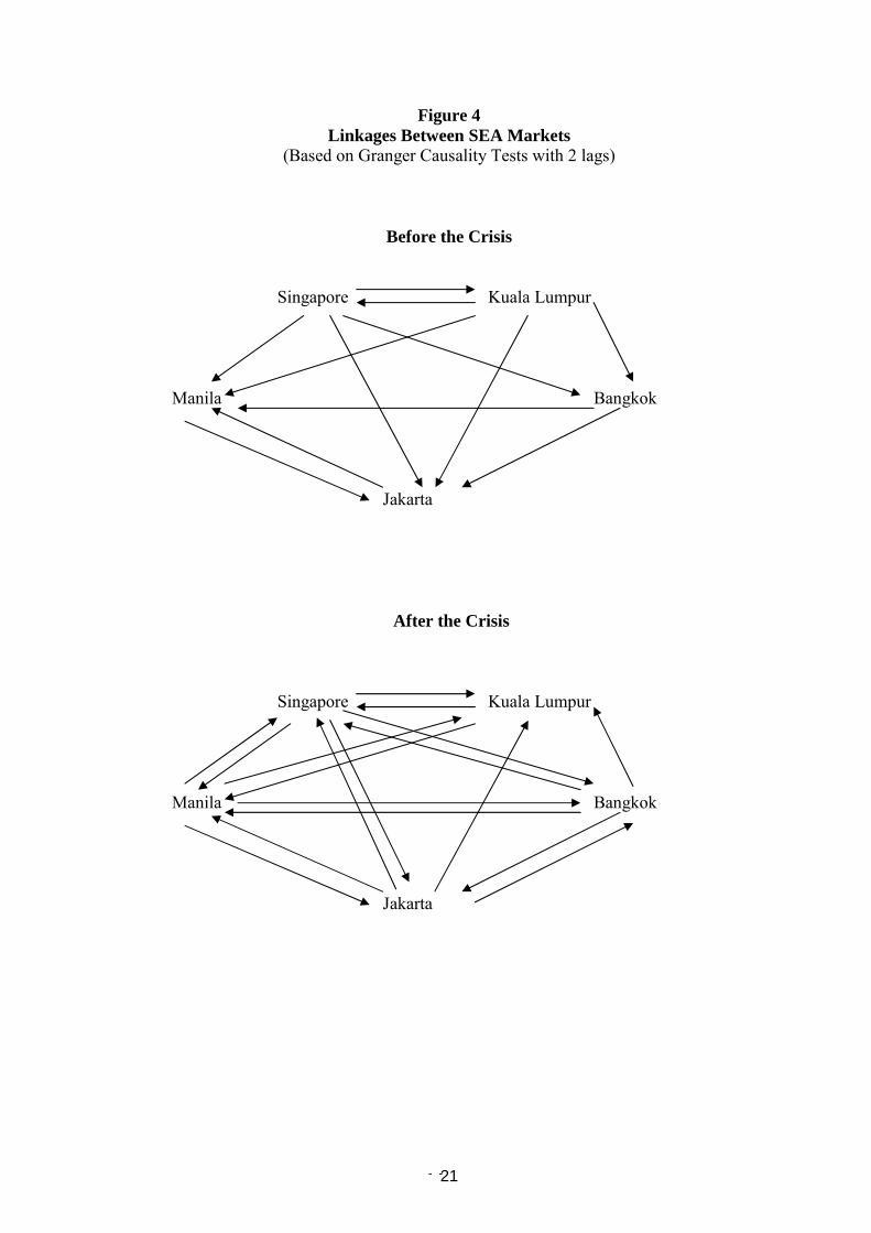
When we look at all the five SEA markets together (see figure 4) we notice that the linkages

have increased after the crisis. We also find that smaller markets (i.e. Bangkok, Jakarta and

Manila) have an increased influence on the larger markets (i.e. Singapore and Kuala Lumpur)

after the crisis.

- - 9

3.3 Results of the VAR Model

On the basis of our results in the previous section we find it unnecessary to include Tokyo in

our VAR model.12 Before we estimate the VAR as defined in equation (1), it is very

important to determine the appropriate number of lags. As we are using daily stock returns

and markets open five days a week, we estimate different VAR models with 30, 25, 20, 15,

10 and 5 to 1 lags. We compare AIC and SBC values of different models, and both statistics

suggest 2 lags. Our results of pair-wise cross-correlograms also suggest that the maximum

number of lags that exhibit correlations is two. Eun and Shim (1989) also find that price

changes in one market are transmitted to the other markets within a maximum of 48 hours.

On the basis of all the above reasons we choose two lags for our VAR model. This is

different from the literature on linkages that use VAR model. Generally the lag length is

taken to be around 15 days. We oppose the idea of long lag length for two reasons. First, it is

not supported by standard statistical criteria. Second, it is unlikely that effects of a shock in

one market on others will extend beyond two days.

Besides determining the lag length, another important decision to make is the ordering of

markets starting from the most exogenous one to the most endogenous one. This ordering is

crucial when we want to decompose the variance of the forecast error of a particular market.

We use market capitalization as the criterion that suggests the following ordering: New York,

Singapore, Kuala Lumpur, Bangkok, Jakarta, and Manila.13 We call this particular ordering

NSKBJM (using first letter of each market�s name).

12 As an exercise we try a VAR model with all seven markets and find that the inclusion of Tokyo does not affect our results. 13 See Figure 1 for details. Kuala Lumpur had a higher market capitalization than Singapore before the crisis but after the crisis Singapore took the lead. To take care of this inter-sample change, we also decompose the variance using NKSBJM ordering. The results are not reported but we discuss them below.

- - 10

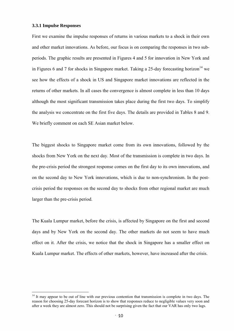
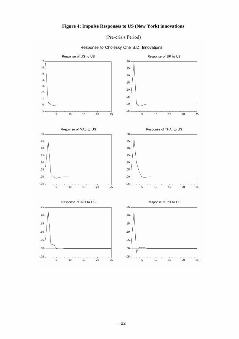
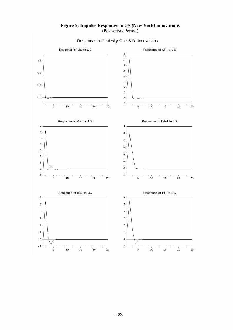
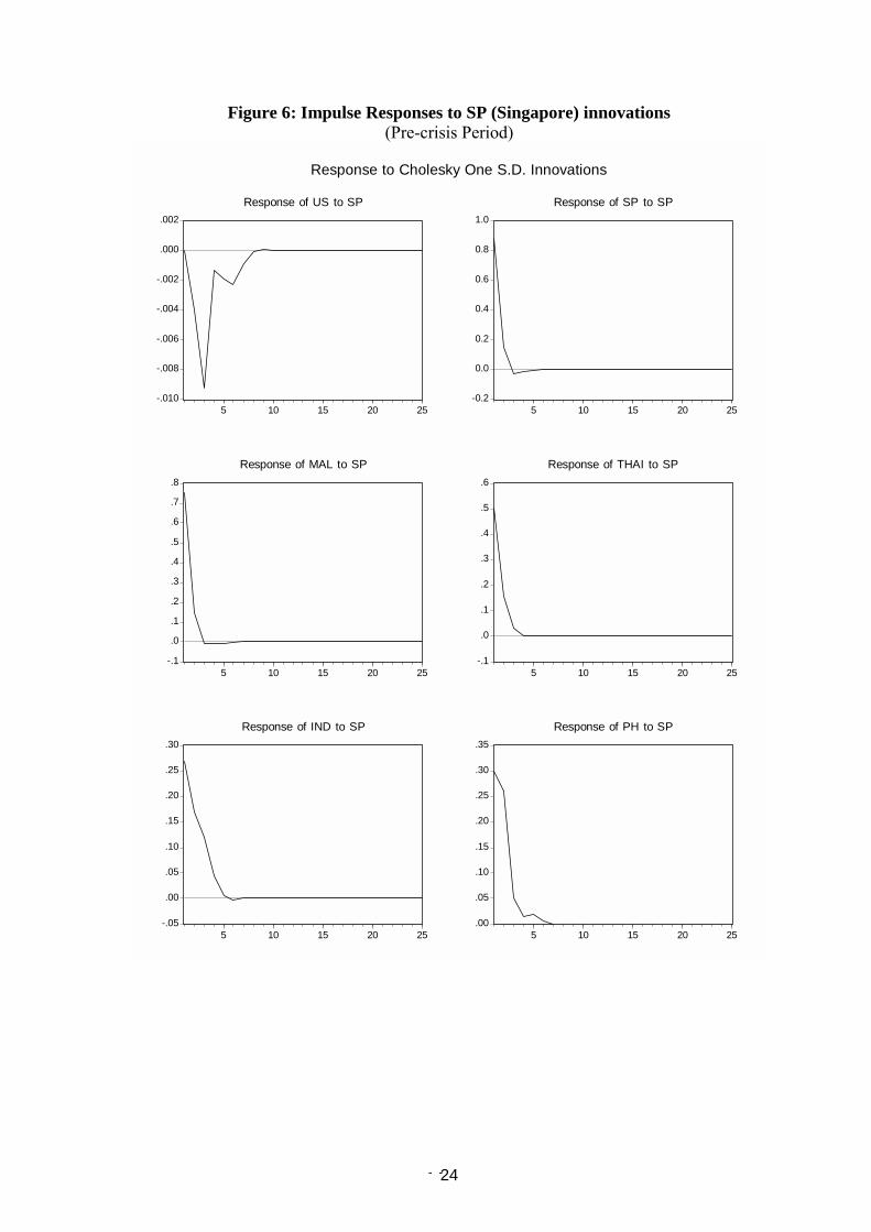
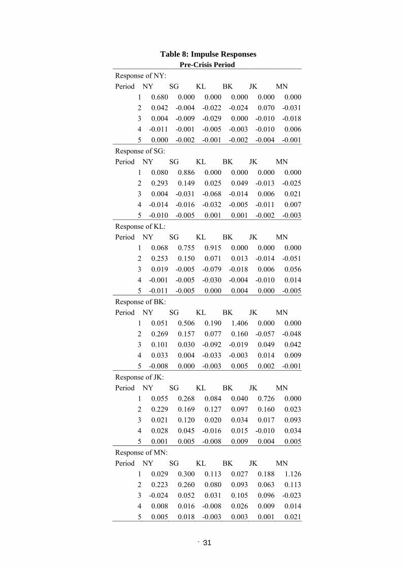
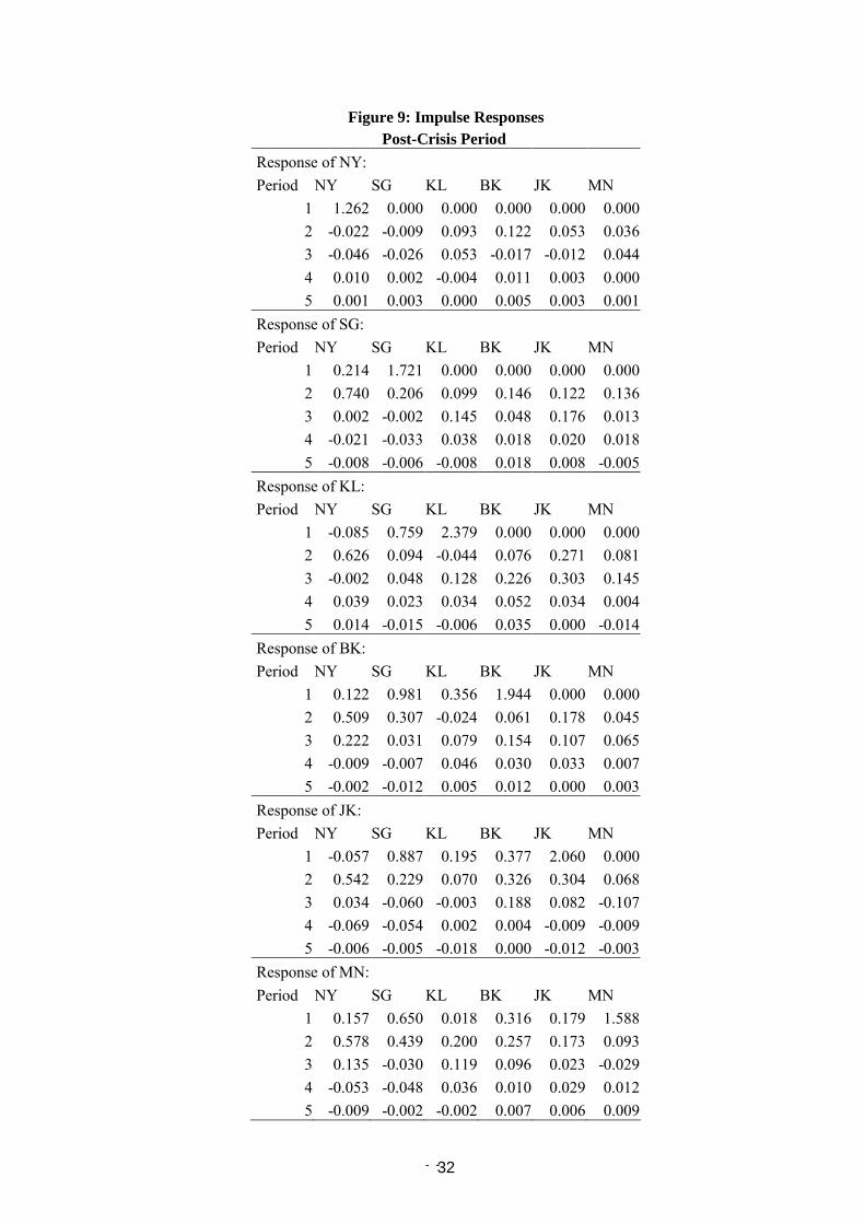
3.3.1 Impulse Responses

First we examine the impulse responses of returns in various markets to a shock in their own

and other market innovations. As before, our focus is on comparing the responses in two sub-

periods. The graphic results are presented in Figures 4 and 5 for innovation in New York and

in Figures 6 and 7 for shocks in Singapore market. Taking a 25-day forecasting horizon14 we

see how the effects of a shock in US and Singapore market innovations are reflected in the

returns of other markets. In all cases the convergence is almost complete in less than 10 days

although the most significant transmission takes place during the first two days. To simplify

the analysis we concentrate on the first five days. The details are provided in Tables 8 and 9.

We briefly comment on each SE Asian market below.

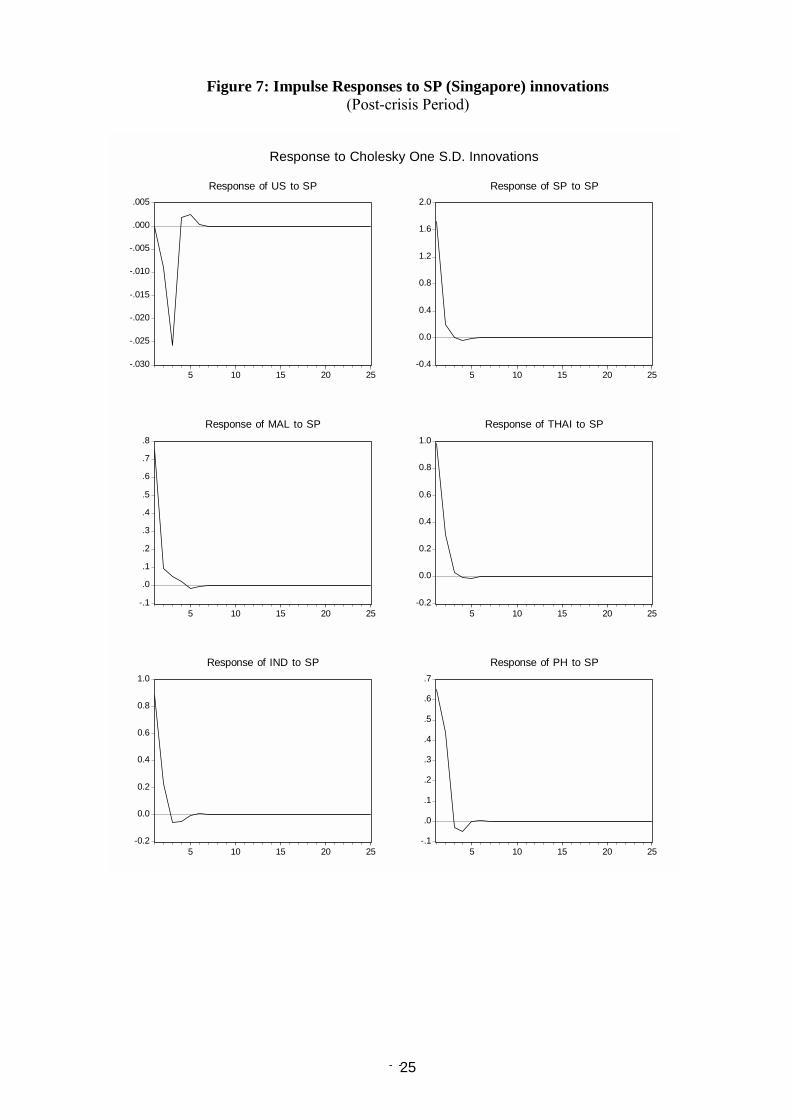
The biggest shocks to Singapore market come from its own innovations, followed by the

shocks from New York on the next day. Most of the transmission is complete in two days. In

the pre-crisis period the strongest response comes on the first day to its own innovations, and

on the second day to New York innovations, which is due to non-synchronism. In the post-

crisis period the responses on the second day to shocks from other regional market are much

larger than the pre-crisis period.

The Kuala Lumpur market, before the crisis, is affected by Singapore on the first and second

days and by New York on the second day. The other markets do not seem to have much

effect on it. After the crisis, we notice that the shock in Singapore has a smaller effect on

Kuala Lumpur market. The effects of other markets, however, have increased after the crisis.

14 It may appear to be out of line with our previous contention that transmission is complete in two days. The reason for choosing 25-day forecast horizon is to show that responses reduce to negligible values very soon and after a week they are almost zero. This should not be surprising given the fact that our VAR has only two lags.

- - 11

In the pre-crisis period, the Bangkok market is affected by Singapore and Kuala Lumpur on

the first day and by New York and Singapore on the second. After the crisis we notice that

Jakarta also affects Bangkok on the second day.

All except Manila affected Jakarta in the pre-crisis period. We observe the same thing after

the crisis but also notice that Bangkok has a stronger effect than before. In case of Manila we

do not see much change after the crisis. For Jakarta and Manila, we also notice that the effect

of Singapore is much higher on the first day in the post-crisis period. This provides support to

the idea of Singapore acting as a regional leader after the crisis. We shall explore this point

further in the following section.

All these results should be interpreted keeping in mind the limitations of a VAR model. First,

we have seen that there are strong contemporaneous relationships between the returns in

these markets but we cannot have the contemporaneous returns from other markets on the

right hand side of the VAR equation for each market. This limitation prevents us to study the

contemporaneous linkages. Second, the ordering is very important in determining the impulse

responses and the market that appear high in our ordering are bound to have strong effect on

the markets that appear low. We also tried NKSBJM ordering (results not shown here) and

found that our broad conclusions remain the same.

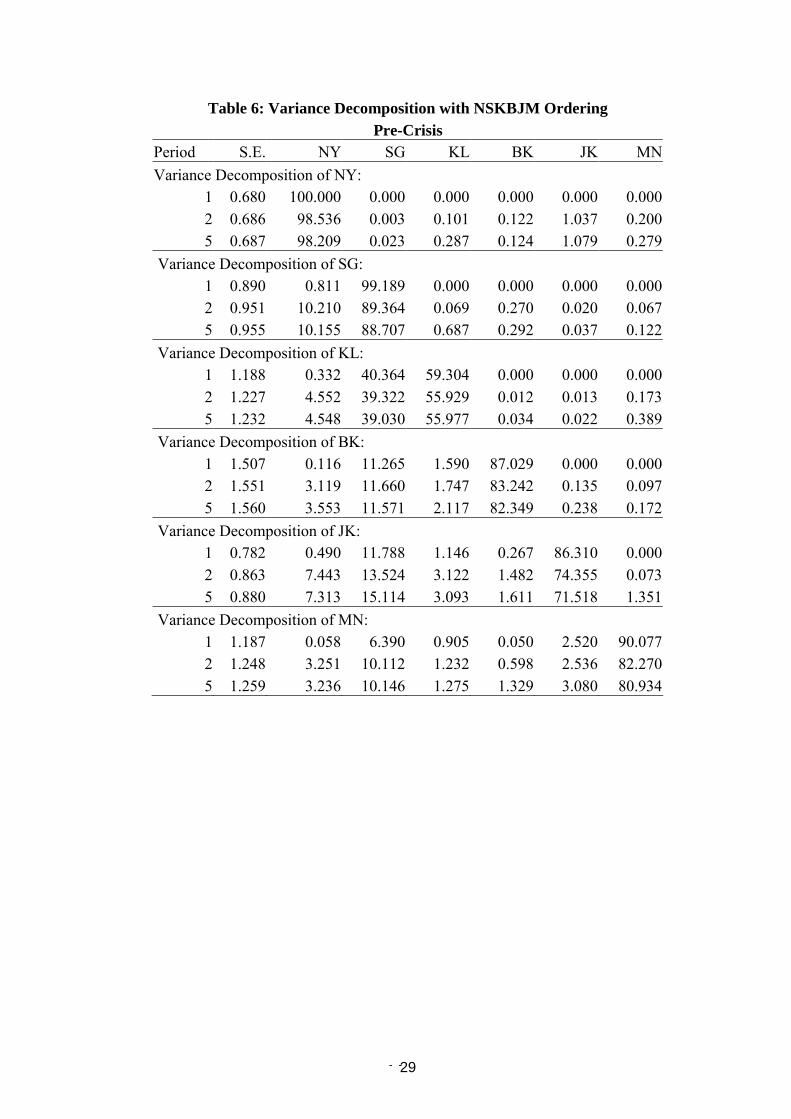
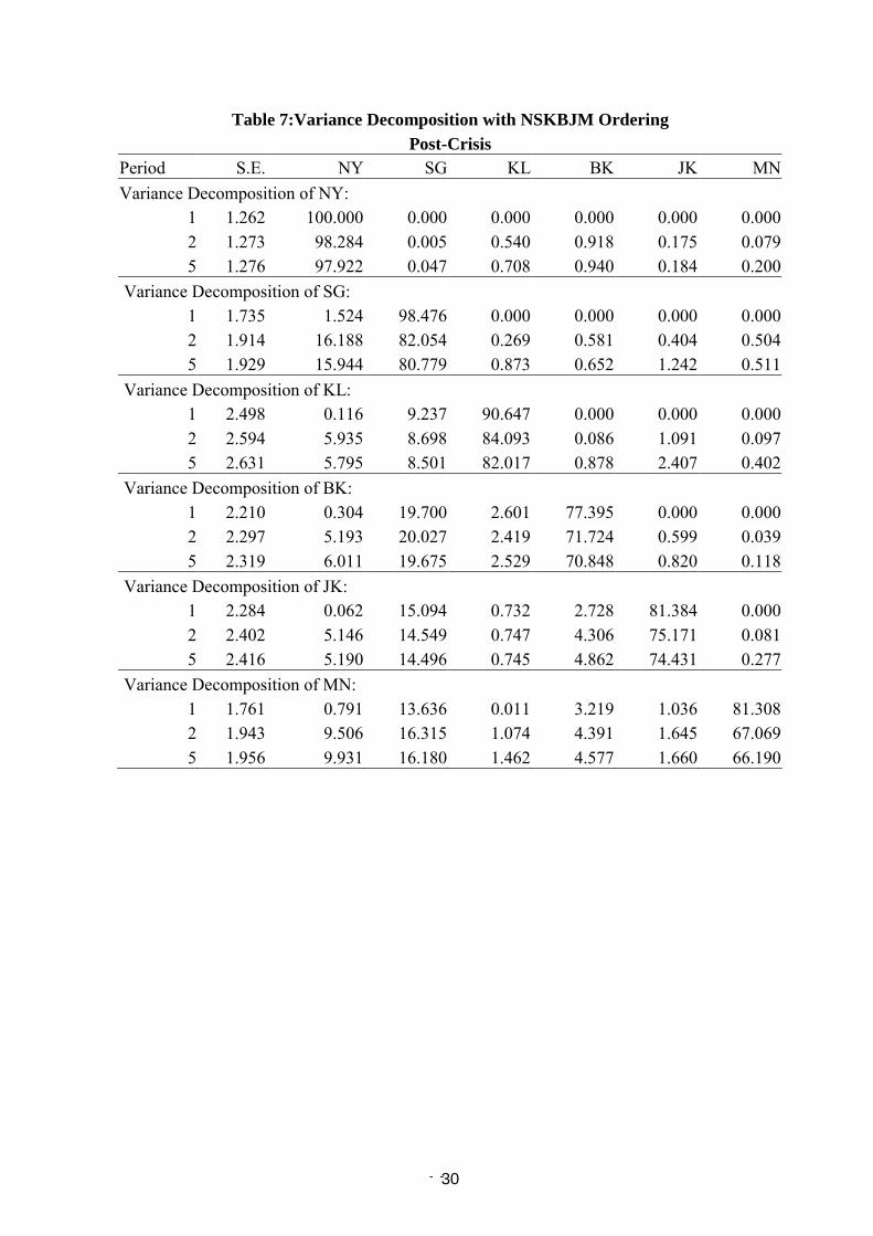
3.3.2 Variance Decomposition

The problem with the impulse responses is that they show the effect of different days

separately. If we are interested in some kind of cumulative effect the variance decomposition

is a better tool. Once again we shall focus on SEA markets and compare the variance

decomposition in two sub-periods. Although most of the transmission is completed in two

days, we allow five days for impulse responses to fully show their effect and then discuss the

- - 12

variance decomposition on the fifth day when transmission is sure to be complete. All the

following discussion is based on Tables 6 and 7.

Starting with Singapore, we see that most of the forecast error variance is explained by

movement in its own returns and by the movement in the returns of New York market.

Important thing to notice is that New York market explains more of the movement in

Singapore market after the crisis.

When we look at the Kuala Lumpur market we find that Singapore explains a major portion

of its variance before the crisis (39%) but after the crisis it falls to mere 8%. When this result

is viewed together with the Granger causality test results, we find some evidence to support

the claim that Kuala Lumpur market has been slightly alienated from the region after the

crisis. One possible explanation could be the way in which Malaysian government responded

to the crisis. The capital controls imposed may have resulted in this isolation.

Its own shock followed by the shocks in Singapore and New York caused the variance in

Bangkok market. It is important to note that the influence of both Singapore and New York

increased after the crisis. Another important thing to note is that Singapore explained 12%

and 20% of the variance in Bangkok market in the two periods respectively, compared to 4%

and 6% respectively explained by the New York market. The implication is that Singapore

acts as a leader for Bangkok market both before and after the crisis and its effect has grown

stronger in the later period.

Singapore also appears to be the leader for Jakarta market in both pre- and post-crisis periods.

However, its influence is almost the same in two periods. Bangkok affects Jakarta more after

the crisis and its effect is almost as much as that of New York. Singapore also has a strong

- - 13

effect on Manila as it explains 10% and 16% of its variance in the two periods respectively.

New York and Jakarta each explained 3% before the crisis. After the crisis New York

explained 9% while Jakarta explained less than 2%. Bangkok explained 5% of variance in

Manila in the second period.

Before we draw any general conclusion from our analysis of variance decomposition it is

worthwhile to mention our variance decomposition results using NKSBJM ordering. We

notice that our conclusion about Singapore�s regional leadership is sensitive to the ordering

in the pre-crisis period. When we change the ordering to NKSBJM, Kuala Lumpur appears to

affect the regional markets more than Singapore in pre-crisis period. However, in the post-

crisis period Singapore emerges as a clear leader regardless of ordering.

We conclude that Singapore is a regional leader and its effect on the regional markets is even

greater than that of New York. This leadership has become stronger after the crisis. Kuala

Lumpur has been slightly alienated from the region after the crisis. Most of the markets have

become more sensitive to changes in Bangkok in the post-crisis period. The possible reason

could be the fact that the crisis started in Thailand and engulfed the region very quickly.

4. Summary and Conclusions

In this paper, the inter-linkages among daily returns in New York, Tokyo and five South East

Asian markets are examined for pre- and post-crisis periods separately, by using simple

correlations, Granger causality tests and VAR models. It is found that SEA markets are

closely linked with one another. The New York market exerts a strong influence on the

region but is not much affected by it. The Tokyo market is virtually unrelated to the region.

- - 14

Singapore emerges as a leader in the region and its leadership is stronger in the post-crisis

period. The basic proof of its leadership lies in the higher percentage of variance in the

regional markets that can be explained by movements in Singapore market. This conclusion

becomes more significant when we observe that the influence of Singapore on the region is

even greater than that of New York. Kuala Lumpur appears to have been slightly alienated

from the region after the crisis. This alienation could be the repercussion of capital control

policies of the Malaysian government. Bangkok appears to affect the region more after the

crisis. Jakarta also has an increased effect while Manila, being the smallest of five SEA

markets studied, does not have much influence on other markets.

Another important conclusion of our study is that inter-linkages among the SEA markets

have increased after the crisis and markets respond more promptly and actively to the

changes in neighboring markets.

- - 15

REFERENCES

Ammer, J and J.Mei (1996) �Measuring International Economic Linkages with Stock Market

Data� The Journal of Finance, 5, 1743-1763.

Arshanapalli, B. and Doukas, J. (1993) �International Stock Market Linkages: evidence from

the pre- and post-October 1987 period, Journal of Banking and Finance, 17, 193-208.

Bekaert, G. and Harvey, C. R. (1995) �Time-Varying World Market Integration�, Journal of

Finance, 50, 403-444.

Bracker, D.S. Docking, P.D. Koch (1999) �Economic Determinants of Evolution in

International Stock Market Integration� Journal of Empirical Finance, 6, 1-27.

Cheung, Y. �L. and Mak, S. �C. (1992) �The International Transmission of Stock Market

Fluctuations between the Developed Markets and the Asia-Pacific Markets�, Applied

Financial Economics, 2, 43-7.

Chowdhury, A. R. (1994) �Stock Market Independencies: Evidence form the Asian NIEs,

Journal of Macroeconomics, 16, 629-51.

Dekker, A., K. Sen and M. R. Young (2001) �Equity Market Linkages in the Asia Pacific

region: A Comparison of the Orthogonalised and Generalised VAR Approaches�,

Global Finance Journal, 12, 1-33.

Eun, C. S. and Shim, S. (1989) � International Transmission of Stock Market Movements�,

Journal of Financial and Quantitative Analysis, 24, 241-56.

Granger, C. W. .J. (1969) �Investigating Causal Relations by Econometric Models and Cross-

Spectral Methods,� Econometrica, 37, 424�438.

Hamilton, J. D. (1994) �Time Series Analysis�, Princeton University Press, Princeton, New

Jersey.

- - 16

Hilliard, J.E. (1979)�The Relationship Between Equity Indices on World Exchanges�,

Journal of Finance, 34, 103-14.

Kasa, K. (1992) �Common Stochastic Trends in International Stock Markets�, Journal of

Monetary Economics, 29, 95-124.

King, M.A., E. Sentana, and S.B. Wadhwani (1994) �Volatility and Links between National

Stock Markets�, Econometrica, 62, 901-933.

Koch, T.W. and P.D. Koch (1993) �Dynamic Relationship among the Daily Level of

National Stock Indexes� in International Financial Market Integration. Stansell, S. R.

(ed.), Blackwells, Mass.

Leachman, L. L. and Fransic, B. (1995) � Long-run Relations among the G-5 and G-7 Equity

Markets: Evidence on the Plaza and Louvre Accords�, Journal of Macroeconomics,

17, 551-77.

Longin, F and B. Solnik (1995) �Is the Correlation in International Equity Returns Constant:

1960-1990?� Journal of International money and Finance, 14, 3-26.

Meric, I. and G. Meric (1989) �Potential Gains from International Portfolio Diversification

and Inter-temporal Stability and Seasonality in International Stock Market

Relationships�, Journal of Banking of Finance, 13, 627-640.

Pan, Ming-Shiun, Y. A. Liu and H. J. Roth (1999) �Common Stochastic Trends and

Volatility in Asian-Pasific Equity Markets�, Global Finance Journal, 10, 161-172.

Pesonen, Hanna (1999) �Assessing Causal Linkages Between the Emerging Stock Markets of

Asia and Russia�, Russsian and East European Finance and Trade, 35, 73-82.

Rangvid, J. (2001) �Increasing Convergence Among European Stock Markets? A Recursive

Common Stochastic Trends Analysis�, Economics Letters, 71, 383-389.

- - 17

Rapach, David E. (2001) �Macro Shocks and Real Stock Prices�, Journal of Economics and

Business, 53, 5-26.

Roca, Eduardo D. (1999) �Short-term and Long-term Price Linkages Between the Equity

Markets of Australia and its Major Trading Partners�, Applied Financial Economics,

9, 501-511.

Roca, Eduardo D. (2000) �Price Interdependence Among Equity Markets in the Asia-Pacific

Region: Focus on Australia and ASEAN�, Ashgate, England.

Siklos, P. L. and N. Patrick (2001) �Integration Among Asia-Pacific and International Stock

Markets: Common Stochastic Trends and Regime Shifts�, Pacific Economic Review,

6, 89-110.

Sims, C. A. (1980) �Macroeconomics and Reality�, Econometrica, 48, 1-48.

Soydemir, Gokce (2000) �International Transmission Mechanism of Stock Market

Movements: Evidence from Emerging Equity Markets�, Journal of Forecasting, 19,

149-176.

Taylor, M. P. and Tonks, I. (1989) �The Internationalization of Stock Markets and the

Abolition of UK exchange Controls�, Review of Economics and Statistics, 71, 332-6.

Yuce, Ayse and C. S. Mugan (2000) �Linkages Among Eastern European Stock Markets and

the Major Stock Exchanges�, Russian and East European Finance and Trade, 36, 54-

69.

- - 18

Figure 1: Official Trading Hours of the Seven Markets GMT 0:00 1:00 2:00 3:00 4:00 5:00 6:00 7:00 8:00 9:00 10:00 11:00 12:00 13:00 14:00 15:00 16:00 17:00 18:00 19:00 20:00 21:00 22:00

Tokyo

Singapore

Manila

Kuala Lumpur

Jakarta*

Bangkok

New York

* Jakarta market trades during these hours from Monday to Thursday. On Friday it trades from 0230 to 0400 GMT only. Source: The Handbook of World Stock and Commodity Exchanges (1994) Basil Blackwell, London.

- - 19

Figure 2: Prices in Seven Markets From 03/01/1994 to 29/12/2000

400

600

800

1000

1200

1400

1600

1994 1995 1996 1997 1998 1999 2000

P_US

12000

14000

16000

18000

20000

22000

24000

1994 1995 1996 1997 1998 1999 2000

P_JAP

400

800

1200

1600

2000

2400

2800

1994 1995 1996 1997 1998 1999 2000

P_SP

200

400

600

800

1000

1200

1400

1994 1995 1996 1997 1998 1999 2000

P_MAL

0

400

800

1200

1600

2000

1994 1995 1996 1997 1998 1999 2000

P_THAI

200

300

400

500

600

700

800

1994 1995 1996 1997 1998 1999 2000

P_IND

1000

1500

2000

2500

3000

3500

1994 1995 1996 1997 1998 1999 2000

P_PH

P_US = S & P 500 Composite Stock Index P_Jap = Nikkei 225 Stock Average P_Sp = Singapore Straits Times Index P_Mal = Kuala Lumpur Composite P_Thai = Bangkok S. E. T. P_Ind = Jakarta S. E. Composite P_Ph = Manila S. E. Composite.

- - 20

Figure 3:Returns in Seven Markets From 03/01/1994 to 29/12/2000

-8

-6

-4

-2

0

2

4

6

1994 1995 1996 1997 1998 1999 2000

US

-8

-4

0

4

8

1994 1995 1996 1997 1998 1999 2000

JAP

-10

-5

0

5

10

15

20

1994 1995 1996 1997 1998 1999 2000

SP

-30

-20

-10

0

10

20

30

1994 1995 1996 1997 1998 1999 2000

MAL

-12

-8

-4

0

4

8

12

1994 1995 1996 1997 1998 1999 2000

THAI

-15

-10

-5

0

5

10

15

1994 1995 1996 1997 1998 1999 2000

IND

-10

-5

0

5

10

15

20

1994 1995 1996 1997 1998 1999 2000

PH

US = New York Jap = Tokyo S = Singapore M = Kuala Lumpur T = Bangkok I = Jakarta and P = Manila

- - 21

Figure 4

Linkages Between SEA Markets (Based on Granger Causality Tests with 2 lags)

Before the Crisis Singapore Kuala Lumpur Manila Bangkok Jakarta

After the Crisis Singapore Kuala Lumpur Manila Bangkok Jakarta

- - 22

Figure 4: Impulse Responses to US (New York) innovations

(Pre-crisis Period)

-.1

.0

.1

.2

.3

.4

.5

.6

.7

5 10 15 20 25

Response of US to US

-.05

.00

.05

.10

.15

.20

.25

.30

5 10 15 20 25

Response of SP to US

-.05

.00

.05

.10

.15

.20

.25

.30

5 10 15 20 25

Response of MAL to US

-.05

.00

.05

.10

.15

.20

.25

.30

5 10 15 20 25

Response of THAI to US

-.05

.00

.05

.10

.15

.20

.25

5 10 15 20 25

Response of IND to US

-.05

.00

.05

.10

.15

.20

.25

5 10 15 20 25

Response of PH to US

Response to Cholesky One S.D. Innovations

- - 23

Figure 5: Impulse Responses to US (New York) innovations (Post-crisis Period)

0.0

0.4

0.8

1.2

5 10 15 20 25

Response of US to US

-.1

.0

.1

.2

.3

.4

.5

.6

.7

.8

5 10 15 20 25

Response of SP to US

-.1

.0

.1

.2

.3

.4

.5

.6

.7

5 10 15 20 25

Response of MAL to US

-.1

.0

.1

.2

.3

.4

.5

.6

5 10 15 20 25

Response of THAI to US

-.1

.0

.1

.2

.3

.4

.5

.6

5 10 15 20 25

Response of IND to US

-.1

.0

.1

.2

.3

.4

.5

.6

5 10 15 20 25

Response of PH to US

Response to Cholesky One S.D. Innovations

- - 24

Figure 6: Impulse Responses to SP (Singapore) innovations (Pre-crisis Period)

-.010

-.008

-.006

-.004

-.002

.000

.002

5 10 15 20 25

Response of US to SP

-0.2

0.0

0.2

0.4

0.6

0.8

1.0

5 10 15 20 25

Response of SP to SP

-.1

.0

.1

.2

.3

.4

.5

.6

.7

.8

5 10 15 20 25

Response of MAL to SP

-.1

.0

.1

.2

.3

.4

.5

.6

5 10 15 20 25

Response of THAI to SP

-.05

.00

.05

.10

.15

.20

.25

.30

5 10 15 20 25

Response of IND to SP

.00

.05

.10

.15

.20

.25

.30

.35

5 10 15 20 25

Response of PH to SP

Response to Cholesky One S.D. Innovations

- - 25

Figure 7: Impulse Responses to SP (Singapore) innovations (Post-crisis Period)

-.030

-.025

-.020

-.015

-.010

-.005

.000

.005

5 10 15 20 25

Response of US to SP

-0.4

0.0

0.4

0.8

1.2

1.6

2.0

5 10 15 20 25

Response of SP to SP

-.1

.0

.1

.2

.3

.4

.5

.6

.7

.8

5 10 15 20 25

Response of MAL to SP

-0.2

0.0

0.2

0.4

0.6

0.8

1.0

5 10 15 20 25

Response of THAI to SP

-0.2

0.0

0.2

0.4

0.6

0.8

1.0

5 10 15 20 25

Response of IND to SP

-.1

.0

.1

.2

.3

.4

.5

.6

.7

5 10 15 20 25

Response of PH to SP

Response to Cholesky One S.D. Innovations

- - 26

Table 1: Market Value (Total Capitalization in US$)

Market Jan, 1994 June, 1997 Dec, 2000 New York (NY) $3,600b $8,600b $16,450b Tokyo (TK) $3,000b $3,100b $3,585b Singapore (SG) $125b $174b $200b Kuala Lumpur (KL) $205b $287b $127b Jakarta (JK) $40b $107b $31b Bangkok (BK) $110b $66b $30b Manila (MN) $32b $72b $16b Source: Asiaweek: Jan 5, 1994; June 27, 1997; December22, 2000.

Table 2: Correlation Matrix (Pre-Crisis Period)

NY(t-1) TK(t) SG(t) KL (t) BK(t) JK(t) MN(t) NY(t-1) 1.00

TK(t) 0.21 1.00

SG(t) 0.31 0.20 1.00

KL (t) 0.20 0.13 0.67 1.00

BK(t) 0.18 0.06 0.39 0.35 1.00

JK(t) 0.25 0.13 0.40 0.35 0.24 1.00

MN(t) 0.18 0.07 0.31 0.27 0.17 0.33 1.00

Table 3: Correlation Matrix (Post-Crisis Period)

NY(t-1) TK(t) SG(t) KL (t) BK(t) JK(t) MN(t) NY(t-1) 1.00

TK(t) 0.36 1.00

SG(t) 0.39 0.35 1.00

KL (t) 0.25 0.22 0.38* 1.00

BK(t) 0.23 0.24 0.50 0.34* 1.00

JK(t) 0.23* 0.21 0.45 0.26* 0.38 1.00

MN(t) 0.30 0.21 0.48 0.20* 0.40 0.35 1.00

* This correlation coefficient is lower than its pre-crisis counterpart.

- - 27

Table 4: Pair-wise Granger Causality Test Results

(Pre-Crisis Period) 2 Lags 5 Lags 15 Lags 2 Lags 5 Lags 15 LagsNY→TK 24.60*** 9.82*** 4.32*** TK→NY 0.34 0.29 0.61

NY→SG 46.50*** 19.22*** 7.72*** SG→NY 0.15 0.89 1.28

NY→KL 19.03*** 8.47*** 4.46*** KL→NY 1.12 1.00 0.84

NY→BK 15.18*** 6.84*** 3.03*** BK→NY 0.75 0.72 1.74**

NY→JK 31.20*** 12.29*** 4.47*** JK→NY 3.62** 1.47 1.43

NY→MN 16.75*** 7.36*** 3.51*** MN→NY 1.15 0.86 1.27

TK→SG 0.31 0.48 1.10 SG→TK 3.71** 1.84 1.37

TK→KL 0.45 0.64 1.00 KL→TK 2.73* 1.38 2.60***

TK→BK 0.80 0.62 1.13 BK→TK 0.04 0.41 2.30***

TK→JK 1.02 1.09 0.75 JK→TK 0.73 1.43 1.15

TK→MN 1.49 0.86 1.01 MN→TK 0.24 1.26 1.05

SP→KL 2.49* 1.78 1.45 KL→SG 3.18** 1.86* 0.79

SP→BK 3.18** 1.54 0.98 BK→SG 1.77 1.33 0.88

SP→JK 10.09*** 4.22*** 1.98** JK→SG 0.13 0.46 1.12

SG→MN 14.03*** 6.24*** 3.13*** MN→SG 0.72 0.79 1.32

KL→BK 3.47** 1.45 0.81 BK→KL 0.30 2.24** 1.06

KL→JK 15.01*** 6.26*** 2.17*** JK→KL 0.09 2.04* 1.24

KL→MN 10.74*** 5.37*** 2.47*** MN→KL 1.91 2.57** 2.68***

BK→JK 11.07*** 4.55*** 1.96** JK→BK 0.61 0.95 0.55

BK→MN 10.10*** 4.35*** 2.27*** MN→BK 0.68 2.22* 1.24

JK→MN 7.39*** 2.95** 1.71** MN→JK 8.61*** 4.02*** 2.12

***, ** and * mean significant at 1, 5 and 10%, respectively.

- - 28

Table 5: Pair-wise Granger Causality Test Results

(Post-Crisis Period) 2 Lags 5 Lags 15 Lags 2 Lags 5 Lags 15 Lags NY→TK 70.56*** 28.62*** 9.93*** TK→NY 0.91 0.34 0.82

NY→SG 75.67*** 33.19*** 11.58*** SG→NY 0.10 0.26 1.02

NY→KL 29.71*** 12.87*** 5.12*** KL→NY 2.48* 1.59 1.29

NY→BK 25.59*** 11.69*** 3.89*** BK→NY 3.69** 1.93 0.95

NY→JK 26.54*** 12.47*** 4.72*** JK→NY 1.45 0.84 1.07

NY→MN 41.48*** 17.20*** 6.39*** MN→NY 0.92 0.78 1.16

TK→SG 0.55 0.34 0.93 SG→TK 2.38* 1.44 1.52*

TK→KL 0.09 1.21 1.58* KL→TK 2.65* 1.57 1.37

TK→BK 1.20 0.53 0.65 BK→TK 2.75* 1.59 2.07***

TK→JK 0.04 0.66 1.01 JK→TK 1.72 0.77 0.86

TK→MN 1.05 0.59 0.67 MN→TK 1.97 1.21 0.74

SP→KL 3.04** 1.69 0.99 KL→SG 2.51* 1.56 0.95

SP→BK 11.30*** 5.29*** 2.45*** BK→SG 3.45** 2.44** 2.36***

SP→JK 2.71* 1.60 1.16 JK→SG 4.79*** 2.01* 1.26

SG→MN 21.17*** 8.27*** 3.46*** MN→SG 5.68*** 3.41*** 1.74**

KL→BK 0.12 0.19 1.19 BK→KL 4.43** 2.55** 1.42

KL→JK 0.32 0.75 2.14*** JK→KL 12.95*** 5.22*** 2.08***

KL→MN 8.85*** 3.63*** 3.92*** MN→KL 6.23*** 2.78** 1.58*

BK→JK 6.02*** 3.30*** 2.03** JK→BK 5.55*** 2.31** 1.30

BK→MN 17.43*** 7.67*** 4.05*** MN→BK 3.71** 1.91* 1.05

JK→MN 10.56*** 4.54*** 2.66*** MN→JK 3.84** 2.06* 1.53*

- - 29

Table 6: Variance Decomposition with NSKBJM Ordering

Pre-Crisis Period S.E. NY SG KL BK JK MNVariance Decomposition of NY:

1 0.680 100.000 0.000 0.000 0.000 0.000 0.0002 0.686 98.536 0.003 0.101 0.122 1.037 0.2005 0.687 98.209 0.023 0.287 0.124 1.079 0.279

Variance Decomposition of SG: 1 0.890 0.811 99.189 0.000 0.000 0.000 0.0002 0.951 10.210 89.364 0.069 0.270 0.020 0.0675 0.955 10.155 88.707 0.687 0.292 0.037 0.122

Variance Decomposition of KL: 1 1.188 0.332 40.364 59.304 0.000 0.000 0.0002 1.227 4.552 39.322 55.929 0.012 0.013 0.1735 1.232 4.548 39.030 55.977 0.034 0.022 0.389

Variance Decomposition of BK: 1 1.507 0.116 11.265 1.590 87.029 0.000 0.0002 1.551 3.119 11.660 1.747 83.242 0.135 0.0975 1.560 3.553 11.571 2.117 82.349 0.238 0.172

Variance Decomposition of JK: 1 0.782 0.490 11.788 1.146 0.267 86.310 0.0002 0.863 7.443 13.524 3.122 1.482 74.355 0.0735 0.880 7.313 15.114 3.093 1.611 71.518 1.351

Variance Decomposition of MN: 1 1.187 0.058 6.390 0.905 0.050 2.520 90.0772 1.248 3.251 10.112 1.232 0.598 2.536 82.2705 1.259 3.236 10.146 1.275 1.329 3.080 80.934

- - 30

Table 7:Variance Decomposition with NSKBJM Ordering

Post-Crisis Period S.E. NY SG KL BK JK MNVariance Decomposition of NY:

1 1.262 100.000 0.000 0.000 0.000 0.000 0.0002 1.273 98.284 0.005 0.540 0.918 0.175 0.0795 1.276 97.922 0.047 0.708 0.940 0.184 0.200

Variance Decomposition of SG: 1 1.735 1.524 98.476 0.000 0.000 0.000 0.0002 1.914 16.188 82.054 0.269 0.581 0.404 0.5045 1.929 15.944 80.779 0.873 0.652 1.242 0.511

Variance Decomposition of KL: 1 2.498 0.116 9.237 90.647 0.000 0.000 0.0002 2.594 5.935 8.698 84.093 0.086 1.091 0.0975 2.631 5.795 8.501 82.017 0.878 2.407 0.402

Variance Decomposition of BK: 1 2.210 0.304 19.700 2.601 77.395 0.000 0.0002 2.297 5.193 20.027 2.419 71.724 0.599 0.0395 2.319 6.011 19.675 2.529 70.848 0.820 0.118

Variance Decomposition of JK: 1 2.284 0.062 15.094 0.732 2.728 81.384 0.0002 2.402 5.146 14.549 0.747 4.306 75.171 0.0815 2.416 5.190 14.496 0.745 4.862 74.431 0.277

Variance Decomposition of MN: 1 1.761 0.791 13.636 0.011 3.219 1.036 81.3082 1.943 9.506 16.315 1.074 4.391 1.645 67.0695 1.956 9.931 16.180 1.462 4.577 1.660 66.190

- - 31

Table 8: Impulse Responses

Pre-Crisis Period Response of NY: Period NY SG KL BK JK MN

1 0.680 0.000 0.000 0.000 0.000 0.000 2 0.042 -0.004 -0.022 -0.024 0.070 -0.031 3 0.004 -0.009 -0.029 0.000 -0.010 -0.018 4 -0.011 -0.001 -0.005 -0.003 -0.010 0.006 5 0.000 -0.002 -0.001 -0.002 -0.004 -0.001

Response of SG: Period NY SG KL BK JK MN

1 0.080 0.886 0.000 0.000 0.000 0.000 2 0.293 0.149 0.025 0.049 -0.013 -0.025 3 0.004 -0.031 -0.068 -0.014 0.006 0.021 4 -0.014 -0.016 -0.032 -0.005 -0.011 0.007 5 -0.010 -0.005 0.001 0.001 -0.002 -0.003

Response of KL: Period NY SG KL BK JK MN

1 0.068 0.755 0.915 0.000 0.000 0.000 2 0.253 0.150 0.071 0.013 -0.014 -0.051 3 0.019 -0.005 -0.079 -0.018 0.006 0.056 4 -0.001 -0.005 -0.030 -0.004 -0.010 0.014 5 -0.011 -0.005 0.000 0.004 0.000 -0.005

Response of BK: Period NY SG KL BK JK MN

1 0.051 0.506 0.190 1.406 0.000 0.000 2 0.269 0.157 0.077 0.160 -0.057 -0.048 3 0.101 0.030 -0.092 -0.019 0.049 0.042 4 0.033 0.004 -0.033 -0.003 0.014 0.009 5 -0.008 0.000 -0.003 0.005 0.002 -0.001

Response of JK: Period NY SG KL BK JK MN

1 0.055 0.268 0.084 0.040 0.726 0.000 2 0.229 0.169 0.127 0.097 0.160 0.023 3 0.021 0.120 0.020 0.034 0.017 0.093 4 0.028 0.045 -0.016 0.015 -0.010 0.034 5 0.001 0.005 -0.008 0.009 0.004 0.005

Response of MN: Period NY SG KL BK JK MN

1 0.029 0.300 0.113 0.027 0.188 1.126 2 0.223 0.260 0.080 0.093 0.063 0.113 3 -0.024 0.052 0.031 0.105 0.096 -0.023 4 0.008 0.016 -0.008 0.026 0.009 0.014 5 0.005 0.018 -0.003 0.003 0.001 0.021

- - 32

Figure 9: Impulse Responses

Post-Crisis Period Response of NY: Period NY SG KL BK JK MN

1 1.262 0.000 0.000 0.000 0.000 0.000 2 -0.022 -0.009 0.093 0.122 0.053 0.036 3 -0.046 -0.026 0.053 -0.017 -0.012 0.044 4 0.010 0.002 -0.004 0.011 0.003 0.000 5 0.001 0.003 0.000 0.005 0.003 0.001

Response of SG: Period NY SG KL BK JK MN

1 0.214 1.721 0.000 0.000 0.000 0.000 2 0.740 0.206 0.099 0.146 0.122 0.136 3 0.002 -0.002 0.145 0.048 0.176 0.013 4 -0.021 -0.033 0.038 0.018 0.020 0.018 5 -0.008 -0.006 -0.008 0.018 0.008 -0.005

Response of KL: Period NY SG KL BK JK MN

1 -0.085 0.759 2.379 0.000 0.000 0.000 2 0.626 0.094 -0.044 0.076 0.271 0.081 3 -0.002 0.048 0.128 0.226 0.303 0.145 4 0.039 0.023 0.034 0.052 0.034 0.004 5 0.014 -0.015 -0.006 0.035 0.000 -0.014

Response of BK: Period NY SG KL BK JK MN

1 0.122 0.981 0.356 1.944 0.000 0.000 2 0.509 0.307 -0.024 0.061 0.178 0.045 3 0.222 0.031 0.079 0.154 0.107 0.065 4 -0.009 -0.007 0.046 0.030 0.033 0.007 5 -0.002 -0.012 0.005 0.012 0.000 0.003

Response of JK: Period NY SG KL BK JK MN

1 -0.057 0.887 0.195 0.377 2.060 0.000 2 0.542 0.229 0.070 0.326 0.304 0.068 3 0.034 -0.060 -0.003 0.188 0.082 -0.107 4 -0.069 -0.054 0.002 0.004 -0.009 -0.009 5 -0.006 -0.005 -0.018 0.000 -0.012 -0.003

Response of MN: Period NY SG KL BK JK MN

1 0.157 0.650 0.018 0.316 0.179 1.588 2 0.578 0.439 0.200 0.257 0.173 0.093 3 0.135 -0.030 0.119 0.096 0.023 -0.029 4 -0.053 -0.048 0.036 0.010 0.029 0.012 5 -0.009 -0.002 -0.002 0.007 0.006 0.009

- - 33