Heterogeneous speculators, endogenous fluctuations and interacting markets: A model of stock prices...

ARTICLE IN PRESS

Contents lists available at ScienceDirect

Journal of Economic Dynamics & Control

Journal of Economic Dynamics & Control 34 (2010) 743–764

0165-18

doi:10.1

� Cor

E-m

journal homepage: www.elsevier.com/locate/jedc

Heterogeneous speculators, endogenous fluctuations andinteracting markets: A model of stock prices and exchange rates

Roberto Dieci a,�, Frank Westerhoff b

a Department of Mathematics for Economics and Social Sciences, University of Bologna, Viale Q. Filopanti 5, I-40126 Bologna, Italyb Department of Economics, University of Bamberg, Feldkirchenstrasse 21, D-96045 Bamberg, Germany

a r t i c l e i n f o

Article history:

Received 29 May 2008

Accepted 21 October 2009Available online 14 November 2009

JEL classification:

C61

D84

F31

G15

Keywords:

Financial market interactions

Nonlinear dynamics and chaos

Bifurcation analysis

89/$ - see front matter & 2009 Elsevier B.V. A

016/j.jedc.2009.11.002

responding author. Tel.: +39 0541 434140; fa

ail addresses: [email protected] (R. Dieci

a b s t r a c t

We develop a discrete-time model in which the stock markets of two countries are

linked via and with the foreign exchange market. The foreign exchange market is

characterized by nonlinear interactions between technical and fundamental traders.

Such interactions may generate complex dynamics and recurrent switching between

‘‘bull’’ and ‘‘bear’’ market phases via a well-known pitchfork and period-doubling

bifurcation path, when technical traders become more aggressive. The two stock

markets are populated by fundamentalists, and prices tend to evolve towards stable

steady states, driven by linear laws of motion. A connection between such markets is

established by allowing investors to trade abroad, and the resulting three-dimensional

dynamical system is analyzed. One goal of our paper is to explore potential spill-over

effects between foreign exchange and stock markets. A second, related goal is to study

how the bifurcation sequence which characterizes the market with heterogeneous

speculators is modified in the presence of interactions with other markets.

& 2009 Elsevier B.V. All rights reserved.

1. Introduction

The literature about the dynamics of prices in speculative markets, based on the interaction of boundedly rationalheterogeneous agents, has become well developed in recent decades. A considerable portion of this literature has focused,in particular, on the dynamics of financial asset prices. Excellent recent surveys include Hommes (2006), LeBaron (2006)and Lux (2008).

Most models include nonlinear elements. Typically, nonlinearity arises from agents’ trading rules or demand functions(e.g. Day and Huang, 1990; Chiarella, 1992; Rosser et al., 2003), from evolutionary switching between available strategies,based on certain fitness measures (e.g. Brock and Hommes, 1997, 1998), and from phenomena of contagion andconsequent transition of speculators among ‘‘optimistic’’ and ‘‘pessimistic’’ groups (Kirman, 1991; Lux, 1995, 1997). Suchnonlinearities are of course the mathematical reason for some typical dynamic outcome of these models, such as long-runprice oscillations (often characterized by chaotic behavior) around an unstable ‘‘fundamental’’ steady state, the existence ofalternative ‘‘nonfundamental’’ equilibria and the emergence of bubbles and crashes.

Within this literature, a large number of models are based on the so-called chartist–fundamentalist approach. We cite,in particular, Day and Huang (1990), Chiarella (1992), Huang and Day (1993), Brock and Hommes (1998), Lux (1998),Chiarella and He (2001), Chiarella et al. (2002), Hommes et al. (2005), De Grauwe and Grimaldi (2005), Anufriev et al.(2006), Diks and Dindo (2008), Georges (2008), and He and Li (2008). Such models are able to capture—albeit in a stylized

ll rights reserved.

x: +39 0541 434120.

), [email protected] (F. Westerhoff).

www.elsevier.com/locate/jedc

dx.doi.org/10.1016/j.jedc.2009.11.002

mailto:[email protected]

mailto:[email protected]

ARTICLE IN PRESS

R. Dieci, F. Westerhoff / Journal of Economic Dynamics & Control 34 (2010) 743–764744

way—an important determinant of price fluctuations. Chartists use technical trading rules to forecast prices, and inparticular believe in the persistence (and thus exploitability) of bullish and bearish market episodes, and formulate theirdemands accordingly. In contrast, fundamentalists place their orders by assuming that prices will return towards their‘‘fundamental value’’, thus playing a stabilizing role in the market. Prices are set as a function of aggregated investors’demand by assuming market clearing or, more often, the mediation of market makers. Endogenous price dynamics are thusgenerated by the interplay between the destabilizing forces of technical trading strategies and the mean reverting forcesset in action by fundamental traders.

Generally speaking, one central insight of these models is that price movements are at least partially driven byendogenous laws of motion. A second important result is that some of these models have the potential to replicate anumber of important stylized facts of financial markets, such as excess volatility, bubbles and crashes, fat tails for thedistribution of the returns and volatility clustering.1 Finally, these models seem to be useful for testing how certainregulatory measures work. For instance, Wieland and Westerhoff (2005) explore the effectiveness of popular central bankintervention strategies, while He and Westerhoff (2005) discuss how price caps may affect the dynamics of commoditymarkets. In a recent paper, Bauer et al. (2009) demonstrate that target zones may stabilize financial market.

Such literature generally focuses on the dynamics of a single speculative market, driven by the interplay of boundedlyrational heterogeneous investors. In particular, most studies of the behavior of asset prices concentrate on the case of astylized market with a single risky asset and a riskless asset. Recently, the basic ideas have been extended so as to modelthe dynamics of a market with multiple risky assets, or more generally to explore the dynamics of interacting speculativemarkets. For instance, Bohm and Wenzelburger (2005) and Chiarella et al. (2005, 2007) establish dynamic setups whereprices and returns of multiple risky assets coevolve over time due to dynamic mean–variance portfolio diversification andupdating of heterogeneous beliefs. Westerhoff (2004) and Westerhoff and Dieci (2006) model the interactions betweendifferent asset markets with fundamental and technical traders, where the connections arise from traders switchingbetween markets, depending on relative profitability. Another related paper is by Corona et al. (2008), in which a modelwith interacting stock and foreign exchange markets is studied via numerical simulations and calibrated such that it is ableto match some statistical properties of actual financial market dynamics. Brock et al. (2009) modify the stylized model ofBrock and Hommes (1998), by including a market for derivative securities, and demonstrate how the latter, by providinghedging opportunities, may destabilize financial markets. Overall, such models show how interactions may destabilizeotherwise stable markets and become a further source of nonlinearity and complex price dynamics, depending on theparameters which characterize agents’ behavior. Apart from such initial contributions, however, the dynamic analysis ofmodels of interacting markets within the ‘‘heterogeneous agent’’ approach still remains a largely unexplored research area.

This paper develops and explores a further stylized model of interacting markets, populated by boundedly rationalheterogeneous investors, namely the case of two stock markets denominated in different currencies, which are linked via

and with the related foreign exchange market. In our simplified model, which obviously neglects several possible channels ofinteraction between the stock markets and the foreign exchange market, connections arise simply because the tradingdecisions of stock market traders who are active abroad are based also on expected exchange rate movements, which areinfluenced by observed exchange rate behavior; in addition, their orders generate transactions of foreign currency and leadto consequent exchange rate adjustments. A model based on such a plain mechanism of interaction is therefore an idealsetup to address the question of potential spillover effects between different speculative markets. In particular, weinvestigate whether the existence of such connections may contribute to dampening, or amplifying and spreading the pricefluctuations which arise in one of the markets due to the interplay of heterogeneous speculators. To do this we assumethat—in the absence of interaction—the dynamics in one of the markets (the foreign exchange market) is governed by achartist–fundamentalist model similar in structure to that developed by Day and Huang (1990). We select this modelbecause it captures in the simplest possible way the essential features of fundamentalist–chartist interaction and itsimpact on price dynamics. Despite its stylized nature, the model is characterized by a rich bifurcation route, which has thepotential to generate erratic switching between ‘‘bull’’ and ‘‘bear’’ market situations. A link between the three markets isintroduced by allowing investors to trade abroad. It turns out that, even in such a simple setup, the role played by marketinteractions (i.e. whether they are stabilizing or rather destabilizing) is strongly dependent on some behavioral parameterswhich govern the intensity of speculative demand. Our findings also allow us to better understand how the well-knownbifurcation route described by Day and Huang (1990) is modified in a higher-dimensional model of interconnectedmarkets.

This paper is structured as follows. In Section 2 we describe the details of the model with regard to traders’ demand andprice adjustment mechanisms. In particular, Sections 2.1 and 2.2 contain our assumptions about the two stock markets,respectively, whereas Section 2.3 focuses on the exchange rate market. Section 3 describes the resulting three-dimensional,nonlinear dynamical system in discrete-time, and derives analytical results about the steady states of the model and theirstability. This is initially done in the case of independent markets (Section 3.1) and subsequently for the full system ofinteracting markets (Section 3.2). Section 4 discusses the conditions under which market interactions have a stabilizing ordestabilizing impact on the dynamics. Such a discussion is based on both the steady-state analysis carried out in Section 3and additional computer simulations. In particular, Section 4 performs a numerical study of the amplitude of price

1 For an overview of the so-called stylized facts of financial markets see Cont (2001), Lux and Ausloos (2002), Lux (2009), among others.

ARTICLE IN PRESS

R. Dieci, F. Westerhoff / Journal of Economic Dynamics & Control 34 (2010) 743–764 745

fluctuations (Section 4.1) and the onset of erratic price behavior (Section 4.2), and provides a brief discussion of robustnessof results and the role of certain model assumptions (Section 4.3). Section 5 concludes the paper and suggests possibleroutes for future research. Appendix A provides a micro-foundation for asset demand functions, whereas Appendices B–Dcontain the proofs of the propositions and some related discussions.

2. The model

In this section we develop a simple three-dimensional discrete-time dynamic model in which two stock markets(denominated in different currencies) are linked via and with the foreign exchange market. Let us denote the two stockmarkets with the superscripts H(ome) and A(broad). In order to highlight the mechanisms by which endogenous dynamics,generated by the interplay of heterogeneous traders, spreads throughout the system of connected markets, we assume thatonly (national and foreign) fundamental traders are active in each stock market, with fixed proportions. In contrast, weassume the existence of heterogeneous speculators, fundamental traders (or fundamentalists) and technical traders (orchartists), who explicitly focus on the foreign exchange market. Their proportions are assumed to vary over time,depending on market circumstances: the larger the mispricing in the foreign exchange market, the more agents rely onfundamental analysis. For all types of agents, the ‘‘beliefs’’ about future price movements are updated in each period as afunction of observed prices.

We focus on a specific mechanism of interaction between markets. Connections occur in two directions. On the onehand, stock market traders who trade abroad base their demand on expected movements of both stock prices andexchange rates. On the other hand, they generate transactions of foreign currencies and consequent exchange rate changes.For each market, we model the price adjustment process by a log-linear price adjustment function. Such a function, whichhas often been adopted in the literature (see Beja and Goldman, 1980, Chiarella, 1992, among others) relates the pricechange to the excess demand.

2.1. The stock market in country H

Let us start with a description of the stock market in country H. According to the assumed price adjustment function,the change of the log stock price (PH

t ) from time t to time tþ1 in country H may be expressed as

PHtþ1 ¼ PH

t þaHðDHHF;t þDHA

F;t Þ; ð1Þ

where aH is a positive price adjustment parameter and DHHF;t , DHA

F;t stand for the demand for asset H of fundamental tradersfrom countries H and A, respectively. Note that we are simply assuming proportionality of log-price changes to the currentexcess demand: prices go up (down) if there is excess demand (supply). This preserves the dimension of the model, thuskeeping it analytically tractable. The price setting rule (1) may also be interpreted as the stylized behavior of a marketmaker, who aggregates agents’ demands, clears the market by taking an offsetting long or short position, and then adjuststhe price for the next period as a function of observed excess demand. The stylized behavioral rule (1) thus captures themarket maker’s role2 of market-clearing and price-setting (see Hommes et al., 2005 for a discussion).

The demand3 by fundamental traders (or fundamentalists) from country H is given as

DHHF;t ¼ bHðFH � PH

t Þ; ð2Þ

where bH is a positive reaction parameter and FH is the log fundamental value of stock H. Fundamentalists seek to profitfrom mean reversion. Hence, their demand is positive when the market is undervalued (and vice versa).

Fundamental traders from abroad may benefit from a price correction in the stock market as well as in the foreignexchange market.4 The log fundamental value of the exchange rate is denoted by FS and the log exchange rate by S. Theirdemand may thus be written as

DHAF;t ¼ cHðFH � PH

t þFS � StÞ; ð3Þ

where cHZ0. Suppose, for instance, that both the stock market and the foreign exchange market are undervalued. Then the

foreign fundamentalists take a larger long position than the national fundamentalists (assuming equal reactionparameters). Should, however, the foreign exchange market be overvalued, then the foreign fundamentalists becomemore cautious and may even enter a short position.5

2 Note that Franke (2009) and Zhu et al. (2009) recently proposed interesting frameworks in which market makers actively manage their inventory

positions, i.e. their price setting behavior also depends on their own positions in the market.3 In our stylized setup the agent’s portfolio position in asset H is zero when there is no mispricing. Alternatively, we may regard (2) as the deviation of

agent’s portfolio position from some target value. The same remark holds for demand functions defined below.4 Here we define the exchange rate as the price of one unit of currency H in terms of currency A: an increase in the exchange rate thus means an

appreciation of currency H.5 As a slightly different interpretation of Eq. (3), note that this may be rewritten as: DHA

F;t ¼ cHðFH� P

H

t Þ, where FH:¼ FHþFS , and P

H

t :¼ PHt þSt are the

log-fundamental value and the log-price of the stock in country H, respectively, measured in terms of currency A.

ARTICLE IN PRESS


2.2. The stock market in country A

Let us now turn to the stock market in country A. We have a set of equations similar to those for stock market H. The logprice adjustment is expressed as

PAtþ1 ¼ PA

t þaAðDAAF;tþDAH

F;t Þ; ð4Þ

where aA40. The demand of the fundamentalists from country A investing in stock market A amounts to

DAAF;t ¼ bAðFA � PA

t Þ; ð5Þ

where bA40 and FA denotes the log-fundamental price of stock market A. The demand of fundamentalists from country H

investing in stock market A results in

DAHF;t ¼ cAðFA � PA

t þSt � FSÞ; ð6Þ

where cAZ0. Apart from the notation, the only obvious difference to the case described in the previous section is that here

agents take the inverse exchange rates into account. The quantity�St ¼ lnð1=expðStÞÞ is the log of the reciprocal value of theexchange rate, and similarly �FS is the logarithm of the inverse fundamental rate.6

A general remark on asset demand functions is in order. In our setup, the diversified portfolio of financial assets of, e.g.fundamentalists from country A, consists of DAA

F;t shares of stock A and DHAF;t shares of stock H, given by (5) and (3),

respectively, which implies that agents’ portfolio share invested in each market does not depend on the mispricing in theother market. Of course, a more general setup should account for possible interdependencies between the two investmentdecisions. Our simplifying assumption is consistent with a mean–variance setup where agents expect zero correlationbetween future stock price movements in market A and H, as shown in Appendix A.7 By neglecting possible correlations inagents’ beliefs, we remove direct links between the two stock markets, and focus only on those connections emergingendogenously via the foreign exchange market.

2.3. The foreign exchange market

In the foreign exchange market, the excess demand for currency H results from portfolio positions taken bystock traders who are active abroad and by foreign exchange speculators. The latter group of agents switch betweentechnical and fundamental trading strategies, depending on market conditions. The log exchange rate at time step tþ1 isdetermined as

Stþ1 ¼ Stþd expðPHt ÞD

HAF;t �

expðPAt Þ

expðStÞDAH

F;t þWC;tDSC;tþð1�WC;tÞD

SF;t

� �; ð7Þ

where d is a positive price adjustment parameter. According to Eq. (7), the log exchange rate adjustment is proportional toexcess demand of currency H, determined by both asset demand of agents who trade abroad and speculative demand inthe foreign exchange market. The first two terms in brackets on the right-hand side of Eq. (7) express the demandgenerated by stock traders. It is important to note that their demand is given in real units. The demand for currency (H or A)of these traders is the product of demand for stock (H or A) times stock prices; in particular, the demand for currency A

from traders H investing in stock A, expðPAt ÞD

AHF;t , generates a demand for currency H of the opposite sign, the amount of

which is obtained by multiplying the above quantity by the inverse exchange rate.8 The quantities DSC;t and DS

F;t denote thedemand generated by technical and fundamental foreign exchange speculators, while WC;t and ð1�WC;tÞ denote theirmarket shares, respectively.

As in Day and Huang (1990), we assume that chartist demand may be formalized as

DSC;t ¼ eðSt � FSÞ; ð8Þ

where e40. According to Eq. (8), chartists believe in the persistence of a ‘‘bull’’ (‘‘bear’’) market, and they thereforeoptimistically hold a long position (pessimistically hold a short position) as long as this is observed. Parameter e governschartists’ confidence in the persistence of deviations from fundamentals, and consequently the ‘‘intensity’’ of theirspeculative demand. This behavioral parameter will be proven to play a crucial role in the following dynamic analysis.Under the above demand specification, chartists do not take past exchange rate changes into account. Their behavior isbased on the simple belief that prices tend to move away from fundamental values. Note that also Brock and Hommes(1998) rely on a model in which chartists behave in a similar manner, and that Boswijk et al. (2007) and Westerhoff and

6 Eq. (6) admits an alternative interpretation in terms of price of stock A measured by currency H, analogous to that provided for Eq. (3).7 Note that demand functions analogous to (5) and (3) are derived from mean–variance utility maximization with multiple risky assets, within the

heterogeneous agent portfolio model developed by Chiarella et al. (2005).8 Note that this introduces an additional nonlinearity in our model. Dieci and Westerhoff (2009) find that if there are also trend extrapolating

chartists in the stock markets (and no speculators in the foreign exchange market) then this ‘‘price-quantity’’ nonlinearity may even be sufficient to create

endogenous motion.

ARTICLE IN PRESS


Franke (2009) find significant empirical evidence for such trading rules. Moreover, by sketching chartist behavior in thesimplest possible way, Eq. (8) avoids the introduction of additional time lags into the model.

By contrast, fundamentalists seek to exploit misalignments and formulate their demand according to

DSF;t ¼ f ðFS � StÞ; ð9Þ

where f 40.9 Following He and Westerhoff (2005), we assume that speculators switch between these two trading ruleswith respect to market circumstances. The proportion of technical traders is defined as

WC;t ¼1

1þgðFS � StÞ2; ð10Þ

which implies that it decreases as the mispricing in the foreign exchange market increases. The rationale for Eq. (10) is asfollows. The more the exchange rate deviates from its fundamental value, the greater the speculators perceive the risk thatthe bull or bear market might collapse. Hence, fundamental analysis gains in popularity at the expense of technicalanalysis. Parameter g40 is a sensitivity parameter. The higher g is, the more sensitive the mass of speculators becomeswith regard to a given misalignment. Weighting mechanisms similar to (10), capturing the idea that agents stop usingtechnical trading rules as the mispricing increases, have also been used in Bauer et al. (2009), Gaunersdorfer and Hommes(2007), and De Grauwe et al. (1993).

3. Dynamical system

Eqs. (1), (4), and (7), which model the price adjustments, combined with Eqs. (2), (3), (5), (6), (8)–(10), which fix theexcess demand of traders in the three markets, result in a three-dimensional discrete-time dynamical system with thefollowing structure:

PHtþ1 ¼ GHðPH

t ; StÞ; PAtþ1 ¼ GAðPA

t ; StÞ; Stþ1 ¼ GSðPHt ; P

At ; StÞ: ð11Þ

Components GH , GA and GS of the map G : R3�!R3, which determines the iteration of the system, are expressed,

respectively, as (we omit the time index)

GHðPH ; SÞ ¼ PHþaHðDHHF þDHA

F Þ; ð12Þ

GAðPA; SÞ ¼ PAþaAðDAAF þDAH

F Þ; ð13Þ

GSðPH; PA; SÞ ¼ Sþd expðPHÞDHAF �

expðPAÞ

expðSÞDAH

F þWCDSCþð1�WCÞD

SF

� �; ð14Þ

where

DHHF ¼ bHðFH � PHÞ; DHA

F ¼ cHðFH � PHþFS � SÞ;

DAAF ¼ bAðFA � PAÞ; DAH

F ¼ cAðFA � PAþS� FSÞ;

DSC ¼ eðS� FSÞ; DS

F ¼ f ðFS � SÞ; WC ¼1

1þgðFS � SÞ2:

Note first that Eqs. (12) and (13), which govern stock price adjustments, are linear in the state variables PH , PA, and S, whilethe exchange rate equation (14) is nonlinear due to both the state-dependent weight WC and the structure of the demandfor currency H from stock market traders. A second important remark concerns the role played by parameters cH and cA,which determine the strength of interactions between the markets. In the particular case where cH ¼ cA ¼ 0, the threeequations of the system are decoupled, and each market evolves as an independent one-dimensional system.10 This ‘‘one-dimensional’’ case will be taken as the starting ‘‘reference’’ case, developed in detail in the next section, before consideringthe dynamic behavior of the full three-dimensional system in Section 3.2.

3.1. The case of no interactions

In this section we set cH ¼ cA ¼ 0, which represents the case where no agent trades abroad. The dynamical system takesthe following simplified form:

PHtþ1 ¼ PH

t þaHbHðFH � PHt Þ; ð15Þ

9 Parameters e, f, together with all other parameters governing agents’ demand in the stock markets (bH , cH , bA , cA) may depend, in general, on traders’

beliefs about the speed of price correction, the number of traders of each type, their risk aversion, etc. Chiarella et al. (2009) provide an overview of how

certain demand functions may be derived from standard utility maximization problems, thus making the role of such parameters explicit.10 Note that from the point of view of dynamic analysis, two ‘‘intermediate’’ cases exist, where either cH ¼ 0 or cA ¼ 0. In such cases, two of the three

equations evolve as an independent two-dimensional system, which makes the model a bit more tractable analytically than in the full 3D case.

ARTICLE IN PRESS


PAtþ1 ¼ PA

t þaAbAðFA � PAt Þ; ð16Þ

Stþ1 ¼ StþdðSt � FSÞ½e� fgðFS � StÞ

2�

1þgðFS � StÞ2

; ð17Þ

i.e. it is described by three independent first-order difference equations, representing the two stock markets and theforeign exchange market, respectively. The stock market equations are linear while the foreign exchange equation isnonlinear (it is of ‘‘cubic’’ type). The steady state11 properties of the three independent markets are stated in the following

Proposition 1. (a) The unique steady state in each stock market is represented by the fundamental price, namely, PH¼ FH ,

PA¼ FA; stock market steady states are globally asymptotically stable iff aHbH o2, aAbAo2, respectively.

(b) The one-dimensional dynamical system (17), modelling the exchange rate behavior, always admits three steady states, the

fundamental steady state, S ¼ FS, and two nonfundamental steady states

Sl ¼ FS �

ffiffiffiffiffie

fg

r; Su ¼ FSþ

ffiffiffiffiffie

fg

r;

located in symmetric positions below and above FS, respectively.

(c) The fundamental steady state of the foreign exchange market is always unstable. If df r1, the nonfundamental steady

states are locally asymptotically stable (LAS), whereas if df 41 they are LAS only for 0oeoeFlip :¼ f=ðdf � 1Þ, at which

parameter value a period doubling bifurcation occurs.

Proof. See Appendix B.

According to Proposition 1(a), fundamental stock prices are stable equilibria provided that fundamental traders or pricesdo not react too strong. This restriction—which ensures ‘‘stable’’ stock markets in the absence of connections with theforeign exchange market—will be assumed in the rest of the paper. The instability of the fundamental equilibrium in theforeign exchange market follows directly from the assumed switching mechanism (10). Near this steady state almost alltraders are chartists, and their demand (8) tends to amplify deviations from the fundamental value. However, the sameswitching rule is also the main reason for the exchange rate dynamics to be bounded, and for two symmetricnonfundamental steady states to exist (Proposition 1(b)). According to Proposition 1(c), such steady states are LAS if theexchange rate is not too responsive to excess demand for currency H (small d). In the opposite case, they undergo a Flipbifurcation when chartists’ reaction to misalignments becomes strong enough (large e). Fig. 1 reports bifurcation diagramsassociated with the qualitative cases df r1 (panels a, b) and df 41 (panels c, d), where e is the bifurcation parameter. Foreach parameter configuration, the diagrams on the same line report the attractors corresponding to two different initialconditions, one above and one below the fundamental value. In the first case (a, b), the attractors are locally stable steadystates which do not change qualitatively as e becomes larger, but only increasingly deviate from the fundamental value. Inthe second case (c, d), both steady states lose stability for e¼ eFlip and are replaced by stable orbits of period 2, which isthen followed by a sequence of period-doubling bifurcations and transition to chaos. This sequence is very similar to thatillustrated by Day and Huang (1990) in their well-known one-dimensional stylized model of an asset market withheterogeneous investors and a market maker. The periodic orbits, or chaotic intervals, resulting from this sequence of Flipbifurcations are located either above or below the fundamental steady state, depending on the initial condition. At first,chaotic dynamics take place either in the ‘‘bull’’ or the ‘‘bear’’ market region, which are therefore disjoint trapping12

regions, but at some point, exchange rates start to wander across both regions: the bifurcation diagrams show a drasticenlargement of the chaotic interval, and the dynamics is characterized by intricate fluctuations and erratic switchingbetween bull and bear market episodes (panel e). From an economic point of view, our analysis thus reveals so far that anincrease in the aggressiveness of chartists (increase of parameter e) destabilizes the foreign exchange market.

For what concerns the dynamic analysis, the merging of the ‘‘bull’’ and ‘‘bear’’ regions is due to a homoclinic bifurcation

of the repelling fundamental steady state. Without going into details about such bifurcations, here we simply provide agraphical visualization in panel f, which represents the map (17) for the parameter setting at which the homoclinicbifurcation occurs. This kind of bifurcation is strictly related to the noninvertibility of the map, which is characterized bytwo critical points, one local maximum and one local minimum. This fact enables a repelling steady state to have further‘‘preimages’’, apart from itself. In the one-dimensional case, such a homoclinic bifurcation occurs at the parameter value forwhich one of these preimages is a critical point of the map. This is indicated by the arrows in panel f. This bifurcation,together with the symmetry13 of the 1D map (17) with respect to the fundamental steady state, determines the ‘‘merging’’of two disjoint trapping intervals into a unique interval (see Dieci et al., 2001; He and Westerhoff, 2005 for the analysis ofthis type of bifurcation arising from one-dimensional economic examples).

11 In the following, an overbar denotes steady-state levels for the dynamic variables.12 I.e. each region is mapped into itself under iteration of (17).13 Note that symmetric points (with respect to FS) are mapped onto symmetric points under iteration of (17). As a consequence, either an attractor is

symmetric with respect to FS or it admits a symmetric attractor with the same stability properties. Note that such a symmetry property is generally lost

when switching to the 3D model of interacting markets, expressed by (12)–(14).

ARTICLE IN PRESS

10 50 90time

0.00

0.03

-0.03

log

exch

ange

rate

panel e

0.00 0.03-0.03log exchange rate in t

0.00

0.03

-0.03log

exch

ange

rate

int+

1

panel f

0 3 6parameter e

0.00

0.03

-0.03

log

exch

ange

rate

panel c

0 3 6parameter e

0.00

0.03

-0.03

log

exch

ange

rate

panel d

0 3 6parameter e

0.00

0.03

-0.03log

exch

ange

rate

panel a

0 3 6parameter e

0.00

0.03

-0.03

log

exch

ange

rate

panel b

Fig. 1. The case of no market interactions. Panels a and b present bifurcation diagrams for the log exchange rate, for d¼ 1, 0oeo6, f ¼ 0:8 and

two different initial conditions. Panels c and d show the same but now for d¼ 1:5 and f ¼ 1. Panel e depicts the evolution of the log exchange rate

in the time domain for d¼ 1:5, e¼ 5:3, and f ¼ 1. Panel f shows the 1D map (17) for d¼ 1:5, eC5:257 and f ¼ 1. The gray arrows in this panel indicate that

the maximum is in fact a pre-image of the repelling fundamental steady state (and is therefore the minimum). The remaining parameters are g ¼ 10 000

and FS ¼ 0.


3.2. The case of interacting markets

We now analyze the full system, which is characterized by the existence of stock market traders who trade abroad. Thismeans that at least one of the parameters cH , cA is strictly positive. The present section explores in depth the effect of‘‘opening’’ the economy, in contrast to the reference case of independent markets. In particular the following questions areaddressed, which arise quite naturally within this model.

The first question concerns the ‘‘destabilizing’’ or ‘‘stabilizing’’ role played by market interactions. In particular, we try(i) to understand the effect of such interactions on the fundamental equilibrium and its stability in all three markets, (ii) toexplore the conditions under which further stable equilibria exist, (iii) to investigate how far these additional equilibria

ARTICLE IN PRESS


may deviate from the fundamental value, and (iv) to study whether market interactions contribute to an amplification ordampening of price fluctuations around the unstable fundamental steady state, compared with the case of independentmarkets.

The second issue concerns the persistence of the bifurcation structure described and discussed in the (one-dimensional)case of no interactions. Namely, we try to understand whether such a structure also ‘‘survives’’ in the (three-dimensional)case of interacting markets. Leaving a rigorous analysis to future research, here we simply aim at providing numericalevidence of the existence of a bifurcation sequence similar in quality to that described in the previous section, and inparticular of the homoclinic bifurcation that marks the transition to a regime of erratic switching between bull and bearmarket phases.

The following proposition concerns the steady states of the full model. In order to simplify the notation, we introducethe deviations from fundamentals, xH :¼ PH � FH , xA :¼ PA � FA, x :¼ S� FS, and express the steady states accordingly. Wealso define FH :¼ expðFHÞ, FA :¼ expðFAÞ, FS :¼ expðFSÞ.

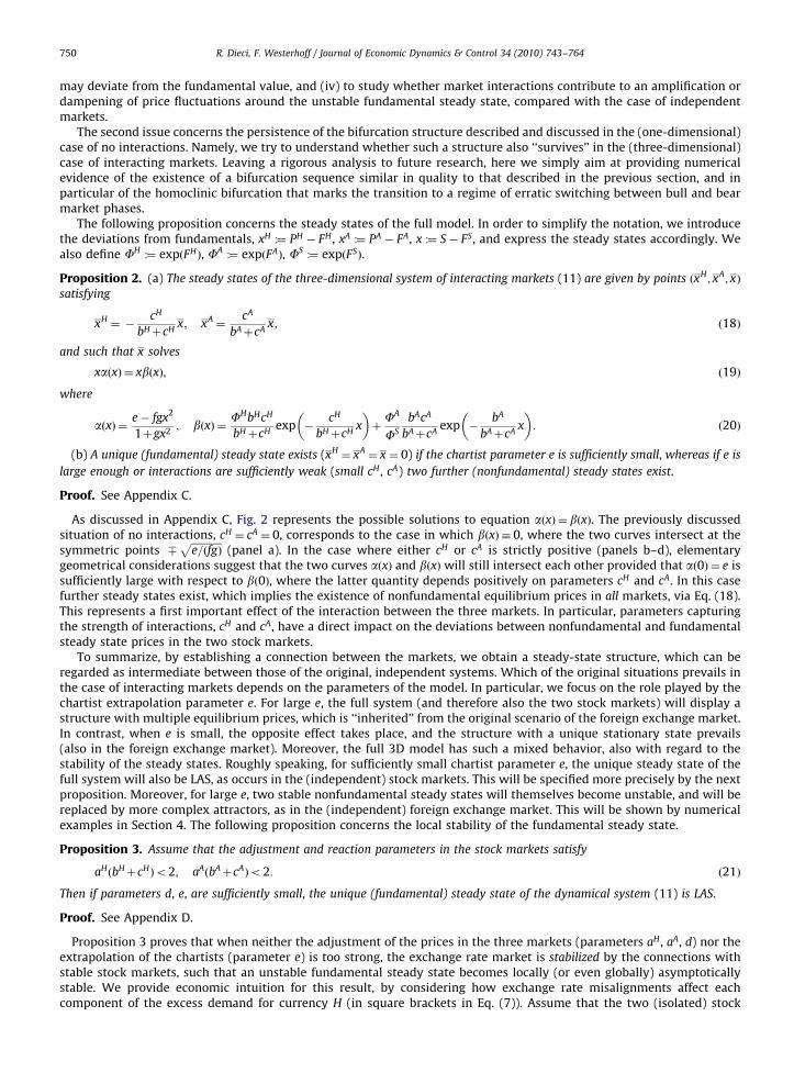
Proposition 2. (a) The steady states of the three-dimensional system of interacting markets (11) are given by points ðxH; xA; xÞ

satisfying

xH¼ �

cH

bHþcHx; xA

¼cA

bAþcAx; ð18Þ

and such that x solves

xaðxÞ ¼ xbðxÞ; ð19Þ

where

aðxÞ ¼ e� fgx2

1þgx2; bðxÞ ¼

FHbHcH

bHþcHexp �

cH

bHþcHx

� �þFA

FS

bAcA

bAþcAexp �

bA

bAþcAx

� �: ð20Þ

(b) A unique (fundamental) steady state exists (xH¼ xA

¼ x ¼ 0) if the chartist parameter e is sufficiently small, whereas if e is

large enough or interactions are sufficiently weak (small cH , cA) two further (nonfundamental) steady states exist.

Proof. See Appendix C.

As discussed in Appendix C, Fig. 2 represents the possible solutions to equation aðxÞ ¼ bðxÞ. The previously discussedsituation of no interactions, cH ¼ cA ¼ 0, corresponds to the case in which bðxÞ � 0, where the two curves intersect at thesymmetric points 8

ffiffiffiffiffiffiffiffiffiffiffiffie=ðfgÞ

p(panel a). In the case where either cH or cA is strictly positive (panels b–d), elementary

geometrical considerations suggest that the two curves aðxÞ and bðxÞ will still intersect each other provided that að0Þ ¼ e issufficiently large with respect to bð0Þ, where the latter quantity depends positively on parameters cH and cA. In this casefurther steady states exist, which implies the existence of nonfundamental equilibrium prices in all markets, via Eq. (18).This represents a first important effect of the interaction between the three markets. In particular, parameters capturingthe strength of interactions, cH and cA, have a direct impact on the deviations between nonfundamental and fundamentalsteady state prices in the two stock markets.

To summarize, by establishing a connection between the markets, we obtain a steady-state structure, which can beregarded as intermediate between those of the original, independent systems. Which of the original situations prevails inthe case of interacting markets depends on the parameters of the model. In particular, we focus on the role played by thechartist extrapolation parameter e. For large e, the full system (and therefore also the two stock markets) will display astructure with multiple equilibrium prices, which is ‘‘inherited’’ from the original scenario of the foreign exchange market.In contrast, when e is small, the opposite effect takes place, and the structure with a unique stationary state prevails(also in the foreign exchange market). Moreover, the full 3D model has such a mixed behavior, also with regard to thestability of the steady states. Roughly speaking, for sufficiently small chartist parameter e, the unique steady state of thefull system will also be LAS, as occurs in the (independent) stock markets. This will be specified more precisely by the nextproposition. Moreover, for large e, two stable nonfundamental steady states will themselves become unstable, and will bereplaced by more complex attractors, as in the (independent) foreign exchange market. This will be shown by numericalexamples in Section 4. The following proposition concerns the local stability of the fundamental steady state.

Proposition 3. Assume that the adjustment and reaction parameters in the stock markets satisfy

aHðbHþcHÞo2; aAðbAþcAÞo2: ð21Þ

Then if parameters d, e, are sufficiently small, the unique (fundamental) steady state of the dynamical system (11) is LAS.

Proof. See Appendix D.

Proposition 3 proves that when neither the adjustment of the prices in the three markets (parameters aH , aA, d) nor theextrapolation of the chartists (parameter e) is too strong, the exchange rate market is stabilized by the connections withstable stock markets, such that an unstable fundamental steady state becomes locally (or even globally) asymptoticallystable. We provide economic intuition for this result, by considering how exchange rate misalignments affect eachcomponent of the excess demand for currency H (in square brackets in Eq. (7)). Assume that the two (isolated) stock

ARTICLE IN PRESS

0.00-0.01 0.01x

0.0

0.4

0.8

alph

a, b

eta

panel c

0.00-0.01 0.01x

0.0

0.4

0.8

alph

a, b

eta

panel d

0.00-0.01 0.01

x

0.0

0.4

0.8

alph

a, b

eta

panel a

0.00-0.01 0.01x

0.0

0.4

0.8

alph

a, b

eta

panel b

Fig. 2. A characterization of the nonfundamental steady states. In the four panels we plot functions aðxÞ (black solid line) and bðxÞ (gray dashed line) for

different parameter combinations. Panel a: cH ¼ 0, cA ¼ 0, and e¼ 0:5. Panel b: cH ¼ 0:4, cA ¼ 0:4, and e¼ 0:5. Panel c: cH ¼ 0:4, cA ¼ 0:4, and e¼ 0:7. Panel

d: cH ¼ 0:1, cA ¼ 0:4, and e¼ 0:5. The remaining parameters are bH ¼ 1, bA ¼ 1:5, d¼ 1, f ¼ 0:8, g ¼ 10 000 and FH ¼ FA ¼ FS ¼ 0.


markets are stable at their fundamental values. If the (isolated) foreign exchange market is such that SoFS, but close to FS,then chartists prevail, and their speculative demand DS

C o0 tends to amplify the initial exchange rate deviation. Now openthe economy, by allowing fundamental traders to trade in both stock markets. Due to SoFS, investors from country A willstart buying stock H, hoping that the price will be corrected. At the same time investors from country H will take negativepositions in stock market A. Consequently, the two components of demand for currency H from stock market investors,expðPHÞDHA

F and �expðPA � SÞDAHF , will be strictly positive. The impact of such traders thus partly offsets that of foreign

exchange speculators, and stabilizes the steady state. This occurs, however, only when stock traders’ impact (cH and cA) isstrong enough and chartist extrapolation (e) is weak. In contrast, for larger e, exchange rate fluctuations break stability inall markets and, in addition, two nonfundamental steady states undergo a sequence of bifurcations similar to thatillustrated for the one-dimensional independent foreign exchange market in Figs. 1 c and d. This will be shown in the nextsection, which contains a broader discussion of the stabilizing/destabilizing impact of interactions.

4. Stabilizing and destabilizing effects of interactions: numerical examples

This section contains numerical examples which illustrate the dynamic behavior of the model and discusses, inparticular, the global bifurcations occurring for increasing values of parameter e, which governs the strength of chartists’speculation. First of all it will be shown that in the case of interacting markets large values of e result in a ‘‘strongerinstability’’ than in the case of independent markets, and produces an enlargement of the range of fluctuations. This effectis therefore totally different from the stabilizing impact proven analytically (and observed numerically) for small e. Second,it will be shown that, by taking e as a bifurcation parameter, the full three-dimensional model undergoes a sequence ofbifurcations which is similar to that observed for the exchange rate market in the one-dimensional case. In particular, wedetect also in the 3D case the effects of a homoclinic bifurcation of the fundamental steady state, similar to that reported inSection 3.1. Finally, we show that similar results may be obtained in a framework in which a nonlinear, unstable stock

ARTICLE IN PRESS


market interacts with a linear, stable foreign exchange market. As will become clear, an instability originating from aspeculative stock market may as well destabilize a foreign exchange market.

Throughout the examples of this section we use the following common parameter setting: aH ¼ 1, aA ¼ 0:8, bH ¼ 1,bA ¼ 1:5, d¼ 1, f ¼ 0:8, g ¼ 10 000, FH

¼FA¼FS

¼ 1 (so that the log fundamental prices FH , FA, FS are all equal to zero); theremaining parameters cH , cA, and e may vary across different examples. Note that parameters d, f, g, and FS are preciselythose used in Figs. 1 a, b: this means that in the absence of interactions, the foreign exchange market would becharacterized by two coexisting and locally stable nonfundamental steady states for any e40.14

4.1. Stability and volatility

Fig. 3 represents bifurcation diagrams for each of the three dynamic variables PH , PA, and S, versus the chartistparameter e. In each panel the asymptotic behavior in a case with market interactions (with cH ¼ cA ¼ 0:4) is comparedwith the corresponding situation with no interactions (cH ¼ cA ¼ 0, gray dashed line). Thus the figure reports the effect ofintroducing connections of a certain intensity for different values of e. The three panels located on the right are obtainedwith a different initial condition from those on the left. Note also that parameters aH , aA, bH , bA, cH , cA, d, FH , FA, and FS

(i.e. those that play a role for the linearized system around the fundamental steady state), satisfy all of the restrictions weimposed in Appendix D to derive analytical results about local stability.15 For a range of low values of parameter e, thestabilizing effect of interactions is clear from the bifurcation diagrams, which confirms our local stability results: stabilityof stock markets remains unaffected, whereas in the foreign exchange market two coexisting LAS nonfundamental steadystates (which surround an unstable fundamental equilibrium) are replaced by a unique stable fundamental equilibrium. Ifwe now increase parameter e (in the case cH ¼ cA ¼ 0:4), the latter loses stability for e¼ bð0ÞC0:6015. The effect of such abifurcation is a ‘‘pitchfork’’ scenario:16 for a certain range of e the phase space is thus characterized by the coexistence oftwo stable equilibria that surround the unstable fundamental steady state, i.e. the two stock markets are destabilized withrespect to the situation of no interactions, and steady state prices deviate from fundamentals. Note, however, that in theforeign exchange market the steady state deviation from the fundamental is less pronounced than in the case ofindependent markets, i.e. a kind of stabilizing effect is still at work here. Larger values of e bring about the sequence ofperiod-doubling bifurcations already reported in the one-dimensional case. Within this range of e we can say thatinteractions destabilize all three markets. In particular, for eC4:856 the diagram reports a sudden, drastic enlargement ofthe chaotic region where asymptotic fluctuations are confined. This phenomenon will be further discussed below.

The economic intuition provided by Fig. 3 is therefore that market interactions, combined with strong extrapolation,result in remarkable spillover effects and market volatility, in contrast to the underlying stable markets withoutinteractions.17

In Fig. 4, the effect of interactions is analyzed from a slightly different perspective. In the upper group of panels wechoose a large value of e (e¼ 6). We also set cA ¼ 0:2 and increase cH . Since this represents the parameter that governs thedemand for stock in country H by fundamentalists from country A, we are thus increasing the strength of interactions fromA to H. By doing this, we notice a transition to increasingly complex dynamics, that is a ‘‘destabilizing effect’’ similar to thatalready observed in Fig. 3. The results are reported in panels a, b and c, d for log stock price H and the log exchange rate,respectively.18 By contrast, in the lower panels we select a small value of e (e¼ 0:5). We also fix cA ¼ 0:4 and increase cH

again. In this case we report the opposite effect, i.e. increasing the strength of interactions stabilizes the system (see panelse, f and g, h for PH and S, respectively). To summarize, the nature of the impact of market interactions (stabilizing ordestabilizing) is determined by the level of a crucial behavioral parameter, strictly related to chartists’ confidence in thepersistence of deviations from fundamentals. The overall impact is due to a balance between chartist extrapolation in theforeign exchange market and the reaction of the investors from one country to the stock market in the other country.

4.2. Homoclinic bifurcation

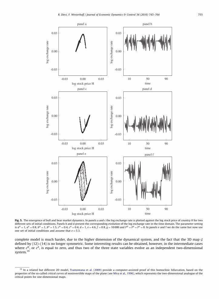
The previous subsection has shown how the fully integrated 3D model is able to display the characteristic behavior ofeach of the starting (independent) markets for different ranges of parameter e. Quite interestingly, as already anticipatedby the bifurcation diagrams in Fig. 3, even the homoclinic bifurcation of the steady state reported in the 1D case survivesalmost identical in the 3D model. Here, two attractors lying in two disjoint regions of the three-dimensional phase-spacemerge into a unique attractor, thus determining a major qualitative change of the dynamics. The situations before and afterthe bifurcation are represented in Fig. 5. Panels a, c and e report the projections of the attractors in the plane of the statevariables PH and S. Before the bifurcation, there are two coexisting attractors (panels a, c) and the asymptotic dynamics ofthe system depends on the initial state. After the bifurcation the two attractors merge into a unique attractor (panel e).

14 Similar phenomena can easily be detected for a wide region of the parameter space.15 One can easily check that conditions (50)–(52) are satisfied for any e40, while condition (49) holds only for eoe�C0:6015.16 Although this is not revealed by the plots in Fig. 3, such a bifurcation occurs via a slightly more complicated mechanism than a pitchfork

bifurcation, as further discussed in Appendix C.17 This simple observation is particularly meaningful in the light of current world financial turmoil.18 Again, left and right panels are characterized by different initial conditions.

ARTICLE IN PRESS

0 3 6parameter e

0.00

0.03

-0.03

log

exch

ange

rat

e

panel e

0 3 6parameter e

0.00

0.03

-0.03

log

exch

ange

rat

e

panel f

0 3 6

parameter e

0.00

0.03

-0.03

log

stoc

k pr

ice

A

panel c

0 3 6parameter e

0.00

0.03

-0.03

log

stoc

k pr

ice

A

panel d

0 3 6parameter e

0.00

0.03

-0.03

log

stoc

k pr

ice

H

panel a

0 3 6parameter e

0.00

0.03

-0.03

log

stoc

k pr

ice

H

panel b

Fig. 3. No market interactions versus market interactions. The six panels present bifurcation diagrams for the log stock price in country H (panels a and

b), the log stock price in country A (panels c and d) and the log exchange rate (panels e and f) for two different sets of initial conditions, respectively. The

parameters are: aH ¼ 1, aA ¼ 0:8, bH ¼ 1, bA ¼ 1:5, cH ¼ 0:4, cA ¼ 0:4, d¼ 1, 0oeo6, f ¼ 0:8, g ¼ 10 000 and FH ¼ FA ¼ FS ¼ 0. The superimposed gray dashed

lines illustrate the reference case of ‘‘no market interactions’’, i.e. cH ¼ 0 and cA ¼ 0, for the same values of the other parameters.


Obviously, this situation is the higher dimensional equivalent of the merging of two coexisting disjoint intervals in Figs. 1 c,d. Panels b, d and f represent the dynamics of the log-exchange rate in the time domain before and after bifurcation. Whileinitially the dynamics take place in a specified (bull or bear) market region, depending on the initial condition (panels b, d),after bifurcation the dynamics covers both regions, but still switches between the two pre-existing regions at seeminglyunpredictable points in time, thus evolving through a series of bubbles and crashes (panel f).

Under the same parameter configuration as Figs. 5e,f, and Fig. 6 (panels a, b, c) represents the time series of all statevariables, and shows that the stock prices also jump back and forth between ‘‘bull’’ and ‘‘bear’’ market episodes, triggeredby exchange rate fluctuations. Finally, panel d plots in the plane ðSt ; Stþ1Þ a trajectory obtained using the same parameters

ARTICLE IN PRESS

0.15 0.15 0.25parameter c_H

0.000

0.003

-0.003log

exch

ange

rate

panel g


0.000

0.003

-0.003log

exch

ange

rate

panel h


0.0000

0.0003

-0.0003log

stoc

k pr

ice

H

panel e


0.0000

0.0003

-0.0003log

stoc

k pr

ice

H

panel f

0 0.25 0.5parameter c_H

0.00

0.03

-0.03

log

exch

ange

rate

panel c


0.00

0.03

-0.03

log

exch

ange

rate

panel d


0.00

0.03

-0.03

log

stoc

k pr

ice

H

panel a


0.00

0.03

-0.03

log

stoc

k pr

ice

H

panel b

Fig. 4. The destabilizing/stabilizing effect of market interactions. Panels a and b (c and d) show bifurcation diagrams for the log stock price in country H

(the log exchange rate) for two different sets of initial conditions. The parameter setting is aH ¼ 1, aA ¼ 0:8, bH ¼ 1, bA ¼ 1:5, 0ocH o0:5, cA ¼ 0:2, d¼ 1,

e¼ 6, f ¼ 0:8, g ¼ 10 000 and FH ¼ FA ¼ FS ¼ 0. In the bottom four panels we repeat these computations but now use 0:15ocH o0:25, cA ¼ 0:4 and e¼ 0:5.


(and with a large number of iterations). If there are no interactions, such a plot would qualitatively reproduce the graph ofthe 1D map underlying the dynamical system (17) (as in Fig. 1 f). Since markets interact and there is hence feedback fromthe stock markets to the foreign exchange market, the plot in panel d does not reduce exactly to such a cubic curve. Putdifferently, the stock markets create some kind of ‘‘deterministic noise’’ for the exchange rate process. Note, however, thatthe two pictures in panel d and Fig. 1 f are very similar to each other. Far from being rigorous, we may argue that thisfeature enables the persistence in the 3D model of the original bifurcation structure, and of the characteristic bull and bearprice dynamics.

We do not push ahead with the analysis of such bifurcation mechanisms here, but leave further exploration to futureresearch. As already discussed in Section 3.1, in the one-dimensional system (17) such phenomena are due to a homoclinicbifurcation of the repelling fundamental steady state, strictly related to the fact that the map is noninvertible, with twocritical points. While in the 1D case much can be said about this bifurcation on analytical grounds, a similar analysis for the

ARTICLE IN PRESS

panel e panel f

panel c panel d

0.00 0.03-0.03

log stock price H

0.00

0.03

-0.03

log

exch

ange

rat

e

0.00

0.03

-0.03

log

exch

ange

rat

e

0.00 0.03-0.03

log stock price H

0.00

0.03

-0.03

log

exch

ange

rat

e

0.00 0.03-0.03

log stock price H

0.00

0.03

-0.03

log

exch

ange

rat

e

panel a

10 50 90time

0.00

0.03

-0.03

log

exch

ange

rat

e

10 50 90time

0.00

0.03

-0.03

log

exch

ange

rat

e

10 50 90time

panel b

Fig. 5. The emergence of bull and bear market dynamics. In panels a and c the log exchange rate is plotted against the log stock price of country H for two

different sets of initial conditions. Panels b and d present the corresponding evolution of the log exchange rate in the time domain. The parameter setting

is aH ¼ 1, aA ¼ 0:8, bH ¼ 1, bA ¼ 1:5, cH ¼ 0:4, cA ¼ 0:4, d¼ 1, e¼ 4:6, f ¼ 0:8, g¼ 10 000 and FH ¼ FA ¼ FS ¼ 0. In panels e and f we do the same but now use

one set of initial conditions and assume that e¼ 5:3.


complete model is much harder, due to the higher dimension of the dynamical system, and the fact that the 3D map Gdefined by (12)–(14) is no longer symmetric. Some interesting results can be obtained, however, in the intermediate caseswhere cH , or cA, is equal to zero, and thus two of the three state variables evolve as an independent two-dimensionalsystem.19

19 In a related but different 2D model, Tramontana et al. (2009) provide a computer-assisted proof of this homoclinic bifurcation, based on the

properties of the so-called critical curves of noninvertible maps of the plane (see Mira et al., 1996), which represents the two-dimensional analogue of the

critical points for one-dimensional maps.

ARTICLE IN PRESS

10 50 90time

0.00

0.03

-0.03

log

exch

ange

rate

panel c

0.00 0.03-0.03log exchange rate in t

0.00

0.03

-0.03

log

exch

ange

rate

in t+

1

panel d

10 50 90time

0.00

0.03

-0.03

log

stoc

k pr

ice

H

panel a

10 50 90time

0.00

0.03

-0.03

log

stoc

k pr

ice

A

panel b

Fig. 6. Bull and bear market dynamics in action. Panels a–c show the evolution of the log stock price of country H, the log stock price of country A and the

log exchange rate in the time domain, respectively. In panel d the log exchange rate at time step tþ1 is plotted against the log exchange rate at time step

t. The parameter setting is aH ¼ 1, aA ¼ 0:8, bH ¼ 1, bA ¼ 1:5, cH ¼ 0:4, cA ¼ 0:4, d¼ 1, e¼ 5:3, f ¼ 0:8, g ¼ 10 000 and FH ¼ FA ¼ FS ¼ 0.


4.3. ‘‘Sources’’ of instability

A final comment concerns the robustness of our analytical and numerical results under possibly different ‘‘sources’’ ofinstability. The main message from our dynamic analysis is that market interactions may be stabilizing or destabilizing,depending on the ‘‘strength’’ of speculative behavior of technical traders. We have observed this by starting from asituation with three independent markets, where the fundamental exchange rate equilibrium is unstable, while thefundamental stock market equilibria are stable. In such a situation, once markets are allowed to interact, the complicateddynamics originating in the foreign exchange market are the main driving force to the unstable and complicated pricedynamics in the stock markets. Therefore, the current model specification cannot be directly used to explore whether theconverse may happen, too, namely, a possible destabilizing effect to an otherwise stable foreign exchange market, due tothe instability of stock markets. The phenomena that we have illustrated are indeed fairly general. One can easily set upsimple variants20 of the model, where technical traders are absent from the foreign exchange market, so that thespeculative demand component in Eq. (7) reduces to the fundamentalist component DS

F;t ¼ f ðFS � StÞ. In the simplest case, achartist demand component DHH

C;t :¼ bHðPH

t � FHÞ from country H to stock market H is then introduced on the side of thefundamentalist component DHH

F;t defined by Eq. (2), together with a weighting mechanism analogous to (10). The resultingdynamical model has, in the case of no interactions (cH ¼ cA ¼ 0), a structure that is formally identical to (15)–(17), whereSt and PH

t are now driven by a linear and a cubic law of motion, respectively. Next, by introducing interactions, the impactof new chartist parameter bH on the model dynamics is analogous to that summarized in Fig. 3 for parameter e.

5. Conclusions

Financial markets are characterized by highly volatile prices and repeatedly display severe bubbles and crashes. Thechartist–fundamentalist approach offers a number of endogenous explanations for these challenging phenomena, by

20 The example sketched below is available from the authors upon request.

ARTICLE IN PRESS


stressing the interplay between the destabilizing impact of technical trading strategies and the mean reverting pricebehavior set in action by fundamentalists. The goal of our paper is to analyze the effect of such a basic determinant of pricefluctuations within a system of internationally connected financial markets. This is achieved by studying a stylizeddeterministic dynamic model of two stock markets that are nonlinearly interwoven—by construction—via and with theforeign exchange market. Such connections are due to the existence of (domestic) stock market traders who trade abroad,based on observed stock price and exchange rate misalignments, and using the foreign exchange market in order toexchange currency. While the stock markets are modelled as simple as possible by means of linear equations, the foreignexchange market ‘‘works’’ in a nonlinear way, in that currency speculators switch between competing linear trading rules.The model results in a three-dimensional discrete-time dynamical system. The focus of our analysis is on how exchangerate movements generated by the interplay of heterogeneous speculators in the foreign exchange market spill over into thestock markets, and affect the overall behavior of the system. In order to get a first insight into this issue we have chosen, asa one-dimensional benchmark, a very simple model of chartist–fundamentalist interaction, similar in structure to thestylized setup of Day and Huang (1990). The main question is therefore how the behavior of stable markets, in which pricesare close to their fundamental values, may be affected by connections to an unstable market, characterized by systematicdeviations from the fundamental value, the interplay between heterogeneous speculators and, in particular, thedestabilizing action of chartists who bet on the persistence of ‘‘bull’’ or ‘‘bear’’ market dynamics. One may wonder which ofthe original scenarios, that characterize each market ‘‘in isolation’’, prevails once the connections have been introduced, orwhether the behavior of the resulting integrated system stays at some intermediate level. We have reported ‘‘mixed’’results, despite the simplicity of the model. We have shown—by means of both analytical study and numericalexperiments—that market interactions may destabilize stock markets, but may also play a stabilizing effect on the foreignexchange market and on the whole system of interacting markets. The nature of the effect is strictly related to theparameters of the model, in particular to parameter e, which governs the speculative demand of chartists. Our findings onthe impact of market interactions may be summarized as follows.

�
Steady state analysis (Section 3.2) reveals a possible stabilizing effect of market interactions for low values of the priceadjustment parameters and of the chartist parameter e. Although one of the markets (the foreign exchange market) hasoriginally an unstable fundamental equilibrium, coexisting with further equilibria, the integrated model displays aunique stable fundamental steady state. Put differently, if the strength of chartist speculation in the foreign exchangemarket is weak, establishing a connection with stable markets results in the stabilization of the whole system. Thisstabilizing effect is also confirmed by the numerical experiments in Section 4.1 (in particular the leftmost part of thebifurcation diagrams versus e, in Fig. 3, and the diagrams in Figs. 4 e–h). � For larger values of e, two further nonfundamental steady states exist, which results in multiple equilibrium prices in
each market. In this case, we observe a ‘‘mixed’’ effect on the steady state structure. On the one hand, connections withstable markets can no more bring the whole system back to ‘‘fundamentals’’, and destabilize the stock markets, too,where prices tend to deviate from their fundamental values in the long run. On the other hand, in the foreign exchangemarket a kind of stabilizing effect is still in action, at least as long as e is not too high, in the sense that steady-statemisalignments are less pronounced than in the case of decoupled markets (see the middle part of the bifurcationdiagrams in Figs. 3 e,f).
� For large values of e, numerical simulation reveals a destabilizing effect of interactions. In all markets, previously stable
(fundamental or nonfundamental) steady states are replaced by periodic motion or complex endogenous dynamics. Thepossible deviations from the fundamentals are wider than in the case of no interaction. The amplitude of fluctuationsincreases with e (as shown in the rightmost part of the bifurcation diagrams in Fig. 3) and with the ‘‘strength’’ ofinteractions (one example is the bifurcation diagrams in Figs. 4 a–d). As long as e remains within a given range,fluctuations stay confined within the ‘‘bull’’ or the ‘‘bear’’ market regions. Afterwards, the interval covered byasymptotic price fluctuations is drastically enlarged, as an effect of a global bifurcation occurring for large e. This bringsabout a typical alternance of bull and bear market dynamics, with repeating bubbles and crashes around fundamentalsin both the foreign exchange and the stock markets, as shown in Section 4.2. Markets that contain neither technicaltraders nor ‘‘behavioral nonlinearities’’ may then switch between bull and bear episodes, due to quite naturalinteraction with more speculative markets.

As already pointed out, our choice to make endogenous motion start from the foreign exchange market is purelyconventional, and the same results could be obtained as well by assuming that heterogeneous speculators operate in one ofthe two stock markets. More generally, our model thus captures the way in which a simple mechanism of interactionbetween stock markets and the foreign exchange market may contribute to spreading or absorbing price fluctuations thatoriginate in one market. It indicates therefore that stock market volatility (exchange rate volatility) may be caused to someextent by exchange rate changes (stock price movements), and suggests how such volatility may be related to the strengthof interactions and the intensity of speculative demand. An immediate generalization of our setup would be that ofintroducing heterogeneous investors in all markets, together with exogenous noise on agents’ demand and fundamentalprices, in order to conduct a more thorough analysis on ‘‘how much’’ of the price volatility in each market can be ascribedto the link with other speculative markets. A further interesting extension concerns the impact, on stability and bifurcation

ARTICLE IN PRESS


routes, of a more general switching mechanism between technical and fundamental trading rules, that allows forasynchronous updating of beliefs, along the lines of Hommes et al. (2005). Finally, an important development is to explorethe impact of regulatory measures, such as financial market liberalizations and central bank interventions, under differentassumptions about agents’ behavioral parameters. This can be done, for instance, along the lines of Wieland andWesterhoff (2005).

Acknowledgments

Earlier versions of this work were presented at the 15th SNDE Annual Symposium (Society for Nonlinear Dynamics andEconometrics), Paris, March 15–16, 2007, the NED 07 Workshop (Nonlinear Economic Dynamics), Bielefeld, July 26–28,2007, and the AMASES 2007 Conference (Italian Association of Mathematics Applied to Economics and Social Sciences),Lecce, September 3–6, 2007. We are grateful to the participants for helpful discussions. We also thank the Managing Editor,Cars Hommes, and three anonymous referees for their constructive comments, that helped us to strengthen thepresentation of our results. The usual disclaimer applies.

Appendix A. Micro-foundation of demand functions

This appendix shows how the stylized demand functions assumed in the present paper can be justified within a mean–variance framework. Without loss of generality, we consider the portfolio problem faced by the (representative)fundamental investor from country A, who decides how much of his/her wealth to invest in stock A and how much in stockH. We assume, for simplicity, that the residual wealth is held as cash (or, equivalently, invested in a riskless asset with zerointerest rate). In the following we denote by (lowercase) pA

t , pHt and st the prices of the two assets and the exchange rate,

respectively. Agent’s wealth (denominated in currency A) evolves from time t to time tþDt according to

OAtþDt ¼OA

t þOAAt rA

tþDtþOHAt xH

tþDt

where OAAt and OHA

t denote the amount of wealth invested in stock A and stock H, respectively, and where

rAtþDt :¼

pAtþDt

pAt

� 1; xHtþDt :¼

pHtþDtstþDt

pHt st

� 1

are the returns on stock A and on wealth invested in stock H, respectively (the latter depending also on the exchange ratereturn stþDt=st). In the following we use log-returns, i.e. we set

rAtþDt � ln

pAtþDt

pAt

!; xH

tþDt � lnpH

tþDt

pHt

stþDt

st

!:

Assume the investor has CARA utility of wealth function, UAðOAtþDtÞ ¼ � expð�yAOA

tþDtÞ, where yA is the constant (absolute)risk aversion coefficient. If future (log-)returns are Gaussian in agent’s beliefs, maximization of expected utility of wealthreduces to the following mean–variance problem:

maxOAA

t ;OHAt

EAt ðO

AtþDtÞ �

yA

2VA

t ðOAtþDtÞ

( ); ð22Þ

where EAt and VA

t denote expectation and variance (of agent A), conditional upon information available at time t. As afundamental trader, the agent believes that price A follows a (geometric) mean reverting process of the type:

DlnpAt :¼ lnpA

tþDt � lnpAt ¼ Z

At ðlnF

At � lnpA

t ÞDtþsAt

ffiffiffiffiffiffiDtp

~eAt ;

where FAt is the fundamental price at time t, ZA

t and sAt are time varying (and possibly state-dependent) mean reversion and

volatility coefficients, respectively, and ~eAt �N ð0;1Þ is an i.i.d. Gaussian noise component. In a similar manner, price H and

the exchange rate are assumed to evolve, respectively, according to

DlnpHt :¼ lnpH

tþDt � lnpHt ¼ Z

Ht ðlnF

Ht � lnpH

t ÞDtþsHt


~eHt ;

Dlnst :¼ lnstþDt � lnst ¼ ZSt ðlnF

St � lnstÞDtþsS

t


~eSt :

We thus obtain

EAt ðO

AtþDtÞ ¼OA

t þOAAt ZA

t ðlnFAt � lnpA

t ÞDtþOHAt ½Z

Ht ðlnF

Ht � lnpH

t ÞþZSt ðlnF

St � lnstÞ�Dt: ð23Þ

Assuming no correlations, in agent’s beliefs, between the random terms ~eA, ~eH , ~eS yields

VAt ðO

AtþDtÞ ¼ ðO

AAt Þ

2ðsA

t Þ2DtþðOHA

t Þ2½ðsH

t Þ2þðsS

t Þ2�Dt: ð24Þ

ARTICLE IN PRESS


Plugging (23) and (24) into (22), the following first-order conditions can be computed:

ZAt ðlnF

At � lnpA

t Þ � yAðsA

t Þ2OAA

t ¼ 0;

ZHt ðlnF

Ht � lnpH

t ÞþZSt ðlnF

St � lnstÞ � yA

½ðsHt Þ

2þðsS

t Þ2�OHA

t ¼ 0:

Note that OAAt ¼DAA

t pAt , OHA

t ¼DHAt pH

t st , where DAAt and DHA

t denote demand for asset A and asset H, respectively, expressed inunits of stock. This finally yields the optimal demands:

DAAt ¼

ZAt

yAðsA

t Þ2pA

t

ðlnFAt � lnpA

t Þ; ð25Þ

DHAt ¼

ZHt

yA½ðsH

t Þ2þðsS

t Þ2�pH

t st

ðlnFHt � lnpH

t ÞþZS

t

ZHt

ðlnFSt � lnstÞ

� �: ð26Þ

Eqs. (25) and (26) reveal the connections between agents’ demands and their risk attitudes and beliefs about the processesof prices and exchange rates. The absence of correlations between different assets, in agents’ beliefs, causes the investmentdecisions of the same speculator operating in two different stock markets to be decoupled. Including possible correlationswould obviously result in interdependent investment decisions, jointly impacting on both prices.

From Eqs. (25) and (26), demand for stock A at a given point in time is thus essentially given by the product of a time-varying reaction coefficient by the log-price misalignment in market A, i.e.

DAAt ¼ bA

t ðlnFAt � lnpA

t Þ; bAt :¼

ZAt

yAðsA

t Þ2pA

t

: ð27Þ

The same holds for the case of the demand for stock H, with the addition of a term with a similar structure, capturing themisalignment on the foreign exchange market, i.e.:

DHAt ¼ cH

t ½ðlnFHt � lnpH

t ÞþgHt ðlnF

St � lnstÞ�; cH

t :¼ZH

t

yA½ðsH

t Þ2þðsS

t Þ2�pH

t st

; gHt :¼

ZSt

ZHt

: ð28Þ

The simplified demand functions used in the paper, (5) and (3), are essentially (27) and (28), respectively, where thefundamental prices and the reaction coefficients bA

t and cHt are assumed to be constant for analytical tractability, and the

speed of mean reversion in different markets is the same (i.e. gHt � 1), in order to reduce the number of parameters.

The optimal portfolio of the trader from country H, investing in stock markets H and A, can be derived in a specular way,starting from wealth denominated in currency H. An even simpler mean–variance setup can be used to obtain optimaldemand for currency H from foreign exchange speculators.

We add a few comments on how asset demand impacts on prices in our model. First, we are implicitly assuming thatthe net supply of each asset is zero. This represents a quite common assumption in such kind of models, and is consistentwith our stylized setup, where the ‘‘risky assets’’ H and A pay no dividends, the risk-free rate of return is zero, and thereforeagents’ steady-state demand is zero, too. Assuming a strictly positive amount of assets H and A would require a more richsetup (where both dividend payments and the risk-free rate are explicitly taken into account) such that the risky assetsearn a strictly positive excess return in the ‘‘fundamental’’ steady state solution. Such a ‘‘risk premium’’ would thus driveinvestors to hold positive amounts of these assets in their steady-state portfolios.21 Second, it follows from our micro-foundation that Eqs. (1) and (4) relate price changes to agents’ (excess) desired asset holdings. This simplifying view hasoften been adopted in the literature, too (see, e.g. Chiarella et al., 2009 and references therein). From a differentperspective, one could model price adjustments as related to net orders, i.e. changes in asset holdings, and rewrite, e.g.Eq. (1) as follows:

PHtþ1 ¼ PH

t þaHðDHHF;t þDHA

F;t � ZHt�1Þ; ð29Þ

where ZHt�1 ¼DHH

F;t�1þDHAF;t�1. This approach would largely increase the dimension of the dynamical system, unless one

strongly simplifies Eq. (29) by simply setting ZHt�1 ¼ 0, i.e. by neglecting the effect of agents’ accumulated positions.22

We remark that such modelling issues are strictly connected, in general, to the underlying view about the role andbehavior of the market maker, as can be argued from the models recently developed by Franke and Asada (2008) and Zhuet al. (2009).23

21 Note that this more general case can usually be reduced to the case of ‘‘zero’’ supply, via suitable changes of parameters (see, e.g. Hommes, 2006).22 We thank one of the referees for suggesting us this alternative interpretation, which may help to reconcile the two approaches based on ‘‘orders’’

and on ‘‘positions’’, respectively.23 Although the ‘‘order-based’’ price setting equation (29) may look more realistic than the ‘‘position-based’’ equation (1), it neglects the possible

price impact of market maker inventories. Roughly speaking, market maker accumulated inventory is inversely related to agents’ aggregate position.

Given that market makers seek to limit their inventories, this observation provides an intuitive justification of price adjustment equation (1). See also the

conceptual discussion in Franke (2008).

ARTICLE IN PRESS


Appendix B. Proof of Proposition 1

The proof of (a) is straightforward.(b) The one-dimensional nonlinear map (17), which governs the exchange rate dynamics in the case of cH ¼ cA ¼ 0, can

be rewritten as

Stþ1 ¼ Stþd f ðFS � StÞþðeþ f ÞðSt � FSÞ

1þgðSt � FSÞ2

" #: ð30Þ

By introducing deviations from the fundamental value, x :¼ S� FS, Eq. (30) takes the form xtþ1 ¼ hðxtÞ, where

hðxÞ ¼ xþd �fxþðeþ f Þx

1þgx2

� �¼ ð1� df Þxþ

dðeþ f Þx

1þgx2: ð31Þ

For strictly positive e, f, g, map hðxÞ admits three fixed points, solutions of hðxÞ ¼ x, given by x ¼ 0, xl ¼ �ffiffiffiffiffiffiffiffiffiffiffiffie=ðfgÞ

p,

xu ¼ffiffiffiffiffiffiffiffiffiffiffiffie=ðfgÞ

p. It follows that the dynamical system (30) has three steady states, namely S ¼ FS, Sl ¼ FS �


p,

Su ¼ FSþffiffiffiffiffiffiffiffiffiffiffiffie=ðfgÞ

p.

(c) In order to study the stability properties of the steady states, we consider the derivative of map (31)

dhðxÞ

dx¼ 1� df þdðeþ f Þ

1� gx2

ð1þgx2Þ2: ð32Þ

Evaluation of (32) at the fundamental steady state yields

dh

dx

��x ¼ 0

¼ 1þde41;

which reveals that the fundamental steady state is always unstable. With regard to the nonfundamental steady statesxl ¼ �


p, xu ¼


p, note first that gx2

l ¼ gx2u ¼ e=f . Therefore we obtain

dh

dx

��x ¼ xl

¼dh

dx

��x ¼ xu

¼ 1�2def

eþ fo1:

The nonfundamental steady states are thus LAS if and only if 1� 2def=ðeþ f Þ4 � 1, i.e.

eðdf � 1Þo f : ð33Þ

By taking the chartist parameter e as a bifurcation parameter, the stability condition (33) holds for any e40 if df r1. In theopposite case, df 41, the stability condition is satisfied only for eoeFlip :¼ f=ðdf � 1Þ, at which value a period doublingbifurcation occurs.

Appendix C. Proof of Proposition 2

(a) The steady states (PH; P

A; S) of the dynamical system (11) are the solutions of the following system of equations

PH¼ GHðP

H; SÞ; P

A¼ GAðP

A; SÞ; S ¼ GSðP

H; P

A; SÞ; ð34Þ

which can be rewritten as follows:

ðbHþcHÞðFH � PHÞþcHðFS � SÞ ¼ 0; ð35Þ

ðbAþcAÞðFA � PAÞþcAðS � FSÞ ¼ 0; ð36Þ

cHðFH � PHþFS � SÞexpðP

HÞ � cAðFA � P

AþS � FSÞexpðP

A� SÞþ

eðS � FSÞ

1þgðFS � SÞ2þ

fgðFS � SÞ3

1þgðFS � SÞ2¼ 0: ð37Þ

Note that from (35) and (36) it follows, respectively, that

PH� FH ¼

cH

bHþcHðFS � SÞ; P

A� FA ¼

cA

bAþcAðS � FSÞ: ð38Þ

The quantities ðFH � PHþFS � SÞ and ðFA � P

AþS � FSÞ in (37) can therefore be rewritten, respectively, as

ðFH � PHþFS � SÞ ¼ �

bH

bHþcHðS � FSÞ;

ðFA � PAþS � FSÞ ¼

bA

bAþcAðS � FSÞ;

ARTICLE IN PRESS


while the quantities expðPHÞ and expðP

A� SÞ in the same equation become

expðPHÞ ¼FHexp �

cH

bHþcHðS � FSÞ

� �;

expðPA� SÞ ¼

FA

FSexp �

bA

bAþcAðS � FSÞ

� �;

where FH :¼ expðFHÞ, FA :¼ expðFAÞ, FS :¼ expðFSÞ. By introducing deviations from fundamentals, xH :¼ PH � FH ,xA :¼ PA � FA, x :¼ S� FS, Eq. (38) simplifies into (18), while (37) can be rewritten as

ex � fgx3

1þgx2�

cHbH

bHþcHxFHexp �

cH

bHþcHx

� ��

cAbA

bAþcAxFA

FSexp �

bA

bAþcAx

� �¼ 0;

or x½aðxÞ � bðxÞ� ¼ 0, that is Eq. (19), where aðxÞ and bðxÞ are defined by (20).(b) Eq. (18) determines equilibrium stock prices as functions of equilibrium exchange rates, where the latter are the

solutions of Eq. (19). Eq. (19) always admits the solution x¼ 0, which corresponds to the fundamental steady statexH ¼ xA ¼ x¼ 0. Further nonfundamental steady states are related to the possible solutions of aðxÞ ¼ bðxÞ. We discuss theconditions for their existence by means of Fig. 2. Note first that in the case cH ¼ cA ¼ 0, quantity bðxÞ is identically equal tozero, so that we are back to the case of no interactions where two symmetric exchange rate equilibria exist, x¼ 8


p(panel a). If either cH or cA is strictly positive, then bðxÞ is represented by a (strictly decreasing) negative exponentialfunction,24 and the graphical visualization of equation aðxÞ ¼ bðxÞ is as in the panels from b to d. The bell-shaped functionaðxÞ intersects the vertical axis at level að0Þ ¼ e, while bðxÞ intersects at the level

bð0Þ ¼FHbHcH

bHþcHþFA

FS

bAcA

bAþcA: ð39Þ

Note that the smaller cH , cA are, the lower the ordinate bð0Þ of the intersection. Therefore, as long as e is sufficiently large(panel c) or market interactions are sufficiently weak, i.e. cH or cA are small enough (panel d), equation aðxÞ ¼ bðxÞ will stilladmit two solutions (and the system will then have three steady states) similarly to the case of no interaction. In particular,eZbð0Þ represents a sufficient condition for the existence of multiple solutions. By contrast, if e is sufficiently small, therewill be no solutions to aðxÞ ¼ bðxÞ (panel b) and the system will admit a unique steady state.

We add a few comments on the proof of this result. Consider, for instance, the transition from panels b to c, which isobtained by increasing parameter e for fixed values of cH , cA. The exact bifurcation value of e at which two new steadystates appear can only be computed numerically. Since aðxÞ is represented by a bell-shaped curve, symmetric with respectto the vertical axis, and bðxÞ is negatively sloped, the tangency between aðxÞ and bðxÞ, and the subsequent crossing, will takeplace for strictly positive x, and the two new solutions will both be positive, initially. For e¼ bð0Þ, one of the two solutionscoincides with x¼ 0, whereas for higher e, the two solutions will have opposite signs. The bifurcation mechanism is in factthat of a saddle-node bifurcation, followed by a transcritical bifurcation of the fundamental steady state. If bðxÞ is sufficientlyflat (as is the case in Fig. 2), the two bifurcations may occur very close to each other. In any case, the ‘‘final’’ result is similarto that of a pitchfork bifurcation.

Appendix D. Proof of Proposition 3

The Jacobian matrix of the system (11), evaluated at the fundamental steady state F :¼ ðFH; FA; FSÞ, is the following:

DGðFÞ ¼

1� aHðbHþcHÞ 0 �aHcH

0 1� aAðbAþcAÞ aAcA

�dFHcH dFA

FScA 1þd e�FHcH �

FA

FScA

" #266664

377775: ð40Þ

For notational purposes, it is convenient to define the following aggregate quantities:

qH :¼ 1� aHðbHþcHÞ; qA :¼ 1� aAðbAþcAÞ; ð41Þ

uH :¼ aHðcHÞ2dFH; uA :¼ aAðcAÞ

2dFA

FS; ð42Þ

k¼ 1� d FHcHþFA

FScA

" #: ð43Þ

24 The graph of bðxÞ, however, looks approximately flat at the scale of Fig. 2.

ARTICLE IN PRESS


With some algebra, the characteristic polynomial of DGðFÞ can be rewritten as

PðlÞ ¼ l3þm1l

2þm2lþm3; ð44Þ

where

m1 ¼ � ðqHþqAþkþdeÞ;

m2 ¼ ðqHþqAÞðkþdeÞþqHqA � ðuHþuAÞ;

m3 ¼ qHuAþqAuH � qHqAðkþdeÞ:

Note that from our assumption (21) and from the fact that aH , bH , aA, bA, are strictly positive and cH , cA are nonnegative, itfollows that jqHjo1, jqAjo1, which implies jqHqAjo1, jqHþqAjo2. The following set of inequalities imposed on thecoefficients of the characteristic polynomial (44) provide a necessary and sufficient condition for all the eigenvalues of(40) to be of modulus smaller than unity (Farebrother, 1973), which implies a locally asymptotically stable steady state:

1þm1þm2þm340; ð45Þ

1�m1þm2 �m340; ð46Þ

1�m2þm3ðm1 �m3Þ40; ð47Þ

m2o3: ð48Þ

Conditions (45)–(48) can be rewritten in terms of the parameters of the model, respectively

ð1� qHÞð1� qAÞ � uHð1� qAÞ � uAð1� qHÞ � ð1� qHÞð1� qAÞðkþdeÞ40; ð49Þ

ð1þqHÞð1þqAÞ � uHð1þqAÞ � uAð1þqHÞþð1þqHÞð1þqAÞðkþdeÞ40; ð50Þ

1� qHqAþuHþuA

� ðqHuAþqAuHÞ2� ðqHuAþqAuHÞðqHþqAÞ

� ½ðqHuAþqAuHÞð1� 2qHqAÞþðqHþqAÞð1� qHqAÞ�ðkþdeÞþqHqAð1� qHqAÞðkþdeÞ240; ð51Þ

qHqA � ðuHþuAÞþðqHþqAÞðkþdeÞo3: ð52Þ

We now discuss conditions (49)–(52) and show, in particular, that they are simultaneously satisfied under condition (21),provided that parameters d, e are not too large. Note that quantities uH , uA, and k depend on d, according to (42) and (43),respectively. In the following we assume that d is as small as necessary, so that in particular quantity k, defined in (43), isstrictly positive. In general we will regard the left-hand side of each of conditions (49)–(52) as a function of parameter e40for sufficiently small values of d and fixed values of the other parameters (satisfying all of the assumed restrictions).

Condition (49) can be rewritten as

ð1� qHÞð1� qAÞdeo ð1� qHÞð1� qAÞð1� kÞ � uHð1� qAÞ � uAð1� qHÞ:

In the above equation, the term on the right-hand side is strictly positive for any d40. To prove this, simply note that

0raHcH

1� qH¼

aHcH

aHðbHþcHÞo1; 0r

aAcA

1� qA¼

aAcA

aAðbAþcAÞo1

and therefore

1� k¼ d FHcHþFA

FScA

" #4d FHcH aHcH

1� qHþFA

FScA aAcA

1� qA

" #¼

uH

1� qHþ

uA

1� qA:

Moreover, since the quantity ð1� qHÞð1� qAÞ is strictly positive, too, it follows that condition (49) is satisfied forsufficiently small e, namely

eo1

d1� k�

uH

1� qH�

uA

1� qA

� �¼FH bHcH

bHþcHþFA

FS

bAcA

bAþcA:¼ e�: ð53Þ

Condition (50) can be rewritten as

ð1þqHÞð1þqAÞð1þkÞ � uHð1þqAÞ � uAð1þqHÞþð1þqHÞð1þqAÞde40:

Since quantities 1þqH ¼ 2� aHðbHþcHÞ and 1þqA ¼ 2� aAðbAþcAÞ are strictly positive under our assumptions,the coefficient of the term containing parameter e is strictly positive, too. The sum of the remaining terms on the

ARTICLE IN PRESS


left-hand side is strictly positive if

1þk�uH

1þqHþ

uA

1þqA

� �40;

which results in

do2 FHcH 2� aHbH

2� aHðbHþcHÞþFA

FScA 2� aAbA

2� aAðbAþcAÞ

" #�1

:¼ d�:

Under such a restriction on d, condition (50) is satisfied for any e40.Condition (51) is much more complicated to deal with, but it can be noted that for d; e-0 (in which case k-1,

uH;uA-0), the left-hand side becomes

ð1� qHqAÞð1� qHÞð1� qAÞ;

which is strictly positive under our assumptions (21). By continuity arguments, (51) will then be satisfied for sufficientlysmall values of d and e.

Condition (52) is obviously satisfied when qHþqAr0, i.e. aHðbHþcHÞþaAðbAþcAÞZ2. Assume now qHþqA40, in whichcase the left-hand side of (52) strictly increases with e. Since our assumptions imply jqHqAjo1, 0oqHþqAo2, 0oko1,we obtain

qHqA � ðuHþuAÞþðqHþqAÞko3:

It follows that when qHþqA40, Eq. (52) is satisfied for sufficiently small e, namely for

eo1

d

3þðuHþuAÞ � qHqA

qHþqA� k

� �:¼ e��: ð54Þ

Our assumptions about aggregate parameters qH , qA, also imply that threshold e�� defined in Eq. (54) is larger than quantitye� in (53). To see this, note that (since jqHqAjo1, 0oqHþqAo2) the following inequalities hold:

de��þk¼3þðuHþuAÞ � qHqA

qHþqA4141�

uH

1� qH�

uA

1� qA¼ de�þk:

This implies that condition (54) is fulfilled whenever (53) holds, and therefore condition (52) is redundant.Our analysis proves that the fundamental steady state is LAS for sufficiently small d and e. It also provides a rough

picture of how local bifurcations may occur. Assume that d is as small as necessary (in particular dod�) and assume alsothat by increasing parameter e condition (51) is satisfied at least for 0oere� (this is actually the case of the parametersused for the numerical examples in Fig. 3). In this case, the steady state loses stability for e¼ e�. Note that bifurcation valuee� is equal to quantity bð0Þ (see Eq. (39) in Appendix C). This means that in this case the loss of stability occurs preciselywhen one of the two newborn nonfundamental steady states collides with the fundamental steady state. Numerical andgraphical analysis suggests that this contact corresponds to a transcritical bifurcation of the fundamental steady state(see also Appendix C).

References

Anufriev, M., Bottazzi, G., Pancotto, F., 2006. Equilibria, stability and asymptotic dominance in a speculative market with heterogeneous traders. Journal ofEconomic Dynamics and Control 30, 1787–1835.

Bauer, C., DeGrauwe, P., Reitz, S., 2009. Exchange rate dynamics in a target zone—a heterogeneous expectations approach. Journal of Economic Dynamicsand Control 33, 329–344.

Beja, A., Goldman, M.B., 1980. On the dynamic behavior of prices in disequilibrium. Journal of Finance 35, 235–248.Bohm, V., Wenzelburger, J., 2005. On the performance of efficient portfolios. Journal of Economic Dynamics and Control 29, 721–740.Boswijk, P., Hommes, C.H., Manzan, S., 2007. Behavioral heterogeneity in stock prices. Journal of Economic Dynamics and Control 31, 1938–1970.Brock, W.A., Hommes, C.H., 1997. A rational route to randomness. Econometrica 65, 1059–1095.Brock, W.A., Hommes, C.H., 1998. Heterogeneous beliefs and routes to chaos in a simple asset pricing model. Journal of Economic Dynamics and Control

22, 1235–1274.Brock, W.A., Hommes, C.H., Wagener, F.O.O., 2009. More hedging instruments may destabilize markets. Journal of Economic Dynamics and Control 33,

1912–1928.Chiarella, C., 1992. The dynamics of speculative behaviour. Annals of Operations Research 37, 101–123.Chiarella, C., Dieci, R., Gardini, L., 2002. Speculative behaviour and complex asset price dynamics: a global analysis. Journal of Economic Behavior and

Organization 49, 173–197.Chiarella, C., Dieci, R., Gardini, L., 2005. The dynamic interaction of speculation and diversification. Applied Mathematical Finance 12, 17–52.Chiarella, C., Dieci, R., He, X.-Z., 2007. Heterogeneous expectations and speculative behaviour in a dynamic multi-asset framework. Journal of Economic

Behavior and Organization 62, 408–427.Chiarella, C., Dieci, R., He, X.-Z., 2009. Heterogeneity, market mechanisms, and asset price dynamics. In: Hens, T., Schenk-Hoppe, K.R. (Eds.), Handbook of

Financial Markets—Dynamics and Evolution, Handbooks in Finance Series. North-Holland, Amsterdam, pp. 277–344.Chiarella, C., He, X.-Z., 2001. Asset price and wealth dynamics under heterogeneous expectations. Quantitative Finance 1, 509–526.Cont, R., 2001. Empirical properties of asset returns: stylized facts and statistical issues. Quantitative Finance 1, 223–236.Corona, E., Ecca, S., Marchesi, M., Setzu, A., 2008. The interplay between two stock markets and a related foreign exchange market: a simulation approach.

Computational Economics 32, 99–119.

ARTICLE IN PRESS


Day, R.H., Huang, W., 1990. Bulls, bears and market sheep. Journal of Economic Behavior and Organization 14, 299–329.De Grauwe, P., Dewachter, H., Embrechts, M., 1993. Exchange rate theories. Chaotic Models of the Foreign Exchange Market. Blackwell, Oxford.De Grauwe, P., Grimaldi, M., 2005. Heterogeneity of agents, transactions costs and the exchange rate. Journal of Economic Dynamics and Control 29,

691–719.Dieci, R., Bischi, G.I., Gardini, L., 2001. From bi-stability to chaotic oscillations in a macroeconomic model. Chaos, Solitons and Fractals 12, 805–822.Dieci, R., Westerhoff, F., 2009. On the inherent instability of international financial markets: natural nonlinear interactions between stock and foreign

exchange markets. Working Paper, University of Bologna.Diks, C., Dindo, P., 2008. Informational differences and learning in an asset market with boundedly rational agents. Journal of Economic Dynamics and

Control 32, 1432–1465.Farebrother, R.W., 1973. Simplified Samuelson conditions for cubic and quartic equations. Manchester School of Economics and Social Studies 41,

396–400.Franke, R., 2008. On the interpretation of price adjustments and demand in asset pricing models with mean–variance optimization. Working Paper,

University of Kiel /www.bwl.uni-kiel.de/gwif/downloads_papers.php?lang=enS.Franke, R., 2009. A prototype model of speculative dynamics with position-based trading. Journal of Economic Dynamics and Control 33, 1134–1158.Franke, R., Asada, T., 2008. Incorporating positions into asset pricing models with order-based strategies. Journal of Economic Interaction and

Coordination 3, 201–227.Gaunersdorfer, A., Hommes, C.H., 2007. A nonlinear structural model for volatility clustering. In: Teyssi�ere, G., Kirman, A. (Eds.), Long Memory in

Economics. Springer, Berlin, pp. 265–288.Georges, C., 2008. Staggered updating in an artificial financial market. Journal of Economic Dynamics and Control 32, 2809–2825.He, X.-Z., Li, Y., 2008. Heterogeneity, convergence and autocorrelations. Quantitative Finance 8, 59–79.He, X.-Z., Westerhoff, F., 2005. Commodity markets, price limiters and speculative price dynamics. Journal of Economic Dynamics and Control 29,

1577–1596.Hommes, C.H., 2006. Heterogeneous agent models in economics and finance. In: Tesfatsion, L., Judd, K. (Eds.), Handbook of Computational Economics,

Agent-based Computational Economics, vol. 2. North-Holland, Amsterdam, pp. 1109–1186.Hommes, C.H., Huang, H., Wang, D., 2005. A robust rational route to randomness in a simple asset pricing model. Journal of Economic Dynamics and

Control 29, 1043–1072.Huang, W., Day, R.H., 1993. Chaotically switching bear and bull markets: the derivation of stock price distributions from behavioral rules. In: Day, R.H.,

Chen, P. (Eds.), Nonlinear Dynamics and Evolutionary Economics. Oxford University Press, Oxford, pp. 169–182.Kirman, A., 1991. Epidemics of opinion and speculative bubbles in financial markets. In: Taylor, M. (Ed.), Money and Financial Markets. Blackwell, Oxford,

pp. 354–368.LeBaron, B., 2006. Agent-based computational finance. In: Tesfatsion, L., Judd, K. (Eds.), Handbook of Computational Economics, Agent-based

Computational Economics, vol. 2. North-Holland, Amsterdam, pp. 1187–1233.Lux, T., 1995. Herd behavior, bubbles and crashes. Economic Journal 105, 881–896.Lux, T., 1997. Time variation of second moments from a noise trader/infection model. Journal of Economic Dynamics and Control 22, 1–38.Lux, T., 1998. The socio-economic dynamics of speculative markets: interacting agents, chaos, and the fat tails of return distributions. Journal of Economic

Behavior and Organization 33, 143–165.Lux, T., 2008. Financial power laws: empirical evidence, models and mechanisms. In: Cioffi-Revilla, C. (Ed.), Power Laws in the Social Sciences: Discovering

Complexity and Non-equilibrium Dynamics in the Social Universe. Cambridge University Press, Cambridge in press.Lux, T., 2009. Stochastic behavioral asset pricing models and the stylized facts. In: Hens, T., Schenk-Hoppe, K.R. (Eds.), Handbook of Financial

Markets—Dynamics and Evolution, Handbooks in Finance Series. North-Holland, Amsterdam, pp. 161–216.Lux, T., Ausloos, M., 2002. Market fluctuations I: scaling, multiscaling, and their possible origins. In: Bunde, A., Kropp, J., Schellnhuber, H. (Eds.), Science of

Disaster: Climate Disruptions, Heart Attacks, and Market Crashes. Springer, Berlin, pp. 373–410.Mira, C., Gardini, L., Barugola, A., Cathala, J.C., 1996. Chaotic Dynamics in Two-dimensional Noninvertible Maps. World Scientific, Singapore.Rosser, B., Ahmed, E., Hartmann, G., 2003. Volatility via social flaring. Journal of Economic Behavior and Organization 50, 77–87.Tramontana, F., Gardini, L., Dieci, R., Westerhoff, F., 2009. The emergence of bull and bear dynamics in a nonlinear model of interacting markets. Discrete

Dynamics in Nature and Society, vol. 2009, Article ID 310471, doi: 10.1155/2009/310471.Westerhoff, F., 2004. Multiasset market dynamics. Macroeconomic Dynamics 8, 596–616.Westerhoff, F., Dieci, R., 2006. The effectiveness of Keynes–Tobin transaction taxes when heterogeneous agents can trade in different markets:

a behavioral finance approach. Journal of Economic Dynamics and Control 30, 293–322.Westerhoff, F., Franke, R., 2009. Converse trading strategies, intrinsic noise and the stylized facts of financial markets. Working paper, University of

Bamberg /http://www.uni-bamberg.de/vwl-wipo/leistungen/team/prof_dr_frank_westerhoff/S.Wieland, C., Westerhoff, F., 2005. Exchange rate dynamics, central bank interventions and chaos control methods. Journal of Economic Behavior and

Organization 58, 117–132.Zhu, M., Chiarella, C., He, X.-Z., Wang, D., 2009. Does the market maker stabilize the market?. Physica A 388, 3164–3180.

www.bwl.uni-kiel.de/gwif/downloads_papers.php?lang=en




10.1155/2009/310471

http://www.uni-bamberg.de/vwl-wipo/leistungen/team/prof_dr_frank_westerhoff/

Heterogeneous speculators, endogenous fluctuations and interacting markets: A model of stock prices...

Documents

Transcript of Heterogeneous speculators, endogenous fluctuations and interacting markets: A model of stock prices...