Interest Rates in Financial Analysis and Valuation - WBI Library
101
Ahmad Nazri Wahidudin, Ph. D Interest Rates in Financial Analysis and Valuation Download free books at
-
Upload
khangminh22 -
Category
Documents
-
view
6 -
download
0
Transcript of Interest Rates in Financial Analysis and Valuation - WBI Library

Ahmad Nazri Wahidudin, Ph. D
Interest Rates in Financial Analysis andValuation
Download free books at

Download free eBooks at bookboon.com
2
Ahmad Nazri Wahidudin, Ph. D
Interest Rates in Financial Analysis and Valuation

Download free eBooks at bookboon.com
3
Interest Rates in Financial Analysis and Valuation© 2011 Ahmad Nazri Wahidudin, Ph. D & bookboon.comISBN 978-87-7681-928-6

Download free eBooks at bookboon.com
Click on the ad to read more
Interest Rates in Financial Analysis and Valuation
4
Contents
Contents
Preface 6
1 Single principal sum 71.1 Simple Interest Rate 71.2 Flat Rate 81.3 Compound Interest Rate 11
2 Multiple stream of cash flows 152.1 Even Stream of Cash Flows 152.2 Uneven Stream of Cash Flows 26
3 The rates of return 293.1 The Term Structure of Interest Rates and Theories 293.2 Forecasting Interest Rates 393.3 Interest Rates in Derivative Contracts 413.4 Rates of Return 53
ENGINEERS, UNIVERSITY GRADUATES & SALESPROFESSIONALSJunior and experienced F/M
Total will hire 10,000 people in 2014. Why not you?
Are you looking for work in process, electrical or other types of engineering, R&D, sales & marketing or support professions such as information technology?
We’re interested in your skills.
Join an international leader in the oil, gas and chemical industry by applying at
www.careers.total.comMore than 700 job openings are now online!
Potential for development
Cop
yrig
ht :
Tota
l/Cor
bis
for development
Potential for exploration

Download free eBooks at bookboon.com
Click on the ad to read more
Interest Rates in Financial Analysis and Valuation
5
Contents
4 Security valuation 594.1 Valuation and Yields of Treasury Bills and Short-term Notes 594.2 Bond Valuation 634.3 Preference Share Valuation 684.4 Ordinary Share Valuation 694.5 Share and Portfolio Performance Measures 71
5 Cost of capital 764.1 Weighted Average Cost 764.2 Cost of Debts 784.3 Cost of Equity 78
6 Capital budgeting 846.1 Net Present Value 84
Appendix 94
www.sylvania.com
We do not reinvent the wheel we reinvent light.Fascinating lighting offers an infinite spectrum of possibilities: Innovative technologies and new markets provide both opportunities and challenges. An environment in which your expertise is in high demand. Enjoy the supportive working atmosphere within our global group and benefit from international career paths. Implement sustainable ideas in close cooperation with other specialists and contribute to influencing our future. Come and join us in reinventing light every day.
Light is OSRAM

Download free eBooks at bookboon.com
Interest Rates in Financial Analysis and Valuation
6
Preface
PrefaceThis pocket book is meant for anyone who is interested in the applications of finance, particularly business students. The applications in financial market and, to some extent, in banking are briefly discussed and shown in examples.
For students it complements the textbooks recommended by lecturers because it serves as an easy guide in financial mathematics and other selected topics in finance. These topics usually found in a course such as financial management or managerial finance at the diploma and undergraduate levels.
The pocket book also covers topics associated with interest rates in particular financial derivatives and securities valuation. There is also a topic on discounted cash flow analysis, which covers cash flow recognition and asset replacement analysis. Both financial mathematics and interest rate are two main elements involved in the computational aspect of these two financial analyses.
The pocket book provides several computational examples in each topic. At the end of each chapter there are exercises for students to work on to help them in understanding the mathematical process involved in each topic area.
The main idea is to help students and others get familiar with the computations.
Ahmad Nazri Wahidudin, Ph. D

Download free eBooks at bookboon.com
Interest Rates in Financial Analysis and Valuation
7
Single principal sum
1 Single principal sumA single sum of money in a present period will certainly have a different value in one period next. Conversely, a single sum of money in one period next will certainly have a different value in a present period albeit a diminished one. Time defines the value of money. This value is correlated with the cost of deferred consumption.
A single principal sum that is deposited today in a savings account is said to have a future value in one period next. In relation to the future sum of money in the period next, it has a present value in the present period. For instance, a single sum of $100 (present value) is deposited in a savings account that pays 5% interest per annum, will become $105 (future value) in one year’s time.
The present value is related to the future value by a time period and an interest rate computed between the points in time based on methods as follows: -
1. Simple interest rate2. Add-on rate3. Discount rate4. (Compounding interest rate
1.1 Simple Interest Rate
In the simple interest method, an interest amount in each period is computed based on a principal sum in the period. The computation can be stated as:
FV = PV (1+i) … (1.1)
Where:FV = future value sum;PV = present value sum; andi = interest rate.
Suppose a sum of $1,000 is deposited into a savings account today that pays 5% per annum. How much will it be in one year? The total sum in one year’s time will be $1,050 (. i.e. $1,000 x 1.05) in which the deposit will earn $50 a year from now. The deposit will similarly earn $50 in a subsequent year if the deposit remained $1,000.
In another example let see in the computation of interest charged on an utilised sum of a revolving credit. Suppose a borrower makes a drawdown of $10,000 and pays back after 30 days. Assume that the borrowing rate is 2% per month. An interest sum of $200 shall be paid to the lender for the 30-day borrowing. Assume that the borrowed sum was not paid until 60 days. Then based on a simple interest an interest sum of $400 is due (10,000 x 0.02 x 2).

Download free eBooks at bookboon.com
Interest Rates in Financial Analysis and Valuation
8
Single principal sum
1.2 Flat Rate
Consumer credit entails a certain number of repayment periods which is obviously more than a year, such as personal loan or hire purchase. For instance, a borrower takes a loan of $10,000 for a 3-year term at a flat rate of interest of 6% p.a.
The computation is based on the simple formulaInterest = Principle x Rate x Time (I = PRT) as follows:
Principle sum : 10,000Interest sum : 1,800 (10,000 x 0.06 x 3)Total sum borrowed : 11,800
This add-on rate method is widely used in consumer credit and financing, and the borrowing is repaid through monthly instalments over a stated number of years. In this case, the instalment sum is $327.78 (i.e. 11,800 ÷ 36).
In some cases instead of adding on an interest sum charged to a borrowing amount, it is deducted from the borrowing amount upfront as follows: -
Principle sum : 10,000Less interest sum : 1,800Net usable sum : 8,200
In this case, the principle sum is the amount due to the lender is $10,000 and the borrower shall pay $277.78 per month for 36 months (i.e. 10,000 ÷ 36). This approach is known as the discount-rate method. The interest rate is higher than that of the original rate used in the computation above. Based on PRT the interest rate for the discount-rate method is as follows:
Rate = 1,800 ÷ 8,200 ÷ 3 = 0.0732 (7.3% p.a.)
The effective interest rate charged differs in both methods because the net amount borrowed is totally different in both cases. In the discount-rate method, the interest sum of $1,800 is due to the borrowed amount of $10,000 while in the add-on method the similar sum of interest is due to total amount of $11,800.
The interest rate is higher in the discount method as indicated below using the periodic compounding rate based on the assumption of average compounding growth of present sum over a certain period into a future sum. The periodic compounding growth rate is given by: -
…(1.2)
where:
FV = future value sum;PV = present value sum; andn = no. of period.

Download free eBooks at bookboon.com
Interest Rates in Financial Analysis and Valuation
9
Single principal sum
Using equation 1.2 above, the interest rate assumeda compounding growth rate for the discount- rate methodis given by: -
.
The annualised rate is 0.0663(or 6.63% p.a.). This rate reflects the assumption of an initial principle sum of $8,200 compounded in each 36 periods at that computed rate. At the terminal end of the period, the sum becomes $10,000.
The interest rate assumed a compounding growth rate for theadd-on rate method is given by: -
.
On an annualised basis, the rate is 0.0553(or 5.53% p.a.). This rate reflects the assumption of an initial principle sum of $10,000 compounded in each 36 periods at that computed rate. At the terminal end of the period, the sum becomes $11,800.
“Rule 78” Interest Factor
In working out interest earned particularly in hire purchase, leasing and other consumer credit such as personal loan, lenders usually use a principle known as the “Rule 78”. The rule is used to compute an interest factor for each period within the hire purchase or borrowing term. The interest factor is given by:
)1(2+nnn
…(1.3)
It is called “Rule 78” because for a period n = 12 months a value equals to 78 is derived from ½ n (n+1), i.e. ½ x 12 x 13. Using equation1.3 the interest factors could be computed and tabulated to facilitate the periodical apportioning of interest sum charged. By this, an interest earned in a particular period could be determined. This also helps to determine an interest rebate due to a hirer or a borrower should he/she makes a settlement before the scheduled time.
Suppose a person takes a hire purchase of electrical items for a total of $10,000. Assume that the purchaser paid $1,000 upfront and taken the hire-purchase of $9,000 on a 24-month term with a flat rate of 6% per year as follows: -
Principle sum : 9,000Interest sum : 1,080 (9,000 x 0.06 x 2)Total sum borrowed : 10,080
In this case, the monthly instalment is $420 in which a certain portion is paid to the interest and the remaining portion is paid to the principle. The interest factor and interest earned can be tabulated as in the example below: -

Download free eBooks at bookboon.com
Interest Rates in Financial Analysis and Valuation
10
Single principal sum
Months To Go
Interest Factor
Interest Earned
Interest Unearned
Months To Go
Interest Factor
Interest Earned
Interest Unearned
24 0.080000 86.40 993.60 12 0.153846 43.20 237.60
23 0.083333 82.80 910.80 11 0.166667 39.60 198.0022 0.086957 79.20 831.60 10 0.181818 36.00 162.0021 0.090909 75.60 756.00 9 0.200000 32.40 129.6020 0.095238 72.00 684.00 8 0.222222 28.80 100.8019 0.100000 68.40 615.60 7 0.250000 25.20 75.6018 0.105263 64.80 550.80 6 0.285714 21.60 54.0017 0.111111 61.20 489.60 5 0.333333 18.00 36.0016 0.117647 57.60 432.00 4 0.400000 14.40 21.6015 0.125000 54.00 378.00 3 0.500000 10.80 10.8014 0.133333 50.40 327.60 2 0.666667 7.20 3.6013 0.142857 46.80 280.80 1 1.000000 3.60 0.00
The interest factor (IF) is derived by using the equation 1.3 above. For instance, for the period 24 months to go the interest factor is 0.08 where:
IF24 =
=
= 0.08
At the beginning of the above schedule there is an interest sum of $1,080 which is considered unearned yet. As the schedule runs down a periodic interest is determined and considered as interest earned.
For example, in the first month (24 months to go) the interest factor is multiplied with the initial interest sum, i.e. $1,080.
Interest earned = 1080 × 0.08 = 86.40
Hence, out of the instalment of $420.00,a sum of $86.40 is paid to the interest portion and the remaining sum of $333.60 is paid to the principle portion. The interest unearned is reduced to $993.60 (i.e. 1080 – 86.40).
The schedule runs down in such manner until in the last instalment, $3.60 is paid to the interest and $416.40 to the principle. Finally, there is zero balance of unearned interest and the schedule expires as the loan or hire purchase is fully paid. We can see that while the interest is paid at a decreasing amount, the principle is progressively increased.
We can also determine the balance of unearned interest sum for any months to go, which is given by:
= [remaining n (n+1) / original n (n+1)] x total interest charged
For example, we wish to determine the balance of unearned interest for the remaining 10 months.

Download free eBooks at bookboon.com
Interest Rates in Financial Analysis and Valuation
11
Single principal sum
= [10 x 11 / 24 x 24] x 1080= [110 / 600] x 1080= 0.1833 x 1080= 198
The remaining unearned interest sum is $198, which is as indicated in the table above.
1.3 Compound Interest Rate
In the compound interest method, interest amount computed at the end of a period is added on to a single principal sum. In each subsequent period, the interest amount computed is capitalised to form a subsequent increasing principal sum,which is used to compute the next interest amount due. The interest computed in like mannerperiods is known as interest compounding method.
Compounding interest rate is commonly used in computing monthly loan repayment such as housing loan, in evaluating investment projects that have a certain period of life, and in valuing securities such as fixed-income securities and shares. The interest rate is taken as an expected rate of return (hurdle rate or discount rate), which is used in discounting future cash flows generated from investment projects or securities so as to equate these future cash flows in present time. Hence, this provides the present value of cash flows.
The computation of future value for a single sum of money is as follows: -
FV = PV (1+i)n …(1.4)
where:
FV = future value;PV = present value;n = number of periods; andi = interest rate.
Example:Consider a sum of $8,200 is deposited into a time deposit account today that pays 5% per annum. How much will it be in the next 5 years if compounded (i) quarterly, (ii) semi-annually and (iii) annually?
Quarterly compounding:FV = $8,200 x (1+0.05/4)5x4 = $8,200 x (1.0125)20 = $10,513
Semi-annually compounding:FV = $8,200 x (1+0.05/2)5x2 = $8,200 x (1.025)10 = $10,497

Download free eBooks at bookboon.com
Click on the ad to read more
Interest Rates in Financial Analysis and Valuation
12
Single principal sum
Annually compounding:FV = $8,200 x (1+0.05)5 = $8,200 x (1.05)5 = $10,466
The present value is the inverse of future value which can be simplified as follows: -
= FV (1+i)-n …(1.5)
Example:Suppose a total sum of $10,500 is needed in 5 years from now. What will be the single sum of money need to be deposited today in an account that pays 5% per annum compounded (i) quarterly, (ii) semi-annually and (iii) annually?
Quarterly compounding:PV = $10,500 x (1+0.0125)-(5x4) = $10,500 x (1.0125)-20 = $8,190
Semi-annually compounding:PV = $10,500 x (1+0.025)-(5x2) = $10,500 x (1.025)-10 = $8,203
Annually compounding:PV = $10,500 x (1+0.05)-5 = $10,500 x (1.05)-5 = $8,227
EADS unites a leading aircraft manufacturer, the world’s largest helicopter supplier, a global leader in space programmes and a worldwide leader in global security solutions and systems to form Europe’s largest defence and aerospace group. More than 140,000 people work at Airbus, Astrium, Cassidian and Eurocopter, in 90 locations globally, to deliver some of the industry’s most exciting projects.
An EADS internship offers the chance to use your theoretical knowledge and apply it first-hand to real situations and assignments during your studies. Given a high level of responsibility, plenty of
learning and development opportunities, and all the support you need, you will tackle interesting challenges on state-of-the-art products.
We welcome more than 5,000 interns every year across disciplines ranging from engineering, IT, procurement and finance, to strategy, customer support, marketing and sales. Positions are available in France, Germany, Spain and the UK.
To find out more and apply, visit www.jobs.eads.com. You can also find out more on our EADS Careers Facebook page.
Internship opportunities
CHALLENGING PERSPECTIVES

Download free eBooks at bookboon.com
Interest Rates in Financial Analysis and Valuation
13
Single principal sum
Stated Interest Rate (j)Stated interest rate (j) can be determined if a present value, a future value and a period (n) are known, which is given by: -
j = (FV / PV)1/n – 1 …(1.6)
Please note that equations 1.2 and 1.6 are similar but each is written in a different form.
Example:Consider a balance sum of $10,500 will be realised in an investment at the end of a 5-year period if a single sum of $8,200 is invested today. What is the stated interest rate (j) per annum given a compounding frequency semi-annually?
j = ($10,500 / $8,200)1/10 – 1 = (1.2805)0.1 – 1 = 0.025 or 2.5% per quarter (10% p.a.)
Period (n)For a given sum of money today, we can also determine its time period (n) if the interest rate and terminal future sum are known, which is given by: -
n = log (FV/PV) ÷ log (1+i) …(1.7)
Examples:Consider placing a lump sum deposit of $8,500 today in a savings account that earns interest at 5% p.a. How long does it take to realise a savings balance of $15,000 if the compounding period is (i) quarterly and (ii) annually?
Quarterly compounding:n = log ($15,000/8,500) ÷ log (1.0125) = log (1.7647) ÷ 0.005395 = 0.24667 ÷ 0.005395 = 45.722 quarters (or 11 years 5 months)
Annually compounding:n = log ($15,000/8,500) ÷ log (1.05) = log (1.7647) ÷ 0.0212 = 0.24667 ÷ 0.0212 = 11 years 7 months
A point to note, in cases where the compounding periods are more than once within a single year, i.e. monthly, quarterly, or semi-annually, then i will have to be adjusted matching with the number of compounding periods.

Download free eBooks at bookboon.com
Interest Rates in Financial Analysis and Valuation
14
Single principal sum
Similarly,n will also be adjusted to reflect the frequency of compounding. For example, for a future value interest factor at 6% p.a. compounded semi-annually for a year, its future value interest factor is 1.0609 where i = 3% and n = 2 periods.
Exercise 1.0
1. What is the future value of $10,000 placed today in a time deposit account for one year at an interest rate of 4% p.a.?
2. What is the present value of $5,734 that will be realised 2 years from now if the investment had earned interest at a rate of 4.5% p.a.?
3. Joe wants to have a sum of $15,000 in his savings account in the next 5 years. His banker is paying interest at the rate of 4.5% p. a. What will be the lump sum of deposit Joe needs to place today in his savings account?
4. John intends to buy a house in 2 years’ time. He will need then a sum of $15,000 as an initial down payment for the purchase. He places a sum of money today in an investment account that pays 6% p.a. for 2 years. What is the sum of money placed today that will eventually equal the initial down payment?
5. A person wants to take a personal loan of $20,000 from a finance company. The company charges a flat rate of 6% p.a (add-on) with a maximum tenure of 7 years. What will be the eventual total sum of principal and interest paid at the end of the loan maturity period? Calculate the monthly instalment due to the lender.
6. Suppose the loan in exercise (5) above is based on discount rate method, calculate the net proceed to the borrower. What is the monthly instalment due to the lender?
7. What is the future value for a sum of $1,000 earning interest at 5% p.a. compounded annually for 5 years?8. What is the future value at the end of one year for a sum of $10,000 earning interest at 10% p.a.
compounded (i) quarterly, (ii) semi-annually and (iii) annually?9. What is the present value for a sum of $8,500 received 5 years from now discounted annually at (i) 10% p.a.,
(ii) 7% p.a. and (iii) 4% p.a.?10. What is the present value for a sum of $15,000 that will be realised at the end of 7 years from today
discounted at 8% p.a. on a (i) quarterly, (ii) semi-annually and (iii) annually basis?11. Eric wishes to save his annual bonus of $12,000 and deposits it in his savings account. The account provides
interest at 6% p.a. compounded semi-annually. What will be his savings balance at the end of (i) 2 years, (ii) 6 years and (iii) 10 years?
12. Allen wants to realise an investment balance of $50,000 in his account in the next 10 years. If the account pays him a return at 8% p.a. compounded semi-annually, how much does he need to deposit today?
13. Jeff takes a mortgage loan for a sum of $80,000 for a 7-year period with an interest charged at 6.5% p.a. compounded annually. What will be the total principal and interest sum paid when the loan matures?
14. If you had an initial sum of $5,000 and realised a final sum of $8,000 after 5 years, what is the nominal interest rate p.a. earned on the investment that compounded quarterly?
15. Susie has a sum of $15,000 and places it in her bank account that pays 4.5% p.a. semi-annually. How long does it take her to realise a balance of $20,000?
16. Di received a sum of $50,000 from her deceased father’s small estate. She wants to know how much she will have at the end of 3 years from now if she just deposits the money in a savings account that pays 5.5% p.a. compounded semi-annually.
Download free eBooks at bookboon.com
Click on the ad to read more
Interest Rates in Financial Analysis and Valuation
15
Multiple stream of cash flows
2 Multiple stream of cash flowsA single principal sum of money invested today for several periods will realise into a higher future sum due its compounding effect, and so does a multiple stream of cash flows. A future stream of cash flows can also be discounted to determine its value in a present period. Broadly, a multiple stream of cash flows may occur in an even stream or in an uneven stream
2.1 Even Stream of Cash Flows
A stream of cash flows that is made in an equal size and at a regular interval is known as annuity. However, a stream of cash flows may also occur irregularly and in different sizes, and therefore the computations of PV or FV will involve more than a single formula.
A series of equal cash payments that comes in at the same point in time when the compounding period occurs is known as simple annuity. In contrast, in a general annuity the annuity payments occur more frequent than interest is compounded or the interest compounding occurs more frequent than annuity payments are made. In short, there is a mismatch of occurrence frequency between annuity made and interest compounded.
Simple annuity comes in four different forms as follows: -a) Ordinary annuity – anannuity payment made at the end of each compounding period;b) Annuity due –a series of equal cash payments made at the beginning of each compounding period;
© Deloitte & Touche LLP and affiliated entities.
360°thinking.
Discover the truth at www.deloitte.ca/careers
© Deloitte & Touche LLP and affiliated entities.
360°thinking.
Discover the truth at www.deloitte.ca/careers
© Deloitte & Touche LLP and affiliated entities.
360°thinking.
Discover the truth at www.deloitte.ca/careers © Deloitte & Touche LLP and affiliated entities.
360°thinking.
Discover the truth at www.deloitte.ca/careers

Download free eBooks at bookboon.com
Interest Rates in Financial Analysis and Valuation
16
Multiple stream of cash flows
c) Deferred annuity – a series of equal cash payments may also occur after a lapse of compounding periods; and
d) Perpetuity– aseries of equal payments occurs forever.
2.1.1 Ordinary Annuity
Future Value
Ordinary annuities are regular payments made at the end of each compounding period. The FV of an ordinary annuity is the sum of all regular equal payments and the compounded interest accumulated at the end of last period. The FV is determined as follows: -
…(2.1)
where:PMT = annuity payment at end of each period.
For example, consider an equal yearly sum of $1,200 deposited regularly for 5 years in a savings account that pays 5% p.a. compounded annually. What is the future value?
Note: The annuity is paid at the end of each year in which there is a total of 5 annuities paid.
FV = $1,200 x = $1,200 x 5.5256 = $6,631
The second component of the formula determines the future value interest factor for annuities (FVIFAi%, n), which in the above example is 5.5256 when n = 5 periods and i = 4.5%.
Present Value
The PV of an ordinary annuity is the sum of all regular equal payments discounted at a certain interest rate in at the end of each period. It is determined as follows: -
…(2.2)

Download free eBooks at bookboon.com
Interest Rates in Financial Analysis and Valuation
17
Multiple stream of cash flows
The second component of the formula determines the present value interest factor for annuities (PVIFAi%,n).
For example, consider an equal yearly sum of $1, 200 deposited regularly for 5 years in a savings account that pays 5% p.a. compounded annually. What is the present value?
Note: The annuity is paid at the end of each year in which there is a total of 5 annuities paid.
PV = $1,200 x
= $1,200 x 4.3295= $5,195
Annuity Payment (PMT)
The amount of annuity payment can also be determined given that its present value or future value is known. Suppose a present value of $5,195 is discounted at a rate of 5% p.a. compounded annually over a 5-year period. What is the annual regular payment made?
PMT = PV ÷ PVIFA5%, 5 yrs
= $5,195 ÷ 4.3295 = $1,200
Annuities can also be viewed from a borrowing perspective. Assume that a loan sum of $50,000 compounded monthly at 12% p.a. for 10 years, what is its monthly payment then?
Monthly payment = 50,000 ÷ PVIFA1%, 120 mos.
= 50,000 ÷ 69.7005 = $717.35
Principle Sum (PRN)
The loan’s opening principal balance at the beginning or its closing principal balance at the end of amortised period can also be determined using equation 2.2. Assume that the loan is already being paid for a period of 48 months, and what is the principal balance at the beginning of 49th month or the balance after 48th month (i.e. 72 months remaining)? The principle balance at the beginning of 49th month is $36,393 which is computed as follow:-

Download free eBooks at bookboon.com
Click on the ad to read more
Interest Rates in Financial Analysis and Valuation
18
Multiple stream of cash flows
PRN = 717.35 x [(1 – (1.01)-72)/0.01] = 71735.47 x 51.15039 = $36,393
Period (n)
Given the PV and FV of annuity payments for a certain period are known, n periods can also be determined using formulas or PVIFAi%, n (or FVIFAi%, n, whichever is applicable). The determination of n periods is given by: -
n = log [PMT/(PMT-PVi)] ÷ log (1+i) …(2.3)
Alternatively, if FV is known instead of PV, then the determination of n periods is given by: -
n = log [(PMT+FVi)/PMT] ÷ log (1+i) …(2.4)
Suppose an equal yearly sum of $1,200 deposited regularly in a savings account that pays 5% p.a. compounded annually. Given a future sum of $6,631, how long does it take to achieve the amount? If the present value of the yearly deposit is $5,195, what is the n period then?
Based on FV:n = log [(1200+6631x0.05)/1200] ÷ log (1.05) = log (1.2763) ÷ log (1.05)
We will turn your CV into an opportunity of a lifetime
Do you like cars? Would you like to be a part of a successful brand?We will appreciate and reward both your enthusiasm and talent.Send us your CV. You will be surprised where it can take you.
Send us your CV onwww.employerforlife.com

Download free eBooks at bookboon.com
Interest Rates in Financial Analysis and Valuation
19
Multiple stream of cash flows
= 0.1059 ÷ 0.0212 = 5 years.
Based on PV:n = log [1200/(1200-5195x0.05)] ÷ log (1.05) = log (1.2763) ÷ log (1.05) = 0.1059 ÷ 0.0212 = 5 years.
Interest Rate (i)
Unlike in a single sum cash flow, the manual computation of interest rate for annuities is tedious. A trial and error approach is the way to do it. The next option is to use the annuity table to determine an unknown interest rate involving annuities if present value or future value, the number of period and compounding frequency are known.
With having spreadsheet applications and financial calculator, manual computation is a thing of the past. But as a student, you will have an added value knowing how these numbers are derived.
Suppose a borrower took a loan of $10,000 (PV) for 3 years and the lender chargedhim 8% p.a. flat rate. Using the add-on rate method, this gives a total amount of $12,400 (FV) due to the lender. The borrower paid a monthly instalment of $344.44 (i.e. 12,400 ÷ 36).
In this case, the borrowing rate is actually higher than 8% p.a. from the perspective of compounding effect of the monthly annuities (instalment made every month). To determine the effective rate of borrowing in the example above, first we find the PVIFA or FVIFA depending whether PV or FV is used in the computation below:
PVIFAi, 36 = 10,000 / 344.44 = 29.0326
Using PVIFA i%, ntable as shown below, look up for a value equals to 29.0326 across the row after going vertically down the column n=36.
n 1% 2% 3%
33 27.9897 23.9886 20.7658
34 28.7027 24.4986 21.1318
35 29.4086 24.9986 21.4872
36 30.1075 25.4888 21.8323
37 30.7995 25.9695 22.1672
The factor of 29.0326 lies in between two factors, i.e. 30.1075 and 25.4888, which indicates that the unknown periodic interest rate is greater than 1% but less than 2%. Using interpolation approach the interest rate can be estimated as follow: -

Download free eBooks at bookboon.com
Interest Rates in Financial Analysis and Valuation
20
Multiple stream of cash flows
d1 = 30.1075 – 29.0326 = 1.0749
d2 = 30.1075 – 25.4888 = 4.6187
Differential ratio = 1.0752 / 4.6187 = 0.2328
The differential ratio of 0.2328 is proportional to the interest rate gap between 1 and 2 percent. By adding to 1%, the monthly periodic interest rate becomes 1.2328%, which on an annualised basis equals to 14.79%. In other words, the borrower paid a rate of interest almost twice than the stated rate.
Now let’s compute the effective interest rate if the interest sum of $2,400 is discounted from the borrowing sum of $10,000. In this case, the present value equals to $7,600 while the future value equals to the borrowing sum. The borrower would pay a monthly instalment of $$277.78 (i.e. 10,000 ÷ 36). The interest factor is as follows: -
PVIFAi, 36 = 7,600 / 277.78 = 27.3598
Using PVIFA i%, n table as shown below, look up for a value equals to 27.3598 across the row after going vertically down the column n=36.
n 1% 2% 3%
33 27.9897 23.9886 20.7658
34 28.7027 24.4986 21.1318
35 29.4086 24.9986 21.4872
36 30.1075 25.4888 21.8323
37 30.7995 25.9695 22.1672
The factor of 27.3598 lies in between two factors, i.e. 30.1075 and 25.4888, which indicates that the unknown periodic interest rate is greater than 1% but less than 2%. Using interpolation approach the interest rate can be estimated as follow: -
d1 = 30.1075 – 27.3598 = 2.7477
d2 = 30.1075 – 25.4888 = 4.6187
Differential ratio = 2.7477 / 4.6187 = 0.5949

Download free eBooks at bookboon.com
Click on the ad to read more
Interest Rates in Financial Analysis and Valuation
21
Multiple stream of cash flows
The differential ratio of 0.5949 is proportional to the interest rate gap of 1 and 2 percent. By adding to 1%, the monthly periodic interest rate is 1.5949%, which on an annualised basis equals to 19.14%. By comparison, the discount rate method attracts a higher effective interest rate which is more than double the stated rate of 8%.
2.1.2 Annuity DueAnnuity due is the same as ordinary annuity with a slight different in the timing of the payments made. The annuity payments are made at the beginning of each compounding period.
The computations of present value and future value therefore have to take into consideration the earlier occurrence of annuity, i.e. at the front end of compounding periods. For instance, an annuity payment of $1,200 is made annually for 5 years with an interest rate of 5% p.a.
In determining the present value, we consider one (1) annuity payment is made in the present and four (4) made in the future periods as indicated in a timeline below: -
Note: the beginning of year 1 is equivalent to the end of year 0, and so on so forth.
Maersk.com/Mitas
�e Graduate Programme for Engineers and Geoscientists
Month 16I was a construction
supervisor in the North Sea
advising and helping foremen
solve problems
I was a
hes
Real work International opportunities
�ree work placementsal Internationaor�ree wo
I wanted real responsibili� I joined MITAS because
www.discovermitas.com

Download free eBooks at bookboon.com
Interest Rates in Financial Analysis and Valuation
22
Multiple stream of cash flows
Taking n = 4 and from equation (2.2), add a factor 1 for annuities made at the beginning of the period, PVIFA5%,4 equals: -
= [(1 – (1.05)-4) / 0.05] + 1= 3.546 + 1 = 4.546
In determining the future value (FV) of an ordinary annuity, if 5 equal payments made in 5 years, we consider n = 5 because the annuities occur at the end of each compounding period. But in the case of annuity due, we consider n = 6 as the annuities occur at the beginning of each compounding period. Taking n = 6 and from equation (2.1), minus a factor 1 since there is no annuity payment made at the beginning of period 6 so as to make FVIFA5%,6 equals: -= [(1.056 - 1) / 0.05] - 1= 6.8019 – 1= 5.8019
2.1.3 Deferred Annuity
There are instances when the annuity payments made after a number of compounding periods have elapsed. Assuming annuity payments made only after 2 years have passed as indicated in a timeline below: -
The annuity is the same as in ordinary annuity except that the even stream of cash flows occurs later in a given compounding periods. For example, we consider the above timeline in which an annuity of $1,200 only occurs at the end of the period 3, 4 and 5. What is the present value if the interest rate is 5% p.a. compounded annually?
To determine the PV, we should consider the following approach: -
= 1200 x (PVIFA5%,5 – PVIFA5%,2)= 1200 x (4.329 – 1.859)= 1200 x 2.47= $2,964
2.1.4 Perpetuity
When annuity payments occur continuously, only the present value of such annuities should be considered. Suppose a non-redeemable preference share provide dividends in perpetuity of $120 per year while the market rate of return is 10% p.a. To determine the PV the even stream of cash flows is simply discounted by 10%, which gives $1,200, i.e. 120 / 0.1 = $1,200.
Download free eBooks at bookboon.com
Interest Rates in Financial Analysis and Valuation
23
Multiple stream of cash flows
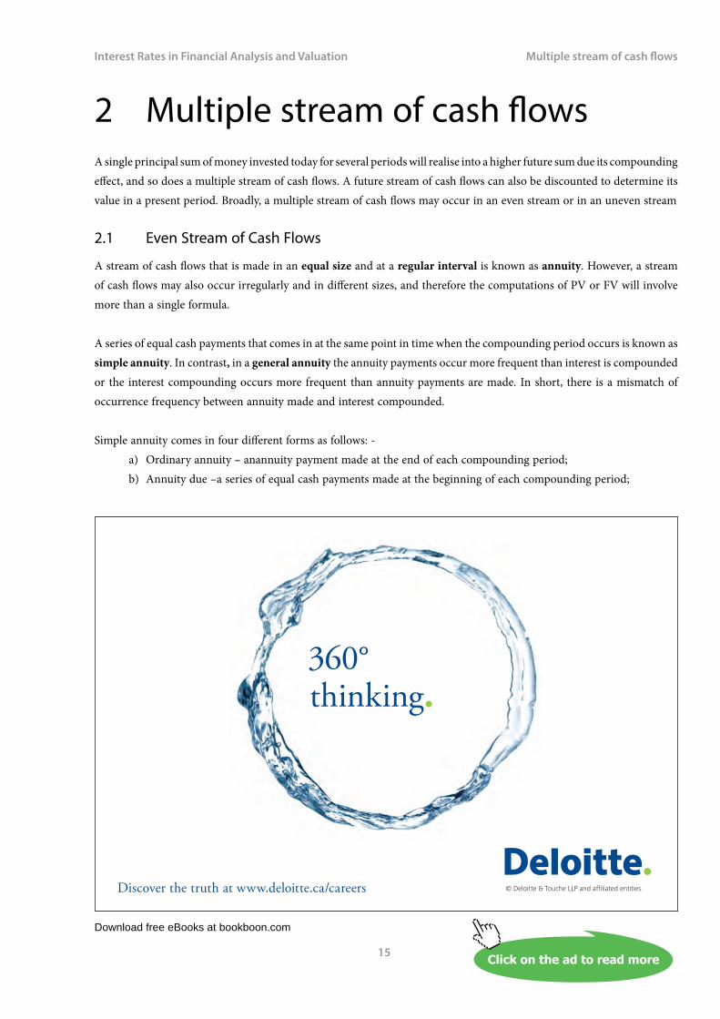
Examples:(All annuities are made at the end of compounding periods unless otherwise mentioned).
a) Consider a stream of cash flows of $1,000 per year for 5 years with an interest rate of 5% p.a. compounded annually. What is the future value and present value?
FV:= 1000 x FVIFA5%,5
= 1000 x 5.5256= $5,526
PV:= 1000 x PVIFA5%,5
= 1000 x 4.3295= $4,329
b) Suppose an investment generate an even income stream of $5,000 per year. What is the future value based on annual compounding (i) 7% p.a. for a period of 3 years, (ii) 3.5% p.a. for a period of 6 years, and (iii) 1.75% p.a. for a period of 12 years?
(i) i = 7%; n = 3 years= 5000 x FVIFA7%,3
= 5000 x 3.2149= $16,075
(ii) i = 3.5%; n = 6 years= 5000 x FVIFA3.5%,6
= 5000 x 6.5502= $32,751
(iii) i = 1.75%; n = 12 years= 5000 x FVIFA1.75%,12
= 5000 x 13.2251= $66,126
c) (c) Using the example (b) above, determine the present value based on the same condition.
(i) i = 7%; n = 3 years= 5000 x PVIFA7%,3
= 5000 x 2.6243= $13,122
(ii) i = 3.5%; n = 6 years= 5000 x PVIFA3.5%,6
= 5000 x 5.3286= $26,643
(iii) i = 1.75%; n = 12 years= 5000 x PVIFA1.75%,12
= 5000 x 10.7395= $53,698
d) Assume that a mortgage loan for $150,000 for a purchase for a house charges a rate of 7% p.a. compounded monthly. What is the monthly loan payment if the loan matures 18 years from now?
Monthly instalment = 150000 / [(1-(1.0058)-216)/0.0058] = 150000 / 122.6273 = $1,223.22

Download free eBooks at bookboon.com
Click on the ad to read more
Interest Rates in Financial Analysis and Valuation
24
Multiple stream of cash flows
e) Suppose a businessman takes up a leasing for a machine with an annual lease payment of $5,000. The lease charges a rate of 6% p.a. compounded annually with the regular payment due at the beginning of each period. What is the total lease value if the lease is for 4 years? (n = 3)
Lease value = 5000 x (PVIFA6%,3 + 1) = 5000 x (2.6730 + 1) = 5000 x 3.6730 = $18,365
Alternatively: = 5000 + (5000 x 2.6730) = 5000 + 13.365 = $18,365
2.1.5 General Annuities
In a general annuity, the compounding of interest does not occur at the same time as an annuity payment is made. Suppose we place a sum of money for a 12-month period in a fixed deposit account and rollover upon maturity in each subsequent year. If the account pays interest semi-annually, effectively the rate of interest earned is greater than the stated or nominal rate.

Download free eBooks at bookboon.com
Interest Rates in Financial Analysis and Valuation
25
Multiple stream of cash flows
To determine its future value or present value, we have to convert the stated interest rate (nominal interest rate) that matches the payment periods, which gives the effective interest rate. This depends on the frequency of compounding period whether it is yearly, semi-annually, quarterly, monthly or daily. The frequency of compounding (m”) is as follows: -
a) Yearly = n x 1b) Semi-annually = n x 2c) Quarterly = n x 4d) Monthly = n x 12e) Daily = n x 365
Based on the compounding periods as indicated above, then “i” is correspondingly reduced by m (compounding frequency per year) as follows: -
a) Yearly = ib) Semi-annually = i/2c) Quarterly = i/4d) Monthly = i/12e) Daily = i/365
An effective interest rate is the nominal/stated interest rate adjusted by the frequency of compounding. It is the rate of interest, which is compounded annually, generates the same amount of interest payment as the nominal rate does when compounded m times per year.The following equation will determine an effective interest rate: -
r = (1+j/m)m – 1 …(2.5)
where:j = nominal interest rate; andm = number of compounding periods.
A Stream of Cash flows Occurs less than the Compounding PeriodFor example, a sum of $1,200 is deposited annually in an investment account for 5 years that provides a return of 5% p.a. compounded semi-annually. In this case m = 2 and so the effective rate is expressed by:
= [(1 + 0.05/2)2 – 1]= 1.0506 – 1= 5.06% p.a.
Using the computed effective rate, then the FV or PV of the cash flows can be determined.

Download free eBooks at bookboon.com
Interest Rates in Financial Analysis and Valuation
26
Multiple stream of cash flows
FV:= 1200 x [(1.0506)5 – 1] / 0.0506= 1200 x 5.46011= $6,552.13
PV:= 1200 x [1 – (1.0506)-5] / 0.0506= 1200 x 4.3223= $5,186.77
A Stream of Cash flows occurs more than the Compounding PeriodNow let consider an even stream of cash flows that occurs more frequently than the compounding period. Suppose a sum of $1,000 per month is deposited into a savings account every month for 3 years with 4% p.a. compounded yearly.
In this case m = 1/12 because the frequency of cash flows is 12 times in a year. If the annuity frequency is every quarter then m = ¼ and so adjusted in like manner in cases of other frequencies such as semi-annually or weekly.
The effective interest rate is computed by:
= (1.04)1/12 – 1= 1.0033 – 1= 0.33% per month.
Using the computed effective rate, then the FV or PV of the cash flows can be determined.
FV:= 1000 x [(1.0033)36 – 1] / 0.0033= 1000 x 38.1589= $38,159
PV:= 1000 x [1 – (1.0033)-36] / 0.0033= 1000 x 33.8912= $33,891
A point to note, in annuities we observe that the present value of annuities is less than the total nominal value, while the future value is of course is greater than the total nominal value. For example, the total nominal value of the above case is $36,000, and the PV is $33,891 while the FV is $38,159.
2.2 Uneven Stream of Cash Flows
A stream of cash flows may not necessarily occur in equal sizes over the life term of an investment. To determine its FV or PV, a single calculation would not be possible as it involves more than a single formula.Assume that an investment generates an income stream in the following manner: -
Year 1 – $2,000Year 2 – $1,500Year 3 – $3,000Year 4 – $3,000
What is the PV if the discount rate is 5% p.a. compounded annually?

Download free eBooks at bookboon.com
Click on the ad to read more
Interest Rates in Financial Analysis and Valuation
27
Multiple stream of cash flows
For Year 1 and 2 each PV has to be calculated individually, while for Year 3 and 4 the cash flows are considered annuities and calculated as follows: -
Yr. 1 2000 x PVIF5%,1 2000 x 0.9524 $1,904.80
Yr. 2 1500 x PVIF5%,2 1500 x 0.9070 $1,360.50
Yr. 3&4 3000 x (PVIFA5%,4 – PVIFA5%,2) 3000 x (3.5460 – 1.8594) $5,059.80
PV = $8,325.10
Exercise 2.0
(All payments made at the end of compounding periods unless otherwise mentioned)
1. Calculate annual cash payments for a principal sum of $20,000 if the interest rate is 6% p.a. compounded annually for a period of (i) 5 years, (ii) 7 years and (iii) 9 years?
2. Calculate the future value of an annuity payment of $5,425 made annually for a period of 6 years with an interest rate of 7% compounded (i) quarterly, (ii) semi-annually and (iii) yearly?
3. Calculate the present value of an annuity payment of $3,550 made annually for a period of 3 years if the interest rate is 5.5% compounded (i) quarterly, (ii) semi-annually and (iii) yearly?
4. What is the present value of monthly annuity payment of $500 made for 4 years if discounted annually at rate of (i) 5%, (ii) 7% and (iii) 9%?
5. Joey takes a housing loan for $150,000 with an interest rate at 6.5% p.a. compounded monthly and a maturity term of 25 years. What is her monthly instalment?
“The perfect start of a successful, international career.”
CLICK HERE to discover why both socially
and academically the University
of Groningen is one of the best
places for a student to be www.rug.nl/feb/education
Excellent Economics and Business programmes at:

Download free eBooks at bookboon.com
Interest Rates in Financial Analysis and Valuation
28
Multiple stream of cash flows
6. Ted wants to save for his son’s college education in an investment plan. He intends to realise a future sum of $60,000 in 8 years from now. The plan provides a return of 8% p.a. compounded annually. What will be his annuity payment in each year?
7. Joe receives a series of cash payments of $2,400 from a trust fund annually. The payment will cease 15 years from today. (i) If the cash flows are discounted at a rate of 7.5% p.a. semi-annually, calculate the present value of annuities, and (ii) what will be the future value had he invested the cash payments at an interest rate of 8% p.a. compounded annually?
8. Jane wants to buy a house that costs $80,000. A bank is willing to provide a mortgage loan up to 90% of the purchase price and charging interest at 7% p.a. monthly compounding. If she is only capable to make a monthly repayment of $836, how long does he need to pay up fully the loan?
9. Using the above exercise 2.1(8), if the bank offers 95% margin of financing and charges interest at 8% p.a. compounded monthly, what will be the monthly repayment then given the loan matures 10 years from now?
10. A landlord receives an annual rental of $36,000 from a corporate tenant who occupies his shop lot for running a business for the next 5 years. He plansto invest the annual rental in an investment account that pays 6.5% p.a. compounded semi-annually. Determine the present value of the expected invested annual rentals for the five years.
11. Matt Ali deposits $1,000 every month in his investment account, which earns interest at a rate of 5% p.a. compounded annually. What will the future value of his savings at the end of 3rd year?
12. David has been saving his annual bonus for the last 5 years, which earns interest at a rate of 3% p.a. compounded annually. What is the future value of the bonus at the end of 5th year given the payment stream in year 1 – $3,000, year 2 – $3,500, year 3 – $8,000, year 4 – $9,000 and year 5 – $9,500?
13. Jason leased out his fully furnished apartment for a period of 3 years to an expatriate couple. The monthly lease rental is $5,800, which is due at the beginning of every leased month. As a security, 2 monthly advance rentals are also due at the onset of the leasing period. Assume that an interest rate of 6% p.a. compounded annually, what is the present value of lease payments plus the two-month advance rental? (Note: Annuity due)

Download free eBooks at bookboon.com
Interest Rates in Financial Analysis and Valuation
29
The rates of return
3 The rates of returnIn asset valuations, there are three elements to be considered, viz.:
1. The timing of cash flows;2. Therisk of assets; and 3. The required rate of return.
The required rate of return may be defined as the sufficient rate at which an investor believes will compensate him/her for bearing the perceived risks in future cash flows generated from holding the asset. The investor’s required rate of return depends on the asset characteristics and his/her own attributes. The characteristics of asset entail the following: -
a) Amount of expected cash flows;b) Timing of expected cash flows; andc) Risk of cash flows.
Based on the above factors and the investor’s assessment of risks and his/her aversion to these risks, the asset value is determined. The value is derived from the present value of expected cash flows that are discounted by the investor’s required rate of return. The rate of return can be decomposed as follows: -
• The risk-free rate of interest; and• The risk premium.
The risk-free rates are indicated by the yields of government securities such as 3-month Treasury bills or 3-year bonds. Investors usually expect a certain premium above and over the corresponding government securities from issuers of private debt securities. The government securities served as a benchmark. Generally, traded securities generate yield curves or the term structure of interest rates in which investors could assume risk and estimate return. This may be explained by three widely known interest rate theories, viz. Pure Expectation Theory, Segmentation Theory and Liquidity Preference Theory.
3.1 The Term Structure of Interest Rates and Theories
The term structure of interest rates or otherwise known as the yield curve is a plot of the yields on securities differing in the term to maturity but sharing similar credit risk, liquidity risk, and taxation. The plot reflects the relationship between the maturities and interest rates of a security and takes on a different shape at different times. There are 3 theories that explained the above relationship or the shapes of yield curves. They are: -
1. Pure Expectation theory2. Market Segmentation theory3. Liquidity Premium theory

Download free eBooks at bookboon.com
Click on the ad to read more
Interest Rates in Financial Analysis and Valuation
30
The rates of return
These theories should explain three important empirical facts that shaped yield curves, which are: -
1. Interest rates on securities of different maturities move together over time.2. When short-term rates are high, a yield curve is expected to be more likely to have an upward slope; when
long-term rates are high, a yield curve is expected to be more likely to have a downward slope or an inverted slope.
3. Yield curves are usually upward sloped.
Pure Expectation TheoryIt is based on the premise that the term structure of interest rates is solely determined by the market expectation of future interest rates. It assumes that securities with differing maturities are perfect substitutes to one another and therefore the expected yields on these securities must be equal. So there are two investment strategies available in the market that entails this theory.
• Purchase a one-year security and when it matures in one year, purchase another one-year security.• Purchase a two-year security and hold it until maturity.
Both strategies must have the same expected yields if investors are holding both one- and two-year securities, i.e. the interest rate on the two-year security must equal the average of two one-year interest rates.
Enhance your career opportunitiesWe offer practical, industry-relevant undergraduate and postgraduate degrees in central London
› Accounting and finance › Global banking and finance› Business, management and leadership › Luxury brand management› Oil and gas trade management › Media communications and marketing
Contact us to arrange a visitApply direct for January or September entry
T +44 (0)20 7487 7505 E [email protected] W regents.ac.uk

Download free eBooks at bookboon.com
Interest Rates in Financial Analysis and Valuation
31
The rates of return
For example, if the current annualised interest rate at time t(spot rate)on a one-year bond is 9% and the future rate or expected rate at time t+1 on one-year bond is 11%, hence an annualised interest rate at time t of two-year bond spot rate should equal to 10%
1-yr bond 9%-----+--------11%2-yr bond --------10%--------- i.e. (it + ie
t+1) / 2
By the above assumption, an investor may hold a one-year bond and another one year bond the following year, or hold a single two-year bond for 2 years. Both strategies should have the same expected return, i.e. the interest rate on the two-year bond should equal the average of holding consecutively two one-year bonds. The yields of securities of one maturity will affect the yields on securities of different maturities.The market expectation (rise or fall) of future interest rates also affects the term structure of interest rates or the yield curves.
Rates implied in spot rates are known as forward rates which are considered an unbiased estimator of future interest rates. Market is generally considered efficient as any relevant information pertaining to risks would have been reflected in the prices of securities.So the information implied by market rates about forward rates has little value to generate abnormal return.
We can determine a one-year forward rate as of one year from now or more than one year from now. A one-year forward rate is expressed by:
11
)1(
1
22
11 −++
=+ ii
rt
tt … (3.1)
where:
ti2 =Two-year Spot Rate;
ti1 = One-year Spot Rate; and
t+1r1 = One-year Forward Rate as of one year from now.
For example, assume that a bond with one year remaining maturity yields 3.03% (one-year spot rate) and a bond with two years remaining maturity yields 3.13% (two-year spot rate). Using equation 3.1 given above we shall compute the one-year forward rate as follow: -
t+1r1 = (1.0313)2 ÷ (1.0303) – 1 = 0.0323 or 3.23%.
We can also determine a one-year forward rate as of two years or more from now (at time t+n), which is given by: -
1)1()1( 1
11 −
++
=+
++ n
nt
nnt
nt ii
r … (3.2)

Download free eBooks at bookboon.com
Interest Rates in Financial Analysis and Valuation
32
The rates of return
where:
tin+1 =(n+1)-year Spot Rate;
tin = n-year Spot Rate; and
t+nr1 = One-year Forward Rate as of n years from now.
Suppose a yield on a three-year bond is 3.45% and a two-year bond is 3.13%, then a one-year forward rate as of two years from now is:
t+2r1 = (1.0345)3 ÷ (1.0313)2 – 1 = 0.0409 or 4.09%.
If we wish to determine the forward rate as of three years from now and assume that four-year bond yields 3.82%, then compute as follow: -
t+3r1 = (1.0382)4 ÷ (1.0345)3 – 1 = 0.0494 or 4.94%.
By this market can estimate the future annualised interest rates on securities at various periods (period t + n) provided information on spot rates are available for computing the forward rates.In addition, we can also estimatethe future annualised interest ratesas of one year from now for securities of different maturities(n-year) which is given by:
11
)1(
1
11 −
++
=+
+n
t
nnt
nt ii
r … (3.3)
where:
tin+1 = (n+1)-year Spot Rate;
ti1 = One-year Spot Rate; and
trn =n-year Forward Rate as of one year from now.
Using the spot rates in previous examples above, we wish to determine the forward rates for two-year and three-year securities. Using equation 3.3 above we compute as follow: -
Two-year Forward Rate:
0366.010303.1
)0345.1( 3
=−= (3.66%)
Three-year Forward Rate:
0408.010303.1
)0382.1(3
4
=−= (4.08%)
From the above computation, we can say that market anticipates that the annualised interest rate on two-year securities is 3.7% and on three-year securities is 4.1%.

Download free eBooks at bookboon.com
Click on the ad to read more
Interest Rates in Financial Analysis and Valuation
33
The rates of return
Expectation of Interest Rates RiseIn a scenario where there is an expectation of a rise in the interest rates,lenders/investors will prefer short-term securities and ignore long term-securities. On the other hand, borrowers/issuers will ignore short-term securities and will prefer long-term securities.
Since interest rates are expected to rise, the investors will prefer to be short and re-invest later at the expected higher interest rates. Hence, short-term securities market is flooded with the demand for short-term securities, i.e. increase in the supply of loanable funds at the shorter end of yield curves.
The issuers will tend to ignore the short-term market and do not issue any short-term securities. Instead, they will issue longer-term securities and thus lock-in with the current lower rates. There will be an increase in the supply of long-term securities, i.e. increase in the demand for loanable funds at the longer end of yield curves.
In general, there will be a downward pressure on the short-term interest rates and an upward pressure on the long-term ones.
The yield curve will be upward sloping (positive curve) at a new equilibrium as illustrated below (Figure 1).
.

Download free eBooks at bookboon.com
Interest Rates in Financial Analysis and Valuation
34
The rates of return
Figure 3.1 – Upward Sloping Yield Curve
The Impact of Expected Interest Rates Rise:
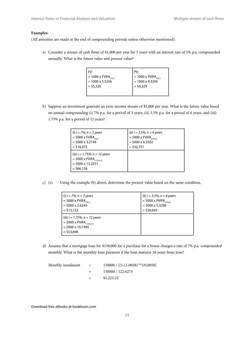
SHORT-TERM MARKET (Figure 2)• Supply of short-term loanable funds (e.g. investors/lenders’demand for short-term notes) increases, i.e. the
supply curve shifts to the right from S1 to S2.• Investors/lenders prefer short-term market, and invest in short-term securities with current rates and re-
invest with expected higher rates.• Demand for loanable funds (e.g. issuers/borrowers’ supply of short-term notes) decreases, i.e. the demand
curve shifts to the left from D1 to D2.• Issuers/borrowers ignore short-term market and prefer to issue long-term securities.• Subsequently, interest rates move downward to a new equilibrium from i1 to i2.
The Impact of Expected Interest RatesRise:
LONG-TERM MARKET (Figure 3)• Demand for loanable funds (e.g. issuers/borrowers’ supply of bonds) increases, i.e. the demand curve shifts
to the right from D1 to D2.• Issuers/borrowers prefer long-term market and issue long-term securities so as to lock-in with current
lower rates.• Supply of long-term loanable funds (e.g. investors/lenders’ demand for bonds) decreases, i.e. the supply
curve shifts to the left from S1 to S2.• Investors/lenders ignore long-term market and prefer to invest in short-term securities.• Subsequently, interest rates move upward to a new equilibrium from i1 to i2.
Download free eBooks at bookboon.com
Interest Rates in Financial Analysis and Valuation
35
The rates of return
Figure 3.2 – Supply and Demand Curves in Short-term Market (positive yield curve)
Figure 3 – Supply and Demand Curves in Long-term Market (positive yield curve)
Expectation of Interest Rates DropThe reverse scenario is true as the interest rates are expected to drop, i.e. there is an upward pressure on short-term rates and a downward pressure on long-term rates. Hence, the yield curve is downward sloping as illustrated below (Figure 4). But the theory has a shortcoming, i.e. it could not justify why the yield curves are always upward sloping (or at least most of the times).

Download free eBooks at bookboon.com
Click on the ad to read more
Interest Rates in Financial Analysis and Valuation
36
The rates of return
Figure 3.4- Downward Sloping Yield Curve
www.mastersopenday.nl
Visit us and find out why we are the best!Master’s Open Day: 22 February 2014
Join the best atthe Maastricht UniversitySchool of Business andEconomics!
Top master’s programmes• 33rdplaceFinancialTimesworldwideranking:MScInternationalBusiness
• 1stplace:MScInternationalBusiness• 1stplace:MScFinancialEconomics• 2ndplace:MScManagementofLearning• 2ndplace:MScEconomics• 2ndplace:MScEconometricsandOperationsResearch• 2ndplace:MScGlobalSupplyChainManagementandChange
Sources: Keuzegids Master ranking 2013; Elsevier ‘Beste Studies’ ranking 2012; Financial Times Global Masters in Management ranking 2012
MaastrichtUniversity is
the best specialistuniversity in the
Netherlands(Elsevier)

Download free eBooks at bookboon.com
Interest Rates in Financial Analysis and Valuation
37
The rates of return
Figure 3.5 – Supply and Demand Curves in Short-term Market (negative yield curve)
The Impact of Expected Interest RatesDrop:SHORT-TERM MARKET (Figure 5)
• Demand for short-term loanable funds (e.g. the supply of short-term notes) increases, i.e. the demand curve shifts to the right from D1 to D2.
• Issuers/borrowers prefer short-term market and issue short-term securities so as to re-borrow at expected lower rates.
• Supply of short-term loanable funds (e.g. the demand for short-term notes) decreases, i.e. the supply curve shifts to the left from S1 to S2.
• Investors/lenders ignore short-term market and prefer to invest in long-term securities.• Subsequently, interest rates move upward to a new equilibrium from i1 to i2.
The Impact of Expected Interest RatesDrop:LONG-TERM MARKET (Figure 6)
• Supply of long-term loanable funds (e.g. the demand for bonds)increases, i.e. the supply curve shifts to the right from S1 to S2.
• Investors/lenders prefer long-term market and invest in long-term securities so as to lock-in at current higher rates
• Demand for long-term loanable funds (e.g. supply of corporate bonds) decreases, i.e. the demand curve shifts to the left from D1 to D2.
• Issuers/borrowers ignore long-term market and prefer to issue short-term securities.• Subsequently, interest rates move downward to a new equilibrium from i1 to i2.

Download free eBooks at bookboon.com
Interest Rates in Financial Analysis and Valuation
38
The rates of return
Figure 3.6 – Supply and Demand Curves in Long-term Market (negative yield curve)
Market Segmentation Theory
This theory assumes that the market preference for one maturity has no bearing or effect on the other (i.e. has no correlation). Securities of different maturities are not substitute for one another and thus the market is segmented each with independent yield. In general, the market prefers short-term securities because of relative certainty as opposed to the long-term ones which are likely exposed to interest rate risk.
Long-term investors and issuers are those, by nature of their investing projects or business, require the long-term securities. e.g. insurance companies managing education or life endowment fund, pension funds managing retirement accounts, or companies involving in projects that have long gestation period. This explains why the yield curve is generally upward sloping. However, the theory could not explain the empirical facts #1 and #2 as outlined at the outset.
Liquidity Premium Theory
The theory proposes:a) A long-term interest rate is equal to the average of a series of short-term rates that cover the corresponding
maturity of the long-term rate; andb) There is a compensating premium (liquidity premium) resulting from the supply and demand of loanable
funds for that particular long-term security market.
Download free eBooks at bookboon.com
Interest Rates in Financial Analysis and Valuation
39
The rates of return
The theory assumes that the securities of different maturities are substitutes for one another. The yields of securities in one maturity have an influence on the yields of another with different maturities. In this case, the yields on securities move together over time. A rise in short-term rates will influence the yields on securities of different maturities.
In general, investors and borrowers prefer short-term market because of its relative lesser interest rate risk and more liquid. Investors are willing to supply long-term loanable funds if borrowers offer a positive liquidity premium to compensate for their longer exposure to the interest rate risk and relative lesser liquidity.
Since (it + iet+1) / n provides an average yield, the liquidity premium theory assumes that the average yield plus a
compensated premium, i.e. (it + iet+1) / n + l where l is the compensated premium. Hence, investors are motivated to hold
longer maturity securities given the liquidity premium. That is why the yield curve is typically upward sloping, which explains the empirical fact #3.
The theory also argues that if short-term rates were very high then a long-term rate, which is equal to the average of those short-term rates, is below the short-term rates despite the adding of liquidity premium. In this case, the yield curve is downward sloping or inverted.
3.2 Forecasting Interest Rates
Interest rate change is a manifestation of changes in various underlying factors in economy, which are as follow: -
• Economic growth;• Inflation;• Money supply;• Government budget; and• Foreign flows of funds.
The changes in the underlying economic forces prompt the movement of interest rates, which in essence is the result of upsetting the current equilibrium of aggregate supply of loanable funds with the aggregate demand for loanable funds. A new equilibrium is achieved once the aggregate supply of and the demand for loanable funds are equal again.
The entities in an economy that provide and needloanable funds are households, businesses, governments and foreigners. Any changes to the quantity level of provision and/or need of the loanable funds by these entities will change the aggregate supply and/or demand of the loanable funds. The resulting changes impacted on the interest rates are important because many security prices are affected by the interest rates movements.
By this, market players could do the forecasting of interest rates movements so that investors and borrowers could make informed or advised decisions with regards to making investments and borrowings. Numerous statistical models have been used to forecast interest rates, which used variables as suggested in the framework below.

Download free eBooks at bookboon.com
Interest Rates in Financial Analysis and Valuation
40
The rates of return
However, a forecast should remain just a forecast as no one model could predict interest rates with absolute certainty. Generally, a forecast for short-term rates may be a little more certain than longer term rates. But a forecast acts as a good guide to investors and borrowers in financial markets. Figure 7 shows the general framework that captures the underlying factors in interest rate forecasting.
Foreign:Future Economy,
Expectation of ForexMovements
Foreign:Future Economy,
Expectation of ForexMovements
Household:Future Income Level,Personal Financing
Plan
Business:Future Expansion,Future Business
Volume
Government:Future Revenues,
Future Expenditures
Government:Central Bank’s
Future Policies onMoney Supply
Growth
Household:Future Income Level
Business:Future Liquidity Plan
Future Demand for
Loanable Funds
Future Supply of
Loanable Funds
Interest Rate Forecasts
Future DomesticEconomy:
Economic Growth,Unemployment,
and Inflation.
Figure 3.7 – Framework for Interest Rate Forecasting

Download free eBooks at bookboon.com
Interest Rates in Financial Analysis and Valuation
41
The rates of return
3.3 Interest Rates in Derivative Contracts
Derivative contractssuch as financial futures, swap and optionact as hedgingtools against any risk from the fluctuation of interest rates.In addition to these derivatives, there are three other interest rate derivative instruments, viz. interest rate caps, floors and collars. Risk-averse investors such as banks and financial institutions use derivatives to shift the risk of interest rate fluctuation to those willing to accept and probably profit from such risk.
Let us assume that a company wants to issue 12-month short-term notes in two months’ time for a nominal sum of $100 million. The company fears a rise in interest rate that is currently 8% for equivalent securities. Based on the current interest rate the marginal cost of borrowing will be as follow: -
Marginal cost = $100 x 0.08 x 365/365 = $8 million.
If interest rate rose to 8.5% the marginal borrowing cost of would increase to $8.5 million as follow: -
100 x 0.085 x 365/365 = 8.5
The additional sum of $500,000 is considered a potential loss and may not be recovered from business investments. To counteract the potential loss the company may do the following in futures market (assume that interest rates actually rise): -
SPOT MARKET FUTURES MARKET
TODAY:Company plans to issue 12-mo. notes for nominal value of $100 million. Current spot rate is 8.0%
TODAYCompany takes a short position by selling futures for 12-mo. rate at a settlement price of 91.50 (i.e. interest rate is 8.5%). Present value = $100 mil.× 1.085-1 = $92.166 mil.
2 MONTHS LATER:Company issues 12-mo. notes for a nominal value of $100 million at 8.5% (assume that the interest rate rises).Discounted sum received: $100 mil. × 1.085-1 = $92.166 mil.
2 MONTHS LATER:Company closes off position by buying futures for 12-mo. rate at a settlement price of 91.00 (i.e. interest rate is 9.0%). Present value = $100 mil. × 1.09-1 = $91.743 mil.
Spot market opportunity loss = 0.5%Futures market gain = 0.5%
Effective borrowing rate = 8.5 – 0.5 = 8.0%
Alternatively we can determine the effective borrowing rate based on the dollar gained. The companyreceived a net discounted sumof $92.166 from the issuance of notes, and the dollar gain in the futures market of $0.423 ($92.166 – 91.743). This gives a total sum of $92.589 (92.166 + 0.423). Therefore,the company effectively borrows at 8% as follow: -
Rate = (36500 ÷ 92.589 - 365) ÷ 365 = 0.08

Download free eBooks at bookboon.com
Click on the ad to read more
Interest Rates in Financial Analysis and Valuation
42
The rates of return
Now let us assume that the interest rate falls and the bank still borrows at 8% as it plans. Suppose the company issues 12-month notes at 7.5% and receives a discounted sum of $93.023 million, i.e. 100 × 1.075-1.
In the futures market the company buys 12-month interest rate at 8%. The present value for a nominal sum of $100 million is $92.593, i.e. 100 × 1.08-1. Therefore, the company makes a loss of $0.427in the futures market, i.e. 92.166 – 92.593, and gets net proceedsof $92.596, i.e. 93.023 – 0.427. The company effectively borrows at 8%, which is given by:
Rate = (36500 ÷ 92.596– 365) ÷ 365 = 0.08
By engaging in the futures market, the bank has covered its exposure to interest rate fluctuation and thereby stabilised its borrowing cost.In the above scenario, the company enjoys a perfect hedge, which is not necessarily true. There is always a basis risk involved in a hedging strategy.
Options are also used to hedge bond portfolios or mortgage portfolios from the changes in interest rates. Investors who are long in asset are exposed to financial downsides if the current value of asset is progressively decreasing. If he or she liquidates the asset, a loss would be realised. On the other hand, investors who are short in asset are exposed to financial downsides if the current value of asset is progressively increasing. Option acts as a hedging tool and if investors used it with a right combination of buying and/or writing calls and/or puts, he or she could protect an investment from any risk of price or value fluctuations.
Let us assume that afirm wants to issue three-month notes in two months’ time as summarised below.
- ©
Pho
tono
nsto
p
> Apply now
redefine your future
AxA globAl grAduAteprogrAm 2014
axa_ad_grad_prog_170x115.indd 1 19/12/13 16:36

Download free eBooks at bookboon.com
Interest Rates in Financial Analysis and Valuation
43
The rates of return
a) A firm initially issued 3-mo. notes for a nominal value of $10 million and wants to rollover for a second three-month period (in two months’ time). Assume that current spot rate for the underlying three-month interest rate is 3.6%. The risk is about rising interest rates.
b) The firm engages a hedging strategy by buying a call option on the underlying 3-mo. T-bill rate at a strike price of 38.20 for a premium of 2.90. It will exercise the call option at the expiration date if the underlying rate is 41.10 (break-even price).
c) Suppose two months later the interest rates do rise. The firm issues the 3-mo. notes for a nominal value of $10 million at a discount rate of 3.9%. There is an opportunity loss here. Had it issued the notes two months ago the interest rate was lower.
d) Assume that the call option expires today, i.e. two months later. The firm exercises its right at ex-settlement priceof 42.00 as the firm is in-the-money. There is a net option gain here (see below).
Gain from the option:Ex-settlement 42.00Strike 38.20Gross gain 3.80Less premium 2.90Net gain 0.90
The illustration below shows the points discussed above.
Issue 3-mo. notes
Buy CALL
Interest Rate %
Breakeven4.11
Net Hedge3.53
Strike Price3.82
Payoff
-0.29 (C)
Fig. 3.9 Long Call(Long Synthetic Put) – 3-month Interest Rate
When the firm issues the 3-month notes, the expected discounted value falls due to the increased in interest rates and the discounted sum is:
10(1.039)-92/365= 9.904million

Download free eBooks at bookboon.com
Interest Rates in Financial Analysis and Valuation
44
The rates of return
The effective borrowing rate is given by:
3.9– 0.09 = 3.81%
Alternatively, we can compute the firm’s effective borrowing rate after taking into consideration the net option gain of $900. The total sum received is $9.905 million (i.e. 9.904 + 0.0009 million). The firm’s effective borrowing rate is:
= (3650 ÷ 9.905 – 365) ÷ 92 = 0.0381
If the price is below 41.10 at the expiration date, the firm will not exercise the option because it is either out-of-the-money or at-the-money. The maximum loss will be the total call premium paid.
Since this a hedging strategy, the out-of-the-money call option turns out the firm to be in-the-money in the spot market. If the interest rate falls below the net hedge position, i.e. 3.53, then there is an opportunity gain here. The firm issues the 3-month notes at a rate lower than it was two months ago.
Likewise, a firm can engage in a put option to protect its spot market position against the risk of falling interest rates. Suppose a firm wants to invest in interest-bearing securities in the future and the prices of such securities will increase with falling interest rates. In such a case, the firm would buy a put option and create a long synthetic call as illustrated below.
Fig. 3.10 Long Put(Long Synthetic Call)

Download free eBooks at bookboon.com
Click on the ad to read more
Interest Rates in Financial Analysis and Valuation
45
The rates of return
The firm will exercise its put option at expiration of the option contract if the interest rates fall below the strike price, which it is in-the-money position. Its net option gain could minimise the opportunity loss of its spot market position. The firm has to buy the debt securities at higher prices.
If the interest rates rise instead of fall, then its maximum loss in the option market is the cost of put premium. In the spot market, the firm would be in-the-money as the interest rates rise above the net hedge point, i.e. strike price plus the cost of put.
Another derivative contract that companies, banks or financial institutions may use is interest-rate swap. Swaps are arrangements that enabling parties to undertake an exchange of interest rate, foreign currency and other financial or non-financial obligations.Swaps are used to achieve lower cost of funds and to hedge against risk exposure derived from the characteristic mismatch between underlying assets and liabilities.
Interest rate swap is an agreement between two parties to make payments in which one party is a fixed rate payer and the other is a floating rate payer. The fixed rate payer will make a payment based on a predetermined interest rate (fixed rate) at the outset of the swap. The floating rate payer will make payment based on any reference rate (e.g. BLR, LIBOR, SIBOR,) agreed to between the contracting parties, and the size of payment depends on the future course of those rates.

Download free eBooks at bookboon.com
Interest Rates in Financial Analysis and Valuation
46
The rates of return
Key features of a standard swap:
The notional principal: Payments by contracting parties are calculated, as were payments of interest on an amount of fund borrowed or lent. This amount refers to as the notional principal, and it never changes hand and remains constant. Nonetheless, it can change over the life of a swap as in case of a non-standard swap. In an amortising swap, the principal decreases over time and in an accreting swap, it increases over time.
The fixed rate: This is the rate applied to the notional principal to compute the fixed rate payment. On a daily basis, market participants quote the price at which they are prepared to execute a particular swap by quoting the fixed rate.
The floating rate: This is also the rate applied to the notional principal to compute the float rate payment. The rate is reviewed at regular intervals as provided in a contract as floating reset dates. This rate is usually reset two days prior to the previous settlement date. The reviewed rate starts to accrue on that previous settlement date. The general framework of interest rate swap is as given below.
IntermediaryInstitution
Underlying assets (floating rate)
Debt Securities(fixed rate)
Company(Party FLT)
Pays floating rate Receives fixed rate
Counterparty having fixed rate swaparrangement with Intermediary
(Party FIX)
Receives Floating Rates Pays Fixed Rates
Figure 3.11 – General Framework of Interest Rate Swap

Download free eBooks at bookboon.com
Interest Rates in Financial Analysis and Valuation
47
The rates of return
In a fixed rate swap,a party has liabilities in the form short-term notes the use of swap will reduce the party floating rate exposure because it pays counterparty at a fixed interest rate. In return, it receives a variable interest rate to match its floating rate liability. Therefore, on a net basis, the party will bear the fixed-rate swap payment liability and the counterparty will assume the floating rate notes liability.
In a floating rate swap, a party has liabilities in the form of fixed rate bonds, the use of swap will reduce the party fixed rate exposure because it pays counterparty at a floating interest rate (e.g. average LIBOR swap) and in return, it receives a fixed rate payment to match its fixed rate bond liabilities. Therefore, on a net basis, the party will bear the floating-rate swap payment liability and its counterparty will assume the fixed rate bond liability.
For example, a special-purpose company (SPC) issued fixed rate asset-backed bonds backed by underlying assets that earned interest income based on a floating rate. The SPC is asset-sensitive and loses (gains) if the floating rate falls (rises). To hedge against the risk from such mismatch the company needs to swap its floating rate cash inflow for a fixed rate and to lock in with a certain effective rate for its coupon liability. The SPC, by using a swap, turns its variable rate asset into a fixed rate asset and thereby matches with its fixed rate liability.
Example: Mechanic of a Average LIBOR Swap (Floating Rate Swap)
• Assume that a bank called Bancorp Commercial Corporation (BCC) issues $100 million of 3-year bonds with a coupon of 7.2% p.a.
• It enters into a three-year interest rate swap by which it agrees to pay Swap Dealer a floating rate of 3-month LIBOR and in turn receives a fixed rate of 7.5%.
• BCB receives monthly scheduled payments from underlying assets at a floating rate of 3-month LIBOR + 0.10.
• The notional principal is $100 million.• The fixed rate will be paid semi-annually and the settlement date is on the first day of after each six months
completion.• The floating rate will be paid monthly on the first day each month. The floating rate reset dates will be two
days prior the previous settlement date. The day count is on the actual/actual basis.• BCB will pay a floating rate of 3-month LIBOR to Swap Dealer on the first day of each month.• Swap Dealer will pay a fixed rate of 7.5% to BCC on completion of every six months.• Every half-yearly the fixed payment will fall due on the same day as the floating rate payment. In this case,
the party owes the greater amount will pay to the other for the net difference.• Swap Dealer will advise BCC to effect a net payment to Swap Dealer’s account, or to receive a net payment
from Swap Dealer, which will be credited directly into the bank’s account.• Example:
Net interest cost during the contractual period of the swap is as follows:Received from Swap Dealer: 7.5%Paid bondholders: 7.2%Basis gained: 0.3%

Download free eBooks at bookboon.com
Click on the ad to read more
Interest Rates in Financial Analysis and Valuation
48
The rates of return
Net interest cost = Rate paid to Swap Dealer – Basis gained = 3-mo. LIBOR – 0.3% = 7 – 0.3 = 6.7 %
Net spread is constant during the swap period:Scheduled payments received: 3-mo. LIBOR + 0.1% (e.g. 7.1%)Less Net interest cost: 3-mo. LIBOR – 0.3% (e.g. 6.7%)Net spread: = 0.4%
In the above case, the bank shall receive a fixed rate of 7.5% from the swap dealer in exchange for three-month LIBOR. Based on the above assumption the bank’s effective interest cost is 6.7% for the first coupon and at the same time makes a positive spread of 0.4% in the swap transaction. The swap dealerin turn earns some spread between bid and offer swap rate. Party FLT will receive the bid swap rate when it pays floating rate to the swap dealer while Party FIX will pay the offer swap rate when it receives floating interest rate. In the above example, the swap dealer makes an onward payment of fixed rate of 7.5% (bid swap rate) to Party FLT and receives an offer swap rate of 7.6% from Party FIX. Though the spread is only one basis point but for a notional sum of $100 million that will be $1 million earning.
Now let us look at a reverse scenario by which a company swaps a fixed rate as given below.In this case, the company is liability-sensitive and loses (gains) if interest rate rises (falls). It converts its variable rate liabilities into a fixed one which matches with the fixed rate asset.
Get Help Now
Go to www.helpmyassignment.co.uk for more info
Need help with yourdissertation?Get in-depth feedback & advice from experts in your topic area. Find out what you can do to improvethe quality of your dissertation!

Download free eBooks at bookboon.com
Interest Rates in Financial Analysis and Valuation
49
The rates of return
Example: Mechanic of a Fixed Rate Swap
• Assume that a company named Master Builders Corporation (MBC) issues $100 million of 3-month discount notes.
• It enters into one-year interest rate swap in which it agrees to pay Swap Dealer a fixed rate of 7.6% and in turn receives an Average 3-month LIBOR.
• MBB receives monthly scheduled payments from underlying rentals at a fixed rate of 7.8%.• The notional principal is RM100 million.• The fixed rate will be paid monthly and the settlement dates are on the first day of after each one-month
completion.• The floating rate will be paid quarterly on the first day each month. The floating rate reset dates will be two
days prior the previous settlement date. The day count is on the actual/actual basis.• MBB will pay a fixed rate of 7.6% to Swap Dealer on the first day of each month.• Swap Dealer would pay an Average 3-month LIBOR to MBC on completion of every three months.• Every quarterly the fixed payment will fall due on the same day as the floating rate payment. In this case, the
party owes the greater amount will pay to the other for the net difference.• Swap Dealer will advise MBC to effect a net payment to Swap Dealer’s account or to receive a net payment
from Swap Dealer, which will be credited directly into MBC’ account.• Example:
The net interest cost during the contractual period of the swap is as follows:
Received from Swap Dealer: Average 3-month LIBOR (e.g. 7.0)Paid noteholder: Prevailing 3-month yield (e.g. 6.9)Basis gained: Average 3-month LIBOR less 3-month yield (e.g. 7.0 – 6.9 = 0.1)
Net interest cost = Paid Swap dealer – Basis gained = 7.6 – 0.1
= 7.5
The net spread during the swap period:Scheduled paymentreceived: 7.8% (rental yield)Less Net interest cost: 7.6% – Basis gain(7.6 – 0.1)Net spread: = 0.2% + Basis gain (0.2 + 0.1)
In the above example the company earns 7.8% from rentals pays 7.6% to the swap dealer in exchange for a three-month LIBOR. The company has locked in a spread of 0.2% in this transaction. The benefits of a swap may be outlined as follow: -
• There is no principal exchange involved;• Only net interest payments are made to one of the sides; and• In the event of default by one party, the other party is no longer required to make payments on the swap.
Alternatively, it may continue the swap with other counterparty.

Download free eBooks at bookboon.com
Interest Rates in Financial Analysis and Valuation
50
The rates of return
• There is no any kind of fees involved in undertaking swap transactions, and the only cost is the effective cost of funding the underlying bonds.
• Swap party uses it as a means of profitably funding fixed-rate assets by converting the cash inflows to variable-rate receivables and pay variable-rate liabilities. Thus eliminates the mismatch between fixed-rate assets and floating-rate liabilities. In a reverse scenario, a similar strategy can also be used to convert variable-rate assets into fixed-rate receivables that pay fixed-rate liabilities.
• Swap provides regularity and certainty in respect to meeting interest obligation since the rate remains the same each payment time during the swap transaction.
While the whole idea of a swap is to minimise interest-rate exposure attributed to a mismatch, on the downsides there is certain degree of credit risk.The validity of a swap depends heavily on each party’s ability and willingness to live up to its end of the bargain. If one party defaults, for whatever reason, then the agreement becomes invalid.There is always a built-in minimal interest rate exposure depending on one’s position.
When a swap is made, a party is actually locking in to a certain amount of loss while a counterparty locking in on at least a small gain or vice versa. The fixed rate party pays generally higher than the average floating rate receives from the counterparty.
Nonetheless, with a proper analysis and correct projection of interest rate movement, one’s overall position will be improved despite the relatively small inherent risk. One should adopt a philosophy that makes acceptable for the built-in losses involved in a swap transaction because it is used for a hedging purpose.
Other than swap,financial institutions or companies may engage in interest rate caps, floors and collars to hedge their interest rate risk or to capitalise on expected interest rate movements.
- By buying an interest rate cap,a buyer will receive payments when a specified reference rate or an interest rate index exceeds a specified ceiling rate or cap rateat a valuation date during an interest rate cap agreement.
- The cap rate agreement can be for a length of time ranges from three to eight years and the valuation dates can be at the end of every agreed regular period, e.g. every quarter or every year.
- The main purpose of buying interest rate cap is to protect from any adversity due to rising interest rates. - The payment is based on the spread between the reference rate and the cap rate multiplies by a notional
principal sum or contract size. - A cap dealer is generally an intermediary financial services firm that matches the buyer with counterparty
who wants to sell an interest rate cap. - The cap rate seller is obligated to make payments to the buyer for a compensation sum or an upfront fee
paid by the buyer at the onset of the agreement. The upfront fee is in essence the cost of premium that the cap buyer bears for having a right to a certain level of interest rate. The cap dealer, as an intermediary, in effect takes a spread between bid and offer premium.

Download free eBooks at bookboon.com
Interest Rates in Financial Analysis and Valuation
51
The rates of return
For instance, the cap buyer pays 2% (offer premium) of notional principal amount to the dealer and the cap seller receives 1% (bid premium) of notional principal amount from the dealer.The magnitude of payment received by the cap buyer depends on:
• The positive spread between the reference rate and the cap rate;• The length of time the spread stays; and• The notional principal or contract size the buyer takes.
Let us assume that a company issues three-yearfloating rate bonds to finance its business investments.To protect itself from the risk of rising interest rate, the company can buy an interest rate cap. Assume that it buys a cap at a ceiling rate of 4.0% with a notional principal valued at $10 million and uses 12-month LIBOR as a reference rate. The company agrees to pay upfront 2% of the notional value as a fee.
In return, the company will receive a payment based on a positive spread between the reference rate and the cap rate multiplies by the notional principal sum at the end of every year. For an illustration, let us assume that the company anticipates 12-month LIBOR at valuation date will be 3.0%, 4.65% and 5.45%, respectively. The cash flow outcomes are as follow: -
At the end of Year
0 1 2 3
12-mo LIBOR 3% 4.65% 5.45%
Ceiling rate 4 4 4
Percent above Ceiling 0 0.65 1.45
Fee paid ($’000) $200
Payment received ($’000) $0 $65 $145
If indeed the interest rate rise, by buying an interest rate cap the company effectively contains its cost of variable-rate borrowing. At worst, the company bears a one-time upfront cost of $200, 000. On the other hand, the company may enjoy some positive cash flow over the three years period.
In essence, the whole structure of interest rate cap behaves like a call option by which a ceiling rate is the strike price and a cap buyer faces three pay-off possibilities at a valuation date. If at avaluation date interest rate rises above a reference rate, a cap buyer is in-the-money. On the other hand, if the interest rate stays below the ceiling rate the cap buyer is out-of-the-money. If the cap buyer wants to be in-the-money then it has to pay a higher premium by buying a lower ceiling rate at a high cost.
In the case of an interest rate floor, a floor buyer receives a payment when the floor rate drops below a reference rate. In this case, the floor seller has the obligation to make the payment good.
- The purpose of buying an interest rate floor is to protect from the risk of interest rate falling. - A floor buyer may want to protect its variable-rate interest receivables or its fixed-rate payables from
declining interest rates.

Download free eBooks at bookboon.com
Click on the ad to read more
Interest Rates in Financial Analysis and Valuation
52
The rates of return
- In essence, an interest rate floor behaves like a put option. If the interest rate falls below the floor rate (strike price) at the valuation date, the investor is in-the-money and receives a payment. If the floor buyer wants to be in-the-money then it has to pay a higher premium by buying a higher ceiling rate at a high cost.
- Like the interest rate cap, a floor buyer has to pay a fee based on a certain percentage of notional principal value.
Let us assume that an investor buys a 3-year interest rate floor with a floor rate of 3.5% and pays a fee 2% of notional principal valued at $10 million. For an illustration, let us assume that the investor anticipates 12-month LIBOR at each valuation date will be 3%, 4.65% and 5.45%, respectively. The cash flow outcomes are as follow: -
At the end of Year
0 1 2 3
12-mo LIBOR 3% 4.65% 5.45%
Floor rate 3.5 3.5 3.5
Percent below Floor 0.5 0 0
Fee paid ($’000) $200
Payment received ($’000) $50 $0 $0
By 2020, wind could provide one-tenth of our planet’s electricity needs. Already today, SKF’s innovative know-how is crucial to running a large proportion of the world’s wind turbines.
Up to 25 % of the generating costs relate to mainte-nance. These can be reduced dramatically thanks to our systems for on-line condition monitoring and automatic lubrication. We help make it more economical to create cleaner, cheaper energy out of thin air.
By sharing our experience, expertise, and creativity, industries can boost performance beyond expectations.
Therefore we need the best employees who can meet this challenge!
The Power of Knowledge Engineering
Brain power
Plug into The Power of Knowledge Engineering.
Visit us at www.skf.com/knowledge

Download free eBooks at bookboon.com
Interest Rates in Financial Analysis and Valuation
53
The rates of return
Suppose the investor believes that interest rates will rise and wants to lessen the cost of buying a cap rate, then the investor can buy interest rate collar. In this case, the investor buys an interest rate cap and sells interest rate floor simultaneously. By selling an interest rate floor the investor receives a fee by which uses it to pay for the cost of buying the interest rate cap.
By buying a collar, the investor anticipates that the interest rate moves within a band and believes that the interest rate will most likely rise. If the interest falls below the floor rate at the valuation date, then it has the obligation to deliver the payment to the floor buyer.
Let us assume that the investor sells an interest rate floor with a rate of 3.0% for a fee of 1% of the notional principal valued at $10 million. At the same time, the investor buys an interest rate capas illustrated in the previous example above. The cash flow outcomes are as follow: -
At the end of Year
Buying of Interest Rate Cap: 0 1 2 3
12-mo LIBOR 3% 4.65% 5.45%
Ceiling rate 4 4 4
Percent above Ceiling 0 0.65 1.45
Fee paid ($’000) $200
Payments received ($’000) $0 $65 $145
Selling of Interest Rate Floor:
Floor rate 3 3 3
Percent below Floor 1 0 0
Fee received ($’000) $100
Paymentsmade ($’000) $100 $0 $0
Net payments received/(made) ($100) ($100) $65 $145
On the net basis, the investor paid $100, 000 for buying an interest rate collar by which it paid $200, 000 to the cap rate seller and received $100, 000 from the floor buyer. In the first year, the investor paid $100, 000 to the floor buyer as the interest rate fell below the floor rate. The following year it received $65, 000 and at the end of third year it received $145, 000 as the rate rose above the cap rate. The investor expected that the interest rate moved within a band of 3 to 4 percent.
3.4 Rates of Return
A return is simply a change in cash flow from an initial period to another and the rate is expressed by dividing the change in the cash flow by an initial cash outflow. The change may be positive which indicates a gain or negative that indicates a loss. The rate of return (R) is given by:
…(3.1)

Download free eBooks at bookboon.com
Interest Rates in Financial Analysis and Valuation
54
The rates of return
where:FV = future value of investment;PV = present value of investment; andR = the rate of return.
For example, an investor made an investment of $1,000 in period t0 and at the end of period t1 the value of the investment is $1,100. Assume that at the end of period t2 the value of the investment has dropped to the original value of $1,000. In the first period, the rate of return is 10% and in the second period, it is a negative 9.1%.
Based on a simple arithmetic mean the rate of return is 0.45%, i.e. [10% + (-9.1%) / 2].Using equation 3.1, we find that the rate of return is zero and using the geometric mean,it is 0%, which is given by:
0199.019.01.11)091.0(11.01 =−=−×=−−+×+=−
gX
We can go for an alternative step by taking nth root (where n is the number of holding period of an investment) of the product of a division between the ending value of investment and the beginning value of investment.
Using this method, which was initially introduced in the first topic of this book, the compounding growth rate of investment in the previous example above is 0% as given by:
110001000
− = 0
Let uslook at another example given below.
Period Share Price Holding-period Return
0 $11.00
1 13.50 22.73%
2 10.00 - 25.93%
3 15.50 55.0%
Assume that an investor initial value of investment is $11.00 per share and at the end of period three; the value has gone up to $15.50. What is the expected rate of return on the investment at end of period three?
Based on a simple average it is 17.27% and geometric mean it is 12.11%, which is computed as follow: -

Download free eBooks at bookboon.com
Click on the ad to read more
Interest Rates in Financial Analysis and Valuation
55
The rates of return
Using the compounding growth approach based on the present and future value sums, the rate is 12.11% as indicated below:
From equation 3.1 perspective, the rate of return is 40.91% for thewhole three periods, which we can say that on average the rate of return is 13.64%. But the rate of return will be relatively meaningful if the compounding annual growth was taken into consideration, which is 12.11%.

Download free eBooks at bookboon.com
Interest Rates in Financial Analysis and Valuation
56
The rates of return
The rate of return entails a risk-free rate and a risk premium, which can be expressed as follow: -
R = Rf + RP …(3.2)
where:Rf = risk-free rate;RP = risk premium; andR = rate of return.
As indicated earlier,government securities are considered default free and the yields on the securities are called risk-free rates. Investors holding government securities expect a certain rate of compensationeven thoughthey are not assuming any riskbutthey are deferring consumption. The interest rate on government securities shall provide such compensation. The risk premium provides what investors expect for assuming risk and they expect a higher premium for assuming a higher risk. If an investor’s expected rate of return is 8% for holding a three-month notes and a corresponding Treasury bill yields 6%, then the risk premium is 2%.
Let assume that a three-year corporate bond yields 8.5% at the current market price while a three-year government bond yields 6.5%. What is the risk premium for holding the corporate bond? If market expected a risk premium of 2.5% for holding any private debt securities, what will be the investor’s expected rate of return then?
Rearranging the equation 3.2, the risk premium equals to 2%, i.e. 8.5 – 6.5, and directly using the equation the investor’s expected rate of return equals to 9.0%, i.e. 6.5 + 2.5.
The risk premium reflects the general market risk, which may be defined as the non-diversifiable risk or otherwise known as the systematic risk. While some investment or securities are very sensitive to the systematic risk, others may not be so. Hence, if a security is as sensitive as the market and the market expected risk premium is 2.5%, then the security should provide the same premium. Assuming that a security is twice as sensitive as the market, the security should provide a risk premium of 5%, i.e. twice the 2.5% market risk premium.
The general market risk measure or beta (β) is equal to 1 and any investments or securities having the same level of market risk should have betas equalled to 1. The required rate of return therefore can be determined as follows: -
R = Rf + β(Rm – Rf) … (3.3)
where:R = required rate of return;Rf = the risk-free rate;β = beta (systematic risk); andRm = expected rate of return for the market as a whole.

Download free eBooks at bookboon.com
Interest Rates in Financial Analysis and Valuation
57
The rates of return
Equation 3.3 is widely known as the Capital Asset Pricing Model (CAPM) using the risk measure beta to determine the security risk sensitivity. The security’s beta determines the magnitude of risk premium that is added to a risk-free rate, which equals to investors’ required rate of return.
For example, the share market provides a rate of return of 5% and a three-month Treasury bill yields 3.5%. Assume that we are buying 100 ordinary shares which have a beta of 1.65. What will our required rate of return be?
Using equation 3.3, the required rate of return is about 6%, i.e. 3.5 + 1.65 × (5 – 3.5). Beta for securities can be estimated using time-series data and running a regression analysis.
Inflation is another risk that an investor has to take into account in determining a minimum required rate of return because any upward inflationary pressure would undermine the real rate of return of investment holding. The relationship between the real and nominal rate of return is known as the Fisher effect. A stated rate of return is a nominal rate and an increase in inflation reduces an investor’s real return.
For example, a savings provides 4% nominal return and assume that a rate of inflation is 1.5%. The real rate of return is 2.5%, i.e. (1.04 ÷ 1.015) -1, which is expressed by:
1r1i1R −
++
= … (3.4)
where:I = nominal rate of interest (return);r = rate of inflation; andR = real rate of return.
Creeping inflation reduces our purchasing power of money by the rate of increase in the inflation. Let us assume that a depositor places a sum of $1,000 for savings expecting a return of 4% a year later. The savings earns $40 which gives a total sum $1,040 after a year. The real value of the money is only $1,024.63 in which the nominal value has been diminished by 1.5%. We can see that the effective rate of return is 2.5% on an initial sum of $1,000.
Exercise 3.0
1. Assume that as of today, the annualised one-year interest rate is 8% and two-year rate is 9%. Determine the one-year forward rate.
2. Assume that as of today, the annualised one-year interest rate is 10% and two-year rate is 12%. Determine the one-year forward rate.
3. Suppose three-year securities yield 4.5% and two-year securities yield 3.5%. Estimate a one-year forward rate as of two years from now.
4. What will be a one-year forward rate as of three years from now if a four-year spot rate is 6% and a three-year spot rate is 5%?
5. The interest rates as of today for the following securities are as follow: -One –year - 3.52%

Download free eBooks at bookboon.com
Click on the ad to read more
Interest Rates in Financial Analysis and Valuation
58
The rates of return
Two-year - 4.30Three-year - 4.15Four-year - 5.90
6. Estimate the forward rates for the two-year securities and three-year securities using the above given rates.7. An investor bought shares at an initial price of $25.00 per share. After a period of two years holding, the
shares were sold at a price of $27.00 per share. What was the investment’s compound annual growth rate over the two years holding period?
8. A company invested in a project with an initial sum of $500,000 and after 5 years, the value of the investment has increased to $962,708. What is the investment’s compound annual growth rate after 5 years?
9. Assume that an investment in capital market will provide an expected return of 5.6%. What will the real rate of return be given an expected inflation rate is 2.3%?
10. A mutual fund company offers a portfolio that provides an expected rate of return of 16%. Inflation rate is expected to be 2.5%. Determine the real rate of return for the portfolio.

Download free eBooks at bookboon.com
Interest Rates in Financial Analysis and Valuation
59
Security valuation
4 Security valuationIntrinsic value of an asset depends on the timing and amount of future cash flows to be received and the rate at which the cash flows are discounted. The rate depends on investors’ perception of risks of the assets. Given a value of asset in the market, an expected rate of return can be determined which implies the investors’perception. This expectation reflects their willingness to bear the risks and to earn a return upon holding the asset. Hence, investors would assess the value of an asset to determine whether it is compatible with his/her risk perception and expected rate of return.
The value of an asset may be defined as the summation of all discounted cash flows received from period 1 to period nof holding plus redemption or liquidated value of the security, which is discounted by an investor’s required rate of return. Given a required rate of return for a security, the value of the security can be expressed by:
∑+
==
n
tt
t
RCV
1 )1( …(4.1)
where:V = Present value of an asset;Ct = Cash flow received in period t; andR = the investor’s required rate of return.
For example, a security with a face value of $100 that provides a fixed income at a regular interval, say $3 a year, and holding it for one year should provide an expected cash flow of $103 at the end of one year. In today’s term, the cash flow is worth $99.52 if an investor’s required rate of return is 3.5%. Had the investor’s required rate of return is only 3% then the current value of the security is $100. So the current market value of an asset is based on investor’s expectation of the market which is implied by interest rates.
4.1 Valuation and Yields of Treasury Bills and Short-term Notes
Treasury bills are government issues that are considered default free and the yields are used as a market benchmark or reference rates. The yields on private issues are a premium above the government yields and the private issues are subject to rating. Generally, Treasury bills and private-issued short-term notes having a face value or par value of $100 and may be issued with a maturity period of 30 days, 180 days, 270 days or 12 months. When issued investors buy them at a discount from the face value based on a rate that should reflect prevailing market position and expectation. A primary issue is done through an auction on a competitive basis in which primary dealers secure their bids at certain yields.
Trading going on after primary issues is on yield basis which reflects investors’ expected required rate of return assuming holding the security instruments until maturity. The expected rate of return is otherwise known as the yield to maturity. Investors generally buy and sell the money market instruments for a certain capital gain that should realise a yield which may align with his/her expected rate of return. At maturity or redemption date, the securities are redeemed at their face value which is also called the redemption value. Trading is also going on for securities not yet issued but already called for auction which is known as when-issued basis of trading.
Download free eBooks at bookboon.com
Interest Rates in Financial Analysis and Valuation
60
Security valuation
Other than Treasury bills, there are other money market instruments such as commercial papers (revolving short-term notes), negotiable certificate of deposits (NCD), repurchase agreements (Repos), banker’s acceptance (BA) and interbank borrowing. They are not exactly having or necessarily having characteristics of a bill or note and in fact, they have no secondary trading except commercial papers and to some extent NCDs and BAs. Money market instruments are traded over the counter as well as in an organised market.
The price or current market value of Treasury bills or short-term notes can be determined by:
)360
nR(ParPr ×−= … (4.2)
where:Par = redemption or face value;R = discount rate or yield;n = remaining days to maturity; andPr = price or current market value.
Let us say that the government treasury issued Treasury bills on August 18 which matures on November 17 the same year. The issue’s maturity period is 91 days. Assume that equivalent government securities yield 4.5%, and a principal dealer is willing to buy the bills at a price discounted by the same prevailing rate. Using equation 4.2, the dealer expects to buy at a price of $98.86, i.e. 100 – (4.5 × 91 ÷ 360).
For newly issued Treasury bills we would like to know the discount rate that is used to discount purchases from par value and is expressedby:
… (4.3)
where:Par = redemption or face value;Pr = purchase price;n = remaining days to maturity; andR = discount rate.
Assume that another principal dealer buys the newly issued bills at $98.75 and what is the discount rate used for the purchase? Using equation 4.3 the computation is as follow: -
Discount rate = (100-98.75) ÷ 100 × (360 ÷ 91) = 0.0495
The dealer buys the newly issued Treasury bills at a discount from par value based on a rate of 4.95%. We can also use another formula to estimate T-bill yield which is called bond-equivalent yield and is expressed as:
… (4.4)

Download free eBooks at bookboon.com
Click on the ad to read more
Interest Rates in Financial Analysis and Valuation
61
Security valuation
where:Disc. rate = discount rate;n = remaining days to maturity; andR = bond-equivalent yield.
For instance, the bond-equivalent yield of newly issued T-bills with a discount rate of 4.3% is:
R = (365 × 0.0495) ÷ (360 – 0.0495 × 91) = 0.0508 or 5.08%.
We can use another approach to estimate T-bill yields.It is called money-market yield.It uses 360 as the number of days in a year instead of 365 for the numerator as follow: -
… (4.5)
where:Disc. rate = discount rate;n = remaining days to maturity; andR = money-market yield.
Using the above example, the money-market yield of newly issued T-bills with a discount rate of 4.3% is:
R = (360 × 0.0495) ÷ (360 – 0.0495 × 91) = 0.0501 or 5.01%.

Download free eBooks at bookboon.com
Interest Rates in Financial Analysis and Valuation
62
Security valuation
We can see that the money-market yield of 5.01% is slightly lower than the bond-equivalent yield. This difference is attributed to the numerator as mentioned above.
In another case, suppose the dealer down sells the bills a day later to its clients and one is willing to buy for a price of $98.95. What will the yield be assume that he or she will hold the bills until maturity? The yield to maturity on Treasury bills or short-term notes is given by:
… (4.6)
where:Par = redemption or face value;Pr = price or current market value;n = remaining days to maturity; andR = yield.
Using equation 4.5 the yield on the T-billsbought at $98.95 is:
R = (100 – 98.95) ÷ 98.95 × 365 ÷ 90 = 0.043
Based on the assumption of holding until maturity, the Treasury bills will provide a yield of 4.3%. Suppose the client plans not to hold the bills until maturity and instead to sell them after 30 days holding based on a price of $99.00, what will the annualised yield be then? The annualised yield for holding discounted debt securities is expressed as:
n365
PPrPPrSPrR ×
−= … (4.7)
where:SPr = selling price;PPr = purchase price or current market value;n = number of days of holding period; andR = annualised yield.
The computation is:
R = (99.0 – 98.75) ÷ 98.75 × 365 ÷ 30 = 0.308
In the above example, the client’s expected annualised return is 3.08% after a 30-day holding of the bills. The yield formula generally uses 365 days as opposed to a discount rate computation it uses 360 days. Moreover, in yield computation the purchase price of securities is used as the denominator. In the computation of discount rate, the par value is used as the denominator.
However, there are various conventionsin computing prices and yields for bills and short-term notes as there are different variants of day count basis which are given below.

Download free eBooks at bookboon.com
Interest Rates in Financial Analysis and Valuation
63
Security valuation
a) 30/360b) Actual/actualc) Actual/360d) Actual/365
The US and European markets adopt a basis of a year of 360 days and a month of 30 days. However, if the last date of maturity period is the last day of February, the month of February is not taken as a 30-day month.
Other market conventions use the actual number of days for maturity period, i.e. if a bill or note is issued on March 1 and will mature on August 31,then its maturity period is 183 days.
The US and European conventions take 180 days as the maturity period.In the “actual/actual” basis, the actual number of days for a year depends whether it is a leap year, which has 366 days, or otherwise which is 365 days.
4.2 Bond Valuation
A bond is a long-term debt security which has two main cash flow components that form the basis for its value or price, and these are coupon payments and face value (or otherwise known as redemption or par value.) The coupon payments, which are actually ordinary annuities and usually paid semi-annually, and the face value are discounted with a rate of return that a bond investor requires assuming holding the bond until its maturity date.
The summation of the discounted cash flows represents the bond present value or the bond price.The present value of a bond, which depends on the yield to maturity (i.e. a rate of return), coupon rate (stated interest rate), maturity period and face value, may deem a fair market price for the bond. The yield to maturity normally reflects the interest rate prevails in the bond market given the equivalent debt securities and the perception of market players.
Government issues are considered default free and the yields are known as risk-free rates. Private issues or private debt securities are subject to rating and must obtain at least investment grade rating. The yields on government securities serve as a benchmark for the market and private debt securities are issued at a premium above the government yields.
The present value of a coupon bond, taking into consideration of the coupon payments is expressed as follows: -
…(4.8)
where:
Vb = market price or current value of a bond;C = coupon payment at the end of each period;R = required rate of return;F = face value or par value of a bond; andn = no. of periods.

Download free eBooks at bookboon.com
Click on the ad to read more
Interest Rates in Financial Analysis and Valuation
64
Security valuation
The coupon payments may occur yearly, semi-annually, or quarterly. In this regards, the interest rate used in discounting the coupon and face value should reflect the number of compounding periods as the case may be.The interest rate (or expected rate of return) used in discounting a bond is known as the yield to maturity (YTM) because bondholders assume holding the bonds until their maturity dates.The bond value has an inverse relationship with the interest rate. In other words, the higher the rate used to discount the cash flows the lower is the bond present value (price). So rising interest rates lowers the bond prices.
If a bond having a face value of $100, paying 6% p.a. semi-annual coupon and a remaining maturity of 3 years provides a yield to maturity (YTM) of 6.5% p.a. compounded semi-annually:
1. What is the present value of the bond?2) Had the prevailing yield is 5.5% p.a., what will be the bond price an investor may willing to pay then?
The computation is:
1. Bond price = 3 [(1-(1.0325)-6)/0.0325] + 100 (1.0325)-6
= 3 x 5.3726 + 100 x 0.8254 = 16.12 + 82.54 = $98.66
ENGINEERS, UNIVERSITY GRADUATES & SALESPROFESSIONALSJunior and experienced F/M
Total will hire 10,000 people in 2014. Why not you?
Are you looking for work in process, electrical or other types of engineering, R&D, sales & marketing or support professions such as information technology?
We’re interested in your skills.
Join an international leader in the oil, gas and chemical industry by applying at
www.careers.total.comMore than 700 job openings are now online!
Potential for development
Cop
yrig
ht :
Tota
l/Cor
bis
for development
Potential for exploration

Download free eBooks at bookboon.com
Interest Rates in Financial Analysis and Valuation
65
Security valuation
2. Bond price = 3 [(1-(1.0275)-6)/0.0275] + 100 (1.0275)-6
= 3 x 5.4624 + 100 x 0.8498 = 16.39 + 84.98 = $101.37
A bond is traded at a discount if the expected rate of return or required rate of return is greater than the coupon rate, i.e. a bond’s price is less than its face value. Conversely, a bond is traded at a premium if the expected or required rate is less than the coupon rate, i.e. the bond’s price is greater than its face value.
The bond as in example # (i) above is a discount bond as its current market value is below par and its yield is greater than the coupon rate. The other bond given in example # (ii) is considered a premium bond as its current market value is above par and its yield is below the coupon rate.
Working on another example let usassume that an investor wanted to buy bonds on August 23, 2005 that provided annual coupons at a rate of 3.917% p.a. The bonds would mature on September30, 2008 and would provide a yield of 3.16%. What would the expected current market value be then?
In this case, the remaining maturity period for the bond is 1133 days which gives to 3.1041 years. The bond’s current market value is $102.20 given by:
Pr = 3.917 [(1-(1.0316-3.1041)/0.0316] + 100(1.0316)-3.1041= 102.20
Equation 4.7 can be used to determine the YTM (bondholders’ expected rate of return) which is implicit in the bond’s market price. This is done on a trial and error basis. However, a gross yield on holding the bond until maturity can also be determined as follows: -
Yldgross= [(Total Coupons + Par) / Bond Value] – 1 …(4.9)
Using the gross yield as a basis, the YTM is approximated and formed as an initial interest rate in starting the trial and error iterations.If an investor wanted to buy bonds, the investor would normally decide what would be the rate of return to buy and may hold the bonds until maturity. By using the required rate of return, the investor can compute the bonds’ current value.
The investor may decide to be just at the margin, i.e. his/her required rate of return is equal to the market expected rate of return, which is implicit in the bonds’ market price. In this case, the investor would buy the bonds at the price traded in the market. In fact, the expected rate of return (YTM) generally reflects the prevailing interest rate in financial market.
Referring to previous example above, suppose an investor bought the bonds at $98.50, what would the bondholder’s expected rate of return (TYM) be then? At $98.50, we know that the yield must be above the coupon rate of 6% p.a. We can infer that the yield to maturity is between 6% p.a. (semi-annual rate = 3%) and 7% p.a. (semi-annual rate = 3.5%).We can start the process by approximating the gross yield as follows: -

Download free eBooks at bookboon.com
Interest Rates in Financial Analysis and Valuation
66
Security valuation
Yldgross = [(Total coupons + Par) / Bond Value] – 1 = [((3 x 6) + 100) / 98.5] – 1 = [118 / 98.5] – 1 = 1.1980 – 1 = 0.1980 (i.e. the yield for a period of 3 yrs.)
Approximation of YTM = 0.1980 / 3 = 0.0659 (or 6.59%).
Using the approximated yield, i.e. 3.3% semi-annual rate as an initial discount rate, the YTM can be determined by calculating the bond value that gives a present value of exactly $98.50. By trial and error iterations, it is found that the discount rate of 3.28% gives:
= 3 [(1-(1.0328)-6)/0.0328] + 100 (1.0328)-6
= (3 x 5.3673) + (100 x 0.8240) = 16.10 + 82.40 = 98.50
At a semi-annual rate of 3.28%, the present value of the bond is exactly $98.50. Therefore, the yield to maturity (YTM) is equal to 6.56% p.a. (i.e. 0.0328 x 2).
In the case of a zero-coupon bond, the face value or par is the only component of cash flow. The bond is issued at a discount and traded in the secondary market at a premium or discount price depending on the prevailing interest rates. The traded price of a zero-coupon bond would imply an investor’s expected rate of return.If held until maturity the expected cash flows would be only from the bond redemption sum which is the par.
Thus, the valuation of a zero-coupon bond is simply equal to the discounted redemption value since it has no stream of interest payments as opposed to the coupon bonds. The present value of a zero-coupon bond is given by:
Vz = F (1+R)-n …(4.10)
where:
Vz = market price or current value of a zero-coupon bond;F = face value or par value of a zero-coupon bond;R = required rate of return; andn = no. of periods.
The above equation takes into account the time value of money in the computation of the value of zero-coupon bonds. However, the price, yield or discount rate of zero-coupon bonds or otherwise known as zeros can be determined using equations described earlier in the topic on money market instruments. Zeros are discounted securities like Treasury bills but having a longer maturity period which is greater than 12 months.

Download free eBooks at bookboon.com
Click on the ad to read more
Interest Rates in Financial Analysis and Valuation
67
Security valuation
For example, assume that a zero-coupon bond would mature on March 31, 2012 and equivalent securities would provide an interest rate of 3.0%. If an investor buys the bond on August 22, 2009, what would be its market price if discounted by the equivalent rate?
Using equation 4.2, the computation is:
Pr = 100 – (3 x 1056/365) = 91.32
If we want to take into account the compounding effect of interest rate as in equation 4.10 above, the market price is:
Vz = 100 × (1.03)-1056/365 = 100 × 0.9180 = 91.80
In this case, the value of the bond is higher when the time value of money is considered. Assume that the investor’s bought the bond at $90.00. What would the yield to maturitybe then?
Using equation 4.6, this would be:
Yld = [(100 – 90) / 90] x (365 / 1056) = 0.0384 or 3.48%
Suppose the investor had planned to hold the bond until April 20, 2011 and then would sell for $95.00. What would the annualised yield be then?
www.sylvania.com
We do not reinvent the wheel we reinvent light.Fascinating lighting offers an infinite spectrum of possibilities: Innovative technologies and new markets provide both opportunities and challenges. An environment in which your expertise is in high demand. Enjoy the supportive working atmosphere within our global group and benefit from international career paths. Implement sustainable ideas in close cooperation with other specialists and contribute to influencing our future. Come and join us in reinventing light every day.
Light is OSRAM
Download free eBooks at bookboon.com
Interest Rates in Financial Analysis and Valuation
68
Security valuation
Using equation 4.7, the computation is:
Yld = [(95 – 90 )/ 90] x (365 / 606) = 0.0335 or 3.35%
The investor’s annualised return rate is 3.35% after holding the bond for slightly more than a year and a half.
4.3 Preference Share Valuation
The valuation of preference shares depends on two broad characteristics, i.e. whether the shares are redeemable or non-redeemable. The redeemable preference shares behave like bonds. The shareholders receive a fixed annual payment (dividends) each year and redeem the shares later. The valuation of redeemable preference shares is done the same way as bonds in which there are a stream of future cash flows and a redemption sum to be taken into consideration.
In the case of non-redeemable preference shares, the fixed annual dividends are the only future cash flows. Since there is no shares’ terminal life the dividends received are in perpetuity as long as the issuing company is not liquidated. The value of such share is given by:
Vp = D / Rp …(4.11)
where:
Vp = market price or current value of non-redeemable preference share;D = amount of fixed annual dividend; andRp = required rate of return.
The value of preference shares is equal to the dividend received discounted by the investor’s required rate of return. By re-arranging the equation and given the market price of shares and dividend sum, the market expected rate of return could be determined by:
Rp=D / Vp … (4.12)
The expected rate of return is implicit in the market price of preference shares. Those investors who want to be at the margin may have their required rate of return just equal to the market expected rate of return. They are willing to buy the shares at the current market price with the stated dividend rate.
For example, a company’s non-redeemable preference shares have a dividend rate of 6% on a par value of $2.00. What would be the current value if an investor’s required rate of return were 4.8%?
Using equation 4.11, it is:
Vp = (0.06 x 2) / 0.048 = 0.12 / 0.048 = $2.50

Download free eBooks at bookboon.com
Interest Rates in Financial Analysis and Valuation
69
Security valuation
Assume that in the above scenario the market price for the preference shares is $3.00. What is the shareholders’ expected rate of return? The answer is 4% which is computed as follow: -
Rp = 0.12 / 3 = 0.04 (4%)
4.4 Ordinary Share Valuation
Like bonds and preference shares, the value of a company’s ordinary shares is equal to all expected future cash flows discounted by an investor’s required rate of return. Unlike bonds and preference shares, these expected future cash flows are entirely based on the company’s profitability. The stream of future cash flows varies with company’s ability to generate profitand its decision to retain a portion of income for its asset expansion and another for dividends.
Should future profits and dividends grow,then these should be manifested in an increased market price of the shares. The value of ordinary shares hinges on the dividend growth and share price appreciation. The value of ordinary shares assumed a single period of holding is given by:
Ve = )R1(P
)R1(D
e
1
e
1
++
+ …(4.13)
where:
Ve = current market price or value of an ordinary share;D1 = expected dividend at the end of period 1;P1 = anticipated market price at the end of period 1; andRe = required rate of return.
The value of an ordinary share with an assumption of one-year holding period is equal to the dividend sum received at the end of one year and the market price of the share at the end of one-year period discounted by the investor’s required rate of return.
For instance, investors expect a company’s ordinary shares are traded at $15.50 by the end of the year. The investors expect the company will pay an annual dividend of $1.20 per share at the end of its financial year. What would be the share’s value if an investor’s required rate of return was 11.3%?
The value of the ordinary share is $15.01given as follows: -
Ve = 1.20/1.113 + 15.50/1.113 = 1.08 + 13.93 = 15.01
Using the above scenario, assume that the investor’s required rate of return is 7.7%. What would be the value of the share then? The value of the ordinary share is $15.50 given by:

Download free eBooks at bookboon.com
Click on the ad to read more
Interest Rates in Financial Analysis and Valuation
70
Security valuation
Ve = 1.20/1.077 + 15.50/1.077 = 1.11 + 14.39 = 15.50
Investors who hold ordinary shares for a long period rather than just for short-term capital gains will benefit from annual dividends that depend on the growth of the company’s earnings. So in the case of multiple holding periods, the expected future cash flows are assumed constant and the valuation of an ordinary share using the constant growth rate model is defined by:
Ve = gR
D
e
1
− …(4.14)
where:
Ve = current market price or value of an ordinary share;D1 = expected dividend at the end of period 1;Re = required rate of return; andg = constant annual compound growth rate
The current value of ordinary shares actually represents the sum of the present value of a constant stream of earnings received from the company’s asset already in operation plus the present value of all future dividends derived from the reinvested earnings. The above equation expressed the present value or current market value of the ordinary shares using the derivation of perpetuity model.
EADS unites a leading aircraft manufacturer, the world’s largest helicopter supplier, a global leader in space programmes and a worldwide leader in global security solutions and systems to form Europe’s largest defence and aerospace group. More than 140,000 people work at Airbus, Astrium, Cassidian and Eurocopter, in 90 locations globally, to deliver some of the industry’s most exciting projects.
An EADS internship offers the chance to use your theoretical knowledge and apply it first-hand to real situations and assignments during your studies. Given a high level of responsibility, plenty of
learning and development opportunities, and all the support you need, you will tackle interesting challenges on state-of-the-art products.
We welcome more than 5,000 interns every year across disciplines ranging from engineering, IT, procurement and finance, to strategy, customer support, marketing and sales. Positions are available in France, Germany, Spain and the UK.
To find out more and apply, visit www.jobs.eads.com. You can also find out more on our EADS Careers Facebook page.
Internship opportunities
CHALLENGING PERSPECTIVES

Download free eBooks at bookboon.com
Interest Rates in Financial Analysis and Valuation
71
Security valuation
Suppose a company paid a $0.50 dividend to its ordinary shareholders at the end of last year and market expectsit continue paying dividend by a rate of 5% per year. Assume that an investor’s required rate of return is 11%, what would be the value of the share? The value of the ordinary share is $8.75 which is computed as follow: -
Ve = 0.50(1.05)/0.11 – 0.05 = 0.525/0.06 = 8.75
By rearranging the above equation 4.13, the investor’s expected rate of return could be determined as follows: -
gVD
Re
e += 1 …(4.15)
The expected rate of return is by definition the sum of dividend yield and annual growth rate of the company’s earning/dividend. The expected rate of return could be realised when receiving dividends and capital gain from share price appreciation.
Using the above scenario, assume that the shares’ current market price is $8.50. What would be the investor’s expected rate of return? The investor’s expected rate of return is 11.2% which is computed as follow: -
Re = 0.50(1.05)/8.50 + 0.05 = 0.062 + 0.05 = 0.112
4.5 Share and Portfolio Performance Measures
There are many methods used to measure share or portfolio performance and some focused on risk-adjusted measures to take into account underlying risk associated with the shares and the market. In this case, we focus on two common methods in which they measure a share’s access return over a risk-free rate and moderate the access returnby a risk measure.
One method,which is known as Sharpe Index, uses a share’s total risk as follows: -
Sharpe Index =
σ
−−
− fRR … (4.16)
where:
R bar = average return of a share;Rf bar = average risk-free rate; andσ = standard deviation of share’s return
The standard deviation is the measure for total risk.

Download free eBooks at bookboon.com
Interest Rates in Financial Analysis and Valuation
72
Security valuation
Treynor Index is the other risk-adjusted share performance measure which is expressed by:
Treynor Index =
β
−−
− fRR … (4.17)
where:
R bar = average return of a share;Rf bar = average risk-free rate; andβ = share’s return to market
Beta measures the variability of asset’s return to market return due to underlying systematic risk or macroeconomic risk.
Fund managers used these risk-adjusted measures to evaluate investment portfolio performances. Treynor Index measure is more suitable for poorly diversified portfolios or small-fund portfolios and individual stocks. If using the Sharpe method, the index is overstated. Sharpe Index is more apt for well diversified portfolios. A portfolio with a higher index indicates it outperforms others.
By diversification, unfavourable company-specific characteristics are offset by favourable company-specific characteristics. Hence, undiversified risk or systematic risk is the focus in a performance measure for a portfolio. Asset price movement attributed to the systematic risk is the main concern for the investors as the company-specific risk is diversified away. In a well diversified portfolio the only risk remained is the systematic risk and thus total risk should be equal to the systematic risk. In a portfolio performance measure, the standard deviation of portfolio return should be more appropriate in adjusting the excess return over a risk-free rate.
Exercise 4.0
1. A dealer planned to buy newly issued Treasury bills on July 17 which would mature on October 18. The dealer felt that a fair bid for the bills would be at a discount of 4.54%. What would the dealer’s bidding price be then?
2. Suppose the dealer bought the newly issued Treasury bills as in question #1 above. Determine the yield if the dealer would hold the bills until maturity.
3. Assume that the dealer had planned to sell the bills at $99.75 for a holding period of 62 days. Determine the annualised yield on the bills for such holding period.
4. Refer to #3 above, if an investor bought the Treasury bills at $99.75 from the dealer after the 62 days holding period, what would the discount rate and bond-equivalent yield be?
5. An investor bought short-term notes on September 18 that would mature on December 10. What would be the purchase price if the investor’s expected yield was 5.15%?
6. Refer to #5 above, suppose the investor sold the notes on October 27 and a buyer was willing to buy at $99.40. What would the buyer’s expected yield be then?
7. A company issued zero-coupon bonds on February 25, 2005 which would mature on January 25, 2008. If an investor would be bidding for the bonds at a discount rate of 6.3%, what would be the investor’s expected price?

Download free eBooks at bookboon.com
Click on the ad to read more
Interest Rates in Financial Analysis and Valuation
73
Security valuation
8. Refer to #7 above, if an investor bought the bonds for $80.00 what would the discount rate be then?9. Assume that the investor bought the bonds as in #8 and would sell them for $85.80 on November 20, 2006.
What would be the investor’s expected annualised yield?10. Zero-coupon bonds were issued on March 1, 2009 having a maturity date on June 30, 2012. A principal
dealer bought the bonds based on a discount rate of 5.9%. On April 20, 2010, the dealer sold the bonds to an investorfor $86.90. The investor later sold the bonds for $91.57 after holding them for 401 days. Determine the dealer’s purchase price when the bonds were issued. What was the investor’s yield had he or she held the bonds until maturity? Determine the investor’s annualised yield after holding the bonds for 401 days.
11. A firm is planning to invest in government securities that pay coupons at 6.5% p.a. semi-annually for each face value of $100. It is considering bonds with 2 years remaining maturity, and with the firm’s required rate of return of 6.0%. What is the bond value?
12. A corporate investor wishes to invest in zero-coupon bonds that have a nominal value of $100 and a remaining maturity of 4 years. What is the fair price should the company pay for a bond if the prevailing yield for an equivalent bond is 4.5% p.a.?
13. Using the above exercise 3.0 (3), Sim& Co is only willing to pay $82.00 for the bond. What is the company’s required rate of return?
14. A company has issued coupon bonds at a face value of $100 each for a total nominal value of $750 million. The bonds pay 5.5% annual coupons and have a maturity of 3 years from now. If you are buying the issues, what is the fair market price for a bond considering YTM for an equivalent debt security prevails in the market is 5%?
© Deloitte & Touche LLP and affiliated entities.
360°thinking.
Discover the truth at www.deloitte.ca/careers
© Deloitte & Touche LLP and affiliated entities.
360°thinking.
Discover the truth at www.deloitte.ca/careers
© Deloitte & Touche LLP and affiliated entities.
360°thinking.
Discover the truth at www.deloitte.ca/careers © Deloitte & Touche LLP and affiliated entities.
360°thinking.
Discover the truth at www.deloitte.ca/careers

Download free eBooks at bookboon.com
Interest Rates in Financial Analysis and Valuation
74
Security valuation
15. Suppose a company is issuing zero-coupon bonds at a face value of $100 each for a total nominal value of $450 million. The bonds have tenure of 3 years from the issue date. The company is estimating the market price for the issues considering the market expected rate of return is 6.5%. What would be the market price of the bond?
16. As a financial manager for a company who intends to invest its idle cash in debt securities, you are looking for AAA coupon bonds in the market. Such bonds with 3 years remaining maturity and a semi-annual coupon of 5% p.a. provide the YTM of 6.5%. What would be the market value of the bond? If yours required rate of return were 7.5%, would you buy the bond?
17. The non-redeemable preference shareholders of a company received annual dividends of $0.50 per share. If their required rate of return were 5.5%, what would be the value of the preference shares?
18. Using the above scenario in exercise 3.0 (8), assume that the preference shares are traded at $10.00 per share. Given the dividend rate of 10% on a par value of $5.00, what would be your expected rate of return if you bought the shares at the market price?
19. Assume that a company has issued non-redeemable preference shares at a par value of $4.50 per share. The company has paid annual dividends to the shareholders at rate of 12% on the par value. You wish to buy more shares with a required rate of return of 9%. What is the expected value of the shares?
20. Using the above scenario in exercise 3.0 (10), suppose the shares are traded at $5.40. What would be the expected rate of return? Given the current market price and your requirement of 9%, should you sell or buy more shares?
21. A company issued preference shares with a par value of $5.00 and a dividend rate of 6% on the par value. The shares’ current price is $7.00. What is the expected rate of return?
22. Using the above scenario in exercise 3.0 (12), if your requirement were 5%, what would be your trading option given the current share price is $7.00? What is the value of the shares based on your required rate of return?
23. Investors expect the ordinary shares of a company are traded at $25.00 in one year’s time. The annual dividend is expected to be paid $1.50 per share then. What would be the current value of the shares if an investor’s required rate of return were to be 12%?
24. uppose a broadcasting company’s ordinary shares are expected to pay $0.75 in dividends and the share market price is anticipated to be $8.50 a year from now. If an investor’s required rate of return is 11%, what would be the current market value of the shares?
25. Apollo Food Holding is expected to pay dividends at $0.80 per ordinary share to its shareholders. The company’s dividend growth rate is 4.3% per year. Assume that your required rate of return is 7%. What would be your expected market price if you want to buy the shares?
26. An industrial product manufacturer, Puma Hume Corporation, is expected to pay dividends to its shareholders at $0.28 per ordinary share. Currently the company’s share trades at $3.62 and the dividend grows at a rate 5% per year. What is the shareholder’s expected rate of return?
27. A public listed company has paid dividends to its shareholders at $0.85 per ordinary share. The dividend is expected to grow at a rate of 10% per year. Assume that your required rate of return is 15%. What would be your expected market price if you want to buy them?
28. Using the scenario in exercise #27 above, suppose the current market price of the shares is $25.00 per share. What is the investors’ expected rate of return?
Download free eBooks at bookboon.com
Interest Rates in Financial Analysis and Valuation
75
Security valuation
29. A company’s ordinary shares provided dividends of $0.08 per share and the shares are traded at $3.82 per share. Assume that your required rate of return is 10%. What is the share value for you? What is the investors’ expected rate of return? If a bond, currently priced at $84.77, provides a semi-annual coupon of 4% per year and has three years remaining maturity, would you buy the bond considering your required return is 10%?
30. A company paid dividends of $0.10 per ordinary share. The dividend is expected to grow at a rate of 8% per year. What is the share value for you assume that your required rate of return is 15%? Suppose the current market price of the share is $2.50. What is the investors’ expected rate of return?
31. A huge conglomerate has preference shares and bonds other than ordinary shares in its funding structure. Its ordinary shares are currently traded at $25.50 and the preference shares at 28.00. The last dividends paid on the ordinary shares were $0.85 per share and is expected to grow at 7% per year. The preference shares provide an annual dividend of 7% per year on a par of $10.00. The company’s bonds are currently traded at $92.30 with a remaining maturity of 3 years. The bond provides a semi-annual coupon of 5.5% per year. What are the values of these securities for you if your required rate of return is 8.5%?
Download free eBooks at bookboon.com
Click on the ad to read more
Interest Rates in Financial Analysis and Valuation
76
Cost of capital
5 Cost of capitalFirms generally financing their asset expansion or working capital using internally generated funds, and/or securing bank borrowings, and/or issuing debt securities (money market and capital market), and/or issuing shares. Whatever the capitals mix, there are always costs directly associated with employing these funding sources. The costs are significantly in the form dividends and interest payments.
A firm may issue money market securities such as short-term notes or issue private debt securities such as bonds. The firm may also issue shares or take up bank loans. The interest payments on bank loans, coupons on bonds and discount rates on notes contribute to the total cost of capital. Dividend payments on ordinary shares and preference shares also contribute to the total cost, which ultimately is expressed as the weighted average cost of capital (WACC).
Depending on the capitals mix, the average cost of capital derived is based upon the proportion of each capital source in the whole capital structure. The greater the proportion of a source in the structure, the greater is the weight attributed to the source and its impact on the average cost of capital.
4.1 Weighted Average Cost
The weighted average cost of capital of a firm may be used as a hurdle rate in discounting future cash flows in capital budgeting or investment analysis. In this regards, the WACC assumes that a firm’s new project employs the same debt/equity mix of the firm, and the project risk is equivalent to the firm risk.
We will turn your CV into an opportunity of a lifetime
Do you like cars? Would you like to be a part of a successful brand?We will appreciate and reward both your enthusiasm and talent.Send us your CV. You will be surprised where it can take you.
Send us your CV onwww.employerforlife.com

Download free eBooks at bookboon.com
Interest Rates in Financial Analysis and Valuation
77
Cost of capital
The WACC can also be viewed as the required rate of return for the firm in which the firm employs the average cost as the rate at which the project or investment must earned to compensate its investors for the use of funds. Summarily, the debt/equity mix determines the weighted average cost, which may be expressed as:
)VD(r)
VE(rr de += …(5.1)
where:
r = WACC;re = cost of equity;rd = cost of debt;E = market value of the firm’s equity;D = market value of the firm’s debt; andV = market value of the firm.
The use of market value, as opposed to book value, is important in deriving the average cost to reflect the current cost in raising funds, which has more economic significance for a project’s evaluation. There is also a corporate tax implication such as interest payments on debts that are charged against earnings. Thus, equation 4.1 can be re-expressed as follows: -
)VD)(t1(r)
VE(rr cde −+= …(5.2)
where:
tc = the firm’s corporate tax rate
For example, a firm has E=$100 and D=$100, and the total market value of the firm is $200. So its capital structure is 50% equity and 50% debt. If the rate of return on equity is 11.6% and on debt is 12%, then the WACC:
r = (0.116 x 0.5) + (0.12 x 0.5) = 0.058 + 0.06 = 11.8%
Assume that a corporate tax rate of 28%, then the after-tax WACC is:
r = (0.116 x 0.5) + 0.12(1 – 0.28) 0.5 = 0.058 + 0.043 = 10.1%
Normally a firm employs various sources of capital fund in financing its operation and investments. Hence, its cost of debt depends on the firm’s debt structure. A preferred share is considered debt security because of its debt-like characteristics. The firm may also employ short-term borrowings such as bank overdraft or short-term notes, or the firm may also use long-term borrowings such as term loans or bonds.

Download free eBooks at bookboon.com
Interest Rates in Financial Analysis and Valuation
78
Cost of capital
4.2 Cost of Debts
The cost of debt is actually the rate of interest charged on borrowing by a lender to a firm. However, the interest rate charged depends on the firm’s credit risk, the borrowing sum, the maturity of debt, and the economic purpose of the debt itself. The source of borrowing is significant because in an intermediary borrowing the interest rate charged may be higher than the rate in direct or capital market borrowing.
Interest charges are allowable for tax deduction because interest payments are considered operating expenditures in a corporate entity. Thus, effectively a firm’s cost of debt is reduced by its corporate tax rate. The after-tax corporate cost of debt is as follows: -
)t1(rr cdd −=−
…(5.3)
where:
−
dr = after-tax cost of debt;rd= before-tax cost of debt; andtc = corporate tax rate.
The cost of debt derived from financial market borrowing is equal to the required rate of return on the debt securities such as bonds, short-term notes and commercial papers. Given the price of these debt securities (and coupon rate in the case of bonds) and their remaining maturity, their yields could be determined, which are considered effectively the costs of debt.
In term loans, whether they are fixed rate or variable rate loans, the quoted borrowing rate is the cost of debt. However, the rate has to be converted to an effective annual rate to maintain consistency in measuring all costs.
4.3 Cost of Equity
The cost of equity is the required rate of return on ordinary shares and preference shares. The preference shares though considered equity are actually debt in nature given their characteristics such as fixed dividends, which in some cases they are cumulative, and senior in claim.
The required rate of return for preference shareholders is equal to dividend rate divided by price of the share, which may be expressed as follows: -
Rp = D/P0 …(5.4)
where:
Rp = required rate of return for preference shareholders;D = expected dollar dividend per yearP0 = current price of preference share

Download free eBooks at bookboon.com
Click on the ad to read more
Interest Rates in Financial Analysis and Valuation
79
Cost of capital
The required rate of return on ordinary shares can be estimated using the dividend growth model and capital asset pricing model (CAPM). By rearranging the variables in the dividend growth model, the required return can be expressed as follows: -
gPDR
0
1E += …(5.5)
where:
RE = required rate of return for ordinary shareholders;D1 = expected dividend in the period 1;P0 = current price of the shares; andg = anticipated rate of dividend growth.
Example:
Assume that a company has the following capital structure as reflected in the balance sheet at the close of its financial year: -
Bank overdraft = $800,000Corporate bonds = $200,000,000Term loan (fixed rate) = $20,000,000Preference shares = $50,000,000Ordinary shares = $300,000,000
Maersk.com/Mitas
�e Graduate Programme for Engineers and Geoscientists
Month 16I was a construction
supervisor in the North Sea
advising and helping foremen
solve problems
I was a
hes
Real work International opportunities
�ree work placementsal Internationaor�ree wo
I wanted real responsibili� I joined MITAS because
www.discovermitas.com

Download free eBooks at bookboon.com
Interest Rates in Financial Analysis and Valuation
80
Cost of capital
Calculate its WACC given the following additional assumptions and data: -
a) The company’s corporate tax rate is 28%.b) (The bank O/D is charged at 6% p.a. compounded daily.c) The bond with a par value $100 has an annual coupon of 8% and will mature in 5 years’ time. Similar bond
currently yields 10%. d) The term loan was charged at 6% for 10 years tenure, and prevailing fixed rate is 8% p.a. The loan has a
remaining maturity of 5 years.e) The preference shares issued at par $10 and a dividend rate of 12%. Currently the shares traded at $25.f) The ordinary shares issued at par $1.00 and currently traded at $5.00. Last year dividend of $0.45 is expected
to grow at a rate of 5.5% p.a.
Solution:
• The book values of debts would be discounted at the current interest rates to derive their current market values. Bank O/D is a short-term borrowing and the book value is the present value.
• The market value of equity shares would be the current market price multiplied by the number of shares.• The proportional weight of each capital item would be the market value of each capital item divided by the
total market value of capitals. • The weighted cost of each capital item would simply be the proportional weight of each capital item
multiplied by its cost.• The weighted average cost of capital (WACC) would be the summation of weighted cost of each capital item.• Interest factors: PVIFA10%,5yrs. = 3.7908; PVIF10%,5yrs. = 0.6209.
PVIFA6%,5yrs. = 4.2124; PVIFA8%,5yrs. = 3.9927.• After-tax capital cost = before-tax cost x (1-tax rate)
Market Values
Capital Item Computation $’000
Bank overdraft Given above 800
Corporate bonds [8 x PVIFA10%,5yrs.
+ 100 x PVIF10%,5yrs.
] x 200 mil/100. 184,833
Term loan [20 mil. ÷ PVIFA6%,5yrs.
] x PVIFA8%,5yrs.
18,957
Preference shares [50 mil. ÷ 10] x $25 125,000
Ordinary shares [300 mil. ÷ 1] x $5 1,500,000

Download free eBooks at bookboon.com
Interest Rates in Financial Analysis and Valuation
81
Cost of capital
Costs (%)
Capital Item Computation Before-tax After-tax
Bank overdraft [(1+(0.06/365)) 365]-1 6.18 4.45
Corporate bonds Given above 10.00 7.20
Term loan Given above 8.00 5.76
Preference shares (0.12 x 10) ÷ 25 4.80 3.46
Ordinary shares [(0.45 x 1.055) ÷ 5] + 0.055 15.00 10.80
WACC of the company:
Capital Item MV ($’000) Weight Cost (%) Weighted Cost (%)
Bank overdraft 800 0.0004 4.45 0.0018
Corporate bonds 184,833 0.1010 7.20 0.7272
Term loan 18,957 0.0104 5.76 0.0599
Preference shares
125,000 0.0683 3.46 0.2363
Ordinary shares 1,500,000 0.8199 10.80 8.8549
Total: 1,829,590 9.8801
The company’s WACC is 9.88%.
Exercise 5.0
1. A company has a total capital at a market value of $567 million in which its capital structure is as follows: -Debts - 25%Preference shares - 10Ordinary shares - 65Suppose the company’s after-tax cost of debts is 5.76% and a 12-month Treasury note rate is 5.5%. Its estimated beta is 1.05 and the market risk premium is 3.5%. The preference shares have a cumulative dividend of 9% and its par is $5.00. Currently the shares are traded at $5.50. If the company tax rate is 28%, what is its WACC?
2. The debt to equity ratio of a company is 30% with the debt market value of $197.1 million. The total market value of company’s capital is $657 million. Assume that the company has paid a dividend of $0.85 per share and it is estimated that the dividend will grow at a rate of 5.5% p.a. for the foreseeable future. Currently the ordinary shares are traded at $6.50. Calculate the company’s WACC if its corporate tax rate and after-tax cost of debt is 6.84%.

Download free eBooks at bookboon.com
Click on the ad to read more
Interest Rates in Financial Analysis and Valuation
82
Cost of capital
3) The market value of each capital item if a company as at the close of its financial year us as follows: -Bank overdraft - $0.958 millionCorporate bonds - $324.022 millionFixed rate term loan - $57.718 millionOrdinary shares - $823.115 million
Given the following additional assumptions, calculate its WACC: -a) The bank O/D is charged at 4.5% p.a. compounded daily.b) The bond has a face value of $100 and pays a semi-annual coupon at 6% p.a. The bond remaining maturity
is 6 years, and similar bonds currently yield 7.5%.c) Currently a fixed rate loan is charged at 6% p.a. for 5-year tenure. The fixed rate loan was charged at 9% with
tenure of 10 years. Its remaining tenure is 5 years now.d) The last dividend paid for ordinary shares was $0.85 and it expected to grow at a rate of 6.5% p.a. The share
is currently traded at $15.e) The company tax rate is 28%.

Download free eBooks at bookboon.com
Interest Rates in Financial Analysis and Valuation
83
Cost of capital
4. At the close of its financial year, a company has the following capitals as indicated in the balance sheet: -Bank overdraft - $2,321,825Corporate bonds - $225,000,000Fixed rate loan - $55,000,000Floating rate loan - $67,858,250Preference shares - $60,000,000Ordinary shares - $435,000,000
Calculate its WACC given the following assumptions: -
a) The company’s tax rate is 28%.b) The bank O/D is charged at 5.5% p.a. compounded daily.c) The bonds with a par value of $100 each have an annual coupon of 7% and will mature in 6 years’ time.
Similar bonds currently yield 8.0%.d) The fixed rate loan was charged at 6.5% for 12 years tenure, and its remaining tenure is 6 years. The
prevailing fixed rate is 7.5%.e) The floating rate loan has 8 years remaining tenure. The current floating rate is 8.5%.f) The preference shares pay dividend at 12% and currently trade at $22.50. The shares were issued at par
$10.00.g) The ordinary shares issued at par $1.00 and currently traded at $8.00. The last dividend paid was $0.95 with
an expected growth rate of 5.0% p.a. for the foreseeable future.
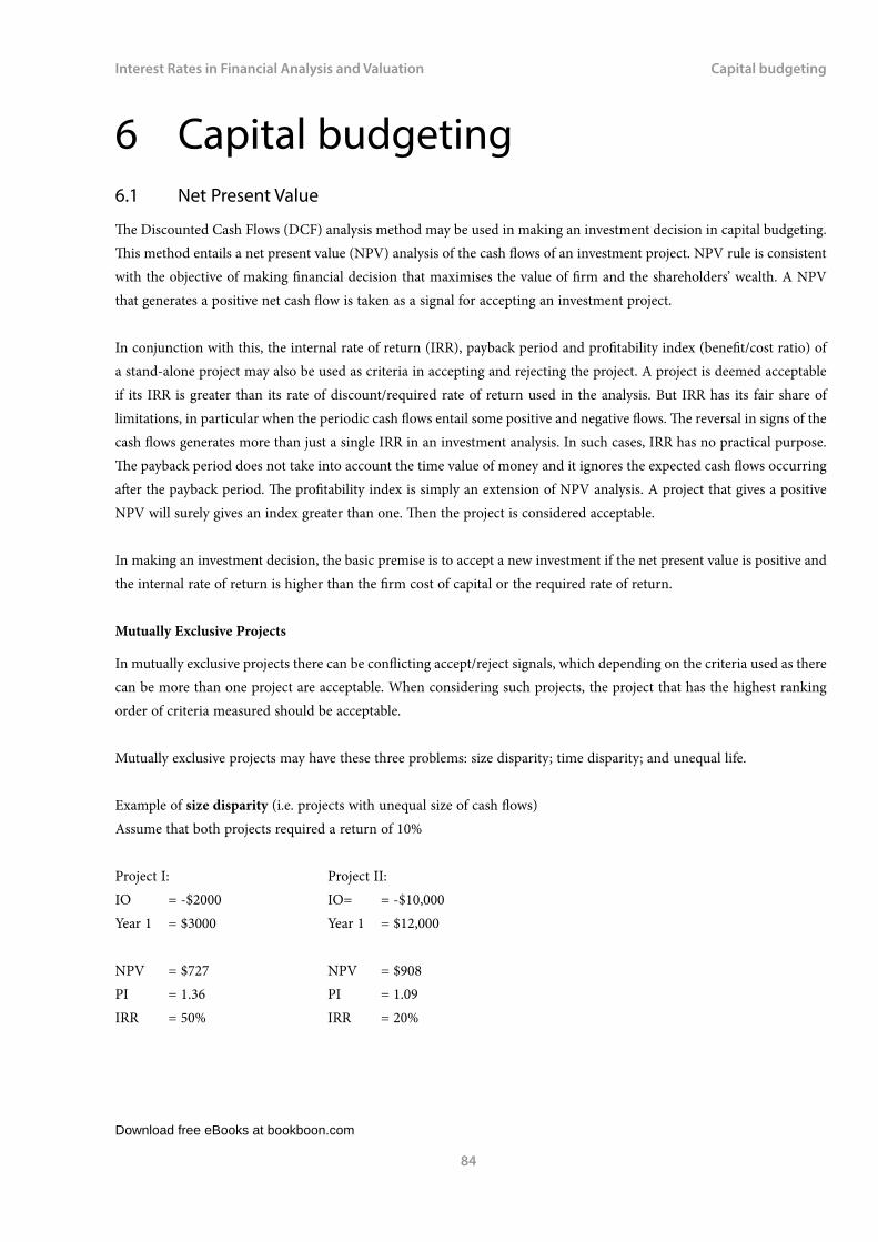
Download free eBooks at bookboon.com
Interest Rates in Financial Analysis and Valuation
84
Capital budgeting
6 Capital budgeting6.1 Net Present Value
The Discounted Cash Flows (DCF) analysis method may be used in making an investment decision in capital budgeting. This method entails a net present value (NPV) analysis of the cash flows of an investment project. NPV rule is consistent with the objective of making financial decision that maximises the value of firm and the shareholders’ wealth. A NPV that generates a positive net cash flow is taken as a signal for accepting an investment project.
In conjunction with this, the internal rate of return (IRR), payback period and profitability index (benefit/cost ratio) of a stand-alone project may also be used as criteria in accepting and rejecting the project. A project is deemed acceptable if its IRR is greater than its rate of discount/required rate of return used in the analysis. But IRR has its fair share of limitations, in particular when the periodic cash flows entail some positive and negative flows. The reversal in signs of the cash flows generates more than just a single IRR in an investment analysis. In such cases, IRR has no practical purpose. The payback period does not take into account the time value of money and it ignores the expected cash flows occurring after the payback period. The profitability index is simply an extension of NPV analysis. A project that gives a positive NPV will surely gives an index greater than one. Then the project is considered acceptable.
In making an investment decision, the basic premise is to accept a new investment if the net present value is positive and the internal rate of return is higher than the firm cost of capital or the required rate of return.
Mutually Exclusive Projects
In mutually exclusive projects there can be conflicting accept/reject signals, which depending on the criteria used as there can be more than one project are acceptable. When considering such projects, the project that has the highest ranking order of criteria measured should be acceptable.
Mutually exclusive projects may have these three problems: size disparity; time disparity; and unequal life.
Example of size disparity (i.e. projects with unequal size of cash flows)Assume that both projects required a return of 10%
Project I: Project II:IO = -$2000 IO= = -$10,000Year 1 = $3000 Year 1 = $12,000
NPV = $727 NPV = $908PI = 1.36 PI = 1.09IRR = 50% IRR = 20%

Download free eBooks at bookboon.com
Click on the ad to read more
Interest Rates in Financial Analysis and Valuation
85
Capital budgeting
In the above example, Project II has the largest NPV, and given the maximum of shareholders’ wealth is the ultimate objective in financial decision so the project is preferable, provided there is no capital rationing.
If it is otherwise, then selecting Project I has a cash outlay saving of $8,000. The saving should be used in a marginal project which provides a net present value at least $181 (i.e. 908-727). Project I and the marginal project should therefore provide a combined net present value greater than $908. With capital rationing then selecting a set of projects should be acceptable.
Example of time disparity (i.e. projects of equal magnitude with a different pattern of cash flows)Assume that both projects required a return of 10% and there is no capital rationing.
Project X: Project Y:IO = -$10,000 IO= = -$10,000Year 1 = $4,000 Year 1 = $5,100Year 2 = $4,800 Year 2 = $5,100Year 3 = $6,000 Year 3 = $5,100
NPV = $3,634 NPV = $3,343PI = 1.36 PI = 1.33IRR = 28% IRR = 30%
“The perfect start of a successful, international career.”
CLICK HERE to discover why both socially
and academically the University
of Groningen is one of the best
places for a student to be www.rug.nl/feb/education
Excellent Economics and Business programmes at:

Download free eBooks at bookboon.com
Interest Rates in Financial Analysis and Valuation
86
Capital budgeting
In the above example, Project X seems to be better based on its net present value and profitability index. However, Project Y is better from the view of cash flows because it generates cash flows earlier and consistently. Which project is better? Given the maximum of shareholders’ wealth is the ultimate objective in financial decision, so Project X is preferable as it gives the largest NPV.
Example of unequal lives (i.e. projects with different life spans)Assume that both projects required a return of 10%
Project Z: Project ZZ:IO = -$10,000 IO= = -$10,000Year 1 = $5,000 Year 1 = $3,000Year 2 = $5,000 Year 2 = $3,000Year 3 = $5,000 Year 3 = $3,000 Year 4 = $3,000 Year 5 = $3,000 Year 6 = $3,000
NPV = $2,213 NPV = $2,787PI = 1.22 PI = 1.28IRR = 23.4% IRR = 20%
In the above example, Project ZZ is better based on NPV and PI, but Project Z comes out better based on IRR. In this case, the projects are not comparable because they have different life spans. It would not be an apple-to-apple comparison.
There are two most common ways to approach this sort of problem, i.e. replacement chain approach and equivalent annual annuity approach.
Using the replacement chain approach, we assume that Project Z will be replaced with a similar project after its 3 years life span. There will be another project runs for a second 3-year span.The first Project Z gives a NPV equals to $2,213 and the replacement project (2nd Project Z) also gives the same NPV. The replacement NPV is discounted to make it to the present value of the first project, i.e. $2,213 x (1.10-3) = $1,662. The total net present value equals $3,875 (2,213 + 1,662).
Now Project Z is comparable to Project ZZ, and based on the combined NPV Project Z should be accepted. The problem with this approach is it may be getting cumbersome when one project has a very long life span while another has a very short life span.
The equivalent annual annuity(EAA) approach is much simpler because each project will be put to a common footing. The EAA of each project is determined by discounting its NPV with its present value interest factor annuity (PVIFA i, n).

Download free eBooks at bookboon.com
Interest Rates in Financial Analysis and Valuation
87
Capital budgeting
Example of EAA:
Project Z - = $2213/2.487 (PVIFA 10%, 3 yrs.) = $889.83
Project ZZ - = $2787/4.355 (PVIFA 10%, 6 yrs.) = $639.95
This means that for Project Z its NPV is equivalent to benefits generated at the rate of $889.83 per year over its life span while Project ZZ at the rate of $639.95 per year over its life span. Based on these annualised benefits then both projects are comparable and Project Z should be accepted as it would generate a higher expected cash flow.
Incremental Cash Flows
In the NPV analysis for capital investment decision, only the incremental net cash flows that are relevant need to be identified and used in the analysis process. Past cost is considered a sunk cost. In determining the incremental net cash flows, the following aspects must be considered: -
1) Income TaxFirms pay taxes depending on the allowable income and deductions, which include loss/gain on disposal of assets as a replacement at the initial period of project life, loss/gain as salvage at the terminal end of project life and net revenue/expenses (including depreciation). For practical purpose, it may be assumed that the tax payment is made in the same year the cash flows occur.
However, if a before-tax analysis is required then all items considered in the analysis must be before-tax to recognise consistency and uniformity. This includes the discount rate used in computing the present value of cash flows. If an after-tax discount rate is required, then it must be reduced by the firm’s corporate tax rate.
2) DepreciationDepreciation is not a cash flow. Firms are allowed to claim depreciation on capital assets used in the business, which provides deductions against assessable income. As such, there is a tax saving or a tax loss generated that affects tax payables, which is a cash flow. Increased in depreciation reduces tax payable, and this generates a positive cash flow, and vice versa.
3) Profit/loss on disposalThere may be a book tax saving or loss on disposals of machineries/equipments at the onset on a new investment and/or at the terminal end of the new investment. There is a tax saving when the salvage value is less than the book value of the disposed machineries/equipments. In this case, a deductible loss arises from the disposal because the sale price of the machineries/equipments is below the book value. The tax saving is derived by multiplying the corporate tax rate and the deductible loss.

Download free eBooks at bookboon.com
Click on the ad to read more
Interest Rates in Financial Analysis and Valuation
88
Capital budgeting
Conversely, when there is a capital gain from the sale of such disposal a taxable profit arises, and the same principle is applied when deriving the tax payable on the gain. Tax savings are considered net cash inflow, and tax payables are outflow.
4) Allocated costsOverhead costs such as wages, salaries, maintenance, or utilities may change by investing in new projects. Any net changes in these expenses must be taken into account, which may arise as savings (or inflows) or loss (or outflows).
The opportunity cost of investing in a new project must also be taken into account. For example, a rental forgone for a building because it is to be used for the proposed project is an opportunity cost and treated as an outflow.
5) Current assets investmentInvesting in a new project may require additional investment in working capital. For instance, increases in inventory, account receivables, cash float and account payables are treated as cash flows and the net working capital are treated as outflow at the initial investment period and will be recovered at the terminal end of project life. All these items will run down (e.g. inventories sold, receivables collected) in the project life. This incremental investment is discounted at the end of project life to a present value.
Enhance your career opportunitiesWe offer practical, industry-relevant undergraduate and postgraduate degrees in central London
› Accounting and finance › Global banking and finance› Business, management and leadership › Luxury brand management› Oil and gas trade management › Media communications and marketing
Contact us to arrange a visitApply direct for January or September entry
T +44 (0)20 7487 7505 E [email protected] W regents.ac.uk

Download free eBooks at bookboon.com
Interest Rates in Financial Analysis and Valuation
89
Capital budgeting
Example – Recognition of cash flows
Suppose a manufacturing company is considering expanding its highly technical facilities on its own vacant lot. The expansion will take 2 years to complete and ready for operation. The facilities should last for 10 years and the equipment will be expected to have a salvage value of $50,000 at the end of project life. Assume that the company’s required rate of return is 10%. Based on a non-tax cash flow evaluation, what is the NPV of this project given the following data and assumptions: -
1. The company has conducted a feasibility studies at a cost of $100,000 to determine the project’s viability. 2. At the initial stage of construction, a cash outflow of $500,000 is required for the technical equipments and
$200,000 for carrying out the construction. The purchased equipments will be depreciated over the project life on a straight-line basis.
3. In the following first year the construction will require a cash outflow of $300,000 so as to complete the construction of the production facilities and to begin operation. This will also increase the working inventory by $100, 000.
4. The first sale from operation will occur at the end of year 2 and it will be sustained at the same level of $600,000 per year until the end of the project life.
5. The fixed operating costs on these sales will be $100,000 per year and the variable costs will be 35% of the yearly sales.
Solution: Pre-tax basis
Initial Outlay of Production Facility: Year 0
Cost of construction -200,000
Cost of technical equipments -500,000
Total initial outlay -700,000
Incremental Cash Flows: Year 1 Yr. 2-10
Construction outflows -300,000
Increased working inventory -100,000
Increased sales 600,000
Increased fixed costs -100,000
Increased variable costs (600,000x0.35) -210,000
Total net incremental cash flows -400,000 290,000
Terminal cash flows: Year 10
Recovery of working inventory 100,000
Disposal of equipments 50,000
Total terminal cash flows 150,000
Download free eBooks at bookboon.com
Interest Rates in Financial Analysis and Valuation
90
Capital budgeting
The following are the interest factors used to discounting the cash flows: -1. PVIF 10%, 1yr. = 0.90912. PVIF 10%, 10yr. = 0.38553. PVIFA 10%, 10yr. = 6.14464. PVIFA 10%, 2 - 10yr. = 6.1446 – 0.9091 = 5.2355
NPV = -700,000 + (-400,000 x 0.9091) + (290,000 x 5.2355) + (150,000 x 0.3855) = -700,000 – 363,640 + 1,518,295 + 57,825 = 512,480
The project’s NPV is $ 512,480 (which acts as a signal to accept the proposal because it is positive).
We can use IRR and profitability index as criteria in accepting and rejecting the analysed project. As long as IRR of the project is greater than the project’s required rate of return, the project is accepted. However, there is a problem in using IRR because the project stream of future cash flows has two signs, i.e. positive and negative signs. IRR is not useful in this case as the project may have multiple IRRs.
We can use the profitability index (benefit/cost ratio), which is given by,
= Present value of future cash flows / Initial cash outlay= (– 363,640 + 1,518,295 + 57,825) / 700,000 = 1.73
So the benefit/cost ratio is 1.73, which indicates the project’s acceptability. This is consistent with the NPV analysis above.
Example – Fixed asset replacement analysis
Auto Credit Leasing is considering upgrading its financial solution systems at a total cost of $300,000 to replace the old systems that was purchased 4 years ago for $200,000. The new systems will be depreciated over its life of 4 years to zero value, and expected to have a salvage value of $30,000 then. The old one is being depreciated at $25,000 per year and has remaining life of 4 years. While at the end of 4 years, it will have no re-sale value;today it is worth $40,000.
The annual operating cost (excluding depreciation and labour) for the old systemsis $70,000 and the new one is expected to be $20,000 only. In addition, the new systems will provide labour savings by $80,000 per year because some staff has indicated to accept jobs voluntarily in associated companies.The new systems will automate some departmental functions. The company tax rate is 28% and its cost of capital is 11%. Should the company purchase the new systems?

Download free eBooks at bookboon.com
Click on the ad to read more
Interest Rates in Financial Analysis and Valuation
91
Capital budgeting
Solution: After-tax basis
Initial Outlay of new system: Year 0
Cost of new systems -300,000
Disposal of old systems 40,000
Total outflow -260,000
Tax savings on loss at disposal -
(40,000-*100,000) X0.28 16,800
Net initial outlay -243,200
*Book value at the end of 4 years [200,000- (25,000 x 4)]
Incremental annual cash flows: Year 1 - 4
Reduced labour 80,000
Reduced operating cost 50,000
Total cash flows 130,000
After-tax net cash flows (130,000x0.72) 93,600
Tax savings on increased depreciation -
(*75,000 – 25,000) x 0.28 14,000
After-tax net cash flows 107,600
*Annual depreciation of new systems [300,000 ÷
.

Download free eBooks at bookboon.com
Interest Rates in Financial Analysis and Valuation
92
Capital budgeting
Terminal end cash flows: Year 4Disposal of new systems – (30,000 x 0.72) 21,600
The following interest factors are used in the discounting the cash flows: -1. PVIFA11%, 4 yrs. = 3.10242. PVIF 11%, 4 yrs. = 0.6587
NPV = -243,200 + (107,600 x 3.1024) + (21,600 x 0.6587) = -243,200 + 333,818 + 14,228 = 104, 846
Profitability Index = 333,818 + 14,228 / 243,200 = 348,046 / 243,228 = 1.4
To determine IRR we can use compute the PVIFAi, n and do several iterations until we find a rate that equalises the present value of cash flow stream with the initial outlay. Any computer spreadsheet will make the work very much easier.The solution is given below.
Cash flow Year 0 Year 1-4 Year 4Initial outlay -243,200 - -Future stream - 107,600 21,600
PV factor - 2.1886 0.3568PV 243,200 235,493 7,707
PVIFA29.389%, 4 yrs. = 2.1886PVIF 29.389%, 4 yrs. = 0.3568
The company may invest in the new systems because the net present value of cash flows is positive ($104,846), the benefit/cost ratio (1.4) is greater than one, and IRR (29.4%) is greater than the company’s capital cost (11.0%).
Exercise 6.0
1. A company is considering investing in a project producing a new product line. The company intends to use a section of its factory premises, which is currently rented out to a forwarding company for $60,000 annually. The investment proposal is based on a feasibility study that was done about a year ago at a cost of $15,000.
The new product will generate sales of $500,000 annually, and the cost of these sales will be 40% of annual sales. New machines for manufacturing the new product will be purchased at a cost of $600,000 and it will incur a yearly maintenance cost of $50,000. The machines will require employment of 5 operators who are individually earning $18,000 per year. These operators will be taken from the current production line. A supervisor from the current production line who is earning $30,000 per year will also be transferred to the new production line.

Download free eBooks at bookboon.com
Interest Rates in Financial Analysis and Valuation
93
Capital budgeting
The new set of machines will last for 8 years just as the project’s life, and it will be depreciated over its life by the straight-line method. At the end of productive life, the machines will be disposed for $100,000. If the company cost of capital is 12% and corporate tax rate is 28%, what is the NPV of this project?
2. Green Can Manufacturing, a company producing tin cans for beverages and foods, is considering replacing its old production line with a new set of machines that will enhance the automation of its manufacturing facilities. By investing in this proposed project, sales will increase by $90,000 annually, and cost of defects will reduce by $3,750 per year. Other overheads will increase by $105,000 per year.
The annual operator cost in the old production line is $130,000 annually, but with the fully automated facilities, operators are not necessary. However, yearly maintenance cost will increase from $50,000 to $80,000 per year. To initiate the operation of fully automated production facilities, inventory investment will need to be increased by 20% from the current level of $250,000 at beginning of Year 1.
Buying the new machines will cost the company $300,000 and their installation will cost $25,000. This new set of machines will have a life of 10 years and it will be depreciated over its life by the straight-line method. This will increase the depreciation by $19,000.
At the end of its life, the machines will be disposed for $60,000. The old set has a remaining life of 10 years, which was brought into commission 5 years ago. While its book value is $110,000, if it is sold now it would be worth $140,000. At the end of its economic life, it will be worth nothing.
The company tax rate is 28% and its required rate of return is 11%. Should the company invest in the new set of machines?
3. Suppose a company is considering investing in a project that manufactures and supplies consumables for science laboratory needs. Assume that the company’s required rate of return is 12%, what is the NPV of the proposed project given the following data and assumptions: -
1. Buying and installing machineries for the production facility will cost the company $1 million. Training of operators will be required at a cost of $200,000. The construction of the production facility on a piece of land owned by the company will cost $500,000.
2. The machineries will have a zero book value at the end of life, as they will be depreciated on the straight-line basis. However, the machineries will be disposed for $70,000 in year 8, which is the end of production life. One-off maintenance of these machineries will cost the company $50,000 in year 4.
3. For a start of production in Year 1, the working inventory will be $105,000. The working inventory will increase by $60,000 in year 5.
4. This project will generate sales of $800,000 annually starting from year 1, and will consume fixed expenses at $200,000 per year. The variable costs will be 30% of annual sales.

Download free eBooks at bookboon.com
Interest Rates in Financial Analysis and Valuation
94
Appendix
AppendixTable 1 – Future value of $1 at the end of n periods.
(1+i)n
n 1% 2% 3% 4% 5% 6% 7% 8% 9% 10%
1 1.0100 1.0200 1.0300 1.0400 1.0500 1.0600 1.0700 1.0800 1.0900 1.1000
2 1.0201 1.0404 1.0609 1.0816 1.1025 1.1236 1.1449 1.1664 1.1881 1.2100
3 1.0303 1.0612 1.0927 1.1249 1.1576 1.1910 1.2250 1.2597 1.2950 1.3310
4 1.0406 1.0824 1.1255 1.1699 1.2155 1.2625 1.3108 1.3605 1.4116 1.4641
5 1.0510 1.1041 1.1593 1.2167 1.2763 1.3382 1.4026 1.4693 1.5386 1.6105
6 1.0615 1.1262 1.1941 1.2653 1.3401 1.4185 1.5007 1.5869 1.6771 1.7716
7 1.0721 1.1487 1.2299 1.3159 1.4071 1.5036 1.6058 1.7138 1.8280 1.9487
8 1.0829 1.1717 1.2668 1.3686 1.4775 1.5938 1.7182 1.8509 1.9926 2.1436
9 1.0937 1.1951 1.3048 1.4233 1.5513 1.6895 1.8385 1.9990 2.1719 2.3579
10 1.1046 1.2190 1.3439 1.4802 1.6289 1.7908 1.9672 2.1589 2.3674 2.5937
11 1.1157 1.2434 1.3842 1.5395 1.7103 1.8983 2.1049 2.3316 2.5804 2.8531
12 1.1268 1.2682 1.4258 1.6010 1.7959 2.0122 2.2522 2.5182 2.8127 3.1384
13 1.1381 1.2936 1.4685 1.6651 1.8856 2.1329 2.4098 2.7196 3.0658 3.4523
14 1.1495 1.3195 1.5126 1.7317 1.9799 2.2609 2.5785 2.9372 3.3417 3.7975
15 1.1610 1.3459 1.5580 1.8009 2.0789 2.3966 2.7590 3.1722 3.6425 4.1772
16 1.1726 1.3728 1.6047 1.8730 2.1829 2.5404 2.9522 3.4259 3.9703 4.5950
17 1.1843 1.4002 1.6528 1.9479 2.2920 2.6928 3.1588 3.7000 4.3276 5.0545
18 1.1961 1.4282 1.7024 2.0258 2.4066 2.8543 3.3799 3.9960 4.7171 5.5599
19 1.2081 1.4568 1.7535 2.1068 2.5270 3.0256 3.6165 4.3157 5.1417 6.1159
20 1.2202 1.4859 1.8061 2.1911 2.6533 3.2071 3.8697 4.6610 5.6044 6.7275
21 1.2324 1.5157 1.8603 2.2788 2.7860 3.3996 4.1406 5.0338 6.1088 7.4002
22 1.2447 1.5460 1.9161 2.3699 2.9253 3.6035 4.4304 5.4365 6.6586 8.1403
23 1.2572 1.5769 1.9736 2.4647 3.0715 3.8197 4.7405 5.8715 7.2579 8.9543
24 1.2697 1.6084 2.0328 2.5633 3.2251 4.0489 5.0724 6.3412 7.9111 9.8497
25 1.2824 1.6406 2.0938 2.6658 3.3864 4.2919 5.4274 6.8485 8.6231 10.8347
26 1.2953 1.6734 2.1566 2.7725 3.5557 4.5494 5.8074 7.3964 9.3992 11.9182
27 1.3082 1.7069 2.2213 2.8834 3.7335 4.8223 6.2139 7.9881 10.2451 13.1100
28 1.3213 1.7410 2.2879 2.9987 3.9201 5.1117 6.6488 8.6271 11.1671 14.4210
29 1.3345 1.7758 2.3566 3.1187 4.1161 5.4184 7.1143 9.3173 12.1722 15.8631
30 1.3478 1.8114 2.4273 3.2434 4.3219 5.7435 7.6123 10.0627 13.2677 17.4494
40 1.4889 2.2080 3.2620 4.8010 7.0400 10.2857 14.9745 21.7245 31.4094 45.2593
50 1.6446 2.6916 4.3839 7.1067 11.4674 18.4202 29.4570 46.9016 74.3575 117.3909
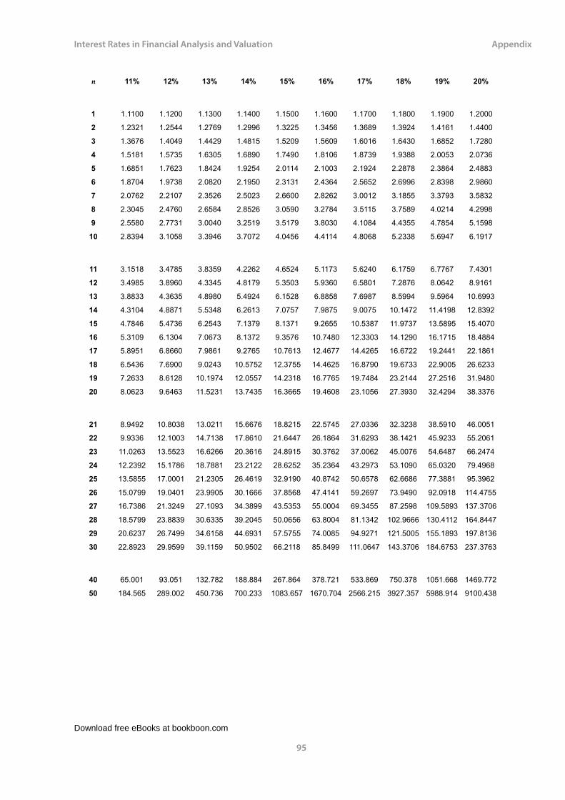
Download free eBooks at bookboon.com
Interest Rates in Financial Analysis and Valuation
95
Appendix
n 11% 12% 13% 14% 15% 16% 17% 18% 19% 20%
1 1.1100 1.1200 1.1300 1.1400 1.1500 1.1600 1.1700 1.1800 1.1900 1.2000
2 1.2321 1.2544 1.2769 1.2996 1.3225 1.3456 1.3689 1.3924 1.4161 1.4400
3 1.3676 1.4049 1.4429 1.4815 1.5209 1.5609 1.6016 1.6430 1.6852 1.7280
4 1.5181 1.5735 1.6305 1.6890 1.7490 1.8106 1.8739 1.9388 2.0053 2.0736
5 1.6851 1.7623 1.8424 1.9254 2.0114 2.1003 2.1924 2.2878 2.3864 2.4883
6 1.8704 1.9738 2.0820 2.1950 2.3131 2.4364 2.5652 2.6996 2.8398 2.9860
7 2.0762 2.2107 2.3526 2.5023 2.6600 2.8262 3.0012 3.1855 3.3793 3.5832
8 2.3045 2.4760 2.6584 2.8526 3.0590 3.2784 3.5115 3.7589 4.0214 4.2998
9 2.5580 2.7731 3.0040 3.2519 3.5179 3.8030 4.1084 4.4355 4.7854 5.1598
10 2.8394 3.1058 3.3946 3.7072 4.0456 4.4114 4.8068 5.2338 5.6947 6.1917
11 3.1518 3.4785 3.8359 4.2262 4.6524 5.1173 5.6240 6.1759 6.7767 7.4301
12 3.4985 3.8960 4.3345 4.8179 5.3503 5.9360 6.5801 7.2876 8.0642 8.9161
13 3.8833 4.3635 4.8980 5.4924 6.1528 6.8858 7.6987 8.5994 9.5964 10.6993
14 4.3104 4.8871 5.5348 6.2613 7.0757 7.9875 9.0075 10.1472 11.4198 12.8392
15 4.7846 5.4736 6.2543 7.1379 8.1371 9.2655 10.5387 11.9737 13.5895 15.4070
16 5.3109 6.1304 7.0673 8.1372 9.3576 10.7480 12.3303 14.1290 16.1715 18.4884
17 5.8951 6.8660 7.9861 9.2765 10.7613 12.4677 14.4265 16.6722 19.2441 22.1861
18 6.5436 7.6900 9.0243 10.5752 12.3755 14.4625 16.8790 19.6733 22.9005 26.6233
19 7.2633 8.6128 10.1974 12.0557 14.2318 16.7765 19.7484 23.2144 27.2516 31.9480
20 8.0623 9.6463 11.5231 13.7435 16.3665 19.4608 23.1056 27.3930 32.4294 38.3376
21 8.9492 10.8038 13.0211 15.6676 18.8215 22.5745 27.0336 32.3238 38.5910 46.0051
22 9.9336 12.1003 14.7138 17.8610 21.6447 26.1864 31.6293 38.1421 45.9233 55.2061
23 11.0263 13.5523 16.6266 20.3616 24.8915 30.3762 37.0062 45.0076 54.6487 66.2474
24 12.2392 15.1786 18.7881 23.2122 28.6252 35.2364 43.2973 53.1090 65.0320 79.4968
25 13.5855 17.0001 21.2305 26.4619 32.9190 40.8742 50.6578 62.6686 77.3881 95.3962
26 15.0799 19.0401 23.9905 30.1666 37.8568 47.4141 59.2697 73.9490 92.0918 114.4755
27 16.7386 21.3249 27.1093 34.3899 43.5353 55.0004 69.3455 87.2598 109.5893 137.3706
28 18.5799 23.8839 30.6335 39.2045 50.0656 63.8004 81.1342 102.9666 130.4112 164.8447
29 20.6237 26.7499 34.6158 44.6931 57.5755 74.0085 94.9271 121.5005 155.1893 197.8136
30 22.8923 29.9599 39.1159 50.9502 66.2118 85.8499 111.0647 143.3706 184.6753 237.3763
40 65.001 93.051 132.782 188.884 267.864 378.721 533.869 750.378 1051.668 1469.772
50 184.565 289.002 450.736 700.233 1083.657 1670.704 2566.215 3927.357 5988.914 9100.438

Download free eBooks at bookboon.com
Interest Rates in Financial Analysis and Valuation
96
Appendix
Table 2 – Present value of $1 at the end of n periods.
PVIF i,n = (1+i)-n
n 1% 2% 3% 4% 5% 6% 7% 8% 9% 10%
1 0.9901 0.9804 0.9709 0.9615 0.9524 0.9434 0.9346 0.9259 0.9174 0.9091
2 0.9803 0.9612 0.9426 0.9246 0.9070 0.8900 0.8734 0.8573 0.8417 0.8264
3 0.9706 0.9423 0.9151 0.8890 0.8638 0.8396 0.8163 0.7938 0.7722 0.7513
4 0.9610 0.9238 0.8885 0.8548 0.8227 0.7921 0.7629 0.7350 0.7084 0.6830
5 0.9515 0.9057 0.8626 0.8219 0.7835 0.7473 0.7130 0.6806 0.6499 0.6209
6 0.9420 0.8880 0.8375 0.7903 0.7462 0.7050 0.6663 0.6302 0.5963 0.5645
7 0.9327 0.8706 0.8131 0.7599 0.7107 0.6651 0.6227 0.5835 0.5470 0.5132
8 0.9235 0.8535 0.7894 0.7307 0.6768 0.6274 0.5820 0.5403 0.5019 0.4665
9 0.9143 0.8368 0.7664 0.7026 0.6446 0.5919 0.5439 0.5002 0.4604 0.4241
10 0.9053 0.8203 0.7441 0.6756 0.6139 0.5584 0.5083 0.4632 0.4224 0.3855
11 0.8963 0.8043 0.7224 0.6496 0.5847 0.5268 0.4751 0.4289 0.3875 0.3505
12 0.8874 0.7885 0.7014 0.6246 0.5568 0.4970 0.4440 0.3971 0.3555 0.3186
13 0.8787 0.7730 0.6810 0.6006 0.5303 0.4688 0.4150 0.3677 0.3262 0.2897
14 0.8700 0.7579 0.6611 0.5775 0.5051 0.4423 0.3878 0.3405 0.2992 0.2633
15 0.8613 0.7430 0.6419 0.5553 0.4810 0.4173 0.3624 0.3152 0.2745 0.2394
16 0.8528 0.7284 0.6232 0.5339 0.4581 0.3936 0.3387 0.2919 0.2519 0.2176
17 0.8444 0.7142 0.6050 0.5134 0.4363 0.3714 0.3166 0.2703 0.2311 0.1978
18 0.8360 0.7002 0.5874 0.4936 0.4155 0.3503 0.2959 0.2502 0.2120 0.1799
19 0.8277 0.6864 0.5703 0.4746 0.3957 0.3305 0.2765 0.2317 0.1945 0.1635
20 0.8195 0.6730 0.5537 0.4564 0.3769 0.3118 0.2584 0.2145 0.1784 0.1486
21 0.8114 0.6598 0.5375 0.4388 0.3589 0.2942 0.2415 0.1987 0.1637 0.1351
22 0.8034 0.6468 0.5219 0.4220 0.3418 0.2775 0.2257 0.1839 0.1502 0.1228
23 0.7954 0.6342 0.5067 0.4057 0.3256 0.2618 0.2109 0.1703 0.1378 0.1117
24 0.7876 0.6217 0.4919 0.3901 0.3101 0.2470 0.1971 0.1577 0.1264 0.1015
25 0.7798 0.6095 0.4776 0.3751 0.2953 0.2330 0.1842 0.1460 0.1160 0.0923
26 0.7720 0.5976 0.4637 0.3607 0.2812 0.2198 0.1722 0.1352 0.1064 0.0839
27 0.7644 0.5859 0.4502 0.3468 0.2678 0.2074 0.1609 0.1252 0.0976 0.0763
28 0.7568 0.5744 0.4371 0.3335 0.2551 0.1956 0.1504 0.1159 0.0895 0.0693
29 0.7493 0.5631 0.4243 0.3207 0.2429 0.1846 0.1406 0.1073 0.0822 0.0630
30 0.7419 0.5521 0.4120 0.3083 0.2314 0.1741 0.1314 0.0994 0.0754 0.0573
40 0.6717 0.4529 0.3066 0.2083 0.1420 0.0972 0.0668 0.0460 0.0318 0.0221
50 0.6080 0.3715 0.2281 0.1407 0.0872 0.0543 0.0339 0.0213 0.0134 0.0085

Download free eBooks at bookboon.com
Interest Rates in Financial Analysis and Valuation
97
Appendix
n 11% 12% 13% 14% 15% 16% 17% 18% 19% 20%
1 0.9009 0.8929 0.8850 0.8772 0.8696 0.8621 0.8547 0.8475 0.8403 0.8333
2 0.8116 0.7972 0.7831 0.7695 0.7561 0.7432 0.7305 0.7182 0.7062 0.6944
3 0.7312 0.7118 0.6931 0.6750 0.6575 0.6407 0.6244 0.6086 0.5934 0.5787
4 0.6587 0.6355 0.6133 0.5921 0.5718 0.5523 0.5337 0.5158 0.4987 0.4823
5 0.5935 0.5674 0.5428 0.5194 0.4972 0.4761 0.4561 0.4371 0.4190 0.4019
6 0.5346 0.5066 0.4803 0.4556 0.4323 0.4104 0.3898 0.3704 0.3521 0.3349
7 0.4817 0.4523 0.4251 0.3996 0.3759 0.3538 0.3332 0.3139 0.2959 0.2791
8 0.4339 0.4039 0.3762 0.3506 0.3269 0.3050 0.2848 0.2660 0.2487 0.2326
9 0.3909 0.3606 0.3329 0.3075 0.2843 0.2630 0.2434 0.2255 0.2090 0.1938
10 0.3522 0.3220 0.2946 0.2697 0.2472 0.2267 0.2080 0.1911 0.1756 0.1615
11 0.3173 0.2875 0.2607 0.2366 0.2149 0.1954 0.1778 0.1619 0.1476 0.1346
12 0.2858 0.2567 0.2307 0.2076 0.1869 0.1685 0.1520 0.1372 0.1240 0.1122
13 0.2575 0.2292 0.2042 0.1821 0.1625 0.1452 0.1299 0.1163 0.1042 0.0935
14 0.2320 0.2046 0.1807 0.1597 0.1413 0.1252 0.1110 0.0985 0.0876 0.0779
15 0.2090 0.1827 0.1599 0.1401 0.1229 0.1079 0.0949 0.0835 0.0736 0.0649
16 0.1883 0.1631 0.1415 0.1229 0.1069 0.0930 0.0811 0.0708 0.0618 0.0541
17 0.1696 0.1456 0.1252 0.1078 0.0929 0.0802 0.0693 0.0600 0.0520 0.0451
18 0.1528 0.1300 0.1108 0.0946 0.0808 0.0691 0.0592 0.0508 0.0437 0.0376
19 0.1377 0.1161 0.0981 0.0829 0.0703 0.0596 0.0506 0.0431 0.0367 0.0313
20 0.1240 0.1037 0.0868 0.0728 0.0611 0.0514 0.0433 0.0365 0.0308 0.0261
21 0.1117 0.0926 0.0768 0.0638 0.0531 0.0443 0.0370 0.0309 0.0259 0.0217
22 0.1007 0.0826 0.0680 0.0560 0.0462 0.0382 0.0316 0.0262 0.0218 0.0181
23 0.0907 0.0738 0.0601 0.0491 0.0402 0.0329 0.0270 0.0222 0.0183 0.0151
24 0.0817 0.0659 0.0532 0.0431 0.0349 0.0284 0.0231 0.0188 0.0154 0.0126
25 0.0736 0.0588 0.0471 0.0378 0.0304 0.0245 0.0197 0.0160 0.0129 0.0105
26 0.0663 0.0525 0.0417 0.0331 0.0264 0.0211 0.0169 0.0135 0.0109 0.0087
27 0.0597 0.0469 0.0369 0.0291 0.0230 0.0182 0.0144 0.0115 0.0091 0.0073
28 0.0538 0.0419 0.0326 0.0255 0.0200 0.0157 0.0123 0.0097 0.0077 0.0061
29 0.0485 0.0374 0.0289 0.0224 0.0174 0.0135 0.0105 0.0082 0.0064 0.0051
30 0.0437 0.0334 0.0256 0.0196 0.0151 0.0116 0.0090 0.0070 0.0054 0.0042
40 0.0154 0.0107 0.0075 0.0053 0.0037 0.0026 0.0019 0.0013 0.0010 0.0007
50 0.0054 0.0035 0.0022 0.0014 0.0009 0.0006 0.0004 0.0003 0.0002 0.0001

Download free eBooks at bookboon.com
Interest Rates in Financial Analysis and Valuation
98
Appendix
Table 3 – Future value of an annuity of $1 for n periods.
FVIFA i, n
= (1+i)n - 1i
n 1% 2% 3% 4% 5% 6% 7% 8% 9% 10%
1 1.0000 1.0000 1.0000 1.0000 1.0000 1.0000 1.0000 1.0000 1.0000 1.0000
2 2.0100 2.0200 2.0300 2.0400 2.0500 2.0600 2.0700 2.0800 2.0900 2.1000
3 3.0301 3.0604 3.0909 3.1216 3.1525 3.1836 3.2149 3.2464 3.2781 3.3100
4 4.0604 4.1216 4.1836 4.2465 4.3101 4.3746 4.4399 4.5061 4.5731 4.6410
5 5.1010 5.2040 5.3091 5.4163 5.5256 5.6371 5.7507 5.8666 5.9847 6.1051
6 6.1520 6.3081 6.4684 6.6330 6.8019 6.9753 7.1533 7.3359 7.5233 7.7156
7 7.2135 7.4343 7.6625 7.8983 8.1420 8.3938 8.6540 8.9228 9.2004 9.4872
8 8.2857 8.5830 8.8923 9.2142 9.5491 9.8975 10.2598 10.6366 11.0285 11.4359
9 9.3685 9.7546 10.1591 10.5828 11.0266 11.4913 11.9780 12.4876 13.0210 13.5795
10 10.4622 10.9497 11.4639 12.0061 12.5779 13.1808 13.8164 14.4866 15.1929 15.9374
11 11.5668 12.1687 12.8078 13.4864 14.2068 14.9716 15.7836 16.6455 17.5603 18.5312
12 12.6825 13.4121 14.1920 15.0258 15.9171 16.8699 17.8885 18.9771 20.1407 21.3843
13 13.8093 14.6803 15.6178 16.6268 17.7130 18.8821 20.1406 21.4953 22.9534 24.5227
14 14.9474 15.9739 17.0863 18.2919 19.5986 21.0151 22.5505 24.2149 26.0192 27.9750
15 16.0969 17.2934 18.5989 20.0236 21.5786 23.2760 25.1290 27.1521 29.3609 31.7725
16 17.2579 18.6393 20.1569 21.8245 23.6575 25.6725 27.8881 30.3243 33.0034 35.9497
17 18.4304 20.0121 21.7616 23.6975 25.8404 28.2129 30.8402 33.7502 36.9737 40.5447
18 19.6147 21.4123 23.4144 25.6454 28.1324 30.9057 33.9990 37.4502 41.3013 45.5992
19 20.8109 22.8406 25.1169 27.6712 30.5390 33.7600 37.3790 41.4463 46.0185 51.1591
20 22.0190 24.2974 26.8704 29.7781 33.0660 36.7856 40.9955 45.7620 51.1601 57.2750
21 23.2392 25.7833 28.6765 31.9692 35.7193 39.9927 44.8652 50.4229 56.7645 64.0025
22 24.4716 27.2990 30.5368 34.2480 38.5052 43.3923 49.0057 55.4568 62.8733 71.4027
23 25.7163 28.8450 32.4529 36.6179 41.4305 46.9958 53.4361 60.8933 69.5319 79.5430
24 26.9735 30.4219 34.4265 39.0826 44.5020 50.8156 58.1767 66.7648 76.7898 88.4973
25 28.2432 32.0303 36.4593 41.6459 47.7271 54.8645 63.2490 73.1059 84.7009 98.3471
26 29.5256 33.6709 38.5530 44.3117 51.1135 59.1564 68.6765 79.9544 93.3240 109.1818
27 30.8209 35.3443 40.7096 47.0842 54.6691 63.7058 74.4838 87.3508 102.7231 121.0999
28 32.1291 37.0512 42.9309 49.9676 58.4026 68.5281 80.6977 95.3388 112.9682 134.2099
29 33.4504 38.7922 45.2189 52.9663 62.3227 73.6398 87.3465 103.9659 124.1354 148.6309
30 34.7849 40.5681 47.5754 56.0849 66.4388 79.0582 94.4608 113.2832 136.3075 164.4940
40 48.886 60.402 75.401 95.026 120.800 154.762 199.635 259.057 337.882 442.593
50 64.463 84.579 112.797 152.667 209.348 290.336 406.529 573.770 815.084 1163.909

Download free eBooks at bookboon.com
Interest Rates in Financial Analysis and Valuation
99
Appendix
n 11% 12% 13% 14% 15% 16% 17% 18% 19% 20%
1 1.0000 1.0000 1.0000 1.0000 1.0000 1.0000 1.0000 1.0000 1.0000 1.0000
2 2.1100 2.1200 2.1300 2.1400 2.1500 2.1600 2.1700 2.1800 2.1900 2.2000
3 3.3421 3.3744 3.4069 3.4396 3.4725 3.5056 3.5389 3.5724 3.6061 3.6400
4 4.7097 4.7793 4.8498 4.9211 4.9934 5.0665 5.1405 5.2154 5.2913 5.3680
5 6.2278 6.3528 6.4803 6.6101 6.7424 6.8771 7.0144 7.1542 7.2966 7.4416
6 7.9129 8.1152 8.3227 8.5355 8.7537 8.9775 9.2068 9.4420 9.6830 9.9299
7 9.7833 10.0890 10.4047 10.7305 11.0668 11.4139 11.7720 12.1415 12.5227 12.9159
8 11.8594 12.2997 12.7573 13.2328 13.7268 14.2401 14.7733 15.3270 15.9020 16.4991
9 14.1640 14.7757 15.4157 16.0853 16.7858 17.5185 18.2847 19.0859 19.9234 20.7989
10 16.7220 17.5487 18.4197 19.3373 20.3037 21.3215 22.3931 23.5213 24.7089 25.9587
11 19.5614 20.6546 21.8143 23.0445 24.3493 25.7329 27.1999 28.7551 30.4035 32.1504
12 22.7132 24.1331 25.6502 27.2707 29.0017 30.8502 32.8239 34.9311 37.1802 39.5805
13 26.2116 28.0291 29.9847 32.0887 34.3519 36.7862 39.4040 42.2187 45.2445 48.4966
14 30.0949 32.3926 34.8827 37.5811 40.5047 43.6720 47.1027 50.8180 54.8409 59.1959
15 34.4054 37.2797 40.4175 43.8424 47.5804 51.6595 56.1101 60.9653 66.2607 72.0351
16 39.1899 42.7533 46.6717 50.9804 55.7175 60.9250 66.6488 72.9390 79.8502 87.4421
17 44.5008 48.8837 53.7391 59.1176 65.0751 71.6730 78.9792 87.0680 96.0218 105.9306
18 50.3959 55.7497 61.7251 68.3941 75.8364 84.1407 93.4056 103.7403 115.2659 128.1167
19 56.9395 63.4397 70.7494 78.9692 88.2118 98.6032 110.2846 123.4135 138.1664 154.7400
20 64.2028 72.0524 80.9468 91.0249 102.4436 115.3797 130.0329 146.6280 165.4180 186.6880
21 72.2651 81.6987 92.4699 104.7684 118.8101 134.8405 153.1385 174.0210 197.8474 225.0256
22 81.2143 92.5026 105.4910 120.4360 137.6316 157.4150 180.1721 206.3448 236.4385 271.0307
23 91.1479 104.6029 120.2048 138.2970 159.2764 183.6014 211.8013 244.4868 282.3618 326.2369
24 102.1742 118.1552 136.8315 158.6586 184.1678 213.9776 248.8076 289.4945 337.0105 392.4842
25 114.4133 133.3339 155.6196 181.8708 212.7930 249.2140 292.1049 342.6035 402.0425 471.9811
26 127.9988 150.3339 176.8501 208.3327 245.7120 290.0883 342.7627 405.2721 479.4306 567.3773
27 143.0786 169.3740 200.8406 238.4993 283.5688 337.5024 402.0323 479.2211 571.5224 681.8528
28 159.8173 190.6989 227.9499 272.8892 327.1041 392.5028 471.3778 566.4809 681.1116 819.2233
29 178.3972 214.5828 258.5834 312.0937 377.1697 456.3032 552.5121 669.4475 811.5228 984.0680
30 199.0209 241.3327 293.1992 356.7868 434.7451 530.3117 647.4391 790.9480 966.7122 1181.8816
40 581.826 767.091 1013.704 1342.025 1779.090 2360.757 3134.522 4163.213 5529.829 7343.858
50 1668.771 2400.018 3459.507 4994.521 7217.716 10435.649 15089.502 21813.094 31515.336 45497.191

Download free eBooks at bookboon.com
Interest Rates in Financial Analysis and Valuation
100
Appendix
Table 4 – Present value of an annuity of $1 for n periods.
PVIFA i, n
= (1-(1+i)-n
i
n 1% 2% 3% 4% 5% 6% 7% 8% 9% 10%
1 0.9901 0.9804 0.9709 0.9615 0.9524 0.9434 0.9346 0.9259 0.9174 0.9091
2 1.9704 1.9416 1.9135 1.8861 1.8594 1.8334 1.8080 1.7833 1.7591 1.7355
3 2.9410 2.8839 2.8286 2.7751 2.7232 2.6730 2.6243 2.5771 2.5313 2.4869
4 3.9020 3.8077 3.7171 3.6299 3.5460 3.4651 3.3872 3.3121 3.2397 3.1699
5 4.8534 4.7135 4.5797 4.4518 4.3295 4.2124 4.1002 3.9927 3.8897 3.7908
6 5.7955 5.6014 5.4172 5.2421 5.0757 4.9173 4.7665 4.6229 4.4859 4.3553
7 6.7282 6.4720 6.2303 6.0021 5.7864 5.5824 5.3893 5.2064 5.0330 4.8684
8 7.6517 7.3255 7.0197 6.7327 6.4632 6.2098 5.9713 5.7466 5.5348 5.3349
9 8.5660 8.1622 7.7861 7.4353 7.1078 6.8017 6.5152 6.2469 5.9952 5.7590
10 9.4713 8.9826 8.5302 8.1109 7.7217 7.3601 7.0236 6.7101 6.4177 6.1446
11 10.3676 9.7868 9.2526 8.7605 8.3064 7.8869 7.4987 7.1390 6.8052 6.4951
12 11.2551 10.5753 9.9540 9.3851 8.8633 8.3838 7.9427 7.5361 7.1607 6.8137
13 12.1337 11.3484 10.6350 9.9856 9.3936 8.8527 8.3577 7.9038 7.4869 7.1034
14 13.0037 12.1062 11.2961 10.5631 9.8986 9.2950 8.7455 8.2442 7.7862 7.3667
15 13.8651 12.8493 11.9379 11.1184 10.3797 9.7122 9.1079 8.5595 8.0607 7.6061
16 14.7179 13.5777 12.5611 11.6523 10.8378 10.1059 9.4466 8.8514 8.3126 7.8237
17 15.5623 14.2919 13.1661 12.1657 11.2741 10.4773 9.7632 9.1216 8.5436 8.0216
18 16.3983 14.9920 13.7535 12.6593 11.6896 10.8276 10.0591 9.3719 8.7556 8.2014
19 17.2260 15.6785 14.3238 13.1339 12.0853 11.1581 10.3356 9.6036 8.9501 8.3649
20 18.0456 16.3514 14.8775 13.5903 12.4622 11.4699 10.5940 9.8181 9.1285 8.5136
21 18.8570 17.0112 15.4150 14.0292 12.8212 11.7641 10.8355 10.0168 9.2922 8.6487
22 19.6604 17.6580 15.9369 14.4511 13.1630 12.0416 11.0612 10.2007 9.4424 8.7715
23 20.4558 18.2922 16.4436 14.8568 13.4886 12.3034 11.2722 10.3711 9.5802 8.8832
24 21.2434 18.9139 16.9355 15.2470 13.7986 12.5504 11.4693 10.5288 9.7066 8.9847
25 22.0232 19.5235 17.4131 15.6221 14.0939 12.7834 11.6536 10.6748 9.8226 9.0770
26 22.7952 20.1210 17.8768 15.9828 14.3752 13.0032 11.8258 10.8100 9.9290 9.1609
27 23.5596 20.7069 18.3270 16.3296 14.6430 13.2105 11.9867 10.9352 10.0266 9.2372
28 24.3164 21.2813 18.7641 16.6631 14.8981 13.4062 12.1371 11.0511 10.1161 9.3066
29 25.0658 21.8444 19.1885 16.9837 15.1411 13.5907 12.2777 11.1584 10.1983 9.3696
30 25.8077 22.3965 19.6004 17.2920 15.3725 13.7648 12.4090 11.2578 10.2737 9.4269
40 32.8347 27.3555 23.1148 19.7928 17.1591 15.0463 13.3317 11.9246 10.7574 9.7791
50 39.1961 31.4236 25.7298 21.4822 18.2559 15.7619 13.8007 12.2335 10.9617 9.9148

Interest Rates in Financial Analysis and Valuation
101
Appendix
n 11% 12% 13% 14% 15% 16% 17% 18% 19% 20%
1 0.9009 0.8929 0.8850 0.8772 0.8696 0.8621 0.8547 0.8475 0.8403 0.8333
2 1.7125 1.6901 1.6681 1.6467 1.6257 1.6052 1.5852 1.5656 1.5465 1.5278
3 2.4437 2.4018 2.3612 2.3216 2.2832 2.2459 2.2096 2.1743 2.1399 2.1065
4 3.1024 3.0373 2.9745 2.9137 2.8550 2.7982 2.7432 2.6901 2.6386 2.5887
5 3.6959 3.6048 3.5172 3.4331 3.3522 3.2743 3.1993 3.1272 3.0576 2.9906
6 4.2305 4.1114 3.9975 3.8887 3.7845 3.6847 3.5892 3.4976 3.4098 3.3255
7 4.7122 4.5638 4.4226 4.2883 4.1604 4.0386 3.9224 3.8115 3.7057 3.6046
8 5.1461 4.9676 4.7988 4.6389 4.4873 4.3436 4.2072 4.0776 3.9544 3.8372
9 5.5370 5.3282 5.1317 4.9464 4.7716 4.6065 4.4506 4.3030 4.1633 4.0310
10 5.8892 5.6502 5.4262 5.2161 5.0188 4.8332 4.6586 4.4941 4.3389 4.1925
11 6.2065 5.9377 5.6869 5.4527 5.2337 5.0286 4.8364 4.6560 4.4865 4.3271
12 6.4924 6.1944 5.9176 5.6603 5.4206 5.1971 4.9884 4.7932 4.6105 4.4392
13 6.7499 6.4235 6.1218 5.8424 5.5831 5.3423 5.1183 4.9095 4.7147 4.5327
14 6.9819 6.6282 6.3025 6.0021 5.7245 5.4675 5.2293 5.0081 4.8023 4.6106
15 7.1909 6.8109 6.4624 6.1422 5.8474 5.5755 5.3242 5.0916 4.8759 4.6755
16 7.3792 6.9740 6.6039 6.2651 5.9542 5.6685 5.4053 5.1624 4.9377 4.7296
17 7.5488 7.1196 6.7291 6.3729 6.0472 5.7487 5.4746 5.2223 4.9897 4.7746
18 7.7016 7.2497 6.8399 6.4674 6.1280 5.8178 5.5339 5.2732 5.0333 4.8122
19 7.8393 7.3658 6.9380 6.5504 6.1982 5.8775 5.5845 5.3162 5.0700 4.8435
20 7.9633 7.4694 7.0248 6.6231 6.2593 5.9288 5.6278 5.3527 5.1009 4.8696
21 8.0751 7.5620 7.1016 6.6870 6.3125 5.9731 5.6648 5.3837 5.1268 4.8913
22 8.1757 7.6446 7.1695 6.7429 6.3587 6.0113 5.6964 5.4099 5.1486 4.9094
23 8.2664 7.7184 7.2297 6.7921 6.3988 6.0442 5.7234 5.4321 5.1668 4.9245
24 8.3481 7.7843 7.2829 6.8351 6.4338 6.0726 5.7465 5.4509 5.1822 4.9371
25 8.4217 7.8431 7.3300 6.8729 6.4641 6.0971 5.7662 5.4669 5.1951 4.9476
26 8.4881 7.8957 7.3717 6.9061 6.4906 6.1182 5.7831 5.4804 5.2060 4.9563
27 8.5478 7.9426 7.4086 6.9352 6.5135 6.1364 5.7975 5.4919 5.2151 4.9636
28 8.6016 7.9844 7.4412 6.9607 6.5335 6.1520 5.8099 5.5016 5.2228 4.9697
29 8.6501 8.0218 7.4701 6.9830 6.5509 6.1656 5.8204 5.5098 5.2292 4.9747
30 8.6938 8.0552 7.4957 7.0027 6.5660 6.1772 5.8294 5.5168 5.2347 4.9789
40 8.9511 8.2438 7.6344 7.1050 6.6418 6.2335 5.8713 5.5482 5.2582 4.9966
50 9.0417 8.3045 7.6752 7.1327 6.6605 6.2463 5.8801 5.5541 5.2623 4.9995