Interactive Learning Modules for Control

Understanding feedback fundamentals through PID control

using interactivity properties

J.L. Guzman, K. J. Astrom, S. Dormido, T. Hagglund, M. Berenguel,

and Y. Piguet

The ability to change properties and immediately see the effects is powerful for both

learning and design in the automatic control field [1], [2]. Changing graphics provides additional

information which is not available when you see only static plots. This feature, which is known

as interactivity, enhances the users’ motivation through a more participating activity. In the sense

of interactive tools (IT), interactivity can be defined as a collection of graphical windows whose

components are active, dynamic, and can be manipulated with the mouse. The use of interactive

and instructional graphics tools reinforces the active participation of the user [3], [4].

This article describes three interactive learning modules which can help students and

practitioners obtain a good intuition and a working knowledge of PID control. These modules

can be viewed as an attempt to make interactive the key ideas in [5] (robustness and performance

of PID controller in time and frequency domains, loop shaping and antiwindup). Distributed as

self-contained applications, they are used for introductory control courses, in academia or in

industry and are suitable for self-study, courses, and demonstrations in lectures.

The design of the modules was developed with the aim of performing consistent structured

interfaces. The modules consist of menus from which process transfer functions and PID

controller structure can be chosen, parameters can be set, and results can be stored and loaded. A

1

graphic display which shows time and frequency responses makes the central part. The graphics

can be manipulated directly by dragging points, lines, and curves with the mouse as well as

by using sliders. Parameters that characterize robustness and performance are also displayed.

All modules have two icons to access Instructions and Theory. Instructions gives access to a

document that contains suggestions for exercises, while Theory provides access to relevant theory

by means of the Internet. The modules can be used in various ways, from full-fledged exercise

with serious analysis and documentation to free experimentation. The modules can be used in

lectures and, as shown in the following sections, multiple exercises can be provided to give a

good intuitive understanding of the properties of PID Control.

The modules are implemented in Sysquake [6], a Matlab-like language with fast execution

and excellent facilities for interactive graphics. The modules are freely available through [7] as

well as the applications section of the Sysquake web site [6]. Windows, Mac, and Linux operating

systems are supported.

The following sections describe the three modules. Firstly, the central module, called

PID Basics, describes closed-loop fundamentals by means of PID control. Then, two auxiliary

modules PID Loop Shaping and PID Windup are presented in order to illustrate loop shaping

technique and windup phenomenon. One consideration that must be kept in mind is that

interactivity, which is the main feature of the tools, cannot be easily illustrated in a written

text. Nevertheless, some of the advantages of the applications are shown. The authors invite the

reader to visit the web site to experience the interactive features of the tools.

2

PID BASICS

The module PID Basics provides a simple and intuitive way to understand PID control

by looking at the response of a closed-loop system in the time domain and observing how

the response depends on the controller parameters. Frequency responses and mixed time and

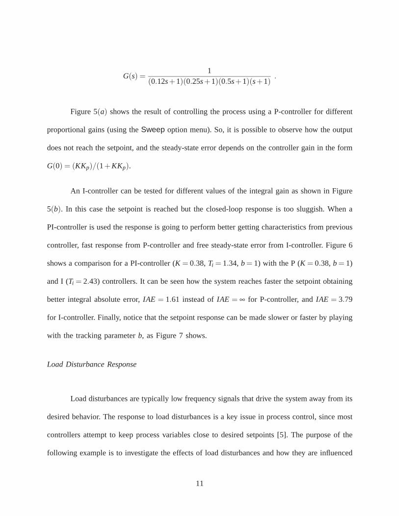
frequency results can also be studied. In order to have a reasonably complete understanding of

a feedback loop, it is essential to consider six responses, the gang of six [5].

In control literature it is customary to show only output responses to steps in load

disturbances or setpoints. At best the control signals required to achieve the responses are also

shown. The development of H∞ theory [8] has shown that it is necessary to show at least six

responses to completely characterize the behavior of a closed-loop system. These responses are

given by

X =PCF

1+PCR+

P1+PC

D− PC1+PC

N (1)

Y =PCF

1+PCR+

P1+PC

D+1

1+PCN (2)

U =CF

1+PCR− PC

1+PCD− C

1+PCN (3)

where P, C and F are the transfer functions for the plant, controller and prefilter respectively. R,

D and N are the Laplace transforms of the reference, load disturbance, and measurement noise,

respectively; and in the same way X , Y and U represent the Laplace transforms of the plant

output without noise, plant output with noise, and the control signal, respectively.

These transfer functions provide very rich information about the control system, and they

can be used to study internal stability, system robustness, the way in which the system reacts to

3

load disturbances and measurement noise, as well as tracking behavior. A possible way to show

this information can be to display the process output and controller output for step commands

in setpoint and load disturbances, as well as the response to noise in the sensor (see Figure 1

in [5]).

Interaction with the tool is straightforward because it is done mainly by using sliders for

controller parameters. Process models can be chosen from a menu which contains a wide range

of transfer functions. It is also possible to enter an arbitrary transfer function with the same

format as in Matlab. The process gain and time delay can be changed interactively. The PID

controller has the structure represented by

U(s) = K

(bYsp −Y +

1sTi

E − sTd

1+ sTd/NdY

), (4)

where K is the proportional gain, Ti the integral time, Td the derivative time, Nd the parameter

of derivative term filter, b is a setpoint weight, and U , Ysp, Y and E are the Laplace transforms

of control signal u, setpoint ysp, process output y and control error e = ysp − y, respectively.

Description of the interactive tool

This section briefly describes the main aspects of PID Basics. The main screen of the

tool is shown in Figure 2.

Notice that the implementation of the modules is reasonably straightforward. Interactive

manipulation of graphical objects is well supported in Sysquake. Numerics for simulation

consist of solving linear differential equations with constant coefficients and simple nonlinearities

representing the saturations. For linear systems the complete system is sampled at a constant

4

sampling rate with zero-order hold and the sampled equations are iterated, which gives

theoretically an exact solution. For systems with saturations, the process and the controller

are sampled separately with first-order holds, the nonlinearities are added, and the difference

equations are then iterated. Delays which are multiples of the sampling period are easily dealt

with because the sampled systems are difference equations of finite order.

Process

The process is characterized by the parameter group located on the left hand side of the

tool screen, just below the icons (see Figure 2). The information contains the process to control,

showing a symbolic representation of the transfer function and several interactive elements to

change the process parameters. From Figure 2 it can be seen that the current example is a fourth

order process with the transfer function

G(s) =Kp

(s+1)n ,

where the interactive parameters are given by Kp (by means of a slider) and n (by means of a text

edit). When the user modifies any plant parameter, the symbolic representation is immediately

updated, with its effect reflected on the rest of IT elements. The user can modify the transfer

function of the process from the Settings menu as shown later.

5

Controller

Five radio buttons are available to select the desired controller; they correspond to propor-

tional (P), integral (I), proportional-integral (PI), proportional-derivative (PD), and proportional-

integral-derivative (PID). Several sliders are available below the radio buttons in order to modify

the controller parameters. The number of sliders shown depends on the chosen controller. For

instance, Figure 2 shows five sliders since the option selected is the PID controller of equation

(4).

Performance and robustness information

Some measures about performance and robustness are provided in order to study the

control designs. The performance category is subdivided into three groups, namely, setpoint

response, load disturbances, and noise response. For the setpoint response the integral absolute

error (IAE) and overshoot (overshoot) measures are given. Integral absolute error (IAE), integral

gain (ki), maximum error (emax), and the time to reach the maximum (tmax) are the information

provided for load disturbances. The integral absolute errors and the maximum error values are

normalized to unit step changes in setpoint and load disturbances. The response to noise is

characterized by the standard deviations of the signals x (signal without noise, sigma x), y

(signal with noise, sigma y), and u (control signal, sigma u). The robustness measures are

maximum sensitivity (Ms), maximum complementary sensitivity (Mt), gain margin (Gm), and

phase margin (Pm). This information can be duplicated in order to compare two designs as

shown below. A deeper description of these measures can be found in reference [5].

6

Graphics

A couple of graphics are shown on the right hand side of the tool (see Figure 2). These

graphics have three representation modes depending on the selected option from Settings menu.

These modes are time domain, frequency domain, and frequency/time domain.

The time domain mode is shown in Figure 2, where the time responses for the system

output (Process Output) and input (Controller Output) are displayed; they provide all the

information evolved in the gang of six (see previous section). There are several interactive

elements on the graphics themselves to interact with the application. The vertical green line

located at time t = 0 allows modifying the setpoint amplitude. The green and black vertical lines

located in the middle of the graphics allow setting the value and instant time for load disturbances

and measurement noise respectively. The vertical and horizontal scales can be modified using

three black triangles available on the graphics (�, �). For instance, in Figure 2, the setpoint is

set to 1, the load disturbance to 0.9 at instant time 32, and the measurement noise to 0.02 at

instant time 60. It is also possible to know the value for the input or output signal at a specific

instant time, by placing the mouse over the curve. Figure 2 shows an example where for the

instant time t = 37.78, the output and input signals are 1.62 and 0.38 respectively. Notice that

all the previous options are available from both graphics, Process Output and Controller Output.

Above the Process Output graphic, there are two checkboxes called save and delete.

These buttons make it easy to store a simulation for comparison. When the save button is

selected, the current design is frozen and displayed in blue. Then, a new design in red appears

allowing to perform a comparison between both designs. Performance and robustness parameters

7

are duplicated showing the values in red and blue colors associated to each design. Legends at

Process Output and Controller Output graphics are also shown with the value of controller

parameters for both designs. Figure 2 shows an example which compares response of PI (K =

0.43, Ti = 2.27, b = 0) and PID (K = 1.13, Ti = 3.36, Td = 1.21, b = 0.54, Nd = 10) controllers for

a process with the transfer function P(s) = 1/(s+1)4. The PID controller gives a better response

to load disturbances by reacting faster, but the noise also generates more control action. The

delete option can be selected in order to remove the undesired design. Note that if the transfer

function of the process or some input signal (setpoint, load disturbance, and measurement noise)

are modified, both sets of results are affected simultaneously. The number of saved designs has

been constrained to two in order to keep a simple user interface.

The last options for the time domain mode are shown above the Controller Output

graphic. Such options show the proportional (P), integral (I), and derivative (D) signals of the

controller. Figure 3 shows an example where the black signal represents the proportional action,

the blue one the integral action, the pink one the derivative action, and the red one the PID

control signal.

The aspect of the frequency domain mode is shown in Figure 4. Once this mode is selected

from the Settings menu, the left side of the tool remains untouched; on the right side, the time

response graphics are replaced by frequency domain ones, Transfer function Magnitude and

Transfer function Phase. The graphics allow the user to modify the vertical and horizontal

scales interactively in the same way that in the time domain, and also to visualize the magnitude

and phase for a specific frequency ω by placing the mouse over the signals. Figure 4(a) shows

an example where the value of ω = 2.15 rad/s is shown in the status bar at the bottom of the

8

tool. The frequency response for the gang of six transfer functions and the open loop transfer

function L(iω) = P(iω)C(iω) can be shown in the graphics using checkboxes placed above the

Transfer function Magnitude graphic (the names of the checkboxes are shown using the relation

of the sensitivity S = 11+PC and complimentary sensitivity T = PC

1+PC functions with the rest of

transfer functions; for instance, PS = P 11+PC ). Figure 4(a) shows an example where all transfer

functions are shown.

It is also possible to show time and frequency domains simultaneously. An example can

be seen in Figure 4(b). The upper graphic represents time domain, and the lower one represents

frequency domain. The default screen shows the output and the magnitude for the time and

frequency domains, respectively. Above the graphics, there exists a couple of radio buttons

which let the user choose between the output or input for time domain, and magnitude or phase

for frequency domain. This mode is very interesting since it is possible to observe the effect of

parameter modifications on both domains simultaneously.

Settings menu

The Settings menu is available in the main menu of PID Basics and is divided into

six groups. From the first entry, Process transfer function, several processes can be selected,

being also available an option to enter an arbitrary transfer function in the numerator (num) and

denominator (den) form used in Matlab. Specific values for controller parameters can be entered

using the Controller parameters menu option. The third entry, Time/Frequency domain,

allows choosing between the three modes commented above, namely, Time domain, Frequency

domain, and Both domains. Results can be stored and recalled using the Load/Save menu

9

(using the options Save design and Load design respectively). The option Save report helps

to save all essential data in ascii format, this possibility being useful for documenting results.

The menu selection Simulation fits the simulation time, the maximum time delay (in order

to avoid slow simulations), and to active the Sweep option to show the results for several

controller parameters simultaneously; that is, it is possible to study the effect of any controller

parameter between specific minimum and maximum values. This last option is only available

in time domain mode. When it is active, new radio buttons appear in the controller parameters

zone to permit the selection of the desired parameter to sweep. The last menu option, Examples

Advanced PID Book, allows loading examples from the book [5], in such a way that the user

can begin with such examples to explore what happens when the parameters are modified.

Illustrative Examples

Some examples extracted from reference [5] are presented in order to test the capabilities

of the tool.

Setpoint response

The response to setpoint is important when making grade changes in process control.

Tracking setpoint is a key issue in motion control. The purpose of this example is to explore

how the setpoint response of the system is influenced by the controller parameters. The load

disturbance and noise amplitude are set to zero using the interactive vertical lines. The transfer

function of the process is given by

10

G(s) =1

(0.12s+1)(0.25s+1)(0.5s+1)(s+1).

Figure 5(a) shows the result of controlling the process using a P-controller for different

proportional gains (using the Sweep option menu). So, it is possible to observe how the output

does not reach the setpoint, and the steady-state error depends on the controller gain in the form

G(0) = (KKp)/(1+KKp).

An I-controller can be tested for different values of the integral gain as shown in Figure

5(b). In this case the setpoint is reached but the closed-loop response is too sluggish. When a

PI-controller is used the response is going to perform better getting characteristics from previous

controller, fast response from P-controller and free steady-state error from I-controller. Figure 6

shows a comparison for a PI-controller (K = 0.38, Ti = 1.34, b = 1) with the P (K = 0.38, b = 1)

and I (Ti = 2.43) controllers. It can be seen how the system reaches faster the setpoint obtaining

better integral absolute error, IAE = 1.61 instead of IAE = ∞ for P-controller, and IAE = 3.79

for I-controller. Finally, notice that the setpoint response can be made slower or faster by playing

with the tracking parameter b, as Figure 7 shows.

Load Disturbance Response

Load disturbances are typically low frequency signals that drive the system away from its

desired behavior. The response to load disturbances is a key issue in process control, since most

controllers attempt to keep process variables close to desired setpoints [5]. The purpose of the

following example is to investigate the effects of load disturbances and how they are influenced

11

by the controller type and parameter settings. The setpoint and noise amplitudes are set to zero,

and the load disturbance is set to 0.9 at instant time t = 0. The process transfer function is given

by

G(s) =1

(s+1)4 .

Firstly, a comparison between a P-controller (K = 0.6, b = 1) and PI-controller (K = 0.6,

Ti = 2, b = 1) is displayed in Figure 8. It can be observed how the P-controller does not eliminate

the effect of the disturbances, while the PI-controller does. This fact can be corroborated from

the transfer function Gyd = YD = P

1+PC , where for a P-controller Gyd(0) = Kp1+KKp

� 1K , and for a

PI-controller Gyd(0) = 0.

So, as commented above, the response of the process variable to load disturbances is

given by [5]

Gyd =P

1+PC= PS =

TC

.

For a system with P(0) �= 0 and a controller with integral action the previous transfer

function can be approximated by [5]

Gyd =TC

≈ 1C

≈ Cki

,

12

where ki = KTi

is the integral gain. Since load disturbances typically have low frequencies the

previous equation is a good measure of load disturbance rejection. So, large values of ki provide

adequate load disturbance responses.

Figure 9 shows the load disturbance responses for two PI controllers with ki values of

0.36 (in red color) and 0.30 (in blue color). As the previous equation indicates, the controller

with larger integral gain leads to better results to load disturbances, obtaining a faster response

and smaller values for IAE and emax, but the stability margins are reduced, as can be observed

from the robustness parameters. Figure 10 shows the frequency responses of Gyd and S for two

PI controllers with large (ki = 0.85) and small (ki = 0.30) values of ki. From this figure, it can

be noticed that large values of ki imply large peaks of the sensitivity function. So, it is necessary

to reach a tradeoff between load disturbance rejection and robustness.

Some tuning methods allow obtaining good compromises between robustness and load

disturbance response. The Approximate M constrained integral gain optimization (AMIGO) [5],

[9], [10], [11] is one of these methods which, in the same way as the well-known Ziegler and

Nichols method [12], [13], focusses on load disturbances by maximizing integral gain but also

adding a robustness constraint. For the previous example, the result of applying this method

is shown in Figure 11. The AMIGO-step method has been used to design a PI controller with

K = 0.414 and Ti = 2.66. A slow response to load disturbances is obtained but with good stability

margins.

13

Response to measurement noise

Measurement noise is a disturbance that distorts the information about the process

obtained by the sensors. Measurement noise typically has high frequencies, and is fed into

the system by feedback. This phenomenon creates control actions and variations in the process

output, being important that measurement noise does not generate too large control actions. The

next example shows how measurement noise affects the system and how this influence can be

reduced [5]. The process transfer function is given by

G(s) =1

(0.01s+1)(0.04s+1)(0.2s+1)(s+1).

Figure 12 shows a simulation for two PID controllers where the measurement noise has been set

to 0.02, and the setpoint and load disturbance amplitudes to zero. A PID controller with K = 1,

Ti = 1, Td = 0.9, b = 0.5, and Nd = 10 is represented in red color. As seen, large control actions

are obtained for this controller. This performance can be improved increasing the filtering effect

[5]. So, the same controller is used but the Nd parameter is reduced to 1.5, showing the results in

blue color. From the figure it can be observed how the control action variations are considerably

reduced.

The previous results can be corroborated from the gang of six transfer functions [5]. The

transfer function that relates the control signal with the measurement noise is given by

Gun =C

1+PC= CS =

TP

,

where, as measurement noise typically has high frequencies, this transfer function can be

14

approximated by Gun = C. So, for a classical PID controller (4), at high frequencies |Gun|

becomes infinite due to the derivative term, which clearly indicates the necessity of filtering

the derivative term. This fact can be tested for the previous time domain example, using the

frequency domain mode in PID Basics. A simple index of the effect of measurement noise is

the largest gain of the transfer function Gun [5]

Mun = maxω

|Gun(iω)| .

Figure 13 shows the frequency responses of |Gun| for the previous two controllers with

Nd = 10 and Nd = 1.5. The magnitude is considerably reduced for Nd = 1.5 being the maximum

value ≈ 3, whereas for Nd = 10 the maximum magnitude is ≈ 11.

PID LOOP SHAPING

There are many interesting issues that have to be dealt with when developing IT for

control that are related to the particular graphics representations used. It is straightforward to

see the effects of parameters on the graphics but not so obvious how the graphical objects must

be manipulated. There are natural ways to modify pole-zero plots, for instance by adding poles

and zeros and by dragging them. Bode plots can be manipulated by dragging the intersections

of the asymptotes. Nevertheless, it is less obvious how a Nyquist plot should be changed. The

tool presented in this section, called PID Loop Shaping, shows the Nyquist plots of the process

transfer function P(s) and the loop transfer functions L(s) = P(s)C(s) (see Figure 14).

15

Description of the interactive tool

This section describes briefly the different elements of PID Loop Shaping and some easy

theoretical aspects.

Process

This description of PID Loop Shaping is very similar to the PID Basics one. However,

the process transfer function is presented as a pole-zero interactive graphic in the s-plane instead

of a symbolic representation. The process transfer function can be modified depending on the

option selected from the Settings menu. Several examples of transfer function are available, and

its parameters can be modified using sliders as in PID Basics. However, a free transfer function

can be selected (Interactive TF menu option), where poles and zeros can be defined graphically

as Figure 14 shows.

Controller

This zone of the tool shows the different parameters and capabilities of PID Loop Shaping

in order to perform loop shaping. Loop shaping is a design method where a controller is chosen

such that the loop transfer function reaches the desired shape. The key idea is that the action

of the controller can be interpreted as mapping the process Nyquist plot to the Nyquist plot of

the loop transfer function. This mapping is performed to a specific design frequency ω . This

frequency determines the desired point to move on the process transfer function, called design

point. Such point is shown by a green circle on the L-plane graphic. The corresponding point

16

at this frequency on the loop transfer function is called target point.

The controller representation used in PID Loop Shaping is given by the following

parametrization [5]

C(s) = k +ki

s+ kds.

The loop transfer function is thus,

L(s) = kP(s)+(ki

s+ kds

)P(s).

The point on the Nyquist curve of the loop transfer function corresponding to the

frequency ω is thus given by

L(iω) = kP(iω)+ i(− ki

ω+ kdω

)P(iω). (5)

PID Loop Shaping provides three ways to tune the parameters in order to move the

process transfer function from the design point to the target point. These ways are shown at the

section Tuning being called Free, Constrained PI, and Constrained PID. The first one allows

performing the loop shaping dragging on the control parameters, and using the other two ones,

the controller parameters are calculated based on some constrains on the target point. That is,

the focus can be set on how the loop transfer function change when controller parameters are

modified, or conversely, what parameters are required to obtain a given shape of the loop transfer

function. For PI and PD control the mapping can be uniquely represented by mapping only one

point (x+ yi). For PID control it is also possible to have an arbitrary slope of the loop transfer

17

function at the target point (x + yi, and ϑ ). When the Free tuning option has been selected,

some sliders appear in order to modify the controller gains k, ki, and kd as shown in Figure 14,

where the controller type can be chosen. The controller gains can also be changed by dragging

arrows as illustrated in the same figure. From equation (5), the proportional gain changes L(iω)

in the direction of P(iω), integral gain ki changes it in the direction of −iP(iω), and derivative

gain kd changes it in the direction of iP(iω).

For Constrained PI and Constrained PID tuning options, the target point can be

constrained to move on the unit circle, the sensitivity circles, or to the real axis. In this way it is

easy to make loop shaping with specifications on gain and phase margins or on the sensitivities.

In the case of Constrained PI it is necessary to find controller gains providing the desired target

point. So, dividing equation (5) by P(iω) and taking real and imaginary parts [5],

k = ℜ(L(iω)

P(iω)

), (6)

− ki

ω+ kdω = ℑ

(L(iω)P(iω)

)= A(ω). (7)

Equations (6) and (7) gives directly the parameters of a PI controller with kd = 0. An

additional condition is required for Constrained PID tuning option. So, it is observed that,

L′(s) = C′(s)P(s)+C(s)P′(s) = C′(s)P(s)+L(s)P′(s)

P(s)=

=(− ki

s2 + kd

)P(s)+

L(s)P′(s)P(s)

.

18

The slope of the Nyquist curve is then given by

dL(iω)dω

= iL′(iω) = i( ki

ω2 + kd)P(iω)+ iC(iω)P′(iω) .

This complex number has the argument ϑ if,

ℑ(iL′(iω)e−iϑ)

= 0,

that implies that,

ki

ω2 + kd =ℜ

(L(iω)

P′(iω)P(iω)

e−iϑ)

ℜ(

P(iω)e−iϑ) = B(ω). (8)

Combining equation (8) with equations (6)-(7) gives the controller parameters,

ki = −ωA(ω)+ω2B(ω), (9)

kd =A(ω)

ω+B(ω). (10)

where A(ω) and B(ω) are given by equations (6)-(8).

The frequency design ω , which determines the design point, can be chosen using the slider

wdesign and graphically by dragging on the green circle on the process Nyquist curve (black

curve). The target point on the Nyquist plot and its slope can be dragged graphically. The slope

can also be changed using the slider slope. Furthermore, it is possible to constrain the target using

the Constraints radio buttons. The target point can be constrained to the unit circle (Pm), the

negative real axis (Gm), circles representing constant sensitivity (Ms), constant complementary

sensitivity (Mt), or constant sensitivity combinations (M). When sensitivity constraints are active,

the associated circles are drawn on the L-plane plot and some sliders appear in order to allow

19

modifying their values. The circles are defined as described in Table [5].

Figure 14 illustrates designs for two PID controllers and a given sensitivity. The target

point is moved to the sensitivity circle and the slope is adjusted so that the Nyquist curve is

outside of the sensitivity circle. The red design shows a PID controller using Free tuning, and

the blue one a Constrained PID.

Robustness and performance parameters

This zone is located below the controller parameters (see Figure 14), showing parameters

that characterize robustness and performance in the same way that in PID Basics. The

measures are maximum sensitivity (Ms), the sensitivity crossover frequency (Ws), maximum

complementary sensitivity (Mt), the complementary sensitivity crossover frequency (Wt), gain

margin (Gm), gain crossover frequency (Wgc), phase margin (Pm), and phase crossover

frequency (Wpc).

L-plane Graphic

It represents the right side of PID loop shaping, as can be seen in Figure 14. This graphic

contains the Nyquist plots of the process transfer function P(s) (in black) and the loop transfer

functions L(s) = P(s)C(s) (in red). Three different views can be shown depending on the tuning

options. Figure 15 shows two views, one for free tuning and another one for constrained PID

tuning. A third view is shown in Figure 14 where two designs are shown simultaneously. The

design and target points can interactively be modified on this graphic. The design point is shown

in green color on the Nyquist curve of the process. The target point is represented in light green

20

color (in the case of free tuning), or in black color (for constrained tuning) as in Figure 14. The

slope of the target point can also be changed interactively.

For free tuning, the controller gains are shown as arrows on the Nyquist plane. The

controller gains can interactively be modified by dragging on the ends of the arrows. Examples

of these arrows are shown in Figures 14 and 15. The scale of the graphic can be changed using

the red triangle located at the bottom of the vertical axis.

As commented above, it is possible to impose constraints on the target point. The

graphical representation of the target point is modified depending on the constraint selected,

restricting its value based on its meaning. Therefore, various target point locations are given

based on the active constraint as Figure 16 shows.

On the top of L-plane graphic the options save and delete can be found. These options

have the same meaning that in PID Basics, being possible to save designs in order to perform

comparisons. Once the save option is active, two pictures appear showing in red color the current

design and in blue the second one (see Figure 14). Then, the modifications on the controller

parameters affect to the current (active) design. The current design can be changed using the

options Design 1 and Design 2 shown on the top of L-plane graphic. Thus, once the current

design is chosen, the associated curve is changed to red color and the controller zone is modified

based on that design. The controller gains values can be shown locating the mouse on the curves.

21

Settings menu

The Settings menu is available on the top menu of PID Loop Shaping and divided into

four groups, following the same structure that in PID Basics. From the first entry, Process

transfer function, several processes can be selected, being also available two options to include

free transfer functions. One of them, called String TF..., allows including a transfer function in a

symbolic way. For instance, P(s) = 1/cosh√

s can be represented as P=’1/cosh(sqrt(s))’.

The alternative option is active to define the process transfer function using the interactive pole-

zero representation at the Process zone. Results can be stored and recalled using the Load/Save

menu. From this menu, data can be saved and recalled using the options Save design and

Load design, respectively. The option Save report can be used to save all essential data in

ascii format, being this possibility useful for documenting results. Specific values for control

parameters can be entered by Parameters menu option. As in PID Basics, the last menu option

(Examples Advanced PID Book) allows loading examples from the book [5].

Illustrative Examples

Some of the capabilities in PID Loop Shaping are shown by means of some examples.

Effect of controller parameters. Free tuning.

As commented above, understanding how the Nyquist plot of the compensated system

changes based on the controller parameters is sometimes complicated. This example has the

purpose of showing basic exercises about this issue.

22

Consider the same process used in PID Basics to study load disturbances, where the

transfer function is given by P(s) = 1/(s + 1)4. When a P-controller is used, the proportional

gain changes the loop transfer function L(iω) = kP(iω) in the direction of P(iω). Figure 17(a)

shows the effect of modifying L(iω) using two proportional controllers. The blue curve is for

k = 2 and the red one for k = 2.6. So, it can be seen how the proportional gain modifies the

Nyquist plot of the process (black curve) at frequency ω (green circle on the black curve) in

the direction of P(iω). Figure 17(b) shows the same study for an I-controller with ki = 1 (red

curve) and ki = 0.6 (blue curve). It is observed how the integral gain ki changes L(iω) in the

direction −iP(iω) (the derivative gain has the same effect but in the direction iP(iω)). When PI

or PD controllers are used, the compensated point at frequency ω is calculated as the sum of two

vectors, the proportional vector, and the integral or derivative one. Examples of this capability

are shown in Figures 17(c) and (d), where the process is controlled by a PI controller (k = 2.3

and ki = 0.7) and PD controller (k = 2.1 and kd = 3.35), respectively.

Some easy exercises can be performed in order to gain skills on the Nyquist plane. For

instance, using the previous process, it can be of interest to obtain the gain for a proportional

controller where the closed-loop system changes from stable to unstable. Before playing on PID

Loop Shaping, the result can be calculated analytically as follows

∠L(iω) = ∠C(iω)P(iω) = −180, ∠k1

( jω +1)4 = −180, ω = 1.

|L(iω)| = |C(iω)P(iω)| = |−1+0 j|, |k 1( jω +1)4 | = −1, k = 4.

So, PID Loop Shaping can be used to interactively verify the result, as Figure 18 shows.

23

This kind of exercises challenges the students and encourage them to make observations and

relate theory with pictures in order to develop a broader and deeper understanding.

On the other hand, free interactive designs can also be performed to compare the results

with consolidated design methods. For instance, PID Loop Shaping can be used to interactively

design a PID controller for the previous process where the maximum sensitivity value is required

to be less than 1.5 (Ms ≤ 1.5). After playing with the IT, a PID controller that fulfils this

constraint is obtained where k = 0.92, Ti = 1.8, ki = 0.5, Td = 1.03 and kd = 0.95. Then, the

AMIGO-frequency method can be used to perform the same design and to compare the results.

The controller obtained is given by k = 1.2, Ti = 2.48, ki = 0.48, Td = 0.93 and kd = 1.12. Figure

19 shows the Nyquist plots and time responses (using PID Basics) for both designs, in blue color

for the free PID controller and in red for the AMIGO method. The obtained Ms values are 1.49

for free PID and 1.46 for AMIGO method. The results are very similar, but the smaller Ms value

of AMIGO gives better robustness properties and load disturbances rejection.

Effect of target point. Constrained designs.

The target point on the Nyquist plot can be reached using a free constraint design.

Thus, the controller gains are interactively adjusted in order to perform this task as shown in

the previous example. Nevertheless, another way is to use the equations (6)-(10), where the

controller gains are calculated once the target point is defined. As discussed above, the target

point can freely be fixed, or constrained in various ways: any point x+ y j, or constrained to a

specific value for phase margin, gain margin, or maximum values of the sensitivity functions.

Figure 20 shows an example where the target point has been set to the point −0.5− 0.5 j.

24

Two constrained designs are shown for a design frequency ω = 0.6. The red curve represents

a compensated system by a constrained PID with k = 1.32, ki = 1.02 and kd = 2.15, while the

blue one represents a constrained PI with k = 1.32 and ki = 0.15. Both controllers reach the

target point, but better results are obtained for the PID controller due to the slope, allowable

third degree of freedom (9)-(10), where for this example the slope ϑ takes the value 22. PID

controller provides better robustness properties getting Ms = 1.45, ki = 1.02, Gm = 5.32, and

Pm = 40.15, versus PI controller with Ms = 1.83, ki = 0.15, Gm = 2.69, and Pm = 75.77.

Similar examples to restrict the target point for phase margin, gain margin, or maximum

values of the sensitivity functions can be performed, as represented in Figure 16. Figure 21(a)

shows an example where a combined sensitivity constraint is required for Ms ≤ 2 and Mt ≤ 2. This

constraint is fulfilled in two different ways using a constrained PID (in red) and a constrained PI

(in blue). Another example combining sensitivity function and gain margin constraints is shown

in Figure 21(b), with the specification that the gain margin is equal to 3 and Ms ≤ 2, maximizing

the integral gain ki. So, the constraint gain margin is chosen and the target point is located in

such a way that Gm = 3. Then, a constrained PID controller is selected, being the design point

and the slope modified until Ms ≤ 2 and the integral gain is maximized. The controller obtained

is given by k = 1.38, ki = 0.52, and kd = 0.54 for ω = 1.02 and slope = 32.

The derivative cliff

This example is available at the Settings menu of PID Loop Shaping [5]. The process

transfer function is the same as in previous examples (P(s) = 1/(s+1)4). It is desired to maximize

integral gain ki subject to the robustness constraint Ms ≤ 1.4. The obtained controller provides

25

the parameters k = 0.925, ki = 0.9, and kd = 2.86 where the Nyquist plot of the loop transfer

function is shown in red in Figure 22(a). It can be observed that the Nyquist curve has a loop.

This phenomenon is called derivative cliff (a deeper explanation can be found in [5]) and it is

due to the fact that the obtained controller has excessive phase lead, which is obtained by having

a PID controller with complex poles (Ti < 4Td , in this example Ti = 0.33Td). Figure 22(b) shows,

in red color, the time response of this controller obtaining oscillatory outputs. For comparison,

the results for a controller with Ti = 4Td are shown in blue color in Figures 22(a) and (b) with

the controller parameters k = 1.1, ki = 0.36 and kd = 0.9. The responses for this controller are

better, even under larger overshoot in response to load disturbance.

Delayed system

Dead-times appear in many industrial processes, usually associated with mass or energy

transport, or due to the accumulation of a great number of low order systems. Dead-times produce

an increase in the system phase lag, therefore decreasing the phase and gain margins and limiting

the response speed of the system (system bandwidth) [14], [15].

An example is described in what follows in order to see the influence of the time delay.

The process transfer function is given by

P(s) = Pn(s)e−tds =e−10s

2s+1,

where Pn(s) represents the delay-free system Pn(s) = 12s+1 .

26

The control for Pn(s) is performed using a PI controller with k = 2.5, ki = 3.58, Ti = 0.7,

obtaining an infinite gain margin. Figure 23 shows the Nyquist plot and the time responses

obtaining fast tracking results and very good load disturbances rejection (notice that ki = 3.58).

When the same PI controller is used to control the plant with delay P(s), the system becomes

unstable as Figure 24 shows. Notice the circles on the Nyquist plot of the process (black). Dead-

times augments the system phase as frequency increases in the form ϕ = −tdω (being ϕ the

phase lag provided by the dead-time). Hence, the circles appear when large values of the system

phase are represented in the Nyquist plot.

Therefore, in order to control the system, it is necessary to reduce its bandwidth,

decreasing the values of the proportional and integral gains. Figure 25 shows the compensated

system for the control parameters k = 0.33, ki = 0.07, Ti = 4.57. The system becomes stable,

but at cost of having very slow responses (see the time scale in Figure 23(b) and Figure 25(b))

and poor load disturbance rejection (notice that ki = 0.07). Some alternative design techniques

can be used to obtain better results [5], [10], [11].

PID WINDUP

Many aspects of PID control can be understood using linear models. There are, however,

some important nonlinear effects that are very common even in simple loops with PID control.

Integral windup can occur in loops where the process has saturations and the controller has

integral action. When the process saturates, the feedback loop is broken and the integral may

reach large values maintaining the control signal saturated for a long time, resulting in large

overshoots and undesirable transients [5].

27

The purpose of this module is to facilitate the understanding of integral windup and

a method for avoiding it (see [5]). There are many different ways to protect against windup.

Tracking is a simple method illustrated in the block diagram in Figure 26. As well-known in the

anti-windup schemes, the system remains free when the saturation is not active. However, when

saturation occurs, the integral term in the controller is modified until the system is out of the

saturation limit, where the modification of the integral element is not performed instantaneously

but dynamically with a time constant Tt [5].

The module shows process outputs and control signals for unlimited control signals,

limited control signals without anti-windup, and limited control signals with anti-windup (see

Figure 27). Process models and controller parameters can be selected in the same way as in the

other modules. The saturation limits of the control signal can be determined either by entering

the values or by dragging the lines in the saturation metaphor. The main aspects of the tool and

some illustrative examples are shown in the following paragraphs.

Description of the interactive tool

This section briefly describes the main aspects of PID Windup. The main screen of the

tool is shown in Figure 27.

Process

It corresponds to the same Process zone that in previous tools. It provides the same

elements that in PID Basics, where a symbolic representation of the process transfer function

is available, and the process parameters can be modified by interactive sliders or text edits (see

28

Figure 27). The time delay is modified using a slider instead of a text edit as in PID Basics

or PID Loop Shaping. Then, the time delay effect on the anti-windup mechanism can be easily

analyzed.

Controller

This section contains the information about the controller parameters and actuator

saturation. Three kind of controllers with integral action can be selected (I, PI, PID), where

several sliders are available to modify the controller parameters including the tracking time

constant Tt used to reduce the integral effect. A saturation metaphor graphic is also available

in this zone. This graphic allows determining the saturation limits dragging on the small red

circle located on the upper saturation value (notice that a symmetric saturation has been used;

this choice has been selected for pedagogical purposes).

Graphics

Time responses for process output, control signal, and integral action are available in three

different graphics (Process Output, Controller Output, Integral term). In the same way that in

PID Basics, there exist multiple interactive graphical elements to modify, namely, setpoint, load

disturbance, measurement noise, and horizontal and vertical scales (see Figure 27). These three

graphics can simultaneously represent the controlled system in linear mode, nonlinear mode with

windup phenomenon, and nonlinear mode with anti-windup technique. Such representations can

be configured using the checkboxes located on the top of Process Output graphic. There are

three checkboxes called Linear, Windup, and Antiwindup to include the associated signal in

29

all graphics, that contain a legend for the three signals, showing the linear mode in red, windup

mode in blue, and antiwindup one in green color. An example can be seen in Figure 28(a) where

the three modes are active.

A dotted pink vertical line that makes it easier to compare the time in the plots is also

available as Figure 28(a) shows. On the other hand, the saturation limits can be modified using

the dotted blue horizontal lines available in the Controller Output graphic (see Figure 28).

The notion of proportional band is useful to understand the windup effect and is included

in PID Windup. The proportional band is defined as the range of process outputs where the

controller output is in the linear range [ymin,ymax]. For a PI controller, the proportional band is

limited by

ymin = bysp +I−umax

K,

ymax = bysp +I−umin

K,

where I is the integral term of a PI controller.

The same expressions hold for PID control whether the proportional band is defined

as the band where the predicted output yp = y + Tddydt is in the proportional band [ymin,ymax].

The proportional band has the width (umax − umin)/K and is centered at bysp + I/K − (umax +

umin)/(2K).

On the top of figure Process Output there are two additional checkboxes called PB

Windup and PB Antiwindup. The activation of these options shows the proportional bands for

the windup and antwindup cases in the Process Output graphic. The proportional bands are

30

shown as dotted green and blue signals respectively, as Figure 28(b) shows.

Settings menu

The Settings menu is defined following the same structure as in previous modules.

The process transfer function can be chosen from the entry Process transfer functions, and

numerical values of the parameters can be introduced using the selection Controller parameters.

Essential data and results can be saved and recalled using the Load/Save menu options. The

menu selection Simulation makes it possible to choose the simulation time, and to activate

the Sweep option that can be used to show the results for several values of the tracking time

constant (as are shown later in an example). Several examples from [5] can be loaded from the

Examples entry.

Illustrative Examples

Some examples to explain integral windup are going to be described using PID Windup.

Understanding Windup Phenomenon

The windup phenomenon can be studied using the first entry from the Examples option

menu. This example has been extracted from [5] and uses a pure integrator process P(s) = 1s

controlled by a PI controller with K = 1, Ti = 1.2, b = 1 with the control signal limited to ±0.1.

Figure 29(a) shows the time responses for this example. The control signal is saturated from the

first time instant. The process output and the integral term are increasing while the control error

is positive. Once the process output exceeds the setpoint, the control error turns to be negative,

31

but the control signal remains saturated due to the large value of the integral term (windup

phenomenon). Looking at the dotted pink vertical line in Figure 29(a), the integral term reaches

its largest value at t = 10, when the error goes through zero. So, the control signal does not

leave the saturation limit until the error has been negative for a sufficiently long time to let the

integral part come down to a small level. An interesting aspect can be observed in Figure 29(b),

as the control signal is working in linear mode when the process output reaches its maximum

value.

The proportional band can be drawn in this example using the PB Windup checkbox

(Figure 30(a)). It can be tested (using the vertical line) how the process output remains inside

of the band while the control signal is working in linear mode, and outside in other case. The

proportional band is too narrow because the system is working in nonlinear mode during a

long time. Hence, an interesting correspondence of the proportional band narrowness and the

controller gain can be obtained. Large controller gains provide narrow proportional bands (more

energetic control signals and therefore more saturation time), and small controller gains gives

wider proportional bands. Figure 30(b) displays this comment, where the proportional controller

gain has been reduced to 0.2, producing a wider proportional band.

Anti-windup

The previous example is useful to understand the anti-windup technique by visualization.

The same controller parameters have been used (K = 1, Ti = 1.2, b = 1) and the tracking time

constant has been set to Tt = 1. Figure 31(a) shows the results where outputs for controller with

(in green) and without (in blue) anti-windup can be observed. The improvements achieved with

32

anti-windup are notorious. Now, the system only remains in saturation for a short time period,

being the output of the integral term considerably reduced. The proportional band for PI controller

with anti-windup is shown in the same figure. It can be observed how a wider proportional band

than for PI without anti-windup (Figure 31(a)) is obtained, remaining the process output inside

of it most of the time. The effect of the tracking time constant is illustrated in Figure 31(b)

for Tt = 0.1, 10, 50 (the Sweep menu option has been used). Very large values of Tt bring the

result to the windup phenomenon producing large integral signals, while small values reset the

integral term quickly getting better results. It may thus seem advantageous to have always very

small values of Tt . However, the next example shows some situations where this choice is not

always advisable.

The tracking time constant

The tracking time constant is an important parameter because it determines the rate of

resetting the integral term of the controller. It seems to be advantageous to have a small value for

this constant. Nevertheless, measurement errors may accidentally reset the integral term whether

the tracking time constant is too small. The following example tries to explain this fact, where

there is a measurement error in the form of a short pulse. The transfer function of the process

is given by

P(s) =1

(0.5s+1)2 ,

and the system is controlled using a PID with K = 3.5, Ti = 0.52, Td = 0.14, Nd = 10, b = 1,

and Tt = 1.

Figure 32(a) shows the control results. Notice the large transient after the pulse. The

33

integral term is excessively reduced, even reaching negative values. Some simple rules that have

been suggested for the tracking time, Tt =√

TiTd and Tt = (Ti +Td)/2 [5], can be used to tune Tt

and avoid these problems. Figure 32(b) shows an example with Tt = (Ti +Td)/2 = 0.33 where

the response has been considerably improved.

CONCLUSION

In this work a set of interactive modules have been presented as support for teaching basic

automatic control concepts. These tools have as main objective the addition of interactivity to the

visual content of [5]. The modules are focused on PID control studying feedback fundamentals

from the point of view of the time and frequency domains, including the robustness problem,

measurement noise filtering, load disturbance rejection, and windup phenomenon.

The role of interactivity in automatic control education has been shown presenting

the powerful of this element in Teaching. In our personal experience, interactivity is an

excellent element as support to teaching and learning that allows to enhance the motivation and

participation of the future engineers. Authors animate to the readers to test these new interactive

features in control education and engineers’ training.

34

REFERENCES

[1] J. L. Guzman, M. Berenguel, and S. Dormido, “Interactive teaching of constrained

generalized predictive control,” IEEE Control Systems Magazine, vol. 25, no. 2, pp. 79–85,

2005, available at http://aer.ual.es/siso-gpcit/.

[2] M. Johansson, M. Gafvert, and K. J. Astrom, “Interactive tools for education in automatic

control,” IEEE Control Systems Magazine, vol. 18, no. 3, pp. 33–40, 1998.

[3] J. L. Guzman, “Interactive Control System Design,” PhD Thesis, University of Almerıa,

Spain, available at http://www.ual.es/∼joguzman/PhdThesisGuzman.pdf.

[4] J. Sanchez, S. Dormido, and F. Esquembre, “The learning of control concepts using

interactive tools,” Computer Applications in Engineering Education, vol. 13, no. 1, pp.

84–98, 2005.

[5] K. J. Astrom and T. Hagglund, Advanced PID Control. ISA - The Instrumentation,

Systems, and Automation Society. Research Triangle Park, NC 27709, 2005.

[6] Y. Piguet, SysQuake 3 User Manual, Calerga Sarl, Lausanne (Switzerland), 2004, Available

at http://www.calerga.com.

[7] J. L. Guzman, K. J. Astrom, S. Dormido, T. Hagglund, M. Berenguel, and Y. Piguet,

Interactive Learning Modules for Feedback Fundamentals using PID Control, 2006,

Available at http://aer.ual.es/ilm/.

[8] G. Zames and B. Francis, “Feedback, minimax sensitivity, and optimal robustness,” IEEE

Transactions on Automatic Control, vol. 28, no. 5, pp. 585–601, 1983.

[9] T. Hagglund and K. J. Astrom, “Revisiting the Ziegler-Nichols tuning rules for PI control,”

Asian Journal of Control, vol. 4, no. 4, pp. 364–380, 2002.

35

[10] ——, “Revisiting the Ziegler-Nichols step response method for PID control,” Journal of

Process Control, vol. 14, no. 6, pp. 635–650, 2004.

[11] ——, “Revisiting the Ziegler-Nichols tuning rules for PI control - part II, the frequency

response method,” Asian Journal of Control, vol. 6, no. 4, pp. 469–482, 2004.

[12] J. G. Ziegler and N. B. Nichols, “Optimum settings for automatic controllers,” Transactions

of the ASME, vol. 64, pp. 759–768, 1942.

[13] ——, “Process lags in automatic-control circuits,” Transactions of the ASME, vol. 65, no. 5,

pp. 433–443, 1943.

[14] T. Hagglund, “An industrial dead-time compensating PI controller,” Control Engineering

Practice, vol. 4, no. 6, pp. 749–756, 1997.

[15] J. Normey-Rico, C. Bordons, and E. Camacho, “Improving the robustness of dead-time

compensating PI controllers,” Control Engineering Practice, vol. 5, no. 6, pp. 801–810,

1997.

36

0 10 20 30 40 50 600

0.5

1

1.5

y

0 10 20 30 40 50 60−0.5

0

0.5

1

1.5

2

u

Figure 1. Basic feedback system properties. In order to have a reasonably completeunderstanding of a feedback loop, it is essential to consider six responses. In [5] these responsesare refereed to as the gang of six (1)-(3). A possible way to show this information can be showingprocess output and controller output for step commands in setpoint and load disturbances, aswell as the response to noise in the sensor, such as shown in this figure. Figure taken from [5].

37

Figure 2. The user interface of the module PID Basics. The plots show the time responseof the Gang of Six transfer functions [5]. Several interactive graphical elements, shown on thesame screen, are used to interactively analyze feedback fundamentals using PID control. In theexample of this picture it is shown a comparison between PI (blue) and PID (red) controllers.

38

Figure 3. PID actions on graphic Controller Output. This graphic shows the simulated controlsignal for the selected controller being possible to study the evolution of the proportional, integral,and derivative actions separately. This possibility provides a great interest from a pedagogic pointof view.

39

(a) Frequency Domain (b) Frequency and Time domains simultaneously

Figure 4. Time and Frequency domains on the interactive tool. The study of a control problemis usually performed in time and frequency domains in order to analyze several properties.However, this study is often developed separately without combining both domains at the sametime. With PID Basics it is possible to work with both domains simultaneously or in a separateway. Therefore, it is possible to observe, in an intuitive way, how a modification parameteraffects to both domains by means of the interactive features of the tool.

40

(a) Proportional controller (b) Integral controller

Figure 5. Example of setpoint response. When students are learning PID control, some ofthe first doubts are related with the effects of the different controller parameters. In this way,PID Basics provides an option called Sweep where users can study a control problem for a setof values of a specific controller parameter. Furthermore, the user can interactively change thecurrent value of this parameter observing how the result is moving between the other curves.This figure shows this idea for a Proportional (left) and Integral controllers (right).

41

(a) P vs PI control (b) I vs PI control

Figure 6. Example of setpoint response. As well-known Proportional controller presents steady-state error for systems without integral behavior. In this case it is necessary to include the integralterm providing, for instance, a PI control. On the other hand, the use of an Integral controllersolves the steady-state error problem but including closed-loop responses too sluggish. Thesetypical comparisons between various controllers can easily performed using PID Basics as shownin this Figure. P and PI controllers are compared in (a) while I and PI controllers are presentedin (b).

42

Figure 7. Effect of b parameter, setpoint weight. The typical feedback structure is that callederror feedback where the controller acts on the error, which is the difference between the setpointand the output. In this paper a more flexible structure is used by treating the setpoint and theprocess output separately [5]. This structure is described by (4) where the setpoint changesdepend on the value of b, which is called setpoint weight. This figure shows clearly the effectof changing b. The overshoot for setpoint changes is smallest for b = 0 (the reference is onlyincluded in the integral term) and increases with increasing b.

43

Figure 8. Example of load disturbance response, P and PI controllers. Attenuation of loaddisturbances is a primary concern for process control. For a process without integral behavior(P �= 0), a P controller presents steady-state error as response to load disturbances, that is,Gyd(0) = K

1+KKp� 0. Therefore, an integral action is required in order to obtain Gyd(0) = 0.

This figure shows the responses to load disturbances for a P and a PI controllers observing howthe steady-state error is eliminated using the PI control.

44

Figure 9. Example of load disturbance response, integral gain (ki) influence. Load disturbancestypically have low frequencies emphasizing the behavior of the transfer function at thesefrequencies. For a system with P(0) �= 0 and a controller with integral action control, thecontroller goes to infinity for small frequencies and it can be approximated to C

kifor small

s. Therefore the integral gain is a good measure of load disturbance rejection. This figure showshow a controller with larger integral gain (in red color) obtain better results to load disturbancesrejection.

45

Figure 10. Example of load disturbance response, a frequency domain interpretation. FromFigure 9 it can be concluded that for high values of the integral gain better responses to loaddisturbances are obtained. This rule is true but it must be used carefully. This figure shows thefrequency domain responses of Gyd and S for a PI with ki = 0.85 (left) and ki = 0.30 (right).As it can be observed large values of ki imply large peaks of the sensitivity function S = 1

1+PC .Therefore, a tradeoff between load disturbance rejection and robustness is necessary.

46

Figure 11. Example of load disturbance response. PI controller using AMIGO-step method.This method allows reaching the compromise described in Figure 10, being focused on loaddisturbances by maximizing integral gain but also adding a robustness constraint. This figureshows a PI controller designed using AMIGO and with K = 0.414 and Ti = 2.66. The responseis a little slower that in Figure 10 at expense of increasing the stability margins.

47

Figure 12. Example of measurement noise response, filtering the derivative. A drawback withderivative action is that an ideal derivative has very gain for high-frequency signals. This meansthat high-frequency measurement noise generates large variations of the control signal. Thisphenomenon can be reduced by filtering the derivative term by a factor N [5]. Small values ofN presents better results. This fact is shown in this figure for PID controllers with N = 1.5 (left)and N = 10 (right).

48

Figure 13. Example of measurement noise response, a frequency domain interpretation. Thehigh-frequency domain of a controller with filtered derivative is K(1+N). Therefore, the effectdescribed in Figure 12 can be also observed from a frequency domain point of view. This figurepresents the frequency response for a PID with N = 10 (left) and N = 1.5 (right) using thetransfer function Gun = C/(1+PC). It can be observed the larger gain for N = 10.

49

Figure 14. The user interface of the module PID Loop Shaping, showing both Free andConstrained PID tuning. Two the loop transfer function is shown for two designs, using theFree design proportional, integral and derivative action are manipulated directly by drawing thearrows. In the Constrained PID tuning the target point is constrained to lie on the sensitivitycircle.

50

Figure 15. The L-plane graphic. This graphic shows the Nyquist plots of the process transferfunction P(s) (in black) and the loop transfer functions L(s) = P(s)C(s) (in red). It is possibleto show various views depending of the tuning options: free tuning, constrained tuning, or bothsimultaneously. This figure shows an example for Free (left) and constrained (right) tuning views.

51

(a) Phase margin constraint (b) Gain margin constraint

(c) Complementary sensitivity constraint (d) Sensitivity constraint

(e) Free constraint (f) Combined sensitivity constraints

Figure 16. Various views of L-plot depending on target point constraints. PID controller param-eters can be automatically obtained in order to reach some specifications. These specificationsare represented by the target point locations being related with phase and gain margins, andconstraints on the sensitivity functions. This figure shows the different views for all possibledesigns.

52

(a) P controller (b) I controller

(c) PI controller (d) PD controller

Figure 17. Nyquist plot modifications depending on the controller type. PID controller can alsobe tuned manually dragging on various arrows associated to proportional gain (blue), integralgain (cyan), and derivative gain (pink). These arrows are shown depending on the controller typeselected. In this figure four examples are shown for P, I, PI, and PD controllers.

53

(a) Nyquist plot (b) Controller and robustness parameters

Figure 18. Proportional gain to reach the critical point −1 + 0 j. A typical example teachingLoop Shaping is to ask for the slower gain that makes the system unstable. This task can easilybe performed with PID Loop Shaping in an interactive way such as this figure shows.

54

(a) Nyquist plot (b) Time responses

Figure 19. Example of loop shaping with Ms < 1.5. The IT can easily be used in orderto compare various designs. In this figure Nyquist plots and time domain responses (usingPID Basics) are shown to compare a free design (k = 0.92, Ti = 1.8, ki = 0.5, Td = 1.03 andkd = 0.95) with another one developed using AMIGO-frequency method (k = 1.2, Ti = 2.48,ki = 0.48, Td = 0.93 and kd = 1.12). It can be observed how AMIGO method gives betterrobustness properties and load disturbances rejection due to lower values in Ms.

55

Figure 20. Example of constrained design with a target point of −0.5− 0.5 j. As describedin Figure 16, the target point can be constrained in order to reach some specifications or reacha specific value. Once this point is constrained, the controller parameters are automaticallycalculated. This figure shows a PI (k = 1.32, ki = 0.15) and a PID (k = 1.32, ki = 1.02, kd = 2.15)controllers both reaching the target point. PID controller provides better results due to the useof the slope as an allowable third degree of freedom (9), (10), where for this example the slopeϑ takes the value 22.

56

(a) Combined sensitivity constrained (b) Gain margin and sensitivity constrained

Figure 21. Example of constrained design. Sensitivity and gain margin constraints. This figureshows an example where the target point has been constrained in order to reach specific valuesfor the combined sensitivity functions (left) with Ms ≤ 2 and Mt ≤ 2, and gain margin withlimited sensitivity values (right) with Gm = 3 and Ms ≤ 2.

57

(a) Nyquist plot (b) Time domain responses

Figure 22. Derivative cliff example. Optimization of ki looking for robustness specificationsoften gives controllers with undesirable properties as shown in this figure in red color, where thecurve presents a loop. This behavior is because of using a controller with excessive phase leadand in the case of a PID controller is given by the presence of complex zeros, Ti < 4Td . Thisfigure shows an example showing the derivative cliff phenomenon (red) and the same examplefor Ti = 4Td where this problem is avoided [5].

58

(a) Nyquist plot (b) Time response

Figure 23. Delayed system example. Control for free-delay system. This examples shows a PIcontroller with k = 2.5, ki = 3.58, Ti = 0.7 for a plant without delay. The results shown in thisfigure are attempt to be compared with those shown in Figure 24 where the influence of thedelay in the control system is studied.

59

(a) Nyquist plot (b) Time response

Figure 24. Delayed system example, unstable results. The presence of delay presents severaleffects on the stability and control of dynamical systems. Delay may induce complex behaviors(oscillations, instability, bad performances) for the closed-loop dynamic, for instance, smalldelays may destabilize some systems, but large delays may stabilize others. This figure showsthe same control problem that in Figure 23 but including delay. It can be observed how thesystem becomes unstable presenting the typical circles for delayed systems on the Nyquist plot.

60

(a) Nyquist plot (b) Time response

Figure 25. Delayed system example, stable system with bandwidth limitation. As well-knownthe presence of delay limits the response speed of the system (system bandwidth) decreasingthe phase and gain margins. Therefore, in order to stabilize the system presented in Figure 24the bandwidth of the system must be reduced. The proportional and integral gains are decreasedk = 0.33, ki = 0.07, Ti = 4.57 making the system stable as this figure shows.

61

Actuatormodel Actuator

− +Σ

Σ

Σ

−y

e = ysp − y

K/Ti

KTds

1/s

1/Ttes

Kv u

Figure 26. PID controller with anti-windup scheme. In this scheme the system remains freewhereas the saturation is not active, but when saturation occurs, the integral term in the controlleris modified up to the system is out the saturation limit, where the modification of the integralelement is not performed instantaneously but dynamically with a time constant Tt [5].

62

Figure 27. The user interface of the module PID Windup, showing windup phenomenon andanti-windup technique. Several interactive graphical elements, shown on the same screen, areused to interactively analyze windup phenomenon, its typical problems and solutions. An exampleis shown in the figure where the windup phenomenon can be observed in blue color and theresult of applying anti-windup technique in green color.

63

(a) Several modes simultaneously (b) Proportional bands

Figure 28. Signal representation in PID Windup module. In the graphics of the tool the usercan represent simultaneously represent the controlled system in linear mode, nonlinear modewith windup phenomenon, and nonlinear mode with anti-windup technique. This figure showsthe three modes representing the linear mode in red, windup mode in blue, and antiwindup onein green color. The checkboxes located on the top of the figures allow showing the differentmodes.

64

(a) Maximum at integral term (b) Maximum at process output

Figure 29. Example windup phenomenon. This figure shows control of an integrating processwith a PI controller. As it can be observed the initial setpoint change is so large that the actuatorsaturate at the high limit. The integral term increases until error goes through zero. However,the control signal remains saturated because of the large value of the integral term. It does notleave the saturation limit until the error has been negative for a sufficiently long time to let theintegral part come down to a small level. Notice how the control signal bounces between itslimits several times [5].

65

(a) Proportional band K = 1 (b) Proportional band K = 0.4

Figure 30. Example windup phenomenon, proportional band. In [5] the notion of proportionalband is described being a very useful tool to understand the windup effect. The proportionalband is an interval such that the actuator does not saturate if the instantaneous value of theprocess output or its predicted value is inside this band. This figure shows a couple of exampleswhere it can be observed how the system is saturated when the process output is inside the bandshown in blue. The interactive pink line of the graphics can easily be used in order to test thisidea.

66

(a) Anti-windup (b) Effect of Tt

Figure 31. Example anti-windup technique, Tt effect. This figure shows the results of applyingthe anti-windup technique to the example shown in Figure 29. It can be seen how the integralsignal has considerably been reduced allowing the system remains in saturation for a shorterperiod of time. The proportional band for the anti-windup technique is also shown in green color.Now the system is most of the time inside the band.

67

(a) Reset by measurement noise (b) Tuning using rules

Figure 32. Tracking time tuning. From the anti-windup scheme 26 it seems useful to workwith small values of Tt . Notice that there may be a disadvantage in moving it too rapidly,since this modification may cause the control signal to decrease unnecessarily. That is, errorsmay accidentally reset the integral term whether the tracking time constant is too small. Thisfigure shows on the left, an example where this problem is observed being the integral term isexcessively reduced. On the other hand, when typical rules are used the problem is reduced asshown on the right picture.

68

Contour Center RadiusMs-circle −1 1/Ms

Mt-circle − M2t

M2t −1

Mt

M2t −1

M-circle −x1 + x2

2x1 − x2

2

x1 = max(

Ms+1Ms

, MtMt−1

)x2 = max

(Ms−1

Ms, Mt

Mt+1

)

Table 1. Sensitivity circles. This table describes the center and radius of circles defining locusfor constant sensitivity Ms, constant complementary sensitivity Mt , constant mixed sensitivity,and equal sensitivities M = Ms = Mt [5].

69

Jose Luis Guzman obtained a computer science engineering degree in 2002 and a Ph.D.in 2006, both from the University of Almerıa, Spain, where he is Assistant Professor and aresearcher of the Automatic control, Electronics, and Robotics group. Currently his scientificinterests are focused on the field of control education and robust model predictive controltechniques, with applications to interactive tools, virtual and remote labs, and agriculturalprocesses. Corresponding author. Address: Universidad de Almerıa, Dpto. de Lenguajes yComputacion, Ctra. Sacramento s/n, 04120, Almerıa, Spain. Telephone number: +34 950015849.Fax number: +34 950015129. Email: joguzman@ual.es.

Karl Johan Astrom received his M.Sc. in engineering physics in 1957 and his Ph.D. incontrol and mathematics in 1960 from the Royal Institute of Technology in Stockholm, Sweden.After graduating, he worked five years for IBM Research. In 1965, he became professor atLund Institute of Technology/Lund University, where he built the new Department of AutomaticControl. He is now emeritus at Lund University and part-time visiting professor at University ofCalifornia in Santa Barbara. He is a Life Fellow of the IEEE. He has broad interests in controland its applications. He has received many awards, including the IEEE Medal of Honor and theQuazza medal from IFAC.

Sebastian Dormido holds a degree in physics from the Complutense University in Madrid,Spain (1968) and a Ph.D. from University of The Basque Country, Spain (1971). In 1981 he wasappointed professor of control engineering at the Universidad Nacional de Educacion a Distancia.His scientific activities include computer control of industrial processes, model-based predictivecontrol, robust control, and model and simulation of continuous processes. He has authored andco-authored more than 150 technical papers in international journals and conferences. From 2002to 2006 he was President of the Spanish Association of Automatic Control CEA-IFAC.

Tore Hagglund received his M.Sc. in Engineering Physics in 1978 and his Ph.D. inAutomatic Control in 1984, both from Lund Institute of Technology, Lund, Sweden, where he iscurrently professor. Between 1985 and 1989 he worked for Alfa Laval Automation (now ABB)on the development of industrial adaptive controllers. He has written several books, for instance,Advanced PID Control (co-author K.J. Astrom) and Process Control in Practice. His currentresearch interests are in the areas of process control, tuning and adaptation, and supervision anddetection.

Manuel Berenguel is Professor at the University of Almerıa, Spain. He obtained anindustrial engineering degree and Ph.D. from University of Seville, Spain, where he received anaward for the best engineering thesis of the year, and was also a researcher and associate professorfor six years. His research interests are in the fields of predictive, adaptive, and robust control,with applications to solar energy systems, agriculture, and biotechnology. He has authored andco-authored more than 50 technical papers in international journals and conferences and is co-author of the book Advanced Control of Solar Plants, published by Springer in 1997.

Yves Piguet is CEO of Calerga Sarl, a company he co-founded in 2001 to develop andcommercialize scientific software such as Sysquake whose he is the main developer. He receiveda diploma in Microtechnics in 1991 and a Ph.D. degree in Control Systems in 1997, both fromEPFL, Lausanne, Switzerland. His research interests include robust control, real-time controllersand their use in mobile robotics, and interactive software and its applications.

70