Integrated Ambient Monitoring Pilot Report
204
Integrated Ambient Monitoring Pilot Report Potential Causes for Impairment of Rainbow Trout Early Lifestages and Loss of Benthic Biodiversity in Indian Creek January 2012 Publication No. 12-03-012
-
Upload
khangminh22 -
Category
Documents
-
view
5 -
download
0
Transcript of Integrated Ambient Monitoring Pilot Report

Integrated Ambient Monitoring Pilot Report
Potential Causes for Impairment of Rainbow Trout Early Lifestages and Loss of Benthic Biodiversity in Indian Creek
January 2012 Publication No. 12-03-012

Publication and Contact Information This report is available on the Department of Ecology’s website at www.ecy.wa.gov/biblio/1203012.html. Data for this project are available at Ecology’s Environmental Information Management (EIM) website www.ecy.wa.gov/eim/index.htm. Search User Study ID, BERA0008.
The Activity Tracker Code for this study is 10-132. For more information contact: Publications Coordinator Environmental Assessment Program P.O. Box 47600, Olympia, WA 98504-7600 Phone: (360) 407-6764 Washington State Department of Ecology - www.ecy.wa.gov/ o Headquarters, Olympia (360) 407-6000 o Northwest Regional Office, Bellevue (425) 649-7000 o Southwest Regional Office, Olympia (360) 407-6300 o Central Regional Office, Yakima (509) 575-2490 o Eastern Regional Office, Spokane (509) 329-3400 Cover photo: Indian Creek at lower study location (Indian 2)
Any use of product or firm names in this publication is for descriptive purposes only and does not imply endorsement by the author or the Department of Ecology.
If you need this document in a format for the visually impaired, call 360-407-6764.
Persons with hearing loss can call 711 for Washington Relay Service. Persons with a speech disability can call 877-833-6341.

Page 1
Integrated Ambient Monitoring Pilot Report
Potential Causes for Impairment of Rainbow Trout Early Lifestages and Loss of Benthic Biodiversity
in Indian Creek
by
Randall Marshall Water Quality Program
and
Brandee Era-Miller
Environmental Assessment Program
Washington State Department of Ecology Olympia, Washington 98504-7710
Waterbody Number: WA-13-1300 (Indian Creek)

Page 2
This page is purposely left blank

Page 3
Table of Contents
Page
List of Figures and Tables....................................................................................................5
Abstract ................................................................................................................................7
Acknowledgements ..............................................................................................................8
Introduction ..........................................................................................................................9 Study Concept ................................................................................................................9 Study Area Description ................................................................................................10 Timing of Field Activities ............................................................................................12
Methods..............................................................................................................................15 Biological Assessments ...............................................................................................15
Trout Toxicity Testing ...........................................................................................15 Daphnia magna Toxicity Testing ..........................................................................17 Periphyton ..............................................................................................................18 Benthic Macroinvertebrates ...................................................................................18
Water Chemistry ..........................................................................................................20 Passive Samplers ....................................................................................................20 Whole Water Samples for Metals and General Chemistry ....................................23
Chemical Analysis .......................................................................................................23 Supplemental Water Chemistry Calculations ..............................................................25
Back-Calculation of Water Concentrations for Metals ..........................................25 Biotic Ligand Model ..............................................................................................25 Back-Calculation of Water Concentrations for PAHs ...........................................25 Estimation of Combined Toxicity of PAHs ...........................................................26
Physical Monitoring .....................................................................................................26 Streamflow .............................................................................................................26 Hydrolab and TidbiT Data .....................................................................................27 Weather ..................................................................................................................27
Supplemental Molecular Biology Measurements ........................................................27 Trout Biomarkers ...................................................................................................27 Gene Microarray Analysis .....................................................................................28
Data Quality .......................................................................................................................30
Results ................................................................................................................................31 In-situ Toxicity Testing................................................................................................31
Trout Results ..........................................................................................................31 Daphnia Results .....................................................................................................34
Benthic Macroinvertebrate and Periphyton Results ....................................................34 Communities ..........................................................................................................34
Organic Compounds in Passive Samplers ...................................................................35 Polycyclic Aromatic Hydrocarbons (PAHs) in SPMDs ........................................35 Carbamates, Herbicides, Pesticides, and BNAs in POCIS ....................................37 Phthalates in SPMD and POCIS ............................................................................37

Page 4
SLMD and DGT ..........................................................................................................38 Estimates from SLMDs Compared to Water Grab Sample Concentrations ..........39
Water Chemistry ..........................................................................................................39 Water Temperature and Weather Data ........................................................................40
Water Temperature ................................................................................................40 Weather ..................................................................................................................41
Supplemental Molecular Biology Results ...................................................................42 Biomarkers .............................................................................................................42 Trout Microarray ....................................................................................................43
Discussion ..........................................................................................................................45 Contribution of the Assessment Techniques to an Integrated Monitoring Approach .45
Test Organisms ......................................................................................................45 Bioassessments ......................................................................................................45 Passive Samplers in General ..................................................................................45 Metals Passive Samplers ........................................................................................46 Supplemental Molecular Biology Measurements ..................................................47 Supplemental Tools ...............................................................................................49
Candidate Chemical Stressors......................................................................................49 Metals .....................................................................................................................50 Polycyclic Aromatic Hydrocarbons (PAHs) and Oxygenated PAHs (OPAHs) ....52 Captan ....................................................................................................................53
What Did Not Contribute to Understanding of Indian Creek Biological Impairment? .................................................................................................................55
Grab Samples .........................................................................................................55 Biotic Ligand Model (BLM) ..................................................................................56 Daphnids as Instream Test Organisms ...................................................................56
Conclusions ........................................................................................................................58
Recommendations ..............................................................................................................59 For Continued Development of the Integrated Ambient Monitoring Approach .........59 For Investigation of Indian Creek Toxicity and Impairment .......................................59
References ..........................................................................................................................61
Appendices .........................................................................................................................67 Appendix A. Glossary, Acronyms, and Abbreviations ................................................69 Appendix B. Detail of Project Activities .....................................................................75 Appendix C. Photographs of Sampling Devices and Methods ....................................77 Appendix D. Daphnia Field and Laboratory Methods.................................................83 Appendix E. Data Quality ............................................................................................87 Appendix F. Nautilus Data Reports .............................................................................91 Appendix G. SPMD and POCIS Analyte Lists .........................................................189 Appendix H. Data Tables and Additional Information ..............................................193 Appendix I. Graphs Showing King County 2009 Stream Monitoring Data ..............199 Appendix J. Data for Woodard Creek ........................................................................201

Page 5
List of Figures and Tables Page
Figures
Figure 1. Indian Creek Watershed and Stations for the Ambient Monitoring Pilot Study. ..11
Figure 2. Timeline of Project Field Activities, Spring 2010. .................................................13
Figure 3. Diagram of In-Situ Trout Hatchbox Deployment. ................................................16
Figure 4. Daphnia magna .....................................................................................................17
Figure 5. Trout Survival - April 29, 2010 (day 9). ...............................................................31
Figure 6. Trout Survival - May 13, 2010 (day 23)................................................................31
Figure 7. Trout Final Survival - May 24, 2010 (day 34). .....................................................32
Figure 8. Trout Post-Hatch Survival. ....................................................................................32
Figure 9. Final Trout Hatch Rate Comparisons. ...................................................................32
Figure 10. Final Trout Length Comparisons.........................................................................33
Figure 11. Daily Sunshine during May 2010 in Olympia. ....................................................41
Figure 12. Mean and Standard Error of Metallothionein in Livers and Gills. ......................42
Tables Table 1. Fish Tissue Composite Sample Information for Metals Analysis. ..........................17
Table 2. Analytical Methods for Water, Passive Samplers, and Fish Tissue. ......................24
Table 3. Metals in Whole Fish Tissue from May 24, 2010. .................................................33
Table 4. Metrics Totals for Stream Health, Sediment Quality, and Metals Exposure. .........34
Table 5. Totals of the More Significant Metrics based upon CV > Published Values. ........34
Table 6. SPMD PAH Concentrations and Estimated Average Stream Concentrations. ......35
Table 7. PAHs Compared to Water Quality Standards (WQS) and Toxicity Equivalency Quotients (TEQs). ....................................................................................................36
Table 8. POCIS Carbamates, Herbicides, Pesticides, and BNAs. ........................................37
Table 9. Estimates of Dissolved Metals Concentrations from SLMDs and DGTs. .............38
Table 10. Comparison of Dissolved Metals from SLMD Estimates and Grab Samples. .....39
Table 11. Water Temperature Data from Early in the Morning on May 10, 2010. ..............40

Page 6
This page is purposely left blank

Page 7
Abstract The study assessed the suitability of a stream for salmon reproduction during spring of 2010 using an integrated set of biological and chemical tests. The approach combined instream toxicity testing and bioassessments with chemical samplers to provide a list of chemicals to which the instream organisms were exposed in case adverse effects were seen. The study stream, Indian Creek, is located in Olympia, Washington and is moderately impaired by its urban surroundings. The upstream station is in a wooded area and the downstream station is in the midst of buildings and parking lots. Biological monitoring included instream exposure of rainbow trout (Oncorhynchus mykiss) embryos in a simulated redd beginning with eyed eggs and ending with swim-up fry. Trout tissue was subjected to microarray analysis looking for differences in gene expression related to exposure. Production of trout biomarkers (metallothionein and vitellogenin) was measured. Periphyton and macroinvertebrate communities were enumerated because they are an important source of food for juvenile salmonids and are also susceptible to pollutant effects. Toxicity testing with an invertebrate was done using caged Daphnia magna placed near the trout. Passive samplers deployed alongside test organisms accumulated the same chemicals to which the test organisms and native stream communities were exposed. Passive samplers were analyzed for metals, polar organics, and nonpolar organics. Clean cobbles in bags were deployed as a form of passive sampler for benthic macroinvertebrates and proved to be a simpler bioassessment approach with results better able to discriminate between sites. Trout and benthic organisms at the downstream station showed adverse effects. The list of candidate chemical stressors includes metals, polycyclic aromatic hydrocarbon photo-reaction products, and a fungicide. The study provided information to guide future monitoring of Indian Creek and for managing its watershed to benefit salmon. The report discussion assesses each technique included in the study.

Page 8
Acknowledgements The authors of this report thank the following people for their contributions to this study:
• Barbara Wood – Thurston County Department of Resource Stewardship, Olympia, WA
• Howard Bailey – Nautilus Environmental, San Diego, CA
• Cat Curran – Nautilus Environmental, Tacoma, WA
• Vicki Marlatt – Nautilus Environmental, Burnaby, BC
• Robert Black and Patrick Moran – United States Geological Survey, Tacoma, WA
• Chris Vulpe, Hun-Je Jo, Don Pham, and Alexandre Loguinov – University of California, Berkeley, CA
• John Stark, Oriki Jack, and Grace Jack – Washington State University, Puyallup, WA
• William Brumbaugh and David Alvarez – United States Geological Survey, Columbia, MO
• Michelle Briscoe and Tiffany Stilwater – Brooks Rand Labs, Seattle, WA
• Terri Spencer – Environmental Sampling Technologies, Saint Joseph, MO
• Jenée Colton – King County Department of Natural Resource Planning, Seattle, WA
• Washington State Department of Ecology staff:
o Scott Collyard and Mark Von Prause for benthic invertebrate and periphyton collection and data analysis
o Michael Friese, Casey Deligeannis, Randy Coots, and Chris Neumiller for field sampling assistance
o Jeff Westerlund, Dickey Huntamer, John Weakland, Karin Feddersen, Nancy Rosenbower, Leon Weiks, and other staff at Manchester Environmental Assessment Program Laboratory
o Dale Norton, Art Johnson, and Karen Adams for reviewing the report
o Donna Seegmueller, Librarian

Page 9
Introduction
Study Concept This Washington State Department of Ecology (Ecology) project demonstrated an approach for assessing the suitability of streams for supporting salmonid (rainbow trout) early lifestages and the food (macroinvertebrates) they need to survive and grow. Successful salmon reproduction is the most highly valued feature of a healthy stream in the Pacific Northwest. Protecting early lifestages of salmon and the food on which they depend is the key to maintaining productive streams. Doing so will tend to protect other fish and wildlife as well. Pacific Northwest fish populations are particularly susceptible to the toxic effects of urban stormwater runoff. Adult salmon return from the ocean to spawn in urban rivers and streams, and their offspring must survive and develop within these urban areas. The forage fish on which adult salmon depend for food are also exposed to stormwater contaminants along urbanized shorelines. Pacific herring spawn along the shores of bays near the mouths of urban streams which are dominated by stormwater during the herring winter spawning season. Chemical analysis of stormwater or receiving water samples is inadequate by itself for evaluating environmental impacts. Many toxic pollutants cannot be detected by commonly available chemical analyses, and many of the chemicals that can be detected have little toxicity information available on them. Most of the chemicals with known toxicity have unknown combined effects when present in complex mixtures. For example, a study of storm runoff in Vancouver, British Columbia (BC) looked into the contribution to toxicity of four metals at concentrations found in stormwater and found that lead enhanced the toxicity of copper and zinc and that iron reduced the toxicity of copper, zinc, and lead (Hall and Anderson, 1988). Getting samples of stormwater discharges that accurately represent the receiving water environment is very difficult. Stormwater toxicity varies widely as pollutant loading rises and falls and as the proportion of toxicants in the dissolved versus suspended state changes rapidly. Hall and Anderson (1988) also measured stormwater toxicity to daphnids in samples taken every 20 minutes during a 4-hour rain event in Vancouver BC and found a toxicity peak in the first flush, a worse peak about 2 hours into the rain event, and then the worst toxicity just past 3 hours into the storm. Seim et al. (1984) found intermittent copper exposures to be worse for steelhead embryos, alevins, and fry than continuous exposures at the same concentrations. Diamond et al. (2008) note that relating effluent toxicity test results, or any other laboratory-based results, to stream community responses is one of the toughest questions in ecology. Their study found little or no relationship between effluent toxicity test results and instream impairment. The discharger in the study with the lowest failure rate for laboratory toxicity tests was the only one with significant changes in fish assemblages from upstream to downstream of the discharge. The first reason suggested for the inadequacy of laboratory toxicity tests was the inability of quarterly testing to account for variability in toxicity. Test organisms placed in a stream (in-situ toxicity testing) experience a realistic environmental exposure and are able to respond to a broad spectrum of toxic chemicals. Returning to sample a

Page 10
stream after toxicity has been detected to look for the responsible chemicals risks failure given the constantly varying stream chemistry. Passive samplers deployed alongside test organisms can accumulate the same chemicals to which the test organisms are exposed and then be analyzed to provide a list of candidate toxicants potentially responsible for any effects seen. Measuring test organism responses at the molecular level using gene microarrays or biomarkers might enhance the ability to relate effects to the chemicals detected in the passive samplers. Bioassessments are the most direct measure available of ecosystem health. Benthic macroinvertebrates and periphyton are by far the easiest organisms to survey for impacts because they are less mobile than organisms which swim or drift in the water column. These benthic organisms sustain a constant exposure by remaining nearly stationary and are easy to collect and quantify. Benthic macroinvertebrates feed on periphyton or detritus and are a key food source for fish in streams. For these reasons, monitoring of benthic macroinvertebrate communities is widely used for evaluations of stream health by use of metrics such as the Benthic Index of Biotic Integrity (B-IBI) (Plotnikoff and Wiseman, 2001). Passive samplers can also provide a list of candidate toxicants for the effects seen in benthic macroinvertebrate or periphyton communities. This report describes the methods, results, and conclusions from a 2010 demonstration of an integrated stream monitoring approach based on in-situ toxicity testing with rainbow trout and Daphnia magna along with passive samplers deployed at the same locations and times. Bioassessments of benthic macroinvertebrates and periphyton were also conducted near the same stream locations used for in-situ toxicity testing and passive sampler deployment. Clean cobbles in bags were deployed as a form of passive sampler for benthic macroinvertebrates that may prove to be a simpler and more flexible bioassessment approach. The most important question addressed by this study was whether information from the various monitoring techniques could be integrated to provide a diagnosis of the causes for any biological impairment seen. Even if the diagnosis is rough, it at least improves knowledge of stream health enough to guide future management and monitoring. The goal of a monitoring approach such as this study should be to show a path forward rather than reach a definite conclusion about instream toxicity and its sources. The routine application of an integrated ambient monitoring approach would be most useful when stormwater controls and other watershed management efforts are nearing completion or before a stream becomes polluted. The project was designed as much to answer questions about the utility of the technologies as to provide information about Indian Creek. The integrated monitoring concept does not always need to involve upstream to downstream comparisons; these were included in this study to help assess the effectiveness of the monitoring approach.
Study Area Description The efforts of the project focused on Indian Creek, an urban stream in Olympia, Washington. Indian Creek is located in South Puget Sound and drains into Budd Inlet (Figure 1). The creek is around 3 miles long and its watershed is approximately 1,500 acres containing 35% impervious surface (Reynolds and Wood, 2011).

Page 11
Figure 1. Indian Creek Watershed and Stations for the Ambient Monitoring Pilot Study.
Indian Creek originates from a wetland complex that includes Bigelow Lake and then flows through a mix of land uses including urban, industrial, residential, and parks. The creek crosses under Interstate 5 twice and under numerous other roads. It eventually joins Moxlie Creek and is then piped under downtown Olympia to the east bay of Budd Inlet. Many of the culverts on Indian Creek are too small or have too much drop for salmon migration. Despite these barriers, resident trout inhabit the stream (City of Olympia, 2010). Indian Creek was chosen for the study because water quality monitoring by the City of Olympia and Thurston County has shown this creek to be moderately impacted by stormwater runoff and other sources of pollution. Thurston County monitored a major stormwater outfall entering Indian Creek from Interstate 5 in 1995 – 1996 (Thurston County, 1996). Storm events were sampled in November, December, and March for a total of 3 stormwater samples. Cadmium and lead exceeded (did not meet)

Page 12
chronic water quality criteria (WQC) in all 3 stormwater samples. Copper exceeded its chronic WQC in 2 of the 3 samples. Zinc exceeded its acute and chronic WQC in one stormwater sample. The average (n = 8 samples) ambient wet-season metals concentrations in Indian Creek at this time were below WQC except for lead. The average ambient lead concentration in Indian Creek during 1995-1996 exceeded the chronic WQC for lead. This outfall now discharges to the Indian Creek Stormwater Treatment Facility, constructed in 2001, before discharging to Indian Creek. The facility is designed to reduce stormwater runoff contaminant levels by 50% before discharge to Indian Creek (City of Olympia, 2010). No stormwater outfalls were sampled for the 2010 study. Thurston County conducted Benthic Invertebrate Index of Biological Integrity (B-IBI) on Indian Creek in July 2009 and July 2010 (unpublished data, 2011). The B-IBI test measures the composition of the macroinvertebrate community in a given stream compared to a regional index. The B-IBI score for Indian Creek was 34 in both 2009 and 2010, which indicates moderate biological integrity on the following scale:
• Low Biological integrity = 0-24. • Moderate Biological integrity = 25-39. • High Biological integrity = >40.
In order to test the tools for the project, an urban creek with moderate pollution was needed. A moderately polluted stream provided a test of the monitoring tools’ ability to detect minor to moderate degradation. There was a risk that using a highly impacted stream would have destroyed the in-situ test organisms, leaving no organisms to test for sublethal effects from chemical stressors. Upper (Indian 1) and lower (Indian 2) locations on Indian Creek were used for the project (Figure 1). Numerous pollution sources, including the Indian Creek Stormwater Treatment Facility, drain into Indian Creek below the upper site. Monitoring at two sites allowed for comparisons between different levels of water quality impairment.
Timing of Field Activities The project took place during late spring of 2010. Spring was selected for several reasons: 1. Spring usually has dry spells between periods of rain, allowing pollutants to build up and
then be discharged in high concentrations to streams. 2. Native rainbow trout reproduction is more robust in the spring than in the fall, making spring
the ideal time for testing impacts to early lifestages. The commercial trout embryos used in this study are of higher quality in the spring.
3. Pierce County conducted a successful study using in-situ trout testing in several urban streams in the spring of 2008 (Nautilus Environmental, 2009).
A timeline of the field work for the project is shown in Figure 2. A detailed table showing all project activities and related analyses is provided in Appendix B.

Page 13
Figure 2. Timeline of Project Field Activities, Spring 2010.
Date Rain (cm)4/10/2010 1.094/11/2010 1.09 rain color key4/12/2010 1.09 1st daphnids in no rain4/13/2010 0.10 lighter rain4/14/2010 0.00 1st daphnids out (48h) heavier rain4/15/2010 0.204/16/2010 0.00 1st daphnids out (96h)4/17/2010 0.614/18/2010 0.004/19/2010 0.00 days4/20/2010 0.20 trout in 1 days4/21/2010 0.20 2 days bug bags in 14/22/2010 0.20 3 1 24/23/2010 0.20 4 2 34/24/2010 0.41 5 3 44/25/2010 0.20 6 4 54/26/2010 0.61 7 2nd daphnids in 5 64/27/2010 0.79 8 6 74/28/2010 0.00 water grab 9 7 84/29/2010 0.00 trout checked 10 8 94/30/2010 0.00 11 2nd daphnids out (96h) 9 105/1/2010 0.00 12 10 115/2/2010 0.20 13 11 125/3/2010 0.79 14 3rd daphnids in 12 135/4/2010 0.00 15 13 145/5/2010 0.10 water grab 16 14 155/6/2010 0.00 17 15 165/7/2010 0.00 18 3rd daphnids out (96h) 16 175/8/2010 0.00 19 17 185/9/2010 0.00 20 18 195/10/2010 0.41 21 4th daphnids in 19 205/11/2010 0.00 22 20 215/12/2010 0.00 23 4th daphnids out (48h) 21 225/13/2010 0.00 trout effects noted 24 22 235/14/2010 0.00 microarray sample 25 23 245/15/2010 0.00 26 24 255/16/2010 0.00 27 25 265/17/2010 0.10 28 5th daphnids in 26 275/18/2010 0.61 water grab 29 27 285/19/2010 0.71 30 5th daphnids out (48h) 28 295/20/2010 1.40 31 passive samplers out 29 305/21/2010 0.10 32 315/22/2010 0.10 33 325/23/2010 0.10 34 335/24/2010 0.10 trout out 35 345/25/2010 1.30 355/26/2010 0.99 365/27/2010 0.10 375/28/2010 1.91 385/29/2010 0.10 395/30/2010 0.30 405/31/2010 0.89 416/1/2010 0.41 426/2/2010 1.40 bug bags out 43
Stream Activities
passive samplers in
benthic invertebrate collection

Page 14
This page is purposely left blank

Page 15
Methods
Biological Assessments Trout Toxicity Testing Environment Canada (1998) developed a toxicity test using the embryo, alevin, and fry (EAF) lifestages of rainbow trout (Oncorhynchus mykiss) because of concern over water quality in salmonid spawning streams. Each lifestage is sensitive to different pollutants. An environmental exposure encompassing all of these lifestages is a true chronic test. The biological effects assessed include mortality, failure to hatch, abnormal development, and reduced growth. The EAF early lifestage test works equally well in a laboratory or in hatchboxes set in a stream. Rainbow trout in-situ testing for the study was conducted by Nautilus Environmental (Nautilus) with assistance from Ecology. Nautilus used a method based on the British Columbia Ministry of the Environment Field Sampling Manual (BC MoE, 2003). Nautilus obtained trout eyed-embryos for the in-situ toxicity testing from Trout Lodge in Sumner, Washington. Ecology acquired Hydraulic Project Approval (HPA), fish transport, and fish stock permits prior to deployment. Nautilus brought washed stream gravel (1 to 2 inch diameter) to Indian Creek to supplement the native stream gravel in filling and covering the cages containing hatchboxes and trout embryos. Thirty eyed-embryos were placed in a Whitlock-Vibert hatchbox at the stream site. Hatchboxes were then closed and placed within nickel-plated steel wire cages (approximately 7 by 14 inches). Gravel was placed around the hatchbox within each cage to hold the boxes in place. Four cages containing one hatchbox each were deployed side-by-side at each stream station. (The laboratory control fish were not exposed to nickel-plated cages and had the same tissue nickel concentration as the trout exposed in nickel-plated cages at the upper Indian Creek station. See Table 2 and Discussion.) The method for instream placement of cages and hatchboxes is intended to create conditions in the hatchboxes that mimic natural salmonid spawning conditions (eggs are exposed to flowing water in gravels while being protected from high-flow events and predators). Field staff selected stream locations that had suitable gravel and a steady unidirectional flow outside of the main current (thalweg). See Figure 3 for a diagram of the arrangement of the cage placements. Excavations were dug at these locations deep enough so the tops of the cages would be at about the same elevation as the stream bed. The four cages were covered with a small mound of gravel after being placed side-by-side in the excavation at each station. Continuous temperature monitors were deployed with the cages.

Page 16
Figure 3. Diagram of In-Situ Trout Hatchbox Deployment.
The lab control was run at a similar temperature to the stream-exposed trout, not only for quality assurance and statistical comparison purposes, but also to track developmental milestones and time field visits to monitor the instream trout. Field visits were timed to coincide with embryo hatch and fry swim-up in the laboratory controls. The field checks involved removal, inspection, and reburial of the cages and hatchboxes. The number hatched, number alive, and general observations on fish health were recorded at each field visit. Photographs taken during key steps in the trout in-situ field work are shown in Appendix C, Figure C-1. Field exposures were terminated when the trout reached swim-up to avoid adverse effects related to malnutrition after complete utilization of the yolk. The trout remaining on May 24 at the end of the test were transported to the Nautilus Laboratory in Fife, Washington for enumeration of deformities and for length and weight measurements. The lab control was terminated at the same time and the control trout received the same measurements. The results from the trout counts and measurements were analyzed using CETIS v1.8.0.4 (Tidepool Scientific, 2010). The timing of trout test initiation, field visits, and termination can be seen in Figure 2. More details on the methods for the trout toxicity tests (in-situ and laboratory) are provided in the reports from Nautilus in Appendix F. Trout Tissue Metals Directly after trout fry were anesthetized and measured at the Nautilus Laboratory, Ecology staff placed composites of whole body fry into certified contaminant-free jars provided by Ecology’s Manchester Environmental Laboratory (MEL). One composite sample each from the upper and lower stations and the lab control were placed on ice and shipped to Manchester for metals analysis. Each composite sample consisted of 9-16 whole fish (Table 1). The fish were digested whole body as part of the analysis preparation method. The tissue samples were analyzed for
Flow
Thalweg
1 2 43

Page 17
cadmium, copper, lead, nickel, and zinc, the same metals analyzed in the passive samplers and stream grab samples.
Table 1. Fish Tissue Composite Sample Information for Metals Analysis.
Station Number in Composite
Sample Weight (g)
Control 16 2.2
Upper (Indian 1) 12 1.5
Lower (Indian 2) 9 1.1 Daphnia magna Toxicity Testing Daphnia magna, a planktonic crustacean (Figure 4), was used for 48-hour and 96-hour in-situ acute toxicity testing. John Stark from Washington State University (WSU) and Barb Wood from Thurston County (TC) led the Daphnia in-situ testing. They are experienced in both lab and in-situ Daphnia toxicity testing. They used a modification of the method described in Appendix D.
Figure 4. Daphnia magna (photo courtesy of Joachim Mergeay) The endpoint for the Daphnia acute toxicity test is survival. Daphnia magna were reared at the WSU laboratory in Puyallup, Washington. On the mornings of deployment, 10-day-old daphnids were placed in glass transport vials at the laboratory for transport to the sampling site. Once onsite, Daphnia were transferred into test chambers in a clean bucket using on-site water. Photographs of the test chambers can be seen in Appendix C, Figure C-2. Several extra vials of Daphnia were transported to the site, left in the vials, transported back to the lab, and kept at 12○ C for the duration of the in-situ test. These Daphnia served as control organisms.

Page 18
Daphnia were deployed in-situ 5 times during the study. At the end of the 48-hour and 96-hour deployment periods, the chambers were collected, placed into a clean bucket containing on-site water, and taken to the WSU laboratory to count the surviving Daphnia. Daphnia from the 1st and 5th deployments were preserved for gene microarray analysis (see Supplemental Molecular Biology Measurements). Daphnia for microarray were pulled at 48 hours instead of 96 hours. The 5th deployment was the only one with laboratory control water known to closely match the instream water chemistry (e.g. hardness, alkalinity, and pH). For quality assurance purposes, Daphnia were also tested at 12○ and 25○ C in the laboratory using water from Indian and Woodard Creeks. These tests were 24 hours in duration. Periphyton Periphyton is a complex community of microbes, algae, and bacteria that live on hard substrate such as rock, shells, and logs in aquatic environments. A common analysis of periphyton, including for this study, focuses on algae or diatoms. Similar to benthic macroinvertebrate assessments, diatom community assessments are a key indicator of stream health. Periphyton was collected from native substrates at the same time as macroinvertebrate collection using a modified method from Wyoming’s Manual of Standard Operating Procedures for Sample Collection and Analysis (WDEQ/WQD, 2005). Rocks (2.5 – 4 inches in diameter) were collected from 8 quadrants across a riffle in the stream. The periphyton was gently scrubbed off the rocks and rinsed off into a container. The rinsate was then poured into a 500 mL Nalgene sample bottle and preserved. Samples were kept in a darkened cooler and then shipped to Rhithron Associates, Inc in Missoula, Montana for analysis. Foil templates of the rocks were made by wrapping the areas where the periphyton sample was removed. These templates were later used to calculate the surface area of periphyton collection. Benthic Macroinvertebrates D-Frame Kicknet Sampling Invertebrates are more sensitive than fish to many pollutants such as metals and insecticides. For this reason, benthic macroinvertebrate assessments are now standard tools for determining stream health. The displacement of pollutant-sensitive species by pollutant-tolerant species can be easily measured. To assess effects on the insects and crustaceans important as food for salmonid fry and juveniles, instream benthic macroinvertebrates were collected from the native substrate at both Indian Creek sites. Benthic macroinvertebrates and periphyton were collected before trout hatchboxes, and passive samplers were installed to avoid disturbance from placement of these devices.

Page 19
Macroinvertebrates were collected by Scott Collyard of Ecology’s Environmental Assessment Program (EAP). He is specialized in macroinvertebrate monitoring and followed Ecology’s collection protocols as described in the Ecology publication: Benthic Macroinvertebrate Biological Monitoring Protocols for Rivers and Streams: 2001 Revision (Plotnikoff and Wiseman, 2001). At each monitoring site, stream reach length was determined by identifying the lower end of the study unit and estimating an upstream distance of 20 times the bankfull width. The lower end of each study unit was located at the point of access to the stream and was below the first upstream riffle encountered. Eight biological samples were collected from riffle habitat in a reach. Two samples were collected from each of 4 riffles. A variety of riffle habitats were chosen within the reach to ensure representativeness of the biological community. This sampling design maximizes the chance of collecting a larger number of benthic macroinvertebrate taxa from a reach than from fewer riffles. Macroinvertebrate samples were collected with a D-Frame 500-micrometer mesh kicknet (Appendix C, Figure C-3). The base of the D-Frame kicknet encloses a one-square-foot area of substrate in front of the sampler. Larger cobble and gravels within the sampled area were scraped by hand and soft brush, visually examined to ensure removal of all organisms, then discarded downstream of the sampler. Remaining substrate within the sampler was thoroughly agitated to a depth of 2 to 3 inches (5 to 8 cm). Net contents were then emptied into a rinse tub by inverting the net and gently pulling it inside out. Tub contents were poured into a U.S. Standard No. 35 sieve. The tub was rinsed and examined to ensure all organisms were removed. This procedure was repeated for each of the 8 sub-samples. All of the sieve contents were placed in a sample bottle. Each bottle was filled about 2/3 full to allow room for an alcohol preservative (85% non-denatured ethanol). Sample bottles were labeled and shipped to Rhithron for analysis. Bug Bags Additional benthic macroinvertebrate assessments were conducted on mesh rock bags (bug bags) deployed near the trout baskets for colonization by native macroinvertebrates. The intent was to determine if the bug bags could be a labor-saving alternative to standard instream collection of benthic invertebrates. By excluding substrate differences as a variable, bug bag data might more clearly reflect water quality. Because the bags are deployed for set periods of time, the instream exposure can coincide with other monitoring techniques such as passive samplers. Bug bags might also be deployable under circumstances where standard macroinvertebrate collection is ineffective or too difficult, such as deeper streams or hard bottoms.

Page 20
The bug bags were set out for approximately 42 days at the upper and lower Indian Creek monitoring stations. This is similar to a method used by the state of Maine (Davies and Tsomides, 2002). The bags were made using 2-inch gravel stuffed inside square pieces of mesh fencing held together at the edges with zip ties. Each bag had the same dimensions of 12 x 18 inches. Three bug bags were distributed in downstream transects at each site, encompassing at least 2 riffles. Distances between the bug bags at each site ranged from 11 to 35 feet. See Appendix C, Figure C-4, for photographs of bug bag field methods. Upon retrieval, the bug bags were gently scooped up from the substrate in a D-Frame kicknet and then transferred into a tub. The mesh bags were cut open allowing rocks, debris, and bugs to fall into the rinse tub. Tub contents were then sieved and placed into sample bottles, in the same way as was done for the instream benthic macroinvertebrate collection. Samples were shipped to Rhithron for analysis.
Water Chemistry Passive Samplers Passive samplers were placed in Indian Creek and retrieved at the end of the exposure period in much the same way as the chambers for the in-situ toxicity test organisms. Passive samplers accumulate chemicals by diffusion from the water column, do not need an energy source, and have no moving parts. The 28-day deployment duration for the passive samplers was comparable to the 34-day trout exposure. Passive samplers accumulate chemicals in proportion to each chemical’s ambient water concentration and acquire a mass for each chemical representative of its overall concentration during the deployment time. Unlike composite samplers which collect water along with the chemicals of interest, passive samplers do not have dilution working to further obscure peak chemical concentrations such as from spills or stormwater runoff. By using passive samplers for metals, polar organics (water soluble compounds), and nonpolar organics (fat soluble compounds), the study covered a wide range of pollutants of concern typically found in stormwater and wastewater. The passive samplers used in the current 2010 study for sampling chemicals were: Semi-Permeable Membrane Devices (SPMDs) SPMDs were developed by the U.S. Geological Survey (USGS) and are an established technology used to concentrate fat or oil soluble (non-polar) chemicals from water (Huckins et al., 2006). SPMDs consist of a lay-flat polyethylene membrane containing triolein, an artificial lipid material. Non-polar chemicals are absorbed by the SPMD and concentrate over the period of deployment. SPMDs mimic the uptake of organic chemicals in the fatty tissue of aquatic organisms like fish.

Page 21
For the current study, the following target compounds were analyzed in the SPMDs: • Chlorinated pesticides. • Organophosphorus pesticides. • Nitrogen pesticides. • Semivolatile organic chemicals such as polycyclic aromatic hydrocarbons (PAHs). SPMD membranes were prepared and preloaded onto spider carriers by Environmental Sampling Technologies (EST) in a clean room environment and shipped in solvent-rinsed metal cans filled with argon gas. The SPMD membranes were kept frozen until deployed. SPMDs were deployed and retrieved following EAP Standard Operating Procedure for Using Semipermeable Membrane Devices to Monitor Hydrophobic Organic Compounds in Surface Water, Version 2.0 (Johnson, 2007). Prior to field deployment, SPMD membranes were spiked with performance reference compounds (PRCs) at EST. PRC loss rates are used to adjust sampling rates of target compounds for effects of water velocity, temperature, and biofouling. The PRCs used for this study were PCB-4, -9, and -50. After retrieval of SPMD samples and prior to extraction of the SPMD membranes, EST spiked the membranes with a cocktail of surrogate compounds to assess recovery of target chemicals provided by Manchester Laboratory. At the stream station, metal cans containing the SPMD membrane carriers were carefully pried open. Three SPMD membranes were placed into one large perforated stainless steel sampling canister on top of previously loaded POCIS (see below). Because they are potent air samplers, the SPMDs were loaded into the canisters as quickly as possible. Each SPMD canister was fixed atop a concrete block that sat on the stream bottom. This way the SPMDs avoided contact with the substrate. SPMDs were placed in pool areas of the stream to ensure adequate depth of water and attached by lanyard to a large tree root. The SPMDs stayed submerged until retrieved. The sampling period was approximately 28 days deployed for upper Indian Creek and 27 days for lower Indian Creek. Retrieval followed the reverse order of deployment. Field personnel wore nitrile gloves during deployment and retrieval and avoided touching membranes. Polar Organic Chemical Integrative Sampler (POCIS) POCIS concentrates water soluble (polar) organic compounds and was also developed by USGS (Alvarez et al., 2004). The POCIS sampler consists of resin/adsorbent mix between polyethersulfone membranes. The membranes have a 0.1 um pore diameter, 2 orders of magnitude larger than the SPMD pore size of 0.001 um. The sequestering mixture contains solutes, bio-bead resins, and carbon-based sorbents which perform well with water soluble pesticides.

Page 22
The following were the target analytes in this study for POCIS analysis: • Carbamate pesticides • Herbicides • Nonylphenol POCIS membranes were also obtained from EST. Three POCIS membranes on a single carrier were placed into each large canister. POCIS are not strong air samplers and went into the canister first to limit air exposure for the SPMDs. See Appendix C, Figure C-5, for photographs of both sampling devices. The sampling period for POCIS was the same as for SPMDs. Retrieval followed the reverse order of deployment. Field personnel wore nitrile gloves during deployment and retrieval and avoided touching membranes. PRCs and surrogate chemicals were not used for POCIS. The POCIS membranes were also extracted by EST. Stabilized Liquid Membrane Devices (SLMDs) SLMDs sample metals. They consist of a hydrophobic reagent mixture sealed inside a polymeric membrane. The reagent diffuses to the outer surface of the membrane, providing a fresh complexing agent that absorbs metals. More information on SLMD technology is available from the USGS website: http://biology.usgs.gov/contaminant/passive_samplers.html. SLMD housing structures were built by Brooks Rand in Seattle, WA following USGS specifications (Brumbaugh et al., 2002 and 2007). Appendix C, Figure C-6, shows the housing structures with SLMDs. Brooks Rand and Ecology deployed and retrieved the samplers in the stream following EPA Method 1669: Sampling Ambient Water for Trace Metals at EPA Water Quality Criteria Levels (EPA, 1996a). The sampling period was approximately 28 days for upper Indian Creek and 27 days for lower Indian Creek. Upon retrieval, the SLMDs and DGTs were rinsed with ultra-pure reagent water (provided by Brooks Rand), placed in pre-cleaned bags on ice, and delivered the same day directly to Brooks Rand. Diffuse Gradients in Thin Film (DGTs) DGTs are manufactured by DGT Research Ltd in the United Kingdom for use in monitoring dissolved substances such as trace metals, phosphate, sulfides, and radionuclides. The DGT for metals utilizes a polyacrylamide diffusive layer combined with a chelex binding layer. The use of DGTs is well documented. More information on DGT technology is available at www.dgtresearch.com/dgtresearch/dgtresearch.pdf. Appendix C, Figure C-7, shows DGT samplers during field deployment and retrieval. The plastic mesh housing for the DGT samplers was designed by Ecology. The mesh was cleaned by

Page 23
washing with Liquinox detergent, rinsed with 10% nitric acid, followed by rinses with deionized water. Brooks Rand and Ecology deployed the samplers in the stream. The sampling period was approximately 28 days deployed at the upper Indian Creek station and 27 days at the lower Indian Creek station. Whole Water Samples for Metals and General Chemistry Grab samples were collected three times each from upper and lower Indian Creek to analyze for the same metals measured in the passive samplers and trout tissue. These samples were also analyzed for parameters needed to run the Biotic Ligand Model (BLM) which predicts metals toxicity under the physical and chemical circumstances of the stream at the time of sampling. Measuring water concentrations of the metals in grab samples helped to interpret passive sampler results and shed light on the comparisons of the two types of samplers. See Supplemental Water Chemistry Calculations. Ecology field staff collected grab samples from the streams on April 28, May 5, and May 18 of 2010 (approximately equally spaced during the time of SLMD and DGT deployment). All water samples were collected by hand as simple grabs from mid-channel following the EAP Standard Operating Procedure for Grab sampling – Fresh water, Version 1.0 (Joy, 2006). Powder-free nitrile gloves were worn by field staff when collecting and handling samples. Sample container types, preservation methods, and holding times are presented in Appendix H, Table H-1. Collection of water samples for metals followed the EAP Standard Operating Procedure (SOP) for the Collection and Field Processing of Metals Samples, Version 1.3 (Ward, 2007). Both total recoverable and dissolved metals were measured. Samples for dissolved metals were filtered in the field using pre-cleaned filters from Brooks Rand. The filter units were 1 liter Nalgene® with a 0.45 micron filter size. Field filtering was generally conducted within 15 minutes of sample collection, with the exception of the May 18, 2010 sampling event when Indian Creek had very high levels of total suspended solids (TSS). Filtering the samples with the high TSS took up to 45 minutes to complete. The samples were acidified by Brooks Rand prior to analysis and within 14 days of sample collection as directed by EPA method 1638 (EPA, 1996b).
Chemical Analysis The analytical methods used for passive samplers, water samples, and fish tissue samples are shown in Table 2. Analyses were conducted by Manchester Laboratory, Manchester, Washington, and Brooks Rand Laboratory (Brooks Rand), Seattle, Washington. See Appendix G for the full list of parameters analyzed for with the semivolatiles (BNAs), carbamate, herbicide, and pesticide methods.

Page 24
Table 2. Analytical Methods for Water, Passive Samplers, and Fish Tissue.
Analysis Matrix Analytical Method Laboratory
DOC & TOC
Water
Standard Methods 5310B
Manchester
TSS Standard Methods 2540D
Chloride EPA 300.0; Standard Methods 4110C
Alkalinity EPA 310.2; Standard Methods 2320B
Sulfate EPA 300.0; Standard Methods 4110C
Ca, K, Mg, Na, and Hardness EPA 200.7; Standard Methods
Pesticides, Herbicides & Semivolatiles (BNAs)
SPMD & POCIS
GCMS, EPA method (modified) SW 846
8270
Carbamates POCIS LCMS,
EPA method (modified) SW 846 8321M
Cadmium, copper, lead, nickel, & zinc Fish Tissue EPA 200.8; Standard Methods
Cadmium, copper, lead, nickel, & zinc
Water, SLMD &
DGT EPA 1638, modified Brooks
Rand
DOC: dissolved organic carbon TOC: Total organic carbon TSS: Total suspended solids Ca: Calcium K: Potassium Mg: Magnesium Na: Sodium SPMD: Semi-Permeable Membrane Device (passive sampler) POCIS: Polar Organic Chemical Integrative Sampler (passive sampler) SLMD: Stabilized Liquid Membrane Device (passive sampler) DGT: Diffusive Gradients in Thin Film (passive sampler) BNAs: Bases, neutrals, and acids (semivolatile chemicals) GCMS: Gas Chromatography/Mass Spectroscopy LCMS: Liquid Chromatography/Mass Spectroscopy

Page 25
Supplemental Water Chemistry Calculations Back-Calculation of Water Concentrations for Metals Metals concentrations in Indian Creek were back-calculated by dividing the measured concentration for each metal on the SLMDs by a sampling rate (L/d) multiplied by the SLMD exposure period of 28 days. The results from the 3 SLMDs were then averaged to provide the estimated water concentrations. Typical SLMD higher (0.75 L/d) and lower (0.50 L/d) sampling rates were used to allow each water concentration to be expressed as a range which likely bracketed the true concentration (William Brumbaugh, personal communication). Back-calculated water concentrations from DGT results were not done due to a lack of sampling rates. Biotic Ligand Model The Biotic Ligand Model (BLM; HydroQual, 2007) predicts heavy metal toxicity after complexation with organic (dissolved organic carbon) and inorganic (e.g., hydroxides, chlorides, carbonate) ligands and allows for competition with alkali and alkaline earth metals for fish gill binding sites. EPA’s Science Advisory Board (EPA, 2000) concluded that the BLM is reasonably accurate (within a factor of 2 of measured values) at predicting the acute toxicities of copper and silver. EPA (2007a) recommended the BLM as a method for determining copper water quality criteria in freshwater. The BLM does not work as well at predicting toxicity from other metals, but the same chemical principles apply. The BLM parameters measured included stream temperature, pH, dissolved organic carbon, calcium, magnesium, sodium, potassium, sulfate, chloride, and alkalinity. Humic acid as a percent of the dissolved organic carbon is also a BLM parameter but is rarely measured. HydroQual (2007) recommend using a default value of 10% for the humic acid content when lacking a measurement. Back-Calculation of Water Concentrations for PAHs A USGS Excel spreadsheet calculator was used to convert the raw concentrations measured in the SPMD extract (ng/per 3 SPMD membranes) to estimated average dissolved concentrations (pg/L) in the water column during the sampling period. Due to a laboratory error, recovery data for PRCs were not reliable. PRC data are required in order to use the most recent version of the USGS spreadsheet calculator (version 5.0). PRC data in version 5.0 help determine uptake/loss rates as affected by temperature, water velocity, and biofouling. The older USGS spreadsheet calculator version 4.1 does not use PRCs, but adjusts for uptake/loss rates based on temperature and exposure time using a linear model. Due to the quality of the PRCs for this study, USGS spreadsheet calculator version 4.1 was used for all the PAH chemicals for which it provided calculations. Where only version 5.0 provided a calculation for a specific PAH, version 5.0 was used to estimate water column concentrations. We estimated the retene water column concentration reported in Tables 5 and 6 using the C4-phenanthrene calculator in version 5.0.

Page 26
Estimation of Combined Toxicity of PAHs Polyaromatic hydrocarbons (PAHs) are a diverse group of chemical compounds all having a structure built from benzene rings. PAHs consist of different numbers of benzene rings linked together into various configurations. Other substances, often methyl groups, can be added (substituted for hydrogen) at locations on these benzene rings, providing additional variations on the structural theme. Therefore, the number of individual types of PAH is large, and these types differ in toxicity, molecular weight, water solubility, and environmental fate. Environmental samples contain mixtures of the different types of PAH. Because the toxicity of individual PAHs varies widely, predicting the combined toxicity of a mixture is difficult. Toxic equivalency factors (TEFs) have been developed to allow an estimate of the combined toxicity from a mixture of PAHs in a sample. TEFs for PAHs were originally developed by Nisbet and LaGoy (1992) and are used for risk estimation by EPA and the Agency for Toxic Substances and Disease Registry (ATSDR), a federal public health agency in the U.S. Department of Health and Human Services. TEFs translate the measured concentration of a PAH to the concentration of another member of the group with a well-established relative toxicity. The standard PAH used for this purpose is benzo(a)pyrene, and multiplying the concentration of a PAH by its TEF adjusts its concentration to be the same as a concentration of benzo(a)pyrene with the same toxicity. Because benzo(a)pyrene is the benchmark for PAH toxicity, its TEF is set equal to 1. A concentration adjusted using a TEF to be the same as a concentration of benzo(a)pyrene with the same toxicity is called the toxic equivalency (TEQ). After the TEQs of all the individual PAHs have been calculated, the TEQs are added together and the sum compared to water quality criteria (WQC) for benzo(a)pyrene in order to estimate the risk from the mixture. The concentration of each PAH detected at upper and lower Indian Creek was multiplied by its TEF, and the TEQs produced were then summed. The sum of TEQs (∑TEQ) was compared to the WQC for benzo(a)pyrene to assess the combined risk from the PAHs detected at the Indian Creek locations. Retene has no established TEF, so we used 0.01 since all published TEFs for similar mass PAHs were at a minimum 0.01. See Table 6 for the Indian Creek PAH results.
Physical Monitoring Streamflow Flow was measured using a Marsh-McBirney flow meter and top-setting rod as described in the EAP Standard Operating Procedure for Estimating Streamflow: Version 1.0 (Sullivan, 2007). Flow was taken only a few times during the project, so as not to disturb the monitoring sites more than necessary. Streamflow gage readings were taken at the lower Indian Creek site. Gage readings were correlated with several manual flow results to create a linear equation that was used to estimate flows at the lower Indian Creek site at various gage levels throughout the study period.

Page 27
Hydrolab and TidbiT Data A MiniSonde® sampler was used to measure ambient stream temperature, pH, conductivity, and dissolved oxygen each time a project-related activity occurred at the monitoring sites (e.g., during passive sampler and in-situ deployment and retrieval). The MiniSonde® was calibrated and operated following the EAP Standard Operating Procedure for Hydrolab® DataSonde® and MiniSonde® Multiprobes, Version 1.0 (Swanson, 2007). TidbiT v1 temperature loggers were deployed with the passive samplers and trout hatchboxes at each site. TidbiTs were set to log on the half hour. More information on TidbiT temperature loggers can be found at the Onset website: www.onsetcomp.com/products/data-loggers-sensors/water-temperature. Weather Weather data were accessed online for the East Olympia Weather Station from the Weather Underground (www.wunderground.com).
Supplemental Molecular Biology Measurements Trout Biomarkers A biomarker is a chemical produced in a living organism in response to chemical exposure. Biomarkers include enzymes produced to fight toxicity or enzymes with another purpose whose production is affected by toxic chemicals. Each biomarker responds to specific types of chemicals and can be a valuable diagnostic tool. Biomarker response is longer lived than microarray response (see below) and can provide useful information for some time after chemical exposure. For example, the presence of metallothionein in an organism indicates it may have been exposed to metals at concentrations sufficient to initiate a toxic response. Biomarker chemicals analyzed on trout from this study include:
• Metallothionein: an enzyme produced in response to a toxic exposure to a metal. • Vitellogenin: a protein produced in response to exposure to an endocrine disruptor
resembling estrogen. Vitellogenin is normally produced during egg production in females. Nautilus analyzed metallothionein in trout fry from the upper site on Indian Creek and from clean control fish from the laboratory. Due to high mortalities at the lower site, there were not enough fish for both metallothionein analysis and microarray. Liver and gill tissues were dissected from 7 to 8 fish and composited separately prior to homogenization for analysis. Nautilus analyzed vitellogenin in tissue from trout fry exposed in laboratory tests to clean water and to water with added estradiol (a synthetic estrogen). Livers were dissected from 5 to 8 trout fry and composited. Heads and tails were removed from the same 5 to 8 trout fry and composited together. The liver tissue and combined head and tail tissue were analyzed for

Page 28
vitellogenin separately for comparison of the ability of such young fry to express vitellogenin in the different tissue types. Detailed information on preparation and analytical methods for metallothionein and vitellogenin can be found in the laboratory reports provided by Nautilus (Appendix F). Gene Microarray Analysis Gene microarray analysis measures the expression of hundreds to thousands of genes from an organism exposed to chemical pollutants. Microarrays for assessing environmental contaminants evolved from microarrays used to study developmental processes or basic physiology. Microarrays note when genes are turned on and when they are turned off. A gene might turn on to resist toxicity or turn off because of interference from a chemical. Gene Microarray for Trout Scientists in Canada (Wiseman et al., 2007) developed a rainbow trout gene microarray targeted on genes with known responses to chemical stressors. This method was used on the trout exposed at the Indian Creek sites, on the lab control fish, and on the fish exposed to primary effluent in the laboratory. The microarray contained oligomers from 705 salmonid genes, including 207 genes from the environmentally targeted microarray in the original study plan (Era-Miller and Marshall, 2010). Both whole bodies and livers were prepared for gene expression analysis by microarray from trout exposed to primary-treated municipal effluent. A comparison of results will reveal whether whole bodies can work as well as livers for measuring gene microarray response. Liver is the site of many responses to toxicity. However, because they are very small, extracting livers from fry requires many fish and much time. Nautilus and USGS worked together to prepare whole-body trout tissue from the in-situ toxicity tests and whole-body and liver tissues from the laboratory toxicity tests. In-situ trout were taken from 1 of the 4 hatchboxes the day after significant mortalities were seen during a routine field check shortly after the trout hatched. The trout were taken for microarray at that time to ensure enough fish for analysis. USGS staff preserved the in-situ trout from 1 replicate hatchbox at the upper and lower sites in RNA Later® stabilization reagent while in the field. All other trout samples were preserved in RNA Later® stabilization reagent at the Nautilus Laboratory. USGS transported the preserved tissue samples to their Tacoma office for shipment to the laboratory performing gene microarray analysis. Preserved tissues were held frozen (below -20°C) prior to gene microarray analysis. The method for the trout gene microarray testing is presented in Denslow et al. (2007) and Wiseman et al. (2007). Gene Microarray for Daphnia Scientists at University of California (UC), Berkeley use a microarray to measure Daphnia magna gene expression in response to environmental pollutants (Poynton et al., 2007). Patterns

Page 29
of microarray response that are diagnostic of copper exposure have been discovered by these scientists (Poynton et al., 2008). Gene expression analysis was conducted on daphnids exposed in Indian Creek and exposed in the laboratory to samples of stream water at 12° and 25° C in order to assess differences in gene expression relative to temperature. Previous daphnid microarray work at UC Berkeley has involved daphnids exposed at a standard 27° C, and responses may be different at other temperatures. Daphnid microarrays were run on samples from whole organisms. Daphnia for microarray analysis were preserved in RNA Later® stabilization reagent at the WSU Puyallup laboratory following a SOP written by Helen Poynton from EPA. The SOP is included in Appendix D. Preserved organisms were frozen (below -20°C) before shipping to UC Berkeley for gene microarray analysis. The daphnid gene microarray tests were conducted by Chris Vulpe and others at the UC following their internal SOPs. Their methods are described in recent publications (Poynton et al., 2007, 2008).

Page 30
Data Quality All data for this project were reviewed by the report authors and contract laboratories. All data were found to meet measurement quality objectives (MQOs) as outlined in the Quality Assurance (QA) Project Plan for the project (Era-Miller and Marshall, 2010). Some of the project data have been qualified due to concerns with data quality, but are acceptable as qualified and reported. A detailed discussion of data quality for this project is available in Appendix E.

Page 31
Results
In-situ Toxicity Testing Trout Results The rainbow trout mortalities observed over the duration of instream exposure are illustrated in Figures 5 – 8. Only 14% of the trout were alive at the lower station at the end of exposure, while most of the trout were still alive at the upper station and in the lab control. Most of the trout deaths at the lower station occurred after hatch (Figure 6). Final hatch rate was slightly, but significantly, reduced at the lower station (Figure 9). Fry length was very slightly, but significantly, reduced at the lower station (Figure 10). Significant abnormalities were not seen.
Figure 5. Trout Survival - April 29, 2010 (day 9).
Figure 6. Trout Survival - May 13, 2010 (day 23).
1st S
urvi
val R
ate
Reject Null
0.0
0.1
0.2
0.3
0.4
0.5
0.6
0.7
0.8
0.9
1.0
LabControl Indian 1 Indian2
2nd
Surv
ival
Rat
e
Reject Null
0.0
0.1
0.2
0.3
0.4
0.5
0.6
0.7
0.8
0.9
1.0
LabControl Indian 1 Indian2

Page 32
Figure 7. Trout Final Survival - May 24, 2010 (day 34).
Figure 8. Trout Post-Hatch Survival.
Figure 9. Final Trout Hatch Rate Comparisons.
Fina
l Sur
viva
l Rat
e
Reject Null
0.0
0.1
0.2
0.3
0.4
0.5
0.6
0.7
0.8
0.9
1.0
LabControl Indian 1 Indian2
Post
-Hat
ch S
urvi
val
Reject Null
0.0
0.1
0.2
0.3
0.4
0.5
0.6
0.7
0.8
0.9
1.0
LabControl Indian 1 Indian2
Fina
l Hat
ch R
ate
Reject Null
0.0
0.1
0.2
0.3
0.4
0.5
0.6
0.7
0.8
0.9
1.0
LabControl Indian 1 Indian2

Page 33
Figure 10. Final Trout Length Comparisons.
Data reports for the trout in-situ toxicity test results are provided in Appendix F. Trout Tissue Metals Results for the metals analysis of whole-trout fry composite samples from the upper and lower monitoring locations on Indian Creek and from the laboratory control are shown in Table 3. Concentrations of copper, nickel and lead were highest at lower Indian Creek. Lead was detected only at lower Indian Creek. Zinc was slightly higher at the upstream Indian Creek site; however both Indian Creek samples were higher in zinc compared to the control fish. Cadmium was not detected in any of the samples.
Table 3. Metals in Whole Fish Tissue (mg/kg, wet weight) from May 24, 2010.
Station Laboratory
Control Indian 1
(upper station) Indian 2
(lower station)
Cadmium 0.10 U 0.10 U 0.10 U
Copper 0.53 0.72 0.86
Nickel 2.24 3.37 J 9.27
Lead 0.10 U 0.10 U 0.17
Zinc 9.4 15.4 14.3
U: not detected at or above the reported concentration. J: result is an estimate. Bolded values represent detected results. Differences between laboratory duplicate concentrations for copper, nickel and lead in fish tissue were smaller than the differences between the upper and lower Indian Creek fish tissue concentrations for the same metals. This suggests that the increased concentrations for copper, nickel and lead in fish tissue at lower Indian Creek are likely a real phenomenon and do not solely represent analytical variability.
Leng
th
Reject Null
0
5
10
15
20
25
30
LabControl Indian 1 Indian2

Page 34
The wire cages holding the trout hatchboxes were nickel-plated. However, the estimated nickel tissue concentration of the upper Indian Creek site resembled the tissue concentration for the laboratory control fish which were not exposed to nickel-plated wire. Daphnia Results No toxicity was found in any of the daphnid deployments. These results indicate that during the short deployment periods, the creek water was not acutely toxic to this species.
Benthic Macroinvertebrate and Periphyton Results Communities Based on weight of evidence, diatom and macroinvertebrate metrics suggest diminished water quality or loss of habitat diversity in lower Indian Creek. Metrics that evaluate stressors indicate metals might be affecting the diversity of the biological communities. Table 4 shows all of the metrics for overall stream health, sediment quality, and metals exposure. Table 5 shows the same metrics, but only includes those thought most significant due to having a coefficient of variation (CV) between stream stations greater than published values from replicate measurements (Bahls, 1993).
Table 4. Metrics Totals for Stream Health, Sediment Quality, and Metals Exposure.
Method Number of Biological Metrics Indicating Stress at Sampling Sites
Overall Stream Health Sediment Metals Upstream Downstream Upstream Downstream Upstream Downstream
Diatoms 2 2 1 0 0 4 D-net 4 4 2 0 1 0 Bug Bags 2 7 0 1 0 1 Totals 8 13 3 1 1 5
Table 5. Totals of the More Significant Metrics based upon CV > Published Values.
Method Number of Biological Metrics Indicating Stress at Sampling Sites
Overall Stream Health Sediment Metals Upstream Downstream Upstream Downstream Upstream Downstream
Diatoms 2 2 1 0 0 2 D-net 3 3 1 0 1 0 Bug Bags 2 4 0 1 0 1 Totals 7 9 2 1 1 3

Page 35
Organic Compounds in Passive Samplers Only a small fraction of the chemicals analyzed for were detected in the SPMD and POCIS passive samplers. Only the detected organic chemicals are discussed below. See Appendix G for the full list of chemicals analyzed. Polycyclic Aromatic Hydrocarbons (PAHs) in SPMDs Fifteen PAHs were found by SPMDs at the upper Indian Creek site, and 13 PAHs were found at the lower Indian Creek site (Table 6). PAH concentrations were slightly higher at the upper station (Indian 1), with the exception of acenaphthene, dibenzofuran, and retene, which were slightly higher downstream (Indian 2). Table 6. SPMD PAH Concentrations and Estimated Average Stream Concentrations.
Polycyclic Aromatic Hydrocarbons
Found in SPMDs
SPMD concentrations Estimated in stream*
Indian 1 Indian 2 Indian 1 Indian 2
ng/ 3 Membranes ug/L
1-Methylnaphthalene2 330 260 0.00132 0.00078
2-Methylnaphthalene2 560 360 0.00202 0.00047
Acenaphthene1 310 780 0.00151 0.00374
Anthracene1 130 250 UJ 0.00025 0.00046 UJ
Benzo(a)anthracene1 200 120 0.00067 0.00041
Benzo(a)pyrene1 93 250 UJ 0.00032 0.00088 UJ
Benzo(b)fluoranthene1 480 310 0.00179 0.00120
Chrysene1 430 260 0.00128 0.00081
Dibenzofuran2 140 190 0.00048 0.00071
Fluoranthene1 2300 900 0.00632 0.00252
Fluorene1 360 190 0.00113 0.00058
Naphthalene2 190 190 0.00114 0.00114
Phenanthrene1 1400 770 0.00364 0.00183
Pyrene1 3400 1800 0.00791 0.00433
Retene2 360 450 0.00044 0.00063
* Estimates are back-calculations using either USGS calculator spreadsheet version 4.1 or 5.0 after blank correction. 1 USGS calculator version 4.1. 2 USGS calculator version 5.0. UJ: not detected at or above the reported approximate concentration.

Page 36
Approximately half (7 out of 15) of the detected PAHs in samples were also detected in the trip blank. Sample results were blank-corrected by subtracting the trip-blank concentration from the sample concentration prior to calculation by the USGS spreadsheet. Back-calculated water concentrations from both stream stations were low relative to environmental standards (Table 7). No individual PAH exceeded (did not meet) EPA or Environment Canada (EC) water quality criteria. Based upon calculated toxicity equivalency quotients (TEQs), PAHs collectively are unlikely to have caused effects to instream organisms. However, available TEFs may not be appropriate for the organisms, lifestages, and effects involved in this study.
Table 7. PAHs Compared to Water Quality Standards (WQS) and Toxicity Equivalency Quotients (TEQs).
PAH EPA WQS (ug/L)
EC WQS (ug/L)
TEF Indian 1 Indian 2
ug/L TEQ ug/L TEQ
Methylated naphthalene (LMW) 1 2-Methylnaphthalene (LMW) 0.001 0.00202 0.0000020 0.00047 0.0000005 Acenaphthene (LMW) 670 6 0.001 0.00108 0.0000011 0.00278 0.0000028 Acenaphthylene (LMW) 0.001 0 0 Anthracene (LMW) 8300 4 0.01 0.00026 0.0000026 0 Fluorene (LMW) 1100 12 0.001 0.00093 0.0000009 0.00051 0.0000005 Naphthalene (LMW) 1 0.001 0.00114 0.0000011 0.00114 0.0000011 Phenanthrene (LMW) 0.3 0.001 0.00317 0.0000032 0.00156 0.0000016 Benzo(a)anthracene (HMW) 0.0038 0.1 0.1 0.00020 0.0000202 0.00014 0.0000138 Benzo(a)pyrene (HMW) 0.0038 0.01 1 0.00011 0.0001069 0 Benzo(b)fluoranthene (HMW) 0.0038 0.1 0.00048 0.0000477 0.00035 0.0000348 Benzo(g,h,i) perylene (HMW) 0.01 0 0 Benzo(k)fluoranthene (HMW) 0.0038 0.1 0 0 Chrysene (HMW) 0.0038 0.1 0.01 0.00043 0.0000043 0.00029 0.0000029 Dibenz(a,h)anthracene (HMW) 0.0038 5 0 0 Fluoranthene (HMW) 130 4 0.001 0.00251 0.0000025 0.00109 0.0000011 Indeno(1,2,3-cd) pyrene (HMW) 0.0038 0.1 0 0 Pyrene (HMW) 830 0.001 0.00357 0.0000036 0.00210 0.0000021 Dibenzofuran 0 0.00048 0 0.00071 0 Retene (HMW) 0.01 0.00044 0.0000044 0.00063 0.0000063 ∑TEQ [compare to WQS for Benzo(a)pyrene] 0.0002005 0.0000675
EPA WQS: US Environmental Protection Agency Water Quality Standards. EC WQS: Environment Canada Water Quality Standards. LMW: low molecular weight. HMW: high molecular weight. TEF: toxicity equivalency factor.

Page 37
Carbamates, Herbicides, Pesticides, and BNAs in POCIS Detected chemicals from the carbamate, herbicide, pesticide, and BNA analyses of the POCIS samples are shown in Table 8.
Table 8. POCIS Carbamates, Herbicides, Pesticides, and BNAs.
Carbamates, Herbicides, Pesticides, and BNAs
found in POCIS Samples
Indian 1 Indian 2
ng/ 3 membranes
Captan 2600 NJ 2400 NJ Bis(2-Ethylhexyl) Phthalate 2300 1000 Di-N-Butylphthalate 1600 710 Diethyl phthalate 1100 590 Pentachlorophenol 420 190 Pentachlorophenol (as BNA) 2700 5000 UJ 4-Methylphenol 320 5000 U Tebuthiuron 110 120 Diuron 99.6 60.2 2,4-D 83 NJ 61 NJ Triclopyr 63 NJ 62 U Monouron 26.5 13.9 2,3,4,6-Tetrachlorophenol 22 NJ 62 U
data qualifiers: NJ: tentatively identified at an approximate concentration. U: not detected at or above the reported concentration. UJ: not detected at or above the reported approximate concentration.
Phthalates in SPMD and POCIS Phthalates were detected in both the SPMDs and POCIS samples, but because trip blanks and processing blanks also contained phthalates at similar concentrations, these results are not considered reliable. See phthalate discussion in Appendix H for more information.

Page 38
SLMD and DGT Metals concentrations in extracts from the SLMD and DGT membranes are shown in Table 9. The SLMD results show that all metals were higher at the lower Indian Creek site. The DGT results were inconclusive about overall metals concentration gradient.
Table 9. Estimates of Dissolved Metals Concentrations from SLMDs and DGTs.
Metals in Passive
Samplers
SLMD (ug/L in extract) DGT (ug/L in extract)
Indian 1 Indian 2 Indian 2 (replicate) Indian 1 Indian 2 Indian 2
(replicate) Cadmium 0.55 0.78 0.59 0.17 0.20 0.19 Copper 11.7 18.0 13.0 14.0 J 11.7 J 15.0 J Nickel 16.0 24.2 18.5 10.9 16.2 15.5 Lead 14.4 23.1 16.9 1.0 0.8 0.4 Zinc 244 329 247 118 123 117
J: result is an estimate due to detections of copper in the DGT blank sample. The SLMD concentrations are based on the average of the 3 SLMD membranes deployed at each location. The DGT results from both stream stations are based on an average of 1 extract from 1 membrane and 1 composite extract from the 2 other membranes. The DGT replicate results for the lower Indian Creek site are based on an average of 3 membranes just as for the SLMDs. Triplicate blank samples for both SLMDs and DGTs were transferred into reagent water-filled containers in the field at the time of deployment and were then retained at the Brooks Rand Laboratory. They were then extracted and analyzed at the same time as the field samples. Contamination in the blanks was minimal. All field sample concentrations were at least 4 times higher than concentrations found in the blanks, with the exception of copper in 1 of the DGT triplicate blanks.

Page 39
Estimates from SLMDs Compared to Water Grab Sample Concentrations Table 10 compares metals concentrations determined from 3 grab samples at each station to the range of estimated water concentrations calculated from SLMD results (water concentrations from grab samples are also shown in Appendix H, Table H-3). The grab samples show higher metals concentrations at the upper station, and the SLMDs show higher metals concentrations at the lower station. Except for copper, the SLMDs produced higher estimated water concentrations than measured in the grab samples.
Table 10. Comparison of Dissolved Metals (ug/L) from SLMD Estimates and Grab Samples.
Indian Creek 1 (Upper Station)
Cd Cu Ni Pb Zn Sample Date 0.01 1.2 0.8 0.2 5 4/28/2010
0.008 0.7 0.8 0.1 4 5/5/2010 0.028 3.5 0.8 0.4 7 5/18/2010 0.015 1.8 0.8 0.2 5 average from water grabs Cd Cu Ni Pb Zn SLMD back-calculated, 28-d avg
0.026 0.6 0.8 0.7 12 lower estimate 0.040 0.8 1.1 1.0 17 upper estimate
Indian Creek 2 (Lower Station)
Cd Cu Ni Pb Zn Sample Date 0.014 1.2 0.8 0.2 5 4/28/2010 0.008 0.8 0.7 0.2 3 5/5/2010 0.010 2.0 0.6 0.2 4 5/18/2010 0.011 1.3 0.7 0.2 4 average from water grabs Cd Cu Ni Pb Zn SLMD back-calculated, 28-d avg
0.037 0.9 1.2 1.1 16 lower estimate 0.055 1.3 1.7 1.7 23 upper estimate
Cd: cadmium; Cu: copper; Ni: nickel; Pb: lead; Zn: zinc.
Water Chemistry Results for metals and other water chemistry parameters (cadmium, potassium, magnesium, sodium, hardness, alkalinity, chlorides, sulfate, TSS, TOC, and DOC) for Indian Creek surface water are given in Appendix H, Table H-3. Stream measurement data taken with the MiniSonde® sampler are provided in Table H-4 and include temperature, conductivity, pH, dissolved oxygen, and flow.

Page 40
Water Temperature and Weather Data Water Temperature Water temperatures were not much different between the upper and lower locations on Indian Creek. The daily temperature statistics for the trout deployment period are shown in Appendix H, Table H-5. The trout lab control was kept at a temperature as close to the stream temperature as possible. According to the Nautilus Environmental scientists conducting the trout testing, daily stream temperature changes were not sufficiently large or sudden enough to have adversely affected trout survival and development. Water temperature increases at the beginning of rain events preceded by dry and sunny days may be surrogates for “first flush” pollutants. A sudden stream temperature increase associated with the rain early on May 10 occurred first and to a greater degree at the lower station because of suspected quicker runoff from the greater amount of surrounding impervious surfaces (see highlighted numbers in Table 11 showing the temperature rise). The area around the upper station has more vegetation and surface soil and less hard-surfaces.
Table 11. Water Temperature Data from Early in the Morning on May 10, 2010. Water Temperatures (ºC)
Measured by TidbiT Attached to Trout Baskets
Date and Time Indian 1 Indian 2
5/10/10 0:00 11.04 11.38 5/10/10 0:30 10.89 11.23 5/10/10 1:00 10.89 11.07 5/10/10 1:30 10.73 11.07 5/10/10 2:00 10.73 11.07 5/10/10 2:30 10.89 11.69 5/10/10 3:00 10.73 11.38 5/10/10 3:30 10.73 11.23 5/10/10 4:00 11.2 10.76 5/10/10 4:30 11.36 10.76 5/10/10 5:00 11.2 10.76 5/10/10 5:30 11.04 10.76 5/10/10 6:00 10.89 10.76 5/10/10 6:30 10.89 10.76 5/10/10 7:00 10.73 10.76 5/10/10 7:30 10.73 10.76 5/10/10 8:00 10.58 10.76
Highlighted cells show greater temperature change.

Page 41
Weather Weather data were accessed online for the East Olympia Weather Station from the Weather Underground (www.wunderground.com). On May 10, 2010 at 2:00 AM a rain event raised the temperature at the lower station by nearly a full degree C in 30 minutes. The reason for the increase was 4 previous days of steady intense sunshine (see Figure 11) on the asphalt parking lots which discharge to Indian Creek via an outfall entering the stream just above the lower station. The upper station is in a wooded area; therefore, the rain event did not raise the water temperature as much or as suddenly. Black (1980) measured stream temperature rise and fall caused by stormwater discharged from a suburban mall parking lot in central New York State and found temperature to track with chemical pollutant indicators such as conductivity. Figure 2 provides daily rainfall data for the full duration of the project. Figure 11 shows the daily mean solar radiation in Olympia during May 2010. The solar radiation not only provides heat to exposed surfaces but can also chemically change pollutants. Photo-modification of pollutants is addressed in more detail in the Discussion below.
Figure 11. Daily Sunshine during May 2010 in Olympia.
0
50
100
150
200
250
300
350watt
s
per
squ
a
r
e
met
e
r
Daily Mean Solar

Page 42
Supplemental Molecular Biology Results Biomarkers Metallothionein Only trout from the upper station and laboratory control were analyzed for metallothionein. There were not enough surviving trout at the lower station for both gene microarray and metallothionein analyses. Metallothionein in trout livers was significantly higher from the upper Indian Creek fish than from the lab controls (see Figure 12). The trout gills expressed several times more metallothionein than livers, but the gill metallothionein measurements may not be related to metals exposure. Gill metallothionein levels were higher in the lab controls, which should have had a much lower exposure to metals than trout deployed in Indian Creek. Data reports for the metallothionein and vitellogenin analyses are provided in Appendix F.
Figure 12. Mean and Standard Error of Metallothionein in Livers and Gills.
Vitellogenin Newly hatched trout alevins were exposed in the lab for 3 weeks to a nominal concentration of 1 ug/L 17β-estradiol (measured values ranged as high as 1.8). After reaching swim-up age, they were analyzed for vitellogenin. The swim-up trout expressed measureable levels of vitellogenin in pooled head and tail tissue. Replicate vitellogenin concentrations ranged from 0.08 to 0.12 ng/ug protein. Liver tissue samples did not contain measureable levels of vitellogenin,
0
0.0001
0.0002
0.0003
0.0004
0.0005
0.0006
Upstream Liver Control Liver Upstream Gill Control Gill
ug M
T/µg
pro
tein

Page 43
perhaps due to the very small size of the livers. However, livers are time-consuming to remove from such very small fish and might be better used for other biomarkers such as metallothionein. For more details, see the Nautilus Environmental report in Appendix F. Trout Microarray USGS (2011) reported that close to 60% of the 705 genes on the microarray produced differences in expression in whole fish tissue from field-exposed trout and trout exposed to primary-treated municipal effluent in the lab. Gene responses were smaller than responses of genes in specific tissues (e.g., brain, liver) taken from later and more active stages of development in a variety of fish species. However, trout genes from this study did provide responses sufficient to generate data amenable to analysis and evaluation. USGS used the software, PRIMER-E (Clark and Gorley, 2006), to conduct multidimensional scaling (MDS) and permutational multivariate analysis of variance (PERMANOVA) to determine significant differences in gene expression between Indian Creek stations. The results were then filtered using the similarity percentage (SIMPER) analysis in PRIMER-E to identify which genes contributed most to the significant differences seen between stations. Genes were then ranked according to percent contribution and examined for known toxicological associations with pollutants. Several genes (hemopexin, prothrombin precursor, triosephosphate isomerase, clusterin precursor, and gelatinase A) associated with hemorrhaging were found among the genes with higher percent contributions to the significant differences between Indian Creek sites. PAHs are known to cause hemorrhaging in fish embryos (Carls and Thedinga, 2010 and Barron et al., 2004). Cytochrome P450 1A2 (CYP1A) was induced in lower Indian Creek trout, but the average response was weak. CYP1A is induced by PAHs (Barron et al., 2004) but also by other stressors. Carls et al. (2005) showed that CYP1A induction in pink salmon (Oncorhynchus gorbuscha) embryos is linked to reduced survival potential and proposed its use as a biomarker. See the discussion of PAHs in Candidate Chemical Stressors in the next section. Several genes for mitochondrial protein (respiration enzymes) precursors were upregulated (induced to produce more mRNA for the protein precursor) in fish from the lower Indian Creek station relative to fish from the upper station, but the toxicological meaning is not clear. Captan exposure may be involved. See the discussion of captan in Candidate Chemical Stressors in the next section. Glutathione peroxidase GI and selenoprotein precursor were upregulated in lower Indian Creek trout and are generally involved in responding to oxidative stress, but again the toxicological significance specific to Indian Creek is unclear. A total of 80% of fish liver genes showed no difference in expression between trout exposed in the lab to wastewater from a primary treatment plant and trout held in nontoxic control water. That is approximately twice the percentage of genes showing no difference in response between

Page 44
a lab control and upstream- or downstream-exposed trout. Those genes from liver tissue which showed differences in expression responded consistently across replicates less than 10% of the time. It might be that the livers in fish subsisting on yolk are not very active. Livers were also not a reliable source for the vitellogenin biomarker. Gene expression in whole-fish tissue was significantly different from the liver-only gene responses after exposure to the primary effluent. The percentage of whole-fish genes demonstrating a difference in expression was similar for trout exposed in Indian Creek and to primary effluent in the lab.

Page 45
Discussion
Contribution of the Assessment Techniques to an Integrated Monitoring Approach Test Organisms The trout performed very well. The lab controls and upstream-exposed trout had good survival and low abnormality. In contrast, the downstream-exposed trout had over 85% mortalities demonstrating a clear site-related effect. Storm flows during the exposure did not dislodge or harm the trout cages. Trout tissue analysis at the end of the exposure period demonstrated an upstream-to-downstream gradient of increased metals concentrations. Only 4 field visits were needed for a 34-day trout exposure in the stream. The trout stations got 1 extra field visit to collect trout tissue for gene expression analysis due to the high mortalities at the lower station seen during a routine field check on May 13. This was done in case none of the fish were alive at the lower station by the end of the planned exposure period. Bioassessments Each of the 3 bioassessment techniques (periphyton assessments, benthic invertebrate assessments, and “bug bag” samplers) provided at least some useful data. Each of the techniques had its own particular strength. Due to the diminished substrate effects from using clean gravel of an appropriate size, the bug- bag data were more consistent and reflective of impaired water quality. Downstream water quality impairment was clearly demonstrated only by the bug bags. Periphyton data provided the only strong signal that stress from metals exposure was higher at the lower station. Diamond et al. (2008) also found periphyton to be the most sensitive indicator of downstream impairment. The kicknet data did not discern the water quality impairment in the lower creek nor did the data indicate metals stress. Passive Samplers in General Passive samplers should be considered to be like 28-day composite samplers in some ways. Passive samplers also obscure the magnitude and duration of peak pollutant concentrations during deployment except that dilution does not play as direct a role in determining final concentrations as it does with composite samplers. Since the magnitude and duration of exposure to a chemical determines whether or not it will be toxic, passive sampler results cannot do much more than provide a list of chemicals which were present in a stream during in-situ exposure. The value of the passive sampler results from the study was found when the list of chemicals detected was compared to the observed effects on the test organisms and benthic communities and then matched to toxicological data in EPA’s EcoTox database.

Page 46
In addition, the passive samplers were easy to deploy and retrieve, remained in place during storm events, and provided a reasonable list of candidate toxicants. Metals Passive Samplers Two types of passive samplers (SLMDs and DGTs) for metals were compared during the project. The intent was to show that SLMDs are comparable to the better established DGTs, which are more expensive. In addition, SLMDs have the potential to be deployed for longer durations than DGTs. SLMDs SLMDs reflected the upstream-to-downstream gradient of metals concentrations seen in the trout tissue samples. The water concentrations estimated from the SLMD results for all 5 metals were consistently higher (1.3 to 1.6 times) at the lower station than the upper. Except for copper, water concentrations estimated from the SLMD results were slightly higher than the metals concentrations measured in the stream grab samples. The SLMD back-calculated water concentrations were 1 to 3 times higher than the grab samples for cadmium and nickel. The SLMD water concentrations were 2 to 5 times higher than the grab samples for zinc, and 3 to 7 times higher for lead. The SLMDs lacked a microporous outer membrane and therefore sampled some from the total metal fraction. The SLMDs likely did not sample much from the total metals fraction since the back-calculated water concentrations resembled the average dissolved metals concentrations from the grab samples more than the average total metals concentrations (see Table 9 and Appendix H, Table H-3). The presence of metals spikes associated with rain events and picked up by the SLMDs would explain the difference relative to grab sample results for all of the metals except copper. The estimated copper water concentrations from the SLMDs were 30% to 70% of the copper concentrations measured in the grab samples. The lesser sampling of copper by the SLMDs relative to the water grabs may represent a shortcoming. DGTs The DGT extracts contained slightly less cadmium (24% of SLMD), copper (83% of SLMD), nickel (64% of SLMD), and zinc (36% of SLMD) than the SLMD extracts, but this fact does not necessarily support a judgment of inadequacy. The SLMDs lacked a microporous outer membrane and may have sampled more from the total metal fraction than the DGTs. However, enough lead was found in the fish tissue from the lower Indian Creek trout for lead to be one of the candidate toxicants discussed below, and the DGTs picked up only 2% of the lead picked up by the SLMDs. This much lower ability of the DGTs to sample lead is a serious concern. The DGTs in general did not pick up as much metal as the SLMDs and hardly picked up any lead at all. Given that the fish tissue from the lower station picked up measureable (0.17 mg/kg) lead, the DGT performance with lead is disappointing.

Page 47
Supplemental Molecular Biology Measurements Biomarkers Livers from the upstream-exposed trout expressed metallothionein to a significantly greater extent than the livers from the lab controls. Unfortunately, we did not have enough trout left at the lower station for metallothionein analysis, but the upper Indian Creek trout results demonstrated that metallothionein responses can occur in early fry. The trout alevins exposed in the laboratory to 1 ug/L 17β-estradiol for 3 weeks beginning just after hatch expressed vitellogenin in tissue from the head and tail. Livers did not express measureable vitellogenin. The 17β-estradiol concentration of 1 ug/L is a factor of 1000 higher than the concentrations reported by Kidd et al. (2007) to be environmentally relevant. The trout were exposed to 1 ug/L in order to increase the chance for a vitellogenin response large enough to be measureable. Kidd and colleagues produced the near extinction of a fathead minnow population in an experimental lake after exposure to a similar synthetic estrogen, 17α-ethynylestradiol, at 5 – 6 ng/L for 3 years. It is necessary to determine whether using early trout lifestages to monitor for pollutants with estrogenic activity will work at environmentally relevant concentrations before concluding that it can be useful. The trout fry did express metallothionein and vitellogenin, but the successful metallothionein assay depended on labor-intensive dissection of livers, and vitellogenin expression was induced by an unrealistically high concentration of 17β-estradiol. The biomarkers demonstrated the potential to contribute to an integrated ambient monitoring approach. However, they were not needed to meet the intended purpose of this project which was to generate a list of candidate chemical stressors of use in further study or management of Indian Creek. In addition, biomarker analysis requires a sufficient amount of tissue from live fish and therefore will not be possible when all of the test trout die. Microarrays As with biomarker analysis, microarrays require a sufficient amount of tissue from live fish and will not be possible when all of the test trout die. Because microarrays detect messenger RNA (mRNA) and mRNA is very short-lived, the tissue for analysis must be collected immediately after exposure to a chemical stressor. This can be very difficult in field-exposed test organisms. The upper Indian Creek trout gene expression had much greater consistency across replicate measurements than the lower Indian Creek trout. The greater consistency may be due to the upper station trout being a homogenous and representative sample while the lower station trout sample was taken after more than half of the trout at the station had died and were no longer available for microarray analysis. In addition, the lower station survivors available to sample for microarray included some fish that continued to die and some that survived to the end of deployment 19 days later.

Page 48
The microarray results were expressed by USGS as a log ratio (log base 2 of the result of gene expression in the sample divided by gene expression in the lab control). So the terms “upregulated” or “downregulated” for the study results mean relative to the lab control. A total of 90% of the gene responses for the upper Indian Creek trout were “downregulated” relative to the lab control. Nevertheless, fish from the upper Indian Creek and control groups had no significant differences in survival, hatch rate, post-hatch survival, or length (Black and Moran, 2011). The lab control may not have been appropriate for calculating log ratios because the water source and incubation conditions were not the same as Indian Creek. The trout at both stream stations were generally exposed to the same pollutants perhaps with differing patterns of peak exposure. The lab control sample was exposed to little or none of these substances and may have had another different set of stressors. The water temperature in Indian Creek varied continuously with changes in weather and time of day. Water temperature for the lab control was held constant for two weeks and then changed abruptly to match the recent average temperature for Indian Creek. These differences in environmental conditions can be minor at the whole organism level, but gene expression is more sensitive and quick to respond. Therefore, the terms “upregulated” and “downregulated” do not have their usual meanings when applied to the study data. The most meaningful comparisons are between gene expression at the stream stations. If the gene expression data had been analyzed and evaluated solely based on responses from fish exposed in Indian Creek, then consistency across replicates, upregulation, and downregulation may all have been seen differently. The results presented by USGS provide some intriguing hints as to the sources of toxicity, but the results might be made more meaningful by excluding the lab control responses from calculations. mRNA from daphnids exposed in Indian Creek and the lab was extracted, converted to cDNA, and applied to microarrays. However, the large number of genes on the array has hindered completion of the statistical analysis. Uncertainty over the comparability of daphnids exposed under different conditions of water chemistry (hardness, alkalinity, and pH) may have contributed to difficulties as well as uncertainty over daphnid age and lifestage. Gene microarrays clearly have potential for use in integrated ambient monitoring. Trout gene expression provided some indications of toxicological cause and effect. However, the technology as it exists today has shortcomings. Because one event can induce a cascade of changes in gene expression, microarrays tend to be comprehensive and include thousands of genes. Comprehensive arrays are helpful for understanding steps in organism development or in carcinogenesis, but even the mere 705 genes on the trout microarray produced results that were complicated to analyze. A shortage of information on gene response to specific pollutant exposures caused conclusions to be general and tentative. If arrays are produced with smaller numbers of genes targeted to known pollutant effects, then microarrays may prove to be very cost-effective in environmental monitoring. Hopefully, such microarrays will also be less dependent on reference sites or lab controls for comparisons of gene expression.

Page 49
Supplemental Tools EPA’s EcoTox database is freely accessible online (http://cfpub.epa.gov/ecotox/). The database contains aquatic toxicity data on many individual chemicals likely to be encountered in ambient monitoring. There are many rainbow trout and daphnid results because they have been for a long time among the most popular test organisms. EcoTox identifies the reference for each test result, allowing further inquiry into its relevance to an ambient monitoring project. EPA’s Causal Analysis/Diagnosis Decision Information System (CADDIS) is also available online (www.epa.gov/caddis/) and could be useful in generating lists of stressors potentially contributing to observed instream effects. The CADDIS instruction manual (EPA, 2007c) is available on the website. An online search produced a good selection of weather stations with downloadable data on rainfall, air temperature, sunlight, etc. Useful weather data were available at various intervals from every 5 minutes to daily summaries. The TidbiT in the study were set to log water temperature every half hour, but could have been set to log more frequently. The use of 3 TidbiT at the upper station allowed a reasonable calculation of coefficients of variation (CVs) for temperature measurements logged at the same time during deployment. The largest CV seen was 2.2%, and the mean CV for all data points (N = 1006) was 0.7%. TidbiT precision was good, and the results enhanced understanding of rain events such as the rain on May 10, 2010 described below in the discussion on metals. The BLM seems more applicable to the daphnids and short exposure durations than to the trout long exposure at 3 lifestages. Accurate BLM toxicity predictions may depend on consistent levels of metals and BLM parameters in the stream during daphnid exposure. Free downloads of the BLM are available: www.hydroqual.com/wr_blm.html or http://water.epa.gov/scitech/swguidance/standards/criteria/aqlife/pollutants/copper/2007_index.cfm. Spreadsheets for calculating TEQs for PAHs are easy to assemble and are a low-cost way to screen for the potential of combined toxicity from PAHs. Spreadsheets for determining PAH source ratios (petrogenic versus pyrogenic) are also easy to construct. (Kim (2009) cautioned that PAH photodegradation must be considered when applying source identification ratios to surface water or sediment data since differences in half-life can affect PAH ratios.) Spreadsheet templates are available by contacting Randall Marshall at [email protected].
Candidate Chemical Stressors Biological observations generally showed greater impairment at the lower station in Indian Creek. Final trout survival was 88.9% at the upper station and 14.4% at the lower station (Figure 7). Both final hatch rate (Figure 9) and fry length (Figure 10) were significantly less at the lower station. Most of the trout deaths at the lower station occurred after hatch (Figure 6).
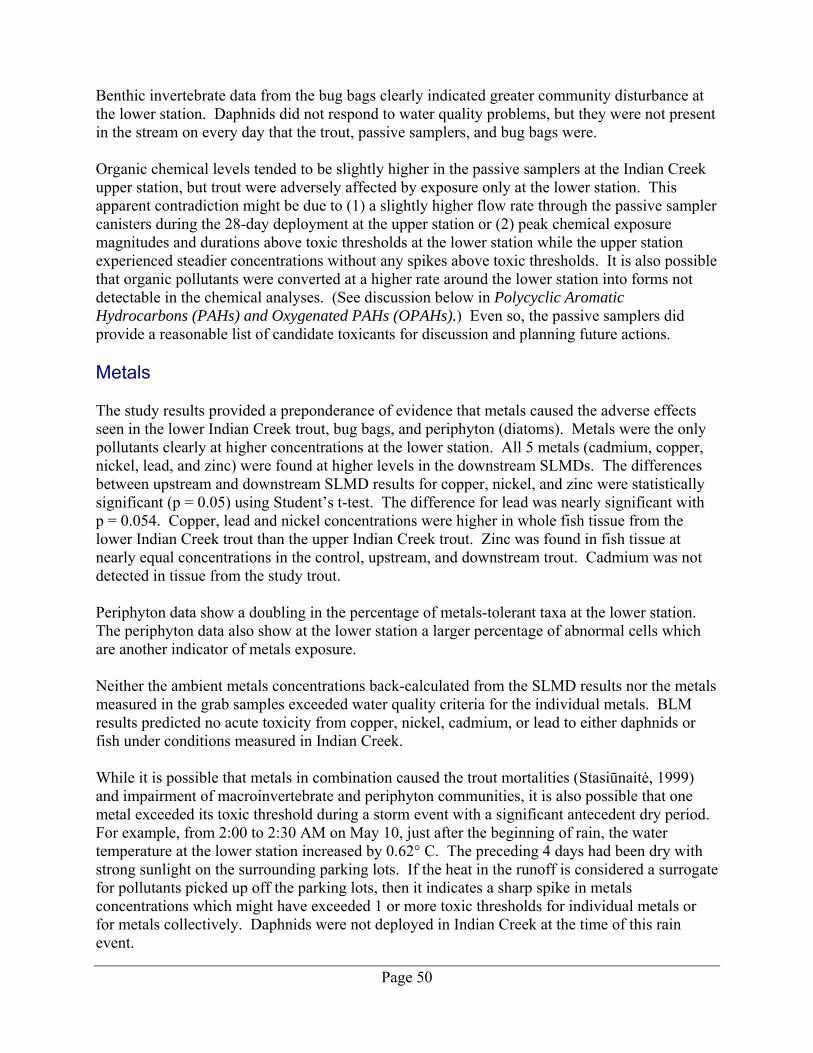
Page 50
Benthic invertebrate data from the bug bags clearly indicated greater community disturbance at the lower station. Daphnids did not respond to water quality problems, but they were not present in the stream on every day that the trout, passive samplers, and bug bags were. Organic chemical levels tended to be slightly higher in the passive samplers at the Indian Creek upper station, but trout were adversely affected by exposure only at the lower station. This apparent contradiction might be due to (1) a slightly higher flow rate through the passive sampler canisters during the 28-day deployment at the upper station or (2) peak chemical exposure magnitudes and durations above toxic thresholds at the lower station while the upper station experienced steadier concentrations without any spikes above toxic thresholds. It is also possible that organic pollutants were converted at a higher rate around the lower station into forms not detectable in the chemical analyses. (See discussion below in Polycyclic Aromatic Hydrocarbons (PAHs) and Oxygenated PAHs (OPAHs).) Even so, the passive samplers did provide a reasonable list of candidate toxicants for discussion and planning future actions. Metals The study results provided a preponderance of evidence that metals caused the adverse effects seen in the lower Indian Creek trout, bug bags, and periphyton (diatoms). Metals were the only pollutants clearly at higher concentrations at the lower station. All 5 metals (cadmium, copper, nickel, lead, and zinc) were found at higher levels in the downstream SLMDs. The differences between upstream and downstream SLMD results for copper, nickel, and zinc were statistically significant (p = 0.05) using Student’s t-test. The difference for lead was nearly significant with p = 0.054. Copper, lead and nickel concentrations were higher in whole fish tissue from the lower Indian Creek trout than the upper Indian Creek trout. Zinc was found in fish tissue at nearly equal concentrations in the control, upstream, and downstream trout. Cadmium was not detected in tissue from the study trout. Periphyton data show a doubling in the percentage of metals-tolerant taxa at the lower station. The periphyton data also show at the lower station a larger percentage of abnormal cells which are another indicator of metals exposure. Neither the ambient metals concentrations back-calculated from the SLMD results nor the metals measured in the grab samples exceeded water quality criteria for the individual metals. BLM results predicted no acute toxicity from copper, nickel, cadmium, or lead to either daphnids or fish under conditions measured in Indian Creek. While it is possible that metals in combination caused the trout mortalities (Stasiūnaitė, 1999) and impairment of macroinvertebrate and periphyton communities, it is also possible that one metal exceeded its toxic threshold during a storm event with a significant antecedent dry period. For example, from 2:00 to 2:30 AM on May 10, just after the beginning of rain, the water temperature at the lower station increased by 0.62° C. The preceding 4 days had been dry with strong sunlight on the surrounding parking lots. If the heat in the runoff is considered a surrogate for pollutants picked up off the parking lots, then it indicates a sharp spike in metals concentrations which might have exceeded 1 or more toxic thresholds for individual metals or for metals collectively. Daphnids were not deployed in Indian Creek at the time of this rain event.

Page 51
Nickel Nickel is the strongest candidate among the metals for being a cause of the mortalities in the downstream trout. The tissue nickel concentration (9.27 mg/kg, wet weight) in the lower Indian Creek trout exceeded the maximum value (5.59 ug/g) reported by USGS from national data (whole-body wet weights) compiled from 1995 to 2004 (Hinck et al., 2009). The national average for nickel reported by USGS was 0.30 ug/g. (Tissue concentrations expressed as mg/kg and ug/g are equivalent and sometimes expressed as parts per million.) Brix et al. (2004) found that the chorion (outer membrane) of trout eggs was only a partial barrier to nickel penetration of the yolk and embryo. All nickel water concentrations (29 to 466 ug/L) in their study resulted in approximately the same relative distribution in trout eggs: 36% in the chorion, 63% in the yolk, and 0.1% in the embryo. The nickel in the yolk might get transferred to the embryo during growth. If a yolk-to-embryo transfer occurred in the trout used in Indian Creek, then the embryos may have received a prolonged exposure during development. Peaks in nickel concentrations during rain events could result in an ongoing embryo exposure afterward. Sztrum et al. (2011) conducted nickel toxicity tests using early lifestages of a South American toad (Rhinella arenarum) and found that, as noted by researchers using other fish and amphibian species, a limited number of individuals tended to be resistant to nickel even in the most lethal treatments. Nebeker et al. (1985) exposed trout eyed embryos to nickel for 52 days and got a lowest observed effects concentration (LOEC) for survival of 1,100 ug/L due to 30% mortality, and yet 28% of the trout were still alive at a concentration of 3,730 ug/L total nickel. Sztrum conducted nickel toxicity testing beginning with specific toad embryo and larval developmental stages. One lifestage (stage 22 - fin development) was 3 to 16 times more susceptible to nickel lethality than any other developmental stage and had a 96-hour LC50 of 0.19 mg/L. Even tests begun at earlier stages and having nickel exposure extended past stage 22 showed fewer mortalities. The timing of first exposure to nickel above a toxic threshold can be important in determining the degree of effect. If this holds true for trout as well, then episodic stream exposures may not produce the same effects as continuous nickel exposures in a lab. The aquatic vertebrate test organism used for this study was not an amphibian but a fish. However, the period of accelerated mortalities in the trout at the lower station after the third week of exposure, and that 14% were still alive 2 weeks later, seem consistent with the results reported by Sztrum for toad embryos and by Nebeker for trout embryos exposed to nickel. NMFS (2011) used data from frog and newt embryo toxicity tests to predict captan developmental and genotoxic effects on salmonids because of the physiological similarities between amphibian early lifestages and fish. Copper and Zinc The highest copper and zinc concentrations measured in stream grab samples or back-calculated from SLMDs overlapped the range of toxic thresholds (LOECs and point estimates for 50% or lower effect levels) reported in EPA’s EcoTox database for diatoms exposed to copper or zinc. There was an overlap of 11% for freshwater diatoms exposed to copper and an overlap of 7% for freshwater diatoms exposed to zinc. None of the concentrations of the other metals measured or

Page 52
estimated for Indian Creek overlapped the range of its diatom toxic thresholds reported in EcoTox. The overlap percentages are estimates that may be biased low due to the EcoTox concentrations being a mix of total and dissolved metals values. Copper and zinc may have contributed to the periphyton effects seen in Indian Creek. The copper concentration (0.86 mg/Kg wet weight) in the lower Indian Creek trout is the same as the national median (0.86 ug/g) and just above the national mean (0.80 ug/g) reported by USGS for whole-body fish composites (Hinck et al., 2009). Zinc concentrations in fish from Indian Creek (14.3 and 15.4 mg/Kg) were more than two times lower than the national mean and median (35.2 and 36.0 ug/g). Lead The lead concentration (0.17 mg/kg wet weight) in the lower Indian Creek trout exceeded the mean (0.07 ug/g) and median (0.10 ug/g) reported by USGS from the same national data (Hinck et al., 2009). The lead concentration in lower Indian Creek trout was below the lowest tissue toxic threshold (0.4 ug/g for brook trout from Holcombe et al., 1976) referenced in the USGS report. Birge et al. (1980) got an LC50 of 220 ug/L total lead using freshly fertilized rainbow trout exposed for 28 days at a hardness of 92 to 110 mg/L. The estimated average lead concentrations in Indian Creek were over 100 times lower than this threshold. The highest estimated Indian Creek average lead concentration was 3 times lower than the lowest EC50s for abundance reported in EcoTox for a diatom (Skeletonema costatum) exposed to lead. Polycyclic Aromatic Hydrocarbons (PAHs) and Oxygenated PAHs (OPAHs) PAHs are common pollutants in urban environments and come from (1) spillage of petroleum products (fuels or lubricants) or (2) combustion byproducts (Stein, 2006). Urban transportation provides an abundance of PAHs from both of these source categories, along with the hard surfaces from which deposited PAHs can run into streams during precipitation events. A total of 10,683 ng of PAHs composed of 15 individual PAH compounds were detected at quantifiable levels from the 3 upper Indian Creek SPMD membranes. Only 13 individual PAH compounds totaling 6,580 ng were detected from the lower Indian Creek SPMD membranes. Given the abundance of parking lots and roads around the lower station relative to the woods and fields around the upper station, it is reasonable to look for a mechanism by which PAHs might be lost from the area around the lower station. Lima et al. (2005) notes that PAHs degrade at a much faster rate in sunlight and that photo-induced degradation is a larger factor than chemical degradation in contributing to PAH loss in strong light. Kim (2009) compiled the half-lives for various PAH compounds from 5 previous studies and his own. The half-lives for the same PAHs found in the SPMDs from Indian Creek ranged from 0.5 hours to 250 hours depending on the type of PAH, the substrate to which they were adsorbed, and the source and intensity of light. A total of 83% of the PAH half-lives reported by Kim were less than 96 hours. The PAHs with greater abundance at the upper station relative to the lower station (at least 1.5 times as high) were the PAHs (fluorene, fluoranthene, and pyrene) with shorter average

Page 53
photo-induced degradation half-lives from the values reported by Kim. ATSDR (2005) reported a half-life of 54 hours for 2-methylnaphthalene, and it had the greatest relative abundance at the Indian Creek upper station (4.3 times the lower). Anthracene and benzo(a)pyrene also have shorter half-lives reported by Kim and were detected at the upper station and not at the lower station, but the detection limits at the lower station were higher than the concentrations measured for the upper station, thus preventing meaningful comparison. Lampi et al. (2005) and Layshock et al. (2010) note that the toxicity of substances contaminated with PAHs is known to increase in the presence of sunlight due to the greater toxicity of the PAH photomodification products such as oxygenated PAHs (OPAHs). The concentrations of these OPAHs can sometimes be higher in environmental samples than the parent PAHs from which they came (Lampi et al., 2005). OPAHs typically have a ketone or quinone group attached to the parent PAH and are generally more polar, soluble, and bioavailable than the parent compounds (Layshock et al., 2010). Layshock also notes that the determination of the sources and sinks of OPAHs in the environment is in its infancy due to the limited number of authentic analytical standards and slow development of extraction and GC-MS procedures. Manchester Laboratory attempted unsuccessfully to identify peaks associated with ketone- or quinone-substituted PAHs in the chromatography results from this study. However, this does not mean that OPAHs could not have been present in toxic quantities at the lower station. There were 9 very sunny days (daily means > 200 watts per square meter) from May 6 through May 15 when many of the trout mortalities occurred, and the extensive parking lots and roads around the lower station are mostly open to the sun and rain. As reported in the Results section above, trout gene expression differences between the upper and lower Indian Creek stations provided some indication of response to PAH exposure. Captan The fungicide captan was tentatively identified at approximately equal concentrations in the POCIS from the upper and lower stations. This concentration was an order of magnitude higher than any other pesticides detected from the POCIS. Given its short half-life and detection in the trip blank, captan may have been recently applied in the area. The timing, duration, and magnitude of peak captan concentrations cannot be determined from POCIS results for either stream station. Captan is discussed in detail in a recent Biological Opinion from the National Marine Fisheries Service (NMFS) requested by EPA to review the impact of 54 registered pesticides on 26 endangered Pacific salmon runs (NMFS, 2011). NMFS states that captan can enter aquatic habitats either from atmospheric drift or stormwater runoff. Raina et al. (2009) determined that atmospheric particle transport is a significant pathway for captan around Abbotsford, British Columbia. Folpet, a very similar fungicide, was also detected but at lower concentrations in the same air samples. The annual maximum concentrations of captan and folpet in the air around Abbotsford occur in spring and early summer. Folpet was not in the list of analytes for this study.

Page 54
The POCIS trip blank (exposed to air at the lower Indian Creek station at deployment and retrieval) had an amount of captan that was 30% of the amount found in the POCIS exposed in the stream. The trip blank result indicates that captan may have been present in the air around the time that the trout and POCIS were exposed in Indian Creek. NMFS reports that captan is widely used on berries, fruit, alfalfa, turf, golf courses, and ornamental grasses and trees. All of these sources exist within a few miles of Indian Creek. As a cost savings measure for the pilot project, the POCIS extraction blank was not analyzed. The extraction blank represents background contamination that could happen solely during POCIS manufacture and dialysis. Analyzing the extraction blank would have given more confidence that captan contamination in the trip blank occurred during exposure to the air at the time of deployment and retrieval and not from laboratory processes: however, EST (POCIS processing lab) believes that the captan exposure likely did not happen at their laboratory. EPA (2007b) describes the mechanism of toxic action for captan as a biocide to be disruption of normal cell division of microorganisms and fungi. EPA also said that captan inhibits oxidative phosphorylation in nontarget fish and aquatic invertebrates, causing toxicity. As reported in the Results section above, the trout microarray results from the lower Indian Creek station showed upregulation of several genes for cellular respiration enzymes which may be an indication of captan exposure. However, other than inhibition of oxidative phosphorylation, EPA provides no information specific to captan that links this chemical to changes in gene expression. NMFS reports that the 4-day captan LC50s for salmonids range from 26.2 to 137 ug/L. These values mean captan is considered to be very highly toxic to salmonids by EPA’s qualitative toxicity classification system (Patterson, 2003). Kikuchi et al. (1996) of the Tokyo Metropolitan Research Institute for Environmental Protection evaluated the toxicity to rainbow trout of chemicals used on golf courses. Kikuchi found the 2-day captan LC50 to be 570 ug/L for rainbow trout embryos and that the 2-day LC50 dropped to around 75 to 180 ug/L for alevins and fry. The survival of trout at the Indian Creek lower station went from 83.3% (on day 9 just after hatch) to 47.8% (on day 23) to 14.4% (on day 34 just after swim-up). This pattern is consistent with Kikuchi’s reported increase in the sensitivity of alevins and fry exposed to captan. NMFS reports that captan breaks down both within organisms and in the environment into trichloromethylthio (TCMT) which is the toxic moiety. TCMT is also the toxic moiety for folpet, a fungicide with a structure very similar to captan. Captan, folpet, and TCMT toxicity is therefore considered by NMFS to be the same and to be additive. According to the NMFS 2011 Biological Opinion, TCMT binds thiols. Cysteine, glutathione, and metallothionein are thiols; cells employ them to resist toxicity from metals or oxidants. It is therefore possible that TCMT can enhance the toxicity of other chemicals. However, neither NMFS nor EPA reports any results from testing of captan combined with other toxicants. NMFS reports that captan degrades into TCMT in the environment with an average half-life of 10 hours (range 2.5 to 24 hours). However, NMFS could not find sufficient information to use in determining the persistence of TCMT in the environment. TCMT breaks down into

Page 55
thiophosgene which is a toxic gas and known to also bind thiols. NMFS could not find any aquatic toxicity data for thiophosgene. In addition to TCMT, the other main breakdown product of captan is tetrahydrophthalidimide (THPI) which is the central ring structure of the parent captan molecule. Based on EPA toxicity data, NMFS considers THPI to be essentially nontoxic to fish and other aquatic life. The concentrations and durations of exposure for captan and its breakdown product and toxic moiety, TCMT, must be combined in an exposure assessment. If folpet is present, it must also be added to a combined risk assessment. The half-life of TCMT is not known, but the half-life of captan in water can be as much as a day. Kikuchi showed that a 2-day exposure to 75 ug/L of captan was sufficient to cause mortalities in rainbow trout alevins and fry. These are the same lifestages present in Indian Creek for 15 days during which time captan may have been applied repeatedly in the area.
What Did Not Contribute to Understanding of Indian Creek Biological Impairment? Grab Samples Considering results from the grab samples alone would have led to an erroneous conclusion about the gradient of metals concentrations in Indian Creek. Results from the 3 grab samples during the month of field work showed all 5 metals to be at higher concentrations at the upper station. SLMD and fish tissue results showed the metals to be higher at the lower station where the trout mortalities occurred. Getting enough samples to characterize one part of one stream at one point in time requires a fair amount of expense and effort. The best description of an adequate monitoring frequency for a local stream might be from Golding (2006) who monitored Mill Creek during three storm events in fall 2005 looking for exceedances of copper and zinc acute water quality criteria. Sampling of Mill Creek was done by compositing 4 subsamples taken every 15 minutes for an hour. The wide variation and rapid changes in metals and hardness concentrations during the storms caused Golding to recommend:
The inclusion of several sub-samples within each hourly sample would provide a better representation of acute, one-hour conditions than would a single sample per hour.
The results of stream monitoring of storm events conducted by King County (unpublished) during a 2009 study of coho prespawn mortalities in Longfellow Creek and Lund’s Gulch Creek showed unique patterns of variation both in the concentrations of metals and in the water quality parameters which influence the toxicity of metals. The patterns were different between streams and different between storms events in the same stream. Drawing conclusions or running a model like the BLM with this data would be hard to justify. Graphs of the King County data shown in Appendix I illustrate this fact. An effort to take grab samples every 15 or 30 minutes during every rain event in all streams would not be affordable. Even when frequent sampling is done, results are difficult to interpret

Page 56
given the complex interactions of metals and toxicity-modifying water chemistry parameters that change concentration independently, often in opposite directions, during a rain event. Biotic Ligand Model (BLM) The BLM run using data input from the Indian Creek grab sample results calculated acute and chronic water quality criteria for dissolved copper at least an order of magnitude above any copper concentration measured in either the grab samples or back-calculated from SLMD results. Every LC50 predicted by the BLM for rainbow trout or Daphnia magna was 2 (cadmium and copper) or 3 (zinc) or 4 (lead) orders of magnitude above concentrations measured in the stream samples. The BLM results are predictions of acute (96-hour LC50) toxicity; these results might explain the lack of toxicity to the daphnids which were deployed instream for an acute (48- to 96-hour) exposure and missed the beginnings of some of the rain events. However, the 34-day exposures of trout in 3 early lifestages do not match the exposure duration and lifestage represented by the BLM. Trout at the lower station had significant mortalities, and they accumulated nickel and lead concentrations that were near to published tissue concentrations associated with mortalities in trout at the same lifestages. Finally, the BLM depends on water chemistry data from grab or composite samples which have limited representativeness in a constantly changing stream environment. In addition, Wood et al. (2011) report that different sources and forms of DOC have large differences in the degree of protection for aquatic organisms from toxic metals. Measured differences in the degree of protection from metals toxicity range from 3-fold to 11-fold for the same amount of DOC. Differences in protection generally arise from differences in the relative amounts of the humic acid fraction of DOC (originating from terrestrial sources) and the fulvic acid fraction of DOC (originating from in-water sources). The accuracy of the BLM in predicting toxicity will be limited until a means has been incorporated to account for differences in DOC quality. This study did not measure humic acid in Indian Creek samples because the instructions from HydroQual included a default input of 10% humic acid for the BLM. Wood reports that the HydroQual BLM does not respond much to changes in the inputted humic acid percentage from 1% to 100%. After comparing the results from 3 different BLM versions run on parameters measured in copper-contaminated wastewater effluents, Constantino et al. (2011) cautioned regulators against use of the BLM unless they understand the model’s limitations related to both thermodynamic and water chemistry parameters. That level of knowledge is generally lacking in regulatory agencies, and only the copper BLM is recommended by EPA at this time. Daphnids as Instream Test Organisms The daphnids had good survival in the laboratory controls and at both of the Indian Creek stations. However, daphnids were only deployed for 35% of the 34 days that the trout were present at the stream stations, and daphnids may have missed the key peak pollutant concentrations. Daphnids had two 4-day deployments and two 2-day deployments instream

Page 57
during the deployments of the trout and passive samplers. These 4 daphnid deployments required 8 field visits. Deploying daphnids for the full duration of trout exposure would have required at least another 12 field visits. The number of field visits needed to deploy daphnids in a linked series of short exposures is a disincentive to their routine use in an integrated monitoring approach intended to be economical. The level of effort to place daphnids into the stream and then retrieve and replace them every 2 to 4 days was large enough to discourage efforts to keep them in place for the full duration of the trout and passive sampler exposures. One of the concepts being tested for the ambient monitoring approach was simplicity and minimal effort. Since the daphnids did not show any adverse effects during any of their 5 in-situ deployments (4 during integrated monitoring and 1 earlier just prior to collection of benthic macroinvertebrates), the only useful information gained was knowledge of when concentrations in the stream were below toxic thresholds for daphnids. Daphnids are known to be sensitive to metals, and if metals caused the trout toxicity, then peak stream concentrations of metals may have occurred when daphnids were absent.

Page 58
Conclusions The Clean Water Act’s objective is to restore and maintain the chemical, physical, and biological integrity of the nation’s waters. For more than 40 years, efforts to achieve this objective have focused on controlling municipal and industrial wastewater discharges. Discharge monitoring has driven the implementation of these controls. However, discharge monitoring does not assess the integrity of a waterbody. Discharge monitoring at best provides a rough estimate of the potential for environmental effects based on limited information on varying pollutant concentrations in relationship to variable receiving stream chemistry and flow. Stormwater discharge monitoring generates information that is especially inadequate for evaluating urban stream health, given the large number of stormwater outfalls discharging highly variable volumes containing rapidly changing pollutant concentrations. Regularly monitoring all stormwater outfalls for every potential pollutant would be very expensive and would generate massive amounts of information of limited usefulness in assessing stream health. In addition, the detection of unknown or illegal discharges to streams is too often left to chance resulting in a potentially serious information gap when considering stream health. The most important steps for controlling damage to streams from stormwater consist of reducing discharge volumes, eliminating surge flows, removing suspended solids, and controlling sources of the metals, pesticides, and PAHs not reduced by solids removal. Until these steps have been completed, monitoring to assess water quality is only a distraction from efforts to achieve good water quality. Once these steps to reduce stormwater impacts have been completed, the streams should be monitored to determine the adequacy of all pollution control efforts. Monitoring of receiving waters already has begun in our state. The SeaTac Airport stormwater permit requires testing stream samples for toxicity to rainbow trout embryos; this requirement has withstood appeal before the Pollution Control Hearings Board. The Port of Seattle (permit holder for the airport) has begun conducting in-situ trout testing as a complement to, and potential substitute for, the lab testing. Pierce County performed a successful study using in-situ trout testing in a few urban streams in spring 2008 (Nautilus Environmental, 2009). The assessment techniques used in this 2010 study performed well. Trout at the upper station had good survival and growth, while trout at the lower station showed significant adverse effects. The passive samplers provided a reasonable list of candidate toxicants. The bug-bag and periphyton data reflected the downstream impairment seen in the trout and suggested metals were the cause. The techniques worked, and we were successful at integrating the results. If an economy of scale can be established to make the approach affordable, we could implement instream monitoring to assess the adequacy of pollutant controls and protection of salmon reproduction in our state’s streams. We might also discover pollution sources that we missed along the way. This approach could help guide us to the watershed management envisioned by the National Research Council in its EPA-sponsored 2008 report, Urban Stormwater Management in the United States (National Research Council, 2008). This report proposes that regulatory responsibility be centered at the local level with state oversight, and all permittees share the cost for monitoring watershed health.

Page 59
Recommendations
For Continued Development of the Integrated Ambient Monitoring Approach • Consider early lifestage testing of trout, instream bioassessments, and passive samplers
(SPMD, POCIS, and SLMD) to be the core components of an integrated ambient monitoring approach and continue to refine the approach. Based on prices from this 2010 pilot study, each application of this approach would cost around $11,000 per station.
• Develop bug bags as an alternative to instream collection of macroinvertebrates. Using bug bags instead of instream collection would reduce cost by at least $300 per station.
• Continue to use SLMDs, but also try analyzing metals in periphyton and in trout tissue at the end of deployment as an indication of exposure. Drop SLMDs from routine monitoring if fish tissue and periphyton metals results are adequately available and precise. Eliminating SLMDs from the approach would reduce the cost by around $1,500 per station based on 2010 prices. However, SLMDs will always be needed when poor trout survival leaves insufficient tissue for analysis or when instream periphyton biomass is too low.
o Improve the reportable detection limits (RDLs) for metals in trout fry tissue.
o Increase the number of metals analyzed in tissue and water.
• Develop the ability to analyze for OPAHs in both SPMD and POCIS passive samplers, and determine which passive sampler works better for these compounds.
• Always use trip blanks for SPMDs and POCIS to assess the contribution of atmospheric contaminant sources. If funding allows, use equipment blanks to prevent doubts about equipment or laboratory handling contributing to detections in environmental samples.
• By keeping their use in mind, encourage the development of targeted trout microarrays and improved knowledge of pollutant responses. The potential for generating useful information and attaining an economy of scale is too large to drop microarrays from the integrated ambient monitoring toolbox. The potential was partially attained in this study, and microarrays should be included in future demonstrations if resources allow.
For Investigation of Indian Creek Toxicity and Impairment • Repeat the integrated ambient monitoring at the Indian Creek lower station in the spring.
• Sample the stormwater pipe just upstream of the lower station in April or May after at least 4 days of dry and sunny weather.
o Analyze the stormwater for metals, PAHs, and OPAHs.
o Use the stormwater sample for rainbow trout toxicity testing in a lab. To make the most of sample holding time, run separate shortened tests bridging the 2 sensitive lifestage transitions, embryo to alevin and alevin to fry. Treat a portion of the sample with EDTA

Page 60
before testing as a screen for metals toxicity, as per EPA’s 1991 Methods for Aquatic Toxicity Identification Evaluation Phase I Toxicity Characterization Procedures (EPA, 1991).
• Time stream samples for late spring to early summer to catch higher levels of the fungicide captan. Confirm the identity and concentration of the compound tentatively identified as captan.
o If the presence of captan is confirmed, conduct rainbow trout laboratory toxicity testing that brackets the measured captan concentration in the stream samples.
o Add folpet to the list of analytes. NMFS (2011) stated that folpet was only registered for use on avocados, but could not confirm the registration status and believed folpet to be worthy of discussion as a risk to salmon. Raina et al. (2009) found folpet in air samples in the lower Fraser River valley just across the border from Washington State and were unclear about its use in Canada.
o Add TCMT (captan breakdown chemical) to the list of analytes if possible.

Page 61
References ATSDR (Agency for Toxic Substance and Disease Registry), 2005. Toxicological profile for Naphthalene, 1-Methylnaphthalene, and 2-Methylnaphthalene. U.S. Department of Health and Human Services, August 2005. Alvarez, D.A., J.D. Petty, J.N. Huckins, T.L. Jones-Lepp, D.T. Getting, and S.E. Manahan, 2004. Development of a Passive, In-Situ, Integrative Sampler for Hydrophilic Organic Contaminants in Aquatic Environments. Environmental Toxicology and Chemistry, 23(7): 1640-1648. Alvarez, D., 2011. Personal communication. Chief of the Environmental Chemistry Branch, United States Geiological Survey, Columbia Environmental Research Center, Columbia, MO. Bahls, L., 1993. Periphyton Bioassessment Methods for Montana Streams. Montana Department of Health and Environmental Sciences, Helena, MT. Bahls, L., 2010. Personal communication. Periphyton Specialist, Hannaea, Helena MT. Barron, M.G., M.G. Carls, R. Heintz, S.D. Rice, 2004. Evaluation of Fish Early Life-Stage Toxicity Models of Chronic Embryonic Exposures to Complex Polycyclic Aromatic Hydrocarbon Mixtures. Toxicological Sciences 78: 60–67. BC MoE, 2003. British Columbia Field Sampling Manual: 2003. For continuous monitoring and the collection of air, air-emission, water, wastewater, soil, sediment, and biological samples. British Columbia Ministry of Environment, Victoria, BC, Canada. Birge, W.J., J.A. Black, A.G. Westerman, and J.E. Hudson, 1980. Aquatic Toxicity Tests on Inorganic Elements Occurring in Oil Shale. In: C.Gale (Ed.), EPA-600/9-80-022, Oil Shale Symposium: Sampling, Analysis and Quality Assurance, March 1979. U.S. Environmental Protection Agency, Cincinnati, OH. pp 519-534. Black, P.E., 1980. Water Quality Parameters during a Storm on a Mall Parking Lot. Water Resources Bulletin 16: 615-620. Black, R. and P. Moran, 2011. Using a Trout Microarray to Identify Potential Water Chemistry Conditions in an Urban Stream. Data Report and Presentation to Department of Ecology: State of Washington as part of the Integrated Ambient Monitoring Pilot Study Report. United States Geological Survey, Washington Water Science Center. October 13, 2011. Bray, J.R. and J.T. Curtis. 1957. An Ordination of Upland Forest Communities of Southern Wisconsin. Ecological Monographs 27: 325-349. Brix KV., J. Keithly, D.K. DeForest, J. Laughlin, 2004. Acute and chronic toxicity of nickel to rainbow trout (Oncorhynchus mykiss). Environmental Toxicology and Chemistry, 23: 2221-2228.

Page 62
Brumbaugh, W.G., Petty, J.D., Huckins, J.N., Manahan, S.E., 2002. Stabilized liquid membrane device (SLMD) for the passive, integrative sampling of labile metals in water. Water, Air, Soil Pollution, 133:109-119. Brumbaugh, W.G., May, T.W., Besser, J.M., Allert, A.L. and Schmitt, C.J., 2007. Assessment of elemental concentrations in streams of the New Lead Belt in southeastern Missouri, 2002–05: U.S. Geological Survey Scientific Investigations Report 2007–5057, 57 p. Brumbaugh, W., 2010. Personal communication. Environmental Research Chemist, United States Geological Survey, Columbia Environmental Research Center, Columbia, MO. Carls, M.G., R.A. Heintz, G.D. Marty, and S.D. Rice, 2005. Cytochrome P4501A induction in oil-exposed pink salmon Oncorhynchus gorbuscha embryos predicts reduced survival potential. Mar. Ecol. Prog. Ser. 301:253-265. Carls, M.G. and J.F. Thedinga, 2010. Exposure of pink salmon embryos to dissolved polynuclear aromatic hydrocarbons delays development, prolonging vulnerability to mechanical damage. Marine Environmental Research. 69:318-325. City of Olympia, 2010. Storm and Surface Water Information. City of Olympia internet homepage – Accessed March 10, 2011. http://olympiawa.gov/city-utilities/storm-and-surface-water.aspx. Clarke, K.R. and R.N. Gorley, 2006. PRIMER v6: User Manual/Tutorial. PRIMER-E, Plymouth, United Kingdom. Constantino, C., M. Scrimshaw, S. Comber, and J. Churchley, 2011. An Evaluation of Biotic Ligand Models Predicting Acute Copper Toxicity to Daphnia magna in Wastewater Effluent. Environmental Toxicology and Chemistry 30: 852-860. Davies, S.P. and L. Tsomides, 2002. Methods for Biological Sampling and Analysis of Maine’s Rivers and Streams. State of Maine Department of Environmental Protection. DEP LW0387-B2002. Denslow, N.D., N. Garcia-Reyero, and D.S. Barber, 2007. Fish ‘n’ chips: the use of microarrays for aquatic toxicology. Mol. BioSyst. 3, 172-177. Diamond, J., J. Stribling, M. Bowersox, and H. Latimer. 2008. Evaluation of Effluent Toxicity as an Indicator of Aquatic Life Condition in Effluent-Dominated Streams: A Pilot Study. Integrated Environmental Assessment and Management. 4: 456-470. Environment Canada, 1998. Biological test method: toxicity tests using early life stages of salmonid fish (rainbow trout). Second edition. EPS/1/RM/28, July 1998. EPA, 1991. Methods for Aquatic Toxicity Identification Evaluation Phase I Toxicity Characterization Procedures. U.S. Environmental Protection Agency, Environmental Research Laboratory, Duluth, MN. Report No. EPA-600/6-91/003.

Page 63
EPA, 1996a. Method 1669: Sampling Ambient Water for Trace Metals at EPA Water Quality Criteria Levels. U.S. Environmental Protection Agency. EPA-821R96011. July 1996. EPA, 1996b. Method 1638: Determination of Trace Elements in Ambient Water by Inductively Coupled Plasma Mass Spectrometry. U.S. Environmental Protection Agency, Office of Water, Engineering and Analysis Division. EPA, February 2000. An SAB Report: Review of the Biotic Ligand Model of the Acute Toxicity of Metals. Prepared by the Ecological Processes and Effects Committee of the Science Advisory Board. EPA-SAB-EPEC-00-006. EPA, 2007a. Aquatic Life Ambient Freshwater Quality Criteria – Copper. U.S. Environmental Protection Agency, Office of Water. EPA-822-R-07-001. February 2007. EPA, 2007b. Risks of Captan Use to Federally Threatened California Red-legged Frog (Rana aurora draytonii). Pesticide Effects Determination. U.S. Environmental Protection Agency, Environmental Fate and Effects Division, Office of Pesticide Programs, Washington D.C. October 18, 2007. EPA, 2007c. CADDIS Literature Resource (CADLit) Search and Download Functions, Version 1.1. U.S. Environmental Protection Agency, Office of Research and Development. November 2007. Era-Miller, B. and R. Marshall, 2010. Quality Assurance Project Plan: Pilot Study of an Ambient Monitoring Approach for Evaluating the Biological Integrity of Urban Streams. Washington State Department of Ecology, Olympia, WA. Publication No. 10-03-114. www.ecy.wa.gov/biblio/1003114.html. Golding, S., 2006. Zinc and Copper Concentrations in an Industrial Area Creek during Storm Events. Washington State Department of Ecology, Olympia, WA. Publication No. 06-03-023. www.ecy.wa.gov/biblio/0603023.html. Hall, K.J. and B.C. Anderson, 1988. The toxicity and chemical composition of urban storm water runoff. Can. J. Civ. Eng. 15: 98-106. Hinck, J.E., C.J. Schmitt, K.A. Chojnacki, D.E. Tillitt, 2009. Environmental contaminants in freshwater fish and their risk to piscivorous wildlife based on a national monitoring program. Environ. Monit. Assess. 152:469-494. Holcombe, G.W., Benoit, D.A., Leonard, E.N., and McKim, J.M., 1976. Long-term effects of lead exposure on three generations of brook trout (Salvelinus fontinalis). Journal of Fisheries Research Board of Canada, 33, 1731–1741. Huckins, J.N., J.D. Petty, and K. Booij, 2006. Monitors of Organic Chemicals in the Environment: Semipermeable Membrane Devices. Springer Science and Business Media, New York, NY. 223 pp.

Page 64
HydroQual, 2007. Biotic Ligand Model Windows Interface, Version 2.2.3 User’s Guide and Reference Manual. HydroQual, Inc, Mahwah, NJ. June 2007. Johnson, A., 2007. Standard Operating Procedure for using Semipermeable Membrane Devices to Monitor Hydrophobic Organic Compounds in Surface Water, Version 2.0. Washington State Department of Ecology, Olympia, WA. SOP Number EAP001. www.ecy.wa.gov/programs/eap/quality.html. Joy, J., 2006. Standard Operating Procedure for Grab sampling – Fresh water, Version 1.0. Washington State Department of Ecology, Olympia, WA. SOP Number EAP015. www.ecy.wa.gov/programs/eap/quality.html. Kidd K.A., Blanchfield P.J., Mills K.H., Palace V.P., Evans R.E., Lazorchak J.M., and Flick R., 2007. Collapse of a fish population following exposure to a synthetic estrogen. Proceedings of the National Academy of Sciences 104(21):8897-8901. Kikuchi, M., T. Miyagaki, and M. Wakabayashi, 1996. Evaluation of Pesticides Used in Golf Links by Acute Toxicity Test on Rainbow Trout. Bull.Jpn.Soc.Sci.Fish. 62(3):414-419. Kim, D., B.M. Kumfer, C. Anastasio, I.M. Kennedy, and T.M. Young, 2009. Environmental Aging of Polycyclic Aromatic Hydrocarbons on Soot and its Effect on Source Identification. Chemosphere. 76(8): 1075-1081. King County. Pre-spawn mortality study unpublished data from 2009. King County Department of Natural Resources and Parks, Water and Land Resources Division, Science Section. Project contact: Jenée Colton. Lampi, M.A., J. Gurska, K.I.C. McDonald, F. Xie, X. Huang, D.G. Dixon, and B.M. Greenberg, 2005. Photoinduced Toxicity of Polycyclic Aromatic Hydrocarbons to Daphnia magna: Ultraviolet-Mediated Effects and the Toxicity of Polycyclic Aromatic Photoproducts. Environmental Toxicology and Chemistry, 25(4): 1079-1087. Layshock, J.A., G. Wilson, and K.A. Anderson, 2010. Ketone- and Quinone-Substituted Polycyclic Aromatic Hydrocarbons in Mussel Tissue, Sediment, Urban Dust, and Diesel Particulate Matrices. Environmental Toxicology and Chemistry, 29(11): 2450-2460. Lima, A.L.C., J.W. Farrington, and C.M. Reddy, 2005. Combustion-Derived Polycyclic Aromatic Hydrocarbons in the Environment - A Review. Environmental Forensics 6:109-131. National Research Council, 2008. Urban Stormwater Management in the United States. The National Academies Press, Washington, D.C. www.nap.edu Nautilus Environmental, 2009. Pierce County Public Works and Utilities – Countywide Water Quality Monitoring Plan. Pilot Test: Rainbow Trout Early Life Stages In-situ Bioassay, Final Report submitted to Brown and Caldwell.

Page 65
Nebeker, A.V., C. Savonen, and D.G. Stevens. 1985. Sensitivity of rainbow trout early life stages to nickel chloride. Environmental Toxicology and Chemistry, 4: 233-239. Nisbet I.C.T. and LaGoy P.K., 1992. Toxic Equivalency Factors (TEFs) for Polycyclic Aromatic Hydrocarbons (PAHs). Regulatory Toxicology and Pharmacology. 16: 290-300 (1992). NMFS (National Marine Fisheries Service), 2011. Endangered Species Act Section 7 Consultation Biological Opinion on Authorization of pesticide products containing the active ingredients 2,3-D, triclopyr BEE, diuron, linuron, captan, and chlorothalonil, and their formulations in the United States and its affiliated territories. Endangered Species Division of the Office of Protected Resources. Final 06/30/2011. Patterson, M., 2003. Captan Analysis of Risks to Endangered and Threatened Salmon and Steelhead. U.S. Environmental Protection Agency, Office of Pesticide Programs, Environmental Field Branch. 92 pp. Plotnikoff, R. and C. Wiseman, 2001. Benthic Macroinvertebrate Biological Monitoring Protocols for Rivers and Streams: 2001 Revision. Washington State Department of Ecology, Olympia, WA. Publication No. 01-03-028. www.ecy.wa.gov/biblio/0103028.html. Poynton, H., J. Varshavsky, B. Chang, G. Cavigiolio, S. Chan, P. Holman, A. Loguinov, D. Bauer, K. Komachi, E. Theil, E. Perkins, O. Hughes, and C. Vulpe, 2007. Daphnia magna Ecotoxicogenomics Provides Mechanistic Insights into Metals Toxicity. Environmental Science and Technology 41:1044-1050. Poynton, H., R. Zuzow, A. Loguinov, E. Perkins, and C. Vulpe, 2008. Gene Expression Profiling in Daphnia magna, Part II: Validation of a Copper Specific Gene Expression Signature with Effluent from Two Copper Mines in California. Environmental Science and Technology 42:6257-6263. Raina, R., W. Belzer, and K. Jones, 2009. Atmospheric Concentrations of Captan and Folpet in the Lower Fraser Valley Agricultural Region of Canada. Air, Soil and Water Research 2: 41–49. Reynolds, O. and B. Wood, 2011. Deschutes Watershed Characterization Report, Thurston County, WA. Thurston County Resource Stewardship Department and Geodata Center. Seim, W.K., L.R. Curtis, S.W. Glenn, and G.A. Chapman, 1984. Growth and survival of developing steelhead trout (Salmo gairdneri) continuously or intermittently exposed to copper. Can. J. Fish. Aquat. Sci. 41: 433-438. Stasiūnaitė P., 1999. Long-term heavy metal mixture toxicity to embryos and alevins of rainbow trout (Oncorhynchus mykiss). Acta Zoologica Lituanica Hydrobiologia 9: 1392-1657. Stribling, J.B., S.R Moulton II, and G.T. Lester, 2003. Determining the Quality of Taxonomic Data. Journal of the North American Benthological Society. 22(4): 621-631.

Page 66
Sullivan, L., 2007. Standard Operating Procedure for Estimating Streamflow, Version 1.0. Washington State Department of Ecology, Olympia, WA. SOP Number EAP024. www.ecy.wa.gov/programs/eap/quality.html. Swanson, T., 2007. Standard Operating Procedure (SOP) for Hydrolab® DataSonde® and MiniSonde® Multiprobes, Version 1.0. Washington State Department of Ecology, Olympia, WA. SOP Number EAP033. www.ecy.wa.gov/programs/eap/quality.html. Sztrum, A.A., J.L. D’Eramo, and J. Herkovits, 2011. Nickel Toxicity in Embryos and Larvae of the South American Toad: Effects on Cell Differentiation, Morphogenesis, and Oxygen Consumption. Environmental Toxicology and Chemistry 30:1146-1152. Thurston County, 1996. Thurston County 1995 Storm Water Special Study Highway Outfall Sampling – June 1996. Thurston County Public Health and Social Services Department, Olympia, WA. Thurston County, 2010. Personal communication with Barb Wood. Thurston County Water Resources Department, Olympia, WA. Thurston County unpublished data, 2011. Thurston County Water Resources Department, Olympia, WA. Tidepool Scientific, 2010. CETIS (Comprehensive Environmental Toxicity Information System) v.1.8.0.4. Tidepool Scientific Software, McKinleyville, CA. Ward, W.J., 2007. Standard Operating Procedure for the Collection and Field Processing of Metals Samples, Version 1.3. Washington State Department of Ecology, Olympia, WA. SOP Number EAP029. www.ecy.wa.gov/programs/eap/quality.html. WDEQ/WQD, 2005. Manual of Standard Operating Procedures for Sample Collection and Analysis. Wyoming Department of Environmental Quality, Water Quality Division, Watershed Program, Cheyenne, WY. Weather data for East Olympia: www.wunderground.com/cgi-bin/findweather/getForecast?query=98501. Wiseman, S., H. Osachoff, E. Bassett, J. Malhotra, J. Bruno, G. VanAggelen, T.P. Mommsen and M.M. Vijayan, 2007. Gene expression pattern in the liver during recovery from an acute stressor in rainbow trout. Comp. Biochem. Physiol. D 2, 234-244. Wood, C.M., H.A. Al-Reasi, and D.S. Smith, 2011. The two faces of DOC. Aquatic Toxicology 105: 3-8.

Page 67
Appendices

Page 68
This page is purposely left blank

Page 69
Appendix A. Glossary, Acronyms, and Abbreviations Glossary Alevin: The salmonid lifestage between hatching from the egg and swimming up into the water column. Alevin are characterized by having a yolk from which they derive the nutrition needed to survival and grow.
Ambient: Surrounding environmental condition (for example, surrounding air temperature).
Benthic: Bottom-dwelling organisms.
Biotic Ligand Model (BLM): The BLM predicts heavy metal toxicity after complexation with organic (dissolved organic carbon) and inorganic (hydroxides, chlorides, carbonate, etc.) ligands and allows for competition with alkali and alkaline earth metals for fish gill binding sites.
Chorion: The acellular envelope surrounding a fish egg. The chorion hardens after fertilization in order to serve as a barrier and thereby protect the developing embryo.
Clean Water Act: A federal act passed in 1972 that contains provisions to restore and maintain the quality of the nation’s waters.
Conductivity: A measure of water’s ability to conduct an electrical current. Conductivity is related to the concentration and charge of dissolved ions in water.
Daphnid: A small planktonic crustacean between 0.2 and 5 mm in length. Daphnia are commonly referred to as water fleas. They live in aquatic environments including swamps, freshwater lakes, ponds, streams, and rivers.
Diffusive Gradients in Thin Film (DGT): DGTs are passive samplers that concentrate metals of interest out of water. DGTs have a microporous outer membrane and so sample mostly the dissolved fraction of metals. See: https://brooksrandlabs.sharefile.com/d/s8db84936f104423b.
Dissolved oxygen (DO): A measure of the amount of oxygen dissolved in water.
Downregulated gene: A gene whose production of mRNA is reduced or stopped. The mRNA contains information for constructing a specific protein such as an enzyme.
EDTA: Ethylenediaminetetraacetic acid (EDTA) binds metals in solution and reduces their bioavailability and toxicity.
Embryo: The fish lifestage occurring inside the egg. The embryo stage is when tissues differentiate and organs and body structures form.
Exceeded criteria: When concentrations of a contaminant are higher than (do not meet) standards such as the Washington State Surface Water Standards for toxics (WAC 173-201A-240).

Page 70
Fry: The salmonid lifestage commencing with swimming up into the water column after the yolk has been completely consumed. Fry must find and catch prey to provide the nutrition needed for survival and growth.
Grab sampling: A discrete sample from a single point in the water column or sediment surface.
In-situ Toxicity Test: A toxicity test conducted by placing test organisms into a container which allows flow-through of water and then placing the container into the stream, lake, or marine water of interest. An in-situ toxicity test provides a realistic environmental exposure without completely sacrificing the controlled conditions of a laboratory test. In particular, an in-situ toxicity test involves test organisms with a known history (age, health, prior chemical exposure, etc.) which are confined to one location for the test period. Because a realistic environmental exposure accepts the possibility of great variability and complexity, establishing cause and effect can be a challenge.
LC50: Lethal Concentration 50 is the concentration of a chemical which kills 50% of a sample population.
LOEC: The Lowest Observed Effects Concentration (LOEC) is the lowest concentration of a substance in a toxicity test having a statistically significant difference from a nontoxic control. The LOEC is an approximation of the toxic threshold for that substance. Because only the concentrations used in the toxicity test are available to be the LOEC, the closeness of the LOEC to the true toxic threshold depends on the number and distribution of the concentrations used in the toxicity test.
Macroinvertebrate: Organisms on or in the stream substrate that are visible with the naked eye.
NOEC: The No Observed Effects Concentration (NOEC) is the highest concentration of a substance in a toxicity test not having a statistically significant difference from a nontoxic control. The NOEC is an approximation of the safe concentration for that substance. Because only the concentrations used in the toxicity test are available to be the NOEC, the extent to which the NOEC is lower than the true safe concentration depends on the number and distribution of the concentrations used in the toxicity test.
Parameter: Water quality constituent being measured (analyte). A physical, chemical, or biological property whose values determine environmental characteristics or behavior.
Passive Sampler: Passive samplers are devices for sampling water or air that do not require human or mechanical (pump) assistance. Passive samplers also do not collect the medium (water or air) along with the pollutants. Because of these features, passive samplers can be deployed for longer exposure times and with less effort. Passive samplers absorb pollutants similarly to living organisms in some ways.
Periphyton: A complex mixture of algae, cyanobacteria, heterotrophic microbes, and detritus that is attached to submerged surfaces.
pH: A measure of the acidity or alkalinity of water. A low pH value (0 to 7) indicates that an acidic condition is present, while a high pH (7 to 14) indicates a basic or alkaline condition. A pH of 7 is considered to be neutral. Since the pH scale is logarithmic, a water sample with a pH of 8 is ten times more basic than one with a pH of 7.

Page 71
Point Estimate: Point estimates, such as the LC50, IC25, or EC15, are derived from toxicity test results to represent the concentration of the toxic substance which would cause a percent reduction equal to the specified effect level. For example, the LC50 is usually described as the concentration predicted to cause 50% mortality in a population of the test organisms. The IC25 estimates the concentration which would cause a 25% reduction in growth or reproduction. A “point estimate” is not really a single number but a range within which there is 95% confidence that the true value occurs.
Polar Organic Chemical Integrative Sampler (POCIS): POCIS are passive samplers that concentrate polar (water soluble) organics out of water. Polar organics include pharmaceuticals and many modern pesticides. See: http://biology.usgs.gov/contaminant/passive_samplers.html.
Pollution: Contamination or other alteration of the physical, chemical, or biological properties of any waters of the state. This includes change in temperature, taste, color, turbidity, or odor of the waters. It also includes discharge of any liquid, gaseous, solid, radioactive, or other substance into any waters of the state. This definition assumes that these changes will, or are likely to, create a nuisance or render such waters harmful, detrimental, or injurious to (1) public health, safety, or welfare, or (2) domestic, commercial, industrial, agricultural, recreational, or other legitimate beneficial uses, or (3) livestock, wild animals, birds, fish, or other aquatic life.
mRNA: The molecule which carries the genetic code from the cell nucleus out into the cytoplasm where it is used to guide protein synthesis.
Salmonid: Any fish that belong to the family Salmonidae. In other words, a salmonid is any species of salmon, trout, or char. www.fws.gov/le/ImpExp/FactSheetSalmonids.htm
Semi-Permeable Membrane Device (SPMD): SPMDs are passive samplers that concentrate nonpolar (fat soluble) organics out of water. Nonpolar organics include substances such as PCBs, PAHs, and DDT. See: http://biology.usgs.gov/contaminant/passive_samplers.html.
Stabilized Liquid Membrane Device (SLMD): SLMDs are passive samplers that concentrate metals of interest out of water. SLMDs lack a microporous outer membrane and sample both dissolved and total metals. See: http://biology.usgs.gov/contaminant/passive_samplers.html.
Stormwater: The portion of precipitation that does not naturally percolate into the ground or evaporate but instead runs off roads, pavement, and roofs during rainfall or snow melt. Stormwater can also come from hard or saturated grass surfaces such as lawns, pastures, playfields, and from gravel roads and parking lots.
Surface waters of the state: Lakes, rivers, ponds, streams, inland waters, salt waters, wetlands and all other surface waters and water courses within the jurisdiction of Washington State.
Swim-up: Trout life stage that begins when the alevin (larval salmonid) has absorbed its yolk sac, and begins to swim upward to emerge from the gravels where eggs were deposited. The swim-up stage is viewed as a distinct life stage because the air bladder is not yet inflated, and the fish are negatively buoyant. They struggle to swim upward toward the water surface, and then gulp air to fill the air bladder. The swim-up stage ends once the air bladder is filled, and the juveniles are referred to simply as ‘fry.’

Page 72
Thalweg: The deepest and fastest moving portion of flow in a stream.
Upregulated gene: A gene whose production of mRNA is increased. The mRNA contains information for constructing a specific protein such as an enzyme.
Water quality criteria: The maximum concentration of a chemical determined by EPA to be safe for aquatic life under short-term (acute) exposure or longer-term (chronic) exposure.
Watershed: A drainage area or basin in which all land and water areas drain or flow toward a central collector such as a stream, river, or lake at a lower elevation.
Whitlock-Vibert hatchbox: The Whitlock-Vibert hatchbox is patented by the Federation of Fly Fishers and was developed for incubating trout and salmon eggs in streams to which these fish were being stocked. The hatchboxes have an upper egg chamber for embryos with slots through which the alevins slip after hatching into a lower nursery chamber. Nautilus adds extra screen to the nursery chamber so the fry cannot exit. Normally fry exit the nursery chamber when they are ready for swim-up. See: www.fedflyfishers.org/Default.aspx?tabid=4384 for more information. Acronyms and Abbreviations BIBI Benthic Invertebrate Index of Biological Integrity BLM Biotic Ligand Model BMP Best management practice BNAs Bases, neutrals, and acids DGT Diffusive Gradients in Thin film (passive sampler) DOC Dissolved organic carbon EAP Environmental Assessment Program Ecology Washington State Department of Ecology EIM Environmental Information Management database EPA U.S. Environmental Protection Agency EST Environmental Sampling Technologies (SPMD/POCIS manufacturer) GCMS Gas Chromatography/Mass Spectroscopy LC50 Lethal Concentration 50 (See Glossary for more information.) LCMS Liquid Chromatography/Mass Spectroscopy LOEC Lowest Observed Effects Concentration (See Glossary for more information.) MQO Measurement quality objectives Nautilus Nautilus Environmental (trout embryo test laboratory) NMFS National Marine Fisheries Service NOEC No Observed Effects Concentration (See Glossary for more information.) PAH Polycyclic aromatic hydrocarbons POCIS Polar Organic Chemical Integrative Sampler POTW Publicly Owned Treatment Works PRC Performance reference compounds Rhithron Rhithron Associates, Inc. (Missoula, MT) RPD Relative percent difference SLMD Stabilized Liquid Membrane Device

Page 73
SOP Standard operating procedures SPMD Semipermeable Membrane Device SRM Standard reference materials TEQ Toxic equivalent quotient TOC Total organic carbon TSS Total suspended solids UC University of California USGS U.S. Geological Survey WQC Water quality criteria WSU Washington State University Units of Measurement cfs cubic feet per second kg kilograms, a unit of mass equal to 1,000 grams. mg/Kg milligrams per kilogram (parts per million)
mg/L milligrams per liter (parts per million) mL milliliters mm millimeters ng/L nanograms per liter (parts per trillion) ug/L micrograms per liter (parts per billion) um micrometer

Page 74
This page is purposely left blank

Page 75
Appendix B. Detail of Project Activities Table B-1. Detail of Project Activities and Analyses for the Pilot Study.
Activity Location, Duration, and Frequency Analysis Comments
Indian Creek Instream Bioassessments benthic invertebrate bioassessment upper & lower stations abundance &
diversity of taxa
done first to avoid interference from other field work periphyton assessment
Test Organisms In-situ Indian Creek
trout in-situ toxicity testing 34 days at upper & lower stations
survival, hatch, development, length, weight
four field visits to deploy, maintain, and retrieve & one visit to harvest for microarray
fish tissue metals from whole fish at end of exposure Cd, Cu, Ni, Pb, & Zn
trout metallothionein end of 34-day exposure at upper station liver & gill
no analysis at lower station (insufficient number of fish)
daphnid in-situ toxicity testing
five 48-hour or 96-hour deployments at upper & lower stations
48-hr or 96-hr survival
last four deployments concurrent with trout in-situ
Passive Samplers in Indian Creek
metals passive samplers concurrent with trout in-situ deployment
DGT 28 days at upper & lower stations
Cd, Cu, Ni, Pb, & Zn
no back-calculated stream concentrations
SLMD stream concentrations back-calculated from SLMD results
organics passive samplers concurrent with trout in-situ deployment
POCIS
28 days at upper & lower stations
herbicides, pesticides, carbamates, & BNAs.
no back-calculated stream concentrations
SPMD BNAs, PAHs, & pesticides
PAH stream concentrations back-calculated from SPMD results
bug bag macroinvertebrate sampler
43 days at upper & lower stations
abundance & diversity of taxa
concurrent with trout in-situ deployment
Supplemental Indian Creek Monitoring
stream grab samples
three samples at upper and lower stations evenly spaced during 28-day metals passive sampler deployments
Cd, Cu, Ni, Pb, Zn, DOC, pH, Ca, Mg, Na, K, SO4, Cl, & alkalinity

Page 76
Activity Location, Duration, and Frequency Analysis Comments
MiniSonde physical and chemical measurements
during field visits - 22 times at upper & 24 times at lower
temperature, conductivity, dissolved oxygen, pH, & flow
TidbiT temperature monitors continuous on trout cages & passive samplers temperature every 30 minutes
Supplemental Calculations for Chemical Results
BLM Hydroqual version 2.2.3 run for Cu, Cd, Pb, & Zn
PAH ∑TEQs sum of concentrations times TEFs compared to benzo(a)pyrene WQC
Laboratory Biological Testing
trout lab control concurrent with trout in-situ deployment
same endpoints as in-situ
temperature matched to Indian Creek
trout gene microarray upper & lower stations plus lab control whole fish & liver waiting on results
trout vitellogenin Three-week alevin lab exposure to 1 ug/L estradiol liver & head/tail tissue
daphnid gene microarray upper & lower stations plus lab controls whole organism waiting on results
Cd: cadmium Cu: copper N: nickel Pb: lead Zn: zinc Ca: calcium Mg: magnesium Na: sodium K: potassium SO4: sulfate Cl: chlorides

Page 77
Appendix C. Photographs of Sampling Devices and Methods
Figure C-1. Trout In-situ Field Methods.
A
F E
D C
B
A. In - situ trout gravel mound at Indian - 2 (downstream site) B. In - situ trout gravel mound at Indian - 1 (upstream site) C. Metal basket holding a single hatchbox surrounded with gravel D. All four replicate trout baskets awaiting burial E. Trout embryos in hatchbox prior to deployment F. Trout alevins in hatchbox during field check

Page 78
Figure C-2. Daphnia Magna In-situ Toxicity Test Chambers.
Figure C-3. Benthic Macroinvertebrate Collection using a D-Frame Kicknet.
B
12.7
cm
5.1 cm
A. Cage with Daphnia chambers deployed in-situB. Diagram of Daphnia sampling chamber
A

Page 79
Figure C-4. Bug Bag Method of Benthic Macroinvertebrate Collection.
18”
12”A. Bug bag dimensionsB. Bags at deploymentC. Retrieval of bags
A
BC

Page 80
Figure C-5. SPMD and POCIS Passive Samplers.
A. Single SPMD membrane on a spider carrierB. 3 POCIS membranes on a carrierC. SPMD and POCIS carriers next to a large size
deployment canister
A
BC

Page 81
Figure C-6. Field Methods for SLMD Metals Passive Sampler.
D E
B C
A
A. Sheathed bare SLMD membranes in the laboratoryB. Transfer of clean membrane into PVC pipe at deploymentC. Housing unit at deploymentD. Closed pipes upon field retrievalE. Pipes inside open housing unit upon retrieval

Page 82
Figure C-7. Field Methods for DGT Metals Passive Sampler.
A. A single clean DGT membrane at deploymentB. Complete sampler unit with 3 DGTs, temperature Tidbit, and rock weightsC. Rinsing off debris from a DGT membrane at retrievalD. DGT sampler unit upon retrieval
A B
C D

Page 83
Appendix D. Daphnia Field and Laboratory Methods Daphnia In-Situ Toxicity Testing Procedures (Provided by Barb Wood of Thurston County) Acute In-Situ Bioassays In-situ testing consists of test chambers constructed from 5.1 cm x 12.7 cm clear liner tubes (cellulose acetate butyrate) capped with two polyethylene closure caps. Two long rectangular windows (6 cm x 2.5 cm) are covered with 74 micron mesh to contain organisms and exclude predators while allowing exposure to test media.
Daphnia magna – 100% Ambient test – 96 hours
The test follows EPA procedure: EPA/600/4-90/027F Methods for Measuring the Acute Toxicity of Effluents and Receiving Waters to Freshwater and Marine Organisms Section 9 (pg. 45-75). MODIFIED. NOTE: This process requires removal of neonates from stock cultures 24 hours before test set-up. • On day of test set-up, remove <24-h neonates from stock cultures. Pool neonates and feed
1:1 YTC and Selenastrum 2 hours before use. • Label 20 ml test tubes with a number, starting with one. Each test site requires a total of 4
replicates. Mark an additional 4 test tubes for travel control data. Generate random test positions using TOXCALC. Mark assigned position below replicate number.
• Fill test tubes half full with MHSW. • Introduce 1 to 2 test organisms/ replicate by submerging 2 mm internal diameter (i.d.) pipette
just under water surface, avoiding any air bubbles. Continue until there are a total of 10 organisms/replicate. Verify that 10 organisms are in each test and control replicate using a fiber light.
• Place test tubes in order of randomized position into a test tube rack. Cover and place in ice
cooler with blue ice for transport to the field site. NOTE: Organisms should be chilled to field water temperature slowly over a minimum of 2 hours.
• At in-situ test set-up, collect and record the physical and chemical measurements using the
YSI 600R multi-meter; D.O. (%, mg/L), temperature (ºC), pH, and conductivity (µS /cm). Optional: Collect a grab sample in an EPA- approved container by rinsing three times with sample water, submerging container at least 12 inches below the surface, and allowing container to fill. Expel all air and seal with no headspace.

Page 84
Termination of In-Situ Test • At in-situ test termination, collect and record the physical and chemical measurements using
the YSI 600R multi-meter; D.O. (%, mg/L), temperature (ºC), pH, and conductivity (µS /cm). • Collect in-situ chambers and place into bucket with sample water for travel back to the
laboratory. At the Laboratory • Slowly remove an end cap from chamber. Rinse sides of chamber to assure all organisms are
collected. • Note and record any mortalities and abnormal behavior in test organisms collected from the
control and test water sites. Record findings on test data sheet. In-situ test acceptability is no less than 80% survival in the control test site. If no control site was used in the field, in-situ test acceptability is no less than 90% in the travel controls. • Analyze survival data using the statistical program TOXCALC or CETIS™.
Preservation of Daphnia magna tissue for RNA Isolation using RNAlater (Provided by Helen Poynton of the U.S. Environmental Protection Agency) Supplies needed • RNAlater: Applied Biosystems, part # AM7020 (100 ml) or AM7021 (500 ml). • Cryogenic vials: Corning round bottom, self-standing, 2.0 ml capacity, (Fisher Scientific)
part #: 03-374-21 (or equivalent). • Fine-tip transfer pipet: Samco, (Fisher Scientific) part # 13-711-30 (or equivalent). • Weigh boats: (Fisher Scientific), part # 08-732-112 (or equivalent). Set-up 1. Place 1.0 ml of RNAlater in a 2.0 ml cryogenic vial. RNAlater is stable at room temperature
and does not have to be refrigerated. 2. Prepare several blunt-end transfer pipettes for daphnid collection by cutting off the tip of the
pipet.

Page 85
Collection of organisms in the field 1. Open in-situ chambers at water surface to access animals, but do not allow the animals to
escape. 2. Remove 5 adult daphnids with a pipet and place in a small weigh boat. Using a fine-tip
transfer pipet remove the excess water from the weigh boat. 3. Open the cryovial containing the RNAlater. Withdraw about 0.25 – 0.5 ml of RNAlater with
a transfer pipet. 4. Holding the weigh boat over the cryovial, add the RNAlater to the weighboat and “pour” the
daphnids into the cryovial. 5. Replace the cap on the cryovial and invert several times to completely submerge the
daphnids and allow for RNAlater penetration of tissues. 6. Place on ice. 7. Repeat until all daphnids are collected. Store all samples overnight at 4o C. Storage and shipping Sample must first be incubated overnight at 4o C. After overnight incubation, whenever possible, samples should be stored at -20o C or -80o C, but they may be shipped overnight on ice. In general, samples preserved with RNAlater may be stored in the following manner:
• Indefinitely at -80o C or -20o C. Samples will not freeze at -20o C, but RNA will remain intact.
• 1 month at 4o C.
• 1 week at 25o C.
• 24-h at 37o C. For more details and for protocols on RNA Isolation, see Applied Biosystems “RNAlater Tissue Collection: RNA Stabilization Solution” Product manual, available at: www.ambion.com/techlib/prot/bp_7020.pdf

Page 86
This page is purposely left blank

Page 87
Appendix E. Data Quality Trout In-Situ Toxicity Testing and Biomarker Analysis Nautilus Environmental in Fife, WA conducted the trout in-situ and laboratory toxicity tests and associated biomarker analyses (metallothionein and vitellogenin). A thorough discussion of the data quality for their work is contained in lab reports included in Appendix F. Trout In-Situ Testing The laboratory control met all test validity criteria in EPS 1/RM/28, Biological Test Method: Toxicity Tests Using Early Lifestages of Salmonid Fish (Rainbow Trout). When adopting the nickel-plated barbecue baskets as the standard wire cages for holding hatchboxes, Nautilus performed laboratory toxicity testing under a variety of conditions to verify that the nickel-plating did not contribute to trout toxic responses. Biomarker Analysis According to the biomarker test kits manufacturers’ instructions, working ranges were determined from standard curves. All measured values were within these working ranges. Daphnid In-Situ Toxicity Testing Daphnid survival in controls was always at least 90% and therefore met the standard acute test control performance criterion. Daphnid survival instream was uniformly good. The water chemistry of the daphnid culture, dilution, and control water varied between water batches in the lab and varied significantly from the ambient water hardness of Indian Creek. This was corrected for the 5th and final in-situ deployment. The hardness and alkalinity concentrations of the laboratory water were adjusted to closely match stream water. This allowed for reasonable comparability between control organisms and in-situ organisms, especially for the gene microarray analysis. Only organisms from the 5th deployment were used for microarray analysis. UC, Berkeley scientists observed that the daphnids received for microarray analysis were noticeably larger from some batches and wondered about whether the ages of the test daphnids were being controlled as per the test method. Because the larger daphnids were from field deployments and the smaller were from lab testing, we could not determine if the ages differed or if the stream-exposed daphnids had a more constant supply of a variety of food items.

Page 88
Microarrays The trout and daphnid microarray data management complied with Minimum Information About Microarray Experiments (MIAME): (www.mged.org/Workgroups/MIAME/miame.html). Instream Bioassessments All Quality Assurance/Quality Control (QA/QC) acceptance limits were met for the benthic macroinvertebrate and periphyton testing as explained in the case narratives provided by Rhithron. QC procedures for taxonomic determinations of invertebrates involved checking accuracy, precision, and enumeration. One sample was randomly selected, and all organisms were re-identified and counted by an independent taxonomist. Taxa lists and enumerations were compared by calculating a Bray-Curtis similarity statistic for the selected sample (Bray and Curtis, 1957). QC procedures for periphyton taxonomy involved the re-identification of diatoms and non-diatom algae from a randomly selected sample by independent taxonomists. Re-identifications of diatoms and non-diatom algae were made internally at Rhithron. Bray-Curtis similarity statistics were generated by comparing the original identifications with the re-identifications, and adjustments to taxonomy were made where appropriate. Results of QC procedures for sub-sampling and taxonomy are given in Table E-1. Sorting efficiency averaged 96.9% for macroinvertebrate samples, taxonomic precision for identification and enumeration was 97.2% for the randomly selected macroinvertebrate QA sample, and data entry efficiency averaged 100% for the project. Taxonomic precision for identification and enumeration was 89.6% for the randomly selected periphyton QA sample. These similarity statistics fall within acceptable industry criteria (Stribling et al., 2003; L. Bahls, personal communication).
Table E-1. Quality Control Results for Macroinvertebrates and Periphyton.
Station Biotic Group Sample Method
Sorting Efficiency
(%)
Bray-Curtis Similarity for Taxonomy and Enumeration (%)
Indian 2 (lower)
Macroinvertebrate D-net
97.2 97.3 Indian 1 (upper) 98.2 -- Indian 2 (lower)
Bug Bag 93.9 97.1
Indian 1 (upper) 98.2 -- Indian 2 (lower)
Periphyton Riffle -- --
Indian 1 (upper) -- 89.6

Page 89
Chemical Analyses Study Measurement quality objectives (MQOs) were included for the following data quality measurements: method blanks, laboratory control samples (LCS), laboratory duplicates, matrix spike recoveries, matrix spike duplicates, and surrogate chemical recoveries (organics analyses only). Fish Tissue Metals All study MQOs were met for the fish tissue metals with the exception of nickel in one sample. The RPD between the laboratory duplicates was 45% compared to the MQO criteria of ≤20%. The associated sample was qualified as an estimate with a “J” data qualifier. Metals in DGTs and SLMDs All study MQOs were met for metals in the DGT and SLMD samples. Bill Kammin, Ecology’s Quality Assurance Officer, reviewed the data and found it to be acceptable as qualified by Brooks Rand Laboratory. SPMD and POCIS Carbamate and herbicide analyses were only conducted on the POCIS samples, and the analyses met all study MQOs. Pesticide and BNA analyses of both the SPMD and POCIS samples met all study MQOs with the exception of some of the LCS and surrogate recoveries. LCS recoveries met the MQO recovery range of 30 – 150% for most of the pesticide and BNA analyses. The percentages of acceptable LCS recoveries by analysis were: • SPMD pesticides – 100% • POCIS pesticides – 78% • SPMD BNAs – 89% • POCIS BNAs – 84% Surrogate recoveries were used only in the pesticide and BNA analyses of the SPMD samples. About half of the surrogate chemicals had low recoveries and therefore did not meet MQOs. All samples associated with these low recoveries were either qualified with a “J” data qualifier if detected or a “UJ” if not detected. Low recovery of surrogate chemicals is not uncommon with organics analyses, as there are often numerous matrix interferences. Stream Chemistry All study MQOs were met for the stream chemistry parameters: TOC, DOC, TSS, hardness, alkalinity, chloride, sulfate, calcium, sodium, magnesium, and potassium. The only exception was one matrix spike recovery for magnesium that recovered at 139%, just outside the MQO limit of 125%. The associated sample was qualified as an estimate with a “J” data qualifier.

Page 90
All MQOs were met for metals: cadmium, copper, nickel, lead, and zinc. Two filter blanks and one field transfer blank were analyzed for the project, and no metals were detected in these blanks. A field replicate was taken on 5/5/2010. The relative percent differences (RPDs) between the replicate results were low, ranging from 0 – 13% (Table E-2). Anything below 20% RPD is acceptable. Field replicates are a powerful measurement of precision because they take into account precision in the laboratory analyses as well as field variability.
Table E-2. Precision of Field Replicates for Stream Chemistry.
Date: 5/5/2010 RPD
Sample No. 1005045-2 1005045-4 Total Metals ug/L Cadmium 0.014 0.015 7% Copper 1.31 1.36 4% Nickel 0.94 1.00 6% Lead 0.630 0.715 13% Zinc 5.63 6.27 11% Cations mg/L Calcium 12.3 12.3 0% Hardness 54.0 54.1 0% Potassium 1.27 1.27 0% Magnesium 6.14 6.22 1% Sodium 8.37 8.38 0%
RPD: relative percent difference.

Page 91
Appendix F. Nautilus Data Reports 1. Results for the Rainbow Trout Early Life Stages In-situ Bioassay – Final Report 2. Results for the Metallothionein Analysis – Final Report 3. Results for the Vitellogenin Proof of Concept – Final Report

Page 92
This page is purposely left blank

Washington Laboratory 5009 Pacific Hwy East Suite 2 Tacoma, WA 98424
Washington Department of Ecology – Ambient Monitoring Project Pilot Test: Rainbow Trout Early Life Stages In Situ Bioassay Final Report Report date: October 19, 2010 Submitted to:
WA State Dept. of Ecology 300 Desmond Dr. SE Olympia, WA 98504
Page 93 - Appendix F

TABLE OF CONTENTS
Page
TABLE OF CONTENTS ............................................................................................................................ 2
1.0 INTRODUCTION............................................................................................................................. 1
2.0 TEST METHODS.............................................................................................................................. 12.1 Design ...................................................................................................................................... 12.2 Field Testing Locations and Site Preparation..................................................................... 22.3 Field Exposure Apparatus..................................................................................................... 32.4 Test Organisms ....................................................................................................................... 52.5 Controls.................................................................................................................................... 52.6 Monitoring of Field Exposures ............................................................................................. 62.7 Test Termination..................................................................................................................... 62.8 Data Analysis .......................................................................................................................... 8
3.0 QA/QC .............................................................................................................................................. 8
4.0 RESULTS ........................................................................................................................................... 94.1 Water Quality Measurements............................................................................................... 94.2 In situ Exposures................................................................................................................... 11
5.0 DICUSSION .................................................................................................................................... 14
6.0 REFERENCES ................................................................................................................................. 15
Page 94 - Appendix F

LIST OF FIGURES
Figure 1: Map of locations of sampling creeks, Downstream Indian Creek above, Upstream Indian Creek below (source: Google Earth).................................................................. 4
Figure 3: Water temperature data at Upstream (Indian 1) and Downstream (Indian 2) sites and the control for the duration of the tests. .............................................................. 10
Figure 4: Hatching success, post-hatch survival, and cumulative survival. Bars are standard deviations........................................................................................................ 13
Figure 5: Length data. Bars are standard deviations. ................................................................ 13 Figure 6: Weight data. Bars are standard deviations................................................................. 14
LIST OF TABLES
Table 1: Summary of the in situ ELS test study design. ................................................................... 2 Table 2: Summary of water quality measurements collected during site visits and control
renewals, including average, (one standard deviation), [Minimum - Maximum]............................................................................................................................................ 10
Table 3: Results for hatching success, survival, and abnormality. The data show the mean and standard deviation. ........................................................................................................ 12
Table 4: Results for growth (mean and standard deviation). ....................................................... 12
LIST OF APPENDICES
APPENDIX A – Raw data APPENDIX B – Statistical Outputs
Page 95 - Appendix F

April/May 2010 In situ testing WDOE Ambient Monitoring Project
Nautilus Environmental Tacoma, WA 1
1.0 INTRODUCTION
This report presents the results of the rainbow trout (RBT) early life stages (ELS) in situ bioassay, as part of the Washington Department of Ecology’s (WDOE) Pilot Study of an Ambient Monitoring Approach for Evaluating the Biological Integrity of Urban Streams. The objective of the pilot study is to determine what components are the most cost-effective in terms of providing quality information at a level of effort suitable for implementing on a wide scale. The in situ bioassay and associated analytical data are intended to serve as a direct indication of attainment of receiving water quality standards and associated beneficial uses related to salmonid spawning and rearing. Applied under the appropriate conditions, it is anticipated that the RBT in situ bioassay will be an effective instream biological monitoring tool for assessing the potential effects of stormwater discharges on the receiving environment. In addition to direct measurements made on the exposed organisms, additional assessments conducted by Nautilus and others included biomarkers and gene microarray analysis on the trout exposed in the creek, grab samples and passives samplers for metal and organic analysis, a daphnid in situ and microarray deployment, and periphyton and benthic macroinvertebrate analyses.
2.0 TEST METHODS Guidance for conducting in situ ELS exposures with salmonids is available from a number of sources. For example, the British Columbia Ministry of Environment has a protocol for an in situ ELS salmonid test (BC MoE, 2003). In addition, Environment Canada has developed both laboratory and in situ test procedures for early lifestages of rainbow trout (Environment Canada, 1998). In the U.S., there are two general laboratory protocols for conducting fish early life stage toxicity tests (EPA, 1996; ASTM, 2005). 2.1 Design The study involved monitoring growth and development of eyed-embryos at two stream locations within Indian Creek, Olympia, WA, with four replicates per site. Indian Creek is a small urban stream located in Thurston County, Washington. The Indian Creek watershed is approximately 1,500 acres, and contains 35% impervious surface (Reynolds and Wood, 2010). Exposure periods covered embryo development from the eyed stage, hatch, the alevin stage (yolk sac present and residing in gravel), and the fry stage (also known as swim up fry; the yolk sac absorbed, and fish leave the gravel to feed independently). These exposure periods were expected to include multiple rain/runoff events and corresponding fluctuations in flow,
Page 96 - Appendix F

April/May 2010 In situ testing WDOE Ambient Monitoring Project
Nautilus Environmental Tacoma, WA 2
contaminant concentrations, temperature, water chemistry, etc. The test installations were designed to mimic natural spawning conditions in terms of substrate type (i.e. gravel), depths (five to seven inches) and habitat types (riffles). The eyed eggs were supplied locally by Trout Lodge (Sumner WA), which supplies these same organisms for the laboratory testing protocols required in several regional NPDES stormwater permits. The organisms were monitored at specific development stages, and were checked approximately every two weeks throughout exposure in order to evaluate hatching, survival, development and growth. Stream temperatures were logged continuously with Tidbit Temperature Loggers supplied by the WDOE (OnSet Computer Corp., Bourne, MA), and weekly temperature measurements were taken to adjust laboratory controls used to signal hatch timing and trigger field inspections. The study design is summarized in Table 1.
Table 1: Summary of the in situ ELS test study design.
Number of stations No. of replicates
No. of embryos
per replicate
No. of embryos required
Indian Creek (Upstream reference) 4 30 120
Indian Creek (Downstream exposure) 4 30 120
Laboratory Control 4 30 120
2.2 Field Testing Locations and Site Preparation The exposures were conducted at two sites (i.e., “Upstream” and “Downstream”) in Indian Creek (Figure 1). Indian Creek was chosen because water quality monitoring by the City of Olympia and Thurston County has shown this creek to be at least moderately impacted by stormwater runoff and other sources of pollution. Many of the culverts on Indian Creek are too small or have too much elevation drop to allow for salmon migration. But, despite these barriers, resident trout inhabit various reaches of the stream (City of Olympia, 2010).
Site preparation took place the morning of test initiation (April 20, 2010). Using hand tools, a 20-cm depression was excavated in the streambed sufficient to contain all four of the replicates. The excavations were placed so that the replicates were oriented across the stream and parallel to each other.
Page 97 - Appendix F

April/May 2010 In situ testing WDOE Ambient Monitoring Project
Nautilus Environmental Tacoma, WA 3
2.3 Field Exposure Apparatus The trout embryos were exposed in modified Whitlock-Vibert hatchboxes (Federation of Flyfishers, MO), which are comprised of two rectangular chambers located one above the other; the upper chamber is for embryo development and the lower chamber for rearing of hatched fish. The external sides of the hatchbox are plastic mesh that allows passage of water through the box, but prevents loss of embryos. The face dividing the embryo chamber from the rearing chamber is comprised of slots that are narrow enough to prevent transfer of unhatched embryos, but wide enough to permit migration of hatched fish into the lower rearing chamber. Thus, upon hatch, alevins are able to migrate through the slots from the embryo chamber into the larger rearing chamber. To prevent escape of the hatched fry into the streams upon swim-up, plastic screening material (Darice® size 7 mesh) was attached to the external faces of the rearing chamber and held in place using small plastic zip ties. The hatchboxes were contained within nickel-plated steel wire rotisserie baskets (typically used for barbequing chicken) that were placed within the streambed. Each basket was half-filled with 1 – 2 inch diameter gravel, the hatchbox placed centrally within the rocks in the basket, and additional gravel used to fill in the space around the hatchbox. Baskets were held closed with color–coded zip ties. The color-coded zip ties corresponded with the replicate order (1-4). The baskets were placed into the streambed so that the top of the hatchbox was at approximately the same level as the streambed. Once all of the baskets were in place, surrounding gravels from the excavation, plus additional imported clean gravels, were then used to cover the baskets.
Page 98 - Appendix F

April/May 2010 In situ testing WDOE Ambient Monitoring Project
Nautilus Environmental Tacoma, WA 4
Figure 1: Map of locations of sampling creeks, Downstream Indian Creek above, Upstream Indian Creek below.
Page 99 - Appendix F

April/May 2010 In situ testing WDOE Ambient Monitoring Project
Nautilus Environmental Tacoma, WA 5
2.4 Test Organisms Eyed-egg stage rainbow trout embryos and were obtained from TroutLodge in Sumner, WA, on April 20th, 2010 (approximately 12:30). As supplied, the eyed embryos had developed to approximately 245 degree-days1, as noted in communication with Troutlodge staff. The embryos were transported to the Nautilus laboratory in Fife, WA, where they were randomly counted into replicate units of 30 embryos apiece in individual opaque plastic food-storage containers. The containers were then placed in a cooler containing ice packs, and transported to the sites where the embryos were transferred into the hatchboxes in the creek that same day. The eyed embryos were transferred to the sites in laboratory control water, and all embryos were installed at the sites between 15:00 and 17:00 on April 20th, 2010. All personnel handling the embryos used nitrile gloves. Containers were pre-cleaned with Liqui-nox soap (Alconox, Jersey City, NJ) and rinsed with deionized water. 2.5 Controls Organism controls were used to assess the influence of the following factors on test results:
1. quality (health and viability) of supplied organisms, 2. transport and handling of organisms, and 3. ambient stream temperatures, which influence the time to developmental milestones
(e.g., hatch).
A laboratory exposure (four replicates of 30 organisms each) of embryos in clean laboratory water (moderately hard synthetic water [MHSW]) was initiated to monitor developmental milestones using the same batch of eyed embryos used to begin the field exposures. The control embryos were first placed in individual replicate containers (i.e., 450-mL opaque Ziploc plastic tubs with MHSW) and transported to the sites in a clean cooler; thus, also serving as transport controls. Upon return to the laboratory after deployment of all field organisms, the control replicates were maintained in 4-L plastic containers in the laboratory at the average site water temperature, ± 1° C, which was adjusted on a weekly basis. Gentle aeration was applied (100-200 bubbles per minute) to the control chambers. The controls were monitored daily for
1 Degree-days are used to standardize descriptions of fish development, regardless of rearing
temperature. For example, it takes rainbow trout approximately 340 degree-days to reach hatch (Quinn,
2005). Thus, at 8°C, it takes approximately 42 days to reach hatch.
Page 100 - Appendix F

April/May 2010 In situ testing WDOE Ambient Monitoring Project
Nautilus Environmental Tacoma, WA 6
mortalities, and dead organisms removed. Water renewals were conducted three times per week (Monday, Wednesday, Friday) using clean MHSW. Dissolved oxygen, pH, conductivity, and temperature were measured before and after water renewals. Developmental milestones (hatch and swim-up) were recorded, and used as a prompt for checks on the field organisms on the same or following day. 2.6 Monitoring of Field Exposures Sites were visited approximately every two weeks to assess the condition of the test organisms. In addition, the sites were visited at specific times when the exposure controls indicated that specific developmental milestones (i.e., hatch and swim up) had been reached. During these checks, organism survival was recorded, as well as qualitative observations of organism health, site conditions and sedimentation within the boxes. All dead organisms observed were recorded and removed on each visit. These observations were recorded on standard field data sheets included in Appendix A. In addition, temperature, dissolved oxygen, pH and conductivity were measured during the site visits using a SympHony meter (model SP90M5, VWR, West Chester, PA). Stream temperatures were monitored continuously at each site by Tidbit Temperature Loggers supplied by the WDOE. These loggers were attached to one of the individual replicate baskets within the stream gravels and downloaded after test termination for water quality measurements. Monitoring of the installations required removal of the substrate overlying the baskets, removing the baskets from the streambed, and removing the hatchboxes from the baskets. The embryos or alevins in each basket were then poured into a white plastic dishpan containing site water where they were enumerated. They were then returned to the hatchbox, placed back into the basket, returned to the streambed and covered with gravel. Care was taken to minimize disturbance and damage to the test organisms. In addition, when the boxes were excavated, sedimentation was recorded on a qualitative basis by noting the approximate extent to which the boxes were filled with sediment. 2.7 Test Termination Upon the 2nd field check of organisms, only half the fish were still alive at the downstream site. It was determined that having fish available to run the microarray analysis was important, and that the fish at the downstream site may not survive to test termination. Consequently, it was
Page 101 - Appendix F

April/May 2010 In situ testing WDOE Ambient Monitoring Project
Nautilus Environmental Tacoma, WA 7
decided that one replicate from each field site be terminated early for collection for microarray analysis. This occurred on May 15th, 2010. The one replicate from each site was brought back to the research vehicles and terminated in the field to reduce the potential of transport stress on the organisms, which could alter their gene expression in the microarray analysis. The remaining field exposures and laboratory controls were terminated when the exposure control organisms (i.e., laboratory controls) reached the swim-up fry stage (i.e., yolk sac absorbed) on May 24th, 2010. Surviving organisms were collected in their original plastic replicate containers, which were filled with site water, transported back to the laboratory and terminated in a lethal solution of MS-222 (tricaine methane sulfonate). Fish were then wet-weighed (to the nearest 0.001 gram) on an analytical balance (Mettler AE 240, Mettler Toledo, Columbus, OH) and measured (total length, from tip of snout to end of tail, to the nearest 0.5 mm). Obvious external malformations were noted, including the affected body part (e.g., head, eye, spine) and type of abnormality (e.g., edema). Abnormality data were recorded on standard data sheets (Appendix A). Fish were then distributed for further analytical analysis, either tissue metals concentrations, microarray analysis, or metallothionein analysis. Laboratory exposure control fish were evaluated similarly on the same day.
Page 102 - Appendix F

April/May 2010 In situ testing WDOE Ambient Monitoring Project
Nautilus Environmental Tacoma, WA 8
2.8 Data Analysis All test data were entered in CETIS (Comprehensive Environmental Toxicity Information System, Tidepool Scientific, McKinleyville, CA), and then analyzed using EPA flow chart methods for all endpoints. One interim endpoint and five terminal endpoints were evaluated using the above method; the endpoints are described below:
1. Hatching success – an interim measure of the number of eggs hatched the day of the hatch inspection, or determined to have hatched based on the number of alevins present at the subsequent inspection, relative to the total number of eggs originally added;
2. Survival post-hatch - the number of organisms surviving at test termination relative to the number of eggs that hatched (these data help determine whether the majority of mortalities occurred pre- or post-hatch, or were distributed throughout the exposure period);
3. Cumulative survival - the total number of surviving organisms at test termination relative to the number of embryos in each replicate at the beginning of the exposure;
4. Abnormality – the total number of abnormal organisms at test termination relative to the number of surviving organisms;
5. Length – Total length, from the tip of the snout to end of the tail, to the nearest 0.5 mm; 6. Weight – to the nearest 0.001 g.
3.0 QA/QC The QA/QC program for the field exposure portion involved the following:
• Consistent field staff leader throughout all visits;
• Field documentation to record all primary data; i.e., the names of individuals collecting the samples, the equipment used, sampling location, time of sampling, site conditions (e.g., degree of sedimentation) and other relevant observations, such as weather and any unusual conditions;
• Calibrated field instruments with calibration logs maintained;
• Pre-cleaned sampling containers, with containers labeled appropriately;
Page 103 - Appendix F

April/May 2010 In situ testing WDOE Ambient Monitoring Project
Nautilus Environmental Tacoma, WA 9
• Storing and transporting organisms in sealed containers in a cold, dark environment; cooling sample containers using ice or gel packs;
• Including transport controls, and rearing these controls in the laboratory to ascertain transport-induced stress;
• Checking field organisms every two weeks to monitor development progress, mortality and abnormality in test organisms;
The QA/QC program for the laboratory portion of the study involved:
• Checks and maintenance of control organisms at regular intervals, including recording primary observations and water quality data on standardized data sheets;
• Review of datasheets by senior laboratory staff;
• Test termination activities (measurements, health assessment) conducted by same staff members using standardized datasheets to ensure identical assessment of abnormalities across all test sites and controls;
• Cleaning laboratory balance between test sites and control fish.
• Use of standard laboratory water for controls.
4.0 RESULTS 4.1 Water Quality Measurements Water quality measurements are summarized in Table 4. Temperature data collected at 30-minute intervals from the loggers attached to the hatchboxes or in the control exposure chamber are presented in Figure 2.
Page 104 - Appendix F

April/May 2010 In situ testing WDOE Ambient Monitoring Project
Nautilus Environmental Tacoma, WA 10
Table 2: Summary of water quality measurements collected during site visits and control renewals, including average, (one standard deviation), [Minimum - Maximum].
Creek DO (mg/L) pH (units) Specific Conductance
(uS/cm) Control 10.51 (0.7)
[8.8-11.9] 7.58 (0.3)
[6.99-8.45] 226.2 (12.6) [203-250]
Upstream Indian Creek
9.52 (0.58) [8.9-10.5]
6.85 (0.14) [6.68-7.02]
133.4 (2.97) [129-136]
Downstream Indian Creek
10.13 (0.25) [9.9-10.5]
6.98 (0.10) [6.85-7.10]
150.0 (4.53) [144-155]
Figure 2: Water temperature data at Upstream (Indian 1) and Downstream (Indian 2) sites and the control for the duration of the tests.
Average Daily Temperatures
0.00
2.00
4.00
6.00
8.00
10.00
12.00
14.00
16.00
4/21/2010 4/26/2010 5/1/2010 5/6/2010 5/11/2010 5/16/2010 5/21/2010 5/26/2010
Date
Tem
pera
ture
C
Control Indian 1 Indian 2
Temperatures between the two field sites were similar and slightly warmer than control temperatures. The field measurements of DO and pH were within the acceptable range (60-100% saturation, 6-9 pH units, respectively) for rainbow trout laboratory bioassays. The pH values were circumneutral and DO ranged from 8.9 to 10.5 mg/L among all stream measurements. Consequently, although limited to weekly measurements, field DO and pH data
Page 105 - Appendix F

April/May 2010 In situ testing WDOE Ambient Monitoring Project
Nautilus Environmental Tacoma, WA 11
suggest good water quality conditions, with no potential for adverse effects on organism survival and development. There was a meter malfunction during one of the checks, and pH was not able to be measured at that time. The conductivity measurements for both sites showed little variability throughout the test. The control chamber lost power overnight on one night during testing, and the temperature rose to a high of 18°C for a short period of time. The temperature increase and loss of aeration does not appear to have affected the fish, as no mortalities were seen during the time or in the following days. 4.2 In situ Exposures The results for hatching success, post-hatch survival, cumulative survival, and abnormalities are summarized in Table 3, and Table 4 presents the growth endpoints. These same data are presented graphically in Figures 3 through 5 for ease of comparison. The replicates from the stream sites that were terminated early for micrarray analysis were not included in any of the endpoints calculated, leaving 3 replicates for the field sites and 4 replicates for the controls. Hatching success – Mean hatching percentage for the controls was 100%, while 95.5% of fish at the Upstream Indian site hatched. Downstream Indian had hatching success of 83.3%. The decrease in hatching success at Downstream Indian was statistically different from the controls, but there was no significant difference between the two Indian Creek sites. Post-hatch survival – Control survival of alevins post-hatch was 95.8%, while Upstream Indian exhibited a 94.2% survival post hatch. Fish at the Downstream Indian, however, exhibited only 18.0% post-hatch survival, which was significantly different from both the laboratory control and the Upstream site. Cumulative survival – Control survival from the start of the test to the end was 95.8%, while Upstream Indian had survival of 90% of the fish through the duration of the exposure. This difference between the laboratory control and the Upstream site was not significantly different. Only 14.4% of the embryos initiated at the Downstream Indian site survived until the end of the test. This result again was significantly different from both the controls and the Upstream site. Abnormalities -- The incidence of abnormalities at termination was <5% across all sites and controls, with no statistical differences between the sites or control. The fish from the Downstream Indian replicate that was terminated early for microarray analysis exhibited a higher incidence (33%) of abnormality than those that survived until termination. All
Page 106 - Appendix F

April/May 2010 In situ testing WDOE Ambient Monitoring Project
Nautilus Environmental Tacoma, WA 12
malformations were related to spinal shape, 3 fish had scoliosis, while 1 had lordosis and the last fish exhibited a bent tail. Growth – Fish grew the largest in the controls with an average weight of 123.5 mg. Upstream fish were slightly smaller at 118.0 mg, while Downstream fish averaged 120.7 mg. None of these differences were significant. Length was also similar across sites, with no difference between the Downstream (25.5 mm) and Upstream (26.4 mm) fish. The controls grew to 26.8 mm, which was significantly different from the Downstream fish.
Table 3: Results for hatching success, survival, and abnormality. The data show the mean and standard deviation.
Site Hatch (%) Post Hatch
Survival (%) Cumulative Survival (%)
Abnormality (%)
Control 100 (0) 95.8 (3.2) a 95.8 (3.2) a 0.83 (1.67) Upstream 95.6 (5.1) 94.2 (1.8) a 90.0 (3.3) a 4.94 (2.14)
Downstream 83.3 (6.6) 18.0 (14.7) b 14.4 (10.7) b 0.0 Notes: 1. Values in gray shade are significantly less than control. 2. Statistically similar sites are denoted by the same letter. 3. Post hatch survival is based on # of hatched embryos, not total number of embryos at start of test. 4. Cumulative survival is based on number of embryos at test initiation (n=30 per replicate).
Table 4: Results for growth (mean and standard deviation).
Site Length (mm) Weight (mg) Control 26.8 (0.29) 123.5 (2.38)
Upstream 26.4 (0.17) 118.0 (1.73) Downstream 25.5 (0.93) 120.7 (1.73)
Notes: 1. Values in gray shade are significantly less than control. 2. Statistically similar sites are denoted by the same letter.
Page 107 - Appendix F

April/May 2010 In situ testing WDOE Ambient Monitoring Project
Nautilus Environmental Tacoma, WA 13
Figure 3: Hatching success, post-hatch survival, and cumulative survival. Bars are standard deviations.
0
0.2
0.4
0.6
0.8
1
1.2
Control Upstream Downstream
% H
atch
/Sur
viva
lHatched Post-Hatch Survival Cumulative Survival
Figure 4: Length data. Bars are standard deviations.
0
5
10
15
20
25
30
Control Upstream Downstream
Leng
th (m
m)
Page 108 - Appendix F

April/May 2010 In situ testing WDOE Ambient Monitoring Project
Nautilus Environmental Tacoma, WA 14
Figure 5: Weight data. Bars are standard deviations.
0
0.02
0.04
0.06
0.08
0.1
0.12
0.14
Control Upstream Downstream
Wei
ght (
mg)
5.0 DICUSSION The results of the rainbow trout in situ early life stage exposure indicated that adverse effects were associated with the Downstream site, compared with both the Upstream site and the laboratory controls. Cumulative survival was the primary endpoint affected, with reduced survival most clearly associated with the post-hatch period. The fact that mortality was not observed until after hatching suggests that hatching and the ensuing early juvenile development are critical life stages for salmonids. As part of the larger effort associated with this study, the potential causes of this difference in response may be able to be determined. In addition, comparisons of the observed response with other endpoints will also be possible. Finally, the responses observed at the Upstream Indian site marks the first time a stream in Western Washington has matched the levels of growth and survival observed in the laboratory and at various pristine field sites. This should be considered a very positive finding in that it suggests urban streams can provide the water quality and habitat conditions necessary to support viable populations of salmonids.
Page 109 - Appendix F

April/May 2010 In situ testing WDOE Ambient Monitoring Project
Nautilus Environmental Tacoma, WA 15
6.0 REFERENCES A.S.T.M. 2005. Standard guide for conducting early life-stage toxicity tests with fishes.
Designation: E 1241-05, September 2005.
BC Ministry of Environment. 2003. British Columbia Field Sampling Manual: 2003. For continuous monitoring and the collection of air, air-emission, water, wastewater, soil, sediment, and biological samples. British Columbia Ministry of Environment, Victoria, BC.
City of Olympia. 2010. Storm and Surface Water Information. City of Olympia internet homepage – Accessed March 12, 2010. http://olympiawa.gov/city-utilities/storm-and-surface-water.aspx
Environment Canada. 1998. Biological test method: toxicity tests using early life stages of salmonid fish (rainbow trout). Second edition. EPS/1/RM/28, July 1998.
Quinn, T.P. 2005. The behavior and ecology of Pacific salmon and trout. University of Washington Press. Seattle, WA 378pp.
Reynolds, O. and B. Wood. 2010. Draft Deschutes Watershed Characterization Report, Thurston County, WA.
US EPA. 1996. Ecological effects test guidelines: Fish early-life stage toxicity test. OPPTS 850.1400. EPA 712-C-96-121
Page 110 - Appendix F

APPENDIX A – Raw data
Page 111 - Appendix F

Field Datasheets
Page 112 - Appendix F

Page 113 - Appendix F

Page 114 - Appendix F

Page 115 - Appendix F

Page 116 - Appendix F

Page 117 - Appendix F

Laboratory Datasheets
Page 118 - Appendix F

Page 119 - Appendix F

Page 120 - Appendix F

Page 121 - Appendix F

Page 122 - Appendix F

Page 123 - Appendix F

Test Termination Datasheets
Page 124 - Appendix F

Page 125 - Appendix F

Page 126 - Appendix F

Page 127 - Appendix F

Page 128 - Appendix F

Page 129 - Appendix F

Page 130 - Appendix F

Page 131 - Appendix F

Page 132 - Appendix F

Page 133 - Appendix F

Page 134 - Appendix F

Page 135 - Appendix F

Page 136 - Appendix F

APPENDIX B – Statistical Outputs
Page 137 - Appendix F

Page 138 - Appendix F

Page 139 - Appendix F

Page 140 - Appendix F

Page 141 - Appendix F

Page 142 - Appendix F

Page 143 - Appendix F

Page 144 - Appendix F

Page 145 - Appendix F

Page 146 - Appendix F

Page 147 - Appendix F

Page 148 - Appendix F

Page 149 - Appendix F

Page 150 - Appendix F

Washington Laboratory
5009 Pacific Hwy East
Suite 2
Tacoma, WA 98424
Washington Department of Ecology – Ambient
Monitoring Project
Pilot Test: Metallothionein Analysis
Final Report
Report date: November 19, 2010
Submitted to:
WA State Dept. of Ecology
300 Desmond Dr. SE
Olympia, WA 98504
Page 151 - Appendix F

Nautilus Environmental I
Tacoma, WA
TABLE OF CONTENTS
Page
TABLE OF CONTENTS .............................................................................................................................I
1.0 INTRODUCTION............................................................................................................................. 1
2.0 TEST METHODS.............................................................................................................................. 1
2.1 Exposure .................................................................................................................................. 1
2.2 Tissue Homogenization and Protein Extraction ................................................................ 2
2.3 Bradford Protein Assay ......................................................................................................... 2
2.4 Metallothionein Assay ........................................................................................................... 3
3.0 RESULTS ........................................................................................................................................... 3
4.0 DICUSSION ...................................................................................................................................... 4
5.0 REFERENCES ................................................................................................................................... 5
LIST OF FIGURES
Figure 1: Metallothionein levels in liver or gill protein extracts from rainbow trout during an
embryo-fry deployment at an Upstream and Control site. Means (+standard
error) for 3 replicates per site are presented. Significant differences from the
respective control site for gills or liver are denoted by asterisks (Mann-Whitney
U, p≤0.05)........................................................................................................................... 4
Page 152 - Appendix F

April/May 2010 In situ testing
Metallothionein Analysis
WDOE Ambient Monitoring Project
Nautilus Environmental
Tacoma, WA 1
1.0 INTRODUCTION
This report presents the results of metallothionein analyses conducted on the rainbow trout
(RBT) early life stages (ELS). The work was conducted as a supplement to the Washington
Department of Ecology’s (WDOE) Pilot Study of an Ambient Monitoring Approach for
Evaluating the Biological Integrity of Urban Streams. The objective of the overall pilot study is
to determine what monitoring tools are most cost-effective in terms of providing quality
information at a level of effort suitable for implementation on a wide scale. The RBT ELS in situ
bioassay and associated analytical data included in the study are intended to provide a direct
indication of attainment of receiving water quality standards and associated beneficial uses
related to salmonid spawning and rearing. Applied under the appropriate conditions, it is
anticipated that the RBT in situ bioassay will be an effective instream biological monitoring tool
for assessing the potential effects of stormwater discharges on the receiving environment. In
addition to direct measurements made on the exposed organisms, additional assessments
conducted by Nautilus and others included gene microarray analysis on the trout exposed in
the creek, grab samples and passives samplers for analysis of metal and organic contaminants, a
daphnid in situ and microarray deployment, and periphyton and benthic macroinvertebrate
community assessments. The focus of the work presented here was to determine if
metallothionein, a biomarker of metals exposure, was expressed in the in situ fish raised in a
Western Washington stream.
2.0 TEST METHODS
2.1 Exposure
The exposure of fish used in this analysis has been reported elsewhere (Nautilus Environmental
2010). Briefly, the study involved monitoring growth and development of eyed-embryos at two
stream locations within Indian Creek, with four replicates per site. Indian Creek is a small urban
stream located in Thurston County, Washington, and receives stormwater discharges from a
variety of sources.
When fish reached swim up, they were brought back to the laboratory for processing. Fish were
sacrificed in a lethal dose of (500 mg/L) of MS-222 (tricaine methanesulphonate; Western
Chemical, Ferndale, WA). Total body lengths and wet body weight of the fish were recorded.
Gills and livers were dissected and placed on dry ice immediately. All tissues were stored at -
Page 153 - Appendix F

April/May 2010 In situ testing
Metallothionein Analysis
WDOE Ambient Monitoring Project
Nautilus Environmental
Tacoma, WA 2
80°C until analyzed for metallothionein. Due to low survival at the downstream station, only
the upstream and control fish were available for testing; all surviving downstream fish were
used for higher priority analyses.
2.2 Tissue Homogenization and Protein Extraction
Tissues were homogenized on ice in plastic tubes using a Glas-Col Tissue Homogenizing
System in 3 volumes of homogenization buffer (0.5 M sucrose, 20 mM Tris-HCl buffer, pH 8.6,
containing 0.01% β-mercaptoethanol, 0.006 mM Leupeptin (VWR International, Mississauga,
ON, Canada), 0.5 mM Phenylmethanesulfonyl fluoride (PMSF; VWR International) and 2
mg/ml aprotinin (G-Biosciences, St. Louis, MO, USA)). Liver and gill tissues were pooled by
tissue type prior to homogenization.
Homogenates were centrifuged at 27,000 x g for 30 min to obtain a supernatant containing
metallothionein. A cold (-20°C) ethanol:chloroform mixture (1.05 mL:80 µl) was added per 1 ml
of supernatant and the sample was centrifuged for 10 min at 6000 x g (4°C). Three volumes of
cold (-20°C) ethanol was added to the resulting supernatant and samples were stored at -20°C
overnight.
The samples were centrifuged for 10 min at 6000 x g (4°C). The resulting pellets were washed
with ethanol:chloroform:homogenization buffer (87:1:12) and centrifuged for 10 min at 6000 x g
(4°C). The pellets were dried under a nitrogen gas stream to complete evaporation, and
subsequently resuspended in resuspension buffer (5 mM Tris-HCl, 1 mM EDTA, pH 7). The
volume of resuspension buffer varied between samples: 40 µl for liver samples (pools of 8
livers); and 50 µl for gill samples (pools of 7).
2.3 Bradford Protein Assay
The Thermo Scientific Coomassie (Bradford) Protein Assay Kit (Thermo Scientific, Rockford, IL,
USA) was used to quantify total protein in each sample according to the manufacturer’s
protocol. Briefly, unknown sample protein concentrations are estimated by reference to
absorbances obtained for a series of standard protein dilutions (bovine serum albumin ranging
from 25 µg/ml to 2000 µg/ml). All standards and samples were tested in duplicate in 96-well
microplate format. A volume of 5 µl of standard, or 1-5 µl of unknown sample, plus 250 µl of
Coomassie Reagent was assayed in each well. Microplates were placed on a shaker for 30 s,
Page 154 - Appendix F

April/May 2010 In situ testing
Metallothionein Analysis
WDOE Ambient Monitoring Project
Nautilus Environmental
Tacoma, WA 3
removed from the shaker and incubated for 10 min at room temperature. Absorbance was
measured at 595 nm on a microplate reader (PowerWave 340 Microplate Spectrophotometer,
Winooski, VT, USA).
2.4 Metallothionein Assay
Metallothionein concentrations in the sample protein extracts were quantified by evaluating the
sulfhydryl group residue content of metallothionein by a spectrophotometric method using
Ellman’s Reagent (G-Biosciences) according to Linde and Garcia-Vazquez (2006). Briefly, a
standard curve of reduced glutathione (Sigma-Aldrich Canada Ltd., Oakville, ON, Canada)
ranging in concentration from 1-100 µM was prepared in resuspension buffer. Duplicate blank
wells (resuspension buffer only), unknown sample protein extracts and reduced glutathione
standards were tested in duplicate (15 µl/well) in a 96-well microplate format. A volume of 285
µl of 0.1 mM Ellman’s reagent was added to each well. Microplates were incubated at room
temperature (20-25°C) for 2 min, and the absorbance was read on a microplate reader
(PowerWave 340 Microplate Spectrophotometer, Winooski, VT, USA) at 412 nm.
3.0 RESULTS
According to the manufacturer’s protocol, a linear regression analysis on the glutathione
standard curve was performed and the working range of the assay was determined to be 5-40
µM. All liver and gill sample absorbance values were above the blank absorbance values and
within the working range of the assay. In general, higher metallothionein concentrations were
measured in the gill samples, compared with liver samples. However, only liver
metallothionein concentrations exhibited a significant increase (~2 fold) in the upstream site
compared to the laboratory control (Figure 1; Mann-Whitney U; p=0.05).
Page 155 - Appendix F

April/May 2010 In situ testing
Metallothionein Analysis
WDOE Ambient Monitoring Project
Nautilus Environmental
Tacoma, WA 4
0
0.0001
0.0002
0.0003
0.0004
0.0005
0.0006
Upstream Liver Control Liver Upstream Gill Control Gill
ug
MT
/µg
pro
tein
Figure 1: Metallothionein levels in liver or gill protein extracts from rainbow trout during an embryo-fry deployment at an Indian Creek Upstream and Control samples. Means (+standard error) for 3 replicates per site are presented. Significant differences from the laboratory control are denoted by asterisks (Mann-Whitney U, p≤0.05).
4.0 DICUSSION
Metallothionein was detectable in rainbow trout swim-up fry reared in the laboratory and at a
field site by employing a low cost, simple spectrophotometric assay using Ellman’s Reagent.
The elevated level of metallothionein in liver preparations from trout reared at the Upstream
site suggests exposure to elevated metal(s) compared with control organisms raised in the
laboratory. In addition, the liver of the fry appears to be more responsive with respect to
metallothionein induction compared to the gills, in spite of higher background concentrations of
this protein in the gills. While these results suggest that this assay has merit for identifying
exposure to metals in this early life-history stage, future laboratory studies establishing the
sensitivity of metallothionein and dose-response relationships with specific metals would be
desirable to ascertain the full potential of metallothionein as a biomarker of metal exposure in
the early life-stage rainbow trout in situ bioassay. Indeed, it is unfortunate that we were unable
to measure metallothionein in fish from the downstream site, as it would have been very
helpful in ascertaining whether the elevated mortalities observed at that site were associated
*
Page 156 - Appendix F

April/May 2010 In situ testing
Metallothionein Analysis
WDOE Ambient Monitoring Project
Nautilus Environmental
Tacoma, WA 5
with elevated metals exposures, assuming that elevated metals would have resulted in a
concomitantly greater level of metallothionein induction compared with the upstream site.
5.0 REFERENCES
Linde AR, Garcia-Vazquez, E. (2006). A simple assay to quantify metallothionein helps learn
about bioindicators and environmental health. Biochem. Mol. Biol. Edu. 34(5):360-363
Nautilus Environmental. (2010). Washington Department of Ecology _ Ambient Monitoring
Project. Pilot Test: Rainbow Trout Early Life Stages In Situ Bioassay. Final Report. 57 pp.
Page 157 - Appendix F

Page 158 - Appendix F

Washington Laboratory
5009 Pacific Hwy East
Suite 2
Tacoma, WA 98424
Thurston County as part of
Washington Department of Ecology – Ambient
Monitoring Project
Pilot Test: Vitellogenin Proof of Concept
Final Report
Report date: November 18, 2010
Submitted to:
Thurston County
929 Lakeridge Dr SW.
Olympia, WA 98502
Page 159 - Appendix F

TABLE OF CONTENTS
Page
TABLE OF CONTENTS ............................................................................................................................ 2
1.0 INTRODUCTION............................................................................................................................. 1
2.0 TEST METHODS.............................................................................................................................. 1
2.1 Exposure .................................................................................................................................. 1
2.2 Tissue Homogenization and Protein Extraction ................................................................ 2
2.3 Bradford Protein Assay ......................................................................................................... 3
2.4 Vitellogenin Assay.................................................................................................................. 3
3.0 RESULTS ........................................................................................................................................... 4
3.1 Exposure Concentrations ...................................................................................................... 4
3.2 Vitellogenin ............................................................................................................................. 4
4.0 DICUSSION ...................................................................................................................................... 6
5.0 REFERENCES ................................................................................................................................... 7
LIST OF FIGURES
Figure 1: Vitellogenin levels in head/tail protein extracts in rainbow trout exposed to control or
1 µg/L 17β-estradiol (E2) treatments from hatching to swim-up fry stage. Four
replicate tanks (A, B, C, D) representing means (+standard error) from 4-5
individual fish for control and E2 treatments. Control and E2 pool samples
represent means (+standard error; n=4) of composite protein extracts of the 4-5
fish per replicate (A, B, C, D) for the control and E2 treatments. Control values
were <DL. .......................................................................................................................... 6
LIST OF TABLES
Table 1. E2 concentrations measured in fresh solutions and at the time of renewal after 24 and
72 hrs of exposure............................................................................................................. 4 Table 2: Liver vitellogenin levels in rainbow trout (pools of 5 whole livers per replicate) exposed
to control or 1 µg/L 17β-estradiol from hatching to swim-up fry stage. ................. 5
Page 160 - Appendix F

April/May 2010 In situ testing
Vitellogenin Proof of Concept
WDOE Ambient Monitoring Project
Nautilus Environmental
Tacoma, WA 1
1.0 INTRODUCTION
This report presents the results of vitellogenin analyses conducted on the rainbow trout (RBT)
early life stages (ELS). The work was conducted as a supplement to the Washington
Department of Ecology’s (WDOE) Pilot Study of an Ambient Monitoring Approach for
Evaluating the Biological Integrity of Urban Streams. The objective of the overall pilot study is
to determine what monitoring tools are most cost-effective in terms of providing quality
information at a level of effort suitable for implementation on a wide scale. The RBT ELS in situ
bioassay and associated analytical data included in the study are intended to provide a direct
indication of attainment of receiving water quality standards and associated beneficial uses
related to salmonid spawning and rearing. Applied under the appropriate conditions, it is
anticipated that the RBT in situ bioassay will be an effective instream biological monitoring tool
for assessing the potential effects of stormwater discharges on the receiving environment. In
addition to direct measurements made on the exposed organisms, additional assessments
conducted by Nautilus and others included biomarkers and gene microarray analysis on the
trout exposed in the creek, grab samples and passives samplers for analysis of metal and
organic contaminants, a daphnid in situ and microarray deployment, and periphyton and
benthic macroinvertebrate community assessments.
The focus of the specific work conducted for Thurston County was to determine if very young
trout (alevins) just reaching swim up, were able to express vitellogenin (VTG) if exposed to an
estrogenic compound. VTG, an egg yolk protein, is often used as a biomarker of exposure to
(anti)estrogenic endocrine disrupting compounds; however, its induction has not been
previously demonstrated in trout at this early stage of development. Thus, RBT alevins were
exposed to 17β-estradiol, an endogenous steroid hormone, from just post-hatch to swim up, and
then analyzed for VTG.
2.0 TEST METHODS
2.1 Exposure
Eyed eggs were supplied locally by Trout Lodge (Sumner, WA), and were raised in the
laboratory in conjunction with the fish used in the in situ test for WDOE with the same batch of
organisms used in the in situ test. The eggs were maintained in a large culture container in the
laboratory at the average site water temperature ± 1° C (from the in situ test conducted
Page 161 - Appendix F

April/May 2010 In situ testing
Vitellogenin Proof of Concept
WDOE Ambient Monitoring Project
Nautilus Environmental
Tacoma, WA 2
concurrently), which was adjusted on a weekly basis. Gentle aeration was applied (100-200
bubbles per minute) to the chambers. The eggs/fish were monitored daily for mortalities, and
dead organisms removed. Water renewals during holding, from eyed stage to hatch, were
conducted three times per week (Monday, Wednesday, Friday) using clean moderately hard
synthetic water (MHSW). Dissolved oxygen, pH, conductivity, and temperature were measured
before and after water renewals.
Just after hatch, the alevins were transferred from the large culture container into 4 replicates of
30 fish each to be exposed to 1 µg/L 17β-estradiol. Replicates were renewed daily, Monday
through Friday, with fresh estradiol (E2). E2 was obtained from Sigma-Aldrich (St. Louis, MO),
dissolved in methanol to achieve a stock concentration of 200 µg/mL. One mL of the stock
solution was added 10 L of MHSW to achieve a nominal 1 µg/L concentration in fresh solutions
used to renew water in the exposure chambers. Samples were collected to verify test
concentrations at the time fresh solutions were prepared, 24 hr later from exposure chambers
just prior to daily renewal, and also from the exposure chambers after 72 hr prior to renewal on
Mondays. Samples were stored in the dark at 4° C until analyzed. E2 concentrations were
measured by Ms. L. Wiborg (City of San Diego) using an ELISA kit (Abraxis, Warminster, PA).
Fish were terminated approximately three weeks after initiation of exposure. Fish were
sacrificed with a lethal dose of (500 mg/L) of MS-222 (tricaine methanesulphonate; Western
Chemical, Ferndale, WA). Total body lengths and wet body weight of the fish were recorded.
Livers and head and tail tissues (refered to as head/tail) were dissected and placed on dry ice
immediately. Heads were removed just behind the operculum, while the tail was removed
from the end of the anal fin. All tissues were stored at -80°C until analyzed for VTG.
2.2 Tissue Homogenization and Protein Extraction
Five fish were selected from each replicate tank for both control and E2-exposed fish. Tissues
were homogenized and protein extracts were prepared according to Linde and Garcia-Vazquez
(2006). Briefly, tissues were homogenized on ice in plastic tubes using a Glas-Col Tissue
Homogenizing System in 3 volumes of homogenization buffer (0.5 M sucrose, 20 mM Tris-HCl
buffer, pH 8.6, containing 0.01% β-mercaptoethanol, 0.006 mM Leupeptin (VWR International,
Mississauga, ON, Canada), 0.5 mM Phenylmethanesulfonyl fluoride (PMSF; VWR
International) and 2 mg/ml aprotinin (G-Biosciences, St. Louis, MO)). Liver tissues were
pooled prior to homogenization, and head/tail preparations were homogenized on an
Page 162 - Appendix F

April/May 2010 In situ testing
Vitellogenin Proof of Concept
WDOE Ambient Monitoring Project
Nautilus Environmental
Tacoma, WA 3
individual fish basis, as well as pooled after protein extraction procedures to evaluate
variability on an individual and replicate basis.
The samples were centrifuged for 10 min at 6000 x g at 4°C. The resulting pellets were washed
with ethanol:chloroform:homogenization buffer (87:1:12) and centrifuged for 10 min at 6000 x g
at 4°C. The pellets were dried under a nitrogen gas stream to complete evaporation, and
subsequently resuspended in resuspension buffer (5 mM Tris-HCl, 1 mM EDTA, pH 7). The
volume of resuspension buffer varied between samples: 40 µl for liver samples (pools of 5-8
livers) and 200 µl for head and tail tissues from individual fish.
2.3 Bradford Protein Assay
The Thermo Scientific Coomassie (Bradford) Protein Assay Kit (Thermo Scientific, Rockford, IL,
USA) was used to quantify total protein in each sample according to the manufacturer’s
protocol. Briefly, unknown sample protein concentrations were estimated by reference to
absorbances obtained for a series of standard protein dilutions (bovine serum albumin ranging
from 25 µg/ml to 2000 µg/ml). All standards and samples were tested in duplicate in 96-well
microplate format. A volume of 5 µl of standard or 1-5 µl of unknown sample plus 250 µl of
Coomassie Reagent was assayed in each well. Microplates were placed on a shaker for 30
seconds, removed from the shaker and incubated for 10 minutes at room temperature.
Absorbance was measured at 595 nm on a microplate reader (PowerWave 340 Microplate
Spectrophotometer, Winooski, VT, USA).
2.4 Vitellogenin Assay
A Rainbow Trout Vitellogenin ELISA Kit (Biosense Laboratories AS, Bergen, Norway) was used
to quantify VTG in the head/tail and liver preparations for the field and laboratory studies
according to the manufacturer’s protocol. Briefly, a rainbow trout VTG standard curve was
prepared ranging in concentration from 0.39-200 ng VTG standard/ml of dilution buffer. All
tissue samples were diluted 1:20. Duplicate non-specific binding (NSB) wells were included on
each 96-well plate (100 ul of dilution buffer per well), and the VTG standards or diluted tissue
samples were tested in duplicate in 100 ul volumes. The plates were sealed and incubated
overnight at 4°C. The plates were washed 3 times with 300 µl of Washing buffer per well and
100 µl of detecting antibody was added to each well. The plates were sealed and incubated on
an orbital shaker at room temperature (20-25°C) for 1 hour. The plates were then washed 5
times with 300 µl Washing buffer per well and 100 µl of Substrate solution was added to each
well. The plates were sealed and incubated in the dark for 1 hour and the absorbance was read
Page 163 - Appendix F

April/May 2010 In situ testing
Vitellogenin Proof of Concept
WDOE Ambient Monitoring Project
Nautilus Environmental
Tacoma, WA 4
on a microplate reader (PowerWave 340 Microplate Spectrophotometer, Winooski, VT, USA) at
405 nm.
3.0 RESULTS
3.1 Exposure Concentrations
Measured concentrations of E2 are summarized in Table 1 and raw data are found in Appendix
A. The average measured concentration of E2 was somewhat higher than the nominal value of 1
µg/L, and concentrations in the exposure chambers appeared to decrease on a linear basis by
approximately 40% per day. Conversely, samples stored at 4⁰C did not exhibit any apparent
decrease in concentration over a storage period of up to 3 weeks (data not shown).
Table 1. E2 concentrations measured in fresh solutions and at the time of renewal after 24 and 72 hrs of exposure.
Time (hrs) Mean (µg/L) Std. Dev. n
0 1.8 0.52 13
24 1.0 0.19 10
72 0.4 0.07 3
3.2 Vitellogenin
According to the manufacturer’s protocol, a linear regression analysis on the VTG standard
curve was performed and the working range of the assay was determined to be 0.78-25 ng
VTG/ml. The manufacturer’s protocol also indicates that samples with NSB-corrected
absorbance values lower than 0.020 are not within the working range of the assay, and
recommends that they should not be considered reportable values.
Although 4 replicates were collected for the liver analysis, one replicate was used in the test
validation step, and so is not presented here. All liver samples from the remaining three
replicates tested from the E2 and control exposures were below the detection limits of this assay
(NSB-corrected absorbance values <0.009; Table 2). Similarly, all head/tail samples from the
control exposures were below the detection limits of this assay (NSB-corrected absorbance
values <0.005; Figure 1). However, head/tail samples from individual fish from the E2
Page 164 - Appendix F

April/May 2010 In situ testing
Vitellogenin Proof of Concept
WDOE Ambient Monitoring Project
Nautilus Environmental
Tacoma, WA 5
exposure exhibited detectable levels of VTG, with the exception of 1 individual in replicate C.
The mean of 5 individuals for each of the four replicates per treatment showed similar variation
and VTG levels across replicate tanks (Figure 1; Control A-D and E2 A-D).
To evaluate variability associated with measuring pooled or individual fish, the results for the
five individual head/tail samples are compared with results for the same fish for which
subsamples of preparations were pooled per replicate after the protein extraction step (Figure
1). As the figure suggests, VTG concentrations and associated variability were similar
regardless of whether the samples were based on individual or pooled fish.
Table 2: Liver vitellogenin levels in rainbow trout (pools of 5 whole livers per replicate) exposed to control or 1 µg/L 17β-estradiol from hatching to swim-up fry stage.
Control 1 µg/L 17β-estradiol
Replicate A B C A B C
Average Corrected-NSB
0.0005 -0.003 0.004 0.009 0.0055 -0.001
ng of VTG/µg of protein
BDL BDL BDL BDL BDL BDL
NSB- Non-specific binding; BDL – below detection limit; VTG – vitellogenin
Page 165 - Appendix F

April/May 2010 In situ testing
Vitellogenin Proof of Concept
WDOE Ambient Monitoring Project
Nautilus Environmental
Tacoma, WA 6
0
0.02
0.04
0.06
0.08
0.1
0.12
0.14
0.16
Control (A) Control (B) Control (C) Control (D) E2 (A) E2 (B) E2 (C) E2 (D) Control POOL
E2 POOL
ng
of
vit
ello
ge
nin
/µg
of
pro
tein
Treatment (Replicate)
Figure 1: Vitellogenin levels in head/tail protein extracts in rainbow trout exposed to control or 1 µg/L 17β-estradiol (E2) treatments from hatching to swim-up fry stage. Four replicate tanks (A, B, C, D) representing means (+standard error) from 4-5 individual fish for control and E2 treatments. Control and E2 pool samples represent means (+standard error; n=4) of composite protein extracts of the 4-5 fish per replicate (A, B, C, D) for the control and E2 treatments. Control values were <DL.
4.0 DICUSSION
To our knowledge, this is the first study demonstrating detectable protein vitellogenin levels in
rainbow trout alevins exposed to E2. However, additional dose-response studies with E2 (and
other estrogenic compounds) would be desirable to determine the sensitivity of this life-stage to
estrogens, particularly at environmentally relevant concentrations. Interestingly, liver protein
extracts in rainbow trout swim-up fry did not have measurable vitellogenin levels in the control
or E2 treatments. The absence of vitellogenin in the liver protein extracts is likely due to the
small size of the liver at this stage (~1 mg/fish) and the limits of detection for the vitellogenin
ELISA used in this study. Future studies pooling livers from more than 5 individual fish could
be conducted to ascertain the utility of liver tissue as an E2-responsive organ at this early
developmental stage, but this will increase the effort associated with terminating the test and
consume tissue that could potentially be used for other analyses. Conversely, head and tail
tissue preparations are comparatively easy to collect, and appear to provide sufficient material
to work with.
Page 166 - Appendix F

April/May 2010 In situ testing
Vitellogenin Proof of Concept
WDOE Ambient Monitoring Project
Nautilus Environmental
Tacoma, WA 7
Collectively, these results suggest that early life-stage rainbow trout is an E2-responsive stage
that produces measurable levels of VTG. Incorporation of this assay into the RBT ELS in situ
exposure methodology increases its diagnostic capabilities to include another class of
contaminants; i.e., endocrine disrupting compounds. While these results clearly demonstrate
the potential of the method, determining response thresholds for various EDCs of interest will
improve its utility for application on a routine basis.
5.0 REFERENCES
Linde AR, Garcia-Vazquez, E. (2006) A simple assay to quantify metallothionein helps learn
about bioindicators and environmental health. Biochem. Mol. Biol. Edu. 34(5):360-363
Page 167 - Appendix F

APPENDIX A – Raw data
Page 168 - Appendix F

Analyte: □ 17 β‐estradiol Lot No.: 10B5737 01/11
Rep A Rep B Mean Stdev %CV %B/Bo
0 (Diluent) 0.838 0.772 0.805 0.047 5.80 100.00
2.5 0.670 0.649 0.660 0.015 2.25 81.93
7.5 0.498 0.526 0.512 0.020 3.87 63.60
25 0.314 0.291 0.303 0.016 5.38 37.58
Slope ‐19.3
Sample
Rep A Rep B Mean Stdev %CV %B/Bo Conc.
Control (10 ppt) 0.4435 0.4282 0.436 0.011 2.48 54.14 11.10
1 (positions 11 & 12) 0.4806 0.4667 0.474 0.010 2.08 58.84 8.70
2 (positions 13 & 14) 0.4439 0.4689 0.456 0.018 3.87 56.70 9.73
3 (positions 15 & 16) 0.3784 0.4390 0.409 0.043 10.48 50.77 13.22
4 (positions 17 & 18) 0.6312 0.6299 0.631 0.001 0.15 78.33 3.17
5 0 6346 0 6645 0 650 0 021 3 25 80 69 2 81
Intercept 100.6
Sample
ID
Absorbance
Magnetic Particle Enzyme‐linked Immunosorbant Assay
Expiration Date:
Std Conc.
(pg/mL; ppt)
Absorbance
Calibration
5 (positions 19 & 20) 0.6346 0.6645 0.650 0.021 3.25 80.69 2.81
6 (positions 21 & 22) 0.6776 0.6733 0.675 0.003 0.45 83.91 2.37
7 (positions 23 & 24) 0.6329 0.6555 0.644 0.016 2.48 80.02 2.90
8 (positions 25 & 26) n.d. n.d. #DIV/0! #DIV/0! #DIV/0! #DIV/0! #DIV/0!
9 (positions 27 & 28) #DIV/0! #DIV/0! #DIV/0! #DIV/0! #DIV/0!
10 (positions 29 & 30) #DIV/0! #DIV/0! #DIV/0! #DIV/0! #DIV/0!
11 (positions 31 & 32) #DIV/0! #DIV/0! #DIV/0! #DIV/0! #DIV/0!
12 (positions 33 & 34) #DIV/0! #DIV/0! #DIV/0! #DIV/0! #DIV/0!
13 (positions 35 & 36) #DIV/0! #DIV/0! #DIV/0! #DIV/0! #DIV/0!
14 (positions 37 & 38) #DIV/0! #DIV/0! #DIV/0! #DIV/0! #DIV/0!
15 (positions 39 & 40) #DIV/0! #DIV/0! #DIV/0! #DIV/0! #DIV/0!
16 (positions 41 & 42) #DIV/0! #DIV/0! #DIV/0! #DIV/0! #DIV/0!
17 (positions 43 & 44) #DIV/0! #DIV/0! #DIV/0! #DIV/0! #DIV/0!
18 (positions 45 & 46) #DIV/0! #DIV/0! #DIV/0! #DIV/0! #DIV/0!
19 (positions 47 & 48) #DIV/0! #DIV/0! #DIV/0! #DIV/0! #DIV/0!
20 (positions 49 & 50) #DIV/0! #DIV/0! #DIV/0! #DIV/0! #DIV/0!
21 (positions 51 & 52) #DIV/0! #DIV/0! #DIV/0! #DIV/0! #DIV/0!
22 (positions 53 & 54) #DIV/0! #DIV/0! #DIV/0! #DIV/0! #DIV/0!
23 (positions 55 & 56 #DIV/0! #DIV/0! #DIV/0! #DIV/0! #DIV/0!
24 (positions 57 & 58) #DIV/0! #DIV/0! #DIV/0! #DIV/0! #DIV/0!
25 (positions 59 & 60) #DIV/0! #DIV/0! #DIV/0! #DIV/0! #DIV/0!
1
Page 169 - Appendix F

Calibration: 17 β‐estradiol Standard Curve
Magnetic Particle Enzyme‐linked Immunosorbant Assay
y = ‐19.3ln(x) + 100.6R² = 0.9946
0.00
10.00
20.00
30.00
40.00
50.00
60.00
70.00
80.00
90.00
1 10 100
%B/Bo
C i ( )
%B/Bo
Log. (%B/Bo)
Sample DescriptionID ID
1 (11‐12) 14 (37‐38)
2 (13‐14) 15 (39‐40)
3 (15‐16) 16 (41‐42)
4 (17‐18) 17 (43‐44)
5 (19‐20) 18 (45‐46)
6 (21‐22) 19 (47‐48)
7 (23‐24) 20 (49‐50)
8 (25‐26) 21 (51‐52)
9 (27‐28) 22 (53‐54)
10 (29‐30) 23 (55‐56)
11 (31‐32) 24 (57‐58)
12 (33‐34) 25 (59‐60)
13 (35‐36)
Analyst: Date:
VTG Control Initial @ 0.5%
VTG Control Final @ 0.5%
VTG Final 5‐12‐2010 @ 1%
VTG Initial 5‐13‐2010 @ 1%
VTG Control Initial @ 1%
VTG Control Final @ 1%
VTG Final 5‐12‐2010 @ 0.5%
VTG Initial 5‐13‐2010 @ 0.5%
y = ‐19.3ln(x) + 100.6R² = 0.9946
0.00
10.00
20.00
30.00
40.00
50.00
60.00
70.00
80.00
90.00
1 10 100
%B/Bo
Concentration (ppt)
%B/Bo
Log. (%B/Bo)
2
Page 170 - Appendix F

Analyte: □ 17 β‐estradiol Lot No.: 10B5737 01/11
Rep A Rep B Mean Stdev %CV %B/Bo
0 (Diluent) 0.983 1.009 0.996 0.018 1.85 100.00
2.5 0.856 0.840 0.848 0.011 1.33 85.14
7.5 0.661 0.634 0.648 0.019 2.95 65.01
25 0.406 0.394 0.400 0.008 2.12 40.16
Slope ‐19.55
Sample
Rep A Rep B Mean Stdev %CV %B/Bo Conc.
Control (10 ppt) 0.5792 0.5646 0.572 0.010 1.81 57.42 10.57
1 (positions 11 & 12) 0.5590 0.5733 0.566 0.010 1.79 56.84 10.89
2 (positions 13 & 14) 0.4488 0.5093 0.479 0.043 8.93 48.10 17.03
3 (positions 15 & 16) 0.5525 0.5590 0.556 0.005 0.83 55.80 11.48
4 (positions 17 & 18) 0.4476 0.4646 0.456 0.012 2.64 45.79 19.16
5 0 4219 0 4337 0 428 0 008 1 95 42 95 22 16
Intercept 103.52
Sample
ID
Absorbance
Magnetic Particle Enzyme‐linked Immunosorbant Assay
Expiration Date:
Std Conc.
(pg/mL; ppt)
Absorbance
Calibration
5 (positions 19 & 20) 0.4219 0.4337 0.428 0.008 1.95 42.95 22.16
6 (positions 21 & 22) 0.7272 0.7536 0.740 0.019 2.52 74.34 4.45
7 (positions 23 & 24) 0.4354 0.4380 0.437 0.002 0.42 43.85 21.17
8 (positions 25 & 26) 0.5340 0.5319 0.533 0.001 0.28 53.51 12.91
9 (positions 27 & 28) 0.4884 0.4714 0.480 0.012 2.50 48.18 16.95
10 (positions 29 & 30) 0.5464 0.5646 0.556 0.013 2.32 55.77 11.50
11 (positions 31 & 32) 0.5669 0.5510 0.559 0.011 2.01 56.12 11.30
12 (positions 33 & 34) 0.5887 0.5764 0.583 0.009 1.49 58.49 10.01
13 (positions 35 & 36) 0.4581 0.4722 0.465 0.010 2.14 46.70 18.29
14 (positions 37 & 38) 0.6733 0.6802 0.677 0.005 0.72 67.95 6.17
15 (positions 39 & 40) 0.4699 0.4653 0.468 0.003 0.70 46.95 18.06
16 (positions 41 & 42) 0.5739 0.5746 0.574 0.000 0.09 57.66 10.44
17 (positions 43 & 44) 0.4476 0.4337 0.441 0.010 2.23 44.24 20.74
18 (positions 45 & 46) 0.6076 0.6018 0.605 0.004 0.68 60.71 8.93
19 (positions 47 & 48) 0.3722 0.3680 0.370 0.003 0.80 37.16 29.80
20 (positions 49 & 50) 0.5741 0.5732 0.574 0.001 0.11 57.60 10.48
21 (positions 51 & 52) 0.4274 0.4385 0.433 0.008 1.81 43.47 21.58
22 (positions 53 & 54) 0.7424 0.7528 0.748 0.007 0.98 75.06 4.29
23 (positions 55 & 56 #DIV/0! #DIV/0! #DIV/0! #DIV/0! #DIV/0!
24 (positions 57 & 58) #DIV/0! #DIV/0! #DIV/0! #DIV/0! #DIV/0!
25 (positions 59 & 60) #DIV/0! #DIV/0! #DIV/0! #DIV/0! #DIV/0!
1
Page 171 - Appendix F

Calibration: 17 β‐estradiol Standard Curve
Magnetic Particle Enzyme‐linked Immunosorbant Assay
y = ‐19.55ln(x) + 103.52R² = 0.9988
0.00
10.00
20.00
30.00
40.00
50.00
60.00
70.00
80.00
90.00
1 10 100
%B/Bo
C i ( )
%B/Bo
Log. (%B/Bo)
Sample DescriptionID ID
1 (11‐12) 14 (37‐38)
2 (13‐14) 15 (39‐40)
3 (15‐16) 16 (41‐42)
4 (17‐18) 17 (43‐44)
5 (19‐20) 18 (45‐46)
6 (21‐22) 19 (47‐48)
7 (23‐24) 20 (49‐50)
8 (25‐26) 21 (51‐52)
9 (27‐28) 22 (53‐54)
10 (29‐30) 23 (55‐56)
11 (31‐32) 24 (57‐58)
12 (33‐34) 25 (59‐60)
13 (35‐36)
Analyst: Date:
VTG Ctrls Fnl. 5‐21‐2010 @ 1%
VTG Ctrls Init. 5‐24‐2010 @ 1%
VTG Ctrls Fnl. 5‐24‐2010 @ 1%
VTG Initial 5‐11‐2010 @ 1%
VTG Final 5‐11‐2010 @ 1%
VTG Initial 5‐12‐2010 @ 1%
VTG Final 5‐12‐2010 @ 1%
VTG Ctrls Init. 5‐21‐2010 @ 1%
VTG 5‐4‐2010 Final@ 1%
VTG 5‐5‐2010 Initial @ 1%
VTG 5‐5‐2010 Final @ 1%
VTG 5‐6‐2010 Initial @ 1%
Trout VTG Initial 5‐10‐2010 @ 1%
Trout VTG Final 5‐10‐2010 @ 1%
VTG Ctrls Fnl. 5‐18‐2010 @ 1%
VTG Ctrls Init. 5‐19‐2010 @ 1%
VTG Ctrls Fnl. 5‐19‐2010 @ 1%
VTG Initial 5‐20‐2010 @ 1%
VTG Final 5‐20‐2010 @ 1%
VTG Ctrls Init. 5‐14‐2010 @ 1%
VTG Ctrls Fnl. 5‐14‐2010 @ 1%
VTG Ctrls Init. 5‐18‐2010 @ 1%
y = ‐19.55ln(x) + 103.52R² = 0.9988
0.00
10.00
20.00
30.00
40.00
50.00
60.00
70.00
80.00
90.00
1 10 100
%B/Bo
Concentration (ppt)
%B/Bo
Log. (%B/Bo)
2
Page 172 - Appendix F

Page 173 - Appendix F

Page 174 - Appendix F

Page 175 - Appendix F

Page 176 - Appendix F

Page 177 - Appendix F

Page 178 - Appendix F

Page 179 - Appendix F

Page 180 - Appendix F

Page 181 - Appendix F

Page 182 - Appendix F

Page 183 - Appendix F

Page 184 - Appendix F

Page 185 - Appendix F

Page 186 - Appendix F

Page 187 - Appendix F

Page 188 - Appendix F
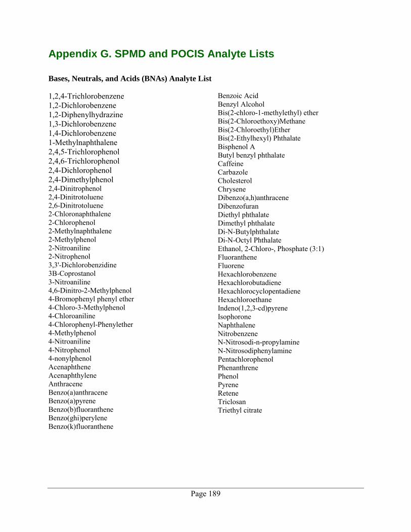
Page 189
Appendix G. SPMD and POCIS Analyte Lists Bases, Neutrals, and Acids (BNAs) Analyte List
1,2,4-Trichlorobenzene 1,2-Dichlorobenzene 1,2-Diphenylhydrazine 1,3-Dichlorobenzene 1,4-Dichlorobenzene 1-Methylnaphthalene 2,4,5-Trichlorophenol 2,4,6-Trichlorophenol 2,4-Dichlorophenol 2,4-Dimethylphenol 2,4-Dinitrophenol 2,4-Dinitrotoluene 2,6-Dinitrotoluene 2-Chloronaphthalene 2-Chlorophenol 2-Methylnaphthalene 2-Methylphenol 2-Nitroaniline 2-Nitrophenol 3,3'-Dichlorobenzidine 3B-Coprostanol 3-Nitroaniline 4,6-Dinitro-2-Methylphenol 4-Bromophenyl phenyl ether 4-Chloro-3-Methylphenol 4-Chloroaniline 4-Chlorophenyl-Phenylether 4-Methylphenol 4-Nitroaniline 4-Nitrophenol 4-nonylphenol Acenaphthene Acenaphthylene Anthracene Benzo(a)anthracene Benzo(a)pyrene Benzo(b)fluoranthene Benzo(ghi)perylene Benzo(k)fluoranthene
Benzoic Acid Benzyl Alcohol Bis(2-chloro-1-methylethyl) ether Bis(2-Chloroethoxy)Methane Bis(2-Chloroethyl)Ether Bis(2-Ethylhexyl) Phthalate Bisphenol A Butyl benzyl phthalate Caffeine Carbazole Cholesterol Chrysene Dibenzo(a,h)anthracene Dibenzofuran Diethyl phthalate Dimethyl phthalate Di-N-Butylphthalate Di-N-Octyl Phthalate Ethanol, 2-Chloro-, Phosphate (3:1) Fluoranthene Fluorene Hexachlorobenzene Hexachlorobutadiene Hexachlorocyclopentadiene Hexachloroethane Indeno(1,2,3-cd)pyrene Isophorone Naphthalene Nitrobenzene N-Nitrosodi-n-propylamine N-Nitrosodiphenylamine Pentachlorophenol Phenanthrene Phenol Pyrene Retene Triclosan Triethyl citrate

Page 190
Carbamate Analyte List 1-Naphthol 3-Hydroxycarbofuran Aldicarb Aldicarb Sulfoxide Aldicarb Sulfone Baygon (Propoxur) Carbaryl Carbofuran Diuron Imidacloprid
Linuron Methiocarb Methomyl Methomyl oxime Monuron Neburon Oxamyl Oxamyl oxime Promecarb
Herbicides Analyte List 2,3,4,5-Tetrachlorophenol 2,3,4,6-Tetrachlorophenol 2,4,5-T 2,4,5-Trichlorophenol 2,4,6-Trichlorophenol 2,4-D 2,4-DB 3,5-Dichlorobenzoic Acid 4-Nitrophenol Acifluorfen (Blazer) Bentazon Bromoxynil Clopyralid
Dacthal (DCPA) Dicamba Dichlorprop Diclofop-Methyl Dinoseb Ioxynil MCPA MCPP (Mecoprop) Pentachlorophenol Picloram Silvex Triclopyr
Pesticide Analyte List
2,4'-DDD 2,4'-DDE 2,4'-DDT 4,4'-DDD 4,4'-DDE 4,4'-DDT 4,4'-Dichlorobenzophenone Acetochlor Alachlor Aldrin Alpha-BHC Atrazine Azinphos-ethyl Azinphos-methyl (Guthion) Benefin Benthiocarb Beta-BHC
beta-Cypermethrin Bifenthrin Bromacil Butachlor Butylate Captan Carboxin Chlorothalonil (Daconil) Chlorpropham Chlorpyrifos O.A. Chlorpyriphos cis-Chlordane cis-Nonachlor cis-Permethrin Coumaphos Cyanazine Cycloate

Page 191
Pesticide Analyte List (cont.) Delta-BHC Deltamethrin Di-allate (Avadex) Diazinon Diazinon O Analog Dichlobenil Dichlorvos (DDVP) Dieldrin Dimethoate Diphenamid Disulfoton (Di-Syston) Disulfoton Sulfone Disulfoton Sulfoxide Diuron Endosulfan I Endosulfan II Endosulfan Sulfate Endrin Endrin Aldehyde Endrin Ketone EPN Eptam Ethalfluralin (Sonalan) Ethion Ethoprop Fenamiphos Fenamiphos Sulfone Fenarimol Fenvalerate (2 isomers) Fipronil Fipronil Desulfinyl Fipronil Sulfide Fipronil Sulfone Fluridone Fonofos Gamma-BHC (Lindane) Heptachlor Heptachlor Epoxide Hexachlorobenzene Hexazinone Imidan Kelthane lambda-Cyhalothrin Linuron Malathion Metalaxyl Methidathion Methoxychlor
Methyl Chlorpyrifos Methyl Paraoxon Methyl Parathion Metolachlor Metribuzin Mevinphos MGK264 Mirex Monocrotophos Naled Napropamide Norflurazon Oryzalin Oxychlordane Oxyfluorfen Parathion Pebulate Pendimethalin Phenothrin Phorate Phorate O.A. Phosmet O.A. Piperonyl Butoxide (PBO) Prometon (Pramitol 5p) Prometryn Pronamide (Kerb) Propachlor (Ramrod) Propargite Propazine Resmethrin Simazine Simetryn Sulfotepp Tebuthiuron Terbacil Tetrachlorvinphos (Gardona) Tokuthion Tralomethrin Trans-Chlordane Trans-Nonachlor Trans-Permethrin Treflan (Trifluralin) Triadimefon Triallate Trichloronate

Page 192
This page is purposely left blank

Page 193
Appendix H. Data Tables and Additional Information Table H-1. Sample Containers, Preservations, and Holding Times for Water Samples.
Parameter Container Preservation Holding Time
DOC
2 – 60 mL poly bottles;
0.45 um pore size filters
Filter in field with 0.45um pore size filter;
1:1 HCl to pH<2; Cool to 6°C
28 days
TOC 2 – 60 mL poly bottles
1:1 HCl to pH<2; Cool to 6°C
28 days
TSS 1 L poly bottle Cool to 6°C 7 days
Chloride 500 mL poly bottle (combined in same
bottle) Refrigerate, 0-6°C
28 days
Alkalinity 14 days Sulfate 28 days
Calcium, Magnesium, Sodium, Potassium, and Hardness
500 mL HDPE bottle
HNO3 to pH<2 by the lab within 24 hours of collection
6 months after
preservation
Cadmium, Copper, Nickel, Lead and Zinc
250 mL HDPE bottle*
Field filter for dissolved; HNO3 to pH<2 by the lab
within 14 days of collection
6 months after
preservation
* Containers and filters were provided by Brooks Rand because they are especially clean for low-level metals analysis; all other water chemistry containers were provided by Manchester Environmental Laboratory.
Phthalate Detection Phthalates were detected in the SPMD and POCIS samples as shown in Table H-2. Phthalates were also detected in similar but slightly lower concentrations in the day 0 blank (processing blank) and trip blank for the SPMD samples, suggesting that the majority of the phthalates detected in the samples deployed in the creek came from lab processing contamination and not from Indian Creek. The presence of phthalates in the SPMD blank samples is not surprising. Phthalates are a common background contaminant in laboratory processing, especially during dialysis and extraction. The specific phthalates and concentrations found in the SPMDs are similar to what USGS commonly finds in their blanks (David Alvarez, personal communication).

Page 194
Phthalates were not detected in the trip blank for POCIS (a day 0 blank was not analyzed for POCIS), but the detection limits for the phthalates were within close range of the concentrations found in the samples.
Table H-2. Phthalates Found in SPMDs, POCIS, and Blanks.
Phthalates Found in BNA Analysis of POCIS and
SPMDs
Concentration as ng/ 3 Membranes
Sampler Indian 1 (Upper)
Indian 2 (Lower)
Trip Blank
Day 0 Blank
Bis(2-Ethylhexyl) Phthalate POCIS 2300 1000 1000 U na
Bis(2-Ethylhexyl) Phthalate SPMD 3200 3500 1500 2300
Butyl benzyl phthalate SPMD 210 230 500 UJ 500 UJ
Diethyl phthalate POCIS 1100 590 500 U na
Diethyl phthalate SPMD 740 990 660 960
Di-N-Butyl phthalate POCIS 1600 710 500 U na
Di-N-Butyl phthalate SPMD 360 300 250 350 U: not detected at or above the reported concentration. UJ: not detected at or above the reported approximate concentration. na: not analyzed for.

Page 195
Table H-3. Metals and Stream Chemistry Data for Indian Creek.
Collection Date: 4/28/2010 5/5/2010 5/18/2010 Time: 15:40 16:40 12:00 10:15 13:30 15:15
Sample No: 1004070-1 1004070-2 1005045-1 1005045-2 1005046-1 1005046-2 Station: Indian 1 Indian 2 Indian 1 Indian 2 Indian 1 Indian 2
Metals (ug/L) Cadmium - Total 0.019
0.028 0.011
0.014
0.246
0.126
Cadmium - Diss 0.010 J 0.014 0.008 J 0.008 J 0.028
0.010 J Copper - Total 2.19
2.72 0.935
1.31
24.5
8.68
Copper - Diss 1.22
1.24 0.724
0.802
3.50
1.96 Nickel - Total 1.15
1.26 0.87
0.94
8.70
4.16
Nickel - Diss 0.76
0.80 0.76
0.71
0.80
0.58 Lead - Total 0.916
1.13 0.438
0.630
17.2
8.00
Lead - Diss 0.189
0.184 0.145
0.150
0.394
0.214 Zinc - Total 12.1
12.0 4.65
5.63
85.3
40.0
Zinc - Diss 4.79 5.00 3.54 3.20 7.19 3.71 Chemistry (mg/L) Calcium 10.9
11.4 11.6
12.3
14.3
12.5
Potassium 1.20
1.34 1.11
1.27
2.05
1.65 Magnesium 4.80
5.73 5.05 J 6.14
6.63
5.94
Sodium 8.05
8.18 8.45
8.37
8.97
8.12 Hardness 45.6
52.3 46.7
54.0
51.3
52.6
Alkalinity 44.6
50.1 45.7
52.5
42.1
47.2 Chlorides 6.48
6.40 6.61
6.66
6.20
5.94
Sulfate 5.83
6.76 7.15
7.86
5.62
6.42 TSS 7
12 3
6
231 J 96
TOC 9.0
7.4 9.5
7.1
11.8
8.7 DOC 8.5 6.9 8.7
6.9
9.4
7.9
Field Measurements DO (mg/L) 10.47
10.37 11.06
11.08
9.95
9.97
pH (pH units) 7.31
7.41 7.24
7.61
7.24
7.47 Conductivity (umhos/cm) 121.1
134.7 128.3
141.9
118.1
128.3
Temp (C◦) 11.18
11.08 9.58
9.06
13.08
13.28 Flow (CFS) na 3.43 na 2.91 na 3.76 TSS: total suspended solids TOC: total organic carbon DOC: dissolved organic carbon DO: dissolved oxygen J: result is an estimate. na: not analyzed for.

Page 196
Table H-4. Stream Measurement Data for Indian Creek.
Location Date Time Temp. (C◦)
Cond. (umhos/cm) pH
Dissolved Oxygen Flow
Co-occurring activity (% Sat) (mg/L) Gage
Reading (CFS)
Indian 1 (upper station)
4/12/10 14:50 10.5 116.3 7.45 97.9 10.94 na na Daphnid deployment 4/14/10 13:40 10.62 121.0 7.16 99.5 11.00 na na Retrieval of 48 hr daphnia 4/16/10 9:55 9.61 122.3 7.49 97.1 11.00 na na Retrieval of 96 hr daphnia; bioassessments 4/20/10 15:15 12.17 126.7 7.32 95.9 10.26 na na Trout basket placement 4/21/10 12:55 10.90 127.2 7.37 96.5 10.63 na 1.98 Bug bag placement 4/22/10 12:00 10.80 128.6 7.40 98.4 10.92 na na Deployment of POCIS/SPMD/SLMD/DGT 4/26/10 12:15 10.34 128.6 7.46 96.2 10.77 na na Daphnid deployment 4/28/10 15:40 11.18 121.1 7.31 97.0 10.47 na na Metals/BLM water sample collection 4/29/10 10:05 9.64 127.9 7.41 97.3 10.86 na na Check on trout baskets at hatch 4/30/10 11:10 10.05 128.4 7.37 98.0 10.84 na na Retrieval of 96 hr daphnia 5/3/10 12:35 10.56 118.7 7.23 97.8 10.71 na na Daphnid deployment 5/5/10 12:00 9.58 128.3 7.24 97.2 11.06 na na Metals/BLM water sample collection 5/7/10 10:25 9.39 127.7 7.41 96.6 11.05 na na Daphnid removal
5/10/10 12:15 10.62 123.2 7.40 95.3 10.60 na na Daphnid deployment 5/12/10 10:00 10.08 131.1 7.42 97.3 10.90 na na Daphnid removal 5/13/10 9:55 10.38 132.3 7.44 96.7 10.75 na na Check on trout baskets (alevin stage) 5/17/10 11:45 12.10 136.8 7.45 94.5 10.11 na na Daphnid deployment 5/18/10 13:30 13.08 118.1 7.24 95.9 9.95 na na Metals/BLM water sample collection 5/19/10 9:50 11.85 136.7 7.56 96.4 10.27 na na Daphnid removal 5/20/10 10:25 10.51 103.0 7.46 97.3 10.72 na na Removal of POCIS/SPMD/SLMD/DGT 5/20/10 16:50 11.82 79.8 7.20 97.5 10.41 na na Heavy rainfall event 5/24/10 10:20 10.25 131.8 7.59 96.2 10.68 na na Removal of trout baskets
Indian 2 (lower station)
4/12/10 12:30 9.48 129.1 7.55 95.1 10.90 0.41 4.42 E Daphnid deployment 4/14/10 11:45 9.62 135.0 7.46 97.0 10.99 0.39 3.52 Retrieval of 48 hr daphnia 4/16/10 9:30 9.35 136.6 7.51 95.6 10.93 0.38 3.43 E Retrieval of 96 hr daphnia; bioassessments 4/20/10 16:45 12.06 141.5 7.47 94.4 10.12 0.37 3.10 E Trout basket placement 4/21/10 11:15 10.63 142.0 7.59 95.0 10.53 0.36 2.91 Bug bag placement 4/22/10 15:20 11.45 143.3 7.34 95.6 10.44 0.34 2.11 E Deployment of SLMD/DGT samplers 4/26/10 11:40 10.20 144.3 7.51 94.9 10.65 0.35 2.44 E Daphnid deployment 4/27/10 12:30 10.77 136.1 7.55 94.9 10.34 0.38 3.43 E Water quality check

Page 197
Location Date Time Temp. (C◦)
Cond. (umhos/cm) pH
Dissolved Oxygen Flow
Co-occurring activity (% Sat) (mg/L) Gage
Reading (CFS)
4/28/10 16:40 11.08 134.7 7.41 95.9 10.37 0.38 3.43 E Metals/BLM water sample collection 4/29/10 11:05 9.66 142.8 7.54 96.7 10.81 na na Check on trout baskets at hatch 4/30/10 10:50 9.97 143.0 7.53 96.1 10.65 na na Retrieval of 96 hr daphnia 5/3/10 11:00 9.89 118.9 7.40 95.6 10.64 0.42 4.04 E Daphnid deployment 5/5/10 10:15 9.06 141.9 7.61 95.9 11.08 0.36 2.77 E Metals/BLM water sample collection 5/7/10 10:00 9.06 144.6 7.42 94.7 10.93 0.35 2.44 E Daphnid removal
5/10/10 11:15 10.71 133.7 7.49 94.2 10.47 0.37 3.10 E Daphnid deployment 5/12/10 9:20 10.04 148.1 7.58 96.4 10.80 0.33 1.78 E Daphnid removal 5/13/10 10:55 10.40 150.7 7.49 95.4 10.63 na na Check on trout baskets (alevin stage) 5/17/10 10:45 12.08 155.8 7.54 93.8 10.02 0.32 1.45 E Daphnid deployment 5/17/10 11:25 12.15 153.2 7.54 93.7 10.01 0.36 2.77 E Readings after pulse of stormwater 5/18/10 15:15 13.28 128.3 7.47 96.7 9.97 0.39 3.76 E Metals/BLM water sample collection 5/19/10 9:25 11.78 153.1 7.66 95.2 10.18 0.33 1.78 E Daphnid removal 5/20/10 12:05 10.64 115.5 7.52 96.6 10.59 0.45 5.74 E Removal of POCIS/SPMD/SLMD/DGT 5/20/10 16:30 11.39 89.2 7.37 97.1 10.46 0.58 10.03 E Heavy rainfall event 5/24/10 10:55 10.11 148.6 7.52 95.0 10.59 0.35 2.44 E Removal of trout baskets
E: estimated flow from rating curve. na: not analyzed for.

Page 198
Table H-5. Daily Water Temperatures and Changes Over Each Day.
Temperature (ºC) Minimum, Maximum, and Overall Change over One Day from TidbiT Attached to Trout Baskets
Date Indian 1 upper station Indian 2 lower station min max ∆T min max ∆T
4/29/10 10.11 11.36 1.25 9.98 11.54 1.56 4/30/10 9.49 10.73 1.24 9.52 10.45 0.93 5/1/10 9.49 11.67 2.18 9.52 10.29 0.77 5/2/10 9.49 10.58 1.09 9.67 10.61 0.94 5/3/10 9.33 10.89 1.56 9.67 10.29 0.62 5/4/10 8.4 10.11 1.71 8.58 9.52 0.94 5/5/10 8.71 10.11 1.4 8.74 10.14 1.4 5/6/10 8.09 10.73 2.64 8.12 10.92 2.8 5/7/10 8.4 11.51 3.11 8.58 11.85 3.27 5/8/10 8.87 11.82 2.95 8.89 12.16 3.27 5/9/10 9.02 11.98 2.96 9.05 12.32 3.27 5/10/10 10.42 11.36 0.94 10.61 11.69 1.08 5/11/10 9.33 11.04 1.71 9.36 11.23 1.87 5/12/10 9.64 11.98 2.34 9.67 12.32 2.65 5/13/10 9.64 12.45 2.81 9.67 12.63 2.96 5/14/10 10.27 12.92 2.65 10.45 13.1 2.65 5/15/10 10.58 12.92 2.34 10.76 13.1 2.34 5/16/10 11.04 13.23 2.19 11.38 13.26 1.88 5/17/10 11.67 13.38 1.71 12.01 13.41 1.4 5/18/10 11.98 14.16 2.18 12.16 13.72 1.56 5/19/10 11.51 14.16 2.65 11.69 13.72 2.03 5/20/10 10.27 11.82 1.55 10.29 12.01 1.72 5/21/10 10.27 10.89 0.62 10.14 10.92 0.78 5/22/10 10.11 11.36 1.25 9.98 11.38 1.4 5/23/10 10.11 11.2 1.09 10.14 11.38 1.24 5/24/10 9.64 10.58 0.94 9.67 10.76 1.09

Page 199
Appendix I. Graphs Showing King County 2009 Stream Monitoring Data
Figure I-1. Longfellow Creek Metals Monitoring Data during Two Rain Events.
Figure I-2. Longfellow Creek and Lund’s Gulch Creek Data during 11/16/09 Storm.
0
0.5
1
1.5
2
2.5
3
3.5
7:20 8:35 9:20 10:00 10:50 11:40 12:25 13:15 14:10 15:20 Time
Longfellow Creek Stream Height and Metals Concentrations (10/23/2009)
Staff Height (ft)
Copper (µg/L)
Lead (µg/L)
Nickel (µg/L)
Zinc (µg/L)
0
1
2
3
4
5
6
7
9:47 11:11 12:49 14:30 16:15 17:00 17:45 18:30 19:15 20:00 Time
Longfellow Creek Stream Height and Metals Concentrations (11/16/2009)
Staff Height (ft)
Copper (µg/L)
Lead (µg/L)
Nickel (µg/L)
Zinc (µg/L)
0
5
10
15
20
25
30
10:15 11:35 13:00 14:05 15:15 16:15 17:15 18:10 19:00 19:55
mg/L
Time
Lund's Gulch Water Chemistry Parameters and Stream Height on 11/16/2009
Stream Height (ft)
DOC
TOC
Magnesium
Calcium
Potassium
Sodium
Chloride
0
2
4
6
8
10
12
14
16
18
20
9:47 11:11 12:49 14:30 16:15 17:00 17:45 18:30 19:15 20:00
mg/L
Time
Longfellow Creek Water Chemistry Parameters and Stream Height on 11/16/2009
Stream Height (ft)
DOC
TOC
Magnesium
Calcium
Potassium
Sodium
Chloride

Page 200
Figure I-3. pH Results Every 5 Minutes in Longfellow Creek and Lund’s Gulch Creek during 11/16/09 Rain Event.
7.1
7.2
7.3
7.4
7.5
7.6
7.7
7.8
8:00 10:24 12:48 15:12 17:36 20:00 22:24
pH
Time
pH During 11/16/09 Rain Event in Longfellow (LF) Creek and Lund's Gulch
Lunds
LF

Page 201
Appendix J. Data for Woodard Creek During the pilot study conducted by Ecology on Indian Creek, the Thurston County Water Resources Program led some additional water quality work on nearby Woodard Creek. Woodard Creek is also located in the south Puget Sound area, but it drains into Henderson Inlet. Data collected for Woodard Creek is shown here and is also available at Ecology’s Environmental Information Management (EIM) website www.ecy.wa.gov/eim/index.htm. Search User Study ID, BERA0008. Five installments of Daphnia magna were conducted at Woodard Creek at the same times as Indian Creek. As with Indian Creek, all the daphnia survived during each deployment, indicating no acute toxicity in Woodard Creek. Table J-1. Stream Measurements for Woodard Creek.
Date Time Temperature (C◦)
Conductivity (umhos/cm) pH
Dissolved Oxygen TSS (mg/L)
TOC (mg/L) (% Sat) (mg/L)
4/12/10 16:00 10.55 125.8 7.38 93.0 10.38 na na 4/14/10 14:20 11.10 132.4 7.42 94.7 10.36 na na 4/16/10 10:35 9.54 132.5 7.47 92.7 10.52 na na
4/26/10 14:50 10.50 135.5 7.36 92.0 10.25 na na 4/27/10 11:10 10.59 130.2 7.46 89.9 9.83 na na
5/3/10 15:00 11.05 120.6 7.32 91.0 9.84 na na
5/5/10 15:30 10.17 131.1 7.30 93.4 10.50 2 J 1.0 5/7/10 11:15 9.40 133.3 7.40 93.1 10.66 na na
5/10/10 14:00 11.02 133.4 7.38 91.9 10.14 na na 5/12/10 10:35 10.33 137.0 7.39 94.0 10.47 na na
5/17/10 12:35 12.42 142.5 7.47 92.4 9.81 na na 5/19/10 10:40 12.34 137.7 7.48 92.9 9.71 na na 5/25/10 12:00 11.16 137.0 7.41 92.3 10.07 na na
na: not analyzed for. J: result is an estimate.
Only the detected chemicals in the POCIS sample for Woodard Creek are shown in Table J-2. Results are given in ng per 3 membranes. Estimated water concentrations were not calculated. Captan, tebuthiuron, and N-Nitrosodiphenylamine were all detected in the POCIS field blank at similar concentrations to the Woodard Creek sample. Phthalates were detected, but at concentrations close to the reporting limits.

Page 202
Table J-2. POCIS Results for Woodard Creek.
Parameter Woodard
Creek POCIS
Field Blank
Result (ng/3 membranes) Captan 1900 NJ 2600 NJ Tebuthiuron 120 110 N-Nitrosodiphenylamine 460 J 430 J Bis(2-Ethylhexyl) Phthalate 1600 1000 U Diethyl phthalate 1600 500 U Di-N-Butyl phthalate 770 1000 U
NJ: analyte is tentatively identified and result is an estimate. J: result is an estimate. U: result was not detected at or below the reported concentration.