lable at ScienceDirect

Renewable Energy 75 (2015) 326e334

Contents lists avai

Renewable Energy

journal homepage: www.elsevier .com/locate/renene

Initial stabilization of a statistical sample of forty-four monocrystallinephotovoltaic modules

Alessandra Colli a, *, Johan Vasquez b, Willem J. Zaaiman c

a Brookhaven National Laboratory, 2 Center Street, Upton, NY 11973, USAb Suffolk County Community College, 533 College Road, Selden, NY 11784, USAc The Renewable Energy Unit, EC Joint Research Centre, Institute for Energy and Transport, 21027 Ispra, Italy

a r t i c l e i n f o

Article history:Received 19 May 2014Accepted 11 September 2014Available online

Keywords:PV module performanceMonocrystalline siliconStabilizationDegradation

* Corresponding author. Tel.: þ1 631 344 2666.E-mail addresses: alessandra.colli@gmail.com (A

(J. Vasquez), willem.zaaiman@jrc.ec.europa.eu (W.J. Z

http://dx.doi.org/10.1016/j.renene.2014.09.0620960-1481/© 2014 Elsevier Ltd. All rights reserved.

a b s t r a c t

The paper discusses the methodology and presents the results of the stabilization process for a statistic offorty-four monocrystalline silicon photovoltaic (PV) modules. The modules have been exposed to realsunlight in three different sessions and have been measured prior exposure and after each exposuresession using a pulsed sun simulator. The first session of exposure shows the highest power loss in themodules, with an average 1.8%. During this initial stabilization step, 17 modules had a loss in themaximum power above 2% (registered losses from 2.1% to a maximum of 2.8%). The overall power lossesare in the range 1.7e3.4%, with an average loss of 2.4% for the considered module population. Visualinspection and the analysis of the measured IeV curves revealed some imperfections in the modules.However, those imperfections do not impact on the actual performance at the present time. After thestabilization, the modules have been installed in the Northeast Solar Energy Research Center (NSERC)array, located at Brookhaven National Laboratory. The array will be used to analyze module degradationin the Northeast environmental conditions and to study the grid impact of utility-level PV plants.

© 2014 Elsevier Ltd. All rights reserved.

1. Introduction

The purpose of this analysis is to evaluate the initial stabilizationprocess of a set of 44 monocrystalline photovoltaic (PV) modulesand use the results as a reference starting point for future annualoutdoor performance degradation analysis of the samemodules. PVmodules are subject to degradation processes during their outdoorexposure and system operation. All degradation factors ultimatelylead to loss of performance or, in the worst case, to a complete lossof power. Different degradation mechanisms can be identified andmainly grouped in the following categories: (1) environmental, (2)high system voltage or potential-induced and (3) compositional/structural (Fig. 1). PV modules, though apparently simple as amacro-structure, are highly complex systems where physical, me-chanical, and chemical interactions are taking place, requiringdetailed compositional analysis entering into micro- and nano-structures to appropriately understand the physics of degrada-tion. Additionally, the use of PV modules within arrays requires

. Colli), jvasq13@gmail.comaaiman).

them to withstand system voltages of 600e1000 V or higher. If notproperly protected, modules can undergo an accelerated degrada-tion process with corrosive characteristics originating from thecontinuous high voltage stress. Potential induced degradation (PID)is a complicated phenomenon [1]; indoor tests show that it isreversible as long as the degradation has not started and it has beenfound to affect both thin-film and crystalline silicon modules.

However the long-term degradation of modules is differentfrom the initial stabilization process, which is a non-linear process[2]. The stabilization process is driven by the metastabilitiesaffecting the different types of PV technologies [3] and it affects theeffective power of the installation with positive or negative varia-tions compared to the power rating declared by the modulemanufacturer [2,4]. This effect is not addressed by the internationalstandards for the qualification of PVmodules (IEC 61215 [5] and IEC61646 [6]), and, given the different nature of the process dependingon the PV material, it would require specific procedures to bedeveloped and applied [6].

The specific amount of 44 PVmodules considered in the presentinvestigation corresponds to the content of two full boxes asdelivered by the manufacturing company. The PV modules underanalysis have been installed in the Brookhaven National Labo-ratory's (BNL) Northeast Solar Energy Research Center (NSERC)

Fig. 1. Main types of degradation affecting PV modules.

A. Colli et al. / Renewable Energy 75 (2015) 326e334 327

array after stabilization and performance characterization. Theycover three strings of the NSERC array: two complete strings of 19modules each and one string having only 6 reference modules, butalways complete with a total of 19 modules of the same type. Thelocationwhere themodules are installed is identified in the array asindicated in Fig. 2, which shows the existing part of the NSERCresearch array with rated DC power of 518 kW. The total number ofmodules presently installed in the array is 1672. The plant is grid-

Fig. 2. Area 1 of the NSERC research array. The indication

connected to the electric grid of BNL and operated independentlyby the laboratory. The need for independence from the utility interms of plant management is required by the reconfigurablecharacteristic of the plant to meet various research needs in thefield of grid integration and smart grids. The entire research arrayincludes two additional areas, already designed but still waiting forconstruction. Area 2 will include single axis tracking systems, whilearea 3 will be devoted to the test of PV modules of different tech-nologies for performance evaluation in the specific Northeast USclimate conditions.

During the lifetime of the NSERC array, the annual degradationof the 44 reference modules will be evaluated with annual mea-surement activities.

It's an established occurrence that the extended illumination ofPV devices, referred to as light soaking, originates changes in thematerial due to metastable phenomena. The extent of thesechanges can be different according to the PV technology (forexample amorphous silicon can register losses about 10e30% [7])and is not always associated to efficiency loss. In fact, some thin-film technologies such as CdTe and CIGS have also shown cases ofefficiency improvement during the initial hours of light soaking [7].

However, light-inducedmetastabilitiesdonot affectonly thin-filmmaterials. PV devices using boron-doped Czochralski-grown mono-crystalline silicon also exhibit an initial light-induced degradationeffect that can reach ~4% power output degradation during the firsthours of light soaking [7,8]. The effect is due to the light-inducedactivation of a metastable boroneoxygen defect which lowers car-rier lifetime and it can be recovered by anneal or dark storage [9].

According to the international standard IEC 61215 [5], “beforebeginning the testing, all modules, including the control, shall beexposed to sunlight (either real or simulated) to an irradiation level of5 kWh/m2 to 5.5 kWh/m2 while open-circuited”. This approach as-sures that crystalline silicon modules are stabilized. Actually, oncestabilized, monocrystalline silicon is considered to remain a verystable material in comparison with other PV technologies.

shows where the 44 reference modules are installed.

Table 1Technical characteristics of the monocrystalline PV modules.

Type Value

Rated power 310 WUncertainty of rated power �0/þ3%Module efficiency 16.02%Voltage at MPP 36.2 VCurrent at MPP 8.56 AOpen circuit voltage 45.7 VShort circuit current 9.06 AUncertainty of electrical parameters ±5%Cells in series 72Cell dopant species Boron, P-type

Fig. 4. PV module position on the Spire test bed. The values indicated on the side ofthe module refers to the distance from the module frame to the test bed border edge.

A. Colli et al. / Renewable Energy 75 (2015) 326e334328

2. Description of the methodology

The technical specifications of the modules tested during thisanalysis are listed in Table 1.

The reason for choosing an amount of 44 modules is primarilygiven by statistical considerations on a total of 1672 modulesdeployed at the PV array location. An additional constraint refers tospace limitations and the need to simultaneously handle all mod-ules so that the level of light received is similar for all samples alongthe process. This will make the measurements comparable duringthe analysis.

The following procedure has been defined for the purpose of theanalysis in subject:

1. Open the two boxes, extract the modules and systematicallyclean the front glass from possible manufacturing residues.

2. Perform the initial visual inspection to detect visible defects andimperfections.

3. Perform first out-of-the-box IeV measurements. IeV charac-terization has been done by using a Spire 4600SLP long pulsesun simulator (Fig. 3). The position of the modules on the Spiretest bed has been maintained constant throughout all themeasurements performed in the present analysis according tothe indications of Fig. 4.

4. Position all modules to be simultaneously exposed to real sun-light in open circuit (Fig. 5). A total of three exposure sessionshave been done to reach the required irradiation.

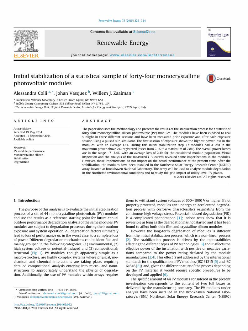
5. Global horizontal (in module plane) irradiance readings havebeen registered every 15 min during each exposure session. AnSP Lite2 semiconductor-based pyranometer has been used andthe irradiance values have been recorded by a Campbell Scien-tific data acquisition system (Fig. 6).

Fig. 3. The Spire SLP4600 pulsed sun simulator at BNL.

6. Move the modules indoor, and let them cool down at roomtemperature. Measurements are performed at a temperature of25 ± 2 �C.

7. Perform IeV measurements after each exposure session.8. Finally reposition themodules into the container boxes, ready to

reach the solar array construction site for installation.Consistency in the measurements has been controlled by pro-

cessing each module two non-consecutive times for every mea-surement stage and considering the average between the twomeasures as the final result. This approach will inherently considerrepositioning and reconnecting effects between each module andthe simulator. The flow is expected to follow the sequence:

1. Measurement of the reference module.2. First measure of all the 44 modules.3. Measurement of the reference module.4. Second measure of all the 44 modules.5. Measurement of the reference module.

The measurement of the reference module at the beginning isnecessary to calibrate the simulator, while at the end of every roundof measurements it will help assuring that no changes in thespectrum of the light intervened.

Finally, the standard deviation of the measurements is calcu-lated to estimate repeatability for the reference module and con-sistency for the statistical analysis.

Fig. 5. The PV modules during the outdoor sunlight exposure for stabilization.

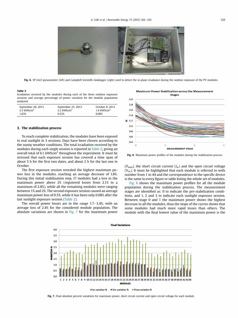
Fig. 6. SP Lite2 pyranometer (left) and Campbell Scientific datalogger (right) used to detect the in-plane irradiance during the outdoor exposure of the PV modules.

Table 2Irradiation received by the modules during each of the three outdoor exposuresessions and average percentage of power variation for the module populationanalyzed.

September 20, 2013 September 25, 2013 October 8, 20132.5 kWh/m2 2.2 kWh/m2 1.4 kWh/m2

1.83% 0.52% 0.08%

Fig. 8. Maximum power profiles of the modules during the stabilization process.

A. Colli et al. / Renewable Energy 75 (2015) 326e334 329

3. The stabilization process

To reach complete stabilization, the modules have been exposedto real sunlight in 3 sessions. Days have been chosen according tothe sunny weather conditions. The total irradiation received by themodules during each single session is reported in Table 2, giving anoverall total of 6.1 kWh/m2 throughout the experiment. It must bestressed that each exposure session has covered a time span ofabout 3 h for the first two dates, and about 2 h for the last one inOctober.

The first exposure session revealed the highest maximum po-wer loss in the modules, reaching an average decrease of 1.8%.During this initial stabilization step, 17 modules had a loss in themaximum power above 2% (registered losses from 2.1% to amaximum of 2.8%), while all the remaining modules were rangingbetween 1% and 2%. The second exposure session caused an averagemaximum power loss of 0.5%, while it has been only 0.08% after thelast sunlight exposure session (Table 2).

The overall power losses are in the range 1.7e3.4%, with anaverage loss of 2.4% for the considered module population. Theabsolute variations are shown in Fig. 7 for the maximum power

Fig. 7. Final absolute percent variations for maximum power, sho

(Pmax), the short circuit current (Isc) and the open circuit voltage(Voc). It must be highlighted that each module is referred to withnumber from 1 to 44 and the correspondence to the specific deviceis the same in every figure or table listing the whole set of modules.

Fig. 8 shows the maximum power profiles for all the modulepopulation during the stabilization process. The measurementstages are identified as: 0 to indicate the pre-stabilization condi-tions, and 1, 2 and 3 to indicate each sunlight exposure session.Between stage 0 and 1 the maximum power shows the highestdecrease in all the modules, thou the slope of the curves shows thatsome modules had much more rapid losses than others. Themodule with the final lowest value of the maximum power is the

rt circuit current and open circuit voltage for each module.

Table 3Average values of Isc [A] and Voc [V] for the pre-stabilization conditions (0) and aftereach sunlight exposure session (1, 2 and 3).

Module Av.Isc0 Av. Voc0 Av. Isc1 Av. Voc1 Av. Isc2 Av. Voc2 Av. Isc3 Av. Voc3

1 8.884 46.12 8.842 45.87 8.808 45.77 8.823 45.802 8.889 46.17 8.882 45.91 8.839 45.86 8.842 45.863 8.905 46.12 8.879 45.85 8.837 45.83 8.848 45.834 8.889 46.15 8.872 45.81 8.831 45.81 8.829 45.785 8.904 46.05 8.886 45.85 8.828 45.79 8.842 45.766 8.887 46.19 8.849 45.87 8.818 45.83 8.841 45.827 8.930 46.21 8.899 45.90 8.857 45.85 8.882 45.858 8.894 46.12 8.869 45.84 8.831 45.82 8.853 45.829 8.874 46.40 8.791 45.94 8.744 45.86 8.768 45.8610 8.862 46.46 8.822 46.04 8.792 45.96 8.784 45.9911 8.875 46.44 8.796 45.97 8.763 45.91 8.777 45.9412 8.870 46.37 8.792 45.94 8.744 45.90 8.771 45.9113 8.875 46.41 8.799 46.04 8.744 46.00 8.753 45.9714 8.880 46.42 8.807 46.01 8.765 45.94 8.793 45.9615 8.870 46.36 8.780 45.98 8.774 45.90 8.779 45.8916 8.841 46.45 8.762 46.02 8.754 46.01 8.754 45.9817 8.860 46.52 8.743 46.07 8.761 46.04 8.761 46.0318 8.898 46.44 8.808 46.03 8.798 46.00 8.792 45.9419 8.900 46.53 8.832 46.09 8.807 46.01 8.806 46.0020 8.903 46.55 8.816 46.05 8.807 46.01 8.804 45.9421 8.880 46.53 8.794 46.05 8.800 45.97 8.797 45.9322 8.900 46.47 8.821 46.10 8.801 46.01 8.806 45.9923 8.862 46.47 8.805 46.03 8.778 45.92 8.768 45.8924 8.879 46.49 8.801 46.06 8.808 46.00 8.786 45.9625 8.931 46.46 8.839 45.99 8.829 45.90 8.835 45.9026 8.909 46.44 8.828 46.01 8.811 45.95 8.816 45.9027 8.912 46.45 8.877 46.05 8.841 45.97 8.823 45.9128 8.872 46.53 8.834 46.14 8.792 46.07 8.781 46.0229 8.889 46.47 8.862 46.07 8.818 46.00 8.798 45.9730 8.870 46.40 8.856 46.06 8.823 46.08 8.806 46.0531 8.867 46.38 8.858 46.05 8.817 46.05 8.814 46.0232 8.850 46.34 8.821 46.02 8.803 46.03 8.814 46.0033 8.852 46.36 8.835 46.07 8.801 46.07 8.799 46.0334 8.873 46.15 8.855 46.02 8.822 45.99 8.813 45.9835 8.871 46.25 8.857 46.00 8.801 45.97 8.823 45.9536 8.845 46.27 8.838 45.98 8.773 46.00 8.794 45.9537 8.837 46.31 8.827 46.06 8.792 46.01 8.783 46.0138 8.862 46.24 8.848 46.01 8.810 46.03 8.808 46.0439 8.836 46.19 8.810 45.92 8.790 45.94 8.775 45.9040 8.866 46.23 8.858 46.06 8.828 46.04 8.803 46.0341 8.857 46.27 8.843 46.03 8.804 45.97 8.809 45.9442 8.894 46.28 8.854 45.96 8.823 45.99 8.806 45.9343 8.875 46.30 8.866 46.11 8.846 46.03 8.826 45.9844 8.849 46.31 9.842 46.07 8.813 46.05 8.809 46.01

A. Colli et al. / Renewable Energy 75 (2015) 326e334330

number 25, while the module which shows the highest powervariation between the first (0) and the last (3) measurement is thenumber 23 (as shown in Fig. 7).

For the interest of the reader, the average values (alwaysintended as average between the two non-consecutive measures

Fig. 9. Average FF for all the 44 modules be

per session) for Isc and Voc registered for each module at everymeasurement session are shown in Table 3.

The fill factor (FF) decreased averagely 0.73% between themeasurements taken before and after the stabilization process,respectively passing from 0.77 to 0.76. The single average values areshown in Fig. 9.

The efficiency of the modules decreased from an initial overallaverage value of 18.08% to a final overall average value if 17.63%,with a loss of 2.46%. The single efficiency losses for all the modulesare shown in Fig. 10.

4. Statistical analysis

Fig 11 shows the average values for Pmax alongwith the variationfrom the two non-consecutive measures taken for every module ateach measurement step. It's interesting to see that the patternidentified by Fig. 11 in the pre-stabilization stage changes after thefirst sunlight exposure, remaining constant also after the secondand third exposure. Differently, the variation around the averagePmax value for the same module changes along the sessions as it ismainly related to the sun simulator uncertainty, including therepositioning of the module on the test bed and the reconnection ofthe electric contacts, which could create variations in the seriesresistance.

The overall average standard deviations between the two non-consecutive measures of respectively Pmax, Isc and Voc at eachmeasurement stage are listed in Table 4.

The reference module used to calibrate the sun simulator priorevery use is a 225 W polycrystalline silicon module. During eachmeasurement session the reference module has been used tocalibrate the simulator and measured again at the end of eachsession to confirm that no change has intervened in the light.Table 5 shows results concerning the good repeatability of all themeasures taken with the reference modules along all theexperiment.

5. Defects encountered

The 44 PV modules characterized and stabilized during thiswork are brand new modules coming directly from the manufac-turer and unpacked at the time of the present study. The initialvisual inspection of the modules has revealed some minor defects,while the presence of a cracked cell has been detected through theanalysis of the IeV curve of the affected module. At the time of thisinvestigation, all the listed defects did not impact on the moduleperformance and all the affectedmodules have been installed in theNSERC array, where they will be monitored for performance anddegradation.

fore and after the stabilization process.

Fig. 10. Final efficiency percent variations for each module.

Fig. 11. Average values of Pmax for every module during each measurement stage along with the bar to identify the respective variation between the two non-consecutive measurestaken at each stage.

A. Colli et al. / Renewable Energy 75 (2015) 326e334 331

Table 4Average standard deviation between the two non-consecutive measures in eachsession for the maximum power, short circuit current and open circuit voltage.

Session: 0 1 2 3

St. Dev Pmax 0.510 0.489 0.465 0.437St. Dev Isc 0.006 0.017 0.013 0.009St. Dev Voc 0.037 0.026 0.029 0.015

Table 5Standard deviation between the measures of the reference module for the SpireSLP4600 simulator taken along the analysis of the module population. Thepercent standard deviation is given as a percentage of Pmax, Isc, Voc and FFrespectively.

St. Dev St. Dev%

Pmax 0.405 0.18%Isc 0.021 0.25%Voc 0.058 0.15%FF 0.001 0.17%

Fig. 13. IeV curve of one module with suspect broken cell. When enlarged, the indi-cated part of the IeV curve shows an evident step, pointing out at a possible brokencell.

A. Colli et al. / Renewable Energy 75 (2015) 326e334332

5.1. Manufacturing defects

Module 44 shows defects in the metallization process. Few cellsin the module present 2 points of interruption in the metallizationgrid (Fig. 12 left). The interruptions are reproduced with a regularpattern on the affected cells, which probably recalls a dirtobstruction in the mask used during the contact printing process.

A large number of modules show light-colored spots on thesilicon nitride antireflective coating in various cells (Fig. 12 right).Also in this case a regular pattern in the position of the spots relatesto the manufacturing process. The spots should actually correspondto the points where the cells are hold in place in the containersduring the antireflective coating deposition process.

However, it has been verified that both the defects identified inFig. 12 do not affect the module performance at this stage of its life.It will be verified with future yearly-based analysis if these defectscan somewhat accelerate the module degradation process, inparticular, given the 1000 V system deployment environmentwhere the modules are located.

5.2. Issues affecting the IeV curve

The IeV characterization of module 26 has highlighted thepresence of a possible broken cell. From the IeV curve a non-linearity with an evident step down of the curve has been detec-ted as shown in Fig. 13. Such behavior could indicate that themodule contains a broken cell. For this reason the investigation has

Fig. 12. Small defects in the metallization grid found in the PV modules 44 (left) and lighte(right) which correspond to the points where the cells are hold in place during the antirefl

been taken further by looking at the module exposed to real sun-light in short circuit conditions with an infrared (IR) camera.

The outcome is shown in Fig. 14, where the cell in the lower leftcorner of each picture clearly shows two different thermal behaviorthat cannot be related to the particular conditions of the moduleback (such as the presence of the junction box) or themodule frame.

The affected cell is positioned in the corner. To exclude anythermal effect of the module aluminum frame on the cell temper-ature, similar IR images have been taken also for other modules, butthey did not show the same diagonal separation among the twopart of the corner cell.

Given that the type of module controls discussed in this workare normally not performed prior installation in commercial orprivate plants, the module 26 has been installed in the researcharray and its conditions will be verified along with its degradationprocess in comparison with the other modules in the analyzedpopulation.

r spots on the silicon nitride antireflective coating of some cells in various PV modulesective coating deposition process.

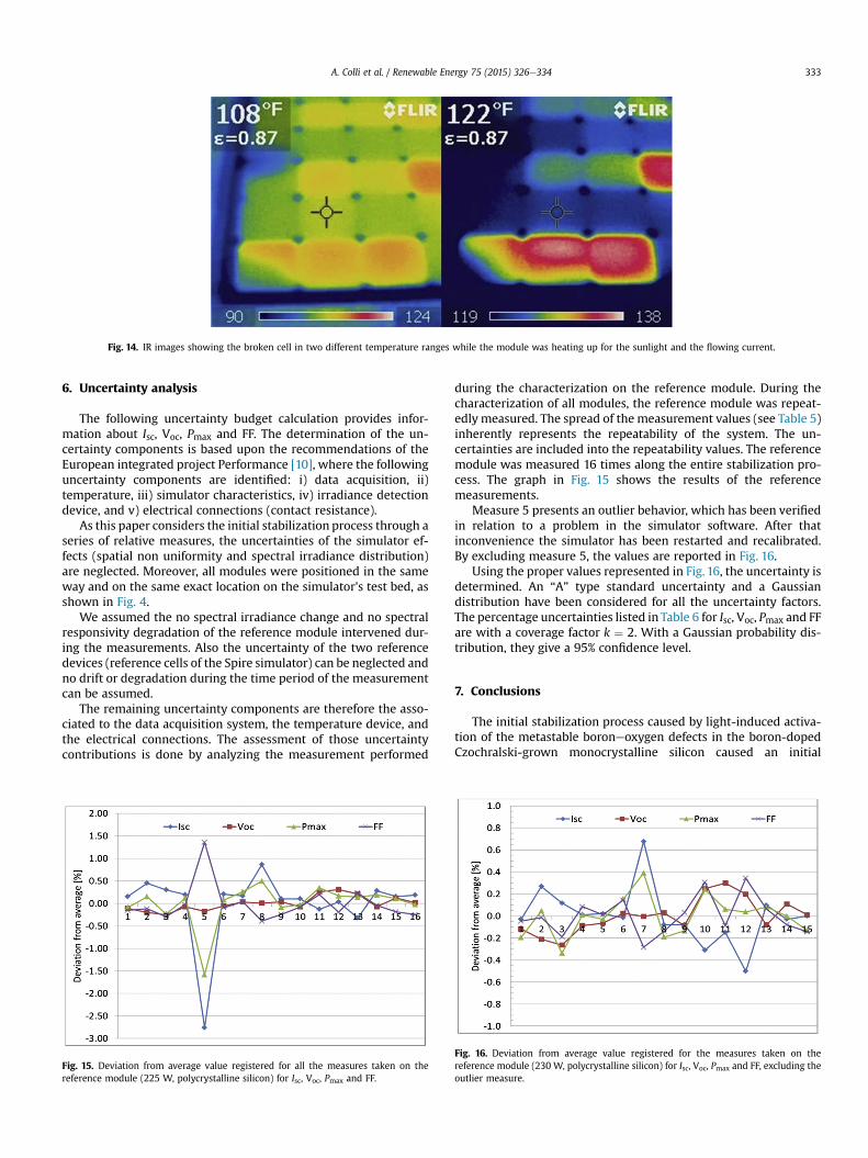
Fig. 14. IR images showing the broken cell in two different temperature ranges while the module was heating up for the sunlight and the flowing current.

A. Colli et al. / Renewable Energy 75 (2015) 326e334 333

6. Uncertainty analysis

The following uncertainty budget calculation provides infor-mation about Isc, Voc, Pmax and FF. The determination of the un-certainty components is based upon the recommendations of theEuropean integrated project Performance [10], where the followinguncertainty components are identified: i) data acquisition, ii)temperature, iii) simulator characteristics, iv) irradiance detectiondevice, and v) electrical connections (contact resistance).

As this paper considers the initial stabilization process through aseries of relative measures, the uncertainties of the simulator ef-fects (spatial non uniformity and spectral irradiance distribution)are neglected. Moreover, all modules were positioned in the sameway and on the same exact location on the simulator's test bed, asshown in Fig. 4.

We assumed the no spectral irradiance change and no spectralresponsivity degradation of the reference module intervened dur-ing the measurements. Also the uncertainty of the two referencedevices (reference cells of the Spire simulator) can be neglected andno drift or degradation during the time period of the measurementcan be assumed.

The remaining uncertainty components are therefore the asso-ciated to the data acquisition system, the temperature device, andthe electrical connections. The assessment of those uncertaintycontributions is done by analyzing the measurement performed

Fig. 15. Deviation from average value registered for all the measures taken on thereference module (225 W, polycrystalline silicon) for Isc, Voc, Pmax and FF.

during the characterization on the reference module. During thecharacterization of all modules, the reference module was repeat-edly measured. The spread of the measurement values (see Table 5)inherently represents the repeatability of the system. The un-certainties are included into the repeatability values. The referencemodule was measured 16 times along the entire stabilization pro-cess. The graph in Fig. 15 shows the results of the referencemeasurements.

Measure 5 presents an outlier behavior, which has been verifiedin relation to a problem in the simulator software. After thatinconvenience the simulator has been restarted and recalibrated.By excluding measure 5, the values are reported in Fig. 16.

Using the proper values represented in Fig. 16, the uncertainty isdetermined. An “A” type standard uncertainty and a Gaussiandistribution have been considered for all the uncertainty factors.The percentage uncertainties listed in Table 6 for Isc, Voc, Pmax and FFare with a coverage factor k ¼ 2. With a Gaussian probability dis-tribution, they give a 95% confidence level.

7. Conclusions

The initial stabilization process caused by light-induced activa-tion of the metastable boroneoxygen defects in the boron-dopedCzochralski-grown monocrystalline silicon caused an initial

Fig. 16. Deviation from average value registered for the measures taken on thereference module (230 W, polycrystalline silicon) for Isc, Voc, Pmax and FF, excluding theoutlier measure.

Table 6Uncertainties for k ¼ 2 related to the measures of the reference module for the sunsimulator.

Isc%

Voc

%Pmax

%FF%

±0.50 ±0.31 ±0.35 ±0.33

A. Colli et al. / Renewable Energy 75 (2015) 326e334334

average power output degradation of 2.4% in the statistic sample of44 modules considered in the analysis.

The modules considered in the analysis, though coming fromthe same manufacturing company, presented slightly differentlevel of degradation as well as profiles in their maximum powerdegradation curves. The stabilization process caused an averagedegradation of 0.73% in the FF and 2.46% in the efficiency of themodules under investigation.

The visual investigation of the modules also highlighted thepresence of some manufacturing imperfections, whose impact onthe module lifetime degradationwill be evaluated on a yearly basis.

This study is the starting reference point for the reliabilityanalysis of monocrystalline modules in the characteristic environ-mental conditions of the Northeast of the U.S., in particular on theLong Island location of Upton, NY.

However, the PV modules are only one component of a PVsystem. Working in close contact with system operators become

relevant to gather important reliability information, that need to becollected in a proper way to serve for future reliability studies.

References

[1] Colli A. The role of sodium in photovoltaic devices under high voltage stress: aholistic approach to understand unsolved aspects. Renew Energy 2013;60:162e8.

[2] Munoz MA, Chenlo F, Alonso-Garcia MC. Influence of initial power stabiliza-tion over crystalline-Si photovoltaic modules maximum power. Prog Photo-vol: Res Appl 2011;19:417e22.

[3] Del Cueto JA, Deline CA, Rummel SR, Anderberg A. Progress toward a stabi-lization and preconditioning protocol for polycrystalline thin-film photovol-taic modules. In: Proceedings of the 35th IEEE photovoltaics specialistsconference, Honolulu, Hawaii; June 20-25, 2010.

[4] Munoz MA, Alonso-Garcia MC, Vela N, Chenlo F. Early degradation of siliconPV modules and guaranty conditions. Sol Energy 2011;85:2264e74.

[5] CEI/IEC 61215. Crystalline silicon terrestrial photovoltaic (PV) modules e

design qualification and type approval. International Standard; 2005.[6] CEI/IEC 61646. Thin-film terrestrial photovoltaic (PV) modules e design

qualification and type approval. International Standard; 2008.[7] Gostein M, Dunn L. Light soaking effects on photovoltaic modules: overview

and literature review. In: Proceedings of the 37th IEEE photovoltaic specialistsConference (PVSC), Seattle, Washington; June 19-24, 2011.

[8] Sopori B, Basnyat P, Devayajanam S, Shet S, Mehta V, Binns J, et al. Under-standing light-induced degradation of c-Si solar cells. In: Proceedings of the38th IEEE photovoltaics specialists conference, Austin, Texas; June 3-8, 2012.

[9] Schmidt J. Light-induced degradation in crystalline silicon solar cells. SolidState Phenom 2004;95-96:187e96.

[10] Partners in the performance FP6 integrated projectGuidelines for PV powermeasurement in industry. 2010. report EUR 24359 EN.