Influences of the Acquisition Geometry of different Lidar Techniques in High-Resolution Outlining of...

R. Marschallinger, W. Wanker, F. Zobl: Beiträge zur COGeo 2010. doi:10.5242/cogeo.2010.0000

1

Influences of the Acquisition Geometry of different Lidar Techniques in High‐Resolution Outlining

of microtopographic Landforms

Andreas RONCAT1, Peter DORNINGER

1, Gábor MOLNÁR2,3, Balázs SZÉKELY

2,3, András ZÁMOLYI4, Thomas

MELZER1,

Norbert PFEIFER2, Peter DREXEL

5

1Christian Doppler Laboratory "Spatial Data from Laser Scanning and Remote Sensing", Vienna University of Technology, Austria, (ar,pdo,tm)@ipf.tuwien.ac.at

2Institute of Photogrammetry and Remote Sensing, Vienna University of Technology, Austria, (gmo,bs,np)@ipf.tuwien.ac.at

3Department of Geophysics and Space Science, Eötvös University, Budapest, Hungary 4Department of Geodynamics and Sedimentology, University of Vienna, Austria, [email protected]

5Landesvermessungsamt Feldkirch, Vorarlberg, Austria, [email protected]

Peer-reviewed COGeo 2010 contribution

doi:10.5242/cogeo.2010.0008

Appendix

doi:10.5242/cogeo.2010.0008.a01

Abstract

In the past 15 years, Airborne Laser Scanning (ALS) has become a core technology for the ac-quisition of 3D topographic data. Laser scanning is also referred to as Lidar (Light Detection and Ranging). Terrestrial laser scanning (TLS) has proven to be capable to deliver results com-parable to those of ALS in both resolution and accuracy for small areas, too.

Although the operating principles of these two techniques are similar, the acquisition geometries of ALS and TLS differ in some important details: First, in the case of ALS the laser beam is directed nearly perpendicularly to the ground. In contrast to this, in TLS the direction of the la-ser beam might be nearly parallel to the terrain or not even hitting it. Second, ALS is always dynamic (each point is recorded from a different position) whereas TLS is mostly static, i.e. the sensor is mounted on a tripod and remains at a fixed place during the scan. The results of these differences are e.g. a higher dynamic range of TLS compared to ALS caused by the broader in-terval of the targets’ distances and a higher variation of incidence angles in TLS. Moreover, vegetation—if regarded as an “obstacle” between the scanner’s position and the terrain—has to be treated with in different ways for ALS and TLS, respectively.

Andreas Roncat et al.

2

In this article, we analyse the effects of the points mentioned above on the results of ALS and TLS regarding geomorphologic and topographic purposes, focusing on the derivation of digital terrain models (DTMs) as well as on filtering and classification of point clouds. Results indicate that surface processes follow and reveal microtectonic features. However, geologic mapping and analysis defining the surface processes typically record structural geologic information at a much larger scale. The additional point-wise field observations, such as dip directions, dip values, and displacement measurements along slickensides, are generally scattered and scarce. By combin-ing the geologic information with the high-resolution ALS and TLS data, the needed detail for the assemblage of continuous, micro-scale geologic datasets suited for the current analysis can be provided.

Empirical evaluation is carried out by means of the data recorded at the Doren landslide (Vorarl-berg, Western Austria). For this area, multi-temporal data sets of both ALS (March and Decem-ber 2007) and TLS (September 2008 and August 2009) are available. This area is situated in the Molasse Zone characterized by various clays, sandstones, and calcareous sandstones. The relief is hilly to mountainous due to the combined effects of the relatively high erodibility of the rocks and the post-glacial surface evolution of the area. Thus, this region provides an ideal training area for the analysis of influences on the acquisition geometry.

Influences of the Acquisition Geometry of different Lidar Techniques in High-Resolution Outlining of microtopographic Landforms

3

1 Introduction

During the last fifteen years, lidar has become the core technology for acquisition of three-dimensional topographic data. It is an active remote sensing technique where a short laser pulse is sent out and the deflection angle as well as the round-trip time of the echo(es) are recorded. Multiplying this round-trip time with the group velocity of the laser (approx. the speed of light) allows for the calculation of 3D coordinates of the scanned targets. Airborne lidar, also known as Airborne Laser Scanning (ALS), has become the standard technique for the derivation of high-resolution digital terrain models (DTMs). For small areas, also ground-based lidar (Terres-trial Laser Scanning, TLS) may be used for this task, resulting in DTMs with sub-meter resolu-tion.

Besides topographic modelling, lidar has a wide area of applications, ranging from documenta-tion of cultural heritage (Dorninger and Briese 2005), 3D city modelling (Dorninger and Pfeifer 2008), power line extraction (Melzer 2007), archaeology (Doneus et al. 2008) to forestry appli-cations and biomass estimation (Hollaus et al. 2007), just to name a few.

This study focuses on the comparison of ALS and TLS for the production of high-resolution digital terrain models in complex landscapes, regarding the points where these two techniques differ in most, i.e.

range of the targets

incidence angle of the laser beam w.r.t. the scanned surface, especially w.r.t. the terrain

point density and regularity of point clouds

We start with the theoretical background of lidar in Section 2. The subsequent section deals with the computation of DTMs using lidar. Section 3 presents the study area and the used data sets, continuing with the presentation of the results in Section 4. The paper concludes with discussion and outlook in the last section.

2 Theory

2.1 Active and Passive Imaging–Photogrammetry vs. Lidar

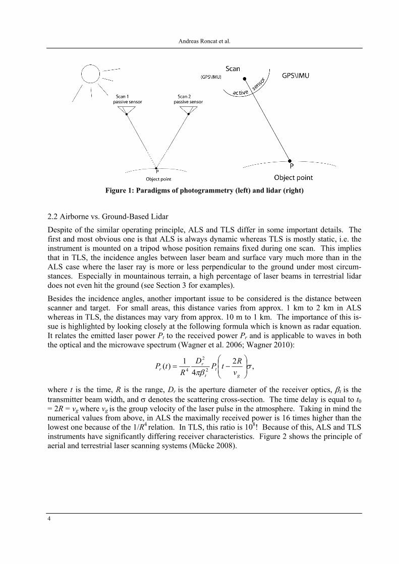
The principle of photogrammetry is based on taking perspective images of one object from two or more positions. If the interior geometry of the respectively used camera is known as well as the relative position and attitude of the images at their exposure times, the intersection of the image rays yields the spatial coordinates of the corresponding point. For each such point, two or more observations are needed, consisting of two image coordinates each.

Photogrammetry is a passive technique, thus dependent on sunlight in natural environment. Moreover, in the case of aerial photogrammetry where the camera is mounted on an airplane and looking in the direction of the nadir, clear-sky conditions are needed, too. In recent years, a huge development for automatization in photogrammetry has taken place. However, the success of matching corresponding image points is highly dependent of the images’ texture.

In contrast to this, lidar is an active technique, as described above, thus neither dependent on sunlight nor on clear sky. Since all three coordinates are observed at the same time, one single scan is sufficient for the computation of a three-dimensional point cloud of the whole object if it is visible from one viewpoint.

In Figure 1, the paradigms of photogrammetry and lidar are depicted (Kraus 2007).


4

Figure 1: Paradigms of photogrammetry (left) and lidar (right)

2.2 Airborne vs. Ground-Based Lidar

Despite of the similar operating principle, ALS and TLS differ in some important details. The first and most obvious one is that ALS is always dynamic whereas TLS is mostly static, i.e. the instrument is mounted on a tripod whose position remains fixed during one scan. This implies that in TLS, the incidence angles between laser beam and surface vary much more than in the ALS case where the laser ray is more or less perpendicular to the ground under most circum-stances. Especially in mountainous terrain, a high percentage of laser beams in terrestrial lidar does not even hit the ground (see Section 3 for examples).

Besides the incidence angles, another important issue to be considered is the distance between scanner and target. For small areas, this distance varies from approx. 1 km to 2 km in ALS whereas in TLS, the distances may vary from approx. 10 m to 1 km. The importance of this is-sue is highlighted by looking closely at the following formula which is known as radar equation. It relates the emitted laser power Pt to the received power Pr and is applicable to waves in both the optical and the microwave spectrum (Wagner et al. 2006; Wagner 2010):

,2

4

1)(

2

2

4

gt

t

rr v

RtP

D

RtP

where t is the time, R is the range, Dr is the aperture diameter of the receiver optics, t is the transmitter beam width, and denotes the scattering cross-section. The time delay is equal to t0

= 2R = vg where vg is the group velocity of the laser pulse in the atmosphere. Taking in mind the numerical values from above, in ALS the maximally received power is 16 times higher than the lowest one because of the 1/R4

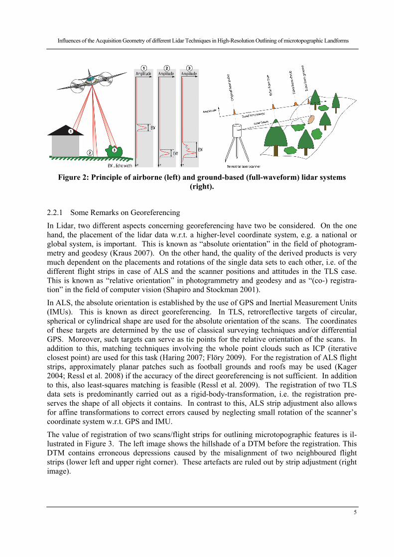
relation. In TLS, this ratio is 108! Because of this, ALS and TLS instruments have significantly differing receiver characteristics. Figure 2 shows the principle of aerial and terrestrial laser scanning systems (Mücke 2008).


5

Figure 2: Principle of airborne (left) and ground-based (full-waveform) lidar systems (right).

2.2.1 Some Remarks on Georeferencing

In Lidar, two different aspects concerning georeferencing have two be considered. On the one hand, the placement of the lidar data w.r.t. a higher-level coordinate system, e.g. a national or global system, is important. This is known as “absolute orientation” in the field of photogram-metry and geodesy (Kraus 2007). On the other hand, the quality of the derived products is very much dependent on the placements and rotations of the single data sets to each other, i.e. of the different flight strips in case of ALS and the scanner positions and attitudes in the TLS case. This is known as “relative orientation” in photogrammetry and geodesy and as “(co-) registra-tion” in the field of computer vision (Shapiro and Stockman 2001).

In ALS, the absolute orientation is established by the use of GPS and Inertial Measurement Units (IMUs). This is known as direct georeferencing. In TLS, retroreflective targets of circular, spherical or cylindrical shape are used for the absolute orientation of the scans. The coordinates of these targets are determined by the use of classical surveying techniques and/or differential GPS. Moreover, such targets can serve as tie points for the relative orientation of the scans. In addition to this, matching techniques involving the whole point clouds such as ICP (iterative closest point) are used for this task (Haring 2007; Flöry 2009). For the registration of ALS flight strips, approximately planar patches such as football grounds and roofs may be used (Kager 2004; Ressl et al. 2008) if the accuracy of the direct georeferencing is not sufficient. In addition to this, also least-squares matching is feasible (Ressl et al. 2009). The registration of two TLS data sets is predominantly carried out as a rigid-body-transformation, i.e. the registration pre-serves the shape of all objects it contains. In contrast to this, ALS strip adjustment also allows for affine transformations to correct errors caused by neglecting small rotation of the scanner’s coordinate system w.r.t. GPS and IMU.

The value of registration of two scans/flight strips for outlining microtopographic features is il-lustrated in Figure 3. The left image shows the hillshade of a DTM before the registration. This DTM contains erroneous depressions caused by the misalignment of two neighboured flight strips (lower left and upper right corner). These artefacts are ruled out by strip adjustment (right image).


6

Figure 3: Hillshade of a DTM before (left) and after strip adjustment (right). This figure was gen-

erously provided by Dr. Michael Doneus, Department of Prehistoric and Medieval Archaeology, University of Vienna

3 Study Area and Data Sets

3.1 The Doren Landslide

The site is situated in the Bregenzer Wald, a hilly region belonging to the Foreland Molasse Zone. The surface lithology consists primarily of freshwater molasse sediments, but Würmian glacial moraine also occurs. The local topography is determined by the rapidly evolving valleys of various watercourses; at Doren the river Weißach is incising into the hosting rock. The dis-charge of Weißach may vary considerably, tending occasionally to flash floods; therefore the settlements are situated on the valley slope, including the village of Doren. The continuous evacuation of sediments by the Weißach together with the active tectonic setting due to the N-S shortening causes instable valley slopes on both sides of the valley. The landslide itself is a long-lasting problem of the local community, but it became increasingly dangerous. The active area is continuously evolving, but major mass movements occurred in the 1980s and in 2005. Figure 4 shows an orthophoto of this area of the year 2006.

Figure 4: Left: orthophoto of the Doren landslide in 2006. Right: perspective view of the DTM de-

rived from the TLS data of the September 2008 campaign (see also Figure 10)


7

3.2 ALS Campaigns 2007

3.2.1 ALS Campaign March 2007

This ALS campaign was operated by TopScan (TopScan 2010) on behalf of the Land Vorarlberg surveying authority (LVA Feldkirch1). It took place on March 6, 2007 using an Optech ALTM 2050 instrument (Optech 2010). The campaign consisted of three laser scanner strips in North-South direction, containing approx. 1.5 million laser points all together with an average point density of 1.8 points/square meter. Figure 5 (left) shows an overview of this campaign.

3.2.2 ALS Campaign December 2007

This ALS campaign was again operated by TopScan on behalf of the Land Vorarlberg surveying authority, taking place on December 19, 2007 using an Optech ALTM 3100 instrument. The campaign consisted of three laser scanner strips in North-South direction, containing approx. 2.3 million laser points all together with an average point density of 2.9 points/square meter. Figure 5 (right) shows an overview of this campaign.

Figure 5: Flight plan of the ALS campaigns in March (left) and December 2007 (right). The blue,

black and green lines indicate the trajectories of the flight strips.

3.3 TLS Campaigns 2008 and 2009

3.3.1 TLS Campaign September 2008

For this campaign, a terrestrial full-waveform instrument Riegl LPM-321 (Riegl 2010) was used. It was generously provided by Riegl LMS and operated by Mr. Thomas Gaisecker in this field campaign from September 1 to 2, 2008. The mentioned instrument is capable of recording ech-oes in a distance up to 6 km and allows for the extraction of three echoes maximum per laser shot with the on-board software. Additionally, the scanner stores the sampled waveform of its echoes on an internal hard disk. These data can be read out and used in post-processing. How-ever, because of the high dynamic range of these data (see Section 2), “classical” full-waveform processing (cf. (Wagner et al. 2006; Jutzi and Stilla 2006; Roncat et al. 2008)) is not applicable to them. However, the appropriate processing of this kind of signals is still an active research question.

1 www.vorarlberg.gv.at/vorarlberg/bauen_wohnen/bauen/landesvermessungsamt/start.htm


8

The campaign consisted of three scans. In the first one, the scanner was placed next to the rim of the land slide (“Doren Oben”). From this position, approx. 1.1 million points were recorded. The next scan took place at the middle of the slope (“Doren Unten”), from where some 600,000 points were recorded. To get more detailed of the whole scene, the scanner was also placed in Krumbach on the other side of the valley. In this scan, approx. 350,000 echoes were recorded.

Figure 6 shows an overview of the campaign layout. For the georeferencing of the scans, retrore-flective targets were used whose positions were determined with the real-time GPS positioning service TEPOS (now EPOSA2) of the Austrian Federal Railways (ÖBB3). The final georeferenc-ing and registration was performed with the software RiProfile which is delivered with the scan-ner (Riegl 2010).

Figure 6: Left: Riegl LPM-321 terrestrial laser scanner (here at the scan position “Doren Unten“).

Right: Layout of the TLS campaign in September 2008. The black circles indicate the scanner positions. The blue, green and magenta lines indicate the outlines of the respective

scans.

3.3.2 TLS Campaign August 2009

For this campaign, a Riegl LMS-Z420i instrument was used (Riegl 2010). The field campaign took place from August 12 to 13, 2009. This instrument records one single echo per shot only. However, it operates at a much higher speed than the LPM-321, thus enabling scans with higher point densities. This allows for the derivations of DTMs with higher resolution (see Section 4).

The campaign consisted of seven scans from five different scan positions. Because of the highly irregular structure of the point clouds, they were thinned out before the actual processing. The following table gives an overview of the single scans:

2 www.eposa.at 3 www.oebb.at


9

Table 1: Single scans of the TLS campaign of August 2009

Scan Position Scan # Points usedDoren Oben 1 of 1 411,000Doren Hilltop 1 of 1 459,000Doren Road Corner 1 of 1 504,000Doren Plateau 1 of 3 286,000

2 of 3 183,0003 of 3 83,000

Krumbach Wald 1 of 1 481,000Sum 2,407,000

Figure 7 shows an overview of the campaign layout. Again, retroreflective targets and real-time GPS were used. The georeferencing and registration of the scans were performed with the soft-ware RiScanPro which is delivered with the scanner (Riegl 2010). Georeferencing and registra-tion of the scans were done in the same procedure as in the 2008 campaign.

Figure 7: Left: Riegl LMS-Z420i scanner (here at the scan position “Doren Oben“). Right: Layout of the TLS campaign in August 2009. The black circles indicate the scanner positions. The blue,

cyan, magenta, orange and yellow lines indicate the outlines of the respective scans.

4 Results

In this section, we discuss the influence of the respective used lidar technology on behalf of the presented data sets regarding point density of the scans, the success in derivation of DTMs, the distribution of the target distances and the distribution of incidence angles.

4.1 Point Density

For this study, the number of points within a sphere of 1 m radius around the single points was taken as measure for the point density. As was expected, the two ALS campaigns showed a very similar and regular pattern of point density over the whole area of interest (see Figure 8). The area of the highest density in the middle of the images in this figure corresponds to the triple overlap of the three respective flight strips. In vegetated areas, the point density is slightly lower than in open areas because of the increased local height variation.


10

Figure 8: Top: Point density map (# points within sphere of 1m radius) of the ALS campaigns of

March 2007 (left) and December 2007 (right). Bottom: According histograms.

In the case of TLS, the situation is very different (see Figure 9). Since the scanner is mounted on a tripod, it records a point cloud in a regular angular pattern but not in a spatially regular pattern. This effect is even intensified by the wide spreading of the appearing distances (see Section 4.3). Only the Krumbach scan of the TLS campaign of 2008 shows a situation slightly similar to ALS because of the high distance from the scanner’s position to the scanned slope.


11

Figure 9: Top: Point density map (# points within sphere of 1m radius) of the TLS campaigns of

September 2008 (left) and August 2009 (right). Bottom: According histograms.

4.2 Digital Terrain Models

The point density of the ALS campaigns allowed for the derivation of DTMs with 0.5 m resolu-tion each. This derivation as well as the filtering of non-terrain points was performed with the software package SCOP++ developed at the Institute of Photogrammetry and Remote Sensing, Vienna University of Technology (SCOP++ 2010). The hillshades of these DTMs are shown in Figure 10 (first two images from the left).


12

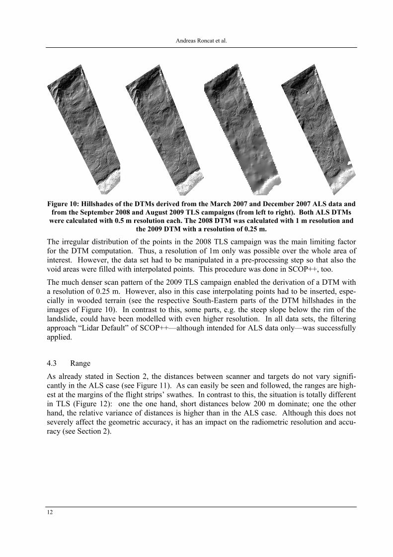
Figure 10: Hillshades of the DTMs derived from the March 2007 and December 2007 ALS data and

from the September 2008 and August 2009 TLS campaigns (from left to right). Both ALS DTMs were calculated with 0.5 m resolution each. The 2008 DTM was calculated with 1 m resolution and

the 2009 DTM with a resolution of 0.25 m.

The irregular distribution of the points in the 2008 TLS campaign was the main limiting factor for the DTM computation. Thus, a resolution of 1m only was possible over the whole area of interest. However, the data set had to be manipulated in a pre-processing step so that also the void areas were filled with interpolated points. This procedure was done in SCOP++, too.

The much denser scan pattern of the 2009 TLS campaign enabled the derivation of a DTM with a resolution of 0.25 m. However, also in this case interpolating points had to be inserted, espe-cially in wooded terrain (see the respective South-Eastern parts of the DTM hillshades in the images of Figure 10). In contrast to this, some parts, e.g. the steep slope below the rim of the landslide, could have been modelled with even higher resolution. In all data sets, the filtering approach “Lidar Default” of SCOP++—although intended for ALS data only—was successfully applied.

4.3 Range

As already stated in Section 2, the distances between scanner and targets do not vary signifi-cantly in the ALS case (see Figure 11). As can easily be seen and followed, the ranges are high-est at the margins of the flight strips’ swathes. In contrast to this, the situation is totally different in TLS (Figure 12): one the one hand, short distances below 200 m dominate; one the other hand, the relative variance of distances is higher than in the ALS case. Although this does not severely affect the geometric accuracy, it has an impact on the radiometric resolution and accu-racy (see Section 2).


13

Figure 11: Distances between scanner and points in the ALS campaigns (top) of March 2007 (left)

and December 2007 (right) and according histograms (bottom)

Figure 12: Distances between scanner and points in the TLS campaigns (top) of September 2008 (left) and August 2009 (right) and according histograms (bottom). The image at the centre shows

histogram of the distances below 1000 m in the 2008 TLS campaign.


14

4.4 Incidence Angle

The incidence angle is defined as the angle between the direction of the laser beam and the local tangent plane of the surface at the target, ranging thus from 0 to 90°. The plane was estimated using an algorithm originally developed for 3D city modelling (Dorninger and Pfeifer 2008). In a radiometric sense, the incidence angle plays an important role since the backscattered energy is directly proportional to the sine of the incidence angle if the target is regarded as a Lambertian scatterer (Wagner 2010).

Looking closer at this quantity makes the most significant difference between ALS and TLS ac-quisition geometry obvious: The incidence angle histogram of a TLS data set seems to be mir-rored in comparison to one of an ALS campaign (see Figure 13). Especially in flat terrain, very shallow intersections may appear since the scanner’s position is only some two meters above the ground. The North-Western part of the TLS incidence angle maps in the figure below shows an example for this.

Figure 13: Top: Incidence angles (angle between the laser beam and the local tangent plane of the surface at the target) in the ALS campaigns of March 2007 (left) and the TLS campaigns of Sep-

tember 2008 (centre) and August 2009 (right). Bottom: According histograms.

5 Discussion and Outlook

In this study, a comparison of the scanning geometries of ALS and TLS was presented, on behalf of empirical data recorded at a land slide in Doren (Vorarlberg, Western Austria).

Regarding the quantities range, incidence angle and point density, the differences were high-lighted where the incidence angles showed the most significant discrepancy between ALS and


15

TLS data sets. Besides, this, also the point density in TLS varies significantly whereas it remains nearly constant in the case of ALS data processing.

Despite of these discrepancies, it was shown that the derivation of high-resolution digital terrain models (sub-meter resolution) using TLS data is possible with commercial software packages originally designed for ALS.

Acknowledgements

The authors want to thank Dr. Michael Doneus (Department of Prehistoric and Medieval Ar-chaeology, University of Vienna) for providing the figures concerning strip adjustment and Mr. Thomas Gaisecker (Riegl Laser Measurement Systems) for providing the TLS instrument, the data acquisition and preparation in the 2008 TLS campaign.

This study was carried out in the framework of the scheme “Geophysics of the Earth’s crust” financed by the Austrian Academy of Sciences (ÖAW).

The ALS data shown in Figure 3 were acquired within the research projects “Celts in the Hinter-land of Carnuntum” and “LiDAR supported archaeological prospection of woodland” which were financed by the Austrian Science Fund (P16449-G02; P18674-G02).


16

References

DONEUS, M.; BRIESE, C.; FERA, M.; JANNER, M. (2008): Archaeological prospection of forested areas using full-waveform airborne laser scanning. Journal of Archaeological Science Vol. 35, No. 4, pp. 882–893. doi:10.1016/j.jas.2007.06.013

DORNINGER, P.; BRIESE C. (2005): Advanced geometric modelling of historical rooms. In XX Symposium of CIPA, ICOMOS & ISPRS Committee on Documentation of Cultural Heritage, Turin, Italy.

DORNINGER, P.; PFEIFER, N. (2008): A comprehensive automated 3d approach for build-ing extraction, reconstruction, and regularization from airborne laser scanning point clouds. Sensors Vol. 8, No. 11, pp. 7323–7343. doi:10.3390/s8117323

FLÖRY, S. (2009): Constrained Matching of Point Clouds and Surfaces. Ph. D. thesis, Insti-tute of Discrete Mathematics and Geometry, Vienna University of Technology.

HARING, A. (2007): Die Orientierung von Laserscanner- und Bilddaten bei der fahrzeug-gestützten Objekterfassung. Ph. D. thesis, Institute of Photogrammetry and Remote Sensing, Vienna University of Technology.

HOLLAUS, M.; WAGNER, W.; MAIER, B.; SCHADAUER, K. (2007): Airborne laser scan-ning of forest stem volume in a mountainous environment. Sensors Vol. 7, No. 8, pp. 1559–1577. doi:10.3390/s7081559

JUTZI, B.; STILLA, U. (2006): Range determination with waveform recording laser systems using a wiener filter. ISPRS Journal of Photogrammetry and Remote Sensing Vol. 61, No. 1, pp. 95–107. doi:10.1016/j.isprsjprs.2006.09.001

KAGER, H. (2004): Discrepancies between overlapping laser scanning strips - simultaneous fitting of aerial laser scanner strips. In International Archives of Photogrammetry and Re-mote Sensing, XXXV, B/1, Istanbul, Turkey, pp. 555–560.

KRAUS, K. (2007): Photogrammetry – Geometry from Images and Laser Scans (2nd ed.). De Gruyter.

MELZER, T. (2007): The mean shift algorithm for clustering point clouds. Journal of Applied Geodesy, Vol. 1, No. 3, pp. 62–75.

MÜCKE, W. (2008): Analysis of full-waveform airborne laser scanning data for the im-provement of DTM generation. Master’s thesis, Institute of Photogrammetry and Remote Sensing, Vienna University of Technology.

OPTECH (2010): www.optech.ca. Homepage of the company Optech, accessed: April 2010. RESSL, C.; KAGER, H.; MANDLBURGER, G. (2008): Quality checking of ALS projects

using statistics of strip differences. In International Archives of Photogrammetry and Re-mote Sensing, Vol. XXXVII, pp. 253–260.

RESSL, C.; MANDLBURGER, G.; PFEIFER, N. (2009): Investigating adjustment of Air-borne Laser Scanning strips without usage of GNSS/IMU trajectory data. In ISPRSWork-shop Laserscanning 2009, Paris, FRANCE, September 1-2, 2009.

RIEGL (2010): www.riegl.com. Homepage of the company RIEGL Laser Measurement Sys-tems, accessed: April 2010.

RONCAT, A.; WAGNER, W.; MELZER, T.; ULLRICH, A. (2008): Echo detection and loca-lization in full-waveform airborne laser scanner data using the averaged square difference function estimator. The Photogrammetric Journal of Finland Vol. 21, No. 1, pp. 62–75.

SCOP++ (2010): www.ipf.tuwien.ac.at/products/products.html. Institute of photogrammetry and Remote Sensing, Vienna University of Technology. Accessed: April 2010.

SHAPIRO, L. G.; STOCKMAN, G. C. (2001): Computer Vision. Prentice Hall. TOPSCAN (2010). www.topscan.de. Homepage of TopScan Gesellschaft zu Erfassung topo-

graphischer Informationen mbH. Accessed: April 2010. WAGNER, W. (2010): Radiometric Calibration of Small-Footprint Full-Waveform Airborne


17

Laser Scanner Measurements: Basic Physical Concepts. ISPRS Journal of Photogrammetry and Remote Sensing (Special Issue: 100 years ISPRS). In Review.

WAGNER, W.; ULLRICH, A.; DUCIC, V.; MELZER, T.; STUDNICKA, N. (2006): Gaus-sian decomposition and calibration of a novel small-footprint full-waveform digitising air-borne laser scanner. ISPRS Journal of Photogrammetry and Remote Sensing Vol. 60, No. 2, pp. 100–112. doi:10.1016/j.isprsjprs.2005.12.001

Influences of the Acquisition Geometry of different Lidar Techniques in High-Resolution Outlining of...

Documents

Transcript of Influences of the Acquisition Geometry of different Lidar Techniques in High-Resolution Outlining of...