WATER RESOURCES RESEARCH, VOL. 30, NO. 11, PAGES 3127-3136, NOVEMBER 1994

Cosmogenic 36C1 accumulation in unstable landforms 2. Simulations and measurements on eroding moraines Marek G. Zreda I and Fred M. Phillips Geoscience Department, New Mexico Tech, Socorro

David Elmore Physics Department, Purdue Rare Isotope Measurement Laboratory, Purdue University West Lafayette, Indiana

Abstract. Cosmogenic 36C1 surface exposure ages obtained for multiple boulders from single landforms are usually characterized by a variance larger than that of the analytical methods employed. This excessive boulder-to-boulder variability, progressively more profound with increasing age of landforms, is due to removal of soil and gradual exposure of boulders at the surface. In our gradual exposure model, boulders are initially buffed in moraine matfix. With time, erosion lowers the moraine surface and the boulders are gradually exposed to cosmic rays. Because the cosmic ray intensity changes with depth, the boulders are subjected to variable production rates of the cosmogenic 36C1. Initial depth of boulders and their chemical composition are variable, which results in different amounts of the accumulated cosmogenic 36C1 and thus different apparent ages of boulders. The shape of the resulting distribution of the apparent ages and the coefficient of variation depend on the erosion depth, while the first moment is a function of the true surface age and the erosion depth. These properties of the apparent age distributions permit calculation of the surface age, the erosion depth, and also the average erosion rate. We tested the model calculations using 26 boulders from a late Pleistocene moraine at Bishop Creek, Sierra Nevada, California. The set exhibited a bimodal distribution of the 36C1 surface exposure ages. We interpreted the older mode as the result of gradual exposure and the younger one as the result of surficia! processes other than soil removal. The !0 samples that constitute the older mode produced a distribution which closely matches the modeled

-2. This distribution calculated using an age of 85 kyr and erosion depth of 570 gcm age is the same as an independent estimate obtained from cation ratio studies, and the

-2 based on a calculated erosion depth is very close to the erosion depth of 600 g cm simple analytical model of soil erosion. These results indicate that our statistical model adequately describes effects of soil erosion on accumulation of cosmogenic 36C1. The approach can be used to simultaneously obtain the true landform age and the erosion rate from apparent 36C1 ages and therefore may help in evaluation of surface exposure ages of eroding landforms.

Introduction

Landforms are evidence of the diverse geological pro- cesses shaping the surface of the Earth. Different geomor- phic surfaces form under different environmental conditions, and these conditions can generally be inferred from detailed studies of the landforms. Analysis of a succession of land- forms can provide information about changes in local pa- leoenvironmental conditions. In many cases a fundamental goal in paleoenvironmental analysis is to determine the age of landform formation, but until recently few numerical dating tools were available for this purpose. Ideally, with

1Now at Department of Hydrology and Water Resources, Uni- versity of Arizona, Tucson.

Copyright 1994 by the American Geophysical Union. Paper number 94WR00760. 0043-1397/94/94 WR-00760505.00

sufficient information from a landform, one could learn not

only about its formation time but also about its subsequent geological history.

Numerical dating of geomorphic surfaces has been signifi- canfly advanced in the past decade and several new methods have been developed. One of these methods is based on accumulation of cosmic ray-induced 36C1 in rocks exposed at the surface of the Earth [Phillips et al., 1986]. The basis of this method in cosmic ray physics has been described by Davis and Schaeffer [!955], Lal and Peters [1967], Phillips eta!. [!986], and Zreda et al. [1990]. This method has been recently cali- brated [Zreda et al., 1991; Zreda, 1994] and applied to dating late Pleistocene moraines [Phillips et al., 1990, also unpub- lished manuscript, 1994; M. G. Zreda et al., Glacial chronology of the eastern White Mountains, California-Nevada by the cosmogenic 36C1 method, submitted to Quaterna.rv Research, 1994], a meteorite impact crater [Phillips eta!., !991], and volcanic deposits [Zreda eta!., 1993]. These studies, although successful, revealed certain limitations of the cosmogenic 36C1

3127

3128 ZREDA ET AL.' COSMOGENIC 36CL ACCUMULATION IN UNSTABLE LANDFORMS, 2

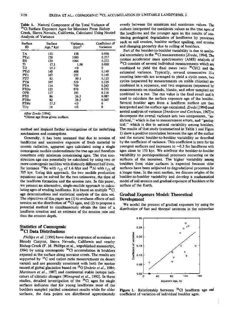
Table 1. Natural Component of the Total Variance of 36C1 Surface Exposure Ages for Moraines From Bishop Creek, Sierra Nevada, California, Calculated Using Nested Analysis of Variance

Surface Surface Variance, Coefficient of ID Age,* kyr (kyr) 2 Variation

TA 122 138 0.096 PTal 128 1083 0.257 SH 120 1064 0.272 Ti 17.1 1.06 0.060 Ti2 15.3 <0 0 PTa3 148 488 0.149 PTil 107 255 0.149 PTi7 82 89.1 0.115 PTi6 105 529 0.219 PTi4 114 769 0.243 PTi3o 123 970 0.253 OPB 117 185 0.116 PTi5 86 56.5 0.087 PTi8o 82 28.5 0.065

PTi8y 17.5 <0 0 Tily 16 <0 0

After Zreda [1994]. *Oldest age from given surface.

method and inspired further investigations of the underlying mechanisms and assumptions.

Generally, it has been assumed that due to erosion of !andforms and successive exposure of fresh material to cosmic radiation, apparent ages calculated using a single cosmogenic nuclide underestimate the true age and therefore constitute only minimum constraining ages. The true con- struction age can potentially be calculated by using two or more cosmogenic nuclides with distinctly different half-lives, for instance løBe with tl/2 of 1.6 Myr and 26A! with tl/2 of 705 kyr. Using this approach, the two nuclide production equations can be solved for the two unknowns, the time of the landform formation and the erosion rate. In this paper, we present an alternative, single-nuclide approach to calcu- lating ages of eroding landforms. It is based on multiple 36C1 age determinations and statistical analysis of the data set. The objectives of this paper are (1) to evaluate effects of soil erosion on the distribution of 36C1 ages, and (2) to propose a potential method to simultaneously obtain the time of a landform creation and an estimate of the erosion rate and

thus the erosion depth.

Statistics of Cosmogenic 36C1 Data Distributions

Phillips et al. [1990] have dated a sequence of moraines at Bloody Canyon, Sierra Nevada, California and nearby Bishop Creek (F. M. Phillips et al., unpublished manuscript, 1994) by using cosmogenic 36C1 accumulation in boulders exposed at the surface along moraine crests. The results are supported by ]4C and cation ratio measurements on desert varnish and are generally consistent with both the marine record of global glaciation based on 180 [Irnbrie et al., 1984; Martinson et al., 1987] and continental stable isotope indi- cators of climatic changes [Winograd et al., 1992]. In these studies, detailed investigation of the 36C1 ages for single surfaces indicates that for young landforms most of the boulders sampled yielded consistent results while for older surfaces, the data points are distributed approximately

evenly between the minimum and maximum values. The authors interpreted the maximum values as the true ages of the landforms and the younger ages as the results of con- tinuing geological degradation of landforms by processes such as soil erosion, boulder surface spalling, and erosion and changing geometry due to rolling of boulders.

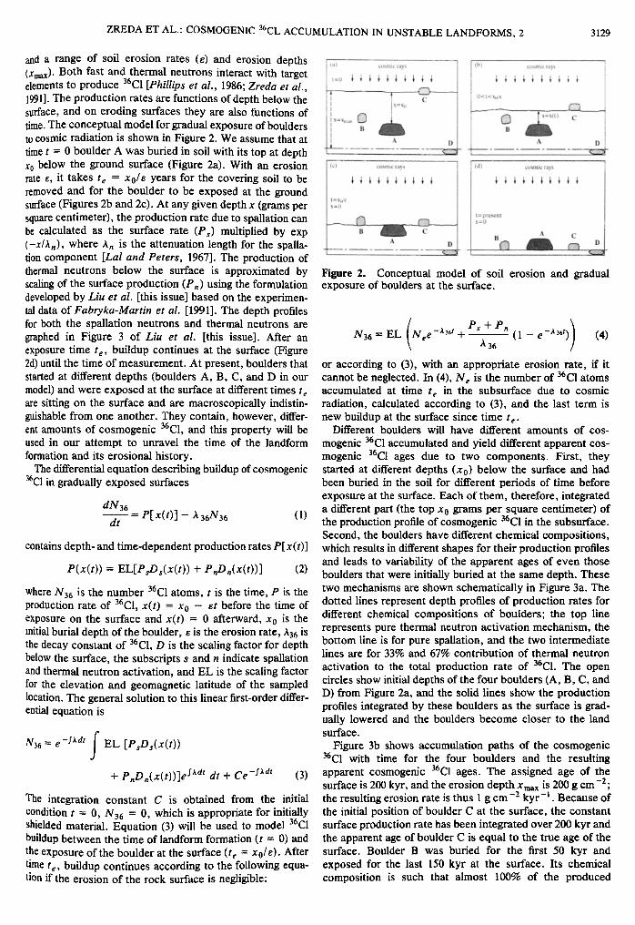
Part of the boulder-to-boulder variability is due to analyt- ical uncertainty in the 36C1 measurements [Zreda, 1994]. The routine accelerator mass spectrometry (AMS) analysis of 36C1 consists of several individual measurements which are combined to yield the final mean ratio 36CL/C1 and the estimated variance. Typically, several consecutive 15-s counting intervals are averaged to yield a cycle mean, two cycles (separated by measurements on stable chlorine) are combined in a sequence, and two sequences (separated by measurements on standards, blanks, and other samples) are combined in a run. The run value is the final result and is used to calculate the surface exposure age of the boulder. Several boulder ages from a landform surface are then interpreted and the surface age calculated. Zreda [1994] used nested analysis of variance [Snedecor and Cochran, 1967] to decompose the overall variance into two components, "an- alytical," which is due to measurement errors, and "geolog- ical," which is due to natural variability among boulders. The results of that study (summarized in Table 1 and Figure 1) show a positive correlation between the age of the surface and the natural boulder-to-boulder variability as described by the coefficient of variance. This coefficient is zero for the youngest surfaces and increases to ---0.3 for landforms with ages close to 150 kyr. We attribute the boulder-to-boulder variability to postdepositional processes occurring on the surfaces of the moraines. The higher variability among boulders from older surfaces is expected because older surfaces have been subjected to degradational processes for a longer time. In the next section, we discuss origins of the boulder-to-boulder variability and develop a mathematical model of soil erosion and gradual exposure of boulders at the surface of the Earth.

Gradual Exposure Model: Theoretical Development

We model the process of gradual exposure by using the distribution of fast and thermal neutrons in the subsurface

0.30

0.25 -

._o " 0.20-

o 0.15-

._ /.2_

" 0.10- o

0.05

0.00 0

O ID .

-

O 0 0 O .

• I, , I t 40 80 120 160

Apparent: age, ky

Figure 1. Relationship between 36C1 landform age •d coefficient of variation of individual boulder ages.

ZREDA ET AL.' COSMOGENIC 36CL ACCUMULATION IN UNST•kBLE LANDFORMS, 2 3129

and a range of soil erosion rates (e) and erosion depths (Xm,,.,)- Both fast and thermal neutrons interact with target elements to produce 36C1 [Phillips et al., 1986; Zreda et al., 1991]. The production rates are functions of depth below the surface, and on eroding surfaces they are also functions of time. The conceptual model for gradual exposure of boulders to cosmic radiation is shown in Figure 2. We assume that at time t = 0 boulder A was buried in soil with its top at depth x0 below the ground surface (Figure 2a). With an erosion rate e, it takes t e = Xo/e years for the covering soil to be removed and for the boulder to be exposed at the ground surface (Figures 2b and 2c). At any given depth x (grams per square centimeter), the production rate due to spallation can be calculated as the surface rate (Px) multiplied by exp i-x/An), where A,• is the attenuation length for the spalla- tion component [Lal and Peters, 1967]. The production of thermal neutrons below the surface is approximated by scaling of the surface production (P,,) using the formulation developed by Liu et al. [this issue] based on the experimen- tal data of Fabo'ka-Martin et al. [1991]. The depth profiles for both the spallation neutrons and thermal neutrons are graphed in Figure 3 of Lite et al. [this issue]. After an exposure time re, buildup continues at the surface (Figure 2d) until the time of measurement. At present, boulders that started at different depths (boulders A, B, C, and D in our model) and were exposed at the surface at different times t e are sitting on the surface and are macroscopically indistin- guishable from one another. They contain, however, differ- ent amounts of cosmogenic 36C1, and this property will be used in our attempt to unravel the time of the landform formation and its erosional history.

The differential equation describing buildup of cosmogenic 36C1 in gradually exposed surfaces

dN36 dt

= P[ x(t) ] - A 36N36 (1)

contains depth- and time-dependent production rates P[ x(t)]

P(r(t)) = EL[PsDs(x(t)) + P•D.(x(t))] (2)

where N36 is the number 36C1 atoms, t is the time, P is the production rate of 36C1, x(t) = x o - et before the time of exposure on the surface and x(t) = 0 afterward, x 0 is the initial burial depth of the boulder, e is the erosion rate, A36 is the decay constant of 36C1, D is the scaling factor for depth below the surface, the subscripts s and n indicate spallation and thermal neutron activation, and EL is the scaling factor for the elevation and geomagnetic latitude of the sampled location. The general solution to this linear first-order differ- ential equation is

N36 = e -['•dt f EL [P•.Ds(x(t)) + P,•Dn(x(t))]e fxat dt + Ce -[*at (3)

The integration constant C is obtained from the initial condition t = 0, N36 = 0, which is appropriate for initially shielded material. Equation (3) will be used to model 36C1 buildup between the time of landform formation (t = 0) and the exposure of the boulder at the surPace (t e = .r0/e). Alier time t,,, buildup continues according to the follov•ing equa- tion if the erosion of the rock surface is negligible:

cosmic rax.s

XmXma x C B

cosmic rat g

B • C A

D

I b) cosmic ra•s

B

A

; d) cosmic rays

t= present x=O

B C D

Figure 2. Conceptual model of soil erosion and gradual exposure of boulders at the surface.

Ps + Pn __•. 36t) ) N36 = EL Nee -,x,•t -e ( 1 - e (4) X3t,

or according to (3), with an appropriate erosion rate, if it cannot be neglected. In (4), N e is the number of 36C1 atoms accumulated at time t e in the subsurface due to cosmic radiation, calculated according to (3), and the last term is new buildup at the surface since time t•.

Different boulders will have different amounts of cos-

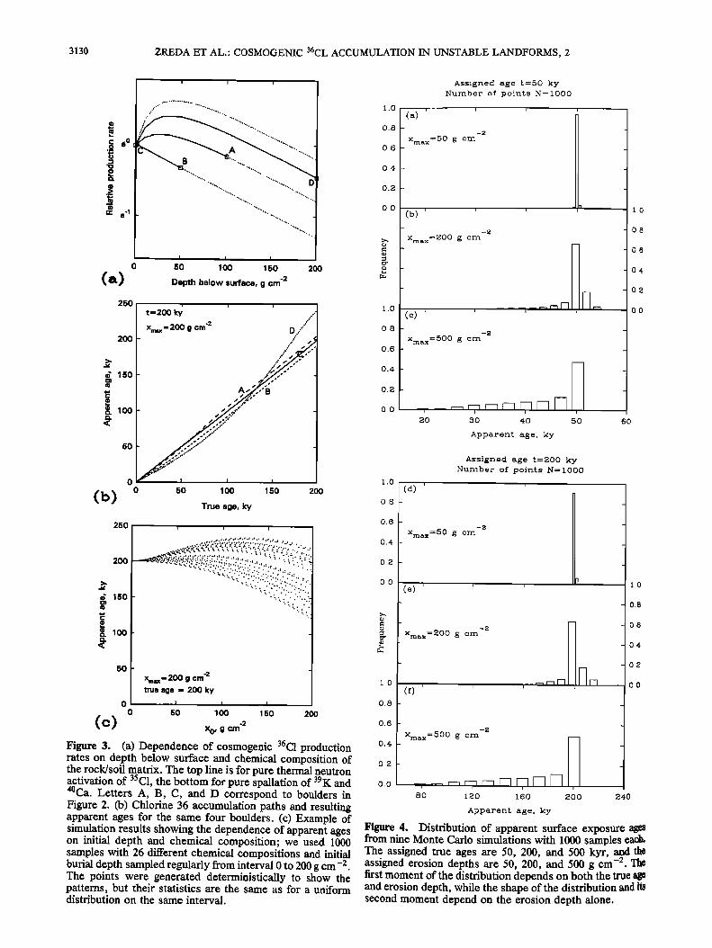
mogenic 36C1 accumulated and yield different apparent cos- mogenic 36C1 ages due to two components. First, they started at different depths (x0) below the surface and had been buffed in the soil for different periods of time before exposure at the surface. Each of them, therefore, integrated a different part (the top x0 grams per square centimeter) of the production profile of cosmogenic 36C1 in the subsurface. Second, the boulders have different chemical compositions, which results in different shapes for their production profiles and leads to variability of the apparent ages of even those boulders that were initially buffed at the same depth. These two mechanisms are shown schematically in Figure 3a. The dotted lines represent depth profiles of production rates for different chemical compositions of boulders; the top line represents pure thermal neutron activation mechanism, the bottom line is for pure spallation, and the two intermediate lines are for 33% and 67% contribution of thermal neutron

activation to the total production rate of 36C1. The open circles show initial depths of the four boulders (A, B, C, and D) from Figure 2a, and the solid lines show the production profiles integrated by these boulders as the surface is grad- ually lowered and the boulders become closer to the land surface.

Figure 3b shows accumulation paths of the cosmogenic 36C! with time for the four boulders and the resulting apparent cosmogenic 36C1 ages. The assigned age of the surface is 200 kyr, and the erosion depth x max is 200 g cm-2; the resulting erosion rate is thus 1 gcm -2 kyr -1. Because of the initial position of boulder C at the surface, the constant surface production rate has been integrated over 200 kyr and the apparent dge of boulder C is equal to the true age of the surface. Boulder B was buried tBr the first 50 kyr and exposed for the last 150 kyr at the surface. Its chemical composition i• such that almost 100'• of the produced

3130 ZREDA ET AL.' COSMOGENIC 36CL ACCUMULATION IN UNSTABLE LANDFORMS, 2

c::: 6o .o_

._>

(a)

I I

50 1 O0 150 200 -2

Depth below surface, g cm

250

200

150

50

0

(b)

250

200

150

•oo

5O

(c)

Figure 3.

! i " i t = 200 k¾ ,.//...' Xm= x = 200 g cm '2 D

..: / , ..e /

:'*,• ..'.,,

:.... .... I I I

150 • O0 • !50 200

True age, ky

Xma x == 200 g cm '2 true age = 200 k¾

00, , I I .. , I .... 50 1 O0 150 200 -2

x O, g cm

(a) Dependence of cosmogenic 36C! production rates on depth below surface and chemical composition of the rock/soil matrix. The top line is for pure thermal neutron activation of 35C1, the bottom for pure spallation of 39K and 4øCa. Letters A, B, C, and D correspond to boulders in Figure 2. (b) Chlorine 36 accumulation paths and resulting apparent ages for the same four boulders. (c) Example of simulation results showing the dependence of apparent ages on initial depth and chemical composition; we used 1000 samples with 26 different chemical compositions and initial burial depth sampled regularly from interval 0 to 200 g cm -2. The points were generated deterministically to show the patterns, but their statistics are the same as for a uniform distribution on the same interval.

1.0

0.8

0.6

0,4

0.2

0.0

1.0

0.8

0.6

0.4

0.2

0.0

Assigned age t=50 ky Number of points N=1000

2O 3O 40 5O 60

Apparent age, ky

1,0

O8

0,6

0.4

0.2

0.0

1.0

0.8

0.6

0.4

0,2

0.0

1,0

0.8

0.6

0.4

0.2

0.0

Assigned age t=200 ky Number of points N=1000

.

_

_

_

-2

Xmax=50 gcm _

-

_

_

-

_ _

_

-2

Xmax=•00 g cm _

-

-

.......... •r'-I •I--1 .... (f) ....

_

_

_

-

-2

Xmax=500 g cm __ _

-

_

_

80 120 160 200 240

1.0

0.8

O6

0.4

O2

0•0

Apparent age, ky

Figure 4. Distribution of apparent surface exposure ages from nine Monte Carlo simulations with 1000 samples eack The assigned true ages are 50, 200, and 500 kyr, •d the assigned erosion depths are 50, 200, and 500 gcm first moment of the distribution depends on both the true age and erosion depth, while the shape of the distribution and its second moment depend on the erosion depth alone.

ZREDA ET AL.' COSMOGENIC 36CL ACCUMULATION IN UNSTABLE LANDFORMS, 2 3131

1.0

0.8

0.6

0.2 -

0.0

_

_

1.0

08

06

04

0,20 -

0.0

Assigned age t=500 ky Number of points N= 1000

Xmax----50 g½m

i

(h)

-2

Xrnax=200 g crn

Xmax=500 gcm

200 300 400 500 600

Apparent age, ky

Figure 4. (continued)

lO

- 0.8

06

0.4

02

o.o

cosmogenic 36C1 is due to spallation reactions with 39K and 4øCa. Because of its chemistry, during the first 50 kyr the boulder integrated production rates lower than the surface rate. Therefore the resulting production path is below the surface production path of boulder C, and the apparent age is lower than the true age of the landform. Boulder A was buried for the first 100 kyr and then exposed. Its chemical composition results in 67% of the 36C1 production due to spallation and 33% due to thermal neutron activation of 35C1. The production profile starts below the surface production rate value, increases with time (and decreasing depth) to reach a maximum value at the depth of about 30 g cm -2, and finally decreases back to the surface value. This history results in the accumulation path that initially goes below the surface path of boulder C. After some time, the boulder enters the shallow depth where the production rate is higher than at the surface. Buildup of cosmogenic 36C1 is faster, and the accumulation path steepens and continues above the path of boulder C. Because of this accelerated accumulation of the cosmogenic 36C1, the apparent age of boulder A is slightly older than the true landform age. Boulder D has been continuously buried in soil and just recently exposed at the surface. Its chemistry dictates that 33% of the cosmogenic 36C1 is produced by spallation of 39K and 4øCa and 67% by thermal neutron activation of 35C1. Because of the large contribution of thermal neutron activation to the total pro- duction of 36C1, only the lowest third of the production profile has values lower than the surface value, whereas the top two thirds is positioned above the surface production .rate value. This distribution of the production rates with depth results in the accumulation path that continues below

the surface path of boulder C for about 140 kyr. At this time the boulder is at the shallow depth where the production rates are highest; the accumulation path thus steepens mark- edly and continues above the path of boulder C. The resulting apparent age is notably higher than the true land- form age.

For the Monte Carlo calculations, we used 1000 boulders with different initial burial depths Xo and variable chemical composition. As an example, a landform with a true age of 200 kyr and erosion depth of 200 gcm -2 yielded the 1000 apparent 36C1 ages shown in Figure 3c. We used 26 different chemical compositions and initial burial depths x 0 uniformly distributed between 0 and 200 gcm -2. The lineations ob- served in Figure 3c (from left to fight) depict samples of the same chemical composition, but of variable Xo. The upper- most points are for the samples with high C1 content and thus relatively high production rate of 36C1 due to thermal neu- tron activation of 35C1, which leads to apparent ages older than the true landform age. On the other hand, the lowest points are for the samples with relatively high spallogenic 36C1, resulting in younger apparent ages. The spread in the vertical direction for samples from the same depth is due to variable chemistry; it increases with increasing x0. The apparent ages of these 1000 boulders are used to construct empirical distributions and calculate their first two moments. These distributions are graphed in Figure 4 for different values of the initial burial depth x0 and true landform age t. An additional condition, boulder heights (sampled from a measured set of values), was added to the model to make the apparent age distributions more realistic.

The distributions of the apparent cosmogenic 36C1 ages depend on the erosion depth of the landform. For small erosion depths, most apparent 36C1 ages are equal to the true ages (Figures 4a, 4d, and 4g). In the case of Figure 4a, a 50-kyr-old surface yielded ages from 49 to 54 kyr with the majority very close to 50 kyr. Surfaces that are 200 and 500 kyr old exhibited similar distributions of the apparent ages. If the erosion depth is increased to 200 gcm -2, only about 60% of samples have the same apparent age as the assigned true age (Figures 4b, 4e, and 4h), about 20% are overesti- mated by up to 10% because the thermal neutron flux increases with depth down to about 45 g cm -2, and the remaining samples form a tail toward younger ages. As in the case of smaller erosion depth, the mean of the apparent ages is very close to the assigned landform age and should be used to estimate the true age. For the erosion depth of 500 g cm -2 the distribution becomes skewed toward the younger ages (Figures 4c, 4f, and 4i) with a half of the samples close to the true age and few or no samples older than the true landform age. In this case the oldest apparent ages are equal to the assigned age, and they should be used to estimate the true age.

The model results lead to the following useful observa- tions. First, the shapes of the apparent age distributions are not sensitive to the surface age, but are very sensitive to the erosion depth. For the same erosion depth, but different true ages, the shapes of the apparent age distributions are almost identical when they are scaled by their respective means. It is therefore possible to estimate the erosion depth by looking at the distribution of the apparent ages (as we did in Figure 4) or, alternatively, at their first two moments (Figure 5a). This property of the apparent age data set might be used to reconstruct the erosional histories of landforms and calcu.

late their formation ages. The coefficient of variation and the

3132 ZREDA ET AL.' COSMOGENIC 36CL ACCUMULATION IN UNSTABLE LANDFORMS, 2

0.3

0.0

(a)

10 1.i 1.2 1.3

t/tapp

250

200

150

zoo

50

i i i

mean+sd

mean-s _

sd•

0 • ' ' • 0 200 400 600 800 1000

-2

Erosion depth, gem

Figure 5. (a) Apparent coefficient of variation versus mean apparent age (tapp). The coefficient of variation is quasi- linearly related to the ratio t/tapp; the graph can therefore be used to estimate the true age and the erosion depth from a set of apparent 36C1 ages. (b) The mean and standard deviation of apparent ages as functions of the erosion depth, based on Monte Carlo simulation with 1000 samples. The mean gen- eral!y decreases and the standard deviation increases with increasing erosion depth; both are independent of the sur- face age.

mean apparent age (tap p in Figure 5a) are strongly inversely correlated, and this correlation can be used to calculate the true landform age from the apparent 36C1 ages.

Another useful observation can be made from a plot of apparent ages and standard deviations versus the erosion depth (Figure 5b). The line representing the mean plus one standard deviation is almost horizontal, i.e., does not change significantly with the erosion depth, and does not deviate markedly from the assigned age of 200 kyr. This property might be used to perform a first cut estimation of landform age using the mean plus one standard deviation calculated for the apparent 36C1 ages. We also observe that the mean decreases less rapidly as the erosion depth increases and in the limit would reach an asymptotic value of half of the true landform age. This is expected because of the distribution of fast and thermal neutrons in the subsurface. As the erosion

depth increases, the maximum production rate at a depth of about 45 gcm -2 becomes progressively less consequential and eventually, for large erosion depth, is negligible. In this case the boulders integrate a production profile essentially identical to that for pure spallation (Figure 3a, boulder B), and the resulting distribution of the apparent 36C1 ages is approximately uniform with the maximum close to the true age and the mean close to half of that value.

The actual age and the erosion depth of a real landform

can be estimated by executing a set of model calculations, each with a different value of the true age (which is the input variable) of the landform. In each calculation the erosion depth (another input variable) is systematically changed, and the first two moments of the apparent 36C1 age distribution are calculated. These two moments can either be obtained directly, by treating N36 in (3) as a random variable and taking appropriate expected values, or indirectly, using Monte Carlo simulations with initial boulder depth sampled from a desired distribution on the interval between 0 and the assigned erosion depth. In the case of morainal deposits it is appropriate to sample x0 from a uniform distribution be. cause material of glacial till is usually very poorly sorted and large boulders are found at all locations within the finer matrix. The shape and/or the first two moments of the simulated distribution can then be compared with those of the experimental distribution based on AMS measurements of cosmogenic 36C! in rock samples. The procedure is reiterated until good agreement is obtained between the theoretical and experimental distributions. For most condi- tions the combination of the first two moments uniquely defines the distribution and allows determination of (1) the true age, which was the input variable in the model calcula- tion that gave the correct first two moments, (2) the erosion depth, the other input variable that produced the correct first two moments, and (3) the erosion rate, which is the erosion depth divided by the true age. We use this procedure in the next section to calculate the age and erosion depth of a late Pleistocene moraine from the Sierra Nevada.

Gradual Exposure Model: Comparison With Data

The model calculations were tested using samples from boulders on an independently dated late Pleistocene glacial moraine from Bishop Creek, Sierra Nevada, California. We collected 26 samples, extracted CI, measured 36C1, con- structed the empirical distribution of the apparent cos, mogenic 36C1 ages, and calculated sample statistics for tMs data set. We then simulated exposure histories for this surface and found the moraine age and the erosion depth that best match the observed data. In addition, we measured •'CI in three surficial soil materials sampled and used them to independently calculate the erosion depth using a simple analytical erosion model.

Sample Collection and Preparation

The samples (Table 2) were collected from two transects along the crest of the "Older Bishop Creek" (PTiS) moraine (F. M. Phillips et al., unpublished manuscript, 1994), at Bishop Creek, eastern Sierra Nevada, California. This par- ticular moraine was chosen because it had been previoufly dated by cosmogenic 36C1 accumulation and varnish cation ratio (F. M. Phillips et al., unpublished manuscript, !994) and because a large number of medium-sized boulders were available on the moraine crest. The sampling criteria were as follows: (!) samples were arbitrarily collected at 5-m inter- vals along two transects parallel to the moraine crest; (2) tM minimum sample size was 10 cm; (3) only relatively fresh samples were collected (i.e., without major chemical firer- ation) in order to avoid samples that might contain meteod:c chlorine in secondary weathering minerals; (4) rounded rather than sharp-edged samples were collected in order to

ZREDA ET AL.: COSMOGENIC 36CL ACCUMULATION IN UNSTABLE LANDFORMS, 2

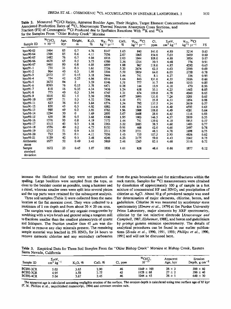
Table 2. Measured 36CL/C1 Ratios, Apparent Boulder Ages, Their Heights, Target Element Concentrations and Associated Production Rates of 36C1, Macroscopic Thermal Neutron Absorption Cross Sections, and Fraction (FS) of Cosmogenic 36C1 Produced due to Spallation Reactions With 39K and 4øCa for the Samples From "Older Bishop Creek" Moraine

3133

36C1/C1, Age, Height, K20, •K, 36C1 CaO, •Ca, 36C1 C1, •crN, •Cl, 36C1 Sample ID x 10 -15 kyr m % kg-1 yr -1 % kg -I yr -• ppm cm 2 kg -• kg -t yr -1 FS

bpcr90-63 1464 83 0.7 4.76 8147 1.63 840 141.0 4.80 5214 0.63 bpcr90-64 1306 85 0.6 4.11 7036 2.07 1065 154.0 5.03 5429 0.60 bpcr90-65 1482 76 0.7 4.04 6916 2.03 1044 108.0 4.88 3924 0.67 bpcr90-66 4670 65 0.5 3.73 6386 2.36 1214 20.5 4.68 776 0.91 bpcr90-67 1461 80 0.8 4.03 6899 1.88 967 118.0 4.85 4292 0.65 bpcr91-1 731 31 0.3 1.61 2756 5.20 2674 62.5 4.63 2393 0.69 bpcr91-2 964 40 0.3 1.93 3304 5.50 2829 64.0 6.05 1758 0.78 bpcr91-3 2572 17 0.15 3.18 5444 1.44 741 8.1 4.27 336 0.95 bpcr01-4 754 42 0.25 4.04 6916 1.64 843 131.0 4.55 5106 0.60 bpcr91-5 3675 84 2 3.59 6146 1.51 777 31.7 4.64 1213 0.85 bpcr91-6 8503 76 0.15 3.78 6471 0.28 144 10.9 4.10 470 0.93 bpcr91-7 818 16 0.35 4.34 7430 1.24 638 35.1 4.25 1462 0.85 bpcr91-8 773 40 0.3 3.94 6745 1.31 674 109.0 4.78 4040 0.65 bpcr91-9 1010 82 1.5 2.30 3938 4.07 2093 !31.0 7.24 3201 0.65 bpcr91-10 1387 21 0.3 4.32 7396 1.11 57! 25.8 4.33 1054 0.88 bpcr01-11 633 36 0.2 3.84 6574 1.54 792 137.5 4.34 5619 0.57 bpcr91-12 850 43 0.3 4.02 6882 1.66 854 114.0 4.40 4592 0.63 bpcr91-13 988 49 0.2 3.95 6762 1.96 1008 108.0 4.49 4281 0.64 bpcr91-14 1294 30 0 1.69 2893 5.07 2608 28.0 4.45 1116 0.83 bpcr91-15 639 38 0.5 3.68 6300 1.95 1003 !46.5 4.37 5939 0.55 bpcr91-16 1576 93 0.8 4.19 7173 1.44 741 139.0 4.18 5915 0.57 bpcr91-17 1315 43 0.3 1.38 2363 5.22 2685 38.5 4.60 1483 0.77 bpcr91-18 1556 49 0.2 4.75 8132 0.91 468 62.0 4.60 2497 0.78 bpcr01-19 1312 51 0.9 1.35 2311 5.29 2721 48.1 4.70 1698 0.75 bpcr91-20 733 33 0.1 4.11 7036 1.43 735 107.5 3.93 4856 0.62 bpcr91-21 1129 42 0.3 2.48 4246 4.23 2175 59.0 4.43 2362 0.73 Arithmetic 1677 52 0.49 3.43 5869 2.46 1265 82.1 4.68 3116 0.72

mean

Sample 1672 23 0.45 1.07 1826 1.61 828 48.6 0.66 1877 0.12 standard deviation

increase the likelihood that they were not products of spal!ing. Large boulders were sampled from the tops, as close to the boulder center as possible, using a hammer and a chisel, whereas smaller ones were split into several pieces and the top parts were retained for the subsequent analysis.

Three soil samples (Table 3) were collected from the same location at the flat moraine crest. They were collected to a maximum of 1 cm depth and from about 20 x 20 cm area.

The samples were cleaned of any organic overgrowths by scrubbing with a wire brush and ground using a tungsten mill to fractions smaller than the smallest phenocrysts of quartz and feldspars. The fraction smaller than 45 t•m was dis- carded to remove any clay minerals present. The remaining sample material was leached in 5% HNO3 for 24 hours to remove meteoric chlorine and any secondary carbonates

from the grain boundaries and the microfractures within the rock matrix. Samples for 36C1 measurements were obtained by dissolution of approximately 100 g of sample in a hot mixture of concentrated HF and HNO3 and precipitation of chlorine as AgC1. About 10 g of powdered sample was used for determination of major elements, chlorine, boron, and gadolinium. Chlorine 36 was measured by accelerator mass spectrometry [Elmore et al., 1979] at the Purdue University Prime Laboratory, major elements by XRF spectrometry, chlorine by the ion selective electrode [Aruscavage and Campbell, !987; Elsheimer, 1988], and boron and gadolinium by prompt gamma emission spectrometry. The details of analytical procedures can be found in our earlier publica- tions [Zreda et al., 1990, 1991, 1993; Phillips et al., 1990, 1991] and will not be discussed here.

Table 3. Empirical Data for Three Soil Samples From the "Older Bishop Creek" Moraine at Bishop Creek, Eastern Sierra Nevada, California

•crN, 36C1/C1, Apparent Erosion Sample ID cm 2 kg -• K2 ¸, % CaO, % C1, ppm 10 -•5 Age, kyr Depth, g cm -2

BCS92-2CR 5.03 3.65 2.90 46 !149 +- 100 28 +_ 3 580 _+ 60 BCS92-3CR 4.95 3.58 2.75 45 1128 _+ 68 27 +- 2 590 _+ 40 BCS92-4CR 5.04 3.67 2.45 46 1044 _-+ 45 26 +- 1 640 _+ 30

The apparent age is calculated assuming negligible erosion of the surface. The erosion depth is calculated using true surface age of 85 kyr (F. M. Phillips et al., unpublished manuscript, !994) and constant erosion rate,

3134 ZREDA ET AL.' COSMOGENIC 36CL ACCUMULATION IN UNSTABLE LANDFORMS, 2

o o 20 •o 60 80 too

Boulder age, ky

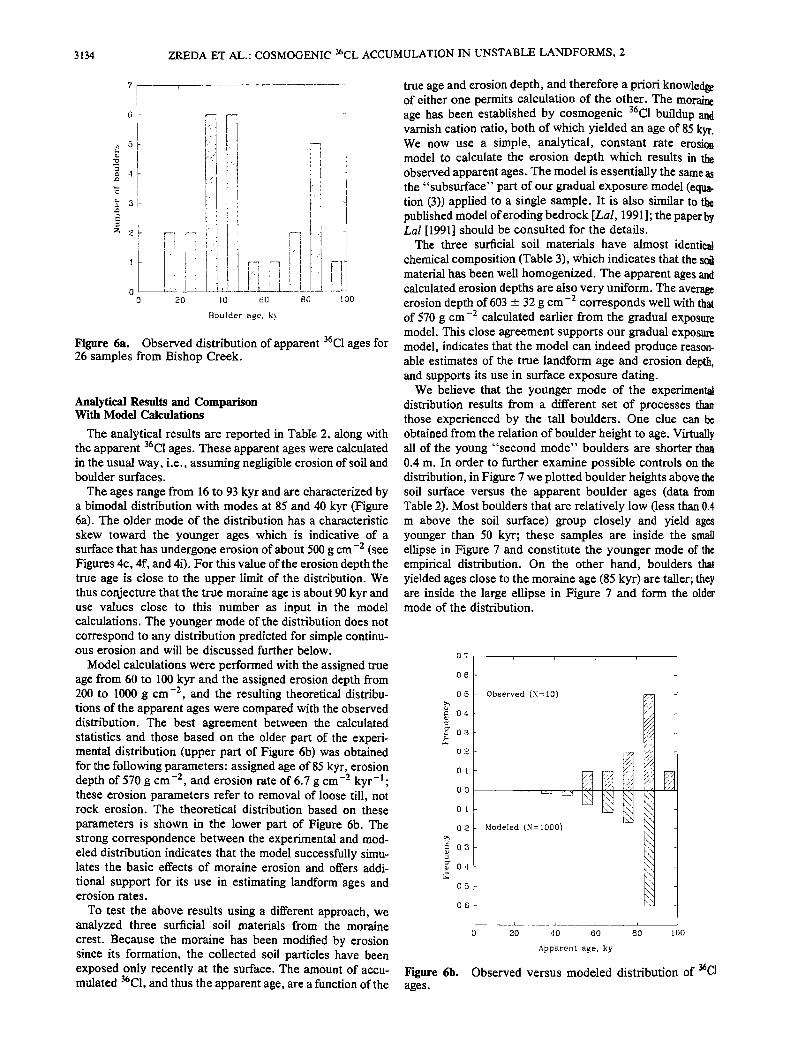
Figure 6a. Observed distribution of apparent 36C! ages for 26 samples from Bishop Creek.

Analytical Results and Comparison With Model Calculations

The analytical results are reported in Table 2, along with the apparent 36C1 ages. These apparent ages were calculated in the usual way, i.e., assuming negligible erosion of soil and boulder surfaces.

The ages range from 16 to 93 kyr and are characterized by a bimodal distribution with modes at 85 and 40 kyr (Figure 6a). The older mode of the distribution has a characteristic skew toward the younger ages which is indicative of a surface that has undergone erosion of about 500 g cm -2 (see Figures 4c, 4f, and 4i). For this value of the erosion depth the true age is close to the upper limit of the distribution. We thus conjecture that the true moraine age is about 90 kyr and use values close to this number as input in the model calculations. The younger mode of the distribution does not correspond to any distribution predicted for simple continu- ous erosion and will be discussed further below.

Model calculations were performed with the assigned true age from 60 to !00 kyr and the assigned erosion depth from 200 to 1000 g cm -2 and the resulting theoretical distribu- tions of the apparent ages were compared with the observed distribution. The best agreement between the calculated statistics and those based on the older part of the experi- mental distribution (upper part of Figure 6b) was obtained for the following parameters' assigned age of 85 kyr, erosion depth of 570 g cm -2 and erosion rate of 6.7 gcm ~ kyr -•- these erosion parameters refer to removal of loose till, not rock erosion. The theoretical distribution based on these

parameters is shown in the lower part of Figure 6b. The strong correspondence between the experimental and mod- eled distribution indicates that the model successfully simu- lates the basic effects of moraine erosion and offers addi-

tional support for its use in estimating landform ages and erosion rates.

To test the above results using a different approach, we analyzed three surficial soil materials from the moraine crest. Because the moraine has been modified by erosion since its formation, the collected soil particles have been exposed only recently at the surface. The amount of accu- mulated 36C1, and thus the apparent age, are a function of the

true age and erosion depth, and therefore a priori knowledge of either one permits calculation of the other. The moraine age has been established by cosmogenic 36C1 buildup and varnish cation ratio, both of which yielded an age of 85 kyr. We now use a simple, analytical, constant rate erosion model to calculate the erosion depth which results in the observed apparent ages. The model is essentially the same as the "subsurface" part of our gradual exposure model (equa- tion (3)) applied to a single sample. It is also similar to the published model of eroding bedrock [Lal, 1991]; the paper by Lal [1991] should be consulted for the details.

The three surficial soil materials have almost identical chemical composition (Table 3), which indicates that the soil material has been well homogenized. The apparent ages and calculated erosion depths are also very uniform. The average erosion depth of 603 - 32 gcm -2 corresponds well with that of 570 g cm -2 calculated earlier from the gradual exposure model. This close agreement supports our gradual exposure model, indicates that the model can indeed produce reason- able estimates of the true landform age and erosion depth, and supports its use in surface exposure dating.

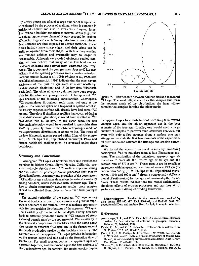
We believe that the younger mode of the experimental distribution results from a different set of processes than those experienced by the tall boulders. One clue can be obtained from the relation of boulder height to age. Virtu•y all of the young "second mode" boulders are shorter than 0.4 m. In order to further examine possible controls on the distribution, in Figure 7 we plotted boulder heights above •e soil surface versus the apparent boulder ages (data from Table 2). Most boulders that are relatively low (less than 0.4 m above the soil surface) group closely and yield ages younger than 50 kyr; these samples are inside the small ellipse in Figure 7 and constitute the younger mode of the empirical distribution. On the other hand, boulders that yielded ages close to the moraine age (85 kyr) are taller; they are inside the large ellipse in Figure 7 and form the older mode of the distribution.

07] ...... 06

05 Observed (N= 10) •.,

• 0.4

02_,-

0.0

0 2. Modeled (N- 1000)

• 04

0.5 •

o 20 ,t o 6o

Apparent age, ky

-i 80 lOO

Figure 6b. ages.

Observed versus modeled distribution of 36C!

ZREDA ET AL.: COSMOGENIC 36CL ACCUMULATION IN UNSTABLE LANDFORMS, 2 3135

The very young age of such a large number of samples can be explained by the process of spalling, which is common in periglacial climate and also in areas with frequent forest fires. When a boulder experiences internal stress (e.g., due to sudden temperature changes) it may respond by spalling off smaller fragments or breaking into two or more pieces; fresh surfaces are thus exposed to cosmic radiation. These pieces initially have sharp edges, and their origin can be easily recognized from their shape. With time they weather into rounded cobbles and eventually may no longer be recognizable. Although we avoided obviously spalled sam- ples, we now believe that many of the low boulders we randomly collected are derived from weathered spall frag- ments. The grouping of the younger ages close to 40 kyr may indicate that the spalling processes were climate controlled. Previous studies [Dorn et al., 1991; Phillips et al., 1990, also unpublished manuscript, 1994] indicate that the most severe glaciations of the past 85 kyr were at about 60-70 kyr (mid-Wisconsin glaciation) and 15-20 kyr (late Wisconsin g!aciation). The older advance could not have been respon- sible for the observed younger mode of the apparent 36C1 ages because of the following consideration. Cosmogenic 36C1 accumulates throughout rock mass, not only at the surface. If a boulder splits or a fragment is spa!led off of it, the freshly exposed surface will already have had some 36C1 present. Therefore if significant spalling had occurred during the mid-Wisconsin glaciation, it would have resulted in 36C1 ages older than 60-70 kyr. On the other hand, the late Wisconsin g!aciation would have resulted in ages older than 20-25 kyr, possibly close to the observed younger mode of the experimental distribution at about 40 kyr. The route of the late Wisconsin glacier passed within 2 km of the sample site (F. M. Phillips et al., unpublished manuscript, 1994), and intense periglacial spalling might be expected under these conditions.

Summary and Conclusions Cosmogenic 36C1 ages of boulders from late Pleistocene

moraines in Bishop Creek, Sierra Nevada, California, pro- vided valuable details about 36C1 surface exposure dating and the nature of postdepositional processes that modify glacial landforms. Accuracy and precision of the cosmogenic 36C1 landform age estimates depend on the natural variability among boulders, which increases with landform age. There- fore to obtain comparably accurate results, more samples should be collected from older surfaces than from younger ones.

The natural variability of the apparent 36C1 ages among morainal boulders is due to soil erosion and gradual expo- sure of boulders at the surface. Two mechanisms are respon- sible for the resulting distributions of the apparent 36C1 ages. The variability of the initial burial depth among boulders leads to different production rates of 36C1 because of atten- uation of cosmic rays by the soil material. The variability in the chemical composition of boulders from the same depth also results in different 36C1 ages due to the dependence of the depth production profile on the boulder chemistry. The distributions of the apparent 36C1 ages provide information on the erosion depth and rate and on the formation time of landforms. For small erosion depths the apparent ages are clustered together, and their mean age is the best estimate of the true landform age. In contrast, for greater erosion depths

1.5-

!.0-

0.5

0.0 0 20 40 60 80 100

Boulder age, ky

Figure 7. Relationship between boulder size and measured 36C1 age. The small ellipse encircles the samples that form the younger mode of the distribution; the large ellipse contains the samples forming the older mode.

the apparent ages form distributions with long tails toward younger ages, and the oldest apparent age is the best estimate of the true age. Ideally, one would need a large number of samples to perform such statistical analysis, but even with only a few samples from a surface one may attempt to calculate the first two moments of the experimen- tal distribution and estimate the true age and erosion param- eters.

We tested the above theoretical results by measuring cosmogenic 36C1 in boulders from a late Pleistocene mo- raine. The distribution of the calculated apparent ages al- lowed us to calculate the "true" age of 85 kyr and the erosion rate of 570 gcm -2. These results are in excellent agreement with independently estimated values of 87 kyr (by cation ratio dating (F. M. Phillips et al., unpublished manu- script, 1994) and 600 gcm -2 (from a conceptually different model of soil erosion) for the age and erosion depth, respec- tively. These results indicate that the model satisfactorily simulates effects of erosion processes and can thus aid in surface exposure dating of eroding landforms.

Acknowledgments. Funding for this research was provided by NSF grants SES-8901437, EAR-8603440, and EAR-8916667. We thank Ronald Dom and Andrew Bach for help in sample collection.

References

Aruscavage, P. J., and E. Y. Campbell, An ion-selective electrode method for determination of chlorine in geological materials, Talanta, 28, 745-749, 1987.

Davis, R., Jr., and O. A. Schaeffer, Chlorine-36 in nature, Ann. N.Y. Acad. Sci., 62, 105-!22, 19.55.

Dom, R. I., F. M. Phillips, M. G. Zreda, E. W. Wolfe, A. J. T. jul1, P. W. Kubik, and P. Sharma, Glacial chronology of Mauna Kea, Hawaii, as constrained by surface-exposure dating, Natl. Geogr. Res. Explore, 7, 456-471, 1991.

Elmore, D., B. R. Fulton, M. R. Clover, J. R. Marsden, H. E. Gove, H. Naylor, K. H. Purser, L. R. Kilius, R. P. Beukins, and A. E.

3!36 ZREDA ET AL.: COSMOGENIC 36CL ACCUMULATION IN UNSTABLE LANDFORMS, 2

Litherland, Analysis of 36C1 in environmental water samples using an electrostatic accelerator, Nature, 277, 22-25, 1979.

Elsheimer, H. N., Application of an ion-selective electrode method to the determination of chloride in 4! international geochemical reference materials, Geostand. Newsl., I1, 115-122, 1988.

Fabryka-Martin, J. F., M. M. Fowler, and R. Biddie, Study of neutron fluxes underground, quarterly report, pp. 82-85, Isot. and Nucl. Chem. Div., Los Alamos Natl. Lab., Los Alamos, N.M., Oct.-I)ec. 1991.

Imbrie, J., J. D. Hays, D. G. Martinson, A. Mcintyre, A. C. Mix, J. J. Morley, N. G. Pisias, W. L. Prell, and N.J. Shackleton, The orbital theory of Pleistocene climate: Support from a revised chronology of the marine 8180 record, in Milankovitch and Climate, Understanding the Response to Orbital Forcing, part 1, edited by A. Berger, J. Imbrie, J. Hays, G. Kukla, and B. Salzman, pp. 269-305, D. Reidel, Norwell, Mass., 1984.

Lal, D., Cosmic ray labelling of erosion surfaces: In situ nuclide production rates and erosion models, Earth Planet. Sci. Lett., 104, 424-439, 1991.

Lal, D., and B. Peters, Cosmic ray produced radioactivity on Earth, in Encyclopedia of Physics, edited by S. Fluegge, vol. 46/1, Cosmic Rays H, edited by K. Sitte, pp. 551-612, Springer-Verlag, New York, 1967.

Liu, B. F. M. Phillips, J. T. Fabryka-Martin, M. M. Fowler, and W. I•. Stone, Cosmogenic 36C1 accumulation in unstable !and- forms, 1, Effects of the thermal neutron distribution, Water Resour. Res., this issue.

Martinson, D. G., N. G. Pisias, J. D. Hays, J. Imbrie, T. C. Moore Jr., and N.J. Shackleton, Age dating and the orbital theory of the ice ages: Development of a high-resolution 0 to 300,000-yr chro- nostratigraphy, Quat. Res., 27, 1-29, 1987.

Phillips, F. M., B. D. Leavy, N. O. Jannik, D. Elmore, and P. W. Kubik, The accumulation of cosmogenic chlorine-36 in rocks: A method for surface exposure dating, Science, 231, 41-43, 1986.

Phillips, F. M., M. G. Zreda, S.S. Smith, D. Elmore, P. W. Kubik, and P. Sharma, A cosmogenic chlorine-36 chronology for glacial

deposits at Bloody Canyon, eastern Sierra Nevada, California, Science, 248, 1529-1532, 1990.

Phillips, F. M., M. G. Zreda, S.S. Smith, D. Elmore, P. W. Kubik, R. I. Dom, and D. J. Roddy, Dating the impact at Meteor Crater: Comparison of 36C1 buildup and varnish 14C with thermolumines. cence, Geochim. Cosmochim. Acta, 55, 2695-2698, 1991.

Snedecor, G. W., and W. D. Cochran, Statistical Methods, 594 pp., Iowa State University Press, Ames, 1967.

Winograd, I. J., T. B. Coplen, J. M. Landwehr, A. C. Riggs, K. R. Ludwig, B. J. Szabo, P. T. Kolesar, and K. M. Revesz, Contin- uous 500,000-year climate record from vein calcite in Devils Hole, Nevada, Science, 258, 255-260, 1992.

Zreda, M. G., Development and Calibration of the Cosmogenic 3•C1 Surface Exposure Dating Method and Its Application to the Chronology of Late Quaternary Glaciations, Ph.D. dissertation, New Mexico Tech, Socorro, 1994.

Zreda, M. G., F. M. Phillips, and S.S. Smith, Cosmogenic 3•C1 dating of geomorphic surfaces, Rep. 90-1, 104 pp., Hydrol. Program, N.M. Tech, Socorro, 1990.

Zreda, M. G., F. M. Phillips, D. Elmore, P. W. Kubik, P. Sharma, and R. I. Dorn, Cosmogenic 36C1 production rates in terrestrial rocks, Earth Planet. Sci. Lett., 105, 94-109, 1991.

Zreda, M. G., F. M. Phillips, P. W. Kubik, P. Sharma, and D. Elmore, Eruption age at Lathrop Wells, Nevada from cosmogenic chlorine-36 accumulation, Geology, 21, 57-60, 1993.

D. Elmore, Physics Department, PRIME Laboratory, Purdue University, West Lafayette, IN 47907.

F. M. Phillips, Geoscience Department, New Mexico Tech, Socorro, NM 87801.

M. G. Zreda, Department of Hydrology and Water Resources, University of Arizona, Tucson, AZ 85721.

(Received June 21, 1993; revised March 8, 1994; accepted March 16, 1994.)