The Cryosphere, 6, 367–382, 2012www.the-cryosphere.net/6/367/2012/doi:10.5194/tc-6-367-2012© Author(s) 2012. CC Attribution 3.0 License.

The Cryosphere

Thermal remote sensing of ice-debris landforms using ASTER:an example from the Chilean Andes

A. Brenning1, M. A. Pena2, S. Long1, and A. Soliman1

1Department of Geography and Environmental Management, University of Waterloo, 200 University Avenue West,Waterloo, Ontario, N2L 3G1, Canada2Centro de Estudio de Recursos Naturales Oterra, Universidad Mayor, Camino La Piramide 5750, Huechuraba,Santiago, Chile

Correspondence to:A. Brenning (brenning@uwaterloo.ca)

Received: 27 September 2011 – Published in The Cryosphere Discuss.: 24 October 2011Revised: 17 February 2012 – Accepted: 26 February 2012 – Published: 30 March 2012

Abstract. Remote sensors face challenges in characteriz-ing mountain permafrost and ground thermal conditions ormapping rock glaciers and debris-covered glaciers. We ex-plore the potential of thermal imaging and in particular ther-mal inertia mapping in mountain cryospheric research, fo-cusing on the relationships between ground surface temper-atures and the presence of ice-debris landforms on one sideand land surface temperature (LST) and apparent thermal in-ertia (ATI) on the other. In our case study we utilize ASTERdaytime and nighttime imagery and in-situ measurementsof near-surface ground temperature (NSGT) in the Mediter-ranean Andes during a snow-free and dry observation periodin late summer. Spatial patterns of LST and NSGT weremostly consistent with each other both at daytime and atnighttime. Daytime LST over ice-debris landforms was de-creased and ATI consequently increased compared to otherdebris surfaces under otherwise equal conditions, but NSGTshowed contradictory results, which underlines the complex-ity and possible scale dependence of ATI in heterogeneoussubstrates with the presence of a thermal mismatch and a heatsink at depth. While our results demonstrate the utility ofthermal imaging and ATI mapping in a mountain cryosphericcontext, further research is needed for a better interpretationof ATI patterns in complex thermophysical conditions.

1 Introduction

Rock glaciers and debris-covered glaciers are distinct typesof ice-debris landforms and elements of the mountaincryosphere in which the high ice contents are not visible at

the surface, creating challenges to remotely-sensed mappingof these features (Janke, 2001; Paul et al., 2004; Bolch etal., 2008; Kargel et al., 2005; Brenning, 2009; Shukla et al.,2010). Similarly, remote sensors have been of limited use inthe characterization of permafrost and ground thermal con-ditions in mountain areas. However, thermal remote sens-ing provides a set of variables that are useful for character-izing thermal and thermophysical surface characteristics ofthe natural and built environment (Watson, 1975; Chen et al.,2008; Pena, 2009). Its potential are yet to be fully exploitedin geomorphological and cryospheric research, and applica-tions in mountain environments are still relatively rare (VanDe Kerchove et al., 2009; Bertoldi et al., 2010), especiallyin the case of thermal inertia mapping (Piatek et al., 2007;Hardgrove et al., 2010).

We therefore explore the utility of remotely-sensed landsurface temperature (LST) and derived apparent thermal in-ertia (ATI) for thermally characterizing and discriminatingperiglacial mountain environments, particularly rock glaciersand debris-covered glaciers. We demonstrate this approachutilizing ASTER daytime and nighttime data in a study areain the Andes of Central Chile, where in-situ near-surfaceground temperature (NSGT) measurements are available forcomparison with remotely-sensed LST (Bodin et al., 2010a;Apaloo et al., 2012).

This paper starts by providing thermophysical and cry-ological background information in Sect. 2. Section 3presents the remote sensing methods, in-situ measurementsand the statistical study design and analysis methods used inthis study, and provides an introduction to the study area andrelevant meteorological conditions. The results of statistical

Published by Copernicus Publications on behalf of the European Geosciences Union.

368 A. Brenning et al.: Thermal remote sensing of ice-debris landforms using ASTER

data analyses relating LST, ATI and NSGT observations tosite characteristics are presented in Sect. 4, focusing in par-ticular on differences between ice-debris landforms and otherdebris surfaces. These empirical findings are discussed inSect. 5 in the context of heat transfer processes between theatmosphere, the surface debris layer, and ground ice.

2 Background

2.1 Remote sensing of LST

Satellite-based thermal infrared (TIR) data can be used to es-timate LST over large and inaccessible areas. TIR is the op-tical region of the spectrum that comprises the wavelengthsof emitted radiation or heat, which ranges from 3 to 14 µm(mid-wave infrared 3–8 µm and longwave infrared 8–14 µm).Earth surface features emit radiation as a function of their in-ternal temperature (i.e. kinetic temperature) and their abilityto emit radiation (i.e. emissivity). Emitted radiation is an ex-ternal manifestation of the feature’s energy state and it can beconverted into radiant temperature of Earth surface featuresor LST (Lillesand et al., 2004).

LST is the external temperature of the Earth surface fea-tures (Weng and Quattrochi, 2006), and is one of the keyparameters combining the results of all surface-atmosphereinteractions and energy fluxes between the atmosphere andthe ground. It is strongly dependent on the thermal proper-ties of the material (Wan, 1997). LST is closely related tothe atmospheric temperature of the layer immediately abovethe surface (Nichol, 1996; Hafner and Kidder, 1999; Wengand Quattrochi, 2006), although there are other influences aswell (Hartz et al., 2006; Pena, 2009).

A critical thermal property of the material that controls thetemporal behaviour of LST is thermal inertia or the responseof a material to temperature changes. Earth surface featureswith high thermal inertia respond slowly to the solar pulseand as a consequence they tend to present a more uniformLST throughout the day and night than features with lowthermal inertia (Watson, 1975; Lillesand et al., 2004). Theutility of satellite-based TIR data for differentiating the LSTof two land cover types can be limited because image acqui-sition time does not necessarily capture the moment whenthese land cover types exhibit their maximum thermal differ-ence. In these cases, the retrieval of thermal inertia is oftena more useful approach because it differentiates both landcover types from the perspective of the temporal behaviourin LST. From satellite-based daytime and nighttime TIR datait is possible to retrieve thermal inertia estimates, as outlinedin the following section.

2.2 Surface energy balance and thermal inertia

The surface energy balance at the air-debris interface and itsdependence on surface, air and debris temperatures,Ts, Ta

andTd respectively, is given by (Reid et al., 2010)

S +L ↓ +L ↑ (Ts)+H(Ts,Ta,u)+LE(Ts)+G(Ts,Td)+P(Ts) = 0 (1)

whereS is the total shortwave net radiation,L ↓ is incominglong wave radiation,L ↑ is outgoing long wave radiation,His sensible heat flux,LE is latent heat flux,G is ground flux,u is wind speed, andP is precipitation flux. Given the dryconditions at the surface, the termsLE andP can be omit-ted. The existence of a hidden frozen layer below the debriswill add a heat sink that will influence the energy balanceEq. (1) by lowering the ground flux, which by consequencewill lower the outgoing long wave flux given the stability ofother flux and radiation terms. Solving the heat conductionequation with LST as an upper boundary condition showsthat the thermal response of a homogeneous ground is con-trolled by a lumped thermal property called thermal inertia,TI, which is given by

TI =√

ρck (2)

whereρ is the bulk density,c is the specific heat capacity andk is the thermal conductivity.

Thermal inertia as a single thermal material property de-termines the surface temperature amplitude of a periodicallyheated half-space. This relationship can be used to estimatethermal inertia from daytime and nighttime LST, which isreferred to as apparent thermal inertia (ATI). It is potentiallyuseful for discriminating a wide variety of geological and ge-omorphological surface characteristics (Watson, 1975; Hard-grove et al., 2010). Thermal inertia is closely related tophysical substrate properties as it correlates positively withdensity, moisture content, silica content, and negatively withthe iron content (e.g. desert varnish) of a substrate’s surface(Watson, 1975).

Different formulas for calculating ATI have been proposedin order to account for different measurement times and sur-face properties such as albedo (Li et al., 2004; Verhoef, 2004;Chen et al., 2008). In this study, we choose a representationthat is based on the daily LST amplitude and accounts forspatially varying albedo and solar radiation. We thereforerepresent ATI by

ATI =((1−γ )S0)

1T(3)

whereγ is surface albedo, determined from the wavelengthsof reflected radiation of the spectrum,S0 is incoming solarradiation and1T is the maximum daily temperature differ-ence. In our study the solar correction factor accounts fortopographic radiation differences whereas previous studiesmodeled latitudinal variation of solar radiation (Nasipuri etal., 2006; Van doninck et al., 2011).

The relation between ATI and thermal inertia takes a linearform with scaling and offset factors, and the validity of ATIis limited to the case where linear coefficients are constantacross the studied area (Price, 1985). There is a high poten-tial in using such simple formulation in dry climates where

The Cryosphere, 6, 367–382, 2012 www.the-cryosphere.net/6/367/2012/

A. Brenning et al.: Thermal remote sensing of ice-debris landforms using ASTER 369

latent heat flux is insignificant and the sensible heat flux isspatially invariant during the summer time.

2.3 Ice-debris landforms and coarse blocky substrates

Rock glaciers and debris-covered glaciers are different typesof ice-debris landforms in high mountain areas that exhibitdifferent internal thermal properties and interact differentlywith the atmosphere (Haeberli et al., 2006; Bodin et al.,2010a; Berthling, 2011). Debris-covered glaciers are typi-cally part of the ablation area of glaciers in dry, continentalmountain areas with high talus production. They present asupragracial debris layer typically up to 1–1.5 m thick and of-ten exhibit melt-out depressions as the expression of verticaland lateral ice melt (Bodin et al., 2010a). Rock glaciers areconsidered to be the geomorphological expression of creep-ing ice-debris bodies under permafrost conditions (Haeberliet al., 2006). Their ice-rich inner part is protected relativelywell against external temperature fluctuations by a season-ally thawing debris layer, the active layer, which is typically3–5 m thick. However, this is not a static system as the ac-tive layer thickness is likely to increase over time as a con-sequence of climatic warming and the creep towards lowerelevations (Haeberli, 2001; Trombotto and Borzotta, 2009).For convenience, we refer to debris-covered glaciers and rockglaciers jointly as “ice-debris landforms” (Berthling, 2011).

TIR imaging and especially thermal inertia mapping ofice-debris landforms is still a relatively novel approach thatmay provide insights into surface energy fluxes of thesecryospheric features with variable debris cover thicknesses.ASTER-derived daytime LST on debris-covered glacier hasbeen found to be several degrees lower than in adjacent ar-eas not underlain by massive ice (Taschner and Ranzi, 2002),and it may serve as a proxy for debris cover thickness, at leastfor thin debris covers<0.6 m (Mihalcea et al., 2008). It fur-ther has been suggested that ATI differs between the surfacesof ice-debris landforms and surrounding areas (Piatek et al.,2007; Piatek, 2009). A quantitative assessment of this con-jecture is presented in this study. Bare, dry soil and cloudlessskies are required to apply this approach (Watson, 1975), andthese conditions are perfectly met in the summer-dry Andesduring the snow-free period.

3 Methods and data

Our research approach is based on remotely-sensed and in-situ data of ground thermal conditions and the use of statis-tical models for data analysis. Knowledge of the meteoro-logical conditions at and before the image acquisition dateand their climatic context is further required to understandatmospheric controls on the thermal state of the ground sur-face. This section starts with a general overview of rele-vant climatic and geomorphic conditions in the study area(Sect. 3.1), and continues by reporting on image acquisition

(Sect. 3.2) and procedures used for processing remote sens-ing data (Sect. 3.3). Meteorological conditions during im-age acquisition (Sect. 3.4) and in-situ measurements are pre-sented next (Sect. 3.5). Finally, the statistical study designand data analysis methods are introduced (Sect. 3.6).

3.1 Study area

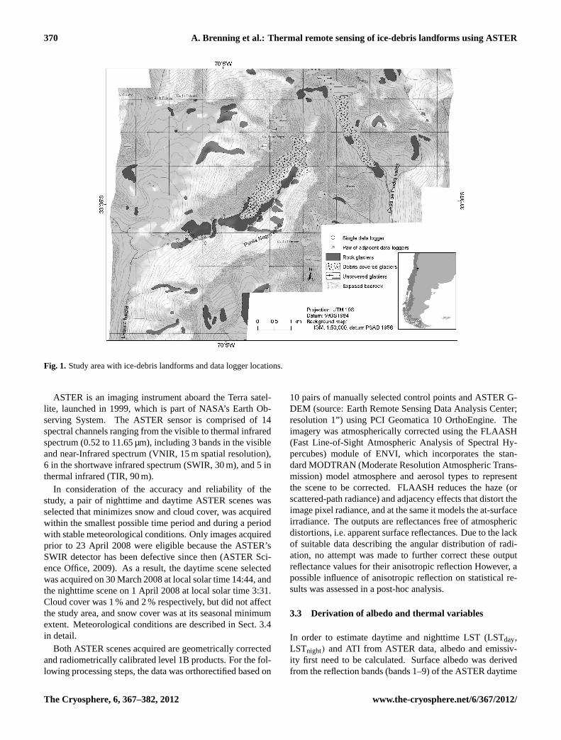
The study area is located in the western Main Cordillera ofcentral Chile at the latitude of Santiago and comprises theLaguna Negra and Casa de Piedra catchments as well as ad-jacent areas above 3000 m a.s.l. (Fig. 1). Rock glaciers and(debris-covered) glaciers are widely distributed in this area(Brenning, 2005a, b; Bodin et al., 2010a; see also Sect. 3.5).The long dry summer season with infrequent cloud cover andthe resulting dry soils provide ideal conditions for thermalimaging and thermal inertia mapping (Watson, 1975).

This study focuses on the area between 3000 and3900 m a.s.l. The 0◦C isotherm altitude (ZIA) of mean an-nual air temperature (MAAT) is located at∼3600 m a.s.l.,and the ZIA rises seasonally to an average elevation of4200 m a.s.l. in summer (Carrasco et al., 2005). Most areasup to 3900 m a.s.l. become snow-free until year-end, and onlysmall snow patches related to snow redistribution last longerand may persist (Bodin et al., 2010a; Apaloo et al., 2012).Vegetation is completely absent above∼3200 m a.s.l. Onlysmall patches of high Andean steppe vegetation exist above∼3000 m a.s.l.

Strong downwasting and widening of thermokarst depres-sions on debris-covered glaciers has been observed in thestudy area (Bodin et al., 2010a). Exposures in melt-out de-pressions show debris-cover thicknesses of∼1 to∼1.5 m onthe surfaces of both debris-covered glaciers in the study area,which show a transition into uncovered glaciers in their up-per parts.

The study area presents mainly dark volcanic rocks of theTertiary Abanico Formation. A granodioritic intrusive unit ispresent in the northwestern corner of the study area, and vol-canic and sedimentary sequences of the Late Cretassic Col-imapu Formation occupy the eastern margin of the study area(Fock et al., 2005; Farıas et al., 2008). All data logger loca-tions are in the dark volcanic area, while a small percentage(<10 %) of the matched samples introduced in Sect. 3.6 arelocated in the other geological units.

3.2 Image acquisition

Two ASTER (Advanced Spaceborne Thermal Emission andReflection Radiometer) scenes of the study area were ob-tained for this study from the Earth Remote Sensing DataAnalysis Center, one acquired at nighttime and one at day-time. ASTER was selected not only because of its high spa-tial resolution, but also its wide spectral range of the short-wave infrared and thermal infrared spectra, which were usedfor deriving albedo, LST, and ATI.

www.the-cryosphere.net/6/367/2012/ The Cryosphere, 6, 367–382, 2012

370 A. Brenning et al.: Thermal remote sensing of ice-debris landforms using ASTER

Fig. 1. Study area with ice-debris landforms and data logger locations.

ASTER is an imaging instrument aboard the Terra satel-lite, launched in 1999, which is part of NASA’s Earth Ob-serving System. The ASTER sensor is comprised of 14spectral channels ranging from the visible to thermal infraredspectrum (0.52 to 11.65 µm), including 3 bands in the visibleand near-Infrared spectrum (VNIR, 15 m spatial resolution),6 in the shortwave infrared spectrum (SWIR, 30 m), and 5 inthermal infrared (TIR, 90 m).

In consideration of the accuracy and reliability of thestudy, a pair of nighttime and daytime ASTER scenes wasselected that minimizes snow and cloud cover, was acquiredwithin the smallest possible time period and during a periodwith stable meteorological conditions. Only images acquiredprior to 23 April 2008 were eligible because the ASTER’sSWIR detector has been defective since then (ASTER Sci-ence Office, 2009). As a result, the daytime scene selectedwas acquired on 30 March 2008 at local solar time 14:44, andthe nighttime scene on 1 April 2008 at local solar time 3:31.Cloud cover was 1 % and 2 % respectively, but did not affectthe study area, and snow cover was at its seasonal minimumextent. Meteorological conditions are described in Sect. 3.4in detail.

Both ASTER scenes acquired are geometrically correctedand radiometrically calibrated level 1B products. For the fol-lowing processing steps, the data was orthorectified based on

10 pairs of manually selected control points and ASTER G-DEM (source: Earth Remote Sensing Data Analysis Center;resolution 1”) using PCI Geomatica 10 OrthoEngine. Theimagery was atmospherically corrected using the FLAASH(Fast Line-of-Sight Atmospheric Analysis of Spectral Hy-percubes) module of ENVI, which incorporates the stan-dard MODTRAN (Moderate Resolution Atmospheric Trans-mission) model atmosphere and aerosol types to representthe scene to be corrected. FLAASH reduces the haze (orscattered-path radiance) and adjacency effects that distort theimage pixel radiance, and at the same it models the at-surfaceirradiance. The outputs are reflectances free of atmosphericdistortions, i.e. apparent surface reflectances. Due to the lackof suitable data describing the angular distribution of radi-ation, no attempt was made to further correct these outputreflectance values for their anisotropic reflection However, apossible influence of anisotropic reflection on statistical re-sults was assessed in a post-hoc analysis.

3.3 Derivation of albedo and thermal variables

In order to estimate daytime and nighttime LST (LSTday,LSTnight) and ATI from ASTER data, albedo and emissiv-ity first need to be calculated. Surface albedo was derivedfrom the reflection bands (bands 1–9) of the ASTER daytime

The Cryosphere, 6, 367–382, 2012 www.the-cryosphere.net/6/367/2012/

A. Brenning et al.: Thermal remote sensing of ice-debris landforms using ASTER 371

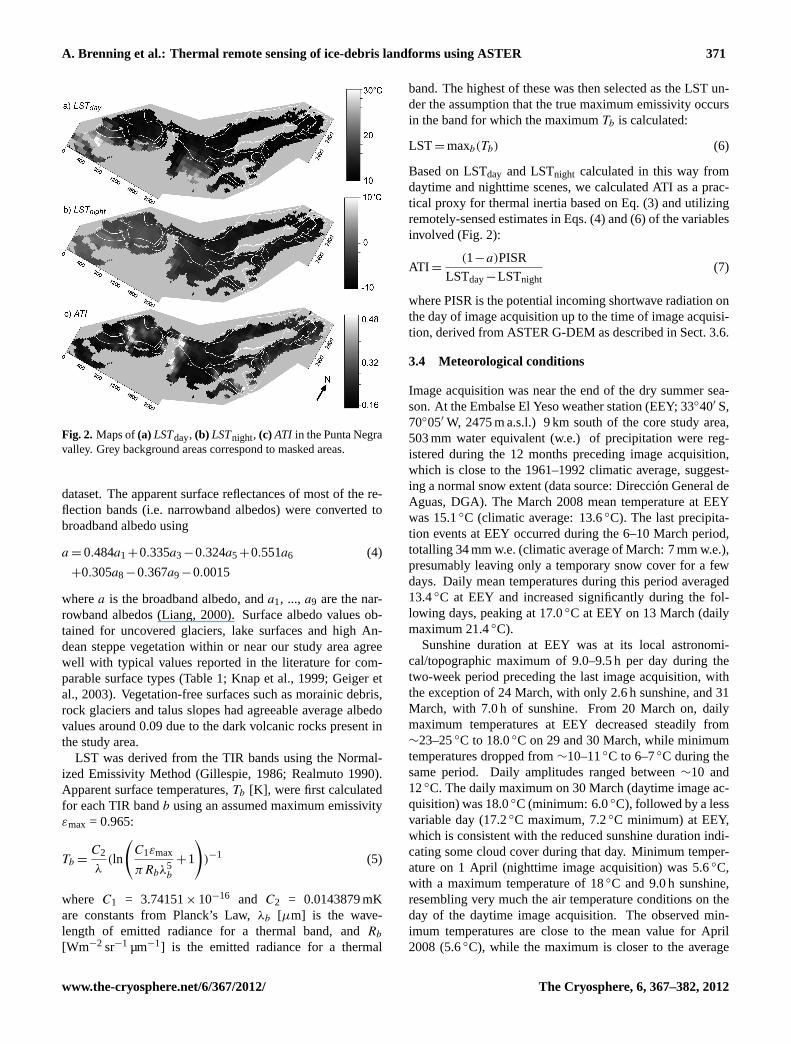
Fig. 2. Maps of(a) LSTday, (b) LSTnight, (c) ATI in the Punta Negravalley. Grey background areas correspond to masked areas.

dataset. The apparent surface reflectances of most of the re-flection bands (i.e. narrowband albedos) were converted tobroadband albedo using

a = 0.484a1+0.335a3−0.324a5+0.551a6 (4)

+0.305a8−0.367a9−0.0015

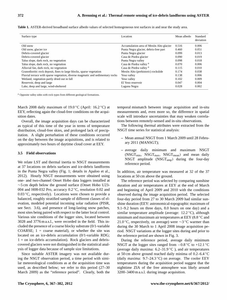
wherea is the broadband albedo, anda1, ..., a9 are the nar-rowband albedos (Liang, 2000). Surface albedo values ob-tained for uncovered glaciers, lake surfaces and high An-dean steppe vegetation within or near our study area agreewell with typical values reported in the literature for com-parable surface types (Table 1; Knap et al., 1999; Geiger etal., 2003). Vegetation-free surfaces such as morainic debris,rock glaciers and talus slopes had agreeable average albedovalues around 0.09 due to the dark volcanic rocks present inthe study area.

LST was derived from the TIR bands using the Normal-ized Emissivity Method (Gillespie, 1986; Realmuto 1990).Apparent surface temperatures,Tb [K], were first calculatedfor each TIR bandb using an assumed maximum emissivityεmax = 0.965:

Tb =C2

λ(ln

(C1εmax

πRbλ5b

+1

))−1 (5)

where C1 = 3.74151× 10−16 and C2 = 0.0143879 mKare constants from Planck’s Law,λb [µm] is the wave-length of emitted radiance for a thermal band, andRb

[Wm−2 sr−1 µm−1] is the emitted radiance for a thermal

band. The highest of these was then selected as the LST un-der the assumption that the true maximum emissivity occursin the band for which the maximumTb is calculated:

LST= maxb(Tb) (6)

Based on LSTday and LSTnight calculated in this way fromdaytime and nighttime scenes, we calculated ATI as a prac-tical proxy for thermal inertia based on Eq. (3) and utilizingremotely-sensed estimates in Eqs. (4) and (6) of the variablesinvolved (Fig. 2):

ATI =(1−a)PISR

LSTday−LSTnight(7)

where PISR is the potential incoming shortwave radiation onthe day of image acquisition up to the time of image acquisi-tion, derived from ASTER G-DEM as described in Sect. 3.6.

3.4 Meteorological conditions

Image acquisition was near the end of the dry summer sea-son. At the Embalse El Yeso weather station (EEY; 33◦40′ S,70◦05′ W, 2475 m a.s.l.) 9 km south of the core study area,503 mm water equivalent (w.e.) of precipitation were reg-istered during the 12 months preceding image acquisition,which is close to the 1961–1992 climatic average, suggest-ing a normal snow extent (data source: Direccion General deAguas, DGA). The March 2008 mean temperature at EEYwas 15.1◦C (climatic average: 13.6◦C). The last precipita-tion events at EEY occurred during the 6–10 March period,totalling 34 mm w.e. (climatic average of March: 7 mm w.e.),presumably leaving only a temporary snow cover for a fewdays. Daily mean temperatures during this period averaged13.4◦C at EEY and increased significantly during the fol-lowing days, peaking at 17.0◦C at EEY on 13 March (dailymaximum 21.4◦C).

Sunshine duration at EEY was at its local astronomi-cal/topographic maximum of 9.0–9.5 h per day during thetwo-week period preceding the last image acquisition, withthe exception of 24 March, with only 2.6 h sunshine, and 31March, with 7.0 h of sunshine. From 20 March on, dailymaximum temperatures at EEY decreased steadily from∼23–25◦C to 18.0◦C on 29 and 30 March, while minimumtemperatures dropped from∼10–11◦C to 6–7◦C during thesame period. Daily amplitudes ranged between∼10 and12◦C. The daily maximum on 30 March (daytime image ac-quisition) was 18.0◦C (minimum: 6.0◦C), followed by a lessvariable day (17.2◦C maximum, 7.2◦C minimum) at EEY,which is consistent with the reduced sunshine duration indi-cating some cloud cover during that day. Minimum temper-ature on 1 April (nighttime image acquisition) was 5.6◦C,with a maximum temperature of 18◦C and 9.0 h sunshine,resembling very much the air temperature conditions on theday of the daytime image acquisition. The observed min-imum temperatures are close to the mean value for April2008 (5.6◦C), while the maximum is closer to the average

www.the-cryosphere.net/6/367/2012/ The Cryosphere, 6, 367–382, 2012

372 A. Brenning et al.: Thermal remote sensing of ice-debris landforms using ASTER

Table 1. ASTER-derived broadband surface albedo values of selected homogeneous test surfaces in and near the study area.

Surface type Location Mean albedo Standarddeviation

Old snow Accumulation area of Meson Alto glacier 0.516 0.006Old snow, glacier ice Punta Negra glacier, debris-free part 0.460 0.051Debris-covered glacier Punta Negra glacier 0.099 0.013Debris-covered glacier Casa de Piedra glacier 0.090 0.019Talus slope, dark rock, no vegetation Punta Negra valley 0.098 0.018Talus slope, dark rock, no vegetation Casa de Piedra valleya 0.070 0.006Alluvial fan, dark rock, no vegetation Casa de Piedra valleya 0.115 0.010Granodioritic rock deposit, fines to large blocks, sparse vegetation Meson Alto (prehistoric) rockslide 0.174 0.038Fluvial terrace with sparse vegetation, diverse magmatic and sedimentary rocks Yeso valley 0.138 0.006Wetland, vegetation partly dried out in fall Yeso valley 0.102 0.009Reservoir, deep and large El Yeso reservoir 0.047 0.004Lake, deep and large, wind-sheltered Laguna Negra 0.028 0.002

a Opposite valley sides with rock types from different geological formations.

March 2008 daily maximum of 19.0◦C (April: 16.2◦C) atEEY, reflecting again the cloud-free conditions on the acqui-sition dates.

Overall, the image acquisition days can be characterizedas typical of this time of the year in terms of temperaturedistribution, cloud-free skies, and prolonged lack of precip-itation. A slight perturbation of these conditions occurredon the day between the image acquisitions, and is related toapproximately two hours of daytime cloud cover at EEY.

3.5 Field observations

We relate LST and thermal inertia to NSGT measurementsat 37 locations on debris surfaces and ice-debris landformsin the Punta Negra valley (Fig. 1; details in Apaloo et al.,2012). Hourly NSGT measurements were obtained usingone- and two-channel Onset Hobo data loggers installed at∼5 cm depth below the ground surface (Onset Hobo U23-004 and H08-032 Pro, accuracy 0.2◦C, resolution 0.02 and0.03◦C, respectively). Locations were chosen to provide abalanced, roughly stratified sample of different classes of el-evation, modeled potential incoming solar radiation (PISR,see Sect. 3.6), and presence of long-lasting snow patches,most sites being paired with respect to the latter local control.Various site conditions of the logger sites, located between3028 and 3776 m a.s.l., were recorded in the field. This in-cluded the presence of a coarse blocky substrate (0/1-variableCOARSE; 1 = coarse material), or whether the site waslocated on an ice-debris accumulation (0/1-variable RDG;1 = on ice-debris accumulation). Rock glaciers and debris-covered glaciers were not distinguished in the statistical anal-ysis of logger data because of sample size limitations.

Since suitable ASTER imagery was not available dur-ing the NSGT observation period, a time period with simi-lar meteorological conditions as at the acquisition time wasused, as described below; we refer to this period (27–30March 2009) as the “reference period”. Clearly, both the

temporal mismatch between image acquisition and in-situmeasurements and, even more so, the difference in spatialscale will introduce uncertainties that may weaken correla-tions between remotely-sensed and in-situ observations.

The following thermal attributes were extracted from theNSGT time series for statistical analysis:

– Mean annual NSGT from 1 March 2009 until 28 Febru-ary 2011 (MANSGT);

– average daily minimum and maximum NSGT(NSGTmin, NSGTmax, NSGTmean) and mean dailyNSGT amplitude (NSGTamp) during the four-dayreference period.

In addition, air temperature was measured at 32 of the 37locations at 50 cm above the ground.

The reference period was selected by comparing sunshineduration and air temperatures at EEY at the end of Marchand beginning of April 2009 and 2010 with the conditionsobserved during the image acquisition period. The selectedfour-day period from 27 to 30 March 2009 had similar sun-shine duration (EEY: astronomical-topographic maximum of9.1–9.2 hours on three days, 8.0 hours on one day) and asimilar temperature amplitude (average: 12.2◦C), althoughminimum and maximum air temperatures at EEY (8.8◦C and21.0◦C, respectively, on average) were∼3◦C warmer thanduring the 30 March to 1 April 2008 image acquisition pe-riod. NSGT variations at the logger sites during and prior tothe reference period are shown in Fig. 3.

During the reference period, average daily minimumNSGT at the logger sites ranged from−0.8◦C to +12.1◦C(average daily maxima: 6.2–31.9◦C ), and air temperaturesat 50 cm above ground reached daily minima of 0.2–6.4◦C(daily maxima: 9.7–24.3◦C) on average. The cooler EEYtemperatures during the acquisition period suggest that thenighttime ZIA of the free atmosphere was likely around3200–3400 m a.s.l. during image acquisition.

The Cryosphere, 6, 367–382, 2012 www.the-cryosphere.net/6/367/2012/

A. Brenning et al.: Thermal remote sensing of ice-debris landforms using ASTER 373

Fig. 3. Hourly NSGT time series at logger sites for location outside (solid lines) and within ice-debris landforms (dashed lines) duringthe 24–30 March 2009 period. The upper panel shows average NSGTs of all data loggers, the lower panels individual logger time seriesas deviation from each logger’s mean NSGT. The reference period is delimited by continuous vertical lines; dotted lines indicate times ofdaytime and nighttime NSGT readings (3 p.m., 3 a.m.).

Geomorphological and cryospheric mapping, includingpresence/absence information on rock glaciers and debris-covered glaciers in the area, was furthermore conductedin the field and based on orthorectified IKONOS imagery(panchromatic resolution: 1 m× 1 m; GeoEye / Pacific Ge-omatics Ltd.). The study area covers 48 km2 between 3000and 3900 m a.s.l., of which 4.9 km2 correspond to ice-debrislandforms (rock glaciers: 3.3 km2). The area of interest isreduced to 21 km2 after removing irrelevant areas such asexposed ice and bedrock. More than 50 rock glaciers arepresent in the study area, the exact number depending onhow multi-part rock glaciers are counted. All rock glaciersincluded in this study are considered to be intact, and all but afew smaller rock glaciers below 3200 m a.s.l. are likely activebased on morphological criteria (Brenning, 2005a, b; Bodinet al., 2010a). Differential GPS measurements on two mor-phologically active features confirmed their activity (Bodinet al., 2010b).

3.6 Statistical analysis

Our statistical analyses are of exploratory character, i.e. theyaim at discovering novel relationships rather than confirmingan existing hypothesis. Linear mixed-effects models that ac-count for grouped sampling were used for this purpose, andthe false-discovery rate (FDR) was controlled in performingmultiple hypothesis tests.

Two different samples are considered. The first one cor-responds to the logger sites described in Sect. 3.5, whichallows us to correlate the remotely-sensed variables withNSGT variables as well as local site conditions observed insitu. This has the disadvantage that logger sites constitutea rather small sample of point observations with a limitedspatial representativity, while the remotely-sensed variableswere derived by combining spectral bands measured at reso-lutions ranging from 15 m× 15 m to 90 m× 90 m.

The second sample avoids these problems by samplinggrid cells directly from the remotely-sensed imagery, but thisapproach is limited to the assessment of elevation and PISR-related influences and comparisons between sites with rockglaciers or debris-covered glaciers versus rock debris sur-faces. First, grid cells located within digitized ice-debrislandforms were randomly sampled, using an upper eleva-tion limit of 3900 m a.s.l. Debris-surface grid cells werethen matched to these samples as controls based on slope an-gle (tolerance±5◦), PISR on the acquisition date (±10 %),albedo (±5 %) and elevation (±50 m). Where multiplematches were available, the most similar one (according toa weighted sum of the mentioned four variables) was se-lected. Matching ensures that several components of thesurface energy balance in Eq. (1) are controlled and do notaffect the comparison of ATI between ice-debris landformsand debris surfaces, which is one of our main objectives.Specifically, differences in net short wave radiation are ac-counted for by matching by albedo and PISR, and upwelling

www.the-cryosphere.net/6/367/2012/ The Cryosphere, 6, 367–382, 2012

374 A. Brenning et al.: Thermal remote sensing of ice-debris landforms using ASTER

long wave radiation is controlled by the elevation variable.The final matched random sample consisted of 1000 gridcells, 379 of which corresponded to rock glacier and 121 todebris-covered glacier areas.

Elevation, slope angle and potential incoming solar radia-tion for the acquisition date of the daytime image were de-rived from ASTER G-DEM elevation data (Hayakawa et al.,2008). In the matched-sample analysis, exposed bedrock ar-eas were masked using a combination of topographic criteriaand bedrock areas digitized from a topographic map (Insti-tuto Geografico Militar, scale 1:50,000). Areas with albedoa < 0.05 ora > 0.20 or ATI > 0.60 were removed in orderto avoid artifacts resulting from mixed pixels involving frac-tional snow cover, melt-out ponds or other local phenomenawith thermophysical characteristics that may bias the coeffi-cient estimates. The rather low albedo cut-off value of 0.20 isdue to the prevailing low albedo of dark volcanic rocks (Ta-ble 1). Only 3.6 % of the samples obtained in the previousfiltering steps were removed based on their extreme albedoor ATI values.

Linear mixed-effects models were used to analyze bothsamples. LSTday, LSTnight, LSTamp and ATI were usedas response variables in both samples, and in the case ofthe logger sites also NSGTday, NSGTnight, NSGTamp andMANSGT. Elevation above 3000 m a.s.l. (ELEV3000) andPISR on the acquisition date (relative to the area-wide av-erage; rPISR = PISR / mean PISR−1) were incorporated inmodels for LST, but not for ATI, which was solar-correctedin Eq. (3). All-day PISR was used for this in the case ofanalyses of LSTnight, and PISR up to the acquisition time(3 pm local time) otherwise (variable rPISRp). In addition,0/1-variables for the presence of rock glaciers (RGL) anddebris-covered glaciers (DGL; 1 = presence) were includedin the case of matched-sample data, and 0/1-variables forice-debris landforms (RDG; 1 = presence of rock glacier ordebris-covered glacier) and for the presence of coarse blockymaterial (COARSE) were tested on the logger data set. Noattempt was made to distinguish between rock glacier anddebris-covered glacier sites in the analysis of logger data be-cause of the small sample size. Descriptive statistics of theresponse variables and site characteristics are summarized inTable 2.

In this model, PISR and elevation account for short andlong wave radiation controls on the surface energy balance,respectively, while the ice-debris landform and coarsenessvariables are proxies for specific properties influencing theground flux. Turbulent heat fluxes are, however, not ac-counted for due to the unknown spatial characteristics of thewind field.

The grouping of logger sites was used as a random-effectterm on the intercept in the case of the logger sample, whilethe grouping in matched pairs defined a random effect on theintercept in the matched-sample analysis. In the matched-sample analysis, a spherical spatial autocorrelation structurewith nugget effect was used initially to account for possible

residual spatial dependence, but the fitted nugget autocorre-lation was consistently near 1, which means that no spatialautocorrelation was present after accounting for the pairedgrouping. Spatial autocorrelation was therefore omitted fromthe final models.

In addition to this main approach, post-hoc analyses wereperformed to examine the sensitivity of the results to sev-eral possible confounders and uncertainties. These includethe choice of the reference period, different PISR parame-terizations, and the additional incorporation of sine and co-sine of aspect into the model to control possible influences ofanisotropic reflection.

The potential utility of ATI for discriminating rock glaciersand other ice-debris landforms was assessed using the areaunder the receiver operating characteristics (ROC) curve, orAUROC, which takes values between 0.5 (no discrimination)and 1.0 (perfect discrimination).

Given the small sample size and large number of statisticalhypothesis tests performed for exploratory purposes, we ap-plied a correction for multiple testing that controls the FDRof the family of tests. The FDR is the proportion of falsepositive hypothesis tests among all positive test outcomes.We controlled the FDR at the≤ 10 % level, i.e. we expectthat of all positive test outcomes reported in this study, nomore than 10 % were incorrectly classified as positive. TheSimes procedure was used for this correction (Benjamini andHochberg, 1995).

All statistical analyses were conducted in the softwareR (version 2.11.1; R Development Core Team, 2010) withits contributed packages “nlme” (Pinheiro et al., 2009) and“ROCR” (Sing et al., 2009), and terrain analysis and geodataprocessing were conducted with SAGA GIS (version 2.0.4;Conrad, 2006) and the “RSAGA” package for R (Brenning,2008).

4 Results

After assessing to what extent the remotely-sensed observa-tions of thermal and thermophysical variables are related toin-situ measurements (Sect. 4.1), we then explore and inter-pret empirical relationships of these variables with respect togeomorphic and climatic site characteristics using statisticalmodels (Sect. 4.2).

4.1 Relationships between remotely-sensed and in-situvariables

Remotely-sensed and in-situ measurements of daytime andnighttime surface temperatures at the logger sites (N= 37)correlated reasonably well (ρ = 0.83 at nighttime and 0.49at daytime; Table 3). Median nighttime and daytime NSGTduring the reference period were, however, 6–7◦C higherthan LST at the logger sites (Table 2). This can be partly ex-plained by 3◦C higher air temperatures during the reference

The Cryosphere, 6, 367–382, 2012 www.the-cryosphere.net/6/367/2012/

A. Brenning et al.: Thermal remote sensing of ice-debris landforms using ASTER 375

Table 2. Descriptive statistics of remotely-sensed and in-situ variables and site characteristics at the logger sites and in the matched randomsample.

Variable Logger sites Median (IQR) Matched sample Median (IQR)

Remotely-sensed variablesLSTday [◦C] 12.2 (7.1) 14.9 (5.9)LSTnight [◦C] −1.2 (5.5) −1.1 (3.2)LSTamp [◦C] 16.3 (7.3) 16.3 (5.6)ATI [−] 0.26 (0.05) 0.25 (0.08)Albedo [−] 0.091 (0.029) 0.093 (0.025)

In-situ variablesNSGTday [◦C] 19.3 (8.9) −

NSGTnight [◦C] 4.5 (5.0) −

NSGTamp [◦C] 13.3 (8.2) −

MANSGT[◦C] 2.9 (4.9) −

Site characteristicsElevation [m a.s.l.] 3466 (462) 3479 (331)rPISR[-] 0.01 (0.24) 0.00 (0.23)rPISRp [−] 0.02 (0.14) 0.01 (0.17)Slope angle [◦] 20.5 (16.9) 15.1 (8.8)

period, and it may also reflect possible differences in turbu-lent heat fluxes or a bias in LST measurements relative toNSGT, which was measured at about 5 cm depth and at apoint scale.

The strongest association between remotely-sensed andin-situ variables measured was found for LSTnight, whichwas strongly correlated (ρ > 0.80) with NSGTnight andMANSGT, and slightly less strongly with NSGTday (Ta-ble 3). The strong correlation of LSTnight is explained bythe spatial homogeneity of surface temperature during nightas controlled by kinetic temperature, surface emissivity andincoming long wave radiation, which yield a better corre-spondence between point measurements (loggers) and areameasurements (ASTER pixels). The spatially much morevariable LSTday, in contrast, was moderately correlated withthese three in-situ temperature variables (ρ ≈ 0.50). LSTampand ATI were only weakly and not significantly correlatedwith in-situ thermal variables. The weak (but significant)positive(!) correlation between LSTnight and NSGTamp islikely a random association. Although the fixed NSGT read-ings at 3 a.m. and 3 p.m. used for calculating NSGTnight andNSGTday do not exactly represent the time of minimum andmaximum NSGT (Fig. 3), neither these correlations nor anyof the further statistical analyses in this study appear to besensitive to whether these fixed readings or actual NSGTminima and maxima are used.

The correlations between LST and NSGT during the dayand at night reflect to a large extent the presence of gen-eral altitudinal trends in temperature. When looking onlyat local temperature variation by removing a linear altitudi-nal trend, much weaker, non-significant positive correlations

Table 3. Correlation of remotely-sensed variables with in-situ vari-ables at the logger sites. Spearman correlation coefficients and tests,non-significant associations in square brackets; FDR controlled at≤

10 %.

Variable LSTday LSTnight LSTamp ATI

NSGTday 0.49 0.75 [0.24] [0.03]NSGTnight 0.47 0.83 [0.14] [−0.14]NSGTamp 0.33 0.40 [0.22] [0.14]MANSGT 0.52 0.89 [0.18] [−0.11]

Table 4. Correlation of detrended remotely-sensed variables withdetrended in-situ variables at the logger sites. Variables were de-trended by resting each variable’s linear trend with elevation. Spear-man correlation coefficients and tests, non-significant associationsin square brackets; FDR controlled at≤10 %.

Variable dLSTday dLSTnight

dNSGTday [0.25] [0.26]dNSGTnight [0.08] [0.20]dMANSGT [0.12] [0.10]

remain (Table 4). The weakness and non-significance of thisrelationship can partly be attributed to the small sample sizeand decorrelation of remotely-sensed and in-situ data due totemporal and scale differences. However, the consistentlypositive correlations suggest that remotely-sensed LST does

www.the-cryosphere.net/6/367/2012/ The Cryosphere, 6, 367–382, 2012

376 A. Brenning et al.: Thermal remote sensing of ice-debris landforms using ASTER

provide insights into local spatial patterns of NSGT otherthan those related to a simple altitudinal lapse rate. As anadhocexample, a 1◦C difference in dLSTnight predicts a 0.5◦Cdifference in NSGTnight according to a linear mixed-effectsmodel relating NSGTnight to ELEV3000and dLSTnight, whichhas a standard deviation of 0.9◦C. While this trend estimatehas a large uncertainty (standard error 0.3◦C), it gives usan idea of the contribution that remotely-sensed LST canmake to explain local variation in the thermal state of thedry ground surface in mountain areas during the snow-freeperiod.

4.2 Relationships with site characteristics

Daytime and nighttime LST in the matched sample werestrongly related to elevation as a proxy for atmospheric tem-peratures and rPISRp as a proxy for radiative controls (Ta-ble 5). rPISRp influenced LSTday much more strongly thanrPISR did for LSTnight, which is plausible because daytimesurface temperatures are controlled mainly by absorption ofincoming solar radiation while nighttime temperatures arecontrolled by emission of heat. In the case of a one-IQR (in-terquartile range) difference in solar radiation, a 3.1◦C dif-ference in LSTday would be predicted compared to a 0.9◦Cdifference at night, all other variables being equal. The LSTamplitude mirrored the LSTday situation as it most stronglydepended on the more variable daytime temperature. Overthe entire study area, model-derived LST lapse rates were ingood agreement with a dry adiabatic lapse rate of air temper-ature.

Empirical relationships found for the logger sites in thePunta Negra valley appear to differ in some important as-pects; however, the observations for this smaller sample arealso subject to substantial uncertainties and random varia-tion related to site selection and instrumentation. At thelogger sites, the model-derived LST and NSGT lapse rateswere close to the dry adiabatic lapse rate of−1◦C/100 mat nighttime but were clearly stronger at daytime (∼ −1.5−

−2◦C/100 m). Near-surface air temperatures at 50 cm aboveground showed a similar daytime lapse rate during the refer-ence period (−1.50◦C/100 m, standard error 0.09◦C/100 m).

Ice-debris landforms in the matched-sample analysis had alower LSTday (∼1–1.5◦C lower) and therefore also a smallerLSTamp (∼1–2◦C smaller). In the case of rock glaciers,this resulted in an ATI being 13 % higher than in non-rockglacier areas under otherwise equal conditions (Table 5).These differences were somewhat weaker in debris-coveredglacier areas compared to rock glaciers, and ATI on debris-covered glaciers was not significantly different from gen-eral debris surfaces under otherwise equal conditions. How-ever, a post-hoc analysis using slope aspect to account forpossible anisotropic reflection resulted in a greater estimateof the daytime temperature anomaly and ATI increase ofdebris-covered glaciers (LSTday 2.53◦C lower under other-wise equal conditions, standard error: 0.37◦C, unadjusted

p-value <0.001; ATI 0.034 higher, standard error 0.006,unadjusted p-value<0.001) while post-hoc coefficient esti-mates for the rock glaciers remained within the confidencelimits of coefficients reported in Table 5.

LST at the logger sites showed a (non-significant) negativedaytime anomaly on ice-debris landforms, as well as a simi-lar negative anomaly on coarse blocky surfaces (on ice-debrislandforms as well as outside of these). However, it should benoted that the local observation of the presence/absence ofcoarse blocky material at the logger’s point location may notbe representative of the area covered by the correspondingASTER grid cell.

While the logger-site LST observations on ice-debris land-forms also showed a (non-significant) negative anomaly fordaytime (and nighttime) LST, the observed (marginally sig-nificant) positive NSGT anomaly at daytime (+3.66◦C) wasinconsistent with this. This positive daytime NSGT anomalyon ice-debris landforms was reproducible under 5-fold cross-validation resampling and therefore cannot be attributed toinfluential outliers, even though the positive anomaly dropsto (non-significant) +2.61◦C (standard error 1.12◦C) if twosamples showing strongest disagreement between LSTdayand NSGTday are removed. Several comparisons with alter-native reference periods during February/March 2009/2010also indicate that this anomaly appears to be a persistent pat-tern during the 2009 summer / early fall period even thoughit tended to be less pronounced than during the selected ref-erence period. It therefore had an effect on MANSGT underotherwise equal conditions, even when controlling for differ-ences in snow cover duration (Apaloo et al., 2012).

The observed differences in mean ATI between the sur-faces of ice-debris landforms and other debris surfaces canalso be expressed with regards to the capability of the ATI todiscriminate between these surface types. The resulting AU-ROC values show, overall, a “fair” discrimination (Table 6),but this would not be sufficient to delineate ice-debris land-forms based on an ATI threshold alone.

Generally speaking, all results related to NSGT mea-surements reproduced very well in comparison with simi-lar alternative reference periods during February/March of2009/2010. Coefficient estimates and correlation coefficientswere well within the uncertainties given by estimated stan-dard errors. Similarly, the use of a PISR correction term inEq. (6) covering only the time span between noon and acqui-sition time has no appreciable influence on the results of ourstatistical analyses considering the estimated standard errorsof model coefficients.

The Cryosphere, 6, 367–382, 2012 www.the-cryosphere.net/6/367/2012/

A. Brenning et al.: Thermal remote sensing of ice-debris landforms using ASTER 377

Table 5. Linear mixed models relating remotely-sensed and in-situ ground thermal variables to site characteristics at the logger sites and inthe matched random sample. Non-significant coefficients in square brackets, FDR of all tests controlled at≤10 %, no tests on the intercept.

Response variable Intercept ELEV3000x 100 rPISRpa RGL DGL RDGL COARSEb

Remotely-sensed variables (matched sample)LSTday 21.32 (0.32) −1.07 (0.06) 17.80 (0.94) −1.51 (0.24) −1.21 (0.33)LSTnight 2.66 (0.11) −0.90 (0.02) 3.87a (0.28) 0.41 (0.08) [0.02] (0.12)LSTamp 18.9 (0.36) −0.23 (0.07) 15.85 (1.10) −1.97 (0.27) −0.97 (0.41)ATI 0.229 (0.006) 0.003 (0.001) 0.032 (0.0004) [0.008] (0.006)

Remotely-sensed variables (logger sites)LSTday 21.29 (1.42) −1.25 (0.24) 14.45 (3.32) [−1.92] (1.14) [−1.25] (1.07)LSTnight 3.53 (0.39) −1.07 (0.07) [1.26]a (0.88) [0.33] (0.27) [−0.27] (0.22)LSTamp 17.34 (1.59) [−0.16] (0.27) 12.29 (3.70) [−1.83] (1.25) [−0.70] (1.14)ATI 0.228 (0.038) [0.002] (0.006) [0.047] (0.031) [0.037] (0.029)

In-situ variables (logger sites)NSGTday 26.31 (1.57) −1.92 (0.26) 13.00 (3.69) 3.66 (1.30) [−1.26] (1.25)NSGTnight 9.08 (0.68) −0.96 (0.12) [1.17] (1.59) [0.70] (0.58) [−1.01] (0.56)NSGTamp 17.18 (1.78) −0.92 (0.30) 12.62 (4.16) [2.91] (1.48) [−0.53] (1.43)MANSGTc 7.96 (0.37) −1.04 (0.06) [1.45] (0.90) [0.72] (0.30) −0.92 (0.28)

a rPISRp was used for all response variables exceptLSTnight NSGTnight andMANSGT, for which rPISRwas used.b In-situ observation at the logger site; not necessarily representative of entire ASTER grid cell.c Compare Apaloo et al. (submitted) for more detailed results relating MANSGT to site characteristics.

Table 6. AUROC values expressing the ability of ATI to discrim-inate between different ice-debris accumulations and other debrissurfaces.

Data set RGL DGL RDGMatched sample 0.617 0.568 0.605Logger sample 0.738

5 Discussion

5.1 Spatial patterns revealed by thermal imaging

Remotely-sensed and in-situ observations of spatial patternsof daytime and nighttime surface temperatures in the highAndes agree reasonably well in terms of their correlation aswell as statistically estimated topoclimatic influences. Theutility of thermal imaging based on ASTER data may there-fore not be limited to debris-covered glaciers with a shal-low (<40 cm) debris cover (Mihalcea et al., 2008), but it alsoshows potential for analysing spatial patterns in periglacialenvironments in snow-free and especially dry conditions(Van De Kerchove et al., 2009; Bertoldi et al., 2010).

Nevertheless, in-situ point observations and spatially ag-gregated remote-sensing data provided contrasting results forthe daytime temperature difference between ice-debris land-forms and their surroundings, under otherwise equal siteconditions. At this time we can only speculate about thecauses of this disagreement, such as scale differences be-tween ASTER data and in-situ measurements or a possible

bias introduced by site selection and the installation of in-strumentation in heterogeneous surface materials and com-plex local topography (e.g. dark desert varnish on more stablerock surfaces; different grain size distributions, Hardgroveet al., 2010). Interestingly, similar disagreements betweenpoint-scale and spatially aggregated results have been foundelsewhere with much larger sample sizes (Gubler et al., 2011:effect size of coarse surfaces +1.66◦C at the intra-footprintscale and−1.66◦C at the inter-footprint scale). Other pos-sible confounders may be related to differences in turbulentwind fluxes between the image acquisition period and the ref-erence period, in spite of our observation that results obtainedfrom in-situ temperature measurements were insensitive tothe choice of a particular reference period.

The spatial patterns of LST are in good agreement withwhat would be expected in this type of environment. Theestimated lapse rate of∼–1◦C/100 m was close to the dryadiabatic lapse rate both at daytime and nighttime, which isconsistent with the consistently dry ground and air conditionsin this climate during the summer months, and contrasts withweaker lapse rates encountered in more humid mountains(Rolland, 2002; Gubler et al., 2011). Daytime NSGT lapserates< −1◦C/100 m in at the logger sites might be related toa greater exposure of the highest “level” of the stepped PuntaNegra valley (above∼3500 m a.s.l.) to westerly air flows,leading to an enhanced cooling effect from the free atmo-sphere. By contrast, thermally-induced air flow that wouldweaken lapse rates appeared to be absent or weak. Temper-ature inversions also appeared to be absent, as evidenced byexploratory analyses showing linear altitudinal trends in day-time and especially nighttime LST and NSGT, supporting

www.the-cryosphere.net/6/367/2012/ The Cryosphere, 6, 367–382, 2012

378 A. Brenning et al.: Thermal remote sensing of ice-debris landforms using ASTER

also that the use of linear lapse rates in this study was appro-priate, in contrast to studies in other periglacial environments(Lewkowicz and Bonnaventure, 2011).

Topographically controlled exposure to solar radiation ex-plained around 3◦C of temperature variation on a dry sum-mer day (under a one-IQR difference in PISR), which reflectsthe strong effects of radiative heating in this generally cloud-less environment during the summer months (Schrott, 1991).

5.2 Thermophysical characteristics of ice-debrislandforms

This first, exploratory study that quantitatively examines dif-ferences in ATI between ice-debris landforms and their sur-roundings detected significant differences in ATI between in-tact rock glaciers and general debris surfaces under otherwiseequal conditions. Although reduced LSTday is the main fac-tor influencing ATI, the observed increase in nighttime LSTthat accompanies the stronger decrease in daytime LST onrock glaciers is consistent with an interpretation in terms ofdiffering thermal inertia as a thermophysical material prop-erty (Watson, 1975).

However, ATI in this study and in cryospheric studies ingeneral is a complex property (Fig. 4). A thermal gradientexists between ground surface and material at greater depth,in particular ground ice, which constitutes a thermal mis-match and a seasonal heat sink. Seasonal heat sinks at thelower boundary condition are not considered in the originalATI expression, which assumes only daily and not annualperiodic heating. ATI in cryospheric conditions is thereforecontrolled by thermal inertia and the thickness of the surfacelayer (Bandfield and Feldman, 2008). Daytime (nighttime)latent heat absorption (release) at the top of ground ice andconductive cooling (warming) of the ground surface by thisheat sink is small in the case of debris-layer thicknesses>1 m(Mihalcea et al., 2008; Mattson et al., 1993; Nicholson andBenn, 2006), but a contribution to a daytime LSTday reduc-tion (nighttime increase) may still be possible. While directobservations of ground ice temperatures and heat fluxes arenot available in this area, the low elevation of rock glacierswith respect to the regional ZIA of MAAT (Brenning, 2005b;Bodin et al., 2010) and borehole observations on such rockglaciers in other parts of the semiarid Andes (Monnier et al.,2011) suggest that ground ice in rock glaciers may likely beat the melting point. These effects are expected to be morepronounced on debris-covered glacier surfaces, which is con-sistent with the results of our post-hoc analysis, which ac-counts for a possible influence of anisotropic reflection.

Differences in thermal conductivity and heat capacity be-tween an ice-free surface layer and a second, ice-rich layermay also influence heat transfer and NSGT at daytime in par-ticular, resulting in a modified ATI. Such effects have beenmeasured for groundwater tables at 1–3.5 m depth (Alkhaieret al., 2009) and may have contributed to ATI differences

observed in this study. Further research of these phenomenais therefore warranted for a debris-ground ice stratification.

The presence of coarse blocky material in the surfacelayer of ice-debris landforms is another possible explanationfor observed ATI and LSTday differences between ice-debrislandforms and other debris surfaces. This influence was con-trolled for in the analysis of logger-site data; it is discussedseparately in Sect. 5.3. However, coarse blocky layers mayonly partly explain the mentioned differences because coarsesurface layers may also be present in other areas such as talusslopes. Additional causes for observed ATI and LSTday dif-ferences may be related to confounding with several factorsincluding rock type, weathering and (less likely here) soilmoisture, each of which has complex relationships with theoverall material density, heat capacity and conductivity.

5.3 Thermophysical characteristics of coarse blockylayers

Coarse blocky substrates, which are often present on ice-debris landforms but also on talus slopes, have been de-scribed by several authors as presenting distinct thermal char-acteristics and thermophysical properties (Fig. 4). In particu-lar, cold air circulation through the snow cover during winterhas been presented as an explanation for undercooled coarsedebris in marginal permafrost environments, and low thermalconductivity has been used to explain a strong thermal off-set between ground surface and top of permafrost in coarseblocky material (Harris and Pedersen, 1998; Delaloye andLambiel, 2005; Gruber and Hoelzle, 2008). While low ther-mal conductivities would reduce the thermal inertia of open-work boulder layers with poor thermal coupling between par-ticles (Eq. (2)), well-coupled, matrix-supported blocky lay-ers may exhibit the contrary effect. In these substrates, largeboulders connecting the ground surface with greater depthsoffer a higher thermal conductivity and density and thereforeincrease thermal inertia relative to finer material or openworkboulders (Fig. 4; Bandfield, 2007; Bandfield and Feldman,2008).

In our study, sites with coarse blocky surface layers werefound to have (non-significantly) reduced daily NSGT andLST amplitudes and increased ATI, suggesting that in thisparticular area reduced thermal conductivities and/or den-sities may have been present in coarse blocky substrates.While the empirical evidence for this phenomenon is lim-ited in this study, this shows that additional in-situ analysesof near-surface sediment structure are required in order tobetter interpret LST patterns. Spatial differences in turbulentheat flux may also constitute a possible uncontrolled con-founder because turbulent heat flux is expected to be higheron coarser surfaces.

The Cryosphere, 6, 367–382, 2012 www.the-cryosphere.net/6/367/2012/

A. Brenning et al.: Thermal remote sensing of ice-debris landforms using ASTER 379

Fig. 4. Effects of substrate type, thermal mismatch and presence of a heat sink on thermophysical properties, thermal conditions andATI under dry, snow-free conditions in summer: a schematic overview. ATI is subject to the combined effects of thermal inertia as athermophysical property and seasonal as well as diurnal heat transfer processes between the ground surface and greater depths.

5.4 Utility of ATI for characterizing ice-debrislandforms

Compared to the direct use of LST to delineate ice-debrislandforms (Taschner and Ranzi, 2002), ATI mapping prac-tically eliminates the need to account for the strong alti-tudinal trend present in LST data. Our results show thegeneral feasibility of ATI mapping in mountain terrain, anddemonstrate the potentials of this approach in periglacialand glacial environments. However, while thermal inertiais usually interpreted based on the assumption of a homo-geneous semi-infinite half space, a more complex situationis often found in these environments due to the presence ofground ice at variable depths and possible vertical materialsorting (Fig. 4; Bandfield, 2007; Bandfield and Feldman,2008). Physically-based modeling of typical layering fea-tures in combination with geophysical investigations would

provide further valuable insight into how these structures arereflected in ATI maps.

The strong spatial variation in daily maximum surfacetemperatures further poses a challenge as it is often relatedto small topographic features that are smaller than the resolu-tion of ASTER thermal imagery or widely available DEMs.A solar-corrected representation of ATI was therefore usedin this study (Eq. (3)), which helped to reduce confoundingwith topographic effects on daytime LST in complex terrain.Methods using the drop in surface temperature between sun-set and sunrise instead of the daily temperature amplitude(Verhoef, 2004) may also be of particular interest in moun-tain areas because of their reduced dependence on local to-pography.

While previous studies emphasized the potential utility ofATI for mapping ice-debris landforms on Earth (southeasternAlaska) and potentially on Mars (Piatek, 2009), the present

www.the-cryosphere.net/6/367/2012/ The Cryosphere, 6, 367–382, 2012

380 A. Brenning et al.: Thermal remote sensing of ice-debris landforms using ASTER

study is the first to produce quantitative assessment of thediscrimination that can be achieved with this method. Inour essentially vegetation-free study area, ATI proved to beof only very limited utility for mapping rock glaciers anddebris-covered glaciers. The (visually) more promising re-sults shown by Piatek (2009) can likely be attributed to theinfluence of vegetation, a darker upper soil horizon or moistsoils on ATI in the area chosen by these authors as a ter-restrial analog of Mars. Our findings are more likely trans-ferable to dry mountain areas on Earth, or to Mars. Giventhe weak (but potentially useful) discrimination of ice-debrislandforms provided by ATI, we suggest combining this vari-able with terrain attributes and other remotely-sensed vari-ables (Brenning, 2009; Brenning and Azocar, 2010).

6 Conclusions

Remotely-sensed LST and ATI provide insights into landsurface processes and thermophysical surface characteristicsthat complement local in-situ observations. In the presentstudy, ASTER-derived daytime and nighttime LST showedsimilar spatial patterns as in-situ observations of NSGT, al-though the comparison of measurements obtained at differ-ent spatial scales creates several challenges. ASTER-derivedATI of rock glaciers and debris-covered glaciers differedfrom the inertia of other vegetation-free debris surfaces inthe study area, and ice-debris landforms exhibited reduceddaytime LST under otherwise equal conditions.

Acknowledgements.This research was funded through an IDRCLatin America and the Caribbean Research Exchange Grant anda NSERC Discovery Grant awarded to A. Brenning. The authorswould like to thank J. B. Apaloo for processing in-situ groundthermal data, X. Bodin and several students for assistance in thefield, and Aguas Andinas and the Direccion General de Aguas forproviding weather data and logistical support. We further thank thereferees for their thoughtful comments, which helped to improvethis paper.

Edited by: A. Nolin

References

Alkhaier, F., Schotting, R. J., and Su, Z.: A qualitative descrip-tion of shallow groundwater effect on surface temperature of baresoil, Hydrol. Earth Syst. Sci., 13, 1749–1756, 2009,http://www.hydrol-earth-syst-sci.net/13/1749/2009/.

Apaloo, J., Brenning, A., and Bodin, X.: Interactions between snowcover, ground surface temperature and topography (Andes ofSantiago, Chile, 33.5◦ S), Permafrost Periglac., submitted, 2012.

ASTER Science Office: ASTER SWIR Data Status Report,13 March 2009, available online at:http://www.science.aster.ersdac.or.jp/en/aboutaster/swiren.pdf, 2009.

Bandfield, J. L.: High-resolution subsurface water-ice distributionson Mars, Nature, 447, 64–67,doi:10.1038/nature05781, 2007.

Bandfield, J. L. and Feldman, W. C.: Martian high latitude per-mafrost depth and surface cover thermal inertia distributions, J.Geophys. R., 113, E08001,doi:10.1029/2007JE003007, 2008.

Benjamini, Y. and Hochberg, Y.: Controlling the false discoveryrate: A practical and powerful approach to multiple testing, J.Roy. Stat. Soc. B, 57, 289–300, 1995.

Berthling, I.: Beyond confusion: rock glaciers as cryo-conditioned landforms, Geomorphology, 131, 98–106,doi:10.1016/j.geomorph.2011.05.002, 2011.

Bertoldi, G., Notarnicola, C., Leitinger, G., Endrizzi, S., Zebisch,M., Della Chiesa, S., and Tappeiner, U.: Topographical and eco-hydrological controls on land surface temperature in an alpinecatchment, Ecohydrology, 3, 189–204, 2010

Bodin, X., Rojas, F., and Brenning, A.: Status and evolution of thecryosphere in the Andes of Santiago (Chile, 33.5◦ S.), Geomor-phology, 118, 453–464.doi:10.1016/j.geomorph.2010.02.016,2010a.

Bodin, X., Azocar, G. F., and Brenning, A.: Recent (2004–2010)variations of surface displacements in an Andean permafrost-glacier environment (Chile, 33◦ S.), in: Abstracts, Third Eu-ropean Conference on Permafrost, 13–17 June 2010, Svalbard,Norway, 46, 2010b.

Bolch, T., Buchroithner, M. F., Kunert, A., and Kamp, U.: Auto-mated delineation of debris-covered glaciers based on ASTERdata, in: GeoInformation in Europe, edited by: Gomarasca, M.A., Proceedings, 27th EARSeL Symposium, 4–7 June 2007,Bozen, Italy, Millpress, Netherlands, 403–410, 2008.

Brenning, A.: Climatic and geomorphological controls of rockglaciers in the Andes of Central Chile: Combining statisticalmodelling and field mapping, Ph.D., Humboldt-Universitat zuBerlin, Berlin, urn:nbn:de:kobv:11-10049648, 2005a.

Brenning, A.: Geomorphological, hydrological and climatic signif-icance of rock glaciers in the Andes of Central Chile (33–35◦ S),Permafrost Periglac., 16, 231–240,doi:10.1002/ppp.528, 2005b.

Brenning, A.: Statistical geocomputing combining R and SAGA:The example of landslide susceptibility analysis with generalizedadditive models, in: SAGA – Seconds out, edited by: Bohner, J.,Blaschke, T., and Montanarella, L., Hamburger Beitrage zur Ph-ysischen Geographie und Landschaftsokologie, 19, 23–32, 2008.

Brenning, A.: Benchmarking classifiers to optimally integrate ter-rain analysis and multispectral remote sensing in automaticrock glacier detection, Remote Sens. Environ., 113, 239–247,doi:10.1016/j.rse.2008.09.005, 2009.

Brenning, A. and Azocar, G. F.: Statistical analysis of topo-graphic and climatic controls and multispectral signatures of rockglaciers in the dry Andes, Chile (27◦–33◦ S), Permafrost andPeriglacial Processes, 21, 54–66,doi:10.1002/ppp.670, 2010.

Carrasco, J. F., Casassa, G., and Quintana, J.: Changes of the 0◦Cisotherm and the equilibrium line altitude in central Chile duringthe last quarter of the 20th century, Hydrologic. Sci. J., 50, 933–948, 2005.

Chen, Z., Li, S., Ren, J., Pan, G., Zhang, M., Wang, L., Xiao, S.,and Jiang, D.: Monitoring and management of agriculture withremote sensing, in: Advances in Land Remote Sensing, editedby: Liang, S., Springer, Dordrecht, 397–421, 2008.

Conrad, O.: SAGA – Program structure and current state of imple-mentation, in: SAGA – Analysis and Modelling Applications,edited by: Bohner, J., McCloy, K. R., and Strobl, J., GottingerGeographische Abhandlungen, 115, 39–52, 2006.

The Cryosphere, 6, 367–382, 2012 www.the-cryosphere.net/6/367/2012/

A. Brenning et al.: Thermal remote sensing of ice-debris landforms using ASTER 381

Delaloye, R. and Lambiel, C.: Evidence of winter ascend-ing air circulation throughout talus slopes and rock glacierssituated in the lower belt of alpine discontinuous per-mafrost (Swiss Alps), Norsk Geogr. Tidsskr., 59, 194–203,doi:10.1080/00291950510020673, 2005.

Farıas, M., Charrier, R., Carretier, S., Martinod, J., Fock, A.,Campbell, A., Caceres, J., and Comte, D.: Late Miocenehigh and rapid surface uplift and its erosional response in theAndes of central Chile (33◦–35◦ S), Tectonics, 27, TC1005,doi:10.1029/2006TC002046, 2008

Fock, A., Charrier, R., Farıas, R., Maksaev, V., Fanning, M.,and Alvarez, P.: Exhumation and uplift of the western MainCordillera between 33◦ and 34◦ S, in: Extended Abstracts, 6thInternational Symposium on Andean Geodynamics, ISAG 2005,Barcelona 273–276, 2005.

Geiger, R., Aron, R. H., and Todhunter, P.: The climate near theground, sixth edition, Rowman and Littlefield Publ., Lanham,MD, USA, 2003.

Gillespie, A.: Lithologic mapping of silicate rocks using TIMS, in:Proceedings of the TIMS data user’s workshop, JPL Publication86–38, Pasadena CA, 29–44, 1986.

Gruber, S. and Hoelzle, M.: The cooling effect of coarse blocks re-visited: a modeling study of a purely conductive mechanism, in:9th International Conference on Permafrost, Fairbanks, Alaska,30 June–3 July 2008, 1, 557–561, 2008.

Gubler, S., Fiddes, J., Keller, M., and Gruber, S.: Scale-dependent measurement and analysis of ground surface temper-ature variability in alpine terrain, The Cryosphere, 5, 431–443,doi:10.5194/tc-5-431-2011, 2011.

Haeberli, W.: Modern research perspectives relating to permafrostcreep and rock glaciers: a discussion, Permafrost Periglac., 11,290–293, 2001.

Haeberli, W., Hallet, B., Arenson, L., Elconin, R., Humlum,O., Kaab, A., Kaufmann, V., Ladanyi, B., Matsuoka, N.,Springman, S., and Vonder Muhll, D.: Permafrost creep androck glacier dynamics, Permafrost Periglac., 17, 189–214,doi:10.1002/ppp.561, 2006.

Hafner, J. and Kidder, S. Q.: Urban heat island modeling in con-junction with satellite-derived surface/soil parameters, J. Appl.Meteorol., 38, 448–465, 1999.

Hardgrove, C., Moersch, J., and Whisner, S.: Thermal imagingof sedimentary features on alluvial fans, Planet. Space Sci., 58,482–508,doi:10.1016/j.pss.2009.08.012, 2010.

Harris, S. A. and Pedersen, D. E.: Thermal regimes be-neath coarse blocky materials, Permafrost Periglac., 9, 107–120, doi:10.1002/(SICI)1099-1530(199804/06)9:2<107::AID-PPP277>3.0.CO;2-G, 1998.

Hartz, D. A., Prashad, L., Hedquist, B. C., Golden, J., and Brazel,A. J.: Linking satellite images and hand-held infrared thermogra-phy to observed neighborhood climate conditions, Remote Sens.Environ., 104, 190–200, 2006.

Hayakawa, Y., Oguchi, T., and Lin, Z.: Comparison ofnew and existing global digital elevation models: ASTERG-DEM and SRTM-3, Geophys. Res. Lett., 35, L17404,doi:10.1029/2008GL035036, 2008.

Janke, J. R.: Rock glacier mapping: a method utilizing enhancedTM data and GIS modeling techniques, Geocarto Int., 16, 5–15,2001.

Kargel, J. S., Abrams, M. J., Bishop, M. P., Bush, A., Hamilton, G.,Jiskoot, H., Kaab, A., Kieffer, H. H., Lee, E. M., Paul, F., Rau, F.,Raup, B., Shroder, J. F., Soltesz, D., Stainforth, D., Stearns, L.,and Wessels, R.: Multispectral imaging contributions to globalland ice measurements from space, Remote Sens. Environ., 99,187–219,doi:10.1016/j.rse.2005.07.004, 2005.

Knap, W. H., Reijmer, C. H., and Oerlemans, J.: Narrowband tobroadband conversion of Landsat TM glacier albedos, Int. J. Re-mote Sens., 20, 2091–2110, 1999.

Lewkowicz, A. G. and Bonnaventure, P. P.: Equivalent elevation:a new method to incorporate variable surface lapse rates intomountain permafrost modelling, Permafrost Periglac., 22, 153–162, 2011.

Li, X., Liu, A., Zhang, S., Wang, Z., Sun, W., and Wang,P.: A study on thermal inertia approach for agriculturedrought monitoring in Shaanxi Province, China by usingNOAA/AVHRR data, in: Proceedings, IEEE InternationalGeoscience and Remote Sensing Symposium, 6, 4031–4033,doi:10.1109/IGARSS.2004.1370014, 20–24 September 2004,Anchorage, AK, 2004.

Liang, S.: Narrowband to broadband conversions of land surfacealbedo I Algorithms, Remote Sens. Environ., 76, 213–238, 2000.

Lillesand, T. M., Kiefer, R. W., and Chipman, J. W.: Remote sens-ing and image interpretation, fifth edition, John Wiley & Sons,New York, 2004.

Mattson, L. E., Gardner, J. S., and Young, G. J.: Ablation on debriscovered glaciers: an example from the Rakhiot Glacier, Punjab,Himalaya, in: IAHS Publ. 218, Snow and Glacier HydrologySymposium, Kathmandu, Nepal, 1992, 289–296, 16–21 Novem-ber 1992, IAHS Press, Institute of Hydrology, Wallingford, Ox-fordshire, UK, 1993.

Mihalcea, C., Brock, B. W., Diolaiuti, G., D’Agata, C., Cit-terio, M., Kirkbride, M. P., Cutler, M. E. J., and Smi-raglia, C.: Using ASTER satellite and ground-based surfacetemperature measurements to derive supraglacial debris coverand thickness patterns on Miage Glacier (Mont Blanc Massif,Italy), Cold Regions Science and Technology, 52, 341–354,doi:10.1016/j.coldregions.2007.03.004, 2008.

Monnier, S., Kinnard, C., Saez, R., Garrido, R., Camerlynck, C.,and Rejiba, F.: The internal structure and the cryologic impor-tance of the rock glaciers of the Los Pelambres mine (UpperChoapa Valley, semi-arid Andes of Chile), Geophys. Res. Abstr.,13, EGU2011-4165, 2011.

Nasipuri, P., Majumdar, T. J., and Mitra, D. S.: Studyof high-resolution thermal inertia over western India oilfields using ASTER data, Astronaut. Acta, 58, 270–278,doi:10.1016/j.actaastro.2005.11.002, 2006.

Nichol, J. E.: High-resolution surface temperature patterns relatedto urban morphology in a tropical city: a satellite-based study, J.Appl. Meteorol., 35, 135–146, 1996.

Nicholson, L. and Benn, D.: Calculating ice melt beneath a debrislayer using meteorological data, J. Glaciol., 52, 463–470, 2006.

Paul, F., Huggel, C., and Kaab, A.: Combining satellite multi-spectral image data and a digital elevation model for mappingof debris-covered glaciers, Remote Sens. Environ., 89, 510–518,doi:10.1016/j.rse.2003.11.007, 2004.

Pena, M. A.: Examination of the land surface temperature responsefor Santiago, Chile, Photogramm. Eng. Rem. S., 75, 1191–1200,2009.

www.the-cryosphere.net/6/367/2012/ The Cryosphere, 6, 367–382, 2012

382 A. Brenning et al.: Thermal remote sensing of ice-debris landforms using ASTER

Piatek, J. L.: Thermophysical properties of terrestrial rock anddebris-covered glaciers as analogs for Martian lobate debrisaprons, 40th Lunar and Planetary Science Conference, Lunar andPlanetary Science XL, held 23–27 March 2009 in The Wood-lands, Texas, 2127, 2009.

Piatek, J. L., Hardgrove, C., and Moersch, J. E.: Potential rockglaciers on Mars: comparison with terrestrial analogs, in: Sev-enth International Conference on Mars, held 9–13 July 2007 inPasadena, California, LPI Contribution No. 1353, 3353, 2007.

Pinheiro, J., Bates, D., DebRoy, S., Sarkar, D., and the R Develop-ment Core Team: linear and nonlinear mixed effects models, Rpackage version 3.1-96, 2009.

Price, J. C.: On the analysis of thermal infrared imagery: the limitedutility of apparent thermal inertia, Remote Sens. Environ., 18,59–73, 1985.

R Development Core Team: R: a language and environment forstatistical computing, R Foundation for Statistical Computing,Vienna, Austria, ISBN 3-900051-07-0, available at:http://www.R-project.org, 2010.

Realmuto, V. J.: Separating the effects of temperature and emissiv-ity: emissivity spectrum normalization, in: Proceedings of the2nd TIMS Workshop, JPL Publication 90–55, Pasadena CA, 23–27, 1990.

Reid, T. D. and Brock, B. W.: An energy-balance model for debris-covered glaciers including heat conduction through the debrislayer J. Glaciol., 56, 903–916, 2010.

Rolland, C.: Spatial and seasonal variations of air temperature lapserates in alpine regions, J. Climate, 16, 1032–1046, 2002.

Schrott, L.: Global solar radiation, soil temperature and permafrostin the Central Andes, Argentina: a progress report, PermafrostPeriglac., 2, 59–66, 1991.

Shukla, A., Arora, M. K., and Gupta, R. P.: Synergistic approach formapping debris-covered glaciers using optical-thermal remotesensing data with inputs from geomorphometric parameters, Re-mote Sens. Environ., 114, 1378–1387, 2010.

Sing, T., Sander, O., Beerenwinkel, N., and Lengauer, T.: ROCR:Visualizing the performance of scoring classifiers, R packageversion 1.0-4, available at:http://CRAN.R-project.org/package=ROCR, The R Foundation for Statistical Computing, Vienna,2009.

Taschner, S. and Ranzi, R.: Comparing the opportunities ofLandsat-TM and Aster data for monitoring a debris coveredglacier in the Italian Alps within the GLIMS project, IEEE Geo-science and Remote Sensing Symposium, 2, 1044–1046, 2002.

Trombotto, D. and Borzotta, E.: Indicators of present global warm-ing through changes in active layer-thickness, estimation ofthermal diffusivity and geomorphological observations in theMorenas Coloradas rockglacier, Central Andes of Mendoza, Ar-gentina, Cold Reg. Sci. Technol., 55, 321–330, 2009.

Van De Kerchove, R., Goossens, R., De Wulf, A., Bourgeois, J.,and Gheyle, W.: Thermal remote sensing imagery in permafroststudies, in: Proceedings of the 28th Symposium of the Eu-ropean Association of Remote Sensing Laboratories, 313–320,doi:10.3233/978-1-58603-986-8-313, 2008.

Van doninck, J., Peters, J., De Baets, B., De Clercq, E. M.,Ducheyne, E., and Verhoest, N. E. C.: The potential of multi-temporal Aqua and Terra MODIS apparent thermal inertia as asoil moisture indicator, Int. J. Appl. Earth Obs Geoinf., 13, 934–941,doi:10.1016/j.jag.2011.07.003, 2011.

Verhoef, A.: Remote estimation of thermal inertia and soil heat fluxfor bare soil, Agr. Forest Meteorol., 123, 221–236, 2004.

Wan, Z.: A physics-based algorithm for retrieving land-surfaceemissivity and temperature from EOS/MODIS data, IEEE T.Geosci. Remote, 35, 980–996, 1997.

Watson, K.: Geologic applications of thermal infrared images, Pro-ceedings of the IEEE, 63, 128–137, 1975.

Weng, Q. and Quattrochi, D. A.: Thermal remote sensing of urbanareas: An introduction to the special issue, Remote Sens. Envi-ron., 104, 119–122, 2006.

The Cryosphere, 6, 367–382, 2012 www.the-cryosphere.net/6/367/2012/