In situ cosmogenic radiocarbon production and 2-D ice flow linemodeling for an Antarctic blue ice area

Christo Buizert,1 Vasilii V. Petrenko,2,3 Jeffrey L. Kavanaugh,4 Kurt M. Cuffey,5

Nathaniel A. Lifton,6 Edward J. Brook,7 and Jeffrey P. Severinghaus8

Received 13 May 2011; revised 10 April 2012; accepted 12 April 2012; published 24 May 2012.

[1] Radiocarbon measurements at ice margin sites and blue ice areas can potentially beused for ice dating, ablation rate estimates and paleoclimatic reconstructions. Part of themeasured signal comes from in situ cosmogenic 14C production in ice, and this componentmust be well understood before useful information can be extracted from 14C data.We combine cosmic ray scaling and production estimates with a two-dimensional ice flowline model to study cosmogenic 14C production at Taylor Glacier, Antarctica. We find(1) that 14C production through thermal neutron capture by nitrogen in air bubbles isnegligible; (2) that including ice flow patterns caused by basal topography can lead to asurface 14C activity that differs by up to 25% from the activity calculated using anablation-only approximation, which is used in all prior work; and (3) that at high ablationmargin sites, solar modulation of the cosmic ray flux may change the strength of thedominant spallogenic production by up to 10%. As part of this effort we model two-dimensional ice flow along the central flow line of Taylor Glacier. We present two methodsfor parameterizing vertical strain rates, and assess which method is more reliable for TaylorGlacier. Finally, we present a sensitivity study from which we conclude that uncertaintiesin published cosmogenic production rates are the largest source of potential error. Theresults presented here can inform ongoing and future 14C and ice flow studies at ice marginsites, including important paleoclimatic applications such as the reconstruction ofpaleoatmospheric 14C content of methane.

Citation: Buizert, C., V. V. Petrenko, J. L. Kavanaugh, K. M. Cuffey, N. A. Lifton, E. J. Brook, and J. P. Severinghaus (2012),In situ cosmogenic radiocarbon production and 2-D ice flow line modeling for an Antarctic blue ice area, J. Geophys. Res., 117,F02029, doi:10.1029/2011JF002086.

1. Introduction

[2] Ice cores from polar regions have been used toreconstruct climate variations as far as 800 ka back in time[e.g., Jouzel et al., 2007]. Old ice can not only be obtained

from deep ice cores, but also at ice margins and Antarcticblue ice areas (BIAs) where it is re-exposed by ablation[Reeh et al., 2002; Bintanja, 1999]. For paleoclimate studiesthis provides an interesting alternative to ice coring, assample retrieval is less challenging from both technologicaland logistical points of view. Old ice can be sampled fromnear the surface, making the method especially well suitedfor experiments that require large ice samples [Petrenkoet al., 2009]. Dating of ice parcels is the principal problemwhen using ablation sites for climatic reconstruction[Sinisalo and Moore, 2010, and references therein]. Severalmethods have been used, including radiometric dating oftephra layers [e.g., Dunbar et al., 2008], flow line modeling[Azuma et al., 1985; Grinsted et al., 2003; Moore et al.,2006], stratigraphical matching of gas and water isotopemeasurements to well-dated ice core records [e.g., Reeh et al.,2002; Petrenko et al., 2006; Aciego et al., 2007; Schaeferet al., 2009], and radiocarbon dating of micro-particles[Jenk et al., 2007]. Early on it was realized that radiocarbondating of the CO2 present in the air bubbles trapped in polarice can potentially be used as an absolute dating method forice cores and BIA samples [Fireman and Norris, 1982;Andree et al., 1984]. In this method the air is extracted fromthe ice sample, after which the CO2 is isolated for 14C

1Centre for Ice and Climate, Niels Bohr Institute, University ofCopenhagen, Copenhagen, Denmark.

2Institute of Arctic and Alpine Research, University of Colorado,Boulder, Colorado, USA.

3Now at Department of Earth and Environmental Sciences, Universityof Rochester, Rochester, New York, USA.

4Department of Earth and Atmospheric Sciences, University of Alberta,Edmonton, Alberta, Canada.

5Department of Geography, University of California, Berkeley,California, USA.

6Earth and Atmospheric Sciences department, Purdue University, WestLafayette, Indiana, USA.

7Department of Geosciences, Oregon State University, Corvallis,Oregon, USA.

8Scripps Institution of Oceanography, University of California, SanDiego, La Jolla, California, USA.

Corresponding author: C. Buizert, Centre for Ice and Climate, NielsBohr Institute, University of Copenhagen, Juliane Maries vej 30, DK-2100Copenhagen, Denmark.

Copyright 2012 by the American Geophysical Union.0148-0227/12/2011JF002086

JOURNAL OF GEOPHYSICAL RESEARCH, VOL. 117, F02029, doi:10.1029/2011JF002086, 2012

F02029 1 of 13

analysis. Interpretation of the 14C data, however, is com-plicated by cosmogenic in situ production of 14C fromoxygen atoms found in ice [Lal et al., 1990]. When thiseffect is corrected for, the air bubbles contained in the icecan be dated with an accuracy of a few thousands of years[Van de Wal et al., 1994; Van Roijen et al., 1995; Van DerKemp et al., 2002; De Jong et al., 2004; Van de Wal et al.,2007].[3] Apart from dating applications, there are other reasons

for studying radiocarbon in ice. First, surface 14C con-centrations (in either 14CO or 14CO2) reflect ablation (oraccumulation) rates at the site under study. At sites with lowablation rates the ice parcels move slowly through the top�5 m (where cosmogenic irradiation is strongest), leading toa high surface 14C activity because the cosmogenic 14Caccumulates over time. The opposite is also true: whereablation rates are high, activity will be low. By this principle,measurements of 14C have been used to estimate BIA abla-tion rates [e.g., Lal et al., 1990; Van Roijen et al., 1995; Vander Borg et al., 2001]. It has also been suggested that 14C inice core samples can be used to infer past changes in accu-mulation rate [Lal et al., 1990, 2000].[4] Second, at well-dated ablation sites paleoclimate

information can be obtained from radiocarbon measure-ments. Fossil carbon sources are depleted in 14C, and in thisway measuring the 14C activity of carbon-containing gasspecies can teach us about the fossil contribution to their pastatmospheric variations. In particular, the 14C variations inmethane (CH4) over the last glacial termination containinformation on how much the destabilization of 14C-depletedmethane hydrates contributed to the observed CH4 increases[Petrenko et al., 2008, 2009].

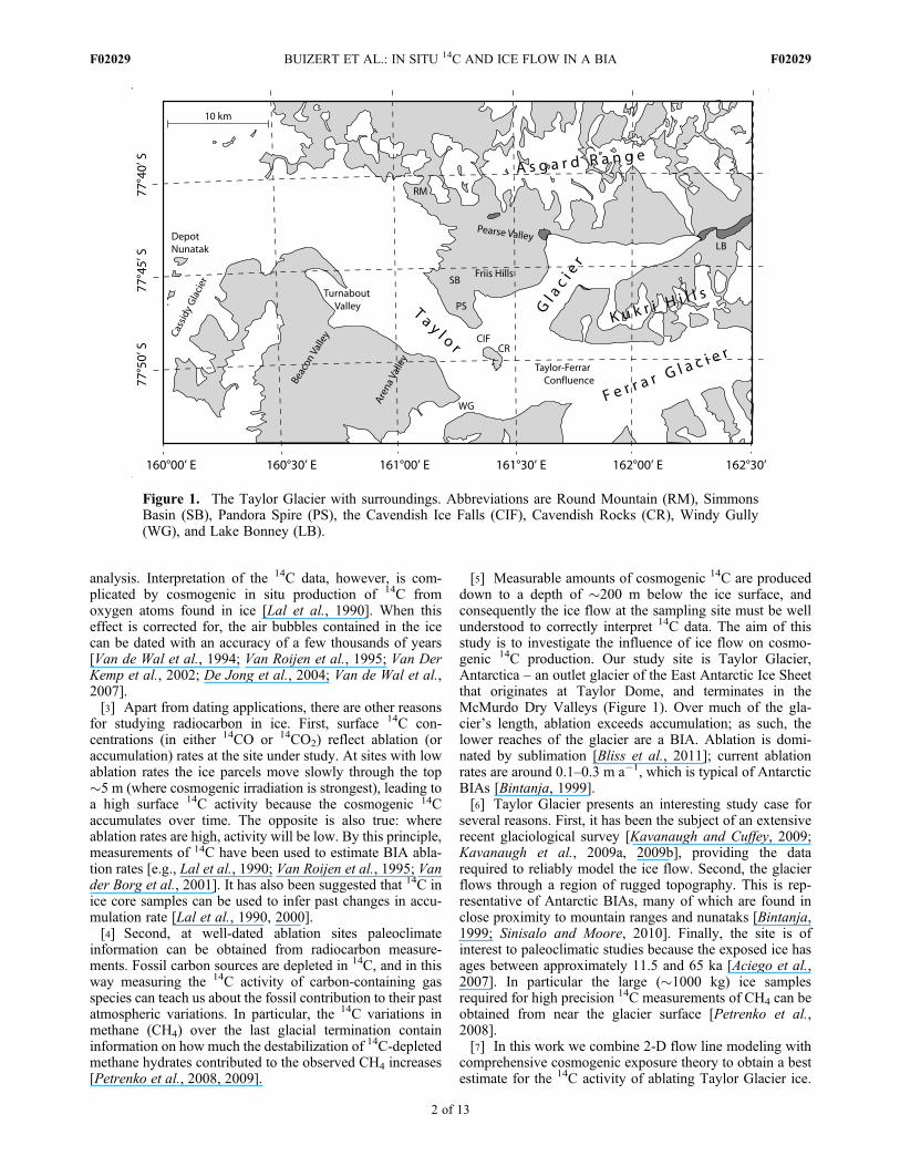
[5] Measurable amounts of cosmogenic 14C are produceddown to a depth of �200 m below the ice surface, andconsequently the ice flow at the sampling site must be wellunderstood to correctly interpret 14C data. The aim of thisstudy is to investigate the influence of ice flow on cosmo-genic 14C production. Our study site is Taylor Glacier,Antarctica – an outlet glacier of the East Antarctic Ice Sheetthat originates at Taylor Dome, and terminates in theMcMurdo Dry Valleys (Figure 1). Over much of the gla-cier’s length, ablation exceeds accumulation; as such, thelower reaches of the glacier are a BIA. Ablation is domi-nated by sublimation [Bliss et al., 2011]; current ablationrates are around 0.1–0.3 m a�1, which is typical of AntarcticBIAs [Bintanja, 1999].[6] Taylor Glacier presents an interesting study case for

several reasons. First, it has been the subject of an extensiverecent glaciological survey [Kavanaugh and Cuffey, 2009;Kavanaugh et al., 2009a, 2009b], providing the datarequired to reliably model the ice flow. Second, the glacierflows through a region of rugged topography. This is rep-resentative of Antarctic BIAs, many of which are found inclose proximity to mountain ranges and nunataks [Bintanja,1999; Sinisalo and Moore, 2010]. Finally, the site is ofinterest to paleoclimatic studies because the exposed ice hasages between approximately 11.5 and 65 ka [Aciego et al.,2007]. In particular the large (�1000 kg) ice samplesrequired for high precision 14C measurements of CH4 can beobtained from near the glacier surface [Petrenko et al.,2008].[7] In this work we combine 2-D flow line modeling with

comprehensive cosmogenic exposure theory to obtain a bestestimate for the 14C activity of ablating Taylor Glacier ice.

Figure 1. The Taylor Glacier with surroundings. Abbreviations are Round Mountain (RM), SimmonsBasin (SB), Pandora Spire (PS), the Cavendish Ice Falls (CIF), Cavendish Rocks (CR), Windy Gully(WG), and Lake Bonney (LB).

BUIZERT ET AL.: IN SITU 14C AND ICE FLOW IN A BIA F02029F02029

2 of 13

The combined model allows us to assess the influence ofbasal topography and solar modulation on the cosmogenic14C production; we demonstrate under which conditionsthese two effects become significant enough to deserveconsideration. We furthermore show production by thermalneutron capture to be negligible under all conditions.Although our focus is primarily on Taylor Glacier, theseconclusions are applicable to all studies of 14C in ice coresand BIAs.[8] The model also has applications that are very specific

to forthcoming 14C samples from Taylor Glacier. During a2010/2011 austral summer field campaign, samples forradiocarbon analyses were taken at Taylor Glacier with thepurpose of better constraining in situ production rates. Wewill show that at the sampling location the influence of iceflow strain rates on 14C activity is minimal, greatly simpli-fying data interpretation. More importantly, the model willserve as a framework for correcting 14CH4 measurementsover the abrupt methane increases observed for the lastglacial termination for the effects of in situ production, withthe purpose of reconstructing of the true paleo-atmosphericsignal.

2. Cosmogenic Production of 14C in Ice

[9] Cosmic rays consist largely of charged subatomicparticles originating from outside the Earth’s magneto-sphere. Upon entering the upper atmosphere, particles ofsufficient energy cause nuclear disintegrations, from which ashower, or cascade, of secondary cosmic ray particles isproduced. On interacting with the materials of Earth’s sur-face, these secondary cosmic rays are capable of producing awide variety of terrestrial cosmogenic nuclei (TCN) (seeGosse and Phillips [2001, and references therein] for anoverview of TCN exposure theory). In ice, 14C is producedcosmogenically, primarily through neutron spallation ofoxygen atoms [Lal et al., 1990]. After production, the 14Catoms are predominantly oxidized to form either 14CO2 or14CO. The reported fraction of 14CO out of the total in situ14C ranges from 0.20–0.57 (the remainder being 14CO2) [Lalet al., 1990; Van Roijen et al., 1995; Lal et al., 2000; VanDer Kemp et al., 2002; De Jong et al., 2004]. A recentstudy, however, suggests 14CH4 is formed in small amountsas well [Petrenko et al., 2009].[10] Ice found in BIAs has experienced two intervals of

exposure: one in the accumulation zone and one duringablation. Interpretation of the ablation signal is morestraightforward because all the cosmogenic 14C is retained. Inthe accumulation zone, the presence of a ventilated porousfirn layer complicates interpretation. Given the results

published to date, it is unclear how much , if any, of the 14Cthat is produced in the accumulation zone is actually retained[e.g., Smith et al., 2000; Lal et al., 2001;De Jong et al., 2004;Van de Wal et al., 2007]. We focus our attention on 14Cproduction in the ablation zone. For ice older than �50 ka,essentially all of the accumulation-zone cosmogenic 14C willhave decayed, and only ablation-zone production is ofimportance. For younger ice inheritance will need to beconsidered separately.[11] We will consider four different mechanisms of in situ

cosmogenic 14C production in ice. Three of these involvenuclear reactions with oxygen; the fourth involves the cap-ture of thermal neutrons by the nitrogen present in the airbubbles found in glacial ice.

2.1. Spallogenic and Muogenic Production

[12] We first consider neutron spallation reactions [Lalet al., 1990, 2000], negative muon capture [Van der Borget al., 2001; Van Der Kemp et al., 2002; Heisinger et al.,2002a], and fast muon reactions [Heisinger et al., 2002b;Nesterenok and Naidenov, 2009]. The neutron and muonfluxes incident on the glacier surface are attenuated in the ice,giving a production rate P(z) that falls off with depthfollowing

PiðzÞ ¼ P0i e

�Z=Li ¼ P0i e

�rz=Li ð1Þ

where Pi0 is the surface production rate, Z the overburden

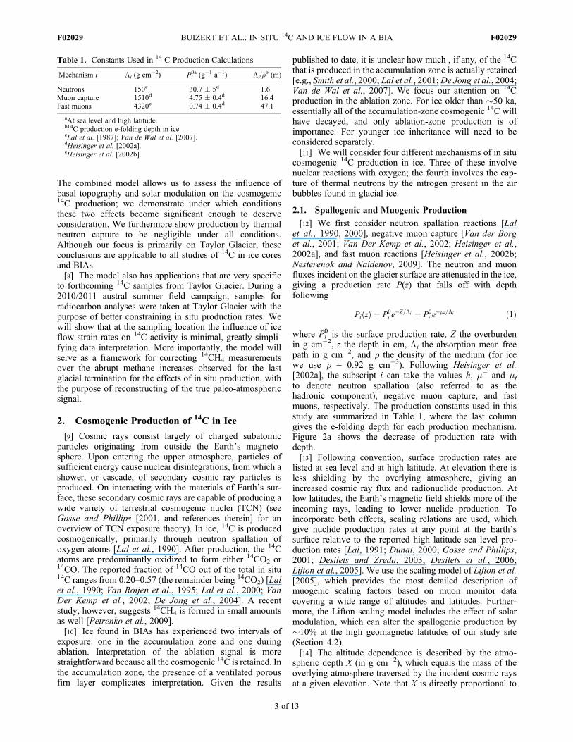
in g cm�2, z the depth in cm, Li the absorption mean freepath in g cm�2, and r the density of the medium (for icewe use r = 0.92 g cm�3). Following Heisinger et al.[2002a], the subscript i can take the values h, m� and mfto denote neutron spallation (also referred to as thehadronic component), negative muon capture, and fastmuons, respectively. The production constants used in thisstudy are summarized in Table 1, where the last columngives the e-folding depth for each production mechanism.Figure 2a shows the decrease of production rate withdepth.[13] Following convention, surface production rates are

listed at sea level and at high latitude. At elevation there isless shielding by the overlying atmosphere, giving anincreased cosmic ray flux and radionuclide production. Atlow latitudes, the Earth’s magnetic field shields more of theincoming rays, leading to lower nuclide production. Toincorporate both effects, scaling relations are used, whichgive nuclide production rates at any point at the Earth’ssurface relative to the reported high latitude sea level pro-duction rates [Lal, 1991; Dunai, 2000; Gosse and Phillips,2001; Desilets and Zreda, 2003; Desilets et al., 2006;Lifton et al., 2005]. We use the scaling model of Lifton et al.[2005], which provides the most detailed description ofmuogenic scaling factors based on muon monitor datacovering a wide range of altitudes and latitudes. Further-more, the Lifton scaling model includes the effect of solarmodulation, which can alter the spallogenic production by�10% at the high geomagnetic latitudes of our study site(Section 4.2).[14] The altitude dependence is described by the atmo-

spheric depth X (in g cm�2), which equals the mass of theoverlying atmosphere traversed by the incident cosmic raysat a given elevation. Note that X is directly proportional to

Table 1. Constants Used in 14 C Production Calculations

Mechanism i Li (g cm�2) Pi0a (g�1 a�1) Li/r

b (m)

Neutrons 150c 30.7 � 5d 1.6Muon capture 1510d 4.75 � 0.4d 16.4Fast muons 4320e 0.74 � 0.4d 47.1

aAt sea level and high latitude.b14C production e-folding depth in ice.cLal et al. [1987]; Van de Wal et al. [2007].dHeisinger et al. [2002a].eHeisinger et al. [2002b].

BUIZERT ET AL.: IN SITU 14C AND ICE FLOW IN A BIA F02029F02029

3 of 13

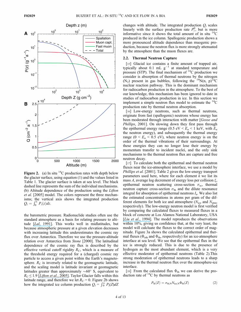
the barometric pressure. Radionuclide studies often use thestandard atmosphere as a basis for relating pressure to alti-tude [Lal, 1991]. This works well in midlatitudes, butbecause atmospheric pressure at a given elevation decreaseswith increasing latitude this underestimates the cosmic rayflux over Antarctica. Therefore we use the pressure-altituderelation over Antarctica from Stone [2000]. The latitudinaldependence of the cosmic ray flux is described by theeffective vertical cutoff rigidity RC, which is a measure ofthe threshold energy required for a (charged) cosmic rayparticle to access a given point within the Earth’s magneto-sphere. RC is inversely related to the geomagnetic latitude,and the scaling model is latitude invariant at geomagneticlatitudes greater than approximately �60� S, equivalent toRC ≤ 1.9 [Lifton et al., 2005]. Taylor Glacier falls within thislatitude range, and therefore we let RC = 0. Figure 2b showshow the integrated ice column production Qi =

R0∞ Pi(Z)dZ

changes with altitude. The integrated production Qi scaleslinearly with the surface production rate Pi

0, but is moreinformative since it shows the total amount of in situ 14Cproduced in the ice column. Spallogenic production shows amore pronounced altitude dependence than muogenic pro-duction, because the neutron flux is more strongly attenuatedby the atmosphere than the muon fluxes are.

2.2. Thermal Neutron Capture

[15] Glacial ice contains a finite amount of trapped air,typically about 0.1 mL g�1 at standard temperature andpressure (STP). The final mechanism of 14C production weconsider is absorption of thermal neutrons by the nitrogen(N2) present in gas bubbles, following the 14N(n, p)14Cnuclear reaction pathway. This is the dominant mechanismfor radiocarbon production in the atmosphere. To the best ofour knowledge, this mechanism has been ignored to date instudies of radiocarbon production in ice. In this section weimplement a simple neutron flux model to estimate the 14Cproduction rate by thermal neutron absorption.[16] Low-energy neutrons, such as thermal neutrons,

originate from fast (spallogenic) neutrons whose energy hasbeen moderated through interaction with matter [Gosse andPhillips, 2001]. On slowing down they first pass throughthe epithermal energy range (0.5 eV < En < 1 keV, with En

the neutron energy), and subsequently the thermal energyrange (0 < En < 0.5 eV), where neutron energy is on theorder of the thermal vibrations of their surroundings. Atthese energies they can no longer lose their energy bymomentum transfer to incident nuclei, and the only sinkmechanisms to the thermal neutron flux are capture and freeneutron decay.[17] To calculate both the epithermal and thermal neutron

fluxes near the ice-atmosphere interface, we use a model byPhillips et al. [2001]. Table 2 gives the low-energy transportparameters used here, where for each element k we list itsmass A, average log decrement of energy loss per collision x,epithermal neutron scattering cross-section ssc, thermalneutron capture cross-section sth and the dilute resonanceintegral for absorption of epithermal neutrons Ia. We also listthe estimated concentrations in atoms per gram of the dif-ferent elements for both ice and atmosphere (Nice and Natm,respectively). The low-energy neutron model is first verifiedby comparing the calculated fluxes to measured fluxes in ablock of concrete at Los Alamos National Laboratory, USA[Liu et al., 1994]. The model reproduces the observationswithin 10%, giving us confidence that, at the very least, themodel will calcluate the fluxes to the correct order of mag-nitude. Figure 3a shows the calculated epithermal and ther-mal fluxes (Feth and Fth, respectively) for an ice-atmosphereinterface at sea level. We see that the epithermal flux in theice is strongly reduced. This is due to the presence ofhydrogen as the most abundant element, which is a veryeffective moderator of epithermal neutrons (Table 2).Thisstrong moderation of epithermal neutrons leads to a sharpincrease in the thermal neutron flux over the atmosphere-iceinterface.[18] From the calculated flux Fth we can derive the pro-

duction rate of 14C by thermal neutrons as

PthðZÞ ¼ sth;NNice;NFthðZÞ ð2Þ

Figure 2. (a) In situ 14C production rates with depth belowthe glacier surface, using equation (1) and the values listed inTable 1. The glacier surface is taken at sea level. The blackdashed line represents the sum of the individual mechanisms.(b) Altitude dependence of the production using the Liftonet al. [2005] model. The colors represent the three mechan-isms; the vertical axis shows the integrated productionQi ¼

R∞0 PiðzÞdz.

BUIZERT ET AL.: IN SITU 14C AND ICE FLOW IN A BIA F02029F02029

4 of 13

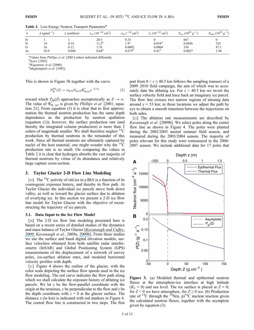
This is shown in Figure 3b together with the curve

PASth ðZÞ ¼ sth;NNice;NF∗

th;icee�Z=Lh ð3Þ

toward which Pth(Z) approaches asymptotically as Z → ∞.The value of Fth, ice

∗ is given by Phillips et al. [2001, equa-tion 21]. From equation (3) it is clear that to first approxi-mation the thermal neutron production has the same depthdependence as the production by neutron spallation(equation (1)); however, the surface production rate (andthereby the integrated column production) is more than 2orders of magnitude smaller. We shall therefore neglect 14Cproduction by thermal neutrons in the remainder of thiswork. Since all thermal neutrons are ultimately captured bynuclei of the host material, one might wonder why the 14Cproduction rate is so small. On comparing the values inTable 2 it is clear that hydrogen absorbs the vast majority ofthermal neutrons by virtue of its abundance and relativelylarge capture cross-section.

3. Taylor Glacier 2-D Flow Line Modeling

[19] The 14C activity of old ice in a BIA is a function of itscosmogenic exposure history, and thereby its flow path. AtTaylor Glacier the individual ice parcels move both downvalley, as well as toward the glacier surface due to ablationof overlying ice. In this section we present a 2-D ice flowline model for Taylor Glacier with the objective of recon-structing the trajectory of ice parcels.

3.1. Data Input to the Ice Flow Model

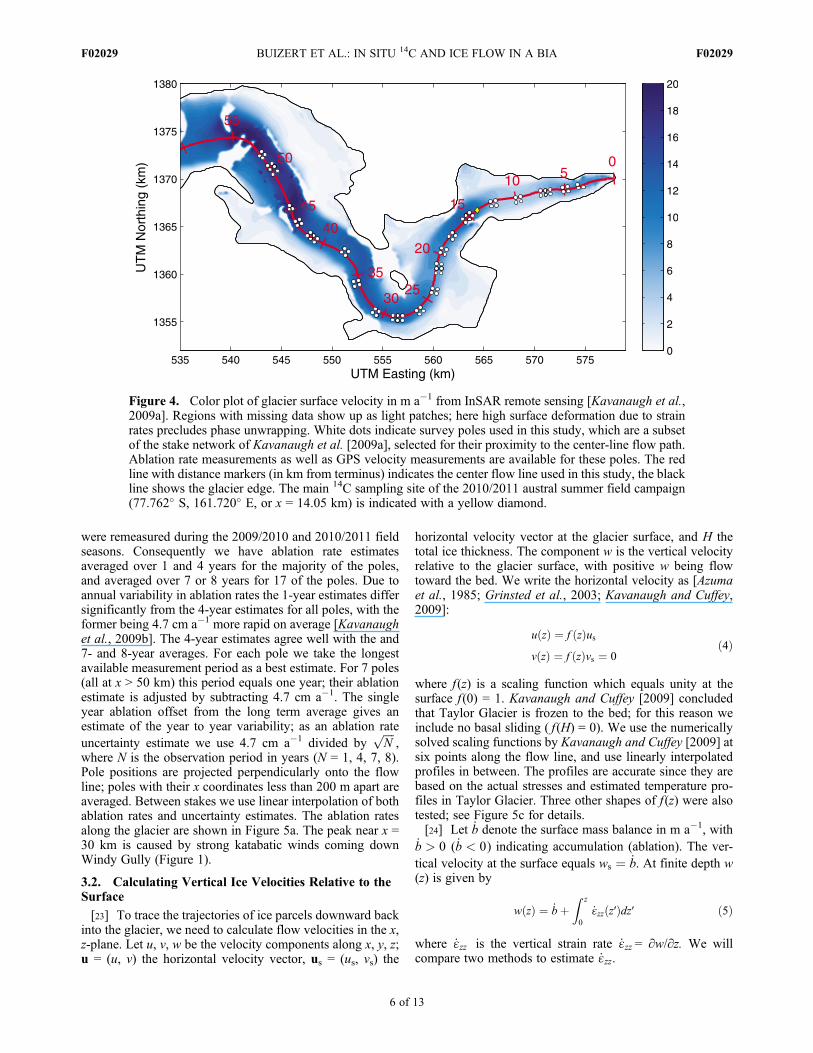
[20] The 2-D ice flow line modeling presented here isbased on a recent series of detailed studies of the dynamicsand mass balance of Taylor Glacier [Kavanaugh and Cuffey,2009; Kavanaugh et al., 2009a, 2009b]. From these studieswe use the surface and basal digital elevation models, sur-face velocities obtained from both satellite radar interfer-ometry (InSAR) and Global Positioning System (GPS)measurements of the displacement of a network of surveypoles, ice-surface ablation rates, and modeled horizontalvelocity profiles with depth.[21] Figure 4 shows the outline of the glacier, with the

color scale depicting the surface flow speeds used in the iceflow modeling. The red curve indicates the flow path alongwhich we shall calculate the exposure history of ablating iceparcels. We let x be the flow-parallel coordinate with theorigin at the terminus, y be perpendicular to the flow and z bethe depth coordinate with z = 0 at the glacier surface. Thedistance x (in km) is indicated with red markers in Figure 4.The central flow line is constructed in two steps. The first

part from 0 < x ≤ 40.5 km follows the sampling transect of a2009–2010 field campaign, the aim of which was to accu-rately date the ablating ice. For x > 40.5 km we invert thesurface velocity field and trace back an imaginary ice parcel.The flow line crosses two narrow regions of missing dataaround x = 53 km; in these locations we adjust the path byeye to obtain a smooth transition between the trajectories onboth sides.[22] The ablation rate measurements are described by

Kavanaugh et al. [2009b]. We select poles along the centerflow line as shown in Figure 4. The poles were plantedduring the 2002/2003 austral summer field season, andmeasured during the 2003/2004 season. The majority ofpoles relevant for this study were remeasured in the 2006/2007 season. We include additional data for 17 poles that

Table 2. Low-Energy Neutron Transport Parametersa

k A (gmol�1) x (unitless) ssc (10�24 cm2) sth (

�24 cm2) Ia (10�24 cm2) Nice (10

20 g�1) Natm (1020 g�1)

H 1 1 20.5 0.33 0 667 0N 14 0.14 11.5b 1.9c 0.034d 0.0456 325O 16 0.12 3.76 0.0002 0.0004 334 87.1Ar 39.9 0.049 0.68b 0.675b 0.41d 0.0027 1.94

aValues from Phillips et al. [2001] unless indicated differently.bSears [1992].cWagemans et al. [2000].dMughabghab et al. [1992].

Figure 3. (a) Modeled thermal and epithermal neutronfluxes at the atmosphere-ice interface at high latitude(RC = 0) and sea level. The ice surface is placed at Z = 0;for Z < 0 we have atmosphere, for Z ≥ 0 ice. (b) Productionrate of 14C through the 14N(n, p)14C nuclear reaction giventhe calculated neutron fluxes, together with the asymptotegiven by equation (3).

BUIZERT ET AL.: IN SITU 14C AND ICE FLOW IN A BIA F02029F02029

5 of 13

were remeasured during the 2009/2010 and 2010/2011 fieldseasons. Consequently we have ablation rate estimatesaveraged over 1 and 4 years for the majority of the poles,and averaged over 7 or 8 years for 17 of the poles. Due toannual variability in ablation rates the 1-year estimates differsignificantly from the 4-year estimates for all poles, with theformer being 4.7 cm a�1 more rapid on average [Kavanaughet al., 2009b]. The 4-year estimates agree well with the and7- and 8-year averages. For each pole we take the longestavailable measurement period as a best estimate. For 7 poles(all at x > 50 km) this period equals one year; their ablationestimate is adjusted by subtracting 4.7 cm a�1. The singleyear ablation offset from the long term average gives anestimate of the year to year variability; as an ablation rateuncertainty estimate we use 4.7 cm a�1 divided by

ffiffiffiffiN

p,

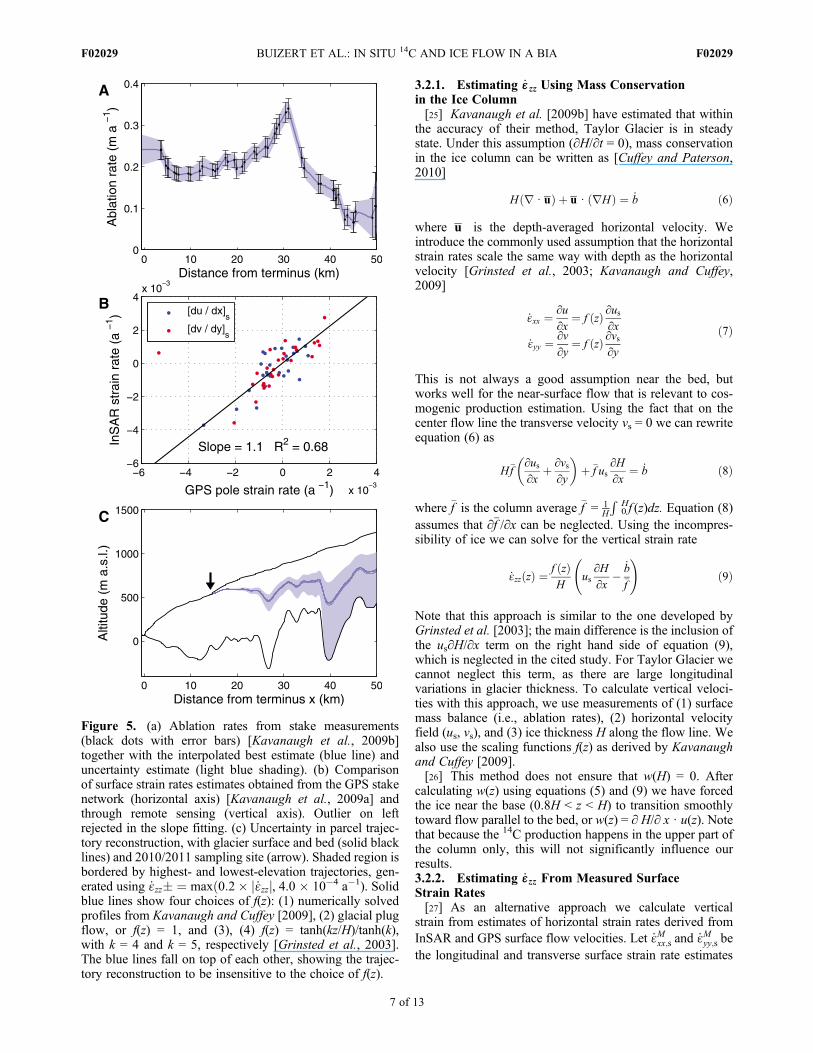
where N is the observation period in years (N = 1, 4, 7, 8).Pole positions are projected perpendicularly onto the flowline; poles with their x coordinates less than 200 m apart areaveraged. Between stakes we use linear interpolation of bothablation rates and uncertainty estimates. The ablation ratesalong the glacier are shown in Figure 5a. The peak near x =30 km is caused by strong katabatic winds coming downWindy Gully (Figure 1).

3.2. Calculating Vertical Ice Velocities Relative to theSurface

[23] To trace the trajectories of ice parcels downward backinto the glacier, we need to calculate flow velocities in the x,z-plane. Let u, v, w be the velocity components along x, y, z;u = (u, v) the horizontal velocity vector, us = (us, vs) the

horizontal velocity vector at the glacier surface, and H thetotal ice thickness. The component w is the vertical velocityrelative to the glacier surface, with positive w being flowtoward the bed. We write the horizontal velocity as [Azumaet al., 1985; Grinsted et al., 2003; Kavanaugh and Cuffey,2009]:

uðzÞ ¼ f ðzÞusvðzÞ ¼ f ðzÞvs ¼ 0

ð4Þ

where f (z) is a scaling function which equals unity at thesurface f (0) = 1. Kavanaugh and Cuffey [2009] concludedthat Taylor Glacier is frozen to the bed; for this reason weinclude no basal sliding ( f (H) = 0). We use the numericallysolved scaling functions by Kavanaugh and Cuffey [2009] atsix points along the flow line, and use linearly interpolatedprofiles in between. The profiles are accurate since they arebased on the actual stresses and estimated temperature pro-files in Taylor Glacier. Three other shapes of f (z) were alsotested; see Figure 5c for details.[24] Let _b denote the surface mass balance in m a�1, with

_b > 0 ( _b < 0) indicating accumulation (ablation). The ver-tical velocity at the surface equals ws ¼ _b. At finite depth w(z) is given by

wðzÞ ¼ _bþZ z

0_ɛzzðz′Þdz′ ð5Þ

where _ɛzz is the vertical strain rate _ɛzz = ∂w/∂z. We willcompare two methods to estimate _ɛzz.

Figure 4. Color plot of glacier surface velocity in m a�1 from InSAR remote sensing [Kavanaugh et al.,2009a]. Regions with missing data show up as light patches; here high surface deformation due to strainrates precludes phase unwrapping. White dots indicate survey poles used in this study, which are a subsetof the stake network of Kavanaugh et al. [2009a], selected for their proximity to the center-line flow path.Ablation rate measurements as well as GPS velocity measurements are available for these poles. The redline with distance markers (in km from terminus) indicates the center flow line used in this study, the blackline shows the glacier edge. The main 14C sampling site of the 2010/2011 austral summer field campaign(77.762� S, 161.720� E, or x = 14.05 km) is indicated with a yellow diamond.

BUIZERT ET AL.: IN SITU 14C AND ICE FLOW IN A BIA F02029F02029

6 of 13

3.2.1. Estimating _ɛzz Using Mass Conservationin the Ice Column[25] Kavanaugh et al. [2009b] have estimated that within

the accuracy of their method, Taylor Glacier is in steadystate. Under this assumption (∂H/∂t = 0), mass conservationin the ice column can be written as [Cuffey and Paterson,2010]

Hðr ⋅ uÞ þ u ⋅ ðrHÞ ¼ _b ð6Þ

where u is the depth-averaged horizontal velocity. Weintroduce the commonly used assumption that the horizontalstrain rates scale the same way with depth as the horizontalvelocity [Grinsted et al., 2003; Kavanaugh and Cuffey,2009]

_ɛxx ¼ ∂u∂x

¼ f ðzÞ ∂us∂x

_ɛyy ¼ ∂v∂y

¼ f ðzÞ ∂vs∂y

ð7Þ

This is not always a good assumption near the bed, butworks well for the near-surface flow that is relevant to cos-mogenic production estimation. Using the fact that on thecenter flow line the transverse velocity vs = 0 we can rewriteequation (6) as

H�f∂us∂x

þ ∂vs∂y

� �þ �f us

∂H∂x

¼ _b ð8Þ

where �f is the column average �f = 1H

R0Hf (z)dz. Equation (8)

assumes that ∂�f /∂x can be neglected. Using the incompres-sibility of ice we can solve for the vertical strain rate

_ɛzzðzÞ ¼ f ðzÞH

us∂H∂x

�_b�f

!ð9Þ

Note that this approach is similar to the one developed byGrinsted et al. [2003]; the main difference is the inclusion ofthe us∂H/∂x term on the right hand side of equation (9),which is neglected in the cited study. For Taylor Glacier wecannot neglect this term, as there are large longitudinalvariations in glacier thickness. To calculate vertical veloci-ties with this approach, we use measurements of (1) surfacemass balance (i.e., ablation rates), (2) horizontal velocityfield (us, vs), and (3) ice thickness H along the flow line. Wealso use the scaling functions f(z) as derived by Kavanaughand Cuffey [2009].[26] This method does not ensure that w(H) = 0. After

calculating w(z) using equations (5) and (9) we have forcedthe ice near the base (0.8H < z < H) to transition smoothlytoward flow parallel to the bed, or w(z) = ∂ H/∂ x ⋅ u(z). Notethat because the 14C production happens in the upper part ofthe column only, this will not significantly influence ourresults.3.2.2. Estimating _ɛzz From Measured SurfaceStrain Rates[27] As an alternative approach we calculate vertical

strain from estimates of horizontal strain rates derived fromInSAR and GPS surface flow velocities. Let _ɛMxx;s and _ɛMyy;s bethe longitudinal and transverse surface strain rate estimates

Figure 5. (a) Ablation rates from stake measurements(black dots with error bars) [Kavanaugh et al., 2009b]together with the interpolated best estimate (blue line) anduncertainty estimate (light blue shading). (b) Comparisonof surface strain rates estimates obtained from the GPS stakenetwork (horizontal axis) [Kavanaugh et al., 2009a] andthrough remote sensing (vertical axis). Outlier on leftrejected in the slope fitting. (c) Uncertainty in parcel trajec-tory reconstruction, with glacier surface and bed (solid blacklines) and 2010/2011 sampling site (arrow). Shaded region isbordered by highest- and lowest-elevation trajectories, gen-erated using _ɛzz� ¼ maxð0:2� j _ɛzzj, 4.0 � 10�4 a�1). Solidblue lines show four choices of f(z): (1) numerically solvedprofiles from Kavanaugh and Cuffey [2009], (2) glacial plugflow, or f(z) = 1, and (3), (4) f(z) = tanh(kz/H)/tanh(k),with k = 4 and k = 5, respectively [Grinsted et al., 2003].The blue lines fall on top of each other, showing the trajec-tory reconstruction to be insensitive to the choice of f(z).

BUIZERT ET AL.: IN SITU 14C AND ICE FLOW IN A BIA F02029F02029

7 of 13

from measurements of us. Using equation (7) and theincompressibility of ice we obtain

_ɛzzðzÞ ¼ � _ɛMxx;s þ _ɛMyy;s� �

f ðzÞ ð10Þ

The reliability of this approach depends on the accuracy ofthe surface strain rate estimates. Figure 5b shows a com-parison between strain rate estimates based on the InSARand GPS data. We see that the slope of the correlation devi-ates significantly from unity; that there is one clear outlier inthe transverse strain rate _ɛyy; that there is much scatter in thedata (R2 = 0.68 when ignoring the outlier); and that for�20% of the points the sign is reversed. In equation (10)the horizontal strain rates are added. By doing so the poten-tial for error is increased further, as their uncertainties alsoadd up.[28] When calculating ice flow trajectories based on ver-

tical velocities from this second approach, we find that theyfail to follow bedrock undulations as required. Furthermore,mass conservation is violated as ice parcels emerge from,and disappear into, the bed. Because the trajectories fail tofollow topological features, an ad-hoc adjustment (as used inthe first method) cannot be applied, because it leads to sharpkinks in the flow trajectories and violations of ice continuity.For the reasons outlined above, we will use the first method(mass conservation in the ice column) to estimate ice parceltrajectories in the remainder of this study.

3.3. Tracing Ice Parcels

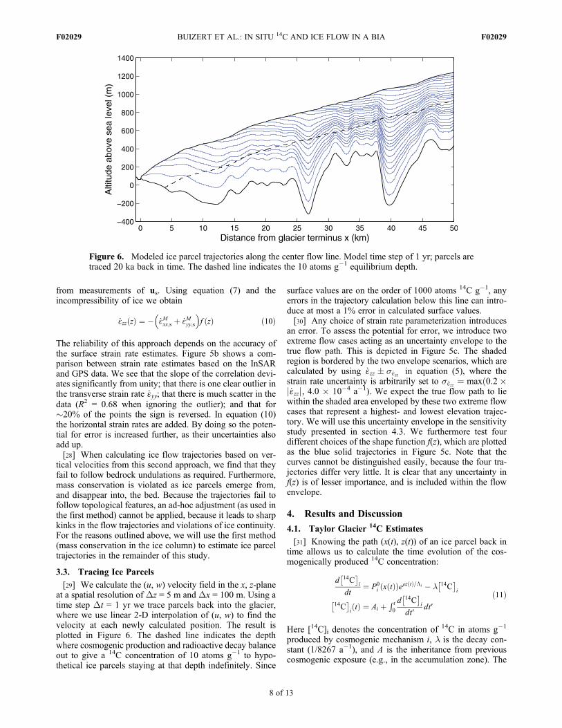
[29] We calculate the (u, w) velocity field in the x, z-planeat a spatial resolution of Dz = 5 m and Dx = 100 m. Using atime step Dt = 1 yr we trace parcels back into the glacier,where we use linear 2-D interpolation of (u, w) to find thevelocity at each newly calculated position. The result isplotted in Figure 6. The dashed line indicates the depthwhere cosmogenic production and radioactive decay balanceout to give a 14C concentration of 10 atoms g�1 to hypo-thetical ice parcels staying at that depth indefinitely. Since

surface values are on the order of 1000 atoms 14C g�1, anyerrors in the trajectory calculation below this line can intro-duce at most a 1% error in calculated surface values.[30] Any choice of strain rate parameterization introduces

an error. To assess the potential for error, we introduce twoextreme flow cases acting as an uncertainty envelope to thetrue flow path. This is depicted in Figure 5c. The shadedregion is bordered by the two envelope scenarios, which arecalculated by using _ɛzz � s _ɛzz in equation (5), where thestrain rate uncertainty is arbitrarily set to s _ɛzz ¼ maxð0:2�j _ɛzzj, 4.0 � 10�4 a�1). We expect the true flow path to liewithin the shaded area enveloped by these two extreme flowcases that represent a highest- and lowest elevation trajec-tory. We will use this uncertainty envelope in the sensitivitystudy presented in section 4.3. We furthermore test fourdifferent choices of the shape function f(z), which are plottedas the blue solid trajectories in Figure 5c. Note that thecurves cannot be distinguished easily, because the four tra-jectories differ very little. It is clear that any uncertainty inf(z) is of lesser importance, and is included within the flowenvelope.

4. Results and Discussion

4.1. Taylor Glacier 14C Estimates

[31] Knowing the path (x(t), z(t)) of an ice parcel back intime allows us to calculate the time evolution of the cos-mogenically produced 14C concentration:

d 14C� �

i

dt¼ P0

i x tð Þð Þerz tð Þ=Li � l 14C� �

i

14C� �

itð Þ ¼ Ai þ

R t0

d 14C� �

i

dt′dt′

ð11Þ

Here [14C]i denotes the concentration of 14C in atoms g�1

produced by cosmogenic mechanism i, l is the decay con-stant (1/8267 a�1), and A is the inheritance from previouscosmogenic exposure (e.g., in the accumulation zone). The

Figure 6. Modeled ice parcel trajectories along the center flow line. Model time step of 1 yr; parcels aretraced 20 ka back in time. The dashed line indicates the 10 atoms g�1 equilibrium depth.

BUIZERT ET AL.: IN SITU 14C AND ICE FLOW IN A BIA F02029F02029

8 of 13

2010/2011 sampling site was selected to have an ice age>50 ka [Aciego et al., 2007], meaning that effectively all the14C inherited from the paleo-atmosphere and cosmogenic pro-duction in the accumulation zone has decayed. Furthermore,

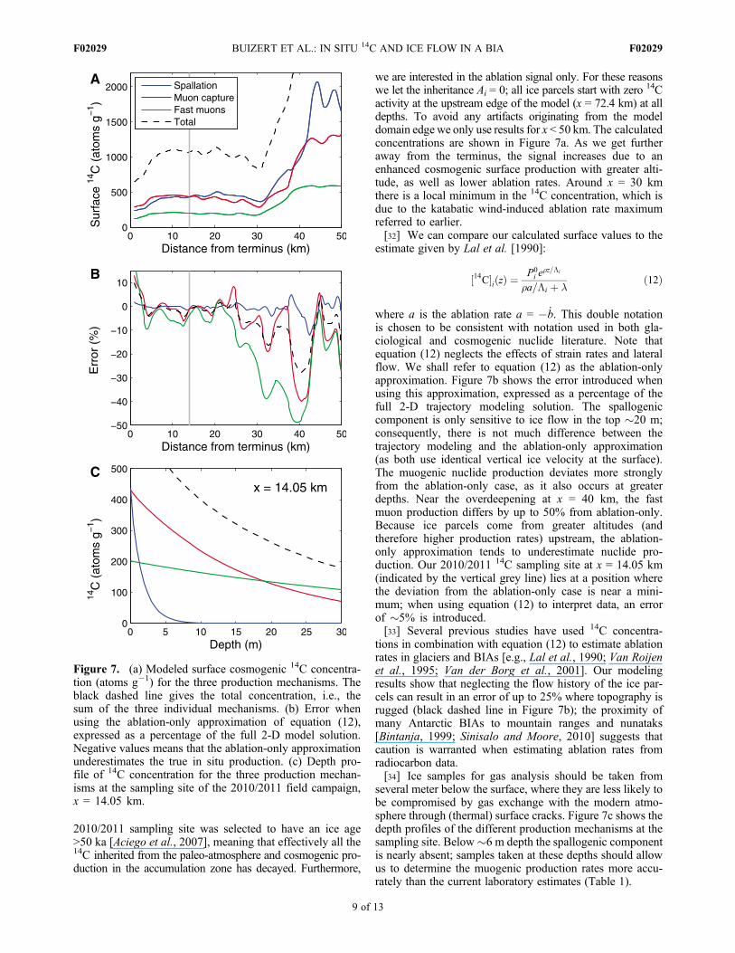
we are interested in the ablation signal only. For these reasonswe let the inheritance Ai = 0; all ice parcels start with zero 14Cactivity at the upstream edge of the model (x = 72.4 km) at alldepths. To avoid any artifacts originating from the modeldomain edge we only use results for x < 50 km. The calculatedconcentrations are shown in Figure 7a. As we get furtheraway from the terminus, the signal increases due to anenhanced cosmogenic surface production with greater alti-tude, as well as lower ablation rates. Around x = 30 kmthere is a local minimum in the 14C concentration, which isdue to the katabatic wind-induced ablation rate maximumreferred to earlier.[32] We can compare our calculated surface values to the

estimate given by Lal et al. [1990]:

½14C�iðzÞ ¼P0i e

rz=Li

ra=Li þ lð12Þ

where a is the ablation rate a = � _b. This double notationis chosen to be consistent with notation used in both gla-ciological and cosmogenic nuclide literature. Note thatequation (12) neglects the effects of strain rates and lateralflow. We shall refer to equation (12) as the ablation-onlyapproximation. Figure 7b shows the error introduced whenusing this approximation, expressed as a percentage of thefull 2-D trajectory modeling solution. The spallogeniccomponent is only sensitive to ice flow in the top �20 m;consequently, there is not much difference between thetrajectory modeling and the ablation-only approximation(as both use identical vertical ice velocity at the surface).The muogenic nuclide production deviates more stronglyfrom the ablation-only case, as it also occurs at greaterdepths. Near the overdeepening at x = 40 km, the fastmuon production differs by up to 50% from ablation-only.Because ice parcels come from greater altitudes (andtherefore higher production rates) upstream, the ablation-only approximation tends to underestimate nuclide pro-duction. Our 2010/2011 14C sampling site at x = 14.05 km(indicated by the vertical grey line) lies at a position wherethe deviation from the ablation-only case is near a mini-mum; when using equation (12) to interpret data, an errorof �5% is introduced.[33] Several previous studies have used 14C concentra-

tions in combination with equation (12) to estimate ablationrates in glaciers and BIAs [e.g., Lal et al., 1990; Van Roijenet al., 1995; Van der Borg et al., 2001]. Our modelingresults show that neglecting the flow history of the ice par-cels can result in an error of up to 25% where topography isrugged (black dashed line in Figure 7b); the proximity ofmany Antarctic BIAs to mountain ranges and nunataks[Bintanja, 1999; Sinisalo and Moore, 2010] suggests thatcaution is warranted when estimating ablation rates fromradiocarbon data.[34] Ice samples for gas analysis should be taken from

several meter below the surface, where they are less likely tobe compromised by gas exchange with the modern atmo-sphere through (thermal) surface cracks. Figure 7c shows thedepth profiles of the different production mechanisms at thesampling site. Below�6 m depth the spallogenic componentis nearly absent; samples taken at these depths should allowus to determine the muogenic production rates more accu-rately than the current laboratory estimates (Table 1).

Figure 7. (a) Modeled surface cosmogenic 14C concentra-tion (atoms g�1) for the three production mechanisms. Theblack dashed line gives the total concentration, i.e., thesum of the three individual mechanisms. (b) Error whenusing the ablation-only approximation of equation (12),expressed as a percentage of the full 2-D model solution.Negative values means that the ablation-only approximationunderestimates the true in situ production. (c) Depth pro-file of 14C concentration for the three production mechan-isms at the sampling site of the 2010/2011 field campaign,x = 14.05 km.

BUIZERT ET AL.: IN SITU 14C AND ICE FLOW IN A BIA F02029F02029

9 of 13

4.2. Solar Modulation of the Cosmic Ray Flux

[35] We will now examine how solar modulation of thecosmic ray flux affects the 14C content of ablating iceparcels. Variations in solar activity mostly influence lowenergy cosmic rays, while high energy rays are less affected[Lifton et al., 2005, and references therein]. At the highlatitudes of our study site the geomagnetic field provideslittle shielding. Thus effectively all cosmic rays are admitted,including the low energy rays that are modulated by solaractivity. Consequently variations in solar activity should beconsidered when studying cosmogenic production in polarregions. Note that spallogenic production is most sensitive tosolar modulation; muons are produced by incoming primarycosmic ray particles of higher median energies, which arenot affected by solar modulation. The scaling model by

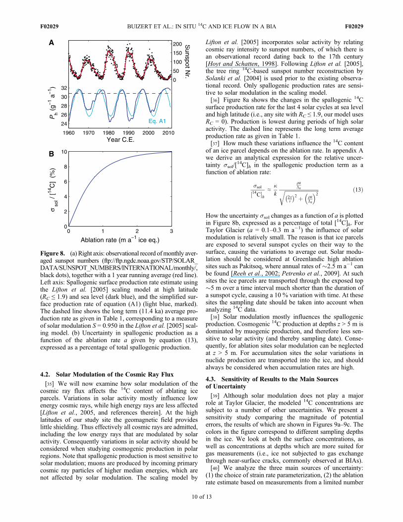
Lifton et al. [2005] incorporates solar activity by relatingcosmic ray intensity to sunspot numbers, of which there isan observational record dating back to the 17th century[Hoyt and Schatten, 1998]. Following Lifton et al. [2005],the tree ring 14C-based sunspot number reconstruction bySolanki et al. [2004] is used prior to the existing observa-tional record. Only spallogenic production rates are sensi-tive to solar modulation in the scaling model.[36] Figure 8a shows the changes in the spallogenic 14C

surface production rate for the last 4 solar cycles at sea leveland high latitude (i.e., any site with RC ≤ 1.9, our model usesRC = 0). Production is lowest during periods of high solaractivity. The dashed line represents the long term averageproduction rate as given in Table 1.[37] How much these variations influence the 14C content

of an ice parcel depends on the ablation rate. In appendix Awe derive an analytical expression for the relative uncer-tainty ssol/[

14C]h in the spallogenic production term as afunction of ablation rate:

ssol

½14C�h≈

kk

raLhffiffiffiffiffiffiffiffiffiffiffiffiffiffiffiffiffiffiffiffiffiffiffiffiffiffiffiffi

2pt

2 þ raLh

� �2r ð13Þ

How the uncertainty ssol changes as a function of a is plottedin Figure 8b, expressed as a percentage of total [14C]h. ForTaylor Glacier (a = 0.1–0.3 m a�1) the influence of solarmodulation is relatively small. The reason is that ice parcelsare exposed to several sunspot cycles on their way to thesurface, causing the variations to average out. Solar modu-lation should be considered at Greenlandic high ablationsites such as Pakitsoq, where annual rates of �2.5 m a�1 canbe found [Reeh et al., 2002; Petrenko et al., 2009]. At suchsites the ice parcels are transported through the exposed top�5 m over a time interval much shorter than the duration ofa sunspot cycle, causing a 10 % variation with time. At thesesites the sampling date should be taken into account whenanalyzing 14C data.[38] Solar modulation mostly influences the spallogenic

production. Cosmogenic 14C production at depths z > 5 m isdominated by muogenic production, and therefore less sen-sitive to solar activity (and thereby sampling date). Conse-quently, for ablation sites solar modulation can be neglectedat z > 5 m. For accumulation sites the solar variations innuclide production are transported into the ice, and shouldalways be considered when accumulation rates are high.

4.3. Sensitivity of Results to the Main Sourcesof Uncertainty

[39] Although solar modulation does not play a majorrole at Taylor Glacier, the modeled 14C concentrations aresubject to a number of other uncertainties. We present asensitivity study comparing the magnitude of potentialerrors, the results of which are shown in Figures 9a–9c. Thecolors in the figure correspond to different sampling depthsin the ice. We look at both the surface concentrations, aswell as concentrations at depths which are more suited forgas measurements (i.e., ice not subjected to gas exchangethrough near-surface cracks, commonly observed at BIAs).[40] We analyze the three main sources of uncertainty:

(1) the choice of strain rate parameterization, (2) the ablationrate estimate based on measurements from a limited number

Figure 8. (a) Right axis: observational record ofmonthly aver-aged sunspot numbers (ftp://ftp.ngdc.noaa.gov/STP/SOLAR_DATA/SUNSPOT_NUMBERS/INTERNATIONAL/monthly/,black dots), together with a 1 year running average (red line).Left axis: Spallogenic surface production rate estimate usingthe Lifton et al. [2005] scaling model at high latitude(RC ≤ 1.9) and sea level (dark blue), and the simplified sur-face production rate of equation (A1) (light blue, marked).The dashed line shows the long term (11.4 ka) average pro-duction rate as given in Table 1, corresponding to a measureof solar modulation S = 0.950 in the Lifton et al. [2005] scal-ing model. (b) Uncertainty in spallogenic production as afunction of the ablation rate a given by equation (13),expressed as a percentage of total spallogenic production.

BUIZERT ET AL.: IN SITU 14C AND ICE FLOW IN A BIA F02029F02029

10 of 13

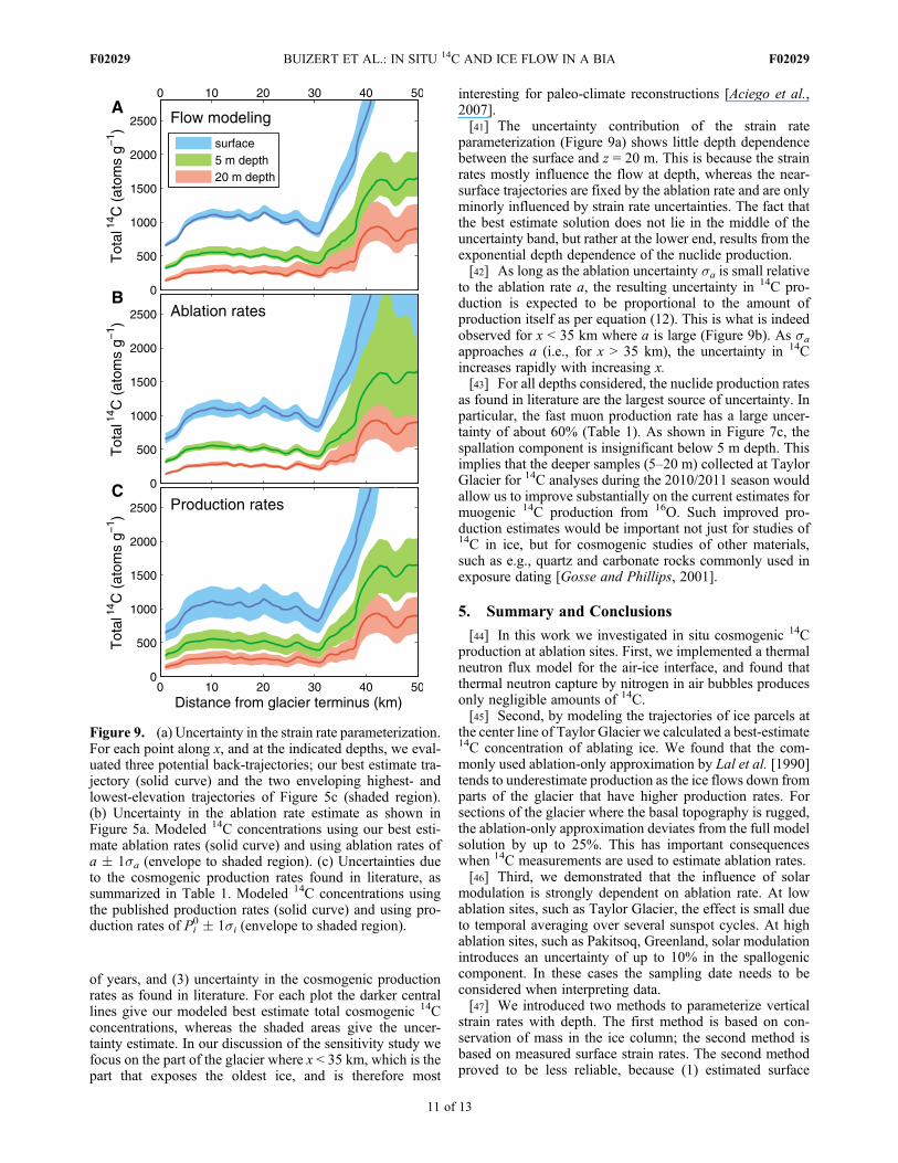
of years, and (3) uncertainty in the cosmogenic productionrates as found in literature. For each plot the darker centrallines give our modeled best estimate total cosmogenic 14Cconcentrations, whereas the shaded areas give the uncer-tainty estimate. In our discussion of the sensitivity study wefocus on the part of the glacier where x < 35 km, which is thepart that exposes the oldest ice, and is therefore most

interesting for paleo-climate reconstructions [Aciego et al.,2007].[41] The uncertainty contribution of the strain rate

parameterization (Figure 9a) shows little depth dependencebetween the surface and z = 20 m. This is because the strainrates mostly influence the flow at depth, whereas the near-surface trajectories are fixed by the ablation rate and are onlyminorly influenced by strain rate uncertainties. The fact thatthe best estimate solution does not lie in the middle of theuncertainty band, but rather at the lower end, results from theexponential depth dependence of the nuclide production.[42] As long as the ablation uncertainty sa is small relative

to the ablation rate a, the resulting uncertainty in 14C pro-duction is expected to be proportional to the amount ofproduction itself as per equation (12). This is what is indeedobserved for x < 35 km where a is large (Figure 9b). As saapproaches a (i.e., for x > 35 km), the uncertainty in 14Cincreases rapidly with increasing x.[43] For all depths considered, the nuclide production rates

as found in literature are the largest source of uncertainty. Inparticular, the fast muon production rate has a large uncer-tainty of about 60% (Table 1). As shown in Figure 7c, thespallation component is insignificant below 5 m depth. Thisimplies that the deeper samples (5–20 m) collected at TaylorGlacier for 14C analyses during the 2010/2011 season wouldallow us to improve substantially on the current estimates formuogenic 14C production from 16O. Such improved pro-duction estimates would be important not just for studies of14C in ice, but for cosmogenic studies of other materials,such as e.g., quartz and carbonate rocks commonly used inexposure dating [Gosse and Phillips, 2001].

5. Summary and Conclusions

[44] In this work we investigated in situ cosmogenic 14Cproduction at ablation sites. First, we implemented a thermalneutron flux model for the air-ice interface, and found thatthermal neutron capture by nitrogen in air bubbles producesonly negligible amounts of 14C.[45] Second, by modeling the trajectories of ice parcels at

the center line of Taylor Glacier we calculated a best-estimate14C concentration of ablating ice. We found that the com-monly used ablation-only approximation by Lal et al. [1990]tends to underestimate production as the ice flows down fromparts of the glacier that have higher production rates. Forsections of the glacier where the basal topography is rugged,the ablation-only approximation deviates from the full modelsolution by up to 25%. This has important consequenceswhen 14C measurements are used to estimate ablation rates.[46] Third, we demonstrated that the influence of solar

modulation is strongly dependent on ablation rate. At lowablation sites, such as Taylor Glacier, the effect is small dueto temporal averaging over several sunspot cycles. At highablation sites, such as Pakitsoq, Greenland, solar modulationintroduces an uncertainty of up to 10% in the spallogeniccomponent. In these cases the sampling date needs to beconsidered when interpreting data.[47] We introduced two methods to parameterize vertical

strain rates with depth. The first method is based on con-servation of mass in the ice column; the second method isbased on measured surface strain rates. The second methodproved to be less reliable, because (1) estimated surface

Figure 9. (a) Uncertainty in the strain rate parameterization.For each point along x, and at the indicated depths, we eval-uated three potential back-trajectories; our best estimate tra-jectory (solid curve) and the two enveloping highest- andlowest-elevation trajectories of Figure 5c (shaded region).(b) Uncertainty in the ablation rate estimate as shown inFigure 5a. Modeled 14C concentrations using our best esti-mate ablation rates (solid curve) and using ablation rates ofa � 1sa (envelope to shaded region). (c) Uncertainties dueto the cosmogenic production rates found in literature, assummarized in Table 1. Modeled 14C concentrations usingthe published production rates (solid curve) and using pro-duction rates of Pi

0 � 1si (envelope to shaded region).

BUIZERT ET AL.: IN SITU 14C AND ICE FLOW IN A BIA F02029F02029

11 of 13

strain rates from InSAR and GPS measurements show apoor correlation, (2) flow lines do not follow bedrock, and(3) mass is not conserved.[48] We presented a sensitivity study where we compared

potential errors introduced by uncertainties in the strain rateparameterization, the ablation rates, and the published cos-mogenic production rates. We found that the cosmogenicproduction rates are the largest source of uncertainty. In the2010/2011 austral summer, Taylor Glacier ice was sampledwith the aim of constraining the cosmogenic productionrates more strongly. By sampling at depths >5 m themuogenic components can be isolated, which have thelargest uncertainty in their production rates. The modelingresults presented here will aid us with the interpretation of14C measurements on these samples.

Appendix A: Derivation of Equation (13)

[49] For simplicity we assume a sinusoidal solar modula-tion of the spallogenic surface production

P0h ¼ k þ Re kexpð2ipt=t þ iqÞf g ðA1Þ

where t = 11 yr is the period of the sunspot (or Schwabe)cycle, q is the phase of the cycle, k = 28.7 and k = 3 are fittedby eye to the modeled production rate curve, and Re :f gdenotes the real part of the expression. The simplified pro-duction of equation (A1) is plotted in Figure 8a, togetherwith the modeled production. Ignoring inheritance andradioactive decay, the spallogenic 14C in an ice parcel thatablates at the glacier surface at t = 0 is given by

½14C�hðzÞ ¼ ReZ �z=a

�∞k þ k exp

2iptt

þ iq� �� �

expratLh

� �dt

( )

ðA2ÞNote that this equation also holds for the accumulation zone,in which case the integral goes from 0 to z/a, and a isreplaced by �a in the integrand. The solution at the surfaceis given by

½14C�hð0Þ ¼kraLh

þ k sin qþ jð Þffiffiffiffiffiffiffiffiffiffiffiffiffiffiffiffiffiffiffiffiffiffiffiffiffiffiffiffi2pt

2 þ raLh

� �2r ðA3Þ

with

j ¼ arcsinraLh

=

ffiffiffiffiffiffiffiffiffiffiffiffiffiffiffiffiffiffiffiffiffiffiffiffiffiffiffiffiffiffiffiffiffiffiffi2pt

� �2

þ raLh

� �2s0

@1A ðA4Þ

The first term in equation (A3) gives the time-invariant long-term average 14C concentration; the second term gives thetime (i.e., q) dependent part caused by solar modulation.When solar variation is neglected in the analysis of 14C data,the phase q of the sunspot cycle is not fixed, and an uncer-tainty ssol is introduced. On dividing the second term inequation (A3) by the first term we obtain for the relativeuncertainty:

ssol

½14C�h≈kk

raLhffiffiffiffiffiffiffiffiffiffiffiffiffiffiffiffiffiffiffiffiffiffiffiffiffiffiffiffi

2pt

2 þ raLh

� �2r ðA5Þ

[50] Acknowledgments. We would like to thank Andy Bliss for hishelp on calculating ablation rates, Daniel Baggenstos for measuring ablationstakes in the field and providing locations of the 2009–2010 samplingtransect, Brent Goehring for fruitful discussions, and Tom Neumann formany constructive comments on the manuscript. C. Buizert would like tothank Thomas Blunier (Center for Ice and Climate, University of Copenhagen),Bruce Vaughn and Jim White (INSTAAR, University of Colorado) for theirsupport and hospitality; V. V. Petrenko has been supported by the NOAAPostdoctoral Fellowship in Climate and Global Change, NSF grants0632222 and 0806387 (White) and NSF grant 0839031 (Severinghaus); thiswork was partially supported by NSF grant OPP-0125579 to K. M. Cuffeyand NSF grant 0838936 to E. J. Brook; N. A. Lifton is grateful for supportby the CRONUS-Earth project (NSF EAR0345150) and the University ofArizona Accelerator Mass Spectrometry Laboratory.

ReferencesAciego, S. M., K. M. Cuffey, J. L. Kavanaugh, D. L. Morse, andJ. P. Severinghaus (2007), Pleistocene ice and paleo-strain rates at TaylorGlacier, Antarctica, Quat. Res., 68, 303–313.

Andree, M., et al. (1984), 14C dating of polar ice, Nucl. Instrum. MethodsPhys. Res., Sect. B, 5(2), 385–388.

Azuma, N., M. Nakawo, A. Higashi, and F. Nishio (1985), Flow patternnear massif a in the yamato bare ice field estimated from the structuresand the mechanical properties of a shallow ice core, Mem. Natl. Inst.Polar Res., Spec. Issue Jpn., 39, 173–183.

Bintanja, R. (1999), On the glaciological, meteorological, and climato-logical significance of Antarctic blue ice areas, Rev. Geophys., 37(3),337–359.

Bliss, A. K., K. M. Cuffey, and J. L. Kavanaugh (2011), Sublimation andsurface energy budget of Taylor Glacier, Antarctica, J. Glaciol., 57(204),684–696.

Cuffey, K., and W. S. B. Paterson (2010), The Physics of Glaciers, 4th ed.,Elsevier, Burlington, Mass.

De Jong, A., C. Alderliesten, K. Van der Borg, C. Van der Veen, andR. Van De Wal (2004), Radiocarbon analysis of the EPICA Dome C icecore: No in situ 14C from the firn observed, Nucl. Instrum. MethodsPhys. Res., Sect. B, 223, 516–520.

Desilets, D., and M. Zreda (2003), Spatial and temporal distribution ofsecondary cosmic-ray nucleon intensities and applications to in situcosmogenic dating, Earth Planet. Sci. Lett., 206(1–2), 21–42.

Desilets, D., M. Zreda, and T. Prabu (2006), Extended scaling factors for insitu cosmogenic nuclides: New measurements at low latitude, EarthPlanet. Sci. Lett., 246(3–4), 265–276.

Dunai, T. J. (2000), Scaling factors for production rates of in situ producedcosmogenic nuclides: A critical reevaluation, Earth Planet. Sci. Lett.,176, 157–169.

Dunbar, N. W., W. C. McIntosh, and R. P. Esser (2008), Physical settingand tephrochronology of the summit caldera ice record at Mount Moulton,West Antarctica, Geol. Soc. Am. Bull., 120(7–8), 796–812.

Fireman, E., and T. Norris (1982), Ages and composition of gas trapped inAllan-Hills and Byrd core ice, Earth Planet. Sci. Lett., 60(3), 339–350.

Gosse, J. C., and F. M. Phillips (2001), Terrestrial in situ cosmogenicnuclides: Theory and application, Quaternary Sci. Rev., 20, 1475–1560.

Grinsted, A., J. Moore, V. B. Spikes, and A. Sinisalo (2003), Dating Ant-arctic blue ice areas using a novel ice flow model, Geophys. Res. Lett.,30(19), 2005, doi:10.1029/2003GL017957.

Heisinger, B., D. Lal, A. J. T. Jull, P. Kubik, S. Ivy-Ochs, K. Knie, andE. Nolte (2002a), Production of selected cosmogenic radionuclides bymuons: 2. Capture of negative muons, Earth Planet. Sci. Lett., 200(3–4),357–369.

Heisinger, B., D. Lal, A. J. T. Jull, P. Kubik, S. Ivy-Ochs, S. Neumaier,K. Knie, V. Lazarev, and E. Nolte (2002b), Production of selected cos-mogenic radionuclides by muons: 1. Fast muons, Earth Planet. Sci. Lett.,200(3–4), 345–355.

Hoyt, D. V., and K. H. Schatten (1998), Group sunspot numbers: A newsolar activity reconstruction, Sol. Phys., 181, 491–491.

Jenk, T. M., S. Szidat, M. Schwikowski, H. W. Gaeggeler, L. Wacker,H.-A. Synal, and M. Saurer (2007), Microgram level radiocarbon 14C)determination on carbonaceous particles in ice, Nucl. Instrum. MethodsPhys. Res., Sect. B, 259(1), 518–525.

Jouzel, J., et al. (2007), Orbital and millennial antarctic climate variabilityover the past 800,000 years, Science, 317(5839), 793–796.

Kavanaugh, J. L., and K. M. Cuffey (2009), Dynamics and mass balance ofTaylor Glacier, Antarctica: 2. Force balance and longitudinal coupling,J. Geophys. Res., 114, F04011, doi:10.1029/2009JF001329.

Kavanaugh, J. L., K. M. Cuffey, D. L. Morse, H. Conway, and E. Rignot(2009a), Dynamics and mass balance of Taylor Glacier, Antarctica:

BUIZERT ET AL.: IN SITU 14C AND ICE FLOW IN A BIA F02029F02029

12 of 13

1. Geometry and surface velocities, J. Geophys. Res., 114, F04010,doi:10.1029/2009JF001309.

Kavanaugh, J. L., K. M. Cuffey, D. L. Morse, A. K. Bliss, and S. M. Aciego(2009b), Dynamics and mass balance of Taylor Glacier, Antarctica:3. State of mass balance, J. Geophys. Res., 114, F04012, doi:10.1029/2009JF001331.

Lal, D. (1991), Cosmic-ray labeling of erosion surfaces: In situ nuclideproduction-rates and erosion models, Earth Planet. Sci. Lett., 104(2–4),424–439.

Lal, D., K. Nishiizumi, and J. R. Arnold (1987), In situ cosmogenic3H, 14C, and 10Be for determining the net accumulation and ablationrates of ice sheets, J. Geophys. Res., 92(B6), 4947–4952.

Lal, D., A. J. T. Jull, D. J. Donahue, D. Burtner, and K. Nishiizumi (1990),Polar ice ablation rates measured using in situ cosmogenic 14C, Nature,346(6282), 350–352.

Lal, D., A. J. T. Jull, G. S. Burr, and D. J. Donahue (2000), On the char-acteristics of cosmogenic in situ 14C in some GISP2 Holocene and lateglacial ice samples, Nucl. Instrum. Methods Phys. Res., Sect. B, 172,623–631.

Lal, D., A. Jull, D. Donahue, G. Burr, B. Deck, J. Jouzel, and E. Steig(2001), Record of cosmogenic in situ produced C-14 in Vostok andTaylor Dome ice samples: Implications for strong role of wind ventilationprocesses, J. Geophys. Res., 106(D23), 31,933–31,941.

Lifton, N. A., J. W. Bieber, J. M. Clem, M. L. Duldig, P. Evenson,J. E. Humble, and R. Pyle (2005), Addressing solar modulation andlong-term uncertainties in scaling secondary cosmic rays for in situ cos-mogenic nuclide applications, Earth Planet. Sci. Lett., 239, 140–161.

Liu, B., F. M. Phillips, J. T. Fabryka-Martin, M. M. Fowler, andW. D. Stone (1994), Cosmogenic 36Cl accumulation in unstable landforms:1. Effects of the thermal neutron distribution, Water Resour. Res., 30(11),3115–3125.

Moore, J. C., F. Nishio, S. Fujita, H. Narita, E. Pasteur, A. Grinsted,A. Sinisalo, and N. Maeno (2006), Interpreting ancient ice in a shallowice core from the South Yamato (Antarctica) blue ice area using flowmodeling and compositional matching to deep ice cores, J. Geophys.Res., 111, D16302, doi:10.1029/2005JD006343.

Mughabghab, S., M. Divadeenam, and N. E. Holden (1992), Neutron Reso-nance Parameters and Thermal Cross Sections, Academic, New York.

Nesterenok, A. V., and V. O. Naidenov (2009), Radiocarbon in the antarcticice: The formation of the cosmic ray muon component at large depths,Geomagn. Aeronomy, 50, 134–140.

Petrenko, V., J. Severinghaus, E. Brook, N. Reeh, and H. Schaefer (2006),Gas records from theWest Greenland ice margin covering the Last GlacialTermination: A horizontal ice core, Quaternary Sci. Rev., 25(9–10),865–875.

Petrenko, V. V., et al. (2008), A novel method for obtaining very largeancient air samples from ablating glacial ice for analyses of methaneradiocarbon, J. Glaciol., 54(185), 233–244.

Petrenko, V. V., et al. (2009), 14CH4 measurements in Greenland ice: Inves-tigating last glacial termination CH4 sources, Science, 324, 506–508.

Phillips, F. M., W. D. Stone, and J. T. Fabryka-Martin (2001), An improvedapproach to calculating low-energy cosmic-ray neutron fluxes near theland/atmosphere interface, Chem. Geol., 175(3–4), 689–701.

Reeh, N., H. Oerter, and H. Thomsen (2002), Comparison betweenGreenland ice-margin and ice-core oxygen-18 records, Ann. Glaciol.,35, 136–144.

Schaefer, H., V. V. Petrenko, E. J. Brook, J. P. Severinghaus, N. Reeh,J. R. Melton, and L. Mitchell (2009), Ice stratigraphy at the Pakitsoq icemargin, West Greenland, derived from gas records, J. Glaciol., 55(191),411–421.

Sears, V. F. (1992), Neutron scattering lengths and cross sections, NeutronNews, 3(3), 26–37.

Sinisalo, A., and J. C. Moore (2010), Antarctic blue ice areas: Towardsextracting palaeoclimate information, Antarct. Sci., 22(2), 99–115.

Smith, A. M., V. A. Levchenko, D. M. Etheridge, D. C. Lowe, Q. Hua,C. M. Trudinger, U. Zoppi, and A. Elcheikh (2000), In search of in-situradiocarbon in law dome ice and firn, Nucl. Instrum. Methods Phys. Res.,Sect. B, 172, 610–622.

Solanki, S., I. Usoskin, B. Kromer, M. Schüssler, and J. Beer (2004),Unusual activity of the Sun during recent decades compared to the previ-ous 11,000 years, Nature, 431(7012), 1084–1087.

Stone, J. O. (2000), Air pressure and cosmogenic isotope production,J. Geophys. Res., 105(B10), 23,753–23,759.

Van der Borg, K., W. Van der Kemp, C. Alderliesten, A. De Jong, andR. Lamers (2001), In-situ radiocarbon production by neutrons andmuons in an antarctic blue ice field at Scharffenbergbotnen: A statusreport, Radiocarbon, 43, 751–757.

Van Der Kemp, W., C. Alderliesten, K. Van Der Borg, A. De Jong,R. Lamers, J. Oerlemans, M. Thomassen, and R. Van De Wal (2002),In situ produced 14C by cosmic ray muons in ablating Antarctic ice,Tellus B, 54(2), 186–192.

Van de Wal, R., J. Van Roijen, D. Raynaud, K. Van der Borg, A. De Jong,J. Oerlemans, V. Lipenkov, and P. Huybrechts (1994), From 14C12Cmeasurements towards radiocarbon dating of ice, Tellus B, 46(2), 94–102.

Van de Wal, R. S. W., H. A. J. Meijer, M. De Rooij, and C. Van der Veen(2007), Radiocarbon analyses along the EDML ice core in Antarctica,Tellus B, 59(1), 157–165.

Van Roijen, J., K. Van der Borg, A. De Jong, and J. Oerlemans (1995),A correction for in-situ 14C in Antarctic ice with 14CO, Radiocarbon, 37,165–169.

Wagemans, J., C. Wagemans, G. Goeminne, and P. Geltenbort (2000),Experimental determination of the 14n(n, p)14c reaction cross section forthermal neutrons, Phys. Rev. C, 61(6), 064601, doi:10.1103/PhysRevC.61.064601.

BUIZERT ET AL.: IN SITU 14C AND ICE FLOW IN A BIA F02029F02029

13 of 13