Spatial analysis of solifluction landforms and process rates in the Abisko Mountains, northern...

PERMAFROST AND PERIGLACIAL PROCESSESPermafrost and Periglac. Process. 21: 241–255 (2010)Published online 4 June 2010 in Wiley Online Library(wileyonlinelibrary.com) DOI: 10.1002/ppp.681

Spatial Analysis of Solifluction Landforms and Process Ratesin the Abisko Mountains, Northern Sweden

Hanna Ridefelt ,1* Bernd Etzelmuller 2 and Jan Boelhouwers 1

1 Department of Social and Economic Geography, Uppsala University, Sweden2 Department of Geosciences, Physical Geography, University of Oslo, Norway

* CoEconE-ma

Copy

ABSTRACT

The occurrence of turf-banked solifluction landforms in the Abisko region was analysed using a grid-based approachand statistical modelling through logistic regression. Significant parameters in the model were the vegetation indexNDVI, annual incoming potential radiation, wetness index, slope gradient and elevation. The model had an acceptablediscrimination capacity and rather low model-fit values, but clearly showed the importance of vegetation patterns forthe occurrence of solifluction at a regional scale. Solifluction movement rates measured at eight sites were combinedwith model parameters and the annual duration of sun hours to regionalise solifluction movement rates through anunsupervised terrain classification. For comparison, the linear relationship between the probability of solifluctionoccurrence and variations in movement rates was also used to regionalise movement rates. Potential geomorphic workwas calculated for six different areas within the region, with the greatest being for Karkevagge, the area with thehighest precipitation. The combination of a logistic regression model of mapped landforms and field measurements ofsolifluction rates represents a promising methodology to assess the occurrence and activity of the process at a regionalscale. Copyright # 2010 John Wiley & Sons, Ltd.

KEY WORDS: solifluction; regional scale; geomorphometry; geomorphic work; geomorphic process; logistic, regression; periglacial;

spatial modelling

INTRODUCTION

Most studies of solifluction processes to date have beenundertaken at a plot or local scale, and regional studies arelimited in number (e.g. Rapp, 1960; Price, 1973; Smith, 1987;Douglas andHarrison, 1996; Berthling et al., 2002). The latterare needed, however, because climatically induced changesin solifluction movement rates can be expected to impactsediment erosion, storage and sedimentation patterns onslopes, and at a catchment scale to affect sediment budgets(Matsuoka, 2001; Ridefelt and Boelhouwers, 2006; Beylich,2008) and landscape evolution (Etzelmuller et al., 2001).

Regional studies generally show that solifluction occur-rence and rates vary greatly within a study area, even wheresurface characteristics are comparable (Berthling et al., 2002;Smith,1987). It is thereforedifficult todrawaconclusionaboutsolifluction activity for a larger region based on a relativelylimited number of measurements. To address this problem,approaches within geomorphometry (Hengl and Reuter,

rrespondence to: Hanna Ridefelt, Department of Social andomic Geography, Box 513, 751 20 Uppsala, Sweden.il: [email protected]

right # 2010 John Wiley & Sons, Ltd.

2009), combiningGIS, remote sensingand statistical analysis,have been developed that can allow modelling of larger areaswithout extensive fieldwork (e.g. Atkinson et al., 1998; Luotoand Seppala, 2002; Hjort et al., 2007). This study uses such anapproach, combining field measurement and modelling, toexamine the occurrence of solifluction in the Abisko region,northern Sweden and to produce an activity map of variationsin solifluction movement rates. To reach this goal, statisticalmodelling is applied to predict the occurrence of solifluctionthrough a set of independent explanatory variables, mainlybased on derivatives of a digital elevation model (DEM). Thedistributed movement rates allow for a variety of geomorphicapplications, for example, calculations of geomorphic workandspatiallydistributedfluxrates.Thefieldarea isparticularlysuitable as it lies in a sensitive periglacial zone which isexpected to respond rapidly to climate change (Akerman andJohansson, 2005; Johansson et al., 2006).

STUDY REGION

The Abisko region (Figure 1) is situated in northernSweden, about 200 km north of the Arctic Circle. The

Received 30 January 2009Revised 29 December 2009

Accepted 29 December 2009

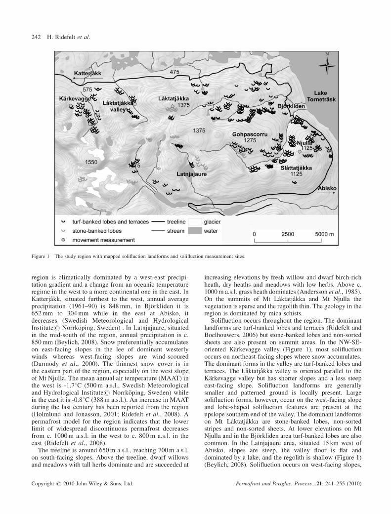
Figure 1 The study region with mapped solifluction landforms and solifluction measurement sites.

242 H. Ridefelt et al.

region is climatically dominated by a west-east precipi-tation gradient and a change from an oceanic temperatureregime in the west to a more continental one in the east. InKatterjakk, situated furthest to the west, annual averageprecipitation (1961–90) is 848mm, in Bjorkliden it is652mm to 304mm while in the east at Abisko, itdecreases (Swedish Meteorological and HydrologicalInstitute# Norrkoping, Sweden) . In Latnjajaure, situatedin the mid-south of the region, annual precipitation is c.850mm (Beylich, 2008). Snow preferentially accumulateson east-facing slopes in the lee of dominant westerlywinds whereas west-facing slopes are wind-scoured(Darmody et al., 2000). The thinnest snow cover is inthe eastern part of the region, especially on the west slopeof Mt Njulla. The mean annual air temperature (MAAT) inthe west is -1.78C (500m a.s.l., Swedish Meteorologicaland Hydrological Institute# Norrkoping, Sweden) whilein the east it is -0.88C (388m a.s.l.). An increase in MAATduring the last century has been reported from the region(Holmlund and Jonasson, 2001; Ridefelt et al., 2008). Apermafrost model for the region indicates that the lowerlimit of widespread discontinuous permafrost decreasesfrom c. 1000m a.s.l. in the west to c. 800m a.s.l. in theeast (Ridefelt et al., 2008).The treeline is around 650m a.s.l., reaching 700m a.s.l.

on south-facing slopes. Above the treeline, dwarf willowsand meadows with tall herbs dominate and are succeeded at

Copyright # 2010 John Wiley & Sons, Ltd.

increasing elevations by fresh willow and dwarf birch-richheath, dry heaths and meadows with low herbs. Above c.1000m a.s.l. grass heath dominates (Andersson et al., 1985).On the summits of Mt Laktatjakka and Mt Njulla thevegetation is sparse and the regolith thin. The geology in theregion is dominated by mica schists.Solifluction occurs throughout the region. The dominant

landforms are turf-banked lobes and terraces (Ridefelt andBoelhouwers, 2006) but stone-banked lobes and non-sortedsheets are also present on summit areas. In the NW-SE-oriented Karkevagge valley (Figure 1), most solifluctionoccurs on northeast-facing slopes where snow accumulates.The dominant forms in the valley are turf-banked lobes andterraces. The Laktatjakka valley is oriented parallel to theKarkevagge valley but has shorter slopes and a less steepeast-facing slope. Solifluction landforms are generallysmaller and patterned ground is locally present. Largesolifluction forms, however, occur on the west-facing slopeand lobe-shaped solifluction features are present at theupslope southern end of the valley. The dominant landformson Mt Laktatjakka are stone-banked lobes, non-sortedstripes and non-sorted sheets. At lower elevations on MtNjulla and in the Bjorkliden area turf-banked lobes are alsocommon. In the Latnjajaure area, situated 15 km west ofAbisko, slopes are steep, the valley floor is flat anddominated by a lake, and the regolith is shallow (Figure 1)(Beylich, 2008). Solifluction occurs on west-facing slopes,

Permafrost and Periglac. Process., 21: 241–255 (2010)

Spatial Analysis of Solifluction Landforms and Process Rates 243

since east-facing slopes are very steep and mainly consist ofrockwalls (Beylich, 2008).

METHODOLOGY

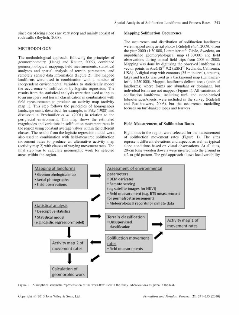
The methodological approach, following the principles ofgeomorphometry (Hengl and Reuter, 2009), combinedgeomorphological mapping, field measurements, statisticalanalyses and spatial analysis of terrain parameters, andremotely sensed data information (Figure 2). The mappedlandforms were used in combination with a number ofindependent environmental variables to statistically modelthe occurrence of solifluction by logistic regression. Theresults from the statistical analysis were then used as inputsto an unsupervised terrain classification in combination withfield measurements to produce an activity map (activitymap 1). This step follows the principles of homogenouslandscape units, described, for example, in Pike (1988) anddiscussed in Etzelmuller et al. (2001) in relation to theperiglacial environment. This map shows the estimatedmagnitudes and variations in solifluction movement rates inthe region using constant average values within the differentclasses. The results from the logistic regression model werealso used in combination with field-measured solifluctionmovement rates to produce an alternative activity map(activity map 2) with classes of varying movement rates. Thefinal step was to calculate geomorphic work for selectedareas within the region.

Figure 2 A simplified schematic representation of the work-flow used in the st


Mapping Solifluction Occurrence

The occurrence and distribution of solifluction landformsweremapped using aerial photos (Ridefelt et al., 2009b) fromthe year 2000 (1:30 000, Lantmateriet# Gavle, Sweden), anunpublished geomorphological map (1:30 000) and fieldobservations during annual field trips from 2003 to 2008.Mapping was done by digitising the observed landforms asvector points in ArcGIS1 9.2 (ESRI# Redlands, California,USA). A digital map with contours (25-m interval), streams,lakes and tracks was used as a background map (Lantmater-iet#, 1:250 000). Mapped landforms delimit areas (units oflandforms) where forms are abundant or dominant, butindividual forms are not mapped (Figure 1). All variations ofsolifluction landforms, including turf- and stone-bankedlobes/terraces/sheets, were included in the survey (Ridefeltand Boelhouwers, 2006), but the occurrence modellingfocuses on turf-banked lobes and terraces.

Field Measurement of Solifluction Rates

Eight sites in the region were selected for the measurementof solifluction movement rates (Figure 1). The sitesrepresent different elevations and aspects, as well as typicalslope conditions based on visual observations. At all sites,20-cm long wooden dowels were inserted into the ground ina 2-m grid pattern. The grid approach allows local variability

udy. Abbreviations as given in the text.


Table 1 Independent variables used in the statistical model.

Type of variable Variable

Topography derived Elevation (m)Slope (8)PR (annual and May-June) (W/m2)Duration of sun hours(annual and May-June) (hours)Curvature (total, plan, profile)(8/100m)Standard Dev of curvatureFlow length (downstream andmean upstream) (no. of pixels)

Potential soil moisture Wetness indexVegetation NDVISnow and permafrost Snow cover index

Permafrost probability

Abbreviations as given in the text.


within lobes and between lobes and the surrounding slope tobe systematically integrated. The mean movement ratesobtained from the grids are thus viewed as representative ofthe slope section and not merely of the lobes or specificsections of a lobe. The grids varied from 20� 30m to50� 100m, depending on the homogeneity of the slopecharacteristics. Aluminium poles with a diameter of 10mmand 0.8m long were used as reference points. Theywere inserted into stable ground at the back of a blockor at depths below 0.6m where movement should notoccur. A string was attached to the poles and served as areference line . At a few lines on the summit sites, whereblocks were absent at the surface and the regolith was verystony, it was difficult to insert the reference poles properly orto find larger boulders. The possibility that the poles couldhave moved at these sites cannot be eliminated and isincluded in the error estimate.Measurements were made using a steel tape over four

years (2004–08). Windy conditions may cause the line tomove, introducing error. Error assessments also included anoperator error and a methodological error. The averageoperator error was 1.5mm. The methodological errors aremore difficult to quantify, but are estimated to representc.� 10mm per year. Where movement rates are small,cumulative movement rates over the period 2004 to 2008exceed the estimated measurement error.Two complementary sites where a few movement lines

were installed are also discussed. The monitoring periods atthese sites were only one and two years. Thus these resultsare not reliable due to the short monitoring period, but arepresented as an indication of the possible variability inmovement rates within the local areas they represent.

Assessment of Environmental and ClimaticParameters

A 50-m DEM (Lantmateriet#) was used to derivetopographic attributes employing functions in ArcGIS1

9.2 and TAS 2.0.9# (Centre for Hydrogeomatics, Universityof Guleph, Canada). The terrain parameters elevation, slopegradient, slope curvature (total, plan and profile), standarddeviation of slope curvature, mean upstream flow length,downstream flow length, wetness index, annual and May toJune (melt season) potential incoming radiation (PR), andduration of sun hours are considered as potentially importantfor explaining the distributional pattern of solifluction(Table 1; Figure 3). The calculation of flow length(downstream and mean upstream) and the wetness indexis based on the D8-algorithm for flow routing. Thisalgorithm is defined as the tangents of the quotient betweenthe upstream contribution area at each grid cell position andthe local slope (Beven and Kirkby, 1979). The annual PRand May – June PR, as well as duration of sun hours arebased on the hemispherical viewshed algorithm (Rich et al.,1994; Fu and Rich, 2002).Parameters for vegetation cover, permafrost occurrence

and snow cover distribution were also considered (Table 1;Figure 3). A normalised difference vegetation index (NDVI)


was used for assessing differences in vegetation cover. Bands4 and 2 of an orthorectified Landsat ETMþ image from 8August 2001 with a resolution of 30m were used (USGeological Survey#, www.eros.usgs.gov, 19 August 2008).Probabilities for permafrost were derived from a permafrostdistribution model (Ridefelt et al., 2008). A simplified indexfor snow cover distributionwas implementedwhere the slopegradient, slope aspect andwind directionwere used to delimitlee and wind-facing areas (cf. Mittaz et al., 2002). Aredistribution of þ25 per cent of the precipitation on leeslopes and�25 per cent on wind-facing slopes was assumedbased on studies in the eastern Swiss Alps (Fierz et al., 1997).Since there is a precipitation gradient in the region, a trendsurface was created based on precipitation data (October–April) from four weather stations in the region. The valueswerenormalised inorder toproducean indexbetween0and1.To obtain the value of 0, the difference between theminimumvalue and 0 was first added to all data and then the data weredivided by the maximum value to obtain 1.

Statistical Analysis and Modelling

Development of the Statistical Model.A grid-based approach was used to predict the overall

occurrence of solifluction landforms at a regional scale usingthe independent variables (e.g. Pereira and Itami, 1991;Atkinson et al., 1998; Luoto and Seppala, 2002).First, the vector layer with all mapped turf-banked lobes

and terraces was converted to a grid using a resolution of200m, resulting in 277 grid points for the response variable.Areas with turf-banked lobes or terraces were given thenumber 1, whereas all other areas were assigned 0. Boxplotsdescribing median values and interquartile ranges were usedto describe the environmental characteristics of the twogroups of the binary variable (0 and 1). The binary variablewas then used as the dependent variable in a logisticregression model.


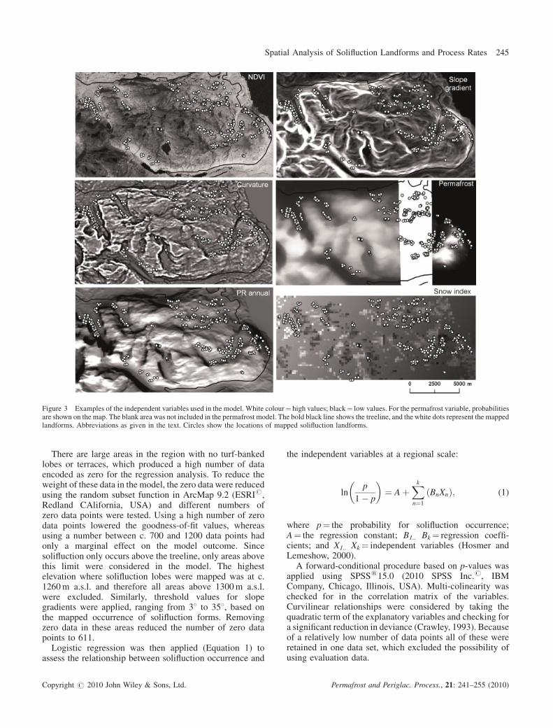
Figure 3 Examples of the independent variables used in the model. White colour¼ high values; black¼ low values. For the permafrost variable, probabilitiesare shown on the map. The blank area was not included in the permafrost model. The bold black line shows the treeline, and the white dots represent the mappedlandforms. Abbreviations as given in the text. Circles show the locations of mapped solifluction landforms.


There are large areas in the region with no turf-bankedlobes or terraces, which produced a high number of dataencoded as zero for the regression analysis. To reduce theweight of these data in the model, the zero data were reducedusing the random subset function in ArcMap 9.2 (ESRI#,Redland CAlifornia, USA) and different numbers ofzero data points were tested. Using a high number of zerodata points lowered the goodness-of-fit values, whereasusing a number between c. 700 and 1200 data points hadonly a marginal effect on the model outcome. Sincesolifluction only occurs above the treeline, only areas abovethis limit were considered in the model. The highestelevation where solifluction lobes were mapped was at c.1260m a.s.l. and therefore all areas above 1300m a.s.l.were excluded. Similarly, threshold values for slopegradients were applied, ranging from 38 to 358, based onthe mapped occurrence of solifluction forms. Removingzero data in these areas reduced the number of zero datapoints to 611.

Logistic regression was then applied (Equation 1) toassess the relationship between solifluction occurrence and


the independent variables at a regional scale:

lnp

1� p

� �¼ A þ

Xk

n¼1

ðBnXnÞ; (1)

where p¼ the probability for solifluction occurrence;A¼ the regression constant; B1.. Bk¼ regression coeffi-cients; and X1.. Xk¼ independent variables (Hosmer andLemeshow, 2000).

A forward-conditional procedure based on p-values wasapplied using SPSS115.0 (2010 SPSS Inc.#, IBMCompany, Chicago, Illinois, USA). Multi-colinearity waschecked for in the correlation matrix of the variables.Curvilinear relationships were considered by taking thequadratic term of the explanatory variables and checking fora significant reduction in deviance (Crawley, 1993). Becauseof a relatively low number of data points all of these wereretained in one data set, which excluded the possibility ofusing evaluation data.



Model Fit and Discrimination Capacity.Model fit was assessed through deviance reduction,

reported as the D2-value ((null deviance – residualdeviance)/null deviance) and its adjusted equivalent (Guisanand Zimmermann, 2000) and the Nagelkerke R2-value.Nagelkerke R2 is a modified version of Cox and Snell’s R2.The area under the curve (AUC) of a receiver-operatingcharacteristic (ROC) plot was used as an indication of thediscrimination capacity of the model (e.g Guisan andZimmermann, 2000; Hjort et al., 2007), which provides ameasure of the overall accuracy (Fielding and Bell, 1997).An ROC plot is obtained by plotting all sensitivity valuesagainst their equivalent values (1-specificity) for allavailable thresholds. The area under the ROC function(AUC) is used as an index which ranges from 0.5 to 1. As ageneral rule, values equivalent to 0.5 suggest no discrimi-nation, 0.7 to <0.8 are considered as acceptable discrimi-nation, 0.8 to <0.9 can be considered as excellentdiscrimination and values �0.9 are considered as out-standing discrimination (Hosmer and Lemeshow, 2000).

Terrain Classification and Solifluction Activity Maps

The environmental parameters showing a difference inmedian values for the two different groups (0 and 1) wereused to perform an unsupervised maximum likelihoodclassification. All values were standardised and normalisedin order to vary from 0 to 1. The classification was based onan iso-cluster algorithm (Jensen, 1996). The optimal numberof clusters is obtained by trial and error (Lo and Yeung,2007) and was here determined to be 15. In combinationwith the field-measured movement rates, this classificationwas used to regionalise annual average movement rates.Since areas where turf-banked lobes and terraces occur areof interest, only classes with these landforms wereconsidered. Two measurement sites that included non-sorted sheets were excluded, as were sites with only one andtwo years of measurements. This reduced the number of sitesfor movement rates used in the classification to six. Allclassifications were performed in ArcGIS1 9.2.To compare results of this terrain classification in

combination with movement rates (activity map 1), thelinear relationship between the probability of solifluctionoccurrence and movement rates of the forms was used toproduce an alternative activity map 2. This map was basedon all ten data points, including data from the grids at the sixvalley sites as well as the two grids in Karkevagge(Akerman’s data (Ridefelt et al., 2009a)) with measurementsfrom 1996 to 2003 (cf. Ridefelt et al., 2009a) and data fromthe Latnjajaure area (cf. Beylich, 2008; Ridefelt et al.,2009a).

Geomorphic Work

Geomorphic work was calculated for the east- and west-facing slopes of Karkevagge and Laktatjakka, the west-facing slope of Mt Njulla and the east-facing slope of Mt


Gohpascorru using Equation 2 (Caine, 1976):

DE ¼ V rgðd sin uÞ (2)

where V¼ volume; r¼ density; g¼ acceleration due togravity; d¼ slope distance; and u¼ slope angle.The volume was calculated by multiplying the depth of

movement by the annual average surface rates and then by afactor of 0.5 to approximate the velocity profile. Profiles forthe depth of movement were obtained at some sites in thefield, generally indicating shallow movement. For Karke-vagge a mean value of 0.2m was used for both slopes. Rapp(1960) estimated a mean depth of 0.25m for the movinglayers of solifluction landforms in Karkevagge. Values of0.1m for Gohpascorru and 0.13m for the west-facing slopeof Njulla were used. These were obtained at locationswhere landforms were present. Since values considered inthis calculation also include movement where no landformsare present, the average depth of movement is probablyeven shallower. Therefore the field-measured values werehalved. No depth of movement was obtained for theLaktatjakka valley so the Karkevagge value of 0.2m wasused.The movement rates used in the calculation of the

volume are based on the linear relationship between theprobability of solifluction occurrence and the averagemovement rate for both developed forms and ground withno developed forms. For this purpose, eight data pointswere used in the regression, including the six grids in thevalleys and Akerman’s data (Ridefelt et al., 2009a) from theadditional two grids in Karkevagge (Ridefelt et al., 2009a)(excluding Beylich’s, 2008, data for landforms only). Therationale for including movement rates for areas with nodeveloped landforms is based on the result of the fieldmeasurements, which showed that there is surficial move-ment in these areas, albeit at lower rates. Thus, the valuesused here provide an estimate of movement for the entireslope section, avoiding the risk of over-representing the roleof solifluction by only including movement values fromsolifluction forms.

RESULTS

Occurrence of Solifluction at a Regional Scale

The median values and range of the data of theenvironmental parameters of groups 0 and 1 of the responsevariable are described in boxplots (Figure 4a and b). Theseshow that elevation, the NDVI, permafrost probability andPR (annual) have differing median values for the two groups,while the spread of the data is quite similar except for thetwo groups of the NDVI (Figure 4a–d). Median values arealso slightly different for the parameter duration of sun hours(annual) (Figure 4e).A global logistic regression model was created for the

whole region (Table 2). The independent parameters in themodel are the NDVI, PR (annual), wetness index, slope


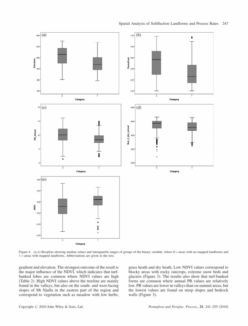
Figure 4 (a–e) Boxplots showing median values and interquartile ranges of groups of the binary variable, where 0¼ areas with no mapped landforms and1¼ areas with mapped landforms. Abbreviations are given in the text.


gradient and elevation. The strongest outcome of the result isthe major influence of the NDVI, which indicates that turf-banked lobes are common where NDVI values are high(Table 2). High NDVI values above the treeline are mainlyfound in the valleys, but also on the south- and west-facingslopes of Mt Njulla in the eastern part of the region andcorrespond to vegetation such as meadow with low herbs,


grass heath and dry heath. Low NDVI values correspond toblocky areas with rocky outcrops, extreme snow beds andglaciers (Figure 3). The results also show that turf-bankedforms are common where annual PR values are relativelylow. PR values are lower in valleys than on summit areas, butthe lowest values are found on steep slopes and bedrockwalls (Figure 3).


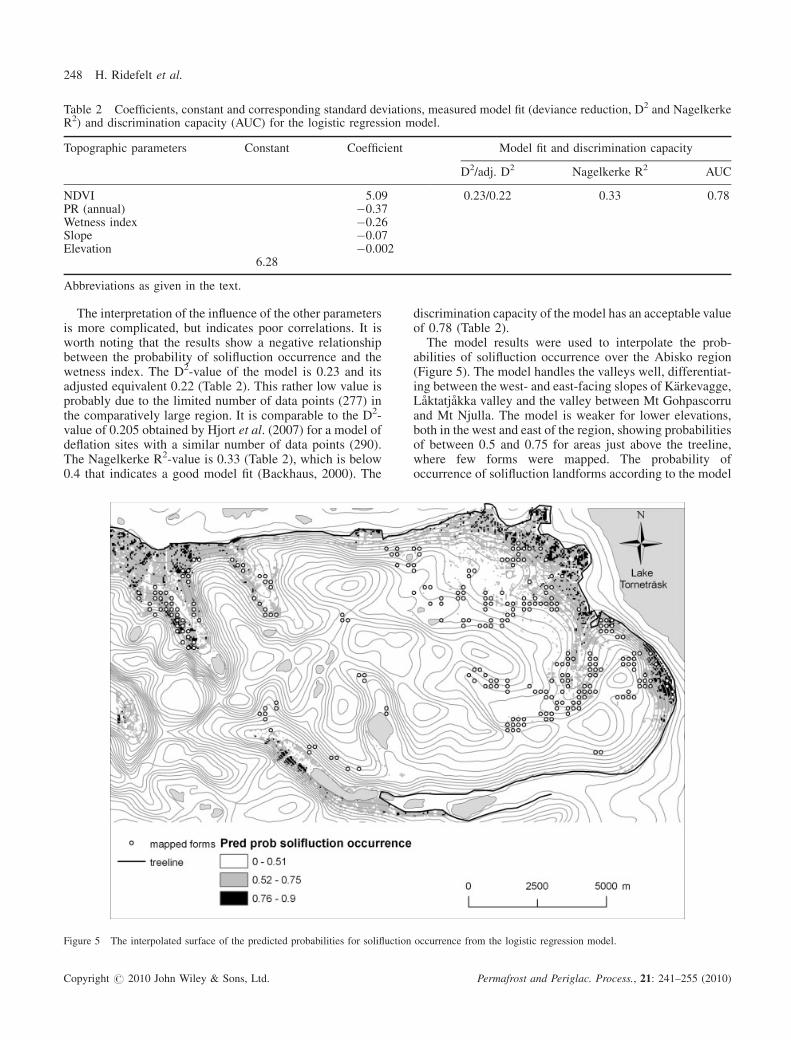
Table 2 Coefficients, constant and corresponding standard deviations, measured model fit (deviance reduction, D2 and NagelkerkeR2) and discrimination capacity (AUC) for the logistic regression model.

Topographic parameters Constant Coefficient Model fit and discrimination capacity

D2/adj. D2 Nagelkerke R2 AUC

NDVI 5.09 0.23/0.22 0.33 0.78PR (annual) �0.37Wetness index �0.26Slope �0.07Elevation �0.002

6.28

Abbreviations as given in the text.


The interpretation of the influence of the other parametersis more complicated, but indicates poor correlations. It isworth noting that the results show a negative relationshipbetween the probability of solifluction occurrence and thewetness index. The D2-value of the model is 0.23 and itsadjusted equivalent 0.22 (Table 2). This rather low value isprobably due to the limited number of data points (277) inthe comparatively large region. It is comparable to the D2-value of 0.205 obtained by Hjort et al. (2007) for a model ofdeflation sites with a similar number of data points (290).The Nagelkerke R2-value is 0.33 (Table 2), which is below0.4 that indicates a good model fit (Backhaus, 2000). The

Figure 5 The interpolated surface of the predicted probabilities for solifluction


discrimination capacity of the model has an acceptable valueof 0.78 (Table 2).The model results were used to interpolate the prob-

abilities of solifluction occurrence over the Abisko region(Figure 5). The model handles the valleys well, differentiat-ing between the west- and east-facing slopes of Karkevagge,Laktatjakka valley and the valley between Mt Gohpascorruand Mt Njulla. The model is weaker for lower elevations,both in the west and east of the region, showing probabilitiesof between 0.5 and 0.75 for areas just above the treeline,where few forms were mapped. The probability ofoccurrence of solifluction landforms according to the model

occurrence from the logistic regression model.



was tested against 21 GPS-mapped landforms in Karke-vagge (Ridefelt et al., 2009b). The results showed that onaverage the probability was 0.64 for all 21 GPS-mappedlandforms, with a standard deviation of 0.09. Seven GPS-mapped landforms corresponded to a probability of morethan 0.7 and only one corresponded to a probability lowerthan 0.5 (0.41).

Movement Rates

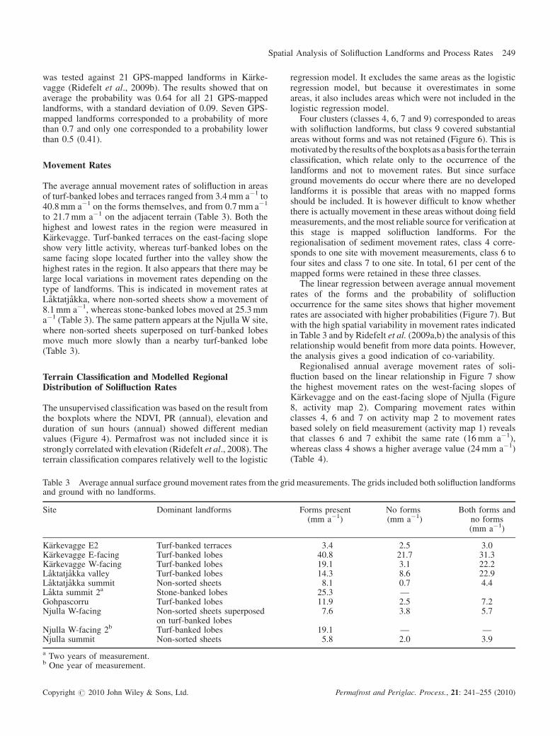
The average annual movement rates of solifluction in areasof turf-banked lobes and terraces ranged from 3.4mm a�1 to40.8mm a�1 on the forms themselves, and from 0.7mm a�1

to 21.7mm a�1 on the adjacent terrain (Table 3). Both thehighest and lowest rates in the region were measured inKarkevagge. Turf-banked terraces on the east-facing slopeshow very little activity, whereas turf-banked lobes on thesame facing slope located further into the valley show thehighest rates in the region. It also appears that there may belarge local variations in movement rates depending on thetype of landforms. This is indicated in movement rates atLaktatjakka, where non-sorted sheets show a movement of8.1mm a�1, whereas stone-banked lobes moved at 25.3mma�1 (Table 3). The same pattern appears at the Njulla W site,where non-sorted sheets superposed on turf-banked lobesmove much more slowly than a nearby turf-banked lobe(Table 3).

Terrain Classification and Modelled RegionalDistribution of Solifluction Rates

The unsupervised classification was based on the result fromthe boxplots where the NDVI, PR (annual), elevation andduration of sun hours (annual) showed different medianvalues (Figure 4). Permafrost was not included since it isstrongly correlated with elevation (Ridefelt et al., 2008). Theterrain classification compares relatively well to the logistic

Table 3 Average annual surface ground movement rates from the griand ground with no landforms.

Site Dominant landforms

Karkevagge E2 Turf-banked terracesKarkevagge E-facing Turf-banked lobesKarkevagge W-facing Turf-banked lobesLaktatjakka valley Turf-banked lobesLaktatjakka summit Non-sorted sheetsLakta summit 2a Stone-banked lobesGohpascorru Turf-banked lobesNjulla W-facing Non-sorted sheets superposed

on turf-banked lobesNjulla W-facing 2b Turf-banked lobesNjulla summit Non-sorted sheets

a Two years of measurement.b One year of measurement.


regression model. It excludes the same areas as the logisticregression model, but because it overestimates in someareas, it also includes areas which were not included in thelogistic regression model.

Four clusters (classes 4, 6, 7 and 9) corresponded to areaswith solifluction landforms, but class 9 covered substantialareas without forms and was not retained (Figure 6). This ismotivatedby the results of theboxplots asabasis for the terrainclassification, which relate only to the occurrence of thelandforms and not to movement rates. But since surfaceground movements do occur where there are no developedlandforms it is possible that areas with no mapped formsshould be included. It is however difficult to know whetherthere is actually movement in these areas without doing fieldmeasurements, and themost reliable source for verification atthis stage is mapped solifluction landforms. For theregionalisation of sediment movement rates, class 4 corre-sponds to one site with movement measurements, class 6 tofour sites and class 7 to one site. In total, 61 per cent of themapped forms were retained in these three classes.

The linear regression between average annual movementrates of the forms and the probability of solifluctionoccurrence for the same sites shows that higher movementrates are associated with higher probabilities (Figure 7). Butwith the high spatial variability in movement rates indicatedin Table 3 and by Ridefelt et al. (2009a,b) the analysis of thisrelationship would benefit from more data points. However,the analysis gives a good indication of co-variability.

Regionalised annual average movement rates of soli-fluction based on the linear relationship in Figure 7 showthe highest movement rates on the west-facing slopes ofKarkevagge and on the east-facing slope of Njulla (Figure8, activity map 2). Comparing movement rates withinclasses 4, 6 and 7 on activity map 2 to movement ratesbased solely on field measurement (activity map 1) revealsthat classes 6 and 7 exhibit the same rate (16mm a�1),whereas class 4 shows a higher average value (24mm a�1)(Table 4).

d measurements. The grids included both solifluction landforms

Forms present(mm a�1)

No forms(mm a�1)

Both forms andno forms(mm a�1)

3.4 2.5 3.040.8 21.7 31.319.1 3.1 22.214.3 8.6 22.98.1 0.7 4.425.3 —11.9 2.5 7.27.6 3.8 5.7

19.1 — —5.8 2.0 3.9


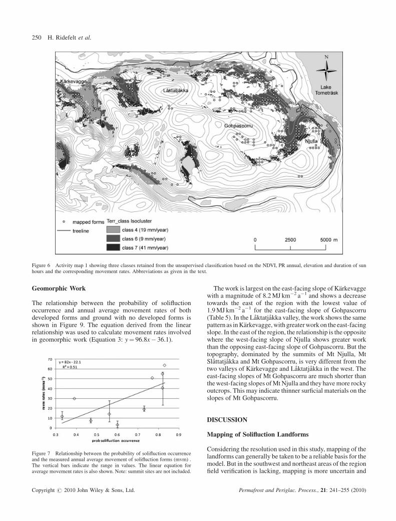
Figure 6 Activity map 1 showing three classes retained from the unsupervised classification based on the NDVI, PR annual, elevation and duration of sunhours and the corresponding movement rates. Abbreviations as given in the text.


Geomorphic Work

The relationship between the probability of solifluctionoccurrence and annual average movement rates of bothdeveloped forms and ground with no developed forms isshown in Figure 9. The equation derived from the linearrelationship was used to calculate movement rates involvedin geomorphic work (Equation 3: y¼ 96.8x� 36.1).

Figure 7 Relationship between the probability of solifluction occurrenceand the measured annual average movement of solifluction forms (mvm) .The vertical bars indicate the range in values. The linear equation foraverage movement rates is also shown. Note: summit sites are not included.


Thework is largest on the east-facing slope of Karkevaggewith a magnitude of 8.2MJ km�2 a�1 and shows a decreasetowards the east of the region with the lowest value of1.9MJ km�2 a�1 for the east-facing slope of Gohpascorru(Table 5). In the Laktatjakka valley, thework shows the samepattern as inKarkevagge,with greaterwork on the east-facingslope. In the east of the region, the relationship is the oppositewhere the west-facing slope of Njulla shows greater workthan the opposing east-facing slope of Gohpascorru. But thetopography, dominated by the summits of Mt Njulla, MtSlattatjakka and Mt Gohpascorru, is very different from thetwo valleys of Karkevagge and Laktatjakka in the west. Theeast-facing slopes of Mt Gohpascorru are much shorter thanthewest-facing slopes ofMtNjulla and they havemore rockyoutcrops. This may indicate thinner surficial materials on theslopes of Mt Gohpascorru.

DISCUSSION

Mapping of Solifluction Landforms

Considering the resolution used in this study, mapping of thelandforms can generally be taken to be a reliable basis for themodel. But in the southwest and northeast areas of the regionfield verification is lacking, mapping is more uncertain and


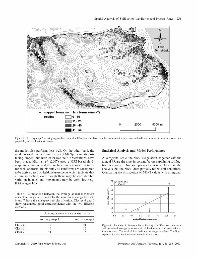
Figure 8 Activity map 2 showing regionalised annual solifluction rates based on the linear relationship between landform movement rates (mvm) and theprobability of solifluction occurrence.


the model also performs less well. On the other hand, themodel is weak on the summit areas of Mt Njulla and its east-facing slopes, but here extensive field observations havebeen made. Hjort et al. (2007) used a GPS-based field-mapping technique and also included indications of activityfor each landform. In this study all landforms are consideredto be active based on field measurements which indicate thatall are in motion, even though there may be considerablevariation in rates and movements may be very slow (e.g.Karkevagge E2).

Table 4 Comparison between the average annual movementrates of activity maps 1 and 2 for the same areas using classes 4,6 and 7 from the unsupervised classification. Classes 4 and 6show reasonably good correspondence with the two differentmethods.

Average movement rates (mm a�1)

Activity map 1 Activity map 2

Class 4 19 24Class 6 9 16Class 7 41 16


Statistical Analysis and Model Performance

At a regional scale, the NDVI (vegetation) together with theannual PR are the most important factors explaining solifluc-tion occurrence. No soil parameter was included in theanalysis, but the NDVI does partially reflect soil conditions.Comparing the distribution of NDVI values with a regional

Figure 9 Relationship between the probability of solifluction occurrenceand the annual average movement of solifluction forms and areas with noforms (mvm) . The vertical bars indicate the range in values. The linearequation for average movement rates is also shown.


Table 5 Geomorphic work at six different valley slopes within the Abisko region based on average movement rates for both formspresent and no forms (Table 3, column five), average movement rates, areas and average slope angles. The areas were defined as theextent of mapped forms within each valley, thus including ground with no visible forms between the mapped forms.

Geomorphic work(MJ km�2 a�1)

Average movementrates (mma�1)

Area(km2)

Slopeangle (8)

Karkevagge E-facing 8.2 33 1.15 18Karkevagge W-facing 5.0 24 0.85 15Laktavalley E-facing 3.6 20 1.39 13Laktavalley W-facing 2.9 14 0.47 15Gohpascorru 1.9 19 1.14 14Njulla W-facing 2.2 6 1.93 15


soil map (Rodhe et al., 1999), it is evident that low NDVIvalues are largely associated with areas of thin, non-cohesivesoil or bedrock areas. Themodel also indicates that rather lowPR values (<�8W/m2) are required. This requirement isfulfilled in the valleys, which are mainly south-northorientated and on north-facing slopes, but the latter generallyhave lowNDVI values. Low PR values indicate later melt andan earlier start of freezing and thus a prolonged freezingseason. The negative relationship between the wetness indexand theprobabilityof solifluctionoccurrencemaybe related tothe resolution of the DEM or the algorithm chosen forcalculating the upstream-contributing area.Different datasets were also tested in the logistic regression

model, where the number of randomly distributed zero datapoints were altered. Most studies have a relatively largenumber of zero data points compared to the number of datapoints for the response variable (e.g. Pereira and Itami, 1991;Atkinson et al., 1998; Luoto and Seppala, 2002; Hjort et al.,2007), but in this study altering the number of zero data pointshad a marginal effect on the final model performance.The independent variables were also tested when

normalised, standardised or log-transformed, and theresolution of the independent parameters was decreasedto 200m to correspond to the resolution of the binaryvariable. None of these data explorations improved theperformance of the model but the same variables weresignificant, including the NDVI, annual PR and wetnessindex. In the final model, slope gradient and elevation alsocontributed significantly. Hjort et al. (2007) found thevariables mean elevation, mean slope angle, elevation-reliefratio, concave topography, aspect and mean canopy cover tobe the most important variables in their logistic regressionmodel for solifluction sheets. Even though their site innorthern Finland is in a similar climate zone, the resultcannot be directly compared to the Abisko region, sincesolifluction sheets and turf-banked lobes do not developunder the same conditions. In the Abisko region, solifluctionsheets are generally found at higher elevations with moreexposed conditions than turf-banked lobes.The performance of the model in this study is similar to

that of other models of periglacial landforms, although in thelower range. Hjort et al. (2007), for example, developedpredictive models for the distribution of palsa, earthhummocks and solifluction sheets, with explained deviancevalues varying from 47–60.1 and with excellent discrimi-


nation capacities. Their model for deflation sites was weaker(explained deviance¼ 20.5 and AUC¼ 0.81). Luoto andSeppala (2002) developed a logistic regression model forpalsa prediction in the same area, with slightly differentpredictor variables and a weaker model. For patternedground models, three of six models had explained deviancesvarying from 0.32–0.36 (Hjort and Luoto, 2006). Modellingof rock glaciers and glaciers has shown AUC values rangingfrom 0.67–0.97 (Brenning and Trombotto, 2006). Alandslide susceptibility model is vaguely described in themodel validation as not having a direct one-to-onecorrelation, but with producing the desired pattern (Atkinsonet al., 1998). This points out the difficulty of comparing theperformance of models, as different authors often usedifferent measures of model fit and discrimination capacity.Differences in resolution and the size of the study area/

region may also affect the results of the models (Luoto andHjort 2006). It is well known in process geomorphology thatsystemcomponents controllinggeomorphicprocessesdependon scale (DeBoer, 1992). The topographic variables that wereused to explain solifluction at a larger scale (5-m resolution) insouthern Norway (Finse area, Etzelmuller et al., 2001)differed fromthoseemployed in this studyand fromthoseusedby Hjort et al. (2007), possibly due to scale issues.

Terrain Classification and Integration of MovementRates for Solifluction Landforms

Terrain classification is another way to model thedistribution of solifluction occurrence. The unsupervisedclassification also allows variations in movement rates(Figure 6, activity map 1) to be regionalised, following theprinciples of homogenous landscape units (e.g. Pike, 1988;Etzelmuller et al., 2001). It compares relatively well to thelogistic regression model (Figure 5), even though itoverestimates areas with solifluction activity in the valleys.Three classes covering areas with solifluction lobes emergedfrom the classification. Regarding regionalised movementrates, a comparison with activity map 2 (Figure 8) showedthat two of the classes correspond to the samemovement rate(Table 4). Thus, this method fails to capture the full variationin movement rates, suggesting that the terrain classificationis too robust to use with the limited number of movementmeasurements. It is more useful as a means to constrainareas of solifluction occurrence and it does not overestimate



them as much as activity map 1 (Figure 6). The approachalso allows continuous variation of movement rates, whichbetter reflects the field conditions.

The regionalised annual average movement rates ofactivity map 2 show the highest rates (>50mma�1) on thewest-facing slopes of Karkevagge and on the east-facingslope of Mt Njulla. The average value for the entire region isestimated to be 18mma�1. The R2-values of the linearrelationships used for the calculation for activity map 2 arefairly low (0.51), which may be due to the limited number ofdata. The estimated values are, however, in the same order ofmagnitude as other field-measured values in this region (e.g.Ridefelt et al., 2009a,b), with the exception of the east-facing slope of Mt Njulla, where very few measurementshave been made. The only comparison that can be made forthis area is with Nyberg’s (1991) field measurements of non-sorted sheets, where average movement rates were30mm a�1 and maximum rates were 50mma�1. In southernNorway, for a much smaller area of 1.05 km2, solifluctionmovement rates were estimated to vary from 12 to39mm a�1 (Berthling et al., 2002).

The field measurements indicate large spatial variations inmovement rates. This has also been shown in other areas(e.g. Rapp, 1960; Price, 1973; Smith, 1987; Berthling et al.,2002). To reliably regionalise variations in movement rates,many measurements in different environmental settingswould be required. Here, eight sites were originally selected,of which two were discarded in this study due to theirlocations on summits. This is a limited number ofmeasurement sites, but for regionalisation purposes thesesites cover essential differences within the region. Table 3and Figure 1 (for mapped stone-banked forms) addimportant information, indicating that summit areasexperience rather slow movement rates, while stone-bankedlobes at steeper slope sections move faster. At the Njullawest-facing site there are also measurements from twodifferent locations within 100m from each other, but withmean values varying from 7.6mm a�1 to 19.1mma�1. Thehigher value is obtained from only one year of measurementand was not considered reliable enough to include in theanalysis. In summary, we believe that the regionalisation ofmovement rates according to activity map 2 gives anadequate picture of solifluction variability in the study area.

Towards a Regional Approximation of GeomorphicInfluence of Solifluction

The linear relationship used to assess movement rates for thecalculation of geomorphic work including movement of allground (Figure 9) has a higher R2-value (0.63) than the linearrelationship for only movement of landforms (0.51). Thecalculated values compare well with previous estimates (e.g.Caine, 1976; Berthling et al., 2002). The geomorphic work inKarkevaggewas estimated to be 8.2MJ km�2 a�1 on the east-facing slope and 5MJ km�2 a�1 on thewest-facing slope, andthus averaged 6.6MJ km�2 a�1 for thewhole valley. Based onRapp’s (1960) data, Caine (1976) estimated the geomorphicwork of solifluction and soil creep in Karkevagge to be


5.2MJ km�2 a�1, which corresponds well with the values ofgeomorphic work from our calculations. In Finse, Norway,geomorphic work by solifluction was estimated to represent atotal of 9.1MJ km�2 a�1 (Berthling et al., 2002), which iswithin 50 per cent of the Karkevagge estimate.

Our rates of solifluction and our estimates of the areaaffected by the process compare reasonably well withpreviously published values. Rapp (1960) estimated thevelocity of solifluction in Karkevagge to be 20mma�1,which is comparable to the 28.5mm a�1 average for bothslopes (Table 5), including both developed forms and groundwith no developed forms. Part of the reason for the higherrate could also be that movements have increased over thepast half-century (Ridefelt et al., 2009). The activesolifluction area in this valley was estimated by Rapp(1960) to be 2.2 km2, while Bartsch et al. (2002, 2009), usingterrain classification, estimated the area in Karkevaggeaffected by solifluction/rill erosion to be 3.3 km2. Our arealestimate based on the linear relationship between solifluc-tion occurrence and movement rates is 2 km2. Beylich(2008) estimated the mass transfer caused by solifluctionand creep to affect an area of 2.8 km2 of the Latnjavaggecatchment (Figure 1), with an average movement of 3mma�1. From our models, the dominant rates in that area varyfrom 0–10mm a�1.

In general, other studies (Rapp, 1960; Caine, 1976;Beylich, 2008) have shown that the impact of solifluctioncompared to other slope denudational processes is ratherlow. Caine (1976) estimated that geomorphic workaccomplished by earth slides and mudflows, rock falls,avalanches and solute transport for Karkevagge was moreimportant than that attributable to solifluction. Similarly,Beylich (2008) estimated for the Latnjavagge catchment thatfluvial solute and suspended transport, rock falls, chemicaland mechanical fluvial slope denudation, and groundavalanches have a greater impact than solifluction andcreep processes. But slush and debris flows, translationslides and deflation are less important there (Beylich, 2008).Elsewhere in the region, there is no quantification of othermass processes, which makes it difficult to assess the relativeimportance of solifluction as a slope denudational agent.Even though movement rates and the geomorphic work ofsolifluction are most important in the western part of theregion, solifluction may still be relatively important forlandscape development elsewhere. In both Karkevagge andLatnjavagge, the topography is dominated by steep rockwalland quite steep slopes, as compared to the other areas.Together with increased precipitation in the western parts ofthe region, which promotes higher soil moisture contents,this may enhance the activity of other mass movementprocesses. Field observations suggest that there is lessevidence of other mass movement processes in the easternpart of the region and on the summit areas.

This study of regionalised sediment fluxes by solifluctioninvites speculation concerning the importance of solifluctionin Holocene and Pleistocene landscape development inScandinavian mountains. Although process rates and geo-morphic work values are lower than for more episodic



landslide processes in the study area, solifluction seems todominate in a particular elevation belt under certain slopeconditions. Berthling et al. (2002) report for a field site in theFinse area, southern Norway that solifluction is a moreimportant process than rapid mass movements for displacingsediments. The regionalisation in this study demonstrates thatsolifluction is dominant over large areas above the treeline.This study has also shown that ground movements occur

even where no landforms have formed, which has beendemonstrated in relatively few other studies (e.g. Berthlinget al., 2002). The presence of landforms is therefore not onlyrelated to movement, but to certain local environmentalfactors. It is thus important to distinguish between thefactors that affect movement rates (activity map 2) and thoseinfluencing the actual formation of the landforms (activitymap 1). Soil moisture and elevation have been identified astwo of the parameters influencing variation of movementrates on a regional scale in this area (Ridefelt, 2009). Inaddition to these two parameters, solifluction occurrence isalso influenced by vegetation patterns, local topography andPR (which includes slope and aspect). This is important toconsider when estimating the regional influence of sedimentmovement rates, as well as for understanding localdynamics. The grid-based field measurement approach usedhere is particularly useful for making this distinction.Solifluction is a slowprocess, but acts over long time scales,

and thus has the potential to mobilise large amounts ofmaterial. Solifluction removes material slowly and enhancesthe possibility for coupling of slopes with sediment-evacuating systems like rivers or episodic rapid slopemovements (Wangensteen et al., 2006). In central Europe,periglacial slope deposits derived mostly from solifluctionprocesses are recognised as the most widely distributedsediment type (Raab et al., 2007) with their own stratigraphy.For intermediate slope areas above the tree limit inScandinavia, solifluction is an important mass movementprocess, removing large amounts of material during inter-glacial periods, and thus is a major landscape-forming factor.

CONCLUSIONS

This study is a novel attempt to regionalise sedimentmovement rates and calculate geomorphic work over a largearea, allowing the varying influence of solifluction to beassessed at the landscape scale. The parameters included inthe logistic model of solifluction occurrence, the NDVI, PR(annual), wetness index, slope and elevation, partiallyexplain the distribution patterns of solifluction occurrence ata regional scale in the Abisko Mountains. The combinationof the occurrence model probability with field-measuredmovement rates allowed for regionalisation of sedimentmovement rates. The results show the highest movementrates on the west-facing slopes of Karkevagge and on theeast-facing slope of Mt Njulla (>50mma�1). The predicteddistribution of the varying movement rates according to thismethod is similar to the distribution of the originally mappedforms. Based on empirical-derived probabilities, values for


geomorphic work were estimated, showing highest values inthe western part of the region, with a maximum of8.2MJ km�2 a�1 in Karkevagge and a decrease towardsthe east where geomorphic work on the east-facing slope ofMt Gohpascorru is estimated to be 1.9MJ km�2 a�1. Theseestimated values are in reasonable accordance with similarstudies. The study also highlights the importance ofconsidering movement on terrain where no landforms haveformed and accounting for this when estimating sedimentfluxes on a regional scale.

ACKNOWLEDGEMENTS

We would like to thank the Swedish Society for Anthro-pology and Geography and Abisko Scientific ResearchStation for major funding of the fieldwork. We would alsolike to thank Ivar Berthling and an anonymous reviewer forinvaluable comments on the manuscript.

REFERENCES

Akerman J, Johansson M. 2005. Changes in permafrost inrelation to climate change and its impacts on terrestrialecosystems in the Subarctic, Sweden. In 2nd EuropeanConference on Permafrost, Programme and Abstract.Kumke T (ed). GeoUnion, Alfred Wegener Stiftung: Berlin,118 pp.

Andersson L, Rafstedt T, von Sydow U. 1985. Fjallens veg-etation, Norrbottens lan. Swedish Environmental ProtectionAgency: Stockholm.

Atkinson J, Jiskoot H, Massari R, Murray T. 1998. Generalizedlinear modelling in geomorphology. Earth Surface Processesand Landforms 23: 1185–1195.

Backhaus K. 2000.Multivariate Analysemethoden: eine anwen-dungsorientierte Einfuhrung. Springer: Heidelberg.

Bartsch A, GudeM, Jonasson C, Scherer D. 2002. Identificationof geomorphic process units in Karkevagge, northern Swe-den, by remote sensing and digital terrain analysis. Geogra-fiska Annaler 84 A: 171–178.

Bartsch A, Gude M, Gurney SD. 2009. Quantifying sedimenttransport processes in periglacial mountain environments at acatchment scale using geomorphic process units.GeografiskaAnnaler 91 A: 1–9.

Berthling I, Etzelmuller B, Kielland Larsen C, Nordahl K. 2002.Sediment fluxes from creep processes at Jomfrunut, southernNorway. Norsk Geografisk Tidskrift 56: 67–73.

Beven KJ, Kirkby MJ. 1979. A physically based, variablecontributing area model of basin hydrology. HydrologicalSciences 24: 43–69.

Beylich AA. 2008. Mass transfers, sediment budget and reliefdevelopment in the Latnjavagge catchment, Arctic-oceanicSwedish Lapland. Zeitschrift fur Geomorphologie, suppl.Issue 52: 149–197.

Brenning A, Trombotto D. 2006. Logistic regression modelingof rock glacier and glacier distribution: Topographic andclimatic controls in the semi-arid Andes. Geomorphology 81:141–154.

Caine N. 1976. A uniform measure of subaerial erosion.Geological Society of America Bulletin 87: 137–140.



Crawley M. 1993. GLIM for Ecologists. Blackwell ScientificPublications: Oxford.

Darmody RG, Thorn CE, Dixon JC, Schlyter P. 2000. Soils andlandscapes of Karkevagge, Swedish Lapland. Soil ScienceSociety of America Journal 64: 1455–1466.

De Boer DH. 1992. Hierarchies and spatial scale in processgeomorphology: a review. Geomorphology 4: 303–318.

Douglas TD, Harrison S. 1996. Turf-banked terraces in Oraefi,Southern Iceland: morphometry, rates of movement andenvironmental controls. Arctic and Alpine Research 28:228–236.

Etzelmuller B, Ødegard RS, Berthling I, Sollid JL. 2001.Terrain parameters and remote sensing data in the analysisof permafrost distribution and periglacial processes:examples from southern Norway. Permafrost and PeriglacialProcesses 12: 79–92. DOI: 10.1002/ppp.384.

Fielding AH, Bell JF. 1997. A review of methods for theassessment of prediction errors in conservation presence/absence models. Environmental Conservation 24: 38–49.

Fierz C, Pluss C, Martin E. 1997. Modelling the snow cover in acomplex alpine topography. Annals of Glaciology 25: 312–316.

Fu PD, Rich PM. 2002. A geometric solar radiation model withapplications in agriculture and forestry. Computers andElectronics in Agriculture 37: 25–35.

Guisan A, Zimmermann NE. 2000. Predictive habitat distri-bution models in ecology. Ecological Modeling 135: 147–186.

Hengl T, Reuter HI (eds). 2009. Geomorphometry – vol. 33:Concepts, Software, Application. Elsevier: Amsterdam.

Hjort J, Luoto M. 2006. Modelling patterned ground distri-bution in Finnish Lapland: an integration of topographical,ground and remote sensing information. Geografiska Annaler88A: 19–29.

Hjort J, Luoto M, Seppala M. 2007. Landscape scale determi-nant of periglacial features in subarctic Finland: A grid-basedmodelling approach. Permafrost and Periglacial Processes18: 115–127. DOI: 10.1002/ppp.584.

Holmlund P, Jonasson C. 2001. Permafrost in Sweden, abstract.1st European Permafrost Conference, Rome, 26–28 March2001.

Hosmer D, Lemeshow S. 2000. Applied logistic regression.John Wiley & Sons: Canada.

Jensen JR. 1996. Issues involving the creation of digitalelevation models and terrain corrected orthoimagery usingsoft-copy photogrammetry. In Digital Photogrammtery: AnAddendum to the Manual Photogrammetry, Greve C (ed.).American Society for Photogrammetry and Remote Sensing:Bethesda, MD; 167–179.

JohanssonM, Christensen TR, Akerman HJ, Callaghan T. 2006.What determines the current presence or absence of perma-frost in the Tornetrask region, a Sub-arctic landscape inNorthern Sweden. Ambio 35: 190–197.

Lo CP, Yeung KW. 2007. Concepts and techniques of geo-graphic information systems, 2nd edition. Prentice Hall:Upper Saddle River, New Jersey.

Luoto M, Hjort J. 2006. Scale matters – a multi-resolution studyof the determinants of patterned ground activity in subarcticFinland. Geomorphology 80: 282–294.

Luoto M, Seppala M. 2002. Modelling the distribution of palsasin Finnish Lapland with logistic regression and GIS. Perma-frost andPeriglacial Processes 13: 17–28. DOI: 10.1002/ppp.404.


Matsuoka N. 2001. Solifluction rates, processes and landforms:a global review. Earth-Science Reviews 55: 107–134.

Mittaz C, Imhof M, Hoelzle M, Haeberli W. 2002. Snowmeltevolution mapping using an energy balance approach over analpine terrain. Arctic, Antarctic and Alpine Research 34:274–281.

Nyberg R. 1991. Geomorphic processes at snowpatch sites inthe Abisko Mountains, northern Sweden. Zeitschrift furGeomorphologie 35: 321–343.

Pereira C, Itami RM. 1991. GIS-based habitat modelling usingmultiple logistic regression: A study of the Mt Graham RedSquirrel. Photogrammetric Engineering and Remote Sensing57: 1475–1486.

Pike RJ. 1988. The geometric signature: Quantifying landslideterrain types from digital elevation models. MathematicalGeology 20: 491–511.

Price LW. 1973. Rates of mass wasting in the Ruby range, YukonTerritory. In North American Contribution, 2nd InternationalConference on Permafrost, Yakutsk. Pewe T, Mackay J (eds).National Academy Press: Washington; 235–245.

Raab T, Leopold M, Volkl J. 2007. Character, age, ecologicalsignificance of Pleistocene periglacial slope deposits inGermany. Physical Geography 28: 451–473.

Rapp A. 1960. Recent development of mountain slopes inKarkevagge and surroundings, northern Scandinavia. Geo-grafiska Annaler 42: 71–200.

Rich PM, Dubayah R, Hetrick WA, Saving SC. 1994. Usingviewshed models to calculate intercepted solar radiation:applications in ecology. American Society for Photogram-metry and Remote Sensing Technical Papers; 524–529.

Ridefelt H. 2009. Spatial and temporal variations on solifluc-tion and related environmental parameters in the AbiskoMountains, northern Sweden. Doctoral thesis, Acta Univer-sitatis Upsaliensis, Uppala University.

Ridefelt H, Boelhouwers J. 2006. Observations on regionalvariations in solifluction landform morphology and environ-ment in the Abisko region, northern Sweden. Permafrost andPeriglacial Processes 17: 253–266. DOI: 10.1002/ppp.560.

Ridefelt H, Boelhouwers J, Etzelmuller B, Jonasson C. 2008.Statistic-empirical modelling of mountain permafrost distri-bution in the Abisko region, sub-Arctic northern Sweden.Norsk Geografisk Tidskrift 62: 278–289.

Ridefelt H, Akerman J, Beylich AA, Boelhouwers J, Kolstrup E,Nyberg R. 2009a. 56 years of solifluction measurements inthe Abisko Mountains, northern Sweden – perspectives ofslow soil surface movement and long-term monitoring. Geo-grafiska Annaler 91: 215–231.

Ridefelt H, Boelhouwers J, Eiken T. 2009b. Measurement ofsolifluction rates using multi-temporal aerial photography.Earth Surface Processes and Landforms 34: 725–737.

Rodhe L, Pyykonen M, Krekula M. 1999. Soil map Abisko(digitized working material).

Smith DJ. 1987. Observations on turf-banked solifluction lobegeomorphometry, Canadian Rocky Mountains. AlbertanGeographer 23: 45–55.

US Geological Survey#, www.eros.usgs.gov accessed 19August 2008. USGS National Center 12201 Sunrise ValleyDrive, Reston, VA 20192, USA.

Wangensteen B, Guomundsson A, Eiken T, Kaab A, Farbrot H,Etzelmuller B. 2006. Surface displacements and surface ageestimates for creeping slope landforms in Northern andEastern Iceland using digital photogrammetry. Geomorpho-logy 80: 59–79.


Spatial analysis of solifluction landforms and process rates in the Abisko Mountains, northern...

Documents

Transcript of Spatial analysis of solifluction landforms and process rates in the Abisko Mountains, northern...