arX

iv:1

310.

1986

v1 [

phys

ics.

optic

s] 8

Oct

201

3

Influence of the intensity gradient upon HHG from free electrons

scattered by an intense laser beam

Ankang Li, Jiaxiang Wang ∗, Na Ren

State Key Laboratory of Precision Spectroscopy,

East China Normal University, Shanghai 200062, China

Pingxiao Wang

Applied Ion Beam Physics Laboratory,

Key Laboratory of the Ministry of Education ,

China and Institute of Modern Physics,

Department of Nuclear Science and Technology,

Fudan University, Shanghai 200433, China

Wenjun Zhu, Xiaoya Li

National Key Laboratory of Shock Wave and

Detonation Physics, Mianyang 621900, Sichuan, China

Ross Hoehn, Sabre Kais

Departments of Chemistry and Physics, Purdue University,

West Lafayette, Indiana 47907, USA and

Qatar Environment and Energy Research Institute, Qatar Foundation, Doha, Qatar

∗ jxwang@phy.ecnu.edu.cn

1

Abstract

When an electron is scattered by a tightly-focused laser beam in vacuum, the intensity gradient is

a critical factor to influence the electron dynamics, for example, the electron energy exchange with

the laser fields as have been explored before [P.X.Wang et al.,J. Appl. Phys. 91, 856 (2002]. In this

paper, we have further investigated its influence upon the electron high-harmonic generation (HHG)

by treating the spacial gradient of the laser intensity as a ponderomotive potential. Based upon

perturbative QED calculations, it has been found that the main effect of the intensity gradient is

the broadening of the originally line HHG spectra. A one-to-one relationship can be built between

the beam width and the corresponding line width. Hence this finding may provides us a promising

way to measure the beam width of intense lasers in experiments. In addition, for a laser pulse, we

have also studied the different influences from transverse and longitudinal intensity gradients upon

HHG.

PACS numbers:

2

1. Introduction

Since the availability of high-power lasers, high harmonic generation (HHG) based upon

nonlinear Compton scattering (NLCS) from free electrons in strong laser fields has drawn

considerable attention [1–10]. This is not only because it is a fundamental non-perturbative

laser-induced phenomena, but also because it is a prospective x-ray or gamma-ray source [11–

13] with remarkable performances in terms of tunability. Moreover, the free-electron laser

interaction is very clean without other uncontrollable physical processes such as ionizations

and collisions, which happen in the interaction between lasers and atoms or plasmas. In

recent years, the observation of NLCS in some experiments [14–16] also renew the interest

in its theoretical study.

The main aim of this paper is to investigate how the effect of the laser intensity gradients

change the radiation of free electron in strong laser field. It is well known that there is

a cycle-averaged force on a charged particle in a spatially inhomogeneous laser field. It is

associated with a time-independent potential energy called ponderomotive potential, which

is due to the laser intensity gradient in an oscillatory field. After the presence of such

ponderomotive potential was first proposed in 1957 by Boot and Harvie [17, 18], it is well

known for the last four decades that the potential could have a significant effect on the matter

interacting with the laser field, such as particle acceleration [19], trapping and cooling of the

atoms [20] , high-field photoionization of atoms [21], self-focusing in plasma [22] and high

harmonic generation [23, 24]. In the classical framework, the mechanical motion of electrons

in a strong laser field will be changed if the ponderomotive potential is taken into account

due to the limited spatial dimensions of the laser focus, which leads to the ponderomotive

broadening of the radiation spectrum [23]. But so far few works are done to study the role of

the ponderomotive effects on the radiation spectrum based on a quantum theory [23, 24, 31].

To gain a clear idea of the influence by the laser intensity gradients on the HHG spectrum

from free electrons in strong laser fields, we start from the scattering of the electron Volkov

state by the ponderomotive potential of the laser beam. The corresponding cross section is

calculated as a second order quantum electrodynamics (QED) laser-assisted process similar

to laser-assisted bremsstrahlung, where an charged particle scatters by the field of a nucleus

in a background strong laser field [25–30].

For notations in this paper, the four-vector product is denoted by a · b = a0b0 − ab and

3

the Feynman dagger is /A = γ · A. The Dirac adjoint is denoted by u = u†γ0 for a bispinor

u and F = γ0F †γ0 for a matrix F.

The outline of this paper is the following. First, we will introduce the scattering model

and derive the theoretical expression for the cross section of the electron radiation. Then,

the numerical estimation of the cross section and the corresponding analyses will be provided

in Sec 3. Concluding remarks are reserved for Sec 4.

2. Theoretical derivation of the scattering cross section

We begin by introducing our scattering mode: Consider there are two monochromatic

laser pulse in space. The first one propagates along z axis, of which the duration is long

enough and the field intensity so strong that it can be modeled by a background classical

plane wave field, described by a four dimension vector potential Aµ:

Aµ = A0[δ cosφǫ1µ + (1− δ2)1/2 sinφǫ2

µ], (1)

Here with the phase factor φ = k · x, in which x is the position vector, and the four

wave vector is related to kµ = ω0

c(1, 0, 0, 1) with ω0 denoting the wave propagation direction

and laser frequency, respectively. The laser is circularly polarized for δ = 1/√2 and linearly

polarized for δ = 0,±1. We define two polarization vectors ǫ1, ǫ2, satisfying ǫi ·k = 0, ǫi ·ǫj =δij (i, j = 1, 2). The laser intensity can be easily described by a dimensionless parameter Q =

eA0/(mc2), which is usually called laser intensity parameter. In the nonrelativistic regime,

the characteristic velocity and energy for an electron moving in such an electromagnetic

field is v ∼ eA0/(mc) and E ∼ e2A20/(mc

2), so relativistic treatment is necessary if v ∼ c

and E ∼ mc2 is satisfied. That’s to say the motion of the electron will become relativistic

for Q ∼ 1. In the optical regime (hω ≈ 1eV ), the corresponding laser intensity is about

1018W/cm2 for Q ∼ 1, which has been achieved in the last decade.

The second field is a tightly focused laser pulse propagating opposite the first one, which

can be described by the lowest-order axicon Gaussian fields with a envelop factor g(φ) =

e

(

−φ2/(∆φ))

. It is far less intense than the first one (the intensity is described by another

dimensionless parameter QG) but much rapidly oscillatory. The electron will be assumed

to be moving with a momentum p in the direction perpendicular to z axis, say, x axis.

4

FIG. 1: The scattering geometry: The incoming electron with four momentum pi have a 90 collision with

a plane laser field while scattering by a time-independent ponderomotive potential AG. The final electron

with Πf and the emitted photon with k′ are projected onto the xz plane in this figure; θf and θ′ denotes

the scattering angle of the outgoing electron and the emitted photon,respectively.

When the electron is placed in the two laser wave field, it will be mainly driven by the

longer-wavelength laser. The interaction of the electron with the plane wave laser will be

treated exactly by introducing the well-known Volcov state. That’s to say, the ”dressed”

electron will have an effective momentum Π = p+e2A2

0

4c2(p·k)with a corresponding effective mass

m′ = m√

1 + Q2

2.While the main effect of the Gaussian laser pulse on the electron can be

described by an time-averaged potential in view of its low intensity and fast oscillation (here

we do not care about the high frequency part of the radiation caused by the fast oscillation).

We assume that the relativistic electron moves so fast that the envelop factor is almost time

independent. The effective pondermotive potential can be described by :

Up =mc2

4QG

2e−

r2

⊥

b02− z2

b12 (2)

The corresponding four vector potential can be written as:

Aµp =

Up

eδµ0 (3)

where the Fourier-transformed pondermotive potential is given by:

Aµp (q) =

mc2π3/2

4eQG

2b02b1δ

µ0e−b0

2

4q2

⊥−

b12

4q2z (4)

5

FIG. 2: Feynman diagrams describing laser-assisted bremsstrahlung. The laser-dressed electron and laser-

dressed electron propagator are denoted by a zigzag line on top of the straight line. The Coulomb field

photon is drawn as a dashed line, and the bremsstrahlung photon as a wavy line.

Here r⊥ and q⊥ refers to the position and momentum in the plane perpendicular to the

propagation dirction, respectively. While is related to the beam waist and is decided by the

pulse duration. Considering the high-frequency character of the pulse, which means a small

wavelength, the paraxial approximation of the laser pulse can be acceptable confidently.

Since QG ≪ Q , we will treat the pondermotive potential as perturbation. The whole

scattering configuration can be seen in Fig 1 and it can be described by two Feynman

diagrams shown in Fig 2.

It’s obvious that the interaction of electron with the intense plane laser wave will leads

to discrete line at a given harmonic on the spectrum if the second weak pulse is absent.

The scattering process is called laser-induced Compton scattering, or Nonlinear Compton

scattering (NLCS) for its nonlinear nature, which has been widely studied since the invention

of laser in 1960 [9–11]. The frequencies of the emitted harmonics are determined from the

energy-momentum conservation laws, which involve both the incident electron condition and

laser parameters. Here we wonder the effect of the pondermotive potential on the discrete

radiation spectrum.

In order to calculate the differential cross-section of the second order laser-assisted pro-

cess, we begin by employing the well-known Volkov state to describe the initial and final

electron state:

ψp,r =1

V

√

mc

Π0ζp(x)ur(p) (5)

ζp(x) =(

1 +e/k/A

2p · k)

eiS (6)

6

S = − Π · xh

− e2A20

8hc2(p · k)(2δ2 − 1) sin 2φ+

eA0

hc(p · k)×

[

δ(p · ǫ1)sinφ − (1− δ2)1/2(p · ǫ2) cosφ]

. (7)

Here ur(p) the free Dirac spinor. Here we employ a box normalization with a normaliza-

tion volume V.

Then the corresponding transition amplitude can be written as:

Sfi = − e2

h2c2

∫

dx4dy4ψpf ,rf (x)[/Ac(x)iG(x− y)/AG(y) + /AG(x)iG(x− y)/Ac(y)]ψpi,ri(y)

(8)

Aµc (x) =

√

2πhω′cǫc

µeik′x stands for the four-momentum of the emitted photo during the

scattering process with ǫcµ the photon polarization vector and k′ = ω′

c(1, ek′) the wave

vector, respectively. As the previous work [28, 29], here we use the Dirac-Volkov propagator

instead of the free electron propagator in view of the strong laser field:

iG(x− y) = −∫

dp4

(2πh)3(2πi)ζp(x)

/p+mc

p2 −m2c2ζp(y) (9)

It has been proven[28] that the use of the Dirac-Volkov propagator is crucial to obtain

correct numerical result in laser-modified QED process.

Here we take average on the initial electron spin (i.e, the electron is unpolarized) and

sum over the both final electron spin and emitted photon polarization. The differential cross

section is calculated with the formula:

d∼σ=

1

2JT

∑

ri,rf ,εc

∣

∣Sfi

∣

∣

2V d3Πf

(2πh)3d3k′

(2π)3. (10)

Here T is the long observation time and J = cV

Π

Π0 stands for the incoming particle flux.

We have d3Πf = |Πf |2dΩf = |Πf |2sinθfdθfdϕf , d3k′ = ω′2

c2dΩ′ = ω′2

c2sinθ′dθ′dϕ′,where

Ω′ and Ωf stands for the the solid angle of the emitted photon and electron, respectively.

After a long but straight-forward deriving process, we finally write down the differential

cross-section as:

7

d∼σ

dω′dΩ′dΩf=

αQ4Gb

40

8(4π)4c2(m2c2

h2b21)

×∑

n,εc

|Πf ||Πi|

e−b0

2

2q2

⊥−

b12

2q2zTr[Rfi,n(pf +mc)Rfi,n(pi +mc)]

(11)

Where:

Rfi,n =∑

s

M−n−s(Πf ,Π, /ǫc, η1Π,Πf

, η2Π,Πf)

i

/p−mcM−s(Πi,Π, γ

0, η1Π,Πi, η2Π,Πi

)

+∑

s′

M−n−s′(Πf ,Π′, γ0, η1Π′,Πf

, η2Π′,Πf)

i

/p′ −mcM−s′(Πi,Π

′, /ǫc, η1Π′,Πi

, η2Π′,Πi)

(12)

With the argument is defined as:

η1p1,p2 =eA0

hcδ[p2 · ǫ1k · p2

− p1 · ǫ1k · p1

]

η2p1,p2 = −eA0

hc(1− δ2)1/2[

p2 · ǫ1k · p2

− p1 · ǫ1k · p1

]

(13)

Π,Π′ is the four momentum of the intermediate electron in the Feynman diagrams shown

in Fig.2. They are determined by the conservation law, together with the four momentum

q transfer from the pondermotive potential, which is given by the corresponding functions

during the calculation process:

Π = πf − (n+ s)hk + hk′

Π′ = πi − shk − hk′

hq = πf − πi + hk′ − nhk

(14)

8

M is a 4× 4 matrix with five arguments:

Ms(p1, p2, F, η1p1,p2, η

2p1,p2) =

[

/F +e2A0

2

8c2/k/F/k

(pi · k)(p2 · k)]

G0s(α, β, ϕ)

+eA0

2cδ[ /ǫ1/k/F

(p1 · k)+

/F/k/ǫ1(p2 · k)

]

G1s(α, β, ϕ)

+eA0

2c(1− δ2)1/2

[ /ǫ2/k/F

(p1 · k)+

/F/k/ǫ2(p2 · k)

]

G2s(α, β, ϕ)

+(δ2 − 1

2)e2A0

2

4c2/k/F/k

(pi · k)(p2 · k)G3

s(α, β, ϕ)

(15)

The generalized Bessel functions are given by:

G0s(α, β, ϕ) =

∑

n

J2n−s(α)Jn(β)ei(s−2n)ϕ,

G1s(α, β, ϕ) =

1

2

(

G0s+1(α, β, ϕ) +G0

s−1(α, β, ϕ))

,

G2s(α, β, ϕ) =

1

2i

(

G0s+1(α, β, ϕ)−G0

s−1(α, β, ϕ))

,

G3s(α, β, ϕ) =

1

2

(

G0s+2(α, β, ϕ) +G0

s−2(α, β, ϕ))

.

(16)

With the corresponding argument:

α = [(η1p1,p2)2 + (η2p1,p2)

2]1/2

β =Qm2c2

8h(2δ − 1)

( 1

k · p1− 1

k · p2)

ϕ = arctan(−η2p1,p2η1p1,p2

)

(17)

The above differential cross-section is related to the spontaneous photon in the frequency

interval dω′ within the solid angle Ω′ and the final electron within the solid angle Ωf . But

it’s difficult to detect the photon and electron in the same time during an actual experiment.

So we integrate the differential cross-section over the scattering electron direction, by which

leads to the doubly differential cross section only differential in the direction of the radiated

photon and its frequency:

dσ

dω′dΩ′=

∫

d∼σ

dω′dΩ′dΩfdΩf (18)

9

As one of the characteristic feature of a second order process, the resonance will happen

when the intermediate electron fall within the mass shell. The physical interpretation, ac-

cording to Roshchupkin [30], may be that the considered second order process effectively

reduces to two sequential first order processes under certain resonance condition. In the

paper, the two sequential lower processes are nonlinear Compton scattering and static pon-

deromotive potential scattering, respectively. The corresponding resonance condition may

be written as Π2 = m′2c2 or Π′2 = m′2c2. When resonance occurs, the scattering cross-

section will be divergent, which indicates that the perturbation method is not applicable in

such situation. To avoid the problem, one has to introduce a small imaginary part of the

mass which results from the high radiative correction, i.e, the self-energy of the laser-dressed

electron, which is determined by the total probability of the Compton scattering in a laser

wave Wc(k · p): Γm(k · p) = Π0

2mWc(k · p) . Then the shifted propagator reads:

1

p−mc=

Π+m′c

Π2 −m′2c2 − i mΠ0

fc(hω′ − (n+ s)hω0)Γm(k · Πf) + imΓm(hk · k′)

(19)

1

p′ −mc=

Π′ +m′c

Π′2 −m′2c2 + i mΠ0

fc(hω′ − shω0)Γm(k · Πi)− imΓm(hk · k′)

(20)

The inclusion of the imaginary part of the electron mass eliminates the resonance singu-

larity, which enable us to evaluate the cross section numerically. Then, the resonance peak

altitude is determined by the lifetime of the immediate electron. Actually, the calculation

of Γm has been discussed in many papers and we can easily obtain the imaginary mass by

taking advantage of the corresponding results of our previous study.

3. Numerical Results

In this section, we will present the numerical results of the differential cross section

referring to the case of 90 laser-electron interaction geometry shown in Fig 1. We consider

the plane wave laser to be circularly polarized with a frequency of ω = 1.17eV and the

dimensionless parameter Q=17.8, which is related to a laser intensity of 7.58× 1022W/cm2.

It should be emphasized that the numerical results in our presentation are more exploratory

than systematic since we shall focus on the influence of ponderomotive potential due to the

10

0 0.5 1 1.5 2 2.5 3 3.5 4 4.5

10−20

10−10

100

ω′/ω0

dσ/

dω

′dΩ

′ (A

rb)

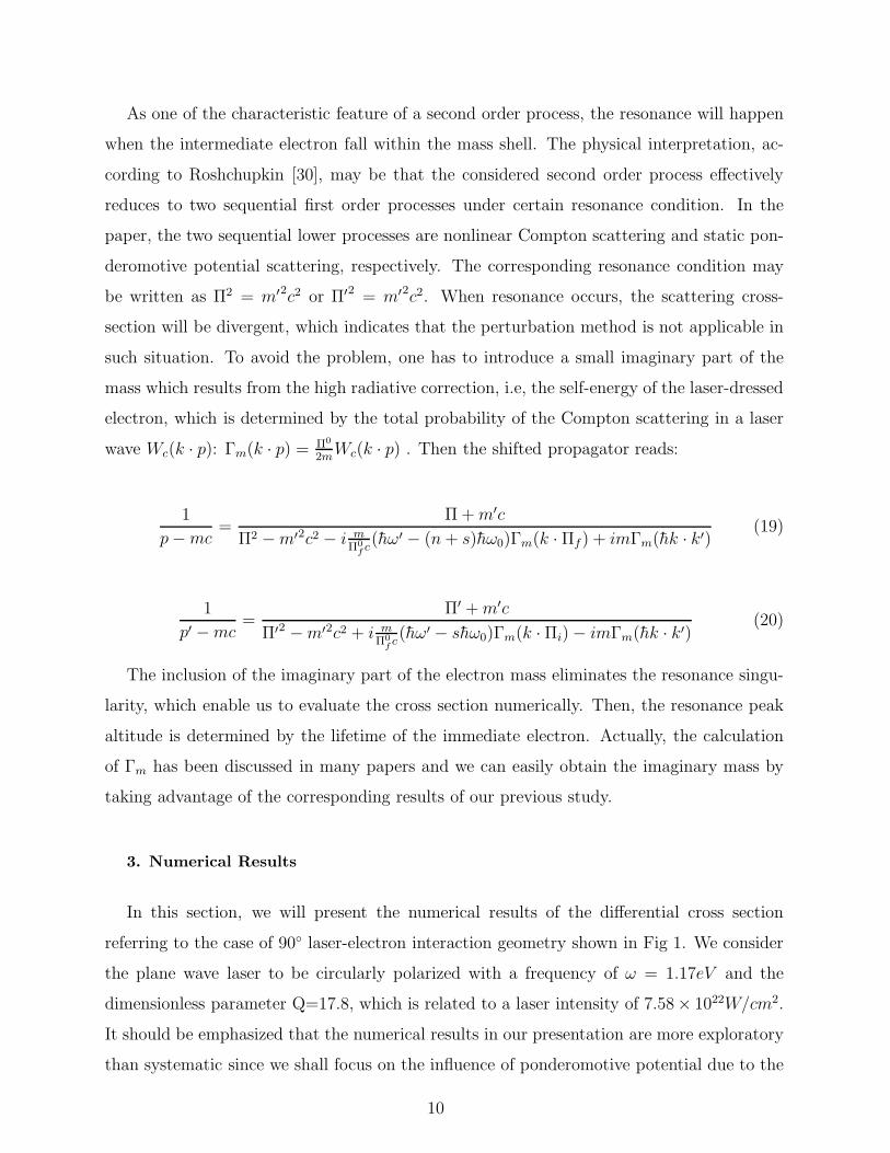
FIG. 3: The cross section for the low order harmonics at emission angle θ′ = 1. Here we consider an

electron with initial energy 5MeV collide with a circularly polarized laser with intensity parameter Q = 17.8

and is scattered by an effective ponderomotive potential for a 90 geometry. The ponderomotive potential

is characterized by two parameter: b0 = 5µm, b1 = 100µm, describing the beam waist size and duration of

the tightly focused laser pulse, respectively.

intensity gradients on the photon radiation. First, we start with the results for a tightly

focused laser pulse with the parameters b0 = 5µm, b1 = 100µm, which means the pulse

duration is very long (i.e., for a pulse with wavelength 0.1µm , the duration is about 0.3ps).

The corresponding differential cross section of the radiated photon for an emission angle

θ′ = 1 is shown in Fig 3. As expected, high harmonics are generated and the positions of

the resonances located in the spectrum coincide with those for NLCS. This is due to the

fact that the resonant second order process can effectively reduce to two sequent lower order

processes as mentioned before while the mechanism responsible for radiation of photons

is the nonlinear Compton scattering process. Furthermore, the main contribution of the

cross section comes from q ≈ 0 at a resonance, which means there’s nearly no momentum

transfer between the electron and the ponderomotive potential. It’s easy to find that the

main influence due to the ponderomotive potential is the broadened spectrum compared

to that of NLCS, which is in accordance with the conclusion based on a classical theory

[24]. The magnitude of the spectrum drops fast when the energy of photon is away from

resonance. From a mathematical point of view, that’s because the differential cross section is

subject to an exponential decay with respect to the transfer momentum q. So the spectrum

broadening effects is determined both the parameter b0 and b1, or the pulse duration and

11

0.7 0.8 0.9 1 1.1 1.2 1.3

10−20

10−10

100

ω′/ω0

dσ/

dω

′dΩ

′ (A

rb)

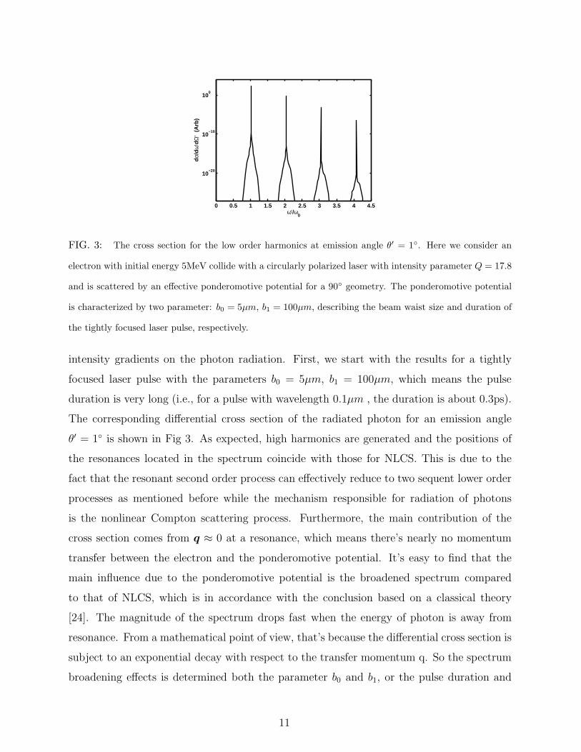
FIG. 4: The cross section for the fundamental harmonic at emission angle θ′ = 1. The condition is same

with Fig 3 except the parameter b0: 5µm for full line and 10µm for dot-dashed line.

the beam waist size.

Now we proceed to investigate how the broadening effect depends on the laser pulse

duration and the beam waist size. In Fig 4, we compare the spectrum of fundamental

harmonics for different beam waist size with same pulse duration. The cross section with

b0 = 5µm is denoted by full line, whereas the dotted-dashed line denote the cross section

with b0 = 10µm. Here the magnitude of the cross section near resonance is a little larger

for a broader beam waist size. This is probably because a laser with certain intensity

has a great energy with the increase of the beam waist size. We can also see from the

expression (11) that the differential cross-section is proportional to the quartic of b0. But

the peak falls off much more quickly for a larger beam waist size. This can be understood by

considering that the differential cross-section is determined exponentially by b0. The physical

interpretation may be that the large beam waist leads to a less field-gradient, which means

a small ponderomotive potential effect. When the beam waist is so large that we can neglect

the spatial gradient if we consider the interaction of the electron with laser field near its

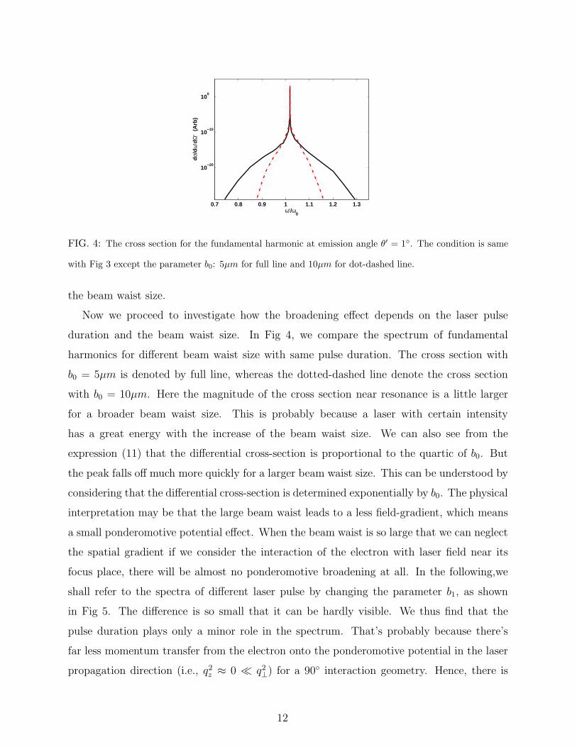
focus place, there will be almost no ponderomotive broadening at all. In the following,we

shall refer to the spectra of different laser pulse by changing the parameter b1, as shown

in Fig 5. The difference is so small that it can be hardly visible. We thus find that the

pulse duration plays only a minor role in the spectrum. That’s probably because there’s

far less momentum transfer from the electron onto the ponderomotive potential in the laser

propagation direction (i.e., q2z ≈ 0 ≪ q2⊥) for a 90 interaction geometry. Hence, there is

12

0.7 0.8 0.9 1 1.1 1.2 1.3 1.4

10−20

10−10

100

ω′/ω0

dσ/

dω

′dΩ

′ (A

rb)

FIG. 5: The cross section for the fundamental harmonic at emission angle θ′ = 1. The condition is same

with Fig 3 except the parameter b1: b1 = 100µm for full line and b1 = 150µm for dot-dashed line.

0.85 0.9 0.95 1 1.05 1.1 1.15 1.2

10−20

10−10

100

ω′/ω0

dσ/

dω

′dΩ

′ (A

rb)

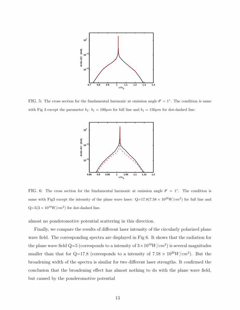
FIG. 6: The cross section for the fundamental harmonic at emission angle θ′ = 1. The condition is

same with Fig3 except the intensity of the plane wave laser: Q=17.8(7.58× 1020W/cm2) for full line and

Q=5(3× 1019W/cm2) for dot-dashed line.

almost no ponderomotive potential scattering in this direction.

Finally, we compare the results of different laser intensity of the circularly polarized plane

wave field. The corresponding spectra are displayed in Fig 6. It shows that the radiation for

the plane wave field Q=5 (corresponds to a intensity of 3×1019W/cm2) is several magnitudes

smaller than that for Q=17.8 (corresponds to a intensity of 7.58 × 1020W/cm2). But the

broadening width of the spectra is similar for two different laser strengths. It confirmed the

conclusion that the broadening effect has almost nothing to do with the plane wave field,

but caused by the ponderomotive potential

13

4. Summary

In this paper, we study the role of the field intensity gradients on the radiation spectrum

emitting from the electron in the laser field. The whole scattering process is calculated as a

laser-modified second order QED process with resonances addressed. Consequently, it shows

that the spectrum is broadening due to the ponderomotive effects compared to that of NLCS,

with the positions of the resonance peak corresponding to the discrete harmonic frequencies

of NLCS. Because the broadening of the spectrum line contains important information about

the laser intensity gradient, it might provide us a feasible way to measure the width of the

intense laser beam. In addition, the broadening effect is determined far more by the beam

waist size than the pulse duration for the case of 90 incidence scattering geometry. Since

the parameters of the corresponding laser field is readily accessible in the lab, it is hoped

that these results could be submitted to the experiment test in the near future.

Acknowledgments

This work is supported by the National Natural Science Foundation of China under

Grant Nos. 10974056 and 11274117. One of the authors, Wenjun Zhu, thanks the support

by the Science and Technology Foundation of National Key Laboratory of Shock Wave and

Detonation Physics (Grant No. 077110).

References

[1] L. S. Brown and T. W. B. Kibble, Phys. Rev. 133, 3 (1964).

[2] Fried Z and Eberly, Phys. Rev. 136, B871 (1964).

[3] E. S. Sarachik and G. T. Schappert, Phys. Rev. D 1, 10 (1970).

[4] Y. I. Salamin and F. H. M. Faisal, Phys. Rev. A 54, 4383 (1996); 55, 3678 (1997); 55, 3964

(1997); J. Phys. B 31, 1319 (1998).

[5] C. Harvey, T. Heinzl, and A. Ilderton, Phys. Rev. A 79, 063407 (2009).

[6] P. Panek, Phys. Rev. A 65, 022712 (2002); Phys. Rev. A 65, 033408 (2002).

[7] D. Y. Ivanov, G. L. Kotkin, and V. G. Serbo, Eur. Phys. J. C 36, 127 (2004).

14

[8] M. Boca, V. Florescu, Phys. Rev. A 80, 053403 (2009).

[9] T. Heinzl, D. Seipt, B. Kampfer, Phys. Rev. A 81, 022125 (2010).

[10] F. Mackenroth and A. Di Piazza, Phys. Rev. A 83, 032106 (2011).

[11] R.W. Schoenlein, W.P. Leemans, A.H. Chin, P. Volfbeyn,, Science 274 236 (1996); Phys. Rev.

Lett. 77 4182 (1996).

[12] P.F. Lan, P.X. Lu, W. Cao, X.L. Wang, Phys. Rev. E 72, 066501 (2005).

[13] P. Paneka, J.Z. Kaminskia, F. Ehlotzkyb, Opt. Commun. 213,121 (2002).

[14] C. Bula et al., Phys. Rev. Lett. 76, 3116 (1996); C. Bamber et al., Phys. Rev. D 60, 092004

(1999).

[15] T. Kumita et al., Laser Phys. 16, 267 (2006).

[16] M. Iinuma et al., Phys. Lett. A 346, 255 (2005).

[17] H. A. H. Boot and R. B. R.-S. Harvie, Nature (180), 1187 (1957).

[18] T.W. B. Kibble, Phys. Rev. Lett (16), 1054 (1966).

[19] Y. I. Salamin, and C. H. Keitel, Phys. Rev. Lett. (88), 095005 (2002).

[20] F. Diedrich, E. Peick, J. M. Chen, W. Quint, and H. Walther, Phys. Rev. Lett. (79), 2931

(1987).

[21] E.Wells, I. Ben-Itzhak, and R. R. Jones, Phys. Rev. Lett. (93), 023001 (2002).

[22] T. Afshar-rad, L. A. Gizzi, M. Desselberger, F. Khattak, Phys. Rev. Lett (86), 942 (1992).

[23] G. A. Krafft, Phys. Rev. Lett. (92), 204802 (2004).

[24] G. A. Krafft, Phys. Rev.E (72), 056502 (2005).

[25] S. P. Roshchupkin, J. Nucl. Phys. (41), 1244 (1985).

[26] S. P. Roshchupkin, Laser Phys. (6), 837 (1996).

[27] S. P. Roshchupkin, Laser Phys. (12), 498 (2002).

[28] E. Lotstedt, U. D. Jentschura, and C. H. Keitel, Phys. Rev. Lett. (98), 043002 (2007).

[29] S. Schnez, E. Lotstedt, U. D. Jentschura, and C. H. Keitel, Phys. Rev. A (75), 053412 (2007).

[30] A. A. Lebed and S. P. Roshchupkin, Phys. Rev. A (83), 033413 (2009).

[31] Fred V. Hartemann and Sheldon S. Q. Wu, Phys. Rev. Lett. (111), 044801 (2013).

15