Regularization of Wavelet Based Fitting

of Scattered Data — Some Experiments∗

Short Title: Regularization of Wavelet Based Fitting of Scattered Data

Daniel Castano Angela KunothInstitut fur Angewandte Mathematik, Universitat Bonn

53115 Bonn, Germanycastano, kunoth@iam.uni-bonn.de

August 28, 2003

Abstract

In [3] an adaptive method to approximate unorganized clouds of points by smoothsurfaces based on wavelets has been described. The general fitting algorithm operateson a coarse–to–fine basis and selects on each refinement level in a first step a reducednumber of wavelets which are appropriate to represent the features of the data set.In a second step, the fitting surface is constructed as the linear combination of thewavelets that minimizes the distance to the data in a least squares sense. This is thenfollowed by a thresholding procedure of the resulting wavelet coefficients to discardthose which are too small to contribute much to the surface representation.

Here we adapt this strategy to a classically regularized least square functional byadding a Sobolev norm, taking advantage of the capability of wavelets to characterizeSobolev spaces of even fractional order. After recalling in this framework the usualcross validation technique to determine the involved smoothing parameters, some ex-amples of fitting severely irregularly distributed data, both synthetically produced andof geophysical origin, are presented. Moreover, in order to reduce computational costs,we introduce a generalized cross validation technique which exploits the hierarchicalsetting based on wavelets and illustrates the performance of the new strategy withsome geophysical data.

Keywords: Wavelets, scattered data, least squares approximation, regularization, frac-tional Sobolev norms, generalized cross validation.AMS Classification: 65T60, 62G09, 93E14, 93E24.

1 Adaptive Least Squares Fitting with Wavelets

We have proposed in [3] an adaptive method of least squares data fitting based on certainwavelets that works on a coarse–to–fine basis. Since we will extend it later to include asmoothing term, we recall briefly our approach and some properties of the wavelets weemploy here.

Consider the set X = xii=1,...,N consisting of irregularly spaced and pairwise disjointpoints xi ∈ Ω := [0, 1]n, n ∈ 1, 2, denoting by zi ∈ IR for each i the corresponding data

∗We acknowledge financial support by the Deutsche Forschungsgemeinschaft (KU 1028/7–1) and by theBasque Government.

1

assembled in the set Z. The problem of scattered data fitting can be formulated as findinga function f : Ω → IR that approximates the cloud of points (X,Z) in a least squaressense, that is, f minimizes the functional

J(f) :=N∑

i=1

(zi − f(xi))2 . (1)

Specifically, we want to construct an expansion of f of the form

f(x) =∑λ∈Λ

dλ ψλ(x), x ∈ Ω. (2)

Here the set ψλλ∈Λ consists of tensor products of certain boundary adapted B–Spline–(pre)wavelets, shortly called wavelets in the remainder of this paper, and Λ is an appro-priately determined lacunary set of indices which results from an adaptive coarse–to–fineprocedure which will further be explained below.

The indices λ ∈ Λ will typically be of the form λ = (j,k, e), where j =: |λ| denotes thelevel of resolution or refinement scale, k is a spatial location, and e distinguishes furthertypes of wavelets in the bivariate case which are induced by tensor products, see e.g. [4].In view of the finite domain, there is a coarsest level j0 := 1. The infinite set of all possibleindices will be denoted by II.

Specifically, we work here with the wavelets ψλ : λ ∈ II constructed in [15] whichhave the following properties. Each ψλ is the tensor product of a certain linear combinationof B–splines. This is very advantageous computationally since one can work with piecewisepolynomials. In particular, the wavelets are compactly supported and satisfy for each λ ∈ IIthe relation diam (suppψλ) ∼ 2−|λ| where a ∼ b means that a can be estimated fromabove and below by a constant multiple of b independent of all parameters on which aor b may depend. The collection ψλ : λ ∈ II constitutes a Riesz basis for L2(Ω) and,moreover, one has norm equivalences for functions in Sobolev spaces Hα = Hα(Ω) (oreven more general in Besov spaces [5]) in the range α ∈ [0, γ) of the form

‖∑

λ=(j,k,e)∈II

dλ ψλ‖2Hα(Ω) ∼

∑j≥j0

22αj∑k,e

|dj,k,e|2. (3)

The parameter γ depends on the smoothness of the wavelet family which is, for instance,γ = 3

2 for piecewise linear wavelets and accordingly higher for smoother wavelets. Theproperty of characterizing such smoothness spaces together with their compact supportsuggests wavelets as a powerful analysis tool for many purposes, see e.g. [4]. In addition,the wavelets we employ here are semi–orthogonal with respect to L2(Ω), i.e., for |λ| 6= |µ|we always have

∫Ω ψλ(x)ψµ(x) dx = 0.

Returning to the least squares fitting problem (1), the adaptivity to the data is per-formed in the construction of the index set Λ ⊂ II. In our implementation, we start withthe coarse level j0 = 1 and take here the set Λj0 of indices of all scaling functions andwavelets on this level. An initial fitting function f j0(x) :=

∑λ∈Λj0

dj0λ ψλ(x) is constructed

on this set by minimizing J(f j0) or, equivalently, solving the normal equations

ATΛj0AΛj0

dj0 = ATΛj0z, (4)

see e.g. [1]. Here the observation matrix AΛj0has entries

(AΛj0)i,λ := ψλ(xi), i = 1, . . . , N, λ ∈ Λj0 , (5)

2

and z and dj0 are vectors comprising the right hand side data zii=1,...,N and the expansioncoefficients dj0

λ λ∈Λj0.

In view of the norm equivalence (3) for α = 0 and the locality of the ψλ, the absolutevalue of a coefficient dj0

λ is a measure of the spatial variability of f j0 on suppψλ: a largevalue of dj0

λ is understood to be an indicator that further resolution in this area of thedomain might be required. Similarly, in order to keep control over irrelevant coefficients,if dj0

λ is below a certain threshold, this coefficient is discarded from the approximation andthe index set is modified accordingly.

This motivates to construct a refined index set Λj0+1 by including those children of thewavelets indexed by Λj0 whose coefficients are above some prescribed thresholding valueand in whose support there are more than a fixed number of data points. Note that thisstrategy generates an approximation on a tree as index structure.

The procedure is repeated until at some dyadic highest resolution level J all the com-puted coefficients are smaller than the thresholding value, or none of the children whosesupports shrinks with each refinement step contains enough points on their support. Ifone of these condition is fulfilled, the algorithm stops growing the tree. Note that as thedata set is finite, the algorithm finishes in finitely many steps, and the level J is solelydetermined by the data.

In the following, we will extend this strategy to include also a regularizing term in theleast squares functional (1) to enforce a smooth approximation.

Multiscale data fitting which may or may not include a smoothing term has beendiscussed also in the following references. On structured grids, in [7] a coarse–to–finestrategy has been presented with hierarchical splines which is suited for gridded, param-eterized data. In [12] scattered functional data is approximated by multilevel B–Splines.

The remainder of this paper is structured as follows. In Section 2 we discuss smoothingin Sobolev spaces and its realization in terms of wavelets. Computation of the weightingparameter called cross validation is discussed in Section 3 together with some experimentson synthetic and geophysical data. A multilevel version of the cross validation procedureis presented in Section 4. We conclude with some numerical realistic examples to illustratethe efficiency of our method.

2 Smoothing with Wavelets

A classical way to extend least squares fitting methods to force them to produce smoothsurfaces is to add a smoothing term in terms of a Sobolev norm to the functional (1), seee.g. [6] for general splines, [14] for splines with variable knots, [10] for multiscale splines,[9] for splines on triangulations, or [8] in a wavelet reformulation of the spline problem.This yields a cost functional of the form

Jν(f) =N∑

i=1

(zi − f(xi))2 + ν‖f‖2Y (6)

where ν > 0 balances the fidelity of the data and the smoothness requirement, and Y isusually chosen as the Sobolev space H1 or H2.

In view of (3), the wavelet formulation allows to represent functions in Sobolev normsin terms of sequence norms of weighted coefficients from their wavelet expansions. Ac-cordingly, replacing ‖ · ‖Y by the corresponding sequence norm on the right hand side of

3

(3), the minimization of the resulting functional is equivalent to the solution of the normalequations

(ATA+ νR)d = AT z. (7)

Here A is shorthand for AΛj , j being the actual level of computation, and the diagonalmatrix R has the structure

R =

22αj0I. . .

22αjI

. (8)

This illustrates some interesting properties of the representation of the smoothing term inthe wavelet context (3):

(I) The different dyadic scales are decoupled. This is interesting in two ways.

(i) It keeps the weak decoupling between levels of the matrix ATA, which is explic-itly used to speed up the efficient numerical solution of the normal equationsas seen in [3].

(ii) It gives an insight into the way regularization works. In fact, the effect of theregularization term boils down to a penalization of the higher frequencies. As νcontrols the balance between fidelity and regularization, α controls the relativepenalization across scales.

(II) One has easy access to the entire scale of fractional Sobolev spaces Hαα>0 whichreduces to a simple diagonal scaling in the wavelet framework.

(III) The formulation is independent of the wavelet family. Only the smoothness of thefamily imposes a limit on the upper bound γ of α for which (3) holds.

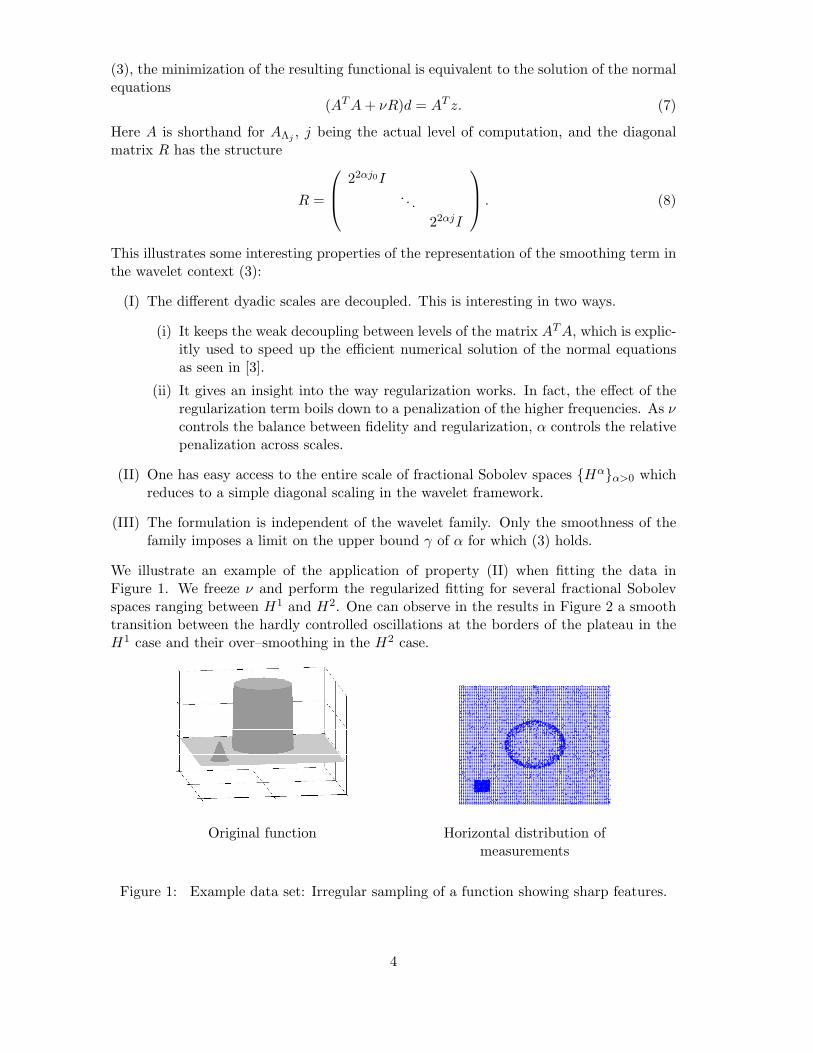
We illustrate an example of the application of property (II) when fitting the data inFigure 1. We freeze ν and perform the regularized fitting for several fractional Sobolevspaces ranging between H1 and H2. One can observe in the results in Figure 2 a smoothtransition between the hardly controlled oscillations at the borders of the plateau in theH1 case and their over–smoothing in the H2 case.

Original function Horizontal distribution ofmeasurements

Figure 1: Example data set: Irregular sampling of a function showing sharp features.

4

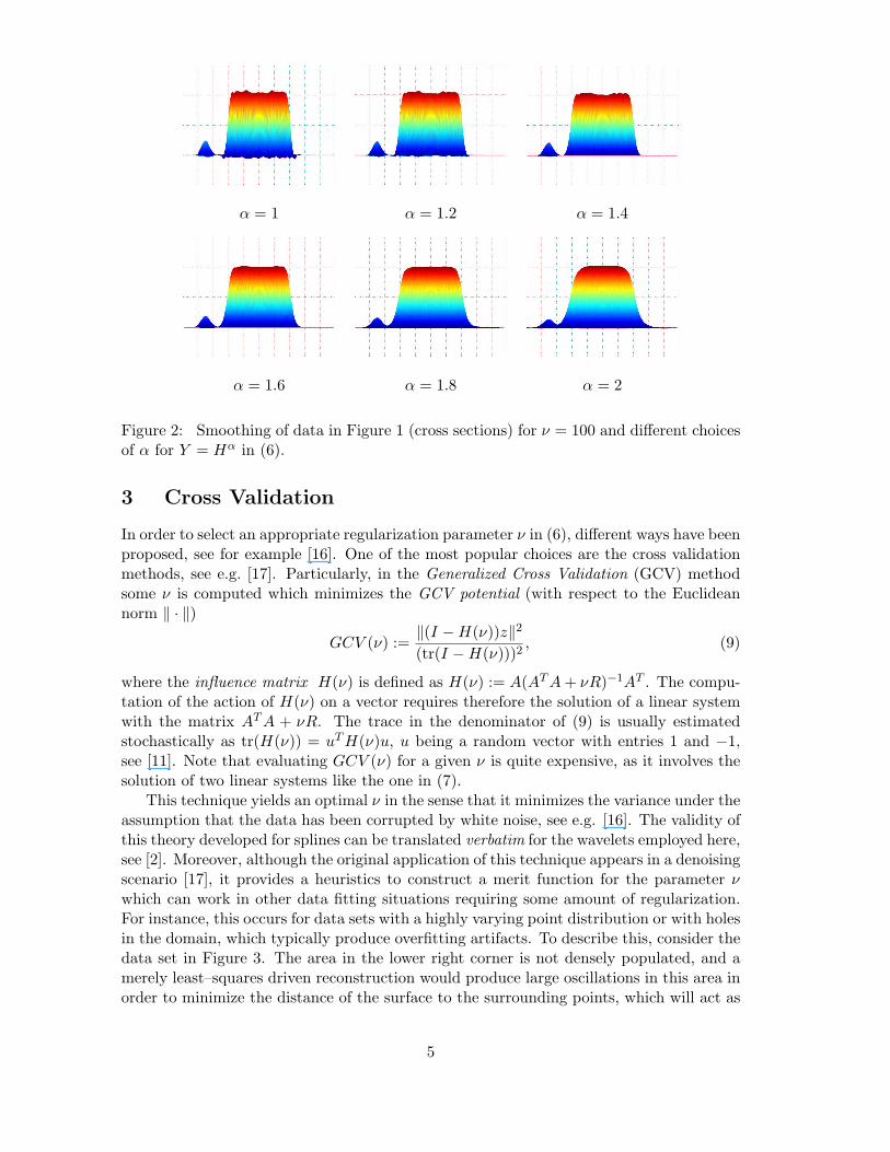
α = 1 α = 1.2 α = 1.4

α = 1.6 α = 1.8 α = 2

Figure 2: Smoothing of data in Figure 1 (cross sections) for ν = 100 and different choicesof α for Y = Hα in (6).

3 Cross Validation

In order to select an appropriate regularization parameter ν in (6), different ways have beenproposed, see for example [16]. One of the most popular choices are the cross validationmethods, see e.g. [17]. Particularly, in the Generalized Cross Validation (GCV) methodsome ν is computed which minimizes the GCV potential (with respect to the Euclideannorm ‖ · ‖)

GCV (ν) :=‖(I −H(ν))z‖2

(tr(I −H(ν)))2, (9)

where the influence matrix H(ν) is defined as H(ν) := A(ATA+ νR)−1AT . The compu-tation of the action of H(ν) on a vector requires therefore the solution of a linear systemwith the matrix ATA + νR. The trace in the denominator of (9) is usually estimatedstochastically as tr(H(ν)) = uTH(ν)u, u being a random vector with entries 1 and −1,see [11]. Note that evaluating GCV (ν) for a given ν is quite expensive, as it involves thesolution of two linear systems like the one in (7).

This technique yields an optimal ν in the sense that it minimizes the variance under theassumption that the data has been corrupted by white noise, see e.g. [16]. The validity ofthis theory developed for splines can be translated verbatim for the wavelets employed here,see [2]. Moreover, although the original application of this technique appears in a denoisingscenario [17], it provides a heuristics to construct a merit function for the parameter νwhich can work in other data fitting situations requiring some amount of regularization.For instance, this occurs for data sets with a highly varying point distribution or with holesin the domain, which typically produce overfitting artifacts. To describe this, consider thedata set in Figure 3. The area in the lower right corner is not densely populated, and amerely least–squares driven reconstruction would produce large oscillations in this area inorder to minimize the distance of the surface to the surrounding points, which will act as

5

a leverage.

Data: Gaussian peaks. Sampling points.

Figure 3: Synthetic data with two zones of different density distributions.

We see in the reconstruction for three values of ν in Figure 4 that the GCV criterionprovides some kind of order of magnitude information, as the value ν = νmin succeeds toreproduce the features of the original data without artifacts, while ν = 1

25νmin is too weaka regularization as it does not eliminate the oscillation predicted for the poorly populatedarea. ν = 25νmin is a too strong regularization, as the height of the peaks has beenreduced by the regularizing term in its effort to globally reduce the oscillating behavior ofthe reconstructed function.

0

1

ν = 125νmin

0

1

ν = νmin

0

0.5

1

ν = 25 νmin

Figure 4: Regularized reconstruction of data from Figure 3 with different ν.

We give a further example in Figure 5, corresponding to sea floor elevation data fromPuerto Rico [13]. This geophysical data set includes a strong irregularity in the horizontaldistribution of measurements, as seen in the graphic on the right. In fact, clusters, linesand holes are present.

Again, the GCV succeeds to provide a good orientation value for the order of magnitudeof the regularizing parameter ν: compare in Figure 6 the spiky reconstruction attainedwith ν = 1

100νmin on the left, and the oversmoothed surface generated with ν = 200νmin

with the reconstruction provided by the value ν = νmin.

4 A Multilevel Version of Generalized Cross–Validation

The main idea presented in this paper is the simultaneous use of the GCV with thehierarchical growth of the wavelet tree as the levels become higher. The basis for this is

6

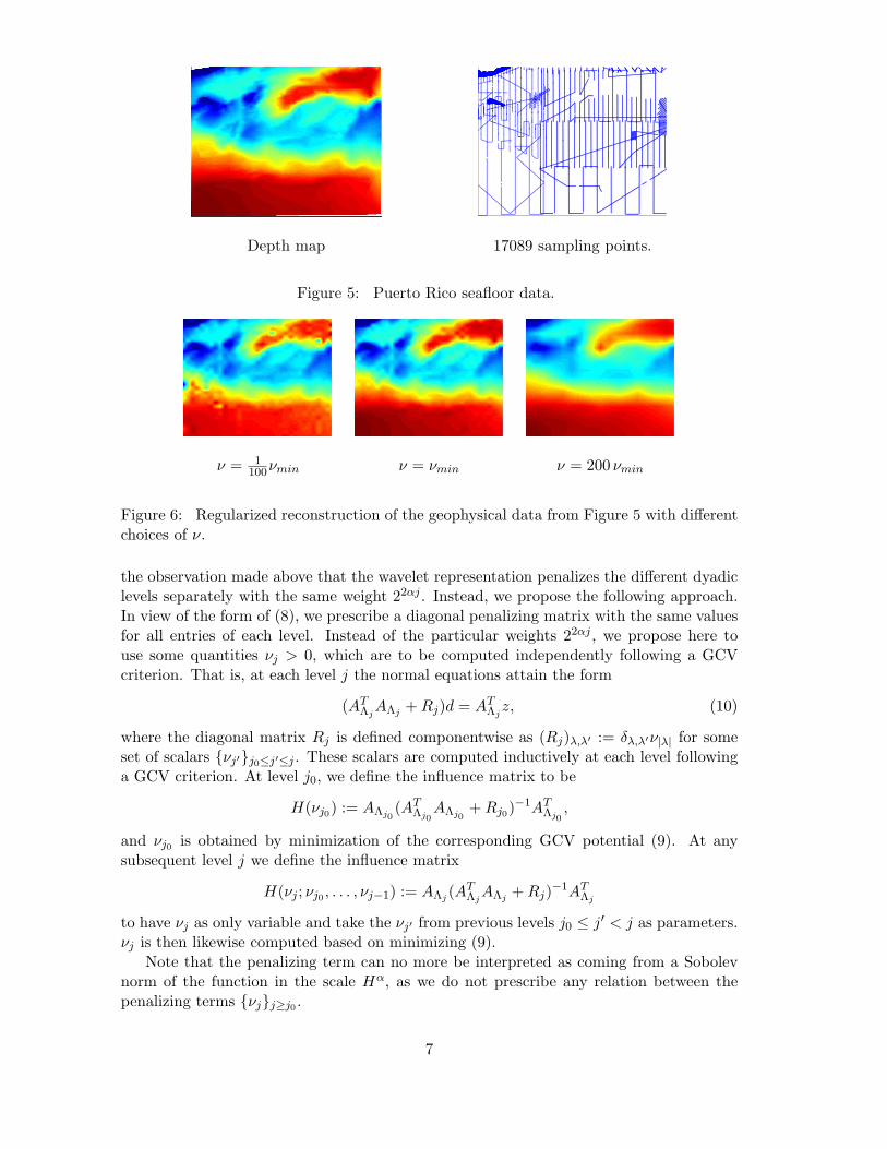
Depth map 17089 sampling points.

Figure 5: Puerto Rico seafloor data.

ν = 1100νmin ν = νmin ν = 200 νmin

Figure 6: Regularized reconstruction of the geophysical data from Figure 5 with differentchoices of ν.

the observation made above that the wavelet representation penalizes the different dyadiclevels separately with the same weight 22αj . Instead, we propose the following approach.In view of the form of (8), we prescribe a diagonal penalizing matrix with the same valuesfor all entries of each level. Instead of the particular weights 22αj , we propose here touse some quantities νj > 0, which are to be computed independently following a GCVcriterion. That is, at each level j the normal equations attain the form

(ATΛjAΛj +Rj)d = AT

Λjz, (10)

where the diagonal matrix Rj is defined componentwise as (Rj)λ,λ′ := δλ,λ′ν|λ| for someset of scalars νj′j0≤j′≤j . These scalars are computed inductively at each level followinga GCV criterion. At level j0, we define the influence matrix to be

H(νj0) := AΛj0(AT

Λj0AΛj0

+Rj0)−1AT

Λj0,

and νj0 is obtained by minimization of the corresponding GCV potential (9). At anysubsequent level j we define the influence matrix

H(νj ; νj0 , . . . , νj−1) := AΛj (ATΛjAΛj +Rj)−1AT

Λj

to have νj as only variable and take the νj′ from previous levels j0 ≤ j′ < j as parameters.νj is then likewise computed based on minimizing (9).

Note that the penalizing term can no more be interpreted as coming from a Sobolevnorm of the function in the scale Hα, as we do not prescribe any relation between thepenalizing terms νjj≥j0 .

7

This approach offers some interesting advantages:

1. The procedure is easily built into the coarse–to–fine growth of the tree.

2. One can attain a higher flexibility for the smoothing effect.

3. Overfitting artifacts are typically localized in scale. This makes a method which isable to disentangle the several scales a natural choice.

4. Computationally, the method is much cheaper, as we will see below at the end ofSection 4.1

We discuss these points by means of two examples.

4.1 Case Study 1: Complexity Reduction

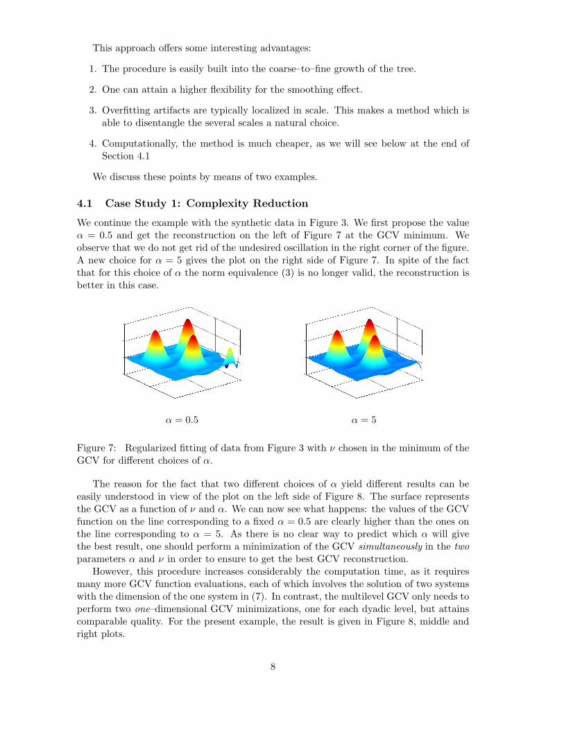
We continue the example with the synthetic data in Figure 3. We first propose the valueα = 0.5 and get the reconstruction on the left of Figure 7 at the GCV minimum. Weobserve that we do not get rid of the undesired oscillation in the right corner of the figure.A new choice for α = 5 gives the plot on the right side of Figure 7. In spite of the factthat for this choice of α the norm equivalence (3) is no longer valid, the reconstruction isbetter in this case.

α = 0.5 α = 5

Figure 7: Regularized fitting of data from Figure 3 with ν chosen in the minimum of theGCV for different choices of α.

The reason for the fact that two different choices of α yield different results can beeasily understood in view of the plot on the left side of Figure 8. The surface representsthe GCV as a function of ν and α. We can now see what happens: the values of the GCVfunction on the line corresponding to a fixed α = 0.5 are clearly higher than the ones onthe line corresponding to α = 5. As there is no clear way to predict which α will givethe best result, one should perform a minimization of the GCV simultaneously in the twoparameters α and ν in order to ensure to get the best GCV reconstruction.

However, this procedure increases considerably the computation time, as it requiresmany more GCV function evaluations, each of which involves the solution of two systemswith the dimension of the one system in (7). In contrast, the multilevel GCV only needs toperform two one–dimensional GCV minimizations, one for each dyadic level, but attainscomparable quality. For the present example, the result is given in Figure 8, middle andright plots.

8

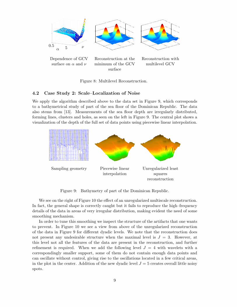
ν0.5α 5

Dependence of GCVsurface on α and ν

Reconstruction at theminimum of the GCV

surface

Reconstruction withmultilevel GCV

Figure 8: Multilevel Reconstruction.

4.2 Case Study 2: Scale–Localization of Noise

We apply the algorithm described above to the data set in Figure 9, which correspondsto a bathymetrical study of part of the sea floor of the Dominican Republic. The dataalso stems from [13]. Measurements of the sea floor depth are irregularly distributed,forming lines, clusters and holes, as seen on the left in Figure 9. The central plot shows avisualization of the depth of the full set of data points using piecewise linear interpolation.

Sampling geometry Piecewise linearinterpolation

Unregularized leastsquares

reconstruction

Figure 9: Bathymetry of part of the Dominican Republic.

We see on the right of Figure 10 the effect of an unregularized multiscale reconstruction.In fact, the general shape is correctly caught but it fails to reproduce the high–frequencydetails of the data in areas of very irregular distribution, making evident the need of somesmoothing mechanism.

In order to tune this smoothing we inspect the structure of the artifacts that one wantsto prevent. In Figure 10 we see a view from above of the unregularized reconstructionof the data in Figure 9 for different dyadic levels. We note that the reconstruction doesnot present any undesirable structure when the maximal level is J = 3. However, atthis level not all the features of the data are present in the reconstruction, and furtherrefinement is required. When we add the following level J = 4 with wavelets with acorrespondingly smaller support, some of them do not contain enough data points andcan oscillate without control, giving rise to the oscillations located in a few critical areas,in the plot in the center. Addition of the new dyadic level J = 5 creates overall little noisyspots.

9

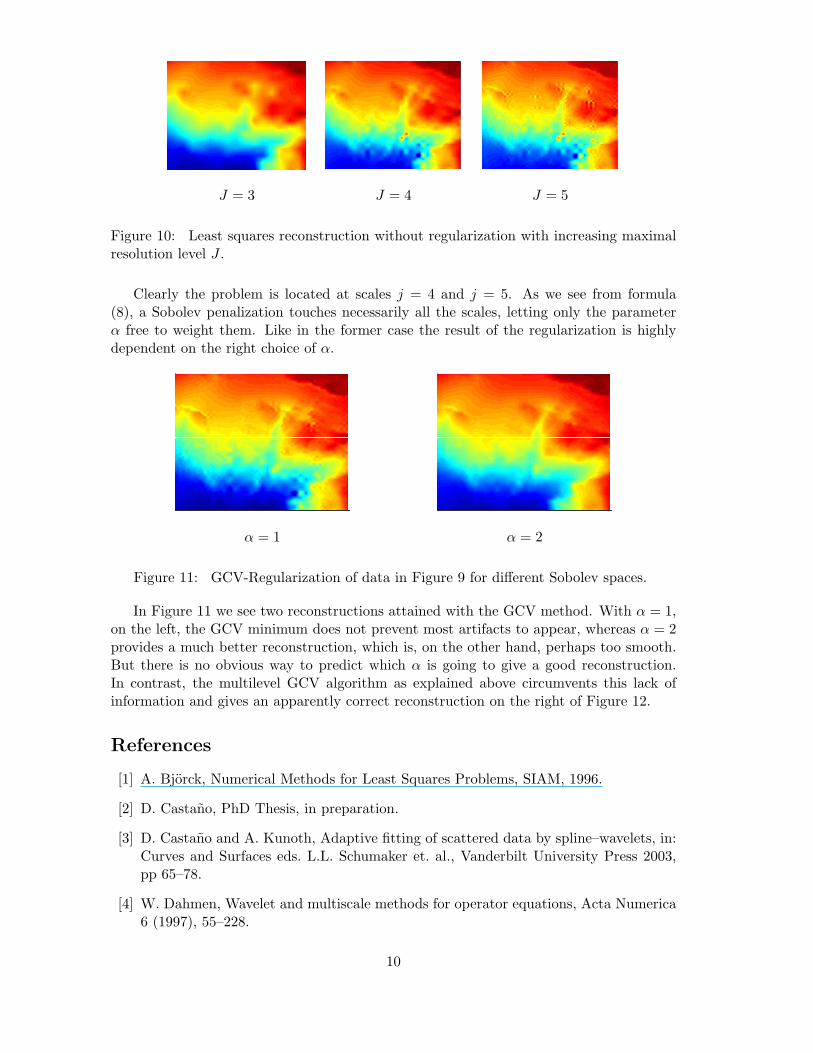
J = 3 J = 4 J = 5

Figure 10: Least squares reconstruction without regularization with increasing maximalresolution level J .

Clearly the problem is located at scales j = 4 and j = 5. As we see from formula(8), a Sobolev penalization touches necessarily all the scales, letting only the parameterα free to weight them. Like in the former case the result of the regularization is highlydependent on the right choice of α.

α = 1 α = 2

Figure 11: GCV-Regularization of data in Figure 9 for different Sobolev spaces.

In Figure 11 we see two reconstructions attained with the GCV method. With α = 1,on the left, the GCV minimum does not prevent most artifacts to appear, whereas α = 2provides a much better reconstruction, which is, on the other hand, perhaps too smooth.But there is no obvious way to predict which α is going to give a good reconstruction.In contrast, the multilevel GCV algorithm as explained above circumvents this lack ofinformation and gives an apparently correct reconstruction on the right of Figure 12.

References

[1] A. Bjorck, Numerical Methods for Least Squares Problems, SIAM, 1996.

[2] D. Castano, PhD Thesis, in preparation.

[3] D. Castano and A. Kunoth, Adaptive fitting of scattered data by spline–wavelets, in:Curves and Surfaces eds. L.L. Schumaker et. al., Vanderbilt University Press 2003,pp 65–78.

[4] W. Dahmen, Wavelet and multiscale methods for operator equations, Acta Numerica6 (1997), 55–228.

10

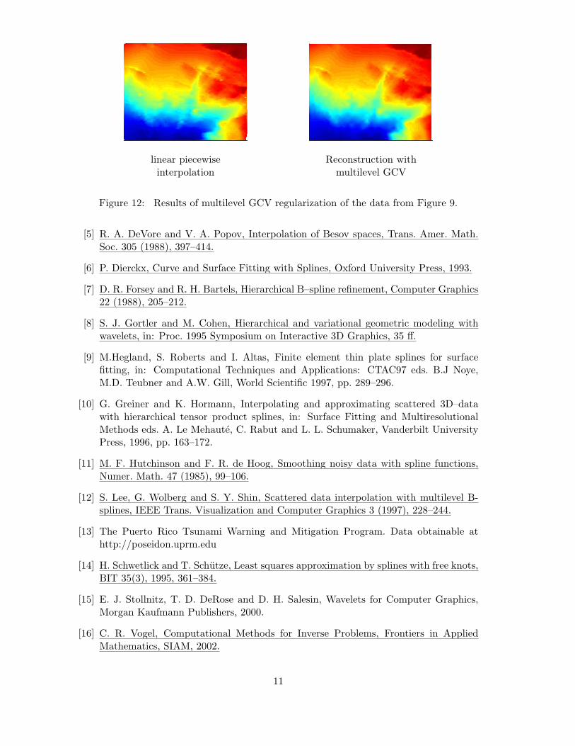
linear piecewiseinterpolation

Reconstruction withmultilevel GCV

Figure 12: Results of multilevel GCV regularization of the data from Figure 9.

[5] R. A. DeVore and V. A. Popov, Interpolation of Besov spaces, Trans. Amer. Math.Soc. 305 (1988), 397–414.

[6] P. Dierckx, Curve and Surface Fitting with Splines, Oxford University Press, 1993.

[7] D. R. Forsey and R. H. Bartels, Hierarchical B–spline refinement, Computer Graphics22 (1988), 205–212.

[8] S. J. Gortler and M. Cohen, Hierarchical and variational geometric modeling withwavelets, in: Proc. 1995 Symposium on Interactive 3D Graphics, 35 ff.

[9] M.Hegland, S. Roberts and I. Altas, Finite element thin plate splines for surfacefitting, in: Computational Techniques and Applications: CTAC97 eds. B.J Noye,M.D. Teubner and A.W. Gill, World Scientific 1997, pp. 289–296.

[10] G. Greiner and K. Hormann, Interpolating and approximating scattered 3D–datawith hierarchical tensor product splines, in: Surface Fitting and MultiresolutionalMethods eds. A. Le Mehaute, C. Rabut and L. L. Schumaker, Vanderbilt UniversityPress, 1996, pp. 163–172.

[11] M. F. Hutchinson and F. R. de Hoog, Smoothing noisy data with spline functions,Numer. Math. 47 (1985), 99–106.

[12] S. Lee, G. Wolberg and S. Y. Shin, Scattered data interpolation with multilevel B-splines, IEEE Trans. Visualization and Computer Graphics 3 (1997), 228–244.

[13] The Puerto Rico Tsunami Warning and Mitigation Program. Data obtainable athttp://poseidon.uprm.edu

[14] H. Schwetlick and T. Schutze, Least squares approximation by splines with free knots,BIT 35(3), 1995, 361–384.

[15] E. J. Stollnitz, T. D. DeRose and D. H. Salesin, Wavelets for Computer Graphics,Morgan Kaufmann Publishers, 2000.

[16] C. R. Vogel, Computational Methods for Inverse Problems, Frontiers in AppliedMathematics, SIAM, 2002.

11

[17] G. Wahba, Spline Models for Observational Data, Series in Applied Mathematics 59,SIAM, 1990.

12