Accepted Manuscript

Influence of the choice of gas-phase mechanism on predictions of key gaseouspollutants during the AQMEII phase-2 intercomparison

Christoph Knote , Paolo Tuccella , Gabriele Curci , Louisa Emmons , John J.Orlando , Sasha Madronich , Rocio Baró , Pedro Jiménez-Guerrero , DeborahLuecken , Christian Hogrefe , Renate Forkel , Johannes Werhahn , Marcus Hirtl ,Juan L. Pérez , Roberto San José , Lea Giordano , Dominik Brunner , KhairunnisaYahya , Yang Zhang

PII: S1352-2310(14)00938-8

DOI: 10.1016/j.atmosenv.2014.11.066

Reference: AEA 13445

To appear in: Atmospheric Environment

Received Date: 9 June 2014

Revised Date: 27 November 2014

Accepted Date: 29 November 2014

Please cite this article as: Knote, C., Tuccella, P., Curci, G., Emmons, L., Orlando, J.J., Madronich, S.,Baró, R., Jiménez-Guerrero, P., Luecken, D., Hogrefe, C., Forkel, R., Werhahn, J., Hirtl, M., Pérez, J.L.,San José, R., Giordano, L., Brunner, D., Yahya, K., Zhang, Y., Influence of the choice of gas-phasemechanism on predictions of key gaseous pollutants during the AQMEII phase-2 intercomparison,Atmospheric Environment (2015), doi: 10.1016/j.atmosenv.2014.11.066.

This is a PDF file of an unedited manuscript that has been accepted for publication. As a service toour customers we are providing this early version of the manuscript. The manuscript will undergocopyediting, typesetting, and review of the resulting proof before it is published in its final form. Pleasenote that during the production process errors may be discovered which could affect the content, and alllegal disclaimers that apply to the journal pertain.

MANUSCRIP

T

ACCEPTED

ACCEPTED MANUSCRIPT

Influence of the choice of gas-phase mechanism on

predictions of key gaseous pollutants during the

AQMEII phase-2 intercomparison

Christoph Knotea,∗, Paolo Tuccellab, Gabriele Curcib, Louisa Emmonsa,John J. Orlandoa, Sasha Madronicha, Rocio Baroc, Pedro

Jimenez-Guerreroc, Deborah Lueckend, Christian Hogrefed, Renate Forkele,Johannes Werhahne, Marcus Hirtlf, Juan L. Perezg, Roberto San Joseg, Lea

Giordanoh, Dominik Brunnerh, Khairunnisa Yahyai, Yang Zhangi

aAtmospheric Chemistry Division, National Center for Atmospheric Research, Boulder,CO USA

bDepartment of Physical and Chemical Sciences, Center of Excellence for the forecast ofSevere Weather (CETEMPS), University of L’Aquila, L’Aquila, Italy

cUniversity of Murcia, Department of Physics, Physics of the Earth. Campus deEspinardo, Ed. CIOyN, 30100 Murcia, Spain

dAtmospheric Modelling and Analysis Division, Environmental Protection Agency,Research Triangle Park, USA

eKarlsruher Institut fur Technologie (KIT), Institut fur Meteorologie undKlimaforschung, Atmospharische Umweltforschung (IMK-IFU), Kreuzeckbahnstr. 19,

82467 Garmisch-Partenkirchen, GermanyfSection Environmental Meteorology, Division Customer Service, ZAMG - Zentralanstalt

fur Meteorologie und Geodynamik, 1190 Wien, AustriagEnvironmental Software and Modelling Group, Computer Science School - TechnicalUniversity of Madrid, Campus de Montegancedo - Boadilla del Monte-28660, Madrid,

SpainhLaboratory for Air Pollution and Environmental Technology, Empa, Dubendorf,

SwitzerlandiDepartment of Marine, Earth, and Atmospheric Sciences, 2800 Faucette Drive, #1125

Jordan Hall, Campus Box 8208, North Carolina State University

Abstract

The formulations of tropospheric gas-phase chemistry (“mechanisms”)

∗Corresponding author. Atmospheric Chemistry Division, NCAR, 3450 Mitchell Lane,Boulder, CO, +1 (303) 497 1874, +1 (303) 497 1400 (fax), knote@ucar.edu

Preprint submitted to Atmospheric Environment November 27, 2014

ManuscriptClick here to download Manuscript: knote_et_al_manuscript_20141127.tex Click here to view linked References

MANUSCRIP

T

ACCEPTED

ACCEPTED MANUSCRIPT

used in the regional-scale chemistry-transport models participating in the

Air Quality Modelling Evaluation International Initiative (AQMEII) Phase

2 are intercompared by the means of box model studies. Simulations were

conducted under idealized meteorological conditions, and the results are rep-

resentative of mean boundary layer concentrations. Three sets of meteorolog-

ical conditions - winter, spring/autumn and summer - were used to capture

the annual variability, similar to the 3-D model simulations in AQMEII Phase

2. We also employed the same emissions input data used in the 3-D model

intercomparison, and sample from these datasets employing different strate-

gies to evaluate mechanism performance under a realistic range of pollution

conditions.

Box model simulations using the different mechanisms are conducted with

tight constraints on all relevant processes and boundary conditions (photol-

ysis, temperature, entrainment, etc.) to ensure that differences in predicted

concentrations of pollutants can be attributed to differences in the formu-

lation of gas-phase chemistry. The results are then compared with each

other (but not to measurements), leading to an understanding of mechanism-

specific biases compared to the multi-model mean. Our results allow us to

quantify the uncertainty in predictions of a given compound in the 3-D sim-

ulations introduced by the choice of gas-phase mechanisms, to determine

mechanism-specific biases under certain pollution conditions, and to identify

(or rule out) the gas-phase mechanism as the cause of an observed discrep-

ancy in 3-D model predictions.

We find that the predictions of the median diurnal cycle of O3 over a set of

emission conditions representing a network of station observations is within

2

MANUSCRIP

T

ACCEPTED

ACCEPTED MANUSCRIPT

4 ppbv (5%) across the different mechanisms. This variability is found to

be very similar on both continents. There are considerably larger differences

in predicted concentrations of NOx (up to +/- 25%), key radicals like OH

(40%), HO2 (25%) and especially NO3 (>100%). Secondary substances like

H2O2 (25%) or HNO3 (10%), as well as key volatile organic compounds like

isoprene (>100%) or CH2O (20%) differ substantially as well. Calculation of

an indicator of the chemical regime leads to up to 20% of simulations being

classified differently by different mechanism, which would lead to different

predictions of the most efficient emission reduction strategies.

All these differences are despite identical meteorological boundary con-

ditions, photolysis rates, as well as identical biogenic and inorganic anthro-

pogenic emissions. Anthropogenic VOC emissions only vary in the way they

are translated in mechanism-specific compounds, but are identical in the

total emitted carbon mass and its spatial distribution.

Our findings highlight that the choice of gas-phase mechanism is crucial

in simulations for regulatory purposes, emission scenarios, as well as pro-

cess studies that investigate other components like secondary formed aerosol

components. We find that biogenic VOCs create considerable variability

in mechanism predictions and suggest that these, together with nighttime

chemistry should be areas of further mechanism improvement.

Keywords: air pollution, box modeling, gas-phase mechanisms,

tropospheric chemistry, model intercomparison, AQMEII

3

MANUSCRIP

T

ACCEPTED

ACCEPTED MANUSCRIPT

1. Introduction1

The large number of unconstrained degrees of freedom in state-of-the-2

art regional chemistry-transport-models (CTMs) severely hinders knowledge3

gain through the evaluation of the result from 3-D simulations. Differences in4

the processes included and the way they are parameterized, unknown initial5

and boundary conditions for trace gas concentrations and aerosol properties,6

as well as unconstrained feedbacks among meteorology, aerosols and trace7

gases offer a range of explanations for an observed discrepancy between model8

results and measurements, and picking the most plausible one is often at9

the discretion of the observer. One way to overcome this problem is to10

disassemble the modeling system and compare core components (such as11

the set of gas-phase chemical reactions) in a tightly constrained setting, so12

as to characterize one model’s component via comparison with that of its13

peers - eliminating all other sources of differences between models. This14

“diagnostic evaluation” (e.g., Zhang et al., 2006; Dennis et al., 2010) aims at15

understanding the reasons for differences between model performance.16

In this work we evaluate the contribution of the choice of a gas-phase17

mechanism to predictions of key pollutants during the Air Quality Modelling18

Evaluation International Initiative Phase 2 (AQMEII, Alapaty et al., 2012).19

Most of the formulations of photochemistry used in current regional CTMs20

have been evaluated against chamber data upon inception (e.g., Stockwell21

et al., 1990; Yarwood et al., 2005; Carter, 2010) and a large body of litera-22

ture exists comparing these gas-phase mechanisms (e.g., Kuhn et al., 1998;23

Gross and Stockwell, 2003; Luecken et al., 2008; Kim et al., 2011; Zhang24

et al., 2012). The regional CTMs participating in AQMEII Phase 2 and the25

4

MANUSCRIP

T

ACCEPTED

ACCEPTED MANUSCRIPT

respective gas-phase mechanism implementations were used and evaluated26

in previous projects (e.g., Grell et al., 2005; Wyat Appel et al., 2007; Knote27

et al., 2011). This does not provide an understanding, though, of the exact28

performance of a certain gas-phase mechanism compared to its peers within29

the AQMEII phase 2 intercomparison. Mechanisms were developed further30

since their last peer-reviewed intercomparison, the very set of mechanisms31

used in AQMEII Phase 2 has never been compared directly, and most pre-32

vious mechanism intercomparisons were conducted under idealized emission33

conditions, or were set up to mimic chamber experiments.34

In the work presented here we extracted the gas-phase chemical mech-35

anisms used in AQMEII Phase 2 and intercompared their performance un-36

der tight constraints for environmental parameters, photolysis rates, removal37

processes and emissions. Box model simulations were made that represent38

mean boundary layer concentrations, and different sets of conditions (photol-39

ysis rates, temperature, diurnal evolution of the boundary layer height) were40

used to describe different seasons. We show differences in predictions of key41

pollutants like O3 or NOx and relate them to the pollution situation (NOx,42

VOC levels) as well as the spatial distribution over the model domain. By43

conducting box model simulations using emissions at the same locations of44

observations used also in the analysis of the 3-D simulations we can attribute45

findings from the 3-D evaluation to the gas-phase mechanism or determine46

possible masking of mechanism performance by other processes. We iden-47

tify reasons for discrepancies among the mechanisms due to the mechanism48

formulation and provide suggestions for mechanism improvement.49

5

MANUSCRIP

T

ACCEPTED

ACCEPTED MANUSCRIPT

2. Box modeling50

A total of 7 mechanisms, variants or updated versions of the Carbon Bond51

Mechanism (CBM, Whitten et al., 1980), the chemical mechanism of the Re-52

gional Acid Deposition Model (RADM, Stockwell, 1986) and the MOZART53

mechanism (Brasseur et al., 1998), were used in the intercomparison (Table54

1). All have been developed for the description of tropospheric gas-phase55

chemistry with a focus on the description of key pollutants like O3. All con-56

tain an explicit description of inorganic chemistry of NOx (NO and NO2) and57

a more or less condensed representation of the chemistry of reactive volatile58

organic compounds (VOCs) required for a realistic representation of radi-59

cal cycling (especially OH, HO2). Halogen chemistry is not considered in60

our simulations even in the mechanisms that contain such reactions. Any61

heterogeneous reactions (e.g. on aerosol surfaces) are switched off as well.62

A number of errors were found in the implementation of some of the mech-63

anisms during our analysis (see section S4 of the Supplementary Material)64

and were reported back to the respective groups.65

All mechanisms were provided by the participants in the form of Kinetic66

PreProcessor (KPP) models (Sandu and Sander, 2006), text descriptions of67

reactions and rate constants which are then converted by KPP into a set of68

Fortran 90 routines that allow for numerical integration of the system over69

time. The KPP descriptions of all mechanisms investigated can be found70

in the Supplementary Material for reference. The Rosenbrock method with71

adaptive time stepping available in KPP (Sandu and Sander, 2006) is used72

for the numerical integration over time for all mechanisms. The mechanisms73

that have been implemented in WRF-Chem using KPP employ the same74

6

MANUSCRIP

T

ACCEPTED

ACCEPTED MANUSCRIPT

Table 1: List of gas-phase chemical mechanisms, groups, and modeling systems participat-

ing in the AQMEII intercomparison. “Group(s)” here refers to the participant(s) in the

AQMEII phase 2 intercomparison using that mechanism. In case of multiple participants,

in bold the group that provided us with the mechanism and the emissions they used.

mechanism group(s) 3-D model

RADM2 (Stockwell et al., 1990) U. Murcia; Karlsruhe Institute

of Technology (KIT/IMK-IFU);

Zentralanstalt fur Meteorologie

und Geodynamik (ZAMG); Uni-

versity of Ljubljana, SPACE-SI

WRF-Chem

RADMKA (Vogel et al., 2009)a Eidgenossische Materi-

alprufungsanstalt (EMPA)

COSMO-ART

RACM-ESRL (Stockwell et al.,

1997)b

U. L’Aquila WRF-Chem

CB05Clx (Yarwood et al., 2005; Sar-

war and Yarwood, 2006; Karam-

chandani et al., 2012)

North Carolina State University

(NCSU)

WRF-Chem

CB05-TUCL (Yarwood et al., 2005;

Whitten et al., 2010)c

U.S. Environmental Protection

Agency (EPA)

WRF-CMAQ

CBMZ (Zaveri and Peters, 1999) U. Politecnica de Madrid WRF-Chem

MOZART-4 (Emmons et al., 2010;

Knote et al., 2013)

National Center for Atmospheric

Research (NCAR)

WRF-Chem

aextended version of RADM2 with updated reaction rates, more detailed heteroge-

neous reactions of N2O5 and HONO, a more detailed isoprene scheme (Geiger et al.,

2003), and additional hydrocarbons.

bextended version of RACM with a more detailed isoprene scheme (Geiger et al.,

2003) and further updates by NOAA Earth System Research Laboratory.

chttp://www.airqualitymodeling.org/cmaqwiki/ index.php?title=CMAQv5.0 Chemistry Notes

7

MANUSCRIP

T

ACCEPTED

ACCEPTED MANUSCRIPT

integration method. Participants that used WRF-Chem with the RADM275

mechanism in the 3-D model intercomparison, however, employed a different76

solver (quasi steady state approximation). For the sake of consistency we here77

also use the Rosenbrock solver for RADM2. All box model simulations were78

carried out on the Yellowstone computing system at the National Center for79

Atmospheric Research (Computational and Information Systems Laboratory,80

Boulder, CO: National Center for Atmospheric Research, 2012), and the81

R-project software (http://www.r-project.org, last accessed 09/13/2014)82

was used for postprocessing.83

The “box” is assumed to be stationary horizontally (not changing location84

over time), have a constant horizontal area and extend vertically from the85

surface up to the top of the (time-varying) boundary layer. It thereby forms86

a time-varying mixing volume in which realistic emission amounts as used87

in the 3-D simulations can be injected. We further represent an idealized88

diurnal cycle through entrainment during boundary layer rise in the morning89

and decoupling of a residual layer at nightfall. The box is considered to90

be always and instantaneously well-mixed. Resulting concentrations hence91

represent the mean boundary layer value. Each simulation starts at midnight92

(local time) and is run for 7 days (168 hours).93

2.1. Initial conditions94

Initial conditions for inorganic species are shown in Table 2. To reflect95

clean and polluted conditions the values for NOx scale with the emission96

situation (the higher the NOx emission, the higher the initial conditions of97

NOx). The fraction NO/NOx is set at 10% for the initial conditions. All98

species not explicitly mentioned in Table 2 are set to 0. This is reasoned by99

8

MANUSCRIP

T

ACCEPTED

ACCEPTED MANUSCRIPT

Table 2: Values for initial conditions used in box model simulations. Values for NO and

NO2 vary depending on emission situation. These values are also used for top entrainment

(see text).

species concentration (ppbv)

H2O 1E+07

CH4 1750

CO 120

O3 30

NO 0 - 1

NO2 0 - 10

SO2 1

N2O 320

all others 0

the fact that the remaining species are VOCs, whose representation differs100

between the mechanisms. While we acknowledge that this will create a bias101

for longer-lived VOCs, providing (arbitrary) boundary conditions for these102

species would likewise create a bias.103

2.2. Temperature and planetary boundary layer height104

To represent the different meterological conditions that occur over the105

course of a full year (which is the time-frame of the 3-D intercomparison) we106

conducted box model simulations with three different sets of temperature,107

boundary layer height and photolysis rates (see next section), depicted in108

Figure 1:109

• ’winter’: a shallow boundary layer, temperatures around freezing, and110

9

MANUSCRIP

T

ACCEPTED

ACCEPTED MANUSCRIPT

Figure 1: Diurnal variation of temperature (blue), height of the boundary layer (red)

and photolysis rates of NO2 for the three conditions investigated. ’Summer’ (solid),

’spring/autumn’ (dashed), and ’winter’ (dotted lines).

cloudy skies.111

• ’spring/autumn’: warmer temperatures, a stronger diurnal cycle in112

PBLH, and stronger insolation.113

• ’summer’: conditions of a clear-sky summer day, large diurnal cycle of114

the PBLH and warm temperatures.115

Temperature ranges between 288.15 and 303.15 K (’summer’) / 278.15116

and 293.15 K (’spring/autumn’) / 268.15 and 278.15 K (’winter’), following117

the solar zenith angle calculated by the photolysis module (see next para-118

graph) with a time lag of 1 hour. The only effect of changing temperatures119

considered is the change in temperature-dependent reaction rates. The di-120

urnal cycle of the height of the planetary boundary layer is modeled after121

boundary layer textbook knowledge (Stull, 1988). The PBLH ranges from122

250 to 1500 m (’summer’) / 100 to 750 m (’spring/autumn’) / 50 to 500123

m (’winter’), and follows the solar zenith angle to describe the morning rise124

(without time lag). During this rise, the additional volume engulfed by the125

box is considered to be entrained air from above, which contains the same126

concentrations as used for initial conditions (Table 2) - hence long-lived (in-127

organic) species are entrained with realistic concentrations, while short-lived128

VOCs are diluted against zero air. In the evening the PBLH stays at the129

10

MANUSCRIP

T

ACCEPTED

ACCEPTED MANUSCRIPT

maximum height until sunset, and then drops to the mimium height within130

an hour. This boundary layer collapse does not change concentrations, but131

affects the mixing volume available for new emissions and increases the effect132

of dry deposition (see 2.4). It hence represents a decoupling of the surface133

from the air above (the residual layer). Diurnal cycles are repeated for the134

duration of the simulation.135

2.3. Photolysis rates136

Photolysis rates are calculated by a stand-alone simulation of radiative137

transfer using the Tropospheric Ultraviolet and Visible (TUV) radiation138

model (Madronich and Flocke, 1997) in version 5.1. Hourly photolysis rates139

are calculated for sea-level, no-aerosol conditions at 40 N on 14th July /140

14th April / 14th January 2010 (’summer’, ’spring/autumn’, ’winter’), a141

cloud optical depth of 0 / 5 / 10, and an overhead O3 column of 325 Dobson142

units using the U.S. Standard Atmosphere 1976. For lumped / surrogate143

VOCs the photolysis rates are usually approximated in the mechanisms as144

(a fraction of) the photolysis rates of (similar) explicit compounds, hence145

we provide the same information from the TUV standalone simulation. For146

rates of explicit compounds not included in TUV we obtained cross-sections147

and quantum yields from the groups and added those rate calculations to148

TUV.149

2.4. Removals150

Removal is considered indirectly through the diurnal cycle of the bound-151

ary layer (entrainment, cutoff of the residual layer), and additionally as time-152

invariant dry deposition first order loss process for the species listed in Table153

11

MANUSCRIP

T

ACCEPTED

ACCEPTED MANUSCRIPT

Table 3: Dry deposition velocities considered (Hauglustaine et al., 1994; Zhang et al.,

2003).

species deposition velocity (cm s−1)

CO 0.03

SO2 1.8

NO 0.016

NO2 0.1

NO3 0.1

N2O5 4

HONO 2.2

HNO3 4

HNO4 4

O3 0.4

H2O2 0.5

CH3OOH 0.1

3 in the form of154

∂Ck

∂t= −vdep,k · Ck/PBLH (1)

with Ck the concentration of a given species k in molecules m−3, t the155

time in seconds, vdep,k the deposition velocity in m s−1, and PBLH the height156

of the planetary boundary layer in m.157

2.5. Emissions158

We test the mechanisms under a realistic range of emission conditions.159

Therefore, we employ the exact emission input (2-D time-varying fields of160

12

MANUSCRIP

T

ACCEPTED

ACCEPTED MANUSCRIPT

emission fluxes) used in the 3-D model intercomparison, and then sample161

from these datasets using different strategies. It is our intention to drive all162

mechanisms with identical emissions to ensure differences found in simulation163

results can be attributed to the gas-phase mechanism only. This consistency164

is easily achieved for all types of emissions but anthropogenic VOC emis-165

sions, which are mechanism-specific, as different approaches are taken to166

lump VOCs into groups / surrogates. The following paragraph outlines our167

approach.168

Anthropogenic emissions for AQMEII Phase 2 were provided by U.S. En-169

vironmental Protection Agency (EPA) (for North America) and the Nether-170

lands Organisation for Applied Scientific Research (TNO) (for Europe) and171

are described in detail in Pouliot et al. (this issue). Emission totals, their172

hourly evolution over time and their spatial distribution (horizontal resolu-173

tion of 12 x 12 km (U.S.) / 0.125 x 0.0625 degrees (Europe)) were hence174

identical for all groups. Participating groups were allowed to choose their175

horizontal coordinate system and grid resolution, and were responsible for176

regridding the emissions provided onto their grid. Each group also had to177

convert emissions of non-methane volatile organic compounds (NMVOCs) to178

the (surrogate or lumped) species available in their respective mechanism.179

In the 3-D model intercomparison, biogenic emissions were calculated180

independently by each group (and on their own grid and resolution) accord-181

ing to schemes that depend on land-use characterization and meteorology182

like the Model of Emissions of Gases and Aerosols from Nature (MEGAN,183

Guenther et al., 2006, http://lar.wsu.edu/megan/, last accessed 18/08/2014)184

or the Biogenic Emission Inventory System (BEIS, http://www.epa.gov/185

13

MANUSCRIP

T

ACCEPTED

ACCEPTED MANUSCRIPT

ttnchie1/emch/biogenic/, last accessed 18/08/2014).186

We asked participating groups to provide us with files describing hourly187

emissions in their respective native model resolution and lumping of anthro-188

pogenic VOCs for the 14th of July 2010. The date was randomly picked and189

only ensures that we receive comparable emissions from the different groups.190

Using files in their native format ensured that we receive the exact input to191

their modeling system, including all changes made through interpolation and192

lumping.193

To achieve consistency for explicit (inorganic) compounds, a base model194

is chosen for each continent to provide emissions of inorganic compounds195

(CO, SO2, NO, NO2, HONO, NH3), methane, and biogenic VOCs (isoprene,196

α-/β-pinene, or total monoterpenes defined as the sum of α- and β-pinene).197

The base model for North America was chosen to be the group from NCAR198

(MOZART-4; WRF-Chem), whereas U. L’Aquila (RACM; WRF-Chem) was199

chosen for Europe.200

Anthropogenic VOC emissions were used from the emission files provided201

by each group. Each mechanism requires a different grouping of VOCs, and202

hence we could not use one set of emission files for all mechanisms. Different203

approaches were taken by the groups to get anthropogenic VOC emissions204

speciated for their mechanism, ranging from involved emissions modeling205

including source- and region-specific activity and composition data (e.g., us-206

ing the Sparse Matrix Operation Kernel Emissions, SMOKE, University of207

North Carolina, 2003) and subsequent lumping onto a certain mechanism, to208

the use (and re-speciation) of emissions data already gridded onto a certain209

model grid and lumped onto a specific mechanism. Nonetheless, they are all210

14

MANUSCRIP

T

ACCEPTED

ACCEPTED MANUSCRIPT

based on the same total amount of NMVOC emissions provided by U.S. EPA211

/ TNO. Figures S20 and S21 in the Supplementary Material show that there212

are no major differences in the amount of anthropogenic VOCs emitted by213

the different mechanisms.214

Vertical distribution of emissions was ignored, all area emissions and an-215

thropogenic point sources are summed up vertically. Emissions from wildfires216

were not considered. For each simulation specific locations were picked from217

the native resolution files - interpolating or averaging depending on the type218

of analysis: for the comparison using the emission situation at station loca-219

tions (see next section), emission amounts are the result of distance-weighted220

interpolation of the closest 4 model grid points. Differences in spatial res-221

olution of the interpolated emissions between groups are not removed. For222

comparisons where we intended to remove the effect of grid resolution (i.e.223

the “raster” approach), averaged emissions from all grid points falling into a224

1 x 1 degree box are used.225

Anthropogenic emissions are identical for the simulations under different226

environment conditions (’winter’, ’spring/autumn’, ’summer’), whereas bio-227

genic emissions are scaled from the original MEGAN input (scaling factors.228

’winter’: 0.01, ’spring/autumn’: 0.1, ’summer’: 1.0).229

As guidance we provide time-averaged emission maps for NOx, total an-230

thropogenic and biogenic VOCs in Figure 2. We present diurnal cycles of231

emissions for all mechanisms for select locations in section S5 of the Supple-232

mentary Material.233

15

MANUSCRIP

T

ACCEPTED

ACCEPTED MANUSCRIPT

Figure 2: 1 x 1 averaged hourly emissions on 14 July of NOx (NO + NO2, top plot),

anthropogenic VOCs (sum of emissions in MOZART-4 for North America, RACM in

Europe, in mole C, middle plot) and biogenic VOCs (sum of isoprene, α-, β-pinene from

MEGAN simulation in mole C, bottom plot).

3. Intercomparison234

The following section presents an intercomparison of the different mecha-235

nisms within the context of AQMEII Phase 2. In each subsection we analyze236

metrics (regulatory figures, averaged diurnal cycles, indices) of select pollu-237

tants simulated by the different mechanisms under a range of emission situa-238

tions by sampling emissions in the AQMEII domains with different strategies.239

We conducted simulations under different environmental conditions to eval-240

uate the range of conditions in all seasons.241

For each sampling point we made 7-day long (168 hours) box model sim-242

ulations with diurnally varying temperature, PBL height and emissions as243

explained above. In our analysis, differences between the mechanisms are244

analyzed with the multi-mechanism mean as reference. The first 24 hours245

of each run are ignored as they represent a spin-up period, and all statistics246

reported are based on days 2 to 7 (hours 25 to 168).247

We first evaluate differences in the spatial pattern of O3 concentrations248

between the mechanisms over a comparable range of emission conditions, re-249

moving differences in horizontal resolution by averaging the emissions input250

to a common grid. Secondly, we highlight differences in the diurnal evolu-251

tion of pollutants by calculating statistics over box model results using the252

16

MANUSCRIP

T

ACCEPTED

ACCEPTED MANUSCRIPT

emissions conditions at the locations of a station network that has been used253

in the 3-D model evaluation of Im et al. (this issue). Thirdly we look at254

predicted O3 as a function of NOx and VOC concentrations. Then we inves-255

tigate indicators that predict NOx/VOC limited regimes to understand how256

mechanisms would react to changes in emissions. Finally, we briefly review257

important (inorganic) rate constants determining O3 and OH formation and258

loss.259

The reader is reminded that no comparison with observations is made260

in our analysis, and any under-/overestimations and biases presented here261

are always versus the multi-model mean. It should also be noted that the262

correction of errors found in the mechanism implementations of MOZART-4263

and CB05Clx did have (considerable) influence on the results. For the sake of264

consistency with the 3-D model intercomparison, simulations were done with265

the uncorrected mechanisms. Figures showing results using the corrected266

mechanisms can be found in section S4 of the Supplementary Material.267

3.1. Spatial differences in maximum 8-hour average O3268

We first sample all land points within the common model domain (in-269

tersection of all models) in 1 steps, using emissions averaged over an area270

of 0.5 x 0.5 to remove effects of different resolution / projections. Running271

the box model with each mechanism for each grid point (see e.g. Figure 3,272

top left panel) provides us with concentration time series for all species in273

all mechanisms at all sampling locations. Note that these results are not274

directly comparable with full 3-D simulations as transport and variability in275

meteorological conditions are not considered in this analysis. Our results do276

however provide insight into the different chemical regimes that exist across277

17

MANUSCRIP

T

ACCEPTED

ACCEPTED MANUSCRIPT

the two continents due to varying emissions. Finally, we conducted these278

simulations using three different sets of temperature, PBLH and photolysis279

rates, and are hence able to sample the annual evolution of meteorology of280

the original 3-D simulations.281

For Figures 3 and 4 we calculated the maximum 8-hour averaged O3 con-282

centrations over the days 2 to 7, a quantity that closely resembles the metrics283

used in air quality standards in North America and Europe. We show the284

multi-mechanism average in the top left plot, and the biases from this aver-285

age for each mechanism in the other plots. The reader can therefrom infer286

at which locations the highest maximum 8-hour average O3 is predicted, and287

also what the variability in this quantity will be depending on the choice288

of gas-phase mechanism. Figures 3 and 4 show the results for ’summer’289

conditions, the corresponding figures for ’spring/autumn’ and ’winter’ condi-290

tions, as well as the results using the error-corrected mechanisms (for North291

America) can be found in sections S1 and S4 in the Supplementary Material292

respectively.293

In North America under ’summer’ conditions we find that, as expected,294

the eastern, and especially north eastern United States exhibit the highest295

levels of maximum 8-hour average O3 due to the strong anthropogenic emis-296

sions (Figure 2). Also, the Gulf coast and major parts of Texas show high297

maximum 8-hour average O3. When analyzing mechanism-specific deviations298

from the mean we find that RADM2 gives consistently higher levels (up to299

+8 ppbv) of maximum 8-hour average O3 than the other mechanisms, espe-300

cially over the Southeastern US. It is very instructive to consult Figure 2,301

as there is a clear spatial correlation between the areas of highest biogenic302

18

MANUSCRIP

T

ACCEPTED

ACCEPTED MANUSCRIPT

emissions and the magnitude of the bias in RADM2 maximum 8-hour aver-303

age O3. MOZART-4 predicts levels of maximum 8-hour average O3 that are304

slightly higher (+ 1 ppbv) than the multi-mechanism mean in the southeast305

and along the Atlantic coast, but considerably lower (up to -8 ppbv) around306

the Great Lakes area and the Midwest. We can show (Figure S19) that307

the low bias of MOZART-4 over the Midwest / Great lakes area is almost308

exclusively due to an error found in the reaction rate constant of NH3 +309

OH. Both CB05 mechanisms exhibit a slightly lower-than-average maximum310

8-hour average O3 in general, with the strongest low bias in the region of311

highest biogenic VOC emissions (approximately over the states of Missouri,312

Arkansas and Louisiana). The CBMZ results are closest to the multi-model313

mean.314

Under ’spring’ conditions, the low bias in MOZART-4 maximum 8-hour315

average O3 is most pronounced (Figure S2, up to -9 ppbv). The observations316

under ’summer’ conditions that RADM2 gives higher concentrations (up to317

+9 ppbv) and that the Carbon Bond mechanisms are closer to the multi-318

model mean still holds. Again the mistake found in the MOZART-4 imple-319

mentation was responsible for this underestimation. In the simulation using320

the corrected version of MOZART-4 (Figure S18) we now find much smaller321

overall deviations from the multi-model mean for all mechanisms (maximum322

of +/- 5 ppbv), and different spatial patterns: large differences in maximum323

8-hour average O3 only appear at grid points where urban areas are included324

in the averaged emissions, with RADM2 responding almost universally with325

higher maximum 8-hour average O3 than the remaining mechanisms, CBMZ326

again at the center of the distribution, and both CB05 mechanisms tend to327

19

MANUSCRIP

T

ACCEPTED

ACCEPTED MANUSCRIPT

predict lower maximum 8-hour average O3. MOZART-4 (corrected) predicts328

lower than average maximum 8-hour average O3 (up to -5 ppbv) over the329

Great Lakes area and grid points with urban influence, but slightly higher330

maximum 8-hour average O3 over the more rural grid points of the South-331

east. Results from the simulations using ’winter’ conditions are very similar332

to those for ’spring’ conditions over North America.333

Looking at the results of the simulations under ’summer’ conditions in334

Europe (Figure 4) we find the expected patterns of multi-model mean max-335

imum 8-hour average O3, with highest concentrations over the polluted re-336

gions of northern Italy (Po valley), northern Switzerland, western Germany337

and Belgium, Netherlands, Luxembourg. The CBMZ mechanism is closest338

to the multi-model mean. RACM and RADM2 tend to predict higher-than-339

multi-model-mean concentrations of maximum 8-hour average O3, with the340

strongest deviations from the mean at grid points with strong influence from341

urban centers (Paris, Berlin, Madrid, Milan, etc.). RADMKA results are342

universally at the lower end of the mechanisms, with underestimations up to343

-10 ppbv over most of Central and Southern Europe. Only over the west of344

France and in parts of Eastern Europe is RADMKA close to the multi-model345

mean. It has become apparent in our work that RADMKA exhibits a low346

bias in O3 compared to the other mechanisms under ’summer’ conditions,347

but we could not identify the exact cause of this finding. The negative bias348

of RADMKA versus the multi-model mean we find is consistent with the neg-349

ative overall bias when comparing the results of the 3-D model simulations350

against station data as it is reported by Im et al. (this issue). A correla-351

tion is apparent between areas of lower biogenic VOC emissions (Figure 2)352

20

MANUSCRIP

T

ACCEPTED

ACCEPTED MANUSCRIPT

Figure 3: Top left: sampling locations for the raster approach, color-coded by O3 con-

centration but not scaled. Remaining panels: color coding shows biases of the different

mechanisms relative to the multi-model mean O3 concentrations, symbol size scales with

O3 concentration. All values represent averages over the hours 0 to 72.

and the magnitude of the underestimation of maximum 8-hour average O3,353

suggesting that the reason for the differences is to be found in the part of354

RADMKA describing the oxidation of biogenic precursors.355

We do not observe the same low bias of RADMKA against the multi-356

mechanism mean in the simulations under ’spring/autumn’ and ’winter’ con-357

ditions (Figures S3 and S4), possibly due to the lower biogenic emissions.358

Under ’spring’ conditions, RADM2 and RACM predict the highest maximum359

8-hour average O3, up to 8 ppbv higher than the multi-model mean at grid360

points with urban-influenced emission conditions. CBMZ is closest to the361

multi-model mean, with a tendency to predict lower-than-mean maximum362

8-hour average O3 under polluted conditions (Berlin, western Germany, Po363

Valley, etc.). RADMKA results now indicate both higher- and lower-than-364

mean maximum 8-hour average O3, with highest negative biases versus the365

multi-model mean over Italy, southeastern Europe and the British Isles, but366

higher-than mean concentrations over northern Germany and parts of France.367

Results look similar under ’winter’ conditions (Figure S3). Simulations in-368

cluding the corrected RACM mechanism showed no observable effect on the369

results in any season.370

21

MANUSCRIP

T

ACCEPTED

ACCEPTED MANUSCRIPT

Figure 4: Same as Figure 3, but for the European domain and participating models.

3.2. Diurnal patterns of select compounds371

In contrast to the previous section where we conducted box model simu-372

lations using average emissions at regular intervals, we will now sample the373

emission datasets at the locations of a given station network. Im et al. (this374

issue) evaluated 3-D model performance during AQMEII Phase 2 through375

comparison against surface observations. They obtained a statistically valid376

comparison through selecting only stations with high data availability and377

spatial representativeness (only background sites), but their selection was378

not intended to get a set of comparisons that are equally distributed across379

the range of NOx and VOC concentrations. Hence, a mechanism with a bias380

within this NOx-VOC plane might have its bias exacerbated or decreased381

based on station selection. To understand mechanism performance for a382

comparison against exactly this particular range of conditions, we conducted383

box model simulations using emission conditions at the locations of these384

observations (511 in Europe, 219 in North America; see Figure S22 in the385

Supplementary Material for a map of station locations).386

We first calculate the average diurnal cycle over days 2 to 7 for compounds387

of interest from a simulation using the emission situation at a station location.388

Doing so for all station locations in the network we derive the hourly 25%,389

50% (i.e., the median) and 75% values, which we present in Figures 5 and 6390

for the simulations under ’summer’ conditions. The corresponding figures for391

the ’spring/autumn’ and ’winter’ conditions, as well as the ones showing the392

22

MANUSCRIP

T

ACCEPTED

ACCEPTED MANUSCRIPT

relative and absolute deviations of the 50% value from the multi-mechanism393

mean 50% value can be found in the Supplementary Material (sections S2394

and S3).395

Looking at the results over North America under ’summer’ conditions,396

we find that the mechanisms agree on the diurnal evolution of the median397

concentrations of O3 within 4 ppbv (5%) (Figures 5, S11), with RADM2398

predicting up to 3 ppbv more O3 than the multi-mechanism average. The399

remaining mechanisms (MOZART-4, CB05Clx, CB05-TU and CBMZ) are400

within 1 ppbv. Im et al. (this issue) highlighted differences in predicted401

O3 between the simulations of U.S. EPA (tagged as ’US6’ in Im et al. (this402

issue)) and North Carolina State University (’US8’). Both groups use a403

similar CB05 mechanisms but differ in the way photolysis is approximated404

for certain VOCs. We find that these differences did not result in differences405

in predictions of O3 (or other compounds investigated), concluding that we406

can rule out the gas-phase mechanism as the responsible process for the407

differences found between those two mechanisms by Im et al. (this issue).408

The mechanisms under investigation achieve these very similar concentra-409

tions of O3 even though their levels of NOx deviate from the multi-mechanism410

mean up to 25%, and daytime levels of key radicals OH and HO2 by up to411

40% / 20% respectively. We find a distinctly different diurnal evolution of OH412

radicals in the MOZART-4 mechanism which we can again attribute to the413

erroneous rate constant for NH3 + OH (Figure S15). Key nighttime species414

like NO3 and N2O5 exhibit a similar evolution over time across mechanisms,415

but vary greatly (several tens of pptv, -75 to above +100%) in the absolute416

concentrations. In our simulations we did not consider a heterogeneous reac-417

23

MANUSCRIP

T

ACCEPTED

ACCEPTED MANUSCRIPT

tion of N2O5 on (aerosol) surfaces as a possible sink for the NO3 radical which418

would introduce additional uncertainty due to model differences in aerosol419

surface area density.420

Isoprene (C5H8), a major precursor of secondary organic aerosol forma-421

tion, and compound of major interest in current research due to its potential422

influence on radical concentrations, varies +/- 40 pptv (-90 to more than423

+100%). This is despite identical biogenic emissions. We note that a large424

fraction of this discrepancy will be due to the differences in predicted con-425

centrations of OH/NO3 radicals amongst the mechanisms.426

Formaldehyde (CH2O), a major oxidation product of anthropogenic and427

biogenic VOCs and often used to evaluate modeling results against station428

measurements as well as satellite observations, has again a very similar di-429

urnal evolution, but concentrations vary by +/- 20%. H2O2 and HNO3 are430

important endpoints for OH and HO2 radicals in the atmosphere, and hence431

are an indicator for the amount of radical cycling. We find that the amount432

of H2O2 formed varies by +/- 25% between the mechanism. HNO3 concen-433

trations vary less during daytime (+/- 10% during the day, with RADM2434

up to 50% more than the multi-mechanism mean), but considerably at night435

(-75 to above +100%). Finally we find that peroxyacetyl nitrates (PAN),436

an important reservoir species for NO2 and hence responsible for remote O3437

production, differs by up to +/- 50% (+/- 0.1 ppbv) between mechanisms,438

with CBMZ and MOZART-4 producing less, and the CB05 mechanisms and439

RADM2 more.440

Examining the simulations under ’spring/autumn’ conditions (Figures441

S6, S10), we find a pronounced overestimation of NOx, underestimation of442

24

MANUSCRIP

T

ACCEPTED

ACCEPTED MANUSCRIPT

O3, and strong suppression of radicals OH and HO2 as well as differences443

in secondary pollutants by the MOZART-4 mechanism. Again we can trace444

this error back to the erroneous rate constant of NH3 + OH, and we can show445

that fixing this mistake will lead to results comparable to that of the other446

mechanisms (Figure S15). In the simulations under ’winter’ conditions we447

find very similar patterns in terms of deviation from the multi-model mean448

compared to the simulations under ’spring/autumn’ conditions.449

We also evaluated the set of mechanisms that have been employed over the450

European domain. When analyzing the results under ’summer’ conditions451

(Figures 6, S14) we find that mechanisms agree within 10 ppbv (3 ppbv with-452

out RADMKA) on the diurnal evolution of median O3. Overall the diurnal453

evolution of species investigated as well as the variability across mechanisms454

is very similar to the results over North America. Two species exhibit consid-455

erably different diurnal cycles, though: firstly, HONO shows a much stronger456

build-up during nighttime for the mechanisms employed over North America457

than over Europe. We attribute this to different direct emissions of HONO.458

And secondly, the diurnal evolution of isoprene concentrations predicted over459

North America shows a much stronger secondary peak at nightfall (once the460

boundary layer collapses) than the mechanisms evaluated over the European461

domain. We attribute this to stronger emissions of isoprene over the North462

American domain (Figure 2).463

For the mechanisms that we evaluated over Europe it becomes evident464

that under ’summer’ conditions RADMKA is the mechanism that stands465

apart. While RADM2, RACM and CBMZ agree on the diurnal evolution466

of median O3 within 3 ppbv (Figure S14), RADMKA predicts up to 6 ppbv467

25

MANUSCRIP

T

ACCEPTED

ACCEPTED MANUSCRIPT

Figure 5: 25 (dashed), 50 (solid) and 75 (dashed)% values for select species as result of

the box model runs under ’summer’ conditions at the observation locations used in Im

et al. (this issue) for the North American domain. Different colors represent different

mechanisms. Grey line is J(NO2) (units not shown). Note logarithmic scale for NOx.

PAN is sum of all PAN species (MOZART-4: PAN + MPAN, CB05Clx: PAN + PANX,

CB05-TUCL: PAN + PANX + OPAN, CBMZ: PAN, RADM2: PAN + TPAN).

Figure 6: Same as Figure 5 but for the European domain and mechanisms. PAN is sum of

all PAN species (RADMKA: PAN + TPAN + MPAN, RADM2: PAN + TPAN, RACM:

PAN + TPAN + MPAN, CBMZ: PAN).

less O3, especially during afternoon and evening hours. This is accompanied468

by distinctly lower concentrations of NOx during afternoon and evening (-469

0.15 ppbv, -25%), lower OH (-100 ppqv, -25%) and HNO3 (-0.2 ppbv, -470

25%)). Striking are also concentrations of PAN that are 3-4 times higher in471

RADMKA than the prediction of the next-highest mechanism.472

The biases found in RADMKA predictions compared to its peers begin473

to disappear when looking at the results under ’spring/autumn’ and ’winter’474

conditions (Figures S7, S8). Mechanisms agree on the diurnal evolution of475

median O3 within 3 ppbv (Figures S12, S13) and the differences in NOx are476

reduced to +/- 10 % (+/- 0.1 ppbv). Differences in nighttime species NO3477

and N2O5, formaldehyde, isoprene and PAN are reduced as well. Differences478

in HNO3 and H2O2 remain similar to ’summer’ conditions, still indicating479

comparable differences in radical cycling numbers. Results from the simula-480

tion under ’winter’ conditions are similar to the ’spring/summer’ results.481

26

MANUSCRIP

T

ACCEPTED

ACCEPTED MANUSCRIPT

Figure 7: Predicted O3 concentrations and biases as a function of NOx and VOC con-

centrations for the stations approach over the NA domain. Biases are relative to the

multi-model mean at each location. Used are only afternoon values (12 - 18 LT).

3.3. Response to varying NOx/VOC conditions482

In the following we look at the dependence of O3 on NOx and VOC levels483

using the same set of simulations at the locations of stations employed in the484

last section. Figures 7 and 8 show O3 concentrations plotted as a function485

of NOx and VOCs. We present each point color-coded by the averaged af-486

ternoon (12-18 LT, days 2 to 7) concentration of O3 at one of the sampling487

points, located at the respective afternoon-averaged concentrations of NOx488

and total VOCs. Also plotted are the relative biases towards the multi-model489

mean at each location. This hence provides the reader with an understanding490

of the pollution situations in which a mechanism might have a certain bias491

for O3 compared to its peers.492

It is obvious from Figures 7 and 8 that all mechanisms are able to repre-493

sent the NOx/VOC dependence of O3 in general. The CB05 mechanisms in494

North America (Figure 7) tend to be biased low in O3 under low NOx / high495

VOC conditions (e.g. the biogenic emissions-rich southeastern US, Figure 2)496

as well as under very high NOx conditions. CBMZ is low biased over pol-497

luted conditions in general, with some erratic high-biased points interspersed.498

MOZART-4 predicts higher O3 concentrations than the multi-model average499

for moderately NOx-polluted regions under high VOC loads (e.g. rural areas500

within a region with high biogenic emissions), and a strong low bias un-501

der high NOx conditions. This underestimation is reduced when using the502

27

MANUSCRIP

T

ACCEPTED

ACCEPTED MANUSCRIPT

Figure 8: Same as Figure 7, but for O3 over the EU domain.

error-corrected MOZART-4 mechanism, but the general pattern still stays503

the same (not shown). The RADM2 mechanism-predicted O3 is often higher504

than the multi-mechanism average, except for situations where we have both505

high VOC as well as NOx concentrations. Again, the southeastern US is a506

prime example of an area where mechanisms differ for O3 (see Figure 3).507

For the mechanisms applied over the European domain, we find RACM508

and CBMZ close to the multi-model mean, with slight overestimations at509

average to high levels of NOx ( 0.5 ppbv) and high VOCs. The RADM2510

mechanism tends to predict higher levels of O3 especially under high VOC511

load conditions across all NOx levels. For RADMKA finally, we find that the512

low bias in O3 observed before is most pronounced under high NOx and/or513

high VOC conditions, again indicating that the isoprene and monoterpene514

oxidation chemistry might be a key factor in explaining these differences.515

3.4. NOx/VOC limited regimes516

Indicators can serve as another useful measure to understand a chemical517

regime. Martin et al. (2004) proposed the use of the ratio of formaldehyde518

(CH2O) over nitrogen dioxide (NO2) to evaluate whether the conditions are519

VOC- or NOx-limited (i.e., ∂O3/∂V OC > ∂O3/∂NOx and vice versa). Such520

a measure is complementary to what we presented in the last section, as it521

represents the slope of the O3 surface in Figures 7 and 8 at a certain point.522

The indicator of Martin et al. (2004) is especially useful as both quantities523

can be observed via satellite instruments and are hence eminently useful for524

28

MANUSCRIP

T

ACCEPTED

ACCEPTED MANUSCRIPT

3-D model evaluation as is done in Zhang et al. (2010) or Campbell et al. (this525

issue). CH2O/NO2 indicates VOC-limited conditions if the ratio is below 1,526

and NOx-limited conditions if above 1.527

We calculated this indicator based on the result of the box model sim-528

ulations using the emission situation at station locations, averaging ratios529

of CH2O to NO2 over the local hours 8 - 12 (similar to Campbell et al.530

(this issue), to match overpass times of the satellite instrument observing531

these variables) of days 2 to 7. Figure 9 shows the resulting histogram of532

NOx/VOC limitation for each season and the two continents. Clearly vis-533

ible is the predominance of VOC-limited conditions during winter, caused534

probably by the much lower emissions of biogenic VOCs. Spring/autumn535

conditions are marked by a transition to more NOx-limited conditions, and536

under summer conditions, over 80% of station locations are NOx-limited.537

This evolution is represented in all mechanisms on both continents. The538

MOZART-4 mechanism predicts the highest fraction of VOC-limited loca-539

tions, especially under spring/autumn conditions where additional 7% / 6%540

of locations would be considered VOC-limited compared to the CB05 mech-541

anisms and CBMZ respectively, and almost 20% more stations compared to542

RADM2. The CB05 mechanisms and CBMZ are very similar over the North543

American domain in predicting NOx/VOC-limited regimes. RADM2 and its544

variant RADMKA predict much lower fractions of VOC-limited conditions545

on both continents, with considerable differences (>10% classified differently)546

especially under spring/autumn conditions.547

Assuming one would attempt a study to investigate the effect of chang-548

ing emissions on tropospheric O3 concentrations, this would lead to different549

29

MANUSCRIP

T

ACCEPTED

ACCEPTED MANUSCRIPT

Figure 9: Histogram of ratios of CH2O/NO2 based on box model simulations using emis-

sion conditions at station locations. Shown are ratios based on values averaged over the

local hours 8 - 12 of days 2 to 7. Ratios above 2 are omitted in the plot for clarity, but

included in the calculations of statistics and percentiles. A value of CH2O/NO2 below

1 indicates VOC-limited, values above 1 NOx-limited conditions. The turnover value is

marked with a red line.

answers depending on the chemical mechanism employed. Especially un-550

der spring/autumn conditions, RADM2/RADMKA-based simulations would551

indicate that reducing NOx will be ’more effective’ in reducing O3 concen-552

trations, in the sense that an additional 10% of stations will exhibit larger553

changes in O3 when reducing NOx than under a comparable change in VOCs.554

RACM, CBMZ and MOZART-4 on the other hand would favor changes in555

VOCs at these station locations. Those results would have important policy556

implications, in particular, they indicate a need to perform ensemble simu-557

lations using different gas-phase mechanisms to support the development of558

robust emission control strategies for O3 pollution.559

3.5. Differences in major inorganic reaction rates560

We briefly analysed individual rate constants in an effort to understand561

the differences in concentrations found across the mechanisms. In Figure 10562

we show the rate constants for reactions important for OH and O3 production563

and loss. We find that primary O3 production reactions (NO + HO2 → NO2564

+ OH and NO + CH3O2 → NO2 + CH2O + HO2) as well as O3P + O2 →565

O3 are consistent across mechanisms, while O3 loss reactions (O3 + OH →566

O2 + HO2, O3 + HO2 → 2 O2 + OH) show minor differences. The reaction567

30

MANUSCRIP

T

ACCEPTED

ACCEPTED MANUSCRIPT

Figure 10: Comparison of reaction rates important for the formation and loss of OH and

O3. Bars show reaction rates at 298.15K, upward pointing triangles at 318.15K, downward

pointing triangles at 278.15K. If triangles are omitted, no temperature dependence is

considered. Note that rates for O1D + H2O, O3P + O2, O3 + OH, and O3 + HO2 are

scaled for presentation purposes.

OH + NO2 → HNO3 is instrumental as a radical termination reaction in568

the troposphere, however there has been considerable uncertainty in the past569

in the reaction rate and products formed (e.g., Zhang and Donahue, 2006,570

and references therein). We find that mechanisms differ in both the value571

at 298K as well as in the magnitude of the temperature dependence of this572

reaction, which could partly explain differences in oxidant levels observed as573

well as the amount of HNO3 formed. Overall the reaction rates investigated574

are - apart from OH + NO2 → HNO3 - very similar, indicating that the575

differences in resulting concentrations that we observe are due to differences576

in the VOC part of the mechanisms.577

4. Discussion578

The largest variability of predicted O3 across mechanisms was found over579

regions with strong biogenic influence. In particular, isoprene chemistry is580

a topic of intense current scientific investigation, as recent findings suggest581

that the loss of OH radicals through oxidation of isoprene is lower than pre-582

viously estimated and the cycling of NOx may be larger than predicted by583

older mechanisms (e.g., Paulot et al., 2009; Taraborrelli et al., 2012). In584

this intercomparison we used mechanisms with very different descriptions of585

31

MANUSCRIP

T

ACCEPTED

ACCEPTED MANUSCRIPT

isoprene chemistry. The RADM2 mechanism uses the original formulation586

from Stockwell (1986). CB05 represents isoprene chemistry as a condensa-587

tion of the detailed mechanism of Carter (1996). RADMKA and RACM588

use updated formulations based e.g. on the work of Geiger et al. (2003).589

MOZART-4 includes a fairly detailed representation of isoprene chemistry,590

including chemistry of first-generation (e.g., MVK, MACR and hydroxycar-591

bonyls) and subsequent generation products (e.g., glycolaldehyde, hydroxy-592

acetone, methylglyoxal, glyoxal). Also included is a representation of isoprene593

hydroxyl-peroxy radical isomerization (e.g., Crounse et al., 2011), leading to594

formation of an isoprene-derived hydroperoxyaldehyde. Furthermore, not595

all mechanisms include a description of monoterpene chemistry. RADM2596

does not consider monoterpenes at all, and CBMZ only includes reactions of597

monoterpenes with radicals to form condensable vapors for SOA production.598

Mechanisms were found to differ more strongly in their predictions of599

O3 levels and other pollutants in regions with strong biogenic VOC emis-600

sions, hence suggesting that these are regions where predictions are more601

uncertain. We did not compare against measurements and hence cannot602

determine which mechanism matches observations best, but we found that603

updates to the oxidation chemistry for biogenic VOCs seem to have had604

strong influence on predicted concentrations. Isoprene chemistry is a rapidly605

evolving field and future refinements to the mechanisms should reflect our606

increased understanding of the relationship between isoprene oxidation and607

HOx and NOx cycling. The reader is referred to the literature for an in-depth608

discussion of differences in isoprene oxidation mechanisms (e.g., Poschl et al.,609

2000; Archibald et al., 2010; Zhang et al., 2011).610

32

MANUSCRIP

T

ACCEPTED

ACCEPTED MANUSCRIPT

Our results further suggest that processes and parameterizations based611

on secondary products / radicals will strongly be affected by the choice of612

gas-phase mechanism, even when a comparison e.g. against observations of613

O3 would suggest excellent agreement. While radical concentrations them-614

selves are not of major importance for regulatory questions, they are key to a615

number of processes like the formation of secondary organic aerosols (SOA).616

SOA is formed through the continuous oxidation of biogenic and anthro-617

pogenic gas-phase precursors like isoprene, aromatics or alkanes by oxidants618

like O3 or OH, but also NO3. In the modeling systems investigated here, SOA619

formation would typically be parameterized in the form of additional prod-620

ucts that are added to the oxidation reaction of a precursor in the gas-phase621

mechanism. Often, aging reactions of these products with OH are included622

as well to consider further oxidation reactions that continue to lower a sub-623

stance’s volatility. The differences in oxidant levels found here would directly624

influence any parameterization of aerosol formation through the oxidation of625

gas-phase precursors, adding yet another source of uncertainty in our ability626

to represent these types of aerosols in state-of-the-art modeling systems.627

Results from the calculation of the CH2O / NO2 indicator are provocative,628

as they classify a considerable fraction of stations (up to 20%) differently.629

This would then also mean that their response to changes in emissions would630

be very different, and that the choice of gas-phase mechanism is also crucial631

in simulations made to derive efficient emission reduction strategies.632

Our study was designed to constrain mechanisms as well as possible,633

so as to remove any differences in the input to the different mechanisms,634

hence allowing to compare the results in terms of the performance of the gas-635

33

MANUSCRIP

T

ACCEPTED

ACCEPTED MANUSCRIPT

phase mechanism itself. We intentionally did not investigate the influence636

of different photolysis schemes, but the reader is reminded that accurate637

photolysis rates are a prerequisite of any successful prediction. Neither did638

we investigate the effect of different numerical solvers on the results. We note,639

however, that for example in WRF-Chem, all mechanisms use the same solver640

as we have used in our study.641

5. Conclusions642

We intercompared the majority of gas-phase mechanisms employed in the643

AQMEII phase 2 model intercomparison in order to understand mechanism-644

specific biases, guide other evaluations and provide the reader with an insight645

into the uncertainties resulting from the choice of gas-phase mechanism for646

their 3-D model simulations. Our analysis methods ensured that the mecha-647

nisms were compared under tight constraints for all processes but the lump-648

ing of anthropogenic VOC emissions (which was done mechanism-specific) so649

that the resulting differences can only be discussed in terms of the gas-phase650

mechanism itself or the lumping of anthropogenic VOC emissions. Simula-651

tions were made under three different sets of environmental constraints to652

represent meteorological conditions of all seasons.653

There are a number of implications from our analysis:654

• An uncertainty in predicted O3 of 4 ppbv (5%) solely due to the choice655

of gas-phase mechanism should be considered in the analysis of 3-D656

model results of O3. For NOx we found an uncertainty up to 25%657

across mechanisms.658

34

MANUSCRIP

T

ACCEPTED

ACCEPTED MANUSCRIPT

• Predicted concentrations of peroxyacetyl nitrates (PAN) are found to659

vary by 50%, highlighting that also remote production of O3 can be660

directly affected by the choice of gas-phase mechanism.661

• Predictions of key VOCs have higher uncertainty (+/- 100% for iso-662

prene, +/- 20% for formaldehyde), which suggests that biases of this663

magnitude e.g., in the comparison against satellite data, could be solely664

due to the choice of the gas-phase mechanism.665

• Differences in daytime OH radical concentrations of up to 40% (20% for666

HO2) imply that parameterizations that depend on this concentration667

(e.g., secondary organic aerosol formation) have an inherent uncertainty668

of this magnitude.669

• Concentrations of compounds central to nighttime chemistry (NO3,670

N2O5) vary by up to 100% between mechanisms, indicating consider-671

able uncertainty in our knowledge of this potentially important part of672

tropospheric chemistry (aerosol formation, e.g., also depends on reac-673

tion with NO3)674

• A variability of 25 / 10% in the radical termination species H2O2 and675

HNO3 suggest substantially different radical cycling numbers.676

• Regions with the highest biogenic VOC emissions tend to produce the677

largest variability in predicted O3, hence suggesting larger uncertainty678

in the chemistry of biogenic VOCs.679

• Classification of stations into chemical regimes differs by up to 20%,680

which will lead to a likewise uncertainty in the answer to the questions681

35

MANUSCRIP

T

ACCEPTED

ACCEPTED MANUSCRIPT

which the most efficient emission reduction strategy would be.682

A number of subtle errors have been discovered in both the implemen-683

tation of mechanisms as well as the preparation of emissions that so far684

went unnoticed in the evaluation of the 3-D simulations. MOZART-4 exhib-685

ited a strong low bias in O3 under ’spring’ conditions over the Great Lakes686

/ Midwest area, which was found to be due to an erroneous rate constant687

(NH3 + OH) in the WRF-Chem implementation of MOZART-4. Simulations688

with the corrected mechanism resulted in MOZART-4 being much closer to689

the multi-model mean. Errors in the implementations of the RACM and690

CB05Clx mechanisms that were found did not result in notable changes of691

the results when employing a corrected version. We observed a strong low692

bias in O3 (versus the multi-model mean) by RADMKA during summer693

months which we attribute to an error in the mechanism, with the magni-694

tude of the bias anti-correlated with the amount of biogenic emissions over695

Europe. This bias was not found under ’spring’ / ’winter’ conditions (with696

lower biogenic emissions). Analysis of the reason for this finding is ongoing.697

All these findings further underline the value of assessing complex modeling698

systems by disassembling them into core components.699

When connecting our results with the results from the 3-D model inter-700

comparison, we found that the two variants of the CB mechanism do not differ701

in their predicted O3 concentrations, which rules out the gas-phase mecha-702

nism as the responsible model component for differences found by Im et al.703

(this issue) in the 3-D model evaluation. On the other hand we can confirm704

a strong negative bias in O3 predictions by the RADMKA mechanism under705

’summer’ conditions, hence suggesting that efforts should be undertaken to706

36

MANUSCRIP

T

ACCEPTED

ACCEPTED MANUSCRIPT

improve this mechanism under these conditions. A spatial correlation of the707

magnitude of this bias with biogenic emission strength suggests the error to708

be found in this part of the mechanism.709

We compare mechanisms that span two decades of research into tropo-710

spheric chemistry, from unaltered RADM2 implementations to current mech-711

anisms like the variants of CB05 or MOZART. While it is out of scope of712

this work to show which mechanism performs the best compared to measure-713

ments, we do presume that advances in our understanding of tropospheric714

chemistry should be considered in mechanisms used for state-of-the-art mod-715

eling efforts, and groups should hence strive to update their gas-phase mech-716

anisms accordingly.717

Most importantly, our work shows that the choice of gas-phase mechanism718

introduces non-negligible uncertainty in predictions made using state-of-the-719

art modeling systems. This uncertainty is not limited to regulated gaseous720

pollutants, but extends to the predictions of radical concentrations as well721

as secondary products, including the ones central to aerosol formation.722

6. Acknowledgements723

Alessandra Balzarini (RSE) is thanked for providing emissions speciation724

information for the CBMZ mechanism. The group of Bernhard Vogel (IMK-725

TRO, KIT) is thanked for providing the KPP files of the RADMKA mech-726

anism. Geoff Tyndall (NCAR) kindly provided assistance in updating the727

MOZART mechanism. Lea Giordano was supported by Swiss State Secre-728

tariat for Education, Research and Innovation, project C11.0144. Y. Zhang729

and K. Yahya acknowledge funding support from the NSF Earth System730

37

MANUSCRIP

T

ACCEPTED

ACCEPTED MANUSCRIPT

Program (AGS-1049200) and high-performance computing support from Yel-731

lowstone by NCAR’s Computational and Information Systems Laboratory,732

sponsored by the National Science Foundation and Stampede, provided as an733

Extreme Science and Engineering Discovery Environment (XSEDE) digital734

service by the Texas Advanced Computing Center (TACC). The UPM au-735

thors gratefully acknowledge the computer resources, technical expertise and736

assistance provided by the Centro de Supercomputacion y Visualizacion de737

Madrid (CESVIMA) and the Spanish Supercomputing Network (BSC). The738

UMU group acknowledges the funding from the project CGL2013-48491-R,739

Spanish Ministry of Economy and Competitiveness. G. Curci and P. Tuc-740

cella were supported by the Italian Space Agency (ASI) in the frame of741

PRIMES project (contract n.I/017/11/0). This research was supported by742

the National Center for Atmospheric Research, which is operated by the743

University Corporation for Atmospheric Research on behalf of the National744

Science Foundation. Any opinions, findings and conclusions or recommen-745

dations expressed in the publication are those of the author(s) and do not746

necessarily reflect the views of the National Science Foundation, the U.S.747

Environmental Protection Agency (EPA) or any other organization partici-748

pating in the AQMEII project. This paper has been subjected to EPA review749

and approved for publication.750

References751

Alapaty, K., Mathur, R., Pleim, J., Hogrefe, C., Rao, S. T., Ramaswamy, V.,752

Galmarini, S., Schaap, M., Makar, P., Vautard, R., Baklanov, A., Kallos,753

G., Vogel, B., Sokhi, R., 2012. New directions: Understanding interactions754

38

MANUSCRIP

T

ACCEPTED

ACCEPTED MANUSCRIPT

of air quality and climate change at regional scales. Atmospheric Environ-755

ment 49, 419–421.756

Archibald, A. T., Jenkin, M. E., Shallcross, D. E., 2010. An isoprene mech-757

anism intercomparison. Atmospheric Environment 44 (40), 5356–5364.758

Brasseur, G., Hauglustaine, D., Walters, S., Rasch, P., Muller, J.-F., Granier,759

C., Tie, X., 1998. MOZART, a global chemical transport model for ozone760

and related chemical tracers: 1. model description. J. Geophys. Res.: At-761

mos. (1984-2012) 103 (D21), 28265–28289.762

Campbell, P., Zhang, Y., Yahya, K., Wang, K., Hogrefe, C., Pouliot, G.,763

Knote, C., Hodzic, A., San Jose, R., Perez, J. L., Jimenez-Guerrero, P.,764

Baro, R., Makar, P., this issue. A Multi-Model Assessment for the 2006765

and 2010 Simulations under the Air Quality Model Evaluation Interna-766

tional Initiative (AQMEII) Phase 2 over North America: Part I. Indica-767

tors of the Sensitivity of O3 and PM2.5 Formation Regimes. Atmospheric768

Environment.769

Carter, W. P., 1996. Condensed atmospheric photooxidation mechanisms for770

isoprene. Atmospheric Environment 30 (24), 4275–4290.771

Carter, W. P., 2010. Development of the SAPRC-07 chemical mechanism.772

Atmospheric Environment 44 (40), 5324–5335.773

Cohan, D. S., Hu, Y., Russell, A. G., 2006. Dependence of ozone sensitivity774

analysis on grid resolution. Atmospheric Environment 40 (1), 126–135.775

Computational and Information Systems Laboratory, Boulder,776

39

MANUSCRIP

T

ACCEPTED

ACCEPTED MANUSCRIPT

CO: National Center for Atmospheric Research, 2012. Yellow-777

stone: IBM iDataPlex System (NCAR Community Computing).778

http://n2t.net/ark:/85065/d7wd3xhc.779

Crounse, J. D., Paulot, F., Kjaergaard, H. G., Wennberg, P. O., 2011. Per-780

oxy radical isomerization in the oxidation of isoprene. Physical Chemistry781

Chemical Physics 13 (30), 13607–13613.782

Dennis, R., Fox, T., Fuentes, M., Gilliland, A., Hanna, S., Hogrefe, C., Irwin,783

J., Rao, S. T., Scheffe, R., Schere, K., Steyn, D., Venkatram, A., 2010. A784

framework for evaluating regional-scale numerical photochemical modeling785

systems. Environmental fluid mechanics 10 (4), 471–489.786

Emmons, L., Walters, S., Hess, P., Lamarque, J.-F., Pfister, G., Fillmore,787

D., Granier, C., Guenther, A., Kinnison, D., Laepple, T., et al., 2010.788

Description and evaluation of the model for ozone and related chemical789

tracers, version 4 (mozart-4). Geoscientific Model Development 3 (1), 43–790

67.791

Geiger, H., Barnes, I., Bejan, I., Benter, T., Spittler, M., 2003. The tropo-792

spheric degradation of isoprene: an updated module for the regional at-793

mospheric chemistry mechanism. Atmospheric Environment 37 (11), 1503–794

1519.795

Grell, G. A., Peckham, S. E., Schmitz, R., McKeen, S. A., Frost, G., Ska-796

marock, W. C., Eder, B., 2005. Fully coupled online chemistry within the797

WRF model. Atmospheric Environment 39 (37), 6957–6975.798

40

MANUSCRIP

T

ACCEPTED

ACCEPTED MANUSCRIPT

Gross, A., Stockwell, W. R., 2003. Comparison of the EMEP, RADM2 and799

RACM mechanisms. Journal of Atmospheric Chemistry 44 (2), 151–170.800

Guenther, A., Karl, T., Harley, P., Wiedinmyer, C., Palmer, P., Geron, C.,801

2006. Estimates of global terrestrial isoprene emissions using MEGAN802

(Model of Emissions of Gases and Aerosols from Nature). Atmospheric803

Chemistry And Physics 6.804

Hauglustaine, D., Granier, C., Brasseur, G., Megie, G., 1994. The importance805

of atmospheric chemistry in the calculation of radiative forcing on the806

climate system. J. Geophys. Res.: Atmos. (1984-2012) 99 (D1), 1173–1186.807

Im, U., Bianconi, R., Solazzo, E., Kioutsioukis, I., Badia, A., Balzarini, A.,808

Baro, R., Bellasio, R., Brunner, D., Chemel, C., Curci, G., Flemming,809

J., Forkel, R., Giordano, L., Jimenez-Guerrero, P., Hirtl, M., Hodzic, A.,810

Honzak, L., Jorba, O., Knote, C., Kuenen, J., Makar, P., Manders-Groot,811

A., Neal, L., Perez, J., Pirovano, G., Pouliot, G., San Jose, R., Savage,812

N., Schroder, W., Sokhi, R., Syrakov, D., Torian, A., Tuccella, P., Wer-813

hahn, K., Wolke, R., Yahya, K., Zabkar, R., Zhang, Y., Zhang, J., Hogrefe,814

C., Galmarini, S., this issue. Evaluation of operational online-coupled re-815

gional air quality models over Europe and North America in the context816

of AQMEII phase 2. Part I: Ozone. Atmospheric Environment.817

Karamchandani, P., Zhang, Y., Chen, S.-Y., Balmori-Bronson, R., 2012.818

Development of an extended chemical mechanism for global-through-urban819

applications. Atmospheric Pollution Research 3 (1).820

Kim, Y., Sartelet, K., Seigneur, C., 2011. Formation of secondary aerosols821

41

MANUSCRIP

T

ACCEPTED

ACCEPTED MANUSCRIPT

over europe: comparison of two gas-phase chemical mechanisms. Atmo-822

spheric Chemistry And Physics 11 (2), 583–598.823

Knote, C., Brunner, D., Vogel, H., Allan, J., Asmi, A., Aijala, M., Carbone,824

S., van der Gon, H., Jimenez, J., Kiendler-Scharr, A., Mohr, C., Poulain,825

L., Prevot, A. S., Swietlicki, E., Vogel, B., 2011. Towards an online-826

coupled chemistry-climate model: evaluation of trace gases and aerosols in827

COSMO-ART. Geoscientific Model Development 4 (4), 1077–1102.828

Knote, C., Hodzic, A., Jimenez, J. L., Volkamer, R., Orlando, J., Baidar, S.,829

Brioude, J., Fast, J., Gentner, D., Goldstein, A., Hayes, P. L., Knighton,830

W. B., Oetjen, H., Setyan, A., Stark, H., Thalman, R. M., Tyndall,831

G. S., Washenfelder, R., Waxman, E., Zhang, Q., 2013. Simulation of832

semi-explicit mechanisms of soa formation from glyoxal in a 3-d model.833

Atmospheric Chemistry and Physics Discussions 13 (10), 26699–26759.834

Kuhn, M., Builtjes, P., Poppe, D., Simpson, D., Stockwell, W., Baart, A.,835

Das, M., Fiedler, F., Hov, Ø., Kirchner, F., et al., 1998. Intercompari-836

son of the gas-phase chemistry in several chemistry and transport models.837

Atmospheric environment 32 (4), 693–709.838

Luecken, D., Phillips, S., Sarwar, G., Jang, C., 2008. Effects of using839

the CB05 vs. SAPRC99 vs. CB4 chemical mechanism on model predic-840

tions: Ozone and gas-phase photochemical precursor concentrations. At-841

mospheric Environment 42 (23), 5805–5820.842

Madronich, S., Flocke, S., 1997. Theoretical estimation of biologically effec-843

42

MANUSCRIP

T

ACCEPTED

ACCEPTED MANUSCRIPT

tive UV radiation at the Earth’s surface. Vol. I52 of NATO ASI Series.844

Springer-Verlag, Berlin.845

Martin, R. V., Fiore, A. M., Van Donkelaar, A., 2004. Space-based diag-846

nosis of surface ozone sensitivity to anthropogenic emissions. Geophysical847

Research Letters 31 (6).848

Paulot, F., Crounse, J., Kjaergaard, H., Kurten, A., St. Clair, J., Seinfeld,849

J., Wennberg, P., 2009. Unexpected epoxide formation in the gas-phase850

photooxidation of isoprene. Science 325 (5941), 730–733.851

Pouliot, G., Denier van der Gon, H., Kuenen, J., Makar, P., Zhang, J.,852

Moran, M., this issue. Analysis of the Emission Inventories and Model-853

Ready Emission Datasets of Europe and North America for Phase 2 of the854

AQMEII Project. Atmospheric Environment.855

Poschl, U., von Kuhlmann, R., Poisson, N., and Crutzen, P., J., 2000. De-856

velopment and intercomparison of condensed isoprene oxidation mecha-857

nisms for global atmospheric modeling. Journal of Atmospheric Chemistry,858

37 (1), 29–52.859

Sandu, A., Sander, R., 2006. Technical note: Simulating chemical systems860

in Fortran90 and Matlab with the Kinetic PreProcessor KPP-2.1. Atmo-861

spheric Chemistry And Physics 6, 187–195.862

Sarwar, G., D. L., Yarwood, G., 2006. Developing and implementing an up-863

dated chlorine chemistry into the community multiscale air quality model.864

presented at the 28th NATO/CCMS International Technical Meeting,865

Leipzig, Germany, May 15-19.866

43

MANUSCRIP

T

ACCEPTED

ACCEPTED MANUSCRIPT

Stockwell, W., Kirchner, F., Kuhn, M., Seefeld, S., 1997. A new mechanism867

for regional atmospheric chemistry modeling. J. Geophys. Res. 102 (D22),868

25847–25879.869

Stockwell, W. R., 1986. A homogeneous gas phase mechanism for use in a870

regional acid deposition model. Atmospheric Environment 20 (8), 1615–871

1632.872

Stockwell, W. R., Middleton, P., Chang, J. S., Tang, X., 1990. The second873

generation regional acid deposition model chemical mechanism for regional874

air quality modeling. J. Geophys. Res.: Atmos. (1984-2012) 95 (D10),875

16343–16367.876

Stull, R. B., 1988. An introduction to boundary layer meteorology. Vol. 13.877

Springer.878

Taraborrelli, D., Lawrence, M. G., Crowley, J. N., Dillon, T. J., Gromov,879

S., Gross, C. B. M., Vereecken, L., Lelieveld, J., 2012. Hydroxyl radical880

buffered by isoprene oxidation over tropical forests. Nature Geoscience 5,881

190–193.882

University of North Carolina, Chapel Hill, N., 2003. Sparse Matrix Opera-883

tor Kernel Emission (SMOKE) modelling system. Carolina Environmental884

Programs.885

Vogel, B., Vogel, H., Baumer, D., Bangert, M., Lundgren, K., Rinke, R.,886

Stanelle, T., 2009. The comprehensive model system cosmo-art – radiative887

impact of aerosol on the state of the atmosphere on the regional scale.888

Atmospheric Chemistry And Physics 9, 8661–8680.889

44

MANUSCRIP

T

ACCEPTED

ACCEPTED MANUSCRIPT

Whitten, G. Z., Heo, G., Kimura, Y., McDonald-Buller, E., Allen, D. T.,890

Carter, W. P. L., Yarwood, G., 2010. A new condensed toluene mechanism891

for carbon bond: Cb05-tu. Atmospheric Environment 44, 5346–5355.892

Whitten, G. Z., Hogo, H., Killus, J. P., 1980. The carbon-bond mechanism: a893

condensed kinetic mechanism for photochemical smog. Environ. Sci. Tech-894

nol. 14 (6), 690–700.895

Wyat Appel, K., Gilliland, A. B., Sarwar, G., Gilliam, R. C., 2007. Evalua-896

tion of the Community Multiscale Air Quality (CMAQ) model version 4.5:897

Sensitivities impacting model performance: Part I—Ozone. Atmospheric898

Environment 41 (40), 9603–9615.899

Yarwood, G., Rao, S., Yocke, M., Whitten, G., Decem-900

ber 2005. Updates to the carbon bond mechanism: CB05.901

Report to the U.S. Environmental Protection Agency902

(http://www.camx.com/publ/pdfs/CB05 Final Report 120805.pdf).903

Zaveri, R. A., Peters, L. K., 1999. A new lumped structure photochemical904

mechanism for large-scale applications. J. Geophys. Res. 104 (D23), 30387–905

30415.906

Zhang, L., Brook, J., Vet, R., 2003. A revised parameterization for gaseous907

dry deposition in air-quality models. Atmospheric Chemistry and Physics908

3 (6), 2067–2082.909

Zhang, J., Donahue, N. M., 2006. Constraining the Mechanism and Kinetics910

of OH + NO2 and HO2 + NO Using the Multiple-Well Master Equation.911

J. Phys. Chem. A 110 (21), 6898–6911.912

45

MANUSCRIP

T

ACCEPTED

ACCEPTED MANUSCRIPT

Zhang, Y., Liu, P., Pun, B., Seigneur, C., 2006. A Comprehensive Perfor-913

mance Evaluation of MM5-CMAQ for the Summer 1999 Southern Oxi-914

dants Study Episode, Part III. Diagnostic and Mechanistic Evaluations.915

Atmospheric Environment 40, 4856–4873.916

Zhang, Y., Liu, X.-H., Olsen, K., Wang, W.-X., Do, B., and Bridgers, G.,917

2010. Responses of Future Air Quality to Emission Controls over North918

Carolina, Part II: Analyses of Future-Year Predictions and Their Policy919

Implications. Atmospheric Environment, 44 (23), 2767–2779.920

Zhang, H., Rattanavaraha, W., Zhou, Y., Bapat, J., Rosen, E. P., Sexton, K.921

G., and Kamens, R. M., 2011. A new gas-phase condensed mechanism of922

isoprene-NOx photooxidation. Atmospheric Environment, 45 (26), 4507–923

4521.924

Zhang, Y., Chen, Y., Sarwar, G., Schere, K., 2012. Impact of gasphase925

mechanisms on Weather Research Forecasting Model with Chemistry926

(WRF/Chem) predictions: Mechanism implementation and comparative927

evaluation. J. Geophys. Res.: Atmos. (1984-2012) 117 (D1).928

46

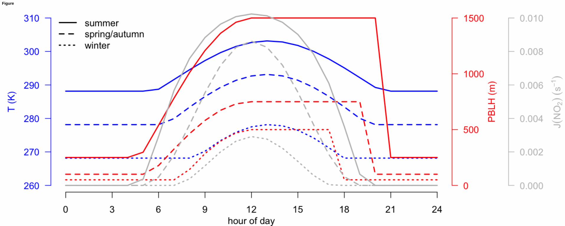
MANUSCRIP

T

ACCEPTED

ACCEPTED MANUSCRIPTFigure

MANUSCRIP

T

ACCEPTED

ACCEPTED MANUSCRIPT

Figure

MANUSCRIP

T

ACCEPTED

ACCEPTED MANUSCRIPTFigure

MANUSCRIP

T

ACCEPTED

ACCEPTED MANUSCRIPTFigure

MANUSCRIP

T

ACCEPTED

ACCEPTED MANUSCRIPT

Figure

MANUSCRIP

T

ACCEPTED

ACCEPTED MANUSCRIPT

Figure

MANUSCRIP

T

ACCEPTED

ACCEPTED MANUSCRIPTFigure

MANUSCRIP

T

ACCEPTED

ACCEPTED MANUSCRIPTFigure

MANUSCRIP

T

ACCEPTED

ACCEPTED MANUSCRIPTFigure

MANUSCRIP

T

ACCEPTED

ACCEPTED MANUSCRIPTFigure

MANUSCRIP

T

ACCEPTED

ACCEPTED MANUSCRIPTSupplementary Material

to

Influence of the choice of gas-phase mechanism on predictions of key gaseous pollutants during the AQMEII phase-2 intercomparison

by Knote et al., 2014

MANUSCRIP

T

ACCEPTED

ACCEPTED MANUSCRIPTS1) Maps of maximum 8-hour average O3 for other seasons

! Figure S1. Like Figure 3 in the main text, but for winter conditions.

MANUSCRIP

T

ACCEPTED

ACCEPTED MANUSCRIPT

! Figure S2. Like Figure 3 in the main text, but for spring conditions.

MANUSCRIP

T

ACCEPTED

ACCEPTED MANUSCRIPT

! Figure S3. Like Figure 4 in the main text, but for winter conditions.

MANUSCRIP

T

ACCEPTED

ACCEPTED MANUSCRIPT

! Figure S4. Like Figure 4 in the main text, but for spring conditions.

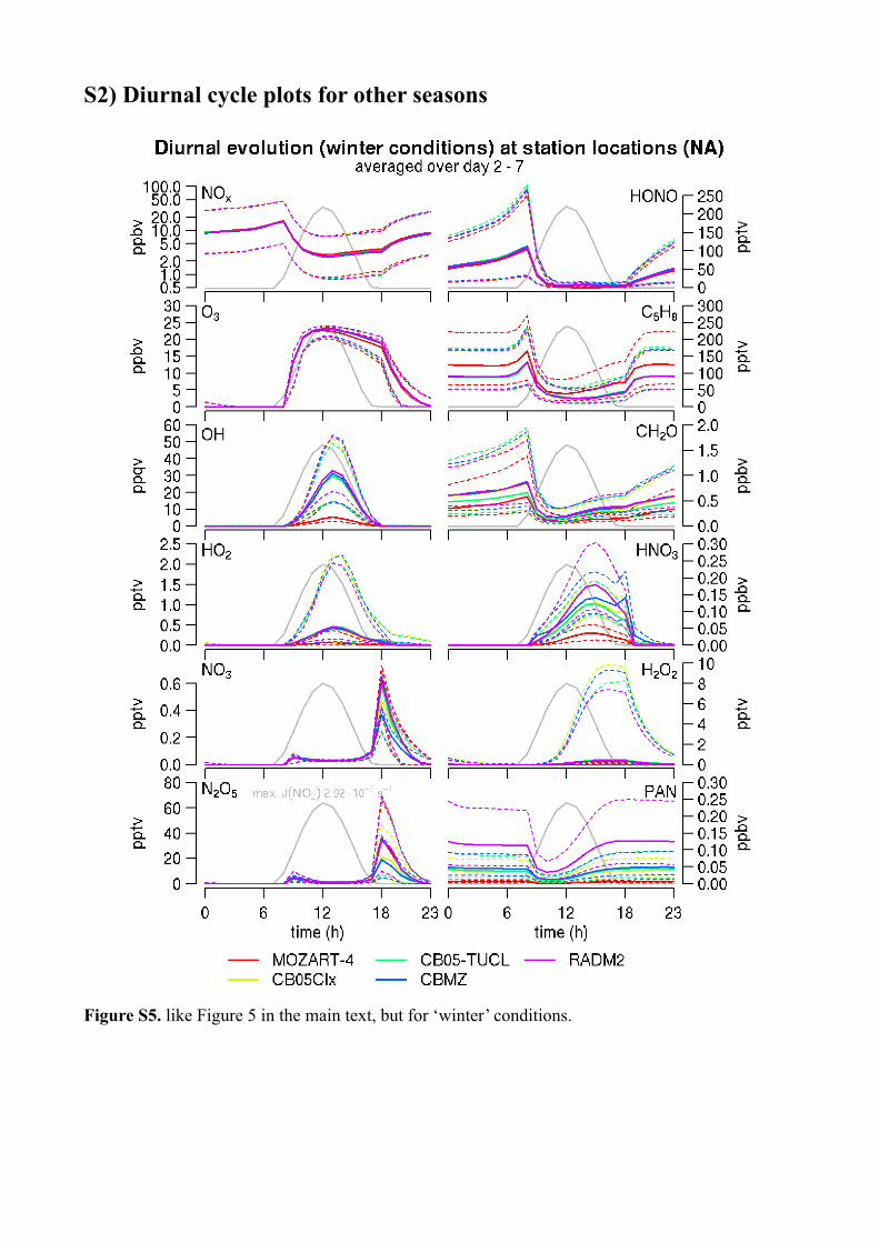
MANUSCRIP

T

ACCEPTED

ACCEPTED MANUSCRIPTS2) Diurnal cycle plots for other seasons

! Figure S5. like Figure 5 in the main text, but for ‘winter’ conditions.

MANUSCRIP

T

ACCEPTED

ACCEPTED MANUSCRIPT

! Figure S6. like Figure 5 in the main text, but for ‘spring’ conditions.

MANUSCRIP

T

ACCEPTED

ACCEPTED MANUSCRIPT

! Figure S7. like Figure 6 in the main text, but for ‘winter’ conditions.

MANUSCRIP

T

ACCEPTED

ACCEPTED MANUSCRIPT

! Figure S8. like Figure 6 in the main text, but for ‘spring’ conditions.

MANUSCRIP

T

ACCEPTED

ACCEPTED MANUSCRIPTS3) Deviations from the multi-mechanism mean diurnal cycle

! Figure S9. Absolute (solid) and relative (dashed lines) deviations from the multi-mechanism average of the median diurnal cycles (shown as solid line in Figures 5 and 6 in the main text, as well as Figures S5 - S8) for ‘winter’ conditions over North America. Relative deviations larger than +/-100% are omitted for presentation purposes.

MANUSCRIP

T

ACCEPTED

ACCEPTED MANUSCRIPT

! Figure S10. Like Figure S9, but for ‘spring/autumn’ conditions over North America.

MANUSCRIP

T

ACCEPTED

ACCEPTED MANUSCRIPT

! Figure S11. Like Figure S9, but for ‘summer’ conditions over North America.

MANUSCRIP

T

ACCEPTED

ACCEPTED MANUSCRIPT

! Figure S12. Like Figure S9, but for ‘winter’ conditions over Europe.

MANUSCRIP

T

ACCEPTED

ACCEPTED MANUSCRIPT

! Figure S13. Like Figure S9, but for ‘spring/autumn’ conditions over Europe.

MANUSCRIP

T

ACCEPTED

ACCEPTED MANUSCRIPT

! Figure S14. Like Figure S9, but for ‘summer’ conditions over Europe.

MANUSCRIP

T

ACCEPTED

ACCEPTED MANUSCRIPTS4) Corrected coding errors

A number of mistakes were discovered in the codified versions of the mechanisms as well as the emission files during preparation of this manuscript. The emissions created for the simulation using RADM2 over North America lacked the contribution from point sources. This led to underestimations of a number of pollutants. The MOZART-4 mechanism used an erroneous rate constant for NH3 + OH → M, which had considerable influence on pollutant concentrations, especially in the spring/autumn simulations (Figures S1/S2). The corrected version (Figure S5) indicates that MOZART-4 is now close to the other mechanisms. An incorrect temperature dependence of all three-body (Troe formalism) reactions and an erroneous rate equation for SOA formation from β-pinene was found in the CB05Clx mechanism. A brief evaluation using WRF-chem found only minor differences in resulting concentrations of major gaseous substances, which we can confirm with box model simulations (Figure S6). Finally, an error was found in the WRF-chem implementation of O3P + O2 → O3 of the RACM mechanism. Box model simulations using the corrected version showed that this did not impact predicted concentrations of the pollutants investigated in this work (not shown).

All these errors have been reported to the respective groups.

MANUSCRIP

T

ACCEPTED

ACCEPTED MANUSCRIPT

! !

! Figure S15: Like Figures 5 in the manuscript and S5 and S6 in the Supplementary Material, but only showing the original MOZART-4 mechanism (used in the 3-D evaluation) and the version with the fixed NH3 + OH rate constant.

MANUSCRIP

T

ACCEPTED

ACCEPTED MANUSCRIPT

! !

! Figure S16: Like Figures 5 in the manuscript and S5 and S6 in the Supplementary Material, but showing only the original CB05Clx mechanism (used in the 3-D evaluation) and the version with the fixed temperature-dependencies.

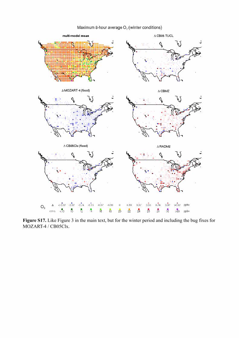
MANUSCRIP

T

ACCEPTED

ACCEPTED MANUSCRIPT

! Figure S17. Like Figure 3 in the main text, but for the winter period and including the bug fixes for MOZART-4 / CB05Clx.

MANUSCRIP

T

ACCEPTED

ACCEPTED MANUSCRIPT

! Figure S18. Like Figure 3 in the main text, but for the spring period and including the bug fixes for MOZART-4 / CB05Clx.

MANUSCRIP

T

ACCEPTED

ACCEPTED MANUSCRIPT

! Figure S19. Like Figure 3 in the main text (summer period), including the bug fixes for MOZART-4 / CB05Clx.

MANUSCRIP

T

ACCEPTED

ACCEPTED MANUSCRIPTS5) Diurnal pattern of emissions at select locations

! Figure S20. Diurnal evolution of emissions used in the simulations over North America at select locations: Urban (‘Detroit’), rural (‘Abilene’), and clean (‘Ozarks’). At each location, emissions are averaged over a 1x1 degree box to remove the influence of different grid resolutions. Locations of each box are shown on the map (top left). Part of the emissions common to all mechanisms (anthropogenic NO, NO2 and CO, as well as biogenic emissions of isoprene and terpenes) are shown on the top left. Speciated anthropogenic VOC emissions are given in the lower plots for each mechanism (in mole C km-2 hr-1 to aid visual comparability). Color coding of VOC emissions resembles compounds with similar structure across mechanisms.

MANUSCRIP

T

ACCEPTED

ACCEPTED MANUSCRIPT

! Figure S21. Like Figure S20, but for the European domain. Locations selected here are again urban (‘Paris’), rural (‘Muensterland’), and clean (‘Kozara’).

MANUSCRIP

T

ACCEPTED

ACCEPTED MANUSCRIPTS6) Location of emission conditions / stations

! Figure S22. Station locations that were used to derive the pool of emission conditions employed in the “stations” approach.