The Distributed Model Intercomparison Project (DMIP) – Phase 2 experiments in the Oklahoma Region,...

UNCORRECTED PROOF

The distributed model intercomparison project (DMIP): motivation

and experiment design

S. Reed, D.-J. Seo, V.I. Koren, M.B. Smith*, Z. Zhang, Q.-Y. Duan, F. Moreda, S. Cong

Hydrology Laboratory, Office of Hydrologic Development, WOHD-12 NOAA/National Weather Service, 1325 East-West Highway,

Silver Spring, MD 20910 USA

Received 7 May 2003; revised 11 June 2003; accepted 29 March 2004

Abstract

The distributed model intercomparison project (DMIP) was formulated as a broad comparison of many distributed models

amongst themselves and to a lumped model used for operational river forecasting in the US. DMIP was intended to provide

guidance on research and implementation directions for the US National Weather Service as well as to address unresolved

questions on the variability of rainfall and its effect on basin response. Twelve groups participated, including groups from

Canada, China, Denmark, New Zealand, and the US. Numerous data sets including seven years of concurrent radar-rainfall and

streamflow data were provided to participants through web access. Detailed modeling instructions specified calibration and

verification periods and modeling points. Participating models were run in ‘simulation’ mode without a forecast component.

DMIP proved to be a successful endeavour, providing the hydrologic research and forecasting communities with a wealth of

results. This paper presents the background and motivations for DMIP and describes the major project elements.

q 2004 Elsevier B.V. All rights reserved.

Keywords: Hydrologic model; Distributed model; Rainfall-runoff; Model comparison; Lumped model; Forecast; Simulation

1. Introduction

The distributed model intercomparison project

(DMIP) arose out of the convergence of several

factors. First, the National Oceanic and Atmospheric

Administration’s National Weather Service

(NOAA/NWS) recognized the need to infuse new

science into its river forecasting capability. Second,

the continued proliferation of geographic information

system (GIS) data sets and exponential increases in

computer capabilities have largely removed historical

barriers from the path for development of complex

distributed models. Finally, but certainly not the least

important, large questions remain regarding the effect

of the variability of precipitation and basin properties

on runoff response. Related to these questions is the

choice of model or approach to best exploit variability

information to generate improved outlet simulations

and to provide useful information at ungaged interior

points. In this section, we begin with a brief discussion

of the specific motivation for distributed models from

the NWS perspective. After this, we will discuss

several scientific motivations for launching DMIP.

Subsequent sections of this paper will describe

0022-1694/$ - see front matter q 2004 Elsevier B.V. All rights reserved.

doi:10.1016/j.jhydrol.2004.03.040

Journal of Hydrology xx (0000) xxx–xxx

www.elsevier.com/locate/jhydrol

* Corresponding author. Tel.: þ1-301-713-0640x128; fax: þ1-

301-713-0963.

E-mail addresses: [email protected] (M.B. Smith),

[email protected] (S. Reed).

HYDROL 14502—16/6/2004—18:10—VEERA—107093 – MODEL 3 – pp. 1–23

ARTICLE IN PRESS

1

2

3

4

5

6

7

8

9

10

11

12

13

14

15

16

17

18

19

20

21

22

23

24

25

26

27

28

29

30

31

32

33

34

35

36

37

38

39

40

41

42

43

44

45

46

47

48

49

50

51

52

53

54

55

56

57

58

59

60

61

62

63

64

65

66

67

68

69

70

71

72

73

74

75

76

77

78

79

80

81

82

83

84

85

86

87

88

89

90

91

92

93

94

95

96

http://www.elsevier.com/locate/jhydrol

UNCORRECTED PROOF

the DMIP goals, design, data, participants, and

modeling instructions. A companion paper (Reed

et al., 2004, this issue) presents the analyses,

conclusions, and recommendations of the DMIP

project. Beyond presenting the motivations for

DMIP, the purpose of this paper is to discuss the

major project elements so as to avoid needless

repetition in subsequent contributions in this issue.

1.1. The NWS motivation

The NWS is uniquely mandated among US federal

government agencies to provide river and flash flood

forecasts for the entire US. To accomplish this

challenging mission, the NWS has deployed the

NWS River Forecast System (NWSRFS) at 13 River

Forecast Centers (RFC) and flash flood monitoring

and prediction tools at over 120 Weather Forecast

Offices (WFO) across the nation. Daily river forecasts

are currently being provided at over 4,000 points, with

high-resolution flash flood forecasts being generated

as needed. Traditionally, forecasts have been gener-

ated through the use of lumped conceptual models.

The Hydrology Lab (HL) supports the NWS mission

by conducting scientific research, software develop-

ment, and data analysis and archival for the RFCs and

WFOs. Interested readers are referred to Glaudemans

et al. (2002), Fread et al. (1995), Larson et al. (1995)

and Stallings and Wenzel (1995) for more information

regarding the NWS river and flood forecasting

mission.

Beven (1985) outlined the benefits of distributed

modeling, including the assessment of (1) the effects

of land-use change and of spatially variable inputs and

outputs; (2) pollutant and sediment movement; and

(3) the hydrological response at ungauged sites. The

NWS recognizes these advantages and sees distrib-

uted modeling as a key pathway to infuse new science

into its river and flash flood forecast operations and

services (Carter, 2002; Koren et al., 2001). In addition

to the scientific attention focused on distributed

modeling, the NWS was also motivated to expedite

its research in this area based on guidance from

National Research Council (1996).

Given the scale of the NWS mission and the

recommendations from external reviewers, it was

clear that an accelerated and focused program was

needed to move the NWS research toward operational

distributed modeling. While numerous distributed

models exist and indeed some are moving into the

operational forecasting environment (e.g. Koren and

Barrett, 1994; Turcotte et al., 2003) it is not clear from

the literature which distributed model or modeling

approach is best to improve the NWS forecasting

capabilities. With guidance from several outside

organizations, the NWS formulated DMIP as a

method to capitalize on the wealth of distributed

modeling research being conducted at academic

institutions and other organizations around the world.

With the advent of 4 km spatial resolution and

hourly temporal resolution Next Generation Radar

(NEXRAD) rainfall estimates in many parts of the

US, the NWS and the research community at large

have access to gridded rainfall estimates at unprece-

dented spatial and temporal resolution. Other parts of

the world have similar quality radar data available

(e.g. Moore and Hall, 2000). Also, the proliferation of

GIS data sets and ever-increasing capabilities of

computer systems have continued to push distributed

modeling to the forefront of hydrologic research and

application. In light of these developments, the major

question facing the NWS and perhaps other oper-

ational organizations is: what is the best way to

exploit the information in high resolution radar

rainfall estimates and GIS data sets to improve river

and flash flood forecasting? Or, in the words of Beven

(1985), under what conditions and for what type of

forecasting is it profitable to implement a distributed

model?

A review of the scientific literature did not provide

clear guidance for the NWS. Formal comparisons of

hydrologic models for river forecasting have been

conducted (e.g. Bell et al., 2001; Moore and Bell,

2001; Moore et al., 2000; WMO, 1992, 1975), but a

coherent comparison of lumped and distributed

modeling techniques has not been published. It is

encouraging that in the development and testing of

their distributed models, several authors have

included a comparison of their results to those using

lumped inputs or from simpler lumped approaches

(Bell and Moore, 1998; Boyle et al., 2001; Smith et al.,

1999; Kull and Feldman, 1998; Michaud and

Sorooshian, 1994b; Obled et al., 1994; Pessoa et al.,

1993; Naden, 1992; Loague and Freeze, 1985). In

addition, Carpenter et al. (2001, 2003) used Monte–

Carlo analysis to evaluate distributed versus lumped


S. Reed et al. / Journal of Hydrology xx (0000) xxx–xxx2

ARTICLE IN PRESS

97

98

99

100

101

102

103

104

105

106

107

108

109

110

111

112

113

114

115

116

117

118

119

120

121

122

123

124

125

126

127

128

129

130

131

132

133

134

135

136

137

138

139

140

141

142

143

144

145

146

147

148

149

150

151

152

153

154

155

156

157

158

159

160

161

162

163

164

165

166

167

168

169

170

171

172

173

174

175

176

177

178

179

180

181

182

183

184

185

186

187

188

189

190

191

192

UNCORRECTED PROOF

model gains in light of parametric and radar rainfall

data uncertainty.

However, we feel that a more organized and

controlled comparative effort is required to guide

NWS distributed modeling research and development.

The emergence of high-resolution data sets, GIS

capabilities, and rapidly increasing computer power

has maintained distributed modeling as an active area

of research. While the utility of distributed models to

predict interior hydrologic processes is well known,

few studies have specifically addressed the improve-

ment of distributed models over lumped models for

predicting basin outflow hydrographs of the type

useful for flood forecasting. As a consequence, the

hypothesis that distributed modeling using higher

resolution data will lead to more accurate outlet

hydrograph simulations remains largely untested.

The specific requirements of the NWS are as

follows:

(a) The distributed model should perform at least as

well in an overall sense as the current operational

lumped model. Simulation improvement should

be achieved in cases of pronounced variability in

rainfall patterns and/or physical basin features

including the hydraulic properties of interior

channels.

(b) The distributed model should be operationally

feasible in current and anticipated computational

environments.

(c) The distributed model should have reliable and

objective procedures for parameterization, cali-

bration, data assimilation, and/or error

correction.

1.2. Scientific background

Major scientific issues also point to the need for

DMIP. Among these are the continuing questions

regarding the effects of rainfall and basin feature

variability on runoff hydrographs and the level of

model complexity needed to achieve a specific

objective. Numerous studies in the past three decades

have investigated the sensitivity of runoff hydro-

graphs to spatial and temporal variations in precipi-

tation as well as basin properties. Singh (1997)

provides at least one comprehensive overview,

and a brief review is provided here to show that

mixed results have been documented.

Several of these studies examined the effects of

rainfall spatial variability in light of rain gage

sampling errors. Using data from five recording

rain gages, Faures et al. (1995) concluded that

distributed modeling on small catchments requires

detailed knowledge of the spatial rainfall patterns.

These results agreed with those of Wilson et al.

(1979), who showed that the spatial distribution of

rainfall had a marked influence on the runoff

hydrograph from a small catchment. On the other

hand, Beven and Hornberger (1982) stated that

rainfall patterns have only a secondary effect on

runoff hydrographs, while a correct assessment of

the global volume of rainfall input in a variable

pattern is more important in simulating streamflow

hydrographs. Troutman (1983) investigated the

effect of rainfall variability on estimating model

parameters. He concluded that improperly repre-

senting the rainfall over a basin due to sampling

errors would lead to overestimating large runoff

events and undersimulating small events. Sub-

sequent research with radar rainfall estimates also

contributed to these mixed results. On a small

watershed, Krajweski et al. (1991) found a greater

sensitivity to the temporal resolution of precipi-

tation than to spatial resolution. Ogden and Julien

(1994) performed synthetic tests that identified

when spatial and temporal variability of precipi-

tation is dominant.

It is interesting to note that some of these and

other studies were based on synthetically generated

precipitation and streamflow records (e.g. Watts

and Calver, 1991; Troutman, 1983; Wei and

Larson, 1971). In many cases, comparisons were

made against a reference or ‘truth’ hydrograph

generated by running the hydrologic model at the

finest data resolution (e.g. Shah et al., 1996; Ogden

and Julien, 1993, 1994; Krajewski et al., 1991;

Chandrasekar, et al., 1990; Troutman, 1983;

Hamlin, 1983). Synthetically generated data were

often used due to the lack of appropriately long

periods of observed data.

Perhaps some of the mixed results from the early

studies arose out of the use of synthetic data,

numerical studies, and the choice of the rainfall-

runoff models. Many of the studies emphasizing


S. Reed et al. / Journal of Hydrology xx (0000) xxx–xxx 3

ARTICLE IN PRESS

193

194

195

196

197

198

199

200

201

202

203

204

205

206

207

208

209

210

211

212

213

214

215

216

217

218

219

220

221

222

223

224

225

226

227

228

229

230

231

232

233

234

235

236

237

238

239

240

241

242

243

244

245

246

247

248

249

250

251

252

253

254

255

256

257

258

259

260

261

262

263

264

265

266

267

268

269

270

271

272

273

274

275

276

277

278

279

280

281

282

283

284

285

286

287

288

UNCORRECTED PROOF

the importance of rainfall spatial variability used

models containing the Hortonian runoff generation

mechanism. It is now recognized that runoff results

from a complex variety of mechanisms and that in

some basins a significant portion of runoff hydro-

graphs is derived from slower responding subsurface

runoff (Wood et al., 1990). Obled et al. (1994)

commented that numerical experiments in the litera-

ture were based on the use of models which may be

only a crude representation of reality. Furthermore,

they argued that the actual processes at work in a

basin may not be those predicted by the model, a

caution echoed by Michaud and Sorooshian (1994a),

Shah et al. (1996) and Morin et al. (2001).

Thus, the research in the literature may have

highlighted the sensitivity of a particular model to the

spatial and temporal variability of (at times synthetic)

precipitation, not the sensitivity of the actual basin.

The work of Obled et al. (1994) is significant in that

they examined the effects of the spatial variation of

rainfall using observed precipitation and streamflow

data rather than simply model output derived using

synthetic data. In addition, the model used in their

studies focused on saturation excess runoff as the

main runoff generation mechanism. In simulations

against observed data, they were unable to prove the

value of distributed inputs as they had intended. A

semi-distributed representation of the basin did not

lead to improved simulations compared to a lumped

basin modeling scenario. The authors reasoned that

the runoff mechanism may be responsible for the lack

of improvement, noting that in runoff generation of

the Dunne type, most of the water infiltrates and local

variations in input will be smoothed. As a result, this

type of mechanism may be much less sensitive to

different rainfall patterns. Loague (1990) concluded

that revised data did not lead to significant improve-

ment in a physically based distributed model because

the model used the Hortonian mechanism while the

basin appeared to function with a combination of

Hortonian and Dunne overland flow. Michaud and

Sorooshian (1994a) recommended that more com-

parative work be performed on Hortonian versus

Dunne overland flow.

Winchell et al. (1997, 1998) extend this theme by

noting that there has been a bias towards the use of

infiltration-excess runoff mechanisms as opposed to

the saturation excess type. Their work with both types

of runoff generation mechanisms found that satur-

ation-excess and infiltration excess models respond

differently to uncertainty in precipitation. They

suggest that generalizations concerning the effects of

rainfall variability on runoff generation and variability

cannot be made. Koren et al. (1999) came to a similar

conclusion based on simulation results from several

different rainfall-runoff partitioning mechanisms.

In the midst of these efforts to understand the

importance of the variability of precipitation, a large

volume of research continues to emerge that addresses

the possibility of improving lumped hydrologic

simulations by using distributed and semi-distributed

modeling approaches containing so-called physically

based or conceptual rainfall-runoff mechanisms.

Indeed, at least one book chapter (Beven, 1985)

followed by two entire books have been published on

such models (Abbot and Refsgaard, 1996; Vieux,

2001). Recently, the availability of high-resolution

precipitation estimates from different weather radar

platforms has intensified these investigations. Many

efforts have focused on event-based modeling and

again, mixed and somewhat surprising results have

been realized.

Refsgaard and Knudsen (1996) compared a

complex distributed model, a lumped conceptual

model, and an intermediate complexity model on

data-sparse catchments in Zimbabwe. Their results

could not strongly justify the use of the complex

distributed model. Pessoa et al. (1993) found that

adequately averaged gridded precipitation estimates

from radar were just as viable as fully distributed

estimates for streamflow simulation using a dis-

tributed model on an 840 km2 basin with low

intensity rainfall. Conversely, Michaud and

Sorooshian (1994a) compared their results with

high intensity rainfall and found that simulated

runoff is greatly sensitive to space-time averaging.

Kouwen and Garland (1989) investigated the effects

of radar data resolution and attempted to develop

guidelines for the proper resolution of input rainfall

data resolution. They noted that spatially coarser

rainfall data sometimes led to better hydrograph

simulation due to the smoothing of errors present

in finer resolution rainfall information. Bell and

Moore (2000) noted a similar model response from

lower resolution rainfall information. Continuing

this theme, Carpenter et al. (2001) examined



ARTICLE IN PRESS

289

290

291

292

293

294

295

296

297

298

299

300

301

302

303

304

305

306

307

308

309

310

311

312

313

314

315

316

317

318

319

320

321

322

323

324

325

326

327

328

329

330

331

332

333

334

335

336

337

338

339

340

341

342

343

344

345

346

347

348

349

350

351

352

353

354

355

356

357

358

359

360

361

362

363

364

365

366

367

368

369

370

371

372

373

374

375

376

377

378

379

380

381

382

383

384

UNCORRECTED PROOF

the gains from distributed versus lumped modeling

in view of radar data and parametric uncertainty. In

several cases a spatially lumped model response

proved to be statistically indistinguishable from a

distributed model response.

In preliminary testing limited to a single

extreme event, Kenner et al. (1996) reported that

a five sub-basin approach produced better hydro-

graph agreement than a lumped representation of

the basin. Sub-basin rainfall hyetographs revealed

spatially varied precipitation totals for the event.

Smith et al. (1999) attempted to capture the spatial

variability of precipitation using sub-basins for

several watersheds in the southern Great Plains of

the US. Using a simple semi-distributed approach

with spatially uniform conceptual model para-

meters, they were unable to realize significant

improvement over a lumped model. For a basin in

the same geographic region, Boyle et al. (2001)

concluded that eight subdivisions of a basin

provided no gain in simulation accuracy compared

to a three sub-basin representation. Apparently, the

more coarse representation of the basin captured

the essential variability of the rainfall and basin

features. However, both simulations were superior

to those from a lumped model. Naden (1992) found

that lumped modeling was appropriate for even a

large 7000 km2 basin.

Refsgaard (1997) illustrated the concepts of

parameterization, calibration, and validation of

distributed parameter models. Noting that hydrolo-

gists often assume that a distributed model

calibrated to basin outlet information will ade-

quately model interior processes, he realized poor

simulations of discharge and piezometric head at

three interior gaging stations. In contrast, Michaud

and Sorooshian (1994b) found that a complex

distributed model calibrated at the basin outlet

was able to generate simulations at eight internal

points that were at least as accurate as the outlet

simulations. These results underscore one of the

mains advantages of distributed parameter hydro-

logic modeling: the ability to predict hydrologic

variables at interior points. They also concluded

that a simple distributed model proved to be just as

accurate as a complex distributed model given that

both were calibrated and noted that model com-

plexity does not necessarily lead to improved

simulation accuracy. Studies such as this may

have caused Robinson and Sivapalan (1995) to

comment that further work is needed to fully

exploit the connection between conceptual and

physically based models to advance the science of

hydrologic prediction. The distributed modeling

work of Koren et al. (2003a,b) is one attempt to

follow this recommendation.

Bell and Moore (1998) compared a simple gridded

distributed model and its variants to a lumped model

used operationally in the UK for flood forecasting.

They concluded that a well-designed lumped model is

preferred for routine operational purposes on the

basins studied. Yet, a distributed model run in parallel

to the lumped model would provide meaningful

information in the cases of significant rainfall

variability.

Seyfried and Wilcox (1995) commented that

many have even questioned the usefulness of

complex physically based models outside of strictly

research applications, especially in light of the

effort required to parameterize, calibrate, and

implement such models.

In light of these findings, DMIP was formulated

as a focused venue to evaluate many distributed

models against both a calibrated lumped model and

observed streamflow data. Compared to some of

the earlier studies on the effects of rainfall

variability, DMIP has the advantages of multi-

year hourly time series of high resolution radar-

based rainfall estimates as well as hourly discharge

measurements at both basin outlets and several

interior points. Over seven years of concurrent

radar rainfall and streamflow data were available.

Another aspect of this venue is that researchers

would have the opportunity to evaluate their

research models with data typically used for

operational forecasting. The availability of these

data sets had already attracted several researchers

to set up and run their models on these basins (e.g.

Vieux and Moreda, 2003; Carpenter et al., 2001;

Finnerty et al., 1997; Bradley, 1997). Moreover, the

study basins are free of major complications such

as orographic influences, significant snow accumu-

lation, and stream regulation, which may mask the

effects of precipitation and basin feature variability.

The basins selected for DMIP range from 65 to

almost 2500 km2, removing the temptation to



ARTICLE IN PRESS

385

386

387

388

389

390

391

392

393

394

395

396

397

398

399

400

401

402

403

404

405

406

407

408

409

410

411

412

413

414

415

416

417

418

419

420

421

422

423

424

425

426

427

428

429

430

431

432

433

434

435

436

437

438

439

440

441

442

443

444

445

446

447

448

449

450

451

452

453

454

455

456

457

458

459

460

461

462

463

464

465

466

467

468

469

470

471

472

473

474

475

476

477

478

479

480

UNCORRECTED PROOF

extrapolate conclusions from small scale hillslope

studies to larger basins of the size typically used

for operational forecasting.

2. Project design

DMIP identified the following science questions.

Some questions were explicitly addressed through the

design of the simulation tests discussed in Section 8

and Appendix B, while for others, it was hoped that

inferences could be made given a broad range of

participating models.

Can distributed models provide increased simu-

lation accuracy compared to lumped models? This

question would be addressed through the use of

multiple distributed model simulations compared to

lumped simulations for a number of basins. In the

absence of data sets such as spatial fields of soil

moisture observations, model calibration and vali-

dation would use observed streamflow data. Improv-

ing simulations at the outlet of basins is the focus of

this effort.

What level of model complexity is required to

realize improvement in basin outlet simulations?

Included in this are questions regarding the use of

conceptual versus so-called physically based models

and the size of computational elements or the use of

semi-distributed approaches. Given a group of

participating models with a wide range of complexity

and modeling scale, it was hoped that inferences could

be made about model complexity and scale.

What level of effort is required for distributed

model calibration? What improvements are realized

compared to non-calibrated and calibrated lumped

models? Participants would provide an overview of

the process to calibrate their models. Modeling

instructions explicitly called for uncalibrated and

calibrated simulations, so that the gains by calibration

could be weighed against the level of effort. Reed

et al., (2003, this issue) discuss the gains provided by

calibration.

What is the potential for distributed models set up

for basin outlet simulations to generate meaningful

hydrographs at interior locations for flash flood

forecasting? Inherent to this question is the hypo-

thesis that better outlet simulations are the result of

accurate hydrologic simulations at points upstream of

the gaged outlet. The NWS is interested in the

concept of a distributed model for forecasting both

outlet hydrographs as well as smaller scale flash

floods upstream of the gage. As noted in the

modeling instructions, calibrated and uncalibrated

simulations at various gaged and ungaged locations

at basin interior points were required. Reed et al.

(2003, this issue) evaluate these interior point

simulations.

What characteristics identify a basin as one

likely to benefit from distributed modeling versus

lumped modeling for basin outlet simulations? Can

these characteristics be quantified? Prior research

on the DMIP basins had shown that distributed

modeling to capture the essential variability of

precipitation and model parameters did not signifi-

cantly improve simulations in the Illinois River

basin. (Carpenter et al., 2001; Smith et al., 1999).

On the other hand, another basin in the same

geographic region did benefit from one level of

distributed modeling (Zhang et al., 2003; Boyle

et al., 2001). What is different between these two

cases? Through additional simulations from a

number of distributed models in DMIP, these

prior results could be verified. Given the validated

conclusion that certain basins benefit from dis-

tributed modeling, one could investigate potential

diagnostic indicators that might be used without the

expense of setting up a distributed model.

How do research models behave with forcing data

used for operational forecasting? DMIP provided a

realistic opportunity for developers to test their

research models in a quasi-operational environment.

Such exposure would hopefully identify needed

model improvements or further tests to bring such

models closer to operational use. Conversely, DMIP

could highlight the need for continued research for

improving radar or multi-sensor methods of precipi-

tation estimation.

What is the nature and effect of rainfall spatial

variability in the DMIP basins? The 7 years of

gridded radar-based rainfall values presented in DMIP

would provide modelers an opportunity to investigate

the dominant forms of rainfall spatial variability.

Moreover, through the application of multiple dis-

tributed models, we hoped to refine our understanding

of the effects of rainfall spatial variability on

simulated basin outlet hydrographs.



ARTICLE IN PRESS

481

482

483

484

485

486

487

488

489

490

491

492

493

494

495

496

497

498

499

500

501

502

503

504

505

506

507

508

509

510

511

512

513

514

515

516

517

518

519

520

521

522

523

524

525

526

527

528

529

530

531

532

533

534

535

536

537

538

539

540

541

542

543

544

545

546

547

548

549

550

551

552

553

554

555

556

557

558

559

560

561

562

563

564

565

566

567

568

569

570

571

572

573

574

575

576

UNCORRECTED PROOF

In addition to these identified issues, the partici-

pants investigated other relevant questions using the

DMIP data sets. These efforts are presented in this

special issue.

3. Operational issues

As with the science questions surrounding DMIP,

issues that need to be addressed before a model can be

implemented in NWSRFS for operational use were

identified. Explicit experiments were not designed in

DMIP to address these issues. Rather, general

concepts were discussed at the DMIP workshop.

1. Computational requirements in an operational

environment. To be effective in an operationally

viable environment, the models need to be

accurate, reliable, robust, and be able to run in

real time.

2. Run time modifications and updates in an oper-

ational forecasting setting.

3. Parameterization and calibration requirements.

4. Does easier parameterization/calibration of a

physically based distributed parameter model

warrant its use, even when it might not provide

improvements over simpler lumped conceptual

models?

4. DMIP study area

4.1. Description of study basins

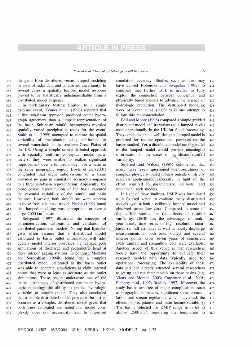
Figs. 1 and 2 present the basins used in the DMIP

comparison. The Illinois River draining to the USGS

gage at Tahlequah, Oklahoma (OK) straddles the

Oklahoma-Arkansas (AR) border and contains the

Illinois River basin above Watts, OK. Baron Fork

drains to the USGS gage in Eldon, OK and then joins

the Illinois River a few miles downstream. The Elk

River flowing to the USGS gage in Tiff City, Missouri

(MO) lies to the north of the Illinois basin, while the

Blue River basin lies to the south near the border with

Fig. 1. Location map of DMIP study basins. Numbers are location of USGS stream gages. Letters are locations of ungaged computational points.

Blue lines are rivers.



ARTICLE IN PRESS

577

578

579

580

581

582

583

584

585

586

587

588

589

590

591

592

593

594

595

596

597

598

599

600

601

602

603

604

605

606

607

608

609

610

611

612

613

614

615

616

617

618

619

620

621

622

623

624

625

626

627

628

629

630

631

632

633

634

635

636

637

638

639

640

641

642

643

644

645

646

647

648

649

650

651

652

653

654

655

656

657

658

659

660

661

662

663

664

665

666

667

668

669

670

671

672

UNCORRECTED PROOF

Texas (TX). These basins are typical of the size used

for operational forecasting in the NWS. The numbers

in Fig. 1 signify the locations of US Geological

Survey (USGS) stream gages at forecast locations and

at interior points. Letters denote the location of

ungaged points specified for the computation of

simulations according to the DMIP modeling instruc-

tions. Hereafter, we will use the terms basin outlet and

interior point when making general statements about

the locations represented by numbers and letters,

respectively.

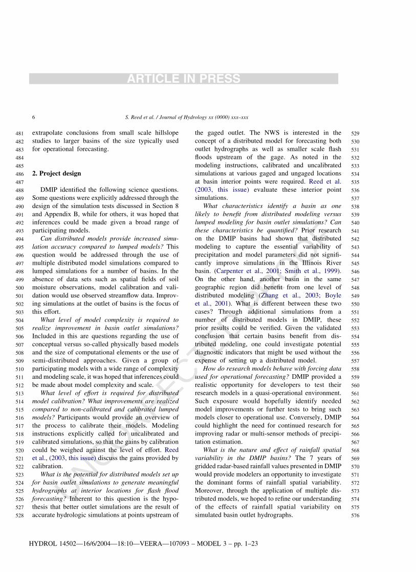
Fig. 2 shows the location of the basins in relation to

state boundaries and the NEXRAD radar locations. It

can be seen that all the DMIP basins are well inside

least one radar umbrella.

Table 1 presents relevant data for the basins. The

annual rainfall statistics in column five for the DMIP

data period were computed using the radar-based data,

while the corresponding climatological statistics were

computed using raingauge data. A measure of basin

shape is included in Table 1, generated by computing

a ratio of long to short basin axes. The Blue basin has

a significantly different aspect ratio compared to the

other candidate basins. Hereafter, and in Reed et al.

(2004, this issue), we will use the shortened names in

column three of Table 1 to refer to the basins.

The dominant soil types in the DMIP basins are

presented in Table 2. The table values are estimates of

percent by volume of soils for all depths reported in the

11-layer grid derived from the State Soil Geographic

(STATSGO) dataset by Miller and White (1999).

Based on visual inspection of the 11 layers for each

basin, the heavier soils tend to occur at greater depths.

For example, in the Tahlequah basin, which is mostly

SIL (silt loam), SICL (silty clay loam), and SIC (silty

clay), the SIL is generally closer to the surface with

SICL deeper and SIC even deeper. Peters and Easton

(1996) describe the Tahlequah basin as a region

comprised of porous limestone overlain by cherty

soils. Areas within the floodplain can contain gravelly

soils and may be too pervious to hold water. It is

notable that the Blue basin contains a very high

Fig. 2. Location of NEXRAD radar sites and coverage of DMIP basins. Circles denote the coverage of each radar. Radius of the radar umbrella

is 230 km.



ARTICLE IN PRESS

673

674

675

676

677

678

679

680

681

682

683

684

685

686

687

688

689

690

691

692

693

694

695

696

697

698

699

700

701

702

703

704

705

706

707

708

709

710

711

712

713

714

715

716

717

718

719

720

721

722

723

724

725

726

727

728

729

730

731

732

733

734

735

736

737

738

739

740

741

742

743

744

745

746

747

748

749

750

751

752

753

754

755

756

757

758

759

760

761

762

763

764

765

766

767

768

UNCORRECTED PROOF

percentage of clay and is much different in its soil

texture composition than the other DMIP basins.

The dominant industry in the Blue, Eldon,

Tahlequah, and Tiff City basins is agriculture,

consisting primarily of poultry production and live-

stock grazing. A small percentage of the Tahlequah

basin is farmed intensively for vegetables, strawber-

ries, fruit orchards, and nurseries (Meo et al., 2002).

Approximately 90% of the Tahlequah basin is

comprised of pasture and forest (Vieux and Moreda,

2003a). The Watts basin contains the Ozark National

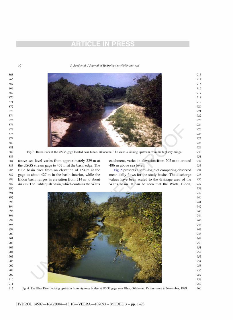
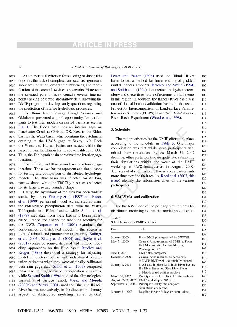
Forest. Fig. 3 shows the Baron Fork upstream of the

gage near Eldon, Oklahoma. Fig. 4 shows the Blue

River looking upstream from the gage near the town

of Blue, Oklahoma.

The topography of the Blue, Tiff City, Eldon, and

Tahlequah basins can be characterized as gently

rolling to hilly. In the Tiff City basin, the elevation

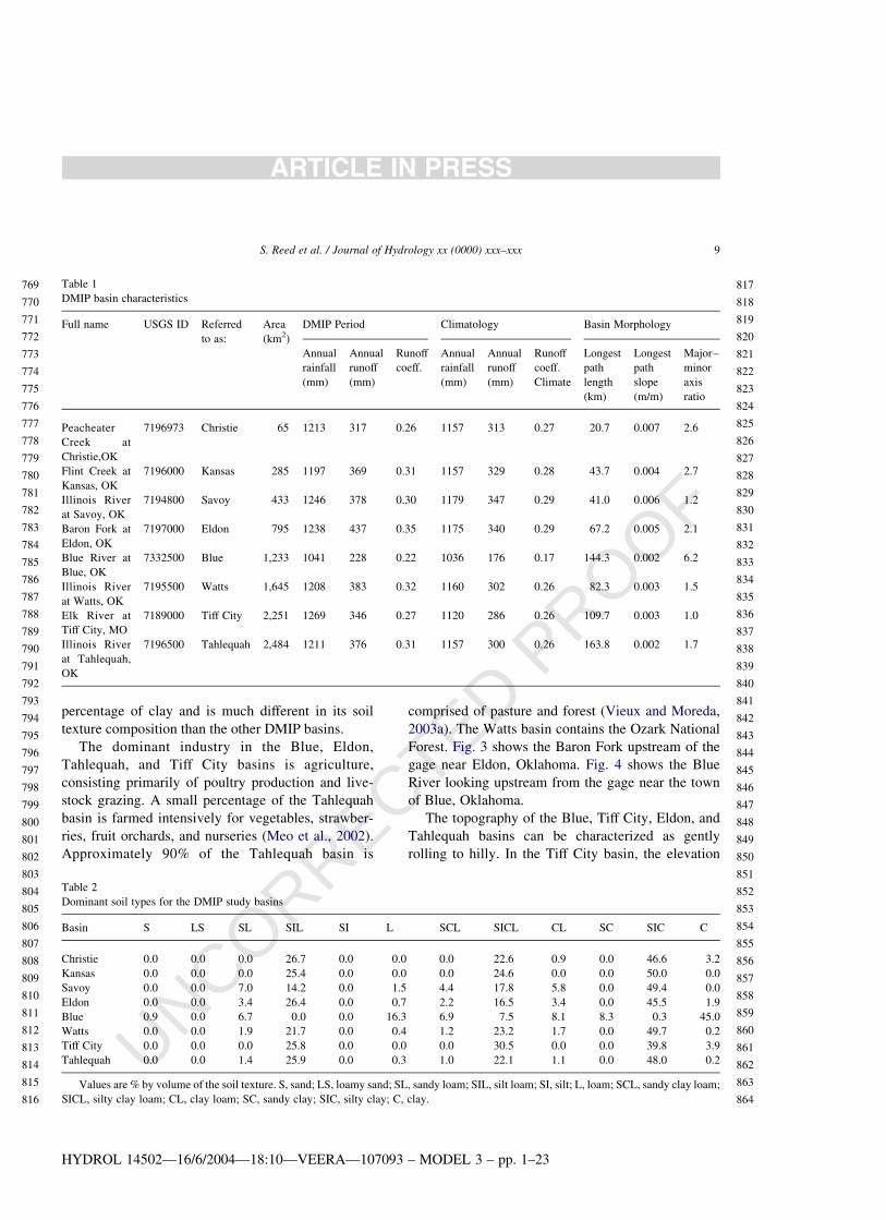
Table 1

DMIP basin characteristics

Full name USGS ID Referred

to as:

Area

(km2)

DMIP Period Climatology Basin Morphology

Annual

rainfall

(mm)

Annual

runoff

(mm)

Runoff

coeff.

Annual

rainfall

(mm)

Annual

runoff

(mm)

Runoff

coeff.

Climate

Longest

path

length

(km)

Longest

path

slope

(m/m)

Major–

minor

axis

ratio

Peacheater

Creek at

Christie,OK

7196973 Christie 65 1213 317 0.26 1157 313 0.27 20.7 0.007 2.6

Flint Creek at

Kansas, OK

7196000 Kansas 285 1197 369 0.31 1157 329 0.28 43.7 0.004 2.7

Illinois River

at Savoy, OK

7194800 Savoy 433 1246 378 0.30 1179 347 0.29 41.0 0.006 1.2

Baron Fork at

Eldon, OK

7197000 Eldon 795 1238 437 0.35 1175 340 0.29 67.2 0.005 2.1

Blue River at

Blue, OK

7332500 Blue 1,233 1041 228 0.22 1036 176 0.17 144.3 0.002 6.2

Illinois River

at Watts, OK

7195500 Watts 1,645 1208 383 0.32 1160 302 0.26 82.3 0.003 1.5

Elk River at

Tiff City, MO

7189000 Tiff City 2,251 1269 346 0.27 1120 286 0.26 109.7 0.003 1.0

Illinois River

at Tahlequah,

OK

7196500 Tahlequah 2,484 1211 376 0.31 1157 300 0.26 163.8 0.002 1.7

Table 2

Dominant soil types for the DMIP study basins

Basin S LS SL SIL SI L SCL SICL CL SC SIC C

Christie 0.0 0.0 0.0 26.7 0.0 0.0 0.0 22.6 0.9 0.0 46.6 3.2

Kansas 0.0 0.0 0.0 25.4 0.0 0.0 0.0 24.6 0.0 0.0 50.0 0.0

Savoy 0.0 0.0 7.0 14.2 0.0 1.5 4.4 17.8 5.8 0.0 49.4 0.0

Eldon 0.0 0.0 3.4 26.4 0.0 0.7 2.2 16.5 3.4 0.0 45.5 1.9

Blue 0.9 0.0 6.7 0.0 0.0 16.3 6.9 7.5 8.1 8.3 0.3 45.0

Watts 0.0 0.0 1.9 21.7 0.0 0.4 1.2 23.2 1.7 0.0 49.7 0.2

Tiff City 0.0 0.0 0.0 25.8 0.0 0.0 0.0 30.5 0.0 0.0 39.8 3.9

Tahlequah 0.0 0.0 1.4 25.9 0.0 0.3 1.0 22.1 1.1 0.0 48.0 0.2

Values are % by volume of the soil texture. S, sand; LS, loamy sand; SL, sandy loam; SIL, silt loam; SI, silt; L, loam; SCL, sandy clay loam;

SICL, silty clay loam; CL, clay loam; SC, sandy clay; SIC, silty clay; C, clay.



ARTICLE IN PRESS

769

770

771

772

773

774

775

776

777

778

779

780

781

782

783

784

785

786

787

788

789

790

791

792

793

794

795

796

797

798

799

800

801

802

803

804

805

806

807

808

809

810

811

812

813

814

815

816

817

818

819

820

821

822

823

824

825

826

827

828

829

830

831

832

833

834

835

836

837

838

839

840

841

842

843

844

845

846

847

848

849

850

851

852

853

854

855

856

857

858

859

860

861

862

863

864

UNCORRECTED PROOF

above sea level varies from approximately 229 m at

the USGS stream gage to 457 m at the basin edge. The

Blue basin rises from an elevation of 154 m at the

gage to about 427 m in the basin interior, while the

Eldon basin ranges in elevation from 214 m to about

443 m. The Tahlequah basin, which contains the Watts

catchment, varies in elevation from 202 m to around

486 m above sea level.

Fig. 5 presents a semi-log plot comparing observed

mean daily flows for the study basins. The discharge

values have been scaled to the drainage area of the

Watts basin. It can be seen that the Watts, Eldon,

Fig. 3. Baron Fork at the USGS gage located near Eldon, Oklahoma. The view is looking upstream from the highway bridge.

Fig. 4. The Blue River looking upstream from highway bridge at USGS gage near Blue, Oklahoma. Picture taken in November, 1999.



ARTICLE IN PRESS

865

866

867

868

869

870

871

872

873

874

875

876

877

878

879

880

881

882

883

884

885

886

887

888

889

890

891

892

893

894

895

896

897

898

899

900

901

902

903

904

905

906

907

908

909

910

911

912

913

914

915

916

917

918

919

920

921

922

923

924

925

926

927

928

929

930

931

932

933

934

935

936

937

938

939

940

941

942

943

944

945

946

947

948

949

950

951

952

953

954

955

956

957

958

959

960

UNCORRECTED PROOF

Tahlequah, and Tiff City basins behave somewhat

similarly with small variations in the hydrograph

recession rates. On the other hand, Blue exhibits quite

distinguishable behavior with much less base flow and

quickly falling hydrograph recessions.

Field trips were conducted on two different

occasions. Personnel from the NWS and the Univer-

sity of Arizona examined points in the Eldon, Watts,

and Tahlequah basins in 1997, while a three day visit

to the Blue basin in November, 1999 was made by

NWS scientists to collect cross-section measure-

ments. Fig. 6 presents a few of these cross sections.

4.2. Rationale for basin selection

The study basins in Fig. 1 were selected for several

reasons. First, these basins had the data required to

conduct the intercomparison, beginning with the

longest and highest quality archive of NEXRAD

radar-based precipitation estimates in the US. The

NWS began measuring precipitation with NEXRAD

radars in this region in 1993, providing the DMIP

project with nearly 8 years of continuous hourly

gridded precipitation estimates. The NEXRAD radars

in this area provide good coverage of the study basins

as shown in Fig. 2. Also, several pertinent studies of

the quality of the NEXRAD precipitation estimates in

this region have been performed. (e.g. Young et al.,

2000; Wang et al., 2000; Smith et al., 1999; Johnson

et al., 1999; Finnerty and Johnson, 1997; and Smith

et al.,1996). Concurrent time series of hourly

discharge data were also available for the basin

outlets and selected interior points.

Fig. 5. Semi-log plot of observed streamflow for the DMIP basins. Discharge values have been scaled to a common drainage area.

Fig. 6. Selected cross-sections for the Blue River. Cross section 1 is

located at the USGS gage. Sections are plotted in meters above

mean sea level (msl).



ARTICLE IN PRESS

961

962

963

964

965

966

967

968

969

970

971

972

973

974

975

976

977

978

979

980

981

982

983

984

985

986

987

988

989

990

991

992

993

994

995

996

997

998

999

1000

1001

1002

1003

1004

1005

1006

1007

1008

1009

1010

1011

1012

1013

1014

1015

1016

1017

1018

1019

1020

1021

1022

1023

1024

1025

1026

1027

1028

1029

1030

1031

1032

1033

1034

1035

1036

1037

1038

1039

1040

1041

1042

1043

1044

1045

1046

1047

1048

1049

1050

1051

1052

1053

1054

1055

1056

UNCORRECTED PROOF

Another critical criterion for selecting basins in this

region is the lack of complications such as significant

snow accumulation, orographic influences, and modi-

fication of the streamflow due to reservoirs. Moreover,

the selected parent basins contain several internal

points having observed streamflow data, allowing the

DMIP program to develop study questions regarding

the prediction of interior hydrologic processes.

The Illinois River flowing through Arkansas and

Oklahoma presented a good opportunity for partici-

pants to test their models on nested basins as seen in

Fig. 1. The Eldon basin has an interior gage on

Peacheater Creek at Christie, OK. Next to the Eldon

basin is the Watts basin, which contains the catchment

draining to the USGS gage at Savoy, AR. Both

the Watts and Kansas basins are nested within the

largest basin, the Illinois River above Tahlequah, OK.

Thus, the Tahlequah basin contains three interior gage

locations.

The Tiff City and Blue basins have no interior gage

locations. These two basins represent additional cases

for testing and comparison of distributed hydrologic

models. The Blue basin was selected for its long

narrow shape, while the Tiff City basin was selected

for its large size and rounded shape.

Lastly, the hydrology of the area has been widely

studied by others. Finnerty et al. (1997) and Koren

et al. (1999) performed model scaling studies using

the radar-based precipitation data from the Watts,

Tahlequah, and Eldon basins, while Smith et al.

(1999) used data from these basins to begin radar-

based lumped and distributed modeling research for

the NWS. Carpenter et al. (2001) examined the

performance of distributed models in this region in

light of rainfall and parameteric uncertainty. Kalinga

et al. (2003), Zhang et al. (2004) and Boyle et al.

(2001) compared semi-distributed and lumped mod-

eling approaches on the Blue basin. Bradley and

Kruger (1998) developed a strategy for adjusting

model parameters for use with radar-based precipi-

tation estimates when they were originally calibrated

with rain gage data. Smith et al. (1996) compared

radar and rain gage-based precipitation estimates,

while Seo and Smith (1996) studied the climatological

variability of surface runoff. Vieux and Moreda

(2003b) and Vieux (2001) used the Blue and Illinois

River basins, respectively, in the discussion of many

aspects of distributed modeling related to GIS.

Peters and Easton (1996) used the Illinois River

basin to test a method for linear routing of gridded

rainfall excess amounts. Bradley and Smith (1994)

and Smith et al. (1994) documented the hydrometeor-

ology and space-time nature of extreme rainfall events

in this region. In addition, the Illinois River basin was

one of six calibration/validation basins in the recent

Project for Intercomparison of Land-surface Parame-

terization Schemes (PILPS) Phase 2(c) Red-Arkansas

River Basin Experiment (Wood et al., 1998).

5. Schedule

The major activities for the DMIP effort took place

according to the schedule in Table 3. One major

complication was that while some participants sub-

mitted their simulations by the March 31, 2002

deadline, other participants were quite late, submitting

their simulations within one week of the DMIP

workshop at NWS headquarters in August, 2002.

This spread of submissions allowed some participants

more time to refine their results. Reed et al. (2003, this

issue) identify the submission dates of the various

participants.

6. SAC-SMA and calibration

For the NWS, one of the primary requirements for

distributed modeling is that the model should equal

Table 3

Schedule for major DMIP activities

Date Task

January, 2000 Basic DMIP plan approved by NWS/HL

May 31, 2000 General Announcement of DMIP at Town

Hall Meeting, AGU spring Meeting,

Washington, DC

June 1, 2000 DMIP plan completed

December 2000 General Announcement to participate

in DMIP DMIP web site officially opened.

January 1, 2001 1. All data in place for Illinois River Basins,

Elk River Basin and Blue River Basin

2. Metadata and utilities in place

March 31, 2002 Participants send results to HL for analysis

August 22-23, 2002 DMIP workshop at NWS/HL

September 30, 2002 Participants verify that analyzed

simulations are correct

January 31, 2003 Deadline for any follow-up submissions.



ARTICLE IN PRESS

1057

1058

1059

1060

1061

1062

1063

1064

1065

1066

1067

1068

1069

1070

1071

1072

1073

1074

1075

1076

1077

1078

1079

1080

1081

1082

1083

1084

1085

1086

1087

1088

1089

1090

1091

1092

1093

1094

1095

1096

1097

1098

1099

1100

1101

1102

1103

1104

1105

1106

1107

1108

1109

1110

1111

1112

1113

1114

1115

1116

1117

1118

1119

1120

1121

1122

1123

1124

1125

1126

1127

1128

1129

1130

1131

1132

1133

1134

1135

1136

1137

1138

1139

1140

1141

1142

1143

1144

1145

1146

1147

1148

1149

1150

1151

1152

UNCORRECTED PROOF

or improve upon the performance of the current

operational lumped approach. To examine this

concern, simulations in DMIP were compared to

both observed hourly streamflow and to simulations

from the current NWS operational model, the

Sacramento Soil Moisture Accounting Model

(SAC-SMA). The SAC-SMA is a two-layer concep-

tual model that generates a number of runoff

components. Interested readers are referred to

Finnerty et al. (1997) and Burnash (1995) for more

information. The SAC-SMA model was calibrated

following the NWS manual procedure outlined in

Smith et al. (2003). Subsequently, the calibrations

were evaluated by an independent expert. Another

indication as to the quality of the calibration is that

the process resulted in a logical and spatially

consistent set of parameters (Koren et al., 2003a,b).

Uncalibrated simulations for the lumped model were

made using the a priori parameter estimates pio-

neered by Koren et al. (2000) and subsequently used

by Duan et al. (2001). While these parameters are

derived from soil texture data, they nonetheless still

require further calibration. In this way they meet the

criteria in the DMIP Modeling Instructions (Section

8) that called for participants to use initial/uncali-

brated parameters in specific cases.

7. Data

Every effort was made to encourage participatin in

DMIP. As such, all data needed for most models were

assembled and made available through a website/ftp

site. A brief discussion of each data set is presented.

7.1. Digital elevation model (DEM) data

Participants were free to use any DEM data

available. However, to encourage participation in

DMIP, DEMs of two different resolutions were

provided: 15 arc s DEM data and 1 arc s data. DMIP

did not require the use of any particular DEM or

modeling resolution. The only constraint was that

modelers had to discretize the basin so that simu-

lations could be produced at the required locations.

The NWS National Operational Hydrologic

Remote Sensing Center (NOHRSC) created a

15 arc s national DEM by resampling 3 arc s DEMs

(1:250,000 scale) distributed by the US Geological

Survey. These data represent sampled elevations at

regularly spaced, 15 arc-second (0.00416668) inter-

vals, in geographic coordinates.

The 1 arc s (30 m) data covering the DMIP study

areas were made available for this project as an

offshoot of the National Basin Delineation project

underway at NOAA’s National Severe Storms

Laboratory (NSSL). The primary goal of the National

Basin Delineation project is to provide small-basin

boundaries for the NWS Flash-flood Monitoring and

Prediction Program (FFMP). To produce the small-

basin boundaries, NSSL is cooperating with the USGS

EROS data center to use the 1 arc s DEM data

available from the USGS National Elevation Dataset

(NED) project. NSSL organizes their data processing

efforts by eight digit USGS Hydrologic Cataloging

Unit (HUC) boundaries. Initial processing steps

include:

1. buffering the HUC boundary of interest to allow for

differences in ridgelines defined by the DEM and

defined by the digitized HUCs

2. merging the required 7.5 minute blocks of DEM

data into a seamless data set covering the HUC of

interest

3. projecting the seemless data set to allow for correct

analysis using Arc/Info software

4. ‘filling’ the DEM to eliminate artificial sinks

(using the Arc/Info fill command).

The filled DEMs (product of Steps 1–4) for HUCs

covering the DMIP basins were made available.

7.2. Channel cross-sections

Representative cross-sections were provided for

only the Blue basin. These were derived from three

sources of data:

1. Measurements taken during a site visit.

2. Measurements taken from bridge plans at selected

locations.

3. Data from hydraulic computations for bridge pier

scour analyses.

Two types of cross-section data were provided.

The first type of cross-section has absolute elevations



ARTICLE IN PRESS

1153

1154

1155

1156

1157

1158

1159

1160

1161

1162

1163

1164

1165

1166

1167

1168

1169

1170

1171

1172

1173

1174

1175

1176

1177

1178

1179

1180

1181

1182

1183

1184

1185

1186

1187

1188

1189

1190

1191

1192

1193

1194

1195

1196

1197

1198

1199

1200

1201

1202

1203

1204

1205

1206

1207

1208

1209

1210

1211

1212

1213

1214

1215

1216

1217

1218

1219

1220

1221

1222

1223

1224

1225

1226

1227

1228

1229

1230

1231

1232

1233

1234

1235

1236

1237

1238

1239

1240

1241

1242

1243

1244

1245

1246

1247

1248

UNCORRECTED PROOF

expressed in meters above mean sea level (msl).

These cross-sections were compiled from sources 1, 2

and 3 above in which the elevations were derived

from surveyed bench marks. In some cases, the valley

section as well as the channel cross-section are

described in order for the user to get a more accurate

picture of the surrounding terrain.

The second type of channel cross-section has

relative elevations. These cross-sections were derived

from measurements taken during a site visit and are

not referenced to known elevations above mean sea

level. Rather, the elevation coordinates of the section

are relative and must be adjusted to fit to the elevation

of the digital elevation model at that location. In all

cases, the cross-section data reflect a representative

channel at that location. Fig. 6 presents a plot of

selected cross-sections showing the diversity of

channel and valley shapes. Photographs were pro-

vided on the DMIP web site showing the channel

where the cross-sections were derived.

7.3. Observed streamflow data

Provisional instantaneous hourly flow data were

obtained from USGS local offices. Some quality

control of the provisional hourly data obtained from

the USGS was performed at NWS-HL. Quality control

was a manual and subjective process accomplished

through visual inspection of observed hydrographs.

Flow values were not interpolated during this quality

control. Most commonly, suspect portions of the

hydrograph were simply set to missing. Hydrographs

sections with (1) a sudden rise and no rain, (2) a sudden

fall, or (3) a perfectly horizontal slope were candidates

for correction. In many cases, the suspicious portions

of the hydrographs identified at HL corresponded to

missing data in the quality-controlled USGS mean

daily flow record. Thus, setting the hourly data to

‘missing’ during these periods seemed justified. In

some cases, the hourly flow data were compared to the

quality-controlled mean daily flow data from USGS.

Also, the hourly flow data were converted to Green-

wich mean time (GMT) to correspond to the radar data.

7.4. Radar-based precipitation data

Rainfall forcing data in the form of NEXRAD

gridded estimates were made available through

the NWS web-accessible archive. Hourly gridded

files covering the study basins had a nominal 4 km by

4 km resolution. This grid, referred to as the hydrologic

rainfall analysis project (HRAP) grid, is based on the

polar stereographic projection. It is a subset of the

limited fine mesh (LFM) grid used by the nested grid

model (NGM) at the NWS National Centers for

Environmental Prediction (NCEP). For further details

of this mapping, the reader is referred to Reed and

Maidment (1999) and Greene and Hudlow (1982).

Along with the data, software code segments were

supplied to enable participants to easily extract the

pertinent sections covering the basins. Examples were

also provided so that participants could check their

processing.

The precipitation estimates provided to DMIP

were copies of the operational data sets created by the

NWS Arkansas-Red Basin (ABRFC) RFC in Tulsa,

Oklahoma. In this way, participants were given the

opportunity to evaluate their models with operational-

quality data. A detailed description of the precipi-

tation processing algorithms is beyond the scope of

this paper. Interested readers are referred to Young

et al. (2000), Seo et al. (1999), Fulton et al. (1998) and

Seo (1998) for more information.

7.5. Soil texture

Soil texture data at the study basin scale in

geographic (latitude/longitude) coordinates were pro-

vided in ASCII format. The texture data provided on

the DMIP site are a subset of data grids produced at

the Pennsylvania State University using State Soil

Geographic (STATSGO) data (Miller and White,

1999). Soil texture classes include: sand, silt, clay, and

various mixtures such as sandy loam and silty clay

loam. Textures are specified for up to 11 layers.

7.6. Meteorological data

Meteorological forcing data other than the NEX-

RAD precipitation estimates were provided to the

DMIP effort. Two sources were used. One set of data

consists of so-called reanalysis data generated from a

numerical weather prediction model. The other set

consisted of observed data.

The first set of energy forcing fields for the DMIP

basins were obtained from the Environmental



ARTICLE IN PRESS

1249

1250

1251

1252

1253

1254

1255

1256

1257

1258

1259

1260

1261

1262

1263

1264

1265

1266

1267

1268

1269

1270

1271

1272

1273

1274

1275

1276

1277

1278

1279

1280

1281

1282

1283

1284

1285

1286

1287

1288

1289

1290

1291

1292

1293

1294

1295

1296

1297

1298

1299

1300

1301

1302

1303

1304

1305

1306

1307

1308

1309

1310

1311

1312

1313

1314

1315

1316

1317

1318

1319

1320

1321

1322

1323

1324

1325

1326

1327

1328

1329

1330

1331

1332

1333

1334

1335

1336

1337

1338

1339

1340

1341

1342

1343

1344

UNCORRECTED PROOF

Modeling Center (EMC) of the NCEP Climate

Prediction Center (CPC). The hourly forcing data

were obtained by converting global 6-hourly reana-

lysis data to hourly data on 1/8th degree grid. The

process involves interpolation in time and space,

elevation correction (for air temperature, specific

humidity, downward long-wave radiation and surface

pressure), zenith angle correction for downward solar

radiation, and fine tuning for air temperature using

reanalysis 6-hourly maximum and minimum

temperature.

The second set of data was derived from the 1/8

degree gridded data files developed by the University

of Washington (Maurer et al., 2002). These data

included air temperature, incoming shortwave and

longwave radiation, atmospheric density, pressure,

and vapor pressure, and wind speed. Most of these

variables were not direct measurements but rather

values calculated from other observations.

7.7. Greenness fraction

Monthly greenness fraction files are derived based

on advanced very high resolution radiometer

(AVHRR) data (Gutman and Ignatov, 1997). The

spatial resolution of these data is 0.1448, or approxi-

mately 16 km.

7.8. Free water surface evaporation data (PE)

Participants were also provided climatic monthly

mean values of potential evaporation (PE) demand in

mm/day. These values were derived using infor-

mation from seasonal and annual free water surface

(FWS) evaporation maps in NOAA Technical Report

33 (Farnsworth et al., 1982) and mean monthly station

data from NOAA Technical Report 34 (Farnsworth

and Thompson, 1982). Summing the monthly values

yields results consistent with the annual and seasonal

maps in NOAA Technical Report 33. Mean monthly

FWS evaporation estimates are used as PE estimates

in the NWS lumped calibrations using the Sacramento

model. In the Sacramento model, PE values are

adjusted to account for the effects of vegetation to

produce ET Demand values; however, the values

provided for DMIP were unadjusted PE values.

7.9. Vegetation data

Seventeen categories of vegetation defined by the

International Geosphere-Biosphere Program (IGBP)

classification system (Eidenshink and Faundeen,

1994) were provided in a 1 km gridded data set.

8. Modeling instructions

DMIP participants were asked to follow explicit

instructions for calibrating and running their models

in order to address the science questions listed in

Section 2, Project Design. Appendix B lists the

explicit instructions. In the analysis of DMIP results

(Reed et al., 2003, this issue), readers will be referred

to Appendix B for the naming of simulations. Other

than following the modeling instructions, the only

constraints were:

(a) Only the archived NEXRAD radar-based rainfall

estimates were to be used for precipitation

forcing.

(b) Participants had to discretize their basin

representations so that the required simulations

could be derived.

While not an explicit constraint, continuous

rather than event simulations were encouraged as

the NWS uses continuous models for all of its

forecasting. Indeed, one participant submitted event

simulations. To allow for a meaningful ‘warm-up’

period for the continuous models, the evaluation

statistics were computed for the period starting April

1, 1994, well after the June 1, 1993 start of the

calibration period. Moreover, no updating was

allowed, as this phase of DMIP did not include a

forecast component. All model runs were generated

in simulation mode. Participants were instructed to

calibrate their models by comparing observed and

simulated streamflow only at the designated basin

outlet during the calibration period. Even though

observed streamflow data existed at some interior

nested locations, modelers were asked to ignore

these data in the calibration process. One emphasis

of DMIP was to assess how well distributed models

predict streamflow at interior locations, especially at

ungaged sites.



ARTICLE IN PRESS

1345

1346

1347

1348

1349

1350

1351

1352

1353

1354

1355

1356

1357

1358

1359

1360

1361

1362

1363

1364

1365

1366

1367

1368

1369

1370

1371

1372

1373

1374

1375

1376

1377

1378

1379

1380

1381

1382

1383

1384

1385

1386

1387

1388

1389

1390

1391

1392

1393

1394

1395

1396

1397

1398

1399

1400

1401

1402

1403

1404

1405

1406

1407

1408

1409

1410

1411

1412

1413

1414

1415

1416

1417

1418

1419

1420

1421

1422

1423

1424

1425

1426

1427

1428

1429

1430

1431

1432

1433

1434

1435

1436

1437

1438

1439

1440

UNCORRECTED PROOF

Modelers were asked to generate and submit to

HL two basic types of simulations at specified

points. The first type of simulation was generated

using initial or uncalibrated values of the hydrologic

model parameters (and any hydraulic routing

parameters). This test was intended to determine

how well so-called ‘physically based’ models per-

form with parameters derived from physical data.

Participants submitted their uncalibrated simulations

from both the calibration and verification periods.

The second type of simulation was generated after

hydrologic and hydraulic model parameters are

calibrated at the basin outlet. This simulation is

meant to show how much calibration is required and

what improvement in simulation accuracy is gained.

Participants submitted their simulations (using

calibrated parameters) for both the calibration and

verification periods.

During the same model runs to generate the basin

outlet hydrographs (with both calibrated and uncali-

brated parameters), participants were required to

simultaneously generate simulations at two types of

interior points. The first type of interior point is

where observed streamflow data are available. As

stated above, there should be no calibration using

these interior observed data. These ‘blind’ simu-

lations were used to assess how well interior

processes can be simulated when calibration was

performed using only basin outlet data. Not all of

the basins have observed interior streamflow data.

The second type of point is an ungaged location

along the main channel or a major tributary of the

basin. These simulations were analyzed by HL

personnel to assess the variability of simulations

from the various distributed models. Consequently,

participants had to discretize their models in order

to generate the interior hydrographs at the specified

locations.

9. Participants

The NWS was pleased with the number of

participants in DMIP. As discussed in Reed et al.

(2003, this issue), the participants used models ranging

from complex physically based distributed models to

sub-basin approaches using lumped conceptual

models. Such a diverse group of models provided a

wealth of data that the NWS can use to assess its

distributed modeling development. The following

institutions and lead investigators participated in

DMIP:

1. Massachusetts Institute of Technology, Dr Rafael

Bras

2. Hydrologic Research Center, Dr Konstantine

Georgakakos

3. DHI Water and Environment, Dr Michael Butts

4. University of Arizona, Dr Hoshin Gupta

5. NCEP/EMC, Dr Kenneth Mitchell, Dr Dag Loh-

man, Dr Christa Peters-Lidard

6. University of Oklahoma, Dr Baxter Vieux

7. University of Waterloo, Ontario, Dr Allyson

Bingeman

8. Utah State U., Dr David Tarboton and National

Institute of Water Research, (NIWR), New

Zealand, Dr Ross Woods.

9. NWS HL, Dr Michael Smith

10. USDA ARS, Dr Jeff Arnold and TAES Blackland

Research Center, Dr Mauro Di Luzio

11. University of California at Berkeley, Dr Xu Liang

12. The Hydraulic and Electrical College of WuHan

University, China, Dr Li Lan.

10. Evaluation of results

As mentioned earlier, DMIP was formulated as a

comparison of distributed models amongst them-

selves as well as to the existing NWS operational

lumped conceptual model. Goodness-of-fit statistics

were selected and relative improvement measures

were derived in order to provide objective answers

to the DMIP science questions in Section 2 of this

paper. These statistical evaluations were performed

on continuous run periods and isolated rainfall-

runoff events (see Reed et al., 2004, this issue) since

previous experience in HL showed distributed

model gains for specific events (compared to

lumped models) are not always readily apparent in

statistics for the entire run period. These statistics

were approved by the DMIP participants during the

course of the project. Appendix A presents all of the

formulae used in the analysis by Reed et al. (2004,

this issue).



ARTICLE IN PRESS

1441

1442

1443

1444

1445

1446

1447

1448

1449

1450

1451

1452

1453

1454

1455

1456

1457

1458

1459

1460

1461

1462

1463

1464

1465

1466

1467

1468

1469

1470

1471

1472

1473

1474

1475

1476

1477

1478

1479

1480

1481

1482

1483

1484

1485

1486

1487

1488

1489

1490

1491

1492

1493

1494

1495

1496

1497

1498

1499

1500

1501

1502

1503

1504

1505

1506

1507

1508

1509

1510

1511

1512

1513

1514

1515

1516

1517

1518

1519

1520

1521

1522

1523

1524

1525

1526

1527

1528

1529

1530

1531

1532

1533

1534

1535

1536

UNCORRECTED PROOF

11. Summary

DMIP represents perhaps the first organized and

published comparison of distributed models amongst

themselves and to a widely used lumped model. This

project was designed to address several long-standing

questions in hydrologic modeling and to guide NWS

research and development toward distributed model-

ing for improved forecasting of US rivers and streams.

Of primary interest to the NWS is the practical

question: can distributed models reliably generate

more accurate streamflow simulations that the exist-

ing operational lumped model? A related question is:

can a distributed model, calibrated with limited data

(i.e. basin outlet discharge information), provide

meaningful hydrologic simulations at interior

ungaged locations for flash flood simulation?

As seen in the paper by Reed et al. (2004, this issue),

DMIP proved to be a successful intercomparison of

distributed models having a wide range of complexity.

Simulations from models founded on the numerical

solutions to the physics equations of water movement

were compared to those from simpler conceptual

approaches applied to sub-basins. Moreover, DMIP

was a venue in which research models were exposed to

operational-quality data typically used for river

forecasting. This exposure served to highlight the

need for continued improvements in the estimation of

rainfall, as well as providing researchers with a

rigorous opportunity to further develop their models.

While DMIP was limited in scope to basins in the

southern Great Plains, we feel that a wealth of

information was generated that is of interest to the

international hydrologic research and operational

communities.

Acknowledgements

We acknowledge Dr Bras of MIT for the seminal

idea of such a model intercomparison at the beginning

of DMIP. We thank Dr Dennis Lettenmaier of the

University of Washington for contributing the large

volume of meteorological data. Also, we acknowledge

Dr Ken Mitchell and Dr Jin Huang of the NWS/NCEP

for contributing the other set of meteorological data.

Lee Ann Alf, Darrell Walters, and others at the USGS

field offices are gratefully acknowledged for providing

the observed streamflow values. The helpful comments

of Dr John Schaake throughout the project and the

endorsement of the GCIP/GAPP project are gratefully

appreciated. We thank Robert Hartman, Hydrologist-

in-Charge at the NWS RFC in Sacramento, CA, and

Arlen Feldman of the US Army Corps of Engineers

Hydrologic Engineering Center in Davis, CA, for their

helpful comments on this manuscript. Finally, we are

grateful for the thoughtful comments of an anonymous

reviewer on an earlier draft of this paper.

Appendix A. Statistics used in the analysis of DMIPresults

Widely used statistics were selected to compare the

DMIP simulations to observed streamflow and to

simulations from the NWS operational lumped model.

Measures of relative improvement were developed to

specifically measure the gain in simulation accuracy

realized by using a distributed versus a lumped model.

Percent bias, PB (%):

PB is a measure of total volume difference between

two time series, and is important in the evaluation of

simulations from continuous hydrologic models. PB is

computed as:

PB ¼

XN

i¼1ðSi 2 OiÞXN

i¼1Oi

£ ð100Þ

where Si is the simulated discharge for each time step

i; Oi is the observed value, and N is the total number

of values within the time period of analysis.

Simulated or observed mean:

�Y ¼

XNi¼1

Yi

N

where Y is any type of data value.

Standard Deviation, s :

sY ¼

ffiffiffiffiffiffiffiffiffiffiffiffiffiffiffiffiffiXNi¼1

ðYi 2 �YÞ2

N 2 1

vuuuutCorrelation coefficient, r

While not used explicitly in the DMIP results

paper by Reed et al. (2004, this issue), we present



ARTICLE IN PRESS

1537

1538

1539

1540

1541

1542

1543

1544

1545

1546

1547

1548

1549

1550

1551

1552

1553

1554

1555

1556

1557

1558

1559

1560

1561

1562

1563

1564

1565

1566

1567

1568

1569

1570

1571

1572

1573

1574

1575

1576

1577

1578

1579

1580

1581

1582

1583

1584

1585

1586

1587

1588

1589

1590

1591

1592

1593

1594

1595

1596

1597

1598

1599

1600

1601

1602

1603

1604

1605

1606

1607

1608

1609

1610

1611

1612

1613

1614

1615

1616

1617

1618

1619

1620

1621

1622

1623

1624

1625

1626

1627

1628

1629

1630

1631

1632

UNCORRECTED PROOF

the formula for the correlation coefficient as

background for the discussion on the modified

correlation coefficient. The correlation coefficient r

is defined as:

r¼NXN

i¼1SiOi2

XN

i¼1Si

XN

i¼1Oiffiffiffiffiffiffiffiffiffiffiffiffiffiffiffiffiffiffiffiffiffiffiffiffiffiffiffiffiffiffiffiffiffiffiffiffiffiffiffiffiffiffiffiffiffiffiffiffiffiffiffiffiffiffiffiffiffiffiffiffiffiffiffiffi

NXN

i¼1S2

i 2XN

i¼1Si

� �2�

NXN

i¼1O2

i 2XN

i¼1Oi

� �2� s

Modified correlation coefficient, Rmod (McCuen and

Snyder, 1975)

Recognizing the tendency of the correlation

coefficient to be overly influenced by outliers and to

be insensitive to differences in the size of hydro-

graphs, McCuen and Snyder (1975) developed a

modified correlation coefficient. We select this

statistic to objectively compare hydrographs for

specific rainfall/runoff events. In this statistic, the

normal correlation coefficient is reduced by the ratio

of the standard deviations of the observed and

simulated hydrographs. The minimum standard devi-

ation (numerator) and maximum standard deviation

(denominator) is selected so as to derive and

adjustment factor less than unity:

rmod ¼ rmin{ssim;sobs}

max{ssim;sobs}

Nash–Sutcliffe efficiency, R2

The coefficient of efficiency R2 (Nash and

Sutcliffe, 1970) is widely used to evaluate hydrologic

model simulations. R2 is defined as:

R2 ¼ 1:0 2

XN

i¼1ðSi 2 OiÞ

2XN

i¼1ðOi 2 �OiÞ

2

In physical terms, R2 is the ratio of the residual

variance to the initial or ‘no-model’ variance, and

represents the proportion of the initial variance

explained by the model. Values of R2 vary from

negative infinity to 1.0. Values closer to 1.0 indicate

good agreement, while negative values of R2 indicate

that the observed mean is a better predictor than the

model.

The following aggregate statistics were generated

for selected individual events.

(a) Percent absolute event runoff error, Er; (%)

This is the absolute value of the runoff bias

from several events expressed as a percentage:

Er ¼

XNi¼1

lBil

NYavg

£ 100

(b) Percent absolute peak error, Ep; (%)

This is the absolute value of error in peak

discharge for several events expressed as a

percentage:

Ep ¼

XNi¼1

lQpi 2 Qpsil

NQpavg

£ 100

(c) Percent absolute peak time error, Et; (h)

This is the absolute value of the error in peak

time for several events expressed as a percen-

tage:

Et ¼

XNi¼1

lTpi 2 Tpsil

N£ 100

where:

Bi is the runoff bias per i-th flood event, mm,

Yavg is the average observed flood event runoff,

mm,

Qp;i is the observed peak discharge of the i-th

flood event, m3 s21,

Qps;i is the simulated peak discharge of the i-th

flood event, m3 s21,

Qp;avg is the average observed peak discharge,

m3 s21,

Tp;i is the observed time to the i-th peak, h,

Tps;i is the simulated time to the i-th peak, h, and

N is the number of selected events.

The following relative improvement statistics were

computed to quantify the gains in simulation accuracy

realized from the use of distributed models versus the

NWS lumped operational model. These statistics were

computed to evaluate one of the fundamental ques-

tions posed in DMIP: can a distributed hydrologic

model generate more accurate basin-outlet simu-

lations than a lumped model?



ARTICLE IN PRESS

1633

1634

1635

1636

1637

1638

1639

1640

1641

1642

1643

1644

1645

1646

1647

1648

1649

1650

1651

1652

1653

1654

1655

1656

1657

1658

1659

1660

1661

1662

1663

1664

1665

1666

1667

1668

1669

1670

1671

1672

1673

1674

1675

1676

1677

1678

1679

1680

1681

1682

1683

1684

1685

1686

1687

1688

1689

1690

1691

1692

1693

1694

1695

1696

1697

1698

1699

1700

1701

1702

1703

1704

1705

1706

1707

1708

1709

1710

1711

1712

1713

1714

1715

1716

1717

1718

1719

1720

1721

1722

1723

1724

1725

1726

1727

1728

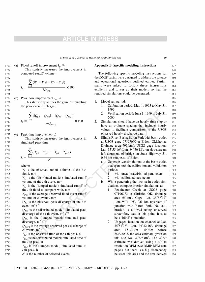
UNCORRECTED PROOF

(a) Flood runoff improvement Iy; %

This statistic measures the improvement in

computed runoff volume:

Iy ¼

XNi¼1

ðlYi 2 Ys;il2 lYi 2 Yz;ilÞ

NYavg

£ 100

(b) Peak flow improvement Ip; %

This statistic quantifies the gain in simulating

the peak event discharge:

Ip ¼

XNi¼1

ðlQp;i 2 Qps;il2 lQp;i 2 Qpz;ilÞ

NQp;avg

£ 100

(c) Peak time improvement It

This statistic measures the improvement in

simulated peak time:

It ¼

XNi¼1

ðlTp;i 2 Tps;il2 lTp;i 2 Tpz;ilÞ

N

where:

Yi is the observed runoff volume of the i-th

flood, mm

Ys;i is the (distributed model) simulated runoff

volume of the i-th event, mm

Yz;i is the (lumped model) simulated runoff of

the i-th flood to compare with, mm

Yavg is the average observed flood event runoff

volume of N events, mm

Qp;i is the observed peak discharge of the i-th

event, m3 s21

Qps;i is the (distributed model) simulated peak

discharge of the i-th event, m3 s21

Qpz;i is the (lumped model) simulated peak

discharge, m3 s21

Qp;avg is the average observed peak discharge of

N events, m3 s21

Tp;i is the observed time of the i-th peak, h

Tps;i is the (distributed model) simulated time of

the i-th peak, h

Tpz;i is the (lumped model) simulated time to

i-th peak, h

N is the number of selected events.

Appendix B. Specific modeling instructions

The following specific modeling instructions for

the DMIP basins were designed to address the science

and operational questions outlined earlier. Partici-

pants were asked to follow these instructions

explicitly and to set up their models so that the

required simulations could be generated.

1. Model run periods

1. Calibration period: May 1, 1993 to May 31,

1999

2. Verification period: June 1, 1999 to July 31,

2000

2. Simulations should have an hourly time step or

have an ordinate spacing that includes hourly

values to facilitate comparison to the USGS

observed hourly discharge data.

3. Illinois River Basin: Baron Fork with basin outlet

at USGS gage 07197000 at Eldon, Oklahoma.

Drainage area 795 km2. USGS gage location:

Lat. 3585501600 Lon. 9485001800, on downstream

left abutment of bridge on State Highway 51,

0.64 km southeast of Eldon.

a. Generate two simulations at the basin outlet

that span both the calibration and validation

periods:

1. with uncalibrated/initial parameters

2. with calibrated parameters

b. While generating the two basin outlet sim-

ulations, compute interior simulations at:

1. Peacheater Creek at USGS gage

07196973 at Christie, OK. drainage

area 65 km2. Gage: Lat. 3585701700

Lon. 9484104600, 0.64 km upstream of

junction with Baron Fork. No cali-

bration is allowed using observed

streamflow data at this point. It is to

be a ‘blind’ simulation.

2. Ungaged location on channel at Lat.

3585403800, Lon. 9483201600, drainage

area 151.3 km2 (Note: before

2/23/2002, the area estimate given on

this site was 208.9 km2. The 208.9

estimate was derived using a 400 m

resolution DEM (See DMIP DEM data

page.), but there is a big discrepancy

between this area and the area derived



ARTICLE IN PRESS

1729

1730

1731

1732

1733

1734

1735

1736

1737

1738

1739

1740

1741

1742

1743

1744

1745

1746

1747

1748

1749

1750

1751

1752

1753

1754

1755

1756

1757

1758

1759

1760

1761

1762

1763

1764

1765

1766

1767

1768

1769

1770

1771

1772

1773

1774

1775

1776

1777

1778

1779

1780

1781

1782

1783

1784

1785

1786

1787

1788

1789

1790

1791

1792

1793

1794

1795

1796

1797

1798

1799

1800

1801

1802

1803

1804

1805

1806

1807

1808

1809

1810

1811

1812

1813

1814

1815

1816

1817

1818

1819

1820

1821

1822

1823

1824

UNCORRECTED PROOF

from the 30 m DEM (151.3 km2). We

believe the area derived from the 30 m

DEM is more accurate.

4. Illinois River Basin: Illinois River with basin

outlet at USGS gage 07195500 at Watts,

Oklahoma. Drainage area 1,645 km2. USGS

gage location: Lat 3680704800 Lon 9483401900, on

downstream side of pier of bridge on Highway

59, 2.4 km north of Watts.



periods:



b. While generating the two basin outlet

simulations, compute interior simulations at:

1. Illinois River at USGS gage 07194800

at Savoy, Arkansas. Drainage area

433 km2. Gage: Lat. 3680601100, Lon.

9482003900

2. Ungaged location on channel at Lat.

368205300, Lon. 9481901600, drainage area

198.1 km2.

5. Illinois River Basin: Illinois River with basin

outlet at USGS gage 07196500 at Tahlequah,

Oklahoma. Drainage area: 2.484 km2. Gage

location: Lat. 3585502200, Lon. 9485502400,

0.32 km downstream from US Highway 62,

3.5 miles northeast of Tahlequah.



periods:



b. While generating the 2 basin outlet simu-

lations, compute interior simulations at:

1. Illinois River at USGS gage in Watts,

OK.

2. Illinois River at USGS gage in Savoy,

Arkansas.

3. Flint Creek at USGS gage 07196000 in

Kansas, OK. Drainage area 285 km2.

Gage location: Lat. 3681101100, Lon.

9484202400 upstream from bridge on US

Highway 412. (Note: no specific cali-

bration using observed streamflow at

these points, even though calibration

was performed for the Illinois River at

Watts, OK for the runs in item B.4

above.).

6. Elk River with basin outlet at USGS gage

07189000 in Tiff City, Missouri. Drainage area

2.251 km2. Gage location: Lat. 3683705300 Lon.

9483501200, on bridge on State Highway 43,

4.83 km southeast of Tiff City.



periods:



b. While generating the two basin outlet

simulations, compute interior simulations

at ungaged location on channel at Lat.

3683503800, Lon. 948901700, drainage area

318.4 km2. (Note: there is no interior

observed streamflow for this basin).

7. Blue River with designated basin outlet at USGS

gage 07332500 in Blue, Oklahoma. Drainage

area 1.233 km2. Gage location: Lat. 3385904900

Lon. 9681402700, on bridge on US Highway 70,

1.61 km west of Blue, Oklahoma.



periods:



b. While generating the two basin outlet simu-

lations, compute interior hydrographs at:

1. Ungaged location on main channel of

the Blue River at Lat. 3483002400, Lon.

9684003000, drainage area 153.2 km2

2. Ungaged location on main channel of

the Blue River at Lat. 3482603900, Lon.

9683703000, drainage area 302.7 km2.

(note: there is no interior observed

streamflow for these two points).

References

Abbott, M.B., Refsgaard, J.C. (Eds.), 1996. Distributed Hydro-

logical Modeling, Kluwer Academic Publishers, Dordrecht.

Bell, V.A., Moore, R.J., 1998. A grid-based distributed flood

forecasting model for use with weather radar data: Part 2. Case

studies. Hydrology and Earth System Sciences 2(3), 283–298.

Bell, V.A., Carrington, D.S., Moore, R.J., 2001. Comparison of

Rainfall-Runoff Models for Flood Forecasting. Part 2:



ARTICLE IN PRESS

1825

1826

1827

1828

1829

1830

1831

1832

1833

1834

1835

1836

1837

1838

1839

1840

1841

1842

1843

1844

1845

1846

1847

1848

1849

1850

1851

1852

1853

1854

1855

1856

1857

1858

1859

1860

1861

1862

1863

1864

1865

1866

1867

1868

1869

1870

1871

1872

1873

1874

1875

1876

1877

1878

1879

1880

1881

1882

1883

1884

1885

1886

1887

1888

1889

1890

1891

1892

1893

1894

1895

1896

1897

1898

1899

1900

1901

1902

1903

1904

1905

1906

1907

1908

1909

1910

1911

1912

1913

1914

1915

1916

1917

1918

1919

1920

UNCORRECTED PROOF

Calibration and Evaluation of Models, Environment Agency

RandD Technical Report W242, Research Contractor: Institute

of Hydrology, Environment Agency, 239 pp.

Beven, K.J., 1985. Chapter 13, Distributed Models. In: Anderson,

M.G., Burt, T.P. (Eds.), Hydrological Forecasting, Wiley, New

York.

Beven, K.J., Hornberger, G.M., 1982. Assessing the effect of spatial

pattern of precipitation in modeling stream flow hydrographs.

Water Resources Bulletin, 823–829.

Boyle, D.B., Gupta, H.V., Sorooshian, S., Koren, V., Zhang, Z.,

Smith, M., 2001. Toward improved streamflow forecasts: value

of semi-distributed modeling. Water Resources Research

37(11), 2749–2759.

Bradley, A., 1997. Use of Weather Radar with Lumped Parameter

Hydrologic Models, 13th AMS Conference on Hydrology, Long

Beach, CA, paper J54, J87-J88.

Bradley, A.A., Kruger, A., 1998. Recalibration of Hydrologic Models

for use with WSR-88D Precipitation Estimates, Paper 2.16 in

Preprints of the Special Symposium on Hydrology, American

Meteorological Society, Phoenix, Arizona, pp. 301–305.

Bradley, A.A., Smith, J.A., 1994. The hydrometeorological environ-

ment of extreme rainstorms in the Southern Plains of the United

States. Journal of Applied Meterology 33, 1418–1431.

Burnash, R.J.C., 1995. The NWS River Forecast System—

Catchment Model. In: Singh, Vijay, P. (Eds.), Computer Models

of Watershed Hydrology, Water Resources Publications,

Chapter 10.

Carpenter, T.M., Georgakakos, K.P., 2004. Impacts of parametric

and radar rainfall uncertainty on the ensemble streamflow

simulations of a distributed hydrologic model. Journal of

Hydrology in press.

Carpenter, T.M., Georgakakos, K.P., Spersflage, J.A., 2001. On the

parametric and NEXRAD-radar sensitivities of a distributed

hydrologic model suitable for operational use. Journal of

Hydrology 253, 169–193.

Carter, G.C., 2002. Infusing new science into the National Weather

Service River Forecast System, Second Federal Interagency

Hydrologic Modeling Conference, Las Vegas, Nevada, 10 pp.

Chandrasekar, V., Krajewski, W.F., Lakshmi, V., 1990. A Monte–

Carlo study of radar-rainfall sampling for hydrological appli-

cations. Eighth Conference on Hydrometerology, American

Meteorological Society, Kananaskis Park, Alta, Canada,

179–183.

Duan, Q., Schaake, J., Koren, V., 2001. A priori estimation of land

surface model parameters. In: Lakshmi, V., Albertson, J.,

Schaake, J. (Eds.), Land Surface Hydrology, Meteorology, and

Climate: Observation and Modeling, Water Science and

Application, vol. 3. AGU, Washington, DC, pp. 77–94.

Eidenshink, J.C., Faundeen, J.L., 1994. The 1-km AVHRR global

land data set: first stages in implementation. International

Journal of Remote Sensing 15, 3443–3462.

Farnsworth, R.K., Thompson, E.S., 1982. Mean Monthly, Seasonal,

and Annual Pan Evaporation for the United States, NOAA

Technical Report NWS 34, Washington, DC, 82 p.

Farnsworth, R.K., Thompson, E.S., Peck, E.L., 1982. Evaporation

Atlas for the Contiguous 48 United States, NOAA Technical

Report NWS 33, Washington, DC.

Faures, J.-M., Goodrich, D.C., Woolhiser, D.A., Sorooshian, S.,

1995. Impact of small-scale spatial rainfall variability on runoff

modeling. Journal of Hydrology 173, 309–326.

Finnerty, B., Johnson, D., 1997. Comparison of mean areal

precipitation estimates derived from NEXRAD radar vs.

raingauge networks. Proceedings of Theme A: Water for a

Changing Global Community, 27th Congress of the Inter-

national Associotion for Hydraulic Research, ASCE Water

Resources Division, 601–606.

Finnerty, B.D., Smith, M.B., Seo, D.-J., Koren, V., Moglen, G.E.,

1997. Space-time sensitivity of the Sacramento model to radar-

gage precipitation inputs. Journal of Hydrology 203, 21–38.

Fread, D.L., Shedd, R.C., Smith, G.F., Farnsworth, R., Hoffeditz,

C.N., Wenzel, L.A., Wiele, S.M., Smith, J.A., Day, G.N., 1995.

Modernization in the National Weather service river and flood

program. Weather and Forecasting 10(3), 477–484.

Fulton, R.A., Breidenbach, J.P., Seo, D.-J., Miller, D.A., 1998.

WSR-88D rainfall algorithm. Weather and Forecasting 13,

377–395.

Glaudemans, M.J., Erb, R.A., Wells, E.B., Zimmerman, J., Hill-

Maxwell, J., Mack, K., 2002. Overview and Status of the

Hydrologic Forecast System in the National Weather Service

Weather Forecast Offices. Interactive Symposium on the

Advanced Weather Interactive Procesing System, (AWIPS),

Orlando, Florida, J173–J178.

Greene, D.R., Hudlow, M.D., 1982. Hydrometeorologic grid map-

ping procedures, AWRA International Symposium on Hydro-

meteor, Denver, CO, available upon request from NWS/HL.

Gutman G., Ignatov A., 1997. Derivation of green vegetation

fraction from NOAA/AVHRR for use in numerical weather

prediction models. Manuscript available from Garik Gutman at

[email protected].

Hamlin, M.J., 1983. The significance of rainfall in the study of

hydrological processes at basin scale. Journal of Hydrology 65,

73–94.

Johnson, D., Smith, M., Koren, V., Finnerty, B., 1999. Comparing

mean areal precipitation estimates from NEXRAD and rain

gauge networks. ASCE Journal of Hydrologic Engineering 4(2),

117–124.

Kalinga, O., Gan, T.Y., Xie, J., 2003. Applying radar rainfall data in

basin hydrological modeling. Proceedings of Weather Radar

Information and Distributed Hydrological Modeling, held

during IUGG2003 at Sapporo, Japan, July, IAHS Publication

no 282, 258–267.

Kenner, S.J., Brich, S., Yang, Y., Hjelmfelt, M.R., Nair, U.S.,

Pielke, R.A., 1996. Atmospheric and surface hydrologic

simulations of an extreme flood event, Preprint volume, Second

International Scientific Conference on the Global Energy and

Water Cycle, Washington, DC.

Koren, V., Barrett, C.B., 1994. Satellite based distributed

monitoring, forecasting, and simulation (MFS) system for the

Nile River. In: Kite, G.W., Pietroniro, A., Pultz, T.J. (Eds.),

Applications of Remote Sensing in Hydrology, Proceedings of

the Second International Workshop, NHRI Symposium No. 14,

Saskatoon, Saskatchewan, pp. 187–200.

Koren, V.I., Finnerty, B.D., Schaake, J.C., Smith, M.B., Seo, D.-J.,

Duan, Q.Y., 1999. Scale dependencies of hydrology models to



ARTICLE IN PRESS

1921

1922

1923

1924

1925

1926

1927

1928

1929

1930

1931

1932

1933

1934

1935

1936

1937

1938

1939

1940

1941

1942

1943

1944

1945

1946

1947

1948

1949

1950

1951

1952

1953

1954

1955

1956

1957

1958

1959

1960

1961

1962

1963

1964

1965

1966

1967

1968

1969

1970

1971

1972

1973

1974

1975

1976

1977

1978

1979

1980

1981

1982

1983

1984

1985

1986

1987

1988

1989

1990

1991

1992

1993

1994

1995

1996

1997

1998

1999

2000

2001

2002

2003

2004

2005

2006

2007

2008

2009

2010

2011

2012

2013

2014

2015

2016

mailto:[email protected]

UNCORRECTED PROOF

spatial variability of precipitation. Journal of Hydrology 217,

285–302.

Koren, V.I., Smith, M., Wang, D., Zhang, Z., 2000. Use of soil

property data in the derivation of conceptual rainfall-runoff

model parameters, Preprints, 15th Conference on Hydrology,

Long Beach, CA, American Meteorological Society,

pp. 103–106.

Koren V., Smith M., Reed S., Zhang Z, 2001. Transition from

lumped to distributed modeling systems. Session H32C, AGU

Spring Meeting, Boston, MA.

Koren, V., Reed, S., Smith, M., Zhang, Z., 2003. Combining

physically based and conceptual approaches in the develop-

ment and parameterization of a distributed system. Infor-

mation from Weather Radar and Distributed Hydrological

Modelling (Proceedings of symposium HS03 to be held

during IUGG2003 at Sapporo, Japan, July 2003) IAHS

publication No. 282.

Koren, V., Smith, M., Duan, Q., 2003. Use of a-priori parameter

estimates in the derivation of spatially consistent parameter

sets of rainfall-runoff models. In: Duan, Q., Gupta, H.V.,

Sorooshian, S., Rousseau, A.N., Turcotte, R. (Eds.), Cali-

bration of Watershed Models, Water Science and Application,

vol. 6. American Geophysical Union, Washington, DC,

pp. 239–254.

Kouwen, K., Garland, G., 1989. Resolution considerations in using

radar rainfall data for flood forecasting. Canadian Journal of

Civil Engineering 16, 279–289.

Krajewski, W.F., Lakshmi, V., Georgakakos, K.P., Jain, S.C., 1991.

A Monte–Carlo study of rainfall sampling effect on a

distributed catchment model. Water Resources Research

27(1), 119–128.

Kull, D.W., Feldman, A.D., 1998. Evolution of Clark’s unit graph

method to spatially distributed runoff. ASCE Journal of

Hydrologic Engineering 1998, 9–19.

Larson, L.W., Ferral, R.L., Strem, E.T., Morin, A.J., Armstrong, B.,

Carrol, T.R., Hudlow, M.D., Wenzel, L.A., Schaefer, G.L.,

Johnson, D.E., 1995. Operational responsibilities of the

National Weather Service river and flood program. Weather

and Forecasting 10(3), 465–476.

Loague, K., 1990. R-5 revisited, 2. Reevaluation of a quasi-

physically-based rainfall-runoff model with supplemental

information. Water Resources Research 26(5), 973–987.

Loague, K.M., Freeze, R.A., 1985. A comparison of rainfall-runoff

modeling techniques on small upland catchments. Water

Resources Research 21(2), 229–248.

Maurer, E.P., Wood, A.W., Adam, J.C., Lettenmaier, D.P., Nijssen,

B., 2002. A long-term hydrologically-based data set of land

surface fluxes and states for the conterminous United States.

Journal of Climate 15, 3237–3251.

McCuen, R.H., Snyder, W.M., 1975. A proposed index for

comparing hydrographs. Water Resources Research 11(6),

1021–1024.

Meo, M., Focht, W., Caneday, L., Lynch, R., Moreda, F., Pettus, B.,

Sankowski, E., Trachtenbert, Z., Vieux, B., Willet, K., 2002.

Negotiating science and values with stakeholders in the Illinois

River basin. Journal of the American Water Resources

Association 38(2), 541–554.

Michaud, J.D., Sorooshian, S., 1994a. Effect of rainfall-sampling

errors on simulation of desert flash floods. Water Resources

Research 30(10), 2765–2775.

Michaud, J., Sorooshian, S., 1994b. Comparison of simple versus

complex distributed runoff models on a midsized semiarid

watershed. Water Resources Research 30(3), 593–605.

Miller, D.A., White, R.A., 1999. A conterminous United States

multi-layer soil characteristics data set for regional climate and

hydrology modeling. Earth Interactions 2, xxxavailable at http://

Earthinteractions.org.

Moore R.J., Bell V.A., 2001. Comparison of rainfall-runoff models

for flood forecasting. Part 1: Literature review of models.

Environment Agency R&D Technical Report W241, Research

Contractor: Institute of Hydrology, September 2001, Environ-

ment Agency. 94pp.

Moore, R.J., Hall, M.J. (Eds.), 2000. HYREX: the Hydrology Radar

Experiment, Special Issue of Hydrology and Earth System

Sciences, vol. 4(4). European Geophysical Society.

Moore, R.J., Bell, V.A., Carrington, D.S., 2000. Intercomparison of

rainfall-runoff models for flood forecasting. In: Lees, M.,

Walsh, P. (Eds.), Flood forecasting: what does current research

offer the practitioner?, Occasional Paper No. 12, British

Hydrological Society, pp. 69–76.

Morin, E., Enzel, Y., Shamir, U., Garti, R., 2001. The characteristic

time scale for basin hydrological response using radar data.

Journal of Hydrology 252, 85–99.

Naden, P.S., 1992. Spatial variability in flood estimation for large

catchments: the exploitation of channel network structure.

Hydrological Sciences Journal 37(1), 53–71.

Nash, J.E., Sutcliffe, J.V., 1970. River flow forecasting through

conceptual models part 1—a discussion of principles. Journal of

Hydrology 10(4), 282–290.

National Research Council, 1996. Toward a new national weather

service: assessment of hydrologic and hydrometeorologic

operations and services. National Weather Service Moderniz-

ation Committee, Commission on Engineering and Technical

Systems, National Academy Press.

Obled, C.H., Wendling, J., Beven, K., 1994. The sensitivity

of hydrological models to spatial rainfall patterns: an

evaluation using observed data. Journal of Hydrology 159,

305–333.

Ogden, F.L., Julien, P.Y., 1993. Runoff sensitivity to temporal and

spatial rainfall variability at runoff plane and small basin scales.

Water Resources Research 29(8), 2589–2597.

Ogden, F.L., Julien, P.Y., 1994. Runoff model sensitivity to radar

rainfall resolution. Journal of Hydrology 158, 1–18.

Pessoa, M.L., Bras, R.L., Williams, E.R., 1993. Use of weather

radar for flood forecasting in the Sieve river basin: a sensitivity

analysis. Journal of Applied Meteorology 32(3), 462–475.

Peters, J.C., Easton, D.J., 1996. Runoff simulation using radar

rainfall data. Water Resources Bulletin 32(4), 753–760.

Reed, S.M., Maidment, D.R., 1999. Coordinate transformations for

using NEXRAD data in GIS-based hydrologic modeling.

Journal of Hydrologic Engineering 4, 174–183.

Reed, S., Koren, V., Smith, M., Zhang, Z., Moreda, F., Seo, D.-J.,

DMIP participants, 2004. Overall distributed model inter-

comparison project results. Journal of Hydrology in press.



ARTICLE IN PRESS

2017

2018

2019

2020

2021

2022

2023

2024

2025

2026

2027

2028

2029

2030

2031

2032

2033

2034

2035

2036

2037

2038

2039

2040

2041

2042

2043

2044

2045

2046

2047

2048

2049

2050

2051

2052

2053

2054

2055

2056

2057

2058

2059

2060

2061

2062

2063

2064

2065

2066

2067

2068

2069

2070

2071

2072

2073

2074

2075

2076

2077

2078

2079

2080

2081

2082

2083

2084

2085

2086

2087

2088

2089

2090

2091

2092

2093

2094

2095

2096

2097

2098

2099

2100

2101

2102

2103

2104

2105

2106

2107

2108

2109

2110

2111

2112

http://Earthinteractions.org

http://Earthinteractions.org

UNCORRECTED PROOF

Refsgaard, J.C., 1997. Parameterisation, calibration, and validation

of distributed hydrological models. Journal of Hydrology 198,

69–97.

Refsgaard, J.C., Knudsen, J., 1996. Operational validation and

intercomparison of different types of hydrological models.


Robinson, J.S., Sivapalan, M., 1995. Catchment-scale runoff

generation model by aggregation and similarity analysis. In:

Kalma, J.D., Sivapalan, M. (Eds.), Scale Issues in Hydrological

Modeling, Wiley, New York, pp. 311–330.

Seo, D.-J., 1998. Real-time estimation of rainfall fields using radar

rainfall and rain gauge data. Journal of Hydrology 208, 37–52.

Seo, D.-J., Smith, J.A., 1996. On the relationship between

catchment scale and climatological variability of surface-runoff

volume. Water Resources Research 32(3), 633–643.

Seo, D.-J., Breidenbach, J.P., Johnson, E.R., 1999. Real-time

estimation of mean field bias in radar rainfall data. Journal of

Hydrology, 131–147.

Seyfreid, M.B., Wilcox, B.P., 1995. Scale and the nature of spatial

variability: Field examples having implications for hydrologic

modeling. Water Resources Research 31(1), 173–184.

Shah, S.M.S., O’Connell, P.E., Hosking, J.R.M., 1996. Modeling

the effects of spatial variability in rainfall on catchment

response. 2. Experiments with distributed and lumped models.

Journal of Hydrology 175, 89–111.

Singh, V.P., 1997. Effect of spatial and temporal variability in

rainfall and watershed characteristics on stream flow hydro-

graph. Hydrological Processes 1, 1649–1669.

Smith, J.A., Bradley, A.A., Baeck, M.L., 1994. The space-time

structure of extreme storm rainfall in the Southern Plains.

Journal of Applied Meteorology 33, 1402–1417.

Smith, J.A., Seo, D.-J., Baeck, M.L., Hudlow, M.D., 1996. An

intercomparison study of NEXRAD precipitation estimates.


Smith M.B., Koren V., Johnson D., Finnerty B.D., Seo D.-J., 1999.

Distributed modeling: phase 1 results. NOAA Technical Report

NWS 44, 210 pp. National Weather Service Hydrology

Laboratory. Copies available upon request.

Smith, M.B., Laurine, D.P., Koren, V.I., Reed, S., Zhang, Z., 2003.

Hydrologic model calibration in the National Weather Service.

In: Duan, Q., Gupta, H.V., Sorooshian, S., Rousseau, A.N.,

Turcotte, R. (Eds.), Calibration of Watershed Models, Water

Science and Application, vol. 6. American Geophysical Union,

pp. 133–152.

Stallings, E.A., Wenzel, L.A., 1995. Organization of the river and

flood program in the National Weather Service. Weather and

Forecasting 10(3), 457–464.

Troutman, B.M., 1983. Runoff prediction errors and bias in

parameter estimation induced by spatial variability of precipi-

tation. Water Resources Research 19(3), 791–810.

Turcotte, R., Rousseau, A.N., Fortin, J.-P., Villeneuve, J.-P., 2003.

A process oriented, multiple-objective calibration strategy

accounting for model structure. In: Duan, Q., Gupta, H.V.,

Sorooshian, S., Rousseau, A.N., Turcotte, R. (Eds.), Calibration

of Watershed Models, Water Science and application, vol. 6.

American Geophysical Union, pp. 153–163.

Vieux, B., 2001. In: Singh, V.P., (Ed.), Distributed Hydrologic

Modeling Using GIS, Water Science and Technology Library,

vol. 38. Kluwer Academic Publishers, Dordrecht.

Vieux, B.E., Moreda, F.G., 2003a. Nutrient loading assessment in

the4 Illinois River using a synthetic approach. Journal of the

American Water Resources Association 39(4), 757–769.

Vieux, B.E., Moreda, F.G., 2003b. Ordered Physics-Based Par-

ameter Adjustment of a Distributed Model. In: Duan, Q., Gupta,

H.V., Sorooshian, S., Rousseau, A.N., Turcotte, R. (Eds.),

Calibration of Watershed Models, Water Science and Appli-

cation, vol. 6. American Geophysical Union, pp. 267–281.

Wang, D., Smith, M.B., Zhang, Z., Reed, S., Koren, V., 2000.

Statistical Comparison of Mean Areal Precipitation Estimates

from WSR-88D, Operational and Historical Gage Networks,

Paper 2.17, 15th Conference on Hydrology, AMS, Long Beach,

CA, pp. 107–110.

Watts, L.G., Calver, A., 1991. Effects of spatially-distributed

rainfall on runoff for a conceptual catchment. Nordic Hydrology

22, 1–14.

Wei, T.C., Larson, C.L., 1971. Effects of areal and time distribution

of rainfall on small watershed runoff hydrgraphs, Bulletin, vol.

30. Water Resources Research Center, University of Minnesota,

118 pp.

Wilson, C.B., Valdes, J.B., Rodriquez-Iturbe, I., 1979. On the

influence of the spatial distribution of rainfall on storm runoff.


Winchell M., Gupta H.V., Sorooshian S. 1997. Effects of radar-

estimated precipitation uncertainty on different runoff gener-

ation mechanisms. Report HWR No. 97-080 Department of

Hydrology and Water Resources, University of Arizona, 285 pp.

Winchell, M., Gupta, H.V., Sorooshian, S., 1998. On the simulation

of infiltration- and saturation- excess runoff using radar-based

rainfall estimates: effects of algorithm uncertainty and pixel

aggregation. Water Resources Research 34(10), 2655–2670.

Wood, E.F., Sivapalan, M., Beven, K., 1990. Similarity and scale in

catchment storm response. Review of Geophysics 28(1), 1–18.

Wood, E.F., Lettenmaier, D.P., Liang, X., Lohmann, D., 1998. and

others, The project for the Intercomparison of land-surface

parameterization schemes (PILPS) phase 2(c)Red-Arkansas

basin experiment: 1. Experiment description and summary

intercomparisons. Global and Planetary Change 19, 115–135.

World Meteorological Organization (WMO), 1975. Intercompar-

ison of conceptual models used in operational hydrological

forecasting. Operational Hydrology Report No. 7, Geneva,

Switzerland, 172 pp.

World Meteorological Organization (WMO), 1992. Simulated real-

time Intercomparison of hydrological models. Operational

Hydrology Report No. 38, Geneva, Switzerland, 241 pp.

Young, C.B., Bradley, A.A., Krajewski, W.F., Kruger, A., 2000.

Evaluating NEXRAD multisensor precipitation estimates for

operational hydrologic forecasting. Journal of Hydrometeorol-

ogy 1, 241–254.

Zhang, Z., Koren, V., Smith, M.B., Reed, S., Wang, D., 2004. Use

of NEXRAD data and basin disaggregation to improve

continuous hydrograph simulation. ASCE Journal of Hydro-

logic Engineering 9(2), 103–115.



ARTICLE IN PRESS

2113

2114

2115

2116

2117

2118

2119

2120

2121

2122

2123

2124

2125

2126

2127

2128

2129

2130

2131

2132

2133

2134

2135

2136

2137

2138

2139

2140

2141

2142

2143

2144

2145

2146

2147

2148

2149

2150

2151

2152

2153

2154

2155

2156

2157

2158

2159

2160

2161

2162

2163

2164

2165

2166

2167

2168

2169

2170

2171

2172

2173

2174

2175

2176

2177

2178

2179

2180

2181

2182

2183

2184

2185

2186

2187

2188

2189

2190

2191

2192

2193

2194

2195

2196

2197

2198

2199

2200

2201

2202

2203

2204

2205

2206

2207

2208

The Distributed Model Intercomparison Project (DMIP) – Phase 2 experiments in the Oklahoma Region,...

Documents

Transcript of The Distributed Model Intercomparison Project (DMIP) – Phase 2 experiments in the Oklahoma Region,...