Indicators and targets for the reduction of the environmental ...

Jo Dewulf, Simone Manfredi, Serenella Sala, Valentina Castellani, Małgorzata Góralczyk Bruno Notarnicola, Giuseppe Tassielli, Pietro A. Renzulli Paulo Ferrão, André Pina, Patrícia Baptista Monica Lavagna

Deliverable 5

Indicators and targets for the reduction of the

environmental impact of EU consumption: Basket-of-

products indicators and prototype targets for the

reduction of environmental impact of EU consumption

2014

European Commission

Joint Research Centre

Institute for Environment and Sustainability

Contact information

Małgorzata Góralczyk

Address: Joint Research Centre, Via Enrico Fermi 2749, TP 290, 21027 Ispra (VA), Italy

E-mail: [email protected]

Tel.: +39 0332 78 9949

Acknowledgements:

The report was created with the support of the experts, who developed the baskets of products for food, housing and

mobility. Their contribution is the following:

o Bruno Notarnicola, Giuseppe Tassielli, Pietro A. Renzulli (Università degli Studi di Bari, Italy): food basket of

products (section 2)

o Paulo Ferrão, André Pina, Patrícia Baptista (Instituto Superior Técnico, Lisboa, Portugal): mobility basket of

products (section 3)

o Monica Lavagna (Politecnico di Milano, ABC Department, Italy) with support of Andrea Campioli, Serena

Giorgi, Anna Dalla Valle: housing basket of products (section 4)

3

Executive summary

Objectives

The objective of this report is to provide the environmental impacts of 3 key consumption categories (food,

housing and mobility), as well as the impacts of representative products within each consumption category in

relation to their relevance for the EU sustainable product policy.

The environmental impact (basket-of-products) indicators are developed in order to help policy makers to

monitor and evaluate the progress towards the reduction of the lifecycle environmental impacts of European

consumption, including helping focus eco-innovation and other different policy activities.

This report also aims at applying the life cycle based methodology proposed in Sala et al 2014 in support to a

comprehensive and systematic target setting. This methodology for target setting has so far been applied on

the food sector as preliminary example.

Description of work

The Basket-of-Products indicators developed provide insights into overall life cycle impacts related to

consumption in key product groups and consumption categories. These are based on product life cycle data

(environmental profiles of products) combined with consumption statistics. This also allows for the

development of more informed targets based on detailed product-group insights than would be feasible using

heavily aggregated macro scale indicators alone.

For each consumption category and associated products the indicators are built for the most relevant

environmental impact categories, as defined in the recent EC Product Environmental Footprint (PEF) method

and the International Reference Life Cycle Data System (ILCD).

Conclusions

Sections 2, 3 and 4 of this report present the results of the BoPs indicators for food, mobility and housing,

expressed per EU citizen, for the 14 considered impact categories. The estimated potential impacts are

subdivided according to the products in the respective baskets and equally according to the life cycle stages

that have been accounted for.

Results show that the production and use phases dominate the impacts with an average contribution of 51.8

and 45.6%, respectively. The End-of-Life (EoL) phase is, on the other hand, far less contributing; for some

impacts, the recovery can even result in some avoided impact – standing for environmental benefits, explaining

the numerically negative contributions. With respect to the production phase, relative contributions to the

overall life cycle impacts are the highest for human toxicity (cancer effects) (89.2%) and terrestrial

eutrophication (82.8%), moderate for impacts like climate change (31.9%) and low for ozone depletion (15.1%).

Analysis of the relative contribution of the use phase to the total life cycle impacts shows that ozone depletion

(85.7%), photochemical ozone formation (71.9%) and climate change (69.8%) are significantly impacted;

human toxicity (non-cancer effects) is instead poorly impacted (13.4%).

When zooming into the production phase, the role of the three BoPs can be analysed. On average, food

production contributes 54.5% to the total impact by production, mobility 34.3%, and shelter 11.2%. Food

production accounts for over 90% of the contribution to acidification, terrestrial eutrophication and land use.

The largest share of mobility is in resource depletion, i.e. 80.0% of the overall impact.

Analysing the impacts of the different BoPs at the use stage, on average it turns out that it is dominated by

housing (51.8%) and mobility (45.9%), while food only accounts for 2.2%. Highest impact for the use phase

for mobility is in land use (70.4%) and for housing in ionizing radiation Ecosystem (73.8%).

With respect to EoL, impacts are dominated by mobility: 90.6% on average. Contributions of food is 9.5%,

whereas housing is negligible with -0.1% on average.

4

Perspectives

A crucial phase in the development of the BoP indicators was the initial definition of the three selected basket

categories (food, mobility and shelter) and, even more important, the population of the three baskets, i.e. the

identification of the representative products to be included in each basket. Given the profound importance of

this phase for the subsequent quantification of the potential environmental impacts associated with each

basket, it is recommended to carefully assess the robustness of the selection of the representative products.

Such a robustness check should in particular be aimed at (1) identify (and avoid) any possible overlaps among

product groups, (2) identify (and avoid) any gaps, i.e. relevant product-groups that have not been included in

the calculations. Also, towards further development of the LC Indicators, it seems relevant to define and

consider not just one basket for each category (e.g. one basket of products for the category food), but – ideally

- a range of different baskets from the “best performing” (from an environmental view point) one to the “worst

performing” one.

The development of country-specific baskets should also be explored via e.g. an ad-hoc feasibility study on the

availability of the necessary country-specific data. While developing 100% country-specific baskets may not

yet be viable, it would be certainly possible to progressively adapt the baskets including more and more

country-specific datasets.

An increased availability of high quality LCI-data would of course help increasing comprehensiveness and

robustness of the assessment. A better integration of existing data with Input/Output (IO) data seems a viable

option, as these data are luckily to already include country-specific and lifecycle-stage specific information,

which is seen as important for developing further the indicators. In order to limit the data collection efforts

(and costs), the present calculations should be carefully checked (via e.g. sensitivity analysis) to identify some

key hotspot / product groups / part of the system that are most relevant in that they influence most the

environmental performance. Data collection efforts could then initially be limited to these identified

components.

It is also noted that a meaningful way to further facilitate the calculation of the BoP LC Indicators through

tailoring the set of impact categories in function of the basket under study. In fact, while some impact

categories could be calculated as default for all baskets (e.g. climate change), others could become basket-

specific. This calls for the definition of relevant criteria for the attribution of impact categories to the three

specific baskets.

The current study considers three key BoPs: food, shelter, and mobility. However, other consumption activities

contribute to the impacts as well. To further complete the impact profile of consumption by the EU citizen, an

extension with other consumption categories can be explored. First, when it comes to the basic needs the

current set of food, housing and mobility might be expanded with health care products and services. Further

on, other but less basic needs could be considered: communication and information products and services and

leisure activities like tourism.

The LCA-based methodology for target setting has been applied on the food sector only. The application of the

methodology has highlighted the need of a complementary approach, where literature review on hotspots is

coupled with LCA. In literature, the majority of the studies focus on energy and climate related impacts of food

supply chains, whereas the LCA applied to the food BoP supports a more holistic hotspot analysis. Indeed, LCA

offers a broader and multi-criteria based assessment of food supply. However, in the future variability and

ranges in the underlying datasets may give further relevant input in target setting. For example, consumer

choice and behaviour and hence associated datasets may vary considerably, leading to different impacts

attributable to the use phase and the overall BoP. In general, an uncertainty analysis of the result should be

conducted in order to highlight what is the relevance of the hotspots under different assumptions. Any

improvement and target should be anyway subject to further evaluation at system level and multi-criteria level

to ensure that a benefit in one impact category or life cycle stage is not leading to higher impacts elsewhere.

5

Table of Contents

Executive summary 3

1 Introduction 7

2 Basket of Products: food 8

2.1 Introduction 8

2.2 Definition of the basket of products for foods 8

2.2.1 Data sources 8

2.2.2 Assumptions 8

2.2.3 Final selection of the Basket of Products for Food (products per capita for one year) 11

2.3 Life cycle Inventory of the selected basket products 14


2.3.2 Assumptions 19

2.3.3 Final selection: overview per product and life cycle stage 25

2.4 Results of the environmental impact of the selected products for one EU citizen 28

2.4.1 Result per product 28

2.4.2 Results per life cycle stage 36

2.4.3 Overall results of the environmental impact assessment of basket products per EU citizen 38

2.5 Interpretation of the results 40

2.6 References 42

3 Basket of Products: mobility 45

3.1 Introduction 45

3.2 Definition of the basket of products for mobility 45

3.2.1 Data Sources 48


3.2.3 Final selection 51

3.3 Life cycle Inventory of the selected products 51



3.3.3 Final selection: overview per product and life cycle stage 59

3.4 Results of the environmental impact of the selected products for one EU citizen 61

3.4.1 Results per product 61

3.4.2 Results per life cycle stage 64

3.4.3 Results overall of environmental impact of mobility for one EU citizen 69

3.5 Interpretation of the results 73

3.6 References 74

Abbreviations 75

4 Basket of Products: housing 76

4.1 Introduction 76

4.2 Definition of the basket of products for housing 76

6

4.2.1 Data Sources 77


4.2.3 Final selection 81

4.3 Life Cycle Inventory of the selected products 89



4.4 Results of the environmental impacts of the selected products for one EU citizen 94

4.4.1 Results per impact category 95

4.4.2 Interpretation of results 113

4.5 References 116

5 Application of the methodology for life cycle based targets setting to food Basket of Products 119

5.1 Identification of key economic sectors 120

5.2 Literature review on hotspots and megatrends about food consumption 122

5.3 LCA of the products in the Basket of products (BoP) food 124

5.4 LCA-based hotspot analysis of BoP food 125

5.5 Feasibility analysis of improvements 130

5.5.1 Identification of possible solutions 130

5.5.2 Quantitative target proposal 133

5.6 Identification of policy options, policy development and stakeholders hearings 138

5.7 Conclusions and outlook 139

5.8 References 140

6 Conclusions and perspectives 143

6.1 Conclusions 143

6.1.1 Conclusions on the BoPs results 143

6.1.2 Interpretation by comparison with other studies 143

6.1.3 Conclusions on the application of a LCA methodology for target setting 143

6.2 Perspectives on methodological issues 145

6.2.1 Definition of the current basket: consistency/overlap + bringing in a range 145

6.2.2 Representativeness/quality (data): country specific vs. European average 146

6.2.3 Impact categories: comprehensiveness/relevance of impact categories – inserting accounting (pressure

indicators) before coming to impacts 146

6.2.4 Basket of Products extension 146

6.2.5 Target methodology 146

7

1 Introduction

This report covers the work performed in the task 5 of the Administrative Arrangement, namely the development of

the basket of products indicators, as well as prototype targets. The basket of products indicators are intended to assess

the environmental impact of the European consumption (with distinction of the consumption categories). The baskets

of products developed under Task 5 cover three key consumption categories: food (section 2), mobility (section 3) and

housing (section 4). For each consumption category and related products the indicators were built for the impact

categories, as defined in the Product Environmental Footprint1 and the International Reference Life Cycle Data System

(ILCD)2. The calculations were made for the European Union as a whole (EU27) for the reference year 2010.

The basket-of-products approach matches statistics on private consumption per capita with life cycle inventory (LCI:

emissions and resource use) for each product consumed. As the products included in the basket are only a subset of

total consumption, the basket-of-products indicators provide an index for monitoring and analysis, and not an absolute

measure of environmental impact per person (EC, 2012c).

In order to develop the each of the basket of products the following steps were performed:

• Quantitative and qualitative analysis of the structure of the European consumption in each of the consumption

category – during the years 2000-2010 – including international trade.

• Selection of a basket of products representative for the structure of consumption for the reference year 2010 and

the development of a detailed list of the available datasets for the identified products with the feasibility

assessment of their application for the purpose of the project.

• Calculation of the environmental impact results for each of the basket as well as per citizen, which included:

o Development of process-based life cycle inventory models for the selected representative products.

o Development of the corresponding process based life cycle inventories (conforming to the ILCD format)

for selected representative products.

• Quantitative and qualitative analysis of the environmental impacts of each of the basket.

The objective of the calculation of the basket of products is to provide the profile of environmental impacts as well as

the impacts of representative products within each consumption category in relation to their relevance for the EU

sustainable product policy. The environmental impact (basket-of-products) indicators are developed in order to help

policy makers to monitor and evaluate the progress towards the reduction of the lifecycle environmental impacts of

European consumption, including helping focus eco-innovation and other different policy activities.

This report also aims at applying the life cycle based methodology in support to a comprehensive and systematic

target setting. This methodology for target setting has so far been applied on the food sector as preliminary example

(section 5).

The report covers also the conclusions and recommendations for the future work (section 6).

1 http://ec.europa.eu/environment/eussd/smgp/pdf/annex2_recommendation.pdf

2 http://lct.jrc.ec.europa.eu/assessment/publications

8

2 Basket of Products: food

2.1 Introduction

The development of baskets of products responds to the needs of analysing and monitoring European consumption

patterns and their global influence in order to shift to more resource efficient consumption. Specifically, basket of

products indicators quantify the environmental impacts for the EU-27 using the life cycle data, as well as data on

expenditure and consumption statistics.

The basket of products regarding human nutrition is particularly significant since food and beverage consumption is

responsible for over one third of the overall environmental burden caused by private consumption (Tukker et al. 2006)..

2.2 Definition of the basket of products for foods

2.2.1 Data sources

In order to identify the most representative food and beverage products to include in the basket, data related to food

consumption was analysed, mainly originating from:

• the Eurostat and FAO databases

• specific nutrition and food consumption literature concerning current emerging consumption trends

Whenever incomplete or incongruent Eurostat data was encountered it was verified, integrated or substituted with the

generic data from the FAO databases concerning food and drinks. Other useful information for the identification of

the basket was gathered from reports on the subject of food consumption and relative environmental aspects within

the EU (EEA 2012, DEFRA 2012, FAO 2011, Eurostat 2011, EC 2012c-d-e, Foster et al. 2006, Tukker et al. 2006).

The basket of products was calculated for the year 2010 based on an analysis of the data regarding food consumption

in EU27 within the 2000-2010 time span.

2.2.2 Assumptions

The summary of the main assumptions and of the approach used for the definition of the basket of products for food

and beverages are presented below.

Identification of the representative food data from the databases

Data concerning the average consumption per capita for EU citizens was collected by Eurostat until 2006. After this

period this specific database was discontinued. Since this data source is no longer available the starting point for the

identification of the apparent consumption of food products is the data from the Eurostat Prodcom Annual Sold (NACE

Rev. 2.) database.

Such data contains information on the production, import and export of all main categories of food and drink products

which allows a calculation of the apparent consumption (availability for human consumption) in terms of mass and

economic value (Consumption = Production - Exports + Imports).

The following Prodcom data about apparent food and drink consumption were not taken into account during the

selection process of the basket products:

• products unfit for human consumption (e.g. wastes such as oilcake and pet food)

• products not directly used by consumers for cooking or that are not directly edible (i.e those requiring further

processing before consumption - e.g. crude palm oil, starches)

• products with incoherent data: the export quantities were superior to the sum of the import plus production

quantities.

The quantities, in terms of mass, of the 2010 apparent consumption of the all Prodcom food products are shown in

Figure 1 (see also Annex 1). These quantities are divided among various food categories, namely processed meat and

seafood, production of meat products, cereal based products, dairy products, sugar based products, oils and fats, fresh

vegetables and fruit, processed and preserved fruit and vegetables, alcoholic and non-alcoholic beverages.

9

Table 1 illustrates the total quantity of EU 27 food and beverage apparent consumption (Prodcom), considered for the

selection of the basket products (excluding fruit for fresh consumption and vegetables), and the per-capita

consumption for the year 2010.

The Prodcom database does not contain information on non-processed or fresh vegetables and fruit. Hence the

Eurostat Agricultural production (apro) database and the FAO database were used to identify such data. The

information on the imports and exports of such food products was obtained from the Eurostat EU trade database-

HS6.

Figure 1 EU 27 main quantities of the apparent consumption of all the PRODCOM food categories for the

year 2010 (in tonnes)

Table 1 EU 27 food and beverage apparent consumption (PRODCOM data 2010): total and per capita

Total apparent consumption of all (Prodcom) products considered for the selection of the basket products,

excluding fruit for fresh consumption and vegetables - year 2010 (t) 468,936,745

EU population 1/1/2011 502,489,100

Per capita apparent consumption (kg/inhabitant.year) 933.2

The trade database was also used for the identification of the countries of origin of the imports of the selected basket

products. Annex 2 lists all the main countries from which at least 90% of the imports originate. Such information was

used in the environmental assessment illustrated in section 2.3 of this report. In some cases the Eurostat trade data

was substituted with more specific data from the FAO database or with data from the EC Agriculture and Rural

Development product reports (e.g. EC 2012c).

Information on the specific EU member countries responsible for the production of the basket products is illustrated

in Annex 3. In some cases, there are some discrepancies between the aggregated values of production supplied by

Eurostat and those calculated by summing the production of each EU27 country. Nonetheless from such data it is

possible to extract a picture of the main producing countries for each basket product.

Prodcom data for the year 2010 was substituted in the following cases:

• Milk and cheese production data per EU country was inconsistent with the aggregated values provided by the

Prodcom database. In such cases the Eurostat Agricultural production (apro) database was used as a data source

for the production information regarding each individual EU member state.

• Butter and sugar production data per EU country was inconsistent with the aggregated values provided by the

Prodcom database. In such cases the FAO Production / Livestock Processed database was used as a data source

for the production information concerning each individual EU member state.

Meat and fish66,765,541t

14%

Fruit and vegetable processing

37,849,295t 8%

Oils and fats22,170,737t

5%

Dairy product65,847,657t

14%

Cereal products43,372,722t

9%

Sugar and confectionaries

32,178,523t7%

Pre prepareed meals

5,300,568t1%

Non alcoholic drinks

127,056,080t 27%

Alcoholic drinks50,847,414t

11%

Other17,548,206t

4%

TOTAL APPARENT CONSUMPTION OF FOOD CATEGORIES FROM PRODCOM DATA (2010):468,936,745t

10

• Sunflower oil production data per EU country was inconsistent with the aggregated values provided by the

Prodcom database for the year 2010. In such case the data related to the production for each country was

extracted from the same database but for the year 2013.

• In some cases, a single missing value for the production/import or export of a product in a specific country was

substituted (whenever possible) either with the value from the preceding/successive year or with the average of

values calculated from the previous years.

Analysis of the structure of the consumption category of food during the period 2000-2010 and

consumption trends

Social, economic and political changes are constantly altering the way in which consumer goods, including food and

beverages, are consumed in the EU27. Specifically the economic crisis, immigration, demographic changes (in terms

of overall population, number of families and people per family, number of people per household), technological

advancements employed both at work and during recreation and leisure time are all affecting nutritional habits (EEA

2012).

The analysis of apparent food consumption for the 2000-2010 period (Annex 5) and the consultation of several

scientific reports and publications regarding food consumption and sustainability (CBI 2009, DEFRA 2012, EEA 2012,

EC 2012b, Eurostat 2011, Eurostat 2013) highlighted the following trends in this consumption category:

• Increase in the purchase of pre-prepared and frozen meals and convenience foods

• Increasing expenditure and frequency of eating take away food and in restaurants

• Increase in imported frozen vegetables and fruit especially from China

• Increase in the consumption of bottled water. Consumption in the EU was on average 105 litres per person in

2009 and was 117 litres per person in 2012 (EU 27).

These trends represent EU average consumption patterns that can actually differ significantly from country to country

since the effects financial and economic crisis have varied considerably in Europe. For example, whilst northern Europe

seems to be slowly exiting the current crisis, the Baltic countries and Greece are still suffering this crisis with a

generalised contraction of consumer goods (Eurostat 2013).

In view of the above considerations ‘prepared meals and dishes’ and ‘mineral water’ were included in the basket of

products as illustrated in Annex 4 and the section 2.2.3.

Data selection criteria and identification of the basket products

This section summarises the criteria with which the food and beverage apparent consumption data from the Prodcom,

other Eurostat databases and FAO databases was analysed in order to define a nutrition basket of products for the

year 2010 for the EU 27.

Among all the identified Prodcom data regarding apparent food and beverage consumption (Figure 1), some entire

specific food categories (according to the Prodcom NACE 2.0 classification) were excluded as potential basket products,

namely:

• ‘Manufacture of other food products n.e.c.’ (Nace 2.0 code 1089): even though these represent 1.6% of the overall

mass and 4.24% of the overall value of all Prodcom apparent consumption, the nature of the individual products

in this category is varied and none of the individual products are consumed in significant quantities.

• ‘Manufacture of homogenised food preparations and dietetic food’ and ‘Manufacture of condiments and

seasonings’ (Nace 2.0 code 1086 and 1084): these represent only modest quantities of the overall mass and of

the overall value of all Prodcom apparent consumption.

The remaining apparent consumption data, including those concerning the principal fresh vegetables and fruits, was

divided among the product groups from which to select the basket products (see Annex 4 and Figure 1). Specific data

concerning apparent consumption of the types of food and beverage products belonging to each of the above

mentioned product groups were then analysed and the final choice of products for the basket was based on criteria

regarding:

• Apparent food and drink consumption and the respective economic value of such amounts of product. Food types

consumed in the largest quantities were considered as potential basket products.

11

• Prior knowledge of the magnitude of environmental impacts of a type of food product. It is well known that the

certain food types, such as meat and dairy products (Foster et al. 2006), are the most impacting not only within

the food category but also amongst all of the privately consumed goods (Tukker et al. 2006) especially in terms

of greenhouse-gas-emissions (GHG) (Gerber et al. 2013). Such food types were included in the basket

independently of the amounts of their apparent consumption.

• Consumption trends of food and drink during the last ten years. Types of food and beverage whose consumption

trend has been increasing during this time period, independently of the magnitude of their environmental impact

and the extent of their apparent consumption, were included in the basket (see previous paragraphs on

consumption trends).

2.2.3 Final selection of the Basket of Products for Food (products per capita for one

year)

Based on the above mentioned criteria, the food and beverage product types illustrated in Table 2 and Table 3 were

identified as those most representative of the nutrition basket for the year 2010 for the EU 27. These are similar in

nature to the main food types of the ‘Farm to Fork’ study (Eurostat 2011) and to those of the previous basket of

products study dating back to 2006 (EC 2012a).

Table 2 Basket of products and respective product groups (year 2010)

Product groups Selected Basket Product

Meat and seafood Beef, Pork, Poultry

Dairy products Milk, Cheese, Butter

Crop based products Olive Oil, Sunflower Oil, Sugar

Cereal based products Bread

Vegetable Potatoes

Fruits Oranges and Apples

Beverages Coffee, Mineral Water, Beer

Pre-prepared meals Meat based meals

With respect to the products included in the basket of the previous 2012 report (EC 2012a), the new basket includes

all the previous product types and adds 4 new ones. Bread is included in order to represent the cereal food category.

Meat based pre-prepared meals have also been included in order to represent a current consumption trend. The other

added products are mineral water and olive oil.

Brief description of each of the basket products (year 2010)

MEAT: Among the meat and fish products category beef, pork and poultry resulted as the most consumed products.

Fish products were the least consumed products of this category and were thus excluded from the basket (Annex 4).

Some meat subcategories representing a mixture of various types of meat (e.g. ‘Edible offal of bovine animals, swine,

sheep, goats, horses and other equines, fresh or chilled’) were not included in the calculations of the overall

consumption of each of the meat types.

Data representing meat consumption (processed meat, e.g. carcasses, fresh cuts, whole chickens and turkeys) does

not include prepared meat products such as sausages etc. Since these prepared products are derived from the

processed meat, the apparent consumption of processed meat implicitly includes the apparent consumption of

prepared meat products. Furthermore the amount of prepared meat (pork, beef and poultry) products imported and

exported are less than 3% of the total of the processed pig and beef meat; this implies that the calculated

environmental impacts for the processed meat are effectively occurring in the EU. Prepared meat products (beef, pork

and poultry) for the year 2010 represent one third of the overall consumption of processed meat.

Some of the processed meat will inevitably end up in other products such as for example meat based pre-prepared

meals and stuffed pasta. In order to avoid double counting issues for the category of meat based ‘prepared meals and

dishes’ (see section 2.3), the environmental impact of the meat production was accounted for only in the assessement

of such dish and was not accounted for in the LCA of the beef basket category. Similarly the sunflower oil and potatoes

used for the preparation of the dish were also only accounted for in the impact assessment of the prepared meal.

12

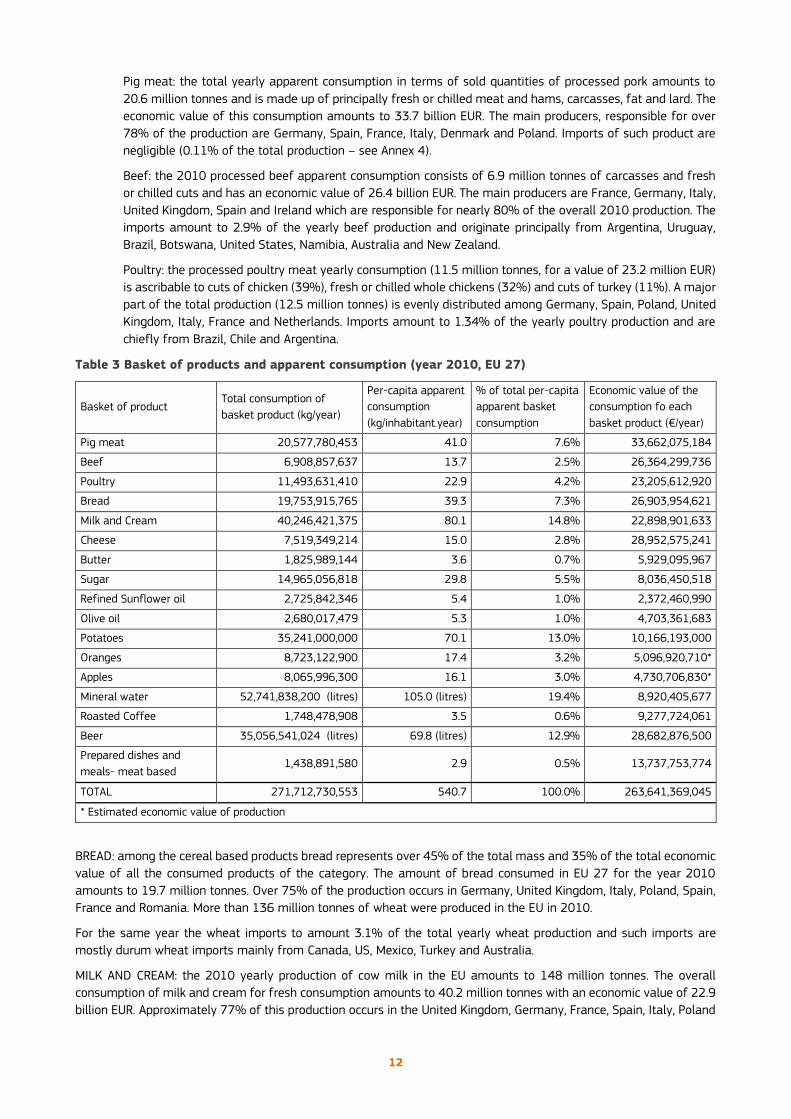
Pig meat: the total yearly apparent consumption in terms of sold quantities of processed pork amounts to

20.6 million tonnes and is made up of principally fresh or chilled meat and hams, carcasses, fat and lard. The

economic value of this consumption amounts to 33.7 billion EUR. The main producers, responsible for over

78% of the production are Germany, Spain, France, Italy, Denmark and Poland. Imports of such product are

negligible (0.11% of the total production – see Annex 4).

Beef: the 2010 processed beef apparent consumption consists of 6.9 million tonnes of carcasses and fresh

or chilled cuts and has an economic value of 26.4 billion EUR. The main producers are France, Germany, Italy,

United Kingdom, Spain and Ireland which are responsible for nearly 80% of the overall 2010 production. The

imports amount to 2.9% of the yearly beef production and originate principally from Argentina, Uruguay,

Brazil, Botswana, United States, Namibia, Australia and New Zealand.

Poultry: the processed poultry meat yearly consumption (11.5 million tonnes, for a value of 23.2 million EUR)

is ascribable to cuts of chicken (39%), fresh or chilled whole chickens (32%) and cuts of turkey (11%). A major

part of the total production (12.5 million tonnes) is evenly distributed among Germany, Spain, Poland, United

Kingdom, Italy, France and Netherlands. Imports amount to 1.34% of the yearly poultry production and are

chiefly from Brazil, Chile and Argentina.

Table 3 Basket of products and apparent consumption (year 2010, EU 27)

Basket of product Total consumption of

basket product (kg/year)

Per-capita apparent

consumption

(kg/inhabitant.year)

% of total per-capita

apparent basket

consumption

Economic value of the

consumption fo each

basket product (€/year)

Pig meat 20,577,780,453 41.0 7.6% 33,662,075,184

Beef 6,908,857,637 13.7 2.5% 26,364,299,736

Poultry 11,493,631,410 22.9 4.2% 23,205,612,920

Bread 19,753,915,765 39.3 7.3% 26,903,954,621

Milk and Cream 40,246,421,375 80.1 14.8% 22,898,901,633

Cheese 7,519,349,214 15.0 2.8% 28,952,575,241

Butter 1,825,989,144 3.6 0.7% 5,929,095,967

Sugar 14,965,056,818 29.8 5.5% 8,036,450,518

Refined Sunflower oil 2,725,842,346 5.4 1.0% 2,372,460,990

Olive oil 2,680,017,479 5.3 1.0% 4,703,361,683

Potatoes 35,241,000,000 70.1 13.0% 10,166,193,000

Oranges 8,723,122,900 17.4 3.2% 5,096,920,710*

Apples 8,065,996,300 16.1 3.0% 4,730,706,830*

Mineral water 52,741,838,200 (litres) 105.0 (litres) 19.4% 8,920,405,677

Roasted Coffee 1,748,478,908 3.5 0.6% 9,277,724,061

Beer 35,056,541,024 (litres) 69.8 (litres) 12.9% 28,682,876,500

Prepared dishes and

meals- meat based 1,438,891,580 2.9 0.5% 13,737,753,774

TOTAL 271,712,730,553 540.7 100.0% 263,641,369,045

* Estimated economic value of production

BREAD: among the cereal based products bread represents over 45% of the total mass and 35% of the total economic

value of all the consumed products of the category. The amount of bread consumed in EU 27 for the year 2010

amounts to 19.7 million tonnes. Over 75% of the production occurs in Germany, United Kingdom, Italy, Poland, Spain,

France and Romania. More than 136 million tonnes of wheat were produced in the EU in 2010.

For the same year the wheat imports to amount 3.1% of the total yearly wheat production and such imports are

mostly durum wheat imports mainly from Canada, US, Mexico, Turkey and Australia.

MILK AND CREAM: the 2010 yearly production of cow milk in the EU amounts to 148 million tonnes. The overall

consumption of milk and cream for fresh consumption amounts to 40.2 million tonnes with an economic value of 22.9

billion EUR. Approximately 77% of this production occurs in the United Kingdom, Germany, France, Spain, Italy, Poland

13

and Sweden. The small amounts of imported milk in 2010 (8.5 thousand tonnes) were mostly from Norway,

Switzerland and Croatia.

CHEESE: cheese consumption for the year 2010 amounts to 7.5 million tonnes with an overall value of 29 billion EUR.

Over 55% of the mass quantity is attributable to cheese whilst the rest is ascribable to cheese spreads and other fresh

cheese. The main producers are Germany, France, Italy, Netherlands Poland, UK and Spain. The main imports are

minimal (0.97% of the overall yearly cheese production) and originate mainly from Switzerland and New Zealand.

BUTTER: butter consumption totals 1.83 million tonnes in 2010 and has a value of 5.9 billion EUR. Over 80% of this

product is produced in France, Germany, Poland, Ireland, Netherlands, United Kingdom and Italy. The imports amount

to 1.96% of the overall butter production (1.9 million tonnes) and originate nearly totally from New Zealand and the

US.

REFINED SUGAR: this yearly consumption totals 14.97 million tonnes and has an economic value of 8 billion EUR. FAO

data on centrifugal sugar indicates that the main producers of such commodity are France, Germany, Poland, Ukraine,

UK and Netherlands. The imports of such refined products amount to 4.53% of the yearly production (16.2 million

tonnes of refined sugar) and originate primarily from Mauritius, Serbia, Croatia, Brazil and Swaziland.

OILS AND FATS: within this category olive oil and sunflower oil consumption amount to over 28% of the mass total

surpassing animal and vegetable fats. Refined colza, palm and rape oil consumption was higher than any other oil,

however they were not selected as basket products since they are not typically used for domestic food preparation

and a large share of these oils is consumed for the production of bio-fuels (EC 2008).

Refined sunflower oil: the 2010 apparent consumption totals 2.7 million tonnes with an economic value of

2.4 billion EUR. The 2013 country specific data regarding such product (2010-11-12 data was incomplete)

indicates that the main production (over 88% of total) occurs in Spain, Italy, Hungary, Germany, France, and

Romania. Imports amount to 4% of the yearly sunflower oil production and are primarily from Ukraine,

Argentina, Russia, Bosnia and Herzegovina and Moldova.

Olive oil: the 2010 apparent consumption amounts to 2.7 million tonnes and is worth 4.7 billion EUR.

Production occurs in the Mediterranean countries with Spain and Italy being responsible for over 95% of the

production. The imports (2.77% of the total EU production) of such product are mainly from the neighbouring

Mediterranean non EU countries such as Tunisia and Morocco.

POTATOES: 2010 potato apparent consumption of all types of potatoes (including seed and early potatoes) according

to the Eurostat data amounts to 55.3 million tonnes. The FAO database indicates an effective per capita potato

consumption of 70.1 kg/year which corresponds to a total apparent consumption for the year 2010 of 35.2 million

tonnes.

The value of the 2010 production amounts to 10.2 billion EUR. Such production is concentrated mostly in the northern

EU countries such as Germany, Poland, Netherlands, France, United Kingdom, Belgium and Romania. In 2012 0.42

million tonnes were imported mainly from Israel and Egypt.

FRUIT: the most consumed fruits in the EU 27 are oranges and apples.

Oranges: this is the most consumed fruit in the EU. In 2010 8.7 million tonnes were consumed. The production

occurs mainly in the Mediterranean countries of the EU, namely Italy, Spain and Greece (these first three

countries responsible for over 97% of the production), Portugal, France and Malta. The production has a value

of 5.1 billion EUR.

Imports for 2010 amount to 0.95 million tonnes and originate principally from South Africa, Egypt, Morocco,

Argentina, Uruguay, Brazil, Zimbabwe and Tunisia. In 2010 the EU production of un-concentrated orange juice

(frozen and non) amounted to 3.1 million tonnes.

Apples: this is the second most consumed fruit in the EU. The overall production of apples for 2010 totals 8.7

million tonnes with Italy, France, Poland and Germany responsible for over 64% of the production. Such

production has a value of 4.7 billion EUR.

In terms of apparent consumption, 8.06 million tonnes of apples for fresh consumption were consumed in

2010. The imports represent 7.1% of the production of apples for fresh consumption and originate mainly

from Chile, New Zealand, South Africa, Brazil, Argentina and The Former Yugoslav Republic Of Macedonia.

14

MINERAL WATER: among the non-alcoholic drinks mineral water resulted by far the most consumed beverage (1.5

times the volume of consumed soft drinks; 5 times the amount of consumed fruit juices). In 2010 52.7 billion litres of

mineral water were consumed with an economic value of 8.9 billion EUR. The Prodcom data concerning the production

of mineral water indicates Italy as the largest producer (26% of the total) followed by France, Spain, Poland, Romania,

United Kingdom, Portugal, Hungary and Greece. The imports are very modest (96 thousand tonnes for 2010) and are

mainly from Turkey, Norway, Croatia, Belarus, Georgia and Switzerland.

ROASTED COFFEE: the apparent consumption of roasted coffee for 2010 totals 1.75 million tonnes (caffeinated and

decaffeinated) with an economic value of 9.2 billion EUR. The production of this roasted coffee occurs mainly (over

80% of the total production) in Germany, Italy, Spain, France, Netherlands, Sweden, Belgium and Finland. Annual

imports (31.4 million kg) represent 1.8% of the annual production and originate predominantly from Switzerland and

Brazil. Green coffee which is used to produce roasted coffee is not cultivated in the EU but it is entirely imported.

Specifically, EU 27 imports of green coffee for 2010 amount to 2.2 million tonnes and originate mainly from Brazil,

Indonesia, Honduras, Peru, India, Uganda, Ethiopia, Colombia, Guatemala, El Salvador, Nicaragua, Kenya, Cameroon

and Mexico.

BEER: this is the most consumed alcoholic drink in the EU 27 (3 times the volume of consumed wine products) and

was thus chosen as a representative basket product. In 2010, 35.1 million litres were consumed for a total value of

28.6 billion EUR. The largest productions occur in Germany (23%), UK (14%), Poland (10%), Spain (9%), Netherlands

(7%), Belgium (5% ), Romania (5% ) and Czech Republic (5%). The imports are modest when compared to the

production (0.71% of the 2010 production of 37.2 million tonnes) and originate mostly from Mexico, Russia, Belarus,

China, Ukraine, US, Thailand, Switzerland, Turkey, Trinidad and Tobago and Croatia.

PREPARED DISHES AND MEALS - MEAT BASED: the overall apparent consumption of prepared dishes and meals in

2010 was 5.3 million tonnes with an economic value of 13.7 billion EUR. Among this main class of products in 2010

‘prepared meals and dishes based on meat, meat offal or blood’ is the most dominant with an apparent consumption

of 1.4 million tonnes/year.

2.3 Life cycle Inventory of the selected basket products

After identification of the nutrition basket-of-products was identified, the individual LCA of each product in the basket

products was implemented. First it was necessary to build a common framework relative to assumptions and models

to be used for the single product assessments in order to achieve consistent LCAs and to obtain comparable results.

The next step was the development of the process-based life cycle inventory models for the selected representative

products and of the corresponding process-based life cycle inventories. The inventories constructed for each product

regard not only the production phase of single food products but all stages of the food chain including losses and end

of life of products and waste. The main methodological considerations for the nutrition category products are given in

the following paragraphs.

Reference System

The reference system refers to the consumption per capita in EU-27 for the above listed products.

Functional Unit

The functional unit is defined as the average food consumption per person in EU in terms of food categories (including

the food losses at each stage).

System Boundaries

System boundaries consider a cradle-to-grave approach. For each stage of the life cycle, the process-based life cycle

inventories were developed for the selected representative products. System boundaries cover the agricultural and

production stage of each product, the logistics including international trade, the internal distribution to the retailer and

the consumer’s home, the packaging production and end of life, the use phase which considers home preparation of

food and food scraps, the end of life which covers the waste management of human excretion by wastewater

treatment plants and the end of life of food scraps into the municipal solid waste system. Food losses throughout the

life cycle have also been accounted for.

15

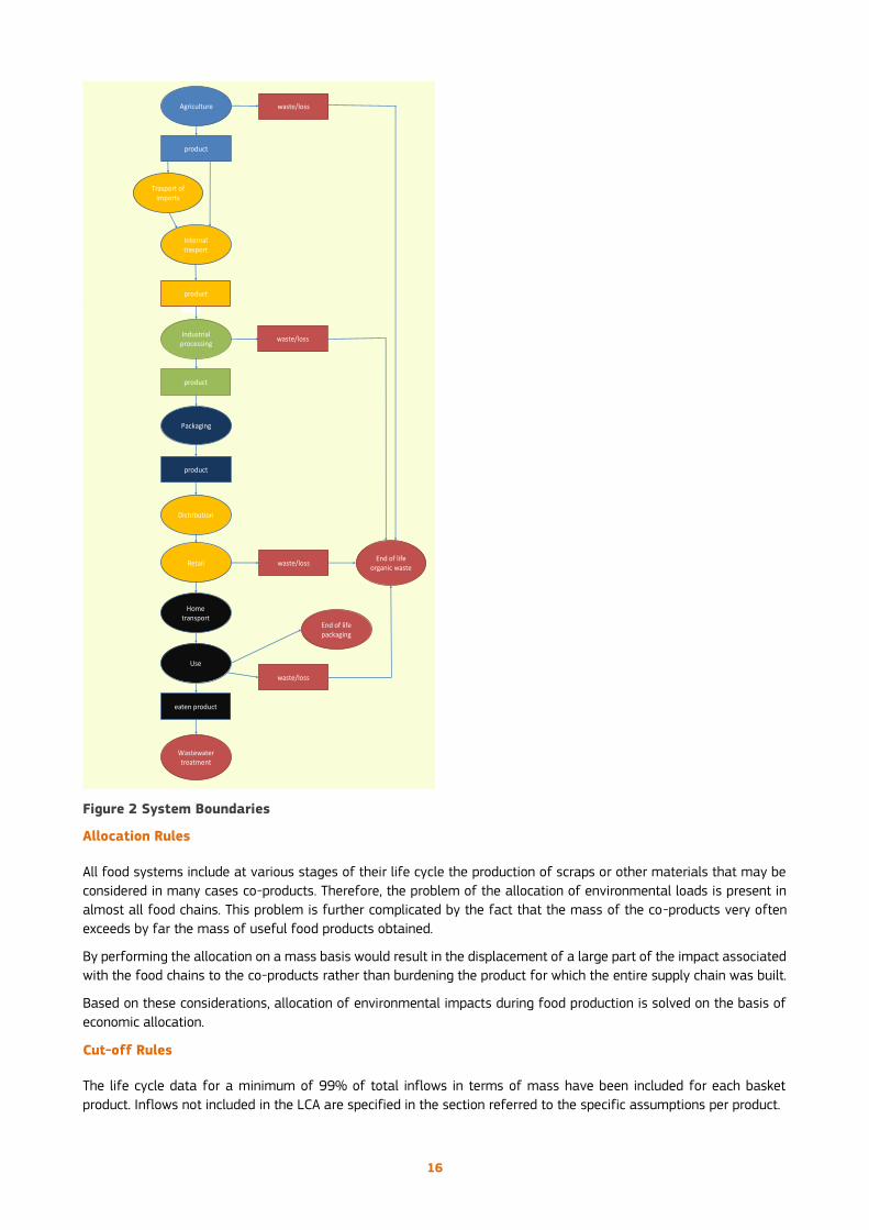
The general system boundaries of the analysed products are shown in Figure 2, divided into six parts:

agriculture/breeding, industrial processing, logistics, packaging, use and end of life. The stages considered in the

different life cycle phases are the following:

Agriculture/breeding

• Cultivation of crops

• Animal rearing

• Food waste management

Industrial processing

• Processing of ingredients

• Slaughtering, processing and storage of meat

• Chilled or frozen storage


Logistics

• International transport of imports

• Transport to manufacturer

• Transport to regional distribution centre

• Distribution

• Transport to retailer


Packaging

• Manufacture of packaging

• Final disposal of packaging

Use

• Transport of the products from retailer to consumer’s home

• Refrigerated storage at home

• Cooking of the meal

End of life

• Final disposal of food waste

• Wastewater treatment and auxiliary processes due to human excretion

In Annex 8 the specific system boundaries and the flow diagrams of the 17 basket products are reported.

16

Figure 2 System Boundaries

Allocation Rules

All food systems include at various stages of their life cycle the production of scraps or other materials that may be

considered in many cases co-products. Therefore, the problem of the allocation of environmental loads is present in

almost all food chains. This problem is further complicated by the fact that the mass of the co-products very often

exceeds by far the mass of useful food products obtained.

By performing the allocation on a mass basis would result in the displacement of a large part of the impact associated

with the food chains to the co-products rather than burdening the product for which the entire supply chain was built.

Based on these considerations, allocation of environmental impacts during food production is solved on the basis of

economic allocation.

Cut-off Rules

The life cycle data for a minimum of 99% of total inflows in terms of mass have been included for each basket

product. Inflows not included in the LCA are specified in the section referred to the specific assumptions per product.

Agriculture

product


product

Trasport of imports

waste/loss

Packaging

product

Distribution

Retail

Home transport

Use

End of life packaging

eaten product

Wastewater treatment

Internal trasport

product

waste/loss

waste/loss

End of life organic waste

waste/loss

17

LCIA Methodology

The impact assessment method for the assessment of inventories is ILCD which refers to midpoint impact categories

(EC 2010). The selected impact categories are those included in the method with the respective characterization

factors. Long-term emissions are excluded from the assessment according to Aronsson et al. (2013).

Data quality requirements

Different data quality requirements have been implemented in order to choose the inventory data which was most

adaptable to the present study and approach, including the country of origin of available data.

Data quality has been assessed on the basis of the following parameters in a pedigree matrix:

• Time-related coverage: age of data

• Geographical coverage: geographical area from which data for unit processes have been collected

• Technology coverage: specific technology or technology mix

• Completeness: type of provided flow

• Consistency: coherence of data with the methodology and assumptions of the study.

The specifications of the indicators with the relative score are given in the Table 4 which shows the Pedigree matrix

used to assess the quality of data sources. The approach followed was partly taken from Weidema et al. (2013) and

modified in order to align it to the objectives of the study.

The overall quality of the data set can be derived from the quality rating of the various quality indicators. This has

been calculated by summing the achieved quality rating for each of the quality components; the sum is then divided

by the number of applicable quality components. Therefore the score of each data is the arithmetic average of the

scores obtained in the various requirements. No further classification of the final overall quality scores was made.

For example, the application of the matrix to the evaluation of the data quality of the paper by Schmidt Rivera et al.

(2014), relative to the pre-prepared meals, was carried out in the following way. Time-related coverage is less than 3

years (score 1). Geographical coverage is respected via the use of data deriving from the area under study (score 1).

As regards technology coverage, the processes and materials under study refer to a specific technology and not to a

representative technology for the whole production; therefore the score is 2. Completeness scores 1 as a complete

tree of processes is provided with a very detailed description; this means that data are given for each of the sub-

processes in which the system can be divided and not as a single aggregate inventory of the whole system. The

consistency gets a score of 2 because the hypotheses and assumptions about allocation and cut-offs are different

from those at the base of this study. In any case, since the inventory of the processes is provided in a disaggregated

way, it is possible to apply much of the methodology and assumptions of the present study, especially with regard to

the agricultural phase of the various products which constitute the inputs of pre-prepared food. The final score obtained

from this data set is equal to 1.4 which is the arithmetic average of the scores obtained for each of the different

requirements. This score was used to identify the representative data set of the product in question.

With regard to the requirement of coherence, many studies report the data in terms of an environmental inventory of

the life cycle of the products in terms of elementary flows. From these data it is not possible to apply the assumptions

made for example for the agricultural phase, since the inventory define the amount of natural resources used by the

system, but these cannot be traced to the amount of fertilizer needed for the estimation of emissions of ammonia,

N2O, etc. In these cases the methodology is therefore not applicable and the score assigned to this requirement is 5.

18

Table 4 Pedigree matrix used to assess the quality of data sources (modified from Weidema et al. 2013).

Indicator score 1 2 3 4 5

Time-related coverage Less than 3 years

of difference to

the time period of

the dataset

Less than 6 years

of difference to

the time period of

the dataset

Less than 10

years of

difference to the

time period of

the dataset

Less than 15 years

of difference to

the time period of

the dataset

Age of data

unknown or more

than 15 years of

difference to the

time period of the

dataset

Geographical coverage Data from area

under study

Average data

from larger area

in which the area

under study is

included

Data from area

with similar

production

conditions

Data from area

with slightly

similar production

conditions

Data from

unknown or

distinctly

different area

Technology coverage Data from

processes and

materials under

study and from

different

technologies

Data from

processes and

materials under

study but from a

specific

technology

Data on related

processes or

materials

Data on outdated

technology

Data on related

processes on

laboratory scale

or from different

technology

Completeness provided a

complete tree of

processes and a

very detailed

description

provided a

complete process

not as a tree

integrated

system of black

boxes

provided an

incomplete

process not as a

tree

incomplete black

box

Consistency applicable the

methodology and

assumptions of

the study

applicable much

of the

methodology and

assumptions of

the study

applicable part

of the

methodology

and assumptions

of the study

applicable to a

small extent the

methodology and

assumptions of

the study

non applicable

the methodology

and assumptions

of the study

2.3.1 Data sources

In order to identify useful datasets representing inventory data for each stage of the lifecycle of the basket products,

described in Section 2.2.3, a literature review of work regarding the environmental assessment of each basket product

(with particular emphasis on the LCA approach) was carried out.

The scientific publications containing relevant inventory information useful for the formation of datasets are listed in

Annex 6 (referred to each basket product). Annex 7 contains a table with the indication, for each of the papers listed

in Annex 6, of the lifecycle phases for which useful inventory data may be extracted from these publications.

By applying the methods described in the Data Quality Requirements section to the collected literature, the most

representative datasets for each product in the basket were identified. In particular, for each process or stage of the

life cycle, choosing the most representative data set was performed by comparing the data quality scores obtained

from the various data sources; the data set chosen was the one which obtained the lowest score (which corresponds

to a higher quality), regardless of the specific level. With the same final score, the data set having a better score in

the geographical coverage requirement was preferred.

LCI datasets of the agriculture/production stage for the basket products are briefly summarized in Table 5. These

datasets have been identified on the basis of data quality requirements, in the above mentioned way. For

completeness, the table also shows the producing country that is the country to which the data in question relates;

this does not necessarily mean that the country could be considered a key producer, representative of the European

production.

Foreground data were obtained from literature and direct industry sources. Background data are mainly taken from

the Agrifootprint and Ecoinvent v.3 databases.

19

Country specific import data for the basket products are taken from Eurostat international trade database for the year

2010 (unless otherwise specified). Import countries distances and modes of transport were also accounted for as

reported in Annex 2.

Table 5 Overview of LCI datasets relative to the agriculture/production phase

Product category Representative

products

Sources of representative datasets

Alcoholic, non-

alcoholic

beverages

Coffee Production of 1 kg roasted coffee. Agricultural production in Brazil in the 2006 reference

year and wet processing for the production of green beans in the 2014 reference year.

Roasting process in the 2009 reference year. Data from Coltro et al. (2006).

Beer Production of 1 L of beer in the 2012 reference year, assuming EU-27 electricity. Data

from Schaltegger et al. (2012).

Mineral water Production of 1 L of mineral water in the 2014 reference year from Vanderheyden and

Aerts (2014).

Cereal based

products

Bread Production of 1 kg of bread in UK in the 2011 reference year. Data for bread production

from Espinoza-Orias et al. (2011). Main data for wheat production are relative to

Germany in the 2014 reference year, assuming EU-27 electricity and pesticides (from

Agri-footprint database).

Meat and

seafood

Beef Production of 1 kg of fresh cut in Ireland in the 2014 reference year. Data on both

rearing and slaughtering are referred to the same country. Main data from Agri-

footprint database.

Pork Production of 1 kg of fresh cut in The Netherlands in the 2014 reference year. Data on

both rearing and slaughtering are referred to the same country. Main data from Agri-

footprint database.

Poultry Production of 1 kg of fresh cut in The Netherlands in the 2014 reference year. Data on

both rearing and slaughtering are referred to the same country. Main data from Agri-

footprint database.

Dairy products Milk Production of 1 kg of milk in the 2014 reference year, assuming EU-27 electricity. Data

on raw milk are referred to The Netherlands (from Agri-footprint database) while data

on processing to Italy (from Fantin et al. 2012).

Butter Production of 1 kg of butter in Serbia in the 2014 reference year, assuming EU-27

electricity. Data from Djekic et al. (2014)

Cheese Production of 1 kg of milk in Serbia in the 2014 reference year, assuming EU-27

electricity. Data from Djekic et al. (2014)

Crop-based

products

Sugar Production of 1 kg of sugar from sugar beet in Germany in the 2014 reference year,

assuming EU-27 electricity and pesticides. Main data from Agri-footprint database.

Sunflower oil Production of 1 kg of sunflower oil in Ukraine in the 2014 reference year, assuming EU-

27 electricity and pesticides. Main data from Agri-footprint database.

Olive oil Production of 1 kg of extra virgin olive oil in Italy in the 2013 reference year. Data on

agricultural production and olive oil processing are directly taken respectively from

producers and industry. Data from Notarnicola et al. (2013).

Vegetables Potatoes Production of 1 kg of potatoes in Germany in the 2014 reference year, assuming EU-

27 electricity and pesticides. Main data from Agri-footprint database.

Fruits Apples Production of 1 kg of apples in Switzerland in the 2006 reference year, assuming EU-

27 electricity and pesticides. Data from Milà i Canals et al. 2007.

Oranges Production of 1 kg of oranges in Italy in the 2013 reference year, assuming EU-27

electricity and pesticides. Data from Pergola et al. (2013).

Pre-prepared

meals

Pre-prepared

meals based on

meat

Production of 1 kg of pre-prepared meal based on meat. Data from Schmidt Rivera et

al. (2014) in the reference year 2014, including poultry meat, potatoes, tomato sauce

and dressings.

2.3.2 Assumptions

The LCI methodology follows in many aspects the methodology used to process Ecoinvent background data

(Frischknecht et al. 2007). The following main assumptions are considered:

20

• Lifetime of food products are considered to be less than 1 year.

• Infrastructure is included with a life time of 50 years and a construction time of 2 years

• Waste management is included.

• EU-27 dataset for electricity is used. In the inventory, electricity consumed in the food chain always refers to low

voltage electricity (LV). In the distribution system of electricity the medium-voltage is used in the intermediate

portions of the electricity grid between the high-voltage receiving stations from the power lines and the cabins of

final transformation for delivery at low-voltage. Low voltage electricity is used in most of the private electrical

systems, both civil and industrial, as well as in secondary distribution networks. Only some large users buy

electricity directly at medium voltage, but in any case they reduce it by providing LV with private cabins. This study

considers low voltage the range of electric voltage between 50 and 1,000 volts in terms of AC current. So the

choice of this voltage seems adequate to represent the actual situation of food plants and consequently, for the

inventory of electricity, the process taken from the ELCD database named “Electricity mix, AC, consumption mix,

at consumer, < 1kV EU-27 S” was used. However this assumption is referred to the foreground of the product

systems and not to all the other background processes which could make use of medium voltage electricity.

• Double counting occurs when considering pre-prepared meals made with other basket products. In this case the

amount of products contained in the pre-prepared meal is subtracted from the relative amount of basket product

calculated and described in section 2.2.3 and allocated to the pre-prepared meal.

• The imports of basket products have been treated as if they were produced domestically (in the EU).

A comprehensive list of assumptions organized by life cycle stages is given in the following paragraphs.

Agricultural/Breeding stage

Fertilizers

The data used for consumption of fertilizers in the various phases of agricultural production depends on the quality of

the bibliographic source used. When consumption data related to the specific fertilizers was available, the specific

environmental inventories extracted from databases were directly associated to such consumption data.

In many cases the data relative to the agricultural phases of the examined processes report the consumption of

fertilizers in terms of N, P2O5 e K2O content and not in terms of fertilizer. Sometimes consumption is reported in more

aggregated terms as the sum of the three main nutrients.

In these cases, the approach used to generate inventory data for fertilizers and their respective emissions was similar

to that followed by the Agri-footprint and Ecoinvent databases (described below), so that the processes obtained were

consistent with those extrapolated from these databases.

Standard distances were used for the transport of materials from their production site to the processing plant or the

farm. This is 500 km by lorry. Ecoinvent transport unit processes are used.

The following section illustrates the hypotheses and assumptions made to estimate the consumption of fertilizers and

subsequently those related to emissions associated with the use of fertilizers.

Synthetic fertilizer application rates

As previously mentioned, in the case in which the data relative to the agricultural phases of the examined processes

report the consumption of fertilizers in terms of N, P2O5 e K2O content and not in terms of fertilizer, an approach for

the estimation of synthetic fertilizer application rates was followed.

The first step is the identification of the type of fertilizer employed (eg. urea or potassium chloride, etc.) starting from

the total consumption of ingredients, in order to associate it to the relevant environmental inventory.

In practice statistical data on the use of fertilizers in a given country were employed in order to disaggregate

consumption given in terms of N, P2O5 e K2O. The relative rates of fertilizer consumption were obtained from the

database of the International Fertilizer Industry Association (IFA 2012) that provides regionalized data on production,

import, export and consumption of fertilizers. The data series used cover the period 2008-2011 and for each data

item the average consumption observed in the four years mentioned was considered. The data were broken down by

country as well as for type of fertilizer.

By using such a database it was possible to reconstruct for each country the percentage of consumption of each type

of fertilizer.

21

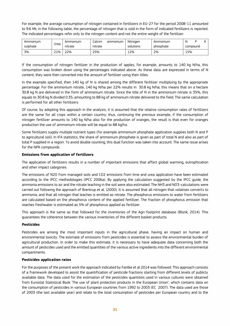
For example, the average consumption of nitrogen contained in fertilizers in EU-27 for the period 2008-11 amounted

to 9.6 Mt; in the following table, the percentage of nitrogen that is sold in the form of indicated fertilizers is reported.

The indicated percentages refer only to the nitrogen content and not the entire weight of the fertilizer.

Ammonium

sulphate Urea

Ammonium

nitrate

Calcim ammonium

nitrate

Nitrogen

solutions

Ammonium

phosphate

N P K

compound

3% 21% 22% 25% 12% 2% 15%

If the consumption of nitrogen fertilizer in the production of apples, for example, amounts to 140 kg N/ha, this

consumption was broken down using the percentages indicated above. As these data are expressed in terms of N

content, they were then converted into the amount of fertilizer using their titles.

In the example specified, then 140 kg of N is shared among the different fertilizer multiplying by the appropriate

percentage. For the ammonium nitrate, 140 kg N/ha per 22% results in 30.8 kg N/ha; this means that on a hectare

30.8 kg N are delivered in the form of ammonium nitrate. Since the title of N in the ammonium nitrate is 35%, this

equals to 30.8 kg N divided 0.35, amounting to 88 kg of ammonium nitrate delivered to the field. The same calculation

is performed for all other fertilizers.

Of course, by adopting this approach in the analysis, it is assumed that the relative consumption rates of fertilizers

are the same for all crops within a certain country; thus, continuing the previous example, if the consumption of

nitrogen fertilizer amounts to 140 kg N/ha also for the production of oranges, the result is that even for oranges

production the use of ammonium nitrate will be equal to 88 kg/ha.

Some fertilizers supply multiple nutrient types (for example ammonium phosphate application supplies both N and P

to agricultural soil). In IFA statistics, the share of ammonium phosphate is given as part of total N and also as part of

total P supplied in a region. To avoid double counting, this dual function was taken into account. The same issue arises

for the NPK compounds.

Emissions from application of fertilizers

The application of fertilizers results in a number of important emissions that affect global warming, eutrophication

and other impact categories.

The emissions of N2O from managed soils and CO2 emissions from lime and urea application have been estimated

according to the IPCC methodologies (IPCC 2006a). By applying the calculation suggested by the IPCC guide, the

ammonia emissions to air and the nitrate leaching in the soil were also estimated. The NH3 and NO3-calculations were

carried out following the approach of Brentrup et al. (2000). It is assumed that all nitrogen that volatises converts to

ammonia, and that all nitrogen that leaches is emitted as nitrate. The phosphorus emissions to water from fertilizers

are calculated based on the phosphorus content of the applied fertilizer. The fraction of phosphorus emission that

reaches freshwater is estimated as 5% of phosphorus applied as fertilizer.

This approach is the same as that followed for the inventories of the Agri-footprint database (Blonk, 2014). This

guarantees the coherence between the various inventories of the different basket products.

Pesticides

Pesticides are among the most important inputs in the agricultural phase, having an impact on human and

environmental toxicity. The estimate of emissions from pesticides is essential to assess the environmental burden of

agricultural production. In order to make this estimate, it is necessary to have adequate data concerning both the

amount of pesticides used and the emitted quantities of the various active ingredients into the different environmental

compartments.

Pesticides application rates

For the purposes of the present work the approach indicated by Fantke et al 2014 was followed. This approach consists

of a framework developed to assist the quantification of pesticide fractions starting from different levels of publicly

available data. The data used for the estimation of the pesticides quantities used in various cultures were obtained

from Eurostat Statistical Book ‘The use of plant protection products in the European Union’, which contains data on

the consumption of pesticides in various European countries from 1992 to 2003 (EC 2007). The data used are those

of 2003 (the last available year) and relate to the total consumption of pesticides per European country and to the

22

consumption per hectare of various categories of pesticides, divided into herbicides, fungicides, insecticides and other

plant protection products.

The report also shows consumption per hectare for various crops and the top five active ingredients used per country

and per chemical class.

Dosages of plant protection products used by crop have been used; these show the consumption of active ingredient

per hectare divided among the major categories. In order to identify the active ingredients associated with each

category the following procedure was used:

• The main chemical classes were identified by crop and then, for each of these classes, the main active ingredients

were identified; these active ingredients were chosen among those listed in the top 10 active ingredients of each

category. A handbook of agriculture was consulted for information on the use of such ingredients in specific crops.

A value equal to the total consumption of the specific category was assigned to the ingredients identified. For

example, for the cultivation of citrus fruits, a total consumption of herbicides in Europe is indicated as 4.0 kg/ha

in terms of active ingredients. A table reports the main chemical classes of herbicides applied to citrus crops. This

table shows that 2,031 tonnes of organophosphorus herbicides are consumed on a total of 2,289 tonnes is used

for the cultivation of citrus fruits; this amounts to about 90% of total herbicides consumption. All other herbicides

have a consumption of less than 3%. Glyphosate is the main herbicide of the organophosphorus herbicides class.

Therefore for the cultivation of citrus fruits a consumption of glyphosate was assumed to be equal to the total of

the class which is 4.0 kg/ha in terms of active ingredient. The total amount of herbicide produced was obtained

starting from the percentage of active ingredient contained in commercial products; this figure is useful for the

purpose of calculating inventories of pesticide production and transport. For glyphosate a content of 40% of active

ingredient weight/weight is considered for the commercial product.

For crops covered by the report, the following approach was used. Eg. apple crop was associated with the cultivation

of fruit trees, oranges to the cultivation of citrus plants, while wheat to the cultivation of cereals. For the rest of the

products for which this type of association was not possible, such as eg. olive oil, data from the specific literature or

from a handbook of agriculture were used (Ribaudo 2011).

Standard distances were used for the transport of materials from their production site to the processing plant or the

farm. This is 500 km by lorry. Ecoinvent transport unit processes were used.

Emissions from application of pesticides

Since there is still no consensus on which model to apply, in order to estimate emissions from the use of pesticides,

and in particular the fate modelling from technosphere to biosphere, the following procedure was used:

• The name of pesticide and the amount active ingredient applied are used to model the environmental fate of

pesticides in the inventory. The environmental fate is assumed to be 100 % to soil. This statement follows the

code of life cycle inventory practice (de Beaufort-Langeveld et al. 2003) which is also applied in the Ecoinvent

background data and in the Agri-footprint database methodology.

Of course the results of this approach represent the worst case scenario.

Animal breeding systems

The analysis of farming systems requires data on animal growth, enteric emissions, feed production. The animal

breeding models taken into account in this study for the various types of products (dairy products, meat from beef,

pork and poultry) are those reported in Blonk Consultants (2014).

In particular, for livestock products the animal enteric fermentation and the type of manure management were

accounted for. The feed production is also taken into account.

The inventories regarding the impacts of livestock are calculated according to the approach indicated by IPCC in chapter

10 Vol.4 (IPCC 2006b).

The main emissions deriving from livestock included in the inventories are the following:

• manure management: the relative emissions are constituted mainly by methane and nitrous oxide deriving from

the aerobic and anaerobic decomposition of the manure and from ammonia;

• enteric fermentation: this includes the emissions of methane produced mainly by ruminant digestive systems and

in minor amount by those of non-ruminant animals.

23

The emissions factors taken from IPCC are specified by category of livestock and regional grouping.

Food losses throughout the supply chain

The loss of matter that takes place in the various life cycles of products has been accounted for. Food losses or waste

are the masses of food lost or wasted in the part of food chains leading to edible products going to human

consumption. Co-products, waste and losses are defined and related to each other in different manners. Co-products

are those useful products obtained together with the main product which have an economic value; waste is the rest

of matter. Co-products leave the system through allocation while waste is sent to the EU27 food waste treatment

scenario. Another distinction is that regarding waste from processes and food loss; food loss is intended as the useful

food that for various reasons is lost within the supply chain and not the physiological waste produced in a process

(according to the definition given in the FAO report used as a main data source). Losses also consist of the food waste

deriving from the inefficiencies of the food chains.

When specific literature data were available, these were used for the calculation of loss in a specific supply chain, as

in the case of apples and oranges. For other cases, the loss data were obtained from the FAO report ‘Global food losses

and food waste – Extent, causes and prevention’ (FAO 2011) which highlights the losses occurring along the entire

food chain, and makes assessments of their magnitude. Data are reported for agricultural production, post-harvest

handling and storage, processing, distribution and consumption.

Data are referred to commodity groups and not to single products. Accordingly, the various basket products were

associated with a reference food commodity group and the loss of the group was then assigned to the single product.

Not all the products can be associated to the groups; in these cases losses are reported only for the life cycle phases

for which data are available.

The end of life of the waste generated from losses was also considered. The end of life scenario of food waste was

evaluated starting from data on the disposal of waste in EU-27. Eurostat contains statistics on the “Treatment of

waste [env_wastrt]” database; the most recent available data is that of 2010. This database details the amount of

waste divided into various types; for the purposes of this study the “Animal and vegetable wastes (subtotal, W091 +

W092 + W093)” waste category was considered, which represents 4% of the total waste. The statistics indicate the

following disposal treatments: 8% of food waste is sent to landfill, 5% is incinerated, and 87% is sent to other recovery

treatments. It is assumed that such a recovery treatment is 80% composting and 20% anaerobic digestion for biogas

production; therefore 69.6% of total waste is set to composting while 17.4% to anaerobic digestion. Food waste coming

from the various supply chains has been assumed to undergo this end of life scenario, with the above mentioned

treatments and percentages.

The assumption made for food losses is that the burden deriving from the treatment of lost matter is attributed the

life cycle phase that generated that loss. E.g. the waste treatment of food matter lost in the distribution stage is

attributed to the distribution phase. Consequently the EU27 waste treatment scenario is applied, including landfill,

incineration, composting and anaerobic digestion.


Data on individual production units were considered for all products that require industrial processing. As regards

refrigeration, which occurs during processing and storage, the electric energy consumption is assumed 1.8 Wh/L per

day for meat and 1.2 Wh/L per day for fruit and vegetables (EPD 2012). For the various products the number of days

of refrigeration and the specific weight is considered as reported in Annex 9.

Packaging

For all basket products the primary packaging was considered; whenever possible even the secondary packaging was

added to inventories.

The packaging phase also includes the end of life of the packaging itself. Specifically, for the packaging used in the

life cycles an end of life scenario was built. This considers that a part of the packaging is recycled and the rest is

destined to incineration and landfill. The percentage of waste sent to the various treatments are different from

material to material and were taken from the Ecoinvent database.

24

Logistics

Logistics can be divided into international trade, distribution and retail.

International trade. For all products in the basket the international trade was considered with the exception of pre-

prepared meals for which data on imports per country were not available; in particular for imports, the relevant amount

in relation to domestic production and the countries of origin were considered. Those countries that represent the

source of at least 90% of the total EU imports of a specific basket product were considered (Annex 2) for the impact

assessment. Logistics linked to international trade has been assumed with regard to the transport of commodities

from the capital of the exporting country to the city of Frankfurt, which is considered a central destination for the

arrival of imports in Europe. For those countries not connected to Europe by land routes, different means of transport

were considered: a transport by lorry between the capital of the exporting country and the country's main port; a

transport by ship from the port of the exporting country to the main European ports and finally, a transport by lorry

between the port of destination and the city of Frankfurt. Rotterdam and Marseilles were considered as the European

ports of arrival of the goods. The distances between ports in kilometres have been taken from http://www.sea-

distances.org/. For those exporting countries directly connected to Europe by land, such as Switzerland or Belarus, only

a transport by lorry was considered from the capital of the exporting country to the city of Frankfurt. Annex 2 contains

all the above mentioned information relative to EU imports of basket products.

Distribution. It consists of a transport by lorry from the manufacturer/farm to a regional distribution centre and a

further transport by lorry from the regional distribution centre to the retailer. The total distance travelled was assumed

to be 500 km for all products. In the case in which the product required a refrigerated transport, a 20% increase in

fuel consumption was assumed (Lalonde et al. 2013).

Retail. The energy consumption associated to the permanence of the product in retail was considered using data taken

from the LCA Food DK database. For those products that require refrigeration, the consumption of electrical energy

associated with this operation was considered equal to 1.2 Wh/L per day (EPD 2012). For the various products the

number of days of refrigeration and the specific weight is considered as reported in Annex 9.

Use phase

The use phase consists of consumer home transport and domestic consumption.

Home transport consists of a transport by passenger car from the consumer’s home to the retailer and back. The

distance travelled was assumed to be 4 km. As consumer spending covers both food products and non, the allocation

of transport between the various products occurs in this phase; in order to solve allocation it was assumed that the

consumer buys a total of 30 products in each purchase. Therefore 3.33% of transport burden has been allocated to

the purchased product as each product represents one of thirty items purchased (Vanderheyden and Aerts 2014). For

each product of the basket the amount of basket product purchased in a journey has been fixed as reported in Annex

9.

Domestic consumption is associated both to the consumption of electricity for the refrigeration of food and to the

impacts due to the preparation and cooking of food.

As regards refrigeration the electric energy consumption of domestic refrigerator is assumed 2.3 Wh/L per day while

the freezer one is 4.2 Wh/L per day (Nielsen et al. 2003). For the various products the number of days of refrigeration

and the specific weight is considered as reported in Annex 9.

As regards to home preparation the following operations are considered together with the specific energy consumption

(Foster et al. 2006):

• Boiling: 2 MJ of natural gas/kg product

• Frying: 7.5 MJ of natural gas/kg product

• Baking: 0.75 kWh electricity/ kg product

• Roasting: 8.5 MJ of natural gas/kg product

End of life

The end of life includes the following elements:

25

• Food scraps and not consumed foods. This is the part of food which is not edible, such as the peel of the apple or

potato, and the proportion of edible food not consumed and thrown away as waste. For both of these food wastes

the end of life scenario described in the section on food losses throughout the supply chain has been applied for

all the solid products. For liquid products, such as beer and coffee, it was assumed that the non-consumed part

of such drink goes from the user’s home to the unpolluted wastewater treatment.

• Human faeces. For the environmental assessment of human metabolism products, the model by Muñoz et al.

(2007) was used. This model includes processes such as human excretion due to food intake, auxiliary processes

related to toilet use, and treatment of human excretion products present in wastewater through a sewage

treatment plant.

2.3.3 Final selection: overview per product and life cycle stage

This paragraph describes the final selection of basket products, based on the application of the hypotheses,

assumptions and data described in the previous paragraphs.

Table 6 summarises the mapping of the coverage in terms of life cycle stages and inventories (LCI) for a given

representative product. The letter “Y” indicates that a life cycle stage is included in the system. The table highlights

that for all the phases of the life cycle of the representative products the life cycle inventories were included. Some

coverage differences are present as far as processes regarding packaging and the inventory of losses are concerned.

In fact a further specification is given in the case of packaging: with “P” specifies the inclusion of data on primary

packaging, while “S” indicates the inclusion of data on secondary packaging. As regards to packaging, the primary

packaging was included for all the products, while the secondary packaging was included only where data was

available. The same applies to the inventory of losses; by applying the information drawn from the indicated data

sources, for a certain number of products, it is possible to calculate losses regarding the whole life cycle. For other

products losses are limited only to the use or retail phases.

Table 6 Mapping of the coverage in terms of life cycle stages, inventories (LCI) for a given representative

product

Representative product Agricultural

production/

livestock

Industrial

processing

Logistics Packaging Use End of

life

other inventory

data - losses

Coffee Y Y Y Y: P-S Y Y Only for use phase

Beer Y Y Y Y: P Y Y Only for use phase

Mineral water Y Y Y Y: P Y Y Only for use phase

Bread Y Y Y Y: P Y Y Y

Beef Y Y Y Y: P Y Y Y

Pork Y Y Y Y: P Y Y Y

Poultry Y Y Y Y: P Y Y Y

Milk Y Y Y Y: P Y Y Y

Butter Y Y Y Y: P Y Y Y

Cheese Y Y Y Y: P-S Y Y Y

Sugar Y Y Y Y: P Y Y Only for use phase

Sunflower oil Y Y Y Y: P Y Y Y

Olive oil Y Y Y Y: P-S Y Y Only for use phase

Potatoes Y Y Y Y: P Y Y Y for retail and use

Apples Y Y Y Y: P Y Y Y

Oranges Y Y Y Y: P Y Y Y

Pre-prepared meals

based on meat

Y Y Y Y: P-S Y Y Y

Y=included P=primary S=secondary

Particular attention was paid to the application of the previously mentioned fertiliser and pesticide models.

Table 7 shows the chosen data sources and models for the agricultural stage of each product of the basket. Most of

data are taken from the Agri-Footprint database; this choice is due to the fact that the methodology used for the

26

inventory building of this database is perfectly comparable with the model adopted in the present study. Therefore

data from the Agri-Footprint database constitutes the main option.

In any case for the datasets, taken from the various databases, data regarding pesticide consumption are replaced,

whenever possible, by those taken from the EU report on pesticide application in Europe, already cited in the paragraph

on pesticide application rates. In order to guarantee the coherence between the various models and data sources, the

pesticide modelling is made by assuming a 100% to soil emission of active ingredients.

Table 7 Application of assumptions to agriculture

Basket products Data sources Fertiliser modelling Pesticide data source Pesticide modelling

apples Milà i Canals et al. 2006

according to the

assumptions EU report 100% soil

barley (beer) Agri-Footprint Agri-Footprint EU report 100% soil

wheat (bread) Agri-Footprint Agri-Footprint EU report 100% soil

coffee Coltro et al. 2006

according to the

assumptions from cited literature 100% soil

olive Notarnicola et al. 2013

according to the

assumptions from cited literature 100% soil

oranges Beccali et al. 2013

according to the

assumptions EU report 100% soil

potatoes Agri-Footprint Agri-Footprint EU report 100% soil

sugar beet Agri-Footprint Agri-Footprint EU report 100% soil

sunflower seed Agri-Footprint Agri-Footprint EU report 100% soil

tomato (pre-prepared) Ecoinvent

according to the

assumptions Ecoinvent 100% soil

onion (pre-prepared) Ecoinvent

according to the


sunflower seed (pre-prepared) Agri-Footprint Agri-Footprint EU report 100% soil

carrot (pre-prepared) Ecoinvent

according to the


pea (pre-prepared) Agri-Footprint Agri-Footprint Agri-Footprint 100% soil

raw milk (milk, cheese, butter) Agri-Footprint - - -

meat - bovine Agri-Footprint - - -

meat - pork Agri-Footprint - - -

meat - poultry Agri-Footprint - - -

mineral water Vanderheyden et al. 2014 - - -

Another calculation was needed for the estimate of the impact of international transport of imported goods on the

environmental profile of the basket. Starting from the country specific import data for the basket products, taken from

Eurostat international trade database for the year 2010, and the import countries distances and modes of transport

reported in Annex 2, the total loads and distances travelled by different means have been calculated. The reference

data are reported in Table 8. It can be noted that in some cases the value of ship transport per kg of product is

particularly relevant, as in the case of butter and apples. No data were found for pre-prepared foods. The share of

production and imports with respect to the total available quantity of commodities are illustrated in

Table 9. The percentage of imports is very low for all products with the exception of green coffee, which is entirely

produced abroad, and oranges which have 10% share of imports.

A comprehensive list of assumptions organized by life cycle stages is given in Annex 9.

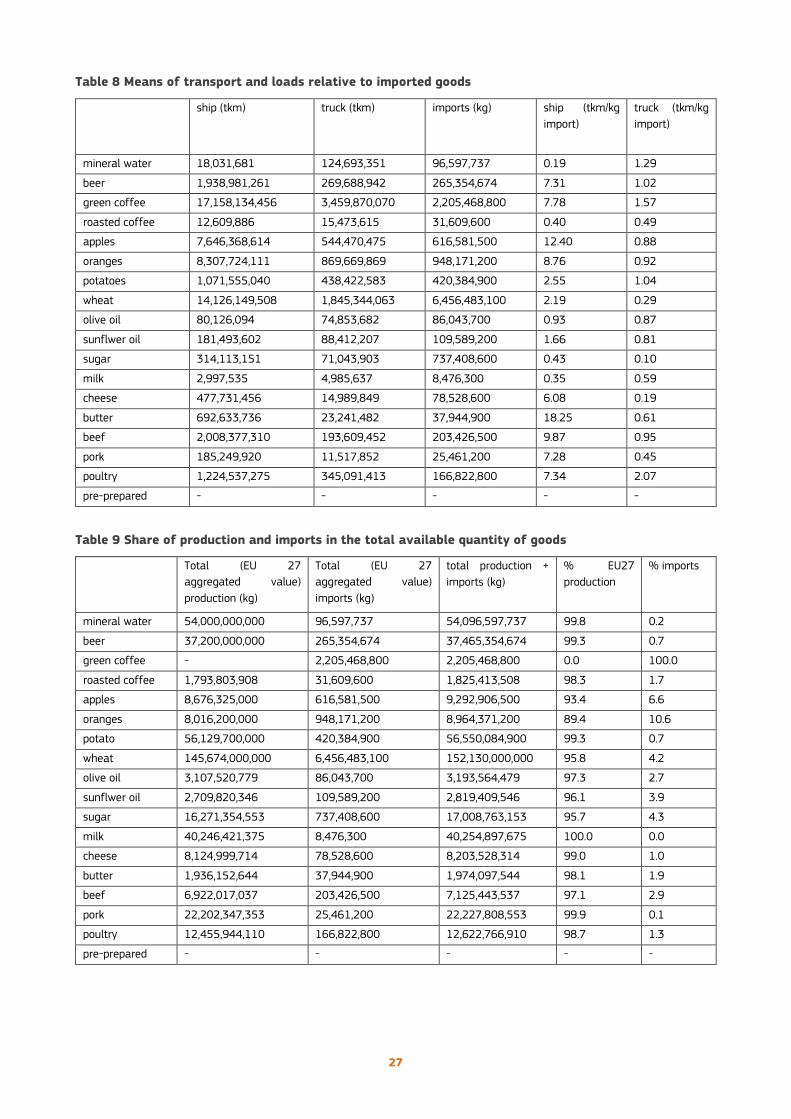
27

Table 8 Means of transport and loads relative to imported goods

ship (tkm) truck (tkm) imports (kg) ship (tkm/kg

import)

truck (tkm/kg

import)

mineral water 18,031,681 124,693,351 96,597,737 0.19 1.29

beer 1,938,981,261 269,688,942 265,354,674 7.31 1.02

green coffee 17,158,134,456 3,459,870,070 2,205,468,800 7.78 1.57

roasted coffee 12,609,886 15,473,615 31,609,600 0.40 0.49

apples 7,646,368,614 544,470,475 616,581,500 12.40 0.88

oranges 8,307,724,111 869,669,869 948,171,200 8.76 0.92

potatoes 1,071,555,040 438,422,583 420,384,900 2.55 1.04

wheat 14,126,149,508 1,845,344,063 6,456,483,100 2.19 0.29

olive oil 80,126,094 74,853,682 86,043,700 0.93 0.87

sunflwer oil 181,493,602 88,412,207 109,589,200 1.66 0.81

sugar 314,113,151 71,043,903 737,408,600 0.43 0.10

milk 2,997,535 4,985,637 8,476,300 0.35 0.59

cheese 477,731,456 14,989,849 78,528,600 6.08 0.19

butter 692,633,736 23,241,482 37,944,900 18.25 0.61

beef 2,008,377,310 193,609,452 203,426,500 9.87 0.95

pork 185,249,920 11,517,852 25,461,200 7.28 0.45

poultry 1,224,537,275 345,091,413 166,822,800 7.34 2.07

pre-prepared - - - - -

Table 9 Share of production and imports in the total available quantity of goods

Total (EU 27

aggregated value)

production (kg)

Total (EU 27

aggregated value)

imports (kg)

total production +

imports (kg)

% EU27

production

% imports

mineral water 54,000,000,000 96,597,737 54,096,597,737 99.8 0.2

beer 37,200,000,000 265,354,674 37,465,354,674 99.3 0.7

green coffee - 2,205,468,800 2,205,468,800 0.0 100.0

roasted coffee 1,793,803,908 31,609,600 1,825,413,508 98.3 1.7

apples 8,676,325,000 616,581,500 9,292,906,500 93.4 6.6

oranges 8,016,200,000 948,171,200 8,964,371,200 89.4 10.6

potato 56,129,700,000 420,384,900 56,550,084,900 99.3 0.7

wheat 145,674,000,000 6,456,483,100 152,130,000,000 95.8 4.2

olive oil 3,107,520,779 86,043,700 3,193,564,479 97.3 2.7

sunflwer oil 2,709,820,346 109,589,200 2,819,409,546 96.1 3.9

sugar 16,271,354,553 737,408,600 17,008,763,153 95.7 4.3

milk 40,246,421,375 8,476,300 40,254,897,675 100.0 0.0

cheese 8,124,999,714 78,528,600 8,203,528,314 99.0 1.0

butter 1,936,152,644 37,944,900 1,974,097,544 98.1 1.9

beef 6,922,017,037 203,426,500 7,125,443,537 97.1 2.9

pork 22,202,347,353 25,461,200 22,227,808,553 99.9 0.1

poultry 12,455,944,110 166,822,800 12,622,766,910 98.7 1.3

pre-prepared - - - - -

28

2.4 Results of the environmental impact of the selected products for one

EU citizen

The results of the LCA of the basket-of-products concerning food and beverage, described in the following pages, are

organised in the following manner:

1. Results per product

2. Results per life cycle stage

3. Overall results of the environmental impact assessment of basket products per EU citizen.

2.4.1 Result per product

The full impact assessment results of the 17 different basket products, for an EU citizen during the 2010 reference

year, is reported in Table 10. In Table 11, the same figure in percentage units is shown; moreover in this table a colour-

based approach has been used to rank the significance of the impact:

• white, not relevant: contribution ≤ 5% of the impact category;

• yellow, slightly relevant: contribution between 6% and 10% of the impact category;

• green, relevant: contribution between 11% and 15% of the impact category;

• brown, significantly relevant: contribution between 16% and 20% of the impact category;

• red, dominant: contribution ≥ 21% of the impact category.

The tables indicate that some of the highest contributions (hot spots) are related to beef and pork meat. Specifically

these two products contribute the most to eleven of the sixteen impact categories. In particular beef has:

• four dominant impacts, on Terrestrial eutrophication (26%) and on Acidification (25%), Climate change and

Particulate matter (both 21%)

• four significantly relevant impacts, Marine Eutrophication (20%), Land Use (20%), Human toxicity cancer effect

(18%), Human toxicity non cancer effect (17%)

Pork has:

• five dominant impacts, on Terrestrial eutrophication (24%) and on Acidification (23%), Marine Eutrophication

(22%), Land use (22%), Human toxicity non cancer effect (21%)

• five significantly relevant impacts, Feshwater ecotoxicity (20%), Feshwater eutrophication (20%), Particulate

matter (19%), Human toxicity cancer effect (18%), Climate change (18%).

The impact categories of Terrestrial eutrophication, Acidification and Marine eutrophication in the beef life cycle are

respectively due to:

• the emissions of ammonia (96%) and nitrogen oxides (3%) which occur during the livestock breeding and

agricultural phases for the production of fodder;

• the emissions of ammonia (95%), nitrogen oxides (2%) and sulphur dioxide (2%) which occur during the livestock

breeding and agricultural phases for the production of fodder;

• the emissions of nitrates in water (78%), ammonia in air (9%), nitrogen in water (9%), nitrogen oxides in air (4%),

which occur during the agricultural operations for pasture and waste water treatment.

Climate change of the beef life cycle is due to methane (52%), di-nitrogen monoxide (20%) and carbon dioxide (26%)

emissions occurring during livestock breeding, manure management, and forage production processes together with

the energy from diesel use and farming operations.

With regards to pork meat consumption, the contributions to the Freshwater eutrophication impact category, is due to

the emissions of phosphates which occur during the domestic wastewater treatment and during the feed production.

Moreover the relevant contributions to the impact categories of Human toxicity non cancer effects (21%) are due to

emissions of zinc to soil (95%) (and other heavy metal such as lead and cadmium) which occur during animal feed

production. The relevant contributions to the impact categories of Feshwater ecotoxicity are due to emissions of

pesticides (50%), zinc to soil (25%) and copper to soil (16%) occurring during feed production.

29

It must be stressed that in this basket the consumption of beef meat is about one third of that of pork. Consequently,

if the comparison were carried out on an equal weight basis, the respective contributions of the two meats would be

completely different.

Beer is characterised by one dominant impact: Mineral fossil & resource depletion (22% contribution) and one

significantly relevant Ozone depletion (18% contribution), due to emissions of Halon and CFC which occur during the

electricity production. Other relevant impacts in the life cycle of beer regard the Ionizing radiation due to the emissions

of Carbon-14 (76%), Cesium-137 (13%), Radon-222 (4%) occurring in the electricity production.

Coffee and bread contribute to over 25% (12 and 13% respectively) of the overall Ionizing radiation impact of the

entire basket due to the emissions occurring during the electricity production.

Cheese has three significantly relevant contributions to three impact categories: Water resource depletion (20%),

Freshwater eutrophication (17%) and Human toxicity non cancer (17%). Cheese has also a relevant contribution to ten

impact categories. In particular Freshwater eutrophication, related to cheese, is due to the emissions of phosphates to

water (99%) and phosphate (1%) and phosphorous to soil which occur in the domestic wastewater depuration, whilst

Human toxicity non cancer indicator is due mainly to heavy metals, in particular zinc to soil, mercury to soil and lead

to soil due agricultural operations regarding crop and grazing grass cultivation.

Milk and poultry are characterised by slightly relevant impacts in almost all impact categories, while potato by a

relevant impact in the Mineral fossil & renewable resource depletion, due to the processes of aluminium production

for packaging (39%), production of pesticides (29%) and production of fertilizers (10%).

The other foods of the basket – mineral water, apple, orange, olive and sunflower oil, sugar, butter, pre-prepared meal

are characterised by slight and not relevant impacts. In particular, pre-prepared meals perform very well in all the

impact categories due essentially to the very small quantities present in the basket of the European citizen, 2.9

kg/citizen per year (0.5% of the per-capita apparent basket consumption).

30

Table 10 Life cycle impact assessment for an average citizen of EU-27 in the nutrition basket-of-products shared for the seventeen representative food

products of the basket

Impact Category

Uni

t

min

eral w

ate

r

beer

66

cL

coff

ee

app

le

orang

e

pota

to

bre

ad

oliv

e oi

l

sunf

low

er o

il

sugar

milk

chee

se

butt

er

mea

t -

beef

mea

t -

pork

mea

t -

poult

ry

pre-

prep

are

d m

eal

Tota

l

Climate change kg CO2 eq. 28.6 80.1 39.6 8.3 11.8 45.8 44.1 13.3 39.0 30.6 112.8 192.6 86.6 313.4 274.1 144.9 18.0 1483.6

Ozone depletion kg CFC-11 eq. 3.85E-06 1.08E-05 5.37E-06 1.08E-06 1.23E-06 6.15E-06 6.21E-06 1.54E-06 1.33E-06 1.40E-06 4.61E-06 6.87E-06 9.88E-07 8.12E-07 3.86E-06 2.14E-06 1.63E-06 5.99E-05

Human toxicity, cancer effects CTUh 3.17E-07 1.09E-06 1.42E-07 6.15E-08 1.04E-07 7.57E-07 5.16E-07 1.15E-07 2.01E-06 6.53E-07 1.56E-06 2.42E-06 1.30E-06 3.48E-06 3.48E-06 1.65E-06 1.68E-07 1.98E-05

Human toxicity, non-cancer effects CTUh 2.27E-06 6.67E-05 1.86E-06 4.22E-07 7.45E-07 5.59E-05 7.21E-05 1.98E-06 7.72E-05 7.40E-05 2.00E-04 3.51E-04 2.01E-04 3.39E-04 4.35E-04 1.60E-04 1.26E-05 2.05E-03

Particulate matter kg PM2.5 eq. 1.57E-02 6.97E-02 2.31E-02 3.79E-03 6.10E-03 2.09E-02 2.52E-02 1.16E-02 2.02E-02 2.67E-02 6.04E-02 9.53E-02 4.73E-02 1.83E-01 1.62E-01 7.35E-02 9.57E-03 8.54E-01

Ionizing radiation HH kBq U235 eq. 2.90 6.09 5.97 1.00 1.03 4.93 6.38 1.17 0.38 0.54 3.82 5.75 0.92 0.60 3.66 2.00 1.71 48.9

Ionizing radiation E (interim) CTUe 2.76E-05 5.72E-05 5.86E-05 9.67E-06 9.77E-06 4.78E-05 6.25E-05 1.11E-05 3.49E-06 4.90E-06 3.67E-05 5.25E-05 8.84E-06 5.72E-06 3.55E-05 1.94E-05 1.64E-05 4.68E-04

Photochemical ozone formation kg NMVOC eq. 0.138 0.316 0.111 0.032 0.043 0.134 0.134 0.062 0.101 0.082 0.221 0.278 0.102 0.407 0.415 0.196 0.040 2.81

Acidification molc H+ eq. 0.18 0.88 0.52 0.07 0.13 0.48 0.67 0.15 0.70 1.00 2.16 3.66 2.00 7.45 6.68 2.68 0.21 29.63

Terrestrial eutrophication molc N eq 0.4647 2.6224 1.4415 0.1899 0.4650 1.5736 2.3598 0.4576 2.8428 4.4037 9.2335 15.7245 8.8413 32.8887 29.5298 11.8197 0.7047 125.56

Freshwater eutrophication kg P eq. 1.22E-03 2.81E-02 2.92E-03 2.43E-04 3.67E-03 2.67E-02 2.35E-02 1.73E-03 1.99E-02 6.83E-03 7.13E-02 7.24E-02 1.20E-02 5.58E-02 8.89E-02 1.76E-02 1.87E-03 4.35E-01

Marine eutrophication kg N eq. 0.048 0.326 0.240 0.030 0.081 0.356 0.566 0.066 0.386 0.491 0.948 1.553 0.627 2.375 2.625 1.098 0.080 11.90

Freshwater ecotoxicity CTUe 16.6 436.6 398.7 48.9 94.7 82.0 72.5 25.8 239.9 73.9 290.7 488.4 273.6 552.6 860.4 376.9 49.9 4382.2

Land use kg C deficit 70.0 398.4 281.1 64.5 98.8 223.5 337.1 476.6 1390.9 301.5 818.8 1373.5 766.8 2864.0 3233.5 1718.9 123.0 14540.9

Water resource depletion m3 water eq. 3.33 1.33 1.35 1.77 4.07 3.13 1.06 1.44 1.70 2.47 3.29 8.73 0.65 5.53 1.71 1.05 1.03 43.63

Mineral, fossil & ren resource

depletion kg Sb eq. 8.56E-04 3.50E-03 1.01E-03 1.58E-04 3.83E-04 1.98E-03 3.84E-04 6.98E-04 8.20E-04 3.92E-04 1.23E-03 9.74E-04 8.51E-04 8.11E-04 1.11E-03 6.09E-04 1.84E-04 1.59E-02

31

Table 11 Life cycle impact assessment for an average citizen of EU-27 in the nutrition basket-of-products shared for the seventeen representative food

products of the basket (in percentage unit)

Impact Category

Unit

min

eral w

ate

r

bee

r 6

6 c

L

coff

ee

app

le

ora

nge

pota

to

bre

ad

oliv

e oi

l

sunfl

ow

er o

il

sugar

milk

chee

se

butt

er

mea

t -

bee

f

mea

t -

pork

mea

t -

poult

ry

pre-

prep

are

d m

eal

Climate change % 2 5 3 1 1 3 3 1 3 2 8 13 6 21 18 10 1

Ozone depletion % 6 18 9 2 2 10 10 3 2 2 8 11 2 1 6 4 3

Human toxicity, cancer effects % 2 5 1 0 1 4 3 1 10 3 8 12 7 18 18 8 1

Human toxicity, non-cancer effects % 0 3 0 0 0 3 4 0 4 4 10 17 10 17 21 8 1

Particulate matter % 2 8 3 0 1 2 3 1 2 3 7 11 6 21 19 9 1

Ionizing radiation HH % 6 12 12 2 2 10 13 2 1 1 8 12 2 1 7 4 3

Ionizing radiation E (interim) % 6 12 13 2 2 10 13 2 1 1 8 11 2 1 8 4 4

Photochemical ozone formation % 5 11 4 1 2 5 5 2 4 3 8 10 4 14 15 7 1

Acidification % 1 3 2 0 0 2 2 1 2 3 7 12 7 25 23 9 1

Terrestrial eutrophication % 0 2 1 0 0 1 2 0 2 4 7 13 7 26 24 9 1

Freshwater eutrophication % 0 6 1 0 1 6 5 0 5 2 16 17 3 13 20 4 0

Marine eutrophication % 0 3 2 0 1 3 5 1 3 4 8 13 5 20 22 9 1

Freshwater ecotoxicity % 0 10 9 1 2 2 2 1 5 2 7 11 6 13 20 9 1

Land use % 0 3 2 0 1 2 2 3 10 2 6 9 5 20 22 12 1

Water resource depletion % 8 3 3 4 9 7 2 3 4 6 8 20 1 13 4 2 2

Mineral, fossil & ren resource depletion % 5 22 6 1 2 12 2 4 5 2 8 6 5 5 7 4 1

dominant - very relevant impact: x ≥ 21% of the impact of the impact category

significantly relevant: 16% ≤ x ≤ 20% of the impact of the impact category

relevant: 11% ≤ x ≤ 15% of the impact of the impact category

slightly relevant: 6% ≤ x ≤ 10% of the impact of the impact category

not relevant: x ≤ 5 of the impact of the impact category

32

In the following figures (Figures 3 to 12) the contributions of the seventeen foods to some selected

impact categories, representative of the environmental profile of the basket, will be illustrated. The

categories have been selected on the basis of the classifications that will be described in paragraph

2.4.2. For the sake of brevity, the impact categories which perform very similar to others have been

excluded and reported in Annex 10. The categories which will be described in the next section are the

following: Climate change, Acidification, Freshwater ecotoxicity, Photochemical ozone formation, Water

resource depletion, Ozone depletion, Mineral fossil and renewable resource depletion, Freshwater

eutrophication.

Climate change

Climate change, which is usually dominated by the use of fossil fuels, in the case of foods is due mainly

to the methane emissions from the enteric fermentation and to the emissions of dinitrogen monoxide

as a consequence of the use of nitrogen fertilizers for forage production (agricultural and livestock

stages). Consequently, it is not surprising that Figure 3 identifies beef (21%), pork (18%) and cheese

(13%) as the basket products contributing the most to climate change. Agriculture results as the most

contributing stage to this category (71%). The most contributing substances to climate change are

carbon dioxide (56%), biogenic methane (27%), dinitrogen monoxide (16%) occurring mainly in the beef

and dairy cattle rearing (21%), animal feed production (14%), electricity production (11%) and diesel use

for machinery (4%).

As regards to the subdivision of this impact among the single lifecycle phases of each basket product:

the agriculture/zoo-technical stage is particularly significant for butter, beef, pork, poultry (respectively

96%, 95%, 84%, 84% of their climate change indicator); industrial processing is particularly significant

for bread (51% of its indicator).

Figure 3 Climate change for one EU-27 citizen due to the consumption of food products

Acidification

The Acidification impact category is also dominated by the agriculture stage (91%). The basket foods

which contribute the most to this indicator are beef (25%), pork (23%) and cheese (12%) (Figure 4).

Ammonia (88%), sulphur dioxide (7%) and nitrogen oxide (4%) emissions, which occur during animal

rearing and agricultural phases, namely grazing grass, manure management and feed production and

during electricity production, are the most significant emissions of the basket of foods to this impact

category.

0

50

100

150

200

250

300

350

min

eral

wat

er

bee

r 6

6 c

L

coff

ee

app

le

ora

nge

po

tato

bre

ad

oliv

e o

il

sun

flo

we

r o

il

suga

r

milk

ch

eese

bu

tte

r

mea

t -

bee

f

mea

t -

po

rk

mea

t -

po

ult

ry

pre

-pre

par

ed m

eal

kg C

O2

eq

.

EoL

Use

Packaging

Logistics


Agriculture

33

Figure 4 Acidification for one EU-27 citizen due to the consumption of food products

Freshwater ecotoxicity

As illustrated in Figure 5, the most burdening basket foods to this impact category are pork (20%), beef

(13%), cheese (11%), coffee (10%) and beer (9%). The agricultural stage has an 87% share of the total

basket impact. The most significant emissions of the whole basket to this indicator are those to soil, in

particular copper (29%) and zinc (22%) and chlorpyriphos (19%) and those to water in terms of zinc

(4%) and chromium (2%) occurring during the agricultural activities.


the end-of-life stage is particularly significant for beer (80% of its respective freshwater ecotoxicity

indicator); the agriculture stage is relevant for butter, beef and pork (respectively 99%, 98% and 97%

of their respective indicator).

Figure 5 Freshwater ecotoxicity for one EU-27 citizen due to the consumption of food

products

Photochemical ozone formation

The agricultural stage contributes for 49% to this impact category, followed by 17% of the logistics and

13% of the industrial processing phases. The foods contributing the most to this impact category are

pork, beef and beer, respectively with 15%, 14% and 11% (Figure 6). The most significant emissions of

the basket foods to this indicator are those in atmosphere, namely nitrogen oxides (60%), nitrogen

dioxide (15%), NMVOC (9%), methane (6%), sulphur dioxide (4%), which occur during the production of

012345678

min

eral

wat

er

bee

r 6

6 c

L

coff

ee

app

le

ora

nge

po

tato

bre

ad

oliv

e o

il

sun

flo

we

r o

il

suga

r

milk

ch

eese

bu

tte

r

mea

t -

bee

f

mea

t -

po

rk

mea

t -

po

ult

ry

pre

-pre

par

ed…

mo

lc H

+ e

q.

EoL

Use

Packaging

Logistics


Agriculture

0100200300400500600700800900

1000

min

eral

wat

er

bee

r 6

6 c

L

coff

ee

app

le

ora

nge

po

tato

bre

ad

oliv

e o

il

sun

flo

we

r o

il

suga

r

milk

ch

eese

bu

tte

r

mea

t -

bee

f

mea

t -

po

rk

mea

t -

po

ult

ry

pre

-pre

par

ed m

eal

CTU

e

EoL

Use

Packaging

Logistics

Industrialprocessing

34

heat, steam and electricity and during transport by lorry and truck, transport by sea ship and packaging

of glass.


the agriculture phase is particularly significant for beef and pork (90% and 72% of their respective

POCP indicator); the packaging stage is significant for beer (51% of its respective indicator) whilst the

logistics phase is relevant for mineral water and apples (respectively 54% and 46% of their indicator).

Also the use phase is significant for coffee and potato (37% and 22% of their indicator) due to boiling

of coffee and boiling, baking and frying of potatoes.

Figure 6 Photochemical ozone formation for one EU-27 citizen due to the consumption of food

products

Water resource depletion

The agricultural stage contributes the most to this impact category with a share of 41%, followed by the

industrial processing with a share of 31%. The most significant contributions to the entire indicator are

those of cheese (20%), beef (13%) and orange (9%) (Figure 7). The water consumption occurs especially

during the energy production; this energy is used in the process of bio-waste composting, during the

transport and in the packaging production phases.


the agriculture/zoo-technical phase is particularly significant for beef (93% of its respective water

depletion indicator); the industrial stage is relevant for cheese (76 % of its respective indicator).

Figure 7 Water resource depletion for one EU-27 citizen due to the consumption of food

products

00.05

0.10.15

0.20.25

0.30.35

0.40.45

min

eral

wat

er

bee

r 6

6 c

L

coff

ee

app

le

ora

nge

po

tato

bre

ad

oliv

e o

il

sun

flo

we

r o

il

suga

r

milk

ch

eese

bu

tte

r

mea

t -

bee

f

mea

t -

po

rk

mea

t -

po

ult

ry

pre

-pre

par

ed m

eal

kg N

MV

OC

eq

EoL

Use

Packaging

Logistics


Agriculture

-2

0

2

4

6

8

10

min

eral

wat

er

bee

r 6

6 c

L

coff

ee

app

le

ora

nge

po

tato

bre

ad

oliv

e o

il

sun

flo

we

r o

il

suga

r

milk

ch

eese

bu

tte

r

mea

t -

bee

f

mea

t -

po

rk

mea

t -

po

ult

ry

pre

-pre

par

ed m

eal

m3

wat

er

eq

.

EoL

Use

Packaging

Logistics


Agriculture

35

Ozone depletion

The impact category of ozone depletion (together with those of Ionizing radiation human health and

Ionizing radiation ecosystems) is dominated by the impacts of electricity production. Consequently, it is

not a surprising result if meat (beef, pork and poultry) score much better than other products in these

impact categories; in fact, the electricity consumption during the life cycle of beef is less of that, for

instance of beer, due to smaller quantities of final food in the basket (consumption of beef, in terms of

mass, is approximately one sixth of that of beer) or lack of glass packaging for the beef. Figure 8

indicates that the foods contributing the most to the ozone depletion of the basket are beer (18%),

cheese (11%), potato and bread (both 10%). The most contributing substances to ozone depletion in the

entire basket are Halon 1301, CFC-114 and CFC-11 emitted to air during electricity production.


the industrial processing phase is particularly significant for bread and cheese (respectively 79% and

77% of the respective ODP indicator) due to the electricity consumption; the use stage for coffee and

potato (respectively 79% and 36%) due respectively to boiling and baking and the industrial processing,

and the packaging stages for beer (35% and 38%).

Figure 8 Ozone depletion for one EU-27 citizen due to the consumption of food products

Mineral, fossil &renewable resource depletion

The packaging stage contributes the most to this impact category with a share of 45%, followed by the

agriculture stage with a share of 32%. Figure 9 highlights that the most contributing basket foods for

this impact category are beer (22%), potato (12%) and milk (8%). Their impact is due to the depletion of

indium (52%), phosphorous (24%), cadmium (6%), and lead (3%); indium is used in the life cycle of

secondary aluminium whilst phosphorous is used for the manufacture of phosphatic fertilisers.

0

0.000002

0.000004

0.000006

0.000008

0.00001

0.000012

min

eral

wat

er

bee

r 6

6 c

L

coff

ee

app

le

ora

nge

po

tato

bre

ad

oliv

e o

il

sun

flo

we

r o

il

suga

r

milk

ch

eese

bu

tte

r

mea

t -

bee

f

mea

t -

po

rk

mea

t -

po

ult

ry

pre

-pre

par

ed m

eal

kg C

FC 1

1 e

q.

EoL

Use

Packaging

Logistics


Agriculture

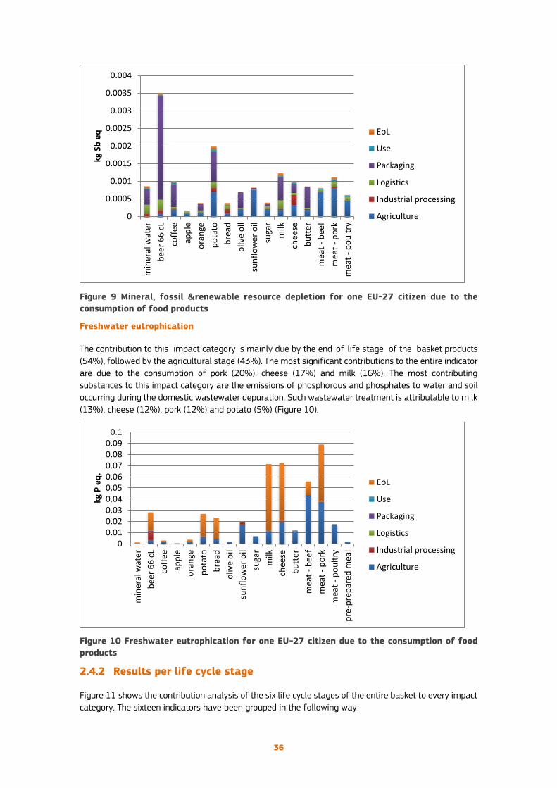
36

Figure 9 Mineral, fossil &renewable resource depletion for one EU-27 citizen due to the

consumption of food products

Freshwater eutrophication

The contribution to this impact category is mainly due by the end-of-life stage of the basket products

(54%), followed by the agricultural stage (43%). The most significant contributions to the entire indicator

are due to the consumption of pork (20%), cheese (17%) and milk (16%). The most contributing

substances to this impact category are the emissions of phosphorous and phosphates to water and soil

occurring during the domestic wastewater depuration. Such wastewater treatment is attributable to milk

(13%), cheese (12%), pork (12%) and potato (5%) (Figure 10).

Figure 10 Freshwater eutrophication for one EU-27 citizen due to the consumption of food

products

2.4.2 Results per life cycle stage

Figure 11 shows the contribution analysis of the six life cycle stages of the entire basket to every impact

category. The sixteen indicators have been grouped in the following way:

0

0.0005

0.001

0.0015

0.002

0.0025

0.003

0.0035

0.004

min

eral

wat

er

bee

r 6

6 c

L

coff

ee

app

le

ora

nge

po

tato

bre

ad

oliv

e o

il

sun

flo

we

r o

il

suga

r

milk

ch

eese

bu

tte

r

mea

t -

bee

f

mea

t -

po

rk

mea

t -

po

ult

ry

kg S

b e

q EoL

Use

Packaging

Logistics


Agriculture

00.010.020.030.040.050.060.070.080.09

0.1

min

eral

wat

er

bee

r 6

6 c

L

coff

ee

app

le

ora

nge

po

tato

bre

ad

oliv

e o

il

sun

flo

we

r o

il

suga

r

milk

ch

eese

bu

tte

r

mea

t -

bee

f

mea

t -

po

rk

mea

t -

po

ult

ry

pre

-pre

par

ed m

eal

kg P

eq

.

EoL

Use

Packaging

Logistics


Agriculture

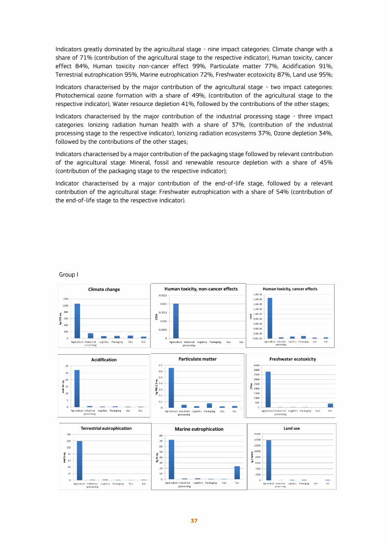
37

Indicators greatly dominated by the agricultural stage - nine impact categories: Climate change with a

share of 71% (contribution of the agricultural stage to the respective indicator), Human toxicity, cancer

effect 84%, Human toxicity non-cancer effect 99%, Particulate matter 77%, Acidification 91%,

Terrestrial eutrophication 95%, Marine eutrophication 72%, Freshwater ecotoxicity 87%, Land use 95%;

Indicators characterised by the major contribution of the agricultural stage - two impact categories:

Photochemical ozone formation with a share of 49%, (contribution of the agricultural stage to the

respective indicator), Water resource depletion 41%, followed by the contributions of the other stages;

Indicators characterised by the major contribution of the industrial processing stage - three impact

categories: Ionizing radiation human health with a share of 37%, (contribution of the industrial

processing stage to the respective indicator), Ionizing radiation ecosystems 37%, Ozone depletion 34%,

followed by the contributions of the other stages;

Indicators characterised by a major contribution of the packaging stage followed by relevant contribution

of the agricultural stage: Mineral, fossil and renewable resource depletion with a share of 45%

(contribution of the packaging stage to the respective indicator);

Indicator characterised by a major contribution of the end-of-life stage, followed by a relevant

contribution of the agricultural stage: Freshwater eutrophication with a share of 54% (contribution of

the end-of-life stage to the respective indicator).

Group I

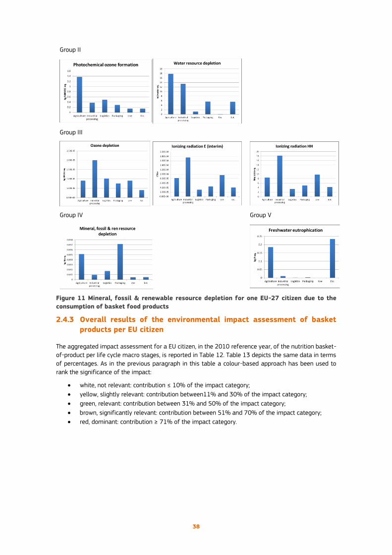
38

Group II

Group III

Group IV Group V

Figure 11 Mineral, fossil & renewable resource depletion for one EU-27 citizen due to the

consumption of basket food products

2.4.3 Overall results of the environmental impact assessment of basket

products per EU citizen

The aggregated impact assessment for a EU citizen, in the 2010 reference year, of the nutrition basket-

of-product per life cycle macro stages, is reported in Table 12. Table 13 depicts the same data in terms

of percentages. As in the previous paragraph in this table a colour-based approach has been used to

rank the significance of the impact:

white, not relevant: contribution ≤ 10% of the impact category;

yellow, slightly relevant: contribution between11% and 30% of the impact category;

green, relevant: contribution between 31% and 50% of the impact category;

brown, significantly relevant: contribution between 51% and 70% of the impact category;

red, dominant: contribution ≥ 71% of the impact category.

39

Table 12 Life cycle impact assessment for an average citizen of EU-27 in the food basket-

of-products

Impact Category

Unit

Agri

cult

ure

Indust

rial pr

oc.

Logis

tics

Pack

agin

g

Use

EoL

Tota

l

Climate change kg CO2 eq. 1059.6 154.8 64.5 74.0 81.4 49.3 1483.6

Ozone depletion kg CFC-11 eq. 9.05E-06 2.01E-05 1.02E-05 7.51E-06 9.02E-06 3.99E-06 5.99E-05

Human toxicity, cancer effects CTUh 1.66E-05 5.34E-07 7.99E-07 1.03E-06 3.84E-07 4.74E-07 1.98E-05

Human toxicity, non-cancer effects CTUh 2.02E-03 8.51E-06 4.73E-06 7.38E-06 1.92E-06 5.06E-06 2.05E-03

Particulate matter kg PM2.5 eq. 6.59E-01 4.88E-02 2.52E-02 7.29E-02 2.06E-02 2.74E-02 8.54E-01

Ionizing radiation HH kBq U235 eq. 8.4 18.2 3.3 4.9 9.8 4.2 48.9

Ionizing radiation E (interim) CTUe 8.25E-05 1.74E-04 3.02E-05 4.53E-05 9.53E-05 4.00E-05 4.68E-04

Photochemical ozone formation kg NMVOC eq. 1.37 0.37 0.49 0.29 0.15 0.15 2.81

Acidification molc H+ eq. 27.09 0.82 0.45 0.55 0.34 0.38 29.63

Terrestrial eutrophication molc N eq 119.77 1.33 1.81 0.96 0.44 1.26 125.56

Freshwater eutrophication kg P eq. 1.85E-01 1.09E-02 9.60E-04 2.86E-03 4.43E-04 2.35E-01 4.35E-01

Marine eutrophication kg N eq. 8.61 0.15 0.17 0.11 0.04 2.81 11.90

Freshwater ecotoxicity CTUe 3834.4 41.1 35.5 46.8 7.8 416.5 4382.2

Land use kg C deficit 13861.4 93.5 158.4 203.1 37.1 187.4 14540.9

Water resource depletion m3 water eq. 17.80 13.42 1.20 5.63 0.06 5.51 43.63

Mineral, fossil & ren resource depletion kg Sb eq. 5.13E-03 9.32E-04 1.72E-03 7.17E-03 4.81E-04 5.07E-04 1.59E-02

Table 13 Life cycle impact assessment for an average citizen of EU-27 in the nutrition basket-

of-products (in percentage unit)

Impact Category Unit Agriculture Industrial

processing Logistics Packaging Use EoL

Climate change % 71 10 4 5 5 3

Ozone depletion % 15 34 17 13 15 7

Human toxicity, cancer effects % 84 3 4 5 2 2

Human toxicity, non-cancer effects % 99 0 0 0 0 0

Particulate matter % 77 6 3 9 2 3

Ionizing radiation HH % 17 37 7 10 20 9

Ionizing radiation E (interim) % 18 37 6 10 20 9

Photochemical ozone formation % 49 13 17 10 5 5

Acidification % 91 3 2 2 1 1

Terrestrial eutrophication % 95 1 1 1 0 1

Freshwater eutrophication % 43 3 0 1 0 54

Marine eutrophication % 72 1 1 1 0 24

Freshwater ecotoxicity % 87 1 1 1 0 10

Land use % 95 1 1 1 0 1

Water resource depletion % 41 31 3 13 0 13


depletion % 32 6 11 45 3 3

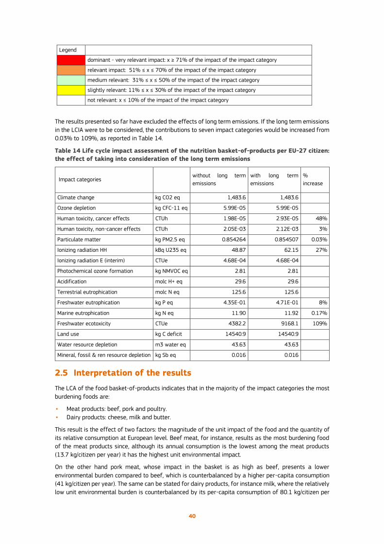
40

Legend

dominant - very relevant impact: x ≥ 71% of the impact of the impact category

relevant impact: 51% ≤ x ≤ 70% of the impact of the impact category

medium relevant: 31% ≤ x ≤ 50% of the impact of the impact category

slightly relevant: 11% ≤ x ≤ 30% of the impact of the impact category

not relevant: x ≤ 10% of the impact of the impact category

The results presented so far have excluded the effects of long term emissions. If the long term emissions

in the LCIA were to be considered, the contributions to seven impact categories would be increased from

0.03% to 109%, as reported in Table 14.

Table 14 Life cycle impact assessment of the nutrition basket-of-products per EU-27 citizen:

the effect of taking into consideration of the long term emissions

Impact categories without long term

emissions

with long term

emissions

%

increase

Climate change kg CO2 eq 1,483.6 1,483.6

Ozone depletion kg CFC-11 eq 5.99E-05 5.99E-05

Human toxicity, cancer effects CTUh 1.98E-05 2.93E-05 48%

Human toxicity, non-cancer effects CTUh 2.05E-03 2.12E-03 3%

Particulate matter kg PM2.5 eq 0.854264 0.854507 0.03%

Ionizing radiation HH kBq U235 eq 48.87 62.15 27%

Ionizing radiation E (interim) CTUe 4.68E-04 4.68E-04

Photochemical ozone formation kg NMVOC eq 2.81 2.81

Acidification molc H+ eq 29.6 29.6

Terrestrial eutrophication molc N eq 125.6 125.6

Freshwater eutrophication kg P eq 4.35E-01 4.71E-01 8%

Marine eutrophication kg N eq 11.90 11.92 0.17%

Freshwater ecotoxicity CTUe 4382.2 9168.1 109%

Land use kg C deficit 14540.9 14540.9

Water resource depletion m3 water eq 43.63 43.63

Mineral, fossil & ren resource depletion kg Sb eq 0.016 0.016

2.5 Interpretation of the results

The LCA of the food basket-of-products indicates that in the majority of the impact categories the most

burdening foods are:

• Meat products: beef, pork and poultry.

• Dairy products: cheese, milk and butter.

This result is the effect of two factors: the magnitude of the unit impact of the food and the quantity of

its relative consumption at European level. Beef meat, for instance, results as the most burdening food

of the meat products since, although its annual consumption is the lowest among the meat products

(13.7 kg/citizen per year) it has the highest unit environmental impact.

On the other hand pork meat, whose impact in the basket is as high as beef, presents a lower

environmental burden compared to beef, which is counterbalanced by a higher per-capita consumption

(41 kg/citizen per year). The same can be stated for dairy products, for instance milk, where the relatively

low unit environmental burden is counterbalanced by its per-capita consumption of 80.1 kg/citizen per

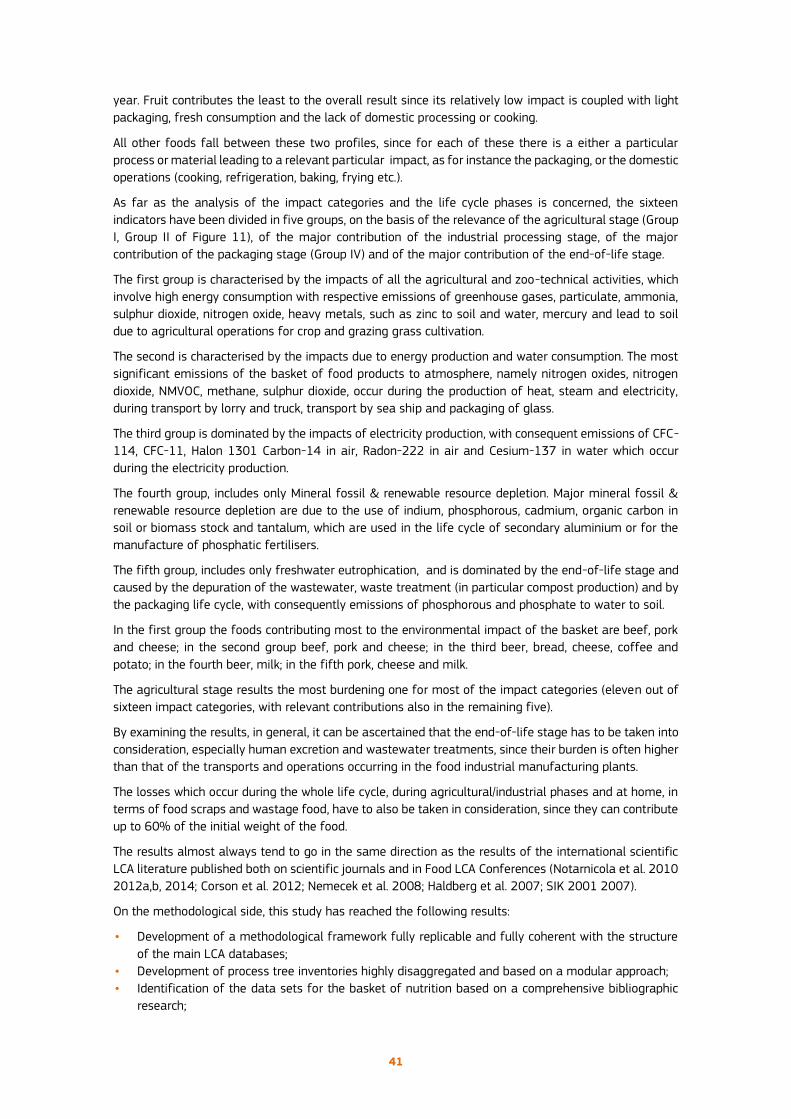
41

year. Fruit contributes the least to the overall result since its relatively low impact is coupled with light

packaging, fresh consumption and the lack of domestic processing or cooking.

All other foods fall between these two profiles, since for each of these there is a either a particular

process or material leading to a relevant particular impact, as for instance the packaging, or the domestic

operations (cooking, refrigeration, baking, frying etc.).

As far as the analysis of the impact categories and the life cycle phases is concerned, the sixteen

indicators have been divided in five groups, on the basis of the relevance of the agricultural stage (Group

I, Group II of Figure 11), of the major contribution of the industrial processing stage, of the major

contribution of the packaging stage (Group IV) and of the major contribution of the end-of-life stage.

The first group is characterised by the impacts of all the agricultural and zoo-technical activities, which

involve high energy consumption with respective emissions of greenhouse gases, particulate, ammonia,

sulphur dioxide, nitrogen oxide, heavy metals, such as zinc to soil and water, mercury and lead to soil

due to agricultural operations for crop and grazing grass cultivation.

The second is characterised by the impacts due to energy production and water consumption. The most

significant emissions of the basket of food products to atmosphere, namely nitrogen oxides, nitrogen

dioxide, NMVOC, methane, sulphur dioxide, occur during the production of heat, steam and electricity,

during transport by lorry and truck, transport by sea ship and packaging of glass.

The third group is dominated by the impacts of electricity production, with consequent emissions of CFC-

114, CFC-11, Halon 1301 Carbon-14 in air, Radon-222 in air and Cesium-137 in water which occur

during the electricity production.

The fourth group, includes only Mineral fossil & renewable resource depletion. Major mineral fossil &

renewable resource depletion are due to the use of indium, phosphorous, cadmium, organic carbon in

soil or biomass stock and tantalum, which are used in the life cycle of secondary aluminium or for the

manufacture of phosphatic fertilisers.

The fifth group, includes only freshwater eutrophication, and is dominated by the end-of-life stage and

caused by the depuration of the wastewater, waste treatment (in particular compost production) and by

the packaging life cycle, with consequently emissions of phosphorous and phosphate to water to soil.

In the first group the foods contributing most to the environmental impact of the basket are beef, pork

and cheese; in the second group beef, pork and cheese; in the third beer, bread, cheese, coffee and

potato; in the fourth beer, milk; in the fifth pork, cheese and milk.

The agricultural stage results the most burdening one for most of the impact categories (eleven out of

sixteen impact categories, with relevant contributions also in the remaining five).

By examining the results, in general, it can be ascertained that the end-of-life stage has to be taken into

consideration, especially human excretion and wastewater treatments, since their burden is often higher

than that of the transports and operations occurring in the food industrial manufacturing plants.

The losses which occur during the whole life cycle, during agricultural/industrial phases and at home, in

terms of food scraps and wastage food, have to also be taken in consideration, since they can contribute

up to 60% of the initial weight of the food.

The results almost always tend to go in the same direction as the results of the international scientific

LCA literature published both on scientific journals and in Food LCA Conferences (Notarnicola et al. 2010

2012a,b, 2014; Corson et al. 2012; Nemecek et al. 2008; Haldberg et al. 2007; SIK 2001 2007).

On the methodological side, this study has reached the following results:

• Development of a methodological framework fully replicable and fully coherent with the structure

of the main LCA databases;

• Development of process tree inventories highly disaggregated and based on a modular approach;

• Identification of the data sets for the basket of nutrition based on a comprehensive bibliographic

research;

42

• Implementation of basket foods with a coverage which represents at least 50% of the European

food consumption.

Future further developments of this study could entail:

• Expansion of the basket-of-products to a greater range of foods covering almost 100% of the

European Food Consumption

• Implementing new data sets

• Implementing a coherent and representative model of commodity transports within the EU.

2.6 References

Aronsson A., Landquist B., Pardo G., Esturo A., Ramos S., Jungbluth N., Flury K. and Stucki M. (2013). Environmental

assessment methodology and sustainability indicators for products and supply chains. SENSE - Harmonised

Environmental Sustanainability in the European food and drink chain, Seventh Framework Programme: Project no.

288974. Funded by EC. Deliverable D 1.3 SIK, Gothenburg.

Blonk Consultants (2014). Agri-footprint Description of data. V 1.0. Retrieved from: www.agri-

footprint.com/assets/Agri-Footprint-Part2-Descriptionofdata-Version1.0.pdf

Brentrup F., Küsters J., Lammel J., Kuhlmann H. (2000). Methods to estimate on-field nitrogen emissions from crop

production as an input to LCA studies in the agricultural sector. The International Journal of Life Cycle Assessment,

5 (6), 349-357.

CBI -Centre for the promotion of imports from developing countries. (2009). Preserved fruit and vegetables. The EU

market for frozen fruit and vegetables. Available from http://www.cbi.eu/system/files/marketintel/2009_-

_Frozen_fruit_and_vegetables1.pdf.

Coltro L., Mourad A.L., Oliveira P.A.P.L.V., Baddini J.P.O.A., Kletecke R.M. (2006). Environmental Profile of Brazilian

Green Coffee. Int J LCA 11 (1) 2006, 16 – 21.

Corson, M.S., van der Werf, H.M.G. (Eds.) (2012). Proceedings of the 8th International Conference on Life Cycle

Assessment in the Agri-Food Sector (LCA Food 2012), 1-4 October 2012, Saint Malo, France. INRA, Rennes, France,

p. 407-412.

de Beaufort-Langeveld A. S. H., Bretz R., van Hoof G., Hischier R., Jean P., Tanner T. and Huijbregts M. A. J. (2003).

Code of Life-Cycle Inventory Practice. SETAC. Retrieved from: www.setac.org.

DEFRA (2012). Family Food (2012). Report published by the Department for Environment, Food and Rural Affairs.

Available on the Defra website: https://www.gov.uk/government/collections/family-food-statistics.

Djekic I., Miocinovic J., Tomasevic I., Smigic N., Tomic N. (2014). Environmental life-cycle assessment of various dairy

products. Journal of Cleaner Production 68 (2014) 64-72

EC (2007). Eurostat Statistical Books: The use of plant protection products in the European Union – Data 1992-2003,

2007 Edition. European Commission, Brussels.

EC (2008). Biofuels in the European Context: Facts and Uncertainties. European Commission, Joint Research Centre,

Institute for Energy.

EC (2010). Joint Research Centre - Institute for Environment and Sustainability: International Reference Life Cycle

Data System (ILCD) Handbook - General guide for Life Cycle Assessment - Detailed guidance. First edition March

2010. EUR 24708 EN. Luxembourg. Publications Office of the European Union.

EC (2012a). Life cycle indicators basket-of-products: development of life cycle based macro-level monitoring

indicators for resources, products and waste for the EU-27. European Commission, Joint Research Centre, Institute

for Environment and Sustainability.

EC (2012b). DG Agriculture & Rural Development. Monitoring Agri-trade Policy - The EU and major world players in

Fruit and Vegetable Trade. Available from: http://ec.europa.eu/agriculture/trade-analysis/map/2012-2_en.pdf.

EC (2012c). European Commission, Agriculture and Rural Development, Fruit and vegetables, Product reports: Apple

and Pears. Available from http://ec.europa.eu/agriculture/fruit-and-vegetables/product-reports/apples-and-

pears/index_en.htm

EC (2012d). European Commission, Agriculture and Rural Development, Fruit and vegetables, Product reports: Apple

and Pears. Available from http://ec.europa.eu/agriculture/fruit-and-vegetables/product-reports/citrus-

fruit/index_en.htm

EC (2012e). European Commission, Agriculture and Rural Development, Fruit and vegetables, Product reports:

Potatoes. Available from http://ec.europa.eu/agriculture/fruit-and-vegetables/product-reports/potatoes/index_en.htm

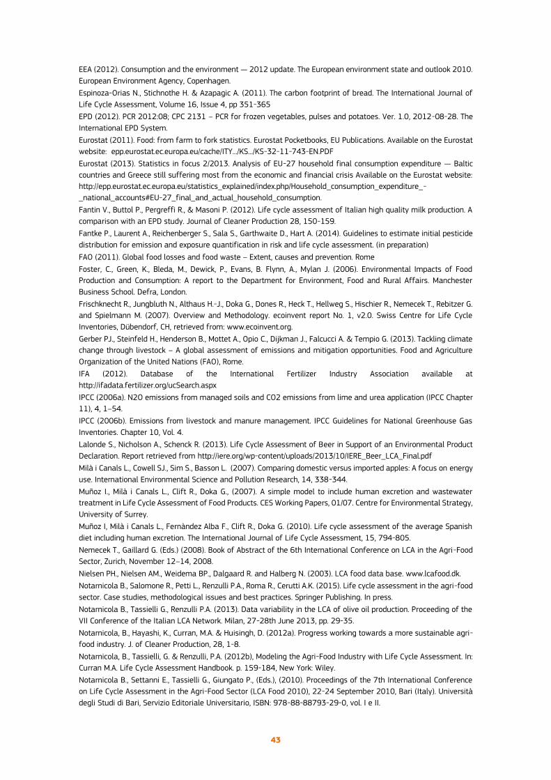
43

EEA (2012). Consumption and the environment — 2012 update. The European environment state and outlook 2010.

European Environment Agency, Copenhagen.

Espinoza-Orias N., Stichnothe H. & Azapagic A. (2011). The carbon footprint of bread. The International Journal of

Life Cycle Assessment, Volume 16, Issue 4, pp 351-365

EPD (2012). PCR 2012:08; CPC 2131 – PCR for frozen vegetables, pulses and potatoes. Ver. 1.0, 2012-08-28. The

International EPD System.

Eurostat (2011). Food: from farm to fork statistics. Eurostat Pocketbooks, EU Publications. Available on the Eurostat

website: epp.eurostat.ec.europa.eu/cache/ITY.../KS.../KS-32-11-743-EN.PDF

Eurostat (2013). Statistics in focus 2/2013. Analysis of EU-27 household final consumption expenditure — Baltic

countries and Greece still suffering most from the economic and financial crisis Available on the Eurostat website:

http://epp.eurostat.ec.europa.eu/statistics_explained/index.php/Household_consumption_expenditure_-

_national_accounts#EU-27_final_and_actual_household_consumption.

Fantin V., Buttol P., Pergreffi R., & Masoni P. (2012). Life cycle assessment of Italian high quality milk production. A

comparison with an EPD study. Journal of Cleaner Production 28, 150-159.

Fantke P., Laurent A., Reichenberger S., Sala S., Garthwaite D., Hart A. (2014). Guidelines to estimate initial pesticide

distribution for emission and exposure quantification in risk and life cycle assessment. (in preparation)

FAO (2011). Global food losses and food waste – Extent, causes and prevention. Rome

Foster, C., Green, K., Bleda, M., Dewick, P., Evans, B. Flynn, A., Mylan J. (2006). Environmental Impacts of Food

Production and Consumption: A report to the Department for Environment, Food and Rural Affairs. Manchester

Business School. Defra, London.

Frischknecht R., Jungbluth N., Althaus H.-J., Doka G., Dones R., Heck T., Hellweg S., Hischier R., Nemecek T., Rebitzer G.

and Spielmann M. (2007). Overview and Methodology. ecoinvent report No. 1, v2.0. Swiss Centre for Life Cycle

Inventories, Dübendorf, CH, retrieved from: www.ecoinvent.org.

Gerber PJ., Steinfeld H., Henderson B., Mottet A., Opio C., Dijkman J., Falcucci A. & Tempio G. (2013). Tackling climate

change through livestock – A global assessment of emissions and mitigation opportunities. Food and Agriculture

Organization of the United Nations (FAO), Rome.

IFA (2012). Database of the International Fertilizer Industry Association available at

http://ifadata.fertilizer.org/ucSearch.aspx

IPCC (2006a). N2O emissions from managed soils and CO2 emissions from lime and urea application (IPCC Chapter

11), 4, 1–54.

IPCC (2006b). Emissions from livestock and manure management. IPCC Guidelines for National Greenhouse Gas

Inventories. Chapter 10, Vol. 4.

Lalonde S., Nicholson A., Schenck R. (2013). Life Cycle Assessment of Beer in Support of an Environmental Product

Declaration. Report retrieved from http://iere.org/wp-content/uploads/2013/10/IERE_Beer_LCA_Final.pdf

Milà i Canals L., Cowell SJ., Sim S., Basson L. (2007). Comparing domestic versus imported apples: A focus on energy

use. International Environmental Science and Pollution Research, 14, 338-344.

Muñoz I., Milà i Canals L., Clift R., Doka G., (2007). A simple model to include human excretion and wastewater

treatment in Life Cycle Assessment of Food Products. CES Working Papers, 01/07. Centre for Environmental Strategy,

University of Surrey.

Muñoz I, Milà i Canals L., Fernàndez Alba F., Clift R., Doka G. (2010). Life cycle assessment of the average Spanish

diet including human excretion. The International Journal of Life Cycle Assessment, 15, 794-805.

Nemecek T., Gaillard G. (Eds.) (2008). Book of Abstract of the 6th International Conference on LCA in the Agri-Food

Sector, Zurich, November 12–14, 2008.

Nielsen PH., Nielsen AM., Weidema BP., Dalgaard R. and Halberg N. (2003). LCA food data base. www.lcafood.dk.

Notarnicola B., Salomone R., Petti L., Renzulli P.A., Roma R., Cerutti A.K. (2015). Life cycle assessment in the agri-food

sector. Case studies, methodological issues and best practices. Springer Publishing. In press.

Notarnicola B., Tassielli G., Renzulli P.A. (2013). Data variability in the LCA of olive oil production. Proceeding of the

VII Conference of the Italian LCA Network. Milan, 27-28th June 2013, pp. 29-35.

Notarnicola, B., Hayashi, K., Curran, M.A. & Huisingh, D. (2012a). Progress working towards a more sustainable agri-

food industry. J. of Cleaner Production, 28, 1-8.

Notarnicola, B., Tassielli, G. & Renzulli, P.A. (2012b), Modeling the Agri-Food Industry with Life Cycle Assessment. In:

Curran M.A. Life Cycle Assessment Handbook. p. 159-184, New York: Wiley.

Notarnicola B., Settanni E., Tassielli G., Giungato P., (Eds.), (2010). Proceedings of the 7th International Conference

on Life Cycle Assessment in the Agri-Food Sector (LCA Food 2010), 22-24 September 2010, Bari (Italy). Università

degli Studi di Bari, Servizio Editoriale Universitario, ISBN: 978-88-88793-29-0, vol. I e II.

44

Pergola M., D’Amico M., Celano G., Palese A.M., Scuderi A., Di Vita G., Pappalardo G., Inglese P. (2013). Sustainability

evaluation of Sicily’s lemon and orange production: An energy, economic and environmental analysis. Journal of

Environmental Management, 128:674–682.

Ribaudo F. (2011). Handbook of agriculture. Hoepli, Milan, Italy.

Schaltegger S., Viere T., Zvezdov D. (2012). Tapping environmental accounting potentials of beer brewing.

Information needs for successful cleaner production. Journal of Cleaner Production 29-30 (2012) 1-10.

Schmidt Rivera X.C., Espinoza Orias N., Azapagic A. (2014). Life cycle environmental impacts of convenience food:

comparison of ready and home-made meals. Journal of Cleaner Production, 1-16.

SIK – The Swedish Institute for Food and Biotechnology (2007). Proceedings from the 5th International Conference,

2007. LCA in Foods 25 – 26 April 2007, Gothenburg, Sweden.

SIK – The Swedish Institute for Food and Biotechnology (2001). Proceedings from the International Conference LCA

in Foods, Goteborg 25-27 April 2001.

Tukker A., Huppes G., Guinée J., Heijungs R., de Koning A., van Oers L., Suh S., Geerken T., Van Holderbeke M., Jansen

B., Nielsen P. (2006). Environmental impacts of products (EIPRO). Analysis of the life cycle environmental impacts

related to the total final consumption of the EU-25. European Commission, Joint Research Centre (JRC), Institute for

Prospective Technological Studies (IPTS), Sevilla, Spain.

Vanderheyden G. and Aerts J. (2014). Comparative LCA assessment of Fontinet filtered tap water vs.Natural sourced

water in a PET bottle. FINAL REPORT 04/03/2014. Futureproofed. Available at:

http://www.futureproofed.com/images/uploads/projects/13506_PWA_LCA_report_final_07.pdf

Weidema BP., Bauer C., Hischier R., Mutel C., Nemecek T., Reinhard J., Vadenbo C. O., Wernet G. (2013). Overview and

methodology. Data quality guideline for the ecoinvent database version 3. Ecoinvent Report 1(v3). St. Gallen: The

Ecoinvent Centre.

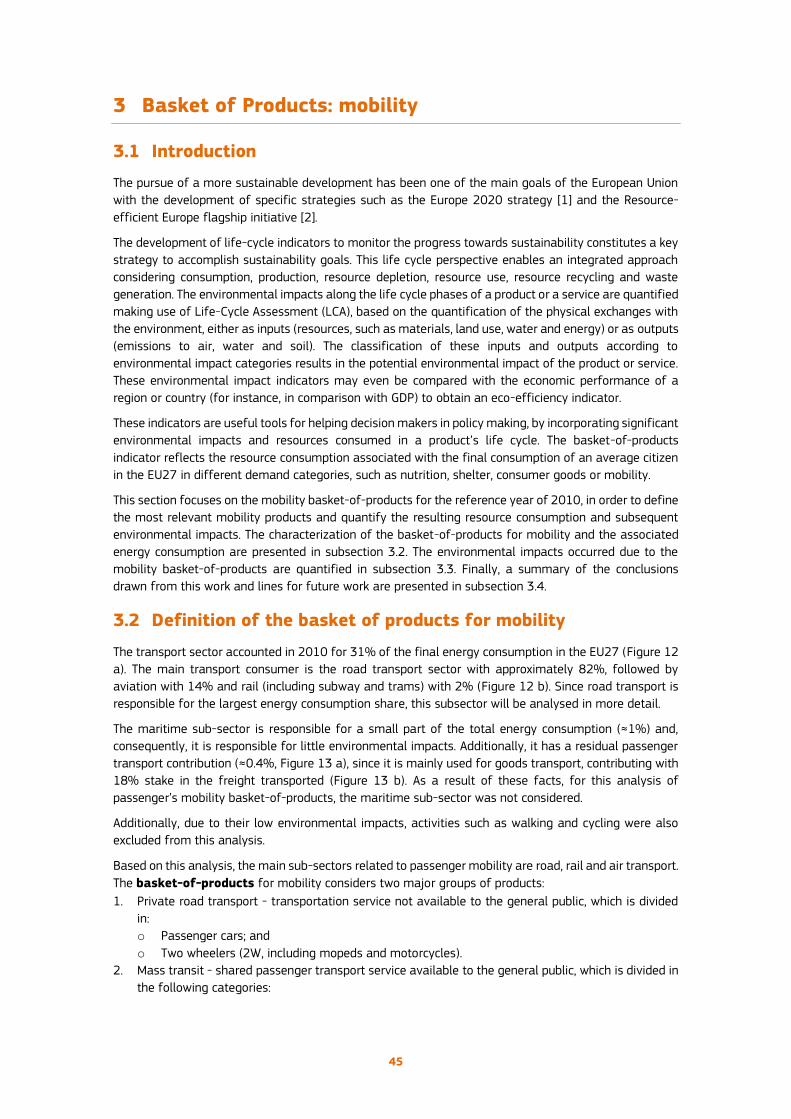
45

3 Basket of Products: mobility

3.1 Introduction

The pursue of a more sustainable development has been one of the main goals of the European Union

with the development of specific strategies such as the Europe 2020 strategy [1] and the Resource-

efficient Europe flagship initiative [2].

The development of life-cycle indicators to monitor the progress towards sustainability constitutes a key

strategy to accomplish sustainability goals. This life cycle perspective enables an integrated approach

considering consumption, production, resource depletion, resource use, resource recycling and waste

generation. The environmental impacts along the life cycle phases of a product or a service are quantified

making use of Life-Cycle Assessment (LCA), based on the quantification of the physical exchanges with

the environment, either as inputs (resources, such as materials, land use, water and energy) or as outputs

(emissions to air, water and soil). The classification of these inputs and outputs according to

environmental impact categories results in the potential environmental impact of the product or service.

These environmental impact indicators may even be compared with the economic performance of a

region or country (for instance, in comparison with GDP) to obtain an eco-efficiency indicator.

These indicators are useful tools for helping decision makers in policy making, by incorporating significant

environmental impacts and resources consumed in a product’s life cycle. The basket-of-products

indicator reflects the resource consumption associated with the final consumption of an average citizen

in the EU27 in different demand categories, such as nutrition, shelter, consumer goods or mobility.

This section focuses on the mobility basket-of-products for the reference year of 2010, in order to define

the most relevant mobility products and quantify the resulting resource consumption and subsequent

environmental impacts. The characterization of the basket-of-products for mobility and the associated

energy consumption are presented in subsection 3.2. The environmental impacts occurred due to the

mobility basket-of-products are quantified in subsection 3.3. Finally, a summary of the conclusions

drawn from this work and lines for future work are presented in subsection 3.4.

3.2 Definition of the basket of products for mobility

The transport sector accounted in 2010 for 31% of the final energy consumption in the EU27 (Figure 12

a). The main transport consumer is the road transport sector with approximately 82%, followed by

aviation with 14% and rail (including subway and trams) with 2% (Figure 12 b). Since road transport is

responsible for the largest energy consumption share, this subsector will be analysed in more detail.

The maritime sub-sector is responsible for a small part of the total energy consumption (≈1%) and,

consequently, it is responsible for little environmental impacts. Additionally, it has a residual passenger

transport contribution (≈0.4%, Figure 13 a), since it is mainly used for goods transport, contributing with

18% stake in the freight transported (Figure 13 b). As a result of these facts, for this analysis of

passenger’s mobility basket-of-products, the maritime sub-sector was not considered.

Additionally, due to their low environmental impacts, activities such as walking and cycling were also

excluded from this analysis.

Based on this analysis, the main sub-sectors related to passenger mobility are road, rail and air transport.

The basket-of-products for mobility considers two major groups of products:

1. Private road transport - transportation service not available to the general public, which is divided

in:

o Passenger cars; and

o Two wheelers (2W, including mopeds and motorcycles).

2. Mass transit - shared passenger transport service available to the general public, which is divided in

the following categories:

46

o Buses (including Urban buses, mainly used for urban transport, and coaches for long distance

transport);

o Rail; and

o Air.

The new suggested basket-of-products considers 76 mobility sub-products (Figure 14 b), including 36

vehicle categories for passenger cars (accounting for 6 vehicle categories sub-divided with 5 Euro

standards), 15 categories for buses, 20 categories for 2W, 2 categories for rail transport (electric and

other energy sources) and 3 categories for air transport (national, intra-EU and extra-EU flights).

The mobility service provided by the Basket-of-products is quantified through an estimation of the level

of service for each sub-product. In the case of mobility this is translated in kilometres travelled and,

more importantly, in number of passengers transported (based on average occupancy factors, presented

in Table A.1 in the Annex), which is reflected in a passenger-kilometres analysis.

The analysis presented in this document performs a study by country, considering different types of

usage conditions of the different mobility products, as is presented in Figure 15.

a)

b)

Figure 12 EU27 energy use by the transport sector in comparison with the total final energy

consumption (a), and disaggregated by mode of transport (b) [3]

0

10,000

20,000

30,000

40,000

50,000

60,000

19

90

19

92

19

94

19

96

19

98

20

00

20

02

20

04

20

06

20

08

20

10

20

12

Ene

rgy

con

sum

pti

on

(P

J)

Final energyconsumption

Transport sector

0

2.000

4.000

6.000

8.000

10.000

12.000

14.000

16.000

18.000

19

90

19

92

19

94

19

96

19

98

20

00

20

02

20

04

20

06

20

08

20

10

20

12

Ene

rgy

con

sum

pti

on

(P

J)

Total

Road

Rail

Aviation

Maritime

Unspecified

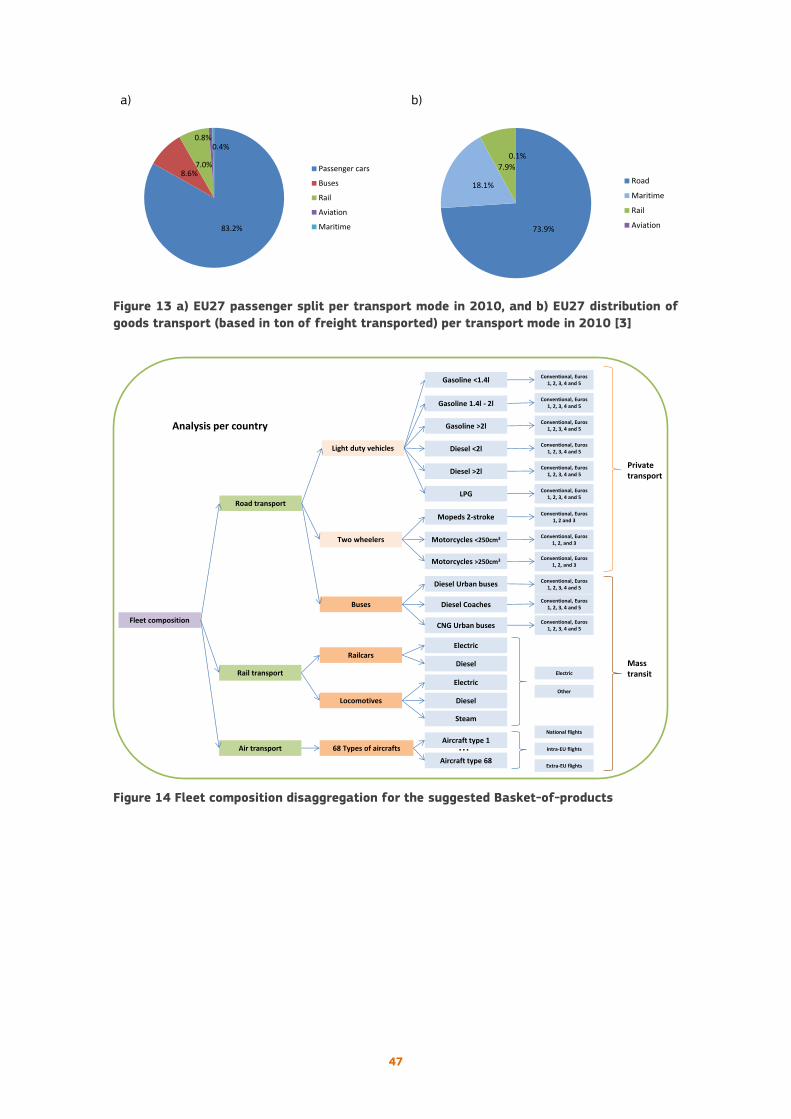
47

a) b)

Figure 13 a) EU27 passenger split per transport mode in 2010, and b) EU27 distribution of

goods transport (based in ton of freight transported) per transport mode in 2010 [3]

Figure 14 Fleet composition disaggregation for the suggested Basket-of-products

83.2%

8.6%7.0%

0.8%0.4%

Passenger cars

Buses

Rail

Aviation

Maritime 73.9%

18.1%

7.9%

0.1%

Road

Maritime

Rail

Aviation

Fleet composition

Road transport

Rail transport

Air transport

Light duty vehicles

Buses

Two wheelers

Diesel <2l

LPG

Diesel Urban buses

CNG Urban buses

Mopeds 2-stroke

68 Types of aircrafts

Railcars

Locomotives

Electric

Diesel

Electric

Diesel

Steam

Conventional, Euros 1, 2, 3, 4 and 5







Diesel CoachesConventional, Euros

1, 2, 3, 4 and 5


Conventional, Euros 1, 2 and 3

Conventional, Euros 1, 2, and 3

Conventional, Euros 1, 2, and 3

Gasoline <1.4l

Gasoline 1.4l - 2l

Gasoline >2l

Diesel >2l

Motorcycles <250cm3

Motorcycles >250cm3

Private transport

Mass transit

Analysis per country

Aircraft type 1

Aircraft type 68

...National flights

Intra-EU flights

Extra-EU flights

Electric

Other

48

Figure 15 Level of service disaggregation

3.2.1 Data Sources

The data sources used for defining and characterizing the Mobility basket-of-products are described

next.

The road transport sector was characterized using the existing Eurostat data sets [4] for EU27 countries,

which included the following variables:

1. Number of vehicles per vehicle technology for several years (for passenger cars, buses, coaches and

two-wheelers, considering the fuel use of gasoline, diesel and LPG – liquefied petroleum gas). These

datasets include passenger cars, independently of whether they are used for private or business

purposes;

2. Engine displacement distribution time series (for passenger cars and two-wheeler); and

3. Vehicle age distribution time series (for passenger cars and buses). The vehicle age distribution

allows characterizing different Euro Standards [5], which have imposed in the last two decades

reductions in local pollutant emissions.

The rail transport sector was characterized using the existing Eurostat data sets [4] for EU27 countries,


1. Total number of vehicles per vehicle technology time series (for locomotives and railcars, considering

the fuel use of diesel, electricity and steam);

2. Number of passenger-vehicles per vehicle type time series (for coaches and railcars);

3. Total passenger-kilometres time series;

4. Vehicle-kilometres travelled per vehicle technology time series (for locomotives and railcars,

considering the fuel use of diesel, electricity and steam, and for goods, passengers or other vehicles);

and

Level of service

Road transport

Rail transport

Air transport

Driving conditions, vkm and average

speed

Average occupancy factors

Highway

Rural

Urban

National flights

Train kilometers

Passenger kilometers

Intra-EU flights

Analysis per country

Extra-EU flights

68 Types of aircraft models

Distance travelled and occupancy

factors

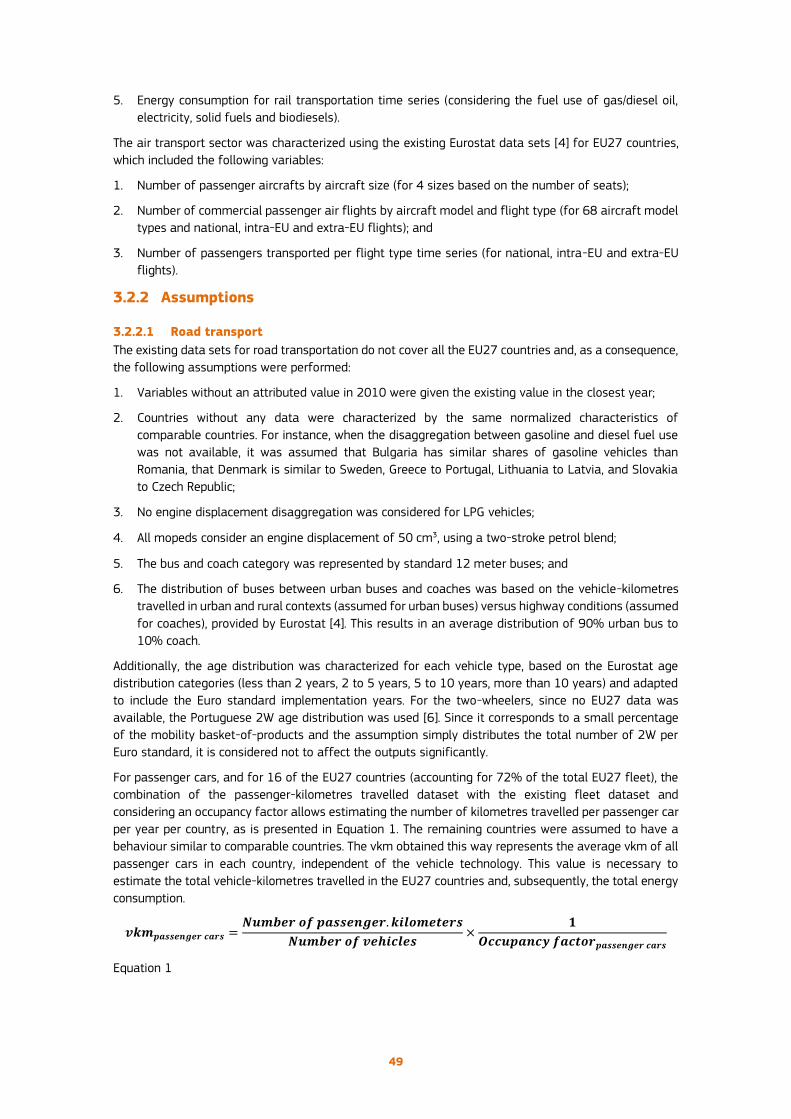
49

5. Energy consumption for rail transportation time series (considering the fuel use of gas/diesel oil,

electricity, solid fuels and biodiesels).

The air transport sector was characterized using the existing Eurostat data sets [4] for EU27 countries,


1. Number of passenger aircrafts by aircraft size (for 4 sizes based on the number of seats);

2. Number of commercial passenger air flights by aircraft model and flight type (for 68 aircraft model

types and national, intra-EU and extra-EU flights); and

3. Number of passengers transported per flight type time series (for national, intra-EU and extra-EU

flights).

3.2.2 Assumptions

3.2.2.1 Road transport

The existing data sets for road transportation do not cover all the EU27 countries and, as a consequence,

the following assumptions were performed:

1. Variables without an attributed value in 2010 were given the existing value in the closest year;

2. Countries without any data were characterized by the same normalized characteristics of

comparable countries. For instance, when the disaggregation between gasoline and diesel fuel use

was not available, it was assumed that Bulgaria has similar shares of gasoline vehicles than

Romania, that Denmark is similar to Sweden, Greece to Portugal, Lithuania to Latvia, and Slovakia

to Czech Republic;

3. No engine displacement disaggregation was considered for LPG vehicles;

4. All mopeds consider an engine displacement of 50 cm3, using a two-stroke petrol blend;

5. The bus and coach category was represented by standard 12 meter buses; and

6. The distribution of buses between urban buses and coaches was based on the vehicle-kilometres

travelled in urban and rural contexts (assumed for urban buses) versus highway conditions (assumed

for coaches), provided by Eurostat [4]. This results in an average distribution of 90% urban bus to

10% coach.

Additionally, the age distribution was characterized for each vehicle type, based on the Eurostat age

distribution categories (less than 2 years, 2 to 5 years, 5 to 10 years, more than 10 years) and adapted

to include the Euro standard implementation years. For the two-wheelers, since no EU27 data was

available, the Portuguese 2W age distribution was used [6]. Since it corresponds to a small percentage

of the mobility basket-of-products and the assumption simply distributes the total number of 2W per

Euro standard, it is considered not to affect the outputs significantly.

For passenger cars, and for 16 of the EU27 countries (accounting for 72% of the total EU27 fleet), the

combination of the passenger-kilometres travelled dataset with the existing fleet dataset and

considering an occupancy factor allows estimating the number of kilometres travelled per passenger car

per year per country, as is presented in Equation 1. The remaining countries were assumed to have a

behaviour similar to comparable countries. The vkm obtained this way represents the average vkm of all

passenger cars in each country, independent of the vehicle technology. This value is necessary to

estimate the total vehicle-kilometres travelled in the EU27 countries and, subsequently, the total energy

consumption.

𝒗𝒌𝒎𝒑𝒂𝒔𝒔𝒆𝒏𝒈𝒆𝒓 𝒄𝒂𝒓𝒔 =𝑵𝒖𝒎𝒃𝒆𝒓 𝒐𝒇 𝒑𝒂𝒔𝒔𝒆𝒏𝒈𝒆𝒓. 𝒌𝒊𝒍𝒐𝒎𝒆𝒕𝒆𝒓𝒔

𝑵𝒖𝒎𝒃𝒆𝒓 𝒐𝒇 𝒗𝒆𝒉𝒊𝒄𝒍𝒆𝒔×

𝟏

𝑶𝒄𝒄𝒖𝒑𝒂𝒏𝒄𝒚 𝒇𝒂𝒄𝒕𝒐𝒓𝒑𝒂𝒔𝒔𝒆𝒏𝒈𝒆𝒓 𝒄𝒂𝒓𝒔

Equation 1

50

A smaller Eurostat dataset for five EU27 countries contained the vehicle-kilometres travelled both for

gasoline and diesel passenger cars. Based on these statistics, a 33% increase in vkm for diesel vehicles

compared to the country’s average vkm and an 11% decrease in vkm for gasoline vehicles compared to

the country’s average vkm was observed. These ratios were used for the remaining EU27 countries.

The average occupancy factor for passenger cars was estimated by comparing the pkm dataset with the

smaller vkm per vehicle dataset, as presented in Equation 2. An average 1.57 value was obtained for

passenger cars.

𝑶𝒄𝒄𝒖𝒑𝒂𝒏𝒄𝒚 𝒇𝒂𝒄𝒕𝒐𝒓𝒑𝒂𝒔𝒔𝒆𝒏𝒈𝒆𝒓 𝒄𝒂𝒓𝒔 =

𝑵𝒖𝒎𝒃𝒆𝒓 𝒐𝒇 𝒑𝒂𝒔𝒔𝒆𝒏𝒈𝒆𝒓. 𝒌𝒊𝒍𝒐𝒎𝒆𝒕𝒆𝒓𝒔𝑵𝒖𝒎𝒃𝒆𝒓 𝒐𝒇 𝒗𝒆𝒉𝒊𝒄𝒍𝒆𝒔

𝑵𝒖𝒎𝒃𝒆𝒓 𝒐𝒇 𝒌𝒊𝒍𝒐𝒎𝒆𝒕𝒆𝒓𝒔 𝒑𝒆𝒓 𝒗𝒆𝒉𝒊𝒄𝒍𝒆

Equation 2

For buses and 2W, the combination of the vehicle-kilometres travelled dataset with the number of

vehicles allowed estimating an average EU27 value of ≈34000 km per bus per year (Equation 3).

Countries without any data entry in vehicle-kilometres travelled were attributed the EU average. For 2W,

the few available data allowed estimating an average value of 3700 km per 2W per year (Equation 3),

which was considered for all EU27 countries.

𝒗𝒌𝒎𝑩𝒖𝒔𝒆𝒔 𝒐𝒓 𝟐𝑾 =𝑵𝒖𝒎𝒃𝒆𝒓 𝒐𝒇 𝒗𝒆𝒉𝒊𝒄𝒍𝒆. 𝒌𝒊𝒍𝒐𝒎𝒆𝒕𝒆𝒓𝒔

𝑵𝒖𝒎𝒃𝒆𝒓 𝒐𝒇 𝒗𝒆𝒉𝒊𝒄𝒍𝒆𝒔

Equation 3

The considered occupancy factor for buses were based on Swiss data from the Ecoinvent database [7],

which refers values of 14 passengers for urban buses and 21 passengers for coaches, due to a lack of

representative data for EU27. A 1.1 occupancy factor was considered for 2W [7].

3.2.2.2 Rail transport

The existing data sets for rail transport did not cover all the EU27 countries and some assumptions were

performed:

1. Variables without an attributed value in 2010 were given the existing value in the closest year;

2. Countries without any data on the partition between passenger-train-kilometres and freight-train-

kilometres by fuel type were assumed to have the same normalized characteristics as countries with

similar energy consumption per train and passenger-kilometre. For instance, when the

disaggregation between electricity and diesel fuel use was not available, it was assumed that

Portugal would have a similar share of electricity and diesel for rail passenger transportation than

Spain, and that Luxembourg would be similar to Belgium.

The level of service provided per vehicle type (electric and others) for the rail transport was estimated

first as the number of vehicle-kilometres travelled for passenger transport (vkmp) and second as the

number of passenger-kilometres travelled (pkm). Given that only 12 countries had data available on the

vkmp for the year 2010, an estimation was performed for the rest of the countries based on data from

other years and energy consumption data (calculating average vehicle efficiencies for years with all data

available and using the 2010 data for energy consumption in rail transport). Average occupancy factors

were estimated for each country based on the total passenger-kilometres and total train-kilometres

travelled. This assumes that the occupancy factor of the electric trains and other trains are the same for

each country. The pkm for each vehicle type were calculated based on the average occupancy factors

and the vkmp.

3.2.2.3 Air transport

The existing data sets for air transport did not have data on the number of flights by aircraft model for

the year 2010, and as such the values for 2011 were used. The level of service provided per flight type

(national, intra-EU and extra-EU) for the air transport was estimated first as the number of vehicle-

kilometres travelled for passenger transport (vkmp) and second as the number of passenger-kilometres

travelled (pkm). The vkmp were estimated based on the number of flights performed in each country, by

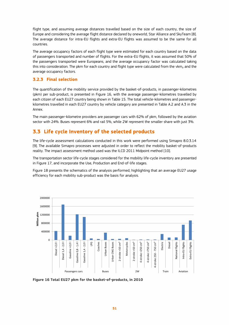
51

flight type, and assuming average distances travelled based on the size of each country, the size of

Europe and considering the average flight distance declared by oneworld, Star Alliance and SkyTeam [8].

The average distance for intra-EU flights and extra-EU flights was assumed to be the same for all

countries.

The average occupancy factors of each flight type were estimated for each country based on the data

of passengers transported and number of flights. For the extra-EU flights, it was assumed that 50% of

the passengers transported were Europeans, and the average occupancy factor was calculated taking

this into consideration. The pkm for each country and flight type were calculated from the vkmp and the

average occupancy factors.

3.2.3 Final selection

The quantification of the mobility service provided by the basket-of-products, in passenger-kilometres

(pkm) per sub-product, is presented in Figure 16, with the average passenger-kilometres travelled by

each citizen of each EU27 country being shown in Table 15. The total vehicle-kilometres and passenger-

kilometres travelled in each EU27 country by vehicle category are presented in Table A.2 and A.3 in the

Annex.

The main passenger-kilometre providers are passenger cars with 62% of pkm, followed by the aviation

sector with 24%. Buses represent 6% and rail 5%, while 2W represent the smaller share with just 3%.

3.3 Life cycle Inventory of the selected products

The life-cycle assessment calculations conducted in this work were performed using Simapro 8.0.3.14

[9]. The available Simapro processes were adjusted in order to reflect the mobility basket-of-products

reality. The impact assessment method used was the ILCD 2011 Midpoint method [10].

The transportation sector life-cycle stages considered for the mobility life-cycle inventory are presented

in Figure 17, and incorporate the Use, Production and End-of-life stages.

Figure 18 presents the schematics of the analysis performed, highlighting that an average EU27 usage

efficiency for each mobility sub-product was the basis for analysis.

Figure 16 Total EU27 pkm for the basket-of-products, in 2010

0

400000

800000

1200000

1600000

2000000

Die

sel >

2,0

l

Die

sel 1

,4 -

2,0

l

Gas

olin

e >2

,0 l

Gas

olin

e 0,

8 -

1,4

l

Gas

olin

e 1,

4 -

2,0

l

LPG

Co

ach

es

Urb

an B

use

s

Urb

an C

NG

Bu

ses

2-s

tro

ke <

50

cm

³

Mo

torc

ycle

s

2-s

tro

ke >

50

cm

³

4-s

tro

ke <

25

0 c

m³

4-s

tro

ke >

75

0 c

m³

4-s

tro

ke 2

50

- 7

50

cm³

Ele

ctri

c

Die

sel

Nat

ion

al f

ligh

ts

Intr

a-EU

flig

hts

Extr

a-EU

flig

hts

Passengers cars Buses 2W Train Aviation

Mill

ion

pkm

52

Table 15 Average passenger-kilometres per citizen for the vehicle categories considered for

each EU27 country, in 2010

Country

Passenger cars

2W

Urban

buses

and

Coaches

Rail Air

Gasoline Diesel LPG Electric Others National

flights

Intra-

EU

flights

Extra-

EU

flights

Austria 3415 6316 0 343 580 938 222 25 2206 2737

Belgium 3557 8354 65 207 753 860 84 1 1692 2182

Bulgaria 2931 1956 0 69 2014 224 57 7 744 581

Cyprus 6260 1041 0 205 2091 0 0 3 8212 5901

Czech Republic 3938 2173 0 552 663 293 334 8 959 1094

Denmark 8306 2035 0 152 1314 329 782 77 3322 3728

Estonia 6048 2999 0 99 1616 23 163 3 971 637

Finland 10057 3645 0 375 1593 598 142 214 1973 1800

France 4285 6940 42 160 772 1094 276 284 955 2295

Germany 6988 3882 96 280 471 702 311 153 1211 2330

Greece 2572 3126 38 953 1235 14 110 176 2261 1393

Hungary 2977 1125 0 84 891 468 296 0 743 599

Ireland 6686 2203 0 65 892 0 369 22 5218 1923

Italy 5819 5951 499 616 850 581 152 238 1172 1170

Latvia 2990 2213 0 71 1564 74 275 0 1902 1889

Lithuania 6559 4008 0 74 1276 8 70 0 748 352

Luxembourg 4683 11558 9 352 1627 616 75 0 2986 2150

Malta 5028 2948 0 203 145 0 0 0 8695 1999

Netherlands 6996 2211 239 289 342 767 191 0 2009 3956

Poland 3461 1915 815 209 837 352 106 12 415 339

Portugal 3325 4040 49 194 733 375 14 245 1986 1453

Romania 1780 1188 0 17 1224 105 153 15 408 185

Slovakia 2838 1566 0 67 630 223 206 1 332 198

Slovenia 6851 5460 0 183 1041 205 151 0 449 936

Spain 3143 5074 0 443 675 389 85 1482 2404 1464

Sweden 8270 2026 0 163 722 1075 119 380 1992 1666

United Kingdom 6337 3891 8 81 1217 305 588 142 2044 3254

3.3.1 Data sources

The process-based life-cycle inventory models were developed and the emissions inventory and impacts

assessment were calculated for the EU27 using the Ecoinvent 3 database [11] in Simapro. Due to

constraints on data availability, the 76 basket-of-products categories were aggregated into 27 Simapro

processes for the Use stage and 11 for the Production and End-of-life stages, as is presented in Table

16.

3.3.2 Assumptions

The energy consumption of each sub-product of the Basket-of-products in the Vehicle use stage was

estimated by combining the fleet composition and the level of service information with international

reference methodologies or data sources. This analysis was performed, firstly, in an energy per vehicle

kilometres approach (MJ/vkm) in order to validate the vehicle technology’s energy efficiency with

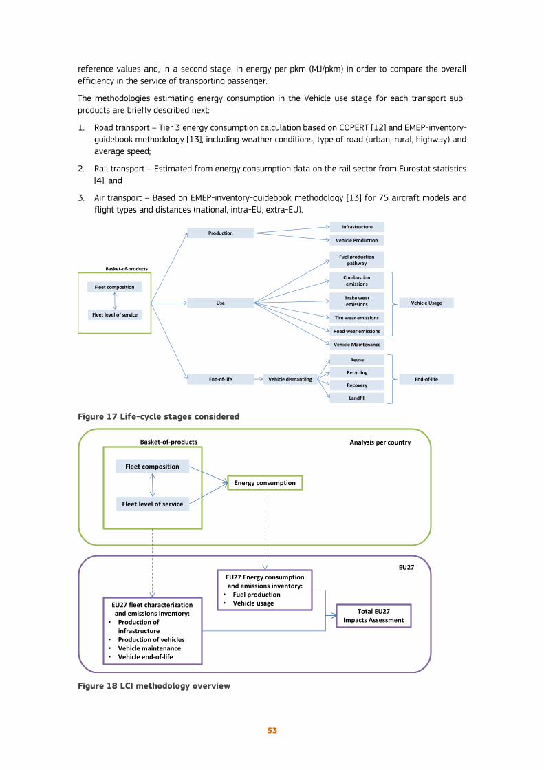
53

reference values and, in a second stage, in energy per pkm (MJ/pkm) in order to compare the overall

efficiency in the service of transporting passenger.

The methodologies estimating energy consumption in the Vehicle use stage for each transport sub-

products are briefly described next:

1. Road transport – Tier 3 energy consumption calculation based on COPERT [12] and EMEP-inventory-

guidebook methodology [13], including weather conditions, type of road (urban, rural, highway) and

average speed;

2. Rail transport – Estimated from energy consumption data on the rail sector from Eurostat statistics

[4]; and

3. Air transport – Based on EMEP-inventory-guidebook methodology [13] for 75 aircraft models and

flight types and distances (national, intra-EU, extra-EU).

Figure 17 Life-cycle stages considered

Figure 18 LCI methodology overview

Fleet composition

Fleet level of service

Basket-of-products

Use

Production

End-of-life

Combustion emissions

Brake wear emissions

Tire wear emissions

Road wear emissions

Fuel production pathway

Infrastructure

Vehicle Maintenance

Vehicle Production

Vehicle dismantling

Vehicle Usage

Reuse

Recycling

Recovery

Landfill

End-of-life

Fleet composition

Fleet level of service

Energy consumption

Basket-of-products Analysis per country

Total EU27Impacts Assessment

EU27

EU27 Energy consumption and emissions inventory:

• Fuel production• Vehicle usageEU27 fleet characterization

and emissions inventory:• Production of

infrastructure• Production of vehicles• Vehicle maintenance• Vehicle end-of-life

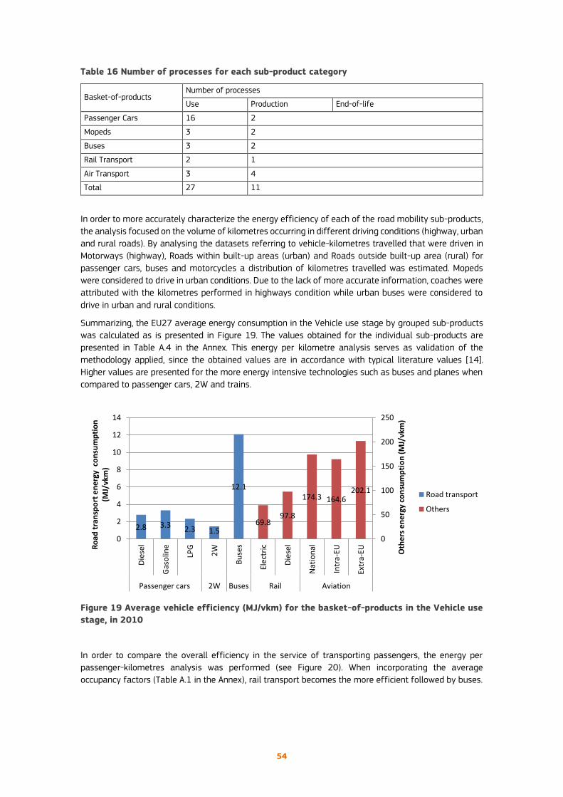
54

Table 16 Number of processes for each sub-product category

Basket-of-products Number of processes

Use Production End-of-life

Passenger Cars 16 2

Mopeds 3 2

Buses 3 2

Rail Transport 2 1

Air Transport 3 4

Total 27 11

In order to more accurately characterize the energy efficiency of each of the road mobility sub-products,

the analysis focused on the volume of kilometres occurring in different driving conditions (highway, urban

and rural roads). By analysing the datasets referring to vehicle-kilometres travelled that were driven in

Motorways (highway), Roads within built-up areas (urban) and Roads outside built-up area (rural) for

passenger cars, buses and motorcycles a distribution of kilometres travelled was estimated. Mopeds

were considered to drive in urban conditions. Due to the lack of more accurate information, coaches were

attributed with the kilometres performed in highways condition while urban buses were considered to

drive in urban and rural conditions.

Summarizing, the EU27 average energy consumption in the Vehicle use stage by grouped sub-products

was calculated as is presented in Figure 19. The values obtained for the individual sub-products are

presented in Table A.4 in the Annex. This energy per kilometre analysis serves as validation of the

methodology applied, since the obtained values are in accordance with typical literature values [14].

Higher values are presented for the more energy intensive technologies such as buses and planes when

compared to passenger cars, 2W and trains.

Figure 19 Average vehicle efficiency (MJ/vkm) for the basket-of-products in the Vehicle use

stage, in 2010

In order to compare the overall efficiency in the service of transporting passengers, the energy per

passenger-kilometres analysis was performed (see Figure 20). When incorporating the average

occupancy factors (Table A.1 in the Annex), rail transport becomes the more efficient followed by buses.

2.8 3.3 2.3 1.5

12.1

69.897.8

174.3 164.6202.1

0

50

100

150

200

250

0

2

4

6

8

10

12

14

Die

sel

Gas

olin

e

LPG

2W

Bu

ses

Ele

ctri

c

Die

sel

Nat

ion

al

Intr

a-EU

Extr

a-EU

Passenger cars 2W Buses Rail Aviation

Oth

ers

en

erg

y co

nsu

mp

tio

n (

MJ/

vkm

)

Ro

ad t

ran

spo

rt e

ne

rgy

co

nsu

mp

tio

n

(MJ/

vkm

)

Road transport

Others

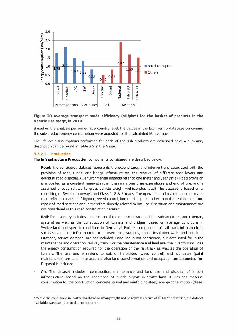
55

Figure 20 Average transport mode efficiency (MJ/pkm) for the basket-of-products in the

Vehicle use stage, in 2010

Based on the analysis performed at a country level, the values in the Ecoinvent 3 database concerning

the sub-product energy consumption were adjusted for the calculated EU average.

The life-cycle assumptions performed for each of the sub-products are described next. A summary

description can be found in Table A.5 in the Annex.

3.3.2.1 Production

The Infrastructure Production components considered are described below:

- Road: The considered dataset represents the expenditures and interventions associated with the

provision of road, tunnel and bridge infrastructures, the renewal of different road layers and

eventual road disposal. All environmental impacts refer to one meter and year (m*a). Road provision

is modelled as a constant renewal rather than as a one-time expenditure and end-of-life, and is

assumed directly related to gross vehicle weight (vehicle plus load). The dataset is based on a

modelling of Swiss motorways and Class 1, 2 & 3 roads. The operation and maintenance of roads

then refers to aspects of lighting, weed control, line marking, etc. rather than the replacement and

repair of road sections and is therefore directly related to km use. Operation and maintenance are

not considered in this road construction dataset.

- Rail: The inventory includes construction of the rail track (track bedding, substructures, and catenary

system) as well as the construction of tunnels and bridges, based on average conditions in

Switzerland and specific conditions in Germany3. Further components of rail track infrastructure,

such as signalling infrastructure, train overtaking stations, sound insulation walls and buildings

(stations, service garages) are not included. Land use is not considered, but accounted for in the

maintenance and operation, railway track. For the maintenance and land use, the inventory includes

the energy consumption required for the operation of the rail track as well as the operation of

tunnels. The use and emissions to soil of herbicides (weed control) and lubricates (point

maintenance) are taken into account. Also land transformation and occupation are accounted for.

Disposal is included.

- Air: The dataset includes construction, maintenance and land use and disposal of airport

infrastructure based on the conditions at Zurich airport in Switzerland. It includes material

consumption for the construction (concrete, gravel and reinforcing steel), energy consumption (diesel

3 While the conditions in Switzerland and Germany might not be representative of all EU27 countries, the dataset

available was used due to data constraints.

1.782.11

1.49 1.330.82

0.490.82

2.42

1.69 1.51

0.0

0.5

1.0

1.5

2.0

2.5

3.0

Die

sel

Gas

olin

e

LPG

2W

Bu

ses

Ele

ctri

c

Die

sel

Nat

ion

al

Intr

a-EU

Extr

a-EU

Passenger cars 2W Buses Rail Aviation

Ener

gy c

on

sum

pti

on

(M

J/p

km)

Road Transport

Others

56

and electricity) for construction, excavation, construction of the building, land transformation and

occupation, energy consumption (electricity, natural gas, light fuel oil, diesel and petrol) for

maintenance and operation, consumption of propylene glycol and ethylene glycol for de-icing of

aircrafts and sealed area, the water consumption (tap water), emissions to air (carbon dioxide,

carbon monoxide, NMVOC and nitrogen oxides), emissions to water (BOD5, DOC, TOC and COD) and

treatment of sewage.

In terms of Vehicle Production the following considerations were taken into account:

- Road (Passenger cars): These datasets represent the production of a petrol and of a diesel

passenger car of compact size. The entries are based on a per kg basis. The model is based on

averages over passenger cars technologies spanning from 2000 to 2010 and is estimated for a

vehicle of about 1234 kg for gasoline and 1314 kg for diesel. It is subdivided in two modules, the

glider and the drivetrain. Each module contains the specific material needs, production efforts and

emissions. The vehicle production includes the impacts of the vehicle production factory. The specific

end-of-life treatment of each module is covered in the respective dataset. The treatment of the

used passenger car only includes the manual dismantling of the car in the various modules. For

passenger cars production and end-of-life, weight correction factors were applied for engine

displacement differences in sub-products (proxy for vehicle size). The assumed material composition

for passenger cars consists mainly of steel and aluminium, as presented in Table 17, and the

production requires a consumption of 2.95 kg of water per kg of vehicle.

- Road (2W): The 50 cm3 scooter data set includes all processes and materials for scooter

manufacturing, containing an ICE motor. Transport to regional storage included. It includes as well

the disposal of a scooter. Data for manufacturing in Asia and retail in Europe. The assumed material

composition for 2W consists mainly of steel, PE and aluminium, as presented in Table 17, and the

production requires a consumption of 2.20 kg of water per kg of vehicle.

- Road (Buses): The Bus dataset represents the production of one bus (material composition, energy

consumption and emissions of the manufacturing). Vehicle manufacturing data are taken from one

production site in Germany. The disposal of bus is also included. It includes the material used for the

production, the energy consumption of the building machines, the water consumption, the airborne

emissions and the emissions to water. The assumed material composition for buses consists mainly

of steel, aluminium and ferro metals, as presented in Table 17, and the production requires a

consumption of 1.53 kg of water per kg of vehicle.

- Rail: The train manufacturing is derived from an assessment of the "IC 2000", a long-distance train

which is currently used for long distance transportation in Switzerland. The life span of the train is

assumed to be 40 years resulting in a life time performance of 20,000,000 vkm. For manufacturing,

electricity and light oil burned in industrial furnace are included. For the transportation of materials,

standard distances are applied. The assumed material composition for trains consists mainly of

aluminium, PE and steel, as presented in Table 17.

- Air: The datasets consider the production of a medium haul aircraft, based on an "Airbus A 320"

with a max. zero fuel weight of 61 t and a typical seating of 150 seats, and the production of a long

haul aircraft, based on an "Airbus A340-600" with 240 t max. zero fuel weight and a typical seating

of 380 seats. It includes material consumption (aluminium and polyethylene), energy consumption

(natural gas, electricity and light fuel oil), water consumption, treatment of sewage and NMVOC

emissions. The vehicle manufacturing data are taken from 16 production site in Germany, France,

Spain and the UK. The assumed material composition for aircrafts consists mainly of aluminium, as

presented in Table 17, and the production requires a consumption of 73.77 kg of water per kg of

medium haul aircraft and of 47.50 kg of water per kg of long haul aircraft.

57

Table 17 Material composition of each vehicle type modelled in Simapro (percentage)

Material type Passenger cars 2W Bus Train Aircraft

Aluminium 12 15 16 50 90

Coppers 1 1 1 3 0

Ferro metals 0 0 14 0 0

Glass 2 0 5 3 0

LO 1 0 1 0 0

Non-ferro 1 1 1 0 0

Others 2 1 5 0 0

Paint 0 0 0 2 0

PE 2 16 5 24 10

PET 0 0 0 0 0

Plastics 2 0 0 0 0

PP 4 7 0 0 0

PUR 2 0 0 0 0

PVC 1 2 0 0 0

Rubber 4 3 4 0 0

Steel 66 52 49 17 0

Textile 1 0 0 0 0

Zincs 0 0 0 0 0

3.3.2.2 Use

In the Use stage, the Fuel Production Pathway considered the following assumptions:

- For all fossil fuel products, the inventory for the distribution of petroleum products to the final

consumer including all necessary transports was considered. Transportation of the product from the

refinery to the end user is considered, as well as the operation of storage tanks and petrol stations.

Emissions from evaporation and treatment of effluents are included.

- For diesel, a 6% (weight) incorporation of biodiesel was considered, as result of the EU directive [15,

16], except for rail transport which considers only diesel. Biodiesel using rape oil as feedstock was

considered. The process includes the esterification process of oil to methyl ester and glycerin,

intermediate storage of the oil and products, treatment of specific wastewater effluents. System

boundary is at the esterification plant. The typical rape oil esterification plant is designed for rape

methyl ester (RME) production (for use in the vehicle fuels market).

- For electricity, the average EU27 mix was calculated based on the share of electricity produced in

each country, estimated from Eurostat. Due to a lack of data for some EU countries (Cyprus, Estonia,

Latvia, Lithuania and Malta), the mix was calculated using only the other countries which account

for 99% of the electricity produced in the EU27. The electricity production in each country includes

the transmission network, direct emissions to air (ozone and N2O), electricity losses during

transmission and losses during transformation.

As for the Vehicle Usage, the assumptions made are presented next.

- Road: The vehicle usage stage includes the emission factors for tailpipe emissions as well as the

road, tire and brake wear emissions. Since the Ecoinvent 3 database available in Simapro only

presented the environmental impacts for the Euro Standards 3, 4 and 5 of each vehicle sub-group,

the Conventional, Euro 1, 2 and 3 products were aggregated and simulated under the Euro 3 process.

- Rail: The vehicle usage includes particulate emissions due to abrasion of rail tracks, wheels, brakes

and overhead contact line, as well as emission of sulphur hexafluoride (SF6) occurring during

conversion at traction substations.

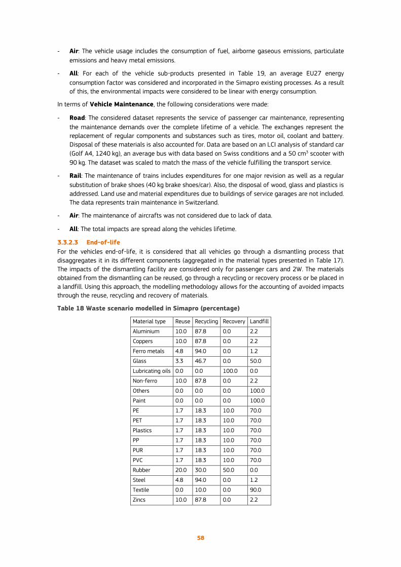
58

- Air: The vehicle usage includes the consumption of fuel, airborne gaseous emissions, particulate

emissions and heavy metal emissions.

- All: For each of the vehicle sub-products presented in Table 19, an average EU27 energy

consumption factor was considered and incorporated in the Simapro existing processes. As a result

of this, the environmental impacts were considered to be linear with energy consumption.

In terms of Vehicle Maintenance, the following considerations were made:

- Road: The considered dataset represents the service of passenger car maintenance, representing

the maintenance demands over the complete lifetime of a vehicle. The exchanges represent the

replacement of regular components and substances such as tires, motor oil, coolant and battery.

Disposal of these materials is also accounted for. Data are based on an LCI analysis of standard car

(Golf A4, 1240 kg), an average bus with data based on Swiss conditions and a 50 cm3 scooter with

90 kg. The dataset was scaled to match the mass of the vehicle fulfilling the transport service.

- Rail: The maintenance of trains includes expenditures for one major revision as well as a regular

substitution of brake shoes (40 kg brake shoes/car). Also, the disposal of wood, glass and plastics is

addressed. Land use and material expenditures due to buildings of service garages are not included.

The data represents train maintenance in Switzerland.

- Air: The maintenance of aircrafts was not considered due to lack of data.

- All: The total impacts are spread along the vehicles lifetime.

3.3.2.3 End-of-life

For the vehicles end-of-life, it is considered that all vehicles go through a dismantling process that

disaggregates it in its different components (aggregated in the material types presented in Table 17).

The impacts of the dismantling facility are considered only for passenger cars and 2W. The materials

obtained from the dismantling can be reused, go through a recycling or recovery process or be placed in

a landfill. Using this approach, the modelling methodology allows for the accounting of avoided impacts

through the reuse, recycling and recovery of materials.

Table 18 Waste scenario modelled in Simapro (percentage)

Material type Reuse Recycling Recovery Landfill

Aluminium 10.0 87.8 0.0 2.2

Coppers 10.0 87.8 0.0 2.2

Ferro metals 4.8 94.0 0.0 1.2

Glass 3.3 46.7 0.0 50.0

Lubricating oils 0.0 0.0 100.0 0.0

Non-ferro 10.0 87.8 0.0 2.2

Others 0.0 0.0 0.0 100.0

Paint 0.0 0.0 0.0 100.0

PE 1.7 18.3 10.0 70.0

PET 1.7 18.3 10.0 70.0

Plastics 1.7 18.3 10.0 70.0

PP 1.7 18.3 10.0 70.0

PUR 1.7 18.3 10.0 70.0

PVC 1.7 18.3 10.0 70.0

Rubber 20.0 30.0 50.0 0.0

Steel 4.8 94.0 0.0 1.2

Textile 0.0 10.0 0.0 90.0

Zincs 10.0 87.8 0.0 2.2

59

For each material type, the shares of materials that go through each of these waste processes were

considered as presented in Table 18. This waste scenario is based on the Advanced Standards of End of

Life Vehicles treatment scenario of a reference report [17]. While based on available data for the end-

of-life of road vehicles, the same waste scenario was applied to all sub-products of the basket-of-

products due to data availability constraints. Nonetheless, this could be improved if new data becomes

available.

The total reuse, recycling, recovery and landfill rates obtained for passenger cars are in accordance with

the Eurostat statistics for 2010 of 87.2% for Recovery and Reuse of cars, which is disaggregated into

83.3% Reuse (including recycling) and 3.9% Recovery [18]. These estimates validate the waste scenario

considered. Furthermore, these values allow the fulfilment of the EU guideline of achieving 85% of

Recovery and Reuse, in place since 2006 [19].

For recovery, the lower heating values used for lubricating oils, plastics and rubber were 39.3, 33.5 and

25.6 MJ/kg, respectively [17]. An efficiency of 7.7% for electricity and 31.3% for heat was considered for

the municipal solid waste incineration facility [17].

3.3.3 Final selection: overview per product and life cycle stage

Table 19 presents the number of sub-products considered (27) and the detailed aggregation performed

in each mobility sub-product modelled in Simapro for the different stages previously defined: Production;

Use; and End-of-life. For each sub-product, the different stages were further characterized as described

in Figure 17, Section 3.3.2 and Table A.5 in the Annex.

Table 19 Mobility sub-products modelled in Simapro

Products Designati

on

Sub-products in Use

stage

Sub-products in Production

stage

Sub-products in End-of-

life stage

Road

transpo

rt

Passeng

er Cars

Mobility

sub-

product

(SP) 1

Gasoline

<1,4 l

Convention

al, Euro 1,

2, 3

Passenger car petrol/natural gas

SP 2 Gasoline

<1,4 l Euro 4

SP 3 Gasoline

<1,4 l Euro 5

SP 4 Gasoline

1,4 - 2,0 l

Convention

al, Euro 1,

2, 3

SP 5 Gasoline

1,4 - 2,0 l Euro 4

SP 6 Gasoline

1,4 - 2,0 l Euro 5

SP 7 Gasoline

>2,0 l

Convention

al, Euro 1,

2, 3

SP 8 Gasoline

>2,0 l Euro 4

SP 9 Gasoline

>2,0 l Euro 5

SP 10 Diesel 1,4

- 2,0 l

Convention

al, Euro 1,

2, 3 Passenger car diesel

SP 11 Diesel 1,4

- 2,0 l Euro 4

60

SP 12 Diesel 1,4

- 2,0 l Euro 5

SP 13 Diesel

>2,0 l

Convention

al, Euro 1,

2, 3

SP 14 Diesel

>2,0 l Euro 4

SP 15 Diesel

>2,0 l Euro 5

SP 16 LPG

Convention

al, Euro 1,

2, 3, 4, 5

Passenger car petrol/natural gas

2W

SP 17 Mopeds

<50 cm³

Convention

al, Euro 1,

2, 3

Motor scooter 50 cm3 (RER) + Motor scooter 50 cm3

(ROW) SP 18

Motorcycl

es <250

cm³

Convention

al

SP 19

Motorcycl

es >250

cm³

Convention

al, Euro 1,

2, 3

Buses

SP 20

Urban

Buses

Standard

15 - 18 t

Convention

al, Euro 1,

2, 3, 4, 5

Bus (RER) + Bus (ROW) SP 21

Coaches

Standard

<=18 t

Convention

al, Euro 1,

2, 3, 4, 5

SP 22

Urban

CNG

Buses

Euro 1, 2, 3

Rail transport SP 23 Electric Train passenger long distance

SP 24 Diesel

Air transport

SP 25 National flights Medium haul aircraft (RER) + Medium haul aircraft

(ROW) SP 26 Intra-EU flights

SP 27 Extra-EU flights Long haul aircraft (RER) + Long haul aircraft (ROW)

The main Simapro input for the quantification of the annual impacts of the mobility products are the

vehicle-kilometres travelled for the road transport sector for each of the vehicle categories considered

or passenger-kilometres travelled for rail and air transport, as is presented in Table 20.

.

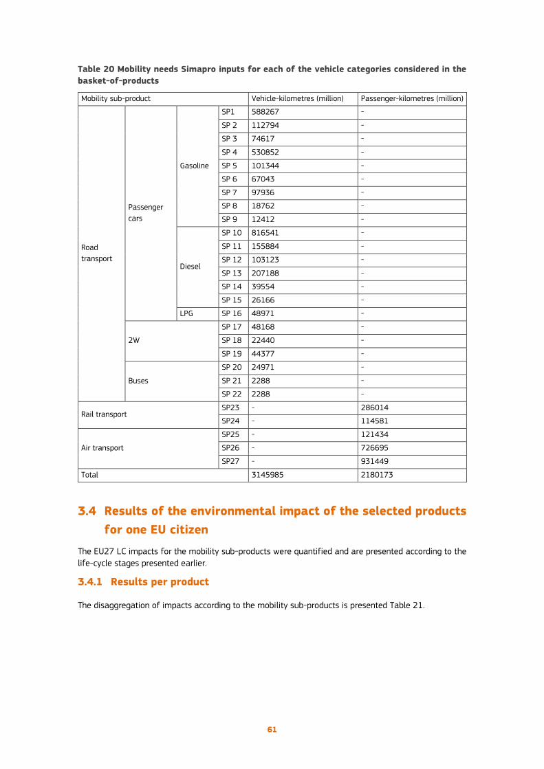
61

Table 20 Mobility needs Simapro inputs for each of the vehicle categories considered in the

basket-of-products

Mobility sub-product Vehicle-kilometres (million) Passenger-kilometres (million)

Road

transport

Passenger

cars

Gasoline

SP1 588267 -

SP 2 112794 -

SP 3 74617 -

SP 4 530852 -

SP 5 101344 -

SP 6 67043 -

SP 7 97936 -

SP 8 18762 -

SP 9 12412 -

Diesel

SP 10 816541 -

SP 11 155884 -

SP 12 103123 -

SP 13 207188 -

SP 14 39554 -

SP 15 26166 -

LPG SP 16 48971 -

2W

SP 17 48168 -

SP 18 22440 -

SP 19 44377 -

Buses

SP 20 24971 -

SP 21 2288 -

SP 22 2288 -

Rail transport SP23 - 286014

SP24 - 114581

Air transport

SP25 - 121434

SP26 - 726695

SP27 - 931449

Total 3145985 2180173

3.4 Results of the environmental impact of the selected products

for one EU citizen

The EU27 LC impacts for the mobility sub-products were quantified and are presented according to the

life-cycle stages presented earlier.

3.4.1 Results per product

The disaggregation of impacts according to the mobility sub-products is presented Table 21.

62

Table 21 Environmental impacts in 2010 for the whole EU27, from each mobility sub-products

Sub-

product

Climate

change

Ozone

depletion

Human

toxicity,

cancer

effects

Human

toxicity,

non-cancer

effects

Particulate

matter

Ionizing

radiation HH

Ionizing

radiation E

(interim)

Photochemical

ozone

formation

Acidifi-

cation

Terrestrial

eutrophi-

cation

Freshwater

eutrophi-

cation

Marine

eutrophi-

cation

Freshwater

ecotoxicity Land use

Water

resource

depletion

Mineral, fossil

& ren

resource

depletion

kg CO2 eq kg CFC-11

eq CTUh CTUh kg PM2.5 eq

kBq U235

eq CTUe kg NMVOC eq molc H+ eq molc N eq kg P eq kg N eq CTUe kg C deficit

m3 water

eq kg Sb eq

SP 1 2.24E+11 1.55E+04 5.91E+03 3.79E+04 6.92E+07 1.63E+10 8.25E+04 5.35E+08 4.87E+08 1.02E+09 1.64E+07 1.01E+08 1.35E+12 2.19E+11 4.40E+10 2.16E+07



























Total 1.45E+12 1.03E+05 3.59E+04 2.68E+05 5.91E+08 1.14E+11 5.55E+05 5.26E+09 4.38E+09 1.39E+10 1.15E+08 1.44E+09 8.05E+12 4.69E+12 3.48E+11 1.22E+08

63

Figure 21 Disaggregation of environmental impacts for the whole EU27 in 2010, by mobility

product

Table 22 Disaggregation of environmental impacts for the whole EU27 in 2010, by mobility

product

Impact category Mobility products

Passenger cars 2W Buses Rail Air

Climate change kg CO2 eq 1.09E+12 1.94E+10 5.28E+10 3.56E+10 2.56E+11

Ozone depletion kg CFC-11 eq 7.78E+04 1.21E+03 4.35E+03 2.66E+03 1.70E+04

Human toxicity, cancer effects CTUh 3.20E+04 2.47E+02 3.54E+02 2.33E+03 9.23E+02

Human toxicity, non-cancer

effects CTUh 2.44E+05 2.10E+03 8.27E+03 8.55E+03 5.71E+03

Particulate matter kg PM2.5 eq 5.07E+08 6.23E+06 2.31E+07 1.42E+07 4.12E+07

Ionizing radiation HH kBq U235 eq 8.18E+10 1.14E+09 3.22E+09 1.27E+10 1.51E+10

Ionizing radiation E (interim) CTUe 4.12E+05 6.68E+03 1.81E+04 2.37E+04 9.47E+04

Photochemical ozone

formation kg NMVOC eq 2.69E+09 5.40E+08 5.08E+08 1.93E+08 1.32E+09

Acidification molc H+ eq 2.58E+09 6.03E+07 4.08E+08 2.23E+08 1.11E+09

Terrestrial eutrophication molc N eq 6.46E+09 2.18E+08 2.01E+09 7.04E+08 4.54E+09

Freshwater eutrophication kg P eq 8.59E+07 5.83E+05 1.75E+06 2.27E+07 4.29E+06

Marine eutrophication kg N eq 7.41E+08 2.04E+07 1.99E+08 6.86E+07 4.15E+08

Freshwater ecotoxicity CTUe 7.55E+12 7.97E+10 1.16E+11 2.18E+11 8.11E+10

Land use kg C deficit 4.08E+12 1.27E+10 4.20E+11 3.55E+10 1.54E+11

Water resource depletion m3 water eq 2.21E+11 1.86E+09 6.25E+09 1.01E+11 1.80E+10


depletion kg Sb eq 1.19E+08 9.27E+05 8.99E+05 8.19E+05 7.13E+05

Figure 21 and Table 22 present the results by transport mode, showing a clear predominance of

passenger cars. Nonetheless, air transport has very significant shares in some impact categories, being

responsible for up to 33% of total impacts. The rail transport is only relevant in 3 impact categories,

while buses and 2W have lower responsibilities of the total impacts. This follows closely the distribution

0%

10%

20%

30%

40%

50%

60%

70%

80%

90%

100%

Clim

ate

chan

ge

Ozo

ne

dep

leti

on

Hu

man

to

xici

ty, c

ance

r ef

fect

s

Hu

man

to

xici

ty, n

on

-can

cer

effe

cts

Par

ticu

late

mat

ter

Ion

izin

g ra

dia

tio

n H

H

Ion

izin

g ra

dia

tio

n E

(in

teri

m)

Ph

oto

chem

ical

ozo

ne

form

atio

n

Aci

dif

icat

ion

Terr

estr

ial e

utr

op

hic

atio

n

Fre

shw

ate

r e

utr

op

hic

atio

n

Mar

ine

eutr

op

hic

atio

n

Fre

shw

ater

eco

toxi

city

Lan

d u

se

Wat

er r

eso

urc

e d

eple

tio

n

Min

eral

, fo

ssil

& r

en r

eso

urc

e…

Per

cen

tage

of

imp

acts

Air

Rail

Buses

2W

Passenger cars

64

of pkm by transport mode presented previously (Figure 16). The results obtained by mobility product and

life cycle stage are presented in Tables A.6 to A.10 in the Annex.

3.4.2 Results per life cycle stage

3.4.2.1 Road transport

The assessment of the environmental impacts of the road transport sub-products included passenger

cars (Figure 22), two-wheelers (Figure 24) and buses (Figure 23). The absolute values for the

environmental impacts are presented in Tables A.6 to A.8 in the Annex.

Passenger cars are accountable for 91% of the environmental impacts of road transport. Within this

category, the most significant contributions are from SP1 (Gasoline <1,4 l Conventional, Euro 1, 2, 3),

SP4 (Gasoline 1.4 - 2.0 l Conventional, Euro 1, 2, 3) and SP10 (Diesel 1.4 - 2.0 l Conventional, Euro 1, 2,

3), which is a result of having the higher number of vehicle-kilometres travelled (Table 20).

A predominance of the Use stage is observed, mainly for buses and two-wheelers. Nonetheless, for some

environmental impacts, the Production and End-of-life stages are also very significant.

Figure 22 Passenger cars environmental impacts for the whole EU27 in 2010. Negative

impacts account for avoided environmental impacts associated to End-of-life processes.

-60%

-40%

-20%

0%

20%

40%

60%

80%

100%

Clim

ate

chan

ge

Ozo

ne

dep

leti

on

Hu

man

to

xici

ty, c

ance

r ef

fect

s

Hu

man

to

xici

ty, n

on

-can

cer

effe

cts

Par

ticu

late

mat

ter

Ion

izin

g ra

dia

tio

n H

H

Ion

izin

g ra

dia

tio

n E

(in

teri

m)

Ph

oto

chem

ical

ozo

ne

form

atio

n

Aci

dif

icat

ion

Terr

est

rial

eu

tro

ph

icat

ion

Fre

shw

ater

eu

tro

ph

icat

ion

Mar

ine

eutr

op

hic

atio

n

Fres

hw

ater

eco

toxi

city

Lan

d u

se

Wat

er r

eso

urc

e d

eple

tio

n

Min

eral

, fo

ssil

& r

en

res

ou

rce

dep

leti

onP

erc

en

tage

of

imp

acts

End-of-life [EOL]

Vehicle maintenance [Use]

Vehicle usage [Use]

Fuel production pathway [Use]

Vehicle production [Production]

Infrastructure [Production]

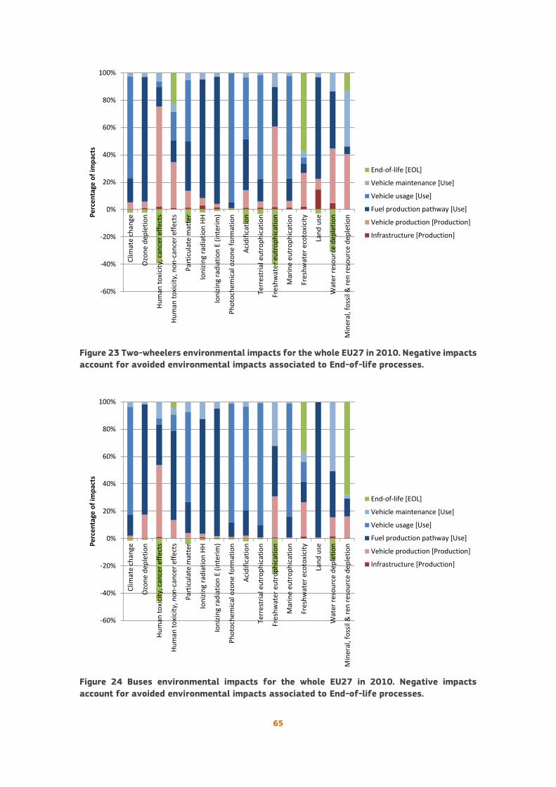
65

Figure 23 Two-wheelers environmental impacts for the whole EU27 in 2010. Negative impacts

account for avoided environmental impacts associated to End-of-life processes.

Figure 24 Buses environmental impacts for the whole EU27 in 2010. Negative impacts


-60%

-40%

-20%

0%

20%

40%

60%

80%

100%

Clim

ate

chan

ge

Ozo

ne

dep

leti

on

Hu

man

to

xici

ty, c

ance

r ef

fect

s

Hu

man

to

xici

ty, n

on

-can

cer

effe

cts

Par

ticu

late

mat

ter

Ion

izin

g ra

dia

tio

n H

H

Ion

izin

g ra

dia

tio

n E

(in

teri

m)

Ph

oto

chem

ical

ozo

ne

form

atio

n

Aci

dif

icat

ion

Terr

est

rial

eu

tro

ph

icat

ion

Fre

shw

ater

eu

tro

ph

icat

ion

Mar

ine

eutr

op

hic

atio

n

Fre

shw

ater

eco

toxi

city

Lan

d u

se

Wat

er r

eso

urc

e d

eple

tio

n

Min

eral

, fo

ssil

& r

en r

eso

urc

e d

eple

tio

nPe

rce

nta

ge o

f im

pac

ts

End-of-life [EOL]


Vehicle usage [Use]




-60%

-40%

-20%

0%

20%

40%

60%

80%

100%

Clim

ate

chan

ge

Ozo

ne

dep

leti

on

Hu

man

to

xici

ty, c

ance

r ef

fect

s

Hu

man

to

xici

ty, n

on

-can

cer

effe

cts

Par

ticu

late

mat

ter

Ion

izin

g ra

dia

tio

n H

H

Ion

izin

g ra

dia

tio

n E

(in

teri

m)

Ph

oto

chem

ical

ozo

ne

form

atio

n

Aci

dif

icat

ion

Terr

est

rial

eu

tro

ph

icat

ion

Fre

shw

ater

eu

tro

ph

icat

ion

Mar

ine

eutr

op

hic

atio

n

Fre

shw

ater

eco

toxi

city

Lan

d u

se

Wat

er r

eso

urc

e d

eple

tio

n

Min

eral

, fo

ssil

& r

en r

eso

urc

e d

eple

tio

nPe

rce

nta

ge o

f im

pac

ts

End-of-life [EOL]


Vehicle usage [Use]




66

3.4.2.2 Rail transport

The environmental impacts of the rail transport are mainly dominated by the Use stage, as can be seen

in Figure 25. The Production stage is the dominant stage in only one category (Land use), being

nonetheless responsible for more than 30% of the impacts in 3 other categories (Human toxicity, cancer

effects; Particulate matter; and Mineral, fossil & renewable resources depletion). The absolute values for

the environmental impacts are presented in Table A.9 in the Annex.

Figure 25 Rail transport environmental impacts for the whole EU27 in 2010. Negative impacts


The electric trains are responsible for 72% of the environmental impacts of the rail transportation sector.

This is mainly due to the high share of passenger-kilometres attributed to the electric rail transport.

3.4.2.3 Air transport

The environmental impacts of the air transport are mainly dominated by the Use stage, as can be seen

in Figure 26. While the Use stage is the most relevant for all categories, the Production stage is still

responsible for more than 30% of the impacts in 3 categories (Freshwater eutrophication; Freshwater

ecotoxicity; and Water resource depletion). The absolute values for the environmental impacts are

presented in Table A.10 in the Annex.

-20%

0%

20%

40%

60%

80%

100%

Clim

ate

chan

ge

Ozo

ne

dep

leti

on

Hu

man

to

xici

ty, c

ance

r ef

fect

s

Hu

man

to

xici

ty, n

on

-can

cer

effe

cts

Par

ticu

late

mat

ter

Ion

izin

g ra

dia

tio

n H

H

Ion

izin

g ra

dia

tio

n E

(in

teri

m)

Ph

oto

chem

ical

ozo

ne

form

atio

n

Aci

dif

icat

ion

Terr

est

rial

eu

tro

ph

icat

ion

Fres

hw

ater

eu

tro

ph

icat

ion

Mar

ine

eutr

op

hic

atio

n

Fre

shw

ater

eco

toxi

city

Lan

d u

se

Wat

er r

eso

urc

e d

eple

tio

n

Min

eral

, fo

ssil

& r

en r

eso

urc

e d

eple

tio

n

Pe

rce

nta

ge o

f im

pac

ts

End-of-life [EOL]


Vehicle usage [Use]




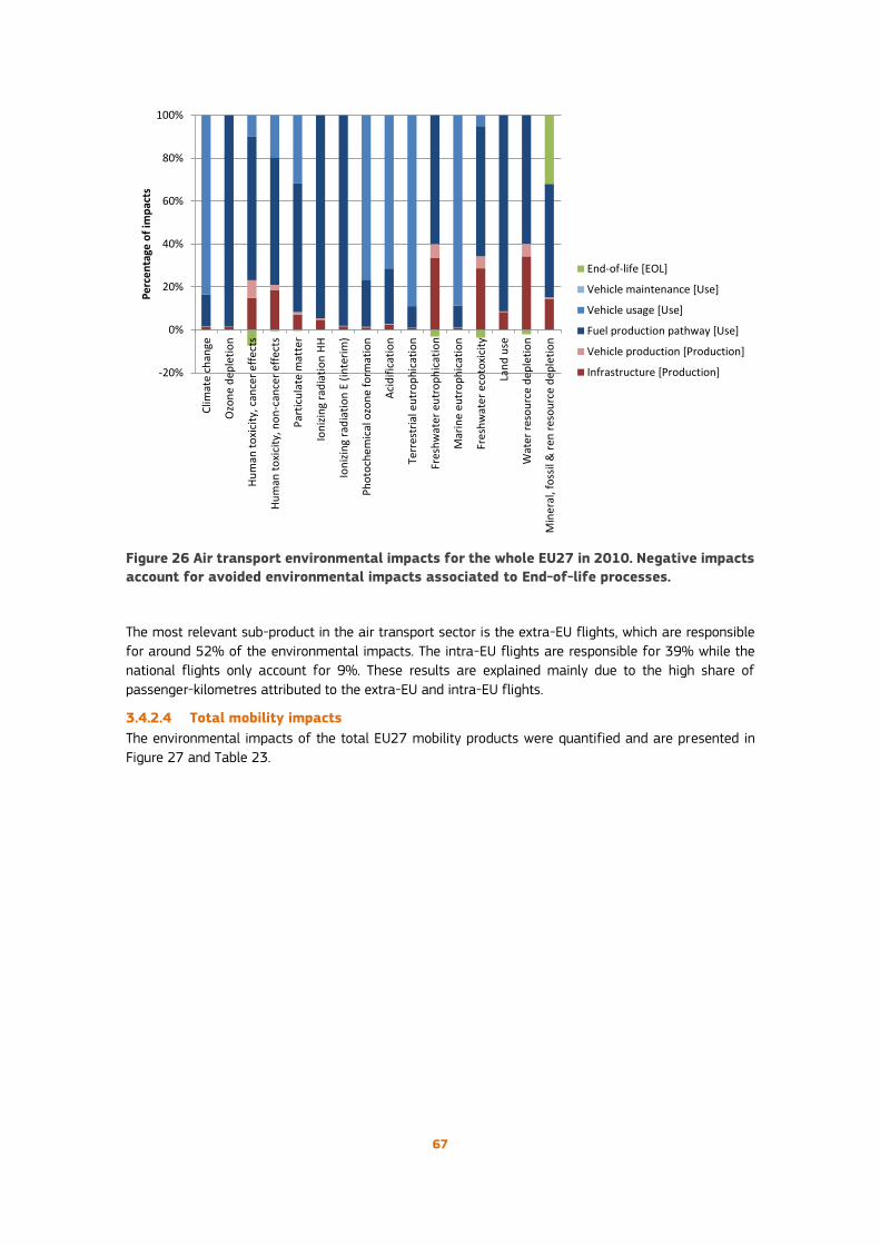
67

Figure 26 Air transport environmental impacts for the whole EU27 in 2010. Negative impacts


The most relevant sub-product in the air transport sector is the extra-EU flights, which are responsible

for around 52% of the environmental impacts. The intra-EU flights are responsible for 39% while the

national flights only account for 9%. These results are explained mainly due to the high share of

passenger-kilometres attributed to the extra-EU and intra-EU flights.

3.4.2.4 Total mobility impacts

The environmental impacts of the total EU27 mobility products were quantified and are presented in

Figure 27 and Table 23.

-20%

0%

20%

40%

60%

80%

100%

Clim

ate

chan

ge

Ozo

ne

dep

leti

on

Hu

man

to

xici

ty, c

ance

r ef

fect

s

Hu

man

to

xici

ty, n

on

-can

cer

effe

cts

Par

ticu

late

mat

ter

Ion

izin

g ra

dia

tio

n H

H

Ion

izin

g ra

dia

tio

n E

(in

teri

m)

Ph

oto

chem

ical

ozo

ne

form

atio

n

Aci

dif

icat

ion

Terr

est

rial

eu

tro

ph

icat

ion

Fres

hw

ater

eu

tro

ph

icat

ion

Mar

ine

eutr

op

hic

atio

n

Fre

shw

ater

eco

toxi

city

Lan

d u

se

Wat

er r

eso

urc

e d

eple

tio

n

Min

eral

, fo

ssil

& r

en r

eso

urc

e d

eple

tio

n

Pe

rce

nta

ge o

f im

pac

ts

End-of-life [EOL]


Vehicle usage [Use]




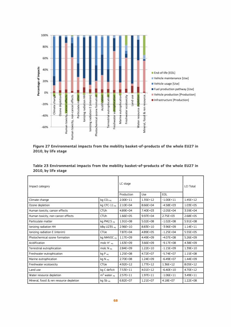
68

Figure 27 Environmental impacts from the mobility basket-of-products of the whole EU27 in

2010, by life stage

Table 23 Environmental impacts from the mobility basket-of-products of the whole EU27 in

2010, by life stage

Impact category LC stage

LCI Total

Production Use EOL

Climate change kg CO2 eq 2.00E+11 1.35E+12 -1.00E+11 1.45E+12

Ozone depletion kg CFC-11 eq 2.10E+04 8.66E+04 -4.58E+03 1.03E+05

Human toxicity, cancer effects CTUh 4.89E+04 7.40E+03 -2.05E+04 3.59E+04

Human toxicity, non-cancer effects CTUh 1.66E+05 9.97E+04 2.75E+03 2.68E+05

Particulate matter kg PM2.5 eq 1.91E+08 5.02E+08 -1.02E+08 5.91E+08

Ionizing radiation HH kBq U235 eq 2.96E+10 8.83E+10 -3.96E+09 1.14E+11

Ionizing radiation E (interim) CTUe 7.87E+04 4.89E+05 -1.25E+04 5.55E+05

Photochemical ozone formation kg NMVOC eq 1.17E+09 4.49E+09 -4.07E+08 5.26E+09

Acidification molc H+ eq 1.63E+09 3.66E+09 -9.17E+08 4.38E+09

Terrestrial eutrophication molc N eq 2.84E+09 1.22E+10 -1.15E+09 1.39E+10

Freshwater eutrophication kg P eq 1.25E+08 4.72E+07 -5.74E+07 1.15E+08

Marine eutrophication kg N eq 2.70E+08 1.24E+09 -6.49E+07 1.44E+09

Freshwater ecotoxicity CTUe 4.92E+12 1.77E+12 1.36E+12 8.05E+12

Land use kg C deficit 7.53E+11 4.01E+12 -6.40E+10 4.70E+12

Water resource depletion m3 water eq 2.57E+11 1.97E+11 -1.06E+11 3.49E+11

Mineral, fossil & ren resource depletion kg Sb eq 6.82E+07 1.21E+07 4.18E+07 1.22E+08

-60%

-40%

-20%

0%

20%

40%

60%

80%

100%

Clim

ate

chan

ge

Ozo

ne

dep

leti

on

Hu

man

to

xici

ty, c

ance

r ef

fect

s

Hu

man

to

xici

ty, n

on

-can

cer

effe

cts

Par

ticu

late

mat

ter

Ion

izin

g ra

dia

tio

n H

H

Ion

izin

g ra

dia

tio

n E

(in

teri

m)

Ph

oto

chem

ical

ozo

ne

form

atio

n

Aci

dif

icat

ion

Terr

est

rial

eu

tro

ph

icat

ion

Fre

shw

ater

eu

tro

ph

icat

ion

Mar

ine

eutr

op

hic

atio

n

Fre

shw

ater

eco

toxi

city

Lan

d u

se

Wat

er r

eso

urc

e d

eple

tio

n

Min

eral

, fo

ssil

& r

en r

eso

urc

e…Per

cen

tage

of

imp

acts

End-of-life [EOL]


Vehicle usage [Use]




69

3.4.3 Results overall of environmental impact of mobility for one EU citizen

The average mobility impacts per EU citizen were also quantified and are presented in Table 24.

Table 24 Environmental impacts per average EU27 citizen in 2010, from the mobility basket-

of-products

Impact category Mobility

Climate change kg CO2 eq 2.91E+03

Ozone depletion kg CFC-11 eq 2.06E-04

Human toxicity, cancer effects CTUh 7.19E-05

Human toxicity, non-cancer effects CTUh 5.38E-04

Particulate matter kg PM2.5 eq 1.18E+00

Ionizing radiation HH kBq U235 eq 2.28E+02

Ionizing radiation E (interim) CTUe 1.11E-03

Photochemical ozone formation kg NMVOC eq 1.05E+01

Acidification molc H+ eq 8.78E+00

Terrestrial eutrophication molc N eq 2.79E+01

Freshwater eutrophication kg P eq 2.31E-01

Marine eutrophication kg N eq 2.89E+00

Freshwater ecotoxicity CTUe 1.61E+04

Land use kg C deficit 9.42E+03

Water resource depletion m3 water eq 6.98E+02

Mineral, fossil & ren resource depletion kg Sb eq 2.44E-01

A more complete description of the environmental impacts per EU27 citizen and by mobility sub-product,

aggregated by mobility product and life cycle stage is shown in Table 25, Table 26 and Table 27,

respectively.

70

Table 25 Environmental impacts in 2010 per average EU27 citizen, from each mobility sub-products

Sub-

product

Climate

change

Ozone

depletion

Human

toxicity,

cancer

effects

Human

toxicity,

non-cancer

effects

Particulate

matter

Ionizing

radiation HH

Ionizing

radiation E

(interim)

Photochemical

ozone

formation

Acidifi-

cation

Terrestrial

eutrophi-

cation

Freshwater

eutrophi-

cation

Marine

eutrophi-

cation

Freshwater

ecotoxicity Land use

Water

resource

depletion

Mineral, fossil

& ren

resource

depletion

kg CO2 eq kg CFC-11

eq CTUh CTUh kg PM2.5 eq

kBq U235

eq CTUe kg NMVOC eq molc H+ eq molc N eq kg P eq kg N eq CTUe kg C deficit

m3 water

eq kg Sb eq

SP 1 4.49E+02 3.11E-05 1.18E-05 7.59E-05 1.39E-01 3.27E+01 1.65E-04 1.07E+00 9.76E-01 2.04E+00 3.29E-02 2.02E-01 2.70E+03 4.39E+02 8.82E+01 4.33E-02

SP 2 7.99E+01 5.67E-06 2.12E-06 1.41E-05 2.48E-02 5.83E+00 3.01E-05 1.81E-01 1.62E-01 3.13E-01 5.77E-03 3.15E-02 5.09E+02 7.81E+01 1.49E+01 8.07E-03


SP 4 4.85E+02 3.45E-05 1.33E-05 8.80E-05 1.50E-01 3.55E+01 1.83E-04 1.10E+00 1.02E+00 2.06E+00 3.61E-02 2.06E-01 3.19E+03 4.77E+02 9.26E+01 5.07E-02









SP 13 1.46E+02 1.06E-05 4.71E-06 4.33E-05 1.05E-01 1.13E+01 5.59E-05 3.99E-01 4.07E-01 1.26E+00 1.23E-02 1.61E-01 1.11E+03 1.24E+03 3.13E+01 1.70E-02





SP 18 8.34E+00 6.95E-07 5.71E-08 1.48E-06 3.91E-03 5.71E-01 3.31E-06 8.60E-02 6.93E-02 3.41E-01 2.74E-04 3.41E-02 1.86E+01 8.03E+01 1.01E+00 1.43E-04



SP 21 7.03E+00 4.39E-07 9.44E-08 7.99E-07 2.26E-03 4.15E-01 2.42E-06 1.95E-01 2.18E-02 7.89E-02 2.20E-04 7.41E-03 3.09E+01 4.67E+00 6.95E-01 3.61E-04





SP 26 2.12E+02 1.41E-05 6.79E-07 4.21E-06 3.27E-02 1.23E+01 7.85E-05 1.10E+00 9.14E-01 3.79E+00 2.79E-03 3.47E-01 5.45E+01 1.22E+02 1.17E+01 5.97E-04


Total 2.91E+03 2.07E-04 7.19E-05 5.38E-04 1.18E+00 2.28E+02 1.11E-03 1.05E+01 8.78E+00 2.79E+01 2.31E-01 2.89E+00 1.61E+04 9.40E+03 6.98E+02 2.44E-01

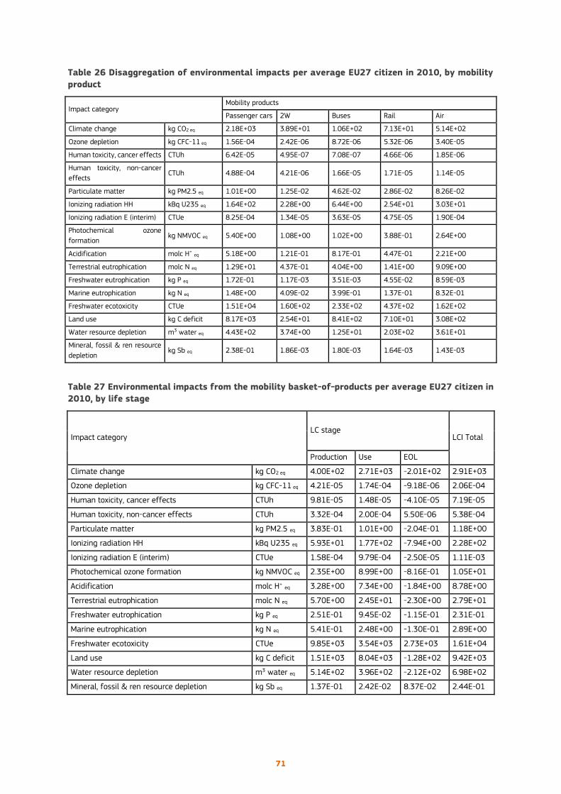
71

Table 26 Disaggregation of environmental impacts per average EU27 citizen in 2010, by mobility

product

Impact category Mobility products

Passenger cars 2W Buses Rail Air

Climate change kg CO2 eq 2.18E+03 3.89E+01 1.06E+02 7.13E+01 5.14E+02

Ozone depletion kg CFC-11 eq 1.56E-04 2.42E-06 8.72E-06 5.32E-06 3.40E-05

Human toxicity, cancer effects CTUh 6.42E-05 4.95E-07 7.08E-07 4.66E-06 1.85E-06


effects CTUh 4.88E-04 4.21E-06 1.66E-05 1.71E-05 1.14E-05

Particulate matter kg PM2.5 eq 1.01E+00 1.25E-02 4.62E-02 2.86E-02 8.26E-02

Ionizing radiation HH kBq U235 eq 1.64E+02 2.28E+00 6.44E+00 2.54E+01 3.03E+01

Ionizing radiation E (interim) CTUe 8.25E-04 1.34E-05 3.63E-05 4.75E-05 1.90E-04

Photochemical ozone

formation kg NMVOC eq 5.40E+00 1.08E+00 1.02E+00 3.88E-01 2.64E+00

Acidification molc H+ eq 5.18E+00 1.21E-01 8.17E-01 4.47E-01 2.21E+00

Terrestrial eutrophication molc N eq 1.29E+01 4.37E-01 4.04E+00 1.41E+00 9.09E+00

Freshwater eutrophication kg P eq 1.72E-01 1.17E-03 3.51E-03 4.55E-02 8.59E-03

Marine eutrophication kg N eq 1.48E+00 4.09E-02 3.99E-01 1.37E-01 8.32E-01

Freshwater ecotoxicity CTUe 1.51E+04 1.60E+02 2.33E+02 4.37E+02 1.62E+02

Land use kg C deficit 8.17E+03 2.54E+01 8.41E+02 7.10E+01 3.08E+02

Water resource depletion m3 water eq 4.43E+02 3.74E+00 1.25E+01 2.03E+02 3.61E+01


depletion kg Sb eq 2.38E-01 1.86E-03 1.80E-03 1.64E-03 1.43E-03

Table 27 Environmental impacts from the mobility basket-of-products per average EU27 citizen in

2010, by life stage

Impact category LC stage

LCI Total

Production Use EOL

Climate change kg CO2 eq 4.00E+02 2.71E+03 -2.01E+02 2.91E+03

Ozone depletion kg CFC-11 eq 4.21E-05 1.74E-04 -9.18E-06 2.06E-04

Human toxicity, cancer effects CTUh 9.81E-05 1.48E-05 -4.10E-05 7.19E-05

Human toxicity, non-cancer effects CTUh 3.32E-04 2.00E-04 5.50E-06 5.38E-04

Particulate matter kg PM2.5 eq 3.83E-01 1.01E+00 -2.04E-01 1.18E+00

Ionizing radiation HH kBq U235 eq 5.93E+01 1.77E+02 -7.94E+00 2.28E+02

Ionizing radiation E (interim) CTUe 1.58E-04 9.79E-04 -2.50E-05 1.11E-03

Photochemical ozone formation kg NMVOC eq 2.35E+00 8.99E+00 -8.16E-01 1.05E+01

Acidification molc H+ eq 3.28E+00 7.34E+00 -1.84E+00 8.78E+00

Terrestrial eutrophication molc N eq 5.70E+00 2.45E+01 -2.30E+00 2.79E+01

Freshwater eutrophication kg P eq 2.51E-01 9.45E-02 -1.15E-01 2.31E-01

Marine eutrophication kg N eq 5.41E-01 2.48E+00 -1.30E-01 2.89E+00

Freshwater ecotoxicity CTUe 9.85E+03 3.54E+03 2.73E+03 1.61E+04

Land use kg C deficit 1.51E+03 8.04E+03 -1.28E+02 9.42E+03

Water resource depletion m3 water eq 5.14E+02 3.96E+02 -2.12E+02 6.98E+02

Mineral, fossil & ren resource depletion kg Sb eq 1.37E-01 2.42E-02 8.37E-02 2.44E-01

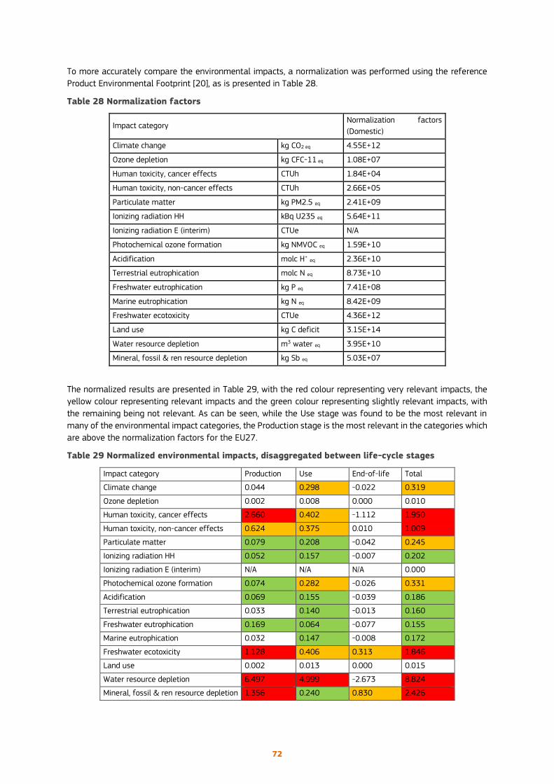
72

To more accurately compare the environmental impacts, a normalization was performed using the reference

Product Environmental Footprint [20], as is presented in Table 28.

Table 28 Normalization factors

Impact category Normalization factors

(Domestic)

Climate change kg CO2 eq 4.55E+12

Ozone depletion kg CFC-11 eq 1.08E+07

Human toxicity, cancer effects CTUh 1.84E+04

Human toxicity, non-cancer effects CTUh 2.66E+05

Particulate matter kg PM2.5 eq 2.41E+09

Ionizing radiation HH kBq U235 eq 5.64E+11

Ionizing radiation E (interim) CTUe N/A

Photochemical ozone formation kg NMVOC eq 1.59E+10

Acidification molc H+ eq 2.36E+10

Terrestrial eutrophication molc N eq 8.73E+10

Freshwater eutrophication kg P eq 7.41E+08

Marine eutrophication kg N eq 8.42E+09

Freshwater ecotoxicity CTUe 4.36E+12

Land use kg C deficit 3.15E+14

Water resource depletion m3 water eq 3.95E+10

Mineral, fossil & ren resource depletion kg Sb eq 5.03E+07

The normalized results are presented in Table 29, with the red colour representing very relevant impacts, the

yellow colour representing relevant impacts and the green colour representing slightly relevant impacts, with

the remaining being not relevant. As can be seen, while the Use stage was found to be the most relevant in

many of the environmental impact categories, the Production stage is the most relevant in the categories which

are above the normalization factors for the EU27.

Table 29 Normalized environmental impacts, disaggregated between life-cycle stages

Impact category Production Use End-of-life Total

Climate change 0.044 0.298 -0.022 0.319

Ozone depletion 0.002 0.008 0.000 0.010

Human toxicity, cancer effects 2.660 0.402 -1.112 1.950

Human toxicity, non-cancer effects 0.624 0.375 0.010 1.009

Particulate matter 0.079 0.208 -0.042 0.245

Ionizing radiation HH 0.052 0.157 -0.007 0.202

Ionizing radiation E (interim) N/A N/A N/A 0.000

Photochemical ozone formation 0.074 0.282 -0.026 0.331

Acidification 0.069 0.155 -0.039 0.186

Terrestrial eutrophication 0.033 0.140 -0.013 0.160

Freshwater eutrophication 0.169 0.064 -0.077 0.155

Marine eutrophication 0.032 0.147 -0.008 0.172

Freshwater ecotoxicity 1.128 0.406 0.313 1.846

Land use 0.002 0.013 0.000 0.015

Water resource depletion 6.497 4.999 -2.673 8.824

Mineral, fossil & ren resource depletion 1.356 0.240 0.830 2.426

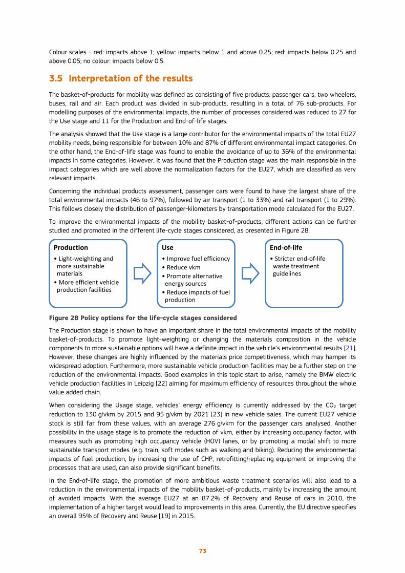
73

Colour scales - red: impacts above 1; yellow: impacts below 1 and above 0.25; red: impacts below 0.25 and

above 0.05; no colour: impacts below 0.5.

3.5 Interpretation of the results

The basket-of-products for mobility was defined as consisting of five products: passenger cars, two wheelers,

buses, rail and air. Each product was divided in sub-products, resulting in a total of 76 sub-products. For

modelling purposes of the environmental impacts, the number of processes considered was reduced to 27 for

the Use stage and 11 for the Production and End-of-life stages.

The analysis showed that the Use stage is a large contributor for the environmental impacts of the total EU27

mobility needs, being responsible for between 10% and 87% of different environmental impact categories. On

the other hand, the End-of-life stage was found to enable the avoidance of up to 36% of the environmental

impacts in some categories. However, it was found that the Production stage was the main responsible in the

impact categories which are well above the normalization factors for the EU27, which are classified as very

relevant impacts.

Concerning the individual products assessment, passenger cars were found to have the largest share of the

total environmental impacts (46 to 97%), followed by air transport (1 to 33%) and rail transport (1 to 29%).

This follows closely the distribution of passenger-kilometers by transportation mode calculated for the EU27.

To improve the environmental impacts of the mobility basket-of-products, different actions can be further

studied and promoted in the different life-cycle stages considered, as presented in Figure 28.

Figure 28 Policy options for the life-cycle stages considered

The Production stage is shown to have an important share in the total environmental impacts of the mobility

basket-of-products. To promote light-weighting or changing the materials composition in the vehicle

components to more sustainable options will have a definite impact in the vehicle’s environmental results [21].

However, these changes are highly influenced by the materials price competitiveness, which may hamper its

widespread adoption. Furthermore, more sustainable vehicle production facilities may be a further step on the

reduction of the environmental impacts. Good examples in this topic start to arise, namely the BMW electric

vehicle production facilities in Leipzig [22] aiming for maximum efficiency of resources throughout the whole

value added chain.

When considering the Usage stage, vehicles’ energy efficiency is currently addressed by the CO2 target

reduction to 130 g/vkm by 2015 and 95 g/vkm by 2021 [23] in new vehicle sales. The current EU27 vehicle

stock is still far from these values, with an average 276 g/vkm for the passenger cars analysed. Another

possibility in the usage stage is to promote the reduction of vkm, either by increasing occupancy factor, with

measures such as promoting high occupancy vehicle (HOV) lanes, or by promoting a modal shift to more

sustainable transport modes (e.g. train, soft modes such as walking and biking). Reducing the environmental

impacts of fuel production, by increasing the use of CHP, retrofitting/replacing equipment or improving the

processes that are used, can also provide significant benefits.

In the End-of-life stage, the promotion of more ambitious waste treatment scenarios will also lead to a

reduction in the environmental impacts of the mobility basket-of-products, mainly by increasing the amount

of avoided impacts. With the average EU27 at an 87.2% of Recovery and Reuse of cars in 2010, the

implementation of a higher target would lead to improvements in this area. Currently, the EU directive specifies

an overall 95% of Recovery and Reuse [19] in 2015.

Production

• Light-weighting and more sustainable materials

• More efficient vehicle production facilities

Use

• Improve fuel efficiency

• Reduce vkm

• Promote alternative energy sources

• Reduce impacts of fuel production

End-of-life

• Stricter end-of-life waste treatment guidelines

74

Overall, the shift from conventional internal combustion engine vehicles to hybrid or electric vehicles could

support the reduction of the environmental impacts in the road transportation sector [24]. Nonetheless, the

possible benefits to be obtained from this shift are highly dependent on the energy sources used for electricity

production, as in the cases in which the electricity for the electric vehicles is produced from fossil fuels the

total impacts might increase [25]. Furthermore, the use of electric vehicles results in an increase of the

environmental impacts of the production stage [25], which is already the most relevant stage in the impact

categories in which the estimated environmental impacts are already above the normalization values for the

EU27. A comprehensive strategy for the transportation, electricity, electronic and metal industry sectors is

therefore required to maximize the potential benefits from shifting to these alternative vehicles [26].

All the presented options related to the vehicle itself are highly influenced by the vehicles’ turnover rates (of

over a decade), which may mean that policy options influencing the amount of vehicle usage, mainly of

passenger cars, may have more immediate results.

Finally, future work should be developed on a country by country analysis with more detailed and accurate

assumptions. Future scenarios should be tested, by considering different compositions of the basket-of-

product, and quantifying the previously mentioned policy options, to estimate the potential environmental

impacts of possible scenarios for the evolution of the mobility sector. A detailed sensitivity analysis should be

performed, possibly considering also best and worst values for each product.

3.6 References

1. European Commission, Europe 2020 - A strategy for smart, sustainable and inclusive growth, COM(2010) 2020

final, 2010.

2. European Commission, Making sustainable consumption and production a reality. A guide for business and policy

makers to Life Cycle Thinking and Assessment. European Commission, 2010, Joint Research Centre, Institute for

Environment and Sustainability,.

3. EUROSTAT, Eurostat – Energy Data Navigation Tree, 2014 [cited April 2010].

4. EUROSTAT, Eurostat – Transport Data Navigation Tree, 2014 [cited June 2014].

5. EU, REGULATION (EC) No 715/2007 OF THE EUROPEAN PARLIAMENT AND OF THE COUNCIL of 20 June 2007 on

type approval of motor vehicles with respect to emissions from light passenger and commercial vehicles (Euro 5 and Euro

6) and on access to vehicle repair and maintenance information, 2007.

6. Autoinforma, Statistics - Portuguese vehicle stock 2010, 2014 [cited 2014; Available from:

http://www.autoinforma.pt/estatisticas/estatisticas.html?MIT=36458.

7. Spielmann, M., C. Bauer, R. Dones, and M. Tuchschmid, Transport Service Data v2.0 (2007) - Ecoinvent Report N.14,

2007.

8. European Commission, Annual Analyses of the EU Air Transport Market 2010 - Final Report, 2011.

9. PRÉconsultants, Simapro 8 LCA software, 2014.

10. European Commission, Characterisation factors of the ILCD Recommended Life Cycle Impact Assessment

methods - Database and Supporting Information, I.f.E.a.S. Joint Research Centre, Editor, 2012.

11. ecoinvent v3, Converted ecoinvent 3.01 data as unit processes, with links to other processes. Compiled October

2013 and revised February 2014., 2014.

12. Gkatzoflias, D., C. Kouridis, L. Ntziachristos, and Samaras. Z., COPERT 4, computer programme to calculate

emissions from road transport, 2014, ETC/AEM.

13. EEA, EMEP/EEA emission inventory guidebook 2013, 2013, European Environment Agency.

14. IEA, World Energy Outlook 2012 by International Energy Agency, 2012.

15. EU, Directive 2003/30/EC on the promotion of the use of biofuels or other renewable fuels for transport. , 2003.

16. EU, RED Directive - DIRECTIVE 2009/28/EC OF THE EUROPEAN PARLIAMENT AND OF THE COUNCIL of 23 April

2009 on the promotion of the use of energy from renewable sources and amending and subsequently repealing Directives

2001/77/EC and 2003/30/EC, 2009.

17. GHK, B.I.S., A study to examine the benefits of the End of Life Vehicles Directive and the costs and benefits of a

revision of the 2015 targets for recycling, re-use and recovery under the ELV Directive, 2006.

18. EUROSTAT, Eurostat – Waste Data Navigation Tree, 2014 [cited June 2014].

19. EU, DIRECTIVE 2000/53/EC OF THE EUROPEAN PARLIAMENT AND OF THE COUNCIL of 18 September 2000 on end-

of life vehicles, 2000.

75

20. EU, Product Environmental Footprint Pilot Guidance, Guidance for the implementation of the EU Product

Environmental Footprint (PEF) during the Environmental Footprint (EF) pilot phase - Version 4.0, 2014.

21. Mayyas, A., A. Qattawi, and M. Oma, Life cycle assessment-based selection for a sustainable lightweight body-in-

white design, Energy, 2012, 39(1), p. 412-425.

22. BMW, Manufacturing facilities, Leipzig plant, 2014 Available from: http://www.bmw-werk-

leipzig.de/leipzig/deutsch/lowband/com/en/index.html.

23. EU, Proposal 2007/0297 for a Regulation of the European Parliament and the Council Setting emission

performance standards for new passenger cars as part of the Community's integrated approach to reduce CO2 emissions

from light-duty vehicles, 2007.

24. Faria, R., et al., Impact of the electricity mix and use profile in the life-cycle assessment of electric vehicles,

Renewable and Sustainable Energy Reviews, 2013, 24, p. 271–287.

25. Ma, H., et al., A new comparison between the life cycle greenhouse gas emissions of battery electric vehicles and

internal combustion vehicles, Energy Policy, 44, p. 160–173.

26. Hawkins, T., B. Singh, G. Majeau-Bettez, and A. Stomman, Comparative Environmental Life Cycle Assessment of

Conventional and Electric Vehicles, Journal of Industrial Ecology, 2012, 17(1), p. 53-64.

Abbreviations

2W Two wheelers

EOL End-of-life

EU European Union

EU27 European Union 27 countries

GDP Gross Domestic Product

ILCD International Reference Life Cycle Data System

LC Life-cycle

LCA Life-cycle assessment

LCI Life-cycle inventory

LO Lubricant oils

LPG Liquid petroleum gas

PE Polyethylene

PET Polyethylene terephthalate

pkm Passenger-kilometer

PP Polypropylene

PUR Polyurethane

PVC Polyvinyl chloride

RER Europe

RME Rape-seed methyl ester

ROW Rest of world

SP Sub-product

vkm Vehicle-kilometers travelled

vkmp Vehicle-kilometers for passengers transport

76

4 Basket of Products: housing

4.1 Introduction

The basket-of-products approach matches statistics on private consumption of housing per capita with life

cycle inventory (LCI) for each product (dwelling). The objective is to identify, through representative products,

the average environmental impact of a citizen in EU-27 in 2010, identifying the impact of the different

representative products and therefore having the possibility to define targets for improvement.

Each representative product (dwelling) is a LCI dataset, containing different datasets related to sub-products

(building materials) and processes (e.g. energy production, waste treatment). The system boundary

encompasses a cradle-to-grave approach. The representative product’s datasets contain all environmentally

relevant flows of resources from and emissions to the natural environmental across the entire life cycle of the

product, from raw material extraction through production, construction, use, maintenance and disposal (end-

of-life).

Once the macro statistics and life cycle inventories have been matched, the potential impacts on the

environment were calculated using impact assessment methods, following the recommendation of ILCD

handbook.

Double counting can occur within the basket-of-products for certain products for e.g. housing and food. The

approach taken to avoid double counting is the following: for flows which are listed under the consumption

category food, the energy and material consumption and waste generation during their use stage are

subtracted from the use stage of a house (e.g. energy for cooking).

To define the impacts per year, the impacts of the production-construction-use-maintenance-EOL stages were

annualized over the lifetime of the product (dwelling). The annualized impacts were then multiplied for the

total number of dwelling of that type and divided by EU-27 population in order to derive total annualized

impacts per capita (for one EU citizen in 2010) by representative product (dwelling).

4.2 Definition of the basket of products for housing

The present report focuses on the stock of permanently occupied dwellings, because the ultimate goal is the

assessment of consumption for housing related to the person, and the housing of the person is his main

residence, the permanently occupied dwelling.

It is important to note that also the statistics are related only to permanently occupied dwellings (few data are

available on vacant dwellings and second homes) and that the "consumptions of the use phase" (especially

those that are related to energy, which are the most important) are only related to the actual use in permanent

dwellings. Therefore, the assessment does not consider:

• vacant dwellings and second homes,

• shelter for homeless and vulnerable people without a home.

A dwelling is defined as a unit of accommodation, such as a building (for example a single family house) or a

part of a building (for example an apartment in a multifamily house). The path to define the average value of

impacts related to housing for each citizen of EU-27 in a year (2010) starts from the definition of

representative products in the category of housing. In order to identify the most representative products for

housing to be included in the basket-of-products, data regarding housing stock was analysed: it was carried

out a quantitative and qualitative analysis of the structure of the housing in the years 2000-2010. It is very

hard to define the aggregate categories of buildings for "classifying” them in product groups and to define then

a representative product for each category. The reasons are several:

• even if materials, components and processes in the building sector can be standardized, building is not a

standardized (repeatable) product (each building is unique);

• a building is a complex product, made by quite a number of (sub)products combined in a different way in

each building, so each building has different characteristics;

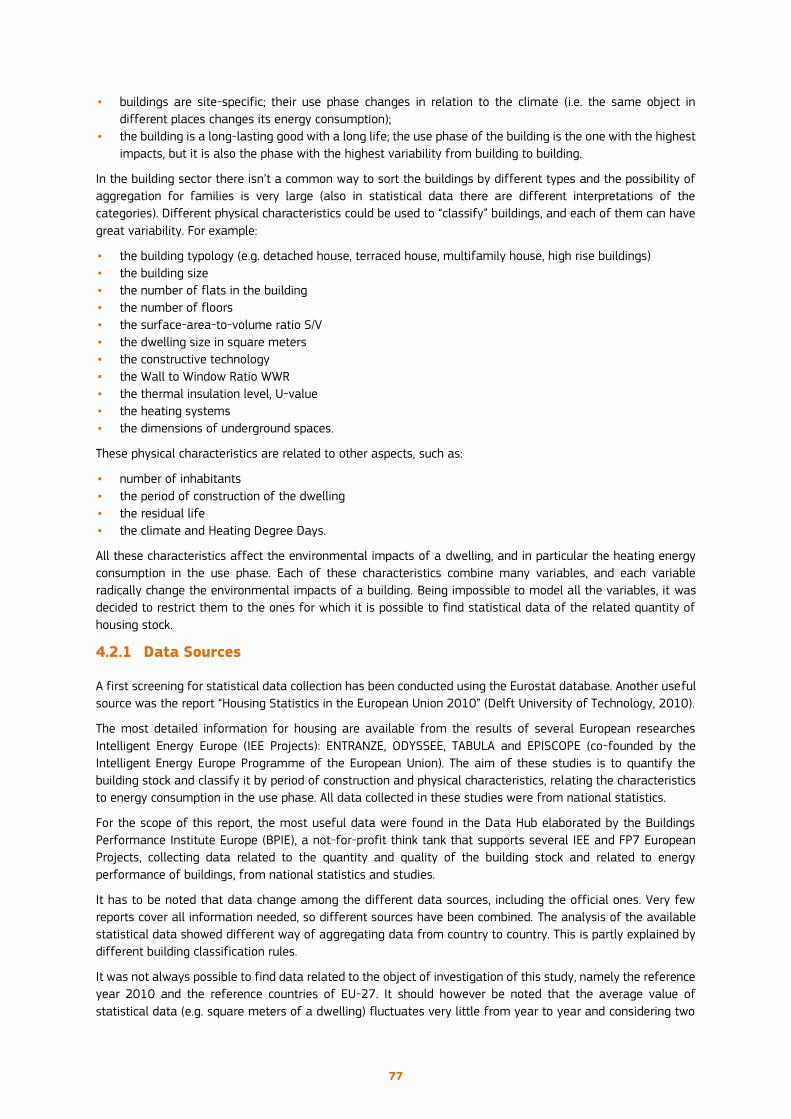
77

• buildings are site-specific; their use phase changes in relation to the climate (i.e. the same object in

different places changes its energy consumption);

• the building is a long-lasting good with a long life; the use phase of the building is the one with the highest

impacts, but it is also the phase with the highest variability from building to building.

In the building sector there isn’t a common way to sort the buildings by different types and the possibility of

aggregation for families is very large (also in statistical data there are different interpretations of the

categories). Different physical characteristics could be used to “classify” buildings, and each of them can have

great variability. For example:

• the building typology (e.g. detached house, terraced house, multifamily house, high rise buildings)

• the building size

• the number of flats in the building

• the number of floors

• the surface-area-to-volume ratio S/V

• the dwelling size in square meters

• the constructive technology

• the Wall to Window Ratio WWR

• the thermal insulation level, U-value

• the heating systems

• the dimensions of underground spaces.

These physical characteristics are related to other aspects, such as:

• number of inhabitants

• the period of construction of the dwelling

• the residual life

• the climate and Heating Degree Days.

All these characteristics affect the environmental impacts of a dwelling, and in particular the heating energy

consumption in the use phase. Each of these characteristics combine many variables, and each variable

radically change the environmental impacts of a building. Being impossible to model all the variables, it was

decided to restrict them to the ones for which it is possible to find statistical data of the related quantity of

housing stock.

4.2.1 Data Sources

A first screening for statistical data collection has been conducted using the Eurostat database. Another useful

source was the report “Housing Statistics in the European Union 2010” (Delft University of Technology, 2010).

The most detailed information for housing are available from the results of several European researches

Intelligent Energy Europe (IEE Projects): ENTRANZE, ODYSSEE, TABULA and EPISCOPE (co-founded by the

Intelligent Energy Europe Programme of the European Union). The aim of these studies is to quantify the

building stock and classify it by period of construction and physical characteristics, relating the characteristics

to energy consumption in the use phase. All data collected in these studies were from national statistics.

For the scope of this report, the most useful data were found in the Data Hub elaborated by the Buildings

Performance Institute Europe (BPIE), a not-for-profit think tank that supports several IEE and FP7 European

Projects, collecting data related to the quantity and quality of the building stock and related to energy

performance of buildings, from national statistics and studies.

It has to be noted that data change among the different data sources, including the official ones. Very few

reports cover all information needed, so different sources have been combined. The analysis of the available

statistical data showed different way of aggregating data from country to country. This is partly explained by

different building classification rules.

It was not always possible to find data related to the object of investigation of this study, namely the reference

year 2010 and the reference countries of EU-27. It should however be noted that the average value of

statistical data (e.g. square meters of a dwelling) fluctuates very little from year to year and considering two

78

countries more or two countries less (for example, EU-27 or EU-29). So, data related to EU-29 and to 2008

were used where there were no data available for EU-27 in 2010.

4.2.2 Assumptions

The variables of housing characteristics were restricted to those for which it was possible to find statistical

data of the distribution of housing stock. From the statistical data analysis emerged that a possible

classification of the housing stock could be done by dwelling type, period of construction and climate area.

As concerns the selection of dwelling type and building typology, dwelling type can be classified as:

• Single Family House (SHF);

• Apartment in a Multi-Family House (MFH).

Statistical data on the quantity of Single Family and Multi-Family House in EU-27 in 2010 are available, so this

classification can support the definition of the product groups.

To define the representative products in each product group it is possible to identify different types of building

for each category of dwelling.

For Single Family House the building typology can be:

• Detached House, that are individual houses inhabited by one family;

• Semi-Detached Houses, that consists of pairs of houses built side by side sharing a party wall;

• Terraced Houses, where a row of identical houses share side walls.

In Multi-Family Houses, multiple separate housing units for residential inhabitants (flats) are contained within

one building.

For Multi-Family House the building typology can be:

• Multi-Family House with less than 10 dwellings

• Multi-Family House with 10 or more dwellings (low-rise)

• Multi-Family House with 10 or more dwellings (high-rise).

In statistical data there is a quantification of dwellings in Single Family Houses and flats in Multi-Family Houses,

but there are no statistical data on the distribution (quantity) of the total Single Family Houses and Multi-

Family Houses by building typology.

Multi-Family Houses can vary greatly in relation to the number of flats and the number of floors. There are no

statistical data to identify the number of buildings in relation to the size.

So, for each product group, one dwelling in a representative building of the group is chosen as the

representative “product” for the group, based on its greater diffusion (even if not supported by the knowledge

of the actual number):

• a Detached House for the product group Single Family House, knowing that 34.4% of the EU-27 population

live in detached houses (Eurostat);

• an apartment in a Multi-Family House low-rise with more than 10 dwellings for the product group

apartment in a Multi-Family House (the diffusion of this building typology is evident even if the exact

quantification is not supported by statistical data).

These two building types are representative of different size and different Surface-area-to-volume ratio. The

environmental impacts per capita in relation to housing change very much in relation to the size of the dwelling

(dwelling type) and therefore to the square meters/person, and in relation to the overall shape of the building

in which the dwelling is located, based on optimizations of the relationship surface-area-to-volume ratio (S/V).

Regarding the selection of the context by climatic area, to be able to define representative products, a

simplification was therefore made, dividing Europe into three climatic zones (Figure 29) in relation to the

average Heating Degree Day (HDD) of each country:

• climatic zone 1, warm climate, 500-2300 HDD

• climatic zone 2, moderate climate, 2301-4000 HDD

79

• climatic zone 3, cold climate, 4001-6000 HDD.

The subdivision in three climatic zone has already been adopted by other studies (Ecofys, 2007; JRC/IPTS,

“IMPRO-Building”, 2008) and reflects the changes of Heating Degree Days related to latitude (35°-45°; 45°-

55° and 55°-70°).

This subdivision does not fully catch the differences of climate in each climatic zone (for example, it must be

taken into account that in Italy, in the Alps, there is the same climate of northern Europe). Both macroclimate

(region) and microclimate (local) influence the energy consumption of the building. In particular it should be

noted that altitude, landscape, presence of water streams, presence of obstructions to solar radiation affect

the microclimate in terms of temperature, relative humidity, solar radiation, sunshine, wind direction. So the

variables of the building (physical characteristics), added to the variables related to the characteristics of the

context, open to virtually infinite possible combinations. The context strongly influences the use phase of the

building, especially from the point of view of energy consumption for heating. The national average Heating

Degree Days, however, return the variation in existing climate at different latitudes that affects the average

heating energy consumption of buildings of the different countries. In any case, it should be emphasized that

in this study the energy consumption in the use phase was not calculated on the basis of national average

degree-days but on the basis of actual energy consumption (for each state).

With reference to the selection of building period of construction, depending on the availability of statistical

data on the distribution of the housing stock by period of construction, four period groups (

Table 30) were chosen and aggregated according to the technological shifts/innovations (single-double glazing,

thickness of insulating materials, radiators-radiant floors, etc.) and to the increasing attention to energy

consumption: before 1945, 1945-1969, 1970-1989, 1990-2008.

Figure 29 Climatic zones in EU-27 and heating degree days. Source: authors.

80

The building age influences the environmental impacts for the following aspects:

• construction (or renovation) impacts (related to construction technologies)

• energy consumption for heating (i.e. thermal performance of the envelope).

Concerning the selection of building technology, typical construction technologies were selected considering

the period of construction of the building and the different climatic zone. The distribution of the building stock

by climatic zone and period of construction is related to different technologies (especially for the building

envelope), different levels of insulation (U-value) and different systems (efficiency of heating systems) that

affect different energy consumption levels in the use phase.

The reference study to define the typical technology of each period and climatic zone was the research TABULA,

founded by Intelligent Energy Europe Program. No representative technologies for the period group before

1945 was selected because this stock is too heterogeneous in the constructive and physical characteristics (it

includes also historical buildings). So the same characteristics of the period 1945-1969 have been assumed

because there wasn’t a relevant change in the use of building materials (that could be considered a valid

assumption for the stock of the period 1900-1945; for the period before 1900 is very difficult to define a

representative technology because it include historical buildings).

All the envelope technical solutions of the representative buildings were sized and defined in the materials in

relation to the thermal average U-value defined in the statistical sources: BPIE data were assumed for the

average transmittance of walls, roof and floor (bottom) and TABULA data were assumed for the average

transmittance of the windows.

Table 30 Distribution of dwellings by period of construction and climatic zone. Source: reworking

of authors (aggregated data) from ENTRANZE. For Latvia only total number of dwellings were

available, so the total number has been divided by period in equal parts.

For the representative products, the heavy construction (concrete structure and bricks envelope) has been

assumed as “typical” solution in EU-27 context in the warm and moderate climate and in the cold climate for

Multi-Family House, instead the light construction (wood structure and wood frame with insulation and

prefabricated panels as covering for the envelope) has been assumed as typical in the cold climate for Single

Malta dwellings 27,353 23,791 34,953 20,367 dwellings 3,612 8,672 10,881 12,211

Cyprus dwellings 9,962 28,902 70,541 105,742 dwellings 146 3,471 28,920 51,592

Portugal dwellings 377,999 446,439 806,382 607,475 dwellings 136,257 249,221 639,602 530,345

Greece dwellings 132,365 481,723 677,673 264,760 dwellings 187,893 683,812 961,968 457,079

Spain dwellings 1,087,668 1,039,326 1,371,712 1,462,011 dwellings 1,098,207 2,846,361 3,869,173 3,966,923

Italy dwellings 2,354,731 1,920,087 2,068,582 555,600 dwellings 4,137,269 7,186,276 6,815,655 1,905,800

total by period dwellings 3,990,078 3,940,268 5,029,842 3,015,954 dwellings 5,563,385 10,977,814 12,326,198 6,923,950

total by climate zone dwellings dwellings

France dwellings 3,471,362 2,745,414 5,773,799 3,261,725 dwellings 3,485,856 2,121,534 3,563,895 2,615,016

Slovenia dwellings 87,114 56,858 79,084 53,238 dwellings 157,575 109,265 134,990 86,033

Hungary dwellings 322,595 641,359 1,051,934 463,112 dwellings 595,265 389,988 264,088 299,660

Romania dwellings 682,803 1,463,096 1,592,752 439,235 dwellings 81,740 752,197 2,181,501 157,823

Bulgaria dwellings 366,620 567,279 490,745 272,391 dwellings 69,248 335,035 525,394 455,288

Ireland dwellings 254,077 236,685 377,392 595,298 dwellings 23,790 15,452 21,119 125,596

Netherlands dwellings 1,145,056 1,200,193 1,518,797 1,011,956 dwellings 443,659 587,910 654,462 424,790

Belgium dwellings 1,367,357 759,643 771,429 431,571 dwellings 422,357 234,643 304,762 231,238

Luxembourg dwellings 41,612 30,654 30,086 17,648 dwellings 11,615 18,301 16,898 21,186

U. Kingdom dwellings 3,810,199 5,895,443 5,787,863 2,910,302 dwellings 701,762 616,248 1,564,014 1,253,385

Slovakia dwellings 281,089 215,703 190,784 161,424 dwellings 135,890 320,052 282,889 141,168

Germany dwellings 4,574,237 5,189,433 4,612,898 3,704,732 dwellings 3,906,371 7,683,325 6,646,956 2,892,118

Austria dwellings 381,000 517,000 536,000 358,000 dwellings 478,000 520,000 420,000 353,000

Czech Rep. dwellings 579,000 444,314 392,986 283,423 dwellings 354,195 873,225 768,060 302,447

Poland dwellings 1,178,000 1,342,308 1,270,286 1,637,406 dwellings 1,569,000 1,705,769 2,292,418 2,426,813

Denmark dwellings 511,253 436,092 397,715 233,940 dwellings 447,538 260,128 208,501 175,522

total by period dwellings 19,053,376 21,741,474 24,874,549 15,835,402 dwellings 12,883,862 16,543,072 19,849,947 11,961,082


Lithuania dwellings 166,280 158,273 159,920 55,077 dwellings 229,214 264,380 396,512 107,262

Latvia dwellings 76,400 76,400 76,400 76,400 dwellings 170,652 170,652 170,652 170,652

Estonia dwellings 72,575 41,519 27,421 22,355 dwellings 49,618 139,120 244,848 55,744

Sweden dwellings 586,454 490,422 539,942 159,182 dwellings 760,574 731,226 582,800 320,400

Finland dwellings 235,296 356,598 454,454 316,652 dwellings 116,891 275,603 437,015 256,490

total by period dwellings 1,137,005 1,123,212 1,258,137 629,666 dwellings 1,326,949 1,580,981 1,831,828 910,548


TOTAL EU dwellings dwellings

NUMBER OF DWELLINGS

4,148,020 5,820,958

101,628,962.06 102,850,268.28

81,504,800

unit <1945 1945-1969 1970-1989 1990-2008 unit <1945

Single Family House Multy-Family House

61,237,963

1945-1969 1970-1989 1990-2008

15,976,142 35,791,347

81

Family House (considering TABULA report, the output from interviews with local architects and the

characteristics of local material culture).

In heavy constructions the structural slabs are made of reinforced concrete and the envelope is made by bricks;

in warm climate the typical slabs are made of reinforced concrete with light precast bricks. In light construction

the structure is made by timber frames and the envelope is in wood frame.

In the Single Family Houses, pitched roof has always been assumed as the typical one (only after 1990, it was

assumed the transition to the flat roof). The attic space (between the roof and the last level floor) has always

been assumed not as living space (unheated) and, when insulation is present, it has been hypothesized to be a

layer of the last level floor. For warm climate, it was assumed that the structure of the sloped roof was made

by concrete and precast bricks, while in moderate and cold climate the pitched roof was assumed with wooden

beams and boards.

The internal walls were considered in bricks in warm climate and in wood frame with plasterboard (light

construction) in moderate and cold climate.

The insulation material chosen for all the representative products is rock wool, which (together with glass wool)

account for 60% of the market; organic foamy materials, expanded and extruded polystyrene and polyurethane

account only for 27% of the market (Papadopoulos, 2005).

For heating, the use of radiators up to 1990 in warm and moderate climates has been assumed. Since 1990,

the transition from radiators to radiant floor have been assumed. Between 1945 and 1970 the steel pipes of

the heating system increase for the change by radiators closest to the hallway (to save the pipes) to the

radiators sub-window (for improving the heat distribution and comfort).

In cold climate, the typical heating systems is related to electricity, so convector heaters have been

hypothesized.

As concerns the selection of dwelling size for each representative product, statistical data about the average

floor per dwelling by dwelling type (Single Family House and Multi-Family House), by climate (warm, moderate

and cold) and by period of construction were used to define the size (square meters) per dwelling of each

product (Table 32).

Starting from the national data, the average values by dwelling type and by period of construction related to

the three climatic zone were calculated. The calculation was done using a weighted average, taking into account

the number of dwellings in each country. The average floor area of each climate zone was also calculated as

the weighted average of the average floor of the different periods of construction.

These data, the size of dwellings in different climatic zones and in different periods of construction related to

the amount of dwellings (Table 32), were used for the development of the dwelling models (representative

products) and calculation of the total EU environmental impacts by representative product.

The average inhabitants by dwelling type, useful to calculate water and energy consumption in the use phase,

has been calculated from statistical data (Table 33). In 2010, 41.8% of the EU-27 population lived in the

apartment, just over a third (34.4%) in detached houses and 23.0% in semi-detached houses (Eurostat).

Starting from the total number of dwellings and known the distribution by climate zone and by period of

construction, with 24 building models (representative products) it is possible to cover the 100% of the dwelling

stock (Table 34).

Moderate climate is the most populated. Single Family Houses (SFH) and apartments in Multi-Family Houses

(MFH) are the same quantity (in number of dwellings). The distribution by period of construction is quite

homogeneous, with the largest number of dwellings in the period 1970-1989.

4.2.3 Final selection

According to data collected, the following criteria were defined:

• two dwelling types (Single Family House, Apartment in Multifamily House),

• four periods of construction (<1945, 1945-1969, 1970-1989, 1990-2010),

82

• three climate areas (warm, moderate, cold).

From the combination of these variables 24 models were derived, 12 for Single Family House and 12 for Multi-

Family House (Table 35).

The detailed description of the characteristics of the representative products is shown in Table 36 and Table

37. For the products <1945, the same characteristics as the products of 1945-1969 were assumed, changing

only the energy consumption of the use phase.

The building models of the representative products were modelled with Archicad 15, a BIM software for

architecture that allows to model the building in 3D (Figure 30), define the characteristics of the building’s

element and quantify the volume of materials in the building (useful information to define the flows and

compile the LCI of the production and maintenance phases). It must be emphasized that, since the

characteristics of the buildings have been defined as average, the building models tend to be very similar

among them. For example, the size of housing in m2, having been derived from average data, fluctuates slightly

from one model to the other (e.g. 90-130 m2 for Multi-Family House), while in reality the size of the

accommodation can vary greatly (e.g. 60-150 m2 for Multi-Family House).

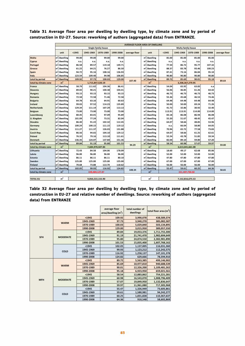
83

Table 31 Average floor area per dwelling by dwelling type, by climate zone and by period of

construction in EU-27. Source: reworking of authors (aggregated data) from ENTRANZE.

Table 32 Average floor area per dwelling by dwelling type, by climate zone and by period of

construction in EU-27 and relative number of dwellings. Source: reworking of authors (aggregated

data) from ENTRANZE

Malta m2/dwelling 99.00 99.00 99.00 99.00 m2/dwelling 85.00 85.00 85.00 85.00

Cyprus m2/dwelling n.a. n.a. n.a. n.a. m2/dwelling n.a. n.a. n.a. n.a.

Portugal m2/dwelling 86.58 89.57 119.18 149.71 m2/dwelling 77.50 86.72 95.77 107.32

Greece m2/dwelling 61.22 64.21 76.27 86.50 m2/dwelling 88.37 83.78 93.46 100.23

Spain m2/dwelling 94.72 95.16 108.16 136.93 m2/dwelling 87.41 73.16 86.84 95.10

Italy m2/dwelling 123.54 109.40 94.98 106.85 m2/dwelling 90.80 90.80 90.80 90.80

total by period m2/dwelling 109.92 97.73 100.03 129.00 m2/dwelling 89.72 85.69 90.01 95.18

total by climate zone m2 m2

France m2/dwelling 58.79 111.62 104.36 86.41 m2/dwelling 54.04 65.92 63.83 n.a

Slovenia m2/dwelling 89.02 90.21 100.38 104.41 m2/dwelling 56.06 46.85 61.26 64.42

Hungary m2/dwelling 93.15 93.15 93.15 93.15 m2/dwelling 46.73 46.73 46.73 46.73

Romania m2/dwelling 72.58 72.58 71.46 72.58 m2/dwelling 55.36 45.68 46.53 74.46

Bulgaria m2/dwelling 64.78 63.16 64.91 60.63 m2/dwelling 64.48 64.48 64.48 64.48

Ireland m2/dwelling 99.03 97.52 114.23 135.89 m2/dwelling 50.00 50.00 69.24 71.26

Netherlands m2/dwelling 129.34 111.14 107.29 113.13 m2/dwelling 41.72 32.86 30.92 32.40

Belgium m2/dwelling 73.00 73.00 73.00 73.00 m2/dwelling 113.91 113.91 114.00 114.00

Luxembourg m2/dwelling 80.45 83.01 97.09 95.89 m2/dwelling 83.18 86.08 86.94 86.08

U. Kingdom m2/dwelling 101.09 77.24 73.31 82.04 m2/dwelling 55.20 51.67 48.45 45.47

Slovakia m2/dwelling 86.40 91.22 102.32 112.45 m2/dwelling 64.07 58.66 48.85 53.96

Germany m2/dwelling 100.24 100.15 111.15 119.12 m2/dwelling n.a. 66.04 58.80 64.05

Austria m2/dwelling 111.27 111.37 126.03 131.88 m2/dwelling 70.96 65.72 77.58 73.83

Czech Rep. m2/dwelling 86.56 94.65 104.10 129.12 m2/dwelling 64.07 58.66 61.25 62.61

Poland m2/dwelling 76.32 79.16 113.10 111.61 m2/dwelling 52.24 43.78 51.85 59.34

Denmark m2/dwelling 136.35 124.07 137.84 151.36 m2/dwelling 82.04 89.10 59.80 57.20



Lithuania m2/dwelling 72.43 84.58 104.06 178.09 m2/dwelling 18.60 49.17 62.68 85.06

Latvia m2/dwelling 96.00 96.00 96.00 96.00 m2/dwelling 52.00 52.00 52.00 52.00

Estonia m2/dwelling 86.11 86.11 86.11 80.10 m2/dwelling 47.80 47.80 47.80 47.80

Sweden m2/dwelling 125.00 125.00 125.00 125.00 m2/dwelling 67.00 67.00 67.00 67.00

Finland m2/dwelling 70.68 73.88 113.70 118.62 m2/dwelling 56.00 56.00 56.00 56.00



TOTAL EU m2 m2

average floor

AVERAGE FLOOR AREA OF DWELLING

Single family house Multy family house

unit <1945 1945-1969 1970-1989 1990-2008 average floor unit <1945 1945-1969 1970-1989 1990-2008

107.40 89.641,715,847,520.19 3,208,367,279.95

94.29 59.007,684,970,507.84 3,613,041,661.08

108.34 58.65449,404,127.87 331,407,734.50

9,850,222,155.90 7,152,816,675.53

<1945 109.92 3,990,078 438,589,374

1945-1969 97.73 3,940,270 385,082,587

1970-1989 100.03 5,029,840 503,134,895

1990-2008 129.00 3,015,950 389,057,550

<1945 89.84 19,053,376 1,711,755,300

1945-1969 91.19 21,741,470 1,982,604,649

1970-1989 95.80 24,874,550 2,382,981,890

1990-2008 101.53 15,835,400 1,607,768,162

<1945 102.05 1,137,005 116,031,360

1945-1969 99.93 1,123,212 112,242,575

1970-1989 116.92 1,258,137 147,101,378

1990-2008 124.82 629,666 78,594,910

<1945 89.72 5,563,385 499,146,902

1945-1969 85.69 10,977,810 940,688,539

1970-1989 90.01 12,326,200 1,109,481,262

1990-2008 95.18 6,923,950 659,021,561

<1945 58.54 12,883,862 754,221,281

1945-1969 60.98 16,543,070 1,008,796,409

1970-1989 57.07 19,849,950 1,132,836,647

1990-2008 59.97 11,961,080 717,305,968

<1945 55.47 1,326,949 73,605,861

1945-1969 59.61 1,580,981 94,242,277

1970-1989 60.25 1,831,828 110,367,637

1990-2008 64.36 910,548 58,602,869

SFH

MFH

WARM

MODERATE

COLD

WARM

MODERATE

COLD

average floor

area/dwelling (m2)

total number of

dwellingstotal floor area (m2)

84

Table 33 Average persons per dwelling by dwelling type and by climatic zone in EU-27 in 2010.

Source: reworking of authors from Eurostat (number of person) and ENTRANZE (number of

dwellings)

Table 34 Distribution of dwellings by type (SFH= Single Family House and MFH = Multi Family

House), climate and period. Source: reworking of authors (aggregated data) from ENTRANZE.

Malta 414,027 210,739.74 106,463.60 201,217.12 35,376.40

Cyprus 819,140 625,822.96 215,147.16 183,487.36 84,129.08

Portugal 10,573,479 6,608,424.38 2,238,294.17 3,922,760.71 1,555,425.57

Greece 11,183,516 4,674,709.69 1,556,521.00 6,508,806.31 2,290,753.00

Spain 46,486,619 16,223,830.03 4,960,716.00 30,216,302.35 11,780,663.00

Italy 59,190,143 26,457,993.92 6,899,000.00 31,607,536.36 20,045,000.00

total by climate zone 54,801,520.72 15,976,141.93 72,640,110.22 35,791,347.06

person/dwelling

France 64,658,856 42,610,186.10 15,252,300.00 21,919,352.18 11,786,300.00

Slovenia 2,046,976 1,455,399.94 276,294.53 583,388.16 487,862.14

Hungary 10,014,324 6,969,969.50 2,479,000.00 2,974,254.23 1,549,000.00

Romania 20,294,683 12,724,766.24 4,177,885.60 7,569,916.76 3,173,261.88

Bulgaria 7,421,766 4,215,563.09 1,697,034.45 3,169,094.08 1,384,965.55

Ireland 4,549,428 4,349,253.17 1,463,452.00 191,075.98 185,956.00

Netherlands 16,574,989 12,779,316.52 4,876,002.57 2,966,923.03 2,110,820.16

Belgium 10,839,905 8,585,204.76 3,330,000.00 2,200,500.72 1,193,000.00

Luxembourg 502,066 332,869.76 120,000.00 166,183.85 68,000.00

U. Kingdom 62,510,197 53,696,259.22 18,403,807.44 8,751,427.58 4,135,409.54

Slovakia 5,390,410 2,711,376.23 849,000.00 2,679,033.77 880,000.00

Germany 81,802,257 36,811,015.65 18,081,300.42 43,600,602.98 21,128,771.28

Austria 8,375,290 4,748,789.43 1,792,000.00 3,542,747.67 1,771,000.00

Czech Rep. 10,462,088 4,885,795.10 1,699,723.27 5,523,982.46 2,297,926.63

Poland 38,167,329 20,228,684.37 5,428,000.00 17,862,309.97 7,994,000.00

Denmark 5,534,738 3,946,268.19 1,579,000.00 1,588,469.81 1,091,690.12


person/dwelling

Lithuania 3,141,976 1,347,907.70 539,549.87 1,781,500.39 997,367.93

Latvia 2,120,504 727,332.87 305,600.00 1,386,809.62 682,610.00

Estonia 1,333,290 466,651.50 163,870.00 859,972.05 489,330.00

Sweden 9,340,682 5,632,431.25 1,776,000.00 3,680,228.71 2,395,000.00

Finland 5,351,427 3,558,698.96 1,363,000.00 1,755,268.06 1,086,000.00


person/dwelling

number of

person lived

Multi-Family

House

number of

dwellings in

Multi-Family

House

number of

person 2010

number of

person lived

Single Family

House

number of

dwellings in

Single Family

House

3.43 2.03

2.71 2.05

2.83 1.67

<1945 24.98%

1945-1969 24.66%

1970-1989 31.48%

1990-2008 18.88%

<1945 23.38%

1945-1969 26.67%

1970-1989 30.52%

1990-2008 19.43%

<1945 27.41%

1945-1969 27.08%

1970-1989 30.33%

1990-2008 15.18%

<1945 15.54%

1945-1969 30.67%

1970-1989 34.44%

1990-2008 19.35%

<1945 21.05%

1945-1969 27.01%

1970-1989 32.41%

1990-2008 19.53%

<1945 23.49%

1945-1969 27.98%

1970-1989 32.42%

1990-2008 16.11%

MULTI

FAMILY HOUSE

50.26%

COLD 5.50%

MODERATE

59.64%

WARM 34.86%

SINGLE FAMILY

HOUSE

49.74%

COLD 4.08%

MODERATE

80.20%

WARM

15.72%

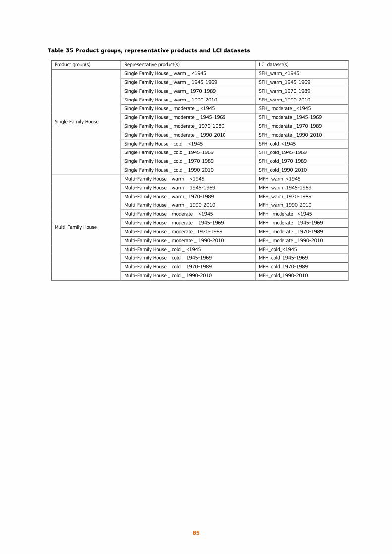
85

Table 35 Product groups, representative products and LCI datasets

Product group(s) Representative product(s) LCI dataset(s)

Single Family House

Single Family House _ warm _ <1945 SFH_warm_<1945

Single Family House _ warm _ 1945-1969 SFH_warm_1945-1969

Single Family House _ warm_ 1970-1989 SFH_warm_1970-1989

Single Family House _ warm _ 1990-2010 SFH_warm_1990-2010

Single Family House _ moderate _ <1945 SFH_ moderate _<1945

Single Family House _ moderate _ 1945-1969 SFH_ moderate _1945-1969

Single Family House _ moderate_ 1970-1989 SFH_ moderate _1970-1989

Single Family House _ moderate _ 1990-2010 SFH_ moderate _1990-2010

Single Family House _ cold _ <1945 SFH_cold_<1945

Single Family House _ cold _ 1945-1969 SFH_cold_1945-1969



Multi-Family House

Multi-Family House _ warm _ <1945 MFH_warm_<1945

Multi-Family House _ warm _ 1945-1969 MFH_warm_1945-1969

Multi-Family House _ warm_ 1970-1989 MFH_warm_1970-1989

Multi-Family House _ warm _ 1990-2010 MFH_warm_1990-2010

Multi-Family House _ moderate _ <1945 MFH_ moderate _<1945

Multi-Family House _ moderate _ 1945-1969 MFH_ moderate _1945-1969

Multi-Family House _ moderate_ 1970-1989 MFH_ moderate _1970-1989

Multi-Family House _ moderate _ 1990-2010 MFH_ moderate _1990-2010

Multi-Family House _ cold _ <1945 MFH_cold_<1945

Multi-Family House _ cold _ 1945-1969 MFH_cold_1945-1969



86

Table 36 Description of representative products of Single Family House

Dwelling type

LCI dataset SFH_warm_<1945 SFH_warm_1945-69 SFH_warm_1970-89 SFH_warm_1990-2010SFH_mod_<1945 SFH_mod_1945-69 SFH_mod_1970-89 SFH_mod_1990-2010SFH_cold_<1945 SFH_cold_1945-69 SFH_cold_1970-89 SFH_cold_1990-2010

Building typology Detached House Detached House Detached House Detached House Detached House Detached House Detached House Detached House Detached House Detached House Detached House Detached House

Building size XS XS XS XS XS XS XS XS XS XS XS XS

Dwelling size (m2) 98 98 100 129 91 91 96 102 100 100 117 125

Model dwelling size (m2) 100 100 100 130 90 90 100 100 100 100 120 120

Number of inhabitants 3.43 3.43 3.43 3.43 2.71 2.71 2.71 2.71 2.83 2.83 2.83 2.83

Year of construction 1945-1969 1945-1969 1970-1989 1990-2010 1945-1969 1945-1969 1970-1989 1990-2010 1945-1969 1945-1969 1970-1989 1990-2010

Lifetime of the building 100 years 100 years 100 years 100 years 100 years 100 years 100 years 100 years 100 years 100 years 100 years 100 years

Number of dwelling 1 1 1 1 1 1 1 1 1 1 1 1

Number of floors 2 2 2 2 2 2 2 2 2 2 2 2

Internal height (m) 2.7 2.7 2.7 2.7 2.5 2.5 2.5 2.5 2.5 2.5 2.5 2.5

Net area (m2) 98 98 98 126 86 86 97 97 99 99 118 118

Gross area (m2) 119 119 119 156 114 114 122 126 108 108 128 128

Underground (m2) 28 28 28 35 26 26 28 30 28 28 32 32

Gross volume (m3) 357 357 357 469 321 321 342 354 317 317 375 377

Heated volume (m3) 293 293 293 379 241 241 271 271 290 290 346 346

Surface/Volume 0.92 0.92 0.92 0.85 0.98 0.98 0.95 0.95 0.92 0.92 0.87 0.87

WallWindowRatio 0.29 0.29 0.29 0.31 0.30 0.30 0.32 0.32 0.30 0.30 0.28 0.28

Constructive technology heavy heavy heavy heavy heavy heavy heavy heavy light, dry assembly light, dry assembly light, dry assembly light, dry assembly

Foundations reinf concr curb reinf concr curb reinf concr curb reinf concr curb reinf concr curb reinf concr curb reinf concr curb reinf concr curb reinf concr curb reinf concr curb reinf concr curb reinf concr curb

Underground retaining walls reinfor concrete reinfor concrete reinfor concrete reinfor concrete reinfor concrete reinfor concrete reinfor concrete reinfor concrete reinfor concrete reinfor concrete reinfor concrete reinfor concrete

Load bearing elements masonry in brick masonry in brick masonry in brick masonry in brick masonry in brick masonry in brick masonry in brick masonry in brick timber frame timber frame timber frame timber frame

Floors (structure) reinfor concr/bricks reinfor concr/bricks reinfor concr/bricks reinfor concr/bricks reinforced concrete reinforced concrete reinforced concrete reinforced concrete timber frame + board timber frame + board timber frame + board timber frame + board

Stairs reinforced concrete reinforced concrete reinforced concrete reinforced concrete reinforced concrete reinforced concrete reinforced concrete reinforced concrete timber frame timber frame timber frame timber frame

masonry brick (25 cm) masonry brick (25 cm) masonry brick (25 cm) masonry brick (25 cm) masonry brick (32 cm) masonry brick (38 cm) masonry brick (30 cm) masonry brick (32 cm) timber frame timber frame timber frame timber frame

no insulation no insulation no insulation insulation (2 cm) no insulation no insulation no insulation insulation (5 cm) insulation (4 cm) insulation (4 cm) insulation (5 cm) insulation (6 cm)

External walls finishes plaster plaster plaster plaster plaster plaster plaster plaster wood wood wood wood

Windows wood frame wood frame wood frame wood frame wood frame wood frame wood frame PVC frame wood frame wood frame wood frame wood frame

single glass single glass single glass single glass single glass single glass single glass double glass single glass single glass double glass triple glass

pitched pitched pitched flat pitched pitched pitched pitched pitched pitched pitched pitched

no insulation no insulation no insulation insulation (2 cm) insulation (2 cm) insulation (2 cm) insulation (5 cm) insulation (10 cm) insulation (4 cm) insulation (4 cm) insulation (4 cm) insulation (7 cm)

Bottom floor no insulation no insulation insulation (1 cm) insulation (1 cm) insulation (1 cm) insulation (1 cm) insulation (2 cm) insulation (8 cm) insulation (7 cm) insulation (7 cm) insulation (8 cm) insulation (11 cm)

Roof finishes brick tiles brick tiles brick tiles brick tiles brick tiles brick tiles brick tiles brick tiles cement tiles cement tiles cement tiles cement tiles

Internal walls hollow brciks hollow brciks hollow bricks hollow bricks wood frame wood frame wood frame wood frame wood frame wood frame wood frame wood frame

Internal walls finishes plaster plaster plaster plaster plasterboard plasterboard plasterboard plasterboard plasterboard plasterboard plasterboard plasterboard

Flooring ceramic tiles ceramic tiles ceramic tiles ceramic tiles ceramic tiles ceramic tiles ceramic tiles ceramic tiles wood wood wood wood

Climate warm warm warm warm moderate moderate moderate moderate cold cold cold cold

HeatingDegreeDays 500-2300 500-2300 500-2300 500-2300 2301-4000 2301-4000 2301-4000 2301-4000 4001-6000 4001-6000 4001-6000 4001-6000

Uvalue walls 1.71 1.71 1.47 0.82 1.54 1.54 0.98 0.5 0.64 0.64 0.52 0.39

Uvalue roof 2.32 2.32 2.19 1.18 1.38 1.38 0.72 0.35 0.75 0.75 0.71 0.47

Uvalue windows 4.00 4.00 3.45 3.00 3.65 3.65 2.65 1.84 2.30 2.30 2.01 1.87

Uvalue bottom floor 1.76 1.76 1.71 1.48 1.63 1.63 1.16 0.49 0.49 0.49 0.43 0.33

Heating energy consumption102 102 76 62 184 184 151 100 175 175 150 115

Heating systems boiler boiler boiler boiler boiler boiler boiler boiler electricity electricity electricity electricity

Heating terminal unit radiators radiators radiators radiant floor radiators radiators radiators radiant floor convector heaters convector heaters convector heaters convector heaters

tot nr. of dwellings in EU-27 3,990,078 3,940,268 5,029,842 3,015,954 19,053,376 21,741,474 24,874,549 15,835,402 1,137,005 1,123,212 1,258,137 629,666

External walls

Insulation

Roof

Insulation

Single Family House

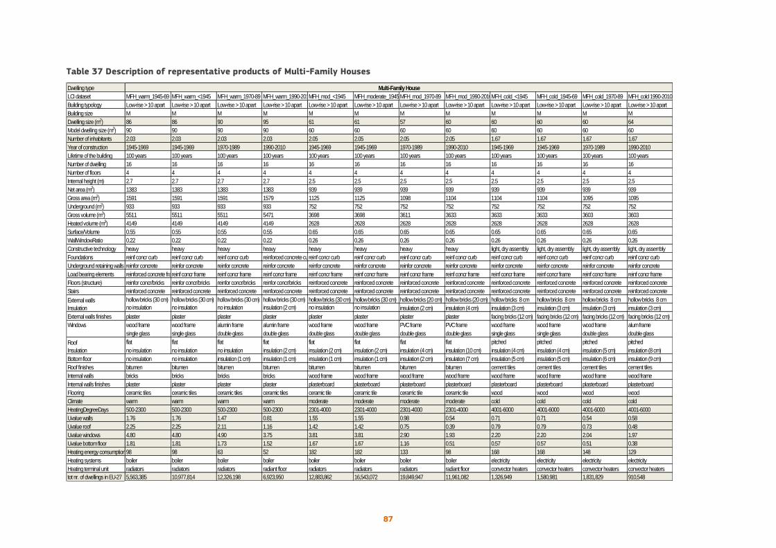
87

Table 37 Description of representative products of Multi-Family Houses

Dwelling type

LCI dataset MFH_warm_1945-69 MFH_warm_<1945 MFH_warm_1970-89 MFH_warm_1990-2010MFH_mod_<1945 MFH_moderate_1945-69MFH_mod_1970-89 MFH_mod_1990-2010MFH_cold_<1945 MFH_cold_1945-69 MFH_cold_1970-89 MFH_cold 1990-2010

Building typology Low-rise > 10 apart Low-rise > 10 apart Low-rise > 10 apart Low-rise > 10 apart Low-rise > 10 apart Low-rise > 10 apart Low-rise > 10 apart Low-rise > 10 apart Low-rise > 10 apart Low-rise > 10 apart Low-rise > 10 apart Low-rise > 10 apart

Building size M M M M M M M M M M M M

Dwelling size (m2) 86 86 90 95 61 61 57 60 60 60 60 64

Model dwelling size (m2) 90 90 90 90 60 60 60 60 60 60 60 60

Number of inhabitants 2.03 2.03 2.03 2.03 2.05 2.05 2.05 2.05 1.67 1.67 1.67 1.67

Year of construction 1945-1969 1945-1969 1970-1989 1990-2010 1945-1969 1945-1969 1970-1989 1990-2010 1945-1969 1945-1969 1970-1989 1990-2010

Lifetime of the building 100 years 100 years 100 years 100 years 100 years 100 years 100 years 100 years 100 years 100 years 100 years 100 years

Number of dwelling 16 16 16 16 16 16 16 16 16 16 16 16

Number of floors 4 4 4 4 4 4 4 4 4 4 4 4

Internal height (m) 2.7 2.7 2.7 2.7 2.5 2.5 2.5 2.5 2.5 2.5 2.5 2.5

Net area (m2) 1383 1383 1383 1383 939 939 939 939 939 939 939 939

Gross area (m2) 1591 1591 1591 1579 1125 1125 1098 1104 1104 1104 1095 1095

Underground (m2) 933 933 933 933 752 752 752 752 752 752 752 752

Gross volume (m3) 5511 5511 5511 5471 3698 3698 3611 3633 3633 3633 3603 3603

Heated volume (m3) 4149 4149 4149 4149 2628 2628 2628 2628 2628 2628 2628 2628

Surface/Volume 0.55 0.55 0.55 0.55 0.65 0.65 0.65 0.65 0.65 0.65 0.65 0.65

WallWindowRatio 0.22 0.22 0.22 0.22 0.26 0.26 0.26 0.26 0.26 0.26 0.26 0.26

Constructive technology heavy heavy heavy heavy heavy heavy heavy heavy light, dry assembly light, dry assembly light, dry assembly light, dry assembly

Foundations reinf concr curb reinf concr curb reinf concr curb reinforced concrete curbreinf concr curb reinf concr curb reinf concr curb reinf concr curb reinf concr curb reinf concr curb reinf concr curb reinf concr curb

Underground retaining walls reinfor concrete reinfor concrete reinfor concrete reinfor concrete reinfor concrete reinfor concrete reinfor concrete reinfor concrete reinfor concrete reinfor concrete reinfor concrete reinfor concrete

Load bearing elements reinforced concrete framereinf concr frame reinf concr frame reinf concr frame reinf concr frame reinf concr frame reinf concr frame reinf concr frame reinf concr frame reinf concr frame reinf concr frame reinf concr frame

Floors (structure) reinfor concr/bricks reinfor concr/bricks reinfor concr/bricks reinfor concr/bricks reinforced concrete reinforced concrete reinforced concrete reinforced concrete reinforced concrete reinforced concrete reinforced concrete reinforced concrete

Stairs reinforced concrete reinforced concrete reinforced concrete reinforced concrete reinforced concrete reinforced concrete reinforced concrete reinforced concrete reinforced concrete reinforced concrete reinforced concrete reinforced concrete

hollow bricks (30 cm) hollow bricks (30 cm) hollow bricks (30 cm) hollow bricks (30 cm) hollow bricks (30 cm) hollow bricks (30 cm) hollow bricks (20 cm) hollow bricks (20 cm) hollow bricks 8 cm hollow bricks 8 cm hollow bricks 8 cm hollow bricks 8 cm

no insulation no insulation no insulation insulation (2 cm) no insulation no insulation insulation (2 cm) insulation (4 cm) insulation (3 cm) insulation (3 cm) insulation (3 cm) insulation (3 cm)

External walls finishes plaster plaster plaster plaster plaster plaster plaster plaster facing bricks (12 cm) facing bricks (12 cm) facing bricks (12 cm) facing bricks (12 cm)

Windows wood frame wood frame alumin frame alumin frame wood frame wood frame PVC frame PVC frame wood frame wood frame wood frame alum frame

single glass single glass double glass double glass double glass double glass double glass double glass single glass single glass double glass double glass

flat flat flat flat flat flat flat flat pitched pitched pitched pitched

no insulation no insulation no insulation insulation (2 cm) insulation (2 cm) insulation (2 cm) insulation (4 cm) insulation (10 cm) insulation (4 cm) insulation (4 cm) insulation (5 cm) insulation (8 cm)

Bottom floor no insulation no insulation insulation (1 cm) insulation (1 cm) insulation (1 cm) insulation (1 cm) insulation (2 cm) insulation (7 cm) insulation (5 cm) insulation (5 cm) insulation (6 cm) insulation (9 cm)

Roof finishes bitumen bitumen bitumen bitumen bitumen bitumen bitumen bitumen cement tiles cement tiles cement tiles cement tiles

Internal walls bricks bricks bricks bricks wood frame wood frame wood frame wood frame wood frame wood frame wood frame wood frame

Internal walls finishes plaster plaster plaster plaster plasterboard plasterboard plasterboard plasterboard plasterboard plasterboard plasterboard plasterboard

Flooring ceramic tiles ceramic tiles ceramic tiles ceramic tiles ceramic tile ceramic tile ceramic tile ceramic tile wood wood wood wood

Climate warm warm warm warm moderate moderate moderate moderate cold cold cold cold

HeatingDegreeDays 500-2300 500-2300 500-2300 500-2300 2301-4000 2301-4000 2301-4000 2301-4000 4001-6000 4001-6000 4001-6000 4001-6000

Uvalue walls 1.76 1.76 1.47 0.81 1.55 1.55 0.98 0.54 0.71 0.71 0.54 0.58

Uvalue roof 2.25 2.25 2.11 1.16 1.42 1.42 0.75 0.39 0.79 0.79 0.73 0.48

Uvalue windows 4.80 4.80 4.90 3.75 3.81 3.81 2.90 1.93 2.20 2.20 2.04 1.97

Uvalue bottom floor 1.81 1.81 1.73 1.52 1.67 1.67 1.16 0.51 0.57 0.57 0.51 0.38

Heating energy consumption98 98 63 52 182 182 133 98 168 168 148 129

Heating systems boiler boiler boiler boiler boiler boiler boiler boiler electricity electricity electricity electricity

Heating terminal unit radiators radiators radiators radiant floor radiators radiators radiators radiant floor convector heaters convector heaters convector heaters convector heaters

tot nr. of dwellings in EU-27 5,563,385 10,977,814 12,326,198 6,923,950 12,883,862 16,543,072 19,849,947 11,961,082 1,326,949 1,580,981 1,831,829 910,548

Multi-Family House

External walls

Insulation

Roof

Insulation

88

Figure 30 Building models of representative products

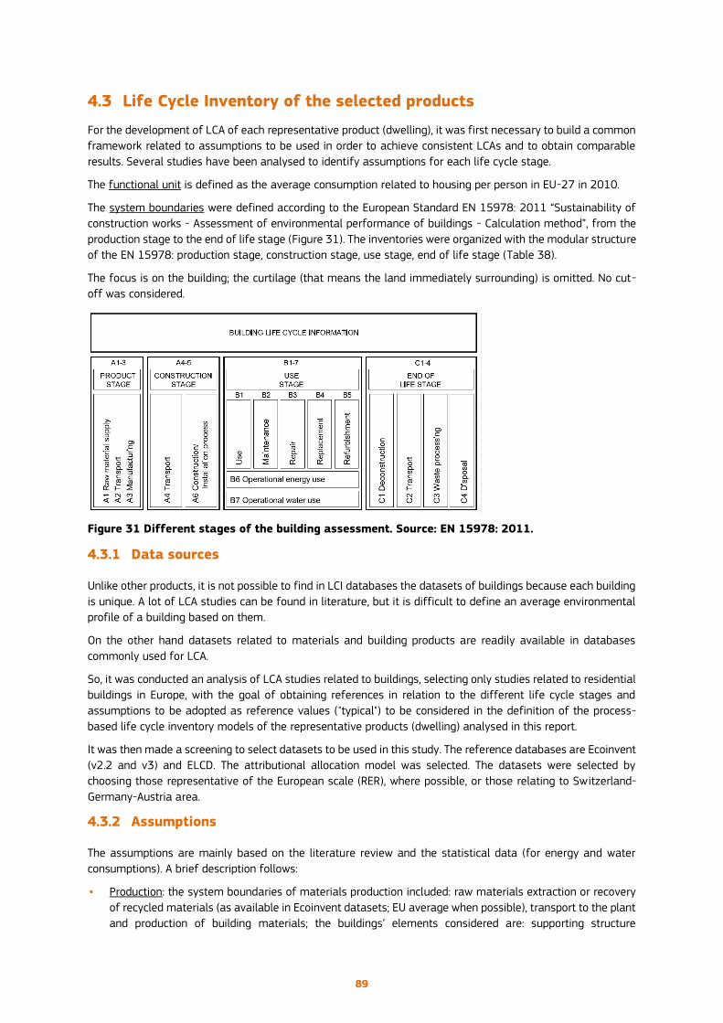
89

4.3 Life Cycle Inventory of the selected products

For the development of LCA of each representative product (dwelling), it was first necessary to build a common

framework related to assumptions to be used in order to achieve consistent LCAs and to obtain comparable

results. Several studies have been analysed to identify assumptions for each life cycle stage.

The functional unit is defined as the average consumption related to housing per person in EU-27 in 2010.

The system boundaries were defined according to the European Standard EN 15978: 2011 “Sustainability of

construction works - Assessment of environmental performance of buildings - Calculation method”, from the

production stage to the end of life stage (Figure 31). The inventories were organized with the modular structure

of the EN 15978: production stage, construction stage, use stage, end of life stage (Table 38).

The focus is on the building; the curtilage (that means the land immediately surrounding) is omitted. No cut-

off was considered.

Figure 31 Different stages of the building assessment. Source: EN 15978: 2011.

4.3.1 Data sources

Unlike other products, it is not possible to find in LCI databases the datasets of buildings because each building

is unique. A lot of LCA studies can be found in literature, but it is difficult to define an average environmental

profile of a building based on them.

On the other hand datasets related to materials and building products are readily available in databases

commonly used for LCA.

So, it was conducted an analysis of LCA studies related to buildings, selecting only studies related to residential

buildings in Europe, with the goal of obtaining references in relation to the different life cycle stages and

assumptions to be adopted as reference values ("typical") to be considered in the definition of the process-

based life cycle inventory models of the representative products (dwelling) analysed in this report.

It was then made a screening to select datasets to be used in this study. The reference databases are Ecoinvent

(v2.2 and v3) and ELCD. The attributional allocation model was selected. The datasets were selected by

choosing those representative of the European scale (RER), where possible, or those relating to Switzerland-

Germany-Austria area.

4.3.2 Assumptions

The assumptions are mainly based on the literature review and the statistical data (for energy and water

consumptions). A brief description follows:

• Production: the system boundaries of materials production included: raw materials extraction or recovery

of recycled materials (as available in Ecoinvent datasets; EU average when possible), transport to the plant

and production of building materials; the buildings’ elements considered are: supporting structure

90

(foundations, underground retaining walls, load-bearing elements, floors, stairs), envelope (external walls,

windows, roof, lower floor), internal walls, finishes, systems (heating, wiring, plumbing, sanitary appliances).

• Construction: the impact of transport from plant to building site were calculated considering an average

distance of 50 km for heavy materials and 100 km for the other materials; the impact of the assembly

phase was evaluated in terms of electrical consumption (2% of the embodied energy of building materials),

as reported in the literature (Scheuer et alii, 2003; Beccali et alii, 2013; Asdrubali et alii, 2013), and of

construction waste (4% of the weight of building products); it was also considered the impact due to the

production of the materials become "construction waste" (4% of the total production impacts).

• Use phase (energy and water): rather than calculate energy consumption of each representative dwelling

from its characteristics, which could lead to assume consumptions peculiar to a single building as if they

were representative of the average, the actual average energy consumption were derived from EU-27

energy statistics; the average heating consumption for each representative product (Table 40) has been

calculated, merging statistical data in BPIE on trend in heating consumption (divided by dwelling type, by

period of construction and by climatic zone) with actual heating consumption data in ODYSSE ( Table 39).

Table 38 Total national heating consumption of dwellings at normal climate (average Heating

Degree Days of the last 30 years) in EU-27. Source: reworking of authors from ODYSSEE

Table 39 Average heating consumption of dwellings in EU-27 (kWh/m2/y). Source: reworking of

authors from BPIE and ODYSSEE data

For the other energy consumptions (water heating, space cooling, lighting, appliances), a European average

value for each energy consumption type have been considered, based on Eurostat statistical data and on

ODYSSEE data related to the person; considering that cooling is a consumption typical of warm climate, the

total cooling consumption in Europe has been attributed to warm climate only; to avoid over-estimation of

Malta toe/dwelling 0.1 dwelling 131,909.00 toe 13,190.90

Cyprus toe/dwelling 0.26 dwelling 331,324.00 toe 86,144.24

Portugal toe/dwelling 0.15 dwelling 3,932,010.00 toe 589,801.50

Greece toe/dwelling 0.73 dwelling 4,572,262.00 toe 3,337,751.26

Spain toe/dwelling 0.46 dwelling 17,626,453.00 toe 8,108,168.38

Italy toe/dwelling 0.87 dwelling 25,175,793.00 toe 21,902,939.91

France toe/dwelling 1.07 dwelling 27,244,700.00 toe 29,151,829.00

Slovenia toe/dwelling 0.99 dwelling 766,177.00 toe 758,515.23

Hungary toe/dwelling 0.98 dwelling 3,878,000.00 toe 3,800,440.00

Romania toe/dwelling 0.55 dwelling 7,450,000.00 toe 4,097,500.00

Bulgaria toe/dwelling 0.52 dwelling 3,071,000.00 toe 1,596,920.00

Ireland toe/dwelling 1.15 dwelling 1,611,986.00 toe 1,853,783.90

Netherlands toe/dwelling 1.01 dwelling 7,044,333.00 toe 7,114,776.33

Belgium toe/dwelling 1.19 dwelling 4,635,382.00 toe 5,516,104.58

Luxembourg toe/dwelling n.d. dwelling 203,427.00 toe n.d.

U. Kingdom toe/dwelling 1.17 dwelling 26,634,800.00 toe 31,162,716.00

Slovakia toe/dwelling 0.88 dwelling 1,744,780.00 toe 1,535,406.40

Germany toe/dwelling 1.1 dwelling 37,925,160.00 toe 41,717,676.00

Austria toe/dwelling 1.32 dwelling 3,624,300.00 toe 4,784,076.00

Czech Rep. toe/dwelling 1.06 dwelling 4,082,148.00 toe 4,327,076.88

Poland toe/dwelling 1.03 dwelling 13,470,000.00 toe 13,874,100.00

Denmark toe/dwelling 1.36 dwelling 2,718,000.00 toe 3,696,480.00

Lithuania toe/dwelling 0.84 dwelling 1,269,970.00 toe 1,066,774.80

Latvia toe/dwelling 1.13 dwelling 817,000.00 toe 923,210.00

Estonia toe/dwelling 0.97 dwelling 627,030.00 toe 608,219.10

Sweden toe/dwelling 0.95 dwelling 4,431,000.00 toe 4,209,450.00

Finland toe/dwelling 1.5 dwelling 2,537,197.00 toe 3,805,795.50

Unit 2010 Unitnumber of

dwellingUnit

total

consumption

Malta kWh 153,410,167

Cyprus kWh 1,001,857,511

Portugal kWh 6,859,391,445

Greece kWh 38,818,047,154

Spain kWh 94,297,998,259

Italy kWh 254,731,191,153

total by climate zone kWh 395,861,895,690

France kWh 339,035,771,270

Slovenia kWh 8,821,532,125

Hungary kWh 44,199,117,200

Romania kWh 47,653,925,000

Bulgaria kWh 18,572,179,600

Ireland kWh 21,559,506,757

Netherlands kWh 82,744,848,718

Belgium kWh 64,152,296,265

Luxembourg kWh n.a.

U. Kingdom kWh 362,422,387,080

Slovakia kWh 17,856,776,432

Germany kWh 485,176,571,880

Austria kWh 55,638,803,880

Czech Rep. kWh 50,323,904,114

Poland kWh 161,355,783,000

Denmark kWh 42,990,062,400

total by climate zone kWh 1,802,503,465,722

Lithuania kWh 12,406,590,924

Latvia kWh

Estonia kWh 7,073,588,133

Sweden kWh 48,955,903,500

Finland kWh 44,261,401,665

total by climate zone kWh 112,697,484,222

FINAL CONSUMPTION OF RESIDENTIAL FOR SPACE

HEATING (with climatic corrections)

Unit 2010

<1945 1945-1969 1970-1989 1990-2008 <1945 1945-1969 1970-1989 1990-2008

total zone warm 108 102 76 62 101 98 63 52

total zone moderate 220 184 151 100 182 182 133 98

total zone cold 190 175 150 115 158 168 148 129

Multy-Family House

HEATING ENERGY CONSUMPTION kWh/m2 a

Single Family House

91

energy consumption in warm climate, the average consumption related to water heating and lighting were

reduced by 30% and the average consumptions were increased in the other climatic zone (increased by 20%

in the moderate climate and 30% in cold climate); these changes have been made verifying that the total

consumption of each climatic zone correspond to the actual total consumption statistical data; the calculated

average consumption for person was then multiplied for the number of average inhabitants of each

representative dwelling; for defining the environmental impacts related to energy consumption it was also

necessary to know the type of energy, so data about the household energy consumption by energy source

(ODYSSEE) were used; the European electricity mix has been assumed; also for water consumption, a European

average value of 150 l/p/d (Eurostat; Lauranson, Mudgal, 2009) has been considered and for wastewater it

was assumed the same quantity of the water consumption; solid waste were not considered because not

building related and also to avoid double counting with food basket of products.

Table 40 Average energy consumption per person in EU-27 in 2010. Source: calculated data starting

from ODYSSEE -Enerdata

total consumption

household EU-27

(Mtoe/year)

nr. persons in EU-27

in 2010

consumption per

person

(toe/year)

consumption per person

(kWh/year)

Water heating 38 499,100,105 0.076 884

Cooling 3 499,100,105 0.006 70

El. appliances 32 499,100,105 0.064 744

Lighting 7 499,100,105 0.014 163

Table 41 Total consumption of residential sector by energy source in EU-27 in 2008. Source:

reworking of authors from ODYSSEE

Malta Mtoe 0.00 0.02 0.00 0.00 0.00 0.06

Cyprus Mtoe 0.00 0.13 n.a. 0.00 0.05 0.14

Portugal Mtoe 0.00 0.55 0.30 n.a. 1.18 1.16

Greece Mtoe 0.01 2.56 0.21 0.04 0.84 1.56

Spain Mtoe 0.19 3.54 3.64 0.00 2.05 5.97

Italy Mtoe 0.00 4.21 13.54 0.04 1.44 5.88

total by fuel Mtoe 0.20 11.01 17.69 0.09 5.57 14.77

total by climate zone Mtoe

percentage of fuel % 0.41 22.32 35.86 0.18 11.29 29.95

France Mtoe 0.19 7.85 13.82 1.51 6.00 12.91

Slovenia Mtoe 0.00 0.32 0.10 0.10 0.32 0.27

Hungary Mtoe 0.17 0.10 3.29 0.55 0.48 0.99

Romania Mtoe 0.05 0.30 2.21 1.21 3.42 0.90

Bulgaria Mtoe 0.21 0.02 0.04 0.35 0.64 0.86

Ireland Mtoe 0.51 1.20 0.67 0.00 0.04 0.73

Netherlands Mtoe 0.00 0.09 7.42 0.26 0.22 2.13

Belgium Mtoe 0.16 3.36 3.30 0.01 0.22 1.68

Luxembourg Mtoe 0.00 0.23 0.20 0.00 0.02 0.07

U. Kingdom Mtoe 0.69 2.87 27.82 0.05 0.33 10.30

Slovakia Mtoe 0.06 0.02 1.18 0.44 0.04 0.39

Germany Mtoe 1.07 16.18 22.46 3.92 5.48 11.99

Austria Mtoe 0.08 1.34 1.18 0.74 1.52 1.44

Czech Rep. Mtoe 0.46 0.02 2.05 1.15 1.06 1.26

Poland Mtoe 5.68 0.86 3.14 4.18 2.46 2.33

Denmark Mtoe 0.00 0.50 0.63 1.52 1.00 0.88




Lithuania Mtoe 0.04 0.04 0.15 0.51 0.57 0.23

Latvia Mtoe 0.02 0.03 0.11 0.39 0.72 0.17

Estonia Mtoe 0.01 0.01 0.05 0.33 0.39 0.16

Sweden Mtoe 0.00 0.24 0.03 2.38 1.04 3.58

Finland Mtoe 0.00 0.53 0.04 1.51 1.21 1.75




49.33

222.50

16.26

CONSUMPTION OF RESIDENTIAL SECTOR BY ENERGY SOURCE 2008

Unit COAL OIL GAS HEAT WOOD ELECTRICITY

92

Table 42 Example of calculation for a representative dwelling (SFH_moderate_<1945): the average

heating consumption (kWh/m2/y) were multiplied for the average size of the dwelling (m2); the

average water heating and lighting consumption (increased by 20% than EU average) and the

appliances consumption were multiplied for the average number of inhabitants of the dwelling; the

total energy consumption was then distributed by energy source (average percentage of Table 12

by climatic zone). Source: authors.

• Use phase (maintenance): the boundary for replacement included the production of the replaced

components, the transportation of the replaced components, the end of life stage of the removed

components; typical replacement intervals were assumed derived by literature (30 years for mineral

insulation, 30 years for windows, 50 years for external walls in wood frame (light construction), 30 years

for internal walls in wood frame (light construction), 20 years for waterproofing, 50 years for finishes

(replacement of 50% of the finishes every 25 years), 50 years for the systems (replacement of 50% of

the systems every 25 years); the typical replacement intervals were applied both in case of new buildings

(as future scenario along the service life) and in case of the old stock (assuming that since it was built

maintenance work has already undergone).

• The total lifetime of the buildings is assumed to be 100 years (considering that an important part of the

building stock has been constructed before 1945).

• End-Of-Life: the system boundaries include the dismantling process, transport to sorting plants, final

disposal of waste materials; benefits from materials recycling and energy recovery (incineration) are not

included in the system boundaries, in accordance with the allocation procedure proposed by Kloepffer

(1996).

kWh/person/y kWh/m2/y m2 kWh/y per/dw kWh/y TOT cons % kWh/y

heating 220 90 19800 19,800 25,223 40.24 10150 gas

water heating 1061 2.71 2,875 kWh/dw/y 15.84 3995 oil

lighting 196 2.71 531 10.45 2636 wood

appliance (electricity) 744 2.71 2,016 7.19 1814 district heat

4.19 1057 coal

22.09 5572 electricity

93

Table 43 Example of the inventory of a representative products (and of the organization of

datasets).

DATASET SFH_cold_1990-2010

120 m2

normalisation: dwelling/year (reference year 2010)

building lifetime: 100 years

number of inhabitants: 2.83

datasets of SimaPro 8.0.3.14 /year /year

PRODUCTION PHASE SFH_cold_1990-2010_A_production

raw materials- transports-manufacturing of building's materials

m3/y kg/y

undergroud structure foundations gravel Gravel, round {CH}, gravel and sand quarry operation, Alloc Def, U 0.032 70.299

foundations reinforced concrete curb (50 cm) Concrete, normal {CH}, production, Alloc Def, U 0.479 1,150.363

undergroud retaining walls reinforced concrete (20 cm) Reinforcing steel, at plant/RER U 0.010 76.300

structure pillars timber frame (20 cm x 20 cm) Sawnwood, hardwood, air/kiln dried, planed {RER}, planing, hardwood, air/kiln dried, Alloc Def, U0.197 98.700

floors timber frame (16 cm x 30 cm)

wood board (2 cm + 2 cm)

stairs timber frame

envelope external walls wood frame Sawnwood, softwood, kiln dried, planed {RER}, planing, softwood, kiln dried, Alloc Def, U0.009 4.350

insulation (4 cm) Rockwool {CH}, production, Alloc Def, U 0.153 7.665

windows wood frame Sawnwood, softwood, kiln dried, planed {RER}, planing, softwood, kiln dried, Alloc Def, U0.007 3.350

triple glass Flat glass, uncoated {RER}, production, Alloc Def, U 0.005 13.500

roof roof battens Sawnwood, softwood, kiln dried, planed {RER}, planing, softwood, kiln dried, Alloc Def, U0.008 4.200

insulation (7 cm)

bottom floor insulation (11 cm)

internal walls internal walls wood frame Sawnwood, softwood, kiln dried, planed {RER}, planing, softwood, kiln dried, Alloc Def, U0.006 2.900

finishes external walls wood cladding Sawnwood, softwood, kiln dried, planed {RER}, planing, softwood, kiln dried, Alloc Def, U0.019 9.250

internal walls Gypsum plasterboard {CH}, production, Alloc Def, U 0.076 68.400

flooring wood Sawnwood, softwood, kiln dried, planed {RER}, planing, softwood, kiln dried, Alloc Def, U0.012 6.100

light concrete screed Concrete, normal {CH}, production, Alloc Def, U 0.114 205.380

roof cement tiles Cement tile {CH}, production, Alloc Def, U 0.022 49.060

systems convector heaters steel Steel, unalloyed {RER}, steel production, converter, unalloyed, Alloc Def, U0.000 1.200

wiring copper Copper {RER}, production, primary, Alloc Def, U 0.000 0.275

plumbing system steel Steel, unalloyed {RER}, steel production, converter, unalloyed, Alloc Def, U0.000 0.486

PVC Polyvinylchloride, suspension polymerised {RER}, polyvinylchloride production, suspension polymerisation, Alloc Def, U0.000 0.180

sanitary appliances ceramic Sanitary ceramics {CH}, production, Alloc Def, U 0.000 4.360

CONSTRUCTION PHASE SFH_cold_1990-2010_B_construction tkm/y

transport to site 50 km Lorry 16-32 t Transport, freight, lorry 16-32 metric ton, EURO3 {RER}, Alloc Def, U 75.117

100 km Lorry 3.5-7.5 t Transport, freight, lorry 3.5-7.5 metric ton, EURO3 {RER}, Alloc Def, U 27.398

MJ

energy electricity 2% embodied energy of production Electricity mix, AC, consumption mix, at consumer, < 1kV EU-27 S 56.77

kg/y

construction waste 4% production SFH_cold_1990-2010_A_production 0.04

construction waste 4% production Waste concrete, not reinforced {CH}, treatment of, sorting plant, Alloc Def, U 59.004

Waste gypsum plasterboard (waste treatment) {CH}, treatment of, sorting plant, Conseq, U 2.736

Waste wood, untreated (waste treatment) {CH}, treatment of waste wood, untreated, municipal inceneration Alloc Def, U5.154

Waste mineral wool (waste treatment) {CH}, treatment of, sorting plant, Alloc Def, U 0.307

USE PHASE energy and water SFH_cold_1990-2010_C_use phase (energy and water)

kWh/y l/y

energy heating natural gas Heat, central or small-scale, natural gas {Europe without Switzerland}, at boiler atmospheric non-modulating <100kW, Alloc Def, U395

water heating oil Heat, central or small-scale, other than natural gas {Europe without Switzerland}, light fuel oil, at boiler 100kW non-modulating, Alloc Def, U883

cooling wood Heat, central or small-scale, other than natural gas {CH}, softwood chips from forest, at furnace 50kW, Alloc Def, U4066

lighting district heat Heat, district or industrail, other than natural gas {CH}, treatment of municipal waste, incineration, Alloc, Def, U6222

appliance (electricity) coal Heat, central or small-scale, other than natural gas {Europe without Switzerland}, hard coal coke, stove 5-15kW, Alloc Def, U72

electricity Electricity mix, AC, consumption mix, at consumer, < 1kV EU-27 S 7162

water consumption Tap water, at user {Europe without Switzerland}, tap water production and supply, Alloc Def, U154,943

wastewater treatment Treatment, sewage, unpolluted, from residence, to wastewater treatment, class 2/CH U 154,943

USE PHASE maintenance SFH_cold_1990-2010_D_use phase (maintenance) m3/y kg/y

substitution of insulation 30 years Rockwool {CH}, production, Alloc Def, U 15.33

wood frame external walls 50 years Sawnwood, softwood, kiln dried, planed {RER}, planing, softwood, kiln dried, Alloc Def, U0.009 4.35

wood frame internal walls 30 years Sawnwood, softwood, kiln dried, planed {RER}, planing, softwood, kiln dried, Alloc Def, U0.012 5.80

windows 30 years Sawnwood, softwood, kiln dried, planed {RER}, planing, softwood, kiln dried, Alloc Def, U0.013 6.700

Flat glass, uncoated {RER}, production, Alloc Def, U 27.000

finishes 30 years Sawnwood, softwood, kiln dried, planed {RER}, planing, softwood, kiln dried, Alloc Def, U0.037 18.500

Gypsum plasterboard {CH}, production, Alloc Def, U 136.800

Sawnwood, softwood, kiln dried, planed {RER}, planing, softwood, kiln dried, Alloc Def, U0.024 12.200

50 years Cement tile {CH}, production, Alloc Def, U 98.120

systems 50 years Steel, unalloyed {RER}, steel production, converter, unalloyed, Alloc Def, U 1.200

Copper {RER}, production, primary, Alloc Def, U 0.275

Steel, unalloyed {RER}, steel production, converter, unalloyed, Alloc Def, U 0.486

Polyvinylchloride, suspension polymerised {RER}, polyvinylchloride production, suspension polymerisation, Alloc Def, U0.180

Sanitary ceramics {CH}, production, Alloc Def, U 4.360

tkm/y

transport 50 km Lorry 16-32 t Transport, freight, lorry 16-32 metric ton, EURO3 {RER}, Alloc Def, U 0.000

100 km Lorry 3.5-7.5 t Transport, freight, lorry 3.5-7.5 metric ton, EURO3 {RER}, Alloc Def, U 34.484

replacement waste window frame, wall frame, finishes Waste wood, untreated (waste treatment) {CH}, treatment of waste wood, untreated, municipal inceneration Alloc Def, U47.550

glass Waste glass sheet (waste treatment) {CH}, treatment of waste glass sheet, sorting plant, Alloc Def, U27.000

plasterboard Waste gypsum plasterboard (waste treatment) {CH}, treatment of, sorting plant, Conseq, U136.800

insulation Waste mineral wool (waste treatment) {CH}, treatment of, sorting plant, Alloc Def, U 15.330

END OF LIFE SFH_cold_1990-2010_E_EOL

deconstruction

transport

sorting plant reinforced concrete Waste reinforced concrete (waste treatment) {CH}, treatment of, sorting plant, Alloc Def, U1,150.36

steel Waste reinforcement steel (waste treatment) {CH}, treatment of, recycling, Alloc Def, U 76.30

glass Waste glass sheet (waste treatment) {CH}, treatment of waste glass sheet, sorting plant, Alloc Def, U13.50

gravel, mortar, screed Waste concrete, not reinforced {CH}, treatment of, sorting plant, Alloc Def, U 324.74

plasterboard Waste gypsum plasterboard (waste treatment) {CH}, treatment of, sorting plant, Conseq, U68.400

insulation Waste mineral wool (waste treatment) {CH}, treatment of, sorting plant, Alloc Def, U 7.67

wood Waste wood, untreated (waste treatment) {CH}, treatment of waste wood, untreated, municipal inceneration Alloc Def, U128.85

PVC Waste polyvinylchloride product (waste treatment) {CH},treatment of waste polyvinylchloride product, collection for final disposal Alloc Def, U0.18

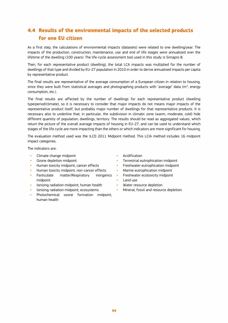
94

4.4 Results of the environmental impacts of the selected products

for one EU citizen

As a first step, the calculations of environmental impacts (datasets) were related to one dwelling/year. The

impacts of the production, construction, maintenance, use and end of life stages were annualized over the

lifetime of the dwelling (100 years). The life-cycle assessment tool used in this study is Simapro 8.

Then, for each representative product (dwelling), the total LCA impacts was multiplied for the number of

dwellings of that type and divided by EU-27 population in 2010 in order to derive annualised impacts per capita

by representative product.

The final results are representative of the average consumption of a European citizen in relation to housing,

since they were built from statistical averages and photographing products with "average" data (m2, energy

consumption, etc.).

The final results are affected by the number of dwellings for each representative product (dwelling

type/period/climate), so it is necessary to consider that major impacts do not means major impacts of the

representative product itself, but probably major number of dwellings for that representative products. It is

necessary also to underline that, in particular, the subdivision in climatic zone (warm, moderate, cold) hide

different quantity of population, dwellings, territory. The results should be read as aggregated values, which

return the picture of the overall average impacts of housing in EU-27, and can be used to understand which

stages of the life cycle are more impacting than the others or which indicators are more significant for housing.

The evaluation method used was the ILCD 2011 Midpoint method. This LCIA method includes 16 midpoint

impact categories.

The indicators are:

• Climate change midpoint

• Ozone depletion midpoint

• Human toxicity midpoint, cancer effects

• Human toxicity midpoint, non-cancer effects

• Particulate matter/Respiratory inorganics

midpoint

• Ionizing radiation midpoint, human health

• Ionizing radiation midpoint, ecosystems

• Photochemical ozone formation midpoint,

human health

• Acidification

• Terrestrial eutrophication midpoint

• Freshwater eutrophication midpoint

• Marine eutrophication midpoint

• Freshwater ecotoxicity midpoint

• Land use

• Water resource depletion

• Mineral, fossil and resource depletion.

95

4.4.1 Results per impact category

Climate change midpoint

Figure 32 Climate change per person per year in EU-27 in 2010 by product

Figure 33 Climate change per person per year in EU-27 in 2010 by product and by life cycle stages

96

Ozone depletion midpoint

Figure 34 Ozone depletion per person per year in EU-27 in 2010 by product

Figure 35 Ozone depletion per person per year in EU-27 in 2010 by product and by life cycle stages

97

Human toxicity midpoint, cancer effects

Figure 36 Human toxicity, cancer effects, per person per year in EU-27 in 2010 by product

Figure 37 Human toxicity, cancer effects, per person per year in EU-27 in 2010 by product and by

life cycle stages

98

Human toxicity, non-cancer effects

Figure 38 Human toxicity, non-cancer effects, per person per year in EU-27 in 2010 by product

Figure 39 Human toxicity, non-cancer effects, per person per year in EU-27 in 2010 by product and

by life cycle stages

99

Particulate matter midpoint

Figure 40 Particulate matter per person per year in EU-27 in 2010 by product

Figure 41 Particulate matter per person per year in EU-27 in 2010 by product and by life cycle

stages.

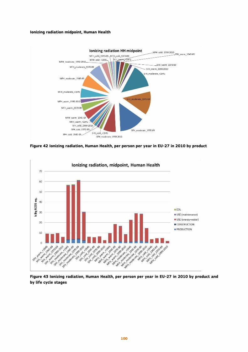
100

Ionizing radiation midpoint, Human Health

Figure 42 Ionizing radiation, Human Health, per person per year in EU-27 in 2010 by product

Figure 43 Ionizing radiation, Human Health, per person per year in EU-27 in 2010 by product and

by life cycle stages

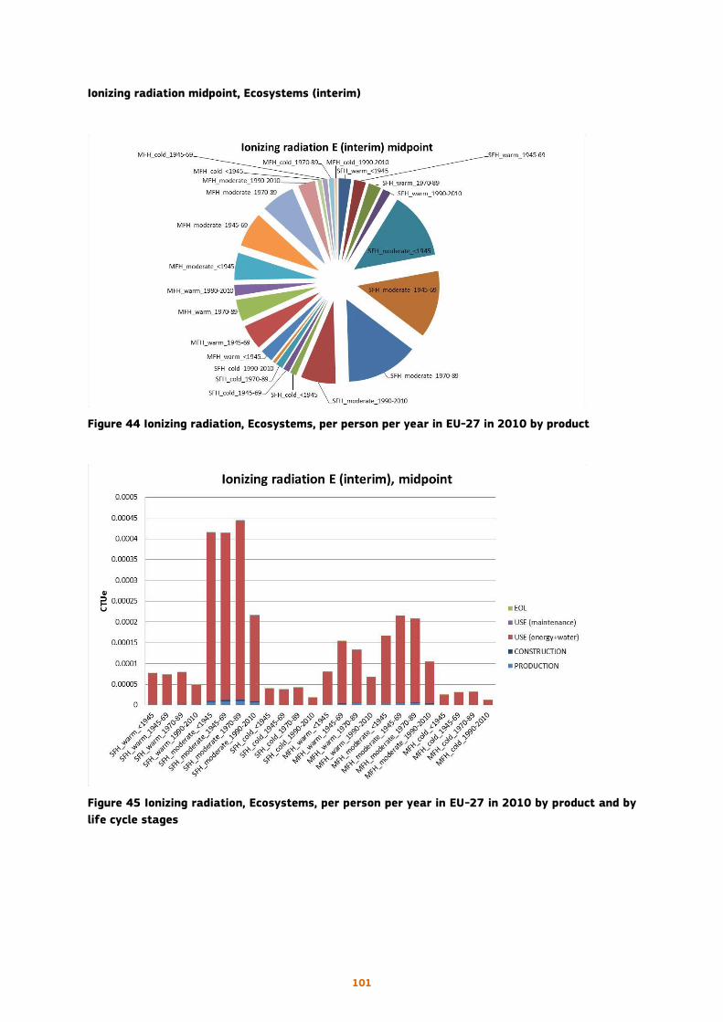
101

Ionizing radiation midpoint, Ecosystems (interim)

Figure 44 Ionizing radiation, Ecosystems, per person per year in EU-27 in 2010 by product

Figure 45 Ionizing radiation, Ecosystems, per person per year in EU-27 in 2010 by product and by

life cycle stages

102

Photochemical ozone formation midpoint

Figure 46 Photochemical ozone formation per person per year in EU-27 in 2010 by product

Figure 47 Photochemical ozone formation per person per year in EU-27 in 2010 by product and by

life cycle stages

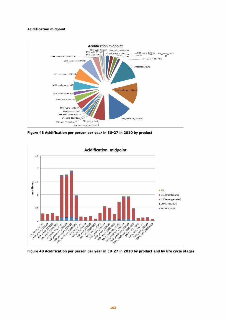
103

Acidification midpoint

Figure 48 Acidification per person per year in EU-27 in 2010 by product

Figure 49 Acidification per person per year in EU-27 in 2010 by product and by life cycle stages

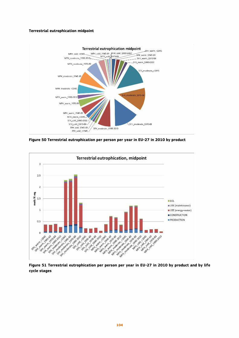
104

Terrestrial eutrophication midpoint

Figure 50 Terrestrial eutrophication per person per year in EU-27 in 2010 by product

Figure 51 Terrestrial eutrophication per person per year in EU-27 in 2010 by product and by life

cycle stages

105

Freshwater eutrophication midpoint

Figure 52 Freshwater eutrophication per person per year in EU-27 in 2010 by product

Figure 53 Freshwater eutrophication per person per year in EU-27 in 2010 by product and by life

cycle stages

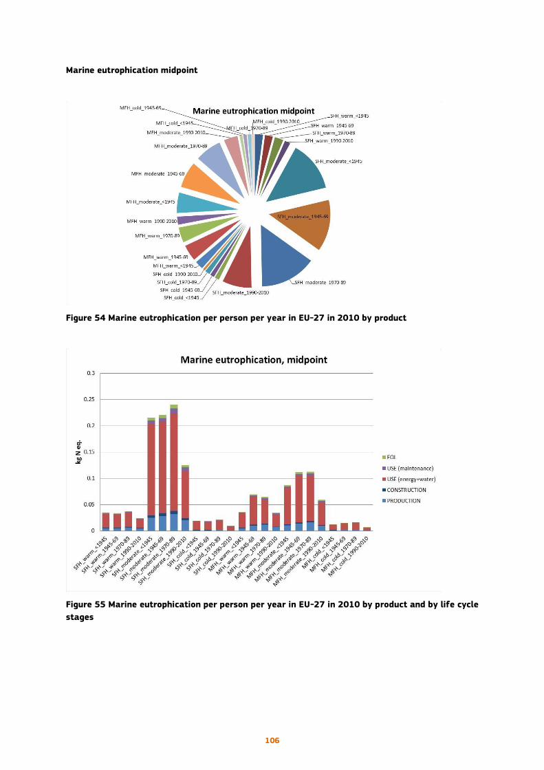
106

Marine eutrophication midpoint

Figure 54 Marine eutrophication per person per year in EU-27 in 2010 by product

Figure 55 Marine eutrophication per person per year in EU-27 in 2010 by product and by life cycle

stages

107

Freshwater ecotoxicity midpoint

Figure 56 Freshwater ecotoxicity per person per year in EU-27 in 2010 by product

Figure 57 Freshwater ecotoxicity per person per year in EU-27 in 2010 by product and by life cycle

stages

108

Land use midpoint

Figure 58 Land use per person per year in EU-27 in 2010 by product

Figure 59 Land use per person per year in EU-27 in 2010 by product and by life cycle stages

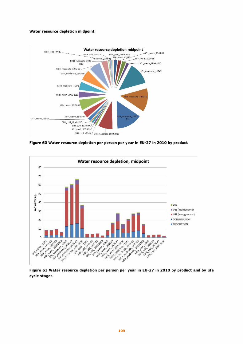
109

Water resource depletion midpoint

Figure 60 Water resource depletion per person per year in EU-27 in 2010 by product

Figure 61 Water resource depletion per person per year in EU-27 in 2010 by product and by life

cycle stages

110

Resource depletion, mineral, fossils and renewables

Figure 62 Resource depletion, mineral, fossil and renewables per person per year in EU-27 in 2010

by product

Figure 63 Resource depletion, mineral, fossil and ren per person per year in EU-27 in 2010 by

product and by life cycle stages

111

Table 44 Total results per person per year in EU-27 in 2010 by product

Impact category Unit SFH

_w

arm

_<

19

45

SFH

_w

arm

_1

94

5-6

9

SFH

_w

arm

_1

97

0-8

9

SFH

_w

arm

_1

99

0-2

01

0

SFH

_m

od

era

te_

<1

94

5

SFH

_m

od

era

te_

19

45

-69

SFH

_m

od

era

te_

19

70

-89

SFH

_m

od

era

te_

19

90

-20

10

SFH

_co

ld_

<1

94

5

SFH

_co

ld_

19

45

-69

SFH

_co

ld_

19

70

-89

SFH

_co

ld_

19

90

-20

10

MFH

_w

arm

_<

19

45

MFH

_w

arm

_1

94

5-6

9

MFH

_w

arm

_1

97

0-8

9

MFH

_w

arm

_1

99

0-2

01

0

MFH

_m

od

era

te_

<1

94

5

MFH

_m

od

era

te_

19

45

-69

MFH

_m

od

era

te_

19

70

-89

MFH

_m

od

era

te_

19

90

-20

10

MFH

_co

ld_

<1

94

5

MFH

_co

ld_

19

45

-69

MFH

_co

ld_

19

70

-89

MFH

_co

ld_

19

90

-20

10

TOTA

L

Climate change kg CO2 eq 50.48 48.34 52.9 33.83 323.7 327.4 350.3 176.4 18.65 17.41 20.11 8.491 52.3 101.3 91.77 47.71 130.2 167.2 165.3 85.02 11.82 14.66 15.66 6.118 2317

Ozone depletion kg CFC-11 eq 7E-06 7E-06 7E-06 4E-06 5E-05 5E-05 5E-05 3E-05 6E-06 6E-06 6E-06 3E-06 7E-06 1E-05 1E-05 6E-06 2E-05 2E-05 2E-05 1E-05 4E-06 5E-06 5E-06 2E-06 4E-04

Human toxicity, cancer effects CTUh 2E-06 2E-06 2E-06 1E-06 1E-05 1E-05 2E-05 9E-06 1E-06 1E-06 1E-06 6E-07 2E-06 5E-06 5E-06 3E-06 6E-06 8E-06 9E-06 5E-06 9E-07 1E-06 1E-06 5E-07 1E-04

Human toxicity, non-cancer effects CTUh 8E-06 8E-06 9E-06 6E-06 5E-05 6E-05 6E-05 3E-05 5E-06 5E-06 6E-06 2E-06 8E-06 2E-05 2E-05 8E-06 2E-05 3E-05 3E-05 2E-05 3E-06 4E-06 5E-06 2E-06 4E-04

Particulate matter kg PM2.5 eq 0.032 0.031 0.035 0.023 0.212 0.217 0.238 0.124 0.019 0.018 0.021 0.009 0.034 0.066 0.062 0.033 0.088 0.113 0.114 0.06 0.012 0.015 0.016 0.006 1.6

Ionizing radiation HH kBq U235 eq 9.196 8.798 9.599 6.053 56.67 57.16 61.42 30.59 6.036 5.619 6.473 2.704 9.587 18.56 16.81 8.643 22.71 29.16 28.69 14.63 3.705 4.607 4.894 1.889 424.2

Ionizing radiation E (interim) CTUe 8E-05 7E-05 8E-05 5E-05 4E-04 4E-04 4E-04 2E-04 4E-05 4E-05 4E-05 2E-05 8E-05 2E-04 1E-04 7E-05 2E-04 2E-04 2E-04 1E-04 2E-05 3E-05 3E-05 1E-05 0.003

Photochemical ozone formation kg NMVOC eq 0.115 0.11 0.122 0.08 0.765 0.78 0.841 0.434 0.062 0.058 0.067 0.029 0.118 0.23 0.212 0.112 0.309 0.397 0.399 0.208 0.039 0.048 0.052 0.02 5.604

Acidification molc H+ eq 0.276 0.264 0.288 0.183 1.757 1.778 1.928 0.975 0.156 0.146 0.173 0.073 0.287 0.555 0.497 0.257 0.733 0.941 0.94 0.487 0.098 0.122 0.131 0.051 13.1

Terrestrial eutrophication molc N eq 0.37 0.356 0.396 0.258 2.296 2.351 2.543 1.321 0.203 0.19 0.22 0.094 0.382 0.742 0.69 0.362 0.927 1.19 1.199 0.629 0.129 0.159 0.17 0.066 17.25

Freshwater eutrophication kg P eq 0.003 0.003 0.004 0.003 0.029 0.031 0.035 0.019 0.002 0.002 0.002 0.001 0.003 0.007 0.008 0.004 0.012 0.016 0.016 0.009 0.001 0.002 0.002 8E-04 0.216

Marine eutrophication kg N eq 0.035 0.033 0.037 0.024 0.215 0.22 0.24 0.125 0.019 0.018 0.021 0.009 0.036 0.069 0.065 0.034 0.087 0.112 0.113 0.059 0.012 0.015 0.016 0.006 1.619

Freshwater ecotoxicity CTUe 122.3 120 139.1 96.28 868.9 930.2 1058 612 87.07 82.11 97.61 42.85 121.3 238.4 254.7 144.2 356.5 457.8 491.2 276.6 58 71.31 78.45 30.94 6836

Land use kg C deficit 72.27 69.27 76.4 48.57 502.1 509.5 553.7 275.7 65.55 61.31 70.31 29.83 74.64 144.7 129.1 66.57 199.6 256.3 252.1 129.3 38.15 47.4 50 18.99 3742

Water resource depletion m3 water eq 8.797 8.566 9.999 6.551 58 61.29 67.03 37.54 4.127 3.903 4.627 2.06 8.659 16.93 27.79 15.44 21.3 27.36 28.48 15.49 2.494 3.07 3.338 1.956 444.8

Mineral, fossil & ren resource depletion kg Sb eq 9E-04 9E-04 0.001 8E-04 0.005 0.006 0.007 0.004 4E-04 4E-04 4E-04 2E-04 1E-03 0.002 0.002 0.001 0.002 0.003 0.003 0.002 2E-04 3E-04 3E-04 1E-04 0.044

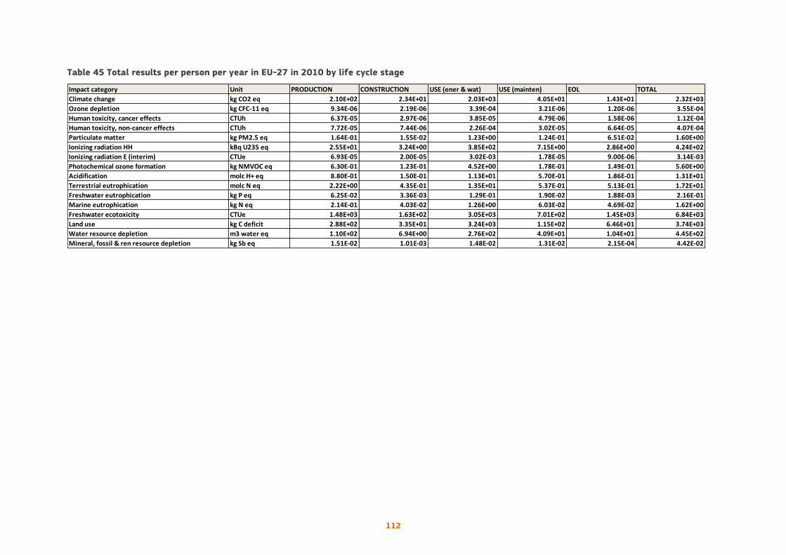
112

Table 45 Total results per person per year in EU-27 in 2010 by life cycle stage

Impact category Unit PRODUCTION CONSTRUCTION USE (ener & wat) USE (mainten) EOL TOTAL

Climate change kg CO2 eq 2.10E+02 2.34E+01 2.03E+03 4.05E+01 1.43E+01 2.32E+03

Ozone depletion kg CFC-11 eq 9.34E-06 2.19E-06 3.39E-04 3.21E-06 1.20E-06 3.55E-04

Human toxicity, cancer effects CTUh 6.37E-05 2.97E-06 3.85E-05 4.79E-06 1.58E-06 1.12E-04

Human toxicity, non-cancer effects CTUh 7.72E-05 7.44E-06 2.26E-04 3.02E-05 6.64E-05 4.07E-04

Particulate matter kg PM2.5 eq 1.64E-01 1.55E-02 1.23E+00 1.24E-01 6.51E-02 1.60E+00

Ionizing radiation HH kBq U235 eq 2.55E+01 3.24E+00 3.85E+02 7.15E+00 2.86E+00 4.24E+02

Ionizing radiation E (interim) CTUe 6.93E-05 2.00E-05 3.02E-03 1.78E-05 9.00E-06 3.14E-03

Photochemical ozone formation kg NMVOC eq 6.30E-01 1.23E-01 4.52E+00 1.78E-01 1.49E-01 5.60E+00

Acidification molc H+ eq 8.80E-01 1.50E-01 1.13E+01 5.70E-01 1.86E-01 1.31E+01

Terrestrial eutrophication molc N eq 2.22E+00 4.35E-01 1.35E+01 5.37E-01 5.13E-01 1.72E+01

Freshwater eutrophication kg P eq 6.25E-02 3.36E-03 1.29E-01 1.90E-02 1.88E-03 2.16E-01

Marine eutrophication kg N eq 2.14E-01 4.03E-02 1.26E+00 6.03E-02 4.69E-02 1.62E+00

Freshwater ecotoxicity CTUe 1.48E+03 1.63E+02 3.05E+03 7.01E+02 1.45E+03 6.84E+03

Land use kg C deficit 2.88E+02 3.35E+01 3.24E+03 1.15E+02 6.46E+01 3.74E+03

Water resource depletion m3 water eq 1.10E+02 6.94E+00 2.76E+02 4.09E+01 1.04E+01 4.45E+02

Mineral, fossil & ren resource depletion kg Sb eq 1.51E-02 1.01E-03 1.48E-02 1.31E-02 2.15E-04 4.42E-02

113

4.4.2 Interpretation of results

The contribution of each representative product (pie charts) is fairly uniform in percentage on all indicators. The

main contribution of the dwellings in the moderate climate and the lower contribution of dwellings in cold climate

is due to the number of dwellings.

Instead, despite the number of dwellings is similar to Multi-Family Houses, the Single Family Houses cause 60%

of the impact on all indicators. The reason is due to the fact that the Single Family Houses have a larger surface

area (60% of the residential area in EU is in Single Family Houses), and consequently higher consumption (energy

and materials used). In warm climate we can observe an increase in the contribution of Multi-Family Houses

compared to Single Family Houses, but it is due to the greater number of dwellings in Multi-Family Houses in this

climatic zone.

The use phase dominates all the impacts (more than 50% on all the indicators), because of energy consumption in

the use phase. The production phase dominates only in one indicator, Human toxicity, cancer effect, due to the

contribution of reinforcing steel. The end of life stands only in two indicators, Human toxicity, non-cancer effects,

and Ecotoxicity freshwater. The contribution of construction phase never exceeds 3% in all indicators.

It can be seen that dwellings of the period 1990-2010 are those with lower impacts (for all the indicators) than

others dwelling groups of the same type and climate zone; the data is influenced by the fact that this age group is

also the one with the fewest number of dwellings.

Climate Change. This impact is dominated (87% as average) by the burning of fossil fuels for the energy

consumption in the use phase of buildings. The contribution of electricity production, considering the European mix,

related to the use phase is always more than 45% in all the representative dwellings. The contribution of the

production phase is always less than 13% and the contribution of the other phases (construction, maintenance,

EOL) is less than 5% each.

It is important to highlight that the reduction of energy consumption and the increased use of energy from

renewable sources in building sector is a strong European objective (Directive 2002/91/EC and Directive 2010/31/EU

on the energy performance of buildings), but the effort related to the European energy directive is not already

readable, because the guidelines of the energy directives have not yet had widespread effect during the period

under observation (2010). It should also be pointed out that new buildings (that are adapted to the new regulatory)

suffered a setback due to the economic crisis of 2009 and existing buildings continue to be upgraded at a very low

rate; it is estimated that the existing European building stock is currently being retrofitted at a rate of approximately

1-3% of total needed per year only (Ascione, de Rossi et al. 2011).

Some authors (Asadi, da Silva et al. 2012; Flourentzou and Roulet 2002; Xing, Hewitt et al. 2011; Biekšaa,

Šiupšinskas et al. 2011; Užšilaitytea and Martinaitis 2010; Ascione, de Rossi et al. 2011; Verbeeck and Hens 2005;

Cohen, Goldman et al. 1991), deal with energy efficiency improvement of buildings through different functional

retrofit technologies; these mainly consist in adopting strategies to reduce building heating and cooling demand,

promoting the use of energy efficient equipment and low energy technologies. It should be emphasized that not

all routes, including legislative ones, to energy efficiency also lead to an overall reduction of environmental impacts.

In fact, while in the old buildings the ratio of impacts related to the production of materials and the impact on

energy consumption in the use phase is 1:10, in the zero energy building that ratio is often 1:1 (Blengini, Di Carlo,

2010; Paleari, Lavagna, Campioli, 2013).

Ozone depletion. This impact is dominated (95% as average) by the use phase of buildings, in particular related to

the electricity consumption (more than 50% of the use phase impact for all the representative dwellings). Also

district heating (by incineration of municipal solid waste) has a great contribution to this impact (due to refrigerant

HCFC-22 and trichloromethane production for wastewater treatment).

Human toxicity, cancer effects. This impact is dominated (57% as average) by the production phase, due to the

contribution of reinforcing steel (disposal to landfill of slag of unalloyed steel produced in electric furnaces, basic

114

oxygen furnace waste and sludge from steel rolling). The use phase (35% as average) contributes, due to

wastewater treatment (due to Chromium VI); natural gas, oil, coal and wood (heat) have a similar contribution;

instead the district heating (by incineration of municipal solid waste) has the greatest contribution to this impact

within the use phase (due to residue from Na-dichromate production and sludge). Small contribution comes from

maintenance (4% as average), due to the production of copper for wiring (Chromium VI and arsenic), aluminium

for windows (Chromium VI) and ceramic tiles (Chromium VI and chromium).

Human toxicity, non-cancer effects. This impact is dominated by use phase (56% as average), mainly due to wood

heat (zinc in wood ashes), district heating (by incineration of municipal solid waste) and electricity, and secondarily

to others energy sources. The production phase contribute (19% as average) due to the contribution of reinforcing

steel and concrete. In the maintenance phase (7% as average) the main contribution comes from the production

of copper (wiring). The end of life stands out in this indicator (16% as average) for the waste treatment of reinforced

concrete.

Particulate matter. This impact is dominated by use phase (77% as average), mainly due to wood heat (due to

combustion of softwood chips from forest), electricity, and secondarily to district heating (by incineration of

municipal solid waste) and coal. The production phase contribute (19% as average) due to the production of

reinforcing steel and concrete. In the maintenance phase (7% as average) the main contribution comes from the

production of copper (wiring). The end of life stand out in this indicator (16% as average) for the waste treatment

of reinforced concrete.

Ionizing radiation, human health. This impact is dominated by use phase (91% as average), mainly due to electricity

(always more than 60% of the impact of the use phase) and secondarily to district heating (15% in moderate

climate and 30% in cold climate).

Ionizing radiation, ecosystems. This impact is dominated by use phase (96% as average), mainly due to electricity

(always more than 90% of the impact of the use phase).

Photochemical ozone formation. This impact is dominated by use phase (81% as average), mainly due to electricity

(always more than 45% of the impact of the use phase), wood heat (always more than 10% of the impact of the

use phase), oil (more than 10% of the impact of the use phase in warm and moderate climate) and secondarily to

coal (more than 10% of the impact of the use phase in moderate climate) and district heating (more than 20% of

the impact of the use phase in cold climate).

Acidification. This impact is dominated by use phase (86% as average), mainly due to electricity (always more than

70% of the impact of the use phase) and secondarily to district heating (20% of the impact of the use phase in

cold climate and 10% in moderate climate) and coal (10% of the impact of the use phase in moderate climate).

Terrestrial eutrophication. This impact is dominated by use phase (79% as average), mainly due to electricity

(always more than 50% of the impact of the use phase) and secondarily to wood heat (20% of the impact of the

use phase in moderate climate and warm climate) and district heating (20% of the impact of the use phase in cold

climate and 10% of the impact of the use phase in moderate climate).

Freshwater eutrophication. This impact is dominated by use phase (60% as average), mainly due to natural gas

(30% of the impact of the use phase in warm climate and 15% of the impact of the use phase in moderate climate),

wood heat (20% of the impact of the use phase in warm climate, 15% of the impact of the use phase in cold

climate and 10% of the impact of the use phase in moderate climate), coal (more than 35% of the impact of the

use phase in moderate climate), and district heating (more than 70% of the impact of the use phase in cold climate

and 20% of the impact of the use phase in moderate climate). Also emerge a role of tap water supply and

wastewater treatment. A significant contribution derive also from production phase (29% as average) due to the

production of reinforcing steel, copper, concrete and bricks.

Marine eutrophication. This impact is dominated by use phase (78% as average), due to electricity (always more

than 50% of the impact of the use phase), wood heat (20% of the impact of the use phase in cold climate and

115

15% of the impact of the use phase in moderate and warm climate) and district heating (25% of the impact of the

use phase in cold climate and 10% of the impact of the use phase in moderate climate).

Freshwater ecotoxicity. This impact is dominated by use phase (45% as average), mainly due to district heating

(50% of the impact of the use phase in moderate climate and 85% of the impact of the use phase in cold climate)

and secondarily to natural gas and coal. Also emerge a significant role of tap water supply and wastewater

treatment. A significant contribution derive also from production phase (22% as average) mainly due to the

production of reinforcing steel and copper, and also of concrete, bricks and ceramic tiles. A significant contribution

derive also from EOL phase (21% as average) mainly due to the waste treatment of reinforcing steel at sorting

plant, and also of bricks, concrete and mineral plaster.

Land use. This impact is dominated by use phase (87% as average), mainly due to wood heat (more than 85% of

the impact of the use phase in warm and cold climate, and 75% of the impact of the use phase in moderate

climate).

Water resource depletion. This impact is dominated by use phase (62% as average), mainly due to tap water

consumption at users (always more than 15% of the impact of the use phase), natural gas (35% of the impact of

the use phase in moderate climate and 30% of the impact of the use phase in warm climate) and district heating

(15% of the impact of the use phase in moderate climate and more than 40% of the impact of the use phase in

cold climate).

Resource depletion, mineral, fossil and renewables. The production phase, the use phase and the maintenance

phase contribute in the same way (30-35%) to this impact. In the use phase, a significant contribution derive from

district heating (90% of the impact of the use phase in cold climate and more than 50% of the impact of the use

phase in moderate climate), tap water supply (25% of the impact of the use phase in warm climate, 10% of the

impact of the use phase in moderate climate and 5% of the impact of the use phase in cold climate) and natural

gas (25% of the impact of the use phase in moderate climate and 40% of the impact of the use phase in warm

climate). In the production phase, the greatest contribution derive from ceramic tile, than concrete, bricks and

copper. In the maintenance phase, the greatest contribution derive from ceramic tiles (3 replacement in 100 years

in the assumption) and copper.

116

4.5 References

Asadi, E., M. G. da Silva, et al. (2012), “Multi-objective optimization for building retrofit strategies: A model and an application”,

Energy Build. 44(0): 81-87.

Ascione, F., F. de Rossi, et al. (2011), “Energy retrofit of historical buildings: theoretical and experimental investigations for the

modelling of reliable performance scenarios”, Energy Build 43(8): 1925-1936.

Asdrubali, F., Baldassarri, C., Fthenakis, V. (2013), “Life cycle analysis in the construction sector: Guiding the optimization of

conventional Italian buildings”, Energy and Buildings 64: 73-89.

Ballarini, I., Corgnati, S. P., Corrado, V. (2014), “Use of reference buildings to assess the energy saving potentials of the residential

building stock: The experience of TABULA project”, Energy Policy 68: 273–284.

Beccali, G., Cellura, M., Fontana, M., Longo, S., Mistretta, M. (2013), “Energy retrofit of a single-family house: Life cycle net energy

saving and environmental benefits”, Renewable and Sustainable Energy Reviews 27: 283–293.

Bertoldi, P. and B. Atanasiu (2006), “Electricity Consumption and Efficiency Trends in the Enlarged European Union – Status

Report 2006”, European Commission, Joint Research Centre, Institute for Environment and Sustainability

Biekšaa, D., G. Šiupšinskas, et al. (2011), “Energy Efficiency Challenges in Multi-Apartment Building Renovation in Lithuania”, J.

Civ. Eng. Manage 17(4): 467-475.

Blengini, G.A., Di Carlo, T. (2010), “The changing role of life cycle phases, subsystems and materials in the LCA of low energy

buildings”, Energy and Buildings 42: 869–880.

BPIE- Buildings Performance Institute Europe, Data Hub,

http://bpie.eu/www.buildingsdata.eu (accessed 28.08.2014)

Cohen, S., C. Goldman, et al. (1991). “Energy savings and economics of retrofitting single-family buildings”, Energy Build 17(4):

297-311.

Delft University of Technology, OTB Research Institute for the Built Environment (2010), “Housing Statistics in the European

Union 2010”,

https://www.bmwfw.gv.at/Wirtschaftspolitik/Wohnungspolitik/Documents/housing_statistics_in_the_european_union_2010.pdf

(accessed 04.08.2014)

EC – European Commission (2002), “Directive 2002/91/EC of the European Parliament and of the Council of 16 December 2002

on the energy performance of buildings”, http://eur-lex.europa.eu/legal-content/EN/ALL/?uri=CELEX:32002L0091(accessed

21.08.2014).

EC – European Commission (2010), “Directive 2010/31/EU of the European Parliament and of the Council of 19 May 2010 on

the energy performance of buildings”, http://eur-lex.europa.eu/legal-content/EN/ALL/?uri=CELEX:32010L0031 (accessed

21.08.2014).

EC – European Commission (2010b), “EU Energy trends to 2030. Update 2009”, European Commission, Directorate-General for

Energy in collaboration with Climate Action DG and Mobility and Transport DG. Authors (E3M-Lab): Capros, P.; Mantzos, L.; Tasios,

N.; De Vita, A.; Kouvaritakis, N.

http://ec.europa.eu/energy/observatory/trends_2030/doc/trends_to_2030_update_2009.pdf (accessed 08.08.2014).

EC – European Commission (2012a), “Life cycle indicators framework: development of life cycle based macro-level monitoring

indicators for resources, products and waste for the EU-27”, European Commission, Joint Research Centre, Institute for

Environment and Sustainability

EC – European Commission (2012b), “Life cycle indicators for resources: development of life cycle based macro-level monitoring

indicators for resources, products and waste for the EU-27”, European Commission, Joint Research Centre, Institute for

Environment and Sustainability

EC – European Commission (2012c), “Life cycle indicators for waste management: development of life cycle based macro-level

monitoring indicators for resources, products and waste for the EU-27”, European Commission, Joint Research Centre, Institute

for Environment and Sustainability

EC Eurostat (2014), “Housing statistics”,

http://epp.eurostat.ec.europa.eu/statistics_explained/index.php/Housing_statistics (accessed 08.08.2014)

EC Eurostat (2014), “Water statistics”,

http://epp.eurostat.ec.europa.eu/statistics_explained/index.php/Water_statistics

(accessed 06.09.2014)

Ecofys, “Mitigation of CO2 Emissions from the Building Stock. Beyond the EU Directive on the Energy Performance of Buildings”,

2003.

http://www.eurima.org/uploads/ModuleXtender/Publications/48/ecofys_repoft_final_160204.pdf (accessed 18.06.2014)

117

Ecofys, “U-values for better energy performance of buildings”, 2007.

http://www.eurima.org/reports/u-values-for-better-energy-performance-of-buildings/

(accessed 18.06.2014)

EEA – European Environment Agency (2011), “End-user GHG emissions from energy. Reallocation of emissions from energy

industries to end users 2005–2009”, EEA Report No 19/2011, European Environment Agency

EEA – European Environment Agency (2012), “Consumption and the environment – 2012 update. The European environment.

State and outlook 2010”, EEA, Copenhagen.

EEA energy indicator ENER 22 (2011), “Energy efficiency and energy consumption in the household sector (ENER 022)”,

http://www.eea.europa.eu/data-and-maps/indicators/energy-efficiency-and-energy-consumption-2/assessment-2#toc-2

(accessed 01.09.2014)

EEA energy indicator ENER 22 (2012), “Energy efficiency and energy consumption in the household sector (ENER 022)”,

http://www.eea.europa.eu/data-and-maps/indicators/energy-efficiency-and-energy-consumption-5/assessment (accessed

01.09.2014)

ETC/SCP (2013), “Housing assessment”,

http://scp.eionet.europa.eu/publications/wp2013_4/wp/wp2013_4 (accessed01.08.2014)

Flourentzou, F. and C. A. Roulet (2002), “Elaboration of retrofit scenarios”, Energy Build 34(2): 185-192.

Graus, W., Blomen, E., Kleßmann, C., Capone, C., Stricker, E. (2009), “Global technical potentials for energy efficiency

improvement”, Presented at IAEE European Conference, September 2009.

IEA – International Energy Agency (2006), “Energy Technology Perspectives 2006 – Scenarios and Strategies to 2050”,

International Energy Agency, Paris.

IEA – International Energy Agency (2009), “Gadgets and Gigawatts. Policies for Energy-efficient electronics”, OECD/IEA,

International Energy Agency, Paris

IEE Project ENTRANZE, “Policies to Enforce the TRAnsition to Nearly Zero Energy buildings in the EU-27”, http://www.entranze.eu

(accessed 01.08.2014)

IEE Project EPISCOPE, “Energy Performance Indicators for Building Stocks”, http://episcope.eu (accessed 01.08.2014)

IEE Project ODYSSEE database, “Energy Efficiency Indicators in Europe”, www.odyssee-indicators.org (accessed 24.07.2014)

IEE Project TABULA, “Typology Approach for Building Stock Energy Assessment”, http://webtool.building-typology.eu (accessed

01.08.2014)

JRC, LCA Resources Directory, http://lct.jrc.ec.europa.eu/assessment/directories.

JRC/IE - Joint Research Centre/Institute for Energy (2009), “Electricity Consumption and Efficiency Trends in the European Union.

Status Report”, JRC Scientific and Technical Reports, EUR 24005 EN, Ispra. Authors: Bertoldi, P., Atanasiu, B.

http://re.jrc.ec.europa.eu/energyefficiency/pdf/EnEff_Report_2009.pdf

(accessed 21.08.2014).

JRC/IPTS - Joint Research Centre/Institute for Prospective Technological Studies (2008), “Environmental Improvement Potentials

of Residential Buildings (IMPRO-Building)”, European Commission, JRC Scientific and Technical Reports, Sevilla. Authors: Nemry,

F., Uihlein, A., Makishi Colodel, C., Wittstock,S., Braune, A., Wetzel, C., Hasan, I., Niemeier, S., Frech, S., Kreißig, J., Gallon, N.

JRC/IPTS (2009), “Towards additional policies to improve the environmental performance of buildings. Part II: Quantitative

assessment”, JRC Scientific and Technical Reports, EUR 24015 EN. Joint Research Centre, Institute for Prospective Technological

Studies, Sevilla.

http://ipts.jrc.ec.europa.eu/publications/pub.cfm?id=2699(accessed09.08.2014).

Kanapeckiene, L., A. Kaklauskas, et al. (2011), “Method and system for Multi-Attribute Market Value Assessment in analysis of

construction and retrofit projects”, Expert Syst. Appl 38(11): 14196-14207.

Kloepffer, W. (1996), “Allocation Rule for Open-Loop Recycling in Life Cycle Assessment”, Springer.

Ma, Z., P. Cooper, et al. (2012), “Existing building retrofits: Methodology and state-of-the-art”, Energy Build 55(0): 889-902.

Mugdal, S., Lauranson, R. (2009), “Study on water performance of buildings”, European Commission (DG ENV), Final report,

Reference: 070307/2008/520703/ETU/D2.

ODYSSEE-MURE/Enerdata (2012), “Energy Efficiency Trends in Buildings in the EU”, Authors: Lapillonne, B., Pollier, K., Sebi, C.

http://www.odyssee-mure.eu/publications/efficiency-by-sector/buildings (accessed 24.07.2014)

ODYSSEE -MURE/Enerdata (2014), “Energy Efficiency Trends for households in the EU”, Authors: Lapillonne, B., Pollier, K.,

http://www.odyssee-mure.eu/publications/efficiency-by-sector/household (accessed 24.07.2014)

Paleari, M., Lavagna, M., Andrea Campioli, A. (2013), “Life Cycle Assessment and Zero Energy Residential Buildings”, in: Werner

Lang (editor), PLEA 2013 29th Conference, Sustainable Architecture for a Renewable Future. Proceedings, Fraunhofer IRB Verlag,

Munich, Germany 10-12 September 2013.

118

Papadopoulos, A.M. (2005), “State of the art in thermal insulation materials and aims for future developments”, Energy and

Buildings 37: 77–86.

Raslanasa, S., J. Alchimovienėa, et al. (2011), “Residential Areas with Apartment Houses: Analysis of the Condition of Bu ildings,

Planning Issues, Retrofit Strategies and Scenarios”, Int. J. Strateg. Prop. M. 15(2): 152-172.

C. Scheuer, G.A. Keoleian, P.Reppe., “Life cycle energy and environmental performance of a new university building: modeling

challenges and design implications”, Energy and Buildings 35 (2003) 1049–1064.

Užšilaitytė, L., Martinaitis, V. (2010), “Search for optimal solution of public building renovation in terms of life cycle” Journal of

environmental engineering and landscape management 18(2): 102-110.

Verbeeck, G. and H. Hens (2005), “Energy savings in retrofitted dwellings: economically viable?”, Energy Build 37(7): 747-754.

Xing, Y., N. Hewitt, et al. (2011), “Zero carbon buildings refurbishment - A Hierarchical pathway”, Renewable Sustainable Energy

Rev. 15(6): 3229-3236.

119

5 Application of the methodology for life cycle based targets

setting to food Basket of Products

A life cycle based methodology for supporting a more comprehensive and systematic approach to target setting

has been developed and proposed in Sala et al 2014. The methodology makes use of LCA in different steps: both

in the hotspots identification, in terms of the most relevant life cycle stages and environmental impacts, and in the

evaluation of the benefits associated to possible improvements to reduce the impacts.

The LCA-based methodological steps for defining targets as presented in the flowchart (figure 64), are as follows:

1. Identification of the key economic sectors4 responsible of the majority of the environmental impacts.

2. LCA of the products selected in the basket of products (BoP)

3. Literature review on hotspots for the specific sector/area of consumption and analysis of the economic,

environmental, technological megatrends

4. LCA-based hotspots analysis of “basket of products” (BoP), assessing the relevant impacts in the different

impact categories ( e.g. climate change, acidification, eutrophication etc) and life cycle stages (raw material

extraction, manufacturing, distribution use, end of life)

5. Feasibility analysis of potential improvements options, entailing the identification of possible solution and the

verification of the associated benefits

6. Quantitative targets proposal

7. Identification of policy options, policy development and stakeholders hearings

In the proposed methodology, hotspots are mentioned several times. It has to be clarified that hotspots are

evaluated at three levels. Hotspots in terms of 1. the most important economic sectors that imply impact in the

environment (e.g. food, mobility, housing); 2. the most relevant products within each category, selected according

to mass/economic coverage of the market; 3 the life cycle stages that contribute most to each impact category,

derived from the results of product life cycle analyses.

The following paragraphs illustrate the application of the methodology, starting from the identification of the key

economic sectors (section 5.1) and then focusing on the case of BoP food (sections 5.2 to 5.6). The feasibility of

the improvements and the numerical formulation of the target should be based on stakeholders and sector’s

experts. Therefore, in the current document, this aspects are partially covered (e.g. feasibility is based on

improvements proposed in sectors specific context, e.g. BAT; numerical targets are reported as they are available

in literature).

4 This could be valid also for areas of consumption and products group

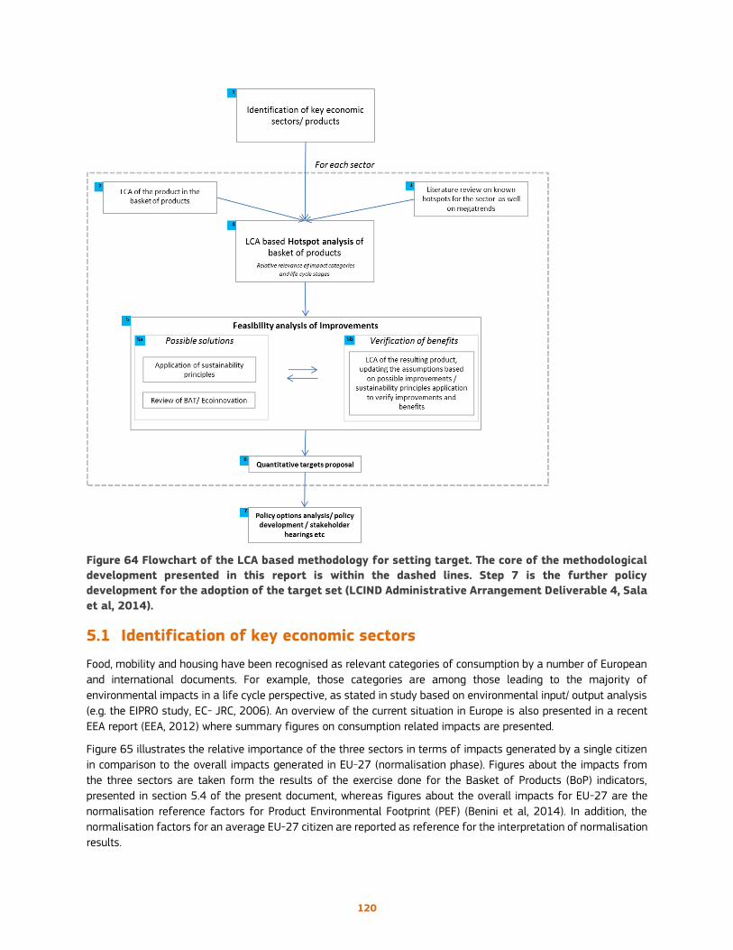
120

Figure 64 Flowchart of the LCA based methodology for setting target. The core of the methodological

development presented in this report is within the dashed lines. Step 7 is the further policy

development for the adoption of the target set (LCIND Administrative Arrangement Deliverable 4, Sala

et al, 2014).

5.1 Identification of key economic sectors

Food, mobility and housing have been recognised as relevant categories of consumption by a number of European

and international documents. For example, those categories are among those leading to the majority of

environmental impacts in a life cycle perspective, as stated in study based on environmental input/ output analysis

(e.g. the EIPRO study, EC- JRC, 2006). An overview of the current situation in Europe is also presented in a recent

EEA report (EEA, 2012) where summary figures on consumption related impacts are presented.

Figure 65 illustrates the relative importance of the three sectors in terms of impacts generated by a single citizen

in comparison to the overall impacts generated in EU-27 (normalisation phase). Figures about the impacts from

the three sectors are taken form the results of the exercise done for the Basket of Products (BoP) indicators,

presented in section 5.4 of the present document, whereas figures about the overall impacts for EU-27 are the

normalisation reference factors for Product Environmental Footprint (PEF) (Benini et al, 2014). In addition, the

normalisation factors for an average EU-27 citizen are reported as reference for the interpretation of normalisation

results.

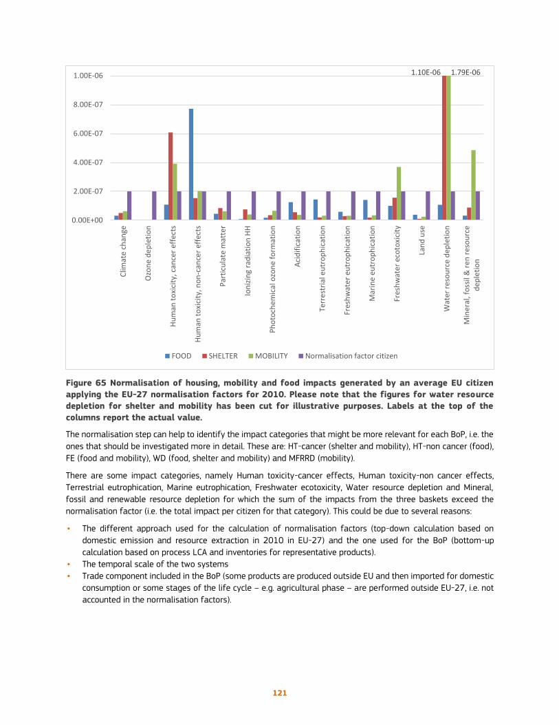
121

Figure 65 Normalisation of housing, mobility and food impacts generated by an average EU citizen

applying the EU-27 normalisation factors for 2010. Please note that the figures for water resource

depletion for shelter and mobility has been cut for illustrative purposes. Labels at the top of the

columns report the actual value.

The normalisation step can help to identify the impact categories that might be more relevant for each BoP, i.e. the

ones that should be investigated more in detail. These are: HT-cancer (shelter and mobility), HT-non cancer (food),

FE (food and mobility), WD (food, shelter and mobility) and MFRRD (mobility).

There are some impact categories, namely Human toxicity-cancer effects, Human toxicity-non cancer effects,

Terrestrial eutrophication, Marine eutrophication, Freshwater ecotoxicity, Water resource depletion and Mineral,

fossil and renewable resource depletion for which the sum of the impacts from the three baskets exceed the

normalisation factor (i.e. the total impact per citizen for that category). This could be due to several reasons:

• The different approach used for the calculation of normalisation factors (top-down calculation based on

domestic emission and resource extraction in 2010 in EU-27) and the one used for the BoP (bottom-up

calculation based on process LCA and inventories for representative products).

• The temporal scale of the two systems

• Trade component included in the BoP (some products are produced outside EU and then imported for domestic

consumption or some stages of the life cycle – e.g. agricultural phase – are performed outside EU-27, i.e. not

accounted in the normalisation factors).

1.10E-06 1.79E-06

0.00E+00

2.00E-07

4.00E-07

6.00E-07

8.00E-07

1.00E-06

Clim

ate

ch

ange

Ozo

ne

dep

leti

on

Hu

man

to

xici

ty, c

ance

r ef

fect

s

Hu

man

to

xici

ty, n

on

-can

cer

effe

cts

Par

ticu

late

mat

ter

Ion

izin

g ra

dia

tio

n H

H

Ph

oto

chem

ical

ozo

ne

form

atio

n

Aci

dif

icat

ion

Terr

est

rial

eu

tro

ph

icat

ion

Fres

hw

ate

r eu

tro

ph

icat

ion

Mar

ine

eutr

op

hic

atio

n

Fres

hw

ate

r ec

oto

xici

ty

Lan

d u

se

Wat

er r

eso

urc

e d

eple

tio

n

Min

eral

, fo

ssil

& r

en r

eso

urc

ed

ep

leti

on

FOOD SHELTER MOBILITY Normalisation factor citizen

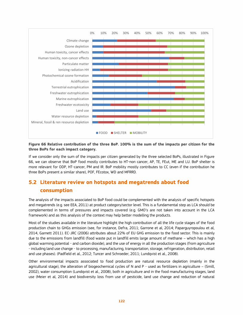
122

Figure 66 Relative contribution of the three BoP. 100% is the sum of the impacts per citizen for the

three BoPs for each impact category.

If we consider only the sum of the impacts per citizen generated by the three selected BoPs, illustrated in Figure

66, we can observe that BoP food mostly contributes to HT-non cancer, AP, TE, FEut, ME and LU. BoP shelter is

more relevant for ODP, HT-cancer, PM and IR. BoP mobility mostly contributes to CC (even if the contribution he

three BoPs present a similar share), POF, FEcotox, WD and MFRRD.

5.2 Literature review on hotspots and megatrends about food

consumption

The analysis of the impacts associated to BoP food could be complemented with the analysis of specific hotspots

and megatrends (e.g. see EEA, 2011) at product category/sector level. This is a fundamental step as LCA should be

complemented in terms of pressures and impacts covered (e.g. GMO’s are not taken into account in the LCA

framework) and as this analysis of the context may help better modelling the products.

Most of the studies available in the literature highlight the high contribution of all the life cycle stages of the food

production chain to GHGs emission (see, for instance, Defra, 2011; Garrone et al, 2014; Paparguyropoulou et al,

2014, Garnett 2011). EC-JRC (2006) attributes about 22% of EU GHG emission to the food sector. This is mainly

due to the emissions from landfill (food waste put in landfill emits large amount of methane – which has a high

global warming potential - and carbon dioxide), and the use of energy in all the production stages (from agriculture

- including land use change - to processing, manufacturing, transportation, storage, refrigeration, distribution, retail

and use phases). (Padfield et al., 2012; Tuncer and Schroeder, 2011; Lundqvist et al., 2008).

Other environmental impacts associated to food production are natural resource depletion (mainly in the

agricultural stage), the alteration of biogeochemical cycles of N and P - used as fertilizers in agriculture – (Smill,

2002), water consumption (Lundqvist et al., 2008), both in agriculture and in the food manufacturing stages, land

use (Meier et al, 2014) and biodiversity loss from use of pesticide, land use change and reduction of natural

0% 10% 20% 30% 40% 50% 60% 70% 80% 90% 100%

Climate change

Ozone depletion

Human toxicity, cancer effects

Human toxicity, non-cancer effects

Particulate matter

Ionizing radiation HH

Photochemical ozone formation

Acidification

Terrestrial eutrophication

Freshwater eutrophication

Marine eutrophication

Freshwater ecotoxicity

Land use

Water resource depletion

Mineral, fossil & ren resource depletion

FOOD SHELTER MOBILITY

123

ecosystems for food and feed cultivation (EEA, 2012). Moreover, food waste along the whole food production chain

is a relevant source of impacts (WRAP, 2009, WRAP 2013).

Some food sectors generate higher environmental impacts than others do. Beef, butter and cheese generally have

higher environmental burdens, especially related to their carbon footprint and material intensity, while vegetables,

cereal products, potatoes and fruit such as apples, when consumed in proper season, generally have much lower

impacts (EEA, 2012).

Within the livestock sector, feed-related emissions (including land-use change) account for about 3.3 Gt CO2-eq,

that is, about half of total emissions from livestock supply chains (Gerber et al., 2013, LEAP, 2014).

Future research for reducing the environmental burden of agricultural systems should address the following issues:

precision agriculture, low leaching cropping systems, management of soil biological processes and maximum

recirculation, reduction of nutrient imbalances (Kirchmann, and Thorvaldsson, 2000).

Regarding the food manufacturing, there are studies pointing out that, due to the highly diversified nature of the

food industry, various food processing, handling and packaging operations create wastes of different quality and

quantity, which, if not treated, could lead to increasing disposal problems and severe pollution problems (Kroyer,

1995).

Extending the analysis from the agriculture and production up to the consumption phase, according to EEA (2012)

food and drink consumption is found to be responsible for around 20–30 % of environmental impacts caused by

consumption in the EU in most impact categories. Since meat and dairy products production chains have a higher

environmental impact, some studies (e.g. Rejinders and Soret, 2003, Scarborough et al, 2012, Saxe et al, 2013,

Westhoek et al, 2014) model the possible environmental impact reduction through dietary shift (e.g. comparing the

environmental impact of different dietary protein choice)

A number of very specific and detailed sector studies are available in literature and they usually cover a specific

typology of impact and life cycle stage at the time. For example, there are specific studies on food waste (e.g.

Garrone et al, 2014; Mirabella et al 2014b, Paparguyropoulou et al, 2014; Parfitt et al, 2010), on non-conventional

agricultural systems such as organic farming (e.g. Schader et al, 2014), on convenience food, i.e. comparing the

impacts of ready and home-made meals (Schmidt Rivera et al, 2014).

Other studies focus on specific food sectors which are considered more environmentally relevant, such as meat

and dairy products (e.g. Westhoeck et al, 2014) or on specific environmental impacts, such as importance of input

of nitrogen for the impact related eutrophication (e.g. Audsley and Wilkinson, 2014; Leip et al 2013).

The literatures also suggest that LCA coupled with other approaches in the food sector provides much more reliable

and comprehensive information on sustainable products and production processes (Roy et al 2009).

Grounding on the existing knowledge from literature, some technical reports and scientific papers (e.g. Garrone et

al, 2014; Tukker et al, 2009; Weidema et al, 2008; WRAP, 2013.) identify three main strategies for reducing the

impacts generated by food supply chains:

i) an environmentally sustainable increase in agricultural productivity coupled with measures aimed at

reducing emissions to air, to water and to soil,

ii) dietary changes on the consumption side (e.g. reducing the consumption of meat and dairy products)

iii) better efficiency in reducing food losses and managing food waste (e.g. through improved rate of food

waste recovery).

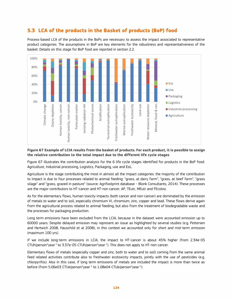
124

5.3 LCA of the products in the Basket of products (BoP) food

Process-based LCA of the products in the BoPs are necessary to assess the impact associated to representative

product categories. The assumptions in BoP are key elements for the robustness and representativeness of the

basket. Details on this stage for BoP food are reported in section 2.2.

Figure 67 Example of LCIA results from the basket of products. For each product, it is possible to assign

the relative contribution to the total impact due to the different life cycle stages

Figure 67 illustrates the contribution analysis for the 6 life cycle stages identified for products in the BoP food:

Agriculture, Industrial processing, Logistics, Packaging, use and EoL.

Agriculture is the stage contributing the most in almost all the impact categories. the majority of the contribution

to impact is due to four processes related to animal feeding: “grass, at dairy farm”, “grass, at beef farm”, “grass

silage” and “grass, grazed in pasture” (source: Agrifootprint database - Blonk Consultants, 2014). These processes

are the major contributors to HT-cancer and HT-non cancer, AP, TEutr, MEutr and FEcotox.

As for the elementary flows, human toxicity impacts (both cancer and non-cancer) are dominated by the emission

of metals to water and to soil, especially chromium VI, chromium, zinc, copper and lead. These flows derive again

from the agricultural process related to animal feeding, but also from the treatment of biodegradable waste and

the processes for packaging production.

Long term emissions have been excluded from the LCIA, because in the dataset were accounted emission up to

60000 years. Despite delayed emission may represent an issue as highlighted by several studies (e.g. Pettersen

and Hertwich 2008, Hauschild et al 2008), in this context we accounted only for short and mid-term emission

(maximum 100 yrs).

If we include long-term emissions in LCIA, the impact to HT-cancer is about 45% higher (from 2.34e-05

CTUh/person*year-1 to 3.37e-05 CTUh/person*year-1). This does not apply to HT-non cancer.

Elementary flows of metals (especially copper and zinc, both to water and to soil) coming from the same animal

feed related activities contribute also to freshwater ecotoxicity impacts, jointly with the use of pesticides (e.g.

chlorpyrifos). Also in this case, if long term emissions of metals are included the impact is more than twice as

before (from 5.06e03 CTUe/person*year-1 to 1.08e04 CTUe/person*year-1).

0%

20%

40%

60%

80%

100%

Clim

ate

ch

ange

Ozo

ne

dep

leti

on

Hu

man

to

xici

ty, c

ance

r…

Hu

man

to

xici

ty, n

on

-can

cer…

Par

ticu

late

mat

ter

Ion

izin

g ra

dia

tio

n H

H

Ph

oto

chem

ical

ozo

ne…

Aci

dif

icat

ion

Terr

est

rial

eu

tro

ph

icat

ion

Fres

hw

ate

r eu

tro

ph

icat

ion

Mar

ine

eutr

op

hic

atio

n

Fres

hw

ate

r ec

oto

xici

ty

Lan

d u

se

Wat

er r

eso

urc

e d

eple

tio

n

Min

eral

, fo

ssil

& r

en…

EoL

Use

Packaging

Logistics


Agriculture

125

Other relevant contributions from agricultural processes derive from ammonia released by animal husbandry

activities (e.g. for acidification potential) and manure management related to grass grazing for animal feeding

(contributing to terrestrial eutrophication).

Industrial processing present overall a less share of the overall impact. Nonetheless, improvement in terms of

resource efficiency (accounting for 17% of energy consumption, Pelletier et al, 2011), waste reduction and emission

reduction (especially those related to eutrophication) are considered important as stated in sectorial studies (e.g.

Tusseau-Vuillemin, 2001, Hall and Howe, 2012, Wattanapinyo and Mol, 2013)). In the basket, hotspot are related

to potential impacts on ODP and IR, mainly due to emission of CFC-114, CFC-11, Halon 1301 Carbon-14 in air,

Radon-222 in air and Cesium-137 in water which occur during the electricity production.

Packaging of products in the BoP contribute mainly to resources depletion (water and other resources). Relevant

processes refer to the raw materials used, e.g. aluminium, glass, PET and paper and also to some packaging

production processes (e.g. glass production, blow moulding of plastic, etc.), especially due to energy consumption.

Water resource depletion is mainly related to cooling water in electricity generation plants. An additional burden on

water is the pollution of water due to the treatment of biodegradable waste.

Logistics and use phase do not appear as hotspots for the food sector in the current study, if compared to other

phases, whereas in sectorial studies logistic is also considered relevant (e.g. accounting for 12% of GHG emission

in Garnett, 2011) . This is of particular relevance when refrigeration is involved (Dabbene et al 2008, Oleglethorpe,

2010). Additionally, consumers’ choice pre and post purchase are considered upmost for several impacts. In the

BoP the consumer behavior has been modeled as defined in Vanderheyden and Aerts (2014) for the transport of

food, Nielsen et al. (2003) for refrigeration and Foster et al. (2006) for home preparation of the food. Multiple

choices/ behaviour are possible ultimately leading to higher impacts (Vázquez-Rowe et al 2013).

Finally, the only impact category to which EoL shows significant contribution is freshwater eutrophication, due to

the human metabolism of food (see section 2.4 for details).

5.4 LCA-based hotspot analysis of BoP food

The results of the process based LCA for BoP are the basis for the LCA-based hotspot analysis. The LCA of each of

the products is carried out up to the so-called ‘normalization’ step i.e. the LCA step in which the indicators associated

to the product are normalized through a set of factors so to make them comparable each other on a given relative

scale5. Generally, normalization factors represent the overall impact generated within a territorial entity (e.g. the

globe, Europe). Thus, by dividing the impacts associated to a product by the total impact observed in the globe it is

possible to understand whether the contribution of that product to the totals is high or not and then to compare

different indicators on a common basis (i.e. the share over the totals).

The normalisation step and the identification of hotspots, in BoP food is made comparing LCA results to STATUS

QUO6 and to DESIRABLE STATUS QUO7 in terms of magnitude of the environmental impacts. The status quo is

assessed through the resource efficiency life cycle indicators (based on inventory of emission and impacts for all

impact categories) used to calculate the set of normalisation factors 8 for 2010. The desirable status quo is

5 Traditionally, normalisation cannot be used as a basis to cross-compare as the absolute indicators for a given region are not directly equivalent

in terms of importance. For example, the impacts of the EU’s climate change contributions cannot be easily compared to the absolute indicator

for resource scarcity. This is only achievable within some area of protection using natural science, but primarily using socio-economic approaches

to weighting.

6 Status quo refers to the baseline situation. In our case, it represents the overall environmental impact of EU27 in 2010 for 14 impact

categories, according to the results of the Life Cycle Indicators for resources (see deliverable 3.)

7 Desirable status quo is the environmental impact of EU 27 that we may expect in the future (e.g.2020) in case our policy targets have been

reached

8 Normalisation factors reflect the overall magnitude of the impact for each impact category (e.g. the global warming potential associated to

the whole emission of CO2 and other greenhouse gases in EU in 2010 correspond to 3.9E12 kg of CO2, 1.87E10 kg of CH4 etc. the potential

126

assessed applying macro-scale targets to the status quo of 2010 (assuming which could be the status quo in 2020

if the targets are all achieved)9.

In the normalisation referred to status quo, impacts values for each of the products in the basket and for the total

BoP food are compared to the total impacts in EU-27 in 2010 (using 2010 normalisation factors for PEF, NF2010).

In order to identify for which products, in which life cycle stage and in which impact category the majority of

impacts occur, two summary tables (Table 46 and Table 47) highlighting hotspots have been prepared. Figure 68,

reporting only to the total normalized values for BoP food is added to provide an additional and simplified

information. These data can help to identify the product categories, the life cycle stages and the impact categories

on which it is necessary to concentrate effort in identifying existing or possible future eco-innovations.

Table 46 Normalisation of BoP food impacts. Normalized values for each phase are colored with a

scale from red (higher value in the table) to green (lower value in the table), to better highlight the

phases that contribute most and the most relevant impact categories

Human toxicity is the most relevant impact generated by the BoP food, followed by water resource depletion,

freshwater and marine eutrophication terrestrial eutrophication and acidification. As mentioned before, agriculture

is the most impacting phase for the majority of impact categories. When normalising impacts, EoL become a higher

contributing stage for eutrophication, ecotoxicity and water depletion, with respect to absolute values presented in

Figure 67.

impact could be expressed considering the global warming potential associated to those emission (4.60 E12 Kg CO2eq ). This figure is the

normalisation factor for EU 2010, namely the magnitude of the impact due to greenhouse gases emission in the specific year) . This set of

normalisation factors entails an hybrid production/ consumption approach (it accounts for emission from industries – production, and from

household – consumption)

9 Applying “future” normalisation factors and compare the results with 2010 figures may highlight areas of possible product improvements in

order to reach macro-scale policy objectives.

Impact Category Unit AgricultureIndustrial

processingLogistics Packaging Use EoL Total

Climate change kg CO2 eq 2.3E-10 3.4E-11 1.4E-11 1.6E-11 1.8E-11 1.1E-11 3.22E-10

Ozone depletion kg CFC-11 eq 8.3E-13 1.9E-12 9.4E-13 6.9E-13 8.3E-13 3.7E-13 5.52E-12

Human toxicity, cancer effects CTUh 9.0E-10 2.9E-11 4.3E-11 5.6E-11 2.1E-11 2.6E-11 1.08E-09


effects CTUh 7.6E-09 3.2E-11 1.8E-11 2.8E-11 7.2E-12 1.9E-11 7.72E-09

Particulate matter kg PM2.5 eq 3.5E-10 2.6E-11 1.3E-11 3.8E-11 1.1E-11 1.4E-11 4.50E-10

Ionizing radiation HH kBq U235 eq 1.5E-11 3.2E-11 5.9E-12 8.7E-12 1.7E-11 7.5E-12 8.66E-11

Photochemical ozone

formation kg NMVOC eq 8.7E-11 2.3E-11 3.1E-11 1.8E-11 9.4E-12 9.3E-12 1.78E-10

Acidification molc H+ eq 1.1E-09 3.5E-11 1.9E-11 2.3E-11 1.4E-11 1.6E-11 1.26E-09

Terrestrial eutrophication molc N eq 1.4E-09 1.5E-11 2.1E-11 1.1E-11 5.1E-12 1.4E-11 1.43E-09

Freshwater eutrophication kg P eq 2.5E-10 1.5E-11 1.3E-12 3.9E-12 6.0E-13 3.2E-10 5.86E-10

Marine eutrophication kg N eq 1.0E-09 1.8E-11 2.0E-11 1.3E-11 4.7E-12 3.3E-10 1.41E-09

Freshwater ecotoxicity CTUe 8.8E-10 9.4E-12 8.1E-12 1.1E-11 1.8E-12 9.5E-11 1.00E-09

Land use kg C deficit 3.7E-10 2.5E-12 4.2E-12 5.4E-12 9.9E-13 5.0E-12 3.89E-10

Water resource depletion m3 water eq 4.4E-10 3.3E-10 3.0E-11 1.4E-10 1.6E-12 1.4E-10 1.07E-09


depletion kg Sb eq 1.0E-10 1.9E-11 3.4E-11 1.4E-10 9.6E-12 1.0E-11 3.17E-10

127

Figure 68 Normalisation of total BoP food impacts

If we analyse more in detail the normalised results for the representative products in the BoP food (Table 47 - part

1 and part 2), we can note that human toxicity-non cancer is a hotspot for most of the products, as it is for the

entire BoP. The same applies to human toxicity-cancer, even if fewer products are classified as hotspot in this

impact category. As already mentioned in the discussion of BoP food absolute results, the products that generate

the highest impacts are those associated with animal husbandry and related feeding: beef, pork and poultry meat

and dairy products. Other hotspots, even if only for some impact categories, are beer, sunflower oil and sugar from

beet and - to a lesser extent – coffee, potato and bread. The products that contribute less to the environmental

impact of an EU-27 citizen, among those selected for the BoP food, are fruits (apple and orange), olive oil, mineral

water and pre-prepared meals. However, it has to be taken into account that, according the megatrends forecast

for food consumption (EEA, 2012), the purchase of pre-prepared meals is likely to significantly increase in the

future consumption habits of people.

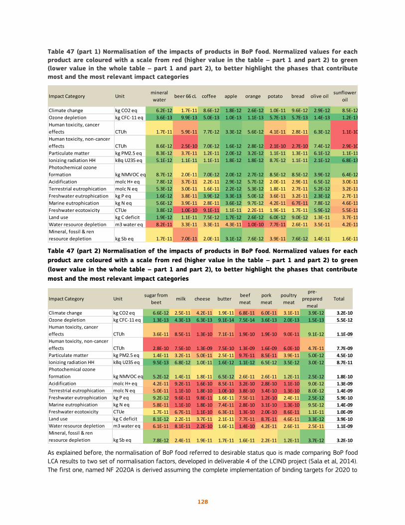
128

Table 47 (part 1) Normalisation of the impacts of products in BoP food. Normalized values for each

product are coloured with a scale from red (higher value in the table – part 1 and part 2) to green

(lower value in the whole table – part 1 and part 2), to better highlight the phases that contribute

most and the most relevant impact categories

Table 47 (part 2) Normalisation of the impacts of products in BoP food. Normalized values for each

product are coloured with a scale from red (higher value in the table – part 1 and part 2) to green

(lower value in the whole table – part 1 and part 2), to better highlight the phases that contribute

most and the most relevant impact categories

As explained before, the normalisation of BoP food referred to desirable status quo is made comparing BoP food

LCA results to two set of normalisation factors, developed in deliverable 4 of the LCIND project (Sala et al, 2014).

The first one, named NF 2020A is derived assuming the complete implementation of binding targets for 2020 to

Impact Category Unitmineral

waterbeer 66 cL coffee apple orange potato bread olive oil

sunflower

oil

sugar from

beet milk cheese butter

beef

meat

pork

meat

poultry

meat

pre-

prepared

meal

Total

Climate change kg CO2 eq 6.2E-12 1.7E-11 8.6E-12 1.8E-12 2.6E-12 1.0E-11 9.6E-12 2.9E-12 8.5E-12 6.6E-12 2.5E-11 4.2E-11 1.9E-11 6.8E-11 6.0E-11 3.1E-11 3.9E-12 3.2E-10

Ozone depletion kg CFC-11 eq 3.6E-13 9.9E-13 5.0E-13 1.0E-13 1.1E-13 5.7E-13 5.7E-13 1.4E-13 1.2E-13 1.3E-13 4.3E-13 6.3E-13 9.1E-14 7.5E-14 3.6E-13 2.0E-13 1.5E-13 5.5E-12

Human toxicity, cancer

effects CTUh 1.7E-11 5.9E-11 7.7E-12 3.3E-12 5.6E-12 4.1E-11 2.8E-11 6.3E-12 1.1E-10 3.6E-11 8.5E-11 1.3E-10 7.1E-11 1.9E-10 1.9E-10 9.0E-11 9.1E-12 1.1E-09



Particulate matter kg PM2.5 eq 8.3E-12 3.7E-11 1.2E-11 2.0E-12 3.2E-12 1.1E-11 1.3E-11 6.1E-12 1.1E-11 1.4E-11 3.2E-11 5.0E-11 2.5E-11 9.7E-11 8.5E-11 3.9E-11 5.0E-12 4.5E-10

Ionizing radiation HH kBq U235 eq 5.1E-12 1.1E-11 1.1E-11 1.8E-12 1.8E-12 8.7E-12 1.1E-11 2.1E-12 6.8E-13 9.5E-13 6.8E-12 1.0E-11 1.6E-12 1.1E-12 6.5E-12 3.5E-12 3.0E-12 8.7E-11

Photochemical ozone

formation kg NMVOC eq 8.7E-12 2.0E-11 7.0E-12 2.0E-12 2.7E-12 8.5E-12 8.5E-12 3.9E-12 6.4E-12 5.2E-12 1.4E-11 1.8E-11 6.5E-12 2.6E-11 2.6E-11 1.2E-11 2.5E-12 1.8E-10

Acidification molc H+ eq 7.8E-12 3.7E-11 2.2E-11 2.9E-12 5.7E-12 2.0E-11 2.9E-11 6.5E-12 3.0E-11 4.2E-11 9.2E-11 1.6E-10 8.5E-11 3.2E-10 2.8E-10 1.1E-10 9.0E-12 1.3E-09

Terrestrial eutrophication molc N eq 5.3E-12 3.0E-11 1.6E-11 2.2E-12 5.3E-12 1.8E-11 2.7E-11 5.2E-12 3.2E-11 5.0E-11 1.1E-10 1.8E-10 1.0E-10 3.8E-10 3.4E-10 1.3E-10 8.0E-12 1.4E-09

Freshwater eutrophication kg P eq 1.6E-12 3.8E-11 3.9E-12 3.3E-13 5.0E-12 3.6E-11 3.2E-11 2.3E-12 2.7E-11 9.2E-12 9.6E-11 9.8E-11 1.6E-11 7.5E-11 1.2E-10 2.4E-11 2.5E-12 5.9E-10

Marine eutrophication kg N eq 5.6E-12 3.9E-11 2.8E-11 3.6E-12 9.7E-12 4.2E-11 6.7E-11 7.8E-12 4.6E-11 5.8E-11 1.1E-10 1.8E-10 7.4E-11 2.8E-10 3.1E-10 1.3E-10 9.5E-12 1.4E-09

Freshwater ecotoxicity CTUe 3.8E-12 1.0E-10 9.1E-11 1.1E-11 2.2E-11 1.9E-11 1.7E-11 5.9E-12 5.5E-11 1.7E-11 6.7E-11 1.1E-10 6.3E-11 1.3E-10 2.0E-10 8.6E-11 1.1E-11 1.0E-09

Land use kg C deficit 1.9E-12 1.1E-11 7.5E-12 1.7E-12 2.6E-12 6.0E-12 9.0E-12 1.3E-11 3.7E-11 8.1E-12 2.2E-11 3.7E-11 2.1E-11 7.7E-11 8.7E-11 4.6E-11 3.3E-12 3.9E-10

Water resource depletion m3 water eq 8.2E-11 3.3E-11 3.3E-11 4.3E-11 1.0E-10 7.7E-11 2.6E-11 3.5E-11 4.2E-11 6.1E-11 8.1E-11 2.2E-10 1.6E-11 1.4E-10 4.2E-11 2.6E-11 2.5E-11 1.1E-09

Mineral, fossil & ren

resource depletion kg Sb eq 1.7E-11 7.0E-11 2.0E-11 3.1E-12 7.6E-12 3.9E-11 7.6E-12 1.4E-11 1.6E-11 7.8E-12 2.4E-11 1.9E-11 1.7E-11 1.6E-11 2.2E-11 1.2E-11 3.7E-12 3.2E-10



sunflower

oil

sugar from


beef

meat

pork

meat

poultry

meat

pre-

prepared

meal

Total









Photochemical ozone













sunflower

oil

sugar from


beef

meat

pork

meat

poultry

meat

pre-

prepared

meal

Total









Photochemical ozone











129

the NF 2010 set. The second one, named NF 2020B, is derived assuming the implementation of both binding and

non-binding targets for 2020 to the NF 2010 set. Results of the normalisation step with the two sets applied to

BoP food are presented in figure 69. The results normalised with the three NF sets (NF 2010, NF 2020A and NF

2020B) show no big differences in general, except for the impact category water resource depletion, where BoP

food has a higher importance when applying NF 2020B. Small differences between NF 2010 and NF 2020 A or

2020 B arise in HT-cancer, PM, AP and eutrophication.

Figure 69 Normalisation of total BoP food impacts applying NF 2010, NF 2020A and NF 2020B

In addition to this, a second set of NF for 2010 (NF 2010C), limited to some of the impact categories included in

ILCD, has been developed by Bjørn and Hauschild (2014), following the carrying capacity approach applied to

planetary boundaries studies. Figure 70 compares the result of BoP food normalisation made with NF 2010 and

NF 2010C (only for the impact categories for which NF 2010C are available). BoP food results normalised with NF

2010C are generally lower than the ones normalised with NF 2010, with the exception of climate change. This is

likely do to the fact that NF 2010C refer to the desirable worldwide impact, whereas NF 2010 refer specifically to

EU-27 impacts, without taking into account the impacts generated by supply chains outside from the EU boundaries.

0.00E+00

1.00E-09

2.00E-09

3.00E-09

4.00E-09

5.00E-09

6.00E-09

7.00E-09

8.00E-09

Clim

ate

ch

ange

Ozo

ne

dep

leti

on

Hu

man

to

xici

ty, c

ance

r ef

fect

s

Hu

man

to

xici

ty, n

on

-can

cer

effe

cts

Par

ticu

late

mat

ter

Ion

izin

g ra

dia

tio

n H

H

Ph

oto

chem

ical

ozo

ne

form

atio

n

Aci

dif

icat

ion

Terr

est

rial

eu

tro

ph

icat

ion

Fres

hw

ate

r eu

tro

ph

icat

ion

Mar

ine

eutr

op

hic

atio

n

Fres

hw

ate

r ec

oto

xici

ty

Lan

d u

se

Wat

er r

eso

urc

e d

eple

tio

n

Min

eral

, fo

ssil

& r

en r

eso

urc

ed

ep

leti

on

Normalized BoP food NF2010 Normalized BoP food NF2020A Normalized BoP food NF2020B

130

Figure 70 Normalisation of total BoP food impacts applying NF 2010 and NF 2010C

5.5 Feasibility analysis of improvements

Direct application of macro-scale targets to sectors and product groups is considered very difficult, as there are

significant differences among sectors and related reduction potentials. A guideline for setting target for the specific

sector/ product group is required and should follow two steps: identification of possible solutions; verification of

the benefits associated to the proposed solutions.

5.5.1 Identification of possible solutions

Possible solutions for reducing impacts of the sector/ product group should strategically address the hotspots (in

terms of product categories, life cycle stages or type of impacts) identified before. Strategies for improvements

are selected according to the sustainability principles listed in the checklist for eco-innovation presented in

deliverable 4 and a literature review on BATs and eco-innovations performed specifically for this work (see section

5.5.3).

As resulting from the figures presented in the previous sections (5.1 to 5.6), the hotspots for BoP food are:

• in terms of impact categories: Human toxicity, followed by water resource depletion, freshwater and marine

ecotoxicity, terrestrial eutrophication and acidification.

• In terms of life cycle stages: agriculture, which contributes to over 85% of impacts in 11 impact categories out

of the 15 considered in ILCD, followed by EoL, which generate eutrophication impacts due to the human

metabolism of food, and industrial processing, especially for what concerns water depletion.

• In terms of product categories: food products related to animal husbandry and related feeding, such as beef,

pork and poultry meat and dairy products. Other hotspots, even if only for some impact categories, are beer,

sunflower oil and sugar from beet and - to a lesser extent – coffee, potato and bread.

Another hotspot, which is cross-cutting among products and life cycle stages, is food loss happening throughout

the whole FSC, from agriculture to food consumption of households.

0.00E+00

2.00E-10

4.00E-10

6.00E-10

8.00E-10

1.00E-09

1.20E-09

1.40E-09

Clim

ate

ch

ange

Ozo

ne

dep

leti

on

Ph

oto

chem

ical

ozo

ne

form

atio

n

Aci

dif

icat

ion

Terr

est

rial

eu

tro

ph

icat

ion

Fres

hw

ate

r eu

tro

ph

icat

ion

Mar

ine

eutr

op

hic

atio

n

Wat

er r

eso

urc

e d

eple

tio

n

NormalizedBoP foodNF2010

NormalizedBoP foodNF2010C

131

As mentioned already in section 5.2, the main strategies for reducing for reducing impacts related to those hotspots

can be grouped in three main areas:

i) an environmentally sustainable increase in agricultural productivity coupled with measures aimed at reducing

emissions to air, to water and to soil,

ii) dietary changes on the consumption side (e.g. reducing the consumption of meat and dairy products),

iii) higher efficiency in reducing food losses and managing food waste (e.g. through improved rate of food waste

recovery).

More detailed improvements and eco-innovations for all the stages of the FSC are presented below.

5.5.1.1 Reduction of emissions:

Agriculture

• Avoiding oversupply of nutrients in the diet of cattle, pig and poultry, to reduce nutrients and metals emissions

in manure (which can be also used in cultivation)

• Avoiding oversupply of nutrients to crops

• Reducing the use of pesticides in crops cultivation

• Land use management option to increase CO2 fixation

• Reducing the use of antibiotics for animal husbandry

• Reducing ammonia emissions from manure storage and management

• Improve energy efficiency in animal husbandry facilities (e.g. lighting in poultry rearing, heating in pigs rearing,

etc.)

• Avoiding overproduction (i.e. production inputs and emissions with no associated outputs)


• Improving energy efficiency in food processing plants

• Implementing water saving measures in food processing plants (e.g. reducing the amount of water used to

clean slaughterhouses facilities)

• Implementing efficient methods to separate solid waste from wastewater, to reduce the need of wastewater

treatments and reduce freshwater eutrophication

Logistics

• Reducing transport distance of raw materials and finished products (paying attention to possible burden

shifting – e.g. higher emissions for electricity generation in a country where the energy mix has a lower share

of renewable energy sources than in more distant countries)

Use

• Implementing dietary choices with preference to less impacting food products (e.g. reducing the amount of

meat and dairy products)

EoL

• Improving the efficiency of wastewater treatment systems to reduce eutrophication from human metabolism

and from the treatment of wastewater from industrial processing plants.

5.5.1.2 Eco-efficiency:

Agriculture

• Reducing/optimising input of resources (water, fertilisers, pesticides, etc.)

132

• Increasing crop yields to reduce the area needed for cultivation

• Optimizing nutrients input in animal diet according to actual requirements (avoiding oversupply). The

optimization of feed inputs helps also to reduce the amount of excretion from animals. In some cases, e.g. for

pigs, a more balanced input of feed can help to reduce also the water needed.


• Reducing energy use

• Reducing water use. Water saving measures can also imply a reduction of the energy use (in case water needs

to be heated or cooled) and of wastewater treatment needs.

Use

• Reducing input (energy and material) for retail activities (e.g. cooling/storage)

• Optimizing the consumption of food in households (e.g. through meal planning), also to avoid waste (see related

section for details)

Packaging

• Reducing the amount of packaging per unit of product (e.g. avoiding or reducing packaging for products that

don’t need packaging for food preservation)

• Reducing the amount of resources needed to perform the same packaging function (e.g. using lighter materials,

avoiding secondary packaging when not needed, etc)

Logistics

• Optimization of logistic to reduce fuel inputs for transport

5.5.1.3 Waste as resource and industrial symbiosis potential

Agriculture

• Reducing losses due to mechanical damage and/or spillage during harvest operation (e.g. threshing or fruit

picking), crops sorted out post-harvest, etc.

• Optimisation of the use of residues in the field

• Reducing product losses during postharvest handling and storage and transportation between farm and

distribution.


• Reducing losses due to spillage and degradation during industrial or domestic processing, e.g. juice production,

canning and bread baking. Losses may occur when crops are sorted out if not suitable to process or during

washing, peeling, slicing and boiling or during process interruptions and accidental spillage.

• Assessment of potential use of by-products of the food manufacturing industries as input for other

process/products. For instance, many wastes in the food sector contain active ingredients that could be used

for cosmetic and nutraceutic products (Mirabella et al 2014), or bio-chemicals (Sheldon, 2014). This kind of

interventions are aimed at fulfilling the objective of zero landfilling for food waste. Examples can be find in

Turon et al (2014), Luque and Clark (2013), Lin et al (2013) and Pleissner et al (2013).

Use

• Reducing losses and waste in the market system, at e.g. wholesale markets, supermarkets, retailers and wet

markets. Food losses at the distribution and retailing stages can be partially avoided through programmes for

the re-distribution of products not suitable for selling but still edible (e.g. through charity initiatives)

133

• Reducing food waste from household consumption, e.g. through accurate meal planning and shopping planning

(e.g. avoiding to buy products not needed because the consumer didn’t check food already available at home

before going to the shop)

• Implementing proper waste separate collection, i.e. allowing for composting of food waste

EoL

• Evaluation of the best options for food waste treatment for recovering resources (e.g. composting, biogas and

bioenergy, etc.)

5.5.2 Quantitative target proposal

Specific targets for the BoP food related to the improvements and eco-innovation needed in the FSC to make these

strategies operational are identified through a review of documents about eco-innovation in the food sector, such

as10: scientific literature, technical reports (e.g. by DGENV/JRC/etc.), IMPRO studies, Best Available Technologies

Reference Document (BREF).

10 Detailed bibliography of the documents used to identify possible improvements in support to targets definition is listed in

Table 3

134

Table 48 List of suggested improvements and related targets for the hotspots of the BoP food. Superscript letters after each improvement

and target indicate the related bibliographic reference: aAudsley and Wilkinson, 2014; bWeidema et al, 2008; cEC-JRC, 2013; dEC, 2005; eEC,

2006; fWesthoek et al, 2014; gSchmidt Rivera et al, 2014; hWRAP, 2013; iEC, 2011; lFrench Ministry for Agriculture, Food and Forests (2010); mDourmad and Jondreville, 2007; nGarrone et al, 2014; oTuron et al (2014); pLuque and Clark (2013); qLin et al (2013); rPleissner et al (2013); sGarnett, 2011; tCordell et al, 2011; uScholz et al, 2013; vScholz et al, 2014; zPetzet and Cornel, 2013

Agriculture Industrial processing

Logistics Packaging Use EoL

Crops Animal husbandry

Pigs and poultry rearing

Slaughterhouses

Manufacturing of food and drinks

Climate change

Suggested improvement

Agronomic measures to increase cereal crops yields and to reduce N inputa

To reduce methane emissions from dairy cows and animal manure (partly by using 50% of all manure for biogas production)b

Efficient use of energy - Applying better lighting schemes and substituting light bulbs with more efficient onesc

Use of defrost-on-demand system for cooled roomsd

Improve energy efficiency and reduce electricity usee

Switch off the engine and refrigerator unit of a vehicle during loading/unloading and when parkede

Diet change - Reduction of the amount of meat and dairyf

Better land use to improve carbon balance (e.g. by sequestration)s

Efficient use of energy - Better insulation of the poultry and pigs housingsc

Eating home-made meals instead of ready-made onesg

Reported range of

input/emission shift or

reported target

Around 5-15% GHG reductiona

18 kg/t milk producedb

up to 75% energy savingsc

up to 30% energy savings for cooled roomsd

up to 15% energy savingse not quantifiede

25–40% reduction in GHGs emissionsf

Controversial, not yet quantified as target

30-50% savings of gas use for poultryc 20% savings of thermal energy use for pigsc

up to 35% reduction GHGs emissiong

Human toxicity


To reduce pesticide usel

To reduce Cu emissions to soilb

To reduce Cu emissions to soilb

To avoid oversupply of Cu and Zn in pig dietm

Reported range of


reported target

50% reduction in pesticide usel

5 kgCu/t milk producedb 2.3 g/pigb

Max conc of Cu in pigs diet: 3g/pigm Max conc of Zn in pigs diet: 9g/pigm

135





Slaughterhouses


Eutrophication


To reduce nitrate leaching from cereal productionb

To reduce nitrate leaching from animal manureb

Reducing emissions to soil from manure storage (e.g. storage on a solid impermeable floor and coverage of manure stored)c

Removing (or avoiding) solids from wastewaterd

Removing (or avoiding) solids from wastewater in fish processinge


Synergic implementation of improved nutritional strategies to reduce ammonia emissionsc

Diet change - Reduction of the amount of meat and dairyf

0.1% reduction of P in feed for pigs and poultryc

Closing the loop of P nutrientt,u,v,z

Reported range of


reported target

6.5 kg N/t cerealsb

6.3 kg N/t milk producedb

10-65% reduction of ammonia emissions from manure storagec

Reduction up tod: 75% COD 70% BOD 55% total N 70% total P 85% fat

Reduction up toe: 40% COD 30% BOD

up to 75% reduction of eutrophication potentialg

up to 70% ammonia emission reductionc

40% reduction in nitrogen emissionsg

20-40% reduction of P excretion for pigsc 20% reduction of P excretion for poultryc

No P emissions from agricultural systemst,u,v,z

136





Slaughterhouses


Acidification


Efficient use of energy - Applying better lighting schemes and substituting light bulbs with more efficient onesc

Use of defrost-on-demand system for cooled roomsd

Switch off the engine and refrigerator unit of a vehicle during loading/unloading and when parkede


Efficient use of energy - Better insulation of the poultry and pigs housingsc

Reported range of


reported target

up to 75% energy savingsc

up to 30% energy savings for cooled roomsd not quantifiede

Up to 75% reduction of acidification potentialg

30-50% savings of gas use for poultryc 20% savings of thermal energy use for pigsc

Ecotoxicity


To reduce pesticide use in agriculturel

To avoid oversupply of Cu and Zn in pig diet

Reported range of


reported target 50% reduction in pesticide usel

Max conc of Cu in pigs diet: 3g/pigMax conc of Zn in pigs diet: 9g/pig

Resource efficiency


To increase cereal crops yields to reduce the area requirementb

3% reduction of proteins in feeding for poultry rearingc

Implementation of water saving measures (e.g. when washing the floor or the equipment)d

Implementation of water saving measurese

To reduce the amount of packaging per unit of product

Reducing the quantity of edible food that is wasted at retailer shops or canteens

Reduction of resource input

137





Slaughterhouses


Reported range of


reported target 4500kgcereals/hab

8% reduction in water needsc

Up to 75% water savingsd

Up to 40% water savingse not quantified

50% of potential food losses avoided in the retailing and consumption stagesn

20% reduction of resource input in the whole FSC as foreseen by Roadmap to a Resource Efficient Europei

Waste


Synergic implementation of improved nutritional strategies (phase feeding) to reduce nutrients emissionsc

Removing (or avoiding) solids from wastewaterd

Removing (or avoiding) solids from wastewater in fish processinge

Prevention of food waste at householdsh

Prevention of food losses throughout the whole stagesi

Avoiding landfilling of food waste through circular economy practicies (e.g. industrial symbiosis for agriculture and food manufacturing waste)

Reported range of


reported target 10-30% reduction of N excretedc

Reduction up tod: 75% COD 70% BOD 55% total N 70% total P 85% fat

Reduction up toe: 40% COD 30% BOD

11.4% reduction of food waste compared to 2012 levels (e.g. in the UK)h

50% food waste reduction target for 2020 set by Roadmap to a Resource Efficient Europei

Zero landfill of food wasteo,p,q,r

138

5.6 Identification of policy options, policy development and

stakeholders hearings

Based on target proposal, several policy options (not only limited to environmental policies, but affecting a

broad range of policy sectors) may be possible and they are besides the scope of this deliverable. However, it

is worthy to discuss how to ensure positive benefits associated to target implementation and support to target

definition in policies.

Many improvements are proposed in literature, focusing on a specific issue at the time. In table 3, in which we

present a selection of the most relevant improvements identified form the review, we cover the impact

categories and the life cycle stages were a hotspot has been identified.

To support the further selection of targets and assessing the real benefits related to their implementation, a

further step is needed. Indeed, in our methodology proposed in Sala et al 2014, all the proposed improvements

and targets should be subjected to an integrated analysis in order to avoid burden shifting. E.g., if the

achievement of the zero food waste target as to be reached, including extensive development of biorefinery

(e.g. see Clark et al 2006), it has to be ensured that the new process introduced are not offsetting the benefit

associated to the used of the waste as resources. This is very much needed to ensure that an improvement in

one impact category/ life cycle stage is not leading to increased impact in another one.

The application of sustainability principles and strategies may indeed lead to situation in which there are

conflicting results and where an LCA may help identifying the best option or supporting a strategy for impact

reduction. We report below a selection of examples where a strategy following sustainability principles may be

challenged by other impacts occurring when implemented.

Buy local vs dietary shift

Despite significant recent public concern and media attention to the environmental impacts of food, few studies

in the United States have systematically compared the life-cycle greenhouse gas (GHG) emissions associated

with food production against long-distance distribution, aka “food-miles.” Weber and Matthews (2008) found

that that although food is transported long distances in general (1640 km delivery and 6760 km life-cycle

supply chain on average) the GHG emissions associated with food are dominated by the production phase,

contributing 83% of the average U.S. household’s 8.1 t CO2e/yr footprint for food consumption. Transportation

as a whole represents only 11% of life-cycle GHG emissions, and final delivery from producer to retail

contributes only 4%. Different food groups exhibit a large range in GHG-intensity; on average, red meat is

around 150% more GHG-intensive than chicken or fish. Thus, they suggest that dietary shift can be a more

effective means of lowering an average household’s food-related climate footprint than “buying local.” Shifting

less than one day per week’s worth of calories from red meat and dairy products to chicken, fish, eggs, or a

vegetable-based diet achieves more GHG reduction than buying all locally sourced food. This could be true for

GHG-related emission but should be verified against all the different impact categories involved.

Buy organic vs systematized logistic for food delivery

Coley et al 2009, provides a critical commentary on the conception of food distance followed by an empirical

application of food distance to two contrasting food distribution systems based on carbon emissions accounting

within these systems. The comparison is between the carbon emissions resultant from operating a large-scale

vegetable box system and those from a supply system where the customer travels to a local farm shop. The

study is based on fuel and energy use data collected from one of the UK’s largest suppliers of organic produce.

The findings suggest that if a customer drives a round-trip distance of more than 6.7 km in order to purchase

their organic vegetables, their carbon emissions are likely to be greater than the emissions from the system of

cold storage, packing, transport to a regional hub and final transport to customer’s doorstep used by large-

scale vegetable box suppliers. Consequently some of the ideas behind localism in the food sector may need to

be revisited. However, other impacts other than GHG may be related to the different choice and should be taken

into account.

139

Organic vs land use intensity and reduced productivity

The choice of organic food is perceived from different point of view as a more sustainable one. Organic

agriculture refers to a farming system that enhance soil fertility through maximizing the efficient use of local

resources, while foregoing the use of agrochemicals, the use of Genetic Modified Organisms (GMO), as well as

that of many synthetic compounds used as food additives. Organic agriculture relies on a number of farming

practices based on ecological cycles, and aims at minimizing the environmental impact of the food industry,

preserving the long term sustainability of soil and reducing to a minimum the use of non-renewable resources.

Several studies carried out a comparative review of the environmental performances of organic agriculture

versus conventional farming, and also discusses the difficulties inherent in this comparison process (Gomiero

et al 2011). Some studies support the fact that, overall, organic agriculture appears to perform better than

conventional farming, and provides also other important environmental advantages, such as halting the use of

harmful chemicals and their spread in the environment and along the trophic chain, and reducing water use.

However, in the case of organic agriculture, the implications of a reduced productivity for increasing land

needed and impact on the socioeconomic system should be considered and suitable agricultural policies worked

out.

Moreover, there are situation in which efficiency should be assessed at a system level and not at a field/

product level. E.g. the objective of increasing productivity when a high amount of yields is left in the field for

economic reasons (e.g. keeping high the price of the product) or in presence of so called “harmful subsides”.

Kummu et al 2012 found that around one quarter of the produced food supply (614 kcal/cap/day) is lost within

the food supply chain (FSC). The production of these lost and wasted food crops accounts for 24% of total

freshwater resources used in food crop production (27 m3/cap/yr), 23% of total global cropland area

(31 × 10− 3 ha/cap/yr), and 23% of total global fertiliser use (4.3 kg/cap/yr). The per capita use of resources

for food losses is largest in North Africa & West-Central Asia (freshwater and cropland) and North America &

Oceania (fertilisers). The smallest per capita use of resources for food losses is found in Sub-Saharan Africa

(freshwater and fertilisers) and in Industrialised Asia (cropland). Relative to total food production, the smallest

food supply and resource losses occur in South & Southeast Asia. If the lowest loss and waste percentages

achieved in any region in each step of the FSC could be reached globally, food supply losses could be halved.

By doing this, there would be enough food for approximately one billion extra people.

Additionally, it has to be noted that targets related to behaviour could be more difficult to be introduced in

policy. However, promoting targets on the eco-friendly behaviour may be couple with health-related claims:

• Healthy and environmentally friendly diet: shift in diet and better health condition (reducing cardiovascular

diseases, cancers, diabetes etc. - e.g. Saxe, 2013, Scarborough, 2012)

• Healthy and environmentally friendly houses: reducing the use of harmful substances in construction

materials may enhance health of house’s occupants (allergies, asthma etc.); reducing average temperature

in the houses may help avoiding seasonal disease;

• Healthy and environmentally friendly mobility options: reducing the use of private car, towards public

transport/ bicycle etc. not only reduces environmental impact but increases the chance of making physical

activity.

Finally, in order to facilitate the understanding of the results for BoP food and to support the discussion in

stakeholder hearings, a summary sheet of the result may be of help. The same summary can also be provided

for specific food categories (e.g. meat, dairy, fruits, etc.) when the discussion need to be more focused on a

single food production sector.

5.7 Conclusions and outlook

The LCA-based methodology for target setting has been applied on the food sector as preliminary example.

The application of the methodology has highlighted the need of a complementary approach, in which literature

review on hotspot is coupled with LCA. In literature, the majority of study focus on energy and climate related

impacts of FSC (e.g. Garnett 2011) whereas the LCA applied to the BoP simultaneously accounting for different

impact categories support a more comprehensive hotspot analysis. Indeed, LCA may give broader and multi-

criteria assessment of FSC while missing some impact due to the variability in specific life cycle stage. For

140

example, consumer choice and behaviour may vary considerably, leading to different impacts attributable to

the use phase and the overall BoP. This should be modelled in order to identify which is the variability

associated to that phase. In general, an uncertainty analysis of the result should be conducted in order to

highlight what is the relevance of the hotspots under different assumptions.

The current selection of improvements has been based on a rather static analysis of impact as from BoP

results, including the adoption of sustainability principles. Indeed, agriculture and the FS are among the sectors

where circular economy could be better developed. This is due to the fact that they are based on biological

materials/biomass and were traditionally based on closed loop, ultimately opened due to industrialization and

globalization. However, agriculture and food are intrinsically able to close the loops. This could be seen as

economic and socially complicated in some circumstances but still is physically possible.

Any improvement and target should be anyway subject to further evaluation at system level and multi-criteria

level to ensure that a benefit in one impact category or life cycle stage is not leading to higher impacts

elsewhere.

5.8 References

Audsley E, Wilkinson M. 2014. What is the potential for reducing national greenhouse gas emissions from crop and livestock

production systems?, Journal of Cleaner Production 73, 263-268

Benini L., Mancini L., Sala S., Schau E.M, Manfredi S, Pant R (2014) Normalisation method and data for Environmental

Footprints. Deliverable 2 of the AA with DG ENV: № 070307/2012/ENV.C.1/635340

Bjørn A., Hauschild M.Z., (2014). Introducing carrying capacity based normalization in LCA: framework and development of

references at midpoint level, submitted

Blonk Consultants (2014). Agri-footprint Description of data. V 1.0. Retrieved from: www.agri-footprint.com/assets/Agri-

Footprint-Part2-Descriptionofdata-Version1.0.pdf

Clark, J. H., Budarin, V., Deswarte, F. E., Hardy, J. J., Kerton, F. M., Hunt, A. J., & Wilson, A. J. (2006). Green chemistry and the

biorefinery: a partnership for a sustainable future. Green Chemistry, 8(10), 853-860.

Coley, D., Howard, M., & Winter, M. (2009). Local food, food miles and carbon emissions: A comparison of farm shop and

mass distribution approaches. Food Policy, 34(2), 150-155.

Cordell, D., Rosemarin, A., Schröder, J. J., & Smit, A. L. (2011). Towards global phosphorus security: A systems framework

for phosphorus recovery and reuse options. Chemosphere, 84(6), 747-758.

Dabbene, F., Gay, P., & Sacco, N. (2008). Optimisation of fresh-food supply chains in uncertain environments, Part I:

Background and methodology. Biosystems Engineering, 99(3), 348-359.

Defra, 2011. Government Review of Waste Policy in England 2011. London.

Dourmad JY and Jondreville C, 2007. Impact of nutrition on nitrogen, phosphorus, Cu and Zn in pig manure, and on emissions

of ammonia and odours, Livestock Science 112, 192–198

EC- JRC (2006). Environmental impacts of products (EIPRO). Analysis of the life cycle environmental impacts related to the

total final consumption of the EU-25. EUR 22284 EN. Institute for Prospective Technological Studies, Sevilla.

http://ec.europa.eu/environment/ipp/pdf/eipro_report.pdf (accessed May 2014)

EC, 2005. Integrated Pollution Prevention and Control Reference Document on Best Available Techniques in the

Slaughterhouses and Animal By-products Industries. May 2005. Luxembourg: Office for official publications of the European

Communities

EC, 2006. Integrated Pollution Prevention and Control Reference Document on Best Available Techniques in the Food, Drink

and Milk Industries, August 2006. Luxembourg: Office for official publications of the European Communities

EC, 2011. Roadmap to a Resource Efficient Europe, COM(2011) 571 final

EC-JRC, 2013. Best Available Techniques (BAT) Reference Document for the Intensive Rearing of Poultry and Pigs, Draft 2-

August 2013. Luxembourg: Office for official publications of the European Communities

EEA -European Environment Agency (2011) The European environment — state and outlook 2010: assessment of global

megatrends, 128 pp. ISBN 978-92-9213-208-8

EEA, (2012). Consumption and the environment – 2012 update. Luxembourg: Publications Office of the European Union,

2012, ISBN 978-92-9213-313-9, doi:10.2800/45669

Foster, C., Green, K., Bleda, M., Dewick, P., Evans, B. Flynn, A., Mylan J. (2006). Environmental Impacts of Food Production

and Consumption: A report to the Department for Environment, Food and Rural Affairs. Manchester Business School. Defra,

London.

141

French Ministry for Agriculture, Food and Forests (2010). Ecophyto 2018 Plan, available at:

http://agriculture.gouv.fr/Ecophyto-in-English-1571

Garnett, T. (2011). Where are the best opportunities for reducing greenhouse gas emissions in the food system (including

the food chain)? Food policy, 36, S23-S32.

Garrone, P., Melacini, M., & Perego, A. (2014). Opening the black box of food waste reduction. Food Policy, 46, 129-139.

Gerber, P. J., Steinfeld, H., Henderson, B., Mottet, A., Opio, C., Dijkman, J., ... & Tempio, G. (2013). Tackling climate change

through livestock: a global assessment of emissions and mitigation opportunities. Food and Agriculture Organization of the

United Nations (FAO).

Gomiero, T., Paoletti, M. G., & Pimentel, D. (2008). Energy and environmental issues in organic and conventional agriculture.

Critical Reviews in Plant Sciences, 27(4), 239-254.

Gomiero, T., Pimentel, D., & Paoletti, M. G. (2011). Environmental impact of different agricultural management practices:

conventional vs. organic agriculture. Critical Reviews in Plant Sciences, 30(1-2), 95-124.

Hall, G. M., & Howe, J. (2012). Energy from waste and the food processing industry. Process Safety and Environmental

Protection, 90(3), 203-212.

Hauschild, M., Olsen, S. I., Hansen, E., & Schmidt, A. (2008). Gone… but not away—addressing the problem of long-term

impacts from landfills in LCA. The International Journal of Life Cycle Assessment, 13(7), 547-554.

Kirchmann, H., & Thorvaldsson, G. (2000). Challenging targets for future agriculture. European Journal of Agronomy, 12(3),

145-161.

Kroyer, G. T. (1995). Impact of food processing on the environment—an overview. LWT-Food Science and Technology, 28(6),

547-552.

Kummu, M., De Moel, H., Porkka, M., Siebert, S., Varis, O., & Ward, P. J. (2012). Lost food, wasted resources: Global food

supply chain losses and their impacts on freshwater, cropland, and fertiliser use. Science of the Total Environment, 438,

477-489.

LEAP, 2014. Environmental performance of animal feeds supply chains: Guidelines for quantification. Livestock

Environmental Assessment and Performance Partnership. FAO, Rome, Italy

Lin, C. S. K., Pfaltzgraff, L. A., Herrero-Davila, L., Mubofu, E. B., Abderrahim, S., Clark, J. H. & Luque, R. (2013). Food waste as

a valuable resource for the production of chemicals, materials and fuels. Current situation and global perspective. Energy

& Environmental Science, 6(2), 426-464.

Lundqvist, J., de Fraiture, C., Molden, D., 2008. Saving Water: From Field to Fork Curbing Losses and Wastage in the Food

Chain. Stockholm.

Luque, R., & Clark, J. H. (2013). Valorisation of food residues: waste to wealth using green chemical technologies. Sustain

Chem Process, 1(10).

Meier, T., Christen, O., Semler, E., Jahreis, G., Voget-Kleschin, L., Schrode, A., & Artmann, M. (2014). Balancing virtual land

imports by a shift in the diet. Using a land balance approach to assess the sustainability of food consumption. Germany as

an example. Appetite, 74, 20-34.

Mirabella N., Castellani V., Sala S. (2014). Current options for the valorization of food manufacturing waste: a review. Journal

of cleaner production 65:28-41

Nielsen PH., Nielsen AM., Weidema BP., Dalgaard R. and Halberg N. (2003). LCA food data base. www.lcafood.dk.

Oglethorpe, D. (2010). Optimising economic, environmental, and social objectives: a goal-programming approach in the

food sector. Environment and Planning A, 42(5), 1239-1254

Padfield, R., Papargyropoulou, E., Preece, C., 2012. A preliminary assessment of greenhouse gas emission trends in the

production and consumption of food in Malaysia. Int. J. Technol. 3 (1), 56-66.

Papargyropoulou, E., Lozano, R., K Steinberger, J., Wright, N., & Ujang, Z. B. (2014). The food waste hierarchy as a framework

for the management of food surplus and food waste. Journal of Cleaner Production, 76, 106-115.

Parfitt, J., Barthel, M., & Macnaughton, S. (2010). Food waste within food supply chains: quantification and potential for

change to 2050. Philosophical Transactions of the Royal Society B: Biological Sciences, 365(1554), 3065-3081.

Pelletier, N., Audsley, E., Brodt, S., Garnett, T., Henriksson, P., Kendall, A., ... & Troell, M. (2011). Energy Intensity of Agriculture

and Food Systems, Annual Review of Environment and Resources, 36, 223-246

Pettersen, J., & Hertwich, E. G. (2008). Critical review: life-cycle inventory procedures for long-term release of metals.

Environmental science & technology, 42(13), 4639-4647.

Petzet, S., & Cornel, P. (2013). Phosphorus Recovery from Wastewater. Waste as a Resource, (37), 110.

Pleissner, D., Lam, W. C., Sun, Z., & Lin, C. S. K. (2013). Food waste as nutrient source in heterotrophic microalgae cultivation.

Bioresource technology, 137, 139-146.

Reijnders, L., & Soret, S. (2003). Quantification of the environmental impact of different dietary protein choices. The

American Journal of Clinical Nutrition, 78(3), 664S-668S.

142

Roy, P., Nei, D., Orikasa, T., Xu, Q., Okadome, H., Nakamura, N., & Shiina, T. (2009). A review of life cycle assessment (LCA)

on some food products. Journal of Food Engineering, 90(1), 1-10.

Sala S, Dewulf J, Benini L, 2014. Indicators and targets for the reduction of the environmental impact of EU consumption:

Methodology for 2020 targets based on environmental impact indicators. Deliverable 4 of the AA with DG ENV: №

070307/2012/ENV.C.1/635340.

Saxe, H., Larsen, T. M., & Mogensen, L. (2013). The global warming potential of two healthy Nordic diets compared with the

average Danish diet. Climatic Change, 116(2), 249-262.

Scarborough, P., Allender, S., Clarke, D., Wickramasinghe, K., & Rayner, M. (2012). Modelling the health impact of

environmentally sustainable dietary scenarios in the UK. European journal of clinical nutrition, 66(6), 710-715.

Schader, C., Jud, K., Meier, M. S., Kuhn, T., Oehen, B., & Gattinger, A. (2014). Quantification of the effectiveness of greenhouse

gas mitigation measures in Swiss organic milk production using a life cycle assessment approach. Journal of Cleaner

Production, 73, 227-235.

Schmidt Rivera, XC, Espinoza Orias, N, Azapagic, A. (2014). Life cycle environmental impacts of convenience food:

Comparison of ready and home-made meals. Journal of Cleaner Production, 73, 294-309

Scholz, R. W., Roy, A. H., & Hellums, D. T. (2014). Sustainable phosphorus management: a transdisciplinary challenge. In

Sustainable Phosphorus Management (pp. 1-128). Springer Netherlands.

Scholz, R. W., Ulrich, A. E., Eilittä, M., & Roy, A. (2013). Sustainable use of phosphorus: A finite resource. Science of the Total

Environment, 461, 799-803.

Sheldon, R. A. (2014). Green and sustainable manufacture of chemicals from biomass: state of the art. Green Chemistry,

16(3), 950-963.

Smil, V. (2002). Nitrogen and food production: proteins for human diets. AMBIO: A Journal of the Human Environment, 31(2),

126-131.

Tukker U, Bausch-Goldbohm S, Verheijden M, de Koning A, Kleijn R, Wolf O, Pérez Dominguez I, 2009. Environmental impacts

of diet changes in the EU. Luxembourg: Office for official publications of the European Communities.

Tuncer, B., Schroeder, P., 2011. In: Eades, A. (Ed.), A Key Solution to Climate Change: Sustainable Consumption and

Production. Making the Link. SWITCH-Asia Network Facility UNEP/Wuppertal Institute Collaborating Centre on Sustainable

Consumption and Production (CSCP), Wuppertal, Germany.

Turon, X., Venus, J., Arshadi, M., Koutinas, M., Lin, C. S., & Koutinas, A. (2014). Food Waste and Byproduct Valorization through

Bio-processing: Opportunities and Challenges. BioResources, 9(4), 5774-5777.

Tusseau-Vuillemin, M. H. (2001). Do food processing industries contribute to the eutrophication of aquatic systems?.

Ecotoxicology and environmental safety, 50(2), 143-152.

Vanderheyden G. and Aerts J. (2014). Comparative LCA assessment of Fontinet filtered tap water vs.Natural sourced water

in a PET bottle. FINAL REPORT 04/03/2014. Futureproofed. Available at:

http://www.futureproofed.com/images/uploads/projects/13506_PWA_LCA_report_final_07.pdf

Vázquez-Rowe, I., Villanueva-Rey, P., Moreira, M., & Feijoo, G. (2013). The role of consumer purchase and post-purchase

decision-making in sustainable seafood consumption. A Spanish case study using carbon footprinting. Food Policy, 41, 94-

102.

Wattanapinyo, A., & Mol, A. P. (2013). Ecological modernization and environmental policy reform in Thailand: the case of

food processing SMEs. Sustainable Development, 21(5), 309-323.

Weber, C. L., & Matthews, H. S. (2008). Food-miles and the relative climate impacts of food choices in the United States.

Environmental science & technology, 42(10), 3508-3513.

Weidema B.P., Wesnaes M, Hermansen J, Kristensen T, Halberg N, 2008. Environmental Improvement Potential of Meat and

Dairy Prodcuts. Editors: P. Eder and L. Delgado. Luxembourg: Office for official publications of the European Communities.

Westhoek H, Lesschen JP, Rood T, Wagner S, De Marco A, Murphy-Bokern D, Leip A, van Grinsven H, Sutton MA, Oenema O,

2014. Food choices, health and environment: Effects of cutting Europe’s meat and dairy intake, Global Environmental

Change 26, 196–205

WRAP, 2009. Household food and drink waste in the UK. Final report. Waste & Resources Action Programme, Banburry.

www.wrap.org.uk/downloads/Household_food_and_drink_waste_in_the_UK_-_report.bca68aba.8048.pdf

WRAP, 2013. Household Food and Drink Waste in the United Kingdom 2012. ISBN: 978-1-84405-458-9

143

6 Conclusions and perspectives

6.1 Conclusions

6.1.1 Conclusions on the BoPs results

The sections 2, 3 and 4 present the results of the BoPs indicators for food, mobility and housing, expressed per

EU citizen, for 14 impact categories. The estimated potential impacts are subdivided according to the products

in the respective baskets and equally according to the life cycle stages that have been accounted for. In the

table 49 in below, a comprehensive overview reporting the role of the life cycle stages of the considered BoPs

is provided.

Interpretation of the results in the table reveals that the production and use phases dominate the impacts with

an average contribution of 51.8 and 45.6%, respectively. The End-of-Life (EoL) phase is, on the other hand, far

less contributing; for some impacts, the recovery can even result in some avoided impact – standing for

environmental benefits, explaining the numerically negative contributions. With respect to the production phase,

relative contributions to the overall life cycle impacts are the highest for human toxicity (cancer effects)

(89.2%) and terrestrial eutrophication (82.8%), moderate for impacts like climate change (31.9%) and low for

ozone depletion (15.1%). Analysis of the relative contribution of the use phase to the total life cycle impacts

shows that ozone depletion (85.7%), photochemical ozone formation (71.9%) and climate change (69.8%) are

significantly impacted; human toxicity (non-cancer effects) is instead poorly impacted (13.4%).

The role of the three BoPs can be analysed in the production phase. On average, food production contributes

54.5% to the total impact by production, mobility 34.3%, and shelter 11.2%. Food production accounts for over

90% of the contribution to acidification, terrestrial eutrophication and land use. The largest share of mobility

is in resource depletion, i.e. 80.0% of the overall impact.

Analysing the impacts of the different BoPs at the use phase, on average it turns out that it is dominated by

housing (51.8%) and mobility (45.9%), while food only accounts for 2.2%. Highest impact for the use phase

for mobility is in land use (70.4%) and for housing in ionizing radiation Ecosystem (73.8%).

With respect to EoL, impacts are dominated by mobility: 90.6% on average. Contributions of food is 9.5%,

whereas housing is negligible with -0.1% on average.

6.1.2 Interpretation by comparison with other studies

The robustness of the current report results can come from a cross check with other reports. E.g. the ETC SCP

reports about 9 tonnes CO2 eq. per capita for the EEA-32, which is quite well matching with the current study

showing that about 7 tonnes result from food, mobility and shelter. In the recent review by Heller et al. (2013),

results for impact by food consumption are summarized, including those for climate change. The impacts

reported in six European countries range from 1500 to 2700 kg CO2 eq. are summarized, quite well matching

with the 1750 kg CO2 eq. in the current study.

6.1.3 Conclusions on the application of a LCA methodology for target setting

The LCA-based methodology proposed in deliverable 4 for targets setting has been tested on BoP food (section

5). LCA results of BoP food were normalised using three different sets of NF factors, referred to status quo (NF

2010) and desirable status quo (NF 2020A and NF 2020B). Normalised results obtained with the three sets

are quite similar, with the exception of water depletion, which become highly more relevant when using NF

2020B (NF factors derived from the implementation of binding and non-binding targets for 2020).

Normalisation is used to support the identification of the hotspots for BoP food. The most relevant impact

category is by far human toxicity- non cancer effects, mainly due to the emissions from agriculture activities.

Among these, the activities related to animal husbandry and related feeding are the biggest contributors. It has

to be noted that human toxicity is dominated by zinc emissions to soil for 90%. This contribution should be

further explored with a deeper analysis of the underlying dataset used for the LCI.

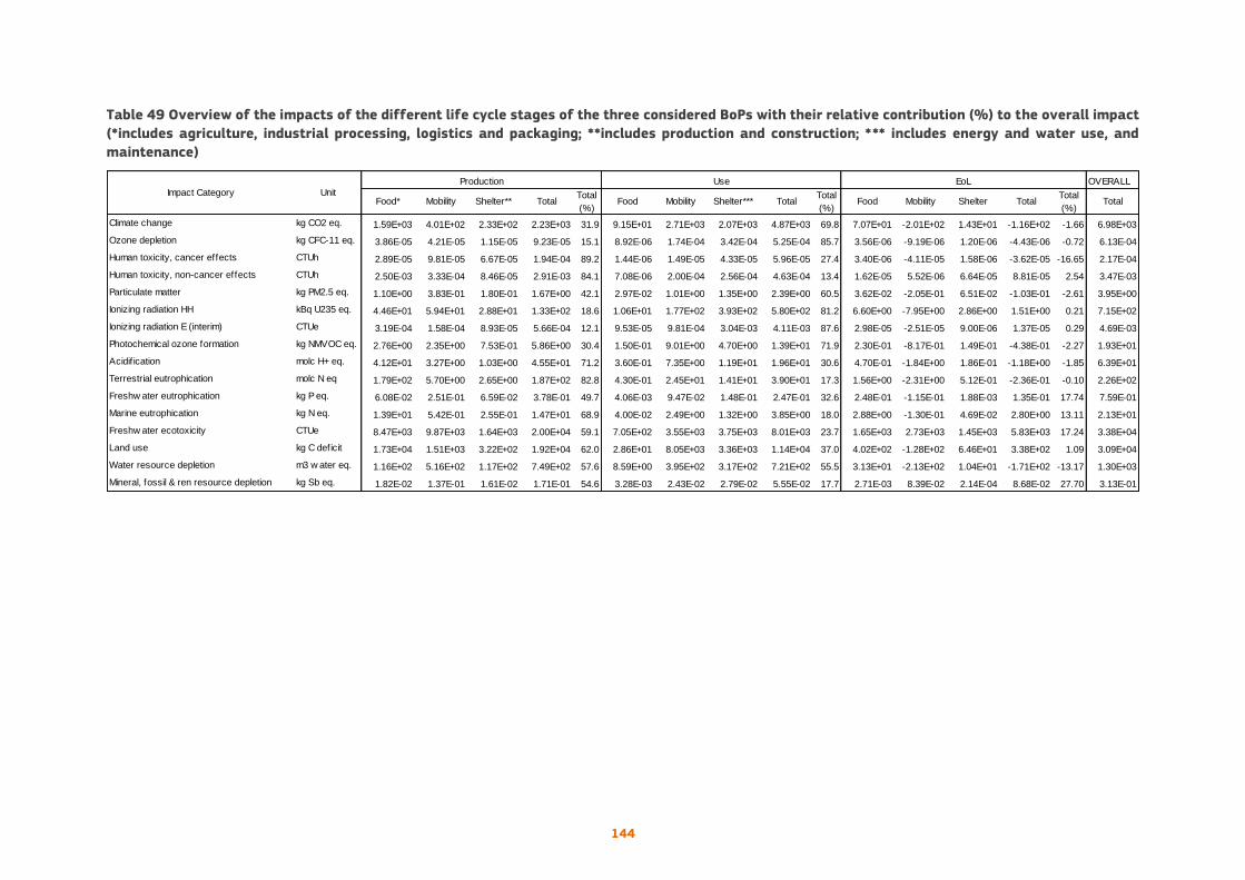
144

Table 49 Overview of the impacts of the different life cycle stages of the three considered BoPs with their relative contribution (%) to the overall impact

(*includes agriculture, industrial processing, logistics and packaging; **includes production and construction; *** includes energy and water use, and

maintenance)

OVERALL

Food* Mobility Shelter** TotalTotal

(%)Food Mobility Shelter*** Total

Total

(%)Food Mobility Shelter Total

Total

(%)Total

Climate change kg CO2 eq. 1.59E+03 4.01E+02 2.33E+02 2.23E+03 31.9 9.15E+01 2.71E+03 2.07E+03 4.87E+03 69.8 7.07E+01 -2.01E+02 1.43E+01 -1.16E+02 -1.66 6.98E+03

Ozone depletion kg CFC-11 eq. 3.86E-05 4.21E-05 1.15E-05 9.23E-05 15.1 8.92E-06 1.74E-04 3.42E-04 5.25E-04 85.7 3.56E-06 -9.19E-06 1.20E-06 -4.43E-06 -0.72 6.13E-04

Human toxicity, cancer effects CTUh 2.89E-05 9.81E-05 6.67E-05 1.94E-04 89.2 1.44E-06 1.49E-05 4.33E-05 5.96E-05 27.4 3.40E-06 -4.11E-05 1.58E-06 -3.62E-05 -16.65 2.17E-04

Human toxicity, non-cancer effects CTUh 2.50E-03 3.33E-04 8.46E-05 2.91E-03 84.1 7.08E-06 2.00E-04 2.56E-04 4.63E-04 13.4 1.62E-05 5.52E-06 6.64E-05 8.81E-05 2.54 3.47E-03

Particulate matter kg PM2.5 eq. 1.10E+00 3.83E-01 1.80E-01 1.67E+00 42.1 2.97E-02 1.01E+00 1.35E+00 2.39E+00 60.5 3.62E-02 -2.05E-01 6.51E-02 -1.03E-01 -2.61 3.95E+00

Ionizing radiation HH kBq U235 eq. 4.46E+01 5.94E+01 2.88E+01 1.33E+02 18.6 1.06E+01 1.77E+02 3.93E+02 5.80E+02 81.2 6.60E+00 -7.95E+00 2.86E+00 1.51E+00 0.21 7.15E+02

Ionizing radiation E (interim) CTUe 3.19E-04 1.58E-04 8.93E-05 5.66E-04 12.1 9.53E-05 9.81E-04 3.04E-03 4.11E-03 87.6 2.98E-05 -2.51E-05 9.00E-06 1.37E-05 0.29 4.69E-03

Photochemical ozone formation kg NMVOC eq. 2.76E+00 2.35E+00 7.53E-01 5.86E+00 30.4 1.50E-01 9.01E+00 4.70E+00 1.39E+01 71.9 2.30E-01 -8.17E-01 1.49E-01 -4.38E-01 -2.27 1.93E+01

Acidif ication molc H+ eq. 4.12E+01 3.27E+00 1.03E+00 4.55E+01 71.2 3.60E-01 7.35E+00 1.19E+01 1.96E+01 30.6 4.70E-01 -1.84E+00 1.86E-01 -1.18E+00 -1.85 6.39E+01

Terrestrial eutrophication molc N eq 1.79E+02 5.70E+00 2.65E+00 1.87E+02 82.8 4.30E-01 2.45E+01 1.41E+01 3.90E+01 17.3 1.56E+00 -2.31E+00 5.12E-01 -2.36E-01 -0.10 2.26E+02

Freshw ater eutrophication kg P eq. 6.08E-02 2.51E-01 6.59E-02 3.78E-01 49.7 4.06E-03 9.47E-02 1.48E-01 2.47E-01 32.6 2.48E-01 -1.15E-01 1.88E-03 1.35E-01 17.74 7.59E-01

Marine eutrophication kg N eq. 1.39E+01 5.42E-01 2.55E-01 1.47E+01 68.9 4.00E-02 2.49E+00 1.32E+00 3.85E+00 18.0 2.88E+00 -1.30E-01 4.69E-02 2.80E+00 13.11 2.13E+01

Freshw ater ecotoxicity CTUe 8.47E+03 9.87E+03 1.64E+03 2.00E+04 59.1 7.05E+02 3.55E+03 3.75E+03 8.01E+03 23.7 1.65E+03 2.73E+03 1.45E+03 5.83E+03 17.24 3.38E+04

Land use kg C deficit 1.73E+04 1.51E+03 3.22E+02 1.92E+04 62.0 2.86E+01 8.05E+03 3.36E+03 1.14E+04 37.0 4.02E+02 -1.28E+02 6.46E+01 3.38E+02 1.09 3.09E+04

Water resource depletion m3 w ater eq. 1.16E+02 5.16E+02 1.17E+02 7.49E+02 57.6 8.59E+00 3.95E+02 3.17E+02 7.21E+02 55.5 3.13E+01 -2.13E+02 1.04E+01 -1.71E+02 -13.17 1.30E+03

Mineral, fossil & ren resource depletion kg Sb eq. 1.82E-02 1.37E-01 1.61E-02 1.71E-01 54.6 3.28E-03 2.43E-02 2.79E-02 5.55E-02 17.7 2.71E-03 8.39E-02 2.14E-04 8.68E-02 27.70 3.13E-01

Impact Category Unit

Production Use EoL

145

Other relevant impact categories are marine and terrestrial eutrophication, acidification, freshwater ecotoxicity

and water resource depletion.

Results of normalization for BoP food for some impact categories are higher than the total impacts attributed

to an average EU-27 citizen. This can be due to the basic difference between the results of a process-based

LCA of a set of products and the overall impact of domestic emissions and resource extraction over a year in

the EU-27.

Given the relevance of the agricultural stage for the BoP food, inherent to FSCs specific features, it is important

to distinguish LCA results among a broader range of life cycle stages than only the three used for the other

baskets.

According to the hotspots analysis, targets for improvements in FSC aimed at reducing impacts have been

defined. The main areas of improvement are: i) an environmentally sustainable increase in agricultural

productivity coupled with measures aimed at reducing emissions to air, to water and to soil, ii) dietary changes

on the consumption side (e.g. reducing the consumption of meat and dairy products), iii) higher efficiency in

reducing food losses and managing food waste (e.g. through improved rate of food waste recovery). The

analysis of documentation on possible improvements in the food sector has shown that lot of research is

available about improvements and suggested eco-innovations. Given that most of the studies are oriented to

assess the effects of single improvements rather than defining targets at sector level, our first focus has been

on documents developed in the policy support context, such as IMPRO (Tukker et al, 2009; Weidema et al, 2008)

and BAT documents on food sectors (EC, 2005; EC, 2006; EC-JRC, 2013).

6.2 Perspectives on methodological issues

The next paragraphs should be regarded as an attempt to formulate some recommendations for improvements

of robustness and usefulness of the BoP indicators, based on the learning and insights from the indicators so

far calculated. These are mainly methodological recommendations focused on a number of identified key

aspects such as the definition of representative baskets, the robustness of the environmental assessment, the

coverage/quality of the input data.

6.2.1 Definition of the current basket: consistency/overlap + bringing in a range

A crucial phase in the development of the BoP indicators was the initial definition of the three selected basket

categories (food, mobility and shelter) and the population of the three baskets, i.e. the identification of the

representative products to be included in each basket. Given the profound importance of this phase for the

subsequent quantification of the potential environmental impacts associated with each basket, a number of

considerations/recommendations can be formulated:

1. The robustness of the selection of the representative products to be included in each basket should

be more carefully checked in order to (1) identify and avoid any possible overlaps among product

groups, (2) identify and avoid any gaps, i.e. relevant groups that have not been included in the

calculation exercise presented in this report.

2. The robustness of the selection of the representative products to be included in each basket could be

also improved by projecting/including in each basket also those products that will become relevant in

the (near) future. This calls for development and consideration of scenarios for the definition of “future

baskets” that would be useful and needed for developing time series of BoP indicators.

3. In connection to the previous point, towards further development of the LC Indicators it seems very

relevant to define and consider not just one basket for each category (e.g. one basket of products for

the category food), but – ideally - a range of different baskets from the “best performing” (from an

environmental view point) one to the “worst performing” one.

4. The development of country-specific baskets should also be explored via e.g. an ad-hoc feasibility

study on the availability of the necessary country-specific data. While developing 100% country-

specific baskets may not yet be viable, it would be certainly possible to progressively adapt the baskets

including more and more country-specific datasets.

146

6.2.2 Representativeness/quality (data): country specific vs. European average

An increased availability of high quality LCI-data would of course help increasing comprehensiveness and

robustness of the assessment. This being said, a number of considerations can be formulated in regards to

possible improvements of the underlying data:

1. In order to limit the data collection efforts for a future refinement of the BoP indicators, the present

calculations should be carefully checked (via e.g. sensitivity analysis) to identify some key hotspot /

product groups / part of the system that are most relevant in that they influence the most the

environmental performance. Data collection efforts could then initially be limited to these identified

components.

2. A better integration of existing data with Input/Output (IO) data seems relevant, as these data are

luckily to already include country-specific and lifecycle-stage specific information, which is seen as

important for developing further the indicators.

3. IO data could also be used to (1) cross check the results obtained so far without using I/O data, and

(2) calculate benchmarks, e.g. - in relation to point 3 under “definition of current baskets” - benchmarks

for the average performing and best/worst performing basket for each category (from an

environmental view point).

6.2.3 Impact categories: comprehensiveness/relevance of impact categories –

inserting accounting (pressure indicators) before coming to impacts

It is noted that a meaningful way to further advance the calculation of the BoP Indicators is to differentiate

the selected impact categories “per basket”. In fact, while some impact categories could be calculated as default

for all baskets, e.g. climate change, others could become basket-specific. This calls for the definition of relevant

criteria for the attribution of impact categories to the three specific baskets, which could be based on the

results (i.e. on the impact potentials) so far obtained. Beyond the ILCD-recommended impact categories,

additional relevant environmental information (as defined in the EC PEF method) could be considered for a

more comprehensive and meaningful interpretation of results (e.g. qualitative/quantitative aspects relative to

GMO use for the food basket).

6.2.4 Basket of Products extension

The current study considered three key BoPs. However, it is clear that other consumption activities contribute

to the impacts as well. To further complete the impact profile of consumption by the EU citizen, an extension

with other consumption categories can be explored. First, when it comes to the basic needs the current set of

food, housing and mobility might be expanded with health care products and services. Further on, other but

less basic needs could be considered: communication and information products and services and leisure

activities like tourism.

6.2.5 Target methodology

The application of the target methodology to BoP food helped to identify hotspots. Through normalization of

the LCA results, the hotspots proved to be in line with those spotted by the review of the existing literature,

except for the contribution of food losses, which are embedded in each phase, hence more difficult to be

identified as a hotspot. In general, the methodology can be considered useful for the identification of hotspots

of the BoPs and the contribution analysis for life cycle stages and product categories in the BoP.

There are some limitations in the use of normalization reference based on production approach (domestic

emissions and resource extraction) when consumption-based LCA is carried out.

Moreover, the use of three different sets of NFs (the one for the status quo and the two about desirable status

quo) did not show relevant differences in the identification of the most relevant impact categories.

The application of the methodology to the BoP food has highlighted the need of a complementary approach,

in which literature review on hotspot is coupled with LCA. In literature, the majority of study focus on energy

147

and climate related impacts of FSC (e.g. Garnett 2011) whereas the LCA applied to the BoP simultaneously

accounting for different impact categories support a more comprehensive hotspot analysis. Indeed, LCA may

give broader and multi-criteria assessment of BoP while missing some impact due to the variability in specific

life cycle stage, e.g. consumers’ habits in the use phase. Therefore, a sensitivity analysis about the main

assumptions made in BoP LCA is needed in support to the definition of targets (e.g. to test the robustness of

hotspots results).

Indicators and targets for the reduction of the environmental ...

Documents

Transcript of Indicators and targets for the reduction of the environmental ...