Contents lists available at ScienceDirect

Atmospheric Environment

journal homepage: www.elsevier.com/locate/atmosenv

Improving ozone simulations in the Great Lakes Region: The role ofemissions, chemistry, and dry deposition

Momei Qina, Haofei Yua,b, Yongtao Hua, Armistead G. Russella, M Talat Odmana,∗, Kevin Dotyc,Arastoo Pour-Biazarc, Richard T. McNiderd, Eladio Knippinge

a School of Civil and Environmental Engineering, Georgia Institute of Technology, Atlanta, GA, USAbNow at Department of Civil, Environmental and Construction Engineering, University of Central Florida, Orlando, FL, USc Earth System Science Center, University of Alabama in Huntsville, Huntsville, AL, USAdDepartment of Atmospheric Science, University of Alabama in Huntsville, Huntsville, AL, USAe Electric Power Research Institute, Washington, DC, USA

A R T I C L E I N F O

Keywords:CMAQOzoneThe great lakes regionCB6MEGANNOx emissions

A B S T R A C T

The Great Lakes Region of the US continues experiencing exceedances of the ozone (O3) standards, despite yearsof emissions controls. In part, this is due to interactions between emissions from surrounding large cities (e.g.,Chicago) and meteorology, which is heavily influenced by the presence of the Great Lakes. These complexmeteorology-emissions interactions pose a challenge to fully capture O3 dynamics, particularly near shores of thelakes, where high O3 levels are often experienced. In a simulation with the Community Multiscale Air Quality(CMAQ) model, using inputs as typically constructed, the model tends to be biased high. A literature reviewindicated that NOx emissions from mobile sources, possibly overestimated in the 2011 National EmissionInventory (NEI), or the version of the Carbon Bond chemical mechanism used in CMAQ could be responsible forhigh biases of O3. As such, a series of sensitivity tests was conducted to identify potential causes for this bias,including emissions biases (e.g., biogenic VOCs, anthropogenic NOx), chemical mechanism choice, and O3 drydeposition to fresh water, for high O3 periods in July 2011. The base model/emissions configuration used thefollowing: Carbon Bond mechanism CB05, biogenic emissions using Biogenic Emission Inventory System (BEIS),and anthropogenic emissions from the 2011 National Emissions Inventory (NEI). Meteorological inputs weredeveloped using the Weather Research and Forecasting (WRF) model (version 3.8.1). Simulated daily maximum8-h average O3 without and with a cutoff of 60 ppb (referred to as MDA8 O3 and elevated MDA8 O3 hereafter,respectively) were evaluated against measurements. The evaluation showed a high bias in MDA8 O3 across thedomain, particularly at coastal sites (by ∼6 ppb), while elevated MDA8 O3 (i.e., greater than 60 ppb) was biasedlow, with exceptions centered along the shore of Lake Michigan. Using the CB6 chemical mechanism or 50%reduction of NOx emissions from on-road mobile sources led to substantial domain-wide decreases in O3 from thebase case, and the model performance improved, particularly along the Lake Michigan shoreline and for thewestern domain. However, elevated MDA8 O3 was more biased against measurements, compared to the modelperformance in the base case, except at a few sites along the shoreline. Using the Model of Emissions of Gasesand Aerosols from Nature (MEGAN) instead of BEIS to estimate biogenic emissions, or increasing dry depositionof O3 to fresh water by a factor of ten (which is unrealistic), had minor impacts on simulated O3 over land. But,combining MEGAN with CB6 resulted in improved elevated MDA8 O3 simulation along the western coast of LakeMichigan. Finally, using CB6 combined with a 30% reduction of on-road mobile NOx emissions and MEGAN ledto the best performance. Two companion papers investigate how meteorological modeling can be improved.Together, the recommended modeling system could serve as a starting point for future O3 modeling in theregion.

https://doi.org/10.1016/j.atmosenv.2019.01.025Received 5 July 2018; Received in revised form 30 December 2018; Accepted 5 January 2019

∗ Corresponding author.E-mail addresses: talat.odman@ce.gatech.edu, odman@gatech.edu (M.T. Odman).

Atmospheric Environment 202 (2019) 167–179

Available online 19 January 20191352-2310/ © 2019 Elsevier Ltd. All rights reserved.

T

1. Introduction

Exceedance of the National Ambient Air Quality Standard (NAAQS)for ozone (O3) has been of concern in the Great Lakes Region for manyyears (Foley et al., 2011). Several counties located in the Milwau-kee–Chicago–Gary urban corridor along Lake Michigan, which aredensely populated areas with a variety of emission sources, have beenviolating the 2008, 0.075 parts per million 8-h O3 standard (US EPA,2018). Those counties are in violation of the more stringent 8-h O3

standard of 70 parts per billion (ppb) promulgated in 2015 (https://www.epa.gov/ozone-designations/additional-designations-2015-ozone-standards), and will likely remain in non-attainment status forthe near future.

Ground-level O3 is primarily formed via chemistry involving volatileorganic compounds (VOCs) and oxides of nitrogen (NOx) in the pre-sence of sunlight (Seinfeld and Pandis, 2012). High-O3 episodes in theGreat Lakes Region during summer have been tied to land-lake circu-lations, which are driven by temperature contrasts between the landand water (Dye et al., 1995; Lennartson and Schwartz, 2002; Levy et al.,2010; Makar et al., 2010b; Sills et al., 2011; Wentworth et al., 2015). Inthe early morning, O3 precursors emitted onshore are transported byland breezes to over the lake. As sunlight intensifies, O3 forms via re-actions of the precursors confined within a shallow layer above thewater and, along with reduced deposition velocities over water andlittle or no titration from fresh NOx emissions, reaches high levels(Cleary et al., 2015; Levy et al., 2010). Offshore, O3-rich air is thenadvected inland by afternoon lake breezes. Larger-scale synoptic flows(e.g., southerly/southwesterly winds over Lake Michigan) can partlyaffect O3 levels over the region as well (Dye et al., 1995; Foley et al.,2011; Levy et al., 2010; Makar et al., 2010b).

The relative importance of NOx and VOC emissions can also vary bylocation. Based on the analysis of 1994–2003 LADCO Aircraft Project(LAP) data, O3 formation over Lake Michigan changes from VOC-lim-ited in the morning to NOx-limited in the afternoon at low altitudes(below 200m), while the air mass is NOx-limited throughout the dayand more photochemically aged above 200m (Foley et al., 2011).Measurements in the Greater Toronto Area from 2000 to 2012 suggestthat O3 production on land has become more sensitive to VOC re-activity, and has not been significantly decreasing in response to re-ductions of precursors over the study period (Pugliese et al., 2014).

In the late 1990s, photochemical grid models (e.g., UAM-IV (UrbanAirshed Model with Carbon Bond IV) and UAM-V (Urban AirshedModel with Variable Grid)) have been applied to simulate O3 episodesduring the 1991 Lake Michigan Ozone Study (LMOS) (Hanna et al.,1996). Daily maximum 1-hr O3 levels were typically overestimated byUAM-IV (by 12% on average) and slightly underestimated by UAM-V(by 3%) which uses higher photolysis rates, with underestimation of O3

precursors (VOCs and NOx) by as much as a factor of two. A major issuewith these simulations was that high observed O3 at 200–500 kmdownwind were both underestimated by 30–40 ppb, possibly due toproblems with the simulated vertical diffusivities or the large under-estimation of precursors, especially in rural areas. Fast and Heilman(2003) simulated O3 that compared well with the observations over thewestern Great Lakes region, with a domain-wide average bias of−1.3 ppb for daily maximum 1-hr value and 5.5 ppb for the minimum.It was found that O3 over the lakes and around the lake shores is verysensitive to lake temperatures: changes of 5°C in temperature con-tributing to as much as 50 ppb changes in O3 mixing ratios. Makar et al.(2010a) demonstrated that substantial improvements in model perfor-mance for O3, e.g., daily 1-hr maximum surface O3 biases decreasingfrom ∼15 ppb to ∼9 ppb, were achieved in AURAMS (A Unified Re-gional Air-quality Modeling System) model through careful choice ofthe method used to specify lateral and top boundary conditions from O3

climatology. However, reduction of surface O3 bias sometimes came atthe expense of significant positive biases in O3 concentrations in thefree troposphere and upper troposphere. Compared to ferry and land-

based O3 measurements, the Community Multiscale Air Quality(CMAQ) model presented higher positive biases over the water of LakeMichigan than over the surrounding land, up to 16 ppb for offshorelocations with an increasing trend to the eastern side of the lake (Clearyet al., 2015). The WRF-Chem (Weather Research and ForecastingChemical) model underpredicted peak O3 during high-O3 episodes inthe forecasting products in support of 2017 LMOS campaign, whichoccurred during May and June 2017 to address the high O3 events incoastal communities surrounding Lake Michigan (Stanier et al., 2017).Such efforts demonstrate that current chemical transport models havedifficulties reproducing high-O3 events due to unique meteorologicaland physical complexities associated with the area, along with generaluncertainties concerning the emissions and chemistry (Simon et al.,2012).

In this study, the CMAQ model was used to simulate O3 over theGreat Lakes Region for July 2011. A series of sensitivity runs withdifferent emissions, chemical mechanisms and/or O3 dry depositionwas conducted to identify model configurations and inputs best cap-turing land-based measurements. Improving O3 modeling from me-teorological perspectives (e.g., examining the roles of mixing and laketemperatures, or utilizing iterative WRF analysis) has been thoroughlyexplored in two companion papers (McNider et al., 2018; Odman et al.,2019b). This work focuses on the impacts of emissions, chemistry, anddeposition, and aims to optimize CMAQ's O3 performance over theGreat Lakes Region.

2. Method

The CMAQ model (Byun and Schere, 2006) was applied to simulateO3 in the Great Lakes Region during July 2011, driven by the WeatherResearch and Forecasting (WRF) model (Skamarock et al., 2005). Julywas selected as the study period because (1) it has the highest MDA8 O3

concentration over the period of April to October and (2) simulated O3

is more biased compared to measurements around Lake Michigan,based on our previous work (Odman et al., 2019a). Each model has a 4-km horizontal resolution domain nested inside a 12-km resolution do-main. Initial conditions (ICs) and lateral boundary conditions (LBCs) forthe outer domain (12×12 km2 grid resolution) simulation were takenfrom the predefined CMAQ profiles, which represent relatively clean airconditions in the eastern-half of the United States (Gipson, 1999), whileLBCs for the inner domain (4×4 km2 grid resolution) simulation wereobtained from the outer domain. The outer domain covers the entirecontiguous US as well as a portion of Canada, while the inner domainfocuses on the area surrounding the lakes (Fig. 1). In the vertical di-rection, there are 35 layers for both domains and the model top isplaced at 50 hPa.

Fig. 1. Modeling domains of WRF (red boxes) and CMAQ (black boxes). A 4-kmgrid over the Great Lakes Region is nested inside a 12-km grid over the con-tiguous US. (For interpretation of the references to color in this figure legend,the reader is referred to the Web version of this article.)

M. Qin et al. Atmospheric Environment 202 (2019) 167–179

168

2.1. Meteorological simulation

We used WRF version 3.8.1 to simulate the meteorological condi-tions. The analysis product of the North American Mesoscale ForecastSystem (NAM-12) provided initial and lateral boundary conditions forthe simulation over the outer domain. The National Land CoverDatabase 2011 (NLCD2011) was used as land use/land cover data. Thespecific model configuration (Table S1) is the same as the initialiteration of iterative WRF analysis in Odman et al. (2019b). The si-mulation began on June 15th, and covered the entire month of July2011. The first five days were used to initialize the deep soil moistureand temperature, as soil nudging was utilized to optimize surfacetemperature and humidity (Pleim and Gilliam, 2009; Pleim and Xiu,2003). The rest of the simulation period used 5.5-day overlapping runsegments, with the first 12 h included as the spin-up period.

2.2. Photochemical simulation

2.2.1. Base caseCMAQ version 5.1 with the latest version of Carbon Bond me-

chanism CB05, i.e., cb05e51, was applied to simulate the photo-chemistry taking place in the Great Lakes Region during the O3 season.In this study, anthropogenic emissions are based on the US EPA 2011National Emission Inventory (NEI). They were processed by the SparseMatrix Operator Kernel Emissions (SMOKE) Modeling System followingthe EPA 2011v6.2 modeling platform (available at https://www.epa.gov/air-emissions-modeling/2011-version-62-platform). In-line plumerise calculations were carried out by CMAQ in this study. Additionally,biogenic emissions were calculated in-line with Biogenic EmissionInventory System (BEIS) version 3.6.1, which is imbedded in CMAQ aswell. The simulation period spanned from June 20th to the end of July.We focused on the 4-km resolution inner domain to investigate modelperformance on simulating O3 events throughout July 2011.

2.2.2. Sensitivity runsFive sensitivity runs were conducted to explore the contributing

factors to O3 biases in the Great Lakes Region (Table 1). These runswere identical to the base case simulation in all respects, except for oneor two factors (e.g., emissions, chemical mechanism or dry depositionof O3) that were changed in the simulation over the inner domain foreach case. Since we did not repeat the outer domain simulation with themodifications (except for the case with CB6), the ICs/LBCs for the innerdomain would not reflect the change. Despite the uncertainties tied tounchanged boundary conditions, the sensitivity runs can still provideinsight into the directionality and magnitude of the O3 response. Assuch, the differences in simulated O3 between a sensitivity run and thebase case over the inner domain can still be attributed to the factor(s)that was (were) changed.

2.2.2.1. Biogenic emissions. Uncertainties in biogenic emissions wereinvestigated by comparing two widely-used biogenic emission models.In the case labeled Megan, the Model of Emissions of Gases and Aerosolsfrom Nature (MEGAN) version 2.1 (Guenther et al., 2012) was

employed to estimate biogenic emissions, in place of BEIS used in thebase case. The major differences between the two models include: (1)BEIS uses a leaf-scale emission factor at standard environmentalconditions whereas MEGAN uses canopy-level emission factors, whichare primarily based on leaf and branch-scale emission measurementsthat are extrapolated to the canopy-scale; (2) The built-in canopymodels in MEGAN and BEIS are different, particularly in leaftemperature algorithms; (3) MEGAN accounts for the effect of leafage and monthly changes of leaf area index (LAI), whereas BEIS doesnot (Bash et al., 2016; Pouliot and Pierce, 2009; Sindelarova et al.,2014).

MEGAN and BEIS were both driven by WRF, which provided me-teorological fields such as temperature and radiation. In the base casewith BEIS, BELD4 (Biogenic Emission Landuse Database) which con-tains gridded vegetation information for 275 vegetation categories,along with a normalized emission factor for each vegetation category,was provided as inputs to estimate emissions for 33 VOCs, CO, andnitric oxide (NO) (Bash et al., 2016). In the sensitivity run withMEGAN, the global gridded high-resolution emission potential map wasutilized to estimate emissions of ten predominant compounds of bio-genic origin (e.g., isoprene, monoterpenes, NO). This dataset wascompiled based on species-specific emission factors and detailed vege-tation species composition data (Guenther et al., 2012). Emissions ofother compounds were estimated using plant functional type (PFT) andthe PFT-specific emission factors. All the inputs including the griddedemission potential map, the PFT dataset and emission factors wereprovided together with MEGAN code except the LAIv (LAI of vegetationcovered surfaces), which was retrieved from several MODIS (ModerateResolution Imaging Spectroradiometer) satellite products as detailed inYu et al. (2017).

2.2.2.2. NOx emissions from mobile sources. 2011 NEI NOx emissions,other than those from power plants, have been considered to beoverestimated in multiple studies, with the magnitude ofoverestimation ranging from 14% to 70% (Anderson et al., 2014; Liet al., 2016; McDonald et al., 2018; Souri et al., 2016). Anderson et al.(2014) claimed high biases of NOx emissions since higher ratios of CO/NOx are measured in ambient air than that estimated by the 2011 NEI.However, the robustness of the basis of this claim has been questionedrecently (Simon et al., 2018). Reductions of non-power-plant NOx

emissions decreased model biases for NOx, inorganic nitrate andboundary layer ozone against aircraft measurements (Travis et al.,2016), and inverse modeling based on satellite NO2 observationsindicated a reduction in emissions from area (44%), mobile (30%),and point sources (60%) in high NOx areas (Souri et al., 2016). Mostimportantly, projected NOx emissions of mobile sources for 2013 usingthe 2011 NEI are 28% higher than the fuel-based inventory, with thelargest discrepancies found in on-road gasoline sector (80% higher inthe NEI), and the uncertainties in estimates of mobile emissions areassociated with spatial and temporal patterns of activity, emissionfactors, and improved emission control technologies over time(McDonald et al., 2018 and references therein). Based on some of theabove studies, mobile emissions that account for over half of NOx

emissions in the US, are most likely responsible for the high biases ofNOx emissions.

Considering that reducing mobile NOx emissions could lead to betteragreement with ambient measurements of NOx or NOy, as well as sa-tellite retrievals of nitrogen dioxide (NO2), and even better capture O3

exceedances (Canty et al., 2015; Li et al., 2016; McDonald et al., 2018;Souri et al., 2016; Travis et al., 2016), a sensitivity run with a 50%reduction of NOx emissions from on-road mobile sources, which aremajor contributors to mobile sources (the case 0.5NOx), was conductedto quantify the impact of a potential NOx emission bias in the 2011 NEIon simulated O3 in the Great Lakes Region.

2.2.2.3. Chemical mechanism. CB6, a newer version of Carbon Bond

Table 1Summary of the base case and five sensitivity simulations.

NO. Case Biogenicemissions

On-roadmobile NOx

emissions

Chemicalmechanism

Dry depositionover freshwater

0 Base BEIS 100% CB05 Default1 Megan MEGAN 100% CB05 Default2 0.5NOx BEIS 50% CB05 Default3 CB6 BEIS 100% CB6 Default4 CB6_megan MEGAN 100% CB6 Default5 Ddep BEIS 100% CB05 10-fold

M. Qin et al. Atmospheric Environment 202 (2019) 167–179

169

chemical mechanism as an update to CB05, aims to better representoxidant formation from long-lived, abundant VOCs, and the fate oforganonitrates, particularly the recycling of NOx (Yarwood et al.,2010). Some notable updates from CB05 to CB6 related to O3

simulation include: (1) updated reactions of alkanes, alkenes andaromatics with the most changes for isoprene and aromatics; (2)long-lived VOCs, specifically propane, benzene, acetone and otherketones being explicitly represented; and (3) changed reaction rates,e.g., increasing the photolysis/OH oxidation rate of NO2 by 5–7%, anddecreasing the reaction rate of N2O5 with water vapor by ∼80%.Several revisions have been made to CB6 (i.e., CB6r1, CB6r2, CB6r3 andCB6r4): for instance, CB6r1 revised the chemistry of isoprene andaromatics, and enhanced NOx-recycling from the evolution oforganonitrates (Yarwood et al., 2012); the fates of organonitrateswere more detailed in CB6r2, with different partitioning into thecondensed phase and dominant degradation pathway between simplythe alkyl nitrates and the multi-functional organonitrates (HildebrandtRuiz and Yarwood, 2013); CB6r3 adopted temperature- and pressure-dependent NO2-alkyl nitrate branching, which might improve O3

simulation in winter (Stoeckenius and McNally, 2014). The thirdversion of CB6 (CB6r3), which was recently implemented inCMAQv5.2, was used in the sensitivity run (the case CB6) in place ofa revised version of CB05 (CB05e51) in the base run. While severalreaction rates and product updates are present in both CB6r3 andCB05e51, CB6r3 has more comprehensive updates (Wyat Appel et al.,2018). Since CB6 is not available in CMAQv5.1, we switched toCMAQv5.2 for this simulation, which includes multiple updates thatmight lead to differences between the two runs collectively.Additionally, unlike other sensitivity runs, CB6 was applied to theouter domain as well as the inner domain for the case CB6.

CB05e51 in CMAQv5.1 has already incorporated detailed isoprenechemistry (Fahey et al., 2017) with some reaction rates and productsfrom CB6r2, but there are slight differences in representation of iso-prene chemistry between CB05e51 and CB6r3. For instance, CB6r3considers the reaction of isoprene peroxy radical (ISO2) with otherperoxy radicals (RO2), while CB05e51 does not; the fates of organo-nitrates via the reaction of isoprene with NO3 radical are not the same,which affects the NOx recycling efficiency. For this reason, the com-bined impact of CB6 with MEGAN emissions (the case CB6_megan) wasalso examined.

2.2.2.4. O3 dry deposition over water. Dry deposition accounts for∼20% of O3 removal from the troposphere (Lelieveld and Dentener,2000). With dry deposition entirely turned off in the model, simulatedsurface O3 increased by up to 50 ppb in the UK, particularly at night(Vieno et al., 2010). Underestimation of dry deposition with the Weselyscheme, based on Wesely (1989), can in part explain high biases of O3

in the eastern US (Lin et al., 2008; Travis et al., 2016). The M3DRYscheme in the CMAQ model yields even lower dry deposition velocitiesthan the Wesely scheme, which will result in higher O3 concentrations,particularly when vegetation-dominated O3 dry deposition over land issignificant (Park et al., 2014). CMAQ v5.1 accounts for the interactionof O3 with iodide in seawater, increasing deposition velocities by an

order of magnitude and reducing summer-time surface O3

concentration by ∼3% over marine regions in the NorthernHemisphere (Sarwar et al., 2015). In this study, the dry depositionvelocity of O3 over the lakes was increased by a factor of 10, which iscomparable to that over seawater in Sarwar et al. (2015), in order toinvestigate if potentially underestimated dry deposition rates over freshwater could be responsible for overestimation of O3 over the lake andalong the shoreline.

2.2.3. The final simulationBased on the evaluation of modeled O3 against ground-based mea-

surements for each sensitivity run, the options for biogenic emission,adjusted NOx emissions from on-road mobile sources and the chemicalmechanism that had the best overall performance were used for thefinal simulations over the outer and inner domains, respectively.

2.3. Evaluation

Model performance was evaluated against the observed concentra-tions of ground-level O3 and NOx, which were obtained from the AirQuality System (AQS) network. The observations and simulations werepaired in space and time. Monitoring sites located within the 4-kmdomain were considered for evaluation and were sorted into threegroups based on the distance from the shoreline, i.e., coastal sites(< 20 km), sites in the buffer area (20–100 km), and inland sites(> 100 km), with 65, 52 and 174 sites, respectively, in each group. Avariety of statistical metrics (Emery et al., 2017) including mean bias(MB), mean error (ME), fractional bias (FB), fractional error (FE),normalized mean bias (NMB), normalized mean error (NME), meannormalized bias (MNB), mean normalized error (MNE), index ofagreement (IOA), coefficient of determination (r2), and root meansquared error (RMSE) were used to evaluate daily maximum 8-hraverage (MDA8) O3, with or without a 60 ppb cutoff (Tables 2–3), andhourly NOx.

3. Results and discussion

3.1. Base case simulation

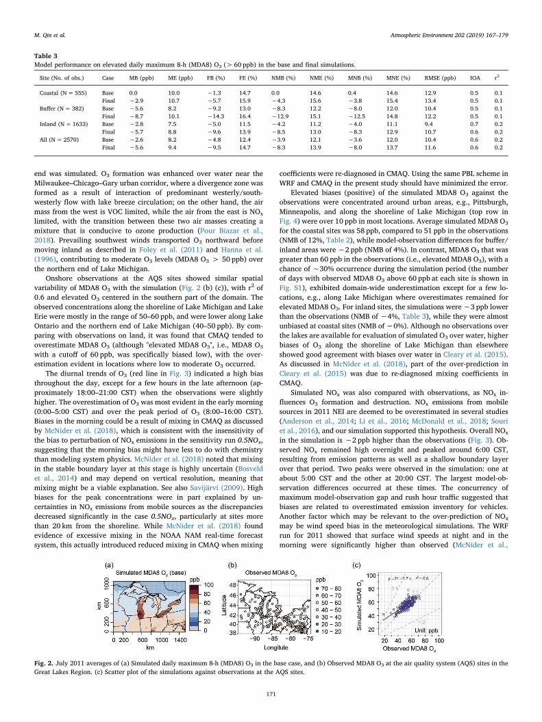
Simulated ground-level MDA8 O3 showed much higher concentra-tions over water than the surrounding land (Fig. 2 (a)), with the max-imum exceeding 90 ppb over the southwestern side of Lake Michigan,corresponding to a land-lake contrast of ∼30 ppb. Although no O3

measurements over the lakes are available during July 2011, the si-mulated land-lake differences are greater than those reported in Levyet al. (2010) for ferry-based O3 measurements over Lake Erie, whichwere 5–10 ppb above observations at rural sites nearby and 10–20 ppblarger than observations at urban sites in the southern Great LakesRegion. The daytime land-lake differences of O3 were attributed to thelower dry deposition of O3 to water than to land, which is true both forthe real atmosphere and the model, and stable air over the lakes leads toconditions conducive to O3 formation. A decreasing trend of simulatedO3 from the southern/central areas of Lake Michigan to the northern

Table 2Model performance on daily maximum 8-h (MDA8) O3 in the base and final simulations.

Site (No. of obs.) Case MB (ppb) ME (ppb) FB (%) FE (%) NMB (%) NME (%) MNB (%) MNE (%) RMSE (ppb) IOA r2

Coastal (N=1946) Base 6.3 10.5 12.4 19.6 12.4 20.4 16.7 23.2 14.1 0.8 0.4Final 4.5 10.0 9.5 19.1 8.8 19.6 13.6 22.3 13.5 0.7 0.3

Buffer (N=1559) Base 1.8 7.1 4.7 14.0 3.5 13.9 6.8 15.4 9.4 0.8 0.5Final 0.0 7.3 1.5 14.6 0.0 14.3 3.6 15.4 9.5 0.8 0.4

Inland (N=5113) Base 2.4 7.5 5.1 14.0 4.4 13.8 7.4 15.6 9.8 0.8 0.4Final 0.1 7.4 1.0 14.1 0.1 13.7 3.1 15.1 9.7 0.8 0.4

All (N=8618) Base 3.2 8.1 6.6 15.3 6.0 15.3 9.4 17.3 10.9 0.8 0.4Final 1.1 8.0 3.0 15.3 2.0 15.1 5.6 16.8 10.6 0.8 0.4

M. Qin et al. Atmospheric Environment 202 (2019) 167–179

170

end was simulated. O3 formation was enhanced over water near theMilwaukee–Chicago–Gary urban corridor, where a divergence zone wasformed as a result of interaction of predominant westerly/south-westerly flow with lake breeze circulation; on the other hand, the airmass from the west is VOC limited, while the air from the east is NOx

limited, with the transition between these two air masses creating amixture that is conducive to ozone production (Pour Biazar et al.,2018). Prevailing southwest winds transported O3 northward beforemoving inland as described in Foley et al. (2011) and Hanna et al.(1996), contributing to moderate O3 levels (MDA8 O3 > 50 ppb) overthe northern end of Lake Michigan.

Onshore observations at the AQS sites showed similar spatialvariability of MDA8 O3 with the simulation (Fig. 2 (b) (c)), with r2 of0.6 and elevated O3 centered in the southern part of the domain. Theobserved concentrations along the shoreline of Lake Michigan and LakeErie were mostly in the range of 50–60 ppb, and were lower along LakeOntario and the northern end of Lake Michigan (40–50 ppb). By com-paring with observations on land, it was found that CMAQ tended tooverestimate MDA8 O3 (although "elevated MDA8 O3", i.e., MDA8 O3

with a cutoff of 60 ppb, was specifically biased low), with the over-estimation evident in locations where low to moderate O3 occurred.

The diurnal trends of O3 (red line in Fig. 3) indicated a high biasthroughout the day, except for a few hours in the late afternoon (ap-proximately 18:00–21:00 CST) when the observations were slightlyhigher. The overestimation of O3 was most evident in the early morning(0:00–5:00 CST) and over the peak period of O3 (8:00–16:00 CST).Biases in the morning could be a result of mixing in CMAQ as discussedby McNider et al. (2018), which is consistent with the insensitivity ofthe bias to perturbation of NOx emissions in the sensitivity run 0.5NOx,suggesting that the morning bias might have less to do with chemistrythan modeling system physics. McNider et al. (2018) noted that mixingin the stable boundary layer at this stage is highly uncertain (Bosveldet al., 2014) and may depend on vertical resolution, meaning thatmixing might be a viable explanation. See also Savijärvi (2009). Highbiases for the peak concentrations were in part explained by un-certainties in NOx emissions from mobile sources as the discrepanciesdecreased significantly in the case 0.5NOx, particularly at sites morethan 20 km from the shoreline. While McNider et al. (2018) foundevidence of excessive mixing in the NOAA NAM real-time forecastsystem, this actually introduced reduced mixing in CMAQ when mixing

coefficients were re-diagnosed in CMAQ. Using the same PBL scheme inWRF and CMAQ in the present study should have minimized the error.

Elevated biases (positive) of the simulated MDA8 O3 against theobservations were concentrated around urban areas, e.g., Pittsburgh,Minneapolis, and along the shoreline of Lake Michigan (top row inFig. 4) were over 10 ppb in most locations. Average simulated MDA8 O3

for the coastal sites was 58 ppb, compared to 51 ppb in the observations(NMB of 12%, Table 2), while model-observation differences for buffer/inland areas were ∼2 ppb (NMB of 4%). In contrast, MDA8 O3 that wasgreater than 60 ppb in the observations (i.e., elevated MDA8 O3), with achance of ∼30% occurrence during the simulation period (the numberof days with observed MDA8 O3 above 60 ppb at each site is shown inFig. S1), exhibited domain-wide underestimation except for a few lo-cations, e.g., along Lake Michigan where overestimates remained forelevated MDA8 O3. For inland sites, the simulations were ∼3 ppb lowerthan the observations (NMB of −4%, Table 3), while they were almostunbiased at coastal sites (NMB of−0%). Although no observations overthe lakes are available for evaluation of simulated O3 over water, higherbiases of O3 along the shoreline of Lake Michigan than elsewhereshowed good agreement with biases over water in Cleary et al. (2015).As discussed in McNider et al. (2018), part of the over-prediction inCleary et al. (2015) was due to re-diagnosed mixing coefficients inCMAQ.

Simulated NOx was also compared with observations, as NOx in-fluences O3 formation and destruction. NOx emissions from mobilesources in 2011 NEI are deemed to be overestimated in several studies(Anderson et al., 2014; Li et al., 2016; McDonald et al., 2018; Souriet al., 2016), and our simulation supported this hypothesis. Overall NOx

in the simulation is ∼2 ppb higher than the observations (Fig. 3). Ob-served NOx remained high overnight and peaked around 6:00 CST,resulting from emission patterns as well as a shallow boundary layerover that period. Two peaks were observed in the simulation: one atabout 5:00 CST and the other at 20:00 CST. The largest model-ob-servation differences occurred at these times. The concurrency ofmaximum model-observation gap and rush hour traffic suggested thatbiases are related to overestimated emission inventory for vehicles.Another factor which may be relevant to the over-prediction of NOx

may be wind speed bias in the meteorological simulations. The WRFrun for 2011 showed that surface wind speeds at night and in themorning were significantly higher than observed (McNider et al.,

Table 3Model performance on elevated daily maximum 8-h (MDA8) O3 (> 60 ppb) in the base and final simulations.

Site (No. of obs.) Case MB (ppb) ME (ppb) FB (%) FE (%) NMB (%) NME (%) MNB (%) MNE (%) RMSE (ppb) IOA r2

Coastal (N=555) Base 0.0 10.0 −1.3 14.7 0.0 14.6 0.4 14.6 12.9 0.5 0.1Final −2.9 10.7 −5.7 15.9 −4.3 15.6 −3.8 15.4 13.4 0.5 0.1

Buffer (N=382) Base −5.6 8.2 −9.2 13.0 −8.3 12.2 −8.0 12.0 10.4 0.5 0.1Final −8.7 10.1 −14.3 16.4 −12.9 15.1 −12.5 14.8 12.2 0.5 0.1

Inland (N=1633) Base −2.8 7.5 −5.0 11.5 −4.2 11.2 −4.0 11.1 9.4 0.7 0.2Final −5.7 8.8 −9.6 13.9 −8.5 13.0 −8.3 12.9 10.7 0.6 0.2

All (N=2570) Base −2.6 8.2 −4.8 12.4 −3.9 12.1 −3.6 12.0 10.4 0.6 0.2Final −5.6 9.4 −9.5 14.7 −8.3 13.9 −8.0 13.7 11.6 0.6 0.2

Fig. 2. July 2011 averages of (a) Simulated daily maximum 8-h (MDA8) O3 in the base case, and (b) Observed MDA8 O3 at the air quality system (AQS) sites in theGreat Lakes Region. (c) Scatter plot of the simulations against observations at the AQS sites.

M. Qin et al. Atmospheric Environment 202 (2019) 167–179

171

2018). This would mean that surface NOx emissions would likely beover diluted in the model. But this would be counter to the direction ofthe NOx bias. Thus, while perhaps important for other emissions, it islikely not a factor in the present NOx over-prediction. We also foundCMAQ performed better on NOx with finer grids, i.e., grid spacing of4 km instead of 12 km (grey line in Fig. 3), particularly in coastal areas,

indicating the mismatch between area represented by the grid-cell andthe monitor location, which could also be responsible for the differ-ences of NOx between the model and observations.

Fig. 3. Diurnal trends of O3 (top) andNOx (bottom) averaged across the do-main (Domainwide), at coastal(< 20 km), buffer (20–100 km), andinland (> 100 km) sites in the GreatLakes Region in July 2011. Monthlymeans of MDA8 O3 and NOx from ob-servations (black), simulations in thebase (red) and final (blue) runs at theAQS sites are shown at the top of eachpanel. Changes in MDA8 O3 and NOx ineach sensitivity run with respect to thebase case are shown in the small boxes.(For interpretation of the references tocolor in this figure legend, the reader isreferred to the Web version of this ar-ticle.)

Fig. 4. Mean biases of simulated MDA8 O3 (with/without a cutoff of 60 ppb) and NOx concentrations from the base (top) and final (bottom) simulations against theobservations in the Great Lakes Region in July 2011.

Fig. 5. (a) Diurnal trends of isoprene emission using BEIS and MEGAN with the daytime (6:00–18:00 CST) averages across the domain shown at the top of the panel.(b) Daytime isoprene emission using BEIS over the Great Lakes Region in July 2011. (c) Differences in isoprene emission between MEGAN and BEIS over the GreatLakes Region in July 2011.

M. Qin et al. Atmospheric Environment 202 (2019) 167–179

172

3.2. The sensitivity simulations

3.2.1. MEGAN vs. BEISMEGAN simulated higher isoprene emissions than BEIS in the Great

Lakes Region during July 2011. This was consistent with previousstudies, e.g., isoprene emissions from MEGAN were approximatelytwice as high as BEIS emissions in Hogrefe et al. (2011), and a factor oftwo difference in VOC reactivity was found between MEGAN and BEISin Carlton and Baker (2011). In this study, MEGAN isoprene emissionsaveraged across the domain in the daytime, i.e., 6:00–18:00 CST, are50% higher than the BEIS emission (Fig. 5), with similar spatialvariability— r2 of ∼0.8 for monthly mean and both showing high va-lues over the southeastern part of the domain (BEIS emissions areshown in Fig. 5 (b)). However, MEGAN emissions were higher in iso-prene-rich locations (the southeastern domain), and northeasternMinnesota, where the Superior National Forest is located, while BEISemissions were not that high (Fig. 5 (c)). Higher emissions with MEGANwere caused by algorithmic differences from BEIS as discussed in Sec-tion 2.2.2.1, as well as using a different light response curve (Hogrefeet al., 2011). Evaluation of the biogenic emissions models suggestedthat simulated isoprene mixing ratio is higher with respect to mea-surements with MEGAN estimates (Bash et al., 2016; Carlton and Baker,2011; Hogrefe et al., 2011; Kota et al., 2015).

Despite substantial changes in biogenic emissions with MEGAN,MDA8 O3 presented little changes (± 1 ppb) over a large portion of thedomain (Fig. 6). The small response of MDA8 O3 to changes in biogenicemissions was consistent with other comparisons (Hogrefe et al., 2011;Zhang et al., 2017), and resulted from the NOx-limited regime overmost of the domain. The most notable enhancement of MDA8 O3 overthe lakes (1–2 ppb) and around Pittsburgh (up to 4–5 ppb) indicatedthat formation in these areas were likely VOC-limited as abundant NOx

transported from upwind directions (e.g., the southwestern coast ofLake Michigan) consumed OH radical and suppressed O3 formation.

As a result of small increases in MDA8 O3 along the shoreline ofLake Michigan, the positive biases of the simulations against observa-tions became slightly larger (higher absolute mean biases), with anindication of worse performance (Fig. 7). On the other hand, biases forelevated MDA8 O3 had little changes, i.e., ± 0.5 ppb in absolute biasesat most sites along Lake Michigan, with better performance in a fewlocations. Improvements of simulated elevated MDA8 O3 could also be

found in the southeastern portion of the domain (Fig. 8). Using MEGANdid not appear to change model-observation agreement in terms of O3

diurnal trends (green line in Fig. 3) as the simulation with MEGANemissions were almost identical to the base case, regardless of the sitecategory. On average, O3 increased by 0.6 ppb at AQS sites within themodeling domain, which is minor compared to the monthly mean of∼50 ppb. Changed biogenic emissions also had a negligible influenceon simulated NOx concentration (not shown here) as biogenic NOx wasminor with respect to NOx emissions of anthropogenic origin in theGreat Lakes Region.

3.2.2. 50% reduction of NOx emissions from on-road mobile sourcesWith 50% reduction of NOx emissions from on-road mobile sources,

MDA8 O3 was lower than the base case over most areas of the domainby at least 1 ppb, with a maximum decrease of ∼4 ppb in Ohio (Fig. 6).In city centers like Chicago, due to sufficient NOx emissions from ve-hicles, MDA8 O3 did not drop as significantly as in the surroundingareas, where O3 formation was largely limited by the abundance ofNOx. MDA8 O3 decreased by 1–3 ppb over the lakes.

Given that MDA8 O3 is lower domain-wide than the base case,which showed high biases along the lakes, the performance improvednear the shoreline with reduction of NOx emissions (Fig. 7). However,in locations with low biases in the base case, e.g., in Michigan, thesimulations became more biased with respect to the observations,corresponding to worse performance. This was also the case for ele-vated MDA8 O3 (Fig. 8), the baseline of which was mostly lower thanobservations and decreased by 2–5 ppb further with reduction of NOx

emissions, though some improvements were also seen at coastal sites.By examining diurnal variations of O3, it was seen that NOx emissionsfrom on-road mobile sources had a distinct impact on peak O3 con-centrations, particularly at sites more than 20 km away from the lake(containing more rural/suburban sites), bringing it down by ∼4 ppbaround noon and becoming closer to the observations. The high biasesof O3 at night and in the early morning (22:00–6:00 CST) were notsensitive to changes in NOx emissions, implying that it could be causedby other issues, such as mixing in the model as discussed in Section 3.1,for example. On average, MDA8 O3 decreased by ∼2 ppb in inlandareas, which could almost fill the gap between observations and si-mulations in the base case. However, only 1.4 ppb reduction of MDA8O3 occurred across the coastal areas, with high biases (∼5 ppb) against

Fig. 6. Changes in MDA8 O3 for each sensitivity run with respect to the base case over the Great Lakes Region in July 2011. Note that the lower right panel displayshalf of the changes in the final simulation.

M. Qin et al. Atmospheric Environment 202 (2019) 167–179

173

observations remaining.It was expected that reduction of NOx emissions would result in

better agreement of simulated NOx concentrations with the observa-tions, and this was true over the period from 22:00 to 7:00 CST (Fig. 3).Overestimates of NOx were suppressed around morning rush-hour.

According to our previous modeling by Odman et al. (2019a), in-accurate representation of land-water-interface could also lead tooverestimates of NOx in coastal areas where the model considers waterand creates boundary layers that are too shallow. However, reducingNOx emissions did not have any effect on high biases of NOx in late

Fig. 7. Changes in absolute mean bias (MB) for MDA8 O3 in each sensitivity run compared to the base case over the Great Lakes Region in July 2011, with negativevalues representing better performance than the base case and positive values representing worse performance.

Fig. 8. Changes in absolute mean biases (MB) for elevated MDA8 O3 (> 60 ppb) in each sensitivity run compared to the base case over the Great Lakes Region in July2011, with negative values representing better performance than the base case and positive values representing worse performance.

M. Qin et al. Atmospheric Environment 202 (2019) 167–179

174

afternoon and early evening (17:00–21:00 CST) when nocturnalboundary layer begins to build. Another major issue with simulatedNOx was the underestimation during the daytime, and reduction of NOx

emissions could deteriorate the simulation over this period, particularlyat coastal sites. This indicated that factors other than emissions, e.g.,vertical mixing, inaccurate spatial/temporal allocation of mobileemissions, etc., which are under investigations (Henderson et al.,2017), could also be responsible for the biases in NOx simulation.Further discussions on evaluations of NOx emissions are beyond thescope of this study; however, more accurate representation of NOx

would likely lead to better performance on O3.Compared to the observations, model performance for NOx in this

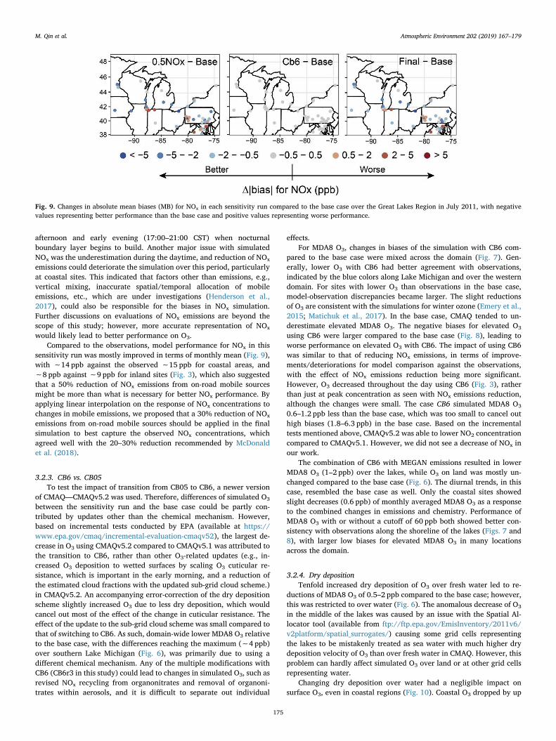
sensitivity run was mostly improved in terms of monthly mean (Fig. 9),with ∼14 ppb against the observed ∼15 ppb for coastal areas, and∼8 ppb against ∼9 ppb for inland sites (Fig. 3), which also suggestedthat a 50% reduction of NOx emissions from on-road mobile sourcesmight be more than what is necessary for better NOx performance. Byapplying linear interpolation on the response of NOx concentrations tochanges in mobile emissions, we proposed that a 30% reduction of NOx

emissions from on-road mobile sources should be applied in the finalsimulation to best capture the observed NOx concentrations, whichagreed well with the 20–30% reduction recommended by McDonaldet al. (2018).

3.2.3. CB6 vs. CB05To test the impact of transition from CB05 to CB6, a newer version

of CMAQ—CMAQv5.2 was used. Therefore, differences of simulated O3

between the sensitivity run and the base case could be partly con-tributed by updates other than the chemical mechanism. However,based on incremental tests conducted by EPA (available at https://www.epa.gov/cmaq/incremental-evaluation-cmaqv52), the largest de-crease in O3 using CMAQv5.2 compared to CMAQv5.1 was attributed tothe transition to CB6, rather than other O3-related updates (e.g., in-creased O3 deposition to wetted surfaces by scaling O3 cuticular re-sistance, which is important in the early morning, and a reduction ofthe estimated cloud fractions with the updated sub-grid cloud scheme.)in CMAQv5.2. An accompanying error-correction of the dry depositionscheme slightly increased O3 due to less dry deposition, which wouldcancel out most of the effect of the change in cuticular resistance. Theeffect of the update to the sub-grid cloud scheme was small compared tothat of switching to CB6. As such, domain-wide lower MDA8 O3 relativeto the base case, with the differences reaching the maximum (∼4 ppb)over southern Lake Michigan (Fig. 6), was primarily due to using adifferent chemical mechanism. Any of the multiple modifications withCB6 (CB6r3 in this study) could lead to changes in simulated O3, such asrevised NOx recycling from organonitrates and removal of organoni-trates within aerosols, and it is difficult to separate out individual

effects.For MDA8 O3, changes in biases of the simulation with CB6 com-

pared to the base case were mixed across the domain (Fig. 7). Gen-erally, lower O3 with CB6 had better agreement with observations,indicated by the blue colors along Lake Michigan and over the westerndomain. For sites with lower O3 than observations in the base case,model-observation discrepancies became larger. The slight reductionsof O3 are consistent with the simulations for winter ozone (Emery et al.,2015; Matichuk et al., 2017). In the base case, CMAQ tended to un-derestimate elevated MDA8 O3. The negative biases for elevated O3

using CB6 were larger compared to the base case (Fig. 8), leading toworse performance on elevated O3 with CB6. The impact of using CB6was similar to that of reducing NOx emissions, in terms of improve-ments/deteriorations for model comparison against the observations,with the effect of NOx emissions reduction being more significant.However, O3 decreased throughout the day using CB6 (Fig. 3), ratherthan just at peak concentration as seen with NOx emissions reduction,although the changes were small. The case CB6 simulated MDA8 O3

0.6–1.2 ppb less than the base case, which was too small to cancel outhigh biases (1.8–6.3 ppb) in the base case. Based on the incrementaltests mentioned above, CMAQv5.2 was able to lower NO2 concentrationcompared to CMAQv5.1. However, we did not see a decrease of NOx inour work.

The combination of CB6 with MEGAN emissions resulted in lowerMDA8 O3 (1–2 ppb) over the lakes, while O3 on land was mostly un-changed compared to the base case (Fig. 6). The diurnal trends, in thiscase, resembled the base case as well. Only the coastal sites showedslight decreases (0.6 ppb) of monthly averaged MDA8 O3 as a responseto the combined changes in emissions and chemistry. Performance ofMDA8 O3 with or without a cutoff of 60 ppb both showed better con-sistency with observations along the shoreline of the lakes (Figs. 7 and8), with larger low biases for elevated MDA8 O3 in many locationsacross the domain.

3.2.4. Dry depositionTenfold increased dry deposition of O3 over fresh water led to re-

ductions of MDA8 O3 of 0.5–2 ppb compared to the base case; however,this was restricted to over water (Fig. 6). The anomalous decrease of O3

in the middle of the lakes was caused by an issue with the Spatial Al-locator tool (available from ftp://ftp.epa.gov/EmisInventory/2011v6/v2platform/spatial_surrogates/) causing some grid cells representingthe lakes to be mistakenly treated as sea water with much higher drydeposition velocity of O3 than over fresh water in CMAQ. However, thisproblem can hardly affect simulated O3 over land or at other grid cellsrepresenting water.

Changing dry deposition over water had a negligible impact onsurface O3, even in coastal regions (Fig. 10). Coastal O3 dropped by up

Fig. 9. Changes in absolute mean biases (MB) for NOx in each sensitivity run compared to the base case over the Great Lakes Region in July 2011, with negativevalues representing better performance than the base case and positive values representing worse performance.

M. Qin et al. Atmospheric Environment 202 (2019) 167–179

175

to ∼0.5 ppb, with the largest decrease at night, which is in goodagreement with the no-dry-deposition test conducted by Vieno et al.(2010). This was likely due to efficient O3 production during the daytime so that the influence of dry deposition was suppressed. The in-sensitivity of O3 to dry deposition over fresh water can be explained bythe insignificance of dry deposition of O3 to water, which is controlledby surface resistance as O3 is not soluble (Seinfeld and Pandis, 2012).High surface resistance for O3 over water yields low dry depositionvelocity; therefore, based on the results of this sensitivity case, drydeposition accounts for a small sink of O3, and could not be responsiblefor the high biases of O3 in the Great Lakes Region.

3.3. Final simulation

The final simulation was conducted as an attempt to achieve thebest overall performance of O3 and NOx by using a combination of 30%reduction of NOx emissions from on-road mobile sources, biogenicemissions with MEGAN, and CB6 chemical mechanism. According tothe sensitivity runs, it was inferred that simulation of MDA8 O3 couldbe improved significantly compared to the base case, while elevatedMDA8 O3 might become worse as the negative biases could be evenlower across the domain, with an exception along Lake Michigan'sshoreline, where elevated MDA8 O3 was overestimated in the base case.However, neither the emissions/chemical mechanism used in the basecase nor the alternatives in each sensitivity run could achieve betterperformance for both MDA8 O3 and elevated MDA8 O3. As a result, theapproach used in the final run can be viewed as a tradeoff. One shouldnote that the meteorology that drives the CMAQ final simulation alsochanged with a different nudging option, i.e., nudging above ∼2 kminstead of nudging above the planetary boundary layer (PBL), to avoiddamping the amplitude of the nocturnal low level jet (Odman et al.,2019b).

The spatial variations of MDA8 O3 across the domain in the final runwere similar to the base case – higher O3 over the lakes with the highestconcentration near the southwestern coast of Lake Michigan (Fig. 11(a)). There was a significant decrease of O3, i.e.,∼10 ppb over southernLake Michigan, along with 4–6 ppb in a large part of the southern do-main (Fig. 6). With lower simulated O3 in the final run, the averagedconcentrations at AQS sites in inland and buffer areas were quite closeto the observations (mean biases near zero in Table 2), with NMB closeto zero. Positive biases for MDA8 O3 at coastal sites decreased as well,but the simulation remained ∼5 ppb higher than observations, with aNMB of 9%. The spatial plot (Fig. 4) showed that overestimations ofMDA8 O3 were centered along the Lake Michigan shore. Comparing theabsolute biases for MDA8 O3 at every AQS site in the two cases (baseand final) gave us an insight into whether the model performed betterin the final run than the base case. It was found that 184 out of 291 siteswithin the domain had better performance in the final run, with lower

absolute biases than in the base case (blue areas in Fig. 11 (b)), and thiswas mainly due to the decreased high biases at most sites. The im-provements were mostly found along the lakeshores and in the westernGreat Lakes Region (Fig. 7). A recent paper gave an alternative hy-pothesis for the common positive biases for surface O3 in multiple airquality models, i.e., the lack of photolysis reduction associated withfoliage and the turbulence reductions due to forest canopies (Makaret al., 2017). This could not explain the significant high biases of O3

along the shoreline in our case; however, it is worth being investigatedin future work, particularly in densely forested areas.

As expected, the final simulation produced lower elevated MDA8 O3

(> 60 ppb) than the base case. This resulted in simulations, which wereoriginally biased low, becoming more biased with respect to the ob-servations (Fig. 11 (c)). However, performance improved at some sitesalong the coast, in southwestern Ohio, and in Pennsylvania (Fig. 8),which accounted for 24% of all AQS sites across the domain. ElevatedMDA8 O3 was biased low by 3–9 ppb in the final run, with NMB rangingfrom −4 to −13%, as compared to the base case with MB of 0 to−6 ppb and NMB of 0 to −8%. Diurnal trends of O3 in the final si-mulation showed that the decrease tended to occur between10:00–17:00 CST, which was very similar to that in the case 0.5NOx,indicating that reduction of NOx emissions had a major effect on si-mulated O3 over land.

With 30% reduction of NOx emissions from on-road mobile sources,simulated NOx was ∼14 ppb at coastal sites compared to the observed∼15 ppb, and∼9 ppb in inland areas, which was almost unbiased fromthe observations (Fig. 3). Similar to the case 0.5NOx, high biases of NOx

in the early evening still existed and daytime NOx was biased low.Overall, 60% of the sites, most of which were located in the south of thedomain, had better simulation performance for NOx than the base case(Fig. 9).

3.4. Impact of lateral boundary conditions (LBCs)

One uncertainty in the simulations is that predefined default LBCsapplied in CMAQ simulations for the outer domain could bias the re-sults. An additional simulation over the 12-km domain was conducted,using LBCs that had been extracted from a GEOS-Chem simulation forJuly 2011, with other inputs or configurations being the same as thefinal run. Using the LBCs from GEOS-Chem leads to lower MDA8 O3

near the western boundary of the 12-km domain (Fig. 12 (a)). In con-trast, MDA8 O3 is higher across most of the continental US, particularlyin the high-elevation region of the intermountain west, which is drivenby higher LBCs of O3 aloft (above ∼4 km) from GEOS-Chem (Fig. S2).Compared to other regions across the US, the Midwest is less impactedby LBCs for the outer domain (the changes in simulated MDA8 O3 are inthe range of± 2 ppb).

An examination of vertical distribution of O3 in LBCs at the western

Fig. 10. Changes in O3 concentration due to tenfold increased dry deposition velocity of O3 over fresh water with respect to the base case in coastal areas over theGreat Lakes Region in July 2011.

M. Qin et al. Atmospheric Environment 202 (2019) 167–179

176

and southern boundary for the 4-km domain showed that they are al-most identical below 2 km, with significant differences in the middle toupper troposphere and stratosphere (Fig. 12 (b)). We do not expect thisto influence the surface O3 within the inner domain substantially, un-less deep convective mixing or stratospheric intrusion occurs. On theother hand, the total contributions of LBCs to surface O3 could be lessdue to efficient formation of O3 regionally in summer (Baker et al.,2015). While the impact of LBCs for the outer domain is insignificant inour 4-km resolution Great Lakes Region simulation, this might not bethe case in a different location or season, or at continental scales(Astitha et al., 2018; Hogrefe et al., 2018; Im et al., 2018; Mathur et al.,2017). Besides, using predefined O3 profiles in CMAQ could lead tosignificantly lower O3 in the middle to upper troposphere, as revealed

by a comparison of the CMAQ simulation in this work with O3 ob-servations from the ozonesonde at Egbert, Canada (Fig. S3). Therefore,we recommend using LBCs from global chemical transport models.

4. Conclusions

This study applied the CMAQ model to simulate surface O3 over theGreat Lakes Region in July 2011 at a resolution of 4 km, and evaluatedmodel performance using ground-based observations at the AQS sites.The model simulated elevated MDA8 O3 over the lakes, with the highestlevel (> 90 ppb) simulated to the southwestern side of Lake Michigan.Coastal O3 was biased high, by ∼6 ppb on average, and O3 at inlandsites (100 km further away from the shoreline) was ∼2 ppb higher than

Fig. 11. (a) Simulated MDA8 O3 in the final simulation overthe Great Lakes Region in July 2011. (b) Scatter plot of biasesfor MDA8 O3 in the final simulation against biases for MDA8O3 in the base case at the AQS sites. (c) Scatter plot of biasesfor elevated MDA8 O3 in the final simulation against biases ofelevated MDA8 O3 in the base case at the AQS sites. (d)Scatter plot of biases for NOx in the final simulation againstbiases of NOx in the base case at the AQS sites. The x axis andy axis in the scatter plots represents perfect performance(bias of zero against observations) for the final simulationand base case, respectively. The blue areas represent that thefinal simulation performed better than the base case, with thered areas showing the opposite. (For interpretation of thereferences to color in this figure legend, the reader is referredto the Web version of this article.)

Fig. 12. (a) Changes in simulated MDA8 O3 (ppb) using lateral boundary conditions (LBCs) from GEOS-Chem instead of the predefined profiles in CMAQ for the outerdomain during July 2011. The inner domain is indicated with the red box. (b) O3 LBCs at the southern and western boundary for the inner domain, derived from 12-km simulations using LBCs from GEOS-Chem (red) and the predefined profiles (blue) in CMAQ, respectively. (For interpretation of the references to color in thisfigure legend, the reader is referred to the Web version of this article.)

M. Qin et al. Atmospheric Environment 202 (2019) 167–179

177

the observations. High biases were more significant during the earlymornings (0:00–5:00 CST) and over periods when O3 was accumulating(8:00–16:00 CST). However, elevated MDA8 O3 (> 60 ppb) was biasedlow throughout the domain, with exceptions centered along the LakeMichigan shore. As such, five sensitivity runs were conducted with: 1)different biogenic emissions by using MEGAN instead of BEIS; 2) 50%reduction of NOx emissions from on-road mobile sources; 3) differentchemical mechanism (i.e., CB6 instead of CB05); 4) a combination ofMEGAN biogenic emissions and CB6 chemical mechanism instead ofBEIS emissions and CB05; and, 5) enhanced dry deposition velocity ofO3 over fresh water; to examine the role of emissions, chemistry anddeposition in the overestimation of O3 in this region.

Despite 50% higher isoprene emissions in the daytime with MEGANcompared to BEIS across the domain, simulated MDA8 O3 with MEGANemissions changed very little from the base case over a large portion ofthe domain, with the most notable enhancement over the lake(1–2 ppb) and around Pittsburgh, Pennsylvania (up to 4–5 ppb). As aresult, using MEGAN did not improve model performance on MDA8 O3,while elevated MDA8 O3 was slightly better than the base case in thesoutheastern domain. Changing O3 dry deposition to fresh water had anegligible effect on simulated O3 as well. Increasing dry deposition ofO3 over water by a factor of 10 decreased MDA8 O3 by no more than2 ppb over water, and hardly affected O3 concentrations over land.

Both the 50% reduction of NOx emissions from on-road mobilesources and using CB6 instead of CB05 led to domain-wide lower MDA8O3 than the base case. The largest decrease with CB6 (∼4 ppb) was overLake Michigan, with smaller changes over land (< 2 ppb); adjustmentof NOx emissions decreased MDA8 O3 by 2–4 ppb over the southeasterndomain and less in urban areas. Improved performance on MDA8 O3 inthese two sensitivity runs were concentrated in coastal areas and thewestern domain, where O3 was mostly biased high in the base case.Elevated MDA8 O3 was more biased than in the base case (except alongthe coast of Lake Michigan) as the original low values now became evenlower. Reduction of NOx emissions made the simulated daily peak O3

closer to the observation and suppressed the high biases of NOx around6:00 CST. The combination of MEGAN and CB6 had slightly betterperformance on O3 along the lakeshores, with noticeable improvementsof elevated MDA8 O3 along the western coast of Lake Michigan.

Based on the sensitivity tests, we recommend a 30% reduction ofNOx emissions from on-road mobile sources if the 2011 NEI is used torepresent anthropogenic emissions, as well as the use of CB6 me-chanism to simulate domain-wide lower MDA8 O3 and decrease thehigh biases across the domain. MEGAN was chosen to estimate biogenicemissions because better performance on elevated MDA8 O3 could beobtained in the coastal areas. The final simulations with these re-commendations resulted in substantial decreases of MDA8 O3, i.e.,∼10 ppb over Lake Michigan and 4–6 ppb in the southern domain.Model performance significantly improved compared to the base case atmost (∼60%) AQS sites, and this was particularly the case along LakeMichigan shoreline. Low biases for elevated O3 over a large part of thedomain were larger in the final run, however, slightly better perfor-mance than in the base case was found along Lake Michigan.Additionally, high biases for peak O3 during the daytime were alsosuppressed in inland/buffer areas primarily due to the adjustment ofNOx emissions.

This study provides a set of choices for chemical mechanism, de-position rate, and emissions to optimize O3 simulations in the GreatLakes Region with the CMAQ model. It is important to note that therecommended choices pertain to 2011, assuming that 2011 NEI is used.Besides, there are still issues with the simulations to be addressed in thefuture; for instance, high biases along the lakeshores remained andMDA8 O3 larger than 60 ppb was biased low across the domain exceptat coastal areas. O3 simulation performance over water could be af-fecting model performance along the shoreline; however, measure-ments offshore, such as ferry-based measurements available for modelevaluation, are too limited to perform an evaluation. O3 vertical

distributions would also be helpful to better understand the causes formodel overestimation and a comparison is warranted once such mea-surements in the Great Lakes Region become available. Given thatbiogenic emissions have a significant impact on simulated MDA8 O3

while evaluation of MDA8 O3 cannot reveal which emission model isbetter, biogenic VOC measurements would be extremely useful for thisregion so that a more informed choice of emission model could be madein the future.

Declaration of interests

The authors declare the following financial interests/personal re-lationships which may be considered as potential competing interests:We declared that co-author Eladio Knipping is employed by the ElectricPower Research Institute, which is one of the organizations funding thisresearch.

Acknowledgements

We are grateful to three anonymous reviewers and Dr. JamesSchauer for their constructive comments that helped us significantlyimprove the manuscript. We would like to thank Dr. Rohit Mathur forhelpful discussions on the impact of lateral boundary conditions, andDr. Tao Zeng for providing us with the GEOS-Chem simulations. Weappreciate the help from Gertrude K. Pavur for language editing. Thisresearch was funded by the Electric Power Research Institute grantnumber 10005953 and the National Aeronautics and SpaceAdministration Applied Sciences Program grant number NNX16AQ29G.The contents of the publication are solely the responsibility of thegrantee and do not necessarily represent the official views of the sup-porting agencies. Further, The USA Government does not endorse thepurchase of any commercial products or services mentioned in thepublication.

Appendix A. Supplementary data

Supplementary data to this article can be found online at https://doi.org/10.1016/j.atmosenv.2019.01.025.

References

Anderson, D.C., Loughner, C.P., Diskin, G., Weinheimer, A., Canty, T.P., Salawitch, R.J.,Worden, H.M., Fried, A., Mikoviny, T., Wisthaler, A., 2014. Measured and modeledCO and NOy in DISCOVER-AQ: an evaluation of emissions and chemistry over theeastern US. Atmos. Environ. 96, 78–87.

Astitha, M., Kioutsoukis, I., Fisseha, G.A., Bianconi, R., Bieser, J., Christensen, J.H.,Cooper, O., Galmarini, S., Hogrefe, C., Im, U., Johnson, B., Liu, P., Nopmongcol, U.,Petropavlovskikh, I., Solazzo, E., Tarasick, D.W., Yarwood, G., 2018. Seasonal ozonevertical profiles over North America using the AQMEII group of air quality models:model inter-comparison and stratospheric intrusions. Atmos. Chem. Phys. 18,13925–13945.

Baker, K.R., Emery, C., Dolwick, P., Yarwood, G., 2015. Photochemical grid model esti-mates of lateral boundary contributions to ozone and particulate matter across thecontinental United States. Atmos. Environ. 123, 49–62.

Bash, J.O., Baker, K.R., Beaver, M.R., 2016. Evaluation of improved land use and canopyrepresentation in BEIS v3. 61 with biogenic VOC measurements in California. Geosci.Model Dev. (GMD) 9, 2191.

Bosveld, F.C., Baas, P., Steeneveld, G.-J., Holtslag, A.A., Angevine, W.M., Bazile, E., deBruijn, E.I., Deacu, D., Edwards, J.M., Ek, M., 2014. The third GABLS inter-comparison case for evaluation studies of boundary-layer models. Part B: results andprocess understanding. Boundary-Layer Meteorol. 152, 157–187.

Byun, D., Schere, K.L., 2006. Review of the governing equations, computational algo-rithms, and other components of the Models-3 Community Multiscale Air Quality(CMAQ) modeling system. Appl. Mech. Rev. 59, 51–77.

Canty, T., Hembeck, L., Vinciguerra, T., Goldberg, D., Carpenter, S., Allen, D., Loughner,C., Salawitch, R., Dickerson, R., 2015. Ozone and NOx chemistry in the eastern US:evaluation of CMAQ/CB05 with satellite (OMI) data. Atmos. Chem. Phys. 15, 10965.

Carlton, A.G., Baker, K.R., 2011. Photochemical modeling of the Ozark isoprene volcano:MEGAN, BEIS, and their impacts on air quality predictions. Environ. Sci. Technol. 45,4438–4445.

Cleary, P., Fuhrman, N., Schulz, L., Schafer, J., Fillingham, J., Bootsma, H., McQueen, J.,Tang, Y., Langel, T., McKeen, S., 2015. Ozone distributions over southern LakeMichigan: comparisons between ferry-based observations, shoreline-based DOASobservations and model forecasts. Atmos. Chem. Phys. 15, 5109–5122.

Dye, T.S., Roberts, P.T., Korc, M.E., 1995. Observations of transport processes for ozone

M. Qin et al. Atmospheric Environment 202 (2019) 167–179

178

and ozone precursors during the 1991 Lake Michigan Ozone Study. J. Appl. Meteorol.34, 1877–1889.

Emery, C., Jung, J., Koo, B., Yarwood, G., 2015. Improvements to CAMx snow covertreatments and Carbon Bond chemical mechanism for winter ozone. UDAQ PO 48052000000001.

Emery, C., Liu, Z., Russell, A.G., Odman, M.T., Yarwood, G., Kumar, N., 2017.Recommendations on statistics and benchmarks to assess photochemical modelperformance. J. Air Waste Manag. Assoc. 67, 582–598.

Fahey, K.M., Carlton, A.G., Pye, H.O., Baek, J., Hutzell, W.T., Stanier, C.O., Baker, K.R.,Appel, K.W., Jaoui, M., Offenberg, J.H., 2017. A framework for expanding aqueouschemistry in the Community Multiscale Air Quality (CMAQ) model version 5.1.Geosci. Model Dev. (GMD) 10, 1587.

Fast, J.D., Heilman, W.E., 2003. The effect of lake temperatures and emissions on ozoneexposure in the western Great Lakes region. J. Appl. Meteorol. 42, 1197–1217.

Foley, T., Betterton, E.A., Jacko, P.R., Hillery, J., 2011. Lake Michigan air quality: the1994–2003 LADCO aircraft Project (LAP). Atmos. Environ. 45, 3192–3202.

Gipson, G.L., 1999. The Initial Concentration and Boundary Condition Processors. ScienceAlgorithms of the EPA Models-3 Community Multiscale Air Quality (CMAQ)Modeling System. EPA-600/R-99/030. US Environmental Protection Agency,Research Triangle Park, NC.

Guenther, A., Jiang, X., Heald, C., Sakulyanontvittaya, T., Duhl, T., Emmons, L., Wang, X.,2012. The Model of Emissions of Gases and Aerosols from Nature Version 2.1(MEGAN2. 1): an Extended and Updated Framework for Modeling BiogenicEmissions.

Hanna, S.R., Moore, G.E., Fernau, M.E., 1996. Evaluation of photochemical grid models(UAM-IV, UAM-V, and the ROM/UAM-IV couple) using data from the Lake MichiganOzone Study (LMOS). Atmos. Environ. 30, 3265–3279.

Henderson, B., Simon, H., Timin, B., Dolwick, P., Owen, R., Eyth, A., Foley, K., Toro, C.,Baker, K., Beardsley, M., Appel, K., McDonald, B., 2017. Evaluation of NOx Emissionsand Modeling, 2017 CMAS Conference. Chapel Hill, NC.

Hildebrandt Ruiz, L., Yarwood, G., 2013. Interactions between Organic Aerosol and NOy:Influence on Oxidant Production, Final Report for AQRP Project 12-012. Prepared forthe Texas Air Quality Research Program.

Hogrefe, C., Isukapalli, S.S., Tang, X., Georgopoulos, P.G., He, S., Zalewsky, E.E., Hao, W.,Ku, J.-Y., Key, T., Sistla, G., 2011. Impact of biogenic emission uncertainties on thesimulated response of ozone and fine particulate matter to anthropogenic emissionreductions. J. Air Waste Manag. Assoc. 61, 92–108.

Hogrefe, C., Liu, P., Pouliot, G., Mathur, R., Roselle, S., Flemming, J., Lin, M., Park, R.J.,2018. Impacts of different characterizations of large-scale background on simulatedregional-scale ozone over the continental United States. Atmos. Chem. Phys. 18.

Im, U., Christensen, J.H., Geels, C., Hansen, K.M., Brandt, J., Solazzo, E., Alyuz, U.,Balzarini, A., Baro, R., Bellasio, R., 2018. Influence of anthropogenic emissions andboundary conditions on multi-model simulations of major air pollutants over Europeand North America in the framework of AQMEII3. Atmos. Chem. Phys. 18,8929–8952.

Kota, S.H., Schade, G., Estes, M., Boyer, D., Ying, Q., 2015. Evaluation of MEGAN pre-dicted biogenic isoprene emissions at urban locations in Southeast Texas. Atmos.Environ. 110, 54–64.

Lelieveld, J., Dentener, F.J., 2000. What controls tropospheric ozone? J. Geophys. Res.:Atmosphere 105, 3531–3551.

Lennartson, G.J., Schwartz, M.D., 2002. The lake breeze–ground‐level ozone connectionin eastern Wisconsin: a climatological perspective. Int. J. Climatol. 22, 1347–1364.

Levy, I., Makar, P., Sills, D., Zhang, J., Hayden, K., Mihele, C., Narayan, J., Moran, M.,Sjostedt, S., Brook, J., 2010. Unraveling the complex local-scale flows influencingozone patterns in the southern Great Lakes of North America. Atmos. Chem. Phys. 10,10895–10915.

Li, J., Mao, J., Min, K.E., Washenfelder, R.A., Brown, S.S., Kaiser, J., Keutsch, F.N.,Volkamer, R., Wolfe, G.M., Hanisco, T.F., 2016. Observational constraints on glyoxalproduction from isoprene oxidation and its contribution to organic aerosol over theSoutheast United States. J. Geophys. Res.: Atmosphere 121, 9849–9861.

Lin, J.-T., Youn, D., Liang, X.-Z., Wuebbles, D.J., 2008. Global model simulation ofsummertime US ozone diurnal cycle and its sensitivity to PBL mixing, spatial re-solution, and emissions. Atmos. Environ. 42, 8470–8483.

Makar, P., Gong, W., Mooney, C., Zhang, J., Davignon, D., Samaali, M., Moran, M., He, H.,Tarasick, D., Sills, D., 2010a. Dynamic adjustment of climatological ozone boundaryconditions for air-quality forecasts. Atmos. Chem. Phys. 10, 8997–9015.

Makar, P., Staebler, R., Akingunola, A., Zhang, J., McLinden, C., Kharol, S., Pabla, B.,Cheung, P., Zheng, Q., 2017. The effects of forest canopy shading and turbulence onboundary layer ozone. Nat. Commun. 8, 15243.

Makar, P., Zhang, J., Gong, W., Stroud, C., Sills, D., Hayden, K., Brook, J., Levy, I., Mihele,C., Moran, M., 2010b. Mass tracking for chemical analysis: the causes of ozone for-mation in southern Ontario during BAQS-Met 2007. Atmos. Chem. Phys. 10, 11151.

Mathur, R., Xing, J., Gilliam, R., Sarwar, G., Hogrefe, C., Pleim, J., Pouliot, G., Roselle, S.,Spero, T.L., Wong, D.C., 2017. Extending the Community Multiscale Air Quality(CMAQ) modeling system to hemispheric scales: overview of process considerationsand initial applications. Atmos. Chem. Phys. 17, 12449.

Matichuk, R., Tonnesen, G., Luecken, D., Gilliam, R., Napelenok, S.L., Baker, K.R.,Schwede, D., Murphy, B., Helmig, D., Lyman, S.N., 2017. Evaluation of the com-munity Multiscale Air quality model for simulating winter ozone formation in theuinta basin. J. Geophys. Res.: Atmosphere 122 (13) 545-513,572.

McDonald, B., McKeen, S., Cui, Y.Y., Ahmadov, R., Kim, S.-W., Frost, G.J., Pollack, I.,Peischl, J., Ryerson, T.B., Holloway, J., 2018. Modeling ozone in the eastern US usinga fuel-based mobile source emissions inventory. Environ. Sci. Technol. 52,7360–7370.

McNider, R.T., Pour-Biazar, A., Doty, K., White, A., Wu, Y., Qin, M., Hu, Y., Odman, M.T.,Cleary, P., Knipping, E., Dornblaser, B., Lee, P., Hain, C., Mckeen, S., 2018.Examination of the physical atmosphere in the Great lakes region and its potentialimpact on air quality— overwater stability and satellite assimilation. Journal ofApplied Meteorology and Climatology 57, 2789–2816.

Odman, M.T., Qin, M., Hu, Y., Russell, A.G., Boylan, J.W., 2019a. 2017 projections andinterstate transport of ozone in the southeastern United States. J. Environ. Manag(submitted).

Odman, M.T., White, A.T., Doty, K., McNider, R.T., Pour-Biazar, A., Qin, M., Hu, Y.,Knipping, E., Wu, Y., Dornblaser, B., 2019b. Examination of the physical atmospherein the Great lakes region and its potential impact on air quality: FDDA strategies.Journal of Applied Meteorology and Climatology (revisions submitted).

Park, R., Hong, S.K., Kwon, H.-A., Kim, S., Guenther, A., Woo, J.-H., Loughner, C., 2014.An evaluation of ozone dry deposition simulations in East Asia. Atmos. Chem. Phys.14, 7929–7940.

Pleim, J.E., Gilliam, R., 2009. An indirect data assimilation scheme for deep soil tem-perature in the Pleim–Xiu land surface model. Journal of Applied Meteorology andClimatology 48, 1362–1376.

Pleim, J.E., Xiu, A., 2003. Development of a land surface model. Part II: data assimilation.J. Appl. Meteorol. 42, 1811–1822.

Pouliot, G., Pierce, T., 2009. Integration of the model of emissions of Gases and aerosolsfrom nature (MEGAN) into the CMAQ modeling system. In: 18th InternationalEmission Inventory Conference, Baltimore, Maryland, pp. 14–17.

Pour Biazar, A., McNider, R.T., Doty, K., White, A., Wu, Y., Qin, M., Hu, Y., Odman, M.T.,Dornblaser, B., Cleary, P., Knipping, E., McKeen, S., Lee, P., 2018. In: MultiyearModel Evaluation over Lake Michigan Region. 2018 CMAS Conference. ChapelHill, NC.

Pugliese, S., Murphy, J., Geddes, J., Wang, J., 2014. The impacts of precursor reductionand meteorology on ground-level ozone in the Greater Toronto Area. Atmos. Chem.Phys. 14, 8197–8207.

Sarwar, G., Gantt, B., Schwede, D., Foley, K., Mathur, R., Saiz-Lopez, A., 2015. Impact ofenhanced ozone deposition and halogen chemistry on tropospheric ozone over theNorthern Hemisphere. Environ. Sci. Technol. 49, 9203–9211.

Savijärvi, H., 2009. Stable boundary layer: parametrizations for local and larger scales. Q.J. R. Meteorol. Soc. 135, 914–921.

Seinfeld, J.H., Pandis, S.N., 2012. Atmospheric Chemistry and Physics: from Air Pollutionto Climate Change.

Sills, D., Brook, J., Levy, I., Makar, P., Zhang, J., Taylor, P., 2011. Lake breezes in thesouthern Great Lakes region and their influence during BAQS-Met 2007. Atmos.Chem. Phys. 11, 7955–7973.

Simon, H., Baker, K.R., Phillips, S., 2012. Compilation and interpretation of photo-chemical model performance statistics published between 2006 and 2012. Atmos.Environ. 61, 124–139.

Simon, H., Valin, L.C., Baker, K.R., Henderson, B.H., Crawford, J.H., Pusede, S.E., Kelly,J.T., Foley, K.M., Owen, R.C., Cohen, R.C., 2018. Characterizing CO and NOy sourcesand relative ambient ratios in the baltimore area using ambient measurements andsource attribution modeling. J. Geophys. Res.: Atmosphere 123, 3304–3320.

Sindelarova, K., Granier, C., Bouarar, I., Guenther, A., Tilmes, S., Stavrakou, T., Müller, J.-F., Kuhn, U., Stefani, P., Knorr, W., 2014. Global data set of biogenic VOC emissionscalculated by the MEGAN model over the last 30 years. Atmos. Chem. Phys. 14,9317–9341.

Skamarock, W.C., Klemp, J.B., Dudhia, J., Gill, D.O., Barker, D.M., Wang, W., Powers,J.G., 2005. A Description of the Advanced Research WRF Version 2. National Centerfor Atmospheric Research Boulder Co Mesoscale and Microscale Meteorology Div.

Souri, A.H., Choi, Y., Jeon, W., Li, X., Pan, S., Diao, L., Westenbarger, D.A., 2016.Constraining NOx emissions using satellite NO2 measurements during 2013DISCOVER-AQ Texas campaign. Atmos. Environ. 131, 371–381.

Stanier, C., Abdioskouei, M., Carmichael, G., Christiansen, M., Sobhani, N., 2017.Meteorological Air Quality Forecasting Using the WRF-Chem Model during theLMOS2017 Field Campaign. AGU Fall Meeting Abstracts.

Stoeckenius, T., McNally, D., 2014. Final Report 2013 Unita Basin Winter Ozone Study.ENVIRON International Corporation, Novato, California.

Travis, K.R., Jacob, D.J., Fisher, J.A., Kim, P.S., Marais, E.A., Zhu, L., Yu, K., Miller, C.C.,Yantosca, R.M., Sulprizio, M.P., 2016. Why do models overestimate surface ozone inthe Southeast United States? Atmos. Chem. Phys. 16, 13561–13577.

United States Environmental Protection Agency (US EPA), 2018. National Map of Ozone(2008) Nonattainment Areas. https://www3.epa.gov/airquality/greenbook/map8hr_2008.html.

Vieno, M., Dore, A., Stevenson, D.S., Doherty, R., Heal, M.R., Reis, S., Hallsworth, S.,Tarrason, L., Wind, P., Fowler, D., 2010. Modelling surface ozone during the 2003heat-wave in the UK. Atmos. Chem. Phys. 10, 7963–7978.

Wentworth, G., Murphy, J., Sills, D., 2015. Impact of lake breezes on ozone and nitrogenoxides in the Greater Toronto Area. Atmos. Environ. 109, 52–60.

Wesely, M., 1989. Parameterization of surface resistances to gaseous dry deposition inregional-scale numerical models. Atmos. Environ. 23 (1967), 1293–1304.

Wyat Appel, K., Napelenok, S., Hogrefe, C., Pouliot, G., Foley, K.M., Roselle, S.J., Pleim,J.E., Bash, J., Pye, H.O.T., Heath, N., Murphy, B., Mathur, R., 2018. Overview andEvaluation of the Community Multiscale Air Quality (CMAQ) Modeling SystemVersion 5.2. Springer International Publishing, Cham, pp. 69–73.

Yarwood, G., Heo, G., Carter, W., Whitten, G., 2012. Environmental ChamberExperiments to Evaluate NOx Sinks and Recycling in Atmospheric ChemicalMechanisms. Final Report, Prepared for Dr. Elena C. McDonald-Buller, Texas AirQuality Research Program. The University of Texas at Austin, AQRP Project, pp.10–042.

Yarwood, G., Jung, J., Whitten, G.Z., Heo, G., Mellberg, J., Estes, M., 2010. Updates to theCarbon Bond Mechanism for Version 6 (CB6), 2010 CMAS Conference. Chapel Hill,NC. October. http://www.cmascenter.org/conference/2010/abstracts/emery_updates_carbon_2010.pdf.

Yu, H., Guenther, A., Gu, D., Warneke, C., Geron, C., Goldstein, A., Graus, M., Karl, T.,Kaser, L., Misztal, P., 2017. Airborne measurements of isoprene and monoterpeneemissions from southeastern US forests. Sci. Total Environ. 595, 149–158.

Zhang, R., Cohan, A., Biazar, A.P., Cohan, D.S., 2017. Source apportionment of biogeniccontributions to ozone formation over the United States. Atmos. Environ. 164, 8–19.

M. Qin et al. Atmospheric Environment 202 (2019) 167–179

179