Atmos. Chem. Phys., 15, 829–843, 2015

www.atmos-chem-phys.net/15/829/2015/

doi:10.5194/acp-15-829-2015

© Author(s) 2015. CC Attribution 3.0 License.

Sunset–sunrise difference in solar occultation ozone measurements

(SAGE II, HALOE, and ACE–FTS) and its relationship to

tidal vertical winds

T. Sakazaki1, M. Shiotani1, M. Suzuki2, D. Kinnison3, J. M. Zawodny4, M. McHugh5, and K. A. Walker6

1Research Institute for Sustainable Humanosphere, Kyoto University, Uji, Japan2Institute of Space and Astronautical Science, Japan Aerospace Exploration Agency, Sagamihara, Japan3National Center for Atmospheric Research, Boulder, USA4NASA Langley Research Center, Hampton, USA5Global Atmospheric Technologies and Sciences, Newport News, USA6Department of Physics, University of Toronto, Toronto, Canada

Correspondence to: T. Sakazaki (takatoshi_sakazaki@rish.kyoto-u.ac.jp)

Received: 9 May 2014 – Published in Atmos. Chem. Phys. Discuss.: 18 June 2014

Revised: 27 October 2014 – Accepted: 9 December 2014 – Published: 23 January 2015

Abstract. This paper contains a comprehensive investiga-

tion of the sunset–sunrise difference (SSD, i.e., the sunset-

minus-sunrise value) of the ozone mixing ratio in the lat-

itude range of 10◦ S–10◦ N. SSD values were determined

from solar occultation measurements based on data ob-

tained from the Stratospheric Aerosol and Gas Experiment

(SAGE) II, the Halogen Occultation Experiment (HALOE),

and the Atmospheric Chemistry Experiment–Fourier trans-

form spectrometer (ACE–FTS). The SSD was negative at al-

titudes of 20–30 km (−0.1 ppmv at 25 km) and positive at

30–50 km (+0.2 ppmv at 40–45 km) for HALOE and ACE–

FTS data. SAGE II data also showed a qualitatively simi-

lar result, although the SSD in the upper stratosphere was

2 times larger than those derived from the other data sets.

On the basis of an analysis of data from the Superconduct-

ing Submillimeter-Wave Limb-Emission Sounder (SMILES)

and a nudged chemical transport model (the specified dy-

namics version of the Whole Atmosphere Community Cli-

mate Model: SD–WACCM), we conclude that the SSD can

be explained by diurnal variations in the ozone concentra-

tion, particularly those caused by vertical transport by the at-

mospheric tidal winds. All data sets showed significant sea-

sonal variations in the SSD; the SSD in the upper strato-

sphere is greatest from December through February, while

that in the lower stratosphere reaches a maximum twice: dur-

ing the periods March–April and September–October. Based

on an analysis of SD–WACCM results, we found that these

seasonal variations follow those associated with the tidal ver-

tical winds.

1 Introduction

Stratospheric ozone (O3) plays a critical role in the cli-

mate system through radiative processes while simultane-

ously protecting the Earth’s surface from harmful ultravio-

let radiation. Since the discovery of the ozone hole, long-

term changes in ozone concentration have been studied ex-

tensively using various ground-based and satellite measure-

ments (WMO, 2011). Useful data sets for long-term mon-

itoring of vertical profiles of ozone levels can be obtained

from solar occultation instruments, such as the Stratospheric

Aerosol and Gas Experiment (SAGE) II (McCormick, 1987;

McCormick et al., 1989), the Halogen Occultation Ex-

periment (HALOE) (Russell et al., 1993), and the Atmo-

spheric Chemistry Experiment–Fourier transform spectrom-

eter (ACE–FTS) (Bernath et al., 2005), as they have mea-

surements that are self-calibrating and have high sensitiv-

ity. These measurements have been used to detect seasonal

and interannual variability, as well as long-term trends, in the

stratospheric ozone concentration (e.g., Shiotani and Hasebe,

1994; Randell and Wu, 1996; Newchurch et al., 2003; WMO

2011; Kyrölä et al., 2013).

Published by Copernicus Publications on behalf of the European Geosciences Union.

830 T. Sakazaki et al.: Sunset–sunrise difference in solar occultation ozone measurements

These solar occultation instruments measure the atmo-

sphere at sunrise and sunset (hereafter SR and SS). It has

been reported that there is a difference in the observed val-

ues between the SR and SS profiles (hereafter this is referred

to as the sunset-minus-sunrise difference, SSD). For SAGE

II, the SSD is reported to be up to 10 % between altitudes of

35 and 55 km, with a maximum occurring in the tropics (cf.

SAGE II version 5.9 data: Wang et al., 1996; version 6.2 data:

McLinden et al., 2009; version 7 data: Kyrölä et al., 2013).

For HALOE (version 17 data), Brühl et al. (1996) reported an

SSD of approximately 5 % in the tropical stratopause. SSD

values based on ACE–FTS observations have yet to be re-

ported as far as we know.

A quantification of the SSD and an understanding of the

source of this difference are necessary for the construction

of combined data sets from SR and SS profiles. As we will

explore in this study, the SSD could be caused by any one of

three factors, including (1) systematic instrumental/retrieval

bias between SR and SS observations, (2) natural diurnal

variations, and (3) sampling issues. The factor (3) relates to

the fact that if the times of SR and SS measurements are

considerably different, the background ozone concentration

changes (background changes occur on timescales longer

than a day, e.g., in the case of subseasonal variations) dur-

ing such periods are misinterpreted as an example of SSD

(see Sect. 3 for details). In this sense, such spurious contri-

butions, or contamination, should be assessed and removed

before discussing the SSD.

In previous studies, the ozone SSD was mainly attributed

to factor (1); in other words, factor (2) was thought to be

negligible (Wang et al., 1996; Brühl et al., 1996). This was

because diurnal variations in stratospheric ozone level were

considered to be small and/or to be symmetric between SS

and SR if only photochemistry processes are taken into ac-

count. However, note that there are few observations of diur-

nal variations in the stratosphere and thus the above assump-

tion has not been confirmed. In addition, factor (3) may not

have been properly considered in some studies (e.g., in the

context of interannual variations of the SSD, as shown by

Kyrölä et al., 2013; see Sect. 3).

Recently, Sakazaki et al. (2013a; hereafter S13) revealed

diurnal variations in ozone concentration from the lower to

upper stratosphere using data from both the Superconduct-

ing Submillimeter-Wave Limb-Emission Sounder (SMILES)

and chemical transport models (CTMs). They showed that

the peak-to-peak difference in ozone levels reaches 8 % dur-

ing a day. An important point here is that, at some altitudes,

the diurnal variations exhibit asymmetric ozone levels when

comparing measurements at SS and SR, with the SSD reach-

ing around 4 % in the upper stratosphere. S13 showed that

the diurnal variations ([O3]′) are largely controlled by the

following equation:

∂[O3]′

∂t=−w′

∂[O3]

∂z+ S′, (1)

where t represents time, w′ the diurnal variations in the ver-

tical winds (tidal vertical winds), z altitude, [O3] the daily,

zonal mean ozone, and S′ the diurnal variations in chemi-

cal production or loss. The first term on the right-hand side

denotes the dynamical variation due to vertical transport by

atmospheric tidal winds, while the second term denotes the

photochemical variation. It should be noted that the dynam-

ical variation results in a maximum at 18:00–20:00 local

time (LT) in the upper stratosphere (and at 00:00–06:00 LT

in the lower stratosphere; cf. Fig. 7d of S13), possibly caus-

ing a positive (negative) SSD. In contrast, although the pho-

tochemical variations are also important above an altitude of

30 km during the daytime, they are almost zero at SR–SS (see

Fig. 7b of S13) and so do not contribute to the SSD. This has

already been demonstrated and discussed in previous studies

(e.g., Pallister and Tuck, 1984; Wang et al., 1996; Brühl et al.,

1996). For the tropical mesosphere and lower thermosphere,

Marsh and Russell (2000) used HALOE data to attribute the

SSD of nitric oxide (NO) to diurnal variations caused by tidal

vertical transport.

With regard to tides, the diurnal migrating tide (i.e., the di-

urnal harmonic component, which depends only on the LT of

a particular latitude band and not on longitude) is basically

dominant over other higher-order harmonics in the tropical

stratosphere. Vertical winds associated with the diurnal mi-

grating tide become maximal in the tropics, so that diurnal

variations in ozone levels caused by vertical transport also

reach a maximum in the tropics (see Fig. 8 of S13). In the

tropical stratosphere, the diurnal migrating tide is known to

exhibit a significant seasonal dependence, with its amplitude

reaching a peak in January–February and July–September, as

seen in satellite-based temperature measurements (e.g., Wu

et al., 1998; Zeng et al., 2008; Huang et al., 2010; Sakazaki

et al., 2012). These findings suggest that the tidal vertical

winds and, consequently, the SSD also show similar seasonal

variations. Note that the tidal vertical wind is relatively diffi-

cult to observe directly because of its rather small amplitude.

We suggest that in the presence of vertical gradient of ozone,

the SSD pertaining to the ozone levels could be used to ob-

tain quasi-observational evidence of tidal vertical winds in

the tropical stratosphere.

As outlined above, SSDs have been noticed but they were

considered independently for each occultation instrument. In

addition, they have not been investigated fully in terms of

diurnal ozone variations. The purpose of this study is first

to quantify the SSD, including its seasonal dependence, by

analyzing and comparing data from three independent solar

occultation instruments: SAGE II, HALOE, and ACE–FTS.

The differences among the data sets due to differences in

measurement times are discussed with the aid of CTM data

(from the specified dynamics version of the Whole Atmo-

sphere Community Climate Model: SD–WACCM), which

provide a homogeneous data set covering the full operational

periods of each of the three satellite missions. Next, we inter-

pret the SSD in terms of diurnal variations based on SMILES

Atmos. Chem. Phys., 15, 829–843, 2015 www.atmos-chem-phys.net/15/829/2015/

T. Sakazaki et al.: Sunset–sunrise difference in solar occultation ozone measurements 831

measurements and 3-hourly, 3-D-gridded SD–WACCM data,

which provide data not only at SR–SS but also for the full

diurnal cycle. The 3-D-gridded SD–WACCM data are also

used to discuss diurnal variations related to vertical transport

and photochemistry. This study focuses on the tropical strato-

sphere at latitudes of 10◦ S–10◦ N between 20 and 60 km in

altitude because the SSD is greatest in the tropics. The re-

mainder of this article is organized as follows: Sects. 2 and

3 describe the data sets and analysis methods, respectively.

Section 4 describes the SSD and its seasonal variations, and

we also discuss the contribution from diurnal ozone varia-

tions. Section 5 summarizes our main results.

2 Data description

In this study, the average SSD in the tropical stratosphere

within the latitude range 10◦ S–10◦ N is analyzed and dis-

cussed using data from three solar occultation instruments:

SAGE II, HALOE, and ACE–FTS. To quantify the SSD

caused by natural diurnal variations in ozone concentration,

data from SMILES limb emission measurements are also

analyzed. In addition, two data sets from SD–WACCM are

used: the satellite coincidence data subset and the full 3-

hourly, 3-D-gridded data. The former is used to discuss the

difference in SSD among the different satellite data sets,

while the latter is used to consider the SSD in terms of di-

urnal variations. All data are analyzed at geometric altitudes

in the stratosphere between 20 and 60 km.

Note that there is no systematic difference in the tracking

procedure between SR and SS. SAGE II tracks the Sun by

moving the field of view (FOV) across the solar disk. As the

FOV went off the edge of the Sun, the scan mirror reverses

direction. HALOE tracks the top edge of the Sun, with the

science FOV held a fixed angle below this. Extensive SR–

SS comparisons have been carried out over the 14-year mea-

surement record and no significant bias in tracking is per-

ceivable. The ACE–FTS is aligned by a tracking system that

keeps it pointed at the radiometric center of the Sun. While

there might exist a very small difference between SR and SS

tracking, this has been examined carefully and no significant

SR–SS bias exists. Further details are provided in the follow-

ing subsections.

2.1 SAGE II

The SAGE mission has deployed three instruments, i.e.,

SAGE I, II, and III. This study uses data from SAGE II be-

cause these measurements cover the longest period. SAGE

II was launched in October 1984 on board the Earth Radia-

tion Budget Satellite (ERBS) and remained operational until

August 2005, providing data for over 21 years. The ERBS

operated in a 610 km altitude, circular orbit with an inclina-

tion of 56◦. SAGE II is a seven-channel spectrometer capable

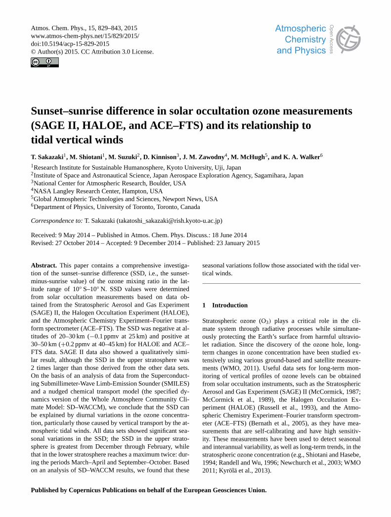
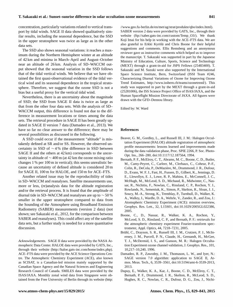
Figure 1. Measurement tracks of (a) SAGE II in 1992, (b) HALOE

in 1992, and (c) ACE–FTS in 2005. Red and blue closed circles

show SR and SS measurements, respectively. Open stars indicate

SR–SS measurement pairs. Dashed lines denote 10◦ S/N.

of obtaining ozone levels from measurements in the 600 nm

Chappuis band (McCormick et al., 1987, 1989).

Figure 1a shows the SAGE II measurement locations ob-

tained in 1992. The latitude coverage ranges from 80◦ S to

80◦ N. SAGE II performed two occultation measurements

per orbit, sampling two narrow latitude regions each day.

As a result, for each day up to 15 SR and 15 SS profiles

were obtained near the same latitude regions but spaced some

24◦ apart in longitude. Approximately 10 times per year, the

tracks of the SR and SS measurements crossed over. The

sampling pattern (i.e., the measurement day of the year at a

particular latitude) changed gradually from year to year and

so covers the whole year when data are collected for several

years.

We analyzed SAGE II version 7 data (Damaedo et al.,

2013) obtained during the period 1985–2005. Data were pro-

vided for geometric altitudes between 0 and 70 km at inter-

vals of 0.5 km. Geometric altitudes were determined by the

viewing geometry with the aid of data from the Modern-

Era Retrospective Analysis for Research and Applications

(MERRA) reanalysis (Rienecker et al., 2011). The uncer-

tainty in altitude registration is less than 20 m (Damaedo

et al., 2013). Ozone mixing ratio is calculated as the ra-

tio of ozone number density to atmospheric density, both of

which are provided in SAGE II data. The atmospheric den-

sity is not measured by SAGE II but derived from MERRA

data; however, the results of SSD (%) (cf. Fig. 5b) do not

change even if the following analysis is done based on ozone

number density. Prior to our detailed analysis, data were

screened following the guidelines provided in the SAGE II

version 7 readme file (https://eosweb.larc.nasa.gov/project/

www.atmos-chem-phys.net/15/829/2015/ Atmos. Chem. Phys., 15, 829–843, 2015

832 T. Sakazaki et al.: Sunset–sunrise difference in solar occultation ozone measurements

sage2/sage2_release_v7_notes) as follows. Any profile with

an error estimate larger than 10 % at altitudes between 30 and

50 km was rejected. Data points with an uncertainty estimate

of 300 % or greater were rejected. Data points at the altitude

of and below the occurrence of an aerosol extinction value

greater than 0.006 km−1 were rejected. Data points at the al-

titude of and below the occurrence of both the 525 nm aerosol

extinction value exceeding 0.001 km−1 and the 525/1020 ex-

tinction ratio of less than 1.4 were rejected. Data points per-

taining to altitudes below 35 km with an uncertainty esti-

mate of 200 % (or larger) were rejected. On the basis of this

screening process, 3.9 % and 5.6 % of all profiles were re-

jected for the times of SR and SS, respectively.

2.2 HALOE

HALOE was launched in September 1991 on board the Up-

per Atmosphere Research Satellite (UARS) and remained

operational until November 2005, providing data over 15

years. UARS was placed in a 585 km circular orbit with

an inclination of 57◦ (Russell et al., 1993). Its ozone mea-

surements were made at mid-infrared (mid-IR) wavelengths

(9.6 µm).

The HALOE measurement locations during 1992 are

shown in Fig. 1b. The latitude coverage was approximately

80◦ S–80◦ N. The instruments measured up to 15 SR and 15

SS profiles each day. Approximately 10 times per year, the

tracks of the SR and SS measurements crossed over. As with

SAGE II, the sampling pattern of HALOE changed gradually

from year to year.

We analyzed HALOE version 19 data obtained over the

period 1991–2005 (e.g., Randall et al., 2003). Data were

provided at 271 pressure levels, i.e., 1000× 10−(i−1)/30 hPa

(i = 1,2, . . . , 271), between 1000 and 10−6 hPa, with a cor-

responding vertical spacing of approximately 0.5 km. Geo-

metric altitudes were also provided in relation to the pressure

levels for each profile so that we mapped ozone mixing ra-

tio data onto geometric altitude levels between 0 and 70 km,

with a spacing of 0.5 km. No screening was performed on the

HALOE data.

HALOE profiles are registered in altitude in an iterative

fashion, and the resulting registration is generally assessed

to be better than 100 m (McHugh et al., 2003, 2005). Ini-

tially, the data are placed on an altitude grid based on the

HALOE measurements versus zenith angle. A first pressure

registration is performed using the measured transmittance

profile from the 2.8 µm channel (dominated by CO2 absorp-

tion). In this process, the altitude grid is shifted to best match

simulated transmittances in the 30 to 45 km altitude range,

assuming the temperature profile from the National Center

for Environmental Prediction (NCEP) reanalysis (Beaver et

al., 1994; Remsberg et al., 2002; see Kalnay et al., 1996

for NCEP reanalysis). Temperatures and corresponding hy-

drostatic pressures are then retrieved in an iterative upward

fashion from 30 km at 1.5 km spacing. Finally the retrieved

T(p) profile is merged into the NCEP profile from 34 (pure

NCEP) to 43 km (pure HALOE retrieval). Pressures are cal-

culated assuming hydrostatic balance. This entire process is

repeated again after retrieval of water vapor and finally after

a retrieval of aerosols to account for all significant interfering

absorption in the 2.8 µm CO2 channel.

2.3 ACE–FTS

ACE–FTS was launched in August 2003 on board the

SCISAT-1 satellite. SCISAT-1 is operating in a circular, low-

Earth orbit, with a 74◦ inclination and an altitude of 650 km

(Bernath et al., 2005). ACE–FTS measures ozone at IR wave-

lengths (9.6 µm).

Figure 1c shows the ACE–FTS measurement locations

during 2005. The latitude coverage is approximately 85◦ S–

85◦ N. The instruments measure up to 15 SR and 15 SS pro-

files each day. Approximately six times per year, the tracks

of the SR and SS measurements cross over. Unlike SAGE

II and HALOE, however, the sampling pattern changes little

from year to year. Thus, data for 10◦ S–10◦ N are obtained

only in February, April, August, and October of each year

(see Fig. 1c).

We analyzed the most recent data, version 3 (Dupuy et

al., 2009; Waymark et al., 2013), obtained between 2004 and

2011. Data were provided at geometric altitudes from 0 to

140 km, with a spacing of 1 km. Some of the data obtained

during this period had measurement problems and were not

used based on the recommendations from the ACE–FTS data

issues list (https://databace.scisat.ca/validation/data_issues.

php).

Altitudes in ACE–FTS measurements are defined as fol-

lows (see Boone et al., 2005 for details). At low altitudes (be-

low ∼ 42 km), pointing information from the satellite is rela-

tively poor and the pointing is quite variable, with refraction

effects plus clouds and aerosols affecting the instrument’s

pointing. Therefore, geometry is derived through analysis of

the ACE–FTS spectra. CO2 volume mixing ratio is fixed to

its “known” profile, and then CO2 lines are analyzed to de-

termine pressure and temperature. Hydrostatic equilibrium

is used to express the altitude separations between measure-

ments in terms of pressure and temperature during the re-

trieval, so geometry is determined simultaneously. At high al-

titudes (above 60–65 km), geometry is relatively well known

from first principles (i.e., given the knowledge of the loca-

tion of the satellite and the look direction to the Sun at a given

time, one can calculate the pointing information). In the mid-

dle (42–60 km), CO2 VMR is still “known” and geometry is

known. This region allows us to determine the pressure at the

“crossover” point (near 42 km) to be used in the calculation

of altitude at low altitudes (below ∼ 43 km) via hydrostatic

equilibrium. A final altitude registration is performed using

the Canadian Meteorological Centre model output at the low-

est altitudes (∼ 15–25 km). The uncertainty on altitude regis-

tration for the ACE–FTS is 150 m.

Atmos. Chem. Phys., 15, 829–843, 2015 www.atmos-chem-phys.net/15/829/2015/

T. Sakazaki et al.: Sunset–sunrise difference in solar occultation ozone measurements 833

2.4 SMILES

SMILES was attached to the Japanese Experiment Module

(JEM) on board the International Space Station (ISS) through

the cooperation of the Japan Aerospace Exploration Agency

(JAXA) and the National Institute of Information and Com-

munications Technology (NICT). The ISS is in a circular or-

bit at a typical altitude between 350 and 400 km, with an

inclination of 51.6◦. Its latitude coverage is 38◦ S–65◦ N.

SMILES measured the Earth’s limb and made global obser-

vations of the minor constituents in the middle atmosphere

in the 600 GHz range between 12 October 2009 and 21 April

2010 (Kikuchi et al., 2010). Unlike the solar occultation mea-

surements (SAGE II, HALOE, and ACE–FTS), limb emis-

sion measurements are made continuously following the or-

bit track, not only at SR and SS but also throughout the day

and night. As a result, two data sets for ascending and de-

scending nodes are obtained every day in each latitude band.

In addition, the ISS is not in a Sun-synchronous orbit, and

its orbital plane rotates every 60 days; consequently, a full

diurnal cycle in the tropics is covered in 30 days by the as-

cending/descending nodes.

For SMILES, we defined the SS and SR profiles as those

characterized by solar zenith angles between 80 and 100◦.

Note, again, that SMILES measurements cover the full diur-

nal cycle as well as during SS and SR. Thus, the SSD related

to diurnal variations in ozone level can be calculated. With

regard to the quality of ozone data from SMILES, Imai et

al. (2013a) compared the ozone concentration profiles from

the SMILES version 2.1 data set with those from five satel-

lite measurements and two CTMs (including SD–WACCM),

and found that in the stratosphere the agreement was gener-

ally better than 10 %. Imai et al. (2013b) compared the ozone

concentrations profiles from the SMILES version 2.3 data set

with those from worldwide ozonesonde stations and found

that the agreement was between 6 and 15 % for 20–26 km at

low latitudes; part of this difference was attributed to issues

related to the ozonesonde measurement system.

In this study, version 2.4 data were analyzed

(JEM/SMILES L2 Products Guide for version 2.4: http:

//smiles.tksc.jaxa.jp/l2data/pdf/L2dataGuide_130703.pdf).

Data were provided at geometric altitudes between 8 and

118 km with a vertical spacing of 2 km (below 58 km) or

3 km (above 58 km). By updating the screening conditions,

the number of retrieved profiles in version 2.4 was signif-

icantly larger than that in version 2. We did not find any

significant differences in diurnal variation between versions

2.4 and 2 (which was used by S13). For stratospheric

diurnal variations in the SMILES data, Parrish et al. (2013)

found good agreement with the results from ground-based

microwave measurements at Mauna Loa (19.5◦ N, 204.5◦ E),

as well as those from the Microwave Limb Sounder onboard

the UARS and Aura satellites.

SMILES does not measure geometric altitude, so that

temperature (from SMILES below ∼ 40 km and from SD–

WACCM above ∼ 40 km for version 2.4) and pressure (from

SMILES) are used to calculate the “relative” altitudes from

some pressure level with the hydrostatic equilibrium assump-

tion. For deriving the “absolute” altitude, pressure at 30 km

from SD–WACCM output is used (for version 2.4) (C. Mit-

suda, personal communication). The uncertainty in altitude

registration for SMILES is considered to be in the same or-

der as that for other data sets. Note that there is no systematic

difference in the altitude registration between SR and SS.

2.5 SD–WACCM

The NCAR WACCM version 4 (WACCM4) is a comprehen-

sive numerical model spanning the range of altitude from the

Earth’s surface to the thermosphere (Garcia et al., 2007; Kin-

nison et al., 2007; Marsh et al., 2013). WACCM4 is based

on the framework of the NCAR Community Atmosphere

Model version 4 (CAM4) and includes all of the physical

parameterizations of CAM4 (Neale et al., 2013) and a fi-

nite volume dynamical core (Lin, 2004) for the tracer advec-

tion. A version of WACCM4 has been developed that allows

the model to be run with specified (external) meteorologi-

cal fields (Kunz et al., 2011). Here SD–WACCM is a CTM

that nudges WACCM4 temperature, horizontal winds, and

surface pressure towards 6-hourly time series from MERRA

reanalysis (Rienecker et al., 2011) below 50 km. The CTM

data were constrained by meteorological conditions with an

hourly timescale so that they could be directly compared

with our observational data. Note that the stratospheric ozone

concentration and its diurnal variations in the SD–WACCM

data have been analyzed and that the results agreed well with

those based on the SMILES data (Imai et al., 2013a; S13).

The horizontal resolution used was 2.5◦ in longitude and

1.9◦ in latitude, and the model time step was 30 min. We pre-

pared and analyzed a satellite coincidence data subset, which

was sampled at the nearest time and grid point to each satel-

lite measurement. The measurement longitude, latitude, and

time were used pertaining to an altitude of 30 km. In other

words, we did not consider any altitude dependence of the

longitude, latitude, or time for a given profile. This may cause

estimation errors in the mesosphere where the ozone concen-

tration changes rapidly at SR and SS (e.g., S13). Data were

provided at 88 pressure levels and mapped onto geometric

altitude grids corresponding to those of the satellite data sets.

The geometric altitude (z) is calculated from geopotential

height (Z) by the equation

www.atmos-chem-phys.net/15/829/2015/ Atmos. Chem. Phys., 15, 829–843, 2015

834 T. Sakazaki et al.: Sunset–sunrise difference in solar occultation ozone measurements

z=rZ

gg0r −Z

, (2)

where g is the gravity at (z,φ), g0 (= 9.80665 ms−2) is

the reference gravity, and r is the radius of the Earth

(cf. Mahoney, 2008, available from the web site http://mtp.

mjmahoney.net/www/notes/pt_accuracy/ptaccuracy.html).

As well as the satellite coincidence data set (only at SR

and SS), we analyzed 3-hourly, 3-D-gridded data obtained

between 2008 and 2010 (hereafter referred to as the “full-

grid” data) to extract the full diurnal cycle. We only used data

for these 3 years because of constraints on data storage. As

well as ozone mixing ratio, vertical wind in geometric alti-

tude (w) and chemical generation or loss (S) in SD–WACCM

data were also analyzed to assess the dynamical and photo-

chemical contributions to the SSD (cf. Eq. 1). On pressure

levels, w was calculated on pressure levels from geometric

altitude (z) and vertical velocity (ω) by using the formula

w =Dz

Dt=∂z

∂t+ u · ∇z+ ρgω, (3)

where u is horizontal wind, ρ is density, and g is gravity

acceleration; then, the calculated w was mapped onto geo-

metric altitude grids.

3 Analysis methods

When calculating the SSD, careful consideration should be

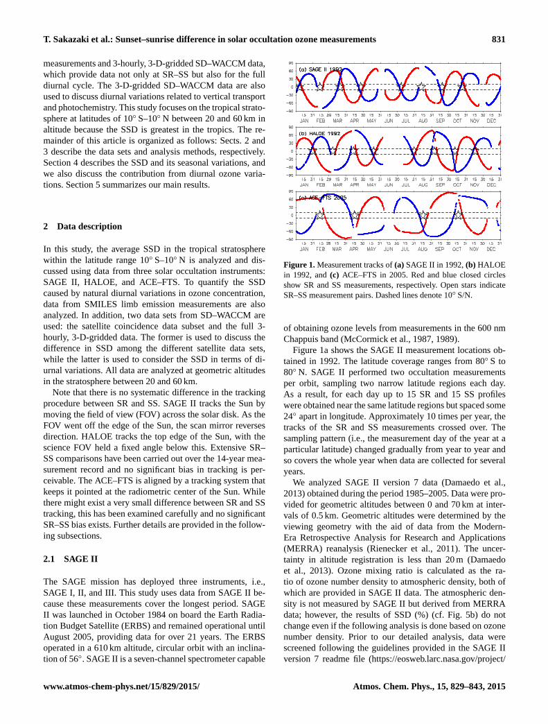
given to the sampling issues. Figure 2 shows the number of

SR (red) and SS (blue) profiles in the latitude range of 10◦ S–

10◦ N obtained during the observation period. We see that the

SR and SS profiles are not distributed evenly; e.g., there are

no SR (SS) profiles from November to January (May to July)

between 2001 and 2005 for SAGE II. This indicates that if

the SSD is calculated by simply averaging all SR and SS pro-

files for a certain period (e.g., Kyrölä et al., 2013), it could

be significantly contaminated by seasonal/interannual varia-

tions in ozone concentrations. In fact, Kyrölä et al. (2013) re-

ported that the SSD profile for 2001–2005 was considerably

different to those recorded in the other periods (1985–1990,

1991–1995, and 1996–2000); we attribute this to contami-

nation caused by uneven sampling during this period. To re-

solve this issue, we calculated the SSD in SR–SS pairs that

have both SR and SS profiles measured at almost the same

time (see the open stars in Fig. 1). A pair is defined such that

it has more than one profile for both SR and SS within 15

days (30 days) for SAGE II and HALOE (ACE–FTS). How-

ever, note that there is still a difference of 10–15 days in the

SR and SS measurement times for each pair. We found that

changes in ozone levels during these 10–15 days also con-

taminate the SSD. Therefore, this effect was further assessed

and removed (see below).

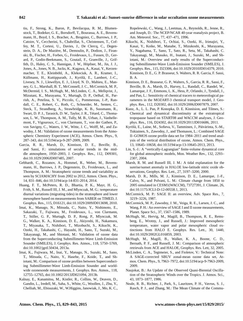
Figure 2. Number of profiles obtained for observations at 10◦ S–

10◦ N from (a) SAGE II, (b) HALOE, and (c) ACE–FTS. Red and

blue bars show the number of SR and SS profiles, respectively.

Approximately eight pairs for both SAGE II and HALOE

and four pairs for ACE–FTS were defined for each year (see

Fig. 1). The differences in measurement days between SR

and SS profiles were less than about 10 days (15 days) for

SAGE II and HALOE (ACE–FTS). The total number of pairs

for the entire period was 128 for SAGE II, 86 for HALOE,

and 25 for ACE–FTS. There were no SR–SS pairs for SAGE

II data after 2001 although the measurements continued until

2005. Also, for ACE–FTS, SR–SS pairs are defined only in

February, April, August, and October. Between 10 and 50

profiles were obtained for SR and SS in each pair (see Fig. 2).

Figure 3 shows the time series of the ozone mixing ratio

at an altitude of 40 km (10◦ S–10◦ N) based on HALOE data

for the period 1992–1993. The mean profile for each SR and

SS for the ith SR–SS pair (SRi and SSi) was produced by

averaging the SR (red open circles) and SS (blue open cir-

cles) data, respectively. Subsequently, for each pair the orig-

inal SSD (SSDiorg) was calculated as the difference between

the mean SS and SR profiles (i.e., SSDiorg = SSi−SRi). Fig-

ure 4 shows individual SSDiorg values averaged at altitudes of

40–45 km based on HALOE data and sorted by time of year

Atmos. Chem. Phys., 15, 829–843, 2015 www.atmos-chem-phys.net/15/829/2015/

T. Sakazaki et al.: Sunset–sunrise difference in solar occultation ozone measurements 835

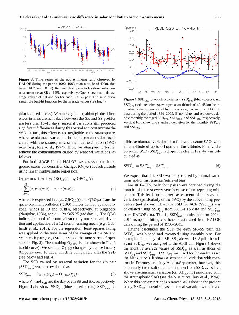
Figure 3. Time series of the ozone mixing ratio observed by

HALOE during the period 1992–1993 at an altitude of 40 km (be-

tween 10◦ S and 10◦ N). Red and blue open circles show individual

measurements at SR and SS, respectively. Open stars denote the av-

erage values of SR and SS for each SR–SS pair. The solid curve

shows the best-fit function for the average values (see Eq. 4).

(black closed circles). We note again that, although the differ-

ences in measurement days between the SR and SS profiles

are less than 10–15 days, seasonal variations still produced

significant differences during this period and contaminate the

SSD. In fact, this effect is not negligible in the stratosphere,

where semiannual variations in ozone concentration asso-

ciated with the stratospheric semiannual oscillation (SAO)

exist (e.g., Ray et al., 1994). Thus, we attempted to further

remove the contamination caused by seasonal variations, as

follows.

For both SAGE II and HALOE we assessed the back-

ground ozone concentration changes (O3_BG) at each altitude

using linear multivariable regression:

O3_BG = b+ at + q1QBO10(t)+ q2QBO30(t)

+

2∑n=1

(cn cos(nωt)+ sn sin(nωt)) , (4)

where t is expressed in days, QBO10(t) and QBO30(t) are the

quasi-biennial oscillation (QBO) indices defined by monthly

zonal winds at 10 and 30 hPa, respectively, at Singapore

(Naujokat, 1986), and ω = 2π /365.25 (rad day−1). The QBO

indices are used after normalization by one standard devia-

tion and application of a 12-month running mean (e.g., Geb-

hardt et al., 2013). For the regression, least-squares fitting

was applied to the time series of the average of the SR and

SS in each pair (i.e., (SRi +SSi)/2, the time series of open

stars in Fig. 3). The resulting O3_BG is also shown in Fig. 3

(solid curve). We see that O3_BG changes by approximately

0.1 ppmv over 10 days, which is comparable with the SSD

(see below and Fig. 4).

The SSD caused by seasonal variation for the ith pair

(SSDiseas) was then evaluated as

SSDiseas = O3_BG(tiSS)−O3_BG(t

iSR), (5)

where t iSS and t iSR are the day of ith SS and SR, respectively.

Figure 4 also shows SSDiseas(blue closed circles). SSDiseas ex-

Figure 4. SSDiorg (black closed circles), SSDiseas (blue crosses), and

SSDicor (red open circles) averaged at an altitude of 40–45 km for in-

dividual SR–SS pairs sorted by time of year, derived from HALOE

data during the period 1990–2005. Black, blue, and red curves de-

note monthly averaged SSDorg, SSDseas, and SSDorg, respectively.

Vertical bars show one standard deviation for the monthly SSDorg

and SSDorg.

hibits semiannual variations that follow the ozone SAO, with

an amplitude of up to 0.1 ppmv at this altitude. Finally, the

corrected SSD (SSDicor; red open circles in Fig. 4) was cal-

culated as

SSDicor = SSDiorg−SSDiseas. (6)

We expect that this SSD was only caused by diurnal varia-

tions and/or instrumental/retrieval bias.

For ACE–FTS, only four pairs were obtained during the

months of interest every year because of the repeating orbit

pattern. This leads to incorrect assessment of the seasonal

variations (particularly of the SAO) by the above fitting pro-

cedure (not shown). Thus, the SSD for ACE (SSDicor) was

calculated using SSDiorg from ACE–FTS data and SSDiseas

from HALOE data. That is, SSDiseas is calculated for 2004–

2011 using the fitting coefficients estimated from HALOE

data during the period of 1990–2005.

Having calculated the SSD for each SR–SS pair, the

SSDicor was binned and averaged using monthly bins. For

example, if the day of a SR–SS pair was 13 April, the rel-

evant SSDicor was assigned to the April bin. Figure 4 shows

the monthly average values of SSDicor as well as those of

SSDiorg and SSDiseas. If SSDorg was used for the analysis (see

the black curve), it shows a semiannual variation with max-

ima in February and July/August/September; however, this

is partially the result of contamination from SSDseas, which

shows a semiannual variation (ca. 0.1 ppmv) associated with

the stratospheric SAO (see the blue curve; Ray et al., 1994).

When this contamination is removed, as is done in the present

study, SSDcor instead shows an annual variation with a max-

www.atmos-chem-phys.net/15/829/2015/ Atmos. Chem. Phys., 15, 829–843, 2015

836 T. Sakazaki et al.: Sunset–sunrise difference in solar occultation ozone measurements

imum between December and February (see the red curve).

This seasonal variation is discussed in Sect. 4.2.

Finally, the annual mean SSD was calculated as the av-

erage of the monthly mean SSDcor. Note that correction for

SSDseas is important in the context of the annual mean SSD

as well. For SAGE II and HALOE, whose measurements

cover the entire year, the annual mean of SSDcor is nearly the

same as that of SSDorg because the annual mean of SSDseas

should be zero. This is, however, not the case for ACE–FTS,

which made tropical measurements only in particular months

(i.e., February, April, August, and October). In this case, the

annual mean of SSDseas is not zero but reaches a maximum

of approximately 0.1 ppmv; thus, the annual mean of SSDorg

is not equal to that of SSDcor (not shown).

For SMILES, two kinds of SSDs are calculated with dif-

ferent procedures. The first kind of SSD is based on SR–SS

pairs. SR–SS pairs that had more than 10 profiles for both

SR and SS were analyzed, and four SR–SS pairs met this

requirement (3 November 2009, 31 December 2009, 29 Jan-

uary 2010, and 29 March 2010). Each pair had more than 200

profiles for both SR and SS. In all cases, SR and SS measure-

ments were taken about 5 days apart. Unlike the solar occul-

tation measurements, SMILES observed the 10◦ S–10◦ N re-

gion almost continuously (see Sect. 2.4). Consequently, the

changes in background ozone concentration, i.e., O3_BG in

Eq. (4), were defined as the time series of ozone concen-

tration over the region 10◦ S–10◦ N to which a 5-day run-

ning mean was applied. Then SSDseas was assessed using

Eq. (5) and SSDcor was obtained from Eq. (6). The average

of the four SSDcors will be used in Sect. 4.1, while the in-

dividual SSDcors are used in Sect. 4.2 in the context of a

discussion of their seasonal dependence. Next, the second

kind of SSD is the SSD caused by diurnal variations. This

quantity is the difference in ozone levels between 18:00 LT

(for SS) and 06:00 LT (for SR), as derived from hourly diur-

nal ozone-concentration variations in the SMILES data av-

eraged over the period of operation (October 2009–April

2010). The method for extracting hourly diurnal variations

from SMILES data was described in S13. Note that the times

of SR and SS are 18:00 LT (±0.3 hr) and 06:00 LT (±0.3 hr),

respectively, for the region 10◦ S–10◦ N.

For the SD–WACCM output for satellite coincidences

(HALOE, SAGE II, and ACE–FTS), the same method was

applied as that used for each satellite data set. In contrast,

for the full-grid SD–WACCM output diurnal variations as

a function of LT were extracted for each latitude and alti-

tude grid point, for each month, as follows. First, 3-hourly

diurnal variations in universal time (UT) were calculated

at each longitude, latitude, and altitude grid point. Then,

along each latitude band, data at the same local time were

averaged to obtain diurnal variations as a function of LT;

e.g., 00:00 LT data were the average of (00:00 UT, 0◦ E),

(03:00 UT, 315◦ E), (06:00 UT, 270◦ E), (09:00 UT, 225◦ E),

(12:00 UT, 180◦ E), (15:00 UT, 135◦ E), (18:00 UT, 90◦ E),

and (21:00 UT, 45◦ E). Using these data, as for SMILES, the

SSD caused by diurnal variations, that is, the difference be-

tween 18:00 and 06:00 LT, was calculated. For SD–WACCM,

as was done by S13, the contributions from vertical transport

and photochemistry were estimated by integrating Eq. (1).

Diurnal variations of vertical wind (w′) and photochemical

generation or loss (S′) were both derived from the full-grid

SD–WACCM output.

4 Results

4.1 Annual mean

Figure 5a shows the annual mean vertical profiles of the SSD

in ozone mixing ratio in the region between 10◦ S and 10◦ N,

using data from the three solar occultation measurements and

from SD–WACCM output during each satellite coincidence.

We see that HALOE (blue solid curve) and ACE–FTS (green

solid curve) agree well with each other for the entire strato-

sphere; SD–WACCM results at times of satellite coincidence

(blue and green dashed curves) are also quantitatively consis-

tent in the stratosphere (below ∼ 55 km). In the lower strato-

sphere, at an altitude of around 25 km, the SR profiles exhibit

0.05–0.1 ppmv more ozone than the SS profiles. This differ-

ence gradually decreases with increasing altitude and reaches

zero at about 30 km. In the upper stratosphere, at 40–45 km,

the SS profiles exhibit up to 0.2 ppmv more ozone than the

SR profiles. Figure 5b shows the ratio of the SSD to the

average ozone mixing ratio during the analysis period. The

SSD is between −2 and −3 % at around 20 km and gradu-

ally increases to 5 % at an altitude of 45 km. The SSD near

the stratopause is quantitatively consistent with the HALOE

result of Brühl et al. (1996), although they only analyzed two

latitude bands at around 18◦ N and 18◦ S.

SAGE II (red solid curve) shows a similar result to

HALOE and ACE–FTS, at least qualitatively, but the SSD

in the upper stratosphere is approximately twice as large as

those resulting from the other data sets. The SAGE II results

are essentially consistent with the results of McLinden et

al. (2009) and Kyrölä et al. (2013), although the latter may be

partially contaminated by seasonal/interannual ozone varia-

tions (see Sect. 3). Considering that the SD–WACCM results

at SAGE II measurement locations (red dashed curve) are

consistent with those at both HALOE and ACE–FTS mea-

surement locations, we suggest that the anomalous SAGE II

values were not due to the differences in the measurement

locations/times compared to HALOE or ACE–FTS. Possible

causes will be discussed in Sect. 5.

There is a disagreement in SSD between satellite measure-

ments and SD–WACCM above 55 km (Fig. 5). This may be

due to the difference in diurnal variations between the model

and observations, as shown by S13 for the altitude region be-

tween 50 and 60 km. S13 also found that such a difference

was attributed to the difference in the lowest altitude of the

dominance of mesospheric diurnal variations that shows a

Atmos. Chem. Phys., 15, 829–843, 2015 www.atmos-chem-phys.net/15/829/2015/

T. Sakazaki et al.: Sunset–sunrise difference in solar occultation ozone measurements 837

Figure 5. SSDcor for 10◦ S–10◦ N in (a) ozone mixing ratio (ppmv) and (b) SSD ratio to the daily mean ( %), derived from SAGE II (red

solid curves), HALOE (blue solid curves), and ACE–FTS (green solid curves). Red, blue, and green dashed curves denote SD–WACCM

results at SAGE II, HALOE, and ACE–FTS coincidence, respectively. Black solid curves show the SMILES result (SR and SS are defined

by those profiles with a solar zenith angle between 80◦ and 100◦). Black dot-dashed curves show the difference between 18:00 and 06:00 LT,

calculated using SMILES data and based on 1-hourly diurnal variations. Horizontal bars for SAGE II, HALOE, and ACE–FTS show 95 %

confidential levels in a t test. For the statistical test, the error is defined as the standard deviation for the monthly SSD; this quantity has been

propagated to the error in annual mean. Then, the t test has been made with the degrees of freedom being the total numbers of SR–SS pairs

for each data set.

marked day–night contrast; i.e., ozone concentration maxi-

mizes (minimizes) during the nighttime (daytime). Another

possible reason for the disagreement in SSD is that the strong

“horizontal” gradient of ozone concentration associated with

the rapid ozone changes at SS/SR in the mesosphere was not

considered in the retrieval of satellite measurements (Natara-

jan et al., 2005).

Figure 5 also shows the two SMILES results. One is the

SSD deduced from the solar zenith angle (black solid curve),

while the other is the difference between 18:00 and 06:00 LT

caused by diurnal variations (black dot-dashed curve). We

see that the HALOE and ACE–FTS results are strongly sup-

ported by the SMILES results, although the SMILES SSD

is about 2 % smaller than that based on HALOE and ACE–

FTS data at an altitude of approximately 45 km. This may

be because SMILES observations have only four SR–SS

pairs in total whereas the HALOE and ACE–FTS have 86

and 24 pairs, respectively. SD–WACCM results at SMILES

locations also exhibit a smaller SSD compared with SD–

WACCM results at HALOE and ACE–FTS locations (not

shown). It should be noted that there is an agreement of

the two results derived from the SMILES data. Also, Fig.

6 compares the SSD from SD–WACCM results at HALOE

measurement locations (gray solid curve) to that caused by

diurnal variations from full-grid SD–WACCM (black solid

curve) and again shows a good agreement. These findings

indicate that the SSD is predominantly caused by natural di-

urnal variations in ozone concentrations (i.e., not by instru-

mental/retrieval bias).

Based on the finding that the SSD is consistent between

satellite measurements (at least HALOE and ACE–FTS) and

SD–WACCM, SD–WACCM data are further examined. Fig-

ure 7 shows diurnal variations in ozone mixing ratio at 42 km,

32 km, and 26 km, as derived from full-grid SD–WACCM

data (black solid curve). The contribution from vertical trans-

port by atmospheric tides (red solid curve) and that from pho-

tochemistry (blue solid curve) are also shown (see Eq. (1)

and Sect. 3). As shown by S13, the sum of the two processes

(black dashed curve) explains almost all characteristics of di-

urnal variations (black solid curve). At 26 km, ozone levels

reach a maximum in the morning and a minimum in the af-

ternoon in the lower stratosphere mainly due to tidal vertical

transport, resulting in a negative SSD. At 32 km, ozone levels

show a significant diurnal variation during the daytime due

to photochemistry but they are almost zero at SR and SS, re-

sulting in almost zero SSD. Chapman mechanism and NOx

chemistry are related to the photochemical variations (Pallis-

ter and Tuck, 1983; Schanz et al., 2014). At 42 km, ozone

levels show a diurnal variation caused by both vertical trans-

port and photochemistry. However, as is the case at 32 km,

photochemical processes do not contribute to the SSD sig-

nificantly. In contrast, the vertical transport generates higher

ozone levels in the late afternoon than in the morning; this

causes a positive SSD. The vertical transport exhibits only

www.atmos-chem-phys.net/15/829/2015/ Atmos. Chem. Phys., 15, 829–843, 2015

838 T. Sakazaki et al.: Sunset–sunrise difference in solar occultation ozone measurements

Figure 6. As Fig. 5a but for the difference between 18:00 and

06:00 LT, as deduced from diurnal variations in ozone concentra-

tion based on full-grid SD–WACCM between 2008 and 2010. Solid

curve is for the diurnal variations, red solid curve is for the contri-

bution from the vertical transport, blue solid curve is for the contri-

bution from photochemical processes, and the dashed solid curve is

for the sum of tidal vertical transport and photochemical processes

(see Eq. (1) and Sect. 3 for details). Solid gray curve shows the SSD

in SD–WACCM data at HALOE measurement locations (the same

as blue dashed curve in Fig. 5) for a reference.

small variations at 32 km because of the small vertical gradi-

ent in the background ozone concentration, i.e.,

∂[O3]

∂z≈ 0 (7)

in Eq. (1) (see Fig. 7d of S13).

Figure 8 shows the amplitude and phase of diurnal migrat-

ing tide in vertical wind averaged between 10◦ S and 10◦ N,

as derived from SD–WACCM data. The amplitude expo-

nentially increases with altitude. The phase basically shows

the downward progression, but it is almost constant around

40 km possibly due to the presence of trapped modes ex-

cited by ozone heating (e.g., Sakazaki et al., 2013b). Con-

sequently, the phase of vertical wind is similar in the whole

stratosphere; thus, the sign of SSD (i.e., negative at 20–30 km

and positive at 35–50 km) is determined by that of vertical

gradient in the background ozone concentration.

Figure 6 summarizes the contributions from vertical trans-

port and photochemistry (blue curve) to the annual mean

SSD profile.As discussed above, the SSD in the tropical

stratosphere is mainly caused by vertical transport while the

contribution from photochemistry is negligible. Note that a

further analysis of SD–WACCM indicated that the photo-

Figure 7. Diurnal variations in ozone mixing ratio averaged over

10◦ S–10◦ N at altitudes of (a) 42 km, (b) 36 km, and (c) 26 km.

Black solid curves are SD–WACCM. Red solid curves show the

contribution from tidal vertical transport and blue solid curves

show the contribution from photochemical processes (see Eq. (1)

and Sect. 3), while black dashed curves show the sum of the two

processes. SR and SS are denoted by thin black solid lines at

06:00 LT and 18:00 LT, respectively. The differences between 18:00

and 06:00 LT in ozone concentration (ppmv) from diurnal varia-

tions (“All”), tidal vertical transport (“VT”), and photochemical

processes (“Chem”) are shown in each panel.

chemical variations cause a SSD of ∼ 0.1 ppmv at high lat-

itudes (> 40◦) where they are not zero at SR and SS (not

shown; cf. Schanz et al., 2014). The relationship between the

SSD and vertical tidal winds will be further demonstrated in

the next section, where we will examine the seasonal varia-

tions of the SSD.

4.2 Seasonal variations

This section examines seasonal variations in the SSD. It

should be emphasized here that by calculating the seasonal

variations in SSD using solar occultation measurements we

could obtain quasi-observational evidence of seasonal varia-

tions in stratospheric vertical tidal winds, which are difficult

to observe directly. This section mainly uses HALOE data

because the SSD based on the HALOE measurements covers

a wider range of months. Figure 9 shows the month–altitude

distribution of the SSD from HALOE and SD–WACCM at

Atmos. Chem. Phys., 15, 829–843, 2015 www.atmos-chem-phys.net/15/829/2015/

T. Sakazaki et al.: Sunset–sunrise difference in solar occultation ozone measurements 839

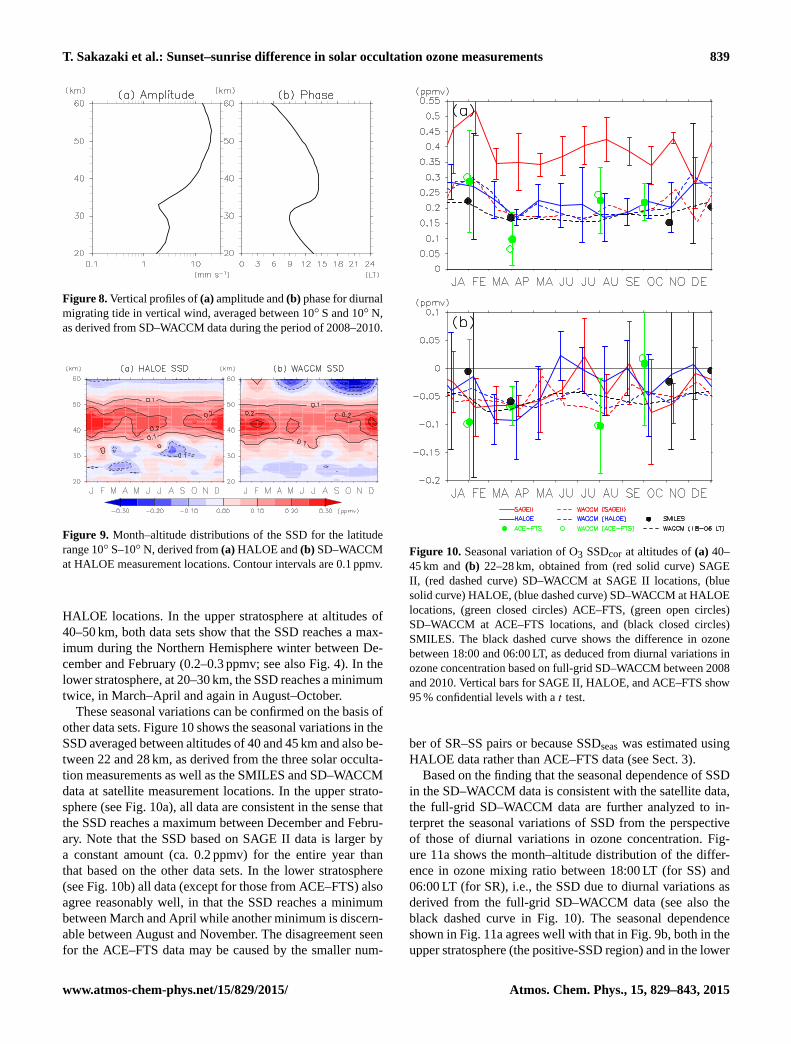
Figure 8. Vertical profiles of (a) amplitude and (b) phase for diurnal

migrating tide in vertical wind, averaged between 10◦ S and 10◦ N,

as derived from SD–WACCM data during the period of 2008–2010.

Figure 9. Month–altitude distributions of the SSD for the latitude

range 10◦ S–10◦ N, derived from (a) HALOE and (b) SD–WACCM

at HALOE measurement locations. Contour intervals are 0.1 ppmv.

HALOE locations. In the upper stratosphere at altitudes of

40–50 km, both data sets show that the SSD reaches a max-

imum during the Northern Hemisphere winter between De-

cember and February (0.2–0.3 ppmv; see also Fig. 4). In the

lower stratosphere, at 20–30 km, the SSD reaches a minimum

twice, in March–April and again in August–October.

These seasonal variations can be confirmed on the basis of

other data sets. Figure 10 shows the seasonal variations in the

SSD averaged between altitudes of 40 and 45 km and also be-

tween 22 and 28 km, as derived from the three solar occulta-

tion measurements as well as the SMILES and SD–WACCM

data at satellite measurement locations. In the upper strato-

sphere (see Fig. 10a), all data are consistent in the sense that

the SSD reaches a maximum between December and Febru-

ary. Note that the SSD based on SAGE II data is larger by

a constant amount (ca. 0.2 ppmv) for the entire year than

that based on the other data sets. In the lower stratosphere

(see Fig. 10b) all data (except for those from ACE–FTS) also

agree reasonably well, in that the SSD reaches a minimum

between March and April while another minimum is discern-

able between August and November. The disagreement seen

for the ACE–FTS data may be caused by the smaller num-

Figure 10. Seasonal variation of O3 SSDcor at altitudes of (a) 40–

45 km and (b) 22–28 km, obtained from (red solid curve) SAGE

II, (red dashed curve) SD–WACCM at SAGE II locations, (blue

solid curve) HALOE, (blue dashed curve) SD–WACCM at HALOE

locations, (green closed circles) ACE–FTS, (green open circles)

SD–WACCM at ACE–FTS locations, and (black closed circles)

SMILES. The black dashed curve shows the difference in ozone

between 18:00 and 06:00 LT, as deduced from diurnal variations in

ozone concentration based on full-grid SD–WACCM between 2008

and 2010. Vertical bars for SAGE II, HALOE, and ACE–FTS show

95 % confidential levels with a t test.

ber of SR–SS pairs or because SSDseas was estimated using

HALOE data rather than ACE–FTS data (see Sect. 3).

Based on the finding that the seasonal dependence of SSD

in the SD–WACCM data is consistent with the satellite data,

the full-grid SD–WACCM data are further analyzed to in-

terpret the seasonal variations of SSD from the perspective

of those of diurnal variations in ozone concentration. Fig-

ure 11a shows the month–altitude distribution of the differ-

ence in ozone mixing ratio between 18:00 LT (for SS) and

06:00 LT (for SR), i.e., the SSD due to diurnal variations as

derived from the full-grid SD–WACCM data (see also the

black dashed curve in Fig. 10). The seasonal dependence

shown in Fig. 11a agrees well with that in Fig. 9b, both in the

upper stratosphere (the positive-SSD region) and in the lower

www.atmos-chem-phys.net/15/829/2015/ Atmos. Chem. Phys., 15, 829–843, 2015

840 T. Sakazaki et al.: Sunset–sunrise difference in solar occultation ozone measurements

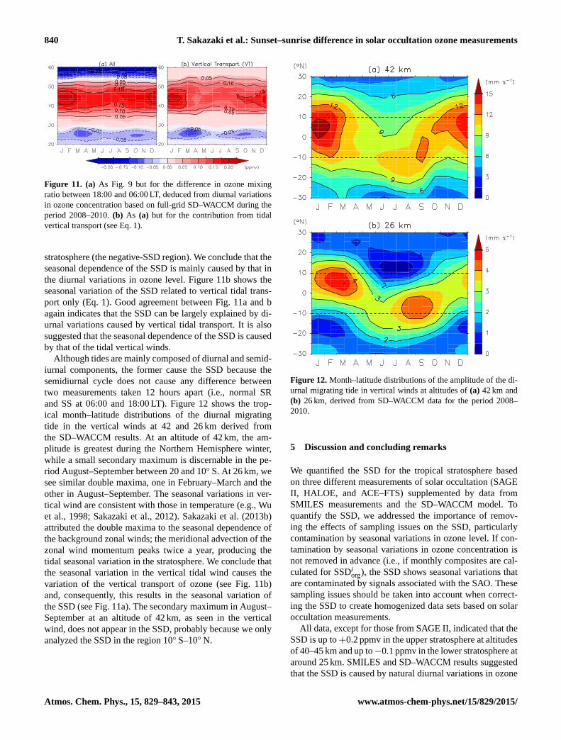
Figure 11. (a) As Fig. 9 but for the difference in ozone mixing

ratio between 18:00 and 06:00 LT, deduced from diurnal variations

in ozone concentration based on full-grid SD–WACCM during the

period 2008–2010. (b) As (a) but for the contribution from tidal

vertical transport (see Eq. 1).

stratosphere (the negative-SSD region). We conclude that the

seasonal dependence of the SSD is mainly caused by that in

the diurnal variations in ozone level. Figure 11b shows the

seasonal variation of the SSD related to vertical tidal trans-

port only (Eq. 1). Good agreement between Fig. 11a and b

again indicates that the SSD can be largely explained by di-

urnal variations caused by vertical tidal transport. It is also

suggested that the seasonal dependence of the SSD is caused

by that of the tidal vertical winds.

Although tides are mainly composed of diurnal and semid-

iurnal components, the former cause the SSD because the

semidiurnal cycle does not cause any difference between

two measurements taken 12 hours apart (i.e., normal SR

and SS at 06:00 and 18:00 LT). Figure 12 shows the trop-

ical month–latitude distributions of the diurnal migrating

tide in the vertical winds at 42 and 26 km derived from

the SD–WACCM results. At an altitude of 42 km, the am-

plitude is greatest during the Northern Hemisphere winter,

while a small secondary maximum is discernable in the pe-

riod August–September between 20 and 10◦ S. At 26 km, we

see similar double maxima, one in February–March and the

other in August–September. The seasonal variations in ver-

tical wind are consistent with those in temperature (e.g., Wu

et al., 1998; Sakazaki et al., 2012). Sakazaki et al. (2013b)

attributed the double maxima to the seasonal dependence of

the background zonal winds; the meridional advection of the

zonal wind momentum peaks twice a year, producing the

tidal seasonal variation in the stratosphere. We conclude that

the seasonal variation in the vertical tidal wind causes the

variation of the vertical transport of ozone (see Fig. 11b)

and, consequently, this results in the seasonal variation of

the SSD (see Fig. 11a). The secondary maximum in August–

September at an altitude of 42 km, as seen in the vertical

wind, does not appear in the SSD, probably because we only

analyzed the SSD in the region 10◦ S–10◦ N.

Figure 12. Month–latitude distributions of the amplitude of the di-

urnal migrating tide in vertical winds at altitudes of (a) 42 km and

(b) 26 km, derived from SD–WACCM data for the period 2008–

2010.

5 Discussion and concluding remarks

We quantified the SSD for the tropical stratosphere based

on three different measurements of solar occultation (SAGE

II, HALOE, and ACE–FTS) supplemented by data from

SMILES measurements and the SD–WACCM model. To

quantify the SSD, we addressed the importance of remov-

ing the effects of sampling issues on the SSD, particularly

contamination by seasonal variations in ozone level. If con-

tamination by seasonal variations in ozone concentration is

not removed in advance (i.e., if monthly composites are cal-

culated for SSDiorg), the SSD shows seasonal variations that

are contaminated by signals associated with the SAO. These

sampling issues should be taken into account when correct-

ing the SSD to create homogenized data sets based on solar

occultation measurements.

All data, except for those from SAGE II, indicated that the

SSD is up to+0.2 ppmv in the upper stratosphere at altitudes

of 40–45 km and up to−0.1 ppmv in the lower stratosphere at

around 25 km. SMILES and SD–WACCM results suggested

that the SSD is caused by natural diurnal variations in ozone

Atmos. Chem. Phys., 15, 829–843, 2015 www.atmos-chem-phys.net/15/829/2015/

T. Sakazaki et al.: Sunset–sunrise difference in solar occultation ozone measurements 841

concentration, particularly variations related to vertical trans-

port by tidal winds. SAGE II data showed qualitatively sim-

ilar results, including the seasonal dependence, but the SSD

in the upper stratosphere was twice as large as in the other

data sets.

The SSD also shows seasonal variations: it reaches a max-

imum during the Northern Hemisphere winter at an altitude

of 42 km and minima in March–April and August–October

near an altitude of 26 km. Analysis of SD–WACCM out-

put showed that the seasonal variation in the SSD follows

that of the tidal vertical winds. We believe that we have ob-

tained the first quasi-observational evidence of the tidal ver-

tical wind and its seasonal dependence in the tropical strato-

sphere. Therefore, we suggest that the ozone SSD is not a

bias but a useful proxy for the vertical tidal wind.

Nevertheless, there is an uncertainty about the magnitude

of SSD; the SSD from SAGE II data is twice as large as

that from the other four data sets. With the analysis of SD–

WACCM output, this difference is found not due to the dif-

ference in measurement locations or times among the data

sets. The retrieval procedure in SAGE II has been greatly up-

dated in SAGE II version 7 data (Damadeo et al., 2013). We

have so far no clear answer to the difference; there may be

several possibilities as discussed in the following.

A SSD could occur if the measurement “altitude” is mis-

takenly defined at SR and/or SS. However, the observed un-

certainty in SSD of ∼ 4 % (the difference in SSD between

SAGE II and the others at 42 km) corresponds to the uncer-

tainty in altitude of∼ 400 m (at 42 km the ozone mixing ratio

changes 1 % per 100 m in vertical); this seems unrealistic be-

cause an uncertainty of defined altitude is considered 20 m

for SAGE II, 100 m for HALOE, and 150 m for ACE–FTS.

Another related issue may be the reproducibility of tides

in SD–WACCM and reanalyses. Satellite measurements use,

more or less, (re)analysis data for the altitude registration

and/or the retrieval process. It is found that the amplitude of

diurnal tide in SD–WACCM and reanalyses are up to∼ 50 %

smaller in the upper stratosphere compared to data from

the Sounding of the Atmosphere using Broadband Emission

Radiometry (SABER) measurements (version 2 data) (not

shown; see Sakazaki et al., 2012, for the comparison between

SABER and reanalyses). This could affect any of the satellite

data sets, but a further study is needed for a more quantitative

discussion.

Acknowledgements. SAGE II data were provided by the NASA At-

mospheric Data Center. HALOE data were provided by GATS, Inc.,

through their website (http://haloe.gats-inc.com/home/index.php).

ACE–FTS data were provided by the ACE Science Operations Cen-

tre. The Atmospheric Chemistry Experiment (ACE), also known

as SCISAT, is a Canadian-led mission mainly supported by the

Canadian Space Agency and the Natural Sciences and Engineering

Research Council of Canada. SMILES data were provided by the

ISAS/JAXA. Monthly zonal wind data from Singapore were ob-

tained from the Free University of Berlin through its website (http:

//www.geo.fu-berlin.de/en/met/ag/strat/produkte/qbo/index.html).

SABER version 2 data were provided by GATS, Inc., through their

website (ftp://saber.gats-inc.com/custom/Temp_O3/). We thank

Koji Imai for his help in working with the ACE–FTS data. We are

also grateful to Erkki Kyrölä and Chris Boone for their helpful

suggestions and comments. Ellis Remsberg and an anonymous

reviewer gave us instructive comments which helped us to improve

the manuscript. T. Sakazaki was supported in part by the Japanese

Ministry of Education, Culture, Sports, Science and Technology

(MEXT) through a grant-in-aid for JSPS Fellows (25483400). T.

Sakazaki and M. Suzuki were also supported by the International

Space Science Institute, Bern, Switzerland (ISSI Team #246,

Characterizing Diurnal Variations of Ozone for Improving Ozone

Trend Estimates, http://www.issbern.ch/teams/ozonetrend/). This

study was supported in part by the MEXT through a grant-in-aid

(25281006), the ISS Science Project Office of ISAS/JAXA, and the

Human Spaceflight Mission Directorate of JAXA. All figures were

drawn with the GFD–Dennou library.

Edited by: W. Ward

References

Beaver, G. M., Gordley, L., and Russell III, J. M.: Halogen Occul-

tation Experiment (HALOE) altitude registration of atmospheric

profile measurements: lessons learned and improvements made

during the data validation phase, Proc. SPIE 2266, P. Soc. Photo-

Opt. Ins., 266–280, doi:10.1117/12.187564, 1994.

Bernath, P. F., McElroy, C. T., Abrams, M. C., Boone, C. D., Butler,

M., Camy-Peyret, C., Carleer, M., Clerbaux, C., Coheur, P.-F.,

Colin, R., DeCola, P., DeMazière, M., Drummond, J. R., Dufour,

D., Evans, W. F. J., Fast, H., Fussen, D., Gilbert, K., Jennings, D.

E., Llewellyn, E. J., Lowe, R. P., Mahieu, E., McConnell, J. C.,

McHugh, M., McLeod, S. D., Michaud, R., Midwinter, C., Nas-

sar, R., Nichitiu, F., Nowlan, C., Rinsland, C. P., Rochon, Y. J.,

Rowlands, N., Semeniuk, K., Simon, P., Skelton, R., Sloan, J. J.,

Soucy, M.-A., Strong, K., Tremblay, P., Turnbull, D., Walker, K.

A., Walkty, I., Wardle, D. A., Wehrle, V., Zander, R., and Zou, J.:

Atomspheric Chemistry Experiment (ACE): mission overview,

Geophys. Res. Lett., 32, L15S01, doi:10.1029/2005GL022386,

2005.

Boone, C., D., Nassar, R., Walker, K. A., Rochon, Y.,

McLeod, S. D., Rinsland, C. P., and Bernath, P. F.: retrievals for

the atmospheric chemistry experiment Fourier-transform spec-

trometer, Appl. Optics, 44, 7218–7231, 2005.

Brühl, C., Drayson, S. R., Russell III, J. M., Crutzen, P. J., McIn-

erney, J. M., Purcell, P. N., Claude, H., Gernandt, H., McGee,

T. J., McDermid, I. S., and Gunson, M. R.: Halogen Occulta-

tion Experiment ozone channel validation, J. Geophys. Res., 101,

10,217–10,240, 1996.

Damadeo, R. P., Zawodny, J. M., Thomason, L. W., and Iyer, N.:

SAGE version 7.0 algorithm: application to SAGE II, At-

mos. Meas. Tech., 6, 3539–3561, doi:10.5194/amt-6-3539-2013,

2013.

Dupuy, E., Walker, K. A., Kar, J., Boone, C. D., McElroy, C. T.,

Bernath, P. F., Drummond, J. R., Skelton, R., McLeod, S. D.,

Hughes, R. C., Nowlan, C. R., Dufour, D. G., Zou, J., Nichi-

www.atmos-chem-phys.net/15/829/2015/ Atmos. Chem. Phys., 15, 829–843, 2015

842 T. Sakazaki et al.: Sunset–sunrise difference in solar occultation ozone measurements

tiu, F., Strong, K., Baron, P., Bevilacqua, R. M., Blumen-

stock, T., Bodeker, G. E., Borsdorff, T., Bourassa, A. E., Bovens-

mann, H., Boyd, I. S., Bracher, A., Brogniez, C., Burrows, J. P.,

Catoire, V., Ceccherini, S., Chabrillat, S., Christensen, T., Cof-

fey, M. T., Cortesi, U., Davies, J., De Clercq, C., Degen-

stein, D. A., De Mazière, M., Demoulin, P., Dodion, J., Firan-

ski, B., Fischer, H., Forbes, G., Froidevaux, L., Fussen, D., Ger-

ard, P., Godin-Beekmann, S., Goutail, F., Granville, J., Grif-

fith, D., Haley, C. S., Hannigan, J. W., Höpfner, M., Jin, J. J.,

Jones, A., Jones, N. B., Jucks, K., Kagawa, A., Kasai, Y., Kerzen-

macher, T. E., Kleinböhl, A., Klekociuk, A. R., Kramer, I.,

Küllmann, H., Kuttippurath, J., Kyrölä, E., Lambert, J.-C.,

Livesey, N. J., Llewellyn, E. J., Lloyd, N. D., Mahieu, E., Man-

ney, G. L., Marshall, B. T., McConnell, J. C., McCormick, M. P.,

McDermid, I. S., McHugh, M., McLinden, C. A., Mellqvist, J.,

Mizutani, K., Murayama, Y., Murtagh, D. P., Oelhaf, H., Par-

rish, A., Petelina, S. V., Piccolo, C., Pommereau, J.-P., Ran-

dall, C. E., Robert, C., Roth, C., Schneider, M., Senten, C.,

Steck, T., Strandberg, A., Strawbridge, K. B., Sussmann, R.,

Swart, D. P. J., Tarasick, D. W., Taylor, J. R., Tétard, C., Thoma-

son, L. W., Thompson, A. M., Tully, M. B., Urban, J., Vanhelle-

mont, F., Vigouroux, C., von Clarmann, T., von der Gathen, P.,

von Savigny, C., Waters, J. W., Witte, J. C., Wolff, M., and Za-

wodny, J. M.: Validation of ozone measurements from the Atmo-

spheric Chemistry Experiment (ACE), Atmos. Chem. Phys., 9,

287–343, doi:10.5194/acp-9-287-2009, 2009.

Garcia, R. R., Marsh, D., Kinnison, D. E., Boville, B.,

and Sassi, F.: simulations of secular trends in the mid-

dle atmosphere, 1950–2003, J. Geophys. Res., 112, D09301,

doi:10.1029/2006JD007485, 2007.

Gebhardt, C., Rozanov, A., Hommel, R., Weber, M., Bovens-

mann, H., Burrows, J. P., Degenstein, D., Froidevaux, L., and

Thompson, A. M.: Stratospheric ozone trends and variability as

seen by SCIAMACHY from 2002 to 2012, Atmos. Chem. Phys.,

14, 831–846, doi:10.5194/acp-14-831-2014, 2014.

Huang, F. T., McPeters, R. D., Bhartia, P. K., Mayr, H. G.,

Frith, S. M., Russell III, J. M., and Mlynczak, M. G.: temperature

diurnal variations (migrating tides) in the stratosphere and lower

mesosphere based on measurements from SABER on TIMED, J.

Geophys. Res., 115, D16121, doi:10.1029/2009JD013698, 2010.

Imai, K., Manago, N., Mitsuda, C., Naito, Y., Nishimoto, E.,

Sakazaki, T., Fujiwara, M., Froidevaux, L., von Clarmann,

T., Stiller, G. P., Murtagh, D. P., Rong, P., Mlynczak, M.

G., Walker, K. A., Kinnison, D. E., Akiyoshi, H., Nakamura,

T., Miyasaka, T., Nishibori, T., Mizobuchi, S., Kikuchi, K.,

Ozeki, H., Takahashi, C., Hayashi, H., Sano, T., Suzuki, M.,

Takayanagi, M., and Shiotani, M.: Validation of ozone data

from the Superconducting Submillimeter-Wave Limb-Emission

Sounder (SMILES), J. Geophys. Res. Atmos., 118, 5750–5769,

doi:10.1002/jgrd.50434, 2013a.

Imai, K., Fujiwara, M., Inai, Y., Manago, N., Suzuki, M., Sano,

T., Mitsuda, C., Naito, Y., Hasebe, F., Koide, T., and Sh-

iotani, M.: Comparison of ozone profiles between Superconduct-

ing Submillimeter-Wave Limb-Emission Sounder and world-

wide ozonesonde measurements, J. Geophys. Res. Atmos., 118,

12755–12765, doi:10.1002/2013JD021094, 2013b.

Kalnay, E., Kanamitsu, M., Kistler, R., Collins, W., Deaven, D.,

Gandin, L., Iredell, M., Saha, S., White, G., Woollen, J., Zhu, Y.,

Chelliah, M., Ebisuzaki, W., W.Higgins, Janowiak, J., Mo, K. C.,

Ropelewski, C., Wang, J., Leetmaa, A., Reynolds, R., Jenne, R.,

and Joseph, D.: The NCEP/NCAR 40-year reanalysis project, B.

Am. Meteorol. Soc., 77, 437–471, 1996.

Kikuchi, K., Nishibori, T., Ochiai, S., Ozeki, H., Irimajiri, Y.,

Kasai, Y., Koike, M., Manabe, T., Mizukoshi, K., Murayama,

Y., Nagahama, T., Sano, T., Sato, R., Seta, M., Takahashi, C.

Takayanagi, M., Masuko, H., Inatani, J., Suzuki, M., and Sh-

iotani, M.: Overview and early results of the Superconduct-

ing Submillimeter-Wave Limb-Emission Sounder (SMILES), J.

Geophys. Res., 115, D23306, doi:10.1029/2010JD014379, 2010.

Kinnison, D. E., G. P. Brasseur, S. Walters, R. R. Garcia, F. Sassi,

B. A.

Kinnison, D. E., Brasseur, G. P., Walters, S., Garcia, R. R., Sassi, F.,

Boville, B. A., Marsh, D., Harvey, L., Randall, C., Randel, W.,

Lamarque, J. F., Emmons, L. K., Hess, P., Orlando, J., Tyndall, J.,

and Pan, L.: Sensitivity of chemical tracers to meteorological pa-

rameters in the MOZART-3 chemical transport model, J. Geo-

phys. Res., 112, D20302, doi:10.1029/2006JD007879, 2007.

Kunz, A., L. L. Pan, P. Konopka, D. E. Kinnision, and Tilmes, S.:

Chemical and dynamical discontinuity at the extratropical

tropopause based on START08 and WACCM analyses, J. Geo-

phys. Res., 116, D24302, doi:10.1029/2011JD016686, 2011.

Kyrölä, E., Laine, M., Sofieva, V., Tamminen, J., Päivärinta, S.-M.,

Tukiainen, S., Zawodny, J., and Thomason, L.: Combined SAGE

II–GOMOS ozone profile data set for 1984–2011 and trend anal-

ysis of the vertical distribution of ozone, Atmos. Chem. Phys.,

13, 10645–10658, doi:10.5194/acp-13-10645-2013, 2013.

Lin, S.-J.: A “vertically-Lagrangian” finite-volume dynamical core

for global atmospheric models, Mon. Weather Rev., 132, 2293–

2307, 2004.

Marsh, R. M. and Russell III, J. M.: A tidal explanation for the

sunrise/sunset anomaly in HALOE low-latitude nitric oxide ob-

servations, Geophys. Res. Lett., 27, 3197–3200, 2000.

Marsh, D. R., Mills, M. J., Kinnison, D. E., Lamarque, J.-F.,

Calvo, N., and Polvani, L. M.: Climate change from 1850 to

2005 simulated in CESM1(WACCM), 73727391, J. Climate, 26,

doi:10.1175/JCLI-D-12-00558.1, 2013.

McCormick, M. P.: SAGE II: an overview, Adv. Space Res., 7,

3219–3226, 1987.

McCormick, M. P., Zawodny, J. M., Veiga, R. E., Larsen, J. C., and

Wang, P. H.: An overview of SAGE I and II ozone measurements,

Planet. Space Sci., 37, 1567–1586, 1989.

McHugh, M., Hervig, M., Magill, B., Thompson, R. E., Rems-

berg, E., Wrotny, J., and Russell, J.: Improved mesospheric

temperature, water vapor and polar mesospheric cloud ex-

tinctions from HALO E. Geophys. Res. Lett., 30, 1440,

doi:10.1029/2002GL016859, 2003.

McHugh, M., Magill, B., Walker, K. A., Boone, C. D.,

Bernath, P. F., and Russell, J. M.: Comparison of atmospheric

retrievals from ACE and HALOE, Geophys. Res. Lett, 32, 2005.

McLinden, C. A., Tegtmeier, S., and Fioletov, V.: Technical Note:

A SAGE-corrected SBUV zonal-mean ozone data set, At-

mos. Chem. Phys., 9, 7963–7972, doi:10.5194/acp-9-7963-2009,

2009.

Naujokat, B.: An Update of the Observed Quasi-Biennial Oscilla-

tion of the Stratospheric Winds over the Tropics. J. Atmos. Sci.,

43, 1873–1877, 1986.

Neale, R. B., Richter, J., Park, S., Lauritzen, P. H., Vavrus, S. J.,

Rasch, P. J., and Zhang, M.: The Mean Climate of the Commu-

Atmos. Chem. Phys., 15, 829–843, 2015 www.atmos-chem-phys.net/15/829/2015/

T. Sakazaki et al.: Sunset–sunrise difference in solar occultation ozone measurements 843

nity Atmosphere Model (CAM4) in Forced SST and Fully Cou-

pled Experiments, J. Climate, 26, 5150–5168, doi:10.1175/JCLI-

D-12-00236.1, 2013.

Newchurch, M. J., Yang, E.-S., Cunnold, D. M., Reinsel, G. C., Za-

wodny, J. M., and Russell III, J. M.: Evidence for slowdown in

stroatospheric ozone loss: first stage of ozone recovery, J. Geo-

phys. Res., 108, 4507, doi:10.1029/2003JD003471, 2003. Pallis-

ter, R. C., and A. F. Tuck, The diurnal variation of ozone in the

Pallister, R. C. and Tuck, A. F.: The diurnal variation of ozone in the

upper stratosphere as a test of photochemical theory, Q. J. Roy.

Meteor. Soc., 109, 271–284, 1983.

Parrish, A., Boyd, I. S., Nedoluha, G. E., Bhartia, P. K., Frith, S. M.,

Kramarova, N. A., Connor, B. J., Bodeker, G. E., Froidevaux, L.,

Shiotani, M., and Sakazaki, T.: Diurnal variations of strato-

spheric ozone measured by ground-based microwave remote

sensing at the Mauna Loa NDACC site: measurement valida-

tion and GEOSCCM model comparison, Atmos. Chem. Phys.

Discuss., 13, 31855–31890, doi:10.5194/acpd-13-31855-2013,

2013.

Randall, C. E,. Rusch, D. W., Bevilacqua, R. M., Hoppel, K. W.,

Lumpe, J. D., Shettle, E., Thompson, E., Deaver, L., Zawodny,

J., Kyrö, E., Johnson, B., Kelder, H., Dorokhov, V. M., König-

Langlo, G., and Gil, M.: Validation of POAM III ozone: Com-

parisons with ozonesonde and satellite data, J. Geophys. Res.,

108, 4367, doi:10.1029/2002JD002944, 2003.

Randel, W. and Wu, F.: Isolation of the ozone QBO in SAGEII data

by singular-value decomposition, J. Atmos. Sci., 53, 2546–2559,

1996.

Ray, E. A. and Holton, J. R.: The tropical semiannual oscillations in

temperature and ozone as observed by the MLS, J. Atmos. Sci.,

51, 3045–3052, 1994.

Rienecker, M. M., Suarez, M. J., Gelaro, R., Todling, R., Bacmeis-

ter, J., Liu, E., Bosilovich, M. G., Schubert, S. D., Takacs, L.,

Kim, G.-K., Bloom, S., Chen, J., Collins, D., Conaty, A.,

da Silva, A., Gu, W., Joiner, J., Koster, R. D., Lucchesi, R.,

Molod, A., Owens, T., Pawson, S., Pegion, P., Redder, C. R., Re-

ichle, R., Robertson, F. R., Ruddick, A. G., Sienkiewicz, M., and

Woollen, J.: MERRA: NASA’s modern-era retrospective anal-

ysis for research and applications, J. Climate, 24, 3624–3648,

doi:10.1175/JCLI-D-11-00015.1, 2011.

Remsberg, E., Deaver, L., Wells, J., Lingenfelser, G., Bhatt, P.,

Gordley, L., Thompson, R., McHugh, M., Russell III, J. M.,

Keckhut, P., and Schmidlin, F.: An assessment of the quality

of Halogen Occultation Experiment temperature profiles in the

mesosphere based on comparisons with Rayleigh backscatter li-

dar and inflatable falling sphere measurements, J. Geophys. Res.

Atmos., 107, 4447, doi:10.1029/2001JD001521, 2002.

Russell, III, J. M., Gordley, L. L., Park, J. H., Drayson, S. R., Hes-

keth, W. D., Cicerone, R. J., Tuck, A. F., Frederick, J. E., Har-

ries, J. E., and Crutzen, P. J.: The halogen occultation experi-

ment, J. Geophys. Res., 98, 10777–10798, 1993.

Sakazaki, T., Fujiwara, M., Zhang, X., Hagan, M. E., and

Forbes, J. M.: Diurnal tides from the troposphere to the lower

mesosphere as deduced with TIMED/SABER satellite data and

six global reanalysis data sets, J. Geophys. Res., 117, D13108,

doi:10.1029/2011JD017117, 2012.

Sakazaki, T., Fujiwara, M., Mitsuda, C., Imai, K., Manago, N.,

Naito, Y., Nakamura, T., Akiyoshi, H., Kinnison, D., Sano, T.,

Suzuki, M., and Shiotani, M.: Diurnal ozone variations in the

stratosphere revealed in observations from the Superconduct-

ing Submillimeter-Wave Limb-Emission Sounder (SMILES) on

board the International Space Station (ISS), J. Geophys. Res. At-

mos., 118, 2991–3006, doi:10.1002/jgrd.50220, 2013a.

Sakazaki, T., Fujiwara, M., and Zhang, X.: Interpretation of the ver-

tical structure and seasonal variation of the diurnal migrating tide

from the troposphere to the lower mesosphere, J. Atmos. Sol.-

Terr. Phys., 105–106, 66–80, 2013b.

Schanz, A., Hocke, K., and Kämpfer, N.: Daily ozone cycle in the

stratosphere: global, regional and seasonal behaviour modelled

with the Whole Atmosphere Community Climate Model, At-

mos. Chem. Phys. Discuss., 14, 5561–5609, doi:10.5194/acpd-

14-5561-2014, 2014.

Shiotani, M. and Hasebe, F.: Stratospheric ozone variations in the

equatorial region as seen in Stratospheric Aerosol and Gas Ex-

periment data, J. Geophys. Res., 99, 14575–14584, 1994.

Wang, H. J., Cunnold, D. M., and Bao, X.: A critical analysis of

Stratospheric Aerosol and Gas Experiment ozone trends, J. Geo-

phys. Res., 101, 12495–12514, 1996.

Waymark, C., Walker, K., Boone, C., and Bernath, P.: ACE-FTS

version 3.0 data set: Validation and data processing update, Ann.

Geophys.-Italy, 56, doi:10.4401/ag-6339, 2013.

World Meteorological Organization (WMO): Scientific assessment

of ozone depletion: 2010, Report 52, Global Ozone Research and

Monitoring Project, Geneva, 2011.

Wu, D. L., McLandress, C., Read, W. G., Waters, J. W., and Froide-

vaux, L.: Equatorial diurnal variations observed in UARS Mi-

crowave Limb Sounder temperature during 1991–1994 and sim-

ulated by the Canadian Middle Atmosphere Model, J. Geophys.

Res., 103, 8909–8917, 1998.

Zeng, Z., Randel, W., Sokolovskiy, S., Deser, C., Kuo, Y.-H., Ha-

gan, M., Du, J., and Ward, W.: Detection of migrating diurnal tide

in the tropical upper troposphere and lower stratosphere using the

Challenging Minisatellite Payload radio occultation data, J. Geo-

phys. Res., 113, D03102, doi:10.1029/2007JD008725, 2008.

www.atmos-chem-phys.net/15/829/2015/ Atmos. Chem. Phys., 15, 829–843, 2015