Impact of nonlinear energy transfer on the wave field in Pacifichindcast experiments

Hitoshi Tamura,1 Takuji Waseda,1,2 and Yasumasa Miyazawa1

Received 30 November 2009; revised 20 July 2010; accepted 25 August 2010; published 16 December 2010.

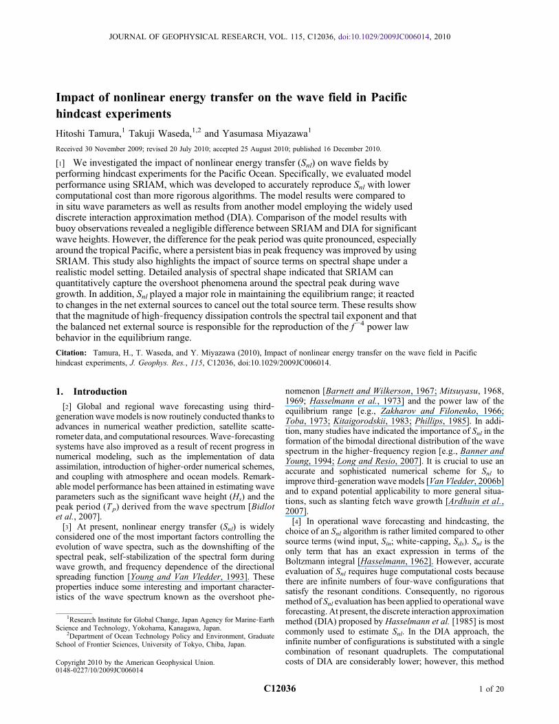
[1] We investigated the impact of nonlinear energy transfer (Snl) on wave fields byperforming hindcast experiments for the Pacific Ocean. Specifically, we evaluated modelperformance using SRIAM, which was developed to accurately reproduce Snl with lowercomputational cost than more rigorous algorithms. The model results were compared toin situ wave parameters as well as results from another model employing the widely useddiscrete interaction approximation method (DIA). Comparison of the model results withbuoy observations revealed a negligible difference between SRIAM and DIA for significantwave heights. However, the difference for the peak period was quite pronounced, especiallyaround the tropical Pacific, where a persistent bias in peak frequency was improved by usingSRIAM. This study also highlights the impact of source terms on spectral shape under arealistic model setting. Detailed analysis of spectral shape indicated that SRIAM canquantitatively capture the overshoot phenomena around the spectral peak during wavegrowth. In addition, Snl played a major role in maintaining the equilibrium range; it reactedto changes in the net external sources to cancel out the total source term. These results showthat the magnitude of high‐frequency dissipation controls the spectral tail exponent and thatthe balanced net external source is responsible for the reproduction of the f −4 power lawbehavior in the equilibrium range.

Citation: Tamura, H., T. Waseda, and Y. Miyazawa (2010), Impact of nonlinear energy transfer on the wave field in Pacifichindcast experiments, J. Geophys. Res., 115, C12036, doi:10.1029/2009JC006014.

1. Introduction

[2] Global and regional wave forecasting using third‐generation wave models is now routinely conducted thanks toadvances in numerical weather prediction, satellite scatte-rometer data, and computational resources.Wave‐forecastingsystems have also improved as a result of recent progress innumerical modeling, such as the implementation of dataassimilation, introduction of higher‐order numerical schemes,and coupling with atmosphere and ocean models. Remark-able model performance has been attained in estimating waveparameters such as the significant wave height (Hs) and thepeak period (Tp) derived from the wave spectrum [Bidlotet al., 2007].[3] At present, nonlinear energy transfer (Snl) is widely

considered one of the most important factors controlling theevolution of wave spectra, such as the downshifting of thespectral peak, self‐stabilization of the spectral form duringwave growth, and frequency dependence of the directionalspreading function [Young and Van Vledder, 1993]. Theseproperties induce some interesting and important character-istics of the wave spectrum known as the overshoot phe-

nomenon [Barnett and Wilkerson, 1967; Mitsuyasu, 1968,1969; Hasselmann et al., 1973] and the power law of theequilibrium range [e.g., Zakharov and Filonenko, 1966;Toba, 1973; Kitaigorodskii, 1983; Phillips, 1985]. In addi-tion, many studies have indicated the importance of Snl in theformation of the bimodal directional distribution of the wavespectrum in the higher‐frequency region [e.g., Banner andYoung, 1994; Long and Resio, 2007]. It is crucial to use anaccurate and sophisticated numerical scheme for Snl toimprove third‐generation wave models [Van Vledder, 2006b]and to expand potential applicability to more general situa-tions, such as slanting fetch wave growth [Ardhuin et al.,2007].[4] In operational wave forecasting and hindcasting, the

choice of an Snl algorithm is rather limited compared to othersource terms (wind input, Sin; white‐capping, Sds). Snl is theonly term that has an exact expression in terms of theBoltzmann integral [Hasselmann, 1962]. However, accurateevaluation of Snl requires huge computational costs becausethere are infinite numbers of four‐wave configurations thatsatisfy the resonant conditions. Consequently, no rigorousmethod of Snl evaluation has been applied to operational waveforecasting. At present, the discrete interaction approximationmethod (DIA) proposed by Hasselmann et al. [1985] is mostcommonly used to estimate Snl. In the DIA approach, theinfinite number of configurations is substituted with a singlecombination of resonant quadruplets. The computationalcosts of DIA are considerably lower; however, this method

1Research Institute for Global Change, Japan Agency for Marine‐EarthScience and Technology, Yokohama, Kanagawa, Japan.

2Department of Ocean Technology Policy and Environment, GraduateSchool of Frontier Sciences, University of Tokyo, Chiba, Japan.

Copyright 2010 by the American Geophysical Union.0148‐0227/10/2009JC006014

JOURNAL OF GEOPHYSICAL RESEARCH, VOL. 115, C12036, doi:10.1029/2009JC006014, 2010

C12036 1 of 20

does not properly represent the nonlinear transfer rate com-pared to the exact solutions for the Boltzmann integral [e.g.,Hasselmann et al., 1985; Tolman, 2004]. Therefore, third‐generation wave forecasting systems will not improve as longasDIA is used [VanVledder et al., 2000].Ardhuin et al. [2007]reported that replacingDIAwith an exact Snlmethod (theWRTmethod; Van Vledder, [2006a]) caused the spectral shape todiffer more from observations. They concluded that this resultwas due to the lack of retuning of the Sin and Sds source terms,which were tuned for DIA in the WAM.[5] Recent advances in computational resources have now

made it possible to apply more expensive Snl schemes to theoperational wave model. New Snl schemes have been devel-oped that extend the original DIA [e.g., Van Vledder, 2001;Tolman, 2004], and other methods have also been proposed[Komatsu, 1996; Tolman et al., 2005; Resio and Perrie,2008]. Komatsu [1996] developed the simplified RIAMmethod (SRIAM), which utilizes 20 resonance configurationsthat retain the general properties of the Snl kernel function.Komatsu [1996] showed that SRIAM performed favorablycompared to the rigorous RIAM method [Komatsu andMasuda, 1996] for duration‐limited wave growth after anabrupt change in wind direction and the evolution of perturbed‐equilibrium spectra. Tamura et al. [2008] also assessed theperformance of SRIAM by applying it to more complex situ-ations, such as wave propagation against a shear current. Theyfound that the use of SRIAM as the numerical scheme for Snlmodified the spectral shape. For example, the spectral shapesestimated by RIAM and SRIAM were much narrower infrequency and directional space than those estimated by DIA,where a peculiar trimodal directional distribution appearedaround the low‐frequency region. In addition, the self‐stabilization effect of Snlwas demonstrated in a realistic wavesimulation forced by reanalysis products of wind and oceancurrents. They concluded that a realistic representation ofthe Snl term is crucial for accurate evaluation of spectralmodulation.[6] The present paper investigates model performance in

more detail using SRIAM based on hindcast experiments.We are interested in how sensitive wave parameters suchas the Hs and the frequency peak ( fp) are to the numericalschemes of Snl under realistic conditions. Specifically, thepresent study was motivated by a desire to elucidate whetheraccurate Snl schemes improve the model representation ofspectral shape in terms of freak wave prediction. Recentstudies [e.g., Onorato et al., 2002; Janssen, 2003; Gramstadand Trulsen, 2007; Waseda et al., 2009a, 2009b] have sug-gested that owing to nonlinear focusing, the probability of afreak wave occurring increases as the wave spectrum nar-rows in the frequency and directional domains. Therefore, it iscrucial to estimate the spectral shape as accurately as possible,which should lead to an improved prediction of abnormalwaves. Whereas numerous studies have noted the importanceof accurate evaluation of nonlinear transfer in operationalwave forecasting, few have attempted to investigate its impactin a realistic situation. The applicability and model perfor-mance of SRIAM are investigated here by comparing in situdata provided by the National Oceanic and AtmosphericAdministration/National Data Buoy Center (NOAA/NDBC)and computational results by DIA for hindcast simulations.We are also interested in the formation mechanism of thewave spectrum in terms of the source balance, as has been

discussed extensively by many researchers. We investigatethe role of Snl in the source balance in conjunction with theparameterization of the Sds term.[7] The remainder of this paper is arranged as follows.

Section 2 describes the model configuration and design of thehindcast experiment. In section 3, we examine the basicproperties of SRIAM for wave parameters by comparing insitu data and computational results obtained using DIA. Insection 4, the effect of nonlinear energy transfer on thespectral shape is investigated in detail, mainly using SRIAM;this section also discusses the role of other source terms.Finally, a summary and discussion are given in section 5.

2. Model Configurations and HindcastExperiments

2.1. Wave Model

[8] Wave hindcast was conducted based on WAVE-WATCH‐III version 2.22 [WW3; Tolman, 2002] with SRIAMas Snl to investigate the impact of the improved Snl scheme onthe wave parameters and to test the applicability of SRIAMunder realistic conditions. Numerical simulation using DIA(i.e., the default setting of WW3) was also conducted as areference. In this study, we compared the model results ofWW3/SRIAM and WW3/DIA. For all calculations, we usedthe same source functions of Sin and Sds and a fixed spectralresolution because our goal was to investigate the impact ofSnl on the hindcast experiments. Tolman and Chalikov’s[1996] (hereafter TC96) wave‐growth and wave‐decaysource terms were used, and the surface wind speed at 10 melevation was modified to consider the instability of the atmo-spheric boundary layer (the “effective” wind speed; Tolman,2002). The spectral space was discretized using 25 frequen-cies ranging from 0.042 to 0.414 (relative frequency of 10%,fm+1 = 1.1 fm, where f is the intrinsic frequency and m is adiscrete grid counter) with 36 directions (D� = 10°). Typicaloperational wave models, including WW3, apply a para-metric spectral tail beyond a cutoff frequency for two primaryreasons: to reduce computational costs and to impose anequilibrium spectrum with empirical law. In WW3, a para-metric tail assuming the f −5 power law was patched to thefrequency range from 2.5fp to the end of the prognostic modelfrequency (here, 0.414 Hz) when 2.5fp is lower than thehighest frequency. Because one of our objectives was toinvestigate the spectral shape in the high‐frequency region,we did not use the parametric spectral tail for either modelsetting (WW3/SRIAM or WW3/DIA). That is, the energydensity in the prognostic frequency region was fully con-trolled by the source and propagation terms. However, thespectral tail is necessary for computing Snl when the highestfrequency corresponding to the four resonant waves is largerthan the highest discrete model frequency. Therefore, weassumed an f −5 spectral tail outside themodel frequency range(greater than 0.414 Hz), as used in the default WW3 settings.For spatial propagation of the wave spectrum, we used thedefault third‐order advection scheme.[9] Using DIA for Snl, the TC96 Sds term was tuned in such

a way that the solution of the wave action equation reproducedthe observed fetch limited wave growth of the total waveenergy [Kahma and Calkoen, 1994] and high‐frequencyenergy level [Hasselmann et al., 1973]. If DIA is simplyreplaced by SRIAM, dynamic properties of the wave growth

TAMURA ET AL.: PACIFIC HINDCAST EXPERIMENTS C12036C12036

2 of 20

and decay will also be altered because other source functions(Sin and Sds) strongly depend on the spectral shape. Therefore,the introduction of SRIAM toWW3distorts the balance of thesource terms and affects the total wave energy. To avoid this,we conducted a preliminary investigation of fetch‐limitedwave growth and reduced the Sds term by a factor of 0.2 (i.e.,Stotal = Sin+Snl

SRIAM + aSds, where a = 0.8) to reproduce theobservational results by Kahma and Calkoen [1994], whichhave been used to tune the default WW3.

2.2. Design of Hindcast Experiments

[10] The computational domain was set to 66°S–66°N lat-itude and 100°E–290°E longitude, covering the Pacific Oceanexcept for its polar region. Hindcast was performed for a1‐year integration period in 2004. The wave model wasdriven by 6‐hourly wind stress from the National Centers forEnvironmental Prediction/National Center for AtmosphericResearch (NCEP/NCAR) reanalysis product [Kalnay et al.,1996], in which the global data set has a resolution of 192 ×94 gaussian grids. Whereas WW3 can incorporate externalparameters such as ice concentration, currents, water levels,and air‐sea temperature differences, these components werenot considered in this study. ETOPO5 [http://www.ngdc.noaa.gov/mgg/global/etopo5.HTML] elevation data were usedto define the bottom topography and coastal lines.We ignoredshallow‐water physics, such as bottom‐induced dissipationand modification of the Snl term.[11] The results of both models (WW3/SRIAM and WW3/

DIA) were validated against wave parameters recorded ateight NOAA/NDBC buoys deployed in deep waters, mainlyin the northeastern Pacific. Figure 1 gives the locations of thebuoys, which fall into three regions: high latitude (46035 and46066), midlatitude (46005, 46006, 46089), and low latitude(51001, 51004, 51028). Hourly wave fields calculated by thetwomodels were compared to in situ data at the nearest points.

3. Statistical Properties and Wave Spectraof Ocean Waves in the Pacific

[12] In the Pacific, enormous quantities of mechanical windenergy are transferred to surface waves in the midlatitudesfrom 30° to 60° N and S [e.g.,Wang andHuang, 2004]. Theselatitudinal bands correspond to strong surface wind fieldsassociated with storm tracks in the Northern and Southernhemispheres. Ocean waves generated in the midlatitudespropagate far from storms and radiate to lower latitudes asswells. On the other hand, in low latitudes, the tradewindsblowing predominantly from the ENE and ESE constantlygenerate local windsea. These features characterize the pat-tern of the surface wind and ocean wave fields in the Pacific.

3.1. Significant Wave Height and Peak Frequency

[13] We first focused onHs and peak frequency ( fp), whichare the basic parameters of wave forecasting. Figure 1 showstypical snapshots of (Figure 1a) Hs and surface wind vectorsand (Figure 1b) Tp and peak wave direction in the NorthPacific calculated byWW3, with SRIAM representing the Snlterm. The spatial distribution of Hs primarily corresponds tosynoptic and subsynoptic scale features of surface winds, asshown in Figure 1a. Hs grew up to 9 m, with a peak period of15 s, inside a storm at midlatitudes (Figures 1a and 1b). Twoswell systems generated by individual storms propagated

toward the southeast in the eastern Pacific (Figure 1b). At lowlatitudes (from 0° to 20° N), the tradewind from the ENE wasdominant and Hs reached about 2–3 m, with a peak period of8–11 s.[14] Figure 2 shows scatterplot comparisons of (a) Hs and

(b) fp values from the SRIAM and DIA runs. To highlight thedifferences in model performance in both zonal and meridi-onal directions, we defined four different regions in the NorthPacific (WP40N: 35°–45°N, 160°E–180°,WP10N: 5°–15°N,160°E–180°, EP40N: 35°–45°N, 160°–140°W, EP10N: 5°–15°N, and 160°–140°W). The annual model results for theseregions were used for the investigations. The differences inmodel performance were also quantified in terms of bias(Bias), root mean square error (RMSE), correlation coeffi-cients (CC), and scatter index (SI) [Cardone et al., 1996].[15] Although there seemed to be some differences in Hs

between the SRIAM and DIA runs, the correspondence wasquite high (Figure 2a); the CCwas always above 99%, and thebias was less than 10 cm in all regions. To implement SRIAMin WW3, the magnitude of the default WW3 Sds term wasreduced by a factor of 0.2. This was done to reproduce theobserved fetch‐limited wave growth, as well as the defaultWW3 run using DIA to represent the Snl term. In this sense,close correspondence between the models (WW3/SRIAMand WW3/DIA) was apparent. However, we also confirmedfor the first time that Hs in a realistic field can also be ade-quately reproduced by this model setting with SRIAMrepresenting the Snl term and tuning for Sds.[16] The scatter of fp was rather large, and the bias and CC

differed with longitude and latitude (Figure 2b). The bias offp was pronounced in the western Pacific (e.g., WP40N:−0.0057 Hz, EP40N: −0.0035 Hz), whereas in the easternPacific the correlation was lower (e.g., WP40N: 88.1%,EP40N: 83.4%), especially in the low‐latitude region (EP10N:82.9%). The scatterplots of fp also revealed the characteristicfrequency dependence of the bias. Peak frequencies calcu-lated by DIA were generally larger (i.e., positive bias) com-pared to those calculated by SRIAM in the high‐frequencyregion (around 0.09 – 0.15 Hz) at WP10N, EP40N andEP10N. However, scatterplots indicated a persistent positivebias in DIA for the entire frequency domain at WP40N.[17] We compared the SRIAM and DIA model results to

observational data in the eastern Pacific, where the correlationof the peak frequency between the twomodels was small. Theprobability density functions (pdfs) of Hs and fp by SRIAMandDIA are shown in Figures 3 and 4, validated against the insitu data as the ground truth. With the exception of 46089, thecomputational results by SRIAM and DIA agreed well witheach other for Hs (Figure 3). This was consistent with theprevious model comparison shown in Figure 2a. Both modelresults also compared favorably well with the observationalresults. In middle to high latitudes (46035, 46066, 46005,46006, and 46089), pdfs of Hs were broadly distributed up to6–8 m. On the other hand, pdfs were quite narrow and con-fined to around 2 m in low latitudes (51001, 51004, and51028). These noticeable tendencies in the pdfs are alsopresent in the model (Figure 2a).[18] The fp was distributed with a single peak in the middle

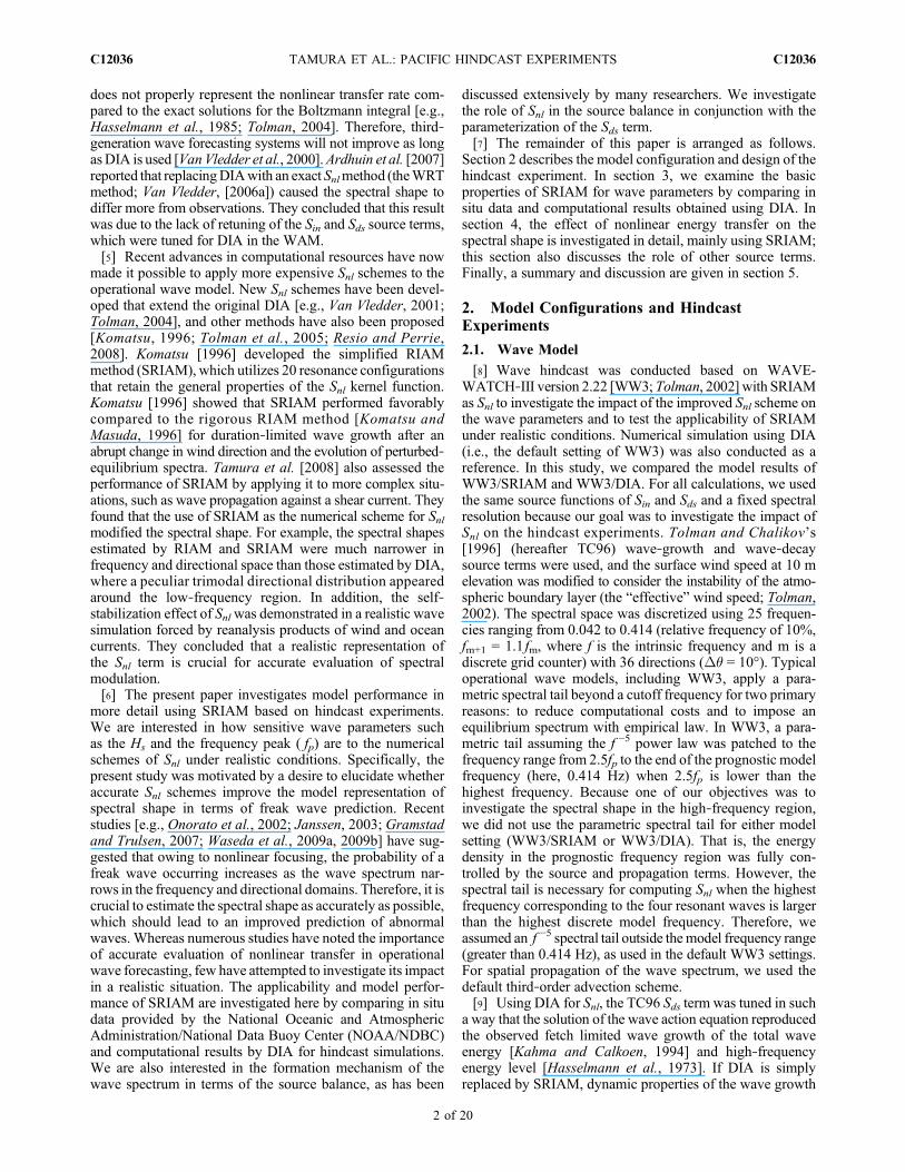
to high latitudes (46035, 46066, 46005, 46006, and 46089),while in low latitudes (51001, 51004, and 51028), the pdf ofthe fpwas characterized by two peak values (Figure 4). Again,the observed pdf features could also be found in the model

TAMURA ET AL.: PACIFIC HINDCAST EXPERIMENTS C12036C12036

3 of 20

Figure 1. Instantaneous plane view (at 1400 UTC, 13 December 2004) of (a) significant wave height (Hs)and surface wind vectors and (b) peak period (Tp) and peak wave direction in the North Pacific calculatedusing SRIAM for the Snl term. Squares show the locations of the NDBC buoys used in the analysis, whichincluded data for a 1‐year integration period.

TAMURA ET AL.: PACIFIC HINDCAST EXPERIMENTS C12036C12036

4 of 20

(Figure 2b). In midlatitudes in the eastern Pacific (EP40N),the model fpwas continuously distributed from about 0.06 Hzto 0.15 Hz, as confirmed by observations at 46066, 46005,and 46006. However, the pdf of the model fp has a localminimum around 0.1 Hz in EP10N, which was the same asthat observed at 51001, 51004, and 51028 (Figure 4). Inaddition, the fp at EP10N (Figure 2b) calculated using DIAindicated a positive bias around fp values greater than 0.1 Hz.For fp values less than 0.1 Hz, the bias became small. Thereproducibility of this bimodality of the peak frequencymanifested as a pronounced difference in the performance ofthe two models (Figure 4). SRIAM successfully captured thisbimodality of the pdf while DIA indicated bimodality butgave values that were not consistent with observations for thehigh‐frequency peak (greater than 0.1 Hz). The differencesbetween the pdfs were statistically significant at the 5% sig-nificance level using a two‐sample Kolmogorov‐Smirnovtest.[19] We further quantified the performance of the two

models against observations using various statistical scores(Table 1). Both models performed well for Hs: The differ-ences in RMSE and CC were within a few centimeters and0.01, respectively, at any buoy location. However, the pre-diction skills of Hs seemed to depend on location. They werenot significantly improved using SRIAM. SRIAM had con-sistently better fp values than DIA, but the difference in theverification scores (RMSR, CC and SI) were rather small. Inthe low‐latitude region (51001, 51004, and 51028), fp alsoimproved (c2 values are shown in Table 1). It is also inter-esting to note that the default parameterization of WW3/DIAhad a tendency to overestimate (underestimate) the fp (Tp) formoderate to strong wind fields, as was seen in Chao et al.

[2005] and Padilla‐Hernández et al. [2007]. Our resultsalso suggest the same features; fp calculated by DIA indicatedpositive bias with the exception of 46089, whereas fp calcu-lated by SRIAM indicated random variance with small bias.[20] In summary, these results can be explained physically

as follows. In the midlatitude Pacific, the pdf of Hs is broadlydistributed because of the prominent westerlies and the strongvariation in surface wind associated with storm tracks. The fpis continuously distributed in this region (Figures 2b and 4),and its spread may be accounted for by the strong variation inlocal winds. In other words, in midlatitudes, the predominantlocal windsea distribution is not significantly affected byswells. Swells coming from the windsea source regions inthe midlatitudes propagate toward low latitudes, particularlythe eastern tropical and subtropical region of the Pacific(Figure 1b). In addition, the surface winds are steadier andmore moderate than those at high latitudes. The pdfs of Hs atlow latitudes are quite narrow and confined, as shown inFigures 2a and 3. This is because the swells and windseaenergies are of the same order of magnitude. The pdf of fp isclearly separated into two peak values; the lower‐frequencypeak corresponds to swells from high latitudes, while thehigher‐frequency peak corresponds to local windsea inducedby the trade wind. Evaluation of the spectral peak due to tradewinds seems to improve when SRIAM is used. These featuresof wave fields in the North Pacific were also confirmed in thespectral evolution and associated wave parameters, asdescribed below.

3.2. Wave Spectral Properties

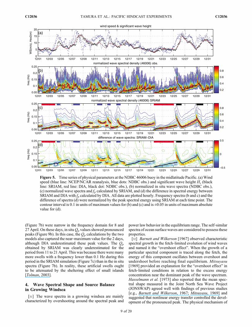
[21] Figure 5 presents a typical winter time‐series com-parison of physical parameters in the midlatitude Pacific

Figure 2. Scatterplot comparison of (a) Hs and (b) fp for the SRIAM and DIA values for four differentregions in the North Pacific (WP40N: 35°N–45°N, 160°E–180°, WP10N: 5°N–15°N, 160°E–180°,EP40N: 35°N–45°N, 160°W–140°W, EP10N: 5°N–15°N, 160°W–140°W). Annual model results overthese regions are used for the investigations. The contour interval is 0.1 in units of maximum values.

TAMURA ET AL.: PACIFIC HINDCAST EXPERIMENTS C12036C12036

5 of 20

(NDBC 46006), showing (Figure 5a) wind speed and Hs,(Figure 5b) in situ wave spectra normalized by peak spectralenergy (Fobs / Fp

obs), (Figure 5c) normalized wave spectracalculated by SRIAM (FSRIAM / Fp

SRIAM), and (Figure 5d) thedifference in normalized wave spectra between SRIAMand DIA ((FSRIAM − FDIA) / Fp

SRIAM), where F is the one‐dimensional wave spectrum in the frequency domain and Fp isthe peak spectral energy. Storms induced significant fluctua-tions in wind speed during the 12 days from 3 to 15 December.Thereafter wind speed gradually decreased from 16 to25 December and then increased again rapidly due to twostorms between 25 and 31 December. The Hs calculated bythe wave models showed close agreement with the observa-tional data, with the exception of 4 and 12–13 December,which may have been due to errors in surface wind forcing.[22] The shapes of wave spectra changed rapidly in the

midlatitudes, and this was associated with temporal changes inlocal wind fields. The time evolution ofwave spectra (shown inFigure 5c) was characterized by strong downshifting (indicatedby black bars) and weak upshifting (indicated by red bars) of

the spectral peak. The former corresponded to wave devel-opment due to the strong local wind field, in which Snlinduced downshifting of the spectral peak. The latter corre-sponded to swell propagation, in which longer swells arrivedfirst, followed by shorter swells due to wave dispersion. Inaddition, storms induced rapid spectral transformation withina few hours (indicated by blue bars). Swells also coexistedwith local windsea from 4 to 19December, indicating spectralevolution in a mixed sea state.[23] The differences in spectral energy between SRIAM

andDIA (Figure 5d) were persistent around the spectral peaksduring the periods indicated by the blue and black bars. Neg-ative and positive differences in the spectral energy across thespectral peaks suggest that the peak frequencies of DIA areshifted to high frequencies. This is also observed in Figure 2b,where the default WW3 tends to indicate a positive bias for fp.This feature was also suggested in previous studies [e.g.,Chaoet al., 2005;Padilla‐Hernández et al., 2007;Xu et al., 2007]. Inaddition, DIA fails to reproduce the spectral shape around thespectral peak, as discussed in the next section.

Figure 3. The probability density functions of Hs calculated by SRIAM (solid line) and DIA (dashed‐dotted line) with in situ data (circle) for each location.

TAMURA ET AL.: PACIFIC HINDCAST EXPERIMENTS C12036C12036

6 of 20

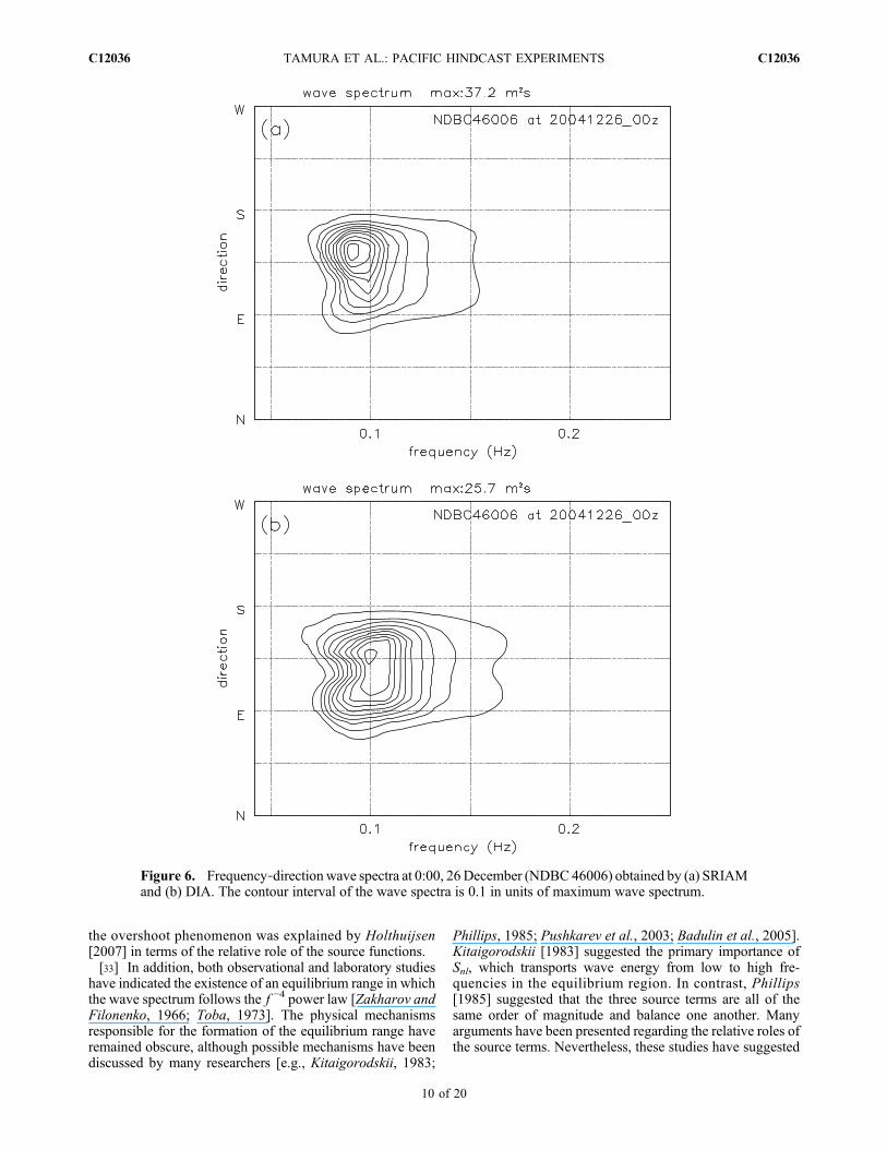
[24] The two‐dimensional (2‐D) wave spectra clearly dif-fered between SRIAM and DIA. Figure 6 presents wavespectral energy densities for “pure” windsea in the frequencyand directional domain at 0:00 on 26 December. Around thespectral peak, the 2‐D wave spectrum calculated by DIA(Figure 6b) is much broader, especially in directional space,than that by SRIAM (Figure 6a). In addition, a bimodal dis-tribution appears on the low‐frequency side of the peak fre-quency. That is, DIA redistributes wave energy atmuch largeroblique angles than expected with exact nonlinear transfer,which is a recognized shortcoming of DIA [Komatsu andMasuda, 1996; Van Vledder, 2006b; Tamura et al., 2008].[25] Figure 7 presents typical examples of the time history of

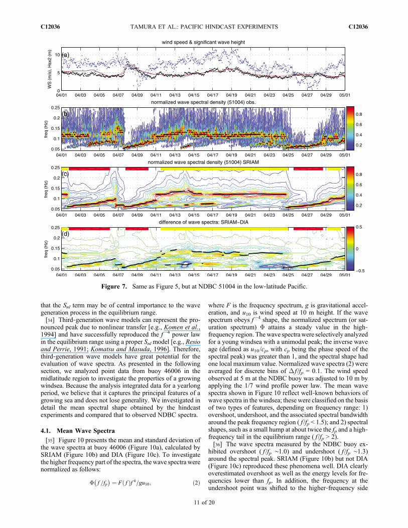
wave parameters in the low‐latitude Pacific (NDBC51004). Atlow latitudes, the surface wind speed fluctuated only graduallyaround 8 m/s, and the estimated Hs calculated by SRIAM andDIA comparedwell with observations (Figure 7a). TheHs timeseries indicated a gradual transition compared to the case athigher latitudes, owing to the different atmospheric conditions.The time evolution of the observed wave spectra (Figures 7b

and 7c) was characterized by persistent spectral peaksaround 0.12 Hz (indicated by yellow bars) and slowlyupshifting spectral peaks from 0.05 to 0.1 Hz (indicated byred bars). The former corresponded to the windsea induced bythe steady tradewind blowing from the ENE, whereas thelatter corresponded to swell propagation from higher lati-tudes. This bimodal behavior of fp values corresponding to thewindsea and swell resulted in the bimodality of the pdf inFigure 2b (EP10N) and Figure 4.[26] The clearest difference between the models was the

peak frequency associated with the tradewind (i.e., higherpeak frequency); DIA clearly overestimated the observed peakwhile SRIAM reproduced this peak reasonably well (Figures 4and 7d). Again, this differencewas easily confirmed in the 2‐Dwave spectrum, where four local maxima of spectral energywere seen (Figure 8). The local maxima of the windsea atfrequencies greater than 0.1 Hz were shifted to higher fre-quencies with DIA as compared to SRIAM, while the swellpeaks at frequencies less than 0.1 Hz were consistent for bothmodels. These features were also apparent in the differences

Figure 4. Same as Figure 3, but for peak frequency.

TAMURA ET AL.: PACIFIC HINDCAST EXPERIMENTS C12036C12036

7 of 20

in pdfs (Figure 4). The discrepancy in the high‐frequencypeaks is mainly because the defaultWW3 has a persistent biasand overestimates of peak frequencies under moderate windconditions. Other possible reasons for this include a well‐known problem of DIA: It fails to adequately calculate theenergy transfer of bimodal wave spectra [e.g., Young and VanVledder, 1993; Komatsu and Masuda, 1996; Van Vledderet al., 2000]. In addition, the spectral bandwidth around thepeak was narrow for the SRIAM runs, correcting the well‐known DIA shortcoming of tending to broaden the wavespectrum around the spectral peak in the frequency anddirectional domains.

3.3. Spectral Shape Parameters

[27] The frequency peakednessQp [Goda, 2000] is definedas follows:

Qp ¼ 2m�20

Z 1

0f

Z 2�

0F f ; �ð Þd�

� �2df ; ð1Þ

where F( f,�) is the wave spectrum defined in the frequency‐directional domain and m0 is the total spectral energy. Qp

provides an adequate indication of the structure and evolutionof wave spectra in the frequency domain (note that VanVledder and Battjes [1992] and Goda [2000] questioned theapplicability of Qp regarding spectral smoothing and resolu-tion). Recent studies have indicated that seas with a highprobability of freak wave occurrence can be parameterized bywave steepness and the spectral bandwidths in frequency anddirection. Therefore,Qp is a relevant parameter for identifyingseas with a high chance of freak waves [Janssen and Bidlot,2003; Waseda et al., 2009a; Tamura et al., 2009]. We com-pared the model results on the basis of SRIAM and DIA withobservational data where in situ Qp values were defined fromthe frequency spectra of the specific NDBC buoys.

[28] Figures 9a and 9b show time series of Qp for the sameduration and location as in Figures 5 and 7. In general, the Qp

estimated by SRIAM was larger than that estimated by DIAbecause SRIAM improves the shortcomings of DIA. DIAtends to broaden the spectra in the frequency domain com-pared to rigorous algorithms for Snl [e.g., Hasselmann et al.,1985]. The most pronounced difference between the modelresults and in situ data appeared during the passage of swells.TheQps calculated by the twomodels showed abrupt changesaround 2 and 22 December (Figure 9a). Thereafter, theymaintained higher values for a few days more than in otherperiods. This is attributable to the propagation of swells overlong distances; quite a narrow spectrum appears in the low‐frequency region (< 0.1 Hz) in Figures 5b and 5c. While thetime series of in situ Qps (open circles) did not show thesechanges, that of the modeled frequency spectrum actuallycaptured the swell propagation at that time (see Figures 5band 5c). Similar in situ Qp fluctuations were observed atother times at this location.[29] The main reason for this discrepancy might be the

coarse frequency resolution of the observed wave spectra(Figure 9a, NDBC 46006 in December). That is, the Qp

parameter is strongly dependent on the resolution of the wavespectrum, which is a recognized shortcoming, as discussed byGoda [2000]. In this case, the in situ frequency spectrum wasgiven by a frequency bin size of 0.01 Hz in the range 0.03–0.4 Hz. The spectral resolution was insufficient to estimateQp

for the quite narrow spectrum, especially in the low‐frequencyregion.[30] On the other hand, the in situ Qp in low latitudes cal-

culated using a higher‐resolution spectrum (Figure 9b,NDBC 51004 in April) showed reasonable agreement withthe computational results, especially those of SRIAM(Figure 9b), for swells propagating at this location (on 8 and27 April). The wave spectra obtained by NDBC buoy 51004

Table 1. Summary of the Bulk Model Statistics for (A) Significant Wave Height and (B) Peak Frequency

(a)

Location Data Bias (cm) RMSE (m) CC SI (%) c2 values

NDBC N SRIAM DIA SRIAM DIA SRIAM DIA SRIAM DIA SRIAM DIA

46035 8753 19.5 26.8 0.71 0.74 0.90 0.90 24.8 25.0 548.4 869.346066 4151 15.0 21.7 0.73 0.72 0.89 0.90 22.1 21.2 167.8 278.946005 8600 6.2 14.2 0.62 0.63 0.89 0.89 22.0 21.8 164.1 235.246006 8761 −12.4 −3.3 0.54 0.54 0.93 0.92 18.8 19.0 221.6 387.446089 1169 −3.6 10.0 0.62 0.62 0.87 0.87 20.2 20.1 223.1 340.751001 7549 −5.5 1.0 0.40 0.41 0.91 0.90 15.5 16.0 86.2 73.451004 8744 9.4 15.2 0.38 0.40 0.79 0.79 16.3 16.6 639.5 1240.951028 8723 13.4 17.8 0.33 0.35 0.61 0.62 15.9 15.8 1189.7 2122.3

(b)

Location Data Bias (Hz) RMSE (Hz) CC SI (%) c2 values

NDBC N SRIAM DIA SRIAM DIA SRIAM DIA SRIAM DIA SRIAM DIA

46035 8753 −0.0025 0.0030 0.032 0.034 0.52 0.49 27.4 29.1 1068.2 1241.946066 4151 0.0018 0.0071 0.025 0.029 0.55 0.51 25.0 27.7 348.3 559.246005 8600 −0.0029 0.0009 0.030 0.032 0.53 0.51 29.5 31.3 772.6 610.346006 8761 −0.0017 0.0017 0.028 0.030 0.47 0.44 29.5 31.2 650.3 574.346089 1169 −0.0050 −0.0020 0.022 0.021 0.42 0.42 25.0 25.2 141.6 121.951001 7549 0.0026 0.0069 0.025 0.028 0.63 0.61 23.6 25.7 344.4 1575.951004 8744 −0.0026 0.0001 0.024 0.027 0.54 0.50 23.1 25.7 367.8 1729.151028 8723 0.0018 0.0029 0.024 0.025 0.43 0.44 25.4 26.8 808.1 1647.4

TAMURA ET AL.: PACIFIC HINDCAST EXPERIMENTS C12036C12036

8 of 20

(Figure 7b) were narrow in the frequency domain for 8 and27April. On these days, in situQp values showed pronouncedpeaks (Figure 9b). In this case, the Qp calculations by the twomodels also captured the near‐maximum value for the 2 days,although DIA underestimated these peak values. The Qp

obtained by SRIAM was clearly underestimated for theperiod from 11 to 21April. This was because there were manymore swells with a frequency lower than 0.1 Hz during thisperiod in the SRIAM simulation (Figure 7c) than in the in situspectra (Figure 7b). In reality, these artificial swells oughtto be attenuated by the sheltering effect of small islands[Tolman, 2003].

4. Wave Spectral Shape and Source Balancein Growing Windsea

[31] The wave spectra in a growing windsea are mainlycharacterized by overshooting around the spectral peak and

power law behavior in the equilibrium range. The self‐similarspectra of ocean surfacewaves are considered to possess theseproperties.[32] Barnett and Wilkerson [1967] observed characteristic

spectral growth in the fetch‐limited evolution of wind wavesand named it the “overshoot effect”. When the growth of aparticular spectral component is traced along the fetch, theenergy of this component oscillates between overshoot andundershoot before reaching final equilibrium. Mitsuyasu[1969] provided an explanation for the “overshoot effect” infetch‐limited conditions in relation to the excess energyconcentration near the dominant peak of the wave spectrum.Hasselmann et al. [1973] also reported that the mean spec-tral shape measured in the Joint North Sea Wave Project(JONSWAP) agreed well with findings of previous studies[e.g., Barnett and Wilkerson, 1967; Mitsuyasu, 1969] andsuggested that nonlinear energy transfer controlled the devel-opment of the pronounced peak. The physical mechanism of

Figure 5. Time series of physical parameters at the NDBC 46006 buoy in the midlatitude Pacific. (a)Windspeed (blue line: NCEP/NCAR reanalysis, blue dots: NDBC obs.) and significant wave height Hs (blackline: SRIAM, red line: DIA, black dot: NDBC obs.), (b) normalized in situ wave spectra (NDBC obs.),(c) normalized wave spectra and fp calculated by SRIAM, and (d) the difference in spectral energy betweenSRIAM and DIA with fp calculated by DIA. All data are plotted hourly. Frequency spectra (b and c) and thedifference of spectra (d) were normalized by the peak spectral energy using SRIAM at each time point. Thecontour interval is 0.1 in units of maximum values for (b) and (c) and is ±0.05 in units of maximum absolutevalue for (d).

TAMURA ET AL.: PACIFIC HINDCAST EXPERIMENTS C12036C12036

9 of 20

the overshoot phenomenon was explained by Holthuijsen[2007] in terms of the relative role of the source functions.[33] In addition, both observational and laboratory studies

have indicated the existence of an equilibrium range in whichthe wave spectrum follows the f −4 power law [Zakharov andFilonenko, 1966; Toba, 1973]. The physical mechanismsresponsible for the formation of the equilibrium range haveremained obscure, although possible mechanisms have beendiscussed by many researchers [e.g., Kitaigorodskii, 1983;

Phillips, 1985; Pushkarev et al., 2003; Badulin et al., 2005].Kitaigorodskii [1983] suggested the primary importance ofSnl, which transports wave energy from low to high fre-quencies in the equilibrium region. In contrast, Phillips[1985] suggested that the three source terms are all of thesame order of magnitude and balance one another. Manyarguments have been presented regarding the relative roles ofthe source terms. Nevertheless, these studies have suggested

Figure 6. Frequency‐direction wave spectra at 0:00, 26 December (NDBC 46006) obtained by (a) SRIAMand (b) DIA. The contour interval of the wave spectra is 0.1 in units of maximum wave spectrum.

TAMURA ET AL.: PACIFIC HINDCAST EXPERIMENTS C12036C12036

10 of 20

that the Snl term may be of central importance to the wavegeneration process in the equilibrium range.[34] Third‐generation wave models can represent the pro-

nounced peak due to nonlinear transfer [e.g., Komen et al.,1994] and have successfully reproduced the f −4 power lawin the equilibrium range using a proper Snl model [e.g., Resioand Perrie, 1991; Komatsu and Masuda, 1996]. Therefore,third‐generation wave models have great potential for theevaluation of wave spectra. As presented in the followingsection, we analyzed point data from buoy 46006 in themidlatitude region to investigate the properties of a growingwindsea. Because the analysis integrated data for a yearlongperiod, we believe that it captures the principal features of agrowing sea and does not lose generality. We investigated indetail the mean spectral shape obtained by the hindcastexperiments and compared that to observed NDBC spectra.

4.1. Mean Wave Spectra

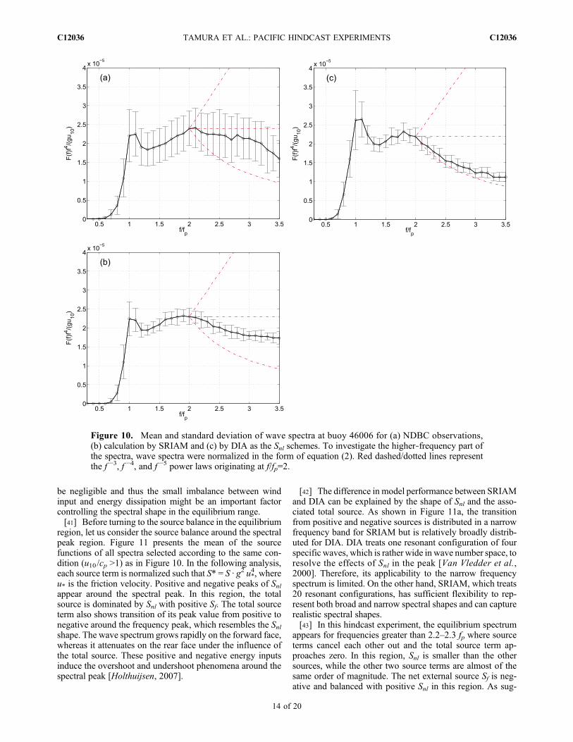
[35] Figure 10 presents the mean and standard deviation ofthe wave spectra at buoy 46006 (Figure 10a), calculated bySRIAM (Figure 10b) and DIA (Figure 10c). To investigatethe higher frequency part of the spectra, thewave spectra werenormalized as follows:

F f =fp� � ¼ F fð Þf 4=gu10; ð2Þ

where F is the frequency spectrum, g is gravitational accel-eration, and u10 is wind speed at 10 m height. If the wavespectrum obeys f −4 shape, the normalized spectrum (or sat-uration spectrum) F attains a steady value in the high‐frequency region. The wave spectra were selectively analyzedfor a young windsea with a unimodal peak; the inverse waveage (defined as u10 /cp, with cp being the phase speed of thespectral peak) was greater than 1, and the spectral shape hadone local maximum value. Normalized wave spectra (2) wereaveraged for discrete bins of D f /fp = 0.1. The wind speedobserved at 5 m at the NDBC buoy was adjusted to 10 m byapplying the 1/7 wind profile power law. The mean wavespectra shown in Figure 10 reflect well‐known behaviors ofwave spectra in the windsea; these were classified on the basisof two types of features, depending on frequency range: 1)overshoot, undershoot, and the associated spectral bandwidtharound the peak frequency region ( f /fp < 1.5); and 2) spectralshapes, such as a small hump at about twice the fp and a high‐frequency tail in the equilibrium range ( f /fp > 2).[36] The wave spectra measured by the NDBC buoy ex-

hibited overshoot ( f /fp ∼1.0) and undershoot ( f /fp ∼1.3)around the spectral peak. SRIAM (Figure 10b) but not DIA(Figure 10c) reproduced these phenomena well. DIA clearlyoverestimated overshoot as well as the energy levels for fre-quencies lower than fp. In addition, the frequency at theundershoot point was shifted to the higher‐frequency side

Figure 7. Same as Figure 5, but at NDBC 51004 in the low‐latitude Pacific.

TAMURA ET AL.: PACIFIC HINDCAST EXPERIMENTS C12036C12036

11 of 20

around f /fp ∼1.4. In contrast, SRIAM reproduced the energylevel around the spectral peak as well as the frequency at theundershoot spectrum ( f /fp ∼1.3) more realistically. Thesedifferences also affected the spectral bandwidth results ofeach model. That of DIAwas much broader than that of the insitu spectrum, whereas SRIAM quantitatively reproduced thespectral bandwidth around the peak frequency.[37] In the equilibrium range (e.g., f /fp: from 2 to 3), the

in situ wave spectrum indicated power law behavior

(Figure 10a), in which the saturation spectrum F was nearlyconstant and the spectral tail seemed to obey the f −4 powerlaw (or the power law with a slightly smaller exponent than−4). In addition, there appeared to be a small local peak at 2 fp.This small hump at about twice the value of fp appeared forinverse wave ages greater than 1 (Long and Resio [2007],their Figure 10), suggesting that wave development is impor-tant for the generation of this small hump. In the higher‐frequency region ( f /fp > 3), the spectral tail gradually diverged

Figure 8. Frequency‐direction wave spectra at 0:00, 19 April (NDBC 51004) obtained by (a) SRIAM and(b) DIA. The contour interval of the wave spectra is 0.1 in units of maximum wave spectrum.

TAMURA ET AL.: PACIFIC HINDCAST EXPERIMENTS C12036C12036

12 of 20

from the f −4 power law and sloped downward. Similar patternsof the deviation from f −4 spectral shapes were confirmed byResio et al. [2004; hereafter RLV04] and Long and Resio[2007]. It is possible that this is either the manifestation ofthe dissipation‐controlled wave spectral slope [Hansen et al.,1990] or measurement error due to the size of the buoy (3 mdiscus buoy). Therefore, we do not discuss the spectral shape inthe frequency range higher than 3.5 fp.[38] The effect of the accuracy of Snl parameterization on

the spectral tail slope was not as direct as that of the spectralshape around the peak frequency. The spectral tail calculatedby DIA clearly followed an alternative power law such as f −5

in the equilibrium range ( f/fp > 2) instead of f −4. On the otherhand, the spectral tail by SRIAM seemed to approach theobservational result and tended to follow the f −4.5 power lawin contrast to the spectral tail of DIA. TC96 developed thewave dissipation term based on the new concept that wavedissipation should be separated into at least two scalesexplicitly for the spectral peak (low‐frequency dissipation)and for the equilibrium range (high‐frequency dissipation).Furthermore, TC96 developed the high‐frequency dissipationso that the spectral tail obeys the f −5 power law in the equi-librium range. Therefore, the spectral tail indicated inFigure 10c is an expected result of the original WW3; how-ever, the model did not reproduce the observational results.On the other hand, the spectral tail calculated by SRIAMseemed to have an improved spectral shape as compared toobservations. However, as discussed later, the Sds term is animportant factor in determining the spectral form in the higher‐frequency region.[39] It is also worth mentioning that both model results

show a hump at about twice the peak frequency that alsoappears in the NDBC buoy data. However, this should notbe interpreted as physically sound model behavior. TC96indicated that an artificial local peak of the wave spec-trum appears in the transition zone between high‐ and low‐

frequency dissipation models (Figure 8b in TC96). Ourmodel results also indicate the same physically incorrectbehavior.

4.2. Source Terms and Their Balance

[40] Following RLV04, we investigated the relationshipbetween wave spectral shape and source term balance. Tomaintain the equilibrium range, the sum of the three sourceterms should be zero within the equilibrium range, as follows:

Sin þ Sds þ Snl ¼ Sf � @GE=@f ¼ 0; ð3Þ

where Sf is the net external force due to wind input and dis-sipation (i.e., Sin + Sds), and GE is the net flux of energy due tothe nonlinear interaction (Snl = −∂GE/∂f ). Resio et al. [2001]indicated that the net nonlinear energy flux has a cubicdependence on the normalized energy density F in the equi-librium range, and RLV04 presented the following relations:

GE fð Þ � GE feq� � �

Zf

feq

@F3

@fdf �

Zf

feq

Sf df ; ð4Þ

where f is an arbitrary frequency inside the equilibrium regionand feq is the lower bound frequency for the equilibriumregion. Equation (4) clearly demonstrates that any net gain orloss of wave energy within the equilibrium range would tendto force the spectrum away from an f −4 shape. If the net effectof Sf is negligible (Sf ∼0) within the equilibrium range, theflux of energy due to nonlinear transfer GE and saturationspectrum F should be constant; that is, GE ( f ) = GE ( feq) =constant, and F 3( f ) = F 3( feq) = constant. Because the fre-quency spectral tails measured in many field observationshave exhibited the f −4 spectral form [e.g., Donelan et al.,1985], the absolute value of the net external force Sf should

Figure 9. Time series of frequency peakedness Qp at (a) NDBC 46006 and (b) NDBC 51004, which cor-respond to Figures 4 and 5, respectively, at the same duration and location; circle: in situ data, solid blackline: SRIAM, dashed‐dotted line: DIA. In situQpwas calculated from historical NDBC data with (a) lower‐frequency resolution of 0.01 Hz bin size and with (b) higher‐frequency resolution of 0.005∼0.02‐Hz binsize, respectively.

TAMURA ET AL.: PACIFIC HINDCAST EXPERIMENTS C12036C12036

13 of 20

be negligible and thus the small imbalance between windinput and energy dissipation might be an important factorcontrolling the spectral shape in the equilibrium range.[41] Before turning to the source balance in the equilibrium

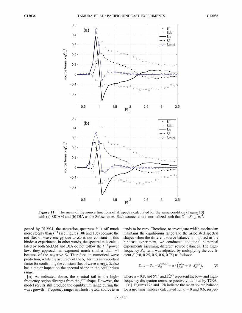
region, let us consider the source balance around the spectralpeak region. Figure 11 presents the mean of the sourcefunctions of all spectra selected according to the same con-dition (u10 /cp >1) as in Figure 10. In the following analysis,each source term is normalized such that S* = S · g2 u*

4, whereu* is the friction velocity. Positive and negative peaks of Snlappear around the spectral peak. In this region, the totalsource is dominated by Snl with positive Sf. The total sourceterm also shows transition of its peak value from positive tonegative around the frequency peak, which resembles the Snlshape. The wave spectrum grows rapidly on the forward face,whereas it attenuates on the rear face under the influence ofthe total source. These positive and negative energy inputsinduce the overshoot and undershoot phenomena around thespectral peak [Holthuijsen, 2007].

[42] The difference in model performance between SRIAMand DIA can be explained by the shape of Snl and the asso-ciated total source. As shown in Figure 11a, the transitionfrom positive and negative sources is distributed in a narrowfrequency band for SRIAM but is relatively broadly distrib-uted for DIA. DIA treats one resonant configuration of fourspecific waves, which is rather wide in wave number space, toresolve the effects of Snl in the peak [Van Vledder et al.,2000]. Therefore, its applicability to the narrow frequencyspectrum is limited. On the other hand, SRIAM, which treats20 resonant configurations, has sufficient flexibility to rep-resent both broad and narrow spectral shapes and can capturerealistic spectral shapes.[43] In this hindcast experiment, the equilibrium spectrum

appears for frequencies greater than 2.2–2.3 fp where sourceterms cancel each other out and the total source term ap-proaches zero. In this region, Snl is smaller than the othersources, while the other two source terms are almost of thesame order of magnitude. The net external source Sf is neg-ative and balanced with positive Snl in this region. As sug-

Figure 10. Mean and standard deviation of wave spectra at buoy 46006 for (a) NDBC observations,(b) calculation by SRIAM and (c) by DIA as the Snl schemes. To investigate the higher‐frequency part ofthe spectra, wave spectra were normalized in the form of equation (2). Red dashed/dotted lines representthe f −3, f −4, and f −5 power laws originating at f/fp=2.

TAMURA ET AL.: PACIFIC HINDCAST EXPERIMENTS C12036C12036

14 of 20

gested by RLV04, the saturation spectrum falls off muchmore steeply than f −4 (see Figures 10b and 10c) because thenet flux of wave energy due to Snl is not constant in thishindcast experiment. In other words, the spectral tails calcu-lated by both SRIAM and DIA do not follow the f −4 powerlaw; they approach an exponent much smaller than −4because of the negative Sf. Therefore, in numerical waveprediction, while the accuracy of the Snl term is an importantfactor for confirming the constant flux of wave energy, Sf alsohas a major impact on the spectral shape in the equilibriumrange.[44] As indicated above, the spectral tail in the high‐

frequency region diverges from the f −4 shape. However, themodel results still produce the equilibrium range during thewave growth in frequency ranges inwhich the total source term

tends to be zero. Therefore, to investigate which mechanismmaintains the equilibrium range and the associated spectralshapes when the different source balance is imposed in thehindcast experiment, we conducted additional numericalexperiments assuming different source balances. The high‐frequency Sds term was adjusted by multiplying the coeffi-cient b (=0, 0.25, 0.5, 0.6, 0.75) as follows:

Stotal ¼ Sin þ SSRIAMnl þ � � Slowds þ � � Shighds

� �; ð5Þ

wherea = 0.8, and Sdslow and Sds

high represent the low‐ and high‐frequency dissipation terms, respectively, defined by TC96.[45] Figures 12a and 12b indicate the mean source balance

for a growing windsea calculated for b = 0 and 0.6, respec-

Figure 11. The mean of the source functions of all spectra calculated for the same condition (Figure 10)with (a) SRIAM and (b) DIA as the Snl schemes. Each source term is normalized such that S* = S · g2u*

−4.

TAMURA ET AL.: PACIFIC HINDCAST EXPERIMENTS C12036C12036

15 of 20

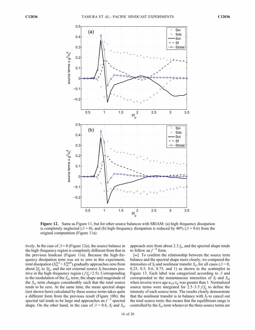
tively. In the case of b = 0 (Figure 12a), the source balance inthe high‐frequency region is completely different from that inthe previous hindcast (Figure 11a). Because the high‐fre-quency dissipation term was set to zero in this experiment,total dissipation (Sds

low+ Sdshigh) gradually approaches zero from

about 2fp to 3fp, and the net external source Sf becomes pos-itive in the high‐frequency region ( f /fp>2.5). Correspondingto the modulation of the Sds term, the shape and magnitude ofthe Snl term changes considerably such that the total sourcetends to be zero. At the same time, the mean spectral shape(not shown here) calculated by these source terms takes quitea different form from the previous result (Figure 10b); thespectral tail tends to be large and approaches an f −3 spectralshape. On the other hand, in the case of b = 0.6, Sf and Snl

approach zero from about 2.3 fp, and the spectral shape tendsto follow an f −4 form.[46] To confirm the relationship between the source term

balance and the spectral shape more clearly, we compared theintensities of Sf and nonlinear transfer Snl for all cases (b = 0,0.25, 0.5, 0.6, 0.75, and 1) as shown in the scatterplot inFigure 13. Each label was categorized according to b andcorresponded to the instantaneous intensities of Sf and Snlwhen inverse wave age u10/cp was greater than 1. Normalizedsource terms were integrated for 2.5–3.5 f /fp to define theintensity of each source term. The results clearly demonstratethat the nonlinear transfer is in balance with Sf to cancel outthe total source term; this means that the equilibrium range iscontrolled by the Snl term whenever the three source terms are

Figure 12. Same as Figure 11, but for other source balances with SRIAM: (a) high‐frequency dissipationis completely neglected (b = 0), and (b) high‐frequency dissipation is reduced by 40% (b = 0.6) from theoriginal computation (Figure 11a).

TAMURA ET AL.: PACIFIC HINDCAST EXPERIMENTS C12036C12036

16 of 20

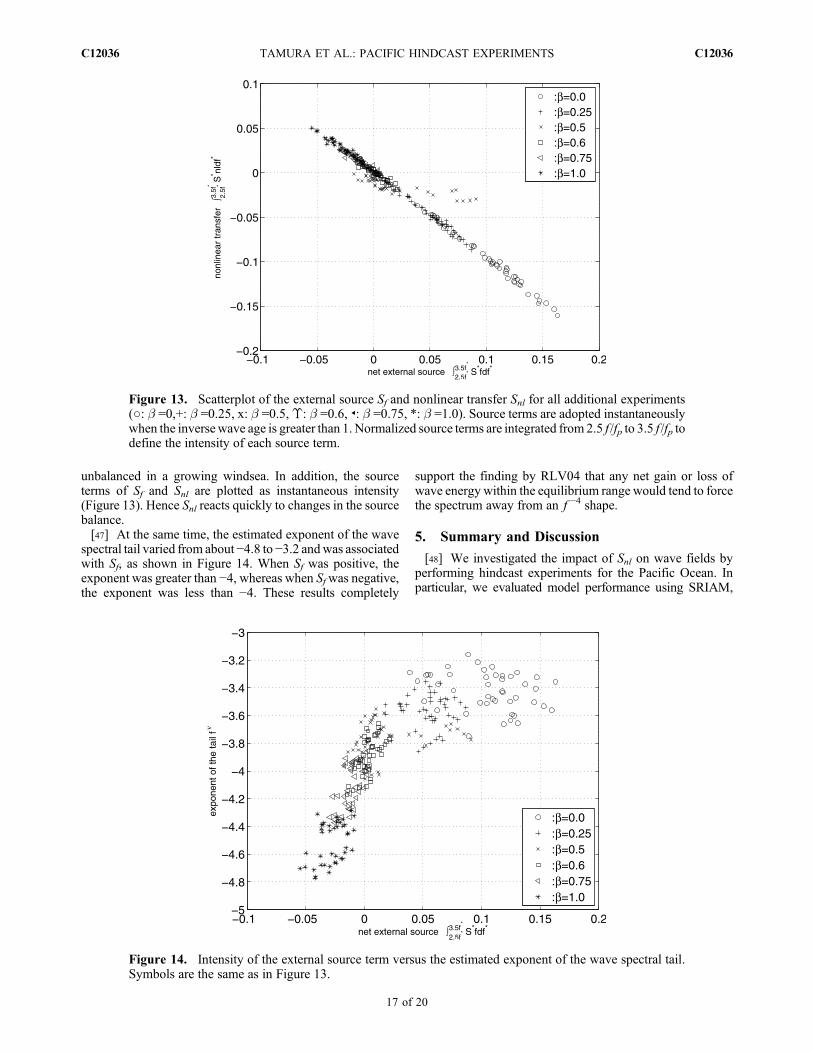
unbalanced in a growing windsea. In addition, the sourceterms of Sf and Snl are plotted as instantaneous intensity(Figure 13). Hence Snl reacts quickly to changes in the sourcebalance.[47] At the same time, the estimated exponent of the wave

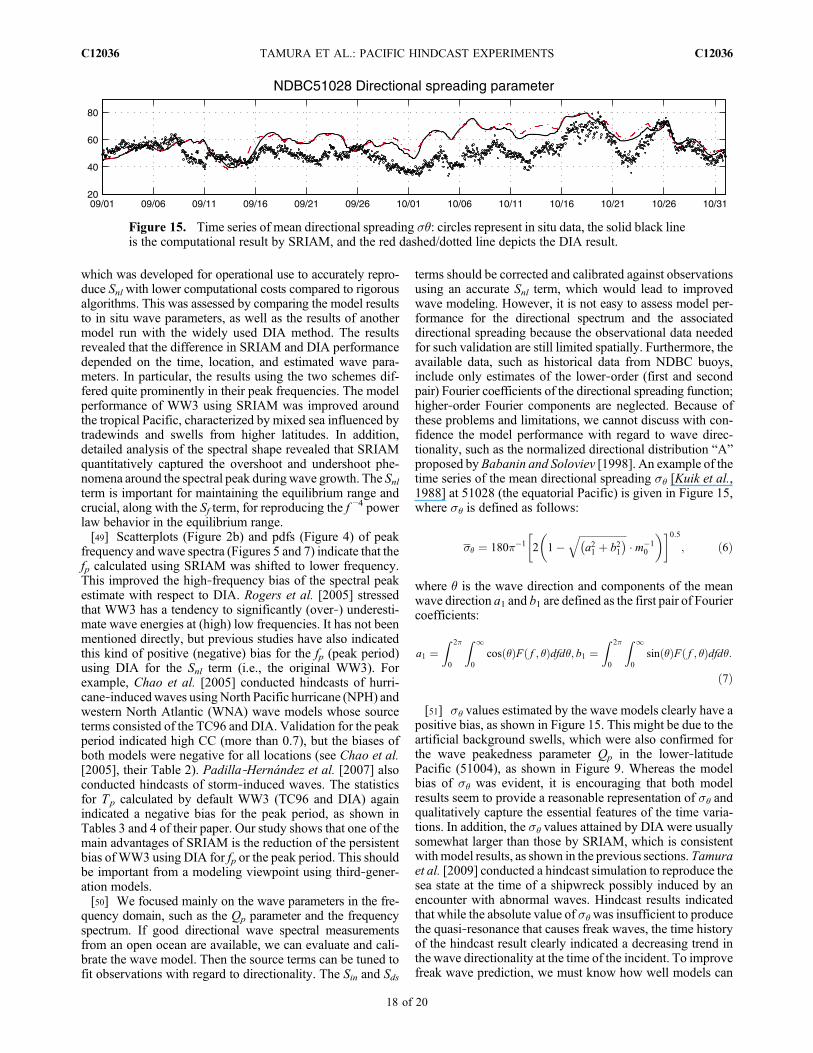
spectral tail varied from about −4.8 to −3.2 andwas associatedwith Sf, as shown in Figure 14. When Sf was positive, theexponent was greater than −4, whereas when Sfwas negative,the exponent was less than −4. These results completely

support the finding by RLV04 that any net gain or loss ofwave energy within the equilibrium range would tend to forcethe spectrum away from an f −4 shape.

5. Summary and Discussion

[48] We investigated the impact of Snl on wave fields byperforming hindcast experiments for the Pacific Ocean. Inparticular, we evaluated model performance using SRIAM,

Figure 13. Scatterplot of the external source Sf and nonlinear transfer Snl for all additional experiments(○: b =0,+: b =0.25, x: b =0.5,ϒ: b =0.6, ◂: b =0.75, *: b =1.0). Source terms are adopted instantaneouslywhen the inversewave age is greater than 1. Normalized source terms are integrated from 2.5 f /fp to 3.5 f /fp todefine the intensity of each source term.

Figure 14. Intensity of the external source term versus the estimated exponent of the wave spectral tail.Symbols are the same as in Figure 13.

TAMURA ET AL.: PACIFIC HINDCAST EXPERIMENTS C12036C12036

17 of 20

which was developed for operational use to accurately repro-duce Snl with lower computational costs compared to rigorousalgorithms. This was assessed by comparing the model resultsto in situ wave parameters, as well as the results of anothermodel run with the widely used DIA method. The resultsrevealed that the difference in SRIAM and DIA performancedepended on the time, location, and estimated wave para-meters. In particular, the results using the two schemes dif-fered quite prominently in their peak frequencies. The modelperformance of WW3 using SRIAM was improved aroundthe tropical Pacific, characterized by mixed sea influenced bytradewinds and swells from higher latitudes. In addition,detailed analysis of the spectral shape revealed that SRIAMquantitatively captured the overshoot and undershoot phe-nomena around the spectral peak duringwave growth. The Snlterm is important for maintaining the equilibrium range andcrucial, along with the Sf term, for reproducing the f −4 powerlaw behavior in the equilibrium range.[49] Scatterplots (Figure 2b) and pdfs (Figure 4) of peak

frequency and wave spectra (Figures 5 and 7) indicate that thefp calculated using SRIAM was shifted to lower frequency.This improved the high‐frequency bias of the spectral peakestimate with respect to DIA. Rogers et al. [2005] stressedthat WW3 has a tendency to significantly (over‐) underesti-mate wave energies at (high) low frequencies. It has not beenmentioned directly, but previous studies have also indicatedthis kind of positive (negative) bias for the fp (peak period)using DIA for the Snl term (i.e., the original WW3). Forexample, Chao et al. [2005] conducted hindcasts of hurri-cane‐inducedwaves usingNorth Pacific hurricane (NPH) andwestern North Atlantic (WNA) wave models whose sourceterms consisted of the TC96 and DIA. Validation for the peakperiod indicated high CC (more than 0.7), but the biases ofboth models were negative for all locations (see Chao et al.[2005], their Table 2). Padilla‐Hernández et al. [2007] alsoconducted hindcasts of storm‐induced waves. The statisticsfor Tp calculated by default WW3 (TC96 and DIA) againindicated a negative bias for the peak period, as shown inTables 3 and 4 of their paper. Our study shows that one of themain advantages of SRIAM is the reduction of the persistentbias of WW3 using DIA for fp or the peak period. This shouldbe important from a modeling viewpoint using third‐gener-ation models.[50] We focused mainly on the wave parameters in the fre-

quency domain, such as the Qp parameter and the frequencyspectrum. If good directional wave spectral measurementsfrom an open ocean are available, we can evaluate and cali-brate the wave model. Then the source terms can be tuned tofit observations with regard to directionality. The Sin and Sds

terms should be corrected and calibrated against observationsusing an accurate Snl term, which would lead to improvedwave modeling. However, it is not easy to assess model per-formance for the directional spectrum and the associateddirectional spreading because the observational data neededfor such validation are still limited spatially. Furthermore, theavailable data, such as historical data from NDBC buoys,include only estimates of the lower‐order (first and secondpair) Fourier coefficients of the directional spreading function;higher‐order Fourier components are neglected. Because ofthese problems and limitations, we cannot discuss with con-fidence the model performance with regard to wave direc-tionality, such as the normalized directional distribution “A”proposed by Babanin and Soloviev [1998]. An example of thetime series of the mean directional spreading s� [Kuik et al.,1988] at 51028 (the equatorial Pacific) is given in Figure 15,where s� is defined as follows:

�� ¼ 180��1 2 1�ffiffiffiffiffiffiffiffiffiffiffiffiffiffiffiffiffiffiffia21 þ b21� �q

� m�10

� �0:5; ð6Þ

where � is the wave direction and components of the meanwave direction a1 and b1 are defined as the first pair of Fouriercoefficients:

a1 ¼Z 2�

0

Z 1

0cos �ð ÞF f ; �ð Þdfd�; b1 ¼

Z 2�

0

Z 1

0sin �ð ÞF f ; �ð Þdfd�:

ð7Þ

[51] s� values estimated by the wave models clearly have apositive bias, as shown in Figure 15. This might be due to theartificial background swells, which were also confirmed forthe wave peakedness parameter Qp in the lower‐latitudePacific (51004), as shown in Figure 9. Whereas the modelbias of s� was evident, it is encouraging that both modelresults seem to provide a reasonable representation of s� andqualitatively capture the essential features of the time varia-tions. In addition, the s� values attained by DIA were usuallysomewhat larger than those by SRIAM, which is consistentwithmodel results, as shown in the previous sections. Tamuraet al. [2009] conducted a hindcast simulation to reproduce thesea state at the time of a shipwreck possibly induced by anencounter with abnormal waves. Hindcast results indicatedthat while the absolute value of s�was insufficient to producethe quasi‐resonance that causes freak waves, the time historyof the hindcast result clearly indicated a decreasing trend inthe wave directionality at the time of the incident. To improvefreak wave prediction, we must know how well models can

Figure 15. Time series of mean directional spreading s�: circles represent in situ data, the solid black lineis the computational result by SRIAM, and the red dashed/dotted line depicts the DIA result.

TAMURA ET AL.: PACIFIC HINDCAST EXPERIMENTS C12036C12036

18 of 20

estimate directional spreading, and the estimated parametersneed to be calibrated against observations.[52] Regarding the equilibrium condition, in many studies

[e.g., Komen et al., 1984; Phillips, 1985; TC96] the totalsource terms were considered to be zero to maintain the equi-librium region of the wave spectrum; i.e., as given inequation (3). Then the shape of the source terms Sin and Sds areassumed to balance each other and to satisfy the necessarycondition as also indicated in equation (3). In particular, theSds term is often considered the “tuning knob” in the wavemodel, derived as the residual of the unknown term inequation (3). However, the present study indicates a differentformation process of the source balance in the equilibriumrange. The total source term approached zero during waveevolution, regardless of which Sf function was used. Snl playsa major role in the adjustment of the total source balance. Ourresults demonstrate that the balance of the equilibrium con-dition (3) is maintained by the Snl term.[53] Previous works have investigated the role of source

terms and their balance in a growing windsea. Kitaigorodskii[1983] derived an f −4 spectral tail based on the assumptionthat the energy flux due to Snl is constant inside the equilib-rium range and that source terms are negligible (Sin ∼ Snl ∼ Sds∼0) to maintain it. On the other hand, Phillips [1985] inves-tigated the relative roles of the source terms and concludedthat all three are of the same order of magnitude (Sin ∼ Snl ∼Sds) in representing the f −4 spectral tail. Banner and Young[1994] investigated the influence of the level of dissipationand demonstrated that the magnitude of Sds influences theamount of energy in the spectral tail but has little influence onthe decay exponent. Young and Van Vledder [1993] alsostated that the energy level in the spectral tail is sensitive to thechoice of Sin and Sds; however, the exponent of the spectraltail is less sensitive. The present study also demonstrates thatthe sum of the three source terms approaches zero largely as aresult of Snl adjustment. However, the exponent of the spectraltail was also quite sensitive to Sf, in agreement with RLV04.SRIAM can reproduce the time evolution of the spectralshape to formulate the f −4 tail when the kinetic equation issimply integrated in time (not shown here). This suggests thatSRIAM can also force the spectral tail to take an f −4 form, asin an exact Snl computation [e.g., Resio et al., 2001]. How-ever, the net external source Sf is the key factor that re-produces the f −4 tail, and “Sf ∼0 inside the equilibrium range”might be considered a constraint in numerical wave modelingto guarantee the −4 exponent.

[54] Acknowledgments. We are grateful to two reviewers for theircareful reading of this paper and their constructive comments, which werevery helpful in improving the manuscript. This work is part of the JapanCoastal Ocean Predictability Experiment (JCOPE) supported by the JapanAgency for Marine‐Earth Science and Technology. Takuji Waseda was alsosupported by a Grant‐in‐Aid for Scientific Research from the Japan Societyfor the Promotion of Science.

ReferencesArdhuin, F., T. H. C. Herbers, G. P. Van Vledder, K. P. Watts, R. Jensen,and H. C. Graber (2007), Swell and slanting fetch effects on wind wavegrowth, J. Phys. Oceanogr., 37, 908–931.

Babanin, A. V., and Y. P. Soloviev (1998), Variability of directional spec-tra of wind‐generated waves, studied by means of wave staff arrays,Mar.Freshwater Res., 49, 89–101.

Badulin, S. I., A. N. Pushkarev, D. Resio, and V. E. Zakharov (2005), Self‐similarity of wind‐driven seas, Nonlin. Proc. Geophys., 12, 891–945.

Banner, M. L., and I. R. Young (1994), Modeling spectral dissipation in theevolution of wind waves. Part I: Assessment of existing model perfor-mance, J. Phys. Oceanogr., 24, 1550–1571.

Barnett, T. P., and J. C. Wilkerson (1967), On the generation of ocean windwaves as inferred from airborne radar measurements of fetch‐limitedspectra, J. Mar. Res., 25, 292–321.

Bidlot, J., et al. (2007), Inter‐comparison of operational wave forecastingsystems, 10th International Workshop on Wave Hindcasting and Fore-casting and Coastal Hazard Symposium, North Shore, Oahu, Hawaii.

Cardone, V. J., R. E. Jensen, D. T. Resio, V. R. Swail, and A. T. Cox(1996), Evaluation of contemporary ocean wave models in rare extremeevents: The “Halloween Storm” of October 1991 and the “Storm of theCentury” of March 1993, J. Atmos. Oceanic Technol., 13, 198–230.

Chao, Y. Y., J. H. G. M. Alves, and H. L. Tolman (2005), An operationalsystem for predicting hurricane‐generated wind waves in the NorthAtlantic Ocean, Weather Forecasting, 20(4), 652–671.

Donelan, M. A., J. Hamilton, and W. H. Hui (1985), Directional spectra ofwind‐generated waves, Philos. Trans. R. Soc. London A, 315, 509–562.

Goda, Y. (2000), Random Seas and Design of Maritime Structures, Adv.Ser. Ocean Eng., vol. 15, 443 pp., Univ. of Tokyo Press, Tokyo, Japan.

Gramstad, O., and K. Trulsen (2007), Influence of crest and group lengthon the occurrence of freak waves, J. Fluid Mech., 582, 463–472.

Hansen, C., K. B. Katsaros, S. A. Kitaigorodskii, and S. E. Larsen (1990),The dissipation range of wind‐wave spectra observed on a lake, J. Phys.Oceanogr., 20, 1264–1277.

Hasselmann, K. (1962), On the nonlinear energy transfer in a gravity‐wavespectrum I, General theory, J. Fluid Mech., 12, 481–500.

Hasselmann, K., et al. (1973), Measurements of wind wave growth andswell decay during the Joint North Sea Wave Project (JONSWAP),Dt. Hydrogr. Z., A8(12), 95 pp.

Hasselmann, S., K.Hasselmann, J.H. Allender, and T. P.Barnett (1985), Com-putations and parameterizations of the nonlinear energy transfer in a gravity‐wave spectrum. Part II: Parameterizations of the nonlinear energy transferfor application in wave models, J. Phys. Oceanogr., 15, 1378–1391.

Holthuijsen, L. H. (2007),Waves in Oceanic andCoastalWaters, CambridgeUniv. Press, Cambridge, U. K., 387 pp.

Janssen, P. A. E. M. (2003), Nonlinear four‐wave interactions and freakwaves, J. Phys. Oceanogr., 33, 863–884.

Janssen, P. A. E. M., and J. Bidlot (2003), New wave parameters to charac-terize freak wave conditions. Research Dept. Memo. R60.9.PJ/0387,ECMWF, Reading, U. K.

Kahma, K. K., and C. J. Calkoen (1994), Growth curve observations, inDynamics and Modelling of Ocean Waves, edited by G. J. Komen et al.,Cambridge Univ. Press, Cambridge, U. K., 174–182.

Kalnay, E., et al. (1996), The NCEP/NCAR 40‐year reanalysis project,Bull. Amer. Meteor. Soc., 77, 437–471.

Kitaigorodskii, S. A. (1983), On the theory of the equilibrium range in the spec-trum of wind‐generated gravity waves, J. Phys. Oceanogr., 13, 816–827.

Komatsu, K. (1996), Development of a new generation wave forecastingmodel based on a new scheme of nonlinear energy transfer among windwaves. Ph.D. thesis, Kyushu University, Japan, 155 pp. (in Japanese)(unpublished).

Komatsu, K., and A. Masuda (1996), A new scheme of nonlinear energytransfer among wind waves: RIAM method. Algorithm and performance,J. Oceanogr., 52, 509–537.

Komen, G. J., K. Hasselmann, andK.Hasselmann (1984), On the existence of afully developed wind‐sea spectrum, J. Phys. Oceanogr., 14(8), 1271–1285.

Komen, G. J., L. Cavaleri, M. Donelan, K. Hasselmann, S. Hasselmann,and P. A. E. M. Janssen (1994), Dynamics and Modelling of OceanWaves, Cambridge Univ. Press, Cambridge, U. K., 532 pp.

Kuik, A. J., G. P. van Vledder, and L. H. Holthuijsen (1988), A method forthe routine analysis of pitch‐and‐roll buoy wave data, J. Phys. Oceanogr.,18, 1020–1034.

Long, C. E., and D. T. Resio (2007), Wind wave spectral observations inCurrituck Sound, North Carolina, J. Geophys. Res., 112, C05001,doi:10.1029/2006JC003835.

Mitsuyasu, H. (1968), On the growth of the spectrum of wind generatedwaves, I. Rept. Res. Inst. Appl. Mech., Kyushu Univ., 16, 459–465.

Mitsuyasu, H. (1969), On the growth of the spectrum of wind generatedwaves, II. Rept. Res. Inst. Appl. Mech., Kyushu Univ., 17, 235–243.

Onorato, M., A. R. Osborne, and M. Serio (2002), Extreme wave events indirectional, random oceanic sea states, Phys. Fluids, 14(4), 25–28.

Padilla‐Hernández, R., W. Perrie, B. Toulany, and P. C. Smith (2007),Modeling of two Northwest Atlantic Storms with third‐generation wavemodels, Weather Forecasting, 22(6), 1229–1242.

Phillips, O. M. (1985), Spectral and statistical properties of the equilibriumrange of wind‐generated gravity waves, J. Fluid Mech., 156, 505–531.

TAMURA ET AL.: PACIFIC HINDCAST EXPERIMENTS C12036C12036

19 of 20

Pushkarev, D., T. Resio, and V. E. Zakharov (2003), Weak turbulentapproach to the wind‐generated gravity sea waves, Physica D‐NonlinearPhenomena, 184, 29–63.

Resio, D. T., and W. Perrie (1991), A numerical study of nonlinear energyfluxes due to wave‐wave interactions. Part 1: Methodology and basicresults, J. Fluid Mech., 223, 609–629.

Resio, D. T., and W. Perrie (2008), A two‐scale approximation for efficientrepresentation of nonlinear energy transfers in a wind wave spectrum.Part I: Theoretical development, J. Phys. Oceanogr., 38, 2801–2816,doi:10.1175/2008JPO3713.1.

Resio, D.T., J. H. Pihl, B. A. Tracy, and C. L. Vincent (2001), Nonlinearenergy fluxes and the finite depth equilibrium range in wave spectra,J. Geophys. Res., 106(C4), 6985–7000, doi:10.1029/2000JC900153.

Resio, D. T., C. E. Long, and C. L. Vincent (2004), Equilibrium‐range con-stant in wind‐generated wave spectra, J. Geophys. Res., 109, C01018,doi:10.1029/2003JC001788.

Rogers, W. E., P. A. Wittmann, D. W. C. Wang, R. M. Clancy, and Y. L.Hsu (2005), Evaluations of global wave prediction at the Fleet NumericalMeteorology andOceanographyCenter,Weather Forecasting, 20, 745–760.

Tamura, H., T. Waseda, Y. Miyazawa, and K. Komatsu (2008), Current‐induced modulation of the ocean wave spectrum and the role of nonlinearenergy transfer, J. Phys. Oceanogr., 38, 2662–2684, doi:10.1175/2008JPO4000.1.

Tamura, H., T. Waseda, and Y. Miyazawa (2009), Freakish sea state andswell‐windsea coupling: Numerical study of the Suwa‐Maru incident,Geophys. Res. Lett., 36, L01607, doi:10.1029/2008GL036280.

Toba, Y. (1973), Local balance in the air‐sea boundary processes III. Onthe spectrum of wind waves, J. Oceanogr. Soc. Japan, 29, 209–220.

Tolman, H. L. (2002), User manual and system documentation of WAVE-WATCH‐III version 2.22. Tech. Note, 222, NOAA/NWS/NCEP/MMAB, 133 pp.

Tolman, H. L. (2003), Treatment of unresolved islands and ice in windwave models, Ocean Modelling, 5, 219–231.

Tolman, H. L. (2004), Inverse modeling of discrete interaction approxima-tions for nonlinear interactions in wind waves, Ocean Modelling, 6,405–422.

Tolman, H. L., andD. V. Chalikov (1996), Source terms in a third‐generationwind wave model, J. Phys. Oceanogr., 26, 2497–2518.

Tolman, H. L., V. M. Krasnopolsky, and D. V. Chalikov (2005), Neuralnetwork approximations for nonlinear interactions in wind wave spectra:Direct mapping for wind seas in deepwater,OceanModelling, 8, 253–278.

Van Vledder, G. P. (2001), Extension of the discrete interaction approxima-tion for computing nonlinear quadruplet wave‐wave interactions in oper-ational wave prediction models, 4th International Symposium on OceanWaves, Measurement & Analysis, San Francisco, Calif.

Van Vledder, G. P. (2006a), The WRT method for the computation of non‐linear four‐wave interactions in discrete spectral wave models, CoastalEng., 53, 223–242.

Van Vledder, G. P. (2006b), Towards an optimal computation of non‐linearfour‐wave interactions in operational wave models, 9th Int. Workshop onWave Hindcasting and Forecasting, Victoria, BC, Canada.

Van Vledder, G. P., and J. A. Battjes (1992), Discussion on list of sea stateparameters, ASCE J. Port, Harbor Ocean Eng., 118, 226–228.

Van Vledder, G. P., T. H. C. Herbers, R. E. Jensen, D. T. Resio, and B.Tracy (2000), Modeling of non‐linear quadruplet wave‐wave interactionsin operational wave models. Proc. 27th Int. Conf. on Coastal Engineer-ing, Sydney, Australia.

Wang, W., and R. X. Huang (2004), Wind energy input to the surfacewaves, J. Phys. Oceanogr., 34, 1276–1280.

Waseda, T., T. Kinoshita, and H. Tamura (2009a), Evolution of a randomdirectional wave and freak wave occurrence, J. Phys. Oceanogr., 38,621–639.

Waseda, T., T. Kinoshita, and H. Tamura (2009b), Interplay of resonantand quasi‐resonant interaction of the directional ocean waves, J. Phys.Oceanogr., 39, 2351–2362.

Xu, F., W. Perrie, B. Toulany, and P.C. Smith (2007), Wind‐generatedwaves in Hurricane Juan, Ocean Modelling, 16, 188–205.

Young, I. R., and G. P. Van Vledder (1993), A review of the central role ofnonlinear interactions in wind‐wave evolution, Trans. R. Soc. London,342, 505–524.

Zakharov, V. E., and N. N. Filonenko (1966), The energy spectrum for sto-chastic oscillation of a fluid’s surface,Dokl. Akad. Nauk., 170, 1992–1995.

Y. Miyazawa, H. Tamura, and T. Waseda, Research Institute for GlobalChange, Japan Agency for Marine‐Earth Science and Technology,Yokohama, Kanagawa, 236‐0001, Japan. (htamura@jamstec.go.jp)

TAMURA ET AL.: PACIFIC HINDCAST EXPERIMENTS C12036C12036

20 of 20