Evolution of the extreme wave region in the North Atlantic using a 23 year hindcast.

Proceedings of the ASME 34th International Conference on Ocean, Offshore and ArcticEngineeringOMAE 2015

May 31-June 5, 2015, St. John’s, Canada

OMAE2015-41438

EVOLUTION OF THE EXTREME WAVE REGION IN THE NORTH ATLANTIC USING A23 YEAR HINDCAST

Sonia Ponce de Leon∗School of Mathematical Sciences/UCD Earth Institute

University College DublinDublinIreland

Email: [email protected]

Joao H. BettencourtSchool of Mathematical Sciences/UCD Earth Institute



Joseph BrennanSchool of Mathematical Sciences/UCD Earth Institute



Frederic DiasSchool of Mathematical Sciences/UCD Earth Institute



ABSTRACTThe IOWAGA data base for the North Atlantic region was

used to identify the region where extreme values of significantwave height are more likely to occur. The IOWAGA database [1]was obtained from the WAVEWATCH III model [2] hindcast us-ing the CFSR (Climate Forecast System Reanalysis) from NOAA[3,4]. The period of the study covers 1990 up to 2012 (23 years).The variability of the significant wave height was assessed bycomputing return periods for sea storms where the significantwave height exceeds a given threshold. The return periods ofsea storms where the Hs exceeds extreme values for the north At-lantic region were computed allowing for the identification of theextreme wave regions which show that extreme waves are morelikely to occur in the storm track regions of the tropical and ex-tratropical north Atlantic cyclones.

∗Address all correspondence to this author.

INTRODUCTION

Extreme sea states are a source of risk for marine struc-tures and operations. These extreme sea states are usually gener-ated by storms that can traverse whole ocean basins and generatehigh-energy swells that can propagate for thousands of kilome-ters. Additionally, rogue waves due to modulation instability [5]are a recognized source of extreme waves [6, 7] that needs to betaken into account when designing for operation at sea.

The north Atlantic ocean is regularly traversed by extra-tropical cyclones and winter low pressure systems originated inthe Western part of the basin that can potentially generate dan-gerous extreme sea states [8–10]. The region where these ex-treme sea states occur is linked to the tracks of the low pres-sure systems in the north Atlantic basin. The variability of thisstorm tracks presents a primary dipole pattern with centers in theextreme northeastern Atlantic and west of Portugal. A strongnortheastward extension of the storm tracks causes strong mar-itime flow giving rise to mild European winters and is primarilyassociated with low-frequency teleconnections [11]. Future cli-

1 Copyright c© 2015 by ASME

mate projections indicate a poleward migration of northern hemi-sphere storm tracks, with a distinct increase of storm track den-sity and mean intensities in an area over the British Isles and tothe north and west while a decrease in number and intensity isprojected in the Mediterranean [12].

Since waves are locally generated by surface winds, theirtrends should be related. Globally, [13] reported a general trendof increasing values of wind speed and wave height (to a lesserextent) based on a 23-year database of satellite altimeter mea-surements. In addition, the report showed a greater rate of in-crease in extreme values of wind speed and wave height. In theNorth Atlantic, the WASA project [14–18] found an increase inthe annual maximum of significant wave height (Hs) over the last40 years in the east of the basin. Results from a 40-year hind-cast using kinematically reanalyzed wind fields [19] also showa increase in extremes of winter wave height in the east, closelyassociated to the North Atlantic Oscillation (NAO) variations.

In the design of maritime structures, one is interested in thereturn periods of extreme events. The 100-year wave, e.g., wouldbe a wave with height exceeded on average once in a 100 yearsperiod. A related concept is the annual exceedance probabilitywhich is the probability that a wave will exceed a given thresholdin 1 year. In percentage terms, the annual exceedance probabilityof the p–year wave is simply 100/p.

Based on wind and wave reanalysis data, [20, 21] providedglobal estimates of 100-year wind speed (U10) and Hs return val-ues using the peaks–over–threshold (POT) method. The Hs 100-year return value estimates are higher in the storm tracks of theNorthern and Southern Hemispheres and lower in the tropics.Decadal variations in the estimates were found to be significantonly in the Northern Hemisphere storm tracks and in the westerntropical Pacific. These differences were attributed to the decadalvariability in the Northern Hemisphere, especially to the NAO.Interdecadal differences for U10 were found to be consistent withthose of the Hs. Nonetheless, a lack of a clear trend in 100-yearreturn value for Hs was reported by [22], using global altime-ter measurements spanning 23 years and the initial distributionmethod.

An equivalent problem of interest for the engineering ofmaritime structures is the prediction of waves that exceed a giventhreshold. The return period of a wave exceeding a given thresh-old was obtained by [23] and [24,25] studied the statistical prop-erties of waves in storms. Later, [26, 27] solved the problem ofthe return period of a sea storm during which the wave heightexceeds a given threshold. Thereafter, extensions to the returnperiod of nonlinear high waves, arbitrary number of waves andgeneralized storm models were presented [28–30].

In this paper, we compute return periods of sea storms wherethe Hs exceeds extreme values for the north Atlantic region. Us-ing a 23 year wave hindcast database covering the whole NorthAtlantic, the distribution of return periods in the basin can becomputed. The hincast interval is then divided in 4 year periods

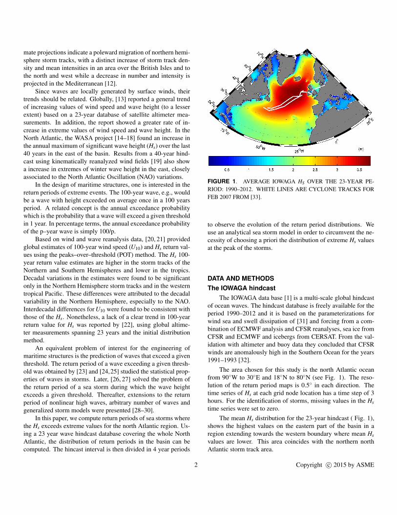
FIGURE 1. AVERAGE IOWAGA HS OVER THE 23-YEAR PE-RIOD: 1990–2012. WHITE LINES ARE CYCLONE TRACKS FORFEB 2007 FROM [33].

to observe the evolution of the return period distributions. Weuse an analytical sea storm model in order to circumvent the ne-cessity of choosing a priori the distribution of extreme Hs valuesat the peak of the storms.

DATA AND METHODSThe IOWAGA hindcast

The IOWAGA data base [1] is a multi-scale global hindcastof ocean waves. The hindcast database is freely available for theperiod 1990–2012 and it is based on the parameterizations forwind sea and swell dissipation of [31] and forcing from a com-bination of ECMWF analysis and CFSR reanalyses, sea ice fromCFSR and ECMWF and icebergs from CERSAT. From the val-idation with altimeter and buoy data they concluded that CFSRwinds are anomalously high in the Southern Ocean for the years1991–1993 [32].

The area chosen for this study is the north Atlantic oceanfrom 90◦W to 30◦E and 18◦N to 80◦N (see Fig. 1). The reso-lution of the return period maps is 0.5◦ in each direction. Thetime series of Hs at each grid node location has a time step of 3hours. For the identification of storms, missing values in the Hstime series were set to zero.

The mean Hs distribution for the 23-year hindcast ( Fig. 1),shows the highest values on the eastern part of the basin in aregion extending towards the western boundary where mean Hsvalues are lower. This area coincides with the northern northAtlantic storm track area.


Equivalent triangular stormA sea storm is defined as a sequence of sea states where the

Hs is above a given threshold hp for a predefined amount of time.In [27], the threshold hp is defined as 1.5Hs with Hs the annualmean of Hs and the continuos time period as 12 hours. With thesetwo conditions and given a record of Hs a sequence of storms canbe defined for a specific location.

Each of the members of this storm sequence can then beapproximated by an analytical function of time that, during thestorm duration b gives the Hs as

h(t) = a[1− (2tb

)], −b2≤ t ≤ b

2, (1)

where values of t < 0 indicate time before the peak of the storm(t = 0). The storm intensity a is the maximum wave heightachievable during the storm. The parameters a and b definedthe equivalent triangular storm (ETS) model [27, 34].

Return period of a storm where Hs exceeds a thresholdConsidering a series of N(τ) storms ocurring at a given lo-

cation during a time interval τ , the time Th during which Hs staysabove a given threshold h is Th = τP(h), where P(h) = P(Hs >h). According to [30], the return period of a storm during whichHs exceeds h can be computed as

Rh =τ

N(τ;Hs > h), (2)

where N(τ;Hs > h) is the average number of storms where theHs exceeds h.

The ETS model can be used to compute the return periodgiven by eqn. 2. The method presented by [30] is described:considering that a and b are realizations of the random vari-ables storm intensity A and storm duration B, the joint proba-bility density function (pdf) of A and B is defined as pA,B(a,b) =pA(a)pB|A(b|a) and pA,B(a,b)dadb as the number of equivalentstorms with intensity between (a,a + da) and duration between(b,b+db). The pdf of A is then

pA(a) =∫

∞

0pA,B(a,b)db, (3)

and the number of equivalent storms having intensity between(a,a+da) and duration between (b,b+db) is

dN(a,b) = N(τ)pA(a)pB|A(b|a)dadb, (4)

from which the average number of equivalent storms with A > hcan be computed as

N(τ;A > h) =∫

∞

a=h

∫∞

0dN(a,b) = N(τ)

∫∞

a=hpA(a)da. (5)

The return period can then be obtained by replacing N(τ;A > h)in eqn. 2. The storm intensity pdf is given by [30]

pA(a) =τ

N(τ)a

b(a)G(λ ,a), (6)

where b(a) is the conditional average duration of B given A = a.The function G(λ ,a) is given for the case of the ETS, by:

G(λ ,a) =d2Pda2 , (7)

with P(h) = P(Hs > h).To compute the conditional average duration b(a) for a given

a, it is approximated by a regression b(a) = K1 log(a)+ K2. Toobtain the regression coefficients, we construct a random se-quence of (a,b) pairs using the actual storm sequence at the lo-cation of interest. The storm intensity a is the maximum Hs foreach storm and the duration is found by requiring that the ex-pected maximum wave height Hmax is the same for the actualand for the equivalent storm.

Computation of exceedance probability P(Hs > h)We assume that the exceedance probability of the Hs is given

by a lower-bounded three parameter Weibull distribution

P(h) = 1− exp[−(h−hl

w)u], h≥ hl , (8)

where the unknown parameters are obtained by least-squares fit-ting to the Hs time series. This method allows to obtain two ofthe three parameters of the Weibull distribution (eqn. 8), namelythe scale parameter w and the location parameter hl . The thirdparameter, the shape parameter u, is chosen as the one that mini-mizes the residue of the correlation between the fitted distributionand the original data. While the Weibull distribution may fail torepresent well the whole distribution, it can fit the low probabilitypart reasonably well [35].

For this reason we have focused our analysis on thresholdsabove the 99th percentile of the Hs exceedance distribution, com-puted from the Weibull distribution parameters fitted at each datapoint and shown in Fig.2. The sharp gradients in the map are dueto the fact that minimization of the correlation residue between


FIGURE 2. SPATIAL DISTRIBUTION OF THE 99T H PER-CENTILE FOR THE HS IN THE PERIOD: 1990–2012.

the fitted distribution and the original data, was performed by di-rect search over a discrete set of values of u, between 0.75 and2.0. Due to the computationally expensive nature of this processfor the amount of grid points, only 15 values of u were used be-tween these limits and thus sharp changes in the u distributionwere obtained, which were reflected in the 99th percentile distri-bution.

RESULTSReturn periods for the 23-year hindcast

The return periods of sea storms where the Hs exceeds agiven threshold were computed for several Hs values in NorthAtlantic.

In Fig. 3 the return period contours for the Hs threshold of20 m are shown. At the 1-year return period level of sea storms,the contours delimit the eastern north Atlantic from 40◦N to Ice-land, the bay of Biscay and several small scale regions in theCaribbean and Atlantic. At the 10-year level, the region is en-larged to the whole north Atlantic northward from 30-36◦N, aportion of the western Atlantic below these latitudes, roughly be-tween 50 and 75◦W and two small regions in the Gulf of Mexicoand in the Caribbean sea. At the 50 and 100 years return periodlevel, the contours practically coincide and limit a region com-bining the two previous ones mentioned for the 10-year returnperiod.

At the 10-year return period level for a sea storm withHs >20 m, the northern Atlantic region matches well with thestorm track region of north Atlantic cyclones [36], while thewestern Atlantic region below 30 ◦N, the Gulf of Mexico andCaribbean sea corresponds to the north Atlantic tropical cyclonepaths. At the 1-year sea storm return period level for the same

FIGURE 3. RETURN PERIODS FOR HS > 20 M. LINES EN-CLOSE REGIONS WHERE RETURN PERIOD IS LESS THAN 1YEAR (BLUE); 10 YEARS (RED); 50 YEARS (BLACK); 100 YEARS(CYAN).

Hs threshold, the region is greatly reduced to the eastern NorthAtlantic in the region with the highest 100-year return values ofHs, already identified in [20] and [13].

Evolution of the extreme wave regionTo study the evolution of the extreme wave region, the 23

year hindcast was divided in five 4 year periods, starting in 1992.In order not to split the winters between differents years, the be-ginning and end of year were set at 1st of July and 30th of June,respectively. In Fig. 4, the return period for sea storms with Hsthreshold set at 25 m is shown for the periods 1992–1996 (toppanel) and 1996–2000 (bottom panel). The major difference wasfound between the 1996–2000 period and the others, where a de-crease in the area delimited by the 50 and 100 years return periodcontours was found. This coincides with a jump in the reanaly-sis winds particularly visible in the 99th percentile winds [32].The 99th percentile has a significant impact on wave height inthe wave model when modelling extreme events such as hur-ricanes.The remaining periods (2000–2004, 2004–2008, 2008–2012) have return period distributions very similar to the 1992–1996 period.

The reduction in area observed in the 1996–2000 period isnot completely clear as to its reasons but the uses of different dataassimilation techniques and inconsistent reanalysis could be thecauses [37]. Also, The 5 year period between 1995-2000 wascharacterized by a multi–decadal increase in sea surface tem-perature and an increase in the number of Atlantic major hur-ricanes [38]. On the other hand, no clear tendency in increaseor reduction of the extreme wave region could be identified inthe whole period, in agreement with the lack of tendency for the100-year Hs return values found by [22].


FIGURE 4. RETURN PERIODS FOR HS > 25 M. TOP PANEL:1992-1996; BOTTOM PANEL: 1996-2000; LINE COLOURING ASIN FIG.3

CONCLUSIONSThe extreme wave regions of the North Atlantic were iden-

tified by computing return periods of sea storms were the Hs ex-ceeds a given threshold. Using a 23-year hindcast of the wholeNorth Atlantic region, spatial distributions of the return periodswere obtained.

The return period maps, show that extreme waves are morelikely to occur in the storm track regions of the tropical and ex-tratropical north Atlantic. For an Hs threshold of 20 m, returnperiods of 1 year or less are limited to the eastern North Atlanticzone above 40◦N. It was not possible to observe any trend in thereturn period values through the time period considered, but adecrease in the 25 m sea storm return period was found for theperiod of 1996–2004. The reason for this reduction is not com-pletely clear and further analysis is needed to clarify this.

The return period estimates based on equivalent storm mod-els presented in this paper appear to be conservative when com-

pared to Hs return values, e.g. [22] reports a 100-year Hs returnlevel of 26 m for the north Atlantic region whereas in this studythe return period of a storm where Hs > 25 m can be lower than50 years. Computations based on the POT method at selected lo-cations (not shown) also show higher return periods for the sameHs level using the ETS model. Other source of error in this workis the extrapolation (implicit in the choice of the Hs threshold) forvalues of return period much larger than the length of availablerecords (measured or hindcasted by models). This procedure isjustified by the need to work with conservative load levels in theprocess of engineering design of marine structures.

To conclude, the ETS provides a valuable tool to computedesign values of wave loads. By using the ETS model of [27], itwas not necessary to impose a distribution type to the distributionof Hs storm peaks. Further work is being done to improve certainaspects of the computation and application to other ocean basinsis being planned.

ACKNOWLEDGMENTThis work is based upon works supported by the European

Research Council (ERC) under the research project ERC-2011-AdG 290562-MULTIWAVE and Science Foundation Ireland un-der grant number SFI/12/ERC/E2227.

REFERENCES[1] Rascle, N., and Ardhuin, F., 2013. “A global wave param-

eter database for geophysical applications. Part 2: Modelvalidation with improved source term parameterization”.Ocean Modelling, 70, pp. 174–188.

[2] Tolman, H. L., and Group, D., 2014. User manual andsystem documentation of WAVEWATCH III version 4.18.Tech. Rep. Tech. Note 316, NOAA/NWS/NCEP/MMAB.

[3] Saha, S., Moorthi, S., Pan, H.-L., Wu, X., Wang, J., Nadiga,S., Tripp, P., Kistler, R., Woollen, J., Behringer, D., et al.,2010. “The NCEP climate forecast system reanalysis”.Bulletin of the American Meteorological Society, 91(8),pp. 1015–1057.

[4] Saha, S., Moorthi, S., Wu, X., Wang, J., Nadiga, S., Tripp,P., Behringer, D., Hou, Y., Chuang, H., Iredell, M., Ek, M.,Meng, J., Yang, R., Mendez, M., van den Dool, H., Zhang,Q., Wang, W., Chen, M., and Becker, E., 2014. “The NCEPclimate forecast system version 2”. Journal of Climate,27(8), pp. 2185–2208.

[5] Onorato, M., Residori, S., Bortolozz, U., Montina, A., andArecchi, F., 2013. “Rogue waves and their generatingmechanisms in different physical contexts.”. Physics Re-ports, 528, pp. 47–89.

[6] Viotti, C., and Dias, F., 2014. “Extreme waves induced bystrong depth transitions: Fully nonlinear results”. Physicsof Fluids, 26(5), p. 051705.


[7] OBrien, L., Dudley, J. M., and Dias, F., 2013. “Extremewave events in Ireland: 14 680 BP-2012”. Natural Hazardsand Earth System Sciences, 13, pp. 625–648.

[8] Shimura, T., Mori, N., and Mase, H., 2013. “Ocean wavesand teleconnection patterns in the northern hemisphere”.Journal of Climate, 26(21), pp. 8654–8670.

[9] Ponce de Leon, S., and Guedes Soares, C., 2014. “Ex-treme wave parameters under north atlantic extratropicalcyclones”. Ocean Modelling, 81, pp. 78–88.

[10] Ponce de Leon, S., and Guedes Soares, C., 2015. “Hindcastof extreme sea states in north atlantic extratropical storms”.Ocean Dynamics, 65, pp. 241–254.

[11] Rogers, J. C., 1997. “North Atlantic storm track variabilityand its association to the north Atlantic oscillation and cli-mate variability of northern Europe”. Journal of Climate,10(7), pp. 1635–1647.

[12] Bengtsson, L., Hodges, K. I., and Roeckner, E., 2006.“Storm tracks and climate change”. Journal of Climate,19(15), pp. 3518–3543.

[13] Young, I., Zieger, S., and Babanin, A., 2011. “Global trendsin wind speed and wave height”. Science, 332(6028),pp. 451–455.

[14] Gunther, H., Rosenthal, W., Stawarz, M., Carretero, J.,Gomez, M., Lozano, I., Serrano, O., and Reistad, M., 1998.“The wave climate of the northeast atlantic over the period1955-1994: The wasa hindcast”. Global Atmosphere OceanSystem, 6, pp. 121–163.

[15] Bouws, E., Jannink, D., and Komen, G. J., 1996. “Theincreasing wave height in the north atlantic ocean”. Bull.Am. Meteorol. Soc., 77(10), pp. 2275–2277.

[16] Gulev, S., and Hasse, L., 1998. “North atlantic wind wavesand wind stress fields from voluntary observing ship data”.Journal of Physical Oceanography, 28, pp. 1107–1130.

[17] Sterl, A., Komen, G. J., and Cotton, P. D., 1998. “Fifteenyears of global wave hindcasts using winds from the eu-ropean centre for medium-range weather forecasts reanal-ysis: Validating the reanalyzed winds and assessing thewave climate”. Journal of Geohysical Research, 103(C3),pp. 5477–5492.

[18] Neu, H. J. A., 1984. “Interannual variations and longer-term changes in the sea state of the north atlantic from1970 to 1982”. Journal of Geophysical Research, 89(C4),pp. 6397–6402.

[19] Wang, X. L., and Swail, V. R., 2002. “Trends of Atlanticwave extremes as simulated in a 40-yr wave hindcast usingkinematically reanalyzed wind fields”. Journal of climate,15(9), pp. 1020–1035.

[20] Caires, S., and Sterl, A., 2005. “100-year return value es-timates for ocean wind speed and significant wave heightfrom the ERA-40 data”. Journal of Climate, 18(7),pp. 1032–1048.

[21] Vinoth, J., and Young, I. R., 2011. “Global estimates of

extreme wind speed and wave height”. Journal of Climate,24, pp. 1647–1665.

[22] Young, I., Vinoth, J., Zieger, S., and Babanin, A., 2012.“Investigation of trends in extreme value wave height andwind speed”. Journal of Geophysical Research: Oceans(1978–2012), 117(C11).

[23] Jasper, N. H., 1956. Statistical distribution patterns ofocean waves and of wave induced ship stresses and motionswith engineering applications, Vol. 921. Catholic Univer-sity of America Press.

[24] Borgman, L. E., 1970. “Maximum wave height proba-bilities for a random number of random intensity storms”.Coastal Engineering Proceedings, 1(12).

[25] Krogstad, H. E., 1985. “Height and period distributions ofextreme waves”. Applied Ocean Research, 7(3), pp. 158–165.

[26] Boccotti, P., 1986. “On coastal and offshore structure riskanalysis”. Excerpta of the Italian Contributions to the Fieldof Hydraulic Engineering, 1, pp. 19–36.

[27] Boccotti, P., 2000. Wave mechanics for ocean engineering,Vol. 64 of Oceanography Series. Elsevier.

[28] Arena, F., and Pavone, D., 2006. “Return period of nonlin-ear high wave crests”. Journal of Geophysical Research:Oceans (1978–2012), 111(C8).

[29] Arena, F., and Pavone, D., 2009. “A generalized approachfor long-term modelling of extreme crest-to-trough waveheights”. Ocean Modelling, 26(3), pp. 217–225.

[30] Fedele, F., and Arena, F., 2010. “Long-term statisticsand extreme waves of sea storms”. Journal of PhysicalOceanography, 40(5), pp. 1106–1117.

[31] Ardhuin, F., Rogers, E., Babanin, A. V., Filipot, J.-F.,Magne, R., Roland, A., Van Der Westhuysen, A., Quef-feulou, P., Lefevre, J.-M., Aouf, L., et al., 2010. “Semiem-pirical dissipation source functions for ocean waves. part i:Definition, calibration, and validation”. Journal of PhysicalOceanography, 40(9), pp. 1917–1941.

[32] Chawla, A., Spindler, D. M., and Tolman, H. L., 2013.“Validation of a thirty year wave hindcast using the climateforecast system reanalysis winds”. Ocean Modelling, 70,pp. 189–206.

[33] Serreze, M. C., 2009. Northern hemisphere cyclone lo-cations and characteristics from ncep/ncar reanalysis data.Tech. rep., National Snow and Ice Data Center, Boulder,Colorado USA.

[34] Laface, V., and F, A., 2013. Long-term statistics withequivalent storm models, for extreme values of significantwave height. http://www.ifremer.fr/web-com/metocean-stats-wrkshp/pres/Laface.pdf.

[35] Ferreira, J., and Guedes Soares, C., 2000. “Modelling dis-tributions of significant wave height”. Coastal Engineering,40(4), pp. 361–374.

[36] Dacre, H. F., and Gray, S. L., 2009. “The spatial distri-


bution and evolution characteristics of north atlantic cy-clones”. Monthly Weather Review, 137(1), pp. 99–115.

[37] Dee, D., Uppala, S., Simmons, A., Berrisford, P., Poli, P.,Kobayashi, S., Andrae, U., Balmaseda, M. A., Balsamo,G., Bauer, P., Bechtold, P., Beljaars, A., van de Berg, L.,Bidlot, J., Bormann, N., Delsol, C., Dragani, R., Fuentes,M., Geer, A., Haimberger, L., Healy, S., Hersbach, H.,Hlm, E., Isaksen, L., Kllberg, P., Khler, M., Matricardi,M., McNally, A., Monge-Sanz, B., Morcrette, J., Park, B.,Peubey, C., de Rosnay, P., Tavolato, C., Thpaut, J., and F,V., 2011. “The ERA-Interim reanalysis: configuration andperformance of the data assimilation system”. QuarterlyJournal, 137, pp. 553–597.

[38] Molinari, R. L., and Mestas-Nunez, A. M., 2003. “Northatlantic decadal variability and the formation of tropicalstorms and hurricanes”. Geophysical research letters,30(10).


Evolution of the extreme wave region in the North Atlantic using a 23 year hindcast.

Documents

Transcript of Evolution of the extreme wave region in the North Atlantic using a 23 year hindcast.