three studies on extreme response style
270
Detection, Avoidance, and Compensation – Three Studies on Extreme Response Style Florian Pargent München 2017
-
Upload
khangminh22 -
Category
Documents
-
view
0 -
download
0
Transcript of three studies on extreme response style

Detection, Avoidance, andCompensation – Three Studies on
Extreme Response Style
Florian Pargent
München 2017

“Hello darkness, my old friend. I’ve come to talk with you again.”— psychometrics and data

Detection, Avoidance, andCompensation – Three Studies on
Extreme Response Style
Florian Pargent
Dissertationan der Fakultät für Psychologie und Pädagogik
der Ludwig–Maximilians–UniversitätMünchen
vorgelegt vonFlorian Pargentaus Kronach
München, den 27.04.2017

Erstgutachter: Prof. Dr. Markus BühnerZweitgutachter: Prof. Dr. Moritz HeeneTag der mündlichen Prüfung: 12.07.2017

Table of Contents
Zusammenfassung xix
Abstract xxv
1 General Introduction 11.1 Definitions of Extreme Response Style . . . . . . . . . . . . . . . . . . . . 21.2 Challenges When Studying ERS . . . . . . . . . . . . . . . . . . . . . . . . 51.3 Methods of Detecting ERS . . . . . . . . . . . . . . . . . . . . . . . . . . . 7
1.3.1 Mixed Rasch Modeling . . . . . . . . . . . . . . . . . . . . . . . . . 71.3.2 Response Style Indices . . . . . . . . . . . . . . . . . . . . . . . . . 9
1.4 Mitigating the Impact of ERS . . . . . . . . . . . . . . . . . . . . . . . . . 101.4.1 Statistical Remedies . . . . . . . . . . . . . . . . . . . . . . . . . . 121.4.2 Procedural Remedies . . . . . . . . . . . . . . . . . . . . . . . . . . 14
2 Study 1: Detecting ERS with Partial Credit Trees 152.1 Introduction . . . . . . . . . . . . . . . . . . . . . . . . . . . . . . . . . . . 15
2.1.1 An Introduction to Partial Credit Trees . . . . . . . . . . . . . . . . 152.1.2 Aim of Study and Research Questions . . . . . . . . . . . . . . . . 17
2.2 Methods . . . . . . . . . . . . . . . . . . . . . . . . . . . . . . . . . . . . . 202.2.1 Description of the Datasets . . . . . . . . . . . . . . . . . . . . . . 202.2.2 Scales . . . . . . . . . . . . . . . . . . . . . . . . . . . . . . . . . . 212.2.3 Indices of Extreme Responding . . . . . . . . . . . . . . . . . . . . 222.2.4 Statistical Analyses . . . . . . . . . . . . . . . . . . . . . . . . . . . 23
2.3 Results . . . . . . . . . . . . . . . . . . . . . . . . . . . . . . . . . . . . . . 252.3.1 NEO-PI-R Dataset . . . . . . . . . . . . . . . . . . . . . . . . . . . 252.3.2 GESIS Dataset . . . . . . . . . . . . . . . . . . . . . . . . . . . . . 31
2.4 Discussion . . . . . . . . . . . . . . . . . . . . . . . . . . . . . . . . . . . . 372.4.1 Summary of Results . . . . . . . . . . . . . . . . . . . . . . . . . . 372.4.2 Partial Credit Trees Are a Valid Method to Detect ERS . . . . . . 372.4.3 ERS Is a Continuous Trait . . . . . . . . . . . . . . . . . . . . . . . 392.4.4 Direct Modeling of ERS . . . . . . . . . . . . . . . . . . . . . . . . 42

vi Table of Contents
3 Study 2: Avoiding ERS with Dichotomous Items 453.1 Introduction . . . . . . . . . . . . . . . . . . . . . . . . . . . . . . . . . . . 45
3.1.1 ERS and Dichotomous Response Formats . . . . . . . . . . . . . . . 453.1.2 An Introduction to the DIF Lasso . . . . . . . . . . . . . . . . . . . 483.1.3 Aim of Study and Research Questions . . . . . . . . . . . . . . . . 50
3.2 Methods . . . . . . . . . . . . . . . . . . . . . . . . . . . . . . . . . . . . . 523.2.1 Scales and Variables . . . . . . . . . . . . . . . . . . . . . . . . . . 523.2.2 Instructions and Questionnaire Design . . . . . . . . . . . . . . . . 553.2.3 Participants . . . . . . . . . . . . . . . . . . . . . . . . . . . . . . . 563.2.4 Statistical Analyses . . . . . . . . . . . . . . . . . . . . . . . . . . . 56
3.3 Results . . . . . . . . . . . . . . . . . . . . . . . . . . . . . . . . . . . . . . 593.3.1 Effectiveness of ERS Measures . . . . . . . . . . . . . . . . . . . . . 593.3.2 Analyses of the Shyness Scale . . . . . . . . . . . . . . . . . . . . . 593.3.3 Analyses of the Achievement Orientation Scale . . . . . . . . . . . . 643.3.4 Supplemental 2PL Analysis . . . . . . . . . . . . . . . . . . . . . . 65
3.4 Discussion . . . . . . . . . . . . . . . . . . . . . . . . . . . . . . . . . . . . 683.4.1 Summary of Results . . . . . . . . . . . . . . . . . . . . . . . . . . 683.4.2 Comparison of ERS Measures . . . . . . . . . . . . . . . . . . . . . 683.4.3 No Effect of ERS in the Dichotomous Scales . . . . . . . . . . . . . 693.4.4 Advantages and Disadvantages of Dichotomous Item Formats . . . 70
4 Study 3: Compensating ERS with Item Instructions 754.1 Introduction . . . . . . . . . . . . . . . . . . . . . . . . . . . . . . . . . . . 75
4.1.1 Instructions for an Experimental Manipulation of ERS . . . . . . . 754.1.2 An Introduction to Predictive Modeling . . . . . . . . . . . . . . . 784.1.3 Predictive Modeling with Random Forests . . . . . . . . . . . . . . 824.1.4 Aim of Study and Research Questions . . . . . . . . . . . . . . . . 88
4.2 Methods . . . . . . . . . . . . . . . . . . . . . . . . . . . . . . . . . . . . . 914.2.1 Scales and Variables . . . . . . . . . . . . . . . . . . . . . . . . . . 914.2.2 Questionnaire Design and ERS Manipulation . . . . . . . . . . . . . 954.2.3 Participants . . . . . . . . . . . . . . . . . . . . . . . . . . . . . . . 984.2.4 Statistical Analyses . . . . . . . . . . . . . . . . . . . . . . . . . . . 98
4.3 Results . . . . . . . . . . . . . . . . . . . . . . . . . . . . . . . . . . . . . . 1024.3.1 Descriptive Statistics . . . . . . . . . . . . . . . . . . . . . . . . . . 1024.3.2 Presence of ERS . . . . . . . . . . . . . . . . . . . . . . . . . . . . 1044.3.3 ERS Manipulation Checks . . . . . . . . . . . . . . . . . . . . . . . 1054.3.4 Potential Order Effects . . . . . . . . . . . . . . . . . . . . . . . . . 1094.3.5 Matching ERS Instructions and the Impact of ERS . . . . . . . . . 1134.3.6 Contribution of ERS to the Prediction of External Criteria . . . . . 1134.3.7 Matching ERS Instructions and Predictive Performance . . . . . . . 117
4.4 Discussion . . . . . . . . . . . . . . . . . . . . . . . . . . . . . . . . . . . . 1224.4.1 Summary of Results . . . . . . . . . . . . . . . . . . . . . . . . . . 1224.4.2 No Impact of ERS on Criterion Validity . . . . . . . . . . . . . . . 1224.4.3 Instructions Were Ineffective in Reducing the Impact of ERS . . . . 125

Table of Contents vii
4.4.4 General Issues in Predictive Modeling Analyses . . . . . . . . . . . 127
5 General Discussion 1315.1 Summary of Empirical Studies . . . . . . . . . . . . . . . . . . . . . . . . . 1315.2 Future Directions . . . . . . . . . . . . . . . . . . . . . . . . . . . . . . . . 132
5.2.1 Improving the Measurement of Psychological Constructs . . . . . . 1335.2.2 Increasing the Predictive Power of Psychological Theories . . . . . . 135
5.3 Conclusion . . . . . . . . . . . . . . . . . . . . . . . . . . . . . . . . . . . . 138
Appendices 141
A Algorithm for the Automatic Selection of Uncorrelated Items 143
B Supplemental Material for Study 1 147B.1 Description of ERS Items (GESIS) . . . . . . . . . . . . . . . . . . . . . . 147B.2 Histograms of ERS Indices (NEO-PI-R) . . . . . . . . . . . . . . . . . . . 149B.3 PC Trees Without Demographic Variables (NEO-PI-R) . . . . . . . . . . . 151B.4 Relative Response Frequencies in PC Trees (NEO-PI-R and GESIS) . . . . 160B.5 Threshold Plots of PC Trees (NEO-PI-R) . . . . . . . . . . . . . . . . . . . 173B.6 PC Trees Including Demographic Variables (NEO-PI-R and GESIS) . . . . 176
C Supplemental Material for Study 2 191C.1 Description of ERS Items . . . . . . . . . . . . . . . . . . . . . . . . . . . 191C.2 Relative Response Frequencies for Dichotomous Scales . . . . . . . . . . . 196C.3 PC Trees of the Order Scale with MRERS as Single Covariate . . . . . . . 198C.4 Lasso Paths of ERS Index, SRERS, and MRERS . . . . . . . . . . . . . . 199
D Supplemental Material for Study 3 201D.1 Description of ERS Items . . . . . . . . . . . . . . . . . . . . . . . . . . . 201D.2 Original Wording of Target Variables . . . . . . . . . . . . . . . . . . . . . 204D.3 Screenshots of ERS Manipulations . . . . . . . . . . . . . . . . . . . . . . . 206D.4 PC Trees Part A, ERS Index as Single Covariate . . . . . . . . . . . . . . . 209D.5 PC Trees Part A, SRERS as Single Covariate . . . . . . . . . . . . . . . . 211D.6 PC Trees Part C, ERS Instruction as Single Covariate . . . . . . . . . . . . 213D.7 Item Responses Control Group Parts A, B, and C . . . . . . . . . . . . . . 215D.8 Target Correlations Control Group Parts A, B, and C . . . . . . . . . . . . 217D.9 PC Trees Aggravation Setting, ERS Index as Single Covariate . . . . . . . 218D.10 PC Trees Control Setting, ERS Index as Single Covariate . . . . . . . . . . 222D.11 Additional Predictive Performance Part A . . . . . . . . . . . . . . . . . . 224D.12 Additional Predictive Performance Matching Median Split ERS Index . . . 226D.13 Predictive Performance Matching SRERS . . . . . . . . . . . . . . . . . . . 229D.14 Additional Predictive Performance Matching SRERS . . . . . . . . . . . . 232
References 235

viii Table of Contents

List of Figures
2.1 Study 1: Histogram neuroERS . . . . . . . . . . . . . . . . . . . . . . . . . 262.2 Study 1: PC Tree N2 . . . . . . . . . . . . . . . . . . . . . . . . . . . . . . 272.3 Study 1: Response Frequencies PC Tree N2 . . . . . . . . . . . . . . . . . 292.4 Study 1: Threshold Plot N2 . . . . . . . . . . . . . . . . . . . . . . . . . . 302.5 Study 1: Histogram ERS (GESIS) . . . . . . . . . . . . . . . . . . . . . . . 322.6 Study 1: PC Tree PA . . . . . . . . . . . . . . . . . . . . . . . . . . . . . . 332.7 Study 1: PC Tree NA . . . . . . . . . . . . . . . . . . . . . . . . . . . . . 342.8 Study 1: PC Tree GEO . . . . . . . . . . . . . . . . . . . . . . . . . . . . . 352.9 Study 1: PC Tree AMM . . . . . . . . . . . . . . . . . . . . . . . . . . . . 36
3.1 Study 2: PC Tree Order ERS Index . . . . . . . . . . . . . . . . . . . . . . 603.2 Study 2: PC Tree Order SRERS . . . . . . . . . . . . . . . . . . . . . . . . 613.3 Study 2: DIF Lasso Summary SHY . . . . . . . . . . . . . . . . . . . . . . 623.4 Study 2: Rasch Tree SHY . . . . . . . . . . . . . . . . . . . . . . . . . . . 633.5 Study 2: DIF Lasso Summary ACHI . . . . . . . . . . . . . . . . . . . . . 643.6 Study 2: Rasch Tree ACHI . . . . . . . . . . . . . . . . . . . . . . . . . . . 663.7 Study 2: ICCs 2PL Model . . . . . . . . . . . . . . . . . . . . . . . . . . . 67
4.1 Study 3: Classification Tree Titanic . . . . . . . . . . . . . . . . . . . . . . 834.2 Study 3: Questionnaire Structure . . . . . . . . . . . . . . . . . . . . . . . 964.3 Study 3: Histograms IMP . . . . . . . . . . . . . . . . . . . . . . . . . . . 1054.4 Study 3: Histograms ORD . . . . . . . . . . . . . . . . . . . . . . . . . . . 1064.5 Study 3: PC Tree IMP Instruction Part B . . . . . . . . . . . . . . . . . . 1074.6 Study 3: PC Tree ORD Instruction Part B . . . . . . . . . . . . . . . . . . 1084.7 Study 3: PC Tree IMP Compensation Median ERS . . . . . . . . . . . . . 1094.8 Study 3: PC Tree IMP Compensation SRERS . . . . . . . . . . . . . . . . 1104.9 Study 3: PC Tree ORD Compensation Median ERS . . . . . . . . . . . . . 1114.10 Study 3: PC Tree ORD Compensation SRERS . . . . . . . . . . . . . . . . 1124.11 Study 3: Performance Part A Binary Targets . . . . . . . . . . . . . . . . . 1144.12 Study 3: Performance Part A Metric Targets . . . . . . . . . . . . . . . . . 1154.13 Study 3: Variable Importance Part A Binary Targets . . . . . . . . . . . . 1164.14 Study 3: Variable Importance Part A Metric Targets . . . . . . . . . . . . 1174.15 Study 3: Partial Dependence Part A Binary Targets . . . . . . . . . . . . . 118

x List of Figures
4.16 Study 3: Partial Dependence Part A Metric Targets . . . . . . . . . . . . . 1194.17 Study 3: Performance Matching Binary Targets Median Split ERS Index . 1204.18 Study 3: Performance Matching Metric Targets Median Split ERS Index . 121
B.1 Study 1: Histogram extraERS . . . . . . . . . . . . . . . . . . . . . . . . . 149B.2 Study 1: Histogram openERS . . . . . . . . . . . . . . . . . . . . . . . . . 149B.3 Study 1: Histogram agreeERS . . . . . . . . . . . . . . . . . . . . . . . . . 150B.4 Study 1: Histogram conscERS . . . . . . . . . . . . . . . . . . . . . . . . . 150B.5 Study 1: PC Tree N5 . . . . . . . . . . . . . . . . . . . . . . . . . . . . . . 152B.6 Study 1: PC Tree E3 . . . . . . . . . . . . . . . . . . . . . . . . . . . . . . 153B.7 Study 1: PC Tree E4 . . . . . . . . . . . . . . . . . . . . . . . . . . . . . . 154B.8 Study 1: PC Tree E5 . . . . . . . . . . . . . . . . . . . . . . . . . . . . . . 155B.9 Study 1: PC Tree O3 . . . . . . . . . . . . . . . . . . . . . . . . . . . . . . 156B.10 Study 1: PC Tree A4 . . . . . . . . . . . . . . . . . . . . . . . . . . . . . . 157B.11 Study 1: PC Tree C2 . . . . . . . . . . . . . . . . . . . . . . . . . . . . . . 158B.12 Study 1: PC Tree C5 . . . . . . . . . . . . . . . . . . . . . . . . . . . . . . 159B.13 Study 1: Response Frequencies PC Tree N5 . . . . . . . . . . . . . . . . . 161B.14 Study 1: Response Frequencies PC Tree E3 . . . . . . . . . . . . . . . . . 162B.15 Study 1: Response Frequencies PC Tree E4 . . . . . . . . . . . . . . . . . 163B.16 Study 1: Response Frequencies PC Tree E5 . . . . . . . . . . . . . . . . . 164B.17 Study 1: Response Frequencies PC Tree O3 . . . . . . . . . . . . . . . . . 165B.18 Study 1: Response Frequencies PC Tree A4 . . . . . . . . . . . . . . . . . 166B.19 Study 1: Response Frequencies PC Tree C2 . . . . . . . . . . . . . . . . . 167B.20 Study 1: Response Frequencies PC Tree C5 . . . . . . . . . . . . . . . . . 168B.21 Study 1: Response Frequencies PC Tree PA . . . . . . . . . . . . . . . . . 169B.22 Study 1: Response Frequencies PC Tree NA . . . . . . . . . . . . . . . . . 170B.23 Study 1: Response Frequencies PC Tree GEO . . . . . . . . . . . . . . . . 171B.24 Study 1: Response Frequencies PC Tree AMM . . . . . . . . . . . . . . . . 172B.25 Study 1: Threshold Plot E3 . . . . . . . . . . . . . . . . . . . . . . . . . . 173B.26 Study 1: Threshold Plot E4 . . . . . . . . . . . . . . . . . . . . . . . . . . 174B.27 Study 1: Threshold Plot E5 . . . . . . . . . . . . . . . . . . . . . . . . . . 175B.28 Study 1: PC Tree N2 Sex and Age . . . . . . . . . . . . . . . . . . . . . . 177B.29 Study 1: PC Tree N5 Sex and Age . . . . . . . . . . . . . . . . . . . . . . 178B.30 Study 1: PC Tree E3 Sex and Age . . . . . . . . . . . . . . . . . . . . . . 179B.31 Study 1: PC Tree E4 Sex and Age . . . . . . . . . . . . . . . . . . . . . . 180B.32 Study 1: PC Tree E5 Sex and Age . . . . . . . . . . . . . . . . . . . . . . 181B.33 Study 1: PC Tree O3 Sex and Age . . . . . . . . . . . . . . . . . . . . . . 182B.34 Study 1: PC Tree A4 Sex and Age . . . . . . . . . . . . . . . . . . . . . . 183B.35 Study 1: PC Tree C2 Sex and Age . . . . . . . . . . . . . . . . . . . . . . 184B.36 Study 1: PC Tree C5 Sex and Age . . . . . . . . . . . . . . . . . . . . . . 185B.37 Study 1: PC Tree PA Sex and Age . . . . . . . . . . . . . . . . . . . . . . 186B.38 Study 1: PC Tree NA Sex and Age . . . . . . . . . . . . . . . . . . . . . . 187B.39 Study 1: PC Tree GEO Sex and Age . . . . . . . . . . . . . . . . . . . . . 188

List of Figures xi
B.40 Study 1: PC Tree AMM Sex and Age . . . . . . . . . . . . . . . . . . . . . 189
C.1 Study 2: SHY Item Summary . . . . . . . . . . . . . . . . . . . . . . . . . 196C.2 Study 2: ACHI Item Summary . . . . . . . . . . . . . . . . . . . . . . . . 197C.3 Study 2: PC Tree Order MRERS . . . . . . . . . . . . . . . . . . . . . . . 198C.4 Study 2: DIF Lasso ERS Path SHY . . . . . . . . . . . . . . . . . . . . . . 199C.5 Study 2: DIF Lasso ERS Path ACHI . . . . . . . . . . . . . . . . . . . . . 200
D.1 Study 3: Extreme-Responding Instruction . . . . . . . . . . . . . . . . . . 206D.2 Study 3: Mid-Responding Instruction . . . . . . . . . . . . . . . . . . . . . 207D.3 Study 3: Neutral Instruction . . . . . . . . . . . . . . . . . . . . . . . . . . 208D.4 Study 3: PC Tree ORD ERS . . . . . . . . . . . . . . . . . . . . . . . . . . 209D.5 Study 3: PC Tree IMP ERS . . . . . . . . . . . . . . . . . . . . . . . . . . 210D.6 Study 3: PC Tree IMP SRERS . . . . . . . . . . . . . . . . . . . . . . . . 211D.7 Study 3: PC Tree ORD SRERS . . . . . . . . . . . . . . . . . . . . . . . . 212D.8 Study 3: PC Tree IMP Instruction Part C . . . . . . . . . . . . . . . . . . 213D.9 Study 3: PC Tree ORD Instruction Part C . . . . . . . . . . . . . . . . . . 214D.10 Study 3: Histograms ORD Control Group . . . . . . . . . . . . . . . . . . 215D.11 Study 3: Histograms IMP Control Group . . . . . . . . . . . . . . . . . . . 216D.12 Study 3: Target Correlations Control Group . . . . . . . . . . . . . . . . . 217D.13 Study 3: PC Tree IMP Aggravation Median Split ERS Index . . . . . . . . 218D.14 Study 3: PC Tree ORD Aggravation Median Split ERS Index . . . . . . . 219D.15 Study 3: PC Tree IMP Aggravation SRERS . . . . . . . . . . . . . . . . . 220D.16 Study 3: PC Tree ORD Aggravation SRERS . . . . . . . . . . . . . . . . . 221D.17 Study 3: PC Tree IMP Control . . . . . . . . . . . . . . . . . . . . . . . . 222D.18 Study 3: PC Tree ORD Control . . . . . . . . . . . . . . . . . . . . . . . . 223D.19 Study 3: Performance Matching Binary Targets SRERS . . . . . . . . . . . 230D.20 Study 3: Performance Matching Metric Targets SRERS . . . . . . . . . . . 231

xii List of Figures

List of Tables
2.1 Study 1: Descriptive Statistics ERS Indices (NEO-PI-R) . . . . . . . . . . 252.2 Study 1: Descriptive Statistics ERS Index (GESIS) . . . . . . . . . . . . . 31
3.1 Study 2: Descriptive Statistics ERS Index . . . . . . . . . . . . . . . . . . 59
4.1 Study 3: Target Variables . . . . . . . . . . . . . . . . . . . . . . . . . . . 944.2 Study 3: Wording of ERS Instructions . . . . . . . . . . . . . . . . . . . . 964.3 Study 3: Descriptive Statistics ERS Index . . . . . . . . . . . . . . . . . . 1034.4 Study 3: Descriptive Statistics Binary Target Variables . . . . . . . . . . . 1034.5 Study 3: Descriptive Statistics Metric Target Variables . . . . . . . . . . . 1034.6 Study 3: Target Correlations . . . . . . . . . . . . . . . . . . . . . . . . . . 104
A.1 Study 1: Parameter Tuning Item Selection Algorithm . . . . . . . . . . . . 145
B.1 Study 1: Labels ERS Items (GESIS) . . . . . . . . . . . . . . . . . . . . . 148
D.2 Study 3: German Wording Target Variables . . . . . . . . . . . . . . . . . 205D.3 Study 3: Performance Part A Binary Targets . . . . . . . . . . . . . . . . . 224D.4 Study 3: Performance Part A Metric Targets . . . . . . . . . . . . . . . . . 225D.5 Study 3: Performance Matching Binary Targets Median Split ERS Index . 227D.6 Study 3: Performance Matching Metric Targets Median Split ERS Index . 228D.7 Study 3: Performance Binary Targets Matching SRERS . . . . . . . . . . . 233D.8 Study 3: Performance Metric Targets Matching SRERS . . . . . . . . . . . 234

xiv List of Tables

List of Abbreviations
2PL model Two Parameter Logistic Item Response Model
A4 Compliance
ACC Accuracy
ACHI Achievement Orientation
AMM Allocentric/Mental Map
ARS Aquiescence Response Style
BIC Bayesian Information Criterion
BMI Body Mass Index
C2 Order
C5 Self-Discipline
CART Classification And Regression Trees
CI Confidence Interval
CTT Classical Test Theory
CV Cross-Validation
DIF Differential Item Functioning
E3 Assertiveness
E4 Activity
E5 Excitement-Seeking
EAS Extremer Antwortstil
ERS Extreme Response Style

xvi List of Abbreviations
FPI-R Revised Freiburger Persöhnlichkeitsinventar
FRS Fragebogen Räumliche Strategien
GEO Global/Egocentric Orientation
ICC Item Characteristic Curve
IMP Impulsivity
IR Impurity Reduction
IRT Item Response Theory
LMU Ludwig-Maximilians-Universität München
MLE Maximum Likelihood Estimation
MMCE Mean Misclassification Error
MMPI-2 Revised Minnesota Multiphasic Personality Inventory
MRERS Extreme Response Style Measure Based on a Polytomous MixedRasch Model
MRS Mid Response Style
MSE Mean Squared Error
NA Negative Affect
NEO-FFI NEO Five-Factor Inventory
NEO-PI-R Revised NEO Personality Inventory
N2 Angry Hostility
N5 Impulsivity
O3 Openness to Feelings
OOB Out-Of-Bag
ORD Order
PA Positive Affetc
PANAS Positive and Negative Affect Schedule
PCB Partial Credit Baum

List of Abbreviations xvii
PCM Partial Credit Model
PC tree Partial Credit Tree
PISA Program for International Student Assessment
pMLE Penalized Maximum Likelihood Estimation
RF Random Forest
RIRS Representative Indicators of Response Styles
RIRSMAC Representative Indicators Response style Means and CovarianceStructure
RMSE Root Mean Squared Error
SENS Sensitivity
SHY Shyness
SPEC Specificity
SRERS Self-Reported Extreme Response Style
ZIS Zusammenstellung Sozialwissenschaftlicher Items und Skalen
ZPID Leibniz-Zentrum für Psychologische Information undDokumentation

xviii List of Abbreviations

Zusammenfassung
Einleitung Menschen unterscheiden sich darin, wie sie die Antwortkategorien von Frage-bogenitems mit Likert Skalenformat verwenden (Vaerenbergh & Thomas, 2013). Stu-dien legen nahe, dass es sich bei diesen Antwortstilen um Personeneigenschaften han-delt, die zeitlich über lange Zeit stabil bleiben (Weijters, Geuens, & Schillewaert, 2010b;Wetzel, Lüdtke, Zettler, & Böhnke, 2016) und gleichermaßen in Fragenbögen zu unter-schiedlichen Konstrukten auftreten (Wetzel, Carstensen, & Böhnke, 2013). Unabhängigvon der zu messenden latenten Eigenschaft tendieren manche Personen dazu extremere Kat-egorien anzukreuzen, während andere Personen eher mittlere Kategorien bevorzugen. Manbezeichnet dieses Phänomen als Extremen Antwortstil (EAS). Bleibt EAS unberücksichtigt,kann dies dazu führen, dass die Varianzen von Skalenwerten (Wetzel & Carstensen, 2015)sowie Korrelationen zwischen psychologischen Konstrukten (Baumgartner & Steenkamp,2001) überschätzt werden.
Die beiden häufigsten Modellierungansätze um EAS zu erkennen, sind das ordinaleMixed Raschmodell (Rost, 1991) und Antwortstilindizes aus heterogenen Items (Green-leaf, 1992). Das Mixed Raschmodell liefert eine attraktive Operationalisierung von EASanhand unterschiedlicher Schwellenabstände im Partial Credit Modell (Masters, 1982). Eserlaubt eine Trennung von Inhalt und Antwortstil, allein mithilfe der Items aus der betref-fenden Skala. Allerdings ist eine Konfundierung des gemessenen Antwortstils durch andereKonstrukte nicht auszuschließen und das Modell nimmt implizit an, dass es sich bei EASum eine kategoriale Eigenschaft handelt. Antwortstilindizes aus heterogenen Items lieferneine bessere Interpretierbarkeit von EAS durch eine objektive Trennung von Inhalt undAntwortstil, setzen jedoch zusätzliche Items für die Berechnung des Index voraus.
Die vorliegende Arbeit beinhaltet drei Studien zu EAS. Diese bedienen sich modernerVerfahren der Item Response Theorie (IRT) und der prädiktiven Modellierung, um eineneue Sichtweise auf Themen zu liefern, die die Psychometrie seit mehr als 60 Jahrenbeschäftigen (Cronbach, 1950). In der ersten Studie wird eine neue Methode zur Erkennungvon EAS vorgestellt, die viele Vorteile von Mixed Raschmodellen und Antwortstilindizesmiteinander vereint. Die zweite Studie untersucht erstmals die häufig getroffene Annahme,dass EAS durch die Verwendung von Items mit nur zwei Antwortkategorien vermieden wer-den kann. Schließlich wird in der dritten Studie der Versuch unternommen, EAS durchspezielle Instruktionen auszugleichen, die an den individuellen Antwortstil des Probandenangepasst werden.

xx Zusammenfassung
Studie 1 Partial Credit Bäume (PCBs; Komboz, Strobl, & Zeileis, 2016) sind ein kürzlichentwickeltes Verfahren zur Erkennung von Differential Item Functioning (DIF), basierendauf kategorialen oder metrischen Kovariablen. Durch die Verwendung eines extremenAntwortstilindex aus heterogenen Items als Kovariable, stellen PCBs ein objektives Ver-fahren zur Entdeckung von EAS dar, das die Operationalisierung von EAS anhand unter-schiedlicher Schwellenabstände beibehält. Indirekt erlaubt es das Verfahren empirisch zuüberprüfen, ob es sich bei EAS eher um ein kontinuierliches oder um ein diskretes Konstruktmit mehreren getrennten Personengruppen handelt. Mit PCBs untersucht wurden Persön-lichkeitsfacetten der Big Five im deutschen nicht klinischen Normdatensatz des revidiertenNEO-Persönlichkeitsinventars (NEO-PI-R; Ostendorf & Angleitner, 2004), sowie Subskalendes deutschen Positive and Negative Affect Schedules (PANAS; Krohne, Egloff, Kohlmann,& Tausch, 1996) und des Fragebogens Räumliche Strategien (FRS; Münzer & Hölscher,2011), erhoben im Rahmen des Panels des GESIS-Leibniz-Institut für Sozialwissenschaften(GESIS, 2015). Analysiert wurden die Daten von 11714 Personen im NEO-PI-R Norm-datensatz und 3835 Personen aus dem GESIS Panel. In allen betrachteten Skalen zeigtesich ein kontinuierliches Muster von EAS. Dieses zeichnet sich durch engere Schwellenab-stände und höhere Antwortwahrscheinlichkeiten für die äußeren Kategorien in Gruppenmit hohen Werten im Antwortstilindex aus. Vor allem im NEO-PI-R Datensatz zeigtesich ein prägnantes Muster, mit einer großen Anzahl von identifizierten Antwortstilgrup-pen. Dieser Befund legt nahe, dass es sich bei EAS um eine kontinuierliche Persönlichkeit-seigenschaft handelt. Weiterhin zeigen die Ergebnisse aus den Daten des längsschnittlichenGESIS Panels die zeitliche Stabilität von EAS. Obwohl durch die Verwendung von PCBsin Kombination mit einem Antwortstilindex EAS objektiv erkannt werden kann, eignetsich das Verfahren nicht zur statistischen Kontrolle von EAS. Spezielle IRT Modelle (Jin &Wang, 2014; Tutz, Schauberger, & Berger, 2016), die EAS in Form eines kontinuierlichenPersonenparameters modellieren, scheinen dazu besser geeignet. Gegen deren praktischeVerwendung spricht momentan jedoch das Vorliegen von DIF bezüglich demografischerVariablen wie Geschlecht und Alter in beiden analysierten Datensätzen.
Studie 2 Die Ergebnisse der ersten Studie legen nahe, dass es sich bei EAS um einallgegenwärtiges Problem bei Likert Items mit mehrkategoriellem Antwortformat handelt.Items mit dichotomem Antwortformat werden im Rahmen der psychologischen Testkon-struktion als wirkungsvolles Mittel diskutiert um EAS zu vermeiden (Bühner, 2011). Ob-wohl dies plausibel erscheint, liegen dazu bisher keine empirischen Studien vor. Es kann je-doch nicht augeschlossen werden, dass EAS auch bei dichotomen Itemformaten unbemerkteine Rolle spielt. Einige Studien deuten an, dass eine hohe Ausprägung von EAS auch einegenerelle Präferenz für extreme Antworten in einem inhaltlichen Sinne beschreibt (Naemi,Beal, & Payne, 2009; Zettler, Lang, Hülsheger, & Hilbig, 2015). Es erscheint daher möglich,dass sich EAS auch bei dichotomen Items auf die Schwellen in IRT Modellen auswirkt.Mithilfe von Rasch Bäumen (Strobl, Kopf, & Zeileis, 2013) und DIF Lasso Modellen(Tutz & Schauberger, 2015) kann der Einfluss von EAS auf die Schwellen im dichotomenRaschmodell untersucht werden. In einem Papier und Bleistift Fragebogen beantworteten

Zusammenfassung xxi
429 Psychologiestudenten die dichotomen Skalen Schüchternheit aus dem deutschen revi-dierten Minnesota Multiphasic Personality Inventory (MMPI-2; Engel & Hathaway, 2003)und Leistungsorientierung aus dem revidierten Freiburger Persönlichkeitsinventar (FPI-R; Fahrenberg, Hampel, & Selg, 2001). EAS wurde auf drei Arten operationalisiert:Durch einen Antwortstilindex aus heterogenen Items mit mehrkatigoriellem Antwortfor-mat, mithilfe der dichotomen Klassifizierung eines ordinalen Mixed Raschmodells basierendauf der Facette Ordentlichkeit des NEO-PI-R und durch eine dichotome Selbsteinschätzungzu extremem Antwortverhalten. Sowohl bei der Analyse mit Rasch Bäumen als auch mitdem DIF Lasso zeigte sich in keiner der beiden dichotomen Skalen ein Einfluss der dreiverwendeten Antwortstilindikatoren auf die Schwellen im Raschmodell. Kontrollanalysenbestätigten jedoch einen Effekt von EAS auf die ordinale Ordentlichkeitsskala, wodurchdie Validität der drei Antwortstilindikatoren nachgewiesen werden konnte. Wie auch inStudie 1 wurde in beiden dichotomen Skalen für einige Items DIF basierend auf Geschlechtund Alter erkannt. Die Ergebnisse legen nahe, dass die Konstruktion von psychologischenFragebögen mit dichotomen Itemformaten eine wirksame Strategie darstellt, um EAS zuvermeiden. Da viele Anwender dichotomen Antwortformaten bisher skeptisch gegenüberstehen, werden Vor- und Nachteile diskutiert.
Studie 3 Da sich mehrkategorielle Antwortformate in der Psychologie großer Beliebtheiterfreuen, ist eine Strategie besonders wünschenswert die den Einfluss von EAS bei ordi-nalen Skalen auszugleichen vermag. Bereits Cronbach (1950) spielte mit dem Gedanken,Antwortstile durch Probandentrainings und spezielle Instruktionen zu kompensieren. An-gelehnt an das kognitive Prozessmodell von Tourangeau, Rips, and Rasinski (2000) wirdeine Instruktion vorgeschlagen, bei der Probanden ihre Itemantwort in eine extremere oderweniger extreme Richtung anpassen sollen, wenn sie sich zwischen zwei Kategorien nichtentscheiden können. Um die Effektivität der Instruktionen hinsichtlich der Kompensationvon EAS zu untersuchen, wird die Güte der Vorhersage von konstruktrelevanten Verhal-tensweisen mithilfe von Itemantworten unter verschiedenen Instruktionsbedingungen be-trachtet: Wir nehmen an, dass die Kriteriumsvalidität zunimmt, falls der Einfluss von EASdurch passende Instruktionen ausgeglichen werden kann. Es erfolgt eine kurze Einführungin die moderne prädiktive Modellierung mit Random Forest Modellen (Breiman, 2001) ein-schließlich wichtiger Grundprinzipien wie Kreuzvalidierung und Overfitting (Hastie, Tib-shirani, & Friedman, 2009).
In einem Onlinefragebogen beantworteten 788 Probanden dreimal die Facetten Impul-sivität und Ordentlichkeit aus dem NEO-PI-R unter verschiedenen Instruktionen. Zunächstabsolvierten alle Probanden beide Skalen unter Standardinstruktionen. In randomisierterReihenfolge erfolgte in der Experimentalgruppe die zweite und dritte Beantwortung ent-weder unter einer Instruktion zum extremen Ankreuzen oder einer Instruktion zum mitt-leren Ankreuzen. Eine Kontrollgruppe beantwortete die Skalen in der zweiten und drit-ten Runde erneut unter neutraler Instruktion. Als Kriteriumsvariablen in prädiktivenModellen dienten Selbstauskunftsfragen zu konkret beobachtbaren impulsiven bzw. or-dentlichen Verhaltensweisen. Weiterhin erhoben wurden heterogene Items zur Berechnung

xxii Zusammenfassung
eines Antwortstilindex und eine dichotome Selbsteinschätzung zu extremen Antwortten-denzen. Mithilfe der beiden Antwortstilindikatoren wurde bestimmt, unter welcher In-struktion ein Proband seine eigenen Antworttendenzen kompensiert bzw. verschlimmert.Itemantworten aus der Kompensations- und Verschlechterungsbedingung wurden dann inneue Pseudodatensätze zusammengefasst, um diese hinsichtlich der Vorhersage der Verhal-tenskriterien vergleichen zu können. Generell konnte ein Effekt der Instruktionen auf dieItemantworten nachgewiesen werden. Jedoch zeigten sich zwischen der Kompensations-,Verschlechterungs- und Kontrollbedingung keine Unterschiede in der Vorhersagegüte derkreuzvalidierten Random Forest Modelle mit den Impulsivitäts- und Ordentlichkeitsitemsals Prädiktoren. In weiteren Analysen mit PCBs konnte auch in der Kompensationsbedin-gung ein Einfluss von EAS festgestellt werden. Dieser war nicht eindeutig schwächer als inder Verschlechterungsbedingung. In prädiktiven Modellen mit den Itemantworten unterStandardinstruktionen und demografischen Variablen als Prädiktoren zeigte sich keineVerbesserung der Vorhersagegüte durch die Hinzunahme der beiden Antwortstilindikatorenin das Modell. Dasselbe Ergebnis lieferte ein Maß für die geschätzte Bedeutung der beidenAntwortstilindikatoren bei der Vorhersage (Out-Of-Bag Permutation Variable Importance).Individuelle Partial Prediction Plots (Goldstein, Kapelner, Bleich, & Pitkin, 2015) ließenbestenfalls einen kleinen Einfluss des Antwortstilindex auf die Vorhersagen mancher Kri-terien vermuten. Obwohl mithilfe der Kontrollgruppe nachgewiesen werden konnte, dassdurch die wiederholte Darbietung der Items Reihenfolgeeffekte auftraten, kann dies dieBefunde nicht erklären. Die Ergebnisse stehen im Einklang mit zwei Simulationsstudien,die einen geringen Einfluss von EAS auf die Kriteriumsvalidität von psychologischen Frage-bögen nahelegen (Plieninger, 2016; Wetzel, Böhnke, & Rose, 2016). Der Einfluss von EASauf die Kriteriumsvalidität hat große praktische Relevanz und sollte daher in zukünftigenStudien weiter erforscht werden. Außerdem werden mögliche Verbesserungsvorschläge fürdie verwendeten Instruktionen diskutiert.
Diskussion Die dargestellten Analysen mit PCBs und Antwortstilindizes aus hetero-genen Items legen nahe, dass EAS bei Items mit mehrkategoriellem Antwortformat all-gegenwärtig ist und sich am besten als stabile Persönlichkeitseigenschaft mit kontinuier-licher Struktur beschreiben lässt. Die Vermutung, dass dichotome Antwortformate geeignetsind um EAS zu vermeiden, konnte mithilfe von Rasch Bäumen und DIF Lasso Modellenerstmals empirisch bestätigt werden. Die Kompensation von EAS mithilfe von speziellenInstruktion war in der hier dargestellten Form nicht erfolgreich. Dabei zeigt sich weitererForschungsbedarf hinsichtlich des Einfluss von EAS auf die Kriteriumsvalidität psycholo-gischer Fragebögen.
Für die zukünftige Erforschung von EAS ergeben sich angelehnt an die präsentiertenStudien zwei Ausrichtungen: Zum einen spielt die Untersuchung von EAS eine wichtigeRolle für die präzise Messung psychologischer Konstrukte. Um die Itemantworten in psy-chologischen Fragebögen angemessen statistisch zu beschreiben, müssen systematische Ein-flüsse wie Antwortstile mitmodelliert werden (Jin & Wang, 2014; Tutz et al., 2016). Dabeilohnt es sich auch Modellansätze zu betrachten, die nicht nur den Einfluss von Antwort-

Zusammenfassung xxiii
stilen auf die Itemantworten treffend beschreiben, sondern auch kognitive Aspekte desAntwortprozesses berücksichtigen (Böckenholt, 2012; Zettler et al., 2015). Diese Multi-prozessmodelle könnten wichtige Hinweise zu den Ursachen von Antwortstilen liefern. Zumanderen wird derzeit eine stärkere Ausrichtung der Psychologie auf prädiktive Fragestel-lungen diskutiert (Yarkoni & Westfall, 2017; Chapman, Weiss, & Duberstein, 2016). Diesgeht zunehmend mit der Aneignung von Methoden aus dem Bereich der prädiktiven Model-lierung einher (Hastie et al., 2009). Werden psychologische Konstrukte als Kriterienin prädiktiven Modellen verwendet, erscheint eine Kontrolle von Antwortstilen mithilfespezieller IRT Modelle (Jin & Wang, 2014; Tutz et al., 2016) notwendig. Andererseitshaben viele Bereiche der Psychologie das Ziel, mithilfe von Fragebögen praktisch relevanteAußenkriterien vorherzusagen. In diesem Fall gilt es in Zukunft zu klären, ob die Vorher-sagekraft von psychologischen Theorien durch die Aufnahme von Antwortstilindikatorenals Prädiktoren in nicht lineare prädiktive Modelle deutlich gesteigert werden kann.

xxiv Zusammenfassung

Abstract
Extreme Response Style (ERS) describes individual differences in selecting extreme re-sponse options in Likert scale items, which are stable over time (Weijters et al., 2010b; Wet-zel, Lüdtke, et al., 2016) and across different psychological constructs (Wetzel, Carstensen,& Böhnke, 2013). This thesis contains three empirical studies on the detection, avoidance,and compensation of ERS:
In the first study, we introduce a new method to detect ERS which uses an ERS indexfrom heterogeneous items as covariate in partial credit trees (PC trees; Komboz et al.,2016). This approach combines the objectivity of ERS indices from heterogeneous items(Greenleaf, 1992) with the threshold interpretation of ERS known from analyses with theordinal mixed-Rasch model (Rost, 1991). We analyzed personality facets of 11714 subjectsfrom the German nonclinical normative sample of the Revised NEO Personality Inventory(NEO-PI-R; Ostendorf & Angleitner, 2004), and 3835 participants of the longitudinal panelof the GESIS - Leibniz-Institute for the Social Sciences (GESIS, 2015), who filled out thePositive and Negative Affect Schedule (Krohne et al., 1996), and the Questionnaire ofSpatial Strategies (Münzer & Hölscher, 2011). ERS was detected in all analyzed scales.The resulting pattern suggests that ERS reflects a stable trait with a continuous structure.
In the second study, we investigate whether data from items with dichotomous responseformats are unaffected by ERS, as has been assumed in the literature (Wetzel, Carstensen,& Böhnke, 2013). In a paper and pencil questionnaire, 429 German psychology studentscompleted the Shyness scale from the Revised Minnesota Multiphasic Personality Inven-tory (Butcher, Dahlstrom, Graham, Tellegen, & Kaemmer, 1989) and the AchievementOrientation scale from the Revised Freiburger Persöhnlichkeitsinventar (Fahrenberg et al.,2001). ERS was assessed by an ERS index from heterogeneous items, a binary ERS mea-sure based on the classification of an ordinal mixed-Rasch model, and a binary self-reportmeasure of ERS. ERS measures were used as covariates in Rasch trees (Strobl et al., 2013)and DIF Lasso models (Tutz & Schauberger, 2015) of the dichotomous scales. We did notfind any effect of ERS on dichotomous item responses. Adopting dichotomous responseformats seems to be a reasonable strategy to avoid ERS.
In the third study, we test whether instructions to give more or less extreme responsesdepending on participants’ individual response tendencies, can counterbalance the impactof ERS. In an online questionnaire, 788 German subjects completed the Impulsivity andOrder facets of the NEO-PI-R three times under different ERS instructions. In the firstround, a standard instruction was used. Participants in the experimental group received

xxvi Abstract
instructions for more or less extreme responses in the second and third round, while sub-jects in the control group responded under neutral instructions. ERS was measured byan ERS index from heterogeneous items and a self-report measure of ERS. Binary ERSclassifications were used to create artificial datasets in which participants received an in-struction which should either compensate or aggravate their individual response tendencies.Predictive performance of Random Forest models (Breiman, 2001), in which self-reportedimpulsive and orderly behaviors were predicted by the item responses, was compared be-tween the compensation, aggravation, and control settings. No differences in predictiveperformance were observed between the settings. Likewise, PC tree analyses suggest thatERS was still present in the compensation setting. Including ERS measures as predictorsdid not increase predictive performance when items were answered under standard instruc-tions. Our findings are in line with simulation studies suggesting that ERS has a smallimpact on applied psychological measurement (Plieninger, 2016; Wetzel, Böhnke, & Rose,2016).
Future research on ERS could improve psychological measurements by considering con-tinuous models of ERS (Jin & Wang, 2014; Tutz et al., 2016). In light of recent calls toturn psychology into a more predictive science (Yarkoni & Westfall, 2017; Chapman et al.,2016), investigating the impact of ERS on criterion validity should also have high priority.
Chapter 1
General Introduction
Individual tendencies of responding to survey items irrespective of item content, commonlyreferred to as response styles, still are an important topic in psychometric research. Underthe term “response sets”, Cronbach (1946) did seminal work on response bias in psycholog-ical measurements and raised many issues which bother the psychometric community upto this day. The term “response style” was first introduced by Jackson and Messick (1958),emphasizing that response styles might be trait-like constructs that are stable over timeand consistent across situations (Cronbach, 1950).
While rigorous empirical evidence was lacking in Cronbach’s time, current research hasfound that large components of response styles are stable over one (Weijters et al., 2010b)or even eight years (Wetzel, Lüdtke, et al., 2016), are consistent across different traits(Wetzel, Carstensen, & Böhnke, 2013), within a longer questionnaire (Weijters, Geuens, &Schillewaert, 2010a) or across different modes of data collection (Weijters, Schillewaert, &Geuens, 2008), and are comparable for scales with different numbers of response categories(Kieruj & Moors, 2013).
The two kinds of response styles which are the focus of current research are ExtremeResponse Style (ERS) and Aquiescence Response Style (ARS). ERS refers to the observa-tion that people differ in their tendency to choose extreme response categories of Likertscale items, independent of their value on the primary latent trait that is measured by theitems. ARS describes varying tendencies to agree with questionnaire items regardless ofthe item content. In this dissertation we examine ERS.1 All methodology could in principlebe applied to ARS or to any other response style postulated in the literature (for a currentreview on response styles, see Vaerenbergh & Thomas, 2013).
This thesis contains three empirical studies on ERS: In the first study, a new method-ological approach to detect ERS is introduced. Two large datasets are used to illustratethe benefits of the technique. In the second study, we empirically investigate the widelyheld assumption that ERS can be avoided by using questionnaire items with dichotomous
1 Henceforth the personal pronoun “we” will be used. Although all work was done by the sole authorof this thesis, he hates forcing his writing into passive speech even more than referring to himselfall the time. Since all of his work was heavily influenced by frequent discussions with his amazingsupervisors, colleagues, and friends, writing in this form feels most natural to him.

2 1. General Introduction
response format. In the third study, we explore the possibility to compensate for the im-pact of ERS by giving subjects specific instructions which work against their own responsetendencies.
Before presenting those studies, we discuss different definitions of ERS, mention fun-damental challenges when studying ERS, describe the two most applied methods to detectERS, and talk about the impact of ERS on psychological measurement as well as differentstrategies to mitigate those effects.
1.1 Definitions of Extreme Response Style
Conceptualizations of ERS found in the literature differ on at least three important at-tributes, which are rarely explicitly discussed: The meaning of extreme responding refersto which item responses are considered a symptom of ERS, the dimensionality of extremeresponding refers to whether the phenomenon of ERS reflects one or more latent processes,and the continuity of extreme responding refers to whether ERS is described as a discreteor as a continuous variable.
Meaning of Extreme Responding The definition of an extreme response is not con-sistent across the literature. The majority of researchers define an extreme response asselecting the highest or lowest response category on a Likert scale (Vaerenbergh & Thomas,2013). With this definition, ERS reflects a special preference for the most extreme cat-egories and can be interpreted as a person’s unconditional probability of selecting thehighest or lowest category of a Likert scale (Greenleaf, 1992). Thus, the person’s valueon the latent trait measured by a specific item is not taken into account. ERS can alsobe thought of as the unconditional general extremeness of a person’s response on Likertscale items (Jin & Wang, 2014; Tutz et al., 2016). In this view, the extremeness of anitem response can be visualized as the location of the average item response, comparedto the mid category of the response scale. Thus, selecting the highest or lowest categoryreflects a more extreme response than choosing the second highest or lowest category andso on. However, no specials role is assigned to the most extreme categories or to the middlecategory if it exists. Any item response carries information about ERS.
Dimensionality of Extreme Responding The majority of research distinguishes ERSfrom midpoint response style (MRS), the tendency to endorse the middle category of arating scale (Baumgartner & Steenkamp, 2001; Weijters et al., 2008). In other concep-tualizations, extreme response tendencies are considered a unidimensional trait. This canbe unipolar with a balanced response pattern on the one side, but high preferences forthe most extreme categories on the other side of the spectrum (Greenleaf, 1992; Wetzel,Böhnke, Carstensen, Ziegler, & Ostendorf, 2013). It can also be bipolar, ranging from ahigh preference for the middle category, to high preferences for the most extreme responsecategories (Jin & Wang, 2014; Tutz et al., 2016).

1.1 Definitions of Extreme Response Style 3
This differentiation is partly dependent on the definition of extreme responding de-scribed in the last paragraph. If ERS is defined as the general extremeness of a person’sresponses, MRS is also interpreted as “mild response style”, and thought to be the exactopposite of ERS (Jin & Wang, 2014). In this line of thought, MRS does not need to betreated as a separate concept. However, if ERS is defined as a person’s tendency to choosethe highest or lowest response category, MRS should be considered as a unique responsestyle, which might be driven by different factors in the response process. For example,Weijters et al. (2010b) argue for a separation of ERS and MRS, given evidence that a sub-sample of old, less educated subjects shows high proportions of mid and extreme responsesat the same time. If such a pattern were replicated in larger samples, this would suggestthat modeling ERS as a unidimensional construct is inappropriate.
Some authors even go one step further and consider responses to a Likert scale itemas series of cognitive decisions that correspond to different aspects of extreme responding(Böckenholt, 2012; Plieninger & Meiser, 2014; Zettler et al., 2015; Böckenholt & Meiser,2017; De Boeck & Partchev, 2012). For example, when dealing with an item with sevenresponse categories, the first decision process controls if the mid category is chosen or not.This is comparable to the concept of MRS. If the mid category is not selected, a seconddecision process is responsible for the direction of the item response. This should bethe content process, only determined by the primary trait measured. The result of a thirddecision process is whether the most extreme category is chosen or not. This is comparableto the definition of ERS as the tendency to choose the highest or lowest response category.If the extreme category is not chosen, a fourth process controls which of the remaining twocategories is chosen, which also reflects a certain extremeness of the response. Notably,the last process would not exist for an item with five or less response categories and thefirst process would not exist if there is no mid category. Thus, in this conceptualization ofERS, the number of dimensions depends on the response scale of the respective items.
Continuity of Extreme Responding In one line or research, ERS is viewed as discretedifferences in item responding, best described by only two distinct groups of people (Rost,1990; Wetzel, Böhnke, Carstensen, et al., 2013; Ziegler & Kemper, 2013; Meiser & Machun-sky, 2008; Eid & Rauber, 2000). The groups are described slightly differently, dependingon the two attributes introduced above. Some define “extreme responders” with high pref-erence for the most extreme categories, and “midpoint responders” with high preferencefor the mid category. This constitutes a bi-dimensional concept of ERS, defined by specialpreferences for the middle and most extreme categories (Ziegler & Kemper, 2013). Othersuse a unidimensional definition with “extreme responders” who prefer the most extremecategories, and “non-extreme responders” who avoid the most extreme categories but donot show a special preference for the mid category (Wetzel, Carstensen, & Böhnke, 2013).Another conceptualization assumes one group with balanced response behavior while theother is either characterized by a special preference for the most extreme categories (Eid& Rauber, 2000), or by an avoidance of those (Meiser & Machunsky, 2008). In contrast tothese discrete conceptualizations, other researchers propose that ERS is a continuous trait

4 1. General Introduction
(Greenleaf, 1992; Weijters et al., 2008; Jin & Wang, 2014; Tutz et al., 2016; Baumgartner& Steenkamp, 2001). Also here, definitions of ERS differ with respect to the other twoERS attributes. Some authors use continuous unidimensional definitions of ERS, whichmay represent the general extremeness of responses (Jin & Wang, 2014; Tutz et al., 2016)or the tendency to select the most extreme categories (Greenleaf, 1992). Others considerseparate continuous versions of ERS and MRS, representing special preferences for themost extreme and mid categories (Baumgartner & Steenkamp, 2001; Weijters et al., 2008)
As already mentioned, the three attributes of ERS are rarely discussed explicitly inthe literature. In most cases, they have to be inferred from stated definitions. This isbecause the highlighted taxonomy is closely related to the methodological approach bywhich ERS is investigated in a specific line of research: So far, all researchers defining ERSas a discrete trait used mixed Rasch modeling (Rost, 1990; Wetzel, Böhnke, Carstensen,et al., 2013; Ziegler & Kemper, 2013; Meiser & Machunsky, 2008; Eid & Rauber, 2000).On the other hand, continuous concepts of ERS based on the special preference for themost extreme response categories have traditionally been studied by computing responsestyle indices from heterogeneous items (Greenleaf, 1992; Baumgartner & Steenkamp, 2001;Weijters et al., 2008). For a more detailed description of these methodological approachessee chapter 1.3.
In previous studies, it is mostly unclear whether the choice of a methodological ap-proach was guided by the researchers’ theoretical conceptualization of ERS, or whetherthey adapted their definition of ERS to their preferred methodological approach. Thisambiguity is important when thinking about the empirical basis of different concepts ofERS. In particular, the issue whether ERS is a continuous construct seems to be a principalquestion about the true nature of ERS, that is accessible to empirical testing. This issuehas been mentioned by Austin, Deary, and Egan (2006), but directed to future researchas the methodology to study ERS as a continuous trait was considered to little developedat the time. Meanwhile, ERS has been detected repeatedly with sophisticated techniquesthat treat it as a continuous trait (Weijters et al., 2008; Jin & Wang, 2014; Tutz et al.,2016). However, to test empirically whether ERS is better described as a discrete or acontinuous trait, a technique is needed that will deliver different results depending on thenature of ERS. In study 1, we introduce an approach to detect ERS, which for the firsttime offers the necessary characteristics to shed light on this important question.
Moreover, the new method allows us to investigate whether extreme responding islimited to the highest and lowest response category of a rating scale, and possibly themid category. If this is the case, subjects with high ERS scores should be expected toshow higher response probabilities on these most extreme response categories, only. IfERS is related to the general extremeness of responses, we should observe higher responseprobabilities for categories next to the most extreme ones, too, as long as the measure ofERS takes this definition of general extremeness into account. Study 1 also investigatesthis issue.
Considering the dimensionality of extreme responding, it is less clear how to comparethe different conceptualizations based on data, or whether they are open for empirical test-

1.2 Challenges When Studying ERS 5
ing at all. The predominant question is whether the most extreme and the mid categories ofa rating scale are qualitatively different from all other response options. Multiprocess mod-els (Böckenholt, 2012; Plieninger & Meiser, 2014; Böckenholt & Meiser, 2017; De Boeck& Partchev, 2012) may be a good way to approach this issues among others. Althoughwe did not apply multiprocess models here, they will be mentioned several times as theyprovide an interesting alternative approach to investigate some of our research questions.
In the original work presented in this dissertation, we conceptualize ERS as a stable,continuous, bipolar, unidimensional trait, that can be interpreted as the unconditionalgeneral extremeness of a person’s responses to Likert scale items, and ranges from highpreference for the mid category to high preferences of the most extreme categories. In theintroduction, the term ERS is used for various definitions of extreme response style, tosimplify the discussion of previous research. However, contrasting definitions of ERS willbe clarified, when necessary.
1.2 Challenges When Studying Extreme Response Style
When studying the impact of ERS on a psychological scale, it is difficult to separate ahigh value of ERS from a high value on the primary trait of interest. Baumgartner andSteenkamp (2001) call this “not to confound stylistic variance with substantive variance”.The most naive way to measure ERS is to calculate the number of responses on the mostextreme categories in a psychological scale of interest. However, this measure of ERSis highly confounded with the primary content of the scale. Subjects with high valueson the primary trait will frequently choose the most extreme categories. Therefore, wewould expect some relationship between the ERS score and the trait score derived fromthe questionnaire, that results from correlating the primary trait with itself. This fallacycan be avoided by either measuring ERS based on a separate set of items that were notused to measure the primary content of interest, or by using psychometric models thatincorporate more sophisticated ways to assess response style and content from the sameset of items. In the next chapter, we describe the most commonly used methodologicalapproach for each strategy.
The difficulty of separating response style and content is most important when studyinghow ERS is associated with other variables. As ERS appears to be stable across time andsituations (Weijters et al., 2010b; Wetzel, Lüdtke, et al., 2016; Wetzel, Carstensen, &Böhnke, 2013), it seems likely that ERS is a behavioral manifestation of a combination ofcertain person characteristics (Naemi et al., 2009). Linking ERS to demographic variableshas yielded mixed results (for a review see Vaerenbergh & Thomas, 2013). While highlevels of ERS have been found to be negatively correlated with education, findings on sexdifferences remain inconclusive. Reported results range from no effect, to higher levels ofERS for both women and men. For age, suggestions range from no effect, over positive ornegative linear effects, to quadratic effects, with both young and old persons showing highlevels of ERS. A possible reason for these inconsistencies is that measures of ERS mightbe confounded with primary content in a large number of studies (Beuckelaer, Weijters, &

6 1. General Introduction
Rutten, 2010). If so, the reported associations may vary depending on how demographicvariables are related to the confounded content.
Studying the relations between ERS and demographic variables is straightforward froma methodological standpoint, as long as ERS measures are not confounded with contentvariance. The situation gets more complicated when investigating the association betweenERS and personality traits. To this day, the established approach to measure personalitytraits are psychological questionnaires. Correlating self-report measures of personality withERS is highly problematic, as any personality score is likely contaminated with responsestyle variance. The study by Plieger, Montag, Felten, and Reuter (2014) represents anexample in which claimed associations between ERS and personality traits are hard to in-terpret. The authors report a positive association between ERS and neuroticism. However,they used the number of extreme responses on a Big Five inventory as their ERS measure,with one fifth of these items also being used to compute the neuroticism score.
Even when efforts are undertaken to obtain an independent ERS variable that is largelyfree of confounding primary content, this does not solve the problem that ERS is somewhatcorrelated with itself due to contaminated personality scores. This was demonstrated bythe study by Austin et al. (2006), who report higher extraversion and conscientiousnessscores for subjects in the high ERS class of mixed Rasch models. However, raw personalityscores were used to estimate this relation, instead of person parameters from the twoclass solution, which would have been somewhat corrected for ERS. These results shouldtherefore be interpreted with caution. The literature documents only two serious attemptsto circumvent these limitations. Naemi et al. (2009) determined personality scores usingpeer ratings instead of self reports. They have found that subjects’ ERS was positivelyrelated to intolerance of ambiguity, preference for simplistic thinking, and decisivenessrated by their peers. Lately, another study also used other ratings to show that ERS,conceptualized as the intensity process in a multiprocess model, is negatively related tohumility (Zettler et al., 2015).2 As other ratings suffer from possible selection bias of theprimary and secondary raters and apparent flaws of using human judgments, Cabooter(2010) decided to avoid direct measurement scales completely. She constructed a set ofscale-free personality measures, and found ERS to be positively associated to a concepttermed promotion focus.3 Unfortunately, this work which was part of her doctoral thesishas not been taken up on since.
In light of this discussion, we think that investigating the relationship between ERSand personal traits is not a very fruitful endeavor at this point. Instead, all three studiespresented here seek to foster our understanding of the true nature of ERS. Hopefully, thiswill contribute to the development of better psychological measures which are less affectedby ERS (see chapter 5.2), or alternatively enable the community to model ERS directlysometime in the future (see chapter 2.4.4).
Until this is achieved, we agree with Cabooter (2010) that ERS should better be relatedto personality without using self-report scales. A promising way would be to substitute
2 Humility constitutes the sixth factor in the HEXACO model of personality (Ashton & Lee, 2007).3 Promotion focused people are likely to take risks and make active choices.

1.3 Methods of Detecting ERS 7
personality questionnaires by predictions of personality traits based on digital footprintsof personality and behavior. It has been shown that self ratings of personality can bepredicted by Facebook likes with comparable accuracy than by other ratings of spouses(Youyou, Kosinski, & Stillwell, 2015). They used techniques derived from predictive mod-eling, demonstrating the great potential of these methods for psychological science. Re-markable performance was achieved by a simple regularized linear model. Even betterpredictions may be possible when using non-linear methods like we did in study 3. Com-bining direct modeling of ERS with predictive models of personality, might yield the firstreliable insights into how ERS is associated with personality traits.
1.3 Methods of Detecting Extreme Response Style
1.3.1 Mixed Rasch Modeling
One of the two most popular approaches to detect ERS are mixed Rasch models (Rost,1990), a combination of Rasch models and latent class analysis. Generally, the polytomousmixed Rasch model is used in this context (Rost, 1991), because rating scale items areanalyzed to detect ERS. Polytomous mixed Rasch models assume that the target popula-tion consists of several latent classes. In each class, item responses follow a partial creditmodel (PCM; Masters, 1982). When fitting a mixed Rasch model, the number of latentclasses must be specified by the researcher. The estimation algorithm then yields latentclasses which maximally differ with respect to their respective model parameters. As withany discrete mixture model, threshold parameters for the PCMs in all latent classes areestimated jointly, and a probability that a subject belongs to a class is estimated for eachof the latent classes. Mixed Rasch models can be thought of as a way to detect differencesin the item response patterns, resulting from a combination of unobserved covariates of thesubjects included in the analyzed sample. Therefore, mixed Rasch models can be used asa rigorous test of measurement invariance in the PCM. Mixed Rasch model solutions withdifferent numbers of classes can be compared against each other, based on informationcriteria. For the special case of one latent class, the polytomous mixed Rasch model isidentical to the PCM. If a mixed Rasch model with two or more classes shows better fitto a set of item response data than the PCM, the unidimensionality assumption of theprimary trait measured by the scale must be rejected. However, the threshold pattern inthe latent classes can be used to gain useful insights into the source of multidimensionality.While different primary traits might be measured within each class, another possibility forthe emergence of multiple classes is that subjects differ in their usage of the response scale.This feature makes the polytomous mixed Rasch model a useful tool to investigate ERS.
Mixed Rasch models have been originally used to investigate measurement invarianceby Rost, Carstensen, and von Davier (1997). Thereby, they discovered signs of ERS in apersonality inventory, the German version of the NEO Five-Factor Inventory (NEO-FFI;Borkenau & Ostendorf, 2008). They found two latent classes in a mixed Rasch analysisof the NEO-FFI. In one class, item thresholds where close together and the probability to

8 1. General Introduction
respond on the highest or lowest scale category was high even for subjects with moderatelyhigh or low values on the latent trait. In contrast, threshold parameters were widely spacedin the second class, with higher probability to use less extreme categories for moderatevalues on the latent trait. This pattern is highly intuitive when considering how ERSshould manifest in item responses of psychological questionnaires. The introduction ofmixed Rasch models made it possible to investigate ERS within the sophisticated modelingframework of item response theory. Similar patterns of ERS have meanwhile been detectedin the English version of the NEO-FFI (Borkenau & Ostendorf, 2008) by Austin et al.(2006) and in its German long version, the Revised NEO Personality Inventory (NEO-PI-R; Ostendorf & Angleitner, 2004) by Wetzel, Böhnke, Carstensen, et al. (2013). Two classpatterns of ERS are prevalent not only in the NEO family of personality inventories, buthave also been detected in inventories on anger expression (Gollwitzer, Eid, & Jürgensen,2005) or leadership performance (Eid & Rauber, 2000).
These findings have had a big impact on describing ERS as a trait that differentiates twodistinct classes of people, one with a high tendency to chose extreme response categoriesand the other with a high tendency to chose the mid category. Although this might be areasonable conceptualization, it does not mean that these two distinct groups with quali-tatively different response tendencies actually exist. In contrast, they could likewise be anartifact of the mixed Rasch methodology. Because of its discrete structure, a mixed Raschmodel can only differentiate between a small number of latent classes. For higher numbersof classes, differentiation gets harder and convergence problems are common (Böckenholt &Meiser, 2017). If ERS is better described as a continuum ranging from high to low tenden-cies to give extreme responses, that structure is insufficiently depicted by a discrete modellike the mixed Rasch model (Bolt & Johnson, 2009). Indeed, mixed Rasch models yieldinappropriate trait estimates when item responses are modeled by a multidimensional itemresponse theory (IRT) model with a continuous ERS variable (Wetzel, Böhnke, & Rose,2016). In practice, more than three latent classes in mixed Rasch analyses are rare. Evenwhen three classes are found, authors usually report the threshold pattern of the third classto be closely comparable to either the class of extreme or mid responders (for an example,see Wetzel, Carstensen, & Böhnke, 2013).
The ability of mixed Rasch models to find differences in response patterns resulting froman unobserved subpopulation, is a great feature when testing for measurement invariancein the PCM. However, when studying response styles, interpretability of the resultingmulti-class solutions is limited, as response styles are only one possible factor inducingdifferences between classes. Even if a pronounced pattern of wide compared to narrowthresholds emerges, response styles can be confounded with differences in the level of theprimary trait, or by other personality characteristics that were not explicitly observed inthe dataset. Moreover, mixed Rasch models have been found to produce spurious latentclasses under certain conditions (Alexeev, Templin, & Cohen, 2011).
To address these problems, Wetzel and colleagues (Wetzel, Carstensen, & Böhnke,2013; Wetzel, Böhnke, Carstensen, et al., 2013) use a constrained version of the mixed

1.3 Methods of Detecting ERS 9
Rasch model, in which item locations are restricted to be equal between latent classes.4These models provide higher confidence that threshold patterns between latent classes canbe interpreted as differences in response scale usage. Model fit of the constrained mixedRasch model can be compared to its unconstrained version based on information criteria. Ifthe model fit of the constrained version is better, one can be more confident that the sameprimary construct is measured in all latent classes. Different threshold patterns betweenclasses can then be attributed more clearly to differences in response styles.
A big advantage of mixed Rasch models is that ERS can be detected based on thesame items which are used for measuring the construct of interest. In contrast to theapproach described in the next section, no additional items are needed to investigate ERS.As a consequence, mixed Rasch models can be applied to assess effects of ERS in anystudy using psychological scales based on a homogeneous set of rating scale items. Moregenerally, they can be considered as a flexible, exploratory, all-purpose tool to deal with avariety of response styles (Böckenholt & Meiser, 2017).
1.3.2 Response Style Indices
The other widely used approach to study response styles focuses on an optimal separation ofresponse style and content of interest. This is achieved by computing a response style indexfrom a set of heterogeneous items. The method was originally introduced by Greenleaf(1992) and extensively developed by Weijters and colleagues (Weijters et al., 2008; Weijterset al., 2010a; Weijters, Cabooter, & Schillewaert, 2010; Weijters et al., 2010b) underthe label Representative Indicators of Response Styles (RIRS). The basic idea is that anindex representing extreme responding in a set of items is minimally confounded with traitvariance when the items measure widely different psychological constructs.
Such indices for ERS typically estimate a subject’s probability to give an extremeresponse by computing how often the highest or lowest response category is chosen onaverage for some heterogeneous item set (Greenleaf, 1992). However, different codingschemes are possible, that also give lower weights to less extreme response categories.Such a weighting scheme was applied in all three studies presented in this thesis.
Previous studies used different numbers of items to compute response style indices,ranging from 16 (Greenleaf, 1992) to 112 (Weijters et al., 2010a). As a rough measure,most studies report the mean absolute inter-item correlation for the items contained by theindex, ranging from 0.071 (Greenleaf, 1992) to 0.12 (Baumgartner & Steenkamp, 2001).
While Weijters et al. (2008) urge researchers to use a minimum of 30 items whenresponse styles are of major interest, Greenleaf (1992) argues, based on analytical reasoning,that reducing the inter-item correlations is more effective to maximize the accuracy of aresponse style index than increasing the number of items. As items are never completelyuncorrelated in practice, low inter-item correlations are easier to achieve with a smallernumber of items.
An obvious disadvantage of response style indices is that additional items are needed.
4 The location of an item is defined as the sum of its threshold parameters.

10 1. General Introduction
Moreover, as these items have to be highly uncorrelated, they should not be taken from thesmall number of scales included in a typical psychological study. In most situations, a set ofheterogeneous items has to be deliberately included in the study design in order to detectresponse styles with the index approach. This has been done repeatedly by Weijters andcolleagues (Weijters et al., 2008; Weijters et al., 2010a; Weijters, Cabooter, & Schillewaert,2010; Weijters et al., 2010b).
Weijters et al. (2008) highly recommend that additional items are randomly sampledfrom a relevant item population. This ensures that findings on response style are general-izable to other items, and that items are heterogeneous in content, thus showing only smallinter-item correlations. In their studies, they sample from a large set of marketing scales,and then draw one item from each selected scale. We use a similar approach in study 2and 3. There, we collected our own data, including a set of heterogeneous items that wesampled from publicly available item banks.
Another possibility to investigate response styles are large scale comprehensive surveys,that often contain a variety of scales used to study a number of different research questions.In these datasets, a set of uncorrelated items can be found from scales that were primarilyincluded for content reasons, as in Baumgartner and Steenkamp (2001), Greenleaf (1992)or Plieninger and Meiser (2014). However, when working with secondary data, ensuringa high level of heterogeneity can be challenging (Beuckelaer et al., 2010). By using analgorithm that automatically selects an uncorrelated set of items from all available itemsin a dataset, heterogeneity can be further improved. We used such a procedure in bothanalyses of study 1. In the first analysis, we selected items to compute an ERS index froma large personality inventory that contains several hundred items, measuring constructswhich are theoretically independent. In the second analysis, we analyzed longitudinal paneldata, where we selected a set of uncorrelated items from a large number of questionnairesthat investigate a wide variety of research questions.
Response style indices can be used in different analysis frameworks, to detect responsestyles or to study the relationship between response styles, demographic person character-istics, and psychological constructs of interest. The most common approach is to estimatea structural equation model, including latent response style variables composed of multipleparcels of response style indicators (Weijters et al., 2008). In study 1 we present a new pro-cedure, using an ERS index as a covariate in partial credit trees (PC trees; Komboz et al.,2016). This combines the rigorous separation of response style and psychological contentfrom the response style indices framework with the intuitive threshold interpretation ofERS known from mixed Rasch modeling.
1.4 Mitigating the Impact of Extreme Response Style
Response styles have been declared “an enemy to validity” by Cronbach (1950). Althoughsome researchers remained skeptical (Rorer, 1965), it is widely assumed today that responsestyles have detrimental effects on psychological measurement:
ERS has been shown to affect means and variances derived from Likert scale mea-

1.4 Mitigating the Impact of ERS 11
sures. Correcting for ERS in cross-cultural research changes the ranking of countries inmean conscientiousness (Mõttus et al., 2012). Sex differences in leadership types disap-pear when considering different levels of ERS between men and women (Moors, 2012). Infacets of the NEO-PI-R, ERS explains 25% of the variance of item responses (Wetzel &Carstensen, 2015). Moreover, ERS influences the estimated relationship between variables.Controlling for response styles often changes the correlations between scales (Baumgartner& Steenkamp, 2001). For example, estimated latent correlations between two dimensionsof Personal Need for Structure decrease when accounting for ERS (Böckenholt & Meiser,2017).
Although a large body of empirical research supports that ERS poses a threat to psycho-logical measurement, two recent simulation studies present different results. The authorsclaim that as long as the response style is not strongly correlated to the primary constructof interest, response styles might have a minor impact in practice (Plieninger, 2016; Wetzel,Böhnke, & Rose, 2016).
Wetzel, Böhnke, and Rose (2016) simulated item response data contaminated withERS. They used an ordinal mixed-Rasch model with two response style groups and abi-dimensional IRT model with a continuous ERS variable. Trait and ERS were eitheruncorrelated or weakly correlated (r = 0.2) in the bi-dimensional model. Simulated datawas analyzed with PCMs, mixed-Rasch models, bi-dimensional IRT models, and a simpleapproach in which sumscores were regressed on an ERS index computed from the sameitems. Trait recovery was evaluated with the correlation and the average absolute differencebetween true and estimated trait parameters. In all conditions, trait recovery with thePCM which ignored ERS was comparable to trait estimates from the true data generatingmodel that took ERS into account. The sample size and the number of items in the scaledid not affect these results. When the PCM was used to simulate data without ERS, traitrecovery with the same model was highly biased. This raises some concerns about theinterpretability of the simulation results in general. One possibility for this unexpectedfinding might be that implausible priors were used in the expected a posteriori estimatesof the person parameters.
Plieninger (2016) simulated data from multidimensional IRT models extended for ERSand ARS. This is the same model class which was also used in the simulation study byWetzel, Böhnke, and Rose (2016). The correlation between the trait and the responsestyle variable in the model was varied systematically. To evaluate the influence of ignoringresponse styles, several measures were considered: Cronbach’s Alpha estimates (Cronbach,1951) were compared to a version of Alpha in which true response styles are partialled out(Bentler, 2016). Correlations between sumscores from two scales were compared to partialcorrelations which control for the true response style values. Correlations of true traitparameters with sumscores were compared between conditions with and without responsestyle. Finally, dichotomous trait classifications based on different percentiles of the sum-scores were compared to the corresponding classifications based on the true trait values.The author concluded that ERS induced little bias, as long as the correlation betweentrait and response style is small. The simulation study suffers from several limitations:First, the effect of ERS on Cronbach’s Alpha is irrelevant. Reliability always depends on
12 1. General Introduction
a certain measurement model. As soon as ERS is present in the data, the essentially tau-equivalent model of classical test theory (CTT) is violated and Cronbach’s Alpha cannotbe interpreted as reliability. It is not clear whether the corrected version of Cronbach’sAlpha is based on an appropriate definition of reliability in the ERS model which was usedfor the simulation. Only then would it make sense to interpret the observed differences be-tween the standard Cronbach’s Alpha estimates and the corrected versions. Moreover, thecomparison between the correlation of sumscores and the corresponding partial correlationcannot be meaningfully interpreted. The partial correlation is not an unbiased estimatorof the true correlation between the latent variables in the data generating IRT model, asERS does not have a linear effect on the sumscore of the scale.
A common caveat of both simulation studies is that only the average effect of ERS wasinvestigated. When averaging across the distribution of both the latent trait and ERS, theimpact of ERS might be small as reported in both simulations. The classification accura-cies reported by Plieninger (2016) suggest that the impact of ERS is stronger for subjectswith a high or low value on the content trait. Trait and response style are supposed tofollow a multivariate normal distribution with small correlation, which seems like a rea-sonable assumption. However, this implies that even for extreme trait values, the majorityof subjects have moderate values on ERS, explaining why bias is still small on average.Ignoring response styles should have the largest impact for people with extreme values onboth the content trait and on ERS. As this applies only to a small number of people, theimpact of ERS appears negligible when averaged across all subjects.
While ERS might be less relevant in studies focusing on correlations and mean differ-ences between groups, its impact on individual diagnostics could be devastating. In manyapplications like clinical psychology and personnel selection, one is genuinely interestedin subjects with extremely high or low values on some latent trait. Under these circum-stances, not controlling for ERS might yield strongly biased trait estimates for people withhigh or low response style values. This can lead to judgment errors that might have seriousconsequences for the examined individual (e.g. a patient is denied insurance) or the clientof the psychological measurement (e.g. a company hires an incompetent employee).
If applied researchers want to mitigate possible effect of ERS in their psychologicalmeasurements, two kinds of strategies can be applied (Podsakoff, MacKenzie, & Podsakoff,2011). Statistical remedies try to correct trait scores for ERS within statistical models,while procedural remedies try to avoid the confounding of item responses with ERS in thefirst place.
1.4.1 Statistical Remedies
In theory, any statistical technique which is capable of detecting ERS can also be used tocorrect for the impact of the response style. How the statistical control works in detail,depends on the applied model class:
In mixed Rasch models, person parameters are regarded as a measure of the latent trait,which is corrected for differences between the latent classes (Rost et al., 1997). If visualinspection suggests that classes capture different levels of extreme responding, estimated

1.4 Mitigating the Impact of ERS 13
person parameters are supposed to be free of ERS. For this interpretation, it is essentialthat the same latent trait is measured within each class, which can be assumed if itemdifficulties are the same for all classes (Wetzel, Carstensen, & Böhnke, 2013).
When a response style index from heterogeneous items is used to measure ERS, cor-rected scores can be obtained by regressing trait scores on the ERS index. In the simplestapproach, sumscores of the scale of interest are regressed on the ERS index in ordinary lin-ear regression, and the resulting residuals are used as corrected trait scores (Baumgartner& Steenkamp, 2001). In the representative indicators response style means and covariancestructure (RIRSMAC) approach (Weijters et al., 2008), a linear structural equation modelis estimated. Item responses from the scale of interest load on a common content factor, aswell as a latent response style factor. The response style factor additionally loads on sev-eral identical ERS indices, which are computed based on separate item parcels. Estimatedfactor scores for the content factor are then considered trait scores which are corrected forERS.
How well the correction works depends on the fit between the true structure of theresponse style, and the structure which is assumed by the applied ERS model. Boththe regression residuals and the RIRSMAC approach assume a linear relationship betweenERS and individual item responses, which makes no theoretical sense. Thus, both methodsshould perform poorly when used to correct for ERS in practice. If ERS is best describedby a continuous trait (Greenleaf, 1992; Weijters et al., 2008; Jin & Wang, 2014; Tutz et al.,2016; Baumgartner & Steenkamp, 2001), mixed Rasch models which implicitly assume acategorical structure can be expected to perform poorly as correction method (Wetzel,Böhnke, & Rose, 2016). In contrast, more simple models might yield more robust correc-tions for ERS, in particular if the sample size or the number of items in the analyzed scaleare small. Wetzel, Böhnke, and Rose (2016) report good performance of using residualsfrom linear regressions with an ERS index as predictor, even when the assumed linearrelationship between ERS and item responses was violated in the simulation process. Thisleads them to the conclusion that model-based approaches can also do more harm thangood under some circumstances. In addition to model complexity, the degree of structurein the model might be important as well. Possibly due to their high flexibility, mixed Raschmodels performed worse in the correction of ERS than multidimensional IRT models witha clear structural representation of ERS (Wetzel, Böhnke, & Rose, 2016). This structuralaspect might explain, why the mixed Rasch model even performed worse than the othermodels, when the mixed Rasch model was used to simulate the data.
These findings lead to the conclusion that ERS should be modeled directly with IRTmodels that assume an appropriate structure for the response style. When a good modelis found, derived trait estimates should substantially reduce the impact of ERS in psycho-logical applications. Exploratory studies on the real structure of ERS are important tochoose between the models which have been proposed in the literature and to stimulatefurther refinements. In study 1, we introduce a new approach to explore ERS, which iswell suited to detect and depict ERS in an objective way but is not a good candidate tocorrect for ERS due to its high flexibility and lack of structure. However, the proposedmethod can yield important insights into the structure of ERS. Based on our empirical

14 1. General Introduction
results, we discuss which models might be most promising for direct modeling of ERS inchapter 2.4.4.
1.4.2 Procedural Remedies
Instead of removing ERS from item response data with statistical techniques, proceduralremedies try to avoid the confounding of item responses with ERS, by adjusting the designof the measurement process.
One aspect of psychological measurements which is supposed to be related to the im-pact of ERS, is the response format of items in psychological questionnaires. The literatureon this topic is mixed. It has been suggested that participants tend to choose more in-termediate item responses when using fully labeled response scales (Weijters, Cabooter,& Schillewaert, 2010). If only endpoints are labeled, Weijters, Cabooter, and Schillewaert(2010) find that increasing the number of response categories leads to a smaller rate ofextreme responses, and a higher rate of midpoint responses. In contrast, other researchersreport that the responses rates for the midpoint and the most extreme categories are un-related to the number of response categories (Kieruj & Moors, 2010, 2013).
Instead of investigating how ordinal item formats should be designed to minimize theimpact of ERS, the most natural strategy to avoid ERS is to use dichotomous items.Although this advice has been voiced in the psychometric literature multiple times (Bühner,2011; Cabooter, Millet, Weijters, & Pandelaere, 2016; Wetzel, Carstensen, & Böhnke,2013), empirical evidence is not available. In study 2, we argue that contrary to thestandard definition of ERS which relies on items with ordinal response formats, extremeresponding might also affect dichotomous item responses. Recently introduced IRT modelsare used in combination with ERS indices from heterogeneous items with ordinal responseformats, to investigate whether dichotomous item responses are unaffected by ERS.
Psychological questionnaires do not only consist of the items and their response format.Another important aspect is how respondents are instructed to answer the questions. Instudy 3, we will investigate specific instructions, which urge participants to give more orless extreme item responses. The appropriate direction of the instruction is selected foreach participants, based on some measure of ERS. As a consequence, individual responsetendencies should be compensated during the response process, and statistical control forERS might be unnecessary. Cronbach (1950) also advocated researchers to reduce responsebias by increasing the testwiseness of participants through specific training sessions. Thisshould be most successful if subjects have some conscious knowledge about their ownresponse tendencies. In studies 2 and 3, we also explore if the self-reported tendency togive extreme responses in questionnaires carries valid information about the impact of ERS.If this is the case, simple training procedures could be developed which focus on increasingparticipants’ awareness of their individual response styles, and help them in adjusting theiritem responses accordingly.

Chapter 2
Study 1: Detecting Extreme ResponseStyle with Partial Credit Trees
2.1 Introduction
2.1.1 An Introduction to Partial Credit Trees
An item in a psychological test is said to display differential item functioning (DIF) if theprobability of item responses under a particular item response model varies between peoplefrom different subgroups (e.g. based on age or sex). Rasch trees (Strobl et al., 2013) and PCtrees (Komboz et al., 2016) were recently introduced as procedures to automatically detectDIF in item response models on the basis of flexible combinations of person covariates. Bothmethods rely on the model-based recursive partitioning framework by Zeileis, Hothorn, andHornik (2008), and are conceptually related to the decision trees introduced in chapter4.1.3.
If no DIF is present in a dataset, fitting a joined item response model for the wholesample is appropriate. Consequently, when the sample is split based on a covariate and anitem response model is computed separately for each subsample (e.g. men and women),the estimated model parameters should be approximately the same. However, if DIF isinduced by available covariates, there is a partition of the sample based on these covariates,in which model parameters differ. Rasch and PC trees do not only provide a global test forDIF (Strobl et al., 2013; Komboz et al., 2016), they also automatically detect subgroupsfor which DIF is present based on available covariates.
In Rasch trees, the underlying item response model is the dichotomous Rasch model,whereas the PCM is used in PC trees. An excellent resource that includes all commonlyused models from IRT is Van der Linden (2016). A Rasch or PC tree takes the responseson a set of dichotomous or polytomous items that belong to a psychological scale, as well asa set of person covariates as input. Then the algorithm repeatedly performs the followingthree steps (Strobl et al., 2013; Komboz et al., 2016):
1. The item response model with all its item parameters is estimated for the current

16 2. Study 1: Detecting ERS with Partial Credit Trees
sample. In the first round, the whole sample is provided.
2. Statistical tests are performed to examine the stability of model parameters withrespect to each covariate.1
3. If significant parameter instability is found, the covariate responsible for the strongestinstability is chosen to split the current samples into two subsamples. Then, the splitis performed at the value of the covariate that results in the highest improvement ofmodel fit in the two subsamples compared to the combined sample.2
These steps are recursively repeated for each subsample until either no significant pa-rameter instability is detected, or the sample size of the subsamples falls below a specifiedthreshold. The statistical tests for detecting parameter instability are Bonferroni adjustedfor the number of covariates, to avoid excessive false-positive rates when a large numberof covariates are available. Furthermore, the selection of a splitting variable is made inde-pendently of choosing the optimal cut point within the splitting variable. This preventsa phenomenon called variable selection bias, in which covariates with a higher number ofpossible cut points have an advantage in being selected as splitting variables due to multi-ple comparisons (Strobl et al., 2013). As a result, Rasch and PC trees provide a global testfor DIF, that preserves a prespecified level of significance. Owing to their recursive nature,Rasch and PC trees are powerful tools to detect DIF caused by complex interactions ofcovariates, as long as a sufficiently large sample is provided. Naturally, the power of thestatistical tests in step 2 depend on sample size. Thus, fewer splits can be expected ifthe total sample size is small, considering that subsamples get approximately halved byeach split. When the recursive splitting algorithm has converged, the same type of itemresponse model (dichotomous Rasch model or PCM) is estimated independently for eachof the final subsamples.
A Rasch or PC tree analysis can be visualized as a tree-like structure, giving theprocedure its name. The tree plot provides a compact summary containing all necessaryinformation for interpreting the results. Starting with the full sample on the top of the tree(this is also called the root), all splits are displayed together with the splitting variable,the respective cut point, and the corrected p-value of the corresponding test of parameterinstability. At the bottom of the tree when no more splits are justified, a graphical displayof the estimated item response model is presented for each final subsample. These are calledthe leaves of the tree. In the leaves of Rasch trees, item difficulties are shown for each itemof the scale. In PC trees, more informative region plots are used in PC trees, which arebased on effect displays by Fox and Hong (2009). In a region plot, each item is representedby a vertical column, consecutively numbered on the x-axis. The y-axis represents thecommon latent trait, measured by all items. Within each item column, the latent variable1 To assess parameter stability, advanced statistical tests from the class of generalized M-fluctuation
tests are used, which form the basis of the model-based recursive partitioning framework. Furtherinformation for the interested reader can be found in Strobl et al. (2013) and Zeileis et al. (2008).
2 The optimal cut point is chosen by maximizing the partitioned log-likelihood over all possible cutpoints of the selected covariate (Strobl et al., 2013).

2.1 Introduction 17
on the y-axis is partitioned into regions where different response categories have the highestresponse probability. These regions are depicted in greyscale. If the threshold parametersof an item are in correct order, the borders of the regions of highest category probabilitycoincide with the threshold parameters of the PCM. However, if thresholds are unordered,there is no region of highest probability for one or more response categories. Then, thosethresholds not corresponding to borders of highest category probability are indicated byred lines (Komboz et al., 2016). Above each region plot, the number of subjects containedin the leaf is reported.
An important caveat of Rasch and PC trees is that DIF can only be detected if thevariables containing DIF were actually observed in the dataset. This is in sharp contrast tomixed Rasch models, which also detect DIF with respect to unobserved subgroups. How-ever, their high level of interpretability is a very appealing aspect of Rasch and PC trees.When a covariate that induces DIF is found, the nature of DIF can be directly observed inthe thresholds patterns of the item response models in the leaves of the tree. This featureis especially meaningful when using PC trees to detect ERS.
2.1.2 Aim of Study and Research Questions
In the following analyses, we show that PC trees can be used to detect ERS in a psycho-logical scale of interest, by applying an ERS index from heterogeneous items as describedin chapter 1.3 as a covariate in the PC tree. This approach combines advantages of bothmixed Rasch model and ERS index approaches. A minor disadvantage is that additionalitems and a large sample are needed to detect ERS. If the analyzed sample is split basedon the ERS index, measurement invariance is rejected, as a single PCM is not appropriatefor the whole sample (Komboz et al., 2016). In this case, an effect of ERS on the analyzedscale is detected as model misfit and can be directly linked to the objective ERS index.More importantly, region plots in the leaves of the PC tree immediately reveal how sub-jects differ in their response patterns, contingent on their value of the ERS index. Thus,it is possible to interpret ERS in terms of threshold patterns as known from mixed Raschmodeling.
The main aim of this study is to present the advantages of our PC tree approach todetect ERS, by analyzing two different datasets. First we use a well known dataset froma large Big Five personality inventory, the German NEO-PI-R (Ostendorf & Angleitner,2004), which has been found to be influenced by ERS using mixed Rasch model analysis.In a second step, we analyze new data from the longitudinal GESIS panel (GESIS, 2015).In the NEO-PI-R dataset, the ERS index contains items from the same questionnaire,but from different factors than the analyzed scales. In the GESIS dataset, the ERS indexcontains heterogeneous items from different waves of the longitudinal panel, which werecompleted several months apart.
Specific research questions concerning our approach to use PC trees in combinationwith an ERS index from heterogeneous items for detecting ERS were:

18 2. Study 1: Detecting ERS with Partial Credit Trees
Ability of PC trees to detect ERS As previous studies found strong evidence of ERSin the NEO-PI-R dataset, we expect PC trees to split the sample based on an ERS indexcomputed from heterogeneous items. It is unclear, if PC trees should split the sample basedon an ERS index in the GESIS panel dataset. On the one hand there is no theoreticalreason why ERS should be restricted to certain personality dimensions or psychologicalscales. On the other hand, the ERS index in the GESIS analysis was computed in a moreconservative way, that should make it more challenging to detect extreme responding.However, if an effect of ERS is found in this setting, stronger conclusions about the natureof ERS can be drawn.
Validation of the Threshold Interpretation of ERS Our approach to combine PCtrees with an ERS index allows us to validate the interpretation of ERS based on thethreshold pattern within the leaves. As stated in chapter 1.3, this understanding of ERSstems from analyses using mixed Rasch models. Although theoretically persuasive, themixed Rasch methodology can not guarantee that the characteristic threshold patternstems from another phenomenon than ERS. If it is appropriate to interpret the thresholdpattern in a mixed Rasch model as an indication of ERS, we expect a similar pattern in theregion plots of a PC tree when an ERS index was selected as splitting variable. In leavescontaining subjects with high ERS, the distances between thresholds in the PCM should besmaller than in leaves with low ERS. Moreover, in leaves with high ERS, extreme responsecategories should have the highest probability for larger regions of the latent variable,compared to leaves with low ERS.
Validation of the ERS index If the PC tree analyses confirm the ERS interpretationof threshold patterns in mixed Rasch analyses, this validates the use of ERS indices basedon heterogeneous items to study ERS. The rationale that an ERS index signals differencesin extreme responding relies on the heterogeneity of the items used for its computation.Although using totally uncorrelated items should eliminate other possible systematic influ-ences, items are never completely uncorrelated in practice. Furthermore, zero correlationdoes not rule out nonlinear dependencies between items that do not represent responsetendencies. If the threshold patterns resulting from splits based on the ERS index canbe convincingly interpreted as different degrees of extreme responding, it strengthens theargument to use an index from heterogeneous items to investigate extreme responding inthe first place.
In addition to the validation of the method, the features of PC trees in combinationwith the characteristics of our datasets allow us to investigate the following questions aboutthe general nature of ERS:
Impact of ERS Compared to DIF Induced by Sex and Age One positive featureof PC trees is that they can handle multiple covariates at the same time. When more thanone covariate is available, the variable responsible for the strongest parameter instability

2.1 Introduction 19
is used for splitting first. Thus, the impact of ERS in a dataset can be compared topotential DIF, induced by other demographic variables. For all analyses, we consider sexand age as additional covariates. These variables are known to have a big impact on themeasurement of psychological constructs and are routinely investigated when consideringmeasurement invariance. If it turns out that an ERS index can have a stronger impacton the measurement model than sex and age, which are considered very important factorsin psychometric research, ERS should be more stringently controlled for in psychologicalmeasurement. On a side note, we also register how the ERS index from heterogeneousitems is associated with sex and age, contributing to a debate based on highly inconsistentfindings in the literature.
Suitability of the Categorical Interpretation of Extreme and Mid RespondersThe investigation of ERS with mixed Rasch models stresses a conceptualization of ERSas two separate groups of people, one preferring extreme and the other mid responding.This is in contrast to concepts that depict ERS as a continuous attribute, ranging frommid to extreme responding. Our approach can differentiate between these two ideas. IfERS is appropriately described by a dichotomous model, we expect PC trees to split basedon an ERS index only once. Thresholds in the resulting two groups should mirror thepattern of two latent classes repeatedly found by mixed Rasch methodology. If ERS isbetter described as a continuum, we would expect to see several splits revealing varyingdegrees of extreme and mid responding.
Consistency of ERS Across Scales and Across Time We expect to detect ERSin all scales of the NEO-PI-R, in which ERS has already been detected by mixed Raschmodels. Additionally, we investigate scales from two different psychological questionnairesin the panel dataset. These scales differ in their measured construct, their general itemdesign, and their response format. If we also detect ERS in these scales, we can rule outthat ERS shows a distinct pattern in measures of Big Five personality factors, or dependson the specific questionnaire format of the NEO inventories. Due to the longitudinalnature of the GESIS panel dataset, we can investigate the stability of ERS over time. TheERS index is computed from items of different panel waves. If our analyses detect ERSin the panel dataset, this means that response patterns in a questionnaire at a certainwave, are associated with extreme responding at earlier and later time points. This wouldcorroborate findings, suggesting that the ERS response pattern is consistent over time.
Meaning of Extreme Responding While most researchers believe that ERS reflectsa person’s probability to endorse the highest or lowest category of a rating scale, ERScan also be thought to reflect the general extremeness of a person’s item responses. If weobserve that subjects with higher values of the ERS index are more likely to endorse notonly the most extreme response categories but also categories next to them, this would beevidence against the notion that the impact of ERS is limited to the lowest and highestresponse categories.

20 2. Study 1: Detecting ERS with Partial Credit Trees
2.2 Methods
2.2.1 Description of the Datasets
NEO-PI-R
In the first analysis, we used the German nonclinical normative sample of the NEO-PI-R(Ostendorf & Angleitner, 2004), which contains 11724 subjects. This is the same datasetthat was analyzed by Wetzel, Carstensen, and Böhnke (2013). They found strong evidencefor ERS in the NEO-PI-R with mixed Rasch models (see chapter 1.3.1).
The original NEO-PI-R by Costa and MacCrae (1992) as well as its German adaptationare widely used to measure the Big Five factors of personality: neuroticism, extraversion,openness, agreeableness, and conscientiousness. The NEO-PI-R consists of 240 items.Each Big Five factor is divided into 6 more homogeneous facets, measured by 8 itemsrespectively. Items are rated on a fully labeled five-point Likert scale (“strongly disagree”,“disagree”, “neutral”, “agree”, “strongly agree”).3
Due to missing values, we could only use a subset of the whole normative sample.11714 subjects had complete data for at least one of the PC tree analyses. This subsamplecontained 4216 men and 7498 women between the age of 16 and 91 (M = 29.92, SD =12.08).
GESIS
In the second analysis, we used data from the longitudinal GESIS panel (GESIS, 2015)4,hosted by the GESIS - Leibniz-Institute for the Social Sciences in Mannheim, Germany.The panel is based on a representative sample of the German population, recruited dur-ing 2013 in face-to-face interviews. These were followed by welcome surveys, conductedbetween June 2013 and February 2014. Since February 2014, panelists attend bimonthlysurveys of about 20 minutes. They either attend online (62% of panelists) or by mail (38%of panelists), depending on which mode they chose during recruiting. With each survey,panelists receive five euros, regardless of completion. Surveys contain a longitudinal corestudy of the GESIS institute, as well as external studies that researchers have to submitto a peer-review process in order to get accepted.
Panel data can be requested from the GESIS institute for scientific use. At the timeof our data request in February 2015, panelists had completed five regular survey waves.During the recruiting phase there were three additional waves in 2013, conducted withonly a subset of the final sample. We do not have access to these waves as they containvariables under privacy protection not included in the standard version of the dataset.
For the first regular wave in February 2014, 4888 active panelists (2356 men and 2532women), between the age of 18 and 70 (M = 45.13, SD = 14.58) were invited to par-ticipate. Due to missing values, we could only use a subset of these participants for our
3 German labels: “starke Ablehnung”, “Ablehnung”, “neutral”, “Zustimmung”, “starke zustimmung”4 For more information, visit http://www.gesis.org/en/services/data-collection/gesis-panel/.

2.2 Methods 21
analyses. Complete data for at least one of our PC tree analyses was available for 3835subjects. This subsample contained 1839 men and 1996 women between the age of 18 and70 (M = 46.34, SD = 14.24).
2.2.2 Scales
NEO-PI-R
We analyzed all scales of the NEO-PI-R for which Wetzel, Carstensen, and Böhnke (2013)showed superior fit of the constraint mixed Rasch model compared to the unconstraintmixed Rasch model. We further reduced our analysis to a subset of facets for which twolatent classes, that could be interpreted as extreme and non-extreme response style, werefound to be most appropriate based on information criteria. This resulted in nine scales:Angry Hostility (N2), Impulsivity (N5), Assertiveness (E3), Activity (E4), Excitement-Seeking (E5), Openness to Feelings (O3), Compliance (A4), Order (C2), and Self-Discipline(C5). Notably this selection includes at least one scale from each of the Big Five factors.5
GESIS
In the GESIS dataset, we considered all multi-item scales with Likert response format inour analyses. The measured psychological constructs had to be one-dimensional at least intheory, to make sure that fitting a PCM was reasonable. Only two questionnaires in ourdataset fit these criteria:
Positive and Negative Affect Schedule The Positive and Negative Affect Schedule(PANAS; Watson, Clark, & Tellegen, 1988) is the most widely used questionnaire to mea-sure self-reported state or trait affect. The PANAS contains two theoretically uncorrelatedfactors, although this conceptualization remains controversial (Crawford & Henry, 2004;Schmukle, Egloff, & Burns, 2002): the Positive Affect scale (PA), involving pleasant emo-tions like feeling enthusiastic, active, or alert, and the Negative Affect scale (NA), a generaldimension of subjective distress involving feeling nervous, afraid, or upset. In the GESISpanel, the German translation of the PANAS by Krohne et al. (1996) was used. Each scaleconsists of ten adjectives rated on a fully labeled five-point Likert scale (“very slightly ornot at all”, “a little”, “moderately”, “quite a bit”, “extremely”).6 The PANAS can be usedwith different time instructions. In our dataset, subjects were asked about their feelingsin general. Notably, the study documentation states that the PANAS was included in theGESIS panel to investigate whether measurement invariance holds for different groups ofsex, age, and education in a general sample of the German population. PANAS items wereincluded in the second regular panel wave, collected from April to June 2014.5 We limited our analysis to this subset of scales because we were not interested in comparing our PC
tree approach to the mixed Rasch methodology directly. As a result, we do not address the possibilitythat our PC tree approach might detect ERS also in those scales for which the evidence from mixedRasch methodology has been inconclusive.
6 German labels: “gar nicht”, “ein bisschen”, “einigermaßen”, “erheblich”, “äußerst”.

22 2. Study 1: Detecting ERS with Partial Credit Trees
Questionnaire of Spatial Strategies The German Questionnaire of Spatial Strategies(Fragebogen Räumliche Strategien, FRS; Münzer & Hölscher, 2011) gathers self-reportsabout spatial navigation. Its final version consists of three correlated dimensions: Theten-item scale Global/Egocentric Orientation (GEO), assessing the ability to orient oneselfbased on knowledge of directions and routes, the seven-item scale Allocentric/Mental Map(AMM), capturing navigation strategies that rely on the formation of a mental map, andthe two-item scale Cardinal Directions, requesting participants to judge their ability toguess cardinal directions. In our dataset, all items were rated on a seven-point Likertscale with labeled extreme categories (“fully disagree”, and “fully agree”).7 The studydocumentation states that the FRS was included in the GESIS panel to obtain normativedata about self-reported sense of direction and spatial strategies in the German generalpopulation. Notably separate norm data for men and women were planned as men reportedhigher orientation abilities as women in the original publication (Münzer & Hölscher, 2011).The authors reasoned that this does either reflect actual ability differences, or is the resultof gender stereotypes. The finding might also indicate that the construct validity is notinvariant between men and women. FRS items were included in the first regular wave ofthe GESIS panel, collected from February to April 2014.
2.2.3 Indices of Extreme Responding
ERS indices in both datasets were computed as follows: The first step was to find a setof 30 items that correlated among themselves as weakly as possible. This was determinedby the test statistic of the Bartlett test of sphericity (Bartlett, 1951).8 The Bartlett testcompares the correlation matrix from a set of variables to the identity matrix, which implieszero correlations between variables. The smaller the test statistic, the closer the observedcorrelation matrix is to the identity matrix. For our analyses, the final item sets wereselected by minimizing the Bartlett test statistic with a handcrafted version of simulatedannealing. Technical details are described in Appendix A.
In a second step, each of the 30 selected ERS items was recoded to a response style scale,where extreme categories were coded with one, the middle category was coded with zeroand all other categories were coded equally spaced in-between. Note that item responseson the new scale reflect how extreme the original responses are in terms of ERS. In thenew scale, the direction of responses is ignored. Thus it does not matter if the originalresponses reflect agreement or disagreement with the question. Finally, an ERS score foreach subject was computed as the mean of all item responses on the recoded ERS items.An ERS index was not computed for a participant if more than 10 responses on the 30ERS items were missing. We did not require participants to have complete responses toavoid unnecessary reduction of sample size.
The result of this procedure is an approximately continuous index about the extreme-ness of subjects’ responses on a variety of comparatively heterogeneous items. An ERS
7 German labels: “trifft überhaupt nicht zu”, “trifft vollkommen zu”.8 In the computation of the correlation matrix for the Bartlett test, missing values were deleted pairwise.

2.2 Methods 23
index takes values between 0 and 1. It is 0 if the subject chose the mid category on allof the 30 ERS items. It is 1 if one of the most extreme categories was chosen on allERS items. For example, an ERS index of exactly 0.5 would result if the second or forthresponse category was endorsed for all ERS items.
NEOPIR Dataset
When computing any response style index, it is essential that the included items are notonly uncorrelated among themselves, but are also unrelated to the items of the primaryscale. As the NEO-PI-R dataset does not contain any additional items except demographicvariables, the ERS index had to be based on NEO-PI-R items. Obviously, items from thescale to be analyzed should not be included into the ERS index. Considering that facetsbelonging to the same Big Five factor also highly correlate given factor construction, allitems of the same Big Five factor as the scale to be analyzed should not be included intothe ERS index. As a result, five different ERS indices were computed, one for each BigFive factor. From now on, we refer to these indices as neuroERS, extraERS, openERS,agreeERS and conscERS. For example, when the subscale A4 of the factor Agreeablenesswas analyzed, the agreeERS index was used, which only contained items of the Big Fivefactors neuroticism, extraversion, openness, and conscientiousness. As all NEO-PI-R itemswere rated on a five point Likert scale, the recoded values on the response style scale were:1, 0.5, 0, 0.5, 1.
GESIS Dataset
We identified 264 items as possible candidates to be selected for the ERS index. Theseincluded items from the welcome survey and the five regular panel waves that were at ourdisposal. All items were measured on a Likert scale with at least four response categories,so that both extreme and non-extreme responses were possible. Items could have an evenor odd number of response categories. For some items all response categories were labeled,for others only the most extreme response categories were labeled. Items were ignored if theresponse categories contained precise quantifications of time, amount, or frequency. We didnot include questions from the face-to-face recruiting interview, as we were only interestedin the effect of ERS in self report questionnaires. Notably, as the number of responsecategories were not the same for all ERS items, the recoded values on the response stylescale also differed. Moreover, as not all items contained a mid category, an ERS index ofzero was not possible in this dataset.
2.2.4 Statistical Analyses
For all ERS indices, histograms and descriptive statistics were computed. These includedthe mean and the standard deviation of the index, the mean absolute correlation betweenitems within the index, the maximum absolute correlation between items within the index,

24 2. Study 1: Detecting ERS with Partial Credit Trees
and 95% confidence intervals for the correlations of the ERS index with sex and age. More-over, correlations between the five ERS indices were computed. All reported correlationsare Pearson product-moment coefficients.
Two PC trees were computed for all scales described in the section above. In the firsttree, the corresponding ERS index was the only covariate. In the second tree, sex and agewere included as additional covariates. PC tree analyses are only presented graphically,as more detailed information is unnecessary to answer the research questions detailed insection 2.1.2.
Pairwise deletion was used for all PC tree analyses and sample sizes are reported foreach tree separately.9 Although listwise deletion would be preferable for simplicity reasons,it would have resulted in a non-acceptable loss of observations (several thousand subjectsin the NEO-PI-R and several hundreds in the GESIS dataset). Descriptive analyses arereported based on all subjects that could be included in at least one of the PC tree analyses.Note that as a result, computations of single coefficients in tables 2.1 and 2.2, correlationsbetween ERS indices in the NEO-PI-R, as well as descriptions of demographic variablessex and age in the methods section, are based on slightly different samples. Because ofthe large overall sample size, descriptive statistics were highly stable. Therefore, differentsample sizes for descriptive analyses can be safely ignored. For easier understandability wethus report the exact number of subjects only for the main analyses.
The significance level for parameter instability tests in all PC trees was set to 0.05. Theminimum number of observations, required in a tree node to permit further splitting, wasset to 200. Fitting PCMs to smaller samples would lead to threshold parameter estimateswith too low precision.
A grid of barplots was computed for each PC tree, to better understand the responsepatterns in different leaves. Relative response frequencies of each response category areshown for each combination of leaf and item. In this way, item response patterns can bedirectly observed without the additional abstraction layer of PCM parameters.
To further illustrate the structure of threshold patterns in the PC tree analyses of theNEO-PI-R dataset, we additionally present threshold plots for the respective PC trees. Inthese line plots, the mean ERS index in each tree leaf is plotted against the estimatedthresholds of the respective PCMs. Thresholds are represented by colored lines, whileitems are depicted in separate plot panels. Threshold plots were not created for the GESISdataset, as the number of leaves in the computed PC trees were too small for an insightfulvisualization. Moreover, threshold plots were only created for a small subset of all analyzedNEO-PI-R facets. It can occur that not all response categories are chosen at least once foreach item in the leaves of a PC tree. With the software package we used, it is currentlynot possible to fit all threshold parameters of an item if the highest or lowest responsecategories are missing. This happened frequently in both datasets. In such cases, itemswith missing categories were automatically treated as if their response scale consisted onlyof the non-missing categories. As a result, some threshold parameters were not estimated.
9 Complete responses on all items of the analyzed scale and the included covariates are needed for PCtree analyses, which cannot deal with missing values.

2.3 Results 25
This poses no problem for our interpretation of the PC trees, as we were interested in thegeneral patterns. However, missing thresholds are problematic for the interpretation ofthreshold plots, as we were interested in the distribution of thresholds across leaves. Thus,threshold plots were not computed for PC trees with missing threshold parameters. Allstatistical analyses were conducted in R (R Core Team, 2016b). PC trees and tree plotswere computed with the psychotree package (Zeileis, Strobl, Wickelmaier, Komboz, &Kopf, 2016). All remaining plots were created with the ggplot2 package (Wickham &Chang, 2016). For the selection algorithm of uncorrelated items, Bartlett test statisticswere computed with the psych package (Revelle, 2017), and beta-binomially distributedrandom numbers were drawn with the emdbook package (Bolker, 2016). The irace package(López-Ibáñez et al., 2015) was used for tuning the selection algorithm. Additionally, weused the packages haven (Wickham & Miller, 2016), plyr (Wickham, 2016a), reshape2(Wickham, 2016b), tidyr (Wickham, 2017), mvtnorm (Genz, Bretz, Miwa, Mi, & Hothorn,2016), progress (Csárdi & FitzJohn, 2016), knitr (Xie, 2016), and xtable (Dahl, 2016).
2.3 Results
2.3.1 NEO-PI-R Dataset
Table 2.1: Descriptive Statistics of ERS Indices in the NEO-PI-R Dataset
ERS Index M SD MeanAC MaxAC rSex CI rAge CI
neuroERS 0.50 0.11 0.04 0.17 [ 0.02, 0.06] [ 0.00, 0.03]extraERS 0.49 0.10 0.05 0.16 [ 0.02, 0.06] [-0.02, 0.02]openERS 0.49 0.10 0.05 0.18 [ 0.04, 0.07] [ 0.03, 0.06]agreeERS 0.49 0.10 0.05 0.18 [ 0.00, 0.04] [-0.01, 0.03]conscERS 0.48 0.11 0.05 0.17 [ 0.03, 0.07] [-0.01, 0.03]
Note. 95% confidence intervals are presented for the correlations of the ERS indiceswith sex and age. Females are coded as one, males are coded as zero. Pairwise deletionwas used to compute absolute correlations between items within ERS indices. Descriptivestatistics were computed for all subjects that appear in at least one of the PC tree analyses(N = 11714). MeanAC = Mean of absolute correlations between all items within an ERSindex. MaxAC = Highest absolute correlation between items within an ERS index.
As illustrated in Table 2.1, descriptive statistics were highly similar for all five ERSindices of the NEO-PI-R dataset. Means of all indices were close to the midpoint ofpossible ERS values. Figure 2.1 shows a histogram of the neuroERS index. Histogramsfor the remaining ERS indices looked very similar and can be found in Appendix B.2.Distributions of ERS indices were clearly unimodal, symmetric, and approximately normal.Our automatic algorithm was able to find sets of highly uncorrelated items. The mean ofabsolute bivariate correlations between all items in an ERS index was very low, as wasthe highest absolute bivariate correlation. ERS indices showed only negligible correlations

26 2. Study 1: Detecting ERS with Partial Credit Trees
0
200
400
600
800
0.00 0.25 0.50 0.75 1.00
neuroERS Index
Fre
quen
cy
Figure 2.1: Histogram of the neuroERS index computed from heterogeneous items (exceptneuroticism) in the NEO-PI-R dataset.
with sex and age.10 The five ERS indices were highly correlated, with correlations rangingbetween 0.89 and 0.93. For the majority of ERS items in all indices, response distributionswere left-skewed.11 The largest imbalance was noted for the extraERS index with 21 left-skewed and 9 right-skewed items.
10 Scatterplot smoothing revealed no sign of a non-linear relationship between ERS indices and age.11 All items were coded in line with their measured Big Five trait.

2.3Resu
lts27
neuroERSp < 0.001
1
≤ 0.54 > 0.54
neuroERSp < 0.001
2
≤ 0.42 > 0.42
neuroERSp < 0.001
3
≤ 0.33 > 0.33
Node 4 (n = 698)
1 2 3 4 5 6 7 8
−6
−4
−2
0
2
4
6
neuroERSp = 0.015
5
≤ 0.38 > 0.38
Node 6 (n = 649)
1 2 3 4 5 6 7 8
−6
−4
−2
0
2
4
6
Node 7 (n = 1585)
1 2 3 4 5 6 7 8
−6
−4
−2
0
2
4
6
neuroERSp < 0.001
8
≤ 0.48 > 0.48
neuroERSp = 0.035
9
≤ 0.46 > 0.46
Node 10 (n = 1444)
1 2 3 4 5 6 7 8
−6
−4
−2
0
2
4
6
Node 11 (n = 1533)
1 2 3 4 5 6 7 8
−6
−4
−2
0
2
4
6
Node 12 (n = 2067)
1 2 3 4 5 6 7 8
−6
−4
−2
0
2
4
6
neuroERSp < 0.001
13
≤ 0.64 > 0.64
neuroERSp < 0.001
14
≤ 0.57 > 0.57
Node 15 (n = 1123)
1 2 3 4 5 6 7 8
−6
−4
−2
0
2
4
6
Node 16 (n = 1411)
1 2 3 4 5 6 7 8
−6
−4
−2
0
2
4
6
neuroERSp < 0.001
17
≤ 0.71 > 0.71
Node 18 (n = 672)
1 2 3 4 5 6 7 8
−6
−4
−2
0
2
4
6
Node 19 (n = 354)
1 2 3 4 5 6 7 8
−6
−4
−2
0
2
4
6
Figure 2.2: PC tree of the NEO-PI-R facet Angry Hostility (N2) with the neuroERS index from heterogeneous items assingle covariate. Regions of highest response category probability are shown in greyscale. Red lines indicate unorderedthresholds in the partial credit model. Missing categories were dropped. N = 11536.

28 2. Study 1: Detecting ERS with Partial Credit Trees
The PC tree for the facet Angry Hostility (N2) with neuroERS as single covariate ispresented in Figure 2.2. PC trees of the remaining facets looked very similar and can befound in Appendix B.3. For all analyzed facets, a single PCM was not appropriate to fit theitem response data. The respective ERS index was repeatedly selected to split the datasetinto smaller subsamples, resulting in PC trees with a very high number of leaves. Notethat for the first split in each tree, the split point for the ERS index corresponding to thehighest parameter instability in the PCM was close to the mean ERS index of about 0.5.Regarding the region plots in the leaves of the PC trees, a clear pattern emerged: Leaveson the left side of the tree contained subjects with low ERS values, while leaves on the rightcontained high ERS participants. The higher subjects’ ERS values in a leaf, the smaller thedistances between thresholds in the respective PCM. Moreover, regions on the latent traitwhere the highest and lowest response categories are most likely to be chosen are widerin leaves with higher ERS values. On the right side of the PC trees, the most extremecategories dominate the latent trait, showing the highest response probability across almostthe whole range. However, this does not mean that the most extreme categories were chosenfor the majority of item responses within these leaves. Figure 2.3 shows the actual relativefrequency of response categories of the N2 facet, separately for each item and each leafof the corresponding PC tree. Plots for the remaining NEO-PI-R facets can be found inAppendix B.4.
For all NEO-PI-R facets, a high number of unordered threshold parameters was ob-served. Threshold crossings were most severe in leaves with high ERS, whereas few or nounordered thresholds were found in leaves with very low ERS values. This can also beconcluded from the threshold plot of the N2 facet in Figure 2.4. In this facet, thresholdsare in the right order only for the leaves with very low ERS. In leaves with medium ERSvalues the second and third thresholds are interchanged and in leaves with very high ERS,even the first and fourth thresholds have the wrong rank order. Threshold plots for thefacets Assertiveness (E3), Activity (E4), and Excitement-Seeking (E5) can be found inAppendix B.5. For all remaining facets, PC trees contained leaves with missing responsecategories, so no threshold plots were computed.
The pattern of narrowing thresholds and increasing regions of highest probability for themost extreme response categories was very consistent with regard to the increase in ERSacross leaves. This can be more easily observed in the threshold plots. For all thresholds,an approximately continuous relationship between the mean ERS index in the leaves andthreshold parameter estimates emerged. The functional relationship seemed close to linearfor the first and fourth threshold. For the second and third threshold, graphs had a non-linear shape and did not monotonically increase or decrease for all PC trees.
When sex and age were added to the analyses as additional covariates, PC trees grewlarger, such that leaves were nearly impossible to interpret. In each PC tree, both sex andage were selected as splitting variables at least once. However, the respective ERS indexalways contained the highest parameter instability and was selected for the first split ineach PC tree. Figures of all PC trees including sex and age can be found in Appendix B.6.12
12 Unfortunately, trees are too large to visualize the threshold patterns in single nodes on a standard A4

2.3 Results 29
4 6 7 10 11 12 15 16 18 19
I6I36
I66I96
I126I156
I186I216
0 1 2 3 4 0 1 2 3 4 0 1 2 3 4 0 1 2 3 4 0 1 2 3 4 0 1 2 3 4 0 1 2 3 4 0 1 2 3 4 0 1 2 3 4 0 1 2 3 4
0.0
0.2
0.4
0.6
0.0
0.2
0.4
0.6
0.0
0.2
0.4
0.6
0.0
0.2
0.4
0.6
0.0
0.2
0.4
0.6
0.0
0.2
0.4
0.6
0.0
0.2
0.4
0.6
0.0
0.2
0.4
0.6
Response Categories
Rel
ativ
e F
requ
ency
Figure 2.3: Bar plots presenting the relative frequencies of response categories withinthe leaves of the PC tree for the NEO-PI-R facet Angry Hostility (N2). Rows representthe items of the scale, numbered according to their position in the NEO-PI-R. Columnsrepresent the leaves of the respective PC tree. Numbers correspond to the node numbersin the leaves of Figure 2.2. Response frequencies sum up to one in each cell.

30 2. Study 1: Detecting ERS with Partial Credit Trees
I6 I36 I66 I96 I126 I156 I186 I216
0.3 0.4 0.5 0.6 0.7 0.3 0.4 0.5 0.6 0.7 0.3 0.4 0.5 0.6 0.7 0.3 0.4 0.5 0.6 0.7 0.3 0.4 0.5 0.6 0.7 0.3 0.4 0.5 0.6 0.7 0.3 0.4 0.5 0.6 0.7 0.3 0.4 0.5 0.6 0.7−5.0
−2.5
0.0
2.5
5.0
Mean neuroERS Index
Thr
esho
ld V
alue ThresholdT1T2T3T4
Figure 2.4: Threshold plot for the PC tree of the NEO-PI-R facet Angry Hostility (N2)with the neuroERS index from heterogeneous items as single covariate. Mean neuroERSvalues for each leaf of the PC tree in Figure 2.2 are plotted against parameter estimatesof the respective partial credit model. Items are shown in separate panels. Thresholds aredepicted as lines. N = 11536.

2.3 Results 31
2.3.2 GESIS Dataset
Descriptive statistics of the ERS index in the GESIS dataset are presented in Table 2.2,while Figure 2.5 shows the corresponding histogram. Overall, the results are similar tothe NEO-PI-R dataset. The mean of the ERS index was slightly higher than 0.5. Themean absolute correlation as well as the highest absolute correlation were lower than inthe NEO-PI-R dataset. To get a better feeling for the items included in the ERS index,a list with the names of all items selected by the automatic algorithm can be found inAppendix B.1. ERS items from the welcome survey as well as all five regular panel waveswere selected for the ERS index. Only one ERS item was from the same wave as the GEOand AMM scales (first wave), and two ERS items were from the same wave as the PA andNA scales (second wave). A majority of 22 ERS items were included in the regular panelwaves three to five. Distributions of item responses were left-skewed for 15 ERS items,and right-skewed for 15 ERS items. ERS items had four different numbers of responsecategories (four-point scale: 3 items, five-point scale: 17 items, six-point scale: 2 items,seven-point scale: 8 items). Similar to the NEO-PI-R, associations of the ERS index withsex and age were negligible.13
Table 2.2: Descriptive Statistics of the ERS Index in theGESIS Dataset
M SD MeanAC MaxAC rSex CI rAge CI
0.54 0.09 0.03 0.13 [-0.03, 0.04] [ 0.06, 0.12]
Note. 95% confidence intervals are presented for the correlations of theERS index with sex and age. Females are coded as one, males are coded aszero. Pairwise deletion was used to compute absolute correlations betweenitems within the ERS index. Descriptive statistics were computed for allsubjects that appear in at least one of the PC tree analyses (N = 3835).MeanAC = Mean of absolute correlations between all items within theERS index. MaxAC = Highest absolute correlation between items withinthe ERS index.
Figures 2.6 and 2.7 show the PC trees of the two PANAS scales, while tree plots ofthe two FRS scales are presented in Figures 2.8 and 2.9. Barplots showing the relativefrequencies of response categories in different leaves can be found in Appendix B.4. Forall scales in the GESIS dataset, less splits were performed than for the NEO-PI-R facets.The number of leaves per PC tree ranged between three for the NA scale of the PANASand five for the AMM scale of the FRS. Despite the different number of leaves, the samethreshold pattern emerged as in the NEO-PI-R dataset: the higher the ERS values in aleaf, the smaller the distance between thresholds, and the wider the regions of highestprobability for the highest and lowest response categories. Compared to the NEO-PI-R
page. However, even under closer inspection, no consistent response patterns were found that wouldbe relevant for the topics discussed here.
13 Again, we found no sign for a non-linear relationship between the ERS index and age.

32 2. Study 1: Detecting ERS with Partial Credit Trees
0
100
200
300
0.00 0.25 0.50 0.75 1.00
ERS Index
Fre
quen
cy
Figure 2.5: Histogram of the ERS index computed from heterogeneous items in the GESISdataset.
facets, a smaller number of unordered thresholds was observed. Unordered thresholds wereagain more frequent in leaves with higher ERS values.

2.3Resu
lts33
ERS Indexp < 0.001
1
≤ 0.66 > 0.66
ERS Indexp < 0.001
2
≤ 0.46 > 0.46
Node 3 (n = 647)
1 2 3 4 5 6 7 8 9 10
−6−4−2
0246
ERS Indexp = 0.042
4
≤ 0.56 > 0.56
Node 5 (n = 1420)
1 2 3 4 5 6 7 8 9 10
−6−4−2
0246
Node 6 (n = 1072)
1 2 3 4 5 6 7 8 9 10
−6−4−2
0246
Node 7 (n = 311)
1 2 3 4 5 6 7 8 9 10
−6−4−2
0246
Figure 2.6: PC tree of the Positive Affect (PA) scale with the ERS index from heterogeneous items as single covariate.Regions of highest response category probability are shown in greyscale. Red lines indicate unordered thresholds in thepartial credit model. Missing categories were dropped. N = 3450.

342.
Study1:
Detectin
gERSwith
Partial
Cred
itTreesERS Indexp < 0.001
1
≤ 0.57 > 0.57
ERS Indexp = 0.002
2
≤ 0.46 > 0.46
Node 3 (n = 570)
1 2 3 4 5 6 7 8 9 10
−4
−2
0
2
4
Node 4 (n = 1738)
1 2 3 4 5 6 7 8 9 10
−4
−2
0
2
4
Node 5 (n = 1179)
1 2 3 4 5 6 7 8 9 10
−4
−2
0
2
4
Figure 2.7: PC tree of the Negative Affect (NA) scale with the ERS index from heterogeneous items as single covariate.Regions of highest response category probability are shown in greyscale. Red lines indicate unordered thresholds in thepartial credit model. Missing categories were dropped. N = 3487.

2.3Resu
lts35
ERS Indexp < 0.001
1
≤ 0.55 > 0.55
ERS Indexp = 0.004
2
≤ 0.44 > 0.44
Node 3 (n = 462)
1 2 3 4 5 6 7 8 910 12
−6
−4
−2
0
2
4
6
Node 4 (n = 1584)
1 2 3 4 5 6 7 8 910 12
−6
−4
−2
0
2
4
6
ERS Indexp < 0.001
5
≤ 0.65 > 0.65
Node 6 (n = 1157)
1 2 3 4 5 6 7 8 910 12
−6
−4
−2
0
2
4
6
Node 7 (n = 389)
1 2 3 4 5 6 7 8 910 12
−6
−4
−2
0
2
4
6
Figure 2.8: PC tree of the Global/Egocentric Orientation (GEO) scale with the ERS index from heterogeneous items assingle covariate. Regions of highest response category probability are shown in greyscale. Red lines indicate unorderedthresholds in the partial credit model. Missing categories were dropped. N = 3592.

362.
Study1:
Detectin
gERSwith
Partial
Cred
itTrees
ERS Indexp < 0.001
1
≤ 0.55 > 0.55
ERS Indexp < 0.001
2
≤ 0.44 > 0.44
Node 3 (n = 474)
1 2 3 4 5 6 7
−6−4−2
0246
ERS Indexp = 0.045
4
≤ 0.5 > 0.5
Node 5 (n = 757)
1 2 3 4 5 6 7
−6−4−2
0246
Node 6 (n = 824)
1 2 3 4 5 6 7
−6−4−2
0246
ERS Indexp < 0.001
7
≤ 0.68 > 0.68
Node 8 (n = 1353)
1 2 3 4 5 6 7
−6−4−2
0246
Node 9 (n = 210)
1 2 3 4 5 6 7
−6−4−2
0246
Figure 2.9: PC tree of the Allocentric/Mental Map (AMM) scale with the ERS index from heterogeneous items as singlecovariate. Regions of highest response category probability are shown in greyscale. Red lines indicate unordered thresholdsin the partial credit model. Missing categories were dropped. N = 3618.

2.4 Discussion 37
When sex and age were added to the analyses as additional covariates, both demo-graphic variables were selected as splitting variables in each PC tree except for the AMMscale of the FRS in which age was not selected. However, contrary to the NEO-PI-Rdataset, the ERS index was selected for the first split only in the PC tree of the AMMscale. For the remaining scales, age contained the highest parameter instability. Again,figures of all PC trees including sex and age can be found in Appendix B.6.
2.4 Discussion
2.4.1 Summary of Results
Overall, results were highly similar for all analyzed scales. In the NEO-PI-R and in theGESIS dataset, sets of largely uncorrelated items could be found, leading to ERS indiceswith an unimodal, symmetric distribution. In both datasets, ERS indices were only neg-ligibly related to sex and age. For PC trees with the ERS index as a single covariate,multiple splits were performed. Here, the final number of leaves was much higher in theNEO-PI-R than in the GESIS dataset. In all PC trees, the same characteristic thresholdpattern emerged. The higher the ERS index, the smaller the distance between thresholds inthe respective PCMs and the larger the regions of highest probability for the most extremeresponse categories. The threshold pattern was reflected in the actual item responses,showing that extreme responses were indeed more prevalent for subjects with high ERSvalues. When sex and age were added as additional covariates, at least one demographicvariable was selected as splitting variable within each PC tree. For all PC tree analyses inthe NEO-PI-R, the respective ERS indices were selected in the first splitting process. Inthe GESIS dataset, the ERS variable was selected in the first splitting process only once.For the remaining three analyses, age had the highest parameter instability.
2.4.2 Partial Credit Trees Are a Valid Method to Detect ExtremeResponse Style
Our analyses of two different datasets illustrate how PC trees (Komboz et al., 2016) incombination with an ERS index from heterogeneous items can be used to detect extremeresponding in a variety of psychological measures. An effect of ERS was detected in bothdatasets and in all analyzed scales: the ERS indices were repeatedly selected as splittingvariables in the PC trees. Our ERS indices from heterogeneous items were very similar tothe ones previously reported in the literature (Greenleaf, 1992; Baumgartner & Steenkamp,2001; Weijters et al., 2008). We could not compute ERS indices based on heterogeneousitems that were included specifically for this purpose, as suggested by Weijters et al. (2008)and Greenleaf (1992). However, we used an optimization algorithm to successfully selectsets of highly uncorrelated items from suitable items in our datasets. This is illustratedby the mean absolute correlations of ERS items, which are the smallest reported so far.ERS indices included left-skewed as well as right-skewed items. While the majority of ERS

38 2. Study 1: Detecting ERS with Partial Credit Trees
items were left-skewed in the NEO-PI-R dataset, skewness was balanced in the GESISdata. Thus, indices indeed captured ERS and not acquiescence. If all ERS items were left-skewed, one could argue that our indices mainly represent a subject’s tendency to agreewith rating scale items (ARS), despite our continuous coding scheme of ERS items. Withbalanced numbers of left- and right-skewed items, this becomes unlikely. Additionally, barplots with relative frequencies of response categories in each leaf clearly show that subjectswith high ERS were more likely to give extreme responses compared to subjects with lowERS on both sides of the response scale. This was true even for items with heavily skewedresponse distribution. PCMs in the leaves of all PC trees showed a parameter patternwith narrow thresholds if ERS was high, and wide thresholds if ERS was low. This isreminiscent of the pattern repeatedly observed in investigations of ERS using the mixedRasch modeling approach (Rost et al., 1997; Gollwitzer et al., 2005; Eid & Rauber, 2000).
Thus, our results strengthen the validity of both the ERS index or RIRS method toinvestigating ERS, as well as the mixed Rasch model approach. In their review on ERS,Vaerenbergh and Thomas (2013) stress that little is known about the convergent validityof different kinds of response style analyses. Our results suggest that ERS indices andmixed Rasch models both carry information about extreme responding. Moreover ourapproach contributes to the question of how both are related. When mixed Rasch modelsare used on their own, an important caveat is that the familiar threshold pattern maybe confounded by processes unrelated to ERS. In the worst case, ERS groups might evenbe considered spurious classes (Alexeev et al., 2011). In our study, the same thresholdpattern can be linked to an ERS index from heterogeneous items. Therefore, the presentfindings increase our confidence that threshold patterns in mixed Rasch models indeedreflect extreme responding. As explained earlier, ERS indices are a conservative way toavoid confounding of ERS measures by unrelated trait variance. However, if used ontheir own, they give little insight into the structure of ERS, compared to the theoreticalunderstanding provided by the threshold interpretation of the mixed Rasch model. Withour approach, we could not only verify that ERS indices are related to personal differencesin responding. The threshold patterns in the leaves were also in line with our theoreticalunderstanding of ERS. In this way, results confirm that combining PC trees with an ERSindex from heterogeneous items retains the intuitive threshold interpretation from mixedRasch models, and places it on a more solid foundation by linking it to an ERS index thatguarantees minimal confounding of the response style measurement.
Another useful feature of PC trees is the ability to detect which covariate is responsiblefor the largest difference in response patterns. Recall that the covariate used in the firstsplit carries the highest overall parameter instability. In the NEO-PI-R dataset, ERSindices induced larger model instability compared to demographic variables. This is inline with previous analyses suggesting that extreme responding is extremely prevalent inNEO inventories (Austin et al., 2006; Wetzel, Böhnke, Carstensen, et al., 2013; Rost et al.,1997). In the GESIS dataset, age seemed to have a larger effect on model stability thanERS. Unfortunately, this discrepancy is hard to interpret. One explanation might be thedifferent sample characteristics of the two datasets. The normative sample of the NEO-PI-R is composed of a variety of convenience samples, with a high percentage of young,

2.4 Discussion 39
female students. In contrast, the GESIS panel is based on a representative sample of theGerman population. This is reflected in a balanced sex distribution, a much higher agemean, and a higher age variance. It seems reasonable, that age effects in the NEO-PI-R were smaller due to this restricted age distribution. Note that in both datasets, ERSindices were only weakly associated with sex and age. In this regard, our results add tothe highly inconsistent findings on the relationship of ERS with demographic variables inthe extant literature(Vaerenbergh & Thomas, 2013).
Smaller effects of ERS in the GESIS panel were also observed with respect to the numberof leaves produced by the ERS index. Both could be a result of different characteristicsof ERS indices between the analyzed datasets. In the GESIS panel, items from differentsurvey waves were included into the ERS index and few ERS items were selected from thesame wave as the analyzed scales. While it is remarkable that ERS could be detected, it isreasonable to assume that the effects should be weaker under these circumstances. It hasbeen previously found that ERS is highly consistent within a single questionnaire (Weijterset al., 2010a), with consistency increasing if items are closer together. Although ERS wasfound to be stable over large periods of time (Weijters et al., 2010b; Wetzel, Lüdtke, et al.,2016), we would expect ERS effects to be stronger in the NEO-PI-R dataset, where itemswere answered in close succession. Moreover, the design of the ERS items and all itemsfrom the analyzed scales was identical in the NEO-PI-R analysis. In the GESIS dataset,ERS items came from different questionnaires with varying response formats and principlesof item wording. Another point worth mentioning is the difference in sample size betweenboth datasets. Due to the included hypotheses tests, the PC tree approach to investigateERS is a very conservative procedure. Its main appeal stems from good interpretabilityand high objectivity. As explained in the introduction, we can expect more splits for biggersamples, where the hypothesis tests of parameter stability have more power. Smaller effectsof ERS in the GESIS dataset are in line with these considerations, as the sample size inthe NEO-PI-R was nearly four times larger.
2.4.3 Extreme Response Style Is a Continuous Trait
PC tree analyses support the commonly held believe that threshold patterns in mixedRasch analyses reflect ERS. However, our results cast doubt on a discrete nature of ERS,as inferred from the mixed Rasch methodology (Rost, 1990; Ziegler & Kemper, 2013). Asstated in the general introduction, the conceptualization of ERS as discrete or continuousshould be an empirical question. The current approach can be used to test this. MixedRasch analyses typically detected two ERS groups (Böckenholt & Meiser, 2017): a groupof non-extreme responders with about two-thirds of participants, and a smaller group ofextreme responders. If ERS were best described by this dichotomous structure, we wouldexpect a one-split solution based on the ERS index in our PC tree approach. The twoleaves should then mirror the latent groups of extreme and midpoint responders in themixed Rasch model. Yet we clearly observed more than one split in all PC trees. Still, PCtrees of NEO-PI-R facets had a much higher number of leaves compared to the analyzedscales in the GESIS dataset. We already mentioned several reasons why a smaller impact

40 2. Study 1: Detecting ERS with Partial Credit Trees
of ERS was observed in the GESIS dataset, with smaller sample size probably being themost deciding factor. We would expect to observe a comparable number of leaves forthe same sample size. The PC trees of the NEO-PI-R facets suggest that ERS has acontinuous structure. The number of leaves was high and differences in threshold patternsfor adjacent leaves were extremely small, suggesting a continuous functional relationshipbetween ERS and thresholds in the PCM. Thus, it is unlikely that ERS is based on ahigh number of discrete classes. Patterns like the one observed here can be expected whencontinuous relationships are modeled with trees. If decision trees are used to model a linearfunction, the number of leaves is known to grow infinitely as sample size is increased (Tutz,2011). Note that PCMs from different leaves of a PC tree are estimated independentlyand on separate subsamples. Therefore, PC trees can capture any functional shape ofthe thresholds across leaves in a data driven fashion (Komboz et al., 2016). Without anunderlying continuous functional relationship, we would not expect the smooth relationshipbetween ERS and threshold estimates which was revealed by the threshold plots.
The PC tree approach provides a conservative test against the two-class structure ofERS. In a strict sense it does not provide a certain test for whether ERS is continuous,because PC trees are discrete models by definition. However, we are convinced that ourvisualizations of the NEO-PI-R facets provide the best evidence for the continuity of ERSpresented in the literature so far. Among others, continuous IRT models for ERS wereproposed by Jin and Wang (2014) and Tutz et al. (2016). In both modeling approaches, it ispossible to test whether ERS was detected. This indirect test for continuity, however, wouldbe inferior to our analyses. Continuous models can be expected to detect signs of ERS,even if the structure of ERS were in fact discrete. After all, mixed Rasch models detectedERS in the NEO-PI-R (Wetzel, Carstensen, & Böhnke, 2013), although our analyses clearlyprovide evidence for a continuous structure.
It has been discussed to what extent ERS represents a personal trait (Aichholzer, 2013;Vaerenbergh & Thomas, 2013). The continuous IRT models by Jin and Wang (2014) andTutz et al. (2016) share a trait-like interpretation of ERS. One requirement for ERS to beconsidered a trait is that the impact of ERS should be consistent across different contentscales. Austin et al. (2006) showed that class membership in mixed Rasch analyses of theNEO-FFI was positively correlated between Big Five traits, with Spearman correlationsup to 0.48. Wetzel, Carstensen, and Böhnke (2013) found ERS to be consistent acrossnine attitudes scales within the 2006 PISA assessment. They used a second order latentclass analysis to show that subjects had a high probability to fall in the same ERS groupof constrained mixed Rasch models in all scales. Additionally, they analyzed the sameNEO-PI-R dataset like us, finding high consistency across NEO-PI-R facets in their latentclass model. We also observed high consistency of ERS across facets in our PC trees. Wecan directly compare PC trees of facets belonging to the same Big Five factor, as they usedthe same ERS index. Not only was the general threshold pattern the same for all PC trees.The partitioning of the ERS index leading to the specific subsamples included in the leaveswas also highly similar. These observations provide strong evidence for the consistency ofERS across NEO-PI-R facets, as subjects within a certain ERS range are included in leavesrepresenting highly similar response patterns for all PC trees. For example, subjects with

2.4 Discussion 41
neuroERS values of 0.65 were included in the second leaf from the right in the N2 treeand the third leaf from the right in the N5 tree. Both leaves show a comparable extremeresponse pattern, illustrated by both the threshold patterns in the tree plots as well asactual response frequencies. Moreover, ERS indices in the NEO-PI-R dataset were highlycorrelated at about 0.9. Thus, we can expect that roughly the same subjects are containedin leaves of PC trees from different Big Five factors.
Our NEO-PI-R analysis as well as previous studies about the consistency of ERS acrosstraits mostly compared different traits within the same measurement instrument. Underthese conditions one can expect higher consistency, as scales usually share many designcharacteristics. Moreover, traits within one instrument are connected by a common theory,otherwise they would not be part of the same measure. These limitations are not presentfor the GESIS analyses, which included two unrelated questionnaires, the PANAS andthe FRS, with two subscales each. In addition to investigating consistency of ERS acrosstraits within the same instrument, we can also compare ERS across traits from differentquestionnaires that vary strongly with respect to response format and question wording.Comparisons are facilitated by the fact that the same ERS index was used here. Dueto the smaller number of splits, subsamples from individual leaves do not match acrossscales as well as in the NEO-PI-R data. Nonetheless, we find evidence for consistency ofERS in the GESIS dataset. Subjects belonging to subsamples showing extreme responsepatterns in one scale also did so in the other scales. For example, subjects with an ERSindex below 0.44 were part of the left leaf in all four PC trees, showing the least extremeresponse pattern within each tree. Note that this consistency is invariant with respect tothe actual distribution of item responses for the respective scale. Whereas relative responsefrequencies for the left leaf in the PA scale are highly symmetric with a high percentage ofmid responses, items in the GEO scale are skewed to the left, and the left leaf of the AMMscale contains left as well as right-skewed items. Most interesting was perhaps the NA scale,where all items were heavily right-skewed with the lowest category being endorsed mostfrequently in all leaves. However, conditional on the skewed distribution of the NA scale,the left leaf still reflected a less extreme response pattern, illustrating that our approachdelivers meaningful results even under extreme conditions. On a side note, our results alsoprovide indirect evidence for the consistency of ERS across response scales, since the ERSindex in the GESIS dataset included items with different numbers of response categories.
Another requirement of a trait is stability over time. One study found that an ERSindex in a representative high school survey correlated at about 0.4 over a four year timeperiod (Bachman & O’Malley, 1984). More recently, Weijters et al. (2010b) have presentedevidence for one year stability of ERS, MRS, and ARS, based on a complex structuralequation model including response style indicators from two sets of randomly sampleditems. Applying the same methodological approach on a different dataset, Wetzel, Lüdtke,et al. (2016) even report stability of ERS over an eight year period. Although not ourmain focus, our analyses of the GESIS dataset indirectly support the stability of ERSover intermediate time intervals. Items from the welcome survey and all five regular studywaves of the ERS panel were included in the ERS index, with consecutive waves beingseparated by two months. Only a small number of ERS items were from the same waves

42 2. Study 1: Detecting ERS with Partial Credit Trees
as the analyzed scales. The majority of ERS items were collected in later waves than thePANAS and the FRS. We found robust patterns of ERS in all scales. This means thatresponses to heterogeneous items from earlier and later waves carried information aboutextreme responding in our homogeneous scales of interest. This provides further evidencefor the stability of ERS.
2.4.4 Direct Modeling of Extreme Response Style
Our results provide strong evidence, that ERS should be regarded as a continuous trait.Moreover, the findings clearly suggest a smooth relationship between ERS and item thresh-olds, best illustrated by the presented threshold plots.
This structure is compatible with two continuous ERS models recently proposed by Jinand Wang (2014) and Tutz et al. (2016). Both are bi-dimensional IRT models, that extendthe PCM by a second continuous person parameter, reflecting extremeness of responding.Threshold parameters in these models still reflect the general characteristics of each item.However, item response functions differ depending on the ERS parameter. The ERS pa-rameter is directly linked to item thresholds of the model. In this sense, item responses arecontrolled by subject-specific thresholds, which are a combination of the item thresholdsand the subject’s ERS parameter. For subjects with high ERS, this leads to larger dis-tances between adjacent thresholds compared to subjects with low ERS14. While the ERSparameter has an additive effect on item thresholds in the model by Tutz et al. (2016),it has a multiplicative effect in the model by Jin and Wang (2014). This poses differentassumptions about the nature of ERS. In the additive model, ERS has the same absoluteimpact on all item thresholds. In the multiplicative model, ERS has a bigger effect onouter compared to inner thresholds, as the degree of expansion depends on the absolutethreshold values.
In both models, ERS has an effect on all thresholds and no exclusive effect on themost extreme response categories. Therefore ERS is implicitly defined as the generalextremeness of responses. Our empirical results support this design. When consideringthe actual relative response frequencies in the leaves of the PC trees, there is evidencethat ERS is not a phenomenon only affecting the lowest and highest response categoriesof the rating scale. If this were the case, we would expect an increase of responses onthe most extreme categories as ERS increases, accompanied by a consistent decrease of allother responses. We observed a steady increase in the most extreme response categoriesalong with a decrease in midpoint responses. However, the remaining categories showeda non monotonic trend. Highest relative response frequencies emerged for medium ERSvalues. Thus, the overall pattern suggests that an increase of ERS shifts the whole response
14 The domain of the ERS parameter is different between both models. In the model by Jin and Wang(2014), the parameter is strictly positive. Values below one reflect a higher tendency towards extremecategories while values greater than one reflect higher tendency towards the midpoint category. Inthe model by Tutz et al. (2016), the parameter lies on the real line. Negative numbers reflect ahigher tendency towards extreme categories, while positive values reflect higher tendency towards themidpoint category

2.4 Discussion 43
distribution towards both poles of the response scale, but does not have a specific effecton the most extreme response categories.
In general, we agree with Jin and Wang (2014) and Tutz et al. (2016) that it wouldbe preferable to model ERS more directly. Our study shows that PC trees are a greatexploratory tool to investigate the nature of ERS, providing insights about its continuity,among other things. However, PC trees are discrete models by construction, without usefulstructural assumptions between model parameters and covariates in the tree. As a resultthey are not well suited to control for ERS in psychometric applications. In principle,one could get estimates for the trait of interest which are adjusted for ERS, by estimatingperson parameters within the PCMs of the leaves. This would be reasonable when facinga discrete relationship between model parameters and ERS (Rost et al., 1997). However,for the continuous ERS effect we observed, this is highly unsatisfactory. Theoretically onewould need one PCM for each separate value of the ERS index. To get a useful correction,a high number of leaves would be necessary. This requires an extremely large sample,as illustrated by our analyses. Also, it would be unclear how to choose the minimumamount of subjects within leaves. On the one hand, higher subsamples in the leaves wouldincrease precision of parameter estimates. On the other hand, this would lead to lessleaves thereby decreasing the effectiveness of the ERS correction. Even if a large samplewere available, the approach would still lead to low precision in parameter estimation, asPCMs are estimated independently within each tree leaf, leading to an enormous number ofmodel parameters, each estimated based on small subsamples. Continuous models directlyimplement assumptions about the relationship between ERS and threshold parameters,which is not possible for PC trees. As a result, these models are more parsimonious. Themodel is estimated in the whole sample, with only one additional parameter per subject,compared to the standard PCM. Most important, no additional items are required andERS is estimated directly from the primary items of interest.
Our PC tree approach to investigate ERS provides promising evidence that the con-tinuous structure in the models by Jin and Wang (2014) and Tutz et al. (2016) is a goodmodel for ERS. From our analyses, it is not clear whether the additive or the multi-plicative model yields a better approximation of ERS. Nevertheless, both models can bereadily tested against each other, as they have the same number of parameters. For ex-ample, information criteria can be used, when estimating both models within the samemarginal likelihood or Bayesian framework. Despite their high theoretical appeal, there isone strong caveat, that speaks against using these continuous models to control for ERSat this point: Using PC trees, we detected DIF on top of the confounding influence of ERSfor all analyzed scales. Although we only included two demographic variables, at least onecarried parameter instability within each PC tree. Like all multidimensional IRT models,continuous ERS models are highly flexible. If ERS is estimated from the same items asthe primary trait, the second dimension might also capture multidimensionality, stemmingfrom other sources than ERS. As a consequence, inferences about the primary trait arehard to interpret, especially if we already know that multidimensionality in addition toERS is present.
Psychometric methods to model item responses are highly developed (Van der Linden,

44 2. Study 1: Detecting ERS with Partial Credit Trees
2016). Unfortunately, measuring instruments in psychology lag behind the psychometricliterature in ensuring unidimensionality of the primary trait. We are convinced that realimprovements in psychometric measurement require more research about how to constructbetter measuring instruments. Questionnaires that precisely measure a psychological traitwith little confounding by demographic variables and other psychological traits are re-quired to further investigate ERS in a meaningful way. This issue will be continued inthe general discussion in chapter 5.2. Considering that ERS has been repeatedly detectedin the literature for a variety of psychological traits and item designs (Vaerenbergh &Thomas, 2013), extreme responding may be unavoidable, when using items with Likertscale formats to measure psychological constructs. Therefore, ERS may still be present forimproved questionnaires and should be corrected for.
In this case, we propose the following procedure:
1. When validating a newly developed questionnaire, also collect possible DIF variablesas well as a set of heterogeneous items to compute an ERS index.
2. Use the PC tree approach presented here with the ERS index from heterogeneousitems and additional DIF variables as covariates.
3. If the ERS index is the only variable chosen to split the sample and the thresholdpattern in the leaves is reminiscent of ERS, use continuous models of ERS like theones by Jin and Wang (2014) or Tutz et al. (2016) to compute parameter estimatesof the primary trait, which are corrected for differences in ERS between subjects.
Chapter 3
Study 2: Avoiding Extreme ResponseStyle with Dichotomous Items
3.1 Introduction
3.1.1 Extreme Response Style and Dichotomous Response For-mats
The previous study together with the large literature on response styles (Vaerenbergh& Thomas, 2013) might suggest that ERS is inevitable in psychological measurementwhen ordinal response formats are used. One possibility to avoid ERS which has beenrepeatedly voiced by experts in psychological test construction is to use questionnaireswith dichotomous response format (e.g. Bühner, 2011). However, this recommendation isnot guided by empirical evidence. It is rather based on the notion that an effect of ERS ondichotomous items seems “inconceivable” (Plieninger & Meiser, 2014) or even “impossible”(Cabooter et al., 2016). At first glance, it appears that extreme item responses do notexist with only two response categories. In a dichotomous item, a given statement canonly be agreed or disagreed with. It is not possible to state different nuances of agreement.On the other hand, it has been suggested that response styles might just be harder todetect in dichotomous items (Dolnicar & Grün, 2007). Note that item response models fordichotomous items are also based on the concept of thresholds. The famous Rasch model(see for example (Van der Linden, 2016)) assumes that the probability to agree with adichotomous item is only a function of the person ability and the item difficulty, which areboth measured in the same unit. If the difficulty of an item is equal to a person’s ability,the probability to agree with the item is exactly 0.5. The item difficulty can be interpretedas a threshold: if the person ability is higher than the item difficulty, agreement becomesmore likely than disagreement and vice versa. The crucial point in the unidimensionalmodels is that item difficulties are the same for all persons. If item difficulties depend onsome characteristics of the respondent, we talk about differential item functioning (DIF).How could ERS have an effect on dichotomous item responses in this framework? Some

46 3. Study 2: Avoiding ERS with Dichotomous Items
studies on the relationship between ERS and personality characteristics might suggest thatERS does not describe a purely methodological preference for specific categories of a ratingscale, but reflects a person’s general tendency to give extreme responses in a more generalsense. It has been indicated that ERS is more prevalent for people who have been ratedby their peers as high on intolerance for ambiguity, preference for simplistic thinking,and decisiveness (Naemi et al., 2009). Moreover, other ratings of humility have beenlinked to low ERS (Zettler et al., 2015). Using scale-free personality measures, extremeresponding has been shown to be more frequent for promotion focused people (Cabooter,2010), which includes a higher preference for making decisions and taking actions. Midpointresponses were linked to prevention focus, which includes tendencies to avoid failures andact conservatively. Cabooter et al. (2016) report that priming subjects with individualpronouns in contrast to collective pronouns leads to more extreme responses on a set ofheterogeneous items, especially if items are related to how subjects view themselves.
We consider again the situation of a person whose value on the latent variable is equalto the item difficulty, as conceptualized in the Rasch model, and discuss how an effectof ERS might come into play: For a person with average ERS, the probability to chooseeach category would still be 0.5. However, for a respondent with high ERS, choosing theextreme category might be more likely than the less extreme category, while a subjectwith low ERS might be more likely to chose the less extreme category. The magnitudeof the ERS effect should not be the same for all items, but depend on the differencein extremeness between the two response options. This still leaves the question, howextremeness could be defined in dichotomous item responses. The easiest conceptualizationis that extremeness of a dichotomous item response is reflected by its relative responsefrequency in the population. For an item with average difficulty, none of the two responseoptions is more extreme and ERS should have no effect. With excessively high or lowitem difficulties, the distinction which response is more extreme gets more pronounced.As a result, the effect of ERS should increase. One could argue, that the relationshipbetween the general item difficulty and the magnitude of the ERS effect should be non-linear. For excessively high or low item difficulties, the attraction of the extreme responsecategory might decline again. The extremeness of a dichotomous item response mightalso be determined by more complicated aspects. The literature on social desirability andevaluative neutralization emphasizes the fact that many items in personality inventoriesare highly evaluatively loaded. An item is considered evaluatively loaded, if its contentheavily complies or disagrees with societal norms (Bäckström & Björklund, 2014). Thismight be intrinsically due to the described behaviors and attributes, or simply be a resultof the chosen item wording. For items with high evaluative load, the less popular responsemight be considered more extreme. Although the most popular responses are often chosenmost frequently, this is not necessarily so. It should always be possible to construct itemsabout an unaccepted behavior which is so common, that a majority of people still endorsesthe undesirable response category. Thus, when considering evaluative load, ERS effectsmight be in the other direction than would be expected based on the relative responsefrequencies. Assuming that the evaluative loading of a dichotomous item is related to howthe item is affected by ERS does not necessarily mean that ERS has to be a symptom of

3.1 Introduction 47
social desirable responding. In particular when ERS is measured based on uncorrelateditems with different skewness, it seems unlikely that the ERS index is confounded withsocial desirability. Also, we know of no studies suggesting a reliable association betweensocial desirability and ERS.
Based on the above discussion several assumptions could be made: It seems theoreticallypossible that dichotomous items are also affected by ERS. Yet, it is not completely clearhow the relationship should look like if it does exist. The most straightforward assumptionwithin a relative simple IRT framework would be that item difficulties vary for peopledepending on their ERS values. While ERS seems to have an effect on all ordinal items,not all items of a dichotomous scale might be affected. If and how strong an item is affectedmight be non-linearly related to the general difficulty of the item, to its evaluative load orto some other content characteristics. While it would be most plausible that people withhigh ERS favor that item response which is less chosen by the respective population, itcould also be the other way round. Furthermore, the direction of ERS for a dichotomousitem might be guided by other aspects of extremeness like social desirability.
To investigate the speculative question if dichotomous items can be affected by ERS,a methodological technique is needed which can link item response probabilities to personcovariates. The technique has to be flexible enough to capture the variety of structuralaspects discussed above. In chapter 2.1.1, Rasch trees (Strobl et al., 2013) were introducedas a powerful tool to detect DIF based on person covariates. By using an ERS measuresas covariate, the Rasch tree methodology makes it possible to investigate an effect of ERSin dichotomous items. In alignment with study 1, our primary operationalization of ERSis an index based on heterogeneous items with ordinal response format. As independentRasch models are estimated for subsamples defined by a combination of covariates, theapproach is flexible enough to model complex effects of ERS on the item difficulties. Nofunctional relationship is assumed for which items are affected by ERS and which are not.The direction in which item difficulties are shifted for each item is also not restricted inany way. If an effect of ERS is found, item characteristics of the affected items can beeasily checked against the item wording of the relevant items. This might give insights intothe mechanisms of ERS in dichotomous items. Another psychometric technique which iswell suited to investigate the effect of ERS in dichotomous items is the DIF Lasso by Tutzand Schauberger (2015). Before the DIF Lasso model will be introduced in the followingchapter, we shortly address another view on how dichotomous item responses might beaffected by ERS .
Thus far, our discussion assumed that ERS in dichotomous items can be conceptual-ized as an effect on the item difficulties. This yields a multidimensional model in whichitem difficulty varies by person. However, it could be deemed more plausible that itemdiscriminations are affected instead of item difficulties. In the standard parametrizationof the two parameter logistic item response model (2PL model; for a description see Vander Linden, 2016), the slope of an item characteristic curve (ICC) is determined by an itemspecific discrimination parameter. In the Rasch model, discrimination is the same for allitems. Supposing that high ERS might reflect less ambiguity and clearer decision making,it is reasonable to assume higher item discriminations for high ERS respondents. Unfortu-

48 3. Study 2: Avoiding ERS with Dichotomous Items
nately, we know of no existing IRT model which specifies an effect of person covariates onitem discriminations. However, there is an indirect way to investigate this: By splitting asample based on an ERS measure and fitting a 2PL model to each subsample, an effect ofERS on the item discriminations can be graphically explored. For example a median splitof an ERS index based on heterogeneous items could be used as splitting criterion. If highERS is connected to better item discrimination, ICCs in the high ERS subsample shouldbe steeper. This approach will be used as a supplemental analysis in the present study.
3.1.2 An Introduction to the DIF Lasso
The DIF Lasso by Tutz and Schauberger (2015) is based on the following general DIFmodel,
log
(P (Xpi = 1)
P (Xpi = 0)
)= θp − (βi + xT
p γi) (3.1)
which can be considered an extension of the dichotomous Rasch model. Similar to theRasch model, the random variable Xpi ∈ {0, 1} represents the response of person p on adichotomous item i, and θp stands for the latent ability parameter of person p. However,the item parameter of an item i in the Rasch model is replaced by βi+xT
pγi, the sum of theitems specific intercept βi and the dot product xT
p γi. The vector xp contains the valuesof person p on a series of C covariates.1 The item specific DIF vector γi quantifies theeffect of the covariates on the difficulty of item i. The covariate vector xp contains possiblecandidate variables which might induce DIF. Covariates can be both metric or categorical.If an item j does not contain DIF, the item specific DIF parameter vector γj contains onlyzeros. Then, the difficulty of the item is the same for all persons and represented by βj.If none of the I items contains DIF, the general DIF model reduces to the Rasch model.Although the βi are generally called difficulty parameters, the familiar interpretation fromthe Rasch model only holds for items without DIF. If an item j contains DIF, the itemdifficulty is given by βj + xT
p γj , which is not the same for two persons differing on acovariate c with γj,c 6= 0. For example, the difficulty of an item might be positively relatedto age or be higher for men than for women.
The general DIF model contains many parameters which complicates parameter esti-mation. Tutz and Schauberger (2015) fit the model with penalized maximum likelihoodestimation (pMLE). While ordinary MLE would maximize the log-likelihood l(α), whereα denotes the total vector of parameters α = (θT ,βT ,γT
1 , ...,γTI ), pMLE maximizes a
penalized log-likelihood of the form
lp(α) = l(α)− λI∑
i=1
‖γi‖ = l(α)− λI∑
i=1
(γ2i1 + ...+ γ2im)1/2 (3.2)
A penalty term∑I
i=1‖γi‖ is subtracted from the log-likelihood, thereby punishing highvalues of the DIF parameters during maximization. The regularization parameter λ de-termines the impact of the penalty. For high values of λ, the penalty is strong and only1 Vectors are depicted in boldface.

3.1 Introduction 49
small DIF parameters are acceptable. The penalty is a modification of the grouped lassoby Yuan and Lin (2006). It has the effect that for the optimal parameter configurationwhich maximizes the penalized log-likelihood, γi contains only zeros for some items. Forthe remaining items, all entries in γi are unequal to zero. Tutz and Schauberger (2015)call their approach the DIF Lasso, as it is capable to single out items which contain DIF.DIF items are those for which pMLE yields γi 6= 0.
How many items are labeled to contain DIF depends on the regularization parameterλ. The higher λ, the smaller the number of DIF items. Consequently, finding the optimalvalue for λ is crucial for the success of the DIF Lasso. If λ is chosen too small, some itemsare falsely identified as DIF items. If λ is chosen too high, some true DIF items are notdetected. Tutz and Schauberger (2015) fit the model for a series of decreasing λ parametersand choose the parameter configuration with the smallest Bayesian Information Criterion(BIC). This requires a measure for model complexity, which is a non trivial task in penalizedestimation. In the original publication, model complexity in the BIC is operationalizedwith degrees of freedom, computed by the method of Yuan and Lin (2006). The softwareimplementation offers an additional approach, called the L2-norm method. This methodalways leads to less or equal degrees of freedom than the method by Yuan and Lin (2006).Thus, the L2-norm method is the less conservative approach, as a higher number of itemsare potentially labeled to contain DIF. Since no method is more appropriate in general, itmakes sense to always consider both solutions in practice.
After choosing the optimal value for the regularization parameter, the estimated itemdifficulties βi of the final model have to be centered on one item j for which γj = 0. Itensures that the model is identified. This approach in combination with the properties ofthe group lasso penalty and the decision to punish high model complexity by using theBIC, reflects the implicit assumption that most items of the analyzed scale are indeedRasch-compatible. Only few items potentially contain DIF with respect to the appliedcovariates. Although this might be a sensible assumption in most circumstances, we willcome back to this when discussing how the DIF Lasso can be used to detect effects of ERS.
To find out which items contain DIF with regard to which covariates, an obvious pro-cedure is to take the model with the optimal value for the regularization parameter, andfocus on the identified DIF parameter estimates γi of those items with γj 6= 0. By stan-dardizing all covariates in the DIF Lasso, the importance of any covariate can be measuredby the absolute values of its DIF parameter estimates (Tutz & Schauberger, 2015).
As with all penalization approaches, the penalized DIF parameter estimates for trueDIF items are downwardly biased in magnitude. To decrease this bias, Tutz and Schauberger(2015) propose an additional refit procedure. In a second step, they estimate the gen-eral DIF model with unpenalized MLE, but only include DIF parameters γi for thoseitems which were diagnosed to contain DIF by the pMLE fit. However, the refit proce-dure increases the variability of the DIF parameter estimates, especially for truly Rasch-compatible items. DIF analyses are mostly used to improve the items of psychologicalquestionnaires, or to justify the use of unidimensional models which are widely applied inpractice. One is mostly interested in which items contain DIF, which covariates induceDIF, which covariates are more important than others, and what is the direction of the

50 3. Study 2: Avoiding ERS with Dichotomous Items
various DIF effects. The numerical values of the DIF parameters are of minor impor-tance, as the DIF model will not be used for measurement of the latent ability anyway. Inthe described scenario, only the penalized solution is necessary, as it provides all requiredinformation.
Due to the structure of the general DIF model and the penalization approach to selectDIF items, the DIF Lasso can be used to model the hypothesized mechanisms of ERSdiscussed in chapter 3.1.1. When measures of ERS are used as covariates, the ERS effecton items difficulties does not have to be in the same direction for all items. Therefore,no assumptions about which response category is more extreme have to be made, as nofunctional relationship is assumed. Furthermore, it is not necessary that ERS has an effecton all items, or that the effect is equally strong for all selected DIF items.
The DIF Lasso serves a similar purpose to Rasch trees. Both methods are designed todetect DIF in scales of dichotomous items, based on a set of person covariates and can beused to investigate the effect of ERS on dichotomous item responses. However, Tutz andSchauberger (2015) discuss some important differences: Due to their tree structure, Raschtrees can easily detect interactions between covariates and highly non-linear relations. Inthe presented form, the linear predictor for the item difficulties in the DIF Lasso containsonly main effects. Moreover, the DIF Lasso is currently not available for Likert scale items,which is the reason why DIF Lasso models were not used in study 1. However, it wouldbe possible to add linear interactions, replace the linear predictor with smooth additivefunctions like splines, or extend the general model to more than two response categories(Tutz & Schauberger, 2015). A bigger difference between both approaches is on whichlevel ERS is detected. The DIF Lasso explicitly selects DIF items but estimates DIFparameters on these items for all covariates. In contrast, Rasch trees identify combinationsof DIF inducing covariates, but do not single out items which are primarily affected bythese covariates. As a consequence, the tree approach might be most sensitive to detectDIF variables, which have a consistent effect on a majority of items. This was the case forthe effect of the ERS index in study 1. The DIF Lasso might be more sensitive to detectDIF items, which are affected by a variety of covariates. This is most useful to single outbad items during the construction process of psychological test.
3.1.3 Aim of Study and Research Questions
The main goal of the present study is to investigate, whether ERS affects dichotomousitem responses. Two dichotomous scales from widely applied psychological questionnairesare analyzed with DIF Lasso models and Rasch trees. In addition to sex and age, threemeasures of ERS are used as covariates in both modeling approaches to assess the impactof extreme responding. The primary measure is an ERS index from heterogeneous itemswith ordinal response format. Additionally, a binary self-report measure of ERS, and ameasure based on the binary classification of a constraint polytomous mixed Rasch modelare used. The polytomous mixed Rasch model is fitted to a scale with ordinal responseformat which has been shown to be affected by an ERS index in study 1. The ordinal scaleis also used to assess the effectiveness of the ERS measures. Specific research questions

3.1 Introduction 51
can be structured as follows:
Effectiveness of ERS Measures
Comparing the three ERS variables might give important insights into different aspectsof extreme responding: We expect the ERS index of heterogeneous items to be correlatedwith the class assignment of a constraint mixed Rasch model which is based on a scalewith ordinal response format. Study 1 suggested that both variables measure ERS but withdifferent granularity. As a secondary research question, we are interested if subjects haveconscious access to their own extreme response style. As it seems plausible that peoplemight have at least some understanding if they rather have a tendency to choose midpointor extreme categories, we also expect self-reported ERS to be related to the other ERSmeasures.
To make sure, that our ERS variables actually capture information about extremeresponding, PC trees of the scale with ordinal response format are computed with the ERSmeasures as covariates. Effective ERS measures should induce splits in the PC tree if usedas a single covariate. When both the ERS index from heterogeneous items as well as theself-report measure of ERS are included in the PC tree, their impact can be meaningfullycompared, by noticing which one is selected as splitting variable first. Trivially, we wouldalways expect that the ERS measure based on a constraint mixed Rasch model of the samescale induces the strongest parameter instability, as the mixed Rasch model is supposedto optimize the differences in response patterns between latent classes. For the ERS indexfrom heterogeneous items, general threshold patterns in the leaves of the PC tree should becomparable to study 1. However, as the sample size is lower in the current study, a smallernumber of leaves can be expected. Assuming that respondents are capable to report theirown response tendencies, the binary self-report measure of ERS should also be selected assplitting variable in the PC tree. If the self-report measure indeed captures ERS insteadof another DIF inducing attribute, threshold patterns in the resulting leaves should reflectgroups of extreme and midpoint responders, comparable to the pattern revealed by thebinary ERS measure of the constraint mixed Rasch model.
ERS in Dichotomous Scales
If dichotomous items do not suffer from effects of ERS, we expect that no DIF items aredetected by the DIF Lasso for a dichotomous scale, when only ERS measures are usedas covariates. When other potential DIF variables like sex and age are included, DIFparameter estimates of the ERS measures should be close to zero for all selected DIFitems. Similarly, no measure of ERS should be selected as a splitting variable in Raschtrees, no matter if ERS measures are the only covariates or used in combination with sexand age.
Rasch trees of the dichotomous scales are a straightforward test of which ERS measurehas the largest impact, as the covariate inducing the highest amount of parameter insta-bility gets selected as splitting variable first. In the corresponding DIF Lasso analyses, the

52 3. Study 2: Avoiding ERS with Dichotomous Items
absolute estimates of the DIF coefficients can be compared between ERS measures. In bothmodeling approaches, the impact of ERS can be compared to the demographic variablessex and age, which are likely candidates to induce DIF in any psychological measurement.
Depending on the true nature of ERS in dichotomous item responses, either Rasch treesor the DIF Lasso should be more sensitive to detect extreme responding, especially if ERSmeasures are the only covariates. If all dichotomous items are affected by ERS, as seemsto be the case for ordinal response formats, an ERS measure might be selected as splittingvariable in the Rasch tree but no DIF items might be detected by the DIF Lasso. If ERSdoes not have a consistent effect on all dichotomous items but interacts with characteristicsof specific items, as discussed in chapter 3.1.1, DIF items might be detected by the DIFLasso but no DIF might be detected by the Rasch tree. Moreover, if each of the three ERSmeasures has a non-zero but rather small effect, the DIF Lasso might be more sensitivecompared to Rasch trees which evaluate each covariate separately.
3.2 Methods
3.2.1 Scales and Variables
A paper and pencil questionnaire was constructed, which contained two dichotomous psy-chological scales as well as several items which were used to compute three different mea-sures of ERS:
Shyness
The 14 item scale Shyness (SHY) was introduced by Ben-Porath, Hostetler, Butcher, andGraham (1989) as a content-homogeneous subscale for the Revised Minnesota MultiphasicPersonality Inventory (MMPI-2; Butcher et al., 1989). It was created by factor analyz-ing the Social Introversion scale of the MMPI-2, and selecting items based on item-totalcorrelations and an increase in Cronbach’s Alpha (Cronbach, 1951). The SHY scale isquite homogeneous in content. It captures tendencies to act shy and feel uncomfortable inthe company of other people, including an incapacity to speak with strangers or in frontof others. Estimates for Cronbach’s Alpha have been reported around 0.80 (Ben-Porathet al., 1989; Sieber & Meyers, 1992), making it one of the most homogeneous scales in theMMPI-2, despite its comparatively small number of items. Of all MMPI-2 scales, the SHYscale was considered most appropriate to be analyzed by a Rasch model, which assumes asingle latent variable for all items. In our study, the German translation of the MMPI-2by Engel and Hathaway (2003) was used. SHY items were rated on the original dichoto-mous scale with categories labeled as “wrong” and “right”.2 Six items of the SHY scale arenegatively keyed.
2 German labels: “falsch”, “richtig”.

3.2 Methods 53
Achievement Orientation
The 12 item scale Achievement Orientation (ACHI) of the German Revised FreiburgerPersöhnlichkeitsinventar (FPI-R; Fahrenberg et al., 2001) contains statements about com-petitive behavior, approaching tasks with high ambitions and energetic vigor, and favoringchallenges at work over leisure activities. The manual reports a Cronbach’s Alpha for theACHI scale of 0.78, which is an average value within the FPI-R. Nevertheless, the ACHIscale was considered most homogeneous in content of all FPI-R scales. In general, FPI-Rscales are designed to be rather diverse (Fahrenberg et al., 2001). Analyses from the man-ual suggest that the Rasch model is generally not appropriate for any of the FPI-R scales,thus we can expect to detect DIF when analyzing the ACHI scale. It is interesting whetherERS might play a part in the reported Rasch model misfit. ACHI items were rated on theoriginal dichotomous scale with categories labeled as “not true” and “true”.3 All items ofthe scale are positively keyed.
ERS Index
The questionnaire contained 50 items of heterogeneous content, which were used to com-pute an ERS index similar to study 1. ERS items were taken from two open access onlinedatabases: the “Zusammenstellung sozialwissenschaftlicher Items und Skalen” (ZIS) pro-vided by the GESIS - Leibniz-Institute for the Social Sciences,4 and the test archive ofthe “Leibniz-Zentrum für Psychologische Information und Dokumentation” (ZPID).5 Toensure heterogeneous content and low inter-item correlations, we randomly sampled itemsfrom these databases, as has been suggested by (Weijters et al., 2008). On the 5th ofJanuary 2015, 210 scales were contained in the ZIS and 171 in the ZPID archive.6 In a twostep procedure, we sampled from the 381 scales, then randomly selected one item of eachchosen scale. Subsequently, the content of each selected item was checked for suitability.An item was discarded if the same scale coincidentally was sampled twice, the item askedabout clinical symptoms or was otherwise unsuitable for our population of students, theitem wording was too long to be included in a standard questionnaire, the item requireda special instruction, appeared highly out of context when presented on its own, or couldnot be used in combination with a Likert response scale. Moreover, items were excluded iftheir content was highly similar either to another ERS item or to any item from the ORD,SHY, and ACHI scales. In fact, 90 items had to be sampled until 50 suitable items werefound. The wording of the final set of ERS items as well as their original source can befound in Appendix C.1.
A seven-point Likert scale with labeled extreme categories was used for all ERS items,irrespective of their original response format. Labels for the extreme categories were takenfrom the original item scale. For almost all ERS items, we retained the original item3 German labels: “stimmt nicht”, “stimmt”.4 The ZIS can be accessed under http://zis.gesis.org/5 The test archive of the ZPID can be accessed under
https://www.zpid.de/index.php?wahl=products&uwahl=frei&uuwahl=userlog.6 Note that an unknown number of scales were included in both databases.

54 3. Study 2: Avoiding ERS with Dichotomous Items
wording. Only in a small number of cases, slight modifications were made to ensure thatthe items were easier to understand when encountered out of context.
Some research suggests that in contrast to labeled extreme categories, a fully labeledresponse format leads to higher preferences for intermediate response categories (Weijters,Cabooter, & Schillewaert, 2010). ERS items are used to detect differences in response ten-dencies, which should be simplified by a high variance of extreme and midpoint responses.Therefore, labeling only the endpoints seemed most appropriate. It is not clear, whetherthe impact of ERS is affected by the number of response categories. When only endpointsare labeled, Weijters, Cabooter, and Schillewaert (2010) found that more response cat-egories (up to seven) lead to a smaller rate of extreme responses, and a higher rate ofmidpoint responses. However, other researchers report that the preference for extremecategories is unrelated to the number of response categories, and that midpoint responsesincrease only for more than seven response categories (Kieruj & Moors, 2010, 2013). Themain reason we opted for a seven point Likert scale is that Weijters and colleagues (Wei-jters et al., 2008; Weijters et al., 2010a; Weijters, Cabooter, & Schillewaert, 2010; Weijterset al., 2010b) always use this format for their randomly sampled response style items.
Self-Reported ERS
We used a dichotomous item to let participants judge their own response tendencies. Wecall this measure Self-Reported Extreme Response Style (SRERS). The item stated thatsome people often tend to choose one of the outer response options in questionnaires, whileothers often tend to choose response options close to the midpoint. Subjects were askedwhich of two response options provided a better description for them: “I often tend tochoose one of the outer response options.” or “I often tend to choose response options closeto the midpoint.”7
To our knowledge, this is the first study which includes a self-report measure of ERS.If it turns out that people have some conscious insight into their own response tendencies,this might have important consequences for developing procedural approaches to avoidERS (see chapter 1.4). For example, it might be possible to give subjects a specific surveytraining, which reduces the detrimental effects of ERS on item response data quality.
Mixed Rasch ERS Based on Order
The eight item scale Order (ORD) is a facet of the Big Five factor conscientiousness inthe NEO-PI-R (see chapter 2.2.1). It captures orderly behavior like cleaning, appearing
7 German wording: “Manche Personen tendieren in Fragebögen häufig dazu, eine der äußeren Antwort-möglichkeiten anzukreuzen, während andere Personen häufig dazu tendieren, eine Antwortmöglichkeitnahe der Mitte anzukreuzen. Wie würden Sie sich spontan am ehesten einschätzen?”
“Ich tendiere häufig dazu, eine der äußeren Antwortmöglichkeiten anzukreuzen.”
“Ich tendiere häufig dazu, eine Antwortmöglichkeit nahe der Mitte anzukreuzen.”

3.2 Methods 55
meticulous and demanding, as well as tendencies to structure your daily life and plan thingsahead. It is one of the nine NEO-PI-R facets for which Wetzel, Carstensen, and Böhnke(2013) showed superior fit of the constraint mixed Rasch model, suggesting that it is agood candidate to reveal effects of ERS. This notion was further supported by the PC treeanalysis of the ORD scale in study 1 (for a reminder, see Figure B.11 in Appendix B.3).ORD items were rated on the original fully labeled five-point Likert scale of the GermanNEO-PI-R (Ostendorf & Angleitner, 2004).
The ORD scale was included in the questionnaire for two reasons. On the one hand, itwas used to compute an ERS measure (MRERS). A constraint polytomous mixed Raschmodel was fitted to the ORD scale, and participants were classified into the two resultingERS classes. MRERS could than be used as an additional covariate in the analyses ofthe dichotomous scales. On the other hand, as extreme responding has been detected forthe ORD scale in study 1, it serves as a control scale to assure that the ERS index fromheterogeneous items as well as the self-reported ERS measure contain information aboutextreme responding. If we do not find an effect of the ERS measures in the ORD scale, wecannot assume that our method is capable of detecting ERS in the dichotomous SHY andACHI scales.
3.2.2 Instructions and Questionnaire Design
At the beginning of the paper and pencil questionnaire, subjects were thanked for theirparticipation. They were informed that their data would be treated anonymously andonly be used for instructional or scientific purposes. This was followed by questions ondemographic variables: Participants reported their age, sex, field of study, their final edu-cational degree, and the number of completed semesters. Subsequent instructions informedthem that the questionnaire consisted of 85 items on a variety of topics and with differentresponse options. They were ensured that there are no right or wrong answers. For allquestions, they should simply choose the single response most applicable to them. Theywere further instructed to answer all questions one by one, without skipping any questionor browsing through the pages.
The order of all items (SHY, ACHI, ORD, and ERS items) was randomized once beforethe construction of the final questionnaire. For two items, the position was changed afterthe randomization, to avoid three consecutive items of the same content scale. The SRERSquestion was the last item in the questionnaire. To avoid that subjects who skimmed thequestionnaire immediately noticed the special SRERS item, the same design was used forall items. Response categories were depicted as small squares without numbers. To ourknowledge, there are no studies investigating the impact of numbered categories on ERS.Items were numbered and followed in direct succession without any blocks. To increasereadability, consecutive items were separated by horizontal lines. The final questionnairewith 85 items consisted of five DIN-A4 pages. In our sample of psychology students,completion time was about 10-15 minutes.

56 3. Study 2: Avoiding ERS with Dichotomous Items
3.2.3 Participants
Throughout the year 2015, a sample of 493 German speaking students was collected inpsychology lectures and seminars at Ludwig-Maximilians-Universität (LMU) and FreseniusUniversity of Applied Sciences in Munich. Subjects participated in exchange for coursecredit. All analyses are reported for the subsample of 429 subjects (76 men and 353 women)between the age of 17 and 52 (M = 22.73, SD = 6.44) who gave complete answers onORD, SHY, ACHI, SRERS, answered enough ERS items for the computation of the ERSindex, and reported their sex and age.
3.2.4 Statistical Analyses
All 50 ERS items were used for the computation of the ERS index. As in study 1, ERSitems were first recoded to a response style scale. Extreme categories were coded with 1,the middle category was coded with 0, and all other categories were coded equally spacedin-between. All ERS items were rated on a seven point Likert scale. Thus, the recodedvalues on the response style scale were 1, 0.67, 0.33, 0, 0.33, 0.67, 1. For each subject,the ERS index was computed as the mean response on the recoded ERS items. The ERSindex was still computed if a subject skipped up to two ERS items.8
For the SRERS measure, subjects were coded as one, if they expressed a tendency tochoose extreme categories and as zero if they expressed a tendency to choose the midpointcategory. To compute the MRERS measure, a constraint mixed Rasch model with twolatent classes was estimated for the items of the ORD scale with the software WINMIRA(Von Davier, 2001). As suggested by (Wetzel, Carstensen, & Böhnke, 2013), the itemlocation of each item was fixed between the latent classes. This should make sure thatclasses mainly captured diverging response patterns instead of different levels of the primaryconstruct. The converged model revealed the typical ERS threshold pattern which isfamiliar from previous applications of the mixed Rasch model (Rost et al., 1997). Tocreate the MRERS index, subjects were coded as one if the mixed Rasch model estimateda higher class probability for the group of extreme responders, and as zero if the estimatedclass probability was higher for the group of midpoint responders.
Similar to study 1, we computed the mean and standard deviation of the ERS index,the mean absolute correlation and the maximum absolute correlation between items withinthe index, as well as 95% confidence intervals for the correlations of the ERS index with sexand age. Furthermore, 95% confidence intervals for the correlations of the ERS index withthe SRERS and MRERS variables were computed. All reported correlations are Pearsonproduct-moment coefficients.
To assure that ERS measures captured information about extreme responding a PC treewas estimated for the ORD scale with the ERS index and SRERS as covariates. MRERSwas not included in this analysis, as the constraint mixed PC model was based on the
8 This decision was made in order to avoid unnecessary reduction of sample size. The distribution ofmissing values for the ERS items revealed, that 55 subjects skipped one or two ERS items while only5 participants skipped more.

3.2 Methods 57
same scale. Trivially, MRERS contains parameter instability when used as a covariate,as the mixed Rasch model detects latent subgroups with maximum differences in responsepatterns (Rost, 1990). In a second step, separate PC trees of the ORD scale with only one ofthe three ERS measures as covariate were estimated to further investigate the effectivenessof the ERS measures.
Relative response frequencies, mean sum scores, and Cronbach’s Alpha (Cronbach,1951) were computed for the dichotomous SHY and ACHI scales. On the one hand, thisserved to detect potential irregularities in our sample by comparing our estimates withthe normative sample. On the other hand, response frequencies might be related to whichdichotomous items are affected by ERS.
For the main analyses, DIF Lasso models were estimated for the dichotomous SHY andACHI scales with different sets of covariates. In the first model, the ERS index, sex, age,SRERS, and MRERS were included, while the second model only contained the three ERSmeasures. Additionally, Rasch trees were estimated for the SHY and ACHI scales withthe same sets of covariates. In each DIF Lasso, the optimal value for the regularizationparameter was determined by the BIC. The degrees of freedoms were once computed basedon the method by Yuan and Lin (2006) and once based on the alternative L2-norm method.The group penalty was used in DIF Lasso models, and all covariates were standardizedbefore entering the analysis. We graphically present estimates of the DIF parameters in thepenalized solution. DIF items labeled by the less conservative L2-norm method are shown.The importance of the DIF inducing covariates decreases from left to right. The refitprocedure is not used, as we are not interested in the actual values of the DIF parameters,as discussed in chapter 3.1.2.
For PC and Rasch trees, a significance level of 0.05 was used. For the minimum numberof observations in a tree node, the default value equal to ten times the number of estimatedparameters was used. The main reason for this decision was the generally small samplesize. Similar to study 1, the results of the PC and Rasch trees analyses are presentedgraphically.
Following the idea that ERS might affect the discrimination of dichotomous itemsinstead of their difficulty, we conducted a supplemental analysis of the SHY and ACHIscales which relied on the 2PL item response model: First, a median split was performedbased on the ERS index. Then 2PL models of both scales were estimated for each ofthe two resulting ERS groups. ICCs were plotted for each 2PL model. If ERS had aconsiderable effect on item discrimination in dichotomous scales, differences should emergein this graphical display. Due to the clearly exploratory nature of this analyses, we refrainedfrom using a statistical test to examine if the discrimination parameters in the 2PL modelsdiffered between the two ERS groups.9
Except for the constraint mixed Rasch model of the ORD scale, all statistical analyseswere conducted in R (R Core Team, 2016b). PC and Rasch trees as well as the corre-sponding tree plots were computed with the psychotree package (Zeileis et al., 2016). All
9 For transparency, it should be noted that the idea that ERS might affect item discriminations aroseafter no effect of ERS was found in the Rasch tree and DIF Lasso analyses of the dichotomous scales.

58 3. Study 2: Avoiding ERS with Dichotomous Items
remaining plots were created with the ggplot2 package (Wickham & Chang, 2016). DIFLasso models were estimated with the DIFlasso package (Schauberger, 2016). The ltmpackage (Rizopoulos, 2013) was used to estimate 2PL models. In addition to those alreadycited in study 1, the packages foreign (R Core Team, 2016a), gtools (Warnes, Bolker, &Lumley, 2015), and gridExtra (Auguie, 2016) were used.

3.3 Results 59
3.3 Results
3.3.1 Effectiveness of ERS Measures
Table 3.1: Descriptive Statistics of the ERS Index
M SD MeanAC MaxAC rSex CI rAge CI rSRERS CI rMRERS CI
0.57 0.09 0.08 0.47 [-0.10, 0.09] [-0.03, 0.16] [0.22, 0.39] [0.17, 0.35]
Note. 95% confidence intervals are presented for the correlations of the ERS index with sex, age, SRERS,and MRERS. Females are coded as one, males are coded as zero. Self-reported extreme responding iscoded as one, self-reported mid responding as zero. Extreme responders classified by the mixed Raschmodel are coded as one, midpoint responders as zero. Pairwise deletion was used to compute absolutecorrelations between items within the ERS index. MeanAC = Mean of absolute correlations betweenall items within the ERS index. MaxAC = Highest absolute correlation between items within the ERSindex. SRERS = self-reported extreme response style. MRERS = extreme response style classified by aconstraint mixed Rasch model of the Order scale.
Descriptive statistics for the primary ERS index from heterogeneous items are shownin Table 3.1. The ERS index was unrelated to sex and age. In the SRERS question, 32%of participants reported a tendency to choose extreme categories. In the constraint mixedRasch model of the ORD scale (MRERS), 15% of participants were classified as extremeresponders. Higher values on the ERS index were related to the extreme response groupsof both the SRERS and MRERS with a medium effect size. While self-reported extremeresponding in the SRERS was weakly correlated with the group of extreme responders inMRERS (rSRERS,MRERS 95% CI: [0.05; 0.23]), both measures were unrelated to sex andage.
The PC tree of the ORD facet with the ERS index, sex, age, and SRERS as covariatesis presented in Figure 3.1. Parameter instability was only detected with respect to theERS index, which was chosen to split the sample once at a value close to the mean. Inthe two leaves, the familiar pattern emerged: In the subsample with higher ERS values,thresholds were more narrow and regions of highest probability for the most extreme re-sponse categories were larger. Although self-reported ERS was not selected as splittingvariable in addition to the ERS index, SRERS was selected to split the sample if it was theonly available covariate. This is shown in Figure 3.2. Trivially, a strong pattern resultedif MRERS was used as a single covariate. The corresponding PC tree can be found inAppendix C.3.
3.3.2 Analyses of the Shyness Scale
Relative response frequencies of the SHY items are presented in Appendix C.2. Responserates were quite low for most items with a median relative response frequency of 0.31.Mean sum scores were 4.54 for male and 5.00 for female subjects. Compared to the Ger-man normative sample with mean sum scores of 4.89 and 5.18, our participants described

60 3. Study 2: Avoiding ERS with Dichotomous Items
ERS Indexp < 0.001
1
≤ 0.54 > 0.54
Node 2 (n = 153)
1 2 3 4 5 6 7 8
−4
−2
0
2
4
6
Node 3 (n = 276)
1 2 3 4 5 6 7 8
−4
−2
0
2
4
6
Figure 3.1: PC tree of the Order (ORD) scale with the ERS index from heterogeneousitems, sex, age, and SRERS as covariates. Regions of highest response category probabilityare shown in greyscale. Red lines indicate unordered thresholds in the partial credit model.Missing categories were dropped. SRERS = self-reported extreme response style.

3.3 Results 61
SRERSp = 0.021
1
mid extreme
Node 2 (n = 293)
1 2 3 4 5 6 7 8
−2
0
2
4
Node 3 (n = 136)
1 2 3 4 5 6 7 8
−2
0
2
4
Figure 3.2: PC tree of the Order (ORD) scale with SRERS as single covariate. Regions ofhighest response category probability are shown in greyscale. Red lines indicate unorderedthresholds in the partial credit model. Missing categories were dropped. SRERS = self-reported extreme response style.

62 3. Study 2: Avoiding ERS with Dichotomous Items
●
●
●
●
●
●
●
● ●
●
−0.20
−0.15
−0.10
−0.05
0.00
Age Sex ERS Index MRERS SRERS
Covariate
γ
Item●
●
9
11
Shyness
Figure 3.3: Summary of the DIF Lasso model for the Shyness (SHY) scale. The ERSindex, sex, age, SRERS, and MRERS were included as covariates. Females are codedas one, males are coded as zero. Self-reported extreme responding is coded as one, self-reported mid responding as zero. Extreme responders classified by the mixed Rasch modelare coded as one, midpoint responders as zero. Degrees of freedom for the BIC werecomputed based on the L2-norm method. The fitting procedure excluded 27 subjects whoendorsed none or all SHY items. SRERS = self-reported extreme response style. MRERS= extreme response style classified by a constraint mixed Rasch model of the Order scale.
themselves as slightly less shy. Cronbach’s Alpha was in line with the previous literature(95% CI: [0.80; 0.85]).
Results of the DIF Lasso model for the SHY scale with the ERS index, sex, age,SRERS, and MRERS as covariates are presented in Figure 3.3. As illustrated, two DIFitems were detected by the BIC when the degrees of freedom were computed based onthe L2-norm method. However, when the method by Yuan and Lin (2006) was used, zeroDIF items were detected. Of the two potential DIF items, the covariates seemed to havea considerable effect only on item nine: “At school, I found it very difficult to speak infront of the class.”10 This item was easier for older, female subjects. With similar levelsof shyness, speaking in front of the class was generally harder for these participants. Allthree response style measures had negligible effects on the difficulties of both potential DIF
10 German wording: “Ich fand es in der Schule sehr schwer, vor der Klasse zu sprechen.”

3.3 Results 63
Agep = 0.001
1
≤ 21 > 21
Node 2 (n = 272)
●
●
●
●
●
●
●
●
●
●
●
●
●
●
1 2 3 4 5 6 7 8 9 10 11 12 13 14
−3.06
1.78Node 3 (n = 157)
●
●
●
●
●
●
●
●● ●
●
●
●
●
1 2 3 4 5 6 7 8 9 10 11 12 13 14
−3.06
1.78
Figure 3.4: Rasch tree of the Shyness (SHY) scale with the ERS index from heterogeneousitems, sex, age, SRERS, and MRERS as covariates. Regions of highest response categoryprobability are shown in greyscale. Red lines indicate unordered thresholds in the partialcredit model. Missing categories were dropped. SRERS = self-reported extreme responsestyle. MRERS = extreme response style classified by a constraint mixed Rasch model ofthe Order scale.
items. Moreover, when only the three response style variables were included in the DIFlasso, zero DIF items were detected, irrespective of which method was used to computethe degrees of freedom. Lasso paths for this model can be found in Appendix C.4. Theoptimal value for the regularization parameter was so high, that a noteworthy effect forany of the three response style measures seems very unlikely.
Figure 3.4 shows the Rasch tree of the SHY scale with the ERS index, sex, age, SRERS,and MRERS as covariates. Age was selected to split the sample once at an age of 21. Noneof the three response style measures was selected as splitting variable. When the ERSmeasures were the only covariates included in the Rasch tree, no DIF was detected anda single Rasch model was estimated for the whole sample. When examining the difficultyestimates of items nine and eleven, the same age pattern emerged as in the DIF Lassomodel. While item nine was easier in the older group, item eleven was more difficult. Itemten was also easier in the older group, with an even bigger effect than for item nine.

64 3. Study 2: Avoiding ERS with Dichotomous Items
●
●
●
● ●
●
●● ●
●
●
●
●
●
●● ● ● ● ●
−0.2
−0.1
0.0
0.1
Age Sex SRERS MRERS ERS Index
Covariate
γ
Item●
●
●
●
7
8
11
12
Achievement Orientation
Figure 3.5: Summary of the DIF Lasso model for the Achievement Orientation (ACHI)scale. The ERS index, sex, age, SRERS, and MRERS were included as covariates. Femalesare coded as one, males are coded as zero. Self-reported extreme responding is coded asone, self-reported mid responding as zero. Extreme responders classified by the mixedRasch model are coded as one, midpoint responders as zero. Degrees of freedom for theBIC were computed based on the L2-norm method. The fitting procedure excluded 7subjects who endorsed none or all ACHI items. SRERS = self-reported extreme responsestyle. MRERS = extreme response style classified by a constraint mixed Rasch model ofthe Order scale.
3.3.3 Analyses of the Achievement Orientation Scale
Relative response frequencies of the ACHI items are presented in Appendix C.2. Responserates were higher compared to the SHY scale, with a median relative response frequency of0.62. Mean sum scores were 7.67 for male and 7.31 for female subjects. Compared to theGerman normative sample with mean sum scores of 7.63 and 6.53 our female participantsdescribed themselves as more achievement oriented.11 Cronbach’s Alpha was lower thanin the normative sample (95% CI: [0.61; 0.70]).
Results of the DIF Lasso model for the ACHI scale with the ERS index, sex, age,
11 In contrast to the MMPI-2, normative data for different age groups are available for the FPI-R. Themean sum score of females between the age of 20 and 29 in the normative sample is 7.04. This ismuch closer to our sample in which 55% of females were of that age.

3.3 Results 65
SRERS, and MRERS as covariates are presented in Figure 3.5. As illustrated, four DIFitems were detected when the degrees of freedom for the BIC were computed based onthe L2-norm method. However, when the method by Yuan and Lin (2006) was used, onlyitem 11 was selected. Of the four potential DIF items, the covariates seemed to have aconsiderable effect only on item 11: “I prefer the action to the making of plans.”12 Thisitem was easier for older, male subjects. With similar levels of achievement orientation,taking action was generally more preferred by these participants. Similar to the SHYscale, all three response style measures had negligible effects on the difficulties of the fourpotential DIF items. When only the three response style variables were included in the DIFLasso, zero DIF items were detected, irrespective of which method was used to computethe degrees of freedom. Lasso paths for this model can be found in Appendix C.4. Whilea noteworthy effect of any of the three response style measures seems unlikely, a specialcase might be item 12: “At my work, I am usually faster than others.”13 For decreasingvalues of the regularization parameter close to the optimal one, this item gets easier forparticipants that reported to frequently choose extreme responses in the SRERS. A weakertrend can also be observed for the ERS index.
Figure 3.6 shows the Rasch tree of the ACHI scale with the ERS index, sex, age, SRERS,and MRERS as covariates. It has three leaves: males up to an age of 25, females up to thesame age and a combined sex group of subjects older than 25. Similar to the SHY scale,none of the three response style measures was selected as splitting variable. This did notchange when the response style measures were the only covariates included in the Raschtree. In that case, no DIF was detected and a single Rasch model was estimated for thewhole sample. When examining the difficulty estimates of the four DIF items selected bythe Lasso, the effects of age and sex were highly comparable. For example, item 11 hadthe highest difficulty estimate in the group of young females, followed by young males andolder subjects. Furthermore, the ranking of the four items in terms of the amount of DIFwas similar in the Rasch tree. The highest differences between leaves emerged for item 11and the smallest differences were found for item 12.
3.3.4 Supplemental 2PL Analysis
Figure 3.7 shows the ICCs for the 2PL models of both scales which were fitted to thesubsamples above and below the median ERS value. With few exceptions, ICCs werehighly similar between the two subsamples. No pattern emerged with respect to the slopeof the ICCs for any of the two scales.
12 German wording: “Ich ziehe das Handeln dem Pläneschmieden vor.”13 German wording: “Bei meiner Arbeit bin ich meist schneller als andere.”

66 3. Study 2: Avoiding ERS with Dichotomous Items
Agep < 0.001
1
≤ 25 > 25
Sexp < 0.001
2
male female
Node 3 (n = 63)
●
●
●
●
●
●
●
●
●
●
●
●
1 2 3 4 5 6 7 8 9 101112
−4.42
2.91Node 4 (n = 297)
●●
●
●
●
●
●
●
●
●
●
●
1 2 3 4 5 6 7 8 9 101112
−4.42
2.91Node 5 (n = 69)
●
●●
●
●
●
●
●
●
●
●
●
1 2 3 4 5 6 7 8 9 101112
−4.42
2.91
Figure 3.6: Rasch tree of the Achievement Orientation (ACHI) scale with the ERS indexfrom heterogeneous items, sex, age, SRERS, and MRERS as covariates. Regions of highestresponse category probability are shown in greyscale. Red lines indicate unordered thresh-olds in the partial credit model. Missing categories were dropped. SRERS = self-reportedextreme response style. MRERS = extreme response style classified by a constraint mixedRasch model of the Order scale.
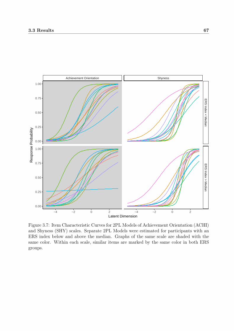
3.3 Results 67
Achievement Orientation Shyness
ER
S Index <
Median
ER
S Index >
Median
−4 −2 0 2 −4 −2 0 2
0.00
0.25
0.50
0.75
1.00
0.00
0.25
0.50
0.75
1.00
Latent Dimension
Res
pons
e P
roba
bilit
y
Figure 3.7: Item Characteristic Curves for 2PL Models of Achievement Orientation (ACHI)and Shyness (SHY) scales. Separate 2PL Models were estimated for participants with anERS index below and above the median. Graphs of the same scale are shaded with thesame color. Within each scale, similar items are marked by the same color in both ERSgroups.

68 3. Study 2: Avoiding ERS with Dichotomous Items
3.4 Discussion
3.4.1 Summary of Results
The inter item correlations between the randomly sampled ERS items turned out to besmall. The resulting ERS index was unrelated to sex and age but showed medium cor-relations with SRERS and MRERS. In the PC tree analyses of the ORD scale, all threeresponse style measures contained parameter instability. The resulting two leaves showedthreshold patterns which suggest that extreme responding was detected by all three mea-sures. In contrast, no measure of ERS had an effect on response patterns in the dichotomousSHY and ACHI scales. For items selected by the Lasso, DIF was primarily caused by thedemographic variables sex and age. When only response style measures were included inthe Lasso, no DIF items were detected. Similarly, no response style measure was selectedas split variable in the Rasch tree analyses. Rasch trees also detected DIF that could becontributed to sex and age. The effects were comparable to the DIF items detected bythe Lasso. Exploratory 2PL models of the dichotomous scales which were estimated forsubsamples resulting from a median split of the ERS index, did not suggest any effect ofERS on item discriminations.
3.4.2 Comparison of ERS Measures
The applied sampling procedure resulted in a set of uncorrelated ERS items. The meanabsolute inter-item correlation was comparable to previous research (e.g. Plieninger &Meiser, 2014). Not surprisingly, single correlations between ERS items were a bit higherthan in study 1, where we used an algorithm to find the most uncorrelated items basedon already collected data. On average, ERS values were slightly higher compared to study1. This might be related to the concrete set of ERS items or our sample of psychologystudents. Another possible explanation could be the mixed presentation of dichotomousand polytomous items in our questionnaire. Without a midpoint category, the dichoto-mous items always required a clear decision. This might have had the effect that subjectsalso chose more extreme and less midpoint responses on the ERS items compared to aquestionnaire which completely lacked dichotomous items.
PC tree analyses of the ORD scale suggest that all three ERS measures carried infor-mation about extreme responding. They were all selected as splitting variable, if used asthe only covariate. As expected, a strong threshold pattern reflecting extreme respondingwas found for the MRERS measure, which was computed based on the same ORD scale.In the combined analyses with the ERS index, sex, age, and SRERS as covariates, only theERS index was selected as splitting variable. In line with study 1, parameter instabilitycontained by the ERS index was larger than for the demographic variables. In contrastto study 1, the ERS index was only selected to split the sample once, at least when usedtogether with the other covariates. Sex and age were not selected as splitting variables inthe ORD analyses at all. This is probably due to the much smaller sample size comparedto study 1, which used the normative sample with several thousand participants.

3.4 Discussion 69
Descriptive analyses showed that subjects with high ERS values were more likely toreport tendencies of extreme responding in the SRERS question, and to be classified as anextreme responder by the constraint mixed Rasch model of the ORD scale. Still, associa-tions were only moderate, suggesting that the different ERS variables are not exchangeablein practice, and might measure slightly different aspects of extreme responding. Especiallythe relationship between SRERS and MRERS turned out to be rather weak.
When SRERS was used as the only covariate in the PC tree of the ORD scale, thresholdsrevealed the familiar ERS pattern although it seemed to be weaker than for the other twoERS measures. The finding implies that people have at least some conscious knowledgeabout their own extreme response tendencies, which has not been investigated in earlierstudies of ERS. This knowledge might be used to find more procedural remedies of ERS.For example, respondents could be assisted in producing more valid questionnaire data, byhelping them recognize their own response tendencies and guiding their responses to moreappropriate categories. These ideas had a big influence on the construction of the thirdstudy which will be presented later.
3.4.3 No Effect of ERS in the Dichotomous Scales
None of the three ERS measures revealed any effect of ERS on the item responses of thetwo analyzed dichotomous scales. No DIF items were detected when ERS measures werethe only covariates in the DIF Lasso and none of the ERS measures was selected as splittingvariable in the Rasch trees. When demographic variables were included, both approachesdetected DIF based on sex and age. When sex and age were included in the model, moreDIF items were detected by the DIF Lasso when using the less conservative L2-normmethod to compute the degrees of freedom for the BIC. However, the method to computethe degrees of freedom did not matter if the ERS measures were the only covariates. DIFresults were highly similar between the DIF Lasso models and the Rasch trees. This wasalso true with respect to DIF based on sex and age. DIF items detected by the Lasso alsoshowed the biggest differences in threshold parameters in the corresponding Rasch tree.Also, the effect of the covariate was always in the same direction. Small differences canpossibly be attributed to the relatively small sample size. As separate models are fittedwithin each leaf of a Rasch tree, the precision of parameter estimates for small leaves isvery low. In these cases, small differences in threshold parameters can be expected even inthe absence of a true DIF effect. On first glance, the Rasch tree of the ACHI scale mightsuggest an interaction effect for sex and age. This could not be modeled by the DIF Lassoin which interaction terms were not included. However, the high age group was so smallthat another split based on sex was not even attempted by the algorithm. Similar reasonsmight also explain why sex was not used to split the resulting age groups in the Rasch treeof the SHY scale. As explained in the introduction, the DIF Lasso results might be moretrustworthy if the focus is not on which variables contain DIF but which items are mostaffected. The main DIF item based on the DIF Lasso of the SHY scale suggested that forequally shy subjects, speaking in front of the class back in school was generally harder forolder women. It is the only item in the SHY scale about a performance situation. DIF

70 3. Study 2: Avoiding ERS with Dichotomous Items
Lasso results of the ACHI scale indicated that for equally achievement oriented subjects,older men more preferred taking action to making plans. While several items of the ACHIscale focus on taking fast actions, the DIF item is the only one mentioning the planningaspect. We refrain from further post hoc interpretations of these findings. Nevertheless,they illustrate that the applied methods were generally capable of detecting DIF in indichotomous items.
In the supplemental analyses with the 2PL model, we investigated the possibility thatERS might have an effect on item discrimination instead of item difficulty. More specifi-cally, the theoretical understanding of ERS might suggest that item discrimination shouldbe higher for people with high extreme response tendencies. However, the graphical inves-tigation of ICCs did not indicate an effect in either direction. Note that we did not use arigorous statistical test and that the power to detect any effects in the more complex 2PLmodel was further reduced by the applied median split. Strobl et al. (2013) mention intheir article on Rasch trees that they would like to extend their methodology to the 2PLmodel, which should also be possible for the DIF Lasso approach. If any of these methodsare developed in the future, investigating the effect of ERS on item discrimination based ona bigger sample should be worthwhile both for dichotomous and ordinal response formats.
3.4.4 Advantages and Disadvantages of Dichotomous Item For-mats
In this study, we presented the first empirical evidence in favor of the widely held as-sumption that dichotomous items are unaffected by ERS. As suggested by a number ofresearchers (Bühner, 2011; Cabooter et al., 2016; Wetzel, Carstensen, & Böhnke, 2013),adopting dichotomous response formats for psychological measurements might be a rea-sonable strategy to deal with ERS.
In light of the mixed opinions in the community about the impact of ERS on psycho-logical measurements with ordinal response formats, avoiding ERS per design seems likea good advice. While many authors claim devastating effects of ERS on the precision ofpsychological measurement (Baumgartner & Steenkamp, 2001; Mõttus et al., 2012), tworecent simulation studies argue that ERS can be savely ignored as long as extreme re-sponding and the primary trait in question are not strongly correlated (Plieninger, 2016;Wetzel, Böhnke, & Rose, 2016). In chapter 1.4, we argued that both simulation studieshave a series of limitations. Until more convincing empirical research suggests that ERShas a low impact in practical applications, preventing ERS seems to be preferable.
In addition to the illustrated insensitivity against extreme responding, further advan-tages of dichotomous items are discussed by proponents of the response format: It has beenfound that completing a questionnaire with dichotomous items takes less time comparedto a version with ordinal response format (Dolnicar, Grün, & Leisch, 2011). The authorsargue that efficiency is crucial in marketing research, where completion times are nega-tively related to survey costs and response rates. Recently, shortened personality measuresare becoming more popular in psychological research (Rammstedt & John, 2007). Two

3.4 Discussion 71
reasons are an increasing number of large scale panel studies and a higher focus on morecomplex research questions which require to assess many psychological constructs at thesame time (Ziegler, Kemper, & Kruyen, 2014). Dichotomous items might be a useful strat-egy to lower completion times in these settings, while still retaining a high number of itemsin a shortened scale. Thereby, constructs could be assessed from different angles, whichincreases the content validity of short scales without sacrificing too much efficiency.
Dichotomous items might also have their disadvantages: The prevalent reason whyordinal response formats are favored by most researchers is the assumption that morefine grained psychological measurements yield higher reliability (Preston & Colman, 2000;Weng, 2004). In contrast, Cronbach (1950) already noted that higher reliability estimatesare precisely what should be expected in light of increased response style variance. Notethat the reliability of the sum score of a psychological scale is only a useful quantity if theessentially tau-equivalent model of CTT holds. Even for the tau-congeneric model, thesum score is a deficient measure for the latent variable and would not be used by anyonewho takes the measurement model seriously. If factor scores are used, the reliability ofthe sum score is not of any interest at all. The pattern found in the PC trees of study 1suggests that ERS is highly prevalent in item response data with ordinal response format.In this case, no unidimensional model from CTT is appropriate and more complex IRTmodels should be investigated (see the discussion in chapter 2.4.4). As the ERS patternis too complex to be described by a simple pattern of correlated errors in classical CTTmodels, the fact that reliability could still be estimated under these circumstances (Gu,Little, & Kingston, 2013; Raykov, 2001) is irrelevant. Of course, the dichotomous responseformat only provide a real advantage with regard to the above argument if measurementmodels hold for the resulting scales. Although we did not encounter any signs of ERS in thedichotomous SHY and ACHI scales, the Rasch model had to be rejected in both cases, asRasch trees and the DIF Lasso detected violations of the model based on age and gender.As long as psychological test construction fails to provide dichotomous scales that showacceptable fit under meaningful measurement models, arguments in favor of dichotomousitems that are mainly based on psychometric properties remain on weak ground. At least,our results suggest that when developing a psychological measure based on dichotomousitems, ERS is one less thing to worry about.
A more convincing point in favor of ordinal response formats could be made, if studieswould suggest higher criterion validity compared to dichotomous items. However, moststudies on this topic report small increases in validity at best (Preston & Colman, 2000;Finn, Ben-Porath, & Tellegen, 2015). Unfortunately, all available studies used psycholog-ical scales as criterion measures instead of genuine external variables that are recordedwithout self-report items. We briefly mention the study by Finn et al. (2015), as it usedthe MMPI-2 with the original dichotomous and a new four-category format. Similar tothe majority of the remaining MMPI-2 scales, correlations between the SHY sum scoreand a series of questionnaires measuring personality or clinical symptoms were indistin-guishable for both versions. In contrast to other studies, some criterion measures consistedof dichotomous items. If both the scale of interest and the criterion measure use itemswith ordinal response format, response styles and other forms of method bias can trivially

72 3. Study 2: Avoiding ERS with Dichotomous Items
increase the correlation between the sum scores (MacKenzie & Podsakoff, 2012; Podsakoffet al., 2011). This makes observed increases in validity hard to interpret.
From a different angle, the study by Plieninger and Meiser (2014) also suggests thatpolytomous items do not necessarily contain more information as dichotomous ones. Twodatasets were analyzed with a sequential multiprocess model (Böckenholt, 2012), in whichitem responses are determined by a MRS process (choosing the midpoint category ornot), followed by a content trait process (agreement or disagreement) and an ERS process(choosing the extreme reponse option of not).14 In both datasets, the content process wascorrelated with relevant external criteria to the same extend as the ordinary sum score orthe trait estimates from a unidimensional IRT model. A similar result was found in a laterstudy (Böckenholt & Meiser, 2017), in which two content processes in a two dimensionalmultiprocess model were correlated to the same extend as the corresponding trait variablesof a two dimensional polytomous mixed Rasch model. Note that based on the multiprocessmodel, the content process should only contain the binary information if the respondentagrees with the item or not, and is therefore conceptually comparable to a dichotomousitem response on the item. These findings provide empirical evidence for some early workby Peabody (1962). Through analytical decompositions of the sum score variance of a seriesof psychological scales, he anticipated that ordinal item responses might primarily containinformation about direction (agreement vs. disagreement). Moreover, he recognized thatthe small part of variance which could be attributed to the intensity of item responsesshowed clear indications of ERS.
Another common argument in favor of ordinal items is that the dichotomous responseformat is less preferred by respondents. In the study by Preston and Colman (2000), thedichotomous format was rated by participants as less adequate to express their feelings.At the same time, it was considered the least easy to use and the quickest to use. Thisis in contrast to another study (Dolnicar et al., 2011), where the dichotomous formatwas perceived as less complex than the ordinal one. In our study, missing values were1.52 times more likely for the dichotomous SHY and ACHI items than for the ordinalORD and ERS items (95% CI of odds ratio from Fisher’s exact test: [1.20; 1.94]).15 It ispossible that our participants also felt that they could not give adequate responses to somedichotomous items. As a consequence, they might have refused to respond to dichotomousitems more often compared to items with ordinal response format.16 Finn et al. (2015)mention an unpublished doctoral thesis by Cox (2011), in which the MMPI-2 has beencompared between the traditional dichotomous and a four-category response format. Inthat study, the dichotomous version was completed faster and also considered easier tocomplete. However, respondents indicated that they could describe themselves better withthe four-category format, which is in line with the findings of Preston and Colman (2000).
Even if ERS seems to be absent in dichotomous item response data, it has been noted
14 The MRS process is missing if the item does not contain a midpoint category. The ERS process isrepeated if the item has more than five response categories.
15 As missing values were rare, note that the relative risk and the odds ratio are virtually the same.16 Of course, it is also possible that missing values were related to the content of the SHY and ACHI
scale.
3.4 Discussion 73
that other response styles like ARS might still be important (Wetzel, Lüdtke, et al., 2016;Rorer, 1965). When Cronbach (1950) demanded researchers not to use item forms infestedby response styles, he also discouraged the use of dichotomous agreement/disagreementresponse scales. It has been found that ERS might have a bigger impact than ARS initems with ordinal response formats (Wetzel & Carstensen, 2015; Kieruj & Moors, 2013).However, this can be hardly generalized to dichotomous items. Recent empirical studiesabout ARS in binary items are scarce, although model-based approaches to investigatethis issue are available (Ferrando & Condon, 2006). By changing the coding of the items,response style indices from heterogeneous items can be used to investigate the occurrenceof ARS. Applying an ARS index in addition to the ERS measures in this study could haveclarified whether ARS was a problem in our data. Before issuing a general recommendationto rely on dichotomous item formats, the here presented work should be extended to theinvestigation of ARS. In the case that further studies find a high prevalence of ARS indichotomous items, this response style has to be addressed in scale construction, too.Multiple studies suggest that ARS can be easily avoided by balancing the number ofpositively and negatively keyed items in a particular scale (Plieninger, 2016). Although ithas been shown that reversely keyed items often pose serious measurement problems, ithas been suggested that detrimental effects on psychometric properties should be rathersmall (Weijters & Baumgartner, 2012) when avoiding negations in the item wording. Withcareful wording, negatively keyed items might be worth the costs if their use leads topsychological scales which are mostly unaffected by the two most important response styles.We briefly note that multidimensional forced-choice response formats could be an alternatestrategy to avoid response styles. Methodological advances in analyzing forced-choice itemresponse data (Brown & Maydeu-Olivares, 2011) have reignited the interest in this itemtype. While forced-choice formats had been endorsed by Cronbach (1950) in the contextof response styles many years ago, they have long been neglected due to methodologicalproblems (Brown &Maydeu-Olivares, 2013). However, a detailed discussion of ThurstonianIRT is beyond the scope of this thesis. General implications for scale construction andpsychometric practice which can be derived from our work on response styles will befurther discussed in chapter 5.2.

74 3. Study 2: Avoiding ERS with Dichotomous Items
Chapter 4
Study 3: Compensating ExtremeResponse Style with Item Instructions
4.1 Introduction
4.1.1 Instructions for an Experimental Manipulation of ExtremeResponse Style
Study 2 suggests that using binary item response formats might be an effective procedureto avoid ERS. Yet, we also discussed some disadvantages of dichotomous items that dis-courage researchers to opt for this response format. Procedural approaches to avoid ERSin items with ordinal response format would be more appealing to the majority of appliedresearchers. Cronbach (1950) has brought up the idea to reduce the impact of responsestyles by altering the instructions which precede most psychological measurements. Whilehe gives an example of how to reduce acquiescence by informing test takers about the ratioof true questions in an ability test, it is not obvious how a similar strategy might be appli-cable to ERS. To design instructions which could reduce the impact of ERS, a theoreticalframework is necessary that tries to explain how subjects respond to questionnaire items.This is important, as some critics stress that conceptual ideas about how item responses arechosen in questionnaires are lacking in most approaches to study response styles (Zettleret al., 2015).
According to a popular cognitive process model for answering questionnaire items(Tourangeau et al., 2000), respondents of self-report questions proceed through four stages.In the comprehension stage, subjects encounter an item and try to interpret its content.Then, relevant beliefs to answer the question are retrieved from memory in the retrievalstage. In the judgment stage, beliefs are combined into an internal judgment of how thesubject ranks on the dimension described by the item. Finally, in the response stage, sub-jects map their internal judgment onto the response categories provided by the item andselect their answer. Several authors have noted that response tendencies can be discussedwithin this framework (Podsakoff et al., 2011; Weijters, Cabooter, & Schillewaert, 2010;

76 4. Study 3: Compensating ERS with Item Instructions
Krosnick, 1991).Considering how ERS might affect item responses during the answering process, the re-
sponse stage might play the most important role. Per definition, ERS describes differencesin the use of the response format. Thus, two respondents which arrive at the same internaljudgment might not select the same response option due to different levels of ERS. Thisidea is corroborated by Weijters, Cabooter, and Schillewaert (2010) who found an effect ofthe response format on the impact of ERS and other response styles. However, patterns initem responses that can be detected by analyses of ERS as demonstrated in study 1 and 2,might also depend on earlier stages of the response process. For example, ERS could assertsome influence in the judgment phase. Subjects with different levels of ERS might cometo different internal judgments, based on an identical memory recall. Direct testing of thishypothesis is only possible through extensive cognitive interviews which aim to separatethe internal judgment from the item responses. This has not been done thus far. However,the body of literature on the relationship between ERS and personality characteristics canbe related to decision making in general (Austin et al., 2006; Naemi et al., 2009; Zettleret al., 2015). This suggests that ERS might already operate in the judgment stage. Cron-bach (1950) noted that response styles seem to be more influential for ambiguous items.If subjects are uncertain how to respond to an item based on its content, response stylesshould have a big impact. If responses are fully determined by the item content due toclear wording, subjects’ individual response tendencies cannot manifest themselves. Thus,ambiguous item wording might have a moderating effect on the impact of ERS on itemresponses, which should take place in the judgment stage.
The last argument might suggest that when designing an instruction to compensateERS, the focus should be on item responses for which a subject perceives a high levelof uncertainty. For those responses, ERS should have the largest impact and subjectsshould be most inclined to adjust their answers according to some external instruction. Incontrast, the impact of response tendencies should be lower, if a subject is highly certainabout an answer. Even if a small effect of ERS is still present, subjects are probablyunwilling to reorient their decision in those cases. In the following study, we propose anERS instruction which urges subjects to adjust their item responses if they are uncertainabout an item. An important question is how respondents should adjust their responses.By using a self-report measure of ERS in study 2, we showed that respondents have someconscious knowledge about their own response tendencies. Thus, subjects could be askedwhether they tend to choose mid or extreme categories in a first step. When confrontedwith questionnaire items, respondents could then be instructed to adjust their responsesto compensate their individual response tendencies. Although self-reported ERS seems tobe a valid indicator of extreme response tendencies, studies 1 and 2 also suggest that moreinformation is contained in an objective measure like the ERS index from heterogeneousitems. Thus, relying on subjects’ self-reported ERS is probably not the most effectiveway to compensate ERS. Moreover, subjects might be overwhelmed if they are not givena concrete procedure how to adjust their responses. An effective instruction should beconcrete to give sufficient guidance but flexible enough to ensure that subjects can useknowledge about their own response tendencies to control whether an item response should

4.1 Introduction 77
be adjusted. In this study, we use an ERS instruction with the following rationale: Ifsubjects cannot decide between two neighboring response categories, they should ratherchoose either the more extreme/the less extreme of the two options. For this instruction, itis necessary to specify if subjects should give more or less extreme responses. In a practicalapplication, it would be necessary to measure each participant’s level of ERS, either byself-report or with an index from heterogeneous items, and select either the extreme or mid-responding instruction, based on a binary ERS classification for each participant. If usingself-reported ERS similar to study 2, such a design could be easily achieved in an onlinesurvey which can be programmed to present a certain instruction dependent on an earlierresponse on the SRERS item. The procedure would be more difficult when using an ERSindex, because a binary cutoff has to be specified beforehand. To compare the effectivenessof both ERS measures, we use a within subject design with an additional control group.All participants first fill out two psychological scales under standard instructions togetherwith a series of heterogeneous items which can be used to compute an ERS index. Subjectsin the experimental group answer the scales again under both the extreme, and the mid-responding instruction. In contrast, the control group fills out the same scales two moretimes under neutral instructions to rule out order effects or other confounding factor of thewithin subject design. Finally, all subjects answer a self-report question of ERS. Duringdata analysis, subjects in the experimental group can be classified into extreme and midresponders based on both the ERS index and self-reported ERS. Different classifications canthen be used to create artificial datasets. Item responses are used from those trials in whichthe ERS instruction leads to a compensation of individual ERS. To better understand theeffectiveness of our design ERS manipulation, item responses can also be analyzed undera matching condition which should lead to an aggravated impact of ERS. If our analysessuggest that compensating ERS with our instructions is successful, the within subjectdesign can be omitted in future studies and an a priori classification based on the superiormeasure can be used to select the respective ERS manipulation.
In the previous studies, we exclusively used psychometric models to detect patterns ofERS in item response data. To investigate whether the impact of ERS can be reducedby specific instructions that are targeted at respondents’ ERS values, a different approachis chosen in the following study. As described in chapter 1.4 ERS is assumed to havea detrimental effect on criterion validity of psychological measures (e.g. Baumgartner &Steenkamp, 2001). Consequently, when item responses with ordinal response format areused to predict external criteria, including an appropriate measure of ERS in the predictivemodel should lead to increased predictive performance. Similarly, the criterion validityof polytomous item responses should be higher if respondents faced an instruction thatwas targeted to compensate their own response style, in contrast to standard instructionsor an instruction which should further aggravate the impact of ERS. To evaluate thepredictive potential of psychological scales, we rely on statistical methods from the fieldof predictive modeling. In the following chapters, we contrast predictive modeling withcommon practices in mainstream psychology and introduce some basic principles, as well asa powerful off-the-shelf prediction algorithm that can be used to investigate the effectivenessof the proposed ERS manipulations.

78 4. Study 3: Compensating ERS with Item Instructions
4.1.2 An Introduction to Predictive Modeling
The American Psychological Association defines psychology as the science of human expe-riences and behavior. It claims that “the understanding of behavior is the enterprise of psy-chologists” (see for example the FAQs on http://www.apa.org/support/about-apa.aspx).As a consequence, statistical inference in psychology aims at explaining psychological phe-nomena. The most common approach is to fit a statistical model to a sample of data andinterpret the estimated coefficients with regard to some psychological theory. A prevalentassumption is that when a model is found which sufficiently describes the relationship be-tween psychological variables in the sample, this model does help to provide insights intotrue psychological processes, but can also be used to predict human experiences and behav-ior. Although the predictive aspect of psychological science is mostly treated as a secondarygoal in the explanatory approach, this has not hindered scholars to make bold claims aboutthe success of psychological theories. Supposedly, a variety of concepts with high societalimportance like job performance (Schmidt & Hunter, 1998; Ziegler, Dietl, Danay, Vogel,& Bühner, 2011) or health issues (Alarcon, Eschleman, & Bowling, 2009; Bogg & Roberts,2004; McEachan, Conner, Taylor, & Lawton, 2011; Faragher, Cass, & Cooper, 2005) canbe accurately predicted. However, it has been noted that these claims of predictive per-formance are seldom evaluated by suitable statistical methods (Yarkoni & Westfall, 2017).Worse, if predictive performance is evaluated in a rigorous way, it often turns out thatthe criterion validity is much lower than initially claimed. The authors convincingly arguethat psychology’s focus on “understanding” human behavior might actually be in conflictwith achieving most accurate predictions of it. On the one hand, psychologists postulatelarge structural models which incorporate a high number of predictor variables. Due togenerally small samples, parameter estimates are often unstable and show high variabilitybetween samples. On the other hand, researches suggest theoretically elegant models witha small number of linear relations, which are too simplistic to appropriately account forcomplex psychological phenomena. In both scenarios, traditional goodness of fit indicescan easily mislead scholars to assume that they were successful in revealing some invariantpsychological law. Research on the replicability of psychological science shows that manyeffects are not recovered if the same model is estimated in new samples (Open Science Col-laboration, 2015). When original model estimates would be used to make predictions fornew observations, this can be expected to fail even more spectacularly. Nevertheless, indi-vidual predictions are central goals in many divisions of psychology like personnel selectionin the industrial-organizational setting, or relapse forecasting in clinical applications.
We agree with Yarkoni and Westfall (2017) that psychology could heavily profit fromprioritizing prediction over explanation in a large number of research settings. Unknown tomany psychologists, a similar claim has been made in statistics several years ago (Breimanet al., 2001). Predictive modeling emerged as a new field in the statistics and machinelearning community which puts a primary focus on maximizing the predictive performanceof statistical models. In contrast to the majority of psychological science, understandinghow a set of predictors is truly related to some target variable is of minor concern here. Thisblind spot justifies the use of “black box” model classes that yield powerful predictions but

4.1 Introduction 79
do not offer human comprehensible model equations which can be easily used to understandsome underlying relationship. Predictive models are primarily evaluated with regard totheir predictive performance, as it is highly difficult to assess their meaningfulness in anycontextual sense. Predictive modeling has developed sophisticated methods to estimatethe predictive performance of statistical models, as this is essential to achieve the maingoal of the field.
Estimating Predictive Performance
Yarkoni andWestfall (2017) note that any statistical model is in some sense also a predictivemodel. In any statistical analysis, a frequently asked question is how useful the estimatedmodel is in predicting new observations. In psychology, the coefficient of determination(R2) is typically reported to assess the goodness of fit for the predominant linear modelsin the field. Yarkoni and Westfall (2017) rightly point out that most authors interpret R2
as the amount of variance, which could be explained if the currently estimated model isused to predict new observations. However, it has been known for a long time that thestandard R2 and commonly used correction methods are overly optimistic (Yin & Fan,2001) for this purpose. This is not a fault of the measure per se, but stems from the factthat R2 is traditionally computed based on model predictions for the same observationswhich were already used to estimate the model coefficients. Naturally, any model betterfits some data on which it was “trained” than on new, previously unseen observations. Inpredictive modeling where predictive performance is the ultimate goal, this bias is takenmore seriously. Intuitively, an appropriate procedure would be to assess the predictiveperformance of a model on different observations than used for model estimation. Afterall, this is exactly how predictions of unknown observations work in practice. However,in many applications only one dataset is available and collecting new data from the samepopulation to evaluate the model would be very costly or even impossible.
Instead of collecting new data, resampling techniques can be applied to use the datasetmost efficiently. The simplest resampling scheme is to randomly split the dataset intoa training set, which is used to estimate the model, and a test or holdout set for whichpredictions are computed based on the estimated model. It makes intuitive sense that theperformance of the estimated model to predict observations in the test set is a reasonableestimate for the performance of the model fitted to the complete dataset to predict ad-ditional unobserved data. While the holdout technique might be sufficient for very largesamples, it has several limitations if the sample is rather small: The crucial decision forholdout is the proportional size of the training and test set. In general, predictive per-formance of a model increases with the size of the training set up to a certain point, asparameter estimates improve if more information is available about the true relationshipin the population. If the training set is chosen too small, performance estimation is down-wardly biased. Predictions of new observations would be of higher quality as they are basedon the whole sample which consists of more training observations. Thus, one goal mightbe to make the training set as big as possible, in order to approximate the performanceof the model based on the whole sample. At the same time, performance estimates based

80 4. Study 3: Compensating ERS with Item Instructions
on small test sets have high variance, as predictive accuracy would greatly vary betweenseveral test sets with few observations. A general principle to reduce variance is to averageacross multiple estimates. For example, if equal sample sizes are chosen for the trainingsand test set in the holdout procedure, the variance of the performance estimation can bereduced by switching the training and test sets, and averaging the two resulting estimatesto gain an aggregated estimate of predictive performance. This approach is called twofold cross-validation (CV). In the general version of k-fold CV, the complete dataset israndomly divided in k equally sized parts. Each subsample serves as a test set which ispredicted based on a model estimated on the combined sample of the remaining k − 1parts. While each observation of the complete sample is used in k − 1 model estimations,each target value is predicted exactly once based on a model for which this observationwas not included in the estimation process. Finally, the average of the k resulting perfor-mance estimates is used as an estimate for the full model based on the whole sample. Intwo fold CV, models are estimated on trainings samples only half the size of the wholedataset, which can result in downwardly biased performance estimates in small samples.Increasing k leads to bigger trainings sets but at the same time reduces the size of thecorresponding test sets. The disadvantage of smaller test sets is somewhat reduced by thefact that performance is averaged across a greater number of estimates. However, as kincreases, training sets highly overlap. This leads to increasingly correlated predictionsof the k estimated models, which reduces the effectiveness of variance reduction achievedby averaging the performance estimates. Empirical results suggest that in most settings,cross-validation with five or ten folds provides a good trade-off between negative bias in-troduced by small training sets, and high variance introduced by small test sets as well asstrongly correlated predictions of the estimated models (Hastie et al., 2009). In additionto k-fold CV, a variety of different resampling strategies exist, which might be preferablein some situations. A detailed description can be found in Bischl, Mersmann, Trautmann,and Weihs (2012). With the presented resampling techniques, it is possible to fairly assessthe predictive performance of any algorithm, including the linear models dominantly usedin psychological science. When doing this, one can expect that specialized algorithms frompredictive modeling would often yield better results. The next paragraph focuses on thequestion why some predictive models might generally perform better than others.
Balancing Model Complexity
Although regularized linear models are highly predictive in many applied settings withvery high numbers of predictors compared to the number of observations (for a detaileddiscussion see Hastie, Tibshirani, & Wainwright, 2015), the rise of predictive modelingis closely related to the development of highly non-linear model classes. Most powerfulprediction algorithms are theoretically capable of reproducing almost arbitrarily complexrelations between predictor and target variables. Flexible algorithms produce statisticalmodels with very low bias in the sense that given enough data with little noise, they areable to mimic the true data generating process. However, high flexibility is not a desirableproperty without any control mechanism, as each dataset contains spurious peculiarities

4.1 Introduction 81
which are not present in the population. When given a single dataset, many algorithmsare flexible enough to perfectly interpolate all data points within the training set, thereby“predicting” them without error. Obviously, such an overfitted model has bad predictiveperformance on new observations, as it does not only incorporates the real target rela-tionship but also the complete noise in the training set. A model which naturally tendsto overfit in the above sense is said to have high variance. Imagine fitting the model toa number of training sets and comparing their predictions on a single test set. As everyfitted model incorporates some specific noise, model predictions on the single test set willstrongly differ as they are highly dependent on the respective trainings sets.
Some model classes naturally have low bias and high variance, while for others it is theother way round. One model class which is very flexible but tends to overfit are classificationand regression trees (CART; Breiman, Friedman, Stone, & Olshen, 1984) which will beintroduced in the next chapter. In the above terminology, the CART algorithm has lowbias but high variance. In contrast, ordinary linear models are on the other side of the bias-variance spectrum. They are very inflexible and are mostly used to model linear functionswhile ignoring all interactions. If the real relationships is highly non-linear or containscomplex interactions, predictions must be biased as, on average, they tend to be be offthe point. At the same time, the inflexibility of the linear model makes it robust againstoverfitting, as long as the number of predictors is not too high. Thus, linear models are saidto have low variance, as predictions based on different training sets tend to be be highlycomparable. It can be shown that when predicting previously unobserved test data, theexpected error of some statistical model is positively related to the bias and variance of itspredictions, as well as the amount of random noise in the data. This bias-variance trade-offhelps to explain why some predictive models show different performance under certain datasituations: If there are strong complex relations between predictor and target variables incombination with high sample size and a high signal to noise ratio, flexible non-linearmodels with higher variance should be successful. In contrast, if the true relationshipis weak or linear, data is sparse and the signal to noise ratio is low, inflexible modelswith low variance might yield good predictive performance. However, the bias-variancetrade-off also comes into play within a single model class. This helps to understand whysome algorithms are more powerful than others across a wider range of problems. Thegenerally most successful prediction algorithms combine a high flexibility to reflect non-linear relationships and interactions, with a series of powerful regularization mechanismsthat prevent the algorithm from overfitting. This makes it possible to efficiently estimatea predictive model with suitable complexity based on a limited amount of training data.
While many algorithms have some built-in mechanisms to automatically reduce overfit-ting, regularization is often achieved via some hyper-parameters which control the flexibil-ity of the estimated model. As the right amount of model flexibility is strongly dependenton the properties of the data generating process, the degree of regularization needs to beadjusted to the nature of the problem at hand. Suitable values for the hyper-parametershave to be found before the final predictive model can be estimated. This tuning processis typically guided by some resampling strategy like k-fold CV. The algorithm is fittedwith different combinations of hyper-parameter values in the training sets and predictive

82 4. Study 3: Compensating ERS with Item Instructions
performance is measured on the test sets. For the final model, the parameter combinationis selected which achieved the best average performance on the k test sets.
The presence of hyper-parameters makes it more complicated to correctly estimatethe predictive performance of the final model. If hyper-parameters are determined oncefor the whole dataset as described above and then applied in all CV iterations, predictiveperformance is typically overestimated, as all observations in the test sets were already usedto find the optimal hyper-parameters. When the final model based on the whole sample isused to predict new unobserved cases, it can be expected to perform worse than estimatedby the resampling scheme, in which the hyper-parameters were overly adapted to therespective test observations. This bias which can pose severe problems is still encounteredin applied published research (Simon, 2007). Fortunately, it can be avoided by repeatingthe tuning of hyper-parameters in each iteration of the resampling process. This procedureis sometimes termed “nested resampling” (Bischl et al., 2012). In an outer loop, predictiveperformance is evaluated similar to the simple case described earlier. However, anotherresampling loop is created within each of the k model estimations to find the most optimalhyper-parameters in the fold. For example, if 10-fold CV is used for the performanceestimation loop, one test set is predicted by nine tenth of the whole sample. If 5-fold CVis used in the inner tuning loop, each training set is again divided into five parts. Fordifferent combinations of hyper-parameters, the five inner test sets are predicted basedon the corresponding inner training sets. The combination with the highest performanceaveraged over the five inner test sets, is then used for model estimation in the outer loop.This results in one of the ten outer performance estimates. The ten estimates in the outerloop are again averaged for an aggregated performance estimate of the final model, whichwould be fitted to the whole sample.
In this chapter, we could only give a brief, informal introduction into basic principles ofpredictive modeling like the bias-variance trade-off and how to evaluate the performanceof predictive algorithms with or without tuning hyper-parameters. A more careful discus-sion can be found in the modern classic by Hastie et al. (2009) and its beginner friendlycompanion (James, Witten, Hastie, & Tibshirani, 2013).
4.1.3 Predictive Modeling with Random Forests
A predictive algorithm which has been found to be highly successful in many applications(Biau & Scornet, 2016) is the random forest (RF) invented by Breiman (2001). The RF iswell suited for an introduction to predictive modeling, as its basic mechanisms are easy tounderstand and do not require strong mathematical or statistical background. Moreover,the RF requires little tuning of hyper-parameters and does not overfit, which makes it moreaccessible to unexperienced users.
A RF is an ensemble method which combines a large number of decision trees into anaggregated estimator that yields better predictive performance than its single components.Each decision tree is constructed with the CART algorithm (Breiman et al., 1984). CARTis a supervised learning algorithm: Some target variable Y is predicted based on a set ofp predictor variables, using training data with known values on both target and predictor

4.1 Introduction 83
sex = male
age >= 9.5
sibsp >= 2.5
died809 500
died682 161
died660 136
survived22 25
died19 1
survived3 24
survived127 339
yes no
Figure 4.1: Classification tree of the Titanic dataset in R. Death is predicted by the covari-ates age, sex, passenger class (pclass), number of siblings or spouses aboard (sibsp), andnumber of parents or children aboard (parch).
variables. In classification trees, Y is a categorical variable withm categories. In regressiontrees, Y is metric. The main idea is to start with some training data, sequentially splitit into smaller subsamples based on rules derived from the available covariates, and makeconstant predictions within each of the final subsamples.
Figure 4.1 shows a classification tree for the Titanic dataset, which is available in R.1The fitted model predicts if a passenger of the Titanic survived the disaster, based on thepassenger variables age, sex, passenger class, number of siblings or spouses aboard, andnumber of parents or children aboard. Each box in the figure is called a tree node andrepresents a subsample of the data, with the whole training set displayed on top of thetree. For each node, we see the number of deceased passengers on the left and the numberof survivors on the right. The label of the most frequent target class is also shown. In ourexample, the first node shows that the training set included 1309 passenger of which 809did not survive. Each non-terminal node further displays the name of a variable in thedataset which is used to split the current sample. The exact split-point value within thisvariable is also shown. Nodes on the bottom of the tree are called leaves. The most frequent
1 The model was estimated with the rpart package. The dataset was taken from the rpart.plotpackage, which was also used to create the Figure 4.1. Default settings of rpart were used except forthe complexity parameter which was set to 0.02.

84 4. Study 3: Compensating ERS with Item Instructions
class label in a leaf can be used to make predictions about other unobserved passengers.For example, the tree would predict that a seven year old boy traveling together with atleast three siblings died, while it would predict that any woman survived regardless of hervalues on the remaining covariates.
The structure of a decision tree is determined by the following algorithm, starting withthe whole training set:
The CART Algorithm
1. Term the current sample the father node F . For all observations in F , compute animpurity measure I(F ). It quantifies some average error per observation that resultsfrom a constant prediction for all observations in F . In regression trees, the impurityfunction is typically the mean squared error (MSE)2, which in this case is identicalto the variance of the target variable in F :
IR(F ) =1
|F |∑
(x,y)∈F(y − yF )2 (4.1)
|F | is the total number of observations in F . In classification trees, the simplestimpurity function is the mean misclassification error (MMCE)3, which is just theratio of observations not belonging to the biggest class in F :
IC(F ) = 1−maxm
nm
|F |(4.2)
2. Iterate over all covariates and for each covariate over all possible split-points, definedby all different covariate values of the observations in F . For each split-point, computethe impurity reduction (IR):
IR = I(F )− |L||F |
I(L)− |R||F |
I(R) (4.3)
L and R reflect the left and right child nodes if the split is performed.
3. Split the sample at the point which yields the largest IR. For metric features, theactual split-point is ambiguous and is typically chosen in the middle between the twoclosest observations.
2 In general, the MSE is defined as MSE = 1n
∑ni=1(yi − yi)
2 and describes the average squareddeviation between some model predictions and the true target values.
3 In general, the MMCE is defined as MMCE = 1n
∑ni=1 I(yi 6= yi) and describes the proportion of
classification errors made by a prediction models. Here, I is the indicator function, returning 1 if thestatement in brackets is true and 0 if it is not. Although the MMCE is well suited to illustrate thegeneral principle for classification, other impurity functions typically yield better predictive perfor-mance in practice. In the classification analyses presented later, the Gini index was used as impurityfunction which is also the default in the original CART algorithm. For further details, we refer theinterested reader to Hastie et al. (2009).

4.1 Introduction 85
4. Recursively repeat steps 1-3 for both child nodes until one of several stopping criteriais satisfied: the minimal number of observations in a node to try further splitting,the minimal number of observations in each leaf, the minimal impurity reduction totry further splitting, and the maximum number of tree levels.
5. Make an optimal constant prediction in each of the final leaves. In regression trees,this is the mean of Y for all observations in the leaf. In classification trees, theconstant prediction is the label of the majority class in the leaf. Predicted valuesfor new observations are obtained by selecting the constant prediction of the leaf towhich they belong, based on their values on all covariates.
CART has several favorable properties: The Titanic example already showed that deci-sion trees are easily interpretable due to their graphical representation. At the same time,they can capture complex interactions between variables and model non-linear functionsbetween the predictors and the target variable. If stopping criteria are chosen in a waywhich allow deep trees with a high number of leaves, CART has very little bias. CART isinvariant to monotone transformations of the covariates and can easily handle categoricalvariables, outliers in the covariates, as well as missing values. Last but not least, CARThas a built-in selection process to deal with a high number of covariates, as the algorithmshould simply ignore irrelevant variables in the splitting process.
One disadvantage of CART is that constant predictions are made within each leaf ofthe tree. Linear or smooth relationships between the predictors and the target variablecan only be approximated by a large number of splits, which typically leads to suboptimalpredictive performance. However, the main problem with CART is its high tendency foroverfitting. Note that in theory, the tree growing algorithm can continue until each leafcontains only a single observation. At least in this case, strong overfitting occurs, as thetree captures the complete noise contained in the training data. To avoid this behavior,the bias-variance trade-off of CART can be controlled by adapting the stopping criteria.4Increasing the number of leaves and reducing the number of observations in each leafdecreases the bias of CART. At the same time this leads to overfitting and an increasein variance. Even with careful tuning of the model complexity, minimal changes to thetraining set can lead to highly different structures of the resulting trees (Hastie et al., 2009).As a consequence, the proclaimed high comprehensibility of CART has to be taken with agrain of salt, as a changing tree structure may imply a completely different interpretationof the estimated model. Moreover, the instability of the tree structure also implies highlyvariable predictions for new observations. This explains why CART and other tree growingalgorithms usually yield only moderate predictive performance in practice.
Decision trees are conceptually related to the Rasch and PC trees introduced in chapter2.1.1, which are built on the model-based recursive partitioning framework (Zeileis et al.,2008). In model-based recursive partitioning, a statistical model is fitted within each leaf of
4 Instead of tuning the stopping criteria, pruning is a popular approach which scales down a fully growntree in an attempt to reduce overfitting. Pruning is not described here, as it is unnecessary for theRF.

86 4. Study 3: Compensating ERS with Item Instructions
a tree, while only constant predictions are computed in simple decision trees. Consequently,the splitting criterion in model-based recursive partitioning relies on hypothesis tests, whichassess the parameter stability of the statistical model in the current node.
The Random Forest Algorithm
Breiman (2001) found a simple, but powerful procedure to increase the predictive perfor-mance of the CART algorithm he invented earlier. The main idea of the RF is to capitalizeon the low bias of deep trees, while reducing their variance. Variance reduction is achievedby fitting a large number of slightly modified decision trees to bootstrap samples of theoriginal training set, and averaging the predictions from all individual trees.
In detail, the RF algorithm works as follows:
1. Draw B full bootstrap samples with replacement from the training set.
2. To each bootstrap sample, fit a tree with the CART algorithm described earlier,except for two modifications:
• Trees are grown as deep as possible with minimal stopping criteria.5
• For each split in the tree, only a sample of mtry randomly drawn covariates areavailable to find the optimal split-point.
3. Aggregate the predictions of the B resulting trees. For regression, the RF estimatoris the mean of all predictions for a certain observation, resulting from all trees. Forclassification, the estimator is the class which is predicted most frequently for theobservation by the trees. This is often called the “majority vote”.
In the RF, the CART algorithm for growing trees is modified for two reasons: Thefirst modification aims at reducing the bias as far as possible, in order to guarantee ahigh flexibility to capture complex dependencies in the data generating process. Thesecond modification is a clever mechanism to “decorrelate” the trees, thereby increasingthe effectiveness of the variance reduction achieved by the final averaging. Intuitively,using lower values of mtry than the total number of predictors p can be thought of as“giving weaker predictors a better chance”. For simplicity, imagine a variable with a muchstronger effect on the target than all the others. Even if all trees in the RF are estimatedbased on slightly different bootstrap samples, the rough structure of all trees might lookhighly similar with mtry = p. The important variable is usually used in the early splits,which have the highest impact on the general tree structure. However, if mtry < p, thestrong predictor might not be available and a weaker variable is chosen instead. Theindividual trees, resulting from this shakeup of the general tree structure, produce morediverse predictions. This leads to a reduced variance of the aggregated RF estimatorwithout inducing a strong bias. Typically, mtry is tuned by CV or fixed to values around5 In the randomForest package in R, the minimum node size is 1 for classification and 5 for regression.
No further stopping criteria are applied per default.

4.1 Introduction 87
√p. It can be shown that low values of mtry are especially useful if the correlation between
the covariates is high (Hastie et al., 2009). It makes intuitive sense that with many highlycorrelated predictors, the tree structure markedly changes only if none of those variablesare available for splitting. This is much more likely if mtry is small.
Variable Importance
The RF typically shows far better predictive performance than single trees, sacrificing onlyone of the important advantages of CART. The interpretability of single decision treesgets lost with the aggregation of the RF. A graphical inspection of several hundred treeswith deep, highly variable structure is not useful. In order to evaluate the impact of singlefeatures in the predictions, several variable importance measures can be computed. A com-mon one is the unstandardized out-of-bag (OOB) permutation measure6, although someimproved versions have been suggested (Strobl, Boulesteix, Kneib, Augustin, & Zeileis,2008). Each tree in the RF is fitted to a full bootstrap sample drawn with replacement.It can be shown that for the estimation of each tree, about one third of the observationsfrom the complete training set is not used. These are called the OOB observations. Toassess the importance of one covariate, subject identifiers for this variable are randomlyshuffled within each of the OOB samples. OOB samples are then predicted by their re-spective trees. The resulting prediction error is compared with the prediction error for theun-shuffled OOB samples. Prediction error is measured by MSE for regression and MMCEfor classification. To compute the final variable importance measure, the differences inprediction error are averaged across all trees.
Reshuffling synthetically destroys all associations of the covariate with the target vari-able. However, as this is done after the model is fit, the decrease in accuracy does notmeasure the best possible performance if the covariate of interest was not available. If theRF were built again without the covariate, other variables might step in (Hastie et al.,2009). It has been shown that the OOB variable importance measure is upwardly biasedfor covariates with a high number of different observed values. This has to be taken intoaccount when comparing variables with varying granularity (Strobl, Boulesteix, Zeileis, &Hothorn, 2007). Further note that the OOB permutation variable importance containsnot only main effects but also all modeled interactions with the remaining covariates. Oneconsequence is that for a variable with high importance, it is unclear how much of its effectis additive (would be unchanged if other variables were missing) or depends on interactions(would be lower if other important variables were missing).
Partial Dependence Plots
Individual partial dependence plots (Goldstein et al., 2015) are a graphical method tovisualize the average additive effect of a covariate and to assess how strong the covariate
6 The OOB permutation measure follows a general principle. If slightly adapted, it can be applied toany predictive modeling algorithm.

88 4. Study 3: Compensating ERS with Item Instructions
interacts with the remaining ones.7 The RF does not easily reveal how a covariate isused in its predictions. The main idea of individual partial dependence plots is that therelationship between one covariate of interest and the target in the estimated model canbe inferred by creating predictions for a series of different values of the covariate. First,a grid of covariate values is chosen between the observed minimum and maximum in thedataset. Then, predictions are computed for all observations, with each covariate valueon the grid. Importantly, original values are used for all the remaining covariates. Whilethe predicted target values are used in regression, predicted class probabilities are usedin classification. In an individual partial dependence plot, the grid of the covariate isplotted against the target predictions, while each observation in the dataset is representedby a single line. Individual partial dependence plots help to identify interactions withthe covariate of interest. If the effect of the covariate is exclusively additive, all linesshould have approximately the same form. As the covariate of interest is fixed by the grid,varying trends can only be attributed to the remaining covariates, on which the observationsnaturally differ.8 If interactions are detected and one is particularly interested in how thecovariate interacts with another categorical variable, lines for observations with the samevalue on the categorical variable can be labeled by the same color. Color patterns canreveal if the categorical variable does interact with the covariate of interest and might helpto interpret the interaction. If one is only interested in the average additive effect of acovariate, individual predictions can be averaged for each value on the grid. This yieldsthe original dependence plots as introduced by Friedman (2001).
The methods presented in this chapter are powerful tools which can be used by re-searchers in psychological science to investigate many important questions (see the discus-sion in Yarkoni & Westfall, 2017). This introduction should help interested psychologiststo delve into the fascinating field of predictive modeling or proceed to other disciplines ofmachine learning.
4.1.4 Aim of Study and Research Questions
The main goal of this study is to examine whether an instruction, which is targeted atcompensating each subject’s extreme response tendencies, can counterbalance the impactof ERS and lead to more valid item responses. The effectiveness of the ERS manipula-tion is investigated by comparing the criterion validity for related self-reported behavior.Different conditions of matching the ERS instruction to subjects’ estimates of ERS areinvestigated. Criterion validity is determined by methods from predictive modeling, usingall questionnaire items as separate predictors in RF models. A within-subjects design isused to administer two different ERS instructions to participants in the experimental con-
7 Similar to the out-of-bag variable importance, partial dependence plots are a useful tool that can beused in combination with any predictive modeling algorithm.
8 To increase the interpretability of the individual partial prediction plots, individual lines are sometimescentered so that the prediction on the first grid point is zero for each observation. In some cases,interactions with the covariate of interest can be seen even better in the centered version, as all linesshould strongly overlap here in the case of a perfectly additive effect.

4.1 Introduction 89
dition, while a control group with neutral instructions is also included. Previous to theERS manipulation, all participants once answered all items under standard instructions.Extreme responding is assessed by an ERS index from additional heterogeneous items andself-report measure of ERS. For the main analyses, both ERS estimates are used to choosethose item responses for each subject which were given under the instruction that shouldeither compensate or aggravate the effect of ERS. The compensation and aggravation set-tings are compared with item responses from the control group. Building up to the primaryanalysis, a series of preliminary analyses are used to check necessary prerequisites. We testthe validity of the ERS instructions, rule out several confounding factors, and investigatewhether measures of ERS contribute to the predictive performance of questionnaire items.
Preliminary Analyses
Presence of ERS Our main research questions require that ERS is present in our data.To ensure that the scales used in the current study are affected by ERS, we compute PCtrees (see chapter 2.1.1) under standard instructions with an ERS index from heterogeneousitems as covariate. We expect several splits based on the ERS index, revealing the samethreshold pattern as in study 1 and 2. A split should also emerge when a binary self-reportmeasure of ERS is used as covariate in the PC trees.
ERS Manipulation Checks To make sure that the developed ERS manipulation hasan effect on item responses, we compute PC trees with the type of instruction (extreme-responding, mid-responding, or neutral) as covariate. If the instructions have an effect onthe subjects’ item responses, PC trees should split the sample in three parts based on thedifferent manipulation conditions. Moreover, we expect that the threshold patterns in theresulting leaves do reflect the corresponding instructions. Specifically, we expect narrowerthresholds and larger regions for the highest and lowest response categories under theextreme-responding instruction than under the mid-responding instruction. The thresholdpattern under the neutral instruction should lie in between. We will also investigate thisgraphically, by comparing histograms of item responses under the different instructions.
Potential Order Effects In the experimental group, the order of the within-subjectsextreme and mid-responding instructions is randomized. However, randomization does nothold when instructions are matched to subject’s ERS estimates for the main analyses. Weinvestigate potential order effects, by graphically comparing histograms of item responsesfor the control subjects who complete the same scales three times under neutral instruc-tions. Without order effects, histograms from the three parts of the questionnaire shouldhave approximately the same shape. To rule out that repeatedly answering the same itemshas an effect on criterion validity which could confound the main analyses, we also comparethe correlation of scale sum scores with the target variables between the three consecutivequestionnaire rounds of the control group. If order effects do not affect criterion validity,questionnaire parts should not be systematically related to the size of the correlations.

90 4. Study 3: Compensating ERS with Item Instructions
Matching ERS Instructions and the Impact of ERS To investigate whether match-ing ERS instructions to participants’ extreme response tendencies reduces the impact ofERS, we compute PC trees under different matching conditions with the ERS index ascovariate: In the compensation setting, participants’ item responses will be taken fromthe part of the questionnaire in which the given ERS instruction should compensate theirindividual ERS tendencies. In the aggravation setting, item responses will be chosen sothat the ERS instruction should further aggravate the response style. In the control set-ting, we analyze item responses of the control group which always respond under neutralinstructions. Matching is either based on a median split of the ERS index from hetero-geneous items or based on the binary self-report measure of ERS. If matching the ERSmanipulations to respondents’ own response style reduces the impact of ERS, we wouldexpect the following pattern: In the control group, the sample should be split based on theERS index, similar to the analyses of the whole sample under the standard instruction. Incontrast, we expect no splits in the compensation setting and a higher number of splitsin the aggravation setting. If no clear order in the number of splits can be observed, weat least expect the respective threshold pattern to suggest a lower impact of ERS in thecompensation setting than in the aggravation setting.
Contribution of ERS Measures to the Prediction of External Criteria The ideathat ERS instructions might compensate effects of ERS, thereby increasing the predictiveperformance of questionnaire items, has an important prerequisite: If measures of ERS areincluded in a predictive model together with questionnaire items, they should contributesomething to the predictive performance. To investigate this, we fit two RF models topredict a series of self-reported behaviors. In the first model, item responses from psy-chological scales under standard instructions, sex, and age are used as predictor variables.In the second model, we further include the ERS index from heterogeneous items and theself-report measure of ERS. For both models, we assess predictive performance using re-sampling techniques. If the ERS measures contribute to the predictions, we expect betterperformance of the model in which ERS variables are included. The impact of ERS onpredictions will be further investigated by estimating variable importance of both ERSmeasures and visualizing the effect of the ERS index in individual partial prediction plots.
Primary Analyses
Matching ERS Instructions and Predictive Performance In the final analysis,we investigate whether item responses under instructions targeted at compensating par-ticipants’ individual ERS tendencies leads to better predictive performance, compared toinstructions that are supposed to aggravate the impact of ERS. In these analyses, we againapply the RF algorithm but use only item responses from the psychological scales as pre-dictors. We match the ERS instructions to subjects’ response style either based on themedian split of the ERS index or based on the self-reported ERS measure. The analysisis then performed under both matching regimes. For all models, predictive performance isagain evaluated with resampling. If matching ERS instructions to subjects’ ERS estimates

4.2 Methods 91
leads to more valid item responses, we expect the highest predictive performance underthe compensation setting and the lowest performance under the aggravation setting. Theperformance in the control setting should lie between the other two conditions. If bothERS measures capture extreme responding, we expect similar results regardless whetherthe ERS index from heterogeneous items or the self-report measure of ERS is used in thematching process.
4.2 Methods
4.2.1 Scales and Variables
Impulsivity and Order
We again used two of the NEO-PI-R facets (see chapter 2.2.1) for which Wetzel, Carstensen,and Böhnke (2013) showed superior fit of the constraint mixed Rasch model, suggestingthat they are good candidates to reveal effects of ERS. This notion was further supportedby the PC tree analyses of those scales in study 1.9 The eight item scale Impulsivity(IMP) is a facet of the Big Five factor neuroticism. It captures impulsive behavior like theinability to control feelings or to suppress the desire for food and other consumer goods. Incontrast to other concepts of impulsivity, it does not entail fast decision making and risktaking. Similar to study 2, the Order (ORD) scale was also used. For a description of thescale see chapter 3.2.1. All IMP and ORD items were rated on the original fully labeledfive-point Likert scale of the German NEO-PI-R (Ostendorf & Angleitner, 2004).
ERS Index
Our questionnaire contained 30 items of heterogeneous content, which were used to com-pute an ERS index similar to the previous studies. ERS items were sampled by the sameprocedure and from the same item data banks as in study 2. For a description of theprocedure see chapter 3.2.1. The wording of the final set of ERS items and their originalsource can be found in Appendix D.1. We sampled 40 questions until enough suitable itemswere found. The original response format of the German NEO-PI-R was also used for theERS items. We mostly retained the original item wording. Some slight modifications weremade to increase comprehensibility when encountered out of context, and to ensure thatitem wordings were compatible with the response format of the NEO-PI-R.
Self-Reported ERS
Self-reported ERS (SRERS) was measured by the same dichotomous item also used instudy 2 (see chapter 3.2.1). While the question wording was exactly the same as in study 2,
9 As a reminder, check out the presented PC trees in Appendix B.3

92 4. Study 3: Compensating ERS with Item Instructions
response categories were slightly altered to improve comprehensibility.10
Target Variables
We constructed a series of questions which would be used as target variables in the mainpredictive modeling analyses. These are listed in Table 4.1 while the German wording ofthe original questions can be found in Appendix D.2. A dichotomous response format withcategories “Yes” and “No” was used for the variables Clothes, Argument, Lying, Electronics,Desk, Dishes, Document, and Bed. For the Snacking question, a check-box was presentednext to each snack to mark if it was consumed, as well as another box to enter the consumedamount. As a result of pretesting the Series question, a third category labeled with “I donot watch any series.” was presented in addition to “Yes” and “No”. Height was reported incentimeters while Weight was reported in kilograms. Both variables were used to computeeach participant’s body mass index (BMI). Height and Weight were not used as separatetarget variables in predictive modeling. For each target variable, either IMP or ORD isconsidered the corresponding primary scale in the sense that the target variable can beexpected to be successfully predicted by the items of this scale. The IMP items should bewell suited to predict the variables Argument, Clothes, Electronics, Lying, Series, Snacking,and BMI. ORD items should be related to Bed, Document, Dishes, Desk, and Vacuum.
As target variables for the IMP scale, we considered impulsive buying and unhealthysnacking, two behaviors which seem to be positively related (Verplanken, Herabadi, Perry,& Silvera, 2005). Impulsive buying has been shown to be associated with personality traits(Verplanken & Herabadi, 2001). Likewise, a general measure of impulsivity which does notfocus on specific behaviors, has been reported to predict self-reported snacking (Churchill,Jessop, & Sparks, 2008). The IMP scale might be an even better predictor of snacking, as itcontains two items which explicitly target the tendency of eating too much. If impulsivity isrelated to snacking, it may have a mediated effect on body weight. Indeed, the IMP facet ofthe NEO-PI-R has been found to be a positive predictor of BMI and other obesity measureslike hip-to-waist ratio in two studies with large samples (Terracciano et al., 2009; Sutin,Ferrucci, Zonderman, & Terracciano, 2011). The relationship even holds prospectively forBMI measured several years after the personality assessment. Interestingly, both studiesalso found a negative relationship between BMI and the ORD facet, although the effectwas weaker than for IMP. In an influential taxonomy of impulsivity, the facet urgency isdescribed as “the tendency to commit rash or regrettable actions as a result of intensenegative affect” (Whiteside & Lynam, 2001). As urgency seems to be closely related to theIMP scale of the NEO-PI-R, the target variables Argument and Lying were constructed10 German wording: “Manche Personen tendieren in Fragebögen häufig dazu, eine der äußeren Antwort-
möglichkeiten anzukreuzen, während andere Personen häufig dazu tendieren, eine Antwortmöglichkeitnahe der Mitte anzukreuzen. Wie würden Sie sich spontan am ehesten einschätzen?”
“Ich tendiere häufiger dazu Antworten anzukreuzen, die in der Mitte liegen.”
“Ich tendiere häufiger dazu Antworten anzukreuzen, die am Rand liegen.”

4.2 Methods 93
to reflect this aspect of impulsivity. Apart from eating, several IMP items assess a generalinability to resist pleasurable stimuli. The Series variable was considered a contemporaryimpulsive behavior which could also be affected by this unspecific aspect of impulsivity.
ORD targets have high face validity, as they are all related to cleaning or other orderlybehaviors of everyday life. All questions were adapted from the Behavioral Indicators ofConscientiousness (Jackson et al., 2010), which have been shown to be positively related toconscientiousness in pure self-report studies. Notably, the Behavioral Indicators of Consci-entiousness also include more impulsive behaviors like shouting at strangers, playing sickto avoid something, spontaneous shopping in contrast to buying stuff from a shopping list,telling lies, and eating until feeling sick. These behaviors seem to be negatively correlatedwith conscientiousness.
As we used an online questionnaire in order to reach an appropriate sample size, wehad to rely on participants’ self-reports. However, when constructing the target questions,we tried to maximize the objectivity of our results, by taking the following aspects intoaccount: Associations between two sets of self-report items can be inflated by ERS andother forms of method bias (Podsakoff et al., 2011). Therefore, we did not use an ordinalresponse format for any of the target variables. A binary response format was used forthe majority of items. According to our results from study 2, Yes/No items are probablyunaffected by ERS. For the remaining questions, subjects could freely report numbers andcheck whether they consumed something or not. These formats should also be free of ERS.Furthermore, we put our focus on concrete behaviors or observations and used a recenttime frame to increase the likelihood that subjects give accurate answers based on activememory retrieval. We also tried to use precise wording to ensure that subjects interpretour questions as similar as possible. Target items were validated in a pretest: All variablesshowed promising correlations with the sum score of their primary scale. Moreover, weasked participants whether they were able to remember the respective behavior. Thisseemed to be the case.

94 4. Study 3: Compensating ERS with Item Instructions
Table 4.1: Target Variables
Impulsivity
Argument Last week, did you say something during an argument which youwould have liked to take back?
Clothes Last week, did you spontaneously buy clothes online or in store,without planning it beforehand?
Electronics In the last two weeks, did you spontaneously buy electronicdevices or consumer electronics, without planning this beforehand?
Lying In the last two weeks, did you lie in order to avoid an appointmentor date?
Series Remember the last time you watched your favorite series. Did youwatch more episodes at a stretch than you had intended?
Snacking Think about yesterday. Which of the following listed snacks/sweetsdid you consume yesterday and how much of them?
One chocolate bar/cereal barOne handful of chips/nuts/saltsticksOne share of chocolate (three pieces)/one chocolate truffleOne large cookie or two small biscuitsOne piece of cake/one piece of pastryOne handful of gummy bears/fruit gums/candiesOne scoop of ice cream/one PopsicleOne cup of yogurt/pudding
Height How tall are you?Weight What is your current weight?
Order
Bed Did you make your bed this morning?Document Remember the last time you received an important document (e.g.
insurance papers, school certificate, contract). Did you immediatelyfile that document?
Dishes At this moment, are there any unwashed dishes you used outsideof the kitchen area?
Desk At this moment, is your desk or workstation tidy?
Vacuum Think about the last two weeks. In that period, how many timesdid you vacuum your bedroom?
Note. Target variables are listed with respect to their primary scale (Impulsivity or Order). Heightand Weight were combined into body mass index (BMI) for all analyses.

4.2 Methods 95
4.2.2 Questionnaire Design and ERS Manipulation
We designed and hosted an online questionnaire on the SoSci Survey framework.11 Thecomplete questionnaire had 29 pages and was presented in German. A progress bar, thelogo of the university and a link to the author’s university email address was shown ontop of each page. Browsing through the questionnaire was achieved by a forward button.If subjects did not respond to all questions on a page, proceeding was not possible and areminder message appeared.
At the beginning of the questionnaire, subjects were thanked for their participationin a study about the relationship between personality and attributes which would takeabout 15-20 minutes. They would get reimbursed with course credit and have the abilityto participate in a lottery. We instructed them to respond honestly to all questions, nomatter if those appeared unusual or similar to earlier questions. They should carefully readall questions and instructions. If respondents felt like they did not know an answer on aquestion, they should choose the most applicable response options instead of skipping thequestion. Finally, subjects were informed that their data would be treated anonymouslyand only be used for instructional and scientific purposes.
After the introduction, we retrieved the following demographic variables: sex, age,highest educational qualification12, and current profession.13 If the student category wasselected in the question about profession, an additional box appeared where participantshad to specify if they are enrolled in psychology or not.
The main part of the questionnaire is visualized in Figure 4.2. It can be structured intothree parts – A, B, and C – followed by the target variables and the SRERS item. Part Acontained the ERS items mixed with the IMP and ORD items. The item order was thesame for all participants. Each page contained a maximum of five items and was alwaysintroduced with the question: “How much do you agree with the following statements?”
Preceding both part B and part C, all participants were informed on a separate pagethat they would now complete some questions again, and that they should reconsider whichresponse is most applicable to them. Moreover, they were ensured that the reason for therepetition is not how good they can remember what they had responded earlier. This wasfollowed by one of three different ERS manipulations, which are presented in Table 4.2.
The extreme and mid-responding instructions were followed by two examples: thedecision process was explained for one case in which a subjects was indecisive betweenthe third and fourth category, as well as another case in which a subject was indecisivebetween the first and second category. Examples were supposed to clarify that participantsshould only alter their response if they were undecided. Responses should be shifted onlyby one category, instead of automatically selecting the midpoint or one of the most extreme
11 For more information, visit https://www.soscisurvey.de/.12 German education categories: Kein Schulabschluss, Hauptschulabschluss/Volksschulabschluss,
Realschulabschluss/Mittlere Reife, Allgemeine Hochschulreife/Fachhochschulreife,Hochschul/Fachhochschulabschluss, Promotion.
13 German profession categories: Schüler/in, in Ausbildung/Lehre, Student/in, Angestellte/r, Selbst-ständig/Freiberuflich, Arbeitslos/Arbeit suchend, Hausmann/Hausfrau.

96 4. Study 3: Compensating ERS with Item Instructions
TargetVariables
ERSInstruc4on
extreme
mid
neutral
mid
extreme
neutral
SRER
S
ERSInstruc4on
IMPORD
ERSItems
IMPORD
IMPORD
A B C
Figure 4.2: Flowchart describing the structure of the online questionnaire. Impulsivity(IMP) and Order (ORD) items where encountered in part A, B, and C of the questionnaire.Within each part, items were presented in mixed order. Participants in the mid-extremeresponding condition answered part B under the mid-responding instruction and part Cunder the extreme-responding instruction. For subjects in the extreme-mid respondingcondition, the order was reversed. The control group answered part B and part C underneutral instructions. SRERS = self-reported extreme response style.
Table 4.2: Wording of ERS Instructions
Extreme IMPORTANT: Should you be unable to decide between two responseoptions, now rather choose that response option which iscloser to the side.
Mid IMPORTANT: Should you be unable to decide between two responseoptions, now rather choose that response option which iscloser to the center.
Neutral If you cannot decide between two response options, try tofind that response option which is more applicable to you.
Note. Instructions for the ERS manipulations were presented in a green box. The box was repeatedon each of the following pages together with the instruction already used in part A.
categories. Examples consisted of explanatory text in combination with pictures showingwhich category to choose. The same item was used for all examples. Screenshots ofquestionnaire pages illustrating the three ERS manipulations can be found in AppendixD.3. On pages displaying the ERS manipulation, the next button stayed invisible for a few

4.2 Methods 97
seconds to avoid that participants accidentally skipped the instructions.Before facing the ERS instruction in part B of the questionnaire, participants were ran-
domly assigned to one of three experimental conditions. Participants in the mid-extremecondition encountered the mid-responding instruction in part B, followed by the extremeresponding manipulation in part C. In the extreme-mid condition, participants encounteredthe extreme-responding manipulation in part B, followed by the mid-responding manip-ulation in part C. We also had a control group whose subjects encountered the neutralmanipulation in both part B and part C of the questionnaire. Urn randomization was usedto ensure that participants were evenly assigned to all three conditions. In part B and C,IMP and ORD items were presented in the same alternating order, starting with the firstIMP item followed by the first ORD item. Four items were shown on each page.
When part C was completed, the target questions were presented in the following or-der: Snacking, Clothes, Vacuum, Argument, Desk, Dishes, Lying, Document, Electronics,Series, Bed, Height, and Weight. Except for Snacking, which was presented on a separatepage, always four target questions were shown at the same time. Finally, the SRERS itemwas displayed on a separate page.14
14 Target questions were followed by one page, on which participants could enter their email addressif they wanted to take part in the lottery. By design of the survey software, addresses could notbe associated with the subjects identifiers to assure privacy. On a final page, subjects were thankedagain to take part in the study. A link was provided to download a certificate for course credit.

98 4. Study 3: Compensating ERS with Item Instructions
4.2.3 Participants
From March until July 2015, 934 participants started our online questionnaire and 789finished it. As participants could not proceed through the questionnaire without answer-ing all questions, there were no further missing data. However, we excluded one femaleparticipant with a BMI score of 9.47 from all analyses.15 Consequently, the analyzedsample consisted of 788 subjects (222 men and 566 women) between the age of 18 and 74(M = 25.35, SD = 8.02). Of 586 included students, 152 were enrolled in psychology. Only48 subjects did not have at least a subject-related entrance qualification for university.
Participants had the possibility to win one of four Amazon vouchers worth of 50 euroand all subjects could get a certificate for course credit. An invitation to the online studywas sent to the study mailing list of LMU Munich. Additionally, the study was promotedin Facebook groups and popular science outlets like www.psychologie-heute.de.
In the analyzed sample, 263 participants were part of the mid-extreme condition, while262 participants were part of the extreme-mid condition. The control group consisted of263 subjects.
4.2.4 Statistical Analyses
All 30 ERS items were used for the computation of the ERS index. Similar to the previousstudies, ERS items were first recoded to a response style scale. As all ERS items wererated on a five-point Likert scale, the recoded values on the response style scale were: 1,0.5, 0, 0.5, 1. A subject’s ERS index was computed as the mean response on the recodedERS items. In the SRERS measure, subjects were coded with one, if they expressed atendency to choose extreme categories and zero if they expressed a tendency to choose themidpoint category. To simplify the predictive modeling analyses, we decided to ignore the“I do not watch any series.” response option of Series and treated it as another binarytarget variable. This increased the accessibility and clarity of our results by avoiding thepeculiarities of classification with more than two classes. Also, we were able to convenientlyreport all classification results side by side. Note that as a consequence, all correlationsand predictive modeling analyses which include the Series variable are based on a reducedsample size, as only subjects who reported “Yes” or “No” were analyzed.
To evaluate whether matching the ERS instruction to the subjects’ own response ten-dencies might reduce the impact of ERS, we used the within-subjects design to constructa series of artificially matched datasets. These were used for the main predictive modelinganalysis, and for one PC tree analysis. Matching was done once based on a median splitof the ERS index, and once based on the SRERS variable. The compensation and aggra-vation settings only included subjects from the experimental conditions mid-extreme andextreme-mid. The remaining subjects were used in the control setting.
15 The excessively low weight of 30kg with a corresponding height of 1.78m was most likely a respondingerror.

4.2 Methods 99
Compensation setting: For each participant with an ERS index above the median,we included the IMP and ORD item responses from the part of the questionnaire withthe mid-responding instruction. For participants with an ERS index below or equal tothe median, item responses under the extreme-responding instruction were used. Whenmatching was based on SRERS, responses under the mid-responding instruction were usedfor participants in the group of extreme responders and vice versa.
Aggravation setting: IMP and ORD item responses under the extreme-responding in-struction were used for each participant with an ERS index above the median and responsesunder the mid-responding instruction were chosen for subjects with an ERS index below themedian. When matching was based on SRERS, responses under the extreme-respondinginstruction were used for participants in the group of extreme responders and vice versa.
Control setting: For each participant in the control group, we randomly selected partB or C of the questionnaire and took all IMP and ORD item responses from the chosen part.
A series of descriptive statistics were computed: Similar to the previous studies, wereport the mean and standard deviation of the ERS index, the mean absolute correlation,as well as the maximum absolute correlation between ERS items, and 95% confidenceintervals for the correlations of the ERS index with sex, age, and SRERS. For binarytarget variables, the frequency of each response category and the ratio of “Yes” responsesare reported. For metric target variables, we show the minimum, maximum, mean, andmedian values, as well as the standard deviation. We further provide the correlations ofthe target variables with the demographic variables, the ERS measures, and the sum scoresof the IMP and ORD scale from part A of the questionnaire. To ease the interpretationof our results, target variables were coded so that a positive correlation could be expectedwith the sum score of the respective primary NEO-PI-R scale. All reported correlationsare Pearson product-moment coefficients.
Several PC trees were computed as part of the preliminary analyses: To ensure thepresence of ERS, we fitted PC trees to the IMP and ORD scales from part A, with theERS index as the only covariate. As a manipulation check for the ERS instructions,separate PC trees were computed for the IMP and ORD scale from part B and C with thetype of instruction (mid-responding, extreme-responding, neutral) as single covariate.
As a graphical manipulation check of the administered ERS instructions, we comparehistograms of item responses under the extreme and mid-responding instructions to thestandard instruction in part A. Note that these plots only contain subjects from bothexperimental conditions, and ignore which instructions were encountered in part B or C.To investigate possible order effects, another series of histograms compare item responsesof the control group for part A, B, and C. If item responses differ between the three partsof the questionnaire in the control group, repeatedly answering the same items could havean effect on the criterion validity of the scale. This might be a confounding factor forthe main analyses because in the process of matching ERS instructions to subjects’ own

100 4. Study 3: Compensating ERS with Item Instructions
response style tendencies, it cannot be controlled if item responses stem from part B or C.To rule out this possibility, we provide another graphical analysis: In the control group,correlations of the target variables with the sum score of the primary NEO-PI-R scalewere contrasted between the three parts. If repeated responses to the same items underneutral instructions leads to better answers, as subjects are more invested to find the mostappropriate answer, we expect a clear order in the correlations of the three parts.
In another analysis, PC trees were fitted to both scales under the compensation, aggra-vation, and control settings. Again, the ERS index was used as the only covariate. For allPC trees, a significance level of 0.05 was used. The minimum number of observations in atree node was set to the default value, which is equal to ten times the number of estimatedparameters. Similar to the previous studies, the results of PC tree analyses are presentedgraphically.
Finally, we performed two predictive modeling analyses based on the RF algorithm:Negatively keyed IMP and ORD items were recoded. As a monotone transformation,recoding does not have any effect on the fitted RFs. However, it makes the interpretationof the following partial dependence plots more intuitive. For binary target variables, thepositive class was chosen so that the predicted probability for the positive class should behigher for high values on the corresponding NEO-PI-R scale.16
In each application of the RF algorithm, we tuned themtry parameter on a grid rangingfrom 1 to 10 with 10-fold CV. The number of trees was fixed to 1500 in all analyses. Whenestimating the predictive performance of a model on new data, nested resampling wasperformed. We used 10-fold CV in the outer loop and repeated the whole procedure 3 times,in order to further reduce the variance of the performance estimation. This is sometimescalled repeated CV (Bischl et al., 2012). For binary target variables, resampling in theinner and outer loop was stratified, which ensures that the class distribution in each foldis the same as in the whole sample.
For binary target variables, Cohen’s κ (Cohen, 1960) was used as the primary perfor-mance measure. This means that it was used to choose the optimal values of mtry inthe hyper-parameter tuning, and to assess the predictive performance estimated by theouter loop of nested resampling. Compared to the commonly used accuracy (ACC =1−MMCE), κ is better suited to capture the performance of a classification model witha single number: Imagine a binary target variable for which 80% of all observations belongto the positive class. In such an unbalanced case, useful predictions are typically harderto achieve, due to the lack of data from the smaller class. Under these circumstances,algorithms tend to predict the positive class with extremely high probability, rendering thepredictive model almost useless. Unfortunately, this behavior is not reflected by the ACCmeasure. In the current example, a model which exclusively predicts the positive classyields an ACC of 0.8. This shows that interpreting ACC is nearly impossible without ad-ditional information. In contrast, κ would be zero for this example, as it takes into accountthe true ratio of positive observations as well as the ratio of positive predictions made bythe predictive model. In this sense, positive κ can only be achieved if the ACC of a predic-
16 “Yes” was the positive class for all binary target variables except for “Dishes”.

4.2 Methods 101
tive model is higher than can be expected “by chance”. As κ is still a single number, it doesnot carry the complete information about predictive performance. To further increase theinterpretability of our results, we also present MMCE, sensitivity (SENS), and specificity(SPEC) as secondary measures in a table. For metric targets, R2 was used as the primaryperformance measure. The MSE and the root mean squared error (RMSE =
√MSE)
are also reported in tables. R2 was chosen over MSE, as it might be more intuitive topsychologists who are familiar with its interpretation from linear models. To aggregate the10 times 3 performance estimates resulting from the repeated CV scheme of each predic-tive modeling exercise, the mean was used for both classification and regression models.Estimated predictive performance of RF analyses will be presented graphically in the formof boxplots. For each predictive model, an observation in the boxplot corresponds to oneof the 10 times 3 performance estimates from the outer loops of nested resampling. Binaryand metric target variables will be presented in separate plots due to the different primaryperformance measures.
The first RF analysis contrasts the ability of two different models to predict each targetvariable. In the first model, all IMP and ORD items from part A of the questionnaire,sex, and age were used as predictors. The second model additionally included the ERSindex and the SRERS measure. To evaluate predictive performance, we repeated thedescribed nested resampling scheme for each target variable. For the prediction modelswhich included the two ERS measures, we further estimated a final RF based on the wholedataset and computed the OOB variable importance. Similar to the earlier performanceestimation,mtry was tuned with 10-fold CV. Variable importance is presented in a separateline plot for each target variable.17 We also present individual partial dependence plotsfor this analysis. Partial predictions were computed for the ERS index on an evenlyspaced grid of length 30, ranging from the lowest to the highest ERS value observed in thecomplete dataset. Similar to the variable importance, partial predictions were based onthe final models which were fitted to the complete sample. Partial dependence plots showthe grid values for the ERS index on the x-axis. Additionally, individual predictions arecolor labeled based on the responses to the NEO-PI-R item with the highest OOB variableimportance for the respective target variable. In chapter 1.4, we noted that ERS mightheavily influence trait estimates for subjects with extremely high or low levels of ERS, butexert only moderate bias on average. Comparing predictive performance between modelswith and without ERS measures highlights the general impact of ERS. In contrast, theindividual partial dependence plots can illustrate the impact of ERS for different levels ofthe ERS index.
The second RF analysis compared the predictive performance for each target variablebetween the compensation, aggravation, and control settings. For these analyses, matchingwas performed by the procedure described earlier. We used the same nested resamplingscheme as in the previous analysis. However, only the IMP and ORD items were used
17 Remember that the OOB variable importance does not provide any information about the directionof the covariate effects. Negative importance values result if predictive performance is improved bypermuting the respective variable. This can be a sign of overfitting.

102 4. Study 3: Compensating ERS with Item Instructions
as predictors. Demographic variables and ERS measures were omitted. By design, theyare unaffected by our experimental conditions and the corresponding matching process.Moreover, ERS measures were already used in the matching process.
In the present study, we did not use ERS measures based on polytomous mixed Raschmodels of the IMP and ORD scales. As discussed in chapter 1.3, the mixed Rasch modelis a less objective method to detect ERS compared to the ERS index from heterogeneousitems and SRERS. Latent classes from mixed Rasch models can capture various factors inaddition to ERS. Classes can differ with respect to the latent trait which is measured by thescale of interest or reflect subgroups based on an unobserved covariate. This confoundingby content is problematic when using an ERS measure derived from the class membershipof a mixed Rasch model as predictor in our predictive models. The RF algorithm is highlyflexible to capture complex relations between the predictors and the target variable. Incontrast to the ERS index from heterogeneous items and SRERS, the classification basedon the mixed Rasch model does not provide strictly new information to the predictivemodel. The classification is just a complex transformation of the item responses which arealready included into the model. Thus, if adding the mixed Rasch ERS measure leads toan increase in predictive performance, the improvement cannot be reliably attributed toERS.
All statistical analyses were conducted in R (R Core Team, 2016b). PC trees togetherwith the corresponding tree plots were computed with the psychotree package (Zeileiset al., 2016). All remaining plots were created with the ggplot2 package (Wickham &Chang, 2016). The predictive modeling analyses were conducted within the infrastructureprovided by the mlr package (Bischl et al., 2017). The mlr package provides a convenientstandardized interface to build predictive models in R, which includes all related steps likehyper-parameter tuning, model fitting, assessing predictive performance, and even modelvisualization (Bischl et al., 2016). To fit the RF models, the algorithm in the randomForestpackage (Breiman, Cutler, Liaw, & Wiener, 2015) was chosen. The unstandardized OOBvariable importance was computed with the same package. In addition to those alreadycited in study 1 and 2, the packages Hmisc (Harrell, 2016), dplyr (Wickham & Francois,2016), parallelMap (Bischl & Lang, 2015), rpart (Therneau, Atkinson, & Ripley, 2015),and rpart.plot (Milborrow, 2017) were used.
4.3 Results
4.3.1 Descriptive Statistics
Descriptive statistics of the ERS index from heterogeneous items are presented in Table4.3. The ERS index was unrelated to sex and age. In the SRERS question, 21% ofparticipants reported a tendency to choose extreme categories. On average, subjects fromthe extreme SRERS group had higher values on the ERS index. They also were slightlyolder (rSRERS,Age 95% CI : [0.03; 0.17]).
Tables 4.4 and 4.5 show descriptive statistics for the binary and metric target variables.

4.3 Results 103
Table 4.3: Descriptive Statistics of the ERS Index
M SD MeanAC MaxAC rSex CI rAge CI rSRERS CI
0.50 0.09 0.07 0.33 [-0.13, 0.01] [-0.08, 0.06] [0.23, 0.36]
Note. 95% confidence intervals are presented for the correlations of the ERS index withsex, age, and SRERS. Females are coded as one, males are coded as zero. Self-reportedextreme responding is coded as one, self-reported mid responding as zero. MeanAC= Mean of absolute correlations between all items within the ERS index. MaxAC =Highest absolute correlation between items within the ERS index. SRERS = self-reportedextreme response style.
Table 4.4: Descriptive Statistics ofBinary Target Variables
Target Yes No Ratio
Argument 137.00 651.00 0.83Clothes 193.00 595.00 0.76Electronics 54.00 734.00 0.93Lying 263.00 525.00 0.67Series* 391.00 299.00 0.57Bed 315.00 473.00 0.60Document 280.00 508.00 0.64Dishes 283.00 505.00 0.64Desk 418.00 370.00 0.53
Note. The Ratio column contains the relativefrequency of the majority class.* In the Series variable, 98 subjects respondedthat they did not watch any series. This op-tion was ignored for computing the ratio.
Table 4.5: Descriptive Statistics of MetricTarget Variables
Target M Med SD Min Max
Snacking 3.17 2.00 3.42 0.00 34.00BMI 22.69 21.89 4.31 15.02 59.52
Vacuum 1.69 1.00 1.84 0.00 14.00
Note. Med = median. Min = minimum, Max = maxi-mum.
The binary targets Argument, Clothes, and Electronics had highly unbalanced distribu-tions. Similarly, the dispersion of the metric variable Vacuum was small as the majorityof participants reported zero or one round of vacuum cleaning.

104 4. Study 3: Compensating ERS with Item Instructions
Table 4.6: Target Correlations
Sex Age ERS Index SRERS IMP ORD
Argument 0.10* -0.10* 0.05 0.03 0.19* -0.08*Clothes 0.18* -0.04 -0.02 -0.02 0.11* -0.01
Electronics -0.09* -0.02 0.02 -0.04 0.08* -0.10*Lying 0.01 -0.06 0.04 0.00 0.15* -0.17*Series -0.06 -0.17* 0.03 -0.04 0.17* -0.12*
Snacking 0.05 0.07 0.00 -0.01 0.17* -0.06BMI -0.17* 0.28* 0.00 -0.02 0.15* -0.12*Bed 0.03 0.11* -0.01 0.06 -0.14* 0.25*
Document 0.06 -0.10* -0.01 0.08* -0.15* 0.31*Dishes 0.00 0.05 0.01 0.01 -0.08* 0.18*Desk 0.07* 0.10* -0.07 0.04 -0.11* 0.37*
Vacuum 0.09* -0.02 0.04 0.11* -0.10* 0.21*
Note. Correlations of target variables with demographic variables, ERS measuresand the sum scores of the Impulsivity (IMP) and Order (ORD) scales. IMP isconsidered the primary scale for variables Argument to BMI, while Bed to Vacuumare target variables for ORD. SRERS = self-reported extreme response style.* p < 0.05.
We present correlations of target variables with demographic variables, ERS measuresand the sum scores of the IMP and ORD scales in Table 4.6. All target variables correlatedwith their primary scale in the expected direction, although all correlations were of smallor medium size. The highest correlation of 0.37 was observed for the relationship betweenDesk and the sum score of the ORD scale. In most cases, we also observed correlationswith the secondary scale. As sum scores of the IMP and ORD scales were negativelycorrelated (rIMP,ORD 95% CI: [−0.35;−0.22]), correlations with the secondary scale werealways in the opposite direction. For Lying and Series, correlations with the secondaryscale were slightly higher in absolute terms than for the primary scale. The ERS indexdid not correlate with any of the target variables. SRERS was slightly correlated withDocument and Vacuum. Some correlations emerged for the demographic variables. Inparticular, BMI was related to participants’ sex and age.
4.3.2 Presence of ERS
Extreme responding clearly affected item responses of the IMP and ORD scale understandard instructions. Appendix D.4 shows PC trees fitted to item responses of part Aof the questionnaire, with the ERS index from heterogeneous items as single covariate.Multiple splits emerged for both scales. The emerging threshold pattern was similar tothe previous studies: In leaves which contain subjects with high values on the ERS index,distances between thresholds were smaller and regions of highest probability for the most

4.3 Results 105
I21R I51 I81R I111 I141R I171 I201 I231R
extreme
mid
standard
0 1 2 3 4 0 1 2 3 4 0 1 2 3 4 0 1 2 3 4 0 1 2 3 4 0 1 2 3 4 0 1 2 3 4 0 1 2 3 4
0
50
100
150
200
250
0
50
100
150
200
250
0
50
100
150
200
250
Item Response
Fre
quen
cy
Figure 4.3: Histograms for item responses of the Impulsivity (IMP) scale given under theextreme-responding, mid-responding, and standard instruction. Only subjects in the twoexperimental conditions were included. Item responses under standard instructions weretaken from part A of the questionnaire. Items are labeled with I for Impulsivity, theposition of the item in the German NEOI-PI-R, and the letter R if the item has beenrecoded.
extreme response categories were larger. As illustrated in Appendix D.5, SRERS was alsoselected as splitting variable when it was used as the single covariate in the PC trees.
4.3.3 ERS Manipulation Checks
The effect of the extreme-responding and mid-responding instructions on participants’ re-sponses on the IMP and ORD items is illustrated in Figures 4.3 and 4.4. Under theextreme-responding instruction, the highest and lowest response categories were chosenslightly more often, compared to the mid-responding and standard instructions. At thesame time, the midpoint category was chosen less frequently under extreme-responding.For some items, midpoint responses seemed to be shifted to the neighboring categories,however this effect was inconsistent. No clear difference could be observed between themid-responding and standard instructions. Importantly, under the mid-responding ma-nipulation, the frequency of the midpoint category was not consistently higher comparedto the standard instruction. Frequencies of the most extreme categories were also not

106 4. Study 3: Compensating ERS with Item Instructions
O10R O40 O70R O100 O130R O160 O190R O220R
extreme
mid
standard
0 1 2 3 4 0 1 2 3 4 0 1 2 3 4 0 1 2 3 4 0 1 2 3 4 0 1 2 3 4 0 1 2 3 4 0 1 2 3 4
0
100
200
300
0
100
200
300
0
100
200
300
Item Response
Fre
quen
cy
Figure 4.4: Histograms for item responses of the Order (ORD) scale given under theextreme-responding, mid-responding, and standard instruction. Only subjects in the twoexperimental conditions were included. Item responses under standard instructions weretaken from part A of the questionnaire. Items are labeled with O for Order, the positionof the item in the German NEOI-PI-R, and the letter R if the item has been recoded.

4.3 Results 107
ERS Instructionp < 0.001
1
mid, neutral extreme
ERS Instructionp = 0.03
2
mid neutral
Node 3 (n = 263)
1 2 3 4 5 6 7 8
−6
−4
−2
0
2
4
Node 4 (n = 263)
1 2 3 4 5 6 7 8
−6
−4
−2
0
2
4
Node 5 (n = 262)
1 2 3 4 5 6 7 8
−6
−4
−2
0
2
4
Figure 4.5: PC tree of the Impulsivity (IMP) scale from part B of the questionnaire, withthe type of ERS instruction as single covariate. Regions of highest response categoryprobability are shown in greyscale. Red lines indicate unordered thresholds in the partialcredit model. Missing categories were dropped.
consistently lower under the mid-responding instruction.
PC trees of IMP and ORD item responses from part B of the questionnaire with theERS instruction as covariate are presented in Figures 4.5 and 4.6. While the IMP scalewas split into three leaves defined by all separate ERS instructions, a combined leaf for themid and neutral-responding condition emerged in the tree of the ORD scale. AppendixD.6 shows the same analyses for part C of the questionnaire. Three splits emerged in bothscales from part C. Otherwise, trees of part B and C were highly similar. In leaves definedby the extreme-responding condition, narrow thresholds and large regions for the mostextreme categories indicated a more extreme response pattern. Differences in thresholdsbetween the mid-responding and neutral conditions were rather small. Under the mid-responding instruction, the region of highest response probability was more pronouncedfor the midpoint category.

108 4. Study 3: Compensating ERS with Item Instructions
ERS Instructionp < 0.001
1
mid, neutral extreme
Node 2 (n = 526)
1 2 3 4 5 6 7 8
−4
−2
0
2
4
Node 3 (n = 262)
1 2 3 4 5 6 7 8
−4
−2
0
2
4
Figure 4.6: PC tree of the Order (ORD) scale from part B of the questionnaire, withthe type of ERS instruction as single covariate. Regions of highest response categoryprobability are shown in greyscale. Red lines indicate unordered thresholds in the partialcredit model. Missing categories were dropped.

4.3 Results 109
ERS Indexp = 0.011
1
≤ 0.5 > 0.5
Node 2 (n = 274)
1 2 3 4 5 6 7 8
−6
−4
−2
0
2
4
ERS Indexp = 0.011
3
≤ 0.63 > 0.63
Node 4 (n = 212)
1 2 3 4 5 6 7 8
−6
−4
−2
0
2
4
Node 5 (n = 39)
1 2 3 4 5 6 7 8
−6
−4
−2
0
2
4
Figure 4.7: PC tree of the Impulsivity (IMP) scale in the compensation setting, with theERS index from heterogeneous items as single covariate. Matching the ERS instructionto individual response style was based on a median split of the ERS index. Regions ofhighest response category probability are shown in greyscale. Red lines indicate unorderedthresholds in the partial credit model. Missing categories were dropped.
4.3.4 Potential Order Effects
Comparing item responses in the control group between the three parts of the question-naires suggested that a small order effect might have affected item response patterns underdifferent ERS instructions (see Appendix D.7). With repeated presentation of the sameitems, responses became slightly more pronounced, in the sense that midpoint responseswere shifted to one of the neighboring categories. Frequencies of the most extreme re-sponse categories seemed to be unaffected by the shifting process. However, possible ordereffects did not influence criterion validity as illustrated in Appendix D.8. Correlations be-tween each target variable and the sum score of the primary scale, computed based on thedifferent parts of the questionnaire in the control group, did not show a consistent ranking.

110 4. Study 3: Compensating ERS with Item Instructions
ERS Indexp < 0.001
1
≤ 0.52 > 0.52
Node 2 (n = 322)
1 2 3 4 5 6 7 8
−3
−2
−1
0
1
2
3
Node 3 (n = 203)
1 2 3 4 5 6 7 8
−3
−2
−1
0
1
2
3
Figure 4.8: PC tree of the Impulsivity (IMP) scale in the compensation setting, with theERS index from heterogeneous items as single covariate. Matching the ERS instructionto individual response style was based on SRERS. Regions of highest response categoryprobability are shown in greyscale. Red lines indicate unordered thresholds in the partialcredit model. Missing categories were dropped. SRERS = self-reported extreme responsestyle.

4.3 Results 111
Node 1 (n = 525)
1 2 3 4 5 6 7 8
−4
−2
0
2
4
Figure 4.9: PC tree of the Order (ORD) scale in the compensation setting, with theERS index from heterogeneous items as single covariate. Matching the ERS instructionto individual response style was based on a median split of the ERS index. Regions ofhighest response category probability are shown in greyscale. Red lines indicate unorderedthresholds in the partial credit model. Missing categories were dropped.

112 4. Study 3: Compensating ERS with Item Instructions
ERS Indexp = 0.005
1
≤ 0.52 > 0.52
Node 2 (n = 322)
1 2 3 4 5 6 7 8
−4
−2
0
2
4
Node 3 (n = 203)
1 2 3 4 5 6 7 8
−4
−2
0
2
4
Figure 4.10: PC tree of the Order (ORD) scale in the compensation setting, with theERS index from heterogeneous items as single covariate. Matching the ERS instructionto individual response style was based on SRERS. Regions of highest response categoryprobability are shown in greyscale. Red lines indicate unordered thresholds in the partialcredit model. Missing categories were dropped. SRERS = self-reported extreme responsestyle.

4.3 Results 113
4.3.5 Matching ERS Instructions and the Impact of ERS
Figures 4.7 and 4.8 show the PC trees for the IMP scale in the compensation setting.For the first plot, instructions were matched to individual response tendencies based ona median split of the ERS index, while matching was based on SRERS in the secondplot. The same analyses for the ORD scale are presented in Figures 4.9 and 4.10. For allanalyses in this section, PC trees included only the ERS index from heterogeneous itemsas covariate.
In spite of the compensatory matching of the ERS instructions, the ERS index wasselected as splitting variable in three of the four models. The PC tree of the ORD scalewith the median ERS index as matching variable was the only condition in which theERS index was not selected. Three leaves emerged for the IMP scale, when matching wasbased on the median split of the ERS index. Compared to the left leaf, the probability formidpoint responses was higher in the mid leaf and the probability for the most extremecategories was lower. Note that the left leaf contained subjects with lower values of theERS index. If SRERS was used in the matching process, two leaves emerged for both scales.The right leaves, which consisted of subjects with higher values on the ERS index, clearlyshowed a pattern of more extreme item responses. PC trees in the aggravation setting forboth scales and matching variables are presented in Appendix D.9. In the PC tree of theIMP scale with SRERS as matching variable, three splits emerged. In each of the remainingmodels, the ERS index was selected as splitting variable once. In comparison to the PCtrees in the compensation setting, differences in the threshold pattern between leaves wereslightly more pronounced in the aggravation setting. The analyses of the control setting arepresented in Appendix D.10. For both scales, the ERS index was not selected as splittingvariable and a single PC model was estimated for all subjects in the control group.
4.3.6 Contribution of ERS to the Prediction of External Criteria
Figure 4.11 visualizes the estimated performance when predicting the binary target vari-ables with item responses of the IMP and ORD scales from part A of the questionnaire.18
Predictive performance for metric target variables is presented in Figure 4.12. For bothvariable types, a table with all used performance measures can be found in AppendixD.11. Predictive performance did not depend on whether the ERS index from heteroge-neous items and SRERS were included in the models. In general, estimated performancewas higher for ORD targets. Robust above-chance predictions could not be achieved forthe IMP target variables Argument, Clothes, Electronics, and Snacking. This was reflectedin negative values of κ or R2. Specificity values very close to one revealed that in the casesof Argument, Clothes, and Electronics, models almost exclusively predicted the majorityclass.
Figures 4.13 and 4.14 show the estimated variable importance if the predictive modelsincluding both ERS measures were fitted to the whole dataset. In line with the perfor-18 Only 690 subjects could be included in the predictive model of the Series variable. The remaining
participants reported that they do not watch any TV series in general.

114 4. Study 3: Compensating ERS with Item Instructions
●
●
●●●
●
●
●
●
●●●
●●
●
●●●
●
●
●
●●
●
●
●
●
●
●
Document Dishes Desk
Lying Series Bed
Argument Clothes Electronics
excluded included excluded included excluded included
0.0
0.2
0.4
0.6
0.0
0.2
0.4
0.6
0.0
0.2
0.4
0.6
κ
ERS Measures excluded included
Figure 4.11: Estimated performance for predicting binary target variables with item re-sponses of the Impulsivity (IMP) and Order (ORD) scale from part A of the questionnaire,sex, age, the ERS index from heterogeneous items and SRERS. Predictive models wereestimated once with and once without the ERS measures. Performance was measured byCohen’s κ. SRERS = self-reported extreme response style.

4.3 Results 115
●●
●●
●
●
Snacking BMI Vacuum
excluded included excluded included excluded included−0.2
−0.1
0.0
0.1
0.2
0.3
R2
ERS Measures excluded included
Figure 4.12: Estimated performance for predicting metric target variables with item re-sponses of the Impulsivity (IMP) and Order (ORD) scale from part A of the questionnaire,sex, age, the ERS index from heterogeneous items and SRERS. Predictive models wereestimated once with and once without the ERS measures. Performance was measured byR2. SRERS = self-reported extreme response style, R2 = coefficient of determination.
mance estimates, both ERS measures mostly ended up in the bottom half of the variableimportance ranking. The ERS index was the most important predictor for Electronics,and the sixth most important one for Desk. Sex and age seemed to have an effect onsome target variables, especially BMI. In most cases, the NEO-PI-R item with the highestvariable importance did belong to the primary scale of the respective target variable. Theonly exceptions were Snacking and BMI. The items with the highest variable importancediffered between target variables. Worth mentioning is the item O40 (“I keep my belong-ings neat and clean.”), which had the highest variable importance for Bed, Document, andDesk.
The effect of the ERS index from heterogeneous items was further investigated with theindividual partial prediction plots shown in Figures 4.15 and 4.16. For most binary targets,two distinct clusters of lines emerged. Except for the variable Desk, individual lines rarelycrossed the 0.5 probability threshold. Thus, for each subject, the models predict the sameclass, regardless of the value of the ERS index. Considering the color labeled responses tothe NEO-PI-R item with the highest variable importance (see Figure 4.13), the clearestpattern in the ranking of item responses emerged for the variable Desk. Subjects whochose the highest category (violet lines) on the corresponding item O40 were predicted tohave a tidy desk with high probability. In contrast, the model assigned small probabilitiesfor subjects who chose the lowest or second lowest response category (orange and yellowlines). To a lesser extent, the same pattern could be observed for the variables Bed andDocument. For Bed, Document, and Desk, the shape of individual partial dependencelines seemed to be related to the item responses on the item with the highest variable

116 4. Study 3: Compensating ERS with Item Instructions
●
●
●
●
●
●
●
●
●
●
●
●
●
●
●
●
●
●
●
●
I111O160
SRERSSex
O190RI81RAge
I141RI171ERS
O10RO130R
I201I51
O40O70RO100I21R
O220RI231R
0.0000 0.0025 0.0050
Argument●
●
●
●
●
●
●
●
●
●
●
●
●
●
●
●
●
●
●
●
AgeERS
O100I231R
O190RI21R
SRERSI81R
O160O10R
I51I111I171
O70RO130R
O40I141R
O220RI201Sex
0.0000 0.0025 0.0050 0.0075
Clothes
●
●
●
●
●
●
●
●
●
●
●
●
●
●
●
●
●
●
●
●
AgeI231RO160O40I51
I141RO190RO70RO10R
I111I21R
SRERSI201
O100I81RSex
O220RO130R
I171ERS
0.0000 0.0005 0.0010 0.0015 0.0020
Electronics
●
●
●
●
●
●
●
●
●
●
●
●
●
●
●
●
●
●
●
●
ERSO100O160I231R
O190RI21RSexI111O40
SRERSI51
I81RO10R
AgeI171
O70RO130R
I201O220RI141R
0.000 0.002 0.004
Pre
dict
ors
Lying
●
●
●
●
●
●
●
●
●
●
●
●
●
●
●
●
●
●
●
●
O190RI21RI111
I141RO70R
ERSO130R
I81RO10RI231R
SRERSO160
SexI201
O100O220R
O40AgeI51
I171
−0.0010.000 0.001 0.002 0.003 0.004
Series
●
●
●
●
●
●
●
●
●
●
●
●
●
●
●
●
●
●
●
●
I81RO70RO160
I51ERSSexI201I171
SRERSO100O10RI21R
I141RI231R
O220RAgeI111
O190RO130R
O40
0.000 0.005 0.010 0.015
Bed
●
●
●
●
●
●
●
●
●
●
●
●
●
●
●
●
●
●
●
●
I171I51
O160O10R
SexI21R
SRERSI231R
I201I141R
I111ERS
O70RI81R
O100O220RO190R
AgeO130R
O40
0.000 0.004 0.008
Document
●
●
●
●
●
●
●
●
●
●
●
●
●
●
●
●
●
●
●
●
ERSI111
I231RI51
I141RI201
SRERSI81R
O10RSex
O160I21R
O220RO70RO100
AgeO40I171
O190RO130R
0.000 0.002 0.004 0.006 0.008
Importance
Dishes
●
●
●
●
●
●
●
●
●
●
●
●
●
●
●
●
●
●
●
●
I231RSRERS
I21RI111
I141RI171SexI201
O160I51
O10RO100I81R
O70RERSAge
O190RO220RO130R
O40
0.00 0.01 0.02 0.03 0.04
Desk
Figure 4.13: Variable importance of predictive models for binary target variables, withitem responses of the Impulsivity (IMP) and Order (ORD) scale from part A of the ques-tionnaire, sex, age, the ERS index from heterogeneous items, and SRERS as predictors.Items are labeled with O for Order or I for Impulsivity, the position of the item in theGerman NEOI-PI-R, and the letter R if the item has been recoded. SRERS = self-reportedextreme response style.

4.3 Results 117
●
●
●
●
●
●
●
●
●
●
●
●
●
●
●
●
●
●
●
●
I201I171
O160O100I81RSex
I21RERS
I231RI141R
O190RO130R
O40Age
O10RI111
O70RSRERS
I51O220R
−0.05 0.00 0.05 0.10
Pre
dict
ors
Snacking
●
●
●
●
●
●
●
●
●
●
●
●
●
●
●
●
●
●
●
●
O100O130R
I201I231RI21R
SRERSO220R
I81RO40
I141RO10RO160O70R
ERSI171I51
I111O190R
SexAge
0.0 0.5 1.0 1.5 2.0
Importance
BMI
●
●
●
●
●
●
●
●
●
●
●
●
●
●
●
●
●
●
●
●
I81RI231RO70R
I51ERSI201AgeO40
O160SRERS
SexI21R
I141RI111
O10RO100
O130RO220R
I171O190R
0.00 0.05
Vacuum
Figure 4.14: Variable importance of predictive models for metric target variables, withitem responses of the Impulsivity (IMP) and Order (ORD) scale from part A of the ques-tionnaire, sex, age, the ERS index from heterogeneous items, and SRERS as predictors.Items are labeled with O for Order or I for Impulsivity, the position of the item in theGerman NEOI-PI-R, and the letter R if the item has been recoded. SRERS = self-reportedextreme response style.
importance, which was the item O40 in all three cases. The relationship was U-shaped forlower item responses and inversely U-shaped for higher item responses. For the variableDesk, a sharp decrease in target probability can be observed around an ERS index of about0.57. However, this phenomenon mostly appeared for subjects who chose the highest orsecond highest category on item O40 (violet and blue lines). It could not be observed forsubjects who chose the lowest of second lowest category (orange and yellow lines).
4.3.7 Matching ERS Instructions and Predictive Performance
We estimated the performance of predicting target variables with item responses of the IMPand ORD scales under the compensation, aggravation, and control settings. ERS instruc-tions were matched to individual response tendencies based on a median split of the ERSindex from heterogeneous items. Results for binary and metric target variables are visual-ized in Figures 4.17 and 4.18. Tables with additional performance measures are presentedin Appendix D.12. We repeated the analysis under the condition that ERS instructionswere matched to individual response tendencies based on SRERS. The corresponding per-formance estimates are presented graphically in Appendix D.13 and additional performancemeasures are reported in Appendix D.14. Both analyses are based on 525 subjects in theexperimental settings, and 263 subjects in the control setting.19
19 For the target Series, only 464 subjects could be analyzed in the compensation and aggravationsettings, and 226 subjects were analyzed in the control setting. The remaining participants in eachsetting reported that they do not watch any TV series in general.

118 4. Study 3: Compensating ERS with Item Instructions
0.00
0.25
0.50
0.75
0.4 0.6 0.8
Argument
0.0
0.2
0.4
0.6
0.8
0.4 0.6 0.8
Clothes
0.0
0.2
0.4
0.6
0.4 0.6 0.8
Electronics
0.25
0.50
0.75
0.4 0.6 0.8
Pro
babi
lity
Lying
0.25
0.50
0.75
0.4 0.6 0.8
Series
0.00
0.25
0.50
0.75
0.4 0.6 0.8
Bed
0.00
0.25
0.50
0.75
0.4 0.6 0.8
Document
0.25
0.50
0.75
1.00
0.4 0.6 0.8
ERS Index
Dishes
0.00
0.25
0.50
0.75
1.00
0.4 0.6 0.8
Desk
Item Response 0 1 2 3 4
Figure 4.15: Individual partial dependence plots of predictive models for binary targetvariables, with item responses of the Impulsivity (IMP) and Order (ORD) scale from partA of the questionnaire, sex, age, the ERS index from heterogeneous items, and SRERS aspredictors. The ERS index is plotted against the predicted probability to belong to thepositive class. Individual predictions are color labeled based on the subjects’ responses tothe NEO-PI-R item with the highest variable importance (see Figure 4.13). Negativelykeyed items were recoded. SRERS = self-reported extreme response style.

4.3 Results 119
5
10
0.4 0.6 0.8
Cou
nt
Snacking
20
25
30
35
40
0.4 0.6 0.8
ERS Index
BM
I
BMI
2
4
6
0.4 0.6 0.8
Cou
nt
Vacuum
Item Response 0 1 2 3 4
Figure 4.16: Individual partial dependence plots of predictive models for metric targetvariables, with item responses of the Impulsivity (IMP) and Order (ORD) scale from partA of the questionnaire, sex, age, the ERS index from heterogeneous items, and SRERS aspredictors. The ERS index is plotted against the targets predictions. Individual predictionsare color labeled based on the subjects’ responses to the NEO-PI-R item with the highestvariable importance (see Figure 4.14). Negatively keyed items were recoded. SRERS =self-reported extreme response style.
No robust differences in predictive performance emerged between the compensation andaggravation settings. If small differences could be observed in favor of the compensationsetting, performance in the control setting was still comparable or even higher in spite ofthe smaller sample size. The variability of performance estimates was slightly higher inthe control setting for most target variables.

120 4. Study 3: Compensating ERS with Item Instructions
●●
●●●●
●
●●●●●●●
●
●
●●●
●
●
●
●
●●
●
●
● ●
●
●
●
●
●
Document Dishes Desk
Lying Series Bed
Argument Clothes Electronics
compensate aggravate control compensate aggravate control compensate aggravate control
−0.25
0.00
0.25
0.50
0.75
−0.25
0.00
0.25
0.50
0.75
−0.25
0.00
0.25
0.50
0.75
κ
ERS Setting compensate aggravate control
Figure 4.17: Estimated performance for predicting binary target variables with item re-sponses of the Impulsivity (IMP) and Order (ORD) scale under the compensation, ag-gravation, and control settings. ERS instructions were matched to individual responsetendencies based on a median split of the ERS index from heterogeneous items. Perfor-mance was measured by Cohen’s κ.

4.3 Results 121
●●●●
●
●
●
●
●● ●●● ●
●
●
●
●
Snacking BMI Vacuum
compensate aggravate control compensate aggravate control compensate aggravate control−1.2
−0.8
−0.4
0.0
R2
ERS Setting compensate aggravate control
Figure 4.18: Estimated performance for predicting metric target variables with item re-sponses of the Impulsivity (IMP) and Order (ORD) scale under the compensation, ag-gravation, and control settings. ERS instructions were matched to individual responsetendencies based on a median split of the ERS index from heterogeneous items. Perfor-mance was measured by R2. R2 = coefficient of determination.

122 4. Study 3: Compensating ERS with Item Instructions
4.4 Discussion
4.4.1 Summary of Results
Descriptive statistics revealed extremely unbalanced response distributions for three bi-nary target variables, and low dispersion for one of the metric targets. We found smallbut consistent correlations of all target variables with their primary NEO-PI-R scale. Thecharacteristics of the ERS index from heterogeneous items was highly similar to the previ-ous studies. The ERS index was uncorrelated with all demographic and target variables.Under standard instructions, response style patterns were detected by PC trees with theERS index or SRERS as covariates. An effect of the ERS instruction on the generalextremeness of item responses could be identified with PC tree analyses with type of in-struction as covariate. This was also shown by the histograms of item responses givenunder different instructions. A comparison of item responses in the control group betweenthe three parts of the questionnaire revealed a small order effect, with less midpoint re-sponses after repeated presentation of the same items. However, correlations between thetarget variables and their primary scale did not vary systematically. PC tree analyses ofthe compensation, aggravation, and control settings provided mixed results. Although PCtrees suggested that ERS still had an effect on item responses when ERS instructions werechosen to compensate individual response tendencies, the impact seemed to be slightlysmaller compared to the aggravation setting. None of the two ERS measures could detectany signs of ERS in the control setting. Target predictions based on demographic variablesand item responses from part A of the questionnaire could not be improved by includingERS measures as predictors in the RF models. In general, predictive performance washigher for ORD targets and target variables with balanced response distributions. Vari-able importance estimates and individual partial dependence plots also suggested negligiblecontributions of both ERS measures. When ERS instructions were matched to individualresponse tendencies, predictive performance did not differ between the compensation andthe aggravation setting. This result did not depend on whether a median split of the ERSindex or SRERS was used in the matching process.
4.4.2 No Impact of Extreme Response Style on Criterion Validity
To evaluate the effectiveness of the developed ERS instructions in reducing the impactof ERS, a necessary prerequisite was that ERS measures can be used to improve thecriterion validity of psychological scales. However, estimated performance of predictivemodels based on demographic variables and item responses under standard instructionsdid not increase when we added the ERS index from heterogeneous items and SRERS aspredictors. Although item responses in the control group revealed a small order effect ofrepeatedly responding to the same items, the relationship between sum scores and targetvariables was unaffected.
Our findings are in line with the simulation studies by Plieninger (2016) and Wetzel,Böhnke, and Rose (2016), which suggest that the impact of ERS on criterion validity is

4.4 Discussion 123
negligible under most circumstances. Both simulation studies assume that apart from theimpact of ERS, item responses reflect a homogeneous trait. This assumption seems tobe violated in our study. Estimated variable importance suggested that the relationshipbetween NEO-PI-R items and target variables was not equally strong for all IMP and ORDitems. In case of a homogeneous trait, the item with the highest reliability should have thehighest variable importance, regardless of the criterion variable. The most important itemwas not always the same for all primary targets of the ORD and IMP scale. This suggeststhat variable importance was also determined by the item content. It makes intuitive sensethat items I141R (“I seldom give in to my impulses.”)20 and I201 (“Sometimes I do things onimpulse that I later regret.”)21 were more important for Lying, while the items I111 (“WhenI am having my favorite foods, I tend to eat to much.”)22 and I171 (“I sometimes eat myselfsick”)23 had a higher rank for BMI. However, these findings should be interpreted carefully,as some important items had a high rank for the majority of target variables and not allvariable importance estimates were equally intuitive: As already mentioned, item O40 (“Ikeep my belongings neat and clean.”)24 was the most important item for the ORD targetsBed, Document, and Desk. In contrast, for the target variables Dishes and Vacuum, theitem O190R (“I’m not compulsive about cleaning.”)25 was more important. Less intuitive,the most important item for BMI from both scales was O190R, and the most importantitem for Series was I171.
All predictive models achieved unsatisfying performance for the unbalanced binary tar-get variables Argument, Clothes, and Electronics. In these cases, sensitivity and specificityrevealed that RF models almost exclusively predicted the majority class. A series of tech-niques like sampling methods, cost-sensitive classification, or threshold tuning are availableto deal with this common problem. For an introduction of these methods, we refer theinterested reader to chapter 16 in Kuhn and Johnson (2013). We did not use any of thismethodology to keep our analyses accessible to our audience in psychology, which is gener-ally not familiar with these methods. Yet, this decision probably did not affect any of ourmain conclusions. For the majority of target variables, distributions were highly balancedand κ indicated rather moderate predictive performance beyond chance-level. One couldargue that predictive performance in general could be improved if no self-report items wereused to measure target variables. However, target items were designed to be as objectiveas possible, which was confirmed by cognitive surveys in the pretest. Thus, we do notexpect results to differ if behavioral observations are used instead of self-reports.
The most important limitation of our study is the relatively small sample size. It is awell known heuristic in predictive modeling that increasing the amount of data is often themost effective way to improve predictive performance (Yarkoni & Westfall, 2017). Thisis especially relevant for our research questions, which postulate a complex relationship
20 German wording: “Ich gebe selten meinen spontanen Gefühlen nach.”21 German wording: “Manchmal handle ich aus einem spontanem Gefühl heraus und bereue es später.”22 German wording: “Ich esse meist zu viel von meinen Lieblingsspeisen.”23 German wording: “Manchmal esse ich, bis mir schlecht wird.”24 German wording: “Ich halte meine Sache ordentlich und sauber.”25 German wording: “Ich bin beim Putzen nicht pingelig.”

124 4. Study 3: Compensating ERS with Item Instructions
between predictors and target variables. In line with the theory of extreme responding,descriptive correlations suggested that ERS measures did not have a main effect on thetarget responses. In order to reflect the hypothesized effects of extreme responding, inter-actions between the ERS measures and item responses have to be modeled. As discussedin the introduction, the RF like many successful predictive modeling algorithms performsimplicit regularization to avoid overfitting. Naturally, if the amount of data is small, higherorder interactions cannot be reliably detected and complexity is reduced by mostly incor-porating main effects into the predictive model. The expected effect of ERS on predictiveperformance might be detectable with bigger samples.
One reason for this assumption are the individual partial dependence plots for variableswith higher predictive performance (Bed, Document, and Desk), which might suggest thatthe ERS index from heterogeneous items did play a small role in the predictive models. Forthe target variable Desk in particular, individual partial predictions did not have the sameshape. This means that some interactions between the ERS index and other predictorvariables were captured (Goldstein et al., 2015). For subjects with a high response onitem O40, the probability to belong to the tidy desk class sharply decreased with an ERSindex above 0.58. This observation would be in line with the theory on ERS: with astrong tendency to give extreme responses, a high response on item O40 might reflectonly moderate ORD levels. Consequently, the probability to show tidy behavior should belower compared to a subject with the same item response, but a lower value on the ERSindex. The partial dependence plots also suggest that even if we captured some influenceof the ERS index, the modeled effect was very weak. For all binary target variables, twoseparated clusters could be observed with respect to the target probability on the y-axis.For the majority of individuals, the same class was predicted by the model, regardless ofany hypothetical ERS values. This explains why predictive performance estimates wereindistinguishable between models with and without ERS measures, even if a small effectof ERS might have been captured.
However, the general U-shaped effect for subjects with low item responses on O40 andthe inverse U-shape for subjects with high item responses is not in line with the theoryof ERS. For low values of the ERS index, the probability to belong to the tidy desk classdecreases for high O40 responders and increases for low O40 responders. The theory on ERSwould have suggested the opposite effect, as extreme item responses should have a strongerimpact for subjects, who tend to give extreme responses regardless of their true level on thelatent construct. We can think about two possible explanations for this unexpected result:The U and inverse U-shapes might be a reflection of some implicit regularization of the RFalgorithm to avoid overfitting. The ERS index was symmetrically distributed around 0.5.For regions of uncommonly low or high ERS values, model predictions might become moreconservative and are shifted closer to a probability of 0.5 as data with extreme ERS valuesis sparse. However, the probability shift already sets in at ERS values close to 0.5. Evenwhen taking the distribution of item responses on O40 into account, enough observationsare still available for ERS values around 0.4 and 0.6. It is therefore rather unlikely that theobserved effect is purely an artifact. Another explanation might be that instead of treatingERS as a single construct, MRS has to be modeled separately. In this view, values of the

4.4 Discussion 125
ERS index above 0.5 should be mainly related to extreme responding and the shift in classprobability at ERS values around 0.58 might reflect the theoretically expected relationship.In contrast, very low values of the ERS index would be related to a high tendency of MRSthat might be qualitatively different than just the absence of extreme response tendencies.Midpoint responses can be a sign of indifference and are sometimes considered an indicatorof bad response quality (MacKenzie & Podsakoff, 2012; Kulas & Stachowski, 2009). Thus,it would be more difficult to make accurate behavioral predictions for high MRS subjectsif their item responses carry less information about the associated constructs of interest.This higher uncertainty might be reflected in a class probability closer to 0.5 for low valuesof the ERS index. Constructing a separate MRS index from heterogeneous items whichonly captures midpoint responses might be a useful endeavor in the future. Including thisindex into the predictive models and investigating the corresponding partial predictionplots could contribute to the discussion of the dimensionality of ERS which was mentionedin the general introduction (see chapter 1.1).
To argue for the importance of considering ERS in practical applications, it has to beshown that correcting for ERS does increase criterion validity (Wetzel, Böhnke, & Rose,2016). This was not the case in our analyses. Nonetheless, investigating whether ERSmeasures can improve the criterion validity of psychological scales is a worthy topic forfurther research. Large datasets from online panels could be used for this purpose, like wedid in study 1. In such datasets, a large number of heterogeneous items are often available.The algorithm used in study 1 and described in Appendix A seems to be a reasonableapproach to find a set of uncorrelated items that can be used to compute an ERS index.Analyzing available panel data with the techniques from predictive modeling introducedhere might give deeper insights into the impact of ERS on criterion validity in appliedwork. Thus far, convincing empirical evidence is still missing in the literature.
4.4.3 Instructions Were Ineffective in Reducing the Impact of Ex-treme Response Style
Our main analysis revealed that matching ERS instructions to compensate individual re-sponse tendencies did not lead to improved predictive performance compared to when ERSinstructions were chosen to further aggravate the impact of ERS. Considering that our pre-dictive models were unable to achieve higher predictive performance if ERS measures wereincluded under standard instructions, it is not surprising that we did not find any effecton predictive performance between the compensation, aggravation, and control settings.PC tree analyses of the different settings with the ERS index from heterogeneous itemsas covariate also suggested that compensating ERS with varying instructions was not suc-cessful, as we repeatedly detected parameter instability with the ERS index. Although thecomparison of PC trees between the compensation and aggravation settings suggested aslightly stronger impact of ERS in the aggravation setting, this difference was small andonly reflected in the threshold patterns, while the number of splits was comparable betweenboth settings. The PC tree of the ORD scale with the median ERS index as matching

126 4. Study 3: Compensating ERS with Item Instructions
variable was the only condition in which the ERS index was not chosen as splitting variablein the compensation setting. We refrain from placing any emphasis on this finding as itmight be a result of the generally low stability of tree models (Strobl et al., 2013). Indeed,differences in extreme responding for the ORD scale are again observed if SRERS is used asmatching variable. For both scales, the ERS index was not used as splitting variable in thecontrol setting, which makes the interpretation of those PC trees even more complicated.Not detecting DIF in the control setting was probably an effect of the smaller sample sizecompared to the whole sample. In the complete sample, we clearly detected an effect ofERS under standard instructions.
It cannot be assumed that the different ERS instructions had no effect on item re-sponses. This was clearly refuted by the PC tree analyses of item responses from part Band C of the questionnaire, with the type of instruction as covariate. Threshold patterns inthese trees revealed that different ERS instructions influenced participants item responsesin line with our expectations. PC trees and histograms suggested that the item responsesunder the extreme-responding instruction differed more strongly from the standard in-struction than the mid-responding manipulation. As a consequence, the mid-respondinginstruction might have been too weak to compensate extremely high levels of ERS. At thesame time, subjects with low levels of ERS might have overcompensated when confrontedwith the extreme-responding instruction. Both arguments might explain the curious find-ing from the PC tree of the IMP scale in the compensation setting, in which subjects withlow ERS values showed a more extreme response pattern than participants with mediumvalues on the ERS index.
Multiprocess models (Böckenholt, 2012; Böckenholt & Meiser, 2017) could be used tofurther investigate the effect of ERS instructions on item responses. If the manipulationworked as intended, instruction type should be related to the mid/indifference and inten-sity process, but not to the content/direction process. In theory, an interaction betweeninstruction type and ERS index could be specified to investigate whether the effect of themanipulation on intensity varies for different levels of ERS.
In hindsight, using binary ERS instructions to compensate a continuous response styleposes several difficulties. To mitigate the full impact of ERS, instructions have to beflexible so that participants can automatically adapt the magnitude of their compensatoryresponse to their individual level of ERS. By instructing participants to sometimes adjusttheir responses if they could not decide between two response categories, we hoped toachieve higher compensation for subjects with extremely low and high values on the ERSindex. PC tree results suggest that this was not successful. In particular, subjects withhigh ERS values did not adequately adjust their responses. Based on studies suggestingthat ERS is related to intolerance of ambiguity and decisiveness (Naemi et al., 2009), itis possible that response certainty increases with ERS. In this case, low ERS subjectsare often undecided, thus adjusting their responses more strongly than high ERS subjectswho mostly feel certain and do not adjust their extreme responses. Also, the specificinstruction to choose the neighboring category might prevent subjects to flexibly adjusttheir item responses.
In future research, different ERS instructions could be tested as procedural remedies

4.4 Discussion 127
against ERS. The current results suggest that a less authoritative variant might be mostpromising. Cronbach (1950) already recommended to reduce the impact of response biasby increasing participants’ testwiseness. It would be interesting to investigate whether anintensive survey training in which respondents’ extreme response tendencies are repeatedlymonitored, could lead to item responses which are not affected by ERS according to PCtree analyses. Although an extensive training of survey respondents is impractical forapplied psychological research, a compact version might be feasible. Our analyses withthe SRERS measure in both studies 2 and 3 showed that when asked explicitly, subjectswithout training already have some valid insight into their own response tendencies. Thisknowledge could be used to develop modified instructions which take extreme respondinginto account but do not explicitly instruct participants how to adjust their responses: In afirst step, respondents could be informed about extreme responding and confronted witha self-report measure of ERS in order to raise awareness on their own response tendencies.Then, subjects could be simply requested to keep their own response style in mind, withoutgiving specific instructions that depend on self-reported ERS. By giving no explicit adviceinto how and when participants should adjust their responses, overall compensation of ERSmight be more effective. Yet, the success of this modified instruction still depends on theassumption that subjects’ insight into their own response tendencies does not depend ontheir own level of ERS. Due to the low cost of such simple instructions, further investigatingthese issues might be worthwhile.
4.4.4 General Issues in Predictive Modeling Analyses
When psychological measures are used to predict external criteria, an important pointnot discussed so far is whether scale scores or single items should be used as variables inpredictive models. Traditionally, psychologists use sum scores of scales as variables in theirstatistical models. While this approach is reasonable from a measurement perspective inwhich all items are supposed to measure a single construct, it might not be ideal if the maingoal is predictive performance. Most psychological constructs are based on factor modelsand the theory of latent variables. In these models, all items are supposed to measure thesame construct and can therefore be combined into an aggregated score which contains allavailable information about the latent variable. The most common aggregated measure isthe sum score of all items in the scale, but factor scores from confirmatory factor analysisor person parameter estimates from IRT models are also used. All those statistics rely ona certain measurement model. Aggregated measures are only useful if the measurementmodel from which they are derived is an appropriate description of the item response data.Therefore, model fit is of utmost importance when the central goal is the measurement ofa certain psychological concept. However, when the focus lies on prediction, measurementmodels can be ignored and aggregating all item responses into a single score might lead tolower predictive performance.
Psychological instruments like personality inventories often consist of several hundreditems. With unregularized linear models, which are the standard approach in psychology,including all items as predictors would lead to overfitting and yield bad predictive perfor-

128 4. Study 3: Compensating ERS with Item Instructions
mance on unobserved data. However, modern predictive algorithms, like the RF (Breiman,2001) are designed to effectively incorporate a large number of predictors without overfit-ting. There are at least two circumstances in which single items can be expected to yieldbetter predictions. First, when unidimensional measurement models do not hold, itemsoften contain information about multiple constructs which can be related to the predictedcriterion in different ways. Those varying contributions can be implemented in the predic-tive model, if single items are used as predictors instead of an aggregated score. Second, ifa construct based on a latent variable model is only weakly related to a certain criterion,the criterion can still be related to the item errors. This is possible even if errors withinone construct are uncorrelated, which is demanded by most common measurement models(Cronbach, 1951). Information in the error terms of a latent variable model is completelylost if only the aggregated score is used as predictor.
Chapman et al. (2016) emphasize that a common latent construct is not necessary tomake useful predictions. In fact, items in a criterion-oriented measure do not have tobe correlated at all. From a theoretical perspective, predictions can be maximized withindependent predictors which make unique contributions to the prediction of the criterion.In this study, single items were used in predictive models, in order to investigate the effect ofERS on item responses. Estimated variable importance was higher for items which sharedsome content with the respective criteria beyond the latent construct of the scale. Althoughitems within each analyzed scale were highly correlated, as assumed by the underlyingpersonality model, unique contributions of single items were possible. We did not compareour predictive model with single items to a model in which only the sum scores of thescales were included, as this was not part of our research questions. However, if predictiveperformance is the main goal, researchers should routinely use resampling techniques tocompare a predictive model with single items against one in which aggregated scale scoresare used as predictors.
Predictive performance is often affected by the model class used in the analysis. Dueto overfitting, ordinary linear models are not appropriate for a large number of predictors.Regularized linear models (Hastie et al., 2015) are an obvious extension which should beadded to the methodological toolkit of every psychological researcher. However, nonlinearrelationships might also be present in psychological research. Possibly, some interestingpsychological phenomena are too complicated to be explained by more interpretable mod-els (Yarkoni & Westfall, 2017). This requires powerful predictive algorithms which canautomatically learn complex nonlinear functions between the predictors and the criterionvariable. Popular non-linear model classes are the RF we used here, gradient boosting, sup-port vector machines, and neural networks. Introductions to all of these methods can befound in Hastie et al. (2009) or James et al. (2013). It is generally hard to predict whethernonlinear methods outperform linear models in a certain setting. Therefore, resamplingtechniques are routinely used to compare models from different classes. Psychological sci-ence would profit from experimenting with non-linear models to find out how they canbe used to answer important research questions in the field. In this study, we used anon-linear model based on theoretical considerations. With our operationalization of ERS,the response style is supposed to have a non-linear effect on item responses. To investi-

4.4 Discussion 129
gate the expected effect, a non-linear model was necessary. We did not find any effectof ERS on predictive performance with the RF algorithm but refrained from comparingdifferent model classes. It is possible that other algorithms might have succeeded in usingour ERS measures to increase predictive performance. Although some experimentationwith a state-of-the-art variant of gradient boosting (Chen & Guestrin, 2016) did not yielda significant increase in predictive performance, this algorithm was also based on decisiontrees. In another unreported analysis, linear models yielded worse predictive performance.However, these issues were not investigated in a rigorous manner. If predictive performancefor other popular algorithms are also insensitive to whether ERS measures are included aspredictors, this will put further weight on our reported null effect.

130 4. Study 3: Compensating ERS with Item Instructions

Chapter 5
General Discussion
5.1 Summary of Empirical Studies
In this dissertation, we presented three empirical studies in which we investigated differentaspects of ERS. In study 1, we introduced a new method to detect ERS. PC trees (Kom-boz et al., 2016) with an ERS index from heterogeneous items (Weijters et al., 2008) ascovariate combine the elegant threshold interpretation of ERS known from ordinal mixedRasch models (Rost et al., 1997), with the high objectivity of response style indices fromheterogeneous items. The effectiveness of the new method was shown by two analyses oflarge datasets. First, we analyzed the nonclinical normative sample of the NEO-PI-R (Os-tendorf & Angleitner, 2004) and detected ERS in facets which had already been found tobe affected by ERS in previous studies. PC trees resulted in a large number of leaves withthreshold patterns that could clearly be interpreted as different levels of extreme respond-ing. The observed pattern suggested that ERS is best understood as a continuous trait. Ina second analysis of data from the GESIS panel (GESIS, 2015), we found the same patternof ERS in scales from the PANAS (Krohne et al., 1996) and the FRS (Münzer & Hölscher,2011). In the GESIS analysis, items for the ERS index were taken from different panelwaves, completed several months apart. Thus, our results can be taken as further evidencefor the stability of ERS across traits and over time. We discussed recent developments ofcontinuous IRT models of ERS and talked about the challenges of using these models tocontrol for ERS in scales which are plagued by DIF beyond the impact of response styles.
In study 2, we provided the first empirical evidence that items with dichotomous re-sponse format are unaffected by ERS. We used three different ERS measures as covariatesin Rasch trees (Strobl et al., 2013) and DIF Lasso models (Tutz & Schauberger, 2015)to analyze scales from the MMPI-2 (Engel & Hathaway, 2003) and the FPI (Fahrenberget al., 2001) in a sample of psychology students: an ERS index from heterogeneous items,a self-report measure of ERS, and an ERS measure based on the classification of an ordinalmixed-Rasch model. We did not find any signs of ERS in the analyzed dichotomous itemresponse data. Yet, control analyses with a NEO-PI-R facet showed that ERS was presentin items with ordinal responses format. This emphasized that not finding an effect of ERS

132 5. General Discussion
in dichotomous items cannot be attributed to deficiencies of our ERS measures. Further-more, our analyses using the self-report measure of ERS are the first to reveal that subjectshave some conscious knowledge about their own response tendencies. Based on our posi-tive results, we discussed possible advantages and disadvantages of using dichotomous itemresponse formats to avoid the impact of ERS in practice.
In study 3, we tested whether individually targeted questionnaire instructions can beused to compensate for the impact of ERS in items with ordinal response format. Wedesigned specific ERS instructions which urged subjects to give either more or less ex-treme responses, when they were uncertain about which category to choose. Respondentsof our online questionnaire completed two NEO-PI-R scales under standard, extreme, andmid-reponding instructions in a within-subjects design. We created artificial datasets inwhich ERS instructions were matched to individual response tendencies, based on eithera median split of an ERS index from heterogeneous items, or a self-report measure ofERS. The effectiveness of the ERS instructions were investigated in a prediction context,using the RF algorithm (Breiman, 2001) and general principles from the field of predic-tive modeling. If the instructions reduce the impact of ERS, we expect an increase inthe criterion validity of the questionnaire items. A series of behavioral target variables,which are theoretically related to the analyzed NEO-PI-R scales Impulsivity and Order,were included in the questionnaire. The performance of predicting these criteria underthe artificial settings in which ERS instructions were matched to compensate individualresponse tendencies was compared to an aggravated setting and to a control group withneutral instructions. Matching ERS instructions did not compensate for ERS: predictiveperformance did not differ between the compensation, aggravation, and control settings.Preliminary analyses with PC trees confirmed that ERS was still present in the compensa-tion setting. Another analysis investigated the performance of predictive models with itemresponses under standard instructions and demographic variables as predictors. Addingthe ERS index from heterogeneous items and self-reported ERS to the set of predictors didnot increase predictive performance. This might indicate that ERS does not always havea high influence on criterion validity which would be in line with recent simulation studies(Plieninger, 2016; Wetzel, Böhnke, & Rose, 2016). We discussed alternative explanationsfor our results and suggested possible improvements for ERS instructions to reduce theimpact of the response style.
5.2 Future Directions for Research on Response Stylesand Test Practice
Response styles have been a flourishing topic in the psychometric literature since the middleof the 20th century. The three studies we reported in this thesis touched many questionswhich were already discussed by Cronbach (1950). Applying recent methods from IRT,we presented a more rigorous analysis of some topics (study 1), were the first to provideempirical evidence for some long held assumptions (study 2), and used methods from

5.2 Future Directions 133
predictive modeling to raise some new ideas which might push the field into unchartedterritory (study 3). In the remainder, we discuss general directions for future research onERS. We emphasize how theoretical research on ERS might be useful to applied researchersfor constructing new psychological tests and applying existing measures more effectively.
5.2.1 Improving the Measurement of Psychological Constructs
ERS seems to be omnipresent whenever items with ordinal Likert scale format are used inpsychological research (Vaerenbergh & Thomas, 2013). Theoretically, ERS poses a severethreat to the measurement of latent variables. Trait estimates can only be considered avalid representation of the underlying concept, if a measurement model with appropriatefit can be found. In the presence of ERS, common measurement models from CTT andIRT do not hold.
In study 1, we introduced a new method to detect ERS, which naturally illustratesthis issue. By using an ERS index from heterogeneous items as a covariate in PC trees(Komboz et al., 2016), we detected ERS in any scale with ordinal response format thatwe analyzed. We observed multiple splits based on the ERS index, showing that a singlePCM is not an adequate description of the item responses. As PC trees are a global modeltest for the PCM (Komboz et al., 2016), our analyses also formally rejected the PCM asan appropriate measurement model.
This emphasizes the necessity for more complex measurement models which take ERSinto account. In practice, multidimensional IRT models that estimate both the trait andthe response style from the item responses of only one scale of interest might be preferred.As discussed in chapter 2.4.3, multidimensional IRT models are very flexible. However,trait estimates can still be confounded by a variety of other influences, especially if themodel does not offer a good description of the response style. We argue that exploratorymethods which rely on an objective measure of ERS, like an index from heterogeneousitems, can be used to investigate the structure of the response style. The results can theninform researchers about the structure of ERS in multidimensional IRT models.
Indeed, PC tree analyses in study 1 gave important insights into what an appropriatemeasurement model could look like. Our results suggest that ERS can be understood as acontinuous trait, which influences the item thresholds in the PCM. This was illustrated bythe large number of leafs as well as the smooth relationship between the ERS index andthe estimated threshold parameters. In chapter 2.4.4, we concluded that the continuousIRT models by Jin and Wang (2014) and Tutz et al. (2016) might be promising candidates.Future empirical studies on a variety of scales should investigate which model reflects amore appropriate representation of ERS.
It has been noted that in order to find IRT models which reflect item response datain their “natural” form, “deeper insights into response processes and the precise way itemproperties and human abilities interact are needed” (Van Der Linden & Hambleton, 1997).In fact, most modeling strategies for ERS do not incorporate conceptual ideas about howparticipants choose between response categories (Zettler et al., 2015). This critique alsoapplies to the continuous ERS models by Jin and Wang (2014) and Tutz et al. (2016).

134 5. General Discussion
Both models offer descriptions of item response data infested by ERS, but do not explainthe cognitive aspects of the response process which lead to the observed item responsepattern. In contrast, multiprocess models (Böckenholt, 2012; Böckenholt & Meiser, 2017;De Boeck & Partchev, 2012) overcome this caveat by modeling the response process moredirectly. These models put less focus on measurement and could be considered part ofmathematical psychology, as they provide a cognitive model for the item response process(Van Der Linden & Hambleton, 1997). It would be interesting to reanalyze the data fromstudy 1 with multiprocess models. NEO-PI-R items are measured on a five-point Likertscale. Thus, the corresponding multiprocess model to study ERS would contain threeresponse processes (Zettler et al., 2015): The indifference process controls the selection ofthe midpoint category. If the mid category is not chosen, the direction process controlswhether agreement or disagreement is expressed and the intensity process reflects whetherthe more or less extreme category is chosen. To validate the multiprocess model, the ERSindex from heterogeneous items could be used as a covariate for each of the three responseprocesses. The ERS index should be negatively related to the indifference process andpositively related to the intensity process.
Multiprocess models can also be used to investigate the dimensionality of ERS (seechapter 1.1). In our studies, ERS was operationalized as a unidimensional construct, con-tinuously ranging from a high preference for midpoint responses to a high preference for themost extreme response categories. The IRT models by Jin and Wang (2014) and Tutz et al.(2016) share this conceptualization of ERS. In contrast, other researchers postulate a bidi-mensional concept and differentiate between ERS and MRS. In study 3, we discussed thatthe inverse U-shape we observed in the individual partial prediction plots might indicatethat item responses are affected by different ERS and MRS processes. The multiprocessmodel clearly differentiates between preferences for the midpoint category and preferencesfor the most extreme categories. If person characteristics that have a distinct effect on ei-ther the indifference of the intensity process could be found, this might indicate that MRSshould be modeled separately from ERS. Moreover, the indifference and intensity processesin the multiprocess model could be restricted to represent the same latent variable. If therestricted model shows worse goodness of fit as the unrestricted model with separate MRSand ERS processes, this would be evidence for the bidimensionality of extreme responding.
Increasing knowledge about response styles should always be reflected in innovationsin psychological test practice. Thus, one important goal of response style research is toguide applied researchers in developing new psychological measures, which are more robustagainst the impact of ERS. We studied multiple procedural remedies against ERS: Asshown in study 2, designing questionnaires with dichotomous items might be a reasonablestrategy to avoid the impact of ERS altogether. Unfortunately, dichotomous responseformats are unpopular for several reasons, although some criticisms seem to be unfounded(see the discussion in chapter 3.4.4). In study 3, we tested a procedural approach toremove the influence of ERS using special instructions targeted at individual responsetendencies in polytomous items, but were unable to compensate for ERS. Nevertheless,the ERS instructions indeed had an effect on item responses. It has been argued that theimpact of response styles might be especially high when subjects are uncertain about their

5.2 Future Directions 135
item responses (Podsakoff et al., 2011; Cronbach, 1950). ERS instructions in study 3 weredesigned based on this assumption. Participants were told to adjust their answers only ifthey could not decide between two categories. The fact that subjects clearly altered theiritem responses under our instructions implies that they were frequently unsure about theiritem responses. This raises the important question whether decreasing the ambiguity ofquestionnaire items might be a useful strategy to reduce ERS in forthcoming psychologicaltests. Despite many attempts to reduce the impact of ERS, our results suggest that ERSis omnipresent in ordinal response formats. Hence, statistical control might be the onlyviable option to deal with ERS in items with ordinal response format at this point. Wediscussed two elegant IRT models which incorporate ERS as a latent person variable thathas an influence on item thresholds (Jin & Wang, 2014; Tutz et al., 2016). In theory, suchmethods seem well suited to provide trait estimates for established psychological measureswhich are adjusted for ERS. However, using continuous models of response styles that donot depend on another item set to construct an independent ERS measure is problematic,when item responses are plagued by further unaccounted sources of systematic variance.In study 1 and 2, we also detected DIF induced by demographic variables. Removing theseconfounding effects might be a necessary first step in test construction, before appropriatestatistical models can be used to deal with the more complex issue of ERS. In any case,larger samples are necessary to yield satisfying precision for ERS adjusted trait estimatesin practical applications.
5.2.2 Increasing the Predictive Power of Psychological Theories
When the focus lies on the accurate measurement of some psychological trait, an appro-priate measurement model is required. High criterion validity is still important in thesesettings. Otherwise, the psychological construct is almost useless in practice. Psychologyis supposed to study human experiences and behavior but makes little effort to accuratelypredict these phenomena (Yarkoni & Westfall, 2017). Psychological science relies heavilyon estimating large linear models. Predictive performance is evaluated based on the samedata used in the estimation process, and the explained variance is often brought up tomake impressive predictive claims (for example Schmidt & Hunter, 1998). However, itis known that this approach overestimates the predictive power of psychological research(Yin & Fan, 2001). If appropriate methods are used to assess predictive performance,psychological effects often decline (Yarkoni & Westfall, 2017). In light of the replicationcrisis in psychology (Open Science Collaboration, 2015), it has been argued that a heavierfocus on predictive methodology might be useful to battle some of the field’s problems(Yarkoni & Westfall, 2017; Chapman et al., 2016). Lately, predictive modeling has risenbeyond its origin in computer science and statistics. This trend includes studies with highmedia coverage (Youyou et al., 2015) and special issues about the topic in psychologicaljournals (Harlow & Oswald, 2016). We used predictive modeling in study 3 and gave ashort introduction on some important principles (see chapter 4.1.2) in the hope that morepsychological research can profit from these methods. In the following, we describe twosettings in which predictive models might be useful for psychological research, and discuss

136 5. General Discussion
the possible role of response styles in these scenarios:
Psychological Constructs As Criteria Psychological concepts like personality traitsare well established beyond the core field of psychology. Consequently, there are appli-cations in which psychological constructs are the target of predictive modeling analyses.In a modern classic, Youyou et al. (2015) present simple linear predictive models for BigFive personality traits. Likes on the social network Facebook serve as predictors in theirmodels. If based on enough likes, predictions for self-reported personality yield compara-ble accuracy to other-ratings of spouses. In this analysis setting, sum scores of personalityquestionnaires are used as the criterion in predictive models and treated as a manifest vari-able. This might be problematic, considering that sum scores are only an estimate of thelatent personality trait, which is attenuated by measurement error and other confoundingfactors like response styles. When the model is trained to predict sum scores as accuratelyas possible, it also learns to predict those systematic response tendencies. Moreover, ifquestionnaire measures are additionally used as predictors, models might suggest overlyoptimistic performance in predicting psychological constructs. As response styles are in-cluded in both the predictors and the criterion, performance estimates reflect the ability topredict both response styles and the psychological trait of interest. This phenomenon hasbeen frequently discussed in studies which examine the impact of ERS on the estimatedrelationship between latent constructs (Plieninger & Meiser, 2014; Böckenholt & Meiser,2017). The situation should be more severe when using nonlinear predictive models whichare well suited to capture the complex relations caused by response styles. In the worstcase, predictive models might be really good in predicting the response biases containedin the criterion, but not in predicting the real psychological trait. Thus, when predictingpsychological constructs, it seems especially important to adjust questionnaire measuresfor response styles before using them as criteria in predictive models. This closes the gap tothe continuous models of ERS (Jin & Wang, 2014; Tutz et al., 2016), which were discussedin chapter 2.4.4. If DIF introduced by other covariates like demographic variables can beremoved through more careful test construction, ERS adjusted trait estimates from thesemodels could be used as criterion in predictive analyses.
In study 3, the inclusion of ERS measures did not increase the predictive performanceof predicting self-reports of every day behaviors. These results are in line with recentsimulation studies, which claim that the effect of ERS on criterion validity might be lowin most practical applications (Plieninger, 2016; Wetzel, Böhnke, & Rose, 2016). Bothfindings might lead to the conclusion that ERS also plays a minor role when psychologicalconstructs are used as criterion in predictive models. However, predictive performance wasonly moderate in our analyses and the sample was relatively small, considering the useof complex nonlinear models. It is possible that ERS can be savely ignored if the signalto noise ratio is low and only crude predictor-criterion relations can be implemented bythe predictive model. However, Yarkoni and Westfall (2017) and Chapman et al. (2016)raise the possibility that applying predictive methods on large datasets could lead to anincrease in the predictive power of psychological theories. At some point, response styles

5.2 Future Directions 137
might become important in improving predictive performance even further.
Psychological Constructs As Predictors In many areas of psychology, the study oflatent constructs is driven by the ultimate goal to predict real life outcomes which areimportant for human society in general. In the first sentence of their famous meta anal-ysis, Schmidt and Hunter (1998) write: “From the point of view of practical value, themost important property of a personnel assessment method is predictive validity: the abil-ity to predict future job performance, job-related learning (such as amount of learning intraining and development programs), and other criteria.” In this context, psychologicalconstructs are used as predictors in statistical models. Predictive modeling is the mostnatural methodological approach, as those tools are designed to maximize predictive per-formance (Yarkoni & Westfall, 2017). In a first step, combining classical linear modelswith the resampling strategies described in chapter 4.1.2 would give a more realistic esti-mate of the predictive performance of psychological constructs. As this will probably yieldunsatisfying results, there are several directions to proceed further:
Most psychological concepts are assessed with questionnaires. Consequently, manyderived measures are likely confounded by response styles. In study 1, we detected astrong impact of ERS on personality measures of the Big Five, which are frequently usedin personnel assessment. Based on the theory of ERS, it is expected that including ameasure of ERS as predictor in predictive models should increase the performance. On theone hand, item responses should be a better reflection of the measured construct, whencontrolling for different response tendencies. This should lead to more accurate predictionsof related criteria. On the other hand, ERS might by itself be a useful predictor for somecriteria. An increasing number of studies support the idea that response styles should betreated as personality traits (Aichholzer, 2013; Wetzel, Lüdtke, et al., 2016). This is in linewith our analysis of the GESIS dataset in study 1, where ERS was found to be stable overtime and across questionnaires which measure different constructs. Furthermore, severalstudies report that ERS is related to other personality characteristics (Naemi et al., 2009;Zettler et al., 2015). These findings suggest that measures of ERS could make a uniquecontribution to predictions in some cases.
Apart from maximizing the predictive performance of existing psychological measures,predictive modeling can also be used to construct new instruments which are optimized forcriterion validity (Chapman et al., 2016). The MMPI-2 (Butcher et al., 1989) which wasdesigned to predict psychiatric diagnosis, is a prominent example for criterion-orientedmeasures. Chapman et al. (2016) make a strong case that criterion oriented measuresmight be more powerful, if appropriate predictive methodology is used in the constructionprocess. In some big data applications, a huge amount of data is easily available (Youyouet al., 2015). In contrast, questionnaires with a small number of items but high potentialto predict relevant life outcomes might be appealing when actively collecting data is ex-pensive. We think that response styles should also be considered in this process. On theone hand, it might be possible to increase predictive performance by avoiding ERS alto-gether. In study 2, we could not detect any effect of ERS in two scales with dichotomous

138 5. General Discussion
items, which included one scale from the MMPI-2. As discussed in chapter 3.4.4, adoptingdichotomous response formats might be a useful strategy to avoid ERS in future test con-struction. On the other hand, items with a large number of response categories might yieldhigher predictive performance, if ERS is controlled for by including an appropriate measurein predictive models. Predictive modeling provides useful tools like cross-validation (seechapter 4.1.2) to reveal which strategies are more promising for researchers who want toconstruct effective criterion-oriented measures.
Yarkoni and Westfall (2017) explain how methods from predictive modeling can beuseful even if predicting a practically relevant criterion is not the main focus of a researchproject. They point out that many topics in psychology could be investigated more clearlyby formulating research questions which can be answered by predictive analyses. Study 3is a good example for this process. To investigate if the impact of ERS can be reduced byspecial instructions, we compared predictive performance for external criteria which shouldbe closely related to the analyzed scales. As our instructions were explicitly targeted toalter certain item responses, the traditional approach of using psychometric models toanalyze item responses under different instructions would not have been meaningful on itsown. Using item responses to predict related criteria was necessary to rule out that ourinstructions removed the pattern of ERS but simultaneously reduced the amount of validinformation in the item responses.
Many predictive models are sometimes considered “black box” algorithms (Breimanet al., 2001) because predictions cannot be described by easily interpretable equations, asis the case in linear models. Nonetheless, shifting the focus on prediction might help tobetter understand psychological phenomena (Yarkoni & Westfall, 2017) and lead to therefinement of theories (Chapman et al., 2016). By estimating predictive models with andwithout measures of ERS in study 3, we achieved an interpretable statement about theimpact of ERS on criterion validity in our dataset. Additionally, we used variable impor-tance measures and individual partial dependence plots (Goldstein et al., 2015) to betterunderstand the effect of ERS on item responses. We suggest that these methods could beapplied in many psychological research projects. Variable importance measures and indi-vidual partial dependence plots might be especially useful in large scale test constructionprojects like the program for international student assessment (PISA), to better understandthe effectiveness of questionnaire items. PISA datasets have already been used to studyresponses styles due to their large sample size (see for example Plieninger & Meiser, 2014).They would be good candidates to continue our work in study 3 by further investigatingthe impact of ERS on criterion validity.
5.3 Conclusion
Although an old topic (Cronbach, 1950), research on response styles has lost none of itsimportance. At first glance, responding to simple questionnaire items is one of the leastcomplex human behavior imaginable. When studying ERS, however, it becomes clear thatthe whole item response process is still poorly understood. This is reason for concern,

5.3 Conclusion 139
given that the majority of psychological research relies on questionnaire measures withordinal response formats. Applied psychological measurement is dominated by simplemeasurement models that completely ignore response styles. We illustrated that ERS canbe detected in an objective way which leaves little doubt that it is a prevalent phenomenon,whenever using items with ordinal response format. By taking “Item Response Theory”literally, psychology should seek to find adequate models that draw a realistic picture ofhow psychological measurement with questionnaires can work. Until satisfying approachesare available, ERS can easily be avoided by using items with dichotomous response formats.Other procedural remedies against ERS, like targeted instructions to reduce the impactof the response style might be promising, but require further research. Last but notleast, a shifted focus on predictive modeling in psychological science (Yarkoni & Westfall,2017) might stimulate new research on response styles. In a predictive setting, a deeperunderstanding of the effect of response styles on the criterion validity of psychologicalmeasures could be extremely valuable. Hopefully, this will help to improve the usefulnessof psychology as an applied science.

140 5. General Discussion

Appendices


Appendix A
Algorithm for the Automatic Selectionof Uncorrelated Items
To find a set of N uncorrelated items in an item pool of M items for the computations ofthe ERS indices in study 1, we devised a handcrafted version of simulated annealing:
In the algorithm, the test statistic of the Bartlett test of sphericity (Bartlett, 1951) isused as the objective function to be minimized. In each of the B iterations, a new set of Nitems is proposed in which one of the previous items is replaced by a new one. The itemto be replaced is found as follows:
1. For each item in the current set, the sum of the squared first order correlations withall other items in the current set is computed. Sums are then ordered decreasingly.
2. A random number x is drawn from a beta-binomial distribution with fixed param-eters n = N − 1, a = 1 and parameter b which is changed dynamically during theoptimization process.
3. The item corresponding to the position x+1 in the ordered list from Step 1 is replacedin the new candidate set.
The new candidate item is found as follows:
1. For each item not in the current set, the sum of the squared first order correlationswith all items in the current set is computed. Sums are then ordered increasingly.
2. A random number y is drawn from a beta-binomial distribution with fixed parametersn = N − 1, a = 1 and dynamical parameter b which is changed dynamically duringthe optimization process.
3. The item corresponding to the position y + 1 in the ordered list from Step 1 is thenew candidate item.
The parameter b in both beta-binomial distributions is changed dynamically during theoptimization process. Starting with b = 1, it is increased by 1 after each b.keep iterations.

144 A. Algorithm for the Automatic Selection of Uncorrelated Items
Note that for a = b = 1 the beta-binomial distribution is the uniform distribution onthe interval [0, n]. If b is increased, the distribution gets skewed and the probability forsmaller values increases until the value 0 has almost probability 1. Thus, in the beginningof the optimization process, all items in the current set are equally likely to be replaced,whereas in later iterations, items with high correlations are much more likely to be replaced.Similarly, at first the N items showing the lowest correlations with the current item set areequally likely to be the new candidate item, whereas in later iterations items with lowercorrelations are much more likely to be selected.
A new candidate item set is always accepted if its Bartlett test statistic is lower thanthe test statistic of the current set (Bartnew − Bartold = ∆Bart < 0). If the test statisticof the candidate set is higher, the new set is probabilistically accepted according to theformula,
PAccept = exp
(− ∆Bart
T
)(A.1)
in which T is called the temperature. When the temperature is high, PAccept is large, evenfor high values of ∆Bart. For low temperatures, PAccept is close to zero for (∆Bart > 0).The temperature is initiated with a high value T.start and is reduced by a factor T.facafter each T.keep iterations.
The resulting algorithm has 5 configurable hyperparameters: B, T.start, T.fac, T.keep,and b.keep. To achieve good optimization performance, we set B = 3000, T.start = 100and tuned the other parameters using iterated F-Racing (Birattari, Yuan, Balaprakash, &Stützle, 2010), a general procedure for configuring optimization algorithms, as implementedin the R package irace (López-Ibáñez et al., 2015).1 We performed 1000 irace experiments.T.keep and b.keep were treated as integer parameters with feasible region between 1 and500 each. T.fac was treated as a real parameter between 0 and 1. An instance for theirace algorithm was generated by drawing 200 observations from a multivariate normaldistribution with zero mean vector and covariance matrix equal to the sample correlationmatrix of all items considered for the ERS index. The sample correlation matrix computedfrom these 200 observations was then used in the simulated annealing algorithm instead ofthe original correlation matrix of all considered items.
For the analysis of the NEO-PI-R dataset in chapter 2, irace tuning was only performedonce, instead of tuning the algorithm for the computation of each of the five ERS indicesseparately. Instances were created by drawing from a multivariate normal distribution witha correlation matrix based on the sample correlation matrix of all NEO-PI-R items, insteadof only four Big Five factors at a time. This resulted in one hyperparameter set which wasthen used in the optimization algorithm for finding the item sets of all five ERS indices.For the analysis of the GESIS dataset, a seperate tuning process was performed, as theGESIS dataset and the NEO-PI-R dataset differ with respect to several characteristics.Table A.1 shows the tuned parameter values used to find sets of uncorrelated items for theNEO-PI-R and the GESIS analyses.
1 We refrain from describing iterated F-Racing here. Please refer to López-Ibáñez, Dubois-Lacoste,Cáceres, Birattari, and Stützle (2016) for further details.

145
Table A.1: Results of Tuning theHyperparameters of the Item SelectionAlgorithm in Study 1 with IteratedF-Racing
T.keep T.fac b.keep
NEO-PI-R 111.00 0.74 284.00GESIS 355.00 0.52 104.00
Note. Remaining parameters were fixed toB = 3000 and T.start = 100. B = totalnumber of iterations, T.start = starting tem-perature, T.keep = number of iterations untilthe temperature is changed, T.fac = factorby which the temperature is reduced, b.keep= number of iterations until the b parameterof the beta-binomial distribution is changed.
In the final item selection process, the item set with the smallest Bartlett test statisticwas used for the computation of ERS indices. Note that this is not necessarily the itemset from the last iteration of the optimization algorithm.2 Also, simulated annealing is notguaranteed to find the global minimum. We refrained from running simulated annealingmultiple times and choosing the best solution, as results only differed slightly and had noimpact on the interpretation of any further analyses.
2 For irace tuning, the Bartlett test statistic at the end of the optimization process was used to evaluatethe performance of the run. This should give a slight advantage to parameter configurations thatminimize the risk of the algorithm to get stuck in local minima.

146 A. Algorithm for the Automatic Selection of Uncorrelated Items

Appendix B
Supplemental Material for Study 1
B.1 Description of ERS Items (GESIS)Labels of the items which were used to compute the ERS index from heterogeneous itemsin the GESIS dataset.

148 B. Supplemental Material for Study 1
Table B.1: Labels of Selected ERS Items in the GESIS Dataset
ERS Items
1 EU-Integration-Einstufung: Die Linke2 Civic duty: Keine Steuern hinterziehen3 Big Five: Habe nur wenig künstlerisches Interesse4 Wahrscheinlichkeit Wahl: SPD5 Verbundenheit: Region6 Verantwortung Wirtschaftliche Lage: Bundesregierung7 Big Five: Bin entspannt, lasse mich durch Stress nicht aus der Ruhe bringen8 Mit Schönheits-Ops auseinandergesetzt9 Big Five: Erledige Aufgaben gründlich10 NEP-Skala: Nähern uns Höchstzahl an Menschen11 NEP-Skala: Menschen Naturgesetzen unterworfen12 Idealer Beruf: Viel Freizeit13 Finanzielle Situation Haushalt heute, Vergleich vor 12 Monaten14 Beeinträchtigung Umwelteinflüsse:Lärmbelästigung15 NEP-Skala: Genügend natürliche Rohstoffe16 Parteiidentifikation Stärke17 Urlaubsmotive: Zeit mit Anderen18 Wochenmarkt: Lebensmittel hohe Qualität19 Politische Entscheidungsfindung: Experten20 Energiewende: Erneuerbare Energien machen Deutschland unabhängig von anderen Län21 Werte: Anderen sagen was sie tun sollen22 EU-Integration-Einstufung: CDU23 Persönliche Priorität: Glückliche Ehe/Partnerschaft24 Attraktivität: Attraktiven Menschen fliegt alles zu25 Wochenmarkt: schlecht erreichbar26 Urlaubsmotive: Unabhängig fühlen27 Freizeitaktivität: entspannen und erholen28 Wahrscheinlichkeit Wahl: FDP29 Wichtigkeit: Arbeit30 Big Five: Schenke anderen leicht Vertrauen, glaube an das Gute im Menschen
Note. Item labels are presented as in the official GESIS dataset.

B.2 Histograms of ERS Indices (NEO-PI-R) 149
B.2 Histograms of ERS Indices (NEO-PI-R)Histograms of the extraERS, openERS, agreeERS, and conscERS indices in the NEO-PI-Rdataset.
0
200
400
600
800
0.00 0.25 0.50 0.75 1.00
extraERS Index
Fre
quen
cy
Figure B.1: Histogram of the extraERS index computed from heterogeneous items (exceptextraversion) in the NEO-PI-R dataset.
0
200
400
600
800
0.00 0.25 0.50 0.75 1.00
openERS Index
Fre
quen
cy
Figure B.2: Histogram of the openERS index computed from heterogeneous items (exceptopenness) in the NEO-PI-R dataset.

150 B. Supplemental Material for Study 1
0
200
400
600
800
0.00 0.25 0.50 0.75 1.00
agreeERS Index
Fre
quen
cy
Figure B.3: Histogram of the agreeERS index computed from heterogeneous items (exceptagreeableness) in the NEO-PI-R dataset.
0
200
400
600
800
0.00 0.25 0.50 0.75 1.00
conscERS Index
Fre
quen
cy
Figure B.4: Histogram of the conscERS index computed from heterogeneous items (exceptconscientiousness) in the NEO-PI-R dataset.

B.3 PC Trees Without Demographic Variables (NEO-PI-R) 151
B.3 PC Trees Without Demographic Variables (NEO-PI-R)
PC trees for the analyzed personality facets in the NEO-PI-R dataset, with the respectiveERS index from heterogeneous items as single covariate.

152B.Supplem
entalMaterial
forStudy1
neuroERSp < 0.001
1
≤ 0.52 > 0.52
neuroERSp < 0.001
2
≤ 0.4 > 0.4
neuroERSp < 0.001
3
≤ 0.33 > 0.33
Node 4 (n = 508)
12 4 6 8
−5
0
5
neuroERSp = 0.021
5
≤ 0.36 > 0.36
Node 6 (n = 478)
12 4 6 8
−5
0
5
Node 7 (n = 845)
12 4 6 8
−5
0
5
neuroERSp < 0.001
8
≤ 0.47 > 0.47
Node 9 (n = 2566)
12 4 6 8
−5
0
5
neuroERSp = 0.007
10
≤ 0.48 > 0.48
Node 11 (n = 1525)
12 4 6 8
−5
0
5
Node 12 (n = 1429)
12 4 6 8
−5
0
5
neuroERSp < 0.001
13
≤ 0.63 > 0.63
neuroERSp < 0.001
14
≤ 0.58 > 0.58
Node 15 (n = 2199)
12 4 6 8
−5
0
5
Node 16 (n = 972)
12 4 6 8
−5
0
5
neuroERSp < 0.001
17
≤ 0.72 > 0.72
neuroERSp = 0.031
18
≤ 0.67 > 0.67
Node 19 (n = 427)
12 4 6 8
−5
0
5
Node 20 (n = 319)
12 4 6 8
−5
0
5
Node 21 (n = 297)
12 4 6 8
−5
0
5
Figure B.5: PC tree of the NEO-PI-R facet Impulsivity (N5) with the neuroERS index from heterogeneous items assingle covariate. Regions of highest response category probability are shown in greyscale. Red lines indicate unorderedthresholds in the partial credit model. Missing categories were dropped. N = 11565.

B.3
PC
Trees
With
outDem
ographic
Variab
les(N
EO-P
I-R)
153extraERSp < 0.001
1
≤ 0.52 > 0.52
extraERSp < 0.001
2
≤ 0.39 > 0.39
extraERSp < 0.001
3
≤ 0.32 > 0.32
Node 4 (n = 490)
1 2 4 6 8
−5
0
5
Node 5 (n = 1309)
1 2 4 6 8
−5
0
5
extraERSp < 0.001
6
≤ 0.43 > 0.43
Node 7 (n = 1863)
1 2 4 6 8
−5
0
5
extraERSp < 0.001
8
≤ 0.5 > 0.5
Node 9 (n = 3109)
1 2 4 6 8
−5
0
5
Node 10 (n = 680)
1 2 4 6 8
−5
0
5
extraERSp < 0.001
11
≤ 0.63 > 0.63
extraERSp < 0.001
12
≤ 0.57 > 0.57
Node 13 (n = 1764)
1 2 4 6 8
−5
0
5
extraERSp = 0.009
14
≤ 0.62 > 0.62
Node 15 (n = 1107)
1 2 4 6 8
−5
0
5
Node 16 (n = 261)
1 2 4 6 8
−5
0
5
extraERSp < 0.001
17
≤ 0.73 > 0.73
Node 18 (n = 792)
1 2 4 6 8
−5
0
5
Node 19 (n = 200)
1 2 4 6 8
−5
0
5
Figure B.6: PC tree of the NEO-PI-R facet Assertiveness (E3) with the extraERS index from heterogeneous items assingle covariate. Regions of highest response category probability are shown in greyscale. Red lines indicate unorderedthresholds in the partial credit model. Missing categories were dropped. N = 11575.

154B.Supplem
entalMaterial
forStudy1
extraERSp < 0.001
1
≤ 0.54 > 0.54
extraERSp < 0.001
2
≤ 0.43 > 0.43
extraERSp < 0.001
3
≤ 0.37 > 0.37
Node 4 (n = 1349)
12 4 6 8
−6
−4
−2
0
2
4
6Node 5 (n = 2313)
12 4 6 8
−6
−4
−2
0
2
4
6
extraERSp < 0.001
6
≤ 0.48 > 0.48
extraERSp = 0.016
7
≤ 0.47 > 0.47
Node 8 (n = 1555)
12 4 6 8
−6
−4
−2
0
2
4
6Node 9 (n = 799)
12 4 6 8
−6
−4
−2
0
2
4
6Node 10 (n = 2077)
12 4 6 8
−6
−4
−2
0
2
4
6
extraERSp < 0.001
11
≤ 0.63 > 0.63
extraERSp < 0.001
12
≤ 0.57 > 0.57
Node 13 (n = 1102)
12 4 6 8
−6
−4
−2
0
2
4
6
extraERSp = 0.016
14
≤ 0.59 > 0.59
Node 15 (n = 457)
12 4 6 8
−6
−4
−2
0
2
4
6Node 16 (n = 923)
12 4 6 8
−6
−4
−2
0
2
4
6
extraERSp < 0.001
17
≤ 0.73 > 0.73
extraERSp = 0.034
18
≤ 0.67 > 0.67
Node 19 (n = 400)
12 4 6 8
−6
−4
−2
0
2
4
6Node 20 (n = 381)
12 4 6 8
−6
−4
−2
0
2
4
6Node 21 (n = 203)
12 4 6 8
−6
−4
−2
0
2
4
6
Figure B.7: PC tree of the NEO-PI-R facet Activity (E4) with the extraERS index from heterogeneous items as singlecovariate. Regions of highest response category probability are shown in greyscale. Red lines indicate unordered thresholdsin the partial credit model. Missing categories were dropped. N = 11559.

B.3
PC
Trees
With
outDem
ographic
Variab
les(N
EO-P
I-R)
155extraERSp < 0.001
1
≤ 0.5 > 0.5
extraERSp < 0.001
2
≤ 0.41 > 0.41
extraERSp < 0.001
3
≤ 0.33 > 0.33
Node 4 (n = 726)
1 4 6 8
−4
−2
0
2
4
6
extraERSp = 0.029
5
≤ 0.4 > 0.4
extraERSp = 0.045
6
≤ 0.38 > 0.38
extraERSp = 0.031
7
≤ 0.35 > 0.35
Node 8 (n = 292)
1 4 6 8
−4
−2
0
2
4
6
Node 9 (n = 355)
1 4 6 8
−4
−2
0
2
4
6
Node 10 (n = 447)
1 4 6 8
−4
−2
0
2
4
6
Node 11 (n = 551)
1 4 6 8
−4
−2
0
2
4
6
extraERSp < 0.001
12
≤ 0.46 > 0.46
Node 13 (n = 2028)
1 4 6 8
−4
−2
0
2
4
6
Node 14 (n = 2375)
1 4 6 8
−4
−2
0
2
4
6
extraERSp < 0.001
15
≤ 0.61 > 0.61
extraERSp < 0.001
16
≤ 0.57 > 0.57
Node 17 (n = 2455)
1 4 6 8
−4
−2
0
2
4
6
Node 18 (n = 814)
1 4 6 8
−4
−2
0
2
4
6
extraERSp < 0.001
19
≤ 0.71 > 0.71
extraERSp = 0.022
20
≤ 0.66 > 0.66
Node 21 (n = 769)
1 4 6 8
−4
−2
0
2
4
6
Node 22 (n = 438)
1 4 6 8
−4
−2
0
2
4
6
Node 23 (n = 334)
1 4 6 8
−4
−2
0
2
4
6
Figure B.8: PC tree of the NEO-PI-R facet Excitement-Seeking (E5) with the extraERS index from heterogeneous itemsas single covariate. Regions of highest response category probability are shown in greyscale. Red lines indicate unorderedthresholds in the partial credit model. Missing categories were dropped. N = 11584.

156B.Supplem
entalMaterial
forStudy1
openERSp < 0.001
1
≤ 0.55 > 0.55
openERSp < 0.001
2
≤ 0.41 > 0.41
openERSp < 0.001
3
≤ 0.34 > 0.34
openERSp = 0.049
4
≤ 0.29 > 0.29
Node 5 (n = 254)
1 2 4 6 8
−4
−2
0
2
4
6
Node 6 (n = 556)
1 2 4 6 8
−4
−2
0
2
4
6
Node 7 (n = 1854)
1 2 4 6 8
−4
−2
0
2
4
6
openERSp < 0.001
8
≤ 0.48 > 0.48
Node 9 (n = 2919)
1 2 4 6 8
−4
−2
0
2
4
6
openERSp = 0.013
10
≤ 0.5 > 0.5
Node 11 (n = 1510)
1 2 4 6 8
−4
−2
0
2
4
6
Node 12 (n = 1886)
1 2 4 6 8
−4
−2
0
2
4
6
openERSp < 0.001
13
≤ 0.67 > 0.67
openERSp < 0.001
14
≤ 0.6 > 0.6
Node 15 (n = 1228)
1 2 4 6 8
−4
−2
0
2
4
6
Node 16 (n = 845)
1 2 4 6 8
−4
−2
0
2
4
6
openERSp < 0.001
17
≤ 0.72 > 0.72
Node 18 (n = 288)
1 2 4 6 8
−4
−2
0
2
4
6
Node 19 (n = 238)
1 2 4 6 8
−4
−2
0
2
4
6
Figure B.9: PC tree of the NEO-PI-R facet Openness to Feelings (O3) with the openERS index from heterogeneous itemsas single covariate. Regions of highest response category probability are shown in greyscale. Red lines indicate unorderedthresholds in the partial credit model. Missing categories were dropped. N = 11578.

B.3
PC
Trees
With
outDem
ographic
Variab
les(N
EO-P
I-R)
157agreeERSp < 0.001
1
≤ 0.52 > 0.52
agreeERSp < 0.001
2
≤ 0.43 > 0.43
agreeERSp < 0.001
3
≤ 0.33 > 0.33
Node 4 (n = 553)
1 4 6 8
−6
−4
−2
0
2
4
6
agreeERSp = 0.005
5
≤ 0.38 > 0.38
Node 6 (n = 1423)
1 4 6 8
−6
−4
−2
0
2
4
6
agreeERSp = 0.03
7
≤ 0.41 > 0.41
Node 8 (n = 593)
1 4 6 8
−6
−4
−2
0
2
4
6
Node 9 (n = 606)
1 4 6 8
−6
−4
−2
0
2
4
6
agreeERSp < 0.001
10
≤ 0.48 > 0.48
agreeERSp = 0.005
11
≤ 0.47 > 0.47
agreeERSp = 0.004
12
≤ 0.45 > 0.45
Node 13 (n = 757)
1 4 6 8
−6
−4
−2
0
2
4
6
Node 14 (n = 794)
1 4 6 8
−6
−4
−2
0
2
4
6
Node 15 (n = 826)
1 4 6 8
−6
−4
−2
0
2
4
6
Node 16 (n = 2141)
1 4 6 8
−6
−4
−2
0
2
4
6
agreeERSp < 0.001
17
≤ 0.67 > 0.67
agreeERSp < 0.001
18
≤ 0.6 > 0.6
agreeERSp = 0.031
19
≤ 0.57 > 0.57
Node 20 (n = 1705)
1 4 6 8
−6
−4
−2
0
2
4
6
Node 21 (n = 746)
1 4 6 8
−6
−4
−2
0
2
4
6
Node 22 (n = 903)
1 4 6 8
−6
−4
−2
0
2
4
6
agreeERSp < 0.001
23
≤ 0.72 > 0.72
Node 24 (n = 293)
1 4 6 8
−6
−4
−2
0
2
4
6
Node 25 (n = 243)
1 4 6 8
−6
−4
−2
0
2
4
6
Figure B.10: PC tree of the NEO-PI-R facet Compliance (A4) with the agreeERS index from heterogeneous items assingle covariate. Regions of highest response category probability are shown in greyscale. Red lines indicate unorderedthresholds in the partial credit model. Missing categories were dropped. N = 11583.

158B.Supplem
entalMaterial
forStudy1
conscERSp < 0.001
1
≤ 0.52 > 0.52
conscERSp < 0.001
2
≤ 0.38 > 0.38
conscERSp < 0.001
3
≤ 0.33 > 0.33
conscERSp = 0.035
4
≤ 0.32 > 0.32
Node 5 (n = 505)
1 2 4 6 8
−6
−4
−2
0
2
4
6
Node 6 (n = 222)
1 2 4 6 8
−6
−4
−2
0
2
4
6
Node 7 (n = 1704)
1 2 4 6 8
−6
−4
−2
0
2
4
6
conscERSp < 0.001
8
≤ 0.46 > 0.46
Node 9 (n = 2817)
1 2 4 6 8
−6
−4
−2
0
2
4
6
Node 10 (n = 2975)
1 2 4 6 8
−6
−4
−2
0
2
4
6
conscERSp < 0.001
11
≤ 0.64 > 0.64
conscERSp < 0.001
12
≤ 0.57 > 0.57
Node 13 (n = 1460)
1 2 4 6 8
−6
−4
−2
0
2
4
6
conscERSp = 0.044
14
≤ 0.58 > 0.58
Node 15 (n = 385)
1 2 4 6 8
−6
−4
−2
0
2
4
6
Node 16 (n = 757)
1 2 4 6 8
−6
−4
−2
0
2
4
6
conscERSp < 0.001
17
≤ 0.69 > 0.69
Node 18 (n = 433)
1 2 4 6 8
−6
−4
−2
0
2
4
6
Node 19 (n = 353)
1 2 4 6 8
−6
−4
−2
0
2
4
6
Figure B.11: PC tree of the NEO-PI-R Order (C2) with the conscERS index from heterogeneous items as single covariate.Regions of highest response category probability are shown in greyscale. Red lines indicate unordered thresholds in thepartial credit model. Missing categories were dropped. N = 11611.

B.3
PC
Trees
With
outDem
ographic
Variab
les(N
EO-P
I-R)
159conscERSp < 0.001
1
≤ 0.52 > 0.52
conscERSp < 0.001
2
≤ 0.41 > 0.41
conscERSp < 0.001
3
≤ 0.35 > 0.35
conscERSp = 0.005
4
≤ 0.31 > 0.31
Node 5 (n = 503)
12 4 6 8
−5
0
5
conscERSp = 0.023
6
≤ 0.34 > 0.34
Node 7 (n = 531)
12 4 6 8
−5
0
5
Node 8 (n = 368)
12 4 6 8
−5
0
5
Node 9 (n = 1648)
12 4 6 8
−5
0
5
conscERSp < 0.001
10
≤ 0.47 > 0.47
Node 11 (n = 2196)
12 4 6 8
−5
0
5
conscERSp = 0.004
12
≤ 0.48 > 0.48
Node 13 (n = 789)
12 4 6 8
−5
0
5
Node 14 (n = 2149)
12 4 6 8
−5
0
5
conscERSp < 0.001
15
≤ 0.63 > 0.63
conscERSp < 0.001
16
≤ 0.57 > 0.57
Node 17 (n = 1474)
12 4 6 8
−5
0
5
Node 18 (n = 1111)
12 4 6 8
−5
0
5
conscERSp < 0.001
19
≤ 0.69 > 0.69
Node 20 (n = 442)
12 4 6 8
−5
0
5
Node 21 (n = 352)
12 4 6 8
−5
0
5
Figure B.12: PC tree of the NEO-PI-R Self-Discipline (C5) with the conscERS index from heterogeneous items as singlecovariate. Regions of highest response category probability are shown in greyscale. Red lines indicate unordered thresholdsin the partial credit model. Missing categories were dropped. N = 11563.

160 B. Supplemental Material for Study 1
B.4 Relative Response Frequencies in PC Trees (NEO-PI-R and GESIS)
Relative response frequencies in the PC trees of analyzed scales in the NEO-PI-R andGESIS datasets.

B.4 Relative Response Frequencies in PC Trees (NEO-PI-R and GESIS) 161
4 6 7 9 11 12 15 16 19 20 21
I21I51
I81I111
I141I171
I201I231
0 1 2 3 4 0 1 2 3 4 0 1 2 3 4 0 1 2 3 4 0 1 2 3 4 0 1 2 3 4 0 1 2 3 4 0 1 2 3 4 0 1 2 3 4 0 1 2 3 4 0 1 2 3 4
0.00.10.20.30.40.5
0.00.10.20.30.40.5
0.00.10.20.30.40.5
0.00.10.20.30.40.5
0.00.10.20.30.40.5
0.00.10.20.30.40.5
0.00.10.20.30.40.5
0.00.10.20.30.40.5
Response Categories
Rel
ativ
e F
requ
ency
Figure B.13: Bar plots presenting the relative frequencies of response categories within theleaves of the PC tree for the NEO-PI-R facet Impulsivity (N5). Rows represent the itemsof the scale, numbered according to their position in the NEO-PI-R. Columns represent theleaves of the respective PC tree. Numbers correspond to the node numbers in the leavesof Figure B.5. Response frequencies sum up to one in each cell.

162 B. Supplemental Material for Study 1
4 5 7 9 10 13 15 16 18 19
I12I42
I72I102
I132I162
I192I222
0 1 2 3 4 0 1 2 3 4 0 1 2 3 4 0 1 2 3 4 0 1 2 3 4 0 1 2 3 4 0 1 2 3 4 0 1 2 3 4 0 1 2 3 4 0 1 2 3 4
0.0
0.2
0.4
0.0
0.2
0.4
0.0
0.2
0.4
0.0
0.2
0.4
0.0
0.2
0.4
0.0
0.2
0.4
0.0
0.2
0.4
0.0
0.2
0.4
Response Categories
Rel
ativ
e F
requ
ency
Figure B.14: Bar plots presenting the relative frequencies of response categories within theleaves of the PC tree for the NEO-PI-R facet Assertiveness (E3). Rows represent the itemsof the scale, numbered according to their position in the NEO-PI-R. Columns represent theleaves of the respective PC tree. Numbers correspond to the node numbers in the leavesof Figure B.6. Response frequencies sum up to one in each cell.

B.4 Relative Response Frequencies in PC Trees (NEO-PI-R and GESIS) 163
4 5 8 9 10 13 15 16 19 20 21
I17I47
I77I107
I137I167
I197I227
0 1 2 3 4 0 1 2 3 4 0 1 2 3 4 0 1 2 3 4 0 1 2 3 4 0 1 2 3 4 0 1 2 3 4 0 1 2 3 4 0 1 2 3 4 0 1 2 3 4 0 1 2 3 4
0.0
0.2
0.4
0.0
0.2
0.4
0.0
0.2
0.4
0.0
0.2
0.4
0.0
0.2
0.4
0.0
0.2
0.4
0.0
0.2
0.4
0.0
0.2
0.4
Response Categories
Rel
ativ
e F
requ
ency
Figure B.15: Bar plots presenting the relative frequencies of response categories within theleaves of the PC tree for the NEO-PI-R facet Activity (E4). Rows represent the items ofthe scale, numbered according to their position in the NEO-PI-R. Columns represent theleaves of the respective PC tree. Numbers correspond to the node numbers in the leavesof Figure B.7. Response frequencies sum up to one in each cell.

164 B. Supplemental Material for Study 1
4 8 9 10 11 13 14 17 18 21 22 23
I22I52
I82I112
I142I172
I202I232
0 1 2 3 4 0 1 2 3 4 0 1 2 3 4 0 1 2 3 4 0 1 2 3 4 0 1 2 3 4 0 1 2 3 4 0 1 2 3 4 0 1 2 3 4 0 1 2 3 4 0 1 2 3 4 0 1 2 3 4
0.00.10.20.30.4
0.00.10.20.30.4
0.00.10.20.30.4
0.00.10.20.30.4
0.00.10.20.30.4
0.00.10.20.30.4
0.00.10.20.30.4
0.00.10.20.30.4
Response Categories
Rel
ativ
e F
requ
ency
Figure B.16: Bar plots presenting the relative frequencies of response categories within theleaves of the PC tree for the NEO-PI-R facet Excitement-Seeking (E5). Rows representthe items of the scale, numbered according to their position in the NEO-PI-R. Columnsrepresent the leaves of the respective PC tree. Numbers correspond to the node numbersin the leaves of Figure B.8. Response frequencies sum up to one in each cell.
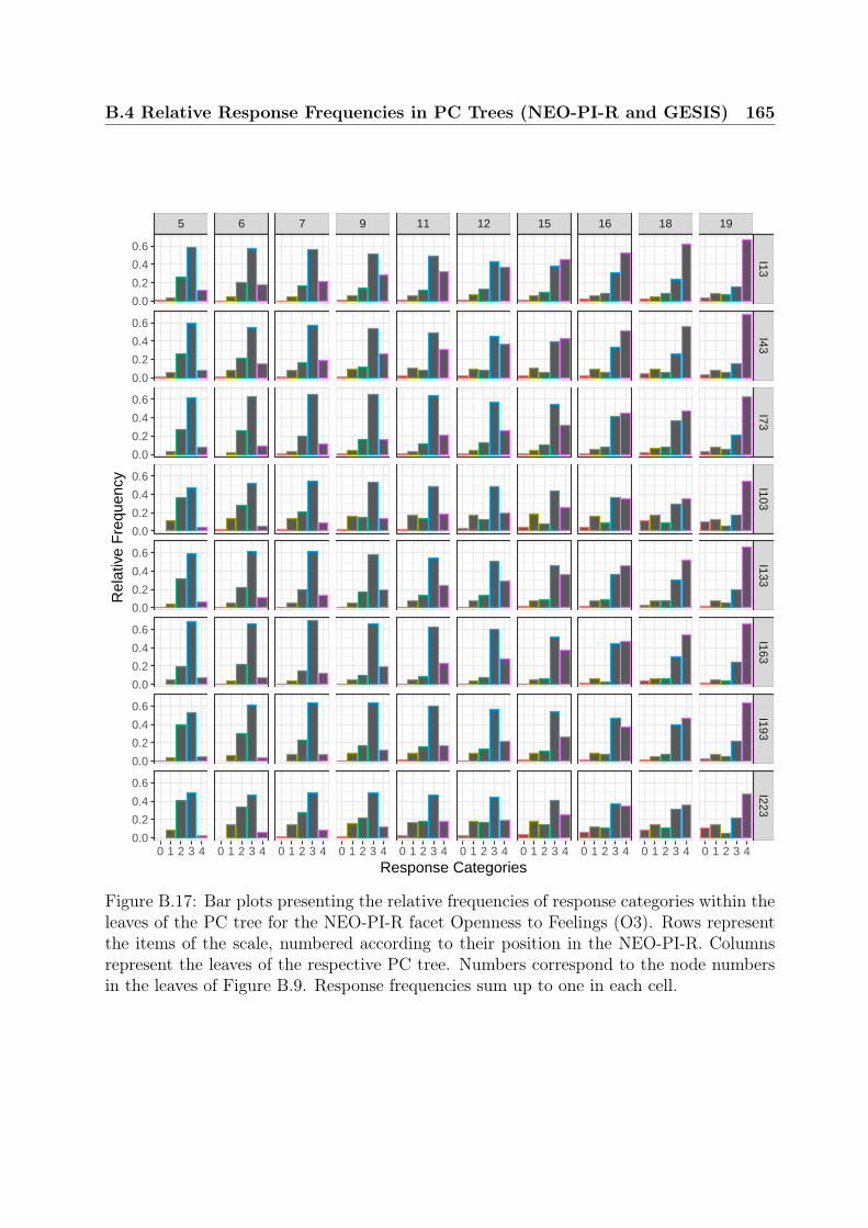
B.4 Relative Response Frequencies in PC Trees (NEO-PI-R and GESIS) 165
5 6 7 9 11 12 15 16 18 19
I13I43
I73I103
I133I163
I193I223
0 1 2 3 4 0 1 2 3 4 0 1 2 3 4 0 1 2 3 4 0 1 2 3 4 0 1 2 3 4 0 1 2 3 4 0 1 2 3 4 0 1 2 3 4 0 1 2 3 4
0.0
0.2
0.4
0.6
0.0
0.2
0.4
0.6
0.0
0.2
0.4
0.6
0.0
0.2
0.4
0.6
0.0
0.2
0.4
0.6
0.0
0.2
0.4
0.6
0.0
0.2
0.4
0.6
0.0
0.2
0.4
0.6
Response Categories
Rel
ativ
e F
requ
ency
Figure B.17: Bar plots presenting the relative frequencies of response categories within theleaves of the PC tree for the NEO-PI-R facet Openness to Feelings (O3). Rows representthe items of the scale, numbered according to their position in the NEO-PI-R. Columnsrepresent the leaves of the respective PC tree. Numbers correspond to the node numbersin the leaves of Figure B.9. Response frequencies sum up to one in each cell.
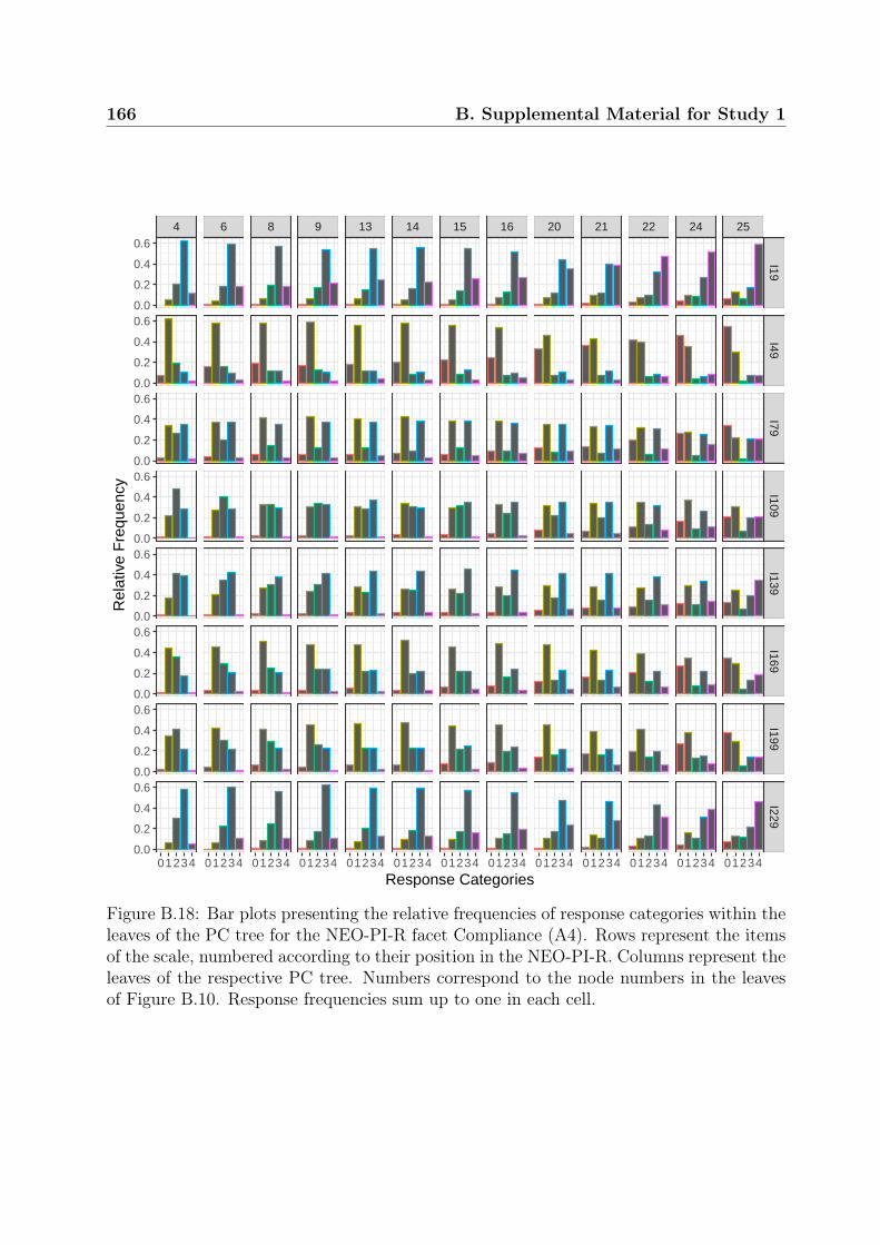
166 B. Supplemental Material for Study 1
4 6 8 9 13 14 15 16 20 21 22 24 25
I19I49
I79I109
I139I169
I199I229
01234 01234 01234 01234 01234 01234 01234 01234 01234 01234 01234 01234 01234
0.0
0.2
0.4
0.6
0.0
0.2
0.4
0.6
0.0
0.2
0.4
0.6
0.0
0.2
0.4
0.6
0.0
0.2
0.4
0.6
0.0
0.2
0.4
0.6
0.0
0.2
0.4
0.6
0.0
0.2
0.4
0.6
Response Categories
Rel
ativ
e F
requ
ency
Figure B.18: Bar plots presenting the relative frequencies of response categories within theleaves of the PC tree for the NEO-PI-R facet Compliance (A4). Rows represent the itemsof the scale, numbered according to their position in the NEO-PI-R. Columns represent theleaves of the respective PC tree. Numbers correspond to the node numbers in the leavesof Figure B.10. Response frequencies sum up to one in each cell.

B.4 Relative Response Frequencies in PC Trees (NEO-PI-R and GESIS) 167
5 6 7 9 10 13 15 16 18 19
I10I40
I70I100
I130I160
I190I220
0 1 2 3 4 0 1 2 3 4 0 1 2 3 4 0 1 2 3 4 0 1 2 3 4 0 1 2 3 4 0 1 2 3 4 0 1 2 3 4 0 1 2 3 4 0 1 2 3 4
0.0
0.2
0.4
0.6
0.0
0.2
0.4
0.6
0.0
0.2
0.4
0.6
0.0
0.2
0.4
0.6
0.0
0.2
0.4
0.6
0.0
0.2
0.4
0.6
0.0
0.2
0.4
0.6
0.0
0.2
0.4
0.6
Response Categories
Rel
ativ
e F
requ
ency
Figure B.19: Bar plots presenting the relative frequencies of response categories within theleaves of the PC tree for the NEO-PI-R facet Order (C2). Rows represent the items ofthe scale, numbered according to their position in the NEO-PI-R. Columns represent theleaves of the respective PC tree. Numbers correspond to the node numbers in the leavesof Figure B.11. Response frequencies sum up to one in each cell.
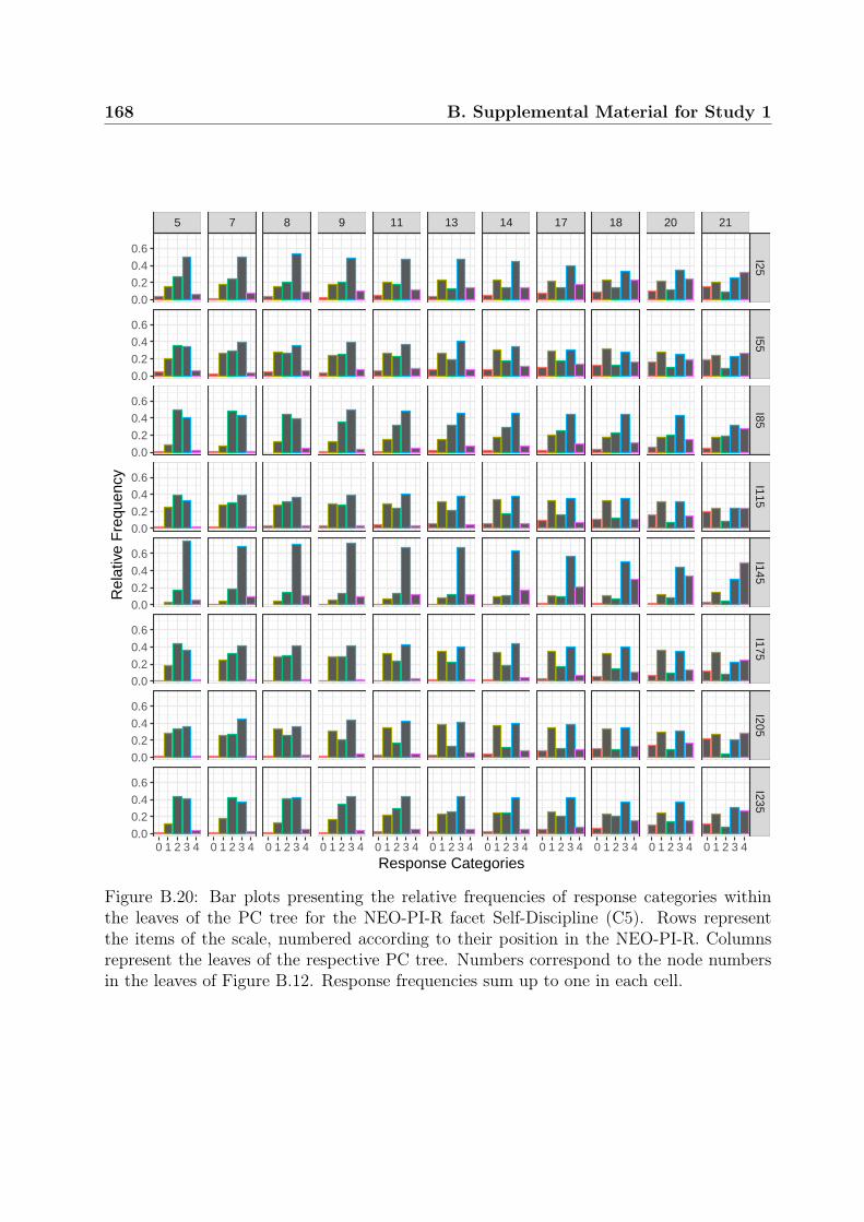
168 B. Supplemental Material for Study 1
5 7 8 9 11 13 14 17 18 20 21
I25I55
I85I115
I145I175
I205I235
0 1 2 3 4 0 1 2 3 4 0 1 2 3 4 0 1 2 3 4 0 1 2 3 4 0 1 2 3 4 0 1 2 3 4 0 1 2 3 4 0 1 2 3 4 0 1 2 3 4 0 1 2 3 4
0.0
0.2
0.4
0.6
0.0
0.2
0.4
0.6
0.0
0.2
0.4
0.6
0.0
0.2
0.4
0.6
0.0
0.2
0.4
0.6
0.0
0.2
0.4
0.6
0.0
0.2
0.4
0.6
0.0
0.2
0.4
0.6
Response Categories
Rel
ativ
e F
requ
ency
Figure B.20: Bar plots presenting the relative frequencies of response categories withinthe leaves of the PC tree for the NEO-PI-R facet Self-Discipline (C5). Rows representthe items of the scale, numbered according to their position in the NEO-PI-R. Columnsrepresent the leaves of the respective PC tree. Numbers correspond to the node numbersin the leaves of Figure B.12. Response frequencies sum up to one in each cell.

B.4 Relative Response Frequencies in PC Trees (NEO-PI-R and GESIS) 169
3 5 6 7
bbal119abbal121a
bbal122abbal124a
bbal128abbal129a
bbal131abbal133a
bbal135abbal136a
0 1 2 3 4 0 1 2 3 4 0 1 2 3 4 0 1 2 3 4
0.0
0.2
0.4
0.0
0.2
0.4
0.0
0.2
0.4
0.0
0.2
0.4
0.0
0.2
0.4
0.0
0.2
0.4
0.0
0.2
0.4
0.0
0.2
0.4
0.0
0.2
0.4
0.0
0.2
0.4
Response Categories
Rel
ativ
e F
requ
ency
Figure B.21: Bar plots presenting the relative frequencies of response categories withinthe leaves of the PC tree for the Positive Affect (PA) scale in the GESIS dataset. Rowsrepresent the items of the scale, labeled according to the official dataset. Columns representthe leaves of the respective PC tree. Numbers correspond to the node numbers in the leavesof Figure 2.6. Response frequencies sum up to one in each cell.

170 B. Supplemental Material for Study 1
3 4 5
bbal120abbal123a
bbal125abbal126a
bbal127abbal130a
bbal132abbal134a
bbal137abbal138a
0 1 2 3 4 0 1 2 3 4 0 1 2 3 4
0.00.20.40.60.8
0.00.20.40.60.8
0.00.20.40.60.8
0.00.20.40.60.8
0.00.20.40.60.8
0.00.20.40.60.8
0.00.20.40.60.8
0.00.20.40.60.8
0.00.20.40.60.8
0.00.20.40.60.8
Response Categories
Rel
ativ
e F
requ
ency
Figure B.22: Bar plots presenting the relative frequencies of response categories withinthe leaves of the PC tree for the Negative Affect (NA) scale in the GESIS dataset. Rowsrepresent the items of the scale, labeled according to the official dataset. Columns representthe leaves of the respective PC tree. Numbers correspond to the node numbers in the leavesof Figure 2.7. Response frequencies sum up to one in each cell.

B.4 Relative Response Frequencies in PC Trees (NEO-PI-R and GESIS) 171
3 4 6 7 baag035abaag038abaag039abaag040abaag042abaag044abaag046abaag047abaag048abaag049abaag051abaag052a
0 1 2 3 4 5 6 0 1 2 3 4 5 6 0 1 2 3 4 5 6 0 1 2 3 4 5 6
0.00.10.20.3
0.00.10.20.3
0.00.10.20.3
0.00.10.20.3
0.00.10.20.3
0.00.10.20.3
0.00.10.20.3
0.00.10.20.3
0.00.10.20.3
0.00.10.20.3
0.00.10.20.3
0.00.10.20.3
Response Categories
Rel
ativ
e F
requ
ency
Figure B.23: Bar plots presenting the relative frequencies of response categories within theleaves of the PC tree for the Global/Egocentric Orientation (GEO) scale in the GESISdataset. Rows represent the items of the scale, labeled according to the official dataset.Columns represent the leaves of the respective PC tree. Numbers correspond to the nodenumbers in the leaves of Figure 2.8. Response frequencies sum up to one in each cell.

172 B. Supplemental Material for Study 1
3 5 6 8 9
baag036abaag037a
baag041abaag043a
baag045abaag050a
baag053a
0 1 2 3 4 5 6 0 1 2 3 4 5 6 0 1 2 3 4 5 6 0 1 2 3 4 5 6 0 1 2 3 4 5 6
0.0
0.1
0.2
0.3
0.0
0.1
0.2
0.3
0.0
0.1
0.2
0.3
0.0
0.1
0.2
0.3
0.0
0.1
0.2
0.3
0.0
0.1
0.2
0.3
0.0
0.1
0.2
0.3
Response Categories
Rel
ativ
e F
requ
ency
Figure B.24: Bar plots presenting the relative frequencies of response categories within theleaves of the PC tree for the Allocentric/Mental Map (AMM) scale in the GESIS dataset.Rows represent the items of the scale, labeled according to the official dataset. Columnsrepresent the leaves of the respective PC tree. Numbers correspond to the node numbersin the leaves of Figure 2.9. Response frequencies sum up to one in each cell.

B.5 Threshold Plots of PC Trees (NEO-PI-R) 173
B.5 Threshold Plots of PC Trees (NEO-PI-R)Threshold plots of PC trees in the NEO-PI-R dataset for which no thresholds were missingin any of the resulting leafs.
I12 I42 I72 I102 I132 I162 I192 I222
0.3 0.4 0.5 0.6 0.7 0.8 0.3 0.4 0.5 0.6 0.7 0.8 0.3 0.4 0.5 0.6 0.7 0.8 0.3 0.4 0.5 0.6 0.7 0.8 0.3 0.4 0.5 0.6 0.7 0.8 0.3 0.4 0.5 0.6 0.7 0.8 0.3 0.4 0.5 0.6 0.7 0.8 0.3 0.4 0.5 0.6 0.7 0.8
−6
−3
0
3
Mean extraERS Index
Thr
esho
ld V
alue Threshold
T1T2T3T4
Figure B.25: Threshold plot for the PC tree of the NEO-PI-R facet Assertiveness (E3)with the extraERS index from heterogeneous items as single covariate. Mean extraERSvalues for each leaf of the PC tree in Figure B.6 are plotted against parameter estimatesof the respective partial credit model. Items are shown in separate panels. Thresholds aredepicted as lines. N = 11575.

174 B. Supplemental Material for Study 1
I17 I47 I77 I107 I137 I167 I197 I227
0.4 0.5 0.6 0.7 0.8 0.4 0.5 0.6 0.7 0.8 0.4 0.5 0.6 0.7 0.8 0.4 0.5 0.6 0.7 0.8 0.4 0.5 0.6 0.7 0.8 0.4 0.5 0.6 0.7 0.8 0.4 0.5 0.6 0.7 0.8 0.4 0.5 0.6 0.7 0.8
−2.5
0.0
2.5
Mean extraERS Index
Thr
esho
ld V
alue ThresholdT1T2T3T4
Figure B.26: Threshold plot for the PC tree of the NEO-PI-R facet Activity (E4) withthe extraERS index from heterogeneous items as single covariate. Mean extraERS valuesfor each leaf of the PC tree in Figure B.7 are plotted against parameter estimates ofthe respective partial credit model. Items are shown in separate panels. Thresholds aredepicted as lines. N = 11559.

B.5 Threshold Plots of PC Trees (NEO-PI-R) 175
I22 I52 I82 I112 I142 I172 I202 I232
0.3 0.4 0.5 0.6 0.7 0.3 0.4 0.5 0.6 0.7 0.3 0.4 0.5 0.6 0.7 0.3 0.4 0.5 0.6 0.7 0.3 0.4 0.5 0.6 0.7 0.3 0.4 0.5 0.6 0.7 0.3 0.4 0.5 0.6 0.7 0.3 0.4 0.5 0.6 0.7
−4
−2
0
2
4
Mean extraERS Index
Thr
esho
ld V
alue ThresholdT1T2T3T4
Figure B.27: Threshold plot for the PC tree of the NEO-PI-R facet Excitement-Seeking(E5) with the extraERS index from heterogeneous items as single covariate. Mean ex-traERS values for each leaf of the PC tree in Figure B.8 are plotted against parameterestimates of the respective partial credit model. Items are shown in separate panels.Thresholds are depicted as lines. N = 11584.

176 B. Supplemental Material for Study 1
B.6 PC Trees Including Demographic Variables (NEO-PI-R and GESIS)
PC trees for the analyzed personality facets in the NEO-PI-R and GESIS datasets, withthe respective ERS index from heterogeneous items, sex, and age as covariates.
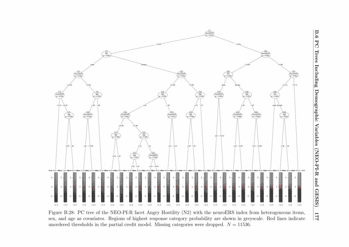
B.6
PC
Trees
Inclu
dingDem
ographic
Variab
les(N
EO-P
I-Ran
dGESIS)
177neuroERSp < 0.001
1
≤ 0.54 > 0.54
Sexp < 0.001
2
male female
neuroERSp < 0.001
3
≤ 0.42 > 0.42
neuroERSp < 0.001
4
≤ 0.34 > 0.34
Node 5 (n = 317)
1 4 8
−5
0
5
Agep = 0.001
6
≤ 33 > 33
Node 7 (n = 641)
1 4 8
−5
0
5
Node 8 (n = 219)
1 4 8
−5
0
5
Agep < 0.001
9
≤ 38 > 38
neuroERSp = 0.044
10
≤ 0.45> 0.45
Node 11 (n = 201)
1 4 8
−5
0
5
Node 12 (n = 1198)
1 4 8
−5
0
5
Node 13 (n = 340)
1 4 8
−5
0
5
neuroERSp < 0.001
14
≤ 0.46 > 0.46
Agep < 0.001
15
≤ 40 > 40
neuroERSp < 0.001
16
≤ 0.38 > 0.38
Agep = 0.005
17
≤ 24 > 24
Node 18 (n = 413)
1 4 8
−5
0
5
Node 19 (n = 230)
1 4 8
−5
0
5
Agep < 0.001
20
≤ 21 > 21
Agep = 0.041
21
≤ 19 > 19
Node 22 (n = 258)
1 4 8
−5
0
5
Node 23 (n = 364)
1 4 8
−5
0
5
neuroERSp = 0.005
24
≤ 0.41> 0.41
Node 25 (n = 296)
1 4 8
−5
0
5
Node 26 (n = 639)
1 4 8
−5
0
5
neuroERSp = 0.017
27
≤ 0.4 > 0.4
Node 28 (n = 249)
1 4 8
−5
0
5
Node 29 (n = 231)
1 4 8
−5
0
5
Agep < 0.001
30
≤ 37 > 37
Agep < 0.001
31
≤ 23 > 23
Node 32 (n = 1004)
1 4 8
−5
0
5
Node 33 (n = 825)
1 4 8
−5
0
5
Node 34 (n = 551)
1 4 8
−5
0
5
neuroERSp < 0.001
35
≤ 0.64 > 0.64
Sexp < 0.001
36
male female
neuroERSp = 0.003
37
≤ 0.57> 0.57
Node 38 (n = 395)
1 4 8
−5
0
5
Node 39 (n = 480)
1 4 8
−5
0
5
Agep < 0.001
40
≤ 25 > 25
neuroERSp = 0.008
41
≤ 0.57> 0.57
Node 42 (n = 394)
1 4 8
−5
0
5
Node 43 (n = 451)
1 4 8
−5
0
5
neuroERSp = 0.002
44
≤ 0.58> 0.58
Node 45 (n = 479)
1 4 8
−5
0
5
Node 46 (n = 335)
1 4 8
−5
0
5
neuroERSp < 0.001
47
≤ 0.71 > 0.71
Sexp < 0.001
48
male female
Node 49 (n = 235)
1 4 8
−5
0
5
Agep = 0.001
50
≤ 26 > 26
Node 51 (n = 207)
1 4 8
−5
0
5
Node 52 (n = 230)
1 4 8
−5
0
5
Node 53 (n = 354)
1 4 8
−5
0
5
Figure B.28: PC tree of the NEO-PI-R facet Angry Hostility (N2) with the neuroERS index from heterogeneous items,sex, and age as covariates. Regions of highest response category probability are shown in greyscale. Red lines indicateunordered thresholds in the partial credit model. Missing categories were dropped. N = 11536.

178B.Supplem
entalMaterial
forStudy1
neuroERSp < 0.001
1
≤ 0.52 > 0.52
neuroERSp < 0.001
2
≤ 0.4 > 0.4
neuroERSp < 0.001
3
≤ 0.33 > 0.33
Sexp < 0.001
4
malefemale
Node 5 (n = 241)
1
−6−4−2
0246
Node 6 (n = 267)
1
−6−4−2
0246
Agep < 0.001
7
≤ 42> 42
Sexp < 0.001
8
malefemale
Node 9 (n = 448)
1
−6−4−2
0246
Node 10 (n = 672)
1
−6−4−2
0246
Node 11 (n = 203)
1
−6−4−2
0246
Sexp < 0.001
12
male female
neuroERSp < 0.001
13
≤ 0.47 > 0.47
Agep = 0.004
14
≤ 31> 31
Node 15 (n = 639)
1
−6−4−2
0246
Node 16 (n = 286)
1
−6−4−2
0246
Agep = 0.011
17
≤ 24> 24
Node 18 (n = 453)
1
−6−4−2
0246
Node 19 (n = 560)
1
−6−4−2
0246
Agep < 0.001
20
≤ 34 > 34
neuroERSp < 0.001
21
≤ 0.46> 0.46
Agep = 0.041
22
≤ 25> 25
Node 23 (n = 865)
1
−6−4−2
0246
Node 24 (n = 337)
1
−6−4−2
0246
Node 25 (n = 1423)
1
−6−4−2
0246
Agep < 0.001
26
≤ 46> 46
Node 27 (n = 501)
1
−6−4−2
0246
Agep = 0.048
28
≤ 53> 53
Node 29 (n = 214)
1
−6−4−2
0246
Node 30 (n = 242)
1
−6−4−2
0246
neuroERSp < 0.001
31
≤ 0.63 > 0.63
Agep < 0.001
32
≤ 37 > 37
Sexp < 0.001
33
male female
neuroERSp < 0.001
34
≤ 0.59> 0.59
Agep = 0.048
35
≤ 24> 24
Node 36 (n = 344)
1
−6−4−2
0246
Node 37 (n = 274)
1
−6−4−2
0246
Node 38 (n = 257)
1
−6−4−2
0246
neuroERSp < 0.001
39
≤ 0.57> 0.57
Agep = 0.022
40
≤ 26 > 26
neuroERSp = 0.046
41
≤ 0.55> 0.55
Node 42 (n = 465)
1
−6−4−2
0246
Node 43 (n = 203)
1
−6−4−2
0246
Node 44 (n = 245)
1
−6−4−2
0246
Node 45 (n = 710)
1
−6−4−2
0246
Sexp < 0.001
46
malefemale
Node 47 (n = 205)
1
−6−4−2
0246
Node 48 (n = 468)
1
−6−4−2
0246
neuroERSp < 0.001
49
≤ 0.72> 0.72
Agep < 0.001
50
≤ 24> 24
Node 51 (n = 302)
1
−6−4−2
0246
Node 52 (n = 444)
1
−6−4−2
0246
Node 53 (n = 297)
1
−6−4−2
0246
Figure B.29: PC tree of the NEO-PI-R facet Impulsivity (N5) with the neuroERS index from heterogeneous items, sex, andage as covariates. Regions of highest response category probability are shown in greyscale. Red lines indicate unorderedthresholds in the partial credit model. Missing categories were dropped. N = 11565.

B.6
PC
Trees
Inclu
dingDem
ographic
Variab
les(N
EO-P
I-Ran
dGESIS)
179extraERSp < 0.001
1
≤ 0.52 > 0.52
extraERSp < 0.001
2
≤ 0.39 > 0.39
Agep < 0.001
3
≤ 36 > 36
Sexp = 0.002
4
male female
Node 5 (n = 576)
16
−5
0
5
Agep = 0.049
6
≤ 20 > 20
Node 7 (n = 259)
16
−5
0
5
Node 8 (n = 557)
16
−5
0
5
Node 9 (n = 407)
16
−5
0
5
Agep < 0.001
10
≤ 36 > 36
extraERSp < 0.001
11
≤ 0.43> 0.43
Node 12 (n = 1435)
16
−5
0
5
Sexp < 0.001
13
male female
Node 14 (n = 1031)
16
−5
0
5
Agep < 0.001
15
≤ 25 > 25
Node 16 (n = 1302)
16
−5
0
5
Node 17 (n = 556)
16
−5
0
5
Sexp < 0.001
18
male female
extraERSp = 0.004
19
≤ 0.46> 0.46
Node 20 (n = 216)
16
−5
0
5
Node 21 (n = 229)
16
−5
0
5
Node 22 (n = 883)
16
−5
0
5
extraERSp < 0.001
23
≤ 0.63 > 0.63
Agep < 0.001
24
≤ 29 > 29
extraERSp < 0.001
25
≤ 0.57> 0.57
Node 26 (n = 1159)
16
−5
0
5
extraERSp = 0.036
27
≤ 0.61> 0.61
Node 28 (n = 558)
16
−5
0
5
Node 29 (n = 341)
16
−5
0
5
Sexp < 0.001
30
male female
Node 31 (n = 353)
16
−5
0
5
Agep = 0.039
32
≤ 47 > 47
Node 33 (n = 510)
16
−5
0
5
Node 34 (n = 211)
16
−5
0
5
extraERSp < 0.001
35
≤ 0.73> 0.73
Agep = 0.037
36
≤ 24 > 24
Node 37 (n = 337)
16
−5
0
5
Node 38 (n = 455)
16
−5
0
5
Node 39 (n = 200)
16
−5
0
5
Figure B.30: PC tree of the NEO-PI-R facet Assertiveness (E3) with the extraERS index from heterogeneous items,sex, and age as covariates. Regions of highest response category probability are shown in greyscale. Red lines indicateunordered thresholds in the partial credit model. Missing categories were dropped. N = 11575.

180B.Supplem
entalMaterial
forStudy1
extraERSp < 0.001
1
≤ 0.54 > 0.54
extraERSp < 0.001
2
≤ 0.43 > 0.43
Agep < 0.001
3
≤ 33 > 33
extraERSp < 0.001
4
≤ 0.36 > 0.36
Sexp = 0.042
5
malefemale
Node 6 (n = 331)
1
−6−4−2
0246
Node 7 (n = 437)
1
−6−4−2
0246
Sexp < 0.001
8
malefemale
Node 9 (n = 727)
1
−6−4−2
0246
Agep < 0.001
10
≤ 19 > 19
Node 11 (n = 231)
1
−6−4−2
0246
Agep = 0.013
12
≤ 22> 22
Node 13 (n = 420)
1
−6−4−2
0246
Node 14 (n = 520)
1
−6−4−2
0246
extraERSp < 0.001
15
≤ 0.38> 0.38
Node 16 (n = 361)
1
−6−4−2
0246
Agep < 0.001
17
≤ 46> 46
Node 18 (n = 332)
1
−6−4−2
0246
Node 19 (n = 303)
1
−6−4−2
0246
Agep < 0.001
20
≤ 39 > 39
Agep < 0.001
21
≤ 26 > 26
Sexp < 0.001
22
male female
extraERSp = 0.044
23
≤ 0.47> 0.47
Node 24 (n = 295)
1
−6−4−2
0246
Node 25 (n = 547)
1
−6−4−2
0246
Agep = 0.028
26
≤ 21 > 21
Agep = 0.016
27
≤ 19> 19
Node 28 (n = 350)
1
−6−4−2
0246
Node 29 (n = 522)
1
−6−4−2
0246
Node 30 (n = 753)
1
−6−4−2
0246
extraERSp = 0.038
31
≤ 0.48> 0.48
Node 32 (n = 555)
1
−6−4−2
0246
Node 33 (n = 514)
1
−6−4−2
0246
Agep = 0.003
34
≤ 57> 57
Node 35 (n = 691)
1
−6−4−2
0246
Node 36 (n = 204)
1
−6−4−2
0246
extraERSp < 0.001
37
≤ 0.63 > 0.63
Agep < 0.001
38
≤ 29 > 29
Sexp < 0.001
39
malefemale
Node 40 (n = 568)
1
−6−4−2
0246
Node 41 (n = 1055)
1
−6−4−2
0246
Agep < 0.001
42
≤ 47> 47
Node 43 (n = 595)
1
−6−4−2
0246
Node 44 (n = 264)
1
−6−4−2
0246
extraERSp < 0.001
45
≤ 0.73> 0.73
Agep < 0.001
46
≤ 30> 30
Node 47 (n = 502)
1
−6−4−2
0246
Node 48 (n = 279)
1
−6−4−2
0246
Node 49 (n = 203)
1
−6−4−2
0246
Figure B.31: PC tree of the NEO-PI-R facet Activity (E4) with the extraERS index from heterogeneous items, sex, andage as covariates. Regions of highest response category probability are shown in greyscale. Red lines indicate unorderedthresholds in the partial credit model. Missing categories were dropped. N = 11559.

B.6
PC
Trees
Inclu
dingDem
ographic
Variab
les(N
EO-P
I-Ran
dGESIS)
181extraERSp < 0.001
1
≤ 0.5 > 0.5
extraERSp < 0.001
2
≤ 0.41 > 0.41
Agep < 0.001
3
≤ 28 > 28
Sexp < 0.001
4
malefemale
extraERSp = 0.027
5
≤ 0.38> 0.38
Node 6 (n = 352)
1
−4
−2
0
2
4
6
Node 7 (n = 231)
1
−4
−2
0
2
4
6
Node 8 (n = 891)
1
−4
−2
0
2
4
6
extraERSp < 0.001
9
≤ 0.33> 0.33
Node 10 (n = 272)
1
−4
−2
0
2
4
6
Sexp = 0.002
11
malefemale
Node 12 (n = 239)
1
−4
−2
0
2
4
6
Node 13 (n = 386)
1
−4
−2
0
2
4
6
Agep < 0.001
14
≤ 32 > 32
Sexp < 0.001
15
male female
Agep = 0.021
16
≤ 21> 21
Node 17 (n = 305)
1
−4
−2
0
2
4
6
Node 18 (n = 833)
1
−4
−2
0
2
4
6
Agep < 0.001
19
≤ 25 > 25
Agep < 0.001
20
≤ 19> 19
Node 21 (n = 362)
1
−4
−2
0
2
4
6
Node 22 (n = 1099)
1
−4
−2
0
2
4
6
extraERSp = 0.039
23
≤ 0.47> 0.47
Node 24 (n = 239)
1
−4
−2
0
2
4
6
Node 25 (n = 283)
1
−4
−2
0
2
4
6
Sexp < 0.001
26
malefemale
Node 27 (n = 430)
1
−4
−2
0
2
4
6
Agep = 0.003
28
≤ 46> 46
Node 29 (n = 458)
1
−4
−2
0
2
4
6
Node 30 (n = 394)
1
−4
−2
0
2
4
6
extraERSp < 0.001
31
≤ 0.61 > 0.61
Agep < 0.001
32
≤ 25 > 25
Sexp < 0.001
33
male female
Agep = 0.008
34
≤ 22> 22
Node 35 (n = 321)
1
−4
−2
0
2
4
6
Node 36 (n = 254)
1
−4
−2
0
2
4
6
extraERSp < 0.001
37
≤ 0.54> 0.54
Node 38 (n = 469)
1
−4
−2
0
2
4
6
Node 39 (n = 665)
1
−4
−2
0
2
4
6
Sexp < 0.001
40
malefemale
Node 41 (n = 545)
1
−4
−2
0
2
4
6
Agep = 0.004
42
≤ 33 > 33
Node 43 (n = 451)
1
−4
−2
0
2
4
6
extraERSp = 0.032
44
≤ 0.55> 0.55
Node 45 (n = 343)
1
−4
−2
0
2
4
6
Node 46 (n = 221)
1
−4
−2
0
2
4
6
extraERSp < 0.001
47
≤ 0.71 > 0.71
Sexp < 0.001
48
malefemale
Node 49 (n = 418)
1
−4
−2
0
2
4
6
Agep < 0.001
50
≤ 23> 23
Node 51 (n = 295)
1
−4
−2
0
2
4
6
Node 52 (n = 494)
1
−4
−2
0
2
4
6
Node 53 (n = 334)
1
−4
−2
0
2
4
6
Figure B.32: PC tree of the NEO-PI-R facet Excitement-Seeking (E5) with the extraERS index from heterogeneous items,sex, and age as covariates. Regions of highest response category probability are shown in greyscale. Red lines indicateunordered thresholds in the partial credit model. Missing categories were dropped. N = 11584.

182B.Supplem
entalMaterial
forStudy1openERSp < 0.001
1
≤ 0.55 > 0.55
openERSp < 0.001
2
≤ 0.41 > 0.41
Agep < 0.001
3
≤ 36 > 36
Sexp < 0.001
4
male female
openERSp = 0.001
5
≤ 0.37> 0.37
Node 6 (n = 529)
1 6
−6−4−2
0246
Node 7 (n = 356)
1 6
−6−4−2
0246
Node 8 (n = 1243)
1 6
−6−4−2
0246
Node 9 (n = 536)
1 6
−6−4−2
0246
Agep < 0.001
10
≤ 38 > 38
Sexp < 0.001
11
male female
openERSp < 0.001
12
≤ 0.47 > 0.47
openERSp = 0.018
13
≤ 0.43> 0.43
Node 14 (n = 407)
1 6
−6−4−2
0246
Node 15 (n = 393)
1 6
−6−4−2
0246
Node 16 (n = 984)
1 6
−6−4−2
0246
openERSp < 0.001
17
≤ 0.48 > 0.48
Agep < 0.001
18
≤ 32 > 32
Node 19 (n = 1728)
1 6
−6−4−2
0246
Node 20 (n = 204)
1 6
−6−4−2
0246
Node 21 (n = 1299)
1 6
−6−4−2
0246
openERSp < 0.001
22
≤ 0.5 > 0.5
Sexp = 0.016
23
malefemale
Node 24 (n = 295)
1 6
−6−4−2
0246
Node 25 (n = 601)
1 6
−6−4−2
0246
Node 26 (n = 404)
1 6
−6−4−2
0246
openERSp < 0.001
27
≤ 0.67 > 0.67
Agep < 0.001
28
≤ 30 > 30
openERSp < 0.001
29
≤ 0.6 > 0.6
Node 30 (n = 789)
1 6
−6−4−2
0246
Node 31 (n = 540)
1 6
−6−4−2
0246
openERSp = 0.004
32
≤ 0.6 > 0.6
Node 33 (n = 439)
1 6
−6−4−2
0246
Node 34 (n = 305)
1 6
−6−4−2
0246
openERSp = 0.002
35
≤ 0.72> 0.72
Node 36 (n = 288)
1 6
−6−4−2
0246
Node 37 (n = 238)
1 6
−6−4−2
0246
Figure B.33: PC tree of the NEO-PI-R facet Openness to Feelings (O3) with the openERS index from heterogeneousitems, sex, and age as covariates. Regions of highest response category probability are shown in greyscale. Red linesindicate unordered thresholds in the partial credit model. Missing categories were dropped. N = 11578.

B.6
PC
Trees
Inclu
dingDem
ographic
Variab
les(N
EO-P
I-Ran
dGESIS)
183agreeERSp < 0.001
1
≤ 0.52 > 0.52
agreeERSp < 0.001
2
≤ 0.43 > 0.43
agreeERSp < 0.001
3
≤ 0.33 > 0.33
Node 4 (n = 553)
1
−6−4−2
0246
Agep < 0.001
5
≤ 30 > 30
Agep < 0.001
6
≤ 19> 19
Node 7 (n = 317)
1
−6−4−2
0246
Sexp < 0.001
8
malefemale
Node 9 (n = 572)
1
−6−4−2
0246
Node 10 (n = 879)
1
−6−4−2
0246
Sexp < 0.001
11
malefemale
Node 12 (n = 329)
1
−6−4−2
0246
agreeERSp = 0.007
13
≤ 0.38> 0.38
Node 14 (n = 263)
1
−6−4−2
0246
Node 15 (n = 262)
1
−6−4−2
0246
Agep < 0.001
16
≤ 39 > 39
Sexp < 0.001
17
male female
Agep = 0.008
18
≤ 23> 23
Node 19 (n = 578)
1
−6−4−2
0246
Node 20 (n = 711)
1
−6−4−2
0246
Agep < 0.001
21
≤ 25 > 25
Agep < 0.001
22
≤ 20 > 20
Agep = 0.017
23
≤ 19> 19
Node 24 (n = 343)
1
−6−4−2
0246
Node 25 (n = 319)
1
−6−4−2
0246
agreeERSp = 0.001
26
≤ 0.48> 0.48
Node 27 (n = 605)
1
−6−4−2
0246
Node 28 (n = 261)
1
−6−4−2
0246
Node 29 (n = 791)
1
−6−4−2
0246
agreeERSp = 0.024
30
≤ 0.48> 0.48
Node 31 (n = 464)
1
−6−4−2
0246
Node 32 (n = 446)
1
−6−4−2
0246
agreeERSp < 0.001
33
≤ 0.67 > 0.67
Agep < 0.001
34
≤ 37 > 37
Sexp < 0.001
35
male female
agreeERSp < 0.001
36
≤ 0.6> 0.6
agreeERSp = 0.048
37
≤ 0.57> 0.57
Agep = 0.018
38
≤ 23> 23
Node 39 (n = 229)
1
−6−4−2
0246
Node 40 (n = 267)
1
−6−4−2
0246
Node 41 (n = 211)
1
−6−4−2
0246
Node 42 (n = 252)
1
−6−4−2
0246
agreeERSp < 0.001
43
≤ 0.6> 0.6
Agep < 0.001
44
≤ 21> 21
Node 45 (n = 472)
1
−6−4−2
0246
Node 46 (n = 774)
1
−6−4−2
0246
Node 47 (n = 455)
1
−6−4−2
0246
agreeERSp < 0.001
48
≤ 0.55> 0.55
Node 49 (n = 260)
1
−6−4−2
0246
Node 50 (n = 434)
1
−6−4−2
0246
agreeERSp < 0.001
51
≤ 0.72> 0.72
Node 52 (n = 293)
1
−6−4−2
0246
Node 53 (n = 243)
1
−6−4−2
0246
Figure B.34: PC tree of the NEO-PI-R facet Compliance (A4) with the agreeERS index from heterogeneous items, sex, andage as covariates. Regions of highest response category probability are shown in greyscale. Red lines indicate unorderedthresholds in the partial credit model. Missing categories were dropped. N = 11583.

184B.Supplem
entalMaterial
forStudy1
conscERSp < 0.001
1
≤ 0.52 > 0.52
conscERSp < 0.001
2
≤ 0.38 > 0.38
Agep < 0.001
3
≤ 37 > 37
Sexp < 0.001
4
male female
conscERSp < 0.001
5
≤ 0.33> 0.33
Node 6 (n = 264)
1
−6−4−2
0246
Node 7 (n = 565)
1
−6−4−2
0246
conscERSp = 0.026
8
≤ 0.33> 0.33
Node 9 (n = 318)
1
−6−4−2
0246
Node 10 (n = 785)
1
−6−4−2
0246
conscERSp < 0.001
11
≤ 0.35> 0.35
Node 12 (n = 285)
1
−6−4−2
0246
Node 13 (n = 214)
1
−6−4−2
0246
Agep < 0.001
14
≤ 36 > 36
Sexp < 0.001
15
male female
conscERSp < 0.001
16
≤ 0.45> 0.45
Node 17 (n = 748)
1
−6−4−2
0246
Node 18 (n = 785)
1
−6−4−2
0246
conscERSp < 0.001
19
≤ 0.48 > 0.48
Agep = 0.015
20
≤ 27 > 27
conscERSp = 0.02
21
≤ 0.43> 0.43
Node 22 (n = 524)
1
−6−4−2
0246
Node 23 (n = 888)
1
−6−4−2
0246
Node 24 (n = 396)
1
−6−4−2
0246
Agep < 0.001
25
≤ 23> 23
Node 26 (n = 587)
1
−6−4−2
0246
Node 27 (n = 500)
1
−6−4−2
0246
Sexp < 0.001
28
male female
Agep = 0.045
29
≤ 48> 48
Node 30 (n = 212)
1
−6−4−2
0246
Node 31 (n = 230)
1
−6−4−2
0246
Agep < 0.001
32
≤ 50> 50
Node 33 (n = 572)
1
−6−4−2
0246
Node 34 (n = 350)
1
−6−4−2
0246
conscERSp < 0.001
35
≤ 0.64 > 0.64
Agep < 0.001
36
≤ 40 > 40
Sexp < 0.001
37
male female
conscERSp < 0.001
38
≤ 0.57> 0.57
Node 39 (n = 432)
1
−6−4−2
0246
Node 40 (n = 334)
1
−6−4−2
0246
Agep < 0.001
41
≤ 23> 23
Node 42 (n = 742)
1
−6−4−2
0246
Node 43 (n = 656)
1
−6−4−2
0246
Node 44 (n = 438)
1
−6−4−2
0246
conscERSp < 0.001
45
≤ 0.69> 0.69
Agep = 0.05
46
≤ 25> 25
Node 47 (n = 203)
1
−6−4−2
0246
Node 48 (n = 230)
1
−6−4−2
0246
Node 49 (n = 353)
1
−6−4−2
0246
Figure B.35: PC tree of the NEO-PI-R Order (C2) with the conscERS index from heterogeneous items, sex, and ageas covariates. Regions of highest response category probability are shown in greyscale. Red lines indicate unorderedthresholds in the partial credit model. Missing categories were dropped. N = 11611.

B.6
PC
Trees
Inclu
dingDem
ographic
Variab
les(N
EO-P
I-Ran
dGESIS)
185conscERSp < 0.001
1
≤ 0.52 > 0.52
conscERSp < 0.001
2
≤ 0.41 > 0.41
Sexp < 0.001
3
male female
Agep < 0.001
4
≤ 30 > 30
conscERSp = 0.018
5
≤ 0.33> 0.33
Node 6 (n = 226)
18
−5
0
5
Node 7 (n = 626)
18
−5
0
5
Node 8 (n = 397)
18
−5
0
5
conscERSp < 0.001
9
≤ 0.35> 0.35
Node 10 (n = 793)
18
−5
0
5
Node 11 (n = 1008)
18
−5
0
5
Agep < 0.001
12
≤ 32 > 32
conscERSp < 0.001
13
≤ 0.47 > 0.47
Agep = 0.05
14
≤ 21 > 21
Node 15 (n = 602)
18
−5
0
5
Node 16 (n = 940)
18
−5
0
5
Agep < 0.001
17
≤ 25 > 25
Sexp = 0.033
18
malefemale
Node 19 (n = 492)
18
−5
0
5
Node 20 (n = 975)
18
−5
0
5
Node 21 (n = 612)
18
−5
0
5
Sexp < 0.001
22
male female
Node 23 (n = 493)
18
−5
0
5
Agep < 0.001
24
≤ 50 > 50
conscERSp = 0.026
25
≤ 0.48> 0.48
Node 26 (n = 415)
18
−5
0
5
Node 27 (n = 292)
18
−5
0
5
Node 28 (n = 313)
18
−5
0
5
conscERSp < 0.001
29
≤ 0.63 > 0.63
Agep < 0.001
30
≤ 30 > 30
conscERSp < 0.001
31
≤ 0.57> 0.57
Sexp = 0.001
32
malefemale
Node 33 (n = 367)
18
−5
0
5
Node 34 (n = 656)
18
−5
0
5
Node 35 (n = 737)
18
−5
0
5
Agep = 0.006
36
≤ 41 > 41
conscERSp = 0.04
37
≤ 0.57> 0.57
Node 38 (n = 213)
18
−5
0
5
Node 39 (n = 200)
18
−5
0
5
Node 40 (n = 412)
18
−5
0
5
conscERSp < 0.001
41
≤ 0.69> 0.69
Node 42 (n = 442)
18
−5
0
5
Node 43 (n = 352)
18
−5
0
5
Figure B.36: PC tree of the NEO-PI-R Self-Discipline (C5) with the conscERS index from heterogeneous items, sex, andage as covariates. Regions of highest response category probability are shown in greyscale. Red lines indicate unorderedthresholds in the partial credit model. Missing categories were dropped. N = 11563.

186B.Supplem
entalMaterial
forStudy1
Agep < 0.001
1
≤ 40 > 40
ERS Indexp < 0.001
2
≤ 0.47 > 0.47
Node 3 (n = 254)
1 4 6 8
−5
0
5
Agep < 0.001
4
≤ 24 > 24
Node 5 (n = 269)
1 4 6 8
−5
0
5
Node 6 (n = 623)
1 4 6 8
−5
0
5
ERS Indexp < 0.001
7
≤ 0.66 > 0.66
ERS Indexp < 0.001
8
≤ 0.52 > 0.52
Agep = 0.04
9
≤ 59 > 59
Node 10 (n = 669)
1 4 6 8
−5
0
5
Node 11 (n = 278)
1 4 6 8
−5
0
5
Sexp = 0.037
12
male female
Node 13 (n = 551)
1 4 6 8
−5
0
5
Node 14 (n = 583)
1 4 6 8
−5
0
5
Node 15 (n = 216)
1 4 6 8
−5
0
5
Figure B.37: PC tree of the Positive Affect scale (PA) with the ERS index from heterogeneous items, sex, and ageas covariates. Regions of highest response category probability are shown in greyscale. Red lines indicate unorderedthresholds in the partial credit model. Missing categories were dropped. N = 3443.

B.6
PC
Trees
Inclu
dingDem
ographic
Variab
les(N
EO-P
I-Ran
dGESIS)
187Age
p < 0.001
1
≤ 48 > 48
Agep < 0.001
2
≤ 31 > 31
Sexp = 0.012
3
male female
Node 4 (n = 316)
1 4 6 8
−4
−2
0
2
4
Node 5 (n = 375)
1 4 6 8
−4
−2
0
2
4
Sexp < 0.001
6
male female
Node 7 (n = 529)
1 4 6 8
−4
−2
0
2
4
Node 8 (n = 585)
1 4 6 8
−4
−2
0
2
4
Sexp < 0.001
9
male female
ERS Indexp < 0.001
10
≤ 0.52 > 0.52
Node 11 (n = 307)
1 4 6 8
−4
−2
0
2
4
Node 12 (n = 507)
1 4 6 8
−4
−2
0
2
4
ERS Indexp = 0.01
13
≤ 0.56 > 0.56
Node 14 (n = 500)
1 4 6 8
−4
−2
0
2
4
Node 15 (n = 361)
1 4 6 8
−4
−2
0
2
4
Figure B.38: PC tree of the Negative Affect scale (NA) with the ERS index from heterogeneous items, sex, and ageas covariates. Regions of highest response category probability are shown in greyscale. Red lines indicate unorderedthresholds in the partial credit model. Missing categories were dropped. N = 3480.

188B.Supplem
entalMaterial
forStudy1
Agep < 0.001
1
≤ 44 > 44
ERS Indexp < 0.001
2
≤ 0.49 > 0.49
Node 3 (n = 456)
1 4 6 8 12
−20−15−10
−505
10
Node 4 (n = 1020)
1 4 6 8 12
−20−15−10
−505
10
Sexp < 0.001
5
male female
ERS Indexp = 0.007
6
≤ 0.54 > 0.54
Node 7 (n = 484)
1 4 6 8 12
−20−15−10
−505
10
Agep = 0.038
8
≤ 57 > 57
Node 9 (n = 282)
1 4 6 8 12
−20−15−10
−505
10
Node 10 (n = 264)
1 4 6 8 12
−20−15−10
−505
10
Agep < 0.001
11
≤ 51 > 51
Node 12 (n = 353)
1 4 6 8 12
−20−15−10
−505
10
Node 13 (n = 725)
1 4 6 8 12
−20−15−10
−505
10
Figure B.39: PC tree of the Global/Egocentric Orientation scale (GEO) with the ERS index from heterogeneous items,sex, and age as covariates. Regions of highest response category probability are shown in greyscale. Red lines indicateunordered thresholds in the partial credit model. Missing categories were dropped. N = 3584.

B.6
PC
Trees
Inclu
dingDem
ographic
Variab
les(N
EO-P
I-Ran
dGESIS)
189ERS Indexp < 0.001
1
≤ 0.55 > 0.55
ERS Indexp < 0.001
2
≤ 0.44 > 0.44
Node 3 (n = 472)
1 2 4 6 7
−6−4−2
0246
Sexp < 0.001
4
male female
ERS Indexp = 0.042
5
≤ 0.51 > 0.51
Node 6 (n = 369)
1 2 4 6 7
−6−4−2
0246
Node 7 (n = 393)
1 2 4 6 7
−6−4−2
0246
Node 8 (n = 819)
1 2 4 6 7
−6−4−2
0246
ERS Indexp < 0.001
9
≤ 0.68 > 0.68
Node 10 (n = 1347)
1 2 4 6 7
−6−4−2
0246
Node 11 (n = 210)
1 2 4 6 7
−6−4−2
0246
Figure B.40: PC tree of the Allocentric/Mental Map scale (AMM) with the ERS index from heterogeneous items, sex, andage as covariates. Regions of highest response category probability are shown in greyscale. Red lines indicate unorderedthresholds in the partial credit model. Missing categories were dropped. N = 3610.

190 B. Supplemental Material for Study 1

Appendix C
Supplemental Material for Study 2
C.1 Description of ERS ItemsWording of the items which were used to compute the ERS index from heterogeneousitems. Items are presented as they were used in study 2. Original wording differed in somecases. ERS items were sampled from the “Zusammenstellung sozialwissenschaftlicher Itemsund Skalen des GESIS - Leibniz-Institut für Sozialwissenschaften” (ZIS) and the “Elektro-nisches Testarchive des Leibniz-Zentrums für Psychologische Information und Dokumen-tation” (ZPID).
Item Wording Original Source
1 Ich habe Schwierigkeiten, mein Verhal-ten an verschiedene Menschen bzw. anverschiedene Situationen anzupassen.
Schyns, B. & Paul, T. (2014). DeutscheSelf-Monitoring Skala. ZIS.
2 Ich bin jemand, der eine lebhafte Phan-tasie, Vorstellungen hat.
Schupp, J., & Gerlitz, J.-Y. (2014). BigFive Inventory-SOEP (BFI-S). ZIS.
3 Selbst wenn mein Partner ärgerlich aufmich ist, liebe ich ihn stark und bedin-gungslos.
Bierhoff, H.W. & Grau, I. (1997).Globalskalen zur Einschätzung vonBeziehungseinstellungen (GSEB).ZPID.
4 Ich habe, innerhalb der letzten 4Wochen, in Situationen anders gehan-delt, als ich es ursprünglich geplanthatte.
Bankstahl, U.S. & Görtelmeyer, R.(2013). Attention and PerformanceSelf-Assessment (APSA) - deutscheFassung. ZPID.
5 Für wie wichtig halten Sie persön-lich gute Aufstiegsmöglichkeiten für dieberufliche Arbeit und den Beruf?
Zentralarchiv für empirische Sozial-forschung (ZA) & Zentrum für Umfra-gen, Methoden und Analysen (ZUMA)e.V. (2014). Wichtigkeit verschiedenerBerufsmerkmale. ZIS.

192 C. Supplemental Material for Study 2
6 Wie wichtig ist Rücksichtslosigkeit,Härte damit jemand in unsererGesellschaft Erfolg hat und sozialaufsteigt?
Sandberger, J. U. (2014). Aufstiegsmo-bilität. ZIS.
7 Ich schätze meine Fähigkeiten als hochein.
von Collani, G. & Schyns, B. (2014)Generalisierte Selbstwirksamkeitser-wartung. ZIS.
8 Für wie wahrscheinlich schätzen Sie esein, dass Ihnen während einer Flugreiseder Magen knurrt?
Mühlberger, A., Herrmann, M.J.& Pauli, P. (1996). Gefahren-erwartungsfragebogen bei Flugreisen(GES). ZPID.
9 Es ist nur natürlich und richtig, wennjeder seine Familie für besser hält alsjede andere.
Lederer, G. (2014). Respekt für elter-liche Autorität. ZIS.
10 Wie sehr beunruhigen, belasten oderstören Sie momentan Probleme mitFreunden und Nachbarn.
Jaekel, J. & Leyendecker, B. (2008).Everyday Stressors Index (ESI) -deutsche Fassung. ZPID.
11 Ich vergesse den Namen einer Personfast sofort nachdem er mir erstmalsgesagt wurde.
Michalak, J., Heidenreich, T., Ströhle,G. & Nachtigall, C. (2008). Mind-ful Attention and Awareness Scale(MAAS) - deutsche Version. ZPID.
12 Ich weiß, was ich tun muss, um meineKarriereziele zu erreichen.
Rowold, J. (2004). Karriereplanung(KP). ZPID.
13 Wenn Sie an Ihre eigenen politischenAnsichten denken, wo würden Sie dieseAnsichten auf einer Skala von linksnach rechts einstufen?
Breyer, B. (2015). Left-Right Self-Placement (ALLBUS) - deutsche Fas-sung. ZIS.
14 Meine Eltern waren für mich da, wennich Probleme hatte.
Bühler, K.-E. (2014). Biographis-cher Fragebogen für Alkoholabhängige(BIFA-AL). ZIS.
15 Bei der Vorbereitung für eine wichtigePrüfung oder einen wichtigen Vortragkann ich mich nicht lange auf den Lern-stoff konzentrieren und schweife immerwieder ab.
Glöckner-Rist, A., Westermann, S.,Engberding, M., Höcker, A., & Rist,F. (2014). Gründe für das Aufschiebenvon Prüfungslernen (GAP). ZIS.
16 Pessimisten sind Menschen, die vollerZweifel in die Zukunft blicken undmeistens Schlechtes erwarten. Wie pes-simistisch sind Sie im Allgemeinen?
Kemper, C.J., Beierlein, C., Kovaleva,A. & Rammstedt, B. (2012). SkalaOptimismus-Pessimismus-2 (SOP2).ZPID.

C.1 Description of ERS Items 193
17 Mit Grammatik in Englisch habe ichSchwierigkeiten.
Jensen, L. (2012). Skala zur Er-fassung des Selbstkonzepts eigenerGrammatikkompetenz in der erstenFremdsprache Englisch (gramSK-L2E).ZPID.
18 In der letzten Woche setzte ich michmit meinen Gefühlen auseinander.
Berking, M. & Znoj, H. (2008). Frage-bogen zur standardisierten Selbstein-schätzung emotionaler Kompetenzen(SEK-27). ZPID.
19 Mir kommen regelmäßig Bilder in denSinn, in denen ich mich als krank sehe.
Bailer, J. & Witthöft, M. (2014).Deutsches modifiziertes Health AnxietyInventory (MK-HAI). ZIS.
20 Heutzutage kann man sich auf nieman-den mehr verlassen.
Beierlein, C., Kemper, C., Kovaleva,A., J. & Rammstedt, B. (2014). Inter-personales Vertrauen (KUSIV3). ZIS.
21 Als Kind konnte ich kaum vorhersehen,ob meine Eltern sich freuen oder ärg-ern würden über etwas, was ich getanhatte.
Lederer, G. (2014). Autoritäre Fami-lienstruktur. ZIS.
22 Wenn ich an Bankomaten denke, werdeich nervös.
Sinkovics, R. (2014). Technophobie-Skala. ZIS.
23 Mit dem Tod verliere ich mein Wesen. Klug, A. (1997). Einstellungen zu Ster-ben, Tod und Danach (FESTD). ZPID.
24 So wie die Zukunft aussieht, kann manes kaum noch verantworten, Kinder aufdie Welt zu bringen.
Zentralarchiv für empirische Sozial-forschung (ZA) & Zentrum für Umfra-gen, Methoden und Analysen (ZUMA)e.V. (2014). Anomie (ALLBUS). ZIS.
25 Wenn ich so auf mein bisheriges Lebenzurückblicke, bin ich zufrieden.
Dalbert, C. (1992). Habituelle sub-jektive Wohlbefindensskala (HSWBS).ZPID.
26 Wie gut fühlen Sie sich persönlich in-formiert über die Antibabypille.
Münch, K., Hübner, M., Reinecke, J.,& Schmidt, P. (2014). Informations-grad Sexualität und Verhütung. ZIS.
27 Die Sozialleistungen in Deutschlandmachen die Menschen faul.
Giza, A. & Scheuer, A. (2014). Bewer-tung der Sozialpolitik. ZIS.
28 Manchmal bin ich energielos. Sellin, I., Schütz, A., Kruglanski, A.W.& Higgins, E.T. (2003). Locomotion-Assessment-Fragebogen (L-A-F).ZPID.
29 Jeder Mensch sollte etwas von seinerZeit für das Wohl seiner Stadt oderGemeinde aufbringen.
Bierhoff, H.W. (2000). Skala dersozialen Verantwortung (SV). ZPID.

194 C. Supplemental Material for Study 2
30 Ich bin mir beim Kauf von Elek-trogeräten darüber bewusst, wieumweltverträglich das jeweilige Gerätist.
Hunecke, M., Blöbaum, A., Matthies,E., & Höger, R. (2014). Bewusstheitvon Handlungskonsequenzen: global.ZIS.
31 Ich bin aggressiv. Krahé, B., Berger, A. & Möller, I.(2007). Instrument zur Erfassung desGeschlechtsrollen-Selbstkonzepts imJugendalter (GRI-JUG). ZPID.
32 Wie oft wurde bei Ihnen zu Hausegemeinsam gesungen bevor Sie 10 Jahrealt waren.
Lüdtke, H. & Neumann, P. (2014).Musikalische Frühsozialisation. ZIS.
33 In den vergangenen Jahren hatte ichein einschneidendes Lebensereignis, andas ich häufig zurückdenke.
Linden, M., Baumann, K., Lieberei,B. & Rotter, M. (2009). Post-Traumatic Embitterment DisorderSelbstbeurteilungsfragebogen (PTED).ZPID.
34 Die PolitikerInnen haben die Pflicht,durch eine Förderung des Radverkehrsdie Luftverschmutzung zu verringern.
Martens, T., Rost, J., & Gresele, C.(2014). Verantwortung für Umwelt-probleme. ZIS.
35 Ich versuche, durch starke körperlicheBetätigung mein Gewicht zu kontrol-lieren.
Böhm, B. (1993). Essverhalten-Test(EVT). ZPID.
36 Ich finde, dass mir bei wichtigenEntscheidungen im Großen undGanzen Gerechtigkeit widerfährt.
Dalbert, C. (1999). PersönlicheGerechte-Welt-Skala (GWPER).ZPID.
37 Vorehelicher Geschlechtsverkehr ist et-was ganz Normales.
Hebler, M., Booh, A. T., Wieczorek, S.,& Schneider, J. F. (2014). Right-WingAutoritarismus. ZIS.
38 Ich zeige einem Partner nicht gern, wiees tief in mir aussieht.
Neumann, E., Rohmann, E. & Bierhoff,H.W. (2007). Bochumer Bindungs-fragebogen (BoBi). ZPID.
39 Ich komme mir wie abgelöst von meinenGedanken vor, so als ob diese unab-hängig von mir existieren.
Michal, M., Sann, U., Niebecker, M.,Lazanowsky, C., Kernhof, K., Aurich,S., Overbeck, G., Sierra, M. & Berrios,G.E. (2004). Cambridge Depersonal-isation Scale (CDS) - deutsche TraitFassung. ZPID.
40 Wenn ich von jemandem irgendwanneinmal ungerecht behandelt oder ver-letzt wurde, werde ich es der Personheimzahlen.
Werner, R. & Appel, C. (2014).Deutscher Vergeltungsfragebogen. ZIS.

C.1 Description of ERS Items 195
41 Ich fühle mich eng verbunden mit denDeutschen.
Leszczensky, L. & Gräbs Santiago, A.(2014). Ethnische und nationale Iden-tität von Kindern und Jugendlichen.ZIS.
42 Bei einigen meiner Arbeitsaufgabenmuss ich mich richtig darum bemühen,dass ich sie nicht zugunsten attrak-tiverer Aufgaben unerledigt lasse.
Neubach, B. & Schmidt, K.-H. (2007).Skalen Impulskontrolle, Überwindenvon Widerständen, AblenkungenWiderstehen (IK-ÜW-AW). ZPID.
43 Bewerten Sie die Qualität IhrerWohngegend bezüglich der Kinderfre-undlichkeit insgesamt.
Schulz, W., Kaindl, M., Waska, B.,Leskovich, I., & Rappold, E. (2014).ZIS.
44 An der Regierung soll jederzeit Kritikgeübt werden können.
Weiss, H., Gravogl, B., & Oberforster,C. (2014). Civil-Rights (Wien). ZIS.
45 Rechtschreibregeln meiner Mutter-sprache verstehe ich nur schwer.
Faber, G. (2007). Fragebogen zurErfassung des rechtschreibbezogenenSelbstkonzepts von Grundschulkindern(rsSK2, revidierte und erweiterte Form07-3-24). ZPID.
46 Ich werde niemals zufrieden sein, bevorich nicht alles das bekomme, was mirzusteht.
von Collani, G. (2014). Modifiziertedeutsche Versionen des NarcissisticPersonality Inventory (NIP-d). ZIS.
47 Abends nach der Arbeit bin ich er-schöpft.
Weyer, G., Hodapp, V., & Neuhäuser,S. (2014). Subjektive Zufriedenheitund Belastung von Arbeit und Beruf.ZIS.
48 Wie sehr bemühen Sie sich der Ein-nahme von Suchtmitteln zu widerste-hen?
Nakovics, H., Diehl, A., Geiselhart, H.& Mann, K. (2009). Mannheimer Crav-ing Scale (MaCS). ZPID.
49 Wenn eine neue Mode herauskommt,dann gefallen mir meine älteren Sachen(nach einiger Zeit) nicht mehr so gut.
Scherhorn, G., Haas, H., Hellenthal, F.,& Seibold, S. (2014). Gütergebunden-heit. ZIS.
50 Ich bin entspannt, lasse mich durchStress nicht aus der Ruhe bringen.
Rammstedt, B., Kemper, C. J., Klein,M. C., Beierlein, C. & Kovaleva, A.,(2014). Big Five Inventory (BFI-10).ZIS.

196 C. Supplemental Material for Study 2
C.2 Relative Response Frequencies for Dichotomous ScalesObserved relative response frequencies for the dichotomous Shyness and Achievement Ori-entation scales in study 2.
●
●
●
●
●
●
●
●
●
●
●
●
●
●
0.00
0.25
0.50
0.75
1.00
1 2 3 4 5 6 7 8 9 10 11 12 13 14
Item
Rel
ativ
e F
requ
enci
es
Shyness
Figure C.1: Relative item response frequencies of Shyness (SHY) scale. An item responseof one reflects higher values on the latent variable for all items. Originally negatively keyeditems are indicated by dotted lines.

C.2 Relative Response Frequencies for Dichotomous Scales 197
● ●
●
●
●
●
●
●
●
●
●
●
0.00
0.25
0.50
0.75
1.00
1 2 3 4 5 6 7 8 9 10 11 12
Item
Rel
ativ
e F
requ
enci
es
Achievement Orientation
Figure C.2: Relative item response frequencies of the Achievement Orientation (ACHI)scale. An item response of one reflects higher values on the latent variable for all items.In the ACHI scale, all items are positively keyed.

198 C. Supplemental Material for Study 2
C.3 PC Trees of the Order Scale with MRERS as SingleCovariate
MRERSp < 0.001
1
mid extreme
Node 2 (n = 366)
1 2 4 6 8
−4
−2
0
2
4
Node 3 (n = 63)
1 2 4 6 8
−4
−2
0
2
4
Figure C.3: PC tree of the Order (ORD) scale with MRERS as single covariate. Regionsof highest response category probability are shown in greyscale. Red lines indicate un-ordered thresholds in the partial credit model. Missing categories were dropped. MRERS= extreme response style classified by a constraint mixed Rasch model of the Order scale.

C.4 Lasso Paths of ERS Index, SRERS, and MRERS 199
C.4 Lasso Paths of ERS Index, SRERS, and MRERSLasso Paths, depicting the estimated DIF parameters γ for the ERS index from heteroge-neous items, SRERS, and MRERS, as a function of the regularization parameter λ.
−0.50
−0.25
0.00
0.25
0 5 10
γ
ERS Index
−0.50
−0.25
0.00
0.25
0 5 10
γ
SRERS
−0.50
−0.25
0.00
0.25
0 5 10
λ
γ
Item 1 2 3 4 5 6 7 8 9 10 11 12 13 14
MRERS
Figure C.4: DIF Lasso Paths of the three extreme response style indices for the Shyness(SHY) scale. The ERS index, SRERS, and MRERS were included as covariates in themodel. Optimal values of the regularization parameter λ based on the BIC are indicatedby vertical lines. For the dashed line, degrees of freedom were estimated by the L2-normmethod whereas the method by Yuan and Lin (2006) was used for the dotted line. SRERS= self-reported extreme response style. MRERS = extreme response style classified by aconstraint mixed Rasch model of the Order scale.

200 C. Supplemental Material for Study 2
−0.4
−0.2
0.0
0.2
0 5 10 15 20
γ
ERS Index
−0.4
−0.2
0.0
0.2
0 5 10 15 20
γ
SRERS
−0.4
−0.2
0.0
0.2
0 5 10 15 20
λ
γ
Item 1 2 3 4 5 6 7 8 9 10 11 12
MRERS
Figure C.5: DIF Lasso Paths of the three extreme response style indices for the Achieve-ment Orientation (ACHI) scale. The ERS index, SRERS, and MRERS were included ascovariates in the model. Optimal values of the regularization parameter λ based on theBIC are indicated by vertical lines. For the dashed line, degrees of freedom were estimatedby the L2-norm method whereas the method by Yuan and Lin (2006) was used for thedotted line. SRERS = self-reported extreme response style. MRERS = extreme responsestyle classified by a constraint mixed Rasch model of the Order scale.

Appendix D
Supplemental Material for Study 3
D.1 Description of ERS ItemsWording of the items which were used to compute the ERS index from heterogeneousitems. Items are presented as they were used in study 3. Original wording differed in somecases. ERS items were sampled from the “Zusammenstellung sozialwissenschaftlicher Itemsund Skalen des GESIS - Leibniz-Institut für Sozialwissenschaften” (ZIS) and the “Elektro-nisches Testarchive des Leibniz-Zentrums für Psychologische Information und Dokumen-tation” (ZPID).
Item Wording Original Source
1 Ich halte die Anwendung der An-tibabypille zur Schwangerschaftsverhü-tung für sinnvoll.
Münch, K., Hübner, M., Reinecke, J.,& Schmidt, P. (2014). Determinantender Pilleneinnahme. ZIS.
2 Zuhause ist es gemütlich. Krämer, L. & Fuchs, R. (2010).Sportbezogenes Barrierenmanagement(SBBM). ZPID.
3 Es fällt mir schwer, meine Gedankenbei einer Aufgabe oder einer Arbeit zubehalten.
Lück, H. & Timaeus, E. (2014). SozialeErwünschtheit (SDS-E). ZIS.
4 Es ist besser, sein Geld heuteauszugeben, als es für das Alteraufzusparen.
Mühleck, K. & Scheller, P. (2014).Gerechtigkeitsideologien mit Bezug zurAltersvorsorge. ZIS.
5 Während einer Flugreise geht mir derGedanke durch den Kopf, dass dasFlugzeug vom Himmel fallen und ab-stürzen könnte.
Mühlberger, A., Herrmann, M.J.& Pauli, P. (1996). Gefahren-erwartungsfragebogen bei Flugreisen(GES). ZPID.
6 Die Ergebnisse von Umfragen sind inden meisten Fällen richtig.
Stocké, V. (2014). Einstellungen zuUmfragen. ZIS.

202 D. Supplemental Material for Study 3
7 Wer sich für die Zwecke anderer aus-nützen lässt, ohne es zu merken, verdi-ent kein Mitleid.
Ulbrich-Herrmann, M. (2014). Machi-avellistische Einstellungen. ZIS.
8 In einer Partnerschaft ist mir Freiraumfür eigene Interessen sehr wichtig.
Münch, K., Hübner, M., Reinecke, J.,& Schmidt, P. (2014). Bedeutung ver-schiedener Bereiche in einer Partner-schaft. ZIS.
9 Falls ein einziges Land die Weltregieren sollte, könnte die Bundesre-publik dies besser als alle anderen Na-tionen.
Lederer, G. (2014). Ausländer-ablehnung. ZIS.
10 Man muss Dinge entsprechend den Um-ständen handhaben.
Bierbrauer, G. & Klinger, E.W. (2000).Skala zur Messung Sozialer Axiome(SAS). ZPID.
11 Ich bin dankbar für Personen, die mirgenau sagen können, was ich tun soll.
Lederer, G. (2014). Respekt für un-spezifische Autorität. ZIS.
12 Ich bin ein Morgenmensch. Randler, C. (2008). Composite Scaleof Morningness (CSM) - deutsche Fas-sung. ZPID.
13 Ich mag das Gefühl, am Rande einesAbgrundes oder in großer Höhe zu ste-hen und herunterzuschauen.
Roth, M. & Mayerhofer, D. (2014).Deutsche Version des Arnett Inventoryof Sensation Seeking (AISS-d). ZIS.
14 Manchmal verärgere ich mir nahe ste-hende Personen dadurch, dass ichwiederholt eine Versicherung von ihnensuche, dass ich ihnen wirklich etwas be-deute.
Schwennen, C. & Bierhoff, H. W.(2014). Skala zur exzessiven Bestäti-gungssuche (BSS). ZIS.
15 Ich habe den Eindruck, dass ichmir über meine inneren Probleme oftGedanken mache.
Giegler, H. & Schürhoff, R. (2014).Gießen-Test (Kurzform). ZIS.
16 Die Welt ist heute so schwierig gewor-den, dass ich nicht mehr weiß was losist.
Gümüs, A., Gömleksiz, M., Glöckner-Rist, A., & Balke, D. (2014). Anomie.ZIS.
17 Ich bin bereit auf Medikamente zuverzichten, deren Nebenwirkung dasKrebsrisiko erhöht.
Montada, L., Kals, E., & Becker, R.(2014). Bereitschaften zur persönlichenKrebsvorsorge. ZIS.
18 Ich habe Angst davor zu sterben. Klug, A. (1997). Einstellungen zu Ster-ben, Tod und Danach (FESTD). ZPID.
19 Momentan bin ich mit meinem Lebenzufrieden.
Ciccarello, L. & Reinhard, M.-A.(2011). Lebensglückskala (LGS).ZPID.
20 Ich halte gerne an alten Traditionenfest.
Hermann, D. (2014). Individuelle re-flexive Werte. ZIS.

D.1 Description of ERS Items 203
21 Kinder sollten immer zu ihren Elternstehen.
Gümüs, A., Gömleksiz, M., Glöckner-Rist, A., & Balke, D. (2014). Einstel-lungen zu Eigengruppenautoritäten.ZIS.
22 Beim Kauf eines Artikels fühle michwohler, wenn ich diesen vorher durchAnfassen eingehend geprüft habe.
Nuszbaum, M., Voss, A., Klauer, K.C.& Betsch, T. (2010). Need for TouchScale (NFT) - deutsche Fassung. ZPID.
23 Es stört mich momentan, dass ich nichtgenug Zeit für die Dinge habe, die ichmachen will.
Jaekel, J. & Leyendecker, B. (2008).Everyday Stressors Index (ESI) -deutsche Fassung. ZPID.
24 Es ist mir wichtig einen Beruf zu haben,der für die Gesellschaft nützlich ist.
Zentralarchiv für empirische Sozial-forschung (ZA) & Zentrum für Umfra-gen, Methoden und Analysen (ZUMA)e.V. (2014). Wichtigkeit verschiedenerBerufsmerkmale. ZIS.
25 Wenn ich Zeitungsberichteüber Umweltprobleme lese oderentsprechende Fernsehsendungen sehe,bin ich oft empört und wütend.
Wingerter, C. (2014). AllgemeinesUmweltbewusstsein. ZIS.
26 Eine verheiratete Frau, die lieber imBeruf weiterkommen möchte und keineKinder haben will, sollte deswegen keinschlechtes Gewissen haben.
Krampen, G. (2014). Geschlechtsrol-lenorientierung. ZIS.
27 Ich mag Gedichte. Lederer, G. (2014). Kernautoritaris-mus. ZIS.
28 Ich bin froh, dass ich für Reisen,Wanderungen oder fürs Picknick Er-frischungsgetränke in leichten Dosenoder Plastikflaschen kaufen kann.
Scherhorn, G., Haas, H., Hellen-thal, F., & Seibold, S. (2014).Naturverträglichkeit. ZIS.
29 Meine Intuition ist ziemlich gut, wennes um das Verständnis der Gefühle undMotive anderer geht.
Schyns, B. & Paul, T. (2014). DeutscheSelf-Monitoring Skala. ZIS.
30 Ich interessiere mich für Politik. Zentralarchiv für empirische Sozial-forschung (ZA) & Zentrum für Umfra-gen, Methoden und Analysen (ZUMA)e.V. (2014). Politikinteresse. ZIS.

204 D. Supplemental Material for Study 3
D.2 Original Wording of Target VariablesOriginal German wording of the behavioral self-report questions that were used as targetvariables in the predictive modeling analyses.

D.2 Original Wording of Target Variables 205
Table D.2: Original German Wording of Target Variables
Impulsivity
Argument Haben Sie in der letzten Woche einer Person im Streit etwas an denKopf geworfen, das Sie am liebsten zurück genommen hätten?
Clothes Haben Sie in der letzten Woche online oder im Geschäft spontanKleidungsstücke gekauft, ohne dass Sie den Kauf geplant hatten?
Electronics Haben Sie in den letzten zwei Wochen spontan elektronische Geräte oderUnterhaltungselektronik gekauft, ohne dass Sie den Kauf geplant hätten?
Lying Haben Sie in den letzten beiden Wochen gelogen, um einen Termin odereine Verabredung nicht wahrnehmen zu müssen?
Series Erinnern Sie sich an das letzte mal zurück, als Sie ihre Lieblingsseriegesehen haben. Haben Sie mehr Folgen am Stück angeschaut, als Sieeigentlich vorhatten?
Snacking Denken Sie an gestern zurück. Welche der folgenden Snacks/Süßigkeiten,die aufgelistet sind, haben Sie gestern konsumiert und wie viel davon?
Einen Schokoriegel/MüsliriegelEine Hand voll Chips/Nüsse/SalzstangenEine Portion Schokolade (drei Stück)/eine PralineEinen großen Cookie bzw. zwei kleine KekseEin Stück KuchenEine Hand voll Gummibärchen/Fruchtgummi/BonbonsEine Kugel Eis/ein Eis am StielEin Becher Joghurt/Pudding
Height Wie groß sind Sie?Weight Wie viel wiegen Sie momentan?
Order
Bed Haben Sie heute morgen ihr Bett gemacht?Document Erinnern Sie sich an das letzte mal, als Sie ein wichtiges Dokument
erhalten haben (z.B. Versicherungsunterlagen, Zeugnis, Vertrag). HabenSie dieses Dokument sofort in einem Ordner abgeheftet?
Dishes Befindet sich in diesem Moment von Ihnen genutztes, ungespültesGeschirr außerhalb des Küchenbereichs?
Desk Ist ihr Schreibtisch bzw. Arbeitsplatz in diesem Moment aufgeräumt?
Vacuum Denken Sie an die letzten zwei Wochen. Wie häufig haben Sie in dieserZeit in ihrem Schlafzimmer Staub gesaugt?
Note. Target variables are listed with respect to their primary scale (Impulsivity or Order). Height andWeight were combined into body mass index (BMI) for all analyses.

206 D. Supplemental Material for Study 3
D.3 Screenshots of ERS ManipulationsScreenshots depicting the original layout and German wording of the extreme, mid, andneutral-responding instructions.
Figure D.1: Screenshot of the extreme-responding instruction. The green box was repeatedon the following questionnaire pages.

D.3 Screenshots of ERS Manipulations 207
Figure D.2: Screenshot of the mid-responding instruction. The green box was repeated onthe following questionnaire pages.

208 D. Supplemental Material for Study 3
Figure D.3: Screenshot of the neutral instruction. The green box was repeated on thefollowing questionnaire pages.

D.4 PC Trees Part A, ERS Index as Single Covariate 209
D.4 PC Trees of Impulsivity and Order from Part A,with the ERS Index as Single Covariate
PC trees of the Impulsivity and Order scales from part A of the questionnaire, with theERS index from heterogeneous items as single covariate.
ERS Indexp < 0.001
1
≤ 0.5 > 0.5
ERS Indexp = 0.004
2
≤ 0.4 > 0.4
Node 3 (n = 122)
1 2 4 6 8
−6
−4
−2
0
2
4
ERS Indexp = 0.035
4
≤ 0.43 > 0.43
Node 5 (n = 81)
1 2 4 6 8
−6
−4
−2
0
2
4
Node 6 (n = 206)
1 2 4 6 8
−6
−4
−2
0
2
4
ERS Indexp = 0.028
7
≤ 0.6 > 0.6
Node 8 (n = 278)
1 2 4 6 8
−6
−4
−2
0
2
4
Node 9 (n = 101)
1 2 4 6 8
−6
−4
−2
0
2
4
Figure D.4: PC tree of the Order (ORD) scale under standard instructions, with the ERSindex from heterogeneous items as single covariate. The analyses is computed for the wholesample with item responses from part A of the questionnaire. Regions of highest responsecategory probability are shown in greyscale. Red lines indicate unordered thresholds in thepartial credit model. Missing categories were dropped.

210 D. Supplemental Material for Study 3
ERS Indexp < 0.001
1
≤ 0.47 > 0.47
Node 2 (n = 305)
1 2 4 6 8
−4
−2
0
2
4
ERS Indexp < 0.001
3
≤ 0.62 > 0.62
Node 4 (n = 412)
1 2 4 6 8
−4
−2
0
2
4
Node 5 (n = 71)
1 2 4 6 8
−4
−2
0
2
4
Figure D.5: PC tree of the Impulsivity (IMP) scale under standard instructions, withthe ERS index from heterogeneous items as single covariate. The analyses is computedfor the whole sample with item responses from part A of the questionnaire. Regions ofhighest response category probability are shown in greyscale. Red lines indicate unorderedthresholds in the partial credit model. Missing categories were dropped.
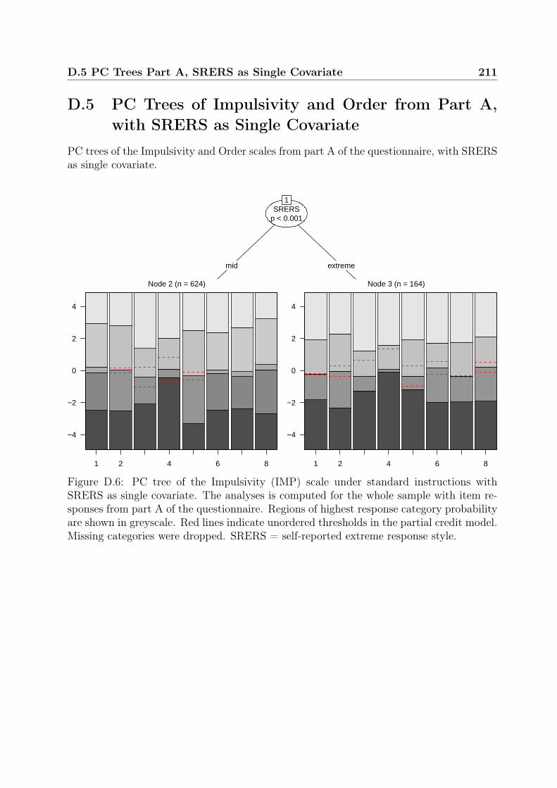
D.5 PC Trees Part A, SRERS as Single Covariate 211
D.5 PC Trees of Impulsivity and Order from Part A,with SRERS as Single Covariate
PC trees of the Impulsivity and Order scales from part A of the questionnaire, with SRERSas single covariate.
SRERSp < 0.001
1
mid extreme
Node 2 (n = 624)
1 2 4 6 8
−4
−2
0
2
4
Node 3 (n = 164)
1 2 4 6 8
−4
−2
0
2
4
Figure D.6: PC tree of the Impulsivity (IMP) scale under standard instructions withSRERS as single covariate. The analyses is computed for the whole sample with item re-sponses from part A of the questionnaire. Regions of highest response category probabilityare shown in greyscale. Red lines indicate unordered thresholds in the partial credit model.Missing categories were dropped. SRERS = self-reported extreme response style.

212 D. Supplemental Material for Study 3
SRERSp < 0.001
1
mid extreme
Node 2 (n = 624)
1 2 4 6 8
−4
−2
0
2
4
Node 3 (n = 164)
1 2 4 6 8
−4
−2
0
2
4
Figure D.7: PC tree of the Order (ORD) scale under standard instructions with SRERS assingle covariate. The analyses is computed for the whole sample with item responses frompart A of the questionnaire. Regions of highest response category probability are shownin greyscale. Red lines indicate unordered thresholds in the partial credit model. Missingcategories were dropped. SRERS = self-reported extreme response style.
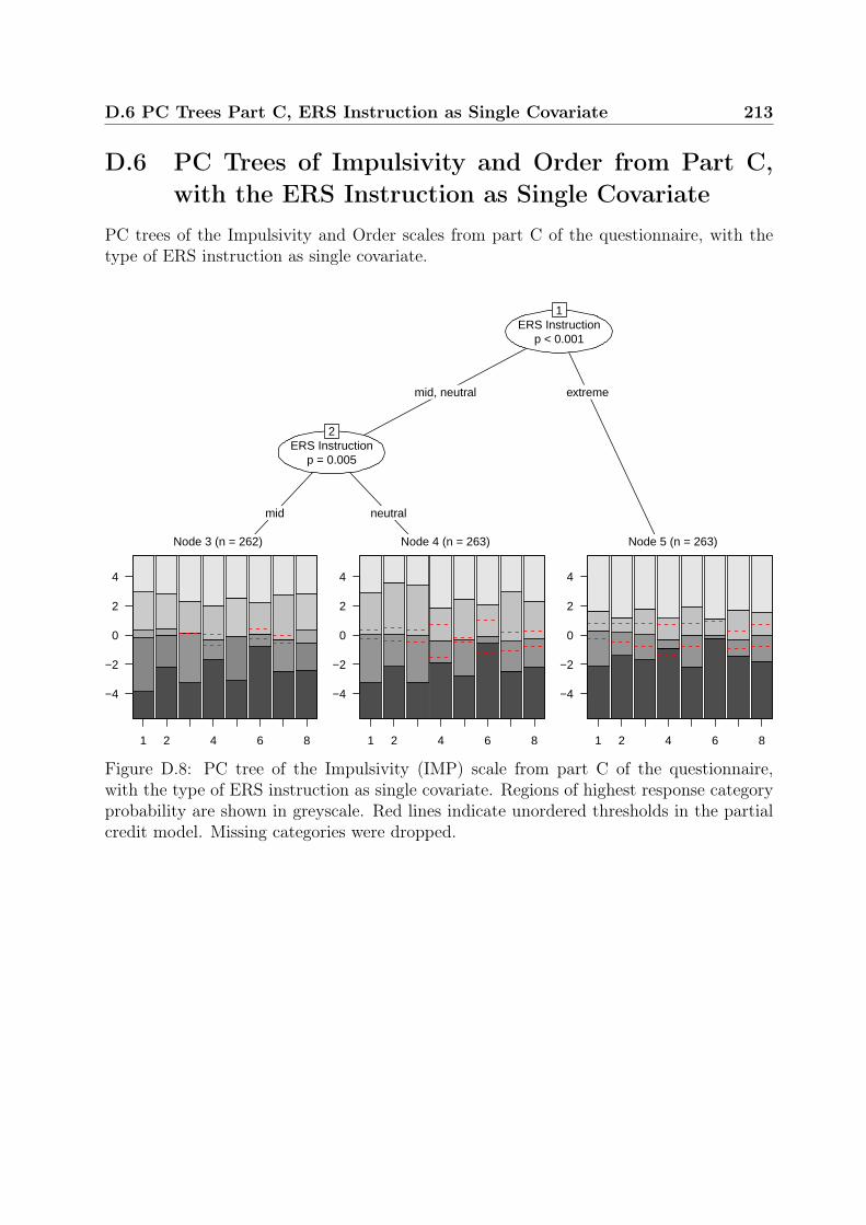
D.6 PC Trees Part C, ERS Instruction as Single Covariate 213
D.6 PC Trees of Impulsivity and Order from Part C,with the ERS Instruction as Single Covariate
PC trees of the Impulsivity and Order scales from part C of the questionnaire, with thetype of ERS instruction as single covariate.
ERS Instructionp < 0.001
1
mid, neutral extreme
ERS Instructionp = 0.005
2
mid neutral
Node 3 (n = 262)
1 2 4 6 8
−4
−2
0
2
4
Node 4 (n = 263)
1 2 4 6 8
−4
−2
0
2
4
Node 5 (n = 263)
1 2 4 6 8
−4
−2
0
2
4
Figure D.8: PC tree of the Impulsivity (IMP) scale from part C of the questionnaire,with the type of ERS instruction as single covariate. Regions of highest response categoryprobability are shown in greyscale. Red lines indicate unordered thresholds in the partialcredit model. Missing categories were dropped.

214 D. Supplemental Material for Study 3
ERS Instructionp < 0.001
1
mid, neutral extreme
ERS Instructionp = 0.048
2
mid neutral
Node 3 (n = 262)
1 2 4 6 8
−4
−2
0
2
4
6
Node 4 (n = 263)
1 2 4 6 8
−4
−2
0
2
4
6
Node 5 (n = 263)
1 2 4 6 8
−4
−2
0
2
4
6
Figure D.9: PC tree of the Order (ORD) scale from part C of the questionnaire, withthe type of ERS instruction as single covariate. Regions of highest response categoryprobability are shown in greyscale. Red lines indicate unordered thresholds in the partialcredit model. Missing categories were dropped.

D.7 Item Responses Control Group Parts A, B, and C 215
D.7 Item Responses in the Control Group for Parts A,B, and C
Item responses of the control group in the Impulsivity and Order scales from parts A, B,and C of the questionnaire.
O100 O10R O130R O160 O190R O220R O40 O70R
ab
c
0 1 2 3 4 0 1 2 3 4 0 1 2 3 4 0 1 2 3 4 0 1 2 3 4 0 1 2 3 4 0 1 2 3 4 0 1 2 3 4
0
50
100
150
0
50
100
150
0
50
100
150
Item Response
Fre
quen
cy
Figure D.10: Histograms for item responses of the Order (ORD) scale in the control group,for all three parts of the questionnaire. Items are labeled with O for Order, the positionof the item in the German NEOI-PI-R and the letter R if the item has been recoded.

216 D. Supplemental Material for Study 3
I111 I141R I171 I201 I21R I231R I51 I81R
ab
c
0 1 2 3 4 0 1 2 3 4 0 1 2 3 4 0 1 2 3 4 0 1 2 3 4 0 1 2 3 4 0 1 2 3 4 0 1 2 3 4
0
50
100
0
50
100
0
50
100
Item Response
Fre
quen
cy
Figure D.11: Histograms for item responses of the Impulsivity (IMP) scale in the controlgroup, for all three parts of the questionnaire. Items are labeled with I for Impulsivity,the position of the item in the German NEOI-PI-R and the letter R if the item has beenrecoded.

D.8 Target Correlations Control Group Parts A, B, and C 217
D.8 Target Correlations in the Control Group for PartsA, B, and C
Correlations in the control group between the sum scores of the Impulsivity and Orderscales with the target variables, for parts A, B, and C of the questionnaire.
●● ●
●●●
●● ●
● ●●
● ●●
●● ●
●● ●
● ● ●
●● ●
●●●
●●●
●● ●Vacuum
Desk
Dishes
Document
Bed
BMI
Snacking
Series
Lying
Electronics
Clothes
Argument
0.1 0.2 0.3 0.4
Correlation with Sum Score of Primary Scale
Targ
et V
aria
bles
Questionnaire Part●
●
●
a
b
c
Figure D.12: Correlation of the target variables in the control group, with the sum scoreof their primary scales. Impulsivity (IMP) is considered the primary scale for variablesArgument to BMI, while Bed to Vacuum are target variables for Order (ORD). Sum scoreswere computed for all three parts of the questionnaire.

218 D. Supplemental Material for Study 3
D.9 PC Trees of Impulsivity and Order in the Aggrava-tion Setting, with the ERS Index as Single Covari-ate
PC trees of the Impulsivity and Order scales in the aggravation setting, with the ERS indexfrom heterogeneous items as single covariate. In the aggravation setting, the instructionwhich should increase the impact of ERS was chosen for each participant in the experi-mental group.
ERS Indexp < 0.001
1
≤ 0.5 > 0.5
Node 2 (n = 274)
1 2 4 6 8
−6
−4
−2
0
2
4
Node 3 (n = 251)
1 2 4 6 8
−6
−4
−2
0
2
4
Figure D.13: PC tree of the Impulsivity (IMP) scale in the aggravation setting, with theERS index from heterogeneous items as single covariate. Matching the ERS instruction toindividual response style was based on a median split of the ERS index from heterogeneousitems. Regions of highest response category probability are shown in greyscale. Red linesindicate unordered thresholds in the partial credit model. Missing categories were dropped.

D.9 PC Trees Aggravation Setting, ERS Index as Single Covariate 219
ERS Indexp < 0.001
1
≤ 0.5 > 0.5
Node 2 (n = 274)
1 2 4 6 8
−6
−4
−2
0
2
4
6
Node 3 (n = 251)
1 2 4 6 8
−6
−4
−2
0
2
4
6
Figure D.14: PC tree of the Order (ORD) scale in the aggravation setting, with theERS index from heterogeneous items as single covariate. Matching the ERS instruction toindividual response style was based on a median split of the ERS index from heterogeneousitems. Regions of highest response category probability are shown in greyscale. Red linesindicate unordered thresholds in the partial credit model. Missing categories were dropped.

220 D. Supplemental Material for Study 3
ERS Indexp < 0.001
1
≤ 0.57 > 0.57
ERS Indexp = 0.013
2
≤ 0.38 > 0.38
Node 3 (n = 49)
1 2 4 6 8
−4
−2
0
2
4
Node 4 (n = 375)
1 2 4 6 8
−4
−2
0
2
4
Node 5 (n = 101)
1 2 4 6 8
−4
−2
0
2
4
Figure D.15: PC tree of the Impulsivity (IMP) scale in the aggravation setting, with theERS index from heterogeneous items as single covariate. Matching the ERS instructionto individual response style was based on SRERS. Regions of highest response categoryprobability are shown in greyscale. Red lines indicate unordered thresholds in the partialcredit model. Missing categories were dropped. SRERS = self-reported extreme responsestyle.

D.9 PC Trees Aggravation Setting, ERS Index as Single Covariate 221
ERS Indexp < 0.001
1
≤ 0.5 > 0.5
Node 2 (n = 274)
1 2 4 6 8
−6
−4
−2
0
2
4
6
Node 3 (n = 251)
1 2 4 6 8
−6
−4
−2
0
2
4
6
Figure D.16: PC tree of the Order (ORD) scale in the aggravation setting, with theERS index from heterogeneous items as single covariate. Matching the ERS instructionto individual response style was based on SRERS. Regions of highest response categoryprobability are shown in greyscale. Red lines indicate unordered thresholds in the partialcredit model. Missing categories were dropped. SRERS = self-reported extreme responsestyle.

222 D. Supplemental Material for Study 3
D.10 PC Trees of Impulsivity and Order in the ControlSetting, with the ERS Index as Single Covariate
PC trees of the Impulsivity and Order scales in the control setting, with the ERS indexfrom heterogeneous items as single covariate. In the control setting, item responses foreach participant in the control group were randomly chosen form either part B, or part Cof the questionnaire.
Node 1 (n = 263)
1 2 4 6 8
−4
−2
0
2
4
Figure D.17: PC tree of the Impulsivity (IMP) scale in the control setting, with the ERSindex from heterogeneous items as single covariate. All item responses for each participantwere randomly chosen either from part B or part C of the questionnaire. Regions ofhighest response category probability are shown in greyscale. Red lines indicate unorderedthresholds in the partial credit model. Missing categories were dropped.

D.10 PC Trees Control Setting, ERS Index as Single Covariate 223
Node 1 (n = 263)
1 2 4 6 8
−4
−2
0
2
4
Figure D.18: PC tree of the Order (ORD) scale in the control setting, with the ERSindex from heterogeneous items as single covariate. All item responses for each participantwere randomly chosen either from part B or part C of the questionnaire. Regions ofhighest response category probability are shown in greyscale. Red lines indicate unorderedthresholds in the partial credit model. Missing categories were dropped.

224 D. Supplemental Material for Study 3
D.11 Additional Performance Measures for PredictiveModels from Part A
Aggregated performance measures for the predictive models in which each target variablewas predicted by item responses of the Impulsivity and Order scales from part A of thequestionnaire, sex, and age. The ERS index from heterogeneous items and SRERS wereeither included of excluded. Cohen’s κ, MMCE, SENS and SPEC are reported for binarytarget variables. R2, MSE, and RMSE are reported for metric target variables.
Table D.3: Additional Performance Estimates from Part A forBinary Targets
Target ERS Measures κ MMCE SENS SPEC
Argument excluded 0.038 0.173 0.029 0.995Argument included 0.003 0.176 0.005 0.997Clothes excluded 0.019 0.249 0.028 0.986Clothes included 0.019 0.245 0.019 0.994Electronics excluded 0.000 0.068 0.000 1.000Electronics included 0.000 0.068 0.000 1.000Lying excluded 0.046 0.349 0.122 0.915Lying included 0.054 0.345 0.123 0.922Series excluded 0.128 0.410 0.779 0.343Series included 0.103 0.418 0.794 0.304Bed excluded 0.199 0.369 0.413 0.777Bed included 0.181 0.374 0.387 0.785Document excluded 0.189 0.341 0.338 0.837Document included 0.180 0.345 0.330 0.835Dishes excluded 0.099 0.366 0.863 0.225Dishes included 0.095 0.363 0.880 0.203Desk excluded 0.325 0.336 0.690 0.635Desk included 0.340 0.328 0.710 0.629
Note. Estimated performance for predicting binary target variables withitem responses of the Impulsivity (IMP) and Order (ORD) scale from part Aof the questionnaire, sex, age, the ERS index from heterogeneous items andSRERS. Predictive models were estimated once with and once without theERS measures. SRERS = self-reported extreme response style, κ = Cohen’sκ, MMCE = mean misclassification error, SENS = sensitivity, SPEC =specificity.

D.11 Additional Predictive Performance Part A 225
Table D.4: Additional Performance Estimates fromPart A for Metric Targets
Target ERS Measures R2 MSE RMSE
Snacking excluded 0.009 11.405 3.377Snacking included -0.006 11.527 3.395BMI excluded 0.121 16.172 4.021BMI included 0.128 16.013 4.002Vacuum excluded 0.043 3.185 1.785Vacuum included 0.043 3.190 1.786
Note. Estimated performance for predicting metric target vari-ables with item responses of the Impulsivity (IMP) and Order(ORD) scale from part A of the questionnaire, sex, age, the ERSindex from heterogeneous items and SRERS. Predictive modelswere estimated once with and once without the ERS measures.SRERS = self-reported extreme response style, R2 = coefficientof determination, MSE = mean squared error, RMSE = rootmean squared error.

226 D. Supplemental Material for Study 3
D.12 Additional Predictive Performance Measures whenMatching ERS Instructions Based on a MedianSplit of the ERS Index
Aggregated performance measures for the predictive models in which each target variablewas predicted by item responses of the Impulsivity and Order scales from part B or C ofthe questionnaire. We compare predictive models in which item responses were given undereither the aggravation, compensation, or control setting. A median split of the ERS indexfrom heterogeneous items was used in the matching process. Cohen’s κ, MMCE, SENSand SPEC are reported for binary target variables. R2, MSE, and RMSE are reported formetric target variables.

D.12 Additional Predictive Performance Matching Median Split ERS Index227
Table D.5: Performance Estimates for Binary Targets andMatching ERS Instructions Based on a Median Split of theERS Index
Target ERS Setting κ MMCE SENS SPEC
Argument aggravation 0.089 0.159 0.075 0.986Argument compensation 0.057 0.161 0.048 0.990Argument control 0.037 0.210 0.050 0.976Clothes aggravation 0.012 0.248 0.024 0.985Clothes compensation -0.003 0.250 0.013 0.985Clothes control -0.007 0.273 0.036 0.958Electronics aggravation 0.000 0.061 0.000 1.000Electronics compensation 0.000 0.061 0.000 1.000Electronics control -0.002 0.085 0.000 0.999Lying aggravation 0.127 0.329 0.218 0.890Lying compensation 0.126 0.321 0.197 0.911Lying control 0.013 0.389 0.156 0.855Series aggravation 0.041 0.460 0.697 0.343Series compensation 0.144 0.411 0.738 0.402Series control 0.168 0.390 0.739 0.425Bed aggravation 0.066 0.411 0.253 0.808Bed compensation 0.144 0.384 0.336 0.799Bed control 0.198 0.374 0.417 0.773Document aggravation 0.133 0.366 0.288 0.833Document compensation 0.143 0.358 0.283 0.849Document control 0.122 0.353 0.286 0.828Dishes aggravation 0.066 0.364 0.886 0.173Dishes compensation 0.079 0.364 0.877 0.191Dishes control 0.012 0.409 0.853 0.158Desk aggravation 0.278 0.360 0.674 0.603Desk compensation 0.308 0.345 0.688 0.620Desk control 0.369 0.303 0.811 0.549
Note. Estimated performance for predicting binary target variables withitem responses of the Impulsivity (IMP) and Order (ORD) scale under thecompensation, aggravation, and control settings. ERS instructions werematched to individual response tendencies based on a median split of theERS index from heterogeneous items. κ = Cohen’s κ, MMCE = meanmisclassification error, SENS = sensitivity, SPEC = specificity.

228 D. Supplemental Material for Study 3
Table D.6: Performance Estimates for MetricTargets and Matching ERS Instructions Based on aMedian Split of the ERS Index
Target ERS Setting R2 MSE RMSE
Snacking aggravation -0.004 11.994 3.463Snacking compensation -0.001 11.806 3.436Snacking control -0.134 11.135 3.337BMI aggravation -0.031 19.370 4.401BMI compensation -0.009 19.164 4.378BMI control -0.107 17.642 4.200Vacuum aggravation 0.016 3.082 1.756Vacuum compensation -0.007 3.136 1.771Vacuum control -0.015 3.416 1.848
Note. Estimated performance for predicting metric target vari-ables with item responses of the Impulsivity (IMP) and Order(ORD) scale under the compensation, aggravation, and controlsettings. ERS instructions were matched to individual responsetendencies based on a median split of the ERS index from het-erogeneous items. R2 = coefficient of determination, MSE =mean squared error, RMSE = root mean squared error.

D.13 Predictive Performance Matching SRERS 229
D.13 Predictive Performance when Matching ERS In-structions Based on SRERS
Visual display of performance measures for the predictive models in which each targetvariable was predicted by item responses of the Impulsivity and Order scales from part Bor C of the questionnaire. We compare predictive models in which item responses weregiven under either the aggravation, compensation, or control setting. SRERS was used inthe matching process. Cohen’s κis depicted for binary target variables, while R2 is shownfor metric target variables.

230 D. Supplemental Material for Study 3
●●
●
●
●
●
●
●●
●
●
●●
●●●●
●
●
●
●●
●●
●
●
●
●
●
●
●
●
Document Dishes Desk
Lying Series Bed
Argument Clothes Electronics
compensate aggravate control compensate aggravate control compensate aggravate control
−0.25
0.00
0.25
0.50
−0.25
0.00
0.25
0.50
−0.25
0.00
0.25
0.50
κ
ERS Setting compensate aggravate control
Figure D.19: Estimated performance for predicting binary target variables with item re-sponses of the Impulsivity (IMP) and Order (ORD) scale under the compensation, ag-gravation, and control settings. ERS instructions were matched to individual responsetendencies based on SRERS. Performance was measured by Cohen’s κ. SRERS = self-reported extreme response style.

D.13 Predictive Performance Matching SRERS 231
●
●
●
●
●●
●●
● ●
●
●
Snacking BMI Vacuum
compensate aggravate control compensate aggravate control compensate aggravate control
−2
−1
0
R2
ERS Setting compensate aggravate control
Figure D.20: Estimated performance for predicting metric target variables with item re-sponses of the Impulsivity (IMP) and Order (ORD) scale under the compensation, ag-gravation, and control settings. ERS instructions were matched to individual responsetendencies based on SRERS. Performance was measured by R2. R2 = coefficient of deter-mination, SRERS = self-reported extreme response style.

232 D. Supplemental Material for Study 3
D.14 Additional Predictive Performance Measures whenMatching ERS Instructions Based on SRERS
Aggregated performance measures for the predictive models in which each target variablewas predicted by item responses of the Impulsivity and Order scales from part B or Cof the questionnaire. We compare predictive models in which item responses were givenunder either the aggravation, compensation, or control setting. SRERS was used in thematching process. Cohen’s κ, MMCE, SENS and SPEC are reported for binary targetvariables. R2, MSE, and RMSE are reported for metric target variables.

D.14 Additional Predictive Performance Matching SRERS 233
Table D.7: Performance Estimates for Binary Targets andMatching ERS Instructions Based on SRERS
Target ERS Setting κ MMCE SENS SPEC
Argument aggravation 0.085 0.163 0.079 0.981Argument compensation 0.084 0.157 0.067 0.990Argument control -0.015 0.224 0.023 0.965Clothes aggravation -0.003 0.249 0.010 0.987Clothes compensation 0.014 0.244 0.018 0.992Clothes control 0.005 0.271 0.049 0.956Electronics aggravation -0.001 0.062 0.000 0.999Electronics compensation 0.000 0.061 0.000 1.000Electronics control 0.000 0.083 0.000 1.000Lying aggravation 0.111 0.330 0.193 0.901Lying compensation 0.106 0.331 0.187 0.902Lying control 0.032 0.378 0.149 0.877Series aggravation 0.015 0.476 0.659 0.356Series compensation 0.186 0.392 0.739 0.443Series control 0.204 0.374 0.741 0.459Bed aggravation 0.098 0.399 0.286 0.806Bed compensation 0.154 0.376 0.330 0.815Bed control 0.176 0.389 0.445 0.727Document aggravation 0.129 0.368 0.289 0.831Document compensation 0.160 0.359 0.323 0.825Document control 0.078 0.364 0.231 0.839Dishes aggravation 0.001 0.385 0.885 0.115Dishes compensation 0.113 0.350 0.889 0.209Dishes control 0.012 0.410 0.843 0.170Desk aggravation 0.274 0.361 0.704 0.569Desk compensation 0.266 0.366 0.669 0.596Desk control 0.285 0.344 0.766 0.514
Note. Estimated performance for predicting binary target variables withitem responses of the Impulsivity (IMP) and Order (ORD) scale under thecompensation, aggravation, and control settings. ERS instructions werematched to individual response tendencies based on SRERS. κ = Cohen’sκ, MMCE = mean misclassification error, SENS = sensitivity, SPEC =specificity, SRERS = self-reported extreme response style.

234 D. Supplemental Material for Study 3
Table D.8: Performance Estimates for Metric Targetsand Matching ERS Instructions Based on SRERS
Target ERS Setting R2 MSE RMSE
Snacking aggravation -0.001 12.006 3.465Snacking compensation -0.014 12.013 3.466Snacking control -0.208 11.028 3.321BMI aggravation -0.016 19.219 4.384BMI compensation 0.011 18.907 4.348BMI control -0.098 18.081 4.252Vacuum aggravation 0.029 3.065 1.751Vacuum compensation -0.018 3.149 1.774Vacuum control -0.028 3.487 1.867
Note. Estimated performance for predicting metric target vari-ables with item responses of the Impulsivity (IMP) and Order(ORD) scale under the compensation, aggravation, and controlsettings. ERS instructions were matched to individual responsetendencies based on SRERS. R2 = coefficient of determination,MSE = mean squared error, RMSE = root mean squared error,SRERS = self-reported extreme response style.

References
Aichholzer, J. (2013). Intra-individual variation of extreme response style in mixed-modepanel studies. Social science research, 42 (3), 957–970.
Alarcon, G., Eschleman, K. J., & Bowling, N. A. (2009). Relationships between personalityvariables and burnout: A meta-analysis. Work & stress, 23 (3), 244–263.
Alexeev, N., Templin, J., & Cohen, A. S. (2011). Spurious latent classes in the mixtureRasch model. Journal of Educational Measurement, 48 (3), 313–332.
Ashton, M. C. & Lee, K. (2007). Empirical, theoretical, and practical advantages of theHEXACO model of personality structure. Personality and social psychology review,11 (2), 150–166.
Auguie, B. (2016). Gridextra: miscellaneous functions for "grid" graphics. R package ver-sion 2.2.1.
Austin, E. J., Deary, I. J., & Egan, V. (2006). Individual differences in response scale use:Mixed Rasch modelling of responses to NEO-FFI items. Personality and IndividualDifferences, 40 (6), 1235–1245.
Bachman, J. G. & O’Malley, P. M. (1984). Yea-saying, nay-saying, and going to extremes:Black-white differences in response styles. Public Opinion Quarterly, 48 (2), 491–509.
Bäckström, M. & Björklund, F. (2014). Social Desirability in Personality Inventories. Jour-nal of Individual Differences, 35, 144–157.
Bartlett, M. S. (1951). The Effect of Standardization on a Chi Square Approximation inFactor Analysis. Biometrika, 38 (3), 337–344.
Baumgartner, H. & Steenkamp, J.-B. E. (2001). Response Styles in Marketing Research:A Cross-National Investigation. Journal of Marketing Research, 38 (2), 143–156.
Ben-Porath, Y. S., Hostetler, K., Butcher, J. N., & Graham, J. R. (1989). New subscalesfor the MMPI-2 Social Introversion (Si) scale. Psychological Assessment: A Journalof Consulting and Clinical Psychology, 1 (3), 169–174.
Bentler, P. M. (2016). Covariate-free and Covariate-dependent Reliability. Psychometrika,81 (4), 907–920.
Beuckelaer, A. D., Weijters, B., & Rutten, A. (2010). Using ad hoc measures for responsestyles: a cautionary note. Quality & Quantity, 44 (4), 761–775.
Biau, G. & Scornet, E. (2016). A random forest guided tour. Test, 25 (2), 197–227.Birattari, M., Yuan, Z., Balaprakash, P., & Stützle, T. (2010). F-Race and Iterated F-
Race: An Overview. In T. Bartz-Beielstein, M. Chiarandini, L. Paquete, & M. Preuss

236 References
(Eds.), Experimental Methods for the Analysis of Optimization Algorithms (pp. 311–336). Springer Berlin Heidelberg.
Bischl, B. & Lang, M. (2015). Parallelmap: unified interface to parallelization back-ends.R package version 1.3.
Bischl, B., Lang, M., Kotthoff, L., Schiffner, J., Richter, J., Jones, Z., . . . Gallo, M. (2017).Mlr: machine learning in r. R package version 2.11.
Bischl, B., Lang, M., Kotthoff, L., Schiffner, J., Richter, J., Studerus, E., . . . Jones, Z. M.(2016). Mlr Machine Learning in R. Journal of Machine Learning Research, 17 (170),1–5.
Bischl, B., Mersmann, O., Trautmann, H., & Weihs, C. (2012). Resampling methods formeta-model validation with recommendations for evolutionary computation. Evolu-tionary Computation, 20 (2), 249–275.
Böckenholt, U. (2012). Modeling multiple response processes in judgment and choice. Psy-chological Methods, 17 (4), 665–678.
Böckenholt, U. & Meiser, T. (2017). Response style analysis with threshold and multi-process IRT models: A review and tutorial. British Journal of Mathematical andStatistical Psychology, 70 (1), 159–181.
Bogg, T. & Roberts, B. W. (2004). Conscientiousness and health-related behaviors: a meta-analysis of the leading behavioral contributors to mortality. Psychological bulletin,130 (6), 887.
Bolker, B. (2016). Emdbook: support functions and data for "ecological models and data".R package version 1.3.9.
Bolt, D. M. & Johnson, T. R. (2009). Addressing Score Bias and Differential Item Func-tioning Due to Individual Differences in Response Style. Applied Psychological Mea-surement, 33 (5), 335–352.
Borkenau, P. & Ostendorf, F. (2008). NEO-FFI: NEO-Fünf-Faktoren-Inventar nach Costaund McCrae (2. Aufl.). Göttingen: Hogrefe.
Breiman, L. (2001). Random forests. Machine learning, 45 (1), 5–32.Breiman, L. et al. (2001). Statistical modeling: The two cultures (with comments and a
rejoinder by the author). Statistical science, 16 (3), 199–231.Breiman, L., Cutler, A., Liaw, A., & Wiener, M. (2015). Randomforest: breiman and cut-
ler’s random forests for classification and regression. R package version 4.6-12.Breiman, L., Friedman, J., Stone, C. J., & Olshen, R. A. (1984). Classification and regres-
sion trees. CRC press.Brown, A. & Maydeu-Olivares, A. (2011). Item response modeling of forced-choice ques-
tionnaires. Educational and Psychological Measurement, 71 (3), 460–502.Brown, A. & Maydeu-Olivares, A. (2013). How IRT can solve problems of ipsative data in
forced-choice questionnaires. Psychological Methods, 18 (1), 36.Bühner, M. (2011). Einführung in die Test-und Fragebogenkonstruktion. Pearson Deutsch-
land GmbH.Butcher, J. N., Dahlstrom, W. G., Graham, J. R., Tellegen, A., & Kaemmer, B. (1989).
MMPI-2: Manual for administration and scoring. Minneapolis: University of Min-nesota Press.

References 237
Cabooter, E. (2010). The impact of situational and dispositional variables on response styleswith respect to attitude measures. (Doctoral Dissertation). Faculty of Economics andBusiness Administration, Ghent University.
Cabooter, E., Millet, K., Weijters, B., & Pandelaere, M. (2016). The ‘I’in extreme respond-ing. Journal of Consumer Psychology, 26 (4), 510–523.
Chapman, B. P., Weiss, A., & Duberstein, P. R. (2016). Statistical learning theory for highdimensional prediction: Application to criterion-keyed scale development. Psycholog-ical methods, 21 (4), 603.
Chen, T. & Guestrin, C. (2016). Xgboost: A scalable tree boosting system. In Proceedingsof the 22Nd ACM SIGKDD International Conference on Knowledge Discovery andData Mining (pp. 785–794).
Churchill, S., Jessop, D., & Sparks, P. (2008). Impulsive and/or planned behaviour: Canimpulsivity contribute to the predictive utility of the theory of planned behaviour?British Journal of Social Psychology, 47 (4), 631–646.
Cohen, J. (1960). A coefficient of agreement for nominal scales. Educational and psycho-logical measurement, 20 (1), 37–46.
Costa, P. T. & MacCrae, R. R. (1992). Revised NEO personality inventory (NEO PI-R) and NEO five-factor inventory (NEO FFI): Professional manual. PsychologicalAssessment Resources.
Crawford, J. R. & Henry, J. D. (2004). The positive and negative affect schedule (PANAS):construct validity, measurement properties and normative data in a large non-clinicalsample. The British Journal of Clinical Psychology / the British Psychological Soci-ety, 43 (3), 245–265.
Cronbach, L. J. (1946). Response sets and test validity. Educational and psychologicalmeasurement, 6 (4), 475–494.
Cronbach, L. J. (1950). Further evidence on response sets and test design. Educational andpsychological measurement, 10 (1), 3–31.
Cronbach, L. J. (1951). Coefficient alpha and the internal structure of tests. psychometrika,16 (3), 297–334.
Csárdi, G. & FitzJohn, R. (2016). Progress: terminal progress bars. R package version 1.1.2.Dahl, D. B. (2016). Xtable: export tables to latex or html. R package version 1.8-2.De Boeck, P. & Partchev, I. (2012). IRTrees: Tree-based item response models of the GLMM
family. Journal of Statistical Software, 48 (1), 1–28.Dolnicar, S. & Grün, B. (2007). How constrained a response: A comparison of binary,
ordinal and metric answer formats. Journal of Retailing and Consumer Services,14 (2), 108–122.
Dolnicar, S., Grün, B., & Leisch, F. (2011). Quick, simple and reliable: Forced binarysurvey questions. International Journal of Market Research, 53 (2), 231.
Eid, M. & Rauber, M. (2000). Detecting measurement invariance in organizational surveys.European Journal of Psychological Assessment, 16 (1), 20.
Engel, R. R. & Hathaway, S. R. (2003). Minnesota multiphasic personality inventory-2:MMPI-2. Huber.

238 References
Fahrenberg, J., Hampel, R., & Selg, H. (2001). FPI-R. Das Freiburger Persönlichkeitsin-ventar. Manual.
Faragher, E. B., Cass, M., & Cooper, C. L. (2005). The relationship between job satisfactionand health: a meta-analysis. Occupational and environmental medicine, 62 (2), 105–112.
Ferrando, P. J. & Condon, L. (2006). Assessing acquiescence in binary responses: IRT-related item-factor-analytic procedures. Structural Equation Modeling, 13 (3), 420–439.
Finn, J. A., Ben-Porath, Y. S., & Tellegen, A. (2015). Dichotomous versus polytomousresponse options in psychopathology assessment: Method or meaningful variance?Psychological assessment, 27 (1), 184.
Fox, J. & Hong, J. (2009). Effect displays in R for multinomial and proportional-odds logitmodels: Extensions to the effects package. Journal of Statistical Software, 32 (1), 1–24.
Friedman, J. H. (2001). Greedy function approximation: a gradient boosting machine.Annals of statistics, 1189–1232.
Genz, A., Bretz, F., Miwa, T., Mi, X., & Hothorn, T. (2016).Mvtnorm: multivariate normaland t distributions. R package version 1.0-5.
GESIS. (2015). GESIS Panel Standard Edition (Version 6.0.0, Datenfile ZA5665). GESISDatenarchiv: Köln.
Goldstein, A., Kapelner, A., Bleich, J., & Pitkin, E. (2015). Peeking inside the blackbox: Visualizing statistical learning with plots of individual conditional expectation.Journal of Computational and Graphical Statistics, 24 (1), 44–65.
Gollwitzer, M., Eid, M., & Jürgensen, R. (2005). Response styles in the assessment of angerexpression. Psychological assessment, 17 (1), 56.
Greenleaf, E. A. (1992). Measuring Extreme Response Style. Public Opinion Quarterly,56 (3), 328–351.
Gu, F., Little, T. D., & Kingston, N. M. (2013). Misestimation of reliability using coefficientalpha and structural equation modeling when assumptions of tau-equivalence anduncorrelated errors are violated. Methodology: European Journal of Research Methodsfor the Behavioral and Social Sciences, 9 (1), 30.
Harlow, L. L. & Oswald, F. L. (2016). Big data in psychology: Introduction to the specialissue. Psychological Methods, 21 (4), 447.
Harrell, F. E., Jr. (2016). Hmisc: harrell miscellaneous. R package version 4.0-2.Hastie, T., Tibshirani, R., & Friedman, J. (2009). The elements of statistical learning 2nd
edition. New York: Springer.Hastie, T., Tibshirani, R., & Wainwright, M. (2015). Statistical learning with sparsity. CRC
press.Jackson, D. N. & Messick, S. (1958). Content and style in personality assessment. Psycho-
logical bulletin, 55 (4), 243.Jackson, J. J., Wood, D., Bogg, T., Walton, K. E., Harms, P. D., & Roberts, B. W. (2010).
What do conscientious people do? Development and validation of the Behavioral

References 239
Indicators of Conscientiousness (BIC). Journal of Research in Personality, 44 (4),501–511.
James, G., Witten, D., Hastie, T., & Tibshirani, R. (2013). An introduction to statisticallearning. Springer.
Jin, K.-Y. & Wang, W.-C. (2014). Generalized IRT models for extreme response style.Educational and Psychological Measurement, 74 (1), 116–138.
Kieruj, N. D. & Moors, G. (2010). Variations in response style behavior by response scaleformat in attitude research. International journal of public opinion research, 22 (3),320–342.
Kieruj, N. D. & Moors, G. (2013). Response style behavior: question format dependent orpersonal style? Quality & Quantity, 47 (1), 193–211.
Komboz, B., Strobl, C., & Zeileis, A. (2016). Tree-Based Global Model Tests for Polyto-mous Rasch Models. Educational and Psychological Measurement.
Krohne, H. W., Egloff, B., Kohlmann, C.-W., & Tausch, A. (1996). Untersuchungen miteiner deutschen Version der "Positive and Negative Affect Schedule" (PANAS). Di-agnostica, 42 (2), 139–156.
Krosnick, J. A. (1991). Response strategies for coping with the cognitive demands of atti-tude measures in surveys. Applied cognitive psychology, 5 (3), 213–236.
Kuhn, M. & Johnson, K. (2013). Applied predictive modeling. Springer.Kulas, J. T. & Stachowski, A. A. (2009). Middle category endorsement in odd-numbered
Likert response scales: Associated item characteristics, cognitive demands, and pre-ferred meanings. Journal of Research in Personality, 43 (3), 489–493.
López-Ibáñez, M., Dubois-Lacoste, J., Cáceres, L. P., Birattari, M., & Stützle, T. (2016).The irace package: Iterated racing for automatic algorithm configuration. OperationsResearch Perspectives, 3, 43–58.
López-Ibáñez, M., Dubois-Lacoste, J., Cáceres, L. P., Stützle, T., Birattari, M., Yuan, E.,& Balaprakash, P. (2015). Irace: iterated racing procedures. R package version 1.07.
MacKenzie, S. B. & Podsakoff, P. M. (2012). Common method bias in marketing: causes,mechanisms, and procedural remedies. Journal of Retailing, 88 (4), 542–555.
Masters, G. N. (1982). A Rasch model for partial credit scoring. Psychometrika, 47 (2),149–174.
McEachan, R. R. C., Conner, M., Taylor, N. J., & Lawton, R. J. (2011). Prospectiveprediction of health-related behaviours with the theory of planned behaviour: A meta-analysis. Health Psychology Review, 5 (2), 97–144.
Meiser, T. & Machunsky, M. (2008). The personal structure of personal need for structure.European Journal of Psychological Assessment, 24 (1), 27–34.
Milborrow, S. (2017). Rpart.plot: plot ’rpart’ models: an enhanced version of ’plot.rpart’.R package version 2.1.1.
Moors, G. (2012). The effect of response style bias on the measurement of transformational,transactional, and laissez-faire leadership. European Journal of Work and Organiza-tional Psychology, 21 (2), 271–298.

240 References
Mõttus, R., Allik, J., Realo, A., Rossier, J., Zecca, G., Ah-Kion, J., . . . Barry, O., etal. (2012). The effect of response style on self-reported conscientiousness across 20countries. Personality and Social Psychology Bulletin, 38 (11), 1423–1436.
Münzer, S. & Hölscher, C. (2011). Entwicklung und Validierung eines Fragebogens zuräumlichen Strategien. Diagnostica, 57 (3), 111–125.
Naemi, B. D., Beal, D. J., & Payne, S. C. (2009). Personality Predictors of Extreme Re-sponse Style. Journal of Personality, 77 (1), 261–286.
Open Science Collaboration. (2015). Estimating the reproducibility of psychological sci-ence. Science, 349 (6251), aac4716.
Ostendorf, F. & Angleitner, A. (2004). NEO-Persönlichkeitsinventar nach Costa und Mc-Crae, Revidierte Fassung (NEO-PI-R). Göttingen, Germany: Hogrefe.
Peabody, D. (1962). Two components in bipolar scales: Direction and extremeness. Psy-chological Review, 69 (2), 65.
Plieger, T., Montag, C., Felten, A., & Reuter, M. (2014). The serotonin transporter poly-morphism (5-HTTLPR) and personality: response style as a new endophenotype foranxiety. International Journal of Neuropsychopharmacology, 17 (6), 851–858.
Plieninger, H. (2016). Mountain or Molehill? A Simulation Study on the Impact of ResponseStyles. Educational and Psychological Measurement.
Plieninger, H. & Meiser, T. (2014). Validity of Multiprocess IRT Models for SeparatingContent and Response Styles. Educational and Psychological Measurement, 74 (5),875–899.
Podsakoff, P. M., MacKenzie, S. B., & Podsakoff, N. P. (2011). Sources of Method Bias inSocial Science Research and Recommendations on How to Control It. Annual Reviewof Psychology, 63 (1), 539–569.
Preston, C. C. & Colman, A. M. (2000). Optimal number of response categories in ratingscales: reliability, validity, discriminating power, and respondent preferences. Actapsychologica, 104 (1), 1–15.
R Core Team. (2016a). Foreign: read data stored by minitab, s, sas, spss, stata, systat,weka, dbase, ... R package version 0.8-67.
R Core Team. (2016b). R: a language and environment for statistical computing. R Foun-dation for Statistical Computing. Vienna, Austria.
Rammstedt, B. & John, O. P. (2007). Measuring personality in one minute or less: A10-item short version of the Big Five Inventory in English and German. Journal ofresearch in Personality, 41 (1), 203–212.
Raykov, T. (2001). Bias of coefficient afor fixed congeneric measures with correlated errors.Applied psychological measurement, 25 (1), 69–76.
Revelle, W. (2017). Psych: procedures for psychological, psychometric, and personality re-search. R package version 1.6.12.
Rizopoulos, D. (2013). Ltm: latent trait models under irt. R package version 1.0-0.Rorer, L. G. (1965). The great response-style myth. Psychological bulletin, 63 (3), 129.Rost, J. (1990). Rasch models in latent classes: An integration of two approaches to item
analysis. Applied Psychological Measurement, 14 (3), 271–282.

References 241
Rost, J. (1991). A logistic mixture distribution model for polychotomous item responses.British Journal of Mathematical and Statistical Psychology, 44 (1), 75–92.
Rost, J., Carstensen, C., & von Davier, M. (1997). Applying the mixed Rasch model topersonality questionnaires. In Applications of latent trait and latent class models inthe social sciences (pp. 324–332). Münster: Waxmann.
Schauberger, G. (2016). Diflasso: a penalty approach to differential item functioning inrasch models. R package version 1.0-2.
Schmidt, F. L. & Hunter, J. E. (1998). The validity and utility of selection methods inpersonnel psychology: Practical and theoretical implications of 85 years of researchfindings. Psychological bulletin, 124 (2), 262.
Schmukle, S. C., Egloff, B., & Burns, L. R. (2002). The relationship between positive andnegative affect in the Positive and Negative Affect Schedule. Journal of Research inPersonality, 36 (5), 463–475.
Sieber, K. O. & Meyers, L. S. (1992). Validation of the MMPI—2 Social Introversionsubscales. Psychological assessment, 4 (2), 185.
Simon, R. (2007). Resampling strategies for model assessment and selection. In Fundamen-tals of data mining in genomics and proteomics (pp. 173–186). Springer.
Strobl, C., Boulesteix, A.-L., Kneib, T., Augustin, T., & Zeileis, A. (2008). Conditionalvariable importance for random forests. BMC bioinformatics, 9 (1), 307.
Strobl, C., Boulesteix, A.-L., Zeileis, A., & Hothorn, T. (2007). Bias in random forest vari-able importance measures: Illustrations, sources and a solution. BMC bioinformatics,8 (1), 25.
Strobl, C., Kopf, J., & Zeileis, A. (2013). Rasch Trees: A New Method for Detecting Dif-ferential Item Functioning in the Rasch Model. Psychometrika, 80 (2), 289–316.
Sutin, A. R., Ferrucci, L., Zonderman, A. B., & Terracciano, A. (2011). Personality andobesity across the adult life span. Journal of personality and social psychology, 101 (3),579.
Terracciano, A., Sutin, A. R., McCrae, R. R., Deiana, B., Ferrucci, L., Schlessinger, D., . . .Costa Jr, P. T. (2009). Facets of personality linked to underweight and overweight.Psychosomatic medicine, 71 (6), 682.
Therneau, T., Atkinson, B., & Ripley, B. (2015). Rpart: recursive partitioning and regres-sion trees. R package version 4.1-10.
Tourangeau, R., Rips, L. J., & Rasinski, K. (2000). The psychology of survey response.Cambridge University Press.
Tutz, G. (2011). Regression for categorical data. Cambridge University Press.Tutz, G. & Schauberger, G. (2015). A penalty approach to differential item functioning in
Rasch models. Psychometrika, 80 (1), 21–43.Tutz, G., Schauberger, G., & Berger, M. (2016). Response Styles in the Partial Credit
Model. Technical Report Number 196, Department of Statistics, University of Mu-nich.
Vaerenbergh, Y. V. & Thomas, T. D. (2013). Response Styles in Survey Research: A Lit-erature Review of Antecedents, Consequences, and Remedies. International Journalof Public Opinion Research, 25 (2), 195–217.

242 References
Van der Linden, W. J. (2016). Handbook of item response theory. CRC Press.Van Der Linden, W. J. & Hambleton, R. K. (1997). Item response theory: Brief history,
common models, and extensions. In Handbook of modern item response theory (pp. 1–28). Springer.
Verplanken, B. & Herabadi, A. (2001). Individual differences in impulse buying tendency:Feeling and no thinking. European Journal of personality, 15 (1), 71–83.
Verplanken, B., Herabadi, A. G., Perry, J. A., & Silvera, D. H. (2005). Consumer styleand health: The role of impulsive buying in unhealthy eating. Psychology & Health,20 (4), 429–441.
Von Davier, M. (2001). WINMIRA 2001. St. Paul, MN: Assessment Systems Corporation.Warnes, G. R., Bolker, B., & Lumley, T. (2015). Gtools: various r programming tools. R
package version 3.5.0.Watson, D., Clark, L. A., & Tellegen, A. (1988). Development and validation of brief
measures of positive and negative affect: The PANAS scales. Journal of Personalityand Social Psychology, 54 (6), 1063–1070.
Weijters, B. & Baumgartner, H. (2012). Misresponse to reversed and negated items insurveys: A review. Journal of Marketing Research, 49 (5), 737–747.
Weijters, B., Cabooter, E., & Schillewaert, N. (2010). The effect of rating scale formaton response styles: The number of response categories and response category labels.International Journal of Research in Marketing, 27 (3), 236–247.
Weijters, B., Geuens, M., & Schillewaert, N. (2010a). The Individual Consistency of Ac-quiescence and Extreme Response Style in Self-Report Questionnaires. Applied Psy-chological Measurement, 34 (2), 105–121.
Weijters, B., Geuens, M., & Schillewaert, N. (2010b). The stability of individual responsestyles. Psychological methods, 15 (1), 96.
Weijters, B., Schillewaert, N., & Geuens, M. (2008). Assessing response styles across modesof data collection. Journal of the Academy of Marketing Science, 36 (3), 409–422.
Weng, L.-J. (2004). Impact of the number of response categories and anchor labels on coef-ficient alpha and test-retest reliability. Educational and Psychological Measurement,64 (6), 956–972.
Wetzel, E., Böhnke, J. R., Carstensen, C. H., Ziegler, M., & Ostendorf, F. (2013). Doindividual response styles matter? Assessing differential item functioning for menand women in the NEO-PI-R. Journal of Individual Differences, 34 (2), 69.
Wetzel, E., Böhnke, J. R., & Rose, N. (2016). A simulation study on methods of correctingfor the effects of extreme response style. Educational and Psychological Measurement,76 (2), 304–324.
Wetzel, E. & Carstensen, C. H. (2015). Multidimensional modeling of traits and responsestyles. European Journal of Psychological Assessment.
Wetzel, E., Carstensen, C. H., & Böhnke, J. R. (2013). Consistency of extreme responsestyle and non-extreme response style across traits. Journal of Research in Personality,47 (2), 178–189.
Wetzel, E., Lüdtke, O., Zettler, I., & Böhnke, J. R. (2016). The stability of extreme responsestyle and acquiescence over 8 years. Assessment, 23 (3), 279–291.

References 243
Whiteside, S. P. & Lynam, D. R. (2001). The five factor model and impulsivity: Using astructural model of personality to understand impulsivity. Personality and individualdifferences, 30 (4), 669–689.
Wickham, H. (2016a). Plyr: tools for splitting, applying and combining data. R packageversion 1.8.4.
Wickham, H. (2016b). Reshape2: flexibly reshape data: a reboot of the reshape package. Rpackage version 1.4.2.
Wickham, H. (2017). Tidyr: easily tidy data with ’spread()’ and ’gather()’ functions. Rpackage version 0.6.1.
Wickham, H. & Chang, W. (2016). Ggplot2: create elegant data visualisations using thegrammar of graphics. R package version 2.2.1.
Wickham, H. & Francois, R. (2016). Dplyr: a grammar of data manipulation. R packageversion 0.5.0.
Wickham, H. & Miller, E. (2016). Haven: import and export ’spss’, ’stata’ and ’sas’ files.R package version 1.0.0.
Xie, Y. (2016). Knitr: a general-purpose package for dynamic report generation in r. Rpackage version 1.15.1.
Yarkoni, T. & Westfall, J. (2017). Choosing prediction over explanation in psychology:Lessons from machine learning. Manuscript submitted for publication.
Yin, P. & Fan, X. (2001). Estimating R 2 shrinkage in multiple regression: a comparisonof different analytical methods. The Journal of Experimental Education, 69 (2), 203–224.
Youyou, W., Kosinski, M., & Stillwell, D. (2015). Computer-based personality judgmentsare more accurate than those made by humans. Proceedings of the National Academyof Sciences, 112 (4), 1036–1040.
Yuan, M. & Lin, Y. (2006). Model selection and estimation in regression with groupedvariables. Journal of the Royal Statistical Society: Series B (Statistical Methodology),68 (1), 49–67.
Zeileis, A., Hothorn, T., & Hornik, K. (2008). Model-Based Recursive Partitioning. Journalof Computational and Graphical Statistics, 17 (2), 492–514.
Zeileis, A., Strobl, C., Wickelmaier, F., Komboz, B., & Kopf, J. (2016). Psychotree: recur-sive partitioning based on psychometric models. R package version 0.15-1.
Zettler, I., Lang, J. W., Hülsheger, U. R., & Hilbig, B. E. (2015). Dissociating Indiffer-ent, Directional, and Extreme Responding in Personality Data: Applying the Three-Process Model to Self-and Observer Reports. Journal of personality, 84 (4), 461–472.
Ziegler, M., Dietl, E., Danay, E., Vogel, M., & Bühner, M. (2011). Predicting trainingsuccess with general mental ability, specific ability tests, and (Un) structured inter-views: A meta-analysis with unique samples. International Journal of Selection andAssessment, 19 (2), 170–182.
Ziegler, M. & Kemper, C. (2013). Extreme response style and faking: Two sides of the samecoin. In Interviewers deviations in surveys–impact, reasons, detection and prevention(pp. 217–233). Frankfurt: Lang.

244
Ziegler, M., Kemper, C. J., & Kruyen, P. (2014). Short scales – Five misunderstandings andways to overcome them. Journal of Individual Differences. Measuring PsychologicalConstructs with Short Scales: Positive Outlooks and Caveats, 35 (4), 185–189.