A PROBABILISTIC APPROACH TO DATA

INTEGRATION

IN BIOMEDICAL RESEARCH: THE IsBIG

EXPERIMENTS

Vibha Anand

Submitted to the faculty of the University Graduate School in partial fulfillment of the requirements

for the degree Doctor of Philosophy

in the School of Informatics, Indiana University

December 2010

ii

Accepted by the Faculty of Indiana University, in partial fulfillment of the requirements for the degree of Doctor of Philosophy.

____________________________ Mathew J. Palakal, Ph.D., Chair

_________________________________ Stephen M. Downs, M.D., M.S.

Doctoral Committee

_________________________________ Anna M. McDaniel, DNS, RN, FAAN

November 30, 2010

_________________________________ Gunther Schadow, M.D., Ph.D.

iii

To my lovely daughters

Ila and Neha

iv

ACKNOWLEDGEMENTS

I express my sincere thanks to all who supported me through these years of study.

I am indebted to Dr. Steve Downs for his unwavering help and support in completing this

thesis. I sincerely thank Dr. Downs for introducing me to probabilistic modeling

techniques and his guidance and mentorship in completing this work. Many thanks to Dr.

Anna McDaniel for being a mentor from the very start and for help in completing this

thesis. I would like to sincerely thank Dr. Gunther Schadow and Dr. Mathew Palakal for

their mentorship and providing valuable feedback during the course of my studies. I also

thank Dr. Marc Rosenman and his data core team at Regenstrief Institute for providing

de-identified EMR data for this study.

I would like to thank the entire faculty and staff at Children’s Health Services

Research program for their support over the years. Among them I would especially like

to thank the CHIRDL team members and Drs. Paul Biondich and Aaron Carroll for their

support.

Last but not the least, I would like to thank my family, my parents Brijesh

Chandra and Usha Mathur for their constant love and support, my parents in law

Rameshwar Sahai and Vimlesh Sahai Anand, my siblings and siblings in law for their

support. I am grateful to my husband, Amit Anand, for helpful discussions and feedback,

but most of all for providing love and encouragement every day, and to our loving

daughters Ila and Neha Anand for their patience, love and support. I could not have

completed this work without their encouragement.

v

ABSTRACT

Vibha Anand

A PROBABILISTIC APPROACH TO DATA INTEGRATION IN BIOMEDICAL

RESEARCH: THE IsBIG EXPERIMENTS

Biomedical research has produced vast amounts of new information in the last

decade but has been slow to find its use in clinical applications. Data from disparate

sources such as genetic studies and summary data from published literature have been

amassed, but there is a significant gap, primarily due to a lack of normative methods, in

combining such information for inference and knowledge discovery.

In this research using Bayesian Networks (BN), a probabilistic framework is built

to address this gap. BN are a relatively new method of representing uncertain

relationships among variables using probabilities and graph theory. Despite their

computational complexity of inference, BN represent domain knowledge concisely. In

this work, strategies using BN have been developed to incorporate a range of available

information from both raw data sources and statistical and summary measures in a

coherent framework. As an example of this framework, a prototype model (In-silico

Bayesian Integration of GWAS or IsBIG) has been developed. IsBIG integrates

summary and statistical measures from the NIH catalog of genome wide association

studies (GWAS) and the database of human genome variations from the international

HapMap project. IsBIG produces a map of disease to disease associations as inferred by

genetic linkages in the population.

Quantitative evaluation of the IsBIG model shows correlation with empiric results

from our Electronic Medical Record (EMR) – The Regenstrief Medical Record System

vi

(RMRS). Only a small fraction of disease to disease associations in the population can

be explained by the linking of a genetic variation to a disease association as studied in the

GWAS. None the less, the model appears to have found novel associations among some

diseases that are not described in the literature but are confirmed in our EMR. Thus, in

conclusion, our results demonstrate the potential use of a probabilistic modeling

approach for combining data from disparate sources for inference and knowledge

discovery purposes in biomedical research.

Mathew J. Palakal, Ph.D., Chair

vii

TABLE OF CONTENTS LIST OF TABLES ....................................................................................................... ix LIST OF FIGURES .......................................................................................................x  Chapter 1 INTRODUCTION .........................................................................................1 Opportunities for Informatics in Biomedical Research ................................................. 1 Challenges for Informatics in Biomedical research ....................................................... 2  Chapter 2 BACKGROUND ...........................................................................................8 Bayesian Networks (BN) ............................................................................................... 8 Computational Methods of BN ...................................................................................... 8 Causal Independence and ICI models .......................................................................... 12 Other Related Models .................................................................................................. 16 BN Vs Other Methods ................................................................................................. 18 Challenges for Knowledge Representation and Inference in Biomedical Domain ..... 20 Existence of silos of datasets ....................................................................................... 21 Access Rights ............................................................................................................... 22 Inference in Patient’s Context ...................................................................................... 22 Receiver Operating Characteristic (ROC) Curve ........................................................ 23  Chapter 3 EXPERIMENTAL STUDIES on BNs and ICI MODELS .........................25 Experiment 1: Bayesian Networks from Electronic Medical Records ........................26 Introduction .................................................................................................................. 26 Methods........................................................................................................................ 26 Results .......................................................................................................................... 35 Discussion .................................................................................................................... 38 Experiment 2: Strategies for Learning BN parameters ................................................39 Introduction .................................................................................................................. 39 Methods........................................................................................................................ 41 Results of Noisy-OR Reformulation ............................................................................ 44 Results of RNOR rule Reformulation .......................................................................... 50 Discussion .................................................................................................................... 52  Chapter 4 PROBABILISTIC INTEGRATION: IsBIG EXPERIMENTS ...................54 Experiment 3: Integrating Published and EMR Data ..................................................57 Introduction .................................................................................................................. 57 Methods........................................................................................................................ 59 Results .......................................................................................................................... 68 Discussion .................................................................................................................... 69 Conclusion ................................................................................................................... 69 Experiment 4: Integrating Disparate Sources of Summary Data .................................70 Introduction .................................................................................................................. 70 Methods........................................................................................................................ 74 Results .......................................................................................................................... 85 

viii

Discussion .................................................................................................................... 87  Chapter 5 VALIDATION AGAINST PRIMARY EMR DATA ................................92 Introduction .................................................................................................................. 92 Methods........................................................................................................................ 92 Results .......................................................................................................................... 97 Discussion .................................................................................................................. 106 Chapter 6 DISCUSSION ...........................................................................................108 Summary of findings.................................................................................................. 108 Summary of contributions.......................................................................................... 109 Limitations ................................................................................................................. 112  APPENDICES ...........................................................................................................114 Appendix A.1 Summary of Studies from GWAS Catalog ........................................ 114 Appendix A.2 AUC and p-values in IsBIG model (I-Model) ................................... 117 Appendix A.3 AUC and p-values in Mixed model (M-Model) ................................. 118 Appendix A.4 AUC and p-value in Clinical Model (C-Model) ................................ 119 Appendix A.5 Relationships evaluated in IsBIG Model (I-Model) ........................... 121 Appendix A.6 Input to the IsBIG Algorithm for constructing I-Model .................... 124 Appendix A.7 Disease prevalence from RMRS data ................................................. 146 Appendix A.8 Java code for RNOR Subroutine ........................................................ 149  REFERENCES ..........................................................................................................155  CURRICULUM VITAE  

ix

LIST OF TABLES Table 2-1 Conditional Independencies in Figure 2-1 ....................................................... 10 Table 3-1 Data Variables for Model – Experiment 1 ....................................................... 29 Table 3-2 Baseline characteristics of training and test sets ............................................. 31 Table 3-3 Operational Characteristics with RMRS test set .............................................. 36 Table 3-4 Operational Characteristics with CHICA test set ............................................. 37 Table 3-5 Link probability of each node to asthma .......................................................... 47 Table 3-6 Statistical comparison of models ...................................................................... 52 Table 4-1 Data Variables – Experiment 4 ......................................................................... 59 Table 4-2 Baseline Characteristics – Clinical model ........................................................ 60 Table 4-3 Literature Summary data adjusted for Asthma prevalence .............................. 62 Table 4-4 Allele Distribution by Race from public sources ............................................. 63 Table 4-5 CPD of Asthma node in clinical and integrated models ................................... 68 Table 4-6 Variables for Model Catalog ............................................................................ 75 Table 4-7 Sample Studies in GWAS catalog .................................................................... 75 Table 4-8 Sample output from SNAP tool ........................................................................ 77 Table 4-9 Pair wise associations from GWAS catalog (by association mining) .............. 78 Table 4-10 CPD from Linkage Disequilibrium and Risk Allele Frequency .................... 81 Table 4-11 Disease linkage patterns from GWAS catalog ............................................... 85 Table 4-12 Effect of LD Threshold on network size ........................................................ 86 Table 4-13 Effect of Partial LD Threshold on network connectivity ............................... 90 Table 5-1 Discriminative power in IsBIG (I-Model) ........................................................ 98 Table 5-2 Predictable diseases in Parameterized IsBIG (M-Model) ................................ 98 Table 5-3 Number of statistically significant diseases predicted by each model ........... 100 Table 5-4 Novel Associations in IsBIG Model (I-Model) .............................................. 104 Table 5-5 Associations common in IsBIG Model with C-Model ................................... 105 

x

LIST OF FIGURES Figure 1-1 A complex dataset example .............................................................................. 3 Figure 1-2 In-silico Bayesian Integration – Conceptual Model .......................................... 4 Figure 2-1 A Directed Acyclic Graph (DAG) .................................................................... 9 Figure 2-2 A Noisy-OR model ......................................................................................... 14 Figure 3-1 Expert’s BN trained with data from RMRS .................................................... 30 Figure 3-2 Plan file for deriving the WinMine model ...................................................... 33 Figure 3-3 BN mined and trained with data from RMRS ................................................. 34 Figure 3-4 ROC curves using test data from RMRS ........................................................ 36 Figure 3-5 ROC curves using test data from CHICA ....................................................... 37 Figure 3-6 BN with Noisy-OR parameters ....................................................................... 42 Figure 3-7 Calculation of Noisy-OR parameters .............................................................. 43 Figure 3-8 Evaluation using test data from RMRS ........................................................... 51 Figure 3-9 Evaluation using test data from CHICA ......................................................... 51 Figure 4-1 Clinical Model (with limited nodes) ............................................................... 60 Figure 4-2 Genomic Model (Genotype) ........................................................................... 63 Figure 4-3 Genomic Model (Alleles) ................................................................................ 63 Figure 4-4 Integrated model – Clinical and Genomic ...................................................... 65 Figure 4-5 Model (with Allele nodes absorbed) ............................................................... 66 Figure 4-6 Model DAG of SNP-Proxy SNP-Disease ....................................................... 80 Figure 4-7 SNP-SNP Triangulations ................................................................................ 82 Figure 4-8 IsBIG DAG (SNP-SNP r2 = 0.3, 1st order partial r2 = 0.8) ............................ 89 Figure 4-9 IsBIG DAG (SNP-SNP r2 = 0.3, 1st order partial r2 = 0.2) ............................ 90 Figure 4-10 In-silico Bayesian Integration of GWAS Algorithm .................................... 91 Figure 5-1 DAG Structure of C-Model learnt from RMRS Training set ......................... 96 Figure 5-2 IsBIG Model performance, statistical significance denoted by .................... 100 Figure 5-3 Change in IsBIG AUC on parameterization ................................................. 101 Figure 5-4 AUC comparison of models .......................................................................... 102 Figure 5-5 Reference count of IsBIG associations also found in C-Model .................... 106 

1

Chapter 1 INTRODUCTION Opportunities for Informatics in Biomedical Research

The past few years have witnessed major advances in the area of biomedical

research due to rapid advances in technology like database management and the

availability of open source software tools to name a few. Due to the latter, the research in

this area has become increasingly collaborative and several major initiatives including the

mapping of entire human genome have been successfully completed in the last decade.

[1]

Informatics, which is viewed as a science of information, is often studied as a

branch of computer science and information technology relating to databases, ontology

and software engineering and is primarily concerned with transformation of information

by computation or communication; by machines or people. Health informatics or

Biomedical informatics is an emerging discipline engaged in study, invention and

implementation of structures and algorithms to improve understanding and management

of medical information. The end objective of biomedical informatics is coalescing of

data, knowledge and the tools necessary to apply the data and knowledge in the decision

making process at the time and place that a decision needs to be made.

Thus, in the post genome era the role of biomedical informatics has shifted from

managing and integrating genetic sequence databases to discovering knowledge from

biomedical databases. More recently integrating this knowledge from disparate sources

such as from biological databases and clinical data from electronic medical records

(EMR) for applications such as personalized medicine has received an increasing amount

of interest from both the National Institutes of Health (NIH) and individual researchers.

2

Challenges for Informatics in Biomedical research

However, in biomedical research, to make inferences based on data especially

using traditional statistical methods, one requires a unified dataset, i.e. a dataset where all

variables are measured on the same set of individuals. Furthermore, making new

discoveries depends on having access to these original datasets. However, in the current

research paradigm the variables of interest are being measured in separate studies and on

different study populations. They are being stored in silos of specialized databases that do

not relate to each other on an individual level. Therefore a significant gap exists in our

ability to draw inference from these datasets in order to further our understanding of the

outcomes of such research and its applicability for instance to clinical care.

For example, Figure 1-1 on the next page shows a model for a common disease

like asthma that is known to have many causes. To gain a full understanding of the

disease and its management, one has to account for all the causes –environmental,

clinical, genetic, socio economic and demographic factors along with any sub clinical

symptoms (phenotypes) that may be presented. Thus asthma presents as a common but a

complex disease involving many risk factors. To apply cutting edge research to this

disease in a clinical application, for example, on how environment or genes may affect an

individual’s disease status, one needs to integrate all such information in a coherent

model and draw inference from it. Thus, finding methods to integrate information from

disparate sources – biological databases, clinical databases, and published literature in a

coherent model for purposes of prediction and eventually pre-emption of disease has

become the goal of biomedical informatics researchers in this decade.

3

Figure 1-1 A complex dataset example

However, at present no such coherent model can be built because data collected

from disparate study populations reside in silos of biomedical databases, with each of

them focused on one of a number of causes, for example, how environmental factors like

tobacco smoke exposure may affect asthma. Due to lacking unified datasets, our best

hope of linking information is by using informatics tools that employ non-traditional

statistical methods, for example, to combine information from available datasets such as

EMR with sources such as summary or statistical measures from published literature.

Environment

Asthma

ABCRace

Wheez_Hospital

Chest_XrayWheezing_ER

Insurance_Category

MedicationsGender

Eosinophilia

Hyperreactivity

Mucus_HypersecretionBronchoconstriction

Genes

Demographics

Clinical Variables…

Diet Smoking Allergens…

Cytokines (TNF-Alpha, IL-9) Recognition (IgE) Antioxidants (GST) Receptors (Beta-adrenergic)…

Sub-phenotypes

Socio economic

4

In this work, we approach the integration problem with probabilistic modeling

tools. We outline a methodology to move beyond the boundary of a dataset that is limited

by a set of variables. Assuming independence of causal influences (ICI) among many

causes that lead to a common effect, we strategically combine disparate sources of

information with a Bayesian Network (BN) framework for identifying associations

among the disparate datasets. Our approach uses available summary and statistical

measures of correlations (r2) and odds ratio (OR) from published literature when no

unifying dataset is present to build a model that integrates information in a systematic and

normative form for further knowledge discovery. Figure 1.2 outlines our conceptual

model for data-information-knowledge discovery.

Figure 1-2 In-silico Bayesian Integration – Conceptual Model

5

We demonstrate our approach by integrating information from at least two

disparate sources in a coherent model - 1) statistical correlation on genetic linkages

(associations) between Single Nucleotide Polymorphisms (SNP) in the human genome,

and 2) data from multiple genome wide association studies (GWAS) where the

magnitude of the association between a SNP and a disease phenotype is measured as an

odds ratio (OR) in each GWAS. SNPs and diseases are modeled as nodes in a BN and

the edges that connect the nodes represent the strength of the relationship between nodes

(i.e. SNP to SNP and SNP to disease). We demonstrate that as the effect of the SNP

nodes from this model are averaged out, i.e. absorbed out, a disease to disease association

map emerges as inferred from genetic linkages and discovered by the integration of these

two disparate sources. We call the methodology In-silico Bayesian Integration and the

model In-silico Bayesian Integration of GWAS (IsBIG).

Thus, IsBIG combines information from various GWAS in a coherent model

which otherwise is not available from a unified dataset. IsBIG therefore also presents a

qualitative and quantitative structure that can be used for further knowledge discovery,

for example, for generating new hypotheses for future studies associating diseases as

inferred by genetic linkages.

This thesis is organized into several major chapters. We first introduce the

background of this research in Chapter 2. We describe existing methods for statistical

analysis and modeling that have been employed for such research and their limitations.

We then describe probabilistic modeling methods as a knowledge representation tool and

give a brief literature review of their use in modeling healthcare data with emphasis on

Bayesian networks.

6

In Chapter 3, we describe our data integration strategy using a series of

experimental studies within the clinical domain. We learn BN from large clinical datasets

and compare their performance with an expert’s version to assess the feasibility of this

modeling technique. When the data available are sparse, we use the causal independence

assumption using the Noisy-OR formalism to learn the conditional probability

distributions in our model BN. We apply the above to a feasibility study in the area of

childhood asthma case finding from our electronic medical record (EMR), the

Regenstrief Medical Record System (RMRS), [2] and find that the results are comparable

to an expert’s model in real world datasets. To model domain causal relationships, over

and above causal independence, we test a recently published algorithm – Recursive Noisy

OR (RNOR) and evaluate it with our previous childhood asthma case finding application.

We find no statistically significant differences between the RNOR and causal

independence approaches with this real world dataset. Therefore we stick to using the

causal independence approach as a data integration strategy for successive experiments.

In Chapter 4, we extend beyond our clinical domain to apply the causal

independence assumption to an experimental study where data from our EMR for

childhood asthma is integrated with statistical and summary data published in one study

of asthma, linking a genotype and environmental tobacco smoke exposure to the risk of

the disease. We develop this approach into a formal method – In-silico Bayesian

Integration and demonstrate its applicability to generate a phenotype to phenotype map

(IsBIG) from statistical and summary data on diseases and / or traits linked to Single

Nucleotide Polymorphisms (SNPs) found in Genome Wide Association Studies (GWAS).

7

In Chapter 5 we empirically evaluate the IsBIG model using data derived from

our EMR, the Regenstrief Medical Record System (RMRS) [2] and literature search.

In Chapter 6, we summarize our work, discuss limitations of our approach as a

knowledge representation tool and data integration strategy and outline some possible

future directions.

8

Chapter 2 BACKGROUND

This chapter introduces the background of our research, including a brief

introduction on Bayesian Networks and their comparison to other statistical and machine

learning techniques and their applicability to our research as a knowledge representation

tool for building a probabilistic framework for biomedical research.

Bayesian Networks (BN)

Bayesian networks are a modeling and inference tool for problems involving

uncertainty. They have been shown to represent domain knowledge with natural

perception of cause and effect. [3] A BN is a graphical model that both represents a

qualitative structure and encodes quantitative parameters of the structure by defining a

unique probability distribution. Because of their concise representation and their ability

for belief propagation; BN have been widely used in many real world problems, [4] for

example, in modeling probabilistic relationships in medical diagnoses. [5]

Computational Methods of BN

A Bayesian network is represented as a directed acyclic graph (DAG). The nodes

within the DAG of BN denote relevant entities or random variables and the directed

edges denote probabilistic relationships among them. For example, the DAG in Figure 2-

1 below models a structure encoding relationships between History of Smoking (H),

Lung Cancer (L), Bronchitis (B), Fatigue (F) and Chest X-ray results (C), as described in

[6]. The numerical values of these relationships are encoded as a joint probability

distribution (JPD) over a set of these random variables.

9

Figure 2-1 A Directed Acyclic Graph (DAG)

In probability theory, the notation P(X | Y) denotes the conditional probability of

a variable X given (denoted by symbol “|”) another variable Y. Two variables X and Y

are independent if the probability of X given Y is the same as the probability of X

occurring alone (i.e. P (X | Y) = P(X)) and vice versa, and when both events are known to

occur with a certain probability, i.e. P(X) ≠ 0 and P(Y) ≠ 0. However there may be times

when two variables are not independent by themselves but independent when conditioned

upon a third variable, say Z, i.e., X and Y are conditionally independent given Z. A

variable X is conditionally independent of Y given Z if

0)|(0)|(),|()|( ZYPandZXPwhenYZXPZXP

i.e. if Z is given, the probability of X will not be affected by the discovery of Y. [3] At

the core of BN is this notion of conditional independence. For example, in the example

above in Figure 2-1, the node Bronchitis (B) is conditionally independent of nodes Lung

cancer (L) and Chest X-ray (C) given that we know about History of smoking (H). Table

2-1 below gives other conditional independencies in this DAG.

10

Table 2-1 Conditional Independencies in Figure 2-1

Another notion that BN model encodes is that of the Markov condition, also

called the Markov independence assumption. This assumption says that each variable is

conditionally independent of the set of all its non-descendents given the set of all its

parents [3, 6], for example, Fatigue (F) is independent of History of Smoking (H) and

Chest X-ray (C) given that we know about Bronchitis (B) and Lung Cancer (L).

Under these two assumptions, i.e. conditional independence and Markov

assumption, the factorization theorem as described by Pearl encodes a unique probability

distribution for a graph G which is described by the following equation (1) [3]

)1()|(1

),....,1

(

GiPaXP

n

inXXP i

Where PaG

are the parent nodes of the variables, Xi, in G. Equation (1) is called the chain

rule for Bayesian Networks. [3] As an example, the graph structure G in Figure 2-1 of a

BN encodes independence assumptions while the conditional probability distributions

(CPD), of the form P(Xi | iPa ) where iPa are parents of Xi, provide the quantitative

parameters for the joint probability distribution (JPD) of the BN represented by this graph

G. The JPD of the DAG shown in Figure 2-1 can be calculated as follows by equation (2)

as follows –

(L), (B) | (H)(H) L

(F), (H, C) | (B, L)(B, L) F

(B), (L, C) | (H)(H) B

(C), (H, B, F) | (L)(L) C

Conditional Independence

Parent Node

11

P (f,c,b,l,h) = P(f|b,l)*P(c|l)*P(b|h)*P(l|h)*P(h) (2)

In a BN, the DAG defines the structure and the CPD values for each variable are

called the parameters. Inference refers to the query for finding the probability

distribution score of a node (node in question) given values of a subset of nodes

(instantiated nodes) in the DAG. For example in Figure 2-1, if we know a patient has

history of smoking and positive chest x-ray, we may be interested in finding the

probability of that patient having lung cancer, i.e. (P(l | h, c) and having bronchitis, i.e.

P(b | h, c). Exact inference is a non-deterministic polynomial time hard (NP-hard)

problem [7]. Algorithms developed earlier such as message passing [3] in DAG,

Symbolic Probabilistic Inference (SPI) [8], arc reversal / node reduction operations [9-

10], and the Junction Tree algorithm, [11-12] all have NP hard computational complexity

in a multiply connected DAG and can become intractable for inference [6] in large

networks. Following this, Cooper [7] obtained a result that the problem of determining

the conditional probabilities is tractable in multiply connected networks and belongs to

the class of problems that is P – complete if the remaining variables in a BN are restricted

to having no more than two states per node and no more than two parents per node but

with no restriction on number of children per node, given that certain variables are

instantiated. Therefore, approximate inference algorithms such as stochastic simulation

and deterministic search [13], finding the most probable explanation also called abductive

inference methods [7] have been developed by many researchers in the field.

Besides the development of approximate algorithms for inference, approximate

algorithms to learn the structure and parameters of BN from data have been developed as

well. When the variable X or its parents are discrete valued (i.e. binary or multinomial),

12

to learn the CPD of a single variable, a beta density function or a dirichlet density

function is used. In case of binary variables, a beta density function is used; in the case of

multinomial variables, a dirichlet density function is used. [6] Unlike the case of discrete

variables, when variable X or its parents are real valued, linear Gaussian conditional

densities [14] or other appropriate density functions [6] are used to represent the

underlying data for assessing CPD values.

In case of discrete variables a conditional probability table (CPT) is defined to

represent the probability of Xi conditioned on each of its parents Pai. Together, the CPTs

of all variables and the DAG define the JPD. For example, if the number of parents of a

node denoted by Pai consists of K binary variables, the table (CPT) for the node defines

2K rows of distributions. Therefore, while a full table form can describe any discrete

conditional probability distribution (CPD), the number of parameters required grows

exponentially in the number of parents Pai.. [3] Therefore methods to reduce the

complexity of parameter estimation for local CPTs have been developed. These methods

all involve independence of causal influence assumption (ICI). Below, we describe these

methods in detail.

Causal Independence and ICI models

A major difficulty in model building using Bayesian networks (BN) arises when

numerical parameters to quantify them for conditional probability tables (CPT) are

needed [15]. The complete CPT for a binary variable with n binary predecessors in a BN

requires 2n independent parameters [3]. Hence the number of parameters in a CPT grows

exponentially with the number of parents and can become prohibitive for model building.

13

The BN however, does not constrain how a variable depends upon its parents; one

interpretation is that the directed edges between parent and the child represent causal

relationships [16]. Nonetheless, as shown previously by other researchers, there is some

structure in the dependencies and probability functions of parents and child that can be

exploited for knowledge acquisition and inference. The dependencies can be stated as

rules [17], trees [18], multinets [19] or some form of binary operation that can be applied

to values from each of the parent variables. Independence of Causal Influence (ICI) or

Causal Independence [3, 20-21] is one such dependency and refers to the situation where

multiple causes independently contribute to the common effect. An assumption of causal

independence among the parent nodes that affect the child node greatly reduces the

number of parameters required.

Noisy-OR Model

The Noisy-OR gate [3, 22], or distribution, is a member of the ICI family. [21,

23-24] The Noisy-OR model [3] makes this assumption and provides a logarithmic

reduction in the number of parameters required relative to the CPT. This model has been

shown to perform reasonably well in the field of medical diagnosis. [5] The word ‘noisy’

reflects the fact that the interaction among the cause(s) and the effect is not deterministic

thus allowing the presence of the effect in presence or absence of any modeled causes.

One can think of Noisy-OR as a probabilistic extension of the deterministic binary OR

model. In practice, it is often impossible to capture all the possible causes for an effect.

To address this issue and help the domain experts in the knowledge engineering process,

Henrion proposed an extension of the Noisy-OR by introducing the concept of “leak” or

14

background probability [23]. Leak can be formally considered as one of the causes of the

effect.

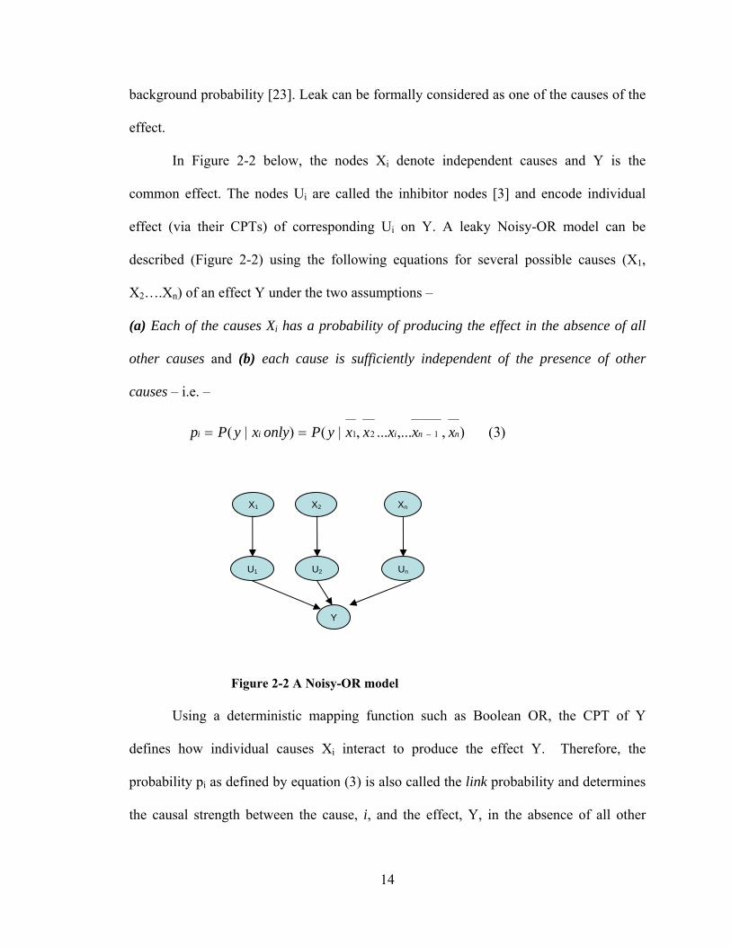
In Figure 2-2 below, the nodes Xi denote independent causes and Y is the

common effect. The nodes Ui are called the inhibitor nodes [3] and encode individual

effect (via their CPTs) of corresponding Ui on Y. A leaky Noisy-OR model can be

described (Figure 2-2) using the following equations for several possible causes (X1,

X2….Xn) of an effect Y under the two assumptions –

(a) Each of the causes Xi has a probability of producing the effect in the absence of all

other causes and (b) each cause is sufficiently independent of the presence of other

causes – i.e. –

)3( ),,...... ,|() |( 121 nniii xxxxxyPonlyxyPp

Figure 2-2 A Noisy-OR model

Using a deterministic mapping function such as Boolean OR, the CPT of Y

defines how individual causes Xi interact to produce the effect Y. Therefore, the

probability pi as defined by equation (3) is also called the link probability and determines

the causal strength between the cause, i, and the effect, Y, in the absence of all other

X1 X2

U1 U2 Un

Y

Xn

15

causes. It has been shown [3] that the probability of Y = y given a subset Xp (xi present),

i.e. a set consisting of causes that are present, is given by the following equation (4) –

4)( 11

X x

)p(Xp)|P(y

pi

i

Under the assumption that causes produce the common effect independently,

equation (4) can calculate the probability value for an effect solely based on the causal

strength pi of each cause to the effect. Therefore using the assumption of causal

independence, the number of values required for CPT elicitation of effect Y reduces from

exponential to linear in number of causes.

Further the leak probability p0 which models un-modeled causes can be defined as

)5( ),,.........,...,|( 1210 nni xxxxxyPp

Let p΄ define the probability that Y is present when xi is present and all other causes of Y

including un-modeled causes (leak) are absent. From [3] for the leaky Noisy-OR model

following is defined –

(6) ) 1( ) 1( ́1 0p-p-p i

(7) 00 pp´ - pp´ only)x|yP( p ii

The two ways of parameterization of CPD using Noisy-OR gate equation (4) is credited

to Henrion [23] and Diez [22]. For calculating the link probability, the difference

between the Henrion method and the Diez method lies in learning Noisy-OR parameters

from equation 7. [15] The Henrion method seeks the pi parameter where as the Diez

method seeks the p΄ parameter.

16

Among the studies in the past, where the Noisy-OR gate model has been

successfully applied are – reformulation of the rule based expert INTERNIST-1/QMR

system into a probabilistic system by combining probabilities from disease profiles and

hospital discharge statistics [5], deriving parameters from small data sets for converting

from single-disorder to multiple-disorder liver disease diagnostic system (HEPAR-II)

[15] and to an artificial domain for comparison of human expert’s judgment of

parameters using the two ways of parameterization credited to Diez [22] and Henrion

[23] in using [25] the Noisy-OR assumption. The result of this last study [25] claims that

the Henrion method is better at providing Noisy-OR parameters from data [15] when the

underlying distribution follows the Noisy-OR assumption, and the Diez method is better

when human experts provide the parameters.

Thus the Noisy-OR model may be suitable for parameter estimation in large scale

domains, such as medical diagnosis, where an observation such as a symptom can be

triggered independently by a number of causes (diseases), or a number of causes can

independently lead to a common complex disease. Similar to Noisy-OR, other forms of

noisy deterministic functions (Noisy-AND, Noisy-MAX, Noisy-MIN, Noisy-ADD) [22-

24, 26-27] have been defined and proposed for assessing values for CPD in a BN using

the assumption of causal independence.

Other Related Models

While these models greatly reduce the complexity of parameter estimation in CPT

and can serve as a good first approximation (Chapter 3) for modeling, the conditional

probability distributions (CPD) in themselves do not account for interactions among

causes that lead to the common effect. Although all of the above models take into account

17

the probability of an effect given each single cause as an input, the interactions defined

among causes (by virtue of the noisy deterministic function) are considered to be

synergistic or reinforcing. [28] Therefore, when multiple causes are present, the causes

may reinforce each other (i.e. making the effect more likely to be present) or may

undermine the impact of each other (i.e. the effect becomes less likely when more causes

are present). As pointed by Xiang et al, [28] all of the above distributions (Noisy-AND,

Noisy-MAX, Noisy-MIN, Noisy-ADD) can only express one type of causal interaction in

a model, i.e. reinforcing.

To address the possibility of reinforcing interactions between causes, recently

Lemmer and Gossink [29] proposed the Recursive Noisy-OR (RNOR) distribution which

allows elicitation of probability parameters of the effect given subsets of causes as input.

RNOR defines the concept of positive causality and how the dependent causes can work

together as being either “synergistic” or “interfering.” The RNOR model can incorporate

an expert provided probability distribution for an effect as well as a subset of values of

causes given as input, wherever applicable and claims to be a generalization of Noisy-OR

model. The RNOR model does not handle expert assertions of interference between

causes. If an expert-provided subset of values implies inhibitions or interference, and the

causes are undermining, RNOR can produce probability values that are greater than one.

[29] Its application to problem domains such as medical diagnosis looks promising

because of its ability to represent a subset of causes but it needs empiric evaluation.

More recently, Xiang and Jia have proposed a variation of this model. The non-

impeding Noisy-AND tree (or NIN-AND tree) model [28] can represent both types of

causal interactions among a set of causes, some of which can be reinforcing and others

18

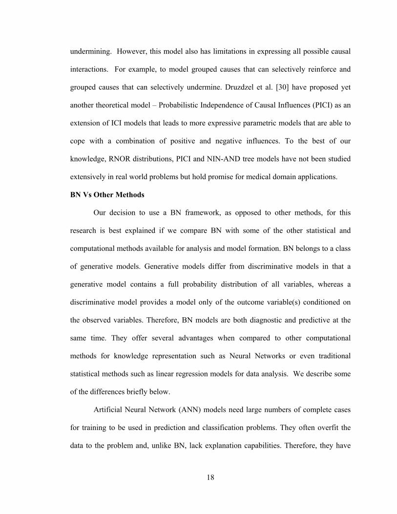
undermining. However, this model also has limitations in expressing all possible causal

interactions. For example, to model grouped causes that can selectively reinforce and

grouped causes that can selectively undermine. Druzdzel et al. [30] have proposed yet

another theoretical model – Probabilistic Independence of Causal Influences (PICI) as an

extension of ICI models that leads to more expressive parametric models that are able to

cope with a combination of positive and negative influences. To the best of our

knowledge, RNOR distributions, PICI and NIN-AND tree models have not been studied

extensively in real world problems but hold promise for medical domain applications.

BN Vs Other Methods

Our decision to use a BN framework, as opposed to other methods, for this

research is best explained if we compare BN with some of the other statistical and

computational methods available for analysis and model formation. BN belongs to a class

of generative models. Generative models differ from discriminative models in that a

generative model contains a full probability distribution of all variables, whereas a

discriminative model provides a model only of the outcome variable(s) conditioned on

the observed variables. Therefore, BN models are both diagnostic and predictive at the

same time. They offer several advantages when compared to other computational

methods for knowledge representation such as Neural Networks or even traditional

statistical methods such as linear regression models for data analysis. We describe some

of the differences briefly below.

Artificial Neural Network (ANN) models need large numbers of complete cases

for training to be used in prediction and classification problems. They often overfit the

data to the problem and, unlike BN, lack explanation capabilities. Therefore, they have

19

limited use in a domain like biomedical research. BN models on the other hand are

probabilistic and can take personal (expert) beliefs (using a subjectivist approach) for

model building – they are well suited to derive prior probability values from small sample

sizes and are able to handle missing data values reasonably well while avoiding over

fitting of data to the model. [4] They model cause and effect in a normative way [3] and

therefore provide a framework for incorporating all available information in a systematic

manner for both model and parameter estimation to produce a predictive distribution.

Linear regression models are non-parametric (distribution free) statistical models

and can also be used for prediction and classification problems like ANN and BN.

However, they do not handle missing data well in the input, and due to their susceptibility

to noise in the data, their use for model building is limited, particularly in the biomedical

domain where data are noisy. As with ANN, linear regression models lack normative

explanation capabilities and also suffer from the “curse of dimensionality” i.e. an

exponential increase in model space with addition of extra dimensions, as is the case in

domains with large number of variables such as the biomedical domain.

Other methods of knowledge acquisition such as systematic review and meta–

analysis aim to more precisely estimate the true “effect size” from a group of studies as

opposed to the less precise estimates derived in a single study under a given set of

assumptions. But these are not computational methods to synthesize a prediction model.

Therefore, despite the computational complexity of inference, BN methods offer

several advantages over traditional methods of knowledge acquisition and representation.

They have been shown to represent domain knowledge with conciseness and normative

form. The product form of equation (1), i.e. the chain rule and the conditional

20

independence assumption makes the BN representation of the JPD compact. Their ability

to handle missing data values and ability to calculate probability scores from small data

sets is another reason to choose BN methods. Most of all, BN methods provide a strategic

framework for our research to incorporate all available information in a systematic

manner for both model and parameter estimation to produce a predictive distribution that

can be used for inference and hypotheses generation. In this research we develop a

methodology using the BN framework and summary and statistical measures from

published studies for integration of information from disparate sources of data in the

biomedical domain.

Challenges for Knowledge Representation and Inference in Biomedical Domain

To gain full understanding of the implications of the research thus far in the

biomedical domain, we first need to understand how we could represent the existing

information, derive knowledge and inference from it. In light of the data gathered from

separate environmental and genetic studies and not on the same individual, a unifying

model is desperately needed to represent such information perhaps in a computational

model (In-silico). Such a model, once constructed could also be used for knowledge

discovery or in clinical applications.

For instance, it is believed that both genetic and environmental risk factors have

an important role to play in most common diseases. [31-32] A 2003 review article titled

“Genomics as a Probe for Disease Biology” in the New England journal of Medicine

highlights the importance of understanding genetics together with the pathology of a

disease in order to unravel the underlying disease processes. [33] Asthma, which is best

considered as a cluster of related disorders, [34] is one such common complex disease.

21

The prevalence of asthma has risen dramatically in the last few decades, [35] suggesting

that environmental risk factors have a key role to play together with genetic factors in

developing a risk of the disease [35-37] in early childhood. As is the case with asthma,

there is also evidence suggesting the role of environmental and genetic factors for most

other common diseases such as diabetes, obesity and heart disease. [38-39]

Recently, it has also been argued that the current classification of human disease

has significant shortcomings as reflected in its lack of sensitivity in identifying pre-

clinical disease and lack of specificity in defining disease unequivocally. [40] Therefore,

it has been proposed that an approach using network principles and linking phenotype or

clinical data with the genotype and environmental data associated with the risk of

disease, can lead to more accurate identification and classification of disease diagnostic

and treatment options. [40] For example, in the field of cancer biology, bioinformatics

methods that integrate diverse data (clinical and genotype) in their analysis for predicting

survival rates have achieved higher accuracy than use of clinical data alone, even when

the data analyzed are from different sources. [41-42]

Given the example above, we believe that the challenges of knowledge

representation and inference in this domain are three fold.

Existence of silos of datasets

First, data are being amassed in silos of biomedical databases. Currently, there are

major initiatives underway by the National Institutes of Health (NIH) to address the rise

in common diseases (like asthma and diabetes) by studying their genetic linkages and

disease-environment interactions [43-47] in Genome Wide Association Studies (GWAS)

and Environment Wide Association Studies (EWAS) respectively. Due to the interplay

22

of environment, lifestyle and small effects of many genes, researchers have focused on

very different aspects, for example pharmacogenetics / pharmacogenomics, [37, 48-49]

gene-environment interaction [47, 50] and clinical environmentally focused [51-52]

studies. Despite their best efforts, researchers find it hard to conduct unbiased studies in

well defined populations that have sufficient power to detect small effects attributed to

genetic or environmental factors. [49, 53-54] Therefore, to date these studies are being

conducted in sub populations and patient level data are being collected and stored within

the individual institution’s repository.

Access Rights

Second, due to lack of data sharing agreements among institutions and patient

privacy concerns, [55-56] the data are not accessible in their raw form to outside entities

like researchers in other institutions for any secondary analysis. The only publicly

accessible results from these studies are published summary and statistical results. Thus,

if any form of computational model needs to be developed to unify the information it

most likely will have to use the published results.

Inference in Patient’s Context

Third, there is a big gap in application of knowledge gained from biomedical

research and its use in patient’s context, for example from an EMR. Research that applies

to clinical management of diseases and many rare disorders which are governed by

straightforward Mendelian rules of inheritance have been known for some time.

However, teasing out the genetic and environmental components for complex disorders

such as diabetes, heart and lung disease, autoimmune and psychiatric disorders and their

clinical management remains challenging [33] due to this application gap.

23

Therefore, there are many practical challenges for application of existing research

in the biomedical domain. In the next chapter we discuss how, based on our background

research, we can use BN for building a probabilistic framework for knowledge

representation and inference in this domain. We specifically develop strategies using this

framework to incorporate all available knowledge in a coherent model from various

sources for example as presented in Figure 1-1 – environmental, genetic, demographic,

socio-economic and clinical phenotypes.

Our hypothesis in building such a model is to 1) find associations across the

domain that are not apparent in the silos of datasets and 2) confirm these associations by

testing – a) against data from our EMR and b) by evaluating against what has been

published in the literature so far. We are interested to know how much of explanation is

provided by a subset of data, for example how well genetic associations can explain the

risk of a complex disorder like asthma or diabetes.

To test our model we use Area under the Curve (AUC) of Receiver Operator

Characteristics (ROC) curves as a performance measure. We describe the ROC

performance measure below.

Receiver Operating Characteristic (ROC) Curve

A ROC curve is a plot of pairs of true positives (Sensitivity) vs. false positives (1

– Specificity) for various cut points of a binary classifier as its discrimination threshold is

varied. The ROC curve has its roots in Signal Detection Theory from World War II and

since then they have been extensively applied as an analysis tool in areas of medicine,

radiology [57], and many other fields. [58]

24

Since ROC curve analysis is a non-parametric method and does not rely on the

underlying distribution, their use as an analysis tool is particularly attractive to the

machine learning community; especially for use as a model comparison tool to select an

optimal model given the data. The area under the curve (AUC) of an ROC curve is equal

to the probability that a classifier will rank a randomly chosen positive instance higher

than a randomly chosen negative one [58] and therefore measures the performance of the

model. A ROC with AUC of 0.5 score has no predictive value and is as good as chance.

25

Chapter 3 EXPERIMENTAL STUDIES on BNs and ICI MODELS

A Bayesian approach to represent domain knowledge

Based on our background research on Bayesian Networks and the breadth of the

challenges involved in building a coherent model in the biomedical domain, we evaluate

the use of a probabilistic framework, combining BN fundamentals of conditional

independence and the Markov condition to encode domain knowledge both qualitatively

and quantitatively. We then evaluate the use of the Independence of Causal Influence

(ICI) assumption as a potential data integration strategy. In this chapter, we describe our

experiments in the clinical domain using data on childhood asthma from our EMR, the

Regenstrief Medical Record System (RMRS) [2] and another independent test data

source from our pediatric decision support system in practice – Child Health

Improvement through Computer Automation (CHICA) system [59] described below.

In experiment 1, we compare performance of a data derived DAG to a domain

expert’s model DAG by testing it on the same test datasets to evaluate the sensitivity of

the BN function to the structure of the DAG with real world datasets.

In experiment 2, we test the validity of the Independence of Causal Influence

(ICI) assumption in particular the Noisy-OR model using the same datasets from

experiment 1. To model domain causal relationships, over and above causal

independence, we test the validity of Recursive Noisy-OR (RNOR) rule.

26

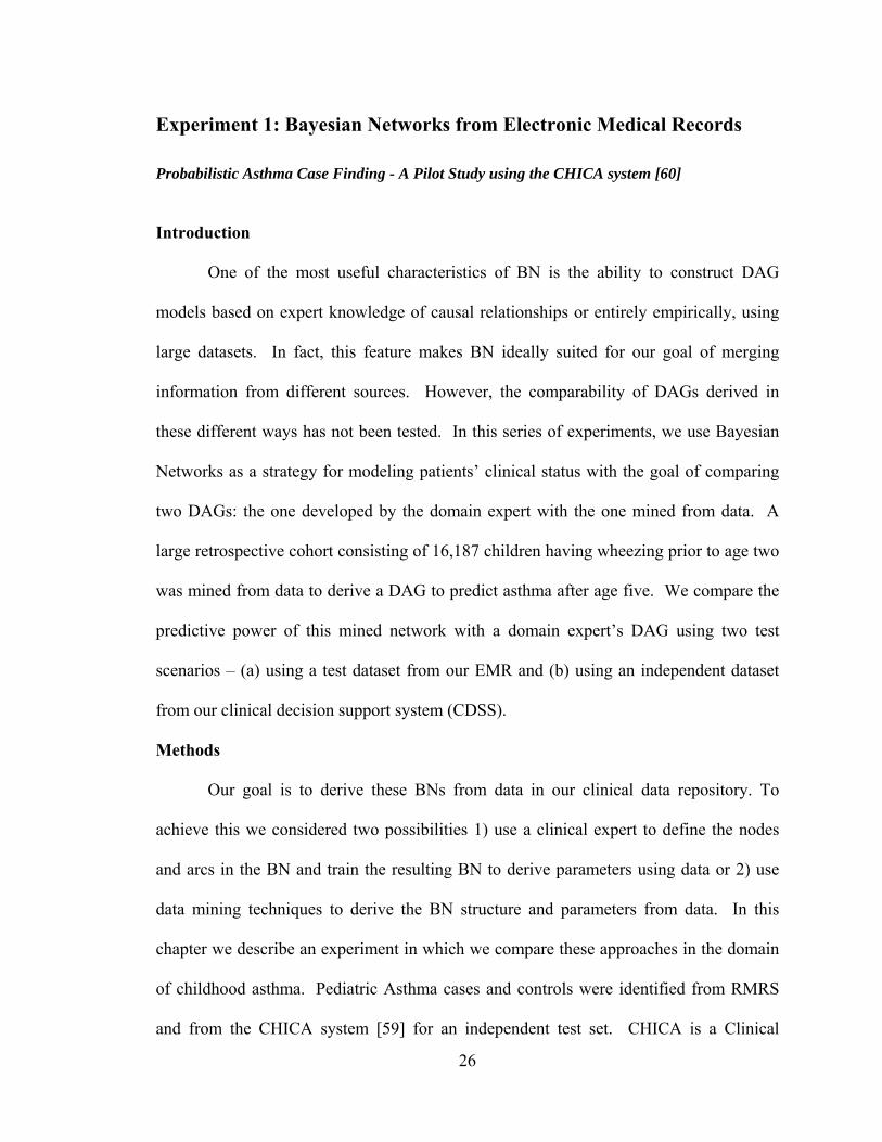
Experiment 1: Bayesian Networks from Electronic Medical Records

Probabilistic Asthma Case Finding - A Pilot Study using the CHICA system [60]

Introduction

One of the most useful characteristics of BN is the ability to construct DAG

models based on expert knowledge of causal relationships or entirely empirically, using

large datasets. In fact, this feature makes BN ideally suited for our goal of merging

information from different sources. However, the comparability of DAGs derived in

these different ways has not been tested. In this series of experiments, we use Bayesian

Networks as a strategy for modeling patients’ clinical status with the goal of comparing

two DAGs: the one developed by the domain expert with the one mined from data. A

large retrospective cohort consisting of 16,187 children having wheezing prior to age two

was mined from data to derive a DAG to predict asthma after age five. We compare the

predictive power of this mined network with a domain expert’s DAG using two test

scenarios – (a) using a test dataset from our EMR and (b) using an independent dataset

from our clinical decision support system (CDSS).

Methods

Our goal is to derive these BNs from data in our clinical data repository. To

achieve this we considered two possibilities 1) use a clinical expert to define the nodes

and arcs in the BN and train the resulting BN to derive parameters using data or 2) use

data mining techniques to derive the BN structure and parameters from data. In this

chapter we describe an experiment in which we compare these approaches in the domain

of childhood asthma. Pediatric Asthma cases and controls were identified from RMRS

and from the CHICA system [59] for an independent test set. CHICA is a Clinical

27

Decision Support System (CDSS) used in our Pediatric Primary Care (PCC) practice in

conjunction with RMRS, [2] and we briefly describe it below.

CHICA Overview

The CHICA system went live on Nov. 5th, 2004 at the Pediatric Primary Care

Center (PCC) of Wishard Hospital, Indianapolis, Indiana, and now has data from over

25,000 patients. The system provides decision support for well child care and

management of common childhood problems. The user interface consists of scannable

paper forms called adaptive turnaround documents (ATD). [61] Data collected on ATDs

are used to generate questions to the patient and reminders to physicians at the point of

care. CHICA uses a knowledge base encoded as Arden Syntax medical logic modules

(MLM) [62] and patient data from the RMRS [2] and CHICA databases to generate

dynamic content on the ATD forms. The MLMs are prioritized using a global priority

scheme to address the most relevant questions and reminders on the ATD. [59, 63] The

CHICA system electronically receives a record of all clinical observations from the

RMRS database for every patient visit.

We analyzed data for all children over 5 years of age in our system. Children

were classified as cases or controls based on the presence of an ICD-9 code for asthma

(493.*) or more than two prescriptions of an asthma medication. From the filtered set we

were able to extract the variables listed in Table 3-1 to get an “Asthma Status,” sex and

race for each patient (ages 5 years or older) who had a visit to the PCC clinic. The

CHICA system in its current state has been described in detail in previous manuscripts.

[59, 64-66]

28

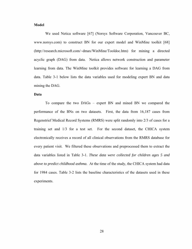
Model

We used Netica software [67] (Norsys Software Corporation, Vancouver BC,

www.norsys.com) to construct BN for our expert model and WinMine toolkit [68]

(http://research.microsoft.com/~dmax/WinMine/Tooldoc.htm) for mining a directed

acyclic graph (DAG) from data. Netica allows network construction and parameter

learning from data. The WinMine toolkit provides software for learning a DAG from

data. Table 3-1 below lists the data variables used for modeling expert BN and data

mining the DAG.

Data

To compare the two DAGs – expert BN and mined BN we compared the

performance of the BNs on two datasets. First, the data from 16,187 cases from

Regenstrief Medical Record Systems (RMRS) were split randomly into 2/3 of cases for a

training set and 1/3 for a test set. For the second dataset, the CHICA system

electronically receives a record of all clinical observations from the RMRS database for

every patient visit. We filtered these observations and preprocessed them to extract the

data variables listed in Table 3-1. These data were collected for children ages 5 and

above to predict childhood asthma. At the time of the study, the CHICA system had data

for 1984 cases. Table 3-2 lists the baseline characteristics of the datasets used in these

experiments.

29

Table 3-1 Data Variables for Model – Experiment 1

Variable Values

Race White, Black, Hispanic, Other, Unknown

Sex Male, Female

Eczema True, False

Wheeze ICD9 or clinic billing diagnosis before age 2 (True, False)

Asthma ICD9 (493.*) or any clinic billing diagnosis after age 5 or at least 3 drugs from a specified list within 12 months after age 5 (True, False)

X-ray Chest x-ray before age 2 (True, False)

Drug

Drugs from a specified list before (True, False)

Wz_hosp Inpatient admission with hospital ICD9 as wheezing (True, False)

Wz_er Any ER visit with billing ICD9 as wheezing (True, False)

Ins_cat Insurance category - first available insurance in the same year of the first wheezing diagnosis (True, False)

30

Figure 3-1 Expert’s BN trained with data from RMRS

31

Table 3-2 Baseline characteristics of training and test sets

Variables

Training Set from RMRS (n = 11,000)

Test Set from RMRS (n = 5,187)

Test Set from CHICA (n = 1,984)

# % # % # %

Race Hispanic 98 1% 373 7% 429 22% Unknown 115 1% 220 4% 24 1% Black 6859 62% 3116 60% 1156 58% White 3806 35% 1385 27% 327 16% Other 122 1% 93 2% 48 2%

Sex Female 5357 49% 2503 48% 916 46% Male 5641 51% 2684 52% 1068 54%

Eczema True 4021 37% 2021 75% NA NA False 6979 63% 3166 61% NA NA

Wheeze True 1661 15% 1431 28% 187 9% False 9339 85% 3756 72% 1797 91%

Asthma True 1561 14% 548 11% 536 27% False 9439 86% 4639 89% 1448 73%

X-ray True 4015 37% 1900 37% 1529 77% False 6985 64% 3287 63% 455 23%

Drug True 3013 27% 1488 29% 529 27% False 7987 73% 3699 71% 1455 73%

Wz_hosp True 433 4% 247 5% 159 8% False 10567 96% 4940 95% 1825 92%

Wz_er True 102 1% 98 2% 143 7% False 10898 99% 5089 98% 1841 93%

Ins_cat Medicaid 4762 43% 4051 78% 1631 82% Unknown 5276 48% 182 4% 64 3% Private 844 8% 893 17% 160 8% Self-pay 118 1% 61 1% 0 0%

rsv_pos True 244 2% 114 2% 17 1% False 10756 98% 5073 98% 1967 99%

32

Expert’s Design of BN with training using Netica

Using the predictor data variables of Table 3-1 as nodes and the domain

knowledge for joining them with arcs, the domain expert (SMD) created a BN as shown

in Figure 3-1. This BN was trained with the training set and compiled using Netica

software. In Figure 3-1 the BN shows marginal probabilities of each node with an

asthma prior probability of 18.6%.

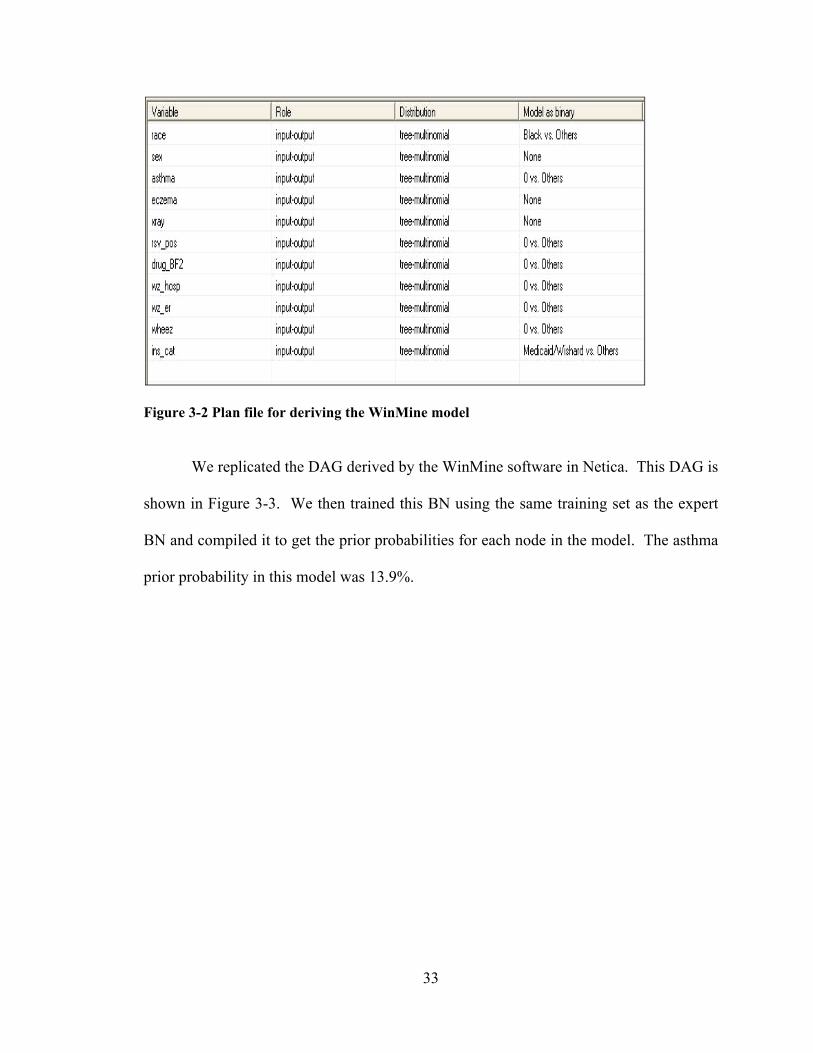
BN Derived using Data Mining Techniques

The training set from RMRS data was used to derive the DAG for this approach.

The software from WinMine toolkit was used to preprocess the data from raw format

(excel tab delimited) to WinMine XML format, which was then used for creating and

editing a plan file to instruct the learning algorithm to model each predictor variable

based on a) the role of each variable – input (used to predict other variables), output

(predicted by other variables) and input-output (both predicted and used to predict) or

ignored (not used); b) the model distribution used for each variable – specifies the tree

versus the table representation and the local distribution of the variable, the

representation chosen in this case is tree for discrete variables and the distribution chosen

is binary multinomial to accommodate missing values; c) Model-as-binary information

(missing vs non-missing values for binary variable or one state vs all other states for

discrete variables.). Figure 3-2 shows the roles, the distributions used and model-as-

binary information for each of the predictor variables for our model in the WinMine

toolkit.

33

Figure 3-2 Plan file for deriving the WinMine model

We replicated the DAG derived by the WinMine software in Netica. This DAG is

shown in Figure 3-3. We then trained this BN using the same training set as the expert

BN and compiled it to get the prior probabilities for each node in the model. The asthma

prior probability in this model was 13.9%.

34

Figure 3-3 BN mined and trained with data from RMRS Testing the Two Models

The two BN models were evaluated, first, using data from our test set from

RMRS data (1/3 split from the large cohort study) and, second, using the CHICA data set

derived from CHICA database.

Netica provides an interface to test the BN using a case file of test data. The

node(s) of interest for prediction are treated as “unobserved nodes”. Asthma was used as

an unobserved node in our tests. The software reports several measures for each

unobserved node. We chose to use the quality of test results, which gives a performance

measure in the form of a table for sensitivity, specificity, positive predictive value and

negative predictive value.

We compared BNs using Receiver Operating Characteristics (ROC) curves [57].

The area under the curve was used as a measure of overall test performance. The ROC

35

curve was obtained by plotting pairs of true positive rate (sensitivity) and false positive

rate (1 - specificity).

Results

We had 5188 cases in our RMRS test set and 2000 cases in the CHICA test set.

Both the Expert and the Mined BN were tested using these sets, the results of which are

listed below in Table 3-3, Figure 3-4 and Table 3-4, Figure 3-5 for RMRS and CHICA

test sets respectively.

36

Using RMRS Test Set

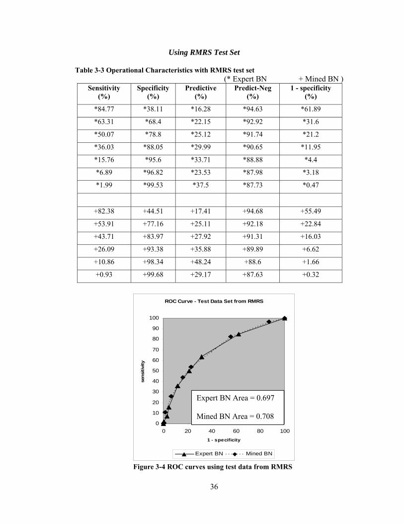
Table 3-3 Operational Characteristics with RMRS test set (* Expert BN + Mined BN )

Sensitivity (%)

Specificity(%)

Predictive(%)

Predict-Neg (%)

1 - specificity(%)

*84.77 *38.11 *16.28 *94.63 *61.89

*63.31 *68.4 *22.15 *92.92 *31.6

*50.07 *78.8 *25.12 *91.74 *21.2

*36.03 *88.05 *29.99 *90.65 *11.95

*15.76 *95.6 *33.71 *88.88 *4.4

*6.89 *96.82 *23.53 *87.98 *3.18

*1.99 *99.53 *37.5 *87.73 *0.47

+82.38 +44.51 +17.41 +94.68 +55.49

+53.91 +77.16 +25.11 +92.18 +22.84

+43.71 +83.97 +27.92 +91.31 +16.03

+26.09 +93.38 +35.88 +89.89 +6.62

+10.86 +98.34 +48.24 +88.6 +1.66

+0.93 +99.68 +29.17 +87.63 +0.32

Figure 3-4 ROC curves using test data from RMRS

ROC Curve - Test Data Set from RMRS

0

10

20

30

40

50

60

70

80

90

100

0 20 40 60 80 100

1 - specificity

sensi

tivi

ty

Expert BN Mined BN

Expert BN Area = 0.697 Mined BN Area = 0.708

37

Using CHICA Test Set

Table 3-4 Operational Characteristics with CHICA test set Sensitivity

(%) Specificity

(%) Predictive

(%) Predict-Neg (%) 1-Specificty

(%)

*75.56 *38.05 *31.11 *80.79 *61.95

*56.53 *64.3 *36.95 *79.98 *35.7

*48.69 *73.69 *40.65 *79.51 *26.31

*30.04 *90.81 *54.76 *77.81 *9.19

*25.56 *93.99 *61.16 *77.33 *6.01

*1.31 *99.93 *87.5 *73.23 *0.07

+77.43 +27.97 +28.46 +77 +72.03

+44.59 +76.66 +41.42 +78.89 +23.34

+40.11 +80.18 +42.83 +78.34 +19.82

+26.87 +89.92 +49.66 +76.86 +10.08

+15.49 +97.24 +67.48 +75.66 +2.76

+5.97 +99.65 +86.49 +74.11 +0.35

* Expert BN + Mined BN

Figure 3-5 ROC curves using test data from CHICA

ROC Curve - Test Data Set from CHICA

0

10

20

30

40

50

60

70

80

90

100

0 20 40 60 80 100

1 - specificity

sen

siti

vity

Expert BN Mined BN

Expert BN Area = 0.637 Mined BN Area = 0.603

38

Discussion

The results of AUC for the ROC for both BNs using the same test set are

comparable. Both the expert BN and the mined BN performed better with the test set

from the RMRS data set when compared with the CHICA data set. We attribute

degraded performance when testing with CHICA data set due to our less stringent

inclusion criteria in the CHICA test set. For example, any chest x-ray observation will

satisfy the inclusion criteria for CHICA data, where as for the RMRS test set only a chest

x-ray finding before age 2 will satisfy the inclusion criteria.

Similar performance of each BN in each test scenario suggests that the mined BN

has a predictive value similar to the DAG derived by the expert. Furthermore, the two

compared BNs in this experiment were derived from two different data sources – a

subjective model based on a clinical expert’s judgment and from data from our EMR.

The data derived BN was as good as the subjective model suggesting the BN method

presents a knowledge representation and inference tool where subjective decisions can be

incorporated to approximate the domain knowledge.

39

Experiment 2: Strategies for Learning BN parameters

Probabilistic asthma case finding: A Noisy-OR reformulation [69]

An Empirical Validation of Recursive Noisy-OR (RNOR) Rule for Asthma Prediction [70] Introduction

Development of a BN to represent the relationships between GWAS results and

gene disequilibrium data requires assumptions about independent causal associations. As

a preliminary evaluation, we wanted to evaluate the Noisy-OR and Recursive Noisy-OR

formalisms by comparing the predictive power of BN developed using these methods to a

“gold standard” BN trained on clinical data.

Noisy-OR: In combining disparate data sets in which one data set describes the

relationship between some causes or risks and their consequences, and another data set

describes the relationship between other causes or risks and the same consequences, there

are no cases from which to infer the combined effect causes recorded in the different

datasets. One approach to this challenge is to assume causal independence among

predecessors (parents) of a given node. In this case, it may be reasonable to apply a

Noisy-OR calculation [3] to estimate the probability of the child node given a particular

combination of values for the parents [22-24]. By assuming these variables have

independent causal effects, the Noisy-OR allows us to assign posterior probabilities

conditioned on causes from these different sets. However, the validity of the

independence assumption is rarely tested. We wanted to test this assumption by applying

the Noisy-OR to combinations of conditioning variables for which we knew the joint

probability distributions.

40

RNOR: To test the Noisy-OR model against a “gold standard,” we need a BN

trained on a data set that represents the joint probability distributions. Several,

algorithms have been developed for training BN by learning their conditional probability

distributions (CPD) from such datasets. [27, 71] However, a challenge arises when the

training data set has no cases representing a particular combination of values for variables

that condition a particular CPD. This is a common problem in complex BN even when

large training sets are available. [22] A common strategy in this situation is to assign a

uniform (uninformed) distribution to the dependent variable, conditioned by this

combination of variables. For example, when the probability of asthma is conditioned on

the sex, race, insurance and past wheezing history of a patient, there may be no cases in

the training data that are male, white, on Medicaid and with a positive history of

wheezing. Under the uniform distribution strategy, the probability of asthma would have

a 50-50 distribution.

The ideal strategy would retain posterior distributions for combinations of parent

node values that exist in the training set while applying the Noisy-OR rule when there are

no cases representing a combination of conditioning variables. In 2004, a potential

solution to this problem was published by Lemmer and Gossink. [29] The Recursive

Noisy-OR (RNOR) rule described by these authors was intended to incorporate expert

estimates of probabilities conditioned on more than one node while applying the Noisy-

OR rule when these higher order conditional probabilities were not available. We

reasoned that the RNOR algorithm might be a successful strategy for training a BN from

a data set that did not contain cases representing all combinations of variables

conditioned on a given node. We hypothesized that this RNOR approach would produce

41

a BN with better predictive power than either a Noisy-OR formulated or traditionally

trained BN. This chapter describes the development and evaluation of this strategy.

Methods

We constructed a BN in the domain of asthma prediction in children, using expert

knowledge to derive a directed acyclic graph (DAG) and applied a commercially

available software package to learn the CPDs (parameters) from a large clinical dataset.

This empiric BN has been described before in Chapter 3 (Figure 3-1). [60] For this study,

we reformulated the CPDs in our domain expert’s BN using both Noisy-OR and the

RNOR rule. Our empiric BN, Noisy-OR BN and RNOR BN were tested against two

independent clinical data sets described below.

EMR Data and Variables

Clinical data for this study were derived from two datasets – RMRS and CHICA

as described in experiment 1 in Tables 3-1 and 3-2.

Bayesian Network and Noisy-OR model

We took the Expert’s BN from Figure 3-1 and reformulated it as a Noisy-OR

model (Figure 3-6). The expert BN was trained with data to derive a CPT for each node.

Since the Noisy-OR model inherently assumes binary causes (absent / present; true/false),

we dichotomized the non-binary nodes i.e. race and, insurance category) into “true” and

“false” condition by assigning “true” to the state that minimized the global leak (p0) when

all the other nodes are in a “false” state. Thus, because boys were more likely to have

asthma, male sex was coded as the “true” state. Similarly, race = Black and ins_cat =

Private were coded as “true” states. The marginal probabilities of all the causal nodes

(sex, eczema, wheeze, xray, drug, rsv_pos, wz_er, wz_hosp) remain the same from our

42

expert BN. For the study, we only wished to compute the local CPT of the node asthma

using the Noisy-OR parameters.

Figure 3-6 BN with Noisy-OR parameters Obtaining Noisy-OR Parameters from Data

To derive the leak parameter for the network in Figure 3-6, we set all the nodes in

the network that had an arc to the node asthma to a state false. The resulting posterior

probability for the node asthma was our leak parameter, p0 (0.014). Using this leak

probability, we calculated the parameter pi (the causal strength when no other cause is

present) of each node (node = True) to the effect (asthma).

We used Netica to compute the posterior probability pi of the effect given only

one of the causes at a time. This is equivalent to eliciting the Henrion parameter which

includes the leak parameter in the posterior probability. From there, we were able to

derive the probability p΄ (Diez parameter) for each cause alone, using equation (7) in

chapter 2.

43

Netica provides an interface to input Noisy-OR parameters for a given node and is

able to calculate the conditional probability distribution for the node from these input

parameters – effect node’s leak, individual link probabilities of causes. We used this

feature to calculate the CPD for the asthma node. This Noisy-OR calculation is achieved

with the function in Figure 3-7. The link parameters are listed in Table 3-5.

P (asthma | sex, eczema, wheez, drug, xray, rsv_pos, wz_er, wz_hosp, race, ins_cat) =

NoisyOrDist (asthma, 0.014, sex == M, 0.022, eczema, 0.048, wheez, 0.17, drug, 0.117,

xray,0.072, rsv_pos, 0.4, wz_er, 0.37, wz_hosp, 0.104, race == Black, 0.042, ins_cat ==

Private, 0.058)

The prior probability of the node asthma computed is slightly different in the two

BNs - Noisy-OR reformulation vs. the Expert BN (16.8% Vs 18.6%).

Testing of Noisy-OR model

The two BN models – Expert (empiric) BN (Figure 3-1) and Noisy-OR

Reformulation (Figure 3-6) were evaluated, first, using data from our test set from RMRS

data (1/3 split, 5187 cases ) and, second, using the CHICA data set derived from the

prospectively collected CHICA database (1984 cases). Netica provides an interface to

test the BN using a case file of test data. The node(s) of interest for prediction are treated

as “unobserved nodes”. Asthma was used as an unobserved node in our tests. We

compared the sensitivity, specificity, positive predictive value and negative predictive

value of the Noisy-OR and the expert BN.

We compared the BNs using Receiver Operating Characteristic (ROC) curves.

[57] The ROC curve was obtained by plotting pairs of true positive rate (sensitivity) and

Figure 3-7 Calculation of Noisy-OR parameters

44

false positive rate (1–specificity). The area under the curve (AUC) was used as a measure

of overall test performance. AUCs were compared using the methods of Hanley, J.A. and

B.J. McNeil. [72]

Results of Noisy-OR Reformulation

We had 5187 cases in our RMRS test set and 1984 cases in the CHICA test set.

The empiric BN and the Noisy-OR reformulation of the empiric BN were tested using

these sets. Results for these tests are plotted in Figures 3-8 and Figure 3-9 respectively.

When comparing the BN that utilized the Noisy-OR assumption to the BN with

the fully data derived CPD (empiric BN), we saw a modest decrement in the AUC (0.697

vs. 0.726) when applied to the evaluation dataset from RMRS. When applied to the

prospectively collected CHICA dataset, the decrement was about the same as before

(0.612 vs. 0.637). However, neither BN (empiric or Noisy-OR reformulated) was

particularly effective with the independent CHICA dataset.

Bayesian Network and Recursive Noisy-OR (RNOR) model

From experiment 1, the Expert (empiric) BN (Figure 3-1) had an 18.6% marginal

probability of asthma. On examining the CPD of asthma in this empiric BN, we found the

majority of its rows contained uninformed priors (i.e., uniformly distributed probability

score – asthma = 50-50). We attributed this to the lack of cases satisfying the particular

combination of causes in the training set (e.g., race = Other, Sex = male, Ins_cat =

selfpay, Eczema = true, Wz_hosp = true). We hypothesized that by using the RNOR rule

(described below) to calculate conditional probability for the CPD row value for asthma

in such cases, the RNOR reformulated BN will outperform the empiric BN.

45

Recursive Noisy-OR Rule

In 2004, a rule for estimating complex probabilistic interactions was published.

[29] The rule builds upon the Noisy-OR equation (4) in Chapter 2, to accommodate non-

independent causes of an effect for calculating RNOR probability pR(x). Interested

readers are encouraged to refer to the original paper [29]. The RNOR rule is a

generalization of Noisy-OR and reduces to Noisy-OR in cases where |x| = 1, i.e. a subset

of a single cause is provided by the expert pE(x). Furthermore, the rule preserves certain

ratios (synergies and interference, see below), and the authors claim a major advantage of

the rule is that it allows for arbitrary causally dependent subsets of probability scores to

be incorporated in the estimation of pR(x), the probability score of effect.

The rule states that as long as the expert provided values for a subset of causes do

not imply inhibition (i.e. abides positive causality, see synergy and interference below) it

can be applied. Expert provided values implying inhibition among a set of causes will

cause RNOR to produce probability scores greater than one, rendering the rule

inapplicable. The RNOR rule is summarized in the following equation 1–

(1)otherwise ,

})){\(1(

})){\(1(1 {

ninformatio providesexpert ),( {

mod)1(,

1

0nii

R

i

Rn

i

E

R

xxxp

xxp

ifxp

(x)P

Synergy and Interference

To judge the rule for semantic correctness (i.e. the numbers produced make

sense), the authors introduce the notion of positive causality. Positive causality refers to

the idea that additional causes always increase the probability of achieving an effect.

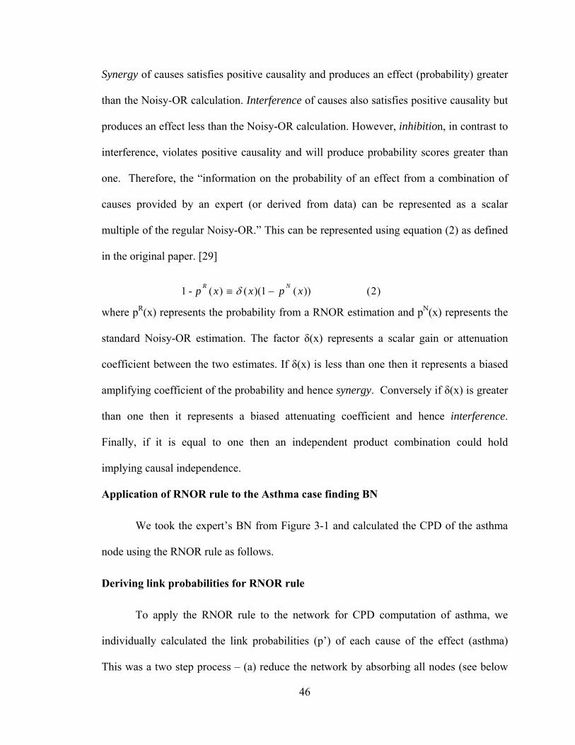
46

Synergy of causes satisfies positive causality and produces an effect (probability) greater

than the Noisy-OR calculation. Interference of causes also satisfies positive causality but

produces an effect less than the Noisy-OR calculation. However, inhibition, in contrast to

interference, violates positive causality and will produce probability scores greater than

one. Therefore, the “information on the probability of an effect from a combination of

causes provided by an expert (or derived from data) can be represented as a scalar

multiple of the regular Noisy-OR.” This can be represented using equation (2) as defined

in the original paper. [29]

)2())(1)(()( -1 xpxxpNR

where pR(x) represents the probability from a RNOR estimation and pN(x) represents the

standard Noisy-OR estimation. The factor δ(x) represents a scalar gain or attenuation

coefficient between the two estimates. If δ(x) is less than one then it represents a biased

amplifying coefficient of the probability and hence synergy. Conversely if δ(x) is greater

than one then it represents a biased attenuating coefficient and hence interference.

Finally, if it is equal to one then an independent product combination could hold

implying causal independence.

Application of RNOR rule to the Asthma case finding BN

We took the expert’s BN from Figure 3-1 and calculated the CPD of the asthma

node using the RNOR rule as follows.

Deriving link probabilities for RNOR rule

To apply the RNOR rule to the network for CPD computation of asthma, we

individually calculated the link probabilities (p’) of each cause of the effect (asthma)

This was a two step process – (a) reduce the network by absorbing all nodes (see below

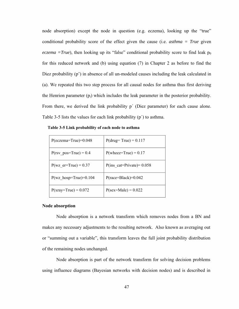
47

node absorption) except the node in question (e.g. eczema), looking up the “true”

conditional probability score of the effect given the cause (i.e. asthma = True given

eczema =True), then looking up its “false” conditional probability score to find leak p0

for this reduced network and (b) using equation (7) in Chapter 2 as before to find the

Diez probability (p’) in absence of all un-modeled causes including the leak calculated in

(a). We repeated this two step process for all causal nodes for asthma thus first deriving

the Henrion parameter (pi) which includes the leak parameter in the posterior probability.

From there, we derived the link probability p΄ (Diez parameter) for each cause alone.

Table 3-5 lists the values for each link probability (p΄) to asthma.

Table 3-5 Link probability of each node to asthma

P(eczema=True)=0.048 P(drug= True) = 0.117

P(rsv_pos=True) = 0.4 P(wheez=True) = 0.17

P(wz_er=True) = 0.37 P(ins_cat=Private)= 0.058

P(wz_hosp=True)=0.104 P(race=Black)=0.042

P(xray=True) = 0.072 P(sex=Male) = 0.022

Node absorption

Node absorption is a network transform which removes nodes from a BN and

makes any necessary adjustments to the resulting network. Also known as averaging out

or “summing out a variable”, this transform leaves the full joint probability distribution

of the remaining nodes unchanged.

Node absorption is part of the network transform for solving decision problems

using influence diagrams (Bayesian networks with decision nodes) and is described in

48

detail in Shachter’s algorithm [9-10]. Shachter’s algorithm involves three simple

reductions. First, any nodes that have no direct successors or “barren” nodes are removed

as their value do not influence the successors and are irrelevant to the decision problem

at hand, second, the propagation of the deterministic node, i.e. if any direct successor j of

a node i has a CPD for which node i is a conditioning variable, that function is

substituted in the distribution of j and in the process, node i is replaced as a conditional

predecessor to node j by the conditional predecessors of the node i, i.e. node i is

absorbed out. This may introduce new directed edges or links if not present between the

predecessors of node i and node j. Third, arc reversal – if there is an arc or a directed

edge from i to j, it is possible to transform the net into an arc from j to i instead and both

i and j inherit each other’s conditional predecessors. The CPD for node i is found by

summing out and the new CPD for node j is calculated from Bayes theorem.

Applying RNOR rule using link probabilities

Using the Java programming language and the Netica application programming

interface, we programmed the RNOR algorithm as defined in [29]. Appendix A.8 details

the code. The algorithm calculated the probability score of asthma in each row of the

CPD using equation (1). An example combination – (s)ex = Male, (r)ace = White,

(w)heez = True is given here –

)3(P(r)1

)P(s, -1

P(s)1

s) P(w, -1

P(w)1

)P(r, -1 1

rw(x)P

R

In the example above (equation 3), the RNOR algorithm calculated the row value

for the CPD by first calculating each of the subsets, multiplying them and subtracting

49

from 1. For this experiment, the probability score for asthma for each combination of

conditioning variables was calculated in three different ways–

Using RNOR rule

The algorithm recursively calculated the probability score for successive

combinations; using the original scores, pE(x), from data learnt CPD wherever they

existed (i.e., not 50-50), using equation (3). For example, if P (Wheez, Sex) was non-

uniform (i.e., not 50-50) in the original data learnt CPD of asthma (from the empiric

BN), it was used in successive calculations for higher order combinations. When the

resulting probability was negative or exceeded 1, suggesting inhibition, the CPD row

was left with 50-50.

Noisy-OR approach

Starting with link probabilities listed in Table 3-5, the algorithm recursively

calculated a probability score of asthma for successive combinations of conditioning

variables without using any values from the original data learnt CPD from the empiric

BN. This essentially reduced the model to a Noisy-OR model.

Adaptive Noisy-OR approach

As with the RNOR calculations, the algorithm computed CPD values recursively

using pE(x) where applicable. However, for those scores resulting in negative values,

instead of leaving a uniform distribution, we used the Noisy-OR value, reasoning that it

would be a better approximation than the 50-50 value in the CPD row. We termed this

“Adaptive Recursive Noisy-OR” or Adaptive RNOR (ARNOR).

BNs with probability tables calculated from these three methods were used in two

separate tests, comparing their predictive abilities in the two test sets.

50

Testing the Models

The BN models were evaluated, first, using data from our original test set of

RMRS data (1/3 split from the large cohort study 5187 cases) and, second, using the data

set derived from the prospectively collected CHICA database (1982 cases), utilizing

Netica’s test interface. We compared the sensitivity, specificity, positive predictive

value, and negative predictive value using Receiver Operating Characteristic (ROC)

curves. [57] The ROC curve was obtained by plotting pairs of true positive rate

(sensitivity) and false positive rate (1 - specificity). The area under the ROC curve

(AUC) was used as a measure of overall test performance. AUCs were compared using

the method of Hanley and McNeil [72] which specifically accounts for comparing ROC

derived from same cases.

Results of RNOR rule Reformulation

We had 5187 cases in our RMRS test set and 1984 cases in the independent test

set (CHICA). Results for the tests are shown in Figures 3-8 and 3-9 respectively. There

were no statistically significant differences between the predictive ability of the RNOR

or Adaptive RNOR and that of the empirically trained BN. Both RNOR and Adaptive

RNOR had larger AUC than the Noisy-OR BN in both RMRS and CHICA datasets but

the difference did not reach statistical significance (Figures 3-8 and 3-9 respectively and

Table 3-6).

51

Figure 3-8 Evaluation using test data from RMRS

Figure 3-9 Evaluation using test data from CHICA

ROC Curve- Test Data Set from RMRS

0

20

40

60

80

100

120

0 20 40 60 80 100 120

1 - specificity

se

ns

itiv

ity

Empiric BN: RNOR BN

Adaptive NOR Noisy-OR BN

ROC Curve - Test Data Set from CHICA

0

20

40

60

80

100

120

0 20 40 60 80 100 120

1 - specificity

sen

siti

vity

Empiric BN RNOR BN Adaptive NOR Noisy-OR BN

Empiric BN = 0.726 RNOR BN = 0.724 Adaptive NOR = 0.724 Noisy-OR = 0.697

Empiric BN = .637 RNOR BN = .629 Adaptive NOR = .630 Noisy-OR = .612

52

Table 3-6 Statistical comparison of models

Discussion

In case of Noisy-OR reformulation, the predictive power of the BN decayed

significantly when applied to another dataset (CHICA), it did not decay as much when

we made the Noisy-OR assumption in the original dataset. This is somewhat surprising

since we wouldn’t necessarily expect the predecessors to the asthma node (xray, drugs,

wheeze) to be independent causes (or even causes at all). Nonetheless, the relatively

small decrement in AUC suggests that the Noisy-OR may be a robust assumption to

make in an array of situations, even if BNs trained in one setting may be less effective in

another. We believe that the Noisy-OR formalism provides sound theoretic background

for combining a number of causes leading to a common disease manifestation if the

underlying distribution follows the assumptions.

In case of RNOR rule reformulation, we had anticipated that the RNOR would

perform better than the empirically trained BN. The RNOR retains the higher level

Dataset AUC1 AUC2 P-value

RMRS Empiric BN RNOR 0.956

RMRS Empiric BN ARNOR 0.968

CHICA Empiric BN RNOR 0.620

CHICA Empiric BN ARNOR 0.625

RMRS Noisy-OR RNOR ~1.0

RMRS Noisy-OR ARNOR ~1.0

CHICA Noisy-OR RNOR ~1.0

CHICA Noisy-OR ARNOR 0.851

53

posterior distributions that can be extracted from the data, but in the absence of cases in

the data, the RNOR estimates posterior distributions that are more reasonable than a

uniform distribution. This is especially true for a variable like asthma where the

posterior probability would never be expected to reach 50%. We observed such a trend,

but the differences were not statistically significant.

In our application of the RNOR we ignored any negative probability scores that

are produced (as a result of recursive calculations in the algorithm). We believe these

negative scores are produced where inhibition exists between subsets of dependent causes

and the scores produced by the algorithm are greater than one. One such example is – sex

= Male, drug = True, xray = True – inhibition between drug and xray (subset

score=1.0034) and sex and drug (subset score = 1.03), though x-ray and sex subset has a

score within bound (subset score = 0.969).

The implication is that the domain chosen for this study may not be an ideal

application of the RNOR strategy but the RNOR algorithm can be used to detect

inhibition in large datasets. Additionally, we have evaluated conditions in our dataset

which render the RNOR rule inapplicable and discussed our use of Noisy-OR

calculations in such situations.

For our domain, the Noisy-OR formalism produced results comparable to the

empirically trained BN. Surprisingly, the RNOR did not contribute significantly more

predictive power than the Noisy-OR. Therefore, we conclude that the Noisy-OR

approach to combine information can serve as a satisfactory strategy for merging data in

the IsBIG experiments described in the next chapter.

54

Chapter 4 PROBABILISTIC INTEGRATION: IsBIG EXPERIMENTS

Using causal independence and statistical measures

In this chapter, we describe experiments that extend the use of causal

independence assumption, using the Noisy-OR approach to link disparate sources in a

normative form. In the absence of complete datasets of all the domain variables, we

present a methodology using summary and statistical measures and the causal

independence assumption.

In experiment 3, we apply the concept of linking disparate data sources for

knowledge representation and inference with BN, again in the domain of childhood

asthma. We combine data from our EMR (RMRS) with published data on the interaction

of genotype and smoking to the risk of asthma using the causal independence assumption.

Our aim is to leverage the BN representation and causal independence assumption

beyond the use case of learning conditional probability distributions from independent

causes. We use causal independence as a data integration strategy to learn and inference

from disparate sources, for example, for testing genetic hypotheses in large clinical data

sets from an EMR. We demonstrate this use case using an experimental study where data

from RMRS and CHICA system are combined with statistical and summary data

published in one study linking a particular genetic variant and an environmental variable

(tobacco smoke exposure) to asthma in an integrated model. We evaluate the integrated

model against our EMR data using a “goodness of fit” metric as a performance measure.

Our aim in experiment 4 is to integrate several published studies. For the purposes

of this research, we choose the domain of genome wide association studies (GWAS)

where findings link a genetic variation of Single Nucleotide Polymorphism (SNP) type

55

with a disease or a trait. However, as discussed in the background chapter (chapter 2), we

have no publicly accessible primary data source for these studies to link with each other

or with a data source like an EMR.

Therefore, in experiment 4, in the absence of any primary data source in the

domain of genome wide association studies, we extend our methodology to integrate

statistical measures of correlations and effect sizes from published studies to incorporate

all available information in a data integration framework – In-silico Bayesian Integration

as previously described in Figure 1-2. Using statistical measures of correlation, we learn

conditional probability distributions of disparate BNs; these BNs are linked to each other

by effect size of common nodes. The common nodes are then “absorbed” because they

are hidden and not the primary variables of interest. The result of the transformation of

absorbing nodes is that it preserves the joint probability distribution of the BN but may

introduce new edges to preserve its quantitative structure. Therefore the integrated BN

may find new relationships which otherwise may be hidden knowledge.

We believe this approach has three main advantages: 1) It can incorporate all

available information across boundaries of individual datasets by either learning directly

from data or assuming certain independencies in the dataset or from secondary sources

such as summary and statistical measures. 2) Once a model is built, it can make

inferences in context, for example, from patient data from an EMR. 3) It creates the

capacity to keep adding more information as it becomes available using the same

framework.

We hypothesize that this approach will discover hidden associations across silos

of biomedical data, for example predictive distributions which are otherwise unknown.

56

We also believe that this approach can demonstrate the state of the current research by

putting it in context with the patient data, for example, from our EMR. This would allow

us to quantify from a domain like GWAS, for example, how much risk of common

disease(s) is explained by genetic linkages. With this aim of linking disparate studies, we

conduct experiment 4 detailed in following pages.

57

Experiment 3: Integrating Published and EMR Data

In-Silico Testing of Genotype-Phenotype Associations with Electronic Medical Records [73]

Introduction

In recent years, several published studies have reported associations of a given

genetic polymorphism with a particular common complex disease. In separate clinical

studies these associations are also stratified by various demographic, racial, ethnic and

environmental factors. However, due to the challenges discussed in the Chapter 2, the

two separate sources of information are almost never combined for use in clinical

practice. Therefore, informatics methods are needed to integrate them with clinical data,

for example, from an EMR to a) validate findings in larger populations and b) generate

higher order hypotheses to study separately and c) for future use in data from an EMR for

application in patient’s context.

In this experiment, we developed a BN methodology to integrate summary and

statistical data from full-text published biomedical literature with records identified from

our EMR system RMRS to test genotype-phenotype associations in our clinical

population. Here we report our results with the methodology in the domain of asthma

risk.

With the advent of microarray technologies, clinical effects can be predicted

based on functional effect(s) of a gene. [40] It has been shown that DNA mutations in

coding regions effect the function or the efficiency of the protein that the gene encodes,

which can lead to physiologic effects that are clinically relevant. [33] Therefore,

strategies applied to genetic diseases like sickle cell anemia (a pure genetic disease) can

58

also be applied to common diseases like asthma, but the task is more complex due to

gene-gene and gene-environment interactions. [33] However, for complex diseases like

asthma, genetics studies can contribute to better healthcare outcomes in one or more

ways.

A considerable number of studies point to a lack of consensus on asthma clinical

subtypes. [40] Therefore a classification of asthma based on genetics and environment

could provide more accurate clinical subtypes. [33, 40] Genetic classification can

provide improved prognostic information including identification of patients who are at

highest risk for severe life threatening episodes of asthma. In addition, a more detailed

understanding of the pathophysiology of the disease can lead to a more precise definition

of the environmental modifications which can most likely reduce the risk of asthma.

Finally, such studies could lead to genetic testing to predict a patient’s response to a drug

or development of new drug therapies. [74]

We report our experimental findings for an asthma case finding application that

integrates summary and statistical data derived from the full-text biomedical literature

and RMRS. The published paper details the association of asthma with the Beta 2

Adrenergic Receptor (β2AR, also referred to as ADRB2 genotype) gene polymorphism

and cigarette Smoking. [50] Our methods utilize Bayesian Networks (BN) to integrate

disparate data sources – a) summary data from literature b) pediatric data from RMRS

and c) self reported smoke exposure data by families from CHICA system. We use a

“goodness to fit” metric [75] as a measure to compare our integrated model with a

clinical only model.

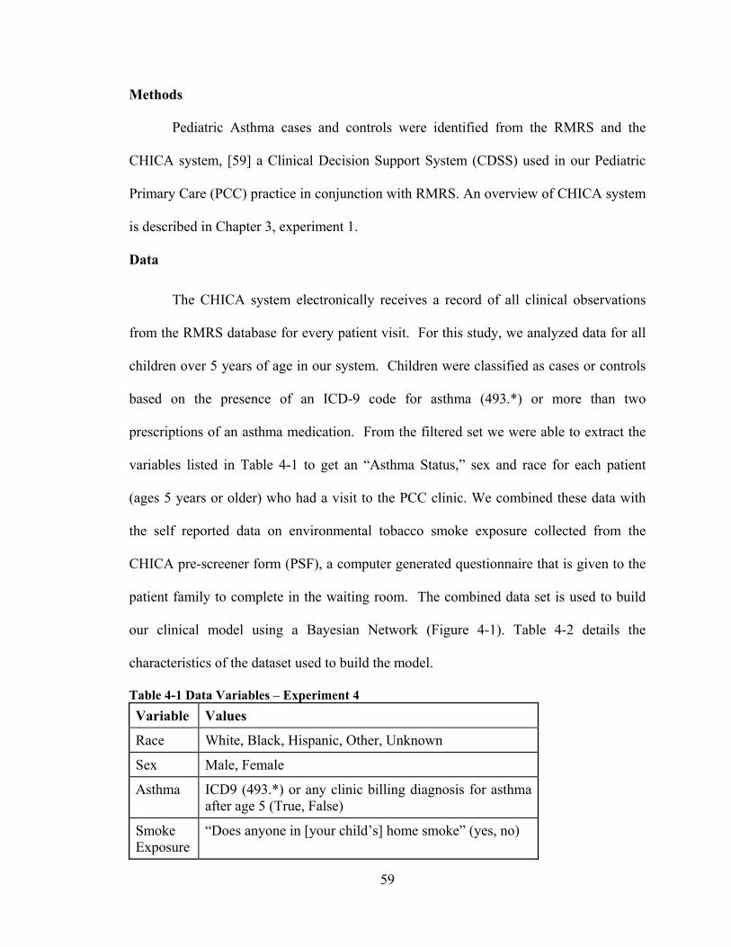
59

Methods

Pediatric Asthma cases and controls were identified from the RMRS and the

CHICA system, [59] a Clinical Decision Support System (CDSS) used in our Pediatric

Primary Care (PCC) practice in conjunction with RMRS. An overview of CHICA system

is described in Chapter 3, experiment 1.

Data

The CHICA system electronically receives a record of all clinical observations

from the RMRS database for every patient visit. For this study, we analyzed data for all

children over 5 years of age in our system. Children were classified as cases or controls

based on the presence of an ICD-9 code for asthma (493.*) or more than two

prescriptions of an asthma medication. From the filtered set we were able to extract the

variables listed in Table 4-1 to get an “Asthma Status,” sex and race for each patient

(ages 5 years or older) who had a visit to the PCC clinic. We combined these data with

the self reported data on environmental tobacco smoke exposure collected from the

CHICA pre-screener form (PSF), a computer generated questionnaire that is given to the

patient family to complete in the waiting room. The combined data set is used to build

our clinical model using a Bayesian Network (Figure 4-1). Table 4-2 details the

characteristics of the dataset used to build the model.

Table 4-1 Data Variables – Experiment 4

Variable Values

Race White, Black, Hispanic, Other, Unknown

Sex Male, Female

Asthma ICD9 (493.*) or any clinic billing diagnosis for asthma after age 5 (True, False)

Smoke Exposure

“Does anyone in [your child’s] home smoke” (yes, no)

60

Figure 4-1 Clinical Model (with limited nodes)

Table 4-2 Baseline Characteristics – Clinical model Variables Training Set (n = 2609)

# %

Race Hispanic (H) 597 23% Spanish (S) 89 3% Asian (X) 29 1% Islander (I) 3 < 1% Unknown (U) 6 0% Black (B) 1408 54% White (W) 382 15% Other (O) 95 4% Sex Female (F) 1246 48% Male (M) 1363 52% Asthma True (T) 666 26% False (F) 1943 75% Smoke Exp True (T) 579 22% False (F) 2030 78%

61

Bayesian Network for Clinical Model

We used Netica software [67] (www.norsys.com) to construct BN for our clinical

model (Figure 4-1). Netica allows network construction and parameter learning from

data. The model parameters were obtained using data from the CHICA database as

specified in the data section. At the time of this experiment the CHICA system provided

data on both asthma and smoke exposure status for about 2600 patients. The baseline

characteristics of the cohort for the training set are shown in Table 4-2. The prior

probability of asthma from this model is 26% (Figure 4-1).

Bayesian Network for the Genetic Model

We used a published case-control study – “Association of Asthma with Beta 2-

Adrenergic Receptor (β2AR) Gene Polymorphism and Cigarette Smoking” [50] to build

a genetic model linking genotype to smoke exposure and asthma. The study reported an

interaction between cigarette smoking and β2AR-16 genotype. It showed a synergistic

relationship between tobacco smoke exposure and the Arg-16 homozygous genotype with

respect to asthma. When compared with Gly-16 homozygotes who never smoked, the

smokers who were Arg-16 homozygotes had a significantly increased risk of asthma

(Odds ratio = 7.81). We used summary data from this study, adjusted for our

population’s asthma prevalence (26%), in our clinical model. Since the study reported

128 cases, our experiment required 364 controls (for a total of 492 subjects, resulting in a

26% prevalence). Therefore, we multiplied the number of controls in each genotype and

smoking status group by a factor*** (f = 2.68) (Table 4-3). We constructed a BN using

Netica software and learnt its parameters using the summary data in Table 4-3. This

constituted our genomic BN (Figure 4-3).

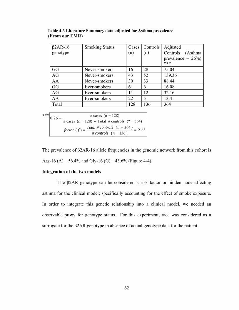
62

Table 4-3 Literature Summary data adjusted for Asthma prevalence (From our EMR)

β2AR-16 genotype

Smoking Status Cases (n)

Controls (n)

Adjusted Controls (Asthma prevalence = 26%) ***

GG Never-smokers 16 28 75.04 AG Never-smokers 43 52 139.36 AA Never-smokers 30 33 88.44 GG Ever-smokers 6 6 16.08 AG Ever-smokers 11 12 32.16 AA Ever-smokers 22 5 13.4 Total 128 136 364

***

68.2)136( #

)364( #)(

364) (? controls # Total 128) (n cases #

128)(n cases # 26.0

ncontrols

ncontrolsTotalffactor

The prevalence of β2AR-16 allele frequencies in the genomic network from this cohort is

Arg-16 (A) – 56.4% and Gly-16 (G) – 43.6% (Figure 4-4).

Integration of the two models

The β2AR genotype can be considered a risk factor or hidden node affecting

asthma for the clinical model; specifically accounting for the effect of smoke exposure.

In order to integrate this genetic relationship into a clinical model, we needed an

observable proxy for genotype status. For this experiment, race was considered as a

surrogate for the β2AR genotype in absence of actual genotype data for the patient.

63

Figure 4-2 Genomic Model (Genotype)

Figure 4-3 Genomic Model (Alleles)

Table 4-4 Allele Distribution by Race from public sources

Race Allele A (%) Allele G (%) White (W) 34.0 66.0 Black (B) 45.0 55.0 Hispanic (H) 44.0 56.0 Other (O)* 50.0 50.0 Spanish (S) 44.0 56.0 Asians (X) 55.0 45.0 Unknown (U)* 50.0 50.0 Islander (I)* 50.0 50.0

*Uniform distribution assumed since no info found

64

Table 4-4 lists the distribution of alleles A and G by race for β2AR genotype. We

obtained this distribution from publicly available databases – ALFRED

(http://alfred.med.yale.edu), PharmGKB (http://www.pharmgkb.org) and entrez SNP

(http://www.ncbi.nlm.nih.gov/snp) databases. Using this observable proxy, we did three

things to integrate as follows –

We first inserted the two explicit nodes for β2AR alleles (Figure 4-3) in the

clinical model (Figure 4-1) and used the distribution described in Table 4-4 to obtain the

conditional probability distribution (CPD) of allele1 and allele2 given race.

Second, since the CPD of asthma in the genetic model reflects the findings that

are reported in the presence or absence of smoke exposure in the study, we used the

adjusted published distribution (i.e. Figure 4-3) to replace the CPD of the asthma node in

our clinical model (Figure 4-1.). In the integrated model, we kept the CPD for smoke

exposure node from the clinical model since this is our population of interest.

Third, we compiled the integrated model using Netica’s compilation tool. This

operation creates a “junction tree” for “belief updating” and also calculates the full joint

probability distribution (JPD) of the resulting network – our integrated model is shown in

Figure 4-4.

65

Figure 4-4 Integrated model – Clinical and Genomic

The resulting prior probabilities of β2AR-16 alleles in this integrated model are –

Arg-16 (A) – 43.4%, Gly-16 (G) – 56.6%. They are different from the prevalence found

in the published study (A - 56.4% and G - 43.6%) and reflect the inferred distribution in

our population based on racial distribution. The network also compiled a resulting prior

probability of asthma (25%); quite close to the marginal prevalence in our clinical model

(26%), suggesting that the relationship between race and asthma could be mediated by

β2AR-16 genotype. In order to compare the two models – clinical with integrated, we

absorbed the allele nodes in the integrated model (Figure 4-5).

66

Figure 4-5 Model (with Allele nodes absorbed)

Also known as “averaging out” or “summing out a variable,” a node absorption

transform leaves the full joint probability distribution of the remaining nodes unchanged

and results in the final integrated model (Figure 4-5) that could be used for comparison.

Comparing the two models We compared the CPD of asthma node for the clinical and integrated models to

see how well the two distributions match. Our hypothesis was that associations between

genotype and phenotype could explain, at least in part, the clinical findings that we

observed in our population, specifically as the relationship between asthma and tobacco

smoke exposure. Table 4-5 lists the distribution of the asthma node in both models.

Goodness of fit Metric

We used a “Goodness of fit” as the comparison metric. [75] This metric is based

on the Chi-square distribution and the method of least squares. [75] The chi-square test

compares the observed frequencies with the expected frequencies, giving the probability

of observed differences under the null hypothesis (there is no difference). [76] The

method of least squares is built on the hypothesis that the optimum description of a set of

67

data is one which minimizes the weighted sum of squares of deviations of data (yi) from

the fitting function y(xi). [75] The variance of the fit s2, which is an estimate of the

variance of data σ2, characterizes this sum for v = N – n – 1 number of degrees of

freedom, where n coefficients fit to N data. Variance of fit s2 is also characterized by the

statistic χ2 as described in equation 1 below. Equation 2 describes the reduced chi-square

χ2v

}2

)]([21

{2

ixyiy

(1)

2

222

s

vv (2)

where σ2 in equation 2 is the weighted average of individual variances. However, the

estimated variance of fit s2 is also a characteristic of both the spread of the data and the

accuracy of the fit. [75] Therefore its definition as a ratio of the estimated variance s2 to

the parent variance σ2 (times the number of degrees of freedom) from equation 2 makes it

a convenient measure of the “goodness of fit.” If the fitting function is a good

approximation to the parent function, the estimated variance s2 should agree well with the

parent variance σ2 and the value of the reduced chi-square should be approximately unity

χ2v = 1. [75] Furthermore, the Q-Statistic defines the probability that a function Q(χ2/ν,

v) for a set of deviations obtained by randomly sampling N observations from normal

distribution would exceed the value for χ2/ν that was obtained by the fitting function. [75]

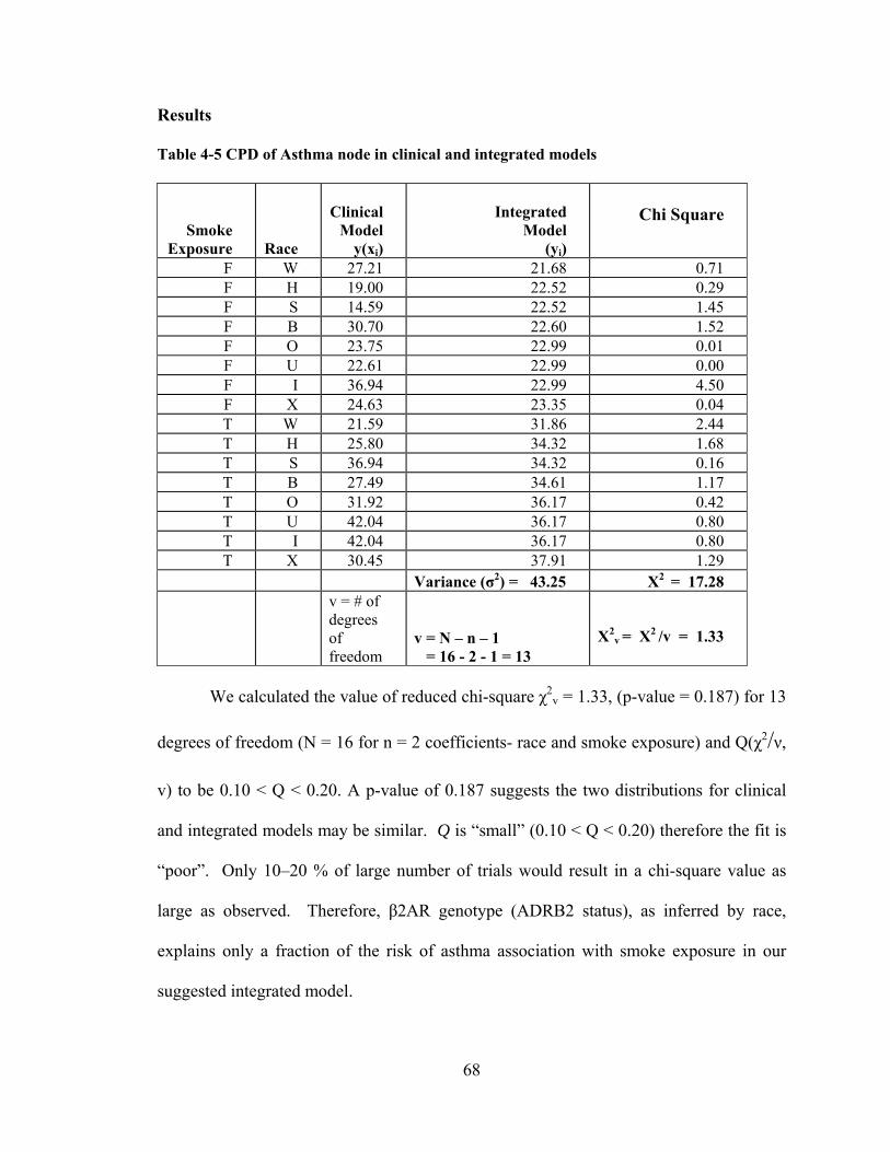
68

Results

Table 4-5 CPD of Asthma node in clinical and integrated models

Smoke Exposure Race

Clinical

Model y(xi)

Integrated Model

(yi)

Chi Square

F W 27.21 21.68 0.71F H 19.00 22.52 0.29F S 14.59 22.52 1.45F B 30.70 22.60 1.52F O 23.75 22.99 0.01F U 22.61 22.99 0.00F I 36.94 22.99 4.50F X 24.63 23.35 0.04T W 21.59 31.86 2.44T H 25.80 34.32 1.68T S 36.94 34.32 0.16T B 27.49 34.61 1.17T O 31.92 36.17 0.42T U 42.04 36.17 0.80T I 42.04 36.17 0.80T X 30.45 37.91 1.29

Variance (σ2) = 43.25 Х2 = 17.28

v = # of degrees of freedom

v = N – n – 1 = 16 - 2 - 1 = 13

Х2v = Х2 /v = 1.33

We calculated the value of reduced chi-square χ2v = 1.33, (p-value = 0.187) for 13

degrees of freedom (N = 16 for n = 2 coefficients- race and smoke exposure) and Q(χ2/ν,

v) to be 0.10 < Q < 0.20. A p-value of 0.187 suggests the two distributions for clinical

and integrated models may be similar. Q is “small” (0.10 < Q < 0.20) therefore the fit is

“poor”. Only 10–20 % of large number of trials would result in a chi-square value as

large as observed. Therefore, β2AR genotype (ADRB2 status), as inferred by race,

explains only a fraction of the risk of asthma association with smoke exposure in our

suggested integrated model.

69

Discussion

Our results are consistent with a minor contribution of the β2AR gene to the

association between asthma and smoke exposure observed in our EMR. One explanation

is that the association between the genotype (ADRB2 or β2AR) and the clinical condition

(asthma) in the literature was reported with “active smoking” in an adult population. Our

experiment models these associations for a pediatric population where the children are

exposed to environmental tobacco smoke or “passive smoking.” Asthma is also thought

to have a multigenic etiology. The incorporation of other associated genes into the model

is likely to improve its predictive power. Finally, the data associating race with genotype

is crude and incomplete. Therefore, race (the only surrogate available to us) is a poor

surrogate for genotype. A better surrogate would be helpful.

Conclusion

We have developed and demonstrated a methodology for integrating a published

data source with a primary data source – EMR. This methodology can be useful for

testing genetic hypotheses in large clinical data sets. The approach is applicable to a wide

range of genotypes that are associated with two or more clinically observed phenomena

(in this case asthma and smoke exposure). We believe this approach is worth

investigating for other common diseases like diabetes and obesity and their associations

with genomic and environmental findings.

70

Experiment 4: Integrating Disparate Sources of Summary Data

In-silico Bayesian Integration of GWA Studies (IsBIG)

Introduction

Our aim for this research is to develop probabilistic methods to integrate disparate

sources of data to form a coherent model even when no primary data are available using

secondary sources of information such as published summary and statistical measures for

knowledge discovery. In the last experiment, we demonstrated integration of genetic,

clinical and environmental sources using both data and published data summaries. To

demonstrate how this approach can be used to link secondary sources of data, we choose

the domain of genome wide association studies (GWAS). Using the NIH compiled

catalog of GWAS (www.genome.gov) and the database of human genome variations

from the international HapMap project (www.hapmap.org), we combine information

from these two secondary sources using BN framework as described in our previous

experiments. We call this model – In Silico Bayesian Integration of GWAS or IsBIG. In

this experiment we describe the methodology and report our preliminary results. In the

next chapter we formally evaluate the IsBIG model using data from our EMR and

published literature identified in the Pubmed database.

Genome Wide Association Studies (GWAS)

Genome Wide Association Studies (GWAS) have become the standard to report

associations of a genetic variation type – Single Nucleotide Polymorphism (SNP) with a

particular disease such as diabetes, heart and lung disease, autoimmune and psychiatric

disorders. It is only in very recent years with the advent of microarray technology and the

mapping of the variations of human genome (http://www.hapmap.org) [77-78] that the

71

tools to conduct genome wide scans for finding associations of gene to disease have

become available. The first results of the genome wide scans started to appear in 2005

[79] and since have become increasingly sophisticated in the number of gene loci that

they can address. Since the genome wide scans follow a specific methodology, they are

now known as Genome Wide Association Studies (GWAS).

At the heart of any GWA study is a cohort of individuals with a known disease or

trait status and a comparable control group without the disease or trait. Their whole

genome is genotyped for known variations of Single Nucleotide Polymorphism (SNP).

Such SNP variations have been cataloged among diverse populations in the international

HapMap [78] project. The results from the GWAS are analyzed for strong statistically

significant (below p < 5 x 10-8) associations between each SNP and the disease or trait

status of interest.

Thus, GWAS differ from traditional genetic linkage studies of the past where a

hypothesis driven candidate gene approach was being used. GWAS, to date, have

amassed large datasets linking genotype to phenotype and have provided many useful

insights [80] into certain diseases such as specific forms of cancer [81] and drug

metabolism, for example warfarin. [82] However, they are resource intensive and require

large sample sizes to detect even modest effect sizes, and yet their applications for

defining new therapies or preventive measures are largely unknown. [83] This is mainly

because the influence of the genetic variation to the phenotype is unclear and there is a

need to point to the causal variants; to move beyond the process of gene identification.

[84]

72

But as GWAS (often conducted by individual groups) reported ever more

potential etiologic and functional implications for similar diseases or traits [85-88], there

was a need to share the results beyond publication. Therefore, summary and statistical

results from these studies have been cataloged as an online resource for future

investigations at http://www.genome.gov/gwastudies [83] at NIH.

This catalog contains the following details on each study – population

characteristics, initial sample size, sub population type, strength of statistical association

as odds ratio (OR) or a beta coefficient (Beta), and the frequency of the risk allele in the

study. [83] However, to the best of our knowledge no secondary use of this catalog has

been reported.

In this catalog, the risk allele is the marker for the SNP that is found to be strongly

associated with the disease or trait. Additionally, from previous knowledge, the reported

SNPs in GWAS are known to follow non-random patterns of association between alleles

from different markers. [89] This is also known as linkage disequilibrium (LD) [90],

which we describe below.

Linkage Disequilibrium (LD)

LD is non-random association between SNP alleles from different markers, i.e.

SNP loci on the same or different chromosomes. Different geographic populations have

different allele frequencies, and therefore, LD differs between them. Thus the non-

random pattern of allele associations varies by sub populations – for example European

descent, Japanese ancestry, etc. [89, 91] LD is measured using correlation coefficient (r2)

[90] and varies between 0-1. Two alleles have a high LD score if the r2 value between

them is greater than 0.5 meaning that they are associated with each other in the population.

73

The international HapMap consortium (http://www.hapmap.org) [77] has developed a

haplotype map of the human genome, the HapMap, describing common patterns of human

DNA sequence variation. It has enabled LD data to be readily cataloged and available in

sub populations. Thus LD data quantitatively associates SNPs with other SNPs and can be

measured in a sub population using a tool such as SNP annotation and proxy search

(SNAP).

The SNAP tool, [92] available from Broad Institute at

(http://www.broadinstitute.org/mpg/snap) computes LD scores (r2) between SNPs up to

500 kilo base pairs apart and takes as input a list of SNPs of interest, a threshold value for

r2 above which to search the database and the sub population of interest. The output of the

tool is a paired list consisting of the input SNP and another SNP henceforth called “proxy”

SNP that exists in a non-random association above the given threshold cutoff value of r2 in

the HapMap database for the desired sub population.

Disparate Sources of information

We reasoned if diseases can be linked with SNPs and SNPs with one another,

then it should be possible to predict associations among diseases that could be mediated

through linked genetic determinants. Predicting quantitatively the associations among

diseases and traits that would be predicted by genetic patterns alone would allow us to

undertake three novel studies: (1) Validate the associations among diseases and traits

with electronic health record data (2) quantify the amount of variation among disease

linkages that can be explained by currently cataloged GWAS and linkage studies, (e.g.

heart disease and obesity) and (3) predict novel associations among diseases that could be

tested in future genetic studies.

74

In this experiment, we build a computational model (IsBIG) to integrate the two

disparate sources – 1) results from the studies cataloged in the NIH catalog [83] linking

SNPs to diseases or traits and 2) HapMap (www.hapmap.org) data associating SNPs to

other SNPs. With the IsBIG model, we hoped to find a disease map linking diseases to

other diseases that would be similar to what one would find in a clinical database such as

our EMR.

Methods

In-silico Bayesian Integration of GWAS (IsBIG) model

The IsBIG model was assembled in the following four steps. 1) Extract Gene-

Disease associations from the NIH catalog for a sub population to form a model catalog;

2) for the SNPs listed in this model catalog, compute genome wide LD scores (r2) from a

comparable sub population from the HapMap database to form a SNP-SNP (proxy)

association dataset; 3) for the SNPs linked by LD in the SNP-SNP (proxy) dataset, find

diseases or traits linked to each other pair wise as a result of LD. This formed the SNP-

SNP-Disease-Disease dataset for input to the IsBIG algorithm described in the following

sections. 4) Using this input, the IsBIG algorithm computes a BN with two separate

components in steps – a) SNP-SNP BN using LD (r2) to calculate CPDs. b) SNP-Disease

BN, using OR to calculate CPDs. Finally, the algorithm absorbs the SNP nodes (as

described below) to compute the disease-disease BN or the output of disease map. The

algorithm is coded using Java API and a commercially available software package for

modeling Bayesian networks – Netica’s API (www.norsys.com) [67]. The details of each

step are listed as follows.

75

Extract Gene-Disease Association

A copy of the GWAS catalog from the http://www.genome.gov/gwastudies/

website was downloaded on 12-28-09. The GWAS catalog contains information from a

wide range of GWAS studies associating specific SNPs to diseases or traits. From the

variables included in the catalog we chose the variables listed in Table 4-6 for the

experiment. Table 4-7 lists sample studies from the GWAS catalog. Appendix A.1

gives a summary of the studies from the GWAS catalog we used.

Table 4-6 Variables for Model Catalog

Table 4-7 Sample Studies in GWAS catalog

Disease /Trait

Risk Allele

SNP Risk Allele Freq

OR

Initial Sample Size

Type 1 diabetes G rs4900384 0.29 1.09

7,514 cases, 9,045 controls

Type 2 diabetes C rs4607103 0.76 1.09

4,549 cases, 5,579 controls

Multiple sclerosis

A rs1335532 0.87 1.28 1,618 cases 3,413 European ancestry controls

We planned to evaluate the model disease map with data from our EMR, the

RMRS [2]. Therefore we decided to use only those studies from the downloaded catalog

DISEASE/TRAIT Disease or trait examined in study

SNPS Strongest SNP

INITIAL SAMPLE SIZE Sample size for Stage 1 of GWAS, population subtype

RISK ALLELE FREQUENCY

Reported risk allele frequency associated with strongest SNP

OR or BETA Reported odds ratio or beta-coefficient associated with strongest SNP risk allele

76

where the initial population originated from European ancestry. Thus, we filtered studies

where the initial sample size variable did not contain population from European descent

(i.e. Japanese, Chinese, Korean, Gambian and other sub populations in the NIH catalog).

Where the sub population was not defined, we assumed it to be of European ancestry.

2564 GWAS studies consisting of 1708 unique SNPs from the GWAS catalog

were downloaded (in Dec. 2009). Of these 807 GWAS studies (Appendix A.1) qualified

as conducted in population with European ancestry. These studies contributed 182

unique disease traits and 850 unique SNPs in this sub population for our Model Catalog.

Gene (SNP) – Gene (SNP) Association

We extracted gene-gene associations from linkage disequilibrium data in the

HapMap database. [77] Since we decided to use studies with European ancestry

population, we used the HapMap CEU dataset (phase 3 release r2). Using the SNAP tool

[92] we derived LD between SNPs reported in our Model Catalog and other SNPs present

genome wide.

For our experiment, we used a LD score (r2) cutoff threshold value of 0.3. This

threshold was chosen empirically to capture weaker associations between SNPs and yet

keep our SNP to SNP (proxy) dataset computationally tractable. Higher and lower values

of cutoff threshold brought in fewer and more SNPs with stronger and weaker associations

respectively. However, empirically, this threshold (r2 = 0.3) provided an optimum set for

this experiment. Table 4-8 gives a snippet of the output from the SNAP tool for our input

SNP (e.g. rs2191566).

77

Table 4-8 Sample output from SNAP tool

SNP SNP (proxy) Distance r2

rs2191566 rs7255512 63311 0.616

rs2191566 rs8104605 77627 0.604

rs2191566 rs4803675 78327 0.561

Pair wise disease-disease associations using LD

When we searched in the HapMap phase 3 release 2 CEU dataset using the SNAP

tool, the 850 unique SNPs were in LD (r2 >= 0.3) with more than 16,000 proxy SNPs.

From these 16,879 proxy SNPs, we were only interested in the proxy SNPs that were also

reported in our Model Catalog and their associated diseases or traits. Therefore, we

imported the proxy SNP data produced by the SNAP tool and our Model Catalog in a

database. From there, we were able to do association mining to obtain SNPs that were

both in our model catalog and had a LD >= 0.3 with another SNP (proxy) in the Model

Catalog and obtain its associated disease or trait.

This resulted in 397 unique SNP to SNP pair-wise associations and their

associated disease or trait relationships (Appendix A.6) where LD between SNPs was < 1

(i.e. r2≠1). The lowest LD found in this association mining step was 0.302 and the highest

LD was 0.983 between two SNPs. Association mining with LD data from HapMap

provided us the ability to examine the model GWAS catalog beyond the pair wise single

SNP to disease or trait association. Table 4-9 shows some associations found between

diseases or traits using the LD scores of correlations (r2) derived from HapMap.

78

Table 4-9 Pair wise associations from GWAS catalog (by association mining)

Disease or Trait associated with a SNP

Disease or Trait associated with a SNP (proxy)

r2

Coronary Disease Glioma 0.384 Rheumatoid arthritis Inflammatory bowel

disease 0.389

Celiac disease Schizophrenia 0.400

Schizophrenia Celiac disease 0.400 Primary biliary cirrhosis Systemic lupus

erythematosus 0.425

Type 1 diabetes Rheumatoid arthritis 0.796

However, traditional statistical methods like correlation can only examine pair

wise relationships, and additionally carry the burden of identifying the actual functional

relationships (in this case between the SNP and the proxy SNP) and suffer from multiple

testing issues as well. Therefore, for analyzing functional relationships between common

diseases studied in GWAS, we need methods that handle complexity beyond the pair

wise paradigm. This is where Bayesian methods are useful – they compute the probability

of hypotheses rather than probability of committing an error [93] and model multiple

random variables whose probability distributions can be factorized into smaller

conditional probability distributions (CPD). [21]

We use this property of BN, to compute CPDs from available subsets of data, i.e.

from statistical data reported in the GWAS and from LD measure of correlations from

HapMap database, to form smaller BNs which, on absorbing the SNP nodes, combine in

one large BN – our disease map. We describe the In-silico Bayesian Integration of

GWAS (IsBIG) algorithm below.

79

In-Silico Bayesian Integration of GWAS (IsBIG) Algorithm (Figure 4-10)

We used the BN approach and causal independence assumption described in

Chapter 2 to draw a DAG of the SNP to SNP and SNP to disease or trait relationship.

The qualitative structure of this model is assembled from the input SNP-SNP-

Disease-Disease dataset (formed from association mining as described above) as

follows. The complete table is listed in Appendix A.6.

A directed edge connecting a SNP to another SNP (proxy) node is drawn

programmatically (using Netica API) if the SNPs are correlated (LD correlation) in

the input dataset. They assume a parent-child relationship from SNP to SNP (proxy).

Similarly a directed edge connecting each SNP to one or more diseases or traits is

drawn if they are correlated in the input GWAS data. Please note that in this dataset,

there are several SNP to SNP links, and therefore, there are N way interactions

because each SNP may be correlated with several others. Similarly, multiple SNPs

can be correlated with a disease. These multiply connected SNPs present a problem in

computing the conditional probability distributions (CPD) of the nodes that have

more than one parent because the data sources only describe one to one association

metrics. We address this problem of multiply connected SNPs with the method of

partial correlations described below.

Figure 4-6 below depicts the DAG of the model GWAS catalog constructed for

this study. In this figure S1, S2… Sn are the SNPs in the Model Catalog, they are in

LD (r2) with each other (from HapMap data) and have been shown to have strong

associations in GWAS with their respective diseases or traits (e.g. S2 to asthma). The

odds ratio (OR) quantifies the strength of each of the relationships between the SNP

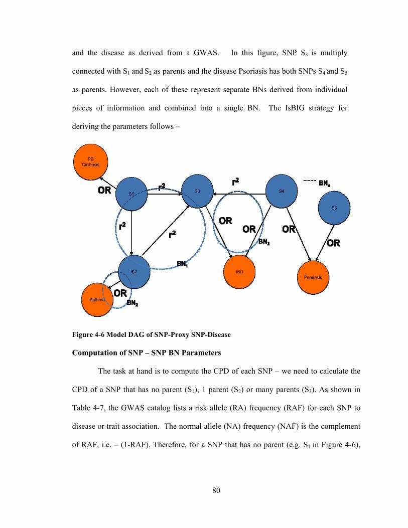
80

and the disease as derived from a GWAS. In this figure, SNP S3 is multiply

connected with S1 and S2 as parents and the disease Psoriasis has both SNPs S4 and S5

as parents. However, each of these represent separate BNs derived from individual

pieces of information and combined into a single BN. The IsBIG strategy for

deriving the parameters follows –

Figure 4-6 Model DAG of SNP-Proxy SNP-Disease Computation of SNP – SNP BN Parameters

The task at hand is to compute the CPD of each SNP – we need to calculate the

CPD of a SNP that has no parent (S1), 1 parent (S2) or many parents (S3). As shown in

Table 4-7, the GWAS catalog lists a risk allele (RA) frequency (RAF) for each SNP to

disease or trait association. The normal allele (NA) frequency (NAF) is the complement

of RAF, i.e. – (1-RAF). Therefore, for a SNP that has no parent (e.g. S1 in Figure 4-6),

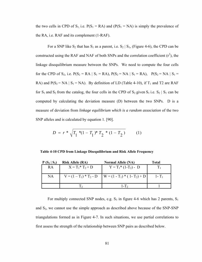
81

the two cells in CPD of S1, i.e. P(S1 = RA) and (P(S1 = NA) is simply the prevalence of

the RA, i.e. RAF and its complement (1-RAF).

For a SNP like S2 that has S1 as a parent, i.e. S2 | S1, (Figure 4-6), the CPD can be

constructed using the RAF and NAF of both SNPs and the correlation coefficient (r2), the

linkage disequilibrium measure between the SNPs. We need to compute the four cells

for the CPD of S2, i.e. P(S2 = RA | S1 = RA), P(S2 = NA | S1 = RA), P(S2 = NA | S1 =

RA) and P(S2 = NA | S1 = NA). By definition of LD (Table 4-10), if T1 and T2 are RAF

for S1 and S2 from the catalog, the four cells in the CPD of S2 given S1 i.e. S2 | S1 can be

computed by calculating the deviation measure (D) between the two SNPs. D is a

measure of deviation from linkage equilibrium which is a random association of the two

SNP alleles and is calculated by equation 1. [90].

Table 4-10 CPD from Linkage Disequilibrium and Risk Allele Frequency

P (S2 | S1) Risk Allele (RA) Normal Allele (NA) Total RA X = T1* T2 + D Y = T1* (1-T2) - D T1

NA V = (1 – T1) * T2 - D W = (1 - T1) * ( 1- T2) + D 1- T1

T2 1-T2 1

For multiply connected SNP nodes, e.g. S3 in figure 4-6 which has 2 parents, S1

and S2, we cannot use the simple approach as described above because of the SNP-SNP

triangulations formed as in Figure 4-7. In such situations, we use partial correlations to

first assess the strength of the relationship between SNP pairs as described below.

)1()2

1(*2

*)1

1(*1

* TTTTrD

82

Computation of CPD for multiply connected SNP

Figure 4-7 SNP-SNP Triangulations

Partial correlation quantifies the correlation between two variables x and y when

conditioning on one or several other variables [94], for example z. The 0th order

correlation is the regular correlation. The 1st order partial correlation between variables

x, y and z in Figure 4-7 is given by equation 2 below. For example, rxy-z is the correlation

between parts of x and y that are uncorrelated with z.

For calculating the CPD of a multiply connected SNP (e.g. S3 in Figure 4-6 which

has 2 parents, S1 and S2), the 1st order partial correlations are computed, ignoring the

directionality of the link to first assess whether the strength of the relationship between

the pairs S1-S2, S2-S3 and S1-S3 are above a predetermined threshold value. If the partial

correlation is below this threshold value (for example, 0.5), the link that has low partial

correlation value in the S1-S2-S3 triangulation is removed thus breaking the triangulation.

If no links are removed, we use partial correlation coefficients (r13-2, r23-1) for S1-S3 and

S2-S3 links to calculate two deviation measures (D) in equation, one for each parent, i.e.

P(S3| S1) and P(S3| S2). Now we have two sets of CPDs (four cells) for S3, one from each

)2()1)(1( 22

.

yzxz

yzxzxy

zxy

rr

rrrr

83

parent that we need to combine. Since these are independent linkages, i.e. S1-S3 and S2-

S3, we can combine them assuming causal independence using a Noisy-OR calculation as

described in Chapter 3. We can apply the same calculations for more than two parents,

however in our Model Catalog, the links were pruned and we rarely needed to calculate

beyond the single deviation measure.

Thus, applying partial correlations to our scenario pruned the links between SNPs

when there were triangulations of SNPs present and reduced the computational

complexity of calculating the CPDs of multiply connected SNPs. Specifically, links that

were weaker than a predetermined threshold value of partial correlation coefficient were

removed. For our experiment, we used a threshold value of 0.2 for 1st order partial

correlation. As we show later in the results, the threshold of partial correlations defined

how sparsely or densely the resulting network connected.

Computation of SNP – Disease BN Parameters

For each SNP-disease association to be modeled from a GWAS, the only data that

are available are the odds ratio (OR). Given a prior probability (aka disease prevalence)

of a disease or trait and the strength of the relationship (OR) from the GWAS, a posterior

probability (CPD) can be derived.

To derive a CPD from the prevalence P(Di), and an odds ratio, P(Di) must first be

converted to the prior odds (Oprior) of the disease according to equation 3. From there, the

posterior odds of the disease Oposterior can be calculated using prior odds and the odds ratio

reported in the GWA study (Ogwa) as in equation 4. [95]

)3()(1

)()(

i

i

DP

DPpriorO

84

From posterior odds of disease (or trait) we can find the probability Pi of the disease

given the SNP, i.e. P(Di | SNP) by equation 5 below.

Pi is the link probability [27] of the SNP to the disease or trait node in absence of any

other cause. For disease or trait nodes that have multiple links from SNPs (e.g. S4 to IBD

and Psoriasis in Figure 4-6), we assume causal independence of SNP to disease (as in the

GWAS). Therefore, in those situations, we calculate the CPD of the disease given the

SNPs, i.e. P (D | S1, S2…) using the Noisy-OR equation below (equation 6).

)6()1(1

pi

ip

ssp)S|P(D

The disease or trait’s prevalence P(Di) measure can either be specified by a

domain expert or from data, for example, from an EMR. Since in this experiment we are

developing the methodology, we arbitrarily assumed certain prevalence of common

diseases. For a formal evaluation of the IsBIG model in the next chapter, we used

prevalence measures from RMRS, our EMR.

)4()(*)()( gwaOpriorOposteriorO

)5()(1

)( )|(

posteriorO

posteriorOSNPDPP ii

85

Deriving Disease – Disease Map

We have constructed two components of a BN: SNP to SNP and SNP to disease

from two separate sources of information. Our goal in the next chapter will be to evaluate

the predictive power of this BN against clinical data from the RMRS. To do this, we

wish to reduce the BN to a disease map by absorbing out the SNP nodes which are

unobserved in clinical data. Node absorption is a network transform and is described in

the experiments in Chapter 3.

Results

Our preliminary results show that from the data in our model catalog, the IsBIG

model linked clinically related nodes of diseases or traits on absorbing the SNP nodes.

For example, testicular germ cell tumor was linked to testicular cancer, and chronic

obstructive pulmonary disease was linked to lung cancer, which was also linked to lung

adenocarcinoma. Similarly, coronary disease was linked to early myocardial infarction.

Some of the diseases the model linked are given in Table 4-11.

Table 4-11 Disease linkage patterns from GWAS catalog

Diet–Environment Obesity, Type 2 diabetes

Autoimmune1 Type 1 diabetes, Celiac disease, Inflammatory bowel disease

Autoimmune2 Psoriasis, Crohn’s Disease, Inflammatory Bowel Disease Celiac Disease, Multiple Sclerosis

Cardiac Coronary Disease, early Myocardial infarction, Intracranial Aneurysm, LDL cholesterol

Lung Lung cancer, Lung adenocarcinoma, Chronic obstructive pulmonary disease

Cancer Colorectal cancer, Prostate cancer

Traits Blond vs Brown hair color, Skin sensitivity to sun, Freckles, Red vs non-red hair color, Melanoma

86

We conducted normative evaluation of the IsBIG model. We used two part

criteria by varying the following network parameters – 1) LD threshold between SNPs

and 2) Partial correlation threshold used for pruning the SNP links and their effect on the

number of nodes and connectivity in the network.

Linkage Disequilibrium Threshold

LD threshold (r2) was chosen as r2 >= 0.1, r2 >= 0.3, and r2 >= 0.5, corresponding to

weak and strong associations between SNPs. Based on the LD threshold value used, we

expected the number of SNPs brought in the model from the HapMap dataset to increase

or decrease. As a result of this variation, the number of disease pairs that became part of

the model changed as well. Table 4-12 below details the number of SNP-SNP pairs and

disease pairs that entered the model based on the choice of LD threshold.

As can be seen in Table 4-12 (from Disease Pairs column) changing the network

parameter for linkage disequilibrium (LD) threshold between SNPs changes the number

of disease nodes that become part of the model. The number of disease nodes that

entered the model varied inversely to the LD threshold value chosen.

Table 4-12 Effect of LD Threshold on network size

LD (r2) Threshold SNP-SNP Pairs From HapMap Disease

Pairs

High / Low

LD

>=0.5 9416 134 0.982/0.505

>=0.3 16879 397 0.982/0.303

>=0.1 41485 518 0.982/0.101

87

Partial Correlation Threshold

Next we changed the partial correlation threshold values determining which links

were pruned between the SNPs when the triangulations existed (Figure 4-7). We

expected the network to become sparse when the partial correlation threshold was set

high ( >= 0.5) and to become dense when it was set low ( >= 0.2). Figure 4-8 shows a

sparsely connected DAG computed by IsBIG when 1st order partial correlation threshold

is set at r2 = 0.8. Figure 4-9 shows a computed DAG when 1st order partial correlation

threshold is set at r2 = 0.2 and when the SNP nodes are absorbed.

Discussion

We outlined a methodology that we call “In-silico Bayesian Integration” and

applied it to the domain of GWAS to build a model – In-silico Bayesian Integration of

GWAS or IsBIG. The IsBIG model is able to find relationships qualitatively and

quantitatively between various diseases or traits as inferred by the linked genetic

determinants of the disease or traits in the GWAS catalog. We made a few assumptions:

1) Where the population was not defined in the catalog, we assumed European descent. 2)

The strength of association between the SNP and the disease or trait (given by odds ratio)

is assumed for a single copy of the allele; the GWAS catalog does not detail about the

haplotype effect. 3) We focused on GWAS with discrete outcomes for diseases or traits

(i.e. absent / present). A majority of studies in the GWAS catalog list discrete outcomes

as opposed to the studies that describe change in a continuous trait like diastolic blood

pressure measured as mm Hg increase / decrease and where the strength of the

association is reported as a beta coefficient. 4) Lastly, we assumed independent causal

88

independence among SNPs affecting a disease or trait. This allowed us to combine the

individual effect using a Noisy-OR gate as described before.

Additionally, we made some empirical observations about the correlation

thresholds. These thresholds were chosen to keep the computational model tractable –

values below these thresholds (i.e. LD threshold value below 0.3 and partial correlation

threshold below 0.2) resulted in many more SNP nodes which had weaker associations.

However when they were included, the algorithm generated out of memory exceptions

when trying to absorb many more nodes due to the physical memory addressing

limitation of the Java Virtual Machine (2GB on a 32 bit operating system.) Exploring this

methodology on systems with greater memory addressing capacity was beyond the scope

of this exploratory research.

In Chapter 5 we evaluate our model quantitatively using data from our EMR, the

RMRS to quantify the amount of variation among disease linkages that can be explained

by studies currently cataloged in the domain of GWAS and to report any novel

associations the model finds.

89

Figure 4-8 IsBIG DAG (SNP-SNP r2 = 0.3, 1st order partial r2 = 0.8)

Primary_biliary_cirrhosis

TrueFalse

12.587.5

Crohn_s_disease

TrueFalse

70.529.5

Type_2_diabetes_and_other_tra

TrueFalse

14.685.4

Type_2_diabetes

TrueFalse

20.579.5

Glioma__high_grade_

TrueFalse

9.3690.6

Inflammatory_bowel_disease

TrueFalse

46.253.8

Myeloproliferative_neoplasms

TrueFalse

12.887.2

Myocardial_infarction__early_

TrueFalse

15.284.8

LDL_cholesterol

TrueFalse

2.2097.8

Glioma

TrueFalse

9.9290.1

Psoriasis

TrueFalse

7.9792.0

AIDS_progression

TrueFalse

1.2498.8

Drug_induced_liver_injury__fl

TrueFalse

3.7196.3

Colorectal_cancer

TrueFalse

15.784.3

Prostate_cancer

TrueFalse

29.071.0

Ulcerative_colitis

TrueFalse

47.552.5

Coronary_disease

TrueFalse

11.188.9

Systemic_lupus_erythematosus

TrueFalse

9.5190.5

Type_1_diabetes

TrueFalse

72.327.7

Multiple_sclerosis

TrueFalse

53.946.1

Inflammatory_bowel_disease__e

TrueFalse

9.1590.8

Schizophrenia

TrueFalse

26.573.5

Celiac_disease

TrueFalse

11.588.5

Rheumatoid_arthritis

TrueFalse

28.971.1

Testicular_germ_cell_tumor

TrueFalse

15.684.4

Testicular_cancer

TrueFalse

12.787.3

Intracranial_aneurysm

TrueFalse

6.9093.1

Amyotrophic_lateral_sclerosis

TrueFalse

7.3392.7

Chronic_Obstructive_Pulmonary

TrueFalse

4.4495.6

Lung_cancer

TrueFalse

18.381.7

Lung_adenocarcinoma

TrueFalse

10.789.3

Asthma

TrueFalse

12.287.8

Male_pattern_baldness

TrueFalse

12.887.2

Obesity__extreme_

TrueFalse

5.5794.4

Obesity__early_onset_extreme_

TrueFalse

6.3893.6

Obesity

TrueFalse

5.3594.6

Restless_legs_syndrome

TrueFalse

21.778.3

Breast_cancer

TrueFalse

13.186.9

Autism

TrueFalse

13.986.1

Melanoma

TrueFalse

1.4198.6

Skin_sensitivity_to_sun

TrueFalse

1.9798.0

Freckles

TrueFalse

2.6197.4

Red_vs_non_red_hair_color

TrueFalse

4.6595.4

Blond_vs__brown_hair_color

TrueFalse

1.6598.3

Atrial_fibrillation

TrueFalse

8.6691.3

90

Figure 4-9 IsBIG DAG (SNP-SNP r2 = 0.3, 1st order partial r2 = 0.2)

Table 4-13 Effect of Partial LD Threshold on network connectivity Partial correlation LD(r2) Threshold

# of triangulations

# of cycles removed

# of edges removed

# of SNPs with > 1 parent

>=0.1 28 7 17 18

>=0.2 28 6 30 13

>=0.35 28 6 41 9

Ulcerative_colitis

TrueFalse

47.552.5

Psoriasis

TrueFalse

7.9792.0

Crohn_s_disease

TrueFalse

70.030.0

Inflammatory_bowel_disease

TrueFalse

45.754.3

Drug_induced_liver_injury__fl

TrueFalse

3.7196.3

AIDS_progression

TrueFalse

1.2498.8

Primary_biliary_cirrhosis

TrueFalse

12.587.5

Asthma

TrueFalse

12.187.9

Myeloproliferative_neoplasms

TrueFalse

12.887.2

Glioma__high_grade_

TrueFalse

14.185.9

Glioma

TrueFalse

9.9290.1

Type_2_diabetes

TrueFalse

22.877.2

Coronary_disease

TrueFalse

11.188.9

Myocardial_infarction__early_

TrueFalse

15.284.8

Intracranial_aneurysm

TrueFalse

7.4592.5

Colorectal_cancer

TrueFalse

15.784.3

Prostate_cancer

TrueFalse

29.071.0

Type_2_diabetes_and_other_tra

TrueFalse

14.685.4

LDL_cholesterol

TrueFalse

2.2097.8

Systemic_lupus_erythematosus

TrueFalse

9.5190.5

Obesity__extreme_

TrueFalse

5.5794.4

Obesity

TrueFalse

6.2093.8

Obesity__early_onset_extreme_

TrueFalse

6.3893.6

Rheumatoid_arthritis

TrueFalse

28.971.1

Type_1_diabetes

TrueFalse

72.028.0

Multiple_sclerosis

TrueFalse

52.048.0

Inflammatory_bowel_disease__e

TrueFalse

9.1590.8

Celiac_disease

TrueFalse

11.588.5

Schizophrenia

TrueFalse

26.573.5

Breast_cancer

TrueFalse

15.484.6

Melanoma

TrueFalse

1.4198.6

Red_vs_non_red_hair_color

TrueFalse

4.6595.4

Freckles

TrueFalse

2.6197.4

Blond_vs__brown_hair_color

TrueFalse

1.6598.3

Skin_sensitivity_to_sun

TrueFalse

1.9798.0

Testicular_cancer

TrueFalse

12.787.3

Testicular_germ_cell_tumor

TrueFalse

15.684.4

Amyotrophic_lateral_sclerosis

TrueFalse

7.3392.7

Lung_adenocarcinoma

TrueFalse

10.789.3

Lung_cancer

TrueFalse

20.679.4

Chronic_Obstructive_Pulmonary

TrueFalse

4.4495.6

Male_pattern_baldness

TrueFalse

12.887.2

Restless_legs_syndrome

TrueFalse

21.778.3

Autism

TrueFalse

13.986.1

Atrial_fibrillation

TrueFalse

8.6691.3

91

Figure 4-10 In-silico Bayesian Integration of GWAS Algorithm

Find unique SNP-Proxy Pairs order by descending r2 value in set M.

Associate each SNP to its list of disease/traits and Proxy SNP to its list of disease trait in a hash map data structure D DrawDAG(): For each SNP in M

Make SNP a parent node p(i) and Proxy a child node c(i), if the nodes do not already exist in DAG. Draw a link from p(i) to c(i)

Triangulate(): For each SNP-Proxy pair in M

If SNP-Proxy have common child c(i)- mark it as a triangulation in set T

RemoveCycles(): For each SNP-Proxy pair in M

If proxy SNP has a child node c(i) that has the gwas SNP as a parent node p(i), reverse the link between c(i) and p(i)

Prune(): For each traingulation in T

Compute 1st order partial correlation of each pair. If 1st order partial correlation > defined threshold, keep the link otherwise mark it for removal in set R. Remove all links in set R, this results in SNP map DAG

DrawDAG_DiseaseTraits(): For each SNP in M

Make SNP a parent node p(i) and disease/trait a child node c(i), if the nodes do not already exist in DAG. Draw a link from p(i) to c(i)

Compute_CPD(): For each SNP-Proxy pair in M

Use known MAF of each SNP – Proxy duo from GWAS and LD (r2) value from HapMap data to compute P(S2|S1) as described using equation (1) and (2)

ComputeCPD_Disease (): For each SNP-Proxy pair in M and each SNP-Disease pair in D

Use equation (3)-(5) to compute P(D|Si). In cases where P(D|S1,S2), use Noisy-OR calculations using equation (6)

CompileNet(): Netica builds a “junction tree” for fast belief updating.

AbsorbSNP(): Absorb out all the SNP nodes in the compiled DAG

WriteDAG(): Serialize the compiled and absorbed DAG

92

Chapter 5 VALIDATION AGAINST PRIMARY EMR DATA

Introduction

In this chapter we present our evaluation of the unified BN constructed using the In-

silico Bayesian Integration methodology described in the previous chapter. In particular

we evaluate the In-silico Bayesian Integration of GWAS, hence forth called the IsBIG

model (or I-Model) with data from our EMR, the Regenstrief Medical Record System

(RMRS). [2]

We evaluate the IsBIG model with the following hypotheses –

1) IsBIG can discover disease-disease associations that are valid. These associations

can be confirmed and quantified meaningfully by testing against a) data from our EMR

and b) by evaluating against what has been published in the literature.

2) IsBIG can discover novel disease-disease associations. These associations do not

exist in the literature.

3) Genetic data can only explain a small fraction of the risk of the disease. IsBIG

model can quantify the proportion of risk of disease that can be explained by linked

genetic determinants.

Below we describe our methods to test the above three hypotheses. We believe

this study is novel as it quantifies the degree of associations found among diseases

determined by genetic linkages alone and compares it to a real world EMR.

Methods

For evaluation of disease-disease associations (hypothesis 1), we construct a

mixed model (M-Model) where the structure of the IsBIG DAG remains the same but its

conditional probability distributions (CPDs) are derived from our EMR, the RMRS. We

93

test the I-Model against this M-Model and PubMed searches. For evaluation of novel

disease-disease associations (hypothesis 2), we evaluate I-Model against published

literature in the PubMed database. To evaluate the proportion of the risk attributed to

linked genetic determinants (hypothesis 3), we evaluate I-Model against a purely clinical

model (C-Model) derived from RMRS. Below we describe each of these models but first

we describe the dataset derived from RMRS that is used for this evaluation.

EMR Data for evaluation

With IRB approval we obtained de-identified data from the Regenstrief EMR

(RMRS) for 169,711 individuals for 89 diseases. These diseases or proxies of these

diseases were also listed in our Model Catalog described in the previous chapter.

Extraction of these data was sought before the disease-disease relationships for I-Model

were known. The data obtained for each patient were extracted from the last 15 years of

the individual’s medical record, and for each disease each individual was coded as a case

or control using the ICD-9 diagnostic codes. The ICD-9 diagnostic codes were selected to

match the diseases in the GWAS catalog by a Regenstrief data core expert physician.

Thus, in this dataset the same individual can be a case for one or more diseases and a

control for others. The dataset had no missing values and henceforth is referred to as the

“Regenstrief dataset”. We randomly split the Regenstrief dataset into 2/3 training set

(112,829 records) and 1/3 test set (56,882 records) for our evaluation. Next, we describe

construction of each of the models, i.e. learning the parameters of the M-Model and

deriving the DAG and parameters of the C-Model from the Regenstrief training set.

94

I-Model Construction

The IsBIG model (I-model) was built using software developed by the author,

using Java and Netica software [67] APIs. The software implements the IsBIG algorithm

as described in Chapter 5 and produces a network file (.dne) suitable for representation

and inference by Netica software. The Java code for the algorithm is included in

Appendix A.9. The input for computing the model consisted of the following network

parameters – LD threshold value of r2 >= 0.3 for SNP to SNP correlation and partial

correlation threshold values = 0.2. These network parameters were chosen empirically to

keep the computational model tractable and yet include weaker correlations of SNPs to

test with a real world sub population using RMRS data. The pre– processed input (from

the GWAS catalog and HapMap data) for the IsBIG algorithm is detailed in Appendix

A.6, and its pre processing (association mining) is described in Chapter 5. The prevalence

data for the modeled diseases was derived from our EMR. (Appendix A.7)

M-Model Construction

The mixed model retained the network structure that was derived from the IsBIG

algorithm, i.e. the DAG structure of the I-Model. Using Netica’s “case file” interface, the

2/3 training set was used to learn the conditional probability distributions (CPD) of each

node (disease) in the I-Model DAG. Netica resets any CPDs to uninformed priors (50-50)

for each of the nodes before a case file is incorporated. Thus, incorporating the training

set transformed the IsBIG model (I-Model) to the mixed model (M-Model) with network

structure derived from the GWAS and SNP data and conditional probability distributions

learnt from the clinical data from RMRS. Similar to the I-Model, the M-Model was also

evaluated for its discriminative power using the same test dataset from RMRS.

95

C-Model Construction

Using the Winmine toolkit [68] and the 2/3 split training set (same as above), we

mined the structure of a DAG that represents the clinical model or the C-Model (Figure

5-1). In this DAG, 42 of the 89 diseases or traits from the initial dataset were connected

by an edge with another disease or trait. The rest of the diseases were either disconnected

or, because in the GWAS catalog they listed as a continuous trait, they could not be

evaluated by the discrete Winmine algorithm.

Winmine uses a greedy algorithm to mine the best structure for the DAG, given the

data. This mined DAG was then implemented using Netica [67] Bayesian Network

software. The conditional probability distributions for this DAG were learnt from the

same 2/3 split training set from which the structure was mined. Thus this model

represented the DAG structure and parameters; both learnt from clinical data and became

our clinical model (C-Model). Similar to the other two models, the C-Model was

evaluated for its discriminative or predictive power using the same test dataset from

RMRS.

96

Figure 5-1 DAG Structure of C-Model learnt from RMRS Training set Performance measure

We use Area Under the Curve (AUC) of Receiver Operating Characteristic

(ROC) curves [57] as a performance measure for evaluating the discriminative power of

the three BNs. The ROC curve performance measure is described before in Chapter 2. A

ROC with AUC of 0.5 score has no predictive value and is as good as chance.

Computing Area under the Curve (AUC)

We used Netica’s “test interface” and the randomly split 1/3 test set from RMRS

to evaluate the performance for discrimination of cases and controls for each disease by

calculating the AUCs for each of the 42 diseases or the subset of them in each of the

DAGs.

Testing for statistical significance

We did a test of hypothesis for each model constructed above as follows. For each

disease node, we tested whether the BN had statistically significant predictive power (i.e.,

97

AUC significantly greater than 0.5) using the Hanley and McNeil method described in

[96] for calculating the standard error from which z-scores can be calculated without

distributional assumptions (i.e. based on the count of normal and abnormal cases in the

test set). The results of these tests are listed in Appendix A.2 to A.4 and described below.

Additionally, to compare the predictive power of the M-Model and the C-Model,

we used the Hanley McNeil method for ROC derived from same cases [72] to compare

ROCs for the same disease. Please note the that both these models differ in structure, but

the conditional probability distributions were learnt from the same training set and they

were tested using the same test set.

Evaluation of IsBIG Compared to Published Literature

To evaluate the I-Model, we evaluated direct pair wise associations (Appendix

A.4) between diseases that the IsBIG algorithm found against – 1) PubMed database

searches, 2) direct pair wise associations between diseases in C-Model, i.e. DAG derived

from EMR and 3) against both of the above combined. We searched the PubMed

database for articles linking the diseases found to be associated in the IsBIG DAG by

searching for one disease as a keyword with a boolean AND condition to the second

condition, for example – Primary Biliary Cirrhosis AND Crohn’s Disease. These

searches were conducted in May 2010. The number of articles meeting these simple

criteria was counted for our measure.

Results

I-Model Evaluation with Test set

29 of the 42 diseases (Appendix A.2) from Regenstrief EMR were included in the

I-Model construction by the IsBIG software with the chosen network parameters

98

described above. With the 1/3 randomly split test set, the I-Model predicted 5 (17%) of

the 29 diseases or traits with an area under the curve (AUC > 0.5, p < 0.05). In other

words the network had the discriminative power to differentiate cases from controls from

our EMR test set for 17% of diseases. The diseases that were predicted with statistical

significance in I-Model are listed in Table 5-1 below and highlighted in Appendix A.2.

Table 5-1 Discriminative power in IsBIG (I-Model)

  Node  AUC p‐value 

1  Coronary Disease  0.6856 0

2  Lung cancer  0.6263 0

3  LDL Cholesterol (Elevated) 0.5823 0

4  Type 2 Diabetes  0.5431 0

5  Obesity  0.5192 4.73E‐09

M-Model Evaluation with Test set

As described before, the I-Model was parameterized for its 29 nodes using the 2/3

randomly split training set. This parameterization transformed the I-Model into the M-

Model. Using the same 1/3 test set (as before), the M-Model predicted 12 (41%) of the 29

diseases or traits with an area under the curve (AUC > 0.5, p < 0.05). The diseases that

were predicted with statistical significance in M-Model are listed in Table 5-2 below and

highlighted in Appendix A.3.

Table 5-2 Predictable diseases in Parameterized IsBIG (M-Model)

  Node  AUC p‐value 1  Myocardia l Infarction Early 0.937 0

2  Coronary Disease  0.7318 0

3  Psoriasis  0.6343 0

4  Lung cancer  0.6263 0

5  Systemic Lupus Erythematosus 0.5947 2.08E‐06

6  LDL Cholesterol Elevated 0.5945 0

7  Rheumatoid Arthritis 0.5871 0

8  Chronic Obstructive Pulmonary Disorder 0.533 1.2E‐10

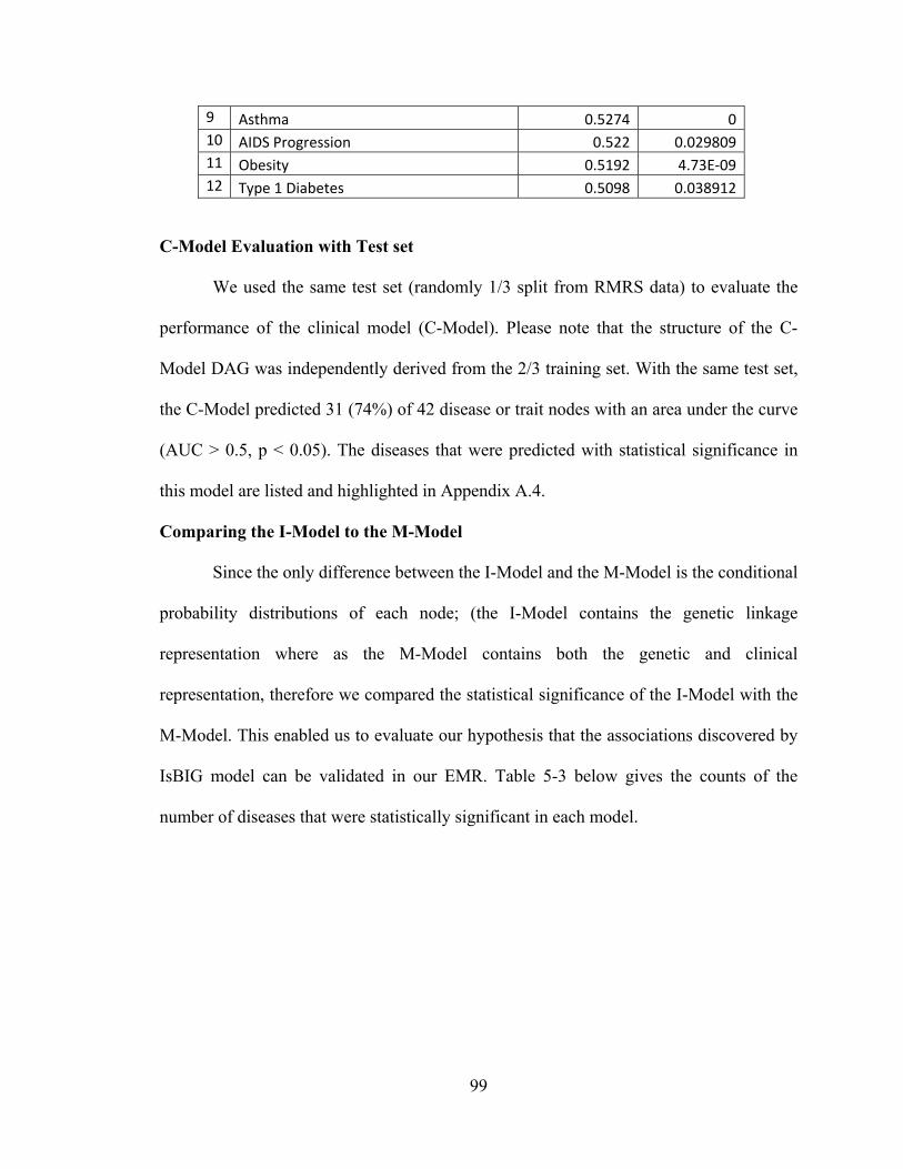
99

9  Asthma  0.5274 0

10  AIDS Progression  0.522 0.029809

11  Obesity  0.5192 4.73E‐09

12  Type 1 Diabetes  0.5098 0.038912

C-Model Evaluation with Test set

We used the same test set (randomly 1/3 split from RMRS data) to evaluate the

performance of the clinical model (C-Model). Please note that the structure of the C-

Model DAG was independently derived from the 2/3 training set. With the same test set,

the C-Model predicted 31 (74%) of 42 disease or trait nodes with an area under the curve

(AUC > 0.5, p < 0.05). The diseases that were predicted with statistical significance in

this model are listed and highlighted in Appendix A.4.

Comparing the I-Model to the M-Model

Since the only difference between the I-Model and the M-Model is the conditional

probability distributions of each node; (the I-Model contains the genetic linkage

representation where as the M-Model contains both the genetic and clinical

representation, therefore we compared the statistical significance of the I-Model with the

M-Model. This enabled us to evaluate our hypothesis that the associations discovered by

IsBIG model can be validated in our EMR. Table 5-3 below gives the counts of the

number of diseases that were statistically significant in each model.

100

Figure 5-2 IsBIG Model performance, statistical significance denoted by

Table 5-3 Number of statistically significant diseases predicted by each model

+ -

+ 4 1

- 8 16

Predicted diseases denoted by +

Of the 29 diseases, 5 were predictable by the I-Model and 12 were predictable by

the M-Model (AUC > 0.5, p < 0.05). There were 4 diseases common to both the I-Model

and the M-Model, i.e. the I-Model is 33% sensitive when compared to M-Model. There

0

0.1

0.2

0.3

0.4

0.5

0.6

0.7

0.8

0.9

1

I‐Model

M‐Model

A U C

I-Model Vs M-Model

M-Model

I-Model

101

were 17 diseases not predictable by the M-Model, of those, 16 were common to both the

models i.e. I-Model is 94% specific when compared to the M-Model. The details of the

disease nodes marked with a colored dot for statistical significance are in Figure 5-2

above.

Of the 4 diseases predictable by the I-Model and the M-Model, the networked

performed the same for Obesity and Lung Cancer i.e. AUCs did not change on

computation of conditional probability distributions (parameterization) of the nodes. For

the other diseases, there was a modest gain (1 to 14%) in the discriminative power of the

IsBIG DAG on parameterization with the EMR data i.e. in the M-Model (Figure 5-3).

Figure 5-3 Change in IsBIG AUC on parameterization

There were a few exceptions though, most notably for early detection of

Myocardial infarction. The M-Model’s discriminative power (AUC) increased by 44%,

i.e. a relative jump of 87% when compared to the I-Model. However, surprisingly on the

‐5%0%5%10%15%20%25%30%35%40%45%

Type_2_d

iabetes

Lung_cancer

Obesity

Type_1_d

iabetes

LDL_cholesterol

Asthma

AIDS_progression

Chronic_O

bstructive_…

Coronary_disease

Rheu

matoid_arthritis

System

ic_lupus_eryth…

Psoriasis

Myocardial_infarction…

Difference in AUC between I‐Model and M‐Model

Difference in AUC between I‐Model and M‐Model

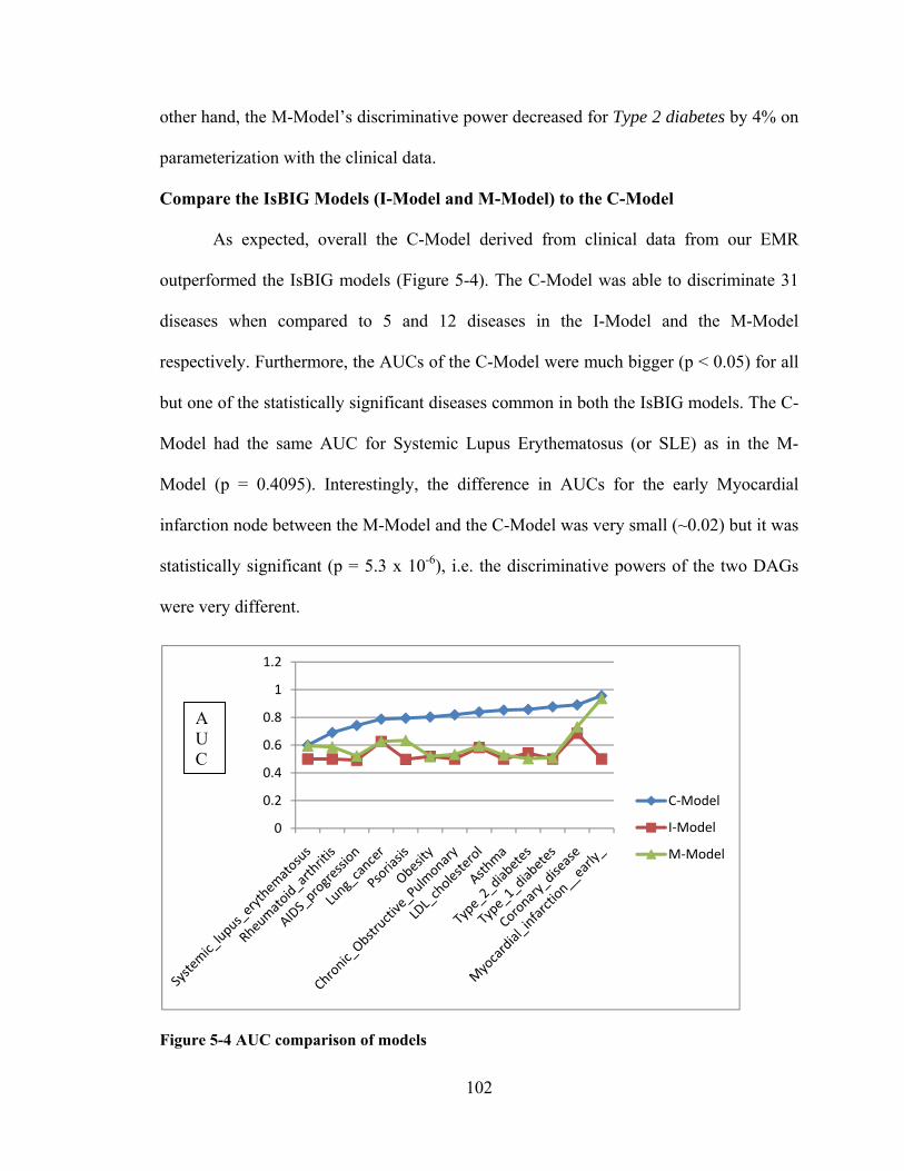
102

other hand, the M-Model’s discriminative power decreased for Type 2 diabetes by 4% on

parameterization with the clinical data.

Compare the IsBIG Models (I-Model and M-Model) to the C-Model

As expected, overall the C-Model derived from clinical data from our EMR

outperformed the IsBIG models (Figure 5-4). The C-Model was able to discriminate 31

diseases when compared to 5 and 12 diseases in the I-Model and the M-Model

respectively. Furthermore, the AUCs of the C-Model were much bigger (p < 0.05) for all

but one of the statistically significant diseases common in both the IsBIG models. The C-

Model had the same AUC for Systemic Lupus Erythematosus (or SLE) as in the M-

Model (p = 0.4095). Interestingly, the difference in AUCs for the early Myocardial

infarction node between the M-Model and the C-Model was very small (~0.02) but it was

statistically significant (p = 5.3 x 10-6), i.e. the discriminative powers of the two DAGs

were very different.

Figure 5-4 AUC comparison of models

0

0.2

0.4

0.6

0.8

1

1.2

C‐Model

I‐Model

M‐Model

A U C

103

Compare the I-Model against PubMed Literature searches

We evaluated 117 direct pair wise (parent-child) associations (Appendix A.4) in the

I-Model against the PubMed database literature searches. Twenty (17%) of the pair wise

associations in the I-Model had no references in the literature and can be possibly

considered novel. At least 1 of these associations (Rheumatoid Arthritis with Systemic

Lupus Erythematosus) was also found in direct pair wise associations in the C-Model

(Table 5-4).

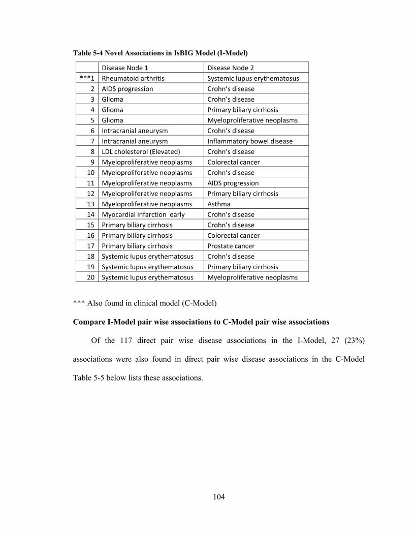
104

Table 5-4 Novel Associations in IsBIG Model (I-Model)

*** Also found in clinical model (C-Model)

Compare I-Model pair wise associations to C-Model pair wise associations

Of the 117 direct pair wise disease associations in the I-Model, 27 (23%)

associations were also found in direct pair wise disease associations in the C-Model

Table 5-5 below lists these associations.

   Disease Node 1  Disease Node 2

***1  Rheumatoid arthritis  Systemic lupus erythematosus 

2  AIDS progression  Crohn’s disease

3  Glioma  Crohn’s disease

4  Glioma  Primary biliary cirrhosis

5  Glioma  Myeloproliferative neoplasms 

6  Intracranial aneurysm Crohn’s disease

7  Intracranial aneurysm Inflammatory bowel disease 

8  LDL cholesterol (Elevated) Crohn’s disease

9  Myeloproliferative neoplasms Colorectal cancer

10  Myeloproliferative neoplasms Crohn’s disease

11  Myeloproliferative neoplasms AIDS progression

12  Myeloproliferative neoplasms Primary biliary cirrhosis

13  Myeloproliferative neoplasms Asthma

14  Myocardial infarction  early  Crohn’s disease

15  Primary biliary cirrhosis Crohn’s disease

16  Primary biliary cirrhosis Colorectal cancer

17  Primary biliary cirrhosis Prostate cancer

18  Systemic lupus erythematosus Crohn’s disease

19  Systemic lupus erythematosus Primary biliary cirrhosis

20  Systemic lupus erythematosus Myeloproliferative neoplasms 

105

Table 5-5 Associations common in IsBIG Model with C-Model (with literature reference count)

   Disease Node 1  Disease Node 2PubMED Ref count

1  Rheumatoid arthritis Systemic lupus erythematosus  0 

2  Coronary disease  Crohn’s disease 1 

3  LDL cholesterol (Elevated) AIDS progression 4 

4  Coronary disease  Glioma 5 

5  Asthma  AIDS progression 6 

6  Myocardial infarction  early  AIDS progression 9 

7  LDL cholesterol (Elevated) Glioma 11

8  LDL cholesterol (Elevated) Inflammatory bowel disease  12

9  Glioma  Asthma 24

10  Crohn’s disease  Ulcerative colitis 32

11  Inflammatory bowel disease Crohn’s disease 33

12  LDL cholesterol (Elevated) Psoriasis 33

13  LDL cholesterol (Elevated) Myocardial infarction  early   35

14  Myocardial infarction  early  Inflammatory bowel disease  38

15  Coronary disease  AIDS progression 50

16  Chronic Obstructive Pulmonary Lung cancer 51

17  Coronary disease  Inflammatory bowel disease  51

18  Coronary disease  Psoriasis 66

19  LDL cholesterol (Elevated) Coronary disease 160

20  Multiple sclerosis  Asthma 233

21  Asthma  Psoriasis 261

22  Inflammatory bowel disease Ulcerative colitis 262

23  Asthma  Inflammatory bowel disease  271

24  Obesity  Type 2 diabetes 320

25  Rheumatoid arthritis Asthma 894

26  Schizophrenia  Type 1 diabetes 931

27  Myocardial infarction  early  Coronary disease 54128

Literature Ref count of pair wise associations in I-Model (also found in C-Model)

Of the 27 pair wise disease associations in the I-Model that were also found in the

C-Model, 1 (4%) association had no literature reference, 5 (19%) had up to 10 references.

These disease associations can be possibly considered as worth exploring further in future

106

studies. Additionally, 9 (33%) associations had only up to 50 references. The details are

listed in Figure 5-4 below and Table 5-5 above.

Figure 5-5 Reference count of IsBIG associations also found in C-Model Discussion

We have described our IsBIG methodology and applied it to combine statistical

correlations between SNPs and GWAS to generate a disease map of common diseases,

the IsBIG model as inferred from genetic underpinnings. We evaluated the model against

both raw clinical data and published literature.

Our results show that IsBIG discovered disease-disease associations are valid.

We tested this by training the IsBIG DAG with RMRS data and found that IsBIG

correctly found 33% of the diseases in the M-Model; and of the associations found by

IsBIG, 80% of them were confirmed in the M-Model. This essentially means that for the

4 diseases or traits (Coronary Disease, Elevated LDL Cholesterol, Lung Cancer and

Obesity) predictable by IsBIG, there is discriminative power in the model as inferred by

genetic variations alone in the population. We also found that the IsBIG model has the

same discriminative power for early detection of Myocardial Infarction as the same

model trained on clinical data (i.e. M-Model).

# of Associations in both PubMED and C‐Model

0

<=10

<=50

<=55,000

107

IsBIG can discover novel disease-disease associations that have not been

described. We compared disease-disease associations to the PubMed database and found

that many had never been described. We believe these associations can be considered as

hypotheses for future studies. Furthermore, we were able to confirm some of them in the

clinical model (C-Model). At least one pair wise disease association (Rheumatoid

arthritis and Systemic lupus Erythematosus) found by IsBIG had no reference in the

literature and can be considered novel, and further, it can be confirmed by the C-Model

derived from our EMR data.

Finally, our results show that probabilistic methods can extract data from

disparate sources and combine them in a normative way such that it correlates with what

we may empirically find in an EMR. Only a fraction of associations among diseases

found in an EMR can be explained by genetics of SNP to disease linkage. We compared

the AUCs of IsBIG and the C-Model and found that the C-Model AUCs were much

bigger. Therefore, genetic data alone can only explain a small fraction of the risk of a

disease.

108

Chapter 6 DISCUSSION

Summary of findings

In this work, we formed a methodology which we call In-silico Bayesian

Integration, to integrate data from disparate sources using probabilistic modeling

methods, specifically the Bayesian Network framework. We demonstrated that this

methodology can combine information in a normative way and that the results can be

validated against real world datasets from our EMR. Additionally, we demonstrated that

the model built using this methodology discovers new knowledge that can be used as

hypotheses for future studies.

As an example of our approach, we combined two disparate sources – the genetic

linkages (associations) found between Single Nucleotide Polymorphisms (SNP) in the

human genome and the effect size linking a SNP with a disease or a trait found in

Genome Wide Association Studies (GWAS). We call this model In-silico Bayesian

Integration of GWAS (or IsBIG). IsBIG produces a map of disease-disease associations

as inferred from their genetic underpinnings.

Seventeen percent of disease-disease associations found by the IsBIG model are not

described in the literature and can be considered novel, with at least one association

confirmed in our EMR. Furthermore, our results show that IsBIG finds meaningful

associations that can be empirically validated against our EMR. The IsBIG model is 33%

sensitive, 94% specific and has a positive predictive value of 80% when we evaluate its

discriminative power compared to our EMR data. We found from this evaluation that

GWA studies in the domain of Obesity, Type 2 Diabetes, elevated LDL Cholesterol trait,

Lung cancer and Coronary Disease have signal to detect effect of genetic variations to

109

disease likelihood in our clinical population and may have potential clinical applications.

By generating a predictive distribution of disease-disease associations, the IsBIG model

has also quantified that the simple linking of genetics to a disease only explains a fraction

of the risk of disease in our EMR.

Summary of contributions

Applying Bayesian Networks to the real world task of integrating data from

disparate sources required the use of causal independence assumptions (Independence of

Causal Influence models, ICI) particularly the Noisy-OR model. Our empiric evaluations

of the BN framework with ICI model using large datasets from our EMR produced

comparable results to that of an expert. Therefore, in this research we have demonstrated

that ICI models provide a successful strategy for computing conditional distributions of a

large BN with many linked nodes in a tractable way. We believe the use of ICI models,

particularly the use of Noisy-OR model seems to be robust under a broad range of

conditions. To the best of our knowledge, this has not been demonstrated before,

especially in the biomedical field.

Additionally, we have also shown that the use of Noisy-OR model provides a

successful strategy for combining disparate sources, where individual conditional

distributions can be computed from effect sizes and statistical correlations. We have

demonstrated it by utilizing odds ratios and correlation and partial correlation coefficients

as strategies to translate genetic data from published GWAS into conditional probability

distributions for disease associations. This has not been demonstrated before to the best

of our knowledge.

110

There is no analytic method, to the best of our knowledge, which computationally

combines disparate source of both raw data and summary measures in a quantitative

framework. Applications of text mining using ontology [97] and more recently

applications of semantic web technology coupled with graph algorithms [98] have been

used to find associations between biological entities from different sources of

information. However, they rely on purely qualitative associations; i.e. subject-predicate-

object relationships, for example, drug A may cause symptom B sometimes is

represented by a triplet such as <A causes B>. However this representation does not

account for the uncertainty (“may”) in the assertion. The knowledge that the relationship

between A and B exists say 2% of the times is not represented in this framework. Such

frameworks lay out a graph of the associations but do not produce predictive distributions

of these associations. On the other hand, quantitative methods such as meta-analysis of

studies are able to give more precise estimates of the effect size by pooling effect sizes

from a number of studies under assumptions, but they are not a computational model that

can be used for future inference. They also do not permit for additional information to be

incorporated as it becomes available. Other quantitative methods, in particular data

mining methods which are computational and can generate predictive distributions,

require a large numbers of cases for model building, training and testing. These datasets

seldom exist in the biomedical domain for use in hypotheses generation tools.

Therefore, due to the lack of these original datasets, in this work, we have

developed a quantitative method using Bayesian Networks framework to combine both

raw data and summary measures in a computational model. The method is able to

discover new associations from disparate sources and is able to produce predictive

111

distributions for these associations. It is also able to incorporate new information as it

becomes available. Our evaluation of this method shows correlation to large real world

datasets.

On Use of Causal Independence Assumption (Noisy-OR)

The Bayesian network framework does not constrain how a variable depends

upon its parents. One interpretation is that the directed edges or arcs represent causal

relationships among the parent and the child. Thus the local structure encodes the

dependencies and probability distributions of parent and child (conditioned upon

parents). The probability distribution of the child node can be approximated assuming

causal independence among the parents using a boolean function such as OR, but since

the parent-child relationship is probabilistic, the relationship is “noisy”.

The underlying assumption in this situation is that each parent acts independently

as a cause to the child (effect) with an independent mechanism of action, and each parent

can sufficiently cause the effect. In the absence of any parent, there is no effect, unless

we assume a leaky model.

Without the causal independence assumption, we had no way of combining the

SNP’s effect size to a disease. These assumptions allowed us to combine the contribution

of each existing cause (SNP) to the effect (disease) with fewer calculations then the

calculations for full conditional probability distribution. Additionally they allowed the

flexibility of tractably adding new causes in the future. It is these capabilities of Noisy-

OR that we exploited in this research to combine information (data or statistical

summaries) in a causal (normative) way.

112

Limitations

One of the limitations of our methodology is the approximation of the underlying

data – we modeled only discrete variables. This assumption allowed us to compute

conditional probability tables (CPTs) using a boolean function such as OR in the Noisy-

OR calculations. For this research, the boolean function “OR” and discrete data fitted our

assumption of the real world datasets but may not hold true for other datasets. In future

studies, there may be disparate sets that may need combinations of other boolean

functions such as AND or XOR, besides OR. Nonetheless, similar methodology can be

applied in such situations by replacing the Noisy-OR calculations with the one that fits

the datasets. For example, if we make the assumption that both genetics and environment

lead to a disease status, we may want to model it using a Noisy AND. For modeling

continuous variables, methods similar to Monte Carlo simulations [99] assuming a-priori

probability distributions can be applied.

Another assumption in this study is that effect sizes or correlations are defined for

one variable to the outcome variable. When using effect sizes (such as odds ratio) to link

two different BNs to calculate CPTs, we are assuming the effect is attributable to a single

variable. For example, for the IsBIG study, it is the odds ratio or strength of association

of single allele to the disease or trait in the study. There may be situations, where this

assumption does not hold true. The effect size could result from more than one variable.

For example, two copies of a specific allele may produce more than an additive effect as

is the case in recessive traits. In those situations, assuming causal independence between

the two causal variables (for e.g. between alleles) and the outcome variable will not be

justified.

113

Lastly, though the IsBIG study illustrated how disparate datasets, summary or

statistical measures from different sources can be combined. However, the information in

both the sources belonged to a similar population (i.e. European Ancestry). We propose

that as a variable, such as the LD measure, varies by a sub-population, this should be

accounted for in the model when disparate sources are combined.

Future Directions

We believe our methodology has been successfully applied in integrating sub

domains, especially in the biomedical domain and has many practical applications. We

envision that using this method secondary data sources such as summary and statistical

data from published sources can be merged with data from primary sources such as

electronic health records to provide a more normative and quantitative evaluation of the

domain.

We are envisioning one such application of this method for dynamic prioritization

of the reminder prompts in our CHICA system. [59] CHICA’s static, global prioritization

scheme limits the flexibility of the system by evaluating the predetermined prompts for

primary care alerts from a set of guidelines for a specific age group. At present there are

many such guidelines and recommendations. [100-104] We plan to use Bayesian

networks (BN) as a strategy for modeling a patient’s clinical status with the idea of

calculating the expected value of making alternative recommendations to physicians in

order to tailor prioritization to the patient, [63] using the research in this thesis.

114

APPENDICES

Appendix A.1 Summary of Studies from GWAS Catalog

Disease/Trait  Number of Studies 

Type 2 diabetes 67

Type 1 diabetes 62

Crohn's disease  61

Bipolar disorder  43

Multiple sclerosis  41

Prostate cancer 37

Amyotrophic lateral sclerosis  28

Rheumatoid arthritis  24

Schizophrenia  24

Ulcerative colitis  19

Acute lymphoblastic leukemia (childhood) 17

Breast cancer  16

Lung cancer  16

Colorectal cancer  15

Parkinson's disease  14

Smoking behavior  14

Obesity (extreme)  13

Psoriasis  12

Response to treatment for acute lymphoblastic leukemia  12

Systemic lupus erythematosus 12

Coronary disease  11

Celiac disease  10

Myocardial infarction (early onset) 9

Nonsyndromic cleft lip with or without cleft palate 9

Inflammatory bowel disease  8

AIDS  7

Alzheimer's disease  7

Glioma  7

Response to citalopram treatment 7

Alcohol dependence  6

Chronic lymphocytic leukemia 6

Drug‐induced liver injury (flucloxacillin) 6

Melanoma  6

Restless legs syndrome  6

Testicular germ cell tumor  6

Type 2 diabetes and other traits 6

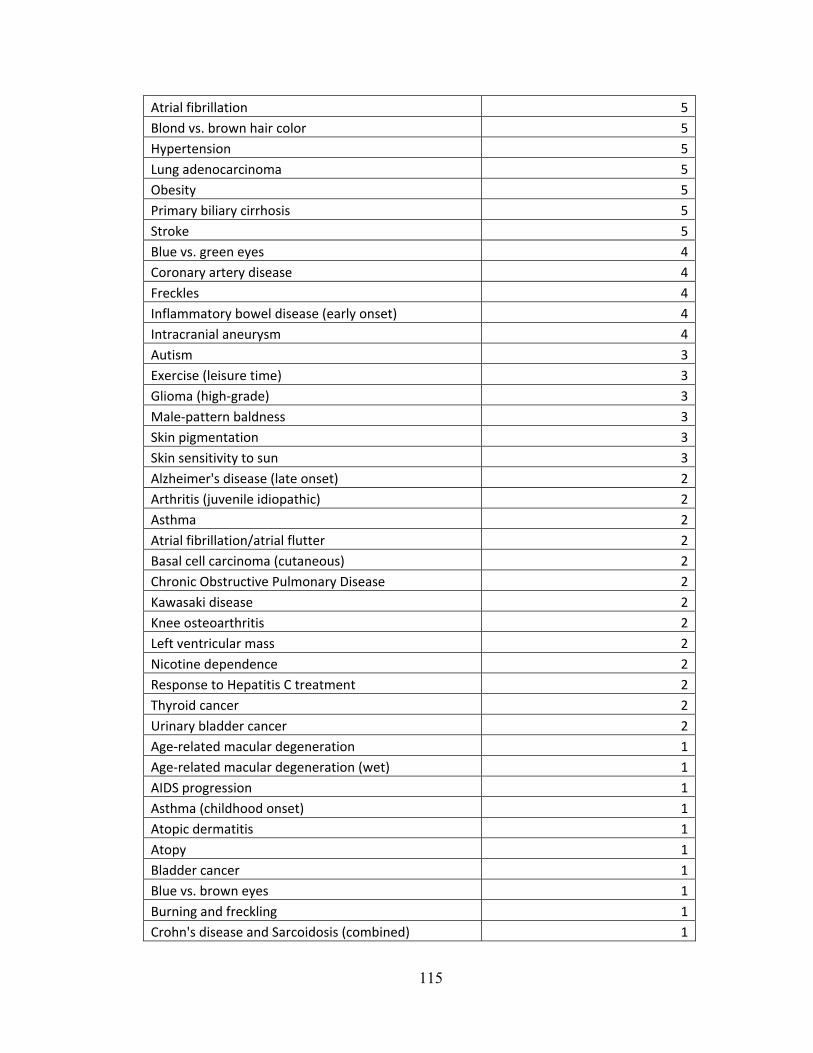
115

Atrial fibrillation  5

Blond vs. brown hair color  5

Hypertension  5

Lung adenocarcinoma  5

Obesity  5

Primary biliary cirrhosis  5

Stroke  5

Blue vs. green eyes  4

Coronary artery disease  4

Freckles  4

Inflammatory bowel disease (early onset) 4

Intracranial aneurysm  4

Autism  3

Exercise (leisure time)  3

Glioma (high‐grade)  3

Male‐pattern baldness  3

Skin pigmentation  3

Skin sensitivity to sun  3

Alzheimer's disease (late onset) 2

Arthritis (juvenile idiopathic)  2

Asthma  2

Atrial fibrillation/atrial flutter  2

Basal cell carcinoma (cutaneous) 2

Chronic Obstructive Pulmonary Disease 2

Kawasaki disease  2

Knee osteoarthritis  2

Left ventricular mass  2

Nicotine dependence  2

Response to Hepatitis C treatment 2

Thyroid cancer  2

Urinary bladder cancer  2

Age‐related macular degeneration 1

Age‐related macular degeneration (wet) 1

AIDS progression  1

Asthma (childhood onset)  1

Atopic dermatitis  1

Atopy  1

Bladder cancer  1

Blue vs. brown eyes  1

Burning and freckling  1

Crohn's disease and Sarcoidosis (combined) 1

116

Diabetic nephropathy  1

Disease/Trait  1

End‐stage renal disease  1

Essential tremor  1

Follicular lymphoma  1

Gallstones  1

Glaucoma (exfoliation)  1

Height  1

Ischemic stroke  1

Kidney stones  1

LDL cholesterol  1

Major depressive disorder  1

Myeloproliferative neoplasms 1

Myocardial infarction  1

Narcolepsy  1

Neuroblastoma  1

Neuroblastoma (high‐risk)  1

Neuroticism  1

Obesity (early onset extreme) 1

Osteonecrosis of the jaw  1

Otosclerosis  1

Ovarian cancer  1

Pancreatic cancer  1

Parkinson's disease (familial)  1

Periodontitis  1

QT interval prolongation  1

Red vs. non‐red hair color  1

Red vs. non‐red hair color  1

Renal function and chronic kidney disease 1

Response to antipsychotic treatment 1

Response to statin therapy  1

Response to ximelagatran treatment 1

Testicular cancer  1

Venous thromboembolism  1

  807

117

Appendix A.2 AUC and p-values in IsBIG model (I-Model)

  Node  AUC p‐value 

1  Coronary Disease  0.6856 0 

2  Lung cancer  0.6263 0 

3  LDL  0.5823 0 

4  Type 2 Diabetes  0.5431 0 

5  Obesity  0.5192 4.73E‐09 

6  AIDS Progression  0.4917 0.234547 

7  Psoriasis  0.4976 0.351112 

8  Asthma  0.4998 0.470214 

9  MI_Early  0.5 0.5 

10  SLE  0.5 0.5 

11  Type 1 Diabetes  0.5 0.5 

12  Prostate Cancer  0.5 0.5 

13  RA  0.5 0.5 

14  COPD  0.5 0.5 

15  Ulcerative Colitis  0.5 0.5 

16  Testicular cancer  0.5 0.5 

17  Schizophrenia  0.5 0.5 

19  Primary Biliary Cirrhosis  0.5 0.5 

19  Myeloproliferative Neoplasms 0.5 0.5 

20  Melanoma 0.5 0.5 

21  Intracranial Aneurysm  0.5 0.5 

22  Inflammatory Bowel Disease 0.5 0.5 

23  Crohn’s Disease  0.5 0.5 

24  Colorectal cancer  0.5 0.5 

25  Celiac Disease  0.5 0.5 

26  Autism  0.5 0.5 

27  Atrial Fibrillation  0.5 0.5 

28  Multiple Sclerosis  0.5 0.5 

29  Glioma  0.4703 0.13301 

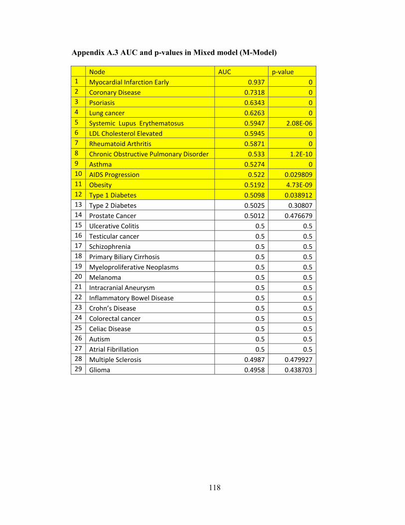
118

Appendix A.3 AUC and p-values in Mixed model (M-Model)

  Node  AUC p‐value 1  Myocardial Infarction Early 0.937 0 2  Coronary Disease  0.7318 0 3  Psoriasis  0.6343 0 4  Lung cancer  0.6263 0 5  Systemic  Lupus  Erythematosus 0.5947 2.08E‐06 6  LDL Cholesterol Elevated  0.5945 0 7  Rheumatoid Arthritis  0.5871 0 8  Chronic Obstructive Pulmonary Disorder 0.533 1.2E‐10 9  Asthma  0.5274 0 10  AIDS Progression  0.522 0.029809 11  Obesity  0.5192 4.73E‐09 12  Type 1 Diabetes  0.5098 0.038912 13  Type 2 Diabetes  0.5025 0.30807 14  Prostate Cancer  0.5012 0.476679 15  Ulcerative Colitis  0.5 0.5 16  Testicular cancer  0.5 0.5 17  Schizophrenia  0.5 0.5 18  Primary Biliary Cirrhosis  0.5 0.5 19  Myeloproliferative Neoplasms 0.5 0.5 20  Melanoma  0.5 0.5 21  Intracranial Aneurysm  0.5 0.5 22  Inflammatory Bowel Disease 0.5 0.5 23  Crohn’s Disease  0.5 0.5 24  Colorectal cancer  0.5 0.5 25  Celiac Disease  0.5 0.5 26  Autism  0.5 0.5 27  Atrial Fibrillation  0.5 0.5 28  Multiple Sclerosis  0.4987 0.479927 29  Glioma  0.4958 0.438703 

119

Appendix A.4 AUC and p-value in Clinical Model (C-Model)

Node AUC p-value 1 Crohn’s Disease 0.9985 0 2 Ulcerative Colitis 0.9969 0 3 Myocardial Infarction Early 0.9568 0 4 Coronary Disease 0.8906 0 5 Type 1 Diabetes 0.8766 0 6 Schizophrenia 0.862 0 7 Type 2 Diabetes 0.8581 0 8 Atrial Fibrilliation 0.8577 0 9 Asthma 0.853 0 10 LDL Cholesterol Elevated 0.8392 0 11 Bipolar 0.8268 0 12 Chronic Obstructive Pulmonary Disorder 0.8192 0 13 Obesity 0.8034 0 14 Nicotine Dependence 0.8013 0 15 Psoriasis 0.7947 0 16 Lung cancer 0.788 0 17 Breast cancer 0.7805 0 18 Ischemic Stroke 0.7603 0 19 Autism 0.7501 0 20 AIDS Progression 0.7423 0 21 Venous thromboembolism 0.7239 0 22 Colorectal Cancer 0.7051 0.001966 23 Knee osteoarthritis 0.7003 0 24 Rheumatoid Arthritis 0.6908 0 25 Prostate Cancer 0.6702 0 26 Glioma 0.6546 2.29E-08 27 Restless Leg Syndrome 0.6241 0.000132 28 Testicular cancer 0.6139 0.001118 29 Systemic Lupus Erythematosus 0.6 5.93E-07 30 Intracranial Aneurysm 0.5884 0.006792 31 Pancreatic Cancer 0.5757 0.005877 32 Follicular Lymphoma 0.5526 0.122542 33 Myeloproliferative Neoplasms 0.5433 0.111934 34 Melanoma 0.5268 0.173608 35 Acute Leukemia 0.5 0.5 36 Otosclerosis 0.5 0.5 37 Celiac Disease 0.5 0.5 38 Chronic Leukemia 0.5 0.5

120

39 IBD 0.5 0.5 40 Multiple Sclerosis 0.5 0.5 41 Parkinson 0.5 0.5 42 Primary Biliary Cirrhosis 0.5 0.5

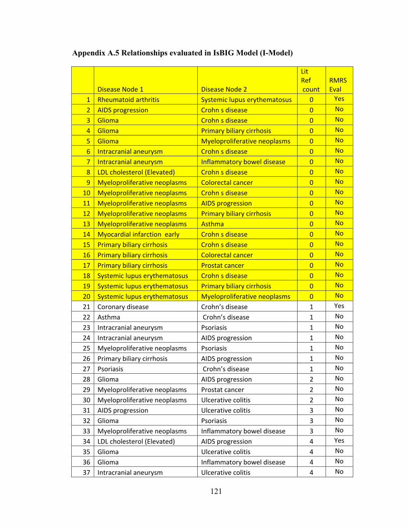
121

Appendix A.5 Relationships evaluated in IsBIG Model (I-Model)

   Disease Node 1  Disease Node 2

Lit Ref  count 

RMRS Eval

1  Rheumatoid arthritis  Systemic lupus erythematosus  0  Yes

2  AIDS progression  Crohn s disease 0  No

3  Glioma  Crohn s disease 0  No

4  Glioma  Primary biliary cirrhosis 0  No

5  Glioma  Myeloproliferative neoplasms  0  No

6  Intracranial aneurysm  Crohn s disease 0  No

7  Intracranial aneurysm  Inflammatory bowel disease 0  No

8  LDL cholesterol (Elevated) Crohn s disease 0  No

9  Myeloproliferative neoplasms Colorectal cancer 0  No

10  Myeloproliferative neoplasms Crohn s disease 0  No

11  Myeloproliferative neoplasms AIDS progression 0  No

12  Myeloproliferative neoplasms Primary biliary cirrhosis 0  No

13  Myeloproliferative neoplasms Asthma 0  No

14  Myocardial infarction  early  Crohn s disease 0  No

15  Primary biliary cirrhosis Crohn s disease 0  No

16  Primary biliary cirrhosis Colorectal cancer 0  No

17  Primary biliary cirrhosis Prostat cancer 0  No

18  Systemic lupus erythematosus Crohn s disease 0  No

19  Systemic lupus erythematosus Primary biliary cirrhosis 0  No

20  Systemic lupus erythematosus Myeloproliferative neoplasms  0  No

21  Coronary disease  Crohn’s disease 1  Yes

22  Asthma   Crohn’s disease 1  No

23  Intracranial aneurysm  Psoriasis 1  No

24  Intracranial aneurysm  AIDS progression 1  No

25  Myeloproliferative neoplasms Psoriasis 1  No

26  Primary biliary cirrhosis AIDS progression 1  No

27  Psoriasis   Crohn’s disease 1  No

28  Glioma  AIDS progression 2  No

29  Myeloproliferative neoplasms Prostat cancer 2  No

30  Myeloproliferative neoplasms Ulcerative colitis 2  No

31  AIDS progression  Ulcerative colitis 3  No

32  Glioma  Psoriasis 3  No

33  Myeloproliferative neoplasms Inflammatory bowel disease 3  No

34  LDL cholesterol (Elevated) AIDS progression 4  Yes

35  Glioma  Ulcerative colitis 4  No

36  Glioma  Inflammatory bowel disease 4  No

37  Intracranial aneurysm  Ulcerative colitis 4  No

122

38  Rheumatoid arthritis   Crohn’s disease 4  No

39  Coronary disease  Glioma 5  Yes

40  Colorectal cancer   Crohn’s disease 5  No

41  Intracranial aneurysm  LDL cholesterol (Elevated) 5  No

42  Asthma  AIDS progression 6  Yes

43  Colorectal cancer  AIDS progression 6  No

44  Myocardial infarction  early  Glioma 7  No

45  Systemic lupus erythematosus AIDS progression 8  No

46  Myocardial infarction  early  AIDS progression 9  Yes

47  Prostate cancer  AIDS progression 10  No

48  LDL cholesterol (Elevated) Glioma 11  Yes

49  Asthma  Primary biliary cirrhosis 11  No

50  Colorectal cancer  Psoriasis 11  No

51  Glioma  Systemic lupus erythematosus  11  No

52  Intracranial aneurysm  Prostat cancer 11  No

53  LDL cholesterol (Elevated) Ulcerative colitis 11  No

54  LDL cholesterol (Elevated) Inflammatory bowel disease 12  Yes

55  AIDS progression  Psoriasis 12  No

56  AIDS progression  Inflammatory bowel disease 12  No

57  Prostate cancer  Psoriasis 15  No

58  Celiac disease  Type 1 diabetes 17  No

59  Multiple sclerosis  Systemic lupus erythematosus  17  No

60  Primary biliary cirrhosis Psoriasis 19  No

61  Prostate cancer  Ulcerative colitis 23  No

62  Glioma  Asthma 24  Yes

63  Prostate cancer  Inflammatory bowel disease 28  No

64   Crohn’s disease  Ulcerative colitis 32  Yes

65  Inflammatory bowel disease  Crohn’s disease 33  Yes

66  LDL cholesterol (Elevated) Psoriasis 33  Yes

67  Multiple sclerosis  Primary biliary cirrhosis 33  No

68  LDL cholesterol (Elevated) Myocardial infarction  early  35  Yes

69  Myocardial infarction  early  Inflammatory bowel disease 38  Yes

70  Intracranial aneurysm  Colorectal cancer 41  No

71  Myocardial infarction  early  Ulcerative colitis 47  No

72  Coronary disease  AIDS progression 50  Yes

73  Chronic Obstructive Pulmonary Lung cancer 51  Yes

74  Coronary disease  Inflammatory bowel disease 51  Yes

75  Multiple sclerosis  Rheumatoid arthritis 58  No

76  Coronary disease  Psoriasis 66  Yes

77  Celiac disease  Asthma 66  No

78  Celiac disease  Multiple sclerosis 68  No

123

79  Glioma  Colorectal cancer 68  No

80  Schizophrenia  Celiac disease 71  No

81  Inflammatory bowel disease Psoriasis 80  No

82  Myocardial infarction  early  Psoriasis 82  No

83  Celiac disease  Primary biliary cirrhosis 86  No

84  Celiac disease  Systemic lupus erythematosus  96  No

85  Type 1 diabetes  Primary biliary cirrhosis 100  No

86  Intracranial aneurysm  Coronary disease 104  No

87  Intracranial aneurysm  Glioma 110  No

88  Intracranial aneurysm  Myocardial infarction  early  117  No

89  Primary biliary cirrhosis Inflammatory bowel disease 117  No

90  Intracranial aneurysm  Type 2 diabetes 137  No

91  Glioma  Prostat cancer 138  No

92  Primary biliary cirrhosis Ulcerative colitis 145  No

93  Coronary disease  Ulcerative colitis 151  No

94  LDL cholesterol (Elevated) Coronary disease 160  Yes

95  Intracranial aneurysm  Systemic lupus erythematosus  166  No

96  Celiac disease  Rheumatoid arthritis 178  No

97  Systemic lupus erythematosus Inflammatory bowel disease 182  No

98  Rheumatoid arthritis  Primary biliary cirrhosis 184  No

99  Psoriasis  Ulcerative colitis 201  No

100  Systemic lupus erythematosus Ulcerative colitis 207  No

101  Multiple sclerosis  Asthma 233  Yes

102  Asthma  Ulcerative colitis 238  No

103  Asthma  Psoriasis 261  Yes

104  Inflammatory bowel disease Ulcerative colitis 262  Yes

105  Asthma  Inflammatory bowel disease 271  Yes

106  Obesity  Type 2 diabetes 320  Yes

107  Systemic lupus erythematosus Psoriasis 521  No

108  Prostate cancer  Colorectal cancer 882  No

109  Rheumatoid arthritis  Asthma 894  Yes

110  Type 1 diabetes  Systemic lupus erythematosus  894  No

111  Schizophrenia  Type 1 diabetes 931  Yes

112  Colorectal cancer  Ulcerative colitis 1019  No

113  Type 1 diabetes  Multiple sclerosis 1032  No

114  Type 1 diabetes  Rheumatoid arthritis 1990  No

115  Intracranial aneurysm  Myeloproliferative neoplasms  4126  No

116  Colorectal cancer  Inflammatory bowel disease 37538  No

117  Myocardial infarction  early  Coronary disease 54128  Yes

124

Appendix A.6 Input to the IsBIG Algorithm for constructing I-Model

  SNP1   SNP2

LD (r2)

SNP1 OR

SNP2 OR

SNP1 RAF 

SNP2 RAF 

1  rs564398  rs1412829 0.983 1.13 1.42 0.56  0.39 

2  rs11190140  rs10883365 0.983 1.2 1.18 0.48  0.48 

3  rs11190140  rs10883365 0.983 1.2 1.2 0.48  0.48 

4  rs10883365  rs11190140 0.983 1.18 1.2 0.48  0.48 

5  rs10883365  rs11190140 0.983 1.2 1.2 0.48  0.48 

6  rs1412829  rs564398 0.983 1.42 1.13 0.39  0.56 

7  rs4263839  rs6478109 0.982 1.22 1.36 0.68  0.69 

8  rs6478109  rs4263839 0.982 1.36 1.22 0.69  0.68 

9  rs6074022  rs4810485 0.977 1.2 1.15 0.25  0.25 

10  rs4810485  rs6074022 0.977 1.15 1.2 0.25  0.25 

11  rs13277113  rs2736340 0.976 1.39 1.19 0.23  0.24 

12  rs2736340  rs13277113 0.976 1.19 1.39 0.24  0.23 

13  rs3135388  rs9271366 0.974 2.75 2.78 0.22  0.15 

14  rs3135388  rs9271366 0.974 1.99 2.78 0.23  0.15 

15  rs9271366  rs3135388 0.974 2.78 2.75 0.15  0.22 

16  rs9271366  rs3135388 0.974 2.78 1.99 0.15  0.23 

17  rs2981582  rs1219648 0.966 1.26 1.2 0.38  0.4 

18  rs7931342  rs10896449 0.966 1.19 1.1 0.51  0.52 

19  rs2241880  rs10210302 0.966 1.45 1.19 0.55  0.48 

20  rs10210302  rs2241880 0.966 1.19 1.45 0.48  0.55 

21  rs1219648  rs2981582 0.966 1.2 1.26 0.4  0.38 

22  rs10896449  rs7931342 0.966 1.1 1.19 0.52  0.51 

23  rs1335532  rs2300747 0.964 1.28 1.3 0.87  0.88 

24  rs2300747  rs1335532 0.964 1.3 1.28 0.88  0.87 

25  rs4506565  rs7901695 0.96 1.36 1.37 0.32  NR 

26  rs7901695  rs4506565 0.96 1.37 1.36 NR  0.32 

27  rs6931514  rs7756992 0.958 1.25 1.2 NR  0.26 

28  rs7756992  rs6931514 0.958 1.2 1.25 0.26  NR 

29  rs3197999  rs9858542 0.956 1.2 1.17 0.27  0.29 

30  rs3197999  rs9858542 0.956 1.2 1.09 0.27  0.28 

31  rs9858542  rs3197999 0.956 1.17 1.2 0.29  0.27 

32  rs9858542  rs3197999 0.956 1.09 1.2 0.28  0.27 

33  rs9941349  rs1121980 0.95 1.48 1.66 0.43  0.41 

34  rs907092  rs2872507 0.95 1.29 1.12 0.45  0.47 

35  rs2872507  rs907092 0.95 1.12 1.29 0.47  0.45 

36  rs1121980  rs9941349 0.95 1.66 1.48 0.41  0.43 

125

37  rs11755527  rs3757247 0.949 1.13 1.13 0.47  NR 

38  rs3757247  rs11755527 0.949 1.13 1.13 NR  0.47 

39  rs477515  rs2395185 0.948 1.38 1.52 0.69  0.67 

40  rs2395185  rs477515 0.948 1.52 1.38 0.67  0.69 

41  rs2903692  rs12708716 0.941 1.54 1.19 0.62  0.65 

42  rs2903692  rs12708716 0.941 1.54 1.23 0.62  0.68 

43  rs12708716  rs2903692 0.941 1.19 1.54 0.65  0.62 

44  rs12708716  rs2903692 0.941 1.23 1.54 0.68  0.62 

45  rs2201841  rs10889677 0.94 1.13 1.29 0.3  0.3 

46  rs10889677  rs2201841 0.94 1.29 1.13 0.3  0.3 

47  rs3764021  rs11052552 0.933 1.57 1.49 0.47  0.49 

48  rs11052552  rs3764021 0.933 1.49 1.57 0.49  0.47 

49  rs3828309  rs2241880 0.932 1.25 1.45 0.53  0.55 

50  rs2241880  rs3828309 0.932 1.45 1.25 0.55  0.53 

51  rs10210302  rs3828309 0.932 1.19 1.25 0.48  0.53 

52  rs8050136  rs1421085 0.932 1.3 1.39 NR  0.4 

53  rs8050136  rs1421085 0.932 1.17 1.39 0.38  0.4 

54  rs8050136  rs1421085 0.932 1.23 1.39 0.4  0.4 

55  rs8050136  rs1421085 0.932 1.15 1.39 NR  0.4 

56  rs3828309  rs10210302 0.932 1.25 1.19 0.53  0.48 

57  rs1421085  rs8050136 0.932 1.39 1.3 0.4  NR 

58  rs1421085  rs8050136 0.932 1.39 1.17 0.4  0.38 

59  rs1421085  rs8050136 0.932 1.39 1.23 0.4  0.4 

60  rs1421085  rs8050136 0.932 1.39 1.15 0.4  NR 

61  rs2814707  rs3849942 0.931 1.22 1.23 0.23  0.23 

62  rs3849942  rs2814707 0.931 1.23 1.22 0.23  0.23 

63  rs7903146  rs4506565 0.921 1.38 1.36 0.3  0.32 

64  rs7903146  rs4506565 0.921 1.31 1.36 NR  0.32 

65  rs7903146  rs4506565 0.921 1.49 1.36 NR  0.32 

66  rs7903146  rs4506565 0.921 1.71 1.36 NR  0.32 

67  rs7903146  rs4506565 0.921 1.34 1.36 0.18  0.32 

68  rs7903146  rs4506565 0.921 1.38 1.36 0.26  0.32 

69  rs7903146  rs4506565 0.921 1.65 1.36 0.3  0.32 

70  rs7903146  rs4506565 0.921 1.37 1.36 NR  0.32 

71  rs7903146  rs4506565 0.921 1.48 1.36 0.27  0.32 

72  rs4506565  rs7903146 0.921 1.36 1.48 0.32  0.27 

73  rs4506565  rs7903146 0.921 1.36 1.38 0.32  0.3 

74  rs4506565  rs7903146 0.921 1.36 1.31 0.32  NR 

75  rs4506565  rs7903146 0.921 1.36 1.49 0.32  NR 

76  rs4506565  rs7903146 0.921 1.36 1.71 0.32  NR 

77  rs4506565  rs7903146 0.921 1.36 1.34 0.32  0.18 

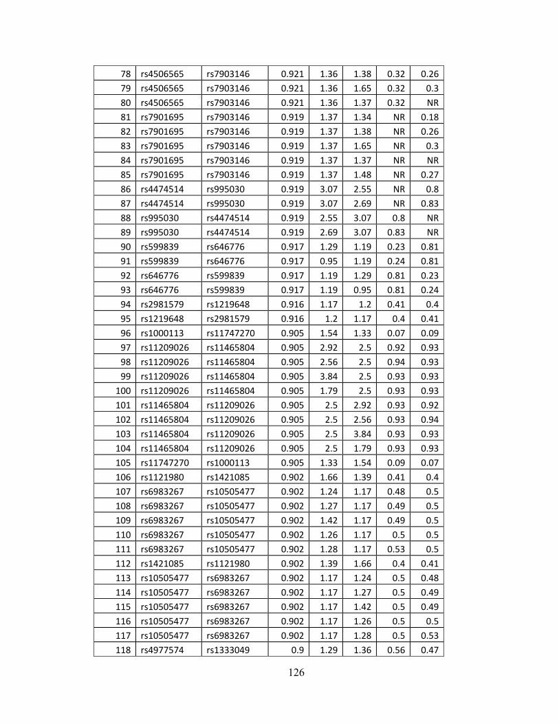
126

78  rs4506565  rs7903146 0.921 1.36 1.38 0.32  0.26 

79  rs4506565  rs7903146 0.921 1.36 1.65 0.32  0.3 

80  rs4506565  rs7903146 0.921 1.36 1.37 0.32  NR 

81  rs7901695  rs7903146 0.919 1.37 1.34 NR  0.18 

82  rs7901695  rs7903146 0.919 1.37 1.38 NR  0.26 

83  rs7901695  rs7903146 0.919 1.37 1.65 NR  0.3 

84  rs7901695  rs7903146 0.919 1.37 1.37 NR  NR 

85  rs7901695  rs7903146 0.919 1.37 1.48 NR  0.27 

86  rs4474514  rs995030 0.919 3.07 2.55 NR  0.8 

87  rs4474514  rs995030 0.919 3.07 2.69 NR  0.83 

88  rs995030  rs4474514 0.919 2.55 3.07 0.8  NR 

89  rs995030  rs4474514 0.919 2.69 3.07 0.83  NR 

90  rs599839  rs646776 0.917 1.29 1.19 0.23  0.81 

91  rs599839  rs646776 0.917 0.95 1.19 0.24  0.81 

92  rs646776  rs599839 0.917 1.19 1.29 0.81  0.23 

93  rs646776  rs599839 0.917 1.19 0.95 0.81  0.24 

94  rs2981579  rs1219648 0.916 1.17 1.2 0.41  0.4 

95  rs1219648  rs2981579 0.916 1.2 1.17 0.4  0.41 

96  rs1000113  rs11747270 0.905 1.54 1.33 0.07  0.09 

97  rs11209026  rs11465804 0.905 2.92 2.5 0.92  0.93 

98  rs11209026  rs11465804 0.905 2.56 2.5 0.94  0.93 

99  rs11209026  rs11465804 0.905 3.84 2.5 0.93  0.93 

100  rs11209026  rs11465804 0.905 1.79 2.5 0.93  0.93 

101  rs11465804  rs11209026 0.905 2.5 2.92 0.93  0.92 

102  rs11465804  rs11209026 0.905 2.5 2.56 0.93  0.94 

103  rs11465804  rs11209026 0.905 2.5 3.84 0.93  0.93 

104  rs11465804  rs11209026 0.905 2.5 1.79 0.93  0.93 

105  rs11747270  rs1000113 0.905 1.33 1.54 0.09  0.07 

106  rs1121980  rs1421085 0.902 1.66 1.39 0.41  0.4 

107  rs6983267  rs10505477 0.902 1.24 1.17 0.48  0.5 

108  rs6983267  rs10505477 0.902 1.27 1.17 0.49  0.5 

109  rs6983267  rs10505477 0.902 1.42 1.17 0.49  0.5 

110  rs6983267  rs10505477 0.902 1.26 1.17 0.5  0.5 

111  rs6983267  rs10505477 0.902 1.28 1.17 0.53  0.5 

112  rs1421085  rs1121980 0.902 1.39 1.66 0.4  0.41 

113  rs10505477  rs6983267 0.902 1.17 1.24 0.5  0.48 

114  rs10505477  rs6983267 0.902 1.17 1.27 0.5  0.49 

115  rs10505477  rs6983267 0.902 1.17 1.42 0.5  0.49 

116  rs10505477  rs6983267 0.902 1.17 1.26 0.5  0.5 

117  rs10505477  rs6983267 0.902 1.17 1.28 0.5  0.53 

118  rs4977574  rs1333049 0.9 1.29 1.36 0.56  0.47 

127

119  rs4977574  rs1333049 0.9 1.29 1.47 0.56  0.47 

120  rs1333049  rs4977574 0.9 1.36 1.29 0.47  0.56 

121  rs1333049  rs4977574 0.9 1.47 1.29 0.47  0.56 

122  rs8034191  rs1051730 0.899 1.4 1.31 0.33  0.35 

123  rs8034191  rs1051730 0.899 1.29 1.31 NR  0.35 

124  rs8034191  rs1051730 0.899 1.3 1.31 0.34  0.35 

125  rs8034191  rs1051730 0.899 1.3 1.31 NR  0.35 

126  rs8034191  rs1051730 0.899 1.38 1.31 NR  0.35 

127  rs8034191  rs1051730 0.899 1.29 1.35 NR  NR 

128  rs8034191  rs1051730 0.899 1.3 1.35 0.34  NR 

129  rs8034191  rs1051730 0.899 1.3 1.35 NR  NR 

130  rs8034191  rs1051730 0.899 1.38 1.35 NR  NR 

131  rs8034191  rs1051730 0.899 1.4 1.35 0.33  NR 

132  rs1051730  rs8034191 0.899 1.31 1.4 0.35  0.33 

133  rs1051730  rs8034191 0.899 1.35 1.4 NR  0.33 

134  rs1051730  rs8034191 0.899 1.35 1.29 NR  NR 

135  rs1051730  rs8034191 0.899 1.35 1.3 NR  0.34 

136  rs1051730  rs8034191 0.899 1.35 1.3 NR  NR 

137  rs1051730  rs8034191 0.899 1.35 1.38 NR  NR 

138  rs1051730  rs8034191 0.899 1.31 1.29 0.35  NR 

139  rs1051730  rs8034191 0.899 1.31 1.3 0.35  0.34 

140  rs1051730  rs8034191 0.899 1.31 1.3 0.35  NR 

141  rs1051730  rs8034191 0.899 1.31 1.38 0.35  NR 

142  rs17221417  rs2076756 0.892 1.29 1.71 0.29  0.27 

143  rs2076756  rs17221417 0.892 1.71 1.29 0.27  0.29 

144  rs2981582  rs2981579 0.884 1.26 1.17 0.38  0.41 

145  rs2981579  rs2981582 0.884 1.17 1.26 0.41  0.38 

146  rs9941349  rs1421085 0.884 1.48 1.39 0.43  0.4 

147  rs9941349  rs8050136 0.884 1.48 1.3 0.43  NR 

148  rs9941349  rs8050136 0.884 1.48 1.17 0.43  0.38 

149  rs9941349  rs8050136 0.884 1.48 1.23 0.43  0.4 

150  rs9941349  rs8050136 0.884 1.48 1.15 0.43  NR 

151  rs1421085  rs9941349 0.884 1.39 1.48 0.4  0.43 

152  rs8050136  rs9941349 0.884 1.3 1.48 NR  0.43 

153  rs8050136  rs9941349 0.884 1.17 1.48 0.38  0.43 

154  rs8050136  rs9941349 0.884 1.23 1.48 0.4  0.43 

155  rs8050136  rs9941349 0.884 1.15 1.48 NR  0.43 

156  rs4975616  rs401681 0.882 1.15 1.15 NR  NR 

157  rs401681  rs4975616 0.882 1.15 1.15 NR  NR 

158  rs8050136  rs1121980 0.87 1.3 1.66 NR  0.41 

159  rs8050136  rs1121980 0.87 1.17 1.66 0.38  0.41 

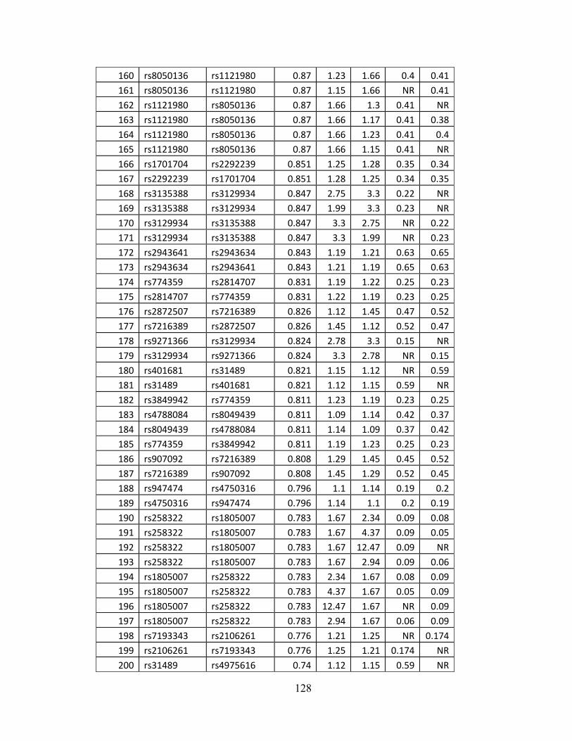
128

160  rs8050136  rs1121980 0.87 1.23 1.66 0.4  0.41 

161  rs8050136  rs1121980 0.87 1.15 1.66 NR  0.41 

162  rs1121980  rs8050136 0.87 1.66 1.3 0.41  NR 

163  rs1121980  rs8050136 0.87 1.66 1.17 0.41  0.38 

164  rs1121980  rs8050136 0.87 1.66 1.23 0.41  0.4 

165  rs1121980  rs8050136 0.87 1.66 1.15 0.41  NR 

166  rs1701704  rs2292239 0.851 1.25 1.28 0.35  0.34 

167  rs2292239  rs1701704 0.851 1.28 1.25 0.34  0.35 

168  rs3135388  rs3129934 0.847 2.75 3.3 0.22  NR 

169  rs3135388  rs3129934 0.847 1.99 3.3 0.23  NR 

170  rs3129934  rs3135388 0.847 3.3 2.75 NR  0.22 

171  rs3129934  rs3135388 0.847 3.3 1.99 NR  0.23 

172  rs2943641  rs2943634 0.843 1.19 1.21 0.63  0.65 

173  rs2943634  rs2943641 0.843 1.21 1.19 0.65  0.63 

174  rs774359  rs2814707 0.831 1.19 1.22 0.25  0.23 

175  rs2814707  rs774359 0.831 1.22 1.19 0.23  0.25 

176  rs2872507  rs7216389 0.826 1.12 1.45 0.47  0.52 

177  rs7216389  rs2872507 0.826 1.45 1.12 0.52  0.47 

178  rs9271366  rs3129934 0.824 2.78 3.3 0.15  NR 

179  rs3129934  rs9271366 0.824 3.3 2.78 NR  0.15 

180  rs401681  rs31489 0.821 1.15 1.12 NR  0.59 

181  rs31489  rs401681 0.821 1.12 1.15 0.59  NR 

182  rs3849942  rs774359 0.811 1.23 1.19 0.23  0.25 

183  rs4788084  rs8049439 0.811 1.09 1.14 0.42  0.37 

184  rs8049439  rs4788084 0.811 1.14 1.09 0.37  0.42 

185  rs774359  rs3849942 0.811 1.19 1.23 0.25  0.23 

186  rs907092  rs7216389 0.808 1.29 1.45 0.45  0.52 

187  rs7216389  rs907092 0.808 1.45 1.29 0.52  0.45 

188  rs947474  rs4750316 0.796 1.1 1.14 0.19  0.2 

189  rs4750316  rs947474 0.796 1.14 1.1 0.2  0.19 

190  rs258322  rs1805007 0.783 1.67 2.34 0.09  0.08 

191  rs258322  rs1805007 0.783 1.67 4.37 0.09  0.05 

192  rs258322  rs1805007 0.783 1.67 12.47 0.09  NR 

193  rs258322  rs1805007 0.783 1.67 2.94 0.09  0.06 

194  rs1805007  rs258322 0.783 2.34 1.67 0.08  0.09 

195  rs1805007  rs258322 0.783 4.37 1.67 0.05  0.09 

196  rs1805007  rs258322 0.783 12.47 1.67 NR  0.09 

197  rs1805007  rs258322 0.783 2.94 1.67 0.06  0.09 

198  rs7193343  rs2106261 0.776 1.21 1.25 NR  0.174 

199  rs2106261  rs7193343 0.776 1.25 1.21 0.174  NR 

200  rs31489  rs4975616 0.74 1.12 1.15 0.59  NR 

129

201  rs4975616  rs31489 0.74 1.15 1.12 NR  0.59 

202  rs7501939  rs4430796 0.734 1.41 1.22 0.57  0.49 

203  rs7501939  rs4430796 0.734 1.41 1.19 0.57  0.52 

204  rs7501939  rs4430796 0.734 1.41 1.18 0.57  0.54 

205  rs4430796  rs7501939 0.734 1.22 1.41 0.49  0.57 

206  rs4430796  rs7501939 0.734 1.19 1.41 0.52  0.57 

207  rs4430796  rs7501939 0.734 1.18 1.41 0.54  0.57 

208  rs4977756  rs1412829 0.724 1.24 1.42 0.6  0.39 

209  rs1412829  rs4977756 0.724 1.42 1.24 0.39  0.6 

210  rs7756992  rs7754840 0.722 1.2 1.12 0.26  0.31 

211  rs7756992  rs7754840 0.722 1.2 1.12 0.26  0.36 

212  rs7754840  rs7756992 0.722 1.12 1.2 0.31  0.26 

213  rs7754840  rs7756992 0.722 1.12 1.2 0.36  0.26 

214  rs4712523  rs7756992 0.722 1.2 1.2 0.32  0.26 

215  rs10946398  rs7756992 0.722 1.18 1.2 NR  0.26 

216  rs10946398  rs7756992 0.722 1.16 1.2 0.32  0.26 

217  rs7756992  rs4712523 0.722 1.2 1.2 0.26  0.32 

218  rs7756992  rs10946398 0.722 1.2 1.18 0.26  NR 

219  rs7756992  rs10946398 0.722 1.2 1.16 0.26  0.32 

220  rs564398  rs4977756 0.71 1.13 1.24 0.56  0.6 

221  rs4977756  rs564398 0.71 1.24 1.13 0.6  0.56 

222  rs2201841  rs11805303 0.7 1.13 1.39 0.3  0.68 

223  rs11805303  rs2201841 0.7 1.39 1.13 0.68  0.3 

224  rs6931514  rs4712523 0.688 1.25 1.2 NR  0.32 

225  rs6931514  rs10946398 0.688 1.25 1.18 NR  NR 

226  rs6931514  rs10946398 0.688 1.25 1.16 NR  0.32 

227  rs4712523  rs6931514 0.688 1.2 1.25 0.32  NR 

228  rs10946398  rs6931514 0.688 1.18 1.25 NR  NR 

229  rs10946398  rs6931514 0.688 1.16 1.25 0.32  NR 

230  rs7754840  rs6931514 0.688 1.12 1.25 0.31  NR 

231  rs7754840  rs6931514 0.688 1.12 1.25 0.36  NR 

232  rs6931514  rs7754840 0.688 1.25 1.12 NR  0.31 

233  rs6931514  rs7754840 0.688 1.25 1.12 NR  0.36 

234  rs10758593  rs7020673 0.674 1.13 1.14 NR  0.5 

235  rs2292239  rs11171739 0.674 1.28 1.34 0.34  0.42 

236  rs7020673  rs10758593 0.674 1.14 1.13 0.5  NR 

237  rs11171739  rs2292239 0.674 1.34 1.28 0.42  0.34 

238  rs6932590  rs13194053 0.653 1.16 1.28 0.78  0.82 

239  rs6932590  rs13194053 0.653 1.16 1.22 0.78  0.86 

240  rs13194053  rs6932590 0.653 1.28 1.16 0.82  0.78 

241  rs13194053  rs6932590 0.653 1.22 1.16 0.86  0.78 

130

242  rs10889677  rs11805303 0.649 1.29 1.39 0.3  0.68 

243  rs11805303  rs10889677 0.649 1.39 1.29 0.68  0.3 

244  rs12722489  rs2104286 0.626 1.25 1.16 0.85  0.73 

245  rs12722489  rs2104286 0.626 1.25 1.15 0.85  0.76 

246  rs2104286  rs12722489 0.626 1.16 1.25 0.73  0.85 

247  rs2104286  rs12722489 0.626 1.15 1.25 0.76  0.85 

248  rs11171739  rs1701704 0.618 1.34 1.25 0.42  0.35 

249  rs1701704  rs11171739 0.618 1.25 1.34 0.35  0.42 

250  rs4598195  rs4730276 0.614 1.23 1.22 0.54  0.39 

251  rs4730276  rs4598195 0.614 1.22 1.23 0.39  0.54 

252  rs2076756  rs5743289 0.612 1.71 1.46 0.27  0.17 

253  rs5743289  rs2076756 0.612 1.46 1.71 0.17  0.27 

254  rs4977574  rs1333040 0.603 1.29 1.29 0.56  0.55 

255  rs1333040  rs4977574 0.603 1.29 1.29 0.55  0.56 

256  rs2180439  rs1160312 0.602 1.82 1.6 0.43  0.43 

257  rs1160312  rs2180439 0.602 1.6 1.82 0.43  0.43 

258  rs9888739  rs11574637 0.556 1.62 1.33 0.13  0.19 

259  rs11574637  rs9888739 0.556 1.33 1.62 0.19  0.13 

260  rs1333049  rs1333040 0.555 1.36 1.29 0.47  0.55 

261  rs1333049  rs1333040 0.555 1.47 1.29 0.47  0.55 

262  rs1333040  rs1333049 0.555 1.29 1.36 0.55  0.47 

263  rs1333040  rs1333049 0.555 1.29 1.47 0.55  0.47 

264  rs4730276  rs4730273 0.551 1.22 1.22 0.39  0.7 

265  rs4730273  rs4730276 0.551 1.22 1.22 0.7  0.39 

266  rs17221417  rs5743289 0.546 1.29 1.46 0.29  0.17 

267  rs5743289  rs17221417 0.546 1.46 1.29 0.17  0.29 

268  rs7014346  rs10505477 0.541 1.19 1.17 0.18  0.5 

269  rs10505477  rs7014346 0.541 1.17 1.19 0.5  0.18 

270  rs477515  rs9272346 0.512 1.38 5.49 0.69  0.61 

271  rs9272346  rs477515 0.512 5.49 1.38 0.61  0.69 

272  rs9465871  rs7756992 0.509 1.18 1.2 0.18  0.26 

273  rs7756992  rs9465871 0.509 1.2 1.18 0.26  0.18 

274  rs17696736  rs653178 0.505 1.22 1.21 0.42  0.48 

275  rs17696736  rs653178 0.505 1.34 1.21 0.42  0.48 

276  rs653178  rs17696736 0.505 1.21 1.22 0.48  0.42 

277  rs653178  rs17696736 0.505 1.21 1.34 0.48  0.42 

278  rs9272346  rs2395185 0.497 5.49 1.52 0.61  0.67 

279  rs2395185  rs9272346 0.497 1.52 5.49 0.67  0.61 

280  rs2412973  rs5753037 0.493 1.15 1.1 0.46  0.39 

281  rs5753037  rs2412973 0.493 1.1 1.15 0.39  0.46 

282  rs7014346  rs6983267 0.488 1.19 1.42 0.18  0.49 

131

283  rs7014346  rs6983267 0.488 1.19 1.26 0.18  0.5 

284  rs7014346  rs6983267 0.488 1.19 1.28 0.18  0.53 

285  rs6983267  rs7014346 0.488 1.24 1.19 0.48  0.18 

286  rs6983267  rs7014346 0.488 1.27 1.19 0.49  0.18 

287  rs6983267  rs7014346 0.488 1.42 1.19 0.49  0.18 

288  rs6983267  rs7014346 0.488 1.26 1.19 0.5  0.18 

289  rs6983267  rs7014346 0.488 1.28 1.19 0.53  0.18 

290  rs7014346  rs6983267 0.488 1.19 1.24 0.18  0.48 

291  rs7014346  rs6983267 0.488 1.19 1.27 0.18  0.49 

292  rs4763879  rs11052552 0.484 1.09 1.49 0.37  0.49 

293  rs11052552  rs4763879 0.484 1.49 1.09 0.49  0.37 

294  rs6897932  rs1445898 0.467 1.12 1.12 0.75  0.55 

295  rs6897932  rs1445898 0.467 1.18 1.12 0.75  0.55 

296  rs6897932  rs1445898 0.467 1.12 1.12 0.71  0.55 

297  rs1445898  rs6897932 0.467 1.12 1.12 0.55  0.75 

298  rs1445898  rs6897932 0.467 1.12 1.18 0.55  0.75 

299  rs1445898  rs6897932 0.467 1.12 1.12 0.55  0.71 

300  rs4763879  rs3764021 0.451 1.09 1.57 0.37  0.47 

301  rs3764021  rs4763879 0.451 1.57 1.09 0.47  0.37 

302  rs10038113  rs4307059 0.45 1.33 1.19 0.59  0.61 

303  rs4307059  rs10038113 0.45 1.19 1.33 0.61  0.59 

304  rs4977756  rs4977574 0.446 1.24 1.29 0.6  0.56 

305  rs4977574  rs4977756 0.446 1.29 1.24 0.56  0.6 

306  rs9296249  rs3923809 0.442 1.67 1.9 0.76  0.66 

307  rs3923809  rs9296249 0.442 1.9 1.67 0.66  0.76 

308  rs10484554  rs2395029 0.432 2.8 3.47 0.15  0.03 

309  rs12191877  rs2395029 0.432 2.64 3.47 0.15  0.03 

310  rs12191877  rs2395029 0.432 2.64 45 0.15  0.05 

311  rs10484554  rs2395029 0.432 2.8 45 0.15  0.05 

312  rs10484554  rs2395029 0.432 2.8 4.1 0.15  0.03 

313  rs12191877  rs2395029 0.432 2.64 4.1 0.15  0.03 

314  rs2395029  rs10484554 0.432 3.47 2.8 0.03  0.15 

315  rs2395029  rs10484554 0.432 45 2.8 0.05  0.15 

316  rs2395029  rs10484554 0.432 4.1 2.8 0.03  0.15 

317  rs2395029  rs12191877 0.432 4.1 2.64 0.03  0.15 

318  rs10974944  rs10758669 0.477 3.1 1.12 NR  0.35 

319  rs10758669  rs10974944 0.477 1.12 3.1 0.35  NR 

320  rs9465871  rs6931514 0.473 1.18 1.25 0.18  NR 

321  rs6931514  rs9465871 0.473 1.25 1.18 NR  0.18 

322  rs6897932  rs1445898 0.467 1.12 1.12 0.75  0.55 

323  rs6897932  rs1445898 0.467 1.18 1.12 0.75  0.55 

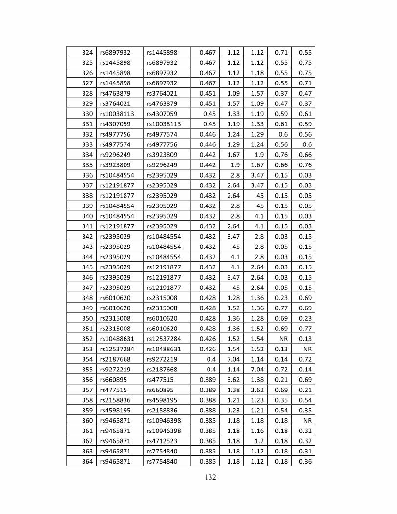
132

324  rs6897932  rs1445898 0.467 1.12 1.12 0.71  0.55 

325  rs1445898  rs6897932 0.467 1.12 1.12 0.55  0.75 

326  rs1445898  rs6897932 0.467 1.12 1.18 0.55  0.75 

327  rs1445898  rs6897932 0.467 1.12 1.12 0.55  0.71 

328  rs4763879  rs3764021 0.451 1.09 1.57 0.37  0.47 

329  rs3764021  rs4763879 0.451 1.57 1.09 0.47  0.37 

330  rs10038113  rs4307059 0.45 1.33 1.19 0.59  0.61 

331  rs4307059  rs10038113 0.45 1.19 1.33 0.61  0.59 

332  rs4977756  rs4977574 0.446 1.24 1.29 0.6  0.56 

333  rs4977574  rs4977756 0.446 1.29 1.24 0.56  0.6 

334  rs9296249  rs3923809 0.442 1.67 1.9 0.76  0.66 

335  rs3923809  rs9296249 0.442 1.9 1.67 0.66  0.76 

336  rs10484554  rs2395029 0.432 2.8 3.47 0.15  0.03 

337  rs12191877  rs2395029 0.432 2.64 3.47 0.15  0.03 

338  rs12191877  rs2395029 0.432 2.64 45 0.15  0.05 

339  rs10484554  rs2395029 0.432 2.8 45 0.15  0.05 

340  rs10484554  rs2395029 0.432 2.8 4.1 0.15  0.03 

341  rs12191877  rs2395029 0.432 2.64 4.1 0.15  0.03 

342  rs2395029  rs10484554 0.432 3.47 2.8 0.03  0.15 

343  rs2395029  rs10484554 0.432 45 2.8 0.05  0.15 

344  rs2395029  rs10484554 0.432 4.1 2.8 0.03  0.15 

345  rs2395029  rs12191877 0.432 4.1 2.64 0.03  0.15 

346  rs2395029  rs12191877 0.432 3.47 2.64 0.03  0.15 

347  rs2395029  rs12191877 0.432 45 2.64 0.05  0.15 

348  rs6010620  rs2315008 0.428 1.28 1.36 0.23  0.69 

349  rs6010620  rs2315008 0.428 1.52 1.36 0.77  0.69 

350  rs2315008  rs6010620 0.428 1.36 1.28 0.69  0.23 

351  rs2315008  rs6010620 0.428 1.36 1.52 0.69  0.77 

352  rs10488631  rs12537284 0.426 1.52 1.54 NR  0.13 

353  rs12537284  rs10488631 0.426 1.54 1.52 0.13  NR 

354  rs2187668  rs9272219 0.4 7.04 1.14 0.14  0.72 

355  rs9272219  rs2187668 0.4 1.14 7.04 0.72  0.14 

356  rs660895  rs477515 0.389 3.62 1.38 0.21  0.69 

357  rs477515  rs660895 0.389 1.38 3.62 0.69  0.21 

358  rs2158836  rs4598195 0.388 1.21 1.23 0.35  0.54 

359  rs4598195  rs2158836 0.388 1.23 1.21 0.54  0.35 

360  rs9465871  rs10946398 0.385 1.18 1.18 0.18  NR 

361  rs9465871  rs10946398 0.385 1.18 1.16 0.18  0.32 

362  rs9465871  rs4712523 0.385 1.18 1.2 0.18  0.32 

363  rs9465871  rs7754840 0.385 1.18 1.12 0.18  0.31 

364  rs9465871  rs7754840 0.385 1.18 1.12 0.18  0.36 

133

NR – Not Reported – assume RAF = 0.5 Disease /Trait associated with each SNP (from above)

SNP1 - Disease SNP2 - Disease1  Type 2 diabetes Glioma (high‐grade)

2  Crohn's disease Crohn's disease

3  Crohn's disease Crohn's disease

4  Crohn's disease Crohn's disease

365  rs7754840  rs9465871 0.385 1.12 1.18 0.31  0.18 

366  rs7754840  rs9465871 0.385 1.12 1.18 0.36  0.18 

367  rs4712523  rs9465871 0.385 1.2 1.18 0.32  0.18 

368  rs10946398  rs9465871 0.385 1.18 1.18 NR  0.18 

369  rs10946398  rs9465871 0.385 1.16 1.18 0.32  0.18 

370  rs1333049  rs4977756 0.384 1.36 1.24 0.47  0.6 

371  rs1333049  rs4977756 0.384 1.47 1.24 0.47  0.6 

372  rs4977756  rs1333049 0.384 1.24 1.36 0.6  0.47 

373  rs4977756  rs1333049 0.384 1.24 1.47 0.6  0.47 

374  rs660895  rs2395185 0.381 3.62 1.52 0.21  0.67 

375  rs2395185  rs660895 0.381 1.52 3.62 0.67  0.21 

376  rs4730273  rs4598195 0.374 1.22 1.23 0.7  0.54 

377  rs4598195  rs4730273 0.374 1.23 1.22 0.54  0.7 

378  rs9929218  rs1728785 0.368 1.1 1.17 0.29  0.76 

379  rs1728785  rs9929218 0.368 1.17 1.1 0.76  0.29 

380  rs17594526  rs9960767 0.35 1.44 1.23 0.03  0.06 

381  rs9960767  rs17594526 0.35 1.23 1.44 0.06  0.03 

382  rs660895  rs6457617 0.344 3.62 2.36 0.21  0.49 

383  rs660895  rs6457620 0.344 3.62 2.55 0.21  0.5 

384  rs6457617  rs660895 0.344 2.36 3.62 0.49  0.21 

385  rs6457620  rs660895 0.344 2.55 3.62 0.5  0.21 

386  rs9272346  rs9271366 0.331 5.49 2.78 0.61  0.15 

387  rs9271366  rs9272346 0.331 2.78 5.49 0.15  0.61 

388  rs3135388  rs9272346 0.322 2.75 5.49 0.22  0.61 

389  rs3135388  rs9272346 0.322 1.99 5.49 0.23  0.61 

390  rs9272346  rs3135388 0.322 5.49 2.75 0.61  0.22 

391  rs9272346  rs3135388 0.322 5.49 1.99 0.61  0.23 

392  rs9272346  rs3129934 0.315 5.49 3.3 0.61  NR 

393  rs3129934  rs9272346 0.315 3.3 5.49 NR  0.61 

394  rs11805303  rs7517847 0.314 1.39 1.61 0.68  0.56 

395  rs7517847  rs11805303 0.314 1.61 1.39 0.56  0.68 

396  rs11228565  rs10896449 0.303 1.23 1.1 0.2  0.52 

397  rs10896449  rs11228565 0.303 1.1 1.23 0.52  0.2 

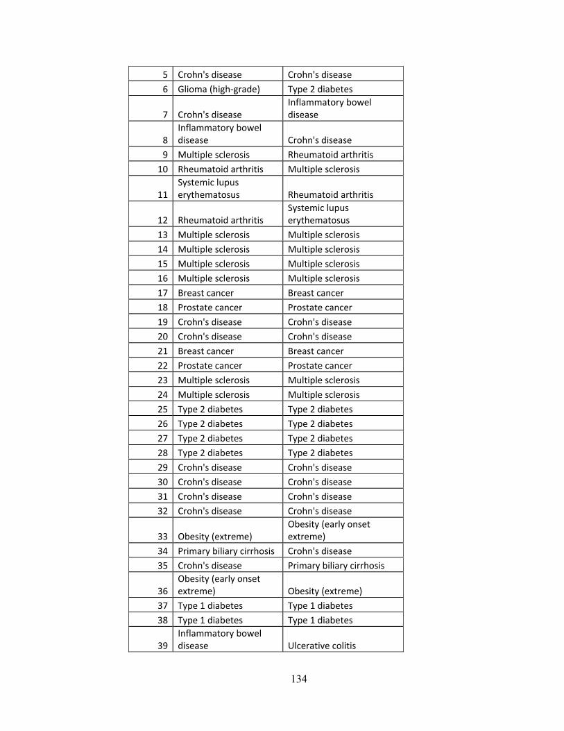
134

5  Crohn's disease Crohn's disease

6  Glioma (high‐grade) Type 2 diabetes

7  Crohn's diseaseInflammatory bowel disease

8 Inflammatory bowel disease  Crohn's disease

9  Multiple sclerosis Rheumatoid arthritis

10  Rheumatoid arthritis Multiple sclerosis

11 Systemic lupus erythematosus Rheumatoid arthritis

12  Rheumatoid arthritisSystemic lupus erythematosus

13  Multiple sclerosis Multiple sclerosis

14  Multiple sclerosis Multiple sclerosis

15  Multiple sclerosis Multiple sclerosis

16  Multiple sclerosis Multiple sclerosis

17  Breast cancer Breast cancer

18  Prostate cancer Prostate cancer

19  Crohn's disease Crohn's disease

20  Crohn's disease Crohn's disease

21  Breast cancer Breast cancer

22  Prostate cancer Prostate cancer

23  Multiple sclerosis Multiple sclerosis

24  Multiple sclerosis Multiple sclerosis

25  Type 2 diabetes Type 2 diabetes

26  Type 2 diabetes Type 2 diabetes

27  Type 2 diabetes Type 2 diabetes

28  Type 2 diabetes Type 2 diabetes

29  Crohn's disease Crohn's disease

30  Crohn's disease Crohn's disease

31  Crohn's disease Crohn's disease

32  Crohn's disease Crohn's disease

33  Obesity (extreme)Obesity (early onset extreme)

34  Primary biliary cirrhosis Crohn's disease

35  Crohn's disease Primary biliary cirrhosis

36 Obesity (early onset extreme)  Obesity (extreme)

37  Type 1 diabetes Type 1 diabetes

38  Type 1 diabetes Type 1 diabetes

39 Inflammatory bowel disease  Ulcerative colitis

135

40  Ulcerative colitisInflammatory bowel disease

41  Type 1 diabetes Type 1 diabetes

42  Type 1 diabetes Type 1 diabetes

43  Type 1 diabetes Type 1 diabetes

44  Type 1 diabetes Type 1 diabetes

45  Psoriasis  Ulcerative colitis

46  Ulcerative colitis Psoriasis

47  Type 1 diabetes Type 1 diabetes

48  Type 1 diabetes Type 1 diabetes

49  Crohn's disease Crohn's disease

50  Crohn's disease Crohn's disease

51  Crohn's disease Crohn's disease

52  Type 2 diabetes Obesity

53  Type 2 diabetes Obesity

54  Type 2 diabetes Obesity

55  Type 2 diabetes Obesity

56  Crohn's disease Crohn's disease

57  Obesity  Type 2 diabetes

58  Obesity  Type 2 diabetes

59  Obesity  Type 2 diabetes

60  Obesity  Type 2 diabetes

61 Amyotrophic lateral sclerosis 

Amyotrophic lateral sclerosis

62 Amyotrophic lateral sclerosis 

Amyotrophic lateral sclerosis

63  Type 2 diabetes Type 2 diabetes

64  Type 2 diabetes Type 2 diabetes

65  Type 2 diabetes Type 2 diabetes

66  Type 2 diabetes Type 2 diabetes

67  Type 2 diabetes Type 2 diabetes

68  Type 2 diabetes Type 2 diabetes

69  Type 2 diabetes Type 2 diabetes

70  Type 2 diabetes Type 2 diabetes

71 Type 2 diabetes and other traits  Type 2 diabetes

72  Type 2 diabetesType 2 diabetes and other traits

73  Type 2 diabetes Type 2 diabetes

74  Type 2 diabetes Type 2 diabetes

75  Type 2 diabetes Type 2 diabetes

76  Type 2 diabetes Type 2 diabetes

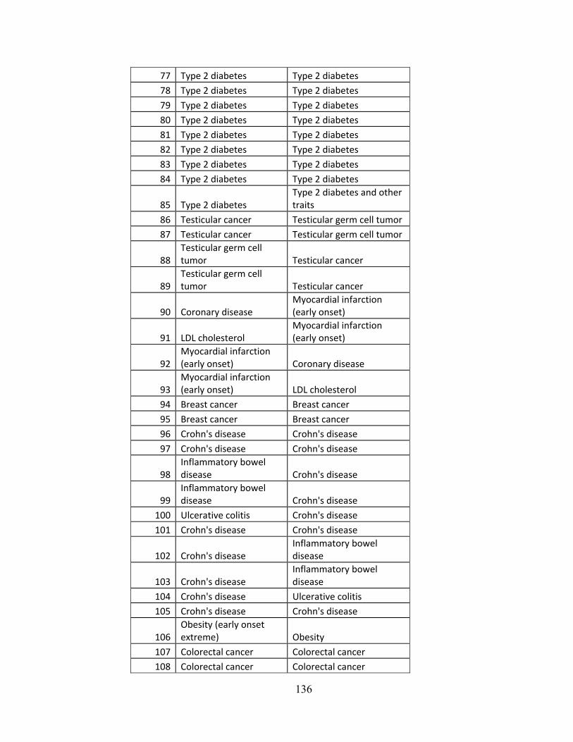
136

77  Type 2 diabetes Type 2 diabetes

78  Type 2 diabetes Type 2 diabetes

79  Type 2 diabetes Type 2 diabetes

80  Type 2 diabetes Type 2 diabetes

81  Type 2 diabetes Type 2 diabetes

82  Type 2 diabetes Type 2 diabetes

83  Type 2 diabetes Type 2 diabetes

84  Type 2 diabetes Type 2 diabetes

85  Type 2 diabetesType 2 diabetes and other traits

86  Testicular cancer Testicular germ cell tumor 

87  Testicular cancer Testicular germ cell tumor 

88 Testicular germ cell tumor  Testicular cancer

89 Testicular germ cell tumor  Testicular cancer

90  Coronary diseaseMyocardial infarction (early onset)

91  LDL cholesterolMyocardial infarction (early onset)

92 Myocardial infarction (early onset) Coronary disease

93 Myocardial infarction (early onset) LDL cholesterol

94  Breast cancer Breast cancer

95  Breast cancer Breast cancer

96  Crohn's disease Crohn's disease

97  Crohn's disease Crohn's disease

98 Inflammatory bowel disease  Crohn's disease

99 Inflammatory bowel disease  Crohn's disease

100  Ulcerative colitis Crohn's disease

101  Crohn's disease Crohn's disease

102  Crohn's diseaseInflammatory bowel disease

103  Crohn's diseaseInflammatory bowel disease

104  Crohn's disease Ulcerative colitis

105  Crohn's disease Crohn's disease

106 Obesity (early onset extreme)  Obesity

107  Colorectal cancer Colorectal cancer

108  Colorectal cancer Colorectal cancer

137

109  Prostate cancer Colorectal cancer

110  Prostate cancer Colorectal cancer

111  Prostate cancer Colorectal cancer

112  Obesity Obesity (early onset extreme)

113  Colorectal cancer Colorectal cancer

114  Colorectal cancer Colorectal cancer

115  Colorectal cancer Prostate cancer

116  Colorectal cancer Prostate cancer

117  Colorectal cancer Prostate cancer

118 Myocardial infarction (early onset) Coronary disease

119 Myocardial infarction (early onset) Coronary disease

120  Coronary diseaseMyocardial infarction (early onset)

121  Coronary diseaseMyocardial infarction (early onset)

122 Chronic Obstructive Pulmonary Disease Lung adenocarcinoma

123  Lung cancer Lung adenocarcinoma

124  Lung cancer Lung adenocarcinoma

125  Lung cancer Lung adenocarcinoma

126  Lung cancer Lung adenocarcinoma

127  Lung cancer Lung cancer

128  Lung cancer Lung cancer

129  Lung cancer Lung cancer

130  Lung cancer Lung cancer

131 Chronic Obstructive Pulmonary Disease Lung cancer

132  Lung adenocarcinomaChronic Obstructive Pulmonary Disease

133  Lung cancerChronic Obstructive Pulmonary Disease

134  Lung cancer Lung cancer

135  Lung cancer Lung cancer

136  Lung cancer Lung cancer

137  Lung cancer Lung cancer

138  Lung adenocarcinoma Lung cancer

139  Lung adenocarcinoma Lung cancer

140  Lung adenocarcinoma Lung cancer

141  Lung adenocarcinoma Lung cancer

142  Crohn's disease Crohn's disease

138

143  Crohn's disease Crohn's disease

144  Breast cancer Breast cancer

145  Breast cancer Breast cancer

146  Obesity (extreme) Obesity

147  Obesity (extreme) Type 2 diabetes

148  Obesity (extreme) Type 2 diabetes

149  Obesity (extreme) Type 2 diabetes

150  Obesity (extreme) Type 2 diabetes

151  Obesity  Obesity (extreme)

152  Type 2 diabetes Obesity (extreme)

153  Type 2 diabetes Obesity (extreme)

154  Type 2 diabetes Obesity (extreme)

155  Type 2 diabetes Obesity (extreme)

156  Lung cancer Lung cancer

157  Lung cancer Lung cancer

158  Type 2 diabetesObesity (early onset extreme)

159  Type 2 diabetesObesity (early onset extreme)

160  Type 2 diabetesObesity (early onset extreme)

161  Type 2 diabetesObesity (early onset extreme)

162 Obesity (early onset extreme)  Type 2 diabetes

163 Obesity (early onset extreme)  Type 2 diabetes

164 Obesity (early onset extreme)  Type 2 diabetes

165 Obesity (early onset extreme)  Type 2 diabetes

166  Type 1 diabetes Type 1 diabetes

167  Type 1 diabetes Type 1 diabetes

168  Multiple sclerosis Multiple sclerosis

169  Multiple sclerosis Multiple sclerosis

170  Multiple sclerosis Multiple sclerosis

171  Multiple sclerosis Multiple sclerosis

172 Type 2 diabetes and other traits  Coronary disease

173  Coronary diseaseType 2 diabetes and other traits

174 Amyotrophic lateral sclerosis 

Amyotrophic lateral sclerosis

139

175 Amyotrophic lateral sclerosis 

Amyotrophic lateral sclerosis

176  Crohn's disease Asthma

177  Asthma  Crohn's disease

178  Multiple sclerosis Multiple sclerosis

179  Multiple sclerosis Multiple sclerosis

180  Lung cancer Lung adenocarcinoma

181  Lung adenocarcinoma Lung cancer

182 Amyotrophic lateral sclerosis 

Amyotrophic lateral sclerosis

183  Type 1 diabetesInflammatory bowel disease (early onset)

184 Inflammatory bowel disease (early onset) Type 1 diabetes

185 Amyotrophic lateral sclerosis 

Amyotrophic lateral sclerosis

186  Primary biliary cirrhosis Asthma

187  Asthma  Primary biliary cirrhosis

188  Type 1 diabetes Rheumatoid arthritis

189  Rheumatoid arthritis Type 1 diabetes

190  Melanoma  Blond vs. brown hair color 

191  Melanoma  Freckles

192  Melanoma  Red vs non‐red hair color

193  Melanoma  Skin sensitivity to sun

194 Blond vs. brown hair color  Melanoma

195  Freckles  Melanoma

196 Red vs non‐red hair color  Melanoma

197  Skin sensitivity to sun Melanoma

198  Atrial fibrillation Atrial fibrillation

199  Atrial fibrillation Atrial fibrillation

200  Lung adenocarcinoma Lung cancer

201  Lung cancer Lung adenocarcinoma

202  Prostate cancer Prostate cancer

203  Prostate cancer Prostate cancer

204  Prostate cancer Prostate cancer

205  Prostate cancer Prostate cancer

206  Prostate cancer Prostate cancer

207  Prostate cancer Prostate cancer

208  Glioma  Glioma (high‐grade)

209  Glioma (high‐grade) Glioma

140

210  Type 2 diabetes Type 2 diabetes

211  Type 2 diabetes Type 2 diabetes

212  Type 2 diabetes Type 2 diabetes

213  Type 2 diabetes Type 2 diabetes

214 Type 2 diabetes and other traits  Type 2 diabetes

215  Type 2 diabetes Type 2 diabetes

216  Type 2 diabetes Type 2 diabetes

217  Type 2 diabetesType 2 diabetes and other traits

218  Type 2 diabetes Type 2 diabetes

219  Type 2 diabetes Type 2 diabetes

220  Type 2 diabetes Glioma

221  Glioma  Type 2 diabetes

222  Psoriasis  Crohn's disease

223  Crohn's disease Psoriasis

224  Type 2 diabetesType 2 diabetes and other traits

225  Type 2 diabetes Type 2 diabetes

226  Type 2 diabetes Type 2 diabetes

227 Type 2 diabetes and other traits  Type 2 diabetes

228  Type 2 diabetes Type 2 diabetes

229  Type 2 diabetes Type 2 diabetes

230  Type 2 diabetes Type 2 diabetes

231  Type 2 diabetes Type 2 diabetes

232  Type 2 diabetes Type 2 diabetes

233  Type 2 diabetes Type 2 diabetes

234  Type 1 diabetes Type 1 diabetes

235  Type 1 diabetes Type 1 diabetes

236  Type 1 diabetes Type 1 diabetes

237  Type 1 diabetes Type 1 diabetes

238  Schizophrenia Schizophrenia

239  Schizophrenia Schizophrenia

240  Schizophrenia Schizophrenia

241  Schizophrenia Schizophrenia

242  Ulcerative colitis Crohn's disease

243  Crohn's disease Ulcerative colitis

244  Multiple sclerosis Multiple sclerosis

245  Multiple sclerosis Multiple sclerosis

246  Multiple sclerosis Multiple sclerosis

247  Multiple sclerosis Multiple sclerosis

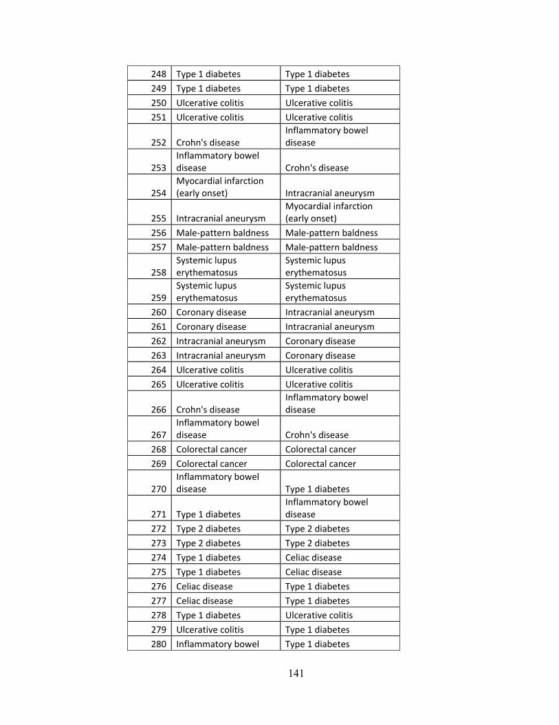
141

248  Type 1 diabetes Type 1 diabetes

249  Type 1 diabetes Type 1 diabetes

250  Ulcerative colitis Ulcerative colitis

251  Ulcerative colitis Ulcerative colitis

252  Crohn's diseaseInflammatory bowel disease

253 Inflammatory bowel disease  Crohn's disease

254 Myocardial infarction (early onset) Intracranial aneurysm

255  Intracranial aneurysmMyocardial infarction (early onset)

256  Male‐pattern baldness Male‐pattern baldness

257  Male‐pattern baldness Male‐pattern baldness

258 Systemic lupus erythematosus

Systemic lupus erythematosus

259 Systemic lupus erythematosus

Systemic lupus erythematosus

260  Coronary disease Intracranial aneurysm

261  Coronary disease Intracranial aneurysm

262  Intracranial aneurysm Coronary disease

263  Intracranial aneurysm Coronary disease

264  Ulcerative colitis Ulcerative colitis

265  Ulcerative colitis Ulcerative colitis

266  Crohn's diseaseInflammatory bowel disease

267 Inflammatory bowel disease  Crohn's disease

268  Colorectal cancer Colorectal cancer

269  Colorectal cancer Colorectal cancer

270 Inflammatory bowel disease  Type 1 diabetes

271  Type 1 diabetesInflammatory bowel disease

272  Type 2 diabetes Type 2 diabetes

273  Type 2 diabetes Type 2 diabetes

274  Type 1 diabetes Celiac disease

275  Type 1 diabetes Celiac disease

276  Celiac disease Type 1 diabetes

277  Celiac disease Type 1 diabetes

278  Type 1 diabetes Ulcerative colitis

279  Ulcerative colitis Type 1 diabetes

280  Inflammatory bowel  Type 1 diabetes

142

disease (early onset)

281  Type 1 diabetesInflammatory bowel disease (early onset)

282  Colorectal cancer Prostate cancer

283  Colorectal cancer Prostate cancer

284  Colorectal cancer Prostate cancer

285  Colorectal cancer Colorectal cancer

286  Colorectal cancer Colorectal cancer

287  Prostate cancer Colorectal cancer

288  Prostate cancer Colorectal cancer

289  Prostate cancer Colorectal cancer

290  Colorectal cancer Colorectal cancer

291  Colorectal cancer Colorectal cancer

292  Type 1 diabetes Type 1 diabetes

293  Type 1 diabetes Type 1 diabetes

294  Multiple sclerosis Type 1 diabetes

295  Multiple sclerosis Type 1 diabetes

296  Type 1 diabetes Type 1 diabetes

297  Type 1 diabetes Multiple sclerosis

298  Type 1 diabetes Multiple sclerosis

299  Type 1 diabetes Type 1 diabetes

300  Type 1 diabetes Type 1 diabetes

301  Type 1 diabetes Type 1 diabetes

302  Autism  Autism

303  Autism  Autism

304  Glioma Myocardial infarction (early onset)

305 Myocardial infarction (early onset) Glioma

306  Restless legs syndrome Restless legs syndrome

307  Restless legs syndrome Restless legs syndrome

308  Psoriasis  AIDS progression

309  Psoriasis  AIDS progression

310  Psoriasis Drug‐induced liver injury (flucloxacillin)

311  Psoriasis Drug‐induced liver injury (flucloxacillin)

312  Psoriasis  Psoriasis

313  Psoriasis  Psoriasis

314  AIDS progression Psoriasis

315 Drug‐induced liver injury (flucloxacillin) Psoriasis

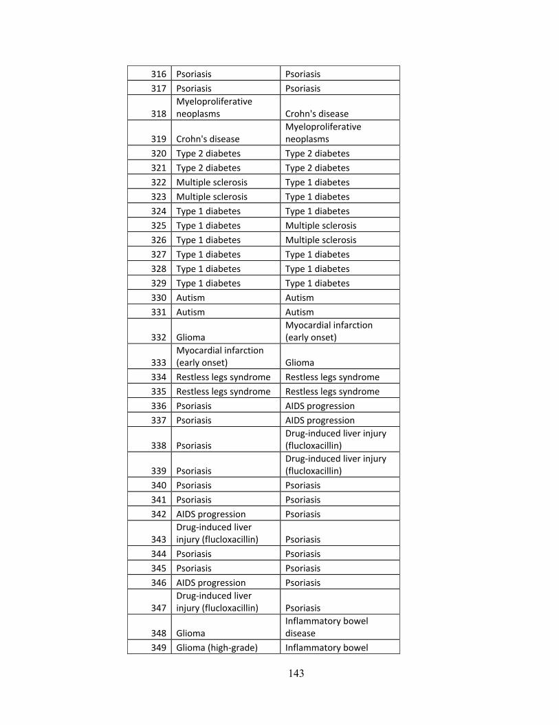
143

316  Psoriasis  Psoriasis

317  Psoriasis  Psoriasis

318 Myeloproliferative neoplasms  Crohn's disease

319  Crohn's diseaseMyeloproliferative neoplasms

320  Type 2 diabetes Type 2 diabetes

321  Type 2 diabetes Type 2 diabetes

322  Multiple sclerosis Type 1 diabetes

323  Multiple sclerosis Type 1 diabetes

324  Type 1 diabetes Type 1 diabetes

325  Type 1 diabetes Multiple sclerosis

326  Type 1 diabetes Multiple sclerosis

327  Type 1 diabetes Type 1 diabetes

328  Type 1 diabetes Type 1 diabetes

329  Type 1 diabetes Type 1 diabetes

330  Autism  Autism

331  Autism  Autism

332  Glioma Myocardial infarction (early onset)

333 Myocardial infarction (early onset) Glioma

334  Restless legs syndrome Restless legs syndrome

335  Restless legs syndrome Restless legs syndrome

336  Psoriasis  AIDS progression

337  Psoriasis  AIDS progression

338  Psoriasis Drug‐induced liver injury (flucloxacillin)

339  Psoriasis Drug‐induced liver injury (flucloxacillin)

340  Psoriasis  Psoriasis

341  Psoriasis  Psoriasis

342  AIDS progression Psoriasis

343 Drug‐induced liver injury (flucloxacillin) Psoriasis

344  Psoriasis  Psoriasis

345  Psoriasis  Psoriasis

346  AIDS progression Psoriasis

347 Drug‐induced liver injury (flucloxacillin) Psoriasis

348  Glioma Inflammatory bowel disease

349  Glioma (high‐grade) Inflammatory bowel 

144

disease

350 Inflammatory bowel disease  Glioma

351 Inflammatory bowel disease  Glioma (high‐grade)

352  Primary biliary cirrhosisSystemic lupus erythematosus

353 Systemic lupus erythematosus Primary biliary cirrhosis

354  Celiac disease Schizophrenia

355  Schizophrenia Celiac disease

356  Rheumatoid arthritisInflammatory bowel disease

357 Inflammatory bowel disease  Rheumatoid arthritis

358  Ulcerative colitis Ulcerative colitis

359  Ulcerative colitis Ulcerative colitis

360  Type 2 diabetes Type 2 diabetes

361  Type 2 diabetes Type 2 diabetes

362  Type 2 diabetesType 2 diabetes and other traits

363  Type 2 diabetes Type 2 diabetes

364  Type 2 diabetes Type 2 diabetes

365  Type 2 diabetes Type 2 diabetes

366  Type 2 diabetes Type 2 diabetes

367 Type 2 diabetes and other traits  Type 2 diabetes

368  Type 2 diabetes Type 2 diabetes

369  Type 2 diabetes Type 2 diabetes

370  Coronary disease Glioma

371  Coronary disease Glioma

372  Glioma  Coronary disease

373  Glioma  Coronary disease

374  Rheumatoid arthritis Ulcerative colitis

375  Ulcerative colitis Rheumatoid arthritis

376  Ulcerative colitis Ulcerative colitis

377  Ulcerative colitis Ulcerative colitis

378  Colorectal cancer Ulcerative colitis

379  Ulcerative colitis Colorectal cancer

380  Schizophrenia Schizophrenia

381  Schizophrenia Schizophrenia

382  Rheumatoid arthritis Rheumatoid arthritis

383  Rheumatoid arthritis Rheumatoid arthritis

145

384  Rheumatoid arthritis Rheumatoid arthritis

385  Rheumatoid arthritis Rheumatoid arthritis

386  Type 1 diabetes Multiple sclerosis

387  Multiple sclerosis Type 1 diabetes

388  Multiple sclerosis Type 1 diabetes

389  Multiple sclerosis Type 1 diabetes

390  Type 1 diabetes Multiple sclerosis

391  Type 1 diabetes Multiple sclerosis

392  Type 1 diabetes Multiple sclerosis

393  Multiple sclerosis Type 1 diabetes

394  Crohn's diseaseInflammatory bowel disease

395 Inflammatory bowel disease  Crohn's disease

396  Prostate cancer Prostate cancer

397  Prostate cancer Prostate cancer

146

Appendix A.7 Disease prevalence from RMRS data

Disease / Trait (listed in GWAS) Prevalence (%) in RMRS 

Acute_lymphoblastic_leukemia_ 0.0002 

AIDS_progression 0.01 

Amyotrophic_lateral_sclerosis 0.0006 

Asthma  0.29 

Atrial_fibrillation  0.0374 

Atrial_fibrillation_atrial_fl 0.0374 

Autism  0.0004 

Biochemical_measures 0.01 

Bipolar_disorder  0.19 

Black_vs__red_hair_color 0.01 

Blond_vs__brown_hair_color 0.01 

Body_mass_index 0.01 

Breast_cancer  0.017 

C_reactive_protein 0.1 

Celiac_disease  0.0004 

Cholesterol__total 0.01 

Chronic_lymphocytic_leukemia 0.00001 

Chronic_Obstructive_Pulmonary 0.06 

Colorectal_cancer 0.0004 

Coronary_disease 0.13 

Crohn_s_disease  0.0064 

Cutaneous_nevi  0.01 

Diastolic_blood_pressure 0.1 

Drug_induced_liver_injury__fl 0.01 

F_cell_distribution 0.01 

Folate_pathway_vitamin_levels 0.1 

Follicular_lymphoma 0.01 

Freckles  0.01 

Glioma  0.0002 

Glioma__high_grade_ 0.00002 

HDL_cholesterol  0.01 

Height  0.1 

Hematocrit  0.01 

Hemoglobin  0.1 

Hemoglobin_levels 0.1 

Inflammatory_bowel_disease 0.01 

Inflammatory_bowel_disease__e 0.01 

Intracranial_aneurysm 0.0012 

147

Ischemic_stroke  0.024 

Knee_osteoarthritis 0.027 

LDL_cholesterol  0.18 

Lung_adenocarcinoma 0.00015 

Lung_cancer  0.015 

Male_pattern_baldness 0.01 

Mean_corpuscular_hemoglobin 0.01 

Mean_corpuscular_volume 0.01 

Melanoma  0.002 

Menarche__age_at_onset_ 0.1 

Multiple_sclerosis 0.0024 

Myeloproliferative_neoplasms 0.0014 

Myocardial_infarction__early_ 0.04 

Nicotine_dependence 0.23 

Nonsyndromic_cleft_lip_with_o 0.01 

Obesity  0.16 

Obesity__early_onset_extreme_ 0.0016 

Obesity__extreme_ 0.0016 

Obesity_related_traits 0.0016 

Other_metabolic_traits 0.01 

Otosclerosis  0.0035 

Pancreatic_cancer 0.0018 

Parkinson_s_disease 0.00025 

Plasma_eosinophil_count 0.01 

Plasma_level_of_vitamin_B12 0.01 

Plasma_levels_of_liver_enzyme 0.01 

Primary_biliary_cirrhosis 0.00035 

Prostate_cancer  0.0037 

Psoriasis  0.04 

Pulmonary_function_measures 0.01 

Quantitative_traits 0.01 

Recombination_rate__females_ 0.01 

Recombination_rate__males_ 0.01 

Red_vs_non_red_hair_color 0.5 

Restless_legs_syndrome 0.01 

Rheumatoid_arthritis 0.01 

Schizophrenia  0.067 

Serum_iron_concentration 0.01 

Serum_markers_of_iron_status 0.01 

Skin_sensitivity_to_sun 0.01 

Systemic_lupus_erythematosus 0.01 

148

Systolic_blood_pressure 0.01 

Testicular_cancer 0.01 

Testicular_germ_cell_tumor 0.01 

Triglycerides  0.01 

Type_1_diabetes  0.05 

Type_2_diabetes  0.064 

Type_2_diabetes_and_other_tra 0.0006 

Ulcerative_colitis  0.0035 

Venous_thromboembolism 0.02 

Waist_circumference_and_relat 0.01 

Weight  0.01 

149

Appendix A.8 Java code for RNOR Subroutine

public Float calculateRNORTrue(NodeList nList, int[] pStates, Node nodeForRNOR)

{ Float retValTrue = 0.0f; Node n1, n2; Float f1,f2,probScoreTrue; NodeList subtractList, numeratorList, denominatorList; float[] cptRow = {0.0f, 0.0f}; float [] vecp = {0.0f, 0.0f}; try { if(nList.size() == 1) { n1 = (Node) nList.get(0); vecp = nodeForRNOR.getCPTable(pStates, null); if(vecp[0] == 0.5) { retValTrue = linkProbsTrue.get(n1.getName()); } else { retValTrue = vecp[0]; }

linkProbsTrue.put(nList.toString(), retValTrue); // also save it for further calculations

printProbsTrue.put(getParentStateName(pStates), retValTrue);

} else if(nList.size() == 2) { n1 = (Node) nList.get(0); n2 = (Node) nList.get(1); f1 = linkProbsTrue.get(n1.getName()); f2 = linkProbsTrue.get(n2.getName()); vecp = nodeForRNOR.getCPTable(pStates, null); if(vecp[0] == 0.5) {

retValTrue = retValTrue = 1 - ( (1 - f1)* (1 - f2)) ;

} else { retValTrue = vecp[0]; }

linkProbsTrue.put(nList.toString(), retValTrue); // also save it for further calculations printProbsTrue.put(getParentStateName(pStates), retValTrue);

}

/************************* RNOR Algorithm ************************/

150

else { subtractList = new NodeList(tempNet); Node nodeToSubtract, nodeToSubtractPlusOne;

ArrayList<Float> resultProbs = new ArrayList<Float>(); ArrayList<Float> resultProbsTrue = new ArrayList<Float>();

for(int i=0; i< nList.size(); i++) { nodeToSubtract = nList.getNode(i); subtractList.clear(); // Numerator numeratorList = new NodeList(nList); subtractList.add((Node) nodeToSubtract);

setSubtract(numeratorList, subtractList); //After the call numeratorSet = nList - subtractList

// Denominator subtractList.clear(); denominatorList = new NodeList(nList); subtractList.add((Node) nodeToSubtract); if((nList.size() - i) == 1)

// Are we at the end of the list, then the plus one subtract node needs to be wrapped

{ nodeToSubtractPlusOne = nList.getNode(0);

} else {

nodeToSubtractPlusOne = nList.getNode(i+1);

} subtractList.add((Node) nodeToSubtractPlusOne); setSubtract(denominatorList, subtractList); //After the call denominatorSet = nList - subtractList

probScoreTrue = calculateTrueProbScore(numeratorList, denominatorList, pStates, nodeForRNOR);

resultProbsTrue.add(probScoreTrue); }

// Now mulitply indivdual scores and subtract from 1 retValTrue = resultProbsTrue.get(0); for(int i=1; i < resultProbsTrue.size(); i++) {

retValTrue = retValTrue*resultProbsTrue.get(i); } retValTrue = 1 - retValTrue; if(retValTrue == 0)

151

{ retValTrue = 0.0f; } else if(retValTrue == 1) { retValTrue = 1.0f; } //if(retValTrue >= 0.0f && retValTrue <= 1.0f) {

if(!linkProbsTrue.containsKey(nList.toString())) // we store it for future calculations if needed

{ linkProbsTrue.put(nList.toString(), retValTrue); // also save it for further calculations

printProbsTrue.put(getParentStateName(pStates), retValTrue); } } //else if(retValTrue < 0.0f || retValTrue > 1.0f) { try {

writerError.write("Combination -VE or +VE for:" + getParentStateName(pStates) + ":" + retValTrue.toString());

writerError.write("\n"); for(int i=0; i < resultProbsTrue.size(); i++) {

writerError.write("val_" + i + ": " + resultProbsTrue.get(i));

writerError.write("\n"); } } catch (IOException e) {

// TODO Auto-generated catch block try { writer.write(e.toString()); } catch (IOException e1) { // TODO Auto-generated catch block e1.printStackTrace(); } e.printStackTrace(); } } } } catch (NeticaException e) { // TODO Auto-generated catch block e.printStackTrace(); } return retValTrue; }

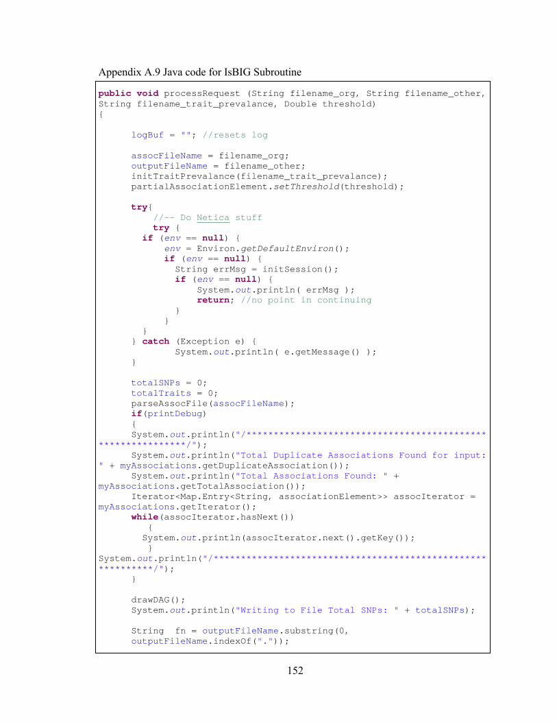
152

Appendix A.9 Java code for IsBIG Subroutine public void processRequest (String filename_org, String filename_other, String filename_trait_prevalance, Double threshold) { logBuf = ""; //resets log assocFileName = filename_org; outputFileName = filename_other; initTraitPrevalance(filename_trait_prevalance); partialAssociationElement.setThreshold(threshold); try{ //-- Do Netica stuff try { if (env == null) { env = Environ.getDefaultEnviron(); if (env == null) { String errMsg = initSession(); if (env == null) { System.out.println( errMsg ); return; //no point in continuing } } } } catch (Exception e) { System.out.println( e.getMessage() ); }

totalSNPs = 0; totalTraits = 0; parseAssocFile(assocFileName); if(printDebug) {

System.out.println("/************************************************************/"); System.out.println("Total Duplicate Associations Found for input: " + myAssociations.getDuplicateAssociation()); System.out.println("Total Associations Found: " + myAssociations.getTotalAssociation()); Iterator<Map.Entry<String, associationElement>> assocIterator = myAssociations.getIterator(); while(assocIterator.hasNext()) { System.out.println(assocIterator.next().getKey()); } System.out.println("/************************************************************/"); } drawDAG(); System.out.println("Writing to File Total SNPs: " + totalSNPs);

String fn = outputFileName.substring(0, outputFileName.indexOf("."));

153

Streamer os1 = new Streamer(fn + "_SNP.dne" ); tempNet.write(os1); triangulate(); prune(); System.out.println("Writing to File Pruned SNPs Network: "); Streamer os2 = new Streamer(fn + "_PrunedSNP.dne" ); tempNet.write(os2); Iterator<snp> snpListIterator= snpListByRSquare.iterator(); if(printDebug)

{ while(snpListIterator.hasNext()) { System.out.println(snpListIterator.next().getName()); }

System.out.println("/************************************************************/");

} drawDAG_traits(); System.out.println("Total Traits: " + totalTraits); Iterator<String> traitListIterator= traitList.iterator(); if(printDebug) { while(traitListIterator.hasNext()) { System.out.println(traitListIterator.next()); }

System.out.println("/************************************************************/");

} removeCyclesBeforeCPT(); computeCPT(); computeCPTofTraits();

boolean compiled = false; while(!compiled) { try{ tempNet.compile(); compiled = true; } catch(NeticaException e) { if(e.getMessage().contains("is a cycle (containing link")) { String [] msg = e.getMessage().split("->"); String [] n = msg[0].split("link"); String [] msgg = msg[1].split("\n"); String c_name = msgg[0].trim(); String n2 = c_name.substring(0,c_name.length()-1); Node child = (Node) tempNet.getNode(n2);

Node parent = (Node) tempNet.getNode(n[1].trim()); removeCycles(parent, child); } else if(e.getMessage().contains("doesn't have a CPT table"))

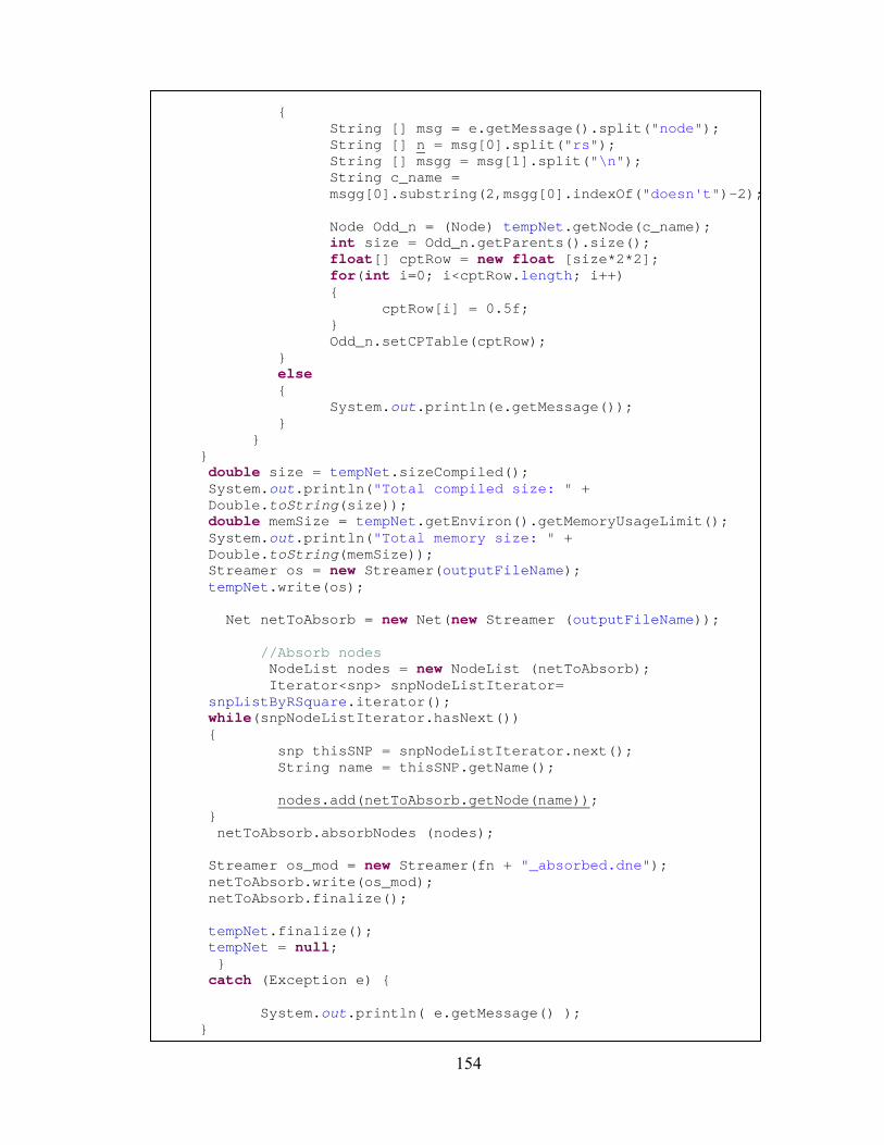
154

{ String [] msg = e.getMessage().split("node"); String [] n = msg[0].split("rs"); String [] msgg = msg[1].split("\n");

String c_name = msgg[0].substring(2,msgg[0].indexOf("doesn't")-2);

Node Odd_n = (Node) tempNet.getNode(c_name); int size = Odd_n.getParents().size(); float[] cptRow = new float [size*2*2]; for(int i=0; i<cptRow.length; i++) { cptRow[i] = 0.5f; } Odd_n.setCPTable(cptRow); } else { System.out.println(e.getMessage()); } } } double size = tempNet.sizeCompiled();

System.out.println("Total compiled size: " + Double.toString(size));

double memSize = tempNet.getEnviron().getMemoryUsageLimit(); System.out.println("Total memory size: " + Double.toString(memSize));

Streamer os = new Streamer(outputFileName); tempNet.write(os); Net netToAbsorb = new Net(new Streamer (outputFileName)); //Absorb nodes NodeList nodes = new NodeList (netToAbsorb);

Iterator<snp> snpNodeListIterator= snpListByRSquare.iterator();

while(snpNodeListIterator.hasNext()) { snp thisSNP = snpNodeListIterator.next(); String name = thisSNP.getName(); nodes.add(netToAbsorb.getNode(name)); } netToAbsorb.absorbNodes (nodes); Streamer os_mod = new Streamer(fn + "_absorbed.dne"); netToAbsorb.write(os_mod); netToAbsorb.finalize(); tempNet.finalize(); tempNet = null; }

catch (Exception e) {

System.out.println( e.getMessage() ); }

155

REFERENCES 1. Potential etiologic and functional implications of genome-wide association loci

for human diseases and traits. Proc Natl Acad Sci U S A, 2009. 106(23): p. 9362-7. Epub 2009 May 27.

2. McDonald, C.J. and et al, The Regenstrief Medical Record System: 20 years of experience in hospitals, clinics, and neighborhood health centers. MD Computing. 1992. 9(4): p. 206-17.

3. Pearl, J., Probabilistic Reasoning in Intelligent Systems: Networks of Plausible Inference. 1988.

4. Heckerman, D.E., A tutorial on learning with Bayesian Networks. In M. Jordan (Ed.), Learning in Graphical Models. Cambridge, MA: MIT Press, 1999.

5. Middleton, B., et al., Probabilistic diagnosis using a reformulation of the INTERNIST-1/QMR knowledge base. II. Evaluation of diagnostic performance. Methods Inf Med, 1991. 30(4): p. 256-67.

6. Neapolitan, R., Learning Bayesian Networks. 2004. 7. Cooper, G.F., The Computational Complexity of Probabilistic Inference Using

Bayesian Belief Networks. Artificial Intelligence, 1990. 33. 8. Li, Z., D'Ambrosio B, Efficient inference in Bayes network as a combinatorial

optimization problem. International Journal of Approximate Reasoning, 1994. 11(1): p. 55-81.

9. Shachter, R., Evaluating Influence Diagrams. Operations Research, 1986. 34: p. 871-882.

10. Shachter, R., Probabilistic Inference and Influence Diagrams. Operations Research, 1988. 36: p. 589-605.

11. Jensen, F., Lauritzen, SL, Olesen, KV, Bayesian Updating in Causal Probabilistic Networks by Local Computation. Computational Statistical Quaterly, 1990. 4.

12. Lauritzen, S.a.S., DJ, Local Computation with Probabilities in Graphical Structures and Their Applications to Expert Systems. Journal of Royal Statistical Society, 1998. 50(2).

13. Castilio, E., Guterrez JM, Hadi AS, Expert Systems and Probabilistic Network Models. 1997: Springer-Verlag, New York.

14. Geiger, D.a.H., D, Learning Gaussian Networks. Proc. 10th Conference on Uncertainty in Artificial Intelligence, 1994: p. 235-243.

15. Onisko, A., Druzdzel, MJ, Wasyluk, H, Learning Bayesian Network Parameters from Small Data Sets: Applictaion of Noisy-OR Gates. 2000. 12th European Conference on Artificial Intelligence, Berlin, Germany.

16. Zhang NL, P., D, Exploiting Causal Independence in Bayesian Network Inference. Journal of Artificial Intelligence Research, 1996. 5(301-328).

17. Poole, D., Probabilistic Horn abduction and Bayesian networks. Artificial Intelligence, 1993. 64(1): p. 81-129.

18. Boutilier, C.P., David, Computing Optimal Policies for Partially Observable Decision Processes using Compact Representations. Proceedings of the Thirteenth National Conference on Artifical Intelligence (AAAi-96), 1996: p. 1168-1175.

156

19. Geiger, D.a.H., D, Learning Bayesian Networks: A unification for discrete and gaussian domains. Proceeding of the Eleventh Conference on Uncertainty in Artificial Intelligence, 1995: p. 274-284.

20. Good, I., A causal calculus (I). British Journal of Philosophy of Science, 1961. 11: p. 305-318.

21. Heckerman, D.E., Breese, J.S, A new look at causal independence. Proceedings of the 10th Annual Conference on Uncertainity in Artifical Intelligence (UAI-94), 1994: p. 286-292.

22. Diez, F., Parameter adjustment in Bayes networks. The generalized noisy-OR-gate. Proceedings of the 9th Conference on Uncertainity in Artifical Intelligence (UAI-94), 1993: p. 286-292.

23. Henrion, M., Some practical issues in constructing belief networks. Uncertainity in Artificial Intelligence 3. New York, NY: ELsivier Science Publishing Company, Inc., 1989: p. 161-173.

24. Srinivas, S., A Generalization of the Noisy-Or Model. Proceedings of the Ninth Annual Conference on Uncertainty in Artificial Intelligence (UAI-93), 1993: p. 208-215.

25. Zagorecki A, D.M., An Empirical Study of Probability Elicitaion under Noisy-OR Assumption. Proceedings of the Seventeenth International Florida Artificial Intelligence Research Society Conference (FLAIRS 2004), 2004: p. 880-885.

26. Diez, F.a.D.M., Canonical probabilistic models for knowledge engineering. 2003. 27. Heckerman, D.E., Breese, J.S, Causal Independence for Probability Assessment

and Inference Using Bayesian Networks. IEEE Transactions on Systems, Man and Cybernetics, 1996. 26: p. 826-831.

28. Xiang, Y.a.J., Ning, Modeling Causal Reinforcement and Undermining for Efficient CPT Elicitation. IEEE Transactions on Knowledge and Data Engineering, 2007. To appear in a future issue.

29. Lemmer, J., Gossink DE, Recursive Noisy OR - A Rule for Estimating Complex Probabilistic Interactions. IEEE Transactions on Systems, Man, And Cybernetics - Part B: Cybernetics, 2004. 34(6).

30. Zagorecki A, D.M., Probabilistic independence of causal influences. Proceedings of the Third European Workshop on Probabilistic Graphical Models (PGM-06), 2006: p. 325-332.

31. Collins, F.S., Shattuck lecture--medical and societal consequences of the Human Genome Project. N Engl J Med, 1999. 341(1): p. 28-37.

32. Marks, G.B., Environmental factors and gene-environment interactions in the aetiology of asthma. Clin Exp Pharmacol Physiol, 2006. 33(3): p. 285-9.

33. Burke, W., Genomics as a Probe for Disease Biology. 2003. p. 969-974. 34. Patino, C.M. and F.D. Martinez, Interactions between genes and environment in

the development of asthma. Allergy, 2001. 56(4): p. 279-86. 35. Mannino, D.M., et al., Surveillance for asthma--United States, 1980-1999.

MMWR Surveill Summ, 2002. 51(1): p. 1-13. 36. Bosse, Y. and T.J. Hudson, Toward a comprehensive set of asthma susceptibility

genes. Annu Rev Med, 2007. 58: p. 171-84. 37. Wills-Karp, M. and S.L. Ewart, Time to draw breath: asthma-susceptibility genes

are identified. Nat Rev Genet, 2004. 5(5): p. 376-87.

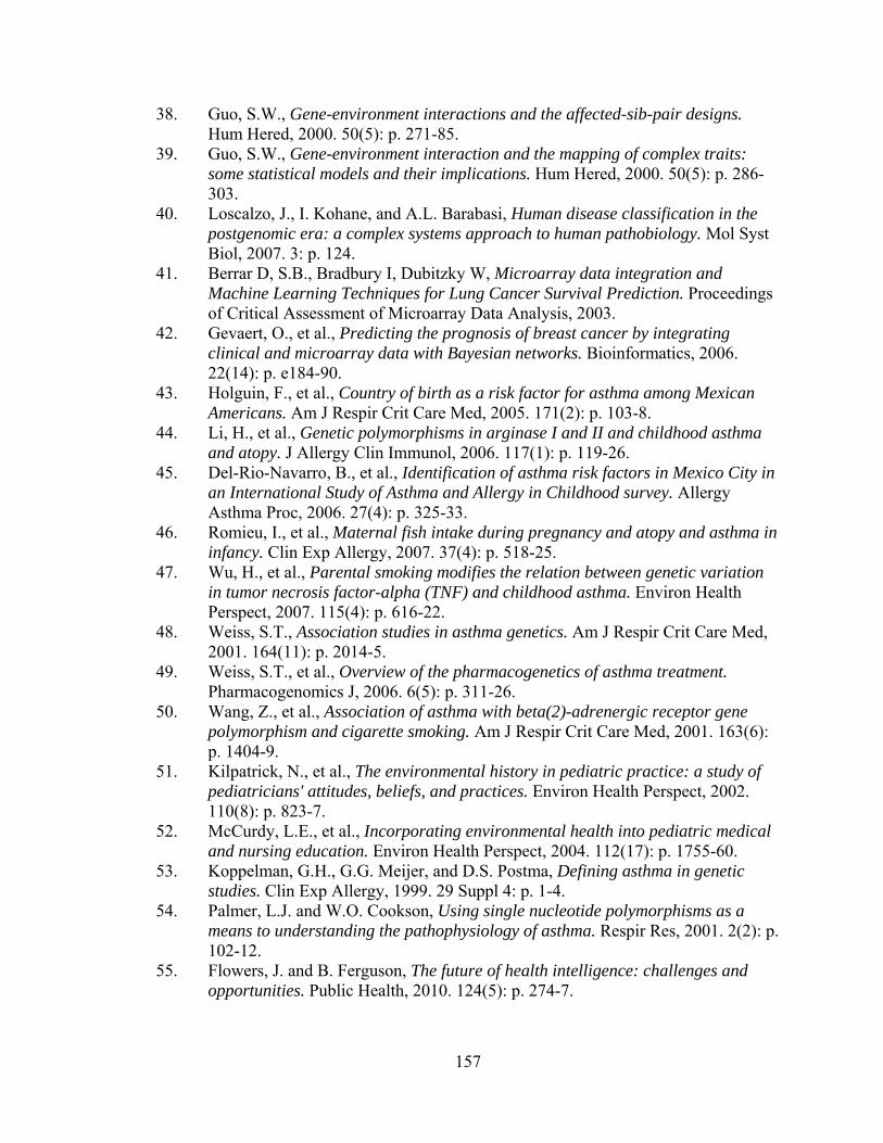
157

38. Guo, S.W., Gene-environment interactions and the affected-sib-pair designs. Hum Hered, 2000. 50(5): p. 271-85.

39. Guo, S.W., Gene-environment interaction and the mapping of complex traits: some statistical models and their implications. Hum Hered, 2000. 50(5): p. 286-303.

40. Loscalzo, J., I. Kohane, and A.L. Barabasi, Human disease classification in the postgenomic era: a complex systems approach to human pathobiology. Mol Syst Biol, 2007. 3: p. 124.

41. Berrar D, S.B., Bradbury I, Dubitzky W, Microarray data integration and Machine Learning Techniques for Lung Cancer Survival Prediction. Proceedings of Critical Assessment of Microarray Data Analysis, 2003.

42. Gevaert, O., et al., Predicting the prognosis of breast cancer by integrating clinical and microarray data with Bayesian networks. Bioinformatics, 2006. 22(14): p. e184-90.

43. Holguin, F., et al., Country of birth as a risk factor for asthma among Mexican Americans. Am J Respir Crit Care Med, 2005. 171(2): p. 103-8.

44. Li, H., et al., Genetic polymorphisms in arginase I and II and childhood asthma and atopy. J Allergy Clin Immunol, 2006. 117(1): p. 119-26.

45. Del-Rio-Navarro, B., et al., Identification of asthma risk factors in Mexico City in an International Study of Asthma and Allergy in Childhood survey. Allergy Asthma Proc, 2006. 27(4): p. 325-33.

46. Romieu, I., et al., Maternal fish intake during pregnancy and atopy and asthma in infancy. Clin Exp Allergy, 2007. 37(4): p. 518-25.

47. Wu, H., et al., Parental smoking modifies the relation between genetic variation in tumor necrosis factor-alpha (TNF) and childhood asthma. Environ Health Perspect, 2007. 115(4): p. 616-22.

48. Weiss, S.T., Association studies in asthma genetics. Am J Respir Crit Care Med, 2001. 164(11): p. 2014-5.

49. Weiss, S.T., et al., Overview of the pharmacogenetics of asthma treatment. Pharmacogenomics J, 2006. 6(5): p. 311-26.

50. Wang, Z., et al., Association of asthma with beta(2)-adrenergic receptor gene polymorphism and cigarette smoking. Am J Respir Crit Care Med, 2001. 163(6): p. 1404-9.

51. Kilpatrick, N., et al., The environmental history in pediatric practice: a study of pediatricians' attitudes, beliefs, and practices. Environ Health Perspect, 2002. 110(8): p. 823-7.

52. McCurdy, L.E., et al., Incorporating environmental health into pediatric medical and nursing education. Environ Health Perspect, 2004. 112(17): p. 1755-60.

53. Koppelman, G.H., G.G. Meijer, and D.S. Postma, Defining asthma in genetic studies. Clin Exp Allergy, 1999. 29 Suppl 4: p. 1-4.

54. Palmer, L.J. and W.O. Cookson, Using single nucleotide polymorphisms as a means to understanding the pathophysiology of asthma. Respir Res, 2001. 2(2): p. 102-12.

55. Flowers, J. and B. Ferguson, The future of health intelligence: challenges and opportunities. Public Health, 2010. 124(5): p. 274-7.

158

56. Brewer, D.D., J.J. Potterat, and S.Q. Muth, Withholding access to research data. Lancet, 2010. 375(9729): p. 1872; author reply 1873.

57. Hanley, J.A. and B.J. McNeil, The meaning and use of the area under a receiver operating characteristic (ROC) curve. Radiology, 1982. 143(1): p. 29-36.

58. Fawcett, T., An introduction to ROC analysis. ROC Analysis in Pattern Recognition, 2006. 27(8): p. 861-874.

59. Anand, V., et al., Child Health Improvement through Computer Automation: the CHICA system. Medinfo, 2004. 11(Pt 1): p. 187-91.

60. Anand, V. and S.M. Downs, Probabilistic Asthma Case Finding - A Pilot Study using the CHICA system. Medinfo, 2007. 12(Pt 1): p. 292.

61. Biondich, P.G., et al., A modern optical character recognition system in a real world clinical setting: some accuracy and feasibility observations. Proc AMIA Symp, 2002: p. 56-60.

62. Jenders, R.A., et al., Medical decision support: experience with implementing the Arden Syntax at the Columbia-Presbyterian Medical Center. Proc Annu Symp Comput Appl Med Care, 1995: p. 169-73.

63. Downs, S.M. and H. Uner, Expected value prioritization of prompts and reminders. Proc AMIA Symp, 2002: p. 215-9.

64. Biondich, P.G., et al., Automating the recognition and prioritization of needed preventive services: early results from the CHICA system. AMIA Annu Symp Proc, 2005: p. 51-5.

65. Downs, S., et al., Using Arden Syntax and adaptive turnaround documents to evaluate clinical guidelines. AMIA Annu Symp Proc, 2006: p. 214-8.

66. Downs, S.M., et al., Human and system errors, using adaptive turnaround documents to capture data in a busy practice. AMIA Annu Symp Proc, 2005: p. 211-5.

67. Netica. Application for Belief Networks and Influence Diagrams. Norsys Software Corp. 1997.

68. Chickering, D.M., The WinMine Toolkit - MSR-TR-2002-103. 2002. 69. Anand, V. and S. Downs, Probabilistic asthma case finding: a noisy or

reformulation. AMIA Annu Symp Proc, 2008: p. 6-10. 70. Anand, V. and S. Downs, An Empirical Validation of Recursive Noisy OR

(RNOR) Rule for Asthma Prediction. AMIA Annu Symp Proc, 2010. 71. Heckerman, D.E., Geiger, D, Chickering, Learning Bayesian Networks: The

combination of knowledge and statistical data. Machine Learning, 1995. 20: p. 197-243.

72. Hanley, J.A. and B.J. McNeil, A method of comparing the areas under receiver operating characteristic curves derived from the same cases. Radiology, 1983. 148(3): p. 839-43.

73. Anand, V. and S. Downs, In-Silico Testing of Genotype-Phenotype Associations with Electronic Medical Records – A case study with Asthma. Medinfo 2010.

74. Hall, I.P., Pharmacogenetics of asthma. Chest, 2006. 130(6): p. 1873-8. 75. Bevington, P.R., Data Reduction and Error Analysis For The Physical Sciences.

1969: McGraw-Hill Book Company. 76. Pagano, M.a.G., K, Principles of Biostatistics. 2000: Duxbury Thomson Learning.

159

77. Frazer, K.A., et al., A second generation human haplotype map of over 3.1 million SNPs. Nature, 2007. 449(7164): p. 851-61.

78. Consortium, I.H., A haplotype map of the human genome. Nature, 2005. 437(7063): p. 1299-320.

79. Altshuler, D., M.J. Daly, and E.S. Lander, Genetic mapping in human disease. Science, 2008. 322(5903): p. 881-8.

80. Knight, J.C., Genetics and the general physician: insights, applications and future challenges. QJM, 2009. 102(11): p. 757-72.

81. Kraft, P. and C.A. Haiman, GWAS identifies a common breast cancer risk allele among BRCA1 carriers. Nat Genet, 2010. 42(10): p. 819-20.

82. Wadelius, M., et al., The largest prospective warfarin-treated cohort supports genetic forecasting. Blood, 2009. 113(4): p. 784-92.

83. Hindorff, L.A., et al., Potential etiologic and functional implications of genome-wide association loci for human diseases and traits. Proc Natl Acad Sci U S A, 2009. 106(23): p. 9362-7.

84. McCarthy, M.I. and J.N. Hirschhorn, Genome-wide association studies: potential next steps on a genetic journey. Hum Mol Genet, 2008. 17(R2): p. R156-65.

85. Sulem, P., et al., Two newly identified genetic determinants of pigmentation in Europeans. Nat Genet, 2008. 40(7): p. 835-7.

86. Sulem, P., et al., Genetic determinants of hair, eye and skin pigmentation in Europeans. Nat Genet, 2007. 39(12): p. 1443-52.

87. Weedon, M.N. and T.M. Frayling, Reaching new heights: insights into the genetics of human stature. Trends Genet, 2008. 24(12): p. 595-603.

88. Weedon, M.N., et al., Genome-wide association analysis identifies 20 loci that influence adult height. Nat Genet, 2008. 40(5): p. 575-83.

89. Eberle, M.A., et al., Allele frequency matching between SNPs reveals an excess of linkage disequilibrium in genic regions of the human genome. PLoS Genet, 2006. 2(9): p. e142.

90. Devlin, B. and N. Risch, A comparison of linkage disequilibrium measures for fine-scale mapping. Genomics, 1995. 29(2): p. 311-22.

91. Myles, S., et al., Worldwide population differentiation at disease-associated SNPs. BMC Med Genomics, 2008. 1(22): p. 22.

92. Johnson, A.D., et al., SNAP: a web-based tool for identification and annotation of proxy SNPs using HapMap. Bioinformatics, 2008. 24(24): p. 2938-9.

93. Sebastiani, P., et al., Genome-wide association studies and the genetic dissection of complex traits. Am J Hematol, 2009. 84(8): p. 504-15.

94. de la Fuente, A., et al., Discovery of meaningful associations in genomic data using partial correlation coefficients. Bioinformatics, 2004. 20(18): p. 3565-74.

95. Sawcer, S., Bayes factors in complex genetics. Eur J Hum Genet, 2010. 18(7): p. 746-50.

96. Hanley, J. and B. McNeil, The meaning and use of the area under a receiver operating characteristic (ROC) curve. Radiology., 1982. 143(1): p. 29-36.

97. Palakal, M., et al., Identification of biological relationships from text documents using efficient computational methods. J Bioinform Comput Biol, 2003. 1(2): p. 307-42.

160

98. Webster, Y.W., et al., A framework for cross-disciplinary hypothesis generation, in Proceedings of the 2010 ACM Symposium on Applied Computing. 2010, ACM: Sierre, Switzerland. p. 1511-1515.

99. Metropolis, N., The beginning of the Monte Carlo Method. Los Alamos Science, 1987(1987 Special Issue dedicated to Stainslaw Ulam): p. 125-130.

100. Biester, D.J., Bright futures. J Pediatr Nurs, 1995. 10(4): p. 264-5. 101. Blaschke, G.S., et al., Choosing the Bright Futures Guidelines: lessons from

leaders and early adopters. Pediatr Ann, 2008. 37(4): p. 262-72. 102. Dinkevich, E. and P.O. Ozuah, Well-child care: effectiveness of current

recommendations. Clin Pediatr (Phila), 2002. 41(4): p. 211-7. 103. Fleming, J.W., Bright Futures: guidelines for health supervision of children.

MCN Am J Matern Child Nurs, 1996. 21(6): p. 269-70. 104. Nowak, A.J., Oral health policies and clinical guidelines. Pediatr Dent, 2007.

29(2): p. 138-9.

CURRICULUM VITAE

Vibha Anand

Education Ph.D. in Health Informatics (2005 – 2010) Indiana University, Indianapolis, Indiana, USA M.S. in Computer Sciences (1992 – 1994) University of New Haven, West Haven, Connecticut, USA B.E. in Electrical and Electronics Engineering (1982 – 1986) Motilal Nehru National Institute of Technology, India Research, Academic, and Professional Experience

Ph.D. student, Indiana University-Purdue University, Indianapolis (2005 – 2010) Develop models for medical decision support using probabilistic methods and

data mining In-Silico Bayesian Integration of GWA Studies (IsBIG) An Empirical Validation of Recursive Noisy OR (RNOR) Rule for Asthma Prediction In-Silico Testing of Genotype-Phenotype Associations with Electronic Medical

Records Probabilistic Asthma Case Finding – A Noisy-OR Reformulation Probabilistic Asthma Case Finding – A Pilot Study using the CHICA system

Research Associate Faculty, Pediatrics, IU School of Medicine (Oct 2008 – Dec 2010) Lead Systems Analyst (May 2002 – Oct 2008)

Direct Children's Health Informatics Research and Development Lab (CHIRDL) for software development. Manage a team of developers.

Medical informatics integration at point of care, Medical informatics applications, Use of healthcare standards

Collaborating with multi-disciplinary team in randomized controlled trials using pediatric decision support system (DSS), The Child Health Improvement through Computer Automation system (CHICA)

Design, development and integration of open source electronic medical record systems (OpenMRS – http://www.openmrs.org) into second generation of CHICA system.

Lead the design and development of the first generation CHICA system for Pediatric care and a DSS for Arthritis use in geriatric care.

Developed an Arden Syntax parser using open source tool (ANTLR) for translating Arden Syntax Medical logic modules based clinical guideline rules into JAVA code

Design and development of Decision Support System for Indiana Statewide Newborn Screening Alert System (using INPC network)

Senior Engineer, Hippo Inc., New Haven, CT (Oct 2000 – Mar 2002)

Designed and developed Voice over IP (VoIP) protocol based software Integrated a third party SIP stack in the firmware

Consultant Engineer, Advanced Decisions Inc., Shelton, CT (Jan 1998 – Oct 2000)

Design and develop software systems for advanced computer telephony interfaces Design and develop software systems for business logic in advanced postal meters

Lead Engineer, Executone Information Systems, Milford, CT (Jul 1993 – Jan 1998)

Design and develop software system for Private Branch Exchanges (PBX) Senior Engineer, Bull HN Info Systems, Melbourne, Australia, (Jun 1989 – Sep 1992)

Design and develop software system for Electronic Funds Transfer Point of Sale systems (EFTPOS)

Engineer Altos / UMCL / Uptron India Ltd, India, (Aug 1986 – Mar 1989)

Design and develop hardware and firmware for personal computers Memberships

American Medical Informatics Association (AMIA) – Member of Knowledge Discovery and Data Mining Working Group

Publications

Anand V, Downs SM (2010) An Empirical Validation of Recursive Noisy-OR (RNOR) Rule for Asthma Prediction, AMIA Annual Fall Symposium 2010, In press

Downs SM, Anand V, Dugan TM, Carroll AE (2010) You Can Lead a Horse to Water: Physician’s Responses to Clinical Reminders, AMIA Annual Fall Symposium 2010, In press

Anand, V., et al., Tailoring Interface for Spanish Language: A Case Study with CHICA System, in Proceedings of the 1st International Conference on Human Centered Design: Held as Part of HCI International 2009. 2009, Springer-Verlag: San Diego, CA. p. 398-407.

Anand V, Downs SM (2008) Probabilistic Asthma Case Finding: A Noisy-OR Reformulation, AMIA Annual Fall Symposium 2008,6-10,Published

Grannis S, Biondich PG, Downs SM, Sheley ME, Anand V, Egg J (2008) Leveraging Open-Source Matching Tools and Health Information Exchange to Improve Newborn Screening Follow-up, Public Health Information Network Conference (PHIN) 2008

Anand V, Downs SM (2007) Probabilistic Asthma Case Finding - A Pilot Study using the CHICA system. Medinfo, 2007. 12(Pt 1): p. 292,Published

Downs SM, Biondich PG, Anand V, Zore MM, Carroll AE (2006) Using Arden syntax and adaptive turnaround documents to evaluate clinical guidelines,, AMIA Fall Symposium, AMIA, 214-8, Published

Downs SM, Carroll AE, Anand V, Biondich PG (2005) Human and system errors, using adaptive turnaround documents to capture data in a busy practice, AMIA Fall Symposium, AMIA, 211-215, Published

Biondich PG, Downs SM, Anand V, Carroll AE (2005) Automating the recognition and prioritization of needed preventive services: early results from the CHICA system, AMIA Fall Symposium, AMIA, 51-55, Published

Anand V (2004) The CHICA RuleBuilder: A practical tool to author Arden Syntax, Medinfo, IMIA, Published

Anand V, Biondich PG, Downs SM (2004) Child Health Improvement through Computer Automation: The CHICA System, MedInfo, IMIA, 187-191, Published

Biondich PG, Anand V, Downs SM, McDonald CJ (2003) Using Adaptive Turnaround Documents to Electronically Acquire Structured Data in Clinical Settings, AMIA fall symposium, AMIA, 56-60, Published

Skills

Software Design and Development Languages - C#, JAVA, 'C', SQL, Assembly, C++, Visual Basic, Visual C++,

Pascal, Basic, Prolog, Lisp, VBScript, XML, Description Logic language Software Libraries / Framework - MFC, ATL, STL, MVC – Spring Framework Source code control – Visual Source Safe, CVS, SCCS, Subversion

(SVN) Databases - Microsoft SQL server, MySQL, Access, Btrieve OS - UNIX tools - SED, AWK, YACC, 'C' shell, K-shell, SCCS, CVS Network Communication protocols / tools - HDLC, DDCMP, NETBIOS,

TCP/UDP/IP, XNS, Windows RPC Windows Sockets, BSD Sockets, SIP, RTP, TSAPI, CSTA, Dialogic CT-Connect, Cisco ICR. Protocol Analyzer, HP In circuit emulators

Healthcare standards – HL7, Arden Syntax, LOINC, SNOMED, UMLS, MeSH, DICOM

Modeling

UML Modeling, ER Diagrams, ANTLR (www.antlr.org) tool Bayesian Networks