Process‐based, morphodynamic hindcast of decadal depositionpatterns in San Pablo Bay, California, 1856–1887

M. van der Wegen,1 B. E. Jaffe,2 and J. A. Roelvink1,3,4

Received 8 December 2009; revised 3 February 2011; accepted 9 February 2011; published 22 April 2011.

[1] This study investigates the possibility of hindcasting‐observed decadal‐scalemorphologic change in San Pablo Bay, a subembayment of the San Francisco Estuary,California, USA, by means of a 3‐D numerical model (Delft3D). The hindcastperiod, 1856–1887, is characterized by upstream hydraulic mining that resulted in ahigh sediment input to the estuary. The model includes wind waves, salt water andfresh water interactions, and graded sediment transport, among others. Simplifiedinitial conditions and hydrodynamic forcing were necessary because detailed historicdescriptions were lacking. Model results show significant skill. The river dischargeand sediment concentration have a strong positive influence on deposition volumes.Waves decrease deposition rates and have, together with tidal movement, the greatesteffect on sediment distribution within San Pablo Bay. The applied process‐based (orreductionist) modeling approach is valuable once reasonable values for model parametersand hydrodynamic forcing are obtained. Sensitivity analysis reveals the dominantforcing of the system and suggests that the model planform plays a dominant role inthe morphodynamic development. A detailed physical explanation of the model outcomesis difficult because of the high nonlinearity of the processes. Process formulationrefinement, a more detailed description of the forcing, or further model parameter variationsmay lead to an enhanced model performance, albeit to a limited extent. The approachpotentially provides a sound basis for prediction of future developments. Parallel useof highly schematized box models and a process‐based approach as described in the presentwork is probably the most valuable method to assess decadal morphodynamic development.

Citation: van der Wegen, M., B. E. Jaffe, and J. A. Roelvink (2011), Process‐based, morphodynamic hindcast of decadaldeposition patterns in San Pablo Bay, California, 1856–1887, J. Geophys. Res., 116, F02008, doi:10.1029/2009JF001614.

1. Introduction

1.1. Need for Research

[2] Managing estuarine system requires understanding ofthe processes governing bathymetric evolution. Examplesof relevant morphodynamic developments are the evolutionof salt marshes [Allen, 2000; Temmerman et al., 2005], thesiltation of access channels to ports [Kirby, 2002], and ero-sion exposing legacy contaminants [van Geen and Luoma,1999; Higgins et al., 2007].[3] The estuarine morphodynamic system is characterized

by coupled interactions acting at different spatial and timescales. This implies that bed level changes at a particularlocation and time are a function of the larger morphody-namic system and cannot be fully understood by analyzinglocal conditions only. Furthermore, significant morphody-

namic developments take place that are not recognized orunderstood over relatively short time spans of years.[4] Bathymetric surveys on the decadal time scale are

invaluable for developing insight into the morphodynamicbehavior of an estuarine system. Since these measurementsare costly and require discipline in timing and coverageof the area of interest, detailed data are scarce and often evennonexistent in many places in the world, especially forlonger time scales (>50 years).[5] Analysis of bathymetric change by itself may not be

able to identify forcing mechanisms and processes. Numer-ical modeling is a way to explore these forcings. In combi-nation with data collection for calibration it is a useful toolto address morphodynamic behavior of estuarine systemsover time.

1.2. Different Modeling Approaches

[6] Several modeling approaches may be followed tostudy, hindcast and forecast the morphological develop-ment of alluvial estuaries. Different definitions for the end‐members of the modeling approaches spectrum are suggested,namely “process‐based” and “aggregated” [De Vriend et al.,1993], “reductionism” versus “universality” [Werner, 2003]

1UNESCO‐IHE, Delft, Netherlands.2USGS Pacific Science Center, Santa Cruz, California, USA.3Delft University of Technology, Delft, Netherlands.4Deltares, Delft, Netherlands.

Copyright 2011 by the American Geophysical Union.0148‐0227/11/2009JF001614

JOURNAL OF GEOPHYSICAL RESEARCH, VOL. 116, F02008, doi:10.1029/2009JF001614, 2011

F02008 1 of 22

and “simulation models” versus “exploratory models” [Murray,2003]. Although they differ in origin and qualification,the definitions of the end‐members roughly range from acomplex, detailed description of processes on the one sideto a more simplified schematization on the other side. Forexample, originating from a river and coastal engineeringbackground De Vriend et al. [1993] distinguish aggregatedmodeling (that focuses on empirical relations between geo-morphic development and hydrodynamic parameters withoutdescribing the underlying physical processes) from process‐based modeling which is based on a detailed description ofthe underlying physical processes. Further, Werner [2003]suggests the useful concept of hierarchical modeling whichassumes a hierarchy in processes that depend on each other,but do not interact. Small‐scale processes can thus act asparameterized input for modeling larger‐scale and longer‐term processes. Still, in practical applications one needs todetermine what processes are considered “small” and howthese should be parameterized in the model.[7] The modeling approach applied in the current study is

based on breaking physical phenomena down into theirsimplest components so that they can be understood at afundamental “physical” level. As will become clear in section3, we endeavor to reduce reality in such a way that no rele-vant processes are lost, but that, at the same time, not toomany processes are included so that the model becomesso complicated that interpretation of the modeling results isequivocal at best and not possible at worse. Given thespectrum of related modeling efforts described in literature,the character of the current study can be categorized as pro-cess‐based [De Vriend et al., 1993], reductionist or hierar-chical [Werner, 2003] or as simulation model [Murray,2003]. In the current work we will refer to a process‐basedmodeling approach.

1.3. Required Model Input Data

[8] Apart from a proper description of the forcing condi-tions, the value of process‐based morphodynamic models de-pends to a high degree on empirically validated formulations,such as sediment transport formulae or roughness formula-tions. These empirical equations include constants associatedwith confidence intervals that are determined by laboratorytests or, more seldom, in nature itself. For example, for cohe-sive sediment the critical shear stress for the initiation of sed-iment motion depends on the character of the bed material,its compaction rate and on the (seasonally varying) presenceof biomass. Thus it becomes a function of time. Further-more, critical shear stress alsowill likely varywith depth belowthe bed surface and throughout the area of interest.[9] One may argue that, for an accurate model prediction

of sedimentation and erosion patterns, it is necessary tomeasure these bed characteristics across the whole modeldomain and over the entire time span of interest. This wouldbe a demanding, if not impossible, task both in terms oftime and cost and it may not really be necessary to do so forall applications. Parameter estimation can also be basedon inverse data assimilation techniques. For example, Yangand Hamrick [2003] explored the possibility of derivingcohesive sediment transport parameter values by iterativelycomparing model outcomes with adjusted parameter settingsfrom an extensive data set. This methodology, however,would require extensive data for assimilation.

[10] Another approach, applied in the current research, isto simply assume “reasonable and averaged” values formodel parameters. This method is particularly useful ifdata are limited or lacking, which is the case for historicalhindcasts. Sensitivity analysis on parameter value variationwould subsequently indicate the parameter space wheremodel will likely perform well.

1.4. Earlier Modeling Studies[11] Schuttelaars and De Swart [1999], Seminara and

Tubino [2001], Schramkowski et al. [2002], and VanLeeuwen and De Swart [2004] (among others) providemodeling efforts describing 2‐D pattern formation char-acteristics. On an embayment length scale Van Dongerenand De Vriend [1994], Hibma et al. [2003a], Friedrichsand Aubrey [1996], Schuttelaars and De Swart [2000],and Lanzoni and Seminara [2002] (among others) adopt aschematized 1‐D approach to investigate equilibrium con-ditions of a longitudinal embayment profile.[12] Hibma et al. [2003b, 2004], van der Wegen and

Roelvink [2008], and van der Wegen et al. [2008] showthat a 2‐D modeling approach leads to relatively stablepatterns and bed profiles in ∼100 km long embaymentsunder idealized conditions such as constant forcing condi-tions and uniform sand distribution over the model domain.These studies distinguish a time scale for pattern forma-tion (approximate decades) and a time scale related to thedevelopment of the full embayment (approximate millen-nia). Others applied a similar methodology to describedecadal development and pattern formation in more realisticgeometries related to Wadden Sea inlets, the Netherlands[Marciano et al., 2005; Dissanayake et al., 2009; Dastgheibet al., 2008] or the Western Scheldt, the Netherlands[van der Wegen and Roelvink, 2008]. Fortunato et al.[2009] assess uncertainty associated with morphodynamicprocess‐based models for a Portuguese lagoon. The studiesmentioned above are governed by tide‐dominated sandtransport. In studies closely related to this research Ganjuet al. [2009] and Ganju and Schoellhamer [2010] focusedon a mud‐dominated estuary with large freshwater flow.They modeled decadal morphodynamic development inSuisun Bay, a subembayment of San Francisco Bay thatis located adjacent to San Pablo Bay. Ganju et al. [2009]found an average error of 37% for bathymetric changeover individual depth ranges and poor spatial amplitudecorrelation performance of the model on a cell‐by‐cell basis,though spatial phase correlation was better, with 61% ofthe domain correctly indicated as erosional or depositional.

1.5. Aim and Approach of the Study

[13] The objective of the current research is to investigatethe processes governing morphodynamic evolution in acomplex alluvial estuary using a process‐based (or reduc-tionist) morphodynamic model. The study focuses on ahindcast of morphodynamic development in a subembay-ment of San Francisco Estuary, San Pablo Bay, during theperiod from 1856 to 1887.[14] The reason for selection of this location and period

is that a rare bathymetric data set is available for modelcalibration. The full data set covers a relatively long period(∼150 years) with intervals of approximately 30 years [Jaffeet al., 2007]. The data set reflects sedimentation and erosion

VAN DER WEGEN ET AL.: MORPHODYNAMIC HINDCAST IN SAN PABLO BAY F02008F02008

2 of 22

patterns of a major sediment pulse caused by hydraulicmining in the mid‐19th century. The 1856–1887 periodis highly depositional and reflects the impact of a majorforcing signal, that is, temporal and excessive sedimentsupply by two major rivers toward the bay. Future studieswill focus on more erosional periods and forecasts for dif-ferent scenarios of sea level rise.[15] One of our modeling dilemmas is that we cannot

determine beforehand which processes, parameter valuesand forcing conditions are essential and dominant. Evenmore, the set of processes may not be and probably is notcomplete. Only comparisons of model results with mea-surements will show to what extent dominant processes arecovered by the model formulations. Because of the largenumber of processes and their mutual, often nonlinear, in-teractions, it will be difficult to assess in a detailed physicalway the driving mechanisms behind the developments tak-ing place. Therefore we carry out a thorough sensitivityanalysis that includes or excludes different processes orforcing conditions and vary the coefficient values used inthe process formulations. In this way we will be able toanswer questions related to the importance of differentprocesses and the required accuracy level of the processdescriptions and model parameter values. Once properlycalibrated and validated with measurements, the approachprovides potentially a sound basis for detailed predictionof future developments.[16] Apart from the focus area, the present study differs

from the Ganju et al. [2009] and Ganju and Schoellhamer[2010] studies in three key ways: (1) the modeling of theinitial bed composition, (2) a highly schematized riverineinput, and (3) emphasis on an extensive sensitivity analysisinvestigating the impact of variations of model parametersettings and processes. Sections 2, 3, and 4 describe, inorder, the historical context of the morphodynamic devel-opments in San Pablo Bay, the model setup and the modelparameter settings, model results in comparison to measureddevelopments, and finally, model results in terms of anextensive sensitivity analysis.

2. Description of San Francisco Estuary

[17] Extensive literature is available on the San FranciscoEstuary. The short introduction given below only aims athighlighting the most relevant aspects for the currentresearch and is based on the review by Kimmerer [2004],if not otherwise stated.

2.1. Geometry

[18] San Francisco Estuary is a drowned tectonicallyreshaped river valley. It consists of a number of intercon-nected subembayments (Figure 1). Two main rivers, theSacramento River and the San Joaquin River, meet in thearea referred to as the Delta, which consists of a complexnetwork of channels, sloughs and shallow lakes. The riverflow discharges from the Delta to Suisun Bay, via therelatively narrow Carquinez Strait, to San Pablo Bay andCentral Bay and, finally, through the narrow and deepGolden Gate into the sea. This area is referred to as thenorthern reach. Additionally, Central Bay connects to SouthBay to the south. South Bay, however, receives considerablyless river flow.

[19] In Suisun Bay the main channel from the Delta splitsinto two main channels, the Northern passage and Southernpassage, of which the latter is the main shipping channel andhas a depth of about 10–15 m. The channels are sandy andsilty with occasional mud banks. The shallows (0–6 mbelow MSL) between the main channels and north of theSuisun Bay are mud covered and partly intertidal. CarquinezStrait has an alluvial bed with a maximum depth of about35 m below MSL and is flanked by rock.[20] The bathymetry of San Pablo Bay is characterized by

a single main channel, about 20–30 m deep, that connectsCarquinez Strait to San Pablo Strait. The latter has a max-imum depth of about 40 m. The main channel has a silty bedwith sandy and muddy patches [Locke, 1971]. Two other,much smaller and shallower, channels in the northern part ofSan Pablo Bay are dredge maintained. The extensive shal-low areas both south and north of the main channel aremuddy (with particles largely smaller than 4 mm) and coverabout 80% of the Bay. About 90% of these shallows are lessthan 4 m deep, and silty intertidal flats are present at thecoastline edges [Locke, 1971].[21] Central Bay is relatively deep and sandy and com-

prises a much lower percentage of shallow, mud‐coveredarea than San Pablo Bay, Suisun Bay or South Bay. CentralBay is covered with a range of bed forms depending on thesand grain size and local tidal velocities [Rubin and McCulloch, 1979].

2.2. Hydrodynamics

[22] The river discharge regime is characterized by a rel-atively dry season (summer/autumn) and a wet season(winter/spring). However, amounts and distribution of yearlydischarge over time are highly variable. Peak discharges mayamount to 17,800 m3 s−1, but can be 300 m3 s−1 during dryyears, whereas low discharges during autumnmay not exceed100 m3 s−1. The San Joaquin River is responsible forabout 10–15% of the discharge and the Sacramento River forabout 80%. The remaining discharge originates from minortributaries. During high discharges the Yolo Bypass, a majormanaged floodplain of the Sacramento River, may convey upto 60% of the Sacramento River discharge. Values and timingof river discharges are subject to human interferences bymeans of managed reservoir releases in the watershed andwater export from the Delta for the purpose of fresh watersupply to Southern California.[23] The tide near the Golden Gate is highly irregular with

strong diurnal components [Smith, 1980]. It consists of adominant semidiurnal M2 component, a spring‐neap tidalvariation and even considerable longer period fluctuations.Median tidal range is about 1.8 m. In the estuary itselffriction and reflection processes complicate the tidalbehavior. Water levels and velocities in North Bay are inphase (i.e., a progressive wave) and water level amplitudesslowly decay, whereas in South Bay the tidal wave showsresonant behavior so that a time lag between water levelsand velocities develops and the water level amplitudeamplifies near the head. During high river discharge no tidalinfluence is present at Sacramento (155 km upstream fromthe Golden Gate), whereas minor tidal fluctuations areobserved during low river discharges. Water levels at GoldenGate show a slight increase (approximate centimeters) incase of high river flows.

VAN DER WEGEN ET AL.: MORPHODYNAMIC HINDCAST IN SAN PABLO BAY F02008F02008

3 of 22

[24] The tidally averaged mean salt intrusion up theestuary depends primarily on fresh water flow and to a lesserextent on spring‐neap tidal variations. The 2 psu isohalineis found most often in Suisun Bay and dam water releaseduring dry periods is managed in such a way that that saltdoes not intrude farther landward. High river flows maycause salinities to decrease to less than 5 psu east of SanPablo Bay. Stratification and gravitational circulation occursin particular during neap tides, when tidally driven mixingprocesses are weak. The location varies depending on the riverdischarge. Ganju et al. [2006] give an example of stratifica-tion measured near Benicia Bridge in Carquinez Strait. Lowriver flows allow for salinities of about 25 psu near BeniciaBridge and considerably reduce stratification. Stacey et al.[2008] further point to the importance of tidally periodicstratification also generating estuarine subtidal circulation.

2.3. Sediment Dynamics

[25] It is generally assumed that most sediment to theestuary is supplied by the two major rivers and thattributaries discharging directly into San Pablo Bay have aminor role in sediment supply [Porterfield, 1980; Krone,1979], although McKee et al. [2006] suggest that sedimentsupply by tributaries will become more important as sedi-ment load from the two major rivers declines. On the basisof measurements, Wright and Schoellhamer [2004 andreferences therein] suggest that suspended load dominatesbed load by approximately an order of magnitude. Importfrom the sea, if any, is considered hardly relevant to thesediment budget of San Pablo Bay, although no measure-ments confirmed this yet.[26] Hydraulic mining from 1850 to 1884 caused an

excess supply of sediments mainly to the Sacramento River[Gilbert, 1917]. Krone [1979] suggests that large volumesof this sediment settled in the Delta, Suisun Bay and SanPablo Bay during the period of hydraulic mining. Mea-surements and comparison of historical bathymetries con-firm this process. After hydraulic mining stopped, SuisunBay started to erode [Cappiella et al., 1999]. San Pablo Bayonly became erosional in the mid‐20th century [Jaffe et al.,1998, 2007]. Water projects like reservoir construction inthe upstream watershed probably enhanced the erosionprocess by upstream trapping of sediments. Based on datafrom 1957 to 2001 in the Sacramento River, Wright and

Schoellhamer [2004] indicate a decreasing trend in sus-pended sediment discharge for a given flow and attributethis to depletion of erodible sediments from hydraulicmining, trapping of sediment in reservoirs, altered land useand construction of protection works and levees.[27] Porterfield [1980] reports a strong dependence of the

sand transport (as percentage of the total transport) on theriver discharge. For low river discharge of the SacramentoRiver at Sacramento sand transport may be limited to sev-eral percent of the total, but increases up to 70% for highdischarges, partly transported as suspended load and partlyas bed load. The yearly average percentage would be about50%. The rest of the material being transported consists ofclay and silt (with a particle diameter smaller than 63mm).Porterfield [1980] reports similar ratios for the mud to sandtransport for the small tributaries (disregarded in the currentstudy) near San Pablo Bay. Porterfield [1980] does notprovide information on the ratio in San Pablo Bay itself.

3. Model Setup

[28] This study uses a 3‐D, hydrostatic, numerical model(Delft3D), described in detail by Lesser et al. [2004].Delft3D solves the Reynolds averaged Navier Stokesequations, including the k‐" turbulence closure model, andapplies a horizontal curvilinear grid with sigma layers forvertical grid resolution. It allows for salt water and freshwater density variations, separate formulae for mud transportand sand transport, and variations in bed composition andspecification (for example, bed layers with different percen-tages of mud and sand and spatial variation of critical shearstress). The impact of wind and waves is added so that, forexample, the effects of wind set up and increased shear stressdue to waves in shallow water are taken into account. Theapplied wave model is SWAN, of which a detailed descrip-tion and its application in Delft3D can be found at the SWANhomepage (http://vlm089.citg.tudelft.nl/swan/index.htm) andby Booij et al. [1999] and Lesser et al. [2004].[29] For every hydrodynamic time step (1 min in this

case) the flow module calculates water levels and velocitiesfrom the shallow water equations. Based on these hydro-dynamic conditions and the wind field, the wave modulecalculates a wavefield every hour and adds wave inducedshear stresses to the shear stresses calculated from the flow

Figure 1. Location of San Pablo Bay and definition of San Pablo Bay subareas on 1856 measuredbathymetry. NWS, Northwest Shoal; NES, Northeast Shoal; SWS, Southwest Shoal; SES, Southeast Shoal.

VAN DER WEGEN ET AL.: MORPHODYNAMIC HINDCAST IN SAN PABLO BAY F02008F02008

4 of 22

module. The wavefield is considered to be constant during1 h. Sediment transport is calculated from the resulting flowfield and the bed is updated based on the divergence of thesediment transport field.[30] The model parameter settings for the San Pablo Bay

case study are described in detail in this section. The settingsare simplified partly to reduce the computational time andpartly because detailed data in time and space are simplynot available.

3.1. Model Domain

[31] The model domain comprises the area from Rio Vistaand Antioch in the Delta (in two separate branches for theSacramento River and the San Joaquin River) to Richmondin Central Bay and thus includes San Pablo Bay as wellas Carquinez Strait and Suisun Bay (Figures 1 and 2).This domain is large enough to have a negligible boundarydefinition effect on the area of interest and the domain issmall enough to allow for relatively fast runs (∼36 h forabout 4 hydrodynamically modeled months on a “heavy”PC (3.0 Ghz, 3.25 Gb RAM, quad core)).[32] A curvilinear grid is applied on the domain and the

condition for a stable and accurate computation (Courantnumber < 10) is met with a grid cell size of approximately 100by 150 m and a time step of 2 min. Density currents and waveeffects benefit from a 3‐D approach. Fifteen Sigma layersdescribe the vertical grid distribution, which is somewhat finernear the bed and the water surface to adequately resolvevelocity shear near the bed and wind and wave effects.[33] The initial bathymetry is composed of measured

bathymetries of Central Bay, San Pablo Bay, and SuisunBay measured in the years 1855, 1856, and 1867, respec-tively. Model results are compared to the bathymetry mea-sured in 1887 in San Pablo Bay. Spatial resolution of themeasurements was much higher than the resolution of themodel grid, so that a grid cell bed level was obtained byspatially averaging the measurements over a grid cell. Themeasured bathymetries were corrected for the fact that theirdatum is a spatially varying MLLW (mean lowest lowwater) and the models’ datum is NAVD 88, which is con-stant over the modeling domain.

3.2. Hydrodynamic Boundary Conditions

[34] Historical data describing boundary conditions forthe 1856–1887 period in detail are not available. An addi-tional complication for a proper setting of the boundarydefinition is that the river discharge is characterized byconsiderable interannual and seasonal variations and that thetide is highly irregular. However, the current research aimsat discriminating major forcing mechanisms in the systemthat may very well be covered by a high level of boundarycondition schematization. Another reason for input sche-matization is the high computational effort that is involvedin hindcasting 30 years of morphodynamic development.A “schematized” hydrodynamic year would capture thehigh variation of the system and reduce computation efforts.This section describes this input reduction.[35] Peak sediment loads are dominant in the sediment

supply to the San Francisco Estuary. For example, on thebasis of more recent data McKee et al. [2006] suggest thatthe January 1997 flood transported about 11% of the total9 year load, and that almost 10% of the yearly sediment load

can be delivered in 1 day, and over 40% within 7 days for anextremely wet year. This suggests that the morphodynamicsystem is strongly characterized by a short wet period anda longer dry period.[36] Ganju et al. [2008] describe a methodology to derive

a “yearly morphological hydrograph” of the SacramentoRiver and San Joaquin River. The idea of their approach isto derive a discharge and sediment load distribution overa year that describes prevailing (decadal‐averaged) riverconditions. This morphological hydrograph can be used asschematized input for decadal predictions by other models.In an effort to further simplify the river boundary withoutlosing relevance, we apply an approach that schematizes thedischarge and sediment load distribution into a high riverdischarge “wet” season and a low river discharge “dry”season. This higher level of schematization reduced riverinflow to three practical “tuning” parameters (i.e., durationof high discharge compared to low discharge and themagnitudes of the high and low river discharges). It furtherallows reduction of computational time by application ofdifferent morphological factors for high‐ and low‐dischargeconditions (see section 3.8 for further explanation of themorphological factor).[37] The river boundary condition is represented by a

block function of 1 month of high river discharge (5000 m3

s−1) and 11 months of relatively low discharge (350 m3 s−1),of which 80% is assigned to the Sacramento River branchand 20% to the San Joaquin branch. At first glance the wetseason discharge might seem large, but it should reflect adischarge that is representative for the sediment pulse,which relates stronger than linearly to water discharge. Theseriver boundary conditions are input for a 3‐D hydrodynamicmodel (Delft3D) covering a model domain ranging fromthe Delta to 20 km offshore including all subembaymentsof San Francisco Estuary. The auxiliary material describesthis large model and its comparison with current data inmore detail.1

[38] In order to generate boundary condition for the modelof the current research we ran the large model on a historicalbathymetry composed of bathymetries measured closest intime to 1856. The tidal forcing of this model consisted of arepresentative monthly tidal cycle of 10 constituents. Run-ning this representative cycle for 12 months describes sim-ilar characteristics as a full year of tides including tidalconstituents with time scale effects larger than a month.[39] Discharge time series were derived from the large

model at the location of the current model’s landwardboundary conditions and water levels were derived at thecurrent model’s seaward boundary. Only the signal of majortidal constituents leading to a long‐term average transport,that is, M2, M4, O1 and K1, at the boundary locations wereselected. Of these, the combination of M2 and M4 clearlyleads to a tidal asymmetry and associated net transport[Fry and Aubrey, 1990; Van de Kreeke and Robaczewska,1993]. Less well known, the combination of M2, O1 andK1 has a similar effect, since the frequencies of O1 and K1

exactly add up to that of M2 [e.g., Hoitink et al., 2003].These latter constituents still describe a neap‐spring tidalcycle, which would complicate the schematization of a wet

1Auxiliary materials are available in the HTML. doi:10.1029/2009JF001614.

VAN DER WEGEN ET AL.: MORPHODYNAMIC HINDCAST IN SAN PABLO BAY F02008F02008

5 of 22

month especially in combination with the morphodynamicupdating technique described in section 3.8. For example, thesediment pulse starting from the landward boundary couldalways reach San Pablo Bay at a spring tide and yearly var-iations would thus be disregarded. A final step in inputreduction was combining O1 and K1 into one artificial diurnalcomponent C1 with frequency half of that of M2, so that theneap‐spring tidal cycle vanishes from the input. The leadingprinciple in this reduction is that the sediment transportgenerated by the C1 signal over a month is equal to thetransport generated by the O1 and K1 components. Lesser[2009] describes the methodology in more detail. In thisprocedure the effects of N2 and S2 components have beenneglected; these are expected to lead to variations within aspring‐neap cycle but not to important long‐term averageeffects. Nontidal forcings at the seaward boundary condition,such as El Niño effects, and storm surges are neglected aswell. In accordance with general observations [Kimmerer,2004], salt concentration is set constant at zero at the land-ward boundary and at 31 psu at the seaward boundary.

3.3. Wind and Waves

[40] The wind climate in San Pablo Bay is determined bya local, short fetch, although waves may enter from CentralBay during southwesterly winds through Point San Pablocross section. Schoellhamer et al. [2008] reported waves inSan Pablo Bay that had a maximum height of 0.6 m with aperiod of 4 s from March to May 2006 when daily averagedwind speeds were 6 m s−1 and gusts were up to 10 m s−1.[41] Prevailing wind conditions are schematized by a

diurnal sinusoidal signal varying from 0 at midnight to7 m s−1 at noon uniformly distributed over the domain basedon the wind climatology described byHayes et al. [1984] andadditional analysis of wind data from CIMIS (http://www.cimis.water.ca.gov/cimis/welcome.jsp). For the wet periodand 6 months of dry period the wind comes from the west andfor the remaining 5 months of dry period from the southeastmimicking the seasonal variations in wind field. Every hour theSWAN model uses wind and hydrodynamic data from theflow calculation to generate a wavefield and returns resultingadapted hydrodynamic parameters to the flow module.

3.4. Sediment Transport

[42] Sediment transport is modeled by a 3‐D advection‐diffusion equation including expressions for erosion anddeposition as source terms. Fall velocities and formula-tions for erosion rate and deposition rate depend on thesediment. The transport of cohesive mud is modeled bythe Partheniades‐Krone formulations [Krone, 1962, 1993;Ariathurai, 1974]:

E ¼ MSe �cw; �cr;e� �

D ¼ wscbSd �cw; �cr;d� �

;ð1Þ

in which

E erosion flux (kg m−2 s−1),M erosion parameter (kg m−2 s−1),D deposition flux (kg m−2 s−1),ws sediment fall velocity (m s−1),cb near bottom concentration (kg m−3),

tcw maximum shear stress due to waves and current(N m−2),

tcr,e critical shear stress for erosion (N m−2),tcr,d critical shear stress for deposition (N m−2),

and

Se �cw; �cr;e� � ¼ �cw

�cr;e� 1

� �for �cw > �cr;e

¼ 0 for �cw � �cr;e

ð2Þ

Sd �cw; �cr;d� � ¼ 1� �cw

�cr;d

� �for �cw < �cr;d

¼ 0 for �cw � �cr;d:

ð3Þ

For the transport of noncohesive sediment, van Rijn’s[1993] approach is followed. Lesser et al. [2004] describethe implementation of the transport formulations in Delft3D.

Figure 2. Numerical grid of model covering San Pablo Bay and Suisun Bay. The upper branch at thelandward side represents the Sacramento River, and the lower branch represents the San Joaquin River.

VAN DER WEGEN ET AL.: MORPHODYNAMIC HINDCAST IN SAN PABLO BAY F02008F02008

6 of 22

3.5. Sediment Fractions

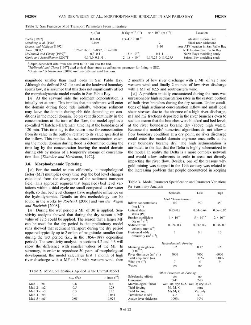
[43] Data on bed composition in San Pablo Bay are verylimited. Only Locke [1971] presents an overview of bedcomposition in 1968 (measured in December) and 1969 and1970 (both measured in February). Bottom sediments of SanPablo Bay are primarily clay and silt, except for the mainchannel, which is sand in places covered with mud banks.However, as specified by equations (1)–(3), the numericalmodel requires input in terms of erosion factor, criticalerosion/deposition shear stress and sediment fall velocity.[44] Preliminary model runs show that reasonable results

can be obtained only by applying multiple sediment fractions(i.e., both sand in the channels and mud on the shoals). Also,applying different fractions allows studying the behaviorof different fractions at the same time. The selection of thefractions is based on adding a range around limited datavalues and “best guesses.”[45] For the sandy fractions 1, 2 and 3, diameters of 500,

300 and 150 mm were chosen following characteristic valuesby Locke [1971]. Table 1 shows various mud transportparameters and their measured values and values applied toSan Francisco Estuary in area models from literature. Valuesapplied in the current research are given Table 2. In addi-tion, for all mud fractions, the erosion parameter (M) is2.0 × 10−4 kg m−2 s−1, the bulk density is 1200 kg m−3, thedry bed density is 500 kg m−3 and, following suggestionsby Winterwerp and Van Kesteren [2004, pp. 144–148], thecritical shear stress for deposition (td,cr) is set at 1000 N m−2.This implies that deposition is determined by concentrationand fall velocity only and is not limited by a critical shearstress value above which no deposition takes place. Themodel does not take into account flocculation processes. Anopportunistic reason for this was to not further complicatethe model descriptions.[46] In itself flocculation and the behavior of flocs over

time is a complex processes that is not fully understood.Laboratory experiments show the importance of shear rate,organic matter, pH and salinity [Mietta et al., 2009], SSC,diatoms and turbulence intensity [Verney et al., 2009] andsand/mud mixtures [Manning et al., 2010]. These para-meters will fluctuate not only over a tidal cycle, but alsoover longer time scales of months or seasons.[47] We are not aware of a flocculation model that en-

compasses all of these parameters. The mud fractions definedin our model may be considered (to a certain extent) as flocfractions, especially considering the fall velocity. Kineke andSternberg [1989] found that flocs in San Pablo Bay com-monly had a diameter of about 100 microns and had a settlingvelocity of 0.5–2 mm s−1, which is an upper limit of thefall velocity of the mud fractions as defined in Table 2. Thisstill leaves the observation that processes related to flocdevelopment and deterioration are not included.

3.6. Initial Bed Composition

[48] Assuming a simple spatial distribution of bed com-position with muddy shallows and sandy channels could bewrong and lead to significant errors in the model. van derWegen et al. [2010] describe a methodology to generate abed composition of different sediment fractions by using aprocess‐based numerical modeling approach similar to thecurrent research, but allowing for only bed composition

adaptations and not for bed level updates. The initial bedcomposition of the current model is generated according tothis methodology under low‐discharge conditions. The finalbed composition of the active layer (the upper 20 cm) fromthe “bed composition run” forms the initial bed compositionof the current model, and it is assumed that this compositionprevails over the entire 8 m of sediments available in thebed. As expected, the bed composition run results in sandydeeper seaward parts of the channel due to the large shearstresses. The coarser mud fractions are clearly present in theshallower and landward portions of the main channel,whereas the finer mud fractions are distributed more on theshallows. The finest mud fraction is hardly present, whichmeans that this fraction was washed out since it could notwithstand the prevailing hydraulic conditions. Fractions m2and m3 dominate the mud presence.

3.7. Sediment Concentration Boundary Conditions

[49] For a specification of the sediment concentrations atthe landward boundary we use the method suggested byGanju et al. [2008] which was developed to estimate dailysediment loads after the start of hydraulic mining 150 yearsago from average annual river discharge. The method useshistorical rainfall data in Sacramento (from 1 October 1850onward), unimpaired flow estimates (from 1906 onward)and current data as a proxy for the historical data. Theypredicted sediment loads based on the estimated historicaldischarges via the relationship suggested by Müller andForstner [1968]:

Qs ¼ aQbþ1r ; ð4Þ

in which Qs is annual sediment load (kg s−1), Qr is annualriver discharge (m3 s−1), and a and b are calibration coef-ficients with units depending on each others values.[50] Parameter b represents the erosive power of the

stream, which is a function of stream/floodplain morphol-ogy. Parameter a is related to sediment availability. For thecurrent watershed this parameter varies strongly with time,in accordance to hydraulic mining, urbanization, andretention of sediment behind dams. On the basis of a com-parison to decadal sediment loads estimated by Gilbert[1917] for the period 1849–1914 and Porterfield [1980]for the period 1909–1966, Ganju et al. [2008] suggest aconstant value of b = 0.13 and a time varying value ofa = 0.02 (before hydraulic mining) to 0.13 (when hydraulicmining stopped in 1884), with the parameter a slowlydecreasing to approximately 0.03 for more recent decades.For the current research sediment concentrations at thelandward boundary were based on b = 0.13 and a = 0.13for the 1856–1887 period. For the case of a river dischargeof 5000 m3 s−1, this leads to a concentration of about390 mg L−1. In the model each of the mud fraction con-centrations is set at 300 mg L−1. In the model formulationthe different mud and sand fractions behave independentlyin the water column. Although the total sum of concen-trations is considerably larger than the suggested value,it allows studying the individual behavior of the five frac-tions with a similar concentration as the one suggested byGanju et al. [2008]. The sand fractions are assigned inflowconcentrations of 10% of the mud fractions. Preliminarymodel results show that sand loads are at least an order of

VAN DER WEGEN ET AL.: MORPHODYNAMIC HINDCAST IN SAN PABLO BAY F02008F02008

7 of 22

magnitude smaller than mud loads in San Pablo Bay.Although the defined SSC for sand at the landward boundaryseems low, it is assumed that this does not significantly affectthe morphodynamic model results in San Pablo Bay.[51] At the seaward side the sediment concentration is

initially set at zero. This implies that no sediment will enterthe domain during flood tide initially, whereas sedimentmay leave the domain during ebb tide depending on con-ditions in the model domain. To prevent discontinuity in theconcentrations at the turn of the flow, the model applies aso‐called “Thatcher‐Harleman” time lag at the boundaries of120 min. This time lag is the return time for concentrationfrom its value in the outflow relative to its value specified inthe inflow. This implies that sediment concentration enter-ing the model domain during flood is determined during thetime lag by the concentration leaving the model domainduring ebb by means of a temporary storage of concentra-tion data [Thatcher and Harleman, 1972].

3.8. Morphodynamic Updating

[52] For the model to run efficiently, a morphologicalfactor (MF) multiplies every time step the bed level changescalculated from the divergence of the sediment transportfield. This approach requires that (upscaled) bed level var-iations within a tidal cycle are small compared to the waterdepth, so that bed level changes have negligible influence onthe hydrodynamics. Details on this methodology can befound in the works by Roelvink [2006] and van der Wegenand Roelvink [2008].[53] During the wet period a MF of 30 is applied. Sen-

sitivity analysis showed that during the dry season a MFvalue of 82.5 could be applied. The reason that a larger MFcan be used for the dry period is that preliminary modelruns showed that sediment transport during the dry periodappeared typically up to 2 orders of magnitudes smaller thanduring the wet period (i.e., in the 1856–1887 depositionperiod). The sensitivity analysis in sections 4.2 and 4.3 willshow the difference with smaller values of the MF. Insummary, in order to reproduce 30 years of morphologicaldevelopment, the model calculates first 1 month of highriver discharge with a MF of 30 with western wind, then

2 months of low river discharge with a MF of 82.5 andwestern wind and finally 2 months of low river dischargewith a MF of 82.5 and southeastern wind.[54] A problem initially encountered during the runs was

unreasonably high sedimentation rates in the eastern portionof both river branches during the dry season. Under condi-tions of high sediment concentration inflow and small localshear stresses due to the absence of a high river discharge,m1 and m2 fractions deposited in the river branches even tosuch an extent that the branches were blocked and bed levelsat the river boundaries became dry (above high water).Because the models’ numerical algorithms do not allow aflow boundary condition at a dry point, no river dischargecould enter the model domain anymore once cells at theriver boundary became dry. The high sedimentation isattributed to the fact that the Delta is highly schematized inthe model. In reality the Delta is a more complex networkand would allow sediments to settle in areas not directlyimpacting the river flow. Besides, one of the reasons whygold mining was stopped in the 19th century was related tothe increasing problem that people encountered in keeping

Table 1. San Francisco Mud Transport Parameters From Literature

te (Pa) M (kg m−2 s−1) w × 10−3 (m s−1) Location

Teeter [1987] 0.1–0.4 1.3–4.7 × 10−5 Alcatraz disposal siteSternberg et al. [1986] 0.049 2 Shoal near RichmondKranck and Milligan [1992] 1–10 near ATF location in San Pablo BayJones [2008]a 0.26–2.56, 0.13–0.92, 0.12–2.08 ATF location San Pablo BayMcDonald and Cheng [1997]b 0.3–0.4 1–5 × 10−5 0.4–1 North Bays modeling studyGanju and Schoellhamer [2007]c 0.1/1.0–0.11/1.1 2–1.8 × 10−5 0.1/0.25–0.11/0.275 Suisun Bay modeling study

aDepth‐dependent data from bed level to ∼27 cm into the bed.bMcDonald and Cheng [1997] used critical shear stress as calibration parameter for fitting to SSC.cGanju and Schoellhamer [2007] use two different mud fractions.

Table 2. Mud Specifications Applied in the Current Model

te,cr (Pa) w (mm s−1)

Mud 1 ‐ m1 0.8 0.4Mud 2 ‐ m2 0.5 0.28Mud 3 ‐ m3 0.3 0.16Mud 4 ‐ m4 0.1 0.064Mud 5 ‐ m5 0.05 0.024

Table 3. Model Parameter Specification and Parameter Variationsfor Sensitivity Analysis

Standard Low High

Mud CharacteristicsInflow concentrations

(mg L−1)300 250 350

Critical shearstress (Pa)

0.05–0.8 0.04–0.64 0.06–0.96

Erosion coefficient(kg m−2 s−1)

1 × 10−4 5 × 10−5 2 × 10−4

Sediment fallvelocity (mm s−1)

0.024–0.4 0.012–0.2 0.036–0.6

Horizontal eddydiffusivity (m2 s−1)

1 0.1 10

Hydrodynamic ForcingManning roughness

(s m−1/3)0.2 0.17 0.23

River discharge (m3 s−1) 5000 4000 6000Tidal amplitude (m) −10% +10%Wind (m s−1) 7 5 9Waves yes no

Other Processes or ForcingSalt/density effects yes noDimension 3‐D 2‐DMorphological factor wet, 30; dry: 82.5 wet, 3; dry: 8.25Tidal forcing M2 M4 C1 noneTidal forcing M2 M4 C1 M2 onlyTurbulence model k‐" k‐LActive layer thickness 100% 10%

VAN DER WEGEN ET AL.: MORPHODYNAMIC HINDCAST IN SAN PABLO BAY F02008F02008

8 of 22

the rivers navigable by dredging. The model would thuscorrectly reproduce, at least qualitatively, the observedhistorical sedimentation in the delta.[55] To solve the problem of the boundary condition

blocking we applied the “dredging” option, maintaining theriver branches at a water depth of 2 m during the dry period.Any surplus material was removed from the model domainduring the run. This did not significantly affect the modelresults in San Pablo Bay, since only little sediment reachesSan Pablo Bay from the Delta area during the dry period.

3.9. Description of Sensitivity Analysis

[56] As described in sections 3.2–3.8, the model applies anumber of simplifications in the parameter settings partly toreduce the model run times by input reduction techniquesand partly because detailed data (both in time and in space)do not exist. In order to address the impact of likely modelparameter variations an extensive sensitivity analysis iscarried out by systematically varying these parameters (oneby one) and comparing the outcomes to a “standard case.”In addition to the standard run, 26 sensitivity runs weremade. The variations can be roughly subdivided into “mudcharacteristics,” “hydrodynamics,” and “other processesor forcing” and are described in Table 3. The alternative

turbulence model is the k‐L turbulence model, which is aso‐called first‐order turbulence closure scheme. It applies ananalytical description of the turbulent length scale includinga damping function depending on the gradient Richardsonnumber [Simonin et al., 1989].This turbulence model waschosen since it is more simplified than the k‐" model,whereas it still accounts for the impact of supposedlyimportant vertical density gradients. The variation of theactive layer refers to the size of the upper (active) bed levellayer of the bed composition model that directly accountsfor bed composition and bed level changes due to depositionand erosion. van der Wegen et al. [2010] give a detaileddescription of the bed composition model.

4. Results

[57] In order to address the main objective of the study,the modeled bathymetric evolution is compared to measureddata using deposition volumes and a Brier Skill Score (BSS)(see Appendix A for a further specification of the BSS).In short, the model performs perfectly when BSS = 1 andmodel results are worse than maintaining the initialbathymetry when BSS < 0. The influence of variations inforcing model parameter settings and process inclusion on

Figure 3. Cumulative mud transports through (a) Point San Pablo (PSB) cross section during 30 monthswet conditions, (b) Carquinez Strait (CS) cross section during 30 months wet conditions, (c) Point SanPablo (PSB) cross section during 330 months of dry conditions, and (d) Carquinez Strait (CS) crosssection during 330 months of dry conditions. Locations of cross sections shown in Figure 1. Negativevalues indicate seaward transport. Transports and time are multiplied by the morphological factor. Blackdenotes m1 fraction, green denotes m2 fraction, red denotes m3 fraction, and blue denotes m4 fraction.Note that black and green lines (m1‐PSB and m2‐PSB transport) almost coincide with the origin.

VAN DER WEGEN ET AL.: MORPHODYNAMIC HINDCAST IN SAN PABLO BAY F02008F02008

9 of 22

the model results is investigated by means of an extensivesensitivity analysis. Because the focus of the current studyis on morphodynamic aspects, the discussion of resultsemphasizes sediment transport and morphology. If nototherwise stated, the presented results reflect the standardcase. First, the model results are described generally.

4.1. Model Performance

[58] The standard case produced regular tidal variations inwater level and velocity after a 1 day spin‐up interval.During the wet month salt does not intrude farther than midSan Pablo Bay, whereas salt intrudes up to east Suisun Bayduring the dry months, which is largely in accordance withgeneral observations [Monismith et al., 2002]. Maximumwaves by westerly winds occur in the southeastern part ofSan Pablo Bay near the entrance to Carquinez Strait anddo not exceed 0.5 m in height and a period of 2.5 s.

Southeastern winds cause waves with a maximum height of0.35 and a maximum period of 2 s on the northwesternshoals. These values are comparable to measurementsdescribed by Schoellhamer et al. [2008].[59] Mean water level is about 20 cm higher during the

wet than during the dry period. During the wet month thehigh sediment transport causes a deposition pulse throughthe model domain, starting in Suisun Bay and arriving somedays later in San Pablo Bay. This pulse can be observed in thedevelopment of cumulative mud transports (Figures 3a and3b; see Figure 1 for definition of locations). The m5 fractionis not shown in Figure 3 since it does not play a major role inthe deposition patterns. Sand transports are not shown inFigure 4 because they are typically at least an order ofmagnitude smaller than the mud transport.[60] During the wet period the inflow through cross sec-

tion CS (import) exceeds the outflow through cross sectionPSB (export) for all mud fractions (Figures 3a, 3b, 4a, and4b). The finer the mud fraction, the faster the importedand exported amounts become (almost) equal. When thishappens net deposition in San Pablo Bay does not take placeanymore. The probable reason why this occurs is that theinitial deposition leads to a bathymetry that enhances theprocess of sediment bypassing through San Pablo Bay. Ashallower bathymetry or a more confined channel area leadto higher velocities so that more sediment is kept in sus-pension which is subsequently washed out seaward by tideresidual flows (of which the river discharge will be themain component).[61] The equilibrium between import and export is not

reached for the coarser mud fractions in the modeled wetperiod (Figures 3a and 3b), although it might be reachedon longer time scales. Figure 4c shows that the deposit isprimarily composed of the m3 fraction. The finer the mudfraction, the less is deposited as percentage of the inflow(Figure 4d).[62] During the dry period the pattern of transport is

more complex. Cumulative transports are typically almost1 order of magnitude smaller than during the wet period(Figures 3a–3d, 4a, and 4b). Tidal fluctuations are clearlypresent, in particular for the finer fractions. Equilibriumbetween import and export develops faster for the coarsermud fractions. In contrast to the coarser mud fractions, theexport of the finest fraction (m4) exceeds the import(Figures 3c, 3d, and 4c). Furthermore, the eroded amountof the finest fractions exceeds the deposited amount of theother larger fractions, so that net erosion of San Pablo Bayoccurs during the dry period. Without the fine fractions,however, San Pablo Bay would still be depositional duringthe dry period. For the larger mud fractions deposition aspercentage of the inflow is lower during the dry period, whichsuggests that high river discharge during the wet createsconditions that favor deposition. Possible explanations forthis behavior are that concentrations and transport gradientsare higher during the wet season, that the larger mud fractionsare able to reach other areas of SPB due to the river flow,or that tidal velocity fluctuations are more damped.[63] Figures 5 and 6 show the bed sediment composition

of the upper, active layer (20 cm below the bed surface) atthe start and at the end of the standard model run. The maindifferences are that the extent of the sand decreases as the

Figure 4. Transport and deposition of mud fractions duringwet and dry periods: (a) inflow of mud through CarquinezStrait cross section, (b) outflow of mud through Point SanPablo cross section, (c) deposition of mud in San PabloBay, and (d) ratio of deposition to inflow. Black bars indi-cate the wet period, and white bars indicate the dry period.Transports are multiplied by the morphological factor. Ero-sion shown as negative deposition.

VAN DER WEGEN ET AL.: MORPHODYNAMIC HINDCAST IN SAN PABLO BAY F02008F02008

10 of 22

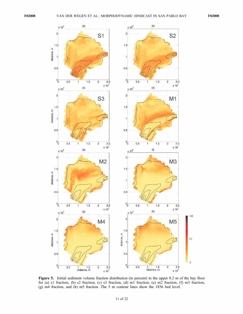
Figure 5. Initial sediment volume fraction distribution (in percent) in the upper 0.2 m of the bay floorfor (a) s1 fraction, (b) s2 fraction, (c) s3 fraction, (d) m1 fraction, (e) m2 fraction, (f) m3 fraction,(g) m4 fraction, and (h) m5 fraction. The 5 m contour lines show the 1856 bed level.

VAN DER WEGEN ET AL.: MORPHODYNAMIC HINDCAST IN SAN PABLO BAY F02008F02008

11 of 22

Figure 6. Final sediment volume fraction distribution (in percent) in the upper 0.2 m of the bay floorfor (a) s1 fraction, (b) s2 fraction, (c) s3 fraction, (d) m1 fraction, (e) m2 fraction, (f) m3 fraction,(g) m4 fraction, and (h) m5 fraction. The 5 m contour lines show the modeled 1887 bed level.

VAN DER WEGEN ET AL.: MORPHODYNAMIC HINDCAST IN SAN PABLO BAY F02008F02008

12 of 22

channel narrows, which was observed, and that the sides ofthe main channel and the NES shallows become muddier.The m1 fraction deposits along the sides of the channeland deposition of the finer fractions is concentrated in theshallows at the margins of San Pablo Bay. The finest frac-tions (m4 and m5) are almost entirely washed out.[64] Figures 7a, 7c, and 7e show the measured 1856

bathymetry, the measured 1887 bathymetry, and the mod-eled 1887 bathymetry, respectively. Cumulative erosion andsedimentation patterns over the 1856–1887 period are givenin Figures 7b and 7d for the measured and modeledbathymetries, respectively. Figure 7f shows the differences(modeled minus measured) of these cumulative patterns.[65] Modeled patterns resemble roughly the distribution

of those measured. Closer analysis of the model resultsindicates that major deposits near CS cross section and theedges along the main channel are mainly caused by the m1fraction (Figure 6d).[66] The large quantity of deposition that occurred along

the sides of the main channel (at least for the southernbanks) is not reproduced well by the model (Figure 8). Thepresence of m1 and s3 fractions seems to play a crucial role(compare Figures 5c and 5d to Figures 6c and 6d). Fur-thermore, it should be taken into account that this area issubject to considerable bed slope effects. Bed slope effectsfor mud are not included in the model and bed slope effectsfor sand are highly parameterized. Reducing the bed slopeeffect for sand improves the results in this region (seesection 5.2). It also diminishes the modeled sand depositionin the center of the main channel near Pinole Point, whichmight be caused by sand sloping down from southernchannel banks by bed slope effects. Minor modeled depo-sitional patches in the northern part of San Pablo Bay are notpresent in the measurements, which is attributed to the factthat tidal exchange and discharges from Petulama Riverand Sonoma Creek (see Figure 1) are not included in themodel schematization.[67] Closer analysis of tidal (diurnal) residual sediment

transports during the wet and dry periods reveals the dom-inant mechanisms in sediment redistribution. The analysis ismade after the wet period when the characteristics are mostpronounced (Figure 8). The wet period tidal residual trans-ports (Figure 8a) are typically an order of magnitude largerthan the dry period tidal residual transports (Figure 8b).During the wet period the largest gradients in the tidalresidual transports are found in the main channel nearCarquinez Strait and Point San Pablo; these are the locationswhere the most sediment deposits and erodes, respectively.Residual transports on the shallows are negligible.[68] Figure 8b shows that a typical tide during the dry

period resuspends the muddy sediments deposited in thechannel during the wet period. The majority of the re-suspended sediment is exported seaward, although there isalso significant transport toward the shoals. There are wakeflows from Carquinez Strait toward the northern and south-ern sides of the main channel and there is a clear transportfrom Point San Pablo toward the Northern shoals, probablyoriginating from the flood entering San Pablo Bay. A prob-able reason why this flood transport is so strong is that theflood during a tide during the dry period is relatively strong,since it is no longer hampered by a large river discharge.

4.2. Comparing Deposition Volumes

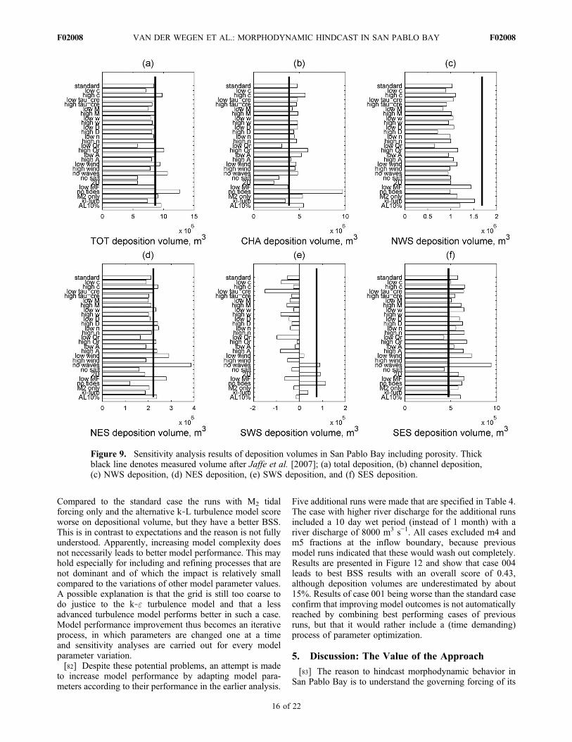
[69] Figure 9a shows the results of the sensitivity analysisof modeled deposition volumes compared to measuredvolumes described by Jaffe et al. [2007]. The most impor-tant observation is that the modeled volumes for many runsare similar to the measured volume and that forcings havinga dominant effect are easily recognized. Depositional vo-lumes are higher for higher inflow concentrations, lowercritical shear stresses, higher erosion coefficients, higher fallvelocities, a lower diffusion coefficient, higher roughness,higher river discharge, lower tidal amplitude and lower windvelocities. Excluding salt water or a 2‐D approach, appli-cation of the k‐L turbulence model lead to lower depositionvolumes, whereas only M2 tidal forcing, a small active layerand the exclusion of tides lead to larger deposition volumes(the latter having the largest effect). The strong positivedependence of deposition volume on river discharge andconcentration follows from the fact that nearly all of themass of the m1, m2 and m3 sediment entering the Bay istrapped there. Since the amount of sediment in these classesentering the bay is roughly equal to river discharge timesconcentration, total deposition volume increases directlywith both these parameters. Also, deposition is generallylarger when more sediment is kept in suspension. A possiblemechanism is that higher SSC will lead to larger amounts ofsediment that are (slowly) moved to lower‐energy areas(i.e., the northern shallows) where it can settle. Counteringthis tendency are wave effects, which will contribute to moresuspension in the shallows but also leads to more erosion inthe major deposition area. For sediments with higher fallvelocities, increases in deposition in lower‐energy areascould outweigh erosion from waves. The prescribed varia-tions in concentration, erosion factor, river discharge, andwind velocity have most impact. Excluding wave effects,density differences and vertically averaging the domain leadsto the worst fit to observed volumes, although these have aneffect that is of the same order of magnitude as the othervariations.[70] An interesting observation is that minimum and

maximum parameter values do not always lead to smaller orlarger deposition volumes, respectively, compared to thestandard case. The cases with a low and high sediment fallvelocity, for example, both lead to smaller deposition vo-lumes. This is attributed to San Pablo Bay geometry.Changing model parameters will not only change depositionand erosion processes as such, but also the locations wherethese processes take place. For example, in shallow areas theimpact of a higher sediment fall velocity may be consider-ably different than in the deep channel.[71] The impact of changing parameter settings on sediment

redistribution within San Pablo Bay may be considerable. Theabsence of waves, for example, leads to approximately 35%increase in deposition volume. NES and SWS have consid-erably more deposition in the absence of waves, whereasNWS has less deposition. This suggests that waves erode NESand SWS and that the suspended sediment partly depositsat NWS and is partly removed seaward.[72] About 47% of the measured deposition is in the

channel, which is reproduced well by the standard case.Measured deposition volumes in NWS, NES, SWS and SESare about 21%, 25%, 1% and 6% of the total measured

VAN DER WEGEN ET AL.: MORPHODYNAMIC HINDCAST IN SAN PABLO BAY F02008F02008

13 of 22

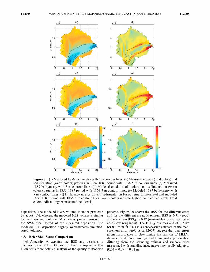
deposition. The modeled NWS volume is under predictedby about 40%, whereas the modeled NES volume is similarto the measured volume. Most cases predict erosion inthe SWS area instead of the measured deposition. Themodeled SES deposition slightly overestimates the mea-sured volumes.

4.3. Brier Skill Score Comparison

[73] Appendix A explains the BSS and describes adecomposition of the BSS into different components thatallow for a more detailed analysis of the quality of modeled

patterns. Figure 10 shows the BSS for the different casesand for the different areas. Maximum BSS is 0.31 (good)and maximum BSSvR is 0.47 (reasonable) for that particularcase (low roughness). The BSSvR assumes a d of 0.2 m3

(or 0.2 m m−2). This is a conservative estimate of the mea-surement error. Jaffe et al. [2007] suggest that bias errors(from inaccuracies in determining the relation of MLLWdatums for different surveys and from grid representationdiffering from the sounding values) and random error(associated with sounding inaccuracy) may locally add up to(0.04 + 0.07 =) 0.11 m.

Figure 7. (a) Measured 1856 bathymetry with 5 m contour lines. (b) Measured erosion (cold colors) andsedimentation (warm colors) patterns in 1856–1887 period with 1856 5 m contour lines. (c) Measured1887 bathymetry with 5 m contour lines. (d) Modeled erosion (cold colors) and sedimentation (warmcolors) patterns in 1856–1887 period with 1856 5 m contour lines. (e) Modeled 1887 bathymetry with5 m contour lines. (f) Difference in erosion and sedimentation for patterns of measured and modeled1856–1887 period with 1856 5 m contour lines. Warm colors indicate higher modeled bed levels. Coldcolors indicate higher measured bed levels.

VAN DER WEGEN ET AL.: MORPHODYNAMIC HINDCAST IN SAN PABLO BAY F02008F02008

14 of 22

[74] Most cases have a BSS around 0.2 (reasonable togood). High concentrations, high river discharge, highamplitude, excluding waves, the 2‐D approach, a low MF,and excluding tidal movement lead to the worst results. NEShas the highest BSS of 0.64 (excellent). NWS scores com-parable to the total area. The channel area scores generallyslightly lower values. Scores for SWS are generally bad andscores for SES are slightly lower than the full domainscores. By far the weakest BSS values are found for the casewith no tides. Tides thus have a significant effect on sedi-ment distribution in San Pablo Bay.[75] These observations are also roughly reflected in the

scores of a (measure of phase error) and b (measure of boththe amplitude and phase error) (Figures 11a and 11b). Besta and b scores are for NWS, NES, and the channel, whereasSWS and SES have the worst scores. Phasing of the pre-diction could be improved on the southern shoals. Includ-ing the amplitude performance with b shows much morevariance in the different cases than considering phases onlywith a, which suggests that the phasing of the pattern is lesssensitive to the changing parameter settings than the patternamplitudes. Logically, g values, shown in Figure 11c, fol-low the deposition volume performance (Figure 10),although they do not discriminate between underpredictionor overprediction. It is noted that volume underestimatesresult in relatively high g values compared to similar mag-nitude volume overestimates.[76] The SWS area scores worst and the NES scores best

both in terms of the deposition volume and the BSS.However, on a more detailed level volumetric (or g values)and BSS performances are not similar. A low sediment fallvelocity, for example, leads to a similar deposition volume,but the BSS of this case is one of the weakest. Anotherexample is that the low river discharge leads to a higher BSSthan the case of the high river discharge, although it scoresworse in terms of deposition volume.[77] A low MF scores well in terms of volume, but leads to

worst results in terms of BSS. This is attributed to a weak bvalue and, to a lesser extent, a weak a value, which implies a

weak phase prediction and, probably with more influence onthe overall BSS value, a weak amplitude prediction. A pos-sible explanation is that the run with a low MF accounts for alarger dispersion of sediments due to subsequent wet and dryseasons. This mechanism is not covered by the runs with onlyone wet‐dry period cycle which emphasize one‐event peaks.Adjusting forcing conditions like river discharge or sedimentconcentrations would probably lead to better results for thelow MF, but also to extensively more calculation time.[78] Although the runs with M2 tidal forcing only and the

alternative k‐L turbulence model score worse on deposi-tional volume, they have a better BSS. This is remarkablesince these runs have a more roughly schematized tidalforcing and a less advanced turbulence model, respectively.One could argue that model performance will increase withmore simplicity and a higher level of process schematiza-tion. Still, the improved model performance is not signifi-cant compared to the improvements by the variations in theother model parameter values.

4.4. Model Improvement

[79] Adding processes (i.e., flocculation), a more detaileddescription of the forcing (i.e., a full tidal signal or a betterwind field both including extreme conditions) and furthermodel parameter adjustment would probably lead to animprovement of the model results.[80] An example of extreme conditions impacting the

model results would be the possible effects of El Nino onthe water level variations at sea, the river discharge or localwind conditions. Another example is the river dischargeschematization. A single high river discharges with highSSC event may transport sediment toward the western partof San Pablo Bay so that deposition increases at NWS andSWS. Multiple peak flows during a year would also movesediment more seaward. This is, however, considered out-side the scope of the present study.[81] With respect to model parameter adjustment, section

4.3 suggests that strategies to improve results by parameteradjustment are not easily deduced from the model results.

Figure 8. Tide residual sediment transport (cubic meters per second per meter perpendicular to flowdirection) at the end of the wet period. Conditions during (a) wet period and (b) dry period. Note differentscales for transport vectors.

VAN DER WEGEN ET AL.: MORPHODYNAMIC HINDCAST IN SAN PABLO BAY F02008F02008

15 of 22

Compared to the standard case the runs with M2 tidalforcing only and the alternative k‐L turbulence model scoreworse on depositional volume, but they have a better BSS.This is in contrast to expectations and the reason is not fullyunderstood. Apparently, increasing model complexity doesnot necessarily leads to better model performance. This mayhold especially for including and refining processes that arenot dominant and of which the impact is relatively smallcompared to the variations of other model parameter values.A possible explanation is that the grid is still too coarse todo justice to the k‐" turbulence model and that a lessadvanced turbulence model performs better in such a case.Model performance improvement thus becomes an iterativeprocess, in which parameters are changed one at a timeand sensitivity analyses are carried out for every modelparameter variation.[82] Despite these potential problems, an attempt is made

to increase model performance by adapting model para-meters according to their performance in the earlier analysis.

Five additional runs were made that are specified in Table 4.The case with higher river discharge for the additional runsincluded a 10 day wet period (instead of 1 month) with ariver discharge of 8000 m3 s−1. All cases excluded m4 andm5 fractions at the inflow boundary, because previousmodel runs indicated that these would wash out completely.Results are presented in Figure 12 and show that case 004leads to best BSS results with an overall score of 0.43,although deposition volumes are underestimated by about15%. Results of case 001 being worse than the standard caseconfirm that improving model outcomes is not automaticallyreached by combining best performing cases of previousruns, but that it would rather include a (time demanding)process of parameter optimization.

5. Discussion: The Value of the Approach

[83] The reason to hindcast morphodynamic behavior inSan Pablo Bay is to understand the governing forcing of its

Figure 9. Sensitivity analysis results of deposition volumes in San Pablo Bay including porosity. Thickblack line denotes measured volume after Jaffe et al. [2007]; (a) total deposition, (b) channel deposition,(c) NWS deposition, (d) NES deposition, (e) SWS deposition, and (f) SES deposition.

VAN DER WEGEN ET AL.: MORPHODYNAMIC HINDCAST IN SAN PABLO BAY F02008F02008

16 of 22

(long‐term) morphodynamic behavior so that, in the end,predictions can be made on morphodynamic development infuture under different scenarios of climate change or anthro-pogenic intervention. The process‐based modeling approachhas its own advantages and disadvantages which make theapproach suitable (or not) for describing morphodynamicevolution in an alluvial estuarine environment. This sectionaims to assess the value of this modeling approach by dis-cussing experience gained during the work and elaboratingfurther on its potential value compared to other methodologies.

5.1. Need for a Complex Model

[84] The results of the process‐based approach arepromising and maybe even surprising.[85] 1. We apply a highly complex process‐based model

that includes highly nonlinear processes, not only by thehydrodynamic equations, but also by the sediment transportsand the feedback between bed level changes, wind wavesand tidal hydrodynamics.[86] 2. There is a high degree of schematization of the

forcing mechanisms (limited tidal constituents, subdivisionin a constant river flow wet month and dry month, constantinflow sediment concentrations, simple wind field).[87] 3. We need to estimate the value of a large number of

unknown parameters. Each mud fraction needs a specifica-

tion of the inflow concentration, the critical shear stress, theerosion coefficient, the fall velocity, the dry bulk densityand the specific density (with a total of 35 unknowns for all5 mud fractions). Each sand fraction needs the specifica-tion of a sediment mean diameter, porosity and bed slopeparameter (9 unknowns for 3 sand fractions). The hydro-dynamic model needs a specification of the eddy diffusivity,horizontal eddy viscosity and Manning roughness parame-ter. In addition, all parameters values may change in timeand space. Already covering 47 unknowns, this list ofparameters is not complete. The applied hydrodynamicequations (including the k‐" turbulence model), the sedimenttransport formulae and bed slope effects are by themselveslimited descriptions, partly even based on calibration factors,and may estimate transport values only by an order of mag-nitude [van Rijn, 1993].[88] 4. Processes of which one may assume that they are

relevant to the morphodynamic process are not included.Examples are flocculation, consolidation, armoring, the pres-ence of (seasonal variations in) vegetation or benthos fauna(like biofilms or bioengineers), or the presence of multiplefractions in the bed and their mutual impact on critical shearstress and erosion parameter values.[89] On the other hand, the complex environment of San

Pablo Bay requires this detailed process‐based approach.The 3‐D model applied in this study exhibits significantskill and excluding dominant processes like fresh waterand salt water interactions or wind waves leads to worseresults. Reasons why the model effort is successful includethe following.[90] (1) The period considered is a period of deposition.

Data on bed consolidation and composition is probably lessrelevant than for a hindcast of a mainly eroding system.[91] (2) The present study considers a long period of about

30 years. The model schematizes only 1 year. It does notexplicitly take into account variability of high river flow orwind fields over the years, although extreme events mayhave considerable effect on the system.[92] (3) It is possible that the large number of unknowns

and roughly estimated parameter values obscure a correctrepresentation of reality, because they may correct for eachother’s (wrongly assumed) values. For example, it is verywell possible that the river flow schematization has a“representative” high river flow that is too low. This maybe corrected by input sediment concentrations that are toohigh so that the total sediment volume entering San PabloBay is more or less correct.[93] (4) The high level of schematization and the large

number of estimated model parameters may cover or evencompensate processes that are relevant but that are notexplicitly formulated in the present model. In that case thelarge number of unknowns can be considered as an expla-nation of the significant model performance and not ascontribution to the model uncertainty.[94] These observations lead to the question of the level of

complexity required for adequate predictions. First, weexpect that model performance will increase with a betterdescription of the processes. For example, including moreprocesses and better estimates for model parameters, mayincrease model performance but also may increase com-plexity to a point where assessment and analysis of thecontributions of each process is difficult, if not impossible.

Figure 10. BSS values. Thick black line denotes BSS forfull San Pablo Bay domain; dotted gray line denotes BSSfor full San Pablo Bay domain including correction for mea-surement accuracy by equation (A1). Circle denotes chan-nel, open square denotes NWS, filled square denotes NES,open triangle denotes SWS (mainly not visible; smaller than−0.25), and filled triangle denotes SES.

VAN DER WEGEN ET AL.: MORPHODYNAMIC HINDCAST IN SAN PABLO BAY F02008F02008

17 of 22

[95] Second, there seems to be a paradox when decreasingcomplexity. In some cases this leads to worse results (forexample by including less processes such as wind waves orsalt/fresh water differences), which suggests that theseprocesses are needed for adequate prediction. Other casesshow that less complexity leads to better results (runs with amore roughly schematized tidal boundary condition orless advanced turbulence model), although differences inmodel outcomes remain small as long as the impact ofthe processes involved is comparatively small. A possibleexplanation for increased model performance with lesscomplexity is that the model setup (related for example tothe grid size or the forcing) is still too coarse to exploit thepotential added information gained using more advancedprocess descriptions.[96] The level of complexity required will probably differ

with the morphodynamic environment and the goals ofthe study. The optimal complexity can only be determinedby a thorough sensitivity analysis. Still, our sensitivityanalysis shows that the complex modeling approach isindeed able to differentiate between governing forcing andsecondary processes.

5.2. Comparison to Alternative Modeling Approach

[97] The value of the process‐based modeling approachcan be best made clear by comparing the results to a moreschematized approach considering morphodynamic devel-opment in the same area described by Jaffe et al. [2007].Their sediment budget model was highly schematized andconsidered Central Bay, San Pablo Bay, Suisun Bay and theDelta merely as interconnected boxes. Based on an analysisof historical hydrographic surveys over 150 years they wereable to quantify sedimentation and erosion volumes inthe subbays for different (decadal) periods over the last150 years and to estimate resulting transports between thesubbays as well as exchange of sediment between the bays

and their adjacent marshes. The advantage of the approachis that it provides a quick and comprehensive insight intobulk transports and deposition volumes under decadal per-iods of different forcing. However, the box model approachalso has disadvantages compared to the process‐basedapproach of the present work, including the following.[98] 1. A box model heavily depends on an extensive data

set of measured bathymetries. This data set is not unique,but where it is not available (as in most other parts of theworld) there is a need for different approaches to investigateand understand the behavior of the system.[99] 2. A box model lacks a physical explanation of the

underlying processes. For example, it cannot explain theimportance of wind wave generation for sediment distribu-tion within San Pablo Bay (see, for example, Figure 10).[100] 3. A box model disregards processes that are rele-

vant to understand the dynamics of the system but that didnot leave a record in the measured data. For example, it doesnot consider sediments that did not settle in the bays. Thismeans that it probably underestimates the sediment loadfrom the delta. Figure 3 indicates it is possible that fines aretransported seaward without settling in the bay.[101] 4. A box model covers only long‐term trends and

does not provide insight into short time scale processes suchas different prevailing sediment transport during a monthof low river flow compared to high river flow (shown inFigure 4) or extreme river flow events.

Table 4. Adapted Model Settings Compared to Standard Case

RunLowc

Highw

Lown

LowQr

HigherQr

Low BedSlope Effect

HighWind

001 * * *002 * * *003 * * * * *004 * * * *005 * * * * *

Figure 11. BSS parameter values. Thick black line denotes BSS for full San Pablo Bay domain. Circledenotes channel, open square denotes NWS, filled square denotes NES, open triangle denotes SWS(mainly not visible; smaller than −0.25), and filled triangle denotes SES. (a) The value a is a measureof phase error, (b) b is a measure of both the amplitude and phase error, and (c) g is a measure of themean error.

VAN DER WEGEN ET AL.: MORPHODYNAMIC HINDCAST IN SAN PABLO BAY F02008F02008

18 of 22

[102] 5. A box model does not resolve a detailed spatialscale, whereas the process‐based model provides insightinto erosion and sedimentation patterns (see Figure 7).[103] It can be questioned whether a box model or a

process‐based approach is better suited to predict (future)morphological changes. The process‐based model includesmore processes (which may give more confidence in itsoutcomes) and has more capacity to explain developmentsin detail. For example, sea level rise may result in large partsof flooded marshland. The box model of Jaffe et al. [2007]does not include this process and its feedback on hydrody-namic behavior and sediment transport patterns, althoughthese may have considerable impact on morphologicaldevelopment. The process‐based approach is at least able todescribe the process and to estimate the effects. At the sametime the complexity is also the weakness, since it requires amore sophisticated model setup and analysis to understandand value the model results. Parallel use of box models anda process‐based approach is probably the most valuableapproach. The value of the box model is that it gives a quickand general insight into relevant forcing mechanisms,whereas the process‐based model can explain, feed backinto, and confirm estimates made in the box model.

6. Summary and Conclusions

[104] The current study investigated the processes gov-erning the morphodynamic development of San Pablo Bayduring the 1856–1887 period using a process‐based mod-eling approach that is able to describe detailed hydrody-namic behavior as well as detailed erosion and depositionpatterns. We schematized the initial conditions and hydro-dynamic forcing and made assumptions on model parametervalues and an extensive (but probably not complete) set ofsupposedly relevant processes.[105] When compared to measured morphodynamic dev-

elopments over 30 years, the present work showed that themodel is capable of reproducing decadal deposition volumesand patterns with significant skill. This suggests that, at leastfor San Pablo Bay during the 1856–1887 depositionalperiod, the model included the processes governing mor-phodynamic development. Model results showed that theriver discharge and sediment concentration have a strongpositive influence on deposition volumes. Together theycontrol the amount of sediment entering San Pablo Bay.

Waves decrease deposition rates and, together with tidalmovement, have the greatest effect on sediment redistribu-tion within San Pablo Bay.[106] The complex process‐based modeling approach

accounts for multiple nonlinear processes and interactionsthat are found in nature. A drawback to this approach is that itis difficult to assess to what extent the schematized andestimated model parameter settings compensate for modelinginadequacies. The extensive sensitivity analysis carried outaddressed the value of our approach. Although all describedprocesses, forcing conditions and model parameter valueshave an observed effect on the model outcome, the sensitivityanalysis clearly distinguishes dominant processes from otherprocesses. Variations in the values of the model parametersand forcing conditions within a reasonable range and inclu-sion or exclusion of some processes appear to be only rele-vant in second order. This suggests that the model geometrydescribing the planform and initial bathymetry plays animportant role in the erosion and deposition patterns.[107] Including more processes, optimizing values of the

model parameters or a better description of the forcingconditions may lead to better model performance. It also ispossible that increasing complexity leads to worse results,probably because a rough and coarse model setup does nothave the resolution to exploit the added information gainedusing advanced process formulations. Similar to the sensi-tivity analysis that shows relatively small effect of variationsin secondary processes, it is expected that the improvementof model performance will be comparatively small.[108] At the other end of the spectrum of complexity in

modeling approaches are box models. Box models provide aquick and comprehensive insight into bulk transports anddeposition volumes under decadal periods of differentforcing. However, the box model approach lacks a physicalexplanation of the underlying processes. For example, itcannot explain the importance of wind wave generation forsediment distribution within San Pablo Bay. Parallel use ofbox models and a process‐based approach as described inthe present work is probably the most valuable approach toasses and explain future morphodynamic development.

Appendix A

[109] In order to assess the skill of morphodynamicmodels Sutherland et al. [2004] suggest the use of the Brier

Figure 12. Model results for improved parameter settings: (a) BSS, (b) total deposition volumes, and(c) cumulative erosion and sedimentation (meters) for case 004.

VAN DER WEGEN ET AL.: MORPHODYNAMIC HINDCAST IN SAN PABLO BAY F02008F02008

19 of 22

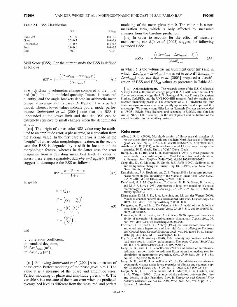
Skill Score (BSS). For the current study the BSS is definedas follows:

BSS ¼ 1�Dvolmod �Dvolmeasð Þ2

D EDvol2meas

� � ; ðA1Þ

in which Dvol is volumetric change compared to the initialbed (m3), “mod” is modeled quantity, “meas” is measuredquantity, and the angle brackets denote an arithmetic mean(a spatial average in this case). A BSS of 1 is a perfectmodel, whereas lower values indicate poorer model perfor-mance. Sutherland et al. [2004] note that the BSS isunbounded at the lower limit and that the BSS can beextremely sensitive to small changes when the denominatoris low.[110] The origin of a particular BSS value may be attrib-

uted to an amplitude error, a phase error, or a deviation fromthe average value. In the first case an error is made in the“height” of a particular morphological feature, in the secondcase the BSS is degraded by a shift in location of themorphologic feature, whereas in the latter case the errororiginates from a deviating mean bed level. In order toassess these errors separately, Murphy and Epstein [1989]suggest to decompose the BSS as follows:

BSS ¼ �� � � � þ "

1þ "; ðA2Þ

in which

� ¼ r2X ′Y ′ ;

� ¼ rX ′Y ′ � �Y ′�X ′

� 2;

� ¼ Y ′h i� X ′h i�X ′

� �2

;

" ¼ X ′h i�X ′

� �2

;

ðA3Þ

and

r correlation coefficient,s standard deviation,X′ Dvolmeas (m

3),Y′ Dvolmod (m

3).

[111] Following Sutherland et al. [2004] a is a measure ofphase error. Perfect modeling of the phase gives a = 1. Thevalue b is a measure of the phase and amplitude error.Perfect modeling of phase and amplitude gives b = 0. Thevariable g is a measure of the mean error when the predictedaverage bed level is different from the measured, and perfect

modeling of the mean gives g = 0. The value " is a nor-malization term, which is only affected by measuredchanges from the baseline prediction.[112] In order to account for the effect of measure-

ment errors, van Rijn et al. [2003] suggest the followingextended BSS:

BSSvR ¼ 1�Dvolmod �Dvolmeasj j � �ð Þ2

D EDvol2meas

� � ; ðA4Þ

in which d is the volumetric measurement error (m3) and inwhich ∣Dvolmod − Dvolmeas∣ − d is set to zero if ∣Dvolmod −Dvolmeas∣ < d. van Rijn et al. [2003] proposed a classifi-cation of BSS and BSSvR values as presented in Table A1.

[113] Acknowledgments. The research is part of the U.S. GeologicalSurvey CASCaDE climate change project (CASCaDE contribution 17).The authors acknowledge the U.S. Geological Survey Priority EcosystemStudies, CALFED, and the UNESCO‐IHE research fund for making thisresearch financially possible. The comments of C. T. Friedrichs and fourother anonymous reviewers were greatly appreciated and improved thismanuscript. We acknowledge Giles Lesser (formerly Deltares and secondedto USGS), Edwin Elias (Deltares and seconded to USGS), and Van LanAnh (UNESCO‐IHE student) for the development and calibration of themodel described in the auxiliary material.

ReferencesAllen, J. R. L. (2000), Morphodynamics of Holocene salt marshes: Areview sketch from the Atlantic and southern North Sea coasts of Europe,Quat. Sci. Rev., 19(12), 1155–1231, doi:10.1016/S0277-3791(99)00034-7.

Ariathurai, C. R. (1974), A finite element model for sediment transport inestuaries, Ph.D. thesis, Univ. of Calif. Davis, Davis.

Booij, N., R. C. Ris, and L. H. Holthuijsen (1999), A third‐generationwave model for coastal regions: I. Model description and validation,J. Geophys. Res., 104(C4), 7649–7666, doi:10.1029/98JC02622.

Cappiella, K., C. Malzone, R. Smith, B.E. Jaffe (1999), Sedimentationand bathymetric change in Suisun Bay 1876–1990, U.S. Geol. Surv.Open File Rep. 9‐563.

Dastgheib, A., J. A. Roelvink, and Z. B. Wang (2008), Long‐term process‐based morphological modeling of the Marsdiep Tidal Basin, Mar. Geol.,256, 90–100, doi:10.1016/j.margeo.2008.10.003.

De Vriend, H. J., M. Capobianco, T. Chesher, H. E. De Swart, B. Latteux,and M. J. F. Stive (1993), Approaches to long term modeling of coastalmorphology: A review, Coastal Eng., 21, 225–269, doi:10.1016/0378-3839(93)90051-9.

Dissanayake, D. M. P. K., J. A. Roelvink, and M. van der Wegen (2009),Modelled channel patterns in a schematized tidal inlet, Coastal Eng., 56,1069–1083, doi:10.1016/j.coastaleng.2009.08.008.

Dongeren, A. D., and H. J. De Vriend (1994), A model of morphologicalbehaviour of tidal basins, Coastal Eng., 22, 287–310, doi:10.1016/0378-3839(94)90040-X.

Fortunato, A. B., X. Bertin, and A. Oliviera (2009), Space and time vari-ability of uncertainty in morphodynamic simulations, Coastal Eng., 56,886–894, doi:10.1016/j.coastaleng.2009.04.006.

Friedrichs, C. T., and D. G. Aubrey (1996), Uniform bottom shear stressand equilibrium hypsometry of intertidal flats, in Mixing in Estuariesand Coastal Seas, Coastal Estuarine Stud., vol. 50, edited by C. Pattiar-atchi, pp. 405–429, AGU, Washington, D. C.

Fry, V., and D. G. Aubrey (1990), Tidal velocity asymmetries and bed-load transport in shallow embayments, Estuarine Coastal Shelf Sci.,30, 453–473, doi:10.1016/0272-7714(90)90067-2.

Ganju, N. K., and D. H. Schoellhamer (2007), Calibration of an estuarinesediment transport model to sediment fluxes as an intermediate step forsimulation of geomorphic evolution, Cont. Shelf Res., 29, 148–158,doi:10.1016/j.csr.2007.09.005.

Ganju, N. K., and D. H. Schoellhamer (2010), Decadal‐timescale estuarinegeomorphic change under future scenarios of climate and sediment sup-ply, Estuaries Coasts, 33, 15–29, doi:10.1007/s12237-009-9244-y.

Ganju, N. K., D. H. Schoellhamer, M. C. Murrell, J. W. Gartner, andS. A. Wright (2006), Constancy of the relation between floc sizeand density in San Francisco Bay, in Estuarine and Coastal FineSediment Dynamics: INTERCOH 2003, Proc. Mar. Sci., vol. 8, pp.75–91,Elsevier, Amsterdam.

Table A1. BSS Classification

BSS BSSvR

Excellent 0.5–1.0 0.8–1.0Good 0.2–0.5 0.6–0.8Reasonable 0.1–0.2 0.3–0.6Poor 0.0–0.1 0.0–0.3Bad <0.0 <0.0

VAN DER WEGEN ET AL.: MORPHODYNAMIC HINDCAST IN SAN PABLO BAY F02008F02008

20 of 22

Ganju, N. K., N. Knowles, and D. H. Schoellhamer (2008), Temporaldownscaling of decadal sediment load estimates to a daily intervalfor use in hindcast simulations, J. Hydrol., 349, 512–523, doi:10.1016/j.jhydrol.2007.11.026.

Ganju, N. K., D. H. Schoellhamer, and B. E. Jaffe (2009), Hindcasting ofdecadal‐timescale estuarine bathymetric change with a tidal‐timescalemodel, J. Geophys. Res., 114, F04019, doi:10.1029/2008JF001191.

Gilbert, G. K. (1917), Hydraulic‐mining debris in the Sierra Nevada, U.S.Geological Surv. Prof. Pap., 105, 148 pp.

Hayes, T. P., J. J. Kinney, and N. J. M. Wheeler (1984), California surfacewind climatology, report, 73 pp., Aerometric Data Div., State of Calif.Air Resour. Board, Sacramento, Calif.

Hibma, A., H. M. Schuttelaars, and Z. B. Wang (2003a), Comparison oflongitudinal equilibrium profiles in idealized and process‐based models,Ocean Dyn., 53(3), 252–269, doi:10.1007/s10236-003-0046-7.

Hibma, A., H. J. de Vriend, and M. J. F. Stive (2003b), Numerical model-ing of shoal pattern formation in well‐mixed elongated estuaries, EstuarineCoastal Shelf Sci., 57, 981–991, doi:10.1016/S0272-7714(03)00004-0.

Hibma, A., H. M. Schuttelaars, and H. J. de Vriend (2004), Initial forma-tion and long‐term evolution of channel‐shoal patterns, Cont. ShelfRes., 24(15), 1637–1650, doi:10.1016/j.csr.2004.05.003.

Higgins, S. A., B. E. Jaffe, and C. C. Fuller (2007), Reconstructing sedi-ment age profiles from historical bathymetry changes in San PabloBay, California, Estuarine Coastal Shelf Sci., 73, doi:10.1016/j.ecss.2006.12.018.

Hoitink, A. J. F., P. Hoekstra, and D. S. van Maren (2003), Flow asym-metry associated with astronomical tides: Implications for the residualtransport of sediment, J. Geophys. Res., 108(C10), 3315, doi:10.1029/2002JC001539.

Jaffe, B. E., R. E. Smith, and L. Zink Toressan (1998), Sedimentation andbathymetric change in San Pablo Bay 1856–1983, U.S. Geol. Surv. OpenFile Rep., 98‐0795.

Jaffe, B. E., R. E. Smith, and A. C. Foxgrover (2007), Anthropogenic influ-ence on sedimentation and intertidal mudflat change in San Pablo Bay,California: 1856–1983, Estuarine Coastal Shelf Sci., 73, 175–187,doi:10.1016/j.ecss.2007.02.017.

Jones, C. (2008), Aquatic transfer facility sediment transport analysis, in Tech-nical Studies for the Aquatic Transfer Facility: Hamilton Wetlands Restora-tion Project, technical report, edited by D. A. Cacchione and P. A. Mull,chap. 4, pp. 305–340, U.S. Army Corps of Eng., San Francisco, Calif.

Kimmerer, W. J. (2004), Open water processes of the San Francisco Estu-ary: From physical forcing to biological responses [online], San Francis-co Estuary Watershed Sci., 2(1), article 1. [Available at http://repositories.cdlib.org/jmie/sfews/vol2/iss1/art1.]

Kineke, G. C., and R. W. Sternberg (1989), The effect of particle settlingvelocity on computed suspended sediment concentration profiles, Mar.Geol., 90, 159–174, doi:10.1016/0025-3227(89)90039-X.

Kirby, R. (2002), Optimized harbor basins, in Dredging ’02: Key Technol-ogies for Global Prosperity [CD‐ROM], edited by S. Garbaciak Jr., Am.Soc. of Civ. Eng., Reston, Va., doi:10.1061/40680(2003)119.

Kranck, K., and T. G. Milligan (1992), Characteristics of suspended parti-cles at an 11‐hour anchor station in San Francisco Bay, California,J. Geophys. Res., 97(C7), 11,373–11,382, doi:10.1029/92JC00950.

Krone, R. B. (1962), Flume studies of the transport of sediment in estuarialshoaling processes, final report, Hydraul. Eng. Lab. and Sanit. Eng. Res.Lab., Univ. of Calif., Berkeley.

Krone, R. B. (1979), Sedimentation in the San Francisco Bay system, in SanFrancisco Bay: The Urbanized Estuary, edited by T. J. Conomos, pp. 85–96,Pac. Div. of the Am. Assoc. for the Adv. of Sci., San Francisco, Calif.

Krone, R. B. (1993), Sedimentation revisited, in Nearshore and EstuarineCohesive Sediment Transport, Coastal Estuarine Stud., vol. 42, edited byA. J. Mehta, pp. 108–125, AGU, Washington, D. C.

Lanzoni, S., and G. Seminara (2002), Long‐term evolution and morphody-namic equilibrium of tidal channels, J. Geophys. Res., 107(C1), 3001,doi:10.1029/2000JC000468.

Lesser, G. R. (2009), An Approach to Medium‐Term Coastal MorphologicalModeling: UNESCO‐IHE Ph.D. Thesis, CRC Press, Boca Raton, Fla.

Lesser, G. R., J. A. Roelvink, J. A. T. M. Van Kester, and G. S. Stelling(2004), Development and validation of a three‐dimensional morphologicalmodel, Coastal Eng., 51, 883–915, doi:10.1016/j.coastaleng.2004.07.014.

Locke, J. L. (1971), Sedimentation and foraminiferal aspects of the recentsediments of San Pablo Bay, M.S. thesis, Fac. of the Dep. of Geol., SanJose State Coll., San Jose, Calif.

Manning, A. J., J. V. Baugh, J. R. Spearman, and R. J. S. Whitehouse(2010), Flocculation settling characteristics of mud: Sand mixtures,Ocean Dyn., 60, 237–253, doi:10.1007/s10236-009-0251-0.

Marciano, R., Z. B. Wang, A. Hibma, H. J. de Vriend, and A. Defina(2005), Modelling of channel patterns in short tidal basins, J. Geophys.Res., 110, F01001, doi:10.1029/2003JF000092.

McDonald, E. T., and R. T. Cheng (1997), A numerical model of sedimenttransport applied to San Francisco Bay, California, J. Mar. Environ.Eng., 4, 1–41.

McKee, L. J., N. K. Ganju, and D. H. Schoellhamer (2006), Estimates ofsuspended sediment entering San Francisco Bay from the Sacramentoand San Joaquin Delta, San Francisco Bay, California, J. Hydrol., 323,335–352, doi:10.1016/j.jhydrol.2005.09.006.

Mietta, F., C. Chassagne, A. J. Manning, and J. C. Winterwerp (2009),Influence of shear rate, organic matter content, pH and salinity on mudflocculation, Ocean Dyn., 59, 751–763, doi:10.1007/s10236-009-0231-4.

Monismith, S. G., W. Kimmerer, J. R. Burau, and M. T. Stacey (2002),Structure and flow‐induced variability of the subtidal salinity field inNorthern San Francisco Bay, J. Phys. Oceanogr., 32, 3003–3019,doi:10.1175/1520-0485(2002)032<3003:SAFIVO>2.0.CO;2.

Müller, G., and U. Forstner (1968), General relationship between sus-pended sediment concentration and water discharge in the Alpenrheinand some other rivers, Nature, 217, 244–245, doi:10.1038/217244a0.

Murphy, A. H., and E. S. Epstein (1989), Skill scores and correlation coef-ficients in model 890 verification, Mon. Weather Rev., 117, 572–582,doi:10.1175/1520-0493(1989)117<0572:SSACCI>2.0.CO;2.

Murray, A. B. (2003) Contrasting the goals, strategies and predictions asso-ciated with simplified numerical models and detailed simulations, in Pre-diction in Geomorphology, Geophys. Monogr. Ser., vol. 135, edited byP. R. Wilcock and R. M. Iverson, pp. 151–165, AGU, Washington, D. C.

Porterfield, G. (1980), Sediment transport of streams tributary to San Fran-cisco, San Pablo, and Suisun Bays, California, 1909–1966, U.S. Geol.Surv. Water Resour. Invest. Rep., 80‐64, 91 pp.

Roelvink, J. A. (2006), Coastal morphodynamic evolution techniques,J. Coastal Eng., 53, 177–187.

Rubin, D. M., and S. D. McCulloch (1979), The movement and equilibriumof bedforms in central San Francisco Bay, in San Francisco Bay:The Urbanized Estuary, edited by T. J. Conomos, Pac. Div. of theAm. Assoc. for the Adv. of Sci, San Francisco, Calif. [Available athttp://www.estuaryarchive.org/archive/conomos_1979.]

Schoellhamer, D. H., N. K. Ganju, and G. G. Shellenbarger (2008), Sedi-ment transport in San Pablo Bay, in Technical Studies for the AquaticTransfer Facility: Hamilton Wetlands Restoration Project, technicalreport, edited by D. A. Cacchione and P. A. Mull, chap. 2, pp. 36–107,U.S. Army Corps of Eng., San Francisco, Calif. [Available at http://www.hamiltonwetlands.org/hw_media/docs/Hamilton ATF SEISAppendices.pdf.]

Schramkowski, G. P., H. M. Schuttelaars, and H. E. De Swart (2002), Theeffect of geometry and bottom friction on local bed forms in a tidalembayment, Cont. Shelf Res., 22, 1821–1833, doi:10.1016/S0278-4343(02)00040-7.

Schuttelaars, H. M., and H. E. De Swart (1999), Initial formation of chan-nels and shoals in a short tidal embayment, J. Fluid Mech., 386, 15–42,doi:10.1017/S0022112099004395.

Schuttelaars, H. M., and H. E. De Swart (2000), Multiple morphodynamicequilibria in tidal embayments, J. Geophys. Res., 105(C10), 24,105–24,118,doi:10.1029/2000JC900110.

Seminara, G., andM. Tubino (2001), Sand bars in tidal channels. Part 1. Freebars, J. Fluid Mech., 440, 49–74, doi:10.1017/S0022112001004748.

Simonin, O., R. E. Uittenbogaard, F. Baron, and P. L. Viollet (1989), Pos-sibilities and limitations to simulate turbulence fluxes of mass andmomentum, measured in a steady stratified mixing layer, paper presentedat the 23rd IAHR Congress, Int. Assoc. for Hydro‐Enviorn. Eng. andRes., Ottawa.

Smith, R. A. (1980), Golden Gate tidal measurements: 1854–1978,J. Waterw. Port Coastal Ocean Div. Am. Soc. Civ. Eng., 106, 407–410.

Stacey, M. T., J. P. Fram, and F. K. Chow (2008), Role of tidally periodicdensity stratification in the creation of estuarine subtidal circulation,J. Geophys. Res., 113, C08016, doi:10.1029/2007JC004581.

Sternberg, D. W., D. A. Cacchione, D. E. Drake, and K. Kranck (1986),Suspended sediment transport in an estuarine tidal channel within SanFrancisco Bay, California, Mar. Geol., 71, 237–258, doi:10.1016/0025-3227(86)90072-1.

Sutherland, J., A. H. Peet, and R. L. Soulsby (2004), Evaluating the perfor-mance of morphological models, Coastal Eng., doi:10.1016/j.coasta-leng.2004.07.015.

Teeter, A. M. (1987), Alcatraz disposal site investigation, San FranciscoBay: Alcatraz disposal site erodibility, Rep. 3, Misc. Pap. HL‐86‐1, U.S.Army Eng. Waterw. Exp. Stn., Vicksburg, Miss.

Temmerman, S., T. J. Bouma, G. Govers, Z. B. Wang, M. B. De Vries,and P. M. J. Herman (2005), Impact of vegetation on flow routing andsedimentation patterns: Three‐dimensional modeling for a tidal marsh,J. Geophys. Res., 110, F04019, doi:10.1029/2005JF000301.

VAN DER WEGEN ET AL.: MORPHODYNAMIC HINDCAST IN SAN PABLO BAY F02008F02008

21 of 22

Thatcher, M. L., and D. R. F. Harleman (1972), A mathematical model forthe prediction of unsteady salinity intrusion in estuaries, Tech. Rep. 144,Dep. of Civ. Eng., Mass. Inst. of Tecnhol., Cambridge.

Van de Kreeke, J., and K. Robaczewska (1993), Tide induced transport ofcoarse sediment; application to the Ems Estuary, Neth. J. Sea Res., 31(3),209–220, doi:10.1016/0077-7579(93)90022-K.

van der Wegen, M., and J. A. Roelvink (2008), Long‐term morphodynamicevolution of a tidal embayment using a two‐dimensional, process‐basedmodel, J. Geophys. Res., 113, C03016, doi:10.1029/2006JC003983.

van der Wegen, M., Z. B. Wang, H. H. G. Savenije, and J. A. Roelvink(2008), Long‐term morphodynamic evolution and energy dissipation ina coastal plain, tidal embayment, J. Geophys. Res., 113, F03001,doi:10.1029/2007JF000898.

van der Wegen, M., A. Dastgheib, B. E. Jaffe, and J. A. Roelvink (2010),Bed composition generation for morphodynamic modeling: Case studyof San Pablo Bay in California, U.S.A, Ocean Dyn., in press,doi:10.1007/s10236-010-0314-2.

van Geen, A., and S. N. Luoma (1999), Impact of human activities on sedi-ments of San Francisco Bay, California: An overview, Mar. Chem., 64,1–6, doi:10.1016/S0304-4203(98)00080-2.

Van Leeuwen, S. M., and H. E. De Swart (2004), Effect of advective anddiffusive sediment transport on the formation of local and global patternsin tidal embayments, Ocean Dyn., 54, 441–451.

van Rijn, L. C. (1993), Principles of Sediment Transport in Rivers, Estuar-ies and Coastal Seas, 535 pp., Aqua Publ., Blokzijl, Netherlands.

van Rijn, L. C., D. J. R. Walstra, B. Grasmeijer, J. Sutherland, S. Pan, andJ. P. Sierra (2003), The predictability of cross‐shore bed evolution ofsandy beaches at the time scale of storms and seasons using process‐

based profile models, Coastal Eng., 47, 295–327, doi:10.1016/S0378-3839(02)00120-5.

Verney, R., R. Lafite, and J.‐C. Brun‐Cottan (2009), Flocculation potentialof estuarine particles: The importance of environmental factors and of thespatial and seasonal variability of suspended particulate matter, EstuariesCoasts, 32, 678–693, doi:10.1007/s12237-009-9160-1.

Werner, B. T. (2003), Modeling landforms as self‐organized, hierarchicaldynamical systems, in Prediction in Geomorphology, Geophys. Monogr.Ser., vol. 135, edited by P. R. Wilcock and R. M. Iverson, pp. 133–150,AGU, Washington, D. C.

Winterwerp, J. C., and W. G. M. Van Kesteren (2004), Introduction to thePhysics of Cohesive Sediment in the Marine Environment, Dev. Sedimen-tol., vol. 56, 466 pp., Elsevier, Amsterdam.

Wright, S. A., and D. H. Schoellhamer (2004), Trends in the sediment yieldof the Sacramento River, California, 1957–2001 [online], San FranciscoEstuary Watershed Sci., 2(2), article 2. [Available at http://repositories.cdlib.org/jmie/sfews/vol2/iss2/art2.]

Yang, Z., and J. M. Hamrick (2003), Variational inverse parameterestimation in a cohesive sediment transport mode: An adjoint approach,J. Geophys. Res., 108(C2), 3055, doi:10.1029/2002JC001423.

B. E. Jaffe, USGS Pacific Science Center, 400 Natural Bridges Dr., SantaCruz, CA 95060, USA. (bjaffe@usgs.gov)J. A. Roelvink and M. van der Wegen, UNESCO‐IHE, PO Box 3015,

NL‐2601DADelft,Netherlands. (d.roelvink@unesco‐ihe.org;m.vanderwegen@unesco‐ihe.org)

VAN DER WEGEN ET AL.: MORPHODYNAMIC HINDCAST IN SAN PABLO BAY F02008F02008

22 of 22