CHAPTER 11

IMAGING SPECTROMETRY OF WATER

Arnold G. DEKKER* & Vittorio E. BRANDO* & Janet M. ANSTEE* & Nicole PINNEL* & Tiit KUTSER** Erin J. HOOGENBOOM*** & Steef PETERS**** & Reinold PASTERKAMP**** & Robert VOS**** & Carsten OLBERT***** & Tim J.M . MALTHUS****** * Environmental Remote Sensing Research Group CSIRO Land and

Water, Canberra, Australia ** CSIRO Marine Research, Canberra, Australia *** National Institute for Coastal and Marine Management/RIKZ,

Ministry of Transport and Waterworks, The Hague, The Netherlands. **** Institute for Environmental Studies, Vrije Universiteit, Amsterdam,

The Netherlands ***** Freie Universität Berlin, Berlin, Germany ****** Department of Geography, University of Edinburgh, Edinburgh,

Scotland

1 Introduction Remote sensing is a suitable technique for large-scale monitoring of inland and coastal water quality and its advantages have long been recognised. Remote sensing provides a synoptic view of the spatial distribution of different biological, chemical and physical variables of both the water column and if visible, the substrate. This knowledge of the distribution is essential in environmental water studies as well as for resource manage-ment. Therefore, recent years have seen increasing interest and research in remote sensing of water quality of inland and coastal waters ([1-6]).

The use of water colour remote sensing for the determination of an optical water quality variable was initially developed for the oceans, as it is virtually the only method for assessing such vast areas. The optical properties of ocean waters are in general only affected by phytoplankton and its breakdown products. These optically relatively simple waters are known as Case 1 waters. Imaging spectrometry is probably overkill for these waters as a few bands in the blue to green spectral areas are sufficient to determine chlorophyll concentrations with sufficient precision for most oceanographic-biological purposes. Apart from that argument, imaging spectrometers from space are only available for civilian purposes since the launch of Hyperion in November 2000. Thus up till now all imaging spectrometry remote sensing work was carried out from

IMAGING SPECTROMETRY OF WATER 3

aircraft: the scale of ocean remote sensing is not suitable for mapping from aircraft. Therefore imaging spectrometry of ocean waters are not discussed further in this paper. All other types of waters, i.e. those waters whose optical properties are influenced by more than just phytoplankton, are determined to be Case 2 waters. These other optical properties are usually a selection of dissolved organic matter from terrestrial origin, dead particulate organic matter and particulate inorganic matter. In addition if the bot-tom reflectance influences the water leaving radiance signal significantly, a water is also considered to be Case 2. In reality this distinction is in Case 1 and 2 waters is be-coming less useful as more and more examples are being published, where this distinct-ion doesn’t hold. For instance, an algal bloom of the cyanobacterium Trichodesmus in ocean waters is technically a Case 1 water in this nomenclature. [7] realise the potential of imaging spectrometry from space for deriving other algal pigments than chlorophyll a in oceanic waters. The optical properties of algal blooms require different remote sensing approaches requiring more spectral bands at longer wavelengths. The relatively simple band ratio algorithms for clear ocean waters do not function well any more in an algal bloom situation. A more useful approach is to describe water in terms of optically significant properties and the substances causing these properties.

Many inland and coastal waters are highly affected by anthropogenic influences. In combination with the complex hydrological situation, highly contrasted structures evolve in time and space in these aquatic environments. It is obvious that a water sys-tem with different optically active substances with temporal and spatial variations is by far more complex and requires more sophisticated models for remote sensing and sepa-ration of the water constituents than a system containing one component only like the ocean waters. Therefore airborne imaging spectrometry mainly gets applied to coastal and inland water environments and not to oceans. The vast dimension of oceans neces-sitates the use of ocean colour sensors on satellite platforms. There fore this chapter focuses on imaging spectrometry as used for detection and monitoring of inland, estua-rine, coastal and coral reef aquatic environments. 2 Light in water 2.1 INTRODUCTION TO THE THEORY The colour of the water is a complex optical feature, influenced by scattering and absorption processes as well as emission by the water column and of reflectance by the substrate (Figure 1). This substrate reflectance (of seagrass, macro-algae, corals, sand, mud, benthic micro-algae etc.) is similarly a function of absorption and scattering and in a lesser degree emission of the substrate materials. Variations are essentially deter-mined by the content of particulate and dissolved substances that absorb and scatter sky and solar radiation penetrating the water surface. The water leaving multi-spectral radiances are masked by the reflection of sun and skylight at the water surface and by extinction and scattering processes in the atmosphere. This exposes bottlenecks in the processing of remote sensing data to water quality maps. To address this bottleneck a

4 A.G. DEKKER ET AL.

Sensor Diffuse skylight

Directsunlight

Water surface

Floor

Refraction

Absorption and scattering by atmosphere

Backscattered skylight

Remote sensing signal

of water body

Reflection atwater surface

CSIRO Land and WaterA. G. Dekker and H. Buettikofer

Figure.1. A schematic diagram of the various processes that contribute to the signal as measured by a remote sensor in an optically shallow water where the substrate has a significant effect on the water leaving radiance

at the water surface. careful and precise simulation of the radiative transfer in the water is required, at the water to air interface and in the atmosphere as a prerequisite for the improvement and development of new algorithms to retrieve the concentrations of selected water consti-tuents. Therefore the relationship between the optical properties and the concentration units of these constituents have to be known for the water column as well as the optical properties of the substrate for substrate mapping. In regard to their optical behaviour, optically active substances can be split into distinct classes. If the inherent optical pro-perties of these classes are sufficiently well characterised, their contribution to water column colour can be discriminated and their content quantified. For substrates there is currently insufficient information on how the optical properties influence the reflectan-ce of substrate materials; therefore it is practice to mainly determine the reflectance of the substrate and not the concentration dependent absorption and scattering. Since the water reflected radiation depends on the quantity and specific optical properties of one or more water constituents, water colour carries spectral information about the concen-tration of some water quality parameters and possibly of the substrate. For the retrieval of different water constituents as well as substrate cover from a remotely sensed hyper-spectral signal a suite of inversion methods are available, ranging from the often used, but less precise regression methods, through to physics based inverse modelling or in-version methods. Knowing the specific optical properties of the water constituents and

IMAGING SPECTROMETRY OF WATER 5

of the substrate and modelling the radiative transfer through water and atmosphere as a function of these water constituents and comparing the modelled multispectral sensor signal with the measured multi-spectral sensor signal, the water colour data can be used to determine the concentrations of the water constituents and the substrate cover quanti-tatively. Analytical methods show better results than empirical, or semi-empirical methods which use simple correlation, or reasonable band ratios only instead of sophis -ticated optical models. However, the exploitation of water colour has greatly been im-peded by the incapability to deal with the optical behaviour and complexity of water constituents. The range of optical water quality properties measurable in the water col-umn that may be estimated by remote sensing has increased from suspended matter to include properties such as vertical attenuation coefficients of downwelling and upwelling light, transparency, coloured dissolved organic matter, chlorophyll a contents, even red tides and blue-green algal blooms. If the water column is sufficiently transparent and the substrate is within the depth where a sufficient amount of light reaches the bottom and is reflected back out of the water body it has been demonstrated that maps may be made of seagrasses, macro-algae, sand and sandbanks, coral reefs etc. 2.2 OPTICALLY DEEP WATERS The large variation in the concentration of suspended sediments, phytoplankton and coloured dissolved organic matter in many inland, estuarine and coastal waters results in a highly variable light climate. Due to the optical complexity of these (often rela-tively turbid) waters, optical models play a key role in understanding and quantifying the effect of water composition on optical variables (obtained from either in situ or remote sensing measurements). Optical modelling is preferred above (semi-) empirical algorithms that have been the standard for many years in operational applications of remote sensing (and still are for ocean types of water). Many (semi-) empirical algo-rithms make extreme simplifications about the water composition, such as the (optical) domination of one constituent over all the others. There is a wide range of optical models available for water, from generic radiative transfer models (eg. HYDROLIGHT , [8], [9]) to models based on simple analytical solutions developed for specific waters or conditions. Analytical models have the important advantage that, due to their relative simplicity, they can be solved very quickly. This is of great importance in a remote sensing application where a model must be evaluated at every pixel of an image. Thus we present an analytical optical model that describes the main light processes in both clear and turbid waters, without and with bottom visibility, taking into account highly variable optical conditions in the water column and the substrate as well as a complex geometry of the incident light field and the viewing angles of a remote sensor.

First the basic optical modelling of light in water is presented: radiative transfer theory. It explains how the radiometric properties, i.e. the radiance and irradiance, change in the water column due to the optical properties of the medium. Next we pre-sent the so-called two-flow model for irradiance, which can be solved analytically for the diffuse attenuation coefficient Kd . With this (approximate) solution an analytical model for the subsurface irradiance reflectance R( )0− is derived and compared with other analytical models from literature. R(0-) is a measure of the colour of water. It is a key parameter in the interpretation of remote sensing of water quality, because it links the measured light to the optical properties of the water. Most of the mathematics and

6 A.G. DEKKER ET AL.

definitions in this chapter are based on the book “Light and water” written by Mobley [8]. From this extensive text we have extracted those parts that are of interest within the limited scope of this study, and combined them with the modelling by [10]. Because the scope of this chapter is imaging spectrometry applications we cannot here build a complete and consistent theoretical frame work showing all the intermediate results, in stead we will state only important intermediate results and refer to others for the details.

2.2.1 Optical properties of the water column for optically deep waters This paragraph introduces the optical properties and variables that are relevant for mod-elling the optical processes in the water column. Thus this discussion also is relevant for the optically deep water. The optical properties and variables are summarised in four tables, one table for each of the four groups that can be identified: • The inherent optical properties (IOP) are the properties of the medium itself (i.e.

water plus constituents), thus regardless the ambient light field; the IOP are mea-sured by active (i.e. having their own light source) optical instruments (Table 1).

• The radiometric variables are the basic properties of the light that is measured by passive optical instruments (using the sun as the light source (Table 2).

• The apparent optical properties (AOP) are combinations of radiometric variables that can be used as indicators for the colour or transparency of the water, for example the reflectance (Table 3).

• The diffuse inherent optical properties are a combination of IOP and AOP and play an intermediate role in the derivation of the analytical model (Table 4).

2.2.2 The inherent optical properties The inherent optical properties (IOP) depend only upon the medium. There are two main optical processes, absorption and elastic scattering, quantified by the absorption coefficient and the volume scattering function, respectively. Their definition is based on a small volume with thickness r∆ , illuminated by a narrow collimated beam of monochromatic light of spectral radiant power Φ i , see Figure 2 and Table 1. Some

part aΦ of the incident power is absorbed within the volume of water. Some part sΦ

is scattered at an angle ψ , within a cone with solid angle ∆Ω . The remaining power

tΦ is transmitted through the volume (see[11]).

IMAGING SPECTROMETRY OF WATER 7

Figure 2. The definitions of the inherent optical properties are based on a collimated beam illuminating an

infinitesimal layer (adapted after [8].) The absorption coefficient is defined as the limit of the fraction absorbed power when

r∆ goes to zero, see Table 1. Likewise the volume scattering function is defined as the limit of the fraction scattered light when both r∆ and ∆Ω go to zero. From the ab-sorption coefficient and the volume scattering function other IOP can be found, such as the scattering coefficient and the beam attenuation coefficient. Their definitions are summarised in Table 1. It must be kept in mind that the absorption and scattering coef-ficients are functions of wavelength, in other words the IOP are spectral properties. The wavelength is omitted from the definitions for brevity.

TABLE 1. Description and definition of the inherent optical properties. Symbol description/definition units/reference a absorption coefficient m-1

ra

r ∆Φ

Φ≡

→∆ i

a

0lim

[11]

β volume scattering function sr-1 m-1

∆Ω∆Φ

ψΦ≡ψβ

→∆Ω→∆ rr i

s

00

)(limlim)(

[11]

b scattering coefficient m-1

ψψψβπ≡ ∫π

db sin)(20

[11]

bb backscattering coefficient m-1

ψψψβπ≡ ∫π

π

db sin)(22

b

[11]

c beam attenuation coefficient m-1 bac +≡ [11] ~β normalized volume scattering function Sr-1

Φa

∆r

ψΦi

Φs∆Ω

Φt

8 A.G. DEKKER ET AL.

b)()(~ ψβ

≡ψβ [11]

P scattering phase function Sr-1 )(~4)( ψβπ=ψP [12]

Fα forward scattering probability -

ψψψβπ≡ ∫α

α dF sin)(~20

[12]

Bα backward scattering probability -

ψψψβπ≡ ∫π

α

α dB sin)(~2

[13]

B backscattering to scattering ratio - TABLE 1 (Cont.)

bb

dB b=ψψψβπ≡ ∫π

π

sin)(~22

[14]

g asymmetry parameter -

ψψψψβπ≡ ∫π

dg sincos)(~20

[8]

ω 0 single-scattering albedo -

ω0 ≡

bc

[11]

ω b backscattering albedo -

b

bb ba

b+

≡ω [15]

2.3 RADIOMETRIC VARIABLES AND APPARENT OPTICAL PROPERTIES The fundamental optical variable measured by most remote sensing instruments is radiance, L . From the radiance a number of other radiometric quantities can be deri-ved, such as the downwelling and upwelling irradiance, see Table 2 (for a more detail-ed description see [8]). Apparent optical properties (AOP) depend both on the medium and on the ambient light field, but they display enough regular features and stability to be useful descriptors of the water body. Definitions of commonly used AOP are listed in Table 3. The fact that the AOP are relatively stable and often behave well with depth, makes it easier to relate them to the water composition than (ir)radiance measurements. In particular, the reflectance just below the surface, R( )0− , and the diffuse attenuation coefficient for downwelling light, Kd , are very suitable, because they are sensitive to changing water compositions. In Figure 3, the geometry of the directional radiance vectors is defined.

IMAGING SPECTROMETRY OF WATER 9

Figure 3. Definition of the geometry. s is a vector which gives the direction of the radiance. The vector is

composed of two components: the zenith angle θ and the azimuth angle φ : following the notation by [12]

TABLE 2 Description and definition of the spectral radiometric variables, where Ξ is the unit sphere (the set of all directions s with solid angle dΩ ) and µ the

cosine of the zenith angle of the horizontal plane. ∂ is the partial derivative). Symbol description/definition Units/reference

L (spectral) radiance W m-1 sr-1 nm-1

∂λ∂Ω∂∂

∂≡

AtQ

L4

[11]

µ cosine zenith angle -

µ θ≡ cos [11]

Ed downwelling irradiance W m-1 nm-1

E L dd

d

= ∫ µ ( )sΞ

Ω [11]

Eu upwelling irradiance W m-1 nm-1

E L du

u

= ∫ µ ( )sΞ

Ω [11]

E0 scalar irradiance W m-1 nm-1

E L d0 = ∫ ( )s

Ξ

Ω [11]

E0d downward scalar irradiance W m-1 nm-1

E L d0d

d

= ∫ ( )sΞ

Ω [11]

E0u upward scalar irradiance W m-1 nm-1

Ξd

Ξu

)(sL

z

θ

φ

y

x

10 A.G. DEKKER ET AL.

E L d0u

u

= ∫ ( )sΞ

Ω [11]

TABLE 3. Description and definition of the apparent optical properties. Symbol description/definition units/reference

R irradiance reflectance -

R

EE

≡ u

d

[11]

R( )0− subsurface irradiance reflectance - ( )

( )

00

d

u

=

=≡

zEzE

R [14]

RL ( )s radiance reflectance -

R

LEL ( ) ( )s s

=π u

d

[12]

Rrs ( )s remote sensing reflectance sr-1

)()(

d

urs E

LR

ss = [8]

Kd diffuse attenuation coefficient of downwelling light m-1

K

EdEdzd

d

d≡ −1

[11]

Ku diffuse attenuation coefficient of upwelling light m-1

K

EdEdzu

u

u≡ −1

[8]

Q ratio of upwelling irradiance to upwelling radiance Sr

QE

L( )

( )s

s≡ u

u

[8]

µd downwelling average cosine -

µd

d

d ≡

EE0

[11]

µ u upwelling average cosine -

µu

u

u ≡

EE0

[8]

Kdnorm normalized diffuse attenuation coefficient of

downwelling light m-1

K Kdnorm

d d= µ [16]

IMAGING SPECTROMETRY OF WATER 11

2.3.1 The diffuse apparent optical properties In addition to the IOP and AOP there is an intermediate set of optical properties, called the diffuse apparent optical properties. They describe the absorption and scattering of down- and upwelling irradiance (Table 4). Most of these properties are only used for mathematical convenience in the derivation of the analytical model. Exceptions are the shape factors for upward and downward scattering functions (Table 4 and Figure 4), since they are not just intermediate parameters, but remain present in the final analy-tical model. The shape factors ‘convert’ the backscattering coefficient into the upward and downward scattering functions. Figure 4 illustrates that the upward scattered pho-tons partly originate from photons that are scattered forward (shaded area). Since most particles in water scatter more light in forward directions than in backward directions, this contribution can be significant [17].

backward

upward

forward

downward

)(sL

)'(sL)'(sL

)'(sL

Figure 4. Left: The fraction of the incident radiance )'(sL that is scattered into the directions s and

contributes to )(sL is given by )',(~ ssβ . The angle between the vectors 's and s is Ψ . Right: The shape factor for downward scattering indicates the difference between downward and forward scattering

(shaded area). Likewise, the shape factor for upward scattering indicates the difference between upward and backward scattering (see shaded area in figure).

2.3.2 The two-flow model for irradiance

2.3.2.1 The radiative transfer equation This chapter considers the radiative transfer equation (RTE) that describes the behaviour of radiance in water. If we think of radiance as a beam of photons, six basic interactions of these photons with water can be distinguished ([8]§ 5.1): • loss of photons by conversion of radiant energy to non-radiant energy (absorption) • loss of photons by scattering to other directions without change in wavelength

(elastic scattering) • loss of photons by scattering with change in wavelength (inelastic scattering) • gain of photons by conversion of non-radiant energy into radiant energy (emission)

12 A.G. DEKKER ET AL.

• gain of photons by scattering from other directions without change in wavelength (elastic scattering)

• gain of photons by scattering with change in wavelength (inelastic scattering) The discussion of the radiative transfer in water will be based on absorption and elastic scattering processes only. Inelastic scattering effects, especially fluorescence of chloro-phyll will only be discussed in the applications section. Now we have defined the in-herent and (diffuse) apparent optical properties we can start with the radiative transfer equation (RTE). Many authors have elaborated on the RTE see for example [10]; [17]; [8] p251). Here we shall give a concise overview. The RTE shows how the radiance L changes due to the optical properties of the water, hence the IOP: the beam attenuation coefficient c , scattering coefficient b and the normalised volume scattering function ~β . As an intermediate step to the analytical model the transfer equations for upwelling and downwelling irradiance must be derived from the RTE for radiance. It is assumed that the water body is source free, i.e. inelastic scattering and true emission are neglected. In addition, it is assumed that the water body is time-independent, horizontally homogenous with a constant index of refraction [8].

Finally, it is assumed that the absorbing and scattering particles are far apart with respect to λ . This latter assumption is flawed when many absorption and scattering particles are tight together, e.g. within one phytoplankton cell. In this case the scatter-ing coefficient is not independent of absorption.

TABLE 4. Description and definition of the diffuse inherent optical properties. Symbol description/definition units/ref.

ad diffuse absorption function for downwelling irradiance m-1

a

ad

d≡µ

[8]

a u diffuse absorption function for upwelling irradiance m-1

a

au

u≡µ

[8]

bdd diffuse downward scattering function for downwelling irradiance m-1

∫ ∫Ξ Ξ

ΩΩ≡d d

')',(~)'(d

dd ddLEbb sss β

[8]

buu diffuse upward scattering function for upwelling irradiance m-1

∫ ∫Ξ Ξ

ΩΩ≡u u

')',(~)'(u

uu ddLEbb sss β

[8]

bdu diffuse downward scattering function for upwelling irradiance m-1

∫ ∫Ξ Ξ

ΩΩ≡d u

')',(~)'(u

du ddLEbb sss β

This study

bud diffuse upward scattering function for downwelling irradiance m-1

IMAGING SPECTROMETRY OF WATER 13

∫ ∫Ξ Ξ

ΩΩ≡u d

')',(~)'(d

ud ddLEbb sss β

This study

cd diffuse attenuation function for downwelling irradiance m-1

c

ca b bd

dd ud dd≡ = + +

µ

[8]

cu diffuse attenuation function for upwelling irradiance m-1

c

ca b bu

uu uu du≡ = + +

µ

[8]

cdd local transmittance functions for downwelling irradiance m-1

c a bdd d ud= + [8]

cuu local transmittance function for upwelling irradiance m-1

c a buu u du= + [8]

rd shape factor for upward scattering -

r

bbb

dud d≡µ

[8]

ru shape factor for downward scattering -

r

bbb

udu u≡µ

[8]

Under all these assumptions the radiative transfer equation for unpolarised radiance is given by

')',(~)'()()(Ω+−= ∫

Ξ

dLbcLdz

dL sssssβµ

(1)

where Ξ is the unit sphere (here the set of all directions s' with solid angle dΩ' ) and µ the cosine of the zenith angle. For sake of brevity the dependence on wavelength and depth is omitted. Equation 1 describes that the change in radiance over a depth interval dz corrected for the zenith angle by µ is equal to that part of the radiance that is not attenuated by absorption or scattering (c = a + b) plus the contribution of the radiance scattered at all angles projected onto the initial direction of radiance s.

2.3.2.2 Two-flow modelling From eq. 1 expressions for the downwelling and upwelling irradiance can be derived by integrating over all angles in the downward and upward hemisphere respectively. With the definitions for the diffuse IOP the derivation of the radiative transfer equat-ions for irradiance can be obtained, by integrating the RTE for radiance over all angles. Through several steps of integration and rewriting (see [8]) the transfer equation for downwelling irradiance can be obtained

( )dEdz

a b E b Edd ud d du u= − + +

(2)

14 A.G. DEKKER ET AL.

Equation 2 describes the change in downwelling irradiance with depth is equal to the downwelling irradiance that is not diffusely absorbed or diffusely scattered upwards plus the diffuse downward scattered fraction of the upwelling irradiance at that depth interval. Following the same line of reasoning, integration of the RTE over all angles in the upward hemis phere gives the irradiance transfer equation for upwelling irradiance

( )− = − + +dEdz

a b E b Euu du u ud d

(3)

Equations 2 and 3 form the two-flow model for the source-free case, as illustrated in Figure 5. We see that the downwelling irradiance: • decreases with depth because of absorption of Ed ; • decreases because of scattering of Ed into Eu ; • increases because of scattering of Eu into Ed .

2.3.2.3 An analytical solution of the irradiance RTE Under certain conditions the two-flow model developed in the previous chapter can be solved for the vertical attenuation coefficient. It is assumed the medium is homo gene-ous, i.e. it is assumed that a set of effective IOP can be used that are constant over depth. Another assumption is that the water is optically deep so bottom effects can be neglected. Furthermore, it is assumed that the downwelling irradiance decays exponen-tially with depth (known as Beer’s law)

( )E z E K zd d d( ) ( )exp= −0 . (4)

[10] derives an analytical expression for Kd that goes one step beyond the single scattering approximation, since it includes a second order scattering effect in the second term. In clear waters this second term is often neglected K cd dd≈

dduu

uddudd cc

bbcKd +−=

(5)

This analytical model for Kd can be rewritten in terms of the absorption and backscat-tering coefficients. Substituting the relevant definitions in Table 4 gives

K a r ba

r ba kb

k r rb b

bd

dd

u d

u d

d u u d

u d = + −

+ +

=++µ

µµ µ

µ µµ µ

1 1 , . (6)

Equation 6 can be considered as a generic model that is exp ected to be valid in both clear and turbid waters. In order to compare the concept of equation 6 with other mod-els found in the literature, it is convenient to neglect the second term in equation 6

K a rbab

dd

d= +

µ1

(7)

Several analytical models similar to eq. 7 can be found in literature. For instance, set-ting the shape factor dr to 1 gives the model of [12] and if, in addition, the µ d is approximated byµ 0 (the cosine of sun zenith) we arrive at the model of Gordon et al. (1975).

IMAGING SPECTROMETRY OF WATER 15

Ed

b Edu u

b Eud d

a Ed d

Eu

a Eu u

b Edu u

b Eud d

ba Figure 5. (a) The change with depth of the downwelling irradiance can be interpreted in terms of absorption

and scattering functions, (b) idem for the upwelling irradiance.

TABLE 5. Several analytical models for the diffuse attenuation coefficient can be found in

literature. Model ref.

K a bab

d0

= +

µ1

[14]

K a bad = +

1 1

6

[18]

K a G g ba

G gg g

d0

0

0 0

= +

= −

− −

µµ

µ µ

1

2 236 2 447 0 849 0 739

( , )

( , ) . . . .

[19]

K a ba

bd

d= +

µ1

[10]; [12]

K a r ba

r ba kb

kr r

b b

bd

dd

u d

u d

d u u d

u d

= + −+ +

=+

+

µµ

µ µ

µ µ

µ µ

1 1 ,

this study

K a rbab

dd

d= +

µ1

[10]

An analytical model is presented for the diffuse attenuation coefficient that can be

expected to be valid for turbid waters. It relates the total absorption and backscattering coefficient to the Kd , and to specify the model in eq.6 four parameters (AOP) are re -quired: µ µd u d, , r and ur . Unfortunately relatively little is known about the values for the shape factors in turbid waters. In most analytical models the shape factors are set to 1. However, Stavn & Weidemann (1989) find that rd can vary between 1.3 and 10 and that ru can vary between 1.8 and 20, during the development of a phytoplankton bloom

16 A.G. DEKKER ET AL.

in Case I (ocean type) waters. These results indicate that the (variation in the) shape factors must be taken into account. As far as we know their values are not yet deter-mined for turbid water types. Hence, research on the shape factors in these waters is highly recommended.

As will be evident from the discussion of optical models in optically shallow waters presented in paragraph 2.4 a clear understanding of the nature of attenuation with depth is essential for remote sensing of bathymetry or a substrate or a substrate cover.

2.3.3 An analytical model for the irradiance reflectance We refer to [10] for a complete derivation of the analytical model for the irradiance reflectance. The reason for choosing this model is that it can act as a reference for understanding all other models of this kind found in literature. In terms of the backscat-tering and absorption coefficients the [10] analytical model for irradiance re flectance can be written as

du

duud

du

ud ,)0(µµµµ

µµµ

++

=++

=−rrk

kbabrR

b

b (8)

This equation for R( )0− states that R( )0− is proportional to the backscattering divi-ded by the sum of absorption and the second order backscattering. In more detail the equation states that the irradiance reflectance is equal to a factor times the backscatter-ing divided by the sum of absorption and the second order backscattering (whereby the second order backscattering is multiplied by a factor that accounts for up and downwel-ling shape factors and the average cosines for up and downwelling irradiance). The multiplication factor takes into account the downwelling shape factor and average co-sines of the up and downwelling irradiances.

Although even this model contains approximations as explained by [10] it may be expected to yield quite accurate results for turbid waters. Various authors have develo-ped analytical models for the subsurface reflectance, which can be related to the remo te sensing reflectance measured from (far) above the water surface. Therefore, the subsurface irradiance reflectance plays an important intermediate role in many remote sensing applications on water quality. Most of the models are developed and validated for relatively clear waters. From the comparison of the models summarised in Table 5 we see that the model in eq. 8 is generic in the sense that most of the other models can be obtained by substituting approximate values for the AOP. For instance, if we set the shape factors to unity, we get the model of [12]. In case of a diffuse upwelling light field ( µ u =0.5) and, µ d being approximated byµ 0 (the cosine of sun zenith), we get the second model by [12]. If in addition the sun zenith is 0 and the backscattering term in the denominator is neglected, we get the well-known model by [14]. If we assume a totally diffuse light field (µ u = µ d =0.5) the model of [15] is obtained. Finally, if we assume unit shape factors and µ u = µ d the exact solution given in [10]) and underlying the derivation of equation 8 simplifies to the model of [20]. Kirk’s models [21, 22] were derived in a different fashion from the more analytically derived models as they are based on Monte Carlo simulations of the underwater light field. If the parameterisation of Kirk’s models applies to the waters under study they are perhaps

IMAGING SPECTROMETRY OF WATER 17

the easiest to apply as apart from the absorption and backscattering coefficients only the average cosine of all photons just under the water surface are required. In a more general applicability and because there is so little information available yet on the shape factors, we recommend using the [12] first model as it has the least assumptions and is easiest to use in simulation models.

TABLE 6. Analytical models for the subsurface reflectance found in literature. model ref.

( )R

b

a b a b bb

b b b

( )02 2

− =+ + + −

[20]

R fb

a bnn

b

b

n

( )00

3

− =+

=∑

[14]

Rbab( ) .0 033− =

[23]

( )Rbab( ) . .0 0 975 0 629 0− = − µ

[24]

RQ

ba b

b

b

( ) .0 0 095−=

+

[25]

R f ba

fb w

bb w

bb w

b

b

b

b

b

b

b

b

( )

. .( )

.( )

. .( )

0

063 022 0 05 0 31 0 252

0

− =

= + − −

− −

µ

[26]

R fb

a bb

b( )0− =

+

[27]

( )Rb

a bb

b( ) . .

.0 1018 0657

0 3610− = −+

µ [[22]

Rb

a bb

b( ) .0 05− =

+

[15]

R ba bd

u

b

b

( )0 1

1− =

+ +µ

µ

[12]

Rb

a bb

b( )0 1

1 2 0− =

+ +µ

[12]

R r ba kb

k r rb

b=

+ +=

++

d u

u d

d u u d

u d, µ

µ µµ µµ µ

[10], this study

Most studies neglect the variation in the shape factor and use empirical correct-ions based on the sun zenith angle in stead of average cosines. [28] investigated the validity of the model by Gordon in three turbid water samples with maximum b ab of

18 A.G. DEKKER ET AL.

0.5. They were not able to fit one model due to the limitations of the Gordon model for variations in the illumination conditions. Main errors that [28] identify are the combined effect of various solar zenith angles and skylight illu mination, and the non-diffuse distribution of the upwelling light. These findings indicate that for turbid waters the values for the average cosines for downwelling and upwelling light play a significant role.

A potential problem is that it is probably impossible to use one set of typical val-ues for µ µd u d, , r and ur . Near many coasts a large spatial gradient of turbidity occurs in the first 20 km. Near the coast and in intertidal area’s large temporal variations in turbidity are measured, caused by the large variation in the concentration of suspended particles: from a few to more than 1000 g m-3 within one tidal period. Since the optical conditions can be so different it may be necessary to use a two-step approach. First, the IOP (and subsequently the constituent concentrations) are calculated from the reflectan-ce using a set of average values for µ µd u d, , r and ur . Second, using the calculated IOP as input these four parameters are calculated with a RTE-model such as HYDRO-LIGHT and then the IOP are calculated again with these adapted values. It is recom-mended to investigate the range of values for the average cosine and the shape factors that may occur in inland, estuarine and coastal waters. Most of the models in Table 5 are developed for the reflectance just below the air-water interface. The subsurface reflectance is most relevant for remote sensing applications. However, in situ measure-ments can be carried out at any depth. In many cases it is preferred to measure at some distance from the surface to minimise wave effects. From our analysis it appears that the model is valid for any depth, provided we assume that the downwelling irradiance decays exponentially with depth and that the water is optically deep. 2.4 OPTICAL SHALLOW WATERS [29] present a clear discussion of the physics of an optical shallow water body where part of the reflectance at the surface is composed of a bottom signal. They describe their analytical model for optically shallow water in the same terms used for describing the physics of the underwater light field for an optically deep system. Therefore the following text is mainly derived from their text. They use an approach derived from the two-flow equations to obtain approximate formulae based on a set of simplifying assumptions.

In optically shallow waters Eu(0), is the sum of upwelling irradiance originating within the water column (where none of the photons have interacted with the substra-te), Eu(0)C, and the upwelling irradiance reflected from the substrate (where each of the photons have interacted with the substrate), Eu(0)B

BuCuu )0()0()0( EEE += (9)

To estimate the first term consider an infinitely thin layer of thickness dZ at depth Z, where the downwelling irradiance is Ed(Z). At this depth the fraction of upwelling irra-diance created by this layer is

dZZEbZdE )()( dbdu = (10)

Ed(Z) can be expressed as in equation 4. Before it reaches the surface , d Eu(Z) is atten-uated along the path of Z to the surface, expressed by

exp( )−κZ (11)

IMAGING SPECTROMETRY OF WATER 19

where κ is the vertical diffuse attenuation coefficient for Eu(Z) as defined by [30]. It is important to realise at this stage that Ku is the vertical attenuation coefficient for diffuse upwelling light Eu measuring it from the surface downwards where as κ is the vertical attenuation coefficient for diffuse upwelling light originating in each layer of the water column and measuring it depth upwards. The contribution of the considered layer in eq. 10 to the upwelling irradiance just below the water surface is expressed as

dZZKEbZdE ])(exp[)0()0( ddbdu κ+−=→ (12)

If it is assumed that bbd, Kd and κ are not depth-dependent, the contribution of all layers between Z and 0 is

dZZKEbZEz

])(exp[)0(),0( d0dbdd κ+−= ∫ (13)

Equivalent to: )])(exp[1)(0()(),0( ddbd

1du dZZKEbKZE κκ +−−+= − (14)

For an infinite water depth eq. 14 reduces to : )0(),0()0()(),0( ddbd

1du EREbKE ∞=+=∞ −κ (15)

R(0, ∞) is in the case of an optical deep water equal to R(0-) as given in Table 6. If we assume a totally absorbing substrate at depth H, eq. 14 becomes:

Cuddu )0(]))(exp[1)(0(),0( EHKERHE =+−−= ∞ κ (16)

equivalent to the first term in eq. 9. For optically shallow water with an albedo A, the upwelling irradiance originating from reflection at the substrate at a level H (imme dia-tely above the bottom) is

]))(exp[)0()0( ddBu HKAEE κ+−= (17)

Filling in eqs 16 and 17 into eq 9 the following equation is obtained )))(exp(])))(exp[1()(0()0( dddu HKAHKREE κκ +−++−−= ∞ (18)

When eq. 18 is divided with Ed(0) the expression is derived for the reflectance just below the surface of a homogeneous water body with a reflecting substrate (identical to that of [31])

])(exp[)(),0( d HKRARHR κ+−∞−+= ∞ (19)

Because there are actually two upwelling light streams: one from the bottom and one from the water column κ can be described as κB and κC respectively. Equation 19 then becomes

)]exp()exp()[exp(),0( d HRHAHKRHR CB κκ −−−−+= ∞∞ (20)

20 A.G. DEKKER ET AL.

2.5 LIGHT ABOVE WATER

2.5.1 Water surface effects Previously we described what happens to downwelling irradiance once it has penetra-ted the water surface. Downwelling irradiance above the water surface will undergo one of two effects. It will either be reflected from the surface itself back into the atmos-phere or it will pass across the air-water interface into the water, being refracted in the process (Figure 6). The surface reflected component is an unwanted signal in remotely sensed imagery used for water quality assessment. We are interested in that fraction of light which passes into the water column, interacts with it and perhaps with the substra-te and then may be reflected back across the interface to be detected by a sensor.

Figure 6. Reflectance and refraction at the water surface. Refraction can be calculated according to Snell’s law: na . sin i = nw . sin j , where nw and na are the refractive indices for both water and air, respectively. Ordinarily, na is usual-ly defined as equal to 1 and for most purposes the refractive index of sea water can be regarded as being 1.338 (although it is affected by both water temperature and salinity, [32]): sinsin

.φφ

a

w

w

a

nn

= = 1338

For freshwater nw = 1.333. The implications of refraction at the air water interface are that, for a flat sea surface, the whole of the hemispherical irradiance from the atmos-phere which passes across the interface is compressed into a cone of underwater light with a half angle of 48.8° (Figure 6). This phenomenon also has implications for reflec-ted radiance. Any backscattered light travelling upwards and striking the surface at angles greater than 48.8° will be totally internally reflected - they will not penetrate the surface. Similarly, the flux contained within the solid angle below the surface will be

Air

Water

Reflection

Refraction

48.8°

i

j

IMAGING SPECTROMETRY OF WATER 21

spread out because of the refraction above the surface when it passes across the inter-face.

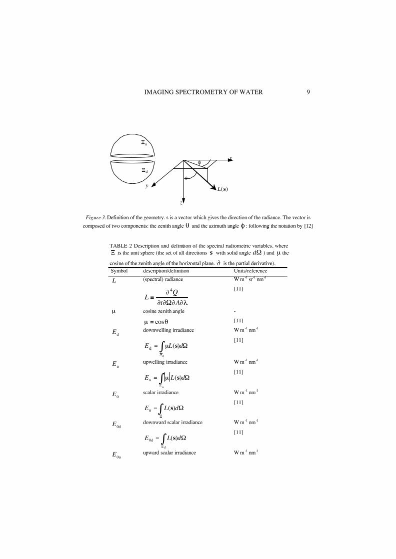
The effects of surface roughness - The surface of a natural water body is almost never flat; wind driven waves will have a major effect on the ability of light to pass across the air water interface. The effect of wind roughening is generally to widen the solid angle through which light will penetrate, i.e. some light will penetrate the water at angles greater than 49 degrees. The presence of slicks and/or whitecaps will further modify the light field in different ways from that of wave action [33] [34]). Oil slicks, apart from having a dampening effect on wave action will cause higher reflectance in certain regions of the spectrum.

2.5.2 Atmospheric effects and atmospheric correction Although the physics of atmospheric correction of remote sensing data over waters is essentially the same as for terrestrial targets, there are a few practical differences that need to be addressed. For any water body it is the signal coming from within the water body that is the desired signal. On land it is the surface reflected signal that is of inte-rest. For water bodies the surface reflected signal is a signal that is considered as noise, and is composed of the reflected component of diffuse skylight and of the direct sun-light impinging on the water surface. Water bodies in general reflect (as subsurface irradiance reflectance) in the range of 1 to 15% of downwelling irradiance. The major-ity of waters reflect between 2 and 6% of downwelling irradiance. Thus to obtain e.g. 40 levels of irradiance reflectance in the range of 2 to 6% reflectance we need a mini-mal accuracy of atmospheric correction to 0.1% reflectance.

Water body surfaces show swell, waves and capillary waves with facets of tens of meters to a few centimetres. Although their distribution can be predicted in a stochastic way, the inherent chaotic nature complicates adequate removal of surface reflectance effects. Therefore flight planning of airborne imaging spectrometry campaigns needs to consider the solar zenith angles and azimuths that minimise (given the FOV of the scanner) imaging of sunglint effects of the water surface. A rule of thumb is that solar zenith angles of 30º to 60º are optimal over water targets and that flight paths should be flown at 0º or 180º headings with respect to the solar azimuth. At low latitudes this will mean flying in a short period around noon in summer to achieve a maximal amount of irradiance. At mid-latitudes the flight time will be dependent on the season: as the max-imum solar zenith angles increases going from summer to winter -the flight time envel-ope decreases from approximately 6 to 8 hours surrounding noon to two hours surroun-ding noon. At low latitudes solar noon must be avoided to avoid sunspot effects (direct reflectance from horizontal water surfaces into the FOV); thus a situation arises with two periods: one in the morning and one in the afternoon.

22 A.G. DEKKER ET AL.

3 Optically deep and shallow waters: applications and case studies 3.1 INTRODUCTION The previous paragraphs described one of the theoretical approaches to describing the processes in the underwater light field. Now we will present literature reviews and case studies of spectral measurement, modelling, simulation and imaging spectrometry ap-plications. First, inland waters and estuaries as the two most studied optically deep water systems will be discussed. Next, seagrasses and coral reefs as the two most stud-ied optically shallow systems will be discussed. After the literature review for inland waters a case study is presented for lakes in Germany where an inverse modelling method was applied to derive images of chlorophyll and suspended matter. These two variables often confuse simpler algorithms as chlorophyll is the pigment in the algae and the algae constitute part of the biomass that is part of the suspended matter. The estuary example will be discussed as it represents an application for optically deep water where it is currently possible to parameterise most of the inherent and apparent optical properties. The estuary example is for modelling and measurement based on in situ spectra only, as there are very few publications that describe actual airborne imag-ing spectrometers flown over estuaries, where there is no bottom visibility. After these optically deep waters the optically shallow waters are discussed. First a discussion on the combined effects of a water column and a substrate takes place. In this discussion bathymetry play an important role. Next a literature review and a case study on seagrass remote sensing is presented. The final subject discussed are the coral reefs. In terms of the analytical model, the seagrass and coral reef examples represent a more hybrid situation where not everything can yet be described in terms of IOPs and AOPs. Therefore, it is necessary to rely more on in situ measured reflectance spectra in combination with analytical modelling or numerical modelling of the effects of the water column. 3.2 OPTICALLY DEEP INLAND AND ESTUARINE WATERS

3.2.1 Imaging spectrometry of optically deep inland waters A review of satellite and airborne remote sensing of aquatic ecosystems is given in [35], summarily updated in [24]. [36] gave a review of airborne remote sensing. [2] wrote a comprehensive review of satellite and airborne remote sensing of inland waters, including imaging spectrometry. [37] present a sound treatise on remote sensing of inland and coastal waters, where the emphasis of the applications is on the Laurentian Great lakes in the USA. [4] reviewed the literature on satellite remote sensing of lakes and [5] presented a review of satellite remote sensing of inland and coastal waters. After 1984 remote sensing of inland waters has taken place mainly using data from sat-ellite based sensors such as Landsat Thematic Mapper and SPOT-HRV (IRS –LISS series, CZCS, NOAA-AVHRR) and airborne remote sensing using instruments varying from multispectral scanners to line spectrometers and imaging spectrometers such as the CASI, AISA, AVIRIS, HYMAP and DAIS-7915. The CASI and AISA (and in a lesser degree HYMAP and AVIRIS) systems are not each one sensor with fixed capabilities.

IMAGING SPECTROMETRY OF WATER 23

They are a family of sensors, whereby there is a progression in sophistication of the sens-or with each new model developed. E.G for the CASI there are now approximately 20 systems operational. Each one of them has slightly different capabilities, whereby each upgrade to an existing sensor (specifically the case for AVIRIS) or each new sensor out-performs the previous version. Notice must be taken that the results of a CASI or AVIRIS flown in 1990 are not the same as the results for a CASI or AVIRIS flown in 2000 becau-se the performance of the instrument has greatly increased. Moreover for the CASI an extra complication in comparing results is that it is a programmable imaging spectro-meter, meaning that each application may have a unique spectral band s et applied. For the development of high spectral resolution remote sensing applications, both imaging and non-imaging (either line or point measurements) data are of interest. Ground-based surf-ace and subsurface spectral measurements may serve as surface calibration and as the link between the remotely sensed signal and the inherent optical properties.

Specific Inherent Optical Properties Inland Waters

0.00

0.01

0.02

0.03

0.04

0.05

0.06

0.07

0.08

400 450 500 550 600 650 700 750Wavelength (nm)

b (w)&

b*(p

hyto

)&a*

/b* (c

pc)&

b*(tr

ipto

n)

(m-1

)

0.00

0.50

1.00

1.50

2.00

2.50

3.00

a (w

)&a*

(CDO

M)&

a*(tr

ipto

n) (m

-1)

b(w)a*(phyto)

b*(phyto)a*(tripton)a*(CPC)

b*(CPC)a(w)

a*(CDOM)b*(tripton)

Figure 7. Inherent optical properties of Dutch inland waters (Dekker 1993). Left axis: b(w), a*(ph), b*(ph),

a*(CPC), b*(CPC) and b*(tr); right axis: a(w), a*(CDOM)norm 440 and a*(tr). Units: a and b in ( m-1) ; a* and b* of phytoplankton, CPC in (mg m-2) and a*(tr) and b*(tr) in (g m-2).

To summarise relevant information from the literature, a literature review is carried out discussing only those studies that actually made use of an airborne spectroradiometer (hand-held) or imaging spectrometer. This selection criteria is strict and excludes a sig-nificant amount of excellent work that discusses underwater and just above water mea-surements of inherent and apparent optical properties. Interested readers are referred to the reviews by [2], [37],[4]and [5]. In order to put the airborne spectrometry review into a correct perspective, simulations of reflectance using a bio-optical model are presented for algae dominated water and for total suspended matter dominated water.

3.2.1.1 Simulations using a bio-optical model Figures 7 to 9 demonstrate the variability of inland water spectra. Figure 7 shows the inherent optical properties of inland waters as determined for Dutch lakes by [27]. In the case of inherent optical properties such as the absorption by the sum of chlorophyll a and phaeophytin (CHL) the specific inherent optical property is given (meaning the amount of absorption or scattering or backscattering per unit weight). Figure 8 shows a

24 A.G. DEKKER ET AL.

simulation run where CHL varied from 0-90 in 10 µ g l-1 steps, CPC varied in 0-135 µ g l-1 steps and a(cdom)440 varied from 1.0 to 1.9 m-1. The non-chlorophyllous suspended matter (tripton) was kept fixed at 1 mg l-1. This is thus a simulation of a deep lake where a cyanobacterial dominated phytoplankton bloom is occurring.

Subsurface reflectance

0.0000.005

0.0100.0150.0200.0250.0300.035

400 450 500 550 600 650 700 750Wavelength

R(0

-)

12345678910

run

run 1 2 3 4 5 6 7 8 9 10 Seston 1.0 1.7 2.4 3.1 3.8 4.5 5.2 5.9 6.6 7.3 Tripton 1.0 1.0 1.0 1.0 1.0 1.0 1.0 1.0 1.0 1.0 CHL 0 10 20 30 40 50 60 70 80 90 CPC 0 15 30 45 60 75 90 105 120 135 a(cdom)440 1.0 1.1 1.2 1.3 1.4 1.5 1.6 1.7 1.8 1.9

Figure 8. Simulation run where CHL varied from 0-90 in 10 µ g l-1 steps, CPC varied in 0-135 µ g l-1 steps

and a(cdom)440 varied from 1.0 to 1.9 m-1.

Figure 9 shows a simulation run where CHL is fixed at 1 µ g l-1, CPC is zero and a(cdom)440 is fixed at 1.0 m-1. The non-chlorophyllous suspended matter (tripton) was varied from 10 mg l-1 to 100 mg l-1. This is thus a simulation of a lake or river where a substantial amount of suspended matter is entering the water column, either through river input or through wave-induced resuspension of bottom sediments. Figure 9 shows that if the main feature varying is TSM, reflectance increases over the entire spectrum, and this increase tends to saturate at higher concentrations of TSM. From the two figures it is clear that CDOM and pigments such as CHL and CPC as well as the tripton all contribute to lowering the reflectance at the blue wavelengths. Centred at 624 and 676 are the CPC and CHL induced reflectance troughs. These troughs are flanked by local reflectance peaks at 570-600 nm, 650 and 704-710 nm respectively. Note that no fluorescence term was required to simulate the often occurring reflectance peak at 706 nm. Many authors erroneously contribute this peak entirely to fluorescence whereas it is mostly due to a combined minimum in absorbing features at this wavelength. Indeed, the work [38], who originally conceived the idea of measuring fluorescence by remote sensing in the eighties,

IMAGING SPECTROMETRY OF WATER 25

demonstrates that above 10 to 20 µ g l-1 CHL the fluorescence signal centred at 683-685 nm is absorbed by the broadening absorption of CHL.

Subsurface reflectance

0.000

0.050

0.100

0.150

0.200

0.250

400 450 500 550 600 650 700 750Wavelength

R(0

-)

12345678910

run

run 1 2 3 4 5 6 7 8 9 10 Seston 10.1 20.1 30.1 40.1 50.1 60.1 70.1 80.1 90.1 100.1 Tripton 10 20 30 40 50 60 70 80 90 100 CHL 1 1 1 1 1 1 1 1 1 1

CPC 0 0 0 0 0 0 0 0 0 0 a(cdom)440 1 1 1 1 1 1 1 1 1 1

Figure 9. Simulation run where CHL is fixed at 1 µ g l-1, CPC is zero and a(cdom)440 is fixed at 1.0 m-1. Only

the tripton part of seston is increased. The simulations in Figures 8 and 9 may be used for optimal spectral band location of programmable imaging spectrometers such as the CASI or AISA.

3.2.1.2 Literature review of imaging spectrometry of optically deep inland waters The earliest airborne imaging spectrometry results are published for the Programmable Multispectral Imager on Canadian waters in 1985; PMI and CASI campaigns over eu-trophic Dutch lakes in 1988 and 1990; AVIRIS used for oligotrophic lake Mono and the saline lake Tahoe in the USA from 1990-1993; a CASI for Tennessee Valley Reser-voirs mapping in the period of 1991-1992. The period 1993-1996 saw imaging spectro-meters - mostly CASI’s- deployed in Australia, Netherlands and German lakes. These more recent researches established a more analytical approach to hyperspectral remote sensing, and are thus to be considered as a breakthrough towards more quantitative, intercomparable, methods.

The largest data set and most consistent application was in the Netherlands where imaging spectrometry missions were flown in 1988, 1990, 1992, 1993,1995 and 1997 using PMI, CAESAR and a sequence of CASI sensors. A development in time is clear from initial more empirical and semi-empirical approaches towards more analytical

26 A.G. DEKKER ET AL.

approaches involving the use of parameterized bio-optical models that are subsequently inverted. Especially the work by [39] and [40] and [41] illustrate the use of inversion methods, whereby optical water quality variables are inverted from the remotely sensed signal taking into account partially covering other optical water quality variables: e.g. estimating chlorophyll contents and TSM, whereby account is taken of the effect of the chlorophyll associated biomass of algae to the TSM contents.

From 1997 onwards, increased activity in Scandinavian countries and Germany is evident. Especially the work by [42] and Schaale et al. (1998) is original and a portent of future methodologies involving the creation of massive amounts of simu lated data based on (i) bio-optical modelling, (ii) air-water interface and atmospheric modelling, as well as (iii) incorporating the sensor look geometry across track, after which (iiii) either look-up tables or neural networks are created for inversion methods. See the case study of the Berlin lakes CASI images discussed later. From the literature (26 studies) it is evident that CHL is the prime variable measured in all cases (26); the blue-green (or cyanobacterial) pigment CPC in 8 cases; total suspended matter (or an equivalent thereof-the definitions and methods of measuring TSM are highly variable) in 16 cases; Secchi depth transparency in 18 cases; vertical attenuation of PAR in 8 cases and a few cases of turbidity (6) and CDOM . The CDOM determinations from the remote sensing data were not really successful as the sensors used all showed low sensitivity in the blue wavelengths, where CDOM absorption is most noticeable. The range in optical water quality variables detected during these campaigns was large:

TABLE 7. Review of measured water quality variables.

variable Min Max CHL (µg l-1) 0 1010 CPC (µg l-1) 0 1519 TSM (mg l-1) 1 700 SD (m) 0.05 8.5 Kd (m-1) 0.4 10 NTU 1 640

An excellent example of the use of imaging spectrometry is the determination of cyanophycocyanin, as only an instrument that can parameterise the absorption feature of CPC at 624 nm, by simultaneously measuring the local reflectance peaks at 600 and 648 nm (See Figure 8) is capable of determining the presence of cyanobacteria [27] [39].

3.2.1.3 Case study: inland water quality with inverse modelling A case study is presented of an inverse modelling approach using a radiative transfer model which is a coupled water-atmosphere model, in this case the MOMO model based on the matrix operator method [43] Fischer, 1984 #382 [44]. MOMO is a highly sophisticated model suited especially for the simu lation of the radiative transfer in clear and turbid atmospheres including the water body with a rough water surface. Comparisons with a water-atmosphere Monte Carlo model as well as comparisons with

IMAGING SPECTROMETRY OF WATER 27

airborne and underwater measurements show excellent agreement [45]. This model allows the computation of spectral, sensor and solar zenith and azimuthal resolved radiances and reflectance. The type and concentration of atmo spheric aerosols and water constituents are introduced by the extinction coefficient, single scattering albedo and the phase (volume scattering) function. The accuracy of the retrie val of water constituents depends on the choice of optical properties.

The CASI was flown on 23 April 1995 over the lake ‘Tegeler See’ an important fresh water reservoir for the city of Berlin, Germany. The instrument was operated in spatial mode with six bands in the visible spectral range and a spatial resolution of 2.5 x 3.5 m during a period of highest biological activity. The overall approach was to (i) convert the CASI sensor signals into radiances by a calibration and a radiometric correction [46], (ii) to obtain the surface reflectance needed in the further analysis [47] through atmospheric correction of the remotely sensed data, (iii) perform geometric correction, (iiii) apply the inversion to the water areas of the images.

The radiative transfer model MOMO was applied for the water constituents CHL, TSM and CDOM, using their optical properties [42]. The substance concentrations and the observation/illumination geometry were varied systematically in a given range (Table 8) to set up a look-up table for the further analysis whilst atmospheric para-meters were fixed to realistic values.

TABLE 8. Substance concentration and observation geometry range for the MOMO run. Variable Range Step size # of values Chlorophyll a 0 – 220 µg l-1 2 µg l-1 111 Suspended matter 0 – 100 mg l-1 2.5 mg l-1 41 CDOM absorption 0 – 35 m-1 @ 254 nm 2.5 m-1 @ 254 nm 15 Sun zenith angle 0° – 82.15° 15.70° – 19.11° 6 Sun-observer azimuth distance 0° –180° 11.25° 17 Observer zenith angle 0° – 82.15° 15.70° – 19.11° 6

At the end of the model simulation runs the look-up table contained 42 million multi-spectral reflectance vectors for six bands. The inversion problem considered here may be solved by a simple look-up table approach, which is computational very time con-suming, or by a faster neural network approach. The look-up table approach is straight-forward and immediately applicable. The neural network approach consists of a sophi-sticated mathematical model and needs an intensive training of the network prior to its application.

Using the look-up table approach both the substance concentrations as well as the observation/illumination geometry has to be interpolated linearly. The neural network approach can be used as a multi-variable non-linear regression method. It was found more useful to represent look-up tables by a neural network including their non-linear interpolating and fast application properties. Each inverse modelling method needs to set up a look-up table where for a number of concentrations of water constituents based on a bio-optical model the reflectance spectra are known. Then, the concentrations, and their spatial distribution can be retrieved from remotely sensed reflectance spectra out of the database. For the inversion of the remote sensing measurements using the look-up table approach for each multi-spectral reflectance vector, or pixel, respectively, this corresponding simulated multi-spectral reflectance vector is searched for within the look-up table, where the Euclidean distance finds its minimum. The observation/illumi-nation geometry was interpolated linearly. The concentrations for chlorophyll a, sus-

28 A.G. DEKKER ET AL.

pended matter, and CDOM are the result of this inversion. A significant advantage of this method is that no further pre-processing of the data is necessary. For the inversion of the remote sensing measurements using the neural network approach several mani-pulations were applied to the model data. Several forms of noise were added to the data.

Figure 10. Spatial distribution of chlorophyll a (left) and suspended matter (right) for lake ‘Tegeler See’ on

23 April 1995 retrieved by a look-up table approach. Then, up to 1 ‰ random chosen input/output data sets were selected from the entire look-up table, and used for the training of an adapted feed-forward radial basis function (RBF) network [48]. 500 training steps in total were used for the training of a total of 25 neurons. The number of learning cycles should be high enough for a slow decrease of the cost function to obtain a robust solution. Three different neural networks were trained for each of the three substances: chlorophyll a, suspended matter, and CDOM.

The application of both inverse modelling methods to the CASI data reveals clear and well structured concentration maps for chlorophyll a as well as for suspended mat-ter (Figure 10 and 11; only chlorophyll is shown here for illustration purposes). The main (north east) part of the lake shows low chlorophyll a and suspended matter con-centrations while the attached waterways (south west) show higher concentrations. This is confirmed by in situ measurements that are in the same order of concentration rang-es. Beside this main feature a variety of local features can be extracted: high gradients of concentration changes at local points (especially on the shore), traces of ships and possibly bottom effects along the shore. For CDOM no useful results were achieved. The spectral characteristics of CDOM overlap those of chlorophyll in the blue spectral region, therefore it is not simple to extract that part of absorption which is caused by CDOM.

The obtained results demonstrate the successful use of inverse modelling methods using MOMO for the retrieval of the spatial distribution of at least two optically active substances (chlorophyll a and suspended matter) by multi-spectral remote sensing mea-surements above inland waters. Compared to the look-up table approach the neural net-work approach produces similar results more efficiently, by requiring less time. The higher effort for the training of the neural network in preparation of the application is the only disadvantage. Nevertheless, both methods allow the use of time consuming radiative transfer models for the simulation of more than one water constituent inde-pendently, and reasonable maps of the quantitative and spatial distribution of several inland water quality parameters can be generated.

IMAGING SPECTROMETRY OF WATER 29

Figure 11. Spatial distribution of chlorophyll a (left) and suspended matter (right) for lake ‘Tegeler See’ on

23 April 1995 retrieved by a neural network approach.

3.2.2 Imaging spectrometry of optically deep estuaries Estuaries are usually dynamic environments where freshwater meets ocean water. They are among the most productive aquatic ecosystems. Pressures from often conflicting uses, causes them to be studied extensively. [49] summarises the developments in the period of 1990-2000 in actual applied remote sensing of estuaries. However, few publications exis t on imaging spectrometry applications over estuaries, based on inversion of analytical models. Some papers have been published on simple empirical methods, but these have no multitemporal or multi-site applicability. The study by [50] is a good illustration of the frequency required for begin ning to understand some of the dynamics in an estuary using remote sensing. Although they did not use imaging spectrometers, they collected in situ spectroradiometric reflectance measurements, a suite of aerial photography taken on different days as well as Airborne Thematic Mapper data (from which they mainly use the thermal band). With all this data they studied frontal systems in the Tay Estuary in Scotland. Another example is the work by [51] who studied the extent of a massive river Oder flood event using several types of satellite imagery, but basing their algorithms on previously carried out measurement and modelling of the underwater light field. They were able to produce maps of CHL, TSM and CDOM from the experimental satellite MOS sensor.

3.2.2.1 Optical properties of estuarine waters The majority of studies that address the issues of spectral reflectance of estuarine waters, focus on the spectral optical properties of estuarine waters, with the aim of developing algorithms for processing satellite images of these estuaries. The following literature study discusses the studies that focussed on understanding the optical varia-bility of estuarine waters. Next, the papers are discussed that proceed from these optical properties to inversion methods. After that, the literature is discussed of studies that continue this thread of analysis and actually apply it to i) non-hyperspectral satellite data, ii) airborne imaging spectrometry data and iii) studies in preparation of MERIS.

30 A.G. DEKKER ET AL.

MERIS will be the first dedicated imaging spectrometry system for coastal waters in space in the near future. It is arguable that MODIS and MOS sensors warrant dis cus-sion here as well. However these sensors are in essence multispectral systems designed for ocean colour analysis and less for inland and coastal waters.

[52] studied the inherent optical properties of the Po Delta in northern Italy, focussing on the absorption coefficients of algal cultures and field samp les and on the backscattering spectra of field samples. From this analysis they propose combinations of spectral bands (similar to that to be found on MERIS and MODIS) for determining CDOM absorption in deltaic waters. [53], measured 119 spectra in coastal North Sea and Dover Strait waters and were able to demonstrate that for this data set only 5 spectral bands were required to reconstruct the whole spectrum. They proved their methodology on an independent data set taken in the Baie de Somme, a turbid tidal estuary off the North France coast. They do admit that further investigation is required if this method would work for algal blooms or for chlorophyll fluorescence. [54] describe the optical properties for the Menai Strait (Wales, UK): this strait is an excellent example of the variability in TSM and algal assemblages possible in one water body. Overall high values of TSM varies with lunar variation due to tidal action. The algal community composition starts off with a two-peaked spring bloom of first diatoms and then a mixture of diatoms and phaeocystis; after the bloom the concentrations decrease and small flagellates dominate. In summer a bloom of coccoid cyanobacteria is possible. Kratzer tried to develop algorithms based on four spectral channels only and concluded that this was an insufficient amount of bands to adequately invert such variations in concentrations.

[55] present a further development of work initiated by [56] [57, 58] [59] which relies on an iterative matrix inversion technique for measuring three optical compo-nents in coastal waters a(CDOM), phytoplankton through CHL and TSM, often aug-mented by one other variable such as aerosol retrieval or a backscattering coefficient of the water. They all admit that these methods are computational intensive and probably not very useful for operational inversion of a remotely sensed signal. [60], present a study on detection of CHL, DOC and TSM in the estuarine mixing zone of Georgia coastal plain rivers. The range of concentrations for these optically active constituents was large and the source composition was highly variable ranging from terrestrial dominated, to riverine dominated to almost ocean type waters. Of particular interest in their study is the establishment of absence of covariance between most of these parameters. Their results demonstrated that many empirically established relationships would fail in remote sensing of such systems. They found poor correlation between DOC and blue wavelength reflectance (thought to be the best spectral region for CDOM/DOC measurements from remote sensing), but higher (inverse) correlation at the green wavelengths. This effect may be explained through the blue reflectance signal being confounded by multiple constituents (pigments, detritus, CDOM), whereas the green signal was dominated by the combined effect of TSM and DOC/CDOM.

[61] discuss the inversion of a(cdom)440 and the sediment refractive index for nonchlorophyllous turbid coastal waters for the Rhone river mouth in France. [62] developed a CDOM, phytoplankton and sediment bio-optical model for the Ebro River in Spain. Forget (2000) combines these two data sets (Ebro and Rhone) and discusses them in the context of two-flow radiative transfer modelling approach from [10]. They specifically pay attention to the stratified system that may exist when a river plume flows in to relatively stable coastal water. In 66% of their inversion cases they were able to detect stratified water masses. Similar work was carried out by [63] who studied

IMAGING SPECTROMETRY OF WATER 31

the spectral re flectance and transparency of river plume waters in the Black Sea and the Arctic Ocean using ship-borne and airborne spectroradiometric measurements. They measured reflectance differences of a factor 10 between river plumes and the ocean water at the other side of the front. They make a convincing case that river plumes spreading into relatively stable ocean waters have three dimensional wedge shape that needs to be considered when remotely sensing such phenomena. From airborne or satellite imagery a high concentration fresh water TSM rich layer overlays a much clearer ocean layer. [64] carried out spectral analysis of waters of the Pamlico Sound estuary and the contributing river waters and found complex relationships relating reflectance to TSM. Their aim was to develop an algorithm for relating Kd (PAR) to reflectance measured by the NOAA-AVHRR 630 nm band; this was partially success-ful. [65] present preliminary results of a campaign intended to determine a method for optically measuring the natural variability of TSM in a heterogeneous and dynamic environment. For this purpose they use a suite of in situ optical properties measurements, ferry based spectroradiometric measurements, airborne imaging spectrometer (the EPS-A) flights and HYDROLIGHT to determine certain optical parameters. They parameterise the [10]/ [12] model and thus are among the first to use the more complete model presented in the section on modelling.

[66] followed the analytical approach to study an estuary in Kalimantan (Indonesia) involving multitemporal use of SPOT and TM images. They determined the spectral IOP’s of river, estuarine and ocean waters, developed a reflectance simulation model, (similar to Figs 8 and 9) to estimate the full range of TSM concen-trations possible in this system and subsequently derived algorithms for analytically determining the TSM in this dynamic tidal estuarine area.

[67] present the first results of AVIRIS flights carried out in 1990 over the Tampa Bay plume in the Florida coastal waters. Although at that time AVIRIS still had a relatively low S:N they were able to demonstrate the use of hyperspectral remote sensing for mapping the absorption coefficient at 415 nm and the backscattering coefficient at 671 nm. This work was followed through by [68] who derived a model for modelling hyperspectral remote sensing reflectance over a variety of case 2 waters from the West Florida Shelf to the Mississippi River plume. Their model is based on the Gordon model and takes into account CDOM , TSM, CHL, Raman scattering and CDOM fluorescence, the only optical active variable missing is fluorescence by algal pigments. In [69] a further development of this methodology is presented applied to AVIRIS data of 1998 (when the S:N has increased dramatically as compared to earlier versions). Because this paper discusses more the bathymetry effects of the substrate on the signal, further discussion takes place in the section on optically shallow waters. Mustard & Staid (1998) describe preliminary re sults of an AVIRIS flight over an estuary in New England (US). They were able to accurately model AVIRIS derived above surface reflectance. [70] followed the same methodology as [66] and were able to closely match AVIRIS data flown over the Hudson/Raritan Estuary (New York) by simulation using a bio-optical modelling tool parameterised for the Hudson/Raritan estuary waters. [71] used an AISA imaging spectrometer over a coastal water area in the Archipelago of the Baltic Sea, also using satellite and in situ data. They tested algo-rithms proposed for MOS, SeaWiFS and MERIS for Secchi Depth transparency, turbi-dity, CHL and TSM. They did not undertake any spectral measurements or modelling. [72] used a CASI to map the sediment plume caused by dredging for a tunnel in the Oresund, a coastal channel between Norway and Denmark. Their sediment maps were compared with a 2-D hydrodynamic model for calibration purposes. After measuring

32 A.G. DEKKER ET AL.

the inherent optical properties, and parameterising the simplified Gordon model it was decided to use the 544 nm spectral band as the band most suitable for determining TSM concentrations.

A special issue of the International Journal of Remote Sensing (1999, Vol 20, no 9) is dedicated to the relevant science surrounding the preparations for the MERIS sen-sor on board of ENVISAT: the first dedicated imaging spectrometry type sensor expli-citly designed for remote sensing of optically deep coastal waters. [73] used data from the literature to develop an neural network based inversion model for MERIS. [74] used the CASI airborne imaging spectrometer to develop and test algorithms for the MERIS space sensor. [75] developed the neural network that will be implemented operationally to derive case II water pro perties from MERIS data on a global scale. [38] presents the research leading up the CHL fluorescence algorithm for MERIS, the first space sensor to have dedicated fluorescence band centred at 683 nm.

3.2.2.2 Case study: The Western Scheldt Estuary Because of the complexity, an estuary is an excellent example to demonstrate the im-portance of the measurement of the specific inherent optical properties to parameterise the optical model. An estuary is a mix of two or more different water types, including at least river water and coastal water. Additionally, different sediment types may ap-pear due to resuspension of bottom material from tidal flats or wind and wave induced resuspension of bed sediments. The history of wind direction and speed, tidal stages and other meteorological conditions are thus of importance for the concentrations and composition of suspended matter. The case considered deals with the analysis of the typical concentration ranges and specific inherent optical properties measured in the Western Scheldt estuary. These modelling results were applied to SPOT data for en-vironmental baseline mapping of an intended area for construction of a [76]. Seasonal measurements of water quality parameters show that the primary parameter describing the optical properties in the estuary is the total suspended matter concentration (TSM). For 1998, the TSM concentration ranged between 4 and 120 mg m-2, whereas chlorophyll a ranged between 2 and 20 µ g m-3 . [77] determined the mean seasonal variation of TSM. On average, mean and standard deviation increase towards the east. Dissolved organic carbon (DOC) concentration on the average increases from 1.5 near the estuary’s mouth to more than 3.5 mg l-1 towards the River Scheldt. There is only minor seasonal variability in the DOC concentration. The analytical model by [12] was used for the light anisotropy factor f. This model (see table 6) is given by

IMAGING SPECTROMETRY OF WATER 33

0

0

(0 , )( )

1

1

0.7 (1 )cos( )0.5sin(sin( ) / )

d

b

b

d

u

u

z

bR fa b

f

F F

a n

λ

µµ

µ θ

µ

θ θ

− =+

= +

= + −

=

=

(21)

A simulation model that calculates reflectance from the specific inherent optical properties and the concentrations is defined as follows

* *

*

440

0.5TCHLw cdom TCHL TSM TSM

b w TSM TSM

cdom cdom

a a a a C a C

b b Bb Ca a g

= + + +

= +

=

(22)

The specific inherent optical properties (SIOP) are the absorption/scattering per unit of mass. The SIOP are the fundamental properties required for optical models. It must be noted here that TSM incorporates all particles not passing through a filter pore size used to measure the CDOM concentration. Thus TSM consists of alive and dead organ-ic particles and of inorganic particles. If possible it would be desirable to enhance the above equation of absorption to a = aw+acdom+a*TCHL CTCHL + a*ISCIS+ a*dCd (24) with a*IS and a*d the specific inherent absorption of inorganic suspended sediment and detritus respectively. In the more simplified model used the main issue is to determine the backscattering ratio for the fraction of light scattered backwards towards the upper hemisphere. This ratio B is determined by fitting the measured reflectance spectra and the modelled reflectance spectra using the [12] optical model, the SIOP and the in-situ concentrations. In this way, an optical closure of the reflectance model is achieved. A note of caution must be issued here: an error in the inherent optical property determination or in the concentration measurements may in fluence the parameterization of the SIOP’s and thus influence the estimation of B.

The in-situ measurements used here were taken in the scope of a project, initiated to monitor the ecological effects due to drilling for a tunnel and the resulting sediment dumping in the estuary using (among other techniques) remote sensing [76]. At five stations the subsurface irradiance reflectance (0 )R − was measured using a hand-held Photo Research (Chatsworth, CA, USA) model PR-650 spectroradiometer, and water samples were taken for subsequent laboratory analysis. Optical properties (absorption and total scattering) were determined together with water quality parameters (TSM and total chlorophyll (Figure 12)), resulting in the specific inherent optical properties for each station (Figure 13).

34 A.G. DEKKER ET AL.

TCHL and TSM for the Western Scheldt on 10/3/99

3.6

5.4

8.7

10.8

8.7

14.7

27.5

53.457.5

40.1

0

2

4

6

8

10

12

TN HW LA BA WS

TCH

L (m

g m

-3)

0

10

20

30

40

50

60

70

TSM

(g m

-3)

TCHLTSM

Figure 12. Measured water quality parameters in the Western Scheldt

For all stations absorption of coloured dissolved organic matter (CDOM ) was consider-able (a(cdom)440 ranging from 1.4 to 1.8 m-1). Apart from station ‘WS’ there is an ap-parent increase in TSM concentration in eastward direction.

Figure 13. CDOM absorption (a), specific pigment absorption (b), specific seston scattering (c) and specific tripton absorption (d) measured for five stations in the Western Scheldt estuary. For CDOM absorption (Figure 13), all exponential slopes are similar, except for the ‘TN’ station, which has a significant lower exponential slope than the other four. This may be attributed to the fact that ‘TN’ is closest to the sea, and might have a different

a)

CDOM absorption

0

1

2

3

4

400 500 600 700wavelength (nm)

aCD

OM

(m-1

)

TNHWLABAWS

b)

TCHL specific pigment absorption

0

0.02

0.04

0.06

0.08

0.1

400 500 600 700wavelength (nm)

a*pi

g (m

2 mg-1

) TNHWLABA

c)

TSM specific seston scattering

0

0.1

0.2

0.3

0.4

0.5

400 500 600 700wavelength (nm)

b*se

s (m

2 g-1

)

TN HWLA BAWS

d)

TSM specific tripton absorption

0

0.04

0.08

0.12

400 500 600 700wavelength (nm)

a*tr (m

2 g-1

)

TNHWLABAWS

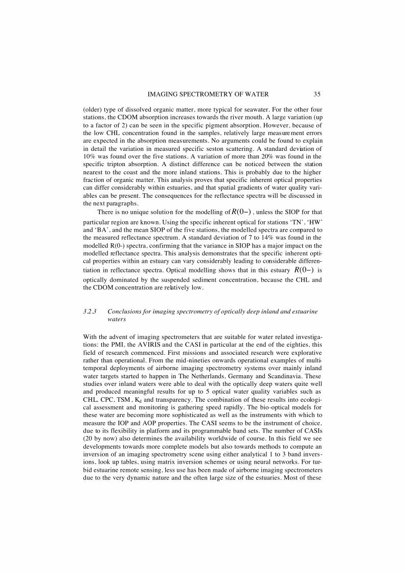
IMAGING SPECTROMETRY OF WATER 35

(older) type of dissolved organic matter, more typical for seawater. For the other four stations, the CDOM absorption increases towards the river mouth. A large variation (up to a factor of 2) can be seen in the specific pigment absorption. However, because of the low CHL concentration found in the samples, relatively large measurement errors are expected in the absorption measurements. No arguments could be found to explain in detail the variation in measured specific seston scattering. A standard deviation of 10% was found over the five stations. A variation of more than 20% was found in the specific tripton absorption. A distinct difference can be noticed between the station nearest to the coast and the more inland stations. This is probably due to the higher fraction of organic matter. This analysis proves that specific inherent optical properties can differ considerably within estuaries, and that spatial gradients of water quality vari-ables can be present. The consequences for the reflectance spectra will be discussed in the next paragraphs.

There is no unique solution for the modelling of (0 )R − , unless the SIOP for that particular region are known. Using the specific inherent optical for stations ‘TN’, ‘HW’ and ‘BA’, and the mean SIOP of the five stations, the modelled spectra are compared to the measured reflectance spectrum. A standard deviation of 7 to 14% was found in the modelled R(0-) spectra, confirming that the variance in SIOP has a major impact on the modelled reflectance spectra. This analysis demonstrates that the specific inherent opti-cal properties within an estuary can vary considerably leading to considerable differen-tiation in reflectance spectra. Optical modelling shows that in this estuary (0 )R − is optically dominated by the suspended sediment concentration, because the CHL and the CDOM concentration are relatively low.

3.2.3 Conclusions for imaging spectrometry of optically deep inland and estuarine waters

With the advent of imaging spectrometers that are suitable for water related investiga-tions: the PMI, the AVIRIS and the CASI in particular at the end of the eighties, this field of research commenced. First missions and associated research were explorative rather than operational. From the mid-nineties onwards operational examples of multi-temporal deployments of airborne imaging spectrometry systems over mainly inland water targets started to happen in The Netherlands, Germany and Scandinavia. These studies over inland waters were able to deal with the optically deep waters quite well and produced meaningful results for up to 5 optical water quality variables such as CHL, CPC, TSM , Kd and transparency. The combination of these results into ecologi-cal assessment and monitoring is gathering speed rapidly. The bio-optical models for these water are becoming more sophisticated as well as the instruments with which to measure the IOP and AOP properties. The CASI seems to be the instrument of choice, due to its flexibility in platform and its programmable band sets. The number of CASIs (20 by now) also determines the availability worldwide of course. In this field we see developments towards more complete models but also towards methods to compute an inversion of an imaging spectrometry scene using either analytical 1 to 3 band invers-ions, look up tables, using matrix inversion schemes or using neural networks. For tur-bid estuarine remote sensing, less use has been made of airborne imaging spectrometers due to the very dynamic nature and the often large size of the estuaries. Most of these

36 A.G. DEKKER ET AL.

studies were intended as illustrations or experiments in preparation of using satellite sensors to monitor these systems. As spaceborne imaging spectrometers become availa-ble this field of application is likely to evolve very fast. 3.3 OPTICALLY SHALLOW WATERS Optically shallow waters are a special case in remote sensing of aquatic systems. It in-volves a measurable signal from a substrate, through the water column and through the air-water interface. In all applications where a substrate is being mapped through a water column, a bathymetry estimate is implicitly or explicitly involved. In the case of a bathymetry estimate from remote sensing a substrate reflectance and a water column optical depth is implicitly or explicitly involved. The bathymetry and the water column optical properties are thus of importance to the following remote sensing applications in aquatic environments: submerged macrophyte mapping, seagrass and macro-algae mapping, coral reef mapping, sand, coral rubble and mud floor mapping and benthic micro -algae mapping. Alternatively one may want to measure the optical properties or the concentration of substances in a water column over a visible substrate. In that case the bathymetry signal is seen as a component that must be corrected for (as with atmos-pheric correction) see e.g. [78].

This section is composed as follows: first there will be a discussion of the literature on bathymetry and substrate mapping (usually brightly reflecting bottoms), how to simu late reflectance signals over such complex environments and what the requirements for imaging spectrometers are. The remainder of this section will discuss more in detail the state-of-the-art in seagrass, macrophyte and coral reef mapping, with a case study on seagrass, macro -algae and substrate mapping in a shallow coastal environment near Adelaide, Australia.

3.3.1 Bathymetry and bright substrate mapping The term “measurable signal from the substrate” sums up one of the problems in per-forming bathymetry or measuring a substrate cover such as seagrass. It will depend on the spectral optical depth of the water column, on the brightness and spectral contrast of the substrate as well as the signal-to-noise performance of a remote sensor whether bathymetry or a substrate cover can actually be determined. If there is no measurable influence of the bottom on the remotely sensed reflectance the water is considered to be optically deep; if there is a measurable reflectance contribution from the substrate or plants in the water column the water is considered to be optically shallow.

In the theory section the model by [29] is presented. Equation 18 expresses the R(0-,H) as a function of the reflectance of an infinitely deep water column, the vertical attenuation coefficients and the irradiance reflectance of the substrate. In Figure 14 a simulation is presented of the following case. The same bio-optical model as used in the inland water simulations calculates the irradiance reflectance for an infinite water column. In this case the concentrations were: CHL = 1 µg l-1 , TSM = 2.1 mg l-1 and the absorption by CDOM is expressed as a(cdom)440 of 0.2 m-1 .

IMAGING SPECTROMETRY OF WATER 37

R(0-) calculated over a 10 % reflecting substrate at depths of 0.5 to 6 m and a R(inf) based on :

CHL=2 µ g l-1,a (cdom)=0.2 m-1 and TSM = 2.1mg l-1

0.00

0.01

0.02

0.03

0.04

0.05

0.06

0.07

0.08

0.09

0.10

400 450 500 550 600 650 700 750wavelength (nm)

R(0

,H)

0.0

0.5

1.0

1.5

2.0

2.5

3.0

Kd

(m-1

)

H=0.5H=1H=2H=3H=4H=5H=6R(inf)Kd

Figure 14. Simulation with CHL = 1 µg l-1 , TSM = 2.1 mg l-1 and the absorption by CDOM is expressed as

a(cdom)440 of 0.2 m-1 This same simulation software calculated the associated Kd, using the [22] model

for relating Kd to the inherent and apparent optical properties. Next a substrate reflect-ance of 10% was assumed (spectral neutral- dark grey). The graphs in figure 14 show the resultant R(0-) calculated with the substrate at depths of 0.5 m, 1, m, 2m...6 m. From the results it can be deduced that for depths of 1, 2 and 3 m it would be required to measure R(0-) with an accuracy of 1 % in the green wavelengths in order to distin-guish R(0-) differences due to the substrate at 1 m depth intervals. In terms of R(0-) this would equate to a discretisation S:N in terms of R(0-) of 100:1, which in turn leads to a S:N requirement of about 200:1 for R(0+) (as 48 % of upwelling irradiance just below the water surface is reflected into the water column). The required S:N in terms of R(0-) to distinguish the substrate between depths of 5 and 6 m quickly increases almost a factor 5 to 500:1 (R(0-) or 1000:1 (R(0+). These latter S:N specifications are about the maximum currently attainable by systems such as AVIRIS and CASI, flown under ideal circumstances. It is also evident from the graph that under these simu lated conditions most information from the substrate reaches the water surface in the wave-lengths of 500 – 600 nm. In reality the situation is more complex as we now assumed a flat water surface, a homogeneous diffuse light field and a neutral spectral behaviour of the substrate (See Table 9 for substrate reflectances).

TABLE 9. Values of high reflectance of bottom substrate from literature. Authors type of substrate RB at 400 nm RB at 700 nm Alberotanza et al. 1989 coral sand 28% 60% Lee et al. 1994 offshore sed. 40% 56%

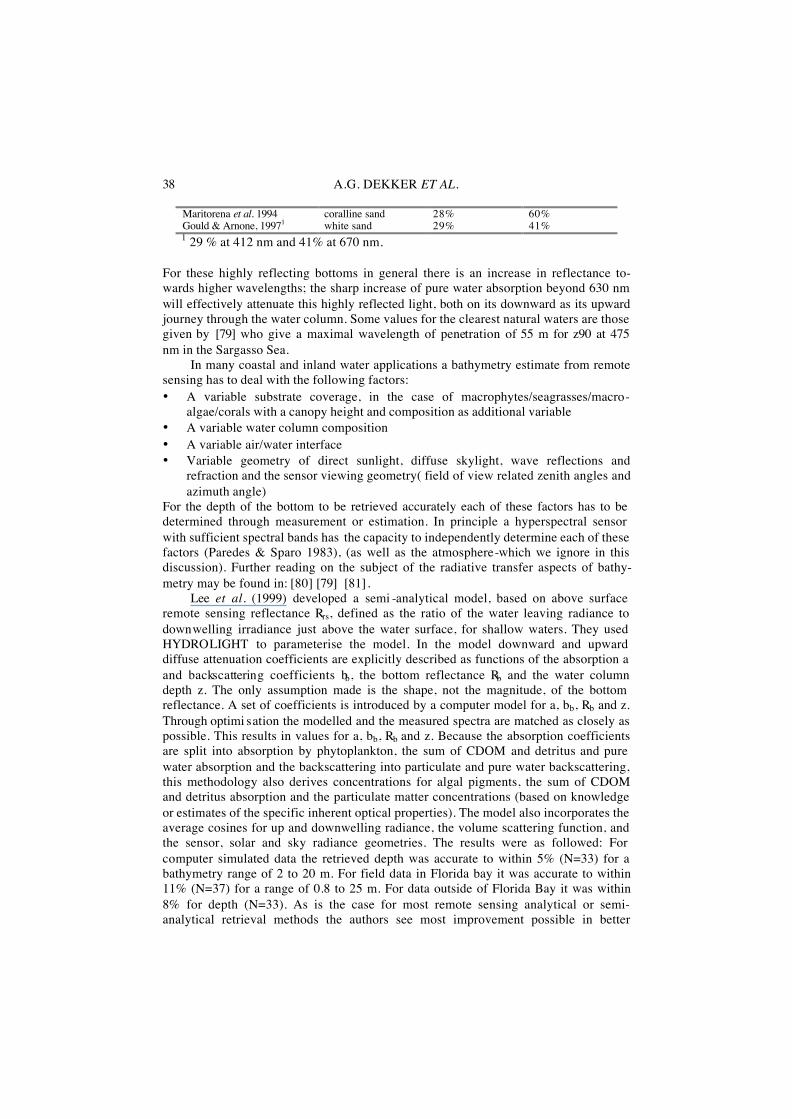
38 A.G. DEKKER ET AL.

Maritorena et al. 1994 coralline sand 28% 60% Gould & Arnone, 19971 white sand 29% 41% 1 29 % at 412 nm and 41% at 670 nm.

For these highly reflecting bottoms in general there is an increase in reflectance to-wards higher wavelengths; the sharp increase of pure water absorption beyond 630 nm will effectively attenuate this highly reflected light, both on its downward as its upward journey through the water column. Some values for the clearest natural waters are those given by [79] who give a maximal wavelength of penetration of 55 m for z90 at 475 nm in the Sargasso Sea.

In many coastal and inland water applications a bathymetry estimate from remote sensing has to deal with the following factors: • A variable substrate coverage, in the case of macrophytes/seagrasses/macro-

algae/corals with a canopy height and composition as additional variable • A variable water column composition • A variable air/water interface • Variable geometry of direct sunlight, diffuse skylight, wave reflections and

refraction and the sensor viewing geometry( field of view related zenith angles and azimuth angle)

For the depth of the bottom to be retrieved accurately each of these factors has to be determined through measurement or estimation. In principle a hyperspectral sensor with sufficient spectral bands has the capacity to independently determine each of these factors (Paredes & Sparo 1983), (as well as the atmosphere-which we ignore in this discussion). Further reading on the subject of the radiative transfer aspects of bathy-metry may be found in: [80] [79] [81].

Lee et al. (1999) developed a semi -analytical model, based on above surface remote sensing reflectance Rrs, defined as the ratio of the water leaving radiance to downwelling irradiance just above the water surface, for shallow waters. They used HYDROLIGHT to parameterise the model. In the model downward and upward diffuse attenuation coefficients are explicitly described as functions of the absorption a and backscattering coefficients bb, the bottom reflectance Rb and the water column depth z. The only assumption made is the shape, not the magnitude, of the bottom reflectance. A set of coefficients is introduced by a computer model for a, bb, Rb and z. Through optimi sation the modelled and the measured spectra are matched as closely as possible. This results in values for a, bb, Rb and z. Because the absorption coefficients are split into absorption by phytoplankton, the sum of CDOM and detritus and pure water absorption and the backscattering into particulate and pure water backscattering, this methodology also derives concentrations for algal pigments, the sum of CDOM and detritus absorption and the particulate matter concentrations (based on knowledge or estimates of the specific inherent optical properties). The model also incorporates the average cosines for up and downwelling radiance, the volume scattering function, and the sensor, solar and sky radiance geometries. The results were as followed: For computer simulated data the retrieved depth was accurate to within 5% (N=33) for a bathymetry range of 2 to 20 m. For field data in Florida bay it was accurate to within 11% (N=37) for a range of 0.8 to 25 m. For data outside of Florida Bay it was within 8% for depth (N=33). As is the case for most remote sensing analytical or semi-analytical retrieval methods the authors see most improvement possible in better

IMAGING SPECTROMETRY OF WATER 39

measurements or estimates of the inherent optical properties of the optically active components.

[82] used data from AVIRIS flown in 1993 over Tampa Bay and in 1996 over the Florida Keys in a neural network system to establish quantitative empirical relationships between depth and remotely sensed spectral radiance. No use was made of any type of physics based processing of the data to remove atmospheric or air/water interface effects. They used an extensive set of tens of thousands of depth soundings spanning a 1952 through to 1995 time range for Tampa Bay and for 1997 in the Florida Keys area. Relative to these depth data sets the RMS was 0.84 m for the Tampa Bay and 0.39 for the Florida Keys area. This RMS could have been reduced if the bathymetry in situ data deeper than 6m had been omitted as there was no bottom visibility beyond that depth. Also the AVIRIS was twice as sensitive in 1996 as in 1993. They also trained the neural network on both data sets which resulted in a RMS of 0.48 m. Apparently a neural network has generalisation capacity based on this research as the Tampa Bay and Florida Keys waters are very different with different substrates. These results indicate the effectiveness of neural networks for fast remote sensing data processing.

3.3.1.1 Bathymetry in inland waters [83] report on an AVIRIS flight in 1990 over the oligotrophic Lake Tahoe. They related the bathymetry of Lake Tahoe to upwelling spectral radiance recorded by AVIRIS using a two-channel multiple linear regression with AVIRIS data at 490 and 560 nm. They assumed a uniform bottom reflectance and were able to map bathymetry between the 3 and 10 meter contours.

George (1997) used a CASI to map bottom topography features in Lake Winder-mere in the UK. The data was flown in 1989 with one of the first versions of the CASI. According to George the shallow water had a higher reflectance in the nearby infrared due to increased bottom reflectance. This appears to be valid down to a depth of 20 m. If we look back at the simple simulation in Figure 14, this seems almost impossible as the Kd for pure water at 700 nm is already 0.57 m-1 and increases to 2.73 m-1 at the wavelength interval of 746-759 used for this study. It is more likely that George found a correlation between resuspended sediment and reflectance in the nearby infrared and mis interpreted the correlation.

[84] performed experiments in mesocosms to investigate how brightness impacts the spectral response of a water column under varied suspended sediment conditions. They used a white aluminium panel as a bright bottom and a flat-black tank liner as the dark bottom. 16 levels of TSM were used. The major findings were that the bright bottom had the highest impact in the visible wavelengths. When suspended sediment levels reached 100 mg l-1 there was no measurable signal from the bottom anymore. They found that substrate brightness had minimal impact at wavelengths between 740 and 900 nm, suggesting that these wavelengths are best for measuring suspended sediment for remote sensing. These findings are in direct contrast to those by George, based on the physics the conclusions by [84] seem more valid. However they should also have realised that the amount of passive solar irradiance at these longer wavelengths becomes lower and the sensitivity of Silicon based CCD arrays as used by many VIS-NIR spectrometers decreases rapidly at these wavelengths. Thus their

40 A.G. DEKKER ET AL.

conclusion that these wavelengths are best for remote sensing of TSM only applies to the case where the water depth is low, and the NIR wavelengths cause high attenuation due to the high water absorption.

3.3.1.2 Conclusions Bathymetry and substrate mapping The [85] methodology seems to be the most advanced approach if the optical properties are more or less known and there is some indication of the spectral shape of the substrate reflectance. The neural network approach by [82] seems to be the alternative. There are two ways of training the neural network: by use of a massive amount of in situ data or by training it with a radiative transfer model such as described by [85] and currently available through HYDROLIGHT. Of course the HYDROLIGHT model requires adequate parameterisation for the water bodies under consideration. The more empirical approaches loose their attractiveness once they are analysed with respect to the physics involved: often the empirical applications show ambiguous results. In many cases it is questionable whether a high signal was recorded due to substrate visibility or due to resuspension in a shallow water area.

3.3.2 Macrophyte/seagrass and macro-algae mapping

3.3.2.1 Introduction Aquatic macrophytes provide an important habitat in both marine and freshwater envi-ronments. Species of macrophytic algae and those of higher plants can play a major role in providing a food resource for coastal and pelagic animals from zooplankton through to waterfowl. In addition, they may provide important refuges or shelters from grazing, provide nursery beds to other plant and animal communities and may help stabilise otherwise unstable or eroded shores.

Freshwater aquatic macrophytes are typically separated into three groups based upon their principal growth habit, a classification that can also be useful for marine species. Some species remain principally submersed throughout their life cycles. Floa-ting leaved plants such as water lilies and some macrophytic marine algae have leaves or blades floating on or near the water surface. Emergent macrophytes penetrate through the water surface. Despite their ecological importance, human disturbance in a number of forms represents the largest threat to macrophyte-dominated communities and the life they support ([86] [87] [88] [89].

The overall condition of macrophyte communities in both lacustrine and marine habitats can be directly related to the quality of the waters in which it lives Nutrients can stimulate the growth of phytoplankton and epiphytic algae that reduce light levels necessary for seagrass survival. There is evidence to suggest that it is extremely diffi-cult, if not impossible, for seagrass species to re-colonise areas after they have died [90, 91]. The need to map and monitor the distribution, abundance and diversity of these areas is therefore, of prime importance in assessing the status of these coastal systems.

IMAGING SPECTROMETRY OF WATER 41

3.3.2.2 Literature review Traditional approaches to surveying the distribution and biomass of aquatic

macrophytes have relied on potentially destructive quadrate and transect based methods similar to those typically used for ground-based survey of plant matter in terrestrial ecosystems. Such methods are also time consuming if the distribution of macrophytes over large areas are to be accurately mapped [92]. For mapping distribution over large areas remote sensing could offer a time-saving and potentially cost-saving non-destructive alternative [93] [94] [95].

A few studies have reported spectra for a range of species and growth habits (e.g. [96] [97] [98]. Figure 15 presents reflectance spectra measured over 7 types of fresh-water macrophytes in Cefni Reservoir, North Wales, UK. These spectra are similar to those presented in [96], and both studies can be used to draw general conclusions about the nature of reflectance from the different growing habitats for both freshwater and marine macrophyte species. Absolute reflectances from submersed species (e.g. Isoetes lacustris) are generally low, often lower than reflectance from deeper or background open water areas. Reflectance generally declines further with increasing wavelength. Red-edge increases in reflectance are generally not discernible except in the shallowest of waters as a result of high absorption by the water itself.

Remotely sensed reflectance over submersed macrophyte communities is influenced by both varying water column depth and turbidity. For example, Figure 16 illustrates a number of simu lated seagrass reflectance compared to measured in situ reflectance of Posidonia around the coast of Sicily. Comparisons between the simulated and field-measured spectra indicate the relative consistency in spectral shape of the simulated output. However, much of the shape of these spectra is influenced principally by the influence of the water column rather than by seagrass reflectance, particularly the strong absorption of light in the longer wavelengths. Further simulations to investigate the influence of water column depth indicate that much of the useful signal reflected from submersed plant material is rapidly attenuated with increasing depth of the water and the bottom reflectance is diminished as it is filtered through the water column [99]. All remotely sensed measurements of reflected radiance over submersed species will be similarly influenced by water column effects which will ultimately affect the accuracy with which spectral classifications of individual species can be performed [100].

Over the last two decades a number of equations have been derived which have allowed for the either the calculation of water column depth, or in revised form the calculation of bottom reflectance after accounting for water column depth and attenu-ation [101] [102] [103] [104] [30] [105] [106] [29] [107] [108]. These techniques rely on the fact that the bottom reflected radiance is approximately a linear function of the bottom reflectance and an exponential function of water depth.

42 A.G. DEKKER ET AL.

0

10

20

30

40

50

400 500 600 700 800 900 1000

Wavelength (nm)

Ref

lect

ance

(%)

Batrachium fluitans (S)

Scirpus

Polygenum (F)

Isoetes (S)

Phragmites/Solanum

Phragmites

Equisetum

Deepwater

Figure 15. Above surface reflectance measured over different aquatic macrophyte species in Cefni Reservoir,

North Wales, UK. Measurements were made using a Spectron SE590 spectroradiometer with a 15° field of view and referenced to above-surface measurements of downwelling irradiance obtained using a second

sensor head fitted with a cosine correcting hemispherical receptor (from [97].

0

2

4

6

8

10

400 500 600 700

Wavelength (nm)

Ref

lect

ance

(Mod

elle

d)

0

0.2

0.4

0.6

0.8

1R

efle

ctan

ce (

field

)0.1

0.20.3

Figure 16. Comparison of sub-surface Posidonia reflectance (thick line) measured in Mediterranean coastal

waters around Sicily with those simulated for increasing plant biomass using a Monte Carlo reflectance model [109]. Differences between the measured and modelled spectra are attributable to the unknown

parameters of the submersed vegetation in the field, the influence of epiphytic material and presence of dead leaves which were not included in the model.

Although uptake in the use of these approaches has been slow, the use of water column correction routines is now considered standard for the objective measurement of habitat change using remote sensing for routine monitoring of bottom habitats. Such a process has been shown to significantly improve the accuracy of classification of such habitats [110] [81].

IMAGING SPECTROMETRY OF WATER 43

In order to address the confounding influence of the water column in optically shallow waters, knowledge of the vertical attenuation for diffuse downwelling irra dian-ce (Kd); the vertical attenuation for diffuse upwelling irra diance(Ku) and for κ the verti-cal attenuation coefficient for diffuse upwelling light originating in each layer of the water column, is necessary. However, few studies have used independently acquired estimates of attenuation, with most extracting Kd values for relevant bands directly from their imagery in areas of uniform bottom type (e.g. sand) and known depth, assu-ming that these may be employed as a constant for attenuation across the image data. The work by [85] presented in the section on bathymetry is an example of trying to infer IOP’s and AOP’s from the imagery itself making as little assump tions as possible. [111] measured the bi-directional reflectance distribution function (BRDF) for varied benthic surfaces in Bahamas and pointed out that in specific cases a specular component does exist, while this parameter is generally assumed to be Lambertian. An investigation into the spatial variation in attenuation in a typical tropical region was undertaken by [112]. Measurements of gross spatial variations in downwelling attenuation around two Caribbean islands indicate a four-fold variation in light attenuation in shallow littoral regions alone. Spectral attenuation measurements suggested that this variation was largely the result of scattering by particulate matter rather than varying concentrations of dissolved organic matter. This finding suggest that the results of studies where single measure ments of 'average' attenuation have been used to depth-correct remotely sensed imagery should be interpreted with a high degree of caution.

Remote sensing techniques for bottom studies can include both sub-surface and above-surface techniques. Aerial photographic techniques have been commonly used for assessing the extent of macrophytes in both marine and freshwater bodies (e.g[113, 114] [115, 116] [117] [118]. However, if manually undertaken, photo-interpretation of such media is more often than not a subjective process and applied as an operational tool can be expensive due to the time taken for effective photo-interpretation [119].

Remote discrimination of substrate types in relatively shallow coastal waters has been limited by the strong attenuation influence of the water column [120, 121] and by the poor spatial and spectral resolution of available sensors[122]. The principle component analysis (PCA), a common used tool in multispectral analysis as data reduction technique, has been successfully applied in many studies to determine the most representative spectra [121] [123] [124]. A number of researchers have investigated the application of airborne imaging spectrometers for mapping benthic plant species. [125] used an airborne CASI with ground based spectroradiometry, to test the ability of imaging radiometers to describe the principal seaweed and seagrass beds along the coast of

Brittany (France). Their analysis showed variation in relation to pigment

characteristics, vegetation structure and environmental conditions. An algorithm was developed to discriminate the dominant species in which visible wavelengths allowed good discrimination between green, red and brown algae and infrared wavelengths allowed separation of brown species, seagrasses and floating seaweed.

The spectral reflectance characteristics of features within a submerged coastal environment are optically similar, so confusion can arise in identification. High spectral resolution sensors are required to perceive the subtle difference, which is demonstrated

44 A.G. DEKKER ET AL.

through analysis of in situ measurements in a study by [126] Here the proportion of correctly identified spectra using first derivatives is 75% with the main source of error resulting from the inability to identify algae-covered surfaces. Similarly, [97] evaluated the ability of Daedalus Airborne Thematic Mapper (ATM) imagery for mapping the dis tribution of freshwater aquatic macrophyte species in Cefni Reservoir on the Isle of Anglesey in the UK (see figure 15). Dis criminant analysis indicated that good identification of macrophytes could be achieved by a combination of green, red and near infrared wavebands. A minimum distance supervised classifier using ATM bands 3, 7 and 8 showed separation of the species surveyed. The results indicated that airborne remotely sensed data have good potential for monitoring freshwater macrophyte species.

Hymap Imagery has been used for the mapping of seagrass distribution in a coast-al environment in the upper Spencer Golf of south Australia [122]. The data have been atmospherically and track illumination corrected. Three feature extraction techniques were evaluated: band ratios, PCA and spectral angle mapping (SAM). SAM was assessed to reliably discriminate features from selected endmembers [127]. Another technique commonly used to extract qualitative maps of submerged aquatic vegetation is to measure reflectance spectra of different substrate in situ or in laboratory in order to create spectral libraries of seagrass meadows and substrate [128]. Higher derivative analysis has been found useful in resolving overlapping spectra, where the fourth derivative peaks occur at the same wavelength as those of the original spectrum enhancing useful information [99].

However, a radiative transfer model is an essential requirement to account for water attenuation and multiple backscatter of a reflective sea bottom[81]. [128] used a two-flow model to create an artificial spectral library of computer-simulated remote sensing reflectance and compared them to in situ spectra. In this analysis they were able to classify hyperspectral images by bottom type and bathymetry. However a two-flow model requires accurate signatures for either bottom albedo or water depths. Spectral libraries maybe a viable alternative to the two-flow model for distinguishing sediment from other bottom types, such as corals or seagrass from remote sensing images. In a study in South Australia CASI imagery has been used for mapping benthic species (see the case study at the end of this section, adapted from [129]. From the CASI imagery it was possible to discriminate different seagrass species, as well as various coverage of seagrass, Ulva and epiphytes within a pixel with high accuracy.

Considerable interest is being shown in hyperspectral sensor data, allowing the ability to overcome the spectral limitations of conventional spaceborne sensors such as Landsat TM and SPOT (e.g. [130]). Airborne hyperspectral sensors such as AVIRIS, HYMAP and CASI show promise and the space-borne hyperspectral instrument HYPERION is worthy of further investigation. This latter narrow-swath, 30 m spatial resolution instrument is the forerunner to several high spectral resolution sensors which will be launched in the near future (e.g. NEMO and ARIES ) and with significant potential for mapping aquatic vegetation. The new genera tion of high spatial resolution satellites such as IKONOS, also show considerable promise for monitoring macrophytes.

In conclusion, the challenges facing digital above-surface approaches to the sur-vey of benthic vegetation on both freshwater and marine environments, include issues associated with spatial, spectral and radiometric resolutions, surface effects and water column depth and turbidity. The ability of such techniques to monitor the extent and state of seagrass and lacustrine meadows is thus dependent on an understanding of the

IMAGING SPECTROMETRY OF WATER 45

interaction between irradiance, the optically active constituents of the water column, the vegetation and the bottom sediment. Optical modelling research is perhaps the most effective approach in order to better understand the nature of above-surface reflectance from macro phytic stands, in particular if quantitative information is to be derived. Further research is required on the spectral signatures of both freshwater and marine macrophyte species at appropriate spatial scales for the development of appropriate in-dices for routine application. There is evidence that it will not be possible to accurate assess macrophytic biomass ([109], but c.f. [131] [94]. New developments in high spatial and spectral resolution instruments show considerable promise for improved mapping capabilities from space. The synergy between these sensors and the information offered by subsurface acoustic instruments also warrants further investigation.

3.3.2.3 Seagrass mapping case study A CASI was flown, in spatial mode using 12 spectral bands (see figure 17) over a portion of shallow coastal water near a sewage treatment plant near Adelaide, Australia in April 1999. The spatial resolution was 0.8 m, 2.0 m and 5.0 m. At the same time field reflectances of the benthos and estimates of the water’s inherent optical properties were determined. Another field trip to validate the classification (see figure 18) was undertaken in February 2000, in similar seasonal conditions. The overall approach was to model the atmospheric and in-water radiative transfer, the air-water interface and to use measured benthic reflectances. After atmospheric and air water interface correction, the image data was classified. A migrating means minimum distance classifier was seeded with 26 classes and then allowed to generate others to a limit of 256 classes. After final iteration 99.97% of pixels were classified. Post classification included canonical variate analyses and incremental sum of squares analyses. The 256 basic classes spawned from the classifier were then aggregated into 46 super classes using a spectral tool (SpecTool) and statistical summaries of the class variance. The SpecTool was used to model the field spectral data ‘through’ the optical water column model. It uses as inputs the spectral reflectance of pure specimens col-lected on the ground (endmembers), water depth information, and the optical water model, which uses the measured inherent water quality properties. Class signatures are compared to the end member spectra adjusted for the appropriate depth [132]. In the classification there were a number of classes that were unidentifiable using the field-derived reflectance. These classes were labelled ‘unknown’.

46 A.G. DEKKER ET AL.

0

1000

2000

3000

4000

5000

Refle

ctan

ce *

1000

0

400 450 500 550 600 650 700 750 800 850 900 Wavelength (nm)

Heterozostera, mature

Heterozostera, young

Posidonia

Class 24

UniSpec Field ReflectancesBolivar

Figure 17. Effects of increased water absorption due to an increased water column depth. The poor fit of the basic Class 24, in Figure 17, to the Posidonia spectrum above 675 nm maybe attributed to increased water

absorption due to an increased water column depth. Each of the markers is the centre wavelength location of a spectral band of the CASI.

The results of the classification are shown in Figure 18. To understand some clas-

ses that appear spectrally distinct and unmatched to library spectra a validation experi-ment was performed in February 2000. The region of interest was directly off the sew-age treatment outlet. Random transects and point dives were carried out with differen-tial GPS position recorded, surface and underwater photographs taken and spectral measurements taken of the benthos using a UniSpec Radiometer equipped with an underwater 10 meter cable. Particular attention was paid to the areas where the class was labeled ‘unknown’. With the help of several taxonomic keys [133] [134] it was possible to identify broad groups of seagrasses and macro-algae in the unknown areas of the 1999 image. However, it was not possible to separate Heterozostera tasmanica from Zostera muelleri, as the distinction is quite subtle. Because H. tasmanica is predominantly intertidal and Z. muelleri is pre dominantly subtidal, the species could be labelled correctly. The field-based separation between the Posidonia ostenfeldii and sinuosa was also quite difficult, but probably involved sinuosa , as it lacked the branching type structure. Quite obvious was P. australis, which had much broader and thicker leaves. Amphibolis antartica was identifiable through the alternate branching structure of the leaves.

The validation results indicate that the classification of the airborne imaging spectrometry data correctly identified 72% of the areas surveyed 11 months after the imagery was flown. The validation results indicated most of the ‘unknown’ classes to be a mix of the Ulva and Heterozostera (Figure 19).

IMAGING SPECTROMETRY OF WATER 47

Figure 18. Hyperspectral Image Classification of benthic substrate species and cover for the February 1999

Bolivar Coastal site (from [129]).

3.3.2.4 Conclusions imaging spectrometry for seagrass mapping Hyperspectral airborne data allowed discrimination of two seagrass species (Posidonia and Heterozostera/Zostera spp) and the green algae Ulva with 72% accuracy. It was also possible to discriminate various coverage’s of seagrasses and Ulva and epiphytic cover within a pixel. Epiphytic infestations were found to complicate the spectral iden-tification of the seagrasses, however linear mixing models were able to provide separa-tion. This level of accuracy could not be obtained without modelling the atmospheric and in-water radiative transfer, air-water interface and benthic reflectance. Aerial photography and hyperspectral imagery quality is dependent on weather. Hyper-spectral imagery offers a significant improvement of aerial photos and can be temporal-ly compared after atmospheric correction.

48 A.G. DEKKER ET AL.

Figure 19. Intertidal zone where species are predominantly Ulva and H. tasmanica and was labeled

‘unknown’ in the classification Hyperspectral imagery processed using this methodology can provide a much higher level of spectral separation than colour aerial photography taken in the same area. This methodology, once fully operational provides an objective classification tool, less dependent of operator interpretation than aerial photography interpretation.

3.3.2.5 Coral Reefs Coral reefs are the most spectacular and divers e marine ecosystems on the planet today and degradation of coral reefs is a major environmental problem worldwide. Coral reefs are often located in remote areas and may have large extent. There is a strong management need for the mapping of coral reefs and for cost-effective assessment of the environmental health or condition of reefs.

Remote sensing could be a valuable tool for mapping and monitoring coral reefs and related ecosystems. A satellite image covers a large geographic area and has good temporal coverage of most areas of interest. In the past, satellite sensors had limited spectral and/or spatial resolution. The use of hyperspectral airborne instruments has in-creased the number of coral reef substrates classes that can be discriminated [135] [95, 108] [136] [100, 110].

There are two different approaches in remote sensing analysis of coral reefs. The first approach is image based. The image is divided into as many as possible classes [137] and each class is named (i.e. mainly sand and rubble with some living corals) after extensive ground truth measurements. This has been the only method suitable for interpretation of satellite images because the 3 to 7 broad wavelength bands (often not suitable for substrate discrimination) do not enable substrate mapping by their reflectance spectra. Hyperspectral images allow the collection of endmembers for spectral unmixing from the image itself and this has been used to increase number of bottom classes resolvable using remote sensing [129]. The other approach is to measure reflectance spectra of different substrates in situ or in laboratory. This allows the

IMAGING SPECTROMETRY OF WATER 49

creation of spectral libraries of coral reef substrates. Some research has been done to collect reflectance spectra of different coral reef benthic types [29, 138, 139] [140] [141] [128] [142] [143] [99] [144]. Most of the results in these papers have a limited regional scope: typically 3-4 species of living corals, a few different algae species and dead corals or sandy bottoms are measured etc. In a few cases a more systematic ap-proach has been taken to create spectral libraries of coral reef benthic types containing reflectance spectra of hard and soft corals, sponges, seagrasses, dead coral covered with different algae, and different sand types ([121, 126, 138] [145-147].

0

0.5

1

1.5

2

2.5

3

3.5

350 400 450 500 550 600 650 700

Wavelength, nm

Norm

aliz

ed re

flect

ance

Figure 20. Variability in reflectance spectra of different living coral species. The “average living coral”

spectrum is represented by the thick solid line. Reflectance values are normalised to a wavelength of 515 nm.

Assessing the biological state of the coral reef requires at least a capability to dis -tinguish living coral (with symbiotic algae, zooxanthellae) from dead coral covered by overgrowth of benthic algae. Changes in substrate type from living corals to benthic algae, seagrasses, sponges or rubble can give valuable information to reef ecologists about the state of the reef. The spectral information required to achieve this discrimina-tion has to be obtained through water with variable depth and optical quality. Methods have been developed to remove water column effects from remote sensing image (see section on bathymetry). Once a hyperspectral library of substrates is available and there is sufficient knowledge about the inherent optical properties of water under investiga-tion it becomes possible to use spectral modelling or other analytical methods to re-move water column effects and improve discrimination of different coral reef substra-tes. It may even make simultaneous detection of water depth and type of benthic substrate possible from remote sensing images [103] [128]. Kutser et al. [146] [147] have measured reflectance of about 140 different coral reef substrates in mid section of The Great Barrier Reef. About half of the studied substrates were living Scleractinians (reef build ing hard corals) of different species (Figure 20). Reflectance spectra of living hard corals are variable both in shape and value. Maxima in reflectance spectra are

50 A.G. DEKKER ET AL.

typically located close to 610 nm and reflectance values at this wavelength vary between 0.06 and 0.42. There are two “shoulders” in reflectance spectra of most measured living hard corals located around 580 nm and 650 nm. Reflectance is relatively lower in the shorter wavelength region of 350-500 nm. In most cases, the between species variability in the reflectance spectrum curve is relatively small in this spectral region. Almost all Acropora species (as well as some others) have a distinct minimum in the UV part of the spectrum (370-380 nm).

[121] [126] [138] [141] [128] [142] have measured reflectance spectra of corals living in other regions of the world ocean. In general the reflectance spectra are similar to those by Kutser et al. [146, 147] from the Great Barrier Reef. Exception here are reflectance spectra measured by [142] in the Red Sea. The Red Sea corals often show a peak close to 570 nm and shoulders near 510 and 630 nm.

0

1

2

3

350 400 450 500 550 600 650 700

Wavelength, nm

Nor

mal

ised

refle

ctan

ce

Figure 21. Reflectance spectra of standing dead corals and coral rubble covered with algae “turf”

(normalized to 515 nm). The average reflectance spectrum is the thick solid line.

Dead coral skeletons, rocks and even sand (in places with low wave action) are often overgrown with filamentous algae (Figure 21). Most of these algae belong to red and green algae that have optical properties that differ from zooxanthellae (dinoflagellates) living in symbiosis with the coral polyps. The most distinctive spectral feature of algae covered substrates is a double peak in the reflectance spectra at around 600-605 and 650 nm. There is tendency that long time dead coral (covered with thick layer of algae) is darker (reflectance max 0.05-0.15) than recently dead coral (bright reflective skele-ton with thin film of algae). Nevertheless, long time dead corals covered with crustose coralline algae have reflectance values (max 0.35) close to most living corals [146, 147]. [140] have found that long time dead corals covered with coralline algae have a higher reflectance than most living corals. This phenomenon can be explained with the low (max 0.17) reflectance of living Porites corals studied by them. It must be noted

IMAGING SPECTROMETRY OF WATER 51

that algae invading the coral skeleton after the death of coral polyp and algae covering long time dead corals are not the same.

0

0.5

1

1.5

2

350 400 450 500 550 600 650 700

Wavelength, nm

Norm

alis

ed re

flect

ance

Figure 22. Normalized reflectance spectra of sandy bottoms in a coral reef environment.

The reflectance of bright white coral sand is much higher than the reflectance of other reef substrates (Figure 22). The shape of the spectrum is relatively flat with monoto-nous increase towards greater wavelengths [29] [138] [146, 148]. This allows bright white sand to be relatively easily separated from other bottom types. Sand is often covered with coral rubble (overgrown with algae) or fine silt and other sediments (containing algae). This could explain why sandy bottom reflectances are not always higher than living or even dead coral reflectance. There is often a double peak in sandy bottom reflectance spectra, which is similar to the spectra of an algae-covered bottom, indicating the presence of algae on surface of sand particles [146, 148] [128] [143].

[138] found the reflectance spectra of recently bleached corals to be higher than those of living corals and similar to the reflectance spectra of bright white coral sand. Kutser et al. [147] [146] [148] were able to study an Acropora hyacintus colony that had been dead for just one month (eaten by crown-of-thorn-starfish). This was already covered with thin film of green filamentous algae and the reflectance spectra were with the double peak typical to dead corals. The fact that the recently dead coral spectrum differs significantly from the living coral reflectance is important in monitoring of bleaching events.

Reflectance spectra of soft corals are similar to those of hard corals [146, 147] [148]. There is a minimum in the UV (370-380nm) of the reflectance spectra of most soft corals and peak close to 610 nm. The shoulder near 650 nm tends to be lower than the shoulder close to 580 nm in case of soft corals, whereas the shoulder reflectance values do not differ much in case of hard corals. Thus the difference between soft and hard coral reflectance is small. This makes differentiation between soft and hard corals difficult using optical methods. The reflectance spectra of different macro-algae species

52 A.G. DEKKER ET AL.

are highly variable and are amongst the lowest of all substrate types. Reflectance values do not exceed 0.09 in most cases. Some of the reflectance are similar to filamentous algae covering dead corals (red algae, blue-green algae), some to corals (bubble algae and brown algae) and some differ from all other reef substrate types corals [147] [146] [148]. This makes reliable discrimination of macro algae from other substrate types difficult. [99] have measured reflectance of fleshy and coralline red algae and brown algae in the Caribbean. Their results are similar to Kutser et al. [147] [146, 148]: red algae have double peak in their reflectance spectra (near 605 and 650 nm) and brown algae reflectance spectra are similar to living corals reflectance (peak near 605 and shoulders near 580 and 650 nm). [29] measured the reflectance of five algae species on coral reefs in French Polynesia. Their results agree well with above mentioned authors: brown algae (Sargassum sp . and Turbinaria sp .) are spectrally similar to living corals, green algae (Boodlea sp .) reflectance is different from all other substrate types and is similar to reflectance of Chlorodesmis measured by Kutser et al. [147] [146] [148] in GBR, and red encrusting algae (Porolithon onkodes and an unidentified algae) spectra are with the double peak (near 605 and 650 nm). [129] found that some seagrasses (Heterozostera, Posidonia) have reflectance spectra similar to Boodlea and Chlorodesmis (very low values below 500 nm, maximum near 550). They have also found that seagrasses covered with an epiphyte (such as Gifforedia) have reflectance spectra with the double peak similar to dead coral covered with filamentous algae. The number of reflectance of different sponges available in literature is too small to draw any conclusion about reflectance of sponges. Some of the spectra are close to living coral spectra, some to dead coral spectra. So, presence of sponges may decrease the level of confidence in remote sensing estimation of living and dead coral cover.

3.3.3 Conclusions imaging spectrometry of optically shallow waters In the optically shallow waters developments have been somewhat different as the bio-optical or physical model describing the interaction of light in the water column and on the substrate is more complex than for optically deep waters and is less easily inverted. This inversion is required to produce meaningful maps of water variables or substrate variables. Similar to the developments in the inland waters, but increasingly complex due to the effect of the substrate, more sophisticated inversion schemes are being pro-posed. For bathymetry assessment over sandy bottoms and for seagrass mapping sever-al successful examples are discussed or presented. Coral reefs are being studied increa-singly as the environmental concern for coral reef health increases. Most work has been done to characterise the IOP’s and especially the AOP’s by establishing spectral libra-ries of coral reef reflectance. Very few imaging spectrometry data sets are available that were analysed for coral reef cover, health or species dis crimination. Most applica-tions were of a qualitative nature. 4 Conclusions The field of imaging spectrometry is currently at a cross-roads: up till now all results for imaging spectrometry came from data gathered by airborne systems, as there were no civilian ima ging spectrometry sensors in space. The successful launch of the EO-1

IMAGING SPECTROMETRY OF WATER 53

platform by TRW/NASA in November 2000, with the imaging spectrometer HYPE-RION on board marks the dawn of a new era- imaging spectrometry from space. This book and chapter is therefore marks the state-of-the-art for aquatic systems imaging spectrometry till the new space sensors results start arriving in the literature. With the advent of imaging spectrometers that were suitable for water related investigations: the PMI, the AVIRIS and the CASI in particular at the end of the eighties, this field of research commenced. First missions and associated research were explorative rather than operational. From the mid-nineties onwards, operational examples of multitemp o-ral deployments of airborne imaging spectrometry systems over, mainly, inland water targets started to happen in The Netherlands, Germany and Scandinavia. These studies over inland waters were able to deal with the optically deep waters quite well and pro-duced meaningful results for up to 5 optical water quality variables such as CHL, CPC, TSM, Kd and transparency. The combination of these results into ecological assessment and monitoring is gathering speed. The bio-optical models for these water are becom-ing more sophisticated as well as the instruments with which to measure the IOP and AOP properties. The CASI seems to be the instrument of choice, due to its flexibility in platform and its programmable band sets. The number of CASI’s (20 by now) also determines the availability worldwide of course. For imaging spectrometry of aquatic ecosystems developments are towards more complete physics-based models but also towards methods to compute an inversion of an imaging spectrometry scene using either analytical 1 to 3 band inversions, look up tables, using matrix inversion schemes or using neural networks. For turbid estuarine remote sensing, less use has been made of airborne imaging spectrometers due to the very dynamic nature and the often large size of the estuaries. Most of these studies were intended as illustrations or experiments in preparation of using satellite sensors to monitor these systems. As spaceborne imaging spectrometers become available this field of application is likely to evolve very fast.

In the optically shallow waters developments have been somewhat different as the bio-optical or physical model describing the interaction of light in the water column and on the substrate is more complex than for optically deep waters and is less easily inverted. This inversion is required to produce meaningful maps of water variables or substrate variables. Similar to the developments in the inland waters, but increasingly complex due to the effect of the substrate, more sophisticated inversion schemes are being proposed. For bathymetry assessment over sandy bottoms and for seagrass map-ping several successful examples are discussed or presented. Coral reefs are being stu-died increasingly as the environmental concern for coral reef health increases. Most work has been done here to characterise the IOP’s and especially the AOP’s by esta-blish

ing spectral libraries of coral reef reflectance. Very few imaging spectrometry data sets are available that were analysed quantitatively for coral reef cover, health or species discrimination.

The last 10 years have seen a development towards more understanding of the physics of how spectral irradiance interacts with the water column and the substrate. Simultaneously the remote sensing sensors have developed towards systems with higher sensitivity and more (flexible) spectral bands available. A concurrent increase in computing power has led to a situation, (together with space imaging spectrometers being launched successfully) where we anticipate an fast expanding field of research, development, demonstration, operationalisation and commercialisation of imaging spectrometry of aquatic ecosystems.

54 A.G. DEKKER ET AL.

As bio-optical and physics based models become more accurate, inversion sche-mes can become more sophisticated, enabling near real time processing of imaging spectrometry data. Simulations of the reflectance spectrum from waters, several exam-ples given in this chapter, reduce the requirement for in situ measurements drastically in the long term. They also enable pre-flight determination of optimal spectral band configurations for specific tasks. As in situ detection and monitoring becomes more expensive (due to rising labour costs) and is shown to be less exact, a remote sensing based approach is beginning to make more and more economical sense. It will be ne-cessary to have available local airborne imaging spectrometry systems or the availabili-ty of data from space sensors. The fact that the water column is an ever changing me di-um, both in space and time as well as in reflectance signature, indicates that imaging spectrometry will be the remote sensing instrument of choice for the future for accurate detection and monitoring of optical water quality and substrate variables. 1. Doerffer, R., Imaging spectroscopy for detection of chlorophyll and suspended

matter, in Imaging spectroscopy: fundamentals and prospective applications, F. Toselli and J. Bodechtel, Editors. 1992, Kluwer: Dordrecht. p. 215-257.

2. Dekker, A.G., T.J.M. Malthus, and H.J. Hoogenboom, The remote sensing of inland water quality, in Advances in Environmental Remote Sensing, F.M. Danson and S.E. Plummer, Editors. 1995, John Wiley & Sons, UK.: Chichester. p. 123-142.

3. Kondratyev, K.Y., D.V. Pozdnyakov, and L.H. Pettersson, Water quality remote sensing in the visible spectrum. International Journal of Remote Sensing, 1998. 19(5): p. 957-979.

4. Lindell, L.T., et al., Manual for monitoring European lakes using remote sensing techniques. 1999, Luxembourg: European Communities. 164.

5. Durand, D., et al., Characterisation of inland and coastal waters with space sensors. 1999, European Commission-Centre for Earth Observation (CEO): Solheimsviken, Norway. p. 1-179.

6. IOCCG, Remote sensing of ocean colour in coastal, and other optically-complex waters. 2000, International Ocean-Colour Coordinating Group: Dartmouth. p. 140.

7. Bricaud, A., A. Morel, and V. Barale, MERIS potential for ocean colour studies in the open ocean. International Journal of Remote Sensing, 1999. 20: p. 1757-1769.

8. Mobley, C.D., Light and water; Radiative transfer in natural waters. 1994, London: Academic Press. 592.

9. Mobley, C.D. and L.K. Sundman, Hydrolight 4.1 technical documentation. 2000, Sequoia Scientific, Inc: WA. p. 76.

10. Aas, E., Two-stream irradiance model for deep waters. Appl.Opt., 1987. 26: p. 2095-2101.

11. Mobley, C.D., The optical properties of water, in Handbook of Optics, I. Bass, Editor. 1995, McGraw-Hill and Optical Society of America: New York. p. 56.

12. Walker, R.E., Marine light field statistics. Wiley series in pure and applied optics, ed. J.W. Goodman. 1994, New York: Wiley. 675.

13. Dekker, A.G., et al. Angular scattering functions of algae and silt: an analysis of backscattering to scattering fraction. in Ocean Optics XIII. 1997. Bellingford, USA: SPIE.

IMAGING SPECTROMETRY OF WATER 55

14. Gordon, H.R., O.B. Brown, and M.M. Jacobs, Computed relationships between the inherent and apparent optical properties of a flat homogeneous ocean. Appl.Opt., 1975. 14(2): p. 417-427.

15. Krijgsman, J., Optical remote sensing of water quality parameters; interpretation of reflectance spectra . 1994, Delft University of Technology: Delft, The Netherlands. p. 1-198.

16. Gordon, H.R., Can the Lambert-Beer law be applied to the diffuse attenuation coefficient of ocean water? Limnol.Oceanogr., 1989. 34(8): p. 1389-1409.

17. Stavn, R.H. and A.D. Weidemann, Shape factors, two-flow models, and the problem of irradiance inversion in estimating optical parameters. Limnol.Oceanogr., 1989. 34(8): p. 1426-1441.

18. Wilson, W.H. and D.A. Kiefer, Reflectance spectroscopy of marine phytoplankton. Part 2 A simple model of ocean color. Limnol.Oceanogr., 1979. 24(4): p. 673-682.

19. Kirk, J.T.O., Volume scattering function, average cosines, and the underwater light field. Limnol.Oceanogr., 1991. 36(3): p. 455-467.

20. Duntley, S.Q., Light in the sea. J.Opt.Soc.America, 1963. 53 : p. 214-233. 21. Kirk, J.T.O., Dependance of relationship between inherent and apparent

optical properties of water on solar altitude. Limnol.Oceanogr., 1984. 29(2): p. 350-356.

22. Kirk, J.T.O., Characteristics of the light field in highly turbid waters: a Monte Carlo study. Limnol.Oceanogr., 1994. 39(3): p. 702-706.

23. Morel, A. and L. Prieur, Analysis of variations in ocean colour. Limnol.Oceanogr., 1977. 22(4): p. 709-722.

24. Kirk, J.T.O., Light & photosynthesis in aquatic ecosystems. 2 ed. 1994, Cambridge, UK: University Press. 1-509.

25. Gordon, H.R., et al., A semianalytical model of ocean colour. J.Geophys.Res., 1988. 93(D9): p. 10909.

26. Morel, A. and B. Gentili, Diffuse reflectance of oceanic waters. II. Bidirectional aspects. Appl.Opt., 1993. 32(33): p. 6864-6879.

27. Dekker, A.G., Detection of optical water quality parameters for eutrophic waters by high resolution remote sensing, in Faculty of Earth Sciences. 1993, Vrije Universiteit: Amsterdam. p. 1-240.

28. Whitlock, C.H., et al., Comparison of reflectance with backscatter and absorption parameters for turbid waters. Appl.Opt., 1981. 20(3): p. 517-522.

29. Maritorena, S., A. Morel, and B. Gentili, Diffuse reflectance of oceanic shallow waters: influence of water depth and bottom albedo. Limnol.Oceanogr., 1994. 39(7): p. 1689-1703.

30. Kirk, J.T.O., The upwelling light stream in natural waters. Limnol.Oceanogr., 1989. 34(8): p. 1410-1425.

31. Philpot, W.D. and A. Vodacek, Laser-induced fluorescence: limits to the remote detection of hydrogen ion, aluminium, and dissolved organic matter. Remote Sens.Environ., 1989. 29: p. 51-65.

32. Plass, G.N. and G.W. Kattawar, Monte Carlo calculations of radiative transfer in the Earth's atmosphere-ocean system. I. Flux in the atmosphere and ocean. J. Phys. Oceanogr, 1972. 2 : p. 139-145.

33. Estep, L. and R.A. Arnone, Effect of whitecaps on determination of chlorophyll concentration from satellite data. Remote Sensing of Environment, 1994. 50: p. 328-334.

56 A.G. DEKKER ET AL.

34. Gordon, H.R. and M.H. Wang, Retrieval of water-leaving radiance and aerosol optical-thickness over the oceans with Seawifs - a preliminary algorithm. Applied Optics, 1994. 33: p. 443-452.

35. Kirk, J.T.O., Light and photosynthesis in aquatic ecosystems. 1983: Cambridge University Press.

36. Hilton, J., Airborne remote sensing for freshwater and estuarine monitoring. Water Res., 1984. 18(10): p. 1195-1223.

37. Bukata, R.P., et al., Optical properties and remote sensing of inland and coastal waters. 1995, Boca Raton, USA: CRC Press. 1-362.

38. Gower, J.F.R., R. Doerffer, and G.A. Borstad, Interpretation of the 685 nm peak in water-leaving radiance spectra in terms of fluorescence, absorption and scattering, and its observation by MERIS. International Journal of Remote Sensing, 1999. 20: p. 1771-1786.

39. Jupp, D.L.B., J.T.O. Kirk, and G.P. Harris, Detection, identification and mapping of cyanobacteria-using remote sensing to measure the optical quality of turbid inland waters. Australian Journal of Marine and Freshwater Research, 1994. 45: p. 801-828.

40. Hoogenboom, H.J., A.G. Dekker, and J.F. De Haan, Retrieval of chlorophyll and suspended matter in inland waters from CASI data by matrix inversion. Canadian Journal of Remote Sensing, 1998. 24(2): p. 144-152.

41. Dekker, A.G., et al., Remote sensing for inland water quality detection and monitoring: State-of-the-art application in Friesland waters, in GIS and Remote Sensing techniques in Land- and Water-management, A. van Dijk and M.G. Bos, Editors. 2001, Kluwer Academic Publishers: Netherlands. p. 17-38.

42. Olbert, C., Bestimmung raumlicher Verteilungsmuster von Wasserinhaltstoffen in ausgewahlten Berliner und Brandenburger Gewassern mit Methoden der Fernerkundung, in Institut fur Weltraumwissenchaften- Strahlung in Atmosphare und Ozean. 2000, Freie Universitat Berlin: Berlin. p. 172.

43. Fischer, J., Fernerkundung von Schwebstoffen im Ozean. 1983, University of Hamburg: Hamburg, Germany.

44. Fell, F. and J. Fischer, Numerical simulation of the light field in the atmosphere-ocean system using the matrix-operator method. J. Quant. Spec. Radiat. Transfer, in press.

45. Fell, F., Validierung eines Modells zur Simulation des Strahlungstransportes in Atmosphäre und Ozean. 1997, Freie Universitat: Berlin.

46. Babey, S.K. and R.J. Soffer, Radiometric calibration of the compact airborne spectrographic imager (CASI). Can.J.Remote Sensing, 1992. 18(4): p. 233-242.

47. Olbert, C., Atmospheric correction for CASI data using an atmospheric radiative transfer model. Can.J.Remote Sensing, 1998. 24(2): p. 114-127.

48. Bishop, C.M., Neural Networks for Pattern Recognition. 1995, New York: Oxford University Press.

49. Cracknell, A.P., Remote sensing techniques in estuaries and coastal zones - an update. International Journal of Remote Sensing, 1999. 20: p. 485-496.

50. Ferrier, G. and J.M. Anderson, The application of remotely sensed data in the study of tidal systems in the Tay Estuary, Scotland, U. K. International Journal of Remote Sensing, 1997. 18(9): p. 2035-2065.

IMAGING SPECTROMETRY OF WATER 57

51. Siegel, H. and M. Gerth, Satellite-Based Studies of the 1997 Oder Flood Event in the Southern Baltic Sea. Remote Sensing of Environment, 2000. 73(2): p. 207-217.

52. Ferrari, G.M., N. Hoepffner, and M. Mingazzini, Optical properties of the water in a deltaic environment: prospective tool to analyze satellite data in turbid waters. Remote Sensing of Environment, 1996. 58(1): p. 69-80.

53. Wernand, M.R., S.J. Shimwell, and J.C.D. Munck, A simple method of full spectrum reconstruction by a five-band approach for ocean colour applications. International Journal of Remote Sensing, 1997. 18(9): p. 1977-1986.

54. Kratzer, S., D. Bowers, and P.B. Tett, Seasonal changes in colour ratios and optically active constituents in the optical Case-2 waters of the Menai Strait, North Wales. International Journal of Remote Sensing, 2000. 21(11): p. 2225-2246.

55. Frette, O., J.J. Stamnes, and K. Stamnes, Optical remote sensing of marine constituents in coastal waters: a feasible study. Appl.Opt., 1998. 37(36): p. 8318-8326.

56. Jain, S.C. and J.R. Miller, Subsurface parameters: optimization approach to their determination from remotely sensed water color data. Appl.Opt., 1976. 15(4): p. 886-890.

57. Doerffer, R. and J. Fischer, Concentrations of chlorophyll, suspended matter and gelbstoff in case II waters derived from satellite coastal zone color scanner with inverse modeling methods. Journal of Geophysical Research, 1994. 99(c4): p. 7457-7466.

58. Doerffer, R. and H. Schiller. Inverse modelling for retrieval of ocean color parameters in Case II coastal waters: an analysis of the minimum error. in Ocean Optics XII . 1994. Bellingham, Washington, USA: SPIE.

59. Tassan, S., Local algorithms using SeaWIFS data for the retrieval of phytoplankton, pigments, suspended sediment, and yellow substance in coastal waters. Appl.Opt., 1994: p. 2369-2378.

60. Schalles, J.F., et al., Estimation of Chlorophyll a from time series measurements of high spectral resolution reflectance in an eutrophic lake. Journal of Phycology, 1998. 34: p. 383-390.

61. Forget, P., et al., Inversion of reflectance spectra of nonchlorophyllous turbid coastal waters. Remote Sensing of Environment, 1999. 68(3): p. 264-272.

62. Lahet, F., S. Ouillon, and P. Forget, A three-component model of ocean color and its application in the Ebro River mouth area. Remote Sensing of Environment, 2000. 72(2): p. 181-190.

63. Vasilkov, A.P., V.I. Burenkov, and K.G. Ruddick, The spectral reflectance and transparency of river plume waters. International Journal of Remote Sensing, 1999. 20: p. 2497-2508.

64. Woodruff, D.L., et al., Remote Estimation of Water Clarity in Optically Complex Estuarine Waters. Remote Sensing of Environment, 1999. 68(1): p. 41-52.

65. Hoogenboom, H.J. and J.R. Roberti. An integral approach to retrieve total suspended matter concentrations in the Marsdiep (Netherlands) . in Ocean Optics XV. 2000. Monaco.

66. Dekker, A.G., et al. Analytical processing of multitemporal SPOT and Landsat images for estuarine management in Kalimantan Indonesia. in 18th

58 A.G. DEKKER ET AL.

EARSeL Symposium on Operational Remote Sensing for Sustainable Development. 1999. Enschede, The Netherlands: Balkema, Rotterdam, The Netherlands.

67. Carder, K.L., et al., Aviris calibration and application in coastal oceanic environments. Remote Sens.Environ., 1993. 44: p. 205-216.

68. Lee, Z., et al., Model for the interpretation of hyperspectral remote-sensing reflectance. Applied Optics, 1994. 33(24): p. 5721-5732.

69. Lee, Z., K.L. Carder, and R.F. Chen. Environmental properties observed from AVIRIS data. in The 9th JPL Airborne Earth Science Workshop. 2000. California: NASA/JPL.

70. Bagheri, S., et al. Comparison of field spectroradiometers in preparation for bio-optical modelling . in 9th JPL Airborne Earth Science Workshop. 2000. California.

71. Eloheimo, K., et al. Coastal monitorng using satellite, airborne and in situ measurement data in the Baltic Sea. in 5th International Conference on Remote Sensing for Marine and Coastal Environments. 1998. San Diego, California: ERIM-Veridian.

72. Jørgensen, P.V. and K. Edelvang, CASI data utilized for mapping suspended matter concentrations in sediment plumes and verification of 2-D hydrodynamic modelling. International Journal of Remote Sensing, 2000. 21(11): p. 2247-2258.

73. Buckton, D., E. Omongain, and S. Danaher, The use of Neural Networks for the estimation of oceanic constituents based on the MERIS instrument. International Journal of Remote Sensing, 1999. 20: p. 1841-1851.

74. Moore, G.F., J. Aiken, and S.J. Lavender, The atmospheric correction of water colour and the quantitative retrieval of suspended particulate matter in Case II waters: application to MERIS. International Journal of Remote Sensing, 1999. 20: p. 1713-1733.

75. Schiller, H. and R. Doerffer, Neural network for emulation of an inverse model - operational derivation of Case II water properties from MERIS data. International Journal of Remote Sensing, 1999. 20: p. 1735-1746.

76. Pasterkamp, R., S.W.M. Peters, and A.G. Dekker. Environmental baseline mapping of total suspended matter concentrations in the Western Scheldt Estuary supported by the use of SPOT images. in Sixth International Conference on Remote Sensing for Marine and Coastal Environments. 2000. Charleston, South Carolina, US: Veridian ERIM International.

77. Maldegem, D.C.v., De slibbalans van het Schelde-estuarium. 1992, Rijkswaterstaat, DGW: Middelburg, The Netherlands.

78. Gould, R.W. and R.A. Arnone, Remote sensing estimates of inherent optical properties in a coastal environment. Remote Sens.Environ., 1997. 61: p. 209-301.

79. Pozdnyakov, D.V. and K.Y. Kondratev, Remote sensing of natural waters in the visible band of the spectrum. 3. Some special questions. Earth Observation & Remote Sensing, 1999. 15: p. 365-385.

80. Kohler, D.D.R. and W.D. Philpot. Comparing in situ and remotely sensed measurements in optically shallow waters. in Ocean Optics XV. 2000. Monaco.

IMAGING SPECTROMETRY OF WATER 59

81. Durand, D., J. Bijaoui, and F. Cauneau, Optical remote sensing of shallow-water environmental parameters. Remote Sensing of Environment, 2000. 73(2): p. 152-161.

82. Sandidge, J.C. and R.J. Holyer, Coastal bathymetry from hyperspectral observations of water radiance. Remote Sensing of Environment, 1998. 65(3): p. 341-352.

83. Hamilton, M.K., et al., Estimating chlorophyll content and bathymetry of Lake Tahoe using AVIRIS data. Remote Sensing of Environment, 1993. 44: p. 217-230.

84. Tolk, B.L., L. Han, and D.C. Rundquist, The impact of bottom brightness on spectral reflectance of suspended sediments. International Journal of Remote Sensing, 2000. 21(11): p. 2259-2268.

85. Lee, Z., et al., Hyperspectral remote sensing for shallow waters: 2. deriving bottom depths and water properties by optimization. Applied Optics, 1999. 38(18): p. 3831-3843.

86. Wilcox, D.A., Wetland and aquatic macrophytes as indicators of anthropogenic hydrologic disturbance. Natural Areas Journal, 1995. 15(3): p. 240-248.

87. Short, F.T. and S. Wyllie -Echeverria, Natural and human-induced disturbance of seagrasses. Environmental Conservation, 1996. 23: p. 17-27.

88. Meinesz, A., Killer algae: the true tale of a biological invasion. 1999, Chicago: University of Chicago Press. 360.

89. Pasqualini, V., et al., Contribution of side scan sonar to the management of Mediterranean littoral ecosystems. International Journal of Remote Sensing, 2000. 21(2): p. 367-378.

90. Hick, P., Determination of water column chaeracteristics in coastal environments using remote sensing, in School of Surveying and Land Information. 1997, Curtin University of Technology: Perth. p. 227.

91. Jernakoff, P. and P. Hick. Spectral measurement of marine habitat: simultaneous field measurements and CASI data. in 7th Australasian Remote Sensing Conference. 1994. Melbourne, Australia.

92. Zhang, X., On the estimation of biomass of submerged vegetation using satellite thematic mapper (TM) imagery: a case study of the Honghu , PR China. International Journal of Remote Sensing, 1998. 19(1): p. 11-20.

93. Lennon, P. and P. Luck, Seagrass mapping using Landsat TM data: a case study in southern Queensland. Asian-Pacific Remote Sensing Journal, 1990. 2(2): p. 6.

94. Mumby, P.J., et al., Measurement of seagrass standing crop using satellite and digital airborne remote sensing. Marine Ecology-Progress Series, 1997. 159: p. 51-60.

95. Clark, C.D., et al., Mapping and measurement of tropical coastal environments with hyperspectral and high spatial resolution data. International Journal of Remote Sensing, 1997. 18(2): p. 237-242.

96. Penuelas, J., et al., Assessing Community Type, Plant Biomass, Pigment Composition, and Photosynthetic Efficiency of Aquatic Vegetation From Spectral Reflectance. Remote Sensing of Environment, 1993. 46(2): p. 110-118.

97. Malthus, T.J. and D.G. George, Airborne remote sensing of macrophytes in Cefni Reservoir, Anglesey, UK. Aquatic Botany, 1997. 58(3-4): p. 317-332.

60 A.G. DEKKER ET AL.

98. Alberotanza, L., et al., Eutrophication and environmental recovery of the Orbetello Lagoon, in Structure and processes in the Mediterranean ecosystems, F.M. Faranda, L. Guglielmo, and G. Spezie, Editors. 1999, Springer.

99. Wittlinger, S. and R. Zimmermann. Hyperspectral remote sensing of subtidal macroalgal assemblages in optically shallow waters. in Ocean Optics XV. 2000. Monaco.

100. Mumby, P.J., et al., Benefits of water column correction and contextual editing for mapping coral reefs. International Journal of Remote Sensing, 1998. 19(1): p. 203-210.

101. Lyzenga, D.R., Remote sensing of bottom reflectance and water attenuation parameters in shallow water using aircraft and Landsat data. International Journal of Remote Sensing, 1981. 2 : p. 71-82.

102. Moussa, H.B., M. Viollier, and T. Belsher, Remote-sensing of macrophytic algae in the Molene Archipelago: ground-radiometry and application to SPOT satellite-data. International Journal of Remote Sensing, 1989. 10: p. 53-69.

103. Bierwirth, P.N., T.J. Lee, and R.V. Burne, Shallow sea-floor reflectance and water depth derived by unmixing multispectral imagery. ISPRS Journal of Photogrammetry and Remote Sensing, 1993. 59(3): p. 331-338.

104. Jupp, D.L.B., K.K. Mayo, and e. al., Remote sensing for planning and managing the Great Barrier Reef of Australia. Photogrammetria, 1985. 40: p. 21-42.

105. Maritorena, S., Remote sensing of water attenuation in coral reefs: case study in French Polynesia. International Journal of Remote Sensing, 1996. 17(1): p. 155-166.

106. Maritorena, S. and N. Guillocheau, Optical properties of water and spectral light absorption by living and non-living particles and by yellow substances in coral reef waters of French Polynesia. Marine Ecol.Progr.Ser., 1996. 131: p. 245-255.

107. Tassan, S., modified Lyzenga's method for macroalgae detection in water with non- uniform composition. International Journal of Remote Sensing, 1996. 17(8): p. 1601-1607.

108. Pratt, P., K.L. Carder, and D.K. Costello. Remote sensing reflectance algorithms developed to correct underwater coral imagery for the effect of optical thickness to assist in benthic classification. in 4th Remote Sensing Conference for Marine and Coastal Environments. 1997. Orlando, Florida: ERIM.

109. Malthus, T.J., et al. Can biophysical properties of submersed macrophytes be determined by remote sensing? in Fourth International Conference on Remote Sensing for Marine and Coastal Environments: Technology and Applications. 1997. Orlando, Florida.: ERIM-Veridian, Michigan.

110. Mumby, P.J., et al., Digital analysis of multispectral airborne imagery of coral reefs. Coral Reefs, 1998. 17(1): p. 59-69.

111. Kenneth, J., H. Zhang, and A. Chapin. Bi-directional reflectance distribution functions (BRDF) of benthic surfaces in the littoral zone. in Ocean Optics XV. 2000. Monaco, France: SPIE.

IMAGING SPECTROMETRY OF WATER 61

112. Karpouzli, E., et al., Underwater light characterisation for correction of remotely sensed images. International Journal of Remote Sensing , 2001. In press.

113. Meulstee, C., P.H. Nienhuis, and H.T.C. van Stokkom, Biomass assessment of estuarine macrophytobenthos using aerial photography. Marine Biology, 1986. 91: p. 331-5.

114. Malthus, T.J.M., E.P.H. Best, and A.G. De kker, An assessment of the importance of emergent and floating-leaved macrophytes to trophic status in the Loosdrecht lakes (The Netherlands). Hydrobiologia, 1987. 191: p. 257-263.

115. Ferguson, R.L., L.L. Wood, and D.B. Graham, Monitoring spatial change in seagrass habitat with aerial- photography. Photogrammetric Engineering and Remote Sensing, 1993. 59(6): p. 1033-1038.

116. Marshall, T.R. and P.F. Lee, Mapping aquatic macrophytes through digital image-analysis of aerial photographs - an assessment. Journal of Aquatic Plant Management, 1994. 32: p. 61-66.

117. Green, E.P., et al., A review of remote-sensing for the assessment and management of tropical coastal resources. Coastal Management, 1996. 24: p. 1-40.

118. Rutchey, K. and L. Vilchek, Air photointerpretation and satellite imagery analysis techniques for mapping cattail coverage in a northern Everglades impoundment. Photogrammetric Engineering and Remote Sensing, 1999. 65: p. 185-191.

119. Jensen, J.R., et al., Remote sensing inland wetlands: a multispectral approach. Photogrammetric Engineering and Remote Sensing, 1986. 52: p. 87-100.

120. Holden, H. and E. LeDrew. Spectral discrimination of bleached and healthy submerged corals based on principal component analysis. in 4th International Conference on Remote Sensing for Marine Coastal Environments. 1997. Orlando, Florida: Waterloo laboratory for Earth Observations, University of Waterloo.

121. Holden, H. and E. LeDrew, Spectral Discrimination of Healthy and Non-Healthy Corals Based on Cluster Analysis, Principal Components Analysis, and Derivative Spectroscopy. Remote Sens.Environ., 1998. 65 : p. 217-224.

122. Dunk, I. and M.R. Lewis. Seagrass and shallow water feature discrimination using Hymap Imagery. in 10th Australian Remote Sensing and Photogrammetry Conference. 1999. Australia: University of Adelaide.

123. Pasqualini, V., C. Pergent-Martini, and C. Fernandez, The use of airborne remote sensing for benthic cartography: advantages and reliability. International Journal of Remote Sensing, 1997. 18(5): p. 1167-1177.

124. Bajjouk, T., J. Populus, and B. Guillaumont, Quantification of subpixel cover fractions using principal component analysis and a linear programming method: application to the coastal zone of Roscoff (France). Remote Sensing of Environment, 1998. 64(2): p. 153-165.

125. Bajjouk, T., B. Guillaumont, and J. Populus, Application of airborne imaging spectrometry system data to intertidal seaweed classification and mapping. Hydrobiologia, 1996. 327: p. 463-471.

126. Holden, H. and E. LeDrew. Hyperspectral identification of coral reef features in Fiji and Indonesia. in 5th international conference on remote sensing for marine and coastal environments. 1998. San Diego, California.

62 A.G. DEKKER ET AL.

127. Alberotanza, L., et al., Hyperspectral aerial images. A valuable tool for submerged vegetation recognition in the Orbetello Lagoons, Italy. International Journal of Remote Sensing, 1999. 20(3): p. 523-533.

128. Louchard, E.M., R.P. Reid, and C.F. Stephens. Classification of sediment types and estimation of water depth using spectral libraries. in Ocean Optics XV. 2000. Monaco.

129. Anstee, J.M., et al. Use of hyperspectral imaging for benthic species mapping in South Australian coastal waters. in 10th Australian Remote Sensing and Photogrammetry Conference. 2000. Adelaide, Australia: The Remote Sensing & Photogrammetry Association of Australia.

130. Jakubauskas, M., et al., Close-range remote sensing of aquatic macrophyte vegetation cover. International Journal of Remote Sensing, 2000. 21(18): p. 3533-3538.

131. Armstrong, R.A., Remote sensing of submerged vegetation canopies for biomass estimation. International Journal of Remote Sensing, 1993. 14(3): p. 621-627.

132. Jupp, D.L.B., et al., Port Philip Bay Benthic Habitat mapping project Task G2.2. 1996, CSIRO Land&Water: Melbourne. p. 40.

133. Phillips, R.C. and Menez, Seagrasses, in Smiths. Contr. Mar. Sci. 1988: Washington, D.C.

134. Kuo, J. and A.J. Mc Comb, A treatise on the biology of seagrass with special reference to the Australian region, in Biology of Seagrass., A.W.D. Larkum, McComb, A.J.Shepherd,S.A., Editor. 1989: Elsevier, Amsterdam. p. 6-73.

135. Borstadt, G.A., et al. Towards a management plan for a tropical reef-lagoon system using airborne multispectral imaging and GIS . in Fourth International Conference on Remote Sensing for Marine and Coastal Environments. 1997. Orlando, Florida: ERIM.

136. Holasek, R., et al. Coral and substrate mapping in Kaneohe Bay, Oahu, Hawaii using the advanced airborne hyperspectral imaging system (AAHIS). in Fifth International Conference on Remote Sensing for Marine and Coastal Environment. 1998. San Diego, California.

137. Mumby, P.J. and A.R. Harborne, Development of a systematic classification scheme of marine habitats to facilitate regional management and mapping of Caribbean coral reefs. Biological Conservation, 1999. 88: p. 155-163.

138. Holden, H. and E. Ledrew, Hyperspectral identification of coral reef features. International Journal of Remote Sensing, 1999. 20: p. 2545-2563.

139. Myers, M.R., et al., Optical spectra and pigmentation of Caribbean reef corals and macroalgae. Coral Reefs, 1999. 18: p. 179-186.

140. Clark, C.D., et al., Spectral discrimination of coral mortality states following a severe bleaching event. International Journal of Remote Sensing, 2000. 21(11): p. 2321-2327.

141. Hochberg, E.J. and M.J. Atkinson, Spectral discrimination of coral reef benthic communities. Coral Reefs, 2000. 19: p. 164-171.

142. Schalles, J.F., et al. Close range, hyperspectral reflectance measurements of healthy Indo-Pacific and Carribean Corals. in Sixth International Conference on Remote Sensing for Marine and Coastal Environments. 2000. Charleston: ERIM-Veridian.

IMAGING SPECTROMETRY OF WATER 63

143. Stephens, A., et al. Effects of micro-algal communities on radiance reflectance of carbonate sediments in optically shallow marine environments. in Ocean Optics XV. 2000. Monaco: SPIE.

144. Zimmermann, R. and S. Wittlinger. Hyperspectral remote sensing of submerged aquatic vegetation in optically shallow waters. in Ocean Optics XV. 2000. Monaco.

145. Holden, H. and E. LeDrew. Hyperspectral versus multispectral imaging for submerged coral detection. in 6th International Conference on Remote Sensing for Marine and Coastal Environments. 2000. Charleston, NC.

146. Kutser, T., et al. Hyperspectral detection of coral reef bottom types. in Ocean Optics XV. 2000. Monaco.

147. Kutser, T., et al., A hyperspectral model for interpretation of passive optical remote sensing data from turbid lakes. The Science of the Total Environment, 2001. 268(1-3): p. 47-58.

148. Kutser, T., et al. Hyperspectral detection of coral reef health . in 10th Australasian Remote Sensing Conference. 2000. Adelaide, Australia.