Mass Spectrometry Applications for Environmental Analysis
302
• Surface, Drinking and Waste Water Analysis • Air and Soil Analysis Mass Spectrometry Applications for Environmental Analysis Application Notebook
-
Upload
khangminh22 -
Category
Documents
-
view
0 -
download
0
Transcript of Mass Spectrometry Applications for Environmental Analysis

• Surface, Drinking and Waste Water Analysis
• Air and Soil Analysis
Mass Spectrometry Applications for Environmental Analysis
Ap
plica
tion
No
teb
oo
k


Mass Spectrometry Applications for Environmental Analysis
Table of Contents • Surface, Drinking and Waste Water Analysis
Pesticides
Pharmaceuticals and Personal Care Products
Polyhalogenated Compounds
Marine Toxins
Contaminants of Emerging Concern and other Water Analysis
Speciation Analysis
• Air and Soil Analysis

Pesticides
Surface, Drinking and Waste Water Analysis
Ap
plica
tion
No
teb
oo
k

Fast and Accurate Identification of Pesticides by Direct Analysis in Real Time (DART) Ionization with Orbitrap Mass SpectrometryJaewon Choi,1 Wonseok Choi,1 Jennifer Massi,2 Mari Prieto Conaway2
1Water Analysis & Research Center, K water, Daejeon 306-711, Korea2Thermo Fisher Scientific, San Jose, CA, USA
Ap
plica
tion
No
te 6
05
Key WordsDirect Analysis in Real Time ionization, DART, Exactive, Orbitrap, pesticides, water analysis
GoalTo describe a method incorporating direct analysis in real time (DART) ionization and Thermo Scientific™ Orbitrap™ high-resolution mass spectrometry for rapid analysis and identification of contaminating substances in water.
IntroductionWhen water or soil is contaminated by chemical substances, quick methods of analysis are required to assess the negative impact on the environment. Accidents that have an impact on drinking water require rapid, real-time diagnosis of the chemical substance involved. The contamination is confirmed in the lab after often tedious extraction and concentration processes and instrumental analysis of the target compounds.
Full-scan mass spectrometry is a powerful compound identification technique. However, conventional quadrupole-type scanning produces low-resolution mass spectra. Most contamination accidents involve concentrations at ng/mL levels; therefore, it is essential that the samples be concentrated prior to instrumental analysis. Care must be taken as to not lose the target compound during the pre-treatment or concentration process. For example, polar substances can be lost during liquid-liquid extraction, and limitations in selectivity of materials used in solid-phase extraction (SPE) can hinder adsorption and concentration of the target compound.
Direct analysis in real time (DART®) has recently been introduced as a desoprtion ionization technology that requires limited or no sample pre-treatment prior to introduction into the mass spectrometer.1 As a direct spray ionization technique, DART bypasses the conventional high-performance liquid chromatography (HPLC) routinely coupled to MS analysis. It is therefore amenable to high-throughput screening (HTP) and attractive to use in forensics, defense, clinical research, and food applications.2 Although DART has successfully been coupled to triple quadrupole mass spectrometry 3,4 technology, combining it with high-resolution, accurate mass (HRAM) mass spectrometry 5-7 might lead to higher probability of identifying unknown substances.
In this study, a method incorporating DART and Orbitrap high-resolution mass spectrometry was developed for rapid analysis and identification of contaminating substances in water. A total of 23 commonly used agricultural pesticide target compounds were analyzed (Table 1). The possibility of screening target compounds at the ng/mL concentration level in water samples, indicative of real case scenarios, was also reviewed.

2 ExperimentalTarget CompoundsTable 1 lists the chemical formulas, molecular weights, and structures of the target pesticides.
Table 1. Target pesticides
Compund CAS Number Formula Molecular Weight Chemical Structure
Acetochlor 34256-82-1 C14
H20
ClNO2
269.7
Azinphos-methyl 86-50-5 C10
H12
N3O
3PS
2317.3
Bromacil 314-40-9 C9H
13BrN
2O
2261.1
Diazinon 333-41-5 C12
H21
N2O
3PS 304.3
Dichlorovos 95828-55-0 C4H
7Cl
2O
4P 220.9
Edifenfos 17109-49-8 C14
H15
O2PS
2310.3
Fenitrothion 122-14-5 C9H
12NO
5PS 277.2
Fenpropathrin 39515-41-8 C22
H23
NO3
349.4
Hexazinone 51235-04-2 C12
H20
N4O
2252.3

Compund CAS Number Formula Molecular Weight Chemical Structure
Iprobenfos 26087-47-8 C13
H21
O3PS 288.3
Isoproturon 34123-59-6 C12
H18
N2O 206.2
Isoxathion 18854-01-8 C13
H16
NO4PS 313.3
Metribuzin 21087-64-9 C8H
14N
4OS 214.2
Phorate 298-02-2 C7H
17O
2PS
3260.3
Procymidone 32809-16-8 C13
H11
Cl2NO
2284.1
Prometryn 7287-19-6 C10
H19
N5S 241.3
Propiconazole 60207-90-1 C15
H17
Cl2N
3O
2342.2
Prothiofos 34643-46-4 C11
H15
Cl2O
2PS
2345.2
Pyrazophos 13457-18-6 C14
H20
N3O
5PS 373.3
3

4Compund CAS Number Formula Molecular
Weight Chemical Structure
Tefluthrin 79538-32-2 C17
H14
ClF7O
2418.7
Terbufos 13071-79-9 C9H
21O
2PS
3288.4
Terbutryn 886-50-0 C10
H19
N5S 241.3
Trichlorfon 66758-31-4 C4H
8Cl
3O
4P 257.4
Direct Analysis in Real Time (DART)A DART source with a Standardized Voltage and Pressure (SVP) controller (IonSense™, MA, USA) was used as the ionization source. The ionization mechanism in DART is Penning ionization.8 It relies upon fundamental principles of atmospheric pressure chemical ionization (APCI). Excited-state helium atoms produce reactive species for analyte ionization.1 Figure 1 shows a schematic diagram of DART technology.
The operating temperature range of the DART-SVP source is 50–500 °C, and the optimal temperature for the studied compounds was found to be 300 °C. The ionization and instrumental analysis time was set to 30 sec. The DART operating conditions are summarized in Table 2.
Figure 1. DART technology
Samples were loaded onto a strip that contained 10 spots for sample deposition. Each sample was individually deposited on a metal mesh and allowed to dry before the strip was fitted on the DART source. The strip was then set to run and each sample was presented in front of the mass spectrometer for analysis. Hot helium gas flowed through the sample/mesh, ionizing the sample by an atmospheric pressure chemical ionization (APCI) -like mechanism.

5Table 2. Operating conditions of desorption ionization probe
Instrument DART-SVP
Temperature 300 ˚C
Sample loading volume 5 µL
Carrier gas, pressure Helium, 75 psi
Mass SpectrometryDue to the absence of separation in the DART source, the whole sample is introduced into the mass spectrometer. This unavoidably leads to a significant number of spectral interferences. To correctly determine the masses of relevant compounds and potential unknowns in the case of fingerprinting analysis, it is essential to separate them from the matrix ions. A mass spectrometer based on Orbitrap™ technology achieves high mass resolving power while maintaining excellent mass accuracy, without the use of internal mass correction.9 These features make it an ideal tool to complement DART ionization for the analysis of complex samples.
A Thermo Scientific™ Exactive™ Orbitrap high-resolution, accurate-mass mass spectrometer was used in full scan mode. The resolving power was set to 50,000 (FWHM) at m/z 200. The detailed conditions for the operation of the mass spectrometer are summarized in Table 3.
Table 3. MS operating conditions
Parameter Setting
Scan range m/z 100–500
Resolving power 50,000 (FWHM at m/z 200)
Polarity Positive
Run time 0.5 min
Spray voltage 0 kV
Capillary temperature 250 °C
Capillary voltage 25 V
Tube lens voltage 170 V
Skimmer voltage 36 V
Results and DiscussionMass Spectrum of Quinine and Mass AccuracyPrior to analyzing the agricultural pesticides under review, quinine (C20H24N2O2) was selected as a standard compound for preliminary testing. A spectrum of quinine was collected and analyzed using the DART-Exactive MS. Five microliters of 1 ng/µL solution was applied to a metal mesh using a micropipette. The mass spectrum for quinine shown in Figure 2, was acquired under the operating conditions outlined in Table 3. Comparison using the simulated elemental composition feature in Thermo Scientific™ Xcalibur™ software version 2.1 confirmed the results and presence of carbon isotopes in the form of [M+H]+. A mass accuracy 0.632 ppm was measured, so it was possible to confirm the compound within an accuracy of <1ppm.
Figure 2. Preliminary expanded ionization spectrum of quinine (C20
H25
O2N
2)
Mass Spectrum Measurement of Target CompoundsA diluted solution of the 23 standard agricultural pesticides was prepared at a concentration of 500 ng/mL each and was measured three times under the DART-Exactive MS conditions described in the previous section. The mass spectra and corresponding mass accuracies were recorded and confirmed by comparison to the simulated elemental composition. The mass spectra and accuracies of the target compounds are summarized in Table 4 and Figure 3. All agricultural pesticides were detected as [M+H]+, similar to quinine. There were no Na+ or NH4
+ adducts detected, confirming the ionization as a Penning-type mechanism. The carbon isotopic distribution was also used to confirm the compounds. Those target compounds with a chlorine atom, such as procymidone, acetochlor, propiconazole, dichlorovos, tefluthrin, and prothiophos, showed isotopic ratios typical of Cl-35 to Cl-37, with its natural abundance ratio of 3:1. Bromacil, with bromine, showed the natural abundance isotopic pattern of Br-79 to Br-81, which is 1:1. Mass accuracy was observed to be in the range of 0.053 to 0.870 ppm, which satisfied the condition of being less than 1 ppm. Thus, DART combined with HRAM mass spectrometry has substantial advantages as an identification analysis method.

6 Table 4. Protonated or molecular and isotopes for identification within 5 ppm mass accuracy
Compound [M+H]+ Qual Ion 1 Qual Ion 2 Qual Ion 3 Qual Ion 4
Acetochlor 270.1255 271.1288 272.1226 273.1262
Azinphos-methyl 318.0131 319.0166 320.0088 321.0211 322.7027
Bromacil 261.0235 262.0266 263.0209 264.0240
Diazinon 305.1083 306.1114 307.1038 308.1071 309.2028
Dichlorovos 222.9497 221.9448 224.9465
Edifenfos 311.0326 312.0306 313.0282
Fenitrothion 278.0247 279.0278 280.0202 281.0232 282.0270
Fenpropathrin 350.1754 351.1784 352.1815 353.1843
Hexazinone 253.1660 254.1668 255.1725
Iprobenfos 289.1022 290.1054 291.0978 292.1010
Isoproturon 207.1494 208.1522 209.1554
Isoxathion 314.0610 315.0639 316.0564 317.0595 318.0609
Metribuzin 215.0962 216.0989 217.0914 218.0946
Phorate 260.9805 261.9837 262.9761
Procymidone 286.0297 287.0275 288.0253
Prometryn 242.1436 243.1459 244.1386 245.1417
Propiconazole 342.0772 344.0739 346.0708
Prothiofos 346.9667 348.9633 350.1746
Pyrazophos 374.0932 375.0101 376.3505
Tefluthrin 419.0645 420.0664 421.0615
Terbufos 289.0515 290.0550 291.0572
Terbutryn 242.1435 243.1462 244.1387 245.1420
Trichlorfon 256.9301 258.9271 260.9241 262.9208

7
Figure 3. Molecular ions and isotopes in expanded spectra of target pesticides
TrichlorfonMass accuracy
0.759 ppm
PrometrynMass accuracy
0.731 ppm
DiazinonMass accuracy
-0.053 ppm
IsoproturonMass accuracy
0.870 ppm
FenpropathrinMass accuracy
0.632 ppm
IprobenfosMass accuracy
0.214 ppm
FenitrothionMass accuracy
0.301 ppm
BromacilMass accuracy
0.587 ppm
Azinphos-methylMass accuracy
0.139 ppm
PhorateMass accuracy
0.254 ppm
IsoxathionMass accuracy
-0.260 ppm
ProcymidoneMass accuracy
0.037 ppm
PropiconazoleMass accuracy
0.325 ppm
MetribuzinMass accuracy
0.473 ppm
AcetochlorMass accuracy
-0.049 ppm

8 Low-Concentration Test Considering Water Contamination The analysis method reviewed in this study enables accurate quantitation analysis within a matter of minutes and is expected to be of significant value in cause identification and result notification, allowing rapid response in the field. However, the majority of water contamination by chemical substances occurs in concentration levels of ng/mL, as observed in dioxane contamination, oil spills, and agricultural pesticide sprays, among others. Thus, there is a need to perform quantitation analysis for low-concentration samples. To review the possibility of detecting trace amounts of the target compounds in low-concentration samples, acetochlor (C14H20ClNO2), one of the pesticides outlined in the previous section, was selected for analysis. The compound was serially diluted using tap water from the lab to 100, 50, 20, 10, 5, and 1 ng/mL solutions, and 10 µL of each of the diluted solutions was applied to the surface of a metal mesh. The mass spectrum for each of the concentrations is shown in Figure 4. The monoisotopic mass of acetochlor is 269.271 amu, with chlorine isotopes at [M+H]+ 270.1258 amu and 272.1231 amu, respectively. These were observed at a ratio of 3:1 at the minimum concentration of 1 ng/mL. We can thus conclude that rapid and accurate quantitation using DART-Exactive MS presents a promising possibility in the analysis of trace amounts of target compounds, the common case in water contamination.
Figure 4. Sensitivity test of acetochlor spiked in tap water

9Productivity and Utilization of DARTChemical terrorism involving contamination of drinking water and/or food targeting a non-specific group creates the need to develop appropriate countermeasures. To confirm the contaminating compound using the conventional microanalysis method on five samples, for example, would require approximately 0.5 to 1 L of sample and take 2.5 to 3 hours for filtration and liquid-liquid extraction (LLE) or solid-phase extraction (SPE) and 1.2 hours for instrumental analysis. On the other hand, the method described here would require only 5 to 10 µL of sample and only 0.5 minutes of analysis time. Thus, DART provides speed in comparison to the conventional method.
Although it was not reviewed in this study, quantitation review cases on the application of the DART-high-resolution mass spectrometry (HRMS) method have been reported.10,11 If the injection method was to be automated, this method could be especially useful in the fields of water, food, and soil quality control, as it could be used to identify the contaminating compound and confirm its concentration at the same time. Also, desorption ionization methods including DART have a simple ionization mechanism. This reduces the time necessary for optimization and the cost related to the solvent, column, and condition establishment time, etc., necessary when using HPLC. As such, this method is expected to have diverse applicability in environmental analysis including quantitation.
ConclusionIn this study, DART, a direct analysis technique that has been introduced for rapid response to water contamination accidents, was combined with Exactive Orbitrap HRAM MS. Its performance as a microanalysis method for trace amounts of contaminants in water was reviewed. Based on the results, the following conclusions were reached:
• An analysis of agricultural pesticides usingDART-Orbitrap MS showed that it was possible toproduce accurate identification with a mass accuracywithin 1 ppm in a very short period of time without anysample pre-treatment.
• This method demonstrated a detection limit of 1 ng/mLin a sensitivity test using acetochlor, without priorextraction or sample concentration, showing thepossibility of using it as a method to detect trace amountsof target compounds.
• The DART method was observed to significantly reducethe analysis time and labor necessary. The speed of themethod could also be an advantage if an urgent analysisis needed in the event of an accident that couldpotentially have a negative impact on the environment.It is also a simple, environmentally-conscious analysistechnique, as it does not require large amounts ofsolvent.

Ap
plica
tion
No
te 6
05
References1. R.B Cody, J.A. Laramee and H.D. Durst, Anal. Chem
2005, 77, 2297-2302.
2. J. Gross, Mass Spectrometry 2011, 2nd ed., DOI10.1007/978-3-642-10711-5_13
3. A.R. Lachapelle and S. Sauvé, 60th ASMS, 2012,WOA, Vancouver, Canada.
4. M. Solliec, D. Masse, D. Lapen and S. Sauvé, 60thASMS, 2012, MP 545, Vancouver, Canada.
5. A.G. Escudero and C. Thompson, 60th ASMS, 2012,TP 623, Vancouver, Canada.
6. S.W. Cha, 60th ASMS, 2012, WP 338, Vancouver,Canada.
7. J.M. Wiseman, D.R. Ifa, A. Venter and R.G. Cooks,Nature Protocols 2008, 3, 517-524
8. L. Song, C.G. Stephen, D. Bhandari, D.C. Kelsey andJ.E. Bartmess, Anal. Chem 2009, 81, 10080-10088.
9. A. Makarov, M. Scigelova, J. Chromatogr A. 2010,1217(25), 3938-45.
10. L. Yan-Jing, W. Zhen-Zhong, B. Yu-An, D. Gang, S.Long-Sheng, Q. Jian-Ping, X. Wei, L. Jia-Chun, W.Yong-Xiang and W. Xue, 60th ASMS, 2012, ThP 644,Vancouver, Canada.
11. M. Haunschmidt, C.W. Klampfl, W. Buchberger andR. Hertsens, Anal. Bioanal.Chem. 2010, 97, 269.
AN64190-EN 0816S
Africa +43 1 333 50 34 0Australia +61 3 9757 4300Austria +43 810 282 206Belgium +32 53 73 42 41Canada +1 800 530 8447China 800 810 5118 (free call domestic)
400 650 5118
Denmark +45 70 23 62 60Europe-Other +43 1 333 50 34 0Finland +358 9 3291 0200France +33 1 60 92 48 00Germany +49 6103 408 1014India +91 22 6742 9494Italy +39 02 950 591
Japan +81 45 453 9100Latin America +1 561 688 8700Middle East +43 1 333 50 34 0Netherlands +31 76 579 55 55New Zealand +64 9 980 6700Norway +46 8 556 468 00Russia/CIS +43 1 333 50 34 0
Singapore +65 6289 1190Spain +34 914 845 965Sweden +46 8 556 468 00Switzerland +41 61 716 77 00UK +44 1442 233555USA +1 800 532 4752
www.thermoscientific.com©2014 Thermo Fisher Scientific Inc. All rights reserved. DART is a registered trademark of JEOL USA, Inc. IonSense is a trademark of IonSense, Inc. All other trademarks are the property of Thermo Fisher Scientific and its subsidiaries. This information is presented as an example of the capabilities of Thermo Fisher Scientific products. It is not intended to encourage use of these products in any manners that might infringe the intellectual property rights of others. Specifications, terms and pricing are subject to change. Not all products are available in all countries. Please consult your local sales representative for details.

A Rapid Solution for Screening and Quantitating Targeted and Non-Targeted Pesticides in Water using the Exactive Orbitrap LC/MSOlaf Scheibner1, Maciej Bromirski1, Nick Duczak2, Tina Hemenway2
1Thermo Fisher Scientific, Bremen, Germany; 2Thermo Fisher Scientific, San Jose, CA, USA
IntroductionWithin the field of environmental analysis, the demand for quick and simple techniques to analyze large numbers of samples is growing each year. While the limits of quantitation (LOQs) required by governmental authorities are lowered almost yearly, the number of analytes of interest is growing exponentially. By using high-resolution, accurate mass (HRAM) liquid chromatography-mass spectrometry (LC-MS) (at least 50,000 resolution) and full-scan experiments, compound identification, screening and quantitation for an unlimited number of compounds in a targeted or non-targeted screening approach can be accomplished with only one chromatographic run.
A very simple, easy-to-reproduce screening and quantitation method to identify pesticides in surface water, ground water, and drinking water is presented here. All samples were analyzed by using online solid phase extraction (SPE) coupled to a Thermo Scientific Exactive high performance benchtop mass spectrometer. The acquired HRAM data was processed by using Thermo Scientific ExactFinder software for unified qualitative and quantitative data processing. All targeted pesticides in the entire mixture were identified, and a number of non-targeted pesticides were found and confirmed by elemental composition. In the same workflow, all samples underwent quantitative analysis.
GoalTo demonstrate a screening and quantitation method for pesticides in water developed for the Thermo Scientific EQuan MAX system utilizing ExactFinder™ software to process the HRAM data.
Experimental
Sample PreparationA variety of water samples, including surface water, ground water, and drinking water, were spiked with 20 pesticides (Table 1) at different levels. The pesticide mixture consisted of very nonpolar analytes together with very polar metabolites, representing the full range of polarity characteristics, apart from ionic compounds, normally found in environmental analyses. A dilution series of the same pesticide mixture was provided in ultrapure water at six different levels for calculation of a calibration curve.
HPLCAll samples were injected onto the EQuan MAX automated high throughput LC-MS system without further treatment (Figure 1). The EQuan MAX system offers online-SPE for preconcentration of samples up to 20 mL. By using the EQuan MAX system, the analysis of compounds in the ng/L or even lower concentrations are possible, saving time and capital by automation of the extraction and preconcentration process. To achieve a reliable extraction of all nonpolar analytes and polar metabolites in one run, two extraction columns with different polarity characteristics were coupled. A nonpolar column with C18 selectivity (Thermo Scientific Hypersil GOLD 20 x 2.1 mm, 12 µm particle size) was placed upstream of a very polar column (Thermo Scientific Hypercarb 10 x 2.1 mm, 5 µm particle size). Elution of the trapped analytes and the transfer to the analytical column (HypersilTM GOLD PFP 100 x 2.1 mm, 1.9 µm particle size) were carried out in backflush mode to prevent retention of the nonpolar compounds trapped on the C18 column through contact with the Hypercarb™ material. The injection volume for all samples was 1000 µL.
Application Note: 535
Key Words
• EQuan MAX
• Exactive
• ExactFinder
• Pesticidescreening
• Water analysis
Table 1. Pesticides and their metabolites spiked into water samples
Compound Name Elemental Composition
Alachlor C14H20NO2Cl
Atrazine C8H14N5Cl
Atrazine Desethyl- C6H10N5Cl
Atrazine Desisopropyl- C5H8N5Cl
Carbamazepine C15H12N2O
Chloridazon C10H8N3OCl
Chloridazon Desphenyl- C4H4N3OCl
Chloridazon Methyl-desphenyl- C5H6N3OCl
Chlortoluron C10H13N2OCl
Diuron C9H10N2OCl2
Isoproturon C12H18N2O
Lenacil C13H18N2O2
Metalaxyl C15H21NO4
Metamitron C10H10N4O
Metazachlor C14H16N3OCl
Metolachlor C15H22NO2Cl
Metribuzin C8H14N4OS
Quinoxyfen C15H8NOCl2F
Simazine C7H12N5Cl
Terbuthylazine C9H16N5Cl

Mass SpectrometryAll experiments were performed on an Exactive™ benchtop LC-MS powered by Thermo Scientific Orbitrap technology using a heated electrospray ionization source (HESI-II). The mass spectrometer was operated in positive/negative switching mode with a full-scan setting.
MS parameter settings:
Spray voltage: 4100 V in positive mode and 3100 V in negative mode
Sheath gas pressure (N2): 30 (arbitrary units)
Auxiliary gas pressure (N2): 5 (arbitrary units)
Capillary temperature: 250 °C
Heater temperature (HESI-II): 300 °C
Resolution: 50,000 (FWHM at m/z 200)
Acquisition time: 20.00 min
Polarity switching: One full cycle in less than 1 sec
The analysis was run using conditions described earlier1,2
without doing any application-specific tuning of the instrument. Quantitative and qualitative data were collected in the same run and data file.
Results and DiscussionData processing was carried out with ExactFinder software for qualitative and quantitative workflows. All analytes gave very good linear response in the calibration range (0.02 to 0.60 µg/L) and did not show any interference with other analytes or matrix components (Figure 2). The quantitation data showed good
Figure 1. EQuan MAX system equipped with the Exactive mass spectrometer and ExactFinder software
reproducibility and good recovery rates, as determined by the addition of internal standard to every sample. The specificity of analysis was achieved by applying a mass window of 5 ppm to the theoretical mass of the analytes.
In addition, both targeted and non-targeted screening processes were applied to all samples. Exact mass and retention time were used as identification criteria in the targeted screen (Figure 3). Confirmation of identity was achieved by automated matching of the given elemental composition with the isotopic pattern of the determined signal. An example of isotopic pattern matching is given in Figure 4. ExactFinder software can also provide compound identification through the following criteria: occurrence of up to five fragment ions, library spectra match, and internet database search via ChemSpider®.
The remaining peaks were also screened against a larger compound list. For all signals, elemental compositions were calculated based on the isotopic distribution of a pre-defined list of elements.
The non-targeted screening yielded additional compounds present in the samples. For example, in addition to the targeted compounds, we found the presence of carbendazim in some of the samples and thiometoxam in one. For most of the signals, elemental compositions were determined. All 20 analytes of interest were easily quantified and assigned as knowns in the automated screen. The non-targeted screening yielded additional identifications of analytes without additional analytical effort.

Figure 2. Quantitation Results section of ExactFinder software
Figure 2. Quantitation Results section of ExactFinder software
Figure 3. Target Screening Results section of ExactFinder software
Figure 3. Target Screening Results section of ExactFinder software
Simulated Isotopic Pattern
Experimental Data
To ensure maximum detection of all possible ions from the samples analyzed, the Exactive mass spectrometer was operated in positive/negative switching mode. This did not affect the mass accuracy or sensitivity of the system at
any time. The same results were achieved by performing the analysis in separate runs with the mass spectrometer operating in positive mode for one run and in negative mode for the other.

Part of Thermo Fisher Scientific
Legal Notices: ©2016 Thermo Fisher Scientific Inc. All rights reserved. ChemSpider is a registered trademark of ChemZoo, Inc. and is a service currently provided by the Royal Society of Chemistry. All other trademarks are the property of Thermo Fisher Scientific Inc. and its subsidiaries. This information is presented as an example of the capabilities of Thermo Fisher Scientific Inc. products. It is not intended to encourage use of these products in any manners that might infringe the intellectual property rights of others. Specifications, terms and pricing are subject to change. Not all products are available in all countries. Please consult your local sales representative for details.
In addition to these
offices, Thermo Fisher
Scientific maintains
a network of represen
tative organizations
throughout the world.
Africa-Other +27 11 570 1840Australia +61 3 9757 4300Austria +43 1 333 50 34 0Belgium +32 53 73 42 41Canada +1 800 530 8447China +86 10 8419 3588Denmark +45 70 23 62 60 Europe-Other +43 1 333 50 34 0Finland/Norway/ Sweden +46 8 556 468 00France +33 1 60 92 48 00Germany +49 6103 408 1014India +91 22 6742 9434Italy +39 02 950 591Japan +81 45 453 9100Latin America +1 561 688 8700Middle East +43 1 333 50 34 0Netherlands +31 76 579 55 55New Zealand +64 9 980 6700Russia/CIS +43 1 333 50 34 0South Africa +27 11 570 1840Spain +34 914 845 965Switzerland +41 61 716 77 00UK +44 1442 233555USA +1 800 532 4752
AN63413_E 08/16S
References 1. Zhang, A., Chang, J., Gu, C., Sanders, M. Non-targeted Screening and
Accurate Mass Confirmation of 510 Pesticides on the High Resolution Exactive Benchtop LC/MS Orbitrap Mass Spectrometer, Thermo Fisher Scientific Application Note 51878, 2010.
2. Beck, J., Yang, C. LC-MS/MS Analysis of Herbicides in Drinking Water at Femtogram Levels Using 20 mL EQuan Direct Injection Techniques, Thermo Fisher Scientific Application Note 437, 2008.
Figure 4. Isotopic pattern matching example
Red line: Theoretical profile Green line: Experimental profile
Figure 4. Isotopic pattern matching example
ConclusionIn this screening and quantitation method to indentify pesticides in water, the combination of two different extraction columns yielded easy access to a wide range of environmental compounds in one general approach. ExactFinder software provided a single streamlined workflow with high productivity and confidence required for targeted and non-targeted screening experiments. Full qualitative data was attained from the same data set in one workflow, and a wide range of confirmation tools for known analytes were available. An additional search led to the identification of a number of non-targeted analytes and yielded a large number of compounds, to which elemental compositions can be assigned in most cases. Lastly, acquiring the data at 50,000 resolution reduces the likelihood of coeluting isobaric interferences and thus diminishes the likelihood of false positives.
www.thermofisher.com

Analysis of Early Eluting Pesticides in a C18-Type Column Using a Divert Valve and LC-MS/MS Eugene Kokkalis1, Anna Rentinioti1, Kostas Tsarhopoulos2, Frans Schoutsen3
1Engene SA, Athens, Greece; 2RigasLabs SA, Thessaloniki, Greece; 3 Thermo Fisher Scientific, Breda, The Netherlands
Ap
plica
tion
No
te 5
72
Key WordsTSQ Quantum Access MAX, Divert Valve, Split Peaks, Reversed-Phase Liquid Chromatography, Pesticides
GoalTo demonstrate the ability to override the solvent effects from a sample extract using gradient solvents with liquid chromatography. Additionally, to increase injection volume without overloading the column.
Introduction Many pesticide analyses are based on the QuEChERS extraction method, which uses acetonitrile (ACN) in the final extraction step. However, injecting a solvent stronger than the HPLC mobile phase can cause peak shape problems, such as peak splitting or broadening, especially for the early eluting analytes (low capacity factor, k). The common practice is to exchange the solvent of the final extraction step for one similar to the mobile phase, for example methanol / water, but this procedure is laborious and can lead to analyte losses.
There are several possible causes of peak splitting or broadening. This study presents the peak shape differences between acetonitrile and methanol / water [1:1 v/v] solutions due to the interaction of gradient and sample solvent, as indicated in Figure 1. The lowest detection limit is achieved when an analyte is in as compact a band as possible within the flow stream of mobile phase and with larger injection volumes. However, this is limited by maximum loop volume and column capacity.
Mobile phase composition and the use of a divert valve have been evaluated for the analysis of seven selected pesticides in acetonitrile solutions (Table 1). The sample solutions were chosen to represent both low and high analyte levels for compounds that elute either early or middle-early from a C18 column. Performance was evaluated in terms of linearity (injection volume range 1–8 µL), robustness (RSD), and sensitivity as measured by signal-to-noise ratio (S/N) and peak area reproducibility.
Figure 1. Chromatograms of 5 µL injections of acephate, omethoate, oxamyl, methomyl, pymetrozin, and monocrotophos in 50 µg/L acetonitrile (A) and methanol / water [1:1 v/v] solution (B), with no divert valve used
A B

2
Experimental Conditions
Sample Preparation Individual stock solutions of pesticides were prepared at concentrations that were sufficient to evaluate the linearity of peak area versus injection volume at the same concentration e.g. 10 µg/L, but different injection volumes (e.g. 1, 2, 3, 4, 5, 6, 7 µL, etc.). Additional solutions with different concentrations (5, 10, 25, 50, 70, 100, 200 µg/L) were prepared to study the linearity of peak area versus compound concentration. Finally, solutions with different solvents (acetonitrile or methanol / water [1:1 v/v]) were prepared to study the solvent effect on the methanol / water gradient mobile phase during the injection.
HPLCHPLC analysis was performed using a Thermo Scientific Accela UHPLC system. The chromatographic conditions were as follows:
The trap column was used to trap the analytes, while the divert valve was switched to the waste position. A tee union between the trap column and the analytical column was connected to the divert valve. The two positions of the divert valve are shown in Figure 2.
Figure 2. Divert valve positions
The gradient used is detailed in Table 2. The duration of the gradient was 21 minutes and the column equilibration time was 10 minutes. The flow rate increased at 21.10 min and decreased at 25.10 min to increase the speed of column equilibration for the next run (larger column volumes in less time). The maximum backpressure was 9,500 psi.
Name Pesticide Class Chemical Formula
Water Solubility [mg/L] / pKow
Vapor Pressure [Pa]
Molecular Weight [g/mol]
Acephate Organophosphorous C4H
10NO
3PS 790,000 / -0.85 2.26 x 10⁻⁴ (24 °C) 183.165862
Aldicarb sulfone Oxime carbamate C7H
14N
2O
4S
10,000 (25 °C) / -0.57 (calculated)
0.012 (25 °C) 222.26206
Metamitron Triazinone C10
H10
N4O
1770 (25 °C; pH 5) / 0.85 (21 °C, not pH dependent)
7.44 x 10⁻⁷ (25 °C) 202.2126
Methomyl Oxime carbamate C5H
10N
2O
2S
55,000 (25 °C, pH 7) / 0.09 (25 °C, pH 4-10)
7.2 x 10⁻⁴ (25 °C) 162.210100
Monocrotophos Organophosphorous C7H
14NO
5P water miscible 2.9 x 10⁻⁴ (20 °C) 223.163522
Omethoate Organophosphorous C5H
12NO
4PS
water-miscible / -0.74 (20 °C)
3.3 x 10⁻³ (20 °C) 213.191842
Oxamyl Oxime carbamate C7H
13N
3O
3S
148,100 (20 °C, pH 5) / -0.44 (25 °C, pH 5)
5.12 x 10⁻⁵ (25 °C) 219.26142
Table 1. List of studied pesticides and their physicochemical properties
HPLC Column Thermo Scientific Hypersil GOLD, 100 mm x 2.1 mm, 1.9 µm particle size
Trap Column Hypersil™ GOLD, 10 mm x 2.1 mm, 5 µm particle size
Column Temperature 40 °C
Mobile Phase A Water with ammonium formate (5 mM) and formic acid (2 mM)
Mobile Phase B Methanol with ammonium formate (5 mM) and formic acid (2 mM)

3Table 2. HPLC Gradient. Mobile phase A is water with ammonium formate (5 mM) and formic acid (2 mM), and mobile phase B is
methanol with ammonium formate (5 mM) and formic acid (2 mM).
Mass SpectrometryMS analysis was carried out on a Thermo Scientific TSQ Quantum Access MAX triple stage quadrupole mass spectrometer with an electrospray ionization (ESI) probe. The MS conditions were as follows:
The divert valve was connected to the front of the TSQ Quantum Access MAX™ and was fully controlled from the data system software.
Results and DiscussionThe comparison of peak shapes between the acetonitrile and methanol / water sample solutions demonstrated that only early eluting analytes were altered by the mobile phase composition (Figure 3). Without the divert valve, the peak shape of omethoate, which elutes earlier than methomyl, was unacceptable in acetonitrile solution; whereas the peak shape of methomyl was better but not optimum (Figure 3a). The peak shape of metamitron, which elutes later than methomyl, was good in both acetonitrile and methanol / water sample solutions (Figures 3a, 3b). With the divert valve switched to the waste position for 1.30 minutes in the beginning of the run, the peak shapes of both omethoate and methomyl resembled those in the methanol / water sample solutions (Figure 3c).
The amount of time the valve was in the waste position affected the combination of peak shape and S/N ratio. As shown in Figure 4, the optimum combination of peak shape and RMS S/N ratio was achieved with a divert valve time of 1.30 minutes. Longer duration times were avoided, since the column equilibration was disturbed.
Figure 5 shows the range of injection volumes used. To assess the dependence between each compound peak area and the corresponding injection volume, eight injection volumes (1–8 µL) at a level of 10 µg/L were run three times each. The linear correlation coefficients (R2 values) of the curve plots for all analytes studied were >0.99, and relative standard deviations were <20% (range 1%–14%). A S/N ratio greater than 10 for acephate and omethoate could not be achieved for injection volumes of 1 µL and 2 µL.
Figure 6 shows the curve of each compound’s peak area versus concentration for a 5 µL injection volume. Seven different concentration levels (5, 10, 25, 50, 70, 100, 200 µg/L) with 5 µL injection volumes were run three times. The linear correlation coefficients (R2 values) of the curve plots for all analytes studied were >0.99 and relative standard deviations were <20% (range 2%–16%). Using 5 µL injections of 5 µg/L acetonitrile solutions, RMS S/N ranged between 75 and 263,000.
No. Time A% B% μL/min
0 0.00 90.0 10.0 450.0
1 2.40 90.0 10.0 450.0
2 7.00 40.0 60.0 450.0
3 14.00 10.0 90.0 450.0
4 21.00 10.0 90.0 450.0
5 21.10 90.0 10.0 560.0
6 25.00 90.0 10.0 560.0
7 25.10 90.0 10.0 450.0
8 31.00 90.0 10.0 450.0
Ion polarity Positive
Q1 Resolution 0.7 Da
Spray Voltage 4000 V
Sheath/Auxiliary Gas Nitrogen
Sheath Gas Pressure 40 (arbitrary units)
Auxiliary Gas Pressure 25 (arbitrary units)
Ion Transfer Tube Temperature 325 °C
Scan Type Selected-Reaction Monitoring (SRM)
Collision Gas Argon
Collision Gas Pressure 1.5 mTorr
Divert Valve Rheodyne® model 7750E-185

4
Figure 3a. Extracted chromatograms of 50 µg/L omethoate, methomyl, and metamitron in acetonitrile solution with no divert valve
Figure 3b. Extracted chromatograms of 50 µg/L omethoate, methomyl, and metamitron in methanol / water [1:1 v/v] solution with no divert valve

5
Figure 3c. Extracted chromatograms of 50 µg/L omethoate, methomyl, and metamitron in acetonitrile solution with divert valve open for 1.30 minutes
Figure 4. Extracted chromatograms of 5 µL injections of omethoate in 50 µg/L acetonitrile solution with various divert valve duration times used

6
Figure 5. Curves for analyte peak area versus injection volumes 1-8 µL in 10 µg/L acetonitrile solution

7
Figure 6. Curves for analyte peak area versus concentration 5-200 µg/L acetonitrile solution with 5 µL injection volume

AN63629_E 08/16S
Africa-Other +27 11 570 1840Australia +61 3 9757 4300Austria +43 1 333 50 34 0Belgium +32 53 73 42 41Canada +1 800 530 8447China +86 10 8419 3588Denmark +45 70 23 62 60
Europe-Other +43 1 333 50 34 0Finland/Norway/Sweden
+46 8 556 468 00France +33 1 60 92 48 00Germany +49 6103 408 1014India +91 22 6742 9434Italy +39 02 950 591
Japan +81 45 453 9100Latin America +1 561 688 8700Middle East +43 1 333 50 34 0Netherlands +31 76 579 55 55New Zealand +64 9 980 6700Russia/CIS +43 1 333 50 34 0South Africa +27 11 570 1840
Spain +34 914 845 965Switzerland +41 61 716 77 00UK +44 1442 233555USA +1 800 532 4752
www.thermofisher.com©2016 Thermo Fisher Scientific Inc. All rights reserved. Rheodyne is a registered trademark of IDEX Health & Science LLC. All other trademarks are the property of Thermo Fisher Scientific Inc. and its subsidiaries. This information is presented as an example of the capabilities of Thermo Fisher Scientific Inc. products. It is not intended to encourage use of these products in any manners that might infringe the intellectual property rights of others. Specifications, terms and pricing are subject to change. Not all products are available in all countries. Please consult your local sales representative for details.
Ap
plica
tion
No
te 5
72
ConclusionThe use of a divert valve proved suitable for the analysis of early eluting pesticides in acetonitrile solutions. Good peak shapes and S/N ratios were achieved and chromatographic problems, such as peak splitting or broadening, were overcome. In addition, the injection volume was increased up to 8 µL, reaching low detection limits with good linearity and repeatability, even for a sample concentration of 5 µg/L. It may be possible to increase the injection volume to 10 µL, and in some cases up to 15 µL, but with a larger loop volume. After the initial experiments, we concluded that a 5 µL injection volume is sufficient to achieve RMS S/N ratio greater than 10.
This technique resolves chromatographic issues involving interactions of gradient and sample solvent in a simple way and offers an increased laboratory sample capacity by avoiding solvent exchange in the final extract.
Reference1. Jake L. Rafferty, J. Ilja Siepmanna, Mark R. SchureJournal of Chromatography A, 2011, 1218, 2203–2213.

Analysis of Regulated Pesticides inDrinking Water Using Accela and EQuanJonathan R. Beck and Charles Yang; Thermo Fisher Scientific, San Jose, CA
Key Words
• TSQ Quantum™
• Accela™
LC System
• EQuan™
• LC-MS/MS
• PesticideAnalysis
• Water Analysis
ApplicationNote: 391
Introduction
Pesticides are used throughout the world to control peststhat are harmful to crops, animals, or people. Becauseof the danger of pesticides to human health and theenviron ment, regulatory agencies control their use and setpesticide residue tolerance levels. The limits of detection(LODs) for many of these substances are at the parts-per-trillion (ppt) level. In order to achieve this levelof detection, offline sample pre-concentration is oftenperformed. However, these sample preparation procedurescan be time consuming, adding as much as one to twodays to the total analysis time. Therefore, a method foronline sample pre-concentration that bypasses the offlinesample pre-concentration provides a significant timesavings over conventional methods.
We describe a method for online sample cleanup andanalysis using the EQuan system. This method couplesa Fast-HPLC system with two Hypersil™ GOLD LCcolumns (Thermo Scientific, Bellefonte, PA)–one for pre-concentration of the sample, the second for the analyticalseparation–and an LC-MS/MS instrument. Large volumesof drinking water samples (1 mL) can be directly injectedonto the loading column for LC-MS/MS analysis, thuseliminating the need for offline sample pre-concen trationand saving overall analysis time. Using this configuration,run times of six minutes are achieved for the analysis ofa mixture of pesticides. For separation prior to analysisusing an LC-MS/MS instrument, Fast-HPLC allows forsignificantly shorter run times than conventional HPLC.
Goal
To demonstrate the use of Fast-HPLC and a large volumeinjection to analyze sub-ppb concentrations of regulatedpesticides in drinking water samples.
Experimental Conditions
Sample Preparation Bottled drinking water was spiked with a mixture ofthe following pesticides: carbofuran, carbaryl, diuron,daimuron, bensulfuron-methyl, tricyclazole, azoxystrobin,halosulfuron-methyl, flazasulfuron, thiodicarb, andsiduron. Concentrations were prepared at the followinglevels: 0.5, 1, 5, 10, 50, 100, 500, and 1000 pg/mL (ppt).
No other sample treatment was performed prior toinjection. The mass transitions and collision energiesfor each compound are listed in Table 1.
HPLCFast-HPLC analysis was performed using the AccelaHigh Speed LC System (Thermo Scientific, San Jose, CA).A 1 mL water sample was injected directly onto a20 mm×2.1 mm ID, 12 µm Hypersil GOLD loadingcolumn in a high aqueous mobile phase at a flow rateof 1 mL/min (see Figure 1a). After approximately oneminute, a 6-port valve on the mass spectrometer wasswitched via the instrument control software. This enabledthe loading column to be back flushed onto the analyticalcolumn (Hypersil GOLD 50×2.1 mm ID, 1.9 µm), wherethe compounds were separated prior to introductioninto the mass spectrometer (Figure 1b). After all of thecompounds were eluted from the analytical column at a
14 151 269.21 Daimuron
24 182 435.11 Halosulfuron-methyl
15 372 404.16 Azoxystrobin
20 137 233.19 Siduron
24 182 408.08 Flazasulfuron
22 149 411.13 Bensulfuron-methyl
20 72 233.05 Diuron
10 145 202.14 Carbaryl
14 165 222.10Carbofuran
14 88 355.06 Thiodicarb
10 106 190.09 Tricyclazole
Collision Energy (eV) Product Mass (m/z) Precursor Mass (m/z) Analyte
Table 1: List of mass transitions and collision energies for each compoundanalyzed.
Figure 1a: 6-port valve positionone (load position), for loading thesample onto the loading column.
Figure 1b: 6-port valve positiontwo (inject position), for eluting thecompounds trapped on the loadingcolumn onto the analytical column.

flow rate of 850 µL/min, the 6-port valve was switchedback to the starting position. The loading and analyticalcolumns were cleaned with a high organic phase beforebeing re-equilibrated to their starting conditions. The totalrun time for each analysis was six minutes. The mobilephases for the analysis were water and acetonitrile, bothcontaining 0.1% formic acid. The gradient profile for eachpump is shown in Figure 2.
The pressure at the beginning of the gradient wasmonitored. At a flow rate of 850 µL/min (at the initialgradient conditions with the flow going through only theHypersil GOLD 50×2.1 mm, 1.9 µm column), the back -pressure for the Fast-HPLC system was approximately450 bar. For comparison, an earlier method which useda Hypersil GOLD 50×2.1 mm, 3 µm column had abackpressure of approximately 150 bar at a flow rateof 200 µL/min.
MSMS analysis was carried out on a TSQ Quantum Accesstriple stage quadrupole mass spectrometer with a heatedelectrospray ionization (H-ESI) probe (Thermo Scientific,San Jose, CA). The MS conditions were as follows:Ion source polarity: Positive ion mode Spray voltage: 4000 V Vaporizer temperature: 450°CSheath gas pressure (N2): 50 units Auxiliary gas pressure (N2): 50 unitsIon transfer tube temperature: 380°CCollision Gas (Ar): 1.0 mTorrQ1/Q3 Peak Resolution: 0.7 uScan Width: 0.002 u
Results and Discussion
Chromatograms for the calibration standard at a con -cen tration of 500 pg/mL are shown in Figure 3. In theFast-HPLC run, all 11 of the individual analytes wereeluted before three minutes. In contrast, none of theanalytes in the standard HPLC run were eluted untilnearly eight minutes into the run. Further optimizationof the chroma tography for the Fast-HPLC would produceeven shorter run times.
Calibration curves for all 11 compounds weregenerated using LCQUAN™ 2.5 software (ThermoScientific, San Jose, CA). Excellent linearity was achievedfor all of the compounds analyzed in this experiment.Figure 4 shows a representative calibration curve for thecompound azoxystrobin over the concentration range0.5 to 1000 pg/mL (ppt). The calibration curve fitparameters and the limits of detection for the analytesare summa rized in Table 2. The final column in the tablelists the Minimum Performance Reporting Limit (MPRL)for these compounds as set by the Japanese Ministry ofHealth, Labour, and Welfare1. All of the compoundswere detected and quantified at levels well below theseregulatory requirements.
Figure 2: Gradient profiles for the two LC pumps used in this experiment.The Fast-HPLC pump gradient is shown on the left, and the loading pumpgradient is show on the right.
Figure 3: Chromatograms showing the SRMs for each of the components inthe mixture. Two different HPLC conditions are shown: the Fast-HPLC runand the standard HPLC run. All compounds in the Fast-HPLC run are elutedin less than three minutes (circled in green). Those in the standard HPLCrun are eluted much later (circled in red). These chromatograms representa calibration level of 500 pg/mL (ppt).
Figure 4: Calibration curve for the compound azoxystrobin. This calibrationcurve covers the range from 0.5 to 1000 pg/mL (ppt)

Conclusion
The implementation of Fast-HPLC, coupled with theonline pre-concentration and sample preparation tech -nique EQuan, yielded analysis of 11 pesticides in drinkingwater in less than one-third the time of conventionalHPLC analysis. All of the compounds eluted within threeminutes, which included a one-minute loading time forthe sample to be pre-concentrated on the loading column.The total run time for the analysis was six minutes. TheFast-HPLC method can be further shortened to producefaster chromatographic run times.
The use of large volume injections achieved resultsbelow the MPRL regulatory requirements for each of the11 pesticides. Because the limits of detection were muchlower than the MPRL values, the integrated peaks yieldedexcellent signal-to-noise ratios and allowed for confidencein reporting the results.
Reference1 http://www.mhlw.go.jp/index.html (Japanese language version),
http://www.mhlw.go.jp/english/index.html (English language version)
50000.50.9974Azoxystrobin
30000.50.9973Siduron
30010.9944Flazasulfuron
40000.50.9933Bensulfuron-methyl
2001000.9978Diuron
5001000.9345Carbaryl
5010.9928Carbofuran
80050.9930Thiodicarb
8000.50.9972Tricyclazole
MPRL(ppt)
Limit ofDetection (ppt)R2Analyte
Table 2: List of calibration curve fit parameters, limits of detection, andMinimum Performance Reporting Levels (MPRL) for each compound fromthe Japanese Ministry of Health, Labour and Welfare. All calibrations werecarried our using a linear curve fit and a weighting factor of 1/X.

Tap our expertise throughout the life of your instrument. Thermo Scientific Services
extends its support throughout our worldwide network of highly trained and certified
engineers who are experts in laboratory technologies and applications. Put our team
of experts to work for you in a range of disciplines – from system installation, training
and technical support, to complete asset management and regulatory compliance
consulting. Improve your productivity and lower the cost of instrument ownership
through our product support services. Maximize uptime while eliminating the
uncontrollable cost of unplanned maintenance and repairs. When it’s time to
enhance your system, we also offer certified parts and a range of accessories and
consumables suited to your application.
To learn more about our products and comprehensive service offerings,
visit us at www.thermo.com.
Laboratory Solutions Backed by Worldwide Service and Support
In addition to these
offices, Thermo Fisher
Scientific maintains
a network of represen -
tative organizations
throughout the world.
Australia+61 2 8844 9500Austria+43 1 333 50340Belgium+32 2 482 30 30Canada+1 800 532 4752China+86 10 5850 3588Denmark+45 70 23 62 60France+33 1 60 92 48 00Germany+49 6103 408 1014India+91 22 6742 9434Italy+39 02 950 591Japan+81 45 453 9100Latin America+1 608 276 5659Netherlands+31 76 587 98 88South Africa+27 11 570 1840Spain+34 91 657 4930Sweden / Norway /Finland+46 8 556 468 00Switzerland+41 61 48784 00UK+44 1442 233555USA+1 800 532 4752
www.thermo.com
AN62449_E 80/16S
Part of Thermo Fisher Scientific
Legal Notices©20016 Thermo Fisher Scientific Inc. All rights reserved. All other trademarks are the property of Thermo Fisher Scientific Inc. and its subsidiaries. This information is presented as an example of the capabilities of Thermo Fisher Scientific Inc. products. It is not intended to encourage use of these products in any manners that might infringe the intellectual property rights of others. Specifications, terms and pricing are subject to change. Not all products are available in all countries. Please consult your local sales representative for details.
View additional Thermo Scientific LC/MS application notes at: www.thermo.com/appnotes

Analysis of Triazine Herbicides in DrinkingWater Using LC-MS/MS and TraceFinderSoftware Jonathan R. Beck, Jamie K. Humphries, Louis Maljers, Kristi Akervik, Charles Yang, Dipankar GhoshThermo Fisher Scientific, San Jose, CA
IntroductionThermo Scientific TraceFinder software includes built-inworkflows for streamlining routine analyses inenvironmental and food safety laboratories. Byincorporating a database of liquid chromatography-massspectrometry (LC/MS) methods that can be customized toinclude unique compounds, TraceFinder™ allows theanalyst to access commonly encountered contaminantsfound in the environment. To demonstrate the capabilitiesof this software, a mixture of triazine compounds spikedinto drinking water samples was analyzed. Using directinjections of 20 mL samples (with on-linepreconcentration), low- and sub-pg/mL (ppt) levels weredetected. The ability to analyze these drinking watersamples with on-line preconcentration saves considerabletime and expense compared to solid phase extractiontechniques.
GoalTo demonstrate the ease-of-use of TraceFinder softwarefor the analysis of triazine herbicides in water samples.
Experimental Conditions
Sample Preparation Water with 0.1% formic acid was spiked with a mixtureof triazines ranging from 0.1 pg/mL to 10.0 pg/mL. Thefollowing triazines were used: ametryn, atraton, atrazine,prometon, prometryn, propazine, secbumeton, simazine,simetryn, terbutryn, and terbuthylazine (Ultra Scientific,North Kingstown, RI).
HPLCHPLC analysis was performed using the Thermo ScientificSurveyor Plus LC pump for loading the samples and aThermo Scientific Accela UHPLC pump for the elution ofthe compounds. The autosampler was an HTC-PalAutosampler (CTC Analytics, Zwingen, Switzerland)equipped with a 20 mL loop.
Sequential 5 mL syringe fills were used to load the 20 mL loop in 4 steps by using a custom CTC macro.Using the Thermo Scientific Equan online sampleenrichment system, 20 mL samples of spiked water,commercial bottled water, diet soda, and blanks (reagentwater) were injected directly onto a loading column(Thermo Scientific Hypersil GOLD 20 × 2.1 mm, 12 µm).
After an appropriate time, depending on the volumeinjected, a multi-port valve was switched to enable theloading column to be back-flushed onto the analyticalcolumn (Hypersil GOLD™ 50 × 2.1 mm, 3 µm), where thecompounds were separated prior to introduction into atriple stage quadrupole mass spectrometer. After all of thecompounds were eluted, the valve was switched back tothe starting position. The loading column and theanalytical column were cleaned with a high organicmobile phase and equilibrated.
MSMS analysis was carried out on a Thermo Scientific TSQQuantum Access MAX triple stage quadrupole massspectrometer with an electrospray ionization (ESI) source.The MS conditions were as follows:
Ion source polarity: Positive ion mode Spray voltage: 4000 V Sheath gas pressure (N2): 30 unitsAuxiliary gas pressure (N2): 5 unitsIon transfer tube temperature: 380 °CCollision gas (Ar): 1.5 mTorrQ1/Q3 Peak resolution: 0.7 DaScan width: 0.002 Da
SoftwareData collection and processing was handled byTraceFinder software. TraceFinder includes methodsapplicable to the environmental and food safety markets,as well as a comprehensive Compound Datastore (CDS).The CDS includes selective reaction monitoring (SRM)transitions and collision energies for several hundredpesticides, herbicides, personal care products, andpharmaceutical compounds that are of interest to theenvironmental and food safety fields. A user can select oneof the included methods in TraceFinder, or quicklydevelop new or modified methods by using the pre-existing SRM transition information in the CDS, thuseliminating time-consuming compound optimizations.
Key Words
• TSQ QuantumAccess MAX
• TraceFindersoftware
• Water analysis
• Environmental
ApplicationNote: 478

Results and DiscussionThe analyst can select in which area to begin working(Figure 1). In this application note, the entire process willbe illustrated, from method development to reporting.
Method DevelopmentThe Method Development section of the software allowsthe user to select the compounds that will be analyzed inthe method. In this experiment, the appropriate SRMtransitions for the triazine mixture were chosen from theCDS and inserted into the method for detection (Figure 2).No compound optimization is necessary for compoundsalready in the data store.
Additionally, the calibration standards, QC levels, and
peak detection settings are defined in the MethodDevelopment section. Results can be flagged based onuser-defined criteria. For example, the user can set a flagfor a compound whose calculated concentration is beyond
the upper limit of linearity, above adefined reporting limit, or below alimit of detection. This allows forfaster data review after collection,and quick identification of positivesamples. Full support for qualifierSRM ion ratios is also included butwas not used in this experiment.
AcquisitionThe Acquisition section provides astep-by-step process to acquire data.The progress is followed in anoverview section on the left side ofthe screen (Figure 3). A greencheckbox indicates that the step hasbeen completed and there are noerrors. The steps include templateselection (pre-defined sample lists,which are helpful in routine analysis),method selection, sample list
definition, report selection, and instrument status. Figure3 shows calibrators, blanks, replicate “unknowns” of a 1 pg/mL sample, and drinking water samples for thisexperiment.
A final status page summarizes the method and all ofthe samples to be run and gives an overall summary of thestatus of the instrument (Figure 4). Three color-coded dotsare shown: green indicates an ‘ok’ status; yellow indicatesthe instrument module is in standby; and red indicates the
Figure 1. TraceFinder Welcome screen
Figure 2. Master Method View, showing the triazine compounds that will be monitored in this method.

Figure 3. Acquisition section with the sample list being defined. The red box at left outlines the overall progress.
Figure 4. Acquisition status section. This is the final view before submitting a batch for analysis, providing the user instant instrument and method feedback.

instrument module is either off or disconnected. From thefinal status page, the batch can be acquired or saved to berun at a later date. A previously saved calibration curvecan be used, so that a calibration need not be run everyday. For example, the save function can be used toprepare for future batches in advance of samplepreparation. When the samples are ready to be run, thepreviously saved batch is loaded and acquisition is begun.
Data ReviewThe targeted analysis of triazine compounds in drinkingwater samples was reviewed in the Data Review section ofTraceFinder. In this section, calibration lines, ion ratios,peak integration, and mass spectra (if applicable) can bemonitored. In addition, the Data Review section can flagsamples that meet certain user-set criteria. For example, alimit can be set on the R2 value of a calibration line. Agreen flag means that all user-set criteria have been met,while a red flag indicates that the sample exceeds or failssome user-set criteria and a yellow flag indicates that thecompound was not found in the sample. Flags can also beused to highlight “positive” or “negative” hits in asample. Figure 5 illustrates the red flags indicating theabsence of peaks in blank samples for the compoundsimazine at its lowest calibration level, 100 fg/mL. Inaddition, flags can be set to alert for the presence ofcarryover in blank samples. In this study, 20 mL injections
of the calibration standards, even at the highest level,resulted in no detectable carryover.
The Data Review pane allows user adjustments, suchas peak reintegration. The effects of the changes on theresults are instantly updated in the results grid. Excellentlinearity was observed for all analytes, with R2 valuesranging from 0.9921 for atrazine to 0.9995 for propazineand terbuthlazine (co-eluting isomers, summed togetherfor this analysis).
As mentioned previously, no carryover was observedin the blank samples, which illustrates the ability to use asingle loading column for multiple analyses of drinkingwater samples. No triazines were detected in the sodasample, but one of the commercial drinking water samplestested positive for atrazine. The concentration of atrazinein the sample was calculated to be 0.24 pg/mL, well belowthe regulatory levels in the United States and Europe.However, using standard injection techniques withoutsample preconcentration, it is unlikely that this amount ofatrazine would be detected in a typical LC-MS/MSanalysis of triazines.
In addition to 20 mL injections, 1 mL and 5 mLinjections were analyzed in a separate experiment. The%RSDs for replicate injections, without internalstandards, at 20 mL are shown with all of the compoundsin Table 1.
Figure 5. Data Review section. The red flags for blank samples indicate that peaks were not found in these samples.

Reporting A large number of customizable report templates areincluded in TraceFinder. The user has the option ofcreating PDF reports, printing reports directly to theprinter, or saving reports in an XML format, which isuseful for LIMS systems. In each method, the user candecide which reports are most applicable to a givenmethod. In this manner, a supervisor or lab director canset up methods and reports, lock the method, and make itnon-editable by technicians. In this way, the integrity of amethod is preserved, which is especially useful incontrolled environments.
An example of one of the reports generated byTraceFinder is shown in Figure 6. This view shows the on-screen preview function available in TraceFinder. Thechromatogram shown is for a 1 pg/mL “unknown” spikedwater sample. The quantitated results follow beneath thechromatogram. At the very top of the page is a samplesummary. TraceFinder can generate results for the entirebatch with the click of a button, or the user can choose toview reports individually and print only those of interest.
ConclusionIn this application note, TraceFinder software was used inconjunction with an online preconcentration system,Equan™, for the robust and reproducible analysis of largevolumes of drinking water. Triazines were quantitated atthe sub-ppt level, and several commercial bottled drinkingwater samples and one sugar-free soda sample wereanalyzed for the presence of triazines. Only one samplecontained any traces of triazines: a commercial drinkingwater sample tested positive for atrazine. TraceFinder canalso be used for traditional LC/MS applications,minimizing method development time. The methoddevelopment capabilities and Compound Datastore ofTraceFinder allowed for the quick creation of a methodfor the analysis of these compounds.
Factor Factor %RSDCompound Area, 1 mL Area, 5 mL Area, 20 mL 1 mL to 5 mL 5 mL to 20 mL (n = 8)
Atraton ND 1.16E+07 5.42E+07 N/A 4.69 11.15Simetryn ND 4.27E+06 1.94E+07 N/A 4.56 8.93Prometon/Secbumeton 3.26E+06 1.07E+07 4.80E+07 3.30 4.47 9.89Ametryn 4.34E+06 1.42E+07 5.99E+07 3.27 4.22 11.59Simazine 3.18E+05 1.28E+06 5.70E+06 4.03 4.44 5.32Prometryn/Terbutryn 6.19E+06 1.89E+07 7.61E+07 3.05 4.02 3.99Atrazine 1.26E+06 4.45E+06 1.55E+07 3.53 3.49 4.97
Figure 6. Report View section. In this report preview, the results of a water sample spiked with 1 pg/mL of the triazine mixture are shown.
Table 1. Reproducibility and peak area enhancement for 1, 5, and 20 mL injections for the mixture of triazines at the 1 pg/mL level (n=20).

Part of Thermo Fisher Scientific
In addition to these
offices, Thermo Fisher
Scientific maintains
a network of represen -
tative organizations
throughout the world.
Africa-Other+27 11 570 1840Australia+61 2 8844 9500Austria+43 1 333 50 34 0Belgium+32 2 482 30 30Canada+1 800 530 8447China+86 10 8419 3588Denmark+45 70 23 62 60Europe-Other+43 1 333 50 34 0Finland / Norway /Sweden+46 8 556 468 00France+33 1 60 92 48 00Germany+49 6103 408 1014India+91 22 6742 9434Italy+39 02 950 591Japan+81 45 453 9100Latin America+1 608 276 5659Middle East+43 1 333 50 34 0Netherlands+31 76 579 55 55South Africa+27 11 570 1840Spain+34 914 845 965Switzerland+41 61 716 77 00UK+44 1442 233555USA+1 800 532 4752
www.thermo.com
AN63184_E 08/16S
Legal Notices©2016 Thermo Fisher Scientific Inc. All rights reserved. CTC is a trademark of CTC Analytics, Zwingen, Switzerland. All other trademarks are the property of Thermo Fisher Scientific and its subsidiaries. All other trademarks are the property of Thermo Fisher Scientific Inc. and its subsidiaries. This information is presented as an example of the capabilities of Thermo Fisher Scientific Inc. products. It is not intended to encourage use of these products in any manners that might infringe the intellectual property rights of others. Specifications, terms and pricing are subject to change. Not all products are available in all countries. Please consult your local sales representative for details.
View additional Thermo Scientific LC/MS application notes at: www.thermo.com/appnotes

Analysis of Triazine Pesticides in DrinkingWater Using LC-MS/MS (EPA Method 536.0)Jonathan Beck, Thermo Fisher Scientific, San Jose, CA, USA
Introduction
The US EPA has recently issued a draft form of a proposedmethod for the analysis of triazine compounds in drinkingwater.1 This method uses a simple method to directly analyzetriazine compounds using LC-MS/MS without requiring anysolid phase extraction (SPE) or other lengthy samplepreparation steps. This application note demonstrates theanalysis of these compounds over the concentration range0.25 – 5.0 ng/mL (ppb) using the Thermo Scientific TSQQuantum Access™ triple stage quadrupole mass spectrometerand the Thermo Scientific Accela™ HPLC system.
Experimental Conditions
The following triazine and triazine degradates were analyzed:Atrazine, Atrazine-desethyl, Atrazine-desisopropyl,Cyanazine, Propazine, and Simazine, purchased fromSigma-Aldrich, St. Louis, MO, and Ultra Scientific, NorthKingstown, RI. The following internal standards were used:Atrazine-d5, Atrazine-desethyl-d7, Atrazine-desisopropyl-d5,Cyanazine-d5, Propazine-d14, and Simazine-d10, purchasedfrom C/D/N Isotopes, Inc., Pointe-Claire, Quebec, Canada.Standards and internal standard stocks were prepared insolutions of methanol and diluted to their appropriateconcentrations prior to analysis.
Sample Preparation
While no SPE was required for this method, samples weretreated as per the EPA’s draft method. The method callsfor the addition of ammonium acetate at 20 mM for pHadjustment and dechlorination and sodium omadine at 64 mg/L to prevent microbial degradation, both purchasedfrom Sigma-Aldrich, St. Louis, MO. All samples wereprepared in reagent water. All samples were spiked withthe internal standard solution, resulting in a finalconcentration of 5 ng/mL (ppb) for each internal standard.Calibration standards were prepared at the followinglevels: 0.25, 0.5, 1, 2, 2.5 and 5 ng/mL.
HPLC Conditions
Column: Thermo Scientific Hypersil GOLD™ 100 x 2.1 mm, 3 µmSolvent A: 5 mM Ammonium AcetateSolvent B: MethanolFlow Rate: 400 µL/minInjection Volume: 100 µLHPLC Gradient: Time %A %B
0:00 98 210:00 98 220:00 10 9025:00 10 9025:06 98 230:00 98 2
Mass Spectrometer Conditions
Ionization Source: Positive Electrospray Sheath Gas: 30 arbitrary unitsAuxiliary Gas: 10 arbitrary unitsESI Voltage: 3.5 kVIon Transfer Tube Temperature: 350 °CCollision Gas: 1.5 mTorrQ1/Q3 Peak Resolution: 0.7 DaScan Width: 0.01 Da
MS Parameters
Precursor Product Collision TubeCompound Mass Mass Energy Lens
Atrazine-desisopropyl 174 132 17 90Atrazine-desethyl 188 146 16 95Simazine 202 124 17 80Atrazine 216 174 16 85Propazine 230 124 17 80Cyanazine 241 214 15 100Atrazine-desisopropyl-d5 179 137 17 85Atrazine-desethyl-d7 195 147 17 95Simazine-d10 212 137 19 95Atrazine-d5 221 179 17 95Propazine-d14 244 196 18 95Cyanazine-d5 246 219 16 100
Key Words
• Drinking WaterAnalysis
• Herbicides
• Hypersil GOLDColumns
• Triazines
• TSQ QuantumAccess
ApplicationNote: 434

Results and Discussion
The triazine compounds eluted from the LC column in 20 minutes. A chromatogram of each compound and theinternal standards is shown in Figure 1. All peaks arechromatographically resolved from one another. Calibrationcurves were generated for each compound over the range0.25-5 ppb. All calibration curves exhibited excellentlinearity, ranging from 0.9964 for Atrazine-desethyl to0.9982 for Atrazine. The calibration curve for Simazine isshown in Figure 2. The other compounds exhibit similarlinearity, and are not shown in this application note.
Conclusion
The TSQ Quantum Access LC-MS/MS is an excellentchoice for the analysis of triazine compounds and theirdegradates. Linearity over the entire calibration range of0.25 to 5 ppb is observed. Separation of all the analytes isachieved with the Hypersil GOLD column allowing forunambiguous identification and quantitation of all of thecompounds in this application note.
References1. Smith, G.A., Pepich, B.V., Munch, D.J. “Determination of Triazine
Pesticides and their Degradates in Drinking Water by LiquidChromatography Electrospray Ionization Mass Spectrometry(LC/ESI/MS)” Draft 5.0, April 2007.
In addition to these
offices, Thermo Fisher
Scientific maintains
a network of represen -
tative organizations
throughout the world.
Africa+43 1 333 5034 127Australia+61 2 8844 9500Austria+43 1 333 50340Belgium+32 2 482 30 30Canada+1 800 530 8447China+86 10 8419 3588Denmark+45 70 23 62 60Europe-Other+43 1 333 5034 127France+33 1 60 92 48 00Germany+49 6103 408 1014India+91 22 6742 9434Italy+39 02 950 591Japan+81 45 453 9100Latin America+1 608 276 5659Middle East+43 1 333 5034 127Netherlands+31 76 579 55 55South Africa+27 11 570 1840Spain+34 914 845 965Sweden / Norway /Finland+46 8 556 468 00Switzerland+41 61 48784 00UK+44 1442 233555USA+1 800 532 4752
www.thermo.com
Part of Thermo Fisher Scientific
AN62880_E 08/16M
Figure 1: Chromatogram of the triazine compounds at 2 ppb, and theirinternal standards
Legal Notices©2016 Thermo Fisher Scientific Inc. All rights reserved. All trademarks are the property of Thermo Fisher Scientific Inc. and its subsidiaries. This information is presented as an example of the capabilities of Thermo Fisher Scientific Inc. products. It is not intended to encourage use of these products in any manners that might infringe the intellectual property rights of others. Specifications, terms and pricing are subject to change. Not all products are available in all countries. Please consult your local sales representative for details.
View additional Thermo Scientific LC/MS application notes at: www.thermo.com/appnotes
Figure 2: Calibration curve for Simazine, 0.25-5 ppb

LC-MS/MS Analysis of Herbicides in DrinkingWater at Femtogram Levels Using 20 mL EQuanDirect Injection TechniquesJonathan R. Beck, Charles Yang, Thermo Fisher Scientific, San Jose, CA, USA
Introduction
As concerns grow over the toxic effects of herbicides andother chemicals in our environment, the need to accuratelymonitor these substances in drinking water and foodsbecomes even more critical. LC-MS/MS is routinely usedby the environmental and food industries to identify andquantify pesticide and herbicide residues. However, thismethod typically requires extensive offline samplepreconcentration methods, which can be expensive andtime-consuming, to meet the stringent requirements andlow limits of detection set forth by federal and internationalregulatory authorities. An online preconcentration andcleanup method has been developed that improves bothsensitivity and precision and yields unmatched throughput.
The Thermo Scientific EQuan™ system for onlinesample cleanup and analysis consists of a triple quadrupolemass spectrometer with an electrospray ionization source(ESI), two LC quaternary pumps, an autosampler, and twoLC columns having C18 selectivity – one for preconcentrationof the sample, the second for analytical separation. A 6-port valve switches between the columns and is controlledby the instrument software. In addition to quantitativeinformation, qualitative full scan product ion spectra arecollected in the same analytical run and data file, using atechnique called Reverse Energy Ramp (RER). This fullscan spectrum provides additional confirmatory informationfor the compounds being analyzed. The resulting production spectra can be library searched for positive identification,or ion ratios can be used to confirm the presence of aparticular compound, helping to eliminate “false positive”samples. This method uses drinking water for direct injectiononto the loading column, with no sample preparation oroffline concentration. This application note provides acomparison of the online sample preconcentration of 1 mL,5 mL, and 20 mL injections of drinking water samplesspiked with herbicide compounds.
Goal
To compare different large volume injections using a loadingcolumn and an analytical column with two HPLC pumps.
Experimental Conditions
Sample Preparation Drinking water containing 0.1% formic acid was spikedwith a mixture of the following herbicides: ametryn, atraton,atrazine, prometon, prometryn, propazine, secbumeton,simetryn, simazine, terbuthylazine, and terbutryn (UltraScientific, North Kingstown, RI). The concentrations ofthe herbicides in the spiked water ranged from 0.1 pg/mLto 10 pg/mL. Calibration standards were prepared at thefollowing concentrations: 0.1, 0.5, 1.0, 5.0, and 10.0 pg/mL.
HPLCSpiked water samples and blank water samples (1 mL, 5 mL,or 20 mL) were injected directly onto a loading column(Thermo Scientific Hypersil GOLD™ 20 mm x 2.1 mm ID,12 µm) using an HTC PAL autosampler (CTC Analytics,Zwingen, Switzerland). After the sample was completelytransferred from the sample loop to the loading column, a6-port valve was switched to enable the loading column tobe back flushed onto the analytical column (Hypersil GOLD50 mm x 2.1 mm ID, 3 µm), where the compounds wereseparated prior to introduction into the mass spectrometer.After all of the compounds were eluted, the valve wasswitched back to the starting position. The loading andanalytical columns were cleaned with a high organic phasebefore being re-equilibrated to their starting conditions(Figure 1a and 1b). Control and timing of the 6-portvalve was through the computer data system, LCQUAN™
(Thermo Fisher Scientific, San Jose, CA).
Key Words
• TSQ QuantumAccess
• EQuan System
• Herbicides
• QED
• Water Analysis
ApplicationNote: 437
Figure 1: a) 6-port valve in position 1 (load position), for loading the sample onto the loading column. b) 6-port valve in position 2 (inject position), for eluting thecompounds trapped on the loading column onto the analytical column.
a b

Figure 2: The method setup screen for the CTC Autosampler, showing thecapability to perform multiple injections from the same vial. The red boxhighlights the parameters used to control the number of syringe fills fromtwo consecutive vials. In this example, a total of 20 mL will be injected.
Slightly different LC programs were used in eachmethod, depending on the volume of the sample injected.The loading pump flow rates ranged from 1 mL/min for 1 mL samples to 5 mL/min for 20 mL samples. This allowedthe run times at the higher injection volumes to be shortenedbecause the time to transfer the sample from the sampleloop to the loading column depends on the flow rate. Thesame LC program was used for the analytical column.
Two HPLC pumps were used for the analysis: one fortransferring the sample from the injection loop to theloading column, and one for back flushing the compoundsoff of the loading column and separating them on theanalytical column. The loading pump was a Surveyor Plus™
LC pump (Thermo Fisher Scientific, San Jose, CA) and theanalytical pump was a U-HPLC Accela™ pump (ThermoFisher Scientific, San Jose, CA).
The HTC autosampler was equipped with a 5 mLsyringe. To accommodate larger injection volumes (> 5 mL),a CTC™ macro sequence was programmed to allow formultiple syringe fills and deliveries to the sample loopfrom a 10 mL vial. For 20 mL samples, two 10 mL vialswere used and the macro allowed sampling from adjacentvials filled with the same sample. The macro is shown inFigure 2. Because this multi-sampling scheme can be quitetime consuming, the ability to perform “look-ahead”injections allows for significant time savings. The loop can be switched to an offline position during a run, andsubsequent samples can be prepared and injected while asample is being run.
MSMS analysis was carried out on a TSQ Quantum Access™
triple stage quadrupole mass spectrometer with anelectrospray ionization (ESI) source (Thermo Scientific,San Jose, CA). The MS conditions were as follows:
Ion Source Polarity: Positive ion modeSpray Voltage: 4000 VIon Transfer Tube Temperature: 300 °CSheath Gas Pressure: 30 arbitrary unitsAuxiliary Gas Pressure: 5 arbitrary unitsCollision Gas (Ar): 1.5 mTorrQ1/Q3 Peak Resolution: 0.7 DaScan Width: 0.002 Da
Quantitative and qualitative data were collected in thesame run and data file.
Results and Discussion
Chromatograms of the herbicide simazine at three differentinjection volumes are shown in Figure 3. A very small peakcan be seen for the 1 mL injection volume; however, theintegration is not shown in the chromatogram. Injectionsat higher volumes show superior signal-to-noise ratios andintensity, which allow for analysis of very low concentrationsamples (pg/mL and sub pg/mL). To test the reproducibilityof the multiple syringe fill method with a 20 mL loop,eight replicate injections were performed using the 1 pg/mLcalibration standard. The results of this study are shownin Table 1. No internal standard was used in this analysis;however, if one were to be included, the % RelativeStandard Deviations (RSD) values would likely improve.Table 1 also shows the peak areas and calculated differencein peak areas between the 1, 5, and 20 mL injections.
FPO
Volume to be pulled per syringe “injection”
Number of syringefills from the first vial.
Number of syringe fillsfrom the second vial (optional).

Factor Factor %RSDCompound Area, 1 mL Area, 5 mL Area, 20 mL 1 mL to 5 mL 5 mL to 20 mL (n = 8)
Atraton ND 1.16E+07 5.42E+07 N/A 4.69 11.15Simetryn ND 4.27E+06 1.94E+07 N/A 4.56 8.93Prometon/Secbumeton 3.26E+06 1.07E+07 4.80E+07 3.30 4.47 9.89Ametryn 4.34E+06 1.42E+07 5.99E+07 3.27 4.22 11.59Simazine 3.18E+05 1.28E+06 5.70E+06 4.03 4.44 5.32Prometryn/Terbutryn 6.19E+06 1.89E+07 7.61E+07 3.05 4.02 3.99Atrazine 1.26E+06 4.45E+06 1.55E+07 3.53 3.49 4.97Table 1: Reproducibility for 20 mL injections (n = 8) at a 1 pg/mL concentration level, without an internal standard.
Figure 3: Chromatograms showing the injection of simazine with 1, 5, and 20 mL injection volumes. The concentration of simazine is 1 pg/mLfor all three injections.
In addition to quantitative data, qualitative data wascollected for each analyte using Quantitation-EnhancedData-Dependent MS/MS (QED-MS/MS) scanning with theReverse Energy Ramp (RER) scan function. The reverseenergy ramp allows the collision energy in Q2 to beramped from a high energy to a lower energy as Q3 isscanning the product ions from Q2 from low mass to highmass. This provides a rich product ion spectrum that canbe used for library searching or ion ratio calculations tohelp eliminate “false positive” results. The RER provides a much “richer” product ion when compared to a Q3product ion scan collected with a static collision energy.For this experiment, the collision energy for the RER wasset to 25 eV and the ramp value was set to 20 eV. Thisresults in a ramp from 45 eV at the low mass range ofQ3. As Q3 scans to higher masses, the collision energy in Q2 is ramped lower and ends at a collision energy of 25 eV. Figure 4 shows the full scan Q3 spectrum that was collected during the analytical run for the calibrationstandard at a level of 1 pg/mL. It also shows a rampillustrating the collision energy ramp applied to Q2.
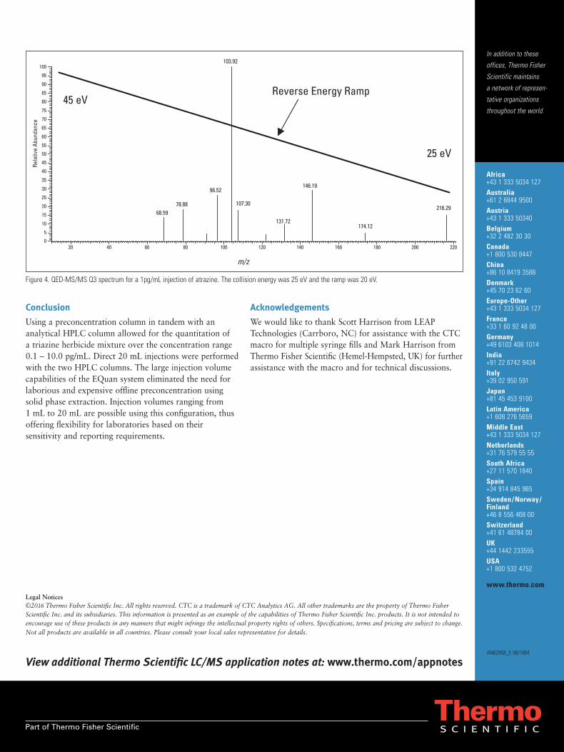
Conclusion
Using a preconcentration column in tandem with ananalytical HPLC column allowed for the quantitation of a triazine herbicide mixture over the concentration range0.1 – 10.0 pg/mL. Direct 20 mL injections were performedwith the two HPLC columns. The large injection volumecapabilities of the EQuan system eliminated the need forlaborious and expensive offline preconcentration usingsolid phase extraction. Injection volumes ranging from 1 mL to 20 mL are possible using this configuration, thusoffering flexibility for laboratories based on theirsensitivity and reporting requirements.
Acknowledgements
We would like to thank Scott Harrison from LEAPTechnologies (Carrboro, NC) for assistance with the CTCmacro for multiple syringe fills and Mark Harrison fromThermo Fisher Scientific (Hemel-Hempsted, UK) for furtherassistance with the macro and for technical discussions.
In addition to these
offices, Thermo Fisher
Scientific maintains
a network of represen -
tative organizations
throughout the world.
Africa+43 1 333 5034 127Australia+61 2 8844 9500Austria+43 1 333 50340Belgium+32 2 482 30 30Canada+1 800 530 8447China+86 10 8419 3588Denmark+45 70 23 62 60Europe-Other+43 1 333 5034 127France+33 1 60 92 48 00Germany+49 6103 408 1014India+91 22 6742 9434Italy+39 02 950 591Japan+81 45 453 9100Latin America+1 608 276 5659Middle East+43 1 333 5034 127Netherlands+31 76 579 55 55South Africa+27 11 570 1840Spain+34 914 845 965Sweden / Norway /Finland+46 8 556 468 00Switzerland+41 61 48784 00UK+44 1442 233555USA+1 800 532 4752
www.thermo.com
Part of Thermo Fisher Scientific
AN62858_E 08/16M
Legal Notices©2016 Thermo Fisher Scientific Inc. All rights reserved. CTC is a trademark of CTC Analytics AG. All other trademarks are the property of Thermo Fisher Scientific Inc. and its subsidiaries. This information is presented as an example of the capabilities of Thermo Fisher Scientific Inc. products. It is not intended to encourage use of these products in any manners that might infringe the intellectual property rights of others. Specifications, terms and pricing are subject to change. Not all products are available in all countries. Please consult your local sales representative for details.
View additional Thermo Scientific LC/MS application notes at: www.thermo.com/appnotes
Figure 4. QED-MS/MS Q3 spectrum for a 1pg/mL injection of atrazine. The collision energy was 25 eV and the ramp was 20 eV.

Sensitive and Rapid Determination of Paraquat and Diquat in Tap and Environmental Waters Chen Jing,1 Xu Qun,1 and Jeffrey Rohrer2
1Thermo Fisher Scientific, Shanghai, People’s Republic of China; 2Thermo Fisher Scientific, Sunnyvale, CA, USA
Ap
plica
tion
No
te 1
05
1
Key WordsAcclaim Trinity P1 Guard Cartridge, Acclaim Trinity Q1 Analytical Column, Herbicides, On-Line SPE, U.S. EPA Method 549.2, Water Analysis
GoalsTo develop an efficient high-performance liquid chromatography (HPLC) method for the sensitive and rapid determination of paraquat and diquat in tap and environmental water samples:
• Using on-line solid phase extraction (SPE) and UV detection inthe absence of an ion-pairing reagent in the mobile phase, and
• With method detection limits (MDLs) equal to or better thanU.S. Environmental Protection Agency (EPA) Method 549.2 andEuropean Union (EU) 98/83/EC
IntroductionParaquat and diquat (structures shown in Figure 1) are widely used as agriculture herbicides to control crop and aquatic weeds. Contamination of drinking and environmental waters with paraquat and diquat is considered a risk factor for liver, heart, lung, and kidney illnesses. The U.S. EPA specified a Maximum Contaminant Level Goal (MCLG) of 20 µg/L for diquat in drinking water,1 and the EU published a general rule with a limit of 0.1 µg/L for pesticides and herbicides in drinking water (98/83/EC).2
Reversed-phase HPLC with UV detection is typically used for sensitive determination of paraquat and diquat, and ion-pairing reagents are added to the mobile phase to achieve baseline separation and symmetrical peaks on conventional reversed-phase columns (C18 or C8). This is the methodology used in EPA Method 549.2.3 The use of other stationary phases, such as those in the
Thermo Scientific™ Acclaim™ Mixed-Mode HILIC-14 and Trinity™ P15 columns, has been reported to achieve baseline separation in the absence of an ion-pairing reagent; however, peak shapes were still less than ideal.
For the HPLC determination of diquat and paraquat in water samples, SPE is the typical method used for sample extraction and enrichment. Whereas EPA Method 549.2 describes off-line SPE for water sample preparation,3 on-line SPE offers the advantages of full automation, the absence of operator influence, time savings, and strict process control. Although the authors previously reported an application of on-line SPE for the determination of diquat and paraquat in water samples by HPLC,5 this more recent work shows an improved method using a new mixed-mode column specifically designed to provide good peak shapes for diquat and paraquat.
H3C _ +N N+ _ CH3
2Cl– 2Br–
N+
N+
DiquatParaquat
Figure 1. Structures of paraquat and diquat.

Equipment• ThermoScientific™ Dionex™ UltiMate™ 3000 x2 Dual
Rapid Separation LC (RSLC) system, including:
– DGP-3600RS Dual Ternary RS Pump System withSRD-3600 Integrated Solvent and Degasser Rack
– WPS-3000TRS RS Wellplate Sampler, Thermostatted,with a 1000 µL sample loop and a 1000 µL syringe
– TCC-3000RS or TCC-3000SD RS ThermostattedColumn Compartment equipped with one 2–6p valve
– DAD-3000RS RS Diode Array Detector - Semi-MicroFlow Cell for DAD-3000 and MWD-3000 Series,SST, 2.5 µL Volume, 7 mm Path Length
• ThermoScientific™ Dionex™ Chromeleon™
Chromatography Data System software, version 7.1
• Thermo Scientific™ Orion™ 2-Star Benchtop pH Meter
• Thermo Scientific™ Target2™ Nylon Syringe Filters,0.45 µm, 30 mm (P/N F2500-1)
Reagents and Standards• Deionized(DI)water,18.2MΩ-cm resistivity
• Acetonitrile(CH3CN), HPLC Grade 99.9%(Fisher Scientific P/N AC610010040)
• AmmoniumAcetate(CH3COONH3), Crystalline/Certified ACS (Fisher Scientific P/N 631-61-8)
• Dimethyldichlorosilane (DMDCS), ≥99% (P/N 75-78-5)
• EPA-549.1STDS2COMP,1ML,DiquatandParaquat Standard
Working Standard Solutions for CalibrationUse the EPA-549.1 Diquat and Paraquat Standard and dilute with DI water to prepare a stock standard solution with 1.0 µg/mL of each compound. Prepare six working standard solutions for the calibration with different concentrations by adding the correct amount of stock standard solution and diluting with DI water. The volumes needed of each solution to make the calibration standards are shown in Table 1.
Sample Preparation Tap water samples were collected at the Thermo Fisher Scientific™ Shanghai Applications Lab. Pond water samples were collected at Zhangjiang High Science and Technology Park located in the Pudong District of Shanghai, China. Samples were filtered using Target2 nylon syringe filters prior to injection. Note: Soak all glassware used to prepare paraquat and diquat standard solutions for calibration or used in sample preparation for at least 8 h in a mixture of CH3CN and DMDCS (9:1, v/v) to avoid loss (adsorption) of diquat and paraquat.
Chromatographic Conditions
On-Line SPE
Column: Acclaim Trinity P1, 3 µm, Guard Cartridges, 3.0 × 10 mm (P/N 071390) with SST Guard Cartridge Holder V-2 (P/N 069580)
Mobile Phase: A: 100 mM Ammonium Acetate (adjust pH 5.0 using acidic acid) B: Acetonitrile C: H2O
Gradient: 0–2 min, 10% A, 5% B 2.1–4.5 min, 55% A, 45% B 4.6–10 min, 10% A, 5% B
Flow Rate: 0.7 mL/min
Inj. Volume: 1000 µL onto the on-line SPE cartridge
Separation
Column: Acclaim Trinity Q1, 3 µm, Analytical, 3.0 × 50 mm (P/N 079716)
Mobile Phase: 35% 100 mM Ammonium Acetate (pH 5.0)/65% Acetonitrile
Flow Rate: 0.5 mL/min
Column Temp: 30 °C
Detection: UV absorbance at 260 nm for paraquat and 310 nm for diquat
Valve Position
0 min, 1_2 2.0 min, 6_1 4.5 min, 1_2
2
Volume of Stock Standard Solution of Paraquat and Diquat, 1.0 µg/mL Each
(mL)
Volume of DI Water (mL)
Final Volume
(mL)
Final Concentration
(µg/L)
0.01 9.99
10
1
0.05 9.95 5
0.50 9.50 50
1.00 9.00 100
5.00 5.00 500
10.0 0.00 1000
Table 1. Preparation of calibration curve standards.

For On-Line SPE
Dual Ternary Pump
Autosampler
For Separation
Waste
Waste
SPE Column
UV
AnalyticalColumn
12
3 45
6
3
The Acclaim Trinity Q1 column has weak cation-exchange functionality rather than the strong cation-exchange functionality of the Acclaim Trinity P1 column. Table 2 lists the performance measurements of the Acclaim Trinity P15 and Q1 columns for the separation of paraquat anddiquatunderchromatographicconditionsoptimizedfor each column. The results demonstrate the superiority of the Trinity Q1 column for this determination.
Analyte
Acclaim Trinity P1 Column Acclaim Trinity Q1 Column
Asymmetry Peak Width (min) Asymmetry Peak Width
(min)
Paraquat 1.68 0.22 0.98 0.17
Diquat 1.39 0.18 0.89 0.12
Table 2. Comparison of column performance for the separation of paraquat and diquat (5 µg/mL) on the Acclaim Trinity P1 and Q1 columns.
Figure 2. Chromatogram of paraquat and diquat (10 mg/L each).
Figure 3. Flow schematic of on-line SPE.
0.00 1.25 2.50 3.75 5.00 6.25 7.00
-20
0
220
1
2
Minutes
mAU
Column: Acclaim Trinity Q1, 3 µm, Analytical (3.0 × 50 mm)Mobile Phase: 35% 100 mM Ammonium
Acetate (pH 5.0)/65% AcetonitrileFlow Rate: 0.5 mL/minTemperature: 30 °CUV Detection: Absorbance at 290 nm
Peaks: 1. Paraquat2. Diquat
Evaluations of On-Line SPE
Figure 3 shows a typical flow schematic of on-line SPE, which is directly coupled to the HPLC column using one 6-port (2 p to 6 p) valve. The filtered sample is injecteddirectly onto the system and delivered to the SPE columnfor enrichment (1_2 position) using the first pump; theanalytical column is simultaneously equilibrated with thesecond pump of the dual-pump module. After the analytesare bound to the SPE column and impurities are washedout, the SPE column is switched into the analytical flowpath to elute the bound analytes (6_1 position); the analytesare then separated on the analytical column and detectedby the UV detector. This method is easily accomplishedusing the UltiMate 3000 x2 Dual RSLC system.
Results and Discussion
Separation of Paraquat and Diquat on the Acclaim Trinity Q1 Column
The Acclaim Trinity Q1 column is based on innovative nanopolymer silica hybrid (NSH) technology and has reversed-phase, anion-exchange, and cation-exchange retention mechanisms that can be independently controlled.6 The weak cation-exchange function provides retention and separation for diquat and paraquat, whereas the weak anion-exchange moiety effectively deactivates the undesirable interaction between the surface silanols and the analytes. As shown in Figure 2, this column provides sufficient retention, excellent resolution, good peak shape, and a fast analysis time for diquat and paraquat.

Optimization of On-Line SPE Conditions
To develop this on-line SPE method, an Acclaim Mixed-Mode WCX-1 Guard and an Acclaim Trinity P1 Guard—both of which have been reported as on-line SPE cartridges for the determination of paraquat and diquat in drinking and environmental waters—were evaluated following the typical on-line SPE flow schematic shown in Figure 3.5 Although either of these products can be used as an SPE cartridge for the enrichment of paraquat and diquat, the Acclaim Trinity P1 Guard cartridge was selected due to the easier elution of paraquat and diquat using an acetonitrile and 100 mM ammonium acetate (pH 5.0) mobile phase—the same as that used for the separation on the Acclaim Trinity Q1 Analytical column.
Optimization of Separation Conditions
The Acclaim Trinity Q1 column is designed for applica-tions using volatile buffers such as ammonium acetate, which are compatible with MS, charged aerosol, and UV (>225 nm) detections.6Theseparationcanbeoptimizedby adjusting the mobile phase buffer concentration, buffer pH value, and organic solvent content.
The ammonium acetate buffer was effective for this application, and its concentration affected retention of both diquat and paraquat. Higher buffer concentration shortened retention times, and 100 mM was selected for the rapid analysis. Buffer pH value has significant effect on the resolution of diquat and paraquat. It has been reported that pH 5 ± 0.5 is a suitable pH range for this application;6 therefore, pH 5.0 was used. Mobile phase organic solvent content affects retention and resolution of both diquat and paraquat. Experiments showed that with 100 mM ammonium acetate, mobile phases containing 55–75% acetonitrile gave excellent resolution and sufficient retention times. Therefore, 65% acetonitrile was used in this application.
Figure 4 illustrates rapid baseline separation of paraquat and diquat following on-line SPE under the specified chromatographic conditions. The entire chromatographic analysis is completed within 7 min. Figure 4. Chromatograms of a paraquat and diquat standard (1.0 µg/L each)
following on-line SPE.
For On-Line SPEColumn: Acclaim Trinity P1, 3 µm, Guard Cartridges (3.0 × 10 mm)
with V-2 HolderMobile Phase: A: 100 mM Ammonium Acetate (pH 5.0)
B: AcetonitrileC: H
2O
Gradient: 0–2 min, 10% A, 5% B2.1–4.5 min, 55% A, 45% B4.6–10 min, 10% A, 5% B
Flow Rate: 0.7 mL/minInj. Volume: 1000 µL onto the on-line SPE cartridge
For SeparationColumn: Acclaim Trinity Q1, 3 µm, Analytical (3.0 × 50 mm) Mobile Phase: 35% 100 mM Ammonium Acetate (pH 5.0)/65% AcetonitrileFlow Rate: 0.5 mL/minTemperature: 30 °CDetection: UV absorbance at 260 nm for paraquat and 310 nm for diquatValve Position: 0 min, 1_2
2.0 min, 6_14.5 min, 1_2
Samples: (a) Absorbance at 260 nm(b) Absorbance at 310 nm
Peaks: 1. Paraquat2. Diquat
0.00 1.25 2.50 3.75 5.00 6.25 7.50 8.75 10.00
-0.25
0.00
2.00 mAU
Minutes
12
a
b
4

Reproducibility, Linearity, and Detection Limits
Method precision using UV detection was estimated by making five consecutive 1000 µL injections of a calibration standard, each with a concentration of 100 µg/L. The reproducibilities of retention time and peak area relativestandarddeviation(RSD)aresummarizedin Table 3.
Calibration linearity for UV detection of paraquat and diquat was investigated by making three consecutive 1000 µL injections of a mixed standard prepared at six different concentrations (i.e., 18 total injections). The external standard method was used to establish the calibration curve and to quantify paraquat and diquat in the drinking and environmental water samples. Excellent linearity was observed from 1 to 1000 µg/L when plotting the concentration versus peak area, and the coefficients of determination were all ≥0.99097 (Table 4).
The MDLs of all compounds subjected to UV detection were calculated using the equation:
Detection Limit = St (n – 1, 1 - α = 0.99)
The symbol S represents standard deviation of replicate analyses, n represents number of replicates, t(n – 1, 1 - α = 0.99) represents Student’s t value for the 99% confidence level with n – 1 degrees of freedom. Five replicate injections of reagent water spiked with 100 µg/L of paraquat and diquat standard mixture were used to determine the MDLs.Table4summarizestheMDLdata,whichshowexcellent method sensitivity with detection limits equivalent to those defined in EPA Method 549.2 and which meet the restriction in 98/83/EC.
Tap Water and Environmental Water Analysis
Figures 5 and 6 show chromatograms of a tap water sample and a pond water sample. No target analytes were found. The analysis results and related data are summarizedinTable5,demonstratingthatthison-lineSPE HPLC method provides good selectivity and suitability for the determination of paraquat and diquat in water samples.
5
Analyte Retention Time RSD Peak Area RSD
Paraquat 0.18 4.85
Diquat 0.15 4.69
Table 3. Reproducibility of peak retention time and area.
Analyte Regression Equation r2 Range of
Standards (µg/L)
MDL* (µg/L)
Paraquat A = 0.1968 c – 1.0993 0.999961–1000
0.09
Diquat A = 0.1557 c – 2.0420 0.99709 0.10
Table 4. Method linearity data and MDLs.
Sample Tap Water Pond Water
Analyte Detected (µg/L)
Added (µg/L)
Found (µg/L)
Recovery (%)
Detected (µg/L)
Added (µg/L)
Found (µg/L)
Recovery (%)
Paraquat Not Detected
100 105 105 Not Detected
100 104 104
Diquat 100 108 108 100 105 105
Table 5. Analysis results of spiked water samples.
* The single-sided Student’s t test method (at the 99% confidence limit) was used for determining MDL, where the standard deviation of the peak area of five injections was multiplied by 4.6 to yield the MDL.

Figure 6. Chromatograms of a pond water sample and the same sample spiked with a paraquat and diquat standard at (A) 260 nm and (B) 310 nm.
For On-Line SPEColumn: Acclaim Trinity P1, 3 µm, Guard Cartridges (3.0 × 10 mm)
with V-2 Holder Mobile Phase: A: 100 mM Ammonium Acetate (pH 5.0)
B: AcetonitrileC: H
2O
Gradient: 0–2 min, 10% A, 5% B2.1–4.5 min, 55% A, 45% B 4.6–10 min, 10% A, 5% B
Flow Rate: 0.7 mL/minInj. Volume: 1000 µL onto the on-line SPE cartridge
For SeparationColumn: Acclaim Trinity Q1, 3 µm, Analytical (3.0 × 50 mm)Mobile Phase: 35% 100 mM Ammonium Acetate (pH 5.0)/65% AcetonitrileFlow Rate: 0.5 mL/minTemperature: 30 °CDetection: UV absorbance at (A) 260 nm for paraquat and
(B) 310 nm for diquatValve Position: 0 min, 1_2
2.0 min, 6_14.5 min, 1_2
Samples: (a) A pond water sample(b) The same sample spiked with a paraquat and diquat standard (100 µg/L each)
Peaks: 1. Paraquat2. Diquat
0.0 2.5 5.0 7.5 10 .0 -20
0
200 mAU
b
a
1
2
A
0.0 2.5 5.0 7.5 10 .0 -20
0
100 mAU
b
a
2
1
B
Minutes
Minutes
6
Figure 5. Chromatograms of a tap water sample and the same sample spiked with a paraquat and diquat standard at (A) 260 nm and (B) 310.
For On-Line SPEColumn: Acclaim Trinity P1, 3 µm, Guard Cartridges (3.0 × 10 mm)
with V-2 Holder Mobile Phase: A: 100 mM Ammonium Acetate (pH 5.0)
B: AcetonitrileC: H
2O
Gradient: 0–2 min, 10% A, 5% B2.1–4.5 min, 55% A, 45% B 4.6–10 min, 10% A, 5% B
Flow Rate: 0.7 mL/minInj. Volume: 1000 µL onto the on-line SPE cartridge
For SeparationColumn: Acclaim Trinity Q1, 3 µm, Analytical (3.0 × 50 mm)Mobile Phase: 35% 100 mM Ammonium Acetate (pH 5.0)/65% AcetonitrileFlow Rate: 0.5 mL/minTemperature: 30 °CDetection: UV absorbance at (A) 260 nm for paraquat and
(B) 310 nm for diquatValve Position: 0 min, 1_2
2.0 min, 6_14.5 min, 1_2
Samples: (a) Tap water sample(b) The same sample spiked with a paraquat and diquat standard (100 µg/L each)
Peaks: 1. Paraquat2. Diquat
0.0 2.5 5.0 7.5 10 .0 -20
0
180
Minutes
mAU
0.0 2.5 5.0 7.5 10 .0 -20
0
100
Minutes
mAU
a
b
b
a
1
1
2
2
A
B

Ap
plica
tion
No
te 1
05
1
Australia +61 3 9757 4486 Austria +43 1 333 50 34 0 Belgium +32 53 73 42 41 Brazil +55 11 3731 5140 China +852 2428 3282
AN70386_E 08/16M
Denmark +45 70 23 62 60France +33 1 60 92 48 00Germany +49 6126 991 0India +91 22 6742 9494Italy +39 02 51 62 1267
Japan +81 6 6885 1213Korea +82 2 3420 8600Netherlands +31 76 579 55 55Singapore +65 6289 1190Sweden +46 8 473 3380
Switzerland +41 62 205 9966Taiwan +886 2 8751 6655UK/Ireland +44 1442 233555USA and Canada +847 295 7500
www.thermofisher.com/dionex©2016 Thermo Fisher Scientific Inc. All rights reserved. All trademarks are the property of Thermo Fisher Scientific Inc. and its subsidiaries. This information is presented as an example of the capabilities of Thermo Fisher Scientific Inc. products. It is not intended to encourage use of these products in any manners that might infringe the intellectual property rights of others. Specifications, terms and pricing are subject to change. Not all products are available in all countries. Please consult your local sales representative for details.
ConclusionThis work describes a method that uses on-line SPE HPLC with UV absorbance for determining paraquat and diquat in drinking and environmental waters in <10 min per sample. The determination is performed on an UltiMate 3000 x2 Dual RSLC system controlled by Chromeleon software. The reduced MDLs achieved using UV detection and on-line SPE provide a convenient method for determining these compounds in drinking and environmental waters. This approach also meets the MDL requirements specified in both U.S. EPA Method 549.2 and EU 98/83/EC.
References1. Basic Information about Regulated Drinking Water
Contaminants; U.S. Environmental ProtectionAgency, Environmental Monitoring and SupportLaboratory: Cincinnati, OH, 1997. [Online] http://water.epa.gov/drink/contaminants/basicinformation/diquat.cfm. (accessed Jan 28, 2013).
2. Directive 98/83/EC. Official Journal of the EuropeanCouncil, Quality of Water Intended for HumanConsumption; L 330/42; 1998.
3. Method 549.2: Determination of Diquat and Paraquatin Drinking Water by Liquid-Solid Extraction andHigh-Performance Liquid Chromatography withUltraviolet Detection; Revision 1.0; U.S. EnvironmentalProtection Agency, Environmental Monitoring andSupport Laboratory: Cincinnati, OH, 1997.
4. Thermo Scientific Application Brief 114: ImprovedSeparation of Diquat and Paraquat Using the AcclaimMixed-Mode HILIC-1 Column. Sunnyvale, CA, 2012.[Online] www.dionex.com/en-us/webdocs/87647-AB114-LC-Diquat-Paraquat-Acclaim-HILIC-1-05Oct2012-AB70230_E.pdf (accessed Jan 30, 2013).
5. Dionex (now part of Thermo Scientific) ApplicationNote 274: Sensitive On-Line SPE–HPLC Determinationof Paraquat and Diquat in Drinking and EnvironmentalWaters. Sunnyvale, CA, 2011. [Online] www.dionex.com/en-us/webdocs/110577-AN274-HPLC-Paraquat-Diquat-Water-05Apr2011-LPN2726.pdf (accessedJan 30, 2013).
6. Product Specifications: Thermo Scientific AcclaimTrinity Q1 Columns for Trace Analysis of Diquatand Paraquat; PS20567_E 07/12S; Thermo Scientific:Sunnyvale, CA, 2012. [Online] www.dionex.com/en-us/webdocs/113757-PS-Acclaim-Trinity-Q1-Jul2012-PS20567_E.pdf (accessed Jan 30, 2013).


Analysis of Diquat and Paraquat Using UHPLC Orbitrap MS – Method Development, Matrix Effects and PerformanceJonathan Beck,1 Paul Yang,2 Xiaodong Liu,1 Chunyan Hao,2 Xiaoming Zhao,2 Franca Morra,2 Charles Yang,1 Maciej Bromirski,1 and Dipankar Ghosh1 1Thermo Fisher Scientifi c, San Jose, USA ; 2Ontario Ministry of the Environment, Ontario, Canada

2 Analysis of Diquat and Paraquat Using UHPLC Orbitrap MS – Method Development, Matrix Effects and Performance
Analysis of Diquat and Paraquat Using UHPLC Orbitrap MS –Method Development, Matrix Effects and PerformanceJonathan Beck1, Paul Yang2, Xiaodong Liu1, Chunyan Hao2, Xiaoming Zhao2, Franca Morra2, Charles Yang1, Maciej Bromirski1 and Dipankar Ghosh1
1Thermo Fisher Scientific, San Jose, USA ; 2Ontario Ministry of the Environment, Ontario, Canada
ConclusionIt is demonstrated that high-resolution and high-sensitivity analysis of PQ and DQ canbe carried out using UHPLC Orbitrap MS coupled with an Acclaim Trinity Q1 column. This method provides the following benefits:
A fast LC, isocratic separation of PQ and DQ in 5 min, without needing tedious sample preparation;
Minimal interference and matrix effects in the analysis by using a MEW of 5ppm;
Identification and confirmation of PQ and DQ can be carried out using molecular ions of PQ and DQ, area ratios of M and (M+1) mass spectral peaks and product ions of from AIF experiment
The method is sensitive and allowed the direct injection analysis of PQ and DQ with MDLs (0.05 and 0.15 µg/L for PQ and DQ) meet the need of various regulatory bodies.
References1. J.E. Norman, K.M. Kuivila, L.H. Nowell, Scientific Investigations Report 2012–
5045, U.S. Department of the Interior and U.S. Geological Survey, 2012.
2. K.C. Wang, S.M. Chen, J.F. Hsu, S.G. Cheng, C.K. Lee. J. Chromatogr. B 876(2008) 211.
3. J.C. Marr, J.B. King, Rapid Commun. Mass Spectrom. 11 (1997) 479.
4. X.P. Lee, T. Kumazawa, M. Fujishiro, C. Hasegawa, T. Arinobu, H. Seno, A. Ishii, K. Sato, J. Mass Spectrom. 39 (2004) 1147.
Overview The purpose of this work was to investigate the effect of ultrahigh-performance liquid chromatography (UHPLC) mobile phases and operational parameters of a UHPLC-Orbitrap™ mass spectrometry system used in the analysis of quaternary ammonium herbicides paraquat (PQ) and diquat (DQ). UHPLC mobile phases of different pH values were evaluated to achieve optimum separation of PQ and DQ on a Thermo Scientific™ Acclaim™ Trinity™ Q1 column which was specifically designed for this application, as well as to observe the relative intensity changes of mass spectral peaks. The signal-to-noise ratio (SNR) of extracted ion chromatograms (XIC) obtained from different m/z at different pH values and declustering potential (corona voltage) of electrospray ionization (ESI) source were evaluated. Based on results obtained from this study, a method was developed for the unambiguous identification of PQ and DQ in environmental water samples with the ability to deliver analytical data with superior SNR, high precision and accuracy.
IntroductionParaquat (PQ, 1,1′-dimethyl-4,4′-bipyridylium dichloride, C12H14N2Cl2) and diquat (DQ,1,1′-ethylene-2,2′-bipyridilium dibromide, C12H12N2Br2) are quaternary amines widely used as non-selective and non-systematic herbicides for both terrestrial and aquatic plant control. Both PQ and DQ are toxic by contact and/or ingestion. The Ontario Drinking Water Quality Standards (Ontario Regulation 169/03) has a standard of 70 and 10 µg/L, respectively for diquat and paraquat. Diquat is also regulated by the United States (U.S.) Environmental Protection Agency (EPA) at a maximum contaminant limit (MCL) of 20 μg/L in drinking water, while PQ is unregulated by the U.S. EPA. The European Union has a drinking water MCL of 0.1 µg/L for any individual pesticide and a combined 0.5 µg/L MCL for all pesticides. Different data quality objectives (DQO) derived from these regulations dictate the need for a reliable/versatile method with a superior analytical sensitivity (i.e. <0.1 µg/L or better) to meet different regulatory requirements.
Methods commonly used for PQ and DQ analysis include the separation by ion-pairing liquid chromatography, capillary electrophoresis, hydrophilic interaction liquid chromatography or ion-exchange chromatography using either ultraviolet (UV) or mass spectrometry for detection. Depending on the technology, method detection limits (MDL) have been established in the low μg/L for PQ and high ng/L for DQ. A 2012 U.S.Geological Survey report showed that about 3 million and 150,000 pounds of PQ andDQ were used annually in the United States (Ref 1).
Liquid chromatography-tandem mass spectrometry (LC-MS/MS) using an ESI interface has been the method of choice for PQ and DQ analysis since late 1990s. Depending on the pH of LC mobile phase and ESI source used, the deprotonated cation [M – H]+ (m/z 183 for DQ and m/z 185 for PQ), the singly charged radical ion [M]+ . (m/z 184 for DQ and m/z 186 for PQ) and, to a less extent, the doubly chargedquasi molecular ion M2+ (m/z 92 for DQ and m/z 93 for PQ) have been observed in the ESI mass spectra. The multiple reaction monitoring (MRM) transitions used in the analysis varied depending on the instrument and mobile phase. Commonly used precursor ions are the singly charged radical ion [M]+ . and deprotonated cation [M –H]+ with a limited mentioning on the use of the doubly charged quasi molecular ion M2+
(Ref 2). Many product ions have been used in the MRM transitions for PQ and DQ analysis. These can be, for example, from the loss of masses 15 ([M – CH3]+, m/z 170) or 27 ([(M – H) – HCN]+, m/z 158) for PQ; while those at m/z 168 ([(M – H) – CH3]+) and m/z 157 ([(M – H) – C2H2]+) for DQ analysis (Ref. 3). Product ions resulted from the loss of masses 16 ([(M – H) – CH3 – H]+, m/z 169) or 42 ([(M – H) – CH3 – HCN]+,m/z 143) for PQ; and at m/z 130 ([(M – H) – C2H2 – HCN]+) for DQ analysis (Ref. 4). A literature review showed more than 10 different MRM transitions may be used in the analysis of these two pesticides.
With the three available precursor ions from PQ (m/z 93, 185 and 186) and DQ (m/z92, 183, 184), products ions of PQ and DQ may be differentiated by 1 amu. As the DQ 13C-isotopic mass at m/z 185 would overlap with the [M – H]+ of PQ, one might expect interference in the analysis of PQ and DQ with inferior LC separation and MS data collected with unit mass resolution. Diquat has been known to have high ionization efficiency, with about 13% intensity of the native mass spectral peak of DQ contributing to PQ through the 13C-isotopic peak, quantitative results obtained for PQ might be biased high. We report in this poster the relationship between pH of mobile phase and the population of the three possible molecular formations of PQ DQ, the root cause of analytical interference and a direct injection UHPLC-Orbitrap MS method for the analysis of PQ and DQ that meets the regulatory need of different jurisdictions.
MethodsSample Preparation and Chemicals
Individual stock solutions of PQ and DQ were purchased from Ultra Scientific Analytical Solutions (Brockville, ON, Canada). Neat standards of deuterium (D) labelled PQ (D8-PQ) and DQ (D4-DQ) were purchased from CDN Isotope (Pointe-Claire, QC, Canada). Native and D-labelled intermediate standard solutions were prepared by mixing the corresponding DQ and PQ stock solutions. Five levels of analytical standard solutions were prepared by diluting intermediate solutions withnanopure water (pure water, generated by passing reverse osmosis water through aThermo Scientific™ Barnstead™ Nanopure™ water purification system, Mississauga, ON, Canada). Due to the high ionic strength of PQ and DQ, plastic labware and/or silanized glassware were used to avoid their adsorption onto the glass surfaces.
ACS reagent grade ammonium acetate (CH3COONH4), acetic acid (CH3COOH) and hydrochloric acid (HCl) were purchased from Sigma-Aldrich (Oakville, ON, Canada). HPLC grade acetonitrile (CH3CN) was purchased from Fisher Scientific (Ottawa, ON, Canada). The current method employs direct injection that does not requires sample preparation. Environmental samples were collected in a 500 mL polypropylene bottle and refrigerated at 5 3 ºC until analysis. Drinking water samples were analyzed as is while surface water samples were filtered through a 0.2 µ filter prior to analysis. A 1 mLaliquot of each sample was transferred to a 1.8-mL plastic autosampler vial, spikedwith 10 µL of 500 µg/L, D-labelled internal standards to the concentration of 5 ng/mL,vortexed and stored under refrigeration until analysis.
Ultra High Performance Liquid Chromatography
The Thermo Scientific™ Dionex™ UltiMateTM 3000 UHPLC used in the analysis consisted of a HRG-3400RS binary pump, WPS-3000 autosampler, and a TCC-3400 column compartment. Separation was achieved on a mixed-mode column Acclaim Trinity Q1 column (2.1 × 50 mm, 3 μm), using isocratic elution and mobile phase of acetonitrile:100 mM, pH5.0 ammonium acetate = 75:25 v/v, at a flow rate 0.45 mL/min. The column oven was set at 35ºC. Both PQ and DQ were eluted within 5 minutes. Mobile phases used in the pH effect study were the same composition used in the analysis but prepared at pH of 3.5, 5, 6.2 and 7.3. Flow injection analysis was done byusing 0.013 mm i.d. x 100 cm polyetherether ketone tubing at a flow rate of 0.4 mL/minand four different pH levels to determine the pH and declustering potential used in theUHPLC Orbitrap MS analysis.
Mass Spectrometry
The UHPLC was interfaced to an Thermo Scientific™ Exactive™ Plus Orbitrap MS using a HESI II probe interface. The Orbitrap MS system was tuned and calibrated in positive mode by infusion of standard mixtures of MSCAL5. High purity nitrogen (>99%) was used in the ESI source (35 L/min) as well as in a higher energy collisional dissociation (HCD) cell, enabling collision induced dissociation (CID) experiment without precursor ion selection, i.e. “all-ion fragmentation” (AIF). The AIF experiment was done by using normalized collision energy (NCE) of 35 14 eV. The UHPLC flowrate of 0.45 mL/min and column used resulted in chromatographic FWHM of 6-8 seconds. Mass spectrometric data were collected using a spray voltage (SV, theequivalent of declustering potential) of 1700 V, an Orbitrap MS resolving power of 140,000 (defined by the full-width-at-half-maximum peak width at m/z 200, RFWHM),resulting a scanning rate of > 1.5 scans/sec when using automatic gain control and aC-trap inject time of 50 msec. Therefore, at least nine data points were available to accurately define each XIC chromatogram from the UHPLC separation of PQ and DQ. The effect of SV on the formation of the three different quasi molecular ions of PQ and DQ was also studied by different SV from 700 to 3200 V.
Data Analysis
Analytical data collected were processed offline using Thermo Scientific™ Xcalibur™,ExactFinder™ and TraceFinder™ data processing packages depending on the need. Xcalibur was used to process mass spectral data for graphic presentation. ExactFinderand TraceFinder softwares were used to derive quantitative data. Depending on thedata, a mass extraction window (MEW) of 5 to 20 ppm (part-per-million) from both sides of the base peak were used to create XIC and quantitative analysis. Results were exported to Microsoft® Excel® for data compilation and statistical evaluation.
Microsoft® Excel® are trademarks of Microsoft Corporation. All other trademarks are the property of Thermo FisherScientific and its subsidiaries.
This information is not intended to encourage use of these products in any manners that might infringe the intellectual property rights of others.
ResultsFlow Injection Analysis
Figure 1 shows results from the flow injection analysis of PQ and DQ using mobilephases of three different pH values (i.e., 5, 6.2 and 7.3) at declustering potential (DP) from 3200 to 700 volts, in decreasing intervals of 500 volts. The purpose of this experiment was to determine an optimal DP such that maximal signal-to-noise ratio(SNR) of PQ and DQ measurement can be achieved in this study. Peak intensities were minimal for PQ and DQ at pH 3.5 and were not shown in the figure. It is evident that DP had very little effect on the sensitivity of PQ and DQ analysis. As a result, a DP of 2000 volts is used throughout this work.
FIGURE 1. Results of flow injection analysis.
Effect of mobile phase pH on the analysis of PQ and DQ
Table 1 lists accurate mass of the three possible quasi molecular ions of PQ and DQ, (i.e., molecular ion M2+, deprotonated cation [M – H]+ and the singly charged radical ion[M]+ .), along with their respective 13C-isotope (M+1) mass spectral peaks. Identification of PQ and DQ can be achieved by accurate mass of the three quasi molecular ions, their respective (M+1) peak and fragment ions obtained from the AIF experiment.
M2+ M2+ (M+1) [M2+ - H+]+ [M2+ - H+]+ (M+1) [M] + . [M]+ . (M+1)Diquat 92.04948 92.55117 183.09167 184.09503 184.09950 185.10289Paraquat 93.05730 93.55900 185.10732 186.11071 186.11515 187.11854
Figure 2 shows mass spectral peaks listed in Table 1 for PQ ([M2+ - H+]+), A (simulated) and C (measured); DQ ([M]+ . (M+1)), B (simulated) and C (measured); DQ ([M2+ - H+]+(M+1)), D (simulated) and F (measured); DQ ([M]+), E (simulated) and F (measured); as well as DQ ([M2+ - H+]+) and DQ ([M2+ - H+]+ (M+1)), shown as simulated (G or H) and measured (I), as an example. It can be seen from Figure 1 that Orbitrap MS delivers excellent mass accuracy measurement and matched perfectly with those theoretically simulated ones (Figures 2A, 2B, 2D, 2E, 2G and 2H). Diquat has much better ESI ionization efficiency than PQ, with a mass spectral separation of < 25 ppm, the use of high resolution MS and a MEW < 5 ppm to separate these interfering peaks in the MS domain becomes imperative for the accurate determination of PQ.
TABLE 1. Expected m/z of PQ and DQ.
From Table 2, deprotonated cation [M – H]+ of PQ and DQ gave the highest area counts and a good RSD followed by doubly-charged molecular ion [M]2+ and radical ion [M] +. had the lowest area counts at all pH values. The deprotonated cation [M – H]+had the best SNR (and the highest area counts) at pH 5 mobile phase and was used in the analysis.
Table 2 shows average area counts and relative standard deviation (RSD, N = 8) obtained from the LC analysis of PQ and DQ using mobile phases at three different pH values (i.e., 5, 6.2 and 7.3) and declustering potential (DP) of 2000 volts. The purpose of this experiment was to determine an optimal mobile phase pH that can be used in the LC separation of PQ and DQ.
pqdq_lev6_ph50_6_130417111717 4/17/2013 11:17:17 AM
C12H13N2: C12 H13 N2 p(gss, s/p:40) Chrg 1R: 14000...
185.090 185.095 185.100 185.105 185.110 185.115m/z
0
10
20
30
40
50
60
70
80
90
100
Re
lative
Ab
un
da
nce
185.10732
C12H11N2: C12 H11 N2 p(gss, s/p:40) Chrg 1R: 14000...
184.085 184.090 184.095 184.100 184.105m/z
0
10
20
30
40
50
60
70
80
90
100
Re
lative
Ab
un
da
nce
184.09503
184.08871184.09801
C12H11N2: C12 H11 N2 p(gss, s/p:40) Chrg 1R: 14000...
183.1 183.2 183.3 183.4 183.5 183.6 183.7 183.8 183.9 184.0 184.1m/z
0
10
20
30
40
50
60
70
80
90
100
Re
lative
Ab
un
da
nce
183.09167
184.09503
C12H12N2: C12 H12 N2 p(gss, s/p:40) Chrg 1R: 14000...
185.090 185.095 185.100 185.105 185.110 185.115m/z
0
10
20
30
40
50
60
70
80
90
100
Re
lative
Ab
un
da
nce
185.10286
185.09653185.10583
C12H12N2: C12 H12 N2 p(gss, s/p:40) Chrg 1R: 14000...
184.085 184.090 184.095 184.100 184.105m/z
0
10
20
30
40
50
60
70
80
90
100
Re
lative
Ab
un
da
nce
184.09950
C12H11N2: C12 H11 N2 p(gss, s/p:40) Chrg 1R: 14000...
183.1 183.2 183.3 183.4 183.5 183.6 183.7 183.8 183.9 184.0 184.1m/z
0
10
20
30
40
50
60
70
80
90
100
Re
lative
Ab
un
da
nce
183.09167
184.09503
pqdq_lev6_ph50_6_130417111717 #287 RT: 2.77 AV: 1 NL: 1.20E5T: FTMS + p ESI Full ms [70.00-300.00]
185.090 185.095 185.100 185.105 185.110 185.115m/z
0
10
20
30
40
50
60
70
80
90
100
Re
lative
Ab
un
da
nce
185.10718
185.10278185.09831
185.09186
pqdq_lev6_ph50_6_130417111717 #288 RT: 2.78 AV: 1 NL: 1.03E6T: FTMS + p ESI Full ms [70.00-300.00]
184.085 184.090 184.095 184.100 184.105m/z
0
10
20
30
40
50
60
70
80
90
100
Re
lative
Ab
un
da
nce
184.09496
184.09932
184.08868
pqdq_lev6_ph50_6_130417111717 #290 RT: 2.80 AV: 1 NL: 7.59E6T: FTMS + p ESI Full ms [70.00-300.00]
183.1 183.2 183.3 183.4 183.5 183.6 183.7 183.8 183.9 184.0 184.1m/z
0
10
20
30
40
50
60
70
80
90
100
Re
lative
Ab
un
da
nce
183.09157
184.09496
183.15744 184.04536
A. PQ, [M2+ - H+]+ G. DQ, [M2+ - H+]+ & [M2+ -H+]+ (M+1)
F. Measured, RT: 2.78 min
E. DQ, [M]+ .
D. DQ, [M2+ - H+]+ (M+1)
C. Measured, RT 2.77 min
B. DQ, [M]+ . (M+1)
I. Measured, RT: 2.78 min
H. DQ, [M2+ - H+]+ & [M2+ -H+]+ (M+1)
FIGURE 2. Simulated and measured mass spectral peaks of selected quasi molecular ions of PQ and DQ and their corresponding (M+1) peaks.
TABLE 1. Average area counts, RSD (N = 8) and area ratios of the threemolecular ions and their respective (M+1) ions.
Confirmation of PQ and DQ in UHPLC-Orbitrap MS analysis
From Table 2 at pH 5, LC retention time, accurate masses of the three molecular ionpeaks (M) and their respective (M+1) peaks, area ratios obtained from the XIC of (M+1) and M peaks can be used to identify PQ and DQ. In addition, a CID experiment carried out via AIF can also be useful in producing product ion information that can beused for the confirmation of PQ and DQ. This is demonstrated in Figure 3 by usingXICs obtained from m/z 169.07574 ([(M – H) – CH3 – H]+) and m/z 153.07280 ([(M –H) – CH3 - HCN]+) for PQ (Ref 4); and m/z 157.07593 ([(M – H) – C2H2]+) (Ref. 3) and m/z 130.06504 ([(M – H) – C2H2 – HCN]+) for DQ analysis (Ref. 4).
FIGURE 3. XICs obtained from product ions of PQ and DQ using AIF experiment for confirmation.
FIGURE 4. Analytical Performance.
Using deprotonated [M - H] + ion of PQ and DQ, we evaluated the linearity of the UHPLC Orbitrap MS system with seven levels of calibration standards inconcentrations ranging from 0.5 to 100 mg/L. The calibration curve is shown in Figure 4 with good R2 > 0.9990 for bothcompounds.
Initial determination of MDL derived byusing the U.S. EPA protocol was 0.05 and 0.15 mg/L for PQ and DQ. This direct injection method, when fullyvalidated, would be able to provide high sensitivity analysis of PQ and DQ that will meet different DQO requirements of various jurisdictions.

3Thermo Scienti� c Poster Note • PN ASMS13_T597_JBeck_E 07/13S
Analysis of Diquat and Paraquat Using UHPLC Orbitrap MS –Method Development, Matrix Effects and PerformanceJonathan Beck1, Paul Yang2, Xiaodong Liu1, Chunyan Hao2, Xiaoming Zhao2, Franca Morra2, Charles Yang1, Maciej Bromirski1 and Dipankar Ghosh1
1Thermo Fisher Scientific, San Jose, USA ; 2Ontario Ministry of the Environment, Ontario, Canada
ConclusionIt is demonstrated that high-resolution and high-sensitivity analysis of PQ and DQ canbe carried out using UHPLC Orbitrap MS coupled with an Acclaim Trinity Q1 column. This method provides the following benefits:
A fast LC, isocratic separation of PQ and DQ in 5 min, without needing tedious sample preparation;
Minimal interference and matrix effects in the analysis by using a MEW of 5ppm;
Identification and confirmation of PQ and DQ can be carried out using molecular ions of PQ and DQ, area ratios of M and (M+1) mass spectral peaks and product ions of from AIF experiment
The method is sensitive and allowed the direct injection analysis of PQ and DQ with MDLs (0.05 and 0.15 µg/L for PQ and DQ) meet the need of various regulatory bodies.
References1. J.E. Norman, K.M. Kuivila, L.H. Nowell, Scientific Investigations Report 2012–
5045, U.S. Department of the Interior and U.S. Geological Survey, 2012.
2. K.C. Wang, S.M. Chen, J.F. Hsu, S.G. Cheng, C.K. Lee. J. Chromatogr. B 876(2008) 211.
3. J.C. Marr, J.B. King, Rapid Commun. Mass Spectrom. 11 (1997) 479.
4. X.P. Lee, T. Kumazawa, M. Fujishiro, C. Hasegawa, T. Arinobu, H. Seno, A. Ishii, K. Sato, J. Mass Spectrom. 39 (2004) 1147.
OverviewThe purpose of this work was to investigate the effect of ultrahigh-performance liquid chromatography (UHPLC) mobile phases and operational parameters of a UHPLC-Orbitrap™ mass spectrometry system used in the analysis of quaternary ammonium herbicides paraquat (PQ) and diquat (DQ). UHPLC mobile phases of different pH values were evaluated to achieve optimum separation of PQ and DQ on a ThermoScientific™ Acclaim™ Trinity™ Q1 column which was specifically designed for this application, as well as to observe the relative intensity changes of mass spectral peaks. The signal-to-noise ratio (SNR) of extracted ion chromatograms (XIC) obtainedfrom different m/z at different pH values and declustering potential (corona voltage) of electrospray ionization (ESI) source were evaluated. Based on results obtained from this study, a method was developed for the unambiguous identification of PQ and DQ in environmental water samples with the ability to deliver analytical data with superior SNR, high precision and accuracy.
IntroductionParaquat (PQ, 1,1′-dimethyl-4,4′-bipyridylium dichloride, C12H14N2Cl2) and diquat (DQ,1,1′-ethylene-2,2′-bipyridilium dibromide, C12H12N2Br2) are quaternary amines widelyused as non-selective and non-systematic herbicides for both terrestrial and aquatic plant control. Both PQ and DQ are toxic by contact and/or ingestion. The Ontario Drinking Water Quality Standards (Ontario Regulation 169/03) has a standard of 70 and 10 µg/L, respectively for diquat and paraquat. Diquat is also regulated by the United States (U.S.) Environmental Protection Agency (EPA) at a maximum contaminant limit (MCL) of 20 μg/L in drinking water, while PQ is unregulated by theU.S. EPA. The European Union has a drinking water MCL of 0.1 µg/L for any individual pesticide and a combined 0.5 µg/L MCL for all pesticides. Different data qualityobjectives (DQO) derived from these regulations dictate the need for a reliable/versatile method with a superior analytical sensitivity (i.e. <0.1 µg/L or better) to meet different regulatory requirements.
Methods commonly used for PQ and DQ analysis include the separation by ion-pairing liquid chromatography, capillary electrophoresis, hydrophilic interaction liquidchromatography or ion-exchange chromatography using either ultraviolet (UV) or mass spectrometry for detection. Depending on the technology, method detection limits (MDL) have been established in the low μg/L for PQ and high ng/L for DQ. A 2012 U.S. Geological Survey report showed that about 3 million and 150,000 pounds of PQ andDQ were used annually in the United States (Ref 1).
Liquid chromatography-tandem mass spectrometry (LC-MS/MS) using an ESI interface has been the method of choice for PQ and DQ analysis since late 1990s. Depending on the pH of LC mobile phase and ESI source used, the deprotonated cation [M – H]+ (m/z 183 for DQ and m/z 185 for PQ), the singly charged radical ion[M]+ . (m/z 184 for DQ and m/z 186 for PQ) and, to a less extent, the doubly chargedquasi molecular ion M2+ (m/z 92 for DQ and m/z 93 for PQ) have been observed in theESI mass spectra. The multiple reaction monitoring (MRM) transitions used in the analysis varied depending on the instrument and mobile phase. Commonly used precursor ions are the singly charged radical ion [M]+ . and deprotonated cation [M –H]+ with a limited mentioning on the use of the doubly charged quasi molecular ion M2+
(Ref 2). Many product ions have been used in the MRM transitions for PQ and DQ analysis. These can be, for example, from the loss of masses 15 ([M – CH3]+, m/z 170) or 27 ([(M – H) – HCN]+, m/z 158) for PQ; while those at m/z 168 ([(M – H) – CH3]+) and m/z 157 ([(M – H) – C2H2]+) for DQ analysis (Ref. 3). Product ions resulted from the loss of masses 16 ([(M – H) – CH3 – H]+, m/z 169) or 42 ([(M – H) – CH3 – HCN]+,m/z 143) for PQ; and at m/z 130 ([(M – H) – C2H2 – HCN]+) for DQ analysis (Ref. 4). Aliterature review showed more than 10 different MRM transitions may be used in the analysis of these two pesticides.
With the three available precursor ions from PQ (m/z 93, 185 and 186) and DQ (m/z92, 183, 184), products ions of PQ and DQ may be differentiated by 1 amu. As the DQ 13C-isotopic mass at m/z 185 would overlap with the [M – H]+ of PQ, one might expect interference in the analysis of PQ and DQ with inferior LC separation and MS data collected with unit mass resolution. Diquat has been known to have high ionization efficiency, with about 13% intensity of the native mass spectral peak of DQ contributing to PQ through the 13C-isotopic peak, quantitative results obtained for PQ might bebiased high. We report in this poster the relationship between pH of mobile phase andthe population of the three possible molecular formations of PQ DQ, the root cause of analytical interference and a direct injection UHPLC-Orbitrap MS method for theanalysis of PQ and DQ that meets the regulatory need of different jurisdictions.
MethodsSample Preparation and Chemicals
Individual stock solutions of PQ and DQ were purchased from Ultra Scientific Analytical Solutions (Brockville, ON, Canada). Neat standards of deuterium (D) labelled PQ (D8-PQ) and DQ (D4-DQ) were purchased from CDN Isotope (Pointe-Claire, QC, Canada). Native and D-labelled intermediate standard solutions were prepared by mixing the corresponding DQ and PQ stock solutions. Five levels of analytical standard solutions were prepared by diluting intermediate solutions with nanopure water (pure water, generated by passing reverse osmosis water through a Thermo Scientific™ Barnstead™ Nanopure™ water purification system, Mississauga, ON, Canada). Due to the high ionic strength of PQ and DQ, plastic labware and/or silanized glassware were used to avoid their adsorption onto the glass surfaces.
ACS reagent grade ammonium acetate (CH3COONH4), acetic acid (CH3COOH) and hydrochloric acid (HCl) were purchased from Sigma-Aldrich (Oakville, ON, Canada). HPLC grade acetonitrile (CH3CN) was purchased from Fisher Scientific (Ottawa, ON, Canada). The current method employs direct injection that does not requires sample preparation. Environmental samples were collected in a 500 mL polypropylene bottle and refrigerated at 5 3 ºC until analysis. Drinking water samples were analyzed as is while surface water samples were filtered through a 0.2 µ filter prior to analysis. A 1 mL aliquot of each sample was transferred to a 1.8-mL plastic autosampler vial, spiked with 10 µL of 500 µg/L, D-labelled internal standards to the concentration of 5 ng/mL,vortexed and stored under refrigeration until analysis.
Ultra High Performance Liquid Chromatography
The Thermo Scientific™ Dionex™ UltiMateTM 3000 UHPLC used in the analysis consisted of a HRG-3400RS binary pump, WPS-3000 autosampler, and a TCC-3400 column compartment. Separation was achieved on a mixed-mode column Acclaim Trinity Q1 column (2.1 × 50 mm, 3 μm), using isocratic elution and mobile phase of acetonitrile:100 mM, pH5.0 ammonium acetate = 75:25 v/v, at a flow rate 0.45 mL/min. The column oven was set at 35ºC. Both PQ and DQ were eluted within 5 minutes. Mobile phases used in the pH effect study were the same composition used in the analysis but prepared at pH of 3.5, 5, 6.2 and 7.3. Flow injection analysis was done by using 0.013 mm i.d. x 100 cm polyetherether ketone tubing at a flow rate of 0.4 mL/min and four different pH levels to determine the pH and declustering potential used in the UHPLC Orbitrap MS analysis.
Mass Spectrometry
The UHPLC was interfaced to an Thermo Scientific™ Exactive™ Plus Orbitrap MS using a HESI II probe interface. The Orbitrap MS system was tuned and calibrated in positive mode by infusion of standard mixtures of MSCAL5. High purity nitrogen (>99%) was used in the ESI source (35 L/min) as well as in a higher energy collisional dissociation (HCD) cell, enabling collision induced dissociation (CID) experiment without precursor ion selection, i.e. “all-ion fragmentation” (AIF). The AIF experiment was done by using normalized collision energy (NCE) of 35 14 eV. The UHPLC flow rate of 0.45 mL/min and column used resulted in chromatographic FWHM of 6-8 seconds. Mass spectrometric data were collected using a spray voltage (SV, the equivalent of declustering potential) of 1700 V, an Orbitrap MS resolving power of 140,000 (defined by the full-width-at-half-maximum peak width at m/z 200, RFWHM),resulting a scanning rate of > 1.5 scans/sec when using automatic gain control and a C-trap inject time of 50 msec. Therefore, at least nine data points were available toaccurately define each XIC chromatogram from the UHPLC separation of PQ and DQ.The effect of SV on the formation of the three different quasi molecular ions of PQ andDQ was also studied by different SV from 700 to 3200 V.
Data Analysis
Analytical data collected were processed offline using Thermo Scientific™ Xcalibur™,ExactFinder™ and TraceFinder™ data processing packages depending on the need. Xcalibur was used to process mass spectral data for graphic presentation. ExactFinderand TraceFinder softwares were used to derive quantitative data. Depending on the data, a mass extraction window (MEW) of 5 to 20 ppm (part-per-million) from both sides of the base peak were used to create XIC and quantitative analysis. Results were exported to Microsoft® Excel® for data compilation and statistical evaluation.
Microsoft® Excel® are trademarks of Microsoft Corporation. All other trademarks are the property of Thermo FisherScientific and its subsidiaries.
This information is not intended to encourage use of these products in any manners that might infringe the intellectual property rights of others.
ResultsFlow Injection Analysis
Figure 1 shows results from the flow injection analysis of PQ and DQ using mobilephases of three different pH values (i.e., 5, 6.2 and 7.3) at declustering potential (DP) from 3200 to 700 volts, in decreasing intervals of 500 volts. The purpose of this experiment was to determine an optimal DP such that maximal signal-to-noise ratio(SNR) of PQ and DQ measurement can be achieved in this study. Peak intensities were minimal for PQ and DQ at pH 3.5 and were not shown in the figure. It is evident that DP had very little effect on the sensitivity of PQ and DQ analysis. As a result, a DP of 2000 volts is used throughout this work.
FIGURE 1. Results of flow injection analysis.
Effect of mobile phase pH on the analysis of PQ and DQ
Table 1 lists accurate mass of the three possible quasi molecular ions of PQ and DQ, (i.e., molecular ion M2+, deprotonated cation [M – H]+ and the singly charged radical ion[M]+ .), along with their respective 13C-isotope (M+1) mass spectral peaks. Identification of PQ and DQ can be achieved by accurate mass of the three quasi molecular ions, their respective (M+1) peak and fragment ions obtained from the AIF experiment.
M2+ M2+ (M+1) [M2+ - H+]+ [M2+ - H+]+ (M+1) [M] + . [M]+ . (M+1)Diquat 92.04948 92.55117 183.09167 184.09503 184.09950 185.10289Paraquat 93.05730 93.55900 185.10732 186.11071 186.11515 187.11854
Figure 2 shows mass spectral peaks listed in Table 1 for PQ ([M2+ - H+]+), A (simulated) and C (measured); DQ ([M]+ . (M+1)), B (simulated) and C (measured); DQ ([M2+ - H+]+(M+1)), D (simulated) and F (measured); DQ ([M]+), E (simulated) and F (measured); as well as DQ ([M2+ - H+]+) and DQ ([M2+ - H+]+ (M+1)), shown as simulated (G or H) and measured (I), as an example. It can be seen from Figure 1 that Orbitrap MS delivers excellent mass accuracy measurement and matched perfectly with those theoretically simulated ones (Figures 2A, 2B, 2D, 2E, 2G and 2H). Diquat has much better ESI ionization efficiency than PQ, with a mass spectral separation of < 25 ppm, the use of high resolution MS and a MEW < 5 ppm to separate these interfering peaks in the MS domain becomes imperative for the accurate determination of PQ.
TABLE 1. Expected m/z of PQ and DQ.
From Table 2, deprotonated cation [M – H]+ of PQ and DQ gave the highest area counts and a good RSD followed by doubly-charged molecular ion [M]2+ and radical ion [M] +. had the lowest area counts at all pH values. The deprotonated cation [M – H]+had the best SNR (and the highest area counts) at pH 5 mobile phase and was used in the analysis.
Table 2 shows average area counts and relative standard deviation (RSD, N = 8) obtained from the LC analysis of PQ and DQ using mobile phases at three different pH values (i.e., 5, 6.2 and 7.3) and declustering potential (DP) of 2000 volts. The purpose of this experiment was to determine an optimal mobile phase pH that can be used in the LC separation of PQ and DQ.
pqdq_lev6_ph50_6_130417111717 4/17/2013 11:17:17 AM
C12H13N2: C12 H13 N2 p(gss, s/p:40) Chrg 1R: 14000...
185.090 185.095 185.100 185.105 185.110 185.115m/z
0
10
20
30
40
50
60
70
80
90
100
Re
lative
Ab
un
da
nce
185.10732
C12H11N2: C12 H11 N2 p(gss, s/p:40) Chrg 1R: 14000...
184.085 184.090 184.095 184.100 184.105m/z
0
10
20
30
40
50
60
70
80
90
100
Re
lative
Ab
un
da
nce
184.09503
184.08871184.09801
C12H11N2: C12 H11 N2 p(gss, s/p:40) Chrg 1R: 14000...
183.1 183.2 183.3 183.4 183.5 183.6 183.7 183.8 183.9 184.0 184.1m/z
0
10
20
30
40
50
60
70
80
90
100
Re
lative
Ab
un
da
nce
183.09167
184.09503
C12H12N2: C12 H12 N2 p(gss, s/p:40) Chrg 1R: 14000...
185.090 185.095 185.100 185.105 185.110 185.115m/z
0
10
20
30
40
50
60
70
80
90
100
Re
lative
Ab
un
da
nce
185.10286
185.09653185.10583
C12H12N2: C12 H12 N2 p(gss, s/p:40) Chrg 1R: 14000...
184.085 184.090 184.095 184.100 184.105m/z
0
10
20
30
40
50
60
70
80
90
100
Re
lative
Ab
un
da
nce
184.09950
C12H11N2: C12 H11 N2 p(gss, s/p:40) Chrg 1R: 14000...
183.1 183.2 183.3 183.4 183.5 183.6 183.7 183.8 183.9 184.0 184.1m/z
0
10
20
30
40
50
60
70
80
90
100
Re
lative
Ab
un
da
nce
183.09167
184.09503
pqdq_lev6_ph50_6_130417111717 #287 RT: 2.77 AV: 1 NL: 1.20E5T: FTMS + p ESI Full ms [70.00-300.00]
185.090 185.095 185.100 185.105 185.110 185.115m/z
0
10
20
30
40
50
60
70
80
90
100
Re
lative
Ab
un
da
nce
185.10718
185.10278185.09831
185.09186
pqdq_lev6_ph50_6_130417111717 #288 RT: 2.78 AV: 1 NL: 1.03E6T: FTMS + p ESI Full ms [70.00-300.00]
184.085 184.090 184.095 184.100 184.105m/z
0
10
20
30
40
50
60
70
80
90
100
Re
lative
Ab
un
da
nce
184.09496
184.09932
184.08868
pqdq_lev6_ph50_6_130417111717 #290 RT: 2.80 AV: 1 NL: 7.59E6T: FTMS + p ESI Full ms [70.00-300.00]
183.1 183.2 183.3 183.4 183.5 183.6 183.7 183.8 183.9 184.0 184.1m/z
0
10
20
30
40
50
60
70
80
90
100
Re
lative
Ab
un
da
nce
183.09157
184.09496
183.15744 184.04536
A. PQ, [M2+ - H+]+ G. DQ, [M2+ - H+]+ & [M2+ -H+]+ (M+1)
F. Measured, RT: 2.78 min
E. DQ, [M]+ .
D. DQ, [M2+ - H+]+ (M+1)
C. Measured, RT 2.77 min
B. DQ, [M]+ . (M+1)
I. Measured, RT: 2.78 min
H. DQ, [M2+ - H+]+ & [M2+ -H+]+ (M+1)
FIGURE 2. Simulated and measured mass spectral peaks of selected quasi molecular ions of PQ and DQ and their corresponding (M+1) peaks.
TABLE 1. Average area counts, RSD (N = 8) and area ratios of the threemolecular ions and their respective (M+1) ions.
Confirmation of PQ and DQ in UHPLC-Orbitrap MS analysis
From Table 2 at pH 5, LC retention time, accurate masses of the three molecular ionpeaks (M) and their respective (M+1) peaks, area ratios obtained from the XIC of (M+1) and M peaks can be used to identify PQ and DQ. In addition, a CID experiment carried out via AIF can also be useful in producing product ion information that can beused for the confirmation of PQ and DQ. This is demonstrated in Figure 3 by usingXICs obtained from m/z 169.07574 ([(M – H) – CH3 – H]+) and m/z 153.07280 ([(M –H) – CH3 - HCN]+) for PQ (Ref 4); and m/z 157.07593 ([(M – H) – C2H2]+) (Ref. 3) and m/z 130.06504 ([(M – H) – C2H2 – HCN]+) for DQ analysis (Ref. 4).
FIGURE 3. XICs obtained from product ions of PQ and DQ using AIF experiment for confirmation.
FIGURE 4. Analytical Performance.
Using deprotonated [M - H] + ion of PQ and DQ, we evaluated the linearity of the UHPLC Orbitrap MS system with seven levels of calibration standards inconcentrations ranging from 0.5 to 100 mg/L. The calibration curve is shown in Figure 4 with good R2 > 0.9990 for bothcompounds.
Initial determination of MDL derived byusing the U.S. EPA protocol was 0.05 and 0.15 mg/L for PQ and DQ. This direct injection method, when fullyvalidated, would be able to provide high sensitivity analysis of PQ and DQ that will meet different DQO requirements of various jurisdictions.

4 Analysis of Diquat and Paraquat Using UHPLC Orbitrap MS – Method Development, Matrix Effects and Performance
Analysis of Diquat and Paraquat Using UHPLC Orbitrap MS –Method Development, Matrix Effects and PerformanceJonathan Beck1, Paul Yang2, Xiaodong Liu1, Chunyan Hao2, Xiaoming Zhao2, Franca Morra2, Charles Yang1, Maciej Bromirski1 and Dipankar Ghosh1
1Thermo Fisher Scientific, San Jose, USA ; 2Ontario Ministry of the Environment, Ontario, Canada
ConclusionIt is demonstrated that high-resolution and high-sensitivity analysis of PQ and DQ canbe carried out using UHPLC Orbitrap MS coupled with an Acclaim Trinity Q1 column. This method provides the following benefits:
A fast LC, isocratic separation of PQ and DQ in 5 min, without needing tedious sample preparation;
Minimal interference and matrix effects in the analysis by using a MEW of 5ppm;
Identification and confirmation of PQ and DQ can be carried out using molecular ions of PQ and DQ, area ratios of M and (M+1) mass spectral peaks and product ions of from AIF experiment
The method is sensitive and allowed the direct injection analysis of PQ and DQ with MDLs (0.05 and 0.15 µg/L for PQ and DQ) meet the need of various regulatory bodies.
References1. J.E. Norman, K.M. Kuivila, L.H. Nowell, Scientific Investigations Report 2012–
5045, U.S. Department of the Interior and U.S. Geological Survey, 2012.
2. K.C. Wang, S.M. Chen, J.F. Hsu, S.G. Cheng, C.K. Lee. J. Chromatogr. B 876(2008) 211.
3. J.C. Marr, J.B. King, Rapid Commun. Mass Spectrom. 11 (1997) 479.
4. X.P. Lee, T. Kumazawa, M. Fujishiro, C. Hasegawa, T. Arinobu, H. Seno, A. Ishii, K. Sato, J. Mass Spectrom. 39 (2004) 1147.
OverviewThe purpose of this work was to investigate the effect of ultrahigh-performance liquid chromatography (UHPLC) mobile phases and operational parameters of a UHPLC-Orbitrap™ mass spectrometry system used in the analysis of quaternary ammonium herbicides paraquat (PQ) and diquat (DQ). UHPLC mobile phases of different pH values were evaluated to achieve optimum separation of PQ and DQ on a ThermoScientific™ Acclaim™ Trinity™ Q1 column which was specifically designed for this application, as well as to observe the relative intensity changes of mass spectral peaks. The signal-to-noise ratio (SNR) of extracted ion chromatograms (XIC) obtainedfrom different m/z at different pH values and declustering potential (corona voltage) of electrospray ionization (ESI) source were evaluated. Based on results obtained from this study, a method was developed for the unambiguous identification of PQ and DQ in environmental water samples with the ability to deliver analytical data with superior SNR, high precision and accuracy.
IntroductionParaquat (PQ, 1,1′-dimethyl-4,4′-bipyridylium dichloride, C12H14N2Cl2) and diquat (DQ,1,1′-ethylene-2,2′-bipyridilium dibromide, C12H12N2Br2) are quaternary amines widelyused as non-selective and non-systematic herbicides for both terrestrial and aquatic plant control. Both PQ and DQ are toxic by contact and/or ingestion. The Ontario Drinking Water Quality Standards (Ontario Regulation 169/03) has a standard of 70 and 10 µg/L, respectively for diquat and paraquat. Diquat is also regulated by the United States (U.S.) Environmental Protection Agency (EPA) at a maximum contaminant limit (MCL) of 20 μg/L in drinking water, while PQ is unregulated by theU.S. EPA. The European Union has a drinking water MCL of 0.1 µg/L for any individual pesticide and a combined 0.5 µg/L MCL for all pesticides. Different data qualityobjectives (DQO) derived from these regulations dictate the need for a reliable/versatile method with a superior analytical sensitivity (i.e. <0.1 µg/L or better) to meet different regulatory requirements.
Methods commonly used for PQ and DQ analysis include the separation by ion-pairing liquid chromatography, capillary electrophoresis, hydrophilic interaction liquidchromatography or ion-exchange chromatography using either ultraviolet (UV) or mass spectrometry for detection. Depending on the technology, method detection limits (MDL) have been established in the low μg/L for PQ and high ng/L for DQ. A 2012 U.S. Geological Survey report showed that about 3 million and 150,000 pounds of PQ andDQ were used annually in the United States (Ref 1).
Liquid chromatography-tandem mass spectrometry (LC-MS/MS) using an ESI interface has been the method of choice for PQ and DQ analysis since late 1990s. Depending on the pH of LC mobile phase and ESI source used, the deprotonated cation [M – H]+ (m/z 183 for DQ and m/z 185 for PQ), the singly charged radical ion[M]+ . (m/z 184 for DQ and m/z 186 for PQ) and, to a less extent, the doubly chargedquasi molecular ion M2+ (m/z 92 for DQ and m/z 93 for PQ) have been observed in theESI mass spectra. The multiple reaction monitoring (MRM) transitions used in the analysis varied depending on the instrument and mobile phase. Commonly used precursor ions are the singly charged radical ion [M]+ . and deprotonated cation [M –H]+ with a limited mentioning on the use of the doubly charged quasi molecular ion M2+
(Ref 2). Many product ions have been used in the MRM transitions for PQ and DQ analysis. These can be, for example, from the loss of masses 15 ([M – CH3]+, m/z 170) or 27 ([(M – H) – HCN]+, m/z 158) for PQ; while those at m/z 168 ([(M – H) – CH3]+) and m/z 157 ([(M – H) – C2H2]+) for DQ analysis (Ref. 3). Product ions resulted from the loss of masses 16 ([(M – H) – CH3 – H]+, m/z 169) or 42 ([(M – H) – CH3 – HCN]+,m/z 143) for PQ; and at m/z 130 ([(M – H) – C2H2 – HCN]+) for DQ analysis (Ref. 4). Aliterature review showed more than 10 different MRM transitions may be used in the analysis of these two pesticides.
With the three available precursor ions from PQ (m/z 93, 185 and 186) and DQ (m/z92, 183, 184), products ions of PQ and DQ may be differentiated by 1 amu. As the DQ 13C-isotopic mass at m/z 185 would overlap with the [M – H]+ of PQ, one might expect interference in the analysis of PQ and DQ with inferior LC separation and MS data collected with unit mass resolution. Diquat has been known to have high ionization efficiency, with about 13% intensity of the native mass spectral peak of DQ contributing to PQ through the 13C-isotopic peak, quantitative results obtained for PQ might bebiased high. We report in this poster the relationship between pH of mobile phase andthe population of the three possible molecular formations of PQ DQ, the root cause of analytical interference and a direct injection UHPLC-Orbitrap MS method for theanalysis of PQ and DQ that meets the regulatory need of different jurisdictions.
MethodsSample Preparation and Chemicals
Individual stock solutions of PQ and DQ were purchased from Ultra Scientific Analytical Solutions (Brockville, ON, Canada). Neat standards of deuterium (D) labelled PQ (D8-PQ) and DQ (D4-DQ) were purchased from CDN Isotope (Pointe-Claire, QC, Canada). Native and D-labelled intermediate standard solutions were prepared by mixing the corresponding DQ and PQ stock solutions. Five levels of analytical standard solutions were prepared by diluting intermediate solutions withnanopure water (pure water, generated by passing reverse osmosis water through aThermo Scientific™ Barnstead™ Nanopure™ water purification system, Mississauga, ON, Canada). Due to the high ionic strength of PQ and DQ, plastic labware and/or silanized glassware were used to avoid their adsorption onto the glass surfaces.
ACS reagent grade ammonium acetate (CH3COONH4), acetic acid (CH3COOH) and hydrochloric acid (HCl) were purchased from Sigma-Aldrich (Oakville, ON, Canada). HPLC grade acetonitrile (CH3CN) was purchased from Fisher Scientific (Ottawa, ON, Canada). The current method employs direct injection that does not requires sample preparation. Environmental samples were collected in a 500 mL polypropylene bottle and refrigerated at 5 3 ºC until analysis. Drinking water samples were analyzed as is while surface water samples were filtered through a 0.2 µ filter prior to analysis. A 1 mLaliquot of each sample was transferred to a 1.8-mL plastic autosampler vial, spikedwith 10 µL of 500 µg/L, D-labelled internal standards to the concentration of 5 ng/mL,vortexed and stored under refrigeration until analysis.
Ultra High Performance Liquid Chromatography
The Thermo Scientific™ Dionex™ UltiMateTM 3000 UHPLC used in the analysis consisted of a HRG-3400RS binary pump, WPS-3000 autosampler, and a TCC-3400 column compartment. Separation was achieved on a mixed-mode column Acclaim Trinity Q1 column (2.1 × 50 mm, 3 μm), using isocratic elution and mobile phase of acetonitrile:100 mM, pH5.0 ammonium acetate = 75:25 v/v, at a flow rate 0.45 mL/min. The column oven was set at 35ºC. Both PQ and DQ were eluted within 5 minutes. Mobile phases used in the pH effect study were the same composition used in the analysis but prepared at pH of 3.5, 5, 6.2 and 7.3. Flow injection analysis was done byusing 0.013 mm i.d. x 100 cm polyetherether ketone tubing at a flow rate of 0.4 mL/minand four different pH levels to determine the pH and declustering potential used in theUHPLC Orbitrap MS analysis.
Mass Spectrometry
The UHPLC was interfaced to an Thermo Scientific™ Exactive™ Plus Orbitrap MS using a HESI II probe interface. The Orbitrap MS system was tuned and calibrated in positive mode by infusion of standard mixtures of MSCAL5. High purity nitrogen (>99%) was used in the ESI source (35 L/min) as well as in a higher energy collisional dissociation (HCD) cell, enabling collision induced dissociation (CID) experiment without precursor ion selection, i.e. “all-ion fragmentation” (AIF). The AIF experiment was done by using normalized collision energy (NCE) of 35 14 eV. The UHPLC flowrate of 0.45 mL/min and column used resulted in chromatographic FWHM of 6-8 seconds. Mass spectrometric data were collected using a spray voltage (SV, theequivalent of declustering potential) of 1700 V, an Orbitrap MS resolving power of 140,000 (defined by the full-width-at-half-maximum peak width at m/z 200, RFWHM),resulting a scanning rate of > 1.5 scans/sec when using automatic gain control and aC-trap inject time of 50 msec. Therefore, at least nine data points were available to accurately define each XIC chromatogram from the UHPLC separation of PQ and DQ. The effect of SV on the formation of the three different quasi molecular ions of PQ and DQ was also studied by different SV from 700 to 3200 V.
Data Analysis
Analytical data collected were processed offline using Thermo Scientific™ Xcalibur™,ExactFinder™ and TraceFinder™ data processing packages depending on the need. Xcalibur was used to process mass spectral data for graphic presentation. ExactFinderand TraceFinder softwares were used to derive quantitative data. Depending on thedata, a mass extraction window (MEW) of 5 to 20 ppm (part-per-million) from both sides of the base peak were used to create XIC and quantitative analysis. Results were exported to Microsoft® Excel® for data compilation and statistical evaluation.
Microsoft® Excel® are trademarks of Microsoft Corporation. All other trademarks are the property of Thermo FisherScientific and its subsidiaries.
This information is not intended to encourage use of these products in any manners that might infringe the intellectual property rights of others.
ResultsFlow Injection Analysis
Figure 1 shows results from the flow injection analysis of PQ and DQ using mobile phases of three different pH values (i.e., 5, 6.2 and 7.3) at declustering potential (DP) from 3200 to 700 volts, in decreasing intervals of 500 volts. The purpose of this experiment was to determine an optimal DP such that maximal signal-to-noise ratio (SNR) of PQ and DQ measurement can be achieved in this study. Peak intensities were minimal for PQ and DQ at pH 3.5 and were not shown in the figure. It is evident that DP had very little effect on the sensitivity of PQ and DQ analysis. As a result, a DP of 2000 volts is used throughout this work.
FIGURE 1. Results of flow injection analysis.
Effect of mobile phase pH on the analysis of PQ and DQ
Table 1 lists accurate mass of the three possible quasi molecular ions of PQ and DQ, (i.e., molecular ion M2+, deprotonated cation [M – H]+ and the singly charged radical ion [M]+ .), along with their respective 13C-isotope (M+1) mass spectral peaks. Identificationof PQ and DQ can be achieved by accurate mass of the three quasi molecular ions, their respective (M+1) peak and fragment ions obtained from the AIF experiment.
M2+ M2+ (M+1) [M2+ - H+]+ [M2+ - H+]+ (M+1) [M] + . [M]+ . (M+1)Diquat 92.04948 92.55117 183.09167 184.09503 184.09950 185.10289Paraquat 93.05730 93.55900 185.10732 186.11071 186.11515 187.11854
Figure 2 shows mass spectral peaks listed in Table 1 for PQ ([M2+ - H+]+), A (simulated) and C (measured); DQ ([M]+ . (M+1)), B (simulated) and C (measured); DQ ([M2+ - H+]+(M+1)), D (simulated) and F (measured); DQ ([M]+), E (simulated) and F (measured); as well as DQ ([M2+ - H+]+) and DQ ([M2+ - H+]+ (M+1)), shown as simulated (G or H) and measured (I), as an example. It can be seen from Figure 1 that Orbitrap MS delivers excellent mass accuracy measurement and matched perfectly with those theoretically simulated ones (Figures 2A, 2B, 2D, 2E, 2G and 2H). Diquat has much better ESI ionization efficiency than PQ, with a mass spectral separation of < 25 ppm, the use of high resolution MS and a MEW < 5 ppm to separate these interfering peaks in the MS domain becomes imperative for the accurate determination of PQ.
TABLE 1. Expected m/z of PQ and DQ.
From Table 2, deprotonated cation [M – H]+ of PQ and DQ gave the highest area counts and a good RSD followed by doubly-charged molecular ion [M]2+ and radical ion [M] +. had the lowest area counts at all pH values. The deprotonated cation [M – H]+had the best SNR (and the highest area counts) at pH 5 mobile phase and was used in the analysis.
Table 2 shows average area counts and relative standard deviation (RSD, N = 8) obtained from the LC analysis of PQ and DQ using mobile phases at three different pH values (i.e., 5, 6.2 and 7.3) and declustering potential (DP) of 2000 volts. The purpose of this experiment was to determine an optimal mobile phase pH that can be used in the LC separation of PQ and DQ.
pqdq_lev6_ph50_6_130417111717 4/17/2013 11:17:17 AM
C12H13N2: C12 H13 N2 p(gss, s/p:40) Chrg 1R: 14000...
185.090 185.095 185.100 185.105 185.110 185.115m/z
0
10
20
30
40
50
60
70
80
90
100
Re
lative
Ab
un
da
nce
185.10732
C12H11N2: C12 H11 N2 p(gss, s/p:40) Chrg 1R: 14000...
184.085 184.090 184.095 184.100 184.105m/z
0
10
20
30
40
50
60
70
80
90
100
Re
lative
Ab
un
da
nce
184.09503
184.08871184.09801
C12H11N2: C12 H11 N2 p(gss, s/p:40) Chrg 1R: 14000...
183.1 183.2 183.3 183.4 183.5 183.6 183.7 183.8 183.9 184.0 184.1m/z
0
10
20
30
40
50
60
70
80
90
100
Re
lative
Ab
un
da
nce
183.09167
184.09503
C12H12N2: C12 H12 N2 p(gss, s/p:40) Chrg 1R: 14000...
185.090 185.095 185.100 185.105 185.110 185.115m/z
0
10
20
30
40
50
60
70
80
90
100
Re
lative
Ab
un
da
nce
185.10286
185.09653185.10583
C12H12N2: C12 H12 N2 p(gss, s/p:40) Chrg 1R: 14000...
184.085 184.090 184.095 184.100 184.105m/z
0
10
20
30
40
50
60
70
80
90
100
Re
lative
Ab
un
da
nce
184.09950
C12H11N2: C12 H11 N2 p(gss, s/p:40) Chrg 1R: 14000...
183.1 183.2 183.3 183.4 183.5 183.6 183.7 183.8 183.9 184.0 184.1m/z
0
10
20
30
40
50
60
70
80
90
100
Re
lative
Ab
un
da
nce
183.09167
184.09503
pqdq_lev6_ph50_6_130417111717 #287 RT: 2.77 AV: 1 NL: 1.20E5T: FTMS + p ESI Full ms [70.00-300.00]
185.090 185.095 185.100 185.105 185.110 185.115m/z
0
10
20
30
40
50
60
70
80
90
100
Re
lative
Ab
un
da
nce
185.10718
185.10278185.09831
185.09186
pqdq_lev6_ph50_6_130417111717 #288 RT: 2.78 AV: 1 NL: 1.03E6T: FTMS + p ESI Full ms [70.00-300.00]
184.085 184.090 184.095 184.100 184.105m/z
0
10
20
30
40
50
60
70
80
90
100
Re
lative
Ab
un
da
nce
184.09496
184.09932
184.08868
pqdq_lev6_ph50_6_130417111717 #290 RT: 2.80 AV: 1 NL: 7.59E6T: FTMS + p ESI Full ms [70.00-300.00]
183.1 183.2 183.3 183.4 183.5 183.6 183.7 183.8 183.9 184.0 184.1m/z
0
10
20
30
40
50
60
70
80
90
100
Re
lative
Ab
un
da
nce
183.09157
184.09496
183.15744 184.04536
A. PQ, [M2+ - H+]+ G. DQ, [M2+ - H+]+ & [M2+ -H+]+ (M+1)
F. Measured, RT: 2.78 min
E. DQ, [M]+ .
D. DQ, [M2+ - H+]+ (M+1)
C. Measured, RT 2.77 min
B. DQ, [M]+ . (M+1)
I. Measured, RT: 2.78 min
H. DQ, [M2+ - H+]+ & [M2+ -H+]+ (M+1)
FIGURE 2. Simulated and measured mass spectral peaks of selected quasi molecular ions of PQ and DQ and their corresponding (M+1) peaks.
TABLE 1. Average area counts, RSD (N = 8) and area ratios of the threemolecular ions and their respective (M+1) ions.
Confirmation of PQ and DQ in UHPLC-Orbitrap MS analysis
From Table 2 at pH 5, LC retention time, accurate masses of the three molecular ionpeaks (M) and their respective (M+1) peaks, area ratios obtained from the XIC of (M+1) and M peaks can be used to identify PQ and DQ. In addition, a CID experiment carried out via AIF can also be useful in producing product ion information that can beused for the confirmation of PQ and DQ. This is demonstrated in Figure 3 by usingXICs obtained from m/z 169.07574 ([(M – H) – CH3 – H]+) and m/z 153.07280 ([(M –H) – CH3 - HCN]+) for PQ (Ref 4); and m/z 157.07593 ([(M – H) – C2H2]+) (Ref. 3) and m/z 130.06504 ([(M – H) – C2H2 – HCN]+) for DQ analysis (Ref. 4).
FIGURE 3. XICs obtained from product ions of PQ and DQ using AIF experiment for confirmation.
FIGURE 4. Analytical Performance.
Using deprotonated [M - H] + ion of PQ and DQ, we evaluated the linearity of the UHPLC Orbitrap MS system with seven levels of calibration standards inconcentrations ranging from 0.5 to 100 mg/L. The calibration curve is shown in Figure 4 with good R2 > 0.9990 for bothcompounds.
Initial determination of MDL derived byusing the U.S. EPA protocol was 0.05 and 0.15 mg/L for PQ and DQ. This direct injection method, when fullyvalidated, would be able to provide high sensitivity analysis of PQ and DQ that will meet different DQO requirements of various jurisdictions.

5Thermo Scienti� c Poster Note • PN ASMS13_T597_JBeck_E 07/13S
Analysis of Diquat and Paraquat Using UHPLC Orbitrap MS –Method Development, Matrix Effects and PerformanceJonathan Beck1, Paul Yang2, Xiaodong Liu1, Chunyan Hao2, Xiaoming Zhao2, Franca Morra2, Charles Yang1, Maciej Bromirski1 and Dipankar Ghosh1
1Thermo Fisher Scientific, San Jose, USA ; 2Ontario Ministry of the Environment, Ontario, Canada
ConclusionIt is demonstrated that high-resolution and high-sensitivity analysis of PQ and DQ canbe carried out using UHPLC Orbitrap MS coupled with an Acclaim Trinity Q1 column. This method provides the following benefits:
A fast LC, isocratic separation of PQ and DQ in 5 min, without needing tedious sample preparation;
Minimal interference and matrix effects in the analysis by using a MEW of 5ppm;
Identification and confirmation of PQ and DQ can be carried out using molecular ions of PQ and DQ, area ratios of M and (M+1) mass spectral peaks and product ions of from AIF experiment
The method is sensitive and allowed the direct injection analysis of PQ and DQ with MDLs (0.05 and 0.15 µg/L for PQ and DQ) meet the need of various regulatory bodies.
References1. J.E. Norman, K.M. Kuivila, L.H. Nowell, Scientific Investigations Report 2012–
5045, U.S. Department of the Interior and U.S. Geological Survey, 2012.
2. K.C. Wang, S.M. Chen, J.F. Hsu, S.G. Cheng, C.K. Lee. J. Chromatogr. B 876(2008) 211.
3. J.C. Marr, J.B. King, Rapid Commun. Mass Spectrom. 11 (1997) 479.
4. X.P. Lee, T. Kumazawa, M. Fujishiro, C. Hasegawa, T. Arinobu, H. Seno, A. Ishii, K. Sato, J. Mass Spectrom. 39 (2004) 1147.
OverviewThe purpose of this work was to investigate the effect of ultrahigh-performance liquid chromatography (UHPLC) mobile phases and operational parameters of a UHPLC-Orbitrap™ mass spectrometry system used in the analysis of quaternary ammonium herbicides paraquat (PQ) and diquat (DQ). UHPLC mobile phases of different pH values were evaluated to achieve optimum separation of PQ and DQ on a ThermoScientific™ Acclaim™ Trinity™ Q1 column which was specifically designed for this application, as well as to observe the relative intensity changes of mass spectral peaks. The signal-to-noise ratio (SNR) of extracted ion chromatograms (XIC) obtainedfrom different m/z at different pH values and declustering potential (corona voltage) of electrospray ionization (ESI) source were evaluated. Based on results obtained from this study, a method was developed for the unambiguous identification of PQ and DQ in environmental water samples with the ability to deliver analytical data with superior SNR, high precision and accuracy.
IntroductionParaquat (PQ, 1,1′-dimethyl-4,4′-bipyridylium dichloride, C12H14N2Cl2) and diquat (DQ,1,1′-ethylene-2,2′-bipyridilium dibromide, C12H12N2Br2) are quaternary amines widelyused as non-selective and non-systematic herbicides for both terrestrial and aquatic plant control. Both PQ and DQ are toxic by contact and/or ingestion. The Ontario Drinking Water Quality Standards (Ontario Regulation 169/03) has a standard of 70 and 10 µg/L, respectively for diquat and paraquat. Diquat is also regulated by the United States (U.S.) Environmental Protection Agency (EPA) at a maximum contaminant limit (MCL) of 20 μg/L in drinking water, while PQ is unregulated by theU.S. EPA. The European Union has a drinking water MCL of 0.1 µg/L for any individual pesticide and a combined 0.5 µg/L MCL for all pesticides. Different data qualityobjectives (DQO) derived from these regulations dictate the need for a reliable/versatile method with a superior analytical sensitivity (i.e. <0.1 µg/L or better) to meet different regulatory requirements.
Methods commonly used for PQ and DQ analysis include the separation by ion-pairing liquid chromatography, capillary electrophoresis, hydrophilic interaction liquidchromatography or ion-exchange chromatography using either ultraviolet (UV) or mass spectrometry for detection. Depending on the technology, method detection limits (MDL) have been established in the low μg/L for PQ and high ng/L for DQ. A 2012 U.S. Geological Survey report showed that about 3 million and 150,000 pounds of PQ andDQ were used annually in the United States (Ref 1).
Liquid chromatography-tandem mass spectrometry (LC-MS/MS) using an ESI interface has been the method of choice for PQ and DQ analysis since late 1990s. Depending on the pH of LC mobile phase and ESI source used, the deprotonated cation [M – H]+ (m/z 183 for DQ and m/z 185 for PQ), the singly charged radical ion[M]+ . (m/z 184 for DQ and m/z 186 for PQ) and, to a less extent, the doubly chargedquasi molecular ion M2+ (m/z 92 for DQ and m/z 93 for PQ) have been observed in theESI mass spectra. The multiple reaction monitoring (MRM) transitions used in the analysis varied depending on the instrument and mobile phase. Commonly used precursor ions are the singly charged radical ion [M]+ . and deprotonated cation [M –H]+ with a limited mentioning on the use of the doubly charged quasi molecular ion M2+
(Ref 2). Many product ions have been used in the MRM transitions for PQ and DQ analysis. These can be, for example, from the loss of masses 15 ([M – CH3]+, m/z 170) or 27 ([(M – H) – HCN]+, m/z 158) for PQ; while those at m/z 168 ([(M – H) – CH3]+) and m/z 157 ([(M – H) – C2H2]+) for DQ analysis (Ref. 3). Product ions resulted from the loss of masses 16 ([(M – H) – CH3 – H]+, m/z 169) or 42 ([(M – H) – CH3 – HCN]+,m/z 143) for PQ; and at m/z 130 ([(M – H) – C2H2 – HCN]+) for DQ analysis (Ref. 4). Aliterature review showed more than 10 different MRM transitions may be used in the analysis of these two pesticides.
With the three available precursor ions from PQ (m/z 93, 185 and 186) and DQ (m/z92, 183, 184), products ions of PQ and DQ may be differentiated by 1 amu. As the DQ 13C-isotopic mass at m/z 185 would overlap with the [M – H]+ of PQ, one might expect interference in the analysis of PQ and DQ with inferior LC separation and MS data collected with unit mass resolution. Diquat has been known to have high ionization efficiency, with about 13% intensity of the native mass spectral peak of DQ contributing to PQ through the 13C-isotopic peak, quantitative results obtained for PQ might bebiased high. We report in this poster the relationship between pH of mobile phase andthe population of the three possible molecular formations of PQ DQ, the root cause of analytical interference and a direct injection UHPLC-Orbitrap MS method for theanalysis of PQ and DQ that meets the regulatory need of different jurisdictions.
MethodsSample Preparation and Chemicals
Individual stock solutions of PQ and DQ were purchased from Ultra Scientific Analytical Solutions (Brockville, ON, Canada). Neat standards of deuterium (D) labelled PQ (D8-PQ) and DQ (D4-DQ) were purchased from CDN Isotope (Pointe-Claire, QC, Canada). Native and D-labelled intermediate standard solutions were prepared by mixing the corresponding DQ and PQ stock solutions. Five levels of analytical standard solutions were prepared by diluting intermediate solutions withnanopure water (pure water, generated by passing reverse osmosis water through aThermo Scientific™ Barnstead™ Nanopure™ water purification system, Mississauga, ON, Canada). Due to the high ionic strength of PQ and DQ, plastic labware and/or silanized glassware were used to avoid their adsorption onto the glass surfaces.
ACS reagent grade ammonium acetate (CH3COONH4), acetic acid (CH3COOH) and hydrochloric acid (HCl) were purchased from Sigma-Aldrich (Oakville, ON, Canada). HPLC grade acetonitrile (CH3CN) was purchased from Fisher Scientific (Ottawa, ON, Canada). The current method employs direct injection that does not requires sample preparation. Environmental samples were collected in a 500 mL polypropylene bottle and refrigerated at 5 3 ºC until analysis. Drinking water samples were analyzed as is while surface water samples were filtered through a 0.2 µ filter prior to analysis. A 1 mLaliquot of each sample was transferred to a 1.8-mL plastic autosampler vial, spikedwith 10 µL of 500 µg/L, D-labelled internal standards to the concentration of 5 ng/mL,vortexed and stored under refrigeration until analysis.
Ultra High Performance Liquid Chromatography
The Thermo Scientific™ Dionex™ UltiMateTM 3000 UHPLC used in the analysis consisted of a HRG-3400RS binary pump, WPS-3000 autosampler, and a TCC-3400 column compartment. Separation was achieved on a mixed-mode column Acclaim Trinity Q1 column (2.1 × 50 mm, 3 μm), using isocratic elution and mobile phase of acetonitrile:100 mM, pH5.0 ammonium acetate = 75:25 v/v, at a flow rate 0.45 mL/min. The column oven was set at 35ºC. Both PQ and DQ were eluted within 5 minutes. Mobile phases used in the pH effect study were the same composition used in the analysis but prepared at pH of 3.5, 5, 6.2 and 7.3. Flow injection analysis was done byusing 0.013 mm i.d. x 100 cm polyetherether ketone tubing at a flow rate of 0.4 mL/minand four different pH levels to determine the pH and declustering potential used in theUHPLC Orbitrap MS analysis.
Mass Spectrometry
The UHPLC was interfaced to an Thermo Scientific™ Exactive™ Plus Orbitrap MS using a HESI II probe interface. The Orbitrap MS system was tuned and calibrated in positive mode by infusion of standard mixtures of MSCAL5. High purity nitrogen (>99%) was used in the ESI source (35 L/min) as well as in a higher energy collisional dissociation (HCD) cell, enabling collision induced dissociation (CID) experiment without precursor ion selection, i.e. “all-ion fragmentation” (AIF). The AIF experiment was done by using normalized collision energy (NCE) of 35 14 eV. The UHPLC flowrate of 0.45 mL/min and column used resulted in chromatographic FWHM of 6-8 seconds. Mass spectrometric data were collected using a spray voltage (SV, theequivalent of declustering potential) of 1700 V, an Orbitrap MS resolving power of 140,000 (defined by the full-width-at-half-maximum peak width at m/z 200, RFWHM),resulting a scanning rate of > 1.5 scans/sec when using automatic gain control and aC-trap inject time of 50 msec. Therefore, at least nine data points were available to accurately define each XIC chromatogram from the UHPLC separation of PQ and DQ. The effect of SV on the formation of the three different quasi molecular ions of PQ and DQ was also studied by different SV from 700 to 3200 V.
Data Analysis
Analytical data collected were processed offline using Thermo Scientific™ Xcalibur™,ExactFinder™ and TraceFinder™ data processing packages depending on the need. Xcalibur was used to process mass spectral data for graphic presentation. ExactFinderand TraceFinder softwares were used to derive quantitative data. Depending on thedata, a mass extraction window (MEW) of 5 to 20 ppm (part-per-million) from both sides of the base peak were used to create XIC and quantitative analysis. Results were exported to Microsoft® Excel® for data compilation and statistical evaluation.
Microsoft® Excel® are trademarks of Microsoft Corporation. All other trademarks are the property of Thermo FisherScientific and its subsidiaries.
This information is not intended to encourage use of these products in any manners that might infringe the intellectual property rights of others.
ResultsFlow Injection Analysis
Figure 1 shows results from the flow injection analysis of PQ and DQ using mobilephases of three different pH values (i.e., 5, 6.2 and 7.3) at declustering potential (DP) from 3200 to 700 volts, in decreasing intervals of 500 volts. The purpose of this experiment was to determine an optimal DP such that maximal signal-to-noise ratio(SNR) of PQ and DQ measurement can be achieved in this study. Peak intensities were minimal for PQ and DQ at pH 3.5 and were not shown in the figure. It is evident that DP had very little effect on the sensitivity of PQ and DQ analysis. As a result, a DP of 2000 volts is used throughout this work.
FIGURE 1. Results of flow injection analysis.
Effect of mobile phase pH on the analysis of PQ and DQ
Table 1 lists accurate mass of the three possible quasi molecular ions of PQ and DQ, (i.e., molecular ion M2+, deprotonated cation [M – H]+ and the singly charged radical ion[M]+ .), along with their respective 13C-isotope (M+1) mass spectral peaks. Identification of PQ and DQ can be achieved by accurate mass of the three quasi molecular ions, their respective (M+1) peak and fragment ions obtained from the AIF experiment.
M2+ M2+ (M+1) [M2+ - H+]+ [M2+ - H+]+ (M+1) [M] + . [M]+ . (M+1)Diquat 92.04948 92.55117 183.09167 184.09503 184.09950 185.10289Paraquat 93.05730 93.55900 185.10732 186.11071 186.11515 187.11854
Figure 2 shows mass spectral peaks listed in Table 1 for PQ ([M2+ - H+]+), A (simulated) and C (measured); DQ ([M]+ . (M+1)), B (simulated) and C (measured); DQ ([M2+ - H+]+(M+1)), D (simulated) and F (measured); DQ ([M]+), E (simulated) and F (measured); as well as DQ ([M2+ - H+]+) and DQ ([M2+ - H+]+ (M+1)), shown as simulated (G or H) and measured (I), as an example. It can be seen from Figure 1 that Orbitrap MS delivers excellent mass accuracy measurement and matched perfectly with those theoretically simulated ones (Figures 2A, 2B, 2D, 2E, 2G and 2H). Diquat has much better ESI ionization efficiency than PQ, with a mass spectral separation of < 25 ppm, the use of high resolution MS and a MEW < 5 ppm to separate these interfering peaks in the MS domain becomes imperative for the accurate determination of PQ.
TABLE 1. Expected m/z of PQ and DQ.
From Table 2, deprotonated cation [M – H]+ of PQ and DQ gave the highest area counts and a good RSD followed by doubly-charged molecular ion [M]2+ and radical ion [M] +. had the lowest area counts at all pH values. The deprotonated cation [M – H]+had the best SNR (and the highest area counts) at pH 5 mobile phase and was used in the analysis.
Table 2 shows average area counts and relative standard deviation (RSD, N = 8) obtained from the LC analysis of PQ and DQ using mobile phases at three different pH values (i.e., 5, 6.2 and 7.3) and declustering potential (DP) of 2000 volts. The purpose of this experiment was to determine an optimal mobile phase pH that can be used in the LC separation of PQ and DQ.
pqdq_lev6_ph50_6_130417111717 4/17/2013 11:17:17 AM
C12H13N2: C12 H13 N2 p(gss, s/p:40) Chrg 1R: 14000...
185.090 185.095 185.100 185.105 185.110 185.115m/z
0
10
20
30
40
50
60
70
80
90
100
Re
lative
Ab
un
da
nce
185.10732
C12H11N2: C12 H11 N2 p(gss, s/p:40) Chrg 1R: 14000...
184.085 184.090 184.095 184.100 184.105m/z
0
10
20
30
40
50
60
70
80
90
100
Re
lative
Ab
un
da
nce
184.09503
184.08871184.09801
C12H11N2: C12 H11 N2 p(gss, s/p:40) Chrg 1R: 14000...
183.1 183.2 183.3 183.4 183.5 183.6 183.7 183.8 183.9 184.0 184.1m/z
0
10
20
30
40
50
60
70
80
90
100
Re
lative
Ab
un
da
nce
183.09167
184.09503
C12H12N2: C12 H12 N2 p(gss, s/p:40) Chrg 1R: 14000...
185.090 185.095 185.100 185.105 185.110 185.115m/z
0
10
20
30
40
50
60
70
80
90
100
Re
lative
Ab
un
da
nce
185.10286
185.09653185.10583
C12H12N2: C12 H12 N2 p(gss, s/p:40) Chrg 1R: 14000...
184.085 184.090 184.095 184.100 184.105m/z
0
10
20
30
40
50
60
70
80
90
100
Re
lative
Ab
un
da
nce
184.09950
C12H11N2: C12 H11 N2 p(gss, s/p:40) Chrg 1R: 14000...
183.1 183.2 183.3 183.4 183.5 183.6 183.7 183.8 183.9 184.0 184.1m/z
0
10
20
30
40
50
60
70
80
90
100
Re
lative
Ab
un
da
nce
183.09167
184.09503
pqdq_lev6_ph50_6_130417111717 #287 RT: 2.77 AV: 1 NL: 1.20E5T: FTMS + p ESI Full ms [70.00-300.00]
185.090 185.095 185.100 185.105 185.110 185.115m/z
0
10
20
30
40
50
60
70
80
90
100
Re
lative
Ab
un
da
nce
185.10718
185.10278185.09831
185.09186
pqdq_lev6_ph50_6_130417111717 #288 RT: 2.78 AV: 1 NL: 1.03E6T: FTMS + p ESI Full ms [70.00-300.00]
184.085 184.090 184.095 184.100 184.105m/z
0
10
20
30
40
50
60
70
80
90
100
Re
lative
Ab
un
da
nce
184.09496
184.09932
184.08868
pqdq_lev6_ph50_6_130417111717 #290 RT: 2.80 AV: 1 NL: 7.59E6T: FTMS + p ESI Full ms [70.00-300.00]
183.1 183.2 183.3 183.4 183.5 183.6 183.7 183.8 183.9 184.0 184.1m/z
0
10
20
30
40
50
60
70
80
90
100
Re
lative
Ab
un
da
nce
183.09157
184.09496
183.15744 184.04536
A. PQ, [M2+ - H+]+ G. DQ, [M2+ - H+]+ & [M2+ -H+]+ (M+1)
F. Measured, RT: 2.78 min
E. DQ, [M]+ .
D. DQ, [M2+ - H+]+ (M+1)
C. Measured, RT 2.77 min
B. DQ, [M]+ . (M+1)
I. Measured, RT: 2.78 min
H. DQ, [M2+ - H+]+ & [M2+ -H+]+ (M+1)
FIGURE 2. Simulated and measured mass spectral peaks of selected quasi molecular ions of PQ and DQ and their corresponding (M+1) peaks.
TABLE 1. Average area counts, RSD (N = 8) and area ratios of the three molecular ions and their respective (M+1) ions.
Confirmation of PQ and DQ in UHPLC-Orbitrap MS analysis
From Table 2 at pH 5, LC retention time, accurate masses of the three molecular ion peaks (M) and their respective (M+1) peaks, area ratios obtained from the XIC of (M+1) and M peaks can be used to identify PQ and DQ. In addition, a CID experiment carried out via AIF can also be useful in producing product ion information that can be used for the confirmation of PQ and DQ. This is demonstrated in Figure 3 by using XICs obtained from m/z 169.07574 ([(M – H) – CH3 – H]+) and m/z 153.07280 ([(M –H) – CH3 - HCN]+) for PQ (Ref 4); and m/z 157.07593 ([(M – H) – C2H2]+) (Ref. 3) andm/z 130.06504 ([(M – H) – C2H2 – HCN]+) for DQ analysis (Ref. 4).
FIGURE 3. XICs obtained from product ions of PQ and DQ using AIF experiment for confirmation.
FIGURE 4. Analytical Performance.
Using deprotonated [M - H] + ion of PQ and DQ, we evaluated the linearity of the UHPLC Orbitrap MS system with seven levels of calibration standards inconcentrations ranging from 0.5 to 100 mg/L. The calibration curve is shown in Figure 4 with good R2 > 0.9990 for bothcompounds.
Initial determination of MDL derived byusing the U.S. EPA protocol was 0.05 and 0.15 mg/L for PQ and DQ. This direct injection method, when fullyvalidated, would be able to provide high sensitivity analysis of PQ and DQ that will meet different DQO requirements of various jurisdictions.

6 Analysis of Diquat and Paraquat Using UHPLC Orbitrap MS – Method Development, Matrix Effects and Performance
Analysis of Diquat and Paraquat Using UHPLC Orbitrap MS –Method Development, Matrix Effects and PerformanceJonathan Beck1, Paul Yang2, Xiaodong Liu1, Chunyan Hao2, Xiaoming Zhao2, Franca Morra2, Charles Yang1, Maciej Bromirski1 and Dipankar Ghosh1
1Thermo Fisher Scientific, San Jose, USA ; 2Ontario Ministry of the Environment, Ontario, Canada
ConclusionIt is demonstrated that high-resolution and high-sensitivity analysis of PQ and DQ can be carried out using UHPLC Orbitrap MS coupled with an Acclaim Trinity Q1 column. This method provides the following benefits:
A fast LC, isocratic separation of PQ and DQ in 5 min, without needing tedioussample preparation;
Minimal interference and matrix effects in the analysis by using a MEW of 5ppm;
Identification and confirmation of PQ and DQ can be carried out using molecularions of PQ and DQ, area ratios of M and (M+1) mass spectral peaks andproduct ions of from AIF experiment
The method is sensitive and allowed the direct injection analysis of PQ and DQwith MDLs (0.05 and 0.15 µg/L for PQ and DQ) meet the need of variousregulatory bodies.
References1. J.E. Norman, K.M. Kuivila, L.H. Nowell, Scientific Investigations Report 2012–
5045, U.S. Department of the Interior and U.S. Geological Survey, 2012.
2. K.C. Wang, S.M. Chen, J.F. Hsu, S.G. Cheng, C.K. Lee. J. Chromatogr. B 876(2008) 211.
3. J.C. Marr, J.B. King, Rapid Commun. Mass Spectrom. 11 (1997) 479.
4. X.P. Lee, T. Kumazawa, M. Fujishiro, C. Hasegawa, T. Arinobu, H. Seno, A. Ishii,K. Sato, J. Mass Spectrom. 39 (2004) 1147.
OverviewThe purpose of this work was to investigate the effect of ultrahigh-performance liquid chromatography (UHPLC) mobile phases and operational parameters of a UHPLC-Orbitrap™ mass spectrometry system used in the analysis of quaternary ammonium herbicides paraquat (PQ) and diquat (DQ). UHPLC mobile phases of different pH values were evaluated to achieve optimum separation of PQ and DQ on a ThermoScientific™ Acclaim™ Trinity™ Q1 column which was specifically designed for this application, as well as to observe the relative intensity changes of mass spectral peaks. The signal-to-noise ratio (SNR) of extracted ion chromatograms (XIC) obtainedfrom different m/z at different pH values and declustering potential (corona voltage) of electrospray ionization (ESI) source were evaluated. Based on results obtained from this study, a method was developed for the unambiguous identification of PQ and DQ in environmental water samples with the ability to deliver analytical data with superior SNR, high precision and accuracy.
IntroductionParaquat (PQ, 1,1′-dimethyl-4,4′-bipyridylium dichloride, C12H14N2Cl2) and diquat (DQ,1,1′-ethylene-2,2′-bipyridilium dibromide, C12H12N2Br2) are quaternary amines widelyused as non-selective and non-systematic herbicides for both terrestrial and aquatic plant control. Both PQ and DQ are toxic by contact and/or ingestion. The Ontario Drinking Water Quality Standards (Ontario Regulation 169/03) has a standard of 70 and 10 µg/L, respectively for diquat and paraquat. Diquat is also regulated by the United States (U.S.) Environmental Protection Agency (EPA) at a maximum contaminant limit (MCL) of 20 μg/L in drinking water, while PQ is unregulated by theU.S. EPA. The European Union has a drinking water MCL of 0.1 µg/L for any individual pesticide and a combined 0.5 µg/L MCL for all pesticides. Different data qualityobjectives (DQO) derived from these regulations dictate the need for a reliable/versatile method with a superior analytical sensitivity (i.e. <0.1 µg/L or better) to meet different regulatory requirements.
Methods commonly used for PQ and DQ analysis include the separation by ion-pairing liquid chromatography, capillary electrophoresis, hydrophilic interaction liquidchromatography or ion-exchange chromatography using either ultraviolet (UV) or mass spectrometry for detection. Depending on the technology, method detection limits (MDL) have been established in the low μg/L for PQ and high ng/L for DQ. A 2012 U.S. Geological Survey report showed that about 3 million and 150,000 pounds of PQ andDQ were used annually in the United States (Ref 1).
Liquid chromatography-tandem mass spectrometry (LC-MS/MS) using an ESI interface has been the method of choice for PQ and DQ analysis since late 1990s. Depending on the pH of LC mobile phase and ESI source used, the deprotonated cation [M – H]+ (m/z 183 for DQ and m/z 185 for PQ), the singly charged radical ion[M]+ . (m/z 184 for DQ and m/z 186 for PQ) and, to a less extent, the doubly chargedquasi molecular ion M2+ (m/z 92 for DQ and m/z 93 for PQ) have been observed in theESI mass spectra. The multiple reaction monitoring (MRM) transitions used in the analysis varied depending on the instrument and mobile phase. Commonly used precursor ions are the singly charged radical ion [M]+ . and deprotonated cation [M –H]+ with a limited mentioning on the use of the doubly charged quasi molecular ion M2+
(Ref 2). Many product ions have been used in the MRM transitions for PQ and DQ analysis. These can be, for example, from the loss of masses 15 ([M – CH3]+, m/z 170) or 27 ([(M – H) – HCN]+, m/z 158) for PQ; while those at m/z 168 ([(M – H) – CH3]+) and m/z 157 ([(M – H) – C2H2]+) for DQ analysis (Ref. 3). Product ions resulted from the loss of masses 16 ([(M – H) – CH3 – H]+, m/z 169) or 42 ([(M – H) – CH3 – HCN]+,m/z 143) for PQ; and at m/z 130 ([(M – H) – C2H2 – HCN]+) for DQ analysis (Ref. 4). Aliterature review showed more than 10 different MRM transitions may be used in the analysis of these two pesticides.
With the three available precursor ions from PQ (m/z 93, 185 and 186) and DQ (m/z92, 183, 184), products ions of PQ and DQ may be differentiated by 1 amu. As the DQ 13C-isotopic mass at m/z 185 would overlap with the [M – H]+ of PQ, one might expect interference in the analysis of PQ and DQ with inferior LC separation and MS data collected with unit mass resolution. Diquat has been known to have high ionization efficiency, with about 13% intensity of the native mass spectral peak of DQ contributing to PQ through the 13C-isotopic peak, quantitative results obtained for PQ might bebiased high. We report in this poster the relationship between pH of mobile phase andthe population of the three possible molecular formations of PQ DQ, the root cause of analytical interference and a direct injection UHPLC-Orbitrap MS method for theanalysis of PQ and DQ that meets the regulatory need of different jurisdictions.
MethodsSample Preparation and Chemicals
Individual stock solutions of PQ and DQ were purchased from Ultra Scientific Analytical Solutions (Brockville, ON, Canada). Neat standards of deuterium (D) labelled PQ (D8-PQ) and DQ (D4-DQ) were purchased from CDN Isotope (Pointe-Claire, QC, Canada). Native and D-labelled intermediate standard solutions were prepared by mixing the corresponding DQ and PQ stock solutions. Five levels of analytical standard solutions were prepared by diluting intermediate solutions withnanopure water (pure water, generated by passing reverse osmosis water through aThermo Scientific™ Barnstead™ Nanopure™ water purification system, Mississauga, ON, Canada). Due to the high ionic strength of PQ and DQ, plastic labware and/or silanized glassware were used to avoid their adsorption onto the glass surfaces.
ACS reagent grade ammonium acetate (CH3COONH4), acetic acid (CH3COOH) and hydrochloric acid (HCl) were purchased from Sigma-Aldrich (Oakville, ON, Canada). HPLC grade acetonitrile (CH3CN) was purchased from Fisher Scientific (Ottawa, ON, Canada). The current method employs direct injection that does not requires sample preparation. Environmental samples were collected in a 500 mL polypropylene bottle and refrigerated at 5 3 ºC until analysis. Drinking water samples were analyzed as is while surface water samples were filtered through a 0.2 µ filter prior to analysis. A 1 mLaliquot of each sample was transferred to a 1.8-mL plastic autosampler vial, spikedwith 10 µL of 500 µg/L, D-labelled internal standards to the concentration of 5 ng/mL,vortexed and stored under refrigeration until analysis.
Ultra High Performance Liquid Chromatography
The Thermo Scientific™ Dionex™ UltiMateTM 3000 UHPLC used in the analysis consisted of a HRG-3400RS binary pump, WPS-3000 autosampler, and a TCC-3400 column compartment. Separation was achieved on a mixed-mode column Acclaim Trinity Q1 column (2.1 × 50 mm, 3 μm), using isocratic elution and mobile phase of acetonitrile:100 mM, pH5.0 ammonium acetate = 75:25 v/v, at a flow rate 0.45 mL/min. The column oven was set at 35ºC. Both PQ and DQ were eluted within 5 minutes. Mobile phases used in the pH effect study were the same composition used in the analysis but prepared at pH of 3.5, 5, 6.2 and 7.3. Flow injection analysis was done byusing 0.013 mm i.d. x 100 cm polyetherether ketone tubing at a flow rate of 0.4 mL/minand four different pH levels to determine the pH and declustering potential used in theUHPLC Orbitrap MS analysis.
Mass Spectrometry
The UHPLC was interfaced to an Thermo Scientific™ Exactive™ Plus Orbitrap MS using a HESI II probe interface. The Orbitrap MS system was tuned and calibrated in positive mode by infusion of standard mixtures of MSCAL5. High purity nitrogen (>99%) was used in the ESI source (35 L/min) as well as in a higher energy collisional dissociation (HCD) cell, enabling collision induced dissociation (CID) experiment without precursor ion selection, i.e. “all-ion fragmentation” (AIF). The AIF experiment was done by using normalized collision energy (NCE) of 35 14 eV. The UHPLC flowrate of 0.45 mL/min and column used resulted in chromatographic FWHM of 6-8 seconds. Mass spectrometric data were collected using a spray voltage (SV, theequivalent of declustering potential) of 1700 V, an Orbitrap MS resolving power of 140,000 (defined by the full-width-at-half-maximum peak width at m/z 200, RFWHM),resulting a scanning rate of > 1.5 scans/sec when using automatic gain control and aC-trap inject time of 50 msec. Therefore, at least nine data points were available to accurately define each XIC chromatogram from the UHPLC separation of PQ and DQ. The effect of SV on the formation of the three different quasi molecular ions of PQ and DQ was also studied by different SV from 700 to 3200 V.
Data Analysis
Analytical data collected were processed offline using Thermo Scientific™ Xcalibur™,ExactFinder™ and TraceFinder™ data processing packages depending on the need. Xcalibur was used to process mass spectral data for graphic presentation. ExactFinderand TraceFinder softwares were used to derive quantitative data. Depending on thedata, a mass extraction window (MEW) of 5 to 20 ppm (part-per-million) from both sides of the base peak were used to create XIC and quantitative analysis. Results were exported to Microsoft® Excel® for data compilation and statistical evaluation.
Microsoft® Excel® are trademarks of Microsoft Corporation. All other trademarks are the property of Thermo FisherScientific and its subsidiaries.
This information is not intended to encourage use of these products in any manners that might infringe the intellectual property rights of others.
ResultsFlow Injection Analysis
Figure 1 shows results from the flow injection analysis of PQ and DQ using mobilephases of three different pH values (i.e., 5, 6.2 and 7.3) at declustering potential (DP) from 3200 to 700 volts, in decreasing intervals of 500 volts. The purpose of this experiment was to determine an optimal DP such that maximal signal-to-noise ratio(SNR) of PQ and DQ measurement can be achieved in this study. Peak intensities were minimal for PQ and DQ at pH 3.5 and were not shown in the figure. It is evident that DP had very little effect on the sensitivity of PQ and DQ analysis. As a result, a DP of 2000 volts is used throughout this work.
FIGURE 1. Results of flow injection analysis.
Effect of mobile phase pH on the analysis of PQ and DQ
Table 1 lists accurate mass of the three possible quasi molecular ions of PQ and DQ, (i.e., molecular ion M2+, deprotonated cation [M – H]+ and the singly charged radical ion[M]+ .), along with their respective 13C-isotope (M+1) mass spectral peaks. Identification of PQ and DQ can be achieved by accurate mass of the three quasi molecular ions, their respective (M+1) peak and fragment ions obtained from the AIF experiment.
M2+ M2+ (M+1) [M2+ - H+]+ [M2+ - H+]+ (M+1) [M] + . [M]+ . (M+1)Diquat 92.04948 92.55117 183.09167 184.09503 184.09950 185.10289Paraquat 93.05730 93.55900 185.10732 186.11071 186.11515 187.11854
Figure 2 shows mass spectral peaks listed in Table 1 for PQ ([M2+ - H+]+), A (simulated) and C (measured); DQ ([M]+ . (M+1)), B (simulated) and C (measured); DQ ([M2+ - H+]+(M+1)), D (simulated) and F (measured); DQ ([M]+), E (simulated) and F (measured); as well as DQ ([M2+ - H+]+) and DQ ([M2+ - H+]+ (M+1)), shown as simulated (G or H) and measured (I), as an example. It can be seen from Figure 1 that Orbitrap MS delivers excellent mass accuracy measurement and matched perfectly with those theoretically simulated ones (Figures 2A, 2B, 2D, 2E, 2G and 2H). Diquat has much better ESI ionization efficiency than PQ, with a mass spectral separation of < 25 ppm, the use of high resolution MS and a MEW < 5 ppm to separate these interfering peaks in the MS domain becomes imperative for the accurate determination of PQ.
TABLE 1. Expected m/z of PQ and DQ.
From Table 2, deprotonated cation [M – H]+ of PQ and DQ gave the highest area counts and a good RSD followed by doubly-charged molecular ion [M]2+ and radical ion [M] +. had the lowest area counts at all pH values. The deprotonated cation [M – H]+had the best SNR (and the highest area counts) at pH 5 mobile phase and was used in the analysis.
Table 2 shows average area counts and relative standard deviation (RSD, N = 8) obtained from the LC analysis of PQ and DQ using mobile phases at three different pH values (i.e., 5, 6.2 and 7.3) and declustering potential (DP) of 2000 volts. The purpose of this experiment was to determine an optimal mobile phase pH that can be used in the LC separation of PQ and DQ.
pqdq_lev6_ph50_6_130417111717 4/17/2013 11:17:17 AM
C12H13N2: C12 H13 N2 p(gss, s/p:40) Chrg 1R: 14000...
185.090 185.095 185.100 185.105 185.110 185.115m/z
0
10
20
30
40
50
60
70
80
90
100
Re
lative
Ab
un
da
nce
185.10732
C12H11N2: C12 H11 N2 p(gss, s/p:40) Chrg 1R: 14000...
184.085 184.090 184.095 184.100 184.105m/z
0
10
20
30
40
50
60
70
80
90
100
Re
lative
Ab
un
da
nce
184.09503
184.08871184.09801
C12H11N2: C12 H11 N2 p(gss, s/p:40) Chrg 1R: 14000...
183.1 183.2 183.3 183.4 183.5 183.6 183.7 183.8 183.9 184.0 184.1m/z
0
10
20
30
40
50
60
70
80
90
100
Re
lative
Ab
un
da
nce
183.09167
184.09503
C12H12N2: C12 H12 N2 p(gss, s/p:40) Chrg 1R: 14000...
185.090 185.095 185.100 185.105 185.110 185.115m/z
0
10
20
30
40
50
60
70
80
90
100
Re
lative
Ab
un
da
nce
185.10286
185.09653185.10583
C12H12N2: C12 H12 N2 p(gss, s/p:40) Chrg 1R: 14000...
184.085 184.090 184.095 184.100 184.105m/z
0
10
20
30
40
50
60
70
80
90
100
Re
lative
Ab
un
da
nce
184.09950
C12H11N2: C12 H11 N2 p(gss, s/p:40) Chrg 1R: 14000...
183.1 183.2 183.3 183.4 183.5 183.6 183.7 183.8 183.9 184.0 184.1m/z
0
10
20
30
40
50
60
70
80
90
100
Re
lative
Ab
un
da
nce
183.09167
184.09503
pqdq_lev6_ph50_6_130417111717 #287 RT: 2.77 AV: 1 NL: 1.20E5T: FTMS + p ESI Full ms [70.00-300.00]
185.090 185.095 185.100 185.105 185.110 185.115m/z
0
10
20
30
40
50
60
70
80
90
100
Re
lative
Ab
un
da
nce
185.10718
185.10278185.09831
185.09186
pqdq_lev6_ph50_6_130417111717 #288 RT: 2.78 AV: 1 NL: 1.03E6T: FTMS + p ESI Full ms [70.00-300.00]
184.085 184.090 184.095 184.100 184.105m/z
0
10
20
30
40
50
60
70
80
90
100
Re
lative
Ab
un
da
nce
184.09496
184.09932
184.08868
pqdq_lev6_ph50_6_130417111717 #290 RT: 2.80 AV: 1 NL: 7.59E6T: FTMS + p ESI Full ms [70.00-300.00]
183.1 183.2 183.3 183.4 183.5 183.6 183.7 183.8 183.9 184.0 184.1m/z
0
10
20
30
40
50
60
70
80
90
100
Re
lative
Ab
un
da
nce
183.09157
184.09496
183.15744 184.04536
A. PQ, [M2+ - H+]+ G. DQ, [M2+ - H+]+ & [M2+ -H+]+ (M+1)
F. Measured, RT: 2.78 min
E. DQ, [M]+ .
D. DQ, [M2+ - H+]+ (M+1)
C. Measured, RT 2.77 min
B. DQ, [M]+ . (M+1)
I. Measured, RT: 2.78 min
H. DQ, [M2+ - H+]+ & [M2+ -H+]+ (M+1)
FIGURE 2. Simulated and measured mass spectral peaks of selected quasi molecular ions of PQ and DQ and their corresponding (M+1) peaks.
TABLE 1. Average area counts, RSD (N = 8) and area ratios of the threemolecular ions and their respective (M+1) ions.
Confirmation of PQ and DQ in UHPLC-Orbitrap MS analysis
From Table 2 at pH 5, LC retention time, accurate masses of the three molecular ionpeaks (M) and their respective (M+1) peaks, area ratios obtained from the XIC of (M+1) and M peaks can be used to identify PQ and DQ. In addition, a CID experiment carried out via AIF can also be useful in producing product ion information that can beused for the confirmation of PQ and DQ. This is demonstrated in Figure 3 by usingXICs obtained from m/z 169.07574 ([(M – H) – CH3 – H]+) and m/z 153.07280 ([(M –H) – CH3 - HCN]+) for PQ (Ref 4); and m/z 157.07593 ([(M – H) – C2H2]+) (Ref. 3) and m/z 130.06504 ([(M – H) – C2H2 – HCN]+) for DQ analysis (Ref. 4).
FIGURE 3. XICs obtained from product ions of PQ and DQ using AIF experiment for confirmation.
FIGURE 4. Analytical Performance.
Using deprotonated [M - H] + ion of PQ and DQ, we evaluated the linearity of the UHPLC Orbitrap MS system with seven levels of calibration standards in concentrations ranging from 0.5 to 100 mg/L. The calibration curve is shown in Figure 4 with good R2 > 0.9990 for both compounds.
Initial determination of MDL derived by using the U.S. EPA protocol was 0.05 and 0.15 mg/L for PQ and DQ. This direct injection method, when fully validated, would be able to provide high sensitivity analysis of PQ and DQ that will meet different DQO requirements of various jurisdictions.

ASMS13_T597_JBeck_E 08/16S
Africa-Other +27 11 570 1840Australia +61 3 9757 4300Austria +43 1 333 50 34 0Belgium +32 53 73 42 41Canada +1 800 530 8447China +86 10 8419 3588Denmark +45 70 23 62 60
Europe-Other +43 1 333 50 34 0Finland/Norway/Sweden
+46 8 556 468 00France +33 1 60 92 48 00Germany +49 6103 408 1014India +91 22 6742 9434Italy +39 02 950 591
Japan +81 45 453 9100Latin America +1 561 688 8700Middle East +43 1 333 50 34 0Netherlands +31 76 579 55 55New Zealand +64 9 980 6700Russia/CIS +43 1 333 50 34 0South Africa +27 11 570 1840
Spain +34 914 845 965Switzerland +41 61 716 77 00UK +44 1442 233555USA +1 800 532 4752
www.thermofisher.com©2016 Thermo Fisher Scientific Inc. All rights reserved. Microsoft Excel® are trademarks of Microsoft Corporation. All other trademarks are the property of Thermo Fisher Scientific, Inc. and its subsidiaries. Specifications, terms and pricing are subject to change. Not all products are available in all countries. Please consult your local sales representative for details.


Tec
hn
ica
l Su
pp
ort N
ote
-00
0
Analysis of Dithiocarbamate Pesticides by GC-MS
Soma Dasgupta1,2, Sumaiyya Mujawar1, Kaushik Banerjee1, Hans-Joachim Huebschmann3
1National Research Center for Grapes, Pune, India, 2Thermo Fisher Scientific, Mumbai, India, 3 Thermo Fisher Scientific, Singapore
IntroductionThe class of dithiocarbamate fungicides (DTCs) is widely used in agriculture. They are non-systemic and both the formulation and their break-down products typically remain at the site of application. DTCs are characterized by a broad spectrum of activity against various plant pathogens, low acute mammal toxicity, and low production costs [1]. The dithiocarbamate moiety is highly reactive: it readily chelates most heavy metals, reacts with sulfhydryl groups of proteins, rendering itself neurotoxic, teratogenic, and cytotoxic.
DTCs are not stable and cannot be extracted or analyzed directly. Contact with acidic plant juices degrades DTCs rapidly and they decompose into carbon disulfide (CS2) and the respective amine [1]. It is not possible to homogenize plant samples and extract DTCs by organic solvents, as it is, for instance, with the QuEChERS standard procedure in pesticide-residue analyses. Maximum residue levels (MRLs) of DTCs are generally expressed as mg CS2/kg food.
Dithiocarbamates can be quantitatively converted to carbon disulphide by reaction with tin(II)chloride in
aqueous HCl (1 : 1) in a closed bottle at 80 ̊C. The CS2 gas produced is absorbed into iso-octane and measured by GC-MS. The analysis of DTCs for this application follows the acid-hydrolysis method using SnCl2/HCl [2]. For method validation of the DTC pesticides, Thiram (99.5% purity) was used as representative bis (dithiocarbamate) compound considering its simple structure (1 mole of Thiram = 2 mole of CS2 =>1 mg of Thiram theoretically generates 0.6333 mg CS2, 1 mL of 100 ppm Thiram in 25 g of grapes = 2.5 ppm of CS2); see Figure 1. The total DTC residues were estimated by analysing CS2 as the DTC hydrolysis products by GC-MS. This is a non-specific DTC sum method that does not distinguish between the different species of DTCs in the sample. Interferences are known from natural precursors e.g. from crops or brassica, that can produce CS2 as well during the hydrolysis [1, 2].
Sample PreparationA previously reported SnCl2/HCl acid-hydrolysis method was employed for sample preparation [3]. The described method follows the established methods applied in the EU reference laboratories and European commercial testing laboratories for CS2 analysis. From the homogenized sample, 25 g are taken in a 250 mL glass bottle, 75 mL of the reaction mixture is added, followed by 25 mL iso-
Keywords: Food safety, Dithiocarbamate fungicides, DTCs, Hydrolysis, Thiram, GC-MS, SIM
Ap
plic
atio
n N
ote
10
33
3
Figure 1. Thiram - 1 mole of Thiram generates 2 mole of CS2.
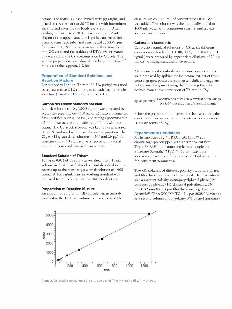
2
octane. The bottle is closed immediately (gas-tight) and placed in a water bath at 80 °C for 1 h with intermittent shaking and inverting the bottle every 20 min. After cooling the bottle to < 20 ˚C by ice water, a 1-2 mL aliquot of the upper isooctane layer is transferred into a micro centrifuge tube, and centrifuged at 5000 rpm for 5 min at 10 °C. The supernatant is then transferred into GC vials, and the residues of DTCs are estimated by determining the CS2 concentration by GC-MS. The sample preparation procedure depending on the type of food used takes approx. 1-2 hrs.
Preparation of Standard Solutions and Reaction MixtureFor method validation, Thiram (99.5% purity) was used as representative DTC compound considering its simple structure (1 mole of Thiram = 2 mole of CS2).
Carbon disulphide standard solutionA stock solution of CS2 (2000 µg/mL) was prepared by accurately pipetting out 79.0 µL of CS2 into a volumetric flask (certified A class, 50 mL) containing approximately 45 mL of iso-octane and made up to 50 mL with iso-octane. The CS2 stock solution was kept in a refrigerator at -20 °C and used within two days of preparation. The CS2 working standard solutions of 200 and 20 µg/mL concentrations (10 mL each) were prepared by serial dilution of stock solution with iso-octane.
Standard Solution of Thiram10 mg (± 0.05) of Thiram was weighed into a 10 mL volumetric flask (certified A class) and dissolved in ethyl acetate up to the mark to get a stock solution of 1000 µg/mL. A 100 µg/mL Thiram working standard was prepared from stock solution by 10-times dilution.
Preparation of Reaction MixtureAn amount of 30 g of tin (II) chloride was accurately weighed in the 1000 mL volumetric flask (certified A
class) to which 1000 mL of concentrated HCL (35%) was added. The solution was then gradually added to 1000 mL water with continuous stirring until a clear solution was obtained.
Calibration StandardsCalibration standard solutions of CS2 at six different concentration levels (0.04, 0.08, 0.16, 0.32, 0.64, and 1.3 µg/mL) were prepared by appropriate dilutions of 20 µg/mL CS2 working standard in iso-octane.
Matrix matched standards at the same concentrations were prepared by spiking the iso-octane extract of fresh control grapes, potato, tomato, green chili, and eggplant (all organically grown) using the following formula derived from above conversion of Thiram to CS2:
Figure 2. Calibration curve, range 0.04 - 1.300 µg/mL Thiram matrix spike, R2 = 0.9990.
Before the preparation of matrix matched standards, the control samples were carefully monitored for absence of DTCs (in terms of CS2).
Experimental ConditionsA Thermo Scientific™ TRACE GC Ultra™ gas chromatograph equipped with Thermo Scientific™ Triplus™ RSH liquid autosampler and coupled to a Thermo Scientific™ ITQ™ 900 ion trap mass spectrometer was used for analysis. See Tables 1 and 2 for instrument parameters.
Two GC columns of different polarity, stationary phase, and film thickness have been evaluated. The first column was a medium polarity cyanopropylphenyl phase (6% cyanopropylphenyl/94% dimethyl polysiloxane, 30 m x 0.32 mm ID, 1.8 µm film thickness, e.g. Thermo Scientific™ TraceGOLD™ TG-624, p/n 26085-3390) and as a second column a low polarity 5%-phenyl stationary
Spike quantity=Concentration to be achive*weight of the sample
0.6333*concentration of the stock solution

phase (5% diphenyl/95% dimethylpolysiloxane, 30 m x 0.25 mm ID, 0.25 µm film thickness, e.g. Thermo Scientific™ TraceGOLD™ TG-5MS p/n 26098-1420). The TG-624 column type is a mid-polarity column ideally suited for the analysis of volatile analytes, whereas
3
Injector, temperature prog. PTV-LVI
40 °C, 0.1 min (injection phase, @ 100 kPa)
10 °C/min to 80 °C, 0.3 min (@ 200 kPa)
10 °C/min to 110 °C (transfer phase)
14.5 °C/min to 290 °C (cleaning phase)
Split flow 20 mL/min
Solvent vent open until 0.17 min
closed until 4.17 min
open until end of run
Injection mode, volume split, 4 µL
Carrier gas, flow Helium, constant flow 1 mL/min
Oven program 40 °C, 5 min
40 °C/min to 200 °C
200 °C, 5 min
Transfer line temperature 205 °C
Table 1. GC Conditions
Ionization EI, 70 eV
Scan mode, range SIM, m/z 76, 78
Acquisition rate 2 scans/s
Ion source temperature 200 °C (optimized for CS2 S/N ratio)
Table 2. MS Conditions
Figure 3. CS2 chromatogram, 5 ppb matrix spike calibration.
the TG-5MS column is more commonly used especially for pesticide analysis and is commonly available in all laboratories. Both columns were thus tested for the applicability of the method. Either column can be used for the DTC analysis.
RT: 0.00 - 2.00 SM: 13GRT: 1 40
55
60
65
70
75
80
85
90
95
100
ndan
ce
RT: 1.40
5
10
15
20
25
30
35
40
45
50
Rel
ativ
e A
bun
0.0 0.2 0.4 0.6 0.8 1.0 1.2 1.4 1.6 1.8Time (min)
0
5

Sample MeasurementsA typical GC-MS batch consisted of matrix-matched calibration standards, samples, one matrix blank and one recovery sample for performance check after a set of every six samples.
The data acquisition was carried out in Full Scan mode using the compound-specific ions m/z 76 and 78 (the 34S isotope, ion ratio 10:1) as extracted chromatograms for a selective identification of CS2.
ResultsSensitivityThe sensitivity of the method was evaluated in terms of the limit of detection (LOD) and limit of quantification (LOQ) which were respectively 0.005 and 0.04 µg/mL. The LOD is the concentration at which the signal to noise ratio (S/N) for the quantifier ion is > 3, whereas LOQ is the concentration for which the S/N is > 10.
4
Figure 4. Chili sample analysis with confirming CS2 ion ratio 100:10 for m/z 76:78.
RT: 0.00 2.60 SM: 13G
90
100RT: 1.50
0.0 0.2 0.4 0.6 0.8 1.0 1.2 1.4 1.6 1.8 2.0 2.2 2.4Time (min)
0
10
20
30
40
50
60
70
80
Rel
ativ
e Ab
unda
nce
RT: 1.93
Time (min)
30
40
50
60
70
80
90
100
Rel
ativ
e Ab
unda
nce
76
50 55 60 65 70 75 80 85 90 95m/z
0
10
20
787764 8960
Spike level [ppb] Grapes [%] Chili [%] Potato [%] Egg plant [%] Tomato [%]
1300 96 (±4) 81 (±10) 90 (±9) 90(±5) 81 (±4)
160 94 (±10) 80 (±13) 94 (±10) 92 (±8) 85 (±10)
40 104 (±15) 79 (±9) 104 (±15) 86 (±10) 96(±15)
Table 3. Recoveries from different foods:
RecoveryThe recovery experiments were carried out on fresh untreated potato, tomato, eggplant, green chili, and grapes by fortifying 25 g of the samples with Thiram solution at 0.04, 0.16, and 1.30 µg/g levels in six replicates. The control samples of each of the tested commodities were obtained from an organic farm near Pune, India, and screened for absence of DTC residues before spiking. The spiked the samples were extracted using the sample preparation method described above. The quantitation of the residues was performed using matrix matched standards.

The GC injection method and column separation has been optimized for the injection of 4 uL of extract, using GC columns of standard film and dimensions, typically used for other types of residue analysis as well, so that a column change to a specific column for CS2 determination only is not required.
The mass spectrometer ion source conditions had been optimized for best sensitivity and S/N ratio. The analysis in SIM mode is preferred providing a high selectivity with easy to integrate chromatograms.
This method has been developed initially for the ITQ ion trap mass spectrometer, but the same parameter setup is suitable for the Thermo Scientific™ ISQ™ series single quadrupole or Thermo Scientific™ TSQ™ Quantum XLS Ultra or Thermo Scientific™ TSQ 8000™ triple quadrupole mass spectrometers, as well.
References
[1] Crnogorac, G., Schwack, W., Residue analysis ofdithiocarbamatefungicides, Trends in AnalyticalChemistry, Vol. 28, No. 1, 2009.
[2] Reynolds, S., Analysis of Dithiocarbamates, presentedat the SELAMAT Workshop, Bangkok 2006.
[3] Analysis of Dithiocarbamate Residues inFoods of Plant Origin involving Cleavage intoCarbon Disulfide, Partitioning into Isooctaneand Determinative Analysis by GC-ECD. http://www.crl-pesticides.eu/library/docs/srm/meth_DithiocarbamatesCS2_EurlSrm.PDF
[4] Amvrazi, Elpiniki G., Fate of Pesticide Residues onRaw Agricultural Crops after Postharvest Storageand Food Processing to Edible Portions, Pesticides- Formulations, Effects, Fate, Prof. MargaritaStoytcheva(Ed.), ISBN: 978-953-307-532-7.
PrecisionThe precision of repeatability was determined by three analysts preparing six samples each on a single day. The intermediate precision was determined by the same analysts with six samples each on six different days. The method precision was determined with 0.04 mg/kg.
General Guidelines for DTC AnalysisThe analysis of cruciferous crops, including brassica samples, may not be unequivocal, because they contain naturally occurring compounds that may generate carbon disulfide.
It is necessary to avoid the use of rubber material (natural/synthetic) e.g. gloves, when performing DTC analyses as they contain dithiocarbamates, and this could lead to contamination problems. Silicone rubber and polyethylene do not contain dithiocarbamate.
Samples, other than fresh foodstuffs, will be comminuted by cryogenic milling. Fresh samples should be sub-sampled prior to extraction by removing segments from fresh samples following current Codex Alimentarius guidelines.
The samples should be analyzed within 4 weeks of cryogenic milling. If the storage of fresh produce is necessary it should be in a cool place (<-10°C) keeping condensation at minimum [4].
ConclusionsA reliable routine method for the analysis of dithiocarbamates with high precision in different vegetable and fruits has been developed. The method allows a wide calibration range of 0.04 – 1.300 µg/mL Thiram. The LOQ has been determined as 0.04 µg/mL.
The extraction uses a SnCl2/HCl acid-hydrolysis with iso-octane as solvent to form CS2 which finally gets quantified by GC-MS. The recovery from different food commodities has been shown to be very high with 79 to 104%.
AN10333_E 08/16S
Africa-Other +27 11 570 1840Australia +61 3 9757 4300Austria +43 1 333 50 34 0Belgium +32 53 73 42 41Canada +1 800 530 8447China +86 10 8419 3588Denmark +45 70 23 62 60
Europe-Other +43 1 333 50 34 0Finland/Norway/Sweden
+46 8 556 468 00France +33 1 60 92 48 00Germany +49 6103 408 1014India +91 22 6742 9434Italy +39 02 950 591
Japan +81 45 453 9100Latin America +1 561 688 8700Middle East +43 1 333 50 34 0Netherlands +31 76 579 55 55New Zealand +64 9 980 6700Russia/CIS +43 1 333 50 34 0South Africa +27 11 570 1840
Spain +34 914 845 965Switzerland +41 61 716 77 00UK +44 1442 233555USA +1 800 532 4752
www.thermoscientific.com©2016 Thermo Fisher Scientific Inc. All rights reserved. All trademarks are the property of Thermo Fisher Scientific Inc. and its subsidiaries. This information is presented as an example of the capabilities of Thermo Fisher Scientific Inc. products. It is not intended to encourage use of these products in any manners that might infringe the intellectual property rights of others. Specifications, terms and pricing are subject to change. Not all products are available in all countries. Please consult your local sales representative for details.


Simplifying Complex Multi-Residue Pesticide Methodology in GC-MS/MS
David Steiniger, Juan Carmona, Stacy Crain, Paul Silcock, and Jason Cole Thermo Fisher Scientific, Austin, TX, USA
Tech
nica
l No
te 1
03
19
Key WordsPesticide analysis, triple quadrupole GC/MS, AutoSRM, SRM, MRM
OverviewEasing Implementation of Multi-Residue Pesticide MethodologyThe task of setting up a triple quadrupole GC/MS pesticide analysis can be daunting, regardless of your starting point. Perhaps you are brand new to GC/MS pesticide analysis, and you need all the help you can get. Maybe you analyze a small set of pesticides and want to expand your target list, or you analyze a large pesticide set in multiple runs on a single quadrupole and want to combine these into a single MRM analysis. Perhaps you already have a comprehensive MRM method, but want to move this to a Thermo Scientific™ TSQ™ 8000 triple quadrupole GC-MS/MS system to take advantage of its robustness, removable ion source under vacuum, and its ease in adding new target pesticides through AutoSRM. Whatever your starting point, when adopting new technology to address complex analytical challenges, you need tools that enable you to be productive, quickly.
With your needs and requirements in mind, the Thermo Scientific TSQ 8000 Pesticide Analyzer (Figure 1) has been developed. Provided within this comprehensive package are all the tools you need to set up a complex pesticide method, regardless of your starting point.
Everyone who is new to pesticide analysis on the TSQ 8000 GC-MS/MS system will appreciate the provided list of optimized pesticide transitions. Also, with an easy to follow step-by-step description of how to develop new transitions using AutoSRM, you’ll find the ease of adding new pesticides to your MRM method is now a competi-tive advantage for your laboratory. And for those who need more assistance, the TSQ 8000 Pesticide Analyzer contains a complete instrument method developed on an included column with provided compound retention times and MRM parameters—eliminating days, if not weeks, of method development.
In addition to simplified method startup, another advantage of using the analyzer is that it utilizes Timed-SRM methodology, allowing for easy-to-use, high-analyte-capacity methodology. The usability and scanning efficiency of Timed-SRM are complemented by the fast-scanning capability of the TSQ 8000 instrument, making the analysis of hundreds of pesticides, with a total of over one thousand transitions, not just possible, but easy.
Finally, the TSQ 8000 Pesticide Analyzer has the ability to analyze full scan data at the same time as your targeted MRM analysis. This allows you to harness the power of existing EI full scan libraries to, for example, find potential high-level contaminants you would otherwise miss in a targeted analysis, or monitor the matrix background for possible interference.
Figure 1. The TSQ 8000 Pesticide Analyzer. Details of its contents can be found in the TSQ 8000 Pesticide Analyzer Brochure (BR10318).

2 Using the Startup KitStarting Point 1: Starting from ScratchWhen creating your method within Thermo Scientific™ TraceFinder™ EFS software, the instrument control and data processing software included with the TSQ 8000 Pesticide Analyzer, the use of the TraceFinder Pesticide Compound Database (CDB) will greatly simplify the method development process. Multiple transitions for each compound in the database have been optimized on the TSQ 8000 instrument with AutoSRM to within ± 1 eV of the optimum collision energy.
Simply select the compounds of interest in the CDB (Figure 2). This will create not only the TraceFinder software processing method, but also the TSQ 8000 mass spectrometer acquisition list. Since the instrument employs Timed-SRM, SRM windows for data acquisition will be centered on your retention times, so that all peaks elute far from acquisition-window breaks. The complete step-by-step procedure, including software screen captures, is detailed in the TSQ 8000 Pesticide Analyzer Installation Guide, which is also included with the TSQ 8000 Pesticide Analyzer.
After selecting your compounds of interest, you are now ready to acquire samples in MRM with your TSQ 8000 instrument.
Starting Point 2: Starting from an Established GC MethodIf you already have a preferred GC method, and know the retention times of your target compounds, you can update the pesticides in the CDB with the known retention times. Next, simply select the compounds you are interested in analyzing from the updated CDB, as shown in Figure 2. Again, this will create both the TraceFinder EFS processing method and the TSQ 8000 system Timed-SRM acquisition list, with acquisition windows centered on the retention times of the target peaks.
If you do not know exact retention times, you can easily widen acquisition windows while in TraceFinder EFS software for all compounds (Figure 3) to ensure your peaks fall within their acquisition window. Now update your TraceFinder EFS software method with the new retention times as you would in a normal data review, and your acquisition windows will be centered on each compound. After updating the retention times, follow the same step to reduce acquisition windows back to defaults in order to maximize dwell time for the analysis.
Figure 2. Selecting compounds from the TraceFinder EFS Compound Data Base. This will populate both your TraceFinder Processing Method and your acquisition list. For more information on creating TSQ 8000 methods with the TraceFinder CDB, see AB52300: Thermo Scientific TSQ 8000 GC-MS/MS Method Sync.
Figure 3. Widening acquisition windows in TraceFinder EFS software to find peaks with unknown retention times.

3Tools to Get You ProductiveThe software features of the TSQ 8000 system have been designed with complex pesticide analysis in mind. These features include AutoSRM, a tool that makes the instrument the easiest for developing and adding new compounds to an existing pesticide method. Another useful feature is Timed-SRM, which enables accurate pesticide identifi cation and quantitation, even for very dense pesticide methodologies. Finally, the ability of the TSQ 8000 instrument to perform simultaneous full scan/MRM provides the capability to identify general unknowns in conjunction with your target pesticides, fi lling a classic gap in targeted MRM analysis.
Addition of New CompoundsFor those compounds provided in the TSQ 8000 Pesticide Analyzer CDB, the addition of new compounds to your methodology is extremely simple. If you are using the method and GC column provided with the TSQ 8000 Pesticide Analyzer, simply select additional compounds to your method from the CDB. The instrument software now adds the selected compounds to both the method acquisition list and the TraceFinder EFS software processing list with the correct retention times.
For those pesticides not yet in the TSQ 8000 Pesticide Analyzer CDB, AutoSRM can be used to quickly develop these new transitions (Figure 4). Once fully developed, the new compounds are easily imported into the CDB and added to your TraceFinder software method. A step-by-step walkthrough of this is described in detail in the TSQ 8000 Pesticide Analyzer Installation Guide, which is provided as part of the TSQ 8000 Pesticide Analyzer package. For more details on how AutoSRM works, see AB52298: Introducing AutoSRM.
a). Precursor Ion Study
b). Product Ion Study
c). Collision Energy Optimization
Figure 4. Screen shots showing the three-step process of AutoSRM. a.) In the fi rst step, AutoSRM acquires full scan data for selecting precursor ions. b.) In the second step, product ions are selected from product ion scan data. c.) In the fi nal step, collision energies are varied for each of the selected SRM’s to determine the optimal collision energy.
a). Precursor Ion Study
b). Product Ion Study
c). Collision Energy Optimization

4 This then forces a compromise between adding many compounds per segment, reducing individual SRM dwell times and sensitivity, and adding segment breaks between closely eluting peaks, which causes the risk of false negatives due to shifts in peak retention times outside of acquisition windows because, for example, a large bit of matrix coelutes with a peak.
The TSQ 8000 system takes an approach called Timed-SRM that eliminates this compromise. Timed-SRM removes the limitations of segmented SRM by centering acquisition windows on the retention time of each peak and allowing for acquisition window overlap, so that acquisition windows for all nearby eluting compounds are not forced to start and stop at the same time (Figure 5). The user simply needs to enter the retention time of each compound, and the instrument method takes care of the rest, eliminating the need for creating segments.
High Compound Capacity MethodsOne of the primary challenges of modern pesticide analysis is the sheer number of pesticides that need monitoring in order to meet international standards. This is particularly true in food analysis where products are transported across country borders, requiring exporters to meet the regulatory demands of many countries. Triple quadrupole instruments help meet this demand due to the high selectivity of MRM analysis, which allows for spectral separation of coeluting peaks due to unique reactions in the collision cell. This enables monitoring of more compounds in a single chromatographic run without prohibitive interference. However, due to the targeted nature of the MRM process, individual scan events must be created for each pesticide to be monitored, placing a strain on the amount of time devoted to the monitoring of each compound, and thus the sensitivity of the analysis of each compound.
With a traditional style analysis, this issue can be partially resolved by slicing up the acquisition list into discreet time segments, so that all transitions are not being monitored at the same time. However, this can quickly lead to problems when analyzing more than 50 pesticides in one run. This is because, due to the density of the peaks in the heart of the method, it is difficult to find a time for a segment break when no target peaks are eluting.
Acquisition windows centered around retention time
Acquisition windows allowed to overlap
Figure 5. The TSQ 8000 system Timed-SRM Acquisition list, showing SRM acquisition windows centered on retention times and overlapping nearby transitions.
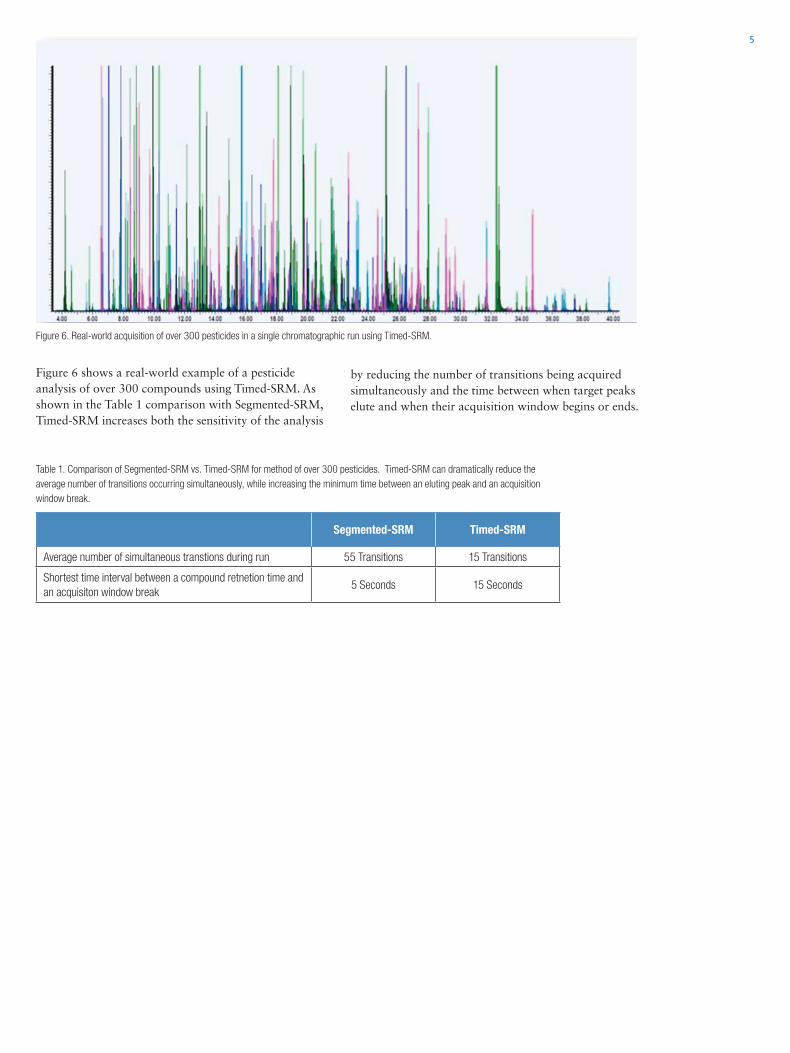
5
by reducing the number of transitions being acquired simultaneously and the time between when target peaks elute and when their acquisition window begins or ends.
Figure 6 shows a real-world example of a pesticide analysis of over 300 compounds using Timed-SRM. As shown in the Table 1 comparison with Segmented-SRM, Timed-SRM increases both the sensitivity of the analysis
Figure 6. Real-world acquisition of over 300 pesticides in a single chromatographic run using Timed-SRM.
Segmented-SRM Timed-SRM
Average number of simultaneous transtions during run 55 Transitions 15 Transitions
Shortest time interval between a compound retnetion time and an acquisiton window break
5 Seconds 15 Seconds
Table 1. Comparison of Segmented-SRM vs. Timed-SRM for method of over 300 pesticides. Timed-SRM can dramatically reduce the average number of transitions occurring simultaneously, while increasing the minimum time between an eluting peak and an acquisition window break.

6 The TSQ 8000 system allows you to set up a full scan acquisition throughout the duration of your MRM analysis. Each acquisition will then have full scan data to identify non-target compounds, in addition to MRM data to confirm and quantitate the target list. This mode of analysis is facilitated with the TraceFinder EFS software qualitative processing view within its standard quantitative batch analysis, which automatically detects, identifies, and reports non-target compounds (Figure 7).
General Unknown ScreeningAnother limitation of the classic MRM approach to pesticide analysis is that, due to its targeted nature, if a compound is not part of your target list, you are not going to find it, even if it is present in large quantities in your sample. This limitation is removed with capability of the TSQ 8000 system to perform simultaneous full scan/MRM.
Figure 7. Qualitative view of TraceFinder EFS software for analyzing fruit juice with simultaneous full scan/Timed-SRM on the TSQ 8000 system. In addition to quantitating and confirming the 158 target compounds by MRM (top), TraceFinder EFS software has identified three high-level unknowns by full scan analysis (bottom): 2,4-bis(1,1-dimethylethyl)-phenol, triethyl citrate, and Vitamin E.

Tech
nica
l No
te 1
03
19
TN10319_E 08/16S
Africa-Other +27 11 570 1840Australia +61 3 9757 4300Austria +43 1 333 50 34 0Belgium +32 53 73 42 41Canada +1 800 530 8447China +86 10 8419 3588Denmark +45 70 23 62 60
Europe-Other +43 1 333 50 34 0Finland/Norway/Sweden
+46 8 556 468 00France +33 1 60 92 48 00Germany +49 6103 408 1014India +91 22 6742 9494Italy +39 02 950 591
Japan +81 45 453 9100Latin America +1 561 688 8700Middle East +43 1 333 50 34 0Netherlands +31 76 579 55 55New Zealand +64 9 980 6700Russia/CIS +43 1 333 50 34 0South Africa +27 11 570 1840
Spain +34 914 845 965Switzerland +41 61 716 77 00UK +44 1442 233555USA +1 800 532 4752
www.thermofisher.com©2016 Thermo Fisher Scientific Inc. All rights reserved. All trademarks are the property of Thermo Fisher Scientific Inc. and its subsidiaries. This information is presented as an example of the capabilities of Thermo Fisher Scientific Inc. products. It is not intended to encourage use of these products in any manners that might infringe the intellectual property rights of others. Specifications, terms and pricing are subject to change. Not all products are available in all countries. Please consult your local sales representative for details.
ConclusionFor the lab just starting up a complex pesticide analysis by triple quadrupole GC-MS, the TSQ 8000 Pesticide Analyzer offers the easiest and quickest path to success. The included methodology, consumables, and SRM transition list with accurate retention times enable the creation of your pesticide method to be as simple as selecting the compounds you want to analyze. With multiple SRM transitions per compound optimized to within ± 1 eV, the pesticide analyzer is useful for anyone who wants to take advantage of the unique features of the TSQ 8000 system designed to make complex pesticide analysis simple.
The TSQ 8000 Pesticide Analyzer fully takes advantage of these features, including the ability to do Timed-SRM, which significantly increases low-level sensitivity through a more efficient SRM scheduling. Also, the full scan/MRM capability of the TSQ 8000 mass spectrometer combines the elite quantitation capabilities of MRM analysis with classic general unknown identification through full scan quadrupole library searching. Finally, the ability to easily develop and add new pesticides to an existing pesticide method through AutoSRM makes the TSQ 8000 Pesticide Analyzer the most flexible system for expanding your pesticide target list to meet future regulatory or client demands.

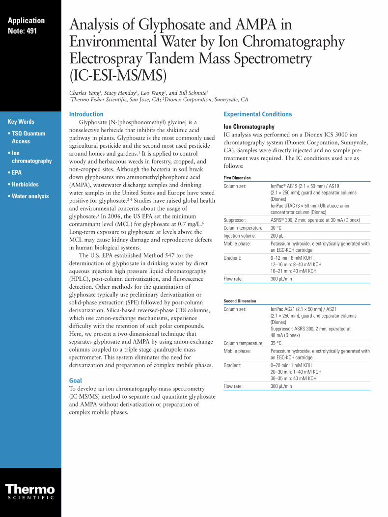
Analysis of Glyphosate and AMPA in Environmental Water by Ion ChromatographyElectrospray Tandem Mass Spectrometry (IC-ESI-MS/MS)Charles Yang1, Stacy Henday2, Leo Wang2, and Bill Schnute2
1Thermo Fisher Scientific, San Jose, CA; 2Dionex Corporation, Sunnyvale, CA
IntroductionGlyphosate [N-(phosphonomethyl) glycine] is a
nonselective herbicide that inhibits the shikimic acidpathway in plants. Glyphosate is the most commonly usedagricultural pesticide and the second most used pesticidearound homes and gardens.1 It is applied to controlwoody and herbaceous weeds in forestry, cropped, andnon-cropped sites. Although the bacteria in soil breakdown glyphosates into aminomethylphosphonic acid(AMPA), wastewater discharge samples and drinkingwater samples in the United States and Europe have testedpositive for glyphosate.2-4 Studies have raised global healthand environmental concerns about the usage ofglyphosate.5 In 2006, the US EPA set the minimumcontaminant level (MCL) for glyphosate at 0.7 mg/L.6
Long-term exposure to glyphosate at levels above theMCL may cause kidney damage and reproductive defectsin human biological systems.
The U.S. EPA established Method 547 for thedetermination of glyphosate in drinking water by directaqueous injection high pressure liquid chromatography(HPLC), post-column derivatization, and fluorescencedetection. Other methods for the quantitation ofglyphosate typically use preliminary derivatization orsolid-phase extraction (SPE) followed by post-columnderivatization. Silica-based reversed-phase C18 columns,which use cation-exchange mechanisms, experiencedifficulty with the retention of such polar compounds.Here, we present a two-dimensional technique thatseparates glyphosate and AMPA by using anion-exchangecolumns coupled to a triple stage quadrupole massspectrometer. This system eliminates the need forderivatization and preparation of complex mobile phases.
GoalTo develop an ion chromatography-mass spectrometry(IC-MS/MS) method to separate and quantitate glyphosateand AMPA without derivatization or preparation ofcomplex mobile phases.
Experimental Conditions
Ion ChromatographyIC analysis was performed on a Dionex ICS 3000 ionchromatography system (Dionex Corporation, Sunnyvale,CA). Samples were directly injected and no sample pre-treatment was required. The IC conditions used are asfollows:
First Dimension
Column set: IonPac® AG19 (2.1 × 50 mm) / AS19 (2.1 × 250 mm); guard and separator columns(Dionex) IonPac UTAC (3 × 50 mm) Ultratrace anionconcentrator column (Dionex)
Suppressor: ASRS® 300, 2 mm; operated at 30 mA (Dionex)Column temperature: 30 °CInjection volume: 200 µLMobile phase: Potassium hydroxide, electrolytically generated with
an EGC-KOH cartridgeGradient: 0–12 min: 8 mM KOH
12–16 min: 8–40 mM KOH16–21 min: 40 mM KOH
Flow rate: 300 µL/min
Second Dimension
Column set: IonPac AG21 (2.1 × 50 mm) / AS21 (2.1 × 250 mm); guard and separator columns(Dionex) Suppressor: ASRS 300, 2 mm; operated at 48 mA (Dionex)
Column temperature: 35 °CMobile phase: Potassium hydroxide, electrolytically generated with
an EGC-KOH cartridgeGradient: 0–20 min: 1 mM KOH
20–30 min: 1–40 mM KOH30–35 min: 40 mM KOH
Flow rate: 300 µL/min
Key Words
• TSQ QuantumAccess
• Ionchromatography
• EPA
• Herbicides
• Water analysis
ApplicationNote: 491

The high-purity IC eluent is automatically produced insitu (Figure 1). The pump delivers water to an eluentgenerator cartridge (EGC) that converts the water into theselected concentration of potassium hydroxide eluentusing electrolysis. After separation on the column, theeluent enters the anion self-regenerating suppressor(ASRS) that produces hydronium ions to exchange withpotassium in the eluent. This makes the mobile phasecompatible with the mass spectrometer liquid inlet system.
Mass SpectrometryMS analysis was carried out on a Thermo Scientific TSQQuantum Access triple stage quadrupole massspectrometer with an electrospray ionization (ESI) source.The MS conditions were as follows:
Ion source polarity: Negative ion modeSpray voltage: 3000 V Sheath gas pressure: 40 arbitrary unitsIon sweep gas pressure: 1 arbitrary unitAuxiliary gas pressure: 2 arbitrary unitsCapillary temperature: 400 °CCollision gas pressure: 1.5 barScan conditions: Table 1
Table 1. MS Scan Conditions
Scan Scan Collision TubeCompound Mass Width Time (s) Energy Lens
AMPA 110.17 / 63.3 0.01 0.5 19 60AMPA 110.17 / 79.2 0.01 0.5 35 60Glyphosate 168.09 / 150.1 0.01 0.5 13 51Glyphosate 168.09 / 79.4 0.01 0.5 40 51
Results and DiscussionThe major matrix peaks of chloride, nitrate, carbonate,and sulfate were well-resolved. The separation of allcompounds occurred in both dimensions in 30 minutes.The calibration curves showed excellent linearity usingonly external quantitative measurements without internalstandards.
For quantitation, samples were run in the MS/MSselective reaction monitoring (SRM) mode on the TSQQuantum Access™ triple stage quadrupole instrument. Thecalibration range was 0.1–50 ppb for AMPA and 0.05–50 ppb for glyphosate. The correlation coefficients(R2) of the 110 → 63 and 110 → 79 SRM transitions ofAMPA were both 0.9997 (Figures 2 and 3). The 168 →150 transition of glyphosate had an R2 of 0.9997 and the168 → 79 transition yielded an R2 of 0.996 (Figures 4 and5, respectively).
The minimum detection limit (MDL) in matrix wascalculated by seven replicate injections of 5 ppb in asimulated matrix with high concentrations of chloride,carbonate, nitrate, and sulfate (250 ppm chloride andsulfate, 150 ppm sodium bicarbonate, 20 ppm nitrate).The MDLs for AMPA and glyphosate were calculated byusing the equation MDL= t99% × S(n-1), where t equals theStudent’s t test at 99% confidence intervals (t 99%, (6) =3.143) and S is the standard deviation. The calculatedMDL for AMPA was 0.313 ppb and 0.252 ppb forglyphosate. This is well below the current MDLs of 6 ppbfor glyphosate in reagent water and 8.99 ppb in groundwater specified by the EPA guidelines found in Method547.
Using ion chromatography to quantitate AMPA andglyphosate accurately at this level without samplepretreatment requires the use of a mass spectrometer.However, the source of the instrument can be subject tofouling from routine analysis of samples of high-ionicstrength. The use of multi-dimensional chromatographysignificantly reduces the introduction of matrix ions to themass spectrometer, increasing the method robustness inchallenging sample matrices. The recoveries for AMPAand glyphosate were 97.2% and 82.1%, respectively, for 5 ppb spiked into high-ionic strength samples. The relativestandard deviations were less than 5% for bothcompounds, even without an internal standard (Figure 6).
Figure 1. The flow schematic for a two-dimensional IC-MS/MS application. The first dimension separates the analytes of interest from a majority of thematrix ions. The second dimension improves peak shape and keeps the source of the MS clean.

The response of the standards decreased over time.However, when using freshly prepared standards, theresponse remained constant; this suggests there may betemperature stability issues with the samples. Althoughexcellent short-term (30 hour) stability yielded standarddeviations less than 5%, using a refrigerated autosamplerand an isotopically-labeled internal standard will helpminimize systematic sample degradation and responsevariation.
AMPA_63Y = -9223.87+23897.5*X R^2 = 0.9997 W: Equal
0 10 20 30 40 50ppb
0
200000
400000
600000
800000
1000000
1200000
Area
AMPA_79Y = -10278.6+35908.4*X R^2 = 0.9997 W: Equal
0 10 20 30 40 50ppb
0
200000
400000
600000
800000
1000000
1200000
1400000
1600000
1800000
Area
Glyphosate_150Y = 10661.8+141089*X R^ 2 = 0.9997 W: Equal
0 10 20 30 40 50ppb
0
1000000
2000000
3000000
4000000
5000000
6000000
7000000
Area
Glyphosate_79Y = -5192.82+49777.1*X R^2 = 0.9996 W: Equal
0 10 20 30 40 50ppb
0
500000
1000000
1500000
2000000
2500000
Area
0 5 10 15 20 25 30 35 40Time (min)
0
20
40
60
80
1000
20
40
60
80
100
Rela
tive
Abun
danc
e
29.32
32.47
32.39
Figure 3. The calibration curve of the SRM 110 → 79 for AMPA.
Figure 4. The calibration curve of the SRM 168 → 150 for glyphosate.
Figure 5. The calibration curve of the SRM 168 → 79 for glyphosate.
Figure 6. The total ion chromatogram (TIC) of 5 ppb of glyphosate and AMPAspiked into a matrix of chloride, nitrate, carbonate and sulfate.
Figure 2. Calibration curve of the 110 → 63 SRM transition for AMPA.

ConclusionThe advantage of the IC-MS/MS methodology describedhere is the elimination of derivatization and acidificationsteps required by EPA Method 547 and other techniques.The analysis requires no sample preparation. Separationof both compounds in both dimensions occurs inapproximately 30 minutes. Calibration levels of 0.05 to50 ppb for glyphosate show that this method can be usedto quantitate low (ppb) levels of glyphosate in high-ionicstrength matrices. Using stable-labeled internal standardswill help compensate for the effects of ion suppression inthe source.
References1. Tu, M.; Hurd, C.; and Randall, J.M. Weed Control Methods Handbook,
The Nature Conservancy, http://tncinvasives.ucdavis.edu, Version: April2001.
2. United States Geological Survey, “Glyphosate Found in WastewaterDischarged to Streams,”http://toxics.usgs.gov/highlights/glyphosate_wastewater.html (AccessedJanuary 7, 2009).
3. Kolpin, D.W.; Thurman, E.M.; Lee, E.A.; Meyer, M.T.; Furlong, E.T.; andGlassmeyer, S.T. “Urban contributions of glyphosate and its degradateAMPA to streams in the United States”; Science of the Total Environment,2006, 354 (2-3), 191-197. doi: 10.1016/j.scitotenv.2005.01.028
4. Beyond Pesticides, “Denmark Restricts Water-Contaminating Herbicide,”http://www.beyondpesticides.org/news/daily_news_archive/2003/9_23_03.htm (Accessed January 8, 2009).
5. Richard, S.; Moslemi, S.; Sipahutar, H.; Benachour, N.; and Seralini, G-E“Differential effects of glyphosate and Roundup on human placental cellsand aromatase”; Environmental Health Perspectives, 2005, 113(6) 716-720. doi:10.1289/ehp.7728
6. Unites States Environmental Protection Agency, “Consumer Factsheet onGlyphosate,”http://www.epa.gov/OGWDW/contaminants/dw_contamfs/glyphosa.html(Accessed January 5, 2008).
7. Unites States Environmental Protection Agency, “Method 547:Determination of glyphosate in drinking water by direct-aqueous-injectionHPLC, post-column derivatization, and fluorescence detection,”http://www.accustandard.com/asi/pdfs/epa_methods/547.pdf (AccessedJanuary 5, 2008).
In addition to these
offices, Thermo Fisher
Scientific maintains
a network of represen tative
organizations
throughout the world.
Africa-Other+27 11 570 1840Australia+61 2 8844 9500Austria+43 1 333 50 34 0Belgium+32 53 73 42 41Canada+1 800 530 8447China+86 10 8419 3588Denmark+45 70 23 62 60Europe-Other+43 1 333 50 34 0Finland / Norway /Sweden+46 8 556 468 00France+33 1 60 92 48 00Germany+49 6103 408 1014India+91 22 6742 9434Italy+39 02 950 591Japan+81 45 453 9100Latin America+1 608 276 5659Middle East+43 1 333 50 34 0Netherlands+31 76 579 55 55South Africa+27 11 570 1840Spain+34 914 845 965Switzerland+41 61 716 77 00UK+44 1442 233555USA+1 800 532 4752
www.thermoscientific.com
Part of Thermo Fisher Scientific
AN63068_E 08/16S
Legal Notices©2016 Thermo Fisher Scientific Inc. All rights reserved. IonPac and ASRS are registered trademarks of Dionex Corporation. All other trademarks are the property of Thermo Fisher Scientific Inc. and its subsidiaries. This information is presented as an example of the capabilities of Thermo Fisher Scientific Inc. products. It is not intended to encourage use of these products in any manners that might infringe the intellectual property rights of others. Specifications, terms and pricing are subject to change. Not all products are available in all countries. Please consult your local sales representative for details.


Pharmaceuticals and Personal Care Products
Surface, Drinking and Waste Water Analysis
Ap
plica
tion
No
teb
oo
k
Quantitative and Semi-Quantitative Determination of PPCPs and Their By-products in Wastewater Treatment Plants Samples Using UHPLC-Orbitrap MS and Data Mining TechnologiesJonathan Beck,1 Tung-Vi Nguyen,2 Ramin Farnood,2 Charles Yang,1 Paul Yang,3 Maciej Bromirski,1 Sonya Kleywegt,3 Shahram Tabe3 and Dipankar Ghosh1 1Thermo Fisher Scientific, San Jose, CA, USA; 2Department of Chemical Engineering & Applied Chemistry, University of Toronto, Toronto, Ontario, Canada; 3Ontario Ministry of the Environment, Etobicoke, Ontario, Canada

2 Quantitative and Semi-Quantitative Determination of PPCPs and Their By-products in Wastewater Treatment Plants Samples Using UHPLC-Orbitrap MSand Data Mining Technologies
Quantitative and Semi-Quantitative Determination of PPCPs and Their By-products in Wastewater Treatment Plants Samples Using UHPLC-Orbitrap MS and Data Mining Technologies Jonathan Beck1, Tung-Vi Nguyen2, Ramin Farnood2, Charles Yang1, Paul Yang3, Maciej Bromirski1, Sonya Kleywegt3, Shahram Tabe3 and Dipankar Ghosh1, 1 Thermo Fisher Scientific, 355 River Oaks Parkway, San Jose, CA 95134-1706, USA; 2 Department of Chemical Engineering & Applied Chemistry, University of Toronto, Toronto, Ontario, M5S 3E5,Canada; 3 Ontario Ministry of the Environment, 125 Resources Road, Etobicoke, Ontario, M9P 3V6, Canada
Conclusion Quantitative results of PPCPs were obtained using HPLC-Orbitrap MS.
Semi-quantitative results, seasonal trends and effect of treatment temperature onPPCP by-products were obtained using TraceFinder and SIEVE software.
Efforts to obtain analytical standards to complete the studies are on-going.
References1. “The Determination of Emerging Organic Pollutants in Environmental Matrices by
Liquid Chromatography-Tandem Mass Spectrometry (LC-MS/MS)”, Ontario Ministry of the Environment method E3454. Available via [email protected].
2. “Monitoring the photochemical degradation of triclosan in wastewater by UV light and sunlight using solid-phase microextraction”. Sanchez-Prado, L., Llompart, M., Lores, M., García-Jares, C., Bayona, J. M., & Cela, R. (2006). Chemosphere, 65(8), pp. 1338-1347.
AcknowledgementsWe would like to thank Dr. Vince Pileggi for providing permeate samples; as well as Ms. Renee Luniewski for providing valuable suggestions to make this work complete.
Overview Purpose: Develop an analytical method to (1) determine PPCP concentrations in wastewater samples, and (2) examine the transformation of selected PPCPs during treatment processes.
Methods: Samples prepared by solid phase extraction (SPE) and analyzed by high performance liquid chromatography-Orbitrap mass spectrometry (HPLC-Orbitrap MS).
Results: Quantitative results of selected pharmaceuticals and personal care products (PPCPs) like DEET, Triclosan (TCS), Triclocarban (TCC), Diclofenac (DCL), Carbamazepine (CBZ) and semi-quantitative of their degradation products were obtained.
Introduction Results obtained from a simple and powerful workflow that can readily determine PPCPs and their by-products in wastewater treatment plant (WWTPs) samples will be presented. This workflow was applied in a survey of 43 permeate samples obtained from a pilot anaerobic membrane bioreactor (AnMBR). Quantitative results show the prevalence of various PPCPs in wastewater, particularly for compounds with high usage and/or poor elimination (e.g., caffeine, carbamazepine (CBZ), DEET, lidocaine, lincomycin, ketoprofen, and bezafibrate). For PPCP by-products, we identified that in-situ microbial degradation was the dominant pathway for triclocarban (TCC) removal; whilst triclosan (TCS), diclofenac (DCF) and CBZ were eliminated via a combination of photodegradation and metabolism. Thirty by-products were detected in this pilot survey, including the toxic compounds chlorophenol and acridone.
Methods Sample Preparation
For this study, permeate samples were chosen due to their complex matrix which poses as a challenge for conventional analytical method. These samples were collected from a pilot anaerobic membrane bioreactor (AnMBR) pilot plant located at the Wastewater Technology Centre (Environment Canada, Burlington, Ontario). A total of 35 permeate samples permeate tank from January 2012 to March 2013. During this time, the reactor were operated at different temperatures at 20, 35 and 55 °C using samples collected, respectively, in summer, winter and winter, to investigate the effect on the removal of PPCPs in permeates. Grab samples were contained in 1L-amber bottles without headspace and stored in dark, cold storage (4°C) until analysis.
Neat standards of native target compounds were purchased from Sigma-Aldrich (Oakville, ON, Canada). Deuterium (D) and 13C-labelled standards were purchased from CDN Isotopes (Pointe-Claire, QC, Canada) and Cambridge isotope Laboratories (Andover, MA, US). Five levels of analytical standard solutions were prepared by diluting intermediate solutions with CH3OH HPLC grade acetonitrile (CH3CN) and methanol (CH3OH) were purchased from Thermo Fisher Scientific (Ottawa, ON, Canada). High purity water used for aqueous mobile phases and sample preparation was produced by passing reverse osmosis water through a Thermo Scientific™ Barnstead™ Nanopure™ water purification system (Mississauga, ON, Canada). Laboratory Services NBranch (LaSB) method E34541 was used to prepare samples for targeted compound analysis and non-targeted compound screening. Waters OASIS® (Mississauga, ON, Canada) HLB solid phase extraction (SPE) cartridge (6 cc, 500 mg) was used in the extraction. Method E3454 has been accredited by the Canadian Association for Laboratory Accreditation (CALA) since 2004.
Liquid Chromatography (or more generically Separations)
Sample analysis was achieved on a Thermo Scientific™ Dionex™ UltiMate™ 3000 HPLC consisting of a HRG-3400RS binary pump, WPS-3000 autosampler, and a TCC-3400 column compartment. Separation was made by injecting 5 mL extracts into a Thermo Scientific™ Betasil™ and a Thermo Scientific™ Hypersil™ Gold, 2.1x100 mm columns, respectively, for positive and negative mode Orbitrap MS analysis.
One positive mode HPLC and two negative mode HPLC separations were used for the analysis of PPCPs and their by-products.
TABLE 1. HPLC mobile phase and gradient used in the analysis
Mass Spectrometry
The HPLC was interfaced to a Thermo Scientific™ Exactive Plus™ Orbitrap MS using a heated electrospray ionization (HESI) interface. The Orbitrap MS system was tuned and calibrated in positive and negative modes by infusion of standard mixtures ofMSCAL5 and MSCAL6. High purity nitrogen (>99%) was used in the ESI source (35 L/min). Spray voltages used were 2500 and 3200 V for positive and negative modes. Mass spectrometric data was acquired at a resolving power of 140000 (defined as full-width-at-half-maximum peakwidth at m/z 200, RFWHM), resulting a scanning rate of > 1.5 scans/sec when using automatic gain control target of 1.0 x 10⁶ and a C-trap inject time of 100 msec.
Data Analysis
Thermo Scientific™ TraceFinder™ software were used to perform quantitativeanalysis for 56 PPCPs. The same software was also used to perform non-targetedscreening along with a database of 312 compounds consisting of pharmaceuticallyactive compounds and their metabolites, steroids, hormones, surfactants andperfluorohydrocarbons. TraceFinder software is used to search for adduct ions(M+H)+, (M+NH4)+ and (M+Na)+ in the positive mode and (M-H)− molecular ion in thenegative mode for compounds listed in the database. The software then creates anextracted ion chromatogram (XIC) using a mass extraction window (MEW) of 5 ppm.Analytes were automatically identified using an XIC area threshold of 50,000(approximately 25–50 pg/mL (ppt) depending on compound), a 5 ppm mass accuracyfor the mono-isotopic mass (M) and at least two isotopic peaks ((M+1) and (M+2)), anda relative intensity of 90% ± 10% from the theoretical values. Typical screening timewas about 65 sec/sample using the 312 CEC database. Results obtained fromTraceFinder software were also exported to Thermo Scientific™ SIEVE™ software tocarry out ChemSpider™ search. Principal component analysis was carried out usingthe SIEVE software too.
ResultsQuantitative Analytical Results
Quantitative analysis determined 43 target PPCPs comprised of pharmaceuticals likeantibiotics, non-steroidal anti-inflammatory drug (NSAID); as well as personal careproducts such as insect repellent and antimicrobial agents (Table 2). Antibiotics (e.g.ciprofloxacin and sulfa drugs) found have the lowest median concentration comparedto other therapeutic classes. As depicted in Figure 1, the highest median concentrationis reported for the antidepressant drug; however since this group only has onerepresentative (i.e., CBZ), it is difficult to draw any conclusion.
FIGURE 1. Median concentrations for selected groups of PPCPs
FIGURE 2. Overall effect of treatment temperatures
Semi-Quantitative Determination of PPCPs
In this presentation, TCS (antimicrobial agent) and CBZ (anticonvulsant drug) will beused for the demonstration of by-product formation during wastewater treatmentprocesses. They are representative of pharmaceuticals and are the two most studiedgroups of medicines. The effect of treatment temperatures and seasonal changeswere first investigated using principal component analysis. As shown in Figure 2,scores for samples treated at 20°C (red, summer) and 55°C (brown, winter) weresimilar; while scores for samples obtained from 35°C (green, winter) and standards(blue) were quite different. An indication that treatment temperatures exerted moreeffect on samples than seasonal changes.
Column oven temperature: 35°C; Flow rate: 450 mL/min
Mobile phase (Positive) A: 5 mM HCOONH4/0.1% HCOOH in 10:90/CH3OH:H2OB: 90:10/CH3OH:H2O
Mobile phase (Negative I) A: 10:90/CH3CN:H2O, pH 6.95±0.3B: CH3CN
Mobile phase (Negative II) A: 5 mM CH3COONH4 in 10:90/CH3CN:H2O, pH 6.95±0.3B: CH3CN
HPLC Gradient
Time (min) % A % B Curve0.0 95 5 52.0 25 75 510.0 5 95 715.0 5 95 515.2 95 5 5
Despite the vast number of TCS by-products proposed in the literature 2, five compounds (i.e., dichlorohydroxy-diphenyl ether, 2- and 4-chlorophenol (Cl-Ph), methyl Triclosan (Me-TCS), and 4- and 5-chloro Triclosan, (Cl-TCS)). Semi-quantitative concentrations of TCS, deuterium labelled TCS (TCS-D3), Cl-Ph, Cl-TCSand Me-TCS are shown in Figure 3, indicating population of Cl-Ph were minimum while other compounds reached their maximum at 35°C.
Compound Name Usage CAS # Occur.
Concentration (ng/L)
Min Max Median
Caffeine Stimulant 58-08-2 100% 2.95E+02 2.52E+04 5.45E+03
Carbamazepine Antiepileptic/antidepressant 298-46-4 100% 6.96E+02 1.12E+04 2.52E+03
DEET insect repellent 134-62-3 100% 2.19E+02 1.81E+03 6.52E+02
Lidocaine anesthetic/anti-arrhythmic 137-58-6 100% 1.75E+02 3.41E+03 6.48E+02
Lincomycin Antibiotic 154-21-2 100% 5.18E+01 9.29E+03 6.36E+02
Ketoprofen analgesic/anti-inflammatory 22071-15-4 100% 4.56E+01 3.51E+02 1.27E+02
Bezafibrate lipid regulator 41859-67-0 100% 3.41E+01 3.24E+02 7.16E+01
Sulfamethazine Antibiotic 57-68-1 97% 1.16E+01 1.14E+02 3.12E+01
Bisphenol A commercial additive 80-05-7 95% 1.60E+03 2.80E+06 9.42E+03
Acetaminophen analgesic/anti-inflammatory 103-90-2 95% 3.52E+02 7.86E+05 8.03E+03
Diclofenac analgesic/anti-inflammatory 15307-86-5 95% 2.70E+00 2.08E+04 1.27E+03
Norfloxacin antibiotic 70458-96-7 95% 1.91E+02 1.03E+03 4.33E+02
Triclocarban antimicrobial/antifungal 101-20-2 95% 1.04E+01 1.27E+03 2.97E+02
Triclosan antibacterial/antifungal 3380-34-5 87% 2.07E+02 1.26E+05 3.30E+03
Estrone estrogen 53-16-7 85% 5.10E+00 1.64E+03 2.65E+02
Oxolinic acid antibiotic 14698-29-4 85% 7.89E+01 6.42E+03 1.62E+02
Oxybenzone sunscreen 131-57-7 82% 1.80E+00 1.43E+04 2.95E+02
Norethindrone ovulation inhibitor 68-22-4 82% 4.64E+01 1.46E+03 2.75E+02
Ciprofloxacin antibiotic 85721-33-1 79% 9.34E+02 5.76E+04 4.00E+03
Estriol estrogen 50-27-1 79% 2.69E+01 2.31E+04 6.57E+02
Ibuprofen analgesic/anti-inflammatory 15687-27-1 77% 1.49E+01 1.25E+05 4.37E+03
TABLE 2. Quantitative results for PPCPS with > 75% occurrence in the 35samples analyzed
0
1000
2000
3000
4000
5000
6000
7000
8000
9000
Con
cent
ratio
n (n
g/L)
25th-75thPercentilemedian
Standards 20°C, Sept 2012 35°C, Jan 2012 55°C, Jan 2013
Figure 3. Relative concentration of TCS and the three TCS by-products found
In comparison with other PPCPs studied, CBZ had the most by-products identified (16)in this work. The unequivocal identification for CBZ by-products thus became achallenge as many of these compounds had the same chemical formula and therefore,the same monoisotopic mass measured by the Orbitrap MS. Without availablereference standards, the chromatographic peak was assigned to the most probablestructure with the most dominated population in the literature. Semi-quantitativeconcentrations of CBZ, deuterium labelled CBZ (CBZ-D10), and the three by-productsfound are shown in Figure 4.
Figure 4. Relative concentration of CBZ and the three CBZ by-products found
Microsoft® and Excel® are trademarks of Microsoft Corporation. OASIS® is trademarks of Waters Corporation. All other trademarks are the property of Thermo Fisher Scientific and its subsidiaries.
Chemspider is a trademark of ChemZoo Inc.
This information is not intended to encourage use of these products in any manners that might infringe theintellectual property rights of others.
PO64109-EN 0614S

3Thermo Scientific Poster Note • PN-64109-ASMS-EN-0614S
Quantitative and Semi-Quantitative Determination of PPCPs and Their By-products in Wastewater Treatment Plants Samples Using UHPLC-Orbitrap MS and Data Mining Technologies Jonathan Beck1, Tung-Vi Nguyen2, Ramin Farnood2, Charles Yang1, Paul Yang3, Maciej Bromirski1, Sonya Kleywegt3, Shahram Tabe3 and Dipankar Ghosh1, 1 Thermo Fisher Scientific, 355 River Oaks Parkway, San Jose, CA 95134-1706, USA; 2 Department of Chemical Engineering & Applied Chemistry, University of Toronto, Toronto, Ontario, M5S 3E5,Canada; 3 Ontario Ministry of the Environment, 125 Resources Road, Etobicoke, Ontario, M9P 3V6, Canada
Conclusion Quantitative results of PPCPs were obtained using HPLC-Orbitrap MS.
Semi-quantitative results, seasonal trends and effect of treatment temperature onPPCP by-products were obtained using TraceFinder and SIEVE software.
Efforts to obtain analytical standards to complete the studies are on-going.
References1. “The Determination of Emerging Organic Pollutants in Environmental Matrices by
Liquid Chromatography-Tandem Mass Spectrometry (LC-MS/MS)”, Ontario Ministry of the Environment method E3454. Available via [email protected].
2. “Monitoring the photochemical degradation of triclosan in wastewater by UV light and sunlight using solid-phase microextraction”. Sanchez-Prado, L., Llompart, M., Lores, M., García-Jares, C., Bayona, J. M., & Cela, R. (2006). Chemosphere, 65(8), pp. 1338-1347.
AcknowledgementsWe would like to thank Dr. Vince Pileggi for providing permeate samples; as well as Ms. Renee Luniewski for providing valuable suggestions to make this work complete.
OverviewPurpose: Develop an analytical method to (1) determine PPCP concentrations inwastewater samples, and (2) examine the transformation of selected PPCPs duringtreatment processes.
Methods: Samples prepared by solid phase extraction (SPE) and analyzed by high performance liquid chromatography-Orbitrap mass spectrometry (HPLC-Orbitrap MS).
Results: Quantitative results of selected pharmaceuticals and personal care products (PPCPs) like DEET, Triclosan (TCS), Triclocarban (TCC), Diclofenac (DCL), Carbamazepine (CBZ) and semi-quantitative of their degradation products wereobtained.
IntroductionResults obtained from a simple and powerful workflow that can readily determinePPCPs and their by-products in wastewater treatment plant (WWTPs) samples will be presented. This workflow was applied in a survey of 43 permeate samples obtained from a pilot anaerobic membrane bioreactor (AnMBR). Quantitative results show the prevalence of various PPCPs in wastewater, particularly for compounds with high usage and/or poor elimination (e.g., caffeine, carbamazepine (CBZ), DEET, lidocaine, lincomycin, ketoprofen, and bezafibrate). For PPCP by-products, we identified that in-situ microbial degradation was the dominant pathway for triclocarban (TCC) removal; whilst triclosan (TCS), diclofenac (DCF) and CBZ were eliminated via a combination of photodegradation and metabolism. Thirty by-products were detected in this pilot survey, including the toxic compounds chlorophenol and acridone.
MethodsSample Preparation
For this study, permeate samples were chosen due to their complex matrix whichposes as a challenge for conventional analytical method. These samples werecollected from a pilot anaerobic membrane bioreactor (AnMBR) pilot plant located atthe Wastewater Technology Centre (Environment Canada, Burlington, Ontario). A totalof 35 permeate samples permeate tank from January 2012 to March 2013. During thistime, the reactor were operated at different temperatures at 20, 35 and 55 °C usingsamples collected, respectively, in summer, winter and winter, to investigate the effecton the removal of PPCPs in permeates. Grab samples were contained in 1L-amberbottles without headspace and stored in dark, cold storage (4°C) until analysis.
Neat standards of native target compounds were purchased from Sigma-Aldrich(Oakville, ON, Canada). Deuterium (D) and 13C-labelled standards were purchasedfrom CDN Isotopes (Pointe-Claire, QC, Canada) and Cambridge isotope Laboratories(Andover, MA, US). Five levels of analytical standard solutions were prepared bydiluting intermediate solutions with CH3OH HPLC grade acetonitrile (CH3CN) andmethanol (CH3OH) were purchased from Thermo Fisher Scientific (Ottawa, ON,Canada). High purity water used for aqueous mobile phases and sample preparationwas produced by passing reverse osmosis water through a Thermo Scientific™Barnstead™ Nanopure™ water purification system (Mississauga, ON, Canada).Laboratory Services NBranch (LaSB) method E34541 was used to prepare samples fortargeted compound analysis and non-targeted compound screening. Waters OASIS®(Mississauga, ON, Canada) HLB solid phase extraction (SPE) cartridge (6 cc, 500 mg)was used in the extraction. Method E3454 has been accredited by the CanadianAssociation for Laboratory Accreditation (CALA) since 2004.
Liquid Chromatography (or more generically Separations)
Sample analysis was achieved on a Thermo Scientific™ Dionex™ UltiMate™ 3000HPLC consisting of a HRG-3400RS binary pump, WPS-3000 autosampler, and a TCC-3400 column compartment. Separation was made by injecting 5 mL extracts into aThermo Scientific™ Betasil™ and a Thermo Scientific™ Hypersil™ Gold, 2.1x100 mmcolumns, respectively, for positive and negative mode Orbitrap MS analysis.
One positive mode HPLC and two negative mode HPLC separations were used for the analysis of PPCPs and their by-products.
TABLE 1. HPLC mobile phase and gradient used in the analysis
Mass Spectrometry
The HPLC was interfaced to a Thermo Scientific™ Exactive Plus™ Orbitrap MS using a heated electrospray ionization (HESI) interface. The Orbitrap MS system was tuned and calibrated in positive and negative modes by infusion of standard mixtures of MSCAL5 and MSCAL6. High purity nitrogen (>99%) was used in the ESI source (35 L/min). Spray voltages used were 2500 and 3200 V for positive and negative modes. Mass spectrometric data was acquired at a resolving power of 140000 (defined as full-width-at-half-maximum peakwidth at m/z 200, RFWHM), resulting a scanning rate of > 1.5 scans/sec when using automatic gain control target of 1.0 x 10⁶ and a C-trap inject time of 100 msec.
Data Analysis
Thermo Scientific™ TraceFinder™ software were used to perform quantitative analysis for 56 PPCPs. The same software was also used to perform non-targeted screening along with a database of 312 compounds consisting of pharmaceutically active compounds and their metabolites, steroids, hormones, surfactants and perfluorohydrocarbons. TraceFinder software is used to search for adduct ions (M+H)+, (M+NH4)+ and (M+Na)+ in the positive mode and (M-H)− molecular ion in the negative mode for compounds listed in the database. The software then creates an extracted ion chromatogram (XIC) using a mass extraction window (MEW) of 5 ppm. Analytes were automatically identified using an XIC area threshold of 50,000 (approximately 25–50 pg/mL (ppt) depending on compound), a 5 ppm mass accuracy for the mono-isotopic mass (M) and at least two isotopic peaks ((M+1) and (M+2)), and a relative intensity of 90% ± 10% from the theoretical values. Typical screening time was about 65 sec/sample using the 312 CEC database. Results obtained from TraceFinder software were also exported to Thermo Scientific™ SIEVE™ software to carry out ChemSpider™ search. Principal component analysis was carried out using the SIEVE software too.
Results Quantitative Analytical Results
Quantitative analysis determined 43 target PPCPs comprised of pharmaceuticals like antibiotics, non-steroidal anti-inflammatory drug (NSAID); as well as personal care products such as insect repellent and antimicrobial agents (Table 2). Antibiotics (e.g. ciprofloxacin and sulfa drugs) found have the lowest median concentration compared to other therapeutic classes. As depicted in Figure 1, the highest median concentration is reported for the antidepressant drug; however since this group only has one representative (i.e., CBZ), it is difficult to draw any conclusion.
FIGURE 1. Median concentrations for selected groups of PPCPs
FIGURE 2. Overall effect of treatment temperatures
Semi-Quantitative Determination of PPCPs
In this presentation, TCS (antimicrobial agent) and CBZ (anticonvulsant drug) will beused for the demonstration of by-product formation during wastewater treatmentprocesses. They are representative of pharmaceuticals and are the two most studiedgroups of medicines. The effect of treatment temperatures and seasonal changeswere first investigated using principal component analysis. As shown in Figure 2,scores for samples treated at 20°C (red, summer) and 55°C (brown, winter) weresimilar; while scores for samples obtained from 35°C (green, winter) and standards(blue) were quite different. An indication that treatment temperatures exerted moreeffect on samples than seasonal changes.
Column oven temperature: 35°C; Flow rate: 450 mL/min
Mobile phase (Positive) A: 5 mM HCOONH4/0.1% HCOOH in 10:90/CH3OH:H2OB: 90:10/CH3OH:H2O
Mobile phase (Negative I) A: 10:90/CH3CN:H2O, pH 6.95±0.3B: CH3CN
Mobile phase (Negative II) A: 5 mM CH3COONH4 in 10:90/CH3CN:H2O, pH 6.95±0.3B: CH3CN
HPLC Gradient
Time (min) % A % B Curve 0.0 95 5 5 2.0 25 75 5
10.0 5 95 7 15.0 5 95 5 15.2 95 5 5
Despite the vast number of TCS by-products proposed in the literature 2, five compounds (i.e., dichlorohydroxy-diphenyl ether, 2- and 4-chlorophenol (Cl-Ph), methyl Triclosan (Me-TCS), and 4- and 5-chloro Triclosan, (Cl-TCS)). Semi-quantitative concentrations of TCS, deuterium labelled TCS (TCS-D3), Cl-Ph, Cl-TCSand Me-TCS are shown in Figure 3, indicating population of Cl-Ph were minimum while other compounds reached their maximum at 35°C.
Compound Name Usage CAS # Occur.
Concentration (ng/L)
Min Max Median
Caffeine Stimulant 58-08-2 100% 2.95E+02 2.52E+04 5.45E+03
Carbamazepine Antiepileptic/antidepressant 298-46-4 100% 6.96E+02 1.12E+04 2.52E+03
DEET insect repellent 134-62-3 100% 2.19E+02 1.81E+03 6.52E+02
Lidocaine anesthetic/anti-arrhythmic 137-58-6 100% 1.75E+02 3.41E+03 6.48E+02
Lincomycin Antibiotic 154-21-2 100% 5.18E+01 9.29E+03 6.36E+02
Ketoprofen analgesic/anti-inflammatory 22071-15-4 100% 4.56E+01 3.51E+02 1.27E+02
Bezafibrate lipid regulator 41859-67-0 100% 3.41E+01 3.24E+02 7.16E+01
Sulfamethazine Antibiotic 57-68-1 97% 1.16E+01 1.14E+02 3.12E+01
Bisphenol A commercial additive 80-05-7 95% 1.60E+03 2.80E+06 9.42E+03
Acetaminophen analgesic/anti-inflammatory 103-90-2 95% 3.52E+02 7.86E+05 8.03E+03
Diclofenac analgesic/anti-inflammatory 15307-86-5 95% 2.70E+00 2.08E+04 1.27E+03
Norfloxacin antibiotic 70458-96-7 95% 1.91E+02 1.03E+03 4.33E+02
Triclocarban antimicrobial/antifungal 101-20-2 95% 1.04E+01 1.27E+03 2.97E+02
Triclosan antibacterial/antifungal 3380-34-5 87% 2.07E+02 1.26E+05 3.30E+03
Estrone estrogen 53-16-7 85% 5.10E+00 1.64E+03 2.65E+02
Oxolinic acid antibiotic 14698-29-4 85% 7.89E+01 6.42E+03 1.62E+02
Oxybenzone sunscreen 131-57-7 82% 1.80E+00 1.43E+04 2.95E+02
Norethindrone ovulation inhibitor 68-22-4 82% 4.64E+01 1.46E+03 2.75E+02
Ciprofloxacin antibiotic 85721-33-1 79% 9.34E+02 5.76E+04 4.00E+03
Estriol estrogen 50-27-1 79% 2.69E+01 2.31E+04 6.57E+02
Ibuprofen analgesic/anti-inflammatory 15687-27-1 77% 1.49E+01 1.25E+05 4.37E+03
TABLE 2. Quantitative results for PPCPS with > 75% occurrence in the 35samples analyzed
0
1000
2000
3000
4000
5000
6000
7000
8000
9000
Con
cent
ratio
n (n
g/L)
25th-75thPercentilemedian
Standards 20°C, Sept 2012 35°C, Jan 2012 55°C, Jan 2013
Figure 3. Relative concentration of TCS and the three TCS by-products found
In comparison with other PPCPs studied, CBZ had the most by-products identified (16)in this work. The unequivocal identification for CBZ by-products thus became achallenge as many of these compounds had the same chemical formula and therefore,the same monoisotopic mass measured by the Orbitrap MS. Without availablereference standards, the chromatographic peak was assigned to the most probablestructure with the most dominated population in the literature. Semi-quantitativeconcentrations of CBZ, deuterium labelled CBZ (CBZ-D10), and the three by-productsfound are shown in Figure 4.
Figure 4. Relative concentration of CBZ and the three CBZ by-products found
Microsoft® and Excel® are trademarks of Microsoft Corporation. OASIS® is trademarks of Waters Corporation. All other trademarks are the property of Thermo Fisher Scientific and its subsidiaries.
Chemspider is a trademark of ChemZoo Inc.
This information is not intended to encourage use of these products in any manners that might infringe theintellectual property rights of others.
PO64109-EN 0614S

4 Quantitative and Semi-Quantitative Determination of PPCPs and Their By-products in Wastewater Treatment Plants Samples Using UHPLC-Orbitrap MSand Data Mining Technologies
Quantitative and Semi-Quantitative Determination of PPCPs and Their By-products in Wastewater Treatment Plants Samples Using UHPLC-Orbitrap MS and Data Mining Technologies Jonathan Beck1, Tung-Vi Nguyen2, Ramin Farnood2, Charles Yang1, Paul Yang3, Maciej Bromirski1, Sonya Kleywegt3, Shahram Tabe3 and Dipankar Ghosh1, 1 Thermo Fisher Scientific, 355 River Oaks Parkway, San Jose, CA 95134-1706, USA; 2 Department of Chemical Engineering & Applied Chemistry, University of Toronto, Toronto, Ontario, M5S 3E5,Canada; 3 Ontario Ministry of the Environment, 125 Resources Road, Etobicoke, Ontario, M9P 3V6, Canada
Conclusion Quantitative results of PPCPs were obtained using HPLC-Orbitrap MS.
Semi-quantitative results, seasonal trends and effect of treatment temperature onPPCP by-products were obtained using TraceFinder and SIEVE software.
Efforts to obtain analytical standards to complete the studies are on-going.
References1. “The Determination of Emerging Organic Pollutants in Environmental Matrices by
Liquid Chromatography-Tandem Mass Spectrometry (LC-MS/MS)”, Ontario Ministry of the Environment method E3454. Available via [email protected].
2. “Monitoring the photochemical degradation of triclosan in wastewater by UV light and sunlight using solid-phase microextraction”. Sanchez-Prado, L., Llompart, M., Lores, M., García-Jares, C., Bayona, J. M., & Cela, R. (2006). Chemosphere, 65(8), pp. 1338-1347.
AcknowledgementsWe would like to thank Dr. Vince Pileggi for providing permeate samples; as well as Ms. Renee Luniewski for providing valuable suggestions to make this work complete.
OverviewPurpose: Develop an analytical method to (1) determine PPCP concentrations inwastewater samples, and (2) examine the transformation of selected PPCPs duringtreatment processes.
Methods: Samples prepared by solid phase extraction (SPE) and analyzed by high performance liquid chromatography-Orbitrap mass spectrometry (HPLC-Orbitrap MS).
Results: Quantitative results of selected pharmaceuticals and personal care products (PPCPs) like DEET, Triclosan (TCS), Triclocarban (TCC), Diclofenac (DCL), Carbamazepine (CBZ) and semi-quantitative of their degradation products wereobtained.
IntroductionResults obtained from a simple and powerful workflow that can readily determinePPCPs and their by-products in wastewater treatment plant (WWTPs) samples will be presented. This workflow was applied in a survey of 43 permeate samples obtained from a pilot anaerobic membrane bioreactor (AnMBR). Quantitative results show the prevalence of various PPCPs in wastewater, particularly for compounds with high usage and/or poor elimination (e.g., caffeine, carbamazepine (CBZ), DEET, lidocaine, lincomycin, ketoprofen, and bezafibrate). For PPCP by-products, we identified that in-situ microbial degradation was the dominant pathway for triclocarban (TCC) removal; whilst triclosan (TCS), diclofenac (DCF) and CBZ were eliminated via a combination of photodegradation and metabolism. Thirty by-products were detected in this pilot survey, including the toxic compounds chlorophenol and acridone.
MethodsSample Preparation
For this study, permeate samples were chosen due to their complex matrix whichposes as a challenge for conventional analytical method. These samples werecollected from a pilot anaerobic membrane bioreactor (AnMBR) pilot plant located atthe Wastewater Technology Centre (Environment Canada, Burlington, Ontario). A totalof 35 permeate samples permeate tank from January 2012 to March 2013. During thistime, the reactor were operated at different temperatures at 20, 35 and 55 °C usingsamples collected, respectively, in summer, winter and winter, to investigate the effecton the removal of PPCPs in permeates. Grab samples were contained in 1L-amberbottles without headspace and stored in dark, cold storage (4°C) until analysis.
Neat standards of native target compounds were purchased from Sigma-Aldrich(Oakville, ON, Canada). Deuterium (D) and 13C-labelled standards were purchasedfrom CDN Isotopes (Pointe-Claire, QC, Canada) and Cambridge isotope Laboratories(Andover, MA, US). Five levels of analytical standard solutions were prepared bydiluting intermediate solutions with CH3OH HPLC grade acetonitrile (CH3CN) andmethanol (CH3OH) were purchased from Thermo Fisher Scientific (Ottawa, ON,Canada). High purity water used for aqueous mobile phases and sample preparationwas produced by passing reverse osmosis water through a Thermo Scientific™Barnstead™ Nanopure™ water purification system (Mississauga, ON, Canada).Laboratory Services NBranch (LaSB) method E34541 was used to prepare samples fortargeted compound analysis and non-targeted compound screening. Waters OASIS®(Mississauga, ON, Canada) HLB solid phase extraction (SPE) cartridge (6 cc, 500 mg)was used in the extraction. Method E3454 has been accredited by the CanadianAssociation for Laboratory Accreditation (CALA) since 2004.
Liquid Chromatography (or more generically Separations)
Sample analysis was achieved on a Thermo Scientific™ Dionex™ UltiMate™ 3000HPLC consisting of a HRG-3400RS binary pump, WPS-3000 autosampler, and a TCC-3400 column compartment. Separation was made by injecting 5 mL extracts into aThermo Scientific™ Betasil™ and a Thermo Scientific™ Hypersil™ Gold, 2.1x100 mmcolumns, respectively, for positive and negative mode Orbitrap MS analysis.
One positive mode HPLC and two negative mode HPLC separations were used for the analysis of PPCPs and their by-products.
TABLE 1. HPLC mobile phase and gradient used in the analysis
Mass Spectrometry
The HPLC was interfaced to a Thermo Scientific™ Exactive Plus™ Orbitrap MS using a heated electrospray ionization (HESI) interface. The Orbitrap MS system was tuned and calibrated in positive and negative modes by infusion of standard mixtures ofMSCAL5 and MSCAL6. High purity nitrogen (>99%) was used in the ESI source (35 L/min). Spray voltages used were 2500 and 3200 V for positive and negative modes. Mass spectrometric data was acquired at a resolving power of 140000 (defined as full-width-at-half-maximum peakwidth at m/z 200, RFWHM), resulting a scanning rate of > 1.5 scans/sec when using automatic gain control target of 1.0 x 10⁶ and a C-trap inject time of 100 msec.
Data Analysis
Thermo Scientific™ TraceFinder™ software were used to perform quantitativeanalysis for 56 PPCPs. The same software was also used to perform non-targetedscreening along with a database of 312 compounds consisting of pharmaceuticallyactive compounds and their metabolites, steroids, hormones, surfactants andperfluorohydrocarbons. TraceFinder software is used to search for adduct ions(M+H)+, (M+NH4)+ and (M+Na)+ in the positive mode and (M-H)− molecular ion in thenegative mode for compounds listed in the database. The software then creates anextracted ion chromatogram (XIC) using a mass extraction window (MEW) of 5 ppm.Analytes were automatically identified using an XIC area threshold of 50,000(approximately 25–50 pg/mL (ppt) depending on compound), a 5 ppm mass accuracyfor the mono-isotopic mass (M) and at least two isotopic peaks ((M+1) and (M+2)), anda relative intensity of 90% ± 10% from the theoretical values. Typical screening timewas about 65 sec/sample using the 312 CEC database. Results obtained fromTraceFinder software were also exported to Thermo Scientific™ SIEVE™ software tocarry out ChemSpider™ search. Principal component analysis was carried out usingthe SIEVE software too.
ResultsQuantitative Analytical Results
Quantitative analysis determined 43 target PPCPs comprised of pharmaceuticals likeantibiotics, non-steroidal anti-inflammatory drug (NSAID); as well as personal careproducts such as insect repellent and antimicrobial agents (Table 2). Antibiotics (e.g.ciprofloxacin and sulfa drugs) found have the lowest median concentration comparedto other therapeutic classes. As depicted in Figure 1, the highest median concentrationis reported for the antidepressant drug; however since this group only has onerepresentative (i.e., CBZ), it is difficult to draw any conclusion.
FIGURE 1. Median concentrations for selected groups of PPCPs
FIGURE 2. Overall effect of treatment temperatures
Semi-Quantitative Determination of PPCPs
In this presentation, TCS (antimicrobial agent) and CBZ (anticonvulsant drug) will beused for the demonstration of by-product formation during wastewater treatmentprocesses. They are representative of pharmaceuticals and are the two most studiedgroups of medicines. The effect of treatment temperatures and seasonal changeswere first investigated using principal component analysis. As shown in Figure 2,scores for samples treated at 20°C (red, summer) and 55°C (brown, winter) weresimilar; while scores for samples obtained from 35°C (green, winter) and standards(blue) were quite different. An indication that treatment temperatures exerted moreeffect on samples than seasonal changes.
Column oven temperature: 35°C; Flow rate: 450 mL/min
Mobile phase (Positive) A: 5 mM HCOONH4/0.1% HCOOH in 10:90/CH3OH:H2OB: 90:10/CH3OH:H2O
Mobile phase (Negative I) A: 10:90/CH3CN:H2O, pH 6.95±0.3B: CH3CN
Mobile phase (Negative II) A: 5 mM CH3COONH4 in 10:90/CH3CN:H2O, pH 6.95±0.3B: CH3CN
HPLC Gradient
Time (min) % A % B Curve0.0 95 5 52.0 25 75 510.0 5 95 715.0 5 95 515.2 95 5 5
Despite the vast number of TCS by-products proposed in the literature 2, five compounds (i.e., dichlorohydroxy-diphenyl ether, 2- and 4-chlorophenol (Cl-Ph), methyl Triclosan (Me-TCS), and 4- and 5-chloro Triclosan, (Cl-TCS)). Semi-quantitative concentrations of TCS, deuterium labelled TCS (TCS-D3), Cl-Ph, Cl-TCSand Me-TCS are shown in Figure 3, indicating population of Cl-Ph were minimum while other compounds reached their maximum at 35°C.
Compound Name Usage CAS # Occur.
Concentration (ng/L)
Min Max Median
Caffeine Stimulant 58-08-2 100% 2.95E+02 2.52E+04 5.45E+03
Carbamazepine Antiepileptic/antidepressant 298-46-4 100% 6.96E+02 1.12E+04 2.52E+03
DEET insect repellent 134-62-3 100% 2.19E+02 1.81E+03 6.52E+02
Lidocaine anesthetic/anti-arrhythmic 137-58-6 100% 1.75E+02 3.41E+03 6.48E+02
Lincomycin Antibiotic 154-21-2 100% 5.18E+01 9.29E+03 6.36E+02
Ketoprofen analgesic/anti-inflammatory 22071-15-4 100% 4.56E+01 3.51E+02 1.27E+02
Bezafibrate lipid regulator 41859-67-0 100% 3.41E+01 3.24E+02 7.16E+01
Sulfamethazine Antibiotic 57-68-1 97% 1.16E+01 1.14E+02 3.12E+01
Bisphenol A commercial additive 80-05-7 95% 1.60E+03 2.80E+06 9.42E+03
Acetaminophen analgesic/anti-inflammatory 103-90-2 95% 3.52E+02 7.86E+05 8.03E+03
Diclofenac analgesic/anti-inflammatory 15307-86-5 95% 2.70E+00 2.08E+04 1.27E+03
Norfloxacin antibiotic 70458-96-7 95% 1.91E+02 1.03E+03 4.33E+02
Triclocarban antimicrobial/antifungal 101-20-2 95% 1.04E+01 1.27E+03 2.97E+02
Triclosan antibacterial/antifungal 3380-34-5 87% 2.07E+02 1.26E+05 3.30E+03
Estrone estrogen 53-16-7 85% 5.10E+00 1.64E+03 2.65E+02
Oxolinic acid antibiotic 14698-29-4 85% 7.89E+01 6.42E+03 1.62E+02
Oxybenzone sunscreen 131-57-7 82% 1.80E+00 1.43E+04 2.95E+02
Norethindrone ovulation inhibitor 68-22-4 82% 4.64E+01 1.46E+03 2.75E+02
Ciprofloxacin antibiotic 85721-33-1 79% 9.34E+02 5.76E+04 4.00E+03
Estriol estrogen 50-27-1 79% 2.69E+01 2.31E+04 6.57E+02
Ibuprofen analgesic/anti-inflammatory 15687-27-1 77% 1.49E+01 1.25E+05 4.37E+03
TABLE 2. Quantitative results for PPCPS with > 75% occurrence in the 35 samples analyzed
0
1000
2000
3000
4000
5000
6000
7000
8000
9000
Con
cent
ratio
n (n
g/L)
25th-75th Percentile median
Standards 20°C, Sept 2012 35°C, Jan 2012 55°C, Jan 2013
Figure 3. Relative concentration of TCS and the three TCS by-products found
In comparison with other PPCPs studied, CBZ had the most by-products identified (16)in this work. The unequivocal identification for CBZ by-products thus became achallenge as many of these compounds had the same chemical formula and therefore,the same monoisotopic mass measured by the Orbitrap MS. Without availablereference standards, the chromatographic peak was assigned to the most probablestructure with the most dominated population in the literature. Semi-quantitativeconcentrations of CBZ, deuterium labelled CBZ (CBZ-D10), and the three by-productsfound are shown in Figure 4.
Figure 4. Relative concentration of CBZ and the three CBZ by-products found
Microsoft® and Excel® are trademarks of Microsoft Corporation. OASIS® is trademarks of Waters Corporation. All other trademarks are the property of Thermo Fisher Scientific and its subsidiaries.
Chemspider is a trademark of ChemZoo Inc.
This information is not intended to encourage use of these products in any manners that might infringe theintellectual property rights of others.
PO64109-EN 0614S

5Thermo Scientific Poster Note • PN-64109-ASMS-EN-0614S
Quantitative and Semi-Quantitative Determination of PPCPs and Their By-products in Wastewater Treatment Plants Samples Using UHPLC-Orbitrap MS and Data Mining Technologies Jonathan Beck1, Tung-Vi Nguyen2, Ramin Farnood2, Charles Yang1, Paul Yang3, Maciej Bromirski1, Sonya Kleywegt3, Shahram Tabe3 and Dipankar Ghosh1, 1 Thermo Fisher Scientific, 355 River Oaks Parkway, San Jose, CA 95134-1706, USA; 2 Department of Chemical Engineering & Applied Chemistry, University of Toronto, Toronto, Ontario, M5S 3E5,Canada; 3 Ontario Ministry of the Environment, 125 Resources Road, Etobicoke, Ontario, M9P 3V6, Canada
Conclusion Quantitative results of PPCPs were obtained using HPLC-Orbitrap MS.
Semi-quantitative results, seasonal trends and effect of treatment temperature onPPCP by-products were obtained using TraceFinder and SIEVE software.
Efforts to obtain analytical standards to complete the studies are on-going.
References1. “The Determination of Emerging Organic Pollutants in Environmental Matrices by
Liquid Chromatography-Tandem Mass Spectrometry (LC-MS/MS)”, Ontario Ministry of the Environment method E3454. Available via [email protected].
2. “Monitoring the photochemical degradation of triclosan in wastewater by UV light and sunlight using solid-phase microextraction”. Sanchez-Prado, L., Llompart, M., Lores, M., García-Jares, C., Bayona, J. M., & Cela, R. (2006). Chemosphere, 65(8), pp. 1338-1347.
AcknowledgementsWe would like to thank Dr. Vince Pileggi for providing permeate samples; as well as Ms. Renee Luniewski for providing valuable suggestions to make this work complete.
OverviewPurpose: Develop an analytical method to (1) determine PPCP concentrations inwastewater samples, and (2) examine the transformation of selected PPCPs duringtreatment processes.
Methods: Samples prepared by solid phase extraction (SPE) and analyzed by high performance liquid chromatography-Orbitrap mass spectrometry (HPLC-Orbitrap MS).
Results: Quantitative results of selected pharmaceuticals and personal care products (PPCPs) like DEET, Triclosan (TCS), Triclocarban (TCC), Diclofenac (DCL), Carbamazepine (CBZ) and semi-quantitative of their degradation products wereobtained.
IntroductionResults obtained from a simple and powerful workflow that can readily determinePPCPs and their by-products in wastewater treatment plant (WWTPs) samples will be presented. This workflow was applied in a survey of 43 permeate samples obtained from a pilot anaerobic membrane bioreactor (AnMBR). Quantitative results show the prevalence of various PPCPs in wastewater, particularly for compounds with high usage and/or poor elimination (e.g., caffeine, carbamazepine (CBZ), DEET, lidocaine, lincomycin, ketoprofen, and bezafibrate). For PPCP by-products, we identified that in-situ microbial degradation was the dominant pathway for triclocarban (TCC) removal; whilst triclosan (TCS), diclofenac (DCF) and CBZ were eliminated via a combination of photodegradation and metabolism. Thirty by-products were detected in this pilot survey, including the toxic compounds chlorophenol and acridone.
MethodsSample Preparation
For this study, permeate samples were chosen due to their complex matrix whichposes as a challenge for conventional analytical method. These samples werecollected from a pilot anaerobic membrane bioreactor (AnMBR) pilot plant located atthe Wastewater Technology Centre (Environment Canada, Burlington, Ontario). A totalof 35 permeate samples permeate tank from January 2012 to March 2013. During thistime, the reactor were operated at different temperatures at 20, 35 and 55 °C usingsamples collected, respectively, in summer, winter and winter, to investigate the effecton the removal of PPCPs in permeates. Grab samples were contained in 1L-amberbottles without headspace and stored in dark, cold storage (4°C) until analysis.
Neat standards of native target compounds were purchased from Sigma-Aldrich(Oakville, ON, Canada). Deuterium (D) and 13C-labelled standards were purchasedfrom CDN Isotopes (Pointe-Claire, QC, Canada) and Cambridge isotope Laboratories(Andover, MA, US). Five levels of analytical standard solutions were prepared bydiluting intermediate solutions with CH3OH HPLC grade acetonitrile (CH3CN) andmethanol (CH3OH) were purchased from Thermo Fisher Scientific (Ottawa, ON,Canada). High purity water used for aqueous mobile phases and sample preparationwas produced by passing reverse osmosis water through a Thermo Scientific™Barnstead™ Nanopure™ water purification system (Mississauga, ON, Canada).Laboratory Services NBranch (LaSB) method E34541 was used to prepare samples fortargeted compound analysis and non-targeted compound screening. Waters OASIS®(Mississauga, ON, Canada) HLB solid phase extraction (SPE) cartridge (6 cc, 500 mg)was used in the extraction. Method E3454 has been accredited by the CanadianAssociation for Laboratory Accreditation (CALA) since 2004.
Liquid Chromatography (or more generically Separations)
Sample analysis was achieved on a Thermo Scientific™ Dionex™ UltiMate™ 3000HPLC consisting of a HRG-3400RS binary pump, WPS-3000 autosampler, and a TCC-3400 column compartment. Separation was made by injecting 5 mL extracts into aThermo Scientific™ Betasil™ and a Thermo Scientific™ Hypersil™ Gold, 2.1x100 mmcolumns, respectively, for positive and negative mode Orbitrap MS analysis.
One positive mode HPLC and two negative mode HPLC separations were used for the analysis of PPCPs and their by-products.
TABLE 1. HPLC mobile phase and gradient used in the analysis
Mass Spectrometry
The HPLC was interfaced to a Thermo Scientific™ Exactive Plus™ Orbitrap MS using a heated electrospray ionization (HESI) interface. The Orbitrap MS system was tuned and calibrated in positive and negative modes by infusion of standard mixtures ofMSCAL5 and MSCAL6. High purity nitrogen (>99%) was used in the ESI source (35 L/min). Spray voltages used were 2500 and 3200 V for positive and negative modes. Mass spectrometric data was acquired at a resolving power of 140000 (defined as full-width-at-half-maximum peakwidth at m/z 200, RFWHM), resulting a scanning rate of > 1.5 scans/sec when using automatic gain control target of 1.0 x 10⁶ and a C-trap inject time of 100 msec.
Data Analysis
Thermo Scientific™ TraceFinder™ software were used to perform quantitativeanalysis for 56 PPCPs. The same software was also used to perform non-targetedscreening along with a database of 312 compounds consisting of pharmaceuticallyactive compounds and their metabolites, steroids, hormones, surfactants andperfluorohydrocarbons. TraceFinder software is used to search for adduct ions(M+H)+, (M+NH4)+ and (M+Na)+ in the positive mode and (M-H)− molecular ion in thenegative mode for compounds listed in the database. The software then creates anextracted ion chromatogram (XIC) using a mass extraction window (MEW) of 5 ppm.Analytes were automatically identified using an XIC area threshold of 50,000(approximately 25–50 pg/mL (ppt) depending on compound), a 5 ppm mass accuracyfor the mono-isotopic mass (M) and at least two isotopic peaks ((M+1) and (M+2)), anda relative intensity of 90% ± 10% from the theoretical values. Typical screening timewas about 65 sec/sample using the 312 CEC database. Results obtained fromTraceFinder software were also exported to Thermo Scientific™ SIEVE™ software tocarry out ChemSpider™ search. Principal component analysis was carried out usingthe SIEVE software too.
ResultsQuantitative Analytical Results
Quantitative analysis determined 43 target PPCPs comprised of pharmaceuticals likeantibiotics, non-steroidal anti-inflammatory drug (NSAID); as well as personal careproducts such as insect repellent and antimicrobial agents (Table 2). Antibiotics (e.g.ciprofloxacin and sulfa drugs) found have the lowest median concentration comparedto other therapeutic classes. As depicted in Figure 1, the highest median concentrationis reported for the antidepressant drug; however since this group only has onerepresentative (i.e., CBZ), it is difficult to draw any conclusion.
FIGURE 1. Median concentrations for selected groups of PPCPs
FIGURE 2. Overall effect of treatment temperatures
Semi-Quantitative Determination of PPCPs
In this presentation, TCS (antimicrobial agent) and CBZ (anticonvulsant drug) will be used for the demonstration of by-product formation during wastewater treatment processes. They are representative of pharmaceuticals and are the two most studied groups of medicines. The effect of treatment temperatures and seasonal changes were first investigated using principal component analysis. As shown in Figure 2, scores for samples treated at 20°C (red, summer) and 55°C (brown, winter) were similar; while scores for samples obtained from 35°C (green, winter) and standards (blue) were quite different. An indication that treatment temperatures exerted more effect on samples than seasonal changes.
Column oven temperature: 35°C; Flow rate: 450 mL/min
Mobile phase (Positive) A: 5 mM HCOONH4/0.1% HCOOH in 10:90/CH3OH:H2OB: 90:10/CH3OH:H2O
Mobile phase (Negative I) A: 10:90/CH3CN:H2O, pH 6.95±0.3B: CH3CN
Mobile phase (Negative II) A: 5 mM CH3COONH4 in 10:90/CH3CN:H2O, pH 6.95±0.3B: CH3CN
HPLC Gradient
Time (min) % A % B Curve0.0 95 5 52.0 25 75 510.0 5 95 715.0 5 95 515.2 95 5 5
Despite the vast number of TCS by-products proposed in the literature 2, five compounds (i.e., dichlorohydroxy-diphenyl ether, 2- and 4-chlorophenol (Cl-Ph), methyl Triclosan (Me-TCS), and 4- and 5-chloro Triclosan, (Cl-TCS)). Semi-quantitative concentrations of TCS, deuterium labelled TCS (TCS-D3), Cl-Ph, Cl-TCS and Me-TCS are shown in Figure 3, indicating population of Cl-Ph were minimum while other compounds reached their maximum at 35°C.
Compound Name Usage CAS # Occur.
Concentration (ng/L)
Min Max Median
Caffeine Stimulant 58-08-2 100% 2.95E+02 2.52E+04 5.45E+03
Carbamazepine Antiepileptic/antidepressant 298-46-4 100% 6.96E+02 1.12E+04 2.52E+03
DEET insect repellent 134-62-3 100% 2.19E+02 1.81E+03 6.52E+02
Lidocaine anesthetic/anti-arrhythmic 137-58-6 100% 1.75E+02 3.41E+03 6.48E+02
Lincomycin Antibiotic 154-21-2 100% 5.18E+01 9.29E+03 6.36E+02
Ketoprofen analgesic/anti-inflammatory 22071-15-4 100% 4.56E+01 3.51E+02 1.27E+02
Bezafibrate lipid regulator 41859-67-0 100% 3.41E+01 3.24E+02 7.16E+01
Sulfamethazine Antibiotic 57-68-1 97% 1.16E+01 1.14E+02 3.12E+01
Bisphenol A commercial additive 80-05-7 95% 1.60E+03 2.80E+06 9.42E+03
Acetaminophen analgesic/anti-inflammatory 103-90-2 95% 3.52E+02 7.86E+05 8.03E+03
Diclofenac analgesic/anti-inflammatory 15307-86-5 95% 2.70E+00 2.08E+04 1.27E+03
Norfloxacin antibiotic 70458-96-7 95% 1.91E+02 1.03E+03 4.33E+02
Triclocarban antimicrobial/antifungal 101-20-2 95% 1.04E+01 1.27E+03 2.97E+02
Triclosan antibacterial/antifungal 3380-34-5 87% 2.07E+02 1.26E+05 3.30E+03
Estrone estrogen 53-16-7 85% 5.10E+00 1.64E+03 2.65E+02
Oxolinic acid antibiotic 14698-29-4 85% 7.89E+01 6.42E+03 1.62E+02
Oxybenzone sunscreen 131-57-7 82% 1.80E+00 1.43E+04 2.95E+02
Norethindrone ovulation inhibitor 68-22-4 82% 4.64E+01 1.46E+03 2.75E+02
Ciprofloxacin antibiotic 85721-33-1 79% 9.34E+02 5.76E+04 4.00E+03
Estriol estrogen 50-27-1 79% 2.69E+01 2.31E+04 6.57E+02
Ibuprofen analgesic/anti-inflammatory 15687-27-1 77% 1.49E+01 1.25E+05 4.37E+03
TABLE 2. Quantitative results for PPCPS with > 75% occurrence in the 35samples analyzed
0
1000
2000
3000
4000
5000
6000
7000
8000
9000
Con
cent
ratio
n (n
g/L)
25th-75thPercentilemedian
Standards 20°C, Sept 2012 35°C, Jan 2012 55°C, Jan 2013
Figure 3. Relative concentration of TCS and the three TCS by-products found
In comparison with other PPCPs studied, CBZ had the most by-products identified (16)in this work. The unequivocal identification for CBZ by-products thus became achallenge as many of these compounds had the same chemical formula and therefore,the same monoisotopic mass measured by the Orbitrap MS. Without availablereference standards, the chromatographic peak was assigned to the most probablestructure with the most dominated population in the literature. Semi-quantitativeconcentrations of CBZ, deuterium labelled CBZ (CBZ-D10), and the three by-productsfound are shown in Figure 4.
Figure 4. Relative concentration of CBZ and the three CBZ by-products found
Microsoft® and Excel® are trademarks of Microsoft Corporation. OASIS® is trademarks of Waters Corporation. All other trademarks are the property of Thermo Fisher Scientific and its subsidiaries.
Chemspider is a trademark of ChemZoo Inc.
This information is not intended to encourage use of these products in any manners that might infringe theintellectual property rights of others.
PO64109-EN 0614S

6 Quantitative and Semi-Quantitative Determination of PPCPs and Their By-products in Wastewater Treatment Plants Samples Using UHPLC-Orbitrap MSand Data Mining Technologies
Quantitative and Semi-Quantitative Determination of PPCPs and Their By-products in Wastewater Treatment Plants Samples Using UHPLC-Orbitrap MS and Data Mining Technologies Jonathan Beck1, Tung-Vi Nguyen2, Ramin Farnood2, Charles Yang1, Paul Yang3, Maciej Bromirski1, Sonya Kleywegt3, Shahram Tabe3 and Dipankar Ghosh1, 1 Thermo Fisher Scientific, 355 River Oaks Parkway, San Jose, CA 95134-1706, USA; 2 Department of Chemical Engineering & Applied Chemistry, University of Toronto, Toronto, Ontario, M5S 3E5,Canada; 3 Ontario Ministry of the Environment, 125 Resources Road, Etobicoke, Ontario, M9P 3V6, Canada
Conclusion Quantitative results of PPCPs were obtained using HPLC-Orbitrap MS.
Semi-quantitative results, seasonal trends and effect of treatment temperature onPPCP by-products were obtained using TraceFinder and SIEVE software.
Efforts to obtain analytical standards to complete the studies are on-going.
References 1. “The Determination of Emerging Organic Pollutants in Environmental Matrices by
Liquid Chromatography-Tandem Mass Spectrometry (LC-MS/MS)”, OntarioMinistry of the Environment method E3454. Available via [email protected].
2. “Monitoring the photochemical degradation of triclosan in wastewater by UV lightand sunlight using solid-phase microextraction”. Sanchez-Prado, L., Llompart,M., Lores, M., García-Jares, C., Bayona, J. M., & Cela, R. (2006). Chemosphere,65(8), pp. 1338-1347.
Acknowledgements We would like to thank Dr. Vince Pileggi for providing permeate samples; as well as Ms. Renee Luniewski for providing valuable suggestions to make this work complete.
OverviewPurpose: Develop an analytical method to (1) determine PPCP concentrations inwastewater samples, and (2) examine the transformation of selected PPCPs duringtreatment processes.
Methods: Samples prepared by solid phase extraction (SPE) and analyzed by high performance liquid chromatography-Orbitrap mass spectrometry (HPLC-Orbitrap MS).
Results: Quantitative results of selected pharmaceuticals and personal care products (PPCPs) like DEET, Triclosan (TCS), Triclocarban (TCC), Diclofenac (DCL), Carbamazepine (CBZ) and semi-quantitative of their degradation products wereobtained.
IntroductionResults obtained from a simple and powerful workflow that can readily determinePPCPs and their by-products in wastewater treatment plant (WWTPs) samples will be presented. This workflow was applied in a survey of 43 permeate samples obtained from a pilot anaerobic membrane bioreactor (AnMBR). Quantitative results show the prevalence of various PPCPs in wastewater, particularly for compounds with high usage and/or poor elimination (e.g., caffeine, carbamazepine (CBZ), DEET, lidocaine, lincomycin, ketoprofen, and bezafibrate). For PPCP by-products, we identified that in-situ microbial degradation was the dominant pathway for triclocarban (TCC) removal; whilst triclosan (TCS), diclofenac (DCF) and CBZ were eliminated via a combination of photodegradation and metabolism. Thirty by-products were detected in this pilot survey, including the toxic compounds chlorophenol and acridone.
MethodsSample Preparation
For this study, permeate samples were chosen due to their complex matrix whichposes as a challenge for conventional analytical method. These samples werecollected from a pilot anaerobic membrane bioreactor (AnMBR) pilot plant located atthe Wastewater Technology Centre (Environment Canada, Burlington, Ontario). A totalof 35 permeate samples permeate tank from January 2012 to March 2013. During thistime, the reactor were operated at different temperatures at 20, 35 and 55 °C usingsamples collected, respectively, in summer, winter and winter, to investigate the effecton the removal of PPCPs in permeates. Grab samples were contained in 1L-amberbottles without headspace and stored in dark, cold storage (4°C) until analysis.
Neat standards of native target compounds were purchased from Sigma-Aldrich(Oakville, ON, Canada). Deuterium (D) and 13C-labelled standards were purchasedfrom CDN Isotopes (Pointe-Claire, QC, Canada) and Cambridge isotope Laboratories(Andover, MA, US). Five levels of analytical standard solutions were prepared bydiluting intermediate solutions with CH3OH HPLC grade acetonitrile (CH3CN) andmethanol (CH3OH) were purchased from Thermo Fisher Scientific (Ottawa, ON,Canada). High purity water used for aqueous mobile phases and sample preparationwas produced by passing reverse osmosis water through a Thermo Scientific™Barnstead™ Nanopure™ water purification system (Mississauga, ON, Canada).Laboratory Services NBranch (LaSB) method E34541 was used to prepare samples fortargeted compound analysis and non-targeted compound screening. Waters OASIS®(Mississauga, ON, Canada) HLB solid phase extraction (SPE) cartridge (6 cc, 500 mg)was used in the extraction. Method E3454 has been accredited by the CanadianAssociation for Laboratory Accreditation (CALA) since 2004.
Liquid Chromatography (or more generically Separations)
Sample analysis was achieved on a Thermo Scientific™ Dionex™ UltiMate™ 3000HPLC consisting of a HRG-3400RS binary pump, WPS-3000 autosampler, and a TCC-3400 column compartment. Separation was made by injecting 5 mL extracts into aThermo Scientific™ Betasil™ and a Thermo Scientific™ Hypersil™ Gold, 2.1x100 mmcolumns, respectively, for positive and negative mode Orbitrap MS analysis.
One positive mode HPLC and two negative mode HPLC separations were used for the analysis of PPCPs and their by-products.
TABLE 1. HPLC mobile phase and gradient used in the analysis
Mass Spectrometry
The HPLC was interfaced to a Thermo Scientific™ Exactive Plus™ Orbitrap MS using a heated electrospray ionization (HESI) interface. The Orbitrap MS system was tuned and calibrated in positive and negative modes by infusion of standard mixtures ofMSCAL5 and MSCAL6. High purity nitrogen (>99%) was used in the ESI source (35 L/min). Spray voltages used were 2500 and 3200 V for positive and negative modes. Mass spectrometric data was acquired at a resolving power of 140000 (defined as full-width-at-half-maximum peakwidth at m/z 200, RFWHM), resulting a scanning rate of > 1.5 scans/sec when using automatic gain control target of 1.0 x 10⁶ and a C-trap inject time of 100 msec.
Data Analysis
Thermo Scientific™ TraceFinder™ software were used to perform quantitativeanalysis for 56 PPCPs. The same software was also used to perform non-targetedscreening along with a database of 312 compounds consisting of pharmaceuticallyactive compounds and their metabolites, steroids, hormones, surfactants andperfluorohydrocarbons. TraceFinder software is used to search for adduct ions(M+H)+, (M+NH4)+ and (M+Na)+ in the positive mode and (M-H)− molecular ion in thenegative mode for compounds listed in the database. The software then creates anextracted ion chromatogram (XIC) using a mass extraction window (MEW) of 5 ppm.Analytes were automatically identified using an XIC area threshold of 50,000(approximately 25–50 pg/mL (ppt) depending on compound), a 5 ppm mass accuracyfor the mono-isotopic mass (M) and at least two isotopic peaks ((M+1) and (M+2)), anda relative intensity of 90% ± 10% from the theoretical values. Typical screening timewas about 65 sec/sample using the 312 CEC database. Results obtained fromTraceFinder software were also exported to Thermo Scientific™ SIEVE™ software tocarry out ChemSpider™ search. Principal component analysis was carried out usingthe SIEVE software too.
ResultsQuantitative Analytical Results
Quantitative analysis determined 43 target PPCPs comprised of pharmaceuticals likeantibiotics, non-steroidal anti-inflammatory drug (NSAID); as well as personal careproducts such as insect repellent and antimicrobial agents (Table 2). Antibiotics (e.g.ciprofloxacin and sulfa drugs) found have the lowest median concentration comparedto other therapeutic classes. As depicted in Figure 1, the highest median concentrationis reported for the antidepressant drug; however since this group only has onerepresentative (i.e., CBZ), it is difficult to draw any conclusion.
FIGURE 1. Median concentrations for selected groups of PPCPs
FIGURE 2. Overall effect of treatment temperatures
Semi-Quantitative Determination of PPCPs
In this presentation, TCS (antimicrobial agent) and CBZ (anticonvulsant drug) will beused for the demonstration of by-product formation during wastewater treatmentprocesses. They are representative of pharmaceuticals and are the two most studiedgroups of medicines. The effect of treatment temperatures and seasonal changeswere first investigated using principal component analysis. As shown in Figure 2,scores for samples treated at 20°C (red, summer) and 55°C (brown, winter) weresimilar; while scores for samples obtained from 35°C (green, winter) and standards(blue) were quite different. An indication that treatment temperatures exerted moreeffect on samples than seasonal changes.
Column oven temperature: 35°C; Flow rate: 450 mL/min
Mobile phase (Positive) A: 5 mM HCOONH4/0.1% HCOOH in 10:90/CH3OH:H2OB: 90:10/CH3OH:H2O
Mobile phase (Negative I) A: 10:90/CH3CN:H2O, pH 6.95±0.3B: CH3CN
Mobile phase (Negative II) A: 5 mM CH3COONH4 in 10:90/CH3CN:H2O, pH 6.95±0.3B: CH3CN
HPLC Gradient
Time (min) % A % B Curve0.0 95 5 52.0 25 75 510.0 5 95 715.0 5 95 515.2 95 5 5
Despite the vast number of TCS by-products proposed in the literature 2, five compounds (i.e., dichlorohydroxy-diphenyl ether, 2- and 4-chlorophenol (Cl-Ph), methyl Triclosan (Me-TCS), and 4- and 5-chloro Triclosan, (Cl-TCS)). Semi-quantitative concentrations of TCS, deuterium labelled TCS (TCS-D3), Cl-Ph, Cl-TCSand Me-TCS are shown in Figure 3, indicating population of Cl-Ph were minimum while other compounds reached their maximum at 35°C.
Compound Name Usage CAS # Occur.
Concentration (ng/L)
Min Max Median
Caffeine Stimulant 58-08-2 100% 2.95E+02 2.52E+04 5.45E+03
Carbamazepine Antiepileptic/antidepressant 298-46-4 100% 6.96E+02 1.12E+04 2.52E+03
DEET insect repellent 134-62-3 100% 2.19E+02 1.81E+03 6.52E+02
Lidocaine anesthetic/anti-arrhythmic 137-58-6 100% 1.75E+02 3.41E+03 6.48E+02
Lincomycin Antibiotic 154-21-2 100% 5.18E+01 9.29E+03 6.36E+02
Ketoprofen analgesic/anti-inflammatory 22071-15-4 100% 4.56E+01 3.51E+02 1.27E+02
Bezafibrate lipid regulator 41859-67-0 100% 3.41E+01 3.24E+02 7.16E+01
Sulfamethazine Antibiotic 57-68-1 97% 1.16E+01 1.14E+02 3.12E+01
Bisphenol A commercial additive 80-05-7 95% 1.60E+03 2.80E+06 9.42E+03
Acetaminophen analgesic/anti-inflammatory 103-90-2 95% 3.52E+02 7.86E+05 8.03E+03
Diclofenac analgesic/anti-inflammatory 15307-86-5 95% 2.70E+00 2.08E+04 1.27E+03
Norfloxacin antibiotic 70458-96-7 95% 1.91E+02 1.03E+03 4.33E+02
Triclocarban antimicrobial/antifungal 101-20-2 95% 1.04E+01 1.27E+03 2.97E+02
Triclosan antibacterial/antifungal 3380-34-5 87% 2.07E+02 1.26E+05 3.30E+03
Estrone estrogen 53-16-7 85% 5.10E+00 1.64E+03 2.65E+02
Oxolinic acid antibiotic 14698-29-4 85% 7.89E+01 6.42E+03 1.62E+02
Oxybenzone sunscreen 131-57-7 82% 1.80E+00 1.43E+04 2.95E+02
Norethindrone ovulation inhibitor 68-22-4 82% 4.64E+01 1.46E+03 2.75E+02
Ciprofloxacin antibiotic 85721-33-1 79% 9.34E+02 5.76E+04 4.00E+03
Estriol estrogen 50-27-1 79% 2.69E+01 2.31E+04 6.57E+02
Ibuprofen analgesic/anti-inflammatory 15687-27-1 77% 1.49E+01 1.25E+05 4.37E+03
TABLE 2. Quantitative results for PPCPS with > 75% occurrence in the 35samples analyzed
0
1000
2000
3000
4000
5000
6000
7000
8000
9000
Con
cent
ratio
n (n
g/L)
25th-75thPercentilemedian
Standards 20°C, Sept 2012 35°C, Jan 2012 55°C, Jan 2013
Figure 3. Relative concentration of TCS and the three TCS by-products found
In comparison with other PPCPs studied, CBZ had the most by-products identified (16) in this work. The unequivocal identification for CBZ by-products thus became a challenge as many of these compounds had the same chemical formula and therefore, the same monoisotopic mass measured by the Orbitrap MS. Without available reference standards, the chromatographic peak was assigned to the most probable structure with the most dominated population in the literature. Semi-quantitative concentrations of CBZ, deuterium labelled CBZ (CBZ-D10), and the three by-products found are shown in Figure 4.
Figure 4. Relative concentration of CBZ and the three CBZ by-products found
Microsoft® and Excel® are trademarks of Microsoft Corporation. OASIS® is trademarks of Waters Corporation. All other trademarks are the property of Thermo Fisher Scientific and its subsidiaries.
Chemspider is a trademark of ChemZoo Inc.
This information is not intended to encourage use of these products in any manners that might infringe theintellectual property rights of others.
PO64109-EN 0614S

www.thermofisher.com©2016 Thermo Fisher Scientific Inc. All rights reserved. Microsoft® and Excel® are trademarks of Microsoft Corporation. OASIS® is trademarks of Waters Corporation.All other trade-marks are the property of Thermo Fisher Scientific and its subsidiaries. This information is presented as an example of the capabilities of Thermo Fisher Scientific products. It is not intended to encourage use of these products in any manners that might infringe the intellectual property rights of others. Specifications, terms and pricing are subject to change. Not all products are available in all countries. Please consult your local sales representative for details.
PN-64109-EN-08/16S
Africa +43 1 333 50 34 0Australia +61 3 9757 4300Austria +43 810 282 206Belgium +32 53 73 42 41Canada +1 800 530 8447China 800 810 5118 (free call domestic)
400 650 5118
Denmark +45 70 23 62 60Europe-Other +43 1 333 50 34 0Finland +358 9 3291 0200France +33 1 60 92 48 00Germany +49 6103 408 1014India +91 22 6742 9494Italy +39 02 950 591
Japan +81 45 453 9100Latin America +1 561 688 8700Middle East +43 1 333 50 34 0Netherlands +31 76 579 55 55New Zealand +64 9 980 6700Norway +46 8 556 468 00Russia/CIS +43 1 333 50 34 0
Singapore +65 6289 1190Spain +34 914 845 965Sweden +46 8 556 468 00Switzerland +41 61 716 77 00UK +44 1442 233555USA +1 800 532 4752


A Novel Screening Method for Anthropogenic Sewage Pollutants in Waste Water, Ground Water and Drinking Water Samples by LC–HRAM AnalysisSebastian Westrup, Nick Duczak, and Michal GodulaThermo Fisher Scientifi c, San Jose, CA

2 A Novel Screening Method for Anthropogenic Sewage Pollutants in Waste Water, Ground Water and Drinking Water Samples by LC–HRAM Analysis
A Novel Screening Method for Anthropogenic Sewage Pollutants in Waste Water, Ground Water and Drinking Water Samples by LC–HRAM AnalysisSebastian Westrup, Nick Duczak, Michal GodulaThermo Fisher Scientific, San Jose, CA , USA
ConclusionThe presented data was based on Q Exactive Full Scan MS in combination with ddMS2 experiments for targeted screening purposes only. For unknown screening tasks it is recommended to generate Full Scan MS + All Ion Fragmentation MS2 data. This gives access to fragment information over the full chromatographic time scale. Because, ddMS2 experiments are strictly based on preset RT windows and precursor masses which have to be investigated and uploaded to inclusion list in advance. Q Exactive inclusion list files can be generated from a compound data base file by a single mouse click.
ExactFinder software coupled with the Q Exactive provided easy access to full quantitative, confirmation and screening data in one package including retrospectivedata analysis. New features like isotopic pattern multi view and improved spectral library comparison algorithm supports quicker investigation and extraction of information of interest.
By using SIEVE, we could generate location surveys for further monitoring investigation and mass balance calculations in ExactFinder. Exported data is fullycompatible.
Overview For the present study, the Thermo Scientific™ Q Exactive™ mass spectrometer was coupled with an Thermo Scientific Accela™ Open Autosampler to do fully automated high-volume injection and sample enrichment of up to 5 mL sample volumes. Samples from waste water to drinking water were investigated for anthropogenic compounds in the water cycle down to low ppt concentration levels without time consuming solid phase extraction for screening of all kinds of water matrices.
Introduction In the last decade, there has been growing public concern about potential contamination of water and the environment with anthropogenic compounds and their degradation products and possible negative impacts on nature and public health. As a response, there is an increased interest in more efficient screening techniques for larger numbers of possible pollutants compared to those traditionally carried out by triple quadrupole mass spectrometers. Full scan MS with high-resolution and accurate-mass does not require optimization of compound-specific parameters and has the ability to properly separate matrix interferences from compounds of interest. A combination of software suites covering the workflow make it possible to acquire and process data on the fly. Data mining in several fields of investigation side by side can help get the full picture about contaminants.
Methods Sample Preparation
Water samples of each location were filtered through 0.25 micrometer PTFE syringe filters prior to analysis.
Liquid Chromatography (or more generically Separations)
Chromatographic analysis was performed using the Thermo Scientific Accela Open U-HPLC system.
Chromatographic conditions were as follows:
Column: Thermo Scientific™ Hypersil™ GOLD aQ C18 column, 100 x 2.1 mm, 3.0 μm particle size. Mobile Phases: A (Water), B (Methanol) ; both buffered with 5 mM ammonium formate + 0.05 % formic acid. Sample Injection Volume: 0.25 – 5 mL; Column Temp.: 25 °C
Gradient
Mass Spectrometry and Source Conditions
HR/MS Scan Range: 120 to 1200 (m/z) Polarity switching: off Resolution: 70k (Full scan), 35k (ddMS2) HDC Fragmentation: Collision Energy 35 eV Heated Electrospray Ion Source Spray Voltage (pos/neg): 4800 V / 3800 V Capillary Temp 300 oC Sheath Gas: 60, Aux Gas: 15 (Ion Sweep Gas: 1) Vaporizer Temperature: 350 oC ChemSpider is a registered US trademark of ChemZoo Inc., Wake Forest North Carolina, and is a Service
currently provided by the Royal Society of Chemistry. CTC is a trademark of CTC Analytics, Zwingen, Switzerland. All other trademarks are the property of Thermo Fisher Scientific Inc. and its subsidiaries.
This information is not intended to encourage use of these products in any manners that might infringe theintellectual property rights of others.
AcknowledgementsThe authors wish to thank to AHW Waste Water Treatment Plant, Heidelberg, Germany, for providing samples for this study.
Gradient
Data Processing ToolsThermo Scientific™ ExactFinder™ software was used for fully automated data processing of generated Full Scan MS + ddMS2 experiments for targeted screening approaches with a simple four-click procedure. Additional features like Isotopic Pattern Match, customized compound data stores and spectral libraries have been applied to find compounds of interest. High-resolution, accurate-mass data files are open to retrospective data analysis also by other software such as Thermo Scientific™ SIEVE™, Thermo Scientific™ MetWorks™, Thermo Scientific™ Mass Frontier™ softwares as well as a ChemSpider™ (ChemZoo Inc, Wake Forest North Carolina)search based on elemental composition proposals from present accurate-mass signals. With these software tools, it was possible to drive investigation in different directions simultaneously with a single injection of a sample set. Therefore, it is recommended to have a second data set ready. This can be generated by using acombination Full Scan MS + All Ion Fragmentation MS2 experiment to have full information for possible fragments as well.
ResultsMapping the Water Cycle in SIEVE SoftwareThe sampling area comprised several locations within a few square miles around a waste water plant (WWTP): Water works, drinking water drainage area, WWTP with its catchment area, and a receiving water course in an area where hospitals are located. To show the impact of a WWTP to downstream waterways including waterworks, SIEVE software has been used to monitor 70 compounds of interest, which are known pollutants to drinking water sources like Carbamazepine, Phenazone, Simazine, and Tramadol. These are known to be persistent in the environment and could be used as tracer substances.
By applying differential analysis to samples from the different locations (Figure 1) we get first information about the sample’s characteristics when we set the blank as a reference. In terms of having similar score levels the locations are well aligned. Trend comparison of the compounds of interest within the different locations has been generated and a visual display of the samples is shown as overlapped chromatograms. SIEVE performs background subtraction and framing before identification of the compounds in the different samples.
Figure 2 shows the heavy pollution impact of the waste water treatment plant effluent to its receiving water course. Carbamazepine passed through the WWTP into the receiving water course towards the water works. In Figure 3, the performance of SIEVE and its automatic background subtraction is shown in detail. This feature is helpful in terms of showing the impact of the WWTP effluent to its receiving watercourse by having instrument background noise eliminated as well.
FIGURE 5. Targeted Screening & Isotopic Pattern Match with ExactFinder
N
N2H O
N 2H
N
O
FIGURE 8. Cleaner Spectra through ddMS2 experiments on Q Exactive MS
The quantitation table in Figure 6 gives an overview about present concentration levels of Carbamazepine within the investigated water cycle from the hospital, WWTP, downstream water ways and drinking water facilities. In drinking water samples concentrations of 54 and 59 ppt has been calculated based on Full Scan MS experiment data. The calibration curve shows linear regression from 10 to 1000 ppt.
Figure 7 shows the confirmation of Carbemazepine by comparison to the Spectral Library.
FIGURE 1. Sample Characteristics Comparison
FIGURE 2. Location Survey of Carbamazepine
River water after final effluent (Reference)
River water before final effluent (Background)
Reference minus Background:
“The Fingerprint”
FIGURE 3. Data processing receiving water sample (background subtraction)
Identify, Confirm & Quantitate in ExactFinder Software
ExactFinder software was used to extract from the raw data information for both confirmation and quantitation in a single processing step. The processing method has set retention time and exact mass and isotopic pattern as identification criteria and spectral library matching using ddMS2 spectra as confirmation criteria. An example of the method setup is shown in Figure 4.
FIGURE 4. ExactFinder Method Setup
FIGURE 7. Spectral Library Confirmation with ExactFinder
FIGURE 6. Quantitation of Carbamazepine from the Full Scan MS experiment
In Figure 8, the ddMS2 spectra is shown compared to an All Ion Fragmentation MS2 spectra. Both scans was generated from the same sample vial. Where the quadrupolefilters the precursor ion before fragmentation, it delivers cleaner spectra for specific confirmation against spectral libraries. Suspected or targeted screening tasks can be applied based on this.
In Figure 5, the extracted information for identification of Carbamazepine is shown as an XIC (5 ppm). Isotopic pattern match in the new visualization mode was used as an identification criteria in addition to accurate mass and retention time checked against standard samples.

3Thermo Scienti� c Poster Note • PN ASMS13_T607_SWestrup_E 07/13S
A Novel Screening Method for Anthropogenic Sewage Pollutants in Waste Water, Ground Water and Drinking Water Samples by LC–HRAM AnalysisSebastian Westrup, Nick Duczak, Michal GodulaThermo Fisher Scientific, San Jose, CA , USA
ConclusionThe presented data was based on Q Exactive Full Scan MS in combination with ddMS2 experiments for targeted screening purposes only. For unknown screening tasks it is recommended to generate Full Scan MS + All Ion Fragmentation MS2 data. This gives access to fragment information over the full chromatographic time scale. Because, ddMS2 experiments are strictly based on preset RT windows and precursor masses which have to be investigated and uploaded to inclusion list in advance. Q Exactive inclusion list files can be generated from a compound data base file by a single mouse click.
ExactFinder software coupled with the Q Exactive provided easy access to full quantitative, confirmation and screening data in one package including retrospectivedata analysis. New features like isotopic pattern multi view and improved spectral library comparison algorithm supports quicker investigation and extraction of information of interest.
By using SIEVE, we could generate location surveys for further monitoring investigation and mass balance calculations in ExactFinder. Exported data is fullycompatible.
OverviewFor the present study, the Thermo Scientific™ Q Exactive™ mass spectrometer was coupled with an Thermo Scientific Accela™ Open Autosampler to do fully automated high-volume injection and sample enrichment of up to 5 mL sample volumes. Samples from waste water to drinking water were investigated for anthropogenic compounds in the water cycle down to low ppt concentration levels without time consuming solid phase extraction for screening of all kinds of water matrices.
IntroductionIn the last decade, there has been growing public concern about potential contamination of water and the environment with anthropogenic compounds and their degradation products and possible negative impacts on nature and public health. As a response, there is an increased interest in more efficient screening techniques for larger numbers of possible pollutants compared to those traditionally carried out bytriple quadrupole mass spectrometers. Full scan MS with high-resolution and accurate-mass does not require optimization of compound-specific parameters and has the ability to properly separate matrix interferences from compounds of interest. Acombination of software suites covering the workflow make it possible to acquire andprocess data on the fly. Data mining in several fields of investigation side by side can help get the full picture about contaminants.
MethodsSample Preparation
Water samples of each location were filtered through 0.25 micrometer PTFE syringe filters prior to analysis.
Liquid Chromatography (or more generically Separations)
Chromatographic analysis was performed using the Thermo Scientific Accela Open U-HPLC system.
Chromatographic conditions were as follows:
Column: Thermo Scientific™ Hypersil™ GOLD aQ C18 column, 100 x 2.1 mm, 3.0 μmparticle size.Mobile Phases: A (Water), B (Methanol) ; both buffered with 5 mM ammonium formate+ 0.05 % formic acid. Sample Injection Volume: 0.25 – 5 mL; Column Temp.: 25 °C
Gradient
Mass Spectrometry and Source Conditions
HR/MS Scan Range: 120 to 1200 (m/z) Polarity switching: off Resolution: 70k (Full scan), 35k (ddMS2)HDC Fragmentation: Collision Energy 35 eVHeated Electrospray Ion SourceSpray Voltage (pos/neg): 4800 V / 3800 VCapillary Temp 300 oCSheath Gas: 60, Aux Gas: 15 (Ion Sweep Gas: 1)Vaporizer Temperature: 350 oC ChemSpider is a registered US trademark of ChemZoo Inc., Wake Forest North Carolina, and is a Service
currently provided by the Royal Society of Chemistry. CTC is a trademark of CTC Analytics, Zwingen, Switzerland. All other trademarks are the property of Thermo Fisher Scientific Inc. and its subsidiaries.
This information is not intended to encourage use of these products in any manners that might infringe theintellectual property rights of others.
AcknowledgementsThe authors wish to thank to AHW Waste Water Treatment Plant, Heidelberg, Germany, for providing samples for this study.
Data Processing Tools Thermo Scientific™ ExactFinder™ software was used for fully automated data processing of generated Full Scan MS + ddMS2 experiments for targeted screening approaches with a simple four-click procedure. Additional features like Isotopic Pattern Match, customized compound data stores and spectral libraries have been applied to find compounds of interest. High-resolution, accurate-mass data files are open to retrospective data analysis also by other software such as Thermo Scientific™ SIEVE™, Thermo Scientific™ MetWorks™, Thermo Scientific™ Mass Frontier™ softwares as well as a ChemSpider™ (ChemZoo Inc, Wake Forest North Carolina) search based on elemental composition proposals from present accurate-mass signals. With these software tools, it was possible to drive investigation in different directions simultaneously with a single injection of a sample set. Therefore, it is recommended to have a second data set ready. This can be generated by using a combination Full Scan MS + All Ion Fragmentation MS2 experiment to have full information for possible fragments as well.
Results Mapping the Water Cycle in SIEVE Software
The sampling area comprised several locations within a few square miles around a waste water plant (WWTP): Water works, drinking water drainage area, WWTP with its catchment area, and a receiving water course in an area where hospitals are located. To show the impact of a WWTP to downstream waterways including waterworks, SIEVE software has been used to monitor 70 compounds of interest, which are known pollutants to drinking water sources like Carbamazepine, Phenazone, Simazine, and Tramadol. These are known to be persistent in the environment and could be used as tracer substances.
By applying differential analysis to samples from the different locations (Figure 1) we get first information about the sample’s characteristics when we set the blank as a reference. In terms of having similar score levels the locations are well aligned. Trend comparison of the compounds of interest within the different locations has been generated and a visual display of the samples is shown as overlapped chromatograms. SIEVE performs background subtraction and framing before identification of the compounds in the different samples.
Figure 2 shows the heavy pollution impact of the waste water treatment plant effluent to its receiving water course. Carbamazepine passed through the WWTP into the receiving water course towards the water works. In Figure 3, the performance of SIEVE and its automatic background subtraction is shown in detail. This feature is helpful in terms of showing the impact of the WWTP effluent to its receiving water course by having instrument background noise eliminated as well.
FIGURE 5. Targeted Screening & Isotopic Pattern Match with ExactFinder
N
N2H O
N 2H
N
O
FIGURE 8. Cleaner Spectra through ddMS2 experiments on Q Exactive MS
The quantitation table in Figure 6 gives an overview about present concentration levels of Carbamazepine within the investigated water cycle from the hospital, WWTP, downstream water ways and drinking water facilities. In drinking water samples concentrations of 54 and 59 ppt has been calculated based on Full Scan MS experiment data. The calibration curve shows linear regression from 10 to 1000 ppt.
Figure 7 shows the confirmation of Carbemazepine by comparison to the Spectral Library.
FIGURE 1. Sample Characteristics Comparison
FIGURE 2. Location Survey of Carbamazepine
River water after final effluent (Reference)
River water before final effluent (Background)
Reference minus Background:
“The Fingerprint”
FIGURE 3. Data processing receiving water sample (background subtraction)
Identify, Confirm & Quantitate in ExactFinder Software
ExactFinder software was used to extract from the raw data information for both confirmation and quantitation in a single processing step. The processing method has set retention time and exact mass and isotopic pattern as identification criteria and spectral library matching using ddMS2 spectra as confirmation criteria. An example of the method setup is shown in Figure 4.
FIGURE 4. ExactFinder Method Setup
FIGURE 7. Spectral Library Confirmation with ExactFinder
FIGURE 6. Quantitation of Carbamazepine from the Full Scan MS experiment
In Figure 8, the ddMS2 spectra is shown compared to an All Ion Fragmentation MS2 spectra. Both scans was generated from the same sample vial. Where the quadrupolefilters the precursor ion before fragmentation, it delivers cleaner spectra for specific confirmation against spectral libraries. Suspected or targeted screening tasks can be applied based on this.
In Figure 5, the extracted information for identification of Carbamazepine is shown as an XIC (5 ppm). Isotopic pattern match in the new visualization mode was used as an identification criteria in addition to accurate mass and retention time checked against standard samples.

4 A Novel Screening Method for Anthropogenic Sewage Pollutants in Waste Water, Ground Water and Drinking Water Samples by LC–HRAM Analysis
A Novel Screening Method for Anthropogenic Sewage Pollutants in Waste Water, Ground Water and Drinking Water Samples by LC–HRAM AnalysisSebastian Westrup, Nick Duczak, Michal GodulaThermo Fisher Scientific, San Jose, CA , USA
ConclusionThe presented data was based on Q Exactive Full Scan MS in combination with ddMS2 experiments for targeted screening purposes only. For unknown screening tasks it is recommended to generate Full Scan MS + All Ion Fragmentation MS2 data. This gives access to fragment information over the full chromatographic time scale. Because, ddMS2 experiments are strictly based on preset RT windows and precursor masses which have to be investigated and uploaded to inclusion list in advance. Q Exactive inclusion list files can be generated from a compound data base file by a single mouse click.
ExactFinder software coupled with the Q Exactive provided easy access to full quantitative, confirmation and screening data in one package including retrospectivedata analysis. New features like isotopic pattern multi view and improved spectral library comparison algorithm supports quicker investigation and extraction of information of interest.
By using SIEVE, we could generate location surveys for further monitoring investigation and mass balance calculations in ExactFinder. Exported data is fullycompatible.
OverviewFor the present study, the Thermo Scientific™ Q Exactive™ mass spectrometer was coupled with an Thermo Scientific Accela™ Open Autosampler to do fully automated high-volume injection and sample enrichment of up to 5 mL sample volumes. Samples from waste water to drinking water were investigated for anthropogenic compounds in the water cycle down to low ppt concentration levels without time consuming solid phase extraction for screening of all kinds of water matrices.
IntroductionIn the last decade, there has been growing public concern about potential contamination of water and the environment with anthropogenic compounds and their degradation products and possible negative impacts on nature and public health. As a response, there is an increased interest in more efficient screening techniques for larger numbers of possible pollutants compared to those traditionally carried out bytriple quadrupole mass spectrometers. Full scan MS with high-resolution and accurate-mass does not require optimization of compound-specific parameters and has the ability to properly separate matrix interferences from compounds of interest. Acombination of software suites covering the workflow make it possible to acquire andprocess data on the fly. Data mining in several fields of investigation side by side can help get the full picture about contaminants.
MethodsSample Preparation
Water samples of each location were filtered through 0.25 micrometer PTFE syringe filters prior to analysis.
Liquid Chromatography (or more generically Separations)
Chromatographic analysis was performed using the Thermo Scientific Accela Open U-HPLC system.
Chromatographic conditions were as follows:
Column: Thermo Scientific™ Hypersil™ GOLD aQ C18 column, 100 x 2.1 mm, 3.0 μmparticle size.Mobile Phases: A (Water), B (Methanol) ; both buffered with 5 mM ammonium formate+ 0.05 % formic acid. Sample Injection Volume: 0.25 – 5 mL; Column Temp.: 25 °C
Gradient
Mass Spectrometry and Source Conditions
HR/MS Scan Range: 120 to 1200 (m/z) Polarity switching: off Resolution: 70k (Full scan), 35k (ddMS2)HDC Fragmentation: Collision Energy 35 eVHeated Electrospray Ion SourceSpray Voltage (pos/neg): 4800 V / 3800 VCapillary Temp 300 oCSheath Gas: 60, Aux Gas: 15 (Ion Sweep Gas: 1)Vaporizer Temperature: 350 oC ChemSpider is a registered US trademark of ChemZoo Inc., Wake Forest North Carolina, and is a Service
currently provided by the Royal Society of Chemistry. CTC is a trademark of CTC Analytics, Zwingen, Switzerland. All other trademarks are the property of Thermo Fisher Scientific Inc. and its subsidiaries.
This information is not intended to encourage use of these products in any manners that might infringe theintellectual property rights of others.
AcknowledgementsThe authors wish to thank to AHW Waste Water Treatment Plant, Heidelberg, Germany, for providing samples for this study.
Data Processing ToolsThermo Scientific™ ExactFinder™ software was used for fully automated data processing of generated Full Scan MS + ddMS2 experiments for targeted screening approaches with a simple four-click procedure. Additional features like Isotopic Pattern Match, customized compound data stores and spectral libraries have been applied to find compounds of interest. High-resolution, accurate-mass data files are open to retrospective data analysis also by other software such as Thermo Scientific™ SIEVE™, Thermo Scientific™ MetWorks™, Thermo Scientific™ Mass Frontier™ softwares as well as a ChemSpider™ (ChemZoo Inc, Wake Forest North Carolina)search based on elemental composition proposals from present accurate-mass signals. With these software tools, it was possible to drive investigation in different directions simultaneously with a single injection of a sample set. Therefore, it is recommended to have a second data set ready. This can be generated by using acombination Full Scan MS + All Ion Fragmentation MS2 experiment to have full information for possible fragments as well.
ResultsMapping the Water Cycle in SIEVE SoftwareThe sampling area comprised several locations within a few square miles around a waste water plant (WWTP): Water works, drinking water drainage area, WWTP with its catchment area, and a receiving water course in an area where hospitals are located. To show the impact of a WWTP to downstream waterways including waterworks, SIEVE software has been used to monitor 70 compounds of interest, which are known pollutants to drinking water sources like Carbamazepine, Phenazone, Simazine, and Tramadol. These are known to be persistent in the environment and could be used as tracer substances.
By applying differential analysis to samples from the different locations (Figure 1) we get first information about the sample’s characteristics when we set the blank as a reference. In terms of having similar score levels the locations are well aligned. Trend comparison of the compounds of interest within the different locations has been generated and a visual display of the samples is shown as overlapped chromatograms. SIEVE performs background subtraction and framing before identification of the compounds in the different samples.
Figure 2 shows the heavy pollution impact of the waste water treatment plant effluent to its receiving water course. Carbamazepine passed through the WWTP into the receiving water course towards the water works. In Figure 3, the performance of SIEVE and its automatic background subtraction is shown in detail. This feature is helpful in terms of showing the impact of the WWTP effluent to its receiving watercourse by having instrument background noise eliminated as well.
FIGURE 5. Targeted Screening & Isotopic Pattern Match with ExactFinder
N
N2H O
N 2H
N
O
FIGURE 8. Cleaner Spectra through ddMS2 experiments on Q Exactive MS
The quantitation table in Figure 6 gives an overview about present concentration levels of Carbamazepine within the investigated water cycle from the hospital, WWTP, downstream water ways and drinking water facilities. In drinking water samples concentrations of 54 and 59 ppt has been calculated based on Full Scan MS experiment data. The calibration curve shows linear regression from 10 to 1000 ppt.
Figure 7 shows the confirmation of Carbemazepine by comparison to the Spectral Library.
FIGURE 1. Sample Characteristics Comparison
FIGURE 2. Location Survey of Carbamazepine
River water after final effluent (Reference)
River water before final effluent (Background)
Reference minus Background:
“The Fingerprint”
FIGURE 3. Data processing receiving water sample (background subtraction)
Identify, Confirm & Quantitate in ExactFinder Software
ExactFinder software was used to extract from the raw data information for both confirmation and quantitation in a single processing step. The processing method has set retention time and exact mass and isotopic pattern as identification criteria and spectral library matching using ddMS2 spectra as confirmation criteria. An example of the method setup is shown in Figure 4.
FIGURE 4. ExactFinder Method Setup
FIGURE 7. Spectral Library Confirmation with ExactFinder
FIGURE 6. Quantitation of Carbamazepine from the Full Scan MS experiment
In Figure 8, the ddMS2 spectra is shown compared to an All Ion Fragmentation MS2 spectra. Both scans was generated from the same sample vial. Where the quadrupolefilters the precursor ion before fragmentation, it delivers cleaner spectra for specific confirmation against spectral libraries. Suspected or targeted screening tasks can be applied based on this.
In Figure 5, the extracted information for identification of Carbamazepine is shown as an XIC (5 ppm). Isotopic pattern match in the new visualization mode was used as an identification criteria in addition to accurate mass and retention time checked against standard samples.

5Thermo Scienti� c Poster Note • PN ASMS13_T607_SWestrup_E 07/13S
A Novel Screening Method for Anthropogenic Sewage Pollutants in Waste Water, Ground Water and Drinking Water Samples by LC–HRAM AnalysisSebastian Westrup, Nick Duczak, Michal GodulaThermo Fisher Scientific, San Jose, CA , USA
ConclusionThe presented data was based on Q Exactive Full Scan MS in combination with ddMS2 experiments for targeted screening purposes only. For unknown screening tasks it is recommended to generate Full Scan MS + All Ion Fragmentation MS2 data. This gives access to fragment information over the full chromatographic time scale. Because, ddMS2 experiments are strictly based on preset RT windows and precursor masses which have to be investigated and uploaded to inclusion list in advance. Q Exactive inclusion list files can be generated from a compound data base file by a single mouse click.
ExactFinder software coupled with the Q Exactive provided easy access to full quantitative, confirmation and screening data in one package including retrospectivedata analysis. New features like isotopic pattern multi view and improved spectral library comparison algorithm supports quicker investigation and extraction of information of interest.
By using SIEVE, we could generate location surveys for further monitoring investigation and mass balance calculations in ExactFinder. Exported data is fullycompatible.
OverviewFor the present study, the Thermo Scientific™ Q Exactive™ mass spectrometer was coupled with an Thermo Scientific Accela™ Open Autosampler to do fully automated high-volume injection and sample enrichment of up to 5 mL sample volumes. Samples from waste water to drinking water were investigated for anthropogenic compounds in the water cycle down to low ppt concentration levels without time consuming solid phase extraction for screening of all kinds of water matrices.
IntroductionIn the last decade, there has been growing public concern about potential contamination of water and the environment with anthropogenic compounds and their degradation products and possible negative impacts on nature and public health. As a response, there is an increased interest in more efficient screening techniques for larger numbers of possible pollutants compared to those traditionally carried out bytriple quadrupole mass spectrometers. Full scan MS with high-resolution and accurate-mass does not require optimization of compound-specific parameters and has the ability to properly separate matrix interferences from compounds of interest. Acombination of software suites covering the workflow make it possible to acquire andprocess data on the fly. Data mining in several fields of investigation side by side can help get the full picture about contaminants.
MethodsSample Preparation
Water samples of each location were filtered through 0.25 micrometer PTFE syringe filters prior to analysis.
Liquid Chromatography (or more generically Separations)
Chromatographic analysis was performed using the Thermo Scientific Accela Open U-HPLC system.
Chromatographic conditions were as follows:
Column: Thermo Scientific™ Hypersil™ GOLD aQ C18 column, 100 x 2.1 mm, 3.0 μmparticle size.Mobile Phases: A (Water), B (Methanol) ; both buffered with 5 mM ammonium formate+ 0.05 % formic acid. Sample Injection Volume: 0.25 – 5 mL; Column Temp.: 25 °C
Gradient
Mass Spectrometry and Source Conditions
HR/MS Scan Range: 120 to 1200 (m/z) Polarity switching: off Resolution: 70k (Full scan), 35k (ddMS2)HDC Fragmentation: Collision Energy 35 eVHeated Electrospray Ion SourceSpray Voltage (pos/neg): 4800 V / 3800 VCapillary Temp 300 oCSheath Gas: 60, Aux Gas: 15 (Ion Sweep Gas: 1)Vaporizer Temperature: 350 oC ChemSpider is a registered US trademark of ChemZoo Inc., Wake Forest North Carolina, and is a Service
currently provided by the Royal Society of Chemistry. CTC is a trademark of CTC Analytics, Zwingen, Switzerland. All other trademarks are the property of Thermo Fisher Scientific Inc. and its subsidiaries.
This information is not intended to encourage use of these products in any manners that might infringe theintellectual property rights of others.
AcknowledgementsThe authors wish to thank to AHW Waste Water Treatment Plant, Heidelberg, Germany, for providing samples for this study.
Data Processing ToolsThermo Scientific™ ExactFinder™ software was used for fully automated data processing of generated Full Scan MS + ddMS2 experiments for targeted screening approaches with a simple four-click procedure. Additional features like Isotopic Pattern Match, customized compound data stores and spectral libraries have been applied to find compounds of interest. High-resolution, accurate-mass data files are open to retrospective data analysis also by other software such as Thermo Scientific™ SIEVE™, Thermo Scientific™ MetWorks™, Thermo Scientific™ Mass Frontier™ softwares as well as a ChemSpider™ (ChemZoo Inc, Wake Forest North Carolina)search based on elemental composition proposals from present accurate-mass signals. With these software tools, it was possible to drive investigation in different directions simultaneously with a single injection of a sample set. Therefore, it is recommended to have a second data set ready. This can be generated by using acombination Full Scan MS + All Ion Fragmentation MS2 experiment to have full information for possible fragments as well.
ResultsMapping the Water Cycle in SIEVE SoftwareThe sampling area comprised several locations within a few square miles around a waste water plant (WWTP): Water works, drinking water drainage area, WWTP with its catchment area, and a receiving water course in an area where hospitals are located. To show the impact of a WWTP to downstream waterways including waterworks, SIEVE software has been used to monitor 70 compounds of interest, which are known pollutants to drinking water sources like Carbamazepine, Phenazone, Simazine, and Tramadol. These are known to be persistent in the environment and could be used as tracer substances.
By applying differential analysis to samples from the different locations (Figure 1) we get first information about the sample’s characteristics when we set the blank as a reference. In terms of having similar score levels the locations are well aligned. Trend comparison of the compounds of interest within the different locations has been generated and a visual display of the samples is shown as overlapped chromatograms. SIEVE performs background subtraction and framing before identification of the compounds in the different samples.
Figure 2 shows the heavy pollution impact of the waste water treatment plant effluent to its receiving water course. Carbamazepine passed through the WWTP into the receiving water course towards the water works. In Figure 3, the performance of SIEVE and its automatic background subtraction is shown in detail. This feature is helpful in terms of showing the impact of the WWTP effluent to its receiving watercourse by having instrument background noise eliminated as well.
FIGURE 5. Targeted Screening & Isotopic Pattern Match with ExactFinder
N
N2H O
N 2H
N
O
FIGURE 8. Cleaner Spectra through ddMS2 experiments on Q Exactive MS
The quantitation table in Figure 6 gives an overview about present concentration levels of Carbamazepine within the investigated water cycle from the hospital, WWTP, downstream water ways and drinking water facilities. In drinking water samples concentrations of 54 and 59 ppt has been calculated based on Full Scan MS experiment data. The calibration curve shows linear regression from 10 to 1000 ppt.
Figure 7 shows the confirmation of Carbemazepine by comparison to the Spectral Library.
FIGURE 1. Sample Characteristics Comparison
FIGURE 2. Location Survey of Carbamazepine
River water after final effluent (Reference)
River water before final effluent (Background)
Reference minus Background:
“The Fingerprint”
FIGURE 3. Data processing receiving water sample (background subtraction)
Identify, Confirm & Quantitate in ExactFinder Software
ExactFinder software was used to extract from the raw data information for both confirmation and quantitation in a single processing step. The processing method has set retention time and exact mass and isotopic pattern as identification criteria and spectral library matching using ddMS2 spectra as confirmation criteria. An example of the method setup is shown in Figure 4.
FIGURE 4. ExactFinder Method Setup
FIGURE 7. Spectral Library Confirmation with ExactFinder
FIGURE 6. Quantitation of Carbamazepine from the Full Scan MS experiment
In Figure 8, the ddMS2 spectra is shown compared to an All Ion Fragmentation MS2 spectra. Both scans was generated from the same sample vial. Where the quadrupolefilters the precursor ion before fragmentation, it delivers cleaner spectra for specific confirmation against spectral libraries. Suspected or targeted screening tasks can be applied based on this.
In Figure 5, the extracted information for identification of Carbamazepine is shown as an XIC (5 ppm). Isotopic pattern match in the new visualization mode was used as an identification criteria in addition to accurate mass and retention time checked against standard samples.

6 A Novel Screening Method for Anthropogenic Sewage Pollutants in Waste Water, Ground Water and Drinking Water Samples by LC–HRAM Analysis
A Novel Screening Method for Anthropogenic Sewage Pollutants in Waste Water, Ground Water and Drinking Water Samples by LC–HRAM AnalysisSebastian Westrup, Nick Duczak, Michal GodulaThermo Fisher Scientific, San Jose, CA , USA
Conclusion The presented data was based on Q Exactive Full Scan MS in combination with ddMS2 experiments for targeted screening purposes only. For unknown screening tasks it is recommended to generate Full Scan MS + All Ion Fragmentation MS2 data. This gives access to fragment information over the full chromatographic time scale. Because, ddMS2 experiments are strictly based on preset RT windows and precursor masses which have to be investigated and uploaded to inclusion list in advance. Q Exactive inclusion list files can be generated from a compound data base file by a single mouse click.
ExactFinder software coupled with the Q Exactive provided easy access to full quantitative, confirmation and screening data in one package including retrospective data analysis. New features like isotopic pattern multi view and improved spectral library comparison algorithm supports quicker investigation and extraction of information of interest.
By using SIEVE, we could generate location surveys for further monitoring investigation and mass balance calculations in ExactFinder. Exported data is fully compatible.
OverviewFor the present study, the Thermo Scientific™ Q Exactive™ mass spectrometer was coupled with an Thermo Scientific Accela™ Open Autosampler to do fully automated high-volume injection and sample enrichment of up to 5 mL sample volumes. Samples from waste water to drinking water were investigated for anthropogenic compounds in the water cycle down to low ppt concentration levels without time consuming solid phase extraction for screening of all kinds of water matrices.
IntroductionIn the last decade, there has been growing public concern about potential contamination of water and the environment with anthropogenic compounds and their degradation products and possible negative impacts on nature and public health. As a response, there is an increased interest in more efficient screening techniques for larger numbers of possible pollutants compared to those traditionally carried out bytriple quadrupole mass spectrometers. Full scan MS with high-resolution and accurate-mass does not require optimization of compound-specific parameters and has the ability to properly separate matrix interferences from compounds of interest. Acombination of software suites covering the workflow make it possible to acquire andprocess data on the fly. Data mining in several fields of investigation side by side can help get the full picture about contaminants.
MethodsSample Preparation
Water samples of each location were filtered through 0.25 micrometer PTFE syringe filters prior to analysis.
Liquid Chromatography (or more generically Separations)
Chromatographic analysis was performed using the Thermo Scientific Accela Open U-HPLC system.
Chromatographic conditions were as follows:
Column: Thermo Scientific™ Hypersil™ GOLD aQ C18 column, 100 x 2.1 mm, 3.0 μmparticle size.Mobile Phases: A (Water), B (Methanol) ; both buffered with 5 mM ammonium formate+ 0.05 % formic acid. Sample Injection Volume: 0.25 – 5 mL; Column Temp.: 25 °C
Gradient
Mass Spectrometry and Source Conditions
HR/MS Scan Range: 120 to 1200 (m/z) Polarity switching: off Resolution: 70k (Full scan), 35k (ddMS2)HDC Fragmentation: Collision Energy 35 eVHeated Electrospray Ion SourceSpray Voltage (pos/neg): 4800 V / 3800 VCapillary Temp 300 oCSheath Gas: 60, Aux Gas: 15 (Ion Sweep Gas: 1)Vaporizer Temperature: 350 oC
ChemSpider is a registered US trademark of ChemZoo Inc., Wake Forest North Carolina, and is a Service currently provided by the Royal Society of Chemistry. CTC is a trademark of CTC Analytics, Zwingen, Switzerland. All other trademarks are the property of Thermo Fisher Scientific Inc. and its subsidiaries.
This information is not intended to encourage use of these products in any manners that might infringe theintellectual property rights of others.
Acknowledgements The authors wish to thank to AHW Waste Water Treatment Plant, Heidelberg, Germany, for providing samples for this study.
Data Processing ToolsThermo Scientific™ ExactFinder™ software was used for fully automated data processing of generated Full Scan MS + ddMS2 experiments for targeted screening approaches with a simple four-click procedure. Additional features like Isotopic Pattern Match, customized compound data stores and spectral libraries have been applied to find compounds of interest. High-resolution, accurate-mass data files are open to retrospective data analysis also by other software such as Thermo Scientific™ SIEVE™, Thermo Scientific™ MetWorks™, Thermo Scientific™ Mass Frontier™ softwares as well as a ChemSpider™ (ChemZoo Inc, Wake Forest North Carolina)search based on elemental composition proposals from present accurate-mass signals. With these software tools, it was possible to drive investigation in different directions simultaneously with a single injection of a sample set. Therefore, it is recommended to have a second data set ready. This can be generated by using acombination Full Scan MS + All Ion Fragmentation MS2 experiment to have full information for possible fragments as well.
ResultsMapping the Water Cycle in SIEVE SoftwareThe sampling area comprised several locations within a few square miles around a waste water plant (WWTP): Water works, drinking water drainage area, WWTP with its catchment area, and a receiving water course in an area where hospitals are located. To show the impact of a WWTP to downstream waterways including waterworks, SIEVE software has been used to monitor 70 compounds of interest, which are known pollutants to drinking water sources like Carbamazepine, Phenazone, Simazine, and Tramadol. These are known to be persistent in the environment and could be used as tracer substances.
By applying differential analysis to samples from the different locations (Figure 1) we get first information about the sample’s characteristics when we set the blank as a reference. In terms of having similar score levels the locations are well aligned. Trend comparison of the compounds of interest within the different locations has been generated and a visual display of the samples is shown as overlapped chromatograms. SIEVE performs background subtraction and framing before identification of the compounds in the different samples.
Figure 2 shows the heavy pollution impact of the waste water treatment plant effluent to its receiving water course. Carbamazepine passed through the WWTP into the receiving water course towards the water works. In Figure 3, the performance of SIEVE and its automatic background subtraction is shown in detail. This feature is helpful in terms of showing the impact of the WWTP effluent to its receiving water course by having instrument background noise eliminated as well.
FIGURE 5. Targeted Screening & Isotopic Pattern Match with ExactFinder
N
N2H O
N 2H
N
O
FIGURE 8. Cleaner Spectra through ddMS2 experiments on Q Exactive MS
The quantitation table in Figure 6 gives an overview about present concentration levels of Carbamazepine within the investigated water cycle from the hospital, WWTP, downstream water ways and drinking water facilities. In drinking water samples concentrations of 54 and 59 ppt has been calculated based on Full Scan MS experiment data. The calibration curve shows linear regression from 10 to 1000 ppt.
Figure 7 shows the confirmation of Carbemazepine by comparison to the Spectral Library.
FIGURE 1. Sample Characteristics Comparison
FIGURE 2. Location Survey of Carbamazepine
River water after final effluent (Reference)
River water before final effluent (Background)
Reference minus Background:
“The Fingerprint”
FIGURE 3. Data processing receiving water sample (background subtraction)
Identify, Confirm & Quantitate in ExactFinder Software
ExactFinder software was used to extract from the raw data information for both confirmation and quantitation in a single processing step. The processing method has set retention time and exact mass and isotopic pattern as identification criteria and spectral library matching using ddMS2 spectra as confirmation criteria. An example of the method setup is shown in Figure 4.
FIGURE 4. ExactFinder Method Setup
FIGURE 7. Spectral Library Confirmation with ExactFinder
FIGURE 6. Quantitation of Carbamazepine from the Full Scan MS experiment
In Figure 8, the ddMS2 spectra is shown compared to an All Ion Fragmentation MS2 spectra. Both scans was generated from the same sample vial. Where the quadrupole filters the precursor ion before fragmentation, it delivers cleaner spectra for specific confirmation against spectral libraries. Suspected or targeted screening tasks can be applied based on this.
In Figure 5, the extracted information for identification of Carbamazepine is shown as an XIC (5 ppm). Isotopic pattern match in the new visualization mode was used as an identification criteria in addition to accurate mass and retention time checked against standard samples.

ASMS13_T607_SWestrup_E 08/16S
Africa-Other +27 11 570 1840Australia +61 3 9757 4300Austria +43 1 333 50 34 0Belgium +32 53 73 42 41Canada +1 800 530 8447China +86 10 8419 3588Denmark +45 70 23 62 60
Europe-Other +43 1 333 50 34 0Finland/Norway/Sweden
+46 8 556 468 00France +33 1 60 92 48 00Germany +49 6103 408 1014India +91 22 6742 9434Italy +39 02 950 591
Japan +81 45 453 9100Latin America +1 561 688 8700Middle East +43 1 333 50 34 0Netherlands +31 76 579 55 55New Zealand +64 9 980 6700Russia/CIS +43 1 333 50 34 0South Africa +27 11 570 1840
Spain +34 914 845 965Switzerland +41 61 716 77 00UK +44 1442 233555USA +1 800 532 4752
www.thermofisher.com©2016 Thermo Fisher Scientific Inc. All rights reserved. ChemSpider is a registered US trademark of ChemZoo Inc., Wake Forest North Carolina, and is a Service currently provided by the Royal Society of Chemistry. CTC is a trademark of CTC Analytics, Zwingen, Switzerland. All other trademarks are the property of Thermo Fisher Scientific, Inc. and its subsidiaries. Specifications, terms and pricing are subject to change. Not all products are available in all countries. Please consult your local sales representative for details.


High Resolution LC-MS for Screening and Quantitative Analysis of Antibiotics in Drinking Water Using an Orbitrap and Online Sample PreparationJonathan Beck, Charles Yang, Dipankar Ghosh, and Kristi Akervik
Thermo Fisher Scientific, San Jose, CA, USA

2 High Resolution LC-MS for Screening and Quantitative Analysis of Antibiotics in Drinking Water Using an Orbitrap and Online Sample Preparation
High Resolution LC-MS for Screening and Quantitative Analysis of Antibiotics in Drinking Water Using an Orbitrap and Online Sample PreparationJonathan Beck, Charles Yang, Dipankar Ghosh, Kristi Akervik; Thermo Fisher Scientific, San Jose, CA, USA
ConclusionThis poster demonstrates:
Online pre-concentration and extraction for 1mL injections of antibiotics at the ppt level.
The quantitation of HR/AM data using TraceFinder software from the Exactive Plus Orbitrap instrument.
Spectral confirmation of MS2 spectrum collected in the same data file as the quantitation data using ExactFinder software.
Ability to quantitate and confirm samples in the same analytical run for antibiotics in water samples.
AcknowledgementsWe would like to thank Paul Yang from the Ontario Ministry for the Environment for supplying the antibiotic standards for this analysis.
OverviewPurpose: To demonstrate online sample pre-concentration and extraction of water samples and analysis with high-resolution, accurate mass (HR/AM) detection, quantitation and confirmation.
Methods: Inject 1 mL water samples directly onto a trapping column. The trapped compounds are then backflushed onto an analytical HPLC column and detected using a Thermo Scientific Orbitrap mass analyzer.
Results: This poster describes a method to perform screening and quantitation of antibiotics at ppt and sub-ppt levels in drinking water using online pre-concentration together with HR/AM confirmations of the compounds.
IntroductionMost current methodologies for the quantitation of antibiotics in drinking water revolve around analysis using triple stage quadrupole platforms with offline sample preparation. While this is a proven technique for the analysis of many contaminants in drinking water, ground water and other environmental water samples, the offline sample preparation steps are time-consuming and prone to operator error and reproducibility problems. In addition, the need to transport large sample volumes from the collection site to the laboratory, typically 1 L samples, is laborious. This poster illustrates the ability to directly inject the water sample without any offline pre-concentration steps, while achieving the same sensitivities required for the experiment. Thus smaller sampling volumes can be used.
The method described here utilizes liquid chromatography-mass spectrometry (LC-MS) with a Thermo Scientific Exactive Plus Orbitrap™ mass spectrometer using HR/AM. While the triple stage quadrupole instrument is routinely used in these types of experiments, we demonstrate the ability to use a benchtop HR/AM instrument to quantitate and confirm the contaminants of interest. The advantages of HR/AM instruments includes high resolution to isolate contaminants of interest from interfering matrix peaks at similar masses as well as the ability to re-interrogate data at a later date for additional compounds. Furthermore, compared to the triple stage quadrupole instrument, method development time is greatly reduced as there is no need to individually optimize each analyte of interest.
MethodsSample Preparation
Samples were prepared from a stock solution of antibiotics in methanol. Calibration solutions were prepared from the stock solutions, resulting in 8 levels of antibiotics for positive analysis. Dilutions were made in laboratory water (HPLC-grade) to create eight different calibration levels. The antibiotic calibration samples were acidified with formic acid to a concentration of 0.1% formic acid. The concentration range varied for each compound, but were in the approximate range of 1 ppt to 10 ppb. This ensured compatibility with the mobile phase for chromatography. No further sample preparation was conducted. The antibiotics studied for this poster were: carbamazepine, erythromycin, ketoprofen, norethindrone, roxithromycin, sulfachloropyridazine, sulfadimethoxine, sulfamerazine, sulfamethazine, sulfamethizole, sulfamethoxazole, sulfathiazole, trimethoprim and tylosin.
Liquid Chromatography
Liquid chromatography was performed using the Thermo Scientific EQuan MAX system. The EQuan MAX system consists of two high pressure liquid chromatography (HPLC) pumps, autosampler and switching valves. The first HPLC pump, a Thermo Scientific Accela 600 pump, is use to transfer the large volume sample from the autosampler loop to the loading column (Thermo Scientific Hypersil GOLD aQ column, 20 x 2.1 mm, 12μ) at a flow rate of 1.0 mL/min. After 1.2 minutes, a six-port valve is switched to back-flush the loading column onto the analytical column (Thermo Scientific Accucore aQ column, 100 x 2.1 mm, 2.6μ), and remains inline for 11 minutes. The analytes are eluted using an 11-minute reversed-phase gradient from the second HPLC pump, the Thermo Scientific Accela 1250 pump. The mobile phases were water (A) and methanol (B), both containing 0.1% formic acid and 4mM ammonium formate.The gradient program for both pumps is shown in Table 1. After 12 minutes of runtime,the loading column is returned to its original position, taking the analytical columnoffline from the loading column, and the system is re-equilibrated for the next injection.The total run time is 15 minutes. The flow diagram for the EQuan MAX system isshown in Figure 1.
ResultsQuantitation
Acquisition and quantitation was carried out using TraceFinder™ software. The theoretical mass of each protonated antibiotic compound was used as the mass for quantitation in this analysis. Calibration lines were created for each compound, and fit with either a linear or quadratic curve. Each calibration level was run in triplicate. Due to the large concentration range of the standards, some compounds exhibited non-linear calibration lines, and were fitted with a quadratic fit. All calibrators used a 1/Xweighting. An example calibration line for the compound sulfamerazine is show inFigure 2. The chromatogram shown in Figure 2 corresponds to the second to lowestlevel, 3 pg/mL.
Mass Spectrometry
The Exactive™ Plus Orbitrap mass spectrometer was used in this experiment. The Exactive Plus was operated in alternating full scan and all ion fragmentation (AIF) mode with positive electrospray ionization. One scan of full scan MS data was collected, and subsequently, all of the ions entering the MS were fragmented in the higher-energy C-trap dissociation (HCD) collision cell at a collision energy (CE) of 30 eV with a 20% stepped CE, and analyzed in the Orbitrap mass analyzer. Theresolution for the full scan experiment was 70,000 and the resolution of the AIFexperiment was 35,000. The mass range 150-1000 amu was monitored in full scan,and 80-1000 amu in the AIF experiments.
Data Analysis
Data was collected and analyzed using Thermo Scientific TraceFinder 2.1 software.Spectral confirmation was carried out with Thermo Scientific ExactFinder, 2.0 software.
All trademarks are the property of Thermo Fisher Scientific and its subsidiaries. This information is not intended toencourage use of these products in any manners that might infringe the intellectual property rights of others.
Limits of Quantitation
The limit of quantitation (LOQ) was determined by the lowest calibration standard group with a %RSD of less than 15%. The LOQ for this experiment is shown in Table 2. The %RSD for each compound at its LOQ is included in Table 2. In some cases, the LOQ was lower than the concentration of the lowest calibration standard.
Spectral Confirmation
To add additional confirmation to the antibiotics detected in the samples, spectral confirmation of the MS2 spectrum collected in the HCD cell was performed using ExactFinder™ software. Samples were submitted to the software after acquisition. The MS2 spectra were searched against the built-in Environmental and Food Safety and Clinical Research spectral libraries. These libraries contain MS2 spectra collected on Orbitrap instruments. Because all Orbitrap platform mass spectrometers are compatible, they provide identical spectra.
The spectral match for the antibiotic trimethoprim is shown in Figure 4. This comparison is from the HCD MS2 spectrum of the calibration standard corresponding to a concentration of 80 pg/mL. The top spectrum is the library reference spectrum. The bottom spectrum is the collected sample spectrum. The library reference spectrum is cleaner, because it was collected using a Thermo Scientific LTQ Velos Pro Orbitrap mass spectrometer by direct infusion. Thus, there is much less background, no co-eluting peaks, or matrix to generate extraneous ions. Nevertheless, the two spectra match in the main fragment peaks, as well as the protonated molecular ion at m/z = 291.1446 amu. This spectral confirmation helps to eliminate the possibility of false-positives, and can be used for identification point scoring systems.
Time(min)
Loading Pump%A
Flow Rate(µL/min)
Time(min)
Analytical Pump%A
Analytical Pump%B
Flow Rate(µL/min)
0.0 100 1000 0.0 98 2 3501.3 100 1000 1.5 98 2 3501.5 100 100 3.0 70 30 350
12.0 100 100 8.0 2 98 35012.1 100 1000 9.0 2 98 35015.0 100 1000 9.1 98 2 350
15.0 98 2 350
TABLE 1. HPLC gradients for the loading and analytical pumps in the method
FIGURE 2. TraceFinder screen shot for the quantitation of the antibiotic sulfamerazine at 3 pg/mL
FIGURE 1. EQuan MAX system flow schematic
2.6 mm Accucore aQAnalytical Column
Exactive Plus Orbitrap Mass Spectrometer
TABLE 2. List of antibiotics analyzed with their theoretical masses, LOQs and reproducibility
Compound Theoretical Mass (m/z) LOQ (pg/mL) % RSD at LOQCarbamazepine 332.14050 0.2 8.90Erythromycin 734.46852 40.0 14.30Ketoprofen 255.10157 1.0 9.90Norethindrone 299.20056 1.0 13.50Roxithromycin 837.53185 9.9 4.20Sulfachloropyridazine 285.02075 1.0 7.30Sulfadimethoxine 311.08085 0.4 4.80Sulfamerazine 265.07537 0.6 4.90Sulfamethazine 279.09102 1.0 3.45Sulfamethizole 256.02089 1.0 6.30Sulfamethoxazole 254.05939 1.0 6.60Sulfathiazole 271.03179 0.6 3.60Trimethoprim 291.14517 1.6 13.10
FIGURE 4. Spectral comparision of the MS2 spectrum of the antibiotic trimethoprim obtained at a concentration of 80 pg/mL. The library reference spectrum is the top spectrum, the lower spectrum is from the sample. The comparison was performed with ExactFinder software.

3Thermo Scientific Poster Note • PN63619_E 06/12S
High Resolution LC-MS for Screening and Quantitative Analysis of Antibiotics in Drinking Water Using an Orbitrap and Online Sample PreparationJonathan Beck, Charles Yang, Dipankar Ghosh, Kristi Akervik; Thermo Fisher Scientific, San Jose, CA, USA
ConclusionThis poster demonstrates:
Online pre-concentration and extraction for 1mL injections of antibiotics at the ppt level.
The quantitation of HR/AM data using TraceFinder software from the ExactivePlus Orbitrap instrument.
Spectral confirmation of MS2 spectrum collected in the same data file as the quantitation data using ExactFinder software.
Ability to quantitate and confirm samples in the same analytical run for antibiotics in water samples.
AcknowledgementsWe would like to thank Paul Yang from the Ontario Ministry for the Environment for supplying the antibiotic standards for this analysis.
OverviewPurpose: To demonstrate online sample pre-concentration and extraction of water samples and analysis with high-resolution, accurate mass (HR/AM) detection, quantitation and confirmation.
Methods: Inject 1 mL water samples directly onto a trapping column. The trapped compounds are then backflushed onto an analytical HPLC column and detected using a Thermo Scientific Orbitrap mass analyzer.
Results: This poster describes a method to perform screening and quantitation of antibiotics at ppt and sub-ppt levels in drinking water using online pre-concentration together with HR/AM confirmations of the compounds.
IntroductionMost current methodologies for the quantitation of antibiotics in drinking water revolve around analysis using triple stage quadrupole platforms with offline sample preparation. While this is a proven technique for the analysis of many contaminants in drinking water, ground water and other environmental water samples, the offline sample preparation steps are time-consuming and prone to operator error and reproducibility problems. In addition, the need to transport large sample volumes from the collection site to the laboratory, typically 1 L samples, is laborious. This poster illustrates the ability to directly inject the water sample without any offline pre-concentration steps, while achieving the same sensitivities required for the experiment. Thus smaller sampling volumes can be used.
The method described here utilizes liquid chromatography-mass spectrometry (LC-MS) with a Thermo Scientific Exactive Plus Orbitrap™ mass spectrometer using HR/AM. While the triple stage quadrupole instrument is routinely used in these types of experiments, we demonstrate the ability to use a benchtop HR/AM instrument to quantitate and confirm the contaminants of interest. The advantages of HR/AMinstruments includes high resolution to isolate contaminants of interest from interfering matrix peaks at similar masses as well as the ability to re-interrogate data at a later date for additional compounds. Furthermore, compared to the triple stage quadrupole instrument, method development time is greatly reduced as there is no need to individually optimize each analyte of interest.
MethodsSample Preparation
Samples were prepared from a stock solution of pesticides in methanol. Calibration solutions were prepared from the stock solutions, resulting in 8 levels of antibiotics for positive analysis. Dilutions were made in laboratory water (HPLC-grade) to create eight different calibration levels. The antibiotic calibration samples were acidified with formic acid to a concentration of 0.1% formic acid. The concentration range varied for each compound, but were in the approximate range of 1 ppt to 10 ppb. This ensured compatibility with the mobile phase for chromatography. No further sample preparation was conducted. The antibiotics studied for this poster were: carbamazepine, erythromycin, ketoprofen, norethindrone, roxithromycin, sulfachloropyridazine, sulfadimethoxine, sulfamerazine, sulfamethazine, sulfamethizole, sulfamethoxazole, sulfathiazole, trimethoprim and tylosin.
Liquid Chromatography
Liquid chromatography was performed using the Thermo Scientific EQuan MAX system. The EQuan MAX system consists of two high pressure liquid chromatography(HPLC) pumps, autosampler and switching valves. The first HPLC pump, a Thermo Scientific Accela 600 pump, is use to transfer the large volume sample from the autosampler loop to the loading column (Thermo Scientific Hypersil GOLD aQ column, 20 x 2.1 mm, 12μ) at a flow rate of 1.0 mL/min. After 1.2 minutes, a six-port valve is switched to back-flush the loading column onto the analytical column (Thermo Scientific Accucore aQ column, 100 x 2.1 mm, 2.6μ), and remains inline for 11 minutes. The analytes are eluted using an 11-minute reversed-phase gradient from the secondHPLC pump, the Thermo Scientific Accela 1250 pump. The mobile phases were water(A) and methanol (B), both containing 0.1% formic acid and 4mM ammonium formate. The gradient program for both pumps is shown in Table 1. After 12 minutes of runtime,the loading column is returned to its original position, taking the analytical columnoffline from the loading column, and the system is re-equilibrated for the next injection.The total run time is 15 minutes. The flow diagram for the EQuan MAX system isshown in Figure 1.
ResultsQuantitation
Acquisition and quantitation was carried out using TraceFinder™ software. The theoretical mass of each protonated antibiotic compound was used as the mass for quantitation in this analysis. Calibration lines were created for each compound, and fit with either a linear or quadratic curve. Each calibration level was run in triplicate. Due to the large concentration range of the standards, some compounds exhibited non-linear calibration lines, and were fitted with a quadratic fit. All calibrators used a 1/Xweighting. An example calibration line for the compound sulfamerazine is show inFigure 2. The chromatogram shown in Figure 2 corresponds to the second to lowestlevel, 3 pg/mL.
Mass Spectrometry
The Exactive™ Plus Orbitrap mass spectrometer was used in this experiment. The Exactive Plus was operated in alternating full scan and all ion fragmentation (AIF) mode with positive electrospray ionization. One scan of full scan MS data was collected, and subsequently, all of the ions entering the MS were fragmented in the higher-energy C-trap dissociation (HCD) collision cell at a collision energy (CE) of 30 eV with a 20% stepped CE, and analyzed in the Orbitrap mass analyzer. The resolution for the full scan experiment was 70,000 and the resolution of the AIF experiment was 35,000. The mass range 150-1000 amu was monitored in full scan, and 80-1000 amu in the AIF experiments.
Data Analysis
Data was collected and analyzed using Thermo Scientific TraceFinder 2.1 software. Spectral confirmation was carried out with Thermo Scientific ExactFinder, 2.0 software.
All trademarks are the property of Thermo Fisher Scientific and its subsidiaries. This information is not intended toencourage use of these products in any manners that might infringe the intellectual property rights of others.
Limits of Quantitation
The limit of quantitation (LOQ) was determined by the lowest calibration standard group with a %RSD of less than 15%. The LOQ for this experiment is shown in Table 2. The %RSD for each compound at its LOQ is included in Table 2. In some cases, the LOQ was lower than the concentration of the lowest calibration standard.
Spectral Confirmation
To add additional confirmation to the antibiotics detected in the samples, spectral confirmation of the MS2 spectrum collected in the HCD cell was performed using ExactFinder™ software. Samples were submitted to the software after acquisition. The MS2 spectra were searched against the built-in Environmental and Food Safety and Clinical Research spectral libraries. These libraries contain MS2 spectra collected on Orbitrap instruments. Because all Orbitrap platform mass spectrometers are compatible, they provide identical spectra.
The spectral match for the antibiotic trimethoprim is shown in Figure 4. This comparison is from the HCD MS2 spectrum of the calibration standard corresponding to a concentration of 80 pg/mL. The top spectrum is the library reference spectrum. The bottom spectrum is the collected sample spectrum. The library reference spectrum is cleaner, because it was collected using a Thermo Scientific LTQ Velos Pro Orbitrap mass spectrometer by direct infusion. Thus, there is much less background, no co-eluting peaks, or matrix to generate extraneous ions. Nevertheless, the two spectra match in the main fragment peaks, as well as the protonated molecular ion at m/z = 291.1446 amu. This spectral confirmation helps to eliminate the possibility of false-positives, and can be used for identification point scoring systems.
Time(min)
Loading Pump%A
Flow Rate(µL/min)
Time(min)
Analytical Pump%A
Analytical Pump%B
Flow Rate(µL/min)
0.0 100 1000 0.0 98 2 3501.3 100 1000 1.5 98 2 3501.5 100 100 3.0 70 30 350
12.0 100 100 8.0 2 98 35012.1 100 1000 9.0 2 98 35015.0 100 1000 9.1 98 2 350
15.0 98 2 350
TABLE 1. HPLC gradients for the loading and analytical pumps in the method
FIGURE 2. TraceFinder screen shot for the quantitation of the antibiotic sulfamerazine at 3 pg/mL
FIGURE 1. EQuan MAX system flow schematic
2.6 mm Accucore aQAnalytical Column
Exactive Plus Orbitrap Mass Spectrometer
TABLE 2. List of antibiotics analyzed with their theoretical masses, LOQs and reproducibility
Compound Theoretical Mass (m/z) LOQ (pg/mL) % RSD at LOQCarbamazepine 332.14050 0.2 8.90Erythromycin 734.46852 40.0 14.30Ketoprofen 255.10157 1.0 9.90Norethindrone 299.20056 1.0 13.50Roxithromycin 837.53185 9.9 4.20Sulfachloropyridazine 285.02075 1.0 7.30Sulfadimethoxine 311.08085 0.4 4.80Sulfamerazine 265.07537 0.6 4.90Sulfamethazine 279.09102 1.0 3.45Sulfamethizole 256.02089 1.0 6.30Sulfamethoxazole 254.05939 1.0 6.60Sulfathiazole 271.03179 0.6 3.60Trimethoprim 291.14517 1.6 13.10
FIGURE 4. Spectral comparision of the MS2 spectrum of the antibiotic trimethoprim obtained at a concentration of 80 pg/mL. The library reference spectrum is the top spectrum, the lower spectrum is from the sample. The comparison was performed with ExactFinder software.

4 High Resolution LC-MS for Screening and Quantitative Analysis of Antibiotics in Drinking Water Using an Orbitrap and Online Sample Preparation
High Resolution LC-MS for Screening and Quantitative Analysis of Antibiotics in Drinking Water Using an Orbitrap and Online Sample PreparationJonathan Beck, Charles Yang, Dipankar Ghosh, Kristi Akervik; Thermo Fisher Scientific, San Jose, CA, USA
ConclusionThis poster demonstrates:
Online pre-concentration and extraction for 1mL injections of antibiotics at the ppt level.
The quantitation of HR/AM data using TraceFinder software from the ExactivePlus Orbitrap instrument.
Spectral confirmation of MS2 spectrum collected in the same data file as the quantitation data using ExactFinder software.
Ability to quantitate and confirm samples in the same analytical run for antibiotics in water samples.
AcknowledgementsWe would like to thank Paul Yang from the Ontario Ministry for the Environment for supplying the antibiotic standards for this analysis.
OverviewPurpose: To demonstrate online sample pre-concentration and extraction of water samples and analysis with high-resolution, accurate mass (HR/AM) detection, quantitation and confirmation.
Methods: Inject 1 mL water samples directly onto a trapping column. The trapped compounds are then backflushed onto an analytical HPLC column and detected using a Thermo Scientific Orbitrap mass analyzer.
Results: This poster describes a method to perform screening and quantitation of antibiotics at ppt and sub-ppt levels in drinking water using online pre-concentration together with HR/AM confirmations of the compounds.
IntroductionMost current methodologies for the quantitation of antibiotics in drinking water revolve around analysis using triple stage quadrupole platforms with offline sample preparation. While this is a proven technique for the analysis of many contaminants in drinking water, ground water and other environmental water samples, the offline sample preparation steps are time-consuming and prone to operator error and reproducibility problems. In addition, the need to transport large sample volumes from the collection site to the laboratory, typically 1 L samples, is laborious. This poster illustrates the ability to directly inject the water sample without any offline pre-concentration steps, while achieving the same sensitivities required for the experiment. Thus smaller sampling volumes can be used.
The method described here utilizes liquid chromatography-mass spectrometry (LC-MS) with a Thermo Scientific Exactive Plus Orbitrap™ mass spectrometer using HR/AM. While the triple stage quadrupole instrument is routinely used in these types of experiments, we demonstrate the ability to use a benchtop HR/AM instrument to quantitate and confirm the contaminants of interest. The advantages of HR/AMinstruments includes high resolution to isolate contaminants of interest from interfering matrix peaks at similar masses as well as the ability to re-interrogate data at a later date for additional compounds. Furthermore, compared to the triple stage quadrupole instrument, method development time is greatly reduced as there is no need to individually optimize each analyte of interest.
MethodsSample Preparation
Samples were prepared from a stock solution of pesticides in methanol. Calibration solutions were prepared from the stock solutions, resulting in 8 levels of antibiotics for positive analysis. Dilutions were made in laboratory water (HPLC-grade) to create eight different calibration levels. The antibiotic calibration samples were acidified with formic acid to a concentration of 0.1% formic acid. The concentration range varied for each compound, but were in the approximate range of 1 ppt to 10 ppb. This ensured compatibility with the mobile phase for chromatography. No further sample preparation was conducted. The antibiotics studied for this poster were: carbamazepine, erythromycin, ketoprofen, norethindrone, roxithromycin, sulfachloropyridazine, sulfadimethoxine, sulfamerazine, sulfamethazine, sulfamethizole, sulfamethoxazole, sulfathiazole, trimethoprim and tylosin.
Liquid Chromatography
Liquid chromatography was performed using the Thermo Scientific EQuan MAX system. The EQuan MAX system consists of two high pressure liquid chromatography(HPLC) pumps, autosampler and switching valves. The first HPLC pump, a Thermo Scientific Accela 600 pump, is use to transfer the large volume sample from the autosampler loop to the loading column (Thermo Scientific Hypersil GOLD aQ column, 20 x 2.1 mm, 12μ) at a flow rate of 1.0 mL/min. After 1.2 minutes, a six-port valve is switched to back-flush the loading column onto the analytical column (Thermo Scientific Accucore aQ column, 100 x 2.1 mm, 2.6μ), and remains inline for 11 minutes. The analytes are eluted using an 11-minute reversed-phase gradient from the secondHPLC pump, the Thermo Scientific Accela 1250 pump. The mobile phases were water(A) and methanol (B), both containing 0.1% formic acid and 4mM ammonium formate. The gradient program for both pumps is shown in Table 1. After 12 minutes of runtime,the loading column is returned to its original position, taking the analytical columnoffline from the loading column, and the system is re-equilibrated for the next injection.The total run time is 15 minutes. The flow diagram for the EQuan MAX system isshown in Figure 1.
ResultsQuantitation
Acquisition and quantitation was carried out using TraceFinder™ software. The theoretical mass of each protonated antibiotic compound was used as the mass for quantitation in this analysis. Calibration lines were created for each compound, and fit with either a linear or quadratic curve. Each calibration level was run in triplicate. Due to the large concentration range of the standards, some compounds exhibited non-linear calibration lines, and were fitted with a quadratic fit. All calibrators used a 1/X weighting. An example calibration line for the compound sulfamerazine is show in Figure 2. The chromatogram shown in Figure 2 corresponds to the second to lowest level, 3 pg/mL.
Mass Spectrometry
The Exactive™ Plus Orbitrap mass spectrometer was used in this experiment. The Exactive Plus was operated in alternating full scan and all ion fragmentation (AIF) mode with positive electrospray ionization. One scan of full scan MS data was collected, and subsequently, all of the ions entering the MS were fragmented in the higher-energy C-trap dissociation (HCD) collision cell at a collision energy (CE) of 30 eV with a 20% stepped CE, and analyzed in the Orbitrap mass analyzer. Theresolution for the full scan experiment was 70,000 and the resolution of the AIFexperiment was 35,000. The mass range 150-1000 amu was monitored in full scan,and 80-1000 amu in the AIF experiments.
Data Analysis
Data was collected and analyzed using Thermo Scientific TraceFinder 2.1 software.Spectral confirmation was carried out with Thermo Scientific ExactFinder, 2.0 software.
All trademarks are the property of Thermo Fisher Scientific and its subsidiaries. This information is not intended toencourage use of these products in any manners that might infringe the intellectual property rights of others.
Limits of Quantitation
The limit of quantitation (LOQ) was determined by the lowest calibration standard group with a %RSD of less than 15%. The LOQ for this experiment is shown in Table 2. The %RSD for each compound at its LOQ is included in Table 2. In some cases, the LOQ was lower than the concentration of the lowest calibration standard.
Spectral Confirmation
To add additional confirmation to the antibiotics detected in the samples, spectral confirmation of the MS2 spectrum collected in the HCD cell was performed using ExactFinder™ software. Samples were submitted to the software after acquisition. The MS2 spectra were searched against the built-in Environmental and Food Safety and Clinical Research spectral libraries. These libraries contain MS2 spectra collected on Orbitrap instruments. Because all Orbitrap platform mass spectrometers are compatible, they provide identical spectra.
The spectral match for the antibiotic trimethoprim is shown in Figure 4. This comparison is from the HCD MS2 spectrum of the calibration standard corresponding to a concentration of 80 pg/mL. The top spectrum is the library reference spectrum. The bottom spectrum is the collected sample spectrum. The library reference spectrum is cleaner, because it was collected using a Thermo Scientific LTQ Velos Pro Orbitrap mass spectrometer by direct infusion. Thus, there is much less background, no co-eluting peaks, or matrix to generate extraneous ions. Nevertheless, the two spectra match in the main fragment peaks, as well as the protonated molecular ion at m/z = 291.1446 amu. This spectral confirmation helps to eliminate the possibility of false-positives, and can be used for identification point scoring systems.
Time(min)
Loading Pump%A
Flow Rate(µL/min)
Time(min)
Analytical Pump%A
Analytical Pump%B
Flow Rate(µL/min)
0.0 100 1000 0.0 98 2 3501.3 100 1000 1.5 98 2 3501.5 100 100 3.0 70 30 350
12.0 100 100 8.0 2 98 35012.1 100 1000 9.0 2 98 35015.0 100 1000 9.1 98 2 350
15.0 98 2 350
TABLE 1. HPLC gradients for the loading and analytical pumps in the method
FIGURE 2. TraceFinder screen shot for the quantitation of the antibiotic sulfamerazine at 3 pg/mL
FIGURE 1. EQuan MAX system flow schematic
2.6 mm Accucore aQAnalytical Column
Exactive Plus Orbitrap Mass Spectrometer
TABLE 2. List of antibiotics analyzed with their theoretical masses, LOQs and reproducibility
Compound Theoretical Mass (m/z) LOQ (pg/mL) % RSD at LOQCarbamazepine 332.14050 0.2 8.90Erythromycin 734.46852 40.0 14.30Ketoprofen 255.10157 1.0 9.90Norethindrone 299.20056 1.0 13.50Roxithromycin 837.53185 9.9 4.20Sulfachloropyridazine 285.02075 1.0 7.30Sulfadimethoxine 311.08085 0.4 4.80Sulfamerazine 265.07537 0.6 4.90Sulfamethazine 279.09102 1.0 3.45Sulfamethizole 256.02089 1.0 6.30Sulfamethoxazole 254.05939 1.0 6.60Sulfathiazole 271.03179 0.6 3.60Trimethoprim 291.14517 1.6 13.10
FIGURE 4. Spectral comparision of the MS2 spectrum of the antibiotic trimethoprim obtained at a concentration of 80 pg/mL. The library reference spectrum is the top spectrum, the lower spectrum is from the sample. The comparison was performed with ExactFinder software.

5Thermo Scientific Poster Note • PN63619_E 06/12S
High Resolution LC-MS for Screening and Quantitative Analysis of Antibiotics in Drinking Water Using an Orbitrap and Online Sample PreparationJonathan Beck, Charles Yang, Dipankar Ghosh, Kristi Akervik; Thermo Fisher Scientific, San Jose, CA, USA
ConclusionThis poster demonstrates:
Online pre-concentration and extraction for 1mL injections of antibiotics at the ppt level.
The quantitation of HR/AM data using TraceFinder software from the ExactivePlus Orbitrap instrument.
Spectral confirmation of MS2 spectrum collected in the same data file as the quantitation data using ExactFinder software.
Ability to quantitate and confirm samples in the same analytical run for antibiotics in water samples.
AcknowledgementsWe would like to thank Paul Yang from the Ontario Ministry for the Environment for supplying the antibiotic standards for this analysis.
OverviewPurpose: To demonstrate online sample pre-concentration and extraction of water samples and analysis with high-resolution, accurate mass (HR/AM) detection, quantitation and confirmation.
Methods: Inject 1 mL water samples directly onto a trapping column. The trapped compounds are then backflushed onto an analytical HPLC column and detected using a Thermo Scientific Orbitrap mass analyzer.
Results: This poster describes a method to perform screening and quantitation of antibiotics at ppt and sub-ppt levels in drinking water using online pre-concentration together with HR/AM confirmations of the compounds.
IntroductionMost current methodologies for the quantitation of antibiotics in drinking water revolve around analysis using triple stage quadrupole platforms with offline sample preparation. While this is a proven technique for the analysis of many contaminants in drinking water, ground water and other environmental water samples, the offline sample preparation steps are time-consuming and prone to operator error and reproducibility problems. In addition, the need to transport large sample volumes from the collection site to the laboratory, typically 1 L samples, is laborious. This poster illustrates the ability to directly inject the water sample without any offline pre-concentration steps, while achieving the same sensitivities required for the experiment. Thus smaller sampling volumes can be used.
The method described here utilizes liquid chromatography-mass spectrometry (LC-MS) with a Thermo Scientific Exactive Plus Orbitrap™ mass spectrometer using HR/AM. While the triple stage quadrupole instrument is routinely used in these types of experiments, we demonstrate the ability to use a benchtop HR/AM instrument to quantitate and confirm the contaminants of interest. The advantages of HR/AMinstruments includes high resolution to isolate contaminants of interest from interfering matrix peaks at similar masses as well as the ability to re-interrogate data at a later date for additional compounds. Furthermore, compared to the triple stage quadrupole instrument, method development time is greatly reduced as there is no need to individually optimize each analyte of interest.
MethodsSample Preparation
Samples were prepared from a stock solution of pesticides in methanol. Calibration solutions were prepared from the stock solutions, resulting in 8 levels of antibiotics for positive analysis. Dilutions were made in laboratory water (HPLC-grade) to create eight different calibration levels. The antibiotic calibration samples were acidified with formic acid to a concentration of 0.1% formic acid. The concentration range varied for each compound, but were in the approximate range of 1 ppt to 10 ppb. This ensured compatibility with the mobile phase for chromatography. No further sample preparation was conducted. The antibiotics studied for this poster were: carbamazepine, erythromycin, ketoprofen, norethindrone, roxithromycin, sulfachloropyridazine, sulfadimethoxine, sulfamerazine, sulfamethazine, sulfamethizole, sulfamethoxazole, sulfathiazole, trimethoprim and tylosin.
Liquid Chromatography
Liquid chromatography was performed using the Thermo Scientific EQuan MAX system. The EQuan MAX system consists of two high pressure liquid chromatography(HPLC) pumps, autosampler and switching valves. The first HPLC pump, a Thermo Scientific Accela 600 pump, is use to transfer the large volume sample from the autosampler loop to the loading column (Thermo Scientific Hypersil GOLD aQ column, 20 x 2.1 mm, 12μ) at a flow rate of 1.0 mL/min. After 1.2 minutes, a six-port valve is switched to back-flush the loading column onto the analytical column (Thermo Scientific Accucore aQ column, 100 x 2.1 mm, 2.6μ), and remains inline for 11 minutes. The analytes are eluted using an 11-minute reversed-phase gradient from the secondHPLC pump, the Thermo Scientific Accela 1250 pump. The mobile phases were water(A) and methanol (B), both containing 0.1% formic acid and 4mM ammonium formate. The gradient program for both pumps is shown in Table 1. After 12 minutes of runtime,the loading column is returned to its original position, taking the analytical columnoffline from the loading column, and the system is re-equilibrated for the next injection.The total run time is 15 minutes. The flow diagram for the EQuan MAX system isshown in Figure 1.
ResultsQuantitation
Acquisition and quantitation was carried out using TraceFinder™ software. The theoretical mass of each protonated antibiotic compound was used as the mass for quantitation in this analysis. Calibration lines were created for each compound, and fit with either a linear or quadratic curve. Each calibration level was run in triplicate. Due to the large concentration range of the standards, some compounds exhibited non-linear calibration lines, and were fitted with a quadratic fit. All calibrators used a 1/Xweighting. An example calibration line for the compound sulfamerazine is show inFigure 2. The chromatogram shown in Figure 2 corresponds to the second to lowest level, 3 pg/mL.
Mass Spectrometry
The Exactive™ Plus Orbitrap mass spectrometer was used in this experiment. The Exactive Plus was operated in alternating full scan and all ion fragmentation (AIF) mode with positive electrospray ionization. One scan of full scan MS data was collected, and subsequently, all of the ions entering the MS were fragmented in the higher-energy C-trap dissociation (HCD) collision cell at a collision energy (CE) of 30 eV with a 20% stepped CE, and analyzed in the Orbitrap mass analyzer. Theresolution for the full scan experiment was 70,000 and the resolution of the AIFexperiment was 35,000. The mass range 150-1000 amu was monitored in full scan,and 80-1000 amu in the AIF experiments.
Data Analysis
Data was collected and analyzed using Thermo Scientific TraceFinder 2.1 software.Spectral confirmation was carried out with Thermo Scientific ExactFinder, 2.0 software.
All trademarks are the property of Thermo Fisher Scientific and its subsidiaries. This information is not intended toencourage use of these products in any manners that might infringe the intellectual property rights of others.
Limits of Quantitation
The limit of quantitation (LOQ) was determined by the lowest calibration standard group with a %RSD of less than 15%. The LOQ for this experiment is shown in Table 2. The %RSD for each compound at its LOQ is included in Table 2. In some cases, the LOQ was lower than the concentration of the lowest calibration standard.
Spectral Confirmation
To add additional confirmation to the antibiotics detected in the samples, spectral confirmation of the MS2 spectrum collected in the HCD cell was performed using ExactFinder™ software. Samples were submitted to the software after acquisition. The MS2 spectra were searched against the built-in Environmental and Food Safety and Clinical Research spectral libraries. These libraries contain MS2 spectra collected on Orbitrap instruments. Because all Orbitrap platform mass spectrometers are compatible, they provide identical spectra.
The spectral match for the antibiotic trimethoprim is shown in Figure 4. This comparison is from the HCD MS2 spectrum of the calibration standard corresponding to a concentration of 80 pg/mL. The top spectrum is the library reference spectrum. The bottom spectrum is the collected sample spectrum. The library reference spectrum is cleaner, because it was collected using a Thermo Scientific LTQ Velos Pro Orbitrap mass spectrometer by direct infusion. Thus, there is much less background, no co-eluting peaks, or matrix to generate extraneous ions. Nevertheless, the two spectra match in the main fragment peaks, as well as the protonated molecular ion at m/z = 291.1446 amu. This spectral confirmation helps to eliminate the possibility of false-positives, and can be used for identification point scoring systems.
Time(min)
Loading Pump%A
Flow Rate(µL/min)
Time(min)
Analytical Pump%A
Analytical Pump%B
Flow Rate(µL/min)
0.0 100 1000 0.0 98 2 3501.3 100 1000 1.5 98 2 3501.5 100 100 3.0 70 30 350
12.0 100 100 8.0 2 98 35012.1 100 1000 9.0 2 98 35015.0 100 1000 9.1 98 2 350
15.0 98 2 350
TABLE 1. HPLC gradients for the loading and analytical pumps in the method
FIGURE 2. TraceFinder screen shot for the quantitation of the antibiotic sulfamerazine at 3 pg/mL
FIGURE 1. EQuan MAX system flow schematic
2.6 mm Accucore aQAnalytical Column
Exactive Plus Orbitrap Mass Spectrometer
TABLE 2. List of antibiotics analyzed with their theoretical masses, LOQs and reproducibility
Compound Theoretical Mass (m/z) LOQ (pg/mL) % RSD at LOQCarbamazepine 332.14050 0.2 8.90Erythromycin 734.46852 40.0 14.30Ketoprofen 255.10157 1.0 9.90Norethindrone 299.20056 1.0 13.50Roxithromycin 837.53185 9.9 4.20Sulfachloropyridazine 285.02075 1.0 7.30Sulfadimethoxine 311.08085 0.4 4.80Sulfamerazine 265.07537 0.6 4.90Sulfamethazine 279.09102 1.0 3.45Sulfamethizole 256.02089 1.0 6.30Sulfamethoxazole 254.05939 1.0 6.60Sulfathiazole 271.03179 0.6 3.60Trimethoprim 291.14517 1.6 13.10
FIGURE 4. Spectral comparision of the MS2 spectrum of the antibiotic trimethoprim obtained at a concentration of 80 pg/mL. The library reference spectrum is the top spectrum, the lower spectrum is from the sample. The comparison was performed with ExactFinder software.

6 High Resolution LC-MS for Screening and Quantitative Analysis of Antibiotics in Drinking Water Using an Orbitrap and Online Sample Preparation
High Resolution LC-MS for Screening and Quantitative Analysis of Antibiotics in Drinking Water Using an Orbitrap and Online Sample PreparationJonathan Beck, Charles Yang, Dipankar Ghosh, Kristi Akervik; Thermo Fisher Scientific, San Jose, CA, USA
ConclusionThis poster demonstrates:
Online pre-concentration and extraction for 1mL injections of antibiotics at the pptlevel.
The quantitation of HR/AM data using TraceFinder software from the ExactivePlus Orbitrap instrument.
Spectral confirmation of MS2 spectrum collected in the same data file as thequantitation data using ExactFinder software.
Ability to quantitate and confirm samples in the same analytical run for antibioticsin water samples.
AcknowledgementsWe would like to thank Paul Yang from the Ontario Ministry for the Environment for supplying the antibiotic standards for this analysis.
OverviewPurpose: To demonstrate online sample pre-concentration and extraction of water samples and analysis with high-resolution, accurate mass (HR/AM) detection, quantitation and confirmation.
Methods: Inject 1 mL water samples directly onto a trapping column. The trapped compounds are then backflushed onto an analytical HPLC column and detected using a Thermo Scientific Orbitrap mass analyzer.
Results: This poster describes a method to perform screening and quantitation of antibiotics at ppt and sub-ppt levels in drinking water using online pre-concentration together with HR/AM confirmations of the compounds.
IntroductionMost current methodologies for the quantitation of antibiotics in drinking water revolve around analysis using triple stage quadrupole platforms with offline sample preparation. While this is a proven technique for the analysis of many contaminants in drinking water, ground water and other environmental water samples, the offline sample preparation steps are time-consuming and prone to operator error and reproducibility problems. In addition, the need to transport large sample volumes from the collection site to the laboratory, typically 1 L samples, is laborious. This poster illustrates the ability to directly inject the water sample without any offline pre-concentration steps, while achieving the same sensitivities required for the experiment. Thus smaller sampling volumes can be used.
The method described here utilizes liquid chromatography-mass spectrometry (LC-MS) with a Thermo Scientific Exactive Plus Orbitrap™ mass spectrometer using HR/AM. While the triple stage quadrupole instrument is routinely used in these types of experiments, we demonstrate the ability to use a benchtop HR/AM instrument to quantitate and confirm the contaminants of interest. The advantages of HR/AMinstruments includes high resolution to isolate contaminants of interest from interfering matrix peaks at similar masses as well as the ability to re-interrogate data at a later date for additional compounds. Furthermore, compared to the triple stage quadrupole instrument, method development time is greatly reduced as there is no need to individually optimize each analyte of interest.
MethodsSample Preparation
Samples were prepared from a stock solution of pesticides in methanol. Calibration solutions were prepared from the stock solutions, resulting in 8 levels of antibiotics for positive analysis. Dilutions were made in laboratory water (HPLC-grade) to create eight different calibration levels. The antibiotic calibration samples were acidified with formic acid to a concentration of 0.1% formic acid. The concentration range varied for each compound, but were in the approximate range of 1 ppt to 10 ppb. This ensured compatibility with the mobile phase for chromatography. No further sample preparation was conducted. The antibiotics studied for this poster were: carbamazepine, erythromycin, ketoprofen, norethindrone, roxithromycin, sulfachloropyridazine, sulfadimethoxine, sulfamerazine, sulfamethazine, sulfamethizole, sulfamethoxazole, sulfathiazole, trimethoprim and tylosin.
Liquid Chromatography
Liquid chromatography was performed using the Thermo Scientific EQuan MAX system. The EQuan MAX system consists of two high pressure liquid chromatography(HPLC) pumps, autosampler and switching valves. The first HPLC pump, a Thermo Scientific Accela 600 pump, is use to transfer the large volume sample from the autosampler loop to the loading column (Thermo Scientific Hypersil GOLD aQ column, 20 x 2.1 mm, 12μ) at a flow rate of 1.0 mL/min. After 1.2 minutes, a six-port valve is switched to back-flush the loading column onto the analytical column (Thermo Scientific Accucore aQ column, 100 x 2.1 mm, 2.6μ), and remains inline for 11 minutes. The analytes are eluted using an 11-minute reversed-phase gradient from the secondHPLC pump, the Thermo Scientific Accela 1250 pump. The mobile phases were water(A) and methanol (B), both containing 0.1% formic acid and 4mM ammonium formate. The gradient program for both pumps is shown in Table 1. After 12 minutes of runtime,the loading column is returned to its original position, taking the analytical columnoffline from the loading column, and the system is re-equilibrated for the next injection.The total run time is 15 minutes. The flow diagram for the EQuan MAX system isshown in Figure 1.
ResultsQuantitation
Acquisition and quantitation was carried out using TraceFinder™ software. The theoretical mass of each protonated antibiotic compound was used as the mass for quantitation in this analysis. Calibration lines were created for each compound, and fit with either a linear or quadratic curve. Each calibration level was run in triplicate. Due to the large concentration range of the standards, some compounds exhibited non-linear calibration lines, and were fitted with a quadratic fit. All calibrators used a 1/Xweighting. An example calibration line for the compound sulfamerazine is show inFigure 2. The chromatogram shown in Figure 2 corresponds to the second to lowest level, 3 pg/mL.
Mass Spectrometry
The Exactive™ Plus Orbitrap mass spectrometer was used in this experiment. The Exactive Plus was operated in alternating full scan and all ion fragmentation (AIF) mode with positive electrospray ionization. One scan of full scan MS data was collected, and subsequently, all of the ions entering the MS were fragmented in the higher-energy C-trap dissociation (HCD) collision cell at a collision energy (CE) of 30 eV with a 20% stepped CE, and analyzed in the Orbitrap mass analyzer. Theresolution for the full scan experiment was 70,000 and the resolution of the AIFexperiment was 35,000. The mass range 150-1000 amu was monitored in full scan,and 80-1000 amu in the AIF experiments.
Data Analysis
Data was collected and analyzed using Thermo Scientific TraceFinder 2.1 software.Spectral confirmation was carried out with Thermo Scientific ExactFinder, 2.0 software.
All trademarks are the property of Thermo Fisher Scientific and its subsidiaries. This information is not intended to encourage use of these products in any manners that might infringe the intellectual property rights of others.
Limits of Quantitation
The limit of quantitation (LOQ) was determined by the lowest calibration standard group with a %RSD of less than 15%. The LOQ for this experiment is shown in Table 2. The %RSD for each compound at its LOQ is included in Table 2. In some cases, the LOQ was lower than the concentration of the lowest calibration standard.
Spectral Confirmation
To add additional confirmation to the antibiotics detected in the samples, spectral confirmation of the MS2 spectrum collected in the HCD cell was performed using ExactFinder™ software. Samples were submitted to the software after acquisition. The MS2 spectra were searched against the built-in Environmental and Food Safety and Clinical Research spectral libraries. These libraries contain MS2 spectra collected on Orbitrap instruments. Because all Orbitrap platform mass spectrometers are compatible, they provide identical spectra.
The spectral match for the antibiotic trimethoprim is shown in Figure 4. This comparison is from the HCD MS2 spectrum of the calibration standard corresponding to a concentration of 80 pg/mL. The top spectrum is the library reference spectrum. The bottom spectrum is the collected sample spectrum. The library reference spectrum is cleaner, because it was collected using a Thermo Scientific LTQ Velos Pro Orbitrap mass spectrometer by direct infusion. Thus, there is much less background, no co-eluting peaks, or matrix to generate extraneous ions. Nevertheless, the two spectra match in the main fragment peaks, as well as the protonated molecular ion at m/z = 291.1446 amu. This spectral confirmation helps to eliminate the possibility of false-positives, and can be used for identification point scoring systems.
Time(min)
Loading Pump%A
Flow Rate(µL/min)
Time(min)
Analytical Pump%A
Analytical Pump%B
Flow Rate(µL/min)
0.0 100 1000 0.0 98 2 3501.3 100 1000 1.5 98 2 3501.5 100 100 3.0 70 30 350
12.0 100 100 8.0 2 98 35012.1 100 1000 9.0 2 98 35015.0 100 1000 9.1 98 2 350
15.0 98 2 350
TABLE 1. HPLC gradients for the loading and analytical pumps in the method
FIGURE 2. TraceFinder screen shot for the quantitation of the antibiotic sulfamerazine at 3 pg/mL
FIGURE 1. EQuan MAX system flow schematic
2.6 mm Accucore aQAnalytical Column
Exactive Plus Orbitrap Mass Spectrometer
TABLE 2. List of antibiotics analyzed with their theoretical masses, LOQs and reproducibility
Compound Theoretical Mass (m/z) LOQ (pg/mL) % RSD at LOQCarbamazepine 332.14050 0.2 8.90Erythromycin 734.46852 40.0 14.30Ketoprofen 255.10157 1.0 9.90Norethindrone 299.20056 1.0 13.50Roxithromycin 837.53185 9.9 4.20Sulfachloropyridazine 285.02075 1.0 7.30Sulfadimethoxine 311.08085 0.4 4.80Sulfamerazine 265.07537 0.6 4.90Sulfamethazine 279.09102 1.0 3.45Sulfamethizole 256.02089 1.0 6.30Sulfamethoxazole 254.05939 1.0 6.60Sulfathiazole 271.03179 0.6 3.60Trimethoprim 291.14517 1.6 13.10
FIGURE 4. Spectral comparision of the MS2 spectrum of the antibiotic trimethoprim obtained at a concentration of 80 pg/mL. The library reference spectrum is the top spectrum, the lower spectrum is from the sample. The comparison was performed with ExactFinder software.

PN63619_E 08/16S
Africa-Other +27 11 570 1840Australia +61 3 9757 4300Austria +43 1 333 50 34 0Belgium +32 53 73 42 41Canada +1 800 530 8447China +86 10 8419 3588Denmark +45 70 23 62 60
Europe-Other +43 1 333 50 34 0Finland/Norway/Sweden
+46 8 556 468 00France +33 1 60 92 48 00Germany +49 6103 408 1014India +91 22 6742 9434Italy +39 02 950 591
Japan +81 45 453 9100Latin America +1 561 688 8700Middle East +43 1 333 50 34 0Netherlands +31 76 579 55 55New Zealand +64 9 980 6700Russia/CIS +43 1 333 50 34 0South Africa +27 11 570 1840
Spain +34 914 845 965Switzerland +41 61 716 77 00UK +44 1442 233555USA +1 800 532 4752
www.thermofisher.com©2016 Thermo Fisher Scientific Inc. All rights reserved. All trademarks are the property of Thermo Fisher Scientific Inc. and its subsidiaries. This information is presented as an example of the capabilities of Thermo Fisher Scientific Inc. products. It is not intended to encourage use of these products in any manners that might infringe the intellectual property rights of others. Specifications, terms and pricing are subject to change. Not all products are available in all countries. Please consult your local sales representative for details.


Detection of Pharmaceuticals, Personal CareProducts, and Pesticides in Water Resources byAPCI-LC-MS/MSLiza Viglino1, Khadija Aboulfald1, Michèle Prévost2, and Sébastien Sauvé1
1Department of Chemistry, Université de Montréal, Montréal, QC, Canada; 2Département of Civil, Geological, and MiningEngineering, École Polytechnique de Montréal, Montréal, QC, Canada
IntroductionPharmaceuticals (PhACs), personal care productcompounds (PCPs), and endocrine disruptors (EDCs),such as pesticides, detected in surface and drinking watersare an issue of increasing international attention due topotential environmental impacts1,2. These compounds aredistributed widely in surface waters from human andanimal urine, as well as improper disposal, posing apotential health concern to humans via the consumptionof drinking water. This presents a major challenge towater treatment facilities.
Collectively referred to as organic wastewatercontaminants (OWCs), the distribution of these emergingcontaminants near sewage treatment plants (STP) iscurrently an area of investigation in Canada andelsewhere3,4. More specifically, some of these compoundshave been detected in most effluent-receiving rivers ofOntario and Québec5,6. However, it is not clear whethercontamination is localized to areas a few meters from STPdischarges or whether these compounds are distributedwidely in surface waters, potentially contaminatingsources of drinking water.
A research project at the University of Montreal’sChemistry Department and Civil, Geological, and MiningEngineering Department was undertaken to establish theoccurrence and identify the major sources of thesecompounds in drinking water intakes in surface waters inthe Montreal region. The identification and quantificationof PhACs, PCPs, and EDCs is critical to determine theneed for advanced processes such as ozonation andadsorption in treatment upgrades.
The establishment of occurrence data is challengingbecause of: (1) the large number and chemical diversity ofthe compounds of interest; (2) the need to quantify lowlevels in an organic matrix; and (3) the complexity ofsample concentration techniques. To address these issues,scientists traditionally use a solid phase extraction (SPE)method to concentrate the analytes and remove matrixcomponents.
After extraction, several different analytical techniquesmay perform the actual detection such as GC-MS/MS andmore recently, LC-MS/MS7,8. Another analytical challengeresides in the different physicochemical characteristics andwide polarity range of organic compounds – makingsimultaneous preconcentration, chromatographyseparation, and determination difficult. Analytical
methods capable of detecting multiple classes of emergingcontaminants would be very useful to any environmentalmonitoring program. However, up to now, it has oftenbeen a necessity to employ a combination of multipleanalytical techniques in order to cover a wide range oftrace contaminants9. This can add significant costs toanalyses, including equipment, labor, and timeinvestments.
GoalsTo develop a simple method for the simultaneousdetermination of trace levels of compounds from a diversegroup of pharmaceuticals, pesticides, and personal careproducts using SPE and liquid chromatography-tandemmass spectrometry (LC-MS/MS).
Determine which selected substances are present insignificant quantities in the water resources around theMontreal region.
Materials and Method
Analyte selection
Compounds were selected from a list of the most-frequently encountered OWCs in Canada4-6 (Figure 1).
Sample collection
Raw water samples were taken from the Mille Iles, desPrairies, and St-Laurent rivers. Three samples werecollected at the same time from each river in pre-cleaned,four-liter glass bottles and kept on ice while beingtransported to the laboratory. These water sources varywidely due to wastewater contamination and seweroverflow discharges.
All samples were acidified with H2SO4 for samplepreservation and stored in the dark at 4 °C. Immediatelybefore analysis, samples were filtered using 0.7 µm pore-size fiberglass filters followed by 0.45 µm pore size mixed-cellulose membranes (Millipore, MA, USA). Samples wereextracted within 24 hours of collection.
Key Words
• TSQ QuantumUltra
• Water Analysis
• Solid PhaseExtraction
ApplicationNote: 466

Personal Care Products
Caffeine (CAF)MW: 194.19, pKa =10.4, Stimulant
Triclocarban (TCC)MW: 315.19,Anti-bacterial agent
Pharmaceuticals
Carbamazepine (CBZ)MW: 236.27, pKa=13.9,Anticonvulsant
Clofibric acidMW: 214.65 Metabolite lipid regulator
Naproxen (NAPRO)MW: 230.26, pKa=4.15 Analgesic
Gemfibrozil (GEM)MW: 250.33,Anti-cholesterol
Salicylic acidMW: 138.12Metabolite of acetylsalicylic acid (aspirin)
Trimethoprim (TRI)MW: 290.30, pKa=7.12 Anti-infective
H3C
O OH
CH3O
CH3
CH3 H3C CH3OH
O
O
Hormones
EstroneMW: 270.4 Estrogen
EstriolMW: 288.4 Estrogen
EstradiolMW: 272.4Estrogen
ProgesteroneMW: 314.15Progestogen
17-α-EthinylestradiolMW: 296.4Synthetic estrogen
Pesticide
Atrazine (ATRA)MW: 215.68, pKa =1.7, Herbicide
Figure 1: Molecular structures of selected compounds
O
H
H
HO
O
H
H
HO
Concentration and Extraction ProcedureThe solid phase extraction procedure is illustrated inFigure 2. Briefly, analytes were concentrated and extractedusing a 200 mg C18-like analytical cartridge. Retainedanalytes were eluted from the cartridges using 3 mLMTBE:MeOH 90/10 and 3 mL MeOH. They were thencollected on the conical-bottom centrifuge tube forevaporation to dryness with N2 (g). Extracted analyteswere reconstituted to 200 µL with 90% water/formic acid0.1% and 5% MeOH solution containing the internalstandards.

LC-MS/MS conditions
HPLC separation was done with a Thermo ScientificSurveyor HPLC system. Separation conditions are given inTable 1. Detection and quantification of the analytes wereperformed with a Thermo Scientific TSQ Quantum Ultratriple stage quadrupole mass spectrometer using selectivereaction monitoring (SRM) (Table 2). Preliminaryexperiments were performed with two atmosphericpressure ionization (API) sources – ESI and APCI – todetect all compounds. Although some compounds showeda slightly higher intensity with the ESI source (i.e.atrazine), APCI was selected because of the highersensitivity provided for steroids. This endocrine disruptionclass is an important analytical challenge due to the lowdetection limits (1 ng/L) required for the determination ofthese compounds. These compounds are known to affectthe living organisms at very low concentrations. Giventhat the aim was to develop a simple analytical method todetect as wide a range of compounds as possible, weselected the APCI source. The small loss in sensitivity forsome easily measured molecules was more thancompensated by the gain in sensitivity for othercompounds that could not have been detected using ESI.Moreover, APCI ionization is known in some cases to beless susceptible to matrix interferences than ESIionization10. Lastly, some authors demonstrated signalsuppression for analysis of various organic wastecompounds in water samples using ESI-LC-MS/MS11.
The identification of analytes was confirmed by theLC retention time12,13. Instrument control and dataacquisition were performed with Thermo ScientificXcalibur software.
➛➛
➛➛
➛➛
➛
Solid Phase Extraction(200 mg, C18-like SPE cartridges)
1 Conditioning:
2 Load:
3 Washing:
4 Drying:
5 Elution:
6 Evaporate:
7 Detection:
MTBE (3 mL)MeOH (3 mL)
Reagent water (3 mL)
1 L filtered sample
Reagent water3 mL
Nitrogen40 min
10/90 MeOH/MTBE (3 mL)MeOH (3 mL)
Nitrogen (Vf = 200 µL)
LC-APCI-MS/MSAnalysis
Surrogate[13C3]-caffeine
Internal standard[13C3]-atrazine and
[13C3]-estradiol
Figure 2: SPE enrichment procedure
Table 1: Instrument Parameters
HP LC MSColumn: Thermo Scientific Hypersil GOLD Ionization mode: APCI+ APCI-
(50 x 2.1 mm, 3 µm)Column temperature: 30 °C Discharge current: 3 µA 4 µAMobile phase A: 0.1% Formic acid/H2O Vaporizer temperature: 500 °C 500 °CMobile phase B: MeOH Capillary temperature: 250 °C 250 °CInjection volume: 20 µL Sheath gas pressure: 40 arb units 30 arb unitsFlow rate: 500 µL/min Aux. gas pressure: 20 arb units 15 arb unitsGradient: T=0, A=90%, B=10% Collision gas pressure: 1.5 mTorr 1.5 mTorr
T=1, A=90%, B=10% Source CID: -10 V 15 VT=15, A=1%, B=99%T=16.5, A=1%, B=99%T=17, A=90%, B=10%T=22, A=90%, B=10%

Table 2: SRM transitions used for detection and quantification
Compound Precursor ion (m/z) Product ion (m/z) CE (eV) Tube lens (V)Trimethoprim 291.16 230.16 22 90Caffeine 195.10 138.10 18 77Estriol 271.24 157.10 18 80Carbamazepine 237.11 194.10 20 80Atrazine 216.11 174.10 34 97Naproxen 231.11 185.10 13 10117-α-Ethinylestradiol 279.16 133.10 31 86Estradiol 255.16 159.10 17 79Estrone 271.24 157.10 18 80Progesterone 315.26 109.10 38 118TCC 316.99 127.04 32 99Gemfibrozil 251.09 129.10 20 118Salicylic acid* 137.04 93.10 31 72Clofibric acid* 213.17 127.10 32 102
*APCI-
Results and DiscussionReproducibility (%RSD), ranging from 3% to 11% for allanalytes, was very good. Accuracy (recovery percentages),ranging between 72% to 94% for all compounds inspiked matrix, was satisfactory and indicated highperformance of our method. Results are shown in Table 3.
Matrix effects are very important when developing anLC-MS/MS method and can affect reproducibility andaccuracy14. This phenomenon was evaluated by comparingrecovery percentages in Milli-Q® water and surface watersamples (Mille Iles River) spiked at 50 ng/L (n = 6). Wecan consider a very low matrix effect in surface waterssince signal suppression varies from 1% to 13%, exceptfor atrazine and TCC showing an enhancement signal of 6% and 2%, respectively (Figure 3).
Good linearity in surface water samples was observedover a concentration range from <LOD to 100 ng/L withcorrelation coefficients greater than 0.99 for allcompounds. Detection limits in surface water were in therange of 0.03 to 2 ng/L (Table 3).
The compounds of interest were investigated usingsamples from various surface waters. Figure 4 showsrepresentative LC-MS/MS chromatograms of selectedcompounds in surface water. The concentrations areillustrated in Figure 5. The selected compounds weredetected in all river samples at various concentrationsdepending on sampling locations (Figure 5 a and b). The highest concentrations were found for caffeine (16-24 ng/L), atrazine (1.5-39 ng/L), salycilic acid (10-33 ng/L) and gemfibrozil (4-14 ng/L). The lowestconcentrations were found for carbamazepine (3-5 ng/L),clofibric acid, and two hormones (progesterone andestradiol). Trimethoprim, triclocarban and other selectedhormones were detected at trace levels (Trace ≤ limit ofdetection).
Overall, concentrations of most of the compoundsanalysed were similar to those reported from other areasin Canada and Europe3,4.
Figure 3: Mean recoveries for the extraction of selected compounds using C18-like cartridges (spiked inMilli-Q water and Mille Iles River water at 50 ng/L, n=6)

Table 3: Retention time, limit of detection (LOD), linearity, recoveries and RSD (%) data for each detected compounds in tap water.
Compound Retention time (min) LOD* (ng/L) R2** Recovery***(%) RSD (%)Trimethoprim 5.46 0.50 0.9998 91 7Caffeine 5.79 0.07 0.9995 87 9Estriol 10.14 0.30 0.9981 84 9Carbamazepine 10.76 0.09 0.9999 86 5Atrazine 11.41 0.03 0.9995 86 3Naproxen 12.62 2.00 0.9996 85 917-α-Ethinylestradiol 12.85 0.50 0.9931 73 10Estradiol 12.88 0.10 0.9979 72 6Estrone 12.94 0.60 0.9989 79 9Progesterone 14.44 0.08 0.9994 94 4TCC 15.10 0.20 0.9970 81 10Gemfibrozil 15.17 2.00 0.9991 84 6Salicylic acid 8.82 0.90 0.9993 77 6Clofibric acid 12.00 0.60 0.9989 83 11
*LOD in surface water (Mille Iles River)**Value for calibration line in river water (0-100 ng/L)***Recoveries over the total method (surface samples spiked at 50 ng/L, n = 6).
Figure 4: Representative SRM chromatograms of some selected compounds detected in water matrix (Mille Iles River). Peak due to interferences are markedby asterisks (*)
Caffeine195.10 → 138.10
Salicylic acid137.04 → 91.10
Carbamazepine237.11 → 194.10
Atrazine216.11 → 174.10
Clofibric acid213.17 → 127.10
Naproxen231.11 → 185.10
Estradiol255.16 → 159.10
Gemfibrozil251.09 → 129.10
* *

In addition to these
offices, Thermo Fisher
Scientific maintains
a network of represen -
tative organizations
throughout the world.
Africa-Other+27 11 570 1840Australia+61 2 8844 9500Austria+43 1 333 50 34 0Belgium+32 2 482 30 30Canada+1 800 530 8447China+86 10 8419 3588Denmark+45 70 23 62 60Europe-Other+43 1 333 50 34 0Finland / Norway /Sweden+46 8 556 468 00France+33 1 60 92 48 00Germany+49 6103 408 1014India+91 22 6742 9434Italy+39 02 950 591Japan+81 45 453 9100Latin America+1 608 276 5659Middle East+43 1 333 50 34 0Netherlands+31 76 579 55 55South Africa+27 11 570 1840Spain+34 914 845 965Switzerland+41 61 716 77 00UK+44 1442 233555USA+1 800 532 4752
www.thermo.com
Part of Thermo Fisher Scientific
.
AN63041_E 08/16S
Legal Notices©2016 Thermo Fisher Scientific Inc. All rights reserved. Milli-Q is a registered trademark of Millipore Corporation. All other trademarks are the property of Thermo Fisher Scientific Inc. and its subsidiaries. This information is presented as an example of the capabilities of Thermo Fisher Scientific Inc. products. It is not intended to encourage use of these products in any manners that might infringe the intellectual property rights of others. Specifications, terms and pricing are subject to change. Not all products are available in all countries. Please consult your local sales representative for details.
View additional Thermo Scientific LC/MS application notes at: www.thermo.com/appnotes
ConclusionWe developed and successfullyapplied an APCI-LC-MS/MS methodfor quantifying a wide range ofcompounds from a diverse group ofpharmaceuticals, pesticides, andpersonal care products atconcentration in the low ng/L rangein surface waters with good precisionand accuracy. Results confirmed thepresence of pharmaceuticals, personalcare products, and endocrinedisruptors in all water resourcesaround the region of Montreal. Theconcentrations of compoundsfluctuated with sampling locationsdue to the variation of these sources,wastewater contamination andcombined sewer overflow discharges.
References1. T. A. Ternes and A. Joss, Eds., Human
Pharmaceuticals, Hormones and Fragrances:The Challenge of Micropollutants in UrbanWater Management, IWA, 2006, p 443.
2. A. Kortenkamp, Env. Health Perspective,2007, pp 1-42.
3. C. Hao, L. Lissemore, B. Nguyen, S. Kleywegt,P. Yang, K. Solomon, Anal. Bioanal. Chem.,2006, 384, 505-513.
4. C. D. Metcalfe, X-S Mia, W. Hua, R. Letcher,M. Servos, Pharmaceuticals in the CanadianEnvironment. In Pharmaceuticals in theEnvironment: Sources, Fate, Effects and Risks,second edition; K. Kummerer, Ed.; Springer-Verlag, 2004, 67-87.
5. F. Gagnè, C. Blaise, C. Andrè, Ecotoxicologyand Environmental Safety 2006, 64, 329-336.
6. P. A. Segura, A. Garcia-Ac, A. Lajeunesse, D.Ghosh, C. Gagnon and S. Sauvè, J. Environ.Monitor., 2007, 9, 307-313.
7. R. A. Trenholm, B. J. Vanderford, J. C. Holady,D. J. Rexing and S. A. Snyder, Chemosphere,2006, 65(11), 1990-1998.
8. C. Zwiener and F. H. Frimmel, Anal. Bioanal.Chem, 2004, 378, 862-874.
9. T. A. Ternes, Trends Anal. Chem., 2001, 20(8),419-434.
10. S. Souverain, S. Rudaz, J-L. Venthey, J.Chrom. A, 2004, 1058, 61-66.
Figure 5: (a) The highest mean concentrations of selected compounds in water samplescollected from Mille-Iles River, des Prairies River and St-Laurent River (n = 6). (b) Thelowest mean concentrations of selected compounds in water samples collected fromMille Iles River, des Prairies River and St-Laurent River (n = 6).
11. B. J. Vanderford, R. A. Pearson, D. J. Rexingand S. A. Snyder, Anal. Chem., 2003, 6265-6274.
12. J. B. Schilling, S. P. Cepa, S. D. Menacherry,L. T. Barda, B. M. Heard and B. L. Stockwell,Anal. Chem., 1996, 68, 1905.
13. L. Y. T. Li, D. A. Campbell, P. K. Bennett andJ. D. Henion, Anal. Chem., 1996, 68, 3397.
14. T. Reemtsa, Trends Anal. Chem., 2001, 20,533-542.

Quantification of EPA 1694 Pharmaceuticals and Personal Care Products in Water at the ng/L Level Utilizing Online Sample Preparation with LC-MS/MSKevin McHale, Mark Sanders; Thermo Fisher Scientific, Somerset, NJ
IntroductionThere is growing environmental concern regarding the health impact of trace levels of pharmaceuticals and personal care products (PPCPs) in water resources. In response to this concern, the U.S. Environmental Protec-tion Agency (EPA) recently published Method 1694, which determines dozens of PPCPs in water, soil, sediment, and biosolids by high performance liquid chromatography combined with tandem mass spectrometry (HPLC-MS/MS).1 The method, which is yet to be promulgated, uses solid phase extraction (SPE) of water samples followed by HPLC-MS/MS analysis using a single transition for each compound to achieve low nanogram/liter (ng/L) limits of quantitation (LOQs).
The target analytes in the EPA method are divided into four groups, with each group representing one HPLC-MS/MS run. Three of the groups are extracted under acidic conditions; the fourth is extracted under basic conditions. These SPE methods can use up to 1 L of sample. Although not sample limited, the storage of large bottles of water requires a great deal of refrigeration space. In addition, manual SPE of 1 L of sample requires several hours of preparation.
One of the opportunities in the analysis of PPCPs in water is to reduce the time required for sample prepara-tion and analysis while maintaining the required sensitivity at the ng/L level and the selectivity to positively identify the analyte of interest. We describe a method for online sample prepara-tion and analysis using the Thermo Scientific EQuan system. This method couples a fast HPLC system with two LC columns – one for pre-concentra-tion of the sample, the second for the analytical analysis – and an LC-MS/MS instrument. Instead of processing 1 L of water by the manual, time-consuming process of SPE described in EPA Method 1694, this alternative approach incorporates online sample preparation in series with LC-MS/MS using smaller volumes of water (0.5-20 mL) to achieve ng/L quantita-tion limits.
GoalTo demonstrate a progressive approach to analyzing PPCPs in environmental sources of water at the ng/L level with online sample preparation using small volumes of water, thus saving time and reducing the cost of analysis.
Experimental ConditionsThe EQuan LC-MS/MS experimental setup is illustrated in Figure 1.
Sample Preparation Aqueous solutions containing 5% – 20% acetonitrile (ACN) and adjusted to pH 2.9, 6.6 or 11.3 were spiked with more than 60 PPCPs at the low ng/L level.
HPLCWater samples of 0.5 mL were directly injected onto a Thermo Scientific Hypersil GOLD aQ pre-concentration trapping column (2.1 x 20 mm, 12 µm) at 1.5 mL/min with H2O + 0.2% formic acid. After sufficient washing of the pre-concentration column, the target compounds were transferred to the Thermo Scientific Betasil C18 analyti-cal column (2.1 x 100 mm, 3 µm) for chromatographic separation by gradient elution prior to introduction into the mass spectrometer.
Application Note: 508
Key Words
• EQuan System
• TSQ Vantage
• PPCPs
• Water Analysis
Autosampler
3 µm Betasil 18Analytical Column
12 µm Hypersil GOLD aQPreconcentration
Column
LargeVolumeSampleLoop
6-PortValve
6-PortValve
Accela 600Pump
Accela 1250Pump
ConventionalVolume Sample Loop
6-PortValve
TSQ Vantage Triple Stage Quadrupole Mass Spectrometer
Figure 1. The EQuan pre-concentration LC-MS/MS experimental setup.

MSMS analysis was carried out on a Thermo Scientific TSQ Vantage triple stage quadrupole mass spectrometer. Two selected reaction monitoring (SRM) transitions per com-pound were acquired: one for quantitation and the other for positive confirmation. To maximize the performance of the triple stage quadrupole, time-specific SRM “win-dows” were employed at the retention times of the target compounds.
Results and DiscussionThe current EPA Method 1694 describes three different LC methods for PPCPs from Groups 1, 2, and 4, which are amenable to positive electrospray ionization (ESI) MS/MS. To simplify the method and reduce the total analysis time, a single 10-minute LC-MS/MS method was developed, which included compounds from additional pharmaceuti-cal classes not included in EPA Method 1694, such as beta-blockers. In total, 67 compounds were analyzed by positive ESI-MS/MS (Table 1). Of these, 54 were from EPA Method 1694 Groups 1, 2, and 4.
Table 1. PPCPs analyzed
Compound Class Compound Class
Trimethoprim Antibiotic 4-epi-Chlorotetracycline Antibiotic, tetracycline
Cefotaxime Antibiotic, cephalosporin Demeclocycline Antibiotic, tetracycline
Norfloxacin Antibiotic, fluoroquinolone Chlorotetracycline Antibiotic, tetracycline
Ofloxacin Antibiotic, fluoroquinolone Doxycycline Antibiotic, tetracycline
Ciprofloxacin Antibiotic, fluoroquinolone Anhydrotetracycline Antibiotic, tetracycline
Lomefloxacin Antibiotic, fluoroquinolone Carbamazepine Anticonvulsant
Enrofloxacin Antibiotic, fluoroquinolone Fluoxetine Antidepressant
Sarafloxacin Antibiotic, fluoroquinolone Miconazole Antifungal
Flumequine Antibiotic, fluoroquinolone Thiabendazole Antihelmintic
Lincomycin Antibiotic, macrolide Diphenhydramine Antihistamine
Azithromycin Antibiotic, macrolide Acetaminophen Analgesic
Erythromycin Antibiotic, macrolide Codeine Analgesic, narcotic
Tylosin Antibiotic, macrolide Cimetidine Antiacid reflux
Anhydroerythromycin Antibiotic, macrolide Ranitidine Antiacid reflux
Clarithromycin Antibiotic, macrolide Digoxigenin Antiarrythmic
Roxithromycin Antibiotic, macrolide Digoxin Antiarrythmic
Ampicillin Antibiotic, penicillin Diltiazem Antiarrythmic, benzothiazepine
Penicillin G Antibiotic, penicillin Dextromethorphan** Antitussive
Penicillin V Antibiotic, penicillin Atenolol Beta-blocker
Oxacillin Antibiotic, penicillin Metoprolol Beta-blocker
Cloxacillin Antibiotic, penicillin Propranolol Beta-blocker
Metformin* Antidiabetic Albuterol Bronchodialator
Sulfadiazine Antibiotic, sulfa Midazolam Sedative, benzodiazepine
Sulfathiazole Antibiotic, sulfa 1-OH Midazolam Sedative, benzodiazepine
Sulfamerazine Antibiotic, sulfa 1-OH Alprazolam Sedative, benzodiazepine
Sulfamethazine Antibiotic, sulfa Alprazolam Sedative, benzodiazepine
Sulfamethizole Antibiotic, sulfa Nordiazepam Sedative, benzodiazepine
Sulfachloropyridazine Antibiotic, sulfa 1,7-Dimethylxanthine Stimulant
Sulfamethoxazole Antibiotic, sulfa Caffeine Stimulant
Sulfadimethoxine Antibiotic, sulfa Benzoylecgonine Stimulant
Minocycline Antibiotic, tetracycline Cocaine Stimulant
Oxytetracycline Antibiotic, tetracycline Cocaethylene Stimulant
4-epi-Tetracycline Antibiotic, tetracycline Cotinine Stimulant
Tetracycline Antibiotic, tetracycline
*Metformin was analyzed using HILIC
**PPCPs not included in EPA 1694

5.5 6.0 6.5Time (min)
0
10
20
30
40
50
60
70
80
90
100
0
10
20
30
40
50
60
70
80
90
100RT: 6.60AA: 13222
RT: 6.60AA: 10873
RT: 5.84AA: 2130
5.5 6.0 6.5Time (min)
RT: 6.61AA: 15386
RT: 6.59AA: 10320RT: 5.88
AA: 6596
5.5 6.0 6.5Time (min)
RT: 6.59AA: 227
RT: 5.87AA: 64258
4-epi-CTC
CTC
pH 2.9 pH 11.3pH 6.6
Figure 2. Chromatograms showing the pH effect on chlorotetracycline (CTC).
With such a diverse range of chemical classes, the chal-lenge was in developing a single LC-MS/MS method with-out compromising the target ng/L sensitivity. Both sample pH and the % ACN in the sample affected the response of PPCPs in water when employing the online sample prepa-ration approach with the EQuan system. To determine the best method for achieving ng/L sensitivity on the TSQ Vantage™ mass spectrometer, the effects of sample pH and %ACN were investigated.
Effects of Sample pHSample pH was found to affect the response of some PPCPs in water based on chemical reactivity. During the method development, PPCPs were added to aqueous solutions at three different pHs: 2.9, 6.6, and 11.3. As shown in the chromatograms in Figure 2, chlorotetracy-cline (CTC) was readily observed at pH 2.9 and pH 6.6. However, at pH 11.3, CTC completely disappeared, being converted to 4-epi-CTC. It is important to note that no 4-epi-CTC was added to the water samples prior toLC-MS/MS analysis. All of the 4-epi-CTC detected wasdue to the conversion of CTC, which has been shown tohave a short half-life in solutions at pH 11.2. A similareffect was observed with erythromycin, which reactedquickly in acidic solution and converted toanhydroerythromycin at pH 2.9.
The pH also affected the solubility of some PPCPs, even within the same compound class. Figure 3 displays the area response for cloxacillin and penicillin. For cloxa-
cillin, the area response at pH 2.9 and pH 6.6 is evident in the bar chart at the top left; whereas at pH 11.3, cloxacil-lin was not observed. A similar effect was seen for ampicil-lin, oxacillin, cefotaxime, and diltiazem. However, the opposite effect was observed for penicillin V (and G), as seen in the bar chart in the bottom right. The same trends were observed with LC-MS/MS (5 µL injection) as with the EQuan method (0.5 mL injection), indicating that this is a sample solubility effect.
The pH effect on the MS response was also observed with several other PPCPs when using the EQuan system. Using ranitidine as an example, the MS response was much greater at pH 11.3 than at pH 2.9 or 6.6, as shown in the chart at the top left of Figure 4. However, this pH effect was not observed when using a 5 µL injection of the water samples directly onto the analytical column at the same mass loading of ranitidine, as seen in the bar chart in the lower right of Figure 4. This difference in response is believed to be attributed to the change in the local partitioning chemistry between ranitidine and the station-ary phase of the pre-concentration column. With a 5 µL injection directly onto the analytical column, the partition-ing chemistry was not affected for a long enough period to change the retention of ranitidine. Nevertheless, under the right sample solution conditions, namely pH 11.3 and 5%-10% ACN, ranitidine and other basic PPCPs, such as cimetidine, codeine, and lincomycin, yielded quantitative trapping recovery using the EQuan system.

Effects of %ACNThe effect on the LC-MS/MS response for the PPCPs was examined as a function of the % ACN in the water sam-ples. Many of the larger, more lipophilic compounds, such as the macrolide antibiotics, showed a significant increase in area response as a function of increasing %ACN in the water sample. For tylosin and roxithromycin, the increased response was most dramatic between 5% and 10% ACN at pH 2.9. The area response increased by a factor of 3 for roxithromycin and a factor of 10 for tylosin when the %ACN was increased from 5% to 10%. The same trend was observed with LC-MS/MS (5 µL injection) as with the EQuan system, indicating that this is a sample solubility ef-fect due to the compounds’ lipophilic nature.
Although increasing the %ACN in the water sample helped the response of certain PPCPs, it caused a signifi-cant decrease in response in others if the percentage was too high (Figure 5). This effect, observed for ciprofloxacin, trimethoprim, fluoroquinolones, and sulfa drugs, was at-tributed to a loss of compound retention on the trapping column, where compounds have a greater affinity for the solvent than the trapping column stationary phase. This effect is similar to compound “break-through” on an SPE cartridge. No fall-off in MS response was observed with a 5 µL injection onto the analytical column.
The effect of decreased analyte retention with increas-ing %ACN in the water sample was also observed with cotinine using a 5 µL injection on the analytical C18 column. As Figure 6 shows, the LC peak splitting for cotinine was readily observed in acidic (red) and neutral (green) water samples. However, at pH 11.3, the cotinine peak was virtually unchanged, even at 20% ACN. This is likely due to the fact that the basic compound cotinine is uncharged at pH 11.3, which increases its affinity for the C18 stationary phase.
As seen with cotinine, the biggest challenge in develop-ing an EQuan method for PPCPs was the small, highly-
polar organic compounds. Different trapping columns and mobile phases were tested, but as expected, compromises had to be made to allow the largest breadth of PPCPs in one LC-MS/MS run. Metformin was the clearest example. Despite many approaches, no satisfactory reverse-phase LC method could be discovered because of its very high polarity. Hence, as described in EPA Method 1694, hydrophilic interaction liquid chromatography (HILIC) was used for the successful LC separation of metformin in water. Again, pH had a dramatic effect on the response of metformin (and other Group 4 PPCPs). The best response for metformin was with the water sample adjusted to pH 11.3 prior to injection on the reverse-phase EQuan trap-ping column.
EQuan Method SummaryDespite all of the challenges in the development of one single LC/MS method for this diverse group of compo-nents, a balance was found that allowed the measurement of the 67 PPCPs in water by the EQuan system, with a large majority being quantified at or below 10 ng/L using a 0.5 mL injection volume with detection on the TSQ Vantage mass spectrometer.
The best compromise for the online sample prepara-tion method was to run an acidified and a basified water sample containing 10% ACN. Figure 7 shows example chromatograms for the PPCPs in water at the ng/L level us-ing this approach. The red chromatograms were the water samples at pH 2.9, and the blue chromatograms were the water samples at pH 11.3. In general, basic conditions were preferable for analyzing the smaller, more polar com-pounds, and acidic conditions were preferable for analyz-ing the larger, more lipophilic compounds.

Figure 3. Area response plots demonstrating the pH effect on the sample solubility.
Figure 4. Area response plots for ranitidine demonstrating the pH effect on the preconcentration column.
Figure 5. Area response plots showing effect of decreased retention with increasing %ACN.

pH 2.9 pH 11.3pH 6.6
0.0 0.5 1.0 1.5 2.0 2.5Time (min)
RT: 1.84AA: 141940
RT: 1.81AA: 137918
RT: 1.84AA: 138950
RT: 1.07AA: 85007
RT: 1.84AA: 56218
0.0 0.5 1.0 1.5 2.0 2.5Time (min)
RT: 1.86AA: 133742
RT: 1.88AA: 140409
RT: 1.84AA: 137257
RT: 1.82AA: 134771
0.0 0.5 1.0 1.5 2.0 2.5Time (min)
0
20
40
60
80
100
0
20
40
60
80
100
0
20
40
60
80
100
0
20
40
60
80
100
RT: 1.83AA: 146721
RT: 1.83AA: 135126
RT: 1.41AA: 71260
RT: 1.84AA: 68484
RT: 1.06AA: 96122
RT: 1.87AA: 42653
20%
15%
10%
5%
Figure 6. Chromatograms showing the %ACN effect on LC column retention for cotinine.
4.0 4.5 5.0 5.5 6.0 6.5 7Time (min)
RT: 6.04AA: 17975
RT: 6.13AA: 37475
RT: 6.29AA: 19715
RT: 6.14AA: 43273
RT: 6.20AA: 8392
RT: 6.19AA: 17142
RT: 6.20AA: 16556
RT: 6.31AA: 71593
3.5 4.0 4.5 5.0 5.5 6.0 6Time (min)
RT: 5.41AA: 16000
RT: 5.47AA: 12712
RT: 5.50AA: 4994
RT: 5.62AA: 76608
RT: 5.63AA: 4510
RT: 5.84AA: 37897
RT: 5.95AA: 8263
2 3 4 5Time (min)
0
50
100
0
50
100
0
50
100
0
50
100
0
50
100
0
50
100
0
50
100
RT: 3.18AA: 17332
RT: 4.60AA: 4059
RT: 4.73AA: 2342
RT: 4.77AA: 14267
RT: 4.75AA: 10378
RT: 4.87AA: 10805
RT: 4.96AA: 10283
Cotinine(100 ng/L)
Albuterol(10 ng/L)
Cimetidine(1 ng/L)
Atenolol(10 ng/L)
Acetaminophen(100 ng/L)
Dimethylxanthine(100 ng/L)
Ranitidine(1 ng/L)
Codeine(10 ng/L)
Sulfadiazine(100 ng/L)
Lincomycin(1 ng/L)
Caffeine(100 ng/L)
Ampicillin(100 ng/L)
Cefotaxime(100 ng/L)
Sulfathiazole(100 ng/L)
Trimethoprim(1 ng/L)
Minocycline(100 ng/L)
Sulfamerazine(10 ng/L)
Norfloxacin(10 ng/L)
Ofloxacin(1 ng/L)
Benzoylecgonine(1 ng/L)
Oxytetracycline(100 ng/L)
Figure 7 (a,b,c). Example chromatograms of the PPCPs in water at the ng/L level. The LLOQ for each compound is listed in parentheses.
a

4.5 5.0 5.5 6.0 6.5 7.0Time (min)
0
50
100
0
50
100
0
50
100
0
50
100
0
50
100
0
50
100
0
50
100
RT: 6.29AA: 5797
RT: 6.43AA: 8520
RT: 6.55AA: 8058
RT: 6.25AA: 2716
RT: 6.61AA: 22391
RT: 6.59AA: 18998
RT: 6.79AA: 7998
RT: 6.81AA: 25414
RT: 6.02AA: 1639
6.0 6.5 7.0 7.5 8.0 8.5Time (min)
RT: 7.70AA: 7901
RT: 7.74AA: 8205
RT: 7.81AA: 8448
RT: 8.10AA: 13156
RT: 8.22AA: 42335
RT: 8.39AA: 8141
RT: 8.43AA: 4026
5 6 7 8Time (min)
RT: 6.98AA: 31162
RT: 7.02AA: 18888
RT: 7.08AA: 4554
RT: 7.14AA: 5093
RT: 7.25AA: 6110
RT: 7.33AA: 15417
RT: 7.63AA: 44411
Ciprofloxacin(1 ng/L)
Lomefloxacin(1 ng/L)
Tetracycline(10 ng/L)
Sulfamethazine(10 ng/L)
Enrofloxacin(1 ng/L)
epi-Chlorotetracycline(100 ng/L)
Sulfamethazole(10 ng/L)
Metoprolol(10 ng/L)
Demeclocycline(100 ng/L)
Sarafloxacin(1 ng/L)
Penicillin G(100 ng/L)
Digoxigenin(10 ng/L)
Cocaine(1 ng/L)
Azithromycin(10 ng/L)
Sulfachloropyridazine(10 ng/L)
Penicillin V(100 ng/L)
Doxycycline(10 ng/L)
Sulfamethoxazole(10 ng/L)
Cocaethylene(1 ng/L)
Digoxin(100 ng/L)
Propranolol(1 ng/L)
Figure 7. Example chromatograms of the PPCPs in water at the ng/L level. The LLOQ for each compound is listed in parentheses. (continued)
8 9 10
Time (min)
RT: 9.32AA: 10169
RT: 9.45AA: 7681
RT: 9.46AA: 58538
RT: 9.50AA: 5640
RT: 9.57AA: 19522
RT: 9.79AA: 1628
RT: 10.29AA: 9502
7.0 7.5 8.0 8.5 9.0 9.5
Time (min)
RT: 8.76AA: 11698
RT: 8.83AA: 57545
RT: 9.01AA: 9582
RT: 9.12AA: 9402
RT: 9.15AA: 74405
RT: 9.27AA: 19291
RT: 9.33AA: 3972
6.5 7.0 7.5 8.0 8.5 9.0
Time (min)
0
50
100
0
50
100
0
50
100
0
50
100
0
50
100
0
50
100
0
50
100
RT: 8.49AA: 23044
RT: 8.56AA: 12492
RT: 8.56AA: 22100
RT: 8.61AA: 6460
RT: 8.69AA: 5490
RT: 8.71AA: 24841
RT: 8.74AA: 28204
Dextromethorphan(1 ng/L)
Erythromycin(10 ng/L)
Midazolam(1 ng/L)
1-OH Midazolam(1 ng/L)
Anhydrotetracycline(10 ng/L)
Diphenhydramine(1 ng/L)
Tylosin(10 ng/L)
Sulfadimethoxine(1 ng/L)
Diltiazem(1 ng/L)
Anhydroerythromycin(1 ng/L)
1-OH Alprazolam(10 ng/L)
Carbamazepine(1 ng/L)
Roxithromycin(1 ng/L)
Clarithromycin(1 ng/L)
Oxacillin(100 ng/L)
Alprazolam(1 ng/L)
Flumequine(1 ng/L)
Fluoxetine(1 ng/L)
Cloxacillin(100 ng/L)
Miconazole(1 ng/L)
Nordiazepam(1 ng/L)
Figure 7. Example chromatograms of the PPCPs in water at the ng/L level. The LLOQ for each compound is listed in parentheses. (continued)
c
b

Part of Thermo Fisher Scientific
www.thermofisfher.comLegal Notices: ©2016 Thermo Fisher Scientific Inc. All rights reserved. All trademarks are the property of Thermo Fisher Scientific Inc. and its subsidiaries. This information is presented as an example of the capabilities of Thermo Fisher Scientific Inc. products. It is not intended to encourage use of these products in any manners that might infringe the intellectual property rights of others. Specifications, terms and pricing are subject to change. Not all products are available in all countries. Please consult your local sales representative for details. AN63352_E 08/16S
In addition to these
offices, Thermo Fisher
Scientific maintains
a network of represen
tative organizations
throughout the world.
Africa-Other +27 11 570 1840Australia +61 3 9757 4300Austria +43 1 333 50 34 0Belgium +32 53 73 42 41Canada +1 800 530 8447China +86 10 8419 3588Denmark +45 70 23 62 60 Europe-Other +43 1 333 50 34 0Finland/Norway/ Sweden +46 8 556 468 00France +33 1 60 92 48 00Germany +49 6103 408 1014India +91 22 6742 9434Italy +39 02 950 591Japan +81 45 453 9100Latin America +1 561 688 8700Middle East +43 1 333 50 34 0Netherlands +31 76 579 55 55New Zealand +64 9 980 6700Russia/CIS +43 1 333 50 34 0South Africa +27 11 570 1840Spain +34 914 845 965Switzerland +41 61 716 77 00UK +44 1442 233555USA +1 800 532 4752
ConclusionThe current EPA Method 1694 describes three different LC methods for PPCPs from Groups 1, 2, and 4, which are amenable to positive ESI-MS/MS. To simplify the method and reduce total analysis time, a single 10-minute LC-MS/MS method was developed on the EQuan system includ-ing compounds from additional pharmaceutical classes not included in the EPA method, such as beta-blockers and benzodiazepines.
The EQuan system significantly reduced sample preparation and analysis time while providing quantifica-tion of PPCPs in water at low ng/L levels. Online sample preparation of the water samples eliminated the need to use two different offline SPE methods on 1 L of water. This reduced the total analysis time from hours to minutes. The sensitivity of the TSQ Vantage mass spectrometer, using time-dependent SRMs to maximize detector duty cycle, provided low- or sub-ng/L limits of quantitation for the targeted PPCPs in water.
References1. EPA Method 1694: Pharmaceuticals and personal care products in water,
soil, sediment, and biosolids by HPLC/MS/MS, December 2007, EPA-821-R-08-002.
2. Loftin, K.A.; Adams, C.D.; Meyer, M.T.; Surampalli, R. “Effects of Ionic Strength, Temperature, and pH on Degradation of Selected Antibiotic” J. Environ. Qual., 2008, 37, 378-386.

LC-MS/MS Analysis of Anti-InfectivesIn Raw and Treated SewageP.A. Segura1, A.Garcia Ac1, A.Lajeunesse2, D.Ghosh3, C. Gagnon2 and S. Sauvé1
1 Département de Chimie, Université de Montréal, C.P. 6128, succursale Centre-ville, Montréal, QC, Canada H3C 3J72 Centre Saint-Laurent, Environnement Canada, 105, rue McGill, Montréal, QC, Canada H2Y 2E73 Thermo Fisher Scientific, San Jose, CA, USA
ApplicationNote: 372
Key Words
• TSQ QuantumUltra™
• Surveyor HPLC™
• Antibiotics
• SPE
Introduction
“Anti-infectives” is a general term that refers to severalclasses of biologically active compounds used to treator prevent infections. Therapeutic agents such as anti -microbials (synthetic) and antibiotics (natural orsemi-natural) are examples of anti-infectives.
The widespread utilization of anti-infectives in urbancenters as well as their resistance to biodegradation orelimination in wastewater treatment plants (WWTPs) hasled to their appearance in effluents and surface waters[1-3].In the last few years there has been a growing concernabout the environmental fate and the possible effects ofthese agents on the aquatic environment[4,5].
The first report on the occurrence of anti-infectivetraces in the aquatic environment was published as earlyas 1983[6]. A later study[7] acknowledged that pharmaceu-ticals would enter the water cycle mainly via a “domesticroute” (i.e. by the excreta of individuals taking medicationat homes, hospitals or clinics). It is therefore important toknow the amounts of these substances released in theaquatic environment to be able to evaluate potential effects.
A sensitive and robust method was developed for thedetermination of some of the most prescribed anti-infec-tives in trace amounts (lower nanogram-per-liter range) inraw and treated wastewaters.
Goals• Quantify several anti-infectives at the lower nanogram-
per-liter level in raw and treated wastewaters.
• Apply two specific single reaction monitoring mode(SRM) transitions and their peak ratio to avoid thepresence of false positives.
Method
Raw sewage (north and south influent) was collected andtreated (effluent) 24-h composite samples at the municipalwastewater treatment plant of the City of Montréal(Québec, Canada). This plant has physico-chemical treat-ments only and its effluent is one of the largest in NorthAmerica. We analyzed six of the most prescribed com-pounds (sulfamethoxazole, trimethoprim, ciprofloxacin,levofloxacin, clarithromycin and azithromycin) (Figure 1),by using solid phase extraction (SPE) and liquid chro-matography-tandem mass spectrometry (LC-MS/MS).The compounds were selected based on drugstore sales.
N H 2
SO
OH N
NO
O
O
ON
N N H 2
N H 2
N
O
O HF
N
H N
O
N
O
O HF
N
N
O
O
N
NN H 2
N H 2
C l
O
O
O
OH OO H
OO
O HN
O O H
OO
O
N
O
O HH OO H
OO
O HN
O O H
OO
Sulfamethoxazole Trimethoprim
Ciprofloxacin Levofloxacin Pyrimethamine (IS)
Clarithromycin Azithromycin
O
ON
N NH2
NH2
N
O
O HF
N
HN
O
F
Diaveridine (IS)
Lomefloxacin (IS)
Josamycin (IS)
O
O
HO O
O
O
OO O O
OHN
OO
OH
O
a. b. c.
Figure 1: Molecular structures of the anti-infectives studied (a), the surrogate standard (b), and the internal standards (c).

Sample Preparation
Wastewater samples were filtered using 1.2 µm pore-sizefiber glass filters and then 0.45 µm pore-size mixed cellu-lose membranes. 50 mM of formic acid and 1 mL of a5% Na2EDTA (w/v) solution were added to 250 mL ofwastewater and the pH adjusted to 3 with NaOH 1.0 M.Pyrimethamine was used as a surrogate standard andspiked at a concentration of 500 ng L-1.
Analytes were pre-concentrated and extracted using a200 mg reversed phase polymeric SPE cartridge on top ofa 200 mg mixed mode polymeric SPE cartridge. Retainedanalytes were eluted from the cartridges using 2× 2.5 mLACN: MeOH 1:1 (reversed phase) and 2× 2.5 mL 5%NH3 in ACN: MeOH 1:1 (mixed mode). The eluates wererecovered from both cartridges and were collected on thesame conical-bottom centrifuge tube and then evaporatedto dryness with N2(g). Extracted analytes were reconsti-tuted to 250 µL with 0.1% formic acid in 90% H2O/5%MeOH/5% ACN solution containing the internal stan-dards (diaveridine, lomefloxacin and josamycin).
LC-MS/MS Conditions
HPLC separation was done with a Thermo ScientificSurveyor HPLC system. Detection and quantification ofthe analytes was performed with a Thermo Scientific TSQQuantum Ultra using the single reaction monitoring mode(SRM) (Table 1). Two specific single reaction monitoring(SRM) transitions were used for each compound as wellas their peak area ratios to reliably confirm the presenceof the targeted anti-infectives. This reduced the possibilityof false positives given that some interfering matrix com-ponents areco-extracted with the analytes and could havethe same SRM transition.[8]
Results and Discussion
MS/MS in the SRM mode proved to be highly selective.Instrument response was linear (r2 ≥ 0.99) in the dynamicrange (25–1000 ng L-1) in spite of the presence of highconcentrations of organic as well as inorganic interfer-ences in the matrix. Limits of detection ranged from
Table 1: Instrument ParametersHPLC MSColumn Thermo Scientific BetaBasic™ C18
(50 × 2.1 mm, 3 µm) Ionization mode ESI+Column temperature 30°C Spray voltage 3500 VMobile phase A 0.1 % formic acid/H2O Ion transfer capillary temperature 350 ºCMobile phase B 0.1% formic acid/MeOH:ACN 1:1 Sheath gas pressure 21 mTorrInjection volume 20 µL Auxiliary gas pressure 4 mTorrFlow rate 200 µLmin-1 Collision gas pressure 1.5 mTorrGradient t=0 min, A=90%, B=10% Source CID –12 V
t=2 min, A=80%, B=20%t=15 min, A=75%, B=25%t=17 min, A=50%, B=50%t=20 min, A=5%, B=95%t=25 min, A=5%, B=95%t=30 min, A=90%, B=10%
Table 2: SRM transitions used for detection and quantification (SRM #1) and confirmation (SRM #2)Compound SRM #1 CE (V) SRM #2 CE (V) Tube Lens
Pyrimethamine 249.10 177.07 40Sulfamethoxazole† 254.08 92.11 36 254.08 108.10 37 70
Diaveridine 261.15 123.11 34Trimethoprim† 291.16 123.10 33 291.16 230.17 34 91Ciprofloxacin‡ 332.16 231.07 49 332.16 288.15 27 82Lomefloxacin 352.17 265.13 34Levofloxacin‡ 362.17 261.12 35 362.17 221.05 43 92
Clarithromycin* 748.55 590.36 19 748.55 115.99 35 96Azithromycin* 375.33 82.96 25 749.54 158.04 38 74/112
Josamycin 828.53 108.87 46 828.53 173.96 47 126†Quantified using diaveridine as the internal standard, ‡Quantified using lomefloxacin as the internal standard, *Quantified using josamycin as the internal standard
Table 3: Analytical method parametersLimit of Detection Standard SRM Sample SRM SRM ratio
Compound r 2 matrix* (ngL-1) ratio±SD† ratio±SD‡ difference^Sulfamethoxazole 0.9995 22 1.53 ± 0.03 1.6 ± 0.2 -2.6
Trimethroprim 0.9998 7 4.2 ± 0.1 4.39 ± 0.07 -3.3Ciprofloxacin 0.9996 21 5.5 ± 0.8 6.59 ± 0.05 -18.9Levofloxacin 0.9996 4 3.65 ± 0.07 3.83 ± 0.06 -5.0
Clarithromycin 0.9997 0.3 1.67 ± 0.04 1.59 ± 0.09 4.3Azithromycin 0.9900 12 1.2 ± 0.1 0.44 ± 0.1 6.4
*Determination coefficient of the calibration curve made using the WWTP effluent diluted by a factor of 10; **Calculated from the effluent data based on a S/N=3;†Standards spiked WWTP effluent diluted by a factor of 10, n=4; ‡WWTP effluent, n=3; ^Percentage difference between the standard and sample SRM ratio.

0.3 to 22 ng L-1 (Table 3). As suggested byHernandez[8], the use of two SRM transi-tions in the analytical method (Figure 3)as well as their peak ratios effectively andunambiguously confirmed the presence ofthe studied anti-infectives in all the samples.SRM peak ratios were reproducible (RSD<10%) and differences with SRM peakratios of spiked standards were not higherthan 20% except for AZI (64%).
The tandem-SPE approach utilized topre-concentrate and extract the analytesfrom untreated and treated sewage improvedthe recovery on all six analytes (Figure 2).
The combination of reversed-phase andion-exchange surface chemistry proved tobe a suitable way to extract compoundshaving different chemical properties suchas pKa and pKow.
All targeted anti-infectives were foundin the wastewater samples in concentrationsranging from 39±1 to 276±7 ng L-1 (Figure 4).
Anti-infective daily mass flows in theSt. Lawrence River were estimated usingthe flow of the sampling day (35 m3 s-1)(Table 4). These results show that whileanti-infective concentration in urban waste-waters are typically in the low nanogram-per-liter range, their daily discharged inputsin surface waters can be substantial.
0
20
40
60
80
100
Sulfam
ethoxa
zole
Trimeth
oprim
Ciprofl
oxacin
Levofl
oxacin
Clarith
romyci
n
Azithrom
ycin
Reco
very
/%
Reversed phase
Reversed phase+ mixed mode
Figure 2: Analytes mean percentage recovery (spiked in the effluent at 500 ng L-1, n=2)
100
50
100
50
100
50
100
50
100
50
100
50
0 2 4 6 8 10 12 14 16 18 20 22 24 26Time (min)
Figures 3a-b: Chromatograms showingtwo SRM transitions of the studiedcompounds in treated wastewater.Peaks due to interferences are markedby asterisks(*).
100
50
100
50
100
50
100
50
100
50
100
50
0 2 4 6 8 10 12 14 16 18 20 22 24 26Time (min)
Sulfamethoxazole254.08 → 92.11
Sulfamethoxazole254.08 → 108.10
Trimethoprim291.16 → 123.70
Trimethoprim291.16 → 230.17
Ciprofloxacin332.76 → 288.15
Ciprofloxacin332.16 → 231.07
Levofloxacin362.17 → 261.12
Levofloxacin362.17 → 221.05
Clarithromycin748.55 → 590.36
Clarithromycin748.55 → 115.99
Azithromycin375.33 → 82.96
Azithromycin749.54 → 158.04
a
b
9.21
6.96
9.16
6.99
9.61
9.67
8.77
8.75
20.23
20.23
20.31
20.30
*
*
*

Conclusions
The developed analytical method allowed the extraction,detection and quantification of six of the most usedanti-infectives in untreated and treated sewage. Detectionlimits ranged from 0.3 to 22 ng L-1 and instrumentresponse was linear (r2 ≥ 0.99) in the dynamic range(25–1000 ng L-1). The use of two specific SRM transitionsand their peak area ratios proved to be a reliable andeffective way to reduce false positives and confirm thepresence of targeted substances. All the studied anti-infectives were found in the wastewater samples in con-centrations ranging from 39 to 276 ng L-1. More studiesare necessary to elucidate the fate of these anti-infectivesafter they are discharged into the St. Lawrence River aswell as their effects on aquatic biota and the environment.
0
100
200
300
Sulfam
ethoxa
zole
Trimeth
oprim
Ciprofl
oxacin
Levofl
oxacin
Clarith
romyci
n
Azithrom
ycin
Conc
entr
atio
n (n
g/L)
North Influent
South Influent
Effluent
Figure 4: Occurrence of the studied anti-infectives in the dissolved phase of raw and treatedsewage of the City of Montréal (n=3)
Table 4: Removal efficiency of the Montréal wastewatertreatement plant and average mass flow of the studiedanti-infectives.
Mean mass flow inthe St. Lawrence
Compound River (g day-1)
Sulfamethoxazole 340 ± 30Trimethroprim 310 ± 20Ciprofloxacin 320 ± 10Levofloxacin 118 ± 2
Clarithromycin 830 ± 60Azithromycin 310 ± 20
References1 Kolpin D.W., Furlong E.T., Meyer M.T., Thurman E.M., Zaugg S.D.,
Barber L.B., and Buxton H.T. (2002) Environmental Science & Technology36:1202-1211.
2 Hirsch R., Ternes T., Haberer K., and Kratz K.L. (1999) Science of theTotal Environment 225:109-118.
3 Metcalfe C.D., Koenig B.G., Bennie D.T., Servos M., Ternes T.A., andHirsch R. (2003) Environmental Toxicology & Chemistry 22:2872-2880.
4 Wilson B.A., Smith V.H., Denoyelles F., and Larive C.K. (2003)Environmental Science & Technology 37:1713-1719.
5 Richards S.M., Wilson C.J., Johnson D.J., Castle D.M., Lam M., MaburyS.A., Sibley P.K., and Solomon K.R. (2004) Environmental Toxicology andChemistry 23:1035-1042.
6 Watts CD, Crathorne B, Fielding M, and Steel CP (1983) Analysis ofOrganic Micropollutants in Water. D. Reidel Publishing Company,Dordrecht.
7 Richardson M.L. and Bowron J.M. (1985) Journal of Pharmacy &Pharmacology 37:1-12.
8 Hernandez F., Ibanez M., Sancho J.V., and Pozo S.J. (2004) AnalyticalChemistry 76:4349-4357.
Part of Thermo Fisher Scientific
Legal Notices©2016 Thermo Fisher Scientific Inc. All rights reserved. All trademarks are the property of Thermo Fisher Scientific Inc. and its subsidiaries. This information is presented as an example of the capabilities of Thermo Fisher Scientific Inc. products. It is not intended to encourage use of these products in any manners that might infringe the intellectual property rights of others. Specifications, terms and pricing are subject to change. Not all products are available in all countries. Please consult your local sales representative for details.
View additional Thermo Scientific LC/MS application notes at: www.thermo.com/appnotes
In addition to these
offices, Thermo Fisher
Scientific maintains
a network of represen -
tative organizations
throughout the world.
Africa+43 1 333 5034 127Australia+61 2 8844 9500Austria+43 1 333 50340Belgium+32 2 482 30 30Canada+1 800 530 8447China+86 10 5850 3588Denmark+45 70 23 62 60Europe-Other+43 1 333 5034 127France+33 1 60 92 48 00Germany+49 6103 408 1014India+91 22 6742 9434Italy+39 02 950 591Japan+81 45 453 9100Latin America+1 608 276 5659Middle East+43 1 333 5034 127Netherlands+31 76 587 98 88South Africa+27 11 570 1840Spain+34 914 845 965Sweden / Norway /Finland+46 8 556 468 00Switzerland+41 61 48784 00UK+44 1442 233555USA+1 800 532 4752
www.thermo.com
AN62489_E 08/16S

Optimizing a Generic Approach to Analyzing PPCPs in River WaterKelly Munro,1 Anthony Edge,2 Claudia Martins,3 David Cowan4 and Leon Barron1 1Analytical & Environmental Sciences Division, King’s College London, UK, 2Thermo Fisher Scientific, Runcorn, UK, 3Thermo Fisher Scientific, Villebon, France 4Drug Control Centre, King’s College London, UK

2 Optimizing a Generic Approach to Analyzing PPCPs in River Water Kelly
Optimizing a Generic Approach to Analyzing PPCPs in River WaterKelly Munro1, Anthony Edge2,Claudia Martins3,David Cowan4 and Leon Barron1
1Analytical & Environmental Sciences Division, King’s College London, UK,2 Thermo Fisher Scientific, Runcorn, UK, 3Thermo Fisher Scientific, Villebon, France4 Drug Control Centre, King’s College London, UK
Introduction
The occurrence of pharmaceutically-related contaminants within the environment continues to be a research area which generates great interest. The full environmental effects of chronic exposure of such pollutants have yet to be fully understood. As such more knowledge is sought on the presence of these contaminants within the environment.
Traditionally, a targeted multi-residue analytical approach is applied to the analysis of environmental waters. A consequence of this can be a somewhat limited estimation of the true breadth of occurrence of pharmaceutically-related drug residues within such waters. Recent advances have seen non-targeted methods proposed as valid alternatives to the traditional approach.
A ‘semi-targeted’ analytical approach is presented herein for the detection of a range of over-the-counter, prescribed andillicit drugs in environmental waters using mixed mode solid phase extraction (SPE) and liquid chromatography-high resolution mass spectrometry (LC-HRMS). The potential to perform retrospective non-target analysis is also presented.
Experimental
A broad analytical screening method, shown in Figure 1, was developed using a selection of structurally diverse specieswhich represented a variety of compounds classes, functionalgroups, pKa and log P values as well as reported environmentaloccurrences.
FIGURE 1. Schematic showing developed semi-targeted analytical approach.
LC-HRMS was performed using a Thermo Scientific™ QExactiveTM system (Thermo Scientific, Bremen,Germany), and the chromatographic and MS conditions are detailed in Table 1.
Column Thermo Scientific™AccucoreTM C18 2.6m,150 x 2.1 mm
LC
Mobile Phase A: 90:10 Aqueous 10mM Ammonium Acetate : Acetonitrile
B: 20:80 Aqueous 10 mM Ammonium Acetate : Acetonitrile
Injection volume 20 μL
Flow Rate 400 μL/min
HRMS
Capillary Temp (°C)
350
Heater Temp (°C)
300
Spray Voltage +ve. 4.5 kV -ve. 3 kVCapillary Voltage
+ve. 52.5 V -ve. 52.5 V
Tube LensVoltage
+ve. 135 V -ve. 135 V
Resolution 50,000 FWHMScan Range m/z: 100-1000AGC Target 1,000,000
Max. Inject Time 100 ms
Fragmentation Mode
HCD (20eV)
Results & Discussion
1. SPE Method Development
The recoveries of compounds were evaluated for two different SPE sorbents using different sample volumes. Figure 2 shows that optimized absolute recoveries for the majority of compounds were obtained using the Retain PEP-functionalized polystyrene-divinylbenzene sorbent with a 100 mL sample when adjusted to pH 2.
2. ‘Semi-Targeted’ Screening of Real Samples
The developed analytical method was applied to the analysis of both Thames river water and influent wastewater. The presence of an analyte was confirmed by comparison with a reference standard. As and example the presence of cocaine is shown in Figure 3.
Week-long qualitative studies of both river water and influent showed that the majority of the targeted compounds were present. This is shown in Figures 4 and 5 respectively. A quantitative analysis is now in preparation.
FIGURE 2. Absolute recoveries obtained using a PS-DVB sorbent (PEP) and a mixed mode cation exchange sorbent (CX) with a sample adjusted to pH 2.
0
50
100
150
Salic
ylic
Acid
Caf
fein
e
SMX
SMZ
Clo
fibric
Acid
Trim
etho
prim
Ket
opro
fen
Beza
fibra
te
War
farin
Coc
aine
Dicl
ofen
ac
Ibup
rofe
n
Car
bam
azep
ine
Prop
rano
lol
Ket
amin
e
Tem
azep
am
Nor
tript
ylin
e
Diaz
epam
Am
itrip
tylin
e
% A
bsol
ute R
ecov
ery
Compound
100mL PEP 1L PEP 100mL CX 1L CX
FIGURE 3. Cocaine confirmation. tR: retention time; AA: Peak Area; AH: Peak Height; BP: Base Peak accurate mass.
0 5 10 15 20 25 30 35Time (min)
0
50
100
0
50
100
0
50
100
% Relative Abundance
0
50
100
tR : 8.96AA: 17705002AH: 1643716BP: 304.1536
tR : 8.95AA: 10123685AH: 977636BP: 182.1172
tR : 9.09AA: 3439759AH: 330415BP: 304.1542
tR : 9.08AA: 2003332AH: 198966BP: 182.1174
m/z 304.1543100 µg/L Standard
m/z 182.1171 Fragment in Standard
m/z 304.1543River Water Sample
m/z 182.1171 Fragment Confirmation in River Water Sample
N
O
O
O
O
Mass Extraction Window : 3ppm
FIGURE 4. Weekly variation of identified compounds in Thames river water.
1E+03
1E+04
1E+05
1E+06
1E+07
Wed T hurs Fri Sat Sun M on T ues
Pea
k In
tens
ity
Amitriptyline
Bezafibrate
Caffeine
Carbamazepine
Cocaine
Diazepam
Nortriptyline
Propranolol
T emazepam
T rimethoprim
Warfarin
Levels of the majority of compounds remain consistent across the week, with the biggest fluctuations beingobserved in river water, in particular for cocaine anddiazepam. It can also been seen that levels were approximately ten fold higher in influent for several compounds.
3. Mephedrone in the Environment
Using the above approach, it was also possible to identify the illicit drug, mephedrone (4-methylmethcathinone) in both river and wastewater.
Figure 6 shows the presence of mephedrone in river water, along with an unknown peak at 8.6 min which has the sameaccurate mass as mephedrone. Comparing a spiked sample with a blank sample it is clear that the intensity of the mephedrone peak increases accordingly whereas the unknown peak stays constant, confirming the presence of mephedrone within the river water. Mephedrone was also detected in influent water, with confirmatory fragment ions (m/z 160.1117 and 145.0883). Again, an unknown peak was present at a similar retention time to that observed in river water. Therefore, this shows that even with HRMS, the optimization of separation conditions is still very important. Ongoing efforts aim to apply this method in a quantitative analysis of both sample types once a complete analyte list is determined based on actual occurrence data.
Conclusion
A developed ‘semi-targeted’ analytical method was used to confirm the presence of several medicinal and illicit species in both river water and influent wastewater. The potential of non-target retrospective analysis was also highlighted with the detection of the illegal drug mephedrone within environmental waters.
FIGURE 5. Weekly variation of identified compoundsin influent wastewater.
1E+04
1E+05
1E+06
1E+07
1E+08
Wed T hurs Fri Sat Sun M on T ues
Pea
k In
tens
ity
Amitriptyline
Bezafibrate
Caffeine
Carbamazepine
Cocaine
Diazepam
Nortriptyline
Ketamine
Propranolol
T emazepam
T rimethoprim
FIGURE 6. Chromatograms indicating the presence of the illicit drug mephedrone within river water and influent wastewater.
0 5 10 15 20 25 30 35Time (min)
0
50
100
0
50
100
0
50
100
% Relative Abundance
0
50
100
tR: 6.75AA: 5011184AH: 343172BP: 178.1223
tR : 6.80AA: 1743875AH: 121215BP: 178.1223
tR : 8.62AA: 315901AH: 58502BP: 178.1224
tR : 8.10AA: 1845674AH: 155293BP: 178.1226
tR : 8.60AA: 451103AH: 60615BP: 178.1224
tR : 6.77AA: 247214AH: 10447BP: 178.1225
tR : 6.99AA: 1166635AH: 108908BP: 178.1226
178.1226100 µg/L Standard
m/z 178.1225River Water Spike
m/z 178.1225River Water Blank
m/z 178.1225Influent Blank
Confirmed with m/z 160 and 145fragments
O HN
Mass Extraction Window : 3ppm
TABLE 1. Chromatographic and MS experimental conditions.
© 2014 Thermo Fisher Scientific Inc. All rights reserved
All trademarks are the property of Thermo Fisher Scientific and its subsidiaries.
This information is not intended to encourage use of these products in any manners that might infringe the intellectual property rights of others.
PO 21027-EN 0814S
Optimizing a Generic Approach to Analyzing PPCPs in River WaterKelly Munro1, Anthony Edge2,Claudia Martins3,David Cowan4 and Leon Barron1
1Analytical & Environmental Sciences Division, King’s College London, UK,2 Thermo Fisher Scientific, Runcorn, UK, 3Thermo Fisher Scientific, Villebon, France4 Drug Control Centre, King’s College London, UK
Introduction
The occurrence of pharmaceutically-related contaminants within the environment continues to be a research area which generates great interest. The full environmental effects of chronic exposure of such pollutants have yet to be fully understood. As such more knowledge is sought on the presence of these contaminants within the environment. Traditionally, a targeted multi-residue analytical approach is applied to the analysis of environmental waters. A consequence of this can be a somewhat limited estimation of the true breadth of occurrence of pharmaceutically-related drug residues within such waters. Recent advances have seen non-targeted methods proposed as valid alternatives to the traditional approach. A ‘semi-targeted’ analytical approach is presented herein for the detection of a range of over-the-counter, prescribed and illicit drugs in environmental waters using mixed mode solid phase extraction (SPE) and liquid chromatography-high resolution mass spectrometry (LC-HRMS). The potential to perform retrospective non-target analysis is also presented. Experimental A broad analytical screening method, shown in Figure 1, was developed using a selection of structurally diverse species which represented a variety of compounds classes, functional groups, pKa and log P values as well as reported environmental occurrences.
FIGURE 1. Schematic showing developed semi-targeted analytical approach.
LC-HRMS was performed using a Thermo Scientific™ QExactiveTM system (Thermo Scientific, Bremen,Germany), and the chromatographic and MS conditions are detailed in Table 1.
Column Thermo Scientific™AccucoreTM C18 2.6m,150 x 2.1 mm
LC
Mobile Phase A: 90:10 Aqueous 10mM Ammonium Acetate : Acetonitrile
B: 20:80 Aqueous 10 mM Ammonium Acetate : Acetonitrile
Injection volume 20 μL
Flow Rate 400 μL/min
HRMS
Capillary Temp (°C)
350
Heater Temp (°C)
300
Spray Voltage +ve. 4.5 kV -ve. 3 kVCapillary Voltage
+ve. 52.5 V -ve. 52.5 V
Tube LensVoltage
+ve. 135 V -ve. 135 V
Resolution 50,000 FWHMScan Range m/z: 100-1000AGC Target 1,000,000
Max. Inject Time 100 ms
Fragmentation Mode
HCD (20eV)
Results & Discussion
1. SPE Method Development
The recoveries of compounds were evaluated for two different SPE sorbents using different sample volumes. Figure 2 shows that optimized absolute recoveries for the majority of compounds were obtained using the Retain PEP-functionalized polystyrene-divinylbenzene sorbent with a 100 mL sample when adjusted to pH 2.
2. ‘Semi-Targeted’ Screening of Real Samples
The developed analytical method was applied to the analysis of both Thames river water and influent wastewater. The presence of an analyte was confirmed by comparison with a reference standard. As and example the presence of cocaine is shown in Figure 3.
Week-long qualitative studies of both river water and influent showed that the majority of the targeted compounds were present. This is shown in Figures 4 and 5 respectively. A quantitative analysis is now in preparation.
FIGURE 2. Absolute recoveries obtained using a PS-DVB sorbent (PEP) and a mixed mode cation exchange sorbent (CX) with a sample adjusted to pH 2.
0
50
100
150
Salic
ylic
Acid
Caf
fein
e
SMX
SMZ
Clo
fibric
Acid
Trim
etho
prim
Ket
opro
fen
Beza
fibra
te
War
farin
Coc
aine
Dicl
ofen
ac
Ibup
rofe
n
Car
bam
azep
ine
Prop
rano
lol
Ket
amin
e
Tem
azep
am
Nor
tript
ylin
e
Diaz
epam
Am
itrip
tylin
e
% A
bsol
ute R
ecov
ery
Compound
100mL PEP 1L PEP 100mL CX 1L CX
FIGURE 3. Cocaine confirmation. tR: retention time; AA: Peak Area; AH: Peak Height; BP: Base Peak accurate mass.
0 5 10 15 20 25 30 35Time (min)
0
50
100
0
50
100
0
50
100
% Relative Abundance
0
50
100
tR : 8.96AA: 17705002AH: 1643716BP: 304.1536
tR : 8.95AA: 10123685AH: 977636BP: 182.1172
tR : 9.09AA: 3439759AH: 330415BP: 304.1542
tR : 9.08AA: 2003332AH: 198966BP: 182.1174
m/z 304.1543100 µg/L Standard
m/z 182.1171 Fragment in Standard
m/z 304.1543River Water Sample
m/z 182.1171 Fragment Confirmation in River Water Sample
N
O
O
O
O
Mass Extraction Window : 3ppm
FIGURE 4. Weekly variation of identified compounds in Thames river water.
1E+03
1E+04
1E+05
1E+06
1E+07
Wed T hurs Fri Sat Sun M on T ues
Pea
k In
tens
ity
Amitriptyline
Bezafibrate
Caffeine
Carbamazepine
Cocaine
Diazepam
Nortriptyline
Propranolol
T emazepam
T rimethoprim
Warfarin
Levels of the majority of compounds remain consistent across the week, with the biggest fluctuations beingobserved in river water, in particular for cocaine anddiazepam. It can also been seen that levels were approximately ten fold higher in influent for several compounds.
3. Mephedrone in the Environment
Using the above approach, it was also possible to identify the illicit drug, mephedrone (4-methylmethcathinone) in both river and wastewater.
Figure 6 shows the presence of mephedrone in river water, along with an unknown peak at 8.6 min which has the sameaccurate mass as mephedrone. Comparing a spiked sample with a blank sample it is clear that the intensity of the mephedrone peak increases accordingly whereas the unknown peak stays constant, confirming the presence of mephedrone within the river water. Mephedrone was also detected in influent water, with confirmatory fragment ions (m/z 160.1117 and 145.0883). Again, an unknown peak was present at a similar retention time to that observed in river water. Therefore, this shows that even with HRMS, the optimization of separation conditions is still very important. Ongoing efforts aim to apply this method in a quantitative analysis of both sample types once a complete analyte list is determined based on actual occurrence data.
Conclusion
A developed ‘semi-targeted’ analytical method was used to confirm the presence of several medicinal and illicit species in both river water and influent wastewater. The potential of non-target retrospective analysis was also highlighted with the detection of the illegal drug mephedrone within environmental waters.
FIGURE 5. Weekly variation of identified compoundsin influent wastewater.
1E+04
1E+05
1E+06
1E+07
1E+08
Wed T hurs Fri Sat Sun M on T ues
Pea
k In
tens
ity
Amitriptyline
Bezafibrate
Caffeine
Carbamazepine
Cocaine
Diazepam
Nortriptyline
Ketamine
Propranolol
T emazepam
T rimethoprim
FIGURE 6. Chromatograms indicating the presence of the illicit drug mephedrone within river water and influent wastewater.
0 5 10 15 20 25 30 35Time (min)
0
50
100
0
50
100
0
50
100
% Relative Abundance
0
50
100
tR: 6.75AA: 5011184AH: 343172BP: 178.1223
tR : 6.80AA: 1743875AH: 121215BP: 178.1223
tR : 8.62AA: 315901AH: 58502BP: 178.1224
tR : 8.10AA: 1845674AH: 155293BP: 178.1226
tR : 8.60AA: 451103AH: 60615BP: 178.1224
tR : 6.77AA: 247214AH: 10447BP: 178.1225
tR : 6.99AA: 1166635AH: 108908BP: 178.1226
178.1226100 µg/L Standard
m/z 178.1225River Water Spike
m/z 178.1225River Water Blank
m/z 178.1225Influent Blank
Confirmed with m/z 160 and 145fragments
O HN
Mass Extraction Window : 3ppm
TABLE 1. Chromatographic and MS experimental conditions.
© 2014 Thermo Fisher Scientific Inc. All rights reserved
All trademarks are the property of Thermo Fisher Scientific and its subsidiaries.
This information is not intended to encourage use of these products in any manners that might infringe the intellectual property rights of others.
PO 21027-EN 0814S
Optimizing a Generic Approach to Analyzing PPCPs in River WaterKelly Munro1, Anthony Edge2,Claudia Martins3,David Cowan4 and Leon Barron1
1Analytical & Environmental Sciences Division, King’s College London, UK,2 Thermo Fisher Scientific, Runcorn, UK, 3Thermo Fisher Scientific, Villebon, France4 Drug Control Centre, King’s College London, UK
Introduction
The occurrence of pharmaceutically-related contaminants within the environment continues to be a research area which generates great interest. The full environmental effects of chronic exposure of such pollutants have yet to be fully understood. As such more knowledge is sought on the presence of these contaminants within the environment.
Traditionally, a targeted multi-residue analytical approach is applied to the analysis of environmental waters. A consequence of this can be a somewhat limited estimation of the true breadth of occurrence of pharmaceutically-related drug residues within such waters. Recent advances have seen non-targeted methods proposed as valid alternatives to the traditional approach.
A ‘semi-targeted’ analytical approach is presented herein for the detection of a range of over-the-counter, prescribed andillicit drugs in environmental waters using mixed mode solid phase extraction (SPE) and liquid chromatography-high resolution mass spectrometry (LC-HRMS). The potential to perform retrospective non-target analysis is also presented.
Experimental
A broad analytical screening method, shown in Figure 1, was developed using a selection of structurally diverse specieswhich represented a variety of compounds classes, functionalgroups, pKa and log P values as well as reported environmentaloccurrences.
FIGURE 1. Schematic showing developed semi-targeted analytical approach.
LC-HRMS was performed using a Thermo Scientific™ QExactiveTM system (Thermo Scientific, Bremen,Germany), and the chromatographic and MS conditions are detailed in Table 1.
Column Thermo Scientific™AccucoreTM C18 2.6m,150 x 2.1 mm
LC
Mobile Phase A: 90:10 Aqueous 10mM Ammonium Acetate : Acetonitrile
B: 20:80 Aqueous 10 mM Ammonium Acetate : Acetonitrile
Injection volume 20 μL
Flow Rate 400 μL/min
HRMS
Capillary Temp (°C)
350
Heater Temp (°C)
300
Spray Voltage +ve. 4.5 kV -ve. 3 kVCapillary Voltage
+ve. 52.5 V -ve. 52.5 V
Tube LensVoltage
+ve. 135 V -ve. 135 V
Resolution 50,000 FWHMScan Range m/z: 100-1000AGC Target 1,000,000
Max. Inject Time 100 ms
Fragmentation Mode
HCD (20eV)
Results & Discussion
1. SPE Method Development
The recoveries of compounds were evaluated for two different SPE sorbents using different sample volumes. Figure 2 shows that optimized absolute recoveries for the majority of compounds were obtained using the Retain PEP-functionalized polystyrene-divinylbenzene sorbent with a 100 mL sample when adjusted to pH 2.
2. ‘Semi-Targeted’ Screening of Real Samples
The developed analytical method was applied to the analysis of both Thames river water and influent wastewater. The presence of an analyte was confirmed by comparison with a reference standard. As and example the presence of cocaine is shown in Figure 3.
Week-long qualitative studies of both river water and influent showed that the majority of the targeted compounds were present. This is shown in Figures 4 and 5 respectively. A quantitative analysis is now in preparation.
FIGURE 2. Absolute recoveries obtained using a PS-DVB sorbent (PEP) and a mixed mode cation exchange sorbent (CX) with a sample adjusted to pH 2.
0
50
100
150
Salic
ylic
Acid
Caf
fein
e
SMX
SMZ
Clo
fibric
Acid
Trim
etho
prim
Ket
opro
fen
Beza
fibra
te
War
farin
Coc
aine
Dicl
ofen
ac
Ibup
rofe
n
Car
bam
azep
ine
Prop
rano
lol
Ket
amin
e
Tem
azep
am
Nor
tript
ylin
e
Diaz
epam
Am
itrip
tylin
e
% A
bsol
ute R
ecov
ery
Compound
100mL PEP 1L PEP 100mL CX 1L CX
FIGURE 3. Cocaine confirmation. tR: retention time; AA: Peak Area; AH: Peak Height; BP: Base Peak accurate mass.
0 5 10 15 20 25 30 35Time (min)
0
50
100
0
50
100
0
50
100
% Relative Abundance
0
50
100
tR : 8.96AA: 17705002AH: 1643716BP: 304.1536
tR : 8.95AA: 10123685AH: 977636BP: 182.1172
tR : 9.09AA: 3439759AH: 330415BP: 304.1542
tR : 9.08AA: 2003332AH: 198966BP: 182.1174
m/z 304.1543100 µg/L Standard
m/z 182.1171 Fragment in Standard
m/z 304.1543River Water Sample
m/z 182.1171 Fragment Confirmation in River Water Sample
N
O
O
O
O
Mass Extraction Window : 3ppm
FIGURE 4. Weekly variation of identified compounds in Thames river water.
1E+03
1E+04
1E+05
1E+06
1E+07
Wed T hurs Fri Sat Sun M on T ues
Pea
k In
tens
ity
Amitriptyline
Bezafibrate
Caffeine
Carbamazepine
Cocaine
Diazepam
Nortriptyline
Propranolol
T emazepam
T rimethoprim
Warfarin
Levels of the majority of compounds remain consistent across the week, with the biggest fluctuations beingobserved in river water, in particular for cocaine anddiazepam. It can also been seen that levels were approximately ten fold higher in influent for several compounds.
3. Mephedrone in the Environment
Using the above approach, it was also possible to identify the illicit drug, mephedrone (4-methylmethcathinone) in both river and wastewater.
Figure 6 shows the presence of mephedrone in river water, along with an unknown peak at 8.6 min which has the sameaccurate mass as mephedrone. Comparing a spiked sample with a blank sample it is clear that the intensity of the mephedrone peak increases accordingly whereas the unknown peak stays constant, confirming the presence of mephedrone within the river water. Mephedrone was also detected in influent water, with confirmatory fragment ions (m/z 160.1117 and 145.0883). Again, an unknown peak was present at a similar retention time to that observed in river water. Therefore, this shows that even with HRMS, the optimization of separation conditions is still very important. Ongoing efforts aim to apply this method in a quantitative analysis of both sample types once a complete analyte list is determined based on actual occurrence data.
Conclusion
A developed ‘semi-targeted’ analytical method was used to confirm the presence of several medicinal and illicit species in both river water and influent wastewater. The potential of non-target retrospective analysis was also highlighted with the detection of the illegal drug mephedrone within environmental waters.
FIGURE 5. Weekly variation of identified compoundsin influent wastewater.
1E+04
1E+05
1E+06
1E+07
1E+08
Wed T hurs Fri Sat Sun M on T ues
Pea
k In
tens
ity
Amitriptyline
Bezafibrate
Caffeine
Carbamazepine
Cocaine
Diazepam
Nortriptyline
Ketamine
Propranolol
T emazepam
T rimethoprim
FIGURE 6. Chromatograms indicating the presence of the illicit drug mephedrone within river water and influent wastewater.
0 5 10 15 20 25 30 35Time (min)
0
50
100
0
50
100
0
50
100
% Relative Abundance
0
50
100
tR: 6.75AA: 5011184AH: 343172BP: 178.1223
tR : 6.80AA: 1743875AH: 121215BP: 178.1223
tR : 8.62AA: 315901AH: 58502BP: 178.1224
tR : 8.10AA: 1845674AH: 155293BP: 178.1226
tR : 8.60AA: 451103AH: 60615BP: 178.1224
tR : 6.77AA: 247214AH: 10447BP: 178.1225
tR : 6.99AA: 1166635AH: 108908BP: 178.1226
178.1226100 µg/L Standard
m/z 178.1225River Water Spike
m/z 178.1225River Water Blank
m/z 178.1225Influent Blank
Confirmed with m/z 160 and 145fragments
O HN
Mass Extraction Window : 3ppm
TABLE 1. Chromatographic and MS experimental conditions.
© 2014 Thermo Fisher Scientific Inc. All rights reserved
All trademarks are the property of Thermo Fisher Scientific and its subsidiaries.
This information is not intended to encourage use of these products in any manners that might infringe the intellectual property rights of others.
PO 21027-EN 0814S

3Thermo Scientific Poster Note • PN21027 ISC 0814S
Optimizing a Generic Approach to Analyzing PPCPs in River WaterKelly Munro1, Anthony Edge2,Claudia Martins3,David Cowan4 and Leon Barron1
1Analytical & Environmental Sciences Division, King’s College London, UK,2 Thermo Fisher Scientific, Runcorn, UK, 3Thermo Fisher Scientific, Villebon, France4 Drug Control Centre, King’s College London, UK
Introduction
The occurrence of pharmaceutically-related contaminants within the environment continues to be a research area which generates great interest. The full environmental effects of chronic exposure of such pollutants have yet to be fully understood. As such more knowledge is sought on the presence of these contaminants within the environment.
Traditionally, a targeted multi-residue analytical approach is applied to the analysis of environmental waters. A consequence of this can be a somewhat limited estimation of the true breadth of occurrence of pharmaceutically-related drug residues within such waters. Recent advances have seen non-targeted methods proposed as valid alternatives to the traditional approach.
A ‘semi-targeted’ analytical approach is presented herein for the detection of a range of over-the-counter, prescribed andillicit drugs in environmental waters using mixed mode solid phase extraction (SPE) and liquid chromatography-high resolution mass spectrometry (LC-HRMS). The potential to perform retrospective non-target analysis is also presented.
Experimental
A broad analytical screening method, shown in Figure 1, was developed using a selection of structurally diverse specieswhich represented a variety of compounds classes, functionalgroups, pKa and log P values as well as reported environmentaloccurrences.
FIGURE 1. Schematic showing developed semi-targeted analytical approach.
LC-HRMS was performed using a Thermo Scientific™ QExactiveTM system (Thermo Scientific, Bremen, Germany), and the chromatographic and MS conditions are detailed in Table 1.
Column Thermo Scientific™ AccucoreTM C18 2.6m, 150 x 2.1 mm
LC
Mobile Phase A: 90:10 Aqueous 10mM Ammonium Acetate : Acetonitrile
B: 20:80 Aqueous 10 mM Ammonium Acetate : Acetonitrile
Injection volume 20 μL
Flow Rate 400 μL/min
HRMS
Capillary Temp (°C)
350
Heater Temp (°C)
300
Spray Voltage +ve. 4.5 kV -ve. 3 kVCapillary Voltage
+ve. 52.5 V -ve. 52.5 V
Tube Lens Voltage
+ve. 135 V -ve. 135 V
Resolution 50,000 FWHM Scan Range m/z: 100-1000 AGC Target 1,000,000
Max. Inject Time 100 ms
Fragmentation Mode
HCD (20eV)
Results & Discussion
1. SPE Method Development
The recoveries of compounds were evaluated for two different SPE sorbents using different sample volumes. Figure 2 shows that optimized absolute recoveries for the majority of compounds were obtained using the Retain PEP-functionalized polystyrene-divinylbenzene sorbent with a 100 mL sample when adjusted to pH 2.
2. ‘Semi-Targeted’ Screening of Real Samples
The developed analytical method was applied to the analysis of both Thames river water and influent wastewater. The presence of an analyte was confirmed by comparison with a reference standard. As and example the presence of cocaine is shown in Figure 3.
Week-long qualitative studies of both river water and influent showed that the majority of the targeted compounds were present. This is shown in Figures 4 and 5 respectively. A quantitative analysis is now in preparation.
FIGURE 2. Absolute recoveries obtained using a PS-DVB sorbent (PEP) and a mixed mode cation exchange sorbent (CX) with a sample adjusted to pH 2.
0
50
100
150
Salic
ylic
Acid
Caf
fein
e
SMX
SMZ
Clo
fibric
Acid
Trim
etho
prim
Ket
opro
fen
Beza
fibra
te
War
farin
Coc
aine
Dicl
ofen
ac
Ibup
rofe
n
Car
bam
azep
ine
Prop
rano
lol
Ket
amin
e
Tem
azep
am
Nor
tript
ylin
e
Diaz
epam
Am
itrip
tylin
e
% A
bsol
ute R
ecov
ery
Compound
100mL PEP 1L PEP 100mL CX 1L CX
FIGURE 3. Cocaine confirmation. tR: retention time; AA: Peak Area; AH: Peak Height; BP: Base Peak accurate mass.
0 5 10 15 20 25 30 35Time (min)
0
50
100
0
50
100
0
50
100
% Relative Abundance
0
50
100
tR : 8.96AA: 17705002AH: 1643716BP: 304.1536
tR : 8.95AA: 10123685AH: 977636BP: 182.1172
tR : 9.09AA: 3439759AH: 330415BP: 304.1542
tR : 9.08AA: 2003332AH: 198966BP: 182.1174
m/z 304.1543100 µg/L Standard
m/z 182.1171 Fragment in Standard
m/z 304.1543River Water Sample
m/z 182.1171 Fragment Confirmation in River Water Sample
N
O
O
O
O
Mass Extraction Window : 3ppm
FIGURE 4. Weekly variation of identified compounds in Thames river water.
1E+03
1E+04
1E+05
1E+06
1E+07
Wed T hurs Fri Sat Sun M on T ues
Pea
k In
tens
ity
Amitriptyline
Bezafibrate
Caffeine
Carbamazepine
Cocaine
Diazepam
Nortriptyline
Propranolol
T emazepam
T rimethoprim
Warfarin
Levels of the majority of compounds remain consistent across the week, with the biggest fluctuations beingobserved in river water, in particular for cocaine anddiazepam. It can also been seen that levels were approximately ten fold higher in influent for several compounds.
3. Mephedrone in the Environment
Using the above approach, it was also possible to identify the illicit drug, mephedrone (4-methylmethcathinone) in both river and wastewater.
Figure 6 shows the presence of mephedrone in river water, along with an unknown peak at 8.6 min which has the sameaccurate mass as mephedrone. Comparing a spiked sample with a blank sample it is clear that the intensity of the mephedrone peak increases accordingly whereas the unknown peak stays constant, confirming the presence of mephedrone within the river water. Mephedrone was also detected in influent water, with confirmatory fragment ions (m/z 160.1117 and 145.0883). Again, an unknown peak was present at a similar retention time to that observed in river water. Therefore, this shows that even with HRMS, the optimization of separation conditions is still very important. Ongoing efforts aim to apply this method in a quantitative analysis of both sample types once a complete analyte list is determined based on actual occurrence data.
Conclusion
A developed ‘semi-targeted’ analytical method was used to confirm the presence of several medicinal and illicit species in both river water and influent wastewater. The potential of non-target retrospective analysis was also highlighted with the detection of the illegal drug mephedrone within environmental waters.
FIGURE 5. Weekly variation of identified compoundsin influent wastewater.
1E+04
1E+05
1E+06
1E+07
1E+08
Wed T hurs Fri Sat Sun M on T ues
Pea
k In
tens
ity
Amitriptyline
Bezafibrate
Caffeine
Carbamazepine
Cocaine
Diazepam
Nortriptyline
Ketamine
Propranolol
T emazepam
T rimethoprim
FIGURE 6. Chromatograms indicating the presence of the illicit drug mephedrone within river water and influent wastewater.
0 5 10 15 20 25 30 35Time (min)
0
50
100
0
50
100
0
50
100
% Relative Abundance
0
50
100
tR: 6.75AA: 5011184AH: 343172BP: 178.1223
tR : 6.80AA: 1743875AH: 121215BP: 178.1223
tR : 8.62AA: 315901AH: 58502BP: 178.1224
tR : 8.10AA: 1845674AH: 155293BP: 178.1226
tR : 8.60AA: 451103AH: 60615BP: 178.1224
tR : 6.77AA: 247214AH: 10447BP: 178.1225
tR : 6.99AA: 1166635AH: 108908BP: 178.1226
178.1226100 µg/L Standard
m/z 178.1225River Water Spike
m/z 178.1225River Water Blank
m/z 178.1225Influent Blank
Confirmed with m/z 160 and 145fragments
O HN
Mass Extraction Window : 3ppm
TABLE 1. Chromatographic and MS experimental conditions.
© 2014 Thermo Fisher Scientific Inc. All rights reserved
All trademarks are the property of Thermo Fisher Scientific and its subsidiaries.
This information is not intended to encourage use of these products in any manners that might infringe the intellectual property rights of others.
PO 21027-EN 0814S

4 Optimizing a Generic Approach to Analyzing PPCPs in River Water Kelly
Optimizing a Generic Approach to Analyzing PPCPs in River WaterKelly Munro1, Anthony Edge2,Claudia Martins3,David Cowan4 and Leon Barron1
1Analytical & Environmental Sciences Division, King’s College London, UK,2 Thermo Fisher Scientific, Runcorn, UK, 3Thermo Fisher Scientific, Villebon, France4 Drug Control Centre, King’s College London, UK
Introduction
The occurrence of pharmaceutically-related contaminants within the environment continues to be a research area which generates great interest. The full environmental effects of chronic exposure of such pollutants have yet to be fully understood. As such more knowledge is sought on the presence of these contaminants within the environment.
Traditionally, a targeted multi-residue analytical approach is applied to the analysis of environmental waters. A consequence of this can be a somewhat limited estimation of the true breadth of occurrence of pharmaceutically-related drug residues within such waters. Recent advances have seen non-targeted methods proposed as valid alternatives to the traditional approach.
A ‘semi-targeted’ analytical approach is presented herein for the detection of a range of over-the-counter, prescribed andillicit drugs in environmental waters using mixed mode solid phase extraction (SPE) and liquid chromatography-high resolution mass spectrometry (LC-HRMS). The potential to perform retrospective non-target analysis is also presented.
Experimental
A broad analytical screening method, shown in Figure 1, was developed using a selection of structurally diverse specieswhich represented a variety of compounds classes, functionalgroups, pKa and log P values as well as reported environmentaloccurrences.
FIGURE 1. Schematic showing developed semi-targeted analytical approach.
LC-HRMS was performed using a Thermo Scientific™ QExactiveTM system (Thermo Scientific, Bremen,Germany), and the chromatographic and MS conditions are detailed in Table 1.
Column Thermo Scientific™AccucoreTM C18 2.6m,150 x 2.1 mm
LC
Mobile Phase A: 90:10 Aqueous 10mM Ammonium Acetate : Acetonitrile
B: 20:80 Aqueous 10 mM Ammonium Acetate : Acetonitrile
Injection volume 20 μL
Flow Rate 400 μL/min
HRMS
Capillary Temp (°C)
350
Heater Temp (°C)
300
Spray Voltage +ve. 4.5 kV -ve. 3 kVCapillary Voltage
+ve. 52.5 V -ve. 52.5 V
Tube LensVoltage
+ve. 135 V -ve. 135 V
Resolution 50,000 FWHMScan Range m/z: 100-1000AGC Target 1,000,000
Max. Inject Time 100 ms
Fragmentation Mode
HCD (20eV)
Results & Discussion
1. SPE Method Development
The recoveries of compounds were evaluated for two different SPE sorbents using different sample volumes. Figure 2 shows that optimized absolute recoveries for the majority of compounds were obtained using the Retain PEP-functionalized polystyrene-divinylbenzene sorbent with a 100 mL sample when adjusted to pH 2.
2. ‘Semi-Targeted’ Screening of Real Samples
The developed analytical method was applied to the analysis of both Thames river water and influent wastewater. The presence of an analyte was confirmed by comparison with a reference standard. As and example the presence of cocaine is shown in Figure 3.
Week-long qualitative studies of both river water and influent showed that the majority of the targeted compounds were present. This is shown in Figures 4 and 5 respectively. A quantitative analysis is now in preparation.
FIGURE 2. Absolute recoveries obtained using a PS-DVB sorbent (PEP) and a mixed mode cation exchange sorbent (CX) with a sample adjusted to pH 2.
0
50
100
150
Salic
ylic
Acid
Caf
fein
e
SMX
SMZ
Clo
fibric
Acid
Trim
etho
prim
Ket
opro
fen
Beza
fibra
te
War
farin
Coc
aine
Dicl
ofen
ac
Ibup
rofe
n
Car
bam
azep
ine
Prop
rano
lol
Ket
amin
e
Tem
azep
am
Nor
tript
ylin
e
Diaz
epam
Am
itrip
tylin
e
% A
bsol
ute R
ecov
ery
Compound
100mL PEP 1L PEP 100mL CX 1L CX
FIGURE 3. Cocaine confirmation. tR: retention time; AA: Peak Area; AH: Peak Height; BP: Base Peak accurate mass.
0 5 10 15 20 25 30 35Time (min)
0
50
100
0
50
100
0
50
100
% Relative Abundance
0
50
100
tR : 8.96AA: 17705002AH: 1643716BP: 304.1536
tR : 8.95AA: 10123685AH: 977636BP: 182.1172
tR : 9.09AA: 3439759AH: 330415BP: 304.1542
tR : 9.08AA: 2003332AH: 198966BP: 182.1174
m/z 304.1543100 µg/L Standard
m/z 182.1171 Fragment in Standard
m/z 304.1543River Water Sample
m/z 182.1171 Fragment Confirmation in River Water Sample
N
O
O
O
O
Mass Extraction Window : 3ppm
FIGURE 4. Weekly variation of identified compounds in Thames river water.
1E+03
1E+04
1E+05
1E+06
1E+07
Wed T hurs Fri Sat Sun M on T ues
Pea
k In
tens
ity
Amitriptyline
Bezafibrate
Caffeine
Carbamazepine
Cocaine
Diazepam
Nortriptyline
Propranolol
T emazepam
T rimethoprim
Warfarin
Levels of the majority of compounds remain consistent across the week, with the biggest fluctuations beingobserved in river water, in particular for cocaine anddiazepam. It can also been seen that levels were approximately ten fold higher in influent for several compounds.
3. Mephedrone in the Environment
Using the above approach, it was also possible to identify the illicit drug, mephedrone (4-methylmethcathinone) in both river and wastewater.
Figure 6 shows the presence of mephedrone in river water, along with an unknown peak at 8.6 min which has the sameaccurate mass as mephedrone. Comparing a spiked sample with a blank sample it is clear that the intensity of the mephedrone peak increases accordingly whereas the unknown peak stays constant, confirming the presence of mephedrone within the river water. Mephedrone was also detected in influent water, with confirmatory fragment ions (m/z 160.1117 and 145.0883). Again, an unknown peak was present at a similar retention time to that observed in river water. Therefore, this shows that even with HRMS, the optimization of separation conditions is still very important. Ongoing efforts aim to apply this method in a quantitative analysis of both sample types once a complete analyte list is determined based on actual occurrence data.
Conclusion
A developed ‘semi-targeted’ analytical method was used to confirm the presence of several medicinal and illicit species in both river water and influent wastewater. The potential of non-target retrospective analysis was also highlighted with the detection of the illegal drug mephedrone within environmental waters.
FIGURE 5. Weekly variation of identified compoundsin influent wastewater.
1E+04
1E+05
1E+06
1E+07
1E+08
Wed T hurs Fri Sat Sun M on T ues
Pea
k In
tens
ity
Amitriptyline
Bezafibrate
Caffeine
Carbamazepine
Cocaine
Diazepam
Nortriptyline
Ketamine
Propranolol
T emazepam
T rimethoprim
FIGURE 6. Chromatograms indicating the presence of the illicit drug mephedrone within river water and influent wastewater.
0 5 10 15 20 25 30 35Time (min)
0
50
100
0
50
100
0
50
100
% Relative Abundance
0
50
100
tR: 6.75AA: 5011184AH: 343172BP: 178.1223
tR : 6.80AA: 1743875AH: 121215BP: 178.1223
tR : 8.62AA: 315901AH: 58502BP: 178.1224
tR : 8.10AA: 1845674AH: 155293BP: 178.1226
tR : 8.60AA: 451103AH: 60615BP: 178.1224
tR : 6.77AA: 247214AH: 10447BP: 178.1225
tR : 6.99AA: 1166635AH: 108908BP: 178.1226
178.1226100 µg/L Standard
m/z 178.1225River Water Spike
m/z 178.1225River Water Blank
m/z 178.1225Influent Blank
Confirmed with m/z 160 and 145fragments
O HN
Mass Extraction Window : 3ppm
TABLE 1. Chromatographic and MS experimental conditions.
© 2014 Thermo Fisher Scientific Inc. All rights reserved
All trademarks are the property of Thermo Fisher Scientific and its subsidiaries.
This information is not intended to encourage use of these products in any manners that might infringe the intellectual property rights of others.
PO 21027-EN 0814S

5Thermo Scientific Poster Note • PN21027 ISC 0814S
Optimizing a Generic Approach to Analyzing PPCPs in River WaterKelly Munro1, Anthony Edge2,Claudia Martins3,David Cowan4 and Leon Barron1
1Analytical & Environmental Sciences Division, King’s College London, UK,2 Thermo Fisher Scientific, Runcorn, UK, 3Thermo Fisher Scientific, Villebon, France4 Drug Control Centre, King’s College London, UK
Introduction
The occurrence of pharmaceutically-related contaminants within the environment continues to be a research area which generates great interest. The full environmental effects of chronic exposure of such pollutants have yet to be fully understood. As such more knowledge is sought on the presence of these contaminants within the environment.
Traditionally, a targeted multi-residue analytical approach is applied to the analysis of environmental waters. A consequence of this can be a somewhat limited estimation of the true breadth of occurrence of pharmaceutically-related drug residues within such waters. Recent advances have seen non-targeted methods proposed as valid alternatives to the traditional approach.
A ‘semi-targeted’ analytical approach is presented herein for the detection of a range of over-the-counter, prescribed andillicit drugs in environmental waters using mixed mode solid phase extraction (SPE) and liquid chromatography-high resolution mass spectrometry (LC-HRMS). The potential to perform retrospective non-target analysis is also presented.
Experimental
A broad analytical screening method, shown in Figure 1, was developed using a selection of structurally diverse specieswhich represented a variety of compounds classes, functionalgroups, pKa and log P values as well as reported environmentaloccurrences.
FIGURE 1. Schematic showing developed semi-targeted analytical approach.
LC-HRMS was performed using a Thermo Scientific™ QExactiveTM system (Thermo Scientific, Bremen,Germany), and the chromatographic and MS conditions are detailed in Table 1.
Column Thermo Scientific™AccucoreTM C18 2.6m,150 x 2.1 mm
LC
Mobile Phase A: 90:10 Aqueous 10mM Ammonium Acetate : Acetonitrile
B: 20:80 Aqueous 10 mM Ammonium Acetate : Acetonitrile
Injection volume 20 μL
Flow Rate 400 μL/min
HRMS
Capillary Temp (°C)
350
Heater Temp (°C)
300
Spray Voltage +ve. 4.5 kV -ve. 3 kVCapillary Voltage
+ve. 52.5 V -ve. 52.5 V
Tube LensVoltage
+ve. 135 V -ve. 135 V
Resolution 50,000 FWHMScan Range m/z: 100-1000AGC Target 1,000,000
Max. Inject Time 100 ms
Fragmentation Mode
HCD (20eV)
Results & Discussion
1. SPE Method Development
The recoveries of compounds were evaluated for two different SPE sorbents using different sample volumes. Figure 2 shows that optimized absolute recoveries for the majority of compounds were obtained using the Retain PEP-functionalized polystyrene-divinylbenzene sorbent with a 100 mL sample when adjusted to pH 2.
2. ‘Semi-Targeted’ Screening of Real Samples
The developed analytical method was applied to the analysis of both Thames river water and influent wastewater. The presence of an analyte was confirmed by comparison with a reference standard. As and example the presence of cocaine is shown in Figure 3.
Week-long qualitative studies of both river water and influent showed that the majority of the targeted compounds were present. This is shown in Figures 4 and 5 respectively. A quantitative analysis is now in preparation.
FIGURE 2. Absolute recoveries obtained using a PS-DVB sorbent (PEP) and a mixed mode cation exchange sorbent (CX) with a sample adjusted to pH 2.
0
50
100
150
Salic
ylic
Acid
Caf
fein
e
SMX
SMZ
Clo
fibric
Acid
Trim
etho
prim
Ket
opro
fen
Beza
fibra
te
War
farin
Coc
aine
Dicl
ofen
ac
Ibup
rofe
n
Car
bam
azep
ine
Prop
rano
lol
Ket
amin
e
Tem
azep
am
Nor
tript
ylin
e
Diaz
epam
Am
itrip
tylin
e
% A
bsol
ute R
ecov
ery
Compound
100mL PEP 1L PEP 100mL CX 1L CX
FIGURE 3. Cocaine confirmation. tR: retention time; AA: Peak Area; AH: Peak Height; BP: Base Peak accurate mass.
0 5 10 15 20 25 30 35 Time (min)
0
50
100
0
50
100
0
50
100
% Relative Abundance
0
50
100
t R : 8.96 AA: 17705002 AH: 1643716 BP: 304.1536
t R : 8.95 AA: 10123685 AH: 977636 BP: 182.1172
t R : 9.09 AA: 3439759 AH: 330415 BP: 304.1542
t R : 9.08 AA: 2003332 AH: 198966 BP: 182.1174
m/z 304.1543 100 µg/L Standard
m/z 182.1171 Fragment in Standard
m/z 304.1543 River Water Sample
m/z 182.1171 Fragment Confirmation in River Water Sample
N
O
O
O
O
Mass Extraction Window : 3ppm
FIGURE 4. Weekly variation of identified compounds in Thames river water.
1E+03
1E+04
1E+05
1E+06
1E+07
Wed T hurs Fri Sat Sun M on T ues
Pea
k In
tens
ity
Amitriptyline
Bezafibrate
Caffeine
Carbamazepine
Cocaine
Diazepam
Nortriptyline
Propranolol
T emazepam
T rimethoprim
Warfarin
Levels of the majority of compounds remain consistent across the week, with the biggest fluctuations beingobserved in river water, in particular for cocaine anddiazepam. It can also been seen that levels were approximately ten fold higher in influent for several compounds.
3. Mephedrone in the Environment
Using the above approach, it was also possible to identify the illicit drug, mephedrone (4-methylmethcathinone) in both river and wastewater.
Figure 6 shows the presence of mephedrone in river water, along with an unknown peak at 8.6 min which has the sameaccurate mass as mephedrone. Comparing a spiked sample with a blank sample it is clear that the intensity of the mephedrone peak increases accordingly whereas the unknown peak stays constant, confirming the presence of mephedrone within the river water. Mephedrone was also detected in influent water, with confirmatory fragment ions (m/z 160.1117 and 145.0883). Again, an unknown peak was present at a similar retention time to that observed in river water. Therefore, this shows that even with HRMS, the optimization of separation conditions is still very important. Ongoing efforts aim to apply this method in a quantitative analysis of both sample types once a complete analyte list is determined based on actual occurrence data.
Conclusion
A developed ‘semi-targeted’ analytical method was used to confirm the presence of several medicinal and illicit species in both river water and influent wastewater. The potential of non-target retrospective analysis was also highlighted with the detection of the illegal drug mephedrone within environmental waters.
FIGURE 5. Weekly variation of identified compoundsin influent wastewater.
1E+04
1E+05
1E+06
1E+07
1E+08
Wed T hurs Fri Sat Sun M on T ues
Pea
k In
tens
ity
Amitriptyline
Bezafibrate
Caffeine
Carbamazepine
Cocaine
Diazepam
Nortriptyline
Ketamine
Propranolol
T emazepam
T rimethoprim
FIGURE 6. Chromatograms indicating the presence of the illicit drug mephedrone within river water and influent wastewater.
0 5 10 15 20 25 30 35Time (min)
0
50
100
0
50
100
0
50
100
% Relative Abundance
0
50
100
tR: 6.75AA: 5011184AH: 343172BP: 178.1223
tR : 6.80AA: 1743875AH: 121215BP: 178.1223
tR : 8.62AA: 315901AH: 58502BP: 178.1224
tR : 8.10AA: 1845674AH: 155293BP: 178.1226
tR : 8.60AA: 451103AH: 60615BP: 178.1224
tR : 6.77AA: 247214AH: 10447BP: 178.1225
tR : 6.99AA: 1166635AH: 108908BP: 178.1226
178.1226100 µg/L Standard
m/z 178.1225River Water Spike
m/z 178.1225River Water Blank
m/z 178.1225Influent Blank
Confirmed with m/z 160 and 145fragments
O HN
Mass Extraction Window : 3ppm
TABLE 1. Chromatographic and MS experimental conditions.
© 2014 Thermo Fisher Scientific Inc. All rights reserved
All trademarks are the property of Thermo Fisher Scientific and its subsidiaries.
This information is not intended to encourage use of these products in any manners that might infringe the intellectual property rights of others.
PO 21027-EN 0814S

6 Optimizing a Generic Approach to Analyzing PPCPs in River Water Kelly
Optimizing a Generic Approach to Analyzing PPCPs in River WaterKelly Munro1, Anthony Edge2,Claudia Martins3,David Cowan4 and Leon Barron1
1Analytical & Environmental Sciences Division, King’s College London, UK,2 Thermo Fisher Scientific, Runcorn, UK, 3Thermo Fisher Scientific, Villebon, France4 Drug Control Centre, King’s College London, UK
Introduction
The occurrence of pharmaceutically-related contaminants within the environment continues to be a research area which generates great interest. The full environmental effects of chronic exposure of such pollutants have yet to be fully understood. As such more knowledge is sought on the presence of these contaminants within the environment.
Traditionally, a targeted multi-residue analytical approach is applied to the analysis of environmental waters. A consequence of this can be a somewhat limited estimation of the true breadth of occurrence of pharmaceutically-related drug residues within such waters. Recent advances have seen non-targeted methods proposed as valid alternatives to the traditional approach.
A ‘semi-targeted’ analytical approach is presented herein for the detection of a range of over-the-counter, prescribed andillicit drugs in environmental waters using mixed mode solid phase extraction (SPE) and liquid chromatography-high resolution mass spectrometry (LC-HRMS). The potential to perform retrospective non-target analysis is also presented.
Experimental
A broad analytical screening method, shown in Figure 1, was developed using a selection of structurally diverse specieswhich represented a variety of compounds classes, functionalgroups, pKa and log P values as well as reported environmentaloccurrences.
FIGURE 1. Schematic showing developed semi-targeted analytical approach.
LC-HRMS was performed using a Thermo Scientific™ QExactiveTM system (Thermo Scientific, Bremen,Germany), and the chromatographic and MS conditions are detailed in Table 1.
Column Thermo Scientific™AccucoreTM C18 2.6m,150 x 2.1 mm
LC
Mobile Phase A: 90:10 Aqueous 10mM Ammonium Acetate : Acetonitrile
B: 20:80 Aqueous 10 mM Ammonium Acetate : Acetonitrile
Injection volume 20 μL
Flow Rate 400 μL/min
HRMS
Capillary Temp (°C)
350
Heater Temp (°C)
300
Spray Voltage +ve. 4.5 kV -ve. 3 kVCapillary Voltage
+ve. 52.5 V -ve. 52.5 V
Tube LensVoltage
+ve. 135 V -ve. 135 V
Resolution 50,000 FWHMScan Range m/z: 100-1000AGC Target 1,000,000
Max. Inject Time 100 ms
Fragmentation Mode
HCD (20eV)
Results & Discussion
1. SPE Method Development
The recoveries of compounds were evaluated for two different SPE sorbents using different sample volumes. Figure 2 shows that optimized absolute recoveries for the majority of compounds were obtained using the Retain PEP-functionalized polystyrene-divinylbenzene sorbent with a 100 mL sample when adjusted to pH 2.
2. ‘Semi-Targeted’ Screening of Real Samples
The developed analytical method was applied to the analysis of both Thames river water and influent wastewater. The presence of an analyte was confirmed by comparison with a reference standard. As and example the presence of cocaine is shown in Figure 3.
Week-long qualitative studies of both river water and influent showed that the majority of the targeted compounds were present. This is shown in Figures 4 and 5 respectively. A quantitative analysis is now in preparation.
FIGURE 2. Absolute recoveries obtained using a PS-DVB sorbent (PEP) and a mixed mode cation exchange sorbent (CX) with a sample adjusted to pH 2.
0
50
100
150
Salic
ylic
Acid
Caf
fein
e
SMX
SMZ
Clo
fibric
Acid
Trim
etho
prim
Ket
opro
fen
Beza
fibra
te
War
farin
Coc
aine
Dicl
ofen
ac
Ibup
rofe
n
Car
bam
azep
ine
Prop
rano
lol
Ket
amin
e
Tem
azep
am
Nor
tript
ylin
e
Diaz
epam
Am
itrip
tylin
e
% A
bsol
ute R
ecov
ery
Compound
100mL PEP 1L PEP 100mL CX 1L CX
FIGURE 3. Cocaine confirmation. tR: retention time; AA: Peak Area; AH: Peak Height; BP: Base Peak accurate mass.
0 5 10 15 20 25 30 35Time (min)
0
50
100
0
50
100
0
50
100
% Relative Abundance
0
50
100
tR : 8.96AA: 17705002AH: 1643716BP: 304.1536
tR : 8.95AA: 10123685AH: 977636BP: 182.1172
tR : 9.09AA: 3439759AH: 330415BP: 304.1542
tR : 9.08AA: 2003332AH: 198966BP: 182.1174
m/z 304.1543100 µg/L Standard
m/z 182.1171 Fragment in Standard
m/z 304.1543River Water Sample
m/z 182.1171 Fragment Confirmation in River Water Sample
N
O
O
O
O
Mass Extraction Window : 3ppm
FIGURE 4. Weekly variation of identified compounds in Thames river water.
1E+03
1E+04
1E+05
1E+06
1E+07
Wed T hurs Fri Sat Sun M on T ues
Pea
k In
tens
ity
Amitriptyline
Bezafibrate
Caffeine
Carbamazepine
Cocaine
Diazepam
Nortriptyline
Propranolol
T emazepam
T rimethoprim
Warfarin
Levels of the majority of compounds remain consistent across the week, with the biggest fluctuations beingobserved in river water, in particular for cocaine anddiazepam. It can also been seen that levels were approximately ten fold higher in influent for several compounds.
3. Mephedrone in the Environment
Using the above approach, it was also possible to identify the illicit drug, mephedrone (4-methylmethcathinone) in both river and wastewater.
Figure 6 shows the presence of mephedrone in river water, along with an unknown peak at 8.6 min which has the sameaccurate mass as mephedrone. Comparing a spiked sample with a blank sample it is clear that the intensity of the mephedrone peak increases accordingly whereas the unknown peak stays constant, confirming the presence of mephedrone within the river water. Mephedrone was also detected in influent water, with confirmatory fragment ions (m/z 160.1117 and 145.0883). Again, an unknown peak was present at a similar retention time to that observed in river water. Therefore, this shows that even with HRMS, the optimization of separation conditions is still very important. Ongoing efforts aim to apply this method in a quantitative analysis of both sample types once a complete analyte list is determined based on actual occurrence data.
Conclusion
A developed ‘semi-targeted’ analytical method was used to confirm the presence of several medicinal and illicit species in both river water and influent wastewater. The potential of non-target retrospective analysis was also highlighted with the detection of the illegal drug mephedrone within environmental waters.
FIGURE 5. Weekly variation of identified compoundsin influent wastewater.
1E+04
1E+05
1E+06
1E+07
1E+08
Wed T hurs Fri Sat Sun M on T ues
Pea
k In
tens
ity
Amitriptyline
Bezafibrate
Caffeine
Carbamazepine
Cocaine
Diazepam
Nortriptyline
Ketamine
Propranolol
T emazepam
T rimethoprim
FIGURE 6. Chromatograms indicating the presence of the illicit drug mephedrone within river water and influent wastewater.
0 5 10 15 20 25 30 35Time (min)
0
50
100
0
50
100
0
50
100
% Relative Abundance
0
50
100
tR: 6.75AA: 5011184AH: 343172BP: 178.1223
tR : 6.80AA: 1743875AH: 121215BP: 178.1223
tR : 8.62AA: 315901AH: 58502BP: 178.1224
tR : 8.10AA: 1845674AH: 155293BP: 178.1226
tR : 8.60AA: 451103AH: 60615BP: 178.1224
tR : 6.77AA: 247214AH: 10447BP: 178.1225
tR : 6.99AA: 1166635AH: 108908BP: 178.1226
178.1226100 µg/L Standard
m/z 178.1225River Water Spike
m/z 178.1225River Water Blank
m/z 178.1225Influent Blank
Confirmed with m/z 160 and 145fragments
O HN
Mass Extraction Window : 3ppm
TABLE 1. Chromatographic and MS experimental conditions.
© 2014 Thermo Fisher Scientific Inc. All rights reserved
All trademarks are the property of Thermo Fisher Scientific and its subsidiaries.
This information is not intended to encourage use of these products in any manners that might infringe the intellectual property rights of others.
PO 21027-EN 0814S

7Thermo Scientific Poster Note • PN21027 ISC 0814S
Optimizing a Generic Approach to Analyzing PPCPs in River WaterKelly Munro1, Anthony Edge2,Claudia Martins3,David Cowan4 and Leon Barron1
1Analytical & Environmental Sciences Division, King’s College London, UK,2 Thermo Fisher Scientific, Runcorn, UK, 3Thermo Fisher Scientific, Villebon, France4 Drug Control Centre, King’s College London, UK
Introduction
The occurrence of pharmaceutically-related contaminants within the environment continues to be a research area which generates great interest. The full environmental effects of chronic exposure of such pollutants have yet to be fully understood. As such more knowledge is sought on the presence of these contaminants within the environment.
Traditionally, a targeted multi-residue analytical approach is applied to the analysis of environmental waters. A consequence of this can be a somewhat limited estimation of the true breadth of occurrence of pharmaceutically-related drug residues within such waters. Recent advances have seen non-targeted methods proposed as valid alternatives to the traditional approach.
A ‘semi-targeted’ analytical approach is presented herein for the detection of a range of over-the-counter, prescribed andillicit drugs in environmental waters using mixed mode solid phase extraction (SPE) and liquid chromatography-high resolution mass spectrometry (LC-HRMS). The potential to perform retrospective non-target analysis is also presented.
Experimental
A broad analytical screening method, shown in Figure 1, was developed using a selection of structurally diverse specieswhich represented a variety of compounds classes, functionalgroups, pKa and log P values as well as reported environmentaloccurrences.
FIGURE 1. Schematic showing developed semi-targeted analytical approach.
LC-HRMS was performed using a Thermo Scientific™ QExactiveTM system (Thermo Scientific, Bremen,Germany), and the chromatographic and MS conditions are detailed in Table 1.
Column Thermo Scientific™AccucoreTM C18 2.6m,150 x 2.1 mm
LC
Mobile Phase A: 90:10 Aqueous 10mM Ammonium Acetate : Acetonitrile
B: 20:80 Aqueous 10 mM Ammonium Acetate : Acetonitrile
Injection volume 20 μL
Flow Rate 400 μL/min
HRMS
Capillary Temp (°C)
350
Heater Temp (°C)
300
Spray Voltage +ve. 4.5 kV -ve. 3 kVCapillary Voltage
+ve. 52.5 V -ve. 52.5 V
Tube LensVoltage
+ve. 135 V -ve. 135 V
Resolution 50,000 FWHMScan Range m/z: 100-1000AGC Target 1,000,000
Max. Inject Time 100 ms
Fragmentation Mode
HCD (20eV)
Results & Discussion
1. SPE Method Development
The recoveries of compounds were evaluated for two different SPE sorbents using different sample volumes. Figure 2 shows that optimized absolute recoveries for the majority of compounds were obtained using the Retain PEP-functionalized polystyrene-divinylbenzene sorbent with a 100 mL sample when adjusted to pH 2.
2. ‘Semi-Targeted’ Screening of Real Samples
The developed analytical method was applied to the analysis of both Thames river water and influent wastewater. The presence of an analyte was confirmed by comparison with a reference standard. As and example the presence of cocaine is shown in Figure 3.
Week-long qualitative studies of both river water and influent showed that the majority of the targeted compounds were present. This is shown in Figures 4 and 5 respectively. A quantitative analysis is now in preparation.
FIGURE 2. Absolute recoveries obtained using a PS-DVB sorbent (PEP) and a mixed mode cation exchange sorbent (CX) with a sample adjusted to pH 2.
0
50
100
150
Salic
ylic
Acid
Caf
fein
e
SMX
SMZ
Clo
fibric
Acid
Trim
etho
prim
Ket
opro
fen
Beza
fibra
te
War
farin
Coc
aine
Dicl
ofen
ac
Ibup
rofe
n
Car
bam
azep
ine
Prop
rano
lol
Ket
amin
e
Tem
azep
am
Nor
tript
ylin
e
Diaz
epam
Am
itrip
tylin
e
% A
bsol
ute R
ecov
ery
Compound
100mL PEP 1L PEP 100mL CX 1L CX
FIGURE 3. Cocaine confirmation. tR: retention time; AA: Peak Area; AH: Peak Height; BP: Base Peak accurate mass.
0 5 10 15 20 25 30 35Time (min)
0
50
100
0
50
100
0
50
100
% Relative Abundance
0
50
100
tR : 8.96AA: 17705002AH: 1643716BP: 304.1536
tR : 8.95AA: 10123685AH: 977636BP: 182.1172
tR : 9.09AA: 3439759AH: 330415BP: 304.1542
tR : 9.08AA: 2003332AH: 198966BP: 182.1174
m/z 304.1543100 µg/L Standard
m/z 182.1171 Fragment in Standard
m/z 304.1543River Water Sample
m/z 182.1171 Fragment Confirmation in River Water Sample
N
O
O
O
O
Mass Extraction Window : 3ppm
FIGURE 4. Weekly variation of identified compounds in Thames river water.
1E+03
1E+04
1E+05
1E+06
1E+07
Wed T hurs Fri Sat Sun M on T ues
Pea
k In
tens
ity
Amitriptyline
Bezafibrate
Caffeine
Carbamazepine
Cocaine
Diazepam
Nortriptyline
Propranolol
T emazepam
T rimethoprim
Warfarin
Levels of the majority of compounds remain consistent across the week, with the biggest fluctuations being observed in river water, in particular for cocaine and diazepam. It can also been seen that levels were approximately ten fold higher in influent for several compounds.
3. Mephedrone in the Environment
Using the above approach, it was also possible to identify the illicit drug, mephedrone (4-methylmethcathinone) in both river and wastewater.
Figure 6 shows the presence of mephedrone in river water, along with an unknown peak at 8.6 min which has the sameaccurate mass as mephedrone. Comparing a spiked sample with a blank sample it is clear that the intensity of the mephedrone peak increases accordingly whereas the unknown peak stays constant, confirming the presence of mephedrone within the river water. Mephedrone was also detected in influent water, with confirmatory fragment ions (m/z 160.1117 and 145.0883). Again, an unknown peak was present at a similar retention time to that observed in river water. Therefore, this shows that even with HRMS, the optimization of separation conditions is still very important. Ongoing efforts aim to apply this method in a quantitative analysis of both sample types once a complete analyte list is determined based on actual occurrence data.
Conclusion
A developed ‘semi-targeted’ analytical method was used to confirm the presence of several medicinal and illicit species in both river water and influent wastewater. The potential of non-target retrospective analysis was also highlighted with the detection of the illegal drug mephedrone within environmental waters.
FIGURE 5. Weekly variation of identified compounds in influent wastewater.
1E+04
1E+05
1E+06
1E+07
1E+08
Wed T hurs Fri Sat Sun M on T ues
Pea
k In
tens
ity
Amitriptyline
Bezafibrate
Caffeine
Carbamazepine
Cocaine
Diazepam
Nortriptyline
Ketamine
Propranolol
T emazepam
T rimethoprim
FIGURE 6. Chromatograms indicating the presence of the illicit drug mephedrone within river water and influent wastewater.
0 5 10 15 20 25 30 35Time (min)
0
50
100
0
50
100
0
50
100
% Relative Abundance
0
50
100
tR: 6.75AA: 5011184AH: 343172BP: 178.1223
tR : 6.80AA: 1743875AH: 121215BP: 178.1223
tR : 8.62AA: 315901AH: 58502BP: 178.1224
tR : 8.10AA: 1845674AH: 155293BP: 178.1226
tR : 8.60AA: 451103AH: 60615BP: 178.1224
tR : 6.77AA: 247214AH: 10447BP: 178.1225
tR : 6.99AA: 1166635AH: 108908BP: 178.1226
178.1226100 µg/L Standard
m/z 178.1225River Water Spike
m/z 178.1225River Water Blank
m/z 178.1225Influent Blank
Confirmed with m/z 160 and 145fragments
O HN
Mass Extraction Window : 3ppm
TABLE 1. Chromatographic and MS experimental conditions.
© 2014 Thermo Fisher Scientific Inc. All rights reserved
All trademarks are the property of Thermo Fisher Scientific and its subsidiaries.
This information is not intended to encourage use of these products in any manners that might infringe the intellectual property rights of others.
PO 21027-EN 0814S

8 Optimizing a Generic Approach to Analyzing PPCPs in River Water Kelly
Optimizing a Generic Approach to Analyzing PPCPs in River WaterKelly Munro1, Anthony Edge2,Claudia Martins3,David Cowan4 and Leon Barron1
1Analytical & Environmental Sciences Division, King’s College London, UK,2 Thermo Fisher Scientific, Runcorn, UK, 3Thermo Fisher Scientific, Villebon, France4 Drug Control Centre, King’s College London, UK
Introduction
The occurrence of pharmaceutically-related contaminants within the environment continues to be a research area which generates great interest. The full environmental effects of chronic exposure of such pollutants have yet to be fully understood. As such more knowledge is sought on the presence of these contaminants within the environment.
Traditionally, a targeted multi-residue analytical approach is applied to the analysis of environmental waters. A consequence of this can be a somewhat limited estimation of the true breadth of occurrence of pharmaceutically-related drug residues within such waters. Recent advances have seen non-targeted methods proposed as valid alternatives to the traditional approach.
A ‘semi-targeted’ analytical approach is presented herein for the detection of a range of over-the-counter, prescribed andillicit drugs in environmental waters using mixed mode solid phase extraction (SPE) and liquid chromatography-high resolution mass spectrometry (LC-HRMS). The potential to perform retrospective non-target analysis is also presented.
Experimental
A broad analytical screening method, shown in Figure 1, was developed using a selection of structurally diverse specieswhich represented a variety of compounds classes, functionalgroups, pKa and log P values as well as reported environmentaloccurrences.
FIGURE 1. Schematic showing developed semi-targeted analytical approach.
LC-HRMS was performed using a Thermo Scientific™ QExactiveTM system (Thermo Scientific, Bremen,Germany), and the chromatographic and MS conditions are detailed in Table 1.
Column Thermo Scientific™AccucoreTM C18 2.6m,150 x 2.1 mm
LC
Mobile Phase A: 90:10 Aqueous 10mM Ammonium Acetate : Acetonitrile
B: 20:80 Aqueous 10 mM Ammonium Acetate : Acetonitrile
Injection volume 20 μL
Flow Rate 400 μL/min
HRMS
Capillary Temp (°C)
350
Heater Temp (°C)
300
Spray Voltage +ve. 4.5 kV -ve. 3 kVCapillary Voltage
+ve. 52.5 V -ve. 52.5 V
Tube LensVoltage
+ve. 135 V -ve. 135 V
Resolution 50,000 FWHMScan Range m/z: 100-1000AGC Target 1,000,000
Max. Inject Time 100 ms
Fragmentation Mode
HCD (20eV)
Results & Discussion
1. SPE Method Development
The recoveries of compounds were evaluated for two different SPE sorbents using different sample volumes. Figure 2 shows that optimized absolute recoveries for the majority of compounds were obtained using the Retain PEP-functionalized polystyrene-divinylbenzene sorbent with a 100 mL sample when adjusted to pH 2.
2. ‘Semi-Targeted’ Screening of Real Samples
The developed analytical method was applied to the analysis of both Thames river water and influent wastewater. The presence of an analyte was confirmed by comparison with a reference standard. As and example the presence of cocaine is shown in Figure 3.
Week-long qualitative studies of both river water and influent showed that the majority of the targeted compounds were present. This is shown in Figures 4 and 5 respectively. A quantitative analysis is now in preparation.
FIGURE 2. Absolute recoveries obtained using a PS-DVB sorbent (PEP) and a mixed mode cation exchange sorbent (CX) with a sample adjusted to pH 2.
0
50
100
150
Salic
ylic
Acid
Caf
fein
e
SMX
SMZ
Clo
fibric
Acid
Trim
etho
prim
Ket
opro
fen
Beza
fibra
te
War
farin
Coc
aine
Dicl
ofen
ac
Ibup
rofe
n
Car
bam
azep
ine
Prop
rano
lol
Ket
amin
e
Tem
azep
am
Nor
tript
ylin
e
Diaz
epam
Am
itrip
tylin
e
% A
bsol
ute R
ecov
ery
Compound
100mL PEP 1L PEP 100mL CX 1L CX
FIGURE 3. Cocaine confirmation. tR: retention time; AA: Peak Area; AH: Peak Height; BP: Base Peak accurate mass.
0 5 10 15 20 25 30 35Time (min)
0
50
100
0
50
100
0
50
100
% Relative Abundance
0
50
100
tR : 8.96AA: 17705002AH: 1643716BP: 304.1536
tR : 8.95AA: 10123685AH: 977636BP: 182.1172
tR : 9.09AA: 3439759AH: 330415BP: 304.1542
tR : 9.08AA: 2003332AH: 198966BP: 182.1174
m/z 304.1543100 µg/L Standard
m/z 182.1171 Fragment in Standard
m/z 304.1543River Water Sample
m/z 182.1171 Fragment Confirmation in River Water Sample
N
O
O
O
O
Mass Extraction Window : 3ppm
FIGURE 4. Weekly variation of identified compounds in Thames river water.
1E+03
1E+04
1E+05
1E+06
1E+07
Wed T hurs Fri Sat Sun M on T ues
Pea
k In
tens
ity
Amitriptyline
Bezafibrate
Caffeine
Carbamazepine
Cocaine
Diazepam
Nortriptyline
Propranolol
T emazepam
T rimethoprim
Warfarin
Levels of the majority of compounds remain consistent across the week, with the biggest fluctuations beingobserved in river water, in particular for cocaine anddiazepam. It can also been seen that levels were approximately ten fold higher in influent for several compounds.
3. Mephedrone in the Environment
Using the above approach, it was also possible to identify the illicit drug, mephedrone (4-methylmethcathinone) in both river and wastewater.
Figure 6 shows the presence of mephedrone in river water, along with an unknown peak at 8.6 min which has the same accurate mass as mephedrone. Comparing a spiked sample with a blank sample it is clear that the intensity of the mephedrone peak increases accordingly whereas the unknown peak stays constant, confirming the presence of mephedrone within the river water. Mephedrone was also detected in influent water, with confirmatory fragment ions (m/z 160.1117 and 145.0883). Again, an unknown peak was present at a similar retention time to that observed in river water. Therefore, this shows that even with HRMS, the optimization of separation conditions is still very important. Ongoing efforts aim to apply this method in a quantitative analysis of both sample types once a complete analyte list is determined based on actual occurrence data.
Conclusion
A developed ‘semi-targeted’ analytical method was used to confirm the presence of several medicinal and illicit species in both river water and influent wastewater. The potential of non-target retrospective analysis was also highlighted with the detection of the illegal drug mephedrone within environmental waters.
FIGURE 5. Weekly variation of identified compoundsin influent wastewater.
1E+04
1E+05
1E+06
1E+07
1E+08
Wed T hurs Fri Sat Sun M on T ues
Pea
k In
tens
ity
Amitriptyline
Bezafibrate
Caffeine
Carbamazepine
Cocaine
Diazepam
Nortriptyline
Ketamine
Propranolol
T emazepam
T rimethoprim
FIGURE 6. Chromatograms indicating the presence of the illicit drug mephedrone within river water and influent wastewater.
0 5 10 15 20 25 30 35 Time (min)
0
50
100
0
50
100
0
50
100
% Relative Abundance
0
50
100
tR: 6.75 AA: 5011184 AH: 343172 BP: 178.1223
t R : 6.80AA: 1743875 AH: 121215 BP: 178.1223
t R : 8.62AA: 315901 AH: 58502 BP: 178.1224
t R : 8.10AA: 1845674 AH: 155293 BP: 178.1226
t R : 8.60AA: 451103 AH: 60615 BP: 178.1224
t R : 6.77AA: 247214 AH: 10447 BP: 178.1225
t R : 6.99AA: 1166635 AH: 108908 BP: 178.1226
178.1226 100 µg/L Standard
m/z 178.1225 River Water Spike
m/z 178.1225 River Water Blank
m/z 178.1225 Influent Blank
Confirmed with m/z 160 and 145 fragments
O HN
Mass Extraction Window : 3ppm
TABLE 1. Chromatographic and MS experimental conditions.
© 2014 Thermo Fisher Scientific Inc. All rights reserved
All trademarks are the property of Thermo Fisher Scientific and its subsidiaries.
This information is not intended to encourage use of these products in any manners that might infringe the intellectual property rights of others.
PO 21027-EN 0814S

www.thermofisfher.com©2016 Thermo Fisher Scientific Inc. All rights reserved. All trademarks are the property of Thermo Fisher Scientific Inc. and its subsidiaries. This information is presented as an example of the capabilities of Thermo Fisher Scientific products. It is not intended to encourage use of these products in any manners that might infringe the intellectual property rights of others. Specifications, terms and pricing are subject to change. Not all products are available in all countries. Please consult your local sales representative for details.
PN21027-EN 0816S
Africa +43 1 333 50 34 0Australia +61 3 9757 4300Austria +43 810 282 206Belgium +32 53 73 42 41Brazil +55 11 3731 5140Canada +1 800 530 8447China 800 810 5118 (free call domestic)
400 650 5118
Denmark +45 70 23 62 60Europe-Other +43 1 333 50 34 0Finland +358 9 3291 0200France +33 1 60 92 48 00Germany +49 6103 408 1014India +91 22 6742 9494Italy +39 02 950 591
Japan +81 6 6885 1213Korea +82 2 3420 8600Latin America +1 561 688 8700Middle East +43 1 333 50 34 0Netherlands +31 76 579 55 55 New Zealand +64 9 980 6700 Norway +46 8 556 468 00
Russia/CIS +43 1 333 50 34 0Singapore +65 6289 1190Sweden +46 8 556 468 00 Switzerland +41 61 716 77 00Taiwan +886 2 8751 6655UK/Ireland +44 1442 233555USA +1 800 532 4752
Optimizing a Generic Approach to Analyzing PPCPs in River WaterKelly Munro1, Anthony Edge2,Claudia Martins3,David Cowan4 and Leon Barron1
1Analytical & Environmental Sciences Division, King’s College London, UK,2 Thermo Fisher Scientific, Runcorn, UK, 3Thermo Fisher Scientific, Villebon, France4 Drug Control Centre, King’s College London, UK
Introduction
The occurrence of pharmaceutically-related contaminants within the environment continues to be a research area which generates great interest. The full environmental effects of chronic exposure of such pollutants have yet to be fully understood. As such more knowledge is sought on the presence of these contaminants within the environment.
Traditionally, a targeted multi-residue analytical approach is applied to the analysis of environmental waters. A consequence of this can be a somewhat limited estimation of the true breadth of occurrence of pharmaceutically-related drug residues within such waters. Recent advances have seen non-targeted methods proposed as valid alternatives to the traditional approach.
A ‘semi-targeted’ analytical approach is presented herein for the detection of a range of over-the-counter, prescribed andillicit drugs in environmental waters using mixed mode solid phase extraction (SPE) and liquid chromatography-high resolution mass spectrometry (LC-HRMS). The potential to perform retrospective non-target analysis is also presented.
Experimental
A broad analytical screening method, shown in Figure 1, was developed using a selection of structurally diverse specieswhich represented a variety of compounds classes, functionalgroups, pKa and log P values as well as reported environmentaloccurrences.
FIGURE 1. Schematic showing developed semi-targeted analytical approach.
LC-HRMS was performed using a Thermo Scientific™ QExactiveTM system (Thermo Scientific, Bremen,Germany), and the chromatographic and MS conditions are detailed in Table 1.
Column Thermo Scientific™AccucoreTM C18 2.6m,150 x 2.1 mm
LC
Mobile Phase A: 90:10 Aqueous 10mM Ammonium Acetate : Acetonitrile
B: 20:80 Aqueous 10 mM Ammonium Acetate : Acetonitrile
Injection volume 20 μL
Flow Rate 400 μL/min
HRMS
Capillary Temp (°C)
350
Heater Temp (°C)
300
Spray Voltage +ve. 4.5 kV -ve. 3 kVCapillary Voltage
+ve. 52.5 V -ve. 52.5 V
Tube LensVoltage
+ve. 135 V -ve. 135 V
Resolution 50,000 FWHMScan Range m/z: 100-1000AGC Target 1,000,000
Max. Inject Time 100 ms
Fragmentation Mode
HCD (20eV)
Results & Discussion
1. SPE Method Development
The recoveries of compounds were evaluated for two different SPE sorbents using different sample volumes. Figure 2 shows that optimized absolute recoveries for the majority of compounds were obtained using the Retain PEP-functionalized polystyrene-divinylbenzene sorbent with a 100 mL sample when adjusted to pH 2.
2. ‘Semi-Targeted’ Screening of Real Samples
The developed analytical method was applied to the analysis of both Thames river water and influent wastewater. The presence of an analyte was confirmed by comparison with a reference standard. As and example the presence of cocaine is shown in Figure 3.
Week-long qualitative studies of both river water and influent showed that the majority of the targeted compounds were present. This is shown in Figures 4 and 5 respectively. A quantitative analysis is now in preparation.
FIGURE 2. Absolute recoveries obtained using a PS-DVB sorbent (PEP) and a mixed mode cation exchange sorbent (CX) with a sample adjusted to pH 2.
0
50
100
150
Salic
ylic
Acid
Caf
fein
e
SMX
SMZ
Clo
fibric
Acid
Trim
etho
prim
Ket
opro
fen
Beza
fibra
te
War
farin
Coc
aine
Dicl
ofen
ac
Ibup
rofe
n
Car
bam
azep
ine
Prop
rano
lol
Ket
amin
e
Tem
azep
am
Nor
tript
ylin
e
Diaz
epam
Am
itrip
tylin
e
% A
bsol
ute R
ecov
ery
Compound
100mL PEP 1L PEP 100mL CX 1L CX
FIGURE 3. Cocaine confirmation. tR: retention time; AA: Peak Area; AH: Peak Height; BP: Base Peak accurate mass.
0 5 10 15 20 25 30 35Time (min)
0
50
100
0
50
100
0
50
100
% Relative Abundance
0
50
100
tR : 8.96AA: 17705002AH: 1643716BP: 304.1536
tR : 8.95AA: 10123685AH: 977636BP: 182.1172
tR : 9.09AA: 3439759AH: 330415BP: 304.1542
tR : 9.08AA: 2003332AH: 198966BP: 182.1174
m/z 304.1543100 µg/L Standard
m/z 182.1171 Fragment in Standard
m/z 304.1543River Water Sample
m/z 182.1171 Fragment Confirmation in River Water Sample
N
O
O
O
O
Mass Extraction Window : 3ppm
FIGURE 4. Weekly variation of identified compounds in Thames river water.
1E+03
1E+04
1E+05
1E+06
1E+07
Wed T hurs Fri Sat Sun M on T ues
Pea
k In
tens
ity
Amitriptyline
Bezafibrate
Caffeine
Carbamazepine
Cocaine
Diazepam
Nortriptyline
Propranolol
T emazepam
T rimethoprim
Warfarin
Levels of the majority of compounds remain consistent across the week, with the biggest fluctuations beingobserved in river water, in particular for cocaine anddiazepam. It can also been seen that levels were approximately ten fold higher in influent for several compounds.
3. Mephedrone in the Environment
Using the above approach, it was also possible to identify the illicit drug, mephedrone (4-methylmethcathinone) in both river and wastewater.
Figure 6 shows the presence of mephedrone in river water, along with an unknown peak at 8.6 min which has the sameaccurate mass as mephedrone. Comparing a spiked sample with a blank sample it is clear that the intensity of the mephedrone peak increases accordingly whereas the unknown peak stays constant, confirming the presence of mephedrone within the river water. Mephedrone was also detected in influent water, with confirmatory fragment ions (m/z 160.1117 and 145.0883). Again, an unknown peak was present at a similar retention time to that observed in river water. Therefore, this shows that even with HRMS, the optimization of separation conditions is still very important. Ongoing efforts aim to apply this method in a quantitative analysis of both sample types once a complete analyte list is determined based on actual occurrence data.
Conclusion
A developed ‘semi-targeted’ analytical method was used to confirm the presence of several medicinal and illicit species in both river water and influent wastewater. The potential of non-target retrospective analysis was also highlighted with the detection of the illegal drug mephedrone within environmental waters.
FIGURE 5. Weekly variation of identified compoundsin influent wastewater.
1E+04
1E+05
1E+06
1E+07
1E+08
Wed T hurs Fri Sat Sun M on T ues
Pea
k In
tens
ity
Amitriptyline
Bezafibrate
Caffeine
Carbamazepine
Cocaine
Diazepam
Nortriptyline
Ketamine
Propranolol
T emazepam
T rimethoprim
FIGURE 6. Chromatograms indicating the presence of the illicit drug mephedrone within river water and influent wastewater.
0 5 10 15 20 25 30 35Time (min)
0
50
100
0
50
100
0
50
100
% Relative Abundance
0
50
100
tR: 6.75AA: 5011184AH: 343172BP: 178.1223
tR : 6.80AA: 1743875AH: 121215BP: 178.1223
tR : 8.62AA: 315901AH: 58502BP: 178.1224
tR : 8.10AA: 1845674AH: 155293BP: 178.1226
tR : 8.60AA: 451103AH: 60615BP: 178.1224
tR : 6.77AA: 247214AH: 10447BP: 178.1225
tR : 6.99AA: 1166635AH: 108908BP: 178.1226
178.1226100 µg/L Standard
m/z 178.1225River Water Spike
m/z 178.1225River Water Blank
m/z 178.1225Influent Blank
Confirmed with m/z 160 and 145fragments
O HN
Mass Extraction Window : 3ppm
TABLE 1. Chromatographic and MS experimental conditions.
© 2014 Thermo Fisher Scientific Inc. All rights reserved
All trademarks are the property of Thermo Fisher Scientific and its subsidiaries.
This information is not intended to encourage use of these products in any manners that might infringe the intellectual property rights of others.
PO 21027-EN 0814S

Polyhalogenated Compounds
Surface, Drinking and Waste Water Analysis
Ap
plica
tion
No
teb
oo
k

Analysis of Perfluoroalkyl Acids in Wastewater, Sludge, and Liver Extracts Using High-Resolution, Accurate Mass LC-MS Frans Schoutsen1, Helen Welchman2, Rossana Bossi3; 1Thermo Fisher Scientific, Breda, The Netherlands; 2Thermo Fisher Scientific, Hemel Hempstead, United Kingdom; 3Aarhus University, Roskilde, Denmark
Application Note: 543
Key Words
• Exactive
• Orbitraptechnology
• Environmentalapplication
• PFAAs
• PFOS
IntroductionPerfluoroalkyl acids (PFAAs) are global pollutants and have been shown to bioaccumulate in the food chain. PFAAs have been detected in livers of fish, birds, and marine mammals from Greenland and the Faroe Islands.1 Biomagnification of perfluorooctane sulfonate (PFOS), the predominant fluorochemical detected, was observed along the marine food chain (Figure 1).
The performance of the Thermo Scientific Exactive mass spectrometer equipped with Orbitrap™ technology has been evaluated for the analysis of ten selected perfluoroalkyl acids in pooled extracts from environmental samples. The following PFAAs were analyzed: perfluoroheptanoic acid (PFHpA), perfluorooctanoic acid (PFOA), perfluorononanoic acid (PFNA), perfluorodecanoic acid (PFDA), perfluoroundecanoic acid (PFUnA), perfluorododecanoic acid (PFDoA), perfluorotridecanoate acid (PFTrA), perfluorohexane sulfonate (PFHxS), perfluorooctane sulfonate (PFOS) and perfluorooctane sulfonamide (PFOSA) (Figure 2).
The sample extracts were chosen to represent both high and low levels of the analytes in complex matrices. Low levels were expected in liver extracts from Antarctic seals. Medium and high levels were expected in Arctic seals, influent water, and sludge from a wastewater treatment plant. The performance has been evaluated in terms of linearity (range 0.1-50 µg/kg), specificity, and sensitivity.
GoalTo demonstrate the performance of the Exactive™ high-resolution, accurate mass benchtop liquid chromatogra-phy-mass spectrometry (LC-MS) system in the analysis of ten selected perfluoroalkyl acids.
Experimental Conditions
SamplePreparationThe sample preparation process is illustrated in Figure 3. Liver samples were extracted by ion pairing with tetrabu-tylammonium hydrogen sulfate (TBAS) and methyl tertiary butyl ether (MTBE). Sludge samples were extracted by sonication with methanol followed by solid phase extrac-tion (SPE). Effluent water samples were extracted by SPE on C18 columns.
HPLCChromatographic analysis was performed using a Thermo Scientific Accela autosampler and pump. The chromatog-raphy conditions were as follows:
HPLC column: Thermo Scientific Hypersil GOLD, 50 mm x 2.1 mm, 1.9 µm
Pre-column: Thermo Scientific Hypercarb, 100 mm x 2.1 mm, 5 µm
Column temperature: 40 ºC
Mobile phase C: Ammonium acetate (2 mM)
Mobile phase D: 90% water, 10% ammonium acetate
A trapping column placed in line with the Accela™ pump and autosampler enabled less contamination of perfluorinated compounds (PFC) into the system, thus achieving a lower background.
Figure 1. PFOS concentration in Arctic mammals, birds, and fish [Bossi et al. (2005)]
1
10
100
1000
10000
Shorthorn SculpinEast Greenland
Black Guillemot West Greenland
Black Guillemot East Greenland
Ringed SealCentral West
Greenland
Ringed Seal NorthwestGreenland
Ringed Seal East Greenland
Long Finned WhaleFaroe Islands
Polar Bears East Greenland
PFOS
(ng/
g we
t wei
ght)
Figure 1. PFOS concentrations (analysis of two samples) in Arctic mammals, birds, and fish [Bossi et al. (2005)]

S O
O
F
F
FF
FF
FF
FF
FF
FF
FF
F
O
PFOA
PFOS
O
F
FF
FF
FF
FF
FF
F
F
F
FO H
Figure 2. Examples of PFAA target compounds – PFOA and PFOS
Organic phaseOrganic phase
Dilution withdeionized water
Extraction with TBASand MTBE
Evaporation todryness
Methanol/Ammonium acetate
Filtration
Homogenization
pH adjustment
5 g Sample
LC-MS ESI
Surrogate standardaddition
Figure 3. Sample preparation process

MassSpectrometryMS analysis was carried out on an Exactive high perfor-mance benchtop LC-MS with an electrospray ionization (ESI) source in negative ion mode. Full scan data with a resolution of 50,000 FWHM at m/z 200-800 was acquired. No lock mass was applied.
Results and DiscussionThe high mass resolution (50,000 FWHM) and mass accuracy (1 ppm) of the Exactive high-resolution, accu-rate mass system provide efficient peak confirmation and decrease the effects of matrix peaks (Figure 4). The concen-tration of the target compound in the liver samples was quantified by linear calibration. The use of lock masses could enhance the mass accuracy; however, the Orbitrap instrument was stable for the duration of the sample analysis.
In Figure 5, the extracted ion chromatograms, normalized to the response, are shown. The blank (a) shows very little background and no significant signal at the appropriate retention time. The 0.1 µg/kg standard (b) has good signal for all compounds, as does the sample of extracted Arctic seal liver (c).
For the calibration curves, three standards per level (0.1, 1, 5, 10, and 50 µg/kg) were run. The calibration curve for PFOA is shown in Figure 6.
The results of the analysis are displayed in Table 1. The extracted liver from Antarctic seals showed significantly lower concentrations of PFAAs than the extracted liver from Arctic seals.
Mass Accuracy = 1.0 ppm
PFOS m/z 498.9302 [M+H]+
Full Scan Data
Figure 4. Mass accuracy of PFOS
Table 1. PFAAs in Antarctic and Arctic seal liver
AntarcticSeal ArcticSeal ArcticSeal ArcticSeal µg/kg µg/kg µg/kg µg/kg
PFHpA – – 0.08 1.05
PFHxS – 0.21 – 0.21
PFOA 0.25 0.35 2.28 4.37
PFNA 0.07 4.78 1.72 1.76
PFOS – 22.95 17.79 2.28
PFDA – 2.82 12.59 1.09
PFOSA – 0.14 – –
PFUnA – 5.45 0.44 –
PFDoA 0.22 0.87 – –
PFTrA – 1.97 – –

Part of Thermo Fisher Scientific
www.thermofisher.comLegal Notices: ©2016 Thermo Fisher Scientific Inc. All rights reserved. All trademarks are the property of Thermo Fisher Scientific Inc. and its subsidiaries. This information is presented as an example of the capabilities of Thermo Fisher Scientific Inc. products. It is not intended to encourage use of these products in any manners that might infringe the intellectual property rights of others. Specifications, terms and pricing are subject to change. Not all products are available in all countries. Please consult your local sales representative for details. AN63478_E 08/16S
In addition to these
offices, Thermo Fisher
Scientific maintains
a network of represen
tative organizations
throughout the world.
Africa-Other +27 11 570 1840Australia +61 3 9757 4300Austria +43 1 333 50 34 0Belgium +32 53 73 42 41Canada +1 800 530 8447China +86 10 8419 3588Denmark +45 70 23 62 60 Europe-Other +43 1 333 50 34 0Finland/Norway/ Sweden +46 8 556 468 00France +33 1 60 92 48 00Germany +49 6103 408 1014India +91 22 6742 9434Italy +39 02 950 591Japan +81 45 453 9100LatinAmerica +1 561 688 8700MiddleEast +43 1 333 50 34 0Netherlands +31 76 579 55 55New Zealand +64 9 980 6700Russia/CIS +43 1 333 50 34 0SouthAfrica +27 11 570 1840Spain +34 914 845 965Switzerland +41 61 716 77 00UK +44 1442 233555USA +1 800 532 4752
ConclusionFull scan in negative mode LC-MS acquisition on the Exactive LC-MS system with Orbitrap technology is suitable for quantification of PFAAs at low concentrations ranging from 0.1 µg/kg to 50 µg/kg in complex matrix extracts. No tuning or fragment determination is required and there is less background with high-resolution, accurate mass acquisition.
Reference1. Bossi, R.; Riget, F.F.; Dietz, R.; Sonne, C.; Fauser, P.; Dam, M.;
Vorkamp, K. Environmental Pollution 2005, 136, 323-329.
0 1 2 3 4 5 6 7T ime (min)
0
50
100
0
50
100
0
50
100
0
50
100
0
50
100
0
50
100
0
50
100
RT : 2.95BP: 362.9700
4.23362.9704
6.37362.9687
1.41362.9699
RT : 3.98BP: 412.9680
5.42412.9666
5.79412.9662
0.07412.9653
3.71412.9654
RT : 4.76BP: 462.9638
RT : 6.40BP: 462.9633
RT : 5.39BP: 512.9619
RT : 5.90BP: 562.9578
RT : 6.33BP: 612.9547
RT : 6.71BP: 662.9509
0 1 2 3 4 5 6 7T ime (min)
0
50
100
0
50
100
0
50
100
0
50
100
Rel
ativ
e A
bund
ance
0
50
100
0
50
100
0
50
100
4.86362.9683 6.19
362.962.95
362.96801.69362.9678
7.90412.9671
5.72412.9665
5.27412.9664
5.99412.9672
3.98412.96611.88
412.9679
6.72462.96356.06
462.9648
0.77512.9608
4.57512.9587
0.50662.9536
4.27662.9530
0 1 2 3 4 5 6 7T ime (min)
0
50
100
0
50
100
0
50
100
0
50
100
0
50
100
0
50
100
RT : 3.93BP: 412.9674
RT : 4.66BP: 462.9639
RT : 5.27BP: 512.9612
RT : 5.75BP: 562.9581
RT : 6.12BP: 612.9557
RT : 6.42BP: 662.9503
PFHpA
PFOA
PFNA
PFDA
PFUnA
PFDoA
PFTrA
PFHpA
PFOA
PFNA
PFDA
PFUnA
PFDoA
PFTrA
PFOA
PFNA
PFDA
PFUnA
PFDoA
PFTrA
PFOAY = 0.0106602*X R^2 = 0.9993 W: Equal
0 5 10 15 20 25 30 35 40 45 50 550.00
0.05
0.10
0.15
0.20
0.25
0.30
0.35
0.40
0.45
0.50
0.55
Area
Rat
io
µg/kg
Figure 5. Extracted chromatograms: (a) Blank, (b) Standard, (c) Arctic seal extract
Figure 6. Calibration curve for PFOA
a) Blank b) Standard c) Arctic Seal Extract

Key Words
• PFC-free Accela
• TSQ Vantage
• High ResolutionMS
• H-SRM
• PerfluorinatedCompounds
Application Note: 51936 Sensitive and Accurate Quantitation of
Perfluorinated Compounds in Human BreastMilk using Selected Reaction Monitoring Assaysby LC/MS/MSChristine Gu, Guifeng Jiang, Robert Szilasie, Stephen Hassan, Allen Zhang, Mark Sanders, Thermo Fisher Scientific, San Jose, CA, USA
Overview
Perfluorinated compounds (PFCs) are ubiquitous andpersistent pollutants that bioaccumulate in animals andhumans. The potential toxicity of these chemicals hasfueled efforts to develop robust analytical techniques formeasuring low levels of PFCs in human matrices. Quan -titative selected reaction monitoring (SRM) assays weredeveloped for six PFCs using the Thermo Scientific TSQVantage triple-stage quadrupole mass spectrometer (MS)coupled to a PFC-free Thermo Scientific Accela LCsystem. Using this method, PFCs were accurately andreproducibly detected at ppt concentrations in neatsolution and in human milk matrix. Exceptionallysensitive and accurate, this integrated LC-MS platform is ideally suited for robust ultra-trace analysis of PFCs in a wide range of matrices.
Introduction
The unique water-, oil-, grease-, stain- and heat-resistantproperties of perfluorinated compounds (PFCs) have ledto their widespread use in diverse industrial applicationsand multiple consumer products for over fifty years.Resistant to degradation, many of these syntheticcompounds have become persistent and ubiquitousenvironmental pollutants. Bioaccumulation of PFCs inwildlife and in humans as well as studies linking some ofthese chemicals to developmental, reproductive and systemictoxicity in laboratory animals have led to efforts to regulatethese compounds and have prompted the need for PFCmonitoring and risk assessment in humans.1,2 PFCs aredetectable in human serum and breast milk and have evenbeen found to be present in the blood of newborns, possiblythrough lactational transfer from mothers.3 Determinationof exposure pathways and health outcomes requiressensitive and accurate methods for trace-level analysis ofPFCs in a range of human and environmental matrices.
PFCs encompass neutral and ionic species that containthe perfluorinated alkyl moiety. While gas chromatography-mass spectrometry (GC/MS) methods have been used toanalyze volatile neutral PFCs and derivatives of ionic PFCs,many of these chemicals are more amenable to otheranalytical techniques. Liquid chromatography-tandemmass spectrometry (LC/MS/MS) is the method of choicefor the analysis of ionic PFCs in a variety of matrices, but
accurate quantification has proven to be difficult using thistechnique due to background PFC contamination and matrixinterferences. These analytical challenges underscore theneed for a high performance LC-MS platform capable ofexceptional sensitivity, selectivity and accuracy.
The TSQ Vantage™ triple-stage quadrupole MScoupled to the Accela™ high speed LC system enablesrapid, accurate and robust LC/MS/MS analysis of smallmolecules and biomolecules. Delivering up to a 10-foldimprovement in signal-to-noise ratio compared to existingtriple-quadrupole MS systems, the TSQ Vantage massspectrometer facilitates high-sensitivity quantitation inmatrix-rich samples and enhances analytical accuracy andprecision. The instrument is capable of high resolution(0.2 Da. FWHM) selection of precursor ions, enablinghighly selective reaction monitoring (H-SRM) for greateranalytical selectivity and accuracy. The Accela system,together with 1.9 µm particle columns, enables fast andefficient chromatographic separations over an expansiverange of flow rates and pressures.
In this note, we demonstrate highly sensitive, accurateand reproducible analysis and quantitation of six PFCs inneat solution and in human breast milk matrix usingselected reaction monitoring (SRM) and H-SRM on theintegrated UHPLC Accela-TSQ Vantage LC-MS platform.Elimination of PFC contamination from the analyticalsystem was achieved by using a PFC-free Accela pump witha pre-cleaned PFC-free degasser and replacing Teflon®
tubing with PEEK tubing. The excellent sensitivity andselectivity afforded by SRM on the TSQ Vantage systemobviated the need for any further modifications of the LCconfiguration, a distinct advantage over other commercialplatforms that require the use of in-line contaminant trapsor column-switching methods for PFC analysis.
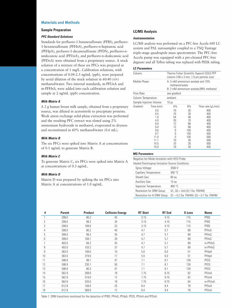
Materials and Methods
Sample Preparation
PFC Standard Solutions
Standards for perfluoro-1-butanesulfonate (PFBS), perfluoro-1-hexanesulfonate (PFHxS), perfluoro-n-heptanoic acid(PFHpA), perfuoro-1-decanesulfonate (PFDS), perfluoro-n-undecanoic acid (PFUnA), and perfluoro-n-dodecanoic acid(PFDoA) were obtained from a proprietary source. A stocksolution of a mixture of these six PFCs was prepared ata concentration of 1 mg/L. Calibration solutions, withconcentrations of 0.04-2.5 ng/mL (ppb), were preparedby serial dilution of the stock solution in 60:40 (v/v)methanol/water. Two internal standards, m-PFUnA andm-PFHxS, were added into each calibration solution andsample at 2 ng/mL (ppb) concentration.
Milk Matrix A
A 2 g human breast milk sample, obtained from a proprietarysource, was diluted in acetonitrile to precipitate proteins.Weak anion exchange solid-phase extraction was performedand the resulting PFC extract was eluted using 2%ammonium hydroxide in methanol, evaporated to drynessand reconstituted in 60% methanol/water (0.6 mL).
Milk Matrix B
The six PFCs were spiked into Matrix A at concentrationsof 0.1 ng/mL to generate Matrix B.
Milk Matrix C
To generate Matrix C, six PFCs were spiked into Matrix Aat concentrations of 0.3 ng/mL.
Milk Matrix D
Matrix D was prepared by spiking the six PFCs intoMatrix A at concentrations of 1.0 ng/mL.
LC/MS Analysis
Instrumentation
LC/MS analysis was performed on a PFC-free Accela 600 LCsystem and PAL autosampler coupled to a TSQ Vantagetriple-stage quadrupole mass spectrometer. The PFC-freeAccela pump was equipped with a pre-cleaned PFC-freedegasser and all Teflon tubing was replaced with PEEK tubing.
LC ParametersColumn: Thermo Fisher Scientific Hypersil GOLD PFP
column (100 x 3 mm, 1.9 µm particle size) Mobile Phase: A: 5 mM ammonium acetate and 10%
methanol/waterB: 2 mM ammonium acetate/99% methanol
Flow Rate: see gradient Column Temperature: ambientSample Injection Volume: 10 µLGradient: Time (min) A% B% Flow rate (µL/min)
0.0 70 30 4000.5 70 30 4001.0 54 46 4004.0 30 70 4009.0 12 88 4009.4 12 88 4009.6 0 100 4009.7 0 100 500
11.0 0 100 50011.1 70 30 50014.5 70 30 50015.0 70 30 400
MS Parameters
Negative Ion Mode Ionization with HESI Probe Heated Electrospray Ionization Source Conditions:
Spray Voltage: 3500 V Capillary Temperature: 300 °CSheath Gas: 60 auAuxiliary Gas: 15 auVaporizer Temperature: 400 °CResolution for SRM Setup: Q1, Q3 = Unit [0.7 Da. FWHM]Resolution for H-SRM Setup: Q1 = 0.2 Da. FWHM; Q3 = 0.7 Da. FWHM
# Parent Product Collision Energy RT Start RT End S-Lens Name1 299.0 80.2 43 3.15 4.15 115 PFBS2 299.0 99.2 34 3.15 4.15 115 PFBS3 299.0 169.0 23 3.15 4.15 115 PFBS4 399.0 80.2 45 4.7 5.7 89 PFHxS5 399.0 99.2 35 4.7 5.7 89 PFHxS6 399.0 169.1 29 4.7 5.7 89 PFHxS7 403.0 84.2 43 4.7 5.7 89 m-PFHxS8 403.0 103.2 37 4.7 5.7 89 m-PFHxS9 363.0 169.0 10 5.0 6.0 51 PFHpA
10 363.0 319.0 17 5.0 6.0 51 PFHpA11 598.9 99.1 47 7.1 8.1 128 PFDS12 598.9 230.1 50 7.1 8.1 128 PFDS13 598.9 80.3 47 7.1 8.1 128 PFDS14 562.9 269.0 18 7.75 8.75 62 PFUnA15 562.9 519.0 12 7.75 8.75 62 PFUnA16 564.9 520.0 18 7.75 8.75 64 m-PFUnA17 612.9 169.0 25 8.4 9.4 78 PFDoA18 612.9 569.0 12 8.4 9.4 78 PFDoA
Table 1: SRM transitions monitored for the detection of PFBS, PFHxS, PFHpA, PFDS, PFUnA and PFDoA.

Results and Discussion
Separation of PFC Standards
A total of fifteen unique SRM transitions were monitoredfor PFBS, PFHxS, PFHpA, PFDS, PFUnA and PFDoA, andthree were monitored for the internal standards m-PFHxSand m-PFUnA (Table 1). Using the modified PFC-free LC-MSplatform, a mixture of the six PFC standards was separatedand detected under 10 minutes (Figure 1). All of thecompounds were baseline resolved with the elution order ofPFBS, PFHxS (m-PFHxS), PFHpA, PFDS, PFUnA (m-PFUnA)and PFDoA. As the majority of interferences from matriceselute early at void volume, elution of the first compoundat 3.64 min ensured a robust quantitation method.
Linearity and Sensitivity
Excellent linearity in detector response was observed overthe range of 0.04-2.5 ppb, with correlation coefficientsgreater than 0.999 for all transitions. Representativecalibration curves for PFBS and PFUnA, obtained usingthe internal standard method, are shown in Figure 2, with coefficients of 0.9997 and 0.9996 respectively.
The sensitivity of the method is dependent on thelevels of interferences that are present in the blank and inthe solvents used. Limits of detection (LODs) and limits ofquantitation (LODs), defined as S/N ratio of 3 and 10,respectively, are shown in Table 2. LODs ranged from 2–174 ppt, and LOQs ranged from 5–756 ppt. PFBS and PFDS were detectable at 2 ppt and quantifiable at 5 ppt. Figure 3 shows the separation and detection of 10 ppt PFBS and 10 ppt PFDS at different SRM transitions,and the corresponding blanks as comparisons. The higherLOD and LOQ values observed for PFHpA, PFUnA andPFDoA may be attributed to interferences present in theblank and mobile phases.
Figure 1: Separation and detection of six PFC standards at 2.5 ppb concentrations.
Compounds SRM LOD (ppt) LOQ (ppt)
PFBS 298.9 > 80.2 2 5 SRM298.9 > 99.2 5 12 SRM
PFHxS 398.9 > 80.2 21 83 SRM398.9 > 99.2 12 66 SRM
PFHpA 362.9 > 169.0 174 756 SRM Blank Contamination
362.9 > 319.0 120 457 SRM Blank ContaminationPFDS 598.9 > 80.2 2 7 SRM
598.9 > 99.2 3 9 SRMPFUnA 562.9 > 269.0 35 156 SRM
562.9 > 519.0 52 235 SRMPFDoA 612.9 > 169.0 59 296 SRM
612.9 > 569.0 64 295 H-SRM
Table 2: LODs and LOQs of the PFC standards. LOQs were estimated from triplicate injections (CV < 15%)of standard solutions at concentration levels corresponding to a signal-to-noise ratio of 10.
Figure 2: Representative calibration curves of PFBS and PFUnA standards.

Figure 4: H-SRM eliminates interference peakswithout any change in signal intensity.
Significant background interferencewas observed for the SRM transition613 > 569 of PFDoA at Q1 resolutionof 0.7 Da. FWHM, therefore H-SRMwas employed. As shown in Figure 4,using the higher Q1 resolution of 0.2 Da. FWHM removed the matrixinterference without compromisingsensitivity. Moreover, sensitive andunambiguous PFC detection wasachieved without the use of in-linetrapping or column switching.
Figure 3. Separation and detectionof 10 ppt of PFBA and PFDS.

Analysis of PFCs in Human Milk Matrix
To evaluate the applicability of this technique to complexmatrices, the SRM assays were used to analyze andquantitate PFCs in human breast milk. UHPLC separationof the six PFC analytes in a spiked milk matrix wasachieved within 9 minutes (Figure 5). All analytes werebaseline resolved using the optimized LC method.
Reproducibility was investigated by analyzing fifteenreplicate injections of a spiked matrix (Table 3). Peakarea RSDs for compounds and internal standards were10.8% and 11.0% respectively, the response ratio RSDwas 1.29%, and retention time RSD was 0.29%,indicating excellent method and system reproducibility,particularly of the LC pump.
Table 4 summarizes the concentrations of the PFCsdetected in a human milk sample (Matrix A). PFBS,PFHxS, PFHpA, PFDS, and PFUnA were detected atconcentrations of less than 60 ppt, while PFDoA was not found to be present in the sample. Assay accuracywas investigated using spiked milk matrices B, C, and Dand internal and external standards (Table 3). For PFHxSand PFUnA, the two PFCs for which internal standardswere available, using the internal standard method wassignificantly more accurate (98–110%) than the externalstandard method (81–144%) in the concentration range0.1–1.0 ng/mL. While internal standards eliminate thematrix effect to facilitate greater quantitative accuracy,they are expensive and may be difficult to obtain. Using the external standard method, the accuracy of all PFC analytes was 81–144% in the concentrationrange 0.1–1.0 ng/mL.
File Peak ISTD Response RTName Area Area Ratio (Min)
Mark D_0 17 149 369 8 268 9 1.806 8.29Mark D_0 18 147 075 8 081 9 1.820 8.27Mark D_0 19 145 882 8 127 6 1.795 8.29Mark D_0 20 146 012 7 990 7 1.827 8.29Mark D_0 21 143 987 8 071 2 1.784 8.27Mark D_0 22 143 095 8 011 6 1.786 8.25Mark D_0 23 140 298 7 802 3 1.798 8.25Mark D_0 67 121 597 6 929 2 1.755 8.25Mark D_0 68 119 763 6 776 4 1.767 8.29Mark D_0 69 119 149 6 654 3 1.791 8.27Mark D_0 70 121 775 6 647 6 1.832 8.32Mark D_0 71 113 885 6 376 6 1.786 8.27Mark D_0 72 115 138 6 271 2 1.836 8.31Mark D_0 73 116 884 6 561 6 1.781 8.24Mark D_0 74 114 601 6 358 6 1.802 8.31
RSD% 11 10.8 1.29 0.29
Table 3: Reproducibility (RSD) of instrument performance for fifteen replicateinjections of Matrix D. Peak area is the LC peak area response for fifteeninjections. Peak area was used for quantitation, both for the internal standardmethod and external standard method. ISTD area = peak area of the internalstandard. Response ratio is the peak area of the compounds over the peakarea of the internal standard, and was used for quantitation with theinternal standard method. RT = retention time.
PFBS PFHxS PFHpA PFDS PFUnA PFDoA
Matrix A (unknown) Measured value with IS (ppt) 48.0 12.0Measured value with ES (ppt) 10.0 40.0 50.0 50.0 35.0 0.0
Matrix B (Matrix A + spiked 100 ppt) Measured value with IS (ppt) 152 115Measured value with ES (ppt) 110 145 185 150 195 130Method Accuracy with IS (%) 103 103Method Accuracy with ES (%) 100 104 123 100 144 130
Matrix C (Matrix A + spiked 300 ppt) Measured value with IS (ppt) 382 340Measured value with ES (ppt) 260 290 365 285 420 280Method Accuracy with IS (%) 110 109Method Accuracy with ES (%) 84 85 104 81 125 93
Matrix D (Matrix A + spiked 1000 ppt) Measured value with IS (ppt) 1023 1042Measured value with ES (ppt) 930 945 1255 935 1495 985Method Accuracy with IS (%) 98 103Method Accuracy with ES (%) 92 91 120 89 144 99
Table 4: PFC concentrations (ppt) in human milk matrix A and spiked milk matrices B, C, and D. Note: The method accuracy was calculated with the formulaof 100 x measure value/(measure value of Matrix A + spiked value).
Figure 5: The separation and detection of the PFCs in human milk matries C

In addition to these
offices, Thermo Fisher
Scientific maintains
a network of represen -
tative organizations
throughout the world.
Africa-Other+27 11 570 1840Australia+61 3 9757 4300Austria+43 1 333 50 34 0Belgium+32 53 73 42 41Canada+1 800 530 8447China+86 10 8419 3588Denmark+45 70 23 62 60Europe-Other+43 1 333 50 34 0Finland / Norway /Sweden+46 8 556 468 00France+33 1 60 92 48 00Germany+49 6103 408 1014India+91 22 6742 9434Italy+39 02 950 591Japan+81 45 453 9100Latin America+1 561 688 8700Middle East+43 1 333 50 34 0Netherlands+31 76 579 55 55New Zealand+64 9 980 6700South Africa+27 11 570 1840Spain+34 914 845 965Switzerland+41 61 716 77 00UK+44 1442 233555USA+1 800 532 4752
Part of Thermo Fisher Scientific
AN51936_E 08/16M
www.thermofisher.comLegal Notices: ©2016 Thermo Fisher Scientific Inc. All rights reserved. Teflon is a registered trademark of E.I. du Pont de Nemours and Company. All other trademarks are the property of Thermo Fisher Scientific Inc. and its subsidiaries. This information is presented as an example of the capabilities of Thermo Fisher Scientific Inc. products. It is not intended to encourage use of these products in any manners that might infringe the intellectual property rights of others. Specifications, terms and pricing are subject to change. Not all products are available in all countries. Please consult your local sales representative for details.
Conclusion
A highly sensitive, accurate and robust SRM-based approachfor PFC analysis was developed on a PFC-free Accela-TSQVantage LC-MS platform. PFCs were accurately andreproducibly detected at ppt levels in neat solution and in human milk. The unique H-SRM capability of the TSQ Vantage instrument removed interference peaks andsignificantly improved selectivity. Furthermore, unlikeother approaches, this platform does not require trappingor column switching techniques to ensure exceptionalsensitivity in high chemical backgrounds.
References1. http://www.epa.gov/oppt/pfoa/
2. http://www.epa.gov/heasd/regulatory/projects/d1b_right_to_know.html
3. Tao, L.; Kannan, K.; Wong, C.M.; Arcaro, K. F.; Butenhoff, J.L.Perfluorinated compounds in human milk from Massachusetts, U.S.A.Environ Sci Technol. 2008 42, 3096-101.

Determination of PCDD/Fs in Environmental Samples using Accelerated Solvent Extraction (ASE) and GC-MS/MSPaul Silcock,1 David Gardner,2 John Fardon,2 Steve Moss2 and Inge de Dobbeleer1 1Thermo Scientific POPs Centre of Excellence, Bremen, Germany2National Laboratory Service - Environment Agency, Leeds, United Kingdom
Ap
plica
tion
No
te 1
03
36
Key WordsDioxins, furans, PCDD, PCDF, environmental, fly ash, sediments, complex matrix, accelerated solvent extraction, isotope dilution, pressurized solvent extraction
IntroductionThe measurement of PCDD/Fs in the environment is a widespread activity carried out by many regulatory agencies globally. The chronic toxicity of these compounds to humans and wildlife at extremely low concentrations requires that the techniques used in determination must be both sensitive and selective enough to allow high confidence results. This is especially true when measuring background levels in environmental matrices, such as soil and sediment or byproducts from waste incineration processes. Traditionally high resolution magnetic sector GC-MS (GC-HRMS) instrumentation has delivered the required analytical performance and has become the gold standard technique. In recent years, there has been more interest in GC triple-quadrupole instrumentation for this purpose, especially in the area of food safety control.1,2 For this area and environmental analysis, it is necessary to deliver data that performs in the range of HRMS systems, which requires especially sensitive triple-quadrupole systems. It is also necessary to incorporate data-processing software specifically designed to handle the complex calculations associated with dioxins analysis.
This application note describes the use of the Thermo Scientific™ TSQ Quantum™ XLS Ultra GC-MS/MS as applied to the analysis of PCDDs/PCDFs in sediments, soils, bottom, and fly ash (as incineration by-products) at the levels of interest and the level of agreement with “gold standard” analysis using GC-HRMS.
During this study, instrumental LOQs using GC-MS/MS were calculated in the low fg/µL concentration ranges. This, along with further analytical performance, is discussed alongside GC-HRMS; especially the degree of agreement between the techniques in some routine sample batches.
Materials and MethodsExtraction and CleanupThe standard spiking protocols, extraction, and cleanup process for all sediment and soil samples were performed using an ISO17025 accredited in-house variation of EPA 1613B3. For incinerator ash samples, an in-house method based upon EN 19484 was applied.
For both of these methods, accelerated solvent extraction was used as the preferred technique for extraction after initial sample processing. This is routinely used in the laboratory to reduce solvent consumption, allow for automation, and to generate efficient sample extractions within the performance limits required.

2 Accelerated Solvent Extraction MethodsASE cells were loaded with a base layer of copper filings then a layer of rinsed Ottawa sand (previously ashed at 450 °C) after which 5 g of sample for soils/sediments (1 g for fly ash). Finally, another layer of sand was added to fill the cell and then extracted (Figure 1).
Figure 1. Cell schematic and method conditions for the extraction of PCDD/Fs from soil, sediment, and fly ash samples.
Table 1. GC and injector conditions.
Table 2. Mass spectrometer parameters.
GC-MS Measurement & Data ProcessingThe GC-MS/MS measurements were performed using a Thermo Scientific™ TRACE™ GC Ultra coupled to a TSQ Quantum XLS Ultra GC-MS/MS system with quantitation performed using Thermo Scientific TargetQuan 3 software. Tables 1 and 2 show the instrument parameters used.
Split/Splitless Injector (PCDD/Fs)
Injection Temperature 260 °C
LinerSplitless straight liner (Siltek) 3 × 8 × 105 mm (PN 453T2121)
Injected Volume 2 µL (toluene)
Splitless Time 1.5 min
Surge Pressure 22 psi (1 min)
GC Program
GC ColumnTraceGOLD TG-5SilMS 60m × 0.25mm × 0.25um (PN 26096-1540)
GC Column Flow 1.2 mL/min constant
Initial Temperature 120 °C
Rate 1 18 °C/min to 200 °C (10 min)
Rate 2 4 °C/min to 290 °C
Final Temperature 290 °C for 15 min
Parameters
Source Temperature 250 °C
Ionization EI
Electron Energy 40 eV
Emission Current 50 µA
Q2 Gas Pressure (Argon) 1.5 mTorr
Collision Energy 22 eV
Q1 Peak Width FWHM 0.7 Da
Q3 Peak Width FWHM 0.7 Da
Extraction Solvent: TolueneExtraction Pressure: 1500 psiOven Temperature: 175 ˚CHeating Time: 8 minutesStatic Time: 5 minutesFlush: 60 % Cell volumePurge: N2 240 Seconds
Ottawa sand
Ottawa sand
Soil/sediment/fly ash
Copper filings
Toluene flow during extraction

3
Table 3. Target congener groups SRM transitions.
The collision cell (Q2) gas pressure and collision energy were optimized for PCDD/F measurement at 22 eV. The monitored selected reaction monitoring (SRM) transitions as well as the MS conditions are given below in Table 3.
Compound Name Abrev. Formula Nominal Mass
Exact Mass
Presursor Ion m/z
Product Ion m/z
Collision Energy [ev]
Tetrachloro-dibenzodioxin TCDD C12
H4O
2Cl
4320 319.8965 319.90 256.93 22
321.89 258.93 22
Pentachloro-dibenzodioxin PeCDD C12
H3O
2Cl
5354 353.8576 355.85 292.89 22
357.85 294.89 22
Hexachloro-dibenzodioxin HeCDD C12
H2O
2Cl
6388 387.8186 387.82 324.86 22
389.82 326.85 22
Heptachloro-dibenzodioxin HpCDD C12
H1O
2Cl
7422 421.7796 423.78 360.81 22
425.77 362.81 22
Octachloro-dibenzodioxin OCDD C12
O2Cl
8456 455.7407 457.74 394.77 22
459.74 396.77 22
Tetrachloro-[13C12
]dibenzodioxin TCDD 13C12
H4O2Cl
4332 331.9368 331.94 267.97 22
333.93 269.97 22
Pentachloro-[13C12
]dibenzodioxin PeCDD 13C12
H3O
2Cl
5366 365.8978 367.90 303.93 22
369.89 305.89 22
Hexachloro-[13C12
]dibenzodioxin HeCDD 13C12
H2O
2C
l6400 399.8589 399.86 335.89 22
401.86 337.89 22
Heptachloro-[13C12
]dibenzodioxin HpCDD 13C12
H1O
2Cl
7434 433.8199 435.82 371.85 22
437.81 373.85 22
Octachloro-[13C12
]dibenzodioxin OCDD 13C12
O2Cl
8468 467.7809 469.78 405.81 22
471.78 407.81 22
Tetrachloro-dibenzofuran TCDF C12
H4OCl
4304 303.9016 303.90 240.94 22
305.90 242.94 22
Pentachloro-dibenzofuran PeCDF C12
H3OCl
5338 337.8627 339.86 276.90 22
341.86 278.89 22
Hexachloro-dibenzofuran HeCDF C12
H2OCl
6372 371.8237 371.82 308.86 22
373.82 310.86 22
Heptachloro-dibenzofuran HpCDF C12
H1OCl
7406 405.7847 407.78 344.82 22
409.78 346.82 22
Octachloro-dibenzofuran OCDF C12
OCl8
440 439.7457 441.76 378.80 22
443.76 380.79 22
Tetrachloro-[13C12
]dibenzofuran TCDF 13C12
H4OCl
4316 315.9419 315.94 251.97 22
317.94 253.97 22
Pentachloro-[13C12
]dibenzofuran PeCDF 13C12
H3OCl
5350 349.9029 351.90 287.93 22
353.90 289.93 22
Hexachloro-[13C12
]dibenzofuran HeCDF 13C12
H2OCl
6384 383.8639 383.86 319.90 22
385.86 321.89 22
Heptachloro-[13C12
]dibenzofuran HpCDF 13C12
H1OCl
7418 417.8250 419.82 355.86 22
421.82 357.85 22
Octachloro-[13C12
]dibenzofuran OCDF 13C12
OCl8
452 451.7860 453.78 389.82 22
455.78 391.81 22

4 Results and DiscussionSensitivity for PCDD/F Analysis The prerequisites for a technique to be applicable to low level PCDD/F determinations is sensitivity and selectivity. The concentration levels where these substances are required to be measured often exceed the performance capability of bench-top GC-MS systems. In order to test the sensitivity of the TSQ Quantum XLS Ultra for this application, a serial dilution of commonly used EPA 1613B CS1 standard was performed, and increasingly low levels were injected onto the system. The limit of detection (LOD) was then calculated using statistical methods. Figure 2 shows the lowest level CS1 dilution (x10 – vial concentrations given in Table 4) used for this study. Quantitative SRM ions are clearly detected along with the confirmatory SRM ions for all PCDD/Fs tested within the QC ion ratio criteria. Precision studies at this level enabled an LOD to be calculated for the methodology. Table 4 gives the precision data obtained and calculated LOD at 99 % confidence limits. The LOD obtained from the TSQ Quantum XLS Ultra was found at a level that is highly applicable for environmental dioxins analysis in a range of sample types.
Table 4. Instrumental LOD (pg/µL) given to 2 d.p. (99% confidence) and precision data (n=10) for PCDD/Fs from GC-MS/MS analysis of a ten times diluted EPA 1613 CS1.
Figure 2. SRM chromatograms of PCDD/Fs after injection of a 10x diluted EPA1613B CS1 standard. (TCDD/F 0.05 pg/µL, PeCDD/F thru HpCDD/F 0.25 pg/µL, OCDD/F 0.5 pg/µL)
Concentration pg/µL
RSD %
LOD (99) pg/µL
2,3,7,8 TCDF 0.05 6.2 0.01
2,3,7,8 TCDD 0.05 11.1 0.01
1,2,3,7,8 PeCDF 0.25 6.0 0.03
2,3,4,7,8-PeCDF 0.25 4.6 0.03
1,2,3,7,8 PeCDD 0.25 9.2 0.05
1,2,3,4,7,8-HxCDF 0.25 7.7 0.04
1,2,3,6,7,8-HxCDF 0.25 4.7 0.03
2,3,4,6,7,8-HxCDF 0.25 4.1 0.02
1,2,3,4,7,8-HxCDD 0.25 7.7 0.04
1,2,3,6,7,8-HxCDD 0.25 6.1 0.03
1,2,3,7,8,9-HxCDD 0.25 5.0 0.03
1,2,3,7,8,9-HxCDF 0.25 4.9 0.03
1,2,3,4,6,7,8-HpCDF 0.25 5.2 0.03
1,2,3,4,6,7,8-HpCDD 0.25 6.8 0.04
1,2,3,4,7,8,9-HpCDF 0.25 5.7 0.03
OCDD 0.5 7.9 0.09
OCDF 0.5 4.8 0.05
32.5 33.0 33.5 34.0 34.5 35.0
40.0 41.0 42.0 43.0
36.0 36.5 37.0 37.5 38.0 39.038.5 39.5
100
0100
0100
0100
0
100
0100
0100
0100
044.0 45.0 46.0 47.0 48.0 49.5 50.5 51.5 52.5 53.5
TCDD/F
HxCDD/F HpCDD/F
PeCDD/F
OCDD/F
Minutes Minutes Minutes
RT: 46.79
RT: 32.70
303.90 > 240.94
305.90 > 242.94
331.94 > 267.97
333.93 > 269.97
371.82 > 308.86
373.82 > 310.86
387.82 > 324.86
389.82 > 326.85
351.90 > 287.93
353.90 > 289.93
367.90 > 303.93
369.89 > 305.89
407.78 > 344.82 441.76 > 378.80
443.76 > 380.79
457.74 > 394.77
459.74 > 396.77
409.78 > 346.82
423.78 > 360.81
425.77 > 362.81
RT: 32.70
RT: 33.31
RT: 33.31
RT: 36.37 RT: 37.30
RT: 36.67
RT: 36.63
RT: 37.30
RT: 37.59
RT: 37.59
RT: 40.29RT: 41.08 RT: 42.15
RT: 40.44 RT: 41.08 RT: 42.16
RT: 41.27RT: 41.72
RT: 41.38RT: 41.72
RT: 44.17
RT: 44.17RT: 46.79
RT: 45.88
RT: 45.88
RT: 52.05
RT: 52.04
RT: 51.65
RT: 51.66

5
Figure 3. Mean GC-MS/MS results for routine laboratory QC samples for the in-house PCDD/Fs method over 3 routine batches of samples. This is plotted as difference to result obtained on the GC-HRMS system.The QCs include a precision and recovery standard (PAR), Incinerator fly ash certified reference material (CRM 490) and a sediment certified reference material (SETOC 738).
Quality Control in Routine Sample BatchesTo evaluate the quantitative performance of the TSQ Quantum XLS Ultra when applied to analytical quality control samples, data was taken and compared with that obtained on currently implemented GC-HRMS systems (see Figure 3). These quality control samples included certified reference materials (CRMs) for sediments SETOC 738 and CRM 490 incinerator fly ash. These were all processed through the entire method procedure which included accelerated sample extraction. All of the compound recovery QC criteria specified in EPA 1613 and EN1948 were satisfied. This gave confidence that the extraction yielded high recoveries throughout the study.
CRM 490 is a highly contaminated incinerator fly ash. This type of sample and level of contamination allows for a great opportunity for interference to occur. The MS/MS system measured consistently higher concentrations for TCDD/F and some penta and hexa furans. This was indeed closer to the true CRM consensus value, so the QC check passed.
SETOC 738 is a sediment CRM sample that is much lower level CRM and had good agreement in the calculated concentrations between the GC-MS/MS and HRMS data.
The GC-MS/MS data on these three types of QC sample all fell within acceptable performance limits for the current methodology suggesting that the selectivity and quantitative performance of the technique is applicable for reporting PCDD/F data in the routine environmental lab.
% D
eviat
ion
from
HRM
S Re
sult
50
0
-50
2378
-TCDF
2378
-TCDD
1237
8-PeC
DF
2347
8-PeC
DF
1237
8-PeC
DD
1234
78-H
xCDF
1236
78-H
xCDF
2346
78-H
xCDD
1234
78-H
xCDD
1236
78-H
xCDD
1237
89-H
xCDD
1237
89-H
xCDF
1234
678-H
pCDF
1234
678-H
pCDD
1234
789-H
pCDF
OCDDOCDF
Par CRM 490 SETOC 738

6
Table 5. Calculated concentrations of TCDD/F congeners in soil and sediment samples run on both GC-MS/MS and GC-HRMS. (ND=not detected)
Soil Sediment 1 Sediment 2 SETOC 738 (CRM
GC-MS/MS ng/kg
GC-HRMS ng/kg
GC-MS/MS ng/kg
GC-HRMS ng/kg
GC-MS/MS ng/kg
GC-HRMS ng/kg
GC-MS/MS ng/kg
GC-HRMS ng/kg
2,3,7,8 TCDF 0.992 1.23 16.0 10.4 2.15 1.51 17.9 17.1
2,3,7,8 TCDD ND ND 1.85 2.29 2.03 5.10 23.1 23.9
1,2,3,7,8 PeCDF 1.26 <1.79 25.4 25.4 4.90 4.52 7.36 6.76
2,3,4,7, 8 PeCDF 1.57 1.96 41.5 44.2 10.7 9.29 47.8 45.4
1,2,3,7,8, PeCDD 0.436 ND 5.49 5.71 9.14 7.95 7.26 6.91
1,2,3,4,7,8,-HxCDF 1.89 1.89 56.1 57.3 64.8 71.9 43.8 45.1
1,2,3,6,7,8,-HxCDF 1.81 2.14 64.8 55.0 223 197 15.1 14.7
2,3,4,6,7,8,-HxCDF 2.53 2.83 86.9 91.5 9.47 11.5 20.2 18.4
1,2,3,4,7,8,-HxCDD 0.271 ND 5.38 6.34 15.0 10.9 10.4 8.62
1,2,3,6,7,8,-HxCDD 0.382 0.905 8.33 8.58 17.6 16.7 28.1 20.1
1,2,3,7,8,9-HxCDD 0.469 ND 6.62 6.97 17.5 14.0 21.4 22.4
1,2,3,7,8,9-HxCDF 0.932 ND 25.8 31.4 15.2 13.4 4.65 5.40
1,2,3,4,6,7,8-HpCDF 12.9 14.2 464 473 5.05 4.58 214 202
1,2,3,4,6,7,8-HpCDD 4.80 5.78 63.4 62.2 18.3 16.6 416 433
1,2,3,4,7,8,9-HpCDF 1.90 3.07 48.8 48.8 68.3 54.4 15.1 15.4
OCDD 24.7 23.8 153 191 6.38 5.38 3020 3030
OCDF 258 291 475 554 47.7 39.5 290 316
Figure 4. TCDD SRM chromatograms for three different sample types typically analyzed in the environmental laboratory. Left: Fly ash (2,3,7,8-TCDD 31.4 ng/kg), Center: Contaminated soil (2,3,7,8-TCDD 1.85 ng/kg), Right: Contaminated sediment (2,3,7,8-TCDD 17.9 ng/kg).
Routine SamplesThe QC performance was reflected in the real sample batches with generally very good agreement in results between the GC-MS/MS and GC-HRMS approach. Larger deviations in calculated value were reported for incinerator fly ash samples, particularly for the lower chlorinated PCDFs. These differences are thought to arise from selectivity differences in the two techniques. The GC-MS/MS result remained valid within the quality control criteria specified within the methodology. SRM chromatograms for TCDDs in three different routine environmental sample types are given in Figure 4. These include both quantifying and confirming SRM transitions. The selective detection of the highly significant 2,3,7,8-TCDD congener was achievable in all samples.
Calculated concentrations for each congener are given in Table 5 for both the GC-MS/MS and GC-HRMS analyses for routine soil, sediment, and a matrix QC sample. Again, these show a good level of agreement in the calculated result. For the soil samples, the TSQ Quantum XLS Ultra showed confirmed detections of PCDD/Fs for the low concentration samples when no result was reported from GC-HRMS. This was due to the lower performance of the GC-HRMS system used in this study and not directly related the more sensitive systems available today.
Relat
ive A
bund
ance
Relat
ive A
bund
ance
Minutes Minutes Minutes
100
0
100
032.0 32.5 33.0 33.5 32.0 32.5 33.0 33.5 32.0 32.5 33.0 33.5
321.89 > 258.93 321.89 > 258.93 321.89 > 258.93Fly Ash Contaminated Soil Contaminated Sediment
319.90 > 256.93 319.90 > 256.93 319.90 > 256.93
2,3,7,8-TCDDRT: 33.31
2,3,7,8-TCDDRT: 33.31
2,3,7,8-TCDDRT: 33.31
32.0233.09
RT: 32.16
RT: 33.31RT: 32.02
RT: 32.15 RT: 33.11
RT: 33.11
RT: 33.54
RT: 33.11
RT: 33.36

Africa-Other +27 11 570 1840Australia +61 3 9757 4300Austria +43 1 333 50 34 0Belgium +32 53 73 42 41Canada +1 800 530 8447China +86 10 8419 3588Denmark +45 70 23 62 60
Europe-Other +43 1 333 50 34 0Finland/Norway/Sweden
+46 8 556 468 00France +33 1 60 92 48 00Germany +49 6103 408 1014India +91 22 6742 9434Italy +39 02 950 591
Japan +81 45 453 9100Latin America +1 561 688 8700Middle East +43 1 333 50 34 0Netherlands +31 76 579 55 55New Zealand +64 9 980 6700Russia/CIS +43 1 333 50 34 0South Africa +27 11 570 1840
Spain +34 914 845 965Switzerland +41 61 716 77 00UK +44 1442 233555USA +1 800 532 4752
www.thermofisher.com©2016 Thermo Fisher Scientific Inc. All rights reserved. All trademarks are the property of Thermo Fisher Scientific Inc. and its subsidiaries. Specifications, terms and pricing are subject to change. Not all products are available in all countries. Please consult your local sales representative for details.
Ap
plica
tion
No
te 1
03
36
AN10336_E 08/16S
Conclusion• TheTSQQuantumXLSUltraGC-MS/MSisahighly
sensitive and selective system applicable to dioxinsand furans analysis in a range of environmental sampletypes and generates results that perform within currentin-house QC criteria.
• Somedifferencesariseinthecalculatedconcentrationbetween the GC-MS/MS and GC-HRMS analysis.These are thought to be related to the differences in theselectivity mechanism of each system.
• GC-MS/MSappliedtoPCDD/Fsstillallowsforfullisotope dilution quantitation as currently used byGC-HRMS systems. TargetQuan 3 software can beused with the TSQ Quantum XLS Ultra to providethe specific calculations required.
• TheThermoScientific™ Dionex™ ASE™ AcceleratedSolvent Extractor system allows for unattended,efficient extractions from all samples and enabledrecoveries well within QC criteria.
References1. Ingelido, A. M.; Brambilla, G.; Abballe, A.;
di Domenico, A.; Fulgenzi, A. R.; Iacovela, N.; Lamiceli,L.; Valentini, S.; De Felip, E. Rapid Commun. MassSpectrom. 2012, 26(3), 236–242.
2. Kotz, A.;, Malisch, R.; Wahl, K.; Bitomsky, N.;Adamovic, K.; Gerteisen, I.; Leswal, S.; Schächtele, J.;Tritschler, R.; Winterhalter, H. Organohalogen Compd.2011, 73, 688–691.
3. Silcock, P.; Krumwiede, D.; de Dobbeleer, I.;Huebschmann, H. J.; Kotz, A. 2011, ThermoScientific Application Note 52266.

Marine Toxins
Surface, Drinking and Waste Water Analysis
Ap
plica
tion
No
teb
oo
k

Comprehensive Solutions for Screening, Quantitation and Discovery of Marine Biotoxins and Their Metabolites in ShellfishMichal Godula, Thermo Fisher Scientific, Prague, Czech Republic
Wh
ite Pap
er 64
018
Executive SummaryIn recent years, many countries have had to deal with the negative effects of toxic microalgal blooms in both marine and fresh water, such as the death of wild animals and domestic livestock. The food most frequently involved in episodes of human poisoning are bivalve mollusks. As they filter large quantities of water for tropical reasons, these shellfish can accumulate and concentrate biotoxins present in the plankton they ingest.
There are a series of regulations issued by the regulatory agencies concerning the control of lipophilic toxins in bivalve mollusks destined to market for human consumption. In the past, bioassays on mice were predominantly used. However, liquid chromatography coupled with mass spectrometry (LC-MS) presents a viable alternative for today’s analysts.
The purpose of this document is to describe possible alternatives for comprehensive analysis of marine biotoxins in various samples, applying LC-MS based on either a triple quadrupole mass spectrometer or a high-resolution accurate-mass mass spectrometer.
IntroductionIn recent years, many countries have had to deal with the negative effects of toxic microalgal blooms in both marine and fresh water, such as the death of wild animals and domestic livestock. Several cases of poisoning in humans have been associated with the direct consumption of shellfish, fish or water contaminated by algal toxins. People may also come into contact with toxins during recreational activities along sea coasts that are affected by episodes of algal blooms. Depending on the type of toxin involved, there are forms of mild and usually self-limiting symptoms, characterized by gastrointestinal disorders or allergy-like episodes. Much more severe neurological symptoms can lead to death of the affected person.
The foods most frequently involved in human poisoning are bivalve mollusks. When filtering large quantities of water for tropical reasons, these shellfish can accumulate and concentrate the biotoxins present in the plankton they ingest. Moreover, it is not possible to evaluate their edibility only by an organoleptic examination. While human ingestion of contaminated food with biotoxins can lead to the onset of different clinical symptoms, in shellfish they usually have only marginal effects. An important risk factor lies in the thermostability of such molecules, which are not completely inactivated by common physical treatments carried out on fish products (cooking, smoking, salting, freezing, housing) and remain virtually unchanged in the finished product.
KeywordsMarine Biotoxins, Exactive Plus, Orbitrap, Triple Quadrupole MS/MS, UHPLC
2 There are a series of regulations issued by the European Union (EU) related to marine biotoxins. Regulation (EC) No 853/20041 concerns the control of lipophilic toxins, establishing maximum levels for lipophilic toxins in bivalve mollusks destined to the market for human consumption:
• For okadaic acid, dinophysistoxins and pectenotoxins together, 160 micrograms of okadaicacid equivalent per kilogram
• For yessotoxin, 1 milligram of yessotoxin equivalent per kilogram
• For azaspiracids, 160 micrograms of azaspiracids equivalent per kilogram
In the past, aside from bioassays on mice, most analytical techniques developed for the determina-tion of marine biotoxins in bivalve mollusks have been based on offline methodologies, i.e. methods involving solid phase extraction (SPE) or liquid-liquid extraction (LLE) followed by high-pressure liquid chromatography (HPLC) with fluorometric or UV-diode array detection, or detection by liquid chromatography coupled with mass spectrometry (LC-MS).
The EU Commission Regulation (EC) No 15/2011,2 amending Regulation (EC) No 2074/2005 about the testing methods for detecting marine biotoxins in bivalve molluscs, describes an LC-MS/MS procedure as the reference method for the quantification of lipophilic marine biotoxins, namely okadaic acid, pectenotoxin 2, azaspiracid 1, and yessotoxin. Moreover, dinophysistoxin 1 (DTX-1) and dinophysistoxin 2 (DTX-2) can be quantified by the calibration curve of okadaic acid, pectenotoxin 1 by the calibration of pectenotoxin 2, azaspiracid 2 and 3 by the calibration of azaspiracid 1 and 45-OH-, and 45-homo-OH-yessotoxin by the calibration of yessotoxin.
The purpose of this document is to describe the possible alternatives for analysis of marine biotoxins in various samples, applying LC-MS based either on triple quadrupole or high-resolution accurate-mass (HRAM) mass spectrometry (MS).
From Mouse Bioassay to Techniques of the 21st CenturyBesides the mouse bioassay test, triple quadrupole LC-MS/MS methods have been the most commonly used detection techniques for marine biotoxins, providing high sensitivity and selectivity. However, this technique requires detection of compounds that are pre-selected and fine tuning of system parameters in order to detect low concentrations in complex matrices. Despite the lack of capabilities to screen for larger number of compounds, unknown toxins or new metabolites of known substances, LC and UHPLC-MS/MS have been used successfully in many routine labs.
Recently, HRAM MS has introduced new advantages to residual analysis. Due to the fact the data acquisition is always performed in the full-scan mode, no special parameter setup or tuning for specific compounds is needed. The selectivity and sensitivity of the method is achieved via post-processing of the data using extraction of accurate mass data from the full scan records. By doing so, selectivity comparable to or better than with triple quadrupole LC-MS/MS technology is obtained.3 In addition, post-processing allows for retrospective analysis in order to search for new, emerging toxins or their metabolites. It also helps to eliminate false positive and false negative results by providing additional, confirmatory information.
Several types of mass spectrometers operating at high resolving power and providing accurate mass information have been introduced in the past. The most recent and most advanced instruments are based on the Thermo Scientific™ Orbitrap™ mass analyzer, originally developed by Makarov and colleagues.4 The improvements introduced by Orbitrap technology, such as ease of use, mass axis accuracy and stability, and ultra-high resolving power, have encouraged the adoption of HRAM systems even in routine laboratories.

3Moving to the Next Step Beyond Triple Quadrupole MS/MS QuantitationThe Thermo Scientific Application Note 635525 describes a quick and simple method for biotoxin analysis based on the EURL LC-MS protocol.6 Utilizing offline sample preparation and determination by the Thermo Scientific™ TSQ Quantum Ultra™ triple quadrupole mass spectrometer, the method meets general performance criteria required for the analysis of lipophilic shellfish toxins. The simplicity of the method makes this approach suitable for any routine lab doing the analysis.
Figure 1 documents the selectivity of the method by showing the extracted ion chromatograms for the analyzed compounds at 40 μg/kg levels. As can be seen, the selectivity of the MS/MS mass spectrometer allows easy detection of all compounds at levels required by regulation.
Figure 1. Chromatogram of sample containing 40 ppb of toxins, analyzed by TSQ Quantum Ultra quadrupole LC-MS (Retention Time: 7.44 min – AZA-1; 7.77 min – AZA-2; 6.88 min – AZA-3; 5.69 min – OA; 7.O5 min – DTX-1; 6.06 min – DTX-2; 5.54 min – YTX; 6.28 min – PTX-2).
In general, the utilization of triple quadrupole LC-MS/MS is a viable solution for any lab performing targeted analysis of the well-defined groups of compounds. It is, however, not suitable for the analysis of a broader range of compounds, metabolites or conjugates for which the structural information is not known.
Future Approaches: Accurate Mass DataAs already mentioned, in response to the need for non-targeted methods that can potentially detect unknowns, metabolites or adducts, HRAM has been successfully implemented for screening and quantification in food safety applications. The lower cost, higher mass accuracy, and ease-of-use of modern quadrupole time-of-flight (QTOF) and Orbitrap—based mass spectrometers have made high-resolution systems viable alternatives to triple quadrupole systems for routine analysis. After full-spectrum data acquisition, specificity is typically achieved by extracting narrow mass windows (ie. 2–5 ppm) centered around a list of target analytes. Using this approach, it has been demonstrated that a resolving power of 50,000 or greater is required for correct mass assignments in complex matrices.3

4 The Thermo Scientific Application Note 52154 describes the use of the Thermo Scientific™ Exactive™ Orbitrap mass spectrometer for screening lipophilic marine biotoxins commonly found in shellfish. The method was optimized using a standard mixture of marine biotoxins applied to mussel tissue extract. In summary, shellfish tissue was homogenized repeatedly with a mixture of methanol and water, centrifuged and directly analyzed by an Exactive Orbitrap LC-MS.7 The LC-HRAM method was based on full scan data acquisition at 50,000 FWHM resolving power and alternating polarity that allowed simultaneous detection of both positive and negative ions.
Figure 2. Exactive Orbitrap LC-MS analysis of a mussel tissue extract showing the total ion chromatogram (TIC; top trace) and 5 ppm mass chromatograms for okadaic acid and DTX1 (lower trace).
A similar approach was recently published by Domenech et al 8 in which the Exactive Orbitrap MS coupled to a Thermo Scientific™ Accela™ UHPLC system was used to determine a group of priority shellfish toxins in mussel samples. The researchers performed a detailed study on the application of a high-energy collision cell (HCD) to fragment precursor ions and obtain confirmatory information. The main aim of this study was to develop a method for the quantitative determination of lipophilic marine toxins using high-resolution (50,000 at m/z 200 full width at half maximum – FWHM) and mass accuracy better than 5 ppm. Fragment and isotope ions and ion ratios were studied and evaluated for confirmation purposes. In-depth characterization of full scan and fragmentation spectrum of the main toxins were carried out. Moreover, the performance of the quantification method using HRAM was evaluated in a validation study. Validation parameters such as accuracy (trueness and precision), linearity, calibration curve check, limit of quantification (LOQ) and specificity were established for all the toxins.

5As documented in Figure 3, obtaining both precursor and fragment ion chromatograms allowed scientists to provide enough confirmatory information to comply with EU analytical method quality criteria.9 Additionally, during the study, researchers performed complete validation of the method and documented excellent performance in routine quantitative analysis.
Figure 3. Extracted ion chromatogram of the lipophilic marine toxins, showing (a) diagnostic ions and (b) fragment ions, with an extraction window of 5 ppm..
However, the scope of the HRAM approach reaches far beyond the details discussed above. The acquisition of accurate mass spectra (MS and MS/MS) enables the creation of libraries that could be used for comprehensive toxin screening. As described in the work of Gerssen et al, the data obtained by the Thermo Scientific™ LTQ Orbitrap XL™ hybrid ion trap-Orbitrap mass spectrometer were processed and corresponding spectra were created.10 The library contains information about compound name, accurate mass, mass deviation (<5 ppm), retention time (min) and retention time deviation (<0.2 min). Gerssen also documented a superior level of precision provided by the Orbitrap MS compared to a TOF technique when screening for compounds by using accurate mass. As can be seen in Figure 4, mass error deviation is almost an order of magnitude lower when the Orbitrap MS is used. This drastic difference in results is related to the fact that, when screening for compounds by using accurate mass, usually a data extraction window of +/– 5 ppm is used. High errors observed in TOF data don’t usually allow the application of such a narrow window, which subsequently negatively influences selectivity of TOF instruments.
Figure 4. Mass error observed within a chromatographic peak of AZA1 recorded by Time-of-Flight (ToF) and Orbitrap MS. Reprinted with permission from: Giessen et al. Analytica Chimica Act 685 (2011) 176–185.

6
Business Benefits As summarized above, there are different approaches to the analysis of shellfish toxins in seafood samples. The traditional mouse bioassay has the clear advantage of providing direct toxicological response. However, the need for specific strains of laboratory mice to perform the test, the potential to build a resistance against toxins, and the unavoidable “cruelty” of the method make this approach the method of the past. Analytical scientists have been searching for alternatives and, although mass spectrometry based on targeted triple quadrupole MS/MS is a very sensitive and quantitative technique, it does not deliver the complete answer. The potential risk of missing a toxin due to a targeted approach creates the need for more comprehensive methods.
From this perspective, there are several benefits of using HRAM technology instead of triple quadrupole MS/MS. The ability to perform screening, quantitation and confirmation in one run combined with unequivocal selectivity and required detection limits that can be achieved make HRAM the key approach for future testing. The inherent possibility to search for a theoretically unlimited number of compounds makes the method easy to expand and develop. The unique properties of full scan accurate mass acquisition allow researchers to search for structural ana-logues of most emerging toxins, their metabolites or adducts, many of which may pose toxicologically relevant effects.
An interesting approach that challenges the capabilities of the technique has been presented by Ciminiello et al.11 The group used the LTQ Orbitrap XL MS to identify new types of large molecular weight toxins belonging to groups produced by Ostreopsis ovata. Ovatoxins and palytoxin are compounds with molecular weights of >2000 Da, which makes them very difficult to detect by conventional triple quadrupole mass spectrometers, which usually have a mass range below 2000 Da. Using a linear ion trap combined with an Orbitrap mass analyzer allowed scientists to detect accurate masses of precursors of toxins as well as to perform structural elucidation and provide fragmentation pathways with accurate mass information. This approach allowed them to identify new structural analogues and to quantify those analogues in order to assess the typical profile of O. ovata strain metabolites.
Figure 5. Structure of palytoxin (PLTX) with cleavage and example of mass spectra of palytoxin documenting the high molecular weight nature of the novel types of compounds. Reprinted with permission from: Ciminiello et al; Rapid Commun. Mass Spectrom. 24 (2010) 2735–2744.

WP64018_E 08/16S
www.thermofisher.com©2016 Thermo Fisher Scientific Inc. All rights reserved. All trademarks are the property of Thermo Fisher Scientific, Inc. and its subsidiaries. Specifications, terms and pricing are subject to change. Not all products are available in all countries. Please consult your local sales representative for details.
Africa +43 1 333 50 34 0Australia +61 3 9757 4300Austria +43 810 282 206Belgium +32 53 73 42 41Canada +1 800 530 8447China 800 810 5118 (free call domestic)
400 650 5118
Denmark +45 70 23 62 60Europe-Other +43 1 333 50 34 0Finland +358 9 3291 0200France +33 1 60 92 48 00Germany +49 6103 408 1014India +91 22 6742 9494Italy +39 02 950 591
Japan +81 45 453 9100Latin America +1 561 688 8700Middle East +43 1 333 50 34 0Netherlands +31 76 579 55 55New Zealand +64 9 980 6700Norway +46 8 556 468 00Russia/CIS +43 1 333 50 34 0
Singapore +65 6289 1190Spain +34 914 845 965Sweden +46 8 556 468 00Switzerland +41 61 716 77 00UK +44 1442 233555USA +1 800 532 4752
ConclusionLC-MS is the key technique to be applied in qualitative and quantitative analysis of shellfish toxins in foods.
Triple quadrupole mass spectrometry presents the traditional approach with benefits of affordability, robustness, simplicity and applicability in many routine laboratories.
HRAM MS, especially if performed on instruments using an Orbitrap mass analyzer, presents a state-of-the-art alternative to triple quadrupole MS. The possibility to perform screening, quantitation and confirmation of an almost unlimited number of compounds in one run improves lab throughput and lowers the cost per test. At the same time, the data provided by high resolution instruments allow retrospective analysis.
In the research labs, the possibility to perform complete identification of the new toxins, their analogues or metabolites opens new areas of research. High-quality MS data obtained by novel hybrid Orbitrap mass analyzers such as the Thermo Scientific™ Q Exactive™ Plus mass spectrom-eter or Thermo Scientific™ Orbitrap Fusion™ Tribrid™ mass spectrometer provide scientists a great tool in this very challenging and interesting area of research. The mass accuracy and stability provided by the new generation of instruments along with ultra-high resolving power deliver unprecedented confidence in data quality—compared to triple quadrupole or TOF-based MS systems. The flexibility of both instruments then allows users to collect both quantitative and qualitative data in a single run and to accelerate the delivery of results both in routine and research labs.
Supporting MaterialApplication notes 63552 and 52154
References and Acknowledgements1. European Parliament, Regulation 853/2004/EC, Off. J. Eur. Common. 2004, 139, 55.
2. European Commission, Commission Regulation 15/2011/EC, Off. J. Eur. Common. 2011,279, 5.
3. Kaufmann et al, Analytical Chemical Act 2010, Volume 673, Issue 1, 60-72.
4. A.A. Makarov, ‘Electrostatic Axially Harmonic Orbital Trapping: A High-performanceTechnique of Mass Analysis’, Anal. Chem. 2000, 72, 1156–1162.
5. Application Note 63552: Determination of Lipophilic Marine Biotoxins in Mollusksby LC-MS/MS using Offline Extraction, Thermo Fisher Scientific 2013.
6. European Union Reference Laboratory for Marine Biotoxins, EU-RL-MB SOP 2011,Version 4.
7. Application Note 52154: Non-Targeted Screening of Lipophilic Marine Biotoxins by LiquidChromatography – High-Resolution Mass Spectrometry, Thermo Fisher Scientific 2011.
8. Domenech et al, Journal of Chromatography A 2014, Volume 1328, 16–25.
9. European Commission, 2002/657/EC, Off. J. Eur. Common. 2002, 221.
10. Giessen et al. Analytica Chimica Acta 2011, 685, 176–185.
11. Ciminiello et al; Rapid Commun. Mass Spectrom. 2010, 24, 2735–2744.
Wh
ite Pap
er 64
018

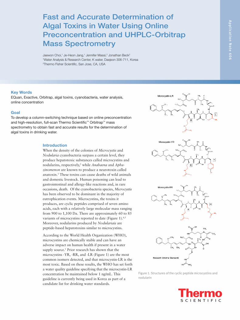
Fast and Accurate Determination of Algal Toxins in Water Using Online Preconcentration and UHPLC-Orbitrap Mass SpectrometryJaewon Choi,1 Je-Heon Jang,1 Jennifer Massi,2 Jonathan Beck2
1Water Analysis & Research Center, K water, Daejeon 306-711, Korea2Thermo Fisher Scientific, San Jose, CA, USA
Ap
plica
tion
No
te 6
06
Key WordsEQuan, Exactive, Orbitrap, algal toxins, cyanobacteria, water analysis, online concentration
GoalTo develop a column-switching technique based on online preconcentration and high-resolution, full-scan Thermo Scientific™ Orbitrap™ mass spectrometry to obtain fast and accurate results for the determination of algal toxins in drinking water.
IntroductionWhen the density of the colonies of Microcystis and Nodularia cyanobacteria surpass a certain level, they produce hepatotoxic substances called microcystins and nodularins, respectively,2 while Anabaena and Apha-zinomenon are known to produce a neurotoxin called anatoxin.3 These toxins can cause deaths of wild animals and domestic livestock. Human poisoning can lead to gastrointestinal and allergy-like reactions and, in rare occasions, death. Of the cyanobacteria species, Microcystis has been observed to be dominant in the majority of eutrophication events. Microcystins, the toxins it produces, are cyclic peptides comprised of seven amino acids, each with a relatively large molecular mass ranging from 900 to 1,100 Da. There are approximately 60 to 85 variants of microcystins reported to date (Figure 1).4,5 Moreover, nodularins produced by Nodulariais are peptide-based hepatotoxins similar to microcystins.
According to the World Health Organization (WHO), microcystins are chemically stable and can have an adverse impact on human health if present in a water supply source.1 Prior research has shown that the microcystins -YR, -RR, and -LR (Figure 1) are the most common isomers detected, and that microcystin-LR is the most toxic. Based on these results, the WHO has set forth a water quality guideline specifying that the microcystin-LR concentration be maintained below 1 ng/mL. This guideline is currently being used in Korea as part of a candidate list for drinking water standards.
Figure 1. Structures of the cyclic peptide microcystins and nodularin

2 In Korea, when an algal bloom is forecasted, samples from the water supply source are collected and the chlorophyll-a concentration and the cyanobacteria cell number are measured. Based on the results, the situation is categorized into one of the following situations: ‘algal bloom watch,’ ‘algal bloom alert,’ or ‘algal bloom.’ In the latter two situations, the cyanotoxins, mainly microcystin-LR, are analyzed.6 Accurate analysis of multiple samples within a short time is required in order to monitor the multiple points of the water supply source and each of the processes taking place at water purification plants.
Traditionally, cyanotoxins have been measured by performing extraction and concentration through solid-phase extraction (SPE) followed by high-performance liquid chromatography with ultraviolet detection (HPLC/UVD) or photodiode array detection. More recently, the analysis time has been reduced and the sensitivity improved through the use of liquid chromatography–mass spectrometry (LC-MS/MS) applying electrospray ionization (ESI).7-13 The conventional SPE process required for all of these methods uses a great deal of time and solvent.
An online preconcentration and injection method can shorten the sample pretreatment process and help detect trace amounts of target substances, while an Orbitrap-type high-resolution mass spectrometry method takes into account the retrospective aspect of data, making possible both accurate identification of the analyzed toxins and post-process quantitation of microcystin isomers. Therefore, we combined these two techniques for the identification and quantitation of microcystin-RR, -YR and -LR as well as nodularin. Then, an optimized method was developed to enhance the reliability and economic efficiency by reducing the run time and the amount of solvent necessary. The method was applied to raw and treated water from water purification plants and river systems.
ExperimentalReagentsMicrocystin-LR, RR, and YR were procured from Wako Pure Chemical Industries, Ltd. (Tokyo, Japan) in a dried crystal form. Nodularin was procured from Cayman Chemical (CA, USA) in a dissolved form (500 μg in 500 μL of ethanol).
Information on each of the standard materials is summarized in Table 1. Solvents were of residual pesticide grade. Water was double distilled by reverse osmosis.
Standard Solutions and Calibration CurvesThe standard solutions containing the cyanotoxins were prepared by dissolving microcystin-LR, -RR, and -YR into methanol at 100 μg/mL and by dissolving nodularin in ethanol to a concentration of 10 μg/mL. Solutions were stored in a cold room at 4 °C. Taking into consideration the sensitivity of the analysis method and the WHO guideline of a microcystin-LR concentration of 1 ng/mL, the solutions were diluted into six different concentrations within the range of 100 to 1000 pg/mL. An external standard method was used for calibration curve verification and sample identification. Then, the ratio of peak areas according to the concentration of standard solution were calculated.
Sample Collection and StorageA total of 173 raw and treated water samples were collected from 59 facilities at the Han (18 sites), Nakdong (18 sites), and Geum-Seomjin (19 sites) Rivers, and in the city of Geoje (4 sites), as well as 55 sites in the Han River basin measurement network area. All samples were refrigerated during transport, transferred directly to a cold room in the lab, and maintained at 4 °C. Sample aliquots were analyzed within three days of delivery.
Pretreatment and Instrumental AnalysisOnline preconcentration using column switching was applied as a means to minimize sample pre-treatment and shorten analysis time. A Thermo Scientific™ EQuan MAX™ online sample concentration UHPLC-MS system equipped with a Thermo Scientific™ Hypersil GOLD aQ™ preconcentration column (20 x 2.1 mm, 12 μm particle size) and a Thermo Scientific™ Hypersil GOLD™ analytical column (50 x 2.1 mm, 1.9 μm particle size) was used. The allowable liquid sample injection range was 1 to 20 mL, and in this study the sample injection amount was set at 1 mL after considering the WHO guideline, equipment sensitivity, peak shape, and concentration ratio of the online injection. The standard material for the calibration curve and all the samples used in the analysis were filtered through a 0.45 μm glass fiber (GF) membrane syringe filter.
A Thermo Scientific™ Exactive™ Orbitrap mass spectrometer was operated in full-scan mode. Resolving power was set to 50,000 (FWHM at m/z 200). The detailed conditions for the online sample concentration and injection and the operation of the Orbitrap mass spectrometer are summarized in Tables 2 and 3, respectively. For the post-analysis identification and quantitation, an external standard method was applied.
Compound Name (CAS) Formula Molecular Weight
Microcystin
Microcystin-LR (101043-37-2)
C49
H67
N10
O12
995.1717
Microcystin-RR (111775-37-4)
C49
H75
N13
O12
1038.1997
Microcystin-YR (101064-48-6)
C52
H72
N10
O13
1045.1873
NodularinNodularin
(118399-22-7)C
41H
60N
8O
10824.9627
Table 1. Chemical formula and molecular weight of target algal toxins

3Table 2. EQuan MAX chromatography conditions used
Table 3. Exactive Orbitrap MS operating conditions
Parameter Setting
Scan range m/z 150–1100
Resolving power 50,000 (FWHM at m/z 200)
Polarity Positive
Measured m/z 995.5543 MC-LR 519.7898 MC-RR 1045.5344 MC-YR 825.4501 Nodularin
Ionization source Electrospray
Spray voltage 4000 V
Capillary temperature 340 °C
Capillary voltage 37 V
Tube lens voltage 85 V
Skimmer voltage 22 V
Results and DiscussionHigh-Resolution Mass Spectra of ToxinsThe standards were prepared at a concentration of 1 ng/mL each and injected using a syringe pump to observe the mass spectra. The molecular ion and carbon isotope spectra of microcystin-LR, -RR, -YR, and nodularin are shown in Figure 2a. Four carbon isotopes were observed for most compounds. Using this isotopic pattern, it was possible to match the experimentally recorded carbon isotopic distribution ratios to the theoretical isotopic ratio to provide confirmation of the toxin using the analysis software. Meanwhile, molecular ions were observed in nodularin at m/z 825 and the isotopic pattern was confirmed (Figure 2b).
Pump 1 Pump 2
Hypersil GOLD aQ (preconcentration column)
Hypersil GOLD (analytical column)
Time %A %B µL/min Time %A %B µL/min
0.00 98 2 1000 0.00 98 2 400
1.01 98 2 1000 1.00 98 2 400
1.20 98 2 100 2.00 2 98 400
3.50 98 2 100 3.50 2 98 400
4.00 98 2 1000 3.51 98 2 400
4.00 98 2 400
Mobile phase A: 0.1% formic acid in water
B: acetonitrile
Mobile phase A: 0.1% formic acid in water
B: acetonitrile
Column temperature: Ambient
Injection volume: 1000 µL

4 A

5
Figure 3. Switching column method for on-line sample injection
From the results of the syringe injection, the quantitation ions for microcystins -LR, -RR, and YR and nodularin were set at 995.5543, 519.7898, 1045.5344, and 825.4501, respectively. In addition, the scanning range for identification and quantitation of the target compounds was between m/z 400 and 1100 for simultaneous analysis. However, the minimum range was set at m/z 150 to allow confirmation and quantitation of various algal toxins, such as anatoxin generated by Anabaena, which occurs just as frequently during an algal bloom.
Optimization of the Online Preconcentration MethodIn this study, 1 mL of each sample was used for the online preconcentration method. During the five minute analysis, adsorption and mobilization of the target toxin and column separation were carried out under the gradient conditions shown in Table 2. First, an injection of 1 mL of sample when the 0.1% formic acid and water/acetonitrile ratio was 98:2 led to the target toxin being adsorbed in the front part of the trap column and the remainder of the water sample being diverted to waste. The valve was then switched to postion 2 for elution from the SPE column onto the analytical column using 98% acetonitrile. A summary of the analysis flow, including online SPE, is shown in Figure 3.
Figure 2. A) Carbon isotope patterns by high-resolution, full-scan MS of microcystins and nodularin, and B) simulated spectrum of nodularin (top) compared to actual spectrum (bottom), confirming isotope pattern.
B

6
0.8 hours for instrumental analysis with the application of UHPLC, and the same amount of time for data analysis and quantitation, for a total of 2 hours. This is an 80% time savings. Other benefits of using this rapid pretreatment method include enhanced productivity when there is a large amount of sample, reduced use of organic solvents, reduced labor for the pretreatment process, and omission of a nitrogen concentration apparatus.
Calibration Curve AssessmentTo review the linearity, the calibration curve of the standard toxin mixture of microcystin -LR, -RR, and -YR and nodularin was measured repeatedly within the range 100 to 1,000 pg/mL. As shown in Figure 5, the correlation coefficient for each of the toxins was between 0.9971 and 0.9996. Reproducibility was ±15%. This is an improvement compared to the quantitation range for algal toxins in the water quality test samples reported.13 Also, it was deemed possible to perform a linearity assessment at lower concentrations if necessary in the future since the signal-to-noise ratio (S/N) was sufficient at the minimum concentration of 0.1 ng/mL. Thus, based on these results, we determined that the online preconcentration high-resolution full-scan MS method has the equivalent trace quantitation capacity as the conventional method of solid-phase extraction and LC-MS/MS.
A comparison of the absolute amount introduced into the mass spectrometer comparing online and offline SPE shows that online SPE has the same concentration-injection effect as pretreating and concentrating a 200 mL sample into 2 mL and injecting 5 μL of the preconcentrated sample. Thus, it is possible to perform a direct injection, online SPE with small volumes microanalysis without a separate using a large offline, pretreatment step. Also, this method uses UPLC-based chromatography and sharp peaks are obtained, as shown in Figure 4.
A comparison of the absolute amount introduced into the mass spectrometer using this online method and offline SPE shows that the online method has the same concentration-injection effect as pretreating and concentrating a 200 mL sample into 2 mL using offline SPE and injecting 5 μL of the preconcentrated sample. Thus, it is possible to perform a microanalysis without a separate pretreatment. Also, this method uses UPLC-based chromatography and sharp peaks are obtained, as shown in Figure 4.
The retention times for microcystin-LR, -RR, and -YR and nodularin using this method were between 2.6 and 2.8 min. Due to the application of a relatively short column and a simple solvent combination, mass separation occurs under high-resolution conditions at a resolving power of 50,000. Therefore, even if there is an overlap of retention times, identification and quantitation based on the difference of the precise mass unique to each of the toxins is possible as shown in Table 3. Thus, there was no actual interference between the toxins (Figure 4).
Compared to the conventional SPE method, which requires the use of 0.5 to 1 L sample, the online injection method effectively reduced the analysis time and amount of sample required. In a typical analysis with five samples, a conventional SPE method would require 8 hours for the filtration, solid-phase extraction, and concentration processes; 2.3 hours for instrumental analysis; and 1 hour for data analysis and quantitation, for a total of 12.3 hours. In contrast, the optimized method developed in this study required 10 minutes for sample division and filtration,
Figure 4. Extracted chromatograms from full-scan data by UHPLC-Orbitrap mass spectrometer
MC-RR
MC-YR
MC-LR
Nodularin

7
Recovery Rate and Detection LimitTo assess the recovery rate of the optimized method, seven 20 mL samples were taken from the 1 L sample of the raw water collected from the Daecheong Dam in which the target toxins were not detected. Then, microcystin-LR, -RR, and -YR and nodularin were added to prepare a solution with 0.1 ng/mL of each. The solution was then filtered through the 0.45 μm glass fiber filter and repeated analyses were conducted to measure the recovery rate for each toxin. As shown in Table 4, the recovery rates for microcystin-LR, -RR, and -YR and nodularin were 113.7%, 70.3%, 103.7%, and 83.9%, respectively. The recovery rates for the three types of microcystin toxins in the conventional SPE method were reported to be 70% to 110%.13,14 Also, as shown in Table 4, the degree of precision of this method was calculated to be 2.5-10.9%. The method detection limit (MDL) was 0.009-0.035 ng/mL and the practical quantitation limit (PQL) was 0.15–0.51 ng/mL. The MDL set forth in the WHO guidelines with respect to microcystin-LR is a hundred times higher than what was achieved. These results are well below the guidelines set forth for microcystin-LR, such as 1 ng/mL in Australia, 0.3 ng/mL in Japan, 0.5 ng/mL in Canada, and 1 ng/mL by WHO.
Figure 5. Calibration curve of microcystin-LR, RR, YR and nodularin
MC-RR
MC-YR
MC-LR
Nodularin

8 Table 4. Validation results of the analytical method
Application to Environmental SamplesThe method was used on the samples collected from the water purification facilities. The raw water and river water samples were treated in an ultrasonic extraction apparatus for 30 min before being filtered through a 0.45 μm glass fiber filter. Also, one sample of cyanobacteria from lake water that was separately stored was analyzed. The four target algal toxins detected in the raw and treated water from the water purification facilities and the river water were well below the quantitation limit and were considered to be not detected. On the other hand, molecular ions of microcystin-LR were detected in cyanobacteria lake water sample and were identified through a comparison of the mass spectrum ratio of the carbon isotope of the standard toxin (Figure 2). It took approximately 16 hours to complete the calibration curve and analysis of the blank sample and all the samples. It was determined that the method could be used to rapidly analyze a large number of samples, to reduce the amount of labor and solvent necessary, and to contribute to making quick responses in the field.
ConclusionIt is difficult to forecast algal blooms; therefore, rapid diagnosis of cyanotoxins produced by cyanobacteria is an important element in making quick responses at water intake and purification facilities. In this study, a combination of the online pre-concentration and injection method and the high-resolution, full-scan mass spectrometry method was used to assess algal toxins including microcystin-LR and applied to environmental samples. Based on the results, the following conclusions were reached:
• Microanalysis can be performed without a complexpretreatment procedure. The online preconcentrationmethod produces 200 times the concentration effectcompared to the solid-phase extraction method, evenwith a small sample of 1 mL. When combined with thehigh-resolution, full-scan mass spectrometry method,the method produced a linearity that was equivalent tothat of the SPE and LC-MS/MS method. The recoveryrate was over 70% and the degree of precision waswithin 10%. At the same time, the method detectionlimit (MDL) and the practical quantitation limit (PQL)were determined to be 0.009-0.035 ng/mL and 0.03-0.11 ng/mL, respectively. Based on these results, it wasdeemed to have the same performance as theconventional method.
• The application of the online preconcentration methoddecreased the analysis time by 80% compared to theconventional method and also reduced the amount oflabor, solvent, and solid-phase cartridge cost required.Productivity was further enhanced with more samplesand, thus, it is expected to substantially improveeconomic efficiency.
• Combining the instrumental analysis with the use ofhigh-resolution, full-scan mass spectrometry makes itpossible to detect non-target compounds. Thus, thismethod could be utilized for retrospective search andsimultaneous quantitation of algal toxins with similarphysicochemical properties such as anatoxin(mol. wt.: 165) and aplysiatoxin (mol. wt.: 672).
CompundFortified Amount (µg/L)
MDL (µg/L)
PQL (µg/L)
Recovery (%)
RSD (%)
Microcystin-LR 0.1 0.009 0.03 113.7 2.5
Microcystin-RR 0.1 0.013 0.04 70.3 5.3
Microcystin-YR 0.1 0.035 0.11 103.7 10.9
Nodularin 0.1 0.009 0.03 83.9 3.7
MDL: SD x t = SD x 3.14, (n=7, 1-a=0.99), PQL: SD x 10
(Ref: Standard Methods 20th Edition, 1030C Method Detection Level)

References1. WHO, Toxic Cyanobacteria in Water, A Guide to
Their Public Health Consequences, Monitoring andManagement, 1999, pp. 163-164.
2. Henriksen, A. S. and Olli, K. Sedimentation andBuoyancy of Aphanizomenon cf. flos-aquac(Nostocales, Cyanophyta) in a Nutrient-Replete andNutrient-Depleted Coastal Area of the Baltic Sea,Phycologia, 1996, 35, 94-101.
3. Repavich, W. M.; Meisner, L. F.; Sonzogni, W. C.;Standridge, J. H.; and Wedepohl, R. E. Cyanobacteria(blue-green algae) in Wisconsin Waters: Acute andChronic Toxicity, Water Research, 1990, 24,225-231.
4. Lee, J. J.; Kim, H. B.; Moon, J. S.; Lee, J. A.; Lee, H.J.; Park, H. K.; Park, J. H.; Seo, J. K. Assessment ofMicrocystin Analysis Methods for ConvenientMonitoring, Korean Society of Water (Fall 2010Conference), 643-644.
5. Sivonen, K., Cyanobacterial Toxins. Encyclopedia ofMicrobiology, 3rd ed., 2009, pp. 290-307.
6. Jang, Je-Heon; Kim,Yun-Seok; Choi, Jae-Won,Journal of Korean Society on Water Environment,2012, 28(6), 843-850.
7. Lawton, L. A.; Codd, G. A.; Edwards, C. Extractionand High-Performance Liquid ChromatographicMethod for the Determination of Microcystins inRaw and Treated Waters, Analyst, 1994, 119,1525-1530.
8. Harada, K.; Matsuura, K.; Suzuki, M. Analysis andPurification of Toxic Peptides from Cyanobacteria byReversed-Phase High-Performance LiquidChromatography, Journal of Chromatography A,1988, 448, 275-283.
9. Yu, S. J.; Han, E. Y.; Hwang, J. Y.; Ryu, J. K.; Yoon,Y. S. Analysis of Microcystins in DaecheongReservior using High-Performance LiquidChromatography, Journal of Korean Society onWater Environment, 1999, 15(4), 517-526.
10. Petrovic, M.; Barcelo, D.; and Tavazzi, S. Column-switching System with Restricted Access Pre-columnPacking for an Integrated Sample Cleanup and LiquidChromatographic - Mass Spectrometric Analysis ofAlkylphenolic Compounds and Steroid SexHormones in Sediment, Journal of ChromatographyA, 2002, 971(20), 37-45.
11. Zweigenbaum, J. A.; Beattie, K. A.; Codd, G. K.;Henion, J. D. Direct Analysis of Microcystins byMicrobore Liquid Chromatography ElectrosprayIonization Ion-trap Tandem Mass Spectrometry,Journal of Pharmaceutical and Biomedical Analysis,2000, 23(4), 723-733.
12. Cong, L.; Chena, Q.; Huang, B.; Lu, B.; Ren, Y.;Zhang, J. Determination of Trace Amount ofMicrocystins in Water Samples using LiquidChromatography Coupled with Triple QuadrupoleMass Spectrometry, Analytica Chimica Acta, 2006,569(31), 157-168.
13. Kim, J. H.; Kim, H. C.; Yun, M. A. Method forSimultaneous Determination of Cyanotoxins in Waterby LC-MS/MS, Journal of Korean Society on WaterEnvironment, 2009, 25(4), 597-605.
14. Fastner, J.; Flieger, I.; Neumann, U. OptimizedExtraction of Microcystins from Field Samples aComparison of Different Solvents and Procedures,Water Research, 1998, 32(10), 3177-3181.
Ap
plica
tion
No
te 6
06
AN64186-EN 0816S
Africa +43 1 333 50 34 0Australia +61 3 9757 4300Austria +43 810 282 206Belgium +32 53 73 42 41Canada +1 800 530 8447China 800 810 5118 (free call domestic)
400 650 5118
Denmark +45 70 23 62 60Europe-Other +43 1 333 50 34 0Finland +358 9 3291 0200France +33 1 60 92 48 00Germany +49 6103 408 1014India +91 22 6742 9494Italy +39 02 950 591
Japan +81 45 453 9100Latin America +1 561 688 8700Middle East +43 1 333 50 34 0Netherlands +31 76 579 55 55New Zealand +64 9 980 6700Norway +46 8 556 468 00Russia/CIS +43 1 333 50 34 0
Singapore +65 6289 1190Spain +34 914 845 965Sweden +46 8 556 468 00Switzerland +41 61 716 77 00UK +44 1442 233555USA +1 800 532 4752
www.thermofisher.com©2016 Thermo Fisher Scientific Inc. All rights reserved. All trademarks are the property of Thermo Fisher Scientific and its subsidiaries. This information is presented as an example of the capabilities of Thermo Fisher Scientific products. It is not intended to encourage use of these products in any manners that might infringe the intellectual property rights of others. Specifications, terms and pricing are subject to change. Not all products are available in all countries. Please consult your local sales representative for details.


Identification and Quantitation of Microcystins by Targeted Full-Scan LC-MS/MS Terry Zhang, Reiko Kiyonami, Leo Wang and Guifeng JiangThermo Fisher Scientific, San Jose, CA, USA
Ap
plica
tion
No
te 5
69
Key WordsVelos Pro, UltiMate, Water Analysis, Cyanobacteria, Microcystin
GoalDevelop a simple and sensitive LC-MS method for definitive identification and quantitation of microcystins in water.
IntroductionCyanobacteria, commonly referred to as blue-green algae, are photosynthetic prokaryotes that occur naturally in surface waters. They contribute significantly to primary production and nutrient cycling. Eutrophic, warm and low turbulent conditions in freshwater bodies typically promote the dominance of cyanobacteria within phytoplankton communities. Excessive proliferation of cyanobacteria leads to blooms that disrupt ecosystems, adversely affect the taste and odor of water, and increase water treatment costs. Blooms of toxic cyanobacteria species in surface drinking water sources and recreational waters threaten human health. Gastrointestinal illness, skin irritation, and death following renal dialysis have been attributed to acute cyanotoxin exposure. Chronic exposure can cause liver damage and may be associated with primary liver cancer.1 The incidence and severity of cyanobacterial blooms are increasing globally, underscoring the importance of cyanotoxin monitoring.
Figure 1. The chemical structure of MC-LR contains leucine (L) and arginine (R) at positions X and Y, respectively. Microcystin nomenclature is based on the L-amino acids present at these two positions.
The most commonly encountered cyanotoxins are the microcystins, a group of hepatotoxic cyclic heptapeptides produced by various genera of cyanobacteria, including Microcystis, Planktothrix, and Anabaena. The chemical structure of a microcystin, depicted in Figure 1, is characterized by the presence of the amino acid 3-amino-9-methoxy-2,6,8-trimethyl-10-phenyl-deca-4,6-dienoicacid (Adda), which modulates the biological activity ofthese toxins, and N-methyldehydroalanine (Mdha).Microcystin nomenclature is based on the L-amino acidspresent at two positions (X and Y in Figure 1) in themolecule. Over 80 structural variants are known,differentiated by the two variable L-amino acids as well asby chain modifications. The inhibition of serine/threonineprotein phosphatases type 1 and 2A is considered themajor mechanism of microcystin toxicity. Microcystin-LR,one of the most prevalent and potent microcystins, isdesignated as possibly carcinogenic to humans by theInternational Agency for Research on Cancer (IARC).2
The potential risk of chronic exposure to microcystins indrinking water supplies prompted the World HealthOrganization (WHO) to issue a provisional guideline of1 μg/L as the maximum concentration of total microcystin-LR(free plus cell-bound) in drinking water.3 Many nationaland regional governments have since adopted thisguideline value directly or have established slightlymodified variants.
2 A toxic cyanobacterial bloom usually consists of multiple microcystin congeners in varying concentrations. Several techniques for the analysis of microcystins have been developed. Mouse bioassays, protein phosphatase inhibition assays, and enzyme-linked immunosorbent assays (ELISA) are effective for rapid screening but lack specificity. Reversed-phase high-performance liquid chromatography (HPLC) with ultraviolet (UV) detection is the most common approach used for the separation, detection and quantitation of microcystins. An ISO method for microcystin analysis by HPLC-UV has been validated for MC-RR, MC-YR and MC-LR.4 However, UV detection is susceptible to interferences from water matrices and requires sample cleanup and concentration to achieve desirable detection limits. Furthermore, UV-based methods do not provide unequivocal identification of known microcystins nor enable identification of unexpected variants. Liquid chromatography in combination with multi-stage mass spectrometry (LC-MSn) enables structural characterization and unambiguous identification of trace levels of microcystins. LC-MS/MS in multiple reaction monitoring (MRM) acquisition mode allows highly selective and sensitive quantitation and confirmation of target microcystins, but this approach requires extensive compound-dependent parameter optimization and cannot be used to detect unexpected toxins. Full-scan MS/MS approaches obviate the need for compound optimization and enable determination of all microcystins present in a sample.
The Thermo Scientific Velos Pro dual-pressure linear ion trap mass spectrometer delivers sensitivity and speed for qualitative and quantitative applications. High-quality full-scan MSn spectra enable confident structural elucidation and identification. Rapid scanning and fast cycle times generate more scans across chromatographic peaks for robust quantitation and allow the acquisition of more MSn spectra in shorter chromatographic runs. A wide dynamic range of up to six orders of magnitude facilitates identification and quantitation of low-abundance compounds in complex matrices. Complementary fragmentation techniques may be performed in parallel to enable more MSn information to be obtained from a single sample. In this application note, we describe a simple and sensitive targeted full-scan LC-MS/MS method for the identification and quantitation of the microcystins MC-RR, MC-YR, and MC-LR using the Velos Pro™ ion trap massspectrometer coupled to a Thermo Scientific DionexUltiMate 3000 x2 Dual RSLC system.
Experimental
Sample PreparationMC-RR, MC-YR and MC-LR standards were purchasedfrom Sigma-Aldrich®. A stock solution of a mixture ofthese three microcystins was prepared at a concentrationof 5 µg/mL. Calibration solutions, with concentrations of0.025 µg/L to 50 µg/L, were prepared by serial dilutionof the stock solution.
LC-MS/MS AnalysisA 50 µL sample was injected on a Thermo Scientific Acclaim 120 guard cartridge with 150 L/min, washed for two minutes to waste and then eluted onto a Thermo Scientific PepMap100 analytical column for separation. LC-MS/MS analysis was performed on an UltiMate™ 3000 x2 Dual RSLC system coupled to an Velos Pro mass spectrometer.
LC Parameters
Guard cartridge: Acclaim™ 120 C18 (10 x 3.0 mm i.d., 5.0 µm particle size, 120 Å pore size)
Analytical column: Acclaim PepMap100 C18 (150 x 1.0 mm i.d., 3.0 µm particle size, 100 Å pore size)
Mobile Phase A: Water containing 0.1% formic acid
Mobile Phase B: Acetonitrile containing 0.1% formic acid
Column temperature: 40 °C
Sample injection volume: 50 µL
Flow rate: 150 µL/min
Gradient: Table 1
Table 1: LC Gradient
MS Parameters
Ionization mode: Positive electrospray ionization (ESI)
Collision energy: 35%
Isolation window: 2
Targeted full-scan MC-RR [M+2H]2+ at m/z 520 [m/z 150-1100]MS/MS: MC-YR [M+H]+ at m/z 1045 [m/z 285-1100]
MC-LR [M+H]+ at m/z 995 [m/z 285-1100]
Time % A % B
0.1 98 2
1.5 98 2
2.0 80 20
3.0 60 40
7.4 40 60
7.5 2 98
7.9 2 98
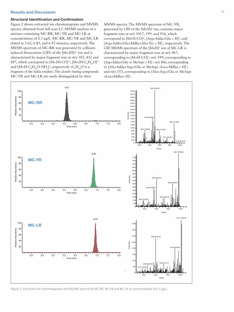
3Results and Discussion
Structural Identification and ConfirmationFigure 2 shows extracted ion chromatograms and MS/MS spectra obtained from full-scan LC-MS/MS analysis of a mixture containing MC-RR, MC-YR and MC-LR at concentrations of 0.5 µg/L. MC-RR, MC-YR and MC-LR eluted at 5.62, 6.85, and 6.93 minutes, respectively. The MS/MS spectrum of MC-RR was generated by collision-induced dissociation (CID) of the [M+2H]2+ ion and is characterized by major fragment ions at m/z 505, 452 and 887, which correspond to [M+2H-CO]2+, [M+2H-C9H10O]2+ and [M+H-C9H10O-NH3]
+, respectively (C9H10O is a fragment of the Adda residue). The closely eluting compounds MC-YR and MC-LR are easily distinguished by their
MS/MS spectra. The MS/MS spectrum of MC-YR, generated by CID of the [M+H]+ ion, contains major fragment ions at m/z 1017, 599, and 916, which correspond to [M+H-CO]+, [Arg+Adda+Glu + H]+, and [Arg+Adda+Glu+Mdha+Ala+Tyr + H]+, respectively. The CID MS/MS spectrum of the [M+H]+ ion of MC-LR is characterized by major fragment ions at m/z 967, corresponding to [M+H-CO]+; m/z 599, corresponding to [Arg+Adda+(Glu or MeAsp) + H]+; m/z 866, corresponding to [Ala+Adda+Arg+(Glu or MeAsp) +Leu+Mdha + H]+; and m/z 553, corresponding to [Ala+Arg+(Glu or MeAsp) +Leu+Mdha+ H]+.
Figure 2. Extracted ion chromatograms and MS/MS spectra for MC-RR, MC-YR and MC-LR at concentrations of 0.5 µg/L
MC-RR
MC-LR
MC-YR

4 Quantitative AnalysisThe high scan speeds and fast analytical cycle time of the Velos Pro mass spectrometer enabled higher numbers of analytical scans across chromatographic peaks for optimal quantitative reliability (Figure 3). Excellent linearity in detector response was observed over the range of 0.05-50 µg/L for all three microcystins. Calibration curves for MC-RR, MC-YR and MC-LR are shown in Figure 4, with coefficients of determination of 0.9986, 0.9994, and 0.9994, respectively. The lowest detectable amount (LOD) of 0.025 µg/L and quantifiable amount (LOQ) of 0.05 µg/L were achieved for each microcystin. Both QC samples, at levels of 0.5 and 5 µg/L, achieved quantitation accuracy better than 94% for all three microcystins. Signal-to-noise ratios of >25 with automatic ICIS algorithm integration in Thermo Scientific Xcalibur software were obtained for MC-LR at the LOQ (Figure 5), demonstrating that thisLC-MS/MS method can be used to determine MC-LR atconcentrations well below the WHO’s recommendedguideline level of 1 µg/L.
Method reproducibility was investigated by analyzing five replicate injections of each analyte. Peak area RSDs for MC-LR and MC-YR were less than 7% and 11%,respectively, over the entire linear dynamic range (Table 2).For MC-RR, peak area RSDs over the range 0.10-50 µg/Lwere under 6%; at the LOQ, the peak area RSD was 16%(Table 2). Retention time precisions were 0.3% RSD orless over the entire dynamic range (Figure 6) for all threemicrocystins. Tap water, filtered water and surface pondwater were analyzed using this method. No microcystinswere in any of the three water sources.
Figure 3. High scan speeds and fast cycle times enable more than 20 data points to be acquired across the MC-LR chromatographic peak.
Figure 4. Calibration curves for quantitation of MC-RR, MC-YR and MC-LR

5
Figure 5. For MC-LR at the LOQ (0.05 µg/L), S/N > 25 and peak area RSD = 6.91%
Figure 6. High retention-time precision (< 0.3% RSD) over a wide linear dynamic range
RT 0.29% RSD
0.025 µg/L
0.1 µg/L
0.2 µg/L
0.5 µg/L
1 µg/L
5 µg/L
10 µg/L
50 µg/L

Table 2. Peak area precision (from five replicate injections) for LC-MS/MS assay of MC-RR, MC-YR and MC-LR
Levels µg/L MC-RR MC-YR MC-LR
0.05 16.01 10.5 6.91
0.10 2.82 5.88 3.97
0.20 3.54 5.25 4.89
0.50 4.86 8.54 3.03
1.00 5.84 1.76 4.25
5.00 2.28 2.13 2.47
10.00 4.54 1.30 1.31
50.00 2.40 1.76 2.66
ConclusionA simple, sensitive and robust LC-MS method for quantitative determination of microcystins was developed. Targeted full-scan MS/MS analysis using the LTQ Velos Pro linear ion trap mass spectrometer provided excellent selectivity and sensitivity for the identification and quantitation of MC-RR, MC-YR and MC-LR across a wide linear dynamic range. The LOD and LOQ were 0.025 µg/L and 0.05 µg/L, respectively. The LOQ was significantly lower than the provisional guideline value established by the WHO for MC-LR concentrations in drinking water. Assays performed in full-scan MS/MS mode enable compound confirmation and quantitation without the need for compound-dependent parameter optimization. The method was used to analyze tap, filtered and surface pond water. No microcystins were detected from these three water sources.
AN63631_E 08/16S
Africa-Other +27 11 570 1840Australia +61 3 9757 4300Austria +43 1 333 50 34 0Belgium +32 53 73 42 41Canada +1 800 530 8447China +86 10 8419 3588Denmark +45 70 23 62 60
Europe-Other +43 1 333 50 34 0Finland/Norway/Sweden
+46 8 556 468 00France +33 1 60 92 48 00Germany +49 6103 408 1014India +91 22 6742 9434Italy +39 02 950 591
Japan +81 45 453 9100Latin America +1 561 688 8700Middle East +43 1 333 50 34 0Netherlands +31 76 579 55 55New Zealand +64 9 980 6700Russia/CIS +43 1 333 50 34 0South Africa +27 11 570 1840
Spain +34 914 845 965Switzerland +41 61 716 77 00UK +44 1442 233555USA +1 800 532 4752
www.thermofisher.com©2016 Thermo Fisher Scientific Inc. All rights reserved. Sigma-Aldrich is a registered trademark of Sigma-Aldrich Biotechnology L.P. All other trademarks are the property of Thermo Fisher Scientific Inc. and its subsidiaries. This information is presented as an example of the capabilities of Thermo Fisher Scientific Inc. products. It is not intended to encourage use of these products in any manners that might infringe the intellectual property rights of others Specifications, terms and pricing are subject to change. Not all products are available in all countries. Please consult your local sales representative for details.
Ap
plica
tion
No
te 5
69
References1. Toxic cyanobacteria in water: A guide to their public
health consequences, monitoring and management;Chorus I, Bartram J, eds. Published by E & FN Spon,London, on behalf of the World Health Organization,Geneva. 1999
2. Ingested Nitrate and Nitrite and Cyanobacterial PeptideToxins. IARC Monogr Eval Carcinog Risks Hum,2010, 94:1–477.
3. WHO Guidelines for Drinking-water Quality, 3rd Ed.,Vol. 1, Recommendations; WHO, Geneva. 2004
4. ISO Water Quality: Determination of microcystins -method using solid phase extraction (SPE) and highperformance liquid chromatography (HPLC) withultraviolet (UV) detection. ISO, Geneva, Switzerland(ISO 20179:2005).

Determination of Lipophilic Marine Biotoxins in Molluscs by LC-MS/MS using Offline ExtractionFrancesca G. Bellagambi, Department of Chemistry and Industrial Chemistry, University of Pisa, Italy Cláudia P. B. Martins, Thermo Fisher Scientific, Barcelona, Spain Michal Godula, Thermo Fisher Scientific, Prague, Czech Republic Alessio Ceccarini, Department of Chemistry and Industrial Chemistry, University of Pisa, Italy
Ap
plica
tion
No
te 6
35
52
Key WordsTSQ Quantum Ultra, Food Safety, Marine Biotoxins
IntroductionIn recent years many countries have had to deal with the consequences of toxic microalgal blooms in both marine and fresh water, such as the deaths of wild animals and domestic livestock.
Several cases of poisoning in humans have been associated with the direct consumption of shellfish, fish, or water contaminated by algal toxins. People may also come into contact with toxins during recreational activities along sea coasts affected by episodes of algal blooms. Depending on the type of toxin involved, there are forms of mild and usually self-limiting symptoms, characterized by gastrointestinal disorders or allergic-like episodes. Much more severe symptoms of the neurological type can lead to death.
The foods most frequently involved in episodes of human poisoning are represented by bivalve molluscs. These shellfish can accumulate and concentrate any biotoxins present in the plankton they ingest through filtering large quantities of water for trophical reasons. It is not possible to evaluate shellfish edibility by an organoleptic examination alone. While human ingestion of contaminated food with biotoxins can lead to the onset of different clinical symptoms, in shellfish it usually has only marginal effects. An important risk factor lies in the thermostability of such molecules which are not completely inactivated by common physical treatments for fish products (cooking, smoking, salting, freezing, housing), but remain virtually unchanged in the finished product.
There are a series of regulations issued by the European Union (EU) that relate to marine biotoxins. One is Regulation (EC) No 853/2004 which concerns the control of lipophilic toxins, establishing maximum levels for lipophilic toxins in bivalve molluscs destined for human consumption:1
• For okadaic acid, dinophysistoxins, and pectenotoxinstogether – 160 micrograms of okadaic acid equivalentsper kilogram
• For yessotoxin – 1 milligram of yessotoxin equivalentper kilogram
• For azaspiracids – 160 micrograms of azaspiracidequivalents per kilogram

In the past, aside from bioassays on mice, most analytical techniques developed for the determination of marine biotoxins in bivalve molluscs have been based on offline methodologies. These include methods involving solid phase extraction (SPE) or liquid-liquid extraction (LLE) followed by high pressure liquid chromatography (HPLC) with fluorimetric or UV-diode array detection, as well as detection by liquid chromatography coupled with mass spectrometry (LC-MS).
The EU Commission Regulation (EC) No 15/2011, amending Regulation (EC) No 2074/2005 about the testing methods for detecting marine biotoxins in bivalve molluscs, describes an LC-MS/MS procedure as the reference method for the quantification of lipophilic marine biotoxins – namely okadaic acid, pectenotoxin 2, azaspiracid 1, and yessotoxin.2,3 Moreover, dinophysis-toxin 1 (DTX-1) and dinophysistoxin 2 (DTX-2) can be quantified by the calibration curve of okadaic acid, pectenotoxin 1 by calibration of pectenotoxin 2, azaspiracid 2 and 3 by calibration of azaspiracid 1 and 45-OH-, and 45-homo-OH-yessotoxin by the calibra-tion of yessotoxin.
In accordance with current European regulations, we propose a quick, selective, sensitive, and accurate analytical method for the determination of lipophilic marine biotoxins in bivalve molluscs using an LC-MS/MS method.
GoalOur goal is to validate analytical procedures proposed in “EU-Harmonised Standard Operating Procedure for determination of Lipophilic marine biotoxins in molluscs by LC-MS/MS – Version 3” by LC-MS/MS using offline extraction.4
Experimental
Sample Preparation
About 1 kg of bivalve molluscs (Mytilus Galloprovincialis) were cleaned with water and put in a solution of NaCl (3.5 g/L). After opening, the molluscs were washed with fresh water, their flesh was removed and placed on a stainless steel net, and they were washed again with deionized water. The whole collected raw tissue, not less than 150 g, was chopped and blended by a mixer.
Extraction procedure
9 mL of 100% methanol (gradient quality) were added to 2.00 ± 0.05 g of blended tissue, put into a centrifuge tube, and mixed by vortex for 3 minutes at maximum speed. After centrifugation at 4000 rpm for 10 minutes, the supernatant solution was transferred into a vial.
A second aliquot of 9 mL of 100% methanol was further added to the residual tissue pellet and homogenized for 1 minute by Ultra-turrax® (IKA®, USA) at 12,000 rpm and the mixture was centrifuged at 4000 rpm for 10 minutes. Then the supernatant solution was transferred and
combined with the first extract and made up to 20 mL with 100% methanol. When not immediately analyzed, the solution was stored at -20 °C.
Spikes of toxin standard solutions can be added to the blended tissue before the extraction procedure.
Purification Procedure
The organic extract was purified by being passed through a C18 SPE cartridge preliminarily conditioned with 1 mL of 100% methanol. A 0.45 μm syringe filter was placed at the end of the cartridge to improve purification.
LC Conditions for the Thermo Scientific Hypersil GOLD Column
System Thermo Scientific Accela UHPLC
Solvent A 100% water with 2 mM ammonium formate and 50 mM formic acid
Solvent B 95% acetonitrile + 5% water with 2 mM ammonium formate and 50 mM formic acid
Flow Rate 200 µL/min
Gradient The mixture started at 30% solvent B (8.0 min) followed by a linear gradient up to 90% solvent B in 3.0 min. It went up to 30% of solvent B in 0.5 min. This composition was maintained for 5.5 min.
Analytical Column Hypersil GOLD™; 50 × 2.1 mm, particle size 1.9 µm, part number 25002-052130
H-ESI II Source Conditions
Ion Source Polarity Positive Ion Mode Negative Ion Mode
Spray Voltage 3000 V 2700 V
Capillary Temperature 270 °C 270 °C
Vaporizer Temperature 240 °C 240 °C
Sheath Gas Pressure (N2) 15 units 15 units
Auxiliary Gas Pressure (N2) 5 units 5 units
MS/MS Setup
MS analysis was carried out on a Thermo Scientific TSQ Quantum Ultra triple quadrupole mass spectrometer equipped with a heated electrospray ionization probe (H-ESI II).
Collision Gas (Ar) 1.5 mTorr
Q1/Q3 Peak Resolution 0.7 u (unit mass resolution)
Scan Time 0.100 s
Scan Width 0.500 m/z
Data Acquisition Mode SRM

The optimization of selective reaction monitoring (SRM) parameters was performed by direct infusion of standards. Collision-induced dissociation (CID) data were recorded for each analyte including optimum collision energies for the selected ion transitions.
Table 1 summarizes all the mass transitions found for each analyte and its relative collision energy (CE) and tube lens values.
Results and DiscussionTo ensure thorough validation of the method, neat standard solutions, standard addition on purified extracts, and spiked blank tissue extracts were prepared and compared.
Table 2 lists the correlation coefficients (r2) indicating the linearity of the calibration curves for the three types of samples analyzed; five concentrations of the sample solution are considered (2, 5, 10, 20, and 50 μg/kg or similar).
To assess the inter-day repeatability of the method, ten replicates of spiked samples were analyzed between days. Solutions were prepared containing all the toxins in the five different concentrations used to perform the calibration curves (2, 5, 10, 20, and 50 μg/kg or similar).
The repeatability of the method expressed as the coefficient of variation percentage (CV %) has been rated less than 20% as shown in Table 3.
Analyte ESI Mode Parent Mass Product Mass Collision Energy Tube Lens
AZA-1 ESI+ 842.3 806.1 51 207
824.2 42 207
AZA-2 ESI+ 856.3 838.1 42 214
820.2 49 214
AZA-3 ESI+ 828.3 792.2 48 192
810.0 40 192
PTX-2 ESI+ 876.3 841.3 35 205
823.0 40 205
805.3 41 205
DTX-1 ESI- 817.0 255.0 69 197
113.1 67 197
DTX-2 ESI- 803.15 255.3 61 207
113.1 50 207
YTX ESI- 1141.5 1061.7 50 240
570.2 467.3 40 240
OA ESI- 803.3 254.9 68 216
113.1 50 216
Table 1: Selected ion transitions (m/z ) of the studied compounds and optimized collision energy and tube lens value for the TSQ Quantum Ultra triple quadrupole mass spectrometer
Analyte Neat Solution Spiked Purified Extract Spiked Extract
AZA-1 0.9932 0.9965 0.9970
AZA-2 0.9973 0.9964 0.9901
AZA-3 0.9972 0.9958 0.9993
DTX-1 0.9964 0.9995 0.9953
DTX-2 0.9973 0.9966 0.9965
YTX 0.9999 0.9923 0.9988
PTX-2 1.0000 0.9977 0.9927
OA 0.9955 0.9924 0.9927
Table 2: Correlation Coefficient (r2) of the calibration curves for the three types of samples analyzed in the concentration range of 2–50 µg/kg)
Analyte Standard Deviation Repeatability CV%
AZA-1 0.25 0.79 20
AZA-2 0.29 0.90 18
AZA-3 0.43 1.37 17
DTX-1 0.18 0.55 2
DTX-2 0.22 0.68 9
YTX 0.12 0.40 12
PTX-2 0.39 1.36 20
OA 0.16 0.48 4
Table 3: Values of CV% obtained for the repeatability of the lower concentrated curve point (2 µg/kg)

Ap
plica
tion
No
te 6
35
52
The calculations, of limit of detection (LOD) and limit of quantification (LOQ) were made in accordance with the UNICHIM Manual N. 179/0 where the calculation of the limit of detection is made through the calibration curve of the instrument used for analysis.5
To estimate the LOD and LOQ of the method (Table 4), ten samples were prepared by adding standard solution to 500 mg of homogenized mussel flesh and repeating the extraction procedure according to the method in “EU-Harmonised Standard Operating Procedure for determination of Lipophilic marine biotoxins in molluscs by LC-MS/MS – Version 3”. LOD and LOQ are expressed in μg/Kg. Recoveries are shown in Table 5.
ConclusionThis method proved to be selective, sensitive, accurate, and reproducible. It can be successfully applied for the quantitative determination of several classes of lipophilic marine biotoxins in bivalve mollusc samples.
References1. Regulation (EC) No 853/2004 of the European Parliament and of the
Council of 29 April 2004. Official Journal of the European Communities L139, 55-255.
2. Commission Regulation (EU) No 15/2011 of 10 January 2011. Official Journal of the European Union. L6, 3-9.
3. Commission Regulation (EC) No 2074/2005 of 5 December 2005. Official Journal of the European Communities, L388, 27-59.
4. European Union Reference Laboratory for Marine Biotoxins (EU-RL-MB), Agencia Española de Seguridad Alimentaria y Nutrición (AESAN). EU-Harmonised Standard Operating Procedure for determination of Lipophilic marine biotoxins in molluscs by LC-MS/MS – Version 3. 2011.
5. UNICHIM, Manual N. 179/0. Linee guida per la convalida di metodi analitici nei laboratori chimici - criteri generali. Milano. 1999.
Hypersil GOLD
Analyte LOD (µg/Kg) LOQ (µg/Kg) Outliers (Huber Test)
AZA-1 0.56 ± 0.18 1.11 NO
AZA-2 0.93 ± 0.31 1.86 NO
AZA-3 1.28 ± 0.43 2.57 NO
DTX-1 5.66 ± 1.02 10.45 NO
DTX-2 0.71 ± 0.23 1.42 NO
YTX 1.67 ± 0.56 3.33 NO
PTX-2 1.40 ± 0.46 2.79 NO
OA 3.95 ± 1.32 7.91 NO
Table 4: LOD and LOQ of the method
Analyte Spiked Purified Extract Spiked Extract
AZA-1 96 ± 11 97 ± 11
AZA-2 101 ± 9 94 ± 14
AZA-3 104 ± 10 99 ± 6
DTX-1 101 ± 6 101 ± 7
DTX-2 101 ± 6 108 ± 42
YTX 99 ± 15 102 ± 17
PTX-2 103 ± 13 102 ± 20
OA 95 ± 7 93 ± 18
Table 5: Recovery values, where R% = {[(µg/Kg)CALCULATED/(µg/Kg)THEORETICAL]*100}
Figure 1: Chromatogram of sample containing 40 ppb of toxins (Retention Time: 7.44 min – AZA-1; 7.77 min – AZA-2; 6.88 min – AZA-3; 5.69 min – OA; 7.O5 min – DTX-1; 6.06 min – DTX-2; 5.54 min – YTX; 6.28 min – PTX-2
AN63552_E 08/16M
Africa-Other +27 11 570 1840Australia +61 3 9757 4300Austria +43 1 333 50 34 0Belgium +32 53 73 42 41Canada +1 800 530 8447China +86 10 8419 3588Denmark +45 70 23 62 60
Europe-Other +43 1 333 50 34 0Finland/Norway/Sweden
+46 8 556 468 00France +33 1 60 92 48 00Germany +49 6103 408 1014India +91 22 6742 9434Italy +39 02 950 591
Japan +81 45 453 9100Latin America +1 561 688 8700Middle East +43 1 333 50 34 0Netherlands +31 76 579 55 55New Zealand +64 9 980 6700Russia/CIS +43 1 333 50 34 0South Africa +27 11 570 1840
Spain +34 914 845 965Switzerland +41 61 716 77 00UK +44 1442 233555USA +1 800 532 4752
www.thermoscientific.com©2016 Thermo Fisher Scientific Inc. All rights reserved. ULTRA-TURRAX and IKA are registered trademarks of IKA-Werke GmbH & Co. All other trademarks are the property of Thermo Fisher Scientific Inc. and its subsidiaries. This information is presented as an example of the capabilities of Thermo Fisher Scientific Inc. products. It is not intended to encourage use of these products in any manners that might infringe the intellectual property rights of others. Specifications, terms and pricing are subject to change. Not all products are available in all countries. Please consult your local sales representative for details.


Contaminants of Emerging Concern and Other Water Analysis
Surface, Drinking and Waste Water Analysis
Ap
plica
tion
No
teb
oo
k

Kiawah Island, SC Pond 25
Pond 5
WWTP Lagoon
Pond 43
agoon
d 5
Charleston, SC
Targeted and Nontargeted MS Analysis of Contaminants in Storm Water Retention PondsGordon Getzinger1, P. Lee Ferguson1, Jonathan Beck2, Charles Yang2, Frans Schoutsen3
1Duke University, Durham, NC, USA 2Thermo Fisher Scientific, San Jose, CA, USA 3Thermo Fisher Scientific, Breda, The Netherlands
Ap
plica
tion
No
te 5
99
Key WordsEnvironmental analysis, water analysis, wastewater, micropollutants, EQuan MAX Plus, TSQ Quantiva, LTQ Orbitrap Velos
GoalTo demonstrate a data-driven environmental monitoring approach for examining the occurrence and distribution of wastewater-derived contaminants and turf-grass management organic compounds in storm water retention ponds.
IntroductionComprehensive assessment of the aquatic fate and effects of organic micropollutants is greatly hindered by the need to develop compound-specific methodologies prior to sampling and analysis. A data-driven workflow, coupling high-resolution, accurate-mass (HRAM) mass spectrometry and highly sensitive online solid phase extraction (SPE) analysis, ensures complete characterization of organic pollutants in aquatic environments. In this work, water samples collected from a coastal golf course community were screened for the presence of trace organic contaminants by a non-targeted HPLC–HRAM mass spectrometry workflow. The occurrence of identified and confirmed contaminants was then quantitatively assessed by a high-throughput online SPE LC-MS/MS method.
ExperimentalSample CollectionSurface water, groundwater, and wastewater effluent samples were collected from Kiawah Island, SC (Figure 1), a coastal golf course community where turf-grass management chemicals are extensively applied and reclaimed wastewater is used for irrigation. Golf course and storm water runoff are collected in ponds, which are interconnected through a series of culverts and communicate with the adjacent tidal estuary through managed outfalls.
Initial sampling for non-targeted screening consisted of 0.5 L grab samples collected and field extracted by SPE over two weeks in May 2010. Similarly, 10 mL grab samples were collected in May 2011 for quantitative analysis.
Sample sites were chosen to represent various routes of micropollutant loading into the aquatic environment and potential routes of chemical exposure as detailed in Table 1. Golf course runoff consists of both turf-grass-management chemicals applied to the course and wastewater-derived contaminants introduced through irrigation.
Table 1. Sample sites and descriptions of potential sources of micropollutants to those site
Sample Site Inputs
Pond 5 Golf course runoff
Pond 25 Golf course runoff
Pond 43 Residential storm water
Wastewater treatment plant lagoon (WWTP)
Treated municipal wastewater
Wastewater composite (WW Comp.)
24 hr composite effluent
Well 1 Infiltration from pond 25
Well 7 Infiltration from pond 5
Figure 1. Aerial view of Kiawah Island, SC. Water collection ponds, shown in blue, are connected as indicated by the red lines.

The MS data was acquired in selected-reaction monitoring (SRM) mode on a Thermo Scientific™ TSQ Quantiva™ triple-stage quadrupole MS equipped with a HESI interface.
MS Conditions
Ion mode Positive HESI
Cycle time (s) 0.75
CID gas pressure (mTorr) 1.5
Spray voltage (V) 3500
Sheath gas (arb units) 60
Aux gas (arb units) 20
Sweep gas (arb units) 2
Ion transfer tube temp (˚C) 350
Vaporizer temp (˚C) 350
RF lens Used calibrated RF lens values
Data processing, calibration, and quality control were performed using Thermo Scientific™ TraceFinder™ software version 3.1.
2 Broad-Spectrum HPLC-HRAM MS ScreeningTo begin analysis, broad-spectrum MS screening was performed on a Thermo Scientific™ LTQ Orbitrap Velos™ hybrid ion trap-Orbitrap MS using heated electrospray ionization (HESI). The instrument was operated in positive full-scan (m/z 100-1000) mode at a resolving power of 60,000 (FWHM) at m/z 400. Data-Dependent Top 3 HRAM MS/MS experiments were performed with dynamic exclusion and peak apex detection.
Non-Targeted Compound IdentificationAfter broad-spectrum data acquisition, Thermo Scientific™ ExactFinder™ software version 2.5 was used for non-targeted compound identification. The HRAM data was screened for approximately 1000 known contaminants using the environmental and food safety (EFS) compound database and HRAM MS/MS spectral library. Automated feature scoring and filtering was based on chromatographic peak shape, mass error (ppm), and isotope pattern. Structures were tentatively assigned by library searching and later confirmed by analysis of authentic standards.
Targeted QuantitationTargeted quantitation was performed with the Thermo Scientific™ EQuan MAX Plus™ online SPE and HPLC system. A 1 mL injection was loaded onto a Thermo Scientific™ Hypersil GOLD aQ™ column (20 x 2.1 mm, 12 µm particle size) and separated on a Thermo Scientific™ Accucore™ aQ analytical column (50 x 2.1 mm, 2.6 µm particle size) by gradient elution with methanol/water mobile phase.
LC Conditions
Loading pump Thermo Scientific™ Dionex™ UltiMate™ 3000 Quaternary Analytical Pump LPG-3400SD
Flow rate Isocratic 1 mL/min
Solvent A (water) 98%
Solvent B (methanol) 2%
Total run time 1 8.4 min
Analytical pump UltiMate 3000 Binary Rapid Separation Pump HPG-3200RS
Solvent A (water) 98%
Solvent B (methanol) 2%
Gradient elution 0.3 mL/min
Gradient Time %A
0 98
1.5 98
12.0 2
15.0 2
15.1 98
Total run time 18.4 min
Autosampler Thermo Scientific™ Open Accela™ autosampler
Valve switching At 1.5 min and 16.6 min

Results and DiscussionHRAM Screening and Non-Targeted IdentificationRepresentative HRAM chromatograms of SPE extracts subjected to non-targeted screening for the identification of organic pollutants and selection of target compounds for quantitative analysis are shown in Figure 2.
Figure 2. Representative HRAM chromatograms from non-targeted screening of SPE extracts from Pond 5 sample (top) and wastewater composite sample (bottom)
3
Pond 5
WW Comp.

4 A partial list of compounds identified by non-targeted screening and the samples in which they were found are listed in Table 2.
Table 2. Compounds identified by non-targeted screening
Compound Sample(s)
Atraton Ponds 25, 43
Atrazine Ponds 5, 25, 43, WWTP, WW Comp.
Atrazine-2-hydroxy Pond 25
Carbamazepin WWTP, WW Comp.
Carbendazim WWTP
DEET Ponds 5, 25, 43, WWTP, WW Comp.
Fluridone Ponds 25, 43
Hydrocortisone WWTP, WW. Comp.
Mefluidide Ponds 5, 25
Metolcarb WWTP
Metoprolol WWTP, WW Comp.
Promecarb WW Comp.
Propanolol WWTP, WW Comp.
Pyroquilon Ponds 5, 25, WWTP, WW Comp.
Sulfamethoxazole WW Comp.
Temeazepam WW Comp.
Trimethoprim WWTP, WW Comp.
WWTP = Wastewater treatment plant lagoonWW Comp = Wastewater composite
Targeted Quantitation by Online SPE LC/MS Based on the results of the non-targeted screening, knowledge of chemical usage on the island, and readily available reference standards, an online SPE LC/MS method was developed to quantify the occurrence and distribution of wastewater- and turf-grass-management-derived organic pollutants on Kiawah Island.
Table 3 provides details of the online SPE LC/MS method, including the compounds monitored and the instrument limits of detection (LOD). Samples were quantitated down to the sub-ppt (ng/L) level.
Figure 4 displays the measured contaminant concentrations in representative storm and wastewater retention ponds.
A
B
C
The non-targeted identification of fluridone in Pond 43 by EFS database screening and spectral library searching in ExactFinder software is demonstrated in Figure 3. Panel A shows an EFS database match for fluridone with a goodness of fit score of 0.93 between a modeled chromatographic peak and the observed peak. Panel B compares a modeled mass spectrum for the proposed pseudomolecular ion [C19H14F3NO+H]+ and the averaged full-scan observed data with excellent mass accuracy (-0.31 ppm) at the mono-isotopic peak and a 100% isotope pattern score. In Panel C, library searching of the observed HRAM CID MS2 spectrum returned a match to the EFS library entry for fluridone with a score of 70%.
Figure 3. Non-targeted identification of fluridone in Pond 43. A) EFS database match for fluridone between a modeled chromatographic peak (gray area) and the observed peak (black trace). B) Comparison of a modeled mass spectrum for the proposed pseudomolecular ion [C
19H
14F
3NO]M+H (blue) and averaged full-scan observed data (black).
C) Library searching of the observed HRAM CID MS2 spectrum (black) returns a match to the EFS library entry for fluridone (blue)with a score of 70%.
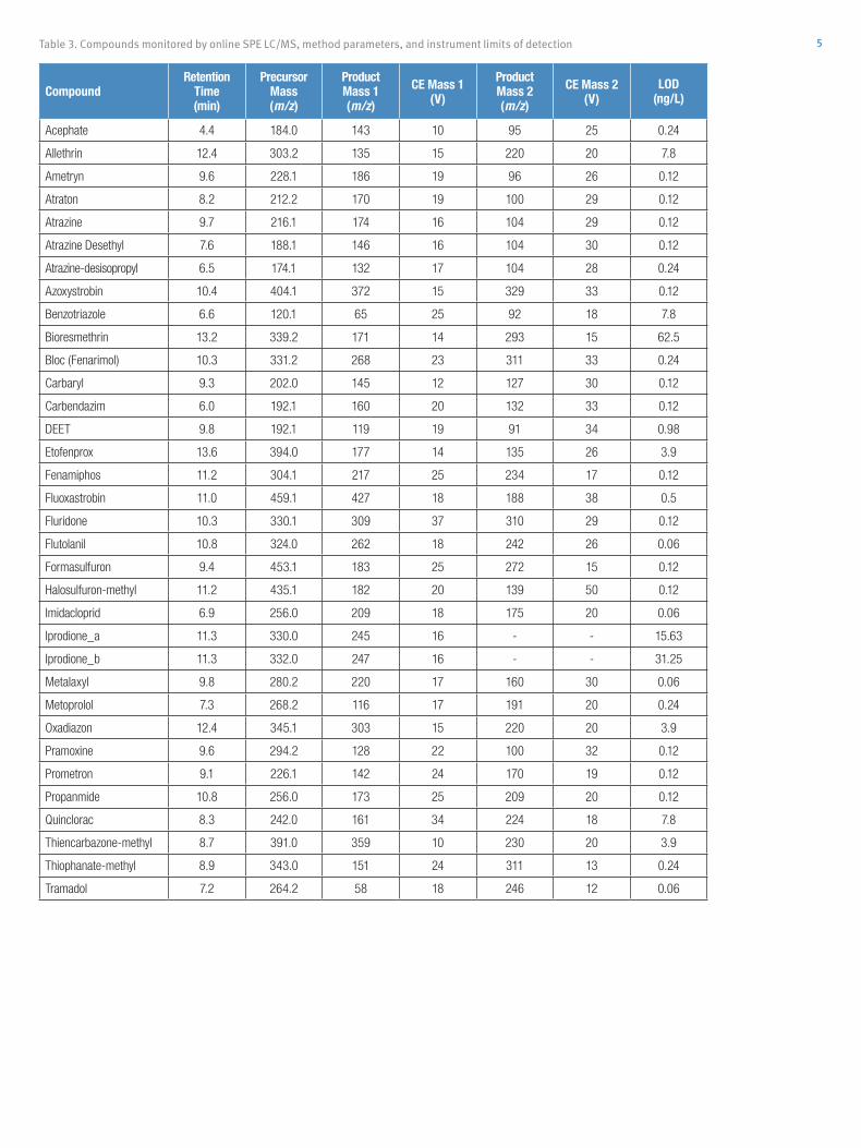
5Table 3. Compounds monitored by online SPE LC/MS, method parameters, and instrument limits of detection
CompoundRetention
Time (min)
Precursor Mass (m/z)
Product Mass 1 (m/z)
CE Mass 1 (V)
Product Mass 2 (m/z)
CE Mass 2 (V)
LOD (ng/L)
Acephate 4.4 184.0 143 10 95 25 0.24
Allethrin 12.4 303.2 135 15 220 20 7.8
Ametryn 9.6 228.1 186 19 96 26 0.12
Atraton 8.2 212.2 170 19 100 29 0.12
Atrazine 9.7 216.1 174 16 104 29 0.12
Atrazine Desethyl 7.6 188.1 146 16 104 30 0.12
Atrazine-desisopropyl 6.5 174.1 132 17 104 28 0.24
Azoxystrobin 10.4 404.1 372 15 329 33 0.12
Benzotriazole 6.6 120.1 65 25 92 18 7.8
Bioresmethrin 13.2 339.2 171 14 293 15 62.5
Bloc (Fenarimol) 10.3 331.2 268 23 311 33 0.24
Carbaryl 9.3 202.0 145 12 127 30 0.12
Carbendazim 6.0 192.1 160 20 132 33 0.12
DEET 9.8 192.1 119 19 91 34 0.98
Etofenprox 13.6 394.0 177 14 135 26 3.9
Fenamiphos 11.2 304.1 217 25 234 17 0.12
Fluoxastrobin 11.0 459.1 427 18 188 38 0.5
Fluridone 10.3 330.1 309 37 310 29 0.12
Flutolanil 10.8 324.0 262 18 242 26 0.06
Formasulfuron 9.4 453.1 183 25 272 15 0.12
Halosulfuron-methyl 11.2 435.1 182 20 139 50 0.12
Imidacloprid 6.9 256.0 209 18 175 20 0.06
Iprodione_a 11.3 330.0 245 16 - - 15.63
Iprodione_b 11.3 332.0 247 16 - - 31.25
Metalaxyl 9.8 280.2 220 17 160 30 0.06
Metoprolol 7.3 268.2 116 17 191 20 0.24
Oxadiazon 12.4 345.1 303 15 220 20 3.9
Pramoxine 9.6 294.2 128 22 100 32 0.12
Prometron 9.1 226.1 142 24 170 19 0.12
Propanmide 10.8 256.0 173 25 209 20 0.12
Quinclorac 8.3 242.0 161 34 224 18 7.8
Thiencarbazone-methyl 8.7 391.0 359 10 230 20 3.9
Thiophanate-methyl 8.9 343.0 151 24 311 13 0.24
Tramadol 7.2 264.2 58 18 246 12 0.06

AN63942_E 08/16S
Africa +43 1 333 50 34 0Australia +61 3 9757 4300Austria +43 810 282 206Belgium +32 53 73 42 41Canada +1 800 530 8447China 800 810 5118 (free call domestic)
400 650 5118
Denmark +45 70 23 62 60Europe-Other +43 1 333 50 34 0Finland +358 9 3291 0200France +33 1 60 92 48 00Germany +49 6103 408 1014India +91 22 6742 9494Italy +39 02 950 591
Japan +81 45 453 9100Latin America +1 561 688 8700Middle East +43 1 333 50 34 0Netherlands +31 76 579 55 55New Zealand +64 9 980 6700Norway +46 8 556 468 00Russia/CIS +43 1 333 50 34 0
Singapore +65 6289 1190Spain +34 914 845 965Sweden +46 8 556 468 00Switzerland +41 61 716 77 00UK +44 1442 233555USA +1 800 532 4752
www.thermofisher.com©2016 Thermo Fisher Scientific Inc. All rights reserved. All trademarks are the property of Thermo Fisher Scientific Inc. and its subsidiaries. This information is presented as an example of the capabilities of Thermo Fisher Scientific products. It is not intended to encourage use of these products in any manners that might infringe the intellectual property rights of others. Specifications, terms and pricing are subject to change. Not all products are available in all countries. Please consult your local sales representative for details.
Ap
plica
tion
No
te 5
99
ConclusionA multifaceted approach to identifying and quantifying non-targeted emerging compounds in environmental surface and ground water samples impacted by reclaimed water irrigation has been demonstrated.
• HRAM can be used to identify organic micropollutantsin wastewater-impacted environments, golf courserunoff, and storm water ponds.
• Online SPE coupled with a triple quadrupole MS canbe used to quantitate micropollutants in water samplesdown to the sub-ppt (ng/L) level.
• Future work will include studying the toxicologicalimpact of these compounds on aquatic species.
Figure 4. Boxplots depicting the measured contaminant concentrations in wastewater storage and storm water retention ponds on Kiawah Island. Purple boxes represent the interquartile range and the bar represents the median value. Hashed lines depict the range of the data and outliers are plotted as open circles.

A Strategy for an Unknown Screening Approach on Environmental Samples using HRAM Mass SpectrometryO. Scheibner,1 P. van Baar,2 F. Wode,2 U. Dünnbier,2 K. Akervik,3 J. Humphries,3 M. Bromirski11Thermo Fisher Scientific, Bremen, Germany; 2Berliner Wasserbetriebe, Berlin, Germany;3Thermo Fisher Scientific, Austin, TX, USA

2 A Strategy for an Unknown Screening Approach on Environmental Samples using HRAM Mass Spectrometry
Overview
Purpose: Run a General Unknown Screening approach
in an automated fashion.
Methods: Surface water samples form the city of Berlin,
Germany were analyzed in full scan / AIF mode with a
Thermo Scientific™ Exactive Plus™ mass spectrometer
and analyzed in a widely automated workflow using
Thermo Scientific TraceFinder™ and Thermo Scientific
SIEVE™ software.
Results: Differences in the load of contaminants could be
easily determined in the different samples; Easy detection
and identification of a significant number of contaminants
could be achieved.
Introduction
The analysis of food and environmental samples for
contaminants by LC-MS has become a quick and cost
effective routine application when run in a targeted
fashion, but this way it disregards events or
circumstances not taken into account beforehand. Run in
a non-targeted fashion, it is known to be laborious and
time consuming, making it everything but a routine
application. New generation software now links in
quantitative and (unknown) screening approaches to one
smoothly integrated workflow, tying together component
detection capabilities of unknown screening workflows
with the identification capabilities of targeted screening
and quantification software. Here we show how one data
set can serve for routine high throughput quantitative
analysis and for versatile non-targeted investigations in a
highly automated manner.
Methods
Sample Preparation
Four samples of surface water from different sources
were taken and analyzed without any further treatment. In
addition, one neat standard as control sample and one
tap water sample as reference sample were run in the
same sequence.
A Strategy for an Unknown Screening Approach on Environmental Samples
using HRAM Mass Spectrometry
O. Scheibner1, P. van Baar2, F. Wode2, U. Dünnbier2 , K. Akervik3, J. Humphries3 , M. Bromirski1
1Thermo Fisher Scientific, Bremen, Germany, 2Berliner Wasserbetriebe, Berlin, Germany, 3Thermo Fisher
Scientific, Austin, TX, USA
FIGURE 1. Schematics of the EQuan online SPE and
separation system.
6-PortValve
6-PortValve
LargeVolumeSample
Loop
ConventionalVolume
Sample Loop
12µm Hypersil GoldPreconcentration
Column
3µm Accucore RP-MS18Analytical Column
Accela 1250 pump
Autosampler Accela 600pump
6-PortValve
Liquid Chromatography
For online sample concentration and chromatographic
separation a Thermo Scientific EQuan™ system was
used. A sample volume of 1000 µL was injected onto a
Thermo Scientific Hypersil Gold™ 20x2.1 mm trapping
column with subsequent elution onto a Thermo Scientific
AccucoreTM RP-MS 18 analytic column. A 6.7 minute
solvent gradient was applied as shown in Fig 1. This
resulted in a total cycle time of 15 minutes for sample
injection, online concentration and chromatographic
separation.
Mass Spectrometry
For mass spectrometric detection a Thermo Scientific
Exactive Plus mass spectrometer was used and run in full
scan / all ion fragmentation (AIF) mode. In this mode full
scans are permanently alternated with AIF fragmentation
scans. A resolution setting of 70,000 (FWHM @ m/z 200)
was used (see Fig. 2). A mass range of m/z 103 to 900
was applied (resp. m/z 70 to 870 and resolution setting
35,000 FWHM for the AIF scans) to be prepared for all
possible contaminants. The mass axis of the system was
calibrated with the standard calibration mix once prior
measurement. Further optimization of the instrument
(compound tuning) was not required.
FIGURE 2. Exactive Plus method setup.
Results
Suspect Screening
The more simple way of screening is the suspect screen,
using a large list of components possibly present in a
sample. It avoids the critical step of condition free
component detection, but works already without analytical
standards which could serve for confirmation by providing
valid retention time, ion ratios and more. In this case, a
built-in database with about 1000 components was used,
containing name, elemental composition and fragment
information. Additionally, a matching spectral library
containing roughly 4000 HRAM MS2 spectra is available
inside the application. As a result, isotopic pattern match,
fragment search and MS2 library search were used for
result confirmation (see Fig. 3).
FIGURE 3. Suspect screening result view.
As to be expected, it was possible to identify a good
number of contaminants, yielding a match on all three
confirming points. On the other it was clear that this way of
screening did not cover all possible compounds, as was
visible from the neat standard (as used normally for target
screening on these samples) measured in the same
batch. A clear benefit could be seen in the fact that
fragment information and library spectra were present for
additional confirmation (see Fig. 4).
In addition, a larger database with 2900 components was
applied still left open the question of contaminants not
found because they may not be members of this list
FIGURE 4. Three stages of confirmation in suspect
screen: isotope pattern match, fragment search andlibrary search; A: isotopic pattern overlay; B:
fragment overlay; C: Library comparison.
A
C
B
Unknown Screening
As a consequence of the limitations of a suspect screen
an unknown screening workflow was run. For this the
measured sequence was transferred to the screening
application SIEVE for unconditioned component
detection. Since all necessary settings and parameters
were transferred from TraceFinder to SIEVE
automatically, the component detection process could be
started immediately. As a result, 5000 components were
detected. Since such a list contains all components
regardless of their significance, refinement of this list was
clearly needed. As part of the process, all samples were
referenced against the tap water sample, so a simple filter
could be applied to remove matrix and background
signals from the result list, leaving 1829 components in
the list. Application of a principal component analysis to
this result revealed that three water samples were closely
related, while on water sample (surface water 1, see Fig.
5) seemed to be rather different in its content, so the filter
for significant components could be further refined.
FIGURE 5. PCA result after filtering for significant
differences.
surface water 3
surface water 4surface water 2
surface water 1 tap water
neat standard
This time the filter was set to look only for significant
changes in the samples surface water 1 and surface water
2. This reduced the list of components to 1671 which were
sent to ChemSpider for identification. This search returned
1529 identifications. Closing of the SIEVE application
automatically transferred this result list back to
TraceFinder, where it was imported as a new compound
database (see Fig. 6).
FIGURE 6. Confirmation of the unknown screening
results from SIEVE, propiconazole taken as an example: The extracted ion chromatogram at the
determined retention time gives a clear signal freefrom interferences, the isotope pattern match showsclose to perfect overlay.
For confirmation and reporting of the results this
compound database was used for a normal suspect
screening. The advantage of looping back the results in
TraceFinder was to be able to handle all data – target,
suspect and unknown screen – in one application and to
be able to use the same data review and report templates.
It became visible that some components were coeluting
with higher amounts of matrix, but it was still possible to
extract significant signals from the surrounding matrix,
maintaining full mass accuracy despite the low signal
intensity. Fig. 7 shows anexample of the component
Loxoprofen, where the surrounding matrix signals have
roughly the same intensity as the first and second isotope
signal of the compound. Still the analyte signals are clearly
resolved from the background and matrix signals, so the
compound can easily be detected and confirmed. Key to
this clear separation of analyte and matrix signals is the
high resolving power of R = 70,000 @ m/z 200 used in this
analysis.
FIGURE 7. Importance of sufficient resolution for
unambiguous identification of components: Themonoisotopic signl (A) and the first isotope signal (B)
are surrounded by matrix signals of similar intensitywhich are only separated by means of the high resolving power used.
Since all final processing was done in one application, the
results of target, suspect and unknown screening could
easily be combined into one result, making result reporting
and archiving one single step. Since all data transfer
between the two applications is fully automated, Fig. 8
shows a short selection of compounds which had not been
part of the initial target screening, but were found in the
unknown screening process.
FIGURE 8. Selection of additional contaminants not
present in previous target and suspect screen.
Compound Name Formula m/z (Apex) m/z (Delta (ppm)) RT (Measured) Isotopic Pattern Score (%)Bisoprolol C18H31NO4 326.2330 0.57 5.12 100Candesartan C24H20N6O3 441.1671 -0.50 6.56 100Carbofuran C12H15NO3 222.1127 -0.19 5.18 98Dibenzylamine C14H15N 198.1277 -0.66 7.31 98Irbesartan C25H28N6O 429.2401 -0.03 6.45 100Loxoprofen C15H18O3 247.1332 0.45 5.52 85Mexacarbate C12H18N2O2 223.1443 -0.06 5.53 96Oxazepam C15H11ClN2O2 287.0584 0.48 6.29 96Propiconazole C15H17Cl2N3O2 342.0774 0.21 7.43 89Tramadol C16H25NO2 264.1961 0.10 4.35 100
Conclusion
In this example of environmental analysis we could show
that it is possible to enhance the capabilities of target and
suspect screening with its limitations by a streamlined
general unknown screening with a high degree of
automation from within one application. The resolving
power of the Exactive Plus bench top Orbitrap MS system
is the driving force behind the selectivity and reliability of
the obtained results because this serves for the separation
of the analyte peaks from background and matrix signals.
Chemspider is a trademark of the Royal Society of Chemistry. All other trademarks are the property ofThermo Fisher Scientific and its subsidiaries. This information is not intended to encourage use of
these products in any manners that might infringe the intellectual property rights of others.
Presented at RAFA, Prague, Czech Republic, Nov 5-8, 2013.

3Thermo Scientific Poster Note • PN64243-RAFA 0914S
Overview
Purpose: Run a General Unknown Screening approach
in an automated fashion.
Methods: Surface water samples form the city of Berlin,
Germany were analyzed in full scan / AIF mode with a
Thermo Scientific™ Exactive Plus™ mass spectrometer
and analyzed in a widely automated workflow using
Thermo Scientific TraceFinder™ 3.1 and Thermo
Scientific SIEVE™ 2.1 software.
Results: Differences in the load of contaminants could be
easily determined in the different samples; Easy detection
and identification of a significant number of contaminants
could be achieved.
Introduction
The analysis of food and environmental samples for
contaminants by LC-MS has become a quick and cost
effective routine application when run in a targeted
fashion, but this way it disregards events or
circumstances not taken into account beforehand. Run in
a non-targeted fashion, it is known to be laborious and
time consuming, making it everything but a routine
application. New generation software now links in
quantitative and (unknown) screening approaches to one
smoothly integrated workflow, tying together component
detection capabilities of unknown screening workflows
with the identification capabilities of targeted screening
and quantification software. Here we show how one data
set can serve for routine high throughput quantitative
analysis and for versatile non-targeted investigations in a
highly automated manner.
Methods
Sample Preparation
Four samples of surface water from different sources
were taken and analyzed without any further treatment. In
addition, one neat standard as control sample and one
tap water sample as reference sample were run in the
same sequence.
A Strategy for an Unknown Screening Approach on Environmental Samples
using HRAM Mass Spectrometry
O. Scheibner1, P. van Baar2, F. Wode2, U. Dünnbier2 , K. Akervik3, J. Humphries3 , M. Bromirski1
1Thermo Fisher Scientific, Bremen, Germany, 2Berliner Wasserbetriebe, Berlin, Germany, 3Thermo Fisher
Scientific, Austin, TX, USA
FIGURE 1. Schematics of the EQuan online SPE and
separation system.
6-PortValve
6-PortValve
Large Volume Sample
Loop
Conventional Volume
Sample Loop
12µm Hypersil Gold Preconcentration
Column
3µm Accucore RP-MS 18Analytical Column
Accela 1250 pump
Autosampler Accela 600 pump
6-PortValve
Liquid Chromatography
For online sample concentration and chromatographic
separation a Thermo Scientific EQuan™ system was
used. A sample volume of 1000 µL was injected onto a
Thermo Scientific Hypersil Gold™ 20 x 2.1 mm trapping
column with subsequent elution onto a Thermo Scientific
AccucoreTM RP-MS C18 analytic column. A 6.7 minute
solvent gradient was applied as shown in Fig 1. This
resulted in a total cycle time of 15 minutes for sample
injection, online concentration and chromatographic
separation.
Mass Spectrometry
For mass spectrometric detection a Thermo Scientific
Exactive Plus mass spectrometer was used and run in full
scan / all ion fragmentation (AIF) mode. In this mode full
scans are permanently alternated with AIF fragmentation
scans. A resolution setting of 70,000 (FWHM @ m/z 200)
was used (see Fig. 2). A mass range of m/z 103 to 900
was applied (resp. m/z 70 to 870 and resolution setting
35,000 FWHM for the AIF scans) to be prepared for all
possible contaminants. The mass axis of the system was
calibrated with the standard calibration mix once prior
measurement. Further optimization of the instrument
(compound tuning) was not required.
FIGURE 2. Exactive Plus method setup.
Results
Suspect Screening
The more simple way of screening is the suspect screen,
using a large list of components possibly present in a
sample. It avoids the critical step of condition free
component detection, but works already without analytical
standards which could serve for confirmation by providing
valid retention time, ion ratios and more. In this case, a
built-in database with about 1000 components was used,
containing name, elemental composition and fragment
information. Additionally, a matching spectral library
containing roughly 4000 HRAM MS2 spectra is available
inside the application. As a result, isotopic pattern match,
fragment search and MS2 library search were used for
result confirmation (see Fig. 3).
FIGURE 3. Suspect screening result view.
As to be expected, it was possible to identify a good
number of contaminants, yielding a match on all three
confirming points. On the other it was clear that this way of
screening did not cover all possible compounds, as was
visible from the neat standard (as used normally for target
screening on these samples) measured in the same
batch. A clear benefit could be seen in the fact that
fragment information and library spectra were present for
additional confirmation (see Fig. 4).
In addition, a larger database with 2900 components was
applied still left open the question of contaminants not
found because they may not be members of this list
FIGURE 4. Three stages of confirmation in suspect
screen: isotope pattern match, fragment search andlibrary search; A: isotopic pattern overlay; B:
fragment overlay; C: Library comparison.
A
C
B
Unknown Screening
As a consequence of the limitations of a suspect screen
an unknown screening workflow was run. For this the
measured sequence was transferred to the screening
application SIEVE for unconditioned component
detection. Since all necessary settings and parameters
were transferred from TraceFinder to SIEVE
automatically, the component detection process could be
started immediately. As a result, 5000 components were
detected. Since such a list contains all components
regardless of their significance, refinement of this list was
clearly needed. As part of the process, all samples were
referenced against the tap water sample, so a simple filter
could be applied to remove matrix and background
signals from the result list, leaving 1829 components in
the list. Application of a principal component analysis to
this result revealed that three water samples were closely
related, while on water sample (surface water 1, see Fig.
5) seemed to be rather different in its content, so the filter
for significant components could be further refined.
FIGURE 5. PCA result after filtering for significant
differences.
surface water 3
surface water 4surface water 2
surface water 1 tap water
neat standard
This time the filter was set to look only for significant
changes in the samples surface water 1 and surface water
2. This reduced the list of components to 1671 which were
sent to ChemSpider for identification. This search returned
1529 identifications. Closing of the SIEVE application
automatically transferred this result list back to
TraceFinder, where it was imported as a new compound
database (see Fig. 6).
FIGURE 6. Confirmation of the unknown screening
results from SIEVE, propiconazole taken as an example: The extracted ion chromatogram at the
determined retention time gives a clear signal freefrom interferences, the isotope pattern match showsclose to perfect overlay.
For confirmation and reporting of the results this
compound database was used for a normal suspect
screening. The advantage of looping back the results in
TraceFinder was to be able to handle all data – target,
suspect and unknown screen – in one application and to
be able to use the same data review and report templates.
It became visible that some components were coeluting
with higher amounts of matrix, but it was still possible to
extract significant signals from the surrounding matrix,
maintaining full mass accuracy despite the low signal
intensity. Fig. 7 shows anexample of the component
Loxoprofen, where the surrounding matrix signals have
roughly the same intensity as the first and second isotope
signal of the compound. Still the analyte signals are clearly
resolved from the background and matrix signals, so the
compound can easily be detected and confirmed. Key to
this clear separation of analyte and matrix signals is the
high resolving power of R = 70,000 @ m/z 200 used in this
analysis.
FIGURE 7. Importance of sufficient resolution for
unambiguous identification of components: Themonoisotopic signl (A) and the first isotope signal (B)
are surrounded by matrix signals of similar intensitywhich are only separated by means of the high resolving power used.
Since all final processing was done in one application, the
results of target, suspect and unknown screening could
easily be combined into one result, making result reporting
and archiving one single step. Since all data transfer
between the two applications is fully automated, Fig. 8
shows a short selection of compounds which had not been
part of the initial target screening, but were found in the
unknown screening process.
FIGURE 8. Selection of additional contaminants not
present in previous target and suspect screen.
Compound Name Formula m/z (Apex) m/z (Delta (ppm)) RT (Measured) Isotopic Pattern Score (%)Bisoprolol C18H31NO4 326.2330 0.57 5.12 100Candesartan C24H20N6O3 441.1671 -0.50 6.56 100Carbofuran C12H15NO3 222.1127 -0.19 5.18 98Dibenzylamine C14H15N 198.1277 -0.66 7.31 98Irbesartan C25H28N6O 429.2401 -0.03 6.45 100Loxoprofen C15H18O3 247.1332 0.45 5.52 85Mexacarbate C12H18N2O2 223.1443 -0.06 5.53 96Oxazepam C15H11ClN2O2 287.0584 0.48 6.29 96Propiconazole C15H17Cl2N3O2 342.0774 0.21 7.43 89Tramadol C16H25NO2 264.1961 0.10 4.35 100
Conclusion
In this example of environmental analysis we could show
that it is possible to enhance the capabilities of target and
suspect screening with its limitations by a streamlined
general unknown screening with a high degree of
automation from within one application. The resolving
power of the Exactive Plus bench top Orbitrap MS system
is the driving force behind the selectivity and reliability of
the obtained results because this serves for the separation
of the analyte peaks from background and matrix signals.
Chemspider is a trademark of the Royal Society of Chemistry. All other trademarks are the property ofThermo Fisher Scientific and its subsidiaries. This information is not intended to encourage use of
these products in any manners that might infringe the intellectual property rights of others.
Presented at RAFA, Prague, Czech Republic, Nov 5-8, 2013.

4 A Strategy for an Unknown Screening Approach on Environmental Samples using HRAM Mass Spectrometry
Overview
Purpose: Run a General Unknown Screening approach
in an automated fashion.
Methods: Surface water samples form the city of Berlin,
Germany were analyzed in full scan / AIF mode with a
Thermo Scientific™ Exactive Plus™ mass spectrometer
and analyzed in a widely automated workflow using
Thermo Scientific TraceFinder™ 3.1 and Thermo
Scientific SIEVE™ 2.1 software.
Results: Differences in the load of contaminants could be
easily determined in the different samples; Easy detection
and identification of a significant number of contaminants
could be achieved.
Introduction
The analysis of food and environmental samples for
contaminants by LC-MS has become a quick and cost
effective routine application when run in a targeted
fashion, but this way it disregards events or
circumstances not taken into account beforehand. Run in
a non-targeted fashion, it is known to be laborious and
time consuming, making it everything but a routine
application. New generation software now links in
quantitative and (unknown) screening approaches to one
smoothly integrated workflow, tying together component
detection capabilities of unknown screening workflows
with the identification capabilities of targeted screening
and quantification software. Here we show how one data
set can serve for routine high throughput quantitative
analysis and for versatile non-targeted investigations in a
highly automated manner.
Methods
Sample Preparation
Four samples of surface water from different sources
were taken and analyzed without any further treatment. In
addition, one neat standard as control sample and one
tap water sample as reference sample were run in the
same sequence.
A Strategy for an Unknown Screening Approach on Environmental Samples
using HRAM Mass Spectrometry
O. Scheibner1, P. van Baar2, F. Wode2, U. Dünnbier2 , K. Akervik3, J. Humphries3 , M. Bromirski1
1Thermo Fisher Scientific, Bremen, Germany, 2Berliner Wasserbetriebe, Berlin, Germany, 3Thermo Fisher
Scientific, Austin, TX, USA
FIGURE 1. Schematics of the EQuan online SPE and
separation system.
6-PortValve
6-PortValve
LargeVolumeSample
Loop
ConventionalVolume
Sample Loop
12µm Hypersil GoldPreconcentration
Column
3µm Accucore RP-MS18Analytical Column
Accela 1250 pump
Autosampler Accela 600pump
6-PortValve
Liquid Chromatography
For online sample concentration and chromatographic
separation a Thermo Scientific EQuan™ system was
used. A sample volume of 1000 µL was injected onto a
Thermo Scientific Hypersil Gold™ 20x2.1 mm trapping
column with subsequent elution onto a Thermo Scientific
AccucoreTM RP-MS 18 analytic column. A 6.7 minute
solvent gradient was applied as shown in Fig 1. This
resulted in a total cycle time of 15 minutes for sample
injection, online concentration and chromatographic
separation.
Mass Spectrometry
For mass spectrometric detection a Thermo Scientific
Exactive Plus mass spectrometer was used and run in full
scan / all ion fragmentation (AIF) mode. In this mode full
scans are permanently alternated with AIF fragmentation
scans. A resolution setting of 70,000 (FWHM @ m/z 200)
was used (see Fig. 2). A mass range of m/z 103 to 900
was applied (resp. m/z 70 to 870 and resolution setting
35,000 FWHM for the AIF scans) to be prepared for all
possible contaminants. The mass axis of the system was
calibrated with the standard calibration mix once prior
measurement. Further optimization of the instrument
(compound tuning) was not required.
FIGURE 2. Exactive Plus method setup.
Results
Suspect Screening
The more simple way of screening is the suspect screen,
using a large list of components possibly present in a
sample. It avoids the critical step of condition free
component detection, but works already without analytical
standards which could serve for confirmation by providing
valid retention time, ion ratios and more. In this case, a
built-in database with about 1000 components was used,
containing name, elemental composition and fragment
information. Additionally, a matching spectral library
containing roughly 4000 HRAM MS2 spectra is available
inside the application. As a result, isotopic pattern match,
fragment search and MS2 library search were used for
result confirmation (see Fig. 3).
FIGURE 3. Suspect screening result view.
As to be expected, it was possible to identify a good
number of contaminants, yielding a match on all three
confirming points. On the other it was clear that this way of
screening did not cover all possible compounds, as was
visible from the neat standard (as used normally for target
screening on these samples) measured in the same
batch. A clear benefit could be seen in the fact that
fragment information and library spectra were present for
additional confirmation (see Fig. 4).
In addition, a larger database with 2900 components was
applied still left open the question of contaminants not
found because they may not be members of this list
FIGURE 4. Three stages of confirmation in suspect
screen: isotope pattern match, fragment search andlibrary search; A: isotopic pattern overlay; B:
fragment overlay; C: Library comparison.
A
C
B
Unknown Screening
As a consequence of the limitations of a suspect screen
an unknown screening workflow was run. For this the
measured sequence was transferred to the screening
application SIEVE for unconditioned component
detection. Since all necessary settings and parameters
were transferred from TraceFinder to SIEVE
automatically, the component detection process could be
started immediately. As a result, 5000 components were
detected. Since such a list contains all components
regardless of their significance, refinement of this list was
clearly needed. As part of the process, all samples were
referenced against the tap water sample, so a simple filter
could be applied to remove matrix and background
signals from the result list, leaving 1829 components in
the list. Application of a principal component analysis to
this result revealed that three water samples were closely
related, while on water sample (surface water 1, see Fig.
5) seemed to be rather different in its content, so the filter
for significant components could be further refined.
FIGURE 5. PCA result after filtering for significant
differences.
surface water 3
surface water 4surface water 2
surface water 1 tap water
neat standard
This time the filter was set to look only for significant
changes in the samples surface water 1 and surface water
2. This reduced the list of components to 1671 which were
sent to ChemSpider for identification. This search returned
1529 identifications. Closing of the SIEVE application
automatically transferred this result list back to
TraceFinder, where it was imported as a new compound
database (see Fig. 6).
FIGURE 6. Confirmation of the unknown screening
results from SIEVE, propiconazole taken as an example: The extracted ion chromatogram at the
determined retention time gives a clear signal freefrom interferences, the isotope pattern match showsclose to perfect overlay.
For confirmation and reporting of the results this
compound database was used for a normal suspect
screening. The advantage of looping back the results in
TraceFinder was to be able to handle all data – target,
suspect and unknown screen – in one application and to
be able to use the same data review and report templates.
It became visible that some components were coeluting
with higher amounts of matrix, but it was still possible to
extract significant signals from the surrounding matrix,
maintaining full mass accuracy despite the low signal
intensity. Fig. 7 shows anexample of the component
Loxoprofen, where the surrounding matrix signals have
roughly the same intensity as the first and second isotope
signal of the compound. Still the analyte signals are clearly
resolved from the background and matrix signals, so the
compound can easily be detected and confirmed. Key to
this clear separation of analyte and matrix signals is the
high resolving power of R = 70,000 @ m/z 200 used in this
analysis.
FIGURE 7. Importance of sufficient resolution for
unambiguous identification of components: Themonoisotopic signl (A) and the first isotope signal (B)
are surrounded by matrix signals of similar intensitywhich are only separated by means of the high resolving power used.
Since all final processing was done in one application, the
results of target, suspect and unknown screening could
easily be combined into one result, making result reporting
and archiving one single step. Since all data transfer
between the two applications is fully automated, Fig. 8
shows a short selection of compounds which had not been
part of the initial target screening, but were found in the
unknown screening process.
FIGURE 8. Selection of additional contaminants not
present in previous target and suspect screen.
Compound Name Formula m/z (Apex) m/z (Delta (ppm)) RT (Measured) Isotopic Pattern Score (%)Bisoprolol C18H31NO4 326.2330 0.57 5.12 100Candesartan C24H20N6O3 441.1671 -0.50 6.56 100Carbofuran C12H15NO3 222.1127 -0.19 5.18 98Dibenzylamine C14H15N 198.1277 -0.66 7.31 98Irbesartan C25H28N6O 429.2401 -0.03 6.45 100Loxoprofen C15H18O3 247.1332 0.45 5.52 85Mexacarbate C12H18N2O2 223.1443 -0.06 5.53 96Oxazepam C15H11ClN2O2 287.0584 0.48 6.29 96Propiconazole C15H17Cl2N3O2 342.0774 0.21 7.43 89Tramadol C16H25NO2 264.1961 0.10 4.35 100
Conclusion
In this example of environmental analysis we could show
that it is possible to enhance the capabilities of target and
suspect screening with its limitations by a streamlined
general unknown screening with a high degree of
automation from within one application. The resolving
power of the Exactive Plus bench top Orbitrap MS system
is the driving force behind the selectivity and reliability of
the obtained results because this serves for the separation
of the analyte peaks from background and matrix signals.
Chemspider is a trademark of the Royal Society of Chemistry. All other trademarks are the property ofThermo Fisher Scientific and its subsidiaries. This information is not intended to encourage use of
these products in any manners that might infringe the intellectual property rights of others.
Presented at RAFA, Prague, Czech Republic, Nov 5-8, 2013.

5Thermo Scientific Poster Note • PN64243-RAFA 0914S
Overview
Purpose: Run a General Unknown Screening approach
in an automated fashion.
Methods: Surface water samples form the city of Berlin,
Germany were analyzed in full scan / AIF mode with a
Thermo Scientific™ Exactive Plus™ mass spectrometer
and analyzed in a widely automated workflow using
Thermo Scientific TraceFinder™ 3.1 and Thermo
Scientific SIEVE™ 2.1 software.
Results: Differences in the load of contaminants could be
easily determined in the different samples; Easy detection
and identification of a significant number of contaminants
could be achieved.
Introduction
The analysis of food and environmental samples for
contaminants by LC-MS has become a quick and cost
effective routine application when run in a targeted
fashion, but this way it disregards events or
circumstances not taken into account beforehand. Run in
a non-targeted fashion, it is known to be laborious and
time consuming, making it everything but a routine
application. New generation software now links in
quantitative and (unknown) screening approaches to one
smoothly integrated workflow, tying together component
detection capabilities of unknown screening workflows
with the identification capabilities of targeted screening
and quantification software. Here we show how one data
set can serve for routine high throughput quantitative
analysis and for versatile non-targeted investigations in a
highly automated manner.
Methods
Sample Preparation
Four samples of surface water from different sources
were taken and analyzed without any further treatment. In
addition, one neat standard as control sample and one
tap water sample as reference sample were run in the
same sequence.
A Strategy for an Unknown Screening Approach on Environmental Samples
using HRAM Mass Spectrometry
O. Scheibner1, P. van Baar2, F. Wode2, U. Dünnbier2 , K. Akervik3, J. Humphries3 , M. Bromirski1
1Thermo Fisher Scientific, Bremen, Germany, 2Berliner Wasserbetriebe, Berlin, Germany, 3Thermo Fisher
Scientific, Austin, TX, USA
FIGURE 1. Schematics of the EQuan online SPE and
separation system.
6-PortValve
6-PortValve
LargeVolumeSample
Loop
ConventionalVolume
Sample Loop
12µm Hypersil GoldPreconcentration
Column
3µm Accucore RP-MS18Analytical Column
Accela 1250 pump
Autosampler Accela 600pump
6-PortValve
Liquid Chromatography
For online sample concentration and chromatographic
separation a Thermo Scientific EQuan™ system was
used. A sample volume of 1000 µL was injected onto a
Thermo Scientific Hypersil Gold™ 20x2.1 mm trapping
column with subsequent elution onto a Thermo Scientific
AccucoreTM RP-MS 18 analytic column. A 6.7 minute
solvent gradient was applied as shown in Fig 1. This
resulted in a total cycle time of 15 minutes for sample
injection, online concentration and chromatographic
separation.
Mass Spectrometry
For mass spectrometric detection a Thermo Scientific
Exactive Plus mass spectrometer was used and run in full
scan / all ion fragmentation (AIF) mode. In this mode full
scans are permanently alternated with AIF fragmentation
scans. A resolution setting of 70,000 (FWHM @ m/z 200)
was used (see Fig. 2). A mass range of m/z 103 to 900
was applied (resp. m/z 70 to 870 and resolution setting
35,000 FWHM for the AIF scans) to be prepared for all
possible contaminants. The mass axis of the system was
calibrated with the standard calibration mix once prior
measurement. Further optimization of the instrument
(compound tuning) was not required.
FIGURE 2. Exactive Plus method setup.
Results
Suspect Screening
The more simple way of screening is the suspect screen,
using a large list of components possibly present in a
sample. It avoids the critical step of condition free
component detection, but works already without analytical
standards which could serve for confirmation by providing
valid retention time, ion ratios and more. In this case, a
built-in database with about 1000 components was used,
containing name, elemental composition and fragment
information. Additionally, a matching spectral library
containing roughly 4000 HRAM MS2 spectra is available
inside the application. As a result, isotopic pattern match,
fragment search and MS2 library search were used for
result confirmation (see Fig. 3).
FIGURE 3. Suspect screening result view.
As to be expected, it was possible to identify a good
number of contaminants, yielding a match on all three
confirming points. On the other it was clear that this way of
screening did not cover all possible compounds, as was
visible from the neat standard (as used normally for target
screening on these samples) measured in the same
batch. A clear benefit could be seen in the fact that
fragment information and library spectra were present for
additional confirmation (see Fig. 4).
In addition, a larger database with 2900 components was
applied still left open the question of contaminants not
found because they may not be members of this list
FIGURE 4. Three stages of confirmation in suspect
screen: isotope pattern match, fragment search and library search; A: isotopic pattern overlay; B:
fragment overlay; C: Library comparison.
A
C
B
Unknown Screening
As a consequence of the limitations of a suspect screen
an unknown screening workflow was run. For this the
measured sequence was transferred to the screening
application SIEVE for unconditioned component
detection. Since all necessary settings and parameters
were transferred from TraceFinder to SIEVE
automatically, the component detection process could be
started immediately. As a result, 5000 components were
detected. Since such a list contains all components
regardless of their significance, refinement of this list was
clearly needed. As part of the process, all samples were
referenced against the tap water sample, so a simple filter
could be applied to remove matrix and background
signals from the result list, leaving 1829 components in
the list. Application of a principal component analysis to
this result revealed that three water samples were closely
related, while on water sample (surface water 1, see Fig.
5) seemed to be rather different in its content, so the filter
for significant components could be further refined.
FIGURE 5. PCA result after filtering for significant
differences.
surface water 3
surface water 4surface water 2
surface water 1 tap water
neat standard
This time the filter was set to look only for significant
changes in the samples surface water 1 and surface water
2. This reduced the list of components to 1671 which were
sent to ChemSpider for identification. This search returned
1529 identifications. Closing of the SIEVE application
automatically transferred this result list back to
TraceFinder, where it was imported as a new compound
database (see Fig. 6).
FIGURE 6. Confirmation of the unknown screening
results from SIEVE, propiconazole taken as an example: The extracted ion chromatogram at the
determined retention time gives a clear signal freefrom interferences, the isotope pattern match showsclose to perfect overlay.
For confirmation and reporting of the results this
compound database was used for a normal suspect
screening. The advantage of looping back the results in
TraceFinder was to be able to handle all data – target,
suspect and unknown screen – in one application and to
be able to use the same data review and report templates.
It became visible that some components were coeluting
with higher amounts of matrix, but it was still possible to
extract significant signals from the surrounding matrix,
maintaining full mass accuracy despite the low signal
intensity. Fig. 7 shows anexample of the component
Loxoprofen, where the surrounding matrix signals have
roughly the same intensity as the first and second isotope
signal of the compound. Still the analyte signals are clearly
resolved from the background and matrix signals, so the
compound can easily be detected and confirmed. Key to
this clear separation of analyte and matrix signals is the
high resolving power of R = 70,000 @ m/z 200 used in this
analysis.
FIGURE 7. Importance of sufficient resolution for
unambiguous identification of components: Themonoisotopic signl (A) and the first isotope signal (B)
are surrounded by matrix signals of similar intensitywhich are only separated by means of the high resolving power used.
Since all final processing was done in one application, the
results of target, suspect and unknown screening could
easily be combined into one result, making result reporting
and archiving one single step. Since all data transfer
between the two applications is fully automated, Fig. 8
shows a short selection of compounds which had not been
part of the initial target screening, but were found in the
unknown screening process.
FIGURE 8. Selection of additional contaminants not
present in previous target and suspect screen.
Compound Name Formula m/z (Apex) m/z (Delta (ppm)) RT (Measured) Isotopic Pattern Score (%)Bisoprolol C18H31NO4 326.2330 0.57 5.12 100Candesartan C24H20N6O3 441.1671 -0.50 6.56 100Carbofuran C12H15NO3 222.1127 -0.19 5.18 98Dibenzylamine C14H15N 198.1277 -0.66 7.31 98Irbesartan C25H28N6O 429.2401 -0.03 6.45 100Loxoprofen C15H18O3 247.1332 0.45 5.52 85Mexacarbate C12H18N2O2 223.1443 -0.06 5.53 96Oxazepam C15H11ClN2O2 287.0584 0.48 6.29 96Propiconazole C15H17Cl2N3O2 342.0774 0.21 7.43 89Tramadol C16H25NO2 264.1961 0.10 4.35 100
Conclusion
In this example of environmental analysis we could show
that it is possible to enhance the capabilities of target and
suspect screening with its limitations by a streamlined
general unknown screening with a high degree of
automation from within one application. The resolving
power of the Exactive Plus bench top Orbitrap MS system
is the driving force behind the selectivity and reliability of
the obtained results because this serves for the separation
of the analyte peaks from background and matrix signals.
Chemspider is a trademark of the Royal Society of Chemistry. All other trademarks are the property ofThermo Fisher Scientific and its subsidiaries. This information is not intended to encourage use of
these products in any manners that might infringe the intellectual property rights of others.
Presented at RAFA, Prague, Czech Republic, Nov 5-8, 2013.

6 A Strategy for an Unknown Screening Approach on Environmental Samples using HRAM Mass Spectrometry
Overview
Purpose: Run a General Unknown Screening approach
in an automated fashion.
Methods: Surface water samples form the city of Berlin,
Germany were analyzed in full scan / AIF mode with a
Thermo Scientific™ Exactive Plus™ mass spectrometer
and analyzed in a widely automated workflow using
Thermo Scientific TraceFinder™ 3.1 and Thermo
Scientific SIEVE™ 2.1 software.
Results: Differences in the load of contaminants could be
easily determined in the different samples; Easy detection
and identification of a significant number of contaminants
could be achieved.
Introduction
The analysis of food and environmental samples for
contaminants by LC-MS has become a quick and cost
effective routine application when run in a targeted
fashion, but this way it disregards events or
circumstances not taken into account beforehand. Run in
a non-targeted fashion, it is known to be laborious and
time consuming, making it everything but a routine
application. New generation software now links in
quantitative and (unknown) screening approaches to one
smoothly integrated workflow, tying together component
detection capabilities of unknown screening workflows
with the identification capabilities of targeted screening
and quantification software. Here we show how one data
set can serve for routine high throughput quantitative
analysis and for versatile non-targeted investigations in a
highly automated manner.
Methods
Sample Preparation
Four samples of surface water from different sources
were taken and analyzed without any further treatment. In
addition, one neat standard as control sample and one
tap water sample as reference sample were run in the
same sequence.
A Strategy for an Unknown Screening Approach on Environmental Samples
using HRAM Mass Spectrometry
O. Scheibner1, P. van Baar2, F. Wode2, U. Dünnbier2 , K. Akervik3, J. Humphries3 , M. Bromirski1
1Thermo Fisher Scientific, Bremen, Germany, 2Berliner Wasserbetriebe, Berlin, Germany, 3Thermo Fisher
Scientific, Austin, TX, USA
FIGURE 1. Schematics of the EQuan online SPE and
separation system.
6-PortValve
6-PortValve
LargeVolumeSample
Loop
ConventionalVolume
Sample Loop
12µm Hypersil GoldPreconcentration
Column
3µm Accucore RP-MS18Analytical Column
Accela 1250 pump
Autosampler Accela 600pump
6-PortValve
Liquid Chromatography
For online sample concentration and chromatographic
separation a Thermo Scientific EQuan™ system was
used. A sample volume of 1000 µL was injected onto a
Thermo Scientific Hypersil Gold™ 20x2.1 mm trapping
column with subsequent elution onto a Thermo Scientific
AccucoreTM RP-MS 18 analytic column. A 6.7 minute
solvent gradient was applied as shown in Fig 1. This
resulted in a total cycle time of 15 minutes for sample
injection, online concentration and chromatographic
separation.
Mass Spectrometry
For mass spectrometric detection a Thermo Scientific
Exactive Plus mass spectrometer was used and run in full
scan / all ion fragmentation (AIF) mode. In this mode full
scans are permanently alternated with AIF fragmentation
scans. A resolution setting of 70,000 (FWHM @ m/z 200)
was used (see Fig. 2). A mass range of m/z 103 to 900
was applied (resp. m/z 70 to 870 and resolution setting
35,000 FWHM for the AIF scans) to be prepared for all
possible contaminants. The mass axis of the system was
calibrated with the standard calibration mix once prior
measurement. Further optimization of the instrument
(compound tuning) was not required.
FIGURE 2. Exactive Plus method setup.
Results
Suspect Screening
The more simple way of screening is the suspect screen,
using a large list of components possibly present in a
sample. It avoids the critical step of condition free
component detection, but works already without analytical
standards which could serve for confirmation by providing
valid retention time, ion ratios and more. In this case, a
built-in database with about 1000 components was used,
containing name, elemental composition and fragment
information. Additionally, a matching spectral library
containing roughly 4000 HRAM MS2 spectra is available
inside the application. As a result, isotopic pattern match,
fragment search and MS2 library search were used for
result confirmation (see Fig. 3).
FIGURE 3. Suspect screening result view.
As to be expected, it was possible to identify a good
number of contaminants, yielding a match on all three
confirming points. On the other it was clear that this way of
screening did not cover all possible compounds, as was
visible from the neat standard (as used normally for target
screening on these samples) measured in the same
batch. A clear benefit could be seen in the fact that
fragment information and library spectra were present for
additional confirmation (see Fig. 4).
In addition, a larger database with 2900 components was
applied still left open the question of contaminants not
found because they may not be members of this list
FIGURE 4. Three stages of confirmation in suspect
screen: isotope pattern match, fragment search andlibrary search; A: isotopic pattern overlay; B:
fragment overlay; C: Library comparison.
A
C
B
Unknown Screening
As a consequence of the limitations of a suspect screen
an unknown screening workflow was run. For this the
measured sequence was transferred to the screening
application SIEVE for unconditioned component
detection. Since all necessary settings and parameters
were transferred from TraceFinder to SIEVE
automatically, the component detection process could be
started immediately. As a result, 5000 components were
detected. Since such a list contains all components
regardless of their significance, refinement of this list was
clearly needed. As part of the process, all samples were
referenced against the tap water sample, so a simple filter
could be applied to remove matrix and background
signals from the result list, leaving 1829 components in
the list. Application of a principal component analysis to
this result revealed that three water samples were closely
related, while on water sample (surface water 1, see Fig.
5) seemed to be rather different in its content, so the filter
for significant components could be further refined.
FIGURE 5. PCA result after filtering for significant
differences.
surface water 3
surface water 4surface water 2
surface water 1 tap water
neat standard
This time the filter was set to look only for significant
changes in the samples surface water 1 and surface water
2. This reduced the list of components to 1671 which were
sent to ChemSpider for identification. This search returned
1529 identifications. Closing of the SIEVE application
automatically transferred this result list back to
TraceFinder, where it was imported as a new compound
database (see Fig. 6).
FIGURE 6. Confirmation of the unknown screening
results from SIEVE, propiconazole taken as an example: The extracted ion chromatogram at the
determined retention time gives a clear signal freefrom interferences, the isotope pattern match showsclose to perfect overlay.
For confirmation and reporting of the results this
compound database was used for a normal suspect
screening. The advantage of looping back the results in
TraceFinder was to be able to handle all data – target,
suspect and unknown screen – in one application and to
be able to use the same data review and report templates.
It became visible that some components were coeluting
with higher amounts of matrix, but it was still possible to
extract significant signals from the surrounding matrix,
maintaining full mass accuracy despite the low signal
intensity. Fig. 7 shows anexample of the component
Loxoprofen, where the surrounding matrix signals have
roughly the same intensity as the first and second isotope
signal of the compound. Still the analyte signals are clearly
resolved from the background and matrix signals, so the
compound can easily be detected and confirmed. Key to
this clear separation of analyte and matrix signals is the
high resolving power of R = 70,000 @ m/z 200 used in this
analysis.
FIGURE 7. Importance of sufficient resolution for
unambiguous identification of components: Themonoisotopic signl (A) and the first isotope signal (B)
are surrounded by matrix signals of similar intensitywhich are only separated by means of the highresolving power used.
Since all final processing was done in one application, the
results of target, suspect and unknown screening could
easily be combined into one result, making result reporting
and archiving one single step. Since all data transfer
between the two applications is fully automated, Fig. 8
shows a short selection of compounds which had not been
part of the initial target screening, but were found in the
unknown screening process.
FIGURE 8. Selection of additional contaminants not
present in previous target and suspect screen.
Compound Name Formula m/z (Apex) m/z (Delta (ppm)) RT (Measured) Isotopic Pattern Score (%)Bisoprolol C18H31NO4 326.2330 0.57 5.12 100Candesartan C24H20N6O3 441.1671 -0.50 6.56 100Carbofuran C12H15NO3 222.1127 -0.19 5.18 98Dibenzylamine C14H15N 198.1277 -0.66 7.31 98Irbesartan C25H28N6O 429.2401 -0.03 6.45 100Loxoprofen C15H18O3 247.1332 0.45 5.52 85Mexacarbate C12H18N2O2 223.1443 -0.06 5.53 96Oxazepam C15H11ClN2O2 287.0584 0.48 6.29 96Propiconazole C15H17Cl2N3O2 342.0774 0.21 7.43 89Tramadol C16H25NO2 264.1961 0.10 4.35 100
Conclusion
In this example of environmental analysis we could show
that it is possible to enhance the capabilities of target and
suspect screening with its limitations by a streamlined
general unknown screening with a high degree of
automation from within one application. The resolving
power of the Exactive Plus bench top Orbitrap MS system
is the driving force behind the selectivity and reliability of
the obtained results because this serves for the separation
of the analyte peaks from background and matrix signals.
Chemspider is a trademark of the Royal Society of Chemistry. All other trademarks are the property ofThermo Fisher Scientific and its subsidiaries. This information is not intended to encourage use of
these products in any manners that might infringe the intellectual property rights of others.
Presented at RAFA, Prague, Czech Republic, Nov 5-8, 2013.

7Thermo Scientific Poster Note • PN64243-RAFA 0914S
Overview
Purpose: Run a General Unknown Screening approach
in an automated fashion.
Methods: Surface water samples form the city of Berlin,
Germany were analyzed in full scan / AIF mode with a
Thermo Scientific™ Exactive Plus™ mass spectrometer
and analyzed in a widely automated workflow using
Thermo Scientific TraceFinder™ 3.1 and Thermo
Scientific SIEVE™ 2.1 software.
Results: Differences in the load of contaminants could be
easily determined in the different samples; Easy detection
and identification of a significant number of contaminants
could be achieved.
Introduction
The analysis of food and environmental samples for
contaminants by LC-MS has become a quick and cost
effective routine application when run in a targeted
fashion, but this way it disregards events or
circumstances not taken into account beforehand. Run in
a non-targeted fashion, it is known to be laborious and
time consuming, making it everything but a routine
application. New generation software now links in
quantitative and (unknown) screening approaches to one
smoothly integrated workflow, tying together component
detection capabilities of unknown screening workflows
with the identification capabilities of targeted screening
and quantification software. Here we show how one data
set can serve for routine high throughput quantitative
analysis and for versatile non-targeted investigations in a
highly automated manner.
Methods
Sample Preparation
Four samples of surface water from different sources
were taken and analyzed without any further treatment. In
addition, one neat standard as control sample and one
tap water sample as reference sample were run in the
same sequence.
A Strategy for an Unknown Screening Approach on Environmental Samples
using HRAM Mass Spectrometry
O. Scheibner1, P. van Baar2, F. Wode2, U. Dünnbier2 , K. Akervik3, J. Humphries3 , M. Bromirski1
1Thermo Fisher Scientific, Bremen, Germany, 2Berliner Wasserbetriebe, Berlin, Germany, 3Thermo Fisher
Scientific, Austin, TX, USA
FIGURE 1. Schematics of the EQuan online SPE and
separation system.
6-PortValve
6-PortValve
LargeVolumeSample
Loop
ConventionalVolume
Sample Loop
12µm Hypersil GoldPreconcentration
Column
3µm Accucore RP-MS18Analytical Column
Accela 1250 pump
Autosampler Accela 600pump
6-PortValve
Liquid Chromatography
For online sample concentration and chromatographic
separation a Thermo Scientific EQuan™ system was
used. A sample volume of 1000 µL was injected onto a
Thermo Scientific Hypersil Gold™ 20x2.1 mm trapping
column with subsequent elution onto a Thermo Scientific
AccucoreTM RP-MS 18 analytic column. A 6.7 minute
solvent gradient was applied as shown in Fig 1. This
resulted in a total cycle time of 15 minutes for sample
injection, online concentration and chromatographic
separation.
Mass Spectrometry
For mass spectrometric detection a Thermo Scientific
Exactive Plus mass spectrometer was used and run in full
scan / all ion fragmentation (AIF) mode. In this mode full
scans are permanently alternated with AIF fragmentation
scans. A resolution setting of 70,000 (FWHM @ m/z 200)
was used (see Fig. 2). A mass range of m/z 103 to 900
was applied (resp. m/z 70 to 870 and resolution setting
35,000 FWHM for the AIF scans) to be prepared for all
possible contaminants. The mass axis of the system was
calibrated with the standard calibration mix once prior
measurement. Further optimization of the instrument
(compound tuning) was not required.
FIGURE 2. Exactive Plus method setup.
Results
Suspect Screening
The more simple way of screening is the suspect screen,
using a large list of components possibly present in a
sample. It avoids the critical step of condition free
component detection, but works already without analytical
standards which could serve for confirmation by providing
valid retention time, ion ratios and more. In this case, a
built-in database with about 1000 components was used,
containing name, elemental composition and fragment
information. Additionally, a matching spectral library
containing roughly 4000 HRAM MS2 spectra is available
inside the application. As a result, isotopic pattern match,
fragment search and MS2 library search were used for
result confirmation (see Fig. 3).
FIGURE 3. Suspect screening result view.
As to be expected, it was possible to identify a good
number of contaminants, yielding a match on all three
confirming points. On the other it was clear that this way of
screening did not cover all possible compounds, as was
visible from the neat standard (as used normally for target
screening on these samples) measured in the same
batch. A clear benefit could be seen in the fact that
fragment information and library spectra were present for
additional confirmation (see Fig. 4).
In addition, a larger database with 2900 components was
applied still left open the question of contaminants not
found because they may not be members of this list
FIGURE 4. Three stages of confirmation in suspect
screen: isotope pattern match, fragment search andlibrary search; A: isotopic pattern overlay; B:
fragment overlay; C: Library comparison.
A
C
B
Unknown Screening
As a consequence of the limitations of a suspect screen
an unknown screening workflow was run. For this the
measured sequence was transferred to the screening
application SIEVE for unconditioned component
detection. Since all necessary settings and parameters
were transferred from TraceFinder to SIEVE
automatically, the component detection process could be
started immediately. As a result, 5000 components were
detected. Since such a list contains all components
regardless of their significance, refinement of this list was
clearly needed. As part of the process, all samples were
referenced against the tap water sample, so a simple filter
could be applied to remove matrix and background
signals from the result list, leaving 1829 components in
the list. Application of a principal component analysis to
this result revealed that three water samples were closely
related, while on water sample (surface water 1, see Fig.
5) seemed to be rather different in its content, so the filter
for significant components could be further refined.
FIGURE 5. PCA result after filtering for significant
differences.
surface water 3
surface water 4surface water 2
surface water 1 tap water
neat standard
This time the filter was set to look only for significant
changes in the samples surface water 1 and surface water
2. This reduced the list of components to 1671 which were
sent to ChemSpider for identification. This search returned
1529 identifications. Closing of the SIEVE application
automatically transferred this result list back to
TraceFinder, where it was imported as a new compound
database (see Fig. 6).
FIGURE 6. Confirmation of the unknown screening
results from SIEVE, propiconazole taken as an example: The extracted ion chromatogram at the
determined retention time gives a clear signal free from interferences, the isotope pattern match shows close to perfect overlay.
For confirmation and reporting of the results this
compound database was used for a normal suspect
screening. The advantage of looping back the results in
TraceFinder was to be able to handle all data – target,
suspect and unknown screen – in one application and to
be able to use the same data review and report templates.
It became visible that some components were coeluting
with higher amounts of matrix, but it was still possible to
extract significant signals from the surrounding matrix,
maintaining full mass accuracy despite the low signal
intensity. Fig. 7 shows anexample of the component
Loxoprofen, where the surrounding matrix signals have
roughly the same intensity as the first and second isotope
signal of the compound. Still the analyte signals are clearly
resolved from the background and matrix signals, so the
compound can easily be detected and confirmed. Key to
this clear separation of analyte and matrix signals is the
high resolving power of R = 70,000 @ m/z 200 used in this
analysis.
FIGURE 7. Importance of sufficient resolution for
unambiguous identification of components: Themonoisotopic signl (A) and the first isotope signal (B)
are surrounded by matrix signals of similar intensitywhich are only separated by means of the high resolving power used.
Since all final processing was done in one application, the
results of target, suspect and unknown screening could
easily be combined into one result, making result reporting
and archiving one single step. Since all data transfer
between the two applications is fully automated, Fig. 8
shows a short selection of compounds which had not been
part of the initial target screening, but were found in the
unknown screening process.
FIGURE 8. Selection of additional contaminants not
present in previous target and suspect screen.
Compound Name Formula m/z (Apex) m/z (Delta (ppm)) RT (Measured) Isotopic Pattern Score (%)Bisoprolol C18H31NO4 326.2330 0.57 5.12 100Candesartan C24H20N6O3 441.1671 -0.50 6.56 100Carbofuran C12H15NO3 222.1127 -0.19 5.18 98Dibenzylamine C14H15N 198.1277 -0.66 7.31 98Irbesartan C25H28N6O 429.2401 -0.03 6.45 100Loxoprofen C15H18O3 247.1332 0.45 5.52 85Mexacarbate C12H18N2O2 223.1443 -0.06 5.53 96Oxazepam C15H11ClN2O2 287.0584 0.48 6.29 96Propiconazole C15H17Cl2N3O2 342.0774 0.21 7.43 89Tramadol C16H25NO2 264.1961 0.10 4.35 100
Conclusion
In this example of environmental analysis we could show
that it is possible to enhance the capabilities of target and
suspect screening with its limitations by a streamlined
general unknown screening with a high degree of
automation from within one application. The resolving
power of the Exactive Plus bench top Orbitrap MS system
is the driving force behind the selectivity and reliability of
the obtained results because this serves for the separation
of the analyte peaks from background and matrix signals.
Chemspider is a trademark of the Royal Society of Chemistry. All other trademarks are the property ofThermo Fisher Scientific and its subsidiaries. This information is not intended to encourage use of
these products in any manners that might infringe the intellectual property rights of others.
Presented at RAFA, Prague, Czech Republic, Nov 5-8, 2013.

8 A Strategy for an Unknown Screening Approach on Environmental Samples using HRAM Mass Spectrometry
Overview
Purpose: Run a General Unknown Screening approach
in an automated fashion.
Methods: Surface water samples form the city of Berlin,
Germany were analyzed in full scan / AIF mode with a
Thermo Scientific™ Exactive Plus™ mass spectrometer
and analyzed in a widely automated workflow using
Thermo Scientific TraceFinder™ 3.1 and Thermo
Scientific SIEVE™ 2.1 software.
Results: Differences in the load of contaminants could be
easily determined in the different samples; Easy detection
and identification of a significant number of contaminants
could be achieved.
Introduction
The analysis of food and environmental samples for
contaminants by LC-MS has become a quick and cost
effective routine application when run in a targeted
fashion, but this way it disregards events or
circumstances not taken into account beforehand. Run in
a non-targeted fashion, it is known to be laborious and
time consuming, making it everything but a routine
application. New generation software now links in
quantitative and (unknown) screening approaches to one
smoothly integrated workflow, tying together component
detection capabilities of unknown screening workflows
with the identification capabilities of targeted screening
and quantification software. Here we show how one data
set can serve for routine high throughput quantitative
analysis and for versatile non-targeted investigations in a
highly automated manner.
Methods
Sample Preparation
Four samples of surface water from different sources
were taken and analyzed without any further treatment. In
addition, one neat standard as control sample and one
tap water sample as reference sample were run in the
same sequence.
A Strategy for an Unknown Screening Approach on Environmental Samples
using HRAM Mass Spectrometry
O. Scheibner1, P. van Baar2, F. Wode2, U. Dünnbier2 , K. Akervik3, J. Humphries3 , M. Bromirski1
1Thermo Fisher Scientific, Bremen, Germany, 2Berliner Wasserbetriebe, Berlin, Germany, 3Thermo Fisher
Scientific, Austin, TX, USA
FIGURE 1. Schematics of the EQuan online SPE and
separation system.
6-PortValve
6-PortValve
LargeVolumeSample
Loop
ConventionalVolume
Sample Loop
12µm Hypersil GoldPreconcentration
Column
3µm Accucore RP-MS18Analytical Column
Accela 1250 pump
Autosampler Accela 600pump
6-PortValve
Liquid Chromatography
For online sample concentration and chromatographic
separation a Thermo Scientific EQuan™ system was
used. A sample volume of 1000 µL was injected onto a
Thermo Scientific Hypersil Gold™ 20x2.1 mm trapping
column with subsequent elution onto a Thermo Scientific
AccucoreTM RP-MS 18 analytic column. A 6.7 minute
solvent gradient was applied as shown in Fig 1. This
resulted in a total cycle time of 15 minutes for sample
injection, online concentration and chromatographic
separation.
Mass Spectrometry
For mass spectrometric detection a Thermo Scientific
Exactive Plus mass spectrometer was used and run in full
scan / all ion fragmentation (AIF) mode. In this mode full
scans are permanently alternated with AIF fragmentation
scans. A resolution setting of 70,000 (FWHM @ m/z 200)
was used (see Fig. 2). A mass range of m/z 103 to 900
was applied (resp. m/z 70 to 870 and resolution setting
35,000 FWHM for the AIF scans) to be prepared for all
possible contaminants. The mass axis of the system was
calibrated with the standard calibration mix once prior
measurement. Further optimization of the instrument
(compound tuning) was not required.
FIGURE 2. Exactive Plus method setup.
Results
Suspect Screening
The more simple way of screening is the suspect screen,
using a large list of components possibly present in a
sample. It avoids the critical step of condition free
component detection, but works already without analytical
standards which could serve for confirmation by providing
valid retention time, ion ratios and more. In this case, a
built-in database with about 1000 components was used,
containing name, elemental composition and fragment
information. Additionally, a matching spectral library
containing roughly 4000 HRAM MS2 spectra is available
inside the application. As a result, isotopic pattern match,
fragment search and MS2 library search were used for
result confirmation (see Fig. 3).
FIGURE 3. Suspect screening result view.
As to be expected, it was possible to identify a good
number of contaminants, yielding a match on all three
confirming points. On the other it was clear that this way of
screening did not cover all possible compounds, as was
visible from the neat standard (as used normally for target
screening on these samples) measured in the same
batch. A clear benefit could be seen in the fact that
fragment information and library spectra were present for
additional confirmation (see Fig. 4).
In addition, a larger database with 2900 components was
applied still left open the question of contaminants not
found because they may not be members of this list
FIGURE 4. Three stages of confirmation in suspect
screen: isotope pattern match, fragment search andlibrary search; A: isotopic pattern overlay; B:
fragment overlay; C: Library comparison.
A
C
B
Unknown Screening
As a consequence of the limitations of a suspect screen
an unknown screening workflow was run. For this the
measured sequence was transferred to the screening
application SIEVE for unconditioned component
detection. Since all necessary settings and parameters
were transferred from TraceFinder to SIEVE
automatically, the component detection process could be
started immediately. As a result, 5000 components were
detected. Since such a list contains all components
regardless of their significance, refinement of this list was
clearly needed. As part of the process, all samples were
referenced against the tap water sample, so a simple filter
could be applied to remove matrix and background
signals from the result list, leaving 1829 components in
the list. Application of a principal component analysis to
this result revealed that three water samples were closely
related, while on water sample (surface water 1, see Fig.
5) seemed to be rather different in its content, so the filter
for significant components could be further refined.
FIGURE 5. PCA result after filtering for significant
differences.
surface water 3
surface water 4surface water 2
surface water 1 tap water
neat standard
This time the filter was set to look only for significant
changes in the samples surface water 1 and surface water
2. This reduced the list of components to 1671 which were
sent to ChemSpider for identification. This search returned
1529 identifications. Closing of the SIEVE application
automatically transferred this result list back to
TraceFinder, where it was imported as a new compound
database (see Fig. 6).
FIGURE 6. Confirmation of the unknown screening
results from SIEVE, propiconazole taken as an example: The extracted ion chromatogram at the
determined retention time gives a clear signal freefrom interferences, the isotope pattern match showsclose to perfect overlay.
For confirmation and reporting of the results this
compound database was used for a normal suspect
screening. The advantage of looping back the results in
TraceFinder was to be able to handle all data – target,
suspect and unknown screen – in one application and to
be able to use the same data review and report templates.
It became visible that some components were coeluting
with higher amounts of matrix, but it was still possible to
extract significant signals from the surrounding matrix,
maintaining full mass accuracy despite the low signal
intensity. Fig. 7 shows anexample of the component
Loxoprofen, where the surrounding matrix signals have
roughly the same intensity as the first and second isotope
signal of the compound. Still the analyte signals are clearly
resolved from the background and matrix signals, so the
compound can easily be detected and confirmed. Key to
this clear separation of analyte and matrix signals is the
high resolving power of R = 70,000 @ m/z 200 used in this
analysis.
FIGURE 7. Importance of sufficient resolution for
unambiguous identification of components: The monoisotopic signl (A) and the first isotope signal (B)
are surrounded by matrix signals of similar intensity which are only separated by means of the high resolving power used.
Since all final processing was done in one application, the
results of target, suspect and unknown screening could
easily be combined into one result, making result reporting
and archiving one single step. Since all data transfer
between the two applications is fully automated, Fig. 8
shows a short selection of compounds which had not been
part of the initial target screening, but were found in the
unknown screening process.
FIGURE 8. Selection of additional contaminants not
present in previous target and suspect screen.
Compound Name Formula m/z (Apex) m/z (Delta (ppm)) RT (Measured) Isotopic Pattern Score (%)Bisoprolol C18H31NO4 326.2330 0.57 5.12 100Candesartan C24H20N6O3 441.1671 -0.50 6.56 100Carbofuran C12H15NO3 222.1127 -0.19 5.18 98Dibenzylamine C14H15N 198.1277 -0.66 7.31 98Irbesartan C25H28N6O 429.2401 -0.03 6.45 100Loxoprofen C15H18O3 247.1332 0.45 5.52 85Mexacarbate C12H18N2O2 223.1443 -0.06 5.53 96Oxazepam C15H11ClN2O2 287.0584 0.48 6.29 96Propiconazole C15H17Cl2N3O2 342.0774 0.21 7.43 89Tramadol C16H25NO2 264.1961 0.10 4.35 100
Conclusion
In this example of environmental analysis we could show
that it is possible to enhance the capabilities of target and
suspect screening with its limitations by a streamlined
general unknown screening with a high degree of
automation from within one application. The resolving
power of the Exactive Plus bench top Orbitrap MS system
is the driving force behind the selectivity and reliability of
the obtained results because this serves for the separation
of the analyte peaks from background and matrix signals.
Chemspider is a trademark of the Royal Society of Chemistry. All other trademarks are the property ofThermo Fisher Scientific and its subsidiaries. This information is not intended to encourage use of
these products in any manners that might infringe the intellectual property rights of others.
Presented at RAFA, Prague, Czech Republic, Nov 5-8, 2013.

www.thermofisher.com©2016 Thermo Fisher Scientific Inc. All rights reserved. Chemspider is a trademark of the Royal Society of Chemistry. All other trademarks are the property of Thermo Fisher Scientific and its subsidiaries. This information is presented as an example of the capabilities of Thermo Fisher Scientific products. It is not intended to encourage use of these products in any manners that might infringe the intellectual property rights of others. Specifications, terms and pricing are subject to change. Not all products are available in all countries. Please consult your local sales representative for details.
PN64243-EN 0816S
Africa +43 1 333 50 34 0Australia +61 3 9757 4300Austria +43 810 282 206Belgium +32 53 73 42 41Canada +1 800 530 8447China 800 810 5118 (free call domestic)
400 650 5118
Denmark +45 70 23 62 60Europe-Other +43 1 333 50 34 0Finland +358 9 3291 0200France +33 1 60 92 48 00Germany +49 6103 408 1014India +91 22 6742 9494Italy +39 02 950 591
Japan +81 45 453 9100Latin America +1 561 688 8700Middle East +43 1 333 50 34 0Netherlands +31 76 579 55 55New Zealand +64 9 980 6700Norway +46 8 556 468 00Russia/CIS +43 1 333 50 34 0
Singapore +65 6289 1190Spain +34 914 845 965Sweden +46 8 556 468 00Switzerland +41 61 716 77 00UK +44 1442 233555USA +1 800 532 4752


Enhancing General Unknown Screening with Data Independent Analysis on a Quadrupole Orbitrap Mass Spectrometry SystemOlaf Scheibner,1 Matthias Ruff,2 Bernadette Vogler,2 Heinz Singer,2 Maciej Bromirski1 1Thermo Fisher Scientific, Bremen, Germany 2Swiss Federal Institute of Aquatic Science and Technology, Dübendorf, Switzerland

2 Enhancing General Unknown Screening with Data Independent Analysis on a Quadrupole Orbitrap Mass Spectrometry System
Conclusion
It could be shown, that with DIA the sensitivity and
selectivity of fragment ions can be increased significantly.
Since this is a technique without targeted precursor ion
selection, no signals are filtered out. This enables all
possibilities for post acquisition processing in a targeted
and untargeted approach the same way, so prerequisites
for General Unknown Screening are given without
compromise.
References
1. B. Vogler, Master Thesis, University of Zurich,
Switzerland, 2013
Overview
Purpose: Enhance the unknown screening
capabilities over the classical All Ion Fragmentation
approach.
Methods: Envoironmental samples were measured with
different scan methods for comparison.
Results: The DIA mode serves for the most versatile data
suitable for unknown screening as well as for targeted
quantitation at the same time
Introduction
In residue analysis of environmental and food samples
the need exists for the analysis of larger sets of analytes
at the same time. Recent developments in scan speed of
triple quadrupole mass spectrometry systems have
fuelled this development, but even more the steadily
increasing use of high resolution accurate mass (HRAM)
mass spectrometry instrumentation (mainly TOF and
OrbitrapTMbased instruments) in residue analysis leads to
numerous new options in this field as well into new
challenges. One of these challenges is the confirmation
step for the analytes, since precursor ion selected
fragmentation comes to its technical limits in terms of the
number of analytes and becomes impossible in case of
analytes yet unknown or disregarded. The alternative of
fragmentation without precursor ion selection (as “All Ion
Fragmentation” or “MSE”) has proven to be very powerful
but still faces some limitations in sensitivity of fragments
for low concentrated components. In the Data
Independent Acquisition (DIA) scan mode of a Thermo
Scientific TM Q ExactiveTM mass spectrometric system, the
full scan mass range is divided into smaller ranges,
typically in the range of 50 to 100 Daltons. This enhances
the dynamic range for the fragment scans, resulting in
significant higher sensitivity of the significant fragments
needed for compound confirmation. At the same time all
options for suspect screening or even General Unknown
Screening remain fully available as in AIF.
Methods
Sample Preparation
Ground water, surface water and waste water samples
were collected and prepared as described earlier1.
Liquid Chromatography
For chromatographic separation, a HPLC system was
used consisting of a CTC Pal autosampler (CTC analytics,
Zwingen, Switzerland) and a Rheos 2200 pump (Flux
Instruments, Switzerland). For separation a XBridge C18
column (50x2.1 mm, 3.5 µm particle size) was used,
applying a gradient of water and methanol, both acidified
with 0.1% formic acid as given in Fig. 2.
Mass Spectrometry
For mass spectrometric analysis a Q Exactive quadrupole
Orbitrap mass spectrometer was used. The final setup
was run in electrospray mode, the spray voltage being +
4000 V (positive mode) or - 3000 V (negative mode). The
capillary temperature was at 320°C. S-lens-level was set
to 50, auxiliary gas flow rate was 15 (arbitrary units) and
sheath gas flow rate was 40 (arbitrary units) for both
ionization modes.
For data dependent experiments, full scan was recorded
with a resolution of 140,000 @ m/z 200, while the data
dependent MS2 scans were recoded with a resolution of
17,500 @ m/z 200.
For AIF experiments, full scan was recorded with a
resolution of 140,000 @ m/z 200 and the fragment
spectra were recorded with a resolution of 17,500 @ m/z
200.
For DIA experiments, full scan was recorded with a
resolution of 70,000 @ m/z 200, automated gain control
was set to 500,000 and the maximal injection time was
200 ms. After the full scan different numbers of data
independent MSMS spectra were recorded. Isolation
widths and mass ranges were set according to Fig. 3.
Resolution was set to 17,500 @ m/z 200, AGC to 200,000
and maximal injection time to 100 ms.
Results
All Ion Fragmentation (AIF)
First, data was acquired in AIF mode as described. After
acquisition, extracted ion chromatograms were generated
for the quasimolecular ion and specific ions for a number
of compounds. Fig. 3 shows the XICs for Morphine and
Sotalol as an example. Some of the fragments are missing
completely and some show an irregular peak shape than
the one of the quasimolecular ion, because the signal
intensity is significant lower, although the concentration of
the used standard was 500 ng/L.
DIA Mode
In DIA mode different setups were evaluated. The
assumption was that with more windows with smaller
resulting isolation windows should yield better sensitivity
on the fragment ion signals. Since the ion flux is bigger on
the smaller masses while the mass range above m/z 500
shows only low amount of matrix ions, the isolation
windows were kept small in the range below m/z 500 with
only one bigger window for the range above m/z 500 (see
Fig. 4).
All trademarks used are the property of Thermo Fisher Scientific and its subsidiaries.
This information is not intended to encourage use of these products in any manners that might infringe the intellectual property rights of others.
Presented at RAFA, Prague, Czech Republic, Nov 5-8, 2013.
As shown in Fig. 5, with increasing number of windows,
leading to smaller window sizes, the fragment signals grow
in intensity and their peak shape becomes similar to the
shape of the signal from the quasimolecular ion, giving full
evidence that the fragments are connected to the
respective quasimolecular ion. Since there is no significant
difference in signal quality between a 5 window experiment
and a 7 window experiment, the favor for routine use could
be on the 5 window experiment due to the total cycle time
and the resulting data rate. As shown in Fig. 6, the different
experiment times yield significantly different cycle times. It
was no surprise, that the AIF experiment shows the
shortest cycle time with little more than 250 ms, while the 8
window DIA experiment has roughly 850 ms. As expected,
the 5 window experiment came up as a good compromise
with about 650 ms. For comparison the so far used data
dependent Top 5 MS2 experiment is shown as well, which
had a cycle time of more than 1 s, due to the small ion flux
in the small isolation windows of 1 Da, which resulted in
very long ion times.
Enhancing General Unknown Screening with Data Independent Analysis on a
Quadrupole Orbitrap Mass Spectrometry System
Olaf Scheibner1, Matthias Ruff2, Bernadette Vogler2, Heinz Singer2, Maciej Bromirski1
1 Thermo Fisher Scientific, Bremen, Germany2 Swiss Federal Institute of Aquatic Science and Technology, Dübendorf, Switzerland
FIGURE 1. Schematics of the Q Exactive mass
spectrometer.
FIGURE 2. Gradient settings for the chromatographic
separation.
FIGURE 4. Isolation windows for different numbers of
isolation windows in DIA mode; the top row showsthe isolation window of the full scan (figure taken
from Ref.1).
RT: 0.03 - 2.47
0.5 1.0 1.5 2.0
Time (min)
0
20
40
60
80
100
0
20
40
60
80
100
0
20
40
60
80
100
0
20
40
60
80
100
Rela
tive
Abu
nd
ance
0
20
40
60
80
100
0
20
40
60
80
1001.341.32
1.341.30 1.361.29 1.371.28
1.401.27 1.431.26 1.48
1.561.24 1.66 1.84 2.30
1.341.33
1.35
1.29 1.381.28
1.42
1.271.50
1.54
1.35
1.29
1.40
1.51
1.331.31
1.34
1.301.37
1.411.28
2.471.44
1.321.36
1.301.37
1.27
1.401.26
1.431.26
1.54 1.61
NL: 1.20E8
m/z=286.1409-286.1467 F:FTMS + p ESI Full ms[100.00-1000.00] MS130516pos_004
NL: 0
m/z=268.1306-268.1360 F:FTMS + p ESI Fullms2 MS130516pos_004
NL: 2.39E6
m/z=201.0892-201.0932 F:FTMS + p ESI Fullms2 MS130516pos_004
NL: 1.03E6
m/z=229.0838-229.0884 F:FTMS + p ESI Fullms2 MS130516pos_004
NL: 2.66E6
m/z=211.0734-211.0776 F:FTMS + p ESI Fullms2 MS130516pos_004
NL: 3.50E6
m/z=183.0787-183.0823 F:FTMS + p ESI Fullms2 MS130516pos_004
RT: 0.79 - 2.70
1.0 1.5 2.0 2.5
Time (min)
0
20
40
60
80
100
0
20
40
60
80
100
0
20
40
60
80
100
Re
lative
Ab
un
da
nce
0
20
40
60
80
100
0
20
40
60
80
1001.891.85
1.89
1.831.92
1.821.95
1.811.96
1.80 1.981.78 2.021.77 2.08
2.141.76 2.39 2.511.26
1.83
1.851.83
1.811.87
1.811.91
1.791.92
1.78 1.952.03 2.44
1.851.82
1.861.80
1.87
1.911.791.941.78
1.77 1.952.07 2.50
2.49
1.861.86 1.891.911.83
1.931.821.941.811.96
1.79 1.991.79
2.021.77 2.07
2.141.75 2.28 2.551.520.86
1.851.84
1.83 1.90
1.82
1.931.79
1.951.772.06
NL: 1.51E8
m/z=273.1250-273.1304 F: FTMS + p ESI Fullms [100.00-1000.00]MS 130516pos_004
NL: 2.57E6
m/z=255.1135-255.1187 F: FTMS + p ESI Fullms2 MS130516pos_004
NL: 3.84E6
m/z=213.0672-213.0714 F: FTMS + p ESI Fullms2 MS130516pos_004
NL: 5.27E7
m/z=133.0747-133.0773 F: FTMS + p ESI Fullms2 MS130516pos_004
NL: 1.21E6
m/z=176.1289-176.1325 F: FTMS + p ESI Fullms2 MS130516pos_004
FIGURE 3. Parent ions (top row) and fragment ions for
Morphine (A) and Sotalol (B) in AIF mode
A B
Another question was if not only the sensitivity, but also the
selectivity could be increased using the DIA approach. The
insect repellant DEET showed an interference in the
fragment m/z 119.0493. With on window (i. e. AIF) a clear
shoulder was visible which was not present in the signal of
the parent ion. This interference signal did not change at
first with increasing the number of windows for DIA, but
with eight windows (isolation width of 50 Da) suddenly the
chromatographic peak showed the same shape as the
parent peak from the full scan. This indicates, that it is
possible to even increase the selectivity with the larger
number of isolation windows in DIA. This is shown clearly
in Fig. 7.
So in total there were eight experiments, starting with the
AIF experiment (row 1), covering the whole mass range
from m/z 100 to 1000. The next experiment divided the
mass rage at m/z 450 (row 2) and the following
experiments subdivided this range into an increasing
number of smaller isolation ranges, ending up with eight
windows, of which seven had an isolation width of 50 Da
(row 8).
FIGURE 6. Cycle times for different experiment types;
DDA: data dependent Top 5 MS2; 1 – 8: DIA experiments with according number of windows as shown in Fig. 4;
numbers in the boxes stand for average ion times.
FIGURE 5. Influence of the number of DIA windows on
the sensitivity of specific fragments on the example ofMorphine in a neat standard.
RT: 0.69 - 2.10
1.0 1.5 2.0
Ti me (m in)
0
20
40
60
80
100
0
20
40
60
80
100
0
20
40
60
80
100
0
20
40
60
80
100
Re
lative
Abu
nd
an
ce
0
20
40
60
80
100
0
20
40
60
80
1001.34
1.321.34
1.311.36
1.30
1.371.29
1.401.27
1.44
1.491.25
1.561.661.23
1.341.33
1.35
1.29
1.42
1.271.50
1.26
1.54
1.35
1.29
1.40
1.51
1.331.31
1.34
1.351.30
1.37
1.28
1.44
1.52
1.321.36
1.30
1.371.27
1.401.26
1.431.26
1.54 1.61
NL: 1.20E8
m/z=
286.1409-286.1467
F: FTMS + p ESI Full
ms [100.00-1000.00]
MS 130516pos_004
NL: 0
m/z=
268.1306-268.1360
F: FTMS + p ESI Full
ms2 MS
130516pos_004
NL: 2.39E6
m/z=
201.0892-201.0932
F: FTMS + p ESI Full
ms2 MS
130516pos_004
NL: 1.03E6
m/z=
229.0838-229.0884
F: FTMS + p ESI Full
ms2 MS
130516pos_004
NL: 2.66E6
m/z=
211.0734-211.0776
F: FTMS + p ESI Full
ms2 MS
130516pos_004
NL: 3.50E6
m/z=
183.0787-183.0823
F: FTMS + p ESI Full
ms2 MS
130516pos_004
RT: 0.70 - 2.10
1.0 1.5 2.0
Time (mi n)
0
20
40
60
80
100
0
20
40
60
80
100
0
20
40
60
80
100
0
20
40
60
80
100
Re
lative
Abu
nd
an
ce
0
20
40
60
80
100
0
20
40
60
80
1001.32
1.311.34
1.291.35
1.27 1.37
1.391.26
1.411.25
1.471.23 1.55
1.67
1.34
1.31
1.381.31 1.45
1.27
1.31
1.311.30
1.36
1.27 1.36
1.401.26
1.24 1.541.55
1.23 1.76
1.321.33
1.291.34
1.35
1.361.29
1.381.27
1.411.26
1.501.74
1.24
1.32
1.33
1.29 1.36
1.361.27
1.24 1.47 1.75
1.31
1.361.28
1.271.39
1.531.24 1.73
NL: 1.27E8
m/z=
286.1409-286.1467
F: FTMS + p ESI Ful l
ms[100.00-1000.00]
MS 130516pos_005
NL: 1.89E6
m/z=
268.1306-268.1360
F: FTMS + p ESI Ful l
ms2 MS
130516pos_005
NL: 5.27E6
m/z=
201.0892-201.0932
F: FTMS + p ESI Ful l
ms2 MS
130516pos_005
NL: 5.28E6
m/z=
229.0838-229.0884
F: FTMS + p ESI Ful l
ms2 MS
130516pos_005
NL: 2.53E6
m/z=
211.0734-211.0776
F: FTMS + p ESI Ful l
ms2 MS
130516pos_005
NL: 9.76E5
m/z=
183.0787-183.0823
F: FTMS + p ESI Ful l
ms2 MS
130516pos_005
RT: 0.69 - 2.12
1.0 1.5 2.0
Ti me (mi n)
0
20
40
60
80
100
0
20
40
60
80
100
0
20
40
60
80
100
0
20
40
60
80
100
Re
lative
Abu
nd
an
ce
0
20
40
60
80
100
0
20
40
60
80
1001.331.32
1.34
1.351.29
1.361.28
1.26 1.39
1.411.25
1.44
1.521.231.60
1.20
1.32
1.33
1.31 1.36
1.381.27
1.401.261.441.25
1.451.241.52
1.23 2.10
1.32
1.331.31
1.29 1.34
1.361.27 1.371.26
1.401.25
1.471.241.561.22 1.77
1.32
1.31 1.34
1.351.28
1.36
1.391.26
1.42
1.471.241.56
1.22 1.78
1.331.32
1.291.34
1.361.27
1.261.39
1.451.24 1.50
1.601.22
1.32
1.291.35
1.271.38
1.391.26
1.25 1.44
1.23 1.542.08
NL: 1.19E8
m/z=
286.1409-286.1467
F: FTMS + p ESI Full
ms [100.00-1000.00]
MS 130516pos_008
NL: 8.52E5
m/z=
268.1306-268.1360
F: FTMS + p ESI Full
ms2 MS
130516pos_008
NL: 4.61E6
m/z=
201.0892-201.0932
F: FTMS + p ESI Full
ms2 MS
130516pos_008
NL: 3.09E6
m/z=
229.0838-229.0884
F: FTMS + p ESI Full
ms2 MS
130516pos_008
NL: 1.88E6
m/z=
211.0734-211.0776
F: FTMS + p ESI Full
ms2 MS
130516pos_008
NL: 1.30E6
m/z=
183.0787-183.0823
F: FTMS + p ESI Full
ms2 MS
130516pos_008
RT: 0.69 - 2.12
1.0 1.5 2.0
Ti me (m in)
0
20
40
60
80
100
0
20
40
60
80
100
0
20
40
60
80
100
0
20
40
60
80
100
Re
lative
Abu
nd
an
ce
0
20
40
60
80
100
0
20
40
60
80
1001.31 1.33
1.30
1.341.29
1.271.36
1.261.39
1.251.41
1.471.231.54
1.761.21
1.321.31
1.34
1.301.35
1.27
1.37
1.381.25
1.411.48
1.231.80
1.321.31
1.341.30
1.27 1.35
1.371.25
1.391.24
1.44
1.23 1.511.58
1.20 1.790.89
1.30 1.32
1.28
1.27 1.35
1.25 1.38
1.411.241.48
1.231.57 1.711.20
1.321.31
1.34
1.271.37
1.25
1.391.24
1.441.511.23
2.08
1.30 1.32
1.281.35
1.271.37
1.25
1.411.24
1.501.23
1.55 1.71
NL: 1.21E8
m/z=
286.1409-286.1467
F: FTMS + p ESI Full
ms [100.00-1000.00]
MS 130516pos_010
NL: 9.15E5
m/z=
268.1306-268.1360
F: FTMS + p ESI Full
ms2 MS
130516pos_010
NL: 3.73E6
m/z=
201.0892-201.0932
F: FTMS + p ESI Full
ms2 MS
130516pos_010
NL: 2.64E6
m/z=
229.0838-229.0884
F: FTMS + p ESI Full
ms2 MS
130516pos_010
NL: 1.71E6
m/z=
211.0734-211.0776
F: FTMS + p ESI Full
ms2 MS
130516pos_010
NL: 1.12E6
m/z=
183.0787-183.0823
F: FTMS + p ESI Full
ms2 MS
130516pos_010
1 window 2 windows 5 windows 7 windows
FIGURE 7. Interferences filtered out by DIA with higher
number of isolation windows on the Example of DEET.
RT: 7.87 - 9.79 SM: 5G
8.0 8.2 8.4 8.6 8.8 9.0 9.2 9.4 9.6
Time (min)
0
50
100
0
50
100
0
50
100
Re
lative
Ab
un
da
nce 0
50
1008.62 8.638.61
8.60 8.668.58 8.68
8.56 8.718.768.54 8.86 9.04 9.16 9.248.50 9.45 9.50 9.648.158.09 8.23
8.638.63 8.658.59 8.66
8.518.688.47
8.718.467.99 8.778.04 8.13 9.288.93 9.07 9.38 9.61
8.70 8.718.698.738.65
8.618.76
8.55 8.788.53 8.82 8.86 8.97 9.24 9.338.49 9.50 9.718.22
8.66 8.688.65
8.718.648.62 8.74
8.59 8.778.818.55 8.91 9.04 9.22 9.32 9.49 9.57 9.668.448.228.128.05
parent ion
1 window
5 windows
8 windows

3Thermo Scientific Poster Note • PN64245-RAFA 0914S
Conclusion
It could be shown, that with DIA the sensitivity and
selectivity of fragment ions can be increased significantly.
Since this is a technique without targeted precursor ion
selection, no signals are filtered out. This enables all
possibilities for post acquisition processing in a targeted
and untargeted approach the same way, so prerequisites
for General Unknown Screening are given without
compromise.
References
1. B. Vogler, Master Thesis, University of Zurich,
Switzerland, 2013
Overview
Purpose: Enhance the unknown screening
capabilities over the classical All Ion Fragmentation
approach.
Methods: Envoironmental samples were measured with
different scan methods for comparison.
Results: The DIA mode serves for the most versatile data
suitable for unknown screening as well as for targeted
quantitation at the same time
Introduction
In residue analysis of environmental and food samples
the need exists for the analysis of larger sets of analytes
at the same time. Recent developments in scan speed of
triple quadrupole mass spectrometry systems have
fuelled this development, but even more the steadily
increasing use of high resolution accurate mass (HRAM)
mass spectrometry instrumentation (mainly TOF and
OrbitrapTMbased instruments) in residue analysis leads to
numerous new options in this field as well into new
challenges. One of these challenges is the confirmation
step for the analytes, since precursor ion selected
fragmentation comes to its technical limits in terms of the
number of analytes and becomes impossible in case of
analytes yet unknown or disregarded. The alternative of
fragmentation without precursor ion selection (as “All Ion
Fragmentation” or “MSE”) has proven to be very powerful
but still faces some limitations in sensitivity of fragments
for low concentrated components. In the Data
Independent Acquisition (DIA) scan mode of a Thermo
Scientific TM Q ExactiveTM mass spectrometric system, the
full scan mass range is divided into smaller ranges,
typically in the range of 50 to 100 Daltons. This enhances
the dynamic range for the fragment scans, resulting in
significant higher sensitivity of the significant fragments
needed for compound confirmation. At the same time all
options for suspect screening or even General Unknown
Screening remain fully available as in AIF.
Methods
Sample Preparation
Ground water, surface water and waste water samples
were collected and prepared as described earlier1.
Liquid Chromatography
For chromatographic separation, a HPLC system was
used consisting of a CTC Pal autosampler (CTC analytics,
Zwingen, Switzerland) and a Rheos 2200 pump (Flux
Instruments, Switzerland). For separation a XBridge C18
column (50x2.1 mm, 3.5 µm particle size) was used,
applying a gradient of water and methanol, both acidified
with 0.1% formic acid as given in Fig. 2.
Mass Spectrometry
For mass spectrometric analysis a Q Exactive quadrupole
Orbitrap mass spectrometer was used. The final setup
was run in electrospray mode, the spray voltage being +
4000 V (positive mode) or - 3000 V (negative mode). The
capillary temperature was at 320°C. S-lens-level was set
to 50, auxiliary gas flow rate was 15 (arbitrary units) and
sheath gas flow rate was 40 (arbitrary units) for both
ionization modes.
For data dependent experiments, full scan was recorded
with a resolution of 140,000 @ m/z 200, while the data
dependent MS2 scans were recoded with a resolution of
17,500 @ m/z 200.
For AIF experiments, full scan was recorded with a
resolution of 140,000 @ m/z 200 and the fragment
spectra were recorded with a resolution of 17,500 @ m/z
200.
For DIA experiments, full scan was recorded with a
resolution of 70,000 @ m/z 200, automated gain control
was set to 500,000 and the maximal injection time was
200 ms. After the full scan different numbers of data
independent MSMS spectra were recorded. Isolation
widths and mass ranges were set according to Fig. 3.
Resolution was set to 17,500 @ m/z 200, AGC to 200,000
and maximal injection time to 100 ms.
Results
All Ion Fragmentation (AIF)
First, data was acquired in AIF mode as described. After
acquisition, extracted ion chromatograms were generated
for the quasimolecular ion and specific ions for a number
of compounds. Fig. 3 shows the XICs for Morphine and
Sotalol as an example. Some of the fragments are missing
completely and some show an irregular peak shape than
the one of the quasimolecular ion, because the signal
intensity is significant lower, although the concentration of
the used standard was 500 ng/L.
DIA Mode
In DIA mode different setups were evaluated. The
assumption was that with more windows with smaller
resulting isolation windows should yield better sensitivity
on the fragment ion signals. Since the ion flux is bigger on
the smaller masses while the mass range above m/z 500
shows only low amount of matrix ions, the isolation
windows were kept small in the range below m/z 500 with
only one bigger window for the range above m/z 500 (see
Fig. 4).
All trademarks used are the property of Thermo Fisher Scientific and its subsidiaries.
This information is not intended to encourage use of these products in any manners that might infringe the intellectual property rights of others.
Presented at RAFA, Prague, Czech Republic, Nov 5-8, 2013.
As shown in Fig. 5, with increasing number of windows,
leading to smaller window sizes, the fragment signals grow
in intensity and their peak shape becomes similar to the
shape of the signal from the quasimolecular ion, giving full
evidence that the fragments are connected to the
respective quasimolecular ion. Since there is no significant
difference in signal quality between a 5 window experiment
and a 7 window experiment, the favor for routine use could
be on the 5 window experiment due to the total cycle time
and the resulting data rate. As shown in Fig. 6, the different
experiment times yield significantly different cycle times. It
was no surprise, that the AIF experiment shows the
shortest cycle time with little more than 250 ms, while the 8
window DIA experiment has roughly 850 ms. As expected,
the 5 window experiment came up as a good compromise
with about 650 ms. For comparison the so far used data
dependent Top 5 MS2 experiment is shown as well, which
had a cycle time of more than 1 s, due to the small ion flux
in the small isolation windows of 1 Da, which resulted in
very long ion times.
Enhancing General Unknown Screening with Data Independent Analysis on a
Quadrupole Orbitrap Mass Spectrometry System
Olaf Scheibner1, Matthias Ruff2, Bernadette Vogler2, Heinz Singer2, Maciej Bromirski1
1 Thermo Fisher Scientific, Bremen, Germany 2 Swiss Federal Institute of Aquatic Science and Technology, Dübendorf, Switzerland
FIGURE 1. Schematics of the Q Exactive mass
spectrometer.
FIGURE 2. Gradient settings for the chromatographic
separation.
FIGURE 4. Isolation windows for different numbers of
isolation windows in DIA mode; the top row shows the isolation window of the full scan (figure taken
from Ref.1).
RT: 0.03 - 2.47
0.5 1.0 1.5 2.0
Time (min)
0
20
40
60
80
100
0
20
40
60
80
100
0
20
40
60
80
100
0
20
40
60
80
100
Rela
tive
Abu
nd
ance
0
20
40
60
80
100
0
20
40
60
80
1001.341.32
1.341.30 1.361.29 1.371.28
1.401.27 1.431.26 1.48
1.561.24 1.66 1.84 2.30
1.341.33
1.35
1.29 1.381.28
1.42
1.271.50
1.54
1.35
1.29
1.40
1.51
1.331.31
1.34
1.301.37
1.411.28
2.471.44
1.321.36
1.301.37
1.27
1.401.26
1.431.26
1.54 1.61
NL: 1.20E8
m/z= 286.1409-286.1467 F: FTMS + p ESI Full ms [100.00-1000.00] MS 130516pos_004
NL: 0
m/z= 268.1306-268.1360 F: FTMS + p ESI Full ms2 MS 130516pos_004
NL: 2.39E6
m/z= 201.0892-201.0932 F: FTMS + p ESI Full ms2 MS 130516pos_004
NL: 1.03E6
m/z= 229.0838-229.0884 F: FTMS + p ESI Full ms2 MS 130516pos_004
NL: 2.66E6
m/z= 211.0734-211.0776 F: FTMS + p ESI Full ms2 MS 130516pos_004
NL: 3.50E6
m/z= 183.0787-183.0823 F: FTMS + p ESI Full ms2 MS 130516pos_004
RT: 0.79 - 2.70
1.0 1.5 2.0 2.5
Time (min)
0
20
40
60
80
100
0
20
40
60
80
100
0
20
40
60
80
100
Re
lative A
bun
da
nce
0
20
40
60
80
100
0
20
40
60
80
1001.891.85
1.89
1.831.92
1.821.95
1.811.96
1.80 1.981.78 2.021.77 2.08
2.141.76 2.39 2.511.26
1.83
1.851.83
1.811.87
1.811.91
1.791.92
1.78 1.952.03 2.44
1.851.82
1.861.80
1.87
1.911.791.941.78
1.77 1.952.07 2.50
2.49
1.861.86 1.891.911.83
1.931.821.941.811.96
1.79 1.991.79
2.021.77 2.07
2.141.75 2.28 2.551.520.86
1.851.84
1.83 1.90
1.82
1.931.79
1.951.772.06
NL: 1.51E8
m/z= 273.1250-273.1304 F: FTMS + p ESI Full ms [100.00-1000.00] MS 130516pos_004
NL: 2.57E6
m/z= 255.1135-255.1187 F: FTMS + p ESI Full ms2 MS 130516pos_004
NL: 3.84E6
m/z= 213.0672-213.0714 F: FTMS + p ESI Full ms2 MS 130516pos_004
NL: 5.27E7
m/z= 133.0747-133.0773 F: FTMS + p ESI Full ms2 MS 130516pos_004
NL: 1.21E6
m/z= 176.1289-176.1325 F: FTMS + p ESI Full ms2 MS 130516pos_004
FIGURE 3. Parent ions (top row) and fragment ions for
Morphine (A) and Sotalol (B) in AIF mode
A B
Another question was if not only the sensitivity, but also the
selectivity could be increased using the DIA approach. The
insect repellant DEET showed an interference in the
fragment m/z 119.0493. With on window (i. e. AIF) a clear
shoulder was visible which was not present in the signal of
the parent ion. This interference signal did not change at
first with increasing the number of windows for DIA, but
with eight windows (isolation width of 50 Da) suddenly the
chromatographic peak showed the same shape as the
parent peak from the full scan. This indicates, that it is
possible to even increase the selectivity with the larger
number of isolation windows in DIA. This is shown clearly
in Fig. 7.
So in total there were eight experiments, starting with the
AIF experiment (row 1), covering the whole mass range
from m/z 100 to 1000. The next experiment divided the
mass rage at m/z 450 (row 2) and the following
experiments subdivided this range into an increasing
number of smaller isolation ranges, ending up with eight
windows, of which seven had an isolation width of 50 Da
(row 8).
FIGURE 6. Cycle times for different experiment types;
DDA: data dependent Top 5 MS2; 1 – 8: DIA experiments with according number of windows as shown in Fig. 4;
numbers in the boxes stand for average ion times.
FIGURE 5. Influence of the number of DIA windows on
the sensitivity of specific fragments on the example of Morphine in a neat standard.
RT: 0.69 - 2.10
1.0 1.5 2.0
Ti me (m in)
0
20
40
60
80
100
0
20
40
60
80
100
0
20
40
60
80
100
0
20
40
60
80
100
Re
lative
Abu
nd
an
ce
0
20
40
60
80
100
0
20
40
60
80
1001.34
1.321.34
1.311.36
1.30
1.371.29
1.401.27
1.44
1.491.25
1.561.661.23
1.341.33
1.35
1.29
1.42
1.271.50
1.26
1.54
1.35
1.29
1.40
1.51
1.331.31
1.34
1.351.30
1.37
1.28
1.44
1.52
1.321.36
1.30
1.371.27
1.401.26
1.431.26
1.54 1.61
NL: 1.20E8
m/z=
286.1409-286.1467
F: FTMS + p ESI Full
ms [100.00-1000.00]
MS 130516pos_004
NL: 0
m/z=
268.1306-268.1360
F: FTMS + p ESI Full
ms2 MS
130516pos_004
NL: 2.39E6
m/z=
201.0892-201.0932
F: FTMS + p ESI Full
ms2 MS
130516pos_004
NL: 1.03E6
m/z=
229.0838-229.0884
F: FTMS + p ESI Full
ms2 MS
130516pos_004
NL: 2.66E6
m/z=
211.0734-211.0776
F: FTMS + p ESI Full
ms2 MS
130516pos_004
NL: 3.50E6
m/z=
183.0787-183.0823
F: FTMS + p ESI Full
ms2 MS
130516pos_004
RT: 0.70 - 2.10
1.0 1.5 2.0
Time (mi n)
0
20
40
60
80
100
0
20
40
60
80
100
0
20
40
60
80
100
0
20
40
60
80
100
Re
lative
Abu
nd
an
ce
0
20
40
60
80
100
0
20
40
60
80
1001.32
1.311.34
1.291.35
1.27 1.37
1.391.26
1.411.25
1.471.23 1.55
1.67
1.34
1.31
1.381.31 1.45
1.27
1.31
1.311.30
1.36
1.27 1.36
1.401.26
1.24 1.541.55
1.23 1.76
1.321.33
1.291.34
1.35
1.361.29
1.381.27
1.411.26
1.501.74
1.24
1.32
1.33
1.29 1.36
1.361.27
1.24 1.47 1.75
1.31
1.361.28
1.271.39
1.531.24 1.73
NL: 1.27E8
m/z=
286.1409-286.1467
F: FTMS + p ESI Ful l
ms [100.00-1000.00]
MS 130516pos_005
NL: 1.89E6
m/z=
268.1306-268.1360
F: FTMS + p ESI Ful l
ms2 MS
130516pos_005
NL: 5.27E6
m/z=
201.0892-201.0932
F: FTMS + p ESI Ful l
ms2 MS
130516pos_005
NL: 5.28E6
m/z=
229.0838-229.0884
F: FTMS + p ESI Ful l
ms2 MS
130516pos_005
NL: 2.53E6
m/z=
211.0734-211.0776
F: FTMS + p ESI Ful l
ms2 MS
130516pos_005
NL: 9.76E5
m/z=
183.0787-183.0823
F: FTMS + p ESI Ful l
ms2 MS
130516pos_005
RT: 0.69 - 2.12
1.0 1.5 2.0
Ti me (mi n)
0
20
40
60
80
100
0
20
40
60
80
100
0
20
40
60
80
100
0
20
40
60
80
100
Re
lative
Abu
nd
an
ce
0
20
40
60
80
100
0
20
40
60
80
1001.331.32
1.34
1.351.29
1.361.28
1.26 1.39
1.411.25
1.44
1.521.231.60
1.20
1.32
1.33
1.31 1.36
1.381.27
1.401.261.441.25
1.451.241.52
1.23 2.10
1.32
1.331.31
1.29 1.34
1.361.27 1.371.26
1.401.25
1.471.241.561.22 1.77
1.32
1.31 1.34
1.351.28
1.36
1.391.26
1.42
1.471.241.56
1.22 1.78
1.331.32
1.291.34
1.361.27
1.261.39
1.451.24 1.50
1.601.22
1.32
1.291.35
1.271.38
1.391.26
1.25 1.44
1.23 1.542.08
NL: 1.19E8
m/z=
286.1409-286.1467
F: FTMS + p ESI Full
ms [100.00-1000.00]
MS 130516pos_008
NL: 8.52E5
m/z=
268.1306-268.1360
F: FTMS + p ESI Full
ms2 MS
130516pos_008
NL: 4.61E6
m/z=
201.0892-201.0932
F: FTMS + p ESI Full
ms2 MS
130516pos_008
NL: 3.09E6
m/z=
229.0838-229.0884
F: FTMS + p ESI Full
ms2 MS
130516pos_008
NL: 1.88E6
m/z=
211.0734-211.0776
F: FTMS + p ESI Full
ms2 MS
130516pos_008
NL: 1.30E6
m/z=
183.0787-183.0823
F: FTMS + p ESI Full
ms2 MS
130516pos_008
RT: 0.69 - 2.12
1.0 1.5 2.0
Ti me (m in)
0
20
40
60
80
100
0
20
40
60
80
100
0
20
40
60
80
100
0
20
40
60
80
100
Re
lative
Abu
nd
an
ce
0
20
40
60
80
100
0
20
40
60
80
1001.31 1.33
1.30
1.341.29
1.271.36
1.261.39
1.251.41
1.471.231.54
1.761.21
1.321.31
1.34
1.301.35
1.27
1.37
1.381.25
1.411.48
1.231.80
1.321.31
1.341.30
1.27 1.35
1.371.25
1.391.24
1.44
1.23 1.511.58
1.20 1.790.89
1.30 1.32
1.28
1.27 1.35
1.25 1.38
1.411.241.48
1.231.57 1.711.20
1.321.31
1.34
1.271.37
1.25
1.391.24
1.441.511.23
2.08
1.30 1.32
1.281.35
1.271.37
1.25
1.411.24
1.501.23
1.55 1.71
NL: 1.21E8
m/z=
286.1409-286.1467
F: FTMS + p ESI Full
ms [100.00-1000.00]
MS 130516pos_010
NL: 9.15E5
m/z=
268.1306-268.1360
F: FTMS + p ESI Full
ms2 MS
130516pos_010
NL: 3.73E6
m/z=
201.0892-201.0932
F: FTMS + p ESI Full
ms2 MS
130516pos_010
NL: 2.64E6
m/z=
229.0838-229.0884
F: FTMS + p ESI Full
ms2 MS
130516pos_010
NL: 1.71E6
m/z=
211.0734-211.0776
F: FTMS + p ESI Full
ms2 MS
130516pos_010
NL: 1.12E6
m/z=
183.0787-183.0823
F: FTMS + p ESI Full
ms2 MS
130516pos_010
1 window 2 windows 5 windows 7 windows
FIGURE 7. Interferences filtered out by DIA with higher
number of isolation windows on the Example of DEET.
RT: 7.87 - 9.79 SM: 5G
8.0 8.2 8.4 8.6 8.8 9.0 9.2 9.4 9.6
Time (min)
0
50
100
0
50
100
0
50
100
Re
lative
Ab
un
da
nce 0
50
1008.62 8.638.61
8.60 8.668.58 8.68
8.56 8.718.768.54 8.86 9.04 9.16 9.248.50 9.45 9.50 9.648.158.09 8.23
8.638.63 8.658.59 8.66
8.518.688.47
8.718.467.99 8.778.04 8.13 9.288.93 9.07 9.38 9.61
8.70 8.718.698.738.65
8.618.76
8.55 8.788.53 8.82 8.86 8.97 9.24 9.338.49 9.50 9.718.22
8.66 8.688.65
8.718.648.62 8.74
8.59 8.778.818.55 8.91 9.04 9.22 9.32 9.49 9.57 9.668.448.228.128.05
parent ion
1 window
5 windows
8 windows

4 Enhancing General Unknown Screening with Data Independent Analysis on a Quadrupole Orbitrap Mass Spectrometry System
Conclusion
It could be shown, that with DIA the sensitivity and
selectivity of fragment ions can be increased significantly.
Since this is a technique without targeted precursor ion
selection, no signals are filtered out. This enables all
possibilities for post acquisition processing in a targeted
and untargeted approach the same way, so prerequisites
for General Unknown Screening are given without
compromise.
References
1. B. Vogler, Master Thesis, University of Zurich,
Switzerland, 2013
Overview
Purpose: Enhance the unknown screening
capabilities over the classical All Ion Fragmentation
approach.
Methods: Envoironmental samples were measured with
different scan methods for comparison.
Results: The DIA mode serves for the most versatile data
suitable for unknown screening as well as for targeted
quantitation at the same time
Introduction
In residue analysis of environmental and food samples
the need exists for the analysis of larger sets of analytes
at the same time. Recent developments in scan speed of
triple quadrupole mass spectrometry systems have
fuelled this development, but even more the steadily
increasing use of high resolution accurate mass (HRAM)
mass spectrometry instrumentation (mainly TOF and
OrbitrapTMbased instruments) in residue analysis leads to
numerous new options in this field as well into new
challenges. One of these challenges is the confirmation
step for the analytes, since precursor ion selected
fragmentation comes to its technical limits in terms of the
number of analytes and becomes impossible in case of
analytes yet unknown or disregarded. The alternative of
fragmentation without precursor ion selection (as “All Ion
Fragmentation” or “MSE”) has proven to be very powerful
but still faces some limitations in sensitivity of fragments
for low concentrated components. In the Data
Independent Acquisition (DIA) scan mode of a Thermo
Scientific TM Q ExactiveTM mass spectrometric system, the
full scan mass range is divided into smaller ranges,
typically in the range of 50 to 100 Daltons. This enhances
the dynamic range for the fragment scans, resulting in
significant higher sensitivity of the significant fragments
needed for compound confirmation. At the same time all
options for suspect screening or even General Unknown
Screening remain fully available as in AIF.
Methods
Sample Preparation
Ground water, surface water and waste water samples
were collected and prepared as described earlier1.
Liquid Chromatography
For chromatographic separation, a HPLC system was
used consisting of a CTC Pal autosampler (CTC analytics,
Zwingen, Switzerland) and a Rheos 2200 pump (Flux
Instruments, Switzerland). For separation a XBridge C18
column (50x2.1 mm, 3.5 µm particle size) was used,
applying a gradient of water and methanol, both acidified
with 0.1% formic acid as given in Fig. 2.
Mass Spectrometry
For mass spectrometric analysis a Q Exactive quadrupole
Orbitrap mass spectrometer was used. The final setup
was run in electrospray mode, the spray voltage being +
4000 V (positive mode) or - 3000 V (negative mode). The
capillary temperature was at 320°C. S-lens-level was set
to 50, auxiliary gas flow rate was 15 (arbitrary units) and
sheath gas flow rate was 40 (arbitrary units) for both
ionization modes.
For data dependent experiments, full scan was recorded
with a resolution of 140,000 @ m/z 200, while the data
dependent MS2 scans were recoded with a resolution of
17,500 @ m/z 200.
For AIF experiments, full scan was recorded with a
resolution of 140,000 @ m/z 200 and the fragment
spectra were recorded with a resolution of 17,500 @ m/z
200.
For DIA experiments, full scan was recorded with a
resolution of 70,000 @ m/z 200, automated gain control
was set to 500,000 and the maximal injection time was
200 ms. After the full scan different numbers of data
independent MSMS spectra were recorded. Isolation
widths and mass ranges were set according to Fig. 3.
Resolution was set to 17,500 @ m/z 200, AGC to 200,000
and maximal injection time to 100 ms.
Results
All Ion Fragmentation (AIF)
First, data was acquired in AIF mode as described. After
acquisition, extracted ion chromatograms were generated
for the quasimolecular ion and specific ions for a number
of compounds. Fig. 3 shows the XICs for Morphine and
Sotalol as an example. Some of the fragments are missing
completely and some show an irregular peak shape than
the one of the quasimolecular ion, because the signal
intensity is significant lower, although the concentration of
the used standard was 500 ng/L.
DIA Mode
In DIA mode different setups were evaluated. The
assumption was that with more windows with smaller
resulting isolation windows should yield better sensitivity
on the fragment ion signals. Since the ion flux is bigger on
the smaller masses while the mass range above m/z 500
shows only low amount of matrix ions, the isolation
windows were kept small in the range below m/z 500 with
only one bigger window for the range above m/z 500 (see
Fig. 4).
All trademarks used are the property of Thermo Fisher Scientific and its subsidiaries.
This information is not intended to encourage use of these products in any manners that might infringe the intellectual property rights of others.
Presented at RAFA, Prague, Czech Republic, Nov 5-8, 2013.
As shown in Fig. 5, with increasing number of windows,
leading to smaller window sizes, the fragment signals grow
in intensity and their peak shape becomes similar to the
shape of the signal from the quasimolecular ion, giving full
evidence that the fragments are connected to the
respective quasimolecular ion. Since there is no significant
difference in signal quality between a 5 window experiment
and a 7 window experiment, the favor for routine use could
be on the 5 window experiment due to the total cycle time
and the resulting data rate. As shown in Fig. 6, the different
experiment times yield significantly different cycle times. It
was no surprise, that the AIF experiment shows the
shortest cycle time with little more than 250 ms, while the 8
window DIA experiment has roughly 850 ms. As expected,
the 5 window experiment came up as a good compromise
with about 650 ms. For comparison the so far used data
dependent Top 5 MS2 experiment is shown as well, which
had a cycle time of more than 1 s, due to the small ion flux
in the small isolation windows of 1 Da, which resulted in
very long ion times.
Enhancing General Unknown Screening with Data Independent Analysis on a
Quadrupole Orbitrap Mass Spectrometry System
Olaf Scheibner1, Matthias Ruff2, Bernadette Vogler2, Heinz Singer2, Maciej Bromirski1
1 Thermo Fisher Scientific, Bremen, Germany2 Swiss Federal Institute of Aquatic Science and Technology, Dübendorf, Switzerland
FIGURE 1. Schematics of the Q Exactive mass
spectrometer.
FIGURE 2. Gradient settings for the chromatographic
separation.
FIGURE 4. Isolation windows for different numbers of
isolation windows in DIA mode; the top row showsthe isolation window of the full scan (figure taken
from Ref.1).
RT: 0.03 - 2.47
0.5 1.0 1.5 2.0
Time (min)
0
20
40
60
80
100
0
20
40
60
80
100
0
20
40
60
80
100
0
20
40
60
80
100
Rela
tive
Abu
nd
ance
0
20
40
60
80
100
0
20
40
60
80
1001.341.32
1.341.30 1.361.29 1.371.28
1.401.27 1.431.26 1.48
1.561.24 1.66 1.84 2.30
1.341.33
1.35
1.29 1.381.28
1.42
1.271.50
1.54
1.35
1.29
1.40
1.51
1.331.31
1.34
1.301.37
1.411.28
2.471.44
1.321.36
1.301.37
1.27
1.401.26
1.431.26
1.54 1.61
NL: 1.20E8
m/z= 286.1409-286.1467 F: FTMS + p ESI Full ms [100.00-1000.00] MS 130516pos_004
NL: 0
m/z= 268.1306-268.1360 F: FTMS + p ESI Full ms2 MS 130516pos_004
NL: 2.39E6
m/z= 201.0892-201.0932 F: FTMS + p ESI Full ms2 MS 130516pos_004
NL: 1.03E6
m/z= 229.0838-229.0884 F: FTMS + p ESI Full ms2 MS 130516pos_004
NL: 2.66E6
m/z= 211.0734-211.0776 F: FTMS + p ESI Full ms2 MS 130516pos_004
NL: 3.50E6
m/z= 183.0787-183.0823 F: FTMS + p ESI Full ms2 MS 130516pos_004
RT: 0.79 - 2.70
1.0 1.5 2.0 2.5
Time (min)
0
20
40
60
80
100
0
20
40
60
80
100
0
20
40
60
80
100
Re
lative A
bun
da
nce
0
20
40
60
80
100
0
20
40
60
80
1001.891.85
1.89
1.831.92
1.821.95
1.811.96
1.80 1.981.78 2.021.77 2.08
2.141.76 2.39 2.511.26
1.83
1.851.83
1.811.87
1.811.91
1.791.92
1.78 1.952.03 2.44
1.851.82
1.861.80
1.87
1.911.791.941.78
1.77 1.952.07 2.50
2.49
1.861.86 1.891.911.83
1.931.821.941.811.96
1.79 1.991.79
2.021.77 2.07
2.141.75 2.28 2.551.520.86
1.851.84
1.83 1.90
1.82
1.931.79
1.951.772.06
NL: 1.51E8
m/z= 273.1250-273.1304 F: FTMS + p ESI Full ms [100.00-1000.00] MS 130516pos_004
NL: 2.57E6
m/z= 255.1135-255.1187 F: FTMS + p ESI Full ms2 MS 130516pos_004
NL: 3.84E6
m/z= 213.0672-213.0714 F: FTMS + p ESI Full ms2 MS 130516pos_004
NL: 5.27E7
m/z= 133.0747-133.0773 F: FTMS + p ESI Full ms2 MS 130516pos_004
NL: 1.21E6
m/z= 176.1289-176.1325 F: FTMS + p ESI Full ms2 MS 130516pos_004
FIGURE 3. Parent ions (top row) and fragment ions for
Morphine (A) and Sotalol (B) in AIF mode
A B
Another question was if not only the sensitivity, but also the
selectivity could be increased using the DIA approach. The
insect repellant DEET showed an interference in the
fragment m/z 119.0493. With on window (i. e. AIF) a clear
shoulder was visible which was not present in the signal of
the parent ion. This interference signal did not change at
first with increasing the number of windows for DIA, but
with eight windows (isolation width of 50 Da) suddenly the
chromatographic peak showed the same shape as the
parent peak from the full scan. This indicates, that it is
possible to even increase the selectivity with the larger
number of isolation windows in DIA. This is shown clearly
in Fig. 7.
So in total there were eight experiments, starting with the
AIF experiment (row 1), covering the whole mass range
from m/z 100 to 1000. The next experiment divided the
mass rage at m/z 450 (row 2) and the following
experiments subdivided this range into an increasing
number of smaller isolation ranges, ending up with eight
windows, of which seven had an isolation width of 50 Da
(row 8).
FIGURE 6. Cycle times for different experiment types;
DDA: data dependent Top 5 MS2; 1 – 8: DIA experiments with according number of windows as shown in Fig. 4;
numbers in the boxes stand for average ion times.
FIGURE 5. Influence of the number of DIA windows on
the sensitivity of specific fragments on the example ofMorphine in a neat standard.
RT: 0.69 - 2.10
1.0 1.5 2.0
Ti me (m in)
0
20
40
60
80
100
0
20
40
60
80
100
0
20
40
60
80
100
0
20
40
60
80
100
Re
lative
Abu
nd
an
ce
0
20
40
60
80
100
0
20
40
60
80
1001.34
1.321.34
1.311.36
1.30
1.371.29
1.401.27
1.44
1.491.25
1.561.661.23
1.341.33
1.35
1.29
1.42
1.271.50
1.26
1.54
1.35
1.29
1.40
1.51
1.331.31
1.34
1.351.30
1.37
1.28
1.44
1.52
1.321.36
1.30
1.371.27
1.401.26
1.431.26
1.54 1.61
NL: 1.20E8
m/z=
286.1409-286.1467
F: FTMS + p ESI Full
ms [100.00-1000.00]
MS 130516pos_004
NL: 0
m/z=
268.1306-268.1360
F: FTMS + p ESI Full
ms2 MS
130516pos_004
NL: 2.39E6
m/z=
201.0892-201.0932
F: FTMS + p ESI Full
ms2 MS
130516pos_004
NL: 1.03E6
m/z=
229.0838-229.0884
F: FTMS + p ESI Full
ms2 MS
130516pos_004
NL: 2.66E6
m/z=
211.0734-211.0776
F: FTMS + p ESI Full
ms2 MS
130516pos_004
NL: 3.50E6
m/z=
183.0787-183.0823
F: FTMS + p ESI Full
ms2 MS
130516pos_004
RT: 0.70 - 2.10
1.0 1.5 2.0
Time (mi n)
0
20
40
60
80
100
0
20
40
60
80
100
0
20
40
60
80
100
0
20
40
60
80
100
Re
lative
Abu
nd
an
ce
0
20
40
60
80
100
0
20
40
60
80
1001.32
1.311.34
1.291.35
1.27 1.37
1.391.26
1.411.25
1.471.23 1.55
1.67
1.34
1.31
1.381.31 1.45
1.27
1.31
1.311.30
1.36
1.27 1.36
1.401.26
1.24 1.541.55
1.23 1.76
1.321.33
1.291.34
1.35
1.361.29
1.381.27
1.411.26
1.501.74
1.24
1.32
1.33
1.29 1.36
1.361.27
1.24 1.47 1.75
1.31
1.361.28
1.271.39
1.531.24 1.73
NL: 1.27E8
m/z=
286.1409-286.1467
F: FTMS + p ESI Ful l
ms[100.00-1000.00]
MS 130516pos_005
NL: 1.89E6
m/z=
268.1306-268.1360
F: FTMS + p ESI Ful l
ms2 MS
130516pos_005
NL: 5.27E6
m/z=
201.0892-201.0932
F: FTMS + p ESI Ful l
ms2 MS
130516pos_005
NL: 5.28E6
m/z=
229.0838-229.0884
F: FTMS + p ESI Ful l
ms2 MS
130516pos_005
NL: 2.53E6
m/z=
211.0734-211.0776
F: FTMS + p ESI Ful l
ms2 MS
130516pos_005
NL: 9.76E5
m/z=
183.0787-183.0823
F: FTMS + p ESI Ful l
ms2 MS
130516pos_005
RT: 0.69 - 2.12
1.0 1.5 2.0
Ti me (mi n)
0
20
40
60
80
100
0
20
40
60
80
100
0
20
40
60
80
100
0
20
40
60
80
100
Re
lative
Abu
nd
an
ce
0
20
40
60
80
100
0
20
40
60
80
1001.331.32
1.34
1.351.29
1.361.28
1.26 1.39
1.411.25
1.44
1.521.231.60
1.20
1.32
1.33
1.31 1.36
1.381.27
1.401.261.441.25
1.451.241.52
1.23 2.10
1.32
1.331.31
1.29 1.34
1.361.27 1.371.26
1.401.25
1.471.241.561.22 1.77
1.32
1.31 1.34
1.351.28
1.36
1.391.26
1.42
1.471.241.56
1.22 1.78
1.331.32
1.291.34
1.361.27
1.261.39
1.451.24 1.50
1.601.22
1.32
1.291.35
1.271.38
1.391.26
1.25 1.44
1.23 1.542.08
NL: 1.19E8
m/z=
286.1409-286.1467
F: FTMS + p ESI Full
ms [100.00-1000.00]
MS 130516pos_008
NL: 8.52E5
m/z=
268.1306-268.1360
F: FTMS + p ESI Full
ms2 MS
130516pos_008
NL: 4.61E6
m/z=
201.0892-201.0932
F: FTMS + p ESI Full
ms2 MS
130516pos_008
NL: 3.09E6
m/z=
229.0838-229.0884
F: FTMS + p ESI Full
ms2 MS
130516pos_008
NL: 1.88E6
m/z=
211.0734-211.0776
F: FTMS + p ESI Full
ms2 MS
130516pos_008
NL: 1.30E6
m/z=
183.0787-183.0823
F: FTMS + p ESI Full
ms2 MS
130516pos_008
RT: 0.69 - 2.12
1.0 1.5 2.0
Ti me (m in)
0
20
40
60
80
100
0
20
40
60
80
100
0
20
40
60
80
100
0
20
40
60
80
100
Re
lative
Abu
nd
an
ce
0
20
40
60
80
100
0
20
40
60
80
1001.31 1.33
1.30
1.341.29
1.271.36
1.261.39
1.251.41
1.471.231.54
1.761.21
1.321.31
1.34
1.301.35
1.27
1.37
1.381.25
1.411.48
1.231.80
1.321.31
1.341.30
1.27 1.35
1.371.25
1.391.24
1.44
1.23 1.511.58
1.20 1.790.89
1.30 1.32
1.28
1.27 1.35
1.25 1.38
1.411.241.48
1.231.57 1.711.20
1.321.31
1.34
1.271.37
1.25
1.391.24
1.441.511.23
2.08
1.30 1.32
1.281.35
1.271.37
1.25
1.411.24
1.501.23
1.55 1.71
NL: 1.21E8
m/z=
286.1409-286.1467
F: FTMS + p ESI Full
ms [100.00-1000.00]
MS 130516pos_010
NL: 9.15E5
m/z=
268.1306-268.1360
F: FTMS + p ESI Full
ms2 MS
130516pos_010
NL: 3.73E6
m/z=
201.0892-201.0932
F: FTMS + p ESI Full
ms2 MS
130516pos_010
NL: 2.64E6
m/z=
229.0838-229.0884
F: FTMS + p ESI Full
ms2 MS
130516pos_010
NL: 1.71E6
m/z=
211.0734-211.0776
F: FTMS + p ESI Full
ms2 MS
130516pos_010
NL: 1.12E6
m/z=
183.0787-183.0823
F: FTMS + p ESI Full
ms2 MS
130516pos_010
1 window 2 windows 5 windows 7 windows
FIGURE 7. Interferences filtered out by DIA with higher
number of isolation windows on the Example of DEET.
RT: 7.87 - 9.79 SM: 5G
8.0 8.2 8.4 8.6 8.8 9.0 9.2 9.4 9.6
Time (min)
0
50
100
0
50
100
0
50
100
Re
lative
Ab
un
da
nce 0
50
1008.62 8.638.61
8.60 8.668.58 8.68
8.56 8.718.768.54 8.86 9.04 9.16 9.248.50 9.45 9.50 9.648.158.09 8.23
8.638.63 8.658.59 8.66
8.518.688.47
8.718.467.99 8.778.04 8.13 9.288.93 9.07 9.38 9.61
8.70 8.718.698.738.65
8.618.76
8.55 8.788.53 8.82 8.86 8.97 9.24 9.338.49 9.50 9.718.22
8.66 8.688.65
8.718.648.62 8.74
8.59 8.778.818.55 8.91 9.04 9.22 9.32 9.49 9.57 9.668.448.228.128.05
parent ion
1 window
5 windows
8 windows

5Thermo Scientific Poster Note • PN64245-RAFA 0914S
Conclusion
It could be shown, that with DIA the sensitivity and
selectivity of fragment ions can be increased significantly.
Since this is a technique without targeted precursor ion
selection, no signals are filtered out. This enables all
possibilities for post acquisition processing in a targeted
and untargeted approach the same way, so prerequisites
for General Unknown Screening are given without
compromise.
References
1. B. Vogler, Master Thesis, University of Zurich,
Switzerland, 2013
Overview
Purpose: Enhance the unknown screening
capabilities over the classical All Ion Fragmentation
approach.
Methods: Envoironmental samples were measured with
different scan methods for comparison.
Results: The DIA mode serves for the most versatile data
suitable for unknown screening as well as for targeted
quantitation at the same time
Introduction
In residue analysis of environmental and food samples
the need exists for the analysis of larger sets of analytes
at the same time. Recent developments in scan speed of
triple quadrupole mass spectrometry systems have
fuelled this development, but even more the steadily
increasing use of high resolution accurate mass (HRAM)
mass spectrometry instrumentation (mainly TOF and
OrbitrapTMbased instruments) in residue analysis leads to
numerous new options in this field as well into new
challenges. One of these challenges is the confirmation
step for the analytes, since precursor ion selected
fragmentation comes to its technical limits in terms of the
number of analytes and becomes impossible in case of
analytes yet unknown or disregarded. The alternative of
fragmentation without precursor ion selection (as “All Ion
Fragmentation” or “MSE”) has proven to be very powerful
but still faces some limitations in sensitivity of fragments
for low concentrated components. In the Data
Independent Acquisition (DIA) scan mode of a Thermo
Scientific TM Q ExactiveTM mass spectrometric system, the
full scan mass range is divided into smaller ranges,
typically in the range of 50 to 100 Daltons. This enhances
the dynamic range for the fragment scans, resulting in
significant higher sensitivity of the significant fragments
needed for compound confirmation. At the same time all
options for suspect screening or even General Unknown
Screening remain fully available as in AIF.
Methods
Sample Preparation
Ground water, surface water and waste water samples
were collected and prepared as described earlier1.
Liquid Chromatography
For chromatographic separation, a HPLC system was
used consisting of a CTC Pal autosampler (CTC analytics,
Zwingen, Switzerland) and a Rheos 2200 pump (Flux
Instruments, Switzerland). For separation a XBridge C18
column (50x2.1 mm, 3.5 µm particle size) was used,
applying a gradient of water and methanol, both acidified
with 0.1% formic acid as given in Fig. 2.
Mass Spectrometry
For mass spectrometric analysis a Q Exactive quadrupole
Orbitrap mass spectrometer was used. The final setup
was run in electrospray mode, the spray voltage being +
4000 V (positive mode) or - 3000 V (negative mode). The
capillary temperature was at 320°C. S-lens-level was set
to 50, auxiliary gas flow rate was 15 (arbitrary units) and
sheath gas flow rate was 40 (arbitrary units) for both
ionization modes.
For data dependent experiments, full scan was recorded
with a resolution of 140,000 @ m/z 200, while the data
dependent MS2 scans were recoded with a resolution of
17,500 @ m/z 200.
For AIF experiments, full scan was recorded with a
resolution of 140,000 @ m/z 200 and the fragment
spectra were recorded with a resolution of 17,500 @ m/z
200.
For DIA experiments, full scan was recorded with a
resolution of 70,000 @ m/z 200, automated gain control
was set to 500,000 and the maximal injection time was
200 ms. After the full scan different numbers of data
independent MSMS spectra were recorded. Isolation
widths and mass ranges were set according to Fig. 3.
Resolution was set to 17,500 @ m/z 200, AGC to 200,000
and maximal injection time to 100 ms.
Results
All Ion Fragmentation (AIF)
First, data was acquired in AIF mode as described. After
acquisition, extracted ion chromatograms were generated
for the quasimolecular ion and specific ions for a number
of compounds. Fig. 3 shows the XICs for Morphine and
Sotalol as an example. Some of the fragments are missing
completely and some show an irregular peak shape than
the one of the quasimolecular ion, because the signal
intensity is significant lower, although the concentration of
the used standard was 500 ng/L.
DIA Mode
In DIA mode different setups were evaluated. The
assumption was that with more windows with smaller
resulting isolation windows should yield better sensitivity
on the fragment ion signals. Since the ion flux is bigger on
the smaller masses while the mass range above m/z 500
shows only low amount of matrix ions, the isolation
windows were kept small in the range below m/z 500 with
only one bigger window for the range above m/z 500 (see
Fig. 4).
All trademarks used are the property of Thermo Fisher Scientific and its subsidiaries.
This information is not intended to encourage use of these products in any manners that might infringe the intellectual property rights of others.
Presented at RAFA, Prague, Czech Republic, Nov 5-8, 2013.
As shown in Fig. 5, with increasing number of windows,
leading to smaller window sizes, the fragment signals grow
in intensity and their peak shape becomes similar to the
shape of the signal from the quasimolecular ion, giving full
evidence that the fragments are connected to the
respective quasimolecular ion. Since there is no significant
difference in signal quality between a 5 window experiment
and a 7 window experiment, the favor for routine use could
be on the 5 window experiment due to the total cycle time
and the resulting data rate. As shown in Fig. 6, the different
experiment times yield significantly different cycle times. It
was no surprise, that the AIF experiment shows the
shortest cycle time with little more than 250 ms, while the 8
window DIA experiment has roughly 850 ms. As expected,
the 5 window experiment came up as a good compromise
with about 650 ms. For comparison the so far used data
dependent Top 5 MS2 experiment is shown as well, which
had a cycle time of more than 1 s, due to the small ion flux
in the small isolation windows of 1 Da, which resulted in
very long ion times.
Enhancing General Unknown Screening with Data Independent Analysis on a
Quadrupole Orbitrap Mass Spectrometry System
Olaf Scheibner1, Matthias Ruff2, Bernadette Vogler2, Heinz Singer2, Maciej Bromirski1
1 Thermo Fisher Scientific, Bremen, Germany2 Swiss Federal Institute of Aquatic Science and Technology, Dübendorf, Switzerland
FIGURE 1. Schematics of the Q Exactive mass
spectrometer.
FIGURE 2. Gradient settings for the chromatographic
separation.
FIGURE 4. Isolation windows for different numbers of
isolation windows in DIA mode; the top row showsthe isolation window of the full scan (figure taken
from Ref.1).
RT: 0.03 - 2.47
0.5 1.0 1.5 2.0
Time (min)
0
20
40
60
80
100
0
20
40
60
80
100
0
20
40
60
80
100
0
20
40
60
80
100
Rela
tive
Abu
nd
ance
0
20
40
60
80
100
0
20
40
60
80
1001.341.32
1.341.30 1.361.29 1.371.28
1.401.27 1.431.26 1.48
1.561.24 1.66 1.84 2.30
1.341.33
1.35
1.29 1.381.28
1.42
1.271.50
1.54
1.35
1.29
1.40
1.51
1.331.31
1.34
1.301.37
1.411.28
2.471.44
1.321.36
1.301.37
1.27
1.401.26
1.431.26
1.54 1.61
NL: 1.20E8
m/z=286.1409-286.1467 F:FTMS + p ESI Full ms[100.00-1000.00] MS130516pos_004
NL: 0
m/z=268.1306-268.1360 F:FTMS + p ESI Fullms2 MS130516pos_004
NL: 2.39E6
m/z=201.0892-201.0932 F:FTMS + p ESI Fullms2 MS130516pos_004
NL: 1.03E6
m/z=229.0838-229.0884 F:FTMS + p ESI Fullms2 MS130516pos_004
NL: 2.66E6
m/z=211.0734-211.0776 F:FTMS + p ESI Fullms2 MS130516pos_004
NL: 3.50E6
m/z=183.0787-183.0823 F:FTMS + p ESI Fullms2 MS130516pos_004
RT: 0.79 - 2.70
1.0 1.5 2.0 2.5
Time (min)
0
20
40
60
80
100
0
20
40
60
80
100
0
20
40
60
80
100
Re
lative
Ab
un
da
nce
0
20
40
60
80
100
0
20
40
60
80
1001.891.85
1.89
1.831.92
1.821.95
1.811.96
1.80 1.981.78 2.021.77 2.08
2.141.76 2.39 2.511.26
1.83
1.851.83
1.811.87
1.811.91
1.791.92
1.78 1.952.03 2.44
1.851.82
1.861.80
1.87
1.911.791.941.78
1.77 1.952.07 2.50
2.49
1.861.86 1.891.911.83
1.931.821.941.811.96
1.79 1.991.79
2.021.77 2.07
2.141.75 2.28 2.551.520.86
1.851.84
1.83 1.90
1.82
1.931.79
1.951.772.06
NL: 1.51E8
m/z=273.1250-273.1304 F: FTMS + p ESI Fullms [100.00-1000.00]MS 130516pos_004
NL: 2.57E6
m/z=255.1135-255.1187 F: FTMS + p ESI Fullms2 MS130516pos_004
NL: 3.84E6
m/z=213.0672-213.0714 F: FTMS + p ESI Fullms2 MS130516pos_004
NL: 5.27E7
m/z=133.0747-133.0773 F: FTMS + p ESI Fullms2 MS130516pos_004
NL: 1.21E6
m/z=176.1289-176.1325 F: FTMS + p ESI Fullms2 MS130516pos_004
FIGURE 3. Parent ions (top row) and fragment ions for
Morphine (A) and Sotalol (B) in AIF mode
A B
Another question was if not only the sensitivity, but also the
selectivity could be increased using the DIA approach. The
insect repellant DEET showed an interference in the
fragment m/z 119.0493. With on window (i. e. AIF) a clear
shoulder was visible which was not present in the signal of
the parent ion. This interference signal did not change at
first with increasing the number of windows for DIA, but
with eight windows (isolation width of 50 Da) suddenly the
chromatographic peak showed the same shape as the
parent peak from the full scan. This indicates, that it is
possible to even increase the selectivity with the larger
number of isolation windows in DIA. This is shown clearly
in Fig. 7.
So in total there were eight experiments, starting with the
AIF experiment (row 1), covering the whole mass range
from m/z 100 to 1000. The next experiment divided the
mass rage at m/z 450 (row 2) and the following
experiments subdivided this range into an increasing
number of smaller isolation ranges, ending up with eight
windows, of which seven had an isolation width of 50 Da
(row 8).
FIGURE 6. Cycle times for different experiment types;
DDA: data dependent Top 5 MS2; 1 – 8: DIA experiments with according number of windows as shown in Fig. 4;
numbers in the boxes stand for average ion times.
FIGURE 5. Influence of the number of DIA windows on
the sensitivity of specific fragments on the example ofMorphine in a neat standard.
RT: 0.69 - 2.10
1.0 1.5 2.0
Ti me (m in)
0
20
40
60
80
100
0
20
40
60
80
100
0
20
40
60
80
100
0
20
40
60
80
100
Re
lative
Abu
nd
an
ce
0
20
40
60
80
100
0
20
40
60
80
1001.34
1.321.34
1.311.36
1.30
1.371.29
1.401.27
1.44
1.491.25
1.561.661.23
1.341.33
1.35
1.29
1.42
1.271.50
1.26
1.54
1.35
1.29
1.40
1.51
1.331.31
1.34
1.351.30
1.37
1.28
1.44
1.52
1.321.36
1.30
1.371.27
1.401.26
1.431.26
1.54 1.61
NL: 1.20E8
m/z=
286.1409-286.1467
F: FTMS + p ESI Full
ms [100.00-1000.00]
MS 130516pos_004
NL: 0
m/z=
268.1306-268.1360
F: FTMS + p ESI Full
ms2 MS
130516pos_004
NL: 2.39E6
m/z=
201.0892-201.0932
F: FTMS + p ESI Full
ms2 MS
130516pos_004
NL: 1.03E6
m/z=
229.0838-229.0884
F: FTMS + p ESI Full
ms2 MS
130516pos_004
NL: 2.66E6
m/z=
211.0734-211.0776
F: FTMS + p ESI Full
ms2 MS
130516pos_004
NL: 3.50E6
m/z=
183.0787-183.0823
F: FTMS + p ESI Full
ms2 MS
130516pos_004
RT: 0.70 - 2.10
1.0 1.5 2.0
Time (mi n)
0
20
40
60
80
100
0
20
40
60
80
100
0
20
40
60
80
100
0
20
40
60
80
100
Re
lative
Abu
nd
an
ce
0
20
40
60
80
100
0
20
40
60
80
1001.32
1.311.34
1.291.35
1.27 1.37
1.391.26
1.411.25
1.471.23 1.55
1.67
1.34
1.31
1.381.31 1.45
1.27
1.31
1.311.30
1.36
1.27 1.36
1.401.26
1.24 1.541.55
1.23 1.76
1.321.33
1.291.34
1.35
1.361.29
1.381.27
1.411.26
1.501.74
1.24
1.32
1.33
1.29 1.36
1.361.27
1.24 1.47 1.75
1.31
1.361.28
1.271.39
1.531.24 1.73
NL: 1.27E8
m/z=
286.1409-286.1467
F: FTMS + p ESI Ful l
ms[100.00-1000.00]
MS 130516pos_005
NL: 1.89E6
m/z=
268.1306-268.1360
F: FTMS + p ESI Ful l
ms2 MS
130516pos_005
NL: 5.27E6
m/z=
201.0892-201.0932
F: FTMS + p ESI Ful l
ms2 MS
130516pos_005
NL: 5.28E6
m/z=
229.0838-229.0884
F: FTMS + p ESI Ful l
ms2 MS
130516pos_005
NL: 2.53E6
m/z=
211.0734-211.0776
F: FTMS + p ESI Ful l
ms2 MS
130516pos_005
NL: 9.76E5
m/z=
183.0787-183.0823
F: FTMS + p ESI Ful l
ms2 MS
130516pos_005
RT: 0.69 - 2.12
1.0 1.5 2.0
Ti me (mi n)
0
20
40
60
80
100
0
20
40
60
80
100
0
20
40
60
80
100
0
20
40
60
80
100
Re
lative
Abu
nd
an
ce
0
20
40
60
80
100
0
20
40
60
80
1001.331.32
1.34
1.351.29
1.361.28
1.26 1.39
1.411.25
1.44
1.521.231.60
1.20
1.32
1.33
1.31 1.36
1.381.27
1.401.261.441.25
1.451.241.52
1.23 2.10
1.32
1.331.31
1.29 1.34
1.361.27 1.371.26
1.401.25
1.471.241.561.22 1.77
1.32
1.31 1.34
1.351.28
1.36
1.391.26
1.42
1.471.241.56
1.22 1.78
1.331.32
1.291.34
1.361.27
1.261.39
1.451.24 1.50
1.601.22
1.32
1.291.35
1.271.38
1.391.26
1.25 1.44
1.23 1.542.08
NL: 1.19E8
m/z=
286.1409-286.1467
F: FTMS + p ESI Full
ms [100.00-1000.00]
MS 130516pos_008
NL: 8.52E5
m/z=
268.1306-268.1360
F: FTMS + p ESI Full
ms2 MS
130516pos_008
NL: 4.61E6
m/z=
201.0892-201.0932
F: FTMS + p ESI Full
ms2 MS
130516pos_008
NL: 3.09E6
m/z=
229.0838-229.0884
F: FTMS + p ESI Full
ms2 MS
130516pos_008
NL: 1.88E6
m/z=
211.0734-211.0776
F: FTMS + p ESI Full
ms2 MS
130516pos_008
NL: 1.30E6
m/z=
183.0787-183.0823
F: FTMS + p ESI Full
ms2 MS
130516pos_008
RT: 0.69 - 2.12
1.0 1.5 2.0
Ti me (m in)
0
20
40
60
80
100
0
20
40
60
80
100
0
20
40
60
80
100
0
20
40
60
80
100
Re
lative
Abu
nd
an
ce
0
20
40
60
80
100
0
20
40
60
80
1001.31 1.33
1.30
1.341.29
1.271.36
1.261.39
1.251.41
1.471.231.54
1.761.21
1.321.31
1.34
1.301.35
1.27
1.37
1.381.25
1.411.48
1.231.80
1.321.31
1.341.30
1.27 1.35
1.371.25
1.391.24
1.44
1.23 1.511.58
1.20 1.790.89
1.30 1.32
1.28
1.27 1.35
1.25 1.38
1.411.241.48
1.231.57 1.711.20
1.321.31
1.34
1.271.37
1.25
1.391.24
1.441.511.23
2.08
1.30 1.32
1.281.35
1.271.37
1.25
1.411.24
1.501.23
1.55 1.71
NL: 1.21E8
m/z=
286.1409-286.1467
F: FTMS + p ESI Full
ms [100.00-1000.00]
MS 130516pos_010
NL: 9.15E5
m/z=
268.1306-268.1360
F: FTMS + p ESI Full
ms2 MS
130516pos_010
NL: 3.73E6
m/z=
201.0892-201.0932
F: FTMS + p ESI Full
ms2 MS
130516pos_010
NL: 2.64E6
m/z=
229.0838-229.0884
F: FTMS + p ESI Full
ms2 MS
130516pos_010
NL: 1.71E6
m/z=
211.0734-211.0776
F: FTMS + p ESI Full
ms2 MS
130516pos_010
NL: 1.12E6
m/z=
183.0787-183.0823
F: FTMS + p ESI Full
ms2 MS
130516pos_010
1 window 2 windows 5 windows 7 windows
FIGURE 7. Interferences filtered out by DIA with higher
number of isolation windows on the Example of DEET.
RT: 7.87 - 9.79 SM: 5G
8.0 8.2 8.4 8.6 8.8 9.0 9.2 9.4 9.6
Time (min)
0
50
100
0
50
100
0
50
100
Re
lative
Ab
un
da
nce 0
50
1008.62 8.638.61
8.60 8.668.58 8.68
8.56 8.718.768.54 8.86 9.04 9.16 9.248.50 9.45 9.50 9.648.158.09 8.23
8.638.63 8.658.59 8.66
8.518.688.47
8.718.467.99 8.778.04 8.13 9.288.93 9.07 9.38 9.61
8.70 8.718.698.738.65
8.618.76
8.55 8.788.53 8.82 8.86 8.97 9.24 9.338.49 9.50 9.718.22
8.66 8.688.65
8.718.648.62 8.74
8.59 8.778.818.55 8.91 9.04 9.22 9.32 9.49 9.57 9.668.448.228.128.05
parent ion
1 window
5 windows
8 windows
Conclusion
It could be shown, that with DIA the sensitivity and
selectivity of fragment ions can be increased significantly.
Since this is a technique without targeted precursor ion
selection, no signals are filtered out. This enables all
possibilities for post acquisition processing in a targeted
and untargeted approach the same way, so prerequisites
for General Unknown Screening are given without
compromise.
References
1. B. Vogler, Master Thesis, University of Zurich,
Switzerland, 2013
Overview
Purpose: Enhance the unknown screening
capabilities over the classical All Ion Fragmentation
approach.
Methods: Envoironmental samples were measured with
different scan methods for comparison.
Results: The DIA mode serves for the most versatile data
suitable for unknown screening as well as for targeted
quantitation at the same time
Introduction
In residue analysis of environmental and food samples
the need exists for the analysis of larger sets of analytes
at the same time. Recent developments in scan speed of
triple quadrupole mass spectrometry systems have
fuelled this development, but even more the steadily
increasing use of high resolution accurate mass (HRAM)
mass spectrometry instrumentation (mainly TOF and
OrbitrapTMbased instruments) in residue analysis leads to
numerous new options in this field as well into new
challenges. One of these challenges is the confirmation
step for the analytes, since precursor ion selected
fragmentation comes to its technical limits in terms of the
number of analytes and becomes impossible in case of
analytes yet unknown or disregarded. The alternative of
fragmentation without precursor ion selection (as “All Ion
Fragmentation” or “MSE”) has proven to be very powerful
but still faces some limitations in sensitivity of fragments
for low concentrated components. In the Data
Independent Acquisition (DIA) scan mode of a Thermo
Scientific TM Q ExactiveTM mass spectrometric system, the
full scan mass range is divided into smaller ranges,
typically in the range of 50 to 100 Daltons. This enhances
the dynamic range for the fragment scans, resulting in
significant higher sensitivity of the significant fragments
needed for compound confirmation. At the same time all
options for suspect screening or even General Unknown
Screening remain fully available as in AIF.
Methods
Sample Preparation
Ground water, surface water and waste water samples
were collected and prepared as described earlier1.
Liquid Chromatography
For chromatographic separation, a HPLC system was
used consisting of a CTC Pal autosampler (CTC analytics,
Zwingen, Switzerland) and a Rheos 2200 pump (Flux
Instruments, Switzerland). For separation a XBridge C18
column (50x2.1 mm, 3.5 µm particle size) was used,
applying a gradient of water and methanol, both acidified
with 0.1% formic acid as given in Fig. 2.
Mass Spectrometry
For mass spectrometric analysis a Q Exactive quadrupole
Orbitrap mass spectrometer was used. The final setup
was run in electrospray mode, the spray voltage being +
4000 V (positive mode) or - 3000 V (negative mode). The
capillary temperature was at 320°C. S-lens-level was set
to 50, auxiliary gas flow rate was 15 (arbitrary units) and
sheath gas flow rate was 40 (arbitrary units) for both
ionization modes.
For data dependent experiments, full scan was recorded
with a resolution of 140,000 @ m/z 200, while the data
dependent MS2 scans were recoded with a resolution of
17,500 @ m/z 200.
For AIF experiments, full scan was recorded with a
resolution of 140,000 @ m/z 200 and the fragment
spectra were recorded with a resolution of 17,500 @ m/z
200.
For DIA experiments, full scan was recorded with a
resolution of 70,000 @ m/z 200, automated gain control
was set to 500,000 and the maximal injection time was
200 ms. After the full scan different numbers of data
independent MSMS spectra were recorded. Isolation
widths and mass ranges were set according to Fig. 3.
Resolution was set to 17,500 @ m/z 200, AGC to 200,000
and maximal injection time to 100 ms.
Results
All Ion Fragmentation (AIF)
First, data was acquired in AIF mode as described. After
acquisition, extracted ion chromatograms were generated
for the quasimolecular ion and specific ions for a number
of compounds. Fig. 3 shows the XICs for Morphine and
Sotalol as an example. Some of the fragments are missing
completely and some show an irregular peak shape than
the one of the quasimolecular ion, because the signal
intensity is significant lower, although the concentration of
the used standard was 500 ng/L.
DIA Mode
In DIA mode different setups were evaluated. The
assumption was that with more windows with smaller
resulting isolation windows should yield better sensitivity
on the fragment ion signals. Since the ion flux is bigger on
the smaller masses while the mass range above m/z 500
shows only low amount of matrix ions, the isolation
windows were kept small in the range below m/z 500 with
only one bigger window for the range above m/z 500 (see
Fig. 4).
All trademarks used are the property of Thermo Fisher Scientific and its subsidiaries.
This information is not intended to encourage use of these products in any manners that might infringe the intellectual property rights of others.
Presented at RAFA, Prague, Czech Republic, Nov 5-8, 2013.
As shown in Fig. 5, with increasing number of windows,
leading to smaller window sizes, the fragment signals grow
in intensity and their peak shape becomes similar to the
shape of the signal from the quasimolecular ion, giving full
evidence that the fragments are connected to the
respective quasimolecular ion. Since there is no significant
difference in signal quality between a 5 window experiment
and a 7 window experiment, the favor for routine use could
be on the 5 window experiment due to the total cycle time
and the resulting data rate. As shown in Fig. 6, the different
experiment times yield significantly different cycle times. It
was no surprise, that the AIF experiment shows the
shortest cycle time with little more than 250 ms, while the 8
window DIA experiment has roughly 850 ms. As expected,
the 5 window experiment came up as a good compromise
with about 650 ms. For comparison the so far used data
dependent Top 5 MS2 experiment is shown as well, which
had a cycle time of more than 1 s, due to the small ion flux
in the small isolation windows of 1 Da, which resulted in
very long ion times.
Enhancing General Unknown Screening with Data Independent Analysis on a
Quadrupole Orbitrap Mass Spectrometry System
Olaf Scheibner1, Matthias Ruff2, Bernadette Vogler2, Heinz Singer2, Maciej Bromirski1
1 Thermo Fisher Scientific, Bremen, Germany2 Swiss Federal Institute of Aquatic Science and Technology, Dübendorf, Switzerland
FIGURE 1. Schematics of the Q Exactive mass
spectrometer.
FIGURE 2. Gradient settings for the chromatographic
separation.
FIGURE 4. Isolation windows for different numbers of
isolation windows in DIA mode; the top row shows the isolation window of the full scan (figure taken
from Ref.1).
RT: 0.03 - 2.47
0.5 1.0 1.5 2.0
Time (min)
0
20
40
60
80
100
0
20
40
60
80
100
0
20
40
60
80
100
0
20
40
60
80
100
Rela
tive
Abu
nd
ance
0
20
40
60
80
100
0
20
40
60
80
1001.341.32
1.341.30 1.361.29 1.371.28
1.401.27 1.431.26 1.48
1.561.24 1.66 1.84 2.30
1.341.33
1.35
1.29 1.381.28
1.42
1.271.50
1.54
1.35
1.29
1.40
1.51
1.331.31
1.34
1.301.37
1.411.28
2.471.44
1.321.36
1.301.37
1.27
1.401.26
1.431.26
1.54 1.61
NL: 1.20E8
m/z=286.1409-286.1467 F:FTMS + p ESI Full ms[100.00-1000.00] MS130516pos_004
NL: 0
m/z=268.1306-268.1360 F:FTMS + p ESI Fullms2 MS130516pos_004
NL: 2.39E6
m/z=201.0892-201.0932 F:FTMS + p ESI Fullms2 MS130516pos_004
NL: 1.03E6
m/z=229.0838-229.0884 F:FTMS + p ESI Fullms2 MS130516pos_004
NL: 2.66E6
m/z=211.0734-211.0776 F:FTMS + p ESI Fullms2 MS130516pos_004
NL: 3.50E6
m/z=183.0787-183.0823 F:FTMS + p ESI Fullms2 MS130516pos_004
RT: 0.79 - 2.70
1.0 1.5 2.0 2.5
Time (min)
0
20
40
60
80
100
0
20
40
60
80
100
0
20
40
60
80
100
Re
lative
Ab
un
da
nce
0
20
40
60
80
100
0
20
40
60
80
1001.891.85
1.89
1.831.92
1.821.95
1.811.96
1.80 1.981.78 2.021.77 2.08
2.141.76 2.39 2.511.26
1.83
1.851.83
1.811.87
1.811.91
1.791.92
1.78 1.952.03 2.44
1.851.82
1.861.80
1.87
1.911.791.941.78
1.77 1.952.07 2.50
2.49
1.861.86 1.891.911.83
1.931.821.941.811.96
1.79 1.991.79
2.021.77 2.07
2.141.75 2.28 2.551.520.86
1.851.84
1.83 1.90
1.82
1.931.79
1.951.772.06
NL: 1.51E8
m/z=273.1250-273.1304 F: FTMS + p ESI Fullms [100.00-1000.00]MS 130516pos_004
NL: 2.57E6
m/z=255.1135-255.1187 F: FTMS + p ESI Fullms2 MS130516pos_004
NL: 3.84E6
m/z=213.0672-213.0714 F: FTMS + p ESI Fullms2 MS130516pos_004
NL: 5.27E7
m/z=133.0747-133.0773 F: FTMS + p ESI Fullms2 MS130516pos_004
NL: 1.21E6
m/z=176.1289-176.1325 F: FTMS + p ESI Fullms2 MS130516pos_004
FIGURE 3. Parent ions (top row) and fragment ions for
Morphine (A) and Sotalol (B) in AIF mode
A B
Another question was if not only the sensitivity, but also the
selectivity could be increased using the DIA approach. The
insect repellant DEET showed an interference in the
fragment m/z 119.0493. With on window (i. e. AIF) a clear
shoulder was visible which was not present in the signal of
the parent ion. This interference signal did not change at
first with increasing the number of windows for DIA, but
with eight windows (isolation width of 50 Da) suddenly the
chromatographic peak showed the same shape as the
parent peak from the full scan. This indicates, that it is
possible to even increase the selectivity with the larger
number of isolation windows in DIA. This is shown clearly
in Fig. 7.
So in total there were eight experiments, starting with the
AIF experiment (row 1), covering the whole mass range
from m/z 100 to 1000. The next experiment divided the
mass rage at m/z 450 (row 2) and the following
experiments subdivided this range into an increasing
number of smaller isolation ranges, ending up with eight
windows, of which seven had an isolation width of 50 Da
(row 8).
FIGURE 6. Cycle times for different experiment types;
DDA: data dependent Top 5 MS2; 1 – 8: DIA experiments with according number of windows as shown in Fig. 4;
numbers in the boxes stand for average ion times.
FIGURE 5. Influence of the number of DIA windows on
the sensitivity of specific fragments on the example ofMorphine in a neat standard.
RT: 0.69 - 2.10
1.0 1.5 2.0
Ti me (m in)
0
20
40
60
80
100
0
20
40
60
80
100
0
20
40
60
80
100
0
20
40
60
80
100
Re
lative
Abu
nd
an
ce
0
20
40
60
80
100
0
20
40
60
80
1001.34
1.321.34
1.311.36
1.30
1.371.29
1.401.27
1.44
1.491.25
1.561.661.23
1.341.33
1.35
1.29
1.42
1.271.50
1.26
1.54
1.35
1.29
1.40
1.51
1.331.31
1.34
1.351.30
1.37
1.28
1.44
1.52
1.321.36
1.30
1.371.27
1.401.26
1.431.26
1.54 1.61
NL: 1.20E8
m/z=
286.1409-286.1467
F: FTMS + p ESI Full
ms [100.00-1000.00]
MS 130516pos_004
NL: 0
m/z=
268.1306-268.1360
F: FTMS + p ESI Full
ms2 MS
130516pos_004
NL: 2.39E6
m/z=
201.0892-201.0932
F: FTMS + p ESI Full
ms2 MS
130516pos_004
NL: 1.03E6
m/z=
229.0838-229.0884
F: FTMS + p ESI Full
ms2 MS
130516pos_004
NL: 2.66E6
m/z=
211.0734-211.0776
F: FTMS + p ESI Full
ms2 MS
130516pos_004
NL: 3.50E6
m/z=
183.0787-183.0823
F: FTMS + p ESI Full
ms2 MS
130516pos_004
RT: 0.70 - 2.10
1.0 1.5 2.0
Time (mi n)
0
20
40
60
80
100
0
20
40
60
80
100
0
20
40
60
80
100
0
20
40
60
80
100
Re
lative
Abu
nd
an
ce
0
20
40
60
80
100
0
20
40
60
80
1001.32
1.311.34
1.291.35
1.27 1.37
1.391.26
1.411.25
1.471.23 1.55
1.67
1.34
1.31
1.381.31 1.45
1.27
1.31
1.311.30
1.36
1.27 1.36
1.401.26
1.24 1.541.55
1.23 1.76
1.321.33
1.291.34
1.35
1.361.29
1.381.27
1.411.26
1.501.74
1.24
1.32
1.33
1.29 1.36
1.361.27
1.24 1.47 1.75
1.31
1.361.28
1.271.39
1.531.24 1.73
NL: 1.27E8
m/z=
286.1409-286.1467
F: FTMS + p ESI Ful l
ms[100.00-1000.00]
MS 130516pos_005
NL: 1.89E6
m/z=
268.1306-268.1360
F: FTMS + p ESI Ful l
ms2 MS
130516pos_005
NL: 5.27E6
m/z=
201.0892-201.0932
F: FTMS + p ESI Ful l
ms2 MS
130516pos_005
NL: 5.28E6
m/z=
229.0838-229.0884
F: FTMS + p ESI Ful l
ms2 MS
130516pos_005
NL: 2.53E6
m/z=
211.0734-211.0776
F: FTMS + p ESI Ful l
ms2 MS
130516pos_005
NL: 9.76E5
m/z=
183.0787-183.0823
F: FTMS + p ESI Ful l
ms2 MS
130516pos_005
RT: 0.69 - 2.12
1.0 1.5 2.0
Ti me (mi n)
0
20
40
60
80
100
0
20
40
60
80
100
0
20
40
60
80
100
0
20
40
60
80
100
Re
lative
Abu
nd
an
ce
0
20
40
60
80
100
0
20
40
60
80
1001.331.32
1.34
1.351.29
1.361.28
1.26 1.39
1.411.25
1.44
1.521.231.60
1.20
1.32
1.33
1.31 1.36
1.381.27
1.401.261.441.25
1.451.241.52
1.23 2.10
1.32
1.331.31
1.29 1.34
1.361.27 1.371.26
1.401.25
1.471.241.561.22 1.77
1.32
1.31 1.34
1.351.28
1.36
1.391.26
1.42
1.471.241.56
1.22 1.78
1.331.32
1.291.34
1.361.27
1.261.39
1.451.24 1.50
1.601.22
1.32
1.291.35
1.271.38
1.391.26
1.25 1.44
1.23 1.542.08
NL: 1.19E8
m/z=
286.1409-286.1467
F: FTMS + p ESI Full
ms [100.00-1000.00]
MS 130516pos_008
NL: 8.52E5
m/z=
268.1306-268.1360
F: FTMS + p ESI Full
ms2 MS
130516pos_008
NL: 4.61E6
m/z=
201.0892-201.0932
F: FTMS + p ESI Full
ms2 MS
130516pos_008
NL: 3.09E6
m/z=
229.0838-229.0884
F: FTMS + p ESI Full
ms2 MS
130516pos_008
NL: 1.88E6
m/z=
211.0734-211.0776
F: FTMS + p ESI Full
ms2 MS
130516pos_008
NL: 1.30E6
m/z=
183.0787-183.0823
F: FTMS + p ESI Full
ms2 MS
130516pos_008
RT: 0.69 - 2.12
1.0 1.5 2.0
Ti me (m in)
0
20
40
60
80
100
0
20
40
60
80
100
0
20
40
60
80
100
0
20
40
60
80
100
Re
lative
Abu
nd
an
ce
0
20
40
60
80
100
0
20
40
60
80
1001.31 1.33
1.30
1.341.29
1.271.36
1.261.39
1.251.41
1.471.231.54
1.761.21
1.321.31
1.34
1.301.35
1.27
1.37
1.381.25
1.411.48
1.231.80
1.321.31
1.341.30
1.27 1.35
1.371.25
1.391.24
1.44
1.23 1.511.58
1.20 1.790.89
1.30 1.32
1.28
1.27 1.35
1.25 1.38
1.411.241.48
1.231.57 1.711.20
1.321.31
1.34
1.271.37
1.25
1.391.24
1.441.511.23
2.08
1.30 1.32
1.281.35
1.271.37
1.25
1.411.24
1.501.23
1.55 1.71
NL: 1.21E8
m/z=
286.1409-286.1467
F: FTMS + p ESI Full
ms [100.00-1000.00]
MS 130516pos_010
NL: 9.15E5
m/z=
268.1306-268.1360
F: FTMS + p ESI Full
ms2 MS
130516pos_010
NL: 3.73E6
m/z=
201.0892-201.0932
F: FTMS + p ESI Full
ms2 MS
130516pos_010
NL: 2.64E6
m/z=
229.0838-229.0884
F: FTMS + p ESI Full
ms2 MS
130516pos_010
NL: 1.71E6
m/z=
211.0734-211.0776
F: FTMS + p ESI Full
ms2 MS
130516pos_010
NL: 1.12E6
m/z=
183.0787-183.0823
F: FTMS + p ESI Full
ms2 MS
130516pos_010
1 window 2 windows 5 windows 7 windows
FIGURE 7. Interferences filtered out by DIA with higher
number of isolation windows on the Example of DEET.
RT: 7.87 - 9.79 SM: 5G
8.0 8.2 8.4 8.6 8.8 9.0 9.2 9.4 9.6
Time (min)
0
50
100
0
50
100
0
50
100
Re
lative
Ab
un
da
nce 0
50
1008.62 8.638.61
8.60 8.668.58 8.68
8.56 8.718.768.54 8.86 9.04 9.16 9.248.50 9.45 9.50 9.648.158.09 8.23
8.638.63 8.658.59 8.66
8.518.688.47
8.718.467.99 8.778.04 8.13 9.288.93 9.07 9.38 9.61
8.70 8.718.698.738.65
8.618.76
8.55 8.788.53 8.82 8.86 8.97 9.24 9.338.49 9.50 9.718.22
8.66 8.688.65
8.718.648.62 8.74
8.59 8.778.818.55 8.91 9.04 9.22 9.32 9.49 9.57 9.668.448.228.128.05
parent ion
1 window
5 windows
8 windows
Conclusion
It could be shown, that with DIA the sensitivity and
selectivity of fragment ions can be increased significantly.
Since this is a technique without targeted precursor ion
selection, no signals are filtered out. This enables all
possibilities for post acquisition processing in a targeted
and untargeted approach the same way, so prerequisites
for General Unknown Screening are given without
compromise.
References
1. B. Vogler, Master Thesis, University of Zurich,
Switzerland, 2013
Overview
Purpose: Enhance the unknown screening
capabilities over the classical All Ion Fragmentation
approach.
Methods: Envoironmental samples were measured with
different scan methods for comparison.
Results: The DIA mode serves for the most versatile data
suitable for unknown screening as well as for targeted
quantitation at the same time
Introduction
In residue analysis of environmental and food samples
the need exists for the analysis of larger sets of analytes
at the same time. Recent developments in scan speed of
triple quadrupole mass spectrometry systems have
fuelled this development, but even more the steadily
increasing use of high resolution accurate mass (HRAM)
mass spectrometry instrumentation (mainly TOF and
OrbitrapTMbased instruments) in residue analysis leads to
numerous new options in this field as well into new
challenges. One of these challenges is the confirmation
step for the analytes, since precursor ion selected
fragmentation comes to its technical limits in terms of the
number of analytes and becomes impossible in case of
analytes yet unknown or disregarded. The alternative of
fragmentation without precursor ion selection (as “All Ion
Fragmentation” or “MSE”) has proven to be very powerful
but still faces some limitations in sensitivity of fragments
for low concentrated components. In the Data
Independent Acquisition (DIA) scan mode of a Thermo
Scientific TM Q ExactiveTM mass spectrometric system, the
full scan mass range is divided into smaller ranges,
typically in the range of 50 to 100 Daltons. This enhances
the dynamic range for the fragment scans, resulting in
significant higher sensitivity of the significant fragments
needed for compound confirmation. At the same time all
options for suspect screening or even General Unknown
Screening remain fully available as in AIF.
Methods
Sample Preparation
Ground water, surface water and waste water samples
were collected and prepared as described earlier1.
Liquid Chromatography
For chromatographic separation, a HPLC system was
used consisting of a CTC Pal autosampler (CTC analytics,
Zwingen, Switzerland) and a Rheos 2200 pump (Flux
Instruments, Switzerland). For separation a XBridge C18
column (50x2.1 mm, 3.5 µm particle size) was used,
applying a gradient of water and methanol, both acidified
with 0.1% formic acid as given in Fig. 2.
Mass Spectrometry
For mass spectrometric analysis a Q Exactive quadrupole
Orbitrap mass spectrometer was used. The final setup
was run in electrospray mode, the spray voltage being +
4000 V (positive mode) or - 3000 V (negative mode). The
capillary temperature was at 320°C. S-lens-level was set
to 50, auxiliary gas flow rate was 15 (arbitrary units) and
sheath gas flow rate was 40 (arbitrary units) for both
ionization modes.
For data dependent experiments, full scan was recorded
with a resolution of 140,000 @ m/z 200, while the data
dependent MS2 scans were recoded with a resolution of
17,500 @ m/z 200.
For AIF experiments, full scan was recorded with a
resolution of 140,000 @ m/z 200 and the fragment
spectra were recorded with a resolution of 17,500 @ m/z
200.
For DIA experiments, full scan was recorded with a
resolution of 70,000 @ m/z 200, automated gain control
was set to 500,000 and the maximal injection time was
200 ms. After the full scan different numbers of data
independent MSMS spectra were recorded. Isolation
widths and mass ranges were set according to Fig. 3.
Resolution was set to 17,500 @ m/z 200, AGC to 200,000
and maximal injection time to 100 ms.
Results
All Ion Fragmentation (AIF)
First, data was acquired in AIF mode as described. After
acquisition, extracted ion chromatograms were generated
for the quasimolecular ion and specific ions for a number
of compounds. Fig. 3 shows the XICs for Morphine and
Sotalol as an example. Some of the fragments are missing
completely and some show an irregular peak shape than
the one of the quasimolecular ion, because the signal
intensity is significant lower, although the concentration of
the used standard was 500 ng/L.
DIA Mode
In DIA mode different setups were evaluated. The
assumption was that with more windows with smaller
resulting isolation windows should yield better sensitivity
on the fragment ion signals. Since the ion flux is bigger on
the smaller masses while the mass range above m/z 500
shows only low amount of matrix ions, the isolation
windows were kept small in the range below m/z 500 with
only one bigger window for the range above m/z 500 (see
Fig. 4).
All trademarks used are the property of Thermo Fisher Scientific and its subsidiaries.
This information is not intended to encourage use of these products in any manners that might infringe the intellectual property rights of others.
Presented at RAFA, Prague, Czech Republic, Nov 5-8, 2013.
As shown in Fig. 5, with increasing number of windows,
leading to smaller window sizes, the fragment signals grow
in intensity and their peak shape becomes similar to the
shape of the signal from the quasimolecular ion, giving full
evidence that the fragments are connected to the
respective quasimolecular ion. Since there is no significant
difference in signal quality between a 5 window experiment
and a 7 window experiment, the favor for routine use could
be on the 5 window experiment due to the total cycle time
and the resulting data rate. As shown in Fig. 6, the different
experiment times yield significantly different cycle times. It
was no surprise, that the AIF experiment shows the
shortest cycle time with little more than 250 ms, while the 8
window DIA experiment has roughly 850 ms. As expected,
the 5 window experiment came up as a good compromise
with about 650 ms. For comparison the so far used data
dependent Top 5 MS2 experiment is shown as well, which
had a cycle time of more than 1 s, due to the small ion flux
in the small isolation windows of 1 Da, which resulted in
very long ion times.
Enhancing General Unknown Screening with Data Independent Analysis on a
Quadrupole Orbitrap Mass Spectrometry System
Olaf Scheibner1, Matthias Ruff2, Bernadette Vogler2, Heinz Singer2, Maciej Bromirski1
1 Thermo Fisher Scientific, Bremen, Germany2 Swiss Federal Institute of Aquatic Science and Technology, Dübendorf, Switzerland
FIGURE 1. Schematics of the Q Exactive mass
spectrometer.
FIGURE 2. Gradient settings for the chromatographic
separation.
FIGURE 4. Isolation windows for different numbers of
isolation windows in DIA mode; the top row showsthe isolation window of the full scan (figure taken
from Ref.1).
RT: 0.03 - 2.47
0.5 1.0 1.5 2.0
Time (min)
0
20
40
60
80
100
0
20
40
60
80
100
0
20
40
60
80
100
0
20
40
60
80
100
Rela
tive
Abu
nd
ance
0
20
40
60
80
100
0
20
40
60
80
1001.341.32
1.341.30 1.361.29 1.371.28
1.401.27 1.431.26 1.48
1.561.24 1.66 1.84 2.30
1.341.33
1.35
1.29 1.381.28
1.42
1.271.50
1.54
1.35
1.29
1.40
1.51
1.331.31
1.34
1.301.37
1.411.28
2.471.44
1.321.36
1.301.37
1.27
1.401.26
1.431.26
1.54 1.61
NL: 1.20E8
m/z=286.1409-286.1467 F:FTMS + p ESI Full ms[100.00-1000.00] MS130516pos_004
NL: 0
m/z=268.1306-268.1360 F:FTMS + p ESI Fullms2 MS130516pos_004
NL: 2.39E6
m/z=201.0892-201.0932 F:FTMS + p ESI Fullms2 MS130516pos_004
NL: 1.03E6
m/z=229.0838-229.0884 F:FTMS + p ESI Fullms2 MS130516pos_004
NL: 2.66E6
m/z=211.0734-211.0776 F:FTMS + p ESI Fullms2 MS130516pos_004
NL: 3.50E6
m/z=183.0787-183.0823 F:FTMS + p ESI Fullms2 MS130516pos_004
RT: 0.79 - 2.70
1.0 1.5 2.0 2.5
Time (min)
0
20
40
60
80
100
0
20
40
60
80
100
0
20
40
60
80
100
Re
lative
Ab
un
da
nce
0
20
40
60
80
100
0
20
40
60
80
1001.891.85
1.89
1.831.92
1.821.95
1.811.96
1.80 1.981.78 2.021.77 2.08
2.141.76 2.39 2.511.26
1.83
1.851.83
1.811.87
1.811.91
1.791.92
1.78 1.952.03 2.44
1.851.82
1.861.80
1.87
1.911.791.941.78
1.77 1.952.07 2.50
2.49
1.861.86 1.891.911.83
1.931.821.941.811.96
1.79 1.991.79
2.021.77 2.07
2.141.75 2.28 2.551.520.86
1.851.84
1.83 1.90
1.82
1.931.79
1.951.772.06
NL: 1.51E8
m/z=273.1250-273.1304 F: FTMS + p ESI Fullms [100.00-1000.00]MS 130516pos_004
NL: 2.57E6
m/z=255.1135-255.1187 F: FTMS + p ESI Fullms2 MS130516pos_004
NL: 3.84E6
m/z=213.0672-213.0714 F: FTMS + p ESI Fullms2 MS130516pos_004
NL: 5.27E7
m/z=133.0747-133.0773 F: FTMS + p ESI Fullms2 MS130516pos_004
NL: 1.21E6
m/z=176.1289-176.1325 F: FTMS + p ESI Fullms2 MS130516pos_004
FIGURE 3. Parent ions (top row) and fragment ions for
Morphine (A) and Sotalol (B) in AIF mode
A B
Another question was if not only the sensitivity, but also the
selectivity could be increased using the DIA approach. The
insect repellant DEET showed an interference in the
fragment m/z 119.0493. With on window (i. e. AIF) a clear
shoulder was visible which was not present in the signal of
the parent ion. This interference signal did not change at
first with increasing the number of windows for DIA, but
with eight windows (isolation width of 50 Da) suddenly the
chromatographic peak showed the same shape as the
parent peak from the full scan. This indicates, that it is
possible to even increase the selectivity with the larger
number of isolation windows in DIA. This is shown clearly
in Fig. 7.
So in total there were eight experiments, starting with the
AIF experiment (row 1), covering the whole mass range
from m/z 100 to 1000. The next experiment divided the
mass rage at m/z 450 (row 2) and the following
experiments subdivided this range into an increasing
number of smaller isolation ranges, ending up with eight
windows, of which seven had an isolation width of 50 Da
(row 8).
FIGURE 6. Cycle times for different experiment types;
DDA: data dependent Top 5 MS2; 1 – 8: DIA experiments with according number of windows as shown in Fig. 4;
numbers in the boxes stand for average ion times.
FIGURE 5. Influence of the number of DIA windows on
the sensitivity of specific fragments on the example ofMorphine in a neat standard.
RT: 0.69 - 2.10
1.0 1.5 2.0
Ti me (m in)
0
20
40
60
80
100
0
20
40
60
80
100
0
20
40
60
80
100
0
20
40
60
80
100
Re
lative
Abu
nd
an
ce
0
20
40
60
80
100
0
20
40
60
80
1001.34
1.321.34
1.311.36
1.30
1.371.29
1.401.27
1.44
1.491.25
1.561.661.23
1.341.33
1.35
1.29
1.42
1.271.50
1.26
1.54
1.35
1.29
1.40
1.51
1.331.31
1.34
1.351.30
1.37
1.28
1.44
1.52
1.321.36
1.30
1.371.27
1.401.26
1.431.26
1.54 1.61
NL: 1.20E8
m/z=
286.1409-286.1467
F: FTMS + p ESI Full
ms [100.00-1000.00]
MS 130516pos_004
NL: 0
m/z=
268.1306-268.1360
F: FTMS + p ESI Full
ms2 MS
130516pos_004
NL: 2.39E6
m/z=
201.0892-201.0932
F: FTMS + p ESI Full
ms2 MS
130516pos_004
NL: 1.03E6
m/z=
229.0838-229.0884
F: FTMS + p ESI Full
ms2 MS
130516pos_004
NL: 2.66E6
m/z=
211.0734-211.0776
F: FTMS + p ESI Full
ms2 MS
130516pos_004
NL: 3.50E6
m/z=
183.0787-183.0823
F: FTMS + p ESI Full
ms2 MS
130516pos_004
RT: 0.70 - 2.10
1.0 1.5 2.0
Time (mi n)
0
20
40
60
80
100
0
20
40
60
80
100
0
20
40
60
80
100
0
20
40
60
80
100
Re
lative
Abu
nd
an
ce
0
20
40
60
80
100
0
20
40
60
80
1001.32
1.311.34
1.291.35
1.27 1.37
1.391.26
1.411.25
1.471.23 1.55
1.67
1.34
1.31
1.381.31 1.45
1.27
1.31
1.311.30
1.36
1.27 1.36
1.401.26
1.24 1.541.55
1.23 1.76
1.321.33
1.291.34
1.35
1.361.29
1.381.27
1.411.26
1.501.74
1.24
1.32
1.33
1.29 1.36
1.361.27
1.24 1.47 1.75
1.31
1.361.28
1.271.39
1.531.24 1.73
NL: 1.27E8
m/z=
286.1409-286.1467
F: FTMS + p ESI Ful l
ms[100.00-1000.00]
MS 130516pos_005
NL: 1.89E6
m/z=
268.1306-268.1360
F: FTMS + p ESI Ful l
ms2 MS
130516pos_005
NL: 5.27E6
m/z=
201.0892-201.0932
F: FTMS + p ESI Ful l
ms2 MS
130516pos_005
NL: 5.28E6
m/z=
229.0838-229.0884
F: FTMS + p ESI Ful l
ms2 MS
130516pos_005
NL: 2.53E6
m/z=
211.0734-211.0776
F: FTMS + p ESI Ful l
ms2 MS
130516pos_005
NL: 9.76E5
m/z=
183.0787-183.0823
F: FTMS + p ESI Ful l
ms2 MS
130516pos_005
RT: 0.69 - 2.12
1.0 1.5 2.0
Ti me (mi n)
0
20
40
60
80
100
0
20
40
60
80
100
0
20
40
60
80
100
0
20
40
60
80
100
Re
lative
Abu
nd
an
ce
0
20
40
60
80
100
0
20
40
60
80
1001.331.32
1.34
1.351.29
1.361.28
1.26 1.39
1.411.25
1.44
1.521.231.60
1.20
1.32
1.33
1.31 1.36
1.381.27
1.401.261.441.25
1.451.241.52
1.23 2.10
1.32
1.331.31
1.29 1.34
1.361.27 1.371.26
1.401.25
1.471.241.561.22 1.77
1.32
1.31 1.34
1.351.28
1.36
1.391.26
1.42
1.471.241.56
1.22 1.78
1.331.32
1.291.34
1.361.27
1.261.39
1.451.24 1.50
1.601.22
1.32
1.291.35
1.271.38
1.391.26
1.25 1.44
1.23 1.542.08
NL: 1.19E8
m/z=
286.1409-286.1467
F: FTMS + p ESI Full
ms [100.00-1000.00]
MS 130516pos_008
NL: 8.52E5
m/z=
268.1306-268.1360
F: FTMS + p ESI Full
ms2 MS
130516pos_008
NL: 4.61E6
m/z=
201.0892-201.0932
F: FTMS + p ESI Full
ms2 MS
130516pos_008
NL: 3.09E6
m/z=
229.0838-229.0884
F: FTMS + p ESI Full
ms2 MS
130516pos_008
NL: 1.88E6
m/z=
211.0734-211.0776
F: FTMS + p ESI Full
ms2 MS
130516pos_008
NL: 1.30E6
m/z=
183.0787-183.0823
F: FTMS + p ESI Full
ms2 MS
130516pos_008
RT: 0.69 - 2.12
1.0 1.5 2.0
Ti me (m in)
0
20
40
60
80
100
0
20
40
60
80
100
0
20
40
60
80
100
0
20
40
60
80
100
Re
lative
Abu
nd
an
ce
0
20
40
60
80
100
0
20
40
60
80
1001.31 1.33
1.30
1.341.29
1.271.36
1.261.39
1.251.41
1.471.231.54
1.761.21
1.321.31
1.34
1.301.35
1.27
1.37
1.381.25
1.411.48
1.231.80
1.321.31
1.341.30
1.27 1.35
1.371.25
1.391.24
1.44
1.23 1.511.58
1.20 1.790.89
1.30 1.32
1.28
1.27 1.35
1.25 1.38
1.411.241.48
1.231.57 1.711.20
1.321.31
1.34
1.271.37
1.25
1.391.24
1.441.511.23
2.08
1.30 1.32
1.281.35
1.271.37
1.25
1.411.24
1.501.23
1.55 1.71
NL: 1.21E8
m/z=
286.1409-286.1467
F: FTMS + p ESI Full
ms [100.00-1000.00]
MS 130516pos_010
NL: 9.15E5
m/z=
268.1306-268.1360
F: FTMS + p ESI Full
ms2 MS
130516pos_010
NL: 3.73E6
m/z=
201.0892-201.0932
F: FTMS + p ESI Full
ms2 MS
130516pos_010
NL: 2.64E6
m/z=
229.0838-229.0884
F: FTMS + p ESI Full
ms2 MS
130516pos_010
NL: 1.71E6
m/z=
211.0734-211.0776
F: FTMS + p ESI Full
ms2 MS
130516pos_010
NL: 1.12E6
m/z=
183.0787-183.0823
F: FTMS + p ESI Full
ms2 MS
130516pos_010
1 window 2 windows 5 windows 7 windows
FIGURE 7. Interferences filtered out by DIA with higher
number of isolation windows on the Example of DEET.
RT: 7.87 - 9.79 SM: 5G
8.0 8.2 8.4 8.6 8.8 9.0 9.2 9.4 9.6
Time (min)
0
50
100
0
50
100
0
50
100
Re
lative
Ab
un
da
nce 0
50
1008.62 8.638.61
8.60 8.668.58 8.68
8.56 8.718.768.54 8.86 9.04 9.16 9.248.50 9.45 9.50 9.648.158.09 8.23
8.638.63 8.658.59 8.66
8.518.688.47
8.718.467.99 8.778.04 8.13 9.288.93 9.07 9.38 9.61
8.70 8.718.698.738.65
8.618.76
8.55 8.788.53 8.82 8.86 8.97 9.24 9.338.49 9.50 9.718.22
8.66 8.688.65
8.718.648.62 8.74
8.59 8.778.818.55 8.91 9.04 9.22 9.32 9.49 9.57 9.668.448.228.128.05
parent ion
1 window
5 windows
8 windows
Conclusion
It could be shown, that with DIA the sensitivity and
selectivity of fragment ions can be increased significantly.
Since this is a technique without targeted precursor ion
selection, no signals are filtered out. This enables all
possibilities for post acquisition processing in a targeted
and untargeted approach the same way, so prerequisites
for General Unknown Screening are given without
compromise.
References
1. B. Vogler, Master Thesis, University of Zurich,
Switzerland, 2013
Overview
Purpose: Enhance the unknown screening
capabilities over the classical All Ion Fragmentation
approach.
Methods: Envoironmental samples were measured with
different scan methods for comparison.
Results: The DIA mode serves for the most versatile data
suitable for unknown screening as well as for targeted
quantitation at the same time
Introduction
In residue analysis of environmental and food samples
the need exists for the analysis of larger sets of analytes
at the same time. Recent developments in scan speed of
triple quadrupole mass spectrometry systems have
fuelled this development, but even more the steadily
increasing use of high resolution accurate mass (HRAM)
mass spectrometry instrumentation (mainly TOF and
OrbitrapTMbased instruments) in residue analysis leads to
numerous new options in this field as well into new
challenges. One of these challenges is the confirmation
step for the analytes, since precursor ion selected
fragmentation comes to its technical limits in terms of the
number of analytes and becomes impossible in case of
analytes yet unknown or disregarded. The alternative of
fragmentation without precursor ion selection (as “All Ion
Fragmentation” or “MSE”) has proven to be very powerful
but still faces some limitations in sensitivity of fragments
for low concentrated components. In the Data
Independent Acquisition (DIA) scan mode of a Thermo
Scientific TM Q ExactiveTM mass spectrometric system, the
full scan mass range is divided into smaller ranges,
typically in the range of 50 to 100 Daltons. This enhances
the dynamic range for the fragment scans, resulting in
significant higher sensitivity of the significant fragments
needed for compound confirmation. At the same time all
options for suspect screening or even General Unknown
Screening remain fully available as in AIF.
Methods
Sample Preparation
Ground water, surface water and waste water samples
were collected and prepared as described earlier1.
Liquid Chromatography
For chromatographic separation, a HPLC system was
used consisting of a CTC Pal autosampler (CTC analytics,
Zwingen, Switzerland) and a Rheos 2200 pump (Flux
Instruments, Switzerland). For separation a XBridge C18
column (50x2.1 mm, 3.5 µm particle size) was used,
applying a gradient of water and methanol, both acidified
with 0.1% formic acid as given in Fig. 2.
Mass Spectrometry
For mass spectrometric analysis a Q Exactive quadrupole
Orbitrap mass spectrometer was used. The final setup
was run in electrospray mode, the spray voltage being +
4000 V (positive mode) or - 3000 V (negative mode). The
capillary temperature was at 320°C. S-lens-level was set
to 50, auxiliary gas flow rate was 15 (arbitrary units) and
sheath gas flow rate was 40 (arbitrary units) for both
ionization modes.
For data dependent experiments, full scan was recorded
with a resolution of 140,000 @ m/z 200, while the data
dependent MS2 scans were recoded with a resolution of
17,500 @ m/z 200.
For AIF experiments, full scan was recorded with a
resolution of 140,000 @ m/z 200 and the fragment
spectra were recorded with a resolution of 17,500 @ m/z
200.
For DIA experiments, full scan was recorded with a
resolution of 70,000 @ m/z 200, automated gain control
was set to 500,000 and the maximal injection time was
200 ms. After the full scan different numbers of data
independent MSMS spectra were recorded. Isolation
widths and mass ranges were set according to Fig. 3.
Resolution was set to 17,500 @ m/z 200, AGC to 200,000
and maximal injection time to 100 ms.
Results
All Ion Fragmentation (AIF)
First, data was acquired in AIF mode as described. After
acquisition, extracted ion chromatograms were generated
for the quasimolecular ion and specific ions for a number
of compounds. Fig. 3 shows the XICs for Morphine and
Sotalol as an example. Some of the fragments are missing
completely and some show an irregular peak shape than
the one of the quasimolecular ion, because the signal
intensity is significant lower, although the concentration of
the used standard was 500 ng/L.
DIA Mode
In DIA mode different setups were evaluated. The
assumption was that with more windows with smaller
resulting isolation windows should yield better sensitivity
on the fragment ion signals. Since the ion flux is bigger on
the smaller masses while the mass range above m/z 500
shows only low amount of matrix ions, the isolation
windows were kept small in the range below m/z 500 with
only one bigger window for the range above m/z 500 (see
Fig. 4).
All trademarks used are the property of Thermo Fisher Scientific and its subsidiaries.
This information is not intended to encourage use of these products in any manners that might infringe the intellectual property rights of others.
Presented at RAFA, Prague, Czech Republic, Nov 5-8, 2013.
As shown in Fig. 5, with increasing number of windows,
leading to smaller window sizes, the fragment signals grow
in intensity and their peak shape becomes similar to the
shape of the signal from the quasimolecular ion, giving full
evidence that the fragments are connected to the
respective quasimolecular ion. Since there is no significant
difference in signal quality between a 5 window experiment
and a 7 window experiment, the favor for routine use could
be on the 5 window experiment due to the total cycle time
and the resulting data rate. As shown in Fig. 6, the different
experiment times yield significantly different cycle times. It
was no surprise, that the AIF experiment shows the
shortest cycle time with little more than 250 ms, while the 8
window DIA experiment has roughly 850 ms. As expected,
the 5 window experiment came up as a good compromise
with about 650 ms. For comparison the so far used data
dependent Top 5 MS2 experiment is shown as well, which
had a cycle time of more than 1 s, due to the small ion flux
in the small isolation windows of 1 Da, which resulted in
very long ion times.
Enhancing General Unknown Screening with Data Independent Analysis on a
Quadrupole Orbitrap Mass Spectrometry System
Olaf Scheibner1, Matthias Ruff2, Bernadette Vogler2, Heinz Singer2, Maciej Bromirski1
1 Thermo Fisher Scientific, Bremen, Germany2 Swiss Federal Institute of Aquatic Science and Technology, Dübendorf, Switzerland
FIGURE 1. Schematics of the Q Exactive mass
spectrometer.
FIGURE 2. Gradient settings for the chromatographic
separation.
FIGURE 4. Isolation windows for different numbers of
isolation windows in DIA mode; the top row showsthe isolation window of the full scan (figure taken
from Ref.1).
RT: 0.03 - 2.47
0.5 1.0 1.5 2.0
Time (min)
0
20
40
60
80
100
0
20
40
60
80
100
0
20
40
60
80
100
0
20
40
60
80
100
Rela
tive
Abu
nd
ance
0
20
40
60
80
100
0
20
40
60
80
1001.341.32
1.341.30 1.361.29 1.371.28
1.401.27 1.431.26 1.48
1.561.24 1.66 1.84 2.30
1.341.33
1.35
1.29 1.381.28
1.42
1.271.50
1.54
1.35
1.29
1.40
1.51
1.331.31
1.34
1.301.37
1.411.28
2.471.44
1.321.36
1.301.37
1.27
1.401.26
1.431.26
1.54 1.61
NL: 1.20E8
m/z=286.1409-286.1467 F:FTMS + p ESI Full ms[100.00-1000.00] MS130516pos_004
NL: 0
m/z=268.1306-268.1360 F:FTMS + p ESI Fullms2 MS130516pos_004
NL: 2.39E6
m/z=201.0892-201.0932 F:FTMS + p ESI Fullms2 MS130516pos_004
NL: 1.03E6
m/z=229.0838-229.0884 F:FTMS + p ESI Fullms2 MS130516pos_004
NL: 2.66E6
m/z=211.0734-211.0776 F:FTMS + p ESI Fullms2 MS130516pos_004
NL: 3.50E6
m/z=183.0787-183.0823 F:FTMS + p ESI Fullms2 MS130516pos_004
RT: 0.79 - 2.70
1.0 1.5 2.0 2.5
Time (min)
0
20
40
60
80
100
0
20
40
60
80
100
0
20
40
60
80
100
Re
lative
Ab
un
da
nce
0
20
40
60
80
100
0
20
40
60
80
1001.891.85
1.89
1.831.92
1.821.95
1.811.96
1.80 1.981.78 2.021.77 2.08
2.141.76 2.39 2.511.26
1.83
1.851.83
1.811.87
1.811.91
1.791.92
1.78 1.952.03 2.44
1.851.82
1.861.80
1.87
1.911.791.941.78
1.77 1.952.07 2.50
2.49
1.861.86 1.891.911.83
1.931.821.941.811.96
1.79 1.991.79
2.021.77 2.07
2.141.75 2.28 2.551.520.86
1.851.84
1.83 1.90
1.82
1.931.79
1.951.772.06
NL: 1.51E8
m/z=273.1250-273.1304 F: FTMS + p ESI Fullms [100.00-1000.00]MS 130516pos_004
NL: 2.57E6
m/z=255.1135-255.1187 F: FTMS + p ESI Fullms2 MS130516pos_004
NL: 3.84E6
m/z=213.0672-213.0714 F: FTMS + p ESI Fullms2 MS130516pos_004
NL: 5.27E7
m/z=133.0747-133.0773 F: FTMS + p ESI Fullms2 MS130516pos_004
NL: 1.21E6
m/z=176.1289-176.1325 F: FTMS + p ESI Fullms2 MS130516pos_004
FIGURE 3. Parent ions (top row) and fragment ions for
Morphine (A) and Sotalol (B) in AIF mode
A B
Another question was if not only the sensitivity, but also the
selectivity could be increased using the DIA approach. The
insect repellant DEET showed an interference in the
fragment m/z 119.0493. With on window (i. e. AIF) a clear
shoulder was visible which was not present in the signal of
the parent ion. This interference signal did not change at
first with increasing the number of windows for DIA, but
with eight windows (isolation width of 50 Da) suddenly the
chromatographic peak showed the same shape as the
parent peak from the full scan. This indicates, that it is
possible to even increase the selectivity with the larger
number of isolation windows in DIA. This is shown clearly
in Fig. 7.
So in total there were eight experiments, starting with the
AIF experiment (row 1), covering the whole mass range
from m/z 100 to 1000. The next experiment divided the
mass rage at m/z 450 (row 2) and the following
experiments subdivided this range into an increasing
number of smaller isolation ranges, ending up with eight
windows, of which seven had an isolation width of 50 Da
(row 8).
FIGURE 6. Cycle times for different experiment types;
DDA: data dependent Top 5 MS2; 1 – 8: DIA experiments with according number of windows as shown in Fig. 4;
numbers in the boxes stand for average ion times.
FIGURE 5. Influence of the number of DIA windows on
the sensitivity of specific fragments on the example of Morphine in a neat standard.
RT: 0.69 - 2.10
1.0 1.5 2.0
Ti me (m in)
0
20
40
60
80
100
0
20
40
60
80
100
0
20
40
60
80
100
0
20
40
60
80
100
Re
lative
Abu
nd
an
ce
0
20
40
60
80
100
0
20
40
60
80
1001.34
1.321.34
1.311.36
1.30
1.371.29
1.401.27
1.44
1.491.25
1.561.661.23
1.341.33
1.35
1.29
1.42
1.271.50
1.26
1.54
1.35
1.29
1.40
1.51
1.331.31
1.34
1.351.30
1.37
1.28
1.44
1.52
1.321.36
1.30
1.371.27
1.401.26
1.431.26
1.54 1.61
NL: 1.20E8
m/z=
286.1409-286.1467
F: FTMS + p ESI Full
ms [100.00-1000.00]
MS 130516pos_004
NL: 0
m/z=
268.1306-268.1360
F: FTMS + p ESI Full
ms2 MS
130516pos_004
NL: 2.39E6
m/z=
201.0892-201.0932
F: FTMS + p ESI Full
ms2 MS
130516pos_004
NL: 1.03E6
m/z=
229.0838-229.0884
F: FTMS + p ESI Full
ms2 MS
130516pos_004
NL: 2.66E6
m/z=
211.0734-211.0776
F: FTMS + p ESI Full
ms2 MS
130516pos_004
NL: 3.50E6
m/z=
183.0787-183.0823
F: FTMS + p ESI Full
ms2 MS
130516pos_004
RT: 0.70 - 2.10
1.0 1.5 2.0
Time (mi n)
0
20
40
60
80
100
0
20
40
60
80
100
0
20
40
60
80
100
0
20
40
60
80
100
Re
lative
Abu
nd
an
ce
0
20
40
60
80
100
0
20
40
60
80
1001.32
1.311.34
1.291.35
1.27 1.37
1.391.26
1.411.25
1.471.23 1.55
1.67
1.34
1.31
1.381.31 1.45
1.27
1.31
1.311.30
1.36
1.27 1.36
1.401.26
1.24 1.541.55
1.23 1.76
1.321.33
1.291.34
1.35
1.361.29
1.381.27
1.411.26
1.501.74
1.24
1.32
1.33
1.29 1.36
1.361.27
1.24 1.47 1.75
1.31
1.361.28
1.271.39
1.531.24 1.73
NL: 1.27E8
m/z=
286.1409-286.1467
F: FTMS + p ESI Ful l
ms [100.00-1000.00]
MS 130516pos_005
NL: 1.89E6
m/z=
268.1306-268.1360
F: FTMS + p ESI Ful l
ms2 MS
130516pos_005
NL: 5.27E6
m/z=
201.0892-201.0932
F: FTMS + p ESI Ful l
ms2 MS
130516pos_005
NL: 5.28E6
m/z=
229.0838-229.0884
F: FTMS + p ESI Ful l
ms2 MS
130516pos_005
NL: 2.53E6
m/z=
211.0734-211.0776
F: FTMS + p ESI Ful l
ms2 MS
130516pos_005
NL: 9.76E5
m/z=
183.0787-183.0823
F: FTMS + p ESI Ful l
ms2 MS
130516pos_005
RT: 0.69 - 2.12
1.0 1.5 2.0
Ti me (mi n)
0
20
40
60
80
100
0
20
40
60
80
100
0
20
40
60
80
100
0
20
40
60
80
100
Re
lative
Abu
nd
an
ce
0
20
40
60
80
100
0
20
40
60
80
1001.331.32
1.34
1.351.29
1.361.28
1.26 1.39
1.411.25
1.44
1.521.231.60
1.20
1.32
1.33
1.31 1.36
1.381.27
1.401.261.441.25
1.451.241.52
1.23 2.10
1.32
1.331.31
1.29 1.34
1.361.27 1.371.26
1.401.25
1.471.241.561.22 1.77
1.32
1.31 1.34
1.351.28
1.36
1.391.26
1.42
1.471.241.56
1.22 1.78
1.331.32
1.291.34
1.361.27
1.261.39
1.451.24 1.50
1.601.22
1.32
1.291.35
1.271.38
1.391.26
1.25 1.44
1.23 1.542.08
NL: 1.19E8
m/z=
286.1409-286.1467
F: FTMS + p ESI Full
ms [100.00-1000.00]
MS 130516pos_008
NL: 8.52E5
m/z=
268.1306-268.1360
F: FTMS + p ESI Full
ms2 MS
130516pos_008
NL: 4.61E6
m/z=
201.0892-201.0932
F: FTMS + p ESI Full
ms2 MS
130516pos_008
NL: 3.09E6
m/z=
229.0838-229.0884
F: FTMS + p ESI Full
ms2 MS
130516pos_008
NL: 1.88E6
m/z=
211.0734-211.0776
F: FTMS + p ESI Full
ms2 MS
130516pos_008
NL: 1.30E6
m/z=
183.0787-183.0823
F: FTMS + p ESI Full
ms2 MS
130516pos_008
RT: 0.69 - 2.12
1.0 1.5 2.0
Ti me (m in)
0
20
40
60
80
100
0
20
40
60
80
100
0
20
40
60
80
100
0
20
40
60
80
100
Re
lative
Abu
nd
an
ce
0
20
40
60
80
100
0
20
40
60
80
1001.31 1.33
1.30
1.341.29
1.271.36
1.261.39
1.251.41
1.471.231.54
1.761.21
1.321.31
1.34
1.301.35
1.27
1.37
1.381.25
1.411.48
1.231.80
1.321.31
1.341.30
1.27 1.35
1.371.25
1.391.24
1.44
1.23 1.511.58
1.20 1.790.89
1.30 1.32
1.28
1.27 1.35
1.25 1.38
1.411.241.48
1.231.57 1.711.20
1.321.31
1.34
1.271.37
1.25
1.391.24
1.441.511.23
2.08
1.30 1.32
1.281.35
1.271.37
1.25
1.411.24
1.501.23
1.55 1.71
NL: 1.21E8
m/z=
286.1409-286.1467
F: FTMS + p ESI Full
ms [100.00-1000.00]
MS 130516pos_010
NL: 9.15E5
m/z=
268.1306-268.1360
F: FTMS + p ESI Full
ms2 MS
130516pos_010
NL: 3.73E6
m/z=
201.0892-201.0932
F: FTMS + p ESI Full
ms2 MS
130516pos_010
NL: 2.64E6
m/z=
229.0838-229.0884
F: FTMS + p ESI Full
ms2 MS
130516pos_010
NL: 1.71E6
m/z=
211.0734-211.0776
F: FTMS + p ESI Full
ms2 MS
130516pos_010
NL: 1.12E6
m/z=
183.0787-183.0823
F: FTMS + p ESI Full
ms2 MS
130516pos_010
1 window 2 windows 5 windows 7 windows
FIGURE 7. Interferences filtered out by DIA with higher
number of isolation windows on the Example of DEET.
RT: 7.87 - 9.79 SM: 5G
8.0 8.2 8.4 8.6 8.8 9.0 9.2 9.4 9.6
Time (min)
0
50
100
0
50
100
0
50
100
Re
lative
Ab
un
da
nce 0
50
1008.62 8.638.61
8.60 8.668.58 8.68
8.56 8.718.768.54 8.86 9.04 9.16 9.248.50 9.45 9.50 9.648.158.09 8.23
8.638.63 8.658.59 8.66
8.518.688.47
8.718.467.99 8.778.04 8.13 9.288.93 9.07 9.38 9.61
8.70 8.718.698.738.65
8.618.76
8.55 8.788.53 8.82 8.86 8.97 9.24 9.338.49 9.50 9.718.22
8.66 8.688.65
8.718.648.62 8.74
8.59 8.778.818.55 8.91 9.04 9.22 9.32 9.49 9.57 9.668.448.228.128.05
parent ion
1 window
5 windows
8 windows
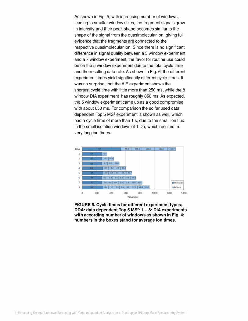
6 Enhancing General Unknown Screening with Data Independent Analysis on a Quadrupole Orbitrap Mass Spectrometry System
Conclusion
It could be shown, that with DIA the sensitivity and
selectivity of fragment ions can be increased significantly.
Since this is a technique without targeted precursor ion
selection, no signals are filtered out. This enables all
possibilities for post acquisition processing in a targeted
and untargeted approach the same way, so prerequisites
for General Unknown Screening are given without
compromise.
References
1. B. Vogler, Master Thesis, University of Zurich,
Switzerland, 2013
Overview
Purpose: Enhance the unknown screening
capabilities over the classical All Ion Fragmentation
approach.
Methods: Envoironmental samples were measured with
different scan methods for comparison.
Results: The DIA mode serves for the most versatile data
suitable for unknown screening as well as for targeted
quantitation at the same time
Introduction
In residue analysis of environmental and food samples
the need exists for the analysis of larger sets of analytes
at the same time. Recent developments in scan speed of
triple quadrupole mass spectrometry systems have
fuelled this development, but even more the steadily
increasing use of high resolution accurate mass (HRAM)
mass spectrometry instrumentation (mainly TOF and
OrbitrapTMbased instruments) in residue analysis leads to
numerous new options in this field as well into new
challenges. One of these challenges is the confirmation
step for the analytes, since precursor ion selected
fragmentation comes to its technical limits in terms of the
number of analytes and becomes impossible in case of
analytes yet unknown or disregarded. The alternative of
fragmentation without precursor ion selection (as “All Ion
Fragmentation” or “MSE”) has proven to be very powerful
but still faces some limitations in sensitivity of fragments
for low concentrated components. In the Data
Independent Acquisition (DIA) scan mode of a Thermo
Scientific TM Q ExactiveTM mass spectrometric system, the
full scan mass range is divided into smaller ranges,
typically in the range of 50 to 100 Daltons. This enhances
the dynamic range for the fragment scans, resulting in
significant higher sensitivity of the significant fragments
needed for compound confirmation. At the same time all
options for suspect screening or even General Unknown
Screening remain fully available as in AIF.
Methods
Sample Preparation
Ground water, surface water and waste water samples
were collected and prepared as described earlier1.
Liquid Chromatography
For chromatographic separation, a HPLC system was
used consisting of a CTC Pal autosampler (CTC analytics,
Zwingen, Switzerland) and a Rheos 2200 pump (Flux
Instruments, Switzerland). For separation a XBridge C18
column (50x2.1 mm, 3.5 µm particle size) was used,
applying a gradient of water and methanol, both acidified
with 0.1% formic acid as given in Fig. 2.
Mass Spectrometry
For mass spectrometric analysis a Q Exactive quadrupole
Orbitrap mass spectrometer was used. The final setup
was run in electrospray mode, the spray voltage being +
4000 V (positive mode) or - 3000 V (negative mode). The
capillary temperature was at 320°C. S-lens-level was set
to 50, auxiliary gas flow rate was 15 (arbitrary units) and
sheath gas flow rate was 40 (arbitrary units) for both
ionization modes.
For data dependent experiments, full scan was recorded
with a resolution of 140,000 @ m/z 200, while the data
dependent MS2 scans were recoded with a resolution of
17,500 @ m/z 200.
For AIF experiments, full scan was recorded with a
resolution of 140,000 @ m/z 200 and the fragment
spectra were recorded with a resolution of 17,500 @ m/z
200.
For DIA experiments, full scan was recorded with a
resolution of 70,000 @ m/z 200, automated gain control
was set to 500,000 and the maximal injection time was
200 ms. After the full scan different numbers of data
independent MSMS spectra were recorded. Isolation
widths and mass ranges were set according to Fig. 3.
Resolution was set to 17,500 @ m/z 200, AGC to 200,000
and maximal injection time to 100 ms.
Results
All Ion Fragmentation (AIF)
First, data was acquired in AIF mode as described. After
acquisition, extracted ion chromatograms were generated
for the quasimolecular ion and specific ions for a number
of compounds. Fig. 3 shows the XICs for Morphine and
Sotalol as an example. Some of the fragments are missing
completely and some show an irregular peak shape than
the one of the quasimolecular ion, because the signal
intensity is significant lower, although the concentration of
the used standard was 500 ng/L.
DIA Mode
In DIA mode different setups were evaluated. The
assumption was that with more windows with smaller
resulting isolation windows should yield better sensitivity
on the fragment ion signals. Since the ion flux is bigger on
the smaller masses while the mass range above m/z 500
shows only low amount of matrix ions, the isolation
windows were kept small in the range below m/z 500 with
only one bigger window for the range above m/z 500 (see
Fig. 4).
All trademarks used are the property of Thermo Fisher Scientific and its subsidiaries.
This information is not intended to encourage use of these products in any manners that might infringe the intellectual property rights of others.
Presented at RAFA, Prague, Czech Republic, Nov 5-8, 2013.
As shown in Fig. 5, with increasing number of windows,
leading to smaller window sizes, the fragment signals grow
in intensity and their peak shape becomes similar to the
shape of the signal from the quasimolecular ion, giving full
evidence that the fragments are connected to the
respective quasimolecular ion. Since there is no significant
difference in signal quality between a 5 window experiment
and a 7 window experiment, the favor for routine use could
be on the 5 window experiment due to the total cycle time
and the resulting data rate. As shown in Fig. 6, the different
experiment times yield significantly different cycle times. It
was no surprise, that the AIF experiment shows the
shortest cycle time with little more than 250 ms, while the 8
window DIA experiment has roughly 850 ms. As expected,
the 5 window experiment came up as a good compromise
with about 650 ms. For comparison the so far used data
dependent Top 5 MS2 experiment is shown as well, which
had a cycle time of more than 1 s, due to the small ion flux
in the small isolation windows of 1 Da, which resulted in
very long ion times.
Enhancing General Unknown Screening with Data Independent Analysis on a
Quadrupole Orbitrap Mass Spectrometry System
Olaf Scheibner1, Matthias Ruff2, Bernadette Vogler2, Heinz Singer2, Maciej Bromirski1
1 Thermo Fisher Scientific, Bremen, Germany2 Swiss Federal Institute of Aquatic Science and Technology, Dübendorf, Switzerland
FIGURE 1. Schematics of the Q Exactive mass
spectrometer.
FIGURE 2. Gradient settings for the chromatographic
separation.
FIGURE 4. Isolation windows for different numbers of
isolation windows in DIA mode; the top row showsthe isolation window of the full scan (figure taken
from Ref.1).
RT: 0.03 - 2.47
0.5 1.0 1.5 2.0
Time (min)
0
20
40
60
80
100
0
20
40
60
80
100
0
20
40
60
80
100
0
20
40
60
80
100
Rela
tive
Abu
nd
ance
0
20
40
60
80
100
0
20
40
60
80
1001.341.32
1.341.30 1.361.29 1.371.28
1.401.27 1.431.26 1.48
1.561.24 1.66 1.84 2.30
1.341.33
1.35
1.29 1.381.28
1.42
1.271.50
1.54
1.35
1.29
1.40
1.51
1.331.31
1.34
1.301.37
1.411.28
2.471.44
1.321.36
1.301.37
1.27
1.401.26
1.431.26
1.54 1.61
NL: 1.20E8
m/z=286.1409-286.1467 F:FTMS + p ESI Full ms[100.00-1000.00] MS130516pos_004
NL: 0
m/z=268.1306-268.1360 F:FTMS + p ESI Fullms2 MS130516pos_004
NL: 2.39E6
m/z=201.0892-201.0932 F:FTMS + p ESI Fullms2 MS130516pos_004
NL: 1.03E6
m/z=229.0838-229.0884 F:FTMS + p ESI Fullms2 MS130516pos_004
NL: 2.66E6
m/z=211.0734-211.0776 F:FTMS + p ESI Fullms2 MS130516pos_004
NL: 3.50E6
m/z=183.0787-183.0823 F:FTMS + p ESI Fullms2 MS130516pos_004
RT: 0.79 - 2.70
1.0 1.5 2.0 2.5
Time (min)
0
20
40
60
80
100
0
20
40
60
80
100
0
20
40
60
80
100
Re
lative
Ab
un
da
nce
0
20
40
60
80
100
0
20
40
60
80
1001.891.85
1.89
1.831.92
1.821.95
1.811.96
1.80 1.981.78 2.021.77 2.08
2.141.76 2.39 2.511.26
1.83
1.851.83
1.811.87
1.811.91
1.791.92
1.78 1.952.03 2.44
1.851.82
1.861.80
1.87
1.911.791.941.78
1.77 1.952.07 2.50
2.49
1.861.86 1.891.911.83
1.931.821.941.811.96
1.79 1.991.79
2.021.77 2.07
2.141.75 2.28 2.551.520.86
1.851.84
1.83 1.90
1.82
1.931.79
1.951.772.06
NL: 1.51E8
m/z=273.1250-273.1304 F: FTMS + p ESI Fullms [100.00-1000.00]MS 130516pos_004
NL: 2.57E6
m/z=255.1135-255.1187 F: FTMS + p ESI Fullms2 MS130516pos_004
NL: 3.84E6
m/z=213.0672-213.0714 F: FTMS + p ESI Fullms2 MS130516pos_004
NL: 5.27E7
m/z=133.0747-133.0773 F: FTMS + p ESI Fullms2 MS130516pos_004
NL: 1.21E6
m/z=176.1289-176.1325 F: FTMS + p ESI Fullms2 MS130516pos_004
FIGURE 3. Parent ions (top row) and fragment ions for
Morphine (A) and Sotalol (B) in AIF mode
A B
Another question was if not only the sensitivity, but also the
selectivity could be increased using the DIA approach. The
insect repellant DEET showed an interference in the
fragment m/z 119.0493. With on window (i. e. AIF) a clear
shoulder was visible which was not present in the signal of
the parent ion. This interference signal did not change at
first with increasing the number of windows for DIA, but
with eight windows (isolation width of 50 Da) suddenly the
chromatographic peak showed the same shape as the
parent peak from the full scan. This indicates, that it is
possible to even increase the selectivity with the larger
number of isolation windows in DIA. This is shown clearly
in Fig. 7.
So in total there were eight experiments, starting with the
AIF experiment (row 1), covering the whole mass range
from m/z 100 to 1000. The next experiment divided the
mass rage at m/z 450 (row 2) and the following
experiments subdivided this range into an increasing
number of smaller isolation ranges, ending up with eight
windows, of which seven had an isolation width of 50 Da
(row 8).
FIGURE 6. Cycle times for different experiment types;
DDA: data dependent Top 5 MS2; 1 – 8: DIA experiments with according number of windows as shown in Fig. 4;
numbers in the boxes stand for average ion times.
FIGURE 5. Influence of the number of DIA windows on
the sensitivity of specific fragments on the example ofMorphine in a neat standard.
RT: 0.69 - 2.10
1.0 1.5 2.0
Ti me (m in)
0
20
40
60
80
100
0
20
40
60
80
100
0
20
40
60
80
100
0
20
40
60
80
100
Re
lative
Abu
nd
an
ce
0
20
40
60
80
100
0
20
40
60
80
1001.34
1.321.34
1.311.36
1.30
1.371.29
1.401.27
1.44
1.491.25
1.561.661.23
1.341.33
1.35
1.29
1.42
1.271.50
1.26
1.54
1.35
1.29
1.40
1.51
1.331.31
1.34
1.351.30
1.37
1.28
1.44
1.52
1.321.36
1.30
1.371.27
1.401.26
1.431.26
1.54 1.61
NL: 1.20E8
m/z=
286.1409-286.1467
F: FTMS + p ESI Full
ms [100.00-1000.00]
MS 130516pos_004
NL: 0
m/z=
268.1306-268.1360
F: FTMS + p ESI Full
ms2 MS
130516pos_004
NL: 2.39E6
m/z=
201.0892-201.0932
F: FTMS + p ESI Full
ms2 MS
130516pos_004
NL: 1.03E6
m/z=
229.0838-229.0884
F: FTMS + p ESI Full
ms2 MS
130516pos_004
NL: 2.66E6
m/z=
211.0734-211.0776
F: FTMS + p ESI Full
ms2 MS
130516pos_004
NL: 3.50E6
m/z=
183.0787-183.0823
F: FTMS + p ESI Full
ms2 MS
130516pos_004
RT: 0.70 - 2.10
1.0 1.5 2.0
Time (mi n)
0
20
40
60
80
100
0
20
40
60
80
100
0
20
40
60
80
100
0
20
40
60
80
100
Re
lative
Abu
nd
an
ce
0
20
40
60
80
100
0
20
40
60
80
1001.32
1.311.34
1.291.35
1.27 1.37
1.391.26
1.411.25
1.471.23 1.55
1.67
1.34
1.31
1.381.31 1.45
1.27
1.31
1.311.30
1.36
1.27 1.36
1.401.26
1.24 1.541.55
1.23 1.76
1.321.33
1.291.34
1.35
1.361.29
1.381.27
1.411.26
1.501.74
1.24
1.32
1.33
1.29 1.36
1.361.27
1.24 1.47 1.75
1.31
1.361.28
1.271.39
1.531.24 1.73
NL: 1.27E8
m/z=
286.1409-286.1467
F: FTMS + p ESI Ful l
ms[100.00-1000.00]
MS 130516pos_005
NL: 1.89E6
m/z=
268.1306-268.1360
F: FTMS + p ESI Ful l
ms2 MS
130516pos_005
NL: 5.27E6
m/z=
201.0892-201.0932
F: FTMS + p ESI Ful l
ms2 MS
130516pos_005
NL: 5.28E6
m/z=
229.0838-229.0884
F: FTMS + p ESI Ful l
ms2 MS
130516pos_005
NL: 2.53E6
m/z=
211.0734-211.0776
F: FTMS + p ESI Ful l
ms2 MS
130516pos_005
NL: 9.76E5
m/z=
183.0787-183.0823
F: FTMS + p ESI Ful l
ms2 MS
130516pos_005
RT: 0.69 - 2.12
1.0 1.5 2.0
Ti me (mi n)
0
20
40
60
80
100
0
20
40
60
80
100
0
20
40
60
80
100
0
20
40
60
80
100
Re
lative
Abu
nd
an
ce
0
20
40
60
80
100
0
20
40
60
80
1001.331.32
1.34
1.351.29
1.361.28
1.26 1.39
1.411.25
1.44
1.521.231.60
1.20
1.32
1.33
1.31 1.36
1.381.27
1.401.261.441.25
1.451.241.52
1.23 2.10
1.32
1.331.31
1.29 1.34
1.361.27 1.371.26
1.401.25
1.471.241.561.22 1.77
1.32
1.31 1.34
1.351.28
1.36
1.391.26
1.42
1.471.241.56
1.22 1.78
1.331.32
1.291.34
1.361.27
1.261.39
1.451.24 1.50
1.601.22
1.32
1.291.35
1.271.38
1.391.26
1.25 1.44
1.23 1.542.08
NL: 1.19E8
m/z=
286.1409-286.1467
F: FTMS + p ESI Full
ms [100.00-1000.00]
MS 130516pos_008
NL: 8.52E5
m/z=
268.1306-268.1360
F: FTMS + p ESI Full
ms2 MS
130516pos_008
NL: 4.61E6
m/z=
201.0892-201.0932
F: FTMS + p ESI Full
ms2 MS
130516pos_008
NL: 3.09E6
m/z=
229.0838-229.0884
F: FTMS + p ESI Full
ms2 MS
130516pos_008
NL: 1.88E6
m/z=
211.0734-211.0776
F: FTMS + p ESI Full
ms2 MS
130516pos_008
NL: 1.30E6
m/z=
183.0787-183.0823
F: FTMS + p ESI Full
ms2 MS
130516pos_008
RT: 0.69 - 2.12
1.0 1.5 2.0
Ti me (m in)
0
20
40
60
80
100
0
20
40
60
80
100
0
20
40
60
80
100
0
20
40
60
80
100
Re
lative
Abu
nd
an
ce
0
20
40
60
80
100
0
20
40
60
80
1001.31 1.33
1.30
1.341.29
1.271.36
1.261.39
1.251.41
1.471.231.54
1.761.21
1.321.31
1.34
1.301.35
1.27
1.37
1.381.25
1.411.48
1.231.80
1.321.31
1.341.30
1.27 1.35
1.371.25
1.391.24
1.44
1.23 1.511.58
1.20 1.790.89
1.30 1.32
1.28
1.27 1.35
1.25 1.38
1.411.241.48
1.231.57 1.711.20
1.321.31
1.34
1.271.37
1.25
1.391.24
1.441.511.23
2.08
1.30 1.32
1.281.35
1.271.37
1.25
1.411.24
1.501.23
1.55 1.71
NL: 1.21E8
m/z=
286.1409-286.1467
F: FTMS + p ESI Full
ms [100.00-1000.00]
MS 130516pos_010
NL: 9.15E5
m/z=
268.1306-268.1360
F: FTMS + p ESI Full
ms2 MS
130516pos_010
NL: 3.73E6
m/z=
201.0892-201.0932
F: FTMS + p ESI Full
ms2 MS
130516pos_010
NL: 2.64E6
m/z=
229.0838-229.0884
F: FTMS + p ESI Full
ms2 MS
130516pos_010
NL: 1.71E6
m/z=
211.0734-211.0776
F: FTMS + p ESI Full
ms2 MS
130516pos_010
NL: 1.12E6
m/z=
183.0787-183.0823
F: FTMS + p ESI Full
ms2 MS
130516pos_010
1 window 2 windows 5 windows 7 windows
FIGURE 7. Interferences filtered out by DIA with higher
number of isolation windows on the Example of DEET.
RT: 7.87 - 9.79 SM: 5G
8.0 8.2 8.4 8.6 8.8 9.0 9.2 9.4 9.6
Time (min)
0
50
100
0
50
100
0
50
100
Re
lative
Ab
un
da
nce 0
50
1008.62 8.638.61
8.60 8.668.58 8.68
8.56 8.718.768.54 8.86 9.04 9.16 9.248.50 9.45 9.50 9.648.158.09 8.23
8.638.63 8.658.59 8.66
8.518.688.47
8.718.467.99 8.778.04 8.13 9.288.93 9.07 9.38 9.61
8.70 8.718.698.738.65
8.618.76
8.55 8.788.53 8.82 8.86 8.97 9.24 9.338.49 9.50 9.718.22
8.66 8.688.65
8.718.648.62 8.74
8.59 8.778.818.55 8.91 9.04 9.22 9.32 9.49 9.57 9.668.448.228.128.05
parent ion
1 window
5 windows
8 windows

7Thermo Scientific Poster Note • PN64245-RAFA 0914S
Conclusion
It could be shown, that with DIA the sensitivity and
selectivity of fragment ions can be increased significantly.
Since this is a technique without targeted precursor ion
selection, no signals are filtered out. This enables all
possibilities for post acquisition processing in a targeted
and untargeted approach the same way, so prerequisites
for General Unknown Screening are given without
compromise.
References
1. B. Vogler, Master Thesis, University of Zurich,
Switzerland, 2013
Overview
Purpose: Enhance the unknown screening
capabilities over the classical All Ion Fragmentation
approach.
Methods: Envoironmental samples were measured with
different scan methods for comparison.
Results: The DIA mode serves for the most versatile data
suitable for unknown screening as well as for targeted
quantitation at the same time
Introduction
In residue analysis of environmental and food samples
the need exists for the analysis of larger sets of analytes
at the same time. Recent developments in scan speed of
triple quadrupole mass spectrometry systems have
fuelled this development, but even more the steadily
increasing use of high resolution accurate mass (HRAM)
mass spectrometry instrumentation (mainly TOF and
OrbitrapTMbased instruments) in residue analysis leads to
numerous new options in this field as well into new
challenges. One of these challenges is the confirmation
step for the analytes, since precursor ion selected
fragmentation comes to its technical limits in terms of the
number of analytes and becomes impossible in case of
analytes yet unknown or disregarded. The alternative of
fragmentation without precursor ion selection (as “All Ion
Fragmentation” or “MSE”) has proven to be very powerful
but still faces some limitations in sensitivity of fragments
for low concentrated components. In the Data
Independent Acquisition (DIA) scan mode of a Thermo
Scientific TM Q ExactiveTM mass spectrometric system, the
full scan mass range is divided into smaller ranges,
typically in the range of 50 to 100 Daltons. This enhances
the dynamic range for the fragment scans, resulting in
significant higher sensitivity of the significant fragments
needed for compound confirmation. At the same time all
options for suspect screening or even General Unknown
Screening remain fully available as in AIF.
Methods
Sample Preparation
Ground water, surface water and waste water samples
were collected and prepared as described earlier1.
Liquid Chromatography
For chromatographic separation, a HPLC system was
used consisting of a CTC Pal autosampler (CTC analytics,
Zwingen, Switzerland) and a Rheos 2200 pump (Flux
Instruments, Switzerland). For separation a XBridge C18
column (50x2.1 mm, 3.5 µm particle size) was used,
applying a gradient of water and methanol, both acidified
with 0.1% formic acid as given in Fig. 2.
Mass Spectrometry
For mass spectrometric analysis a Q Exactive quadrupole
Orbitrap mass spectrometer was used. The final setup
was run in electrospray mode, the spray voltage being +
4000 V (positive mode) or - 3000 V (negative mode). The
capillary temperature was at 320°C. S-lens-level was set
to 50, auxiliary gas flow rate was 15 (arbitrary units) and
sheath gas flow rate was 40 (arbitrary units) for both
ionization modes.
For data dependent experiments, full scan was recorded
with a resolution of 140,000 @ m/z 200, while the data
dependent MS2 scans were recoded with a resolution of
17,500 @ m/z 200.
For AIF experiments, full scan was recorded with a
resolution of 140,000 @ m/z 200 and the fragment
spectra were recorded with a resolution of 17,500 @ m/z
200.
For DIA experiments, full scan was recorded with a
resolution of 70,000 @ m/z 200, automated gain control
was set to 500,000 and the maximal injection time was
200 ms. After the full scan different numbers of data
independent MSMS spectra were recorded. Isolation
widths and mass ranges were set according to Fig. 3.
Resolution was set to 17,500 @ m/z 200, AGC to 200,000
and maximal injection time to 100 ms.
Results
All Ion Fragmentation (AIF)
First, data was acquired in AIF mode as described. After
acquisition, extracted ion chromatograms were generated
for the quasimolecular ion and specific ions for a number
of compounds. Fig. 3 shows the XICs for Morphine and
Sotalol as an example. Some of the fragments are missing
completely and some show an irregular peak shape than
the one of the quasimolecular ion, because the signal
intensity is significant lower, although the concentration of
the used standard was 500 ng/L.
DIA Mode
In DIA mode different setups were evaluated. The
assumption was that with more windows with smaller
resulting isolation windows should yield better sensitivity
on the fragment ion signals. Since the ion flux is bigger on
the smaller masses while the mass range above m/z 500
shows only low amount of matrix ions, the isolation
windows were kept small in the range below m/z 500 with
only one bigger window for the range above m/z 500 (see
Fig. 4).
All trademarks used are the property of Thermo Fisher Scientific and its subsidiaries.
This information is not intended to encourage use of these products in any manners that might infringe the intellectual property rights of others.
Presented at RAFA, Prague, Czech Republic, Nov 5-8, 2013.
As shown in Fig. 5, with increasing number of windows,
leading to smaller window sizes, the fragment signals grow
in intensity and their peak shape becomes similar to the
shape of the signal from the quasimolecular ion, giving full
evidence that the fragments are connected to the
respective quasimolecular ion. Since there is no significant
difference in signal quality between a 5 window experiment
and a 7 window experiment, the favor for routine use could
be on the 5 window experiment due to the total cycle time
and the resulting data rate. As shown in Fig. 6, the different
experiment times yield significantly different cycle times. It
was no surprise, that the AIF experiment shows the
shortest cycle time with little more than 250 ms, while the 8
window DIA experiment has roughly 850 ms. As expected,
the 5 window experiment came up as a good compromise
with about 650 ms. For comparison the so far used data
dependent Top 5 MS2 experiment is shown as well, which
had a cycle time of more than 1 s, due to the small ion flux
in the small isolation windows of 1 Da, which resulted in
very long ion times.
Enhancing General Unknown Screening with Data Independent Analysis on a
Quadrupole Orbitrap Mass Spectrometry System
Olaf Scheibner1, Matthias Ruff2, Bernadette Vogler2, Heinz Singer2, Maciej Bromirski1
1 Thermo Fisher Scientific, Bremen, Germany2 Swiss Federal Institute of Aquatic Science and Technology, Dübendorf, Switzerland
FIGURE 1. Schematics of the Q Exactive mass
spectrometer.
FIGURE 2. Gradient settings for the chromatographic
separation.
FIGURE 4. Isolation windows for different numbers of
isolation windows in DIA mode; the top row showsthe isolation window of the full scan (figure taken
from Ref.1).
RT: 0.03 - 2.47
0.5 1.0 1.5 2.0
Time (min)
0
20
40
60
80
100
0
20
40
60
80
100
0
20
40
60
80
100
0
20
40
60
80
100
Rela
tive
Abu
nd
ance
0
20
40
60
80
100
0
20
40
60
80
1001.341.32
1.341.30 1.361.29 1.371.28
1.401.27 1.431.26 1.48
1.561.24 1.66 1.84 2.30
1.341.33
1.35
1.29 1.381.28
1.42
1.271.50
1.54
1.35
1.29
1.40
1.51
1.331.31
1.34
1.301.37
1.411.28
2.471.44
1.321.36
1.301.37
1.27
1.401.26
1.431.26
1.54 1.61
NL: 1.20E8
m/z=286.1409-286.1467 F:FTMS + p ESI Full ms[100.00-1000.00] MS130516pos_004
NL: 0
m/z=268.1306-268.1360 F:FTMS + p ESI Fullms2 MS130516pos_004
NL: 2.39E6
m/z=201.0892-201.0932 F:FTMS + p ESI Fullms2 MS130516pos_004
NL: 1.03E6
m/z=229.0838-229.0884 F:FTMS + p ESI Fullms2 MS130516pos_004
NL: 2.66E6
m/z=211.0734-211.0776 F:FTMS + p ESI Fullms2 MS130516pos_004
NL: 3.50E6
m/z=183.0787-183.0823 F:FTMS + p ESI Fullms2 MS130516pos_004
RT: 0.79 - 2.70
1.0 1.5 2.0 2.5
Time (min)
0
20
40
60
80
100
0
20
40
60
80
100
0
20
40
60
80
100
Re
lative
Ab
un
da
nce
0
20
40
60
80
100
0
20
40
60
80
1001.891.85
1.89
1.831.92
1.821.95
1.811.96
1.80 1.981.78 2.021.77 2.08
2.141.76 2.39 2.511.26
1.83
1.851.83
1.811.87
1.811.91
1.791.92
1.78 1.952.03 2.44
1.851.82
1.861.80
1.87
1.911.791.941.78
1.77 1.952.07 2.50
2.49
1.861.86 1.891.911.83
1.931.821.941.811.96
1.79 1.991.79
2.021.77 2.07
2.141.75 2.28 2.551.520.86
1.851.84
1.83 1.90
1.82
1.931.79
1.951.772.06
NL: 1.51E8
m/z=273.1250-273.1304 F: FTMS + p ESI Fullms [100.00-1000.00]MS 130516pos_004
NL: 2.57E6
m/z=255.1135-255.1187 F: FTMS + p ESI Fullms2 MS130516pos_004
NL: 3.84E6
m/z=213.0672-213.0714 F: FTMS + p ESI Fullms2 MS130516pos_004
NL: 5.27E7
m/z=133.0747-133.0773 F: FTMS + p ESI Fullms2 MS130516pos_004
NL: 1.21E6
m/z=176.1289-176.1325 F: FTMS + p ESI Fullms2 MS130516pos_004
FIGURE 3. Parent ions (top row) and fragment ions for
Morphine (A) and Sotalol (B) in AIF mode
A B
Another question was if not only the sensitivity, but also
the selectivity could be increased using the DIA approach.
The insect repellant DEET showed an interference in the
fragment m/z 119.0493. With one window (i.e. AIF) a clear
shoulder was visible which was not present in the signal of
the parent ion. This interference signal did not change at
first with increasing the number of windows for DIA, but
with eight windows (isolation width of 50 Da) suddenly the
chromatographic peak showed the same shape as the
parent peak from the full scan. This indicates, that it is
possible to even increase the selectivity with the larger
number of isolation windows in DIA. This is shown clearly
in Fig. 7.
So in total there were eight experiments, starting with the
AIF experiment (row 1), covering the whole mass range
from m/z 100 to 1000. The next experiment divided the
mass rage at m/z 450 (row 2) and the following
experiments subdivided this range into an increasing
number of smaller isolation ranges, ending up with eight
windows, of which seven had an isolation width of 50 Da
(row 8).
FIGURE 6. Cycle times for different experiment types;
DDA: data dependent Top 5 MS2; 1 – 8: DIA experiments with according number of windows as shown in Fig. 4;
numbers in the boxes stand for average ion times.
FIGURE 5. Influence of the number of DIA windows on
the sensitivity of specific fragments on the example ofMorphine in a neat standard.
RT: 0.69 - 2.10
1.0 1.5 2.0
Ti me (m in)
0
20
40
60
80
100
0
20
40
60
80
100
0
20
40
60
80
100
0
20
40
60
80
100
Re
lative
Abu
nd
an
ce
0
20
40
60
80
100
0
20
40
60
80
1001.34
1.321.34
1.311.36
1.30
1.371.29
1.401.27
1.44
1.491.25
1.561.661.23
1.341.33
1.35
1.29
1.42
1.271.50
1.26
1.54
1.35
1.29
1.40
1.51
1.331.31
1.34
1.351.30
1.37
1.28
1.44
1.52
1.321.36
1.30
1.371.27
1.401.26
1.431.26
1.54 1.61
NL: 1.20E8
m/z=
286.1409-286.1467
F: FTMS + p ESI Full
ms [100.00-1000.00]
MS 130516pos_004
NL: 0
m/z=
268.1306-268.1360
F: FTMS + p ESI Full
ms2 MS
130516pos_004
NL: 2.39E6
m/z=
201.0892-201.0932
F: FTMS + p ESI Full
ms2 MS
130516pos_004
NL: 1.03E6
m/z=
229.0838-229.0884
F: FTMS + p ESI Full
ms2 MS
130516pos_004
NL: 2.66E6
m/z=
211.0734-211.0776
F: FTMS + p ESI Full
ms2 MS
130516pos_004
NL: 3.50E6
m/z=
183.0787-183.0823
F: FTMS + p ESI Full
ms2 MS
130516pos_004
RT: 0.70 - 2.10
1.0 1.5 2.0
Time (mi n)
0
20
40
60
80
100
0
20
40
60
80
100
0
20
40
60
80
100
0
20
40
60
80
100
Re
lative
Abu
nd
an
ce
0
20
40
60
80
100
0
20
40
60
80
1001.32
1.311.34
1.291.35
1.27 1.37
1.391.26
1.411.25
1.471.23 1.55
1.67
1.34
1.31
1.381.31 1.45
1.27
1.31
1.311.30
1.36
1.27 1.36
1.401.26
1.24 1.541.55
1.23 1.76
1.321.33
1.291.34
1.35
1.361.29
1.381.27
1.411.26
1.501.74
1.24
1.32
1.33
1.29 1.36
1.361.27
1.24 1.47 1.75
1.31
1.361.28
1.271.39
1.531.24 1.73
NL: 1.27E8
m/z=
286.1409-286.1467
F: FTMS + p ESI Ful l
ms[100.00-1000.00]
MS 130516pos_005
NL: 1.89E6
m/z=
268.1306-268.1360
F: FTMS + p ESI Ful l
ms2 MS
130516pos_005
NL: 5.27E6
m/z=
201.0892-201.0932
F: FTMS + p ESI Ful l
ms2 MS
130516pos_005
NL: 5.28E6
m/z=
229.0838-229.0884
F: FTMS + p ESI Ful l
ms2 MS
130516pos_005
NL: 2.53E6
m/z=
211.0734-211.0776
F: FTMS + p ESI Ful l
ms2 MS
130516pos_005
NL: 9.76E5
m/z=
183.0787-183.0823
F: FTMS + p ESI Ful l
ms2 MS
130516pos_005
RT: 0.69 - 2.12
1.0 1.5 2.0
Ti me (mi n)
0
20
40
60
80
100
0
20
40
60
80
100
0
20
40
60
80
100
0
20
40
60
80
100
Re
lative
Abu
nd
an
ce
0
20
40
60
80
100
0
20
40
60
80
1001.331.32
1.34
1.351.29
1.361.28
1.26 1.39
1.411.25
1.44
1.521.231.60
1.20
1.32
1.33
1.31 1.36
1.381.27
1.401.261.441.25
1.451.241.52
1.23 2.10
1.32
1.331.31
1.29 1.34
1.361.27 1.371.26
1.401.25
1.471.241.561.22 1.77
1.32
1.31 1.34
1.351.28
1.36
1.391.26
1.42
1.471.241.56
1.22 1.78
1.331.32
1.291.34
1.361.27
1.261.39
1.451.24 1.50
1.601.22
1.32
1.291.35
1.271.38
1.391.26
1.25 1.44
1.23 1.542.08
NL: 1.19E8
m/z=
286.1409-286.1467
F: FTMS + p ESI Full
ms [100.00-1000.00]
MS 130516pos_008
NL: 8.52E5
m/z=
268.1306-268.1360
F: FTMS + p ESI Full
ms2 MS
130516pos_008
NL: 4.61E6
m/z=
201.0892-201.0932
F: FTMS + p ESI Full
ms2 MS
130516pos_008
NL: 3.09E6
m/z=
229.0838-229.0884
F: FTMS + p ESI Full
ms2 MS
130516pos_008
NL: 1.88E6
m/z=
211.0734-211.0776
F: FTMS + p ESI Full
ms2 MS
130516pos_008
NL: 1.30E6
m/z=
183.0787-183.0823
F: FTMS + p ESI Full
ms2 MS
130516pos_008
RT: 0.69 - 2.12
1.0 1.5 2.0
Ti me (m in)
0
20
40
60
80
100
0
20
40
60
80
100
0
20
40
60
80
100
0
20
40
60
80
100
Re
lative
Abu
nd
an
ce
0
20
40
60
80
100
0
20
40
60
80
1001.31 1.33
1.30
1.341.29
1.271.36
1.261.39
1.251.41
1.471.231.54
1.761.21
1.321.31
1.34
1.301.35
1.27
1.37
1.381.25
1.411.48
1.231.80
1.321.31
1.341.30
1.27 1.35
1.371.25
1.391.24
1.44
1.23 1.511.58
1.20 1.790.89
1.30 1.32
1.28
1.27 1.35
1.25 1.38
1.411.241.48
1.231.57 1.711.20
1.321.31
1.34
1.271.37
1.25
1.391.24
1.441.511.23
2.08
1.30 1.32
1.281.35
1.271.37
1.25
1.411.24
1.501.23
1.55 1.71
NL: 1.21E8
m/z=
286.1409-286.1467
F: FTMS + p ESI Full
ms [100.00-1000.00]
MS 130516pos_010
NL: 9.15E5
m/z=
268.1306-268.1360
F: FTMS + p ESI Full
ms2 MS
130516pos_010
NL: 3.73E6
m/z=
201.0892-201.0932
F: FTMS + p ESI Full
ms2 MS
130516pos_010
NL: 2.64E6
m/z=
229.0838-229.0884
F: FTMS + p ESI Full
ms2 MS
130516pos_010
NL: 1.71E6
m/z=
211.0734-211.0776
F: FTMS + p ESI Full
ms2 MS
130516pos_010
NL: 1.12E6
m/z=
183.0787-183.0823
F: FTMS + p ESI Full
ms2 MS
130516pos_010
1 window 2 windows 5 windows 7 windows
FIGURE 7. Interferences filtered out by DIA with higher
number of isolation windows on the Example of DEET.
RT: 7.87 - 9.79 SM: 5G
8.0 8.2 8.4 8.6 8.8 9.0 9.2 9.4 9.6
Time (min)
0
50
100
0
50
100
0
50
100
Re
lative
Ab
un
da
nce 0
50
1008.62 8.638.61
8.60 8.668.58 8.68
8.56 8.718.768.54 8.86 9.04 9.16 9.248.50 9.45 9.50 9.648.158.09 8.23
8.638.63 8.658.59 8.66
8.518.688.47
8.718.467.99 8.778.04 8.13 9.288.93 9.07 9.38 9.61
8.70 8.718.698.738.65
8.618.76
8.55 8.788.53 8.82 8.86 8.97 9.24 9.338.49 9.50 9.718.22
8.66 8.688.65
8.718.648.62 8.74
8.59 8.778.818.55 8.91 9.04 9.22 9.32 9.49 9.57 9.668.448.228.128.05
parent ion
1 window
5 windows
8 windows

www.thermofisher.com©2016 Thermo Fisher Scientific Inc. All rights reserved. All trademarks are the property of Thermo Fisher Scientific and its subsidiaries. This information is presented as an example of the capabilities of Thermo Fisher Scientific products. It is not intended to encourage use of these products in any manners that might infringe the intellectual property rights of others. Specifications, terms and pricing are subject to change. Not all products are available in all countries. Please consult your local sales representative for details.
PN64245-EN 0816S
Africa +43 1 333 50 34 0Australia +61 3 9757 4300Austria +43 810 282 206Belgium +32 53 73 42 41Canada +1 800 530 8447China 800 810 5118 (free call domestic)
400 650 5118
Denmark +45 70 23 62 60Europe-Other +43 1 333 50 34 0Finland +358 9 3291 0200France +33 1 60 92 48 00Germany +49 6103 408 1014India +91 22 6742 9494Italy +39 02 950 591
Japan +81 45 453 9100Latin America +1 561 688 8700Middle East +43 1 333 50 34 0Netherlands +31 76 579 55 55New Zealand +64 9 980 6700Norway +46 8 556 468 00Russia/CIS +43 1 333 50 34 0
Singapore +65 6289 1190Spain +34 914 845 965Sweden +46 8 556 468 00Switzerland +41 61 716 77 00UK +44 1442 233555USA +1 800 532 4752
Conclusion
It could be shown, that with DIA the sensitivity and
selectivity of fragment ions can be increased significantly.
Since this is a technique without targeted precursor ion
selection, no signals are filtered out. This enables all
possibilities for post acquisition processing in a targeted
and untargeted approach the same way, so prerequisites
for General Unknown Screening are given without
compromise.
References
1. B. Vogler, Master Thesis, University of Zurich,
Switzerland, 2013
Overview
Purpose: Enhance the unknown screening
capabilities over the classical All Ion Fragmentation
approach.
Methods: Envoironmental samples were measured with
different scan methods for comparison.
Results: The DIA mode serves for the most versatile data
suitable for unknown screening as well as for targeted
quantitation at the same time
Introduction
In residue analysis of environmental and food samples
the need exists for the analysis of larger sets of analytes
at the same time. Recent developments in scan speed of
triple quadrupole mass spectrometry systems have
fuelled this development, but even more the steadily
increasing use of high resolution accurate mass (HRAM)
mass spectrometry instrumentation (mainly TOF and
OrbitrapTMbased instruments) in residue analysis leads to
numerous new options in this field as well into new
challenges. One of these challenges is the confirmation
step for the analytes, since precursor ion selected
fragmentation comes to its technical limits in terms of the
number of analytes and becomes impossible in case of
analytes yet unknown or disregarded. The alternative of
fragmentation without precursor ion selection (as “All Ion
Fragmentation” or “MSE”) has proven to be very powerful
but still faces some limitations in sensitivity of fragments
for low concentrated components. In the Data
Independent Acquisition (DIA) scan mode of a Thermo
Scientific TM Q ExactiveTM mass spectrometric system, the
full scan mass range is divided into smaller ranges,
typically in the range of 50 to 100 Daltons. This enhances
the dynamic range for the fragment scans, resulting in
significant higher sensitivity of the significant fragments
needed for compound confirmation. At the same time all
options for suspect screening or even General Unknown
Screening remain fully available as in AIF.
Methods
Sample Preparation
Ground water, surface water and waste water samples
were collected and prepared as described earlier1.
Liquid Chromatography
For chromatographic separation, a HPLC system was
used consisting of a CTC Pal autosampler (CTC analytics,
Zwingen, Switzerland) and a Rheos 2200 pump (Flux
Instruments, Switzerland). For separation a XBridge C18
column (50x2.1 mm, 3.5 µm particle size) was used,
applying a gradient of water and methanol, both acidified
with 0.1% formic acid as given in Fig. 2.
Mass Spectrometry
For mass spectrometric analysis a Q Exactive quadrupole
Orbitrap mass spectrometer was used. The final setup
was run in electrospray mode, the spray voltage being +
4000 V (positive mode) or - 3000 V (negative mode). The
capillary temperature was at 320°C. S-lens-level was set
to 50, auxiliary gas flow rate was 15 (arbitrary units) and
sheath gas flow rate was 40 (arbitrary units) for both
ionization modes.
For data dependent experiments, full scan was recorded
with a resolution of 140,000 @ m/z 200, while the data
dependent MS2 scans were recoded with a resolution of
17,500 @ m/z 200.
For AIF experiments, full scan was recorded with a
resolution of 140,000 @ m/z 200 and the fragment
spectra were recorded with a resolution of 17,500 @ m/z
200.
For DIA experiments, full scan was recorded with a
resolution of 70,000 @ m/z 200, automated gain control
was set to 500,000 and the maximal injection time was
200 ms. After the full scan different numbers of data
independent MSMS spectra were recorded. Isolation
widths and mass ranges were set according to Fig. 3.
Resolution was set to 17,500 @ m/z 200, AGC to 200,000
and maximal injection time to 100 ms.
Results
All Ion Fragmentation (AIF)
First, data was acquired in AIF mode as described. After
acquisition, extracted ion chromatograms were generated
for the quasimolecular ion and specific ions for a number
of compounds. Fig. 3 shows the XICs for Morphine and
Sotalol as an example. Some of the fragments are missing
completely and some show an irregular peak shape than
the one of the quasimolecular ion, because the signal
intensity is significant lower, although the concentration of
the used standard was 500 ng/L.
DIA Mode
In DIA mode different setups were evaluated. The
assumption was that with more windows with smaller
resulting isolation windows should yield better sensitivity
on the fragment ion signals. Since the ion flux is bigger on
the smaller masses while the mass range above m/z 500
shows only low amount of matrix ions, the isolation
windows were kept small in the range below m/z 500 with
only one bigger window for the range above m/z 500 (see
Fig. 4).
All trademarks used are the property of Thermo Fisher Scientific and its subsidiaries.
This information is not intended to encourage use of these products in any manners that might infringe the intellectual property rights of others.
Presented at RAFA, Prague, Czech Republic, Nov 5-8, 2013.
As shown in Fig. 5, with increasing number of windows,
leading to smaller window sizes, the fragment signals grow
in intensity and their peak shape becomes similar to the
shape of the signal from the quasimolecular ion, giving full
evidence that the fragments are connected to the
respective quasimolecular ion. Since there is no significant
difference in signal quality between a 5 window experiment
and a 7 window experiment, the favor for routine use could
be on the 5 window experiment due to the total cycle time
and the resulting data rate. As shown in Fig. 6, the different
experiment times yield significantly different cycle times. It
was no surprise, that the AIF experiment shows the
shortest cycle time with little more than 250 ms, while the 8
window DIA experiment has roughly 850 ms. As expected,
the 5 window experiment came up as a good compromise
with about 650 ms. For comparison the so far used data
dependent Top 5 MS2 experiment is shown as well, which
had a cycle time of more than 1 s, due to the small ion flux
in the small isolation windows of 1 Da, which resulted in
very long ion times.
Enhancing General Unknown Screening with Data Independent Analysis on a
Quadrupole Orbitrap Mass Spectrometry System
Olaf Scheibner1, Matthias Ruff2, Bernadette Vogler2, Heinz Singer2, Maciej Bromirski1
1 Thermo Fisher Scientific, Bremen, Germany2 Swiss Federal Institute of Aquatic Science and Technology, Dübendorf, Switzerland
FIGURE 1. Schematics of the Q Exactive mass
spectrometer.
FIGURE 2. Gradient settings for the chromatographic
separation.
FIGURE 4. Isolation windows for different numbers of
isolation windows in DIA mode; the top row showsthe isolation window of the full scan (figure taken
from Ref.1).
RT: 0.03 - 2.47
0.5 1.0 1.5 2.0
Time (min)
0
20
40
60
80
100
0
20
40
60
80
100
0
20
40
60
80
100
0
20
40
60
80
100
Rela
tive
Abu
nd
ance
0
20
40
60
80
100
0
20
40
60
80
1001.341.32
1.341.30 1.361.29 1.371.28
1.401.27 1.431.26 1.48
1.561.24 1.66 1.84 2.30
1.341.33
1.35
1.29 1.381.28
1.42
1.271.50
1.54
1.35
1.29
1.40
1.51
1.331.31
1.34
1.301.37
1.411.28
2.471.44
1.321.36
1.301.37
1.27
1.401.26
1.431.26
1.54 1.61
NL: 1.20E8
m/z=286.1409-286.1467 F:FTMS + p ESI Full ms[100.00-1000.00] MS130516pos_004
NL: 0
m/z=268.1306-268.1360 F:FTMS + p ESI Fullms2 MS130516pos_004
NL: 2.39E6
m/z=201.0892-201.0932 F:FTMS + p ESI Fullms2 MS130516pos_004
NL: 1.03E6
m/z=229.0838-229.0884 F:FTMS + p ESI Fullms2 MS130516pos_004
NL: 2.66E6
m/z=211.0734-211.0776 F:FTMS + p ESI Fullms2 MS130516pos_004
NL: 3.50E6
m/z=183.0787-183.0823 F:FTMS + p ESI Fullms2 MS130516pos_004
RT: 0.79 - 2.70
1.0 1.5 2.0 2.5
Time (min)
0
20
40
60
80
100
0
20
40
60
80
100
0
20
40
60
80
100
Re
lative
Ab
un
da
nce
0
20
40
60
80
100
0
20
40
60
80
1001.891.85
1.89
1.831.92
1.821.95
1.811.96
1.80 1.981.78 2.021.77 2.08
2.141.76 2.39 2.511.26
1.83
1.851.83
1.811.87
1.811.91
1.791.92
1.78 1.952.03 2.44
1.851.82
1.861.80
1.87
1.911.791.941.78
1.77 1.952.07 2.50
2.49
1.861.86 1.891.911.83
1.931.821.941.811.96
1.79 1.991.79
2.021.77 2.07
2.141.75 2.28 2.551.520.86
1.851.84
1.83 1.90
1.82
1.931.79
1.951.772.06
NL: 1.51E8
m/z=273.1250-273.1304 F: FTMS + p ESI Fullms [100.00-1000.00]MS 130516pos_004
NL: 2.57E6
m/z=255.1135-255.1187 F: FTMS + p ESI Fullms2 MS130516pos_004
NL: 3.84E6
m/z=213.0672-213.0714 F: FTMS + p ESI Fullms2 MS130516pos_004
NL: 5.27E7
m/z=133.0747-133.0773 F: FTMS + p ESI Fullms2 MS130516pos_004
NL: 1.21E6
m/z=176.1289-176.1325 F: FTMS + p ESI Fullms2 MS130516pos_004
FIGURE 3. Parent ions (top row) and fragment ions for
Morphine (A) and Sotalol (B) in AIF mode
A B
Another question was if not only the sensitivity, but also the
selectivity could be increased using the DIA approach. The
insect repellant DEET showed an interference in the
fragment m/z 119.0493. With on window (i. e. AIF) a clear
shoulder was visible which was not present in the signal of
the parent ion. This interference signal did not change at
first with increasing the number of windows for DIA, but
with eight windows (isolation width of 50 Da) suddenly the
chromatographic peak showed the same shape as the
parent peak from the full scan. This indicates, that it is
possible to even increase the selectivity with the larger
number of isolation windows in DIA. This is shown clearly
in Fig. 7.
So in total there were eight experiments, starting with the
AIF experiment (row 1), covering the whole mass range
from m/z 100 to 1000. The next experiment divided the
mass rage at m/z 450 (row 2) and the following
experiments subdivided this range into an increasing
number of smaller isolation ranges, ending up with eight
windows, of which seven had an isolation width of 50 Da
(row 8).
FIGURE 6. Cycle times for different experiment types;
DDA: data dependent Top 5 MS2; 1 – 8: DIA experiments with according number of windows as shown in Fig. 4;
numbers in the boxes stand for average ion times.
FIGURE 5. Influence of the number of DIA windows on
the sensitivity of specific fragments on the example ofMorphine in a neat standard.
RT: 0.69 - 2.10
1.0 1.5 2.0
Ti me (m in)
0
20
40
60
80
100
0
20
40
60
80
100
0
20
40
60
80
100
0
20
40
60
80
100
Re
lative
Abu
nd
an
ce
0
20
40
60
80
100
0
20
40
60
80
1001.34
1.321.34
1.311.36
1.30
1.371.29
1.401.27
1.44
1.491.25
1.561.661.23
1.341.33
1.35
1.29
1.42
1.271.50
1.26
1.54
1.35
1.29
1.40
1.51
1.331.31
1.34
1.351.30
1.37
1.28
1.44
1.52
1.321.36
1.30
1.371.27
1.401.26
1.431.26
1.54 1.61
NL: 1.20E8
m/z=
286.1409-286.1467
F: FTMS + p ESI Full
ms [100.00-1000.00]
MS 130516pos_004
NL: 0
m/z=
268.1306-268.1360
F: FTMS + p ESI Full
ms2 MS
130516pos_004
NL: 2.39E6
m/z=
201.0892-201.0932
F: FTMS + p ESI Full
ms2 MS
130516pos_004
NL: 1.03E6
m/z=
229.0838-229.0884
F: FTMS + p ESI Full
ms2 MS
130516pos_004
NL: 2.66E6
m/z=
211.0734-211.0776
F: FTMS + p ESI Full
ms2 MS
130516pos_004
NL: 3.50E6
m/z=
183.0787-183.0823
F: FTMS + p ESI Full
ms2 MS
130516pos_004
RT: 0.70 - 2.10
1.0 1.5 2.0
Time (mi n)
0
20
40
60
80
100
0
20
40
60
80
100
0
20
40
60
80
100
0
20
40
60
80
100
Re
lative
Abu
nd
an
ce
0
20
40
60
80
100
0
20
40
60
80
1001.32
1.311.34
1.291.35
1.27 1.37
1.391.26
1.411.25
1.471.23 1.55
1.67
1.34
1.31
1.381.31 1.45
1.27
1.31
1.311.30
1.36
1.27 1.36
1.401.26
1.24 1.541.55
1.23 1.76
1.321.33
1.291.34
1.35
1.361.29
1.381.27
1.411.26
1.501.74
1.24
1.32
1.33
1.29 1.36
1.361.27
1.24 1.47 1.75
1.31
1.361.28
1.271.39
1.531.24 1.73
NL: 1.27E8
m/z=
286.1409-286.1467
F: FTMS + p ESI Ful l
ms[100.00-1000.00]
MS 130516pos_005
NL: 1.89E6
m/z=
268.1306-268.1360
F: FTMS + p ESI Ful l
ms2 MS
130516pos_005
NL: 5.27E6
m/z=
201.0892-201.0932
F: FTMS + p ESI Ful l
ms2 MS
130516pos_005
NL: 5.28E6
m/z=
229.0838-229.0884
F: FTMS + p ESI Ful l
ms2 MS
130516pos_005
NL: 2.53E6
m/z=
211.0734-211.0776
F: FTMS + p ESI Ful l
ms2 MS
130516pos_005
NL: 9.76E5
m/z=
183.0787-183.0823
F: FTMS + p ESI Ful l
ms2 MS
130516pos_005
RT: 0.69 - 2.12
1.0 1.5 2.0
Ti me (mi n)
0
20
40
60
80
100
0
20
40
60
80
100
0
20
40
60
80
100
0
20
40
60
80
100
Re
lative
Abu
nd
an
ce
0
20
40
60
80
100
0
20
40
60
80
1001.331.32
1.34
1.351.29
1.361.28
1.26 1.39
1.411.25
1.44
1.521.231.60
1.20
1.32
1.33
1.31 1.36
1.381.27
1.401.261.441.25
1.451.241.52
1.23 2.10
1.32
1.331.31
1.29 1.34
1.361.27 1.371.26
1.401.25
1.471.241.561.22 1.77
1.32
1.31 1.34
1.351.28
1.36
1.391.26
1.42
1.471.241.56
1.22 1.78
1.331.32
1.291.34
1.361.27
1.261.39
1.451.24 1.50
1.601.22
1.32
1.291.35
1.271.38
1.391.26
1.25 1.44
1.23 1.542.08
NL: 1.19E8
m/z=
286.1409-286.1467
F: FTMS + p ESI Full
ms [100.00-1000.00]
MS 130516pos_008
NL: 8.52E5
m/z=
268.1306-268.1360
F: FTMS + p ESI Full
ms2 MS
130516pos_008
NL: 4.61E6
m/z=
201.0892-201.0932
F: FTMS + p ESI Full
ms2 MS
130516pos_008
NL: 3.09E6
m/z=
229.0838-229.0884
F: FTMS + p ESI Full
ms2 MS
130516pos_008
NL: 1.88E6
m/z=
211.0734-211.0776
F: FTMS + p ESI Full
ms2 MS
130516pos_008
NL: 1.30E6
m/z=
183.0787-183.0823
F: FTMS + p ESI Full
ms2 MS
130516pos_008
RT: 0.69 - 2.12
1.0 1.5 2.0
Ti me (m in)
0
20
40
60
80
100
0
20
40
60
80
100
0
20
40
60
80
100
0
20
40
60
80
100
Re
lative
Abu
nd
an
ce
0
20
40
60
80
100
0
20
40
60
80
1001.31 1.33
1.30
1.341.29
1.271.36
1.261.39
1.251.41
1.471.231.54
1.761.21
1.321.31
1.34
1.301.35
1.27
1.37
1.381.25
1.411.48
1.231.80
1.321.31
1.341.30
1.27 1.35
1.371.25
1.391.24
1.44
1.23 1.511.58
1.20 1.790.89
1.30 1.32
1.28
1.27 1.35
1.25 1.38
1.411.241.48
1.231.57 1.711.20
1.321.31
1.34
1.271.37
1.25
1.391.24
1.441.511.23
2.08
1.30 1.32
1.281.35
1.271.37
1.25
1.411.24
1.501.23
1.55 1.71
NL: 1.21E8
m/z=
286.1409-286.1467
F: FTMS + p ESI Full
ms [100.00-1000.00]
MS 130516pos_010
NL: 9.15E5
m/z=
268.1306-268.1360
F: FTMS + p ESI Full
ms2 MS
130516pos_010
NL: 3.73E6
m/z=
201.0892-201.0932
F: FTMS + p ESI Full
ms2 MS
130516pos_010
NL: 2.64E6
m/z=
229.0838-229.0884
F: FTMS + p ESI Full
ms2 MS
130516pos_010
NL: 1.71E6
m/z=
211.0734-211.0776
F: FTMS + p ESI Full
ms2 MS
130516pos_010
NL: 1.12E6
m/z=
183.0787-183.0823
F: FTMS + p ESI Full
ms2 MS
130516pos_010
1 window 2 windows 5 windows 7 windows
FIGURE 7. Interferences filtered out by DIA with higher
number of isolation windows on the Example of DEET.
RT: 7.87 - 9.79 SM: 5G
8.0 8.2 8.4 8.6 8.8 9.0 9.2 9.4 9.6
Time (min)
0
50
100
0
50
100
0
50
100
Re
lative
Ab
un
da
nce 0
50
1008.62 8.638.61
8.60 8.668.58 8.68
8.56 8.718.768.54 8.86 9.04 9.16 9.248.50 9.45 9.50 9.648.158.09 8.23
8.638.63 8.658.59 8.66
8.518.688.47
8.718.467.99 8.778.04 8.13 9.288.93 9.07 9.38 9.61
8.70 8.718.698.738.65
8.618.76
8.55 8.788.53 8.82 8.86 8.97 9.24 9.338.49 9.50 9.718.22
8.66 8.688.65
8.718.648.62 8.74
8.59 8.778.818.55 8.91 9.04 9.22 9.32 9.49 9.57 9.668.448.228.128.05
parent ion
1 window
5 windows
8 windows

Qualitative and Quantitative Analysis of Contaminants of Emerging Concern in Biosolids Using Dilute-and-Shoot UHPLC-Orbitrap MS MethodCharles Yang,1 Ahmed Mostafa,2 Shelly Bonte-Gelok,3 Jonathan Beck,1 Maciej Bromirski1 and Dipankar Ghosh1 and Paul Yang3 1Thermo Fisher Scientific, San Jose, CA,USA; 2Department of Chemistry and Biology, Ryerson University, Toronto, Ontario, Canada; 3Ontario Ministry of the Environment, Etobicoke, Ontario, Canada

2 Qualitative and Quantitative Analysis of Contaminants of Emerging Concernin Biosolids Using Dilute-and-Shoot UHPLC-Orbitrap MS Method
Qualitative and Quantitative Analysis of Contaminants of Emerging Concern in Biosolids Using Dilute-and-Shoot UHPLC-OrbitrapMS MethodCharles Yang1, Ahmed Mostafa2, Shelly Bonte-Gelok3, Jonathan Beck1, Maciej Bromirski1 and Dipankar Ghosh1 and Paul Yang31 Thermo Fisher Scientific, 355 River Oaks Parkway, San Jose, CA 95134-1706, USA; 2 Department of Chemistry and Biology, Ryerson University, Toronto, Ontario, M5B 2K3, Canada; 3 Ontario Ministry of the Environment, 125 Resources Road, Etobicoke, Ontario, M9P 3V6, Canada
Conclusion Quantitative results of PPCPs were obtained using HPLC-Orbitrap MS.
Semi-quantitative results showed the presence of surfactants, musks and treatment by-products in biosolids.
Efforts to obtain analytical standards to complete the studies are on-going.
Acknowledgements Dr. Ahmed Mostafa would like to acknowledge Canadian Water Network funding support for his postdoctal fellowship.
Overview Purpose: Develop a workflow to (1) do quantitatively analyze contaminants of emerging concerns (CECs) in biosolids samples, and (2) screen for 381 targeted CECs in samples.
Methods: Samples were prepared by ultrasonic extraction and analyzed by high performance liquid chromatography-Orbitrap mass spectrometry (HPLC-Orbitrap MS).
Results: Quantitative results of CECs in typical biosolids samples are presented. Targeted screening of CECs in biosolids showed the presence of different categories of CECs including parent pharmaceuticals and personal care products (PPCPs), e.g., DEET, Triclosan (TCS), Triclocarban (TCC), musks, Carbamazepine (CBZ), their degradation products, and surfactants.
Introduction A rapid dilute-and-shoot method for the quantitative determination of targeted CECs, e.g., endocrine disrupting chemicals, pharmaceuticals, personal care products, as well as their degradation by-products has been developed. Using ultrasonic based sample preparation and HPLC-Orbitrap MS analysis without any sample cleanup, this method has been optimized for the determination of 49 CECs present in biosolids and terrestrial biomes exposed to biosolids amended soils (BAS). The quantitative information on the CECs in biosolids and biological tissues would allow for the assessment, when and where appropriate, of potential uptake and bioaccumulation. In addition, full scan HRMS data provides information on the possible environmental transformation by-products for possible environmental accumulation and ecological effects that would not be available with other technology.
Methods Sample Preparation
For this study, model biosolid samples and biosolids amended samples were used in the evaluation of the method. Grab biosolid samples were contained in 1L-amber bottles without headspace and stored in dark, cold storage (4°C) until analysis. The same biosolids were also used to prepare BAS at Ryerson University and used to observe the fate of CECs from October 2013 to March 2014.
Neat standards of native target compounds were purchased from Sigma-Aldrich (Oakville, ON, Canada). Deuterium (D) and 13C-labelled standards were purchased from CDN Isotopes (Pointe-Claire, QC, Canada) and Cambridge isotope Laboratories (Andover, MA, US). Five levels of analytical standard solutions were prepared by diluting intermediate solutions with CH3OH HPLC grade acetonitrile (CH3CN) and methanol (CH3OH) were purchased from Thermo Fisher Scientific (Ottawa, ON, Canada). High purity water used for aqueous mobile phases and sample preparation was produced by passing reverse osmosis water through a Thermo Scientific™ Barnstead™ Nanopure™ water purification system (Mississauga, ON, Canada).
Biosolids and BAS samples were dried in fumehood for 96 hours, sieved through a 200 micron mesh, homogenized and stored in freezer until ready for extraction. Sample extraction was done using 5.0 g of sample in glass centrifuge tubes, 20 mL of the extraction solvent A (acetonitrile: 0.1% acetic acid in H2O, 70:30 (v/v), 1 mM ethylenediaminetetraacetic acid (EDTA) and isotopically labelled surrogates. The tubes were shaken for 5 min and sonicated for 20 min, shaken for another 5 min and centrifuged for 8 min at 3500 rpm. The supernatant was transferred into another glass centrifuge tube (50 mL). The cycle was repeated using solvent B (acetonitrile:Acetone, 50:50 (v/v)). The combined extracts volumes were brought up to 50 mL, centrifuged for 3 min at 5000 rpm and 10 mL of the extract was evaporated to dryness. The residues were dissolved in 100 µL of the internal standard then injected into the HPLC-Orbitrap MS for analysis.
High Pressure Liquid Chromatography Separation
Sample analysis was achieved on a Thermo Scientific™ Dionex™ UltiMate™ 3000 HPLCconsisting of a HRG-3400RS binary pump, WPS-3000 autosampler, and a TCC-3400column compartment. Separation was made by injecting 5 mL extracts into a ThermoScientific™ Betasil™ and a Thermo Scientific™ Hypersil™ Gold, 2.1x100 mm column,respectively, for positive and negative mode Orbitrap MS analysis. Three HPLCseparations were used for the analysis of PPCPs and their by-products.
TABLE 1. HPLC mobile phase and gradient used in the analysis
FIGURE 1. Optimization of extraction solvent
Column oven temperature: 35°C; Flow rate: 450 mL/min
Mobile phase (Positive) A: 5 mM HCOONH4/0.1% HCOOH in 10:90/CH3OH:H2OB: 90:10/CH3OH:H2O
Mobile phase (Negative I) A: 10:90/CH3CN:H2O, pH 6.95±0.3B: CH3CN
Mobile phase (Negative II) A: 5 mM CH3COONH4 in 10:90/CH3CN:H2O, pH 6.95±0.3B: CH3CN
HPLC Gradient
Time (min) % A % B Curve0.0 95 5 52.0 25 75 510.0 5 95 715.0 5 95 515.2 95 5 5 TABLE 2. Method performance for targeted compound analysis. MDL (method
detection limit) is derived from eight replicate spikes. (RSD: relative standard deviation; REC: recovery)
Microsoft® and Excel® are trademarks of Microsoft Corporation. All other trademarks are the property of Thermo FisherScientific and its subsidiaries.
Chemspider is a trademark of ChemZoo Inc.
This information is not intended to encourage use of these products in any manners that might infringe the intellectualproperty rights of others.
PO64108-EN 0614S
Current extraction procedure has been validated for the analysis of 49 targeted compounds. Table 2 showed the performance data for these 49 PPCPs.
Quantitative Determination of PPCPs in Biosolids Samples
Quantitative determination of targeted PPCPs in biosolids are shown in Table 3. Fivecompounds, i.e., bisphenol A, caffeine, CBZ, TCC and TCS, were found in all six samplesat the high ppb range.
Table 4 showed targeted screening results from the same samples with 100%occurrence. These include known treatment by-products of CBZ, TCC and TCS, artificialsweeteners, surfactants, musks were abundant along with organphosphorus flameretardant and quaternary ammonium surfactants.
Mass SpectrometryThe HPLC was interfaced to a Thermo Scientific™ Exactive Plus™ Orbitrap™ MS using a heated electrospray ionization (HESI) interface. The Orbitrap MS system was tuned and calibrated in positive and negative modes by infusion of standard mixtures of MSCAL5 and MSCAL6. High purity nitrogen (>99%) was used in the ESI source (35 L/min). Sprayvoltages used were 2500 and −3200 V for positive and negative modes, respectively. Mass spectrometric data was acquired at a resolving power of 140,000 (full-width-at-half-maximum , at m/z 200, RFWHM), resulting a scanning rate of > 1.5 scans/sec when using automatic gain control target of 1.0x10⁶ and a C-trap inject time of 100 msec.
Data Analysis
Thermo Scientific™ TraceFinder™ software were used to perform quantitative analysisfor 56 PPCPs. The same software was also used to perform non-targeted screeningalong with a database of 312 compounds consisting of PPCPs and their metabolites,steroids, hormones, perfluorohydrocarbons, surfactants, and organophosphorus flameretardants. Quantitative analysis identified targeted compounds by retention time (RT)obtained from extracted ion chromatogram (XIC) using a mass extraction window (MEW)of 5 ppm. Non-targeted screening searched compounds listed in a database using(M+H)+, (M+NH4)+ and (M+Na)+ adduct ions in the positive mode and (M-H)− quasi-molecular ion in the negative mode, and created XICs for each compound. Those non-targeted analytes with area counts larger than 200,000 (approximately 25–50 pg/mLdepending on compound), had a 5 ppm mass accuracy for the mono-isotopic mass (M)and two isotopic peaks ((M+1) and (M+2)), and a relative intensity of 90% ± 10% from thetheoretical values were considered to be identified. Results obtained from TraceFindersoftware were also exported to Thermo Scientific™ SIEVETM software to carry out aChemSpider™ search.
ResultsMethod PerformanceFigure 1 shows extraction method parameters with 100% CH3CN, CH3CN:H2O (0.1%acetic acid in H2O, 70:30 (v/v), 1 mM EDTA), 100% CH3OH and CH3OH:H2O (0.1%acetic acid in H2O, 70:30 (v/v). Both acetone and methanol extraction showed similar recovery. Acetone was used in place of methanol to facilitate the evaporation step used during the sample preparation.
Compound #1 #2 #3 #4 #5 #6Bisphenol A 30,200 9,220 3,680 84,280 85,700 47,750Caffeine 356 2,500 807 1,230 1,260 1,170Carbamazepine 3,490 3,520 3,600 3,300 3,600 3,500Clofibric acid 91 73 36 84 34 106DEET 174 218 190 273 214 210Esterone 1,984 2,400 938 <MDL 631 <MDLEstriol <MDL 955 <MDL <MDL <MDL <MDLLidocaine 190 105 80 123 94 <MDLOxybenzone 326 81 31 <MDL 418 484Triclocarban* 2,947 2,770 2,040 1,510 2,080 1,130Triclosan* 3,290 3,070 2,290 1,680 2,580 1,390
TABLE 3. Results of quantitative determination of different biosolids
*Semi-quantitative results
TABLE 4. Results of targeted screening of different biosolids
Compound Name RT (Min.) Compound Name RT (Min.)Ethofumesate 1.6 Dihexadecyldimethylammonium 11.8Fenofibric-Acid 3.8 Dodecyltrimethylammonium 10.1Metoprolol 3.9 Galaxolide 11.7Neotame 2.5 Galaxolidone 11.2Spiroxamine 10.9 Hexadecyltrimethylammonium 10.8Sucralose 2 Isoproturon 2.54-Chloro-2-(2,4-dichloro-phenoxyl)-phenol 10.6 Mefenamic acid 9.24- & 6-Chloro-triclosan 10.9 Methyl-Benzotriazol 5.1Acridine 3.1 Metoprolol 3.8acridone-N-carbaldehyde 5.8 Myristyltrimethylammonium 10.6Benzotriazol 3.4 N-Desvenlafaxine 3.5Benzyldimethyldodecylammonium 10.4 Nonylphenol diethoxylate 11.6Benzyldimethylhexadecylammonium 10.9 Nonylphenol monoethoxylate 9.2Benzyl-dimethyl-tetradecylammonium 10.7 O-Desvenlafaxine 3.5Carbamazepin-10,11-dihydroxy 5.3 Phenazon (Antipyrine) 7.5Carbamazepine-10,11-epoxid 5.4 Primidon 3.5Dibutyl Phthalate 11.1 Tonalide 11.7Didecyldimethylammonium 10.8 Tramadol 3.5Diethyl Phthalate 9.3 Tributyl Phosphate 11.1Diethylhexyl Phthalate 12.8
Compound RSD MDL Rec Compound RSD MDL Rec19-Norethisterone 10 27 75 Hydrocortisone 41 42 56Acetamidophenol 2.4 21 57 Ibuprofen 3.7 51 114a-Estradiol 13 572 112 Indomethacin 4.6 15 92a-Ethynyl Estradiol 3.9 68 97 Ketoprofen 16 18 64Atenolol 4.7 39 91 Lidocaine 8.4 6 73b-Estradiol 3 121 98 Lincomycin HCl 7.4 11 80Bisphenol A 20 135 76 Naproxen 13 44 95Caffeine 9.9 26 72 Norfloxacin 9.9 27 76Carbadox 16 99 88 Ofloxacin 6.1 39 89Carbamazepine 8.2 6 80 Oxolinic Acid 8.7 63 100Chloramphenicol 5.6 7 73 Oxybenzone 14 14 54Chlorotetracycline 9.3 110 132 Oxytetracycline HCl 8.3 57 128Ciprofloxacin 5.6 35 88 Progesterone 5.9 20 96Clofibric acid 1.9 7 94 Roxithromycin 13 65 141DEET 16 10 67 Sulfachloropyridazine 10 14 76Diazepam 8 33 57 Sulfadiazine sodium 15 269 50Diclofenac sodium 6.6 16 88 Sulfadimethoxine 9.4 11 66Doxycycline HCl 15 94 87 Sulfamerazine 17 22 73Enrofloxacin 10 56 78 Sulfamethazine 7.1 9 74Equilin 3.9 20 98 Sulfamethizole 6.7 9 74Esterone 2.8 23 93 sulfamethoxazole 7.1 12 91Estriol 9.6 81 94 Sulfathiazole 9.4 13 80Gemfibrozil 12 15 116 Trimethoprim 20 70 98Glipizide 7.7 9 78 Tylosin 9.9 287 97

3Thermo Scientific Poster Note • PN-64108-ASMS-EN-0614S
Qualitative and Quantitative Analysis of Contaminants of Emerging Concern in Biosolids Using Dilute-and-Shoot UHPLC-OrbitrapMS MethodCharles Yang1, Ahmed Mostafa2, Shelly Bonte-Gelok3, Jonathan Beck1, Maciej Bromirski1 and Dipankar Ghosh1 and Paul Yang31 Thermo Fisher Scientific, 355 River Oaks Parkway, San Jose, CA 95134-1706, USA; 2 Department of Chemistry and Biology, Ryerson University, Toronto, Ontario, M5B 2K3, Canada; 3 Ontario Ministry of the Environment, 125 Resources Road, Etobicoke, Ontario, M9P 3V6, Canada
Conclusion Quantitative results of PPCPs were obtained using HPLC-Orbitrap MS.
Semi-quantitative results showed the presence of surfactants, musks and treatment by-products in biosolids.
Efforts to obtain analytical standards to complete the studies are on-going.
Acknowledgements Dr. Ahmed Mostafa would like to acknowledge Canadian Water Network funding support for his postdoctal fellowship.
OverviewPurpose: Develop a workflow to (1) do quantitatively analyze contaminants of emergingconcerns (CECs) in biosolids samples, and (2) screen for 381 targeted CECs in samples.
Methods: Samples were prepared by ultrasonic extraction and analyzed by high performance liquid chromatography-Orbitrap mass spectrometry (HPLC-Orbitrap MS).
Results: Quantitative results of CECs in typical biosolids samples are presented. Targeted screening of CECs in biosolids showed the presence of different categories of CECs including parent pharmaceuticals and personal care products (PPCPs), e.g., DEET, Triclosan (TCS), Triclocarban (TCC), musks, Carbamazepine (CBZ), their degradationproducts, and surfactants.
IntroductionA rapid dilute-and-shoot method for the quantitative determination of targeted CECs, e.g., endocrine disrupting chemicals, pharmaceuticals, personal care products, as well as their degradation by-products has been developed. Using ultrasonic based sample preparation and HPLC-Orbitrap MS analysis without any sample cleanup, this method has been optimized for the determination of 49 CECs present in biosolids and terrestrial biomes exposed to biosolids amended soils (BAS). The quantitative information on the CECs in biosolids and biological tissues would allow for the assessment, when and where appropriate, of potential uptake and bioaccumulation. In addition, full scan HRMS dataprovides information on the possible environmental transformation by-products for possible environmental accumulation and ecological effects that would not be available with other technology.
MethodsSample Preparation
For this study, model biosolid samples and biosolids amended samples were used in theevaluation of the method. Grab biosolid samples were contained in 1L-amber bottleswithout headspace and stored in dark, cold storage (4°C) until analysis. The samebiosolids were also used to prepare BAS at Ryerson University and used to observe thefate of CECs from October 2013 to March 2014.
Neat standards of native target compounds were purchased from Sigma-Aldrich (Oakville,ON, Canada). Deuterium (D) and 13C-labelled standards were purchased from CDNIsotopes (Pointe-Claire, QC, Canada) and Cambridge isotope Laboratories (Andover, MA,US). Five levels of analytical standard solutions were prepared by diluting intermediatesolutions with CH3OH HPLC grade acetonitrile (CH3CN) and methanol (CH3OH) werepurchased from Thermo Fisher Scientific (Ottawa, ON, Canada). High purity water used foraqueous mobile phases and sample preparation was produced by passing reverseosmosis water through a Thermo Scientific™ Barnstead™ Nanopure™ water purificationsystem (Mississauga, ON, Canada).
Biosolids and BAS samples were dried in fumehood for 96 hours, sieved through a 200micron mesh, homogenized and stored in freezer until ready for extraction. Sampleextraction was done using 5.0 g of sample in glass centrifuge tubes, 20 mL of theextraction solvent A (acetonitrile: 0.1% acetic acid in H2O, 70:30 (v/v), 1 mMethylenediaminetetraacetic acid (EDTA) and isotopically labelled surrogates. The tubeswere shaken for 5 min and sonicated for 20 min, shaken for another 5 min and centrifugedfor 8 min at 3500 rpm. The supernatant was transferred into another glass centrifuge tube(50 mL). The cycle was repeated using solvent B (acetonitrile:Acetone, 50:50 (v/v)). Thecombined extracts volumes were brought up to 50 mL, centrifuged for 3 min at 5000 rpmand 10 mL of the extract was evaporated to dryness. The residues were dissolved in 100µL of the internal standard then injected into the HPLC-Orbitrap MS for analysis.
High Pressure Liquid Chromatography Separation
Sample analysis was achieved on a Thermo Scientific™ Dionex™ UltiMate™ 3000 HPLC consisting of a HRG-3400RS binary pump, WPS-3000 autosampler, and a TCC-3400 column compartment. Separation was made by injecting 5 mL extracts into a Thermo Scientific™ Betasil™ and a Thermo Scientific™ Hypersil™ Gold, 2.1x100 mm column, respectively, for positive and negative mode Orbitrap MS analysis. Three HPLC separations were used for the analysis of PPCPs and their by-products.
TABLE 1. HPLC mobile phase and gradient used in the analysis
FIGURE 1. Optimization of extraction solvent
Column oven temperature: 35°C; Flow rate: 450 mL/min
Mobile phase (Positive) A: 5 mM HCOONH4/0.1% HCOOH in 10:90/CH3OH:H2O B: 90:10/CH3OH:H2O
Mobile phase (Negative I) A: 10:90/CH3CN:H2O, pH 6.95±0.3B: CH3CN
Mobile phase (Negative II) A: 5 mM CH3COONH4 in 10:90/CH3CN:H2O, pH 6.95±0.3B: CH3CN
HPLC Gradient
Time (min) % A % B Curve 0.0 95 5 5 2.0 25 75 5 10.0 5 95 7 15.0 5 95 5 15.2 95 5 5 TABLE 2. Method performance for targeted compound analysis. MDL (method
detection limit) is derived from eight replicate spikes. (RSD: relative standard deviation; REC: recovery)
Microsoft® and Excel® are trademarks of Microsoft Corporation. All other trademarks are the property of Thermo FisherScientific and its subsidiaries.
Chemspider is a trademark of ChemZoo Inc.
This information is not intended to encourage use of these products in any manners that might infringe the intellectualproperty rights of others.
PO64108-EN 0614S
Current extraction procedure has been validated for the analysis of 49 targeted compounds. Table 2 showed the performance data for these 49 PPCPs.
Quantitative Determination of PPCPs in Biosolids Samples
Quantitative determination of targeted PPCPs in biosolids are shown in Table 3. Fivecompounds, i.e., bisphenol A, caffeine, CBZ, TCC and TCS, were found in all six samplesat the high ppb range.
Table 4 showed targeted screening results from the same samples with 100%occurrence. These include known treatment by-products of CBZ, TCC and TCS, artificialsweeteners, surfactants, musks were abundant along with organphosphorus flameretardant and quaternary ammonium surfactants.
Mass Spectrometry The HPLC was interfaced to a Thermo Scientific™ Exactive Plus™ Orbitrap™ MS using a heated electrospray ionization (HESI) interface. The Orbitrap MS system was tuned and calibrated in positive and negative modes by infusion of standard mixtures of MSCAL5 and MSCAL6. High purity nitrogen (>99%) was used in the ESI source (35 L/min). Spray voltages used were 2500 and −3200 V for positive and negative modes, respectively. Mass spectrometric data was acquired at a resolving power of 140,000 (full-width-at-half-maximum , at m/z 200, RFWHM), resulting a scanning rate of > 1.5 scans/sec when using automatic gain control target of 1.0x10⁶ and a C-trap inject time of 100 msec.
Data Analysis
Thermo Scientific™ TraceFinder™ software were used to perform quantitative analysis for 56 PPCPs. The same software was also used to perform non-targeted screening along with a database of 312 compounds consisting of PPCPs and their metabolites, steroids, hormones, perfluorohydrocarbons, surfactants, and organophosphorus flame retardants. Quantitative analysis identified targeted compounds by retention time (RT) obtained from extracted ion chromatogram (XIC) using a mass extraction window (MEW) of 5 ppm. Non-targeted screening searched compounds listed in a database using (M+H)+, (M+NH4)+ and (M+Na)+ adduct ions in the positive mode and (M-H)− quasi-molecular ion in the negative mode, and created XICs for each compound. Those non-targeted analytes with area counts larger than 200,000 (approximately 25–50 pg/mL depending on compound), had a 5 ppm mass accuracy for the mono-isotopic mass (M) and two isotopic peaks ((M+1) and (M+2)), and a relative intensity of 90% ± 10% from the theoretical values were considered to be identified. Results obtained from TraceFinder software were also exported to Thermo Scientific™ SIEVETM software to carry out a ChemSpider™ search.
ResultsMethod PerformanceFigure 1 shows extraction method parameters with 100% CH3CN, CH3CN:H2O (0.1%acetic acid in H2O, 70:30 (v/v), 1 mM EDTA), 100% CH3OH and CH3OH:H2O (0.1%acetic acid in H2O, 70:30 (v/v). Both acetone and methanol extraction showed similar recovery. Acetone was used in place of methanol to facilitate the evaporation step used during the sample preparation.
Compound #1 #2 #3 #4 #5 #6Bisphenol A 30,200 9,220 3,680 84,280 85,700 47,750Caffeine 356 2,500 807 1,230 1,260 1,170Carbamazepine 3,490 3,520 3,600 3,300 3,600 3,500Clofibric acid 91 73 36 84 34 106DEET 174 218 190 273 214 210Esterone 1,984 2,400 938 <MDL 631 <MDLEstriol <MDL 955 <MDL <MDL <MDL <MDLLidocaine 190 105 80 123 94 <MDLOxybenzone 326 81 31 <MDL 418 484Triclocarban* 2,947 2,770 2,040 1,510 2,080 1,130Triclosan* 3,290 3,070 2,290 1,680 2,580 1,390
TABLE 3. Results of quantitative determination of different biosolids
*Semi-quantitative results
TABLE 4. Results of targeted screening of different biosolids
Compound Name RT (Min.) Compound Name RT (Min.)Ethofumesate 1.6 Dihexadecyldimethylammonium 11.8Fenofibric-Acid 3.8 Dodecyltrimethylammonium 10.1Metoprolol 3.9 Galaxolide 11.7Neotame 2.5 Galaxolidone 11.2Spiroxamine 10.9 Hexadecyltrimethylammonium 10.8Sucralose 2 Isoproturon 2.54-Chloro-2-(2,4-dichloro-phenoxyl)-phenol 10.6 Mefenamic acid 9.24- & 6-Chloro-triclosan 10.9 Methyl-Benzotriazol 5.1Acridine 3.1 Metoprolol 3.8acridone-N-carbaldehyde 5.8 Myristyltrimethylammonium 10.6Benzotriazol 3.4 N-Desvenlafaxine 3.5Benzyldimethyldodecylammonium 10.4 Nonylphenol diethoxylate 11.6Benzyldimethylhexadecylammonium 10.9 Nonylphenol monoethoxylate 9.2Benzyl-dimethyl-tetradecylammonium 10.7 O-Desvenlafaxine 3.5Carbamazepin-10,11-dihydroxy 5.3 Phenazon (Antipyrine) 7.5Carbamazepine-10,11-epoxid 5.4 Primidon 3.5Dibutyl Phthalate 11.1 Tonalide 11.7Didecyldimethylammonium 10.8 Tramadol 3.5Diethyl Phthalate 9.3 Tributyl Phosphate 11.1Diethylhexyl Phthalate 12.8
Compound RSD MDL Rec Compound RSD MDL Rec19-Norethisterone 10 27 75 Hydrocortisone 41 42 56Acetamidophenol 2.4 21 57 Ibuprofen 3.7 51 114a-Estradiol 13 572 112 Indomethacin 4.6 15 92a-Ethynyl Estradiol 3.9 68 97 Ketoprofen 16 18 64Atenolol 4.7 39 91 Lidocaine 8.4 6 73b-Estradiol 3 121 98 Lincomycin HCl 7.4 11 80Bisphenol A 20 135 76 Naproxen 13 44 95Caffeine 9.9 26 72 Norfloxacin 9.9 27 76Carbadox 16 99 88 Ofloxacin 6.1 39 89Carbamazepine 8.2 6 80 Oxolinic Acid 8.7 63 100Chloramphenicol 5.6 7 73 Oxybenzone 14 14 54Chlorotetracycline 9.3 110 132 Oxytetracycline HCl 8.3 57 128Ciprofloxacin 5.6 35 88 Progesterone 5.9 20 96Clofibric acid 1.9 7 94 Roxithromycin 13 65 141DEET 16 10 67 Sulfachloropyridazine 10 14 76Diazepam 8 33 57 Sulfadiazine sodium 15 269 50Diclofenac sodium 6.6 16 88 Sulfadimethoxine 9.4 11 66Doxycycline HCl 15 94 87 Sulfamerazine 17 22 73Enrofloxacin 10 56 78 Sulfamethazine 7.1 9 74Equilin 3.9 20 98 Sulfamethizole 6.7 9 74Esterone 2.8 23 93 sulfamethoxazole 7.1 12 91Estriol 9.6 81 94 Sulfathiazole 9.4 13 80Gemfibrozil 12 15 116 Trimethoprim 20 70 98Glipizide 7.7 9 78 Tylosin 9.9 287 97

4 Qualitative and Quantitative Analysis of Contaminants of Emerging Concernin Biosolids Using Dilute-and-Shoot UHPLC-Orbitrap MS Method
Qualitative and Quantitative Analysis of Contaminants of Emerging Concern in Biosolids Using Dilute-and-Shoot UHPLC-OrbitrapMS MethodCharles Yang1, Ahmed Mostafa2, Shelly Bonte-Gelok3, Jonathan Beck1, Maciej Bromirski1 and Dipankar Ghosh1 and Paul Yang31 Thermo Fisher Scientific, 355 River Oaks Parkway, San Jose, CA 95134-1706, USA; 2 Department of Chemistry and Biology, Ryerson University, Toronto, Ontario, M5B 2K3, Canada; 3 Ontario Ministry of the Environment, 125 Resources Road, Etobicoke, Ontario, M9P 3V6, Canada
Conclusion Quantitative results of PPCPs were obtained using HPLC-Orbitrap MS.
Semi-quantitative results showed the presence of surfactants, musks and treatment by-products in biosolids.
Efforts to obtain analytical standards to complete the studies are on-going.
Acknowledgements Dr. Ahmed Mostafa would like to acknowledge Canadian Water Network funding support for his postdoctal fellowship.
OverviewPurpose: Develop a workflow to (1) do quantitatively analyze contaminants of emergingconcerns (CECs) in biosolids samples, and (2) screen for 381 targeted CECs in samples.
Methods: Samples were prepared by ultrasonic extraction and analyzed by high performance liquid chromatography-Orbitrap mass spectrometry (HPLC-Orbitrap MS).
Results: Quantitative results of CECs in typical biosolids samples are presented. Targeted screening of CECs in biosolids showed the presence of different categories of CECs including parent pharmaceuticals and personal care products (PPCPs), e.g., DEET, Triclosan (TCS), Triclocarban (TCC), musks, Carbamazepine (CBZ), their degradationproducts, and surfactants.
IntroductionA rapid dilute-and-shoot method for the quantitative determination of targeted CECs, e.g., endocrine disrupting chemicals, pharmaceuticals, personal care products, as well as their degradation by-products has been developed. Using ultrasonic based sample preparation and HPLC-Orbitrap MS analysis without any sample cleanup, this method has been optimized for the determination of 49 CECs present in biosolids and terrestrial biomes exposed to biosolids amended soils (BAS). The quantitative information on the CECs in biosolids and biological tissues would allow for the assessment, when and where appropriate, of potential uptake and bioaccumulation. In addition, full scan HRMS dataprovides information on the possible environmental transformation by-products for possible environmental accumulation and ecological effects that would not be available with other technology.
MethodsSample Preparation
For this study, model biosolid samples and biosolids amended samples were used in theevaluation of the method. Grab biosolid samples were contained in 1L-amber bottleswithout headspace and stored in dark, cold storage (4°C) until analysis. The samebiosolids were also used to prepare BAS at Ryerson University and used to observe thefate of CECs from October 2013 to March 2014.
Neat standards of native target compounds were purchased from Sigma-Aldrich (Oakville,ON, Canada). Deuterium (D) and 13C-labelled standards were purchased from CDNIsotopes (Pointe-Claire, QC, Canada) and Cambridge isotope Laboratories (Andover, MA,US). Five levels of analytical standard solutions were prepared by diluting intermediatesolutions with CH3OH HPLC grade acetonitrile (CH3CN) and methanol (CH3OH) werepurchased from Thermo Fisher Scientific (Ottawa, ON, Canada). High purity water used foraqueous mobile phases and sample preparation was produced by passing reverseosmosis water through a Thermo Scientific™ Barnstead™ Nanopure™ water purificationsystem (Mississauga, ON, Canada).
Biosolids and BAS samples were dried in fumehood for 96 hours, sieved through a 200micron mesh, homogenized and stored in freezer until ready for extraction. Sampleextraction was done using 5.0 g of sample in glass centrifuge tubes, 20 mL of theextraction solvent A (acetonitrile: 0.1% acetic acid in H2O, 70:30 (v/v), 1 mMethylenediaminetetraacetic acid (EDTA) and isotopically labelled surrogates. The tubeswere shaken for 5 min and sonicated for 20 min, shaken for another 5 min and centrifugedfor 8 min at 3500 rpm. The supernatant was transferred into another glass centrifuge tube(50 mL). The cycle was repeated using solvent B (acetonitrile:Acetone, 50:50 (v/v)). Thecombined extracts volumes were brought up to 50 mL, centrifuged for 3 min at 5000 rpmand 10 mL of the extract was evaporated to dryness. The residues were dissolved in 100µL of the internal standard then injected into the HPLC-Orbitrap MS for analysis.
High Pressure Liquid Chromatography Separation
Sample analysis was achieved on a Thermo Scientific™ Dionex™ UltiMate™ 3000 HPLCconsisting of a HRG-3400RS binary pump, WPS-3000 autosampler, and a TCC-3400column compartment. Separation was made by injecting 5 mL extracts into a ThermoScientific™ Betasil™ and a Thermo Scientific™ Hypersil™ Gold, 2.1x100 mm column,respectively, for positive and negative mode Orbitrap MS analysis. Three HPLCseparations were used for the analysis of PPCPs and their by-products.
TABLE 1. HPLC mobile phase and gradient used in the analysis
FIGURE 1. Optimization of extraction solvent
Column oven temperature: 35°C; Flow rate: 450 mL/min
Mobile phase (Positive) A: 5 mM HCOONH4/0.1% HCOOH in 10:90/CH3OH:H2OB: 90:10/CH3OH:H2O
Mobile phase (Negative I) A: 10:90/CH3CN:H2O, pH 6.95±0.3B: CH3CN
Mobile phase (Negative II) A: 5 mM CH3COONH4 in 10:90/CH3CN:H2O, pH 6.95±0.3B: CH3CN
HPLC Gradient
Time (min) % A % B Curve0.0 95 5 52.0 25 75 510.0 5 95 715.0 5 95 515.2 95 5 5 TABLE 2. Method performance for targeted compound analysis. MDL (method
detection limit) is derived from eight replicate spikes. (RSD: relative standard deviation; REC: recovery)
Microsoft® and Excel® are trademarks of Microsoft Corporation. All other trademarks are the property of Thermo FisherScientific and its subsidiaries.
Chemspider is a trademark of ChemZoo Inc.
This information is not intended to encourage use of these products in any manners that might infringe the intellectualproperty rights of others.
PO64108-EN 0614S
Current extraction procedure has been validated for the analysis of 49 targeted compounds. Table 2 showed the performance data for these 49 PPCPs.
Quantitative Determination of PPCPs in Biosolids Samples
Quantitative determination of targeted PPCPs in biosolids are shown in Table 3. Fivecompounds, i.e., bisphenol A, caffeine, CBZ, TCC and TCS, were found in all six samplesat the high ppb range.
Table 4 showed targeted screening results from the same samples with 100%occurrence. These include known treatment by-products of CBZ, TCC and TCS, artificialsweeteners, surfactants, musks were abundant along with organphosphorus flameretardant and quaternary ammonium surfactants.
Mass SpectrometryThe HPLC was interfaced to a Thermo Scientific™ Exactive Plus™ Orbitrap™ MS using a heated electrospray ionization (HESI) interface. The Orbitrap MS system was tuned and calibrated in positive and negative modes by infusion of standard mixtures of MSCAL5 and MSCAL6. High purity nitrogen (>99%) was used in the ESI source (35 L/min). Sprayvoltages used were 2500 and −3200 V for positive and negative modes, respectively. Mass spectrometric data was acquired at a resolving power of 140,000 (full-width-at-half-maximum , at m/z 200, RFWHM), resulting a scanning rate of > 1.5 scans/sec when using automatic gain control target of 1.0x10⁶ and a C-trap inject time of 100 msec.
Data Analysis
Thermo Scientific™ TraceFinder™ software were used to perform quantitative analysisfor 56 PPCPs. The same software was also used to perform non-targeted screeningalong with a database of 312 compounds consisting of PPCPs and their metabolites,steroids, hormones, perfluorohydrocarbons, surfactants, and organophosphorus flameretardants. Quantitative analysis identified targeted compounds by retention time (RT)obtained from extracted ion chromatogram (XIC) using a mass extraction window (MEW)of 5 ppm. Non-targeted screening searched compounds listed in a database using(M+H)+, (M+NH4)+ and (M+Na)+ adduct ions in the positive mode and (M-H)− quasi-molecular ion in the negative mode, and created XICs for each compound. Those non-targeted analytes with area counts larger than 200,000 (approximately 25–50 pg/mLdepending on compound), had a 5 ppm mass accuracy for the mono-isotopic mass (M)and two isotopic peaks ((M+1) and (M+2)), and a relative intensity of 90% ± 10% from thetheoretical values were considered to be identified. Results obtained from TraceFindersoftware were also exported to Thermo Scientific™ SIEVETM software to carry out aChemSpider™ search.
ResultsMethod PerformanceFigure 1 shows extraction method parameters with 100% CH3CN, CH3CN:H2O (0.1%acetic acid in H2O, 70:30 (v/v), 1 mM EDTA), 100% CH3OH and CH3OH:H2O (0.1%acetic acid in H2O, 70:30 (v/v). Both acetone and methanol extraction showed similar recovery. Acetone was used in place of methanol to facilitate the evaporation step used during the sample preparation.
Compound #1 #2 #3 #4 #5 #6Bisphenol A 30,200 9,220 3,680 84,280 85,700 47,750Caffeine 356 2,500 807 1,230 1,260 1,170Carbamazepine 3,490 3,520 3,600 3,300 3,600 3,500Clofibric acid 91 73 36 84 34 106DEET 174 218 190 273 214 210Esterone 1,984 2,400 938 <MDL 631 <MDLEstriol <MDL 955 <MDL <MDL <MDL <MDLLidocaine 190 105 80 123 94 <MDLOxybenzone 326 81 31 <MDL 418 484Triclocarban* 2,947 2,770 2,040 1,510 2,080 1,130Triclosan* 3,290 3,070 2,290 1,680 2,580 1,390
TABLE 3. Results of quantitative determination of different biosolids
*Semi-quantitative results
TABLE 4. Results of targeted screening of different biosolids
Compound Name RT (Min.) Compound Name RT (Min.)Ethofumesate 1.6 Dihexadecyldimethylammonium 11.8Fenofibric-Acid 3.8 Dodecyltrimethylammonium 10.1Metoprolol 3.9 Galaxolide 11.7Neotame 2.5 Galaxolidone 11.2Spiroxamine 10.9 Hexadecyltrimethylammonium 10.8Sucralose 2 Isoproturon 2.54-Chloro-2-(2,4-dichloro-phenoxyl)-phenol 10.6 Mefenamic acid 9.24- & 6-Chloro-triclosan 10.9 Methyl-Benzotriazol 5.1Acridine 3.1 Metoprolol 3.8acridone-N-carbaldehyde 5.8 Myristyltrimethylammonium 10.6Benzotriazol 3.4 N-Desvenlafaxine 3.5Benzyldimethyldodecylammonium 10.4 Nonylphenol diethoxylate 11.6Benzyldimethylhexadecylammonium 10.9 Nonylphenol monoethoxylate 9.2Benzyl-dimethyl-tetradecylammonium 10.7 O-Desvenlafaxine 3.5Carbamazepin-10,11-dihydroxy 5.3 Phenazon (Antipyrine) 7.5Carbamazepine-10,11-epoxid 5.4 Primidon 3.5Dibutyl Phthalate 11.1 Tonalide 11.7Didecyldimethylammonium 10.8 Tramadol 3.5Diethyl Phthalate 9.3 Tributyl Phosphate 11.1Diethylhexyl Phthalate 12.8
Compound RSD MDL Rec Compound RSD MDL Rec 19-Norethisterone 10 27 75 Hydrocortisone 41 42 56 Acetamidophenol 2.4 21 57 Ibuprofen 3.7 51 114 a-Estradiol 13 572 112 Indomethacin 4.6 15 92 a-Ethynyl Estradiol 3.9 68 97 Ketoprofen 16 18 64 Atenolol 4.7 39 91 Lidocaine 8.4 6 73 b-Estradiol 3 121 98 Lincomycin HCl 7.4 11 80 Bisphenol A 20 135 76 Naproxen 13 44 95 Caffeine 9.9 26 72 Norfloxacin 9.9 27 76 Carbadox 16 99 88 Ofloxacin 6.1 39 89 Carbamazepine 8.2 6 80 Oxolinic Acid 8.7 63 100 Chloramphenicol 5.6 7 73 Oxybenzone 14 14 54 Chlorotetracycline 9.3 110 132 Oxytetracycline HCl 8.3 57 128 Ciprofloxacin 5.6 35 88 Progesterone 5.9 20 96 Clofibric acid 1.9 7 94 Roxithromycin 13 65 141 DEET 16 10 67 Sulfachloropyridazine 10 14 76 Diazepam 8 33 57 Sulfadiazine sodium 15 269 50 Diclofenac sodium 6.6 16 88 Sulfadimethoxine 9.4 11 66 Doxycycline HCl 15 94 87 Sulfamerazine 17 22 73 Enrofloxacin 10 56 78 Sulfamethazine 7.1 9 74 Equilin 3.9 20 98 Sulfamethizole 6.7 9 74 Esterone 2.8 23 93 sulfamethoxazole 7.1 12 91 Estriol 9.6 81 94 Sulfathiazole 9.4 13 80 Gemfibrozil 12 15 116 Trimethoprim 20 70 98 Glipizide 7.7 9 78 Tylosin 9.9 287 97

5Thermo Scientific Poster Note • PN-64108-ASMS-EN-0614S
Qualitative and Quantitative Analysis of Contaminants of Emerging Concern in Biosolids Using Dilute-and-Shoot UHPLC-OrbitrapMS MethodCharles Yang1, Ahmed Mostafa2, Shelly Bonte-Gelok3, Jonathan Beck1, Maciej Bromirski1 and Dipankar Ghosh1 and Paul Yang31 Thermo Fisher Scientific, 355 River Oaks Parkway, San Jose, CA 95134-1706, USA; 2 Department of Chemistry and Biology, Ryerson University, Toronto, Ontario, M5B 2K3, Canada; 3 Ontario Ministry of the Environment, 125 Resources Road, Etobicoke, Ontario, M9P 3V6, Canada
Conclusion Quantitative results of PPCPs were obtained using HPLC-Orbitrap MS.
Semi-quantitative results showed the presence of surfactants, musks and treatment by-products in biosolids.
Efforts to obtain analytical standards to complete the studies are on-going.
Acknowledgements Dr. Ahmed Mostafa would like to acknowledge Canadian Water Network funding support for his postdoctal fellowship.
OverviewPurpose: Develop a workflow to (1) do quantitatively analyze contaminants of emergingconcerns (CECs) in biosolids samples, and (2) screen for 381 targeted CECs in samples.
Methods: Samples were prepared by ultrasonic extraction and analyzed by high performance liquid chromatography-Orbitrap mass spectrometry (HPLC-Orbitrap MS).
Results: Quantitative results of CECs in typical biosolids samples are presented. Targeted screening of CECs in biosolids showed the presence of different categories of CECs including parent pharmaceuticals and personal care products (PPCPs), e.g., DEET, Triclosan (TCS), Triclocarban (TCC), musks, Carbamazepine (CBZ), their degradationproducts, and surfactants.
IntroductionA rapid dilute-and-shoot method for the quantitative determination of targeted CECs, e.g., endocrine disrupting chemicals, pharmaceuticals, personal care products, as well as their degradation by-products has been developed. Using ultrasonic based sample preparation and HPLC-Orbitrap MS analysis without any sample cleanup, this method has been optimized for the determination of 49 CECs present in biosolids and terrestrial biomes exposed to biosolids amended soils (BAS). The quantitative information on the CECs in biosolids and biological tissues would allow for the assessment, when and where appropriate, of potential uptake and bioaccumulation. In addition, full scan HRMS dataprovides information on the possible environmental transformation by-products for possible environmental accumulation and ecological effects that would not be available with other technology.
MethodsSample Preparation
For this study, model biosolid samples and biosolids amended samples were used in theevaluation of the method. Grab biosolid samples were contained in 1L-amber bottleswithout headspace and stored in dark, cold storage (4°C) until analysis. The samebiosolids were also used to prepare BAS at Ryerson University and used to observe thefate of CECs from October 2013 to March 2014.
Neat standards of native target compounds were purchased from Sigma-Aldrich (Oakville,ON, Canada). Deuterium (D) and 13C-labelled standards were purchased from CDNIsotopes (Pointe-Claire, QC, Canada) and Cambridge isotope Laboratories (Andover, MA,US). Five levels of analytical standard solutions were prepared by diluting intermediatesolutions with CH3OH HPLC grade acetonitrile (CH3CN) and methanol (CH3OH) werepurchased from Thermo Fisher Scientific (Ottawa, ON, Canada). High purity water used foraqueous mobile phases and sample preparation was produced by passing reverseosmosis water through a Thermo Scientific™ Barnstead™ Nanopure™ water purificationsystem (Mississauga, ON, Canada).
Biosolids and BAS samples were dried in fumehood for 96 hours, sieved through a 200micron mesh, homogenized and stored in freezer until ready for extraction. Sampleextraction was done using 5.0 g of sample in glass centrifuge tubes, 20 mL of theextraction solvent A (acetonitrile: 0.1% acetic acid in H2O, 70:30 (v/v), 1 mMethylenediaminetetraacetic acid (EDTA) and isotopically labelled surrogates. The tubeswere shaken for 5 min and sonicated for 20 min, shaken for another 5 min and centrifugedfor 8 min at 3500 rpm. The supernatant was transferred into another glass centrifuge tube(50 mL). The cycle was repeated using solvent B (acetonitrile:Acetone, 50:50 (v/v)). Thecombined extracts volumes were brought up to 50 mL, centrifuged for 3 min at 5000 rpmand 10 mL of the extract was evaporated to dryness. The residues were dissolved in 100µL of the internal standard then injected into the HPLC-Orbitrap MS for analysis.
High Pressure Liquid Chromatography Separation
Sample analysis was achieved on a Thermo Scientific™ Dionex™ UltiMate™ 3000 HPLCconsisting of a HRG-3400RS binary pump, WPS-3000 autosampler, and a TCC-3400column compartment. Separation was made by injecting 5 mL extracts into a ThermoScientific™ Betasil™ and a Thermo Scientific™ Hypersil™ Gold, 2.1x100 mm column,respectively, for positive and negative mode Orbitrap MS analysis. Three HPLCseparations were used for the analysis of PPCPs and their by-products.
TABLE 1. HPLC mobile phase and gradient used in the analysis
FIGURE 1. Optimization of extraction solvent
Column oven temperature: 35°C; Flow rate: 450 mL/min
Mobile phase (Positive) A: 5 mM HCOONH4/0.1% HCOOH in 10:90/CH3OH:H2OB: 90:10/CH3OH:H2O
Mobile phase (Negative I) A: 10:90/CH3CN:H2O, pH 6.95±0.3B: CH3CN
Mobile phase (Negative II) A: 5 mM CH3COONH4 in 10:90/CH3CN:H2O, pH 6.95±0.3B: CH3CN
HPLC Gradient
Time (min) % A % B Curve0.0 95 5 52.0 25 75 510.0 5 95 715.0 5 95 515.2 95 5 5 TABLE 2. Method performance for targeted compound analysis. MDL (method
detection limit) is derived from eight replicate spikes. (RSD: relative standard deviation; REC: recovery)
Microsoft® and Excel® are trademarks of Microsoft Corporation. All other trademarks are the property of Thermo FisherScientific and its subsidiaries.
Chemspider is a trademark of ChemZoo Inc.
This information is not intended to encourage use of these products in any manners that might infringe the intellectualproperty rights of others.
PO64108-EN 0614S
Current extraction procedure has been validated for the analysis of 49 targeted compounds. Table 2 showed the performance data for these 49 PPCPs.
Quantitative Determination of PPCPs in Biosolids Samples
Quantitative determination of targeted PPCPs in biosolids are shown in Table 3. Fivecompounds, i.e., bisphenol A, caffeine, CBZ, TCC and TCS, were found in all six samplesat the high ppb range.
Table 4 showed targeted screening results from the same samples with 100%occurrence. These include known treatment by-products of CBZ, TCC and TCS, artificialsweeteners, surfactants, musks were abundant along with organphosphorus flameretardant and quaternary ammonium surfactants.
Mass SpectrometryThe HPLC was interfaced to a Thermo Scientific™ Exactive Plus™ Orbitrap™ MS using a heated electrospray ionization (HESI) interface. The Orbitrap MS system was tuned and calibrated in positive and negative modes by infusion of standard mixtures of MSCAL5 and MSCAL6. High purity nitrogen (>99%) was used in the ESI source (35 L/min). Sprayvoltages used were 2500 and −3200 V for positive and negative modes, respectively. Mass spectrometric data was acquired at a resolving power of 140,000 (full-width-at-half-maximum , at m/z 200, RFWHM), resulting a scanning rate of > 1.5 scans/sec when using automatic gain control target of 1.0x10⁶ and a C-trap inject time of 100 msec.
Data Analysis
Thermo Scientific™ TraceFinder™ software were used to perform quantitative analysisfor 56 PPCPs. The same software was also used to perform non-targeted screeningalong with a database of 312 compounds consisting of PPCPs and their metabolites,steroids, hormones, perfluorohydrocarbons, surfactants, and organophosphorus flameretardants. Quantitative analysis identified targeted compounds by retention time (RT)obtained from extracted ion chromatogram (XIC) using a mass extraction window (MEW)of 5 ppm. Non-targeted screening searched compounds listed in a database using(M+H)+, (M+NH4)+ and (M+Na)+ adduct ions in the positive mode and (M-H)− quasi-molecular ion in the negative mode, and created XICs for each compound. Those non-targeted analytes with area counts larger than 200,000 (approximately 25–50 pg/mLdepending on compound), had a 5 ppm mass accuracy for the mono-isotopic mass (M)and two isotopic peaks ((M+1) and (M+2)), and a relative intensity of 90% ± 10% from thetheoretical values were considered to be identified. Results obtained from TraceFindersoftware were also exported to Thermo Scientific™ SIEVETM software to carry out aChemSpider™ search.
ResultsMethod PerformanceFigure 1 shows extraction method parameters with 100% CH3CN, CH3CN:H2O (0.1%acetic acid in H2O, 70:30 (v/v), 1 mM EDTA), 100% CH3OH and CH3OH:H2O (0.1%acetic acid in H2O, 70:30 (v/v). Both acetone and methanol extraction showed similar recovery. Acetone was used in place of methanol to facilitate the evaporation step used during the sample preparation.
Compound #1 #2 #3 #4 #5 #6 Bisphenol A 30,200 9,220 3,680 84,280 85,700 47,750 Caffeine 356 2,500 807 1,230 1,260 1,170 Carbamazepine 3,490 3,520 3,600 3,300 3,600 3,500 Clofibric acid 91 73 36 84 34 106 DEET 174 218 190 273 214 210 Esterone 1,984 2,400 938 <MDL 631 <MDL Estriol <MDL 955 <MDL <MDL <MDL <MDL Lidocaine 190 105 80 123 94 <MDL Oxybenzone 326 81 31 <MDL 418 484 Triclocarban* 2,947 2,770 2,040 1,510 2,080 1,130 Triclosan* 3,290 3,070 2,290 1,680 2,580 1,390
TABLE 3. Results of quantitative determination of different biosolids
*Semi-quantitative results
TABLE 4. Results of targeted screening of different biosolids
Compound Name RT (Min.) Compound Name RT (Min.) Ethofumesate 1.6 Dihexadecyldimethylammonium 11.8 Fenofibric-Acid 3.8 Dodecyltrimethylammonium 10.1 Metoprolol 3.9 Galaxolide 11.7 Neotame 2.5 Galaxolidone 11.2 Spiroxamine 10.9 Hexadecyltrimethylammonium 10.8 Sucralose 2 Isoproturon 2.5 4-Chloro-2-(2,4-dichloro-phenoxyl)-phenol 10.6 Mefenamic acid 9.2 4- & 6-Chloro-triclosan 10.9 Methyl-Benzotriazol 5.1 Acridine 3.1 Metoprolol 3.8 acridone-N-carbaldehyde 5.8 Myristyltrimethylammonium 10.6 Benzotriazol 3.4 N-Desvenlafaxine 3.5 Benzyldimethyldodecylammonium 10.4 Nonylphenol diethoxylate 11.6 Benzyldimethylhexadecylammonium 10.9 Nonylphenol monoethoxylate 9.2 Benzyl-dimethyl-tetradecylammonium 10.7 O-Desvenlafaxine 3.5 Carbamazepin-10,11-dihydroxy 5.3 Phenazon (Antipyrine) 7.5 Carbamazepine-10,11-epoxid 5.4 Primidon 3.5 Dibutyl Phthalate 11.1 Tonalide 11.7 Didecyldimethylammonium 10.8 Tramadol 3.5 Diethyl Phthalate 9.3 Tributyl Phosphate 11.1 Diethylhexyl Phthalate 12.8
Compound RSD MDL Rec Compound RSD MDL Rec19-Norethisterone 10 27 75 Hydrocortisone 41 42 56Acetamidophenol 2.4 21 57 Ibuprofen 3.7 51 114a-Estradiol 13 572 112 Indomethacin 4.6 15 92a-Ethynyl Estradiol 3.9 68 97 Ketoprofen 16 18 64Atenolol 4.7 39 91 Lidocaine 8.4 6 73b-Estradiol 3 121 98 Lincomycin HCl 7.4 11 80Bisphenol A 20 135 76 Naproxen 13 44 95Caffeine 9.9 26 72 Norfloxacin 9.9 27 76Carbadox 16 99 88 Ofloxacin 6.1 39 89Carbamazepine 8.2 6 80 Oxolinic Acid 8.7 63 100Chloramphenicol 5.6 7 73 Oxybenzone 14 14 54Chlorotetracycline 9.3 110 132 Oxytetracycline HCl 8.3 57 128Ciprofloxacin 5.6 35 88 Progesterone 5.9 20 96Clofibric acid 1.9 7 94 Roxithromycin 13 65 141DEET 16 10 67 Sulfachloropyridazine 10 14 76Diazepam 8 33 57 Sulfadiazine sodium 15 269 50Diclofenac sodium 6.6 16 88 Sulfadimethoxine 9.4 11 66Doxycycline HCl 15 94 87 Sulfamerazine 17 22 73Enrofloxacin 10 56 78 Sulfamethazine 7.1 9 74Equilin 3.9 20 98 Sulfamethizole 6.7 9 74Esterone 2.8 23 93 sulfamethoxazole 7.1 12 91Estriol 9.6 81 94 Sulfathiazole 9.4 13 80Gemfibrozil 12 15 116 Trimethoprim 20 70 98Glipizide 7.7 9 78 Tylosin 9.9 287 97
Qualitative and Quantitative Analysis of Contaminants of Emerging Concern in Biosolids Using Dilute-and-Shoot UHPLC-OrbitrapMS MethodCharles Yang1, Ahmed Mostafa2, Shelly Bonte-Gelok3, Jonathan Beck1, Maciej Bromirski1 and Dipankar Ghosh1 and Paul Yang31 Thermo Fisher Scientific, 355 River Oaks Parkway, San Jose, CA 95134-1706, USA; 2 Department of Chemistry and Biology, Ryerson University, Toronto, Ontario, M5B 2K3, Canada; 3 Ontario Ministry of the Environment, 125 Resources Road, Etobicoke, Ontario, M9P 3V6, Canada
Conclusion Quantitative results of PPCPs were obtained using HPLC-Orbitrap MS.
Semi-quantitative results showed the presence of surfactants, musks and treatment by-products in biosolids.
Efforts to obtain analytical standards to complete the studies are on-going.
Acknowledgements Dr. Ahmed Mostafa would like to acknowledge Canadian Water Network funding support for his postdoctal fellowship.
OverviewPurpose: Develop a workflow to (1) do quantitatively analyze contaminants of emergingconcerns (CECs) in biosolids samples, and (2) screen for 381 targeted CECs in samples.
Methods: Samples were prepared by ultrasonic extraction and analyzed by high performance liquid chromatography-Orbitrap mass spectrometry (HPLC-Orbitrap MS).
Results: Quantitative results of CECs in typical biosolids samples are presented. Targeted screening of CECs in biosolids showed the presence of different categories of CECs including parent pharmaceuticals and personal care products (PPCPs), e.g., DEET, Triclosan (TCS), Triclocarban (TCC), musks, Carbamazepine (CBZ), their degradationproducts, and surfactants.
IntroductionA rapid dilute-and-shoot method for the quantitative determination of targeted CECs, e.g., endocrine disrupting chemicals, pharmaceuticals, personal care products, as well as their degradation by-products has been developed. Using ultrasonic based sample preparation and HPLC-Orbitrap MS analysis without any sample cleanup, this method has been optimized for the determination of 49 CECs present in biosolids and terrestrial biomes exposed to biosolids amended soils (BAS). The quantitative information on the CECs in biosolids and biological tissues would allow for the assessment, when and where appropriate, of potential uptake and bioaccumulation. In addition, full scan HRMS dataprovides information on the possible environmental transformation by-products for possible environmental accumulation and ecological effects that would not be available with other technology.
MethodsSample Preparation
For this study, model biosolid samples and biosolids amended samples were used in theevaluation of the method. Grab biosolid samples were contained in 1L-amber bottleswithout headspace and stored in dark, cold storage (4°C) until analysis. The samebiosolids were also used to prepare BAS at Ryerson University and used to observe thefate of CECs from October 2013 to March 2014.
Neat standards of native target compounds were purchased from Sigma-Aldrich (Oakville,ON, Canada). Deuterium (D) and 13C-labelled standards were purchased from CDNIsotopes (Pointe-Claire, QC, Canada) and Cambridge isotope Laboratories (Andover, MA,US). Five levels of analytical standard solutions were prepared by diluting intermediatesolutions with CH3OH HPLC grade acetonitrile (CH3CN) and methanol (CH3OH) werepurchased from Thermo Fisher Scientific (Ottawa, ON, Canada). High purity water used foraqueous mobile phases and sample preparation was produced by passing reverseosmosis water through a Thermo Scientific™ Barnstead™ Nanopure™ water purificationsystem (Mississauga, ON, Canada).
Biosolids and BAS samples were dried in fumehood for 96 hours, sieved through a 200micron mesh, homogenized and stored in freezer until ready for extraction. Sampleextraction was done using 5.0 g of sample in glass centrifuge tubes, 20 mL of theextraction solvent A (acetonitrile: 0.1% acetic acid in H2O, 70:30 (v/v), 1 mMethylenediaminetetraacetic acid (EDTA) and isotopically labelled surrogates. The tubeswere shaken for 5 min and sonicated for 20 min, shaken for another 5 min and centrifugedfor 8 min at 3500 rpm. The supernatant was transferred into another glass centrifuge tube(50 mL). The cycle was repeated using solvent B (acetonitrile:Acetone, 50:50 (v/v)). Thecombined extracts volumes were brought up to 50 mL, centrifuged for 3 min at 5000 rpmand 10 mL of the extract was evaporated to dryness. The residues were dissolved in 100µL of the internal standard then injected into the HPLC-Orbitrap MS for analysis.
High Pressure Liquid Chromatography Separation
Sample analysis was achieved on a Thermo Scientific™ Dionex™ UltiMate™ 3000 HPLCconsisting of a HRG-3400RS binary pump, WPS-3000 autosampler, and a TCC-3400column compartment. Separation was made by injecting 5 mL extracts into a ThermoScientific™ Betasil™ and a Thermo Scientific™ Hypersil™ Gold, 2.1x100 mm column,respectively, for positive and negative mode Orbitrap MS analysis. Three HPLCseparations were used for the analysis of PPCPs and their by-products.
TABLE 1. HPLC mobile phase and gradient used in the analysis
FIGURE 1. Optimization of extraction solvent
Column oven temperature: 35°C; Flow rate: 450 mL/min
Mobile phase (Positive) A: 5 mM HCOONH4/0.1% HCOOH in 10:90/CH3OH:H2OB: 90:10/CH3OH:H2O
Mobile phase (Negative I) A: 10:90/CH3CN:H2O, pH 6.95±0.3B: CH3CN
Mobile phase (Negative II) A: 5 mM CH3COONH4 in 10:90/CH3CN:H2O, pH 6.95±0.3B: CH3CN
HPLC Gradient
Time (min) % A % B Curve0.0 95 5 52.0 25 75 510.0 5 95 715.0 5 95 515.2 95 5 5 TABLE 2. Method performance for targeted compound analysis. MDL (method
detection limit) is derived from eight replicate spikes. (RSD: relative standard deviation; REC: recovery)
Microsoft® and Excel® are trademarks of Microsoft Corporation. All other trademarks are the property of Thermo FisherScientific and its subsidiaries.
Chemspider is a trademark of ChemZoo Inc.
This information is not intended to encourage use of these products in any manners that might infringe the intellectualproperty rights of others.
PO64108-EN 0614S
Current extraction procedure has been validated for the analysis of 49 targeted compounds. Table 2 showed the performance data for these 49 PPCPs.
Quantitative Determination of PPCPs in Biosolids Samples
Quantitative determination of targeted PPCPs in biosolids are shown in Table 3. Five compounds, i.e., bisphenol A, caffeine, CBZ, TCC and TCS, were found in all six samples at the high ppb range.
Table 4 showed targeted screening results from the same samples with 100% occurrence. These include known treatment by-products of CBZ, TCC and TCS, artificial sweeteners, surfactants, musks were abundant along with organphosphorus flame retardant and quaternary ammonium surfactants.
Mass SpectrometryThe HPLC was interfaced to a Thermo Scientific™ Exactive Plus™ Orbitrap™ MS using a heated electrospray ionization (HESI) interface. The Orbitrap MS system was tuned and calibrated in positive and negative modes by infusion of standard mixtures of MSCAL5 and MSCAL6. High purity nitrogen (>99%) was used in the ESI source (35 L/min). Sprayvoltages used were 2500 and −3200 V for positive and negative modes, respectively. Mass spectrometric data was acquired at a resolving power of 140,000 (full-width-at-half-maximum , at m/z 200, RFWHM), resulting a scanning rate of > 1.5 scans/sec when using automatic gain control target of 1.0x10⁶ and a C-trap inject time of 100 msec.
Data Analysis
Thermo Scientific™ TraceFinder™ software were used to perform quantitative analysisfor 56 PPCPs. The same software was also used to perform non-targeted screeningalong with a database of 312 compounds consisting of PPCPs and their metabolites,steroids, hormones, perfluorohydrocarbons, surfactants, and organophosphorus flameretardants. Quantitative analysis identified targeted compounds by retention time (RT)obtained from extracted ion chromatogram (XIC) using a mass extraction window (MEW)of 5 ppm. Non-targeted screening searched compounds listed in a database using(M+H)+, (M+NH4)+ and (M+Na)+ adduct ions in the positive mode and (M-H)− quasi-molecular ion in the negative mode, and created XICs for each compound. Those non-targeted analytes with area counts larger than 200,000 (approximately 25–50 pg/mLdepending on compound), had a 5 ppm mass accuracy for the mono-isotopic mass (M)and two isotopic peaks ((M+1) and (M+2)), and a relative intensity of 90% ± 10% from thetheoretical values were considered to be identified. Results obtained from TraceFindersoftware were also exported to Thermo Scientific™ SIEVETM software to carry out aChemSpider™ search.
ResultsMethod PerformanceFigure 1 shows extraction method parameters with 100% CH3CN, CH3CN:H2O (0.1%acetic acid in H2O, 70:30 (v/v), 1 mM EDTA), 100% CH3OH and CH3OH:H2O (0.1%acetic acid in H2O, 70:30 (v/v). Both acetone and methanol extraction showed similar recovery. Acetone was used in place of methanol to facilitate the evaporation step used during the sample preparation.
Compound #1 #2 #3 #4 #5 #6Bisphenol A 30,200 9,220 3,680 84,280 85,700 47,750Caffeine 356 2,500 807 1,230 1,260 1,170Carbamazepine 3,490 3,520 3,600 3,300 3,600 3,500Clofibric acid 91 73 36 84 34 106DEET 174 218 190 273 214 210Esterone 1,984 2,400 938 <MDL 631 <MDLEstriol <MDL 955 <MDL <MDL <MDL <MDLLidocaine 190 105 80 123 94 <MDLOxybenzone 326 81 31 <MDL 418 484Triclocarban* 2,947 2,770 2,040 1,510 2,080 1,130Triclosan* 3,290 3,070 2,290 1,680 2,580 1,390
TABLE 3. Results of quantitative determination of different biosolids
*Semi-quantitative results
TABLE 4. Results of targeted screening of different biosolids
Compound Name RT (Min.) Compound Name RT (Min.)Ethofumesate 1.6 Dihexadecyldimethylammonium 11.8Fenofibric-Acid 3.8 Dodecyltrimethylammonium 10.1Metoprolol 3.9 Galaxolide 11.7Neotame 2.5 Galaxolidone 11.2Spiroxamine 10.9 Hexadecyltrimethylammonium 10.8Sucralose 2 Isoproturon 2.54-Chloro-2-(2,4-dichloro-phenoxyl)-phenol 10.6 Mefenamic acid 9.24- & 6-Chloro-triclosan 10.9 Methyl-Benzotriazol 5.1Acridine 3.1 Metoprolol 3.8acridone-N-carbaldehyde 5.8 Myristyltrimethylammonium 10.6Benzotriazol 3.4 N-Desvenlafaxine 3.5Benzyldimethyldodecylammonium 10.4 Nonylphenol diethoxylate 11.6Benzyldimethylhexadecylammonium 10.9 Nonylphenol monoethoxylate 9.2Benzyl-dimethyl-tetradecylammonium 10.7 O-Desvenlafaxine 3.5Carbamazepin-10,11-dihydroxy 5.3 Phenazon (Antipyrine) 7.5Carbamazepine-10,11-epoxid 5.4 Primidon 3.5Dibutyl Phthalate 11.1 Tonalide 11.7Didecyldimethylammonium 10.8 Tramadol 3.5Diethyl Phthalate 9.3 Tributyl Phosphate 11.1Diethylhexyl Phthalate 12.8
Compound RSD MDL Rec Compound RSD MDL Rec19-Norethisterone 10 27 75 Hydrocortisone 41 42 56Acetamidophenol 2.4 21 57 Ibuprofen 3.7 51 114a-Estradiol 13 572 112 Indomethacin 4.6 15 92a-Ethynyl Estradiol 3.9 68 97 Ketoprofen 16 18 64Atenolol 4.7 39 91 Lidocaine 8.4 6 73b-Estradiol 3 121 98 Lincomycin HCl 7.4 11 80Bisphenol A 20 135 76 Naproxen 13 44 95Caffeine 9.9 26 72 Norfloxacin 9.9 27 76Carbadox 16 99 88 Ofloxacin 6.1 39 89Carbamazepine 8.2 6 80 Oxolinic Acid 8.7 63 100Chloramphenicol 5.6 7 73 Oxybenzone 14 14 54Chlorotetracycline 9.3 110 132 Oxytetracycline HCl 8.3 57 128Ciprofloxacin 5.6 35 88 Progesterone 5.9 20 96Clofibric acid 1.9 7 94 Roxithromycin 13 65 141DEET 16 10 67 Sulfachloropyridazine 10 14 76Diazepam 8 33 57 Sulfadiazine sodium 15 269 50Diclofenac sodium 6.6 16 88 Sulfadimethoxine 9.4 11 66Doxycycline HCl 15 94 87 Sulfamerazine 17 22 73Enrofloxacin 10 56 78 Sulfamethazine 7.1 9 74Equilin 3.9 20 98 Sulfamethizole 6.7 9 74Esterone 2.8 23 93 sulfamethoxazole 7.1 12 91Estriol 9.6 81 94 Sulfathiazole 9.4 13 80Gemfibrozil 12 15 116 Trimethoprim 20 70 98Glipizide 7.7 9 78 Tylosin 9.9 287 97

6 Qualitative and Quantitative Analysis of Contaminants of Emerging Concernin Biosolids Using Dilute-and-Shoot UHPLC-Orbitrap MS Method
Qualitative and Quantitative Analysis of Contaminants of Emerging Concern in Biosolids Using Dilute-and-Shoot UHPLC-OrbitrapMS MethodCharles Yang1, Ahmed Mostafa2, Shelly Bonte-Gelok3, Jonathan Beck1, Maciej Bromirski1 and Dipankar Ghosh1 and Paul Yang31 Thermo Fisher Scientific, 355 River Oaks Parkway, San Jose, CA 95134-1706, USA; 2 Department of Chemistry and Biology, Ryerson University, Toronto, Ontario, M5B 2K3, Canada; 3 Ontario Ministry of the Environment, 125 Resources Road, Etobicoke, Ontario, M9P 3V6, Canada
Conclusion Quantitative results of PPCPs were obtained using HPLC-Orbitrap MS.
Semi-quantitative results showed the presence of surfactants, musks and treatment by-products in biosolids.
Efforts to obtain analytical standards to complete the studies are on-going.
Acknowledgements Dr. Ahmed Mostafa would like to acknowledge Canadian Water Network funding support for his postdoctal fellowship.
OverviewPurpose: Develop a workflow to (1) do quantitatively analyze contaminants of emergingconcerns (CECs) in biosolids samples, and (2) screen for 381 targeted CECs in samples.
Methods: Samples were prepared by ultrasonic extraction and analyzed by high performance liquid chromatography-Orbitrap mass spectrometry (HPLC-Orbitrap MS).
Results: Quantitative results of CECs in typical biosolids samples are presented. Targeted screening of CECs in biosolids showed the presence of different categories of CECs including parent pharmaceuticals and personal care products (PPCPs), e.g., DEET, Triclosan (TCS), Triclocarban (TCC), musks, Carbamazepine (CBZ), their degradationproducts, and surfactants.
IntroductionA rapid dilute-and-shoot method for the quantitative determination of targeted CECs, e.g., endocrine disrupting chemicals, pharmaceuticals, personal care products, as well as their degradation by-products has been developed. Using ultrasonic based sample preparation and HPLC-Orbitrap MS analysis without any sample cleanup, this method has been optimized for the determination of 49 CECs present in biosolids and terrestrial biomes exposed to biosolids amended soils (BAS). The quantitative information on the CECs in biosolids and biological tissues would allow for the assessment, when and where appropriate, of potential uptake and bioaccumulation. In addition, full scan HRMS dataprovides information on the possible environmental transformation by-products for possible environmental accumulation and ecological effects that would not be available with other technology.
MethodsSample Preparation
For this study, model biosolid samples and biosolids amended samples were used in theevaluation of the method. Grab biosolid samples were contained in 1L-amber bottleswithout headspace and stored in dark, cold storage (4°C) until analysis. The samebiosolids were also used to prepare BAS at Ryerson University and used to observe thefate of CECs from October 2013 to March 2014.
Neat standards of native target compounds were purchased from Sigma-Aldrich (Oakville,ON, Canada). Deuterium (D) and 13C-labelled standards were purchased from CDNIsotopes (Pointe-Claire, QC, Canada) and Cambridge isotope Laboratories (Andover, MA,US). Five levels of analytical standard solutions were prepared by diluting intermediatesolutions with CH3OH HPLC grade acetonitrile (CH3CN) and methanol (CH3OH) werepurchased from Thermo Fisher Scientific (Ottawa, ON, Canada). High purity water used foraqueous mobile phases and sample preparation was produced by passing reverseosmosis water through a Thermo Scientific™ Barnstead™ Nanopure™ water purificationsystem (Mississauga, ON, Canada).
Biosolids and BAS samples were dried in fumehood for 96 hours, sieved through a 200micron mesh, homogenized and stored in freezer until ready for extraction. Sampleextraction was done using 5.0 g of sample in glass centrifuge tubes, 20 mL of theextraction solvent A (acetonitrile: 0.1% acetic acid in H2O, 70:30 (v/v), 1 mMethylenediaminetetraacetic acid (EDTA) and isotopically labelled surrogates. The tubeswere shaken for 5 min and sonicated for 20 min, shaken for another 5 min and centrifugedfor 8 min at 3500 rpm. The supernatant was transferred into another glass centrifuge tube(50 mL). The cycle was repeated using solvent B (acetonitrile:Acetone, 50:50 (v/v)). Thecombined extracts volumes were brought up to 50 mL, centrifuged for 3 min at 5000 rpmand 10 mL of the extract was evaporated to dryness. The residues were dissolved in 100µL of the internal standard then injected into the HPLC-Orbitrap MS for analysis.
High Pressure Liquid Chromatography Separation
Sample analysis was achieved on a Thermo Scientific™ Dionex™ UltiMate™ 3000 HPLCconsisting of a HRG-3400RS binary pump, WPS-3000 autosampler, and a TCC-3400column compartment. Separation was made by injecting 5 mL extracts into a ThermoScientific™ Betasil™ and a Thermo Scientific™ Hypersil™ Gold, 2.1x100 mm column,respectively, for positive and negative mode Orbitrap MS analysis. Three HPLCseparations were used for the analysis of PPCPs and their by-products.
TABLE 1. HPLC mobile phase and gradient used in the analysis
FIGURE 1. Optimization of extraction solvent
Column oven temperature: 35°C; Flow rate: 450 mL/min
Mobile phase (Positive) A: 5 mM HCOONH4/0.1% HCOOH in 10:90/CH3OH:H2OB: 90:10/CH3OH:H2O
Mobile phase (Negative I) A: 10:90/CH3CN:H2O, pH 6.95±0.3B: CH3CN
Mobile phase (Negative II) A: 5 mM CH3COONH4 in 10:90/CH3CN:H2O, pH 6.95±0.3B: CH3CN
HPLC Gradient
Time (min) % A % B Curve0.0 95 5 52.0 25 75 510.0 5 95 715.0 5 95 515.2 95 5 5 TABLE 2. Method performance for targeted compound analysis. MDL (method
detection limit) is derived from eight replicate spikes. (RSD: relative standard deviation; REC: recovery)
Microsoft® and Excel® are trademarks of Microsoft Corporation. All other trademarks are the property of Thermo FisherScientific and its subsidiaries.
Chemspider is a trademark of ChemZoo Inc.
This information is not intended to encourage use of these products in any manners that might infringe the intellectualproperty rights of others.
PO64108-EN 0614S
Current extraction procedure has been validated for the analysis of 49 targeted compounds. Table 2 showed the performance data for these 49 PPCPs.
Quantitative Determination of PPCPs in Biosolids Samples
Quantitative determination of targeted PPCPs in biosolids are shown in Table 3. Fivecompounds, i.e., bisphenol A, caffeine, CBZ, TCC and TCS, were found in all six samplesat the high ppb range.
Table 4 showed targeted screening results from the same samples with 100%occurrence. These include known treatment by-products of CBZ, TCC and TCS, artificialsweeteners, surfactants, musks were abundant along with organphosphorus flameretardant and quaternary ammonium surfactants.
Mass SpectrometryThe HPLC was interfaced to a Thermo Scientific™ Exactive Plus™ Orbitrap™ MS using a heated electrospray ionization (HESI) interface. The Orbitrap MS system was tuned and calibrated in positive and negative modes by infusion of standard mixtures of MSCAL5 and MSCAL6. High purity nitrogen (>99%) was used in the ESI source (35 L/min). Sprayvoltages used were 2500 and −3200 V for positive and negative modes, respectively. Mass spectrometric data was acquired at a resolving power of 140,000 (full-width-at-half-maximum , at m/z 200, RFWHM), resulting a scanning rate of > 1.5 scans/sec when using automatic gain control target of 1.0x10⁶ and a C-trap inject time of 100 msec.
Data Analysis
Thermo Scientific™ TraceFinder™ software were used to perform quantitative analysisfor 56 PPCPs. The same software was also used to perform non-targeted screeningalong with a database of 312 compounds consisting of PPCPs and their metabolites,steroids, hormones, perfluorohydrocarbons, surfactants, and organophosphorus flameretardants. Quantitative analysis identified targeted compounds by retention time (RT)obtained from extracted ion chromatogram (XIC) using a mass extraction window (MEW)of 5 ppm. Non-targeted screening searched compounds listed in a database using(M+H)+, (M+NH4)+ and (M+Na)+ adduct ions in the positive mode and (M-H)− quasi-molecular ion in the negative mode, and created XICs for each compound. Those non-targeted analytes with area counts larger than 200,000 (approximately 25–50 pg/mLdepending on compound), had a 5 ppm mass accuracy for the mono-isotopic mass (M)and two isotopic peaks ((M+1) and (M+2)), and a relative intensity of 90% ± 10% from thetheoretical values were considered to be identified. Results obtained from TraceFindersoftware were also exported to Thermo Scientific™ SIEVETM software to carry out aChemSpider™ search.
ResultsMethod PerformanceFigure 1 shows extraction method parameters with 100% CH3CN, CH3CN:H2O (0.1%acetic acid in H2O, 70:30 (v/v), 1 mM EDTA), 100% CH3OH and CH3OH:H2O (0.1%acetic acid in H2O, 70:30 (v/v). Both acetone and methanol extraction showed similar recovery. Acetone was used in place of methanol to facilitate the evaporation step used during the sample preparation.
Compound #1 #2 #3 #4 #5 #6Bisphenol A 30,200 9,220 3,680 84,280 85,700 47,750Caffeine 356 2,500 807 1,230 1,260 1,170Carbamazepine 3,490 3,520 3,600 3,300 3,600 3,500Clofibric acid 91 73 36 84 34 106DEET 174 218 190 273 214 210Esterone 1,984 2,400 938 <MDL 631 <MDLEstriol <MDL 955 <MDL <MDL <MDL <MDLLidocaine 190 105 80 123 94 <MDLOxybenzone 326 81 31 <MDL 418 484Triclocarban* 2,947 2,770 2,040 1,510 2,080 1,130Triclosan* 3,290 3,070 2,290 1,680 2,580 1,390
TABLE 3. Results of quantitative determination of different biosolids
*Semi-quantitative results
TABLE 4. Results of targeted screening of different biosolids
Compound Name RT (Min.) Compound Name RT (Min.)Ethofumesate 1.6 Dihexadecyldimethylammonium 11.8Fenofibric-Acid 3.8 Dodecyltrimethylammonium 10.1Metoprolol 3.9 Galaxolide 11.7Neotame 2.5 Galaxolidone 11.2Spiroxamine 10.9 Hexadecyltrimethylammonium 10.8Sucralose 2 Isoproturon 2.54-Chloro-2-(2,4-dichloro-phenoxyl)-phenol 10.6 Mefenamic acid 9.24- & 6-Chloro-triclosan 10.9 Methyl-Benzotriazol 5.1Acridine 3.1 Metoprolol 3.8acridone-N-carbaldehyde 5.8 Myristyltrimethylammonium 10.6Benzotriazol 3.4 N-Desvenlafaxine 3.5Benzyldimethyldodecylammonium 10.4 Nonylphenol diethoxylate 11.6Benzyldimethylhexadecylammonium 10.9 Nonylphenol monoethoxylate 9.2Benzyl-dimethyl-tetradecylammonium 10.7 O-Desvenlafaxine 3.5Carbamazepin-10,11-dihydroxy 5.3 Phenazon (Antipyrine) 7.5Carbamazepine-10,11-epoxid 5.4 Primidon 3.5Dibutyl Phthalate 11.1 Tonalide 11.7Didecyldimethylammonium 10.8 Tramadol 3.5Diethyl Phthalate 9.3 Tributyl Phosphate 11.1Diethylhexyl Phthalate 12.8
Compound RSD MDL Rec Compound RSD MDL Rec19-Norethisterone 10 27 75 Hydrocortisone 41 42 56Acetamidophenol 2.4 21 57 Ibuprofen 3.7 51 114a-Estradiol 13 572 112 Indomethacin 4.6 15 92a-Ethynyl Estradiol 3.9 68 97 Ketoprofen 16 18 64Atenolol 4.7 39 91 Lidocaine 8.4 6 73b-Estradiol 3 121 98 Lincomycin HCl 7.4 11 80Bisphenol A 20 135 76 Naproxen 13 44 95Caffeine 9.9 26 72 Norfloxacin 9.9 27 76Carbadox 16 99 88 Ofloxacin 6.1 39 89Carbamazepine 8.2 6 80 Oxolinic Acid 8.7 63 100Chloramphenicol 5.6 7 73 Oxybenzone 14 14 54Chlorotetracycline 9.3 110 132 Oxytetracycline HCl 8.3 57 128Ciprofloxacin 5.6 35 88 Progesterone 5.9 20 96Clofibric acid 1.9 7 94 Roxithromycin 13 65 141DEET 16 10 67 Sulfachloropyridazine 10 14 76Diazepam 8 33 57 Sulfadiazine sodium 15 269 50Diclofenac sodium 6.6 16 88 Sulfadimethoxine 9.4 11 66Doxycycline HCl 15 94 87 Sulfamerazine 17 22 73Enrofloxacin 10 56 78 Sulfamethazine 7.1 9 74Equilin 3.9 20 98 Sulfamethizole 6.7 9 74Esterone 2.8 23 93 sulfamethoxazole 7.1 12 91Estriol 9.6 81 94 Sulfathiazole 9.4 13 80Gemfibrozil 12 15 116 Trimethoprim 20 70 98Glipizide 7.7 9 78 Tylosin 9.9 287 97

www.thermofisher.com©2016 Thermo Fisher Scientific Inc. All rights reserved. Microsoft® and Excel® are trademarks of Microsoft Corporation. All other trademarks are the property of Thermo Fisher Scientific and its subsidiaries. This information is presented as an example of the capabilities of Thermo Fisher Scientific products. It is not intended to encourage use of these products in any manners that might infringe the intellectual property rights of others. Specifications, terms and pricing are subject to change. Not all products are available in all countries. Please consult your local sales representative for details.
PN-64108-EN-0816S
Africa +43 1 333 50 34 0Australia +61 3 9757 4300Austria +43 810 282 206Belgium +32 53 73 42 41Canada +1 800 530 8447China 800 810 5118 (free call domestic)
400 650 5118
Denmark +45 70 23 62 60Europe-Other +43 1 333 50 34 0Finland +358 9 3291 0200France +33 1 60 92 48 00Germany +49 6103 408 1014India +91 22 6742 9494Italy +39 02 950 591
Japan +81 45 453 9100Latin America +1 561 688 8700Middle East +43 1 333 50 34 0Netherlands +31 76 579 55 55New Zealand +64 9 980 6700Norway +46 8 556 468 00Russia/CIS +43 1 333 50 34 0
Singapore +65 6289 1190Spain +34 914 845 965Sweden +46 8 556 468 00Switzerland +41 61 716 77 00UK +44 1442 233555USA +1 800 532 4752

Routine, Targeted and Non-Targeted Analysis of Environmental Contaminants of Emerging Concern – Development and Validation of a UHPLC Orbitrap MS MethodP. Yang,2 C. Yang,1 T. Nguyen,3 V. Pileggi,2 K. Akervik,1 C. Hao,2 X. Zhao,2 S. Thach,2 J. Newman,2 Y. Lu,2
S. Kleywegt,2 S. Tabe,2 R. Farnood,2 J. Beck,1 M. Bromirski1 and D. Ghosh1
1ThermoFisher Scientifi c, San Jose, CA; 2Ontario Ministry of the Environment, Ontario, Canada;3University of Toronto, Ontario, Canada

2 Routine, Targeted and Non-Targeted Analysis of Environmental Contaminants of Emerging Concern – Development and Validation of a UHPLC Orbitrap MS Method
Routine, Targeted and Non-Targeted Analysis of Environmental Contaminants of Emerging Concern –Development and Validation of a UHPLC Orbitrap MS MethodP. Yang2, C. Yang1, T. Nguyen3, V. Pileggi2, K. Akervik1,C. Hao2, X. Zhao2, S. Thach2, J. Newman2, Y. Lu2, S. Kleywegt2, S. Tabe2, R. Farnood3, J. Beck1, M. Bromirski1 and D. Ghosh11ThermoFisher Scientific, San Jose, CA; 2Ontario Ministry of the Environment, Ontario, Canada; 3University of Toronto, Ontario, Canada
ConclusionIt is demonstrated that the combination Orbitrap MS hardware and TraceFindersoftware is a powerful tool in the analysis of contaminants of emerging concern, with improved data quality, confidence and credibility in analytical results. These include the lack of a analytical standards and hence, chromatographic retention time for the confirmation of non-targeted compounds dictated that caution must be taken to avoidthe false-identification of CECs.
True positive identification of targeted and tentative identification of non-targeted compounds including pharmaceutically active compounds, endocrine disruptingcompounds and environmental metabolites;
To achieve unambiguous identification of targeted and non-targeted analytes, a mass resolving power of 140,000 should always be used along with a 2.1x100mm UHPLC column that produces chromatographic peak of full-width-at-half-maximum of 3–5 sec.
Identification by accurate mass of M and isotopic (M+1) peaks and their relativeintensity of M/(M+1) can achieve reliable results. Confirmation by fragment ion(s), as suggested by SANCO (Ref. 2), library search and complementaryUHPLC information can be useful to improve the confidence and credibility of results.
References1. “The Determination of Emerging Organic Pollutants in Environmental Matrices
by Liquid Chromatography-Tandem Mass Spectrometry (LC-MS/MS)”, Ontario Ministry of the Environment method E3454. Available via [email protected].
2. “Method validation and quality control procedures for pesticide residues analysis in food and feed” , Document N° SANCO/12495/2011.
AcknowledgementsWe would like to thank Dr. Vince Taguchi, Dr. Eric Reiner and Ms. Renee Luniewski for providing valuable suggestions to make this work possible.
Overview The purpose of this work was to develop a method for the targeted, quantitative analysis of 61 contaminants of emerging concern (CECs) and non-targeted screening of 312 CECs in wastewater treatment plant (WWTP) samples. The method used a solid phase extraction procedure (SPE), ultrahigh performance liquid chromatography (UHPLC) separation, Thermo Scientific™ Orbitrap™ mass spectrometry analysis (UHPLC-Orbitrap MS) and the Thermo Scientific™ TraceFinder™ software tool. An in-house compound database consisting of 312 CECs including parents products and their metabolites, conjugates and treatment by-products was used in the verification of the workflow as well as the non-targeted identification of CECs. Samples collected from WWTPs were used to demonstrate the effectiveness of this method for both targeted and non-targeted CEC analysis without using analytical standards.
IntroductionContaminants of emerging concern in the environment are generally described as compounds that are unknown or unrecognized, undetected or not routinely monitored, and represent a diverse group of chemicals that may pose a risk to human health and the environment. New CECs were discovered by using recently available analytical technologies and implicated by a prior knowledge of the process details. Due to limited analytical capability and available resources (e.g., hardware, software, analytical standards and capacity), monitoring of CECs has been focused on selected analytesrather than a holistic approach which includes as many known chemical classes in the analysis as possible. Presented in this poster is a new analytical method that can be used in the quantitative analysis of 61 targeted and 312 non-targeted CECs. Analytical results obtained for a series of WWTP samples were used to evaluate and demonstrate the effectiveness of this method.
MethodsSamplingGrab samples were collected from a pilot WWTP (Figure 1) and two WWTPs (Figure 2) using a nitrifying process and ultraviolet disinfection technologies. Followingscreening, primary sewage grab samples were taken from the aerated grit tank(Figures 1 and 2, S1) and thickened waste activated sludge tank (Figure 1, TWAS,S2). Primary effluent samples (Figure 2, S3) were taken after primary sedimentation(with settled solids removed at this stage) and after the first point of addition of ferricchloride to reduce total phosphorous through precipitation. Secondary and finaleffluent grab samples (Figure 2, S4 and S6) and permeate (Figure 1, S5) were alsocollected from the WWTPs. A total of ten samples were collected and stored at 4±2 ºCuntil ready for analysis.
Splenda is a Registered trademark of McNeil Nutritionals, LLC. Microsoft and Excel are registered trademarks ofMicrosoft Corporation. Waters is a trademark of Waters Corporation. All other trademarks are the property of Thermo Fisher Scientific and its subsidiaries. This information is not intended to encourage use of these products in anymanner that might infringe the intellectual property rights of others.
Table 2 lists screening results of non-targeted compounds found in these 10 WWTPsamples along with their occurrence in both the positive and negative mode using the312 CEC database. Of the 48 compounds in the top 10th percentile of area counts, bisphenol A was the only one positively identified.
TABLE 1. Results of targeted compound analysis.
FIGURE 3. Sample preparation and analysis using UHPLC-Orbitrap MS.
Figure 1. Schematic of the pilot WWTP identifying the three locations of sampling points.
Chemicals, Sample Preparation and UHPLC Orbitrap MS Analysis
HPLC grade acetonitrile (CH3CN) and methanol (CH3OH) were purchased from Fisher Scientific (Ottawa, ON, Canada). High purity water used for aqueous mobile phases and sample preparation was produced by passing reverse osmosis water through aThermo Scientific™ Barnstead™ Nanopure™ water purification system (Mississauga, ON, Canada). Laboratory Services NBranch (LaSB) method E34541 was used toprepare samples for targeted compound analysis and non-targeted compound screening. Waters OASIS® (Mississauga, ON, Canada) HLB solid phase extraction (SPE) cartridge (6 cc, 500 mg) was used in the extraction. Method E3454 has beenaccredited by the Canadian Association for Laboratory Accreditation (CALA) since 2004.
Neat standards of native target compounds were purchased from Sigma-Aldrich(Oakville, ON, Canada). Deuterium (D) and 13C-labelled standards were purchasedfrom CDN Isotopes (Pointe-Claire, QC, Canada) and Cambridge isotope Laboratories (Andover, MA, US). Native and isotopically-labelled intermediate standard solutions were prepared by mixing the corresponding stock solutions in CH3OH. Five levels of analytical standard solutions were prepared by diluting intermediate solutions withCH3OH.
Sample analysis was achieved on a Thermo Scientific™ Dionex™ UltiMate™ 3000 UHPLC consisting of a HRG-3400RS binary pump, WPS-3000 autosampler, and a TCC-3400 column compartment. Separation was made by injecting 5 µL extracts into a Thermo Scientific™ Betasil™ column (positive mode) and an Agilent XDB C-18, 2.1x100 mm coreshell technology column, respectively, for positive and negative mode Orbitrap MS analysis. Details of the UHPLC analysis is available on request (Ref. 1). The UHPLC was interfaced to a Thermo Scientific™ Exactive™ Plus Orbitrap MSusing a heated electrospray ionization (H-ESI II) interface. The Orbitrap MS system was tuned and calibrated in positive and negative modes by infusion of standard mixtures of MSCAL5 and MSCAL6. High purity nitrogen (>99%) was used in the ESI source (35 L/min). Spray voltages used were 2,500 and 3,200 V for positive and negative modes. Mass spectrometric data was acquired at a resolving power of 140,000 (defined as full-width-at-half-maximum peak width at m/z 200, RFWHM),resulting a scanning rate of > 1.5 scans/sec when using automatic gain control target of 1.6x10⁶ and a C-trap inject time of 50 msec.
Data Analysis
TraceFinder software was used to perform targeted, quantitative analysis of 61 CECs. The same software was also used to perform non-targeted screening along with a database of 312 CECs consisting of pharmaceutically active compounds, steroids, hormones, surfactants and perfluorohydrocarbon. TraceFinder software is used tosearch for adduct ions (M+H)+, (M+NH4)+ and (M+Na)+ in the positive mode and (M-H)− molecular ion in the negative mode for compounds listed in the database. The software then creates an extracted ion chromatogram (XIC) using a mass extractionwindow (MEW) of 5 ppm. Analytes were automatically identified using an XIC areathreshold of 50,000 (approximately 25–50 pg/mL (ppt) depending on compound), a 5 ppm mass accuracy for the mono-isotopic mass (M) and an isotopic (M+1) peak threshold of 90% with relative intensity variation of < 10%. Typical screening time was about 65 sec/sample using the 312 CEC database. Analytical results were interpretedmanually for the top 10th percentile compounds and exported to Microsoft Excel® with which analytical data were compiled for the presentation.
S1 S2
S5
S3 S4 S6
ResultsTargeted Compound Analysis
Table 1 lists results obtained from targeted compound analysis in the collected samples along with their respective method detection limits (MDL). A total of 21 of the 61 target compounds were found in the ten samples analyzed.
Screening of Non-targeted Compounds
The identification of non-targeted compounds uses accurate mass of the monoisotopic peak M and isotopic (M+1) peaks, relative intensities of the M/(M+1) peaks andisotopic pattern of the halogenated compounds. Manual inspection of line shape of the XIC chromatogram, major fragment ions from the mass spectrum will also improve theconfidence and credibility of analytical results. Figure 4 shows examples of true positive identification of 3-phenoxybenzoic acid, a common primary metabolite of the synthetic pyrethroid insecticides (4A); a halogen containing xenobiotic 3,5-dibromo-4-hydroxybenzoic acid (4B); and an artificial sweetener sucralose (Splenda®) (4C).
Figure 5 shows an example of false-positive identification of desethylatrazine, an environmental metobolite of the pesticide atrazine. The mono-isotopic peak M has amass error of 0.2454 ppm and the XIC has a perfect Gaussian shape and can be considered as a positive identification. However, mismatch of chlorine isotopic patternconcludes that the compound in question is not desethylatrazine.
Figure 2. Schematic of the WWTP identifying the three sampling locations.
MDL #1, PS #1, PS #2, PS #1, TWAS #1, PE #2, PE #2, SE #1, FE Permate Permate
Acetamidophenol 100 <MDL <MDL 578.5 111.5 1952.5 4026.5 <MDL <MDL 105.0 <MDLAtenolol 50 <MDL <MDL <MDL <MDL 143.5 579.5 288.5 <MDL <MDL <MDLAtorvastatin 10 147.5 3419.5 3417.5 107.5 <MDL 165.0 <MDL 3419.5 110.0 72.5Bezafibrate 20 <MDL <MDL <MDL 49.0 53.0 109.0 23.0 <MDL <MDL <MDLCaffeine 20 147.5 75.5 525.0 34.5 4426.5 <MDL 35.0 <MDL 288.0 105.5Carbadox 200 <MDL <MDL <MDL <MDL <MDL <MDL <MDL <MDL <MDL <MDLCarbamazepine 2 332.5 <MDL <MDL 107.0 24.0 235.5 115.0 <MDL 262.0 183.5Ciprofloxacin 100 918.0 289.0 289.5 316.0 304.5 319.5 315.0 298.5 606.5 536.0DEET 150 <MDL <MDL <MDL <MDL <MDL 338.5 <MDL <MDL <MDL <MDLDiclofenac sodium 100 <MDL <MDL <MDL 166.5 <MDL 148.5 <MDL <MDL <MDL <MDLHydrocortisone 5 1781.5 <MDL <MDL 7.5 8.0 11.0 9.5 <MDL 976.5 636.5Lidocaine 10 38.0 <MDL <MDL 114.0 <MDL 118.5 54.5 <MDL 32.5 35.5Oxolinic Acid 20 <MDL <MDL <MDL 81.0 <MDL 125.5 49.0 <MDL <MDL <MDLProgesterone 20 29.0 <MDL <MDL <MDL <MDL 957.5 <MDL <MDL 108.5 <MDLBisphenol A 200 4458.0 617.5 1252.5 522.0 1211.0 1675.5 213.0 249.0 3621.5 3383.5Equilin 50 1619.0 449.5 <MDL <MDL 678.0 1531.0 1337.0 <MDL 1441.0 345.5Estriol 200 <MDL 472.5 <MDL 1006.0 216.5 <MDL <MDL <MDL <MDL <MDLGemfibrozil 10 <MDL 121.5 193.0 281.0 174.0 125.0 77.5 127.0 260.0 227.0Oxybenzone 50 158.5 346.0 <MDL 170.0 237.0 166.5 170.0 196.0 159.5 159.5Triclocarban 50 <MDL 734.0 429.0 366.5 1176.5 532.0 247.5 411.0 <MDL <MDLTriclosan 120 3068.5 <MDL <MDL 2422.0 <MDL <MDL <MDL 343.5 777.5 912.0
ng/LCompound
FIGURE 4. Examples of true-positive identification.
FIGURE 5. Example of a false-positive identification.
TABLE 2. Results of non-targeted compound analysis (Occu.: Occurrence; CBZ:Carbamazepine).
Compound Name Occu. Compound Name Occu.Benzotriazol 100% Isoproturon-didemethyl 80%Methyl-Benzotriazol 100% Primidon 80%N,N-Didesvenlafaxin 100% 3-(4-Methylbenzylidene)-camphor 70%N-Desvenlafaxine 100% Valsartan 70%O-Desvenlafaxine 100% Acridone 60%Tramadol 100% Dimethachlor 60%Venlafaxine 100% 2-(2-Hydroxy-5-methylphenyl)benzotriazole 50%Lamotrigin 100% 2-Ethylhexyl-4-methoxycinnamate 50%Metoprolol 100% Clarithromycin 50%Acridine 100% Valsartan 80%Dinoseb 100% OH-Diclofenac 80%n-Perfluorooctanoic acid 100% 2-(2,4-Dichlorophenoxyl)-phenol 80%Galaxolidone 100% 5-Chloro-2-(2-chlorophenoxyl)-phenol 80%Nonylphenol monoethoxylate 100% 5-Chloro-2-(4-chloro-2-hydroxyl-phenyl)phenol 80%Perfluorooctane sulfonate 100% 5-Chloro-2-(4-chlorophenoxyl)-phenol 80%Carbamazepine-10,11-epoxide 100% Irbesartan 70%10,11-Epoxide-CBZ 100% Bentazon 70%OH-CBZ 100% Ethofumesate 70%Fenofibric-Acid 100% Oxazepam 70%3-Phenoxybenzoic acid 90% Prometon 60%Sucralose 90% Terbumeton 60%Nonylphenol diethoxylate 90% Phenazon (Antipyrine) 60%Di-OH-CBZ 90% Primidon 60%Perfluorohexane sulfonate 90% Fluconazole 60%
Reconstituted in 250 ul vialinsert using 100 ul H20
Filtered samples were extracted at pH7 using Waters™ HLB SPEcartridge
Grab sample collected in 1-L brown glass bottles
Extracts evaporated to near dryness
UHPLC Orbitrap MS Analysis Quantitative and non-targeted analysis by TraceFinder software

3Thermo Scienti� c Poster Note • PN ASMS13_T589_Yang_E 07/13S
Routine, Targeted and Non-Targeted Analysis of Environmental Contaminants of Emerging Concern –Development and Validation of a UHPLC Orbitrap MS MethodP. Yang2, C. Yang1, T. Nguyen3, V. Pileggi2, K. Akervik1,C. Hao2, X. Zhao2, S. Thach2, J. Newman2, Y. Lu2, S. Kleywegt2, S. Tabe2, R. Farnood3, J. Beck1, M. Bromirski1 and D. Ghosh11ThermoFisher Scientific, San Jose, CA; 2Ontario Ministry of the Environment, Ontario, Canada; 3University of Toronto, Ontario, Canada
ConclusionIt is demonstrated that the combination Orbitrap MS hardware and TraceFindersoftware is a powerful tool in the analysis of contaminants of emerging concern, with improved data quality, confidence and credibility in analytical results. These include the lack of a analytical standards and hence, chromatographic retention time for the confirmation of non-targeted compounds dictated that caution must be taken to avoidthe false-identification of CECs.
True positive identification of targeted and tentative identification of non-targeted compounds including pharmaceutically active compounds, endocrine disruptingcompounds and environmental metabolites;
To achieve unambiguous identification of targeted and non-targeted analytes, a mass resolving power of 140,000 should always be used along with a 2.1x100mm UHPLC column that produces chromatographic peak of full-width-at-half-maximum of 3–5 sec.
Identification by accurate mass of M and isotopic (M+1) peaks and their relativeintensity of M/(M+1) can achieve reliable results. Confirmation by fragment ion(s), as suggested by SANCO (Ref. 2), library search and complementaryUHPLC information can be useful to improve the confidence and credibility of results.
References1. “The Determination of Emerging Organic Pollutants in Environmental Matrices
by Liquid Chromatography-Tandem Mass Spectrometry (LC-MS/MS)”, Ontario Ministry of the Environment method E3454. Available via [email protected].
2. “Method validation and quality control procedures for pesticide residues analysis in food and feed” , Document N° SANCO/12495/2011.
AcknowledgementsWe would like to thank Dr. Vince Taguchi, Dr. Eric Reiner and Ms. Renee Luniewski for providing valuable suggestions to make this work possible.
OverviewThe purpose of this work was to develop a method for the targeted, quantitative analysis of 61 contaminants of emerging concern (CECs) and non-targeted screening of 312 CECs in wastewater treatment plant (WWTP) samples. The method used a solid phase extraction procedure (SPE), ultrahigh performance liquid chromatography(UHPLC) separation, Thermo Scientific™ Orbitrap™ mass spectrometry analysis (UHPLC-Orbitrap MS) and the Thermo Scientific™ TraceFinder™ software tool. An in-house compound database consisting of 312 CECs including parents products andtheir metabolites, conjugates and treatment by-products was used in the verification of the workflow as well as the non-targeted identification of CECs. Samples collectedfrom WWTPs were used to demonstrate the effectiveness of this method for both targeted and non-targeted CEC analysis without using analytical standards.
IntroductionContaminants of emerging concern in the environment are generally described as compounds that are unknown or unrecognized, undetected or not routinely monitored, and represent a diverse group of chemicals that may pose a risk to human health and the environment. New CECs were discovered by using recently available analytical technologies and implicated by a prior knowledge of the process details. Due to limited analytical capability and available resources (e.g., hardware, software, analytical standards and capacity), monitoring of CECs has been focused on selected analytesrather than a holistic approach which includes as many known chemical classes in the analysis as possible. Presented in this poster is a new analytical method that can be used in the quantitative analysis of 61 targeted and 312 non-targeted CECs. Analytical results obtained for a series of WWTP samples were used to evaluate anddemonstrate the effectiveness of this method.
MethodsSamplingGrab samples were collected from a pilot WWTP (Figure 1) and two WWTPs (Figure 2) using a nitrifying process and ultraviolet disinfection technologies. Followingscreening, primary sewage grab samples were taken from the aerated grit tank (Figures 1 and 2, S1) and thickened waste activated sludge tank (Figure 1, TWAS, S2). Primary effluent samples (Figure 2, S3) were taken after primary sedimentation (with settled solids removed at this stage) and after the first point of addition of ferric chloride to reduce total phosphorous through precipitation. Secondary and final effluent grab samples (Figure 2, S4 and S6) and permeate (Figure 1, S5) were also collected from the WWTPs. A total of ten samples were collected and stored at 4±2 ºCuntil ready for analysis.
Splenda is a Registered trademark of McNeil Nutritionals, LLC. Microsoft and Excel are registered trademarks ofMicrosoft Corporation. Waters is a trademark of Waters Corporation. All other trademarks are the property of Thermo Fisher Scientific and its subsidiaries. This information is not intended to encourage use of these products in anymanner that might infringe the intellectual property rights of others.
Table 2 lists screening results of non-targeted compounds found in these 10 WWTPsamples along with their occurrence in both the positive and negative mode using the312 CEC database. Of the 48 compounds in the top 10th percentile of area counts, bisphenol A was the only one positively identified.
TABLE 1. Results of targeted compound analysis.
FIGURE 3. Sample preparation and analysis using UHPLC-Orbitrap MS.
Figure 1. Schematic of the pilot WWTP identifying the three locations of sampling points.
Chemicals, Sample Preparation and UHPLC Orbitrap MS Analysis
HPLC grade acetonitrile (CH3CN) and methanol (CH3OH) were purchased from Fisher Scientific (Ottawa, ON, Canada). High purity water used for aqueous mobile phases and sample preparation was produced by passing reverse osmosis water through a Thermo Scientific™ Barnstead™ Nanopure™ water purification system (Mississauga, ON, Canada). Laboratory Services NBranch (LaSB) method E34541 was used to prepare samples for targeted compound analysis and non-targeted compound screening. Waters OASIS® (Mississauga, ON, Canada) HLB solid phase extraction (SPE) cartridge (6 cc, 500 mg) was used in the extraction. Method E3454 has been accredited by the Canadian Association for Laboratory Accreditation (CALA) since 2004.
Neat standards of native target compounds were purchased from Sigma-Aldrich(Oakville, ON, Canada). Deuterium (D) and 13C-labelled standards were purchased from CDN Isotopes (Pointe-Claire, QC, Canada) and Cambridge isotope Laboratories (Andover, MA, US). Native and isotopically-labelled intermediate standard solutions were prepared by mixing the corresponding stock solutions in CH3OH. Five levels of analytical standard solutions were prepared by diluting intermediate solutions with CH3OH.
Sample analysis was achieved on a Thermo Scientific™ Dionex™ UltiMate™ 3000 UHPLC consisting of a HRG-3400RS binary pump, WPS-3000 autosampler, and a TCC-3400 column compartment. Separation was made by injecting 5 µL extracts into a Thermo Scientific™ Betasil™ column (positive mode) and an Agilent XDB C-18, 2.1x100 mm coreshell technology column, respectively, for positive and negative mode Orbitrap MS analysis. Details of the UHPLC analysis is available on request (Ref. 1). The UHPLC was interfaced to a Thermo Scientific™ Exactive™ Plus Orbitrap MS using a heated electrospray ionization (H-ESI II) interface. The Orbitrap MS system was tuned and calibrated in positive and negative modes by infusion of standard mixtures of MSCAL5 and MSCAL6. High purity nitrogen (>99%) was used in the ESI source (35 L/min). Spray voltages used were 2,500 and 3,200 V for positive and negative modes. Mass spectrometric data was acquired at a resolving power of 140,000 (defined as full-width-at-half-maximum peak width at m/z 200, RFWHM),resulting a scanning rate of > 1.5 scans/sec when using automatic gain control target of 1.6x10⁶ and a C-trap inject time of 50 msec.
Data Analysis
TraceFinder software was used to perform targeted, quantitative analysis of 61 CECs. The same software was also used to perform non-targeted screening along with a database of 312 CECs consisting of pharmaceutically active compounds, steroids, hormones, surfactants and perfluorohydrocarbon. TraceFinder software is used to search for adduct ions (M+H)+, (M+NH4)+ and (M+Na)+ in the positive mode and (M-H)− molecular ion in the negative mode for compounds listed in the database. The software then creates an extracted ion chromatogram (XIC) using a mass extraction window (MEW) of 5 ppm. Analytes were automatically identified using an XIC area threshold of 50,000 (approximately 25–50 pg/mL (ppt) depending on compound), a 5 ppm mass accuracy for the mono-isotopic mass (M) and an isotopic (M+1) peak threshold of 90% with relative intensity variation of < 10%. Typical screening time was about 65 sec/sample using the 312 CEC database. Analytical results were interpreted manually for the top 10th percentile compounds and exported to Microsoft Excel® with which analytical data were compiled for the presentation.
S1 S2
S5
S3 S4 S6
ResultsTargeted Compound Analysis
Table 1 lists results obtained from targeted compound analysis in the collected samples along with their respective method detection limits (MDL). A total of 21 of the 61 target compounds were found in the ten samples analyzed.
Screening of Non-targeted Compounds
The identification of non-targeted compounds uses accurate mass of the monoisotopic peak M and isotopic (M+1) peaks, relative intensities of the M/(M+1) peaks andisotopic pattern of the halogenated compounds. Manual inspection of line shape of the XIC chromatogram, major fragment ions from the mass spectrum will also improve theconfidence and credibility of analytical results. Figure 4 shows examples of true positive identification of 3-phenoxybenzoic acid, a common primary metabolite of the synthetic pyrethroid insecticides (4A); a halogen containing xenobiotic 3,5-dibromo-4-hydroxybenzoic acid (4B); and an artificial sweetener sucralose (Splenda®) (4C).
Figure 5 shows an example of false-positive identification of desethylatrazine, an environmental metobolite of the pesticide atrazine. The mono-isotopic peak M has amass error of 0.2454 ppm and the XIC has a perfect Gaussian shape and can be considered as a positive identification. However, mismatch of chlorine isotopic patternconcludes that the compound in question is not desethylatrazine.
Figure 2. Schematic of the WWTP identifying the three sampling locations.
MDL #1, PS #1, PS #2, PS #1, TWAS #1, PE #2, PE #2, SE #1, FE Permate Permate
Acetamidophenol 100 <MDL <MDL 578.5 111.5 1952.5 4026.5 <MDL <MDL 105.0 <MDLAtenolol 50 <MDL <MDL <MDL <MDL 143.5 579.5 288.5 <MDL <MDL <MDLAtorvastatin 10 147.5 3419.5 3417.5 107.5 <MDL 165.0 <MDL 3419.5 110.0 72.5Bezafibrate 20 <MDL <MDL <MDL 49.0 53.0 109.0 23.0 <MDL <MDL <MDLCaffeine 20 147.5 75.5 525.0 34.5 4426.5 <MDL 35.0 <MDL 288.0 105.5Carbadox 200 <MDL <MDL <MDL <MDL <MDL <MDL <MDL <MDL <MDL <MDLCarbamazepine 2 332.5 <MDL <MDL 107.0 24.0 235.5 115.0 <MDL 262.0 183.5Ciprofloxacin 100 918.0 289.0 289.5 316.0 304.5 319.5 315.0 298.5 606.5 536.0DEET 150 <MDL <MDL <MDL <MDL <MDL 338.5 <MDL <MDL <MDL <MDLDiclofenac sodium 100 <MDL <MDL <MDL 166.5 <MDL 148.5 <MDL <MDL <MDL <MDLHydrocortisone 5 1781.5 <MDL <MDL 7.5 8.0 11.0 9.5 <MDL 976.5 636.5Lidocaine 10 38.0 <MDL <MDL 114.0 <MDL 118.5 54.5 <MDL 32.5 35.5Oxolinic Acid 20 <MDL <MDL <MDL 81.0 <MDL 125.5 49.0 <MDL <MDL <MDLProgesterone 20 29.0 <MDL <MDL <MDL <MDL 957.5 <MDL <MDL 108.5 <MDLBisphenol A 200 4458.0 617.5 1252.5 522.0 1211.0 1675.5 213.0 249.0 3621.5 3383.5Equilin 50 1619.0 449.5 <MDL <MDL 678.0 1531.0 1337.0 <MDL 1441.0 345.5Estriol 200 <MDL 472.5 <MDL 1006.0 216.5 <MDL <MDL <MDL <MDL <MDLGemfibrozil 10 <MDL 121.5 193.0 281.0 174.0 125.0 77.5 127.0 260.0 227.0Oxybenzone 50 158.5 346.0 <MDL 170.0 237.0 166.5 170.0 196.0 159.5 159.5Triclocarban 50 <MDL 734.0 429.0 366.5 1176.5 532.0 247.5 411.0 <MDL <MDLTriclosan 120 3068.5 <MDL <MDL 2422.0 <MDL <MDL <MDL 343.5 777.5 912.0
ng/LCompound
FIGURE 4. Examples of true-positive identification.
FIGURE 5. Example of a false-positive identification.
TABLE 2. Results of non-targeted compound analysis (Occu.: Occurrence; CBZ:Carbamazepine).
Compound Name Occu. Compound Name Occu.Benzotriazol 100% Isoproturon-didemethyl 80%Methyl-Benzotriazol 100% Primidon 80%N,N-Didesvenlafaxin 100% 3-(4-Methylbenzylidene)-camphor 70%N-Desvenlafaxine 100% Valsartan 70%O-Desvenlafaxine 100% Acridone 60%Tramadol 100% Dimethachlor 60%Venlafaxine 100% 2-(2-Hydroxy-5-methylphenyl)benzotriazole 50%Lamotrigin 100% 2-Ethylhexyl-4-methoxycinnamate 50%Metoprolol 100% Clarithromycin 50%Acridine 100% Valsartan 80%Dinoseb 100% OH-Diclofenac 80%n-Perfluorooctanoic acid 100% 2-(2,4-Dichlorophenoxyl)-phenol 80%Galaxolidone 100% 5-Chloro-2-(2-chlorophenoxyl)-phenol 80%Nonylphenol monoethoxylate 100% 5-Chloro-2-(4-chloro-2-hydroxyl-phenyl)phenol 80%Perfluorooctane sulfonate 100% 5-Chloro-2-(4-chlorophenoxyl)-phenol 80%Carbamazepine-10,11-epoxide 100% Irbesartan 70%10,11-Epoxide-CBZ 100% Bentazon 70%OH-CBZ 100% Ethofumesate 70%Fenofibric-Acid 100% Oxazepam 70%3-Phenoxybenzoic acid 90% Prometon 60%Sucralose 90% Terbumeton 60%Nonylphenol diethoxylate 90% Phenazon (Antipyrine) 60%Di-OH-CBZ 90% Primidon 60%Perfluorohexane sulfonate 90% Fluconazole 60%
Reconstituted in 250 ul vialinsert using 100 ul H20
Filtered samples were extracted at pH7 using Waters™ HLB SPEcartridge
Grab sample collected in 1-L brown glass bottles
Extracts evaporated to near dryness
UHPLC Orbitrap MS Analysis Quantitative and non-targeted analysis by TraceFinder software

4 Routine, Targeted and Non-Targeted Analysis of Environmental Contaminants of Emerging Concern – Development and Validation of a UHPLC Orbitrap MS Method
Routine, Targeted and Non-Targeted Analysis of Environmental Contaminants of Emerging Concern –Development and Validation of a UHPLC Orbitrap MS MethodP. Yang2, C. Yang1, T. Nguyen3, V. Pileggi2, K. Akervik1,C. Hao2, X. Zhao2, S. Thach2, J. Newman2, Y. Lu2, S. Kleywegt2, S. Tabe2, R. Farnood3, J. Beck1, M. Bromirski1 and D. Ghosh11ThermoFisher Scientific, San Jose, CA; 2Ontario Ministry of the Environment, Ontario, Canada; 3University of Toronto, Ontario, Canada
ConclusionIt is demonstrated that the combination Orbitrap MS hardware and TraceFindersoftware is a powerful tool in the analysis of contaminants of emerging concern, with improved data quality, confidence and credibility in analytical results. These include the lack of a analytical standards and hence, chromatographic retention time for the confirmation of non-targeted compounds dictated that caution must be taken to avoidthe false-identification of CECs.
True positive identification of targeted and tentative identification of non-targeted compounds including pharmaceutically active compounds, endocrine disruptingcompounds and environmental metabolites;
To achieve unambiguous identification of targeted and non-targeted analytes, a mass resolving power of 140,000 should always be used along with a 2.1x100mm UHPLC column that produces chromatographic peak of full-width-at-half-maximum of 3–5 sec.
Identification by accurate mass of M and isotopic (M+1) peaks and their relativeintensity of M/(M+1) can achieve reliable results. Confirmation by fragment ion(s), as suggested by SANCO (Ref. 2), library search and complementaryUHPLC information can be useful to improve the confidence and credibility of results.
References1. “The Determination of Emerging Organic Pollutants in Environmental Matrices
by Liquid Chromatography-Tandem Mass Spectrometry (LC-MS/MS)”, Ontario Ministry of the Environment method E3454. Available via [email protected].
2. “Method validation and quality control procedures for pesticide residues analysis in food and feed” , Document N° SANCO/12495/2011.
AcknowledgementsWe would like to thank Dr. Vince Taguchi, Dr. Eric Reiner and Ms. Renee Luniewski for providing valuable suggestions to make this work possible.
OverviewThe purpose of this work was to develop a method for the targeted, quantitative analysis of 61 contaminants of emerging concern (CECs) and non-targeted screening of 312 CECs in wastewater treatment plant (WWTP) samples. The method used a solid phase extraction procedure (SPE), ultrahigh performance liquid chromatography(UHPLC) separation, Thermo Scientific™ Orbitrap™ mass spectrometry analysis (UHPLC-Orbitrap MS) and the Thermo Scientific™ TraceFinder™ software tool. An in-house compound database consisting of 312 CECs including parents products andtheir metabolites, conjugates and treatment by-products was used in the verification of the workflow as well as the non-targeted identification of CECs. Samples collectedfrom WWTPs were used to demonstrate the effectiveness of this method for both targeted and non-targeted CEC analysis without using analytical standards.
IntroductionContaminants of emerging concern in the environment are generally described as compounds that are unknown or unrecognized, undetected or not routinely monitored, and represent a diverse group of chemicals that may pose a risk to human health and the environment. New CECs were discovered by using recently available analytical technologies and implicated by a prior knowledge of the process details. Due to limited analytical capability and available resources (e.g., hardware, software, analytical standards and capacity), monitoring of CECs has been focused on selected analytesrather than a holistic approach which includes as many known chemical classes in the analysis as possible. Presented in this poster is a new analytical method that can be used in the quantitative analysis of 61 targeted and 312 non-targeted CECs. Analytical results obtained for a series of WWTP samples were used to evaluate anddemonstrate the effectiveness of this method.
MethodsSamplingGrab samples were collected from a pilot WWTP (Figure 1) and two WWTPs (Figure 2) using a nitrifying process and ultraviolet disinfection technologies. Followingscreening, primary sewage grab samples were taken from the aerated grit tank (Figures 1 and 2, S1) and thickened waste activated sludge tank (Figure 1, TWAS, S2). Primary effluent samples (Figure 2, S3) were taken after primary sedimentation (with settled solids removed at this stage) and after the first point of addition of ferric chloride to reduce total phosphorous through precipitation. Secondary and final effluent grab samples (Figure 2, S4 and S6) and permeate (Figure 1, S5) were also collected from the WWTPs. A total of ten samples were collected and stored at 4±2 ºCuntil ready for analysis.
Splenda is a Registered trademark of McNeil Nutritionals, LLC. Microsoft and Excel are registered trademarks ofMicrosoft Corporation. Waters is a trademark of Waters Corporation. All other trademarks are the property of Thermo Fisher Scientific and its subsidiaries. This information is not intended to encourage use of these products in anymanner that might infringe the intellectual property rights of others.
Table 2 lists screening results of non-targeted compounds found in these 10 WWTPsamples along with their occurrence in both the positive and negative mode using the312 CEC database. Of the 48 compounds in the top 10th percentile of area counts, bisphenol A was the only one positively identified.
TABLE 1. Results of targeted compound analysis.
FIGURE 3. Sample preparation and analysis using UHPLC-Orbitrap MS.
Figure 1. Schematic of the pilot WWTP identifying the three locations of sampling points.
Chemicals, Sample Preparation and UHPLC Orbitrap MS Analysis
HPLC grade acetonitrile (CH3CN) and methanol (CH3OH) were purchased from Fisher Scientific (Ottawa, ON, Canada). High purity water used for aqueous mobile phases and sample preparation was produced by passing reverse osmosis water through aThermo Scientific™ Barnstead™ Nanopure™ water purification system (Mississauga, ON, Canada). Laboratory Services NBranch (LaSB) method E34541 was used toprepare samples for targeted compound analysis and non-targeted compound screening. Waters OASIS® (Mississauga, ON, Canada) HLB solid phase extraction (SPE) cartridge (6 cc, 500 mg) was used in the extraction. Method E3454 has beenaccredited by the Canadian Association for Laboratory Accreditation (CALA) since 2004.
Neat standards of native target compounds were purchased from Sigma-Aldrich(Oakville, ON, Canada). Deuterium (D) and 13C-labelled standards were purchasedfrom CDN Isotopes (Pointe-Claire, QC, Canada) and Cambridge isotope Laboratories (Andover, MA, US). Native and isotopically-labelled intermediate standard solutions were prepared by mixing the corresponding stock solutions in CH3OH. Five levels of analytical standard solutions were prepared by diluting intermediate solutions withCH3OH.
Sample analysis was achieved on a Thermo Scientific™ Dionex™ UltiMate™ 3000 UHPLC consisting of a HRG-3400RS binary pump, WPS-3000 autosampler, and a TCC-3400 column compartment. Separation was made by injecting 5 µL extracts into a Thermo Scientific™ Betasil™ column (positive mode) and an Agilent XDB C-18, 2.1x100 mm coreshell technology column, respectively, for positive and negative mode Orbitrap MS analysis. Details of the UHPLC analysis is available on request (Ref. 1). The UHPLC was interfaced to a Thermo Scientific™ Exactive™ Plus Orbitrap MSusing a heated electrospray ionization (H-ESI II) interface. The Orbitrap MS system was tuned and calibrated in positive and negative modes by infusion of standard mixtures of MSCAL5 and MSCAL6. High purity nitrogen (>99%) was used in the ESI source (35 L/min). Spray voltages used were 2,500 and 3,200 V for positive and negative modes. Mass spectrometric data was acquired at a resolving power of 140,000 (defined as full-width-at-half-maximum peak width at m/z 200, RFWHM),resulting a scanning rate of > 1.5 scans/sec when using automatic gain control target of 1.6x10⁶ and a C-trap inject time of 50 msec.
Data Analysis
TraceFinder software was used to perform targeted, quantitative analysis of 61 CECs. The same software was also used to perform non-targeted screening along with a database of 312 CECs consisting of pharmaceutically active compounds, steroids, hormones, surfactants and perfluorohydrocarbon. TraceFinder software is used tosearch for adduct ions (M+H)+, (M+NH4)+ and (M+Na)+ in the positive mode and (M-H)− molecular ion in the negative mode for compounds listed in the database. The software then creates an extracted ion chromatogram (XIC) using a mass extractionwindow (MEW) of 5 ppm. Analytes were automatically identified using an XIC areathreshold of 50,000 (approximately 25–50 pg/mL (ppt) depending on compound), a 5 ppm mass accuracy for the mono-isotopic mass (M) and an isotopic (M+1) peak threshold of 90% with relative intensity variation of < 10%. Typical screening time was about 65 sec/sample using the 312 CEC database. Analytical results were interpretedmanually for the top 10th percentile compounds and exported to Microsoft Excel® with which analytical data were compiled for the presentation.
S1 S2
S5
S3 S4 S6
ResultsTargeted Compound Analysis
Table 1 lists results obtained from targeted compound analysis in the collected samples along with their respective method detection limits (MDL). A total of 21 of the 61 target compounds were found in the ten samples analyzed.
Screening of Non-targeted Compounds
The identification of non-targeted compounds uses accurate mass of the monoisotopic peak M and isotopic (M+1) peaks, relative intensities of the M/(M+1) peaks and isotopic pattern of the halogenated compounds. Manual inspection of line shape of the XIC chromatogram, major fragment ions from the mass spectrum will also improve the confidence and credibility of analytical results. Figure 4 shows examples of true positive identification of 3-phenoxybenzoic acid, a common primary metabolite of the synthetic pyrethroid insecticides (4A); a halogen containing xenobiotic 3,5-dibromo-4-hydroxybenzoic acid (4B); and an artificial sweetener sucralose (Splenda®) (4C).
Figure 5 shows an example of false-positive identification of desethylatrazine, an environmental metobolite of the pesticide atrazine. The mono-isotopic peak M has a mass error of 0.2454 ppm and the XIC has a perfect Gaussian shape and can be considered as a positive identification. However, mismatch of chlorine isotopic pattern concludes that the compound in question is not desethylatrazine.
Figure 2. Schematic of the WWTP identifying the three sampling locations.
MDL #1, PS #1, PS #2, PS #1, TWAS #1, PE #2, PE #2, SE #1, FE Permate Permate
Acetamidophenol 100 <MDL <MDL 578.5 111.5 1952.5 4026.5 <MDL <MDL 105.0 <MDLAtenolol 50 <MDL <MDL <MDL <MDL 143.5 579.5 288.5 <MDL <MDL <MDLAtorvastatin 10 147.5 3419.5 3417.5 107.5 <MDL 165.0 <MDL 3419.5 110.0 72.5Bezafibrate 20 <MDL <MDL <MDL 49.0 53.0 109.0 23.0 <MDL <MDL <MDLCaffeine 20 147.5 75.5 525.0 34.5 4426.5 <MDL 35.0 <MDL 288.0 105.5Carbadox 200 <MDL <MDL <MDL <MDL <MDL <MDL <MDL <MDL <MDL <MDLCarbamazepine 2 332.5 <MDL <MDL 107.0 24.0 235.5 115.0 <MDL 262.0 183.5Ciprofloxacin 100 918.0 289.0 289.5 316.0 304.5 319.5 315.0 298.5 606.5 536.0DEET 150 <MDL <MDL <MDL <MDL <MDL 338.5 <MDL <MDL <MDL <MDLDiclofenac sodium 100 <MDL <MDL <MDL 166.5 <MDL 148.5 <MDL <MDL <MDL <MDLHydrocortisone 5 1781.5 <MDL <MDL 7.5 8.0 11.0 9.5 <MDL 976.5 636.5Lidocaine 10 38.0 <MDL <MDL 114.0 <MDL 118.5 54.5 <MDL 32.5 35.5Oxolinic Acid 20 <MDL <MDL <MDL 81.0 <MDL 125.5 49.0 <MDL <MDL <MDLProgesterone 20 29.0 <MDL <MDL <MDL <MDL 957.5 <MDL <MDL 108.5 <MDLBisphenol A 200 4458.0 617.5 1252.5 522.0 1211.0 1675.5 213.0 249.0 3621.5 3383.5Equilin 50 1619.0 449.5 <MDL <MDL 678.0 1531.0 1337.0 <MDL 1441.0 345.5Estriol 200 <MDL 472.5 <MDL 1006.0 216.5 <MDL <MDL <MDL <MDL <MDLGemfibrozil 10 <MDL 121.5 193.0 281.0 174.0 125.0 77.5 127.0 260.0 227.0Oxybenzone 50 158.5 346.0 <MDL 170.0 237.0 166.5 170.0 196.0 159.5 159.5Triclocarban 50 <MDL 734.0 429.0 366.5 1176.5 532.0 247.5 411.0 <MDL <MDLTriclosan 120 3068.5 <MDL <MDL 2422.0 <MDL <MDL <MDL 343.5 777.5 912.0
ng/LCompound
FIGURE 4. Examples of true-positive identification.
FIGURE 5. Example of a false-positive identification.
TABLE 2. Results of non-targeted compound analysis (Occu.: Occurrence; CBZ:Carbamazepine).
Compound Name Occu. Compound Name Occu.Benzotriazol 100% Isoproturon-didemethyl 80%Methyl-Benzotriazol 100% Primidon 80%N,N-Didesvenlafaxin 100% 3-(4-Methylbenzylidene)-camphor 70%N-Desvenlafaxine 100% Valsartan 70%O-Desvenlafaxine 100% Acridone 60%Tramadol 100% Dimethachlor 60%Venlafaxine 100% 2-(2-Hydroxy-5-methylphenyl)benzotriazole 50%Lamotrigin 100% 2-Ethylhexyl-4-methoxycinnamate 50%Metoprolol 100% Clarithromycin 50%Acridine 100% Valsartan 80%Dinoseb 100% OH-Diclofenac 80%n-Perfluorooctanoic acid 100% 2-(2,4-Dichlorophenoxyl)-phenol 80%Galaxolidone 100% 5-Chloro-2-(2-chlorophenoxyl)-phenol 80%Nonylphenol monoethoxylate 100% 5-Chloro-2-(4-chloro-2-hydroxyl-phenyl)phenol 80%Perfluorooctane sulfonate 100% 5-Chloro-2-(4-chlorophenoxyl)-phenol 80%Carbamazepine-10,11-epoxide 100% Irbesartan 70%10,11-Epoxide-CBZ 100% Bentazon 70%OH-CBZ 100% Ethofumesate 70%Fenofibric-Acid 100% Oxazepam 70%3-Phenoxybenzoic acid 90% Prometon 60%Sucralose 90% Terbumeton 60%Nonylphenol diethoxylate 90% Phenazon (Antipyrine) 60%Di-OH-CBZ 90% Primidon 60%Perfluorohexane sulfonate 90% Fluconazole 60%
Reconstituted in 250 ul vial insert using 100 ul H20
Filtered samples were extracted at pH7 using Waters™ HLB SPE cartridge
Grab sample collected in 1-L brown glass bottles
Extracts evaporated to near dryness
UHPLC Orbitrap MS Analysis Quantitative and non-targeted analysis by TraceFinder software

5Thermo Scienti� c Poster Note • PN ASMS13_T589_Yang_E 07/13S
Routine, Targeted and Non-Targeted Analysis of Environmental Contaminants of Emerging Concern –Development and Validation of a UHPLC Orbitrap MS MethodP. Yang2, C. Yang1, T. Nguyen3, V. Pileggi2, K. Akervik1,C. Hao2, X. Zhao2, S. Thach2, J. Newman2, Y. Lu2, S. Kleywegt2, S. Tabe2, R. Farnood3, J. Beck1, M. Bromirski1 and D. Ghosh11ThermoFisher Scientific, San Jose, CA; 2Ontario Ministry of the Environment, Ontario, Canada; 3University of Toronto, Ontario, Canada
ConclusionIt is demonstrated that the combination Orbitrap MS hardware and TraceFindersoftware is a powerful tool in the analysis of contaminants of emerging concern, with improved data quality, confidence and credibility in analytical results. These include the lack of a analytical standards and hence, chromatographic retention time for the confirmation of non-targeted compounds dictated that caution must be taken to avoidthe false-identification of CECs.
True positive identification of targeted and tentative identification of non-targeted compounds including pharmaceutically active compounds, endocrine disruptingcompounds and environmental metabolites;
To achieve unambiguous identification of targeted and non-targeted analytes, a mass resolving power of 140,000 should always be used along with a 2.1x100mm UHPLC column that produces chromatographic peak of full-width-at-half-maximum of 3–5 sec.
Identification by accurate mass of M and isotopic (M+1) peaks and their relativeintensity of M/(M+1) can achieve reliable results. Confirmation by fragment ion(s), as suggested by SANCO (Ref. 2), library search and complementaryUHPLC information can be useful to improve the confidence and credibility of results.
References1. “The Determination of Emerging Organic Pollutants in Environmental Matrices
by Liquid Chromatography-Tandem Mass Spectrometry (LC-MS/MS)”, Ontario Ministry of the Environment method E3454. Available via [email protected].
2. “Method validation and quality control procedures for pesticide residues analysis in food and feed” , Document N° SANCO/12495/2011.
AcknowledgementsWe would like to thank Dr. Vince Taguchi, Dr. Eric Reiner and Ms. Renee Luniewski for providing valuable suggestions to make this work possible.
OverviewThe purpose of this work was to develop a method for the targeted, quantitative analysis of 61 contaminants of emerging concern (CECs) and non-targeted screening of 312 CECs in wastewater treatment plant (WWTP) samples. The method used a solid phase extraction procedure (SPE), ultrahigh performance liquid chromatography(UHPLC) separation, Thermo Scientific™ Orbitrap™ mass spectrometry analysis (UHPLC-Orbitrap MS) and the Thermo Scientific™ TraceFinder™ software tool. An in-house compound database consisting of 312 CECs including parents products andtheir metabolites, conjugates and treatment by-products was used in the verification of the workflow as well as the non-targeted identification of CECs. Samples collectedfrom WWTPs were used to demonstrate the effectiveness of this method for both targeted and non-targeted CEC analysis without using analytical standards.
IntroductionContaminants of emerging concern in the environment are generally described as compounds that are unknown or unrecognized, undetected or not routinely monitored, and represent a diverse group of chemicals that may pose a risk to human health and the environment. New CECs were discovered by using recently available analytical technologies and implicated by a prior knowledge of the process details. Due to limited analytical capability and available resources (e.g., hardware, software, analytical standards and capacity), monitoring of CECs has been focused on selected analytesrather than a holistic approach which includes as many known chemical classes in the analysis as possible. Presented in this poster is a new analytical method that can be used in the quantitative analysis of 61 targeted and 312 non-targeted CECs. Analytical results obtained for a series of WWTP samples were used to evaluate anddemonstrate the effectiveness of this method.
MethodsSamplingGrab samples were collected from a pilot WWTP (Figure 1) and two WWTPs (Figure 2) using a nitrifying process and ultraviolet disinfection technologies. Followingscreening, primary sewage grab samples were taken from the aerated grit tank (Figures 1 and 2, S1) and thickened waste activated sludge tank (Figure 1, TWAS, S2). Primary effluent samples (Figure 2, S3) were taken after primary sedimentation (with settled solids removed at this stage) and after the first point of addition of ferric chloride to reduce total phosphorous through precipitation. Secondary and final effluent grab samples (Figure 2, S4 and S6) and permeate (Figure 1, S5) were also collected from the WWTPs. A total of ten samples were collected and stored at 4±2 ºCuntil ready for analysis.
Splenda is a Registered trademark of McNeil Nutritionals, LLC. Microsoft and Excel are registered trademarks ofMicrosoft Corporation. Waters is a trademark of Waters Corporation. All other trademarks are the property of Thermo Fisher Scientific and its subsidiaries. This information is not intended to encourage use of these products in anymanner that might infringe the intellectual property rights of others.
Table 2 lists screening results of non-targeted compounds found in these 10 WWTP samples along with their occurrence in both the positive and negative mode using the 312 CEC database. Of the 48 compounds in the top 10th percentile of area counts, bisphenol A was the only one positively identified.
TABLE 1. Results of targeted compound analysis.
FIGURE 3. Sample preparation and analysis using UHPLC-Orbitrap MS.
Figure 1. Schematic of the pilot WWTP identifying the three locations of sampling points.
Chemicals, Sample Preparation and UHPLC Orbitrap MS Analysis
HPLC grade acetonitrile (CH3CN) and methanol (CH3OH) were purchased from Fisher Scientific (Ottawa, ON, Canada). High purity water used for aqueous mobile phases and sample preparation was produced by passing reverse osmosis water through aThermo Scientific™ Barnstead™ Nanopure™ water purification system (Mississauga, ON, Canada). Laboratory Services NBranch (LaSB) method E34541 was used toprepare samples for targeted compound analysis and non-targeted compound screening. Waters OASIS® (Mississauga, ON, Canada) HLB solid phase extraction (SPE) cartridge (6 cc, 500 mg) was used in the extraction. Method E3454 has beenaccredited by the Canadian Association for Laboratory Accreditation (CALA) since 2004.
Neat standards of native target compounds were purchased from Sigma-Aldrich(Oakville, ON, Canada). Deuterium (D) and 13C-labelled standards were purchasedfrom CDN Isotopes (Pointe-Claire, QC, Canada) and Cambridge isotope Laboratories (Andover, MA, US). Native and isotopically-labelled intermediate standard solutions were prepared by mixing the corresponding stock solutions in CH3OH. Five levels of analytical standard solutions were prepared by diluting intermediate solutions withCH3OH.
Sample analysis was achieved on a Thermo Scientific™ Dionex™ UltiMate™ 3000 UHPLC consisting of a HRG-3400RS binary pump, WPS-3000 autosampler, and a TCC-3400 column compartment. Separation was made by injecting 5 µL extracts into a Thermo Scientific™ Betasil™ column (positive mode) and an Agilent XDB C-18, 2.1x100 mm coreshell technology column, respectively, for positive and negative mode Orbitrap MS analysis. Details of the UHPLC analysis is available on request (Ref. 1). The UHPLC was interfaced to a Thermo Scientific™ Exactive™ Plus Orbitrap MSusing a heated electrospray ionization (H-ESI II) interface. The Orbitrap MS system was tuned and calibrated in positive and negative modes by infusion of standard mixtures of MSCAL5 and MSCAL6. High purity nitrogen (>99%) was used in the ESI source (35 L/min). Spray voltages used were 2,500 and 3,200 V for positive and negative modes. Mass spectrometric data was acquired at a resolving power of 140,000 (defined as full-width-at-half-maximum peak width at m/z 200, RFWHM),resulting a scanning rate of > 1.5 scans/sec when using automatic gain control target of 1.6x10⁶ and a C-trap inject time of 50 msec.
Data Analysis
TraceFinder software was used to perform targeted, quantitative analysis of 61 CECs. The same software was also used to perform non-targeted screening along with a database of 312 CECs consisting of pharmaceutically active compounds, steroids, hormones, surfactants and perfluorohydrocarbon. TraceFinder software is used tosearch for adduct ions (M+H)+, (M+NH4)+ and (M+Na)+ in the positive mode and (M-H)− molecular ion in the negative mode for compounds listed in the database. The software then creates an extracted ion chromatogram (XIC) using a mass extractionwindow (MEW) of 5 ppm. Analytes were automatically identified using an XIC areathreshold of 50,000 (approximately 25–50 pg/mL (ppt) depending on compound), a 5 ppm mass accuracy for the mono-isotopic mass (M) and an isotopic (M+1) peak threshold of 90% with relative intensity variation of < 10%. Typical screening time was about 65 sec/sample using the 312 CEC database. Analytical results were interpretedmanually for the top 10th percentile compounds and exported to Microsoft Excel® with which analytical data were compiled for the presentation.
S1 S2
S5
S3 S4 S6
ResultsTargeted Compound Analysis
Table 1 lists results obtained from targeted compound analysis in the collected samples along with their respective method detection limits (MDL). A total of 21 of the 61 target compounds were found in the ten samples analyzed.
Screening of Non-targeted Compounds
The identification of non-targeted compounds uses accurate mass of the monoisotopic peak M and isotopic (M+1) peaks, relative intensities of the M/(M+1) peaks andisotopic pattern of the halogenated compounds. Manual inspection of line shape of the XIC chromatogram, major fragment ions from the mass spectrum will also improve theconfidence and credibility of analytical results. Figure 4 shows examples of true positive identification of 3-phenoxybenzoic acid, a common primary metabolite of the synthetic pyrethroid insecticides (4A); a halogen containing xenobiotic 3,5-dibromo-4-hydroxybenzoic acid (4B); and an artificial sweetener sucralose (Splenda®) (4C).
Figure 5 shows an example of false-positive identification of desethylatrazine, an environmental metobolite of the pesticide atrazine. The mono-isotopic peak M has amass error of 0.2454 ppm and the XIC has a perfect Gaussian shape and can be considered as a positive identification. However, mismatch of chlorine isotopic patternconcludes that the compound in question is not desethylatrazine.
Figure 2. Schematic of the WWTP identifying the three sampling locations.
MDL #1, PS #1, PS #2, PS #1, TWAS #1, PE #2, PE #2, SE #1, FE Permate Permate
Acetamidophenol 100 <MDL <MDL 578.5 111.5 1952.5 4026.5 <MDL <MDL 105.0 <MDLAtenolol 50 <MDL <MDL <MDL <MDL 143.5 579.5 288.5 <MDL <MDL <MDLAtorvastatin 10 147.5 3419.5 3417.5 107.5 <MDL 165.0 <MDL 3419.5 110.0 72.5Bezafibrate 20 <MDL <MDL <MDL 49.0 53.0 109.0 23.0 <MDL <MDL <MDLCaffeine 20 147.5 75.5 525.0 34.5 4426.5 <MDL 35.0 <MDL 288.0 105.5Carbadox 200 <MDL <MDL <MDL <MDL <MDL <MDL <MDL <MDL <MDL <MDLCarbamazepine 2 332.5 <MDL <MDL 107.0 24.0 235.5 115.0 <MDL 262.0 183.5Ciprofloxacin 100 918.0 289.0 289.5 316.0 304.5 319.5 315.0 298.5 606.5 536.0DEET 150 <MDL <MDL <MDL <MDL <MDL 338.5 <MDL <MDL <MDL <MDLDiclofenac sodium 100 <MDL <MDL <MDL 166.5 <MDL 148.5 <MDL <MDL <MDL <MDLHydrocortisone 5 1781.5 <MDL <MDL 7.5 8.0 11.0 9.5 <MDL 976.5 636.5Lidocaine 10 38.0 <MDL <MDL 114.0 <MDL 118.5 54.5 <MDL 32.5 35.5Oxolinic Acid 20 <MDL <MDL <MDL 81.0 <MDL 125.5 49.0 <MDL <MDL <MDLProgesterone 20 29.0 <MDL <MDL <MDL <MDL 957.5 <MDL <MDL 108.5 <MDLBisphenol A 200 4458.0 617.5 1252.5 522.0 1211.0 1675.5 213.0 249.0 3621.5 3383.5Equilin 50 1619.0 449.5 <MDL <MDL 678.0 1531.0 1337.0 <MDL 1441.0 345.5Estriol 200 <MDL 472.5 <MDL 1006.0 216.5 <MDL <MDL <MDL <MDL <MDLGemfibrozil 10 <MDL 121.5 193.0 281.0 174.0 125.0 77.5 127.0 260.0 227.0Oxybenzone 50 158.5 346.0 <MDL 170.0 237.0 166.5 170.0 196.0 159.5 159.5Triclocarban 50 <MDL 734.0 429.0 366.5 1176.5 532.0 247.5 411.0 <MDL <MDLTriclosan 120 3068.5 <MDL <MDL 2422.0 <MDL <MDL <MDL 343.5 777.5 912.0
ng/LCompound
FIGURE 4. Examples of true-positive identification.
FIGURE 5. Example of a false-positive identification.
TABLE 2. Results of non-targeted compound analysis (Occu.: Occurrence; CBZ:Carbamazepine).
Compound Name Occu. Compound Name Occu.Benzotriazol 100% Isoproturon-didemethyl 80%Methyl-Benzotriazol 100% Primidon 80%N,N-Didesvenlafaxin 100% 3-(4-Methylbenzylidene)-camphor 70%N-Desvenlafaxine 100% Valsartan 70%O-Desvenlafaxine 100% Acridone 60%Tramadol 100% Dimethachlor 60%Venlafaxine 100% 2-(2-Hydroxy-5-methylphenyl)benzotriazole 50%Lamotrigin 100% 2-Ethylhexyl-4-methoxycinnamate 50%Metoprolol 100% Clarithromycin 50%Acridine 100% Valsartan 80%Dinoseb 100% OH-Diclofenac 80%n-Perfluorooctanoic acid 100% 2-(2,4-Dichlorophenoxyl)-phenol 80%Galaxolidone 100% 5-Chloro-2-(2-chlorophenoxyl)-phenol 80%Nonylphenol monoethoxylate 100% 5-Chloro-2-(4-chloro-2-hydroxyl-phenyl)phenol 80%Perfluorooctane sulfonate 100% 5-Chloro-2-(4-chlorophenoxyl)-phenol 80%Carbamazepine-10,11-epoxide 100% Irbesartan 70%10,11-Epoxide-CBZ 100% Bentazon 70%OH-CBZ 100% Ethofumesate 70%Fenofibric-Acid 100% Oxazepam 70%3-Phenoxybenzoic acid 90% Prometon 60%Sucralose 90% Terbumeton 60%Nonylphenol diethoxylate 90% Phenazon (Antipyrine) 60%Di-OH-CBZ 90% Primidon 60%Perfluorohexane sulfonate 90% Fluconazole 60%
Reconstituted in 250 ul vialinsert using 100 ul H20
Filtered samples were extracted at pH7 using Waters™ HLB SPEcartridge
Grab sample collected in 1-L brown glass bottles
Extracts evaporated to near dryness
UHPLC Orbitrap MS Analysis Quantitative and non-targeted analysis by TraceFinder software

6 Routine, Targeted and Non-Targeted Analysis of Environmental Contaminants of Emerging Concern – Development and Validation of a UHPLC Orbitrap MS Method
Routine, Targeted and Non-Targeted Analysis of Environmental Contaminants of Emerging Concern –Development and Validation of a UHPLC Orbitrap MS MethodP. Yang2, C. Yang1, T. Nguyen3, V. Pileggi2, K. Akervik1,C. Hao2, X. Zhao2, S. Thach2, J. Newman2, Y. Lu2, S. Kleywegt2, S. Tabe2, R. Farnood3, J. Beck1, M. Bromirski1 and D. Ghosh11ThermoFisher Scientific, San Jose, CA; 2Ontario Ministry of the Environment, Ontario, Canada; 3University of Toronto, Ontario, Canada
ConclusionIt is demonstrated that the combination Orbitrap MS hardware and TraceFindersoftware is a powerful tool in the analysis of contaminants of emerging concern, with improved data quality, confidence and credibility in analytical results. These include the lack of a analytical standards and hence, chromatographic retention time for the confirmation of non-targeted compounds dictated that caution must be taken to avoid the false-identification of CECs.
True positive identification of targeted and tentative identification of non-targetedcompounds including pharmaceutically active compounds, endocrine disruptingcompounds and environmental metabolites;
To achieve unambiguous identification of targeted and non-targeted analytes, amass resolving power of 140,000 should always be used along with a 2.1x100mm UHPLC column that produces chromatographic peak of full-width-at-half-maximum of 3–5 sec.
Identification by accurate mass of M and isotopic (M+1) peaks and their relativeintensity of M/(M+1) can achieve reliable results. Confirmation by fragmention(s), as suggested by SANCO (Ref. 2), library search and complementaryUHPLC information can be useful to improve the confidence and credibility ofresults.
References1. “The Determination of Emerging Organic Pollutants in Environmental Matrices
by Liquid Chromatography-Tandem Mass Spectrometry (LC-MS/MS)”, OntarioMinistry of the Environment method E3454. Available [email protected].
2. “Method validation and quality control procedures for pesticide residues analysisin food and feed” , Document N° SANCO/12495/2011.
AcknowledgementsWe would like to thank Dr. Vince Taguchi, Dr. Eric Reiner and Ms. Renee Luniewski for providing valuable suggestions to make this work possible.
OverviewThe purpose of this work was to develop a method for the targeted, quantitative analysis of 61 contaminants of emerging concern (CECs) and non-targeted screening of 312 CECs in wastewater treatment plant (WWTP) samples. The method used a solid phase extraction procedure (SPE), ultrahigh performance liquid chromatography(UHPLC) separation, Thermo Scientific™ Orbitrap™ mass spectrometry analysis (UHPLC-Orbitrap MS) and the Thermo Scientific™ TraceFinder™ software tool. An in-house compound database consisting of 312 CECs including parents products andtheir metabolites, conjugates and treatment by-products was used in the verification of the workflow as well as the non-targeted identification of CECs. Samples collectedfrom WWTPs were used to demonstrate the effectiveness of this method for both targeted and non-targeted CEC analysis without using analytical standards.
IntroductionContaminants of emerging concern in the environment are generally described as compounds that are unknown or unrecognized, undetected or not routinely monitored, and represent a diverse group of chemicals that may pose a risk to human health and the environment. New CECs were discovered by using recently available analytical technologies and implicated by a prior knowledge of the process details. Due to limited analytical capability and available resources (e.g., hardware, software, analytical standards and capacity), monitoring of CECs has been focused on selected analytesrather than a holistic approach which includes as many known chemical classes in the analysis as possible. Presented in this poster is a new analytical method that can be used in the quantitative analysis of 61 targeted and 312 non-targeted CECs. Analytical results obtained for a series of WWTP samples were used to evaluate anddemonstrate the effectiveness of this method.
MethodsSamplingGrab samples were collected from a pilot WWTP (Figure 1) and two WWTPs (Figure 2) using a nitrifying process and ultraviolet disinfection technologies. Followingscreening, primary sewage grab samples were taken from the aerated grit tank (Figures 1 and 2, S1) and thickened waste activated sludge tank (Figure 1, TWAS, S2). Primary effluent samples (Figure 2, S3) were taken after primary sedimentation (with settled solids removed at this stage) and after the first point of addition of ferric chloride to reduce total phosphorous through precipitation. Secondary and final effluent grab samples (Figure 2, S4 and S6) and permeate (Figure 1, S5) were also collected from the WWTPs. A total of ten samples were collected and stored at 4±2 ºCuntil ready for analysis.
Splenda is a Registered trademark of McNeil Nutritionals, LLC. Microsoft and Excel are registered trademarks ofMicrosoft Corporation. Waters is a trademark of Waters Corporation. All other trademarks are the property of Thermo Fisher Scientific and its subsidiaries. This information is not intended to encourage use of these products in anymanner that might infringe the intellectual property rights of others.
Table 2 lists screening results of non-targeted compounds found in these 10 WWTPsamples along with their occurrence in both the positive and negative mode using the312 CEC database. Of the 48 compounds in the top 10th percentile of area counts, bisphenol A was the only one positively identified.
TABLE 1. Results of targeted compound analysis.
FIGURE 3. Sample preparation and analysis using UHPLC-Orbitrap MS.
Figure 1. Schematic of the pilot WWTP identifying the three locations of sampling points.
Chemicals, Sample Preparation and UHPLC Orbitrap MS Analysis
HPLC grade acetonitrile (CH3CN) and methanol (CH3OH) were purchased from Fisher Scientific (Ottawa, ON, Canada). High purity water used for aqueous mobile phases and sample preparation was produced by passing reverse osmosis water through aThermo Scientific™ Barnstead™ Nanopure™ water purification system (Mississauga, ON, Canada). Laboratory Services NBranch (LaSB) method E34541 was used toprepare samples for targeted compound analysis and non-targeted compound screening. Waters OASIS® (Mississauga, ON, Canada) HLB solid phase extraction (SPE) cartridge (6 cc, 500 mg) was used in the extraction. Method E3454 has beenaccredited by the Canadian Association for Laboratory Accreditation (CALA) since 2004.
Neat standards of native target compounds were purchased from Sigma-Aldrich(Oakville, ON, Canada). Deuterium (D) and 13C-labelled standards were purchasedfrom CDN Isotopes (Pointe-Claire, QC, Canada) and Cambridge isotope Laboratories (Andover, MA, US). Native and isotopically-labelled intermediate standard solutions were prepared by mixing the corresponding stock solutions in CH3OH. Five levels of analytical standard solutions were prepared by diluting intermediate solutions withCH3OH.
Sample analysis was achieved on a Thermo Scientific™ Dionex™ UltiMate™ 3000 UHPLC consisting of a HRG-3400RS binary pump, WPS-3000 autosampler, and a TCC-3400 column compartment. Separation was made by injecting 5 µL extracts into a Thermo Scientific™ Betasil™ column (positive mode) and an Agilent XDB C-18, 2.1x100 mm coreshell technology column, respectively, for positive and negative mode Orbitrap MS analysis. Details of the UHPLC analysis is available on request (Ref. 1). The UHPLC was interfaced to a Thermo Scientific™ Exactive™ Plus Orbitrap MSusing a heated electrospray ionization (H-ESI II) interface. The Orbitrap MS system was tuned and calibrated in positive and negative modes by infusion of standard mixtures of MSCAL5 and MSCAL6. High purity nitrogen (>99%) was used in the ESI source (35 L/min). Spray voltages used were 2,500 and 3,200 V for positive and negative modes. Mass spectrometric data was acquired at a resolving power of 140,000 (defined as full-width-at-half-maximum peak width at m/z 200, RFWHM),resulting a scanning rate of > 1.5 scans/sec when using automatic gain control target of 1.6x10⁶ and a C-trap inject time of 50 msec.
Data Analysis
TraceFinder software was used to perform targeted, quantitative analysis of 61 CECs. The same software was also used to perform non-targeted screening along with a database of 312 CECs consisting of pharmaceutically active compounds, steroids, hormones, surfactants and perfluorohydrocarbon. TraceFinder software is used tosearch for adduct ions (M+H)+, (M+NH4)+ and (M+Na)+ in the positive mode and (M-H)− molecular ion in the negative mode for compounds listed in the database. The software then creates an extracted ion chromatogram (XIC) using a mass extractionwindow (MEW) of 5 ppm. Analytes were automatically identified using an XIC areathreshold of 50,000 (approximately 25–50 pg/mL (ppt) depending on compound), a 5 ppm mass accuracy for the mono-isotopic mass (M) and an isotopic (M+1) peak threshold of 90% with relative intensity variation of < 10%. Typical screening time was about 65 sec/sample using the 312 CEC database. Analytical results were interpretedmanually for the top 10th percentile compounds and exported to Microsoft Excel® with which analytical data were compiled for the presentation.
S1 S2
S5
S3 S4 S6
ResultsTargeted Compound Analysis
Table 1 lists results obtained from targeted compound analysis in the collected samples along with their respective method detection limits (MDL). A total of 21 of the 61 target compounds were found in the ten samples analyzed.
Screening of Non-targeted Compounds
The identification of non-targeted compounds uses accurate mass of the monoisotopic peak M and isotopic (M+1) peaks, relative intensities of the M/(M+1) peaks andisotopic pattern of the halogenated compounds. Manual inspection of line shape of the XIC chromatogram, major fragment ions from the mass spectrum will also improve theconfidence and credibility of analytical results. Figure 4 shows examples of true positive identification of 3-phenoxybenzoic acid, a common primary metabolite of the synthetic pyrethroid insecticides (4A); a halogen containing xenobiotic 3,5-dibromo-4-hydroxybenzoic acid (4B); and an artificial sweetener sucralose (Splenda®) (4C).
Figure 5 shows an example of false-positive identification of desethylatrazine, an environmental metobolite of the pesticide atrazine. The mono-isotopic peak M has amass error of 0.2454 ppm and the XIC has a perfect Gaussian shape and can be considered as a positive identification. However, mismatch of chlorine isotopic patternconcludes that the compound in question is not desethylatrazine.
Figure 2. Schematic of the WWTP identifying the three sampling locations.
MDL #1, PS #1, PS #2, PS #1, TWAS #1, PE #2, PE #2, SE #1, FE Permate Permate
Acetamidophenol 100 <MDL <MDL 578.5 111.5 1952.5 4026.5 <MDL <MDL 105.0 <MDLAtenolol 50 <MDL <MDL <MDL <MDL 143.5 579.5 288.5 <MDL <MDL <MDLAtorvastatin 10 147.5 3419.5 3417.5 107.5 <MDL 165.0 <MDL 3419.5 110.0 72.5Bezafibrate 20 <MDL <MDL <MDL 49.0 53.0 109.0 23.0 <MDL <MDL <MDLCaffeine 20 147.5 75.5 525.0 34.5 4426.5 <MDL 35.0 <MDL 288.0 105.5Carbadox 200 <MDL <MDL <MDL <MDL <MDL <MDL <MDL <MDL <MDL <MDLCarbamazepine 2 332.5 <MDL <MDL 107.0 24.0 235.5 115.0 <MDL 262.0 183.5Ciprofloxacin 100 918.0 289.0 289.5 316.0 304.5 319.5 315.0 298.5 606.5 536.0DEET 150 <MDL <MDL <MDL <MDL <MDL 338.5 <MDL <MDL <MDL <MDLDiclofenac sodium 100 <MDL <MDL <MDL 166.5 <MDL 148.5 <MDL <MDL <MDL <MDLHydrocortisone 5 1781.5 <MDL <MDL 7.5 8.0 11.0 9.5 <MDL 976.5 636.5Lidocaine 10 38.0 <MDL <MDL 114.0 <MDL 118.5 54.5 <MDL 32.5 35.5Oxolinic Acid 20 <MDL <MDL <MDL 81.0 <MDL 125.5 49.0 <MDL <MDL <MDLProgesterone 20 29.0 <MDL <MDL <MDL <MDL 957.5 <MDL <MDL 108.5 <MDLBisphenol A 200 4458.0 617.5 1252.5 522.0 1211.0 1675.5 213.0 249.0 3621.5 3383.5Equilin 50 1619.0 449.5 <MDL <MDL 678.0 1531.0 1337.0 <MDL 1441.0 345.5Estriol 200 <MDL 472.5 <MDL 1006.0 216.5 <MDL <MDL <MDL <MDL <MDLGemfibrozil 10 <MDL 121.5 193.0 281.0 174.0 125.0 77.5 127.0 260.0 227.0Oxybenzone 50 158.5 346.0 <MDL 170.0 237.0 166.5 170.0 196.0 159.5 159.5Triclocarban 50 <MDL 734.0 429.0 366.5 1176.5 532.0 247.5 411.0 <MDL <MDLTriclosan 120 3068.5 <MDL <MDL 2422.0 <MDL <MDL <MDL 343.5 777.5 912.0
ng/LCompound
FIGURE 4. Examples of true-positive identification.
FIGURE 5. Example of a false-positive identification.
TABLE 2. Results of non-targeted compound analysis (Occu.: Occurrence; CBZ: Carbamazepine).
Compound Name Occu. Compound Name Occu.Benzotriazol 100% Isoproturon-didemethyl 80%Methyl-Benzotriazol 100% Primidon 80%N,N-Didesvenlafaxin 100% 3-(4-Methylbenzylidene)-camphor 70%N-Desvenlafaxine 100% Valsartan 70%O-Desvenlafaxine 100% Acridone 60%Tramadol 100% Dimethachlor 60%Venlafaxine 100% 2-(2-Hydroxy-5-methylphenyl)benzotriazole 50%Lamotrigin 100% 2-Ethylhexyl-4-methoxycinnamate 50%Metoprolol 100% Clarithromycin 50%Acridine 100% Valsartan 80%Dinoseb 100% OH-Diclofenac 80%n-Perfluorooctanoic acid 100% 2-(2,4-Dichlorophenoxyl)-phenol 80%Galaxolidone 100% 5-Chloro-2-(2-chlorophenoxyl)-phenol 80%Nonylphenol monoethoxylate 100% 5-Chloro-2-(4-chloro-2-hydroxyl-phenyl)phenol 80%Perfluorooctane sulfonate 100% 5-Chloro-2-(4-chlorophenoxyl)-phenol 80%Carbamazepine-10,11-epoxide 100% Irbesartan 70%10,11-Epoxide-CBZ 100% Bentazon 70%OH-CBZ 100% Ethofumesate 70%Fenofibric-Acid 100% Oxazepam 70%3-Phenoxybenzoic acid 90% Prometon 60%Sucralose 90% Terbumeton 60%Nonylphenol diethoxylate 90% Phenazon (Antipyrine) 60%Di-OH-CBZ 90% Primidon 60%Perfluorohexane sulfonate 90% Fluconazole 60%
Reconstituted in 250 ul vialinsert using 100 ul H20
Filtered samples were extracted at pH7 using Waters™ HLB SPEcartridge
Grab sample collected in 1-L brown glass bottles
Extracts evaporated to near dryness
UHPLC Orbitrap MS Analysis Quantitative and non-targeted analysis by TraceFinder software

ASMS13_T589_Yang_E 08/16S
Africa-Other +27 11 570 1840Australia +61 3 9757 4300Austria +43 1 333 50 34 0Belgium +32 53 73 42 41Canada +1 800 530 8447China +86 10 8419 3588Denmark +45 70 23 62 60
Europe-Other +43 1 333 50 34 0Finland/Norway/Sweden
+46 8 556 468 00France +33 1 60 92 48 00Germany +49 6103 408 1014India +91 22 6742 9434Italy +39 02 950 591
Japan +81 45 453 9100Latin America +1 561 688 8700Middle East +43 1 333 50 34 0Netherlands +31 76 579 55 55New Zealand +64 9 980 6700Russia/CIS +43 1 333 50 34 0South Africa +27 11 570 1840
Spain +34 914 845 965Switzerland +41 61 716 77 00UK +44 1442 233555USA +1 800 532 4752
www.thermofisher.com©2016 Thermo Fisher Scientific Inc. All rights reserved. Splenda is a Registered trademark of McNeil Nutritionals, LLC. Microsoft and Excel are registered trademarks of Microsoft Corporation. Waters is a trademark of Waters Corporation. All other trademarks are the property of Thermo Fisher Scientific, Inc. and its subsidiaries. Specifications, terms and pricing are subject to change. Not all products are available in all countries. Please consult your local sales representative for details.


Fully Automated, Trace-Level Determination of Parent and Alkylated PAHs in Environmental Waters by Online SPE-LC-APPI-MS/MSCesar E. Ramirez1, Chengtao Wang1, Piero R. Gardinali1, Jennifer Massi2, Jonathan Beck2 1Florida International University, Department of Chemistry and Biochemistry, North Miami Beach, FL 2Thermo Fisher Scientific, San Jose, CA
Ap
plica
tion
No
te 5
98
Key WordsOnline SPE, dopant-assisted APPI, seawater, reclaimed water, rainwater runoff, PAH, alkylated PAHs, EQuan, TSQ Quantum Access, mass spectrometry
GoalTo develop a fast, fully automated protocol for determining a large number of parent PAHs and alkylated PAHs in environmental waters, using online solid–phase extraction coupled with liquid chromatography and tandem mass spectrometry.
IntroductionPolycyclic aromatic hydrocarbons (PAHs) are persistent organic pollutants produced by both human activities and natural phenomena. PAHs enter surface waters mainly by atmospheric fallout, urban runoff, municipal and industrial effluents, and the spill or leakage of petroleum and its derivates.1,2 Petroleum-derived mixtures contain large amounts of PAHs3 and these compounds are often used as markers to determine the source, fate, and potential effects on natural resources after such substances are released to the environment.4,5 Many PAHs have been found to have toxic, carcinogenic, and mutagenic properties,6,7 which have prompted the imposition of strict regulations on their releases in industrial and municipal effluents and their concentrations in environmental waters and drinking water supplies. Both the United States Environmental Protection Agency (US EPA) and the European Union have considered at least 16 parent PAHs as priority pollutants for environmental monitoring purposes.8
Well-established methodologies are available for the analysis of PAHs in waste and surface waters, usually involving liquid–liquid extraction (LLE) with n-hexane, toluene, benzene, methylene chloride, or cyclohexane,1 followed by cleanup steps and detection by gas chromatography and mass spectrometry (GC-MS).9-12 However, LLE requires a high volume of sample, is labor intensive, and time consuming, which severely limits sample throughput. In addition, large amounts of organic solvents are evaporated to concentrate the analytes. Release of the solvent vapor into the atmosphere causes environmental concerns.1,13,14
Solid-phase extraction (SPE) provides an alternative to LLE for sample preparation for PAH analysis. The well-established approach of injecting the sample into a large-volume sample loop connected between the SPE pump and the SPE column allows for sample handling by automated autosamplers.15-17 In this application note, a fast, fully automated protocol for the determination of parent and alkylated PAHs in environmental waters is presented on the basis of work using online SPE coupled with liquid chromatography (LC) and tandem mass spectrometry (MS/MS) detection with the Thermo Scientific™ EQuan™ online SPE LC-MS system.18 Optimized conditions for SPE extraction, carryover control, LC separation, and APPI-MS/MS detection are also presented. A comparison between the developed method and LLE-GC-MS in terms of chromatographic resolution and sensitivity was performed, and examples of environmental applications are shown.

2 ExperimentalMaterials and ReagentsCertified PAH and isotopically labeled PAH standard mixtures, along with additional single PAH standards, were used.18 Standard reference materials (SRM 2260a and SRM 1491a) were obtained from NIST (Gaithersburg, MD). Stock solutions were stored at −20 °C until needed. Chlorobenzene dopant (extra dry, 99.8% pure) is available from Thermo Fisher Scientific. Artificial seawater (3.5% w/v) was prepared using the commercially available Instant Ocean® salt. Chromatographic studies were performed using Fisher Chemical™ Optima™ LC/MS-grade acetonitrile, methanol, and water.
Sample CollectionAll glassware used to collect and store samples was cleaned by heating to 450 °C for at least 6 h before use. Field samples were collected using 60 mL amber glass vials rinsed once with surface water, filled, and capped with PTFE-lined plastic caps being careful to eliminate trapped air. Vials were then placed in plastic bags and transported on ice to the laboratory. A sampling blank, consisting of a 60 mL vial filled with artificial seawater, was placed on ice and transported during sampling. Seawater samples were collected in a single trip during August 2012 around Northern Biscayne Bay, adjacent to the metropolitan area of Miami, Florida. Two reclaimed water samples were collected from the North District Wastewater Treatment Plant in the Miami-Dade County during August and September 2012.
Rainwater runoff samples were collected during a heavy rain event in June 2013 from drainage openings in two parking lots at the Florida International University (FIU) Biscayne Bay campus and at the parking lot of a nearby residential complex. A reference rainwater sample was collected during the same event using a 1 L amber glass bottle and a glass funnel. All samples were stored at 4 °C. Seawater samples were analyzed no more than 14 days after collection. Rainwater, rainwater runoff, and reclaimed waters were analyzed within 24 h of collection.
Sample PreparationEnvironmental waterWorking solutions of all PAHs were prepared each analysis day in methanol from stock solutions or certified standards. Refrigerated samples were allowed to reach room temperature before preparation. Vials were vigorously shaken for at least 20 s. Then 10 mL aliquots of raw water samples were transferred using disposable glass graduated pipettes directly from the sampling containers into 10 mL LC vials containing 0.55 mL of a methanol solution of isotopically labeled PAHs and 0.45 mL of water. The resulting solutions contained 5% methanol and 95% water with 100 ng/L of each isotopically labeled PAH. Solutions were capped, thoroughly mixed, and loaded into the online SPE system without further treatment.
Calibration solutionsMatrix-matched calibration solutions (5–500 ng/L) were prepared using the same procedure, using artificial seawater and working solutions containing analytes and internal standards in methanol. A seven-point set of calibration solutions was freshly prepared for each analysis batch.
Liquid ChromatographyOnline preconcentration was performed using an EQuan online SPE system consisting of an HTC-PAL™ autosampler system (CTC Analytics, Zwingen, Switzerland) equipped with a 5 mL glass syringe, a Thermo Scientific™ Accela™ 1000 LC pump as an analytical HPLC pump, and an Accela 600 LC pump as an SPE loading pump. The online SPE column was a Thermo Scientific™ Hypersil GOLD aQ™ column (20 × 2.1 mm, 12 μm particle size). Analytical separations were carried out using a Hypersil Green PAH column (150 × 2.1 mm, 3 μm particle size), protected by a Hypersil Green PAH guard column (10 × 2.1 mm, 3 μm particle size). Stainless steel tubing was used throughout the SPE-LC-MS/MS system. Dopant to assist photo-ionization was delivered using the combined output of two programmable syringe pumps.
The samples, quality controls, and calibration solutions were loaded onto the 10 mL stainless steel loop (rotary valve A, Figure 1). The SPE column was placed in a second rotary valve (valve B, Figure 1), allowing connection with either the loading pump or the analytical pump. Analysis steps, determined by valve turning events, are graphically presented in Figure 1. Ten milliliters of sample were passed through the SPE column within 5 min, followed by 2 mL of 1% methanol in water to remove inorganic species. Then, 0.5 mL of a short gradient to 60% methanol and 0.5 mL of 60% methanol were passed to prepare the SPE column for connection with the organic-rich analytical stream (Step 1). The SPE column was connected to the analytical column and gradient separation was started, while the sample loop was completely filled with methanol from the SPE LC pump (Step 2). At 15 min, valve A turned and the methanol-filled sample loop was connected with the injection port. The autosampler sequentially injected 5 mL of methanol, 5 mL of water, and two 5 mL portions of the next sample in the queue while the chromato-graphic separation continued (Step 3). Finally, at 24 min, valve B turned again (Step 4) and connected the SPE LC pump to the SPE column, which was then cleaned with 1 mL of acetonitrile and progressively taken to the highly aqueous initial conditions. These steps added to a total run time of 28 min per sample.

3
Mass SpectrometryDetection of analytes was performed on a Thermo Scientific™ TSQ Quantum Access™ triple-stage quadrupole mass spectrometer equipped with a Thermo Scientific™ Ion Max™ API source with an APPI probe.
Hydrocarbons (PAHs) are difficult to ionize by conventional LC/MS techniques and yield poor response. Using a dopant-assisted atmospheric pressure photo-ionization (APPI) interface, an intermediary compound was introduced at high concentrations into the APPI source. This produced large numbers of ions, which in turn underwent a kinetically favored charge transfer with the eluting analytes, provided substantial sensitivity gain relative to dopant-free photoionization.
Figure 1. Online SPE system and automated analysis steps. Active flows are shown by arrows and thicker lines. Red: sample and PAHs; blue: mobile phases
The following parameters were used for all analytes:
Ion mode Positive
Skimmer offset −10 V
Sheath gas (N2) 40 arbitrary units
Auxiliary gas (N2) 20 arbitrary units
Capillary temperature 250 °C
Vaporizer temperature 250 °C
Collision gas (Ar) pressure 2.1 mTorr
Scan time 0.020 s
Scan width 0.020 m/z
To reduce unnecessary instrument scans, two detection segments were used (segment 1, 8–18 min, and segment 2, 18–28 min). Chlorobenzene dopant was introduced to the APPI source only during the detection period (8–28 min) through the nitrogen auxiliary gas line, delivered by two programmable syringe pumps operating simultaneously for total flow rate of 10% of that of the column eluent. Selected-reaction monitoring (SRM) scan events were obtained by direct infusion of individual PAH solutions and are listed in Table 1.

4
Table 1. Summary of PAH compounds and their SRM scan events for PAHs tested with this method (bold: 16 US EPA priority PAHs, italic: labeled PAH internal standards)
PAHCAS
NumberM+• Ion (m/z)
Quant. Product (m/z)
CE (V)Confirm.Product (m/z)
CE (V)Confirm. Product Int. (%)a
Tube Lens (V)
RT (min) Scan Seg.b
Acenaphthene 83-32-9 154 153 16 152 29 72 82 13.1 1
Acenaphthene-D10 15067-26-2 164 162 23 160 35 70 72 12.9 1
Acenaphtylene 208-96-8 152 151 16 150 23 50 69 12.1 1
Anthanthrene 191-26-4 276 274 43 272 69 99 108 24.2 2
Anthracene 120-12-7 178 176 29 152 22 54 82 14.9 1
Benz[a]anthracene 56-55-3 228 226 35 225 52 22 92 17.6 1+2
Benzo[a]fluoranthene 203-33-8 252 250 73 248 41 38 120 18.5 1+2
Benzo[a]pyrene 50-32-8 252 250 73 248 41 42 120 20.3 1+2
Benzo[a]pyrene-D12 63466-71-7 264 260 51 236 47 15 82 20.0 2
Benzo[b]fluoranthene, perylenec 205-99-2, 198-55-0 252 250 73 248 41 38 120 19.1 1+2
Benzo[b]fluorene 243-17-4 216 215 14 213 38 50 53 17.4 1+2
Benzo[c]phenanthrene 195-19-7 228 226 35 225 52 24 92 16.3 1+2
Benzo[e]pyrene, benzo[j]fluoranthenec 192-97-2, 205-82-3 252 250 73 248 41 37 120 18.8 1+2
Benzo[g,h,i]perylene 191-24-2 276 274 43 272 69 60 108 22.0 2
Benzo[k]fluoranthene 207-08-9 252 250 73 248 41 35 120 19.9 1+2
Biphenyl 92-52-4 154 152 29 153 16 90 82 12.4 1
C1-chrysenes - 242 239 42 241 22 65 80 18-20 1+2
C1-dibenzothiophenes - 198 197 10 165 25 49 68 14-16 1+2
C1-fluoranthenes/pyrenes - 216 215 14 213 38 50 53 15-17 1+2
C1-fluorenes - 180 165 19 164 35 21 53 14-16 1
C1-naphthalenes - 142 141 21 115 32 71 57 12.5 1
C1-phenanthrenes/anthracenes - 192 191 22 189 40 90 67 15-18 1+2
C2-dibenzothiophenes - 212 211 20 152 39 30 83 15-19 1+2
C2-naphthalenes - 156 141 19 115 33 60 55 13-15 1
C2-phenanthrenes/anthracenes - 206 189 39 191 22 58 137 17-19 1+2
C3-naphthalenes - 170 155 18 153 30 34 75 14-16 1
C4-phenanthrenes/anthracenes - 234 219 11 204 22 75 10 17-19 1+2
Carbazole 86-74-8 167 166 40 165 40 13 80 10.9 1
Chrysene 218-01-9 228 226 35 225 52 22 92 18.0 1+2
Chrysene-D12 1719-03-5 240 236 37 212 34 14 108 17.8 1+2
Dibenz[a,h]anthracene 53-70-3 278 276 42 274 65 62 105 21.9 2
Dibenzothiophene 132-65-0 184 152 30 139 39 90 85 14.0 1
Fluoranthene 206-44-0 202 200 40 199 57 16 73 15.6 1
Fluorene 86-73-7 166 165 21 164 33 23 101 13.6 1
Fluorene-D10 81103-79-9 176 174 28 172 38 21 65 13.5 1
Indeno[1,2,3-cd]pyrene 193-39-5 276 274 43 272 69 48 108 22.7 2
Naphthalene 91-20-3 128 127 25 102 20 90 48 11.5 1
Naphthalene-D8 1146-65-2 136 134 30 108 30 59 80 11.4 1
Naphthobenzothiophene 239-35-0 234 202 25 189 33 90 100 18.2 1+2
Perylene-D12 1520-96-3 264 260 51 236 47 9 82 18.9 2
Phenanthrene 85-01-8 178 176 29 152 22 75 82 14.2 1
Phenanthrene-D10 1517-22-2 188 184 40 160 32 98 82 14.0 1
Pyrene 129-00-0 202 200 40 199 57 20 73 16.0 1
Triphenylene 217-59-4 228 226 35 225 52 23 92 16.8 1+2
aRelative to quantification product ion. bSegment 1: 8-18 min, segment 2: 18-28 min. cCoelutions observed in Standard Reference Material 2260a.

5Data AnalysisData analysis was performed using Thermo Scientific™ TraceFinder™ EFS software version 3.0.
Results and DiscussionOptimization of Dopant-Assisted APPI DetectionPure chlorobenzene provides efficient charge transfer ionization for all PAH in the presence of water, methanol, and acetonitrile.19 Therefore, commercially available high-purity chlorobenzene was used as dopant in this study without any treatment. Under these conditions, a strong positive molecular ion (M+·) for each analyte was always observed and isolated as the precursor ion for the SRM scan events, which is consistent with observations by other authors who have used chlorobenzene as dopant for APPI-LC-MS analysis of PAHs.20
Two programmable syringe pumps and a spraying device placed in the auxiliary nitrogen gas stream were used. With this system, little or no backpressure was applied to the syringe pumps, which translated into stable dopant delivery. Since analytical signals maximized at a dopant flow rate of approximately 10% of the eluent flow rate, using a programmable dopant system has the advantage of maintaining this optimum ratio as the eluent flow rate changes during the chromatographic separation.
The spraying system was tested with two syringe pumps equipped with four 10 mL syringes (40 mL total), which provided 26 runs (approximately 12 h of continuous operation) before syringe refills were required. This translates into a consumption of about 1.5 mL of chlorobenzene per sample. In comparison, the traditional LLE-GC-MS approach may require up to 150 mL (3 × 50 mL extractions) with organic solvents, such as methylene chloride, to ensure a high recovery.Chlorobenzene has a much shorter atmospheric persistence (half-life of 20–40 h) than methylene chloride and is not considered a carcinogen. Thus, both the lower quantity and the nature of the halogenated waste produced suggest that the online SPE-LC-APPI-MS/MS is a more environmentally friendly methodology than LLE-GC-MS.
Optimization of Chromatographic Separation During compound optimization for SRM detection, it was observed that PAHs with the same parent masses have similar behavior upon collision-induced dissociation (same product ions, same collision energy, see Table 1), eliminating the possibility of selective detection of isobaric PAHs. Because comprehensive PAH analysis requires quantitation beyond the 16 priority PAHs, a carefully controlled LC separation is required to solve most of these isobaric interferences. In addition, since PAH molecules have fixed planar conformations, chromatographic selectivity is governed solely by their molecular dimensions.21
Furthermore, complete chromatographic resolution of the 16 PAHs listed as priority by the EPA using the Hypersil Green PAH stationary phase has been previously reported.22,23 This stationary phase was selected to explore the possibility of a liquid chromatography separation of most alkylated PAHs as these compounds are often used as markers to identify pollution sources and environmental transformations.4, 24 Light PAHs
(i.e., alkylnaphthalenes) could be only efficiently separated using a methanol/water gradient system, as the use of acetonitrile/water caused fast elution with no resolution control. On the other hand, methanol proved to be a weak solvent for PAHs m/z 228 and above, causing excessively high retention times and peak shape broadening even at 100% methanol isocratic elution. A second gradient between methanol and acetonitrile was then used after the water/methanol system. Still, retention times for PAHs m/z 252 and above were also very high even at 100% acetonitrile conditions. To perform an efficient, wide mass range separation, a flow rate gradient was also used in combination with solvent strength control, taking advantage of the steep backpressure drop observed as water is removed from the analytical column during the gradient.
Figure 2 compares the obtained resolution of alkylated PAHs contained in the Standard Reference Material 1491a to that obtained by traditional GC-MS analysis. Although resolution for C1-naphthalenes was lower than GC, two marginally resolved peaks are observed in the SPE-LC-MS/MS separation of these compounds that differ only in the position of a single methyl group between adjacent carbon atoms. Since C1-naphthalenes are detected as a group, the limited resolution does not affect quantitation. As analyte mass increased, the observed resolution behavior tended to be similar to that obtained by GC-MS. Both techniques had the same difficulty in separating C1-fluoranthenes and C1-pyrenes (four peaks should be observed in the m/z 216 chromatogram), while complete resolution was observed for 3-methylchrysene and 6-methylchrysene in both methods. All four methylphenanthrenes are visible and well separated from the 2-methylanthracene signal, in contrast to the GC-MS separation where a coelution of the two groups is observed. These results indicate that isobaric-alkylated PAHs can be partially resolved using single-column liquid chromatography.
Figure 2. Comparison of peaks of PAHs contained in the Standard Reference Material 1491a, obtained by GC-MS analysis (1/10 dilution in hexane, top) and by SPE-LC-MS/MS analysis (1/27,500 serial dilution in seawater, bottom ). Reference material listed compounds: C1-naphthalenes (1-methyl, 2-methyl); C2-naphthalenes (1,2-dimethyl, 1,6-dimethyl, 2,6-dimethyl); C1-phenanthrenes (1-methyl, 2-methyl, 3-methyl, 9-methyl); C1-anthracenes (2-methyl); C1-fluoranthenes (1-methyl, 3-methyl); C1-pyrenes (1-methyl, 4-methyl); C1-chrysenes (3-methyl, 6 methyl). Standard Reference Material 1491a alsocontains one C2- phenanthrene (1,7-dimethyl, not shown)

6 Although the observed resolution of alkylated PAHs may not be enough to replace capillary GC-MS for PAH fingerprinting applications, the resolution obtained by SPE-LC-MS/MS could be enough to be used as a screening tool to decide if a given sample should be analyzed using those time-consuming techniques, taking advantage of the low sample consumption and the speed of this methodology. Additionally, the absence of sample preparation could provide the ability to track in almost real time the extent of a contamination by monitoring for the alkylated PAH-specific concentration patterns observed at the pollution source. With the gradient separation used, baseline resolution of the 16 priority PAHs from their isobaric interferences present in Standard Reference Material 2260a was obtained except for benzo[b]fluoranthene, which coeluted with perylene. Attempts to separate these compounds without a significant increase in run time were unsuccessful, and since method speed was a priority, these compounds were quantified as a group.
Optimization of the Online SPE ProcedureSPE column loading, washing, and reconditioning parameters were optimized for extraction recovery, seawater salt elimination, and prevention of carryover using isotopically labeled PAHs as testing compounds. Same-day 10 mL injections of 100 ng/L (online SPE) and 100 μL direct injections of 10,000 ng/L solutions in 70% methanol/water were made, accounting for 1.0 ng on column for each compound (the 5 mL injection mode was tested against 50 μL direct-injection, 0.5 ng on column). Percent recoveries were obtained using averaged peak areas, using at least three direct-injection runs and two online SPE runs. The direct-injection method had the same analytical gradient as the online SPE method. The observed retention times were in agreement with an 8 min offset due to the online SPE time, ensuring similar APPI source conditions at elution in both injection modes thus enabling the direct comparison of peak areas. Passing at least 2 mL of aqueous mobile phase through the loading column after the SPE step was enough to prevent the transfer of salt residues to the APPI source.
Method Validation Calibration and quality control Calibration curves were obtained by plotting the peak area ratio of each PAH to an isotopically labeled PAH internal standard against concentration in nanograms per liter. Linearity was observed for all analytes in the range used (R2>0.99; 5 to 500 ng/L). Calibration stability was evaluated every 10 runs by injecting seawater fortified at 100 ng/L. Calibration and method accuracy was verified by injecting artificial seawater fortified with serially
diluted standard reference materials 1491a and 2260a. With every analysis batch, a negative (reagent and sampling) and a positive (fortified at 100 ng/L) blank were also used. Additionally, one sample duplicate and one fortified matrix experiment were always analyzed per every five samples. The system was continuously tested for carryover by injecting a reagent blank after the highest calibration standard and after every calibration verification standard. Compound identification was considered positive when signals with a S/N ratio above 3 were present in both the quantification and confirmation SRM transitions, with a maximum retention time difference of 0.2 min relative to calibration standards or standard reference materials. Calculated concentrations below method detection limits (MDLs) were considered non-detections. A reporting limit (RL) of three times the MDLs was set in order to reduce the risk of false positives and ensure data quality.
Determination of method detection limits MDLs were calculated by multiplying the standard deviation from seven measurements by the Student t value (t (7–1, 99)=3.143), according to procedures outlined by the US EPA,9 using natural seawater (from FIU Campus Beach, see Table 2), fortified at 50 ng/L. For sensitivity comparison, MDLs for the traditional LLE+GC-MS methodology were determined using 1,000 mL of the same seawater sample also fortified to 50 ng/L and extracted three times with 50 mL portions of methylene chloride. The extract was obtained, evaporated, and cleaned according to established methods (EPA 3510C and 3630C)10,11 and analyzed by a GC-MS method available elsewhere.12 The average MDLs corrected for sample size obtained by LLE-GC-MS analysis are an order of magnitude higher than those obtained by SPE-LC-MS/MS.18 Although in practice lower MDL values can be obtained with LLE due to the possibility of using larger sample volumes, the higher per volume sensitivity of the online SPE approach is more useful when limited amounts of sample are available. Also, the low sample volume required and high sample throughput of this method facilitate the analysis of multiple quality controls such as duplicates and fortified matrix experiments.
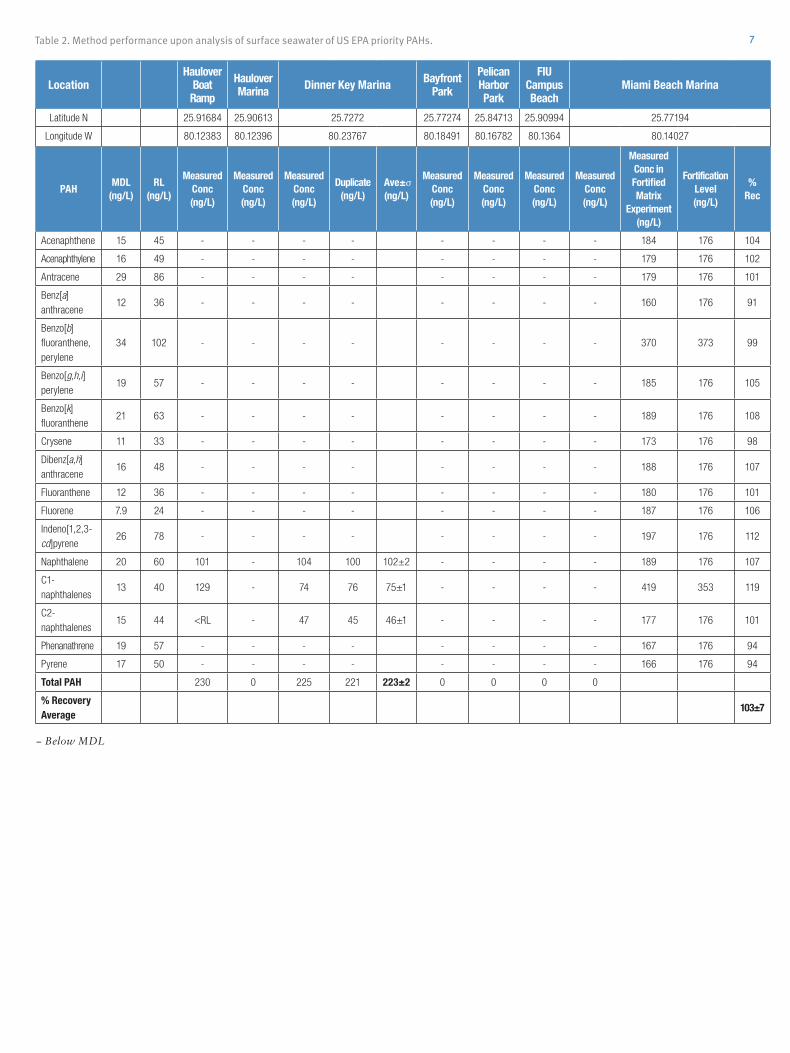
7
LocationHaulover
Boat Ramp
Haulover Marina Dinner Key Marina Bayfront
Park
Pelican Harbor Park
FIU Campus Beach
Miami Beach Marina
Latitude N 25.91684 25.90613 25.7272 25.77274 25.84713 25.90994 25.77194
Longitude W 80.12383 80.12396 80.23767 80.18491 80.16782 80.1364 80.14027
PAHMDL
(ng/L)RL
(ng/L)
Measured Conc (ng/L)
Measured Conc (ng/L)
Measured Conc (ng/L)
Duplicate (ng/L)
Ave±σ (ng/L)
Measured Conc (ng/L)
Measured Conc (ng/L)
Measured Conc (ng/L)
Measured Conc (ng/L)
Measured Conc in Fortified Matrix
Experiment (ng/L)
Fortification Level (ng/L)
% Rec
Acenaphthene 15 45 - - - - - - - - 184 176 104
Acenaphthylene 16 49 - - - - - - - - 179 176 102
Antracene 29 86 - - - - - - - - 179 176 101
Benz[a]anthracene
12 36 - - - - - - - - 160 176 91
Benzo[b]fluoranthene, perylene
34 102 - - - - - - - - 370 373 99
Benzo[g,h,i]perylene
19 57 - - - - - - - - 185 176 105
Benzo[k]fluoranthene
21 63 - - - - - - - - 189 176 108
Crysene 11 33 - - - - - - - - 173 176 98
Dibenz[a,h]anthracene
16 48 - - - - - - - - 188 176 107
Fluoranthene 12 36 - - - - - - - - 180 176 101
Fluorene 7.9 24 - - - - - - - - 187 176 106
Indeno[1,2,3-cd]pyrene
26 78 - - - - - - - - 197 176 112
Naphthalene 20 60 101 - 104 100 102±2 - - - - 189 176 107
C1-naphthalenes
13 40 129 - 74 76 75±1 - - - - 419 353 119
C2-naphthalenes
15 44 <RL - 47 45 46±1 - - - - 177 176 101
Phenanathrene 19 57 - - - - - - - - 167 176 94
Pyrene 17 50 - - - - - - - - 166 176 94
Total PAH 230 0 225 221 223±2 0 0 0 0
% Recovery Average
103±7
Table 2. Method performance upon analysis of surface seawater of US EPA priority PAHs.
− Below MDL

8
Table 3. Method performance upon analysis of rainwater and rainwater runoff of US EPA priority PAHs.
Sample Source Direct Collection Apartment Complex FIU Biscayne Bay Campus
Sample Description
Reference Rainwater
Partially Flooded Parking LotParking Lot A
Parking Lot B
PAH MDL (ng/L)
RL (ng/L)
Measured Conc (ng/L)
Measured Conc (ng/L)
Duplicate (ng/L)
Ave±σ (ng/L)
Measured Conc (ng/L)
Measured Conc (ng/L)
Measured Conc
in Fortified Matrix
Experiment (ng/L)
Fortification Level (ng/L)
% Rec
Acenaphthene 15 45 - - - - - 105 110 95
Acenaphthylene 16 49 - - - - - 119 110 109
Antracene 29 86 - - - - - 118 110 107
Benz[a]anthracene 12 36 - 190 202 196±6 - - 105 110 96
Benzo[b]fluoranthene, perylene
34 102 - 112 108 110±2 - - 216 220 98
Benzo[g,h,i ]perylene
19 57 - 60 61 60.4±0.7 - - 124 110 113
Benzo[k]fluoranthene
21 63 - <RL <RL - - 105 110 96
Crysene 11 33 - 153 169 161±8 - - 112 110 101
Dibenz[a,h]anthracene
16 48 - - - - - 137 110 124
Fluoranthene 12 36 - 410 387 399±12 - - 104 110 95
Fluorene 7.9 24 - <RL <RL - - 100 110 91
Indeno[1,2,3-cd ]pyrene
26 78 - <RL <RL - - 130 110 118
Naphthalene 20 60 - - - - - 91 110 83
C1-naphthalenes 13 40 - - - - - 209 220 95
C2-naphthalenes 15 44 - - - - - 111 110 101
Phenanathrene 19 57 - 183 186 184±1 - - 116 110 105
Pyrene 17 50 - 293 315 304±11 - - 117 110 107
Total PAH 0 1401 1428 1415±14 0 0
% Recovery Average
102±10
Examples of Environmental ApplicationsThe developed methodology was tested by analyzing a group of multi-origin environmentally relevant water samples. Seawater collections were made from seven sites in northern Biscayne Bay. Naphthalene and alkylnaphthalenes were detected in two of the sites in which activity of small vessels was observed (Table 2). The elevated water solubility of naphthalenes relative to other PAHs1 may increase their permanence in the water long enough to be detected by the grab sampling performed. Although the method sensitivity was not enough to detect background concentrations in samples where no active boating was observed, a capability of fast detection of focalized emission of petroleum-derived products was demonstrated.
Suspended particles in rainwater runoff resulting from the erosion of impervious surfaces have been documented as an important source of PAHs in the environment.25,26 To assess the performance of the developed methodology
for this type of monitoring, rainwater and runoff samples from the drainage openings at three parking lots were collected during a heavy rain event in June 2013. As can be seen in Table 3, PAHs were detected in runoff from only the partially flooded parking lot located in a residential complex. Chromatograms for the priority PAHs detected in that sample are compared with reference rainwater in Figure 3, showing that interference-free detection and positive identification were obtained for these analytes except for benzo[b]fluoranthene, which is not resolved from perylene by this methodology as discussed before. Also, since no PAHs were observed in the reference rainwater, this data strongly suggests that the parking lot was the source of the contamination. The high number of parent PAHs detected, the predominance of heavy PAHs such as fluoranthene and pyrene, and their relative concentrations are in agreement with previous reports of PAHs in rainwater runoff from coated parking lots,27 suggesting that the presented methodology is applicable for this type of study.
− Below MDL, <RL Detection below reporting limit (RL=3×MDL)

9
Although not enough data is available to explain the non-occurrence of PAHs in runoff from the campus parking lots, the residential parking lot had a much slower drainage capability, and thus, the sample was collected under moderate flooding conditions. The lower drainage rate may have enhanced the possibility of detections as PAH-containing suspended particles could not be washed out by the rain as fast as in the campus parking lots. It is also possible that the nature of the coatings is different, as it has been shown that asphalt-based coatings contain many fewer PAHs than coal-based coatings.25
Samples of reclaimed water used for irrigation at FIU Biscayne Bay campus were collected in two different dates and analyzed in order to assess the performance of the developed methodology to detect PAHs discharged with WWTP effluents. Alkylnaphthalenes were detected in one on the samples (Table 4), but concentrations were lower than the reporting limit. Good recoveries were obtained in the fortified matrix experiment for reclaimed water, suggesting that method sensitivity rather than a severe matrix effect prevented positive quantification in these samples. Excellent recoveries were also obtained in fortified matrix experiments with the other two types of environmental waters tested with this method, which may suggest that the use of a wide range of molecular sizes of isotopically labeled PAHs normalizes analyte behavior during the automated preconcentration and analysis, keeping matrix effects under control in spite of the lack of any other sample preparation steps such as filtration. In addition, method reproducibility was also good upon analysis of duplicates of PAH-containing seawater and runoff samples.
Figure 3. Chromatograms obtained upon analysis of a rainwater runoff sample from a residential parking lot and its comparison with reference rainwater. (Blue trace: main (quantitative) SRM transition in runoff sample; green trace: secondary (confirmation) SRM transition in runoff sample; red trace: main SRM transition from injection of reference rainwater)

10
PAH MDL (ng/L)
RL (ng/L)
Measured Conc (ng/L)
Measured Conc (ng/L)
Measured Conc
in Fortified Matrix
Experiment (ng/L)
Fortification Level (ng/L)
% Recovery
Acenaphthene 15 45 - - 203 176 115
Acenaphthylene 16 49 - - 162 176 92
Antracene 29 86 - - 185 176 105
Benz[a]anthracene 12 36 - - 164 176 117
Benzo[b]fluoranthene, perylene
34 102 - - 363 373 97
Benzo[g,h,i ]perylene
19 57 - - 150 176 85
Benzo[k]fluoranthene
21 63 - - 219 176 124
Crysene 11 33 - - 210 176 119
Dibenz[a,h]anthracene
16 48 - - 156 176 88
Fluoranthene 12 36 - - 209 176 116
Fluorene 7.9 24 - - 168 176 95
Indeno[1,2,3-cd ]pyrene
26 78 - - 174 176 99
Naphthalene 20 60 - - 161 176 91
C1-naphthalenes 13 40 - - 364 353 103
C2-naphthalenes 15 44 - <RL 228 176 118
Phenanathrene 19 57 - - 175 176 99
Pyrene 17 50 - - 200 176 111
Total PAH 0 0
% Recovery Average
104±12
Table 4. Method performance upon analysis of reclaimed water obtained from the Miami-Dade North District Wastewater Treatment Plant for US EPA priority PAHs.
ConclusionAn automated protocol for the comprehensive analysis of 28 parent PAHs and their extended alkylated homologues by online SPE-LC-MS/MS was successfully developed with optimized parameters for extraction, separation, and detection using dopant-assisted APPI. Method performance and the control of matrix effects were demonstrated by obtaining good recoveries upon analysis of seawater, reclaimed water, and rainwater runoff fortified with certified standards, showing the utility of this method to survey the occurrence of PAHs in waters at the urban environment. A survey of PAH concentration in a seawater environment influenced by a large urban area was conducted, and although background concentrations were below MDLs, localized PAH input events from boating activities were detected above reporting limits. With lower run times, very simple sample preparation, lower generation of toxic solvent waste, and higher sensitivity per volume of sample used, this method could represent a viable alternative to LLE-GC-MS for routine PAH monitoring, providing laboratories with a much higher sample throughput while reducing overall operation costs and the environmental impact of PAH analysis.

1112. Denoux, G.J.; Gardinali, P.; Wade, T.L. Quantitativedetermination of polynuclear aromatic hydrocarbons bygas chromatography/mass spectrometry (GC/MS)-selectedion monitoring (SIM) mode. In Sampling and analyticalmethods of the National Status and Trends ProgramMussel Watch Project: 1993–1996 update, Lauenstein,G.G.; Cantillo, A.Y. (eds). National Oceanic andAtmospheric Administration, Silver Spring, 1998, pp129–139. 36, 63–72.
13. Rawa-Adkonis, M.; Wolska, L.; Namiesnik, J.Analytical procedures for PAH and PCB determination inwater samples—error sources. Crit Rev Anal Chem, 2006,
14. Smith, R.M. Before the injection—modern methods ofsample preparation for separation techniques. JChromatogr A, 2003, 1000(1-2), 3-27.
15. Garcia-Ac, A.; Segura, P.A.; Viglino, L.; Furtos, A.;Gagnon, C.; Prevost, M.; Sauve, S. On-line solid-phaseextraction of large-volume injections coupled to liquidchromatography-tandem mass spectrometry for thequantitation and confirmation of 14 selected trace organiccontaminants in drinking and surface water.J Chromatogr A , 2009, 1216, 8518–8527.
16. Wang, C.T.; Gardinali, P.R. Comparison of multipleAPI techniques for the simultaneous detection ofmicroconstituents in water by on-line SPE-LC-MS/MS.J Mass Spectrom, 2012, 47, 1255–1268.
17. Busetti, F.; Backe, W.J.; Bendixen, N.; Maier, U.; Place,B.; Giger, W.; Field, J.A. Trace analysis of environmentalmatrices by large-volume injection and liquidchromatography-mass spectrometry. Anal Bioanal Chem,2012, 402, 175–186.
18. Ramirez, C.E.; Wang, C.; Gardinali, P.R. Fullyautomated trace level determination of parent andalkylated PAHs in environmental waters by onlineSPE-LC-APPI-MS/MS. Anal Bioanal Chem, 2014, 406,329–344., doi:10.1007/s00216-013-7436-6.
19. Smith, D.R.; Robb, D.B.; Blades, M.W. Comparisonof dopants for charge exchange ionization of nonpolarpolycyclic aromatic hydrocarbons with reversed-phaseLC-APPI-MS. J Am Soc Mass Spectrom, 2009, 20, 73–79.
20. Cai, S.S.; Syage. J.A.; Hanold, K.A.; Balogh, M.P.Ultra performance liquid chromatography-atmosphericpressure photoionization-tandem mass spectrometry forhigh-sensitivity and high-throughput analysis of USEnvironmental Protection Agency 16 priority pollutantspolynuclear aromatic hydrocarbons. Anal Chem, 2009,81, 2123–2128.
21. Sander, L.C.; Pursch, M.; Wise, S.A. Shape selectivityfor constrained solutes in reversed-phase liquidchromatography. Anal Chem, 1999, 71, 4821–4830.
References1. Manoli, E.; Samara, C.Polycyclic aromatichydrocarbons in natural waters: sources, occurrence andanalysis. Trac-Trends Anal Chem, 1999, 18, 417–428.
2. Wolska, L.; Mechlinska, A.; Rogowska, J.; Namiesnik,J. Sources and fate of PAHs and PCBs in the marineenvironment. Crit Rev Environ Sci Technol, 2012, 42,1172–1189.
3. Wang, Z.D.; Stout, S.A., Fingas, M. Forensicfingerprinting of biomarkers for oil spill characterizationand source identification. Environ Forensic, 2006,7:105–146.
4. Boehm, P.D.; Douglas, G.S.; Burns, W.A.; Mankiewicz,P.J.; Page, D.S.; Bence, A.E. Application of petroleumhydrocarbon chemical fingerprinting and allocationtechniques after the Exxon Valdez oil spill. Mar PollutBull, 1997, 34, 599–613.
5. Boehm, P.D.; Neff, J.M.; Page, D.S. Assessment ofpolycyclic aromatic hydrocarbon exposure in the watersof Prince William Sound after the Exxon Valdez oil spill:1989–2005. Mar Pollut Bull, 2007, 54,339–356.
6. Agency for Toxic Substances and Disease Registry(ATSDR) (1995) Toxicological profile for polycyclicaromatic hydrocarbons (PAHs). U.S. Department ofHealth and Human Services, Atlanta.
7. Manzetti, S. Ecotoxicity of polycyclic aromatichydrocarbons, aromatic amines, and nitroarenes throughmolecular properties. Environ Chem Lett, 2012, 10,349–361.
8. Lerda, D. Polycyclic aromatic hydrocarbons (PAHs)factsheet. European Commission, Joint Research Centre,Institute for Reference Materials and Measurements,2012, Belgium.
9. US EPA (2010) Definition and procedures for thedetermination of the method detection limit. Guidelinesestablishing test procedures for the analysis of pollutants.Appendix B, part 136. Definition and procedures for thedetermination of the method detection limit. U.S. Code ofFederal Regulations, Title 40. Revision 1.11.
10. US EPA (1996) Method 3510C. Separatory funnelliquid-liquid extraction, online test methods for evaluatingsolid waste, physical/ chemical methods (SW-846),Washington, D.C., USA., Revision 3.
11. US EPA (1996) Method 3630C. Silica gel cleanup,online test methods for evaluating solid waste, physical/chemical methods (SW-846), Washington, D.C. USA.,Revision 3.

AN63941_E 08/16S
Africa +43 1 333 50 34 0Australia +61 3 9757 4300Austria +43 810 282 206Belgium +32 53 73 42 41Canada +1 800 530 8447China 800 810 5118 (free call domestic)
400 650 5118
Denmark +45 70 23 62 60Europe-Other +43 1 333 50 34 0Finland +358 9 3291 0200France +33 1 60 92 48 00Germany +49 6103 408 1014India +91 22 6742 9494Italy +39 02 950 591
Japan +81 45 453 9100Latin America +1 561 688 8700Middle East +43 1 333 50 34 0Netherlands +31 76 579 55 55New Zealand +64 9 980 6700Norway +46 8 556 468 00Russia/CIS +43 1 333 50 34 0
Singapore +65 6289 1190Spain +34 914 845 965Sweden +46 8 556 468 00Switzerland +41 61 716 77 00UK +44 1442 233555USA +1 800 532 4752
www.thermofisher.com©2016 Thermo Fisher Scientific Inc. All rights reserved. Instant Ocean is a registered trademark of Spectrum Brands, Inc. All other trademarks are the property of Thermo Fisher Scientific and its subsidiaries. This information is presented as an example of the capabilities of Thermo Fisher Scientific products. It is not intended to encourage use of these products in any manners that might infringe the intellectual property rights of others. Specifications, terms and pricing are subject to change. Not all products are available in all countries. Please consult your local sales representative for details.
Ap
plica
tion
No
te 5
98
22. Rimmer, C.; Sander, L.; Wise, S. Selectivity of longchain stationary phases in reversed phase liquidchromatography. Anal Bioanal Chem, 2005, 382,698–707.
23. Horak, J.; Lindner, W. Contribution of sulfonyl-aromatic and sulfonic acid-aromatic interactions in novelsulfonyl/sulfonic acid-embedded reversed phase materials.J Chromatogr A, 2008, 1191, 141–156.
24. Wang, Z.D.; Fingas, M.; Page, D.S. Oil spillidentification. J Chromatogr A, 1999, 843, 369–411.
25. Mahler, B.J.; Van Metre, P.C.; Crane, J.L.; Watts,A.W.; Scoggins, M.; Williams, E.S. Coal-tar-basedpavement sealcoat and PAHs: implications for theenvironment, human health, and stormwatermanagement. Environ Sci Technol, 2012, 46, 3039–3045.
26. Watts, A.W.; Ballestero, T.P.; Roseen, R.M.; Houle,J.P. Polycyclic aromatic hydrocarbons in stormwaterrunoff from sealcoated pavements. Environ Sci Technol,2010, 44, 8849–8854.
27. Mahler, B.J.; Van Metre, P.C.; Bashara, T.J.; Wilson,J.T.; Johns, D.A. Parking lot sealcoat: an unrecognizedsource of urban polycyclic aromatic hydrocarbons.Environ Sci Technol, 2005, 39, 5560–5566.

Quantification of Haloacetic Acids in Tap Water Using a Dedicated HAA LC Column with LC-MS/MS DetectionThermo Fisher Scientific, San Jose, CA
Ap
plica
tion
No
te 5
90
Key WordsHaloacetic acid, Water Supply Act, LC-MS/MS, TSQ Quantum Ultra, Acclaim HAA HPLC column
GoalTo develop an LC-MS/MS method for measuring haloacetic acids in tap water using a dedicated HPLC column.
IntroductionIn April 2012, methods provided by the Japanese Ministry of Health, Welfare and Labour based on provisions in the Water Quality Standards Ordinance (Ministry of Health, Welfare and Labour, Notification 261, July 2003) were revised, and the inspection method for haloacetic acids (HAAs) was expanded to include an analysis method using liquid chromatography paired with mass spectrometry (LC/MS or LC-MS/MS) as an alternative to gas chromatography with mass spectrometry (GC/MS).
The LC-MS(/MS) method does not require derivatization of samples and is therefore a simple measurement method. However, tap water typically contains on the order of several to several dozen mg/L of chloride, sulfate, carbonate, and nitrate anions. When performing LC-MS analysis, these anions inhibit the ionization of haloacetic acids and cause signal suppression in the MS detector. In addition, when using a standard reversed-phase column, the retention varies depending on matrix differences, the infusion amount, and the column lot, resulting in poor recoveries, robustness, and detection limits.
A number of LC-MS/MS methods for haloacetic acids using C18 (ODS) columns have already been developed. However, separation from the many ionic matrix components contained in tap water has been insufficient in these methods. Retention times varied widely between neat standards and real samples, making it difficult to obtain reproducible results.
The Thermo Scientific™ Acclaim™ HAA column is designed for analyzing haloacetic acids in drinking water by LC/MS. It is based on mixed-mode column technology and offers reversed-phase and anion-exchange retention mechanisms that enable separation of haloacetic acids in high ion matrices. This results in robust performance in real drinking water samples that contain matrix ions. In addition, sample preparation costs are reduced because analysis is possible without sample preparation or concentration.
This application note describes the LC-MS(/MS) separation using the Acclaim HAA column for haloacetic acid analysis in drinking water.

2 ExperimentalSample PreparationPreparation of standardsA methyl tertiary-butyl ether (MTBE) solution combining four types of haloacetic acids [monochloroacetic acid (MCAA), dichloroacetic acid (DCAA), trichloroacetic acid (TCAA), and monobromoacetic acid (MBAA), 100 mg/L of each, Kanto Kagaku] was used for the haloacetic acid standard solution. The solution was diluted in ultrapure water and used to prepare the calibration curve.
Preparation of laboratory fortified matrixThe following anions were added to a final concentration as shown: Cl-, 35 mg/L; SO4
2-, 35 mg/L; NO3-, 50 mg/L.
Ascorbic acid was added at 10 mg/L level.
Preparation of the sampleAfter sampling the tap water, ascorbic acid was added at the level of 10 mg/L for residual chlorine removal.
Liquid Chromatography
Equipment: Thermo Scientific™ Dionex™ UltiMate™ 3000 RSLC system, which included the LPG-3400RS Quaternary Rapid Separation Pump, WPS-3000TRS Rapid Separation Thermostatted Wellplate Sampler, and TCC-3000RS Rapid Separation Thermostatted Column Compartment
Column: Acclaim HAA column (2.1 x 50 mm, 3 µm), P/N SP6917
Mobile phase A: Water (LC/MS grade)
Mobile phase B: 200 mM aqueous ammonium sulfate solution
Mobile phase C: Acetonitrile
Gradient: Refer to Figure 1
Flow rate: 0.3 mL/min
Operating temperature: 25.0 °C
Injection volume: 50 µL
Figure 1. LC gradient
To extend the life of the columns, they should be stored in a 100 mM acetic ammonium (pH 5.0)/acetonitrile (1:4 v/v) solution.
Mass Spectrometry
Equipment: Thermo Scientific™ TSQ Quantum Ultra™ triple-stage quadrupole MS
Ionization method: Negative ESI
Spray voltage: 500 V
Sheath gas: 60 arbitrary units
Aux gas: 10 arbitrary units
Capillary temperature: 250 °C
Vaporizer temperature: 400 °C
Skimmer offset: 10 V
Collision gas pressure: Ar, 0.8 mTorr
Cycle time: 2 ms
Mass resolution: Q1: 1.5 Da (SRM mode)
SRM transitions: Refer to Table 1
Results and DiscussionSeparation of Matrix IonsWhen optimizing separation conditions, it is important to adequately separate matrix ions and haloacetic acids. However, further care is required to separate chloride ions and MCAA. Detection close to the MCAA retention time was confirmed using accurate mass MS.1 Cl- (m/z 35) is detected as fragment ions from NaCl2
- (m/z 93) using CID. It is therefore detected in the same transition as MCAA. If the retention mechanism is unclear, or if separation of MCAA and chloride cannot be confirmed, false quantification could result, depending on the behavior of the chloride ions. This is why processing to remove chloride ions is recommended in analysis systems using ODS columns.
In this investigation for the Acclaim HAA column, the resolution of HAAs from interfering anions in a synthetic sample matrix spiked with HAAs is demonstrated (Figure 2).
Compound Name
Precursor (m/z)
Product (m/z)
CE (eV)
MCAA quantitation ion 93 35 10
MCAA qualifying ion 95 37 10
DCAA quantitation ion 127 83 10
DCAA qualifying ion 129 85 10
TCAA quantitation ion 161 117 10
TCAA qualifying ion 163 119 10
Table 1. SRM transitions

3
SensitivityBased on the Japanese Water Quality Standards Ordinance, the method needs to be able to detect three regulated haloacetic acids at concentration levels ten times lower than the regulated amounts. Among the three haloacetic acids, the compound MCAA has lowest regulated amount at 20 µg/L. The HAA column method was able to confirm all three haloacetic acids at the 2 µg/L level, which is ten times lower than 20 µg/L (Figures 3 and 4).
1
0 2 4 6 8 10 12 14 16 18 20 22 24 26 28 30 Time (min)
2 3
a b c d
RT: 5.21 - 9.40 SM: 7G
6 7 8 9Time (min)
0
20
40
60
80
100
Rel
ativ
e A
bund
ance
RT: 7.30SN: 23
NL:2.42E3TIC F: - c ESI SRM ms2 93.000 [34.999-35.001] MS Genesis 25Jun005
RT: 12.63 - 16.82 SM: 7G
14 16Time (min)
0
20
40
60
80
100
Rel
ativ
e A
bund
ance
RT: 14.83SN: 133
NL:1.31E5TIC F: - c ESI SRM ms2 127.000 [82.999-83.001] MS Genesis 25Jun005
RT: 18.23 - 22.41 SM: 7G
20 22Time (min)
0
20
40
60
80
100
Rel
ativ
e A
bund
ance
RT: 20.36SN: 496
NL:1.49E5TIC F: - c ESI SRM ms2 161.000 [116.999-117.001] MS Genesis 25Jun005
a) b) c)
Figure 3. SRM chromatograms for 2 µg/L standard solution: a) MCAA, b) DCAA, c) TCAA
Figure 4. SRM chromatograms for tap water spiked with 2 µg/L standard solution: a) MCAA, b) DCAA, c) TCAA
*A peak from contaminant compound sources was detected before the peak in monochloroacetic acid. The identity of this
contaminant as a chloride ion cluster ion (NaCl2-) was confirmed using a Thermo Scientific accurate-mass MS.
RT: 5.21 - 9.40 SM: 7G
6 7 8 9Time (min)
0
20
40
60
80
100
Rel
ativ
e A
bund
ance
RT: 7.20SN: 14
6.07
8.82
NL:2.69E3TIC F: - c ESI SRM ms2 93.000 [34.999-35.001] MS 25Jun046
RT: 12.63 - 16.82 SM: 7G
14 16Time (min)
0
20
40
60
80
100
Rel
ativ
e A
bund
ance
RT: 14.76SN: 482
NL:2.68E5TIC F: - c ESI SRM ms2 127.000 [82.999-83.001] MS Genesis 25Jun046
RT: 18.23 - 22.41 SM: 7G
20 22Time (min)
0
20
40
60
80
100
Rel
ativ
e A
bund
ance
RT: 20.19SN: 807
NL:2.92E5TIC F: - c ESI SRM ms2 161.000 [116.999-117.001] MS Genesis 25Jun046
Figure 2. Separation on the Acclaim HAA column. Upper section: Haloacetic acids 1: Monochloroacetic acid (MCAA), 2: Dichloroacetic acid (DCAA), 3: Trichloroacetic acid (TCAA). Lower section: Matrix components a: Ascorbic acid, b: Chloride, c: Nitrate, d: Sulfate

4
Confirmation of Recovery Level A spike recovery test was performed for the tap water sample spiked with standards to 2 µg/L. Good recoveries in the range of 92% to 101% were obtained (Table 2). The same test was performed for the spiked fortified matrix sample and favorable results were obtained (Table 3).
MCAA DCAA TCAA
Standard 2 µg/L
2 µg/L of spiked tap water
Standard 2 µg/L
2 µg/L of spiked tap water
Standard 2 µg/L
2 µg/L of spiked tap water
Blanks (ultrapure or tap water)
NF 6136 NF 2013784 NF 3602064
n=5 (area value)
33492 33192 1369465 3000890 2434743 5301570
32335 33581 1355191 3079005 2465008 5241249
32605 34016 1361893 3083660 2476721 5325868
33295 34005 1381170 3059149 2472097 5257085
33406 34025 1387243 3061388 2474253 5281431
%CV 1.6% 1.1% 1.0% 1.1% 0.7% 0.6%
Table 2. Area value reproducibility for 2 µg/L of standard product and 2 µg/L of spiked tap water
MCAAY = 3131.43+14503.1*X R^2 = 0.9990 W: 1/X
0 5 10 15 20ug/L
0
50000
100000
150000
200000
250000
300000
Are
a
DCAAY = 246802+528094*X R^2 = 0.9959 W: 1/X
0 5 10 15 20ug/L
0
2000000
4000000
6000000
8000000
10000000
Are
a
TCAAY = 620778+827509*X R^2 = 0.9916 W: 1/X
0 5 10 15 20ug/L
0
2000000
4000000
6000000
8000000
10000000
12000000
14000000
16000000
18000000
Are
a
a) b) c)
Figure 5. Calibration curves: a) MCAA, b) DCAA, c) TCAA
Calibration Curve and ReproducibilityThe calibration curves were created over a range from 1 to 20 µg/L with linearities greater than 0.99 (Figure 5). Reproducible results were obtained for 2 µg/L of standard solution and for tap water spiked with 2 µg/L of standard solution. Coefficients of variation were less than 1.6% (Table 2).

5
MCAA DCAA TCAA
2 µg/L spiked tap water
2 µg/L laboratory fortified matrix
2 µg/L spiked tap water
2 µg/L laboratory fortified matrix
2 µg/L spiked tap water
2 µg/L laboratory fortified matrix
Blanks (tap water or ultrapure water)
0.282 NF 3.346 NF 3.603 NF
n=5 (quantitation
value)
2.090 1.910 5.215 1.894 5.656 1.894
2.116 1.885 5.363 1.902 5.584 1.954
2.145 1.834 5.372 1.881 5.686 1.907
2.144 1.939 5.325 1.836 5.603 1.890
2.146 1.863 5.330 1.871 5.632 1.860
Average value 2.128 1.886 5.321 1.877 5.632 1.901
Average value minus blank value
1.846 1.886 1.975 1.877 2.029 1.901
Recovery level 92% 94% 99% 94% 101% 95%
%RSD 1.2% 2.2% 1.2% 1.4% 0.7% 1.8%
Table 3. Recovery levels in 2 µg/L of spiked tap water and 2 µg/L of added laboratory fortified matrix
Accuracy and PrecisionFive replicates were quantitated for spiked tap water samples (two concentrations) using a calibration curve created from the five tests. The average recovery level and %RSD for each set of replicates are reported in Table 4.
Table 4. Parallel test results
*The average concentration was calculated using the value aftersubtracting the blank concentration.
ConclusionA highly sensitive LC-MS/MS method for measuring haloacetic acids using a dedicated Acclaim HAA HPLC column has been established. Under these analysis conditions, the ionization-inhibiting chloride ions, nitric acid ions, sulfuric acid ions, and haloacetic acids can be separated, making it possible to perform reliable measurements even when interfering anions are not removed using an SPE cartridge or alternative sample preparation. In addition, reproducible results were obtained for samples at concentrations more than ten times lower than regulated amounts. Accuracy and precision in tap water was confirmed in repeated testing.
MCAA DCAA TCAA
20 µg/L of spiked tap water
Average concentration*
19.53 18.48 19.26
Recovery level 98% 91% 95%
%RSD 2% 1% 2%
2 µg/L of spiked tap water
Average concentration*
1.82 1.96 2.16
Recovery level 91% 98% 108%
%RSD 4% 3% 6%

Ap
plica
tion
No
te 5
90
Reference1. Oral presentation 2E-5 at the 2012 Japan Society for
Environmental Chemistry Symposium, “Quantificationanalysis of haloacetic acid based on LC-MS/MS usingmixed mode columns”.
AN63863_E 08/16S
Africa-Other +27 11 570 1840Australia +61 3 9757 4300Austria +43 810 282 206Belgium +32 53 73 42 41Canada +1 800 530 8447China 800 810 5118 (free call domestic)
400 650 5118
Denmark +45 70 23 62 60Europe-Other +43 1 333 50 34 0Finland +358 9 3291 0200France +33 1 60 92 48 00Germany +49 6103 408 1014India +91 22 6742 9494Italy +39 02 950 591
Japan +81 45 453 9100Latin America +1 561 688 8700Middle East +43 1 333 50 34 0Netherlands +31 76 579 55 55New Zealand +64 9 980 6700Norway +46 8 556 468 00Russia/CIS +43 1 333 50 34 0
Singapore +65 6289 1190South Africa +27 11 570 1840Spain +34 914 845 965Sweden +46 8 556 468 00Switzerland +41 61 716 77 00UK +44 1442 233555USA +1 800 532 4752
www.thermofisher.com©2016 Thermo Fisher Scientific Inc. All rights reserved. All trademarks are the property of Thermo Fisher Scientific and its subsidiaries. This information is presented as an example of the capabilities of Thermo Fisher Scientific products. It is not intended to encourage use of these products in any manners that might infringe the intellectual property rights of others. Specifications, terms and pricing are subject to change. Not all products are available in all countries. Please consult your local sales representative for details.

Introduction
Haloacetic acids (HAAs) are formed as disinfection by-products when water is chlorinated to remove microbialcontent. The chlorine reacts with naturally occurringorganic and inorganic matter in the water, such asdecaying vegetation, to produce by-products that includeHAAs. Of the nine species of HAAs, five are currentlyregulated by the EPA (HAA5): monochloroacetic acid(MCAA), dichloroacetic acid (DCAA), trichloroacetic acid(TCAA), monobromoacetic acid (MBAA), anddibromoacetic acid (DBAA). The remaining four HAAsare unregulated: bromochloroacetic acid (BCAA),bromodichloroacetic acid (BDCAA), dibromochloroaceticacid (DBCAA), and tribromoacetic acid (TBAA).
According to the U.S. Environmental ProtectionAgency (EPA), there might be an increased risk of cancerassociated with long-term consumption of watercontaining levels of HAAs that exceed 0.6 mg/L.1 EPAMethods 552.1, 552.2, and 552.3, are used to determinethe level of all nine HAAs in drinking water.2,3,4 Thesemethods require derivatization and multiple extractionsteps followed by gas chromatography (GC) with electroncapture detection (ECD).
In comparison to the conventional EPA methods usingGC with ECD, the combination of ion chromatographyand mass spectrometry (IC-MS and IC-MS/MS) offerssensitive and rapid detection without the need for samplepre-treatment. Ion chromatography is a form of liquidchromatography that uses ion-exchange resins to separateatomic and molecular ions. The retention time in thecolumn is predominantly controlled by the interactions ofthe ions of the solute with the resin. Coupling IC with thehighly selective detection of a triple quadrupole massspectrometer allows unambiguous identification ofsubstance peaks. Matrix interference effects are greatlyreduced, which improves the sensitivity and lowers thedetection limits.
In the method described here, water samples can beinjected directly into an ion chromatography system thatis coupled to a Thermo Scientific TSQ Quantum Accesstriple stage quadrupole mass spectrometer. The separationof all nine HAAs addressed in the EPA methods isachieved with an anion-exchange column using anelectrolytically formed hydroxide gradient.
Goal
To develop a simple, rapid, and sensitive IC-MS/MSmethod for analyzing haloacetic acids in water.
Experimental Conditions
Ion Chromatography
IC analysis was performed on a Dionex ICS 3000 system(Dionex Corporation, Sunnyvale, CA). Samples weredirectly injected and no sample pre-treatment wasrequired. The IC conditions used are shown in Table 1.
Column Set: Dionex IonPac® AG24 (2 × 50 mm), IonPac AS24 (2 × 250 mm)
Suppressor: ASRS® 300, 2 mm Column Temperature: 15 °CInjection Volume: 100 µLFlow Rate: 0.3 mL/min KOH gradient, electrolytically generated
(Table 2)
Table 1. Ion chromatography system conditions
Retention Time (min) [KOH] mM
0.00 7.015.1 7.030.8 18.031.0 60.046.8 60.047.0 7.0
Table 2. Electrolytically formed hydroxide gradient details
The separation performed on the IonPac AS24 columnused a hydroxide gradient. It is known that hydroxide isnot a recommended eluent for mass spectrometers. Theaddition of an ASRS 300 anion self-regeneratingsuppressor is critical. This suppressor is placed in lineafter the column and electrolytically converts thehydroxide into water, making the separation compatiblewith mass spectrometric detection. See Figure 1.
Analysis of Haloacetic Acids in Drinking Waterby IC-MS/MSCharles Yang1 and Stacy Henday2
1Thermo Fisher Scientific, San Jose, CA; 2Dionex Corporation, Sunnyvale, CA
Key Words
• TSQ QuantumAccess
• EPA
• Ionchromatography
• Water analysis
ApplicationNote: 454

In addition, a matrix diversion valve was placed inline prior to the mass spectrometer. This valve functions todivert the high sample matrix waste from the MS source,prolonging the time in between cleanings. Acetonitrile wasteed into the eluent stream after the matrix diversionvalve. The acetonitrile had two main purposes: to assist inthe desolvation of the mobile phase and to act as a make-up flow when the IC eluent was diverted to waste.
Mass Spectrometry
MS analysis was carried out on a TSQ Quantum Access™
triple stage quadrupole mass spectrometer with a heatedelectrospray ionization (H-ESI) probe. The MS conditionsused are shown in Table 3.
Figure 1: Flow schematic of the IC-MS/MS system
Skimmer Q1 Q3 CE Tube Lens Offset Scan Time
Analyte (m/z) (m/z) (V) (V) (V) (s)MCAA 93.01 35.60 10 26 0 1.25MBAA 136.99 79.09 12 33 0 1.25DCAA 127.02 83.20 11 26 0 1.25DBAA 214.80 79.20 24 33 0 1.25BCAA 171.00 79.20 35 44 0 1.25TCAA 161.06 117.10 10 69 0 1.60
BDCAA 79.00 79.00 15 30 0 1.60DBCAA 206.74 79.13 15 30 0 2.50TBAA 250.70 79.10 25 26 0 2.50
MCAA-ISTD 94.01 35.60 10 26 0 1.25MBAA-ISTD 138.00 79.09 12 33 0 1.25DCAA-ISTD 128.01 84.20 11 26 0 1.25TCAA-ISTD 162.06 118.10 10 69 0 1.60
Table 4. MS conditions for the various HAAs and internal standards
Ion source polarity: Positive ion modeSpray voltage: 4000 VSheath gas pressure: 40 unitsAuxiliary gas pressure: 15 unitsCapillary temperature: 270 °C
Table 3. Mass spectrometer conditions
Individual standards were infused into the massspectrometer to determine optimum tube lens settings andcollision energies for the product ions. Table 4 describesthe MS conditions for specific HAAs and internalstandards.

Figure 2: These chromatograms show the progress of the pump pressure and front end detector data along with the TSQQuantum Access MS data. The left side of the screen shows the status of the ion chromatography system and the status ofthe TSQ Quantum Access.
The status of the ion chromatography system wasmonitored at the same time as the MS data acquisition, asshown in Figure 2.
Results and Discussion
The separation of the nine HAAs is shown in Figure 3.The selectivity of the IC-MS/MS system allows separationof the HAAs from common inorganic matrix ions. Thisallows matrix peaks of chloride, sulfate, nitrate, andbicarbonate to be diverted to waste during the analyticalrun and avoids premature fouling of the ESI-MS/MSinstrument source.
An internal standard mixture of 13C labeled MCAA,MBAA, DCAA, and TCAA was spiked into each sampleat 3 ppb. The calibration curves were generated usinginternal standard calibrations for all of the HAAcompounds in water. Excellent linearity results wereobserved for all compounds as shown in Figures 4, 5, and6. Analytes were run at levels of 250 ppt to 20 ppb. Itmust be noted that the TCAA analyte could not be
detected at levels below 2.5 ppb. TCAA sensitivity is verystrongly correlated with the source temperature of themass spectrometer. To improve the TCAA detection, thetemperature was lowered. However, lowering thetemperature impacted the detection of the other eightanalytes. This phenomenon of TCAA temperaturesensitivity has been reported in studies with other MSinstrumentation configurations.5
To test the recoveries of all nine HAAs, spiked matrixsamples were run in a matrix of 250 mg/L of each ofchloride and sulfate, 150 mg/L of bicarbonate, 30 mg/L of
TSQ Quantum Access™

1. Monochloroacetic acid (MCAA)2. Monobromoacetic acid (MBAA)3. Dichloroacetic acid (DCAA)4. Bromochloroacetic acid (BCAA)5. Dibromoacetic acid (DBAA)
6. Trichloroacetic acid (TCAA)7. Bromodichloroacetic acid (BDCAA)8. Dibromochloroacetic acid (DBCAA)9. Tribromoacetic acid (TBAA)
Figure 3: Separation and detection of the nine haloacetic acids using an ISC-3000 system with an IonPac AS24 column,coupled to a TSQ Quantum Access MS/MS system. Analyte levels were 2.5 ppb each in deionized water with aninjection volume of 100 µL.
Figure 4: Calibration curve overlay of the HAA compounds in water by IC-MS/MS

Figure 5: Overlay of calibration curves of dibromochloroacetic acid and tribromoacetic acid in water by IC-MS/MS
Figure 6: Overlay of calibration curves of dibromoacetic acid and bromodichloroacetic acid in water by IC-MS/MS
nitrate, and 100 mg/L ammonium chloride preservative,for a total chloride concentration of 316 mg/L. The resultsare shown in Table 5. Excellent recoveries andreproducibility were achieved for most of the samples.However, difficulty was observed when quantitating lowlevels of DBCAA in matrix. DBCAA does not ionize asstrongly as the other analytes in the method and is verysusceptible to temperature changes in the column.
Method detection limits (Table 6) were calculated by
seven replicate injections of 1.0 ppb of each analyte andthe equation MDL=t99%xS(n-7), where: t is Student’s t at99% confidence intervals (t99%, n=7 = 3.143) and S is thestandard deviation. Table 6 compares these results to thecalculated MDL values of EPA Method 552.2, which usesliquid-liquid extraction and methylation of the carboxylicacids before determination by GC-ECD. The resultsobtained by the IC-MS/MS method were comparable tothose achieved in EPA Method 552.2.

In addition to these
offices, Thermo Fisher
Scientific maintains
a network of represen -
tative organizations
throughout the world.
Africa-Other+27 11 570 1840Australia+61 2 8844 9500Austria+43 1 333 50 34 0Belgium+32 2 482 30 30Canada+1 800 530 8447China+86 10 8419 3588Denmark+45 70 23 62 60Europe-Other+43 1 333 50 34 0Finland / Norway /Sweden+46 8 556 468 00France+33 1 60 92 48 00Germany+49 6103 408 1014India+91 22 6742 9434Italy+39 02 950 591Japan+81 45 453 9100Latin America+1 608 276 5659Middle East+43 1 333 50 34 0Netherlands+31 76 579 55 55South Africa+27 11 570 1840Spain+34 914 845 965Switzerland+41 61 716 77 00UK+44 1442 233555USA+1 800 532 4752
www.thermo.com
Part of Thermo Fisher Scientific
AN62963_E 08/16S
Legal Notices©2016 Thermo Fisher Scientific Inc. All rights reserved. IonPac, ASRS, and Dionex are registered trademarks of Dionex Corporation. All other trademarks are the property of Thermo Fisher Scientific Inc. and its subsidiaries. This information is presented as an example of the capabilities of Thermo Fisher Scientific Inc. products. It is not intended to encourage use of these products in any manners that might infringe the intellectual property rights of others. Specifications, terms and pricing are subject to change. Not all products are available in all countries. Please consult your local sales representative for details.
View additional Thermo Scientific LC/MS application notes at: www.thermo.com/appnotes
Conclusion
IC-MS/MS is a powerful tool used in the quantitation ofhaloacetic acid samples. When compared to theconventional EPA methods using GC with electroncapture, using IC-MS/MS to analyze for haloacetic acidssaves analysts several hours of sample preparationbecause there is no requirement for sample pre-treatment. The resolution between the matrix peaks andhaloacetic acids is excellent, which allows for minimuminterference in detection.
Excellent recoveries and reproducibility wereachieved when samples were spiked into a simulatedmatrix containing 250 mg/L of each of chloride andsulfate, 150 mg/L bicarbonate, 30 mg/L of nitrate and100 mg/L ammonium chloride preservative for a totalchloride concentration of 316 mg/L. Results arecomparable to those achieved in EPA Method 552.2.
Analyte Average RT %RSD RT Average Area %RSD AreaMCAA 12.59 0.00 764439 2.34MBAA 14.06 0.27 1627886 2.91DCAA 24.44 0.02 11236488 3.98BCAA 26.88 0.18 2468467 4.85DBAA 30.09 0.16 731710 3.26TCAA 39.05 0.24 4855405 10.98
BDCAA 45.13 0.04 1212887 4.78DBCAA 43.55 0.07 1064 22.20TBAA 47.44 0.25 1333 17.60
Calculated EPA MethodAnalyte MDL (µL/L) 552.2 MDL (µL/L)MCAA 0.203 0.273MBAA 0.392 0.204DCAA 0.097 0.242BCAA 0.136 0.251DBAA 0.100 0.066TCAA 0.403 0.079
BDCAA 0.159 0.091DBCAA 0.459 0.468TBAA 0.407 0.820
References 1. U.S. Environmental Protection Agency, Microbial Health Effects Tables:
Potential Adverse Health Effects from High/Long-term Exposure toHazardous Chemicals in Drinking Water, 2002.
2. U.S. Environmental Protection Agency, Method 552.1, Determination ofHaloacetic Acids and Dalapon in Drinking Water by Ion ExchangeLiquid-Solid Extraction and Gas Chromatography with ElectronCapture Detection, Rev. 1.0, 1992.
3. U.S. Environmental Protection Agency, Method 552.2, Determination ofHaloacetic Acids and Dalapon in Drinking Water by Liquid-LiquidExtraction, Derivatization, and Gas Chromatography with ElectronCapture Detection, Rev 1.0, 1995.
4. U.S. Environmental Protection Agency, Method 552.3, Determination ofHaloacetic Acids and Dalapon in Drinking Water Liquid-LiquidMicroextraction, Derivatization, and Gas Chromatography withElectron Capture Detection, Rev 1.0, 2003.
5. Slignsby, R.; Saini, C.; Pohl, C.; Jack, R. The Measurement of HaloaceticAcids in Drinking Water Using IC-MS/MS–Method Performance,Presented at the Pittsburgh Conference, New Orleans, LA, March 2008.
Table 5. Reproducibility of area and retention time in the TSQ Quantum Access for seven injectionsof 2 ppb concentration in simulated matrix
Table 6. Calculated MDL response of HAA9 on the TSQ Quantum Access

Simultaneous Determination of Oil Dispersants in Seawater and Crude Oil by LC and Tandem MS Cesar E. Ramirez,1,2 Sudha Rani Batchu,1 and Piero R. Gardinali1,2
1Department of Chemistry and Biochemistry, Florida International University, Miami, FL2Southeast Environmental Research Center, Florida International University, Miami, FL
Ap
plica
tion
No
te 5
86
Key WordsEnvironmental analysis, oil spill, Corexit®, Deepwater Horizon, Gulf of Mexico, seawater
GoalTo develop a liquid chromatography with tandem mass spectrometry (LC-MS/MS) method capable of simultaneously detecting and quantifying DOSS and 2-butoxyethanol in a single chromatographic run without preconcentration or cleanup steps. This method can serve as a tool to track Corexit® after its usage in oil spills and determine if Corexit EC9527A was employed.
IntroductionOn April 20, 2010 the Deepwater Horizon (MC-252) oil platform caught fire and sank in the Gulf of Mexico, creating a large release of oil and gas from the riser pipe and uncapped well head. Efforts to contain and clean up the spill included heavy use of oil dispersants both above and below the surface. The dispersants Corexit EC9500A and Corexit EC9527A (formerly Corexit 9500 and Corexit 9527, produced by Nalco, Naperville, IL) were approved for use in the Gulf of Mexico oil spill by the U.S. Environmental Protection Agency (EPA).1 At least 1.8 million gallons of dispersants were applied during the response and recovery process.2 Corexit EC9500A was the main product used in that effort.
Figure 1. Satellite view of oil slick in the Gulf of Mexico on May 24, 2010
According to available material safety data sheets, the components of Corexit EC9500A are dioctyl sulfosuccinate sodium salt (DOSS) (10–30% w/w), hydrotreated light petroleum distillates (10–30% w/w), and propylene glycol (1–5% w/w).3 Corexit EC9527A contains mainly 2-butoxyethanol (30–60% w/w) and DOSS (10–30% w/w).5 These mixtures of solvents and surfactants reduce the interfacial tension between water and oil, facilitating the breakup of the oil into tiny droplets that are easily dispersed by wind and wave action.4 The structures of 2-butoxyethanol and DOSS are shown in Figure 2.
Figure 2. 2-butoxyethanol and dioctyl sulfosuccinate (DOSS), the
main components of Corexit formulations
Although Corexit formulations have been found to have only low-to-moderate toxicity to most aquatic species, tracking these formulations in the environment is still a priority because much of their fate is still not well understood.6 The large amounts of Corexit used in the Gulf of Mexico gave rise to the need for an analytical method capable of detecting its presence in seawater even when large dilution factors are expected.
2-butoxyethanol is of interest because it is found only inCorexit EC9527A. Despite the fact that a variety of othersources can contribute to its presence in coastal areas,chronic background environmental concentrations of2-butoxyethanol are expected to be low because of itshigh miscibility in water and its fast biodegradation(half-life of 1–4 weeks) in environmental waters.7
2-Butoxyethanol
Dioctyl sulfosuccinate
Image from NASA/GSFC, MODIS Rapid Response and demis.nl

2 However, applications of Corexit EC9527A in an oil spill response could potentially yield localized high concentrations of 2-butoxyethanol in surface waters. Therefore, an LC-MS/MS method capable of simultaneously detecting and quantifying the two main components of Corexit EC9527A could be useful to assess if this formulation was used.
Experimental
Reagents and Solvents2-butoxyethanol was from the Acros Organics brand, partof Thermo Fisher Scientific. The surrogate standardssodium dodecyl-d25 sulfate (DDS-2H25) and2-butoxyethanol-2H4 were purchased from CDN IsotopeLaboratories (Quebec, Canada). Certified DOSS andDOSS-13C4 standards were purchased from CambridgeIsotopes Laboratories (Andover, MA). Stock and workingsolutions of all compounds were prepared in acetonitrile.The concentrations of the stock solutions were as follows:DOSS and DOSS-13C4 were 100 mg/L (certified standards);2-butoxyethanol was 8000 mg/L; 2-butoxyethanol-2H4
was 20000 mg/L; and DDS-2H25 was 72 mg/L. Workingsolutions concentrations are presented in the SamplePreparation section. Artificial seawater was prepared to3.5% w/v using the commercially available Instant Ocean®
sea salt. Chromatographic studies were performed usingFisher Chemical™ Optima™ LC/MS-grade formic acid,acetonitrile, and water.
Sample PreparationSeawaterSeawater samples were collected from Biscayne Bay in Florida and filtered through 0.45 µm fiberglass filters. A 5 mL seawater subsample was placed in a glass vial containing 2.5 mL of Optima-grade acetonitrile and stored until analysis. Then, 1200 µL of the acetonitrile-diluted seawater was transferred to a 2 mL amber LC vial already containing 47 µL of acetonitrile and 200 µL of artificial seawater. To that was added 18.9 µL of DDS-2H25 surrogate (7.9 mg/L in acetonitrile), 18.8 µL of 2-butoxyethanol-2H4 surrogate (8.0 mg/L in acetonitrile),and 15.8 µL of DOSS-13C4 surrogate (1.9 mg/L in acetonitrile) for a final volume of 1500 µL that maintained the 33.3% v/v of acetonitrile. The samples were thoroughly mixed using a vortex and analyzed directly by LC-MS/MS.
Crude oilA sample of sweet-light crude oil from the MC-252 riser, known to contain DOSS, and a sweet-light crude oil from the Wilcox formation in Texas, were used to test the method. The crude oil samples (5.0 µL) were added to 2 mL amber LC vials and spiked with 37.5 µL of 2-butoxyethanol-2H4 surrogate and 40.0 µL of DOSS-13C4
surrogate. The surrogate-fortified oil was suspended in 1260 µL of acetonitrile, capped, and mixed using a vortex for 2 min. This resulted in a two-phase system with undissolved oil on the vial walls. For instrumental analysis, an aliquot from the acetonitrile phase of each sample was added to a new 2 mL amber LC vial containing 1000 µL of artificial seawater and 18.9 µL DDS-2H25 surrogate. Acetonitrile was added to make a final volume of 1500 µL. To minimize analysis time and ensure method uniformity, the injected sample was prepared to match the 66% seawater and 33% acetonitrile matrix of the calibration solutions and seawater samples.
Calibration solutionsCalibration solutions were prepared in artificial seawater with the same salt and acetonitrile ratio of the analysis-ready seawater and oil samples. Then, 1000 µL of artificial seawater was transferred to a 2 mL LC amber vial, and 18.9 µL of DDS-2H25 surrogate, 18.8 µL of 2-butoxyethanol-2H4 surrogate, and 15.8 µL of DOSS-13C4 surrogate were added. Increasing amounts of DOSSand 2-butoxyethanol were added to the solutions, andacetonitrile was added to make a final volume of 1500 µL.A seven-point calibration set was freshly prepared foreach analysis day.
Liquid ChromatographyHPLC analysis was performed using a Thermo Scientific™ Accela™ quaternary pump equipped with an HTC-PAL™ autosampler system (CTC Analytics, Zwingen, Switzerland).
LC Parameters
Column: Thermo Scientific™ Hypersil GOLD™ aQ column (50 mm × 2.1 mm, 3 µm particle size)
Pre-column Hypersil GOLD aQ (10 mm x 2.1 mm, 3 µm particle size)
Injection volume 20 µL
Run time 10 min
Flow rate 325 µL/min
Mobile phase A 0.1% formic acid and 1% water in acetonitrile
Mobile phase B 0.1% formic acid in water
Gradient Time %A %B 0.0 2 98 0.9 2 98 3.7 98 2 5.6 98 2 5.9 2 98 10.0 2 98
Instrument control and data acquisition was performed using Thermo Scientific™ Xcalibur™ software version 2.1.

3Mass SpectrometryDetection of analytes was performed on a Thermo Scientific™ TSQ Quantum Access™ triple-stage quadrupole mass spectrometer equipped with a Thermo Scientific™ Ion Max™ API source with an electrospray ionization (ESI) probe. The source was operated in positive ion mode for the first 4 min of the chromatographic separation for the detection of 2-butoxyethanol and 2-butoxyethanol-2H4 and then switched to negative ion mode to enable detection of DOSS, DOSS-13C4, and DDS-2H25. Optimized MS parameters were as follows:
MS Parameters
Positive ion mode segment
Capillary voltage 4.5 kV
Tube lens 50 V
Auxiliary gas (N2) 15 arbitrary units
Negative ion mode segment
Capillary voltage 4 kV
Tube lens -80 V
Auxiliary gas (N2) Not used
Both segments
Capillary temperature 325 °C
Sheath gas (N2) 60 arbitrary units
Data were acquired in selected-reaction monitoring (SRM) mode. Identities of the precursor and product ions and the optimized collision parameters are provided in Table 1. The flow from the LC was diverted to waste for the first 1.5 min to prevent the accumulation of salts into the mass spectrometer source. A typical chromatogram for a spiked seawater sample is shown in Figure 3.
Table 1. Summary of the retention times, masses, and optimized SRM parameters
Figure 3. LC-ESI-MS/MS chromatograms of DOSS and 2-butoxyethanol in seawater at spike levels of 0.778 µg/L and2.56 µg/L, respectively, and their surrogates
Compound RT (min)
Parent ion
(m/z)
Collision Pressure (mTorr)
Quantifying ion
(m/z)
Collision energy
(eV)
Qualifying ion
(m/z)
Collision energy
(eV)
2-butoxyethanol 3.4 119.2 0.8 63.3 5 45.4 9
2-butoxyethanol-2H4
3.4 123.2 0.8 67.3 6 - -
DDS-2H25
4.7 290.1 1.5 98.0 42 - -
DOSS 5.1 421.1 1.5 81.0 25 227.1 21
DOSS-13C4
5.1 425.1 1.5 81.0 25 - -

4Results and DiscussionChromatographic Method DevelopmentPreliminary work indicated that 2-butoxyethanol needs to be ionized in a very narrowly defined pH range in the electrospray ionization source. Therefore, the pH was kept constant throughout the run by adding the same concentration of formic acid to both the aqueous and the organic mobile phases. A solution of 0.1% formic acid in water (pH 2.8) was used in combination with 0.1% formic acid and 1% water in acetonitrile. This approach provided acceptable peak shape and intensity for the negative mode signals and allowed good ionization of 2-butoxyethanol (Figure 3).
Seawater Sample-Preparation DevelopmentSignal suppression was observed for all analytes when fortified, undiluted seawater was injected relative to solutions of the same concentration in deionized water. Two experiments were conducted to determine the optimum dilution conditions that would provide adequate signals for quantification. In a first experiment, acetonitrile was compared to deionized water as a dilution solvent. A fortified seawater sample was diluted from 100% to 50%, with the dilution solvent being progressively changed from deionized water to acetonitrile, while keeping the dilution factor constant. As observed in Figure 4, the DOSS peak area increased to a maximum as the percentage of acetonitrile increased, indicating that acetonitrile was a better dilution solvent than water.
Figure 4. Comparison between acetonitrile and deionized water as solvents
In a second experiment, the optimal seawater-to-acetonitrile ratio was established by progressively diluting a fortified seawater solution. Figure 5 shows that DOSS peak area increases to a maximum between 20% and 30% v/v of acetonitrile, before following the expected dilution trend.
Figure 5. Dilution experiment of a 10 µg/L DOSS-fortified seawater sample
These results suggested that acetonitrile may reduce the interaction between DOSS and the glass vial surface. To investigate the storage effect of sample containers, 5 µg/L DOSS-fortified seawater samples were stored in three common types of sampling bottles (glass, PTFE, and PE) at or below 4 °C. Subsamples were taken at 0, 1, 3, and 25 hours and analyzed. Based on the dilution experiment results, a second set of fortified seawater samples were stored in the same bottle types and acetonitrile was added to 33% v/v (5:1 seawater/acetonitrile ratio). The results are shown in Figure 6. In the absence of acetonitrile, the recoveries of DOSS were severely reduced from the start of the experiment in all three types of sampling bottles. However, the samples preserved with 33% v/v acetonitrile produced stable DOSS signals up to 25 h. Therefore, dispensing 10.0 mL seawater + 5.0 mL acetonitrile into a 20 mL glass vial (33% acetonitrile) at the moment of sample collection allows for sample storage and transport to the laboratory with minimal losses.

5
Method Performance on Seawater SamplesCalibration curves were produced by plotting the peak area ratio (analyte/isotopically labeled surrogate) against the concentration of each analyte, from the injection of seven standard solutions run in triplicates. The concentration ranges in artificial seawater varied from 0.5 to 20 µg/L and 2.5 to 30 µg/L for DOSS and 2-butoxyethanol, respectively. Linearity was observed forboth analytes in the range used (R2 > 0.995). Since therewas no extraction or clean-up step in the analysis ofseawater, the quantitation of DOSS was performeddirectly from the DOSS/DOSS-13C4 peak area ratio.DDS-2H25 was added to match the matrix to that of thecalibration curves, as this compound is necessary forquantitation in crude oil. However, the use of the DOSS/DDS-2H25 peak area ratio for quantitative purposes inseawater yielded very similar results, suggesting thatDDS-2H25 could also be used as a suitable surrogate if theisotopically labeled DOSS is unavailable or is prohibitelyexpensive.
To calculate the method detection limits (MDL) for the target analytes, seven replicates of seawater samples were spiked at concentrations of 4.53 µg/L for DOSS and 23.3 µg/L for 2-butoxyethanol. The MDLs were calculated according to procedures outlined by the EPA.8 The results are shown in Table 2. Excellent recoveries were obtained from fortified seawater samples, and the method is adaptable to other matrices like crude oil.
The EPA has listed aquatic life benchmarks of 165 µg/L for 2-butoxyethanol and 40 µg/L for DOSS and has suggested reporting limits for environmental analysis of 125 µg/L and 20 µg/L, respectively.9 The detection limits reported in this work for 2-butoxyethanol (2.36 µg/L) and DOSS (1.34 µg/L) are well below the required reporting limits and are suited for environmental monitoring.
Figure 6. Glass, PTFE, and PE bottles effect on the recovery of 5 µg/L DOSS from seawater samples and acetonitrile-diluted seawater samples
Table 2. Method detection limits and recovery in fortified seawater and light-sweet crude oil from the Wilcox formation in Texas. Water fortification levels were 23.7 and 4.53 µg/L for 2-butoxyethanol and DOSS, respectively. For the Wilcox formation crude oil, fortification levels were 16.8 and 2.45 mg/kg.
Matrix Type Unit 2-Butoxyethanol
MDL* Mean Average % Recovery
DOSS MDL Mean Average %
Recovery
Seawater µg/L 2.36 22.4 96 ± 3 1.34 4.44 98 ± 9
Crude Oil mg/kg 4.46 17.5 104 ± 8 0.723 2.26 92 ± 9
* Method detection limit (MDL = 3.143 x SD), n=7

AN63678_E 08/16S
Africa-Other +27 11 570 1840Australia +61 3 9757 4300Austria +43 1 333 50 34 0Belgium +32 53 73 42 41Canada +1 800 530 8447China +86 10 8419 3588Denmark +45 70 23 62 60
Europe-Other +43 1 333 50 34 0Finland/Norway/Sweden
+46 8 556 468 00France +33 1 60 92 48 00Germany +49 6103 408 1014India +91 22 6742 9434Italy +39 02 950 591
Japan +81 45 453 9100Latin America +1 561 688 8700Middle East +43 1 333 50 34 0Netherlands +31 76 579 55 55New Zealand +64 9 980 6700Russia/CIS +43 1 333 50 34 0South Africa +27 11 570 1840
Spain +34 914 845 965Switzerland +41 61 716 77 00UK +44 1442 233555USA +1 800 532 4752
©2016 Thermo Fisher Scientific Inc. All rights reserved. Corexit is a registered trademark of Nalco Company. PAL is a trademark of CTC Analytics AG. Instant Ocean is a registered trademark of Spectrum Brands. All other trademarks are the property of Thermo Fisher Scientific Inc. and its subsidiaries. This information is presented as an example of the capabilities of Thermo Fisher Scientific Inc. products. It is not intended to encourage use of these products in any manners that might infringe the intellectual property rights of others. Specifications, terms and pricing are subject to change. Not all products are available in all countries. Please consult your local sales representative for details.
Crude Oil AnalysisCalibration curves for the crude oil analysis were produced by plotting the peak-area ratio (analyte/DDS-2H25) against the analyte concentration in the injected solution and then calculating the concentration in the original weight of crude oil used. To correct for the extraction step, the average relative response factor (RRF) of each isotopically labeled surrogate was used.
Method detection limits for the crude oil analysis are shown in Table 2. Excellent recoveries were obtained for both analytes, suggesting that the single-step extraction procedure with acetonitrile is enough to quantify both tracers in the crude oil matrix. As expected, none of the analytes were detected in the sweet-light crude oil from the Wilcox formation. The oil that originated at the MC-252 riser contained 4.0 ± 0.2 mg/kg of DOSS. However, 2-butoxyethanol was not detected in theMC-252 oil sample.
ConclusionThe method provides a simple yet robust tool for the quantification of two key indicator components of commercial Corexit formulations in seawater and crude oil. It could be used to monitor the fate and transport of dispersant in the months following an unintended oil release. This direct-injection LC-MS/MS method with simultaneous detection of both tracer compounds in two different matrices could be quickly adopted by many laboratories with LC-MS/MS capabilities.
www.thermofisher.com
References1. U.S. Environmental Protection Agency, Emergency
Management. National Contingency Plan ProductSchedule. http://www.epa.gov/emergencies/content/ncp/product_schedule.htm (Accessed on 11/12/2012.)
2. U.S. Government. 2010. Official federal portal for theDeepwater BP oil spill response and recovery.Operations and Ongoing Response August 28, 2010.http://www.restorethegulf.gov/release/ 2010/08/28/operations-and-ongoing-response-august-28-2010.(Accessed on 10/12/2010.)
3. NALCO. 2012. NALCO safety data sheet productCorexit® EC9500A. http://www.nalcoesllc.com/nes/documents/MSDS/NESLLC- COREXIT-EC9500A-March_2012.pdf. (Accessed 02/05/2013)
4. Chapman, H.; Purnel,l K.; Law, R.J.; Kirby, MarinePollution Bulletin 2007, 54, 827-838. doi:10.1016/j.marpolbul.2007.03.012
5. NALCO. 2012. NALCO safety data sheet productCorexit® EC9527A. http://www.nalcoesllc.com/nes/documents/MSDS/NESLLC-COREXIT-_EC9527A-March_2012.pdf. (Accessed on 02/05/2013.)
6. Georges-Ares, A.; Clark, J.R. Aquatic toxicity oftwo Corexit® dispersants. Chemosphere 2000, 40,897-906.
7. Harris, O.; Wilbur, S.; George, J.; Eisenmann, C. 1998.Toxicological Profile for 2-butoxyethanol and2-butoxyethanol acetate. U.S. Department of Healthand Human Services, Agency for Toxic Substances andDisease Registry, Atlanta, GA. USA., 296.
8. U.S. Environmental Protection Agency, 2010, U.S.Code of Federal Regulations, Title 40. Part 136,Appendix B: Definition and procedures for thedetermination of the method detection limit-Revision1.11. Office of the Federal Register, Washington, DC.USA.
9. U.S. Environmental Protection Agency, 2010,Emergency Management. Methods for DetectingDispersants in Water. 11/12/2012. (http://www.epa.gov/bpspill/dispersant-methods.html).
Ap
plica
tion
No
te 5
86

Quantification of Polyphosphonates and ScaleInhibitors in High Ionic Strength MatrixEffluents Using IC-MS/MSCharles Yang1, Stacy Henday2, Leo Wang2, and Bill Schnute2
1Thermo Fisher Scientific, San Jose, CA; 2Dionex Corporation, Sunnyvale, CA
IntroductionScale deposits and corrosion formation in aqueousindustrial cooling systems reduce the efficiency of heattransfer and can lead to equipment failure and increasedoperating costs. The addition of scale and corrosioninhibitors to cooling tower water streams helps tominimize corrosion formation by allowing dissolvedminerals to remain soluble in water instead of depositingas scale. In turn, these additives permit the repeatedcycling of water in cooling systems.
Before scale and corrosion inhibitors were commonlyused, all cooling systems were “once-through” systems.Copious amounts of water were removed from lakes andstreams by the cooling systems, greatly stressing aquaticlife and negatively affecting the environment. By addingpolyphosphonate compounds, such as HEDP (1-hydroxy ethylidene-1, 1-diphosphonic acid) and PBTC (2-phosphonobutane-1,2,4-tricarboxylic acid), tocooling water, corrosion and scale are minimized so thatthe cooling water can be cycled repeatedly through thesystem before it is released back into the environment.
When the cooling water is released back to the lake orstream, it must meet the standards of the United StatesEnvironmental Protection Agency (US EPA) Clean WaterAct (CWA). Section 316(b) requires industrial plants toemploy the best technology available to protect fish andaquatic life.1 With the increased use of scale and corrosioninhibitors, polyphosphonates are now an emergingenvironmental contaminant and few quantitation methodsexist. The ion chromatography – mass spectrometry (IC-MS/MS) technique described here provides robustquantitation in less than 20 minutes for five common scaleand corrosion inhibitors in cooling water effluents –ATMP (amino trimethylene phosphonic acid), HEDP,PBTC, HPMA (hydrolyzed polymaleic anhydride), andPSO (a proprietary phosphinosuccinic oligomer)2-4.
GoalTo develop a robust IC-MS/MS method for thequantitation of scale and corrosion inhibitors in a highanionic matrix.
Experimental Conditions
Ion ChromatographyIC analysis was performed on a Dionex ICS 3000 ionchromatography system (Dionex Corporation, Sunnyvale,CA). The polyphosphonate and scale inhibitor sampleswere directly injected and no sample pre-treatment wasrequired. The IC conditions were as follows:
Column set: IonPac® AG21 (2.1 × 50 mm) / AS21 (2.1 × 250 mm); guard and separatorcolumns (Dionex)
Suppressor: ASRS® 300, 2 mm; operated at 38 mA(Dionex)
Column temperature: 30 °CInjection volume: 100 µLMobile phase: Potassium hydroxide, electrolytically
generated with an EGC-KOH cartridgeGradient: 0–7 min: 20 mM KOH
7–12 min: 20–60 mM KOH12–17 min: 60 mM KOH17.1 min: 20 mM KOH
Flow rate: 300 µL/min
Eluent generation technology allows automatic in-situproduction of high-purity IC eluent (Figure 1). The pumpdelivers water to an eluent generator cartridge (EGC) thatconverts the water into a selected concentration ofpotassium hydroxide eluent using electrolysis. Afterseparation on the column, the eluent enters the ASRSsuppressor, which produces hydronium ions to exchangewith potassium in the eluent and neutralizes thehydroxide. This makes the mobile phase compatible withan atmospheric ionization source as featured on LC-MSand LC-MS/MS systems.
Key Words
• TSQ QuantumAccess
• SRM
• Ionchromatography
• Water analysis
ApplicationNote: 479

Mass SpectrometryMS analysis was carried out on a Thermo Scientific TSQ Quantum Access triple stage quadrupole massspectrometer with an electrospray ionization (ESI) source.The MS conditions were as follows:
Ion source polarity: Negative ion modeSpray voltage: 4000 V Sheath gas pressure: 40 arbitrary unitsIon sweep gas pressure: 1 arbitrary unitAuxiliary gas pressure: 2 arbitrary unitsCapillary temperature: 300 °CCollision gas pressure: 1.2 barSkimmer offset: 0 VDetection mode: Selective reaction monitoring
(SRM); see Table 1 for details.
The cooling water matrix ions eluted prior to the analytes;therefore, the first 7.5 minutes of elution were divertedfrom the mass spectrometer to decrease source fouling.While the eluent was diverted, a make up flow ofmethanol was supplied to the mass spectrometer.
Table 1. SRM conditions
Name SRM Collision Scan Scan TubeTransitions Energy (V) Width (Da) Time (s) Lens (V)
HEDP 204.580 → 168.860 16 0.01 0.5 49204.580 → 186.855 13
PBTC 268.910 → 188.925 20 0.01 0.5 45268.910 → 206.911 16
ATMP 297.770 → 197.896 26 0.01 0.5 54297.770 → 215.870 20
PSO* 296.850 → 118.749 27 0.01 0.5 34296.850 → 146.832 19
HPMA 337.490 → 318.829 16 0.01 0.5 60318.960 → 230.997 13
*PSO is a proprietary molecule. For this oligomer, m/z 296.85 was found tobe a consistent marker ion.
Results and DiscussionCalibration curves generated on the TSQ QuantumAccess™ mass spectrometer show excellent linearity usingonly external quantitative measurements with no internalstandard correction. The detection range for allcompounds was 5-5000 ppb (Figure 2 and Table 2).
The method detection limit (MDL) in matrix wascalculated by seven replicate injections of 100 ppb in asimulated matrix of fluoride (20 ppm), chloride (30 ppm),nitrate (100 ppm), phosphate (150 ppm), and sulfate (150 ppm). Using the equation MDL= t99% × S(n-1), wheret equals the Student’s t test at 99% confidence intervals (t99%, (6) = 3.143) and S is the standard deviation, theMDLs for all compounds were calculated (Table 2). Figure 3 shows the response of the analytes spiked in thesimulated matrix. The recoveries of all of the compoundswere within 15% of the 100 ppb spike. Thereproducibility of all the matrix-spiked samples waswithin 5%, without internal standard correction.
Table 2. Linearity and calculated detection limits of the analytes
Compound R2 MDL in matrix (ppb)
HEDP 0.9979 8.3PBTC 0.9975 3.7ATMP 0.9998 16.5HPMA 0.9985 16.5PSO 0.9965 8.8
Figure 1. The flow schematic for an IC-MS application shows how an eluent generator cartridge produces potassium hydroxide. The eluent then passesthrough a suppressor, making it compatible with a mass spectrometer.

Water treatment chemistry is a specialized field thatoften uses proprietary technology. As such, it is difficult toevaluate methods to reduce the environmental impactfrom the operation of cooling water systems. The methoddescribed here can detect the scale and corrosioninhibitors at sub-part-per-billion levels, although mostcooling streams have part-per-million levels of scale andcorrosion inhibitors. Any adverse matrices are dilutedwhen the sample is diluted into the calibration range of 5-5000 ppb.
Compounds such as PSO and HPMA are proprietaryblends with many components. When issued, they are soldin controlled, blended formulations. In the sample wereceived, one main marker and its transitions wereexamined. These marker ions, of m/z 297 and m/z 337,respectively for PSO and HMPA, showed excellentlinearity over the quantitation range (Table 2).
ConclusionThe addition of scale and corrosion inhibitors to the waterstream in industrial cooling systems reduces corrosion andallows repeat water cycling. While there is no current EPAguideline for the amount of corrosion and scale inhibitorsreleased into the environment, interest in thequantification of these products in released water hasincreased. The minimum detection level established by thismethod shows that low-level quantitation of scale andcorrosion inhibitors is possible, even in a highconcentration of laboratory-simulated matrix.
References 1. U.S. Environmental Protection Agency, Clean Water Act - Sec. 316(b) -
Thermal Discharges: http://www.epa.gov/waterscience/316b/basic.htm(Accessed 07-19-09)
2. Wanjie International Co., Phosphonates Scale and Corrosion Inhibitors:http://www.wuzhouchem.com/cataloged/WWP_SCI.htm (accessed 11-25-09)
3. Shangdong Taihe Water Treatment Co., Hydrolyzed Polymaleic Anhydride(HPMA): http://www.thwater.net/03-HPMA.htm (accessed 11-25-09)
4. Nalco Co., Phosphinosuccinic Oligomer (PSO):http://extranet.nalco.com/PDF/o3267_final.pdf (accessed 11-25-09)
Figure 2. Calibration curves from 5 ppb to 5000 ppb for the analytes ofinterest, determined by linear regression analysis with equal weighting ofthe data.
Figure 3. The response of 100 ppb analytes spiked into a high ionic strengthmatrix. The analytes showed excellent recoveries (within 15% of the 100 ppb spike) when spiked into the matrix.

In addition to these
offices, Thermo Fisher
Scientific maintains
a network of represen -
tative organizations
throughout the world.
Africa-Other+27 11 570 1840Australia+61 2 8844 9500Austria+43 1 333 50 34 0Belgium+32 2 482 30 30Canada+1 800 530 8447China+86 10 8419 3588Denmark+45 70 23 62 60Europe-Other+43 1 333 50 34 0Finland / Norway /Sweden+46 8 556 468 00France+33 1 60 92 48 00Germany+49 6103 408 1014India+91 22 6742 9434Italy+39 02 950 591Japan+81 45 453 9100Latin America+1 608 276 5659Middle East+43 1 333 50 34 0Netherlands+31 76 579 55 55South Africa+27 11 570 1840Spain+34 914 845 965Switzerland+41 61 716 77 00UK+44 1442 233555USA+1 800 532 4752
www.thermo.com
Part of Thermo Fisher Scientific
AN63140_E 08/16S
Legal Notices©2016 Thermo Fisher Scientific Inc. ASRS and IonPac are registered trademarks of Dionex Corporation. All other trademarks are the property of Thermo Fisher Scientific and its subsidiaries.All rights reserved. This information is presented as an example of the capabilities of Thermo Fisher Scientific Inc. products. It is not intended to encourage use of these products in any manners that might infringe the intellectual property rights of others. Specifications, terms and pricing are subject to change. Not all products are available in all countries. Please consult your local sales representative for details.
View additional Thermo Scientific LC/MS application notes at: www.thermo.com/appnotes

Detection and Quantitation of Brominated and Chlorinated Hydrocarbons by DART with Linear Ion Trap and Triple Quadrupole TechnologyMary L. Blackburn1, Scott J. Harrison2, and Maria C. Prieto Conaway1
1Thermo Fisher Scientific, San Jose, CA, USA; 2AgResearch, Palmerston North, New Zealand

2 Detection and Quantitation of Brominated and Chlorinated Hydrocarbons by DART with Linear Ion Trap and Triple Quadrupole Technology
Detection and Quantitation of Brominated and Chlorinated Hydrocarbons by DART with Linear Ion Trap and Triple QuadrupoleTechnologyMary L. Blackburn1, Scott J. Harrison2, Maria C. Prieto Conaway1; 1Thermo Fisher Scientific, San Jose, CA, USA; 2AgResearch, Palmerston North, New Zealand
OverviewPurpose: Halogenated compounds such as brominated flame retardants (BFRs) and chlorinated pesticides (OCs) have been in use for many years. Both BFRs and OCs are persistent in the environment1 and pose potential health risks. Therefore, detection and monitoring of these compounds is critical. This experiment is developed to quantitate BFRs and OCs using liquid chromatography-mass spectrometry (LC-MS).
Methods: The DART-SVP source (IonSense Corp.) was used to reduce sample preparation and provide ionization. Both ion trap and triple stage quadrupole (TSQ) technology were used for this study.
Results: Ionization modes and fragmentation determined on the linear ion trap were confirmed on the TSQ. Further optimization and breakdown curves for the TSQ method were achieved using DART-infusion of the BFRs chosen for further study.
IntroductionBrominated hydrocarbons also known as BFRs have been used in various industries for decades. Recently, several classes of BFRs have been detected in the biosphere. OCs have also been used for many years primarily as pesticides, the most infamous of these being DDT. While most OCs have been banned in the United States, their use still occurs in developing countries. The continued use of BFRs and OCs, as well as their persistence in the environment and potential deleterious activity therein, makes the detection and monitoring of these compounds an important topic. We propose DART as a simple, rapid, easy-to-use technique; eliminating the need for chromatographic method development, and reducing or eliminating sample preparation, for detection and quantitation of both BFRs and OCs.
MethodsSample Preparation
Compounds listed in Table 1 were dissolved in acetone at 1 mg/mL to make stock solutions. Stock solutions were diluted serially to give the following standards: 100 ppm, 50 ppm, 5 ppm, 1 ppm, 500 ppb, 100 ppb, 50 ppb, 10 ppb. Kepone was spiked in at a constant level of 100 ppb as a reference point. Spiked and un-spiked water samples were analyzed directly with no additional preparation.
DART Methodology
Preliminary data was acquired on the Thermo Scientific LTQ linear ion trap mass spectrometer using the DART-SVP source in 1D transmission mode, with a grid voltage of 300V and temperature of 200 ºC. Full scan and MS/MS data were acquired for all compounds. To confirm the linear ion trap data, further optimize ionization, and obtain collision energies (CE) breakdown curves, the DART-SVP source was run in direct infusion mode on the Thermo Scientific TSQ Quantum Access MAX triple stage quadrupole mass spectrometer. Subsequent quantitation data on the TSQ Quantum Access MAX™ MS was obtained with the DART-SVP source in 1D transmission mode, with a grid voltage of 300V and temperature of 400 ºC.
Mass Spectrometry
Negative ion full scan and MS/MS mass spectral data was acquired on the LTQ™ linear ion trap MS with the following conditions: capillary temperature 270 ºC, tube lens -100V. Negative mode selective ion monitoring (SIM) and selected reaction monitoring(SRM) were acquired on the TSQ Quantum Access MAX MS with the followingconditions: capillary temperature 200 ºC, skimmer offset 0V. SRM data was acquiredwith a Q1 and Q3 resolution of 0.7 FWHM, collision gas pressure of 1.5, withcompound dependent CE and tube lens voltages.
ResultsCompound optimization
Initial studies were performed on the linear ion trap MS due to the full scan sensitivity and high scan rate which is necessary when optimizing on spots with an average signal duration of 5 to 10 seconds that results when using the DART-SVP in 1D transmission mode. All but three of the selected compounds were detected and precursor masses were determined (see Table 1). Additionally, MS/MS spectra were acquired to determine potential fragments for quantitation (see Figure 2). Confirmation of the precursor masses was achieved on the TSQ MS using the DART-SVP in direct infusion mode.
FIGURE 1. Caption is Arial 13 pt Bold. The caption is always positioned abovethe figure. Figures no longer have a visible box around them. Always leave at least one line of space between the last line of the caption and the figure. Always leave space between the figure caption and the vertical rule to the right. Do not change the width of the caption box unless you are putting figures side by side. Figures spanning multiple columns are forbidden. Each column is over a foot wide when printed full size. If a figure has so much detail that it needs to be more than two feet wide to be readable, no one is going to have the time to read all that detail anyway.
Excel is a trademark of Microsoft Corporation. DART-SVP is a trademark of IonSense. All other trademarks are the property of Thermo Fisher Scientific and its subsidiaries.
This information is not intended to encourage use of these products in any manners that might infringe the intellectual property rights of others.
FIGURE 5. Caption.
Compound Molecular Structure Formula Theoreticalmonoisotopic (most
intense isotope) m/z
Observed precursorfor MS/MS and proposed ionization mechanism
Fragments(monitored
SRM transitions)
allyl 2,4,6-tribromophenyl ether*
C9H7Br3O 367.8 (369.8) 306.9[M+OH-HBr]-
C9H7Br2O2
265.8
1,2,5,6-tetrabromo cyclooctane*
C8H12Br4 423.8 (427.8) 459.6 [M+O2]-
C8H12Br4O2
Weakfragmentation
2,3,4,5,6-pentabromoethylbenzene
C8H5Br5 495.6 (499.63) 436.7[M+OH-HBr]-
C8H5Br4O
81.0, 274.7,356.6
2-bromo-1,3-bis(dibromomethyl)benzene
C8H5Br5 495.6 (499.6) 370.8[M+O+OH-2HBr]-
C8H4Br3O2
79.0, 81.0,326.7
hexabromobenzene C6Br6 545.51 (551.5) 486.5[M+OH-HBr]-
C6Br5O
378.0, 380.0
tetrabromobisphenol A C15H12Br4O2 539.8 (543.8) 542.8 [M-H]-
C15H11Br4O2
290.8, 417.8,419.8
tris(2,3-dibromopropyl)isocyanurate
C12H15Br6N3O3 722.6 (728.6) 727.5 [M-H]-
C12H14Br6N3O3
79.0, 81.0
tetrabromophthalicanhydride*
C8Br4O3 459.7 (463.7) 398.7[M+OH-HBr]-
C8Br3O4
326.8, 354.8
1,2,5,6,9,10-hexabromocyclododecane
C12H18Br6 635.7 (641.6) 640.62 [M-H]-
C12H17Br6
79.0, 81.0
kepone C10Cl10O 485.7 (489.7) 506.8[M+OH]-
C10Cl10O2H
424.8, 426.8
TABLE 1. Compounds analyzed with structures, formulas, proposed ionization mechanisms, observed precursors, and monitored SRM transitions. All precursor masses detected by the linear ion trap were confirmed on the triple stage quadrupole with DART-SVP infusion. Compounds marked with an asterisk were not detected initially but were seen with DART-SVP infusion.
Sample Area Calc Amount
100ppbQC 16028 128
Spiked Water 49620 258
Sample Area Calc Amount
100ppbQC 1326 92.7
Spiked Water 11558 331.0
Sample Area Calc Amount
100ppbQC 878 117
Spiked Water 2489 332
Direct infusion was achieved by connecting an electrospray needle via peek tubing to asyringe pump. The needle was held by forceps in a multi-positional clamp. The needlewas then positioned directly between the DART-SVP source and the ceramic capillaryinterfaced with the mass spectrometer. Compounds were infused at rates ranging from 1 to 5 µL/min and a concentration of 100 ppm. The infusion studies showed that thecompounds required higher DART-SVP source temperatures for optimum ionizationthan were initially utilized. The optimum temperature was determined to be 400 ºC. Theresults of the infusion studies shown in Figure 1 confirm the linear ion trap MS data. Italso shows it was possible to ionize the three compounds that were not initiallyobserved on the linear ion trap MS due to the DART-SVP source temperature being toolow.
It is interesting to note that the results shown in Figure 1 demonstrate a pattern in theionization pathway of the molecules. Compounds containing a hydrogen bonded to anon-aromatic carbon, such as tetrabromobisphenol A, tended to lose a proton to formthe [M-H]- species. Alternatively, compounds containing no hydrogen atoms or hydrogen bonded to an aromatic carbon tended to add OH- and lose HBr.
In addition to optimizing precursor detection the DART-SVP infusion method was usedto determine: tube lens values, fragment ions and CE breakdown curves for the quantitative experiments on the TSQ MS. In the process of acquiring the CE breakdown curves it was noted that the fragments differed from those observed in the linear ion trap, as shown in Figure 2. This is not surprising as the fragmentation in the TSQ MS is more energetic than that in the linear ion trap MS.
allyl 2,4,6-tribromophenyl ether
300 305 310 315m/z
0
20
40
60
80
1000
20
40
60
80
100
Rel
ativ
e Ab
unda
nce
306.61
304.93 308.71
301.01 310.11 312.84 317.04
306.88
304.89 308.88
309.95 313.00
NL:1.50E52-4-6--tribromophenyl-allyl-ether#30-54 RT: 0.26-0.46 AV: 25 T: - p NSI Q1MS[217.070-517.000]
NL:1.06E4C 9 H7 Br 2 O 2:C 9 H7 Br 2 O 2p (gss, s /p:40) Chrg -1R: 500 Res .Pwr . @FWHM
1,2,5,6-tetrabromo cyclooctane
454 456 458 460 462 464 466m/z
0
20
40
60
80
1000
20
40
60
80
100
Rel
ativ
e Ab
unda
nce
459.67
461.64461.99457.56
463.61455.59
459.75
457.76 461.75
455.76 463.75
464.80
NL:4.67E3tetraBromoCycloOctane_SIM#613-811 RT: 3.15-4.17 AV: 199 T: - p NSI Q1MS[454.670-464.600]
NL:8.06E3C 8 H12 Br 4 O 2:C 8 H12 Br 4 O 2p (gss, s /p:40) Chrg -1R: 800 Res .Pwr . @FWHM
2,3,4,5,6,-pentaBromoEthylBenzene
430 435 440 445m/z
0
20
40
60
80
1000
20
40
60
80
100
Rel
ativ
e Ab
unda
nce
436.60
434.64 438.42
432.68 440.73441.64431.00 444.93
436.70
434.70 438.70
432.72 440.70
441.78 443.86
NL:2.01E6PentaBromoEthylBenzene#433-475 RT: 7.45-8.18 AV: 43 T: - p NSI Q1MS[249.700-749.630]
NL:8.08E3C 8 H5 Br 4 O: C 8 H5 Br 4 O 1p (gss, s /p:40) Chrg -1R: 700 Res .Pwr . @FWHM
2-bromo-1,3-bis(dibromomethyl)benzene
366 368 370 372 374 376 378m/z
0
20
40
60
80
1000
20
40
60
80
100
Rel
ativ
e Ab
unda
nce
370.61 372.71
368.79 374.67
375.58365.36 379.29370.78 372.77
368.78 374.77
375.85 377.88
NL:7.51E52-Br-1-3-bis-dibromomethyl-benzene#225-292 RT: 3.84-4.99 AV: 68 T: - p NSI Q1MS [299.070-699.000]
NL:8.16E3C 8 H4 Br 3 O 2:C 8 H4 Br 3 O 2p (gss, s /p:40) Chrg -1R: 600 Res .Pwr . @FWHM
hexabromo benzene
480 485 490 495m/z
0
20
40
60
80
1000
20
40
60
80
100
Rel
ativ
e Ab
unda
nce
486.57 488.53488.81
484.47 490.42
482.51 492.66493.64480.62
486.58 488.58
484.58 490.58
482.59 492.58494.67
NL:8.32E4HexaBromoBenzene#101-255 RT: 1.75-4.40 AV: 155 T: - p NSI Q1MS[301.070-801.000]
NL:6.97E3C 6 Br 5 O:C 6 Br 5 O 1p (gss, s /p:40) Chrg -1R: 800 Res .Pwr . @FWHM
tetra-bromo bisphenol A
530 535 540 545 550 555m/z
0
20
40
60
80
1000
20
40
60
80
100
Rela
tive
Abun
danc
e
542.65
540.69 544.54
538.66 546.64547.69 558.82556.65537.96528.93
542.75
540.73 544.75
546.76547.84
NL:2.31E5TetraBromoBisPhenolA#80-140 RT: 1.37-2.41 AV: 61 T: - p NSI Q1MS[293.870-793.800]
NL:7.53E3C 15 H 11 Br 4 O 2:C 15 H 11 Br 4 O 2p (gss, s /p:40) Chrg -1R: 800 Res .Pwr . @FWHM
FIGURE 1. TSQ full scan infusion data. Acquired spectra versus theoretical spectra for observed precursors demonstrating proposed ionization mechanisms. Top spectrum in each pair is the acquired data; lower spectrum is theoretically generated spectrum based on proposed formulas.
FIGURE 4. Calibration curves and results for; tris(2,3-dibromopropyl)isocyanurate, 1,2,5,6,9,10-hexabromocyclododecane, tetrabromobisphenol A
Panel B of Figure 2 depicts a spectrum automatically generated on the TSQ MS from the auto-tune procedure in which the CE is automatically stepped from low to high andthe most intense fragments are automatically selected as transition ions (Table 1).
Quantitative experiments
After the infusion experiments, the 10-spot linear rail for 1D transmission experiments was installed. Kepone was selected as a reference compound, due to its highly efficient ionization, and spiked into all samples at a level of 100 ppb. Data was acquired in the free run mode with a constant rail speed of 0.7 mm/sec. This mode was chosen to generate the best approximation of Gaussian shaped peaks (Figure 3) and avoid spiking that can occur when the rail moves discretely to each spot.
The results of calibrators and samples are shown in Figure 3, each peak represents the signal from a single spot. Each chromatogram should contain a total of ten peaks from one pass through the 10-spot rail. 5 µL of sample was applied to each spot in a horizontal line through the center of the spot. This process was repeated twice for a total application of 10 µL. Several of the compounds were detected as low as 50 ppb, specifically tetrabromobisphenol A, 1,2,5,6,9,10-hexabromocyclododecane, and tris(2,3-dibromopropyl)isocyanurate. Unfortunately, the reproducibility at this level was poor. It was determined that each compound responded differently. Thus, it was not possible to normalize responses with kepone, our reference compound. Poor reproducibility was most likely a function of the spotting technique and could easilyhave been compensated for by the use of labeled internal standards. However, even given the variation in response from spot to spot it was possible to obtain some quantitative information. Peak areas for each chromatogram were exported to Excel.
A San Francisco (SF) water sample was analyzed by spotting 10µL, as previouslydescribed, and drying at 60 ºC for ten minutes. No BFRs or OCs were detected (Figure 3). It is interesting to note that when the 500 ppb standard was spiked into the SF water sample the compound response varied greatly, most noticeably with anenhancement of tetrabromophthalic anhydride and a lower-than-expected response for tetrabromobisphenol A, 1,2,5,6,9,10-hexabromocyclododecane, and tris(2,3-dibromopropyl)isocyanurate (Figure 3). This variation indicates the importance of applying the standards in the same matrix as the sample that is being analyzed. Thus, while sample variation was observed, the method shows promise as a quick, simple method of detecting and quantitating BFRs and OCs, with additional work to address the effect of labeled standards and matrixes.
Conclusions The linear ion trap MS with the DART-SVP in 1D transmission mode provided an
excellent method of detecting BFRs and OCs, providing precursor and fragment ion information.
The Quantum Access MAX MS with the DART-SVP in direct infusion mode generated full scan spectra for BFRs and OCs that 1) generated a high qualitymatch to theoretical spectra confirming the precursor information provided by the linear ion trap and 2) facilitated the automated optimization of tube lens voltages, transition fragments, and collision energies.
BFR and OC quantitative experiments were performed and LODs were found to be as low as 50 ppb for several compounds.
Further work to minimize sample response variation and investigate the effect of matrix on sample response will be performed.
DART-SVP provides a quick simple method of analyzing BFRs and OCs without the need for sample preparation or chromatographic method development.
References1. Emerging Brominated Flame Retardants in the Environment, Cynthia A. de Wit,
Amelie Kierkegaard, Niklas Ricklund, and Ulla Sellstro¨m, E. Eljarrat and D. Barcelo´ (eds.), Brominated Flame Retardants, Springer-Verlag Berlin Heidelberg 2010, Published online: 9 December 2010
AcknowledgementsWe would like to thank IonSense Corporation for providing the DART-SVP source.
FIGURE 2. MS/MS Spectra for tetrabromobisphenol A. Panel A depicts linear ion trap data, Panel B depicts triple quad data. Linear ion trap data was acquired with a normalized collision energy of 35V, triple quadrupole data was generated with stepped collision energy in the auto-tune process.
A
B
542_8_BFRs_225C_008#13-14 RT:0.11-0.11 AV: 2 NL:5.27E3T:ITMS - p NSI Full ms2 [email protected] [145.00-550.00]
150 200 250 300 350 400 450 500 550m/z
05
101520253035404550556065707580859095
100
Rela
tive
Abun
danc
e
527.67
445.83
291.00460.92
542.83419.92
515.17498.08478.92
FIGURE 3. TSQ MS data for calibrators and unknowns. Each panel depicts the compounds in the following order from top to bottom:1) kepone 6) hexabromobenzene2) allyl 2,4,6-tribromophenyl ether 7) tetrabromobisphenol A3) 2-bromo-1,3-bis(dibromomethyl)benzene 8) 1,2,5,6,9,10-hexabromocyclododecane4) tetrabromophthalic anhydride 9) tris(2,3-dibromopropyl)isocyanurate5) 2,3,4,5,6-pentabromoethylbenzene
C:\Blackburn\...\50ppb_AC 5/3/2012 7:45:48 PM 50 ppb5uL line 2X, 10uL totalRT: 0.00 - 4.10 SM: 7G
0.0 0.2 0.4 0.6 0.8 1.0 1.2 1.4 1.6 1.8 2.0 2.2 2.4 2.6 2.8 3.0 3.2 3.4 3.6 3.8 4.0Time (min)
0
50
1000
50
1000
50
100
Rela
tive
Abun
danc
e
0
50
1000
50
100RT: 2.91
RT: 3.22RT: 2.31 RT: 2.61RT: 0.49 RT: 2.00RT: 1.09RT: 0.79 RT: 1.40 RT: 1.70RT: 3.94RT: 3.73RT: 0.24
RT: 2.54RT: 2.09
RT: 3.17RT: 1.71RT: 0.61 RT: 3.76RT: 1.27RT: 0.99RT: 0.21
RT: 0.87 RT: 1.46RT: 2.01RT: 1.77 RT: 3.85RT: 3.40RT: 2.69RT: 2.45RT: 0.25
RT: 1.39 RT: 3.23RT: 2.92RT: 2.24RT: 1.03
RT: 3.72RT: 2.43RT: 2.05RT: 0.23
RT: 3.23RT: 2.93RT: 1.94
NL: 1.24E4TIC F: - c NSI SRM ms2 506.690 [424.802-424.804, 426.759-426.761] MS ICIS50ppb_ACNL: 2.56E1TIC F: - c NSI SRM ms2 306.855 [265.826-265.828] MS ICIS 50ppb_AC
NL: 2.12E1TIC F: - c NSI SRM ms2 370.757 [79.200-79.202,81.098-81.100, 326.725-326.727] MS ICIS50ppb_ACNL: 1.96E1TIC F: - c NSI SRM ms2 398.711 [326.725-326.727, 354.834-354.836] MS ICIS50ppb_ACNL: 1.85E1TIC F: - c NSI SRM ms2 436.716 [81.055-81.057,247.648-247.650, 356.593-356.595] MSGenesis 50ppb_AC
RT: 0.00 - 4.02 SM: 7G
0.0 0.2 0.4 0.6 0.8 1.0 1.2 1.4 1.6 1.8 2.0 2.2 2.4 2.6 2.8 3.0 3.2 3.4 3.6 3.8 4.0Time (min)
0
50
1000
50
1000
50
100
Rela
tive
Abun
danc
e 0
50
100
RT: 2.91RT: 1.40
RT: 0.77 RT: 1.09RT: 2.00 RT: 3.22RT: 0.47 RT: 2.33RT: 1.74 RT: 2.65
RT: 2.59 RT: 2.94
RT: 0.79 RT: 2.29RT: 1.10 RT: 3.24RT: 1.70RT: 1.38 RT: 2.01RT: 0.49RT: 2.92RT: 2.60
RT: 3.18RT: 1.06 RT: 2.01RT: 1.38
RT: 1.67RT: 0.81 RT: 2.31
NL: 7.17TIC F: - c NSI SRM ms2 486.588[377.999-378.001, 379.727-379.729] MS50ppb_AC
NL: 1.40E3TIC F: - c NSI SRM ms2 542.707[290.795-290.797, 417.949-417.951,419.722-419.724] MS Genesis50ppb_ACNL: 1.71E2TIC F: - c NSI SRM ms2 640.651[79.095-79.097, 81.055-81.057] MSGenesis 50ppb_AC
NL: 1.02E2TIC F: - c NSI SRM ms2 727.605[79.298-79.300, 81.030-81.032] MSGenesis 50ppb_AC
50 ppbC:\Blackburn\...\1ppm_AC 5/3/2012 8:08:56 PM 1 ppm5uL line 2X, 10uL totalRT: 0.00 - 4.10 SM: 7G
0.0 0.2 0.4 0.6 0.8 1.0 1.2 1.4 1.6 1.8 2.0 2.2 2.4 2.6 2.8 3.0 3.2 3.4 3.6 3.8 4.0Time (min)
0
50
1000
50
1000
50
100
Rela
tive
Abun
danc
e
0
50
1000
50
100RT: 3.08RT: 2.78RT: 1.88 RT: 2.49RT: 2.19RT: 0.96 RT: 1.58RT: 1.26 RT: 3.38RT: 0.67 RT: 3.55 RT: 4.05
RT: 3.18
RT: 1.36 RT: 1.65 RT: 1.95 RT: 2.56RT: 2.25 RT: 2.86 RT: 3.47RT: 1.04RT: 0.74 RT: 4.07RT: 3.62RT: 2.18
RT: 2.80RT: 1.82 RT: 4.00RT: 3.68RT: 3.35RT: 2.98RT: 1.38RT: 1.08RT: 0.64RT: 0.49RT: 0.15
RT: 1.29RT: 3.09 RT: 3.39RT: 1.58
RT: 2.20 RT: 2.49RT: 0.97 RT: 2.81RT: 0.65 RT: 3.81RT: 3.58
RT: 0.15RT: 3.11
RT: 1.90 RT: 2.81RT: 2.20RT: 1.60RT: 1.25
RT: 0.97RT: 0.67 RT: 2.51 RT: 3.42
NL: 6.54E3TIC F: - c NSI SRM ms2 506.690 [424.802-424.804, 426.759-426.761] MS ICIS1ppm_ACNL: 5.51E3TIC F: - c NSI SRM ms2 306.855 [265.826-265.828] MS ICIS 1ppm_AC
NL: 2.42E1TIC F: - c NSI SRM ms2 370.757 [79.200-79.202, 81.098-81.100,326.725-326.727] MS ICIS 1ppm_ACNL: 4.56E3TIC F: - c NSI SRM ms2 398.711 [326.725-326.727, 354.834-354.836] MS ICIS1ppm_ACNL: 8.04E2TIC F: - c NSI SRM ms2 436.716 [81.055-81.057, 247.648-247.650,356.593-356.595] MS Genesis 1ppm_AC
RT: 0.00 - 4.32 SM: 7G
0.0 0.2 0.4 0.6 0.8 1.0 1.2 1.4 1.6 1.8 2.0 2.2 2.4 2.6 2.8 3.0 3.2 3.4 3.6 3.8 4.0 4.2Time (min)
0
50
1000
50
1000
50
100
Rela
tive
Abun
danc
e 0
50
100RT: 3.42RT: 2.79RT: 0.97
RT: 2.19 RT: 3.11RT: 1.90RT: 1.26 RT: 2.51RT: 1.60
RT: 1.26 RT: 3.10RT: 2.78RT: 2.19 RT: 2.49RT: 1.60 RT: 3.40RT: 0.98 RT: 1.91
RT: 0.69
RT: 3.10RT: 2.78RT: 1.89RT: 1.26 RT: 2.48RT: 0.96 RT: 2.17 RT: 3.41RT: 1.59
RT: 0.68
RT: 3.10RT: 2.48 RT: 2.78RT: 1.26 RT: 3.41RT: 0.96 RT: 1.89 RT: 2.19RT: 1.57
RT: 0.68
NL: 1.78E2TIC F: - c NSI SRM ms2 486.588 [377.999-378.001, 379.727-379.729] MSGenesis 1ppm_AC
NL: 5.96E4TIC F: - c NSI SRM ms2 542.707 [290.795-290.797, 417.949-417.951,419.722-419.724] MS Genesis1ppm_ACNL: 9.59E3TIC F: - c NSI SRM ms2 640.651 [79.095-79.097, 81.055-81.057] MSGenesis 1ppm_AC
NL: 4.99E3TIC F: - c NSI SRM ms2 727.605 [79.298-79.300, 81.030-81.032] MSGenesis 1ppm_AC
1 ppm
C:\Blackburn\...\SF_Water_AC 5/3/2012 8:59:14 PM SF Water5uL line 2X, 10uL totalRT: 0.00 - 4.10 SM: 7G
0.0 0.2 0.4 0.6 0.8 1.0 1.2 1.4 1.6 1.8 2.0 2.2 2.4 2.6 2.8 3.0 3.2 3.4 3.6 3.8 4.0Time (min)
0
50
1000
50
1000
50
100
Rela
tive
Abun
danc
e
0
50
1000
50
100RT: 2.82
RT: 3.96RT: 3.26RT: 2.18RT: 1.95RT: 1.48RT: 0.72RT: 0.45RT: 0.28
RT: 1.94
RT: 1.22
RT: 3.88RT: 3.61RT: 3.42RT: 3.19RT: 2.55RT: 2.26RT: 2.04RT: 1.75RT: 1.58RT: 0.86RT: 0.56RT: 0.12
RT: 3.35
RT: 2.72RT: 2.13 RT: 2.44 RT: 3.88RT: 1.40
NL: 9.83TIC F: - c NSI SRM ms2 506.690 [424.802-424.804, 426.759-426.761] MS ICISSF_Water_ACNL: 9.02TIC F: - c NSI SRM ms2 306.855 [265.826-265.828] MS ICIS SF_Water_AC
NL: 1.94E1TIC F: - c NSI SRM ms2 370.757 [79.200-79.202,81.098-81.100, 326.725-326.727] MS ICISSF_Water_ACNL: 7.29E1TIC F: - c NSI SRM ms2 398.711 [326.725-326.727, 354.834-354.836] MS ICISSF_Water_ACNL: 1.82E1TIC F: - c NSI SRM ms2 436.716 [81.055-81.057,247.648-247.650, 356.593-356.595] MS GenesisSF_Water_AC
RT: 0.00 - 4.23 SM: 7G
0.0 0.2 0.4 0.6 0.8 1.0 1.2 1.4 1.6 1.8 2.0 2.2 2.4 2.6 2.8 3.0 3.2 3.4 3.6 3.8 4.0 4.2Time (min)
0
50
1000
50
1000
50
100
Rela
tive
Abun
danc
e 0
50
100
RT: 0.97RT: 3.19RT: 2.14RT: 1.84
NL: 7.05TIC F: - c NSI SRM ms2 486.588 [377.999-378.001, 379.727-379.729]MS SF_Water_AC
NL: 1.07E1TIC F: - c NSI SRM ms2 542.707 [290.795-290.797, 417.949-417.951,419.722-419.724] MS SF_Water_AC
NL: 1.16E1TIC F: - c NSI SRM ms2 640.651 [79.095-79.097, 81.055-81.057] MSGenesis SF_Water_AC
NL: 7.02TIC F: - c NSI SRM ms2 727.605 [79.298-79.300, 81.030-81.032] MSSF_Water_AC
SF WaterC:\Blackburn\...\SF_Water_SpikedI_AC 5/3/2012 9:16:41 PM SF Water spiked w/ 500ppb5uL line 2X, 10uL totalRT: 0.00 - 4.10 SM: 7G
0.0 0.5 1.0 1.5 2.0 2.5 3.0 3.5 4.0Time (min)
0
50
1000
50
1000
50
100
Rela
tive
Abun
danc
e
0
50
1000
50
100RT: 1.01
RT: 1.66 RT: 3.19RT: 2.57RT: 2.25RT: 0.73 RT: 3.67RT: 2.85RT: 1.92RT: 0.25
RT: 3.18RT: 0.78RT: 2.24
RT: 1.88RT: 1.36 RT: 2.86RT: 1.59 RT: 4.08RT: 3.68RT: 3.39RT: 0.47RT: 0.26RT: 1.35RT: 0.68
RT: 3.49RT: 1.08 RT: 3.13 RT: 3.68RT: 2.81RT: 2.56RT: 2.18RT: 1.93RT: 1.78
RT: 3.51RT: 2.58 RT: 3.21RT: 1.94 RT: 2.85RT: 2.24RT: 1.67RT: 1.37RT: 1.04RT: 0.72RT: 3.97RT: 0.50RT: 0.23
RT: 1.44 RT: 3.47RT: 1.92
RT: 2.89RT: 2.54RT: 2.34RT: 1.12 RT: 1.62
NL: 3.42E1TIC F: - c NSI SRM ms2 506.690 [424.802-424.804,426.759-426.761] MS ICIS SF_Water_SpikedI_AC
NL: 7.46E1TIC F: - c NSI SRM ms2 306.855 [265.826-265.828]MS ICIS SF_Water_SpikedI_AC
NL: 2.23E1TIC F: - c NSI SRM ms2 370.757 [79.200-79.202,81.098-81.100, 326.725-326.727] MS ICISSF_Water_SpikedI_ACNL: 8.66E3TIC F: - c NSI SRM ms2 398.711 [326.725-326.727,354.834-354.836] MS ICIS SF_Water_SpikedI_AC
NL: 8.35E1TIC F: - c NSI SRM ms2 436.716 [81.055-81.057,247.648-247.650, 356.593-356.595] MS GenesisSF_Water_SpikedI_AC
RT: 0.00 - 4.49 SM: 7G
0.0 0.5 1.0 1.5 2.0 2.5 3.0 3.5 4.0Time (min)
0
50
1000
50
1000
50
100
Rela
tive
Abun
danc
e 0
50
100 RT: 1.90RT: 1.64RT: 0.73
RT: 1.05 RT: 2.26 RT: 2.64
RT: 3.48RT: 3.18RT: 2.57
RT: 1.96RT: 1.68 RT: 2.27 RT: 2.85RT: 1.36RT: 1.05RT: 0.75
RT: 1.04RT: 2.53RT: 1.95RT: 1.62 RT: 2.23 RT: 3.44RT: 0.71 RT: 2.84 RT: 3.14RT: 1.32
RT: 1.04 RT: 1.95 RT: 2.54 RT: 3.12 RT: 3.47RT: 1.64 RT: 2.23 RT: 2.84
RT: 1.34RT: 0.72
NL: 1.50E1TIC F: - c NSI SRM ms2 486.588 [377.999-378.001, 379.727-379.729] MSGenesis SF_Water_SpikedI_AC
NL: 1.89E4TIC F: - c NSI SRM ms2 542.707 [290.795-290.797, 417.949-417.951,419.722-419.724] MS GenesisSF_Water_SpikedI_ACNL: 3.81E3TIC F: - c NSI SRM ms2 640.651 [79.095-79.097, 81.055-81.057] MS GenesisSF_Water_SpikedI_AC
NL: 7.31E2TIC F: - c NSI SRM ms2 727.605 [79.298-79.300, 81.030-81.032] MS GenesisSF_Water_SpikedI_AC
SF Water spiked w/ 500 ppb
C:\Blackburn\...\100ppbQC 5/3/2012 7:03:19 PM 100ppb sample as QC5uL line spotted 2X, total 10uLRT: 0.00 - 4.00 SM: 7G
0.0 0.2 0.4 0.6 0.8 1.0 1.2 1.4 1.6 1.8 2.0 2.2 2.4 2.6 2.8 3.0 3.2 3.4 3.6 3.8Time (min)
0
50
1000
50
1000
50
100
Rela
tive
Abun
danc
e
0
50
1000
50
100RT: 3.62RT: 3.33RT: 1.51 RT: 2.14RT: 1.82 RT: 3.01RT: 2.73RT: 2.42RT: 1.21RT: 0.91
RT: 0.53RT: 1.86RT: 1.29 RT: 2.51
RT: 1.60RT: 2.20 RT: 2.79 RT: 3.10 RT: 3.40RT: 1.01 RT: 3.91RT: 3.74RT: 0.54
RT: 2.98RT: 2.76RT: 1.56 RT: 3.48RT: 2.32RT: 2.02RT: 1.07RT: 0.76RT: 0.35
RT: 3.27
RT: 3.59RT: 2.72RT: 0.88 RT: 1.51 RT: 2.45RT: 1.77 RT: 2.09 RT: 3.95RT: 0.54RT: 1.02 RT: 1.51 RT: 1.93
RT: 2.82 RT: 3.12RT: 2.53
NL: 7.06E3TIC F: - c NSI SRM ms2 506.690[424.802-424.804, 426.759-426.761] MS ICIS100ppbQCNL: 1.35E2TIC F: - c NSI SRM ms2 306.855[265.826-265.828] MS ICIS 100ppbQC
NL: 1.48E1TIC F: - c NSI SRM ms2 370.757 [79.200-79.202,81.098-81.100, 326.725-326.727] MS ICIS100ppbQCNL: 3.80E2TIC F: - c NSI SRM ms2 398.711[326.725-326.727, 354.834-354.836] MS ICIS100ppbQCNL: 8.81E1TIC F: - c NSI SRM ms2 436.716 [81.055-81.057,247.648-247.650, 356.593-356.595] MSGenesis 100ppbQC
RT: 0.00 - 4.01 SM: 7G
0.0 0.2 0.4 0.6 0.8 1.0 1.2 1.4 1.6 1.8 2.0 2.2 2.4 2.6 2.8 3.0 3.2 3.4 3.6 3.8 4.0Time (min)
0
50
1000
50
1000
50
100
Rela
tive
Abun
danc
e 0
50
100RT: 3.29
RT: 2.76RT: 2.14RT: 1.02
RT: 2.73
RT: 1.51 RT: 3.03RT: 1.84RT: 1.21 RT: 2.43 RT: 3.62RT: 2.14RT: 0.93 RT: 3.32
RT: 3.36RT: 1.84 RT: 3.66RT: 2.14RT: 1.50 RT: 2.73 RT: 3.02
RT: 2.43RT: 1.23
RT: 0.93RT: 3.62
RT: 3.34RT: 1.50 RT: 3.02RT: 0.87 RT: 1.82 RT: 2.75RT: 2.43RT: 1.22 RT: 2.09
NL: 1.73E1TIC F: - c NSI SRM ms2 486.588[377.999-378.001, 379.727-379.729] MSGenesis 100ppbQC
NL: 5.97E3TIC F: - c NSI SRM ms2 542.707[290.795-290.797, 417.949-417.951,419.722-419.724] MS Genesis100ppbQCNL: 4.32E2TIC F: - c NSI SRM ms2 640.651[79.095-79.097, 81.055-81.057] MSGenesis 100ppbQC
NL: 4.45E2TIC F: - c NSI SRM ms2 727.605[79.298-79.300, 81.030-81.032] MSGenesis 100ppbQC
100 ppb QC
All compound peaks corresponding to each kepone peak were averaged to generate adata point at each level. A minimum of nine peaks were required for the level to beincluded in a curve. Chromatograms and results for some of the compounds are shownin Figure 4.

3Thermo Scientific Poster Note • PN63560_E 06/12S
Detection and Quantitation of Brominated and Chlorinated Hydrocarbons by DART with Linear Ion Trap and Triple QuadrupoleTechnologyMary L. Blackburn1, Scott J. Harrison2, Maria C. Prieto Conaway1; 1Thermo Fisher Scientific, San Jose, CA, USA; 2AgResearch, Palmerston North, New Zealand
OverviewPurpose: Halogenated compounds such as brominated flame retardants (BFRs) and chlorinated pesticides (OCs) have been in use for many years. Both BFRs and OCs are persistent in the environment1 and pose potential health risks. Therefore, detection and monitoring of these compounds is critical. This experiment is developed to quantitate BFRs and OCs using liquid chromatography-mass spectrometry (LC-MS).
Methods: The DART-SVP source (IonSense Corp.) was used to reduce sample preparation and provide ionization. Both ion trap and triple stage quadrupole (TSQ) technology were used for this study.
Results: Ionization modes and fragmentation determined on the linear ion trap were confirmed on the TSQ. Further optimization and breakdown curves for the TSQ method were achieved using DART-infusion of the BFRs chosen for further study.
IntroductionBrominated hydrocarbons also known as BFRs have been used in various industries for decades. Recently, several classes of BFRs have been detected in the biosphere. OCs have also been used for many years primarily as pesticides, the most infamous of these being DDT. While most OCs have been banned in the United States, their use still occurs in developing countries. The continued use of BFRs and OCs, as well as their persistence in the environment and potential deleterious activity therein, makes the detection and monitoring of these compounds an important topic. We propose DART as a simple, rapid, easy-to-use technique; eliminating the need for chromatographic method development, and reducing or eliminating sample preparation, for detection and quantitation of both BFRs and OCs.
MethodsSample Preparation
Compounds listed in Table 1 were dissolved in acetone at 1 mg/mL to make stock solutions. Stock solutions were diluted serially to give the following standards: 100 ppm, 50 ppm, 5 ppm, 1 ppm, 500 ppb, 100 ppb, 50 ppb, 10 ppb. Kepone wasspiked in at a constant level of 100 ppb as a reference point. Spiked and un-spikedwater samples were analyzed directly with no additional preparation.
DART Methodology
Preliminary data was acquired on the Thermo Scientific LTQ linear ion trap mass spectrometer using the DART-SVP source in 1D transmission mode, with a grid voltage of 300V and temperature of 200 ºC. Full scan and MS/MS data were acquired for all compounds. To confirm the linear ion trap data, further optimize ionization, and obtain collision energies (CE) breakdown curves, the DART-SVP source was run in direct infusion mode on the Thermo Scientific TSQ Quantum Access MAX triple stage quadrupole mass spectrometer. Subsequent quantitation data on the TSQ Quantum Access MAX™ MS was obtained with the DART-SVP source in 1D transmission mode, with a grid voltage of 300V and temperature of 400 ºC.
Mass Spectrometry
Negative ion full scan and MS/MS mass spectral data was acquired on the LTQ™ linear ion trap MS with the following conditions: capillary temperature 270 ºC, tube lens -100V. Negative mode selective ion monitoring (SIM) and selected reaction monitoring (SRM) were acquired on the TSQ Quantum Access MAX MS with the following conditions: capillary temperature 200 ºC, skimmer offset 0V. SRM data was acquired with a Q1 and Q3 resolution of 0.7 FWHM, collision gas pressure of 1.5, with compound dependent CE and tube lens voltages.
ResultsCompound optimization
Initial studies were performed on the linear ion trap MS due to the full scan sensitivityand high scan rate which is necessary when optimizing on spots with an average signal duration of 5 to 10 seconds that results when using the DART-SVP in 1D transmission mode. All but three of the selected compounds were detected and precursor masses were determined (see Table 1). Additionally, MS/MS spectra were acquired to determine potential fragments for quantitation (see Figure 2). Confirmation of the precursor masses was achieved on the TSQ MS using the DART-SVP in direct infusion mode.
FIGURE 1. Caption is Arial 13 pt Bold. The caption is always positioned abovethe figure. Figures no longer have a visible box around them. Always leave at least one line of space between the last line of the caption and the figure. Always leave space between the figure caption and the vertical rule to the right. Do not change the width of the caption box unless you are putting figures side by side. Figures spanning multiple columns are forbidden. Each column is over a foot wide when printed full size. If a figure has so much detail that it needs to be more than two feet wide to be readable, no one is going to have the time to read all that detail anyway.
Excel is a trademark of Microsoft Corporation. DART-SVP is a trademark of IonSense. All other trademarks are the property of Thermo Fisher Scientific and its subsidiaries.
This information is not intended to encourage use of these products in any manners that might infringe the intellectual property rights of others.
FIGURE 5. Caption.
Compound Molecular Structure Formula Theoreticalmonoisotopic (most
intense isotope) m/z
Observed precursorfor MS/MS and proposed ionization mechanism
Fragments(monitored
SRM transitions)
allyl 2,4,6-tribromophenyl ether*
C9H7Br3O 367.8 (369.8) 306.9[M+OH-HBr]-
C9H7Br2O2
265.8
1,2,5,6-tetrabromo cyclooctane*
C8H12Br4 423.8 (427.8) 459.6 [M+O2]-
C8H12Br4O2
Weak fragmentation
2,3,4,5,6-pentabromoethylbenzene
C8H5Br5 495.6 (499.63) 436.7[M+OH-HBr]-
C8H5Br4O
81.0, 274.7, 356.6
2-bromo-1,3-bis(dibromomethyl)benzene
C8H5Br5 495.6 (499.6) 370.8[M+O+OH-2HBr]-
C8H4Br3O2
79.0, 81.0, 326.7
hexabromobenzene C6Br6 545.51 (551.5) 486.5[M+OH-HBr]-
C6Br5O
378.0, 380.0
tetrabromobisphenol A C15H12Br4O2 539.8 (543.8) 542.8 [M-H]-
C15H11Br4O2
290.8, 417.8, 419.8
tris(2,3-dibromopropyl)isocyanurate
C12H15Br6N3O3 722.6 (728.6) 727.5 [M-H]-
C12H14Br6N3O3
79.0, 81.0
tetrabromophthalicanhydride*
C8Br4O3 459.7 (463.7) 398.7[M+OH-HBr]-
C8Br3O4
326.8, 354.8
1,2,5,6,9,10-hexabromocyclododecane
C12H18Br6 635.7 (641.6) 640.62 [M-H]-
C12H17Br6
79.0, 81.0
kepone C10Cl10O 485.7 (489.7) 506.8[M+OH]-
C10Cl10O2H
424.8, 426.8
TABLE 1. Compounds analyzed with structures, formulas, proposed ionization mechanisms, observed precursors, and monitored SRM transitions. All precursor masses detected by the linear ion trap were confirmed on the triple stage quadrupole with DART-SVP infusion. Compounds marked with an asterisk were not detected initially but were seen with DART-SVP infusion.
Sample Area Calc Amount
100ppbQC 16028 128
Spiked Water 49620 258
Sample Area Calc Amount
100ppbQC 1326 92.7
Spiked Water 11558 331.0
Sample Area Calc Amount
100ppbQC 878 117
Spiked Water 2489 332
Direct infusion was achieved by connecting an electrospray needle via peek tubing to a syringe pump. The needle was held by forceps in a multi-positional clamp. The needle was then positioned directly between the DART-SVP source and the ceramic capillary interfaced with the mass spectrometer. Compounds were infused at rates ranging from 1 to 5 µL/min and a concentration of 100 ppm. The infusion studies showed that the compounds required higher DART-SVP source temperatures for optimum ionization than were initially utilized. The optimum temperature was determined to be 400 ºC. The results of the infusion studies shown in Figure 1 confirm the linear ion trap MS data. It also shows it was possible to ionize the three compounds that were not initially observed on the linear ion trap MS due to the DART-SVP source temperature being too low.
It is interesting to note that the results shown in Figure 1 demonstrate a pattern in the ionization pathway of the molecules. Compounds containing a hydrogen bonded to a non-aromatic carbon, such as tetrabromobisphenol A, tended to lose a proton to form the [M-H]- species. Alternatively, compounds containing no hydrogen atoms or hydrogen bonded to an aromatic carbon tended to add OH- and lose HBr.
In addition to optimizing precursor detection the DART-SVP infusion method was used to determine: tube lens values, fragment ions and CE breakdown curves for the quantitative experiments on the TSQ MS. In the process of acquiring the CE breakdown curves it was noted that the fragments differed from those observed in the linear ion trap, as shown in Figure 2. This is not surprising as the fragmentation in the TSQ MS is more energetic than that in the linear ion trap MS.
allyl 2,4,6-tribromophenyl ether
300 305 310 315m/z
0
20
40
60
80
1000
20
40
60
80
100
Rel
ativ
e Ab
unda
nce
306.61
304.93 308.71
301.01 310.11 312.84 317.04
306.88
304.89 308.88
309.95 313.00
NL:1.50E52-4-6--tribromophenyl-allyl-ether#30-54 RT: 0.26-0.46 AV: 25 T: - p NSI Q1MS[217.070-517.000]
NL:1.06E4C 9 H7 Br 2 O 2:C 9 H7 Br 2 O 2p (gss, s /p:40) Chrg -1R: 500 Res .Pwr . @FWHM
1,2,5,6-tetrabromo cyclooctane
454 456 458 460 462 464 466m/z
0
20
40
60
80
1000
20
40
60
80
100
Rel
ativ
e Ab
unda
nce
459.67
461.64461.99457.56
463.61455.59
459.75
457.76 461.75
455.76 463.75
464.80
NL:4.67E3tetraBromoCycloOctane_SIM#613-811 RT: 3.15-4.17 AV: 199 T: - p NSI Q1MS[454.670-464.600]
NL:8.06E3C 8 H12 Br 4 O 2:C 8 H12 Br 4 O 2p (gss, s /p:40) Chrg -1R: 800 Res .Pwr . @FWHM
2,3,4,5,6,-pentaBromoEthylBenzene
430 435 440 445m/z
0
20
40
60
80
1000
20
40
60
80
100
Rel
ativ
e Ab
unda
nce
436.60
434.64 438.42
432.68 440.73441.64431.00 444.93
436.70
434.70 438.70
432.72 440.70
441.78 443.86
NL:2.01E6PentaBromoEthylBenzene#433-475 RT: 7.45-8.18 AV: 43 T: - p NSI Q1MS[249.700-749.630]
NL:8.08E3C 8 H5 Br 4 O: C 8 H5 Br 4 O 1p (gss, s /p:40) Chrg -1R: 700 Res .Pwr . @FWHM
2-bromo-1,3-bis(dibromomethyl)benzene
366 368 370 372 374 376 378m/z
0
20
40
60
80
1000
20
40
60
80
100
Rel
ativ
e Ab
unda
nce
370.61 372.71
368.79 374.67
375.58365.36 379.29370.78 372.77
368.78 374.77
375.85 377.88
NL:7.51E52-Br-1-3-bis-dibromomethyl-benzene#225-292 RT: 3.84-4.99 AV: 68 T: - p NSI Q1MS [299.070-699.000]
NL:8.16E3C 8 H4 Br 3 O 2:C 8 H4 Br 3 O 2p (gss, s /p:40) Chrg -1R: 600 Res .Pwr . @FWHM
hexabromo benzene
480 485 490 495m/z
0
20
40
60
80
1000
20
40
60
80
100
Rel
ativ
e Ab
unda
nce
486.57 488.53488.81
484.47 490.42
482.51 492.66493.64480.62
486.58 488.58
484.58 490.58
482.59 492.58494.67
NL:8.32E4HexaBromoBenzene#101-255 RT: 1.75-4.40 AV: 155 T: - p NSI Q1MS[301.070-801.000]
NL:6.97E3C 6 Br 5 O:C 6 Br 5 O 1p (gss, s /p:40) Chrg -1R: 800 Res .Pwr . @FWHM
tetra-bromo bisphenol A
530 535 540 545 550 555m/z
0
20
40
60
80
1000
20
40
60
80
100
Rela
tive
Abun
danc
e
542.65
540.69 544.54
538.66 546.64547.69 558.82556.65537.96528.93
542.75
540.73 544.75
546.76547.84
NL:2.31E5TetraBromoBisPhenolA#80-140 RT: 1.37-2.41 AV: 61 T: - p NSI Q1MS[293.870-793.800]
NL:7.53E3C 15 H 11 Br 4 O 2:C 15 H 11 Br 4 O 2p (gss, s /p:40) Chrg -1R: 800 Res .Pwr . @FWHM
FIGURE 1. TSQ full scan infusion data. Acquired spectra versus theoretical spectra for observed precursors demonstrating proposed ionization mechanisms. Top spectrum in each pair is the acquired data; lower spectrum is theoretically generated spectrum based on proposed formulas.
FIGURE 4. Calibration curves and results for; tris(2,3-dibromopropyl)isocyanurate, 1,2,5,6,9,10-hexabromocyclododecane, tetrabromobisphenol A
Panel B of Figure 2 depicts a spectrum automatically generated on the TSQ MS from the auto-tune procedure in which the CE is automatically stepped from low to high andthe most intense fragments are automatically selected as transition ions (Table 1).
Quantitative experiments
After the infusion experiments, the 10-spot linear rail for 1D transmission experiments was installed. Kepone was selected as a reference compound, due to its highly efficient ionization, and spiked into all samples at a level of 100 ppb. Data was acquired in the free run mode with a constant rail speed of 0.7 mm/sec. This mode was chosen to generate the best approximation of Gaussian shaped peaks (Figure 3) and avoid spiking that can occur when the rail moves discretely to each spot.
The results of calibrators and samples are shown in Figure 3, each peak represents the signal from a single spot. Each chromatogram should contain a total of ten peaks from one pass through the 10-spot rail. 5 µL of sample was applied to each spot in a horizontal line through the center of the spot. This process was repeated twice for a total application of 10 µL. Several of the compounds were detected as low as 50 ppb, specifically tetrabromobisphenol A, 1,2,5,6,9,10-hexabromocyclododecane, and tris(2,3-dibromopropyl)isocyanurate. Unfortunately, the reproducibility at this level was poor. It was determined that each compound responded differently. Thus, it was not possible to normalize responses with kepone, our reference compound. Poor reproducibility was most likely a function of the spotting technique and could easilyhave been compensated for by the use of labeled internal standards. However, even given the variation in response from spot to spot it was possible to obtain some quantitative information. Peak areas for each chromatogram were exported to Excel.
A San Francisco (SF) water sample was analyzed by spotting 10µL, as previouslydescribed, and drying at 60 ºC for ten minutes. No BFRs or OCs were detected (Figure 3). It is interesting to note that when the 500 ppb standard was spiked into the SF water sample the compound response varied greatly, most noticeably with anenhancement of tetrabromophthalic anhydride and a lower-than-expected response for tetrabromobisphenol A, 1,2,5,6,9,10-hexabromocyclododecane, and tris(2,3-dibromopropyl)isocyanurate (Figure 3). This variation indicates the importance of applying the standards in the same matrix as the sample that is being analyzed. Thus, while sample variation was observed, the method shows promise as a quick, simple method of detecting and quantitating BFRs and OCs, with additional work to address the effect of labeled standards and matrixes.
Conclusions The linear ion trap MS with the DART-SVP in 1D transmission mode provided an
excellent method of detecting BFRs and OCs, providing precursor and fragment ion information.
The Quantum Access MAX MS with the DART-SVP in direct infusion mode generated full scan spectra for BFRs and OCs that 1) generated a high qualitymatch to theoretical spectra confirming the precursor information provided by the linear ion trap and 2) facilitated the automated optimization of tube lens voltages, transition fragments, and collision energies.
BFR and OC quantitative experiments were performed and LODs were found to be as low as 50 ppb for several compounds.
Further work to minimize sample response variation and investigate the effect of matrix on sample response will be performed.
DART-SVP provides a quick simple method of analyzing BFRs and OCs without the need for sample preparation or chromatographic method development.
References1. Emerging Brominated Flame Retardants in the Environment, Cynthia A. de Wit,
Amelie Kierkegaard, Niklas Ricklund, and Ulla Sellstro¨m, E. Eljarrat and D. Barcelo´ (eds.), Brominated Flame Retardants, Springer-Verlag Berlin Heidelberg 2010, Published online: 9 December 2010
AcknowledgementsWe would like to thank IonSense Corporation for providing the DART-SVP source.
FIGURE 2. MS/MS Spectra for tetrabromobisphenol A. Panel A depicts linear ion trap data, Panel B depicts triple quad data. Linear ion trap data was acquired with a normalized collision energy of 35V, triple quadrupole data was generated with stepped collision energy in the auto-tune process.
A
B
542_8_BFRs_225C_008#13-14 RT:0.11-0.11 AV: 2 NL:5.27E3T:ITMS - p NSI Full ms2 [email protected] [145.00-550.00]
150 200 250 300 350 400 450 500 550m/z
05
101520253035404550556065707580859095
100Re
lativ
e Ab
unda
nce
527.67
445.83
291.00460.92
542.83419.92
515.17498.08478.92
FIGURE 3. TSQ MS data for calibrators and unknowns. Each panel depicts the compounds in the following order from top to bottom:1) kepone 6) hexabromobenzene2) allyl 2,4,6-tribromophenyl ether 7) tetrabromobisphenol A3) 2-bromo-1,3-bis(dibromomethyl)benzene 8) 1,2,5,6,9,10-hexabromocyclododecane4) tetrabromophthalic anhydride 9) tris(2,3-dibromopropyl)isocyanurate5) 2,3,4,5,6-pentabromoethylbenzene
C:\Blackburn\...\50ppb_AC 5/3/2012 7:45:48 PM 50 ppb5uL line 2X, 10uL totalRT: 0.00 - 4.10 SM: 7G
0.0 0.2 0.4 0.6 0.8 1.0 1.2 1.4 1.6 1.8 2.0 2.2 2.4 2.6 2.8 3.0 3.2 3.4 3.6 3.8 4.0Time (min)
0
50
1000
50
1000
50
100
Rela
tive
Abun
danc
e
0
50
1000
50
100RT: 2.91
RT: 3.22RT: 2.31 RT: 2.61RT: 0.49 RT: 2.00RT: 1.09RT: 0.79 RT: 1.40 RT: 1.70RT: 3.94RT: 3.73RT: 0.24
RT: 2.54RT: 2.09
RT: 3.17RT: 1.71RT: 0.61 RT: 3.76RT: 1.27RT: 0.99RT: 0.21
RT: 0.87 RT: 1.46RT: 2.01RT: 1.77 RT: 3.85RT: 3.40RT: 2.69RT: 2.45RT: 0.25
RT: 1.39 RT: 3.23RT: 2.92RT: 2.24RT: 1.03
RT: 3.72RT: 2.43RT: 2.05RT: 0.23
RT: 3.23RT: 2.93RT: 1.94
NL: 1.24E4TIC F: - c NSI SRM ms2 506.690 [424.802-424.804, 426.759-426.761] MS ICIS50ppb_ACNL: 2.56E1TIC F: - c NSI SRM ms2 306.855 [265.826-265.828] MS ICIS 50ppb_AC
NL: 2.12E1TIC F: - c NSI SRM ms2 370.757 [79.200-79.202,81.098-81.100, 326.725-326.727] MS ICIS50ppb_ACNL: 1.96E1TIC F: - c NSI SRM ms2 398.711 [326.725-326.727, 354.834-354.836] MS ICIS50ppb_ACNL: 1.85E1TIC F: - c NSI SRM ms2 436.716 [81.055-81.057,247.648-247.650, 356.593-356.595] MSGenesis 50ppb_AC
RT: 0.00 - 4.02 SM: 7G
0.0 0.2 0.4 0.6 0.8 1.0 1.2 1.4 1.6 1.8 2.0 2.2 2.4 2.6 2.8 3.0 3.2 3.4 3.6 3.8 4.0Time (min)
0
50
1000
50
1000
50
100
Rela
tive
Abun
danc
e 0
50
100
RT: 2.91RT: 1.40
RT: 0.77 RT: 1.09RT: 2.00 RT: 3.22RT: 0.47 RT: 2.33RT: 1.74 RT: 2.65
RT: 2.59 RT: 2.94
RT: 0.79 RT: 2.29RT: 1.10 RT: 3.24RT: 1.70RT: 1.38 RT: 2.01RT: 0.49RT: 2.92RT: 2.60
RT: 3.18RT: 1.06 RT: 2.01RT: 1.38
RT: 1.67RT: 0.81 RT: 2.31
NL: 7.17TIC F: - c NSI SRM ms2 486.588[377.999-378.001, 379.727-379.729] MS50ppb_AC
NL: 1.40E3TIC F: - c NSI SRM ms2 542.707[290.795-290.797, 417.949-417.951,419.722-419.724] MS Genesis50ppb_ACNL: 1.71E2TIC F: - c NSI SRM ms2 640.651[79.095-79.097, 81.055-81.057] MSGenesis 50ppb_AC
NL: 1.02E2TIC F: - c NSI SRM ms2 727.605[79.298-79.300, 81.030-81.032] MSGenesis 50ppb_AC
50 ppbC:\Blackburn\...\1ppm_AC 5/3/2012 8:08:56 PM 1 ppm5uL line 2X, 10uL totalRT: 0.00 - 4.10 SM: 7G
0.0 0.2 0.4 0.6 0.8 1.0 1.2 1.4 1.6 1.8 2.0 2.2 2.4 2.6 2.8 3.0 3.2 3.4 3.6 3.8 4.0Time (min)
0
50
1000
50
1000
50
100
Rela
tive
Abun
danc
e
0
50
1000
50
100RT: 3.08RT: 2.78RT: 1.88 RT: 2.49RT: 2.19RT: 0.96 RT: 1.58RT: 1.26 RT: 3.38RT: 0.67 RT: 3.55 RT: 4.05
RT: 3.18
RT: 1.36 RT: 1.65 RT: 1.95 RT: 2.56RT: 2.25 RT: 2.86 RT: 3.47RT: 1.04RT: 0.74 RT: 4.07RT: 3.62RT: 2.18
RT: 2.80RT: 1.82 RT: 4.00RT: 3.68RT: 3.35RT: 2.98RT: 1.38RT: 1.08RT: 0.64RT: 0.49RT: 0.15
RT: 1.29RT: 3.09 RT: 3.39RT: 1.58
RT: 2.20 RT: 2.49RT: 0.97 RT: 2.81RT: 0.65 RT: 3.81RT: 3.58
RT: 0.15RT: 3.11
RT: 1.90 RT: 2.81RT: 2.20RT: 1.60RT: 1.25
RT: 0.97RT: 0.67 RT: 2.51 RT: 3.42
NL: 6.54E3TIC F: - c NSI SRM ms2 506.690 [424.802-424.804, 426.759-426.761] MS ICIS1ppm_ACNL: 5.51E3TIC F: - c NSI SRM ms2 306.855 [265.826-265.828] MS ICIS 1ppm_AC
NL: 2.42E1TIC F: - c NSI SRM ms2 370.757 [79.200-79.202, 81.098-81.100,326.725-326.727] MS ICIS 1ppm_ACNL: 4.56E3TIC F: - c NSI SRM ms2 398.711 [326.725-326.727, 354.834-354.836] MS ICIS1ppm_ACNL: 8.04E2TIC F: - c NSI SRM ms2 436.716 [81.055-81.057, 247.648-247.650,356.593-356.595] MS Genesis 1ppm_AC
RT: 0.00 - 4.32 SM: 7G
0.0 0.2 0.4 0.6 0.8 1.0 1.2 1.4 1.6 1.8 2.0 2.2 2.4 2.6 2.8 3.0 3.2 3.4 3.6 3.8 4.0 4.2Time (min)
0
50
1000
50
1000
50
100
Rela
tive
Abun
danc
e 0
50
100RT: 3.42RT: 2.79RT: 0.97
RT: 2.19 RT: 3.11RT: 1.90RT: 1.26 RT: 2.51RT: 1.60
RT: 1.26 RT: 3.10RT: 2.78RT: 2.19 RT: 2.49RT: 1.60 RT: 3.40RT: 0.98 RT: 1.91
RT: 0.69
RT: 3.10RT: 2.78RT: 1.89RT: 1.26 RT: 2.48RT: 0.96 RT: 2.17 RT: 3.41RT: 1.59
RT: 0.68
RT: 3.10RT: 2.48 RT: 2.78RT: 1.26 RT: 3.41RT: 0.96 RT: 1.89 RT: 2.19RT: 1.57
RT: 0.68
NL: 1.78E2TIC F: - c NSI SRM ms2 486.588 [377.999-378.001, 379.727-379.729] MSGenesis 1ppm_AC
NL: 5.96E4TIC F: - c NSI SRM ms2 542.707 [290.795-290.797, 417.949-417.951,419.722-419.724] MS Genesis1ppm_ACNL: 9.59E3TIC F: - c NSI SRM ms2 640.651 [79.095-79.097, 81.055-81.057] MSGenesis 1ppm_AC
NL: 4.99E3TIC F: - c NSI SRM ms2 727.605 [79.298-79.300, 81.030-81.032] MSGenesis 1ppm_AC
1 ppm
C:\Blackburn\...\SF_Water_AC 5/3/2012 8:59:14 PM SF Water5uL line 2X, 10uL totalRT: 0.00 - 4.10 SM: 7G
0.0 0.2 0.4 0.6 0.8 1.0 1.2 1.4 1.6 1.8 2.0 2.2 2.4 2.6 2.8 3.0 3.2 3.4 3.6 3.8 4.0Time (min)
0
50
1000
50
1000
50
100
Rela
tive
Abun
danc
e
0
50
1000
50
100RT: 2.82
RT: 3.96RT: 3.26RT: 2.18RT: 1.95RT: 1.48RT: 0.72RT: 0.45RT: 0.28
RT: 1.94
RT: 1.22
RT: 3.88RT: 3.61RT: 3.42RT: 3.19RT: 2.55RT: 2.26RT: 2.04RT: 1.75RT: 1.58RT: 0.86RT: 0.56RT: 0.12
RT: 3.35
RT: 2.72RT: 2.13 RT: 2.44 RT: 3.88RT: 1.40
NL: 9.83TIC F: - c NSI SRM ms2 506.690 [424.802-424.804, 426.759-426.761] MS ICISSF_Water_ACNL: 9.02TIC F: - c NSI SRM ms2 306.855 [265.826-265.828] MS ICIS SF_Water_AC
NL: 1.94E1TIC F: - c NSI SRM ms2 370.757 [79.200-79.202,81.098-81.100, 326.725-326.727] MS ICISSF_Water_ACNL: 7.29E1TIC F: - c NSI SRM ms2 398.711 [326.725-326.727, 354.834-354.836] MS ICISSF_Water_ACNL: 1.82E1TIC F: - c NSI SRM ms2 436.716 [81.055-81.057,247.648-247.650, 356.593-356.595] MS GenesisSF_Water_AC
RT: 0.00 - 4.23 SM: 7G
0.0 0.2 0.4 0.6 0.8 1.0 1.2 1.4 1.6 1.8 2.0 2.2 2.4 2.6 2.8 3.0 3.2 3.4 3.6 3.8 4.0 4.2Time (min)
0
50
1000
50
1000
50
100
Rela
tive
Abun
danc
e 0
50
100
RT: 0.97RT: 3.19RT: 2.14RT: 1.84
NL: 7.05TIC F: - c NSI SRM ms2 486.588 [377.999-378.001, 379.727-379.729]MS SF_Water_AC
NL: 1.07E1TIC F: - c NSI SRM ms2 542.707 [290.795-290.797, 417.949-417.951,419.722-419.724] MS SF_Water_AC
NL: 1.16E1TIC F: - c NSI SRM ms2 640.651 [79.095-79.097, 81.055-81.057] MSGenesis SF_Water_AC
NL: 7.02TIC F: - c NSI SRM ms2 727.605 [79.298-79.300, 81.030-81.032] MSSF_Water_AC
SF WaterC:\Blackburn\...\SF_Water_SpikedI_AC 5/3/2012 9:16:41 PM SF Water spiked w/ 500ppb5uL line 2X, 10uL totalRT: 0.00 - 4.10 SM: 7G
0.0 0.5 1.0 1.5 2.0 2.5 3.0 3.5 4.0Time (min)
0
50
1000
50
1000
50
100
Rela
tive
Abun
danc
e
0
50
1000
50
100RT: 1.01
RT: 1.66 RT: 3.19RT: 2.57RT: 2.25RT: 0.73 RT: 3.67RT: 2.85RT: 1.92RT: 0.25
RT: 3.18RT: 0.78RT: 2.24
RT: 1.88RT: 1.36 RT: 2.86RT: 1.59 RT: 4.08RT: 3.68RT: 3.39RT: 0.47RT: 0.26RT: 1.35RT: 0.68
RT: 3.49RT: 1.08 RT: 3.13 RT: 3.68RT: 2.81RT: 2.56RT: 2.18RT: 1.93RT: 1.78
RT: 3.51RT: 2.58 RT: 3.21RT: 1.94 RT: 2.85RT: 2.24RT: 1.67RT: 1.37RT: 1.04RT: 0.72RT: 3.97RT: 0.50RT: 0.23
RT: 1.44 RT: 3.47RT: 1.92
RT: 2.89RT: 2.54RT: 2.34RT: 1.12 RT: 1.62
NL: 3.42E1TIC F: - c NSI SRM ms2 506.690 [424.802-424.804,426.759-426.761] MS ICIS SF_Water_SpikedI_AC
NL: 7.46E1TIC F: - c NSI SRM ms2 306.855 [265.826-265.828]MS ICIS SF_Water_SpikedI_AC
NL: 2.23E1TIC F: - c NSI SRM ms2 370.757 [79.200-79.202,81.098-81.100, 326.725-326.727] MS ICISSF_Water_SpikedI_ACNL: 8.66E3TIC F: - c NSI SRM ms2 398.711 [326.725-326.727,354.834-354.836] MS ICIS SF_Water_SpikedI_AC
NL: 8.35E1TIC F: - c NSI SRM ms2 436.716 [81.055-81.057,247.648-247.650, 356.593-356.595] MS GenesisSF_Water_SpikedI_AC
RT: 0.00 - 4.49 SM: 7G
0.0 0.5 1.0 1.5 2.0 2.5 3.0 3.5 4.0Time (min)
0
50
1000
50
1000
50
100
Rela
tive
Abun
danc
e 0
50
100 RT: 1.90RT: 1.64RT: 0.73
RT: 1.05 RT: 2.26 RT: 2.64
RT: 3.48RT: 3.18RT: 2.57
RT: 1.96RT: 1.68 RT: 2.27 RT: 2.85RT: 1.36RT: 1.05RT: 0.75
RT: 1.04RT: 2.53RT: 1.95RT: 1.62 RT: 2.23 RT: 3.44RT: 0.71 RT: 2.84 RT: 3.14RT: 1.32
RT: 1.04 RT: 1.95 RT: 2.54 RT: 3.12 RT: 3.47RT: 1.64 RT: 2.23 RT: 2.84
RT: 1.34RT: 0.72
NL: 1.50E1TIC F: - c NSI SRM ms2 486.588 [377.999-378.001, 379.727-379.729] MSGenesis SF_Water_SpikedI_AC
NL: 1.89E4TIC F: - c NSI SRM ms2 542.707 [290.795-290.797, 417.949-417.951,419.722-419.724] MS GenesisSF_Water_SpikedI_ACNL: 3.81E3TIC F: - c NSI SRM ms2 640.651 [79.095-79.097, 81.055-81.057] MS GenesisSF_Water_SpikedI_AC
NL: 7.31E2TIC F: - c NSI SRM ms2 727.605 [79.298-79.300, 81.030-81.032] MS GenesisSF_Water_SpikedI_AC
SF Water spiked w/ 500 ppb
C:\Blackburn\...\100ppbQC 5/3/2012 7:03:19 PM 100ppb sample as QC5uL line spotted 2X, total 10uLRT: 0.00 - 4.00 SM: 7G
0.0 0.2 0.4 0.6 0.8 1.0 1.2 1.4 1.6 1.8 2.0 2.2 2.4 2.6 2.8 3.0 3.2 3.4 3.6 3.8Time (min)
0
50
1000
50
1000
50
100
Rela
tive
Abun
danc
e
0
50
1000
50
100RT: 3.62RT: 3.33RT: 1.51 RT: 2.14RT: 1.82 RT: 3.01RT: 2.73RT: 2.42RT: 1.21RT: 0.91
RT: 0.53RT: 1.86RT: 1.29 RT: 2.51
RT: 1.60RT: 2.20 RT: 2.79 RT: 3.10 RT: 3.40RT: 1.01 RT: 3.91RT: 3.74RT: 0.54
RT: 2.98RT: 2.76RT: 1.56 RT: 3.48RT: 2.32RT: 2.02RT: 1.07RT: 0.76RT: 0.35
RT: 3.27
RT: 3.59RT: 2.72RT: 0.88 RT: 1.51 RT: 2.45RT: 1.77 RT: 2.09 RT: 3.95RT: 0.54RT: 1.02 RT: 1.51 RT: 1.93
RT: 2.82 RT: 3.12RT: 2.53
NL: 7.06E3TIC F: - c NSI SRM ms2 506.690[424.802-424.804, 426.759-426.761] MS ICIS100ppbQCNL: 1.35E2TIC F: - c NSI SRM ms2 306.855[265.826-265.828] MS ICIS 100ppbQC
NL: 1.48E1TIC F: - c NSI SRM ms2 370.757 [79.200-79.202,81.098-81.100, 326.725-326.727] MS ICIS100ppbQCNL: 3.80E2TIC F: - c NSI SRM ms2 398.711[326.725-326.727, 354.834-354.836] MS ICIS100ppbQCNL: 8.81E1TIC F: - c NSI SRM ms2 436.716 [81.055-81.057,247.648-247.650, 356.593-356.595] MSGenesis 100ppbQC
RT: 0.00 - 4.01 SM: 7G
0.0 0.2 0.4 0.6 0.8 1.0 1.2 1.4 1.6 1.8 2.0 2.2 2.4 2.6 2.8 3.0 3.2 3.4 3.6 3.8 4.0Time (min)
0
50
1000
50
1000
50
100
Rela
tive
Abun
danc
e 0
50
100RT: 3.29
RT: 2.76RT: 2.14RT: 1.02
RT: 2.73
RT: 1.51 RT: 3.03RT: 1.84RT: 1.21 RT: 2.43 RT: 3.62RT: 2.14RT: 0.93 RT: 3.32
RT: 3.36RT: 1.84 RT: 3.66RT: 2.14RT: 1.50 RT: 2.73 RT: 3.02
RT: 2.43RT: 1.23
RT: 0.93RT: 3.62
RT: 3.34RT: 1.50 RT: 3.02RT: 0.87 RT: 1.82 RT: 2.75RT: 2.43RT: 1.22 RT: 2.09
NL: 1.73E1TIC F: - c NSI SRM ms2 486.588[377.999-378.001, 379.727-379.729] MSGenesis 100ppbQC
NL: 5.97E3TIC F: - c NSI SRM ms2 542.707[290.795-290.797, 417.949-417.951,419.722-419.724] MS Genesis100ppbQCNL: 4.32E2TIC F: - c NSI SRM ms2 640.651[79.095-79.097, 81.055-81.057] MSGenesis 100ppbQC
NL: 4.45E2TIC F: - c NSI SRM ms2 727.605[79.298-79.300, 81.030-81.032] MSGenesis 100ppbQC
100 ppb QC
All compound peaks corresponding to each kepone peak were averaged to generate adata point at each level. A minimum of nine peaks were required for the level to beincluded in a curve. Chromatograms and results for some of the compounds are shownin Figure 4.

4 Detection and Quantitation of Brominated and Chlorinated Hydrocarbons by DART with Linear Ion Trap and Triple Quadrupole Technology
Detection and Quantitation of Brominated and Chlorinated Hydrocarbons by DART with Linear Ion Trap and Triple QuadrupoleTechnologyMary L. Blackburn1, Scott J. Harrison2, Maria C. Prieto Conaway1; 1Thermo Fisher Scientific, San Jose, CA, USA; 2AgResearch, Palmerston North, New Zealand
OverviewPurpose: Halogenated compounds such as brominated flame retardants (BFRs) and chlorinated pesticides (OCs) have been in use for many years. Both BFRs and OCs are persistent in the environment1 and pose potential health risks. Therefore, detection and monitoring of these compounds is critical. This experiment is developed to quantitate BFRs and OCs using liquid chromatography-mass spectrometry (LC-MS).
Methods: The DART-SVP source (IonSense Corp.) was used to reduce sample preparation and provide ionization. Both ion trap and triple stage quadrupole (TSQ) technology were used for this study.
Results: Ionization modes and fragmentation determined on the linear ion trap were confirmed on the TSQ. Further optimization and breakdown curves for the TSQ method were achieved using DART-infusion of the BFRs chosen for further study.
IntroductionBrominated hydrocarbons also known as BFRs have been used in various industries for decades. Recently, several classes of BFRs have been detected in the biosphere. OCs have also been used for many years primarily as pesticides, the most infamous of these being DDT. While most OCs have been banned in the United States, their use still occurs in developing countries. The continued use of BFRs and OCs, as well as their persistence in the environment and potential deleterious activity therein, makes the detection and monitoring of these compounds an important topic. We propose DART as a simple, rapid, easy-to-use technique; eliminating the need for chromatographic method development, and reducing or eliminating sample preparation, for detection and quantitation of both BFRs and OCs.
MethodsSample Preparation
Compounds listed in Table 1 were dissolved in acetone at 1 mg/mL to make stock solutions. Stock solutions were diluted serially to give the following standards: 100 ppm, 50 ppm, 5 ppm, 1 ppm, 500 ppb, 100 ppb, 50 ppb, 10 ppb. Kepone wasspiked in at a constant level of 100 ppb as a reference point. Spiked and un-spikedwater samples were analyzed directly with no additional preparation.
DART Methodology
Preliminary data was acquired on the Thermo Scientific LTQ linear ion trap mass spectrometer using the DART-SVP source in 1D transmission mode, with a grid voltage of 300V and temperature of 200 ºC. Full scan and MS/MS data were acquired for all compounds. To confirm the linear ion trap data, further optimize ionization, and obtain collision energies (CE) breakdown curves, the DART-SVP source was run in direct infusion mode on the Thermo Scientific TSQ Quantum Access MAX triple stage quadrupole mass spectrometer. Subsequent quantitation data on the TSQ Quantum Access MAX™ MS was obtained with the DART-SVP source in 1D transmission mode, with a grid voltage of 300V and temperature of 400 ºC.
Mass Spectrometry
Negative ion full scan and MS/MS mass spectral data was acquired on the LTQ™ linear ion trap MS with the following conditions: capillary temperature 270 ºC, tube lens -100V. Negative mode selective ion monitoring (SIM) and selected reaction monitoring (SRM) were acquired on the TSQ Quantum Access MAX MS with the following conditions: capillary temperature 200 ºC, skimmer offset 0V. SRM data was acquired with a Q1 and Q3 resolution of 0.7 FWHM, collision gas pressure of 1.5, with compound dependent CE and tube lens voltages.
ResultsCompound optimization
Initial studies were performed on the linear ion trap MS due to the full scan sensitivityand high scan rate which is necessary when optimizing on spots with an average signal duration of 5 to 10 seconds that results when using the DART-SVP in 1D transmission mode. All but three of the selected compounds were detected and precursor masses were determined (see Table 1). Additionally, MS/MS spectra were acquired to determine potential fragments for quantitation (see Figure 2). Confirmation of the precursor masses was achieved on the TSQ MS using the DART-SVP in direct infusion mode.
FIGURE 1. Caption is Arial 13 pt Bold. The caption is always positioned abovethe figure. Figures no longer have a visible box around them. Always leave at least one line of space between the last line of the caption and the figure. Always leave space between the figure caption and the vertical rule to the right. Do not change the width of the caption box unless you are putting figures side by side. Figures spanning multiple columns are forbidden. Each column is over a foot wide when printed full size. If a figure has so much detail that it needs to be more than two feet wide to be readable, no one is going to have the time to read all that detail anyway.
Excel is a trademark of Microsoft Corporation. DART-SVP is a trademark of IonSense. All other trademarks are the property of Thermo Fisher Scientific and its subsidiaries.
This information is not intended to encourage use of these products in any manners that might infringe the intellectual property rights of others.
FIGURE 5. Caption.
Compound Molecular Structure Formula Theoreticalmonoisotopic (most
intense isotope) m/z
Observed precursorfor MS/MS and proposed ionization mechanism
Fragments(monitored
SRM transitions)
allyl 2,4,6-tribromophenyl ether*
C9H7Br3O 367.8 (369.8) 306.9[M+OH-HBr]-
C9H7Br2O2
265.8
1,2,5,6-tetrabromo cyclooctane*
C8H12Br4 423.8 (427.8) 459.6 [M+O2]-
C8H12Br4O2
Weakfragmentation
2,3,4,5,6-pentabromoethylbenzene
C8H5Br5 495.6 (499.63) 436.7[M+OH-HBr]-
C8H5Br4O
81.0, 274.7,356.6
2-bromo-1,3-bis(dibromomethyl)benzene
C8H5Br5 495.6 (499.6) 370.8[M+O+OH-2HBr]-
C8H4Br3O2
79.0, 81.0,326.7
hexabromobenzene C6Br6 545.51 (551.5) 486.5[M+OH-HBr]-
C6Br5O
378.0, 380.0
tetrabromobisphenol A C15H12Br4O2 539.8 (543.8) 542.8 [M-H]-
C15H11Br4O2
290.8, 417.8,419.8
tris(2,3-dibromopropyl)isocyanurate
C12H15Br6N3O3 722.6 (728.6) 727.5 [M-H]-
C12H14Br6N3O3
79.0, 81.0
tetrabromophthalicanhydride*
C8Br4O3 459.7 (463.7) 398.7[M+OH-HBr]-
C8Br3O4
326.8, 354.8
1,2,5,6,9,10-hexabromocyclododecane
C12H18Br6 635.7 (641.6) 640.62 [M-H]-
C12H17Br6
79.0, 81.0
kepone C10Cl10O 485.7 (489.7) 506.8[M+OH]-
C10Cl10O2H
424.8, 426.8
TABLE 1. Compounds analyzed with structures, formulas, proposed ionization mechanisms, observed precursors, and monitored SRM transitions. All precursor masses detected by the linear ion trap were confirmed on the triple stage quadrupole with DART-SVP infusion. Compounds marked with an asterisk were not detected initially but were seen with DART-SVP infusion.
Sample Area Calc Amount
100ppbQC 16028 128
Spiked Water 49620 258
Sample Area Calc Amount
100ppbQC 1326 92.7
Spiked Water 11558 331.0
Sample Area Calc Amount
100ppbQC 878 117
Spiked Water 2489 332
Direct infusion was achieved by connecting an electrospray needle via peek tubing to asyringe pump. The needle was held by forceps in a multi-positional clamp. The needlewas then positioned directly between the DART-SVP source and the ceramic capillaryinterfaced with the mass spectrometer. Compounds were infused at rates ranging from 1 to 5 µL/min and a concentration of 100 ppm. The infusion studies showed that thecompounds required higher DART-SVP source temperatures for optimum ionizationthan were initially utilized. The optimum temperature was determined to be 400 ºC. Theresults of the infusion studies shown in Figure 1 confirm the linear ion trap MS data. Italso shows it was possible to ionize the three compounds that were not initiallyobserved on the linear ion trap MS due to the DART-SVP source temperature being toolow.
It is interesting to note that the results shown in Figure 1 demonstrate a pattern in theionization pathway of the molecules. Compounds containing a hydrogen bonded to anon-aromatic carbon, such as tetrabromobisphenol A, tended to lose a proton to formthe [M-H]- species. Alternatively, compounds containing no hydrogen atoms or hydrogen bonded to an aromatic carbon tended to add OH- and lose HBr.
In addition to optimizing precursor detection the DART-SVP infusion method was usedto determine: tube lens values, fragment ions and CE breakdown curves for the quantitative experiments on the TSQ MS. In the process of acquiring the CE breakdown curves it was noted that the fragments differed from those observed in the linear ion trap, as shown in Figure 2. This is not surprising as the fragmentation in the TSQ MS is more energetic than that in the linear ion trap MS.
allyl 2,4,6-tribromophenyl ether
300 305 310 315m/z
0
20
40
60
80
1000
20
40
60
80
100
Rel
ativ
e Ab
unda
nce
306.61
304.93 308.71
301.01 310.11 312.84 317.04
306.88
304.89 308.88
309.95 313.00
NL:1.50E52-4-6--tribromophenyl-allyl-ether#30-54 RT: 0.26-0.46 AV: 25 T: - p NSI Q1MS[217.070-517.000]
NL:1.06E4C 9 H7 Br 2 O 2:C 9 H7 Br 2 O 2p (gss, s /p:40) Chrg -1R: 500 Res .Pwr . @FWHM
1,2,5,6-tetrabromo cyclooctane
454 456 458 460 462 464 466m/z
0
20
40
60
80
1000
20
40
60
80
100
Rel
ativ
e Ab
unda
nce
459.67
461.64461.99457.56
463.61455.59
459.75
457.76 461.75
455.76 463.75
464.80
NL:4.67E3tetraBromoCycloOctane_SIM#613-811 RT: 3.15-4.17 AV: 199 T: - p NSI Q1MS [454.670-464.600]
NL:8.06E3C 8 H12 Br 4 O 2:C 8 H12 Br 4 O 2p (gss, s /p:40) Chrg -1R: 800 Res .Pwr . @FWHM
2,3,4,5,6,-pentaBromoEthylBenzene
430 435 440 445m/z
0
20
40
60
80
1000
20
40
60
80
100
Rel
ativ
e Ab
unda
nce
436.60
434.64 438.42
432.68 440.73441.64431.00 444.93
436.70
434.70 438.70
432.72 440.70
441.78 443.86
NL:2.01E6PentaBromoEthylBenzene#433-475 RT: 7.45-8.18 AV: 43 T: - p NSI Q1MS [249.700-749.630]
NL:8.08E3C 8 H5 Br 4 O: C 8 H5 Br 4 O 1p (gss, s /p:40) Chrg -1R: 700 Res .Pwr . @FWHM
2-bromo-1,3-bis(dibromomethyl)benzene
366 368 370 372 374 376 378m/z
0
20
40
60
80
1000
20
40
60
80
100
Rel
ativ
e Ab
unda
nce
370.61 372.71
368.79 374.67
375.58365.36 379.29370.78 372.77
368.78 374.77
375.85 377.88
NL:7.51E52-Br-1-3-bis-dibromomethyl-benzene#225-292 RT: 3.84-4.99 AV: 68 T: - p NSI Q1MS [299.070-699.000]
NL:8.16E3C 8 H4 Br 3 O 2:C 8 H4 Br 3 O 2p (gss, s /p:40) Chrg -1R: 600 Res .Pwr . @FWHM
hexabromo benzene
480 485 490 495m/z
0
20
40
60
80
1000
20
40
60
80
100
Rel
ativ
e Ab
unda
nce
486.57 488.53488.81
484.47 490.42
482.51 492.66493.64480.62
486.58 488.58
484.58 490.58
482.59 492.58494.67
NL:8.32E4HexaBromoBenzene#101-255 RT: 1.75-4.40 AV: 155 T: - p NSI Q1MS [301.070-801.000]
NL:6.97E3C 6 Br 5 O: C 6 Br 5 O 1p (gss, s /p:40) Chrg -1R: 800 Res .Pwr . @FWHM
tetra-bromo bisphenol A
530 535 540 545 550 555m/z
0
20
40
60
80
1000
20
40
60
80
100
Rela
tive
Abun
danc
e
542.65
540.69 544.54
538.66 546.64547.69 558.82556.65537.96528.93
542.75
540.73 544.75
546.76547.84
NL:2.31E5TetraBromoBisPhenolA#80-140 RT: 1.37-2.41 AV: 61 T: - p NSI Q1MS [293.870-793.800]
NL:7.53E3C 15 H 11 Br 4 O 2:C 15 H 11 Br 4 O 2p (gss, s /p:40) Chrg -1R: 800 Res .Pwr . @FWHM
FIGURE 1. TSQ full scan infusion data. Acquired spectra versus theoretical spectra for observed precursors demonstrating proposed ionization mechanisms. Top spectrum in each pair is the acquired data; lower spectrum is theoretically generated spectrum based on proposed formulas.
FIGURE 4. Calibration curves and results for; tris(2,3-dibromopropyl)isocyanurate, 1,2,5,6,9,10-hexabromocyclododecane, tetrabromobisphenol A
Panel B of Figure 2 depicts a spectrum automatically generated on the TSQ MS from the auto-tune procedure in which the CE is automatically stepped from low to high andthe most intense fragments are automatically selected as transition ions (Table 1).
Quantitative experiments
After the infusion experiments, the 10-spot linear rail for 1D transmission experiments was installed. Kepone was selected as a reference compound, due to its highly efficient ionization, and spiked into all samples at a level of 100 ppb. Data was acquired in the free run mode with a constant rail speed of 0.7 mm/sec. This mode was chosen to generate the best approximation of Gaussian shaped peaks (Figure 3) and avoid spiking that can occur when the rail moves discretely to each spot.
The results of calibrators and samples are shown in Figure 3, each peak represents the signal from a single spot. Each chromatogram should contain a total of ten peaks from one pass through the 10-spot rail. 5 µL of sample was applied to each spot in a horizontal line through the center of the spot. This process was repeated twice for a total application of 10 µL. Several of the compounds were detected as low as 50 ppb, specifically tetrabromobisphenol A, 1,2,5,6,9,10-hexabromocyclododecane, and tris(2,3-dibromopropyl)isocyanurate. Unfortunately, the reproducibility at this level was poor. It was determined that each compound responded differently. Thus, it was not possible to normalize responses with kepone, our reference compound. Poor reproducibility was most likely a function of the spotting technique and could easily have been compensated for by the use of labeled internal standards. However, even given the variation in response from spot to spot it was possible to obtain some quantitative information. Peak areas for each chromatogram were exported to Excel.
A San Francisco (SF) water sample was analyzed by spotting 10µL, as previouslydescribed, and drying at 60 ºC for ten minutes. No BFRs or OCs were detected (Figure 3). It is interesting to note that when the 500 ppb standard was spiked into the SF water sample the compound response varied greatly, most noticeably with anenhancement of tetrabromophthalic anhydride and a lower-than-expected response for tetrabromobisphenol A, 1,2,5,6,9,10-hexabromocyclododecane, and tris(2,3-dibromopropyl)isocyanurate (Figure 3). This variation indicates the importance of applying the standards in the same matrix as the sample that is being analyzed. Thus, while sample variation was observed, the method shows promise as a quick, simple method of detecting and quantitating BFRs and OCs, with additional work to address the effect of labeled standards and matrixes.
Conclusions The linear ion trap MS with the DART-SVP in 1D transmission mode provided an
excellent method of detecting BFRs and OCs, providing precursor and fragment ion information.
The Quantum Access MAX MS with the DART-SVP in direct infusion mode generated full scan spectra for BFRs and OCs that 1) generated a high qualitymatch to theoretical spectra confirming the precursor information provided by the linear ion trap and 2) facilitated the automated optimization of tube lens voltages, transition fragments, and collision energies.
BFR and OC quantitative experiments were performed and LODs were found to be as low as 50 ppb for several compounds.
Further work to minimize sample response variation and investigate the effect of matrix on sample response will be performed.
DART-SVP provides a quick simple method of analyzing BFRs and OCs without the need for sample preparation or chromatographic method development.
References1. Emerging Brominated Flame Retardants in the Environment, Cynthia A. de Wit,
Amelie Kierkegaard, Niklas Ricklund, and Ulla Sellstro¨m, E. Eljarrat and D. Barcelo´ (eds.), Brominated Flame Retardants, Springer-Verlag Berlin Heidelberg 2010, Published online: 9 December 2010
AcknowledgementsWe would like to thank IonSense Corporation for providing the DART-SVP source.
FIGURE 2. MS/MS Spectra for tetrabromobisphenol A. Panel A depicts linear ion trap data, Panel B depicts triple quad data. Linear ion trap data was acquired with a normalized collision energy of 35V, triple quadrupole data was generated with stepped collision energy in the auto-tune process.
A
B
542_8_BFRs_225C_008#13-14 RT:0.11-0.11 AV: 2 NL:5.27E3T:ITMS - p NSI Full ms2 [email protected] [145.00-550.00]
150 200 250 300 350 400 450 500 550m/z
05
101520253035404550556065707580859095
100
Rela
tive
Abun
danc
e
527.67
445.83
291.00460.92
542.83419.92
515.17498.08478.92
FIGURE 3. TSQ MS data for calibrators and unknowns. Each panel depicts the compounds in the following order from top to bottom:1) kepone 6) hexabromobenzene2) allyl 2,4,6-tribromophenyl ether 7) tetrabromobisphenol A3) 2-bromo-1,3-bis(dibromomethyl)benzene 8) 1,2,5,6,9,10-hexabromocyclododecane4) tetrabromophthalic anhydride 9) tris(2,3-dibromopropyl)isocyanurate5) 2,3,4,5,6-pentabromoethylbenzene
C:\Blackburn\...\50ppb_AC 5/3/2012 7:45:48 PM 50 ppb5uL line 2X, 10uL totalRT: 0.00 - 4.10 SM: 7G
0.0 0.2 0.4 0.6 0.8 1.0 1.2 1.4 1.6 1.8 2.0 2.2 2.4 2.6 2.8 3.0 3.2 3.4 3.6 3.8 4.0Time (min)
0
50
1000
50
1000
50
100
Rela
tive
Abun
danc
e
0
50
1000
50
100RT: 2.91
RT: 3.22RT: 2.31 RT: 2.61RT: 0.49 RT: 2.00RT: 1.09RT: 0.79 RT: 1.40 RT: 1.70RT: 3.94RT: 3.73RT: 0.24
RT: 2.54RT: 2.09
RT: 3.17RT: 1.71RT: 0.61 RT: 3.76RT: 1.27RT: 0.99RT: 0.21
RT: 0.87 RT: 1.46RT: 2.01RT: 1.77 RT: 3.85RT: 3.40RT: 2.69RT: 2.45RT: 0.25
RT: 1.39 RT: 3.23RT: 2.92RT: 2.24RT: 1.03
RT: 3.72RT: 2.43RT: 2.05RT: 0.23
RT: 3.23RT: 2.93RT: 1.94
NL: 1.24E4TIC F: - c NSI SRM ms2 506.690 [424.802-424.804, 426.759-426.761] MS ICIS50ppb_ACNL: 2.56E1TIC F: - c NSI SRM ms2 306.855 [265.826-265.828] MS ICIS 50ppb_AC
NL: 2.12E1TIC F: - c NSI SRM ms2 370.757 [79.200-79.202,81.098-81.100, 326.725-326.727] MS ICIS50ppb_ACNL: 1.96E1TIC F: - c NSI SRM ms2 398.711 [326.725-326.727, 354.834-354.836] MS ICIS50ppb_ACNL: 1.85E1TIC F: - c NSI SRM ms2 436.716 [81.055-81.057,247.648-247.650, 356.593-356.595] MSGenesis 50ppb_AC
RT: 0.00 - 4.02 SM: 7G
0.0 0.2 0.4 0.6 0.8 1.0 1.2 1.4 1.6 1.8 2.0 2.2 2.4 2.6 2.8 3.0 3.2 3.4 3.6 3.8 4.0Time (min)
0
50
1000
50
1000
50
100
Rela
tive
Abun
danc
e 0
50
100
RT: 2.91RT: 1.40
RT: 0.77 RT: 1.09RT: 2.00 RT: 3.22RT: 0.47 RT: 2.33RT: 1.74 RT: 2.65
RT: 2.59 RT: 2.94
RT: 0.79 RT: 2.29RT: 1.10 RT: 3.24RT: 1.70RT: 1.38 RT: 2.01RT: 0.49RT: 2.92RT: 2.60
RT: 3.18RT: 1.06 RT: 2.01RT: 1.38
RT: 1.67RT: 0.81 RT: 2.31
NL: 7.17TIC F: - c NSI SRM ms2 486.588[377.999-378.001, 379.727-379.729] MS50ppb_AC
NL: 1.40E3TIC F: - c NSI SRM ms2 542.707[290.795-290.797, 417.949-417.951,419.722-419.724] MS Genesis50ppb_ACNL: 1.71E2TIC F: - c NSI SRM ms2 640.651[79.095-79.097, 81.055-81.057] MSGenesis 50ppb_AC
NL: 1.02E2TIC F: - c NSI SRM ms2 727.605[79.298-79.300, 81.030-81.032] MSGenesis 50ppb_AC
50 ppbC:\Blackburn\...\1ppm_AC 5/3/2012 8:08:56 PM 1 ppm5uL line 2X, 10uL totalRT: 0.00 - 4.10 SM: 7G
0.0 0.2 0.4 0.6 0.8 1.0 1.2 1.4 1.6 1.8 2.0 2.2 2.4 2.6 2.8 3.0 3.2 3.4 3.6 3.8 4.0Time (min)
0
50
1000
50
1000
50
100
Rela
tive
Abun
danc
e
0
50
1000
50
100RT: 3.08RT: 2.78RT: 1.88 RT: 2.49RT: 2.19RT: 0.96 RT: 1.58RT: 1.26 RT: 3.38RT: 0.67 RT: 3.55 RT: 4.05
RT: 3.18
RT: 1.36 RT: 1.65 RT: 1.95 RT: 2.56RT: 2.25 RT: 2.86 RT: 3.47RT: 1.04RT: 0.74 RT: 4.07RT: 3.62RT: 2.18
RT: 2.80RT: 1.82 RT: 4.00RT: 3.68RT: 3.35RT: 2.98RT: 1.38RT: 1.08RT: 0.64RT: 0.49RT: 0.15
RT: 1.29RT: 3.09 RT: 3.39RT: 1.58
RT: 2.20 RT: 2.49RT: 0.97 RT: 2.81RT: 0.65 RT: 3.81RT: 3.58
RT: 0.15RT: 3.11
RT: 1.90 RT: 2.81RT: 2.20RT: 1.60RT: 1.25
RT: 0.97RT: 0.67 RT: 2.51 RT: 3.42
NL: 6.54E3TIC F: - c NSI SRM ms2 506.690 [424.802-424.804, 426.759-426.761] MS ICIS1ppm_ACNL: 5.51E3TIC F: - c NSI SRM ms2 306.855 [265.826-265.828] MS ICIS 1ppm_AC
NL: 2.42E1TIC F: - c NSI SRM ms2 370.757 [79.200-79.202, 81.098-81.100,326.725-326.727] MS ICIS 1ppm_ACNL: 4.56E3TIC F: - c NSI SRM ms2 398.711 [326.725-326.727, 354.834-354.836] MS ICIS1ppm_ACNL: 8.04E2TIC F: - c NSI SRM ms2 436.716 [81.055-81.057, 247.648-247.650,356.593-356.595] MS Genesis 1ppm_AC
RT: 0.00 - 4.32 SM: 7G
0.0 0.2 0.4 0.6 0.8 1.0 1.2 1.4 1.6 1.8 2.0 2.2 2.4 2.6 2.8 3.0 3.2 3.4 3.6 3.8 4.0 4.2Time (min)
0
50
1000
50
1000
50
100
Rela
tive
Abun
danc
e 0
50
100RT: 3.42RT: 2.79RT: 0.97
RT: 2.19 RT: 3.11RT: 1.90RT: 1.26 RT: 2.51RT: 1.60
RT: 1.26 RT: 3.10RT: 2.78RT: 2.19 RT: 2.49RT: 1.60 RT: 3.40RT: 0.98 RT: 1.91
RT: 0.69
RT: 3.10RT: 2.78RT: 1.89RT: 1.26 RT: 2.48RT: 0.96 RT: 2.17 RT: 3.41RT: 1.59
RT: 0.68
RT: 3.10RT: 2.48 RT: 2.78RT: 1.26 RT: 3.41RT: 0.96 RT: 1.89 RT: 2.19RT: 1.57
RT: 0.68
NL: 1.78E2TIC F: - c NSI SRM ms2 486.588 [377.999-378.001, 379.727-379.729] MSGenesis 1ppm_AC
NL: 5.96E4TIC F: - c NSI SRM ms2 542.707 [290.795-290.797, 417.949-417.951,419.722-419.724] MS Genesis1ppm_ACNL: 9.59E3TIC F: - c NSI SRM ms2 640.651 [79.095-79.097, 81.055-81.057] MSGenesis 1ppm_AC
NL: 4.99E3TIC F: - c NSI SRM ms2 727.605 [79.298-79.300, 81.030-81.032] MSGenesis 1ppm_AC
1 ppm
C:\Blackburn\...\SF_Water_AC 5/3/2012 8:59:14 PM SF Water5uL line 2X, 10uL totalRT: 0.00 - 4.10 SM: 7G
0.0 0.2 0.4 0.6 0.8 1.0 1.2 1.4 1.6 1.8 2.0 2.2 2.4 2.6 2.8 3.0 3.2 3.4 3.6 3.8 4.0Time (min)
0
50
1000
50
1000
50
100
Rela
tive
Abun
danc
e
0
50
1000
50
100RT: 2.82
RT: 3.96RT: 3.26RT: 2.18RT: 1.95RT: 1.48RT: 0.72RT: 0.45RT: 0.28
RT: 1.94
RT: 1.22
RT: 3.88RT: 3.61RT: 3.42RT: 3.19RT: 2.55RT: 2.26RT: 2.04RT: 1.75RT: 1.58RT: 0.86RT: 0.56RT: 0.12
RT: 3.35
RT: 2.72RT: 2.13 RT: 2.44 RT: 3.88RT: 1.40
NL: 9.83TIC F: - c NSI SRM ms2 506.690 [424.802-424.804, 426.759-426.761] MS ICISSF_Water_ACNL: 9.02TIC F: - c NSI SRM ms2 306.855 [265.826-265.828] MS ICIS SF_Water_AC
NL: 1.94E1TIC F: - c NSI SRM ms2 370.757 [79.200-79.202,81.098-81.100, 326.725-326.727] MS ICISSF_Water_ACNL: 7.29E1TIC F: - c NSI SRM ms2 398.711 [326.725-326.727, 354.834-354.836] MS ICISSF_Water_ACNL: 1.82E1TIC F: - c NSI SRM ms2 436.716 [81.055-81.057,247.648-247.650, 356.593-356.595] MS GenesisSF_Water_AC
RT: 0.00 - 4.23 SM: 7G
0.0 0.2 0.4 0.6 0.8 1.0 1.2 1.4 1.6 1.8 2.0 2.2 2.4 2.6 2.8 3.0 3.2 3.4 3.6 3.8 4.0 4.2Time (min)
0
50
1000
50
1000
50
100
Rela
tive
Abun
danc
e 0
50
100
RT: 0.97RT: 3.19RT: 2.14RT: 1.84
NL: 7.05TIC F: - c NSI SRM ms2 486.588 [377.999-378.001, 379.727-379.729]MS SF_Water_AC
NL: 1.07E1TIC F: - c NSI SRM ms2 542.707 [290.795-290.797, 417.949-417.951,419.722-419.724] MS SF_Water_AC
NL: 1.16E1TIC F: - c NSI SRM ms2 640.651 [79.095-79.097, 81.055-81.057] MSGenesis SF_Water_AC
NL: 7.02TIC F: - c NSI SRM ms2 727.605 [79.298-79.300, 81.030-81.032] MSSF_Water_AC
SF WaterC:\Blackburn\...\SF_Water_SpikedI_AC 5/3/2012 9:16:41 PM SF Water spiked w/ 500ppb5uL line 2X, 10uL totalRT: 0.00 - 4.10 SM: 7G
0.0 0.5 1.0 1.5 2.0 2.5 3.0 3.5 4.0Time (min)
0
50
1000
50
1000
50
100
Rela
tive
Abun
danc
e
0
50
1000
50
100RT: 1.01
RT: 1.66 RT: 3.19RT: 2.57RT: 2.25RT: 0.73 RT: 3.67RT: 2.85RT: 1.92RT: 0.25
RT: 3.18RT: 0.78RT: 2.24
RT: 1.88RT: 1.36 RT: 2.86RT: 1.59 RT: 4.08RT: 3.68RT: 3.39RT: 0.47RT: 0.26RT: 1.35RT: 0.68
RT: 3.49RT: 1.08 RT: 3.13 RT: 3.68RT: 2.81RT: 2.56RT: 2.18RT: 1.93RT: 1.78
RT: 3.51RT: 2.58 RT: 3.21RT: 1.94 RT: 2.85RT: 2.24RT: 1.67RT: 1.37RT: 1.04RT: 0.72RT: 3.97RT: 0.50RT: 0.23
RT: 1.44 RT: 3.47RT: 1.92
RT: 2.89RT: 2.54RT: 2.34RT: 1.12 RT: 1.62
NL: 3.42E1TIC F: - c NSI SRM ms2 506.690 [424.802-424.804,426.759-426.761] MS ICIS SF_Water_SpikedI_AC
NL: 7.46E1TIC F: - c NSI SRM ms2 306.855 [265.826-265.828]MS ICIS SF_Water_SpikedI_AC
NL: 2.23E1TIC F: - c NSI SRM ms2 370.757 [79.200-79.202,81.098-81.100, 326.725-326.727] MS ICISSF_Water_SpikedI_ACNL: 8.66E3TIC F: - c NSI SRM ms2 398.711 [326.725-326.727,354.834-354.836] MS ICIS SF_Water_SpikedI_AC
NL: 8.35E1TIC F: - c NSI SRM ms2 436.716 [81.055-81.057,247.648-247.650, 356.593-356.595] MS GenesisSF_Water_SpikedI_AC
RT: 0.00 - 4.49 SM: 7G
0.0 0.5 1.0 1.5 2.0 2.5 3.0 3.5 4.0Time (min)
0
50
1000
50
1000
50
100
Rela
tive
Abun
danc
e 0
50
100 RT: 1.90RT: 1.64RT: 0.73
RT: 1.05 RT: 2.26 RT: 2.64
RT: 3.48RT: 3.18RT: 2.57
RT: 1.96RT: 1.68 RT: 2.27 RT: 2.85RT: 1.36RT: 1.05RT: 0.75
RT: 1.04RT: 2.53RT: 1.95RT: 1.62 RT: 2.23 RT: 3.44RT: 0.71 RT: 2.84 RT: 3.14RT: 1.32
RT: 1.04 RT: 1.95 RT: 2.54 RT: 3.12 RT: 3.47RT: 1.64 RT: 2.23 RT: 2.84
RT: 1.34RT: 0.72
NL: 1.50E1TIC F: - c NSI SRM ms2 486.588 [377.999-378.001, 379.727-379.729] MSGenesis SF_Water_SpikedI_AC
NL: 1.89E4TIC F: - c NSI SRM ms2 542.707 [290.795-290.797, 417.949-417.951,419.722-419.724] MS GenesisSF_Water_SpikedI_ACNL: 3.81E3TIC F: - c NSI SRM ms2 640.651 [79.095-79.097, 81.055-81.057] MS GenesisSF_Water_SpikedI_AC
NL: 7.31E2TIC F: - c NSI SRM ms2 727.605 [79.298-79.300, 81.030-81.032] MS GenesisSF_Water_SpikedI_AC
SF Water spiked w/ 500 ppb
C:\Blackburn\...\100ppbQC 5/3/2012 7:03:19 PM 100ppb sample as QC5uL line spotted 2X, total 10uLRT: 0.00 - 4.00 SM: 7G
0.0 0.2 0.4 0.6 0.8 1.0 1.2 1.4 1.6 1.8 2.0 2.2 2.4 2.6 2.8 3.0 3.2 3.4 3.6 3.8Time (min)
0
50
1000
50
1000
50
100
Rela
tive
Abun
danc
e
0
50
1000
50
100RT: 3.62RT: 3.33RT: 1.51 RT: 2.14RT: 1.82 RT: 3.01RT: 2.73RT: 2.42RT: 1.21RT: 0.91
RT: 0.53RT: 1.86RT: 1.29 RT: 2.51
RT: 1.60RT: 2.20 RT: 2.79 RT: 3.10 RT: 3.40RT: 1.01 RT: 3.91RT: 3.74RT: 0.54
RT: 2.98RT: 2.76RT: 1.56 RT: 3.48RT: 2.32RT: 2.02RT: 1.07RT: 0.76RT: 0.35
RT: 3.27
RT: 3.59RT: 2.72RT: 0.88 RT: 1.51 RT: 2.45RT: 1.77 RT: 2.09 RT: 3.95RT: 0.54RT: 1.02 RT: 1.51 RT: 1.93
RT: 2.82 RT: 3.12RT: 2.53
NL: 7.06E3TIC F: - c NSI SRM ms2 506.690[424.802-424.804, 426.759-426.761] MS ICIS100ppbQCNL: 1.35E2TIC F: - c NSI SRM ms2 306.855[265.826-265.828] MS ICIS 100ppbQC
NL: 1.48E1TIC F: - c NSI SRM ms2 370.757 [79.200-79.202,81.098-81.100, 326.725-326.727] MS ICIS100ppbQCNL: 3.80E2TIC F: - c NSI SRM ms2 398.711[326.725-326.727, 354.834-354.836] MS ICIS100ppbQCNL: 8.81E1TIC F: - c NSI SRM ms2 436.716 [81.055-81.057,247.648-247.650, 356.593-356.595] MSGenesis 100ppbQC
RT: 0.00 - 4.01 SM: 7G
0.0 0.2 0.4 0.6 0.8 1.0 1.2 1.4 1.6 1.8 2.0 2.2 2.4 2.6 2.8 3.0 3.2 3.4 3.6 3.8 4.0Time (min)
0
50
1000
50
1000
50
100
Rela
tive
Abun
danc
e 0
50
100RT: 3.29
RT: 2.76RT: 2.14RT: 1.02
RT: 2.73
RT: 1.51 RT: 3.03RT: 1.84RT: 1.21 RT: 2.43 RT: 3.62RT: 2.14RT: 0.93 RT: 3.32
RT: 3.36RT: 1.84 RT: 3.66RT: 2.14RT: 1.50 RT: 2.73 RT: 3.02
RT: 2.43RT: 1.23
RT: 0.93RT: 3.62
RT: 3.34RT: 1.50 RT: 3.02RT: 0.87 RT: 1.82 RT: 2.75RT: 2.43RT: 1.22 RT: 2.09
NL: 1.73E1TIC F: - c NSI SRM ms2 486.588[377.999-378.001, 379.727-379.729] MSGenesis 100ppbQC
NL: 5.97E3TIC F: - c NSI SRM ms2 542.707[290.795-290.797, 417.949-417.951,419.722-419.724] MS Genesis100ppbQCNL: 4.32E2TIC F: - c NSI SRM ms2 640.651[79.095-79.097, 81.055-81.057] MSGenesis 100ppbQC
NL: 4.45E2TIC F: - c NSI SRM ms2 727.605[79.298-79.300, 81.030-81.032] MSGenesis 100ppbQC
100 ppb QC
All compound peaks corresponding to each kepone peak were averaged to generate adata point at each level. A minimum of nine peaks were required for the level to beincluded in a curve. Chromatograms and results for some of the compounds are shownin Figure 4.

5Thermo Scientific Poster Note • PN63560_E 06/12S
Detection and Quantitation of Brominated and Chlorinated Hydrocarbons by DART with Linear Ion Trap and Triple QuadrupoleTechnologyMary L. Blackburn1, Scott J. Harrison2, Maria C. Prieto Conaway1; 1Thermo Fisher Scientific, San Jose, CA, USA; 2AgResearch, Palmerston North, New Zealand
OverviewPurpose: Halogenated compounds such as brominated flame retardants (BFRs) and chlorinated pesticides (OCs) have been in use for many years. Both BFRs and OCs are persistent in the environment1 and pose potential health risks. Therefore, detection and monitoring of these compounds is critical. This experiment is developed to quantitate BFRs and OCs using liquid chromatography-mass spectrometry (LC-MS).
Methods: The DART-SVP source (IonSense Corp.) was used to reduce sample preparation and provide ionization. Both ion trap and triple stage quadrupole (TSQ) technology were used for this study.
Results: Ionization modes and fragmentation determined on the linear ion trap were confirmed on the TSQ. Further optimization and breakdown curves for the TSQ method were achieved using DART-infusion of the BFRs chosen for further study.
IntroductionBrominated hydrocarbons also known as BFRs have been used in various industries for decades. Recently, several classes of BFRs have been detected in the biosphere. OCs have also been used for many years primarily as pesticides, the most infamous of these being DDT. While most OCs have been banned in the United States, their use still occurs in developing countries. The continued use of BFRs and OCs, as well as their persistence in the environment and potential deleterious activity therein, makes the detection and monitoring of these compounds an important topic. We propose DART as a simple, rapid, easy-to-use technique; eliminating the need for chromatographic method development, and reducing or eliminating sample preparation, for detection and quantitation of both BFRs and OCs.
MethodsSample Preparation
Compounds listed in Table 1 were dissolved in acetone at 1 mg/mL to make stock solutions. Stock solutions were diluted serially to give the following standards: 100 ppm, 50 ppm, 5 ppm, 1 ppm, 500 ppb, 100 ppb, 50 ppb, 10 ppb. Kepone wasspiked in at a constant level of 100 ppb as a reference point. Spiked and un-spikedwater samples were analyzed directly with no additional preparation.
DART Methodology
Preliminary data was acquired on the Thermo Scientific LTQ linear ion trap mass spectrometer using the DART-SVP source in 1D transmission mode, with a grid voltage of 300V and temperature of 200 ºC. Full scan and MS/MS data were acquired for all compounds. To confirm the linear ion trap data, further optimize ionization, and obtain collision energies (CE) breakdown curves, the DART-SVP source was run in direct infusion mode on the Thermo Scientific TSQ Quantum Access MAX triple stage quadrupole mass spectrometer. Subsequent quantitation data on the TSQ Quantum Access MAX™ MS was obtained with the DART-SVP source in 1D transmission mode, with a grid voltage of 300V and temperature of 400 ºC.
Mass Spectrometry
Negative ion full scan and MS/MS mass spectral data was acquired on the LTQ™ linear ion trap MS with the following conditions: capillary temperature 270 ºC, tube lens -100V. Negative mode selective ion monitoring (SIM) and selected reaction monitoring (SRM) were acquired on the TSQ Quantum Access MAX MS with the following conditions: capillary temperature 200 ºC, skimmer offset 0V. SRM data was acquired with a Q1 and Q3 resolution of 0.7 FWHM, collision gas pressure of 1.5, with compound dependent CE and tube lens voltages.
ResultsCompound optimization
Initial studies were performed on the linear ion trap MS due to the full scan sensitivityand high scan rate which is necessary when optimizing on spots with an average signal duration of 5 to 10 seconds that results when using the DART-SVP in 1D transmission mode. All but three of the selected compounds were detected and precursor masses were determined (see Table 1). Additionally, MS/MS spectra were acquired to determine potential fragments for quantitation (see Figure 2). Confirmation of the precursor masses was achieved on the TSQ MS using the DART-SVP in direct infusion mode.
FIGURE 1. Caption is Arial 13 pt Bold. The caption is always positioned abovethe figure. Figures no longer have a visible box around them. Always leave at least one line of space between the last line of the caption and the figure. Always leave space between the figure caption and the vertical rule to the right. Do not change the width of the caption box unless you are putting figures side by side. Figures spanning multiple columns are forbidden. Each column is over a foot wide when printed full size. If a figure has so much detail that it needs to be more than two feet wide to be readable, no one is going to have the time to read all that detail anyway.
Excel is a trademark of Microsoft Corporation. DART-SVP is a trademark of IonSense. All other trademarks are the property of Thermo Fisher Scientific and its subsidiaries.
This information is not intended to encourage use of these products in any manners that might infringe the intellectual property rights of others.
FIGURE 5. Caption.
Compound Molecular Structure Formula Theoreticalmonoisotopic (most
intense isotope) m/z
Observed precursorfor MS/MS and proposed ionization mechanism
Fragments(monitored
SRM transitions)
allyl 2,4,6-tribromophenyl ether*
C9H7Br3O 367.8 (369.8) 306.9[M+OH-HBr]-
C9H7Br2O2
265.8
1,2,5,6-tetrabromo cyclooctane*
C8H12Br4 423.8 (427.8) 459.6 [M+O2]-
C8H12Br4O2
Weakfragmentation
2,3,4,5,6-pentabromoethylbenzene
C8H5Br5 495.6 (499.63) 436.7[M+OH-HBr]-
C8H5Br4O
81.0, 274.7,356.6
2-bromo-1,3-bis(dibromomethyl)benzene
C8H5Br5 495.6 (499.6) 370.8[M+O+OH-2HBr]-
C8H4Br3O2
79.0, 81.0,326.7
hexabromobenzene C6Br6 545.51 (551.5) 486.5[M+OH-HBr]-
C6Br5O
378.0, 380.0
tetrabromobisphenol A C15H12Br4O2 539.8 (543.8) 542.8 [M-H]-
C15H11Br4O2
290.8, 417.8,419.8
tris(2,3-dibromopropyl)isocyanurate
C12H15Br6N3O3 722.6 (728.6) 727.5 [M-H]-
C12H14Br6N3O3
79.0, 81.0
tetrabromophthalicanhydride*
C8Br4O3 459.7 (463.7) 398.7[M+OH-HBr]-
C8Br3O4
326.8, 354.8
1,2,5,6,9,10-hexabromocyclododecane
C12H18Br6 635.7 (641.6) 640.62 [M-H]-
C12H17Br6
79.0, 81.0
kepone C10Cl10O 485.7 (489.7) 506.8[M+OH]-
C10Cl10O2H
424.8, 426.8
TABLE 1. Compounds analyzed with structures, formulas, proposed ionization mechanisms, observed precursors, and monitored SRM transitions. All precursor masses detected by the linear ion trap were confirmed on the triple stage quadrupole with DART-SVP infusion. Compounds marked with an asterisk were not detected initially but were seen with DART-SVP infusion.
Sample Area Calc Amount
100ppbQC 16028 128
Spiked Water 49620 258
Sample Area Calc Amount
100ppbQC 1326 92.7
Spiked Water 11558 331.0
Sample Area Calc Amount
100ppbQC 878 117
Spiked Water 2489 332
Direct infusion was achieved by connecting an electrospray needle via peek tubing to asyringe pump. The needle was held by forceps in a multi-positional clamp. The needlewas then positioned directly between the DART-SVP source and the ceramic capillaryinterfaced with the mass spectrometer. Compounds were infused at rates ranging from1 to 5 µL/min and a concentration of 100 ppm. The infusion studies showed that thecompounds required higher DART-SVP source temperatures for optimum ionizationthan were initially utilized. The optimum temperature was determined to be 400 ºC. Theresults of the infusion studies shown in Figure 1 confirm the linear ion trap MS data. Italso shows it was possible to ionize the three compounds that were not initiallyobserved on the linear ion trap MS due to the DART-SVP source temperature being toolow.
It is interesting to note that the results shown in Figure 1 demonstrate a pattern in theionization pathway of the molecules. Compounds containing a hydrogen bonded to anon-aromatic carbon, such as tetrabromobisphenol A, tended to lose a proton to formthe [M-H]- species. Alternatively, compounds containing no hydrogen atoms or hydrogen bonded to an aromatic carbon tended to add OH- and lose HBr.
In addition to optimizing precursor detection the DART-SVP infusion method was usedto determine: tube lens values, fragment ions and CE breakdown curves for the quantitative experiments on the TSQ MS. In the process of acquiring the CE breakdown curves it was noted that the fragments differed from those observed in the linear ion trap, as shown in Figure 2. This is not surprising as the fragmentation in the TSQ MS is more energetic than that in the linear ion trap MS.
allyl 2,4,6-tribromophenyl ether
300 305 310 315m/z
0
20
40
60
80
1000
20
40
60
80
100
Rel
ativ
e Ab
unda
nce
306.61
304.93 308.71
301.01 310.11 312.84 317.04
306.88
304.89 308.88
309.95 313.00
NL:1.50E52-4-6--tribromophenyl-allyl-ether#30-54 RT: 0.26-0.46 AV: 25 T: - p NSI Q1MS[217.070-517.000]
NL:1.06E4C 9 H7 Br 2 O 2:C 9 H7 Br 2 O 2p (gss, s /p:40) Chrg -1R: 500 Res .Pwr . @FWHM
1,2,5,6-tetrabromo cyclooctane
454 456 458 460 462 464 466m/z
0
20
40
60
80
1000
20
40
60
80
100
Rel
ativ
e Ab
unda
nce
459.67
461.64461.99457.56
463.61455.59
459.75
457.76 461.75
455.76 463.75
464.80
NL:4.67E3tetraBromoCycloOctane_SIM#613-811 RT: 3.15-4.17 AV: 199 T: - p NSI Q1MS[454.670-464.600]
NL:8.06E3C 8 H12 Br 4 O 2:C 8 H12 Br 4 O 2p (gss, s /p:40) Chrg -1R: 800 Res .Pwr . @FWHM
2,3,4,5,6,-pentaBromoEthylBenzene
430 435 440 445m/z
0
20
40
60
80
1000
20
40
60
80
100
Rel
ativ
e Ab
unda
nce
436.60
434.64 438.42
432.68 440.73441.64431.00 444.93
436.70
434.70 438.70
432.72 440.70
441.78 443.86
NL:2.01E6PentaBromoEthylBenzene#433-475 RT: 7.45-8.18 AV: 43 T: - p NSI Q1MS[249.700-749.630]
NL:8.08E3C 8 H5 Br 4 O: C 8 H5 Br 4 O 1p (gss, s /p:40) Chrg -1R: 700 Res .Pwr . @FWHM
2-bromo-1,3-bis(dibromomethyl)benzene
366 368 370 372 374 376 378m/z
0
20
40
60
80
1000
20
40
60
80
100
Rel
ativ
e Ab
unda
nce
370.61 372.71
368.79 374.67
375.58365.36 379.29370.78 372.77
368.78 374.77
375.85 377.88
NL:7.51E52-Br-1-3-bis-dibromomethyl-benzene#225-292 RT: 3.84-4.99 AV: 68 T: - p NSI Q1MS [299.070-699.000]
NL:8.16E3C 8 H4 Br 3 O 2:C 8 H4 Br 3 O 2p (gss, s /p:40) Chrg -1R: 600 Res .Pwr . @FWHM
hexabromo benzene
480 485 490 495m/z
0
20
40
60
80
1000
20
40
60
80
100
Rel
ativ
e Ab
unda
nce
486.57 488.53488.81
484.47 490.42
482.51 492.66493.64480.62
486.58 488.58
484.58 490.58
482.59 492.58494.67
NL:8.32E4HexaBromoBenzene#101-255 RT: 1.75-4.40 AV: 155 T: - p NSI Q1MS[301.070-801.000]
NL:6.97E3C 6 Br 5 O:C 6 Br 5 O 1p (gss, s /p:40) Chrg -1R: 800 Res .Pwr . @FWHM
tetra-bromo bisphenol A
530 535 540 545 550 555m/z
0
20
40
60
80
1000
20
40
60
80
100
Rela
tive
Abun
danc
e
542.65
540.69 544.54
538.66 546.64547.69 558.82556.65537.96528.93
542.75
540.73 544.75
546.76547.84
NL:2.31E5TetraBromoBisPhenolA#80-140 RT: 1.37-2.41 AV: 61 T: - p NSI Q1MS[293.870-793.800]
NL:7.53E3C 15 H 11 Br 4 O 2:C 15 H 11 Br 4 O 2p (gss, s /p:40) Chrg -1R: 800 Res .Pwr . @FWHM
FIGURE 1. TSQ full scan infusion data. Acquired spectra versus theoretical spectra for observed precursors demonstrating proposed ionization mechanisms. Top spectrum in each pair is the acquired data; lower spectrum is theoretically generated spectrum based on proposed formulas.
FIGURE 4. Calibration curves and results for; tris(2,3-dibromopropyl)isocyanurate, 1,2,5,6,9,10-hexabromocyclododecane, tetrabromobisphenol A
Panel B of Figure 2 depicts a spectrum automatically generated on the TSQ MS from the auto-tune procedure in which the CE is automatically stepped from low to high andthe most intense fragments are automatically selected as transition ions (Table 1).
Quantitative experiments
After the infusion experiments, the 10-spot linear rail for 1D transmission experiments was installed. Kepone was selected as a reference compound, due to its highly efficient ionization, and spiked into all samples at a level of 100 ppb. Data was acquired in the free run mode with a constant rail speed of 0.7 mm/sec. This mode was chosen to generate the best approximation of Gaussian shaped peaks (Figure 3) and avoid spiking that can occur when the rail moves discretely to each spot.
The results of calibrators and samples are shown in Figure 3, each peak represents the signal from a single spot. Each chromatogram should contain a total of ten peaks from one pass through the 10-spot rail. 5 µL of sample was applied to each spot in a horizontal line through the center of the spot. This process was repeated twice for a total application of 10 µL. Several of the compounds were detected as low as 50 ppb, specifically tetrabromobisphenol A, 1,2,5,6,9,10-hexabromocyclododecane, and tris(2,3-dibromopropyl)isocyanurate. Unfortunately, the reproducibility at this level was poor. It was determined that each compound responded differently. Thus, it was not possible to normalize responses with kepone, our reference compound. Poor reproducibility was most likely a function of the spotting technique and could easilyhave been compensated for by the use of labeled internal standards. However, even given the variation in response from spot to spot it was possible to obtain some quantitative information. Peak areas for each chromatogram were exported to Excel.
A San Francisco (SF) water sample was analyzed by spotting 10µL, as previouslydescribed, and drying at 60 ºC for ten minutes. No BFRs or OCs were detected (Figure 3). It is interesting to note that when the 500 ppb standard was spiked into the SF water sample the compound response varied greatly, most noticeably with anenhancement of tetrabromophthalic anhydride and a lower-than-expected response for tetrabromobisphenol A, 1,2,5,6,9,10-hexabromocyclododecane, and tris(2,3-dibromopropyl)isocyanurate (Figure 3). This variation indicates the importance of applying the standards in the same matrix as the sample that is being analyzed. Thus, while sample variation was observed, the method shows promise as a quick, simple method of detecting and quantitating BFRs and OCs, with additional work to address the effect of labeled standards and matrixes.
Conclusions The linear ion trap MS with the DART-SVP in 1D transmission mode provided an
excellent method of detecting BFRs and OCs, providing precursor and fragment ion information.
The Quantum Access MAX MS with the DART-SVP in direct infusion mode generated full scan spectra for BFRs and OCs that 1) generated a high qualitymatch to theoretical spectra confirming the precursor information provided by the linear ion trap and 2) facilitated the automated optimization of tube lens voltages, transition fragments, and collision energies.
BFR and OC quantitative experiments were performed and LODs were found to be as low as 50 ppb for several compounds.
Further work to minimize sample response variation and investigate the effect of matrix on sample response will be performed.
DART-SVP provides a quick simple method of analyzing BFRs and OCs without the need for sample preparation or chromatographic method development.
References1. Emerging Brominated Flame Retardants in the Environment, Cynthia A. de Wit,
Amelie Kierkegaard, Niklas Ricklund, and Ulla Sellstro¨m, E. Eljarrat and D. Barcelo´ (eds.), Brominated Flame Retardants, Springer-Verlag Berlin Heidelberg 2010, Published online: 9 December 2010
AcknowledgementsWe would like to thank IonSense Corporation for providing the DART-SVP source.
FIGURE 2. MS/MS Spectra for tetrabromobisphenol A. Panel A depicts linear ion trap data, Panel B depicts triple quad data. Linear ion trap data was acquired with a normalized collision energy of 35V, triple quadrupole data was generated with stepped collision energy in the auto-tune process.
A
B
542_8_BFRs_225C_008#13-14 RT:0.11-0.11 AV: 2 NL:5.27E3T:ITMS - p NSI Full ms2 [email protected] [145.00-550.00]
150 200 250 300 350 400 450 500 550m/z
05
101520253035404550556065707580859095
100
Rela
tive
Abun
danc
e
527.67
445.83
291.00460.92
542.83419.92
515.17498.08478.92
FIGURE 3. TSQ MS data for calibrators and unknowns. Each panel depicts the compounds in the following order from top to bottom:1) kepone 6) hexabromobenzene2) allyl 2,4,6-tribromophenyl ether 7) tetrabromobisphenol A3) 2-bromo-1,3-bis(dibromomethyl)benzene 8) 1,2,5,6,9,10-hexabromocyclododecane4) tetrabromophthalic anhydride 9) tris(2,3-dibromopropyl)isocyanurate5) 2,3,4,5,6-pentabromoethylbenzene
C:\Blackburn\...\50ppb_AC 5/3/2012 7:45:48 PM 50 ppb5uL line 2X, 10uL totalRT: 0.00 - 4.10 SM: 7G
0.0 0.2 0.4 0.6 0.8 1.0 1.2 1.4 1.6 1.8 2.0 2.2 2.4 2.6 2.8 3.0 3.2 3.4 3.6 3.8 4.0Time (min)
0
50
1000
50
1000
50
100
Rela
tive
Abun
danc
e
0
50
1000
50
100RT: 2.91
RT: 3.22RT: 2.31 RT: 2.61RT: 0.49 RT: 2.00RT: 1.09RT: 0.79 RT: 1.40 RT: 1.70RT: 3.94RT: 3.73RT: 0.24
RT: 2.54RT: 2.09
RT: 3.17RT: 1.71RT: 0.61 RT: 3.76RT: 1.27RT: 0.99RT: 0.21
RT: 0.87 RT: 1.46RT: 2.01RT: 1.77 RT: 3.85RT: 3.40RT: 2.69RT: 2.45RT: 0.25
RT: 1.39 RT: 3.23RT: 2.92RT: 2.24RT: 1.03
RT: 3.72RT: 2.43RT: 2.05RT: 0.23
RT: 3.23RT: 2.93RT: 1.94
NL: 1.24E4TIC F: - c NSI SRM ms2 506.690 [424.802-424.804, 426.759-426.761] MS ICIS 50ppb_ACNL: 2.56E1TIC F: - c NSI SRM ms2 306.855 [265.826-265.828] MS ICIS 50ppb_AC
NL: 2.12E1TIC F: - c NSI SRM ms2 370.757 [79.200-79.202, 81.098-81.100, 326.725-326.727] MS ICIS 50ppb_ACNL: 1.96E1TIC F: - c NSI SRM ms2 398.711 [326.725-326.727, 354.834-354.836] MS ICIS 50ppb_ACNL: 1.85E1TIC F: - c NSI SRM ms2 436.716 [81.055-81.057, 247.648-247.650, 356.593-356.595] MS Genesis 50ppb_AC
RT: 0.00 - 4.02 SM: 7G
0.0 0.2 0.4 0.6 0.8 1.0 1.2 1.4 1.6 1.8 2.0 2.2 2.4 2.6 2.8 3.0 3.2 3.4 3.6 3.8 4.0Time (min)
0
50
1000
50
1000
50
100
Rela
tive
Abun
danc
e 0
50
100
RT: 2.91RT: 1.40
RT: 0.77 RT: 1.09RT: 2.00 RT: 3.22RT: 0.47 RT: 2.33RT: 1.74 RT: 2.65
RT: 2.59 RT: 2.94
RT: 0.79 RT: 2.29RT: 1.10 RT: 3.24RT: 1.70RT: 1.38 RT: 2.01RT: 0.49RT: 2.92RT: 2.60
RT: 3.18RT: 1.06 RT: 2.01RT: 1.38
RT: 1.67RT: 0.81 RT: 2.31
NL: 7.17TIC F: - c NSI SRM ms2 486.588 [377.999-378.001, 379.727-379.729] MS 50ppb_AC
NL: 1.40E3TIC F: - c NSI SRM ms2 542.707 [290.795-290.797, 417.949-417.951, 419.722-419.724] MS Genesis 50ppb_ACNL: 1.71E2TIC F: - c NSI SRM ms2 640.651 [79.095-79.097, 81.055-81.057] MS Genesis 50ppb_AC
NL: 1.02E2TIC F: - c NSI SRM ms2 727.605 [79.298-79.300, 81.030-81.032] MS Genesis 50ppb_AC
50 ppbC:\Blackburn\...\1ppm_AC 5/3/2012 8:08:56 PM 1 ppm5uL line 2X, 10uL totalRT: 0.00 - 4.10 SM: 7G
0.0 0.2 0.4 0.6 0.8 1.0 1.2 1.4 1.6 1.8 2.0 2.2 2.4 2.6 2.8 3.0 3.2 3.4 3.6 3.8 4.0Time (min)
0
50
1000
50
1000
50
100
Rela
tive
Abun
danc
e
0
50
1000
50
100RT: 3.08RT: 2.78RT: 1.88 RT: 2.49RT: 2.19RT: 0.96 RT: 1.58RT: 1.26 RT: 3.38RT: 0.67 RT: 3.55 RT: 4.05
RT: 3.18
RT: 1.36 RT: 1.65 RT: 1.95 RT: 2.56RT: 2.25 RT: 2.86 RT: 3.47RT: 1.04RT: 0.74 RT: 4.07RT: 3.62RT: 2.18
RT: 2.80RT: 1.82 RT: 4.00RT: 3.68RT: 3.35RT: 2.98RT: 1.38RT: 1.08RT: 0.64RT: 0.49RT: 0.15
RT: 1.29RT: 3.09 RT: 3.39RT: 1.58
RT: 2.20 RT: 2.49RT: 0.97 RT: 2.81RT: 0.65 RT: 3.81RT: 3.58
RT: 0.15RT: 3.11
RT: 1.90 RT: 2.81RT: 2.20RT: 1.60RT: 1.25
RT: 0.97RT: 0.67 RT: 2.51 RT: 3.42
NL: 6.54E3TIC F: - c NSI SRM ms2 506.690 [424.802-424.804, 426.759-426.761] MS ICIS 1ppm_ACNL: 5.51E3TIC F: - c NSI SRM ms2 306.855 [265.826-265.828] MS ICIS 1ppm_AC
NL: 2.42E1TIC F: - c NSI SRM ms2 370.757 [79.200-79.202, 81.098-81.100, 326.725-326.727] MS ICIS 1ppm_ACNL: 4.56E3TIC F: - c NSI SRM ms2 398.711 [326.725-326.727, 354.834-354.836] MS ICIS 1ppm_ACNL: 8.04E2TIC F: - c NSI SRM ms2 436.716 [81.055-81.057, 247.648-247.650, 356.593-356.595] MS Genesis 1ppm_AC
RT: 0.00 - 4.32 SM: 7G
0.0 0.2 0.4 0.6 0.8 1.0 1.2 1.4 1.6 1.8 2.0 2.2 2.4 2.6 2.8 3.0 3.2 3.4 3.6 3.8 4.0 4.2Time (min)
0
50
1000
50
1000
50
100
Rela
tive
Abun
danc
e 0
50
100RT: 3.42RT: 2.79RT: 0.97
RT: 2.19 RT: 3.11RT: 1.90RT: 1.26 RT: 2.51RT: 1.60
RT: 1.26 RT: 3.10RT: 2.78RT: 2.19 RT: 2.49RT: 1.60 RT: 3.40RT: 0.98 RT: 1.91
RT: 0.69
RT: 3.10RT: 2.78RT: 1.89RT: 1.26 RT: 2.48RT: 0.96 RT: 2.17 RT: 3.41RT: 1.59
RT: 0.68
RT: 3.10RT: 2.48 RT: 2.78RT: 1.26 RT: 3.41RT: 0.96 RT: 1.89 RT: 2.19RT: 1.57
RT: 0.68
NL: 1.78E2TIC F: - c NSI SRM ms2 486.588 [377.999-378.001, 379.727-379.729] MS Genesis 1ppm_AC
NL: 5.96E4TIC F: - c NSI SRM ms2 542.707 [290.795-290.797, 417.949-417.951, 419.722-419.724] MS Genesis 1ppm_ACNL: 9.59E3TIC F: - c NSI SRM ms2 640.651 [79.095-79.097, 81.055-81.057] MS Genesis 1ppm_AC
NL: 4.99E3TIC F: - c NSI SRM ms2 727.605 [79.298-79.300, 81.030-81.032] MS Genesis 1ppm_AC
1 ppm
C:\Blackburn\...\SF_Water_AC 5/3/2012 8:59:14 PM SF Water5uL line 2X, 10uL totalRT: 0.00 - 4.10 SM: 7G
0.0 0.2 0.4 0.6 0.8 1.0 1.2 1.4 1.6 1.8 2.0 2.2 2.4 2.6 2.8 3.0 3.2 3.4 3.6 3.8 4.0Time (min)
0
50
1000
50
1000
50
100
Rela
tive
Abun
danc
e
0
50
1000
50
100RT: 2.82
RT: 3.96RT: 3.26RT: 2.18RT: 1.95RT: 1.48RT: 0.72RT: 0.45RT: 0.28
RT: 1.94
RT: 1.22
RT: 3.88RT: 3.61RT: 3.42RT: 3.19RT: 2.55RT: 2.26RT: 2.04RT: 1.75RT: 1.58RT: 0.86RT: 0.56RT: 0.12
RT: 3.35
RT: 2.72RT: 2.13 RT: 2.44 RT: 3.88RT: 1.40
NL: 9.83TIC F: - c NSI SRM ms2 506.690 [424.802-424.804, 426.759-426.761] MS ICIS SF_Water_ACNL: 9.02TIC F: - c NSI SRM ms2 306.855 [265.826-265.828] MS ICIS SF_Water_AC
NL: 1.94E1TIC F: - c NSI SRM ms2 370.757 [79.200-79.202, 81.098-81.100, 326.725-326.727] MS ICIS SF_Water_ACNL: 7.29E1TIC F: - c NSI SRM ms2 398.711 [326.725-326.727, 354.834-354.836] MS ICIS SF_Water_ACNL: 1.82E1TIC F: - c NSI SRM ms2 436.716 [81.055-81.057, 247.648-247.650, 356.593-356.595] MS Genesis SF_Water_AC
RT: 0.00 - 4.23 SM: 7G
0.0 0.2 0.4 0.6 0.8 1.0 1.2 1.4 1.6 1.8 2.0 2.2 2.4 2.6 2.8 3.0 3.2 3.4 3.6 3.8 4.0 4.2Time (min)
0
50
1000
50
1000
50
100
Rela
tive
Abun
danc
e 0
50
100
RT: 0.97RT: 3.19RT: 2.14RT: 1.84
NL: 7.05TIC F: - c NSI SRM ms2 486.588 [377.999-378.001, 379.727-379.729] MS SF_Water_AC
NL: 1.07E1TIC F: - c NSI SRM ms2 542.707 [290.795-290.797, 417.949-417.951, 419.722-419.724] MS SF_Water_AC
NL: 1.16E1TIC F: - c NSI SRM ms2 640.651 [79.095-79.097, 81.055-81.057] MS Genesis SF_Water_AC
NL: 7.02TIC F: - c NSI SRM ms2 727.605 [79.298-79.300, 81.030-81.032] MS SF_Water_AC
SF WaterC:\Blackburn\...\SF_Water_SpikedI_AC 5/3/2012 9:16:41 PM SF Water spiked w/ 500ppb5uL line 2X, 10uL totalRT: 0.00 - 4.10 SM: 7G
0.0 0.5 1.0 1.5 2.0 2.5 3.0 3.5 4.0Time (min)
0
50
1000
50
1000
50
100
Rela
tive
Abun
danc
e
0
50
1000
50
100RT: 1.01
RT: 1.66 RT: 3.19RT: 2.57RT: 2.25RT: 0.73 RT: 3.67RT: 2.85RT: 1.92RT: 0.25
RT: 3.18RT: 0.78RT: 2.24
RT: 1.88RT: 1.36 RT: 2.86RT: 1.59 RT: 4.08RT: 3.68RT: 3.39RT: 0.47RT: 0.26RT: 1.35RT: 0.68
RT: 3.49RT: 1.08 RT: 3.13 RT: 3.68RT: 2.81RT: 2.56RT: 2.18RT: 1.93RT: 1.78
RT: 3.51RT: 2.58 RT: 3.21RT: 1.94 RT: 2.85RT: 2.24RT: 1.67RT: 1.37RT: 1.04RT: 0.72RT: 3.97RT: 0.50RT: 0.23
RT: 1.44 RT: 3.47RT: 1.92
RT: 2.89RT: 2.54RT: 2.34RT: 1.12 RT: 1.62
NL: 3.42E1TIC F: - c NSI SRM ms2 506.690 [424.802-424.804, 426.759-426.761] MS ICIS SF_Water_SpikedI_AC
NL: 7.46E1TIC F: - c NSI SRM ms2 306.855 [265.826-265.828] MS ICIS SF_Water_SpikedI_AC
NL: 2.23E1TIC F: - c NSI SRM ms2 370.757 [79.200-79.202, 81.098-81.100, 326.725-326.727] MS ICIS SF_Water_SpikedI_ACNL: 8.66E3TIC F: - c NSI SRM ms2 398.711 [326.725-326.727, 354.834-354.836] MS ICIS SF_Water_SpikedI_AC
NL: 8.35E1TIC F: - c NSI SRM ms2 436.716 [81.055-81.057, 247.648-247.650, 356.593-356.595] MS Genesis SF_Water_SpikedI_AC
RT: 0.00 - 4.49 SM: 7G
0.0 0.5 1.0 1.5 2.0 2.5 3.0 3.5 4.0Time (min)
0
50
1000
50
1000
50
100
Rela
tive
Abun
danc
e 0
50
100 RT: 1.90RT: 1.64RT: 0.73
RT: 1.05 RT: 2.26 RT: 2.64
RT: 3.48RT: 3.18RT: 2.57
RT: 1.96RT: 1.68 RT: 2.27 RT: 2.85RT: 1.36RT: 1.05RT: 0.75
RT: 1.04RT: 2.53RT: 1.95RT: 1.62 RT: 2.23 RT: 3.44RT: 0.71 RT: 2.84 RT: 3.14RT: 1.32
RT: 1.04 RT: 1.95 RT: 2.54 RT: 3.12 RT: 3.47RT: 1.64 RT: 2.23 RT: 2.84
RT: 1.34RT: 0.72
NL: 1.50E1TIC F: - c NSI SRM ms2 486.588 [377.999-378.001, 379.727-379.729] MS Genesis SF_Water_SpikedI_AC
NL: 1.89E4TIC F: - c NSI SRM ms2 542.707 [290.795-290.797, 417.949-417.951, 419.722-419.724] MS Genesis SF_Water_SpikedI_ACNL: 3.81E3TIC F: - c NSI SRM ms2 640.651 [79.095-79.097, 81.055-81.057] MS Genesis SF_Water_SpikedI_AC
NL: 7.31E2TIC F: - c NSI SRM ms2 727.605 [79.298-79.300, 81.030-81.032] MS Genesis SF_Water_SpikedI_AC
SF Water spiked w/ 500 ppb
C:\Blackburn\...\100ppbQC 5/3/2012 7:03:19 PM 100ppb sample as QC5uL line spotted 2X, total 10uLRT: 0.00 - 4.00 SM: 7G
0.0 0.2 0.4 0.6 0.8 1.0 1.2 1.4 1.6 1.8 2.0 2.2 2.4 2.6 2.8 3.0 3.2 3.4 3.6 3.8Time (min)
0
50
1000
50
1000
50
100
Rela
tive
Abun
danc
e
0
50
1000
50
100RT: 3.62RT: 3.33RT: 1.51 RT: 2.14RT: 1.82 RT: 3.01RT: 2.73RT: 2.42RT: 1.21RT: 0.91
RT: 0.53RT: 1.86RT: 1.29 RT: 2.51
RT: 1.60RT: 2.20 RT: 2.79 RT: 3.10 RT: 3.40RT: 1.01 RT: 3.91RT: 3.74RT: 0.54
RT: 2.98RT: 2.76RT: 1.56 RT: 3.48RT: 2.32RT: 2.02RT: 1.07RT: 0.76RT: 0.35
RT: 3.27
RT: 3.59RT: 2.72RT: 0.88 RT: 1.51 RT: 2.45RT: 1.77 RT: 2.09 RT: 3.95RT: 0.54RT: 1.02 RT: 1.51 RT: 1.93
RT: 2.82 RT: 3.12RT: 2.53
NL: 7.06E3TIC F: - c NSI SRM ms2 506.690 [424.802-424.804, 426.759-426.761] MS ICIS 100ppbQCNL: 1.35E2TIC F: - c NSI SRM ms2 306.855 [265.826-265.828] MS ICIS 100ppbQC
NL: 1.48E1TIC F: - c NSI SRM ms2 370.757 [79.200-79.202, 81.098-81.100, 326.725-326.727] MS ICIS 100ppbQCNL: 3.80E2TIC F: - c NSI SRM ms2 398.711 [326.725-326.727, 354.834-354.836] MS ICIS 100ppbQCNL: 8.81E1TIC F: - c NSI SRM ms2 436.716 [81.055-81.057, 247.648-247.650, 356.593-356.595] MS Genesis 100ppbQC
RT: 0.00 - 4.01 SM: 7G
0.0 0.2 0.4 0.6 0.8 1.0 1.2 1.4 1.6 1.8 2.0 2.2 2.4 2.6 2.8 3.0 3.2 3.4 3.6 3.8 4.0Time (min)
0
50
1000
50
1000
50
100
Rela
tive
Abun
danc
e 0
50
100RT: 3.29
RT: 2.76RT: 2.14RT: 1.02
RT: 2.73
RT: 1.51 RT: 3.03RT: 1.84RT: 1.21 RT: 2.43 RT: 3.62RT: 2.14RT: 0.93 RT: 3.32
RT: 3.36RT: 1.84 RT: 3.66RT: 2.14RT: 1.50 RT: 2.73 RT: 3.02
RT: 2.43RT: 1.23
RT: 0.93RT: 3.62
RT: 3.34RT: 1.50 RT: 3.02RT: 0.87 RT: 1.82 RT: 2.75RT: 2.43RT: 1.22 RT: 2.09
NL: 1.73E1TIC F: - c NSI SRM ms2 486.588 [377.999-378.001, 379.727-379.729] MS Genesis 100ppbQC
NL: 5.97E3TIC F: - c NSI SRM ms2 542.707 [290.795-290.797, 417.949-417.951, 419.722-419.724] MS Genesis 100ppbQCNL: 4.32E2TIC F: - c NSI SRM ms2 640.651 [79.095-79.097, 81.055-81.057] MS Genesis 100ppbQC
NL: 4.45E2TIC F: - c NSI SRM ms2 727.605 [79.298-79.300, 81.030-81.032] MS Genesis 100ppbQC
100 ppb QC
All compound peaks corresponding to each kepone peak were averaged to generate adata point at each level. A minimum of nine peaks were required for the level to beincluded in a curve. Chromatograms and results for some of the compounds are shownin Figure 4.

6 Detection and Quantitation of Brominated and Chlorinated Hydrocarbons by DART with Linear Ion Trap and Triple Quadrupole Technology
Detection and Quantitation of Brominated and Chlorinated Hydrocarbons by DART with Linear Ion Trap and Triple QuadrupoleTechnologyMary L. Blackburn1, Scott J. Harrison2, Maria C. Prieto Conaway1; 1Thermo Fisher Scientific, San Jose, CA, USA; 2AgResearch, Palmerston North, New Zealand
OverviewPurpose: Halogenated compounds such as brominated flame retardants (BFRs) and chlorinated pesticides (OCs) have been in use for many years. Both BFRs and OCs are persistent in the environment1 and pose potential health risks. Therefore, detection and monitoring of these compounds is critical. This experiment is developed to quantitate BFRs and OCs using liquid chromatography-mass spectrometry (LC-MS).
Methods: The DART-SVP source (IonSense Corp.) was used to reduce sample preparation and provide ionization. Both ion trap and triple stage quadrupole (TSQ) technology were used for this study.
Results: Ionization modes and fragmentation determined on the linear ion trap were confirmed on the TSQ. Further optimization and breakdown curves for the TSQ method were achieved using DART-infusion of the BFRs chosen for further study.
IntroductionBrominated hydrocarbons also known as BFRs have been used in various industries for decades. Recently, several classes of BFRs have been detected in the biosphere. OCs have also been used for many years primarily as pesticides, the most infamous of these being DDT. While most OCs have been banned in the United States, their use still occurs in developing countries. The continued use of BFRs and OCs, as well as their persistence in the environment and potential deleterious activity therein, makes the detection and monitoring of these compounds an important topic. We propose DART as a simple, rapid, easy-to-use technique; eliminating the need for chromatographic method development, and reducing or eliminating sample preparation, for detection and quantitation of both BFRs and OCs.
MethodsSample Preparation
Compounds listed in Table 1 were dissolved in acetone at 1 mg/mL to make stock solutions. Stock solutions were diluted serially to give the following standards: 100 ppm, 50 ppm, 5 ppm, 1 ppm, 500 ppb, 100 ppb, 50 ppb, 10 ppb. Kepone wasspiked in at a constant level of 100 ppb as a reference point. Spiked and un-spikedwater samples were analyzed directly with no additional preparation.
DART Methodology
Preliminary data was acquired on the Thermo Scientific LTQ linear ion trap mass spectrometer using the DART-SVP source in 1D transmission mode, with a grid voltage of 300V and temperature of 200 ºC. Full scan and MS/MS data were acquired for all compounds. To confirm the linear ion trap data, further optimize ionization, and obtain collision energies (CE) breakdown curves, the DART-SVP source was run in direct infusion mode on the Thermo Scientific TSQ Quantum Access MAX triple stage quadrupole mass spectrometer. Subsequent quantitation data on the TSQ Quantum Access MAX™ MS was obtained with the DART-SVP source in 1D transmission mode, with a grid voltage of 300V and temperature of 400 ºC.
Mass Spectrometry
Negative ion full scan and MS/MS mass spectral data was acquired on the LTQ™ linear ion trap MS with the following conditions: capillary temperature 270 ºC, tube lens -100V. Negative mode selective ion monitoring (SIM) and selected reaction monitoring (SRM) were acquired on the TSQ Quantum Access MAX MS with the following conditions: capillary temperature 200 ºC, skimmer offset 0V. SRM data was acquired with a Q1 and Q3 resolution of 0.7 FWHM, collision gas pressure of 1.5, with compound dependent CE and tube lens voltages.
ResultsCompound optimization
Initial studies were performed on the linear ion trap MS due to the full scan sensitivityand high scan rate which is necessary when optimizing on spots with an average signal duration of 5 to 10 seconds that results when using the DART-SVP in 1D transmission mode. All but three of the selected compounds were detected and precursor masses were determined (see Table 1). Additionally, MS/MS spectra were acquired to determine potential fragments for quantitation (see Figure 2). Confirmation of the precursor masses was achieved on the TSQ MS using the DART-SVP in direct infusion mode.
FIGURE 1. Caption is Arial 13 pt Bold. The caption is always positioned abovethe figure. Figures no longer have a visible box around them. Always leave at least one line of space between the last line of the caption and the figure. Always leave space between the figure caption and the vertical rule to the right. Do not change the width of the caption box unless you are putting figures side by side. Figures spanning multiple columns are forbidden. Each column is over a foot wide when printed full size. If a figure has so much detail that it needs to be more than two feet wide to be readable, no one is going to have the time to read all that detail anyway.
Excel is a trademark of Microsoft Corporation. DART-SVP is a trademark of IonSense. All other trademarks are the property of Thermo Fisher Scientific and its subsidiaries.
This information is not intended to encourage use of these products in any manners that might infringe the intellectual property rights of others.
FIGURE 5. Caption.
Compound Molecular Structure Formula Theoreticalmonoisotopic (most
intense isotope) m/z
Observed precursorfor MS/MS and proposed ionization mechanism
Fragments(monitored
SRM transitions)
allyl 2,4,6-tribromophenyl ether*
C9H7Br3O 367.8 (369.8) 306.9[M+OH-HBr]-
C9H7Br2O2
265.8
1,2,5,6-tetrabromo cyclooctane*
C8H12Br4 423.8 (427.8) 459.6 [M+O2]-
C8H12Br4O2
Weakfragmentation
2,3,4,5,6-pentabromoethylbenzene
C8H5Br5 495.6 (499.63) 436.7[M+OH-HBr]-
C8H5Br4O
81.0, 274.7,356.6
2-bromo-1,3-bis(dibromomethyl)benzene
C8H5Br5 495.6 (499.6) 370.8[M+O+OH-2HBr]-
C8H4Br3O2
79.0, 81.0,326.7
hexabromobenzene C6Br6 545.51 (551.5) 486.5[M+OH-HBr]-
C6Br5O
378.0, 380.0
tetrabromobisphenol A C15H12Br4O2 539.8 (543.8) 542.8 [M-H]-
C15H11Br4O2
290.8, 417.8,419.8
tris(2,3-dibromopropyl)isocyanurate
C12H15Br6N3O3 722.6 (728.6) 727.5 [M-H]-
C12H14Br6N3O3
79.0, 81.0
tetrabromophthalicanhydride*
C8Br4O3 459.7 (463.7) 398.7[M+OH-HBr]-
C8Br3O4
326.8, 354.8
1,2,5,6,9,10-hexabromocyclododecane
C12H18Br6 635.7 (641.6) 640.62 [M-H]-
C12H17Br6
79.0, 81.0
kepone C10Cl10O 485.7 (489.7) 506.8[M+OH]-
C10Cl10O2H
424.8, 426.8
TABLE 1. Compounds analyzed with structures, formulas, proposed ionization mechanisms, observed precursors, and monitored SRM transitions. All precursor masses detected by the linear ion trap were confirmed on the triple stage quadrupole with DART-SVP infusion. Compounds marked with an asterisk were not detected initially but were seen with DART-SVP infusion.
Sample Area Calc Amount
100ppbQC 16028 128
Spiked Water 49620 258
Sample Area Calc Amount
100ppbQC 1326 92.7
Spiked Water 11558 331.0
Sample Area Calc Amount
100ppbQC 878 117
Spiked Water 2489 332
Direct infusion was achieved by connecting an electrospray needle via peek tubing to asyringe pump. The needle was held by forceps in a multi-positional clamp. The needlewas then positioned directly between the DART-SVP source and the ceramic capillaryinterfaced with the mass spectrometer. Compounds were infused at rates ranging from 1 to 5 µL/min and a concentration of 100 ppm. The infusion studies showed that thecompounds required higher DART-SVP source temperatures for optimum ionizationthan were initially utilized. The optimum temperature was determined to be 400 ºC. Theresults of the infusion studies shown in Figure 1 confirm the linear ion trap MS data. Italso shows it was possible to ionize the three compounds that were not initiallyobserved on the linear ion trap MS due to the DART-SVP source temperature being toolow.
It is interesting to note that the results shown in Figure 1 demonstrate a pattern in theionization pathway of the molecules. Compounds containing a hydrogen bonded to anon-aromatic carbon, such as tetrabromobisphenol A, tended to lose a proton to formthe [M-H]- species. Alternatively, compounds containing no hydrogen atoms or hydrogen bonded to an aromatic carbon tended to add OH- and lose HBr.
In addition to optimizing precursor detection the DART-SVP infusion method was usedto determine: tube lens values, fragment ions and CE breakdown curves for the quantitative experiments on the TSQ MS. In the process of acquiring the CE breakdown curves it was noted that the fragments differed from those observed in the linear ion trap, as shown in Figure 2. This is not surprising as the fragmentation in the TSQ MS is more energetic than that in the linear ion trap MS.
allyl 2,4,6-tribromophenyl ether
300 305 310 315m/z
0
20
40
60
80
1000
20
40
60
80
100
Rel
ativ
e Ab
unda
nce
306.61
304.93 308.71
301.01 310.11 312.84 317.04
306.88
304.89 308.88
309.95 313.00
NL:1.50E52-4-6--tribromophenyl-allyl-ether#30-54 RT: 0.26-0.46 AV: 25 T: - p NSI Q1MS[217.070-517.000]
NL:1.06E4C 9 H7 Br 2 O 2:C 9 H7 Br 2 O 2p (gss, s /p:40) Chrg -1R: 500 Res .Pwr . @FWHM
1,2,5,6-tetrabromo cyclooctane
454 456 458 460 462 464 466m/z
0
20
40
60
80
1000
20
40
60
80
100
Rel
ativ
e Ab
unda
nce
459.67
461.64461.99457.56
463.61455.59
459.75
457.76 461.75
455.76 463.75
464.80
NL:4.67E3tetraBromoCycloOctane_SIM#613-811 RT: 3.15-4.17 AV: 199 T: - p NSI Q1MS[454.670-464.600]
NL:8.06E3C 8 H12 Br 4 O 2:C 8 H12 Br 4 O 2p (gss, s /p:40) Chrg -1R: 800 Res .Pwr . @FWHM
2,3,4,5,6,-pentaBromoEthylBenzene
430 435 440 445m/z
0
20
40
60
80
1000
20
40
60
80
100
Rel
ativ
e Ab
unda
nce
436.60
434.64 438.42
432.68 440.73441.64431.00 444.93
436.70
434.70 438.70
432.72 440.70
441.78 443.86
NL:2.01E6PentaBromoEthylBenzene#433-475 RT: 7.45-8.18 AV: 43 T: - p NSI Q1MS[249.700-749.630]
NL:8.08E3C 8 H5 Br 4 O: C 8 H5 Br 4 O 1p (gss, s /p:40) Chrg -1R: 700 Res .Pwr . @FWHM
2-bromo-1,3-bis(dibromomethyl)benzene
366 368 370 372 374 376 378m/z
0
20
40
60
80
1000
20
40
60
80
100
Rel
ativ
e Ab
unda
nce
370.61 372.71
368.79 374.67
375.58365.36 379.29370.78 372.77
368.78 374.77
375.85 377.88
NL:7.51E52-Br-1-3-bis-dibromomethyl-benzene#225-292 RT: 3.84-4.99 AV: 68 T: - p NSI Q1MS [299.070-699.000]
NL:8.16E3C 8 H4 Br 3 O 2:C 8 H4 Br 3 O 2p (gss, s /p:40) Chrg -1R: 600 Res .Pwr . @FWHM
hexabromo benzene
480 485 490 495m/z
0
20
40
60
80
1000
20
40
60
80
100
Rel
ativ
e Ab
unda
nce
486.57 488.53488.81
484.47 490.42
482.51 492.66493.64480.62
486.58 488.58
484.58 490.58
482.59 492.58494.67
NL:8.32E4HexaBromoBenzene#101-255 RT: 1.75-4.40 AV: 155 T: - p NSI Q1MS[301.070-801.000]
NL:6.97E3C 6 Br 5 O:C 6 Br 5 O 1p (gss, s /p:40) Chrg -1R: 800 Res .Pwr . @FWHM
tetra-bromo bisphenol A
530 535 540 545 550 555m/z
0
20
40
60
80
1000
20
40
60
80
100
Rela
tive
Abun
danc
e
542.65
540.69 544.54
538.66 546.64547.69 558.82556.65537.96528.93
542.75
540.73 544.75
546.76547.84
NL:2.31E5TetraBromoBisPhenolA#80-140 RT: 1.37-2.41 AV: 61 T: - p NSI Q1MS[293.870-793.800]
NL:7.53E3C 15 H 11 Br 4 O 2:C 15 H 11 Br 4 O 2p (gss, s /p:40) Chrg -1R: 800 Res .Pwr . @FWHM
FIGURE 1. TSQ full scan infusion data. Acquired spectra versus theoretical spectra for observed precursors demonstrating proposed ionization mechanisms. Top spectrum in each pair is the acquired data; lower spectrum is theoretically generated spectrum based on proposed formulas.
FIGURE 4. Calibration curves and results for; tris(2,3-dibromopropyl)isocyanurate, 1,2,5,6,9,10-hexabromocyclododecane, tetrabromobisphenol A
Panel B of Figure 2 depicts a spectrum automatically generated on the TSQ MS from the auto-tune procedure in which the CE is automatically stepped from low to high andthe most intense fragments are automatically selected as transition ions (Table 1).
Quantitative experiments
After the infusion experiments, the 10-spot linear rail for 1D transmission experiments was installed. Kepone was selected as a reference compound, due to its highly efficient ionization, and spiked into all samples at a level of 100 ppb. Data was acquired in the free run mode with a constant rail speed of 0.7 mm/sec. This mode was chosen to generate the best approximation of Gaussian shaped peaks (Figure 3) and avoid spiking that can occur when the rail moves discretely to each spot.
The results of calibrators and samples are shown in Figure 3, each peak represents the signal from a single spot. Each chromatogram should contain a total of ten peaks from one pass through the 10-spot rail. 5 µL of sample was applied to each spot in a horizontal line through the center of the spot. This process was repeated twice for a total application of 10 µL. Several of the compounds were detected as low as 50 ppb, specifically tetrabromobisphenol A, 1,2,5,6,9,10-hexabromocyclododecane, and tris(2,3-dibromopropyl)isocyanurate. Unfortunately, the reproducibility at this level was poor. It was determined that each compound responded differently. Thus, it was not possible to normalize responses with kepone, our reference compound. Poor reproducibility was most likely a function of the spotting technique and could easilyhave been compensated for by the use of labeled internal standards. However, even given the variation in response from spot to spot it was possible to obtain some quantitative information. Peak areas for each chromatogram were exported to Excel.
A San Francisco (SF) water sample was analyzed by spotting 10µL, as previously described, and drying at 60 ºC for ten minutes. No BFRs or OCs were detected (Figure 3). It is interesting to note that when the 500 ppb standard was spiked into the SF water sample the compound response varied greatly, most noticeably with anenhancement of tetrabromophthalic anhydride and a lower-than-expected response for tetrabromobisphenol A, 1,2,5,6,9,10-hexabromocyclododecane, and tris(2,3-dibromopropyl)isocyanurate (Figure 3). This variation indicates the importance of applying the standards in the same matrix as the sample that is being analyzed. Thus, while sample variation was observed, the method shows promise as a quick, simple method of detecting and quantitating BFRs and OCs, with additional work to address the effect of labeled standards and matrixes.
Conclusions The linear ion trap MS with the DART-SVP in 1D transmission mode provided an
excellent method of detecting BFRs and OCs, providing precursor and fragmention information.
The Quantum Access MAX MS with the DART-SVP in direct infusion modegenerated full scan spectra for BFRs and OCs that 1) generated a high qualitymatch to theoretical spectra confirming the precursor information provided by thelinear ion trap and 2) facilitated the automated optimization of tube lens voltages,transition fragments, and collision energies.
BFR and OC quantitative experiments were performed and LODs were found tobe as low as 50 ppb for several compounds.
Further work to minimize sample response variation and investigate the effect ofmatrix on sample response will be performed.
DART-SVP provides a quick simple method of analyzing BFRs and OCs withoutthe need for sample preparation or chromatographic method development.
References1. Emerging Brominated Flame Retardants in the Environment, Cynthia A. de Wit,
Amelie Kierkegaard, Niklas Ricklund, and Ulla Sellstro¨m, E. Eljarrat and D.Barcelo´ (eds.), Brominated Flame Retardants, Springer-Verlag BerlinHeidelberg 2010, Published online: 9 December 2010
AcknowledgementsWe would like to thank IonSense Corporation for providing the DART-SVP source.
FIGURE 2. MS/MS Spectra for tetrabromobisphenol A. Panel A depicts linear ion trap data, Panel B depicts triple quad data. Linear ion trap data was acquired with a normalized collision energy of 35V, triple quadrupole data was generated with stepped collision energy in the auto-tune process.
A
B
542_8_BFRs_225C_008#13-14 RT:0.11-0.11 AV: 2 NL:5.27E3T:ITMS - p NSI Full ms2 [email protected] [145.00-550.00]
150 200 250 300 350 400 450 500 550m/z
05
101520253035404550556065707580859095
100
Rela
tive
Abun
danc
e
527.67
445.83
291.00460.92
542.83419.92
515.17498.08478.92
FIGURE 3. TSQ MS data for calibrators and unknowns. Each panel depicts the compounds in the following order from top to bottom:1) kepone 6) hexabromobenzene2) allyl 2,4,6-tribromophenyl ether 7) tetrabromobisphenol A3) 2-bromo-1,3-bis(dibromomethyl)benzene 8) 1,2,5,6,9,10-hexabromocyclododecane4) tetrabromophthalic anhydride 9) tris(2,3-dibromopropyl)isocyanurate5) 2,3,4,5,6-pentabromoethylbenzene
C:\Blackburn\...\50ppb_AC 5/3/2012 7:45:48 PM 50 ppb5uL line 2X, 10uL totalRT: 0.00 - 4.10 SM: 7G
0.0 0.2 0.4 0.6 0.8 1.0 1.2 1.4 1.6 1.8 2.0 2.2 2.4 2.6 2.8 3.0 3.2 3.4 3.6 3.8 4.0Time (min)
0
50
1000
50
1000
50
100
Rela
tive
Abun
danc
e
0
50
1000
50
100RT: 2.91
RT: 3.22RT: 2.31 RT: 2.61RT: 0.49 RT: 2.00RT: 1.09RT: 0.79 RT: 1.40 RT: 1.70RT: 3.94RT: 3.73RT: 0.24
RT: 2.54RT: 2.09
RT: 3.17RT: 1.71RT: 0.61 RT: 3.76RT: 1.27RT: 0.99RT: 0.21
RT: 0.87 RT: 1.46RT: 2.01RT: 1.77 RT: 3.85RT: 3.40RT: 2.69RT: 2.45RT: 0.25
RT: 1.39 RT: 3.23RT: 2.92RT: 2.24RT: 1.03
RT: 3.72RT: 2.43RT: 2.05RT: 0.23
RT: 3.23RT: 2.93RT: 1.94
NL: 1.24E4TIC F: - c NSI SRM ms2 506.690 [424.802-424.804, 426.759-426.761] MS ICIS50ppb_ACNL: 2.56E1TIC F: - c NSI SRM ms2 306.855 [265.826-265.828] MS ICIS 50ppb_AC
NL: 2.12E1TIC F: - c NSI SRM ms2 370.757 [79.200-79.202,81.098-81.100, 326.725-326.727] MS ICIS50ppb_ACNL: 1.96E1TIC F: - c NSI SRM ms2 398.711 [326.725-326.727, 354.834-354.836] MS ICIS50ppb_ACNL: 1.85E1TIC F: - c NSI SRM ms2 436.716 [81.055-81.057,247.648-247.650, 356.593-356.595] MSGenesis 50ppb_AC
RT: 0.00 - 4.02 SM: 7G
0.0 0.2 0.4 0.6 0.8 1.0 1.2 1.4 1.6 1.8 2.0 2.2 2.4 2.6 2.8 3.0 3.2 3.4 3.6 3.8 4.0Time (min)
0
50
1000
50
1000
50
100
Rela
tive
Abun
danc
e 0
50
100
RT: 2.91RT: 1.40
RT: 0.77 RT: 1.09RT: 2.00 RT: 3.22RT: 0.47 RT: 2.33RT: 1.74 RT: 2.65
RT: 2.59 RT: 2.94
RT: 0.79 RT: 2.29RT: 1.10 RT: 3.24RT: 1.70RT: 1.38 RT: 2.01RT: 0.49RT: 2.92RT: 2.60
RT: 3.18RT: 1.06 RT: 2.01RT: 1.38
RT: 1.67RT: 0.81 RT: 2.31
NL: 7.17TIC F: - c NSI SRM ms2 486.588[377.999-378.001, 379.727-379.729] MS50ppb_AC
NL: 1.40E3TIC F: - c NSI SRM ms2 542.707[290.795-290.797, 417.949-417.951,419.722-419.724] MS Genesis50ppb_ACNL: 1.71E2TIC F: - c NSI SRM ms2 640.651[79.095-79.097, 81.055-81.057] MSGenesis 50ppb_AC
NL: 1.02E2TIC F: - c NSI SRM ms2 727.605[79.298-79.300, 81.030-81.032] MSGenesis 50ppb_AC
50 ppbC:\Blackburn\...\1ppm_AC 5/3/2012 8:08:56 PM 1 ppm5uL line 2X, 10uL totalRT: 0.00 - 4.10 SM: 7G
0.0 0.2 0.4 0.6 0.8 1.0 1.2 1.4 1.6 1.8 2.0 2.2 2.4 2.6 2.8 3.0 3.2 3.4 3.6 3.8 4.0Time (min)
0
50
1000
50
1000
50
100
Rela
tive
Abun
danc
e
0
50
1000
50
100RT: 3.08RT: 2.78RT: 1.88 RT: 2.49RT: 2.19RT: 0.96 RT: 1.58RT: 1.26 RT: 3.38RT: 0.67 RT: 3.55 RT: 4.05
RT: 3.18
RT: 1.36 RT: 1.65 RT: 1.95 RT: 2.56RT: 2.25 RT: 2.86 RT: 3.47RT: 1.04RT: 0.74 RT: 4.07RT: 3.62RT: 2.18
RT: 2.80RT: 1.82 RT: 4.00RT: 3.68RT: 3.35RT: 2.98RT: 1.38RT: 1.08RT: 0.64RT: 0.49RT: 0.15
RT: 1.29RT: 3.09 RT: 3.39RT: 1.58
RT: 2.20 RT: 2.49RT: 0.97 RT: 2.81RT: 0.65 RT: 3.81RT: 3.58
RT: 0.15RT: 3.11
RT: 1.90 RT: 2.81RT: 2.20RT: 1.60RT: 1.25
RT: 0.97RT: 0.67 RT: 2.51 RT: 3.42
NL: 6.54E3TIC F: - c NSI SRM ms2 506.690 [424.802-424.804, 426.759-426.761] MS ICIS1ppm_ACNL: 5.51E3TIC F: - c NSI SRM ms2 306.855 [265.826-265.828] MS ICIS 1ppm_AC
NL: 2.42E1TIC F: - c NSI SRM ms2 370.757 [79.200-79.202, 81.098-81.100,326.725-326.727] MS ICIS 1ppm_ACNL: 4.56E3TIC F: - c NSI SRM ms2 398.711 [326.725-326.727, 354.834-354.836] MS ICIS1ppm_ACNL: 8.04E2TIC F: - c NSI SRM ms2 436.716 [81.055-81.057, 247.648-247.650,356.593-356.595] MS Genesis 1ppm_AC
RT: 0.00 - 4.32 SM: 7G
0.0 0.2 0.4 0.6 0.8 1.0 1.2 1.4 1.6 1.8 2.0 2.2 2.4 2.6 2.8 3.0 3.2 3.4 3.6 3.8 4.0 4.2Time (min)
0
50
1000
50
1000
50
100
Rela
tive
Abun
danc
e 0
50
100RT: 3.42RT: 2.79RT: 0.97
RT: 2.19 RT: 3.11RT: 1.90RT: 1.26 RT: 2.51RT: 1.60
RT: 1.26 RT: 3.10RT: 2.78RT: 2.19 RT: 2.49RT: 1.60 RT: 3.40RT: 0.98 RT: 1.91
RT: 0.69
RT: 3.10RT: 2.78RT: 1.89RT: 1.26 RT: 2.48RT: 0.96 RT: 2.17 RT: 3.41RT: 1.59
RT: 0.68
RT: 3.10RT: 2.48 RT: 2.78RT: 1.26 RT: 3.41RT: 0.96 RT: 1.89 RT: 2.19RT: 1.57
RT: 0.68
NL: 1.78E2TIC F: - c NSI SRM ms2 486.588 [377.999-378.001, 379.727-379.729] MSGenesis 1ppm_AC
NL: 5.96E4TIC F: - c NSI SRM ms2 542.707 [290.795-290.797, 417.949-417.951,419.722-419.724] MS Genesis1ppm_ACNL: 9.59E3TIC F: - c NSI SRM ms2 640.651 [79.095-79.097, 81.055-81.057] MSGenesis 1ppm_AC
NL: 4.99E3TIC F: - c NSI SRM ms2 727.605 [79.298-79.300, 81.030-81.032] MSGenesis 1ppm_AC
1 ppm
C:\Blackburn\...\SF_Water_AC 5/3/2012 8:59:14 PM SF Water5uL line 2X, 10uL totalRT: 0.00 - 4.10 SM: 7G
0.0 0.2 0.4 0.6 0.8 1.0 1.2 1.4 1.6 1.8 2.0 2.2 2.4 2.6 2.8 3.0 3.2 3.4 3.6 3.8 4.0Time (min)
0
50
1000
50
1000
50
100
Rela
tive
Abun
danc
e
0
50
1000
50
100RT: 2.82
RT: 3.96RT: 3.26RT: 2.18RT: 1.95RT: 1.48RT: 0.72RT: 0.45RT: 0.28
RT: 1.94
RT: 1.22
RT: 3.88RT: 3.61RT: 3.42RT: 3.19RT: 2.55RT: 2.26RT: 2.04RT: 1.75RT: 1.58RT: 0.86RT: 0.56RT: 0.12
RT: 3.35
RT: 2.72RT: 2.13 RT: 2.44 RT: 3.88RT: 1.40
NL: 9.83TIC F: - c NSI SRM ms2 506.690 [424.802-424.804, 426.759-426.761] MS ICISSF_Water_ACNL: 9.02TIC F: - c NSI SRM ms2 306.855 [265.826-265.828] MS ICIS SF_Water_AC
NL: 1.94E1TIC F: - c NSI SRM ms2 370.757 [79.200-79.202,81.098-81.100, 326.725-326.727] MS ICISSF_Water_ACNL: 7.29E1TIC F: - c NSI SRM ms2 398.711 [326.725-326.727, 354.834-354.836] MS ICISSF_Water_ACNL: 1.82E1TIC F: - c NSI SRM ms2 436.716 [81.055-81.057,247.648-247.650, 356.593-356.595] MS GenesisSF_Water_AC
RT: 0.00 - 4.23 SM: 7G
0.0 0.2 0.4 0.6 0.8 1.0 1.2 1.4 1.6 1.8 2.0 2.2 2.4 2.6 2.8 3.0 3.2 3.4 3.6 3.8 4.0 4.2Time (min)
0
50
1000
50
1000
50
100
Rela
tive
Abun
danc
e 0
50
100
RT: 0.97RT: 3.19RT: 2.14RT: 1.84
NL: 7.05TIC F: - c NSI SRM ms2 486.588 [377.999-378.001, 379.727-379.729]MS SF_Water_AC
NL: 1.07E1TIC F: - c NSI SRM ms2 542.707 [290.795-290.797, 417.949-417.951,419.722-419.724] MS SF_Water_AC
NL: 1.16E1TIC F: - c NSI SRM ms2 640.651 [79.095-79.097, 81.055-81.057] MSGenesis SF_Water_AC
NL: 7.02TIC F: - c NSI SRM ms2 727.605 [79.298-79.300, 81.030-81.032] MSSF_Water_AC
SF WaterC:\Blackburn\...\SF_Water_SpikedI_AC 5/3/2012 9:16:41 PM SF Water spiked w/ 500ppb5uL line 2X, 10uL totalRT: 0.00 - 4.10 SM: 7G
0.0 0.5 1.0 1.5 2.0 2.5 3.0 3.5 4.0Time (min)
0
50
1000
50
1000
50
100
Rela
tive
Abun
danc
e
0
50
1000
50
100RT: 1.01
RT: 1.66 RT: 3.19RT: 2.57RT: 2.25RT: 0.73 RT: 3.67RT: 2.85RT: 1.92RT: 0.25
RT: 3.18RT: 0.78RT: 2.24
RT: 1.88RT: 1.36 RT: 2.86RT: 1.59 RT: 4.08RT: 3.68RT: 3.39RT: 0.47RT: 0.26RT: 1.35RT: 0.68
RT: 3.49RT: 1.08 RT: 3.13 RT: 3.68RT: 2.81RT: 2.56RT: 2.18RT: 1.93RT: 1.78
RT: 3.51RT: 2.58 RT: 3.21RT: 1.94 RT: 2.85RT: 2.24RT: 1.67RT: 1.37RT: 1.04RT: 0.72RT: 3.97RT: 0.50RT: 0.23
RT: 1.44 RT: 3.47RT: 1.92
RT: 2.89RT: 2.54RT: 2.34RT: 1.12 RT: 1.62
NL: 3.42E1TIC F: - c NSI SRM ms2 506.690 [424.802-424.804,426.759-426.761] MS ICIS SF_Water_SpikedI_AC
NL: 7.46E1TIC F: - c NSI SRM ms2 306.855 [265.826-265.828]MS ICIS SF_Water_SpikedI_AC
NL: 2.23E1TIC F: - c NSI SRM ms2 370.757 [79.200-79.202,81.098-81.100, 326.725-326.727] MS ICISSF_Water_SpikedI_ACNL: 8.66E3TIC F: - c NSI SRM ms2 398.711 [326.725-326.727,354.834-354.836] MS ICIS SF_Water_SpikedI_AC
NL: 8.35E1TIC F: - c NSI SRM ms2 436.716 [81.055-81.057,247.648-247.650, 356.593-356.595] MS GenesisSF_Water_SpikedI_AC
RT: 0.00 - 4.49 SM: 7G
0.0 0.5 1.0 1.5 2.0 2.5 3.0 3.5 4.0Time (min)
0
50
1000
50
1000
50
100
Rela
tive
Abun
danc
e 0
50
100 RT: 1.90RT: 1.64RT: 0.73
RT: 1.05 RT: 2.26 RT: 2.64
RT: 3.48RT: 3.18RT: 2.57
RT: 1.96RT: 1.68 RT: 2.27 RT: 2.85RT: 1.36RT: 1.05RT: 0.75
RT: 1.04RT: 2.53RT: 1.95RT: 1.62 RT: 2.23 RT: 3.44RT: 0.71 RT: 2.84 RT: 3.14RT: 1.32
RT: 1.04 RT: 1.95 RT: 2.54 RT: 3.12 RT: 3.47RT: 1.64 RT: 2.23 RT: 2.84
RT: 1.34RT: 0.72
NL: 1.50E1TIC F: - c NSI SRM ms2 486.588 [377.999-378.001, 379.727-379.729] MSGenesis SF_Water_SpikedI_AC
NL: 1.89E4TIC F: - c NSI SRM ms2 542.707 [290.795-290.797, 417.949-417.951,419.722-419.724] MS GenesisSF_Water_SpikedI_ACNL: 3.81E3TIC F: - c NSI SRM ms2 640.651 [79.095-79.097, 81.055-81.057] MS GenesisSF_Water_SpikedI_AC
NL: 7.31E2TIC F: - c NSI SRM ms2 727.605 [79.298-79.300, 81.030-81.032] MS GenesisSF_Water_SpikedI_AC
SF Water spiked w/ 500 ppb
C:\Blackburn\...\100ppbQC 5/3/2012 7:03:19 PM 100ppb sample as QC5uL line spotted 2X, total 10uLRT: 0.00 - 4.00 SM: 7G
0.0 0.2 0.4 0.6 0.8 1.0 1.2 1.4 1.6 1.8 2.0 2.2 2.4 2.6 2.8 3.0 3.2 3.4 3.6 3.8Time (min)
0
50
1000
50
1000
50
100
Rela
tive
Abun
danc
e
0
50
1000
50
100RT: 3.62RT: 3.33RT: 1.51 RT: 2.14RT: 1.82 RT: 3.01RT: 2.73RT: 2.42RT: 1.21RT: 0.91
RT: 0.53RT: 1.86RT: 1.29 RT: 2.51
RT: 1.60RT: 2.20 RT: 2.79 RT: 3.10 RT: 3.40RT: 1.01 RT: 3.91RT: 3.74RT: 0.54
RT: 2.98RT: 2.76RT: 1.56 RT: 3.48RT: 2.32RT: 2.02RT: 1.07RT: 0.76RT: 0.35
RT: 3.27
RT: 3.59RT: 2.72RT: 0.88 RT: 1.51 RT: 2.45RT: 1.77 RT: 2.09 RT: 3.95RT: 0.54RT: 1.02 RT: 1.51 RT: 1.93
RT: 2.82 RT: 3.12RT: 2.53
NL: 7.06E3TIC F: - c NSI SRM ms2 506.690[424.802-424.804, 426.759-426.761] MS ICIS100ppbQCNL: 1.35E2TIC F: - c NSI SRM ms2 306.855[265.826-265.828] MS ICIS 100ppbQC
NL: 1.48E1TIC F: - c NSI SRM ms2 370.757 [79.200-79.202,81.098-81.100, 326.725-326.727] MS ICIS100ppbQCNL: 3.80E2TIC F: - c NSI SRM ms2 398.711[326.725-326.727, 354.834-354.836] MS ICIS100ppbQCNL: 8.81E1TIC F: - c NSI SRM ms2 436.716 [81.055-81.057,247.648-247.650, 356.593-356.595] MSGenesis 100ppbQC
RT: 0.00 - 4.01 SM: 7G
0.0 0.2 0.4 0.6 0.8 1.0 1.2 1.4 1.6 1.8 2.0 2.2 2.4 2.6 2.8 3.0 3.2 3.4 3.6 3.8 4.0Time (min)
0
50
1000
50
1000
50
100
Rela
tive
Abun
danc
e 0
50
100RT: 3.29
RT: 2.76RT: 2.14RT: 1.02
RT: 2.73
RT: 1.51 RT: 3.03RT: 1.84RT: 1.21 RT: 2.43 RT: 3.62RT: 2.14RT: 0.93 RT: 3.32
RT: 3.36RT: 1.84 RT: 3.66RT: 2.14RT: 1.50 RT: 2.73 RT: 3.02
RT: 2.43RT: 1.23
RT: 0.93RT: 3.62
RT: 3.34RT: 1.50 RT: 3.02RT: 0.87 RT: 1.82 RT: 2.75RT: 2.43RT: 1.22 RT: 2.09
NL: 1.73E1TIC F: - c NSI SRM ms2 486.588[377.999-378.001, 379.727-379.729] MSGenesis 100ppbQC
NL: 5.97E3TIC F: - c NSI SRM ms2 542.707[290.795-290.797, 417.949-417.951,419.722-419.724] MS Genesis100ppbQCNL: 4.32E2TIC F: - c NSI SRM ms2 640.651[79.095-79.097, 81.055-81.057] MSGenesis 100ppbQC
NL: 4.45E2TIC F: - c NSI SRM ms2 727.605[79.298-79.300, 81.030-81.032] MSGenesis 100ppbQC
100 ppb QC
All compound peaks corresponding to each kepone peak were averaged to generate a data point at each level. A minimum of nine peaks were required for the level to be included in a curve. Chromatograms and results for some of the compounds are shown in Figure 4.

PN63560_E 08/16S
Africa-Other +27 11 570 1840Australia +61 3 9757 4300Austria +43 1 333 50 34 0Belgium +32 53 73 42 41Canada +1 800 530 8447China +86 10 8419 3588Denmark +45 70 23 62 60
Europe-Other +43 1 333 50 34 0Finland/Norway/Sweden
+46 8 556 468 00France +33 1 60 92 48 00Germany +49 6103 408 1014India +91 22 6742 9434Italy +39 02 950 591
Japan +81 45 453 9100Latin America +1 561 688 8700Middle East +43 1 333 50 34 0Netherlands +31 76 579 55 55New Zealand +64 9 980 6700Russia/CIS +43 1 333 50 34 0South Africa +27 11 570 1840
Spain +34 914 845 965Switzerland +41 61 716 77 00UK +44 1442 233555USA +1 800 532 4752
www.thermofisher.com©2016 Thermo Fisher Scientific Inc. All rights reserved. All trademarks are the property of Thermo Fisher Scientific Inc. and its subsidiaries. This information is presented as an example of the capabilities of Thermo Fisher Scientific Inc. products. It is not intended to encourage use of these products in any manners that might infringe the intellectual property rights of others. Specifications, terms and pricing are subject to change. Not all products are available in all countries. Please consult your local sales representative for details.


Determination of 1,4-Dioxane in Drinking Water by Gas Chromatography/Mass Spectrometry (GC/MS) with Selected Ion Monitoring (SIM)Mark Belmont, David Steiniger, Eric Phillips, Sergio Guazzotti, Pat O’Brien, Alexander SemyonovThermo Fisher Scientific, Austin, TX
Ap
plica
tion
No
te 5
22
95
Key WordsISQ Single Quadrupole GC-MS, TRACE GC Ultra, TriPlus RSH autosampler, PTV inlet, Sequential SIM/Full Scan, EPA Method 522, Environmental
Introduction1,4-Dioxane is used mainly as a stabilizer for 1,1,1-trichloroethane for transport in aluminum containers. It is an irritant to eyes and respiratory system and suspected of causing damage to nervous system, liver, and kidneys.1 In 2008, testing sponsored by the U.S. Organic Consumers Association found dioxane in almost half of tested organic personal-care products.1 Of the total 1.163 million pounds of 1,4-dioxane released into the U.S. environment in 1992, as reported to the Toxics Release Inventory, 680 thousand pounds (58.5%) were released into the atmosphere, 450 thousand pounds (38.7%) were released into surface waters, and 33 hundred pounds (2.8%) were released onto the land (TRI92 1994).2 In 2005, the New Hampshire Department of Environmental Services Waste Management Division started enforcement of an Ambient Groundwater Quality Standard reporting limit of 3 µg/L and trending towards a detection limit of 0.25 µg/L. 1,4-Dioxane has been detected in drinking water in the U.S. at a concentration of 1 µg/L. This application highlights the use of SIM/Full Scan to identify unknowns with a NIST library, while producing accurate results that meet EPA Method 522 requirements.
Experimental ConditionsData was collected using a Thermo Scientific ISQ single quadrupole mass spectrometer utilizing the Thermo Scientific TriPlus RSH autosampler and a PTV inlet (CT-Splitless mode) on a Thermo Scientific TRACE GC Ultra gas chromatograph. The mass spectrometry data was collected in Full Scan (FS), selected ion monitoring (SIM), and SIM/Scan modes. A Thermo Scientific TraceGOLD TG-624 column (30 m × 0.25 mm ID, 1.4 µm film thickness; p/n 26085-3320) was used with a Siltek® deactivated baffle liner (p/n 453T2120). Table 1 lists the GC parameters. The ion source temperature of the mass spectrometer was set to 230 °C. The instrument was tuned to meet the bromofluorobenzene (BFB) criteria for this method. See Figure 1.
1,4-Dioxane calibration standards were prepared in dichloromethane as per the method to provide a range from 0.05 ppb to 40 ppb of dioxane.
Table 1. GC parameters
GC Oven Ramp
Ramp Temp Hold
30 ˚C 1 min
7 ˚C/min 90 ˚C 0 min
20 ˚C/min 200 ˚C 3 min
PTV Inlet
Temperature 200 ˚C
Split Flow 30 mL/min
Splitless Time 0.50 min
Solvent Valve Temp 100 ˚C

2
Figure 1. BFB and EPA Method 522 criteria
m/z Criteria Ion Intensity TIC % Criteria % Pass/Fail
50 15%-40% of mass 95 871150 23.88 23.88 Pass
75 30%-80% of mass 95 1759792 48.25 48.25 Pass
95 Base peak 3647589 100.00 100.00 Pass
96 5%-9% of mass 95 240562 6.60 6.60 Pass
173 <2% of mass 174 21386 0.59 0.71 Pass
174 >50% of mass 174 2993264 82.06 82.06 Pass
175 5%-9% of mass 174 206831 5.67 6.91 Pass
176 >95% but <101% of mass 174 3003238 82.33 100.33 Pass
177 5%-9% of mass 176 173848 4.77 5.79 Pass

Full Scan ResultsA calibration curve was created in Full Scan mode from 0.05 to 40 ppb of 1,4-dioxane. Figure 2 demonstrates the peak shape and S/N ratio at 0.1 ppb. The Full Scan calibration curve with an R2 value of 0.9998 is presented in Figure 3.
Figure 2. 1,4 -Dioxane at a concentration of 0.1 ppb with S/N = 43 in Full Scan
3
Figure 3. Full Scan calibration curve 0.05 to 40 ppb of 1,4-dioxane
SIM ResultsA calibration curve was created in SIM mode from 0.05 to 40 ppb of 1,4-dioxane by monitoring three ions for the internal standard (46, 78, and 80), three ions for the surrogate (62, 64, 96), and two for the target compound (58, 88). Figure 4 shows the resulting calibration curve with an R2 value of 0.9998. The chromatogram of the 0.05 ppb standard is depicted in Figure 5. At half the concentration of the full scan the S/N ratio is twice as high, highlighting the power of selected ion monitoring.
Figure 4. SIM mode calibration curve 0.05 to 40 ppb of 1,4-dioxane
Figure 5. SIM analysis of 1,4-dioxane at 0.05 ppb with S/N = 97. Note the two-fold improvement in the S/N ratio in the SIM mode at one-half the concentration of 1,4-dioxane shown in the full scan in Figure 2.
Sequential SIM/Full ScanThe advantage of the SIM/Full Scan mode (tandem Full Scan/SIM) is the ability to identify additional peaks in unknown samples using a NIST or other library. Figure 6 provides the setup parameters for the SIM/Full Scan method in the software. Each scan segment contains both the SIM ions and scanning from 45 to 450 amu (Full Scan). SIM and the Full Scan alternate during the data collection. This is visualized in Figure 7, where the shorter scans are the SIM scans and the taller scans are the Full Scans. 1,4-Dioxane standards were analyzed from 0.05 to 40 ppb (Figure 8). According to EPA Method 522, each point on the curve must be within ± 20% of the true value, except the lowest point on the curve, which must be within ± 40%.3 Even though the calibration curve is linear (R2 = 0.9999), the curve only meets this criteria down to 0.5 ppb. By weighting the curve 1/x, the curve meets the criteria down to 0.05 ppb (Figure 9). Weighting the curve 1/x places more importance on the lower concentrations and has less influence in skewing the results, providing better accuracy at lower levels.
Figure 6. MS Method Parameters page from software showing SIM/Full Scan. Note that each segment can have its own specific tune file.

4
Figure 7. Chromatogram demonstrating the alternating SIM/Full Scan mode of data collection
Figure 8. Sequential SIM/Full Scan calibration curve 0.05 to 40 ppb of dioxane
Specified Amount Calculated Amount Specified Amount Calculated Amount
0.050 0.157 0.050 0.061
0.070 0.176 0.070 0.081
0.100 0.199 0.100 0.103
0.200 0.287 0.200 0.193
0.500 0.514 0.500 0.423
1.000 0.980 1.000 0.896
2.000 1.940 2.000 1.869
5.000 4.757 5.000 4.724
10.000 9.840 10.000 9.877
20.000 19.997 20.000 20.172
40.000 40.074 40.000 40.523
Figure 9. Equal weighting (left) vs. 1/x weighting (right) results for calibration curves. 1/x weighting provides better accuracy at lower concentrations

Sample Name Area ISTD Area Area Ratio Amount RT
70ppt_Rep_2 28,335 14,060,852 0.002 0.069 8.236
70ppt_Rep_3 34,444 14,363,502 0.002 0.081 8.243
70ppt_Rep_4 31,241 13,625,849 0.002 0.078 8.234
70ppt_Rep_5 27,271 14,377,709 0.002 0.066 8.235
70ppt_Rep_6 31,189 14,662,503 0.002 0.073 8.234
70ppt_Rep_7 32,470 15,052,986 0.002 0.074 8.244
70ppt_Rep_8 38,823 15,153,194 0.003 0.086 8.240
Avg 31,967 14,470,942 0.002 0.075 8.238
StDev 3,868 539,063 0.000 0.007 0.004
%RSD 12.10 3.73 10.33 9.13 0.05
5
Sample Name Area ISTD Area Area Ratio Amount RT
2ppm_Rep_2 823,612 15,064,599 0.055 1.655 8.238
2ppm_Rep_3 843,990 15,169,091 0.056 1.684 8.235
2ppm_Rep_4 857,227 15,163,169 0.057 1.711 8.231
2ppm_Rep_5 866,259 15,280,099 0.057 1.715 8.227
2ppm_Rep_6 822,302 14,467,495 0.057 1.720 8.239
2ppm_Rep_7 858,037 14,998,817 0.057 1.731 8.246
2ppm_Rep_8 839,242 14,638,036 0.057 1.735 8.236
Avg 844,381 14,968,758 0.056 1.707 8.236
StDev 17,202 301,550 0.001 0.029 0.006
%RSD 2.04 2.01 1.68 1.67 0.07
Figure 11. Precision in SIM/Full Scan mode at 0.07 and 2.0 ppb
ComparisonFigure 10 is a comparison of the peak shape of 0.05 ppb in Full Scan, SIM and sequential SIM/Full Scan modes. No loss of precision or accuracy results from using SIM/Full Scan vs. SIM alone. However, by using the SIM/Full Scan mode additional compounds can be identified using a NIST or other library.
Figure 10. 0.05 ppb of 1,4-dioxane in Full Scan (S/N = 24), SIM (S/N = 151), and SIM/Full Scan (S/N = 87) modes
Reproducibility of the SIM/Full Scan mode was tested by injecting seven replicates from the same vial at concentrations of 0.07 and 2.0 ppb. The results are reported in Figure 11.
FULL SCAN
SIM
SIM/FULL SCAN

Ap
plica
tion
No
te 5
22
95
ConclusionThe ISQ™ single quadrupole GC-MS system utilizing the TriPlus™ RSH autosampler and a PTV inlet (CT-Splitless mode) demonstrated its capability to analyze 1,4-dioxane according to EPA Method 522. It easily met the criteria for tuning with BFB and for calibration down to a level of 0.05 ppb. For better accuracy at the lower end of the curve, 1/x weighting was used to meet all of the criteria of the initial calibration of EPA Method 522. SIM analysis gave excellent results at low concentrations. The added advantage of the SIM/Full Scan mode is the ability to identify unknowns with a NIST or other library, while producing accurate results for 1,4-dioxane.
References1) International Chemical Safety Card: 1,4-Dioxane.
National Institute for Occupational Safety and Health.http://www.cdc.gov/niosh/ipcsneng/neng0041.html.Retrieved 15 May 2012.
2) http://www.organicconsumers.org/bodycare/DioxaneRelease08.cfm
3) “1, 4-Dioxane Fact Sheet: Support Document”. OPPTChemical Fact Sheets. United States EnvironmentalProtection Agency. February 1995.
4) EPA/600/R-08/101, Method 522 Determination of1,4-Dioxane in Drinking Water by Solid PhaseExtraction (SPE) and Gas Chromatography/MassSpectrometry (GC/MS) with Selected Ion Monitoring(SIM), Version 1.0, September, 2008, Jean W. Munchand Paul E. Grimmett.
AN52295_E 08/16C
Africa-Other +27 11 570 1840Australia +61 3 9757 4300Austria +43 1 333 50 34 0Belgium +32 53 73 42 41Canada +1 800 530 8447China +86 10 8419 3588Denmark +45 70 23 62 60
Europe-Other +43 1 333 50 34 0Finland/Norway/Sweden
+46 8 556 468 00France +33 1 60 92 48 00Germany +49 6103 408 1014India +91 22 6742 9434Italy +39 02 950 591
Japan +81 45 453 9100Latin America +1 561 688 8700Middle East +43 1 333 50 34 0Netherlands +31 76 579 55 55New Zealand +64 9 980 6700Russia/CIS +43 1 333 50 34 0South Africa +27 11 570 1840
Spain +34 914 845 965Switzerland +41 61 716 77 00UK +44 1442 233555USA +1 800 532 4752
www.thermofisher.com©2016 Thermo Fisher Scientific Inc. All rights reserved. Siltek is a registered trademark of SilcoTek Corporation. All other trademarks are the property of Thermo Fisher Scientific Inc. and its subsidiaries. This information is presented as an example of the capabilities of Thermo Fisher Scientific Inc. products. It is not intended to encourage use of these products in any manners that might infringe the intellectual property rights of others. Specifications, terms and pricing are subject to change. Not all products are available in all countries. Please consult your local sales representative for details.


Speciation Analysis
Surface, Drinking and Waste Water Analysis
Ap
plica
tion
No
teb
oo
k

Sample and calibration solution preparation Daily working standards were prepared by diluting the appropriate quantity of commercially available stock solutions (1000 µg/mL) of each chromium standard in a 0.1 mol/L ammonium nitrate solution adjusted to a pH of 4. Drinking water was collected in a PFA bottle previouslyrinsed with high purity nitric acid. The water wasanalyzed directly without dilution or pH adjustment inorder to keep the species unchanged before analysis.
Instrument configurationChromatographic separations were carried out using the Thermo Scientific Dionex ICS-5000 ion chromatography system. Due to its completely metal-free solvent pathway, this system is non-contaminating and is therefore perfectly suited for elemental speciation studies at the trace levels required by this application. For the separation of the two Cr species, a Thermo Scientific Dionex AG-7 anion exchange column (2 x 50mm) was used throughout this study. Although this column is designed to be used as a guard column, its highly effective separation medium contains capacities for the separation of both cationic and anionic species3 and it is therefore able to completely separate both Cr species in less than three minutes. A Thermo Scientific iCAP Qc ICP-MS was used as a high performing elemental detector of the Cr species eluted from the ICS-5000. Due to the use of flatapole technology in the Thermo Scientific QCell collision cell, the iCAP Q series of ICP-MS instruments offer the selectivity to suppress spectral interferences while maintaining the high sensitivity for trace metal detection in coupled applications such as IC-ICP-MS.
Speciation analysis of Cr (III) and Cr (VI) in drinking waters using anion exchange chromatography coupled to the Thermo Scientific iCAP Q ICP-MS Daniel Kutscher, Shona McSheehy, Julian Wills, Thermo Fisher Scientific, Germany, Detlef Jensen, Thermo Fisher Scientific, Switzerland
Ap
plica
tion
No
te 4
30
98
Key WordsiCAP Q, Cr speciation, Ion chromatography, Drinking water, ICS-5000
GoalTo develop a sensitive, robust and high throughput method for the trace level analysis of Cr (III) and Cr (VI) species in natural waters using IC-ICP-MS.
IntroductionDue to it widespread use in industrial applications such as chromium plating, dye manufacturing and preservation of wood and leather materials, chromium concentrations in environmental samples are monitored on a routine basis. Both the United States EPA and the European Union have specified maximum admissible chromium concentrations in their respective drinking water directives. As with many other trace elements, chromium (Cr) is typically found in more than one chemical form, each of which with different chemical properties and behavior, such as bioavailability and toxicity. For chromium, Cr (III) is essential to human beings and involved in different processes in the body while Cr (VI) is highly toxic. Total Cr content therefore in, for example, a drinking water sample does not provide sufficient information to evaluate potential hazards to populations exposed to it. In order to provide this critical information a supporting speciation analysis is required to determine the amounts of the different Cr species in the sample. The speciation analysis of Cr however is a challenging task, since the stability of different Cr species is easily affected by conditions during sample collection and treatment1. For example, low pH values may lead to the degradation of Cr (VI) to Cr (III) due to the increased redox potential, while high pH values may lead to the precipitation of Cr (III) as Cr(OH)3
2. An additional difficulty in the accurate speciation analysis of Cr by ICP-MS are the numerous spectral interferences
(e.g. 35Cl16O1H+ or 40Ar12C+) on the most abundant chromium isotope, 52Cr.

2 General analytical conditionsThe iCAP Qc ICP-MS was equipped with a peltier cooled PFA spray chamber and a PFA-LC nebulizer (Elemental Scientific, Omaha, NE, USA). The PFA-LC nebulizer has a very low dead volume and is compatible with LC fittings making it ideal for chromatographic analyses. The demountable torch was equipped with a 2 mm I.D. injector. For interference-free detection of 52Cr+ and 53Cr+, all measurements were carried out in a single collision cell mode, with kinetic energy discrimination (KED), using pure He as collision gas.
The instrument was operated using the following parameters:
Parameter Value
Forward power 1550 W
Nebulizer gas 0.80 L/min
Injector 2 mm I.D.
Cell gas flow / KED voltage 4.8 mL/min He / 2V
Dwell time 100 ms
Table 1: iCAP Q operating parameters.
Chromatographic separations on the ICS-5000 were carried out using the parameters summarized in Table 2. For the elution of the different Cr species, anion exchange chromatography was chosen using isocratic elution with nitric acid. Although the two species have different charges, (Cr (III) is present predominantly as [Cr(H2O)6]
3+ and Cr (VI) as H2CrO4, HCrO4
-, CrO42- or Cr2O7
2- depending on the pH), the Dionex AG-7 column can elute both due to its capacities for the separation of both cations and anions3. In contrast to other techniques based on reversed phase ion pairing chromatography, no prior incubation with complexing agents such as EDTA is required with the method described. Sample pre-treatment is therefore no longer required, eliminating any possible risk of contamination as well as maximizing sample
throughput. Under the applied conditions, complete separation of Cr (III) and Cr (VI) is accomplished in less than 150 s.
Column Dionex AG-7 (2 mm i. D., 50 mm length)
Elution Isocratic
Mobile phase 0.4 mol/L HNO3
Flow rate 400 µL/min
Injection volume 20 µL
Duration 150 s
Table 2: ICS-5000 operating parameters
Coupling between instruments was achieved by direct connection of the column outlet to the nebulizer. Bi-directional communication was established by using a trigger cable that attached to the I/O panel next to the iCAP Q’s sample introduction system. All quantification (evaluation of peak areas and concentrations etc) were achieved using the tQuant features of the Thermo Scientific Qtegra control software.
Results and Discussion For initial method development, a mixture containing 5 ng/g of each Cr species was separated using different mobile phases. The resulting chromatograms are shown in Figure 1 as screenshots from the Qtegra™ software package. While the Cr (VI) was easily eluted from the column with all the mobile phases tested, Cr (III) was strongly retained and only eluted as a distinguishable peak at nitric acid concentrations higher than 0.3 mol/L. At even higher concentrations, however, the redox potential of Cr (VI) is increased and could potentially lead to its reduction and therefore possible loss. For this reason, a compromise nitric acid concentration limited to 0.4 mol/L was used for the elution of both Cr species in this study. At this concentration, cycle times of under 150 s were achieved for a complete separation of Cr (III) and Cr (VI).
Fig. 1: Cr (III) and Cr (VI) chromatograms obtained using 0.2 (a), 0.3 (b) and 0.4 (c) mol/L nitric acid as mobile phase. Please note that the x-axis in(c) has been shortenedto 300 s.

3In order to determine the effect of any degradation of Cr (VI) to Cr (III) at these conditions, a linear calibration between 0.75 ng/g and 15 ng/g of each species was performed. The resulting calibration curves are shown in Figure 2. As can be seen, the detection sensitivity was determined to be 220 kcps / ng/g for both species, showing them to be unaffected by the HNO3 matrix used. Detection limits (LOD) of 0.20 pg/g for Cr (VI) and 0.38 pg/g for Cr (III) were calculated from these calibrations.
Figure 2: Calibration graphs for Cr (VI) and Cr (III).
As additional proof of the effectiveness of the proposed chromatographic separation, mixtures of both species were quantified against these calibrations in a spike recovery test. Each sample was analyzed in triplicate. The results obtained are shown in Table 3:
These values indicate that recovery for both species is quantitative and therefore both species reach the plasma in their original chemical form. Furthermore, the achieved precisions indicate the excellent stability of the chromatographic separation.
In a second experiment, the reproducibility of the method was investigated. For routine analysis, retention times and peak areas should remain constant to avoid repeated calibration blocks. To test this, a mixture of both species with a concentration of 5 ng/g was repeatedly injected into the LC system over 2.5 h (20 individual injections). Stabilities of < 1.5 % for retention time and < 0.3 % for peak area were obtained (Figure 3).
Conc. spiked [ng/g] Cr (VI) Cr (III) Found (ng/g) Recovery (%) Found (ng/g) Recovery (%)
2.34 of each 2.31 ± 0.01 99 ± 1 2.35 ± 0.02 100 ± 1
6.03 Cr (VI); 1.90 Cr (III) 6.01 ± 0.02 100 ± 1 2.00 ± 0.01 105 ± 1
1.87 Cr (VI); 6.20 Cr (III) 1.85 ± 0.01 99 ± 1 6.15 ± 0.03 99 ± 1
Table 3: Recovery of Cr (VI) and (III) species

Figure 3: Overlay of 20 repeated injections of Cr (VI) and Cr (III)
Quantification of Cr (III) and Cr (VI) in tap waterPotable water was collected locally and analyzed using the proposed method. As can be seen from the chromatogram in Figure 4, only trace amounts of Cr (VI), at a retention time of ~40 s, could be detected in this sample. After external calibration, the amount of Cr (VI) observed was found to be 42.5 ± 1 pg/g. As an additional proof that the detected peak corresponds to Cr and is not affected by possibly co-eluting compounds causing spectral interferences (e.g. chlorine or carbon based polyatomic species), the isotope ratio 52Cr+/53Cr+ was calculated and corresponds well to the theoretical value of 8.81).
ConclusionsThrough the combination of the ICS-5000 ion chromatography system with the iCAP Qc ICP-MS, a sensitive, robust method for the speciation analysis of trace levels of Cr (III) and Cr (VI) in natural waters has been developed. The method developed enables fast and reliable speciation analysis of both Cr (III) and Cr (VI) species in water samples without prior incubation steps and with high purity nitric acid as mobile phase. The short, but highly efficient Dionex AG-7 column, provides complete separation of both species in under 150 s, enabling high sample throughput for the routine analysis of water samples.
thermofisher.com
© 2016 Thermo Fisher Scientific Inc. All rights reserved. All trademarks are the property of Thermo Fisher Scientific Inc. and its subsidiaries. Specifications, terms and pricing are subject to change. Not all products are available in all countries. Please consult your local sales representative for details.
Finland /Norway/Sweden +46 8 556 468 00France +33 1 60 92 48 00Germany +49 6103 408 1014India +91 22 6742 9434Italy +39 02 950 591Japan +81 45 453 9100Latin America +1 608 276 5659
Middle East +43 1 333 50 34 0Netherlands +31 76 579 55 55South Africa +27 11 570 1840Spain +34 914 845 965Switzerland +41 61 716 77 00UK +44 1442 233555USA +1 800 532 4752
Africa-Other +27 11 570 1840 Australia +61 2 8844 9500 Austria +43 1 333 50 34 0 Belgium +32 53 73 42 41 Canada +1 800 530 8447 China +86 10 8419 3588 Denmark +45 70 23 62 60 Europe-Other +43 1 333 50 34 0
AN43098_E 08/16C
Ap
plica
tion
No
te 4
30
98
The new flatapole cell technology introduced in the iCAP Q ICP-MS provides interference-free detection of the 52Cr and 53Cr ions. Sub-ppt detection limits are achievable due to the completely metal free pathway of the ICS-5000 and the high instrumental sensitivity offered by the iCAP Q’s He KED mode.
References1. Séby, F., Charles, S., Gagean, M., Garraud, H., Donard,O. F. X., J. Anal. At. Spectrom. 18 (2003), 1386-1390
2. Xing, L., Beauchemin, D., J. Anal. At. Spectrom. 25(2010), 1046-1055
3. Dionex homepage (http://www.dionex.com/en-us/products/columns/ic-rfic/specialty-packed/ionpac-as7/lp-73274.html)
Chemicals Used in this Note
Chemical Fisher Scientific Catalogue Number
IonPac AG-7 Guard Column (2 x 50 mm) 063099
Fisher Optima grade nitric acid A467-500
For more information please contact your local Fisher Scientific organization and/or visit: www.fishersci.com or www.acros.com
Figure 4: 52Cr and 53Cr chromatograms of a locally source potable water.


Air and Soil Analysis
Ap
plica
tion
No
teb
oo
k

Simultaneous UHPLC/MS Analyses of Explosive CompoundsGuifeng Jiang, Thermo Fisher Scientific, San Jose, CA, USA
Introduction
Explosive compounds, which are recognized as four majorcategories, nitroaromatics, nitroamines, nitrate esters andperoxides according to their chemical structures, arewidely used in warfare, mining industries, terrorist attacksand civil constructions. Explosive contaminated soils aremostly found on firing points, impact areas and trainingranges. Hexahydro-1,3,5-trinitro-1,3,5-triazine (RDX) is aprimary explosive found on the training ranges, as well as2,4,6-trinitrotoluene (TNT), 2,6-dinitrotoluene (2,6-DNT)and 2,4-dinitrotoluene (2,4-DNT). The explosivecontaminates in soil are possible sources for surface andground water contaminations, posing the environmentaland public health risks due to the compounds’ toxicity,carcinogenicity and mutagenicity.1,2 The increasedterrorism activities have brought the world’s attention onexplosive compounds, especially peroxide explosives.Triacetone triperoxide (TATP) became a well knownperoxide explosive after its use by a terrorist in 2001. Theanalyses of explosive compounds are demanded by theenvironmental monitoring and protection agencies, crimescene investigations and homeland securities. Explosiveanalyses are challenging processes because most of theexplosive materials degrade quickly after their explosionand the sample matrices vary from one to the other.Furthermore, the peroxide explosives are not suitable forUV detection because of their lack of chromophores andtheir instability under the illumination of UV light.
The U.S. Environmental Protection Agency (USEPA)method 8330 is the current standard method for theidentification of explosive compounds, which uses HPLCseparation and UV detection of nitroaromatic andnitroamine compounds. However, the lack of selectivity ofUV detection makes compound identification incomplicate matrices ambiguous. Mass spectrometry hasbeen employed in TATP detection with Agilent LC/MSDTOF instrument; however, the Agilent instrument andmethod demonstrated poor sensitivity with limit ofquantitation (LOQ) at 1 mg/L.3
In this application, we developed an ultra highperformance liquid chromatography/mass spectrometry(UHPLC/MS) method to efficiently separate, detect andquantitate all four classes of explosive compounds, includingeight nitroaromatics, two nitroamines, five nitrate estersand two peroxides. The explosives were separated on aThermo Scientific Hypersil GOLD PFP, 1.9 µm, 2.1 x 100 mmcolumn and detected by selected ion monitoring (SIM) onan Thermo Scientific MSQ Plus Mass Detector – a fastscanning, single-quadrupole mass spectrometer.
Experimental Conditions
Standard Preparation
Hexamethylenetriperoxidediamine (HMTD), octohydro-1,3,5,7-tetranitro-1,3,5,7-tetrazocine (HMX), hexahydro-1,3,5-trinitro-1,3,5-triazine (RDX), ethylene glycoldinitrate (EGDN), diethylene glycol dinitrate (DEGDN),1,3,5-trinitrobenzene (1,3,5-TNB), 1,3-dinitrobenzene(1,3-DNB), methyl-2,4,6-trinitrophenylnitramine (Tetryl),4-amino-2,6-dinitrotoluene (4A-DNT), 2-amino-4,6-dinitrotoluene (2A-DNT), nitroglycerin (NG), 2,4,6-trinitrotoluene (TNT), 2,6-dinitrotoluene (2,6-DNT),2,4-dinitrotoluene (2,4-DNT), pentaerythritol tetranitrate(PETN), trimethylolethane trinitrate (TMETN), andtriacetone triperoxide (TATP) were purchased fromAccuStandard® (New Heaven, CT, USA) as 100 mg/Lstandard solution in acetonitrile or in solid form. Thestock solutions of 1000 mg/L of RDX, TNT, Tetryl andPETN standard were prepared by dissolving accuratelyweighed solids in acetonitrile or methanol. The calibrationstandards were prepared by diluting the 100 mg/L stocksolutions with water to 0.010, 0.032, 0.160, 0.800, 4.00,and 20.00 mg/L.
Sample Preparation
Blank soil sample (San Jose, CA) was dried andhomogenized. Each 2.0 g of the dried blank soil samplewas amended with 0.04 µL, 0.2 µL, 1 µL, 2 µL and 10 µLstandard solution containing 100 mg/L RDX, TNT, Tetryl and PETN, which corresponded to 2, 10, 50, 100and 500 µg/kg for each analyte in soil. The amended soilsamples (2.0 g) were added to 5 mL of acetonitrile. Thesolutions were capped and sonicated for 15 min. Thesupernatants (3.5 mL) were transferred to a clean vial,evaporated at 37 °C to dryness under nitrogen. Theresidues were reconstituted with 200 µL acetonitrile assamples for LC/MS analyses.
Key Words
• MSQ PlusMass Detector
• Explosives
• Library Spectra
• Sensitivity
• UHPLC
ApplicationNote: 51879

Chromatographic Conditions
Instruments: Thermo Scientific Accela pumpThermo Scientific Accela Autosampler
Columns: Hypersil GOLD PFP, 1.9 µm, 100 x 2.1 mmFlow Rate: 0.5 mL/minMobile Phase: A: water, 1 mM ammonium formate
B: methanolGradients: Time (min) A(%) B(%) µL/min
0.0 80.0 20.0 50010.0 45.0 55.0 50012.0 20.0 80.0 50012.1 5.0 95.0 50012.9 5.0 95.0 50013.0 80.0 20.0 50015.0 80.0 20.0 500
Injection Volume: 2 µL partial loop injection, 25 µL loop size
Mass Spectrometer Conditions
Instrument: MSQ Plus Mass Detector Ionization: Atmospheric Pressure Chemical Ionization (APCI)Polarity: Positive and NegativeProbe Temperature: 350 °CCone Voltage: 60.0 VScan Mode: Full scan with mass range of 50-400 amu
or selected ion monitoring (SIM) Corona Current: 30 µAScan Time: 0.5 s for full scan, 0.25 s for SIM
Results and Discussion
UHPLC Separation and MS Detection
USEPA 8330 method provides sensitive UV detection fornitroaromatic and nitroamine explosives. However, twoanalytical columns with different stationary phases arerequired to separate and identify the isomers, 2,4-DNTand 2,6-DNT, 4-A-2,6-DNT and 2-A-4,6-DNT, whichmake this method time consuming and results in lowsample throughput.
The simultaneous separation and detection ofseventeen explosive compounds was achieved throughUHPLC/MS, using the Thermo Scientific Accela systemwith a fast scanning, single quadrupole mass spectrometer(Figure 1). Water and methanol were used as the mobilephases and the optimized gradient is shown in theChromatographic Conditions. The elution order of thecompounds and their retention times are shown in Figure 1.Hypersil GOLD™ PFP has a fluorinated phenyl group inthe stationary phase which improves selectivity towardsaromatic compounds. It also provides better resolutionsfor polar compounds containing hydroxyl, carboxyl, nitroor other polar groups. Eight nitroaromatic compounds,two nitroamine compounds, five nitrate ester compoundsand two peroxides were separated with baseline resolutionon a Hypersil GOLD PFP, 1.9 µm, 100 x 2.1 mm column.The isomer pairs, 2,4-DNT and 2,6-DNT , 4-A-2,6-DNTand 2-A-4,6-DNT, were separated with the peak resolutionof 2.8 and 7.3 respectively (Peaks 9 and 11, 12 and 16).
Figure 1: UHPLC/MS separation and detection of the 17 explosives standard with negative APCI (a-c) and positive APCI (d) ionizations. a) Extracted ionchromatogram at m/z of 61.96; b) Extracted ion chromatogram at m/z of 102.05; c) Extracted ion chromatogram at m/z of 213.02, 168.09, 227.01, 182.07,197.04 and 241.02; d) Extracted ion chromatogram at m/z of 209.04 and 348.08.
Peak Compound Retention Time (min)
1 HMTD 1.42
2 EGDN 4.06
3 TNB 4.64
4 DEGDN 5.58
5 HMX 5.95
6 1,3-DNB 6.36
7 RDX 6.77
8 TNT 7.43
9 2,6-DNT 8.40
10 NG 8.58
11 2,4-DNT 8.96
12 4-A-2,6-DNT 9.28
13 TATP 9.37
14 TETRYL 9.55
15 TMETN 10.60
16 2-A-4,6-DNT 10.94
17 PETN 11.13
Page 2 of 8
d
c
b
a

The MSQ™ Plus Mass Detector was employed for thedetection of the explosive compounds. Full scan modewith a mass range of 50-400 amu was employed for thecompound identification and confirmation, while SIMmode was used for the sensitivity and quantitation studies.
The mass spectra for some explosive compounds aredifficult to be predicted because of their reactivity. An arrayof the ions, such as additive adducts and decomposing ions,is observed in the LC/MS analyses of explosives.4 Theobserved ion signals vary depending on many factors, forexample, the ionization sources, analytes concentrations,additive concentrations, impurities in the mobile phasesand the contaminations of the LC/MS system.
APCI was used in the MS detection of the explosivesbecause it gave better sensitivities than ESI. Nitroaromatics,nitroamines and nitrate esters were detected using APCInegative mode, while peroxides were detected using APCIpositive ionization (Figure 2). Some explosive standards,including TNB, 1,3-DNB, TNT, 2,6-DNT, 2,4-DNT, 4-A-2,6-DNT and 2-A-4,6-DNT, showed both molecular ionsignals ([M]- or [M-H]-) and decomposing ions ([M-30]-
and/or [M-17]-) in their MS spectra. Other explosivestandards showed only decomposing ions: the nitrateesters, including EGDN, DEGDN, NG, TMETN andPETN, showed decomposing ions of [NO3]- at m/z 61.95;the nitroamines, including RDX and HMX, showeddecomposing ions at m/z 102.05 and 129.16. TATPformed adduct ions with its decomposing ions andammonium, [M+NH4 +H(OOC(CH3)2OOH]+ at m/z of348.08. In this case, the addition of 1 mM ammoniumacetate in the mobile phase A was critical, providing thesources of ammonium ions to facilitate the formation ofthe ammonium adduct.
The two isomer pairs, 2,6-DNT and 2,4-DNT, 4-A-2,6-DNT and 2-A-4,6-DNT, demonstrated significantdifferences in their fragmentation MS spectra with thesource induced fragmentation (SID) of the MSQ PlusMass Detector. The spectrum of the 2,6-DNT showed onemajor fragmentation ion [M-30]- at m/z 152.10, while2,4-DNT gave two major fragmentation ions [M-30]- atm/z 152.11 and [M-17]- at m/z 165.15. 4-A-2,6-DNTshowed one major fragmentation ion [M-30]- at m/z167.09, while 2-A-4,6-DNT gave two major fragmentationions [M-30]- at m/z 167.10 and [M-17]- at m/z 180.16.Thus, the identification of these isomers was strengthenedwith the single quadrupole MS detector.
The identification of the explosive compounds withEPA 8330 method is based solely on the retention times ofLC separations. The interference of the sample matricesalters the retention times of target compounds and causesfalse identifications. With the current UHPLC/MS method,target compounds are identified and confirmed bymatching the APCI mass spectra against the MS spectralibrary. Figure 3A showed a total ion chromatogram (TIC)of a customer sample collected by this method. TNT and2,4-DNT were easily identified by library spectra searchagainst more than 20 explosive compounds (Figure 3).The Thermo Scientific Xcalibur software displayed thesearching result with a list of compounds ranked by theirmatching scores. The implementation of the MS spectralibrary in compound identification provided moreconfirmative results compared to EPA 8330 method.
Detection Linearity and Sensitivity
The detection linearity of the UHPLC/MS system wasinvestigated using the explosives standard. Calibrationcurves of seventeen standards were constructed over aconcentration range of 10-100,000 ng/mL (ppb). Correlationcoefficients of 0.999 or better were achieved for most ofthe standards (Table 1). The calibration curves for TNB,TNT, 2,6-DNT, 2,4-DNT and TETRYL showed linearityover four orders of magnitude working ranges (Table 1).
Improved sensitivities were observed by highthroughput UHPLC because of the sharper and tallerpeaks produced by the sub-2 µm particle columns. TheSIM mode of the MSQ Plus Mass Detector furtherextended the detection sensitivity compared to thetraditional UV detector. The limit of quantitation (LOQ)and the limit of detection (LOD) for seventeen standardexplosive compounds were examined. The sensitivitieswere achieved at ppb level for TNB, 1,3-DNB, TNT, 2,6-DNT, 2,4-DNT, TATP and TETRYL (Table 1). Thisrepresents a thirty-five times improvement in the detectionsensitivity for TATP relative to the detection sensitivity ofthe Agilent instrument and method. The detectionsensitivities obtained by the UHPLC/MS method withlibrary matching of APCI mass spectra was more thantenfold versus the EPA 8330 method.
Page 3 of 8

Figure 2: The MS spectra of the 17 explosive standards
Page 4 of 8

Page 5 of 8

Figure 3: The identifications of the explosives in customer sample using library spectra search: a) Total ion chromatography of the customer sample and the twoMS spectra at 7.18 and 7.83 minute, respectively; b) The MS library search result for peak at 7.18 minute; c) The MS library search result for peak at 7.83 minute.
3b
3a
3c
Page 6 of 8

Compound Monoisotopic Mass Observed Mass Linearity Range ng/mL Correlation Coefficients LOQ ng/mL LOD ng/mL
HMTD 208.07 209.04 1000-100,000 0.9915 1136 341
EGDN 152.01 61.96 200-100,000 0.9997 79 24
TNB 213.00 213.00 10-100,000 0.9971 8 2
DEGDN 196.12 61.96 200-100,000 0.9991 617 185
HMX 296.05 102.05 225-100,000 0.9990 55 16
1,3-DNB 168.02 168.09 32-100,000 0.9950 16 5
RDX 222.03 102.05 225-100,000 0.9990 89 27
TNT 227.02 227.01 10-100,000 0.9977 8 2
2,6-DNT 182.03 152.07 10-100,000 0.9996 3 1
TATP 222.11 348.08 100-100,000 0.9964 28 8
NG 227.00 61.95 200-100,000 0.9994 265 79
2,4-DNT 182.03 152.07 10-100,000 0.9995 7 2
4-A-2,6-DNT 197.04 197.04 160-100,000 0.9998 91 27
TETRYL 287.01 241.02 10-100,000 0.9924 10 3
TMETN 255.14 61.95 200-100,000 0.9990 110 33
2-A-4,6-DNT 197.04 196.04 160-100,000 0.9965 75 22
PETN 316.01 61.95 200-100,000 0.9994 76 23
Table 1: LOQ and LOD of seventeen standard compounds
Analyses of Explosive Compounds in Soil Matrices
The explosive compounds, extracted from soil samplewith acetonitrile, were analyzed using the UHPLC/MSmethod. Figure 4 showed the chromatography traces ofRDX, TNT, Tetryl and PETN at 500 µg/kg, 10 µg/kg andthe solvent extraction blank. The sample extractionrecoveries from the soil matrices were evaluated. Fourcompounds, RDX, TNT, Tetryl and PETN, were tested at500 µg/kg and 10 µg/kg levels (Table 2). Greater than94% extraction recovery at 500 µg/kg level and more than82% recovery at 10 µg/kg level were achieved for all thecompounds tested. The method linearity and sensitivitywere investigated for those compounds in soil matrices inthe range of 2 to 500 µg/kg. Linear correlation coefficientsof 0.996 or better were obtained (Figure 5). LOD of 0.2to 0.6 µg/kg were achieved for TNT, Tetryl and PETN insoil matrices (Table 3).
Extraction Recovery %Compound 10 µg/kg 500 µg/kg
RDX 89.7 96.2
TNT 92.1 98.5
Tetryl 90.6 95.4
PETN 82.3 94.3
Table 2: Extraction recoveries in soil matrices
LOQ µg/kg LOD µg/kg
RDX 16.5 5.0
TNT 0.7 0.2
Tetryl 1.8 0.6
PETN 2.0 0.6
Table 3: The method LOQ and LOD for compounds in soil matrices
Figure 4: The UHPLC/MS analyses of the explosives in soil matrices
Page 7 of 8

Part of Thermo Fisher Scientific
In addition to these
offices, Thermo Fisher
Scientific maintains
a network of represen -
tative organizations
throughout the world.
Africa-Other+27 11 570 1840Australia+61 2 8844 9500Austria+43 1 333 50 34 0Belgium+32 53 73 42 41Canada+1 800 530 8447China+86 10 8419 3588Denmark+45 70 23 62 60Europe-Other+43 1 333 50 34 0Finland / Norway /Sweden+46 8 556 468 00France+33 1 60 92 48 00Germany+49 6103 408 1014India+91 22 6742 9434Italy+39 02 950 591Japan+81 45 453 9100Latin America+1 608 276 5659Middle East+43 1 333 50 34 0Netherlands+31 76 579 55 55South Africa+27 11 570 1840Spain+34 914 845 965Switzerland+41 61 716 77 00UK+44 1442 233555USA+1 800 532 4752
www.thermo.com
AN51879_E 08/16M
Legal Notices©2016 Thermo Fisher Scientific Inc. All rights reserved. AccuStandard is a registered trademark of AccuStandard, Inc. All other trademarks are the property of Thermo Fisher Scientific Inc. and its subsidiaries. This information is presented as an example of the capabilities of Thermo Fisher Scientific Inc. products. It is not intended to encourage use of these products in any manners that might infringe the intellectual property rights of others. Specifications, terms and pricing are subject to change. Not all products are available in all countries. Please consult your local sales representative for details.
Figure 5: Linearity of the UHPLC/MS method for the analyses of explosives compounds in soil matrices
Conclusions
The simultaneous analyses of nitroamines, nitroaromatics,nitrate esters, and peroxide explosives by UHPLC/MS wereaccomplished. The UHPLC method, utilizing sub-2 µmparticles, improved the separation efficiencies and resolutions.The MS detection method offered improved sensitivities,good selectivity and additional MS confirmations. Thedetection sensitivities were further increased by the pre-concentration step implemented in the sample preparationprocess. The more confirmative identifications of explosiveswere achieved by comparing of the collected APCI massspectra to the comprehensive MS spectra library of theexplosive residues. We demonstrated the improvedseparation performance, increased detection sensitivityand better selectivity, compared to the current USEPA8330 method. We also achieved 35 times detectionsensitivity for TATP compared to the Agilent instrumentand method.
References1. D.R. Felt, S.L. Larson and L.Escalon, An extraction/concentration procedure
for analysis of low-level explosives in soils; Talanta 76, (2008) 21-28.
2. R. Tachon, V. pichon, M. B. Le Borgne, J-J. Minet, J. Chromatogr. A(2007), doi : 10.1016/j.chroma.2007.03.059
3. Agilent Application : Analysis of Trace Residues of Explosive Materials byTime-of-Flight LC/MS
4. A. Gapeev, M. Sigman and J. Yinon, Liquid chromatography/massspectrometric analysis of explosives: RDX adduct ions; Rapid Commun.Mass Spectrum. 2003;17:943-948

Quantitative Analysis of Environmental AirContaminants Using APCI-MS/MS in MobileLaboratoriesGermain Tremblay, Lise Blanchard, Dominic Lortie – Ministère du Développement durable, de l’Environnement et des Parcs,Laval, Québec, Canada; Calin G. Znamirovschi – Thermo Fisher Scientific, West Palm Beach, Florida, USA
IntroductionThere are many potential hazards in our environment.Chemical emissions, accidental chemical spills and firesare of particular concern. A real-time analyticalatmospheric pressure chemical ionization-tandem massspectrometry (APCI-MS/MS) method for the quantitativeanalysis of air contaminants has been developed using acustomized, direct-sampling APCI device coupled with aThermo Scientific TSQ series triple stage quadrupole massspectrometer. This method is critical for bothenvironmental monitoring in areas of steady or long-termexposure and also for accidental or emergency instances.In such situations, timely and accurate qualitative andquantitative information on the types and levels of varioustoxic chemical contaminants is required to evaluate thehazard and prevent public exposure. Methods have beendeveloped for chemicals related to the ambient air qualitycriteria, governed by the Ministère du Développementdurable, de l’Environnement et des Parcs (MDDEP) ofQuébec, Canada. Criteria are illustrated in Table 1, for alimited selection of contaminants. A TSQ Series triplestage quadrupole mass spectrometer, with a customizedAPCI device for direct sampling, has been used (Figure 1).
Figure 1: TSQ Series triple stage quadrupole with the ion source customizedfor direct air sampling.
Table 1. Ambient air quality criteria for common contaminants (limits ofacceptance)
Limit Concentration Limit of Detection(maximum mean/4 minutes) (MS/MS)
Compound (µg/m3) (µg/m3)
Acetone 8600 4Acrylic acid 270 0.1Ethyl-3-ethoxypropionate 300 0.02Ethylacetate 20 16Hydrogen chloride 1150 8Methyl-ethyl ketone 740 6Naphthalene 200 2Phenol 160 0.4Propylene glycol monomethyl ND 1ether (PGME)Sulfur dioxide 1050 0.3Triethylamine 22 5
Goal1) To develop a rapid, on-site, real-time air analysis
method to identify and quantitate several common aircontaminants.
2) To demonstrate the advantages of using the ThermoScientific Ion Max source and tandem massspectrometry (MS/MS) for the detection anddetermination of a selected range of atmosphericpollutants.
3) To establish and validate methods for air qualitycontrol programs, emission inventory and reporting,compliance and enforcement.
Key Words
• EnvironmentalMonitoring
• TSQ Series TripleQuadrupole MS
ApplicationNote: 493

Experimental
Preparation of Standards
Standards were prepared by infusing saturated vapor ofstandard-grade samples of phenol, propylene glycolmonomethyl ether (PGME), methyl-ethyl ketone (MEK),and ethylacetate, respectively into a flow of ambient airusing a gastight syringe pumping system connected to theIon Max™ source of the mass spectrometer (Figure 2). Theconcentrations of standards were calculated as a functionof the infusion rate of saturated vapor of the respectivestandards into a non-contaminated, continuous flow ofatmospheric air, drawn under normal conditions oftemperature and pressure. See Tables 2 and 3.
Ps = Vapor pressure of the compound (mm Hg at 21 ºC)
Pa = Atmospheric pressure (mm Hg at 21 ºC)
I = Infusion rate (µL/min)
F = Sampling pump flow (L/min)
W = Molecular weight of analyzed compound
V = Volume (24 liters at 21 ºC)
Sample Analysis
Air samples were drawn directly from open atmosphereinto the Ion Max source housing through the built-inprobe aperture. The set-up consisted of an infusion pumpregenerative blower, with the drain tube of the sourcechamber serving as the outlet. Following APCI, theresulting ions entered the mass spectrometer through theion transfer tube interface.
MS Conditions
Mass spectrometer: Thermo Scientific TSQ QuantumDiscovery MAX
APCI corona voltage: 4 kV (- 4 kV in negative ion mode)Ion transfer tube temperature: 180 ºCSkimmer offset: 5 VCID gas pressure: 1.5 mTorrResolution: Unit Resolution (0.7 FWHM)Analytical scan type: Selective reaction monitoring
(SRM)SRM conditions: Scan time: 50 ms
Scan width: 1.000 Da
The MS/MS experimental conditions for SRM areshown in Table 4.
Conc(ppb) = PsPa × I
F ×1000
V
WppbConcmµgConc ×= )()/( 3
Syringe capacity Syringe speed
1 2 3 4 5 6 7 8 9
Flow rate (µL/min)
10 µL 0.1 0.15 0.20 0.35 0.50 0.75 1.0 1.5 2.5100 µL 1.0 1.5 2.0 3.5 5.0 7.5 10 15 251 mL 10 15 20 35 50 75 100 150 2502.5 mL 25 38 50 88 125 188 250 375 6255 mL 50 75 100 175 250 375 500 750 125010 mL 100 150 200 350 500 750 1000 1500 250050 mL 350 560 720 1230 1800 2560
Phenol Ethylacetate MEK PGME
Vapor pressure (Ps) 0.62 75.1 75.6 12Syringe capacity (mL) 5 1 1 1Speed setting 9 7 2 7Infusion rate (µL/min) 1250 100 15 100Sampling pump flow (L/min) 57 57 55 57Molecular weight 94 88 72 90Concentration (ppb) 18 173 27 28Concentration (µg/m3) 70 636 81 104
Detector
TSQ Quantum Analyser
Ambient airinlet
Sampling Pump
IonizationSource(APCI)
Figure 2: Block diagram of the TSQ Series triple stage quadrupole massspectrometer custom source.
Table 2. Calibration of the infusion pump (Correlation between syringe speed and infusion rate).
Table 3. Sample calculation of concentrations of compounds of interest.

Table 4. MS/MS experimental conditions for SRM.
Results and DiscussionIn negative ion mode, 13C2-acetic acid was used as aninternal standard. Acetic acid produced a deprotonatedmolecule (m/z 94) [13CH3
13COOH·O2]- which, under CIDconditions, produces CH3COO- (m/z 61). Phenol forms ananalog adduct [C6H5OH·O2]- (m/z 126), which yields aproduct ion at m/z 93, C6H5O-.
In positive ion mode, acetone-d6 (m/z 65 to m/z 33)was used as an internal standard. Two precursor ion –product ion transitions were monitored, m/z 91 to m/z 31and m/z 91 to m/z 73, respectively, in multiple reactionmonitoring (MRM) mode for the analysis of PGME.
The limit of detection (LOD) is the concentrationequivalent of 3x standard deviation of the response at thebackground level (i.e., ambient air, in the absence of thesubject compound).
The calibration data for ethylacetate, MEK, PGME,and phenol are shown in Figures 3 through 10. Thequantitative results are listed in Tables 5 through 8.
Precursor Ion Product Ion Tube Lens CollisionCompound (m/z) (m/z) Voltage (V) Energy (V)
13C2-acetic acid 94 61 56 11d6-acetone 65 33 82 18Ethylacetate 89 61 45 8MEK 73 43 108 13PGME 91 31 54 21PGME 91 73 54 5Phenol 126 93 35 13

Table 5. Quantitative results for ethylacetate and LOD determination.
ETHYLACETATE
ISTD: Acetone d6, syringe 1 mL, Speed 2 SRM (m/z 65→m/z 33)
RT (min.) SyringeSpeed Average Height
Background Subtracted
10.5 OFF 26000 15.55 2 130873 104873
Ethylacetate SRM (m/z 89→m/z 61)
RT (min) SyringeSpeed Average Height
Background Subtracted
Response/ISTD Ratio
Concentration (µg/m3)
1.2 - 2.0 9 32602596 22190201 3.4 - 4.2 7 27961558 17549163 5.5 - 6.3 5 22186498 11774103 112.3 317.87.5 - 8.3 3 15989249 5576854 53.2 127.1
9.4 - 10.2 1 13090732 2678337 25.5 63.6OFF 10412395 0 0.0 0 Std. Dev. = 218065
(3 x Std. Dev.) = 654194 6.24 16.2 LOD
RT: 0.00 - 16.16 SM: 7B
0 2 4 6 8 10 12 14Time (min)
0
5
10
15
20
25
30
35
40
45
50
55
60
65
70
75
80
85
90
95
100
Rela
tive
Abun
danc
e
1589 ug/m3Av. Ht. = 32602596
635.7 ug/m3Av. Ht. = 27961558
317.8 ug/m3Av. Ht. = 22186498
127.1 ug/m3Av. Ht. = 15989249
63.6 ug/m3Av. Ht. = 13090732
BackgroundAv. Ht. = 10412395
NL: 3.43E7TIC F: + c APCI sid=5.00 SRM ms2 [email protected] [60.500-61.500] MS acetethyle courb
Calibration CurveETHYLACETATEy = 0.0062x2 + 2.1287x
R 2 = 0.9993
0
50
100
150
200
250
300
350
0 20 40 60 80 100 120
Conc
. ug/
m3
Ratio (m/z 89 → m/z 61)/ISTD
Figure 4: Calibration curve for ethylacetate.
Figure 3: Reconstructed ion trace for ethylacetate to produce the calibrationcurve.

RT: 0.00 - 15.03 SM: 7B
0 1 2 3 4 5 6 7 8 9 10 11 12 13 14 15Time (min)
0
5
10
15
20
25
30
35
40
45
50
55
60
65
70
75
80
85
90
95
100
Rela
tive
Abun
danc
e
819 ug/m3Av. Ht. = 293769
409 ug/m3Av. Ht. = 195508
191 ug/m3Av. Ht. = 113608
82 ug/m3Av. Ht. = 63065
55 ug/m3Av. Ht. = 49746
BackggroundAv. Ht. = 26646
NL: 3.04E5TIC F: + c APCI sid=5.00 SRM ms2 [email protected] [42.583-43.583] MS MEK
METHYL-ETHYL KETONE (MEK)
RT SyringeSpeed Aver Height
Background Subtracted
3.03 OFF 45240 2.38 91628 46388
Methyl-ethyl ketone
RT (min) SyringeSpeed Average Height
Background Subtracted
Response/ISTD Ratio
Concentration (µg/m3)
5.4 - 6.0 9 293769 267123 5.8 8197.5 -8.1 7 195508 168862 3.6 409
9.5 - 10.1 5 113608 86962 1.9 19111.1 - 10.7 3 63065 36419 0.8 8212.4 - 13.0 1 49746 23100 0.5 5513.6 - 14.2 OFF 26646 0 0.0 0 Std. Dev. = 1100
(3 x Std. Dev.) = 3300 0.1 6 LOD
ISTD: Acetone d6, syringe 1 mL, Speed 2 SRM (m/z 65→m/z 33)
SRM (m/z 65→m/z 33)
Calibration CurveMETHYL-ETHYL KETONEy = 11.107x 2 + 77.148x
R 2 = 0.9982
0
100
200
300
400
500
600
700
800
900
0 1 2 3 4 5 6
Ratio (m/z 73 → m/z 43)/ISTD
Conc
ug/
m3
7
Figure 5: Reconstructed ion trace for MEK to produce the calibration curve.
Figure 6: Calibration curve for MEK.
Table 6. Quantitative results for MEK, and LOD determination.

PROPYLENE GLYCOL MONOMETHYL ETHER (PGME)
RT SyringeSpeed Aver Height
Background Subtracted
11.00 OFF 12500 7.30 68039 55539
Propylene Glycol Monomethyl Ether (PGME)
RT (min) SyringeSpeed Average Height
Background Subtracted
Response/ISTD Ratio
Concentration (µg/m3)
9.8 - 10.6 9 9237720 8943477 161.0 26012.2 -13.0 7 4458866 4164623 75.0 10414.8 - 15.6 5 2181745 1887502 34.0 5217.1 - 17.9 3 1015925 721682 13.0 2119.1 - 19.9 1 659715.5 365473 6.6 1021.2 - 22.0 OFF 294243 0 0.0 0 Std. Dev. = 15262
(3 x Std. Dev.) = 45785 0.8 1 LOD
ISTD: Acetone d6, syringe 1 mL, Speed 2 SRM (m/z 65→m/z 33)
MRM (m/z 91→m/z 33 + m/z 91→m/z 73)
RT: 7.80 - 22.30 SM: 7B
8 9 10 11 12 13 14 15 16 17 18 19 20 21 22Time (min)
0
5
10
15
20
25
30
35
40
45
50
55
60
65
70
75
80
85
90
95
100
Rela
tive A
bund
ance
260 ug/m3Av. Ht. = 9237720
104 ug/m3Av. Ht. = 4458866
52 ug/m3Av. Ht. = 2181745
21 ug/m3Av. Ht. = 1015925
10 ug/m3Av. Ht. = 659715
BackgroundAv. Ht. = 294243
NL: 9.84E6TIC F: + c APCI sid=5.00 SRM ms2 [email protected] [30.500-31.500; 72.500-73.500] MS PGMEcourb
Calibration CurvePROPYLENE GLYCOL MONOMETHYL ETHER
y = 0.0018x2 + 1.3112xR 2 = 0.9986
0
50
100
150
200
250
300
0 20 40 60 80 100 120 140 160 180
Conc
. ug/
m3
Ratio (m/z 91 → m/z 31 + m/z 91 → m/z 73)/ISTD
Figure 8: Calibration curve for PGME.
Figure 7: Reconstructed ion trace for PGME to produce the calibration curve.
Table 7. Quantitative results for PGME, and LOD determination.

RT: 6.57 - 18.36 SM: 7B
7 8 9 10 11 12 13 14 15 16 17 18Time (min)
0
5
10
15
20
25
30
35
40
45
50
55
60
65
70
75
80
85
90
95
100
Rela
tive
Abun
danc
e
70 ug/m3Av. Ht. = 1447020
28 ug/m3Av. Ht. = 802015
14 ug/m3Av. Ht. = 470651
5.6 ug/m3Av. Ht. = 228736
2.8 ug/m3Av. Ht. = 159554
BackgroundAv. Ht. = 91223
NL: 1.68E6TIC F: - c APCI sid=5.00 SRM ms2 [email protected] [92.500-93.500] MS Phenolcourb
PHENOL
RT SyringeSpeed Aver Height
Background Subtracted
6.0 OFF 57639 4.6 249205 191566
Phenol
RT (min) SyringeSpeed Average Height
Background Subtracted
Response/ISTD Ratio
Concentration (µg/m3)
7.4 - 8.2 9 1447020 1355797 7.1 709.1 - 9.9 7 802015 710792 3.7 28
10.9 - 11.7 5 470651 379428 2.0 1412.6 - 13.4 3 228736 137513 0.7 5.614.4 - 15.2 1 159554 68331 0.4 2.816.0 - 16.8 OFF 91223 0 0.0 0 Std. Dev. = 3871
(3 x Std. Dev.) = 11613 0.06 0.4 LOD
ISTD: Acetic acid 13D2, syringe 1 mL, Speed 2 SRM (m/z 94→m/z 61)
SRM (m/z 126→m/z 93)
Calibration CurvePHENOLy = 0.6023x 2 + 5.5954x
R 2 = 0.999
0
10
20
30
40
50
60
70
80
0.0 1.0 2.0 3.0 4.0 5.0 6.0 7.0 8.0
Conc
. ug/
m3
Ratio (m/z 126 → m/z 93)/ISTD
Figure 10: Calibration curve for phenol.
Figure 9: Reconstructed ion trace for phenol to produce the calibration curve.
Table 8. Quantitative results for phenol, and LOD determination.

Part of Thermo Fisher Scientific
In addition to these
offices, Thermo Fisher
Scientific maintains
a network of represen -
tative organizations
throughout the world.
Africa-Other+27 11 570 1840Australia+61 3 9757 4300Austria+43 1 333 50 34 0Belgium+32 53 73 42 41Canada+1 800 530 8447China+86 10 8419 3588Denmark+45 70 23 62 60Europe-Other+43 1 333 50 34 0Finland /Norway /Sweden+46 8 556 468 00France+33 1 60 92 48 00Germany+49 6103 408 1014India+91 22 6742 9434Italy+39 02 950 591Japan +81 45 453 9100Latin America+1 561 688 8700Middle East+43 1 333 50 34 0Netherlands+31 76 579 55 55New Zealand+64 9 980 6700South Africa+27 11 570 1840Spain+34 914 845 965Switzerland+41 61 716 77 00UK+44 1442 233555USA+1 800 532 4752
AN63193_E 08/16S
www.thermoscientific.com
Legal Notices©2016 Thermo Fisher Scientific Inc. All rights reserved. All trademarks are the property of Thermo Fisher Scientific Inc. and its subsidiaries. This information is presented as an example of the capabilities of Thermo Fisher Scientific Inc. products. It is not intended to encourage use of these products in any manners that might infringe the intellectual property rights of others. Specifications, terms and pricing are subject to change. Not all products are available in all countries. Please consult your local sales representative for details.
Conclusion
The custom TSQ Series triple stage quadrupole massspectrometer system allows the detection and quantitativeanalysis of a series of chemical pollutants in ambient air.Concentration of these pollutants can be determined in areal-time fashion for immediate action in case of chemicalspills, fire, etc., or for the purpose of trending inenvironmental monitoring.
This application demonstrates that LODs can beachieved with the TSQ Series triple stage quadrupole massspectrometer in real time, without sample pre-concentration or any separation technique. The achieved
LOD values are lower than the regulatory limits for therespective compounds.
The custom configuration of the TSQ Series triplestage quadrupole mass spectrometer is well-suited forinstallation in mobile laboratories (Figure 11). Suchconfiguration demonstrates, in addition to the reliabilityand ruggedness of the TSQ instrumentation, applicabilityof the system to on-site environmental analysis. Inemergency situations, like fires or chemical spills, thesemobile facilities are essential for real-time ambient airanalysis.
Figure 11: The mobile laboratory of MDDEP Québec, Canada, containing therugged and reliable TSQ Series triple quadrupole system functioningdynamically on-board.

Consolidated GC-MS/MS Analysis of OCPs, PAHs, and PCBs in Environmental SamplesInge de Dobbeleer, Joachim Gummersbach, Hans-Joachim Huebschmann, Anton Mayer, Paul SilcockThermo Fisher Scientific, Dreieich, Germany
Ap
plica
tion
No
te 5
23
89
Key WordsOrganochlorine pesticides, polychlorinated biphenyls, polyaromatic hydrocarbons, soil samples, water samples, building material, repeatability, linearity
GoalTo describe the analysis of semivolatile compounds in various environmental matrices, showing the productivity and high quality results of the GC-MS/MS system.
IntroductionOrganochlorine pesticides (OCP), polyaromatic hydrocarbons (PAH), and polychlorinated biphenyls (PCB) are compound classes that are highly familiar to routine environmental or contract testing laboratories. Various approaches are taken to address these compound classes in the diverse matrix environment experienced by these laboratories.
Gas chromatography-mass spectrometry (GC-MS) is well suited for the analysis of OCPs, PAHs, and PCBs. Single quadrupole GC-MS has offered the opportunity for the environmental laboratory to increase selectivity for these analytes over that of classical detectors, such as UV and fluorescence detectors in HPLC and ECD and FID detectors in GC. This has allowed for limited optimization of sample preparation procedures to increase time to result and ultimately reduce laboratory costs.
Triple quadrupole GC-MS/MS provides a significant increase in selectivity when compared to single quadrupole GC-MS. This selectivity has a profound effect on the ability to cut through chemical background (interference), which enhances the capability and productivity of an environmental testing laboratory. This technique is being increasingly utilized by many environmental laboratories, especially those looking for a competitive edge. Unfortunately, for laboratories newer to GC-MS/MS, the adoption of this technique presents a challenge in realizing the productivity advantages offered without significantly impacting continued laboratory operations.1,2
This application note describes a high performance, highly productive analysis of OCPs, PAHs and PCBs in environmental samples through a consolidated GC-MS/MS method using the Thermo Scientific™ TRACE™ 1310 GC and the TSQ™ 8000 triple quadrupole GC-MS/MS. Also described is the use of smart software tools that are integrated into the method development and analysis workflow to minimize the time needed to implement and maintain the methodology in routine.
Experimental ConditionsSample PreparationWater samplesTo 1 L of sample, n-hexane was added and the mixture was shaken. After the separation of water and organic phases, the organic phase was removed and dried with anhydrous Na2SO4. An aliquot of the organic extract was evaporated to a volume of 3–4 mL and then evaporated under a gentle nitrogen stream to the final volume.
Solid samplesInto a glass jar, 10 g of the sample (soil, sediment, or building material) was weighed, then anhydrous Na2SO4 and 40 mL of extraction solvent mixture (hexane and acetone) were added. The glass jar was sealed with a Teflon® seal and sonicated for 20 min. An aliquot of the sample extract was placed into a Kuderna – Danish apparatus, and another 40 mL of extraction solvent mixture was added to the sample and the extraction was repeated. An aliquot of second extraction was added to the first extraction aliquot. The extract was evaporated to a volume of 3–4 mL and then evaporated under a gentle nitrogen stream to the final volume.

2 Method SetupA method was developed for the Thermo Scientific TRACE™ 1310 Gas Chromatograph and the TSQ 8000 Mass Spectrometer (Table 1).
Table 1. Recommended instrument conditions
TRACE 1310 GC
Injection Volume: 1 μL
Liner: Siltec baffled liner (P/N 453T2120)
Carrier Gas: He, constant flow, 1.15 mL/min
Column Type: 20 m, 18 mm ID, 0.18 µm df, TG-XLBMS (P/N 26079-5780)
Column Oven: Initial 60 ˚C, hold 1 min. Ramp 30.0 ˚C min to 200 ˚C. Ramp 10.0 ˚C min to 320 ˚C. Hold 2.0 min.
Transfer Line: 320 ˚C
TRACE 1310 GC PTV program
Injector Temperature: 80 ˚C, Splitless Injection 1 min
PTV Inject: 80 ˚C, 0.1 min. 600 ˚C/min to transfer step
PTV Transfer: 320 ˚C, 5 min, 870 ˚C/min to clean step
PTV Clean: 325 ˚C, 15 min, clean flow 25 mL/min
TSQ 8000 Mass Spectrometer in EI mode
Source Temperature: 350 ˚C
Ionization: EI, 70 eV
Emission Current: 50 μA
Resolution: Q1 normal
Collision Gas: Argon
Method Adoption: Mass Spectrometer Acquisition Method and Quantitation MethodWith the TSQ 8000 GC-MS/MS system, the operator can perform automated SRM method development, shortening the method development time considerably.
AutoSRM accelerated the method development process. The optimized parameters were tracked in a clear and simple way. The program started from a Full Scan analysis, and the peaks were identified with a library search. Clicking on each peak revealed a list of most intense ions, and those were selected to be pushed into a working list and used for the second injection, the product ion scan.
The results were again plotted into a chromatogram and, by clicking on the peaks, the product ions were listed into a table of decreasing intensity. Finally those product ions were pushed into a working list, and the final optimization started where the ions were subjected to increasing collision energy. This was plotted into a graphical representation and into a third working list. Selecting this working list created a SRM method for all compounds, which was linked to a full instrument method. Furthermore, the transitions and the retention times were exported into a compound data base, linking the method automatically to a quantitative method in Thermo Scientific TraceFinder™ software.
A comprehensive explanation is found in application brief AB52998: Introducing AutoSRM: MRM Simplicity for High Performance Results.3
TuningA complete automated tuning was provided with the TSQ 8000 GC-MS, ensuring reproducible tuning, even when different users were working with the instrument. The tune contained an automated leak check using the ratio between the native air/water background and a metered amount of air introduced into the source.
The tuning was saved to the instrument automatically and the last tune file was coupled to the instrument method by default, but it was also perfectly possible to attach another tune file to the method.
Figure 1. Graphical representation of the links between the various software parts within the compound database

3Results and DiscussionMethod Productivity & PerformanceThe goal of the developed method was to decrease the total work required by the laboratory for the analyses of so many compounds. For this entire list of compounds to be analyzed effectively, the TRACE 1310 GC and TG-XLBMS column were used to optimize the chromatographic separation of critical isomer pairs.
The chromatographic performance was such that all compounds eluted within 17 minutes. The same separations were observed after more than 100 injections of water, soil, and building material extracts.
b
e
c
f
a
d
Same compounds 100 injections later
Figure 2: Chromatograms of several critical separations in a standard at 2000 pg absolute injection; except for benzo(b) and (k) fluoranthene that are depicted in building material with a concentration of 400 pg
a: phenanthrene and anthracene b: chrysene and benzo(a)anthracene c: benzo(b) and benzo(k)fluroanthene d: indeno (1,2,3,c,d)pyrene and dibenzo(a,h) anthracene e: o,p DDD and p,p DDT f: benzo(b) and benzo(k)fluoranthene in building material after 100 injections of samples

4 Calibration CurvesCalibration curves were produced in the range of 2 µg/L to 700 µg/L for the OCPs and PCBs. A higher range, 2 µg/L to 2,500 µg/L, was necessary for the PAHs. The curves were not corrected for internal standard calibration.
All curves had a regression coefficient higher than 0.995. Curves for a selection of target compounds are plotted in Figures 3 & 4.
a: naphthalene with R2=0.9991 b: phenanthrene with R2= 0.9994 c: benzo(a) anthracene with R2= 0.9985 d: fluorene with R2= 0.9998 e: benzoperylene with R2= 0.9993
a: PCB153 with R2=0.9999b: aldrin with R2= 0.9993c: alpha endosulfan with R2= 0.9996d: tetrachlorobenzene with R2= 0.9999e: trifluralin with R2= 0.9999
a
d
b
e
c
a
d
b
e
c
Figure 3: Calibration curves of various PAHs. The compounds and their respective regression coefficients were:
Figure 4: Calibration curves of various pesticides. The compounds and their respective regression coefficients were:
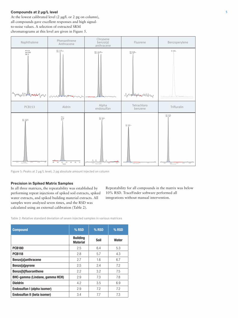
5Compounds at 2 µg/L levelAt the lowest calibrated level (2 µg/L or 2 pg on column), all compounds gave excellent responses and high signal-to-noise values. A selection of extracted SRM chromatograms at this level are given in Figure 5.
Precision in Spiked Matrix SamplesIn all three matrices, the repeatability was established by performing repeat injections of spiked soil extracts, spiked water extracts, and spiked building material extracts. All samples were analyzed seven times, and the RSD was calculated using an external calibration (Table 2).
RT: 4.14AA: 91767SN: 15
10.1 10.2 10.3 10.4 10.5Time (min)
RT: 10.21AA: 32608SN: 568
RT: 7.04AA: 117284SN: 24
8.00 8.05 8.10 8.15 8.20 8.25 8.30Time (min)
RT: 8.11AA: 3895SN: 38
RT: 11.44AA: 282645SN: 65
9 9.0 9.1 9.2 9.3Time (min)
RT: 9.11AA: 4468SN: 35
RT: 6.04AA: 82901SN: 12
5.1 5.2 5.3 5Time (min)
RT: 5.07AA: 28578SN: 125
16.42 - 17.10 SM: 7GRT: 16.69AA: 205975
6.2 6.3 6.4 6.5 6.6Time (min)
RT: 6.26AA: 7123SN: 254
Naphthalene
PCB153
Phenanthrene Anthracene
Aldrin
Chrysene benzo(a)
anthracene
Alpha endosulfan
Fluorene
Tetrachloro benzene
Benzoperylene
Trifluralin
Compound % RSD % RSD % RSD
Building Material
Soil Water
PCB180 2.5 6.4 5.3
PCB118 2.8 5.7 4.3
Benzo[a]anthracene 2.7 1.6 6.7
Benzo[a]pyrene 2.5 2.4 7.2
Benzo[b]fluoranthene 2.2 3.2 7.5
BHC-gamma (Lindane, gamma HCH) 2.9 7.3 7.8
Dieldrin 4.2 3.5 6.9
Endosulfan I (alpha isomer) 2.9 7.2 7.2
Endosulfan II (beta isomer) 3.4 7.7 7.3
Repeatability for all compounds in the matrix was below 10% RSD. TraceFinder software performed all integrations without manual intervention.
Figure 5: Peaks at 2 µg/L level; 2 pg absolute amount injected on column
Table 2: Relative standard deviation of seven injected samples in various matrices

6 Ion Ratio StabilityAll compounds had at least two transitions in the method, and the two ions had been monitored throughout the samples, blanks, and standards.
Figure 6: Ion ratio of hexachloroethane, plotted with the upper and lower allowed limit according to the EU guidelines for performance of analytical methods.4 The average and the
standard deviation are shown in the table above.
Throughout the complete series of calibration curves, water samples, soil samples, and building materials, the ion ratios were calculated. The ion ratio precision demonstrated good confirmation in both samples and standard injections across the concentration range.
Sample ResultsA small selection of compound peaks at low levels in matrix is shown in Figure 7, demonstrating the sensitivity and selectivity of the measurements.
Below, a selection of matrix and compounds at low levels, and the concentrations, are given as the absolute amount on column.
Figure 7: Compound peaks in various sample matrices at low levels
Hexachloroethane Ratio Benzoperylene Ratio
Average 0.479 Average 2.910
Standard deviation 0.025 Standard deviation 0.124
RSD 5.3% RSD 4.3%
Hexachloroethane in water at 0.5 pg
Pentachlorobenzene in water at 1.6 pg
Lindane in soil at 1 pg
Indenopyrene in soil at 2 pg
Benzo(ghi) perylene in soil at 1 pg
Anthracene in soil at 1.5 pg
o,p DDE in soil at 2 pg
Heptachlorepoxide in water at 2 pg
Dieldrin in water at 2 pg
PCB 180 in water at 0.86 pg

7References1. Analysis of emerging persistent organic pollutants using
GC-MS/MS; Kalachova et al. SETAC, Berlin 2012.
2. Ziegenhals, K.; Hubschmann, H.J. Fast-GC/HRMS toquantify the EU priority PAH. J. Sep. Sci. 2008, 31,1779 – 1786.
3. Thermo Scientific Application Brief AB52998:Introducing AutoSRM: MRM Simplicity for HighPerformance Results; Cole J.
4. REGULATION (EC) No 2002/657 on analyticalperformance criteria.
5. Pesticides Method Reference, 2nd ed. 2011, ThermoFisher Scientific, Austin, TX, USA, P/N 120390.
Conclusions• TheTSQ8000GC-MS/MSenabledsimplemethod
development, validation, and management using acombination of integrated software tools.
• Thenewmethodincreasedproductivityinthelaboratory by combining three separate methods intoone, from three injections down to one injection.
• Quantitativeperformanceofthesystemandmethodology was excellent with a good level oflinearity, excellent sensitivity, and high precision in avariety of environmental sample types.
Parent Mass (Da)
Product Mass (Da)
Collision Energy (V)
RT (min)
Start Time*
(min)Stop Time*
(min)Name
427.77 357.80 25 13.20 12.68 13.68 2,2',3,3',4,4',5,5'-Octachlorobiphenyl (BZ #194)
429.76 357.80 25 13.20 12.68 13.682,2',3,3',4,4',5,5'-Octachlorobiphenyl (BZ #194) Confirming 1
391.81 321.84 25 11.70 11.16 12.16 2,2',3,4,4',5,5'-Heptachlorobiphenyl (BZ #180)
393.81 323.84 25 11.70 11.16 12.162,2',3,4,4',5,5'-Heptachlorobiphenyl (BZ #180) Confirming 1
357.84 287.88 25 10.20 9.70 10.70 2,2',4,4',5,5'-Hexachlorobiphenyl (BZ #153)
359.84 289.87 25 10.20 9.70 10.702,2',4,4',5,5'-Hexachlorobiphenyl (BZ #153) Confirming 1
289.92 219.94 20 7.87 7.37 8.37 2,2',5,5'-Tetrachlorobiphenyl (BZ #52)
291.92 219.94 20 7.87 7.37 8.37 2,2',5,5'-Tetrachlorobiphenyl (BZ #52) Confirming 1
323.88 253.91 20 9.88 9.38 10.38 2,3',4,4',5-Pentachlorobiphenyl (BZ #118)
325.88 255.91 20 9.88 9.38 10.38 2,3',4,4',5-Pentachlorobiphenyl (BZ #118) Confirming 1
255.96 185.97 20 7.48 6.98 7.98 2,4,4'-Trichlorobiphenyl (BZ #28)
257.96 185.97 20 7.48 6.98 7.98 2,4,4'-Trichlorobiphenyl (BZ #28) Confirming 1
153.07 126.05 45 5.58 5.08 6.08 acenaphtene
153.07 151.07 40 5.58 5.08 6.08 acenaphtene Confirming 1
164.14 160.00 30 5.55 5.05 6.05 acenaphtene D10
164.14 162.00 20 5.55 5.05 6.05 acenaphtene D10 Confirming 1
152.06 102.03 30 5.43 4.93 5.93 acenaphtylene
152.06 126.05 20 5.43 4.93 5.93 acenaphtylene Confirming 1
276.08 272.08 60 16.70 16.20 17.20 benzo[ghi[perylene
276.08 274.08 40 16.70 16.20 17.20 benzo[ghi[perylene Confirming 1
216.89 180.91 8 6.48 5.98 6.98 BHC-alpha (benzene hexachloride)
218.89 182.91 8 6.48 5.98 6.98 BHC-alpha (benzene hexachloride) Confirming 1
240.17 212.00 30 11.40 10.94 11.94 chrysene D12
240.17 236.00 30 11.40 10.94 11.94 chrysene D12 Confirming 1
235.01 164.98 20 9.50 9.00 10.00 DDD-o,p'
237.01 164.98 20 9.50 9.00 10.00 DDD-o,p' Confirming 1
495.69 425.73 25 14.30 13.79 14.79 Decachlorobiphenyl (BZ #209)
497.69 427.73 25 14.30 13.79 14.79 Decachlorobiphenyl (BZ #209) Confirming 1
278.08 274.08 60 16.30 15.82 16.82 dibenzo[ah]anthracene
Addendum: SRM Transitions
* Start and Stop Times are set automatically in timed-SRM mode of the TSQ 8000 by using a standard acquisition window of 60 s for all compounds

8
Parent Mass (Da)
Product Mass (Da)
Collision Energy (V)
RT (min)
Start Time*
(min)Stop Time*
(min)Name
278.08 276.08 30 16.30 15.82 16.82 dibenzo[ah]anthracene Confirming 1
170.96 135.97 15 4.88 4.38 5.38 Dichlorobenzonitrile, 2,6- (Dichlobenil)
172.96 137.97 15 4.88 4.38 5.38 Dichlorobenzonitrile, 2,6- (Dichlobenil) Confirming 1
276.91 240.92 12 9.50 9.00 10.00 Dieldrin
278.91 242.92 12 9.50 9.00 10.00 Dieldrin Confirming 1
165.08 139.04 30 6.04 5.54 6.54 fluorene
165.08 163.08 30 6.04 5.54 6.54 fluorene Confirming 1
269.88 234.89 15 7.67 7.17 8.17 Heptachlor
271.88 236.89 15 7.67 7.17 8.17 Heptachlor Confirming 1
283.81 248.84 20 6.57 6.07 7.07 Hexachlorobenzene
285.81 250.83 20 6.57 6.07 7.07 Hexachlorobenzene Confirming 1
224.80 189.90 18 4.26 3.76 4.76 Hexachlorobutadiene
226.90 189.90 18 4.26 3.76 4.76 Hexachlorobutadiene Confirming 1
226.90 191.90 18 4.26 3.76 4.76 Hexachlorobutadiene Confirming 2
310.83 240.87 25 8.25 7.75 8.75 Isobenzan (Telodrin)
312.83 242.87 25 8.25 7.75 8.75 Isobenzan (Telodrin) Confirming 1
227.01 169.01 20 10.80 10.30 11.30 Methoxychlor, o,p'-
227.01 184.08 20 10.80 10.30 11.30 Methoxychlor, o,p'- Confirming 1
128.06 77.05 30 4.15 3.65 4.65 naphtalene
128.06 102.03 20 4.15 3.65 4.65 naphtalene Confirming 1
136.11 108.03 25 4.12 3.62 4.62 naphtalene D8
136.11 134.06 25 4.12 3.62 4.62 naphtalene D8 Confirming 1
247.85 141.92 25 5.68 5.18 6.18 Pentachlorobenzene
247.85 212.87 25 5.68 5.18 6.18 Pentachlorobenzene Confirming 1
264.00 230.00 30 14.40 13.85 14.85 perylene D12
264.00 260.00 30 14.40 13.85 14.85 perylene D12 Confirming 1
188.00 158.00 30 7.01 6.51 7.51 phenathrene D10
188.00 160.00 30 7.01 6.51 7.51 phenathrene D10 Confirming 1
207.00 136.00 16 6.14 5.64 6.64 TCMX
244.00 209.00 16 6.14 5.64 6.64 TCMX Confirming 1
242.00 207.00 16 6.14 5.64 6.64 TCMX Confirming 2
213.89 107.95 30 4.84 4.34 5.34 Tetrachlorobenzene, 1,2,4,5 +1,2,3,5
213.89 142.93 30 4.84 4.34 5.34 Tetrachlorobenzene, 1,2,4,5 +1,2,3,5 Confirming 1
264.09 160.05 15 6.26 5.76 6.76 Trifluralin
306.10 264.09 15 6.26 5.76 6.76 Trifluralin Confirming 1
213.89 107.95 30 5.07 4.57 5.57 Tetrachlorobenzene, 1,2,3,4-
213.89 142.93 30 5.07 4.57 5.57 Tetrachlorobenzene, 1,2,3,4- Confirming 1
218.89 182.91 8 6.75 6.25 7.25 BHC-beta Confirming 1
216.89 180.91 8 6.75 6.25 7.25 BHC-beta
218.89 182.91 8 6.85 6.35 7.35 BHC-gamma (Lindane, gamma HCH) Confirming 1
216.89 180.91 8 6.85 6.35 7.35 BHC-gamma (Lindane, gamma HCH)
178.08 152.07 25 7.04 6.54 7.54 phenathrene
178.08 176.08 20 7.04 6.54 7.54 phenathrene Confirming 1
178.08 152.07 25 7.11 6.61 7.61 anthracene
178.08 176.08 20 7.11 6.61 7.61 anthracene Confirming 1
216.89 180.91 8 7.14 6.64 7.64 BHC-delta
Addendum: SRM Transitions
* Start and Stop Times are set automatically in timed-SRM mode of the TSQ 8000 by using a standard acquisition window of 60 s for all compounds

9
Parent Mass (Da)
Product Mass (Da)
Collision Energy (V)
RT (min)
Start Time*
(min)Stop Time*
(min)Name
218.89 182.91 8 7.14 6.64 7.64 BHC-delta Confirming 1
216.89 180.91 8 7.24 6.74 7.74 BHC-epsilon
218.89 182.91 8 7.24 6.74 7.74 BHC-epsilon Confirming 1
188.14 160.00 30 7.53 7.03 8.03 Alachlor Confirming 1
188.14 158.00 30 7.53 7.03 8.03 Alachlor
352.83 252.88 15 8.60 8.10 9.10 Heptachlor exo-epoxide (isomer B)
352.83 281.88 15 8.60 8.10 9.10 Heptachlor exo-epoxide (isomer B) Confirming 1
288.86 252.88 15 8.65 8.15 9.15 Heptachlor endo-epoxide (isomer A) Confirming 1
288.86 218.95 15 8.65 8.15 9.15 Heptachlor endo-epoxide (isomer A)
246.05 175.97 25 8.93 8.43 9.43 DDE-o,p'
317.94 245.95 20 8.93 8.43 9.43 DDE-o,p' Confirming 1
325.88 255.91 20 8.99 8.49 9.49 2,2',4,5,5'-Pentachlorobiphenyl (BZ #101) Confirming 1
323.88 253.91 20 8.99 8.49 9.49 2,2',4,5,5'-Pentachlorobiphenyl (BZ #101)
202.08 200.08 30 9.10 8.60 9.60 pyrene Confirming 1
202.08 176.08 35 9.10 8.60 9.60 pyrene
246.05 175.97 25 9.39 8.89 9.89 DDE-p,p'
317.94 245.95 20 9.39 8.89 9.89 DDE-p,p' Confirming 1
242.89 207.91 10 9.95 9.45 10.45 Endosulfan II (beta isomer) Confirming 1
240.89 205.91 10 9.95 9.45 10.45 Endosulfan II (beta isomer)
235.01 164.98 20 10.00 9.52 10.52 DDD-p,p'
237.01 164.98 20 10.00 9.52 10.52 DDD-p,p' Confirming 1
237.01 165.07 20 10.10 9.56 10.56 DDT-o,p' Confirming 1
235.01 165.07 20 10.10 9.56 10.56 DDT-o,p'
359.84 289.87 25 10.60 10.13 11.132,2',3,4,4',5'-Hexachlorobiphenyl (BZ #138) Confirming 1
357.84 287.88 25 10.60 10.13 11.13 2,2',3,4,4',5'-Hexachlorobiphenyl (BZ #138)
237.01 165.07 20 10.50 10.03 11.03 DDT-p,p' Confirming 1
235.01 165.07 20 10.50 10.03 11.03 DDT-p,p'
228.08 202.08 35 11.50 11.00 12.00 benzo[a]anthracene
228.08 226.08 30 11.50 11.00 12.00 benzo[a]anthracene Confirming 1
228.08 202.08 35 11.40 10.94 11.94 chrysene
228.08 226.08 30 11.40 10.94 11.94 chrysene Confirming 1
252.09 226.08 35 13.60 13.12 14.12 benzo[b]fluoranthene
252.09 250.09 30 13.60 13.12 14.12 benzo[b]fluoranthene Confirming 1
252.09 250.09 30 14.30 13.76 14.76 benzo[a]pyrene Confirming 1
252.09 226.08 35 14.30 13.76 14.76 benzo[a]pyrene
252.09 250.09 30 13.70 13.21 14.21 benzo[k]fluoranthene Confirming 1
252.09 226.08 35 13.70 13.21 14.21 benzo[k]fluoranthene
202.08 176.08 35 8.72 8.22 9.22 fluoranthene Confirming 1
202.08 200.08 30 8.72 8.22 9.22 fluoranthene
292.90 185.93 30 8.11 7.61 8.61 Aldrin
292.90 257.91 10 8.11 7.61 8.61 Aldrin Confirming 1
262.91 192.93 30 8.48 7.98 8.98 Isodrin
262.91 190.93 30 8.48 7.98 8.98 Isodrin Confirming 1
240.89 205.91 10 9.11 8.61 9.61 Endosulfan I (alpha isomer)
242.89 207.91 10 9.11 8.61 9.61 Endosulfan I (alpha isomer) Confirming 1
* Start and Stop Times are set automatically in timed-SRM mode of the TSQ 8000 by using a standard acquisition window of 60 s for all compounds

Ap
plica
tion
No
te 5
23
89
AN52389_E 08/16S
Africa-Other +27 11 570 1840Australia +61 3 9757 4300Austria +43 1 333 50 34 0Belgium +32 53 73 42 41Canada +1 800 530 8447China +86 10 8419 3588Denmark +45 70 23 62 60
Europe-Other +43 1 333 50 34 0Finland/Norway/Sweden
+46 8 556 468 00France +33 1 60 92 48 00Germany +49 6103 408 1014India +91 22 6742 9434Italy +39 02 950 591
Japan +81 45 453 9100Latin America +1 561 688 8700Middle East +43 1 333 50 34 0Netherlands +31 76 579 55 55New Zealand +64 9 980 6700Russia/CIS +43 1 333 50 34 0South Africa +27 11 570 1840
Spain +34 914 845 965Switzerland +41 61 716 77 00UK +44 1442 233555USA +1 800 532 4752
www.thermofisher.com©2016 Thermo Fisher Scientific Inc. All rights reserved. Teflon is a registered trademark of DuPont. All other trademarks are the property of Thermo Fisher Scientific Inc. and its subsidiaries. This information is presented as an example of the capabilities of Thermo Fisher Scientific Inc. products. It is not intended to encourage use of these products in any manners that might infringe the intellectual property rights of others. Specifications, terms and pricing are subject to change. Not all products are available in all countries. Please consult your local sales representative for details.
Addendum: SRM Transitions
Parent Mass (Da)
Product Mass (Da)
Collision Energy (V)
RT (min)
Start Time*
(min)Stop Time*
(min)Name
276.08 272.08 60 16.30 15.77 16.77 indeno[123cd]pyrene
276.08 274.08 40 16.30 15.77 16.77 indeno[123cd]pyrene Confirming 1
202.90 167.90 10 3.51 3.01 4.01 Hexachloroethane Confirming 1
117.00 82.00 25 3.51 3.01 4.01 Hexachloroethane Confirming 2
200.90 165.9 10 3.51 3.01 4.01 Hexachloroethane
* Start and Stop Times are set automatically in timed-SRM mode of the TSQ 8000 by using a standard acquisition window of 60 s for all compounds


AI63770-EN 08/16S
Africa +43 1 333 50 34 0Australia +61 3 9757 4300Austria +43 810 282 206Belgium +32 53 73 42 41Canada +1 800 530 8447China 800 810 5118 (free call domestic)
400 650 5118
Denmark +45 70 23 62 60Europe-Other +43 1 333 50 34 0Finland +358 9 3291 0200France +33 1 60 92 48 00Germany +49 6103 408 1014India +91 22 6742 9494Italy +39 02 950 591
Japan +81 45 453 9100Korea +82 2 3420 8600Latin America +1 561 688 8700Middle East +43 1 333 50 34 0Netherlands +31 76 579 55 55New Zealand +64 9 980 6700Norway +46 8 556 468 00
Russia/CIS +43 1 333 50 34 0Singapore +65 6289 1190Spain +34 914 845 965Sweden +46 8 556 468 00Switzerland +41 61 716 77 00UK +44 1442 233555USA +1 800 532 4752
www.thermofisher.com©2014 Thermo Fisher Scientific Inc. All rights reserved. All trademarks are the property of Thermo Fisher Scientific and its subsidiaries. This information is presented as an example of the capabilities of Thermo Fisher Scientific products. It is not intended to encourage use of these products in any manners that might infringe the intellectual property rights of others. Specifications, terms and pricing are subject to change. Not all products are available in all countries. Please consult your local sales representative for details.