Recent changes in macrophyte colonisation patterns: an imaging spectrometry-based evaluation of...

Recent changes in macrophyte colonisation patterns: an imaging spectrometry-based evaluation of southern

Lake Garda (northern Italy)

Claudia Giardinoa, Marco Bartolib, Gabriele Candiania, Mariano Bresciania, and Luca Pellegrinia,b

a Optical Remote Sensing Group, CNR-IREA Via Bassini 15, 20133 Milano, Italy

[email protected] Environmental Science Department, University of Parma

Viale G.P. Usberti 11/A, 43100 Parma, Italy

Abstract. Temporal variation in the extent of submerged macrophytes along the littoral zone of Sirmione Peninsula in the southern part of Lake Garda (Northern Italy) was investigated using imaging spectrometry. Two images, with a spatial resolution of 5 m were acquired by the Multispectral Infrared and Visible Imaging Spectrometer (MIVIS) in the summers of 1997 and 2005. Image data were first geocoded and then corrected for both atmospheric and skylight reflection effects at the water surface using the 6S radiative transfer code. The two images were inverted using a bio-optical model, which was parameterised with the inherent optical properties of the lake. The inversion utilized the spectral range from 0.48-0.60 mbecause it simultaneously provided the lowest environmental noise and the best atmospheric correction performances for the two scenes and produced images of bottom depth and of two substrate classes: bare sand and submerged vegetation, representing a mixture of valuable freshwater species. The MIVIS-derived bottom depth ranges and patterns were comparable to a bathymetry chart with a deviation less than 5%. In 2005, the image was consistent with contemporaneous in-situ derived knowledge on macrophyte distribution. In 1997, the substrate image map was deemed reasonable with respect to the macrophyte distribution documented in 2000. The comparison of the substrate products for the two dates showed a marked decrease in macrophyte beds, with a concomitant increase in sandy substrates. In the 8-year interval the extent of submerged macrophyte decreased from 72% to 52%. We expect that this study will contribute to increased knowledge of macrophyte colonisation patterns of the Sirmione Peninsula, where, despite their ecological significance, changes have been poorly documented.

Keywords: imaging spectrometry, freshwater, submerged macrophytes, change detection.

1 INTRODUCTION Shallow coastal areas of oligotrophic lakes are often inhabited by a variety of aquatic phanerogams (or macrophytes), which are those plants that produce seeds and have morphologic and physiological adaptations necessary for life in water. Prairies of rooted macrophytes comprise of many different species and represent an extremely valuable component of the aquatic ecosystem as they have well recognised ecological functions (as in [1] and references therein). They stabilise and oxidise sediments through their rhyzosphere, enhance nitrification and denitrification coupling, act as nursery areas for fishes and invertebrates, produce oxygen in the bottom water and control the concentration of dissolved nutrients through uptake via roots and leaves and the conversion of recalcitrant biomass [2, 3]. Macrophyte meadows are also indicators of water and sediment quality as their disappearance from many freshwater and coastal marine environments has been attributed mainly to

Journal of Applied Remote Sensing, Vol. 1, 011509 (26 December 2007)

© 2007 Society of Photo-Optical Instrumentation Engineers [DOI: 10.1117/1.2834807]Received 10 Apr 2007; accepted 20 Dec 2007; published 26 Dec 2007 [CCC: 19313195/2007/$25.00]Journal of Applied Remote Sensing, Vol. 1, 011509 (2007)

Journal of Applied Remote Sensing, Vol. 1, 011509 (2007)

eutrophication phenomena [4]. Excess nutrient availability uncouples input and uptake processes and favors blooms of microalgae (pelagic and attached) that limit light penetration and turn surface sediments more organic and reduced. In such conditions phanerogams are replaced by other opportunistic primary producers [5]. Coastal eutrophication would appear to be associated with a trend in the disappearance of macrophyte meadows, which are being replaced by micro and macroalgae [6, 7]. Also in oligotrophic freshwater environments, shifts to more eutrophic conditions are well documented and based on increased concentrations of water column nutrient or chlorophyll-a [8, 9, 10, 11].

Macrophytes are potentially an important long-term limnological indicator of water and sediment quality but monitoring of their distribution using standard limnological approaches requires significant time and costly field campaigns. Measurements are generally performed over relatively small areas, and for this reason are not representative of larger scale processes. Furthermore, due to the huge sampling effort, such characterisations are not repeated annually. Remote sensing represents a suitable technology to fill these gaps, due to its repeatability and synoptic spatial coverage.

Remote sensing has been used to make large-scale inventories of benthic photosynthetic organisms such as macrophytes, seagrasses and corals (as in [12] and references therein). Retrieval methods may involve classification techniques that, although precise (e.g., Reguzzoni et al. [13]), are effectively limited to application on single scenes. In order to promote automation and the removal of subjectivity from the classification process, the techniques can be combined with physically-based approaches [14, 15]. This allows the extension of the application to additional sampling locations and time-scales. To classify the substrate coverage and simultaneously derive bottom depths and water column properties fully physically-based approaches are necessary. For instance, using a bio-optical model-driven optimisation technique applied to atmospherically corrected Airborne Visible InfraRed Imaging Spectrometer (AVIRIS) data, Lee et al. [16] simultaneously derived a number of water quality components, bottom albedo and bottom depth in shallow coastal environments.

The main objective of this study was to evaluate variations in the submerged vegetation of the largest Italian lake from hyperspectral airborne data acquired during the summers of 1997 and 2005. The approach is physically-based and includes the discrimination of two substrates: bare sand and submerged vegetation, which represents a mixture of valuable freshwater species. Utilizing atmospheric correction, a bio-optical inversion model, and a sensitivity analysis, an estimates of bottom depth and the distribution of colonised substrates were generated. A nautical chart and knowledge on macrophyte distribution were used to evaluate the performance of the proposed method.

2 MATERIAL AND METHODS

2.1 Study Area Lake Garda belongs to a distinct typology of Italian Subalpine lakes located on the southern edge of the Alps, characterised by high depths and large volumes. With a surface of 368 km2

Lake Garda is the largest Italian lake. It is oligomitic with summer stratification between June and October. According to the Organisation for Economic Co-operation and Development (OECD) [17], Lake Garda can be classified as an oligo-mesotrophic basin.

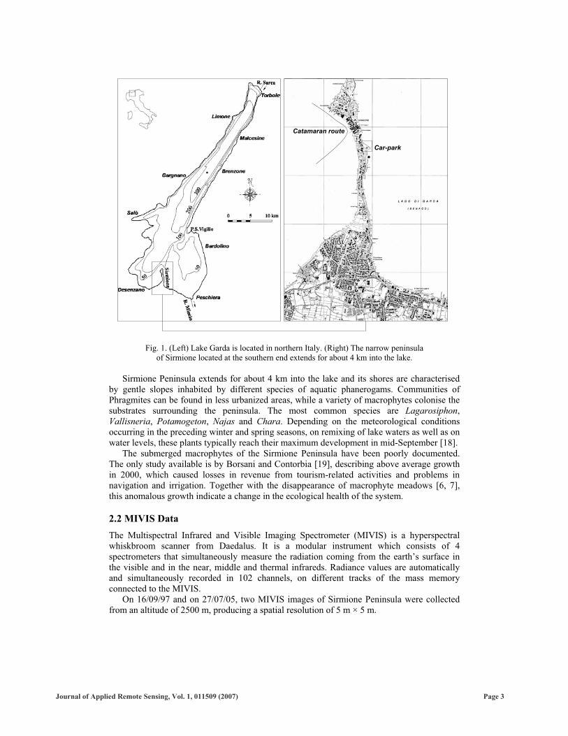
Located in the most densely populated and industrialized region of Italy, Lake Garda represents an essential renewable resource for the environment of the surrounding regions because of the multiple uses of its waters (human consumption, irrigation, energy, transportation, recreational purposes). In particular, the Sirmione Peninsula, located at the southern end of the lake (Fig. 1), is one of the most popular tourist destinations in Italy with attractions such as the ruins of a number of Roman villas, the Scaligeri castle, as well as for hot-springs and spa facilities ( 690,000 guests per year, excluding day visitors [18]).


Fig. 1. (Left) Lake Garda is located in northern Italy. (Right) The narrow peninsula of Sirmione located at the southern end extends for about 4 km into the lake.

Sirmione Peninsula extends for about 4 km into the lake and its shores are characterised by gentle slopes inhabited by different species of aquatic phanerogams. Communities of Phragmites can be found in less urbanized areas, while a variety of macrophytes colonise the substrates surrounding the peninsula. The most common species are Lagarosiphon,Vallisneria, Potamogeton, Najas and Chara. Depending on the meteorological conditions occurring in the preceding winter and spring seasons, on remixing of lake waters as well as on water levels, these plants typically reach their maximum development in mid-September [18].

The submerged macrophytes of the Sirmione Peninsula have been poorly documented. The only study available is by Borsani and Contorbia [19], describing above average growth in 2000, which caused losses in revenue from tourism-related activities and problems in navigation and irrigation. Together with the disappearance of macrophyte meadows [6, 7], this anomalous growth indicate a change in the ecological health of the system.

2.2 MIVIS Data The Multispectral Infrared and Visible Imaging Spectrometer (MIVIS) is a hyperspectral whiskbroom scanner from Daedalus. It is a modular instrument which consists of 4 spectrometers that simultaneously measure the radiation coming from the earth’s surface in the visible and in the near, middle and thermal infrareds. Radiance values are automatically and simultaneously recorded in 102 channels, on different tracks of the mass memory connected to the MIVIS.

On 16/09/97 and on 27/07/05, two MIVIS images of Sirmione Peninsula were collected from an altitude of 2500 m, producing a spatial resolution of 5 m × 5 m.

Catamaran route

Car-park


2.3 Fieldwork and Supporting Data Vegetation samples of Ceratophyllum, Chara, Lagharosiphon, Vallisneria and Potamogetonspecies were collected during three surveys carried out around the Sirmione Peninsula from June to September 2005. During each survey the nadir-viewing reflectance of extracted macrophytes was derived ex-situ above water using an ASD-FieldSpec radiometer and a Spectralon reflectance panel. The reflected radiation field over macrophyte samples was assumed to be Lambertian and the vegetation albedo was computed by averaging the nadir-viewing reflectance values of the different measured species.

On 27/07/05, coincident with the second MIVIS over-flight, in-situ reflectance values over a car-park surface (Fig. 1) were measured to obtain a reference spectrum to evaluate the accuracy of atmospheric correction. For this purpose the measured surface was assumed to be Lambertian and not affected by bidirectional reflectance-related effects. Moreover, to evaluate the atmospheric correction of MIVIS 1997 data the surface was assumed optically invariant.

Other supporting data include in-situ measurements from more than 30 days during 5 years [20, 21, 22, 23] which were included to create a comprehensive dataset of water component concentrations and of apparent and inherent optical properties. In particular the dataset comprising the concentrations of chlorophyll-a, suspended particulate matter and coloured dissolved organic matter at 440 nm, in addition to the absorption spectra of coloured dissolved organic matter and particles as well as the back-scattering coefficients of particles at 6 wavelengths allowed the parameterisation of the bio-optical model used in the study.

2.4 Image Preprocessing The atmospheric correction of the MIVIS data was carried out using the 6S code [24]. Table 1 shows the main 6S inputs for the two images: the atmospheric profiles were collected from radiosonde databases [25]; the aerosol type was set as continental, while the aerosol concentration, expressed as Atmospheric Optical Thickness (AOT) at 550 nm, was taken from AERONET [26], in correspondence to the nearest stations to the study area (i.e., Ispra and Venice, about 100 km to the west and 80 km to the east, respectively).

Table 1. Main 6S inputs for the atmospheric correction of MIVIS data

Altitude of target 60 m Lat/Long 45.5/10.6 Flight time ~11.5 UTC (for both acquisitions) Flight altitude 2560 m a.s.l. (for both acquisitions) Dates (DD/MM/YY) 16/09/97; 27/07/05

Target/image properties

Sun zenith/azimuth angles 43°/170° (16/09/97); 27°/144° (27/07/05) Climatic zone Mid-latitude summer Aerosol model Continental AOT at 550 nm 0.22 (16/09/97); 0.57 (27/07/05)

Definition of the atmosphere

Visibility ranges* 24 km (16/09/97); 7 km (27/07/05) Spectral range from 440 to 820 nm Wavelengths Full width half maximum 10 nm

*Visibility ranges computed by 6S from AOT at 550 nm inputs.

The 6S-derived reflectance values R (for brevity, wavelength dependence may not be explicitly included) were compared to in-situ data measured during the 2005 MIVIS overflight over the car-park surface. The comparison was performed for the 1997 MIVIS data as well. In Fig. 2, image-derived spectra are plotted together with in-situ spectrum. The relative average reflectance differences between in-situ and atmospherically corrected MIVIS


data from the full spectral range from 0.44-0.82 m were approximately 16% and 21% for 2005 and 1997, respectively.

The most likely cause of the mismatch was the inadequacy of the available models to describe the aerosol composition in the 6S code [27, 28]. Since the lake is located in the most urbanised and industrialized region of Italy, where multiple aerosol sources may exist, the “continental” model can fail in describing such a complex mixture. However, a more appropriate aerosol model was not available and the currently best available one was selected. Ignoring the effects of light polarization can also lead to large errors (5% to 10% and higher depending on the “atmosphere” type) [29]. Because the polarization effects tend to increase with AOT, they were probably present in the two MIVIS scenes, which were acquired with significant AOT values. Correction for polarization effects was not included in the scalar 6S version utilised in this study but it should be considered in the future.

A better result was achieved within the spectral range from 0.47-0.60 m where the relative difference of reflectance values between in-situ and MIVIS data was 7% for 2005 and 13% for 1997. On average for the two dates, the atmospheric correction uncertainty of MIVIS data was around 10%.

0.00

0.05

0.10

0.15

0.20

0.25

0.42 0.47 0.52 0.57 0.62 0.67 0.72 0.77 0.82

Wavelength [ m]

R [-

]

MIVIS 1997 MIVIS 2005 In situ

Fig. 2. Comparison between MIVIS reflectance values R derived from 6S over the car park surface and in-situ spectrum measured on the same surface on 27/07/05.

After atmospheric correction the reflectance values represent the above water surface reflectance including the contribution of the reflected diffuse sky radiance reflected from the water. To apply the inversion of the bio-optical model this portion of the signal should be removed. In order to achieve this, the 6S-derived reflectances were converted into remote sensing reflectance Rrs (sr-1), by subtracting the contribution of the diffuse sky radiance using the equation

02.0fR1R rs , (1)

where f is the diffuse to total irradiance ratio (provided by 6S) and 0.02 is the Fresnel reflectance for low wind speed (during both acquisitions the wind speed was 1 ms-1 [18]) and solar incidence angle less than 45° [30]. Although none of the glint-effects described in Mustard et al. [31] were observed in the two MIVIS scenes, Rrs spectra derived from equation


1 were assumed to still potentially include minor glint effects. As such, these minor influences were corrected in the optimisation process directly.

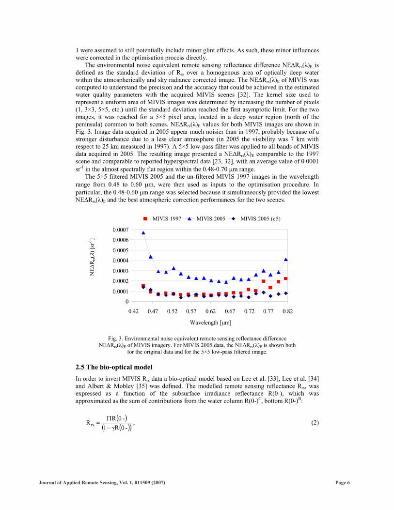
The environmental noise equivalent remote sensing reflectance difference NE Rrs( )E is defined as the standard deviation of Rrs over a homogenous area of optically deep water within the atmospherically and sky radiance corrected image. The NE Rrs( )E of MIVIS was computed to understand the precision and the accuracy that could be achieved in the estimated water quality parameters with the acquired MIVIS scenes [32]. The kernel size used to represent a uniform area of MIVIS images was determined by increasing the number of pixels (1, 3×3, 5×5, etc.) until the standard deviation reached the first asymptotic limit. For the two images, it was reached for a 5×5 pixel area, located in a deep water region (north of the peninsula) common to both scenes. NE Rrs( )E values for both MIVIS images are shown in Fig. 3. Image data acquired in 2005 appear much noisier than in 1997, probably because of a stronger disturbance due to a less clear atmosphere (in 2005 the visibility was 7 km with respect to 25 km measured in 1997). A 5×5 low-pass filter was applied to all bands of MIVIS data acquired in 2005. The resulting image presented a NE Rrs( )E comparable to the 1997 scene and comparable to reported hyperspectral data [23, 32], with an average value of 0.0001 sr-1 in the almost spectrally flat region within the 0.48-0.70 m range.

The 5×5 filtered MIVIS 2005 and the un-filtered MIVIS 1997 images in the wavelength range from 0.48 to 0.60 m, were then used as inputs to the optimisation procedure. In particular, the 0.48-0.60 m range was selected because it simultaneously provided the lowest NE Rrs( )E and the best atmospheric correction performances for the two scenes.

0

0.0001

0.0002

0.0003

0.0004

0.0005

0.0006

0.0007

0.42 0.47 0.52 0.57 0.62 0.67 0.72 0.77 0.82

Wavelength [ m]

MIVIS 1997 MIVIS 2005 MIVIS 2005 (c5)

Fig. 3. Environmental noise equivalent remote sensing reflectance difference NE Rrs( )E of MIVIS imagery. For MIVIS 2005 data, the NE Rrs( )E is shown both

for the original data and for the 5×5 low-pass filtered image.

2.5 The bio-optical model In order to invert MIVIS Rrs data a bio-optical model based on Lee et al. [33], Lee et al. [34] and Albert & Mobley [35] was defined. The modelled remote sensing reflectance Rrs, was expressed as a function of the subsurface irradiance reflectance R(0-), which was approximated as the sum of contributions from the water column R(0-)C, bottom R(0-)B:

-0R1-0RRrs , (2)

NE

Rrs(

) [sr

-1]


HDcos

1

1

HDcos

1

0dpBC

Bu

w

Cu

w eAeA1-0R-0R-0R-0R ,(3)

uugg-0R 2g10

dp , (4)

where R(0-)dp is the subsurface irradiance reflectance for optically deep waters. The parameters and describe the transmission through the air-water interface and take into account the viewing angle and the water column properties, H is the water depth, w is the underwater Sun zenith angle, while the definition of model parameters g0, g1, g2, A0, A1 and of C

uD , BuD and (the last three being functions of total absorption and total backscattering

coefficients), can be found in Lee et al. [33]. With respect to Lee et al. [33] who described bottom albedo ( ) as the albedo value at a

reference wavelength, in this study the ( ) in equation 3 was expressed as a linear combination of two substrates having different albedo values:

2

1iiib , with

2

1ii 1b (5)

where bi represents the relative distribution of the substrate albedo i( ) characterising the study area. The sand spectrum 1( ) was obtained by reducing a coral sand spectra directly provided by HYDROLIGHT (ver. 4.2) [36, 37] by 50%. This spectrum compared favourably with preliminary measurements of ex-situ samples from the study area. The vegetation spectra

2( ) was the average value of measured reflectance spectra of different macrophyte species growing in the study area. Because the coefficient of variation was less than 0.5 for all wavelengths, it was assumed that the average was a good indicator of the albedo variability of the selected macrophyte. Figure 4 illustrates albedo values of the two substrates considered in this study: sand and vegetation.

0

0.1

0.2

0.3

0.4

0.40 0.45 0.50 0.55 0.60 0.65 0.70 0.75 0.80

Wavelength [ m]

() [

-]

Sand

Vegetation

Fig. 4. Albedo values of the two substrates considered in this study: sand and submerged vegetation.

Still following Lee et al. [33] and Lee et al. [34], the quantity u in equation 3 was expressed as a function of total absorption a( ) and total backscattering bb( ) coefficients:


bab

ub

b , (6)

but rather than deriving a( ) and bb( ) as in Lee et al. [33] the inherent optical properties were then directly related to concentration of water components.

The total absorption coefficient a( ) was expressed as the sum of three components which account for the contribution of pure water (w), total particle (p) (phytoplankton and nonalgal particles), and coloured dissolved organic matter (CDOM):

aaaa CDOMpw . (7)

The pure water absorption coefficient aw( ) was taken from Pope and Fry [38] and Smith and Baker [39]. The total particle absorption coefficient ap( ) was modelled as in Feng et al. [40] by fitting particle absorption spectra to measured chlorophyll concentrations (CHL) of the lake [21, 22].

B*pp CHLACHLaCHLa (8)

On average, the derived A( ) and B( ) values were similar to “Type 3” Tokyo Bay waters [40], whose concentrations were comparable to those of Lake Garda.

Table 2. A( ) and B( ) data used in this study (given each 0.02 m in the same wavelength range used by Feng et al. [40])

Wavelength [ m] A( ) B( )0.40 0.08969 0.76164 0.42 0.10493 0.75651 0.44 0.11156 0.75743 0.46 0.09621 0.79951 0.48 0.08355 0.80590 0.50 0.06702 0.75408 0.52 0.04186 0.67576 0.54 0.02819 0.53830 0.56 0.01995 0.40323 0.58 0.01574 0.44722 0.60 0.01297 0.53517 0.62 0.01503 0.55713 0.64 0.01515 0.57050 0.66 0.02380 0.66836 0.68 0.04131 0.70758 0.70 0.00661 0.57347


y = 0.0067x-0.3828

R2 = 0.92490.0000.005

0.0100.015

0.0200.025

0.0300.035

0.00 0.05 0.10 0.15 0.20 0.25 0.30 0.35 0.40

aCDOM(440) [m-1]

S CD

OM

[nm

-1]

Fig. 5. Relationship between the slope factor SCDOM of aCDOM( ) and aCDOM(440);0.0067 and 0.3828 are the two scalars C and D of equation (9).

The absorption coefficient of coloured dissolved organic matter aCDOM( ) was modelled as:

440440aCCDOM

440SCDOMCDOM

DCDOMCDOM e440ae440aa , (9)

where SCDOM, the slope factor of CDOM absorption spectrum, was modelled using two scalars C and D, which relate SCDOM to aCDOM(440) (Fig. 5) [21, 22].

The total backscattering coefficient bb( ) was divided into two components:

bbb bpbwb , (10)

where bbw( ) and bbp( ) are the backscattering coefficients of pure water and total particle, respectively, with bbw( ) defined according to Dall’Olmo and Gitelson [41] and bbp( )modelled as:

F*bpbp

440ESPMbSPMb , (11)

where SPM is the concentration of suspended particulate matter, b*bp is the specific

particle backscattering coefficient and E and F are two scalars used to model the b*bp .

Table 3 defines the model parameters used in this study: , , g0, g1, g2, A0, A1, DC0, DC

1,DB

0 and DB1. They were derived fitting equations 2 and 3 to a set of more than 6000 Rrs and

R(0-) curves, generated by HYDROLIGHT in the spectral range from 0.4 to 0.8 m (10 nm resolution). HYDROLIGHT was run with surface concentrations of water quality parameters (CHL, SPM, aCDOM(440)), which were obtained according to their probability density functions based on long-term historical data of the lake [21, 22]. For the simulation ten different concentrations for each water quality parameter were selected; sun zenith angles were set to 0°, 20° and 40°; bottom albedo was used with values in Fig. 4; visibility ranges were set to 10, 20 and 50 km, wind speeds were set to 0, 5 and 10 ms-1, and bottom depth was set to 1, 5, 10 m and infinitely deep.


Table 3. List of the bio-optical model parameters used in this study

Parameter Value Description 0.119

1.535 g0 0.311 g1 0.649 g2 0.782 A0 1 A1 1 DC

0 0.836 DC

1 0.501 DB

0 1.310 DB

1 0.492

Model parameters derived with HYDROLIGHT runs

30° for 16/09/97 w 21° for 27/07/05

Underwater Sun zenith angles at the moment of the two over flights

C 0.00667 D 0.3828

Gain and exponent of the power function relating SCDOM to aCDOM(440) to describe aCDOM( )

E 0.0825 F 0.75738

Gain and exponent of the power function used to describe b*

bp

2.6 Sensitivity analysis and Model inversion A first-order sensitivity analysis of the bio-optical model was performed prior to running the optimisation process to investigate how the uncertainty of the atmospheric correction potentially impacted the retrieval of water quality components. In particular, the model sensitivity was assessed by computing the relative change of Rrs, integrated in the 0.48-0.60

m interval, due to variations of each parameter. The sensitivity of the model to variations of bottom depth (H) was computed from 10

forward runs of the bio-optical model. The model was run changing H from 1 to 10 m and fixing CHL, SPM and aCDOM(440) to the long-term average values of the lake: 2.52 mgm-3,1.51 gm-3 and 0.09 m-1, respectively [23]. In the simulation, the distribution of sand and macrophytes was also fixed (b1=b2=0.5). The sensitivity of the model to variations of the substrate classes was than evaluated by 10 forwards runs of the bio-optical model, performed by changing b1 from 1 to 0 (hence incrementing b2 from 0 to 1) and fixing CHL, SPM and aCDOM(440) to the long term average values of the lake. The simulations were performed for three bottom depths. In order to indicate the model sensitivity with a single value only, the 9 normalised Rrs differences, derived from the 10 model runs were averaged. The sensitivity of the model to variations of each water column component (i.e., CHL, aCDOM(440), SPM) was finally computed from 10 further forward runs of the bio-optical model. For each component, the model was run fixing b1=b2=0.5 and keeping the other two components constant. CHL was changed from 1 to 5 mgm-3 (and fixing SPM=1.51 gm-3 and aCDOM(440)=0.09 m-1), aCDOM(440) was changed from 0.03 to 0.3 m-1 (and fixing SPM=1.51 gm-3 and CHL=2.52 mgm-3) and SPM was changed from 1 to 5 gm-3 (and fixing CHL=2.52 mgm-3 and aCDOM(440)=0.09 m-1). The simulations were performed for two bottom depths and, as for the substrate classes analysis, the model sensitivity was expressed as the average of the 9 normalised Rrs differences.

Table 4 summarises the results of the sensitivity analysis of the bio-optical model. The normalised Rrs differences, due to a 1m variation of bottom depth, were 29% going from 0.1 to 1 m; 25% from 1 to 2 m; 22% from 2 to 3 m and so on, until the physical limit of the model


in depth retrieval is reached, which results from the strong absorption and scattering properties of the water column. The normalised Rrs differences dropped to 6%, by incrementing H from 7 to 8 m, and to 3% for H ranging from 9 to 10 m. Bottom property retrieval was hence limited to the first 7 meters because for H>7 m the normalised Rrsdifferences due to bottom depth variations were less than the uncertainty of MIVIS-derived spectra. For H=7 m, the average normalised Rrs difference to variations of the substrate classes was 10% and comparable to the uncertainty of MIVIS spectra. As expected, simulations for H<7 m provided larger Rrs difference values, resulting from the weak absorption and scattering properties of a short water column. In particular, the model sensitivity to variations of the substrate class variations increased to 12% for H=6 m and to 25% for H=1 m. The average normalised Rrs difference to variations of CHL, aCDOM(440) and SPM were 4%, 3% and 16% respectively, for H=7 m. Similar simulations for H<7 m provided smaller values of the normalised Rrs differences. For instance, for H=3 m, the average Rrs differences due to variations of CHL, aCDOM(440) and SPM dropped to 3%, 2% and 9%, respectively and fall within the uncertainty of the MIVIS spectra.

Table 4. Sensitivity analysis of the bio-optical model to variations of bottom depth in the 0.48-0.60 mrange, substrate albedo and water column components, independently. For each parameter, the

sensitivity is expressed as the average value of the relative Rrs differences computed by 10 forward runs of the bio-optical model.

Parameter and range of variation Fixed parameters Sensitivity

Bottom depth H: from 0 to 10 m

CHL=2.52 mgm-3

SPM=1.51 gm-3

aCDOM(440)=0.09 m-1

b1=b2=0.5

29% (H: 0.1-1 m) 25% (H: 1-2 m) 22% (H: 2-3 m) 6% (H: 7-8 m) 3% (H: 9-10 m)

Bottom albedo b1: from 1 to 1 (hence b2: from 1 to 0)

CHL=2.52 mgm-3

SPM=1.51 gm-3

aCDOM(440)=0.09 m-1

10% (H=7 m) 12% (H=6 m) 25% (H=1 m)

CHL: from 1 to 5 mgm-3SPM=1.51 gm-3

aCDOM(440)=0.09 m-1

b1=b2=0.5

4% (for H=7 m) 3% (for H=3 m)

aCDOM(440): from 0.03 to 0.3 m-1CHL=2.52 mgm-3

SPM=1.51 gm-3

b1=b2=0.5

3% (for H=7 m) 2% (for H=3 m)

SPM: from 1 to 5 gm-3CHL=2.52 mgm-3

aCDOM(440)=0.09 m-1

b1=b2=0.5

16% (for H=7 m) 9% (for H=3 m)

In general, in the 0-7 m depth range, the model sensitivity to variations of bottom depth and bottom albedo was higher than model sensitivity to variations of water column components, whose retrieval require very accurate input spectra [28, 32]. The depth range was sufficient for the purposes of this study because beyond 7 m the macrophyte species of the lake decrease as a function of the diminishing light availability [19]. The 10% uncertainty of the atmospheric correction was considered inappropriate for estimating the water column components and only bottom depth and bottom albedo were allowed to vary in the predictor-corrector procedure. In the optimisation process, CHL, SPM, and aCDOM(440) were fixed to the long term average values of the lake. These values seemed appropriate for the target, because the two MIVIS scenes were acquired in the same limnological season and in the absence of wind driven re-suspension phenomena.


The optimisation process was carried out using the merit function which measures the spectral distance between modelled and MIVIS derived remote sensing reflectance:

max

min

2rsrs R̂R , with MIVIS

rsrs RR̂ . (12)

Where MIVISrsR is the remote sensing reflectance of the MIVIS data, computed with

equation 1 and is a spectrally constant offset. represents a residual signal of the atmospherically corrected data [34] which may be caused by minor glint effects present in the images. Starting from H=3 m, b1=0.5 and =0, the predictor-corrector procedure changed the values of the unknowns (H, b1 and ) in the bio-optical model and computed the distance function (equation 12), until reached a minimum.

3 RESULTS AND DISCUSSION Figure 6 shows the MIVIS-derived images of bottom depths ranging from 0 to 7 m for the two dates, accompanied by a bathymetric map obtained by interpolation of a nautical chart from 1980. The retrieved bottom depths were adjusted to the datum of the nautical chart, by considering the difference between the lake water levels during the two over-flights with respect to the lake standard [18]. The water levels of 31 cm and 90 cm recorded above the standard during the 2005 and 1997 acquisitions [18] were subtracted from bottom depths calculated by the inversion process. The average depths derived from MIVIS 2005 and MIVIS 1997 and from the 1980 bathymetry were 3.11 m, 3.01 m and 2.97 m, respectively. With respect to the nautical chart, the average depths from MIVIS 2005 and MIVIS 1997 were overestimated by 4.7% and 1.3%, respectively. Overall, the MIVIS-derived maps show similar patterns to the nautical chart. In the two maps the deeper channel used by ferryboats to the north-west of Sirmione Peninsula is evident as is the steep slope bottom region at the top end of the peninsula.

Fig. 6. Bottom depth maps; from left to right the two products derived from MIVIS data and the map obtained by interpolation of a nautical chart from 1980.

The other two products of the optimisation process were the substrate maps (Fig. 7), depicting the fraction of sand (b1) with respect to macrophyte (b2) (or vice versa), for the two

Bot

tom

dep

th [m

] 7654321

MIVIS 1997 MIVIS 2005 Bathymetry 1980

Catamaran route


dates. These products allowed the evaluation of the submerged vegetation extensions in 1997 and in 2005 and their variations within the 8-years time range. For slight differences of flight-routes between the two MIVIS acquisitions, the total area mapped is 450 ha for 1997 and 464 ha for 2005. The substrates appeared less colonised by macrophytes in 2005 than in 1997; a clear example of macrophyte disappearing was evident in the north-western region of the Sirmione Peninsula (Fig. 7). In 1997, this region was largely colonised by macrophytes and sandy substrates appeared only in correspondence with the main route used by the catamarans; in 2005, the vegetation beds had almost disappeared and sandy substrates were visible not only in the catamaran channel.

The MIVIS 2005-derived substrate map qualitatively confirmed knowledge on macrophyte distribution in the study area. Yellow circles in Fig. 7 indicate the stations which, since 2001, are periodically visited by the Environmental Monitoring Unit of Sirmione to monitor bathing water quality. The presence of large vegetation beds at station A and the scarcity of macrophytes at locations B and C were in agreement with in-situ surveys from the summer of 2005 [18]. Verification of the 1997 data was more difficult because no information on macrophyte distribution exists in the area before 2000. However, a report from 2000 describes the presence of dense macrophyte beds in regard to concerns related to navigation and irrigation [19]. Thus, for comparison in this analysis it was assumed that the extension of macrophytes in this report was comparable to that in 1997 and thus used to evaluate the 1997 MIVIS-derived map. Results from the 1997 image analysis were found to be generally consistent with the observed macrophyte distribution.

Fig. 7. Maps of the substrates from MIVIS data acquired in 1997 and in 2005; the colour scale depicts the variation of b1 (representing the relative distribution of sand)

versus b2 (the relative distribution of macrophytes). The yellow circles on MIVIS 2005 indicate locations periodically visited by the Environmental Monitoring Unit

of Sirmione.

Figure 8 depicts the percentage area of sandy bottoms with respect to colonised substrates. For each image the relative distribution of sand (b1) and vegetation (b2, being b1+b2=1) was divided into three classes: sand (b1=1), sparse macrophytes (0<b2 0.5), dense macrophytes (0.5<b2 1). In 1997, only 28% of the 450 ha of mapped area were covered by sand, and the remaining 72% of the substrate was colonised by submerged vegetation beds, with a

MIVIS 1997 MIVIS 2005

b1=0; b2=1

b1=b2=0.5

b1=1; b2=0

Catamaran route

A

B

C


predominance of dense macrophytes. In 2005, only 52% of the mapped area (464 ha) was colonised by macrophytes. Within this area, only 10% of the pixels were colonised by dense macrophytes.

The most likely cause of macrophyte reduction was attributable to the rising anthropogenic pressure: from 1997 to 2005 the number of catamarans operating in Sirmione increased from 1 to 5, thus adding more traffic around the peninsula [42]. Moreover, the small rivers entering the lake in the proximity of station C (Fig. 7) discharge about 300 tons/year of nitrates, 17 tons/year of phosphorous and an amount of coliform bacteria, which strongly reduce the percentage of dissolved oxygen, 25 times higher than the bathing water standard [43]. The poor water quality conditions of these waters may be also partially responsible for macrophyte reductions but further investigations would be necessary since the river water quality is monitored only since 2002.

Fig. 8. Distributions of sand and macrophytes derived from MIVIS for both dates. Within each pixel macrophytes were classified as sparse (0<b2 0.5) and dense

(0.5<b2 1).

4 SUMMARY AND CONCLUSIONS This work presented a procedure to assess recent changes in macrophyte colonisation patterns in southern Lake Garda using a bio-optical model-driven optimisation technique applied to hyperspectral MIVIS data acquired in summer 1997 and summer 2005. The bio-optical model was parameterised with both inherent optical properties of the lake and with HYDROLIGHT derived parameters. MIVIS data were atmospherically corrected using the radiative transfer code 6S with an accuracy which was considered sufficient for the purposes of this study. The 6S-corrected images were further corrected for diffuse skylight reflections at the water surface and then converted into Rrs values. The optimisation procedure provided bottom depth ranges and patterns comparable to a nautical chart of the study area. With respect to the nautical chart, the average image-derived depth from MIVIS 2005 and MIVIS 1997 were overestimated by 4.7% and 1.3%, respectively. The substrate maps showed a reduction of macrophyte beds between the two dates of about 20%, which was qualitatively confirmed by the in-situ-derived knowledge on macrophyte distribution. The most likely cause of the macrophyte reduction of the Sirmione Peninsula area could be the increased anthropogenic pressure, although to prove this a longer time-series and future surveys are required.

We expect that the definition of an aerosol model more appropriately describing the aerosol composition in the lake region could improve the atmospheric correction results. The implementation of a vector version of the 6S code which corrects for the effects of polarization will also allow a 0.1% accuracy to be achieved [29], therefore providing Rrsvalues within the environmental noise of MIVIS. Future studies would also benefit from more information on bottom albedo variation over time, including bi-directional effects, using measurements of the sandy bottom of the lake.

1997 2005

SandSparse macrophytesDense macrophytes

28%

9%63%

48%

42%

10%


The present study increases knowledge of macrophyte colonisation patterns of the Sirmione Peninsula, where changes have been poorly documented despite their ecological importance. The methodology presented is also applicable to other earth observation sensors and may be useful for retrospective analysis of time-series imagery (as in Dekker et al., [44]) but the variations of inherent optical properties in the water column should be included in the bio-optical model [12], while advanced schemes for examining model sensitivity [45] should be adopted. Rather than using fixed values for the water properties and retrieving only the bottom properties, the concentrations of water column components could be simultaneously retrieved (as in Lee et al. [16]). Not only would this make the model more robust, but it would also provide additional information for monitoring shore areas of the Sirmione Penisula.

Acknowledgments MIVIS data were acquired by CGR-Parma (Italy). We thank G. Zibordi and L. Alberotanza for the AERONET data. The authors are grateful to L. Fila from the Environmental Monitoring Unit of Sirmione for the data on Lake Garda kindly provided for the study and for the helpful comments on the MIVIS-derived maps. We acknowledge the Italian Space Agency and CNR/CSIRO Agreement (2004-06 Program), for supporting our research on the remote sensing of lakes. We are very grateful to the anonymous reviewers for their comments and constructive criticisms, and to N. Dwyer and D. Stroppiana for the English revision of the manuscript.

References [1] E. Jeppesen, M. Søndergaard, M. Søndergaard, and K. Christoffersen, (Eds.), The

Structuring Role of Submerged Macrophytes in Lakes, pp. 423, Ecological Series (vol. 131), Springer-Verlag (1998).

[2] S. R. Carpenter and D. M. Lodge, “Effects of submersed macrophytes on ecosystem processes,” Aqua. Bot. 26, 341-370 (1986) [doi:10.1016/0304-3770(86)90031-8].

[3] J. D. Madsen, P. A. Chambers, W. F. James, E. W. Koch and D. F. Westlake, “The interaction between water movement, sediment dynamics and submersed macrophtes,” Hydrobiologia 444, 71-84 (2001) [doi:10.1023/A:1017520800568].

[4] W. Schramm and P.H. Nienhuis (Eds.), “Marine Benthic Vegetation. Recent Changes and the Effects of Eutrophication,” p. 465, Springer, Berlin (1996).

[5] G. M. Carr, H. C.Duthie and W. D. Taylor, “Models of aquatic plant productivity: a review of the factors that influence growth,” Aqua. Bot. 59, 195-215 (1997) [doi:10.1016/S0304-3770(97)00071-5].

[6] J. Castel, P. Caumette and R. Herbert, “Eutrophication gradients as exemplified dy the Bassin d’Arcachon and the Etang du Prévost,” Hydrobiologia 329 (Dev. Hydrobiologia.117), xi-xxx (1996).

[7] I. Valiela, J. McClelland, J. Hauxwell, P. J. Behr, D. Hersh and K, Foreman, “Macroalgal blooms in shallow estuaries: controls and ecophysiological and ecosystem consequences,” Limnol. Oceanogr. 42, 1105-1118 (1997).

[8] J. T. A. Verhoeven, “The ecology of Ruppia-dominated communities in western Europe. III. Aspects of production, consumption and decomposition,” Aqua. Bot. 8,209-253 (1980) [doi:10.1016/0304-3770(80)90053-4].

[9] W. Van Vierssen, and T. C. Prins, “On the relationship between the growth of algae and aquatic macrophytes in brackish water,” Aqua. Bot. 21, 165-179 (1985) [doi:10.1016/0304-3770(85)90087-7].

[10] K. Sand-Jensen and J. Borum, “Interactions among phytoplankton, periphyton, and macrophytes in temperate freshwaters and estuaries,” Aqua. Bot. 41, 137-175 (1990) [doi:10.1016/0304-3770(91)90042-4].


[11] R. Portielje and D. T. Van der Molen, “Relationships between eutrophication variables: from nutrient loading to transparency,” Hydrobiologia 408/409, 375-387 (1999) [doi:10.1023/A:1017090931476].

[12] N. Pinnel, “A method for mapping submerged macrophytes in lakes using hyperspectral remote sensing,” Ph.D. Thesis, Department für Ökologie und Ökosystemmanagement, Fachbereich für Limnologie, Technische Universität München, Germany (2007).

[13] M. Reguzzoni, F. Sansò, G. Venuti and P. A. Brivio, “Bayesian classification by data augmentation,” Int. J. Rem. Sens. 24, 3961-3981 (2003) [doi:10.1080/0143116031000103817].

[14] A. G. Dekker, V. E. Brando, J. M. Anstee, N. Pinnel, T. Kutser, H. J. Hogenboom, R. asterkamp, S. W. M. Peters, R. J. Vos, C. Olbert and T. J. Malthus, Imaging Spectrometry: Basic principles and prospective applications (vol. IV, Remote Sensing and Digital Image Processing), pp. 307-359, Dordrecht: Kluwer Academic Publishers (2001).

[15] L. Alberotanza, V. E. Brando, G. Ravagnan and A. Zandonella, “Hyperspectral aerial images. A valuable tool for submerged vegetation recognition in the Orbetello Lagoons, Italy,” Int. J. Rem. Sens. 20, 523-533 (1999) [doi:10.1080/014311699213316].

[16] Z. Lee, K. L. Carder, R. F. Chen and T. G. Peacock, “Properties of the water column and bottom derived from Airborne Visible Infrared Imaging Specrometer (AVIRIS) data,” J. Geophys. Res. 106, 11,639-11,651 (2001) [doi:10.1029/2000JC000554].

[17] R. A. Vollenweider and J. J. Kerekes, Eutrophication of waters: monitoring assessment and control, pp. 150, Organisation for Economic Co-operation and Development (OECD), Paris (1982).

[18] L. Fila, Centro Rilevamento Ambientale, Sirmione, private communication (2007). [19] G. Borsani and S. Contorbia, “Indagine conoscitiva delle macrofite sommerse nel

lago di Garda e piano per la loro gestione”, Autorità di Bacino del Fiume Po, Parma, Italy, pp. 127 (2000).

[20] T. Lindell, D. Pierson, G. Premazzi and E. Zilioli, E., (Eds.), Manual for monitoring European lakes using remote sensing techniques, Office for Official Publications of the European Communities, EUR Report n. 18665 EN, Luxembourg, pp. 164 (1999).

[21] E. Zilioli, “Experimentation of a Remote Sensing Integrated System for Lake Water Monitoring”, Ninfa Technical Report 1, ASI-CNR n. I/R/073/01, Milano, Italy, pp. 47 (2002).

[22] E. Zilioli, “Experimentation of a Remote Sensing Integrated System for Lake Water Monitoring, Ninfa Technical Report 2, ASI-CNR n. I/R/073/01, Milano, Italy, pp. 28 (2004).

[23] C. Giardino, V. E. Brando, A. G. Dekker, N. Strömbeck and G. Candiani, “Assessment of water quality in Lake Garda (Italy) using Hyperion,” Rem. Sens. Environ. 109, 183-195 (2007) [doi:10.1016/j.rse.2006.12.017].

[24] E. Vermote, D. Tanré, J. L. Deuzé, M. Herman and J. J. Morcrette, “Second simulation of satellite signal in the solar spectrum (6S),” 6S User guide (v. 2) and 6S code (v. 4.1), pp. 54 (1997).

[25] NOAA, “Radiosonde Database Access,” August 2007, <http://raob.fsl.noaa.gov/>(24 October 2007).

[26] NASA, “AErosol RObotic NETwork (AERONET),” September 2007, <http://aeronet.gsfc.nasa.gov/> (24 October 2007).

[27] D. Floricioiu and H. Rott, “Atmospheric correction of MERIS data over perialpine regions,” MERIS-(A)ATSR Workshop, Frascati, Italy, 26-30 September 2005, CD-ROM ISBN 92-9092-908-1 ESA (2005).


[28] P. A. Keller, “Comparison of two inversion techniques of a semi-analytical model for the determination of lake water constituents using imaging spectrometry data,” Sci. Tot. Environ. 268, 189-196 (2001) [doi:10.1016/S0048-9697(00)00690-2].

[29] S. Y. Kotchenova, E. F. Vermote, R. Matarrese and F. J. Klemm Jr., “Validation of a vector version of the 6S radiative transfer code for atmospheric correction of satellite data. Part I: Path radiance,” Appl. Opt. 45, 6762-6774 (2006) [doi:10.1364/AO.45.006762].

[30] N. G. Jerlov, Marine Optics, Elsevier, New York, pp. 163-172 (1976). [31] J. F. Mustard, M. I. Staid and W. J. Fripp, “A semianalytical approach to the

calibration of AVIRIS data to reflectance over water application in a temperate estuary,” Rem. Sens. Environ. 75, 335-349 (2001) [doi:10.1016/S0034-4257(00)00177-2].

[32] V. E. Brando and A. G. Dekker, “Satellite hyperspectral remote sensing for estimating estuarine and coastal water quality,” Trans. Geosci. Rem. Sens. 41, 1378-1387 (2003) [doi:10.1109/TGRS.2003.812907].

[33] Z. Lee, K. L. Carder, C. D. Mobley, R. G. Steward and J. S. Patch, “Hyperspectral remote sensing for shallow waters: 1. A semianalytical model,” Appl. Opt. 37, 6329-6338 (1998).

[34] Z. Lee, K. L. Carder, C. D. Mobley, R. G. Steward and J. S. Patch, “Hyperspectral remote sensing for shallow waters: 2. Deriving bottom depths and water properties by optimization,” Appl. Opt. 38, 3831-3843 (1999).

[35] A. Albert and C. D. Mobley, “An analytical model for subsurface irradiance and remote sensing reflectance in deep and shallow case-2 waters,” Opt. Exp. 11, 2873-2890 (2003).

[36] S. Maritorena, A. Morel and B. Gentili, “Diffuse Reflectance of Oceanic Shallow Waters: Influence of the Water Depth and Bottom Albedo,” Limnol. Oceanogr. 39,1689-1703 (1994).

[37] C. D. Mobley and L. K. Sundman, “HYDROLIGHT 4.2,” Users’ Guide, Sequoia Scientific, Redmond, pp. 87 (2001).

[38] R. M. Pope and E. S. Fry, “Absorption spectrum (380-700 nm) of pure water. II. Integrating cavity measurements,” Appl. Opt. 36, 8710-8723 (1997).

[39] R. C. Smith and K. S. Baker, “Optical properties of the clearest natural waters (200-800 nm),” Appl. Opt. 20, 177-184 (1981).

[40] H. Feng, J. W. Campbell, M. D. Dowell and T. S. Moore, “Modeling spectral reflectance of optically complex waters using bio-optical measurements from Tokyo Bay,” Rem. Sens. Environ. 99, 232-243 (2005) [doi:10.1016/j.rse.2005.08.015].

[41] G. Dall’Olmo and A. A. Gitelson, “Effect of bio-optical parameter variability and uncertainties in reflectance measurements on the remote estimation of chlorophyll-a concentration in turbid productive waters: modelling results,” Appl. Opt. 45, 3577-3592 (2006) [doi:10.1364/AO.45.003577].

[42] Gestione Governativa Navigazione Laghi, September 2007, <www.navigazionelaghi.it> (24 October 2007).

[43] M. Bresciani, L. Fila and P. Tessari, “Monitoraggio degli ambienti acquatici”, Fondazione Comunità Bresciana, Centro Rilevamento Ambientale, Sirmione, Italy pp. 43 (2005).

[44] A. G. Dekker, V. E. Brando and J. M. Anstee, “Retrospective seagrass change detection in a shallow coastal tidal Australian lake,” Rem. Sens. Environ. 97, 415-433 (2005) [doi:10.1016/j.rse.2005.02.017].

[45] A. Albert and P. Gege, “Inversion of irradiance and remote sensing reflectance in shallow water between 400 and 800 nm for calculations of water and bottom properties,” Appl. Opt. 45, 2331-2343 (2006) [doi:10.1364/AO.45.002331].

Recent changes in macrophyte colonisation patterns: an imaging spectrometry-based evaluation of...

Documents

Transcript of Recent changes in macrophyte colonisation patterns: an imaging spectrometry-based evaluation of...