University of South FloridaScholar Commons

Graduate Theses and Dissertations Graduate School

February 2013

Hydraulic Evaluation of a Community ManagedWastewater Stabilization Pond System in BoliviaLouis LizimaUniversity of South Florida, llizima@mail.usf.edu

Follow this and additional works at: http://scholarcommons.usf.edu/etd

Part of the Engineering Commons

This Thesis is brought to you for free and open access by the Graduate School at Scholar Commons. It has been accepted for inclusion in GraduateTheses and Dissertations by an authorized administrator of Scholar Commons. For more information, please contact scholarcommons@usf.edu.

Scholar Commons CitationLizima, Louis, "Hydraulic Evaluation of a Community Managed Wastewater Stabilization Pond System in Bolivia" (2013). GraduateTheses and Dissertations.http://scholarcommons.usf.edu/etd/4360

Hydraulic Evaluation of a Community Managed Wastewater Stabilization

Pond System in Bolivia

by

Louis Ader Lizima

A thesis submitted in partial fulfillment

of the requirements for the degree of

Master of Science in Civil Engineering

Department of Civil and Environmental Engineering

College of Engineering

University of South Florida

Major Professor: James R. Mihelcic, Ph.D.

Andrés E. Tejada-Martinez, Ph.D.

Kamal Alsharif, Ph.D.

Date of Approval:

November 2, 2012

Keywords: Sanitation, Water Reuse, Short-Circuiting, Mean Residence Time

Distribution, Dye Tracer

Copyright © 2012, Louis Ader Lizima

DEDICATION

First and foremost I would like to thank Jesus for His saving grace, love and

peace in the midst of many storms. I would like to thank my father and mother who have

shown me the meaning of hard work, to DW for being a joy, to Ubuntu for community

and to a host of others whose lives have touched mine and imparted growth. Thank you

all.

ACKNOWLEDGMENTS

I would like to acknowledge my major professor Dr. James Mihelcic for his

steady guidance which was integral to this work and contributed to my personal and

professional growth as well as my committee members, Dr.Andres Tejada, and Dr.

Kamal Alsharif. I would like to thank the program directors for the field study, Nathan

Reents, and Gabicha Gemio. I would like to acknowledge students at the University of

South Florida for their assistance in the field research phase such as: Matthew Verbyla,

Pablo Cornejo-Warner, Michael Maccarthy, Jie Zhang, Mary-Ann, and Paoula Garcia, as

well as Bolivian students from UTB’s class of 201l. I would like to acknowledge Dr.

Steven Reader for his assistance in GIS, and my parents Beatrice and Vilaire for their

love and support. This material is based upon work supported by the National Science

Foundation under grant No’s 0965743 and 0966410. Any opinions, findings, and

conclusions or recommendations expressed in this material are those of the author and do

not necessarily reflect the views of the National Science Foundation.

i

TABLE OF CONTENTS

LIST OF TABLES ............................................................................................................. iii

LIST OF FIGURES ........................................................................................................... iv

ABSTRACT ..................................................................................................................... viii

CHAPTER 1: INTRODUCTION ....................................................................................... 1

CHAPTER 2: LITERATURE REVIEW ............................................................................ 6

CHAPTER 3: METHODS ................................................................................................ 18

3.1 Study locations and system characteristics ..................................................... 18

3.2 Dye study procedure ....................................................................................... 19

CHAPTER 4: RESULTS AND DISCUSSION ................................................................ 25

4.1 Sludge depth calculation method .................................................................... 28

4.2 Discussion of sludge volume determination method ...................................... 34

4.3 Computational fluid dynamics ........................................................................ 36

4.4 Computational fluid modeling results ............................................................. 39

4.5 Dye tracer study results and discussion .......................................................... 52

CHAPTER 5: CONCLUSIONS AND RECOMMENDATIONS .................................... 63

REFERENCES ................................................................................................................. 67

APPENDIX A: TRACER STUDY CALCULATIONS AND RESULTS ....................... 72

A1 Lagoon parameters .......................................................................................... 72

A2 Tracer field readings ....................................................................................... 73

APPENDIX B: FLOW DATA COLLECTED IN THE FIELD AT THE LAGOON

SYSTEM IN SAN ANTONIO ............................................................................. 79

B1 Flow averages recorded at sample point B...................................................... 79

APPENDIX C: TRACER CALCULATIONS FOR PARAMETERS NEEDED TO

SOLVE FOR MHRT ............................................................................................ 84

APPENDIX D: TRACER DATA EXTRAPOLATION................................................... 90

D1 Initial simple R2 approximations .................................................................... 90

D2 Simple models (TIS and DFRM) .................................................................. 100

ii

APPENDIX E SLUDGE ACCUMULATION STUDY AT POINT B IN

SAN ANTONIO ................................................................................................. 106

APPENDIX F COMPUTATIONAL FLUID DYNAMICS STUDY ............................. 126

F1 Configurations of 2-d pond at different elevations for

Facultative pond at San Antonio (coordinates extracted from ArcGIS). ............ 126

F2 Cfd tracer results for different configurations of 2-d pond representation

of facultative pond at San Antonio ..................................................................... 127

APPENDIX G ORANGE TRACER STUDY PERFORMED AT SAN ANTONIO

LAGOON THAT PROVIDES VISUAL EVIDENCE OF THE PRESENCE

OF DEAD ZONES ............................................................................................. 137

iii

LIST OF TABLES

Table 1 Dye sampling schedule at pond influent and effluent .......................................... 20

Table 2 Parameters for the facultative lagoon in 3-d ........................................................ 48

Table 3 Parameters for the facultative lagoon in 2-d ........................................................ 49

Table 4 Actual nominal retention time for configurations at flow rate of 60 m3/day ....... 52

Table 5 Predicted mean residence time value and hydraulic efficiency for

configurations at 60 m3/day .................................................................................. 52

Table 6 Comparison of model run predictions at 60 m3/day and experimental data ........ 52

Table 7 Facultative lagoon properties ............................................................................... 54

Table 8 Mass recovery of dye tracer at point B ................................................................ 55

Table 9 Mass balance of tracer at point B ......................................................................... 56

Table 10 Sludge estimates from manual interpolation ..................................................... 60

Table 11 Water balance for facultative lagoon ................................................................. 61

Table A1 Lagoon dimensions for Sapecho and San Antonio ........................................... 72

Table A2 Raw tracer results and dilution ......................................................................... 73

Table B1 Tracer run recorded flow at point B in San Antonio ......................................... 79

Table C1 Calculations on tracer data ................................................................................ 84

Table D1 Tracer interpolation analysis ............................................................................. 92

Table D2 Simple model analysis .................................................................................... 100

Table E1 Sludge analysis ................................................................................................ 107

Table F1 Cfd model run results ...................................................................................... 127

iv

LIST OF FIGURES

Figure 1 The study site is located in the rural town of San Antonio Bolivia ...................... 2

Figure 2 Facultative pond reactions and products .............................................................. 8

Figure 3 Notice that both the short circuiting curve and the completely mixed

curve have the same initial time............................................................................ 10

Figure 4 Schematic of San Antonio Lagoon System showing four sample locations

(A-D) ..................................................................................................................... 20

Figure 5 Reading the sample fluorescence. . .................................................................... 23

Figure 6 Scum concentrated in lower left corner a possible site of a back eddie due to

protrusion and also rounded upper left corner.. .................................................... 25

Figure 7 Boat used to make sludge accumulation measurements. .................................... 26

Figure 8 White towel being wrapped around the pole used for measurements ................ 27

Figure 9 Manually interpolated sludge accumulation values in centimeters .................... 28

Figure 10 Bathymetric sludge accumulation in meters ..................................................... 30

Figure 11 Model errors for Bathymetric map of sludge accumulation (in meters) .......... 30

Figure 12 Laterally inverted plan view of pond and sludge accumulation (right) with

corresponding histogram highlighted values in meters (left). .............................. 31

Figure 13 Laterally inverted plan view of pond and highlighted peak sludge

accumulation occurring near inlet (right) with corresponding histogram in

meters (left). .......................................................................................................... 32

Figure 14 Normal QQ plot laterally inverted plan view of pond and sludge

accumulation (right) with corresponding QQ plot highlighted point (left). ........ 32

Figure 15 Fishnet grid used to extract sludge accumulation values at specific points

from Kriging sludge accumulation prediction map .............................................. 35

Figure 16 Sludge area represented by green circles on the left display sludge

accumulation corresponding to minimum elevation of 1.11 m ............................ 37

v

Figure 17 Mesh for manual interpolation area generated by Gmsh to describe

geometry for Openfoam solver. ........................................................................... 39

Figure 18 Plan view of pond where blue highlighted points show sludge

accumulation values that had a model error larger than 40% ............................... 40

Figure 19 Sludge accumulation considered at minimum 15 cm above pond bottom ....... 41

Figure 20 Base case of flow through lagoon with no obstruction at 58 m3/day ............... 42

Figure 21 Base case of flow through lagoon with no obstruction at 98 m3/day ............... 43

Figure 22 Manual interpolation generated obstruction due to solids accumulation at

steady flow of 58 m3/day ...................................................................................... 44

Figure 23 Manual interpolation generated obstruction due to solids accumulation at

steady flow of 98 m3/day ...................................................................................... 44

Figure 24 Kriging generated obstruction due to solids accumulation at steady flow of

58 m3/day corresponding to sludge with Kriging model error of at least 40% ..... 45

Figure 25 Kriging generated obstruction due to solids accumulation at steady flow

of 98 m3/day corresponding to sludge considered with Kriging model error

of at least 40% ...................................................................................................... 46

Figure 26 Kriging generated obstruction due to solids accumulation at steady flow

of 58 m3/day corresponding to sludge considered at minimum elevation of

1.11 m ................................................................................................................... 46

Figure 27 Kriging generated obstruction due to solids accumulation at steady flow

of 98 m3/day corresponding to sludge considered at minimum elevation of

1.11 m ................................................................................................................... 47

Figure 28 Kriging generated obstruction due to solids accumulation at steady flow

of 58 m3/day corresponding to sludge considered at minimum elevation of

15 cm ..................................................................................................................... 47

Figure 29 Kriging generated obstruction due to solids accumulation at steady flow

of 98 m3/day corresponding to sludge considered at minimum elevation of .

15 cm ................................................................................................................... 478

Figure 30 Configuration A mesh for points with larger than 40% error (9,658

grid cells) .............................................................................................................. 49

Figure 31 Configuration B mesh for points at the inlet elevation of 1.11m

(9,582 grid cells). .................................................................................................. 49

vi

Figure 32 Configuration C mesh for points at the base elevation (considered for

elevations ≥ 15 cm) (16,645 grid cells). ............................................................... 50

Figure 33 Configuration D mesh for pond without obstacle or sludge (10,982

grid cells). ............................................................................................................. 50

Figure 34 Configuration A velocity profile for points with larger than 40%

error at a flow rate of 60 m3/day (flow is from left to right) ................................. 50

Figure 35 Configuration B velocity profile for points at the inlet elevation of

1.11m at a flow rate of 60 m3/day (flow is from left to right). ............................. 51

Figure 36 Configuration C velocity profile for points at the base elevation at a

flow rate of 60 m3/day (considered for elevations ≥ 15 cm) (flow is from left

to right).................................................................................................................. 51

Figure 37 Configuration D velocity profile for pond without obstacle or sludge at a

flow rate of 60 m3/day (flow is from left to right). ............................................... 51

Figure 38 Tracer results with (red) and without (blue) dye measurements corrected

for background fluorescence ................................................................................. 56

Figure 39 Tracer dye measurements (blue points) compared with model results at

flows of 58 m3/day and 98 m

3/day (red and green points) from manual

interpolation method ............................................................................................. 57

Figure 40 Tracer dye measurements (blue points) compared with model results at

flows of 58 m3/day and 98 m

3/day (red and green points) from Kriging

generated sludge accumulation points that have a Kriging model error of

40% or more .......................................................................................................... 57

Figure 41 Tracer dye measurements (blue points) compared with model results at

flows of 58 m3/day and 98 m

3/day (red and green points) from Kriging

generated sludge accumulation points that have a minimum elevation

of 1.11 m............ ................................................................................................. 578

Figure 42 Tracer dye measurements (blue points) compared with model results at

flows of 58 m3/day and 98 m

3/day (red and green points)....... ............................. 59

Figure 43 Tracer dye measurements (blue points) compared to no obstruction ............... 59

Figure 44 Twenty four hour wastewater flow distribution ............................................... 60

Figure D1 Power series ..................................................................................................... 90

Figure D2 Linear series ..................................................................................................... 90

vii

Figure D3 Exponential series ............................................................................................ 91

Figure D4 Polynomial series ............................................................................................. 91

Figure D5 Log series ......................................................................................................... 92

Figure D6 Power series extrapolation ............................................................................. 103

Figure D7 Exit age distribution comparison ................................................................... 104

Figure D8 Exit age distribution comparison with extrapolation ..................................... 104

Figure D9 TIS model comparison with tracer data ......................................................... 105

Figure E1 Manually interpolated sludge accumulation .................................................. 106

Figure E2 Semivariogram ............................................................................................... 125

Figure E3 Model run configurations ............................................................................... 126

Figure F1 Graph of manual interpolation ....................................................................... 131

Figure F2 Graph of 40% model error ............................................................................. 132

Figure F3 Graph of points with minimum elevation of 1.11 m ...................................... 132

Figure F4 Graph of points with minimum elevation of 15 cm ....................................... 133

Figure F5 Graph of manual interpolation over 25 days .................................................. 133

Figure F6 Graph of points with larger than 40% model error over 25 days ................... 134

Figure F7 Graph of points with minimum elevation of 15 cm over 25 days .................. 134

Figure F8 Graph of points with minimum elevation of 1.11 m over 25 days................. 135

Figure F9 Comparison of cfd runs and actual tracer data ............................................... 136

Figure F9 Orange surface flow pattern study ................................................................. 137

viii

ABSTRACT

This work explores the hydraulic performance of a wastewater lagoon system

located in San Antonio, Bolivia. The system consists of one facultative pond and two

maturation ponds in series and is managed through a locally elected water committee. A

tracer study was performed on the primary facultative pond and an analysis of the solids

accumulation on the bottom of the facultative lagoon was also performed. The results

were used to generate residence time distribution curves and provide an estimate of mean

residence time in the system. The data was used to examine hydraulic efficiency as it

relates to short-circuiting and dead zones. A sludge study accumulation study was

performed using the white towel method and the resulting measurements were

interpolated to determine a total estimated sludge volume of 169 m3 (which is 8% of the

facultative pond volume). An orange study was also performed to assess the surface flow

pattern in the system. The results were compared with a computational 2-d model. The 2-

d model incorporated the estimated sludge distribution and provided a good fit for the

tracer dye concentrations measured in the field over the 12 day study period. Simple

models such as the Tanks in Series and the Completely mixed model were evaluated and

abandoned because of their inability to model the physical behavior in the system. The

Completely mixed model did however perform better than the Plug flow model. After

comparing the tracer results from the reactor models that were considered: Tanks in

Series, Completely mixed fluid, manual interpolation and the results from the 2-d cfd

flow simulation, the results that provided the best fit for the data over 12 days was the

ix

manual interpolation method at a flow rate of 98 m3/day and configuration D at 60

m3/day. However, because of uncertainty as to what depth to obtain a representative area

for the 2-d simplification and sensitivity to flow; all four configurations were considered

for estimating the MHRT at the lowest measured flow rate of 60 m3/day. The results at a

flow rate of 60 m3/day varied between 10.88 and 13.04 days for the MHRT with a

hydraulic efficiency that varied between 33-51.6% (accounting for sludge volume). This

is much shorter than the actual nominal retention time of 37 days and the design nominal

retention time of 26 days. As a result it was concluded that short-circuiting was occurring

in the facultative lagoon.

1

CHAPTER 1: INTRODUCTION

The failure rate of development projects in developing nations has been very high.

As a result, sustainability has become a major conceptual framework for any proposed

solution. The Brundtland Commission definition of sustainability (World Commission on

Environment and Development, 1987), that resources should be used in such a way as to

be fully available for future generations has typically served as the definitional base. The

goals of elimination of global poverty and improvement of human health, which includes

the provision of improved drinking water and sanitation for the global population without

such access, serve as important drivers for the Millennium Development Goals that

followed the Brundtland Commission’s report. An example is Latin America where it has

been estimated only 6% of all collected wastewater receives adequate treatment (Oakley,

2005). This has led to the proposed use of waste stabilization ponds as one technology for

developing nations to meet their needs to provide improved sanitation to their unserved

populations while also protecting the environment (see Figure 1 for study site). Research

has indicated that properly functioning waste stabilization ponds may be a sustainable

option for the treatment of wastewater (Muga and Mihelcic, 2008). Waste stabilization

ponds may also provide effluent that has been treated to remove pathogens so the

resulting wastewater can be used for irrigation or aquaculture (Yánez, 1992).

Characterized by large land area and minimal cost, waste stabilization ponds (referred to

as lagoons in this thesis) are popular in many developed nations.

2

Figure 1 The study site is located in the rural town of San Antonio Bolivia

For example, in Quebec, Canada, aerated lagoons account for 70% of municipal

wastewater treatment systems (Safieddine, 2007). However, more research is needed to

ensure that this technology is truly sustainable because several studies have shown

system failures (Oakley, 2000; Herrera and Castillo, 2000; Oakley, 2005; Ballard et al.,

2008). One key issue related to system performance has been the lack of adequately

funded operation and maintenance plans (Oakley, 2000; Ballard et al., 2008). In addition,

in light of the concept of the three pillars of sustainability, research is also being done to

turn wastewater such as lagoon effluent into an asset, whether by recovering the treated

water for beneficial use or using the nutrients contained in the treated wastewater as plant

fertilizer (Guest et al., 2009). However, to be used as a source of nutrients, pond effluent

should meet the unrestricted irrigation wastewater reuse guideline Maximum Number

Permitted (MNP) fecal coliform of 1000 per 100 ml established by the World Health

Organization (WHO) (World Health Organization, 2006).

In the Americas wastewater lagoons have been in use since the 1950’s for both

industry and domestic use and have mainly been designed using equations provided by

3

the Pan American Center for Sanitary Engineering and Environmental Sciences (CEPIS)

(Sáenz, 1993; Oakley, 2000). However, these design equations predict better efficiency

than what is actually achieved in practice (Oakley, 2000). As a result, many relatively

new lagoon systems have not been designed with good hydraulic efficiency (Oakley,

1998). One key factor in their underperformance has been identified as hydraulic short

circuiting (Lloyd, 2003). Short-circuiting can be caused by many factors that include

system geometry, flow rate, and inlet and outlet configuration (Thirumurthi, 1969;

Mangelson and Watters, 1972; Houang et al., 1989; Pearson et al., 1995; Shilton, 2001;

Safieddine, 2007). Short-circuiting leads to decreased hydraulic residence times which

can lead to inadequate treatment.

Interest in lagoon technology has grown in South America where it has been

estimated that the tropical climate allows a lagoon to treat a cubic meter of wastewater

for a tenth the cost of treating it in a conventional plant (Sáenz, 1993). The low cost is

attributed to: increased reaction rates from the higher temperatures typically found in

South America; free energy in the form of wind and solar; elimination of disinfectants,

and low price of land. Sáenz has remarked (1993) that even in cases where land is more

expensive it may be looked at as an investment that accrues in value with time. However,

money spent on generating power is gone forever. The interest in waste stabilization

technology has led to research efforts to examine the treatment efficiency and

sustainability of these systems. However, due to limited time and resources full scale

tracer tests necessary for the evaluation of hydraulic efficiency of lagoons have not often

been performed (especially for the evaluation of lagoon design equations used for

developing nations). The author is aware of a few other lagoon tracer studies that have

4

taken place in South America (Herrera and Castillo, 2000; Vorkas and Lloyd, 2000).The

system studied by Herrera and Castillo (2000) was commissioned as part of the Chilean

authorities’ national response to the Cholera epidemic that arrived in 1999. The name of

the system is La Esmeralda WSP system, and it is located 60 km from the capital of the

country, Santiago. The system studied by Vorkas and Lloyd (2000), was located in

Ginebra municipality, a small town in southwest Columbia. As the town’s sole

wastewater treatment plant it belongs to Aquavalle, the regional water company, and it is

being developed in partnership with the Cinara Institute at the University del Valle in

Cali. Neither of these systems is managed by the local community. However, the system

studied in this thesis research is unique in that it is managed and run through a water

committee of five locally elected members from the community. The system is combined

with a water supply service and both are financed by a monthly service fee of $1.62 U.S.

Local contribution to the construction of the system was estimated to be 23.64% of the

total project cost in the form of labor. The system is the result of a local partnership with

a South American NGO known as ACDI VOCA and the local municipality of San

Antonio. The implementation of the system included a technical component to train and

educate members of the water committee for water supply and sewerage tasks such as:

administration, operation, and maintenance of the system. It was designed with the

principle that greater local community involvement increases the likelihood that the

system will be sustainable. Also, this project was a recipient of USAID financing through

the Alternative Development Program. Therefore, this tracer study is also unique because

it reviews a system that was designed with sustainability principals such as fostering local

community ownership through local financial contribution as well as managing the

5

system. The results from this study will provide the community with recommendations to

improve and continue to maintain their system. Also this study will provide data to help

evaluate the effectiveness of the USAID financing method as relates to Millennium

Development Goal 7 (sustainable access to water resources).Typically, development

projects are not reviewed after implementation.

There is a need for research to examine whether wastewater stabilization ponds

located in South America do not receive adequate treatment because of design or

operation factors that lead to hydraulic short-circuiting. There has been and continues to

be much research into developing more efficient design standards for waste stabilization

ponds with the aim to make them sustainable in a developing world setting. This specific

study will focus on a South American system that was partly financed through USAID

and the results will provide data to examine the claim that hydraulic short-circuiting is

typically occurring in these systems. Therefore, the overall objective of this research is to

analyze the hydraulic performance of a community managed waste stabilization pond

system located in San Antonio, Bolivia, based on results from a dye tracer study. The

following hypothesis is developed to lead the research effort.

As a result of inefficient design (as measured by nominal retention time), short-

circuiting and associated dead zones exist in the San Antonio (Bolivia) lagoon system.

6

CHAPTER 2: LITERATURE REVIEW

For developing nations in the Americas polluted surface waters play a large role

in the transmission of excreta-related contagions, yet large amounts of untreated waste

are discharged to waters used for irrigation, bathing and washing. In Central America, the

response has been the requirement of water supply and sewerage services in all

internationally funded development aid projects over the past 15 years (Oakley, 2000). In

developing nations, lagoons have been the treatment option of choice (Oakley, 2000) to

help solve the problem of disease spread through inadequate sanitation (Muga and

Mihelcic, 2008). Guidelines for treatment are provided by WHO in the form of fecal

coliform reduction to meet the maximum number permitted (MNP) fecal coliform of

1,000 per 100 ml. Fecal coliform is an indicator that is easier to measure than specific

microbial pathogens. Fecal coliform reduction of 2-3 log units is needed for restricted

irrigation and 6-7 log units for unrestricted irrigation. The 6-7 log reduction can be

achieved by combining a 4-log reduction waste treatment process with field die-off after

irrigation (0.5-2 log per day) and washing produce with clean water (1-log). While issues

may arise because the field die-off rate depends on climatic conditions and washing

depends on the availability of clean water, this treatment goal has been an objective for

many research efforts (Marais, 1974). It has been noted that theoretically a lagoon system

should be able to achieve 3-4 log cycles of removal (Oakley, 2000; Lloyd et al., 2003;

Fry et al., 2010). However, fecal coliform removal has not been as good as theoretically

predicted. For example, in La Esmeralda, Melipilla in Chile, WHO guidelines for

7

unrestricted irrigation were not met (Herrera and Castillo, 2000). In addition, in a study

of eight lagoon systems in Nicaragua none were able to consistently meet a lower

national fecal coliform requirement of 10,000 MPN/100ml (Oakley, 2000).

Facultative ponds are a type of waste stabilization pond used for primary or

secondary sedimentation of wastewater. The primary treatment mechanism in a

facultative pond is sedimentation. These ponds are shallow but deep enough to 3 have

treatment zones (see Figure 2). The pond in the study had a typical depth of 1.8m. Unlike

maturation ponds which are shallower and primarily for the treatment of pathogens

facultative ponds allow for the removal of biological oxygen demand (BOD) (Crittenden,

2005). The main source of dissolved oxygen (DO) in a facultative pond system is

produced by Algae through photosynthesis and the use of organic compounds (CO2, NO3-

, NH3, and PO4-) (Shilton, 2003). Aerobic bacteria present in the pond stabilize waste by

using DO to oxidize BOD producing CO2 and new bacteria (sludge). Anaerobic bacteria

are involved in methane formation and sulfate reduction. Protozoan’s and other

organisms provide additional treatment by feeding on bacteria and algae (promoting

flocculation and sedimentation). Pathogens are also inactivated and destroyed through

solar radiation (Crittenden, 2005). Figure 2 displays the different zones found in a

facultative lagoon as well as the different reactions and products that occur.

Originally modeled after natural lagoon systems the design and maintenance of

waste lagoons was first performed using empirical methods. However, a foundation for

theoretical design was established in 1946, when Camp demonstrated that plug flow was

the ideal flow regime for contaminant removal (Bracho et al., 2006). Two ideal reactors

used to understand this result are the Plug Flow Reactor (PFR) and Completely Mixed

8

Flow Reactor (CMFR). A PFR has no mixing of fluid elements, all elements have the

same residence time (the ratio of the volume and flow rate) and all fluid particles travel in

parallel paths.

Figure 2 Facultative pond reactions and products

In contrast, a CMFR has instantaneous and complete mixing of all elements,

various residence times, a constant reaction rate, uniform temperature, and the probability

of a water particle being at any one location in the reactor is the same (Crittenden, 2005).

Both of these ideal reactors have continuous flow and are useful bounds to help

characterize actual or non-ideal flow in reactors like wastewater lagoons. Hydraulic

inefficiencies like short-circuiting are not possible in plug flow because all the particles

have the same residence time, however in CMFRs some effluent will always show up

early due to instantaneous mixing.

Short-circuiting is a common problem where some constituents enter the system

and leave before the necessary treatment time. Design features that contribute to this

hydraulic behavior are: inlet and outlet structures; circulation patterns from factors like

wind and density differences; and reactor length as compared to depth or width (aspect

9

ratio). Research has shown that reactor performance can be improved by appropriately

managing flow distribution at the inlet and outlet. This can be accomplished by using

baffles to diffuse or increase flow velocity (Crittenden et al., 2005). Multiple inlets and

outlets as well as diffusers have been proven to prevent short-circuiting in ponds

(Middlebrooks et al., 1982; Moreno, 1990). Researchers believe that the reduction of

organic contaminants and pathogens follows ‘first order kinetics.’ As a result wastewater

that short-circuits through a pond misses out on a significant amount of treatment

(Shilton and Harrison, 2003).

One method used to evaluate this is the index of short-circuiting. It is the ratio of

the time at which tracer first appears and theoretical residence time. This ratio is 1 for

plug flow and approaches zero for increased short-circuiting. However this index does

not differentiate between completely mixed flow and flow that has short-circuited. This is

another reason why the mean hydraulic retention time needs to be calculated. See Figure

3 for a visual example of short circuiting, completely mixed flow, and plug flow for a

pulse tracer.

The occurrence of short-circuiting is very prevalent in waste stabilization ponds

(Bokil and Agrawal, 1977; Monte and Mara, 1987; Shilton, 2001). Typically outlet

structures for facultative ponds are located below the liquid level for minimization of

short-circuiting and reduction of scum (Agunwamba, 2006). Mangleson and Watters

(1972) investigated the effect of two types of outlet configurations with a number of inlet

variations on pond hydraulic efficiency. They demonstrated that pond inlet and outlet

type had a significant effect on hydraulic characteristics and subsequent treatment

efficiency. They concluded that reduced dispersion and improved treatment efficiency

10

was achieved most effectively by increasing the reactor basin length-to-width ratio

(Mangelson and Watters, 1972). Their work firmly established the role of hydraulics in

determining waste stabilization pond treatment efficiency.

Figure 3 Notice that both the short circuiting curve and the completely mixed curve

have the same initial time. The completely mixed flow has a peak that slow washes

out while the short circuited flow curve has a sharp peak and then a slow draw

down later on.

Shilton (2001) performed a more systematic study using a computation fluid

dynamics mathematical model and a laboratory scale model that were both validated

against tracer results from a full-scale field pond. His results concluded that a mid-depth

inlet resulted in an unstable flow arrangement and like Mangleson and Watters showed

that flow patterns remained independent of flow rates and hydraulic retention time

(Agunwamba, 2006).

While Mangleson and Watters (1972) had proposed deviation from plug flow as a

measure of efficiency it was recognized by others as impossible to achieve theoretical

11

plug flow conditions in practice (Thackston et al., 1987). Furthermore, Thirumurthi

(1974) recommended that a completely mixed formula should never be proposed for the

rational design of waste stabilization ponds because of investigations that showed the

ponds exhibit incompletely mixed non-ideal flow patterns (Lloyd et al., 2003).

Thirumurthi’s plug flow based design equation contrasted with Marais who in the same

year developed a completely mixed version that approximated plug flow by placing pond

units in series (Lloyd et al., 2003). While Thirumurthi (1974) was able to demonstrate

that Marais hydraulic flow assumption was flawed their equations did not meet treatment

standards. However, Marais did demonstrate that subdividing a pond into smaller units in

series resulted in significant improvement in treatment and approximated plug flow.

Muttamara and Puetpaiboon (1997) improved upon this work by demonstrating under

pilot-scale conditions that subdividing a pond with baffles also produced significant

improvement in treatment and that it was possible to approach plug flow in practice with

a 79:1 length-to-width ratio. This solution of adding baffles saves land and costs as

opposed to having to add multiple ponds in series.

Plug flow conditions are expected to remove greater than four orders of

magnitude more bacteria than perfectly mixed ponds (Juanico and Shelef, 1991).

Furthermore, under plug flow conditions fluid particles in a reactor vessel have the same

residence time (Levenspiel, 1999). This means no “dead space (zones),” which in

practice is any region of a reactor vessel with a fluid retention time 5-10 times that of the

bulk fluid (Bischoff and McCracken, 1966).

In a lagoon system which is assumed to be a closed reactor, fluid transport is

mainly limited to pressure gradients. The internal hydrodynamics are influenced by

12

system characteristics such as pond shape, depth, inlet and outlet position, climatology

and dominant wind direction (Kenneth and Gary, 1972; Marecos do Monte and Mara,

1987; Moreno, 1990; Agunwamba et al., 1992; Torres, 1995; Frederick and Lloyd, 1996;

Dorego and Leduc, 1996; Torres et al., 1997a). As such it can be considered working in

continuous flow mode as “closed reactors” in agreement with the definition suggested by

Levenspiel (1999). The “closed” boundary condition approximates the physical situation

in which the flow approaches the inlet to the reactor in idealized plug flow (Pe = ∞),

transforms to dispersed flow within the reactor and returns to idealized plug flow at the

exit (Martin, 2000). Pipe flow leading to and away from the system can be considered as

idealized plug flow and the internal ponds can be considered as dispersed flow

reinforcing the closed reactor assumption. This is summed up by the general statement

that for a closed system there is no diffusion across the system (pond) boundary. The

closed system assumption is necessary to be able to determine the exit age distribution

function from an impulse tracer test.

Open reactors would have dispersion and diffusion with back-mixing at inlets.

Dispersion is longitudinal mixing caused by fluid turbulence; fluid stretching, shearing

between fluid layers and random fluid motion. The “open” boundary condition is

physically achieved when the flow is undisturbed at the inlet and outlet. If dispersion

occurs across the inlet or outlet of the reactor this assumption is not valid (Martin, 2000).

The dispersion number (d) indicates the degree of mixing in a fluid regime. It has been

characterized by Whener and Wilheml (1956) and Levenspiel (1972). For ideal plug flow

conditions the dispersion number equals zero and increases as flow becomes more mixed.

In practice values of d > 0.25 indicate a high degree of dispersion (Metcalf and Eddy,

13

2003). Thirumurthi and Vorkas (1969) showed respectively that the dispersion number

was inversely proportional to biochemical oxygen demand (BOD) removal and fecal

coliform removal (Vorkas, 1999; Lloyd et al., 2002). In addition, Mangelson and Watters

(1972) demonstrated that the reduction of the dispersion number was associated with

reduced short-circuiting. This finding was later supported by Shilton and Harrison

(2002). Molecular diffusion is caused by thermal agitation from the impact of the random

movement of particles (Brownian motion) and is governed by Fick’s law. It is irreversible

and does not depend on the bulk movement of water. For most cases in water treatment

diffusion is negligible to dispersion except for cases of very low flow as in groundwater

(Crittenden, et al., 2005).

Design standards for waste stabilization ponds advanced as a result of the studies

described above. For example, the Water Pollution Control Federation (1990) specifically

recommended that ponds should be designed for plug flow. Other recognized elements of

good hydraulic design are: (1) use of rectangular reactors; (2) positioning inlets and

outlets as far apart as possible; (3) the use of manifolds with multiple inlet and outlet

'ducts' and (4) using a horizontal inlet pipe configuration extending the entire width of the

vessel (Moreno, 1990; Levenspiel, 1999; Persson, 1999; Shilton and Harrison, 2003).

Mangelson and Watters (1972) also introduced the deviation from plug flow parameter as

a measure of efficiency based on the idea that plug flow is the most efficient flow

condition. The concept of hydraulic efficiency was expanded to include both near-plug

flow conditions and effective volume utilization (Persson, 1999).

Typical selection and design of reactors depends on the stoichiometric and kinetic

descriptions of the chemical reactions as well as knowledge of the flow patterns

14

(Crittenden, 2005). It is recommended that for good hydraulic performance the main axis

of pond flow should never be aligned with prevailing winds to avoid short-circuiting. Yet

due to the benefit of wind aeration it has been recommended that ponds should not be

shielded from wind mixing effects and that wind obstructions should be kept at least 200

m away. However, algae are more significant for pond aeration and Shilton (2003) has

indicated that wind is less likely to provide benefits and more likely to encourage flow

patterns that increase short-circuiting. It has also been recommended that inlets should be

located as far apart as possible to minimize the occurrence of short-circuiting (Moreno,

1990). Pond shape should be rectangular with rounded edges to reduce short-circuiting

(WHO, 1987). Baffles improve performance but also increase cost (Kilani and

Ogunrombi, 1984; Moreno, 1990). Using a 2-dimensional depth integrated model

(referred to as MIKE 21) Persson (1999) showed that elongated pond shapes or baffled

systems provided high hydraulic efficiency. Wood (1998) also used a 2-D model on a

waste stabilization pond with different inlet and outlet configurations from Levenspiel

(1972).Although he noted that a 3-D model would provide more accurate results; he

concluded that the simplified 2-D model was useful for examining the qualitative impact

of the inlet on fluid patterns.

However, the design of lagoons especially in developing countries is typically

based on the nominal retention time (i.e. the reactor volume divided by the flow rate).

This design approach does not account for short-circuiting and dead -zones which impact

the effluent quality. This is especially important because of efforts to achieve WHO reuse

guidelines using fecal coliform indicators for lagoon effluent. The nominal retention

time value is normally used as the input for loading rate equations used in pond design.

15

The majority of pond systems developed in Central America have been designed using

the organic surface loading equation developed by the Pan American Center for Sanitary

Engineering (CEPIS) in Lima, Peru (Sanez, 1985: Yanez, 1992). Developed from

extensive studies of Peruvian pond systems it specifies a maximum organic loading rate

of 357.4 kg BOD5/ha-d at 20°C (Oakley, 2000).

A tracer test is needed to measure the residence time distribution (RTD) directly.

This data can be used to analyze reactor performance and predict the impact from design

changes. For this dye study a pulse tracer injection method is used. Essentially a slug or

pulse of tracer is injected into the pond’s inlet and the change in tracer concentration is

monitored at the reactor’s outlet. For an ideal CMFR the resulting concentration curve

would accelerate rapidly to a peak and then gradually decrease as the tracer is washed out

of the system. The concentration curve for a PFR would be a narrow spike of maximum

concentration at the mean theoretical retention time (refer back to Figure 3). Most tracer

studies result in a mean hydraulic retention time (MHRT) less than the theoretical

residence time due to tracer loss and limitations on capturing the tail of the tracer. Dead

spaces that capture and slow release tracer lead to the long tail and at times may result in

multiple peaks on the concentration curve. The actual MHRT and dye mass recovered

should be used to normalize the curves (Crittenden, 2005). For a pulse tracer test the

RTD exit curve is often referred to as the “E curve” (this is shortened from Exit Age

Distribution). MacMullin and Weber first proposed the idea of using residence time

distribution in the evaluation of chemical reactor performance (Fogler et al., 2006).

Residence time distribution assumes that all the water molecules that are in a flowing

system with one inlet and outlet will have various residence times as water molecules

16

enter and leave the system. These times that will vary around a mean value (Weinstein

and Dudukovic, 1975). As the flow becomes more like plug flow the mean value will

approach the theoretical retention time V/Q. The concept gained traction early in the

1950s after Professor P.V. Danckwerts formally defined most of the distributions of

interest (Fogler et al., 2006). The definitions that resulted were (Weinstein and

Dudukovic, 1975):

Residence time density function= Exit age density=

Residence time distribution=

The average mean residence time of the fluid (the apparent mean residence time) is by

definition the mean (first moment) of the residence time density function (Weinstein and

Dudukovic, 1975).

Adjusted for spreadsheet calculations:

This can be adjusted to account for variable flow in the form:

For more detailed information on the mean residence time distribution please refer to

Weinstein and Dudukovic (1975).

When tracer data is not available two-single parameter models that can be used to

model the RTD are the Tank in Series (TIS) model and the Dispersed Flow Model

(DFM) (Crittenden, 2005). The DFM model is more difficult to use than the TIS model

17

because the user is often left in some doubt as to the degree to which the “open”

condition is achieved in the system under investigation (Martin, 2000). Theoretically plug

flow conditions are more hydraulically efficient than fully mixed flow because it allows

each element of water to have exactly the same residence time needed for treatment while

in fully mixed systems particles spend varying amounts of time in the system. Placing

CMFRs in series has been shown to approximate plug flow and serves as the basis for the

TIS reactor model. Indexes used to evaluate pond performance based off of plug flow

superiority include the index of short-circuiting. This is the ratio of the time at which

tracer first appears and theoretical residence time. This ratio is 1 for plug flow and

approaches zero for increased short-circuiting. The dispersion number can be obtained as

the inverse of the Peclet number (Pe), which is the ratio between mass transports by

advection to dispersion (Crittenden, 2005).

When performing a tracer study it is important to realize that the calculation of the

MHRT is sensitive to the endpoint selected. Arbitrary indexes for selection of the

endpoint in numerical tracer models are: the Morril Index which is the ratio of 90% of the

injected tracer to pass at the effluent end to the amount to pass at 10%; and the Index of

Short-Circuiting which is the difference of dye amount at 50% and the peak dye amount

divided by the amount at 50% (Thirumurthi, 1969). However for field studies, the

endpoint is defined either by the detection limit of the tracer or a pre-specified tracer

recovery amount with the unaccounted tracer assumed lost in the system (Persson, 1999).

18

CHAPTER 3: METHODS

3.1 Study locations and system characteristics

The system studied in this research is located in the rural town of San Antonio,

Bolivia (refer to Figure 1 in Chapter 1). The community of San Antonio manages their

own wastewater treatment system with a design population of 727 people. San Antonio’s

sewer system collects and directs wastewater through a network collection of 2,420 m of

6 inch diameter PVC pipe to a pretreatment unit grid. After pretreatment, wastewater

passes through a high emission line of 6 inch diameter PVC protected by reinforced

concrete beams that are 507 m in length. These beams rest on 48 reinforced concrete

supports with 10 m spacing and lead to the lagoon system.

The treatment system consists of one facultative lagoon and two maturation

lagoons arranged in series. The average influent rate is 59.6 m3/day. All ponds are

underlined with a synthetic polyethylene liner. The local plant operator maintains the

system by skimming plant growth and scum off the pond surface (it takes two people to

skim the surface). The system of San Antonio does not have a Parshall flume or other

system to measure the flow. Flow is required to calculate the organic and hydraulic load.

Currently you need to use a bag or some other method to measure the flow (Fry et al.,

2010). The bag method consists of placing a plastic bag (purchased locally) beneath a

discharge point and recording the volume for a given time interval. Additional

information on the sanitation system employed in this location is provided by Fuchs and

Mihelcic (2011) and Verbyla (2012).

19

3.2 Dye study procedure

To begin the dye study, a standard of 300-ppb Rhodamine Wt (20% solution) is

prepared. The dye was purchased from Bright Dyes (Miamisburg, Ohio). This can be

done by weighing out 1 gram of dye directly into a 100-ml volumetric flask. Distilled

water is added (providing dilution) to the flask mark to obtain a 10-g/liter (10 parts per

thousand) concentration of tracer. Three ml of this solution was pipetted (or one can

weigh 3 grams of the solution) into a clean 100-ml volumetric flask and diluted to the

mark with distilled water mixing thoroughly to obtain a 300-ppm, dilution. Continuing, 1

ml (or weighs 1 gram) of the 300-ppm dilution was pipetted into a clean 1-liter

volumetric flask filling to the mark with waste stabilization pond water. This was mixed

thoroughly and resulted in a final dilution of 300-ppb.

Having prepared the standard the Turner Design AquaFluor handheld fluorometer

(Equipco, Concord, California) was then calibrated. This was done with the pond water

according to the directions provided in the Turner Design AquaFluor User Manual.

Calibration effectively dampens background interference by establishing the pond system

water as zero. Once calibrated, several successive readings were obtained from the

fluorometer from the 300-ppb dilution to make sure that the machine was functioning

properly. The readings were checked for values close to 300-ppb. Completing this

process the fluorometer was ready for use in the waste stabilization pond.

At the waste stabilization pond the calibrated fluorometer was used to take

readings of the system water at Point A and Point B (the inlet and outlet of the facultative

pond respectively) (see Figure 4). These results were recorded to represent the pond

water without the addition of the tracer. Afterward, using a several liter pitcher, 3 liters of

20

pond inflow were collected at point A and added to a 6-liter bucket. Additionally, 2.17 L

of Rhodamine Wt tracer was poured into this bucket while swirling and agitating. This

Figure 4 Schematic of San Antonio Lagoon System showing four sample locations

(A-D)

mixture was then carefully poured into the inlet box at point A. Immediately after,

fluorometer readings of the system water were obtained at Point C and D, the inlet and

outlet of the second maturation pond respectively. The pitcher was rinsed out three times

with pond influent at Point C. Then, using the pitcher three liters of pond influent at Point

C were collected and placed into a new clean 6 liter plastic bucket. Additionally, 629 ml

of Rhodamine Wt tracer was poured into this bucket swirling and agitating to simulate

fully mixed conditions. A set sampling schedule was then followed as displayed in Table

1. This is the actual sampling schedule that was adjusted due to site specific factors.

Table 1 Dye sampling schedule at pond influent and effluent Run: point A Date/Time Run: point B Date/Time

1

6/12/2011

16:45 1

6/12/2011

16:22

2

6/13/2011

14:40 2

6/13/2011

12:25

3

6/13/2011

18:44 3

6/13/2011

14:13

4

6/14/2011

11:32 4

6/13/2011

18:22

21

Table 1 continued

5

6/14/2011

14:55 5

6/14/2011

11:24

6

6/14/2011

16:19 6

6/14/2011

14:47

7

6/15/2011

10:25 7

6/14/2011

16:10

8

6/15/2011

10:57 8

6/15/2011

10:18

9

6/15/2011

16:30 9

6/15/2011

10:50

10

6/15/2011

17:11 10

6/15/2011

16:19

11

6/15/2011

17:40 11

6/15/2011

17:04

12

6/16/2011

9:36 12

6/15/2011

17:31

13

6/16/2011

10:05 13

6/16/2011

9:45

14

6/16/2011

10:30 14

6/16/2011

10:11

15

6/16/2011

15:33 15

6/16/2011

10:35

16

6/16/2011

16:08 16

6/16/2011

15:24

17

6/16/2011

16:53 17

6/16/2011

16:00

18

6/17/2011

11:16 18

6/16/2011

16:44

19

6/17/2011

12:01 19

6/17/2011

11:01

20

6/17/2011

15:40 20

6/17/2011

11:50

21

6/17/2011

16:28 21

6/17/2011

15:28

22

6/17/2011

17:04 22

6/17/2011

16:18

23

6/18/2011

11:22 23

6/17/2011

16:56

24

6/18/2011

12:06 24

6/18/2011

11:12

25

6/18/2011

16:15 25

6/18/2011

11:55

26

6/18/2011

16:51 26

6/18/2011

16:03

27

6/19/2011

10:41 27

6/18/2011

16:42

28

6/19/2011

11:34 28

6/19/2011

10:37

29

6/19/2011

16:00 29

6/19/2011

11:22

22

Table 1 continued

30

6/19/2011

16:54 30

6/19/2011

15:43

31

6/20/2011

10:59 31

6/19/2011

16:46

32

6/20/2011

11:53 32

6/20/2011

10:48

33

6/20/2011

16:51 33

6/20/2011

11:40

34

6/20/2011

17:19 34

6/20/2011

16:43

35

6/20/2011

17:12

However, as has been cited in the literature it is important to collect more data points at

the beginning of the study where there is higher variability and to assure the accurate

capture of the peak (Shilton et al., 2000).

In order to measure the flow at the four sampling points (A, B, C and D in Figure

1) wooden weirs were constructed in the influent and effluent boxes to aid flow

measurements. The sampling was performed with a minimum of two people for each data

point. One person wore gloves and boots, while the other person carried the fluorometer,

timer, and notebook. The gloved person placed a bucket beneath the weir and quickly

removed it before it was full (it may be necessary to stand in the monitoring box to fully

capture flow). Correspondingly, the note taker began the timer on the motion of the

bucket being placed beneath the flow and recorded the end time when it was removed.

The bucket was marked with volume marks in order to allow flow rate to be measured.

Additionally, the gloved person also placed a ruler within the bucket and called out the

apparent surface height of the water along with the estimated volume. The record keeper

recorded both of these values. The bucket was then emptied and the process was repeated

two additional times to obtain three flow measurements. If the design of the weir does not

23

permit the bucket sufficient space to effectively capture the flow, then a plastic bag can

be substituted for the bucket to collect water over a set period of time.

After the third flow measurement was taken, a sample of pond water was then

collected with a clean 3 liter plastic pitcher. The note taker passed a laboratory wipe to

the gloved sampler who used the wipe to obtain a clean cuvette from the instrument field

case. Carefully holding the cuvette at an angle away from their body, the gloved

Figure 5 Reading the sample fluorescence. The fluorometer is at the bottom of the

image. The sampler is pouring system water into a cuvette which is being held with

a wipe.

sampler carefully placed the cuvette along the lip of the pitcher and carefully poured out

system water into the cuvette to the recommended height for testing according to the

fluorometer manual. The gloved sampler then gently dried the outside of the cuvette and

placed the cuvette with the sample into the fluorometer. The double gloved sampler took

the instrument, operated it and read out the value which was entered into the laboratory

notebook. (The three values for each of the three pitcher samples were averaged onsite

24

and only the final average was recorded resulting in three recorded values per sample not

6). This process was repeated three times for one sample (see Figure 5). Two additional

samples were collected from the sampling point and each time the above procedure was

followed. In addition, the materials used to capture flow (cuvette, bucket, pitcher) were

rinsed 3 times with pond water from each new sampling point.

25

CHAPTER 4: RESULTS AND DISCUSSION

At the beginning of the study photos were taken to identify what appeared to be

dead zones. Dead zones are typically located in areas of low flow movement such as in

corners. Slower settling organic material (pond scum) driven by flow tends to build-up in

these areas (Shilton and Harrison, 2003). As seen in Figure 6, the appearance of surface

material provides evidence that there are two dead zones located in the two corners near

the entrance as the water exits the influent distribution center.

Figure 6 Scum concentrated in lower left corner a possible site of a back eddie due

to protrusion and also rounded upper left corner. Pond exit is to the right.

Dead Zone

Inlet

Dead

Zone

26

In addition, later during the field investigation, the bottom topography of sludge

that had accumulated on the bottom of the facultative pond was determined by the “white

towel method” as described by Pearson (1987) and outlined in Lloyd and Vorkas (1999).

This method consisted of utilizing a boat to access the pond and a pole with a fixed white

towel on one end that allowed for measuring the length of the sludge that had settled to

the bottom by inserting the pole with the white blanket into the pond bottom at various

locations. The towel was rinsed between measurements by swirling it in the pond (see

Figure 7 and 8).

Figure 7 Boat used to make sludge accumulation measurements. One of the

recorders is standing on the edge of the bank (near top left corner of pond) and a

measurement is being read

With this method depth measurements were made at 19 different points located

throughout the facultative lagoon. It was assumed that the greatest deposit of sludge

would occur in the facultative pond (and not the two maturation ponds) because sludge

27

deposition is most evident in primary ponds where sedimentation is predominant and

organic loads are highest (Nelson et al., 2004; Morgan, 2010). While sludge distribution

in stabilization ponds has been shown to have high variability (Nelson et al., 2004; Picot

et al., 2005) typically higher concentrations occur near the inlet, outlet and in the corners

(Abis and Mara, 2005).

Figure 8 White towel being wrapped around the pole used for measurements

Furthermore, there is a growing body of evidence that in facultative ponds with

single inlets, the majority of sludge accumulates directly in front of the inlet

(Middlebrooks et al., 1965; Schneiter et al., 1983; Carre et al., 1990; Franci, 1999;

Nelson et al., 2004). As a result, most readings were taken near the inlet proceeding

further away in each direction and looking for when values of sludge began to decrease

by 50% or more. All of these points were later extrapolated and used to create a

bathymetric map and to determine the volume of accumulated sludge.

28

4.1 Sludge depth calculation method

Two methods were used to determine the accumulated volume of sludge. In one

method an excel grid was generated with 50 × 28 cells for the pond length and width

respectively (where each cell represented 1 m × 1 m) (see Figure 9). The actual sludge

depth measurements were inserted in red and a manual interpolation was performed by

taking the average values between the known elevations. The resulting grid was

integrated to find the total sludge volume. The estimation of sludge accumulation

provided by this method indicated that the effective pond volume was reduced by 5%.

Figure 9 Manually interpolated sludge accumulation values in centimeters

Another method to determine the volume of sludge used was the Kriging method.

This was done through the use of a geostatistical interpolation tool called Ordinary

Kriging available in ArcGIS (West Palm Beach, FL). Kriging has been used in previous

bathymetric modeling of sludge depth (Nelson et al., 2004; Alvarado et al., 2011).

Ordinary Kriging is the simplest geostatistical model because it makes the fewest

29

assumptions and assumes a constant but unknown mean. This is unlike Simple Kriging

which expects the random field to be known (Cressie, 1993). The Kriging method uses a

semi-variogram that looks at the statistical correlation and distance between sample

points and attempts to fit a model that represents the spatial distribution of the sample

points. It is similar to a distance weighted method but it automatically corrects for

clusters or oversampled points, provides predictions for values and the model error, and

is similar to a confidence interval (Isaaks and Srivastava, 1989). Due to the sludge height

collection method only consolidated sludge was accounted for and the sludge in

suspension was neglected.

Figure 10 shows the plan view of the bathometric map generated in this study and

Figure 11 shows the model error. Figure 10 shows that the highest values of solids

accumulation occurred near the pond inlet, which is located at the midpoint of the pond.

The treatment system had been in operation since 2007 (sampling for the sludge depth

was performed in June 2011 which is the driest month of the year). Through the use of

the ArcGIS tool Geostatistical Analyst a histogram of the sludge accumulation point was

developed. This histogram was divided into seven bins and displayed three peaks. The

mean value of accumulated sludge depth was 0.56081 m and the median value was

0.4572 m which is a percent difference of 18.5%. Typically if these values are close in

value it provides evidence that the data is normally distributed. Further visual analysis of

the histogram provided evidence that the point distribution did not fit a Gaussian model

because the histogram did not have a clear tail (see Figure 12). The histogram and the use

of ArcMap led to the observation that the four highest accumulation points occurred in

the area immediately surrounding the inlet represented by the 7th

bin in the histogram (see

30

Figure 13). The second highest frequency occurred in the first bin which had an elevation

(where the base of the pond is the baseline) range of 7 cm through 19 cm. These points

were the lowest sludge accumulation measurements and tended to be distributed around

the outside of higher measurements.

Figure 10 Bathymetric sludge accumulation in meters

Figure 11 Model errors for Bathymetric map of sludge accumulation (in meters)

31

Figure 12 Laterally inverted plan view of pond and sludge accumulation (right) with

corresponding histogram highlighted values in meters (left). Stars correspond to

sludge accumulation and blue dots to sludge accumulation elevations highlighted in

histogram

The Normal QQ plot indicates that the data may benefit from a log

transformation. The three points that have the worst fit have the highest sludge value

which lies directly in the path of the inlet and two of the lowest values which are located

to the right of the inlet when viewed from point A facing the outlet. After applying a log

transformation the worst fit appeared to result solely for the highest sludge accumulation

value at 132 cm. More evidence for a non-Gaussian distribution was provided through the

use of a Normal QQ plot (see Figure 14). This type of plot displays the data point value

on the vertical axis and a normal distribution on the horizontal axis. This normal

distribution is obtained by generating a cumulative distribution of the data set and then

using the corresponding normal values from the unit normal distribution (Anon, 2010).

32

Figure 13 Laterally inverted plan view of pond and highlighted peak sludge

accumulation occurring near inlet (right) with corresponding histogram in meters

(left). Stars correspond to sludge accumulation and blue dots to sludge

accumulation elevations highlighted in histogram

Figure 14 Normal QQ plot laterally inverted plan view of pond and sludge

accumulation (right) with corresponding QQ plot highlighted point (left). Stars

correspond to sludge accumulation and blue dots to highlighted sludge

accumulation

Another feature that is provided through the use of the ArcGIS tool Geostatistical

Analyst is a semi-variogram that allows for the search direction to be changed. Only the

data that falls within the search field is displayed on the variogram. A sense of the search

field is provided by a three pronged image shown in Appendix E. This feature allows for

33

the investigation of anisotropy in the data specifically whether sludge accumulation is

occurring at a greater rate in a particular direction. Using this feature the semi-variogram

cloud was viewed at 45 degree increments starting with zero and ending with 315

degrees. The semi-variogram shows how x and y vary for different z values. This

analysis did not appear to provide evidence that anisotropy was occurring.

For Kriging the rule of thumb for data that has been collected at irregular intervals

is that the product of the lag size and lag number have to be no less than half the largest

distance between data points (Cressie, 1993). The largest distance between measured

points occurred along the length of the pond and was approximately the difference

between the length values of 18.9 m and 5.8 m (this is an under estimation because the

points are not along a straight line but actually are at an angle). The difference is given by

13.1 m and half of that distance is 6.55 m.

As a result of the preliminary analysis of the data for the Ordinary Kriging

analysis a log transformation was added to the data as well as a linear trend. Afterwards

the optimized model function was used to generate parameters for the model. This led to

the use of 12 lags at a lag size of 0.54. The product of this lag and lag size is 6.48 and it is

less than the ideal minimum recommended value of 6.55. However, the difference was

such that the author assumed the error it introduced was negligible. As expected the

model predicted values increased in accuracy as the model approached the original 19

input values. The resulting Prediction map (Figure 10) was extrapolated to the pond

boundaries at the base of the inlet however the region on the far right in the extrapolation

method did not have enough information to provide values.

34

4.2 Discussion of sludge volume determination method

The method used to determine the sludge volume is based on the assumption that

the data collected in the field reflects sludge accumulation. The purpose of the sludge

volume determination was not to determine if the sludge consisted of grit or organic

solids. For this research the item of concern was identifying the correct geometry of the

obstruction and not the composition of the obstruction. (This system does not have a grit

chamber).

The facultative pond side slope was designed to be 2:1. The base of the pond was

at 452.68 m and the base of the inlet was 453.79 m (this is a difference of 1.11 m).

Accordingly, the maximum recorded sludge accumulation value was estimated at 1.32 m

according to the Ordinary Kriging results (refer back to Figure 10 in Section 4.1) and was

located around the site of the inlet with other high values. The magnitude of these values

and their proximity to the inlet indicated that they lay in the path of influent flow and had

a direct impact on the hydraulics of the pond. In plan view the pond was 27.5 m×49.6 m

at the surface (in the field these values were roughly verified).The midpoint of the inlet

was at an elevation of 454 m. The surface of the water was at an elevation of 454.48 m

and the pond bank at 455.18 m according to the design plans. From the bank to the

surface the design height of water was 0.7 m (determined by 455.18-454.48=0.7). For the

bottom of the inlet the plan view dimensions were (454.48-452.68= 1.8), (49.6-2×1.8=

46, 27.5-2×1.8 =23.9) 23.9 m × 46 m. The inlet and outlet were 0.5 m in width (lower

width at 12.75 m and top width at 13.25 m, their center line was 13 m). The inlet was

3.33 m in length and the outlet was 3.29 m in length.

35

ArcGIS’s Create Fishnet Tool was used to generate a grid of rectangular cells and

the create Label Points option was selected to generate points at each grid intersection

(see Figure 15). The resulting points were inputted with the predicted Kriging values

using the ArcMap tool “GA Layer to Points”. The points were then exported into excel.

Figure 15 Fishnet grid used to extract sludge accumulation values at specific points

from Kriging sludge accumulation prediction map

The area surrounding each point (see Figure 15), was measured within ArcGIS using the

provided measurement tool. Using this area and the predicted sludge accumulation values

the total estimated sludge volume was determined to be 169 m3 and to occupy 8% of the

facultative pond volume. Also the portion of estimated sludge accumulation volume at an

elevation higher than the base of the inlet was located directly in front of the inlet in the

influent flow path. The base area of this estimated sludge was about 20 m2 and about 17

m 3 in volume. The effect of this sludge deposition on the hydraulics of the flow was

explored through the use of a 2- computational fluid dynamics model.

36

4.3 Computational fluid dynamics

There were three steps required to develop the computational fluid model used in

the study: 1) preprocessing, 2) solving, and 3) post processing. The tools used to carry out

these steps are all open software and were respectively: Gmsh, OpenFoam, and ParaView

(Henderson, 2007). Gmsh is a fine element mesh generator (Geuzaine and Remacle,

2009). In this study Gmsh was used to develop the 2-D mesh for the plan view of the

pond, inlet, outlet and the accumulated sludge. Four plan view geometries were

developed for the sludge: 1) the plan view area of sludge considered corresponding to the

elevation of the inlet base at 1.11 m (see Figure 16); 2) the smoothed area from the

manual interpolation and from the Kriging method (see Figure 17); 3) the plan view of

points with model errors larger than 40% (see Figure 18 and 19); 4) the plan view sludge

area corresponding to the sludge at the base elevation of the pond where the sludge

values considered are no less than 15 cm. In Figures 18 and 19 the highlighted points

represent the sludge accumulation distribution considered respectively for sludge area

corresponding to a minimum elevation of 15 cm and sludge area corresponding to a

minimum elevation of 1.11 m (inlet elevation). The largest model errors (greater than

40%) occurred nearest the inlet and also correlated with elevations of at least 48.6 cm.

Even though sludge accumulation readings were concentrated near the inlet, the Kriging

model does not perform as well in capturing the distribution with sludge depth and

distance between readings near the inlet. The poor fit with the model near the inlet

indicates the high variability or unpredictability in sludge elevation values near the inlet.

Gmsh was also used to generate the inlet and outlet. The mesh was needed as an input for

the solvers to provide the geometry needed to solve the governing flow equations. In this

37

case the governing equation was the Navier Stokes equation. Solving the Navier Stokes

equation resulted in a flow field that displayed the velocity distribution around the pond.

Openfoam was then used to apply and solve the Navier Stokes equation for governing

flow in 2-D.

Figure 16 Sludge area represented by green circles on the left display sludge

accumulation corresponding to minimum elevation of 1.11 m

The Openfoam solvers simpleFoam was used to solve the Navier Stokes equations

for flow and the scalar TransportFoam was used to solve the transport equation for dye

tracer as a passive scalar. Assumptions made for simpleFoam was that the flow was

steady state, incompressible fluid and turbulent flow. Using standard Newtonian fluid

properties for water at an assumed water temperature of 20°C, a density of 998.2 kgm-3

and a dynamic viscosity of 1.003×10-3

kgm-1

s-1

were chosen. The turbulence was

modeled using the standard k-ε model and the effects of wind and temperature were

neglected. These are similar to the parameters used by Wood (1998) who noted that

because suspended solids (SS) in waste stabilization ponds are typically ≤ 100 mg/L, they

38

are too low to significantly affect the fluid properties. The system had an area of 1,364 m3

and a depth of approximately 1.8 m. Therefore, the pond was assumed to be shallow and

therefore it could be described using a 2-d method.

For the 2-d analysis it was necessary to reduce the flow from units of length

cubed per time to units of length squared per time. Also for appropriate comparison of

residence time distribution between the model prediction and the actual system (as

determined by the dye study) it was necessary that both have the same theoretical

retention time. An appropriate conversion from the 3-d flow rate (Q) to the 2-d flow rate

(q) and accounting for nominal retention time (t) was developed as follows:

Final post processing of the model was performed with ParaView. This was used to

generate the final image of the velocity distribution. The results from the tracer

simulation through Transport Foam were exported to excel and compared with the actual

tracer data graphically.

The mesh generated for the manual interpolation method is displayed in Figure

17. All of the simulations were initially performed for two flow rates, 58 m3/day and 98

m3/day. Ninety eight m

3/day was an approximation for the average hourly averaged flow

rates obtained from the tracer run at sample point B (the actual value was 99 m3/day).

Fifty eight m3/day was an approximation for the total average of hourly flow rates

obtained during a 24-hour sampling event at Point B (the actual value was 60 m3/day).

39

These initial model runs were all ended after about 80% of the dye had been recovered

because the size of the time steps used in the model.

Figure 17 Mesh for manual interpolation area generated by Gmsh to describe

geometry for Openfoam solver. The arrows represent inlet and outlet locations. The

green represents the pond geometry that can transport fluid, while the blue

represents solid boundaries in this case the pound boundaries around the green

rectangle and the sludge boundary within the green rectangle.

4.4 Computational fluid modeling results

The flow rate was converted to a discharge value with the ratio of flow to pond

depth to provide the input for the 2-d simulation case. In Figure 20 the base case with no

obstruction was considered for a flow rate of 58 m3/day and in Figure 21 the base case

with no obstruction was considered for 98 m3/day. In Figure 22 the condition flow rate of

58 m3/day was modified with the addition of the obstruction from sludge accumulation

generated through the manual interpolation method. The magnitude of the velocity

calculated by all the CFD models are presented in flow units of m/s. Figure 23 provides

the results for the manually interpolated flow at 98 m3/day.

40

Figure 18 Plan view of pond where blue highlighted points show sludge

accumulation values that had a model error larger than 40%

Figures 20-29 provide the velocity stream lines for two different flow rates and

for the three different sludge accumulation areas considered previously in Figures 16, 18

and 19. The base case considered the lagoon without an accumulated sludge obstruction

at both flow rates and resulted in three identifiable areas of low flow circulation or dead

zones: 1) the inlet; 2) the left pond corners; 3) the center of the lagoon. Comparing

Figures 20 and 21 indicated that there was a preferential flow (high velocity) path that

shifted from the top edge of the pond at low flow rates to the lower edge of the pond at

higher flow rates.

Because sludge is expected to accumulate in areas of low flow velocity, higher

sludge accumulation value was expected to be observed in the three identified dead zone

areas. Comparing areas of high estimated sludge accumulation (previously shown in

Figures 16-19) with the zones of low flow velocity for the pond without an obstruction,

zone 1 corresponds with the high sludge values shown at the inlet. Evidence for zone 2

41

Figure 19 Sludge accumulation considered at minimum 15 cm above pond bottom

in the velocity field was provided through visual observation of scum concentrating in the

left corners of the lagoon. Evidence for zone 3 in the velocity field was not supported by

the data collected for sludge accumulation during the white towel field test. The results

for the manually interpolated sludge accumulation near the inlet showed that regardless

of flow rate, there was a preferential flow path along the top edge of the pond, unlike the

flow case with no obstruction. This supports the result provided previously in Figures 9

and 10 (Section 4.1) where sludge accumulation appeared to be distributed in greater

amounts toward the lower portion of the pond. Unlike any of the other facultative pond

corners the lower left corner lacks a rounded edge to allow for a boat to access the

lagoon. The lower flow velocities and greater sludge accumulation occurring towards the

bottom edge of the pond provide evidence that the lower corner design is causing a

preferential flow path to develop along the top edge of the lagoon.

42

Figure 20 Base case of flow through lagoon with no obstruction at 58 m3/day

The 2-d case was performed considering the sludge accumulation obstruction

from Kriging values with the largest model errors. Looking at the resulting figures

(Figure 24 and 25) for both flow rates considered at 58 m3/day and at 98 m

3/day, the flow

velocity distribution appears to indicate large fluid recirculation zones and stagnant

points. Unlike the previous two cases the dead zones in the left side of the pond have

shifted closer to the top and bottom edges and closer to the pond center. Sludge

accumulation is a secondary function of fluid flow (Shilton and Harrison, 2003).

Therefore, the sludge accumulation pattern indicates the flow pattern. The Kriging model

attempts to capture the function that describes the sludge accumulation pattern. Sites of

43

Figure 21 Base case of flow through lagoon with no obstruction at 98 m

3/day

high Kriging model errors are areas where the Kriging model performs poorly for the

given data. It is interesting to note that these sites were all near the inlet (refer back to

Figure 18). This indicates that accumulation near the inlet was highly variable as a result

of highly variable influent flow. It may be that with better mixing of the influent the

sludge distribution would be less variable and the Kriging model error would be lower.

The flow distribution shows the streamlines converging after the obstruction while in the

previous cases the streamlines diverged.

Figures 26 and 27 investigate flow velocity profiles at the inlet elevation and

revealed large recirculation zones near the corners. This provides further evidence that

the corners are sites of low flow circulation or dead zones. At a flow of 58 m3/day Figure

26 shows a preferential flow path that diverges at an angle away from the inlet and

around the top edge of the top lagoon boundary before reaching the outlet. When the

44

Figure 22 Manual interpolation generated obstruction due to solids accumulation at

steady flow of 58m3/day

Figure 23 Manual interpolation generated obstruction due to solids accumulation at

steady flow of 98 m3/day

45

Figure 24 Kriging generated obstruction due to solids accumulation at steady flow

of 58m3/day corresponding to sludge with Kriging model error of at least 40%

flow rate increases to 98 m3/day Figure 27 shows that dead zones in the left corners

increase in size and the high velocity flow path appears to converge faster to the inlet

around the edge of the top lagoon boundary before exiting the lagoon. This figure

provides evidence that the lower left corner is causing a preferential flow path along the

top edge of the facultative lagoon.

After the above analysis was performed it appeared that the higher flow rate of 98

m3/day led to better fits with the data then the lower flow rate of 58 m

3/day. This

indicated that the results were sensitive to flow rate (see Figures 30-35). Using the

Kriging accumulation results the cfd analysis was rerun at the exact flow rate of 60

m3/day with a smaller time step interval to ensure full recovery of the tracer mass.

46

Figure 25 Kriging generated obstruction due to solids accumulation at steady flow

of 98m3/day corresponding to sludge considered with Kriging model error of at least

40%

Figure 26 Kriging generated obstruction due to solids accumulation at steady flow

of 58m3/day corresponding to sludge considered at minimum elevation of 1.11 m

47

Figure 27 Kriging generated obstruction due to solids accumulation at steady flow

of 98m3/day corresponding to sludge considered at minimum elevation of 1.11 m

Figure 28 Kriging generated obstruction due to solids accumulation at steady flow

of 58m3/day corresponding to sludge considered at minimum elevation of 15 cm

48

Figure 29 Kriging generated obstruction due to solids accumulation at steady flow

of 98m3/day corresponding to sludge considered at minimum elevation of 15 cm

Figure 28 provides support for a preferential flow path along the top of the lagoon and is

supported by the collected accumulation values and remains. At the higher flow rate

considered the result remains the same (see Figure 29). Also, using the 60 m3/day

allowed for a more exact comparison of MHRT between the actual system and the cfd

model To use the model results to evaluate hydraulic efficiency it is important that both

the 2-d model and the actual 3-d system have the same nominal retention time (see Table

2 and 4). The 2-d meshes for the Kriging results were refined with more grids and the

configurations were relabeled (Figures 30-33). Comparing the tracer results for the

different configurations at 60 m3/day (see Table 6) it indicates that configuration 4

modeled the actual data most closely.

Table 2 Parameters for the facultative lagoon in 3-d

Item

Dimensions Length × width × depth = 49.6m × 27.5m

× 1.8m

49

Table 2 continued

Mean flow rate 60 m3/day

Cross-section of Inlet and outlet 0.5m × 0.5m square

Theoretical residence time 33 days

Table 3 Parameters for the facultative lagoon in 2-d

Item

Dimensions Length × width = 49.6m × 27.5m

Mean flow rate 33.33m2/day = 60m

3/day / 1.8m

or 3.858E-4m2/sec

Inlet and outlet 0.139m = 0.5m × 0.5m / 1.8m

Theoretical residence time 33 days

Figure 30 Configuration A mesh for points with larger than 40% error (9,658 grid

cells)

Figure 31 Configuration B mesh for points at the inlet elevation of 1.11m (9,582 grid

cells).

50

Figure 32 Configuration C mesh for points at the base elevation (considered for

elevations ≥ 15 cm) (16,645 grid cells).

Figure 33 Configuration D mesh for pond without obstacle or sludge (10,982 grid

cells).

Figure 34 Configuration A velocity profile for points with larger than 40% error at

a flow rate of 60 m3/day (flow is from left to right)

51

Figure 35 Configuration B velocity profile for points at the inlet elevation of 1.11m

at a flow rate of 60 m3/day (flow is from left to right).

Figure 36 Configuration C velocity profile for points at the base elevation at a flow

rate of 60 m3/day (considered for elevations ≥ 15 cm) (flow is from left to right).

Figure 37 Configuration D velocity profile for pond without obstacle or sludge at a

flow rate of 60 m3/day (flow is from left to right).

52

Table 4 Actual nominal retention time for configurations at flow rate of 60 m3/day

Configuration Actual theoretical residence times

A 30.61

B 32.69

C 24.94

D 33.00

Table 5 Predicted mean residence time value and hydraulic efficiency for

configurations at 60 m3/day

Configuration Predicted mean

residence time / day

Predicted mean

residence time /

original theoretical

residence time (33

days)

Predicted mean

residence time /

actual theoretical

residence time

A 12.34 37.4% 40.3%

B 13.04 39.5% 39.9%

C 12.87 39.0% 51.6%

D 10.88 33.0% 33.0%

Table 6 Comparison of model run predictions at 60 m3/day and experimental data

Configuration The time when the

conc. at outlet

reaches to 5E-4g/L /

day

Relative error The time when the

conc. at outlet

reaches to the first

peak / day

Experimental data 0.84 NA Somewhere

between 0.91 to

1.79

1 2.32 176.2% 2.79

2 1.71 103.6% 2.18

3 2.68 219.0% 3.25

4 0.59 29.8% 0.73

4.5 Dye tracer study results and discussion

The detention time for a dye study should be twice as long as the theoretical

detention time according to Levenspiel (1999). Because of resource limitations such as

insufficient field time, the current dye study was performed for a time period much

53

shorter than this condition. That is, instead of a recommended 52 days, the dye study was

conducted over a period of 12 days or about half the theoretical retention time. However,

the current study appears to have captured ascending and descending portions of the

concentration versus time c-curve (see Figure 38). Due to the large time intervals at the

beginning of the study as well as the rapidly changing concentration values it is possible

that the exact peak of the tracer concentration was not captured. However the tracer data

that was recovered suggested that a peak had occurred before the second day. The tracer

data also displayed concentration decreasing in value after the first two--day period at a

decelerating rate before beginning a slight rise after the eighth day (see Figure 38). It was

assumed that the trend after the first two days was that the dye had become better mixed.

The general expectation was that with time the measured dye concentration would

suggest something closer to fully mixed conditions because new influent that does not

contain dye would progressively dilute and lower the dye concentration. It has been

identified in past research efforts that the part of the curve that is most unpredictable and

difficult to repeat is the early part of the curve (Shilton, 2001). However, it may be

possible to extrapolate the part of the curve that is fully mixed. Also note that in original

readings there is a peak flow value much higher than expected max concentration for

fully mixed conditions after accounting for background influence. The reason for the

higher concentration is that the initial concentration value was based on the dye being

fully mixed within the entire pond volume; however the initial concentration of the dye in

the bucket that originally entered the point was much higher (see Table 2 for details). The

high peak of tracer exiting the facultative lagoon at point B (see Figure 38) indicated that

the lagoon was either behaving as a fully mixed reactor or short circuiting was occurring.

54

The 2-d model generated tracer data was compared with the actual tracer data over the

study period of 12 days. The four cases are displayed from Figure 38 through Figure 43.

In a tracer test it is important to account for the mass of tracer that is recovered to confirm

results from a mean residence time distribution calculation (see Table 9). For flow rates

generated from the 2-d cfd model the mass balance of tracer was used as an arbitrary

stopping point for the simulation. The mass percentage of tracer that was recovered at

point B (see Table 8 and 9) is less than the 90% recommended (Crittenden, 2005)

however it provides model validation for the initial 12 days. Visual inspection of the full

model result suggested that the manual interpolation results provided the best fit with the

field data (see Appendix A5).

However, there is uncertainty relating to the appropriate depth to consider a

representative area to appropriately simplify flow dynamics from a 3-d simulation. Also

there is uncertainty as to whether or not the actual peak sludge accumulation value was

collected. As shown in the dye schedule (refer back to Table 1) the early time intervals

were large and the dye concentration was changing rapidly. Due to these uncertainties

several configurations at different depths were attempted.

Table 7 Facultative lagoon properties

Facultative Volume Vf 2.21 109 (mL)

Original Dye Volume Vfd 2170 (mL)

Vf/Vfd 9.8 10-7

Initial Concentration (given fully mixed-pond) Co 980 (ppb)

Initial Concentration (in-bucket) Co 1.45 108 (ppb)

Background Concentration Cave (ppb) 252 (ppb)

Design Theoretical Retention Time tth 26 (days)

Design Theoretical Retention Time Factoring short-circuiting &

Dead Zones tth 13 (days) Actual Theoretical Retention Time (based on flow rate of 60

m3/day) tth 37 (days)

55

Table 8 Mass recovery of dye tracer at point B

delta t (days) Q (L/d) C(g/L) dye amount (g)

0 69756 0 0

0.417708333 64230 0.000227985 6.116673926

0.0375 57024 0.000538516 1.151562254

0.086458333 68256 0.00090876 5.362868033

0.354861111 64577 0.000812483 18.61884249

0.070486111 59616 0.000406382 1.707656919

0.028819444 71059 0.000526039 1.077267273

0.377777778 64238 0.000619869 15.04279514

0.011111111 66295 0.000592499 0.436441119

0.114236111 69756 0.000517882 4.126847492

0.015625 67844 0.000417282 0.442345492

0.009375 60781 0.000516482 0.294303923

0.338194444 56050 0.000517332 9.806395782

0.009027778 60259 0.000448682 0.244087019

0.008333333 64238 0.000452882 0.24243574

0.100347222 65269 0.000387247 2.536292627

0.0125 71059 0.000361169 0.320804514

0.015277778 69756 0.000416632 0.444013967

0.380902778 66295 0.00040686 10.27399969

0.017013889 65388 0.000398882 0.443755572

0.075694444 65269 0.000394259 1.947834289

0.017361111 69756 0.000318329 0.385511876

0.013194444 67844 0.000307241 0.275031251

0.380555556 66295 0.000332263 8.382631595

0.014930556 65388 0.000287525 0.280703317

0.086111111 71059 0.000231734 1.417975447

0.013541667 69756 0.000243274 0.229800912

0.373263889 64238 0.000213174 5.111433837

0.015625 64577 0.000191632 0.193360995

0.090625 65269 0.000173466 1.026050508

0.021875 67844 0.00022754 0.337689767

0.375694444 66295 0.000251656 6.267893791

0.018055556 64577 0.000180428 0.21037475

0.105208333 69756 0.000156649 1.149639891

0.010069444 67844 0.000153439 0.10482241

0.366319444 66295 0.000144344 3.505406714

0.015972222 64577 0.000141757 0.146214672

0.099652778 69756 0.000175171 1.217684656

0.016666667 67844 0.000212379 0.24014464

0.36875 66295 0.00026003 6.356749071

0.019791667 65388 0.000225503 0.291830458

0.099652778 69756 0.000180624 1.255595592

0.014236111 67844 0.000213742 0.20643947

0.885416667 64577 0.000243424 13.91845844

56

Table 9 Mass balance of tracer at point B

Total Dye Collected 133.1486673 g

Original Dye 434 g

Missing dye 300.8513327 g

Percent Dye

Recovered 30.67941643 %

An evaluation was also performed to characterize the flow and water budget for

the facultative pond (see Table 11 and Figure 44). The flow was sampled at points A

through D (refer back to Figure 4 in Section 3.2 for the location of the sampling points)

every hour for a 24-hour period on Jun 25 through the 26 in 2011. Due to the difference

in flow measured at the influent (point A) and effluent (point and hydraulic efficiency) it

was determined that 21% of the inflow was lost to evaporation (see Table 11).

Figure 38 Tracer results with (red) and without (blue) dye measurements corrected

for background fluorescence

0

200

400

600

800

1000

1200

1400

1600

0.00 2.00 4.00 6.00 8.00 10.00 12.00

Co

nce

ntr

atu

ion

(p

pb

)

Time (day)

OriginalConcentrations

57

Figure 39 Tracer dye measurements (blue points) compared with model results at

flows of 58 m3/day and 98 m

3/day (red and green points) from manual interpolation

method

Figure 40 Tracer dye measurements (blue points) compared with model results at

flows of 58 m3/day and 98 m

3/day (red and green points) from Kriging generated

sludge accumulation points that have a Kriging model error of 40% or more.

0

0.0002

0.0004

0.0006

0.0008

0.001

0.0012

0.0014

0.0016

0.0018

0.002

0.00 5.00 10.00 15.00

Concentration (g/L)

Days

Experimental data

Flux58

Flux98

0

0.0002

0.0004

0.0006

0.0008

0.001

0.0012

0.0014

0.0016

0.0018

0.002

0.00 5.00 10.00 15.00

Concentration (g/L)

Days

Experimental data

Flux58

Flux98

58

Figure 41 Tracer dye measurements (blue points) compared with model results at

flows of 58 m3/day and 98 m

3/day (red and green points) from Kriging generated

sludge accumulation points that have a minimum elevation of 1.11 m.

The results from this study showed that an obstruction in the path of the influent

had an effect on the flow pattern in the pond. Similar to Wood (1998) it appears that

parameters that affect the influent have a significant impact on fluid patterns.

The 24 hour flow rate was also graphed and compared with previous historical flow data.

Figure 44 shows this analysis and reveals the expected pattern of water use in the area

with peak flows in the evening and afternoon. These results in terms of time that peak

flows occur as well as magnitude of the flows are similar to what has been measured

other years at this lagoon (Mihelcic and Zimmerman, 2010).

0

0.0002

0.0004

0.0006

0.0008

0.001

0.0012

0.0014

0.0016

0.0018

0.002

0.00 5.00 10.00 15.00

Concentration (g/L)

Days

Experimental data

Flux58

Flux98

59

Figure 42 Tracer dye measurements (blue points) compared with model results at

flows of 58 m3/day and 98 m

3/day (red and green points). From Kriging generated

sludge accumulation points that have a minimum elevation of 15 cm.

Figure 43 Tracer dye measurements (blue points) compared to no obstruction

0

0.0002

0.0004

0.0006

0.0008

0.001

0.0012

0.0014

0.0016

0.0018

0.002

0.00 5.00 10.00 15.00

Concentration (g/L)

Days

Experimental data

Flux58

Flux98

0

1

2

3

4

5

6

7

8

9

0.00 5.00 10.00 15.00

Concentration (g/L)

Days

Experimental data

60

Table 10 Sludge estimates from manual interpolation

Sludge Volume Estimation

1,4708 m2·cm

147 m3 Total

70 m3 Low

109 m3 Average

Estimated Facultative Pond Volume

2,213 m3 Design

2,066 m3 Total

2,143 m3 Actual Low

2,104 m3 Actual Average

Obstruction

6.645533751 % Total

3.185341773 % Low

4.915437762 % Average

Figure 44 Twenty four hour wastewater flow distribution. Obtained from

facultative lagoon influent (San Antonio Point A) on June 201l

0.00

0.20

0.40

0.60

0.80

1.00

1.20

1.40

1.60

9:36 14:24 19:12 0:00 4:48 9:36 14:24

Flo

w (

l/s)

Time (hr:min)

June 2011

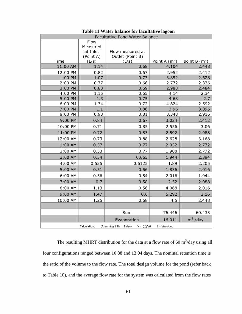
61

Table 11 Water balance for facultative lagoon

Facultative Pond Water Balance

Time

Flow

Measured

at Inlet

(Point A)

(L/s)

Flow measured at

Outlet (Point B)

(L/s) Point A (m3) point B (m3)

11:00 AM 1.14 0.68 4.104 2.448

12:00 PM 0.82 0.67 2.952 2.412

1:00 PM 1.07 0.73 3.852 2.628

2:00 PM 0.77 0.66 2.772 2.376

3:00 PM 0.83 0.69 2.988 2.484

4:00 PM 1.15 0.65 4.14 2.34

5:00 PM 1.3 0.75 4.68 2.7

6:00 PM 1.34 0.72 4.824 2.592

7:00 PM 1.1 0.86 3.96 3.096

8:00 PM 0.93 0.81 3.348 2.916

9:00 PM 0.84 0.67 3.024 2.412

10:00 PM 0.71 0.85 2.556 3.06

11:00 PM 0.72 0.83 2.592 2.988

12:00 AM 0.73 0.88 2.628 3.168

1:00 AM 0.57 0.77 2.052 2.772

2:00 AM 0.53 0.77 1.908 2.772

3:00 AM 0.54 0.665 1.944 2.394

4:00 AM 0.525 0.6125 1.89 2.205

5:00 AM 0.51 0.56 1.836 2.016

6:00 AM 0.56 0.54 2.016 1.944

7:00 AM 0.7 0.58 2.52 2.088

8:00 AM 1.13 0.56 4.068 2.016

9:00 AM 1.47 0.6 5.292 2.16

10:00 AM 1.25 0.68 4.5 2.448

Sum 76.446 60.435

Evaporation 16.011 m3 /day

Calculation: (Assuming 23hr ≈ 1 day) V = ∑Q*Δt E = Vin-Vout

The resulting MHRT distribution for the data at a flow rate of 60 m3/day using all

four configurations ranged between 10.88 and 13.04 days. The nominal retention time is

the ratio of the volume to the flow rate. The total design volume for the pond (refer back

to Table 10), and the average flow rate for the system was calculated from the flow rates

62

recorded at point B (refer back to Table 11) in the facultative lagoon. The average flow

rate was calculated to be 60 m3/day (rounded to the nearest m

3/day) and this resulted in a

nominal retention of 37 (rounded to the nearest day) for the system. The hydraulic

efficiency range was determined as 33-51.6% according to Table 6.

63

CHAPTER 5: CONCLUSIONS AND RECOMMENDATIONS

This research was motivated by a need to examine whether waste stabilization

ponds located in South America may not receive adequate treatment because of design or

operation factors leading to hydraulic short-circuiting. The overall objective of this

research was to analyze the hydraulic performance of a community managed waste

stabilization pond system located in San Antonio, Bolivia based on results from a dye

tracer study and 2-d computational modeling. The study hypothesis was that as a result of

inefficient design (as measured by nominal retention time); short-circuiting and

associated dead zones exist in the San Antonio (Bolivia) lagoon system.

Visual observations, the field dye study, and hydraulic modeling confirmed that

short-circuiting was occurring and associated dead zones were found to exist in the San

Antonio (Bolivia) facultative wastewater lagoon. Due to having a design flaw of one inlet

and one outlet incoming flow is not effectively mixed with stationary pond fluid. This

appears to be contributing to the accumulation of sludge around the inlet. It was

estimated the accumulated sludge volume was 169 m3 and occupied 8% of the facultative

pond volume, directly in front of the inlet. The use of the computational 2-d model

combined with estimated sludge distribution provided a better match for the tracer

concentrations over the 12-day study period. Simple models such as the Tanks in Series

and the Completely mixed model provided poorer fits with the data (see Appendix A).

The Completely mixed model did however perform better than the Plug flow model.

After comparing the tracer results from the reactor models that were considered: tanks in

64

series, completely mixed fluid, manual interpolation and the results from the 2-d cfd flow

simulation the results that provided the best fit for the data over 12 days was the manual

interpolation method. However, because of uncertainty as to what depth to obtain a

representative area for the 2-d simplification, all four configurations were considered for

estimating the MHRT. The results varied between 10.88 and 13.04 days for the MHRT

with a hydraulic efficiency that varied between 33-51.6% (accounting for sludge volume.

This is much shorter than the theoretical detention time of 37 days for the facultative

pond system (as well as the design nominal retention time of 26 days) and indicates that

short-circuiting is occurring in the facultative lagoon. One measure of uncertainty in the

sludge estimation is whether or not the obstruction is caused by sludge accumulation or

grit.

This type of system is recommended to have a grit chamber placed before the

facultative pond to collect grit before it enters the system (Oakley, 2005). The model

results indicate that for the 2-d base case with no obstruction the fit with the experimental

data was much poorer then all the cases where the sludge mound obstruction was

considered except for the flow rate of 60 m3/day. This suggests that the obstruction near

the inlet has a significant influence on the pond hydraulic characteristics and subsequent

treatment efficiency of the wastewater lagoon. Shilton (2003) has noted that the

distribution of settled solids is a secondary function of the flow. Therefore, improving the

flow distribution can improve the solids distribution. While baffles are often

recommended to reduce short-circuiting in this particular case the inlet and outlet are

located directly across from one another. Therefore it is recommended to install a diffuser

over the entire inlet to distribute the incoming flow. The outlet structure for the

65

facultative pond studied in this research is located below the liquid level for minimization

of short-circuiting and reduction of scum. The models that fit best with the data indicate

that the lower left corner of the lagoon that is unrounded is causing a preferential flow

path to occur around the top edge of the lagoon. It is recommended to round the lower

left corner of the lagoon and provide an alternative means for loading a boat into the

pond.

Other recognized elements of good hydraulic design that should be incorporated

into the lagoon studied in this research are: (1) use of rectangular reactors; (2) positioning

inlets and outlets as far apart as possible; (3) the use of manifolds with multiple inlet and

outlet ducts and (4) using a horizontal inlet pipe configuration extending the entire width

of the reactor (Moreno, 1990; Levenspiel, 1999; Persson, 1999; Shilton and Harrison,

2003). The facultative pond from this study is rectangular in shape however the inlet and

outlet are located directly across from one another at the same elevation. This can

contribute to inefficient behaviors such as short-circuiting.

The primary recommendation for the pond studied in this research is to install a

grit chamber or screen to prevent greater accumulation rates in the facultative pond. It is

also recommended, to increase the distance between the inlet and outlet by only adjusting

the inlet arrangement because the outlet has proper hydraulic design. The pond edges do

meet World Health Organization recommendations (WHO, 1987) as they are mostly

rounded. The tracer curve obtained from the dye study showed a high early peak of dye

exiting the pond which provides evidence that either short-circuiting is occurring or the

system is operating as an ideal CMFR. At the beginning of the study pictures taken at the

site revealed pond scum concentrated in the corners near the inlet. And this provides

66

additional evidence that the corners are sites of low flow circulation or dead zones.

Similar to previous studies of facultative ponds with single inlets the majority of sludge

accumulation was found directly in front of the inlet. The model produced through the

Kriging method shows uniform streamlines as distance increases from the inlet and it also

showed several stagnant points including one directly in the path of the inlet which is the

site of solids accumulation.

For developing nations in the Americas lack of improved sanitation has led to

polluted surface waters that play a large role in the transmission of waterborne diseases

us untreated wastewater is discharged to surface waters used for drinking, irrigation,

bathing and washing. Because lagoons have been the treatment option of choice in some

parts of Central and South America, it is important to properly design and operate

lagoons so they can achieve their full potential for protection of human health and the

environment. It has been noted that theoretically a lagoon system should be able to

achieve 3-4 log cycles of pathogen removal; however, observations of fecal coliform

removal has not been as good as theoretically predicted in many situations. This research

shows the importance of proper hydraulic performance that has the potential to increase

the treatment performance of wastewater lagoons. Importantly, improving performance

of existing and future wastewater treatment lagoons can lead to realizing their potential to

serve as sources of reclaimed water, something that requires sufficient hydraulic

performance that will ensure adequate destruction of microbial pathogens.

67

REFERENCES

Abbas, H.,Nasr, R., Seif, H. (2006). Study of waste stabilization pond geometry for the

wastewater treatment efficiency. Ecological Engineering, 28(1): 25-34.

Abis, K. and Mara, D. (2005). Research on waste stabilization ponds in the United

Kingdom: Sludge accumulation in pilot-scale primary facultative ponds.

Environmental Technology, 26(4): 449-458.

Agunwamba, J. (2006). Effect of the location of the inlet and outlet structures on short-

circuiting: Experimental investigation. Water Envrionment Research, 78(6): 580-

589.

Alvarado, A., Vedantam, S., Durazno, G. and Nopens, I. (2011). Hydraulic assessment of

waste stabilization ponds: Comparison of computational fluid dynamics

simulations against tracer data. Maskana, 2(1): 81-89.

Anon., 2010. ArcGIS Resource Center. [Online]

Available at:

http://help.arcgis.com/en/arcgisdesktop/10.0/help/index.html#//00q90000003z000

000

[Accessed 1 10 2012].

Ballard, M., Clarke, A., Sather-Knutsen, A., Barkdoll, B. and Mihelcic, J. R. (2008).

Collaborative International Research: Technology Transfer & Efficiency of

Wastewater Treatment Systems in Rural Communities of Bolivia, ASCE World

Environmental and Water Resources Congress 2008: pp.1-10, (doi

http://dx.doi.org/10.1061/40976(316)182).

Bokil, S. and Agrawal, G. (1977). Stratification in laboratory simulations of hhallow

stabilization ponds. Water Research, 11: 1025-1030.

Bracho, N., Lloyd, B. and Aldana, G. (2006). Optimisation of hydraulic performance to

maximise faecal coliform removal in maturation ponds. Water Research, 40:

1677-1685.

Carre, J., Laigre, M. and Legeas, M. (1990). Sludge removal from some wastewater

stabilization ponds. Water Science Technology, 22(3-4): 247-252.

Childs, C. Interpolating Surfaces in ArcGIS Spatial Analyst. [Online]

Available at: http://webapps.fundp.ac.be/geotp/SIG/interpolating.pdf

[Accessed 1 10 2012].

68

Cressie, N. (1993). Statistics for Spatial Data Revised Edition. John Wiley & Sons; New

York, USA.

Crittenden, J. C., Trussel, R. R., Hand, D. W., Howe, K. J. and Tchobanoglous, G.

(2005). Water Treatment Principles and Design. John Wiley & Sons; New Jersey,

USA.

Feeny, D., Berkes, F., McCay, B. and Acheson, J. (1990). The tragedy of the commons:

twenty-two years later. Human Ecology,18(1): 1-19.

Fogler, H., Vennema, A., and Vennema, C. (2006). Elements of Chemical Reaction

Engineering. Pearson Education Inc.; New Jersey, USA.

Franci, R. (1999). Gerenciamento do lodo de lagoas de estabilizacao (Management of

sludge from non-mechanized stabilization ponds), Rio de Janeiro: Programa de

PesPesquisa em Saneamento Basico (PROSAB).

Fry, L., Hoyt, A., Matus, J. and Mihelcic, J. R. (2010). Sustainable Water Management

Research Experience in Bolivia: Influence of a Dynamic World on Technological

and Societal Solutions. University of South Florida; Tampa, USA

Fuchs, V. and Mihelcic, J. (2011). Analyzing appropriateness in sanitation projects in the

Alto Beni region of Bolivia. Waterlines, 30(2): 122-134.

Geuzaine, C. and Remacle, J (2009). Gmsh: a three-dimensional finite element mesh

generator with built-in pre- and post-processing facilities. International Journal

for Numerical Methods in Engineering, 79(11): 1309-1331.

Guest, J., Skerlos, S., Barnard, J., Beck, M., Daigger, Glen., Hilger, H., Jackson, S.,

Karvazy, K., Kelly, L., Macpherson, L., Mihelcic, J. R., Pramanik, A., Raskin, L.,

Loosdrecht, M., Yeh, D. and Love, N. (2009). A new planning and design

paradigm to achieve sustainable resource recovery from wastewater.

Environmental Science and Technology, 43: 6126-6130.

Herrera, L. and Castillo, G. (2000). Dynamics of a waste stabilization pond in Chile.

Water Science and Technology, 42(10-11): 83-90.

Henderson, A. (2007). ParaView Guide: A Parallel Visualization Application. Kitware

Inc; New Mexico, USA.

Houang, P., Schaegger, M. and Zoulalian, A. (1989). Influence de la géométrie sur la

distribution des temps de séjour et les performances d'un système lagunaire non

aéré isotherme. The Chemical Engineering Journal, 42(3), : 175-186.

69

Juanico, M. and Shelef, G. (1991). The performance of stabilization reservoirs as a

function of design and operation parameters. Water Science Technology, 23:

1509-1516.

Kilani, J. and Ogunrombi, J. (1984). Effects of baffles on the performance of model

waste stabilization ponds. Water Research, 18(8): 941-944

Kumar, S. and Nikam, K. (2010). Numerical Estimation of Residence Time Distribution

in Steel Tundish using OpenFOAM, Pune, India: Computational Research

Laboratories.

Levenspiel, O. (1972). Chemical reaction engineering. Al Che Journal, 19(1): 206-207.

Levenspiel, O. (1999). Chemical Reaction Engineering. John Wiley & Sons; New York,

USA.

Lloyd, B., Leitner, A., Vorkas, C. and Guganesharajah, R. (2003). Under-performance

evaluation and rehabilitation strategy for waste stabilization ponds in Mexico.

Water Science and Technology, 48(2): 35-43.

Mangelson, K. and Watters, G. (1972). Treatment efficiency of waste stabilization ponds.

Journal of the Sanitary Engineering Division, ASCE, SA2: 407-425.

Marais, G. (1974). Faecal bacterial kinetics in stabilization ponds. Journal of the

Environmental Engineering Division, ASCE, EE1: 120-139.

Martin, A. (2000). Interpretation of residence time distribution data. Chemical

Engineering Science, 55(23): 5907-5917.

Middlebrooks, E., Middlebrooks, C., Reynolds, J., Watters, G., Reed, S. and George, D.

(1982). Wastewater Stabilization Lagoon Design, Performance and Upgrading.

Macmillan Publishing; New York, USA.

Middlebrooks, E., Panagiotou, A. and Williford, H. (1965). Sludge accumulation in

municipal sewage lagoons. Water Sewage Works, 112(1): 63-68.

Mihelcic, J. R. and Zimmerman, J. B. (2010). Environmental Engineering Fundamentals,

Sustainability, Design. John Wiley & Sons; New Jersey, USA

Isaaks, E. and Srivastava, R. (1989). An introduction to Applied Geostatistics. Oxford

University Press; New York, USA.

Monte, M. and Mara, D. (1987). The hydraulic performance of waste stabilization ponds

in Portugal.Water Science Technology, 19( 12): 219-227.

70

Moreno, M. (1990). A tracer study of the hydraulics of facultative stabilization ponds.

Water Research, 24(8): 1025-1030.

Morgan, D. (2010). Application of Sonar for the Measurement of Sludge Heights in

Wastewater Stabilisation Ponds, The University of Western Austrailia.

Muga, H. and Mihelcic, J. R. (2008). Sustainability of wastewater treatment technologies.

Journal of Environmental Management, 88: 437-447.

Nelson, K., Cisnerosb, B., Tchobanoglousc, G. and Darby, J. (2004). Sludge

accumulation, characteristics, and pathogen inactivation in four primary waste

stabilization ponds in central Mexico. Water Research, 38(1): 111-127.

Oakley, S. (2000). Waste stabilization pond in use in central America: The experiences of

El Salvador, Guatemala, Honduras, and Nicaragua. Water Science Technology,

42(10): 51-58.

Oakley, S. (2004). Monitoring of Wastewater Stabilization Ponds in Honduras,

Department of Civil Engineering: California, USA.

Oakley, S. (2005). A Case Study of the use of wastewater stabilization ponds in

Honduras. Small Flows Quarterly, 6(2): 36-51.

Pearson, H., Mara, D. and Arridge, H. (1995). The influence of pond geometry and

configuration on facultative and maturation waste stabilisation pond performance

and efficiency. Water Science Technology, 31(12): 129-139.

Persson, J., Somes, N. and Wong, T. (1999). Hydraulics efficiency of constructed

wetlands and ponds. Water Science and Technology, 40(3): 291-289.

Picot, B., Sambuco, J., Brouillet, J. and Riviere, Y. (2005). Wastewater stabilization

ponds: sludge accumulation, technical and financial study on desludging and

sludge disposal case studies in France. Water Science & Technology, 51(12): 227-

234.

Sáenz, R. (1993). Stabilization ponds in the tropics: Promtion of the sanitary reuse of

water. Wastewater Treatment, 27(3): 215-223.

Safieddine, T. (2007). Hydrodynamics of Waste Stabilization Ponds and Aerated

Lagoons, McGill University: Montreal.

Schneiter, R., Middlebrooks, E. and Sletten, R. (1983). Cold region wastewater lagoon

sludge accumulation. Water Research, 17: 1201-1206.

Shilton, A. (2001). Studies into the Hydraulics of Waste Stabilization Ponds Massey

University,Turitea Campus: Palmerston North, New Zealand.

71

Shilton, A. and Harrison, J. (2003). Guidelines for the Hydraulic Design of Waste

Stabilsation Ponds, Institute of Technology and Engineering Massey University:

Palmerstone North, New Zealand.

Shilton, A., Wilks, T., Smyth, J. and Bickers, P. (2000). Tracer studies of a New Zealand

waste stabilisation pond, analysis of treatment efficiency. Water Science and

Technology, 42(10-11): 343-348.

Thirumurthi, D. (1969). A break-through in the tracer studies of sedimentation tanks.

Water Pollution Control Federation, 41(11): R405-R418.

Vorkas, C. and Lloyd, B. (2000). The application of a diagnostic methodology for the

identification of hydraulic design deficiencies affecting pathogen removal. Water

Science and Technology, 42(10): 99-109.

Watters, G., Mangelson, K. and George, R. (1972). The Hydraulics of Waste Stabilization

Ponds. Research Report; Utah Water Research Laboratory, College of

Engineering, Utah State University; Utah, USA.

Weinstein, H. and Dudukovic, M. (1975). Topics in Transport Phenomena: Bioprocesses

Mathematical Treatment, Mechanisms. C. Guthfinger ed., Hemisphere Publishing

Co., John Wiley & Sons, New York, USA.

World Commission on Environment and Development. (1987). Our Common Future,

Oxford University Press: New York, USA.

World Health Organization. (2006). Guidelines for the safe use of wastwater, excreta and

greywater. Volume 4: Excreta and greywater use in agriculture,World Health

Organization .

Yánez, F. (1992). Lagunas de Estabilización: Teoría, Diseño, Evaluación, y

Mantenimiento, Instituto Ecuatoriano de Obras Sanitarias, Ministerio de Salud

Pública: Quito, Ecuador.

72

APPENDIX A: TRACER STUDY CALCULATIONS AND RESULTS

A1 Lagoon parameters

Table A1 Lagoon dimensions for Sapecho and San Antonio. Pre-Study and HRT Dimensions Estimate Estimate

Site L

m

W

m

D

m

ES run/

rise

SS run/

rise At Ab Am

Vol

(m3)

MHRT

(day)

MHRT

(including short-

circuiting

and dead zones)

(day)

Sapecho mat1

59.8

20.9

1.5 1 1 1249.82 1016.72 1131.02 1698 22.98103476

11.5

Sapecho

mat2

59.

8

22.

8

1.5 1 1 1363.44 1124.64 1241.79 1864 25.2302631

6

12.6

San Ant Fac

49.6

27.5

1.8 1 1 1364 1099.4 1228.46 2213 25.61541667

12.8

San Ant

mat1

38.

8

12.

6

1.5 1 1 488.88 343.68 414.03 622 7.20104166

7

3.6

San Ant mat2

39.3

12.8

1.5 1 1 503.04 355.74 427.14 642 7.428645833

3.7

Total lagoon volume V = (d/6)*(At+Ab+4Am)

Lagoon water mirror at top At = L*W

Lagoon water mirror at base Ab = (L-2*ES*d)(W-2*SS*d)

Lagoon water mirror at mid-depth Am = (L-ES*d)(W-SS*d)

(Pre-study) taking into account evaporation Ave

Influent (L/s) Effluent (L/s) Ave m3/day

Sapecho 0.94 0.77 0.855 73.872

San Antonio 1.2 0.8 1 86.4

System HRT total (day) Vol (m3)

Sapecho mat1 +2 24.1 3561

San Antonio mat1 +2 7.3 1264

DYE TRACER

ALLOCATION

Site Vol (mL)

Sapecho mat1 740

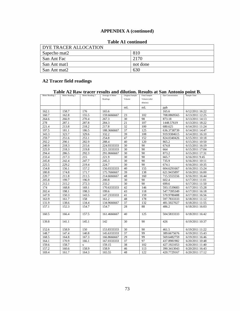
73

APPENDIX A (continued)

Table A1 continued

DYE TRACER ALLOCATION

Sapecho mat2 810

San Ant Fac 2170

San Ant mat1 not done

San Ant mat2 630

A2 Tracer field readings

Table A2 Raw tracer results and dilution. Results at San Antonio point B. Meter Reading 1 Meter Reading 2 Meter Reading 3 Average of Meter

Readings

Original Sample

Volume

Final Sample

Volume (after

dilution)

Dye Concentration Sample Time

mL mL ppb

162.1 158.7 176 165.6 165.6 6/12/2011 16:22

160.7 162.8 155.5 159.6666667 23 102 708.0869565 6/13/2011 12:25

264.6 266.9 270.4 267.3 30 98 873.18 6/13/2011 14:13

278 287.1 287.8 284.3 21 107 1448.57619 6/13/2011 18:22

221.4 213.8 218.2 217.8 32 100 680.625 6/14/2011 11:24

197.5 181.1 186.5 188.3666667 37 125 636.3738739 6/14/2011 14:47

343.3 323.7 329.6 332.2 39 108 919.9384615 6/14/2011 16:10

259.7 251.6 253.1 254.8 47 152 824.0340426 6/15/2011 10:18

292.2 290.1 282.9 288.4 40 120 865.2 6/15/2011 10:50

240.9 218.3 215.6 224.9333333 30 90 674.8 6/15/2011 16:19

225.9 218.3 219.8 221.3333333 30 90 664 6/15/2011 17:04

294.4 286.5 292.3 291.0666667 30 90 873.2 6/15/2011 17:31

233.4 217.3 215 221.9 30 90 665.7 6/16/2011 9:45

245.8 242.4 247.7 245.3 30 90 735.9 6/16/2011 10:11

225.5 229.2 219.4 224.7 30 90 674.1 6/16/2011 10:35

154.8 156.1 157.2 156.0333333 40 155 604.6291667 6/16/2011 15:24

180.8 174.8 171.7 175.7666667 39 138 621.9435897 6/16/2011 16:00

220.7 211.8 211.5 214.6666667 48 160 715.5555556 6/16/2011 16:44

205.8 199.7 196.9 200.8 30 90 602.4 6/17/2011 11:01

212.1 215.2 272.3 233.2 30 90 699.6 6/17/2011 11:50

174 168.8 169.1 170.6333333 42 146 593.1539683 6/17/2011 15:28

202.4 198.1 198.3 199.6 43 118 547.7395349 6/17/2011 16:18

147.9 150.3 143.5 147.2333333 41 159 570.9780488 6/17/2011 16:56

163.9 161.7 158 161.2 48 178 597.7833333 6/18/2011 11:12

131.9 138.6 134.4 134.9666667 37 132 481.5027027 6/18/2011 11:55

157.1 152.3 154.7 154.7 28 88 486.2 6/18/2011 16:03

160.5 166.4 157.5 161.4666667 40 125 504.5833333 6/18/2011 16:42

139.8 141.1 145.1 142 30 90 426 6/19/2011 10:37

152.6 158.9 150 153.8333333 30 90 461.5 6/19/2011 11:22

148.7 147.4 140.8 145.6333333 37 99 389.6675676 6/19/2011 15:43

168.5 164.8 167.3 166.8666667 29 99 569.6482759 6/19/2011 16:46

164.1 170.9 166.1 167.0333333 37 97 437.8981982 6/20/2011 10:48

159.6 158.7 x 159.15 38 102 427.1921053 6/20/2011 11:40

157.2 160.6 158.9 158.9 46 113 390.3413043 6/20/2011 16:43

169.4 161.7 164.3 165.55 48 122 420.7729167 6/20/2011 17:12

74

APPENDIX A (continued)

Table A2 continued

RAW TRACER RESULTS AND DILUTIONS FOR DYE STUDY

FACULTATIVE LAGOON SAN ANTONIO INLET Meter

Reading 1

Meter

Reading 2

Meter

Reading 3

Average of

Meter Readings

Original

Sample

Volume

Final

Sample

Volume (after

dilution)

Dye

Concentration

Sample Time

mL mL ppb

162.1 158.7 160 160.2666667 160.2666667 6/12/2011 16:45

178.5 174.3 176.1 176.3 176.3 6/13/2011

14:40

296.1 283.2 285.8 288.3666667 288.3666667 6/13/2011 18:44

276.6 267.2 273.8 272.5333333 272.5333333 6/14/2011

11:32

127.5 130.6 131.7 129.9333333 129.9333333 6/14/2011 14:55

243.6 245.4 259.7 249.5666667 249.5666667 6/14/2011

16:19

284.6 277.2 280.5 280.7666667 280.7666667 6/15/2011 10:25

114 109.5 107.8 110.4333333 110.4333333 6/15/2011

10:57

172.4 172.5 171.1 172 172 6/15/2011 16:30

229.8 231.8 230.5 230.7 230.7 6/15/2011

17:11

324.3 315.8 307.4 315.8333333 315.8333333 6/15/2011 17:40

368.2 383.6 395.8 382.5333333 382.5333333 6/16/2011

9:36

295.1 292.9 286.6 291.5333333 291.5333333 6/16/2011

10:05

171.3 171.7 168.4 170.4666667 170.4666667 6/16/2011

10:30

284.1 262.4 283.9 276.8 276.8 6/16/2011 15:33

251.1 250 253.4 251.5 251.5 6/16/2011

16:08

407 389.8 397.2 398 398 6/16/2011 16:53

192.6 189.7 187 189.7666667 189.7666667 6/17/2011

11:16

207.1 217 215.6 213.2333333 213.2333333 6/17/2011 12:01

266.8 260 271.2 266 266 6/17/2011

15:40

345.4 338 343.5 342.3 342.3 6/17/2011

16:28

304.8 304.2 300.7 303.2333333 303.2333333 6/17/2011

17:04

106.3 101 101.9 103.0666667 103.0666667 6/18/2011

11:22

121.4 112.8 120.7 118.3 118.3 6/18/2011

12:06

75

APPENDIX A (continued)

Table A2 continued 199.3 193.8 193.6 195.5666667 195.5666667 6/18/2011

16:15

288.6 302.3 300.1 297 297 6/18/2011 16:51

314.3 299.5 309.4 307.7333333 307.7333333 6/19/2011

10:41

240.5 223.1 230.4 231.3333333 231.3333333 6/19/2011 11:34

261.2 253.5 276.1 263.6 263.6 6/19/2011

16:00

238 238.8 235.5 237.4333333 237.4333333 6/19/2011 16:54

142.8 144.4 186.6 157.9333333 157.9333333 6/20/2011

10:59

321 314.7 312.3 316 316 6/20/2011

11:53

569.3 575.6 578.9 574.6 574.6 6/20/2011

16:51

285.8 314.8 291.5 297.3666667 297.3666667 6/20/2011 17:19

RAW TRACER RESULTS AND DILUTIONS FOR DYE STUDY

MATURATION LAGOON 2 OUTLET Meter

Reading 1

Meter

Reading 2

Meter

Reading 3

Average of

Meter Readings

Original

Sample

Volume

Final

Sample

Volume (after

dilution)

Dye

Concentration

Sample Time

mL mL ppb

144 146.5 167 152.5 152.5 6/12/2011 16:00

228 224.5 217.7 223.4 20 118 1318.06 6/13/2011

12:13

171.4 178 179.1 176.1666667 25 123 866.74 6/13/2011

14:00

224.2 221.3 223.6 223.0333333 20 123 1371.655 6/13/2011

17:50

254.6 254.3 249.7 252.8666667 30 141 1188.473333 6/14/2011 11:09

179.7 178.5 177.8 178.6666667 32 139 776.0833333 6/14/2011

14:33

218.2 228.4 220.1 222.2333333 33 129 868.730303 6/14/2011 15:50

246.8 240.7 245.9 244.4666667 29 139 1171.754023 6/15/2011

9:58

305.3 298.2 297.2 300.2333333 54 185 1028.57716 6/15/2011 10:34

147.8 151.7 146.5 148.6666667 30 130 644.2222222 6/15/2011

15:53

159.1 161 165.3 161.8 30 130 701.1333333 6/15/2011

16:39

189 180.8 183.9 184.5666667 30 130 799.7888889 6/15/2011

17:17

188.2 190 190.7 189.6333333 30 120 758.5333333 6/16/2011

9:58

76

APPENDIX A (continued)

Table A2 continued 208 210.5 202.4 206.9666667 30 120 827.8666667 6/16/2011

10:22

196.5 189.6 190.5 192.2 30 120 768.8 6/16/2011 10:47

168.4 165.4 164.1 165.9666667 36 158 728.4092593 6/16/2011

15:02

162.6 160.7 156.3 159.8666667 37 164 708.5981982 6/16/2011 15:42

165.2 163.9 167.8 165.6333333 39 177 751.7205128 6/16/2011

16:28

202.2 206 199.2 202.4666667 30 120 809.8666667 6/17/2011 10:36

163.7 164 165.8 164.5 30 120 658 6/17/2011

11:32

174 168.8 169.1 170.6333333 42 146 593.1539683 6/17/2011

15:05

232.7 234.2 228.5 231.8 43 119 641.4930233 6/17/2011

15:57

192 188.5 188.6 189.7 40 123 583.3275 6/17/2011 16:38

238.8 240.1 231.6 236.8333333 40 118 698.6583333 6/18/2011

10:38

185.9 185.5 183.8 185.0666667 35 125 660.952381 6/18/2011

11:38

205.9 194.7 196.2 198.9333333 35 98 557.0133333 6/18/2011

15:30

158.5 157.7 152.1 156.1 32 115 560.984375 6/18/2011

16:23

127 128 126.6 127.2 30 120 508.8 6/19/2011

10:12

136 135.5 131 134.1666667 30 120 536.6666667 6/19/2011

11:04

169.7 161.3 157.2 162.7333333 37 138 606.9513514 6/19/2011

15:13

197.1 192.6 195.7 195.1333333 39 109 545.3726496 6/19/2011

16:13

199.4 196.2 207.8 201.1333333 35 104 597.6533333 6/20/2011

10:18

223.1 211.5 215.3 216.6333333 45 110 529.5481481 6/20/2011

11:18

201.8 195.6 200.2 199.2 35 102 580.5257143 6/20/2011

16:26

222.7 219.2 214.4 218.7666667 50 120 525.04 6/20/2011

16:59

RAW TRACER RESULTS AND DILUTIONS FOR DYE STUDY

MATURATION LAGOON 2 INLET Meter

Reading 1

Meter

Reading 2

Meter

Reading 3

Average of

Meter Readings

Original

Sample Volume

Final

Sample Volume

(after

dilution)

Dye

Concentration

Sample Time

mL mL ppb

160 161 159 160 160 6/12/2011

16:13

77

APPENDIX A (continued)

Table A2 continued 181.1 186.4 179.7 182.4 182.4 6/13/2011

18:06

263.9 257.7 255.7 259.1 259.1 6/14/2011 11:17

249.3 248.9 247.1 248.4333333 248.4333333 6/14/2011

14:43

282.2 288 281.8 284 284 6/14/2011 16:03

246.1 240.6 233.8 240.1666667 73 137 450.7237443 6/15/2011

10:10

148 146 144.6 146.2 41 116 413.6390244 6/15/2011 10:42

163.1 162.5 158.7 161.4333333 30 60 322.8666667 6/15/2011

16:13

226.1 237.4 223.6 229.0333333 30 60 458.0666667 6/15/2011

16:46

255.9 245.8 246.9 249.5333333 30 60 499.0666667 6/15/2011

17:24

309.5 299 290.2 299.5666667 30 60 599.1333333 6/16/2011 9:51

301.7 300.8 282.9 295.1333333 30 60 590.2666667 6/16/2011

10:16

248.4 248.1 254.1 250.2 30 60 500.4 6/16/2011

10:41

178.1 171.9 169.8 173.2666667 33 95 498.7979798 6/16/2011

15:16

200.9 201.9 192.4 198.4 39 103 523.9794872 6/16/2011

15:51

123.7 115 121.2 119.9666667 33 163 592.5626263 6/16/2011

16:36

250.9 256.5 247.9 251.7666667 30 60 503.5333333 6/17/2011

10:51

239.8 239.7 241.1 240.2 30 60 480.4 6/17/2011

11:42

125.3 127.9 126.7 126.6333333 40 122 386.2316667 6/17/2011

15:15

164.7 164.3 165.8 164.9333333 39 102 431.3641026 6/17/2011

16:08

126.1 122.8 126.6 125.1666667 35 118 421.9904762 6/17/2011

16:48

143.6 141 141.3 141.9666667 33 108 464.6181818 6/18/2011

10:58

138.1 141.1 138 139.0666667 40 108 375.48 6/18/2011

11:46

200.7 202.2 196 199.6333333 52 102 391.5884615 6/18/2011

15:53

220.1 221.7 224.2 222 94 187 441.6382979 6/18/2011

16:34

215.7 217 216.3 216.3333333 30 60 432.6666667 6/19/2011 10:24

204.3 204.2 199.6 202.7 30 60 405.4 6/19/2011

11:13

181.4 181.8 179.6 180.9333333 41 98 432.4747967 6/19/2011 15:31

78

APPENDIX A (continued)

Table A2 continued 221.4 222.2 218.8 220.8 41 90 484.6829268 6/19/2011

16:32

157.8 152.8 153.5 154.7 30 90 464.1 6/20/2011 10:34

118.4 112.5 115.1 115.3333333 34 117 396.8823529 6/20/2011

11:30

286.1 294.8 288.3 289.7333333 48 82 494.9611111 6/20/2011 16:35

257.8 257.3 262.8 259.3 60 110 475.3833333 6/20/2011

17:06

79

APPENDIX B: FLOW DATA COLLECTED IN THE FIELD AT THE LAGOON

SYSTEM IN SAN ANTONIO

B1 Flow averages recorded at sample point B

Table B1 Tracer run recorded flow at point B in San Antonio

TRACER RUN RECORDED FLOW AT POINT B IN SAN ANTONIO Time (L/d) (L/s)

6/13/2011 14:21 25920 0.3

6/15/2011 16:55 24979.59184 0.3

6/15/2011 17:16 27674.40494 0.3

6/16/2011 9:49 61766.80851 0.7

6/16/2011 10:17 56622.18713 0.7

6/16/2011 15:29 74651.55807 0.9

6/16/2011 16:05 67737.6 0.8

6/16/2011 16:49 97222.92994 1.1

6/17/2011 10:57 65828.57143 0.8

6/17/2011 11:47 55440 0.6

6/17/2011 15:36 55886.15783 0.6

6/17/2011 16:24 69756.37394 0.8

6/17/2011 17:00 62132.97151 0.7

6/18/2011 11:15 76906.81502 0.9

6/18/2011 12:01 76855.09326 0.9

6/18/2011 16:09 89280 1.0

6/18/2011 16:47 79920 0.9

6/19/2011 10:32 71853.95538 0.8

6/19/2011 11:18 64577.31959 0.7

6/19/2011 15:53 74834.64567 0.9

6/19/2011 16:50 70125.57427 0.8

6/20/2011 10:52 63692.30769 0.7

6/20/2011 11:49 71367.31107 0.8

6/20/2011 16:47 75727.05882 0.9

6/20/2011 17:16 93888 1.1

24 HOUR SAMPLING AT POINT B IN SAN ANTONIO Time (L/d) (L/s)

6/25/2011 11:00 58752 0.68

6/25/2011 12:00 57888 0.67

6/25/2011 13:00 63072 0.73

6/25/2011 14:00 57024 0.66

6/25/2011 15:00 59616 0.69

6/25/2011 16:00 56160 0.65

6/25/2011 17:00 64800 0.75

6/25/2011 18:00 62208 0.72

6/25/2011 19:00 74304 0.86

6/25/2011 20:00 69984 0.81

6/25/2011 21:00 57888 0.67

6/25/2011 22:00 73440 0.85

6/25/2011 23:00 71712 0.83

6/26/2011 0:00 76032 0.88

6/26/2011 1:00 66528 0.77

6/26/2011 2:00 66528 0.77

80

APPENDIX B (continued)

Table B1 continued 6/26/2011 3:00 57456 0.665

6/26/2011 4:00 52920 0.6125

6/26/2011 5:00 48384 0.56

6/26/2011 6:00 46656 0.54

6/26/2011 7:00 50112 0.58

6/26/2011 8:00 48384 0.56

6/26/2011 9:00 51840 0.6

6/26/2011 10:00 58752 0.68

VALUES FOR AVERAGE HOURLY FLOW OVER SAN ANTONIO FACULTATIVE

LAGOON FROM COMBINED COMPOSITE AND ORIGINAL FLOW DATA. (I=

interpolated, A=actual during dye tracer run, C=24 hour composite flow data) Time (hr) Flow (L/d) Sample type and amount

11:00:00 66294.92354 4 points

11:30:00 64577.31959 A-1 point

12:00:00 65387.60108 4 points

12:30:00 64229.80054 I-2 points

13:00:00 63072 C-1 point

13:30:00 60048 I-2 points

14:00:00 57024 C-1 point

14:30:00 25920 A-1 point

15:00:00 59616 C-1 point

15:30:00 65268.85795 2 points

16:00:00 71059.2 3 points

16:30:00 69756.37394 A-1 point

17:00:00 67844.01805 7 points

17:30:00 60781.20247 2 points

18:00:00 62208 C-1 point

18:30:00 68256 I-2 points

19:00:00 74304 C-1 point

19:30:00 72144 I-2 points

20:00:00 69984 C-1 point

20:30:00 63936 I-2 points

21:00:00 57888 C-1 point

21:30:00 65664 I-2 points

22:00:00 73440 C-1 point

22:30:00 72576 I-2 points

23:00:00 71712 C-1 point

23:30:00 73872 I-2 points

0:00:00 76032 C-1 point

0:30:00 71280 I-2 points

1:00:00 66528 C-1 point

1:30:00 66528 I-2 points

2:00:00 66528 C-1 point

2:30:00 61992 I-2 points

3:00:00 57456 C-1 point

3:30:00 57456 I-2 points

4:00:00 52920 1 point

4:30:00 50652 I-2 points

5:00:00 48384 1 point

5:30:00 47520 I-2 points

6:00:00 46656 1 point

6:30:00 48384 I-2 points

7:00:00 50112 1 point

7:30:00 49248 I-2 points

8:00:00 48384 1 point

8:30:00 50112 I-2 points

9:00:00 51840 1 point

9:30:00 56049.70213 I-2 points

10:00:00 60259.40426 2 points

10:30:00 64238.07125 2 points

81

APPENDIX B (continued)

Table B1 continued

MASS BALANCE OF DYE USING AVERAGE FLOW FROM 24 HOUR

COMPOSITE FLOWS COLLECTED AT SAN ANTONIO AT POINTS A AND B t (day) Ĉ(g/L) delta t (day) Q (L/d) C (g) t* Ĉ *Q*delta t Ĉ *Q*delta t

0.00 0 0 60435.00 0 0 0

0.84 0.000227985 0.417708333 60435.00 5.755290933 4.808065967 5.755290933

0.91 0.000538516 0.0375 60435.00 1.22044516 1.111113614 1.22044516

1.08 0.00090876 0.086458333 60435.00 4.748372737 5.144070465 4.748372737

1.79 0.000812483 0.354861111 60435.00 17.4245347 31.24315874 17.4245347

1.93 0.000406382 0.070486111 60435.00 1.731116578 3.348027548 1.731116578

1.99 0.000526039 0.028819444 60435.00 0.916202935 1.824770846 0.916202935

2.75 0.000619869 0.377777778 60435.00 14.15222012 38.87929361 14.15222012

2.77 0.000592499 0.011111111 60435.00 0.39786333 1.101860388 0.39786333

3.00 0.000517882 0.114236111 60435.00 3.575386937 10.71871209 3.575386937

3.03 0.000417282 0.015625 60435.00 0.394038422 1.193608053 0.394038422

3.05 0.000516482 0.009375 60435.00 0.292627603 0.891904549 0.292627603

3.72 0.000517332 0.338194444 60435.00 10.5736428 39.37947661 10.5736428

3.74 0.000448682 0.009027778 60435.00 0.244798288 0.916123591 0.244798288

3.76 0.000452882 0.008333333 60435.00 0.228082875 0.857369863 0.228082875

3.96 0.000387247 0.100347222 60435.00 2.348452994 9.29922151 2.348452994

3.98 0.000361169 0.0125 60435.00 0.272840403 1.087193218 0.272840403

4.02 0.000416632 0.015277778 60435.00 0.384681465 1.544602937 0.384681465

4.78 0.00040686 0.380902778 60435.00 9.365862994 44.74150801 9.365862994

4.81 0.000398882 0.017013889 60435.00 0.410144547 1.973250987 0.410144547

4.96 0.000394259 0.075694444 60435.00 1.803576299 8.950247385 1.803576299

5.00 0.000318329 0.017361111 60435.00 0.333996865 1.669056557 0.333996865

5.02 0.000307241 0.013194444 60435.00 0.244996009 1.230764673 0.244996009

5.78 0.000332263 0.380555556 60435.00 7.641676216 44.20497422 7.641676216

5.81 0.000287525 0.014930556 60435.00 0.259442229 1.50854846 0.259442229

5.99 0.000231734 0.086111111 60435.00 1.205971164 7.219914863 1.205971164

6.01 0.000243274 0.013541667 60435.00 0.199093177 1.197324245 0.199093177

6.76 0.000213174 0.373263889 60435.00 4.808822835 32.50964604 4.808822835

6.79 0.000191632 0.015625 60435.00 0.180957832 1.229005276 0.180957832

6.97 0.000173466 0.090625 60435.00 0.950060479 6.624692547 0.950060479

7.02 0.00022754 0.021875 60435.00 0.300811798 2.110696119 0.300811798

7.77 0.000251656 0.375694444 60435.00 5.713863763 44.38561115 5.713863763

7.80 0.000180428 0.018055556 60435.00 0.196880238 1.536486189 0.196880238

8.01 0.000156649 0.105208333 60435.00 0.996016319 7.982655791 0.996016319

8.03 0.000153439 0.010069444 60435.00 0.093375106 0.750243039 0.093375106

8.77 0.000144344 0.366319444 60435.00 3.195557721 28.01660849 3.195557721

8.80 0.000141757 0.015972222 60435.00 0.136835715 1.204059266 0.136835715

9.00 0.000175171 0.099652778 60435.00 1.054968429 9.493250623 1.054968429

9.03 0.000212379 0.016666667 60435.00 0.213919248 1.932106766 0.213919248

9.77 0.00026003 0.36875 60435.00 5.79486497 56.61261139 5.79486497

9.81 0.000225503 0.019791667 60435.00 0.269726576 2.645755477 0.269726576

10.01 0.000180624 0.099652778 60435.00 1.087813419 10.8871993 1.087813419

10.04 0.000213742 0.014236111 60435.00 0.183894906 1.845717417 0.183894906

11.81 0.000243424 0.885416667 60435.00 13.02565732 153.802258 13.02565732

% recovered 28.64732361 2 day % recovered

7.326258765

MHRT 5.064070482

82

APPENDIX B (continued)

Table B1 continued CN (g/L) 0.000406243 CN (ppb/L) 406.24

FLOW RATE AVERAGE EVERY HALF HOUR FROM COMBINED COMPOSITE

AND ORIGINAL FLOW DATA COLLECTED AT SAN ANTONIO AT POINTS A

AND B t (day) Ĉ(g/L) delta t (day) Q (L/d) C (g) t* Ĉ *Q*delta t Ĉ *Q*delta t 0.00 0 0 69756.37 0 0 0 0.84 0.000227985 0.417708333 64229.80 6.116673926 5.109971342 6.116673926 0.91 0.000538516 0.0375 57024.00 1.151562254 1.048401468 1.151562254 1.08 0.00090876 0.086458333 68256.00 5.362868033 5.809773702 5.362868033 1.79 0.000812483 0.354861111 64577.32 18.61884249 33.38461896 18.61884249 1.93 0.000406382 0.070486111 59616.00 1.707656919 3.302655917 1.707656919 1.99 0.000526039 0.028819444 71059.20 1.077267273 2.145557318 1.077267273 2.75 0.000619869 0.377777778 64238.07 15.04279514 41.3259011 15.04279514 2.77 0.000592499 0.011111111 66294.92 0.436441119 1.208699432 0.436441119 3.00 0.000517882 0.114236111 69756.37 4.126847492 12.37194488 4.126847492 3.03 0.000417282 0.015625 67844.02 0.442345492 1.339938219 0.442345492 3.05 0.000516482 0.009375 60781.20 0.294303923 0.897013832 0.294303923 3.72 0.000517332 0.338194444 56049.70 9.806395782 36.52201429 9.806395782 3.74 0.000448682 0.009027778 60259.40 0.244087019 0.913461766 0.244087019 3.76 0.000452882 0.008333333 64238.07 0.24243574 0.911322683 0.24243574 3.96 0.000387247 0.100347222 65268.86 2.536292627 10.04301428 2.536292627 3.98 0.000361169 0.0125 71059.20 0.320804514 1.278316875 0.320804514 4.02 0.000416632 0.015277778 69756.37 0.444013967 1.782839416 0.444013967 4.78 0.00040686 0.380902778 66294.92 10.27399969 49.07975267 10.27399969 4.81 0.000398882 0.017013889 65387.60 0.443755572 2.134957365 0.443755572 4.96 0.000394259 0.075694444 65268.86 1.947834289 9.666127661 1.947834289 5.00 0.000318329 0.017361111 69756.37 0.385511876 1.926488513 0.385511876 5.02 0.000307241 0.013194444 67844.02 0.275031251 1.381650049 0.275031251 5.78 0.000332263 0.380555556 66294.92 8.382631595 48.49119527 8.382631595 5.81 0.000287525 0.014930556 65387.60 0.280703317 1.632172829 0.280703317 5.99 0.000231734 0.086111111 71059.20 1.417975447 8.489143282 1.417975447 6.01 0.000243274 0.013541667 69756.37 0.229800912 1.38199715 0.229800912 6.76 0.000213174 0.373263889 64238.07 5.111433837 34.5554225 5.111433837 6.79 0.000191632 0.015625 64577.32 0.193360995 1.313243426 0.193360995 6.97 0.000173466 0.090625 65268.86 1.026050508 7.154564686 1.026050508

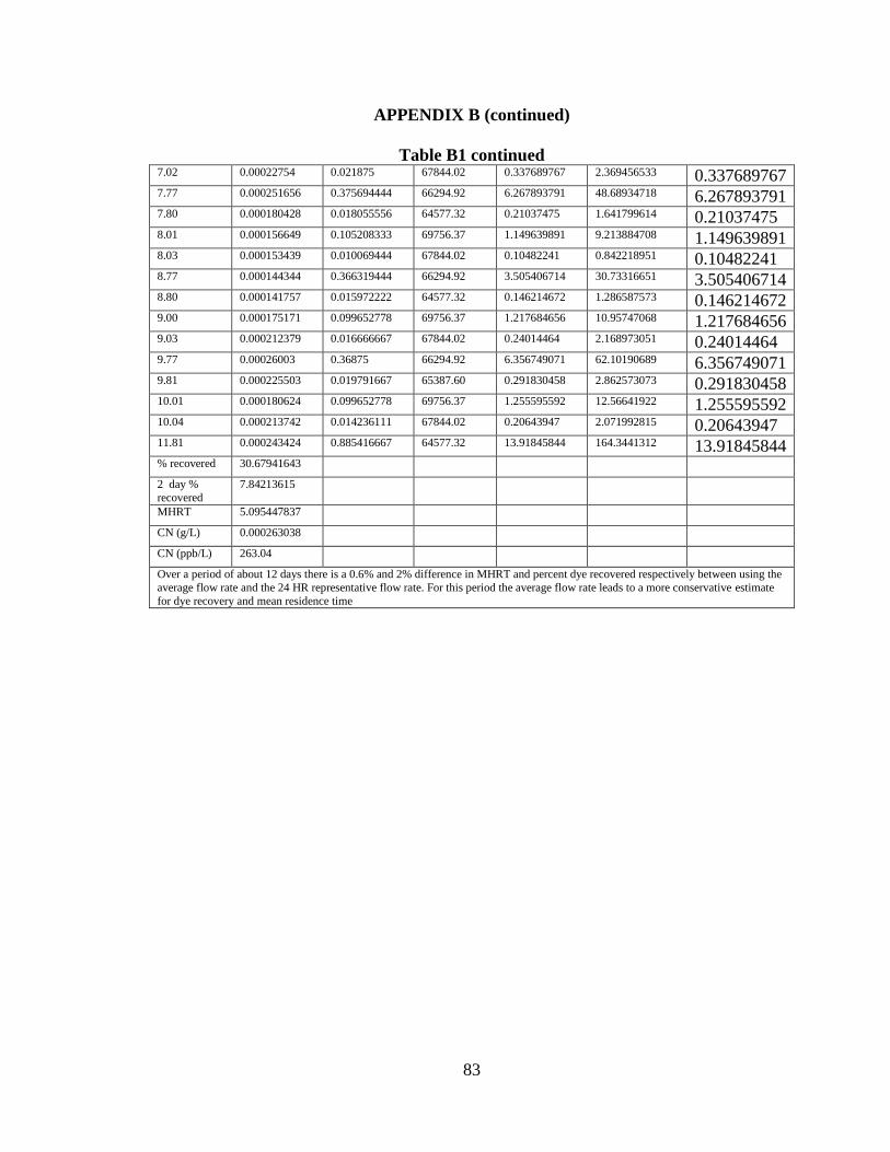
83

APPENDIX B (continued)

Table B1 continued 7.02 0.00022754 0.021875 67844.02 0.337689767 2.369456533 0.337689767 7.77 0.000251656 0.375694444 66294.92 6.267893791 48.68934718 6.267893791 7.80 0.000180428 0.018055556 64577.32 0.21037475 1.641799614 0.21037475 8.01 0.000156649 0.105208333 69756.37 1.149639891 9.213884708 1.149639891 8.03 0.000153439 0.010069444 67844.02 0.10482241 0.842218951 0.10482241 8.77 0.000144344 0.366319444 66294.92 3.505406714 30.73316651 3.505406714 8.80 0.000141757 0.015972222 64577.32 0.146214672 1.286587573 0.146214672 9.00 0.000175171 0.099652778 69756.37 1.217684656 10.95747068 1.217684656 9.03 0.000212379 0.016666667 67844.02 0.24014464 2.168973051 0.24014464 9.77 0.00026003 0.36875 66294.92 6.356749071 62.10190689 6.356749071 9.81 0.000225503 0.019791667 65387.60 0.291830458 2.862573073 0.291830458 10.01 0.000180624 0.099652778 69756.37 1.255595592 12.56641922 1.255595592 10.04 0.000213742 0.014236111 67844.02 0.20643947 2.071992815 0.20643947 11.81 0.000243424 0.885416667 64577.32 13.91845844 164.3441312 13.91845844 % recovered 30.67941643 2 day %

recovered

7.84213615

MHRT 5.095447837 CN (g/L) 0.000263038 CN (ppb/L) 263.04 Over a period of about 12 days there is a 0.6% and 2% difference in MHRT and percent dye recovered respectively between using the

average flow rate and the 24 HR representative flow rate. For this period the average flow rate leads to a more conservative estimate

for dye recovery and mean residence time

84

APPENDIX C: TRACER CALCULATIONS FOR PARAMETERS NEEDED TO

SOLVE FOR MHRT

Table C1 Calculations on tracer data. This is for point B at San Antonio

INITIAL CALCULATIONS ON RAW TRACER DATA FROM POINT B AT SAN

ANTONIO

Recall formula for varying flow rate:

T (day) Ĉ=(Ci-1+Ci)*0.5 (ppb) Q (L/s) Delta t (days)

0.00 0 0.81 0

0.84 436.8434783 0.74 0.417708333

0.91 790.6334783 0.66 0.0375

1.08 1160.878095 0.79 0.086458333

1.79 1064.600595 0.75 0.354861111

1.93 658.4994369 0.69 0.070486111

1.99 778.1561677 0.82 0.028819444

2.75 871.986252 0.74 0.377777778

2.77 844.6170213 0.77 0.011111111

3.00 770 0.81 0.114236111

3.03 669.4 0.79 0.015625

3.05 768.6 0.70 0.009375

3.72 769.45 0.65 0.338194444

3.74 700.8 0.70 0.009027778

3.76 705 0.74 0.008333333

3.96 639.3645833 0.76 0.100347222

3.98 613.2863782 0.82 0.0125

4.02 668.7495726 0.81 0.015277778

4.78 658.9777778 0.77 0.380902778

4.81 651 0.76 0.017013889

4.96 646.3769841 0.76 0.075694444

5.00 570.4467516 0.81 0.017361111

5.02 559.3587918 0.79 0.013194444

5.78 584.3806911 0.77 0.380555556

5.81 539.643018 0.76 0.014930556

5.99 483.8513514 0.82 0.086111111

6.01 495.3916667 0.81 0.013541667

6.76 465.2916667 0.74 0.373263889

6.79 443.75 0.75 0.015625

6.97 425.5837838 0.76 0.090625

7.02 479.6579217 0.79 0.021875

7.77 503.773237 0.77 0.375694444

7.80 432.5451517 0.75 0.018055556

8.01 408.7667048 0.81 0.105208333

8.03 405.5571105 0.79 0.010069444

8.77 396.4614583 0.77 0.366319444

8.80 393.875 0.75 0.015972222

9.00 427.2883721 0.81 0.099652778

9.03 464.497144 0.79 0.016666667

9.77 512.1472335 0.77 0.36875

9.81 477.6209177 0.76 0.019791667

10.01 432.7420715 0.81 0.099652778

10.04 465.8596154 0.79 0.014236111

11.81 495.5416667 0.75 0.885416667

85

APPENDIX C (continued)

Table C1 continued

TRACER MASS RECOVERY ON RAW DATA WITH BACKGROUND Q (L/d) C(g/L) Tracer Mass (g)

69756.37394 0 0

64229.80054 0.000436843 11.72021475

57024 0.000790633 1.69069063

68256 0.001160878 6.850689903

64577.31959 0.001064601 24.39636529

59616 0.000658499 2.767080484

71059.2 0.000778156 1.59357564

64238.07125 0.000871986 21.16111455

66294.92354 0.000844617 0.622153565

69756.37394 0.00077 6.1358966

67844.01805 0.0006694 0.709606026

60781.20247 0.0007686 0.437966552

56049.70213 0.00076945 14.58546173

60259.40426 0.0007008 0.381241164

64238.07125 0.000705 0.377398669

65268.85795 0.000639365 4.187549407

71059.2 0.000613286 0.544745492

69756.37394 0.00066875 0.712701386

66294.92354 0.000658978 16.64045447

65387.60108 0.000651 0.724235794

65268.85795 0.000646377 3.193418989

69756.37394 0.000570447 0.690838488

67844.01805 0.000559359 0.500717925

66294.92354 0.000584381 14.74328287

65387.60108 0.000539643 0.526839022

71059.2 0.000483851 2.960679967

69756.37394 0.000495392 0.467955669

64238.07125 0.000465292 11.15664833

64577.31959 0.00044375 0.447752899

65268.85795 0.000425584 2.517323932

67844.01805 0.000479658 0.711854515

66294.92354 0.000503773 12.54729587

64577.31959 0.000432545 0.504338728

69756.37394 0.000408767 2.999919161

67844.01805 0.000405557 0.277056977

66294.92354 0.000396461 9.628113916

64577.31959 0.000393875 0.406259729

69756.37394 0.000427288 2.97025941

67844.01805 0.000464497 0.525222544

66294.92354 0.000512147 12.52008087

65387.60108 0.000477621 0.618103369

69756.37394 0.000432742 3.008170346

67844.01805 0.00046586 0.449943512

64577.31959 0.000495542 28.33399968

Total Dye Collected 228.9452188

Original Dye 434

Missing dye 205.0547812

Percent Dye Recovered 52.75235457

86

APPENDIX C (continued)

Table C1 continued

CONCENTRATION OF DYE MEASURED (after subtracting background) C (ppb) Time

0 6/12/2011 16:22

455.9693095 6/13/2011 12:25

621.0623529 6/13/2011 14:13

1196.458543 6/13/2011 18:22

428.5073529 6/14/2011 11:24

384.2562268 6/14/2011 14:47

667.8208145 6/14/2011 16:10

571.9163955 6/15/2011 10:18

613.0823529 6/15/2011 10:50

422.6823529 6/15/2011 16:19

411.8823529 6/15/2011 17:04

621.0823529 6/15/2011 17:31

413.5823529 6/16/2011 9:45

483.7823529 6/16/2011 10:11

421.9823529 6/16/2011 10:35

352.5115196 6/16/2011 15:24

369.8259427 6/16/2011 16:00

463.4379085 6/16/2011 16:44

350.2823529 6/17/2011 11:01

447.4823529 6/17/2011 11:50

341.0363212 6/17/2011 15:28

295.6218878 6/17/2011 16:18

318.8604017 6/17/2011 16:56

345.6656863 6/18/2011 11:12

229.3850556 6/18/2011 11:55

234.0823529 6/18/2011 16:03

252.4656863 6/18/2011 16:42

173.8823529 6/19/2011 10:37

209.3823529 6/19/2011 11:22

137.5499205 6/19/2011 15:43

317.5306288 6/19/2011 16:46

185.7805511 6/20/2011 10:48

175.0744582 6/20/2011 11:40

138.2236573 6/20/2011 16:43

168.6552696 6/20/2011 17:12

120.0323529 6/21/2011 10:47

163.4823529 6/21/2011 11:33

186.8590971 6/21/2011 16:20

237.8998968 6/21/2011 17:08

282.159276 6/22/2011 10:50

168.8472652 6/22/2011 11:47

192.4015837 6/22/2011 16:34

235.0823529 6/22/2011 17:15

251.7656863 6/24/2011 11:45

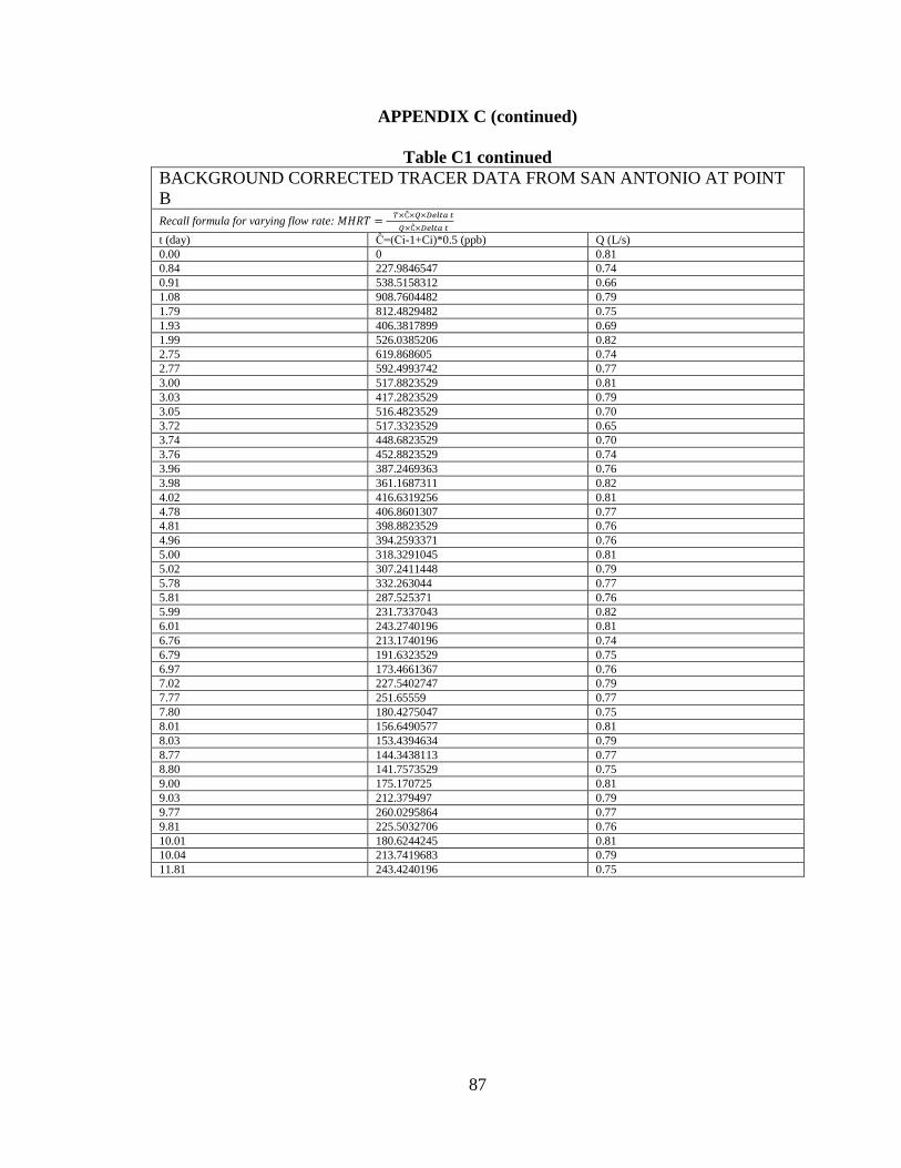
87

APPENDIX C (continued)

Table C1 continued

BACKGROUND CORRECTED TRACER DATA FROM SAN ANTONIO AT POINT

B

Recall formula for varying flow rate:

t (day) Ĉ=(Ci-1+Ci)*0.5 (ppb) Q (L/s)

0.00 0 0.81

0.84 227.9846547 0.74

0.91 538.5158312 0.66

1.08 908.7604482 0.79

1.79 812.4829482 0.75

1.93 406.3817899 0.69

1.99 526.0385206 0.82

2.75 619.868605 0.74

2.77 592.4993742 0.77

3.00 517.8823529 0.81

3.03 417.2823529 0.79

3.05 516.4823529 0.70

3.72 517.3323529 0.65

3.74 448.6823529 0.70

3.76 452.8823529 0.74

3.96 387.2469363 0.76

3.98 361.1687311 0.82

4.02 416.6319256 0.81

4.78 406.8601307 0.77

4.81 398.8823529 0.76

4.96 394.2593371 0.76

5.00 318.3291045 0.81

5.02 307.2411448 0.79

5.78 332.263044 0.77

5.81 287.525371 0.76

5.99 231.7337043 0.82

6.01 243.2740196 0.81

6.76 213.1740196 0.74

6.79 191.6323529 0.75

6.97 173.4661367 0.76

7.02 227.5402747 0.79

7.77 251.65559 0.77

7.80 180.4275047 0.75

8.01 156.6490577 0.81

8.03 153.4394634 0.79

8.77 144.3438113 0.77

8.80 141.7573529 0.75

9.00 175.170725 0.81

9.03 212.379497 0.79

9.77 260.0295864 0.77

9.81 225.5032706 0.76

10.01 180.6244245 0.81

10.04 213.7419683 0.79

11.81 243.4240196 0.75

88

APPENDIX C (continued)

Table C1 continued

TRACER MASS RECOVERY ON DATA CORRECTED FOR

BACKGROUND Delta t Q (L/d) C(g/L) Tracer Mass (g) 0 69756 0 0 0.417708333 64230 0.000227985 6.116673926 0.0375 57024 0.000538516 1.151562254 0.086458333 68256 0.00090876 5.362868033 0.354861111 64577 0.000812483 18.61884249 0.070486111 59616 0.000406382 1.707656919 0.028819444 71059 0.000526039 1.077267273 0.377777778 64238 0.000619869 15.04279514 0.011111111 66295 0.000592499 0.436441119 0.114236111 69756 0.000517882 4.126847492 0.015625 67844 0.000417282 0.442345492 0.009375 60781 0.000516482 0.294303923 0.338194444 56050 0.000517332 9.806395782 0.009027778 60259 0.000448682 0.244087019 0.008333333 64238 0.000452882 0.24243574 0.100347222 65269 0.000387247 2.536292627 0.0125 71059 0.000361169 0.320804514 0.015277778 69756 0.000416632 0.444013967 0.380902778 66295 0.00040686 10.27399969 0.017013889 65388 0.000398882 0.443755572 0.075694444 65269 0.000394259 1.947834289 0.017361111 69756 0.000318329 0.385511876 0.013194444 67844 0.000307241 0.275031251 0.380555556 66295 0.000332263 8.382631595 0.014930556 65388 0.000287525 0.280703317 0.086111111 71059 0.000231734 1.417975447 0.013541667 69756 0.000243274 0.229800912 0.373263889 64238 0.000213174 5.111433837 0.015625 64577 0.000191632 0.193360995 0.090625 65269 0.000173466 1.026050508

89

APPENDIX C (continued)

Table C1 continued 0.021875 67844 0.00022754 0.337689767 0.375694444 66295 0.000251656 6.267893791 0.018055556 64577 0.000180428 0.21037475 0.105208333 69756 0.000156649 1.149639891 0.010069444 67844 0.000153439 0.10482241 0.366319444 66295 0.000144344 3.505406714 0.015972222 64577 0.000141757 0.146214672 0.099652778 69756 0.000175171 1.217684656 0.016666667 67844 0.000212379 0.24014464 0.36875 66295 0.00026003 6.356749071 0.019791667 65388 0.000225503 0.291830458 0.099652778 69756 0.000180624 1.255595592 0.014236111 67844 0.000213742 0.20643947 0.885416667 64577 0.000243424 13.91845844 Total Dye Collected 133.1486673 g Original Dye 434 g Missing dye 300.8513327 g Percent Dye Recovered 30.67941643 %

90

APPENDIX D TRACER DATA EXTRAPOLATION

D1 Initial simple R2 approximations

Figure D1 Power series

Figure D2 Linear series

y = 0.0011x-0.783 R² = 0.8022

0

0.0002

0.0004

0.0006

0.0008

0.001

0.0012

0.00 5.00 10.00 15.00

C (g)

t (d)

C vs t

Series1

Power (Series1)

y = -5E-05x + 0.0007 R² = 0.6901

0

0.0001

0.0002

0.0003

0.0004

0.0005

0.0006

0.0007

0.0008

0.0009

0.001

0.00 5.00 10.00 15.00

C (g)

t (d)

C vs t

Series1

Linear (Series1)

91

APPENDIX D (continued)

Figure D3 Exponential series

Figure D4 Polynomial series

y = 0.0007e-0.152x R² = 0.7435

0

0.0001

0.0002

0.0003

0.0004

0.0005

0.0006

0.0007

0.0008

0.0009

0.001

0.00 5.00 10.00 15.00

C (g)

t (d)

C vs t

Series1

Expon. (Series1)

y = 1E-05x2 - 0.0002x + 0.001 R² = 0.8615

0

0.0001

0.0002

0.0003

0.0004

0.0005

0.0006

0.0007

0.0008

0.0009

0.001

0.00 5.00 10.00 15.00

C (g)

t (d)

C vs t

Series1

Poly. (Series1)

92

APPENDIX D (continued)

Figure D5 Log series

Table D1 Tracer interpolation analysis

EXTRAPOLATION WITH POWER SERIES FUNCTION ON DATA AT POINT B IN

SAN ANTONIO t (days) Ĉ(g/L) delta t (days) Q (L/d) C (g) t*Ĉ*Q*delta t Ĉ*Q*delta t

0.00 0 0 69756 0 0 0

0.84 0.000227985 0.417708333 64230 6.116673926 5.109971342 6.116673926

0.91 0.000538516 0.0375 57024 1.151562254 1.048401468 1.151562254

1.08 0.00090876 0.086458333 68256 5.362868033 5.809773702 5.362868033

1.79 0.000812483 0.354861111 64577 18.61884249 33.38461896 18.61884249

1.93 0.000406382 0.070486111 59616 1.707656919 3.302655917 1.707656919

1.99 0.000526039 0.028819444 71059 1.077267273 2.145557318 1.077267273

2.75 0.000619869 0.377777778 64238 15.04279514 41.3259011 15.04279514

2.77 0.000592499 0.011111111 66295 0.436441119 1.208699432 0.436441119

3.00 0.000517882 0.114236111 69756 4.126847492 12.37194488 4.126847492

3.03 0.000417282 0.015625 67844 0.442345492 1.339938219 0.442345492

3.05 0.000516482 0.009375 60781 0.294303923 0.897013832 0.294303923

3.72 0.000517332 0.338194444 56050 9.806395782 36.52201429 9.806395782

3.74 0.000448682 0.009027778 60259 0.244087019 0.913461766 0.244087019

3.76 0.000452882 0.008333333 64238 0.24243574 0.911322683 0.24243574

3.96 0.000387247 0.100347222 65269 2.536292627 10.04301428 2.536292627

3.98 0.000361169 0.0125 71059 0.320804514 1.278316875 0.320804514

4.02 0.000416632 0.015277778 69756 0.444013967 1.782839416 0.444013967

4.78 0.00040686 0.380902778 66295 10.27399969 49.07975267 10.27399969

4.81 0.000398882 0.017013889 65388 0.443755572 2.134957365 0.443755572

4.96 0.000394259 0.075694444 65269 1.947834289 9.666127661 1.947834289

y = -3E-04ln(x) + 0.0008 R² = 0.8303

0

0.0001

0.0002

0.0003

0.0004

0.0005

0.0006

0.0007

0.0008

0.0009

0.001

0.00 5.00 10.00 15.00

C (g)

t (d)

C vs t

Series1

Log. (Series1)

93

APPENDIX D (continued)

Table D1 continued 5.00 0.000318329 0.017361111 69756 0.385511876 1.926488513 0.385511876

5.02 0.000307241 0.013194444 67844 0.275031251 1.381650049 0.275031251

5.78 0.000332263 0.380555556 66295 8.382631595 48.49119527 8.382631595

5.81 0.000287525 0.014930556 65388 0.280703317 1.632172829 0.280703317

5.99 0.000231734 0.086111111 71059 1.417975447 8.489143282 1.417975447

6.01 0.000243274 0.013541667 69756 0.229800912 1.38199715 0.229800912

6.76 0.000213174 0.373263889 64238 5.111433837 34.5554225 5.111433837

6.79 0.000191632 0.015625 64577 0.193360995 1.313243426 0.193360995

6.97 0.000173466 0.090625 65269 1.026050508 7.154564686 1.026050508

7.02 0.00022754 0.021875 67844 0.337689767 2.369456533 0.337689767

7.77 0.000251656 0.375694444 66295 6.267893791 48.68934718 6.267893791

7.80 0.000180428 0.018055556 64577 0.21037475 1.641799614 0.21037475

8.01 0.000156649 0.105208333 69756 1.149639891 9.213884708 1.149639891

8.03 0.000153439 0.010069444 67844 0.10482241 0.842218951 0.10482241

8.77 0.000144344 0.366319444 66295 3.505406714 30.73316651 3.505406714

8.80 0.000141757 0.015972222 64577 0.146214672 1.286587573 0.146214672

9.00 0.000175171 0.099652778 69756 1.217684656 10.95747068 1.217684656

9.03 0.000212379 0.016666667 67844 0.24014464 2.168973051 0.24014464

9.77 0.00026003 0.36875 66295 6.356749071 62.10190689 6.356749071

9.81 0.000225503 0.019791667 65388 0.291830458 2.862573073 0.291830458

10.01 0.000180624 0.099652778 69756 1.255595592 12.56641922 1.255595592

10.04 0.000213742 0.014236111 67844 0.20643947 2.071992815 0.20643947

11.81 0.000243424 0.885416667 64577 13.91845844 164.3441312 13.91845844

12.23 0.000237654 0.209848138 47520.00 2.369884416 28.97737106 2.369884416

12.65 0.000232796 0.209848138 65268.86 3.188502756 40.3250946 3.188502756

13.07 0.000228191 0.209848138 66528.00 3.185724136 41.62698986 3.185724136

13.49 0.000223818 0.209848138 64577.32 3.033059798 40.90513044 3.033059798

13.91 0.00021966 0.209848138 65664.00 3.026795499 42.09098224 3.026795499

14.33 0.000215699 0.209848138 48384.00 2.190052424 31.37428925 2.190052424

14.75 0.00021192 0.209848138 62208.00 2.766458737 40.79285277 2.766458737

15.17 0.000208312 0.209848138 52920.00 2.313334412 35.08220006 2.313334412

15.58 0.00020486 0.209848138 57024.00 2.451435841 38.2053956 2.451435841

16.00 0.000201556 0.209848138 71280.00 3.014863377 48.25168738 3.014863377

16.42 0.000198388 0.209848138 60259.40 2.508676772 41.20325469 2.508676772

16.84 0.000195348 0.209848138 69984.00 2.868878631 48.32337501 2.868878631

17.26 0.000192427 0.209848138 48384.00 1.953771573 33.7293077 1.953771573

17.68 0.000189619 0.209848138 69756.37 2.775694403 49.08367763 2.775694403

18.10 0.000186917 0.209848138 61992.00 2.43158187 44.01912848 2.43158187

18.52 0.000184313 0.209848138 64229.80 2.484266674 46.01552333 2.484266674

18.94 0.000181803 0.209848138 72576.00 2.76885078 52.44888829 2.76885078

19.36 0.000179381 0.209848138 50112.00 1.886355966 36.5239484 1.886355966

19.78 0.000177042 0.209848138 68256.00 2.535847017 50.16379129 2.535847017

20.20 0.000174782 0.209848138 48384.00 1.774614203 35.84998313 1.774614203

20.62 0.000172596 0.209848138 59616.00 2.159234091 44.52612906 2.159234091

21.04 0.000170481 0.209848138 66528.00 2.380050621 50.07854268 2.380050621

21.46 0.000168433 0.209848138 66294.92 2.343217497 50.28697816 2.343217497

21.88 0.000166448 0.209848138 57888.00 2.02196273 44.24125124 2.02196273

22.30 0.000164524 0.209848138 64238.07 2.217824496 49.45758781 2.217824496

22.72 0.000162657 0.209848138 67844.02 2.31574368 52.6130991 2.31574368

23.14 0.000160845 0.209848138 57456.00 1.939319084 44.87475437 1.939319084

23.56 0.000159086 0.209848138 60048.00 2.004632837 47.22741485 2.004632837

23.98 0.000157376 0.209848138 73872.00 2.439624147 58.49933487 2.439624147

94

APPENDIX D (continued)

Table D1 continued 24.40 0.000155713 0.209848138 56049.70 1.831490137 44.68566187 1.831490137

24.82 0.000154097 0.209848138 72144.00 2.332912019 57.89873177 2.332912019

25.24 0.000152523 0.209848138 47520.00 1.520958841 38.38583713 1.520958841

25.66 0.000150991 0.209848138 71059.20 2.251530025 57.76889277 2.251530025

26.08 0.0001495 0.209848138 66528.00 2.087129624 54.42673095 2.087129624

26.50 0.000148046 0.209848138 65387.60 2.031406042 53.82618326 2.031406042

26.92 0.000146629 0.209848138 73440.00 2.259732727 60.8245588 2.259732727

27.34 0.000145247 0.209848138 48384.00 1.47473462 40.31393709 1.47473462

27.76 0.000143899 0.209848138 62208.00 1.878489197 52.13952906 1.878489197

28.18 0.000142583 0.209848138 52920.00 1.583410177 44.61383841 1.583410177

28.60 0.000141299 0.209848138 25920.00 0.768561644 21.97739676 0.768561644

29.02 0.000140044 0.209848138 71280.00 2.094781716 60.78048155 2.094781716

29.43 0.000138819 0.209848138 64238.07 1.871313568 55.08189496 1.871313568

29.85 0.000137621 0.209848138 63936.00 1.846445814 55.12486197 1.846445814

30.2

7

0.000136451 0.209848138 48384.00 1.385423144 41.94268129 1.385423144

30.6

9

0.000135306 0.209848138 69756.37 1.980638495 60.79366113 1.980638495

31.11

0.000134186 0.209848138 61992.00 1.745610373 54.31234089 1.745610373

31.5

3

0.00013309 0.209848138 63072.00 1.761517584 55.54657493 1.761517584

31.95

0.000132017 0.209848138 71712.00 1.986680443 63.48051965 1.986680443

32.3

7

0.000130967 0.209848138 51840.00 1.424730869 46.12246539 1.424730869

32.79

0.000129939 0.209848138 74304.00 2.026078984 66.44009921 2.026078984

33.2

1

0.000128931 0.209848138 48384.00 1.309078905 43.4773236 1.309078905

33.63

0.000127944 0.209848138 59616.00 1.600623587 53.83192477 1.600623587

34.0

5

0.000126977 0.209848138 66528.00 1.772697226 60.36307319 1.772697226

34.47

0.000126029 0.209848138 64577.32 1.707867642 58.87231162 1.707867642

34.8

9

0.000125099 0.209848138 65664.00 1.723792676 60.14473659 1.723792676

35.31

0.000124187 0.209848138 49248.00 1.283418382 45.31831208 1.283418382

35.7

3

0.000123292 0.209848138 60781.20 1.572564463 56.1882419 1.572564463

36.15

0.000122414 0.209848138 57456.00 1.475946937 53.35551555 1.475946937

36.5

7

0.000121552 0.209848138 60048.00 1.531672509 56.01283351 1.531672509

36.99

0.000120706 0.209848138 73872.00 1.871174334 69.21364482 1.871174334

37.4

1

0.000119876 0.209848138 60259.40 1.515864815 56.70715621 1.515864815

37.8

3

0.00011906 0.209848138 69984.00 1.748513946 66.14419835 1.748513946

38.2

5

0.000118259 0.209848138 46656.00 1.157831231 44.2853128 1.157831231

95

APPENDIX D (continued)

Table D1 continued 38.6

7

0.000117471 0.209848138 71059.20 1.751690981 67.73473816 1.751690981

39.09

0.000116698 0.209848138 66528.00 1.629192429 63.68170557 1.629192429

39.5

1

0.000115938 0.209848138 65387.60 1.590833396 62.84999849 1.590833396

39.93

0.00011519 0.209848138 73440.00 1.775224729 70.87991146 1.775224729

40.3

5

0.000114455 0.209848138 50112.00 1.203602696 48.56174069 1.203602696

40.77

0.000113733 0.209848138 68256.00 1.629040027 66.41055665 1.629040027

41.1

9

0.000113022 0.209848138 50652.00 1.201337954 49.47875935 1.201337954

41.6

1

0.000112323 0.209848138 25920.00 0.610954511 25.41941891 0.610954511

42.0

3

0.000111635 0.209848138 71280.00 1.669836292 70.17615719 1.669836292

42.45

0.000110958 0.209848138 64238.07 1.495744905 63.48759106 1.495744905

42.8

7

0.000110292 0.209848138 63936.00 1.479773767 63.43074418 1.479773767

43.2

8

0.000109636 0.209848138 64238.07 1.477925893 63.97181475 1.477925893

43.7

0

0.000108991 0.209848138 67844.02 1.551697352 67.81624359 1.551697352

44.1

2

0.000108355 0.209848138 57456.00 1.306443553 57.64584473 1.306443553

44.5

4

0.000107729 0.209848138 63072.00 1.425856162 63.51326333 1.425856162

44.9

6

0.000107113 0.209848138 71712.00 1.611901122 72.47694931 1.611901122

45.3

8

0.000106506 0.209848138 51840.00 1.158623044 52.58218466 1.158623044

45.8

0

0.000105907 0.209848138 74304.00 1.651363576 75.63746735 1.651363576

46.2

2

0.000105318 0.209848138 47520.00 1.050225586 48.54429739 1.050225586

46.6

4

0.000104737 0.209848138 65268.86 1.434530363 66.90998174 1.434530363

47.0

6

0.000104164 0.209848138 66528.00 1.454210542 68.43823984 1.454210542

47.4

8

0.0001036 0.209848138 64577.32 1.403922273 66.66078796 1.403922273

47.9

0

0.000103043 0.209848138 65664.00 1.419879141 68.01436713 1.419879141

48.3

2

0.000102494 0.209848138 49248.00 1.059239194 51.18372473 1.059239194

48.74

0.000101953 0.209848138 62208.00 1.330923625 64.87043016 1.330923625

49.1

6

0.00010142 0.209848138 52920.00 1.126283935 55.36880239 1.126283935

49.58

0.000100894 0.209848138 57024.00 1.207330753 59.85982545 1.207330753

50.0

0

0.000100374 0.209848138 71280.00 1.501398071 75.06990354 1.501398071

96

APPENDIX D (continued)

Table D1 continued

Dye

Recovere

d

69.61348718 %

MHRT

18.15927758 days

CN 0.000167474 (g/L)

CN 167.47 (ppb/L)

The last data point was at 11.81 days. Time was then extrapolated with a "delta t" of 0.25 to make 4 data points per day. The

24 hour representative flow rate was then used to fill the gaps. The equation for concentration was obtained by fixing the best fit trend line to a scatter plot of the available data for dye concentration vs time. For the scatter plot I neglected the points

before the peak value that occurred within the first 24 hours where the dye was increasing, (in the literature it was noted that

the early portion of a tracer curve is very unpredictable). The equation that had the highest R2 value was the power series with about 0.75 (The Power function was: y = 0.0011x^ (-0.612)). According to the literature tracer test should only be done for up

to 2 times the theoretical detention time after which the result becomes unreliable. Therefore, the extrapolation using the

power series method was done for a length of 50 days. This resulted in a dye mass percentage recovery of about 70% and a mean hydraulic retention time of 18 days. The literature says that the exponential function is a good assumption for the latter

portion of a tracer curve and this was attempted as well. However this result did not agree well with the total mass recovery of

tracer that was added to the system. Also it was an arbitrary method that did not allow for modeling the characteristics of the system. This method was abandoned.

EXTRAPOLATION WITH EXPONENTIAL FUNCTION FOR DATA AT

POINT B IN SAN ANTONIO t (days) Ĉ(g/L) delta t (days) Q (L/d) C (g) t*Ĉ*Q*delta t Ĉ*Q*d

elta t

0.00 0 0 69756.37 0 0 0

0.84 0.000227985 0.417708333 64229.80 6.116673926 5.109971342 6.116673926

0.91 0.000538516 0.0375 57024.00 1.151562254 1.048401468 1.1515

62254

1.08 0.00090876 0.086458333 68256.00 5.362868033 5.809773702 5.362868033

1.79 0.000812483 0.354861111 64577.32 18.61884249 33.38461896 18.618

84249

1.93 0.000406382 0.070486111 59616.00 1.707656919 3.302655917 1.7076

56919

1.99 0.000526039 0.028819444 71059.20 1.077267273 2.145557318 1.0772

67273

2.75 0.000619869 0.377777778 64238.07 15.04279514 41.3259011 15.042

79514

2.77 0.000592499 0.011111111 66294.92 0.436441119 1.208699432 0.4364

41119

3.00 0.000517882 0.114236111 69756.37 4.126847492 12.37194488 4.1268

47492

3.03 0.000417282 0.015625 67844.02 0.442345492 1.339938219 0.4423

45492

3.05 0.000516482 0.009375 60781.20 0.294303923 0.897013832 0.2943

03923

3.72 0.000517332 0.338194444 56049.70 9.806395782 36.52201429 9.8063

95782

3.74 0.000448682 0.009027778 60259.40 0.244087019 0.913461766 0.2440

87019

97

APPENDIX D (continued)

Table D1 continued 3.76 0.000452882 0.008333333 64238.07 0.24243574 0.911322683 0.2424

3574

3.96 0.000387247 0.100347222 65268.86 2.536292627 10.04301428 2.536292627

3.98 0.000361169 0.0125 71059.20 0.320804514 1.278316875 0.3208

04514

4.02 0.000416632 0.015277778 69756.37 0.444013967 1.782839416 0.444013967

4.78 0.00040686 0.380902778 66294.92 10.27399969 49.07975267 10.273

99969

4.81 0.000398882 0.017013889 65387.60 0.443755572 2.134957365 0.443755572

4.96 0.000394259 0.075694444 65268.86 1.947834289 9.666127661 1.9478

34289

5.00 0.000318329 0.017361111 69756.37 0.385511876 1.926488513 0.3855

11876

5.02 0.000307241 0.013194444 67844.02 0.275031251 1.381650049 0.2750

31251

5.78 0.000332263 0.380555556 66294.92 8.382631595 48.49119527 8.382631595

5.81 0.000287525 0.014930556 65387.60 0.280703317 1.632172829 0.2807

03317

5.99 0.000231734 0.086111111 71059.20 1.417975447 8.489143282 1.4179

75447

6.01 0.000243274 0.013541667 69756.37 0.229800912 1.38199715 0.2298

00912

6.76 0.000213174 0.373263889 64238.07 5.111433837 34.5554225 5.1114

33837

6.79 0.000191632 0.015625 64577.32 0.193360995 1.313243426 0.1933

60995

6.97 0.000173466 0.090625 65268.86 1.026050508 7.154564686 1.0260

50508

7.02 0.00022754 0.021875 67844.02 0.337689767 2.369456533 0.3376

89767

7.77 0.000251656 0.375694444 66294.92 6.267893791 48.68934718 6.2678

93791

7.80 0.000180428 0.018055556 64577.32 0.21037475 1.641799614 0.2103

7475

8.01 0.000156649 0.105208333 69756.37 1.149639891 9.213884708 1.1496

39891

8.03 0.000153439 0.010069444 67844.02 0.10482241 0.842218951 0.1048

2241

8.77 0.000144344 0.366319444 66294.92 3.505406714 30.73316651 3.5054

06714

8.80 0.000141757 0.015972222 64577.32 0.146214672 1.286587573 0.1462

14672

9.00 0.000175171 0.099652778 69756.37 1.217684656 10.95747068 1.2176

84656

9.03 0.000212379 0.016666667 67844.02 0.24014464 2.168973051 0.24014464

9.77 0.00026003 0.36875 66294.92 6.356749071 62.10190689 6.3567

49071

9.81 0.000225503 0.019791667 65387.60 0.291830458 2.862573073 0.291830458

10.01 0.000180624 0.099652778 69756.37 1.255595592 12.56641922 1.2555

95592

10.04 0.000213742 0.014236111 67844.02 0.20643947 2.071992815 0.20643947

11.81 0.000243424 0.885416667 64577.32 13.91845844 164.3441312 13.918

45844

12.30 0.000113418 0.244822828 64238.07 1.78 21.93 1.78

12.79 0.00010549 0.244822828 74304.00 1.92 24.54 1.92

13.28 9.81157E-05 0.244822828 48384.00 1.16 15.43 1.16

98

APPENDIX D (continued)

Table D1 continued 13.77 9.1257E-05 0.244822828 68256.00 1.52 20.99 1.52

14.26 8.48778E-05 0.244822828 46656.00 0.97 13.82 0.97

14.75 7.89444E-05 0.244822828 62208.00 1.20 17.73 1.20

15.24 7.34259E-05 0.244822828 47520.00 0.85 13.01 0.85

15.72 6.82931E-05 0.244822828 60781.20 1.02 15.98 1.02

16.21 6.35192E-05 0.244822828 48384.00 0.75 12.20 0.75

16.70 5.90789E-05 0.244822828 67844.02 0.98 16.39 0.98

17.19 5.49491E-05 0.244822828 50652.00 0.68 11.72 0.68

17.68 5.11079E-05 0.244822828 69756.37 0.87 15.43 0.87

18.17 4.75352E-05 0.244822828 52920.00 0.62 11.19 0.62

18.66 4.42123E-05 0.244822828 71059.20 0.77 14.35 0.77

19.15 4.11217E-05 0.244822828 57456.00 0.58 11.08 0.58

19.64 3.82471E-05 0.244822828 65268.86 0.61 12.00 0.61

20.13 3.55735E-05 0.244822828 57456.00 0.50 10.07 0.50

20.62 3.30868E-05 0.244822828 59616.00 0.48 9.96 0.48

21.11 3.07739E-05 0.244822828 61992.00 0.47 9.86 0.47

21.60 2.86227E-05 0.244822828 25920.00 0.18 3.92 0.18

22.09 2.66218E-05 0.244822828 66528.00 0.43 9.58 0.43

22.58 2.47608E-05 0.244822828 57024.00 0.35 7.81 0.35

23.07 2.303E-05 0.244822828 66528.00 0.38 8.65 0.38

23.56 2.14201E-05 0.244822828 60048.00 0.31 7.42 0.31

24.05 1.99227E-05 0.244822828 66528.00 0.32 7.80 0.32

24.54 1.853E-05 0.244822828 63072.00 0.29 7.02 0.29

25.03 1.72347E-05 0.244822828 71280.00 0.30 7.53 0.30

25.52 1.60299E-05 0.244822828 64229.80 0.25 6.43 0.25

26.01 1.49094E-05 0.244822828 71280.00 0.26 6.77 0.26

26.50 1.38672E-05 0.244822828 65387.60 0.22 5.88 0.22

26.99 1.28978E-05 0.244822828 73872.00 0.23 6.30 0.23

27.48 1.19962E-05 0.244822828 64577.32 0.19 5.21 0.19

27.97 1.11576E-05 0.244822828 71712.00 0.20 5.48 0.20

28.46 1.03776E-05 0.244822828 66294.92 0.17 4.79 0.17

28.95 9.65219E-06 0.244822828 72576.00 0.17 4.96 0.17

29.43 8.97747E-06 0.244822828 64238.07 0.14 4.16 0.14

29.92 8.34991E-06 0.244822828 73440.00 0.15 4.49 0.15

30.41 7.76621E-06 0.244822828 60259.40 0.11 3.48 0.11

30.90 7.22332E-06 0.244822828 65664.00 0.12 3.59 0.12

31.39 6.71838E-06 0.244822828 56049.70 0.09 2.89 0.09

31.88 6.24874E-06 0.244822828 57888.00 0.09 2.82 0.09

32.37 5.81193E-06 0.244822828 51840.00 0.07 2.39 0.07

32.86 5.40565E-06 0.244822828 63936.00 0.08 2.78 0.08

33.35 5.02777E-06 0.244822828 50112.00 0.06 2.06 0.06

33.84 4.67631E-06 0.244822828 69984.00 0.08 2.71 0.08

34.33 4.34942E-06 0.244822828 48384.00 0.05 1.77 0.05

34.82 4.04538E-06 0.244822828 72144.00 0.07 2.49 0.07

35.31 3.76259E-06 0.244822828 49248.00 0.05 1.60 0.05

35.80 3.49957E-06 0.244822828 74304.00 0.06 2.28 0.06

36.29 3.25493E-06 0.244822828 64238.07 0.05 1.86 0.05

36.78 3.0274E-06 0.244822828 68256.00 0.05 1.86 0.05

37.27 2.81577E-06 0.244822828 48384.00 0.03 1.24 0.03

37.76 2.61894E-06 0.244822828 62208.00 0.04 1.51 0.04

38.25 2.43586E-06 0.244822828 46656.00 0.03 1.06 0.03

99

APPENDIX D (continued)

Table D1 continued 38.74 2.26559E-06 0.244822828 60781.20 0.03 1.31 0.03

39.23 2.10721E-06 0.244822828 47520.00 0.02 0.96 0.02

39.72 1.95991E-06 0.244822828 67844.02 0.03 1.29 0.03

40.21 1.82291E-06 0.244822828 48384.00 0.02 0.87 0.02

40.70 1.69548E-06 0.244822828 69756.37 0.03 1.18 0.03

41.19 1.57696E-06 0.244822828 50652.00 0.02 0.81 0.02

41.68 1.46672E-06 0.244822828 71059.20 0.03 1.06 0.03

42.17 1.36419E-06 0.244822828 52920.00 0.02 0.75 0.02

42.66 1.26883E-06 0.244822828 65268.86 0.02 0.86 0.02

43.14 1.18013E-06 0.244822828 57456.00 0.02 0.72 0.02

43.63 1.09764E-06 0.244822828 59616.00 0.02 0.70 0.02

44.12 1.02091E-06 0.244822828 57456.00 0.01 0.63 0.01

44.61 9.49541E-07 0.244822828 25920.00 0.01 0.27 0.01

45.10 8.83164E-07 0.244822828 61992.00 0.01 0.60 0.01

45.59 8.21427E-07 0.244822828 57024.00 0.01 0.52 0.01

46.08 7.64006E-07 0.244822828 66528.00 0.01 0.57 0.01

46.57 7.10599E-07 0.244822828 60048.00 0.01 0.49 0.01

47.06 6.60925E-07 0.244822828 66528.00 0.01 0.51 0.01

47.55 6.14724E-07 0.244822828 63072.00 0.01 0.45 0.01

48.04 5.71752E-07 0.244822828 66528.00 0.01 0.45 0.01

48.53 5.31784E-07 0.244822828 64229.80 0.01 0.41 0.01

49.02 4.94611E-07 0.244822828 71280.00 0.01 0.42 0.01

49.51 4.60035E-07 0.244822828 65387.60 0.01 0.36 0.01

50.00 4.27877E-07 0.244822828 76032.00 0.01 0.40 0.01

Dye Recovered

36.16910755 %

MHRT 7.16899844 days

CN 0.000220411 (g/L)

CN 220.41 (ppb/L)

The extrapolation using the exponential method was done for a length of 50 days. This resulted in a dye mass percentage recovery of about 36% and a mean hydraulic retention time of 7 days. The literature says

that the exponential function is a good assumption for the latter portion of a tracer curve. However, due to

the low recovery of dye this appears unreliable here.

RESULTS FOR MANUAL INTERPOLATION

Dye Recovered 100.1053741 %

MHRT 7.82749793 days

CN 0.000558711 (g/L)

CN 558.7113358 (ppb/L)

Results for points with larger than 40% Error

Dye Recovered 100.2748972 %

MHRT 8.415127513 days

CN 0.000520577 (g/L)

CN 520.5765194 (ppb/L)

100

APPENDIX D (continued)

D2 Simple models (TIS and DFRM)

Table D2 Simple model analysis

TRACER DATA NORMALIZED TO OBTAIN EXIT AGE DISTRIBUTION FOR

DATA AT POINT B IN SAN ANTONIO This allows for comparison of the data from this study with results from other tracer studies that have different parameters

t-mean (day) 26

CN (ppb) 263.04

θ=t/tmean E(θ)=C/CN

0 0

0.03213141 0.866737986

0.035016026 2.047296243

0.041666667 3.454869371

0.068963675 3.088847515

0.074385684 1.544957202

0.076602564 1.999860774

0.105662393 2.356578196

0.106517094 2.252527544

0.115304487 1.968853159

0.11650641 1.586398289

0.117227564 1.963530725

0.143242521 1.966762203

0.143936966 1.705772871

0.144577991 1.721740172

0.152297009 1.472211496

0.153258547 1.373068986

0.154433761 1.583925535

0.183733974 1.546775728

0.185042735 1.516446305

0.190865385 1.498870809

0.192200855 1.210203938

0.193215812 1.168050417

0.222489316 1.263177129

0.223637821 1.093096205

0.230261752 0.880990891

0.231303419 0.92486415

0.260016026 0.810431828

0.261217949 0.728536049

0.268189103 0.65947285

0.269871795 0.865048569

0.298771368 0.956728686

0.300160256 0.685938149

0.308253205 0.595538717

0.309027778 0.58333668

0.337206197 0.548757391

0.338434829 0.538924353

0.346100427 0.665953249

0.347382479 0.807411261

0.375747863 0.988564429

0.377270299 0.857304413

0.384935897 0.686686786

0.386030983 0.81259102

0.454139957 0.92543441

101

APPENDIX D (continued)

Table D2 continued

SIMPLE MODELS: TANK IN SERIES (TIS) AND DISPERSED FLOW MODEL

(DFM) AT POINT B AT SAN ANTONIO WHERE THERE ARE TWO ADJUSTABLE

VARIABLES “n” AND “tmean” FOR THE TANK IN SERIES AND “Pe (peclet

number)” AND “tmean” FOR THE DFM tmean= 37 (days) CN= 263.04 (ppb) DFM TIS

θ E(θ) E(θ) (Refer to:

(Crittenden, 2005) (eq. 6 pg. 104)

Sum of error E(θ) (Refer to:

(Crittenden, 2005) (eq. 6 pg.108)

Sum of error

θ=t/tmean E(θ)=C/CN

0 0 0 0 0 0

0.022578829 0.866737986 0.101220642 0.586016804 0.977674165 0.012306836

0.024605856 2.047296243 0.116354632 3.728535503 0.9756944 1.148330508

0.029279279 3.454869371 0.14749666 10.93871425 0.971145206 6.16888573

0.048460961 3.088847515 0.225166739 8.200667587 0.952694531 4.563149573

0.052271021 1.544957202 0.233694396 1.719410145 0.949071614 0.355079634

0.053828829 1.999860774 0.236733614 3.108617382 0.947594293 1.107264746

0.074249249 2.356578196 0.259970473 4.395763943 0.928440252 2.039577987

0.07484985 2.252527544 0.260320426 3.968889199 0.927882798 1.754683704

0.081024775 1.968853159 0.263190449 2.90928528 0.922170845 1.095543867

0.081869369 1.586398289 0.263490387 1.750085317 0.921392313 0.442232949

0.082376126 1.963530725 0.263660746 2.889557945 0.920925509 1.087025636

0.100656907 1.966762203 0.266073665 2.892341503 0.904243219 1.128946591

0.101144895 1.705772871 0.266061431 2.07276903 0.903802067 0.64315717

0.101595345 1.721740172 0.266047451 2.119041297 0.903395041 0.669688753

0.10701952 1.472211496 0.265692799 1.455687366 0.898508134 0.329135548

0.107695195 1.373068986 0.265626538 1.226428777 0.897901239 0.225784387

0.108521021 1.583925535 0.265539502 1.738141733 0.897160035 0.471646851

0.12911036 1.546775728 0.261738773 1.651319976 0.878876967 0.446088755

0.13003003 1.516446305 0.261514849 1.574852959 0.878069062 0.407525504

0.134121622 1.498870809 0.260480052 1.533611667 0.874483702 0.389859259

0.13506006 1.210203938 0.260234561 0.902441818 0.873663438 0.113259508

0.135773273 1.168050417 0.260046118 0.824471807 0.873040552 0.087030821

0.156343844 1.263177129 0.254105077 1.018226407 0.855265062 0.166392254

0.157150901 1.093096205 0.253858116 0.70432057 0.854575093 0.056892321

0.161805556 0.880990891 0.252421678 0.395099256 0.850606584 0.000923206

0.162537538 0.92486415 0.25219415 0.452484929 0.849984183 0.005607009

0.182713964 0.810431828 0.245833241 0.318771565 0.833006392 0.000509611

0.183558559 0.728536049 0.24556567 0.233260388 0.832303136 0.010767608

0.188457207 0.65947285 0.244015385 0.172604905 0.828235945 0.028480982

0.18963964 0.865048569 0.243641792 0.386146383 0.827257191 0.001428188

0.209947447 0.956728686 0.237299013 0.517579055 0.810626845 0.021345748

0.210923423 0.685938149 0.236998838 0.201546505 0.809836079 0.015350697

0.21661036 0.595538717 0.235260173 0.12980063 0.805243663 0.043976164

0.217154655 0.58333668 0.235094735 0.121272452 0.804805493 0.049048435

0.236955706 0.548757391 0.229202877 0.102115087 0.789026237 0.057729118

0.237819069 0.538924353 0.2289519 0.096082922 0.788345314 0.062210816

0.243205706 0.665953249 0.2273977 0.192330969 0.784110201 0.013961065

0.244106607 0.807411261 0.227139745 0.336715031 0.783404114 0.000576343

0.264039039 0.988564429 0.221580392 0.588264514 0.767943559 0.048673568

0.265108859 0.857304413 0.221290067 0.404514249 0.767122437 0.008132789

0.270495495 0.686686786 0.219840741 0.21794523 0.763001337 0.005823911

0.271265015 0.81259102 0.219635393 0.351596376 0.762414418 0.002517691

0.319125375 0.92543441 0.207675198 0.515178287 0.726784423 0.039461818

Sum of error= 69.642507

Sum of error= 25.32601366

Pe= 0.2 n= 1

d = 1/Pe d (dispersion#) 5

minimize sum (of error) by changing value of Pe or n

102

APPENDIX D (continued)

Table D2 continued

SIMPLE MODEL RESULTS CONVERTED TO PBB USING AVERAGE FLOW

RATE OF 60 M3/DAY TO ALLOW FOR TRACER MASS RECOVERY

ANALYSIS AND COMPARISON WITH ACTUAL DATA t (days) C (ppb) TIS (ppb) C (g) t*Ĉ*Q*delta t Ĉ*Q*delta t

0 0 0 0 0 0

0.835416667 227.9846547 257.1650378 6.491926452 5.423463557 6.491926452

0.910416667 538.5158312 256.6442853 0.581636152 0.529531247 0.581636152

1.083333333 908.7604482 255.4476762 1.334742048 1.445970552 1.334742048

1.793055556 812.4829482 250.5944555 5.374256523 9.636340516 5.374256523

1.934027778 406.3817899 249.6414921 1.063429849 2.056702868 1.063429849

1.991666667 526.0385206 249.2529014 0.434124557 0.86463141 0.434124557

2.747222222 619.868605 244.2146689 5.575665105 15.31759108 5.575665105

2.769444444 592.4993742 244.0680374 0.163891687 0.453888922 0.163891687

2.997916667 517.8823529 242.5655792 1.674638648 5.020427113 1.674638648

3.029166667 417.2823529 242.3607961 0.228860542 0.693256726 0.228860542

3.047916667 516.4823529 242.2380092 0.137246757 0.418316678 0.137246757

3.724305556 517.3323529 237.8499402 4.861362897 18.10520085 4.861362897

3.742361111 448.6823529 237.7339006 0.12970613 0.485407178 0.12970613

3.759027778 452.8823529 237.6268373 0.119674816 0.449860957 0.119674816

3.959722222 387.2469363 236.3413974 1.433288711 5.675425162 1.433288711

3.984722222 361.1687311 236.1817612 0.178420559 0.710956367 0.178420559

4.015277778 416.6319256 235.9867967 0.217889559 0.874887105 0.217889559

4.777083333 406.8601307 231.1776628 5.321677288 25.42209588 5.321677288

4.811111111 398.8823529 230.9651534 0.23748631 1.142573026 0.23748631

4.9625 394.2593371 230.022069 1.052257519 5.221827939 1.052257519

4.997222222 318.3291045 229.8063087 0.241117088 1.20491567 0.241117088

5.023611111 307.2411448 229.6424663 0.183118338 0.919915317 0.183118338

5.784722222 332.263044 224.9668447 5.17398434 29.93006219 5.17398434

5.814583333 287.525371 224.7853568 0.20283015 1.179372807 0.20283015

5.986805556 231.7337043 223.7414899 1.164378681 6.970908758 1.164378681

6.013888889 243.2740196 223.5777751 0.182973955 1.100385036 0.182973955

6.760416667 213.1740196 219.111978 4.942772507 33.41520164 4.942772507

6.791666667 191.6323529 218.9269953 0.206732078 1.40405536 0.206732078

6.972916667 173.4661367 217.8571714 1.193186708 8.31999148 1.193186708

7.016666667 227.5402747 217.5997222 0.287670233 2.018486133 0.287670233

7.768055556 251.65559 213.2253165 4.841300802 37.60749359 4.841300802

7.804166667 180.4275047 213.0173153 0.232441832 1.814014795 0.232441832

8.014583333 156.6490577 211.8093373 1.346740029 10.79356019 1.346740029

8.034722222 153.4394634 211.6940821 0.128825772 1.035079294 0.128825772

8.767361111 144.3438113 207.5435449 4.594706011 40.2834468 4.594706011

8.799305556 141.7573529 207.3644367 0.200165003 1.76131302 0.200165003

8.998611111 175.170725 206.2504429 1.242146515 11.17759343 1.242146515

9.031944444 212.379497 206.0647153 0.207558685 1.874658508 0.207558685

9.769444444 260.0295864 201.9980086 4.501607684 43.97820618 4.501607684

9.809027778 225.5032706 201.7820227 0.241353369 2.367441902 0.241353369

10.00833333 180.6244245 200.6980185 1.208706952 12.09714208 1.208706952

10.03680556 213.7419683 200.5436368 0.172539598 1.731746396 0.172539598

11.80763889 243.4240196 191.1716093 10.22962269 120.7876906 10.22962269

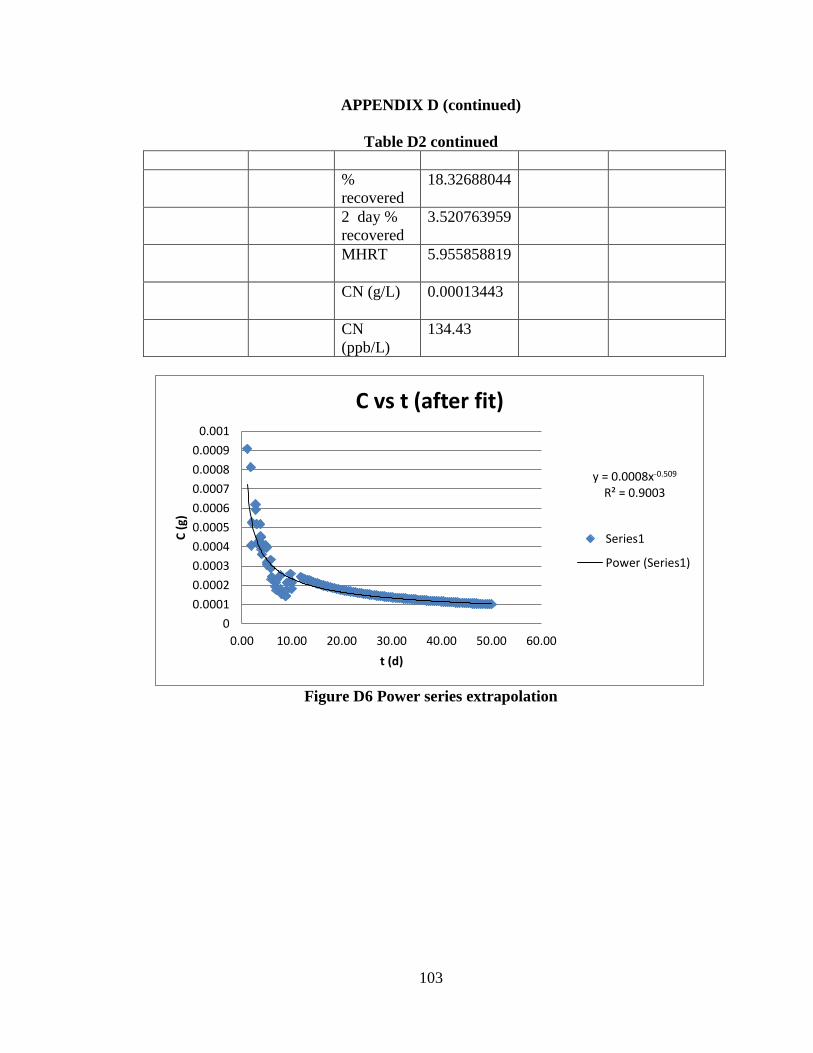
103

APPENDIX D (continued)

Table D2 continued

%

recovered

18.32688044

2 day %

recovered

3.520763959

MHRT 5.955858819

CN (g/L) 0.00013443

CN

(ppb/L)

134.43

Figure D6 Power series extrapolation

y = 0.0008x-0.509 R² = 0.9003

0

0.0001

0.0002

0.0003

0.0004

0.0005

0.0006

0.0007

0.0008

0.0009

0.001

0.00 10.00 20.00 30.00 40.00 50.00 60.00

C (

g)

t (d)

C vs t (after fit)

Series1

Power (Series1)

104

APPENDIX D (continued)

Figure D7 Exit age distribution comparison

Figure D8 Exit age distribution comparison with extrapolation

-0.5

0

0.5

1

1.5

2

2.5

0 0.5 1 1.5 2 2.5

Exit

age

dis

trib

uti

on

, E(θ

)

Normalized time, θ

DFM

TIS

0

0.5

1

1.5

2

2.5

3

3.5

0 0.5 1 1.5 2 2.5 3Exit

age

dis

trib

uti

on

, E(θ

)

Normalized time, θ

Power Seriesextrapolation

DFM

TIS

105

APPENDIX D (continued)

Figure D9 TIS model comparison with tracer data

0

100

200

300

400

500

600

700

800

900

1000

0 2 4 6 8 10 12 14

Exit

Co

nce

ntr

atio

n, (

pp

b)

Time, Day

Actual

TIS

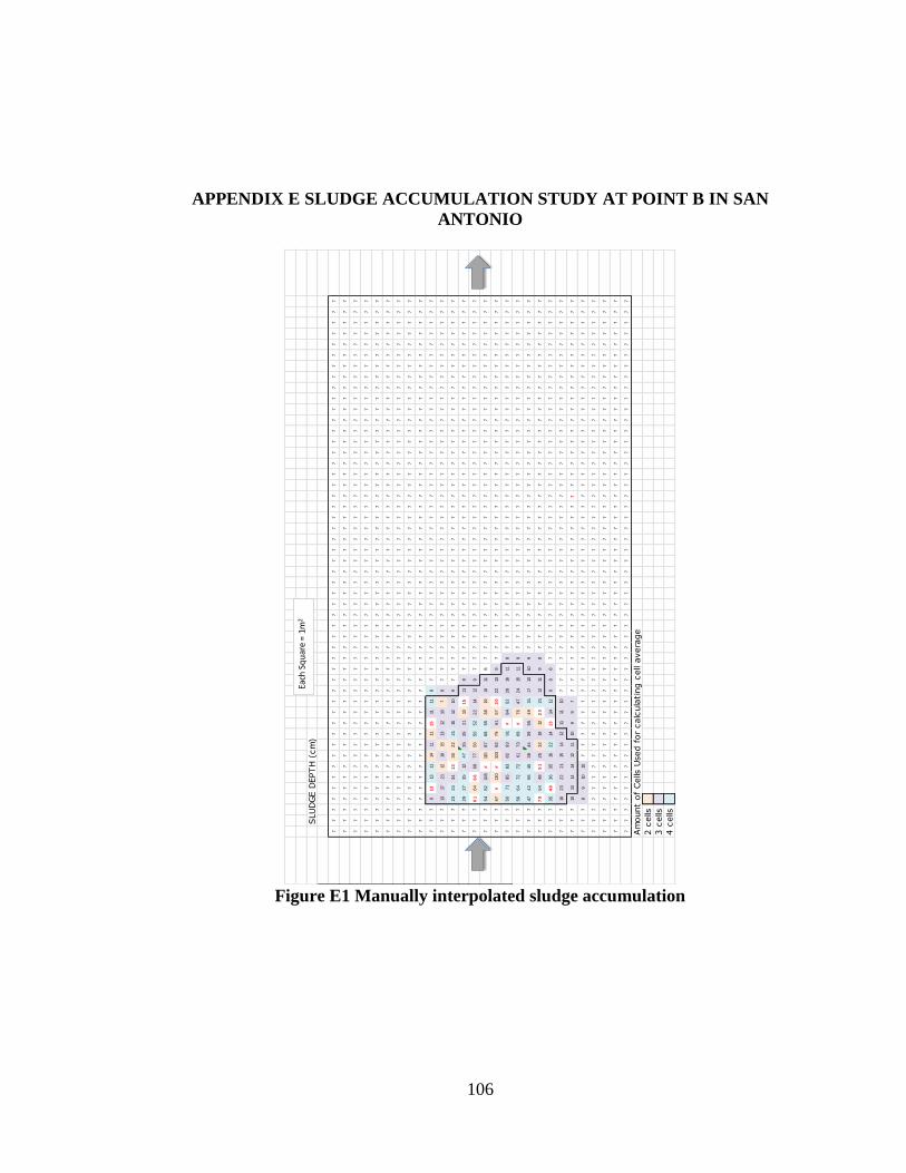
106

APPENDIX E SLUDGE ACCUMULATION STUDY AT POINT B IN SAN

ANTONIO

Figure E1 Manually interpolated sludge accumulation

SLUDGE D

EPTH (

cm

)

77

77

77

77

77

77

77

77

77

77

77

77

77

77

77

77

77

77

77

77

77

77

77

77

77

77

77

77

77

77

77

77

77

77

77

77

77

77

77

77

77

77

77

77

77

77

77

77

77

77

77

77

77

77

77

77

77

77

77

77

77

77

77

77

77

77

77

77

77

77

77

77

77

77

77

77

77

77

77

77

77

77

77

77

77

77

77

77

77

77

77

77

77

77

77

77

77

77

77

77

77

77

77

77

77

77

77

77

77

77

77

77

77

77

77

77

77

77

77

77

77

77

77

77

77

77

77

77

77

77

77

77

77

77

77

77

77

77

77

77

77

77

77

77

77

77

77

77

77

77

77

77

77

77

77

77

77

77

77

77

77

77

77

77

77

77

77

77

77

77

77

77

77

77

77

77

77

77

77

77

77

77

77

77

77

77

77

77

77

77

77

77

77

77

77

77

77

77

77

77

77

77

77

77

77

77

77

77

77

77

77

77

77

77

77

77

77

77

77

77

77

77

77

77

77

77

79

13

1311

1411

111

511

118

77

77

77

77

77

77

77

77

77

77

77

77

77

77

77

77

77

77

77

713

172

112

1915

1312

107

87

77

77

77

77

77

77

77

77

77

77

77

77

77

77

77

77

77

7

77

72

32

43

41

33

02

22

115

1210

97

77

77

77

77

77

77

77

77

77

77

77

77

77

77

77

77

77

7

77

72

92

73

512

47

35

35

21

131

511

87

77

77

77

77

77

77

77

77

77

77

77

77

77

77

77

77

77

77

76

16

46

66

87

75

65

05

22

214

129

77

77

77

77

77

77

77

77

77

77

77

77

77

77

77

77

77

7

77

75

48

210

8#

115

87

68

55

38

1916

118

77

77

77

77

77

77

77

77

77

77

77

77

77

77

77

77

77

77

76

7#

130

#10

39

27

96

15

73

02

213

97

77

77

77

77

77

77

77

77

77

77

77

77

77

77

77

77

7

77

75

07

19

58

38

29

39

1#

84

52

28

1611

87

77

77

77

77

77

77

77

77

77

77

77

77

77

77

77

77

77

75

66

47

27

26

17

36

9#

76

47

24

1511

97

77

77

77

77

77

77

77

77

77

77

77

77

77

77

77

77

77

74

74

25

64

53

84

43

95

54

93

117

1310

97

77

77

77

77

77

77

77

77

77

77

77

77

77

77

77

77

77

77

95

44

85

12

53

219

122

32

112

119

87

77

77

77

77

77

77

77

77

77

77

77

77

77

77

77

77

77

73

54

63

63

516

22

141

314

129

98

77

77

77

77

77

77

77

77

77

77

77

77

77

77

77

77

77

77

716

23

22

21

1514

1211

1110

77

77

77

77

77

77

77

77

77

77

77

77

77

77

77

77

77

77

7

77

710

1314

1412

1110

99

77

77

77

77

77

77

77

77

77

77

77

77

77

77

77

77

77

77

77

77

78

910

107

77

77

77

77

77

77

77

77

77

77

77

77

77

77

77

77

77

77

77

77

77

77

77

77

77

77

77

77

77

77

77

77

77

77

77

77

77

77

77

77

77

77

77

77

77

77

77

77

77

77

77

77

77

77

77

77

77

77

77

77

77

77

77

77

77

77

77

77

77

77

77

77

77

77

77

77

77

77

77

77

77

77

77

77

77

77

77

77

77

77

77

77

77

77

77

77

77

77

77

77

77

77

77

77

77

77

77

77

77

77

77

77

77

77

77

77

77

77

77

77

77

Am

ount

of

Cells

Used f

or

calc

ula

ting c

ell

avera

ge

2 c

ells

3 c

ells

4 c

ells

Each

Sq

uar

e =

1m2

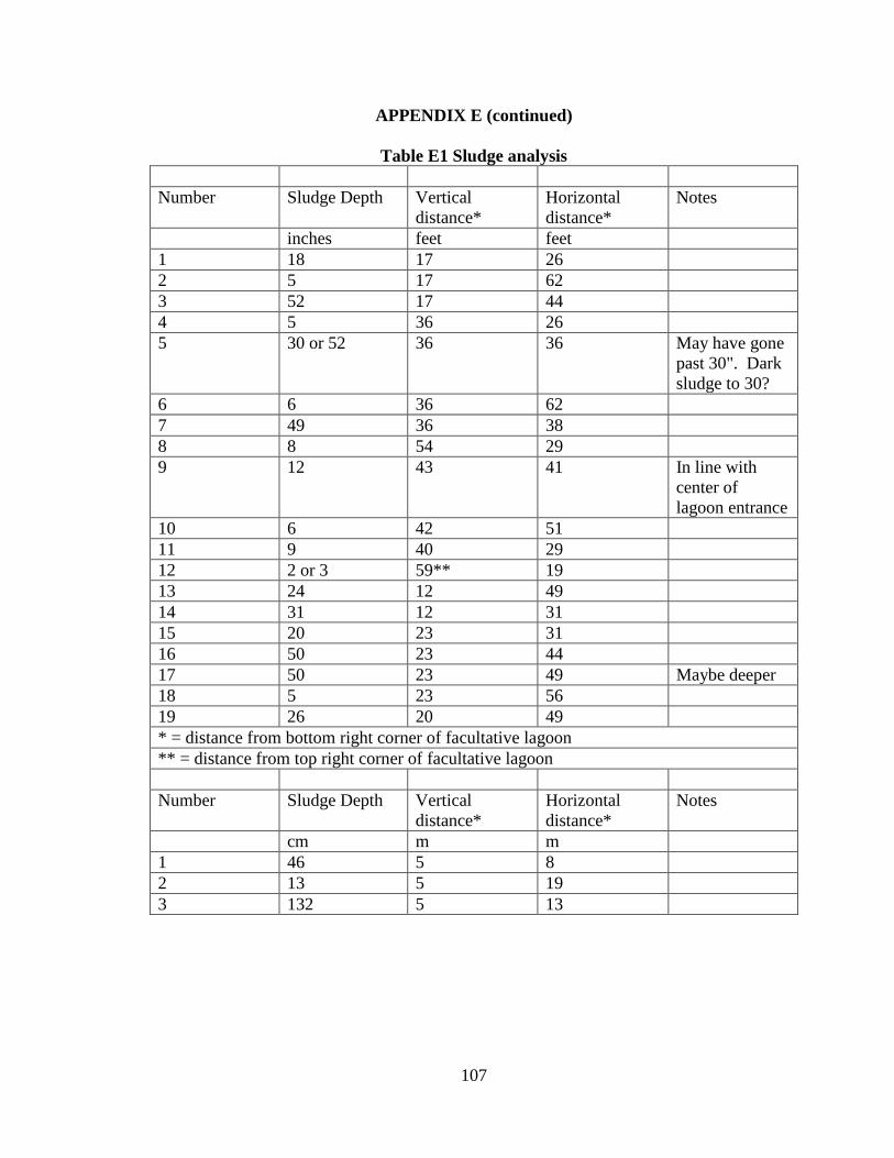
107

APPENDIX E (continued)

Table E1 Sludge analysis

Number Sludge Depth Vertical

distance*

Horizontal

distance*

Notes

inches feet feet

1 18 17 26

2 5 17 62

3 52 17 44

4 5 36 26

5 30 or 52 36 36 May have gone

past 30". Dark

sludge to 30?

6 6 36 62

7 49 36 38

8 8 54 29

9 12 43 41 In line with

center of

lagoon entrance

10 6 42 51

11 9 40 29

12 2 or 3 59** 19

13 24 12 49

14 31 12 31

15 20 23 31

16 50 23 44

17 50 23 49 Maybe deeper

18 5 23 56

19 26 20 49

* = distance from bottom right corner of facultative lagoon

** = distance from top right corner of facultative lagoon

Number Sludge Depth Vertical

distance*

Horizontal

distance*

Notes

cm m m

1 46 5 8

2 13 5 19

3 132 5 13

108

APPENDIX E (continued)

Table E1 continued

4 13 11 8

5 104 11 11 May have gone

past 30". Dark

sludge to 30?

6 15 11 19

7 124 11 12

8 20 16 9

9 30 13 13 In line with

center of

lagoon entrance

10 15 13 16

11 23 12 9

12 7 32 6

13 61 4 15

14 79 4 9

15 51 7 9

16 127 7 13

17 127 7 15 Maybe deeper

18 13 7 17 19 66 6 15

* = distance from bottom right corner of facultative lagoon

KRIGING RESULTS FOR INTERPOLATION OF SLUDGE ACCUMULATION AT

SAN ANTONIO FOR TOTAL SLUDGE VOLUME CALCULATION

Predicted Model error Vol (m3)

0.488755548 0.49113689 0.426760856

0.509676734 0.512022199 0.445028358

0.605623271 0.576875522 0.528804851

0.53651784 0.511024879 0.468464887

0.380688805 0.353984606 0.332401505

0.337812455 0.314110773 0.294963675

0.300320775 0.279249968 0.262227511

0.239879464 0.240643247 0.209452692

0.214837502 0.215521055 0.1875871

0.199429732 0.214724497 0.174133682

0.180959845 0.194826895 0.15800655

0.165459921 0.178159196 0.144472667

0.179702466 0.166918243 0.15690866

0.135526066 0.125912095 0.118335679

0.132493253 0.119556165 0.115687554

0.125157661 0.113072171 0.109282423

109

APPENDIX E (continued)

Table E1 continued 0.120662358 0.109021763 0.105357313

0.129183452 0.116759829 0.112797575

0.090524917 0.08293764 0.079042563

0.057790214 0.052952388 0.050459992

0.055889357 0.051433665 0.048800244

0.063784845 0.058703242 0.055694253

0.060659959 0.055828758 0.052965734

0.066590024 0.061285407 0.058143617

0.062884493 0.057870238 0.054908103

0.063927047 0.057124907 0.055818418

0.062279962 0.055635325 0.054380252

0.013323383 0.012428442 0.01163342

0.021206965 0.019742516 0.018517033

0.030910408 0.028734516 0.026989672

0.593641068 0.59577317 0.518342494

0.52632171 0.527861184 0.459562053

0.466609765 0.467717879 0.407424086

0.554645772 0.527383917 0.484293437

0.479768317 0.454508366 0.418913582

0.349730695 0.324606659 0.305370181

0.310718612 0.288408746 0.271306466

0.276733097 0.256856247 0.24163174

0.228454902 0.245524966 0.199477243

0.205665685 0.220910987 0.179578654

0.186646038 0.200451252 0.162971496

0.198379908 0.183949399 0.173217019

0.184949547 0.171576644 0.161490191

0.173927644 0.161438746 0.151866328

0.166190128 0.149979321 0.145110253

0.132046735 0.119192168 0.115297674

0.143791275 0.129853744 0.125552513

0.128471708 0.11760932 0.11217611

0.122453063 0.112132076 0.106920881

0.121949937 0.112177329 0.106481573

0.097340171 0.089558756 0.084993357

0.066100233 0.060825072 0.057715952

0.068491474 0.063030098 0.059803884

0.073752805 0.067871075 0.064397857

0.076696136 0.068538003 0.06696785

0.074458788 0.066519531 0.065014292

0.069358753 0.061927229 0.060561156

0.068742322 0.063983212 0.060022914

0.019659628 0.018259537 0.017165963

0.034774544 0.034847018 0.030363674

0.033971372 0.033865412 0.029662378

0.611789336 0.612299575 0.534188801

0.543203746 0.54277644 0.474302739

0.482223935 0.481193921 0.421057725

0.428054593 0.426828227 0.373759326

0.496109259 0.468142725 0.433181807

0.36207118 0.334757865 0.316145376

0.321362659 0.297182897 0.280600402

0.285640292 0.264127392 0.249409129

0.263250963 0.254553188 0.229859705

110

APPENDIX E (continued)

Table E1 continued 0.211495195 0.22593699 0.184668738

0.215319763 0.198822387 0.18800819

0.203455698 0.188002352 0.177648987

0.190141027 0.175904323 0.166023174

0.17600983 0.163299173 0.153684405

0.171712834 0.154635029 0.149932448

0.163670862 0.147454701 0.142910535

0.140254705 0.128117139 0.122464529

0.135328471 0.123698987 0.118163148

0.134110448 0.123192685 0.117099621

0.128101764 0.117746714 0.11185309

0.123813816 0.113861737 0.108109033

0.102208367 0.094024747 0.089244062

0.10179846 0.093664685 0.088886148

0.082384661 0.073620516 0.071934832

0.086141654 0.076965379 0.075215281

0.081973266 0.073207813 0.07157562

0.078602894 0.073190202 0.068632752

0.075594765 0.070229567 0.06600618

0.068582908 0.068669202 0.05988372

0.025202179 0.025018143 0.022005486

0.040343023 0.039568379 0.035225836

0.630172708 0.627109174 0.550240391

0.560421682 0.555523114 0.489336719

0.498205426 0.492196345 0.435012092

0.442796976 0.436710009 0.386631757

0.384268254 0.37957274 0.33552693

0.456304744 0.427643752 0.398426174

0.332013336 0.304756955 0.289900127

0.294015633 0.269813891 0.256722126

0.269385521 0.258475389 0.235216144

0.255376628 0.224068818 0.222984166

0.219687123 0.201086589 0.191821586

0.207625815 0.190383594 0.181290158

0.191507146 0.176393533 0.167216011

0.181327351 0.167549527 0.158327442

0.177579621 0.159212009 0.155055081

0.177011683 0.160829932 0.154559181

0.169032294 0.153769283 0.147591913

0.195627503 0.181319368 0.170813735

0.140669587 0.128912628 0.122826786

0.135360547 0.124227424 0.118191155

0.129179266 0.118686769 0.11279392

0.124173291 0.114171984 0.108422913

0.115639415 0.103308672 0.100971489

0.112447186 0.10046688 0.098184169

0.08868167 0.079217993 0.077433117

0.091814948 0.085550636 0.080168964

0.087991091 0.081843449 0.076830132

0.077927069 0.078189133 0.06804265

0.074482108 0.074053387 0.065034654

0.034093332 0.033342291 0.029768868

0.047850566 0.045568644 0.041781108

0.05970925 0.054955894 0.052135614

111

APPENDIX E (continued)

Table E1 continued 0.649351538 0.638954238 0.566986541

0.578431681 0.563908678 0.505062295

0.514718971 0.497537674 0.449431028

0.457858153 0.440696963 0.399782545

0.398887414 0.384371759 0.348291768

0.354408517 0.342640002 0.30945466

0.342308893 0.309850168 0.298889775

0.300997907 0.272250418 0.262818754

0.28768318 0.249221983 0.251192893

0.255911486 0.220797693 0.223451182

0.232687658 0.200570354 0.203173108

0.206225889 0.186217307 0.180067801

0.19559628 0.177963313 0.170786472

0.186640979 0.171094414 0.162967079

0.192156853 0.172529357 0.167783309

0.183646142 0.165181943 0.160352113

0.21085735 0.193305667 0.184111799

0.170875527 0.155248624 0.149201347

0.162519697 0.148219676 0.141905386

0.140922144 0.128949258 0.123047308

0.134892902 0.123730841 0.117782827

0.140505828 0.125379916 0.122683799

0.134219451 0.119859333 0.117194798

0.11819301 0.105575715 0.103201181

0.120423706 0.112263835 0.105148931

0.099318783 0.092499202 0.086720998

0.089594757 0.090195291 0.078230386

0.084116176 0.084120409 0.073446718

0.080107106 0.079012972 0.069946167

0.076257333 0.073160232 0.066584706

0.0510368 0.046449936 0.044563194

0.055323963 0.046144021 0.048306565

1.025592605 0.989362851 0.895504469

0.776255082 0.713194208 0.677793396

0.532155792 0.49075526 0.464656129

0.472727698 0.430691845 0.412766009

0.414879171 0.378989715 0.3622551

0.369614806 0.342188492 0.322732154

0.324881517 0.304105522 0.283672921

0.33162883 0.279049948 0.289564392

0.283690341 0.238694759 0.247706513

0.247864976 0.205640034 0.216425306

0.223414343 0.184982368 0.195076038

0.216575754 0.181252208 0.18910487

0.198680122 0.17641125 0.173479153

0.206984853 0.181280418 0.180730496

0.199757773 0.175574691 0.174420113

0.227001436 0.20298342 0.198208138

0.185995713 0.165145783 0.16240366

0.176112477 0.157662618 0.153774032

0.1664719 0.150400018 0.145356284

0.157341797 0.143211764 0.137384261

0.151943266 0.135067658 0.13267049

0.144112937 0.128444932 0.125833375

112

APPENDIX E (continued)

Table E1 continued 0.137123697 0.122383738 0.119730663

0.124728987 0.116263756 0.108908122

0.120091512 0.111927919 0.104858874

0.111355865 0.112396604 0.097231273

0.095489781 0.096040881 0.083377674

0.089792958 0.089591634 0.078403447

0.085206409 0.083547119 0.074398665

0.080882385 0.076374693 0.070623108

0.076761694 0.066742712 0.067025093

0.064899274 0.046853085 0.056667325

0.065476503 0.032447669 0.057171337

1.033134177 0.963856467 0.902089453

0.890678017 0.794239755 0.777702706

0.675818062 0.553708586 0.590096001

0.590707263 0.456096185 0.515780819

0.454546477 0.361895617 0.396890929

0.388936608 0.332605822 0.339603141

0.433308025 0.363229424 0.378346402

0.367236338 0.307302584 0.320655376

0.276768249 0.215315813 0.241662432

0.223357401 0.167631718 0.195026319

0.204773954 0.153253667 0.178800032

0.209521545 0.163385334 0.18294543

0.242802391 0.197740247 0.21200487

0.214575169 0.180720858 0.187358042

0.241932544 0.206986507 0.211245355

0.204006694 0.171962968 0.178130093

0.192891079 0.163888561 0.168424404

0.181148806 0.157278164 0.158171543

0.169757198 0.150753647 0.148224869

0.173673905 0.152508248 0.151644773

0.163486373 0.144808996 0.142749448

0.146953311 0.130767446 0.12831347

0.142353749 0.132495881 0.124297326

0.134584152 0.125405658 0.11751324

0.116500155 0.117727026 0.101723052

0.111533659 0.112563969 0.097386516

0.105624583 0.106222653 0.092226958

0.094686689 0.094454262 0.082676447

0.089513267 0.087722722 0.078159233

0.08467937 0.079838863 0.073938476

0.080107879 0.069315575 0.069946842

0.080654789 0.05696524 0.070424381

0.0719252 0.031096832 0.062802069

1.039340696 0.919596174 0.907508725

0.877770997 0.710760634 0.766432837

0.708639671 0.49444674 0.618754454

0.538333218 0.297897015 0.470049999

0.506838474 0.31810602 0.442550108

0.503227732 0.367390073 0.43939736

0.444304518 0.346696616 0.387948079

0.370315773 0.290051585 0.323344209

0.281613178 0.204339838 0.245892821

0.193698927 0.11049563 0.169129783

113

APPENDIX E (continued)

Table E1 continued 0.176054608 0.100372279 0.153723503

0.212561893 0.144735417 0.185600134

0.239684109 0.180185551 0.209282116

0.250077964 0.196955054 0.218357595

0.223712149 0.175266052 0.19533607

0.212701017 0.160249238 0.185721611

0.199232563 0.152290484 0.173961522

0.185280251 0.151410775 0.161778948

0.185980175 0.156921576 0.162390092

0.173855476 0.15108484 0.151803313

0.162741271 0.143536778 0.142098855

0.156328294 0.144812602 0.136499313

0.142537897 0.132557088 0.124458116

0.126933728 0.128205813 0.11083321

0.119253215 0.120501875 0.104126908

0.111194398 0.112247783 0.097090287

0.104446319 0.105116298 0.091198147

0.109031518 0.108508316 0.09520175

0.103845815 0.101871838 0.090673812

0.097222654 0.092611207 0.084890746

0.090619519 0.081485521 0.079125165

0.082067739 0.066715085 0.071658109

0.082478654 0.060146032 0.072016903

1.020869145 0.826632065 0.891380141

0.878170399 0.608985112 0.766781579

0.697493185 0.393264962 0.60902181

0.502761627 0.135317516 0.438990376

0.519445812 0.256485482 0.453558307

0.531391561 0.328625722 0.463988834

0.482306904 0.333962286 0.42113017

0.407102679 0.299072906 0.355464993

0.300251905 0.199798392 0.262167377

0.180042049 0.073003336 0.15720517

0.163582427 0.061507471 0.142833317

0.213984471 0.107625168 0.186842269

0.255895321 0.170907194 0.223437067

0.265475703 0.194534926 0.231802255

0.234157329 0.160830891 0.204456364

0.217637343 0.121756807 0.190031804

0.201346847 0.117578093 0.175807626

0.19827842 0.145116448 0.173128404

0.185094183 0.151782066 0.161616481

0.172043962 0.148069396 0.150221575

0.164030562 0.150066933 0.14322461

0.153136019 0.141633708 0.133711952

0.133534112 0.134482792 0.116596389

0.140842026 0.141582338 0.122977353

0.132058294 0.132856211 0.115307766

0.12494833 0.125631071 0.109099644

0.115239041 0.115614966 0.1006219

0.106363307 0.10618895 0.092871981

0.098534996 0.097417944 0.086036628

0.099495173 0.096609627 0.086875014

0.092799116 0.087454242 0.081028298

114

APPENDIX E (continued)

Table E1 continued 0.086351053 0.078201536 0.075398119

0.091034623 0.079986422 0.079487617

0.08119016 0.071864548 0.070891844

1.041219711 0.769745433 0.909149402

0.906565789 0.439823416 0.791575243

0.747659388 0.320467086 0.652824835

0.661242917 0.352916796 0.577369595

0.597068946 0.317613635 0.521335574

0.526311788 0.2005853 0.45955339

0.542560537 0.297795591 0.473741116

0.517797086 0.354949439 0.452118709

0.410231495 0.279496287 0.358196944

0.326858182 0.188184105 0.285398862

0.281539877 0.129744939 0.245828818

0.260123485 0.078100776 0.227128922

0.287233552 0.175624715 0.250800296

0.281634273 0.197614368 0.24591124

0.243165232 0.158195782 0.212321687

0.21798141 0.086944607 0.190332229

0.203687883 0.091874538 0.177851721

0.195359124 0.137573558 0.170579397

0.181685445 0.147599261 0.158640114

0.185420271 0.164672129 0.161901207

0.173058635 0.157801054 0.151107545

0.157324719 0.156642344 0.13736935

0.146556923 0.146902609 0.127967362

0.137106481 0.13782765 0.119715631

0.128247934 0.129049149 0.11198072

0.120019197 0.120743603 0.104795731

0.113539822 0.114067117 0.099138213

0.102691828 0.102852507 0.089666199

0.094962517 0.094567927 0.082917289

0.100523921 0.099155252 0.087773274

0.093721665 0.091186749 0.081833829

0.087296003 0.083647326 0.076223211

0.06610189 0.062718082 0.057717399

0.085963827 0.08174946 0.07506001

1.079884305 0.807812509 0.942909705

0.9663902 0.50173872 0.84381141

0.899860773 0.4429065 0.785720704

0.854008052 0.528970352 0.74568403

0.759796998 0.451480456 0.663422887

0.654225321 0.290304178 0.571242124

0.64955103 0.366480858 0.567160729

0.678524618 0.462338652 0.592459252

0.647530426 0.430779163 0.565396423

0.620851697 0.350771748 0.542101675

0.529009579 0.276447429 0.461908988

0.418432598 0.2378746 0.365357803

0.349316715 0.230240319 0.305008712

0.30571399 0.218622088 0.26693664

0.275753064 0.194183596 0.240776015

0.233674842 0.149258618 0.204035076

0.212159097 0.13928467 0.18524843

115

APPENDIX E (continued)

Table E1 continued 0.200826242 0.15304121 0.175353056

0.192287572 0.164124356 0.167897447

0.178677702 0.159762484 0.156013879

0.161761513 0.159165311 0.141243372

0.150193048 0.149711392 0.131142273

0.139487733 0.1398828 0.121794841

0.131693426 0.13242088 0.114989179

0.122861486 0.123664601 0.107277499

0.115019337 0.115776076 0.100430063

0.109391883 0.110028619 0.095516406

0.098126869 0.098529171 0.085680268

0.090554131 0.090651423 0.079068071

0.083528374 0.083233592 0.072933475

0.0934222 0.092540291 0.081572349

0.08698959 0.085659437 0.075955664

0.062988706 0.06180876 0.054999098

0.090597634 0.088970814 0.079106056

1.123590281 0.885585543 0.981071931

1.096256898 0.776223593 0.957205567

1.03449178 0.702045564 0.903274855

1.039799449 0.711206428 0.907909289

1.001356178 0.675461265 0.874342237

0.928609772 0.605558097 0.810823125

0.931683993 0.633272071 0.813507405

0.883499624 0.62093078 0.771434834

0.923964107 0.588120237 0.806766725

1.026691116 0.392202138 0.896463642

0.873714202 0.343407966 0.762890614

0.553833917 0.324577658 0.483584559

0.389901037 0.252301282 0.34044524

0.322890099 0.22905035 0.281934099

0.284501421 0.210327232 0.248414714

0.233222133 0.175928372 0.20363979

0.209035296 0.161396182 0.182520857

0.193377917 0.15861595 0.168849491

0.184282709 0.162254184 0.160907936

0.16555656 0.160824424 0.144557048

0.152837679 0.151243833 0.133451454

0.141417664 0.1412887 0.123479976

0.131002459 0.131498714 0.114385855

0.121359591 0.122084251 0.105966107

0.116077543 0.116873773 0.101354045

0.105470287 0.106211386 0.092092233

0.097335811 0.097985631 0.08498955

0.092811791 0.093350685 0.081039365

0.085451783 0.085822058 0.074612915

0.07877976 0.078955712 0.068787184

0.091992218 0.091967373 0.080323748

0.085639247 0.085418103 0.0747766

0.059783939 0.059552111 0.052200829

0.095352769 0.095010536 0.08325804

1.019435837 0.833464592 0.890128637

1.177632732 0.91198654 1.028259534

1.19231462 0.843523982 1.041079143

116

APPENDIX E (continued)

Table E1 continued 1.261682789 0.832342054 1.10164852

1.212889775 0.789294347 1.059044506

1.153469806 0.749534451 1.00716148

1.102835331 0.75177412 0.962949579

1.01824995 0.725540195 0.88909317

1.010373188 0.654140764 0.882215512

1.08345723 0.470722554 0.946029433

0.905149937 0.386600645 0.79033898

0.534394197 0.270699379 0.46661061

0.349539443 0.16333725 0.305203189

0.302393362 0.193999829 0.264037207

0.271826719 0.202776604 0.237347696

0.222602044 0.176910913 0.194366773

0.204245917 0.170937723 0.178338972

0.183864821 0.157587571 0.160543054

0.161940938 0.147651719 0.141400039

0.154700749 0.152273119 0.135078209

0.142284815 0.141632504 0.124237136

0.131307089 0.131523839 0.114651845

0.121405448 0.122000305 0.106006148

0.112315895 0.113043711 0.098069531

0.108170681 0.10894596 0.094450104

0.096048405 0.096755384 0.083865441

0.090012397 0.090663427 0.078595052

0.086278953 0.086868394 0.075335165

0.079824673 0.080316439 0.069699558

0.073589742 0.073975936 0.064255478

0.067798688 0.068084584 0.059198972

0.049156382 0.049319049 0.042921292

0.056575122 0.056734478 0.049399025

0.041981307 0.042104136 0.036656318

1.021584793 0.817593824 0.892005015

1.053056536 0.770831368 0.919484822

1.240261681 0.779772869 1.082944506

1.369501548 0.622699216 1.195791341

1.364362258 0.685935831 1.191303928

1.249912981 0.555007621 1.091371617

1.134261543 0.649216205 0.990389629

1.004165619 0.701231186 0.876795323

0.891578438 0.619572808 0.778488916

0.824340185 0.530113255 0.719779292

0.667216508 0.400965579 0.582585484

0.430147308 0.217568442 0.375586597

0.293398869 0.108912335 0.256183592

0.269842717 0.168792557 0.235615348

0.247544026 0.186104225 0.216145067

0.205171604 0.166238015 0.179147244

0.188532148 0.161547677 0.164618368

0.164480257 0.149824267 0.143617265

0.148961723 0.13768836 0.130067132

0.135860131 0.12677613 0.118627371

0.130554367 0.130559307 0.1139946

0.120280504 0.120741835 0.105023894

0.111077199 0.111732414 0.096987954

117

APPENDIX E (continued)

Table E1 continued 0.102680563 0.103393682 0.089656363

0.09419393 0.094893433 0.082246191

0.08724287 0.087905304 0.076176817

0.082258796 0.082881274 0.071824932

0.079262673 0.079849167 0.069208843

0.07385304 0.074378196 0.064485378

0.068115932 0.068574327 0.059475977

0.062780969 0.063177439 0.05481771

0.043596593 0.04385654 0.038066717

0.053396529 0.05370492 0.046623611

0.038236266 0.038458682 0.033386304

0.92012773 0.692978954 0.803416961

0.965669082 0.607469195 0.84318176

1.012361804 0.53953844 0.883951888

1.168442765 0.420012253 1.02023524

1.248607362 0.539395415 1.090231605

1.327820911 0.45207214 1.159397556

1.184868273 0.613980857 1.034577305

0.921047244 0.627465086 0.804219842

0.743055734 0.546835244 0.648805117

0.672382002 0.491514461 0.587095777

0.496851429 0.338139961 0.433829839

0.359458231 0.221557765 0.313863858

0.281356489 0.169977039 0.245668691

0.240732647 0.16737058 0.210197655

0.205869396 0.158939469 0.179756526

0.183750843 0.150683675 0.160443533

0.159421408 0.138593056 0.13920009

0.148775257 0.136973558 0.129904318

0.134881211 0.125600102 0.117772619

0.123016258 0.115304558 0.107412639

0.1127781 0.106108015 0.098473109

0.108822058 0.109411785 0.095018859

0.100437068 0.101106081 0.087697437

0.0916572 0.092327242 0.080031225

0.084809844 0.085456313 0.074052401

0.078244604 0.078850664 0.068319908

0.074563871 0.075142288 0.065106046

0.074390939 0.074963357 0.064955049

0.067720777 0.068233927 0.059130943

0.062515839 0.062979943 0.05458621

0.057665582 0.058084283 0.050351169

0.038310636 0.038583621 0.033451242

0.050271453 0.050626117 0.043894925

0.034705693 0.034951086 0.030303556

0.795563098 0.557628393 0.694652346

0.720643135 0.311119166 0.629235375

0.706955564 0.273102065 0.617283962

0.772971925 0.384405285 0.674926681

0.750604298 0.203336349 0.655396207

1.248139293 0.319624342 1.089822907

1.029417952 0.524710608 0.898844601

118

APPENDIX E (continued)

Table E1 continued 0.751377916 0.514994625 0.656071697

0.575689805 0.430111712 0.502668205

0.456016129 0.337704518 0.398174167

0.36939172 0.247868187 0.322537364

0.258701396 0.140388127 0.225887214

0.220048316 0.121589035 0.192136964

0.211587028 0.148966795 0.184748923

0.202777363 0.162720758 0.177056693

0.156840206 0.133094206 0.136946293

0.141389443 0.123786549 0.123455334

0.127729085 0.113586609 0.111527683

0.1205746 0.112746159 0.105280686

0.11006335 0.103432634 0.096102703

0.100922215 0.095095339 0.088121047

0.092887254 0.087648663 0.081105257

0.089873467 0.09051897 0.078473744

0.081625417 0.082243133 0.071271893

0.068890626 0.069425161 0.060152406

0.069370261 0.069914229 0.060571204

0.066639165 0.067163017 0.058186526

0.066728946 0.067252213 0.058264918

0.061593349 0.062073585 0.05378073

0.056929809 0.057370281 0.049708723

0.052572053 0.052975516 0.045903713

0.033369631 0.033624019 0.029136963

0.034262099 0.034522387 0.029916229

0.031392176 0.031630848 0.027410332

0.676703501 0.494890027 0.590869129

0.587371958 0.34272432 0.512868571

0.546864885 0.296652946 0.477499492

0.519339192 0.301773824 0.453465211

0.493961954 0.240695835 0.431306871

0.572020079 0.259602295 0.499463953

0.561489083 0.31583742 0.490268729

0.500508559 0.346853626 0.437023092

0.424364499 0.317365468 0.370537291

0.347082228 0.253462707 0.303057651

0.264676454 0.171871772 0.231104384

0.183246772 0.072879901 0.160003399

0.167332036 0.072400599 0.146107319

0.177540853 0.123899157 0.15502123

0.177497602 0.143911559 0.154983465

0.145734948 0.124251033 0.127249647

0.124315236 0.109479899 0.108546853

0.112783491 0.100662945 0.098477817

0.10259216 0.09217264 0.089579174

0.097548553 0.091819303 0.085175307

0.089484483 0.08439558 0.078134099

0.082372125 0.077765474 0.071923886

0.076022724 0.071807374 0.066379856

0.065151604 0.065310711 0.056887649

0.054147684 0.054286502 0.047279488

0.057257962 0.057407883 0.049995252

0.053370353 0.053511058 0.046600755

119

APPENDIX E (continued)

Table E1 continued 0.049599418 0.049730039 0.043308133

0.050309618 0.050441342 0.04392825

0.046569676 0.046690592 0.040662689

0.026952426 0.027164023 0.023533729

0.042750351 0.043085161 0.037327815

0.030862865 0.031104275 0.02694816

0.028297796 0.028519205 0.024708449

0.566773821 0.485648378 0.49488314

0.490156842 0.36674789 0.427984406

0.420946798 0.29294805 0.367553097

0.355892362 0.233588596 0.310750291

0.280599855 0.158309238 0.24500803

0.205290108 0.076713317 0.179250717

0.243249874 0.130595674 0.212395593

0.27779093 0.194251295 0.242555395

0.311925062 0.228767655 0.272359888

0.273299477 0.197192105 0.238633646

0.229825835 0.155882796 0.200674285

0.177597415 0.109824592 0.155070618

0.144193908 0.093071669 0.125904075

0.164119454 0.124266242 0.143302227

0.161075799 0.134428808 0.140644635

0.148609588 0.129670652 0.129759662

0.116734022 0.102906498 0.101927254

0.099014534 0.08865876 0.086455341

0.090202303 0.081180107 0.07876087

0.082450569 0.074389629 0.071992381

0.0787813 0.074345911 0.068788528

0.072528154 0.06849396 0.063328543

0.0669444 0.063242928 0.058453044

0.053093986 0.050166824 0.046359443

0.046662039 0.04678397 0.040743336

0.050182043 0.050315014 0.043816857

0.04393606 0.044053098 0.038363125

0.043830588 0.043947437 0.038271032

0.045140701 0.045260841 0.039414968

0.041852792 0.04196386 0.036544103

0.020863698 0.020918891 0.018217306

0.035906275 0.036001019 0.031351854

0.025061994 0.025128038 0.021883083

0.022998915 0.023059541 0.020081688

0.46150046 0.415475328 0.402962855

0.355026739 0.285280312 0.309994465

0.297750656 0.212217818 0.259983391

0.241817163 0.148406393 0.211144609

0.184851305 0.103071382 0.16140441

0.13744547 0.059463696 0.120011623

0.162430529 0.092831317 0.141827529

0.19618382 0.138819765 0.171299487

0.221708502 0.159877703 0.19358657

0.214153238 0.139008095 0.18698963

0.189808594 0.122252824 0.165732908

0.152851796 0.10694226 0.133463781

0.13349963 0.100604411 0.11656628

120

APPENDIX E (continued)

Table E1 continued 0.118333557 0.095551366 0.103323901

0.142955638 0.122823912 0.12482287

0.13447583 0.1191861 0.117418658

0.123689611 0.111471811 0.108000584

0.093098752 0.08318754 0.081289928

0.078952281 0.071157307 0.068937822

0.072192113 0.065180337 0.063035127

0.063445224 0.060859312 0.05539771

0.063510479 0.059990853 0.055454688

0.056459927 0.053343958 0.049298441

0.045472364 0.042967735 0.039704562

0.042110582 0.039793265 0.036769195

0.039528843 0.039634292 0.034514929

0.038113785 0.03821585 0.033279359

0.03882619 0.038930278 0.033901402

0.040286161 0.040394134 0.035176187

0.01954799 0.019600335 0.017068486

0.017776828 0.017824378 0.015521981

0.024434444 0.024499743 0.021335132

0.022422328 0.022482223 0.019578237

0.02059698 0.020652005 0.017984419

0.319906265 0.288889114 0.27932874

0.252613206 0.208067016 0.220571261

0.203446183 0.132739131 0.177640678

0.156216414 0.056322946 0.136401624

0.145517632 0.074254948 0.127059896

0.142853155 0.090867036 0.124733386

0.153319554 0.106959508 0.133872207

0.168054358 0.123797628 0.14673802

0.175922413 0.117988313 0.153608076

0.171554687 0.076037808 0.149794361

0.154395735 0.07112159 0.134811883

0.136844588 0.093701953 0.119486958

0.119202322 0.093738381 0.104082471

0.104690765 0.087612638 0.091411587

0.09288121 0.080433145 0.081099979

0.116533867 0.104302162 0.101752487

0.108465529 0.098201557 0.094707553

0.081290562 0.072795806 0.070979511

0.074114028 0.066564393 0.064713262

0.060540981 0.056976559 0.052861847

0.055342971 0.053104878 0.048323162

0.050928315 0.048886177 0.044468469

0.041727537 0.039427548 0.036434736

0.038758365 0.036624857 0.03384218

0.03585433 0.033881893 0.031306498

0.032600898 0.030807941 0.028465737

0.034481358 0.03258521 0.030107676

0.034404636 0.034497109 0.030040686

0.03579459 0.035890812 0.031254335

0.016568099 0.016612627 0.01446657

0.020561669 0.020616911 0.017953587

0.022003616 0.022062714 0.019212635

0.019998066 0.020051769 0.017461473

121

APPENDIX E (continued)

Table E1 continued 0.019698552 0.019751453 0.017199949

0.238757017 0.222835079 0.208472618

0.202747893 0.1730406 0.177030961

0.164950431 0.115611283 0.144027801

0.130463716 0.064144905 0.113915448

0.130277114 0.076991844 0.113752515

0.14113911 0.102359644 0.123236754

0.146328999 0.11413089 0.127768348

0.152523969 0.116994233 0.133177536

0.15594777 0.107714618 0.136167055

0.139209815 0.073268749 0.121552175

0.128788821 0.069345724 0.112453

0.118446096 0.084748384 0.103422166

0.103799061 0.084091334 0.090632988

0.091388127 0.078099864 0.079796281

0.081127864 0.071154109 0.07083745

0.072418513 0.064393174 0.06323281

0.092671179 0.084205263 0.080916589

0.086385865 0.078824773 0.075428516

0.063162121 0.060097472 0.055150516

0.057731473 0.055000129 0.050408702

0.048306996 0.045507132 0.042179644

0.042122834 0.039692106 0.036779893

0.032717756 0.030833573 0.028567773

0.0325465 0.030458381 0.028418239

0.030401916 0.028729761 0.026545679

0.027525408 0.026011741 0.024034032

0.029441821 0.027822898 0.025707364

0.035812373 0.033843216 0.031269863

0.015314119 0.015355339 0.013371647

0.014000971 0.014038656 0.012225061

0.021558752 0.021616774 0.018824199

0.019791475 0.019844735 0.017281086

0.017784009 0.017831865 0.015528251

0.196281244 0.188192499 0.171384554

0.169505484 0.154132757 0.148005083

0.139522237 0.112780592 0.121824969

0.12311958 0.092742915 0.107502856

0.11481207 0.088497605 0.100249086

0.134114429 0.107947739 0.117103097

0.134038236 0.111564623 0.117036568

0.139873687 0.1151134 0.12213184

0.12059629 0.094158083 0.105299625

0.11282741 0.082863673 0.098516164

0.104615892 0.077332026 0.091346212

0.093281783 0.074201149 0.081449743

0.088864135 0.074799234 0.077592437

0.078961768 0.06870383 0.068946106

0.070455213 0.062381236 0.061518539

0.063078127 0.056370228 0.055077176

0.056574176 0.050809595 0.049398199

0.075891957 0.074192561 0.066265676

0.071213893 0.069748045 0.062180986

0.050144122 0.047789502 0.043783745

122

APPENDIX E (continued)

Table E1 continued 0.043189584 0.041178861 0.037711334

0.03001321 0.028283158 0.026206276

0.027738548 0.026141897 0.024220137

0.02546 0.023995454 0.022230605

0.024730145 0.023144217 0.021593326

0.023093969 0.021613131 0.020164685

0.028497592 0.026670348 0.024882903

0.01481594 0.014001299 0.012936658

0.013593611 0.012846185 0.011869372

0.008300356 0.00832271 0.007247523

0.019361708 0.019413852 0.016905831

0.017784263 0.017832158 0.015528473

0.017958163 0.018006526 0.015680316

0.163410906 0.160493111 0.142683553

0.136207578 0.124579588 0.118930747

0.121047098 0.107519646 0.105693251

0.109499118 0.095242251 0.095610039

0.101795206 0.08875263 0.088883306

0.096934043 0.085941102 0.084638743

0.125292971 0.108387019 0.10940057

0.097481644 0.086454899 0.085116885

0.094407405 0.082478166 0.082432588

0.095346666 0.079190243 0.083252712

0.084984293 0.070850059 0.074204722

0.077158574 0.065716465 0.067371632

0.06920548 0.060337554 0.060427324

0.067815845 0.059881679 0.059213953

0.060920671 0.054334365 0.053193376

0.05477 0.049127678 0.047822868

0.046006297 0.043868611 0.04017077

0.0413626 0.039523194 0.036116088

0.059680778 0.058487529 0.052110753

0.043483424 0.041452819 0.037967903

0.030336593 0.028927907 0.026488641

0.027877742 0.026586767 0.024341676

0.023476018 0.022125221 0.020498275

0.018364146 0.01730795 0.016034802

0.020754777 0.019423872 0.018122201

0.022450432 0.021010902 0.019602776

0.012486934 0.011686293 0.010903067

0.012408893 0.011613267 0.010834925

0.00536689 0.005022781 0.004686143

0.019871427 0.018597332 0.017350897

0.017376963 0.017423775 0.015172836

0.015968988 0.016012007 0.013943451

0.016439336 0.016483621 0.014354139

0.128993581 0.122386591 0.112631787

0.115134784 0.108135212 0.100530867

0.103693833 0.096317486 0.090541108

0.094731079 0.087331386 0.082715207

0.088059382 0.081127762 0.076889761

0.089493008 0.081939656 0.078141543

0.095642303 0.092310972 0.083510849

0.081889049 0.075160886 0.071502085

123

APPENDIX E (continued)

Table E1 continued 0.078211473 0.071476084 0.06829098

0.073929828 0.067331361 0.064552427

0.073484534 0.064316225 0.064163615

0.064307866 0.056658189 0.056150933

0.058456337 0.051968231 0.051041623

0.052879352 0.047367828 0.046172033

0.052515684 0.047080154 0.045854494

0.044294393 0.042209773 0.038676007

0.03995065 0.038157241 0.034883233

0.036007412 0.034434329 0.031440162

0.0324291 0.031033102 0.028315731

0.032893481 0.032261878 0.028721209

0.02570912 0.0245175 0.022448126

0.023593271 0.022501623 0.020600656

0.021402256 0.020412804 0.018687553

0.017266531 0.016273581 0.015076411

0.016086608 0.015161634 0.014046152

0.009827881 0.009197726 0.008581294

0.010574318 0.009896318 0.009233051

0.010410996 0.009743473 0.009090445

0.006468643 0.006053894 0.005648148

0.01781823 0.016675784 0.015558132

0.016389757 0.0153389 0.014310849

0.020581876 0.020637327 0.017971231

0.100774345 0.096394169 0.087991933

0.097286049 0.092656308 0.084946099

0.088267457 0.083701894 0.077071443

0.081029305 0.076609068 0.070751392

0.081379981 0.076055662 0.071057588

0.085749077 0.084288525 0.074872499

0.081343948 0.080065749 0.071026125

0.077303464 0.076064339 0.067498144

0.06536499 0.061094988 0.057073969

0.061565845 0.057508303 0.053756715

0.057438075 0.053725789 0.050152519

0.061626609 0.05443666 0.053809771

0.049531006 0.044492904 0.043248398

0.04515712 0.040697521 0.039429304

0.037183607 0.035699243 0.032467167

0.038246557 0.036524521 0.03339529

0.034611029 0.033093605 0.0302209

0.031275944 0.029925992 0.027308843

0.019838831 0.018989904 0.017322435

0.01755537 0.016807578 0.015328613

0.01920207 0.018313167 0.016766443

0.016959638 0.016175377 0.014808445

0.014917078 0.014227623 0.013024967

0.015855706 0.015123045 0.013844538

0.005915492 0.005575366 0.00516516

0.008112304 0.007592158 0.007083324

0.00896678 0.008391855 0.007829416

0.005797492 0.005425775 0.005062127

0.017350863 0.016238383 0.015150046

0.015972687 0.014948572 0.01394668

124

APPENDIX E (continued)

Table E1 continued 0.01469672 0.013754416 0.01283256

0.084238527 0.080933464 0.07355355

0.076570217 0.073432688 0.066857904

0.08115443 0.076828903 0.070860646

0.074695219 0.07062874 0.065220734

0.05990058 0.061651835 0.052302675

0.073178118 0.072777259 0.063896065

0.069088404 0.06873409 0.060325099

0.065362608 0.065021791 0.057071889

0.061738878 0.061391214 0.0539078

0.058053174 0.057716102 0.050689598

0.048307238 0.045677024 0.042179855

0.050045639 0.046588518 0.043697754

0.048139195 0.04287655 0.042033127

0.034943143 0.033581354 0.030510887

0.031891307 0.03069194 0.027846152

0.029015961 0.027952927 0.025335521

0.02991861 0.02862639 0.026123676

0.019042679 0.018227076 0.016627269

0.016923764 0.016202363 0.014777122

0.015013659 0.014375327 0.013109298

0.013299941 0.012735228 0.011612951

0.010399316 0.009918605 0.009080247

0.011160425 0.010644689 0.009744815

0.004107829 0.003918029 0.003586784

0.006882096 0.006564134 0.006009157

0.003965352 0.003711104 0.003462379

0.005179643 0.00484754 0.004522647

0.01688035 0.015798037 0.014739214

0.015549103 0.014552147 0.013576825

0.014316538 0.01339861 0.012500601

0.070534272 0.067918582 0.06158757

0.06974781 0.066353005 0.060900864

0.064131697 0.0609683 0.055997109

0.05478117 0.056708124 0.047832621

0.066468403 0.066479337 0.058037423

0.062278844 0.062291383 0.054379276

0.058642547 0.058658928 0.051204213

0.055334891 0.05534923 0.048316107

0.052175426 0.052184462 0.045557395

0.049043688 0.049053482 0.042822893

0.045882138 0.045905918 0.04006236

0.042431255 0.039650199 0.037049193

0.036008734 0.036625038 0.031441317

0.035724489 0.033648884 0.031193126

0.032745685 0.030861154 0.02859216

0.020500015 0.019763687 0.017899754

0.015894792 0.015328691 0.013878666

0.016144645 0.015456361 0.014096827

0.014393426 0.013781326 0.012567736

0.010234125 0.009799507 0.008936009

0.008997706 0.008615877 0.00785642

0.004040328 0.003868936 0.003527845

0.004171992 0.003979221 0.003642809

125

APPENDIX E (continued)

Table E1 continued 0.004993886 0.004763158 0.004360452

0.002113023 0.002015401 0.001845003

0.015127295 0.014157383 0.01320852

0.01393469 0.013041245 0.012167187

Kriging Results at San Antonio Facultative Pond

Total estimated sludge

volume

168.5392683 m3

Estimated Facultative Pond Volume

2213 m3 Design

2045 m3 Estimated

Obstruction

7.615281069 % Total

Volume above Inlet 17.16433075 m3

Area above Inlet 19.65775862 m2

Figure E2 Semivariogram

126

APPENDIX F COMPUTATIONAL FLUID DYNAMICS STUDY

F1 Configurations of 2-d pond at different elevations for facultative pond at San

Antonio (coordinates extracted from ArcGIS).

Figure E3 Model run configurations

Configration 1 Configration 2points with larger than 40% Error 1.11m Inlet Elevation

X Y X Y

1 2.26 16.7 1 2.26 10.946

2 3.1 16.7 2 5.02 13.802

3 4.1 15.7 3 6.86 14.754

4 8.7 15.7 4 7.78 13.802

5 11.5 13.8 5 7.78 12.85

6 12.4 11.9 6 6.86 11.898

7 12.4 10.9 7 2.26 10.946

8 11.5 10

9 9.62 10

10 6.86 7.14

11 4.1 5.24

12 4.1 3.33

13 3.18 2.38

14 2.6 2.38

15 2.6 16.7

Configration 3Base Elevation (considered for 15cm and higher)

X Y

1 2.26 21.4

2 6.86 16.7

3 7.78 16.7

4 7.78 18.6

5 8.7 19.5

6 9.62 19.5

7 15.1 16.7

8 21.6 10

9 21.6 7.14

10 20.7 5.24

11 16.1 2.38

12 2.26 2.38

13 2.26 21.4

0.009491

0

5

10

15

20

0 5 10 15

0

5

10

15

20

0 5 10

0

5

10

15

20

25

0 10 20 30

127

APPENDIX F (continued)

F2 Cfd tracer results for different configurations of 2-d pond representation of

facultative pond at San Antonio

Table F1 Cfd model run results. Results from San Antonio point B.

CFD MODEL TRACER RESULTS INCORPORATING DATA FROM SAN

ANTONIO FACULTATIVE LAGOON AT 58 m3/day

Experimental data Manual Interpolation Results

Sum of squares Sum of squares

days concentration Flux58 [col.2-col.3]2 Flux98 [col.2-col.3]2

0.00 0 0 0

0.84 0.000227985 5.1977E-08 3.2443E-08

0.91 0.000538516 2.89999E-07 9.76481E-08

1.08 0.00090876 8.25796E-07 8.51567E-08

1.79 0.000812483 5.78121E-07 1.13958E-10

1.93 0.000406382 2.01743E-06 9.51211E-08

1.99 0.000526039 1.71205E-06 2.52365E-08

2.75 0.000619869 5.05986E-08 3.05116E-09

2.77 0.000592499 5.51005E-08 7.51936E-10

3.00 0.000517882 3.69574E-08 2.3404E-09

3.03 0.000417282 8.10009E-08 2.20051E-08

3.05 0.000516482 3.28147E-08 2.36545E-09

3.72 0.000517332 1.93276E-08 3.29302E-10

3.74 0.000448682 4.26117E-08 2.33828E-09

3.76 0.000452882 4.04197E-08 1.78137E-09

3.96 0.000387247 6.33187E-08 7.37861E-09

3.98 0.000361169 7.61142E-08 1.19878E-08

4.02 0.000416632 4.76144E-08 2.59942E-09

4.78 0.00040686 3.77587E-08 6.26194E-11

4.81 0.000398882 4.02479E-08 8.81879E-12

4.96 0.000394259 3.8543E-08 1.36514E-10

5.00 0.000318329 7.28392E-08 3.75186E-09

5.02 0.000307241 7.78988E-08 4.91172E-09

5.78 0.000332263 3.71448E-08 1.53917E-10

5.81 0.000287525 5.53809E-08 9.17658E-10

5.99 0.000231734 7.81257E-08 5.56781E-09

6.01 0.000243274 7.08814E-08 3.75987E-09

6.76 0.000213174 6.31735E-08 2.0948E-09

6.79 0.000191632 7.34951E-08 4.29825E-09

6.97 0.000173466 7.79213E-08 5.45466E-09

7.02 0.00022754 4.95967E-08 3.05473E-10

7.77 0.000251656 2.57047E-08 1.84689E-09

7.80 0.000180428 5.28013E-08 7.10349E-10

8.01 0.000156649 5.92169E-08 1.709E-09

8.03 0.000153439 6.03179E-08 1.91072E-09

8.77 0.000144344 4.88476E-08 5.94702E-10

8.80 0.000141757 4.93761E-08 6.6757E-10

9.00 0.000175171 3.24813E-08 2.09648E-10

9.03 0.000212379 2.00509E-08 2.79102E-09

9.77 0.00026003 4.08799E-09 1.53528E-08

9.81 0.000225503 9.39421E-09 8.19655E-09

10.01 0.000180624 1.79995E-08 2.63377E-09

10.04 0.000213742 9.99177E-09 7.26479E-09

11.81 0.000243424 9.68262E-11 2.42376E-08

128

APPENDIX F (continued)

Table F1 continued Sum of Residual Error 7.18463E-06 4.92198E-07

POINTS WITH LARGER THAN 40% MODEL AREA Experimental data Configuration 1 Results

Sum of squares Sum of squares

day concentration Flux58 [col.2-col.3]2 Flux98 [col.2-col.3]2

0.00 0 0 0

0.84 0.000227985 5.17841E-08 0.268465967

0.91 0.000538516 2.85265E-07 1.425997767

1.08 0.00090876 4.12984E-07 4.453329116

1.79 0.000812483 0.050953815 0.554024941

1.93 0.000406382 0.115351674 0.367719284

1.99 0.000526039 0.149655988 0.319501866

2.75 0.000619869 0.619000946 0.163656763

2.77 0.000592499 0.626010891 0.163341669

3.00 0.000517882 0.672701987 0.162092491

3.03 0.000417282 0.676198206 0.162189615

3.05 0.000516482 0.677743061 0.162133882

3.72 0.000517332 0.655717197 0.164279169

3.74 0.000448682 0.654156336 0.164252946

3.76 0.000452882 0.652591115 0.164158773

3.96 0.000387247 0.633087173 0.161849919

3.98 0.000361169 0.630621542 0.161398909

4.02 0.000416632 0.62745943 0.160723511

4.78 0.00040686 0.551951136 0.130094491

4.81 0.000398882 0.548710737 0.128397607

4.96 0.000394259 0.534354773 0.120865209

5.00 0.000318329 0.531194147 0.119211836

5.02 0.000307241 0.528727866 0.117931636

5.78 0.000332263 0.458468116 0.085945563

5.81 0.000287525 0.455820062 0.084943379

5.99 0.000231734 0.44034806 0.079348843

6.01 0.000243274 0.437899465 0.07850292

6.76 0.000213174 0.372669746 0.059239581

6.79 0.000191632 0.37005732 0.058574826

6.97 0.000173466 0.354954445 0.054830219

7.02 0.00022754 0.351286723 0.053938418

7.77 0.000251656 0.292649995 0.041020971

7.80 0.000180428 0.290076573 0.040511856

8.01 0.000156649 0.274978948 0.037517502

8.03 0.000153439 0.273564105 0.037242655

8.77 0.000144344 0.225490743 0.028438322

8.80 0.000141757 0.223552362 0.028105598

9.00 0.000175171 0.211709337 0.026099317

9.03 0.000212379 0.209748997 0.025767512

9.77 0.00026003 0.170601191 0.019604472

9.81 0.000225503 0.168715971 0.019329479

10.01 0.000180624 0.159387288 0.017969235

129

APPENDIX F (continued)

Table F1 continued 10.04 0.000213742 0.15806052 0.017772425

11.81 0.000243424 0.093392323 0.009239723

Sum of Residual Error 16.12962106 10.69956018

POINTS WITH MINIMUM ELEVATION OF 1.11 m Experimental data Configuration 2 Results

Sum of squares Sum of Squares

days concentration Flux58 [col.2-col.3]2 Flux98 [col.2-col.3]2

0.00 0 0 0

0.84 0.000227985 0.000190291 5.117015044

0.91 0.000538516 0.001615725 2.031484321

1.08 0.00090876 0.037025164 0.411423772

1.79 0.000812483 0.793867665 0.285108494

1.93 0.000406382 0.799392669 0.231865958

1.99 0.000526039 0.789034184 0.21544447

2.75 0.000619869 0.595136848 0.233123004

2.77 0.000592499 0.59204484 0.23131146

3.00 0.000517882 0.561868854 0.195585167

3.03 0.000417282 0.557802425 0.189716623

3.05 0.000516482 0.555085373 0.186069308

3.72 0.000517332 0.446647168 0.109438344

3.74 0.000448682 0.443857506 0.108709553

3.76 0.000452882 0.441214934 0.108027333

3.96 0.000387247 0.411632279 0.102127384

3.98 0.000361169 0.408265832 0.101619306

4.02 0.000416632 0.404134029 0.100982456

4.78 0.00040686 0.330666562 0.082861733

4.81 0.000398882 0.328258087 0.081725726

4.96 0.000394259 0.317952468 0.07664301

5.00 0.000318329 0.315758212 0.075539593

5.02 0.000307241 0.314054615 0.074685653

5.78 0.000332263 0.268300936 0.055543996

5.81 0.000287525 0.266659122 0.055014394

5.99 0.000231734 0.257129382 0.0520384

6.01 0.000243274 0.255633105 0.051581553

6.76 0.000213174 0.21714279 0.040598553

6.79 0.000191632 0.215641696 0.040187967

6.97 0.000173466 0.20696907 0.037830458

7.02 0.00022754 0.204856228 0.037257284

7.77 0.000251656 0.171700296 0.02909356

7.80 0.000180428 0.170285447 0.028785728

8.01 0.000156649 0.161950992 0.026945994

8.03 0.000153439 0.161174596 0.026777578

8.77 0.000144344 0.135180241 0.021290795

8.80 0.000141757 0.134145833 0.021079335

9.00 0.000175171 0.127831154 0.019792784

9.03 0.000212379 0.126781302 0.019576941

9.77 0.00026003 0.106045298 0.01555133

9.81 0.000225503 0.105056041 0.015370916

10.01 0.000180624 0.100131347 0.014465925

10.04 0.000213742 0.09942182 0.014331743

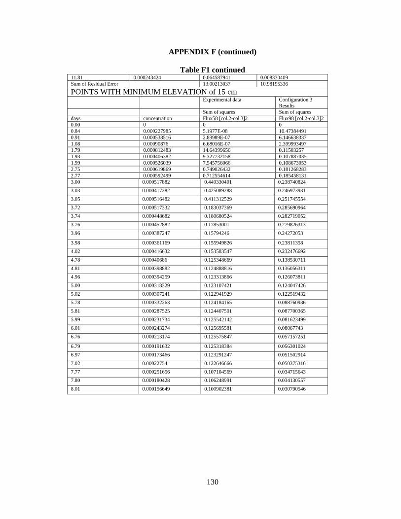
130

APPENDIX F (continued)

Table F1 continued 11.81 0.000243424 0.064587941 0.008330409

Sum of Residual Error 13.00213037 10.98195336

POINTS WITH MINIMUM ELEVATION of 15 cm Experimental data Configuration 3

Results

Sum of squares Sum of squares

days concentration Flux58 [col.2-col.3]2 Flux98 [col.2-col.3]2

0.00 0 0 0

0.84 0.000227985 5.1977E-08 10.47384491

0.91 0.000538516 2.89989E-07 6.146638337

1.08 0.00090876 6.68016E-07 2.399993497

1.79 0.000812483 14.64399656 0.11503257

1.93 0.000406382 9.327732158 0.107887035

1.99 0.000526039 7.545756066 0.108673053

2.75 0.000619869 0.749026432 0.181268283

2.77 0.000592499 0.712554614 0.185458131

3.00 0.000517882 0.449330401 0.238740824

3.03 0.000417282 0.425089288 0.246973931

3.05 0.000516482 0.411312529 0.251745554

3.72 0.000517332 0.183037369 0.285690964

3.74 0.000448682 0.180680524 0.282719052

3.76 0.000452882 0.17853001 0.279826313

3.96 0.000387247 0.15794246 0.24272053

3.98 0.000361169 0.155949826 0.23811358

4.02 0.000416632 0.153583547 0.232476692

4.78 0.00040686 0.125348669 0.138530711

4.81 0.000398882 0.124888816 0.136056311

4.96 0.000394259 0.123313866 0.126073811

5.00 0.000318329 0.123107421 0.124047426

5.02 0.000307241 0.122941929 0.122519432

5.78 0.000332263 0.124184165 0.088760936

5.81 0.000287525 0.124407501 0.087700365

5.99 0.000231734 0.125542142 0.081623499

6.01 0.000243274 0.125695581 0.08067743

6.76 0.000213174 0.125575847 0.057157251

6.79 0.000191632 0.125318384 0.056301024

6.97 0.000173466 0.123291247 0.051502914

7.02 0.00022754 0.122646666 0.050375316

7.77 0.000251656 0.107104569 0.034715643

7.80 0.000180428 0.106248991 0.034130557

8.01 0.000156649 0.100902381 0.030790546

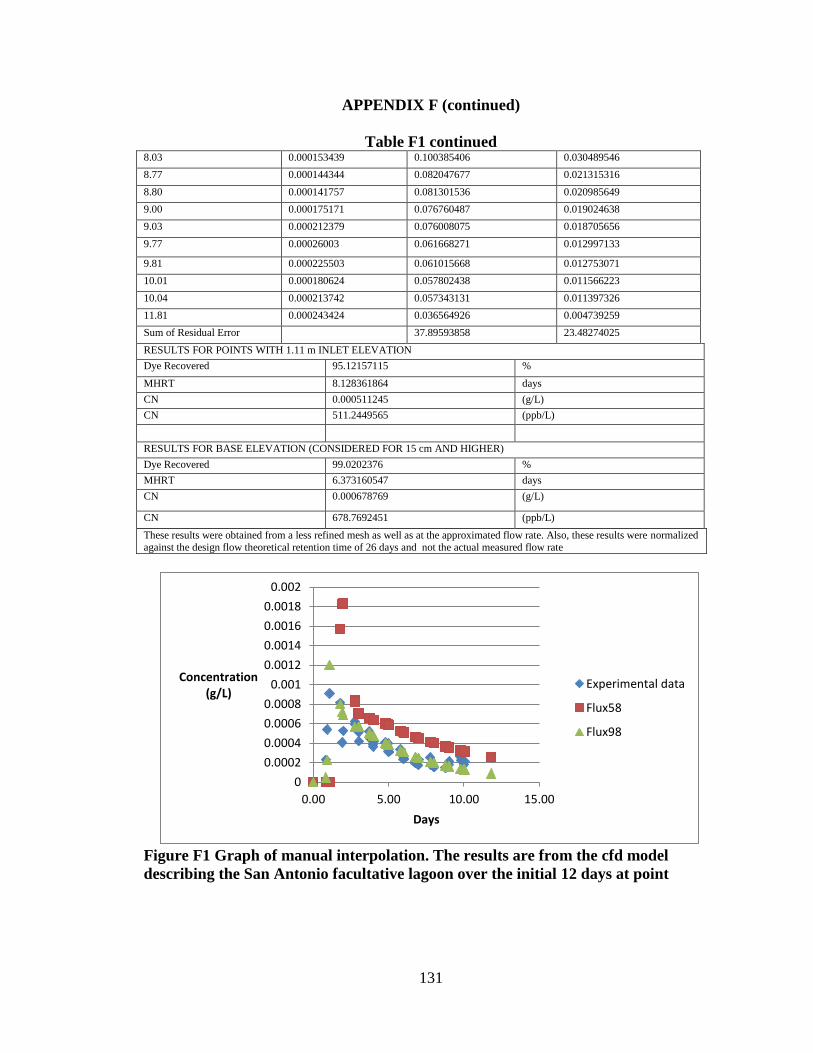
131

APPENDIX F (continued)

Table F1 continued 8.03 0.000153439 0.100385406 0.030489546

8.77 0.000144344 0.082047677 0.021315316

8.80 0.000141757 0.081301536 0.020985649

9.00 0.000175171 0.076760487 0.019024638

9.03 0.000212379 0.076008075 0.018705656

9.77 0.00026003 0.061668271 0.012997133

9.81 0.000225503 0.061015668 0.012753071

10.01 0.000180624 0.057802438 0.011566223

10.04 0.000213742 0.057343131 0.011397326

11.81 0.000243424 0.036564926 0.004739259

Sum of Residual Error 37.89593858 23.48274025

RESULTS FOR POINTS WITH 1.11 m INLET ELEVATION

Dye Recovered 95.12157115 %

MHRT 8.128361864 days

CN 0.000511245 (g/L)

CN 511.2449565 (ppb/L)

RESULTS FOR BASE ELEVATION (CONSIDERED FOR 15 cm AND HIGHER)

Dye Recovered 99.0202376 %

MHRT 6.373160547 days

CN 0.000678769 (g/L)

CN 678.7692451 (ppb/L)

These results were obtained from a less refined mesh as well as at the approximated flow rate. Also, these results were normalized against the design flow theoretical retention time of 26 days and not the actual measured flow rate

Figure F1 Graph of manual interpolation. The results are from the cfd model

describing the San Antonio facultative lagoon over the initial 12 days at point

0

0.0002

0.0004

0.0006

0.0008

0.001

0.0012

0.0014

0.0016

0.0018

0.002

0.00 5.00 10.00 15.00

Concentration (g/L)

Days

Experimental data

Flux58

Flux98

132

APPENDIX F (continued)

Figure F2 Graph of 40% model error. The results are from the cfd model describing

the San Antonio facultative lagoon over the initial 12 days at point B.

Figure F3 Graph of points with minimum elevation of 1.11 m. The results are from

the cfd model describing the San Antonio facultative lagoon over the initial 12 days

at point B.

0

0.0002

0.0004

0.0006

0.0008

0.001

0.0012

0.0014

0.0016

0.0018

0.002

0.00 5.00 10.00 15.00

Concentration (g/L)

Days

Experimental data

Flux58

Flux98

0

0.0002

0.0004

0.0006

0.0008

0.001

0.0012

0.0014

0.0016

0.0018

0.002

0.00 5.00 10.00 15.00

Concentration (g/L)

Days

Experimental data

Flux58

Flux98

133

APPENDIX F (continued)

Figure F4 Graph of points with minimum elevation of 15 cm. The results are from

the cfd model describing the San Antonio facultative lagoon over the initial 12 days

at point B.

Figure F5 Graph of manual interpolation over 25 days. The results are from the cfd

model describing the San Antonio facultative lagoon at point B.

0

0.0005

0.001

0.0015

0.002

0.00 5.00 10.00 15.00

Concentration (g/L)

Days

Experimental data

Flux58

Flux98

134

APPENDIX F (continued)

Figure F6 Graph of points with larger than 40% model error over 25 days. The

results are from the cfd model describing the San Antonio facultative lagoon at

point B.

Figure F7 Graph of points with minimum elevation of 15 cm over 25 days. The

results are from the cfd model describing the San Antonio facultative lagoon at

point B.

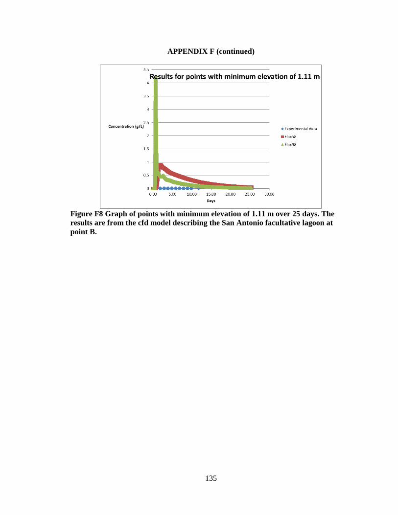
135

APPENDIX F (continued)

Figure F8 Graph of points with minimum elevation of 1.11 m over 25 days. The

results are from the cfd model describing the San Antonio facultative lagoon at

point B.

136

APPENDIX F (continued)

Figure F9 Comparison of cfd runs and actual tracer data. The results are from the

cfd model describing the San Antonio facultative lagoon at point B.

137

APPENDIX G ORANGE TRACER STUDY PERFORMED AT SAN ANTONIO

LAGOON THAT PROVIDES VISUAL EVIDENCE OF THE PRESENCE OF

DEAD ZONES

A portion of oranges was released from the bank directly in front of the inlet.

Another portion of the oranges were thrown by hand further out in the lagoon in front of

the inlet where bubbles had risen to the surface providing an indication that it was the site

of influent. At the end of the study all the oranges were located at one of the two corners

Figure F10 Orange surface flow pattern study

Left corner Right corner

138

APPENDIX G (continued)

along the inlet side of the pond as can be seen in the two figures below. The bottom left

figure is the corner to the left of the inlet from the perspective of the inlet and the bottom

right figure is the right corner.